geosciences

Article

Modelling and Mapping Total and Bioaccessible Arsenic andLead in Stoke-on-Trent and Their Relationships with Industry

Joanna Wragg * and Mark Cave

Citation: Wragg, J.; Cave, M.

Modelling and Mapping Total and

Bioaccessible Arsenic and Lead in

Stoke-on-Trent and Their

Relationships with Industry.

Geosciences 2021, 11, 515. https://

doi.org/10.3390/geosciences11120515

Academic Editors: Javier Lillo and

Jesus Martinez-Frias

Received: 8 November 2021

Accepted: 13 December 2021

Published: 15 December 2021

Publisher’s Note: MDPI stays neutral

with regard to jurisdictional claims in

published maps and institutional affil-

iations.

Copyright: © 2021 by the authors.

Licensee MDPI, Basel, Switzerland.

This article is an open access article

distributed under the terms and

conditions of the Creative Commons

Attribution (CC BY) license (https://

creativecommons.org/licenses/by/

4.0/).

British Geological Survey, Keyworth, Nottingham NG12 5GG, UK; mrca@bgs.ac.uk* Correspondence: jwrag@bgs.ac.uk

Abstract: This study was based on a geochemical soil survey of Stoke-on-Trent in the UK of747 surface soil samples analysed for 53 elements. A subset of 50 of these soil samples were analysedfor their bioaccessible As and Pb content using the Unified Barge Method. Random Forest modelling,using the total element data as predictor variables, was used to predict bioaccessible As and Pbfor all 747 samples. Random Forest modelling, using inverse distance weighed predictors andbedrock and superficial geology, was also used to map both total and bioaccessible As and Pb ona 400 × 400 spatial prediction grid with a 50 m resolution. The predicted bioaccessible As rangedfrom ca. 1 to 8 mg/kg and the total As ca. 8 to 45 mg/kg. The bioaccessible Pb and the total Pb bothcovered the range ca. 16–1200 mg/kg, with the highest values for both forms of Pb showing similarspatial distributions. Predictor variable importance and information on past industry suggest thatthe source of both of these elements is driven by anthropogenic causes.

Keywords: arsenic; lead; soil; Stoke-on-Trent; bioaccessibility

1. Introduction

Soils act as sinks and sources of potentially harmful elements (PHE), which can beassociated with the underlying geology and deposition of contaminants from previous landuse. The range and distribution of past and present industrial activity provides a challengefor understanding the complex mixtures of contaminants in soils. The potential hazard tohuman health from reuse of this land (e.g., housing and greenspace) can be assessed by theidentification and quantification of the total soil PHE content, but this can overestimate thepotential hazard to human health, as it assumes that the total content will be available foruptake in the human body after accidental exposure [1,2]. To reflect solubility of soil PHEafter accidental exposure, bioaccessible studies provide a physicochemical estimation ofthe amount of contaminant available for uptake in the body. Understanding the sources ofPHE and, as a result, the potential mobility is therefore important in efforts to understandthe potential for—and impacts of—repurposing of land.

Stoke-on-Trent is a post-industrial city in North Staffordshire, UK. The city, an amal-gam of six towns (Burslem, Longton, Stoke, Tunstall, Fenton and Hanley), covers an areaof 36 square miles (93 km2) and has a combined population of ca. 250,000 (Figure 1) [3].Known as the ‘potteries’, Stoke was the home of the pottery industry in England, withover 100 potteries between the 1700s and the present day [4,5]. Many of these were ownedby different generations of the same families and, with others, amalgamated over time.Notable pottery manufacturers include Royal Doulton, Middleport and Wedgewood inBurslem, Dresden and Gladstone in Longton and Spode and Minton in Stoke [5]. In ad-dition to tableware potteries, there were sanitary ware manufacturers, such as ArmitageShanks and Twyfords. The pottery industry was initially founded on the abundance ofcoal and clay suitable for earthenware and brick production (e.g., Grey and Etruria Marls,Fireclays) which overlay the Coal Measures [6,7]. Later, the importation of China claysupported the development of more delicate tableware.

Geosciences 2021, 11, 515. https://doi.org/10.3390/geosciences11120515 https://www.mdpi.com/journal/geosciences

Geosciences 2021, 11, 515 2 of 22

Geosciences 2021, 11, x FOR PEER REVIEW 2 of 22

Fireclays) which overlay the Coal Measures [6,7]. Later, the importation of China clay supported the development of more delicate tableware.

Figure 1. Map of Stoke-on-Trent and surrounding towns.

Manufacture of colours and chemicals for potteries, glazed bricks manufacturers, glassmakers and enamellers were also present across the area. The variety and colour of pottery was derived from the metal oxides (Cd, Cr, Cu, Co, Fe, Mn, Ni, U and V) and the composition of the glazes (SiO2, Al2O3, CaO, SnO2 PbO and FeTiO2) used in the decorative processes [8].

The Staffordshire coalfield supported the development of Stoke as an industrial city. Stretching from Madely in the west, the coalfields went as far as the Towerhill colliery in the north and the Foxfield and Hem Heath collieries in the east and south, respectively [9]. Early workings of the coal measures were established around the Hanley, Burslem, Tunstall and Longton areas of the city, with deep pits at Chatterly, Whitfield and the Red Street area central to opencast mining. Naturally elevated concentrations of PHE, such as As, V, Mo, Cu, Ni, Zn, Pb, can be found in the coal measures that surround the city [8].

Stoke-on-Trent was also home to numerous steel and iron works. The largest of these was the Shelton Bar Steelworks, which stretched across the Etruria Valley. The works, at its height, employed a workforce of 10,000 and included multiple coal mines, steelworks, rolling mills and blast furnaces before finally closing in 2000. To reduce the distance be-tween the fuel and the furnace, furnaces would be on the same site as the coal mine.

Industrial activity in Stoke, including provision of raw materials for both the pottery and steel industries (and exportation of products), was supported by multiple transport

Figure 1. Map of Stoke-on-Trent and surrounding towns.

Manufacture of colours and chemicals for potteries, glazed bricks manufacturers,glassmakers and enamellers were also present across the area. The variety and colour ofpottery was derived from the metal oxides (Cd, Cr, Cu, Co, Fe, Mn, Ni, U and V) and thecomposition of the glazes (SiO2, Al2O3, CaO, SnO2 PbO and FeTiO2) used in the decorativeprocesses [8].

The Staffordshire coalfield supported the development of Stoke as an industrial city.Stretching from Madely in the west, the coalfields went as far as the Towerhill colliery inthe north and the Foxfield and Hem Heath collieries in the east and south, respectively [9].Early workings of the coal measures were established around the Hanley, Burslem, Tunstalland Longton areas of the city, with deep pits at Chatterly, Whitfield and the Red Street areacentral to opencast mining. Naturally elevated concentrations of PHE, such as As, V, Mo,Cu, Ni, Zn, Pb, can be found in the coal measures that surround the city [8].

Stoke-on-Trent was also home to numerous steel and iron works. The largest of thesewas the Shelton Bar Steelworks, which stretched across the Etruria Valley. The works, atits height, employed a workforce of 10,000 and included multiple coal mines, steelworks,rolling mills and blast furnaces before finally closing in 2000. To reduce the distancebetween the fuel and the furnace, furnaces would be on the same site as the coal mine.

Industrial activity in Stoke, including provision of raw materials for both the potteryand steel industries (and exportation of products), was supported by multiple transportlinks. Railway lines running through the city included what is now known as the WestCoast Mainline (WCM) and the North Staffordshire Railway (NSR). Tramways and mineralrailway lines crossed the region, providing vital links between the coalfields and claypitsand the potteries and local industries. One such linkage was the potteries’ loop line [10].

Geosciences 2021, 11, 515 3 of 22

The loop line ran from the Etruria works to Kidsgrove. Additional support was providedthrough the construction of the Trent/Mersey and Cauldon canals, which ran alongsidethe WCM and NSR, respectively. Engineering, carriage and wagon works were situated inthe area to support rail activity.

The rapid growth of the local pottery and steel industries (and the large supportingcoal industry) resulted in a large conurbation mixing residential, retail and industrialdevelopments. The by-products of the range of activities in Stoke included furnace slagand ceramic waste, which were often repurposed as sources of urban fill and made intoground material for the building of required urban infrastructure as the city grew [8].

The industry of Stoke has left a landscape rich in industrial heritage, as shown inFigure 2, characterised by the once widespread bottle kilns, canals, wharfages and dis-used railways. Regeneration of Stoke has repurposed large areas of previously used andpotentially contaminated land for industrial, residential and community/greenspace use(Figure 3, Table 1) today, over one third of the city is green, open space [11].

In this work, we chose to study the total bioaccessible concentrations and spatialdistribution of As and Pb, common priority soil contaminants, for human health riskassessment. The work used modelling approaches to identify PHE relationships to naturallyoccurring and anthropogenic elements from historical land use found concurrently in soilsamples for the development of predictive distribution maps to support future urbanplanning activities.

Geosciences 2021, 11, x FOR PEER REVIEW 3 of 22

links. Railway lines running through the city included what is now known as the West Coast Mainline (WCM) and the North Staffordshire Railway (NSR). Tramways and min-eral railway lines crossed the region, providing vital links between the coalfields and clay-pits and the potteries and local industries. One such linkage was the potteries’ loop line [10]. The loop line ran from the Etruria works to Kidsgrove. Additional support was pro-vided through the construction of the Trent/Mersey and Cauldon canals, which ran along-side the WCM and NSR, respectively. Engineering, carriage and wagon works were situ-ated in the area to support rail activity.

The rapid growth of the local pottery and steel industries (and the large supporting coal industry) resulted in a large conurbation mixing residential, retail and industrial de-velopments. The by-products of the range of activities in Stoke included furnace slag and ceramic waste, which were often repurposed as sources of urban fill and made into ground material for the building of required urban infrastructure as the city grew [8].

The industry of Stoke has left a landscape rich in industrial heritage, as shown in Figure 2, characterised by the once widespread bottle kilns, canals, wharfages and disused railways. Regeneration of Stoke has repurposed large areas of previously used and poten-tially contaminated land for industrial, residential and community/greenspace use (Fig-ure 3, Table 1) today, over one third of the city is green, open space [11].

Figure 2. Location of selected industrial sites in Stoke-on-Trent. Figure 2. Location of selected industrial sites in Stoke-on-Trent.

Geosciences 2021, 11, 515 4 of 22Geosciences 2021, 11, x FOR PEER REVIEW 4 of 22

Figure 3. Greenspace development of industrial sites.

Table 1. Regeneration of Industrial sites.

Location/Land Use Land Use Post Regeneration Apedale Mine/Ironworks Country Park Birchenwood Colliery Tip Industrial Estate

Chatterly Whitfield Parkland Chell Railway Cutting Colliery infill Parkland

Chell Quarry Athletic Stadium Cobridge Clay Pit Industrial Estate

Etruria, Festival Park Country Park Fenton Colliery Tip Industrial Estate Lightwood Quarry Housing Estate

Parkhouse Colliery Tip Industrial Estate Red Street Opencast Mine Housing

Rowhurst Clay Pit Industrial Estate Silverdale Colliery Tip Pasture/Country Park

Shelton Colliery Tip/Ironworks Industrial Estate Sneyd Hill Community Land

Tunstall Clay Pit Industrial Estate

In this work, we chose to study the total bioaccessible concentrations and spatial dis-tribution of As and Pb, common priority soil contaminants, for human health risk assess-ment. The work used modelling approaches to identify PHE relationships to naturally

Figure 3. Greenspace development of industrial sites.

Table 1. Regeneration of Industrial sites.

Location/Land Use Land Use Post Regeneration

Apedale Mine/Ironworks Country Park

Birchenwood Colliery Tip Industrial Estate

Chatterly Whitfield Parkland

Chell Railway Cutting Colliery infill Parkland

Chell Quarry Athletic Stadium

Cobridge Clay Pit Industrial Estate

Etruria, Festival Park Country Park

Fenton Colliery Tip Industrial Estate

Lightwood Quarry Housing Estate

Parkhouse Colliery Tip Industrial Estate

Red Street Opencast Mine Housing

Rowhurst Clay Pit Industrial Estate

Silverdale Colliery Tip Pasture/Country Park

Shelton Colliery Tip/Ironworks Industrial Estate

Sneyd Hill Community Land

Tunstall Clay Pit Industrial Estate

Geosciences 2021, 11, 515 5 of 22

2. Materials and Methods2.1. Soil Sampling and Analysis

The soil samples were part of the British Geological Survey (BGS) Geochemical Surveyof Urban Environments (GSUE) project [8], an integral part of the wider G-BASE andTellusNI programmes. The aim of the programme was to provide an overview of thegeochemical signature of urban environments. Four samples were collected from withineach national grid—one km square on 1:25,000 topographic Ordnance Survey map. Eachwas collected from the least disturbed area of unbuilt ground as close as possible to thecentre of 500 m sub-cells. Areas sampled included domestic gardens, allotments, parks,recreational ground, or road verges, avoiding point sources of contamination. The surfacesoils (n = 747), collected in 1993, were sampled at a depth of 0.15 m using a handheld auger,air-dried and sieved to <2 mm. Fordyce et al. [8] described the details of the samplingprocedures and soil preparation as well as analytical details for the measurement of totalelement concentrations by X-Ray fluorescence (XRF).

Bioaccessibility measurements (As and Pb) were carried out on a subset of 50 of the747 soil samples collected. In order to ensure that the 50 samples were representative of theoverall data set, the soil geochemical data was clustered according to elemental groupings.The geochemistry dataset was mean-centered and scaled to unit variance and clusteredusing the “mclust” model-based clustering algorithm based on parameterized finite Gaus-sian mixture models [12] within the R programming language [13]. Four clusters wereidentified as being a parsimonious representation of different variations in geochemistryover the region. They also represented the underlying geology. Between 10 and 17 sampleswere randomly chosen from each group to make up 50 samples.

The <2 mm soil samples were further sieved to <250 µm for total and bioaccessiblePHE determination. Total element (e.g., Al, As, Ba, Ca, Cd, Co, Cr, Cu, Fe, K, Mg, Mn, Mo,Na, Ni, P, Pb, Se, Si, Sr, V and Zn) concentrations in each sample were determined aftermixed acid (HNO3, HF, HClO4

−) digestion. The PHE bioaccessibility was measured aftersimulated gastrointestinal extraction using the Unified Barge Method (UBM). The UBMsimulated the physicochemical conditions of the mouth, stomach and intestine by a 3-stagesequential extraction. Details of the background to the UBM and the procedure have beendescribed in previous publications [14,15]. The total and bioaccessible concentrations weremeasured using Inductively Coupled Plasma-Mass Spectrometry as described in works byMiddleton et al. [16] and Watts et al. [17].

For quality control purposes, one duplicate, one quality control soil (BGS 102) and oneblank were extracted within every batch, at maximum, 10 unknown samples. Extractiondata were in good agreement with the consensus values [18], with bioaccessible As andPb concentrations for BGS 102 of 3.96 ± 0.12 mg/kg and 16.22 ± 1.62 mg/kg, respectively,and were also within the guidance values [18] and those reported by Hamilton et al., [19].The repeatability (RSD) of both total and bioaccessible extraction duplicates was <10% RSD.All blank extractions (total and bioaccessible) returned values below the method detection limits.

2.2. Bioaccessibility Modelling

Bioaccessibility modelling, in this work, refers to the statistical analysis, data process-ing and quality assessment of actual measurements made in a subset of 50 representativesamples for the production of reliable As and Pb bioaccessibility estimates for all 747 soilsamples used in this study. Random Forest (RF) models for the bioaccessibility of As andPb were set up using the UBM-measured bioaccessibility of the selected 50 samples as thedependent variable and a combination of the total element concentrations of 53 elementsobtained by the G-BASE programme, with the sample elevations and the superficial andbedrock geology as possible predictor variables. The modelling was carried out usingthe R programming language [13] with the ranger library for RF modelling [20] and theBoruta library for selecting significant predictor variables [21]. The Boruta algorithm hasbeen described in detail [21]; however, briefly: the Boruta Algorithm produces a duplicatepredictor data set with each predictor randomly shuffled and joins the shuffled data set

Geosciences 2021, 11, 515 6 of 22

with the original predictors. It then builds a random forest model on the merged dataset,making a comparison between the importance of the original variables with the randomisedvariables. Only variables having higher importance than the randomised variables areconsidered important.

The RF model set up for the two elements followed the procedure below:

1. Make an RF model for the bioaccessibility of the element in question using theranger library.

2. Use the Boruta package to select out the significant predictors.3. Optimise the new RF model r-square by varying the “mtry” parameter (the number of

variables randomly sampled as candidates at each split) [20].4. Run the optimised model 500 times, each time on a resampled dataset, predicting the

bioaccessibility at all 747 sampling locations.5. Take median and median absolute deviation (mad) values for the 500 predictions at

each location to provide an estimate of the bioaccessibility and its associated modelleduncertainty at each location.

2.3. Spatial Modelling

Spatial modelling here refers to the statistical analysis, data processing and qualityassessment procedures for the production of reliable estimates of As and Pb totals andbioaccessibility across a regular prediction grid of points covering the area of interest from747 soil locations. Spatial modelling and prediction, for the purposes of illustrating the2D distribution of a contaminant in soil, has traditionally been carried out using kriging-related techniques [22,23]. Recently, Hengl et al. [24] summarised the problems associatedwith kriging and demonstrated the use and advantages of a machine learning method(Random Forest, RF) for spatial modelling where buffer distances from observation pointswere used as explanatory variables. In other studies, Kirkwood et al. [25] used an RF modelwith high resolution geophysics and remote sensed data as covariates to produce a highresolution geochemical map of the South West of England. Additionally, Sekulic et al. [26]successfully demonstrated a similar RF approach using the nearest observations and theirdistances to the prediction location as covariates.

Random Forest (RF) is a popular machine learning algorithm that consists of anensemble of randomised decision trees. Each tree is grown on a random subsampleof the training data and a random subset of the predictor variables to choose from ateach decision node. In this study, we used the RF modelling approach suggested byCave [27], in which inverse distance weighted (IDW) covariates are used as the predictorvariables and subsequently used to predict the spatial distribution of persistent organicpollutants in London [28]. Inverse distance weighted (IDW) interpolation explicitly makesthe assumption that samples that are close to one another are more alike than those that arefurther apart [29]. To predict a value for any unmeasured location, IDW uses the measuredvalues surrounding the prediction location. The measured values closest to the predictionlocation have more influence on the predicted value than those further away. IDW assumesthat each measured point has a local influence that diminishes with distance. It gives greaterweights to points closest to the prediction location, and the weights diminish as a functionof distance—hence, the name inverse distance weighted [29]. IDW predictions require2 parameters (the inverse distance power (p) and the number of nearest neighbours (n)) touse. While the premise behind IDW is broadly correct, the choice of p and n is subjectiveand there is no relation between the prediction and the actual spatial variability as in manyother methods (e.g., in kriging, the model relates to the spatial variance of the parameter ofinterest through the variogram). In this instance, we took a series of IDW predictors withvarying combinations of p and n and used these as the predictor covariates. Then, the RFmodel combined these covariates to model the estimated soil parameters at the predictionlocations. The training set was produced by using leave-one-out (loo) IDW predictions foreach sampled point and its associated contaminant concentration at each combination of pand n. IDW pseudo-predictions at the points where the predicted soil concentrations were

Geosciences 2021, 11, 515 7 of 22

required were then calculated and used as predictor variables on the RF model producedon the training data.

The underlying geology of a region has been shown to be an important control on thegeochemical composition of surface soils [30]. In addition to the IDW predictor covariates,the superficial geology and bedrock geology were used as predictor variables by attributingboth the soil sample points and the prediction grid with the two geology variables.

2.3.1. Spatial Modelling Procedure

The data analysis was carried out using the R programming Language [13] andassociated libraries. The “sf” R library [31] was used to attribute the geology data to thesampling points and prediction grid. The “ranger” R library [20] was used to carry out RFmodelling. The Boruta R library [21] was used to select the significant predictor variablesin the RF model. Preliminary checks (not reported) showed that, after the top 5–10 mostimportant IDW predictor combinations, the inclusion of further IDW predictors did notmeaningfully improve the root mean square error of prediction (RMSEP). The modellingand interpolation were carried out in the following stages:

1. A series of IDW predictor variables were made up from all combinations of nearestneighbour values of 3, 5, 7, 9,11,13,15 and inverse distance power values of 0.1, 0.5,0.9, 1.3, 1.7, 2.1, 2.5, 2.9 (56 combinations). For the training set, the IDW predictorswere calculated for each individual point using a leave-one-out strategy. An RF modelwas set up using the 56 IDW combinations as predictor variables for the determinandin question.

2. The top 5 most important IDW combinations (measured in the RF model by the gini-index [17]) were chosen and combined with the geology data and used to produce asecond RF model for the determinand in question. The second model was then sub-jected to the Boruta algorithm, which selected out the significant predictors (comparedto randomly shuffled predictor variables [21]).

3. A third RF model using the significant geology and IDW predictors was then opti-mised to get the best value of “mtry” (the number of variables randomly sampled ascandidates at each split in the decision trees used in the RF model [20]).

4. Finally, the third optimised RF model was applied to 100 bootstrap resamplings ofthe original sampling points (recalculating the IDW predictors for each bootstrapresample), with each of the resampling rounds producing data on the model fitand predictions for the determinand in question on the prediction grid. The finaldeterminand prediction values at the prediction grid were calculated as the medianvalue from the 100 resampling rounds.

2.3.2. Modelling Accuracy and Precision

Accuracy and precision [20] for the RF bioaccessibility modelling of As and Pb wereassessed by comparing the so called “out of bag” (OOB) predicted values against themeasured bioaccessible values for the selected 50 soil samples used to set up the model.The OOB data were, in effect, equivalent to cross-validated data (i.e., independent sampleswith measured values not used in setting up the model) because, within each of the RFmodel decision trees, bootstrapped samples of the original data were used so that thesamples left out by the resampling could act as independent check samples.

A similar approach was used to estimate accuracy and precision [20] for the RF spa-tialmodelling, this time using all 747 soil samples.

2.3.3. Selecting Significant Predictors

The Boruta algorithm [21] selects significant predictors by comparing their perfor-mance to a shadow set of predictors formed by randomly shuffling the original data.Through an iterative process, those parameters which perform better than the shadow pre-dictors are selected as significant. The DALEX library in the R programming language [31]provides a method for post-analysing the RF model to derive the relative importance of the

Geosciences 2021, 11, 515 8 of 22

predictor variables by measuring how much the root mean square error (RMSE) increaseswhen a given parameter is randomly shuffled.

Similar approaches were used for both bioaccessibility and spatial modelling using 50and 747 soil samples, respectively.

2.4. Relationship with Industry

The geochemistry maps were superimposed onto the Ordnance Survey New PopularEdition Historic map (1 inch to the mile) of Stoke-on-Trent (1940s) using QGIS [32] tovisualise linkages between the industrial past and the spatial soil geochemistry of the area.This information, in conjunction with field notes taken at the time of sampling (e.g., wastematerial at the sampling locations) and information on the History of the County ofStafford [33] was used to identify previous land uses. Eight land uses were chosen forfurther discussion, but the sites referenced in this work were not a complete history of theactivities, as a myriad of industries were prolific across the whole area. Table 2 provides anoverview of land uses for the purposes of this work.

Table 2. Land use classifications.

Area Dominant Industries

Tunstall (including Chell) Potteries, coal and ironstone mining, foundry,Al works

Burslem (including Longport,Middleport and Cobridge)

Potteries, coal and ironstone mining, brickworks,gasworks, flint mill

Longton Potteries, coal and ironstone mining, brickworks

Hanley (including Shelton and Etruria) Potteries, foundry, flint mill, coal mining, brick andtileworks, gasworks

Stoke (including Boothen) Potteries, gasworks

Fenton Potteries, flint mill, coal and ironstone mining,brickwork and tileworks, locomotive works, foundry

3. Results3.1. Bioaccessibility Modelling

The samples identified for bioaccessibility testing came from a variety of land uses,including industrial and railway sites, road junctions, housing estates and urban greenspaces. The bioaccessible As concentration ranged between 0.66 and 11.4 mg/kg andbioaccessible Pb ranged from 5.77 to 413.9 mg/kg.

3.1.1. Arsenic Bioaccessibility

The fifty selected samples for bioaccessibility testing were originally analysed (<2 mm)for their total element content using XRF [8]. When the bioaccessibility of the <250 µm sub-samples was determined, the total As concentration was also measured by acid sample di-gestion and inductively-coupled plasma mass spectrometry (ICPMS). Figure 4A shows thatthere was good agreement between the XRF and ICPMS data, with the XRF As vs. ICPMS Aslying close to the line of equivalence. Figure 4 also shows the observed linear relationshipbetween the XRF total As and the stomach phase bioaccessible As (R-square = 0.54), with aslope suggesting that, on average, the bioaccessible As was ca. 21% of the total As.

The RF modelling accuracy and precision for the bioaccessible As, assessed from theOOB predicted values against the measured bioaccessible values for the selected 50 soilsamples, are shown in (Figure 5). The distance of the points from the line of equivalenceand the size of the vertical error bars on the OOB predictions provide the estimates for theaccuracy and precision, respectively. The majority of the OOB-predicted values agreedwith the actual values within the errors indicated by the error bars.

Geosciences 2021, 11, 515 9 of 22

Geosciences 2021, 11, x FOR PEER REVIEW 9 of 22

relationship between the XRF total As and the stomach phase bioaccessible As (R-square = 0.54), with a slope suggesting that, on average, the bioaccessible As was ca. 21% of the total As.

Figure 4. (A) Comparison of the XRF-determined total As with the ICPMS-determined As in 50 soil samples with line of equivalence. (B) Comparison of the XRF-determined total As with the bioaccessible stomach phase As in 50 soil samples with linear regression line and 90% confidence limit.

The RF modelling accuracy and precision for the bioaccessible As, assessed from the OOB predicted values against the measured bioaccessible values for the selected 50 soil samples, are shown in (Figure 5). The distance of the points from the line of equivalence and the size of the vertical error bars on the OOB predictions provide the estimates for the accuracy and precision, respectively. The majority of the OOB-predicted values agreed with the actual values within the errors indicated by the error bars.

Figure 4. (A) Comparison of the XRF-determined total As with the ICPMS-determined As in 50 soil samples with line ofequivalence. (B) Comparison of the XRF-determined total As with the bioaccessible stomach phase As in 50 soil sampleswith linear regression line and 90% confidence limit.

Geosciences 2021, 11, x FOR PEER REVIEW 9 of 22

relationship between the XRF total As and the stomach phase bioaccessible As (R-square = 0.54), with a slope suggesting that, on average, the bioaccessible As was ca. 21% of the total As.

Figure 4. (A) Comparison of the XRF-determined total As with the ICPMS-determined As in 50 soil samples with line of equivalence. (B) Comparison of the XRF-determined total As with the bioaccessible stomach phase As in 50 soil samples with linear regression line and 90% confidence limit.

The RF modelling accuracy and precision for the bioaccessible As, assessed from the OOB predicted values against the measured bioaccessible values for the selected 50 soil samples, are shown in (Figure 5). The distance of the points from the line of equivalence and the size of the vertical error bars on the OOB predictions provide the estimates for the accuracy and precision, respectively. The majority of the OOB-predicted values agreed with the actual values within the errors indicated by the error bars.

Figure 5. Accuracy and precision of the RF model for bioaccessible As. Straight line represents the line of equivalence anderror bars are ± the median absolute deviation.

The Boruta algorithm selects significant predictors by comparing their performance toa shadow set of predictors formed by randomly shuffling the original data. Through aniterative process, those parameters which perform better than the shadow predictors areselected as significant. The DALEX library in the R programming language [34] provides amethod for post-analysing the RF model to derive the relative importance of the predictorvariables by measuring how much the root mean square error increases when a givenparameter is randomly shuffled. This measure of importance provides some insight on thegeochemical factors controlling the bioaccessible As in the Stoke-on-Trent soils. Figure 6shows that total Ca in the soil is the most important predictor, followed by the total As.

Geosciences 2021, 11, 515 10 of 22

The sample elevations and the superficial and subsurface geology were not found to besignificant predictor variables.

Geosciences 2021, 11, x FOR PEER REVIEW 10 of 22

Figure 5. Accuracy and precision of the RF model for bioaccessible As. Straight line represents the line of equivalence and error bars are ± the median absolute deviation.

The Boruta algorithm selects significant predictors by comparing their performance to a shadow set of predictors formed by randomly shuffling the original data. Through an iterative process, those parameters which perform better than the shadow predictors are selected as significant. The DALEX library in the R programming language [34] provides a method for post-analysing the RF model to derive the relative importance of the predic-tor variables by measuring how much the root mean square error increases when a given parameter is randomly shuffled. This measure of importance provides some insight on the geochemical factors controlling the bioaccessible As in the Stoke-on-Trent soils. Figure 6 shows that total Ca in the soil is the most important predictor, followed by the total As. The sample elevations and the superficial and subsurface geology were not found to be significant predictor variables.

Figure 6. Relative importance of predictor variables for the RF model of the bioaccessible As.

This suggests that the bioaccessible As was associated with a carbonate phase in the soil. In addition, other significant predictors (such as Sb, Cu, Pb, Sn, Hg and Cd) are com-monly associated with anthropogenic sources. This is in contrast with a study of North-ampton [35] which is situated on underlying ironstone geology and where the bioaccessi-ble As, measured using UBM, was associated with naturally-occurring fine-grained Fe oxyhydroxide in the soil. There, on average, the bioaccessible As was ca. 8% of the total As.

3.1.2. Lead Bioaccessibility In a similar manner to the total As and bioaccessible measurements, Figure 7 shows

that there was good agreement between the XRF and ICPMS data, with the XRF Pb vs. ICPMS Pb lying close to the line of equivalence. Figure 7 also shows that the relationship between the XRF total Pb and the stomach phase bioaccessible Pb was linear (R-square = 0.82), with a slope suggesting that, on average, the bioaccessible Pb was ca. 33% of the total Pb.

Figure 6. Relative importance of predictor variables for the RF model of the bioaccessible As.

This suggests that the bioaccessible As was associated with a carbonate phase inthe soil. In addition, other significant predictors (such as Sb, Cu, Pb, Sn, Hg and Cd)are commonly associated with anthropogenic sources. This is in contrast with a studyof Northampton [35] which is situated on underlying ironstone geology and where thebioaccessible As, measured using UBM, was associated with naturally-occurring fine-grained Fe oxyhydroxide in the soil. There, on average, the bioaccessible As was ca. 8% ofthe total As.

3.1.2. Lead Bioaccessibility

In a similar manner to the total As and bioaccessible measurements, Figure 7 showsthat there was good agreement between the XRF and ICPMS data, with the XRF Pb vs.ICPMS Pb lying close to the line of equivalence. Figure 7 also shows that the relationship be-tween the XRF total Pb and the stomach phase bioaccessible Pb was linear (R-square = 0.82),with a slope suggesting that, on average, the bioaccessible Pb was ca. 33% of the total Pb.

Figure 8 shows the accuracy and precision of the RF model for bioaccessible Pb.Figure 9 shows the relative importance of the significant predictor variables. In a similarmanner to the As bioaccessibility, the sample elevations and the superficial and subsurfacegeology were not found to be significant predictor variables. In line with previous stud-ies [36], Figure 9 shows that total Pb was the most significant predictor for bioaccessible Pb.However, the average bioaccessible Pb (as a fraction of total Pb) was towards the low end(ca. 33%, Figure 7B) compared to that previously reported (38% [36]) for the UK. In amore detailed study of Pb in the town of Northampton, it was suggested that the source ofbioaccessible Pb in both rural and urban soils was a fine-grained pyromorphite mineral. Inthis instance, Figure 9 shows that the additional most important predictors (Hg, Ag, Sn)were more likely to be associated with industrial processes (e.g., Hg was used in gildeddecoration on ceramics [37,38]) associated with the ceramics industry.

Geosciences 2021, 11, 515 11 of 22Geosciences 2021, 11, x FOR PEER REVIEW 11 of 22

Figure 7. (A) Comparison of the XRF-determined total Pb with the ICPMS determined Pb in 50 soil samples with line of equivalence. (B) Comparison of the XRF-determined total Pb with the bioaccessible stomach phase Pb in 50 soil samples with linear regression line and 90% confidence limit.

Figure 8 shows the accuracy and precision of the RF model for bioaccessible Pb. Fig-ure 9 shows the relative importance of the significant predictor variables. In a similar man-ner to the As bioaccessibility, the sample elevations and the superficial and subsurface geology were not found to be significant predictor variables. In line with previous studies [36], Figure 9 shows that total Pb was the most significant predictor for bioaccessible Pb. However, the average bioaccessible Pb (as a fraction of total Pb) was towards the low end (ca. 33%, Figure 7B) compared to that previously reported (38% [36]) for the UK. In a more detailed study of Pb in the town of Northampton, it was suggested that the source of bio-accessible Pb in both rural and urban soils was a fine-grained pyromorphite mineral. In this instance, Figure 9 shows that the additional most important predictors (Hg, Ag, Sn) were more likely to be associated with industrial processes (e.g., Hg was used in gilded decoration on ceramics [37,38]) associated with the ceramics industry.

Figure 7. (A) Comparison of the XRF-determined total Pb with the ICPMS determined Pb in 50 soil samples with line ofequivalence. (B) Comparison of the XRF-determined total Pb with the bioaccessible stomach phase Pb in 50 soil sampleswith linear regression line and 90% confidence limit.

Geosciences 2021, 11, x FOR PEER REVIEW 11 of 22

Figure 7. (A) Comparison of the XRF-determined total Pb with the ICPMS determined Pb in 50 soil samples with line of equivalence. (B) Comparison of the XRF-determined total Pb with the bioaccessible stomach phase Pb in 50 soil samples with linear regression line and 90% confidence limit.

Figure 8 shows the accuracy and precision of the RF model for bioaccessible Pb. Fig-ure 9 shows the relative importance of the significant predictor variables. In a similar man-ner to the As bioaccessibility, the sample elevations and the superficial and subsurface geology were not found to be significant predictor variables. In line with previous studies [36], Figure 9 shows that total Pb was the most significant predictor for bioaccessible Pb. However, the average bioaccessible Pb (as a fraction of total Pb) was towards the low end (ca. 33%, Figure 7B) compared to that previously reported (38% [36]) for the UK. In a more detailed study of Pb in the town of Northampton, it was suggested that the source of bio-accessible Pb in both rural and urban soils was a fine-grained pyromorphite mineral. In this instance, Figure 9 shows that the additional most important predictors (Hg, Ag, Sn) were more likely to be associated with industrial processes (e.g., Hg was used in gilded decoration on ceramics [37,38]) associated with the ceramics industry.

Figure 8. Accuracy and precision of the RF model for bioaccessible Pb. Straight line represents the line of equivalence anderror bars are ± the median absolute deviation.

Geosciences 2021, 11, 515 12 of 22

Geosciences 2021, 11, x FOR PEER REVIEW 12 of 22

Figure 8. Accuracy and precision of the RF model for bioaccessible Pb. Straight line represents the line of equivalence and error bars are ± the median absolute deviation.

Figure 9. Relative importance of predictor variables for the RF model of the bioaccessible Pb.

3.2. Spatial Modelling of Total and Bioaccessible Concentrations Spatial predictions of total As and total Pb and bioaccessible As and Pb were made

over a 400 × 400 spatial prediction grid with a 50 m resolution which encompassed the soil sample locations. Table 3 gives the acronyms and the description of the bedrock and su-perficial geology that appear in various combinations as significant predictor variables for both As and Pb and their related bioaccessibility values.

Table 3. Significant geology predictor variables for the spatial modelling.

Formation Acronym Formation Name Formation Description

Formation Origin Geology Type

HA Halesowen formation Sandstone Sedimentary Bedrock

CHES Chester formation Sandstone and conglomerate, inter-

bedded Sedimentary Bedrock

ETM Etruria formation Sandstone Sedimentary Bedrock

PUCM Pennine upper coal measures for-mation

Mudstone, siltstone and sandstone Sedimentary Bedrock

PMCM Pennine middle coal measures for-mation Mudstone, siltstone and sandstone Sedimentary Bedrock

ALV Alluvium Clay, silt, sand and gravel Sedimentary Superficial

In line with the RF bioaccessibility modelling, the performance and significant pre-dictor variables for spatial modelling of total and bioaccessible As and Pb over the Stoke-on-Trent area were assessed by comparing the actual values with the OOB predictions and the significant variables. Additionally, we compared their relative importance using the Boruta algorithm [21] and DALEX post-processing of the optimized rf models [34].

In order to understand how the spatial predictions from the model were influenced by the predictor variables, Ceteris-paribus (Latin for “other things held constant”) profiles were constructed. These show how a model’s prediction will change if the value of a single

Figure 9. Relative importance of predictor variables for the RF model of the bioaccessible Pb.

3.2. Spatial Modelling of Total and Bioaccessible Concentrations

Spatial predictions of total As and total Pb and bioaccessible As and Pb were madeover a 400 × 400 spatial prediction grid with a 50 m resolution which encompassed thesoil sample locations. Table 3 gives the acronyms and the description of the bedrock andsuperficial geology that appear in various combinations as significant predictor variablesfor both As and Pb and their related bioaccessibility values.

Table 3. Significant geology predictor variables for the spatial modelling.

FormationAcronym Formation Name Formation Description Formation

OriginGeology

Type

HA Halesowen formation Sandstone Sedimentary BedrockCHES Chester formation Sandstone and conglomerate, interbedded Sedimentary BedrockETM Etruria formation Sandstone Sedimentary Bedrock

PUCM Pennine upper coal measures formation Mudstone, siltstone and sandstone Sedimentary Bedrock

PMCM Pennine middle coalmeasures formation Mudstone, siltstone and sandstone Sedimentary Bedrock

ALV Alluvium Clay, silt, sand and gravel Sedimentary Superficial

In line with the RF bioaccessibility modelling, the performance and significant predic-tor variables for spatial modelling of total and bioaccessible As and Pb over the Stoke-on-Trent area were assessed by comparing the actual values with the OOB predictions andthe significant variables. Additionally, we compared their relative importance using theBoruta algorithm [21] and DALEX post-processing of the optimized rf models [34].

In order to understand how the spatial predictions from the model were influencedby the predictor variables, Ceteris-paribus (Latin for “other things held constant”) profileswere constructed. These show how a model’s prediction will change if the value of a singleexploratory variable is changed while keeping all other variables constant. By taking theaverages of CP profiles for each of the training set samples for a given predictor variable,a partial dependence predictor profile for each variable was produced. This provided someinsight into how that variable contributed to the overall model output.

Figure 10 shows the spatial extent of the each of the predictor geologies.

Geosciences 2021, 11, 515 13 of 22

Geosciences 2021, 11, x FOR PEER REVIEW 13 of 22

exploratory variable is changed while keeping all other variables constant. By taking the averages of CP profiles for each of the training set samples for a given predictor variable, a partial dependence predictor profile for each variable was produced. This provided some insight into how that variable contributed to the overall model output.

Figure 10 shows the spatial extent of the each of the predictor geologies.

Figure 10. Significant bedrock (A) and superficial (B) geology predictors.

3.2.1. Arsenic The accuracy and precision of the total and bioaccessible As values are shown in Fig-

ure 11. In both instances, apart from a few outliers, the majority of the OOB-predicted values agreed with the actual values within the errors indicated by the error bars. There was also some indication (Figure 11) that there was a small positive bias in both forms of As (total As > ca. 35 mg/kg and bioaccessible As > 5.5 mg/kg).

Figure 12 shows the relative importance of the predictor variables for the spatial pre-diction of total and bioaccessible As and Figure 13 shows the partial dependence of these predictor variables. For total As predictions, geology predictor variables were more im-portant than bioaccessible As (Figure 12), with higher total As in the Etruria formation (ETM) and Pennine middle coal measures formation (PMCM) and lower As in the Chester formation (CHES) and Halesowen formation HA (Figure 13). For the bioaccessible As, the IDW variables were the most important predictor variables, with three geology predictors (ALV:Alluvium,]; PUCM: Pennine upper coal measures formation; PMCM: Pennine up-per coal measures formation) found to be significant but still less important (Figure 12). With all three of these geological predictors, there was an increase in bioaccessible As in these formations (Figure 13). There was also a contrast in the shape of the partial depend-ence plots for the IDW predictors between the total and bioaccessible As (Figure 13). For the bioaccessible As, there was a relatively linear relationship between predicted values and the IDW prediction. Nevertheless, for total As, the relationship showed a relatively flat response, followed by a sharp increase at a breakpoint around IDW values of 20 mg/kg.

Figure 10. Significant bedrock (A) and superficial (B) geology predictors.

3.2.1. Arsenic

The accuracy and precision of the total and bioaccessible As values are shown inFigure 11. In both instances, apart from a few outliers, the majority of the OOB-predictedvalues agreed with the actual values within the errors indicated by the error bars. Therewas also some indication (Figure 11) that there was a small positive bias in both forms ofAs (total As > ca. 35 mg/kg and bioaccessible As > 5.5 mg/kg).

Geosciences 2021, 11, x FOR PEER REVIEW 14 of 22

Figure 11. Calibration check for spatial predictions of total (A) and bioaccessible As (B). Solid line indicates the line of equivalence, points indicate the median predicted value and error bars are ± the median absolute deviation.

Figure 12. Relative importance of predictor variables for total (A) and bioaccessible As (B).

Figure 11. Calibration check for spatial predictions of total (A) and bioaccessible As (B). Solid line indicates the line ofequivalence, points indicate the median predicted value and error bars are ± the median absolute deviation.

Figure 12 shows the relative importance of the predictor variables for the spatialprediction of total and bioaccessible As and Figure 13 shows the partial dependence ofthese predictor variables. For total As predictions, geology predictor variables were moreimportant than bioaccessible As (Figure 12), with higher total As in the Etruria formation(ETM) and Pennine middle coal measures formation (PMCM) and lower As in the Chester

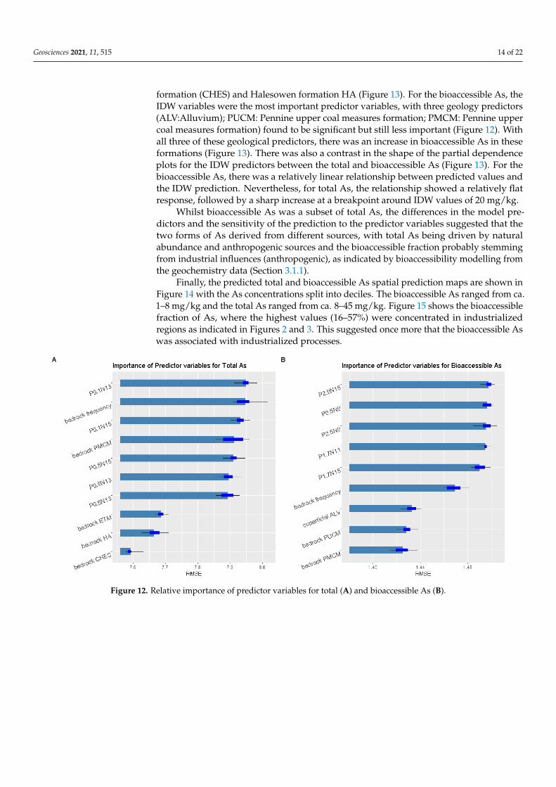
Geosciences 2021, 11, 515 14 of 22

formation (CHES) and Halesowen formation HA (Figure 13). For the bioaccessible As, theIDW variables were the most important predictor variables, with three geology predictors(ALV:Alluvium); PUCM: Pennine upper coal measures formation; PMCM: Pennine uppercoal measures formation) found to be significant but still less important (Figure 12). Withall three of these geological predictors, there was an increase in bioaccessible As in theseformations (Figure 13). There was also a contrast in the shape of the partial dependenceplots for the IDW predictors between the total and bioaccessible As (Figure 13). For thebioaccessible As, there was a relatively linear relationship between predicted values andthe IDW prediction. Nevertheless, for total As, the relationship showed a relatively flatresponse, followed by a sharp increase at a breakpoint around IDW values of 20 mg/kg.

Whilst bioaccessible As was a subset of total As, the differences in the model pre-dictors and the sensitivity of the prediction to the predictor variables suggested that thetwo forms of As derived from different sources, with total As being driven by naturalabundance and anthropogenic sources and the bioaccessible fraction probably stemmingfrom industrial influences (anthropogenic), as indicated by bioaccessibility modelling fromthe geochemistry data (Section 3.1.1).

Finally, the predicted total and bioaccessible As spatial prediction maps are shown inFigure 14 with the As concentrations split into deciles. The bioaccessible As ranged from ca.1–8 mg/kg and the total As ranged from ca. 8–45 mg/kg. Figure 15 shows the bioaccessiblefraction of As, where the highest values (16–57%) were concentrated in industrializedregions as indicated in Figures 2 and 3. This suggested once more that the bioaccessible Aswas associated with industrialized processes.

Geosciences 2021, 11, x FOR PEER REVIEW 14 of 22

Figure 11. Calibration check for spatial predictions of total (A) and bioaccessible As (B). Solid line indicates the line of equivalence, points indicate the median predicted value and error bars are ± the median absolute deviation.

Figure 12. Relative importance of predictor variables for total (A) and bioaccessible As (B). Figure 12. Relative importance of predictor variables for total (A) and bioaccessible As (B).

Geosciences 2021, 11, 515 15 of 22Geosciences 2021, 11, x FOR PEER REVIEW 15 of 22

Figure 13. Partial dependence profiles for spatial prediction of total and bioaccessible As in soil.

Whilst bioaccessible As was a subset of total As, the differences in the model predic-tors and the sensitivity of the prediction to the predictor variables suggested that the two forms of As derived from different sources, with total As being driven by natural abun-dance and anthropogenic sources and the bioaccessible fraction probably stemming from industrial influences (anthropogenic), as indicated by bioaccessibility modelling from the geochemistry data (Section 3.1.1)

Finally, the predicted total and bioaccessible As spatial prediction maps are shown in Figure 14 with the As concentrations split into deciles. The bioaccessible As ranged from ca. 1–8 mg/kg and the total As ranged from ca. 8–45 mg/kg. Figure 15 shows the bioaccessible fraction of As, where the highest values (16–57%) were concentrated in in-dustrialized regions as indicated in Figure 2 and Figure 3. This suggested once more that the bioaccessible As was associated with industrialized processes.

Figure 13. Partial dependence profiles for spatial prediction of total and bioaccessible As in soil.

Geosciences 2021, 11, x FOR PEER REVIEW 16 of 22

Figure 14. Spatial prediction of total and bioaccessible As in soil in Stoke-on-Trent along with locations of historic industry.

Figure 15. Bioaccessible fraction of As in soil in Stoke-on-Trent.

3.2.2. Lead The accuracy and precision of the total and bioaccessible Pb are shown in Figure 16

For total Pb, apart from a few outliers, the majority of the OOB-predicted values agreed with the actual values within the errors indicated by the error bars. For bioaccessible Pb, the OOB-predicted values agreed with the actual values within errors, up to ca. 180 mg/kg. At higher values, there was some evidence of a positive bias (Figure 16).

Figure 14. Spatial prediction of total and bioaccessible As in soil in Stoke-on-Trent along with locations of historic industry.

Geosciences 2021, 11, 515 16 of 22

Geosciences 2021, 11, x FOR PEER REVIEW 16 of 22

Figure 14. Spatial prediction of total and bioaccessible As in soil in Stoke-on-Trent along with locations of historic industry.

Figure 15. Bioaccessible fraction of As in soil in Stoke-on-Trent.

3.2.2. Lead The accuracy and precision of the total and bioaccessible Pb are shown in Figure 16

For total Pb, apart from a few outliers, the majority of the OOB-predicted values agreed with the actual values within the errors indicated by the error bars. For bioaccessible Pb, the OOB-predicted values agreed with the actual values within errors, up to ca. 180 mg/kg. At higher values, there was some evidence of a positive bias (Figure 16).

Figure 15. Bioaccessible fraction of As in soil in Stoke-on-Trent.

3.2.2. Lead

The accuracy and precision of the total and bioaccessible Pb are shown in Figure 16For total Pb, apart from a few outliers, the majority of the OOB-predicted values agreedwith the actual values within the errors indicated by the error bars. For bioaccessible Pb,the OOB-predicted values agreed with the actual values within errors, up to ca. 180 mg/kg.At higher values, there was some evidence of a positive bias (Figure 16).

Geosciences 2021, 11, x FOR PEER REVIEW 17 of 22

Figure 16. Calibration check for spatial predictions of total (A) and bioaccessible Pb (B). Solid line indicates the line of equivalence, points indicate the median predicted value and error bars are ± the median absolute deviation.

Figure 17 shows the relative importance of the predictor variables for the spatial pre-diction of total and bioaccessible Pb and Figure 18 shows the partial dependence of these predictor variables. The IDW predictors were of the highest importance for both forms of Pb. There is an observably similar S shape for the partial dependence plots for the IDW predictors between the total and bioaccessible Pb (Figure 18) The similarity in the im-portance of predictor variables, the lack of importance of geological predictors, and the similarity of sensitivity to predictor variables (as shown by the partial dependence plots) suggested that both forms of lead were derived from a similar source (likely to be of in-dustrial origin, as discussed in Section 3.1.2).

Figure 16. Calibration check for spatial predictions of total (A) and bioaccessible Pb (B). Solid line indicates the line ofequivalence, points indicate the median predicted value and error bars are ± the median absolute deviation.

Geosciences 2021, 11, 515 17 of 22

Figure 17 shows the relative importance of the predictor variables for the spatialprediction of total and bioaccessible Pb and Figure 18 shows the partial dependence ofthese predictor variables. The IDW predictors were of the highest importance for bothforms of Pb. There is an observably similar S shape for the partial dependence plots forthe IDW predictors between the total and bioaccessible Pb (Figure 18) The similarity inthe importance of predictor variables, the lack of importance of geological predictors, andthe similarity of sensitivity to predictor variables (as shown by the partial dependenceplots) suggested that both forms of lead were derived from a similar source (likely to be ofindustrial origin, as discussed in Section 3.1.2).

The predicted total and bioaccessible Pb spatial prediction maps are shown in Figure 19with the Pb concentrations split into deciles. The bioaccessible Pb and total Pb both rangedfrom ca. 16–1234 mg/kg, with the highest values for both forms of Pb showing similarspatial distributions. Figure 20 shows the bioaccessible fraction of Pb which, in contrast toAs, showed lower % bioaccessibility over the more industrialised areas, indicating that itwas less environmentally mobile than As. The Pb bioaccessibility modelling (Section 3.1.2)suggested that bioaccessible Pb related to the glazes used in the ceramic industry were likelyto be less mobile. The spatial distribution of the bioaccessible fraction could be explained byhigher concentrations of the this less mobile form in areas related to ceramics production.

Geosciences 2021, 11, x FOR PEER REVIEW 17 of 22

Figure 16. Calibration check for spatial predictions of total (A) and bioaccessible Pb (B). Solid line indicates the line of equivalence, points indicate the median predicted value and error bars are ± the median absolute deviation.

Figure 17 shows the relative importance of the predictor variables for the spatial pre-diction of total and bioaccessible Pb and Figure 18 shows the partial dependence of these predictor variables. The IDW predictors were of the highest importance for both forms of Pb. There is an observably similar S shape for the partial dependence plots for the IDW predictors between the total and bioaccessible Pb (Figure 18) The similarity in the im-portance of predictor variables, the lack of importance of geological predictors, and the similarity of sensitivity to predictor variables (as shown by the partial dependence plots) suggested that both forms of lead were derived from a similar source (likely to be of in-dustrial origin, as discussed in Section 3.1.2).

Figure 17. Relative importance of predictor variables for total (A) and bioaccessible Pb (B).

Geosciences 2021, 11, 515 18 of 22

Geosciences 2021, 11, x FOR PEER REVIEW 18 of 22

Figure 17. Relative importance of predictor variables for total (A) and bioaccessible Pb (B).

Figure 18. Partial dependence profiles for spatial prediction of total and bioaccessible Pb in soil.

The predicted total and bioaccessible Pb spatial prediction maps are shown in Figure 19 with the Pb concentrations split into deciles. The bioaccessible Pb and total Pb both ranged from ca. 16–1234 mg/kg, with the highest values for both forms of Pb showing similar spatial distributions. Figure 20 shows the bioaccessible fraction of Pb which, in contrast to As, showed lower % bioaccessibility over the more industrialised areas, indi-cating that it was less environmentally mobile than As. The Pb bioaccessibility modelling (Section 3.1.2) suggested that bioaccessible Pb related to the glazes used in the ceramic industry were likely to be less mobile. The spatial distribution of the bioaccessible fraction could be explained by higher concentrations of the this less mobile form in areas related to ceramics production.

Figure 18. Partial dependence profiles for spatial prediction of total and bioaccessible Pb in soil.

Geosciences 2021, 11, x FOR PEER REVIEW 19 of 22

Figure 19. Spatial prediction of total and bioaccessible Pb in soil in Stoke-on-Trent along with locations of historic industry.

Figure 20. Bioaccessible fraction of Pb in soil in Stoke-on-Trent.

3.3. Relationship with Industry The Coal Measures, which underlie the city, are naturally elevated in many PHE such

as As, V, Mo, Cu, Ni, Zn, Pb [8]. The high concentrations of Pb in particular areas are a likely result of its use as a key constituent in pottery making. English earthenware pottery in the 18th century typically contained PbO (50%wt) compared to 30% in the medieval era [39]. Lead was a key constituent of pottery glazes, acting as a flux, as it was easily and

Figure 19. Spatial prediction of total and bioaccessible Pb in soil in Stoke-on-Trent along with locations of historic industry.

Geosciences 2021, 11, 515 19 of 22

Geosciences 2021, 11, x FOR PEER REVIEW 19 of 22

Figure 19. Spatial prediction of total and bioaccessible Pb in soil in Stoke-on-Trent along with locations of historic industry.

Figure 20. Bioaccessible fraction of Pb in soil in Stoke-on-Trent.

3.3. Relationship with Industry The Coal Measures, which underlie the city, are naturally elevated in many PHE such

as As, V, Mo, Cu, Ni, Zn, Pb [8]. The high concentrations of Pb in particular areas are a likely result of its use as a key constituent in pottery making. English earthenware pottery in the 18th century typically contained PbO (50%wt) compared to 30% in the medieval era [39]. Lead was a key constituent of pottery glazes, acting as a flux, as it was easily and

Figure 20. Bioaccessible fraction of Pb in soil in Stoke-on-Trent.

3.3. Relationship with Industry

The Coal Measures, which underlie the city, are naturally elevated in many PHE suchas As, V, Mo, Cu, Ni, Zn, Pb [8]. The high concentrations of Pb in particular areas are alikely result of its use as a key constituent in pottery making. English earthenware potteryin the 18th century typically contained PbO (50%wt) compared to 30% in the medievalera [39]. Lead was a key constituent of pottery glazes, acting as a flux, as it was easilyand cheaply obtained, had a wide firing temperature range [40], gave good even coveragewithout fingerprints, prevented crazing and produced brilliant white colour [41]. Lead isalso often used in steel production to improve machinability [42]. The steel workings acrossStoke-on-Trent and the subsequent use of waste materials for infill material are potentialcontributors to the dispersal of Pb across the area (Figure 19).

Compared to the distribution pattern of Pb the maps of total and bioaccessible Asare more diffuse in nature, reflecting the natural background concentrations associatedwith the underlying coal measures [43]. High concentrations of total As (>35 mg/kg) werefound in Longton near a brick and pipe works and in the surrounding area, in Tunstalland around the Chatterley Whitfield coal workings (Figure 14). Sites with bioaccessibleAs concentrations greater than 7.4 mg/kg were dotted across the area. In particular, highconcentrations were seen at locations of gas and Al works, tile works, brick works andpotteries. However, the bioaccessible concentrations were significantly lower than thetotal concentrations.

The pattern of PHE distribution along the railway lines (WCML, NSR, potteries loopline) served to highlight the association of the presence of Pb in surface soil with thetransport of materials to and from industrial activities, e.g., coal, metal production andpottery. Figures 14 and 19 show the close proximity of a range of industrial activities acrossStoke-on-Trent. Sites of previous pottery making were often co-located with gasworks,foundries, tileworks and brickworks sites. For example, in Etruria, the potteries were closelyassociated with a foundry; in Hanley, with a colliery and a foundry and, in Middleport, apottery and brick/tileworks.

Geosciences 2021, 11, 515 20 of 22

The Stoke-on-Trent Brownfield register for 2021 [44] showed a large number of siteson or close to sites with high concentrations of both total and bioaccessible Pb, primarilynear pottery locations, in the east of Etruria and north east of Longport.

4. Conclusions

A combination of laboratory-based bioaccessibility testing, understanding contami-nants’ chemical forms and spatial geochemistry (with land use information) was used tohighlight the impact of historical land use and industrial activities on human exposure toPHE in cities. The bioaccessibility maps represent an important resource for contaminatedland risk assessments and land use planning and could be applied as a standard approachfor urban centres. Inclusion of predictive bioaccessible fraction mapping provides anindication of the relative mobility of PHE compared to the total PHE concentrations on awider spatial scale.

This study examined how the combination of RF with IDW predictors could be usedto produce spatial prediction models of the total and bioaccessible fractions of poten-tially harmful elements in an urban environment with quantitative assessment of accu-racy and precision. For the purposes of risk assessment, however, the outcomes of themodels—namely, the predicted bioaccessible and bioaccessible fractions of As and Pb andtheir associated uncertainty—were the key measurements arising from the study. Thesedata can be directly used in risk assessment models.

The lack of mineral deposits of Pb and As in the area suggested that the surfacecontamination was a result of industrial activity. The distribution of As and Pb was mostlikely driven by industrial activity across Stoke-on-Trent, which is interlinked throughtransport routes, some of which were specific to particular industries and the linkagesbetween them (e.g., the potteries loop lines, minerals railways and canals). Widespreaddistribution can be attributed to the plethora of mining activities across the region.

Author Contributions: Conceptualization, methodology, formal analysis, writing—original draftpreparation, writing—review and editing J.W. and M.C.; software, M.C. All authors have read andagreed to the published version of the manuscript.

Funding: This research received no external funding.

Data Availability Statement: Total element data from the GSUE sampling programme are availableas part of the UK Open Government License.

Acknowledgments: This paper is published with the permission of the Director of the British Geo-logical Survey (Natural Environment Research Council). The contribution of all BGS staff involvedin the collection and analysis of samples from the G-BASE survey is gratefully acknowledged. Theauthors would like to thank the BGS geochemistry laboratories for preparing and analyzing thesamples and Antonio Ferreira for his internal review and suggested edits.

Conflicts of Interest: The authors declare no conflict of interest.

References1. Cave, M.R.; Wragg, J.; Dentys, S.; Jondreville, C.; Feidt, C. Oral Bioavailability. In Dealing with Contaminated Sites, from Theory

towards Practical Application; Springer: Berlin/Heidelberg, Germany, 2011; pp. 287–324.2. Cave, M.; Wragg, J. Application of Bioavailability Measurements in Medical Geology. In Practicalities of Medical Geology; Springer:

Berlin/Heidelberg, Germany, 2021; pp. 235–262.3. Office for National Statistics. Estimates of the population for the UK, England and Wales, Scotland and Northern Ireland.

Available online: https://www.ons.gov.uk/peoplepopulationandcommunity/populationandmigration/populationestimates/datasets/populationestimatesforukenglandandwalesscotlandandnorthernireland (accessed on 24 January 2021).

4. Barker, D. The industrialization of the Staffordshire potteries. In The Archaeology of Industrialization; Routledge: London, UK, 2020;pp. 203–221.

5. Henrywood, R.K. Staffordshire Potters, 1781–1900: A Comprehensive List Assembled from Contemporary Directories with Selected Marks;Antique Collectors’ Club: Woodbridge, Suffolk, UK, 2002.

6. MacCarthy, F.; Tisdale, R.; Ayers, W. Geological controls on coalbed prospectivity in part of the North Staffordshire Coalfield, UK.Geol. Soc. Lond. Spec. Publ. 1996, 109, 27–42. [CrossRef]

Geosciences 2021, 11, 515 21 of 22

7. Wilson, A.; Rees, J.; Crofts, R.; Howard, A.; Buchanan, J.; Waine, P. Stoke-on-Trent: A Geological Background for Planning andDevelopment. 1992. Available online: http://nora.nerc.ac.uk (accessed on 13 May 2021).

8. Fordyce, F.; Ander, E. Urban Soils Geochemistry and GIS-Aided Interpretation: A Case Study from Stoke-on-Trent. 2003. Availableonline: http://nora.nerc.ac.uk/id/eprint/7018/ (accessed on 13 May 2021).

9. Chapman, N. The South Staffordshire Coalfield; The History Press: Gloucester, UK, 2005.10. Baker, A.D. The Potteries Loop Line; Trent Valley Publications: Manchester, UK, 1986.11. Gidlow, C.; Ellis, N.; Smith, G.; Fairburn, J. Promoting Green Space in Stoke-on-Trent (ProGreSS). Young Child. 2010, 4, 113.12. Scrucca, L.; Fop, M.; Murphy, T.B.; Raftery, A.E. Mclust 5: Clustering, classification and density estimation using Gaussian finite

mixture models. R J. 2016, 8, 289. [CrossRef] [PubMed]13. R Core Team. R: A Language and Environment for Statistical Computing; Foundation for Statistical Computing: Vienna, Austria, 2020.14. Denys, S.; Caboche, J.; Tack, K.; Rychen, G.; Wragg, J.; Cave, M.; Jondreville, C.; Feidt, C. In Vivo Validation of the Unified

BARGE Method to Assess the Bioaccessibility of Arsenic, Antimony, Cadmium, and Lead in Soils. Environ. Sci. Technol. 2012,46, 6252–6260. [CrossRef]

15. Wragg, J.; Cave, M.; Basta, N.; Brandon, E.; Casteel, S.; Denys, S.; Gron, C.; Oomen, A.; Reimer, K.; Tack, K.; et al. An inter-laboratory trial of the unified BARGE bioaccessibility method for arsenic, cadmium and lead in soil. Sci. Total. Environ. 2011,409, 4016–4030. [CrossRef]

16. Middleton, D.R.; Watts, M.J.; Beriro, D.J.; Hamilton, E.M.; Leonardi, G.S.; Fletcher, T.; Close, R.M.; Polya, D.A. Arsenic inresidential soil and household dust in Cornwall, south west England: Potential human exposure and the influence of historicalmining. Environ. Sci. Process. Impacts 2017, 19, 517–527. [CrossRef]

17. Watts, M.J.; Button, M.; Brewer, T.S.; Jenkin, G.R.; Harrington, C.F. Quantitative arsenic speciation in two species of earthwormsfrom a former mine site. J. Environ. Monit. 2008, 10, 753–759. [CrossRef] [PubMed]

18. Wragg, J. BGS Guidance Material 102, Ironstone Soil, Certificate of Analysis; IR/09/006; British Geological Survey: Keyworth,Nottingham, UK, 2009.

19. Hamilton, E.M.; Barlow, T.S.; Gowing, C.J.; Watts, M.J. Bioaccessibility performance data for fifty-seven elements in guidancematerial BGS 102. Microchem. J. 2015, 123, 131–138. [CrossRef]

20. Wright, M.N.; Ziegler, A. Ranger: A fast implementation of random forests for high dimensional data in C++ and R. J. Stat. Softw.2017, 77, 1–17. [CrossRef]

21. Kursa, M.B.; Rudnicki, W.R. Feature selection with the Boruta package. J. Stat. Softw. 2010, 36, 1–13. [CrossRef]22. Minasny, B.; McBratney, A.B. Spatial prediction of soil properties using EBLUP with the Matérn covariance function. Geoderma

2007, 140, 324–336. [CrossRef]23. Zhu, Q.; Lin, H.S. Comparing Ordinary Kriging and Regression Kriging for Soil Properties in Contrasting Landscapes. Pedosphere

2010, 20, 594–606. [CrossRef]24. Hengl, T.; Nussbaum, M.; Wright, M.N.; Heuvelink, G.B.; Gräler, B. Random forest as a generic framework for predictive

modeling of spatial and spatio-temporal variables. PeerJ 2018, 6, e5518. [CrossRef]25. Kirkwood, C.; Cave, M.; Beamish, D.; Grebby, S.; Ferreira, A. A machine learning approach to geochemical mapping. J. Geochem.

Explor. 2016, 167, 49–61. [CrossRef]26. Sekulic, A.; Kilibarda, M.; Heuvelink, G.; Nikolic, M.; Bajat, B. Random Forest Spatial Interpolation. Remote Sens. 2020, 12, 1687.

[CrossRef]27. Cave, M. A Machine Learning Approach to Geostatistics Applied to Contaminants in Soil 6D.2. In Proceedings of the 7th

International Contaminated Site Remediation Conference incorporating the 1st International PFAS Conference, Melbourne,Australia, 10–14 September 2017; pp. 330–331.

28. Vane, C.H.; Kim, A.W.; Beriro, D.; Cave, M.R.; Lopes Dos Santos, R.A.; Ferreira, A.M.; Collins, C.; Lowe, S.R.; Nathanail, C.P.;Moss-Hayes, V. Persistent Organic Pollutants in Urban Soils of Central London, England, UK. 2021. Measurement and SpatialModelling of Black Carbon (BC), Petroleum Hydrocarbons (TPH), Polycyclic Aromatic Hydrocarbons (PAH) and PolychlorinatedBiphenyls (PCB). Adv. Environ. Eng. Res. 2021, 2, 42. [CrossRef]

29. Fortin, M.-J.; Dale, M. Spatial Analysis: A Guide for Ecologists; Cambridge University Press: Cambridge, UK, 2006.30. Rawlins, B.; McGrath, S.; Scheib, A.; Breward, N.; Cave, M.; Lister, T.; Ingham, M.; Gowing, C.; Carter, S. The Advanced Soil

Geochemical Atlas of England and Wales; British Geological Survey: Nottingham, England, UK, 2012.31. Pebesma, E. sf: Simple Features for R. R J. 2018, 10, 439–446. [CrossRef]32. Team, Q.D. QGIS Geographic Information System; Open Source Geospatial Foundation Project, 2021. Available online: https:

//www.qgis.org/en/site/about/index.html (accessed on 12 January 2021).33. Jenkins. A History of the County of Stafford: Volume 8. Edited by J G Jenkins. Gives a Detailed Account of the History of Newcastle-Under-

Lyme and Stoke-on-Trent; Victoria County History: London, UK, 1963.34. Biecek, P. DALEX: Explainers for complex predictive models in R. J. Mach. Learn. Res. 2018, 19, 3245–3249.35. Cave, M.R.; Wragg, J.; Harrison, H. Measurement modelling and mapping of arsenic bioaccessibility in Northampton, UK.

J. Environ. Sci. Health Part A 2013, 48, 629–640. [CrossRef] [PubMed]36. Appleton, J.; Cave, M.; Wragg, J. Modelling lead bioaccessibility in urban topsoils based on data from Glasgow, London,

Northampton and Swansea, UK. Environ. Pollut. 2012, 171, 265–272. [CrossRef] [PubMed]37. Anheuser, K. The practice and characterization of historic fire gilding techniques. JOM 1997, 49, 58–62. [CrossRef]

Geosciences 2021, 11, 515 22 of 22

38. Hunt, L.B. Gold in the pottery industry. Gold Bull. 1979, 12, 116–127. [CrossRef]39. Tite, M.; Freestone, I.; Mason, R.; Molera, J.; Vendrell-Saz, M.; Wood, N. Lead glazes in antiquity—Methods of production and

reasons for use. Archaeometry 1998, 40, 241–260. [CrossRef]40. This Day in Pottery History. Available online: https://thisdayinpotteryhistory.wordpress.com/category/pottery-types/lead-glaze/

(accessed on 18 June 2021).41. Staffordshire County Council. Staffordshire Past Track. Available online: https://www.search.staffspasttrack.org.uk/Details.

aspx?&ResourceID=15195&PageIndex=8&SearchType=2&ThemeID=515 (accessed on 18 June 2021).42. Lead in Steel. Available online: https://www.ispatguru.com/lead-in-steels/#:~:text=Influence%20of%20lead%20on%20steels,

and%20permitting%20increased%20machine%20spee (accessed on 18 June 2021).43. Appleton, J.D.; Cave, M.R.; Wragg, J. Anthropogenic and geogenic impacts on aresenic bioaccessibility in UK topsoils. Sci. Total.

Environ. 2012, 435–436, 21–29. [CrossRef]44. Stoke-on Trent Brownfield Register. Available online: https://data.gov.uk/dataset/1368fc6f-3975-4bf1-b234-1f5d6055b7dd/

stoke-on-trent-brownfield-register (accessed on 12 January 2021).