MODELING THE UNDISCOVERED GROSS DOMESTIC ...
35
MODELING THE UNDISCOVERED GROSS DOMESTIC PRODUCT 2010/2018 2010/2018 Gross domestic product is the total value of goods produced and services provided within a country during one year. The problem is there are neither fiscal policy instruments nor records of GDP during Pagume in Ethiopia. Thus, the hypothesis is there is no relationship between the UGDP and Pagume over the long run. The general objective of the study is to model the Undiscovered GDP in Ethiopia. The specific objectives of the study are to analyze the difference between Ethiopian budget year and Gregorian budget year (modeling three categories of four years in the medium term), estimate the model of undiscovered GDP over the study period (1989-2004), determine the amount of undiscovered GDP at the base year (1988) and its growth rate and forecast the Undiscovered GDP (2005-2017). The undiscovered gross domestic product (UGDP) was generated as the product of average daily gross domestic product (actual GDP divided by 360 days) and 5 days (if the year was an ordinary) and 6 days (if the year was leap year). Next, the undiscovered gross domestic product is regressed against time over years. The findings are we reject the null hypothesis and accept the alternative that there is strong relationship between UGDP and time, as time increases by a unit UGDP increases by 402.50 millions Birr; 432.51 million Birr is the adjusted level of UGDP for the base year (1988) and the undiscovered gross domestic product increased at a 18.02 % annual rate from 1988 to 2004. Therefore, if the government amends and applies universal business income tax schedules the undiscovered Gross Domestic Product will be discovered. Undiscovered Gross Domestic Product (UGDP), Broadening income tax bases, Additional income tax revenue and Additional disposable income, Linear Trend Analysis of the UGDP model, Growth Trend Analysis of Undiscovered Gross Domestic Product, Forecasting the UGDP with Linear and Growth Trend Comparison.
-
Upload
khangminh22 -
Category
Documents
-
view
4 -
download
0
Transcript of MODELING THE UNDISCOVERED GROSS DOMESTIC ...
MODELING THE UNDISCOVEREDGROSS DOMESTIC PRODUCT
2010/20182010/2018
Gross domestic product is the total value of goods produced and servicesprovided within a country during one year. The problem is there are neitherfiscal policy instruments nor records of GDP during Pagume in Ethiopia.Thus, the hypothesis is there is no relationship between the UGDP andPagume over the long run. The general objective of the study is to model theUndiscovered GDP in Ethiopia. The specific objectives of the study are toanalyze the difference between Ethiopian budget year and Gregorian budgetyear (modeling three categories of four years in the medium term), estimatethe model of undiscovered GDP over the study period (1989-2004),determine the amount of undiscovered GDP at the base year (1988) and itsgrowth rate and forecast the Undiscovered GDP (2005-2017). Theundiscovered gross domestic product (UGDP) was generated as the productof average daily gross domestic product (actual GDP divided by 360 days)and 5 days (if the year was an ordinary) and 6 days (if the year was leapyear). Next, the undiscovered gross domestic product is regressed againsttime over years. The findings are we reject the null hypothesis and acceptthe alternative that there is strong relationship between UGDP and time, astime increases by a unit UGDP increases by 402.50 millions Birr; 432.51million Birr is the adjusted level of UGDP for the base year (1988) and theundiscovered gross domestic product increased at a 18.02 % annual ratefrom 1988 to 2004. Therefore, if the government amends and appliesuniversal business income tax schedules the undiscovered Gross DomesticProduct will be discovered.
Undiscovered GrossDomestic Product(UGDP), Broadeningincome tax bases,Additional income taxrevenue and Additionaldisposable income, LinearTrend Analysis of theUGDP model, GrowthTrend Analysis ofUndiscovered GrossDomestic Product,Forecasting the UGDPwith Linear and GrowthTrend Comparison.

1
Contents Pages1. Introduction .......................................................................................................................................... 3
1.1. Statement of the Problem ............................................................................................................3
1.2. Objectives of the study .................................................................................................................5
1.3. Significance of the study ...............................................................................................................5
1.4. Concepts of the Undiscovered Economics .....................................................................................5
2. Literature Review.................................................................................................................................. 6
2.1. Critical review of theory of time..................................................................................................... 7
2.1.1. Ancient Babylon ....................................................................................................................7
2.1.2. Ancient Greek........................................................................................................................7
2.1.3. Ancient Ethiopia....................................................................................................................8
2.1.4. Ancient Rome........................................................................................................................8
2.2. Birth of Christos ............................................................................................................................8
2.2.1. Amete Mehret and Anno Domini..........................................................................................8
2.2.2. Map of the first globe ........................................................................................................... 8
2.3. The European Renaissance ........................................................................................................... 9
2.3.1. Copernicus’ theory was not as accurate as Ptolemy’s..........................................................9
2.4. Empirical evidence ......................................................................................................................12
2.4.1. Moderate and extreme seasons .........................................................................................12
2.4.2. Recording technology .........................................................................................................13
2.4.3. Economics as Science..........................................................................................................13
2.5. Benefits of the previous literatures ..............................................................................................15
3. Methodology .......................................................................................................................................16
3.1. Descriptive and Inferential methods ..........................................................................................16
3.2. Study periods and source of data ...............................................................................................16
3.4. Model Specification ....................................................................................................................17
CHAPTER FOUR ...........................................................................................................................................19
4. RESULTS AND DISCUSSION..................................................................................................................19
4.1. Model of the Undiscovered Gross Domestic Product.................................................................19
4.1.1. Results of the Undiscovered Gross Domestic Product...................................................19
4.1.2. Linear Trend Analysis of the UGDP model ...........................................................................19
4.2. Growth Trend Analysis of Undiscovered Gross Domestic Product .....................................23

2
4.3. Forecasting the UGDP with Linear and Growth Trend Comparison..................................25
5. Conclusion and Policy Implications ................................................................................................27
5.1. Conclusion .................................................................................................................................27
5.2. Policy Implications....................................................................................................................29
6. References ..........................................................................................................................................30
7. Appendices..........................................................................................................................................32
3
MODELING THE UNDISCOVERED GROSS DOMESTIC PRODUCT
1. Introduction
1.1. Statement of the ProblemGross Domestic Product is the total value of final goods and services produced in acountry during a calendar year. GDP per person is the simplest overall measure ofincome in a country. Economic growth is measured by change in GDP from year toyear [Streak, 2003:129]. But, GDP’s definition of calendar year is too general.Because, we discovered there are two new theories of time. New theories of time arethe Tropics rotate and revolve faster than the Temperates. Consistently; there are alsotwo technologies of time1. The first technology of time that records faster day, week,month and year of Amete Mehert is called Ethiopian calendar. Whereas the secondtechnology that records slower day, week, month and year of Anno Domini is calledGregorian calendar.
Besides recording, each calendar uses to make fiscal instruments that link factors ofproduction, organization and productive labour force. For example, financialregulation of the country declared the Ethiopia’s budget year runs from 1st Hamle ofthis year to 30th Sene of next year. This budget year or fiscal year months’ use tomake fiscal policy instruments such as income tax schedules. Income tax schedules inturn use to estimate, legislate and execute activities of budget during a year, mediumperiod (4 years) and long year period (28 years). Consistently, Ethiopia’s income taxlaw verbally obliges every employer how to apply the individual income tax base of12 months such as 11 of 30 days (Meskerem to Hamle) and one special month of 35and 36 days (Nehase and Pagume).
“Employers have an obligation to withhold the tax from eachpayment to an employee, and to pay the withheld amounts to the TaxAuthority the amount withheld during each calendar month, inapplying preceding income attributable to the months of Nehase andPagume shall be aggregated and treated as the income of onemonth.” Income tax law (series of income tax laws: 1953, 1994 and2008).
Nonetheless, there are several economic, natural and social problems. The firstproblem is that neither salary income and rental income nor income tax revenue isoperational for 5 and 6 marginal days in the short run. The second problem ismoderate seasons and shorter variations of day and night of the year in which we arenaturally observing, but not recognized and institutionalized. The third problem is thecurrent growth and transformation plan (GTP) projected revenue, expenditure anddeficit neither from domestic nor external sources for a period of 26 days. The fourthproblem is the available long run/historical data of GDP represent only informationof 360 days in each fiscal year.
1According to Hackett (1983:217), using science knowledge to develop betterproducts is called technology.

4
Why all of the above economic, natural and social problems do exist? Because, thereare several organizations do use the Gregorian calendar. Thus, what are the adverseimpacts of using the Gregorian calendar in the GTP? The opportunity cost of usingthe Gregorian calendar in Ethiopia is foregoing/scarifying the use of Ethiopiancalendar in the Tropics that naturally shows more than 84% of the Earth. As a result,Pagume is known neither by English-English dictionaries nor by any Encyclopedias.
Therefore, bilingual modern dictionaries, for example, English Amharic Dictionary,excluded Pagume by adopting April is Miyazia, August is Nehase, etc. andSeptember is Meskerem. Thus the expected value of Ethiopian calendar months bothin an ordinary and leap year is 30 days, whereas, the expected value of Gregoriancalendar months in an ordinary year is 30.42 and in a leap year is 30.5 days. Thecomparison shows the statistics of Pagume does exist neither in an ordinary year norin a leap year (look at Table 1.1 in the Appendices).
As result two traditional complementary policies such as fiscal policy involvesgovernment’s powers to design tax, collect tax, spend, and borrow, and the effects ofthese activities on the economy, and monetary policy that concerned with thevolume, availability, cost and types of money, credit, foreign reserve and interest rateare neither designed nor operational during Pagume. Consequently, there are nofinancial records both by private sector and public sector (national incomeaccounting). Besides, agricultural activity in Ethiopia is naturally depends on eventsof four moderate seasons: Kermpt, Metsew, Bega and Tseday. But the impact ofusing the Gregorian calendar is hiding moderate seasons that reveal agriculturalactivities and its linkage with industry and service sectors.
Series of the above problems do exist because there are no concept of Pagume, policyinstruments, records of economics and moderate seasons. What is the primarysolution? The primary solution is discovering the statistics of Pagumeby comparingthe Ethiopian calendar and Gregorian calendar using programs (complexmathematical formula of Excel).As a result an expected value of Ethiopian calendarmonths increased from 30 days to 30.42 in an ordinary year and 30.5 days in a leapyear (look at Table 1.2 in the Appendices).
Discovering the statistics of Pagume helps to conceptualize Pagume in terms of itsnature such as days, moderate seasons, month and three categories of four years.Thus, first, Pagume is five and six faster rotations of the Tropics, where 6 to 10 and11 of September is slower rotations of the Temperates. Second, Pagume recur after30th Nehase and before 1st Meskerem. Thus we are observing that it is part of Kermptin the east-west north and Bega in the east-west south Tropics simultaneously. Third,Pagume is 5 and 6 marginal days of the year that cause it is a subset of 12th month,i.e., Nehase & Pagume has 35 days and 36 days in an ordinary and leap years.
We have been engaged in searching the economic problem of Pagume since 1992A.M. Thus discovering and conceptualizing the statistics of Pagume are a means to
5
innovate new theories and fiscal technologies. For example, we innovated neweconomics (new theories of income taxation):
Broadening income tax bases yield additional tax revenue andadditional disposable income.
To translate new theories into practices, new fiscal policy instruments have beeninnovated from the current. Two complementary employment income tax schedulesfor income tax period of 35 and 36 days (2002) and Two Universal Business Incometax Schedules for income tax period of 365 and 366 days (2005). But the furtherproblem is these new fiscal policy instruments have not been yet amended forapplication. As a result economic variables remain undiscovered. Thus, there areseveral short, medium and long period specific questions.
What is the undiscovered GDP over the study period (1989-2004)? What is the amount of GDP at the base year and its growth rate over the
study period? , and What is the forecasted undiscovered GDP for (2005-2015 A.M)?
1.2. Objectives of the study
The objectives of the study are to Estimate the model of undiscovered GDP,
Determine the amount of undiscovered GDP at the base year and itsgrowth rate.
Forecast the Undiscovered GDP (2005-2017)
1.3. Significance of the study
Its significance is that modeling the Undiscovered GDP in Ethiopia is new methodsthat use to discover new economics. It benefits not only the government but alsobusiness men. Stakeholders such as policy makers, academicians and practitionerswill be involved in the process of transforming the models into reality. It gives newknowledge and skills about two theories of time and application of Ethiopiancalendar in the Tropics and Gregorian calendar in the Temperates. It equips andexpands new knowledge and skills of economics exponentially.
1.4. Concepts of the Undiscovered EconomicsAdditional Disposable Income is disposable income of 365/366 days minusdisposable income of 360 days.Additional income tax revenue is income tax revenue of 365/366 days minusincome tax revenue of 360 days.Amete Mehert
6
Broad income tax schedule is series of seven income tax brackets and marginaltaxes that use to determine income tax bases and income tax revenue per period of360 days.Broader income tax schedule is series of seven income tax brackets and marginaltaxes that use to detrmine income tax bases and income tax revenue per period of 365days.Brodest income tax schedule is series of seven income tax brackets and marginaltaxes that use to detrmine income tax bases and income tax revenue per period of 366days.Category one is the first year in which New Year begins on Meskerem 1 and ends onPagume 5 in the Tropics, when September 12 to September 10 recurs in theTemperates.Category two is there are two years (the 2nd and 3rd),each year begins on Meskerem1 and ends on Pagume 5 in the Tropics, when September 11 to September 10 recursin the Temperates.Category three is the leap year that begins on Meskerem 1 and ends on Pagume 6,when September 11 to September 11recurs in the Temperates.Econometrics is mathematics in economics that deals with the application ofmathematical and statistical techniques to the undiscovered economic data andproblems of Pagume.Economics studies the allocation and distribution of scarce resources (land, labor,capital and entrepreneurs) so as to meet aggregate human wants per period of time.Ethiopian calendar is technology records faster units of time such as week, monthand Amete Mehret.Gregorian calendar is technology records slower units of time such as week, monthand Anno Domini.Microeconomics is branch of economics that studies how an individual units makedecision at a point of time.Macroeconomics is branch of economics that studies the performance of theeconomy in view of economic growth, distribution of income, stabilization of price,employment generation and favorable balance of payment over a period of calendaryear.Public Finance/Public Economics is applied economics that studies how optimalincome tax schedules are designed and applied to meet growth, efficiency and equitytargets of the country per period of time.Pagume is five and six faster rotation of tropical earth, when September 6 to10/11 isslower rotation of the Temperates.Undiscovered broader business income tax revenue is theoretical income taxrevenue of 365 days minus income tax revenue of 360 days. Undiscovered broadestincome tax revenue is broadest income tax revenue minus current income taxrevenue.
2. Literature ReviewIt is hardly easy to get literature that deals with the theory of the undiscovered grossdomestic product. Reviewing scientific methods of time is novelty to understand howthe knowledge of time evolved from the known sources. Besides, reviewing recentliterature that speaks about uses of calendars is useful. Finally theory of nationalincome and gross domestic product would be reviewed.

7
2.1. Critical review of theory of timeWaugh (1937:1) asserted a large portion of all human knowledge has come down tous from unknown sources. The method by which it was originally discovered is notknown. Contrary to Waugh argument, literatures show a large portion of all humanknowledge has come down to us from known sources. In the following sections wewill discuss the extraordinary source of knowledge in chronologicalorder.
2.1.1. Ancient Babylon
Babylonians was the first known source of knowledge. According to Merton(1943:172) the ancient Babylonians gave the measure for the circle. They thought thetime take the earth to make one revolution around the sun was 360 days; and hence,the distance traveled in one day would be 1/360 of a circle. They invented a calendarof 12 months of 30 days each. Besides, 360 degrees that measures the circumferenceof sphere was invented by them. Moreover, as one of the earliest known civilizations,the 6,000-year-old society of Lagash, Sumer, in present-day Iraq, taxation supportedmassive warfare.
Moreover, the Babylonians used arithmetic and simple algebra to exchange moneyand merchandise, compute simple and compound interest, calculate taxes, andallocate shares of a harvest to the state, temple, and farmer. The building of canals,granaries, and other public works also required using arithmetic and geometry.Calendar reckoning, used to determine the times for planting and for religious events,was another important application of mathematics. Finally, the division of the circleinto 360 parts and the division of the degree and the minute each into 60 partsoriginated in Babylonian astronomy. The Babylonians also divided the day into 24hours, the hour into 60 minutes, and the minute into 60 seconds.The Babylonians devised tables of reciprocals (numbers that yield 1 whenmultiplied, such as 3 and 1/3), tables of squares and square roots, tables of cubes andcube roots, and tables of compound interest.
2.1.2. Ancient Greek
Ancient Greek was the second known source of knowledge. Parmenides (Greekphilosopher) divided the world into five zones, by lines of latitude (using 360 ° ofancient Babylon) in the 5th century BC. Those five zones were a torrid zone betweenthe Tropic of Cancer (about 23 .5° N) and the Tropic of Capricorn (about 23 .5° S);the north and south Temperate zones between the Tropics and the polar circles (66.5° N and S); and the north and south frigid zones, which lie between the polar circlesand the poles. Although, Parmenides was the first man who brought down 360degrees of Babylon, classifying north and south Tropics as one zone was capitalmistake.
Moreover, it is the greatest substance that the ancient Greeks added 5.25 days to theBabylonians’ 360 days. Thus, they discovered an average solar year - time taken forthe Earth to move around the Sun, is equal to 365.25 days in 519 Amete Feda.Barnett (1980:129) explains in 240 A.F Eratosthenes measured the circumference ofEarth at the equator is 40,046.6 km on Sene 14 when the sun is overhead at theTropic of Cancer.

8
Archimedes, the greatest mathematician of antiquity, produced theorems oncomplicated areas and volumes and proved them rigorously. Archimedes measuredsurface area of earth from the equator that amounts 511,248,288.6 square km[ = 4 ( ) ; where pie or constant number of 22/7 and r is radius ofearth at the equator].
Hipparchus (190-120 A.F) discovered the precession of the equinoxes. The conceptequinox is time of equal day and night, either of the two annual crossings of theequator by the Sun, once in each direction, when the lengths of day and night areapproximately equal everywhere on Earth on Meskerem 13 and Megabit 12. Hiscalculation of the tropical year, the length of the year measured by the sun, waswithin 6.5 minutes of modern measurements. He devised a method of locatinggeographic positions by means of latitudes and longitudes.
2.1.3. Ancient EthiopiaConsistent to the series of the above source of knowledge, the Ethiopian calendar thatconsists 12 months of 30 days in which 11 of 30 days (Meskerem to Hamle) and 1special month of 35 and 36 days (Nehase and Pagume) and 7 days of week was madein 519 A.M. It has been called three categories of four years calendar since 519 A.F.(Fassil Tassew, 2005:67-113,160).
2.1.4. Ancient RomeBrandwein (1970:457) explained the Julian calendar was made in 46 B.C. based onan average solar year of 365.25 days. The arrangement of 12 months of the Juliancalendar was not scientific in such a way that Julius Caesar’s successor, Augustus
Caesar, retained the Julian calendar but changed the names of 7th
and 8th
months toJuly and August. He also gave 31 days to each of them by taking two days fromFebruary. The names of the days are based on the seven heavenly bodies used intraditional astrology (the sun, the moon, Mars, Mercury, Jupiter, Venus, and Saturn).The seven-day week became part of the Roman calendar in 321A.D.
2.2. Birth of ChristosOne of the most recognized source of modern knowledge which we use universally isthe point of the birth of Christos. Waugh (1937:281) writes that time is reckonedfrom the birth of Christ.
2.2.1. Amete Mehret and Anno DominiGetachew Haile (2006:23) explained the time period since the birth of Christos iscalled Amte Mehert (A.M) in the Ethiopian calendar and where it is called AnnoDomini (A.D) in the Julian and currently in the Gregorian calendar. Thus Christoswas born Maksegnoelt, Meskerem 1,0 A.M. but according to the Julian calendar, itwas Tuesday, September 12, 7 A.D.
2.2.2. Map of the first globeRogers (1979:49) explains the first people who really made a science of map makingwere the ancient Greeks. During the 100s Amete Mehret, Ptolemy compiled mostGreek geographic knowledge up to his time. He divided the equatorial circle into 360

9
degrees and constructed an imaginary north-south, east-west network over the surfaceof the earth to serve as a reference grid for locating the relative positions of knownlandmasses, such as islands and continents. Therefore, it is worth noting that Ptolemycontributed useful descriptions and maps of the known world that includes Ethiopiainterior in south Tropic (look at Figure 2.1 below).
Besides, scientific literature of Doresse (1967:28) shows the king of Aksum who hadan extensive area under his direct control, were in trading relations with Egypt byway of the Nile about the middle of the first century.
2.3. The European RenaissanceAdditional knowledge was made during the European Renaissance.Renaissance wasthe period of time in Europe between the 14th and 17th centuries, when the art,literature, and ideas of ancient Greece were discovered again and widely studies,causing a rebirth of activity in all these things.
2.3.1. Copernicus’ theory was not as accurate as Ptolemy’sKuhn (1962:154) explained Copernicus’ theory was not more accurate thanPtolemy’s and did not lead directly to any improvement in the calendar. Therefore,according to Kuhn, two problems can be detected from the second map of earth andcalendar of the Gregorian that were made during the European Renaissance.The first problem is detected from the second world map which was made in 1540A.D. Second world map referred to the map that were made next to Ptolemy’s.Nevertheless, Figure 2.2 reveal the Western Half of the World does exclude the entireTropics by measurement of degrees. Because, for example, as you see from the globebelow 75°W and 135° W which are written in the western north Caribbean Sea andPacific Ocean(west north Tropic) exist neither by nature nor by default.

10
Therefore, it is natural the imaginary daylight line that connects 23.5°EN and 156.5°WS is traditionally called Tropic of Cancer, and now it is called Sene 14. Besides, theimaginary daylight line that connects 0° East and 180° west traditionally is called anEquator, now it is called Meskerem 13. Thus the drawer of the second world mapshould have known surface area of west north Tropic is in the range of degreesbetween 156.5°EN and 180° W.
The second problem which were made during the European Renaissance is that theGregorian calendar has been deformed from the Julian since October 5, 1582 A.D.Nowadays we are observing several scandals in the Gregorian calendar. Firstly, anaverage solar year cannot be less than 365.25 days; secondly, they did not cancel 11days; thirdly, they violated the rule of three categories of four years, because theymade leap year day in category one and also at the end of their secondmonth’s(February 28 changed to February 29), fourthly, they did and do not makeclock and watch that use to record slower motion of seconds, minutes and hours thatrecur in the Temperates and fifthly their prescription of canceling a day in every fourhundred years from their calendar is neither natural nor scientific.
Despite the above scandals, the Gregorian calendar benefited us two fundamentalelements of time. First, the Gregorian calendar rediscovered five optimum days of theTemperates such as end of June 21, September 23, December 21, March 21 and June21 that reveal the cycle of extreme seasons in a year. Second, the Gregorian calendarhas invented name of English week from the Julian week since 1752 A.D.
Although the units of time recorded on the calendar are week, day of month andAmete Mehert, the source of week was unknown. For example, week (from Latinvicis,”change”) is period of seven days now in universal use as a division of time.According to the western literature, the source of week is Hebrew. It is Hebrew orChaldean origin and is mentioned as a unit of time in the Bible (Genesis 29:27). On

11
the contrary, it has been known that a Biblical ‘time’ or year =12*30 days=360(Rev.11.2, 3:6, 14).Those contradictions guided us to discover the source of week. According to theprecision of three categories of four years (Ethiopian calendar), the source of week isan average solar year of 365.25 days. Number of days of Pagume 6 is equal to 0.25times number of years. Thus 7 days emanate from Pagume 6, because 6 hours ofPagume 6 multiplied by 28 years. Therefore, week has been known since 519 A.F.but, the Problem is week of Geze such as Segno through Ehud does show neitheretymological meaning of 24 hours nor 12 hours of night and 12 hours of daylight.The second problem is the symbol of Geze number is not scientific. Besides itexcluded the beginning year of category one or number 0. Effects of the firstproblem is that interpreter of English dictionary interprets Segno through Ehud asMonday through Sunday.
It is necessary to learn and know that English people innovated English week bysuffixing the word day upon the Julian week. English week are Sunday (Sol),Monday (Moon), Tuesday (Tui, the Saxon Mars), Wednesday (Woden, or Mercury),Thursday (Thor, or Jupiter), Friday (Frygga, or Venus), and Saturday (Saturn)—come from Roman or Norse names for the planets. English week which has beeninnovated and used since 1752 A.D. reveal etymological meaning of each week daythat one rotation of earth that has 12 hours daylight and 12 hours night.
Barnett (1980:232) describes that the development of the Cartesian coordinate systemrepresented a very important advance in mathematics, it was through the use of thissystem that Rene Descartes (1596-1650), a French philosopher-mathematiciantransformed geometric problems requiring long tedious reasoning into algebraicproblems that could be solved almost mathematically. This joining of algebra andgeometry has now become known as analytic geometry.
Lewis (1999:120) explains that astronomer is built on Greek astron, star, and nomos,arrangement, law or order. The astronomer is interested in the arrangement of starsand other celestial bodies. The science is astronomy and the adjective isastronomical. A word often used in non-heavenly sense, as in “the astronomical sizeof the national debt”. Astronomy deals in such enormous distances (the sun, forexample, is 148,800,000 kilometers from the equator, and light from the stars travels297,600 km per second) that the adjective astronomical is applied to anytremendously large figure.
Daniel (1956:144) describes how the measurement of weight depends on earth. Thushe defined the weight of a body is the force (or pull) with which the body and theEarth attract each other. To understand what this means we have to know somethingabout this force of attraction which exists between Earth and bodies on or above theEarth’s surface, called the force of gravity. Isaac Newton (1642-1727), explains howobjects move on Earth as well as through the heavens (Mechanics). His mathematicalinsights led him to invent the area of mathematics called calculus (which Germanmathematician Gottfried Wilhelm Leibniz also developed independently). Inventionof calculus gave science one of its most versatile and powerful tools.
Roazzi (2005:169) explained Einstein’s theory of relativity as follows.

12
“In Einstein’s theory of relativity, he discusses time and space to be so closelyassociated that they are inseparable. It’s like having a dog that is half collie andSt. Bernard, but you cannot separate the collie half from the St. Bernard half.That is how closely space and time are associated. They call it a space-timecontinuum. In fact, no physicist today uses the word ‘space’ or ‘time’independent of each other anymore. The space-time continuum adds the fourthdimension to what we know as a three-dimensional world. This is where it getssticky, because our minds cannot comprehend a four-dimensional world. Infact, we cannot even explain it using the language of English, but it is easilyexplained with the language of mathematics”.
Brandwein (1960:154) explained that west northern people unified 24 hours of theGreek and 360 degrees of the Babylon at the equator in 1884 A.D.
“In 1884, at the Washington Meridian Conference, the nations of theworld agreed to divide the earth into time zones based on lines oflongitude 15 degrees apart. Since 360 divided by 15 equals 24, you couldsee that each time zone marks one hour of a day’s time. As the earthrotates, one hour passes for every 15 degrees of earth’s surface that goesby a given point”.
The critic here is that the above agreement holds true only on the longestcircumference which is called an equator. We know in 24 hours the earth makes onerotation. Thus, if they have known one hour passes for every 13.76 degrees of earth’ssurface at the Tropic of Cancer or Capricorn and 5.98 degrees of earth’s surface atthe Arctic or Antarctic Circle, they would have prescribed use of the Gregoriancalendar in the Tropics.
2.4. Empirical evidence
2.4.1. Moderate and extreme seasonsModerate and extreme seasons are annual cycles caused by Earth’s faster and slowerrotations and revolution to its longer and long orbits around the Sun. Earth makes onecomplete orbit in one year of 365.25 days, the Tropics rotate and revolve faster thanthe Temperates. Thus, events of moderate and extreme seasons in the Tropics andTemperates are naturally observed.
But traditional divisions of seasonal year by the west-north people were concernedonly extreme seasons of the Temperates. For example, summer, autumn, winter andsprings are extreme seasons in north Temperate. Thus moderate seasons of theTropics remain undiscovered. Because Grisdale (1965:33) erratically concluded thatthere are only two seasons, a dry season and a rainy season. He partially andextraordinarily discovered how Ethiopians are to be regarded with suspicion aboutmoderate seasons as follows.
“In Ethiopia there is a misleading tendency to call the 'RainySeason'-the Northern Summer-'Kermpt' meaning winter, because theclimate is more unpleasant in this season. This tendency should bechecked; instead of using the terms winter and summer it is better to
13
use more meaningful expressions 'Rainy Season' and 'Dry Season',remembering whilst so-doing what we truly mean by the seasons".
He observed that Kermpt cannot be called summer. His partial discovery is worthnoticing. Because moderate season is a period for particular activity or a period of theyear during which a particular activity usually takes place in the tropical humanworld or among plants and animals of equatorial rain forest regions.
2.4.2. Recording technology
Brandwein (1970:463) asserts a calendar records the number of times Earth rotateson its axis during one revolution around the sun-about 365.25 times. Grisdale(1965:37) compared the Ethiopian calendar and the Gregorian calendar withreference to leap year, the fourth year, which February has 29 days instead of theusual 28, and the month of Pagume has 6 days instead of 5.
Musgrave (1959:504) explains the information in the schedule is of some interest, buthas no operational meaning unless they could translate into calendar terms theconcept of a period. This statement shows the information written in the income taxschedule cannot be described unless one does know the period of time in thecalendar.
2.4.3. Economics as ScienceHanson (1967:5) writes that economists, like other scientists, observe facts, selectand classify them, and make them the basis for generalizations. Economic laws arebased on the deductions of pure theory, and so state only what will happen if certainassumed conditions are fulfilled. As in other sciences, certain assumptions are made,though some of the assumptions of economics are not realistic, as. For example, theassumption that people in their economic activity are always perfectly rational intheir behavior. Whereas, too, the practical scientist can conduct his experiments in hislaboratory, the economist, like other social scientists, has to study his special aspectof human behavior in the world at large. In principle, however, what is true of allscientific laws is also true of economic laws. Thus there is no fundamental differencebetween economics and other sciences.
Robert (1968:2-3) defined Economics is the study of a process we find in all humansocieties- the process of providing for material well-being of society. In the simplestterms, economics is the study of how man earns his daily bread. Yet, if man does notlive by bread alone, it is obvious that he cannot live without bread. Like every otherliving thing, the human being must eat- the imperious first rule of continuedexistence. And this first prerequisite is less to be taken for granted than it firstappears, for human organism is not, in itself, a highly efficient mechanism forsurvival. From each hundred calories of food it consumes, it can deliver only abouttwenty calories of mechanical energy. On a decent diet, man can produce just aboutone horsepower-hour of work daily, and with this he must replenish his exhaustedbody. With what is left over, he is free to build a civilization.
OrioGiarini (2011:30) confirmed economics has been developed for over twocenturies on the basis of the cultural background of a “static” Newtonian notion of
14
time/space, which goes hand in hand with the assumption of certainty (as anacceptable, achievable goal) that still dominates today’s thinking.
Microeconomics is a branch of economics that studies how an individual makedecision at a point of time. Where macroeconomics studies the performance of theeconomy, price stability, full employment and favorable balance of payment over aperiod of time. Tian (2006:14) asserted that modern economics developed in last fiftyyears. It systematically studies individuals' economic behavior and economicphenomena by the scientific studying method observation-theory –observation- andthrough the use of various analytical approaches. An economic theory, which can beconsidered an axiomatic approach, consists of a set of assumptions and conditions, ananalytical framework, and conclusions (explanations and/or predications) that arederived from the assumptions and the analytical framework. Like any science,economics is concerned with the explanation of observed phenomena and also makeseconomic predictions and assessments based on economic theories. Economictheories are developed to explain the observed phenomena in terms of a set of basicassumptions and rules. Microeconomic theory aims to model economic activities asthe interaction of individual economic agents pursuing their private interests (ibid:15).
Macroeconomics studies about the performance of the general economy in such away that how economic growth (GDP changes), employment generation, equitabledistribution of income, price stabilization and favorable balance of payment of thecountry are targeted and achieved over a period of time. Gross Domestic Product(GDP), the total value of goods and services produced in a country over a period oftime. GDP may be calculated in three ways: (1) by adding up the value of all goodsand services produced, (2) by adding up the expenditure on goods and services at thetime of sale, or (3) by adding up producers’ incomes from the sale of goods orservices. Total income of nation is the total money earned or gained by all residentsof a country over a period of time, including income from rent, profits, interest,government benefits, salaries, and wages. National Incomeis, in the theory of economics, the total net income earned by the people of a countryin producing the national output of goods and services over a period of time, usuallya calendar year. However, it is difficult to measure GDP precisely, partly becauseevery country has an unofficial economy, often called a black economy that consistsof transactions not reported to government.
Mankiw (2004:21) stated economists involve in rigorous science and policy advisor.When economists attempt to explain the world as it is, they act as scientists. Wheneconomists attempt to improve the world, they act as policy advisors. Thus policyadvisor makes one of the most known policy instrument of the government is calledfiscal policy.
The purpose of fiscal policy is not only to manage government revenue andexpenditure but also to make equal distribution of resources among the society. The

15
most traditionally applied fiscal policy tool is called progressive income taxschedules. The first income tax bracket is the principal element of progressiveincome tax schedule; it determines income necessary for subsistence existence is freefrom taxation. Income level free from tax is alike to the consumer budget line.Besides the first income tax brackets, there are series of income tax brackets andmarginal taxes that use to address distribution of income among the society.Therefore, progressive income tax schedule links microeconomics andmacroeconomics in Ethiopia (Getnet, 2008:27).
2.5. Benefits of the previous literaturesEvidences of the above literatures show us there are two recording technology oftime. Ethiopian calendar is the image of Tropics and sun (the first solar calendar yearthat consists of three categories of four years: three ordinary years, each has 365 daysand a leap year with 366 days or Pagume 6, 12 months such as 11 of 30 days -Meskerem to Hamle and 1 of 35 and 36 days-Nehase and Pagume and 7 days ofweek has been invented since 519 Amete Feda), where the Gregorian calendar whichhas been deformed from the Julian calendar ( was made in 46 B.C.) since 1582 A.D.is the image of Temperates and sun.
We could be able to understand that two solstices such as Sene 14 and Tahisas 12 andtwo equinoxes such as Meskerem 13 and Megabit 12 of the Tropics were discoveredby Parmenides and Hipparchus respectively. Thus, according to the precision ofEthiopian calendar forecasting power, Jesus Christos was born at the end of Segnoelt,Pagume 6,6019 A.F. and beginning of Maksegnoelt, Meskerem 1, 0 A.M. Butaccording to the Julian calendar he was born on Tuesday, September 12, 7 A.D.Therefore, it is an automatic to discover that the Julian calendar excluded sevenyears such as the first three categories of four years (0,1, 2 and 3) and three years (4,5and 6 years) from the second category.
We can imagine that Newton’s outstanding contribution enabled the English peopleto invent English week. Thus innovating Amharic week from Geze is necessary andvery simple. Elt is the concept of time in Amharic language that shows one fasterrotation of earth in which 12 hours of qune, i.e. daylight and 12 hours of lelit, i.e.night. Suffixing elt on the Geze week yield Amharic week such as Segnoelt throughEhudelt (look at Table 2.1 in the appendices).
The second uses of calendars are recording moderate and extreme seasonsduring one faster and slower revolution. Therefore, five optimum days in theTropics are called end of Sene 14, Meskerem 13, Tahisas 12, Megabit 12 andSene 14. Whereas five optimum days in the Temperates are called the end ofJune 21, September 23, December 21, March 21 and June 21.
The third uses of calendars are to make other technologies such as machines andfiscal policy instruments. Gregorian calendar is an example for making machineriesand Ethiopian calendar is an example for making fiscal policy instruments. The forthuses of calendars are to plan, legislate, execute and monitor activities.

16
3. Methodology
3.1. Descriptive and Inferential methodsInformation used for problem solving is called data. Descriptive statistics involvegathering, categorizing, analyzing and presenting data. Thus we use descriptivestatistics to discover moderate seasons and extreme seasons, to derive 48 months ofthe medium term period and to calculate seven steps additional income tax revenueand disposable income for an ordinary year and leap year respectively.
Inferential statistics deals with analysis of a sample data in order to infer about thepopulation. We use inferential analysis to estimate the undiscovered gross domesticproduct, test the hypothesis (slope of UGDP is zero), estimate the UGDP in the baseyear, discover its growth rate and forecast the undiscovered gross domestic product.
3.2. Study periods and source of data
There are three study periods. The first is the short run or one year, 1stHamle to30thSene.It is called 6 hours of Pagume 6.Thus, in the short run, there are two-twofour moderate symmetrical seasons recur in the Tropics from end of Sene 14 to Sene14, where two-two four extreme symmetrical seasons recur in the Temperates fromend of June 21 to June 21. The second period is medium term period or threecategories of four years or it is called a day of Pagume 6. The third period is the longrun period that cover 16 years (1989 to 2004), and when the long run period isextended to 28 years, it is called week of Pagume 6.
The source short run and medium term data are the current theoretical income taxschedule C, calendar of Ethiopia and calendar of Gregorian and date website. Thesource of long term time series data are national income accounts of different fiscalyears from Central Statistical Office and series of Ethiopian calendar.
3.3. Producers or Research DesignThe multipliers of UGDP are 5 and 6, when the reference years an ordinary and leapyear respectively. Leap year is unique year that has 366 days. Here linear equation ofleap year is used to determine the multiplier.= 0.25 + 0.25Where y is dependent variable that represents the number of series of year and x is anindependent variable that represents the number of leap year. We substitute thenumber of any year in the variable x and solve for the variable y, if the result is aninteger, that year is leap year, otherwise it is an ordinary year.
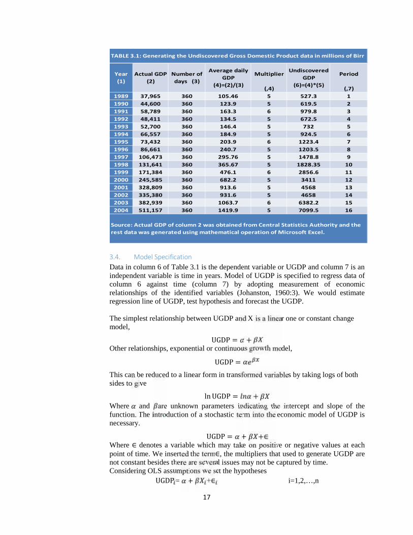
Therefore, four steps are involved to generate the UGDP data. Collect the actual data,calculate the average daily actual gross domestic product as the ratio of actual grossdomestic product data to 360 days; determine the multiplier whether it is 5 or 6 days,and multiply the result of the second step by the multiplier so as to generate theUndiscovered Gross Domestic Product [please refer TABLE 3.1].
17
3.4. Model SpecificationData in column 6 of Table 3.1 is the dependent variable or UGDP and column 7 is anindependent variable is time in years. Model of UGDP is specified to regress data ofcolumn 6 against time (column 7) by adopting measurement of economicrelationships of the identified variables (Johanston, 1960:3). We would estimateregression line of UGDP, test hypothesis and forecast the UGDP.
The simplest relationship between UGDP and X is a linear one or constant changemodel, UGDP = +Other relationships, exponential or continuous growth model,UGDP =This can be reduced to a linear form in transformed variables by taking logs of bothsides to give ln UGDP = +Where and are unknown parameters indicating the intercept and slope of thefunction. The introduction of a stochastic term into the economic model of UGDP isnecessary. UGDP = + +∈Where ∈ denotes a variable which may take on positive or negative values at eachpoint of time. We inserted the term∈, the multipliers that used to generate UGDP arenot constant besides there are several issues may not be captured by time.Considering OLS assumptions we set the hypothesesUGDP = + +∈ i=1,2,…,n
Multiplier Period
(,4) (,7)1989 37,965 360 105.46 5 527.3 11990 44,600 360 123.9 5 619.5 21991 58,789 360 163.3 6 979.8 31992 48,411 360 134.5 5 672.5 41993 52,700 360 146.4 5 732 51994 66,557 360 184.9 5 924.5 61995 73,432 360 203.9 6 1223.4 71996 86,661 360 240.7 5 1203.5 81997 106,473 360 295.76 5 1478.8 91998 131,641 360 365.67 5 1828.35 101999 171,384 360 476.1 6 2856.6 112000 245,585 360 682.2 5 3411 122001 328,809 360 913.6 5 4568 132002 335,380 360 931.6 5 4658 142003 382,939 360 1063.7 6 6382.2 152004 511,157 360 1419.9 5 7099.5 16
Source: Actual GDP of column 2 was obtained from Central Statistics Authority and therest data was generated using mathematical operation of Microsoft Excel.
TABLE 3.1: Generating the Undiscovered Gross Domestic Product data in millions of Birr
Year(1)
Actual GDP(2)
Number ofdays (3)
Average dailyGDP
(4)=(2)/(3)
UndiscoveredGDP
(6)=(4)*(5)

18
to test there is no relationship between UGDP and time at the base year ( = 0)? isthe slope coefficient, = 0? Or is there no relationship between UGDP and time (X)over the study period?
Least Squares Estimators of UGDP = +the least –squares estimators , the estimated line passes through the point ofmeans( , ). Thus, the slope of the estimated line= ∑ ∑= −Where is estimate of in millions of Birr per year and is estimate ofin millions of Birr at the base year.
Forecasting Model
To predict the value of that corresponds to a value of any time in the future,say = , the unbiased linear regression of prediction equation= +To predict the in any future period, we simply subtract the base year (1988)from the year in question to determine a relevant value for .
19
CHAPTER FOUR
4. RESULTS AND DISCUSSION
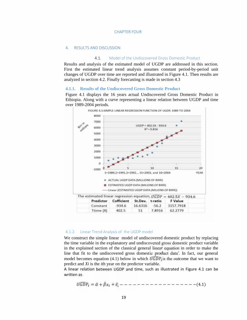
4.1. Model of the Undiscovered Gross Domestic ProductResults and analysis of the estimated model of UGDP are addressed in this section.First the estimated linear trend analysis assumes constant period-by-period unitchanges of UGDP over time are reported and illustrated in Figure 4.1. Then results areanalyzed in section 4.2. Finally forecasting is made in section 4.3
4.1.1. Results of the Undiscovered Gross Domestic ProductFigure 4.1 displays the 16 years actual Undiscovered Gross Domestic Product inEthiopia. Along with a curve representing a linear relation between UGDP and timeover 1989-2004 periods.
4.1.2. Linear Trend Analysis of the UGDP modelWe construct the simple linear model of undiscovered domestic product by replacingthe time variable in the explanatory and undiscovered gross domestic product variablein the explained section of the classical general linear equation in order to make theline that fit to the undiscovered gross domestic product data’. In fact, our generalmodel becomes equation (4.1) below in which is the outcome that we want topredict and Xi is the ith year on the predictor variable.A linear relation between UGDP and time, such as illustrated in Figure 4.1 can bewritten as = + + −−−−−−−−−−−−−−−−−−(4.1)

20
The coefficient of this equation can be estimated by using UGDP data for the 1989-2004 periods and the least squares regression methods as follows (t statistics inparentheses):= −934.60 + 402.50 − − − − −−−−−−−−−−−−(4.2)
(7.8916) ;R = 0.82This regression line estimated two things: the slope of the line denoted by =402.5and the point at which the line crosses the vertical axis of the graph (known asintercept of the line) denoted by = −934.6.
Residual plot a graphical test of the adequacy of regression assumptions shows that ascatter plot of standardized residuals versus fitted values should exhibit no apparentpattern, moreover, a successful fitting of a regression model should producestandardized residuals within (-2.25,2.5), roughly speaking, and a regression analysiscannot be complete without an examination of residuals (Chatterjee, Hnandcock andSimonnoff, 1995:150). Therefore, our regression is assumed to be satisfactory thatresidual plot of the UGDP shows there is no apparent pattern between standardizedUGDP residual and fitted value of UGDP. Its standardized residual is within (-1.344,1.695) in which it is within the interval of a successful fitting of a regression line.
Before we use the linear trend prediction of UGDP, it is useful to test our nullhypothesis that there is no relationship between UGDP and time over the 1989-2004periods. Both the standard error test and the Student’s test of the null hypothesisshow our estimate was significant that there is a strong relationship between UGDPand time. We accept that our parameter estimate is statistically significant at the 5per cent level of significance for a two-tail test, because standard error of thecoefficient (51) is less than half of the estimated slope coefficient (201.25=402.50/2),
21
and the observed or sample value of the t ratio is 7.8916 (estimated slope coefficientdivided by the standard error of the coefficient) is greater than 2.145 (the theoreticalvalue of t obtained from the t-table with 14 degrees of freedom (n-k=16-2)2.
Thus, we reject the null hypothesis, we accept the alternative one: = 402.50 isstatistically significant, this means that there is strong relationship between UGDPand time, as time increases by a unit UGDP increases by 402.50 million Birr3.
Moreover, the 95 per cent confidence interval for slope coefficient is estimated from293.31 up to 512.1 million of Birr4. To interpret, let’s round the values. If thegovernment amends and applies these two universal business income tax schedules,it definitely expects that the undiscovered Gross Domestic Product that will bediscovered increases by 402.5 million of Birr, as year increases by a unit. It is likelythe slope of the undiscovered GDP will range from 293.31 to 512.1 million of Birr.Thus = 402.50 is taken as reliable estimate that lies in theranges.
Thus, using the linear trend equation estimated over the 1989-2004 periods, we canforecast the UGDP for the future periods. To forecast UGDP in any future periodsubtract 1988 from the year in question to determine a relevant value for time(x).The other important methods we learn are from the confidence and predictionintervals for UGDP data reported in Fig.4.2.
The following Figure 4.2 shows simple regression plot that illustrates the use ofConfidence intervals and prediction intervals of UGDP. Considering the estimatedregression line of = −934.60 + 402.50 . Two possible use of the line are:what is our best estimate for the true average annual UGDP over the study period?What is the best estimate for the value of UGDP for one particular year in thepopulation that has change in time is equal to some value? Each of these questions isanswered by substituting that value of number of year difference into the regressionequation, but estimates have different levels of variability associated with them. Theconfidence interval (sometimes called interval for the fitted value) provides arepresentation of accuracy of an estimate of the average target value for all periods
2 Theoretical value of t table is referred from Koutsoyiannis (2010:660).3 Moreover the observed F* ratio (=62.3) is also compared with the theoretical F value withv1=K-1=1 and v2=N-K=15 degrees of freedom (at the 95 per cent level of significance). Fromthe F table we find F0.05=7.26. Given that F*>F0.05 we reject the null hypothesis and we acceptthat the regression is significant, that time (Xi) is a significant explanatory factor for thevariation in UGDP(Y).
4The 95 per cent confidence interval estimate of the slope of regression line of UGDPis from 293.31 up to 512.1 was determined by substituting the estimated values of= 402.7 and = 51 in the formula = ± 2.145 ∗ . (293.31 < <512.1) = 0.95.

22
with a given predicted value, while the prediction interval (sometimes called theconfidence interval for a predicted value) provides a representation of accuracy of aprediction of the target value for a particular observation or year with a givenpredicting value.
This plot of CI and PI of UGDP illustrates a few interesting points. First, the pointwise confidence interval (represented by inner LLCI line and ULCI lines) is muchnarrower than the point wise prediction interval (represented by the outer pair ofLLPI and ULPI lines), since the former interval is based on the variability of+ as an estimator of + , the latter interval also reflects theinherent variability of time about the regression line in the population itself. Second,it should be noted that the interval is narrowest in the center of the plot, and getswider at the extremes; this shows that the predictions become progressively lesaccurate as the predicting value gets more extreme compared with the bulk of thepoints (this is more apparent in the confidence interval than it is in the predictioninterval). Thus in the following sections we will see how prediction interval iscalculated.
Thus, using the linear trend equation estimated over the 1989-2004 periods, we canforecast the UGDP for the future periods. To forecast UGDP in any future periodsubtract 1988 from the year in question to determine a relevant value for time(x). Theother important methods we learn from the confidence and prediction intervals forUGDP data reported in Fig.4.4.
Figure 4.4 state that a confidence and prediction intervals take the form of two bands(groups) around the least squares line. The relationship between point estimate andinterval predictions for different values of shown by the graph. A point predictionis always shown by the fitted least squares line.
The point prediction of UGDP for the year 2013 is= −934.6 + 402.5( ), ℎ = 25 = 2008 − 1988= −934.60 + 402.50(25)

23
= −934.60 + 10062.5 = 9127.9Similarly the point prediction of UGDP for the year 2015 is= −934.6 + 402.5( ), ℎ = 27 = 2015 − 1988= −934.60 + 402.50(27)= −934.60 + 10,867.5 = 9,932.9Suppose the standard error of the forecast is about 5.5439, and If we select 1−∝=0.95,then = 2.145 and the 95% prediction interval for ( )± ( ) = 9127.9 ± 2.145(5.5439)Thus, the 95 per cent prediction interval for these who plan, legislate and executebudget, the UGDP lies between 9116.01 and 9139.79 millions of Birr. Theinterpretation is that if the government amends and applies policies, rules andregulation that use to plan, legislate and execute resources during Pagume, it canexpect to mobilize the undiscovered gross domestic product of 9127.9 million of Birrin the year 2013. It is likely these undiscovered gross domestic product will rangefrom 9116 to 9139.79 million of Birr. 5
Note that the undiscovered GDP projections are based on a linear trend line, whichimplies that UGDP increase by a constant Birr amount each year; in this example, it isprojected to grow by 402.5 million Birr per year.
It is known that the least squared regression line minimizes the sum of squaredresiduals between the actual and fitted values over the sample data. Therefore, Figure4.1 shows differences between actual and fitted values of UGDP are generally positivein both early (1989-1994) and latter (2002) periods, where as they are generallynegative and constant in the intervening 1995-2001 period. These differences suggestthat the shape of the undiscovered gross domestic product /time relation may not beconstant but rather may be generally increasing over the 1989-2004 periods. Underthese circumstances, it may be more convenient to assume that undiscovered grossdomestic product is changing at a constant annual rate than a constant annual amount.
4.2. Growth Trend Analysis of Undiscovered Gross Domestic Product
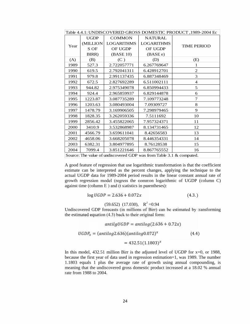
Two fundamental questions of the study are what were the amount the UGDP in thebase year (1988) and the annual growth rate? These questions can be answered byusing the traditional growth trend analysis that assumes a constant period-by-periodpercentage change in an important economic variable over time. Table 4.4.1 revealsthe actual UGDP in millions of Birr (column B) and transformed into logarithmic ofbase 10 (column C) and natural log (column D) for the periods 1989 to 2004 (columnA).
5Such moderate interval means that our point forecast of 9127.9 million Birr issomehow reliable.
24
A good feature of regression that use logarithmic transformation is that the coefficientestimate can be interpreted as the percent changes, applying the technique to theactual UGDP data for 1989-2004 period results in the linear constant annual rate ofgrowth regression model (regress the common logarithmic of UGDP (column C)against time (column E ) and (t statistics in parentheses):log = 2.636 + 0.072 (4.3. )
(59.652) (17.030), R2 =0.94Undiscovered GDP forecasts (in millions of Birr) can be estimated by transformingthe estimated equation (4.3) back to their original form:= (2.636 + 0.72 )= ( 2.636)( 0.072) (4.4)= 432.51(1.1803)In this model, 432.51 million Birr is the adjusted level of UGDP for x=0, or 1988,because the first year of data used in regression estimation=1, was 1989. The number1.1803 equals 1 plus the average rate of growth using annual compounding, ismeaning that the undiscovered gross domestic product increased at a 18.02 % annualrate from 1988 to 2004.
Year
UGDP(MILLION
S OFBIRR)
COMMONLOGARITHMS
OF UGDP(BASE 10)
NATURALLOGARITHMS
OF UGDP(BASE e)
TIME PERIOD
(A) (B) (C ) (D) (E)1989 527.3 2.722057771 6.267769647 11990 619.5 2.792041311 6.428912701 21991 979.8 2.991137435 6.887348469 31992 672.5 2.827692289 6.511002111 41993 944.82 2.975349078 6.850994433 51994 924.4 2.965859937 6.829144878 61995 1223.87 3.087735289 7.109773248 71996 1203.63 3.080493004 7.09309727 81997 1478.79 3.169906505 7.298979465 91998 1828.35 3.262059336 7.5111692 101999 2856.42 3.455822065 7.957324371 112000 3410.9 3.532868987 8.134731465 122001 4566.79 3.659611041 8.42656583 132002 4658.06 3.668205078 8.446354331 142003 6382.31 3.804977895 8.76128538 152004 7099.4 3.851221646 8.867765552 16
Table 4.4.1: UNDISCOVERED GROSS DOMESTIC PRODUCT ,1989-2004 Ec
Source: The value of undiscovered GDP was from Table 3.1 & computed.

25
To forecast Undiscovered GDP in any future year by using this model, subtract 1988from the year being forecast to determine x. therefore, a constant annual rate ofgrowth model forecast for UGDP in 2013 is
X=2013-1988=25
UGDP2013=Birr 432.51(1.1803)25
= 27,277.61 million Birr,
Similarly, a constant annual rate of growth model forecast for UGDP in 2015 is
X=2015-1988=27
UGDP2015=Birr 432.51(1.1803)27
= 38,000.66 million Birr.
Another frequently used form of the constant growth model is based on an underlyingassumption of continuous, as opposed to annual, compounding. The continuousgrowth model is expressed by the exponential equation:=Taking the natural logarithm (to the base e) of both sides of the above equation gives= +Under an exponential rate of growth assumption, the regression model estimate of theslope coefficient, g, is a direct estimate of the continuous rate of growth. For example,a continuous growth model estimate for UGDP is (t statistics in parentheses):= 6.071 + 0.167 − − − − −−−−−−−−(4.5)
(59.652) (17.030), R2 =0.97
In this equation, the coefficient 0.167 (=16.7%) is a direct estimate of the continuouscompounding growth rate for UGDP. Notice that t statistics for the slope coefficientare identical for the constant annual rate of growth regression model (Eq.4.3).
Again, UGDP forecasts (in millions of Birr) can be derived by transforming thisestimated equation 4.5 back to its original form:= ( 6.071)( 0.167)= 433.11 (1.1817) (4.6)The very small difference between the estimate of Eq.4.4 and 4.6 can be attributed torounding error; otherwise they are similar.
4.3. Forecasting the UGDP with Linear and Growth Trend Comparison
The importance of selecting the correct structural form for a trending model can bedemonstrated by comparing the Undiscovered Gross Domestic Product projection thatresults from the two basic approaches that have been considered. Remember with the
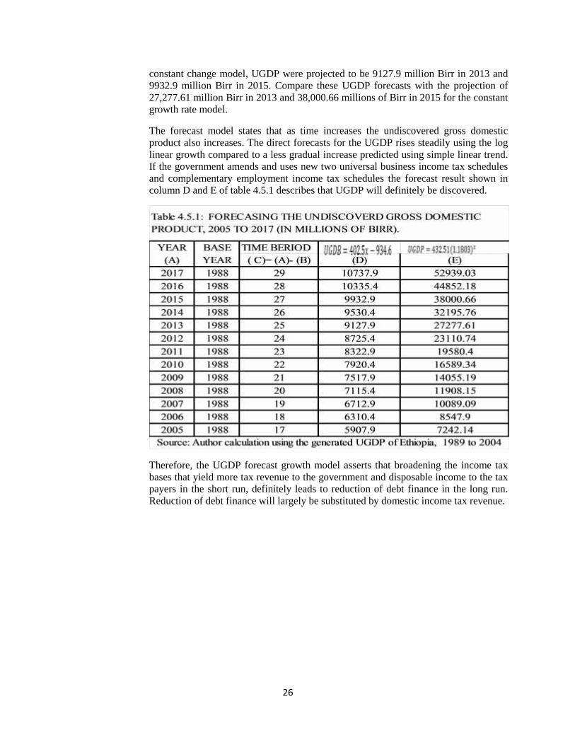
26
constant change model, UGDP were projected to be 9127.9 million Birr in 2013 and9932.9 million Birr in 2015. Compare these UGDP forecasts with the projection of27,277.61 million Birr in 2013 and 38,000.66 millions of Birr in 2015 for the constantgrowth rate model.
The forecast model states that as time increases the undiscovered gross domesticproduct also increases. The direct forecasts for the UGDP rises steadily using the loglinear growth compared to a less gradual increase predicted using simple linear trend.If the government amends and uses new two universal business income tax schedulesand complementary employment income tax schedules the forecast result shown incolumn D and E of table 4.5.1 describes that UGDP will definitely be discovered.
Therefore, the UGDP forecast growth model asserts that broadening the income taxbases that yield more tax revenue to the government and disposable income to the taxpayers in the short run, definitely leads to reduction of debt finance in the long run.Reduction of debt finance will largely be substituted by domestic income tax revenue.

27
5. Conclusion and Policy Implications
5.1. ConclusionThe observed problem was the first and second GTP plan did project revenue,expenditure and deficit finance neither from domestic nor external sources for aperiod of 26 days, because of the fact that the Ministry of Finance and EconomicDevelopment used the Gregorian calendar. The opportunity cost of using theGregorian calendar in Ethiopia in general and in the GTP in particular is scarifying theuse of Ethiopian calendar in the entire Tropics.
Thus, the total projected revenue, expenditure and deficit finance were 615,592;690,959 and 75,367 billion Birr respectively were only for a period of 1800 days (360days * 5 years). The average daily projected revenue, expenditure and deficit financewere proportionally calculated as 342,384 and 42 billion Birr respectively. Therefore,the average daily projected revenue, expenditure and deficit finance multiplied by 26days is equal to the value of resources 8,892; 9,984 and 1,092 billion Birr that wereneither projected nor included in the first GTP. There are neither factors income suchas salary income for labor, rental income for building, interest income for capital andprofit for an entrepreneurs or income tax revenues from these source sides during 26days. These imply that neither private accounting of the firm nor the national incomeaccounting of Ethiopia provides economic data. Therefore, the final impact of usingthe Gregorian calendar in the GTP is the available historical data of Ethiopia’s GDPexcluded the period of 5 and 6 days (undiscovered period). That is why we choose theundiscovered gross domestic product as the dependent variable.
Thus modeling the undiscovered gross domestic product is the time series analysis for16 years period (1989 to 2004). Therefore, the hypothesis of the study is there is norelationship between the undiscovered GDP and number of years in Ethiopia. Thespecific research questions are: What are the universal standards of Ethiopia’sbudgetary months over the medium term public expenditure plan? , what are sevensteps additional undiscovered business income tax revenue and disposable income inthree categories of four years? What is the undiscovered GDP over the study period?What is the relationship between the undiscovered GDP and time?, and What is theundiscovered GDP in the base year and its growth rate?
The Undiscovered Gross Domestic Product (UGDP) Data, which was generated fromthe various years’ national accounts of Ethiopia, is the big picture in estimating theeconomic model of UGDP. The data of actual national income accounts were obtainedfrom the Central Statistics Authority of Ethiopia. Actual GDP data at market price forthe years 1989 to 1993 and 1994 to 2004 were taken from national income accounts of1995 and 2005 respectively. There are four steps this study uses to generate theundiscovered gross domestic product data: first, collect the actual GDP data from theCentral Statistical Office, second, calculate the average daily actual gross domesticproduct as the ratio of actual gross domestic product data to 360 days; third, determinethe multiplier whether it is 5 or 6 days, and fourth multiply the result of the secondstep by the multiplier so as to generate a proxy for the universal gross domesticproduct data of each year over the study period ( look at Table 3.1).
Undiscovered gross domestic product model was made by replacing the time variablein the explanatory and undiscovered gross domestic product variable in the explainedsection of the classical general linear equation in order to make the line that fit to the

28
undiscovered gross domestic product data’. The estimated undiscovered grossdomestic product regression line reported in Figure 4.1. The estimated undiscoveredgross domestic product model has two things: the slope the line denoted by = 402.5and the point at which the line crosses the vertical axis of the graph (known asintercept of the line) denoted by = −934.6.
Before we used the linear trend prediction of UGDP, we tested the null hypothesis thatthere is no relationship between UGDP and time over the 1989-2004 periods. Both thestandard error test and the Student’s test of the null hypothesis show our estimate wassignificant that there is a strong relationship between UGDP and time. We accept thatour parameter estimate is statistically significant at the 5 per cent level of significancefor a two-tail test, because standard error of the coefficient (51) is less than half of theestimated slope coefficient (201.25=402.50/2), and the observed or sample value ofthe t ratio is 7.8916 (estimated slope coefficient divided by the standard error of thecoefficient) is greater than 2.145 (the theoretical value of t obtained from the t-tablewith 14 degrees of freedom (n-k=16-2). Thus, we reject the null hypothesis, we acceptthe alternative one: = 402.50 is statistically significant, this means that there isstrong relationship between UGDP and time, as time increases by a unit UGDPincreases by 402.50millions Birr.
Moreover, the 95 per cent confidence interval for slope coefficient is estimated from293.31 up to 512.1 million of Birr. The interpretation was it is likely the slope of theundiscovered gross domestic product will range from 293.31 to 512.1 million of Birr.Thus = 402.50 is taken as reliable estimate that lies in the ranges.
Thus, using the linear trend equation estimated over the 1989-2004 periods, theUGDP for the future periods forecasted (2005-2013). To forecast UGDP in any futureperiod subtract 1988 from the year in question to determine a relevant value fortime(x). The other important methods we learn are from the confidence and predictionintervals for UGDP data reported in Fig.4.4.
Transforming the actual UGDP in millions of Birr into logarithmic of base andregressing the result against time for the periods 1989 to 2004 used to answer twofundamental questions of the study, what were the amounts the UGDP in the base year(1988) and the annual growth rate?’.
The finding shows 432.51 million Birr is the adjusted level of UGDP for x=0, or1988, because the first year of data used in regression estimation=1, was 1989.Besides, the number 1.1803 equals 1 plus the average rate of growth using annualcompounding, is meaning that the undiscovered gross domestic product increased at a18.02 % annual rate from 1988 to 2004.
Finally, the Undiscovered Gross Domestic Product projection made with the constantchange model of 9127.9 million Birr in 2013 and 9932.9 million Birr in 2015.Compare these UGDP forecasts with the projection of 27,277.61 million Birr in 2013and 38,000.66 millions of Birr in 2015 for the constant growth rate model.

29
5.2. Policy ImplicationsWhen we added seven steps additional undiscovered business income tax revenue(column F of Table 4.7), we obtained 1613 Birr and more. Likewise, when weaggregated seven steps undiscovered disposable income (column F of Table 4.8), weobtained 7556.51 Birr. The theories broadening income tax bases yield additional taxrevenue and disposable income is true. Therefore, if the government of Ethiopiaamends and applies these new seven steps business income tax schedules, additionalincome tax revenue of 1613 and disposable income of 7556.51 Birr will bediscovered per business man.
Therefore, if the government amends and applies universal business income taxschedules and GTP uses 48 months of three categories, the undiscovered GrossDomestic Product that will be discovered and increases by 402.5 million of Birr, asyear increases by a unit.
The UGDP forecast growth model asserts use of 48 months of three categories in themedium term GTP and broadening the income tax bases that yield more tax revenueto the government and disposable income to the tax payers in the medium term,definitely will get out the use of Gregorian calendar. So that both private accountingof the firm and national income accounting will use the Ethiopian fiscal year inaccordance with the country’s legal framework. Thus, the following recommendationsare forwarded.
The Federal Government of Ethiopia must amend and use new fiscal policyinstruments such as two universal business income tax schedules (Annexes B andC).
All budgetary institutes of the government, public enterprises, private sector andinternational organizations must use the Ethiopian calendar or budget year ofEthiopia when they plan, legislate, implement and monitor budget.
All employers whether private or public must pay salary during Pagume byaggregating with the month of Nehase. The government must amend and applytwo complementary income tax schedules for the income tax periods of 35 and 36days respectively.

30
6. ReferencesAbraham, I. W (1969): National Income and Economic Accounting. Prentice Hall,Inc., Englewood Cliffs, New Jersey.
Barnett, R. A (1980): INTERMEDIATE ALGEBRA. Structure and use, McGraw. Hill, Inc.printed in the United States of America.
Borkowski K.M (1991:121-130): THE TROPICAL YEAR AND SOLAR CALENDAR. TheJournal of the Royal Astronomical Society of Canada; Vol.85, No.3 June 1991 wholeNo.630.
Chatterjee, S.; Handcock, S. and Simonoff, J.S (1995). A Casebook for A First Coursein Statistics and Data Analysis. John Wiley &Sond, Inc. United States of America.
Daniel F. (1956): GENERAL SCIENCE FOR TROPICAL SCHOOLS, Cambridge.
Eshetu Chole (1980). “Income Taxation in Pre-and Post-Revolution EthiopiaComparative Review”: Ethiopian Journal of Development Research, Vol. 9, No.1.Institute of development Research, Addis Ababa.
Fantahun Belew (1992)." Government’s Employees Income Tax Computation", AddisAbaba, Ethiopia: Economic Focus, EEA. Vol.3.No.5.
Fassil Tassew (2005). Ethiopian Calendar Belongs to Whom? Pagume 6. BanawiPrinting Press. Addis Ababa, Ethiopia.
____________. (2002).“Analysis of Personal Income Tax and Revenue Forecasting(PITRF)"PROCEEDINGS OF THE THIRD NATIONAL CONFERENCE ONASSESSMENT OF THE PRACTICES OF CIVIL SERVICE REFORM PROGRAMIN ETHIOPIA. Ethiopian Civil Service College and Ethiopian Management Institute,Addis Ababa.
____________. (1993 EC.). "Response to Comments on an Employment Income TaxComputations’ and Computing Half Employment Income Tax", Addis Ababa,Ethiopia: Economic Focus, EEA. Vol.4. No.1.
Federal Democratic Republic of Ethiopia [FDRE]. (1996). Federal Government ofEthiopia Financial Administration Proclamation. Proclamation N0.57. Addis Ababa,Ethiopia: BerhanennaSelam Printing Press.
(1995). Democratic Republic of Ethiopia’s ConstitutionNo.1, Addis Ababa,Ethiopia: BerhanennaSelam Printing Press.
__________. (2008). Income Tax Law. Proclamation No. 286. Addis Ababa,Ethiopia: BerhanennaSelam Printing Press.

31
GetenetDemissie (2008). Exploring and Modeling the Undiscovered BusinessIncome Tax Revenue: Specific to Ethiopia’s Tax System. Unpublished master thesis,Unity University.
Grant F.L and Hill A.M (1965): Commercial Arithmetic. Longmans, Green and CoLtd,Great Britain.
Grisdale W. (1965 GC): A General Geography. For secondary schools in Ethiopiaprinted by the Institute for the publication of Textbook of the Republic of Serbia,ObilicevVenac, Begrade, and Yugoslaua.
Hanson, J,L.(1967). Economics for Students. Great Britain; by Richard Clay,Ltd.
Hirschery, M. (1996). Managerial Economics. U.S.A: The Dryden Press Harcourt,Inc.
IMF (2013). Web: International Monetary Fund Washington, D.C.http://www.imf.org
Koutsayiannis A. (2010). Theory of Econometrics, 2nd Edition, New york,PalgravePublishers Ltd.
Imprial Ethiopian Government (1954 EC): Second Five Year Development Plan1955-1959E.C/1963-1967 G.C. Addis Ababa: BerhanennaSelam Printing Press.
Kearsey.C.W.(1964).GENERAL PHYSICS.LONGMAN,GREEN AND COLTD,London.
Last G.C. (1968 GC). Geography. Ministry of Education and Fine Arts. AddisAbaba: BerhanennaSelam Printing Press.
Leslau.W (1971 GC). English-Amharic Context Dictionary. Printed in Belgium byImprimrieOrentaliste. Louvain.
Lewis. N (1999). Word Power Made Easy. Bloomsbury Publishing Plc, U.K.
Mankiw. N. G (2005). MACROECONOMICS, Harvard University, Printed in theUnited States of America First Printing 2009 Worth Publishers 41 Madison AvenueNew York, NY 10010
McConnell, C.R and Brue,S.L.(1993). MacroEconomics, 12th edition, McGraw-Hill,Inc. New York.
MicrosofEncartEnyclopida Standard Edition 2008, software
Musgrave, R.A. (1959 GC). The Theory of Public Finance, New York: McGraw-Hill.
Myles, Gareth D.( 2001). Public Economics, Printed in the United States of America.
32
Peters, M and Schaaf, W.L (1965) MATHEMATICS a modern approach D. VanNostrandCampany, Inc.
Robert L.H. (1968). The Making of Economic Society, 2nd Ed. USA: PRETICE-HALL,INC, ENGEEWOOD CLIFFS, NEWJERSY.
Schwab, P. (1970 GC). “Tax System of Ethiopia”; The American Journal ofEconomics and Sociology, Nairobi, Kenya: East African Publishing House.
Smith, Adam (1904) An Enquiry into the Nature and Causes of The Wealth ofNations, Volume II, London (Grant Richards) [original edition 1776]
TegegnworkGebre. (1991EC.). "Comments on Employment Income TaxComputations": Economic Focus, EEA. Vol.2. No.5. Addis Ababa, Ethiopia.
Shrivastava, O.S (1996). Economics of Growth Development and Planning, VikasPublishing House Pvt Ltd, New Delhi.
Yamane, T(1973).STATISTICS, An Introductory Analysis, 3rd edition. Harper&Row, Publishers, New York, Evanston, San Francisco, London.
Waugh. (1943). Elements of Statistical Method; Connecticut state College, Storrs,Corn.
7. Appendices
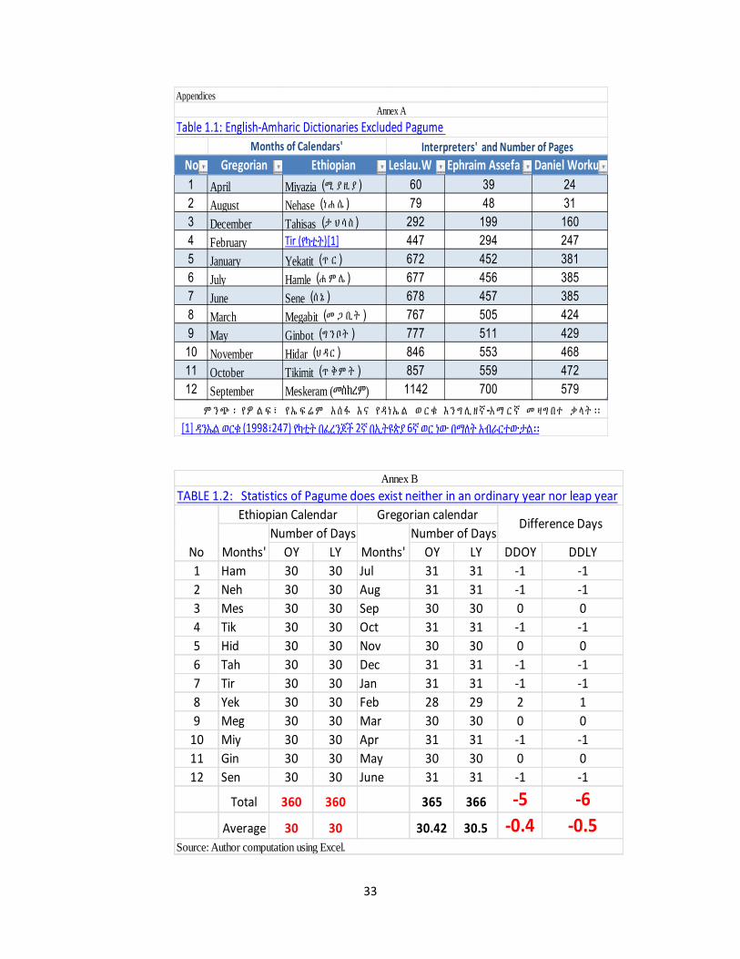
33
No Gregorian Ethiopian Leslau.W Ephraim Assefa Daniel Worku1 April Miyazia ሚ ያ ዚ ያ ( ) 60 39 242 August Nehase ነ ሐ ሴ ( ) 79 48 313 December Tahisas ታ ህ ሳ ስ ( ) 292 199 1604 February Tir (የካቲት)[1] 447 294 2475 January Yekatit ጥ ር ( ) 672 452 3816 July Hamle ሐ ም ሌ ( ) 677 456 3857 June Sene ሰ ኔ ( ) 678 457 3858 March Megabit መ ጋ ቢት ( ) 767 505 4249 May Ginbot ግ ን ቦት ( ) 777 511 42910 November Hidar ህ ዳር ( ) 846 553 46811 October Tikimit ጥ ቅም ት ( ) 857 559 47212 September Meskeram (መስከረም) 1142 700 579
ም ን ጭ ፡ የ ዎ ል ፍ ፣ የ ኤ ፍ ሬ ም አ ሰ ፋ እ ና የ ዳ ነ ኤ ል ወ ር ቁ እ ን ግ ሊ ዘ ኛ አ ማ ር ኛ መ ዛግ በተ ቃ ላት ፡፡-[1] ዳንኤል ወርቁ (1998፣247) የካቲት በፈረንጆች 2ኛ በኢትዩጵያ 6ኛ ወር ነው በማለት አብራርተውታል፡፡
Table 1.1: English-Amharic Dictionaries Excluded PagumeMonths of Calendars' Interpreters' and Number of Pages
AppendicesAnnex A
OY LY OY LY DDOY DDLY1 Ham 30 30 Jul 31 31 -1 -12 Neh 30 30 Aug 31 31 -1 -13 Mes 30 30 Sep 30 30 0 04 Tik 30 30 Oct 31 31 -1 -15 Hid 30 30 Nov 30 30 0 06 Tah 30 30 Dec 31 31 -1 -17 Tir 30 30 Jan 31 31 -1 -18 Yek 30 30 Feb 28 29 2 19 Meg 30 30 Mar 30 30 0 0
10 Miy 30 30 Apr 31 31 -1 -111 Gin 30 30 May 30 30 0 012 Sen 30 30 June 31 31 -1 -1
Total 360 360 365 366 -5 -6Average 30 30 30.42 30.5 -0.4 -0.5
Annex B
Source: Author computation using Excel.
Difference Days
TABLE 1.2: Statistics of Pagume does exist neither in an ordinary year nor leap year
No
Ethiopian Calendar Gregorian calendar
Months'Number of Days
Months'Number of Days

34
Table 2.1 Innovating and re-discovering weeks for calendar functionsNumberof weeks
Week of Ethiopian calendarWeek of Gregorian
Calendar1 Segnoelt Monday2 Maksegnoelt Tuesday3 Robelt Wednesday4 Hamuselt Thursday5 Arbelt Friday6 Kidamelt Saturday7 Ehudelt Sunday
Source: Author innovation
OY LY OY LY DDOY DDLY1 Ham 30 30 Jul 31 31 -1 -12 N&P 35 36 Aug 31 31 4 53 Mes 30 30 Sep 30 30 0 04 Tik 30 30 Oct 31 31 -1 -15 Hid 30 30 Nov 30 30 0 06 Tah 30 30 Dec 31 31 -1 -17 Tir 30 30 Jan 31 31 -1 -18 Yek 30 30 Feb 28 29 2 19 Meg 30 30 Mar 30 30 0 0
10 Miy 30 30 Apr 31 31 -1 -111 Gin 30 30 May 30 30 0 012 Sen 30 30 June 31 31 -1 -1
Total 365 366 365 366 0 0Average 30.42 30.5 30.42 30.5 0 0
Annex C
Source: Authors' calculation using Excel
Difference Days
TABLE 1.3: Discovering the Statistics of Pagume in an ordinary and leap years
NoEthiopian Calendar Gregorian calendar
Months'Name
Number of Days Months'Name
Number of Days