MODELING THE POWER DISTRIBUTION NETWORK ... - CORE
84
MODELING THE POWER DISTRIBUTION NETWORK OF A VIRTUAL CITY AND STUDYING THE IMPACT OF FIRE ON THE ELECTRICAL INFRASTRUCTURE A Thesis by ARIJIT BAGCHI Submitted to the Office of Graduate Studies of Texas A&M University in partial fulfillment of the requirements for the degree of MASTER OF SCIENCE December 2009 Major Subject: Electrical Engineering brought to you by CORE View metadata, citation and similar papers at core.ac.uk provided by Texas A&M University
-
Upload
khangminh22 -
Category
Documents
-
view
3 -
download
0
Transcript of MODELING THE POWER DISTRIBUTION NETWORK ... - CORE

MODELING THE POWER DISTRIBUTION NETWORK OF A
VIRTUAL CITY AND STUDYING THE IMPACT OF FIRE ON THE
ELECTRICAL INFRASTRUCTURE
A Thesis
by
ARIJIT BAGCHI
Submitted to the Office of Graduate Studies of
Texas A&M University
in partial fulfillment of the requirements for the degree of
MASTER OF SCIENCE
December 2009
Major Subject: Electrical Engineering
brought to you by COREView metadata, citation and similar papers at core.ac.uk
provided by Texas A&M University

MODELING THE POWER DISTRIBUTION NETWORK OF A
VIRTUAL CITY AND STUDYING THE IMPACT OF FIRE ON THE
ELECTRICAL INFRASTRUCTURE
A Thesis
by
ARIJIT BAGCHI
Submitted to the Office of Graduate Studies of
Texas A&M University
in partial fulfillment of the requirements for the degree of
MASTER OF SCIENCE
Approved by:
Co-Chairs of Committee, Chanan Singh
Alexander Sprintson
Committee Members, Garng M. Huang
Thomas E. Wehrly
Head of Department, Costas N. Georghiades
December 2009
Major Subject: Electrical Engineering

iii
ABSTRACT
Modeling the Power Distribution Network of a Virtual City and Studying the Impact of
Fire on the Electrical Infrastructure. (December 2009)
Arijit Bagchi, B.E., Birla Institute of Technology, MESRA, India
Co-Chairs of Advisory Committee: Dr. Chanan Singh
Dr. Alexander Sprintson
The smooth and reliable operation of key infrastructure components like water
distribution systems, electric power systems, and telecommunications is essential for a
nation‟s economic growth and overall security. Tragic events such as the Northridge
earthquake and Hurricane Katrina have shown us how the occurrence of a disaster can
cripple one or more such critical infrastructure components and cause widespread
damage and destruction. Technological advancements made over the last few decades
have resulted in these infrastructure components becoming highly complicated and inter-
dependent on each other. The development of tools which can aid in understanding this
complex interaction amongst the infrastructure components is thus of paramount
importance for being able to manage critical resources and carry out post-emergency
recovery missions.
The research work conducted as a part of this thesis aims at studying the effects
of fire (a calamitous event) on the electrical distribution network of a city. The study has
been carried out on a test bed comprising of a virtual city named Micropolis which was
modeled using a Geographic Information System (GIS) based software package. This

iv
report describes the designing of a separate electrical test bed using Simulink, based on
the GIS layout of the power distribution network of Micropolis. It also proposes a
method of quantifying the damage caused by fire to the electrical network by means of a
parameter called the Load Loss Damage Index (LLDI). Finally, it presents an innovative
graph theoretic approach for determining how to route power across faulted sections of
the electrical network using a given set of Normally Open switches. The power is routed
along a path of minimum impedance.
The proposed methodologies are then tested by running numerous simulations on
the Micropolis test bed, corresponding to different fire spread scenarios. The LLDI
values generated from these simulation runs are then analyzed in order to determine the
most damaging scenarios and to identify infrastructure components of the city which are
most crucial in containing the damage caused by fire to the electrical network. The
conclusions thereby drawn can give useful insights to emergency response personnel
when they deal with real-life disasters.

v
ACKNOWLEDGMENTS
I would like to thank my advisor, Dr. Chanan Singh, for the extensive support
and guidance he provided me throughout the course of this research work. I would also
like to thank my co-advisor, Dr. Alexander Sprintson, for his constant encouragement
towards the successful completion of my thesis.
Special thanks to my other committee members as well – Dr. Garng M. Huang
and Dr. Thomas E. Wehrly – for all their time and support. Thank you Dr. Wehrly for
agreeing to join my committee at such short notice.
Thanks are also due to Ian Horbaczewski and Kimberley Jones for their
contributions to the modeling of the electrical distribution network of Micropolis using
ArcMap, to Jacob Torres for all the help and guidance he provided me regarding
working with ArcMap, to Dr. Elizabeth C. Bristow for her help with the MUFS code and
MUFS files, to Susan Louis for her help with formatting this document and finally, to
my family and friends for their continuous support and encouragement.
This work was supported in part by NSF Grant EECS – 0725823.
vi
TABLE OF CONTENTS
Page
ABSTRACT .......................................................................................................... iii
ACKNOWLEDGMENTS ...................................................................................... v
TABLE OF CONTENTS ....................................................................................... vi
LIST OF FIGURES ............................................................................................... viii
LIST OF TABLES ................................................................................................. ix
CHAPTER
I INTRODUCTION ................................................................................... 1
II LAYOUT OF VIRTUAL CITY MICROPOLIS ...................................... 4
III MODEL OF URBAN FIRE SPREAD (MUFS) ....................................... 7
3.1. MUFS Simulation Input Parameters ................................................ 7
3.2. MUFS Simulation Outputs .............................................................. 9
IV DESIGNING OF ELECTRICAL TEST BED USING SIMULINK ......... 10
4.1. Determination of Distribution Transformer Constants ..................... 10
4.2. Determination of Conductor Sizing Based on Ampacity.................. 13
4.3. Determination of Line Parameters ................................................... 15
4.4. Formulation of Protection Scheme for Electrical Test Bed .............. 28
4.5. Assigning of System Loads ............................................................. 31
4.6. Source of Power Supply .................................................................. 31
4.7. Conclusion ...................................................................................... 32
V METHODOLOGY USED FOR ELECTRICAL SIMULATION
RUNS...................................................................................................... 33
5.1. Assumptions ................................................................................... 33
5.2. Definitions of Important Terms ....................................................... 34
5.3. General Treatment of Faulted Components ..................................... 35
5.4. Load Loss Damage Index (LLDI) ................................................... 36
5.5. Electrical Simulation Algorithm ...................................................... 37
vii
CHAPTER Page
VI ANALYSIS OF ELECTRICAL SIMULATION RUNS .......................... 39
6.1. Most Damaging SIDP ..................................................................... 39
6.2. Most Damaging UFIP ..................................................................... 42
VII GRAPH THEORY APPLICATIONS FOR ROUTING OF POWER
DURING EMERGENCIES ..................................................................... 44
7.1. Assumptions ................................................................................... 44
7.2. General Treatment of Faulted Components ..................................... 44
7.3. Overall Electrical Simulation Algorithm ......................................... 47
7.4. Formulation of Graph Theoretic Approach for Power Routing ........ 49
VIII ANALYSIS OF SIMULATIONS RUN INCORPORATING
POWER ROUTING ................................................................................ 64
IX CONCLUSIONS ..................................................................................... 69
REFERENCES ...................................................................................................... 72
VITA ..................................................................................................................... 75
viii
LIST OF FIGURES
FIGURE Page
2.1 Layout of the electrical infrastructure components
for the city of Micropolis ...................................................................... 5
4.1 Snapshot of the electrical test bed representing the
distribution network of Micropolis ........................................................ 11
4.2A Equivalent circuit of a transformer ........................................................ 12
4.2B Approximate equivalent circuit of the transformer ................................ 12
4.3 Underground cable burial configuration ................................................ 17
4.4 Three phase, single circuit overhead line conductor configuration......... 19
4.5 Single phase overhead line conductor configuration .............................. 23
4.6 Three phase, double circuit overhead line conductor configuration ....... 24
4.7 Two phase overhead line conductor configuration ................................ 27
4.8 Layout of the power distribution network for the city
of Micropolis ........................................................................................ 29
4.9 Snapshot of the three phase over-current relay module.......................... 29
6.1 Results of electrical simulations run using MUFS data.......................... 40
7.1 Layout of the electrical distribution network of Micropolis ................... 45
7.2 Equivalent graph representing the electrical distribution
network of Micropolis .......................................................................... 51
7.3 Equivalent graph representing a part of a sample electrical
network ................................................................................................ 58
7.4 Graph representing part of a sample distribution network ..................... 62
8.1 Results of electrical simulations run incorporating power routing ......... 65

ix
LIST OF TABLES
TABLE Page
2.1 Voltage and load profiles for consumers across Micropolis ................... 6
2.2 System and individual feeder loading information ................................ 6
3.1 Supporting infrastructure damage profile (SIDP) .................................. 8
3.2 Urban fire ignition points (UFIP) .......................................................... 8
4.1 Micropolis electrical test bed conductor sizings .................................... 15
4.2 Sequence impedance and capacitance values for three phase
single circuit overhead lines .................................................................. 22
4.3 Resistance, inductance and capacitance values for single phase
overhead lines ....................................................................................... 23
4.4 Sequence impedance and capacitance values for three phase
double circuit overhead lines ................................................................ 26
6.1 Most damaging UFIP ............................................................................ 43
7.1 Weights assigned to the edges and the links of the
equivalent graph ................................................................................... 53
8.1 Average LLDI values calculated for different UFIP profiles ................. 67

1
CHAPTER I
INTRODUCTION
The U.S.A. PATRIOT Act of 2001 [1] defines the term “Critical Infrastructure”
as “systems and assets, whether physical or virtual, so vital to the United States that the
incapacity or destruction of such systems and assets would have a debilitating impact on
security, national economic security, national public health or safety or any combination
of those matters.” The Critical Infrastructure Protection (CIP) Program [2], as set forth
through the Presidential Decision Directive (PDD - 63) of May 1998, identifies the
following sectors as key to the smooth functioning of any modern day society:
telecommunications, energy, water systems and emergency services, transportation and
banking and finance. With the advent of cutting-edge technologies leading to ever
increasing levels of automation in our daily lives, these infrastructure components have
not only become increasingly complicated but also heavily inter-dependent on each
other. The development of models ([3] – [6]) which can simulate this complex
interaction amongst the infrastructure components is thus an important area of research,
as they might be helpful for civic authorities and emergency response personnel when
they deal with an actual disaster.
The research work conducted as a part of this thesis proposes a methodology to
study and quantify the damage caused by fire to the electrical distribution network of a
___________ This thesis follows the style of IEEE Transactions on Power Delivery.

2
city. The fire is assumed to be initiated either by natural means, e.g. a lightning stroke or
a wildfire; or deliberately, e.g. a terrorist attack. This study has been carried out on a test
bed comprising of a virtual city named Micropolis, which was laid out using a
Geographic Information System (GIS) based software package by researchers at the
Department of Civil Engineering and the Department of Electrical and Computer
Engineering here at Texas A&M University. The remainder of this report has been
structured in the following fashion.
Chapter II gives an overview of the layout of the virtual city of Micropolis [7]
along with its civil and electrical ([8] – [9]) infrastructure components.
Chapter III briefly describes the Model of Urban Fire Spread (MUFS) [10],
which is a software package used to simulate an urban fire along with its subsequent
suppression.
Chapter IV describes the modeling of a separate electrical test bed using
Simulink, based on the GIS layout of the power distribution network of Micropolis. It
discusses the methodology used for determining the distribution transformer ratings
([11] – [12]), lists the standard formulae used for calculating the line parameters
(impedance and capacitance values per unit length) ([13] – [16]) and describes the
operation of the protection system components (relays, isolators and breakers) ([17] –
[18]) of the distribution network of Micropolis.
Chapter V proposes a methodology for studying the effects of fire on the
electrical distribution network of a city. It lists the relevant assumptions, definitions and
algorithms [8] pertaining to the development and the implementation of the proposed
3
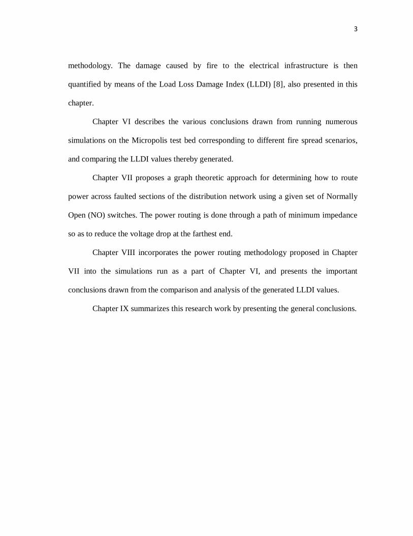
methodology. The damage caused by fire to the electrical infrastructure is then
quantified by means of the Load Loss Damage Index (LLDI) [8], also presented in this
chapter.
Chapter VI describes the various conclusions drawn from running numerous
simulations on the Micropolis test bed corresponding to different fire spread scenarios,
and comparing the LLDI values thereby generated.
Chapter VII proposes a graph theoretic approach for determining how to route
power across faulted sections of the distribution network using a given set of Normally
Open (NO) switches. The power routing is done through a path of minimum impedance
so as to reduce the voltage drop at the farthest end.
Chapter VIII incorporates the power routing methodology proposed in Chapter
VII into the simulations run as a part of Chapter VI, and presents the important
conclusions drawn from the comparison and analysis of the generated LLDI values.
Chapter IX summarizes this research work by presenting the general conclusions.

4
CHAPTER II
LAYOUT OF VIRTUAL CITY MICROPOLIS
The September 11, 2001 terrorist attacks on the World Trade Center prompted
the United States government to start treating all information related to a city‟s
infrastructure layout as classified. While on one hand this prevents the misuse of such
information by malicious elements, it also makes it difficult for researchers to test their
developed models with real life data. The designing of a virtual city with all the key
infrastructure components embedded in it is thus an important part of any research work
conducted in this area.
The virtual city of Micropolis, as represented by the layout of Fig. 2.1, was
designed for the purpose of it being used as a test bed for carrying out studies on the
effects of disasters on the interdependent infrastructure components of a city. Micropolis
was developed using GIS (ArcMap) and hydraulic modeling (EPANet) based software,
as described in [7]. The electrical distribution network of the city was then modeled and
its corresponding components added to the GIS layout of [7], as described in [8].
Micropolis, a city of around 5000 residents, covers an area of approximately 2 square
miles. To make the design as realistic as possible, a developmental timeline of 130 years
was taken into consideration [7]. While this timeline is manifested by the choice of pipe
material, pipe diameter etc. for the civil infrastructure model, it does not have a
significant impact on the electrical modeling as most electrical components are either
upgraded or replaced after every 30-40 years [9].

5
Fig. 2.1. Layout of the electrical infrastructure components for the city of Micropolis.
It is assumed that Micropolis does not have a power generation facility of its
own, but it obtains its power from a sub-transmission line (138 KV rating) running
through the heart of the city, as shown in Fig. 2.1. The city has just one substation,
where the sub-transmission level voltage of 138 KV is stepped down to the distribution
level voltage of 13.8 KV [8]. Two three-phase feeder lines (each of 13.8 KV rating)
emanate from the substation, and by repeated branching off into smaller three-phase sub-
branches and finally into single-phase laterals, they deliver the power from the
substation across the entire city. Overhead conductors are represented by the solid lines
of Fig. 2.1; while underground cables are shown using dotted lines. The overhead
conductors are supported on wooden poles, which are represented by the yellow dots in
Fig. 2.1. Distribution transformers rated 100 KVA or above are pad-mounted, while
6
others are mounted on the poles unless they are fed by underground cables (in which
case they are always pad-mounted) ([8] – [9]). All pad-mounted distribution
transformers are assumed to be enclosed in iron casings.
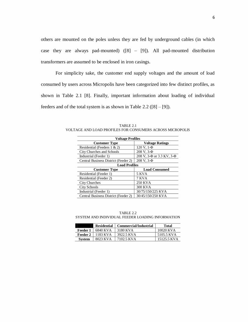
For simplicity sake, the customer end supply voltages and the amount of load
consumed by users across Micropolis have been categorized into few distinct profiles, as
shown in Table 2.1 [8]. Finally, important information about loading of individual
feeders and of the total system is as shown in Table 2.2 ([8] – [9]).
TABLE 2.1 VOLTAGE AND LOAD PROFILES FOR CONSUMERS ACROSS MICROPOLIS
Voltage Profiles
Customer Type Voltage Ratings
Residential (Feeders 1 & 2) 120 V, 1-Φ
City Churches and Schools 208 V, 3-Φ
Industrial (Feeder 1) 208 V, 3-Φ or 3.3 KV, 3-Φ
Central Business District (Feeder 2) 208 V, 3-Φ
Load Profiles
Customer Type Load Consumed
Residential (Feeder 1) 5 KVA
Residential (Feeder 2) 7 KVA
City Churches 250 KVA
City Schools 300 KVA
Industrial (Feeder 1) 30/75/150/225 KVA
Central Business District (Feeder 2) 30/45/150/250 KVA
TABLE 2.2 SYSTEM AND INDIVIDUAL FEEDER LOADING INFORMATION
Residential Commercial/Industrial Total
Feeder 1 6840 KVA 3180 KVA 10020 KVA
Feeder 2 1183 KVA 3922.5 KVA 5105.5 KVA
System 8023 KVA 7102.5 KVA 15125.5 KVA

7
CHAPTER III
MODEL OF URBAN FIRE SPREAD (MUFS)
The Model of Urban Fire Spread (MUFS), as described and tested in [10], is a
numerical tool used to simulate an urban fire starting from one or more user-defined
points of ignition. The model calculates the extent of the fire spread area, taking into
consideration the fire suppression efforts made by the community‟s emergency response
personnel. To determine the efficiency of fire suppression, MUFS also takes into
account the simultaneous (i.e., along with the spread of fire) damage or destruction of
one or more supporting infrastructures for fire response (e.g., water distribution system,
telecommunication networks, etc.) [10]. The following sections briefly describe the
various inputs and outputs pertaining to a given fire spread simulation run using MUFS.
3.1. MUFS Simulation Input Parameters
The MUFS code requires the following user-defined inputs in order to run a
given fire spread simulation.
3.1.1. Supporting Infrastructure Damage Profile (SIDP)
For the purpose of this thesis, ten different damage profiles corresponding to one
or more supporting infrastructures for fire response have been considered, as shown in
Table 3.1 [8].
3.1.2. Urban Fire Ignition Points (UFIP)
The extent of fire spread damage will not only depend on the particular SIDP
selected, but also on the specific point(s) of ignition of fire chosen for a given simulation

8
[10]. For the purpose of this thesis, four different fire ignition point profiles have been
considered, as shown in Table 3.2 [8].
3.1.3. Wind Direction
As the rate of spread of fire will be the highest along the direction of flow of
wind, varying the wind direction for a given SIDP and UFIP combination will give rise
to a quite different fire spread scenario [10]. For the purpose of this research, four
cardinal wind directions have been considered: East, West, North and South [8].
TABLE 3.1 SUPPORTING INFRASTRUCTURE DAMAGE PROFILE (SIDP)
Damage
Profile Remarks
A01 All three high-service pumps of Micropolis permanently taken out of service.
A03 One out of the three high-service pumps of Micropolis permanently taken out of service.
B03 All three high-service pumps of Micropolis temporarily taken out of service after two hours since start of simulation, for a duration of two hours.
D01 Elevated storage tank of Micropolis unavailable for the entire duration of the simulation.
D02 Elevated storage tank of Micropolis becomes unavailable after an hour since start of simulation, and remains so till simulation ends.
AD1 Combination of profiles A01 and D02.
E02 Water main breach near the Central Business District.
F01 Water contamination (and subsequent isolation) at south-east side of town.
F04 Water contamination (and subsequent isolation) in highest-density residential area towards north-east side of town.
UND No supporting infrastructures damaged. This profile has been deliberately included in order to compare its effects vis-à-vis those of the others.
TABLE 3.2 URBAN FIRE IGNITION POINTS (UFIP)
Ignition
Point
Acronym
Remarks
GOV Government Buildings (Community Center, City Hall, Post Office and Rail Museum), represented by buildings marked „G‟ in Fig. 2.1.
SCH City Schools, represented by buildings marked „S‟ in Fig. 2.1.
CHU City Churches, represented by buildings marked „C‟ in Fig. 2.1.
ECO Ecological targets (Printing Press and Timber Mill), represented by buildings marked „E‟ in Fig. 2.1.

9
By considering different combinations of such SIDPs, UFIP profiles and wind
directions; a variety of „fire spread scenarios‟ can therefore be generated.
3.2. MUFS Simulation Outputs
Once all relevant user-defined inputs have been provided to MUFS, it is ready to
run the concerned fire spread simulation. A constant wind speed of 10 mph is assumed
for all simulation runs. A particular simulation run corresponds to 12 hours of physical
fire spread. Starting from a user-defined point of ignition, the model calculates the
incremental distance advanced by the fire every five minutes. It is assumed that the fire
spreads along the direction of each of the four „fire spread vectors‟, the orientations of
which are determined with respect to the dominant wind direction as: „downwind‟ (along
the flow of wind), „upwind‟ (opposite to wind flow), „sidewind right‟ (90° to the right of
„downwind‟) and „sidewind left‟ (opposite to „sidewind right‟) [10]. The „fire polygon‟
thus created by joining the tips of the fire spread vectors for a given time step is
therefore a quadrilateral, and it represents the area covered by the fire until that time.
The MUFS program thus essentially outputs the fire polygon vertex coordinates after
every five minutes until the end of simulation (corresponding to 12 hours of physical fire
spread).
10
CHAPTER IV
DESIGNING OF ELECTRICAL TEST BED USING SIMULINK
This chapter describes the designing of an electrical test bed, which has been
modeled using Simulink (MATLAB) based on the GIS layout of the electrical
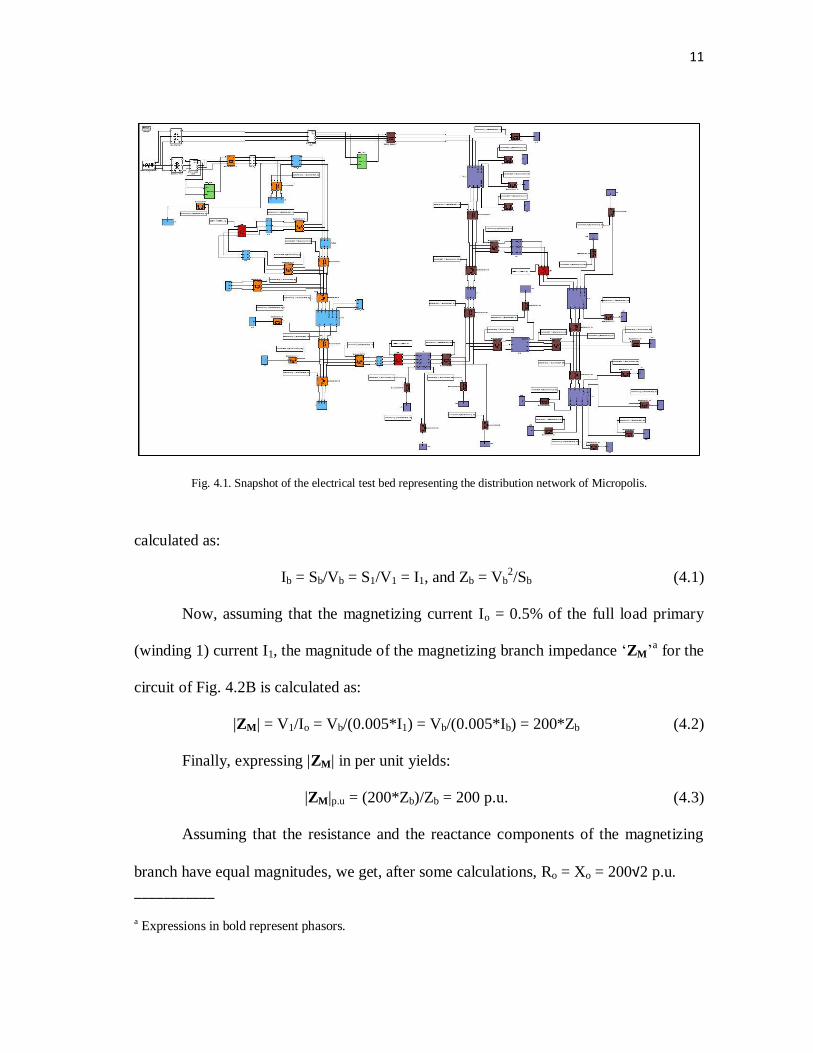
distribution network of Micropolis [8]. Fig. 4.1 presents a snapshot of the layout of the
electrical infrastructure components as modeled in the test bed. The following sections
explain the different stages in the design phase in a step-by-step fashion.
4.1. Determination of Distribution Transformer Constants
Fig. 4.2A shows the equivalent circuit of a transformer, with all secondary
parameters (impedance, current, voltage) referred to the primary. The turns ratio of the
transformer is denoted by „a‟. Since the magnetizing current Io is only a small fraction of
the full load primary current, I2‟ in Fig. 4.2A is practically equal to I1 [11]. Therefore, the
equivalent circuit of Fig. 4.2A can be further approximated into the circuit of Fig. 4.2B.
Transformer constants are usually calculated by performing open circuit and
short circuit tests on a given machine. Since such test data is not easily available for all
the different transformer configurations used across the electrical network of Micropolis,
we use the „%Z‟ and „X/R‟ values available in standard tables [12] for our calculations.
4.1.1. Determination of Magnetizing Branch Constants
Assuming the base voltage „Vb‟ and the base power „Sb‟ for the circuit of Fig.
4.2B to be equal to the nominal voltage of winding 1 „V1‟ and the nominal power rating
of the transformer „S1‟ respectively, the base current „Ib‟ and the base impedance „Zb‟ are
11
Fig. 4.1. Snapshot of the electrical test bed representing the distribution network of Micropolis.
calculated as:
Ib = Sb/Vb = S1/V1 = I1, and Zb = Vb2/Sb (4.1)
Now, assuming that the magnetizing current Io = 0.5% of the full load primary
(winding 1) current I1, the magnitude of the magnetizing branch impedance „ZM‟a for the
circuit of Fig. 4.2B is calculated as:
|ZM| = V1/Io = Vb/(0.005*I1) = Vb/(0.005*Ib) = 200*Zb (4.2)
Finally, expressing |ZM| in per unit yields:
|ZM|p.u = (200*Zb)/Zb = 200 p.u. (4.3)
Assuming that the resistance and the reactance components of the magnetizing
branch have equal magnitudes, we get, after some calculations, Ro = Xo = 200√2 p.u.
___________ a Expressions in bold represent phasors.

12
Fig. 4.2A. Equivalent circuit of a transformer.
Fig. 4.2B. Approximate equivalent circuit of the transformer.
4.1.2. Determination of Primary and Secondary Winding Leakage Impedances
Using the „%Z‟ and the „X/R‟ values available in standard tables [12], the
primary and secondary winding leakage impedances are calculated in the following
fashion. Assuming the „%Z‟ value for a given transformer is equal to „z‟ p.u and its
„X/R‟ ratio is equal to „b‟, the per unit resistance and reactance values are calculated as:
z/100 = √(Rp.u2 + Xp.u
2) = √(Rp.u
2 + b
2*Rp.u
2) = Rp.u √(1 + b
2) (4.4)
Rp.u = z/(100* 1 + b2), and Xp.u = b*Rp.u (4.5)
The per unit resistance and reactance values calculated using equations (4.4) and
(4.5) represent the total resistance (R1 + R2‟) and reactance (X1 + X2
‟) terms respectively,
13
as shown in Fig. 4.2B. It is however generally assumed that the primary and the
secondary (as referred to the primary) winding leakage impedances have equal
contributions to the total leakage impedance associated with the circuit of Fig. 4.2B [11].
The primary and secondary (as referred to the primary) winding leakage impedances are
therefore calculated by dividing the results obtained from equation (4.5) by two. Since
the resistance and reactance values calculated are already expressed in per unit, the
secondary winding leakage impedance (as referred to the primary) still remains the same
on being referred back to the secondary side.
4.2. Determination of Conductor Sizing Based on Ampacity
Since the load consumed by users across Micropolis have been categorized into
few distinct profiles as shown in Table 2.1, the total load demand associated with a given
line „i‟ in the system can be calculated by adding up the individual loads associated with
each downstream customer. Denoting the load demand associated with the line „i‟ as
„KVAi‟ and assuming 5% losses associated with the flow of power, the total power
carried by the line is then given as (KVAi/0.95). The r.m.s value of the line current is
then calculated in the following fashion.
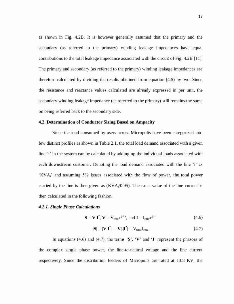
4.2.1. Single Phase Calculations
S = V.I*, V = Vrms.e
j.θv, and I = Irms.e
j.θi (4.6)
|S| = |V.I*| = |V|.|I
*| = Vrms.Irms (4.7)
In equations (4.6) and (4.7), the terms „S‟, „V‟ and „I‟ represent the phasors of
the complex single phase power, the line-to-neutral voltage and the line current
respectively. Since the distribution feeders of Micropolis are rated at 13.8 KV, the

14
corresponding single phase line-to-neutral voltage (r.m.s value) can be found to be equal
to 13.8/√3, or, 8 KV (assuming balanced three phase configuration of the system). The
r.m.s value of the line current can thus be calculated by substituting the terms |S| and
Vrms in equation (4.7) by (KVAi/0.95) and 8 KV respectively.
4.2.2. Three Phase Calculations
S = Van.Ian* + Vbn.Ibn
* + Vcn.Icn
* (4.8)
Van = Vrms.ej.0
, Vbn = Vrms.ej.(2∏/3)
, and Vcn = Vrms.e-j.(2∏/3)
(4.9)
Ian = Irms.e-j.Φ
, Ibn = Irms.ej.(2∏/3 - Φ)
, and Icn = Irms.e-j.(2∏/3 + Φ)
(4.10)
In equations (4.8) – (4.10), the term „S‟ denotes the phasor of the total three
phase complex power; „Van‟, „Vbn‟ and „Vcn‟ denote the phasors of the three line-to-
neutral voltages; and „Ian‟, „Ibn‟ and „Icn‟ denote the phasors of the three line currents.
„Vrms‟ and „Irms‟ represent the r.m.s values of the line-to-neutral voltage and the line
current respectively, and „Φ‟ signifies the phase difference between the voltage and the
current phasors. Using equations (4.8) – (4.10) and assuming balanced three phase
configuration of the system, the total three phase complex power is then given as:
S = 3*Vrms*Irms*ej.Φ
= √3*Vrms,L-L*Irms*ej.Φ
(4.11)
|S| = √3*Vrms,L-L*Irms (4.12)
In equation (4.11), the term „Vrms,L-L‟ represents the r.m.s value of the three phase
line-to-line voltage. Since the distribution feeders of Micropolis are rated at 13.8 KV, the
r.m.s value of the line current can thus be calculated by substituting the terms |S| and
Vrms,L-L in equation (4.12) by (KVAi/0.95) and 13.8 KV respectively.

15
Once the r.m.s values of the line currents are calculated using equations (4.7) or
(4.12), they are compared with the different conductor ampacity ratings available in
manufacturer specification sheets ([19] – [20]). While All Aluminum Conductor (AAC)
is used for the construction of the overhead lines, the underground lines are laid using
Aluminum Conductor TRXLPE Insulation Concentric Neutral cables. An appropriate
ampacity rating greater than the magnitude of the line current calculated is chosen, and
the corresponding conductor size is then assigned to the concerned line. Table 4.1 shows
the various conductor sizings used in the modeling of the electrical test bed for
Micropolis ([19] – [20]).
TABLE 4.1 MICROPOLIS ELECTRICAL TEST BED CONDUCTOR SIZINGS
Overhead Lines
Conductor Size Ampacity (Amps)
6 AWGb 110 A
2 AWG 195 A
3/0 AWG 350 A
4/0 AWG 410 A
266.8 kcmilc 475 A
397.5 kcmil 615 A
Underground Cables
Conductor Size Ampacity (Amps)
2 AWG 130 A
bAWG = American Wire Gage,
c1
kcmil = 1000 circular mills = 0.5067 mm
2.
4.3. Determination of Line Parameters
Once the conductor sizings for the different overhead lines and underground
cables of the electrical distribution network of Micropolis are decided, the next step is to
calculate the impedance and capacitance values associated with each such line or cable.
The following subsections explain the different formulae used for this purpose.

16
4.3.1. Underground Cables, Three Phase
The three phase underground cables present in the electrical distribution network
of Micropolis consist of seven strands of 2 AWG thick Al conductors, a 175 mils thick
TRXLPE insulation layer, a “one-third” concentric neutral comprising of six strands of
14 AWG thick Cu wires and a LLDPE encapsulating jacket. The cable burial
configuration is as shown in Fig. 4.3. The positive (Z1) and zero (Z0) sequence
impedances for three phase concentric neutral underground cables are calculated using
the following formulae [13].
Z1 = Zaa – Zab – ((Zax – Zab)2/(Zxx – Zab)) (4.13)
Z0 = Zaa + (2*Zab) – ((Zax + 2*Zab)2/(Zxx + 2*Zab)) (4.14)
Zaa = RΦ + Re + j*k1*log10(De/GMRΦ) (4.15)
Zab = Re + j*k1*log10(De/GMDΦ) (4.16)
Zxx = RN + Re + j*k1*log10(De/GMRN) (4.17)
Zax = Re + j*k1*log10(De/DN2) (4.18)
In equations (4.13) – (4.18), „Zaa‟ represents the self impedance of each phase
conductor, „Zab‟ represents the mutual impedance between two conductors, „Zax‟
represents the mutual impedance between a phase conductor and its concentric neutral,
and „Zxx‟ denotes the self impedance of each concentric neutral. „RΦ‟ is the resistance of
each phase conductor expressed in ohms/1000 feet (data available in standard tables,
[13]), „RN‟ is the resistance of the neutral (resistance of a „one-third‟ neutral is thrice that
of the phase conductor [13]) expressed in ohms/1000 feet, „k1‟ is equal to 0.0529
ohms/1000 feet, „GMRΦ‟ is the geometric mean radius of the phase conductor expressed

17
Fig. 4.3. Underground cable burial configuration.
in inches (data available in standard tables, [13]), „GMDΦ‟ is equal to dAB ∗ dBC ∗ dCA3
(inches, see Fig. 4.3.), „Re‟ is the resistance of the earth return path and is equal to
0.01807 ohms/1000 feet, „De‟ is the equivalent depth of the earth return current and is
equal to 25920 ρ/60 inches, „ρ‟ is the earth resistivity and is equal to 100 Ω-m,
„GMRN‟ is the geometric mean radius of the concentric neutral and is equal to
0.7788 ∗ n ∗ DN2(n−1)
∗ rn
n
inches, „n‟ is the number of neutral wire strands, „rn‟ is the
radius of each neutral strand in inches, and „DN2‟ is the distance from the center of the
phase conductor to the center of the neutral strand (inches, see Fig. 4.3.). The sequence
impedance components are thus calculated by substituting the relevant terms of
equations (4.13) – (4.18) by their corresponding values as obtained from standard tables
([13], [20]) and from Fig. 4.3. Thus, we get:
Z1 = 1.1072 + j*0.33794 Ω/km, and Z0 = 2.08044 + j*1.48226 Ω/km (4.19)
18
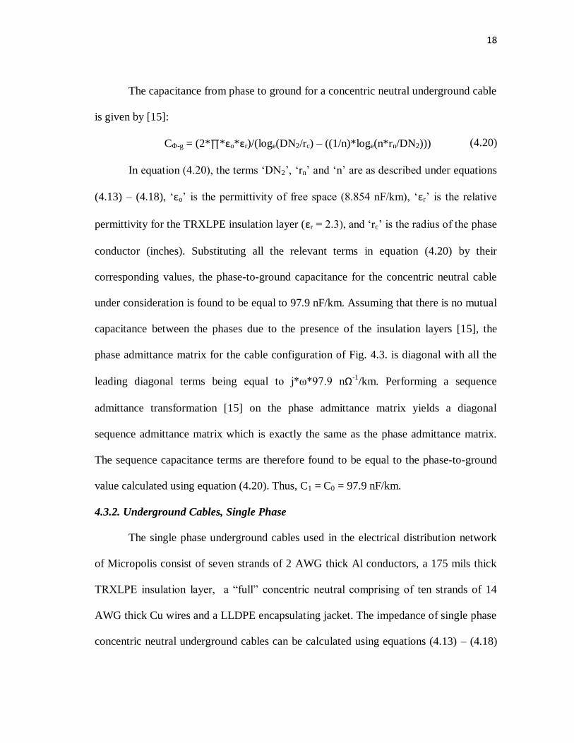
The capacitance from phase to ground for a concentric neutral underground cable
is given by [15]:
CΦ-g = (2*∏*εo*εr)/(loge(DN2/rc) – ((1/n)*loge(n*rn/DN2))) (4.20)
In equation (4.20), the terms „DN2‟, „rn‟ and „n‟ are as described under equations
(4.13) – (4.18), „εo‟ is the permittivity of free space (8.854 nF/km), „εr‟ is the relative
permittivity for the TRXLPE insulation layer (εr = 2.3), and „rc‟ is the radius of the phase
conductor (inches). Substituting all the relevant terms in equation (4.20) by their
corresponding values, the phase-to-ground capacitance for the concentric neutral cable
under consideration is found to be equal to 97.9 nF/km. Assuming that there is no mutual
capacitance between the phases due to the presence of the insulation layers [15], the
phase admittance matrix for the cable configuration of Fig. 4.3. is diagonal with all the
leading diagonal terms being equal to j*ω*97.9 nΩ-1/km. Performing a sequence
admittance transformation [15] on the phase admittance matrix yields a diagonal
sequence admittance matrix which is exactly the same as the phase admittance matrix.
The sequence capacitance terms are therefore found to be equal to the phase-to-ground
value calculated using equation (4.20). Thus, C1 = C0 = 97.9 nF/km.
4.3.2. Underground Cables, Single Phase
The single phase underground cables used in the electrical distribution network
of Micropolis consist of seven strands of 2 AWG thick Al conductors, a 175 mils thick
TRXLPE insulation layer, a “full” concentric neutral comprising of ten strands of 14
AWG thick Cu wires and a LLDPE encapsulating jacket. The impedance of single phase
concentric neutral underground cables can be calculated using equations (4.13) – (4.18)
19
after substituting the term „Zab‟ by 0. The phase-to-ground capacitance can then be
calculated using equation (4.20). The impedance and capacitance values thus calculated
are given as:
Z = 1.5075 + j*0.6055 Ω/km, C = 106.9 nF/km (4.21)
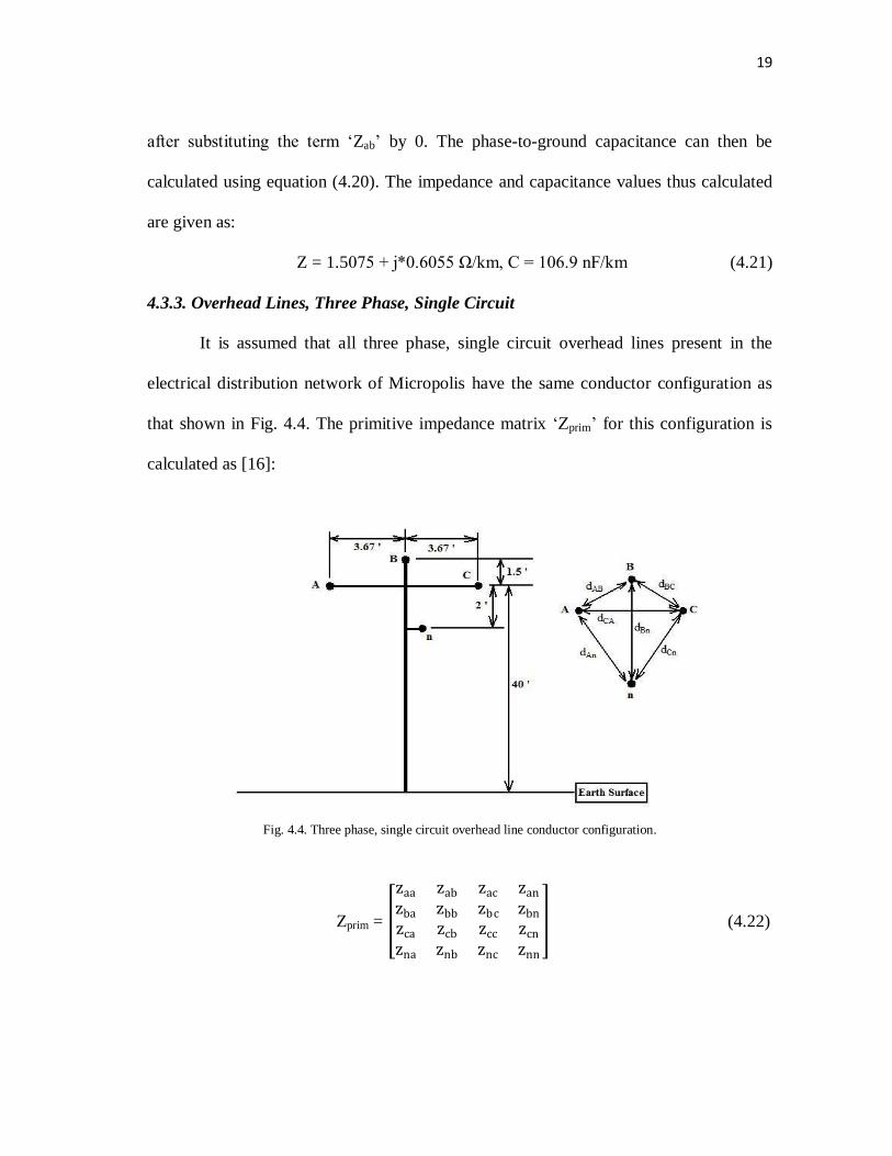
4.3.3. Overhead Lines, Three Phase, Single Circuit
It is assumed that all three phase, single circuit overhead lines present in the
electrical distribution network of Micropolis have the same conductor configuration as
that shown in Fig. 4.4. The primitive impedance matrix „Zprim‟ for this configuration is
calculated as [16]:
Fig. 4.4. Three phase, single circuit overhead line conductor configuration.
Zprim =
zaa zab zac zan
zba zbb zbc zbn
zca zcb zcc zcn
zna znb znc znn
(4.22)
20
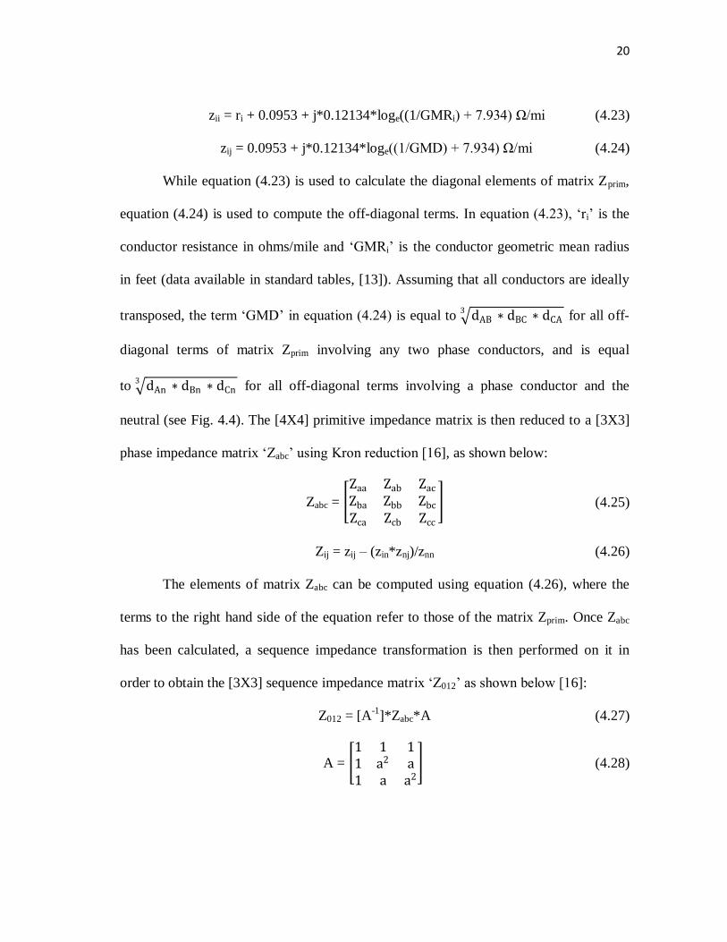
zii = ri + 0.0953 + j*0.12134*loge((1/GMRi) + 7.934) Ω/mi (4.23)
zij = 0.0953 + j*0.12134*loge((1/GMD) + 7.934) Ω/mi (4.24)
While equation (4.23) is used to calculate the diagonal elements of matrix Zprim,
equation (4.24) is used to compute the off-diagonal terms. In equation (4.23), „ri‟ is the
conductor resistance in ohms/mile and „GMRi‟ is the conductor geometric mean radius
in feet (data available in standard tables, [13]). Assuming that all conductors are ideally
transposed, the term „GMD‟ in equation (4.24) is equal to dAB ∗ dBC ∗ dCA3
for all off-
diagonal terms of matrix Zprim involving any two phase conductors, and is equal
to dAn ∗ dBn ∗ dCn3
for all off-diagonal terms involving a phase conductor and the
neutral (see Fig. 4.4). The [4X4] primitive impedance matrix is then reduced to a [3X3]
phase impedance matrix „Zabc‟ using Kron reduction [16], as shown below:
Zabc = Zaa Zab Zac
Zba Zbb Zbc
Zca Zcb Zcc
(4.25)
Zij = zij – (zin*znj)/znn (4.26)
The elements of matrix Zabc can be computed using equation (4.26), where the
terms to the right hand side of the equation refer to those of the matrix Zprim. Once Zabc
has been calculated, a sequence impedance transformation is then performed on it in
order to obtain the [3X3] sequence impedance matrix „Z012‟ as shown below [16]:
Z012 = [A-1
]*Zabc*A (4.27)
A =
1 1 11 a2 a1 a a2
(4.28)
21
In equation (4.28), the operator „a‟ represents the complex quantity ej*(2*∏/3)
. The
calculated sequence impedance matrix has the following diagonal structure, where „Z0‟
represents the zero sequence impedance of the concerned overhead line and „Z1‟ the
positive sequence impedance.
Z012 = Z0 0 00 Z1 00 0 Z2
(4.29)
For calculating the sequence capacitance values for three phase overhead lines,
the first step is to form the [4X4] potential coefficient matrix „Ppot‟ as shown below [14]:
Ppot =
paa pab pac pan
pba pbb pbc pbn
pca pcb pcc pcn
pna pnb pnc pnn
(4.30)
pii = (1/(2*∏*εo))*loge(2*hi/ri) km/nF (4.31)
pij = (1/(2*∏*εo))*loge(Dij/dij) km/nF (4.32)
While equation (4.31) is used to calculate the diagonal elements of matrix Ppot,
equation (4.32) is used to compute the off-diagonal terms. In equation (4.31), „hi‟
represents the average height above ground (feet) of conductor „i‟ (see Fig. 4.4); while
„ri‟ is the conductor radius in feet (data available in standard tables, [13]). In equation
(4.32), „Dij‟ is the distance in feet between the conductor „i‟ and the image below earth
surface of the conductor „j‟, and „dij‟ is the distance in feet between the conductors „i‟
and „j‟ (see Fig. 4.4). „εo‟ is the permittivity of free space and is equal to 8.854 nF/km.
The [4X4] potential coefficient matrix is then reduced to a [3X3] matrix „Pred‟ using the
Kron reduction formula as given in equation (4.26). The capacitance matrix „Cred‟ is then

22
obtained by inverting matrix Pred. Thus, Cred = [Pred]-1
(nF/km). Finally, the sequence
capacitance values are computed by performing a sequence admittance transformation
on the matrix Cred, using the same procedure as was outlined through equations (4.27) –
(4.28). Thus,
C012 = [A-1
]*Cred*A (4.33)
Table 4.2 shows the calculated sequence impedance and capacitance values
associated with the different three phase overhead lines present in the electrical
distribution network of Micropolis.
TABLE 4.2 SEQUENCE IMPEDANCE AND CAPACITANCE VALUES FOR THREE PHASE SINGLE CIRCUIT
OVERHEAD LINES
Conductor Size Z1
(Ω/km)
Z0
(Ω/km)
C1
(nF/km)
C0
(nF/km)
6 AWG 2.6411 + j*0.5102 3.0341 + j*1.803 8.6643 4.6495
2 AWG 1.0433 + j*0.4762 1.5173 + j*1.4968 9.3391 4.9021
3/0 AWG 0.4134 + j*0.4411 0.7597 + j*1.1775 10.131 5.1929
4/0 AWG 0.3281 + j*0.432 0.6285 + j*1.1261 10.354 5.2741
266.8 kcmil 0.2602 + j*4235 0.5171 + j*1.0858 10.5836 5.3569
397.5 kcmil 0.1752 + j*0.4044 0.3702 + j*1.0259 11.0303 5.5173
4.3.4. Overhead Lines, Single Phase
It is assumed that all single phase overhead lines of the electrical distribution
network of Micropolis have the same conductor configuration as that shown in Fig. 4.5.
The value of the conductor resistance (Ω/km) is obtained from standard tables as given
in [19]. The inductance per conductor and the capacitance across the conductors of Fig.
4.5 are calculated as ([21] – [22]):
LΦ = 0.2*loge(GMD/GMR) mH/km, and CΦ-n = 1/(36*loge(D/r)) μF/km (4.34)

23
Fig. 4.5. Single phase overhead line conductor configuration.
In equation (4.34), „GMR‟ is the conductor‟s geometric mean radius expressed in
feet, „r‟ is the physical radius of the conductor expressed in feet (data available in
standard tables, [13]), and „D‟ is the distance of separation (feet) between the
conductors. Assuming that both the phase and the neutral conductors have the same
cross-section area and number of strands, the term „GMD‟ in equation (4.34) is
approximately equal to the distance of separation between the two conductors [13].
Table 4.3 shows the calculated resistance, inductance and capacitance values associated
with the different single phase overhead lines present in the electrical distribution
network of Micropolis.
TABLE 4.3 RESISTANCE, INDUCTANCE AND CAPACITANCE VALUES FOR SINGLE PHASE OVERHEAD LINES
Conductor Size R
(Ω/km)
L
(mH/km)
C
(nF/km)
6 AWG 2.6411 1.2876 4.5362
2 AWG 1.0433 1.1972 4.9062

24
4.3.5. Overhead Lines, Three Phase, Double Circuit
The distribution feeders of Micropolis run in a double circuit configuration for
some distance after emanating from the substation, before branching off into their
respective service areas. The concerned configuration is as shown in Fig. 4.6. The
calculation of the sequence impedance and capacitance values for this configuration
follows the same steps as were explained in Section 4.3.3 [15].
Fig. 4.6. Three phase, double circuit overhead line conductor configuration.
As can be observed from Fig. 4.6, the primitive impedance matrix „Zprim‟ for this
situation would be of the order [7X7]. The primitive impedance matrix is then reduced to
a [6X6] phase impedance matrix „Zabc,12‟ using the Kron reduction formula as given in
equation (4.26). The matrix Zabc,12 has the following structure:

25
Zabc,12 =
Z1a,1a Z1a,1b Z1a,1c | Z1a,2a Z1a,2b Z1a,2c
Z1b,1a Z1b,1b Z1b,1c | Z1b ,2a Z1b,2b Z1b,2c
Z1c,1a Z1c,1b Z1c,1c | Z1c,2a Z1c,2b Z1c,2c
− − − + − − −Z2a,1a Z2a,1b Z2a,1c | Z2a,2a Z2a,2b Z2a,2c
Z2b,1a Z2b,1b Z2b,1c | Z2b,2a Z2b ,2b Z2b ,2c
Z2c,1a Z2c,1b Z2c,1c | Z2c,2a Z2c,2b Z2c,2c
(4.35)
The matrix Zabc,12 is then partitioned as shown in equation (4.35) in order to yield
four [3X3] matrices. While the phase impedance matrix corresponding to line 1in Fig.
4.6 is obtained by the partitioning of the first three rows and columns, the phase
impedance matrix for line 2 is obtained by the partitioning of the last three rows and
columns. The other two partitioned matrices represent the mutual coupling between the
two lines. The sequence impedance components corresponding to a given line is then
obtained by performing a sequence impedance transformation, as given in equations
(4.27) – (4.28), on the partitioned phase impedance matrix corresponding to that line.
Similarly, for calculating the sequence capacitance values for the configuration
of Fig. 4.6, we first form the [7X7] potential coefficient matrix „Ppot‟ as outlined in
Section 4.3.3. The matrix Ppot is then reduced to a [6X6] matrix „Pred,12‟ using the Kron
reduction formula as given in equation (4.26). The capacitance matrix „Cred,12‟ is
thereafter obtained by inverting the matrix Pred,12. Thus, Cred,12 = [Pred,12]-1
(nF/km). The
[6X6] capacitance matrix Cred,12 is then partitioned as explained above in order to yield
four [3X3] matrices. The sequence capacitance values associated with each line of Fig.
4.6 are then obtained by performing a sequence admittance transformation on the [3X3]
capacitance matrix corresponding to the concerned line.

26
The different sequence impedance and capacitance values thus calculated for the
three phase, double circuit overhead lines present in the electrical distribution network of
Micropolis are as shown in Table 4.4.
TABLE 4.4 SEQUENCE IMPEDANCE AND CAPACITANCE VALUES FOR THREE PHASE DOUBLE CIRCUIT
OVERHEAD LINES
Conductor Size Z1
(Ω/km)
Z0
(Ω/km)
C1
(nF/km)
C0
(nF/km)
Line 1 397.5 kcmil 0.1752 + j*0.3948 0.3532 + j*1.1693 11.7681 7.5193
Line 2 266.8 kcmil 0.2602 + j*4138 0.4475 + j*1.1187 11.2772 7.8502
4.3.6. Overhead Lines, Two Phase
It is assumed that all two phase overhead lines of the electrical distribution
network of Micropolis have the same conductor configuration as that shown in Fig. 4.7.
As can be observed from the figure, the primitive impedance matrix for this situation
would be of the order [3X3] as shown below [15]:
Zprim =
zaa zac zan
zca zcc zcn
zna znc znn
(4.36)
The primitive impedance matrix of equation (4.36) is then reduced to a [2X2]
phase impedance matrix „Zac‟ using the Kron reduction formula as given in equation
(4.26). The [3X3] „phase frame‟ matrix „Zabc‟ is then constructed from Zac by filling in
„0‟s for the missing phase as shown [15]:
Zabc =
Zaa 0 Zac
0 0 0Zca 0 Zcc
(4.37)

27
Fig. 4.7. Two phase overhead line conductor configuration.
The sequence impedance components are then calculated by performing a
sequence impedance transformation on Zabc, as explained using equations (4.27) –
(4.28).
The sequence capacitance terms are calculated by first forming the [3X3]
potential coefficient matrix „Ppot‟ corresponding to the configuration of Fig. 4.7. The
matrix Ppot is then reduced to a [2X2] matrix „Pred,ac‟ using the Kron reduction formula as
given in equation (4.26). The capacitance matrix „Cred,ac‟ is thereafter obtained by
inverting the matrix Pred,ac. Thus, Cred,ac = [Pred,ac]-1
(nF/km). The [3X3] „phase frame‟
matrix „Cred,abc‟ is then constructed from Cred,ac by filling in „0‟s for the missing phase as
shown:
Cred,abc =
Caa 0 Cac
0 0 0Cca 0 Ccc
(4.38)
The sequence capacitance terms are then obtained by performing a sequence
admittance transformation on Cred,abc, as explained using equation (4.33). The sequence

28
impedance and capacitance values thus calculated for the configuration of Fig. 4.7 are
given as:
Z1 = 1.8021 + j*0.4941 Ω/km, and Z0 = 1.9263 + j*0.9011 Ω/km (4.39)
C1 = 5.0289 nF/km, and C0 = 3.7739 nF/km (4.40)
4.4. Formulation of Protection Scheme for Electrical Test Bed
The layout of the electrical distribution network of Micropolis is as shown in Fig.
4.8. Defining a „Line‟ as a switchable section of the network formed by one or more
isolating elements at its ends, one may observe from Fig. 4.8 how a faulted Line can be
isolated by opening its corresponding terminating isolators. Since Micropolis is a small
city covering an area of approximately 2 square miles, it is assumed that all isolators
present in the distribution system are manually operated. The utility personnel thus
typically rely on customer calls in order to locate a particular fault, before isolating it
physically and carry out repair and restoration services.
The substation breakers of the distribution network, however, are assumed to be
operated through over-current relays. In the event that a short circuit fault occurs at some
point in the distribution system, the relay trips the breaker open. After a sufficient delay
during which the maintenance personnel are assumed to have located and isolated the
concerned fault, the breaker is closed in order to restore service to the remaining parts of
the network. This logic is implemented in the test bed using the relay module of Fig. 4.9
([17] – [18]). As can be observed from the figure, the instantaneous values of the phase
currents are first converted to their corresponding r.m.s values before being compared to

29
Fig. 4.8. Layout of the power distribution network for the city of Micropolis.
Fig. 4.9. Snapshot of the three phase over-current relay module.

30
prefixed bounds in the „comparison module‟. While the upper bound corresponds to 1.5
times the r.m.s value of the nominal phase current under normal operating conditions of
the system, the lower bound is equal to a current level of 0.5 A (any small positive value
will do). Thus, under normal operating conditions, the r.m.s values of the phase currents
satisfy these boundary conditions and hence the output of the corresponding „AND‟
blocks are all „1‟. The „OR‟ blocks at the end of the „delay module‟ thus all output „1‟
such that the breaker trip signal is „1‟ as well (corresponding to breaker being closed).
Assuming that a phase A-to-ground short circuit fault now occurs at some point
in the distribution system, the r.m.s value of the phase A fault current exceeds the upper
bound, and hence the output of the corresponding „AND‟ block becomes „0‟. The
„On/Off Delay‟ block operates in the following fashion. It normally outputs a „0‟ signal,
but when its input changes from „0‟ to „1‟; its output becomes „1‟ after a specified time
delay as long as its input is still „1‟. Thus, under normal operating conditions of the
system, when the „AND‟ blocks at the end of the comparison module all output „1‟, the
inputs to the on/off delay blocks through the „NOT‟ gates are all „0‟. When the above
mentioned fault occurs, the „AND‟ block corresponding to phase A outputs a „0‟, so that
the corresponding delay block sees a „1‟ at its input. At this time, since the outputs of the
„AND‟ and the delay block for phase A are both „0‟, the corresponding „OR‟ block
outputs a „0‟ as well, so that the relay trips the breaker open.
Once the breaker opens, the system current falls to 0, and hence the r.m.s. values
of all the phase currents now drop below their corresponding lower bounds. The outputs
of the „AND‟ blocks at the end of the comparison module are therefore all held at „0‟. As

31
a result, the on/off delay blocks still see a „1‟ at their inputs after the specified delay
period (which corresponds to the time the utility personnel take in manually clearing the
concerned fault) is over, and hence they output a „1‟ at this time. This is turn causes the
outputs of the corresponding „OR‟ blocks to become „1‟, and hence the breaker trip
signal is „1‟ as well. The breaker is thus closed again in order to restore service to the
healthy parts of the electrical network.
4.5. Assigning of System Loads
For simplicity sake, the various users across Micropolis have been categorized
into different profiles (e.g. residential, commercial, industrial etc.), and it is assumed that
the customers belonging to each such profile have a fixed load demand (KVA) all
through the year. The different load profiles are as shown in Table 2.1. It is further
assumed that the local electric utility maintains a constant power factor of 0.95 for all
load points across the city. Thus, all buildings connected to a given distribution
transformer are modeled in the test bed as a single load point with a fixed KW and
KVAR demand associated with it.
4.6. Source of Power Supply
Though it was mentioned in Chapter II that Micropolis does not have a power
generation facility of its own owing to its small size, a three phase voltage source rated
at 138 KV (the rating of the sub-transmission line) has been added to the test bed as a
source of power for the entire distribution network.

32
4.7. Conclusion
Though it was originally planned to use this test bed for running the fire spread
simulations on the electrical distribution network of Micropolis, the excessive time
required to complete any given simulation run was a major deterrent to this approach.
The fire spread studies were therefore carried out using an alternative methodology as
proposed in the subsequent chapters. This test bed, however, might still prove to be
helpful for researchers who wish to carry out any form of electrical analysis (e.g. short
circuit analysis, power flow studies, etc.) of the distribution system, as a part of studying
the effects of disasters on the interconnected infrastructure components of a city.
33
CHAPTER V
METHODOLOGY USED FOR ELECTRICAL SIMULATION RUNS
As mentioned in Chapter IV, since the original plan of using the Simulink based
test bed for carrying out the fire spread studies on the electrical distribution network of
Micropolis was abandoned, an alternative approach was devised as described in this and
the subsequent chapters. Though the proposed methodologies and algorithms have been
explained using the example of Micropolis, they are quite general in scope and can be
easily implemented on any given distribution network.
This chapter describes how we can use the fire polygon vertex coordinates output
by the MUFS code for studying and quantifying the damage caused by a given fire
spread scenario to the electrical network. The following sections discuss all relevant
assumptions, definitions and algorithms pertaining to the formulation and the
implementation of the proposed methodology [8].
5.1. Assumptions
1) We are dealing with a radial distribution system.
2) Though there are three Normally Open switches located across the electrical
distribution network of Micropolis (as shown in Fig. 4.8), they are assumed to be non-
functional for the time being.
3) The Micropolis electrical distribution system is assumed to be connected to an
infinite bus, so that events like a sudden loss of system load does not cause any system
stability issues.

34
4) Since fire spreads along the ground, its effect on the electrical system can be
accounted for by considering the status of only two types of electrical components: poles
and pad-mounted transformers.
5) Any pole or pad-mounted transformer which is found to be partially or fully
enclosed inside the fire polygon area for a given time step is considered to be faulted.
6) Repair and restoration of electrical components is not being considered during
fire spread.
7) Since the fire spread duration of 12 hours is only a small fraction of the Mean
Up Time of an electrical component, it is assumed that all faults occurring during the
course of a given simulation are a result of the fire only.
5.2. Definitions of Important Terms
1) Line: A „Line‟ is a switchable section of the electrical network formed by one
or more isolating element(s) at its ends. The location of the isolators and the
nomenclature of the Lines (as shown in Fig. 4.8) are purely a matter of system design.
For any given Line, its „upstream‟ end is the one through which power flows into it; the
other end being the „downstream‟ end.
2) Isolator Bank: An „Isolator Bank‟ (or just a „Bank‟) is a point in the
distribution network where a three-phase section of the feeder branches off into two or
more three-phase sub-branches. The intersection point of Lines 1, 9 and 7 in Fig. 4.8 is
an example of a Bank.
3) Upstream vs. Downstream: A component „X‟ is said to be „upstream‟ with
respect to a component „Y‟ if X is electrically closer to the substation than Y. In other

35
words, if we trace a path joining the substation to X and Y such that we move along the
flow of power, we shall come across X first and then Y.
5.3. General Treatment of Faulted Components
Under assumptions 4 and 5 (see Section 5.1), if a pole or a pad-mounted
transformer is found to be enclosed inside the fire polygon area for a given simulation
time step, the concerned component is then isolated from the rest of the network using
the following methodology [8].
5.3.1. Faulted Pole
If a pole belonging to any Line is found to be faulted, the concerned Line is
isolated irrespective of the type of the fault (short or open circuit). This is done taking
into consideration the fact that even though the fault might just be a local open circuit,
the fire will eventually cause the wooden poles to crumble down along with the
overhead conductors mounted on them. The isolation of the Line thus ensures that there
are no live wire ends present on the ground during the time when people are being
evacuated from the fire spread area. If, however, the affected pole represents a Bank, it is
isolated by opening the „upstream‟ end isolator of the Line which is immediately
upstream with respect to the Bank. For example, assuming that the Bank represented by
the intersection point of Lines 7, 8 and 10 in Fig. 4.8 gets faulted, it is isolated by
opening the isolator of Line 7 represented by the filled black square with a white cross
marked across it.

36
5.3.2. Faulted Pad-Mounted Transformer
On the lines of the approach proposed in subsection 5.3.1, if a pad-mounted
transformer belonging to any Line is found to be faulted, the concerned Line is isolated
as well. Since pad-mounted transformers are enclosed in iron casings, there is an
enormous build-up of gas and soot particles inside the casing once the fire engulfs it.
Leaving a high voltage live wire end in the casing can cause the gas to get ionized and
may even result in some dangerous blasts.
5.4. Load Loss Damage Index (LLDI)
Distribution system reliability indices like SAIDI, SAIFI, and CAIDI [23] are
generally used by electric utilities for planning and operational purposes. A closer look
at the indices, however, reveals that these are all average values calculated using data
collected from the observation of the system over a pre-defined period of time (usually
annually). As mentioned earlier, since the focus of this research is only on the window of
time during which the fire spreads, these indices are not really suitable for this study.
An alternative, the Load Loss Damage Index (LLDI), is therefore being proposed
and defined as [8]:
LLDI = KVAi ∗ (T − t ∗ i)T/ti=1 KVAh (5.1)
In equation (5.1), „KVAi‟ represents the total load (in KVA) lost in simulation
time step „i‟ due to the isolation of faulted Lines and/or Banks. The terms „t‟ and „T‟
respectively represent the total duration (in hours) of the physical fire spread which one
time step and one complete run of the MUFS simulation corresponds to. As mentioned
in Chapter III, the relevant values of „t‟ and „T‟ are equal to 1/12 hours (5 minutes) and

37
12 hours respectively. The expression within the parenthesis of equation (5.1) therefore
represents the time (in hours) left till the end of simulation, with respect to the current
time step. The LLDI value (in KVAh) thus calculated can therefore be used to measure
the extent of the damage caused to the electrical network for a given fire spread scenario.
5.5. Electrical Simulation Algorithm
Keeping in mind the assumptions and the general methods of treatment of faulted
components as proposed in the earlier sections, the electrical simulations are run using
the following algorithm [8].
1) Read the fire polygon coordinates for a given time step from the MUFS output
files.
2) Determine which all poles and/or transformers are fully or partially enclosed
inside the fire spread area for the given time step. Note that the fire polygon and the
individual pole and transformer coordinates all conform to the GIS layout of Micropolis
in ArcMap (see Chapter II).
3) Determine all Lines and/or Banks that are affected by the faulted poles and/or
transformers as found in step (2).
4) Scan all Line/Bank numbers as found in step (3) to determine which of those
are downstream with respect to the others. Eliminate all such downstream Line/Bank
numbers from the list of (3) as they will anyways be getting isolated by the isolation of
their concerned upstream components.
5) Isolate each of the upstream Lines/Banks as identified in step (4). For each
such isolated upstream component, scan all Lines/Banks which are located downstream

38
with respect to it. If any of such downstream Lines/Banks is found to be live till now, it
will also get „effectively isolated‟ as a result of the isolation of the concerned upstream
component.
6) For each Line/Bank getting physically or effectively isolated in the current
time step, calculate the total load (KVA) lost as a result of such outages.
7) Are all upstream Lines/Banks as found in step (4) isolated? If yes, go to (8). If
not, go to (5).
8) Calculate the current time step‟s contribution to the LLDI using equation
(5.1).
9) Check if the MUFS simulation has been completed (entire 12 hours of
simulation data has been generated) OR if both the substation breakers of Micropolis
have been opened (in which case, the city has been blacked out). If either of the
conditions is satisfied, end simulation and print results. Else, increase iteration count and
go to step (1).
The above mentioned algorithm is then used to implement the methodology
proposed in this chapter for studying and quantifying the damage caused by fire to the
electrical network. The following chapter discusses all relevant results obtained from
running numerous simulations on the Micropolis distribution system, corresponding to
different fire spread scenarios.

39
CHAPTER VI
ANALYSIS OF ELECTRICAL SIMULATION RUNS
This chapter presents the results [8] obtained from running numerous simulations
on the electrical distribution network of Micropolis, corresponding to different fire
spread scenarios. A close look at Tables 3.1 and 3.2 indicates that with the different
numbers of supporting infrastructure damage profiles, urban fire ignition point profiles
and wind directions considered for the purpose of this research, a total of 10*4*4 = 160
different fire spread scenarios can be generated. The various conclusions drawn from
these simulation runs have been arranged in the following two categories.
6.1. Most Damaging SIDP
Ten different simulations corresponding to the various supporting infrastructure
damage profiles were run for a given UFIP and wind direction combination. The LLDI
values calculated for all such simulation runs were then compared to determine the worst
infrastructure damage profile. The results of all relevant simulation runs are as shown in
Figs. 6.1(a) – (d). The following conclusions can be drawn from these figures [8].
1) Damage Profile AD1, which simulates the simultaneous destruction of all
three high-service pumps and the elevated storage tank, is by far the most damaging
profile across all different wind direction and UFIP combinations. This is natural as the
water pressure at the fire hydrants is seriously affected due to the unavailability of both
the storage tank and the high-service pumps. The fire thus spreads rapidly and this leads

40
(a)
(b)
(c)
Fig. 6.1. Results of electrical simulations run using MUFS data.

41
(d)
Fig. 6.1. continued.
to the outage of more Lines/Banks in the earlier stages of the simulation, thereby
yielding a high LLDI value.
2) The next most damaging profiles can be mostly found to be those of A01 and
D01. While A01 is a subset of AD1, the interesting thing to note about D01 is that its
LLDI value is mostly higher than that of D02. The reason for this is that while in the
case of D01 the storage tank is unavailable for the entire duration of simulation, it is
assumed to be available during the first hour of fire spread in the case of D02. The fire is
thus better contained towards the beginning of the simulation for D02, leading to less
electrical outages and hence a lower LLDI value.
3) As expected, the LLDI value for the UND profile is usually the least, as it
does not simulate the damage of any supporting infrastructure for fire response. Thus,
the fire fighters have better resources to contain the fire, leading to less electrical
outages.

42
4) Damage Profiles A03 and B03, which are really a subset of profile A01, can
be found to be having significantly lower LLDI values than that of A01.
5) Though the LLDI values for profiles E02, F01 or F04 are generally found to
be on the lower side, they have a greater degree of variation with respect to the different
wind direction and UFIP combinations. This is probably because these profiles do not
have any significant impact on the fire suppression efforts.
Note that the LLDI values corresponding to three out of the above mentioned 160
different fire spread scenarios are missing from the Figs. 6.1(a) – (d). This is either
because MUFS generated some run-time errors while simulating such scenarios, or
because the data required for such simulation runs was unavailable. Also, the LLDI
value for damage profile UND (GOV, East) is found to be exceptionally high. The LLDI
value, however, just reflects the typical pattern of the fire polygon coordinates as output
by the MUFS code for that simulation. These four cases account for just 2.5% of the
total simulations run, and can therefore be safely ignored.
6.2. Most Damaging UFIP
Table 6.1 shows the average LLDI values calculated over all combinations of
SIDPs and wind directions for a given UFIP profile. As can be seen, the two most
damaging ignition point profiles turn out to be those comprising of the city‟s government
buildings and the ecological targets respectively [8].
Referring to Fig. 2.1, where the government buildings had been represented by a
„G‟ marked on them, one may note their proximity to the city‟s central business district,
the industrial area and the two feeders coming out of the city‟s substation. Thus, a fire

43
starting from these buildings causes a heavy loss of load in the early stages of the
simulations, thereby yielding high LLDI values.
TABLE 6.1 MOST DAMAGING UFIP
Ignition Point Acronym Average LLDI value (MVAh)
GOV 160.811
ECO 76.845
CHU 70.889
SCH 55.909
The city‟s ecological targets, on the other hand, comprise of buildings containing
highly inflammable materials. It is therefore quite obvious that a fire starting from them
will be spreading very fast and will be difficult to contain, thereby leading to more
electrical outages and a higher average LLDI value.
The results presented in this chapter are based on the principal assumption that
the Normally Open (NO) switches present in the electrical distribution network of
Micropolis are unavailable. Thus, routing of power during emergencies is not possible
under this configuration. Electric power utilities, however, typically have numerous NO
switches located at strategic points across the distribution network for reliability
purposes. The following chapter proposes a methodology for routing power across
faulted sections of the electrical network at times of emergencies. The proposed
methodology is then implemented by means of an algorithm.

44
CHAPTER VII
GRAPH THEORY APPLICATIONS FOR ROUTING OF POWER
DURING EMERGENCIES
Assuming that some parts of the electrical distribution network of a city have
been faulted and subsequently isolated due to fire, this chapter presents a graph theoretic
approach [24] for routing power across the isolated sections using a given set of NO
switches. The routing is so done that the power flows along a path of minimum
impedance. The following sections illustrate the proposed approach along with its
associated algorithms using the example of Micropolis.
7.1. Assumptions
Since the methodology proposed in this chapter is basically an extension of the
one presented in Chapter V, all assumptions listed in Section 5.1 hold for this approach
as well, except for the second one. Figure 7.1 shows the layout of the electrical
distribution network of Micropolis along with the three NO switches located at strategic
points across it. It is assumed that all three of them are of the Triple Pole Single Throw
(3PST) type [25].
7.2. General Treatment of Faulted Components
Under assumptions 4 and 5 of Section 5.1, if an electrical component (a pole or a
pad-mounted transformer or a NO switch) is found to be enclosed inside the fire polygon
area for a given simulation time step, it is then isolated from the rest of the network
using the following methodology. Though the approaches described in this section are

45
very similar to those presented in Section 5.3, there are however some differences which
are highlighted through the following subsections [24].
Fig. 7.1. Layout of the electrical distribution network of Micropolis.
7.2.1. Faulted Pole
If a pole belonging to any Line (see definition in Section 5.2) is found to be
faulted, the concerned Line is isolated irrespective of the type of the fault (short or open
circuit). This is done taking into consideration the fact that even though the fault might
just be a local open circuit, the fire will eventually cause the wooden poles to crumble
down along with the overhead conductors mounted on them. The isolation of the Line
thus ensures that there are no live wire ends present on the ground during the time when

46
people are being evacuated from the fire spread area. If, however, the affected pole
represents a Bank, it is isolated by opening the terminating isolators of the Lines incident
at the Bank; such that the isolators themselves are not located at the Bank. If any of such
terminating isolators happens to be a NO switch, it also has to be permanently opened in
order to isolate the faulted Bank. For example, assuming that the Bank represented by
the intersection point of Lines 7, 8 and 10 in Fig. 7.1 gets faulted, it is isolated by
permanently opening the NO switch 1 and by opening the isolators of Lines 7 and 10
represented by the filled black squares with a white cross marked across them.
7.2.2. Faulted Pad-Mounted Transformer
On the lines of the approach proposed in subsection 7.2.1, if a pad-mounted
transformer belonging to any Line is found to be faulted, we again isolate the concerned
Line. Since pad-mounted transformers are enclosed in iron casings, there is an enormous
build-up of gas and soot particles inside the casing once the fire engulfs it. Leaving a
high voltage live wire end in the casing can cause the gas to get ionized and may even
result in some dangerous blasts.
7.2.3. Faulted NO Switch
The NO switches located across the electrical network of Micropolis are assumed
to be either pole or pad mounted, depending on whether they span across two overhead
lines or two underground cables. Now, during the course of the electrical simulations, if
it is determined that a pole or a pad containing a given NO switch is under fire, it can be
isolated by opening the terminating isolators of the Lines across which the switch is
physically present; such that the isolators themselves are not located at the site of the

47
switch. For example, assuming that the pole on which NO switch 2 is mounted (see Fig.
7.1) gets faulted, it is isolated by opening the isolators of Lines 9 and 12 represented by
the filled black squares with a white circle marked on them.
7.3. Overall Electrical Simulation Algorithm
This section presents an extension of the algorithm of Section 5.5, by
incorporating in it the concept of power routing during emergencies. The following
algorithm [24] calls a subroutine, which in turn implements a graph theoretic approach
(see Section 7.4) for routing power across faulted sections of the electrical network using
a given set of NO switches.
1) Read the fire polygon vertex coordinates for a given time step from the MUFS
output files.
2) Determine which poles and/or transformers are fully or partially enclosed
inside the fire spread area for the given time step. Note that the fire polygon and the
individual pole and transformer coordinates all conform to the GIS layout of Micropolis
in ArcMap (see Chapter II).
3) Determine all Lines, Banks and/or NO switches that are affected by the faulted
poles and/or transformers as found in step (2).
4) Scan all Line numbers as found in step (3) to determine which of those are
downstream with respect to any other Line or a Bank or a NO switch as also found to be
faulted in (3). Eliminate all such downstream Line numbers from the list of (3) as they
will anyways be getting isolated by the isolation of their concerned upstream
components.

48
5) Isolate each of the upstream Lines/Banks/NO switches as identified in step (4).
For each such isolated upstream component, scan all Lines which are located
downstream with respect to it. If any of such downstream Lines is found to be live till
now, it will also get „effectively isolated‟ as a result of the isolation of the concerned
upstream component.
6) Are all upstream Lines/Banks/NO switches as found in step (4) isolated? If
yes, go to step (7). If not, repeat step (5).
7) Call the graph theoretic subroutine explained in the next section with an
argument containing the IDs of all Lines and NO switches which are getting physically
or effectively isolated in the current time step.
8) The graph theoretic subroutine returns back an argument containing a list of
the IDs of NO switches that need to be closed for routing power to the affected parts of
the system, and a list of the IDs of isolators that need to be opened for preventing bi-
directional power flows at the network nodes (see subsection 7.4.6). Perform all such
actions (closing of switches and opening of isolators) and proceed to step (9).
9) For all Lines, Banks and/or NO switches getting physically or effectively
isolated in the current time step, add up the total load (KVA) lost as a result of such
outages. Calculate the current time step‟s contribution to the LLDI using equation (5.1).
10) Check if the MUFS simulation has been completed (entire 12 hours of
simulation data has been generated) OR if both the substation breakers of Micropolis
have been opened (in which case, the city has been blacked out). If either of the

49
conditions is satisfied, end simulation and print results. Else, increase iteration count and
go to step (1).
7.4. Formulation of Graph Theoretic Approach for Power Routing
This section proposes a graph theoretic approach [24] for routing power across
faulted sections of the electrical distribution network of a city using a given set of NO
switches. This approach forms part of the overall algorithm presented in Section 7.3. The
proposed methodology is explained through the following subsections using the example
of Micropolis.
7.4.1. Drawing the Equivalent Graph
The first step in implementing the graph theoretic approach, however, would be
to represent the electrical distribution network of a city such as Micropolis by an
equivalent graph. In doing so, all single phase laterals which branch off from any given
line in the distribution network are ignored while constructing the equivalent graph. This
is because in the event that a „parent‟ line (e.g. Line 11 in Fig. 7.1) from which a
concerned lateral (e.g. Line 30 in Fig. 7.1) branches out gets faulted and isolated, the
lateral gets effectively isolated as well. This also makes the resultant graph look less
bulky. Similarly, any three-phase tapping (e.g. Line 6 in Fig. 7.1) which branches out of
a line in the electrical network and which gets terminated by itself, i.e. it neither
branches off into any more sub-branches nor ends in a NO switch, is ignored as well.
The equivalent graph representing the distribution network of Micropolis, as
shown in Fig. 7.2, is constructed by „stitching together‟ two tree structures, with each
tree representing the network associated with a given feeder. Each edge of a tree thus

50
represents a particular Line in the electrical network of Fig. 7.1. The topmost node in a
given tree is termed as a „source node‟, and it represents the source of power for the
corresponding distribution feeder. Nodes 1 and 13 in Fig. 7.2 are thus the source nodes
for our case. The trees are then stitched together using „links‟ belonging to either of the
following two categories:
7.4.1.1. Link, Type I
The edges of the individual trees, which correspond to lines across which a NO
switch is physically present in the electrical network, are joined using a Type I link. The
Type I links are represented by the red lines of Fig. 7.2.
7.4.1.2. Link, Type II
All source nodes of the equivalent graph are connected to a single hypothetical
„super node‟ (Node 0) by means of Type II links, as represented by the magenta lines of
Fig. 7.2. The purpose of incorporating the concept of the super node is explained in a
later subsection.
7.4.2. Assigning Weights
The next step after the construction of the equivalent graph is to assign weights
to its individual edges and links. Each edge is assigned a weight equal to the total
impedance of its corresponding line in the electrical network. Referring to Chapter IV,
where the different formulae used for the impedance (Ω/km) calculations of overhead
conductors and underground cables were explained, the total impedance (Ω) of a given
line is calculated by multiplying its impedance (Ω/km) with its corresponding length in
the distribution system. For a two or a three phase line, the weight assigned to its
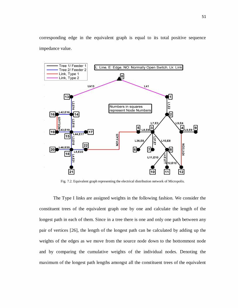
51
corresponding edge in the equivalent graph is equal to its total positive sequence
impedance value.
Fig. 7.2. Equivalent graph representing the electrical distribution network of Micropolis.
The Type I links are assigned weights in the following fashion. We consider the
constituent trees of the equivalent graph one by one and calculate the length of the
longest path in each of them. Since in a tree there is one and only one path between any
pair of vertices [26], the length of the longest path can be calculated by adding up the
weights of the edges as we move from the source node down to the bottommost node
and by comparing the cumulative weights of the individual nodes. Denoting the
maximum of the longest path lengths amongst all the constituent trees of the equivalent

52
graph by „Lmax‟, the weight assigned to each of the Type I links is equal to „k*Lmax‟,
where „k‟ is a multiplier greater than one. This is done to ensure that in the event that we
run a shortest path algorithm on the equivalent graph under normal operating conditions
of the system (i.e. when all lines are healthy and all NO switches are open), the shortest
path between any given edge and its corresponding source node is along its own tree
structure itself and not through any Type I link. The value of „k‟ is chosen to be equal to
ten for the purpose of this research.
All Type II links are assigned „0‟ weights as they are hypothetical and as such do
not physically exist in the electrical network.
The weights thereby assigned to the edges and the links of the equivalent graph
of Fig. 7.2 are as shown in Table 7.1. Note that these weights are all one-time
assignments made at the start of a given fire spread simulation.
7.4.3. Dijkstra’s Shortest Path Algorithm (Run I)
The graph theoretic subroutine, which is used to implement the approach
proposed in this section, reads the list of the faulted Line and NO switch IDs as sent by
the overall electrical simulation algorithm of Section 7.3; and removes the corresponding
edges and links from the equivalent graph. In the actual program, the removal of an edge
or a link is simulated by replacing its previously assigned weight (as given in Table 7.1)
by a very large number, say „N‟ [26]. For the purpose of this research, the value of „N‟ is
chosen to be equal to the summation of the weights of all the edges and the links of the
equivalent graph of Fig. 7.2. A preliminary run of the Dijkstra‟s shortest path algorithm
is then performed in order to calculate the shortest path distance (Ω) between the super

53
node and every other node in the equivalent graph. The advantage of using the super
node is that we can calculate its shortest path distance from all the other nodes in the
graph by running Dijkstra‟s algorithm only once. Otherwise, we would have had to
perform as many runs of the algorithm as there are source nodes in the graph, which in
turn could be a computationally intensive process for a large distribution system.
TABLE 7.1 WEIGHTS ASSIGNED TO THE EDGES AND THE LINKS OF THE EQUIVALENT GRAPH
Type ID Line/NO switch
Number
Weight
(Ω)
Edge 2 Line 1 0.1182 Ω
Edge 3 Line 7 0.1212 Ω
Edge 4 Line 9 0.1323 Ω
Edge 5 Line 8 0.1212 Ω
Edge 6 Line 36 0.4386 Ω
Edge 7 Line 37 0.4386 Ω
Edge 8 Line 10 0.1323 Ω
Edge 9 Line 9 0.2389 Ω
Edge 10 Line 11 0.2901 Ω
Edge 11 Line 27 1.2847 Ω
Edge 12 Line 12 0.1323 Ω
Edge 14 Line 2 0.2593 Ω
Edge 15 Line 2 0.0606 Ω
Edge 16 Line 42 0.7092 Ω
Edge 17 Line 44 0.5293 Ω
Edge 18 Line 3 0.1474 Ω
Edge 19 Line 43 0.7692 Ω
Edge 20 Line 46 0.9161 Ω
Edge 21 Line 4 0.9101 Ω
Edge 22 Line 5 0.0737 Ω
Link, Type I 23 NO Switch 1 16.564d Ω
Link, Type I 24 NO Switch 2 16.564 Ω
Link, Type I 25 NO Switch 3 16.564 Ω
Link, Type II 1 Not Applicable 0
Link, Type II 13 Not Applicable 0
dLmax for the equivalent graph of Fig. 7.2 is equal to 1.6564 Ω.
The Dijkstra‟s algorithm is run according to the following steps [26]:
1) Assign a permanent label of „0‟ to the super node and temporary labels of
„106‟ to all the remaining nodes in the graph.

54
2) Set variable „ni‟, corresponding to a given node „i‟ in the graph, to 0 (ID of the
super node).
3) Scan through all the temporarily labeled nodes in the graph in order to
determine which of them are connected to node „i‟ through an edge or a link. Any node
„j‟ found so connected then gets a new temporary label equal to min(old label of „j‟, (old
label of „i‟+dij)), where „dij‟ is the weight of the edge or the link connecting nodes „i‟ and
„j‟.
4) After all temporary labeled nodes have been scanned and new temporary
labels assigned wherever applicable, the minimum of all the temporary labels is found
and that becomes the permanent label for the corresponding node. In case of a tie, any
one of the concerned nodes is selected and is permanently labeled.
5) Assign the ID of the node which was just permanently labeled in step (4) to
the variable „ni‟.
6) Are all nodes in the equivalent graph permanently labeled? If yes, proceed to
the next subsection. If not, go to step (3).
The permanent label thereby assigned to a given node in the graph is actually the
length of the shortest path joining that node to the super node. Since the calculated
length is in ohms, it also represents the minimum impedance path connecting the two
points.
7.4.4. Determining Network Connectivity
Assuming that at a particular time step during the course of a given fire spread
simulation, Lines 10 and 12 become faulted; it can be observed from Fig. 7.1. that Lines

55
11 and 27 will be effectively isolated as well due to lack of connectivity with the rest of
the network. This subsection explains how the graph theoretic subroutine finds out
which additional lines (i.e. apart from the ones which the overall electrical simulation
algorithm of Section 7.3 determines as being faulted) have lost power in the current time
step due to lack of network connectivity.
After the first run of the Dijkstra‟s shortest path algorithm is performed, we scan
through each edge of the equivalent graph which corresponds to some healthy line in the
electrical network. For each such edge, we compare the lengths (Ω) of the minimum
impedance path associated with its two terminating nodes, and assign the node
corresponding to the shorter of those two lengths as its „target node‟. The minimum
impedance path length associated with a given line in the electrical network is thus equal
to the length of the minimum impedance path connecting the super node to the target
node of the edge corresponding to the concerned line.
There might be some instances in the distribution system where one line may
have multiple edges representing itself in the equivalent graph (e.g. Lines 2 and 9 in Fig.
7.2). For such situations if we consider the constituent edges of the line one by one and
assign target nodes to each of them, the same line will end up having more than one
target node. This in turn implies that there will be more than one minimum impedance
path associated with the same line and hence power can flow into the line from more
than one point. Since a „Line‟ (as defined in Section 5.2) has isolating elements at its
ends only, this kind of configuration might lead to a bi-directional flow of power to
occur on the same line, which is unacceptable. In order to avoid such situations, we have

56
to therefore ensure that all the edges of the graph belonging to the same line are assigned
just one target node. To do so, we consider as a whole the chain of edges corresponding
to a given line, and compare the minimum impedance path lengths associated with the
two nodes present at the extreme ends of the chain. For edges 4 and 9 belonging to Line
9 in Fig. 7.2, the two extreme end nodes would therefore be those with the IDs 2 and 9.
Thereafter, the node corresponding to the shorter of the two lengths is assigned as the
target node for the entire chain of edges belonging to the same line.
Denoting the length of the minimum impedance path associated with a given line
„i‟ as „Lmin,i‟, we can draw the following conclusions regarding its connectivity status for
the current time step.
7.4.4.1. Lmin,i <= Lmax
The satisfaction of this inequality implies that the concerned line is healthy and is
receiving power as it would under normal operating conditions of the system. In other
words, the minimum impedance path connecting the super node to the edge
corresponding to the given line does not involve any Type I link.
7.4.4.2. Lmax < Lmin,i < N
The satisfaction of this inequality implies that the concerned line is healthy but it
receives power through the closure of at least one NO switch. In other words, the
minimum impedance path connecting the super node to the edge corresponding to the
given line involves at least one Type I link.

57
7.4.4.3. Lmin,i >= N
The satisfaction of this inequality implies that the concerned line has become
effectively isolated due to lack of network connectivity. In other words, the edge
corresponding to the given line cannot be connected to the super node without passing
through at least one faulted edge or a faulted Type I link.
The graph theoretic subroutine thus calculates the Lmin,i values associated with all
healthy lines in the electrical network, and groups them into the three different
categories as described above. While lines satisfying the first inequality continue to
receive power as they would under normal operating conditions of the system, those
satisfying the second inequality are assigned shortest impedance paths using the
available NO switches of the electrical network. Finally, lines satisfying the third
inequality are declared as being effectively isolated from the current time step onwards.
7.4.5. Assigning Shortest Impedance Paths for Power Routing
The graph theoretic subroutine keeps a record of the order in which the various
nodes of the equivalent graph get permanently labeled while performing the first run of
the Dijkstra‟s algorithm. This record is stored in a row matrix „A‟. For a given line
satisfying the second inequality of subsection 7.4.4, let us assume that the target node of
its corresponding edge in the equivalent graph is stored in column „i‟ of the „A‟ matrix.
The minimum impedance path for the concerned line can then be constructed by
working backwards from the „ith
‟ column of the „A‟ matrix till we reach column „0‟;
such that we go to that predecessor column whose corresponding node label differs from
that of the current column by an amount equal to the weight of the connecting edge or

58
link [26]. One may however observe that the minimum impedance paths so traced using
the „A‟ matrix as obtained from the primary run of the Dijkstra‟s algorithm may not
always produce the most optimal results. This is owing to the fact that even though a
closed NO switch is supposed to be represented in the equivalent graph by a Type I link
of „0‟ weight, we had assigned artificially high weights of „k*Lmax‟ to all the Type I links
for reasons explained in subsection 7.4.2. This argument can be further illustrated using
the example of a sample network, as represented by the equivalent graph of Fig. 7.3.
Fig. 7.3. Equivalent graph representing a part of a sample electrical network.
Assuming that at a particular time step during the course of a given fire spread
simulation, Lines 3 and 6 of Fig. 7.3 become faulted; one may observe that Line 7 can be
connected to the rest of the network through either of the following two paths: „Lk1, L1

59
L2, Lk5, L4, Lk6, L8‟ or „Lk4, L9, L10, Lk7‟. Assuming that Lmax for the network of
Fig. 7.3 is equal to 10Ω, the weights assigned to each of the Type I links would therefore
be equal to 100Ω (refer to subsection 7.4.2). Under this situation, the primary run of the
Dijkstra‟s algorithm would therefore designate the latter path as the minimum
impedance path for routing power to Line 7. Since a closed NO switch, as is required for
the routing of power, should be represented in the equivalent graph by a Type I link of
„0‟ weight, one may however observe under this assumption that the former path
actually has a lower impedance than the latter. The minimum impedance path for routing
power to Line 7, as calculated from the first run of the Dijkstra‟s algorithm, does not
therefore give us the most optimal solution in this case.
To solve this issue, we freeze the permanent labels (as obtained from the first run
of the Dijkstra‟s algorithm) of all nodes in the equivalent graph which are associated
with edges satisfying the first inequality of subsection 7.4.4. This is done to ensure that
we retain the configuration of those parts of the network which are receiving power as
they would under normal operating conditions of the system. The weights of all healthy
Type I links of the equivalent graph are then set to 0, and a second run of the Dijkstra‟s
shortest path algorithm is performed. The minimum impedance paths associated with
lines satisfying the second inequality of subsection 7.4.4 are then constructed using the
„A‟ matrix as obtained from the second run of the Dijkstra‟s algorithm. Note that the
graph theoretic subroutine resets the weights of all healthy Type I links back to their
original values before proceeding to the next subsection.

60
One may further observe that even the approach described above may not always
generate the absolute minimum impedance paths for power routing. To illustrate this, let
us now assume that only Line 6 in Fig. 7.3 is faulted. Using the above mentioned
approach, the minimum impedance path as calculated for routing power to Line 7 would
now be along „Lk2, L3, Lk 6, L8‟, and not along „Lk1, L1 L2, Lk5, L4, Lk6, L8‟. This is
in spite of the fact that the latter path has a lower impedance than the former. This
anomaly can be resolved by observing that our main focus is to provide uninterrupted
service to customers who are already receiving power without the need of any routing.
The above mentioned approach can therefore be best regarded as a compromise between
finding the absolute minimum impedance path for routing power to a concerned line and
retaining the configuration of those parts of the electrical network which are receiving
power as they would under normal operating conditions of the system.
7.4.6. Resolving Bi-directional Power Flow Issues
Referring again to Fig. 7.2, let us assume that at a particular simulation time step,
Line 7 gets faulted by fire. Let us also assume that the target nodes for edges 5 and 8, as
determined from the second run of the Dijkstra‟s shortest path algorithm, are nodes 5
and 8 respectively. Under such circumstances, the minimum impedance path associated
with Line 8 will be along „Lk13, E14, E15, E18, E22, Lk23‟, while that associated with
Line 10 will be along „Lk1, E2, E4, Lk24, E12‟. It can thus be easily observed that there
will be a bi-directional flow of power occurring at node 3. This section presents an
algorithm to check for and correct bi-directional power flows occurring at different
nodes across the equivalent graph.

61
1) Scan through each node of the graph except for the super node.
2) For a given node, determine which all edges and Type I links are incident
(in/out) at it, and store their corresponding IDs in a temporary matrix „X‟. In doing so,
ignore any faulted edge, faulted Type I link or even any healthy Type I link where the
corresponding NO switch has an „open‟ status for the current time step.
3) For a given ID stored in matrix X, does that correspond to an edge? If yes, go
to step (4). If not, go to step (5).
4) Check if the target node corresponding to the edge being examined in step (3)
is different from the node being examined in step (2). If yes, go to step (6). If not, store
the ID of the concerned edge in another matrix „Y‟. Also, check the constituents of the
minimum impedance path associated with this current edge and store in matrix „Y‟ the
ID of the edge or link from which power flows into this edge. Proceed to step (6).
5) For the Type I link being examined in step (3), the graph theoretic subroutine
retrieves the ID of the edge from which power flows into this link. Check if this
concerned edge is also incident at the same node as was being examined in step (2). If
yes, store the concerned edge and Type I link IDs in matrix Y and go to step (6). If not,
directly go to step (6).
6) Are all the edge and link IDs as stored in matrix X in step (2) analyzed? If yes,
go to step (7). If not, pick up the next available ID and go to step (3).
7) For each ID stored in matrix X, check if it appears in matrix Y as well. If it
does, go to step (8). If not, open the terminating isolator of the line corresponding to the

62
edge whose ID was not found in Y; such that the isolator is located at that point in the
electrical network which corresponds to the node being examined in step (2). Go to (8).
8) Have all IDs stored in matrix X been checked against those in matrix Y? If
yes, go to step (9). If not, pick up the next available ID and repeat (7).
9) Have all nodes of the graph except for the super node been scanned for the
current time step? If yes, stop running subroutine and return back control to the overall
electrical simulation algorithm of Section 7.3. If not, pick up the next available node and
go to step (2).
To better explain the above mentioned algorithm, let us consider a part of a
sample distribution network, as represented by the graph of Fig. 7.4. Consider node 2
and assume that the edges 1, 2, 3 and 4 and the Type I link 5 are all incident at it as
shown in Fig. 7.4. Also assume that for a given simulation time step, the resultant power
flow in the network is as shown by the arrows in Fig. 7.4.
Fig. 7.4. Graph representing part of a sample distribution network.

63
Now, assuming that edge 2 receives its power from edge 1, one may conclude
that the target node and the immediately upstream edge ID for edge 2 would be those of
node 2 and edge 1 respectively. Since the graph theoretic subroutine assigns a unique
minimum impedance path to a given target node, any edge which is incident at node 2
and which gets its power through that node will have the same target node and
immediately upstream edge ID combination as edge 2. Thus, following the steps
mentioned in the algorithm above, matrices X and Y for the network of Fig. 7.4 would
look like: X = [1;2;3;4;5] and Y = [1;2;3;5]. Note that since the target node for edge 4 is
node 5 (and not node 2); it does not appear in matrix Y. Thus, the bi-directional power
flow encountered at node 2 can be prevented by opening the terminating isolator of the
line corresponding to edge 4; such that the isolator is located at that point in the
electrical network which corresponds to node 2 (as shown by the cross marked on edge 4
in Fig. 7.4).
Thus the electrical algorithm of Section 7.3 calls a graph theoretic subroutine,
which in turn implements the general approach presented in Section 7.4. The important
results obtained from running different fire spread simulations on the electrical
distribution network of Micropolis using the algorithm of Section 7.3 are presented in
the next chapter.
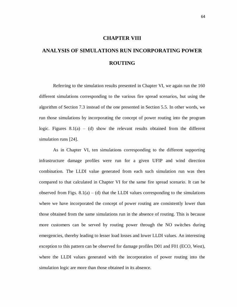
64
CHAPTER VIII
ANALYSIS OF SIMULATIONS RUN INCORPORATING POWER
ROUTING
Referring to the simulation results presented in Chapter VI, we again run the 160
different simulations corresponding to the various fire spread scenarios, but using the
algorithm of Section 7.3 instead of the one presented in Section 5.5. In other words, we
run those simulations by incorporating the concept of power routing into the program
logic. Figures 8.1(a) – (d) show the relevant results obtained from the different
simulation runs [24].
As in Chapter VI, ten simulations corresponding to the different supporting
infrastructure damage profiles were run for a given UFIP and wind direction
combination. The LLDI value generated from each such simulation run was then
compared to that calculated in Chapter VI for the same fire spread scenario. It can be
observed from Figs. 8.1(a) – (d) that the LLDI values corresponding to the simulations
where we have incorporated the concept of power routing are consistently lower than
those obtained from the same simulations run in the absence of routing. This is because
more customers can be served by routing power through the NO switches during
emergencies, thereby leading to lesser load losses and lower LLDI values. An interesting
exception to this pattern can be observed for damage profiles D01 and F01 (ECO, West),
where the LLDI values generated with the incorporation of power routing into the
simulation logic are more than those obtained in its absence.
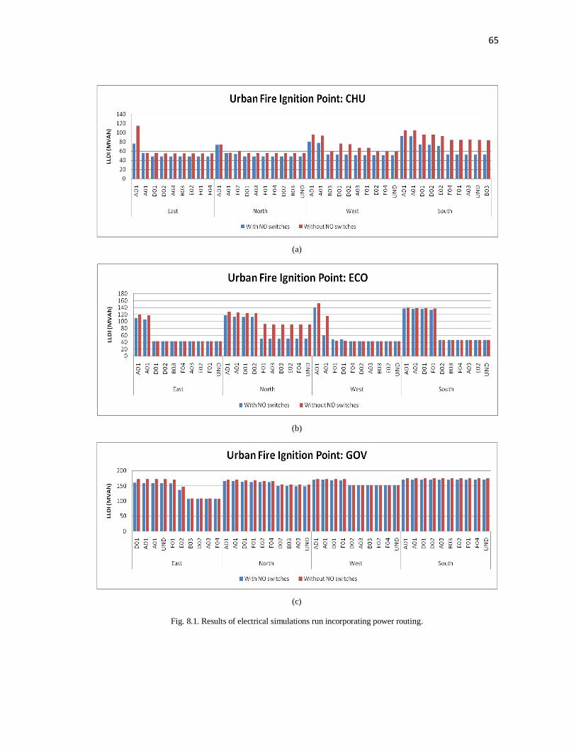
65
(a)
(b)
(c)
Fig. 8.1. Results of electrical simulations run incorporating power routing.
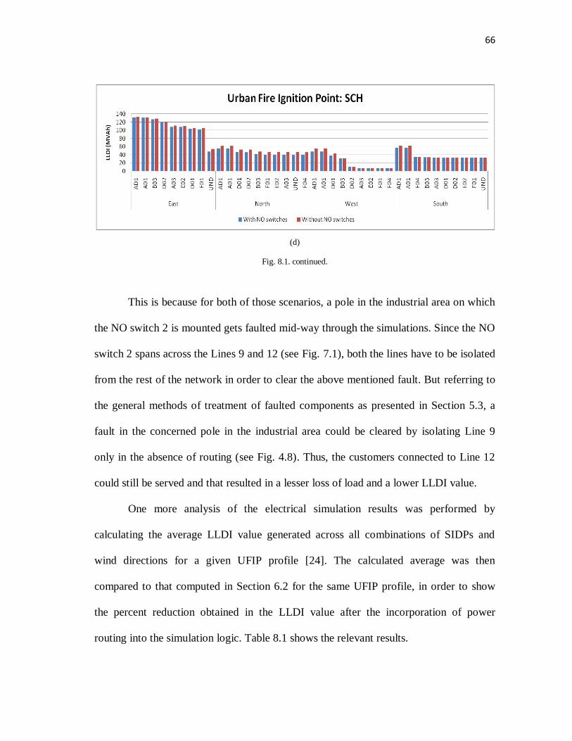
66
(d)
Fig. 8.1. continued.
This is because for both of those scenarios, a pole in the industrial area on which
the NO switch 2 is mounted gets faulted mid-way through the simulations. Since the NO
switch 2 spans across the Lines 9 and 12 (see Fig. 7.1), both the lines have to be isolated
from the rest of the network in order to clear the above mentioned fault. But referring to
the general methods of treatment of faulted components as presented in Section 5.3, a
fault in the concerned pole in the industrial area could be cleared by isolating Line 9
only in the absence of routing (see Fig. 4.8). Thus, the customers connected to Line 12
could still be served and that resulted in a lesser loss of load and a lower LLDI value.
One more analysis of the electrical simulation results was performed by
calculating the average LLDI value generated across all combinations of SIDPs and
wind directions for a given UFIP profile [24]. The calculated average was then
compared to that computed in Section 6.2 for the same UFIP profile, in order to show
the percent reduction obtained in the LLDI value after the incorporation of power
routing into the simulation logic. Table 8.1 shows the relevant results.

67
TABLE 8.1 AVERAGE LLDI VALUES CALCULATED FOR DIFFERENT UFIP PROFILES
Ignition Point
Acronym
Average LLDI values
(MVAh) Percent
Reduction Without routing With routing
GOV 160.811 156.131 2.9%
ECO 76.845 67.453 12.22%
CHU 70.889 57.277 19.2%
SCH 55.909 52.827 5.51%
One may observe from Table 8.1 that the percent reductions obtained for the
UFIP profiles comprising of the city‟s government buildings and the schools are much
lesser than those obtained for the „ECO‟ and „CHU‟ profiles. Looking at Fig. 2.1, where
the government buildings have been represented by a „G‟ marked on them, one may note
their proximity to the city‟s central business district, the industrial area and the two
feeders coming out of the city‟s substation. A fire starting from these buildings thus
causes a heavy loss of load towards the early stages of the simulations, so much so that
the entire city is blacked out in a few hours of fire spread. The NO switches are thus
rendered useless for the maximum part of the simulations, thereby not producing a
significant reduction in the calculated average LLDI value.
For the city schools, which are buildings with a „S‟ marked on them in Fig. 2.1,
one may see that they are mostly located in a sparsely populated residential area towards
the leftmost boundary of the city. A fire starting from these buildings thus takes a lot of
time to cover enough ground so as to fault some important feeder line and require the
closure of NO switches for routing of power. The percent reduction obtained in the
average LLDI value calculated for this profile is therefore not anything significant either.

68
The city‟s ecological targets and its churches, on the other hand, can be found to
be much more evenly distributed across the city (see Fig. 2.1). Thus, even if the fire
takes down some important feeder line, its adverse effect can be offset by routing power
using the healthy NO switches of the network; thereby producing higher percent
reductions in the calculated average LLDI values.

69
CHAPTER IX
CONCLUSIONS
The research work presented in this thesis aims at studying the effects of fire on
the electrical distribution network of a city. Starting with the modeling of the city‟s
electrical infrastructure components, this thesis explains how one can use the outputs of
the MUFS code for analyzing and quantifying the damage caused by fire to the electrical
network. The proposed methodology is explained using the example of a virtual city
named Micropolis.
The thesis also proposes an efficient algorithm which incorporates graph
theoretic concepts for routing power across faulted sections of the electrical network
using a given set of Normally Open switches. The power is so routed that it flows along
a path of minimum impedance. The proposed algorithm is again implemented using the
example of Micropolis.
A set of two simulations are run on the distribution system of Micropolis
corresponding to a given fire spread scenario – one incorporating the concept of power
routing using the Normally Open switches of the electrical network and the other
assuming the absence of routing. The LLDI values obtained from each such set are then
compared to each other in order to understand the advantages of power routing during
emergencies. The LLDI values generated from simulations run across all combinations
of SIDPs, UFIP profiles and wind directions are also compared to each other in order to

70
determine which targets and infrastructure components of the city are of paramount
importance in containing the damage caused by fire to the electrical network.
One of the important contributions of this research work is the use of LLDI as a
means of quantifying the damage caused by fire to the electrical network. The electrical
test bed described in Chapter IV can prove to be a useful resource for researchers who
wish to perform similar studies on the effects of disasters on the interdependent
infrastructure components of a city. Finally, the results obtained from the different
simulation runs, as presented in Chapters VI and VIII, can give really useful insights to
civic authorities and emergency response personnel when they deal with an actual
disaster.
Though the various methodologies and algorithms proposed throughout this
thesis have been explained using the example of Micropolis, they are as such very
general in scope, and with some minor modifications can be easily applied to bigger
distribution systems and to different disaster scenarios.
One of the major limitations of this research work is the fact that we have not
carried out any electrical analysis (e.g. short circuit studies, power flows etc.) of the
system while running the fire spread simulations. Though this would not have had any
significant impact on the results owing to the small size of Micropolis and the
assumption that the city‟s distribution network is connected to an infinite bus, the
designing of a bigger city with transmission and distribution systems and inter-city tie
lines in place would prove to be an excellent test bed to carry out a more detailed
analysis on.

71
Referring to the graph theoretic approach proposed in Chapter VII, one may note
that we are ignoring the ampacity ratings of the different conductors while assigning the
minimum impedance paths for routing power during emergencies. Since these
restorations are being performed under emergency conditions, this seems to be a quite
reasonable approach. However, one may construct an interesting optimization problem
with the objective function being that representing the power losses occurring in the
different conductors and the constraint equation representing the inequality that the
conductor currents should not exceed their corresponding ampacity ratings.
Finally, one may observe that while carrying out the simulations on the electrical
network, the flow of information occurs from the MUFS code to the electrical program
only. Since many of the civil and communication infrastructure components of a
city(e.g. water pumps, cell towers etc.) depend on electric power supply for their smooth
operation, the occurrence of a fault in an electrical line supplying power to any of such
components would have an adverse effect on the overall fire spread scenario. The
construction of a closed loop system comprising of the civil, electrical and
communication infrastructure components, where each interacts with the other and with
the MUFS code, would thus also be an excellent topic for future research.
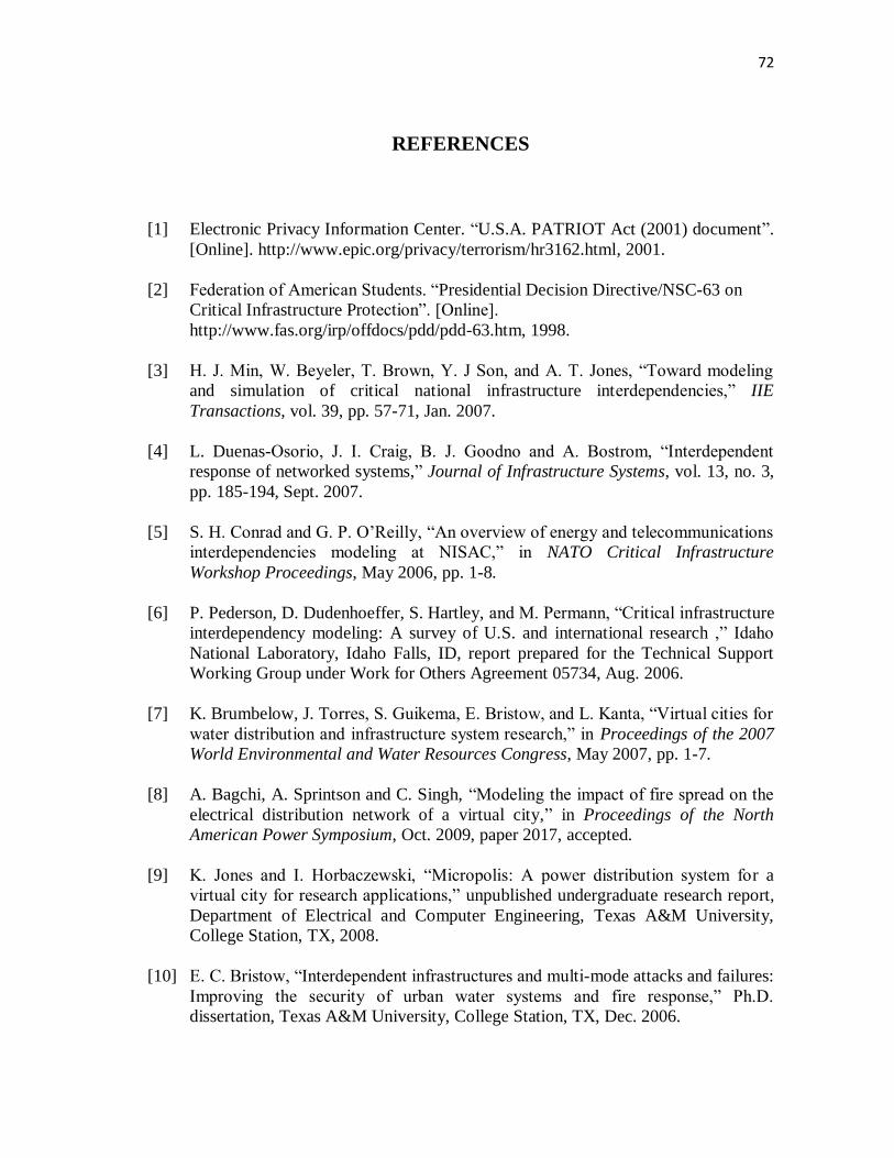
72
REFERENCES
[1] Electronic Privacy Information Center. “U.S.A. PATRIOT Act (2001) document”.
[Online]. http://www.epic.org/privacy/terrorism/hr3162.html, 2001.
[2] Federation of American Students. “Presidential Decision Directive/NSC-63 on
Critical Infrastructure Protection”. [Online].
http://www.fas.org/irp/offdocs/pdd/pdd-63.htm, 1998.
[3] H. J. Min, W. Beyeler, T. Brown, Y. J Son, and A. T. Jones, “Toward modeling
and simulation of critical national infrastructure interdependencies,” IIE
Transactions, vol. 39, pp. 57-71, Jan. 2007.
[4] L. Duenas-Osorio, J. I. Craig, B. J. Goodno and A. Bostrom, “Interdependent
response of networked systems,” Journal of Infrastructure Systems, vol. 13, no. 3,
pp. 185-194, Sept. 2007.
[5] S. H. Conrad and G. P. O‟Reilly, “An overview of energy and telecommunications
interdependencies modeling at NISAC,” in NATO Critical Infrastructure
Workshop Proceedings, May 2006, pp. 1-8.
[6] P. Pederson, D. Dudenhoeffer, S. Hartley, and M. Permann, “Critical infrastructure
interdependency modeling: A survey of U.S. and international research ,” Idaho
National Laboratory, Idaho Falls, ID, report prepared for the Technical Support
Working Group under Work for Others Agreement 05734, Aug. 2006.
[7] K. Brumbelow, J. Torres, S. Guikema, E. Bristow, and L. Kanta, “Virtual cities for
water distribution and infrastructure system research,” in Proceedings of the 2007
World Environmental and Water Resources Congress, May 2007, pp. 1-7.
[8] A. Bagchi, A. Sprintson and C. Singh, “Modeling the impact of fire spread on the
electrical distribution network of a virtual city,” in Proceedings of the North
American Power Symposium, Oct. 2009, paper 2017, accepted.
[9] K. Jones and I. Horbaczewski, “Micropolis: A power distribution system for a
virtual city for research applications,” unpublished undergraduate research report,
Department of Electrical and Computer Engineering, Texas A&M University,
College Station, TX, 2008.
[10] E. C. Bristow, “Interdependent infrastructures and multi-mode attacks and failures:
Improving the security of urban water systems and fire response,” Ph.D.
dissertation, Texas A&M University, College Station, TX, Dec. 2006.

73
[11] A. S. Langsdorf, Theory of Alternating-Current Machinery, 2nd
ed., New York:
McGraw-Hill, 1955.
[12] ARCAD. “Transformer X/R ratios specification sheet”. Available:
http://www.arcadvisor.com/pdf/GET3550Fapp41-43.pdf . Accessed: Aug. 2009.
[13] T. A. Short, Electric Power Distribution Handbook, Boca Raton, FL: CRC Press,
2004.
[14] H. W. Beaty, Handbook of Electric Power Calculations, 3rd
ed., New York:
McGraw-Hill, 2001.
[15] W. H. Kersting, Distribution System Modeling and Analysis, 2nd
ed., Boca Raton,
FL: CRC Press, 2007.
[16] W. H. Kersting and W. H. Phillips, “Distribution feeder line models,” IEEE Trans.
on Industry Applications, vol. 31, no. 4, pp. 715-720, Jul. 1995.
[17] Y. Zhang, J. L. Bastos, N. N. Schulz and D. Patel, “Modeling and testing of
protection devices for SPS using MATLAB/Simulink and VTB,” in Proc. Electric
Ship Technologies Symposium, 2007, pp. 103-108.
[18] S. S. Martin and M. B. Fernandez, “Model and performance simulation for
overcurrent relay and fault-circuit-breaker using Simulink,” International Journal
of Electrical Engineering Education, vol. 43, no. 1, pp. 80-91, Jan. 2006.
[19] General Cable. “AAC bare overhead conductor specification sheet”. Available:
http://www.generalcable.com/NR/rdonlyres/00CCF8A8-5CF2-4719-A396-
33C69E63F327/0/p054_056_BareOvhead.pdf. Accessed: Jul. 2008.
[20] General Cable. “Underground distribution cable 5-46 KV specification sheet”.
Available: http://www.generalcable.com/NR/rdonlyres/2EE1B961-8934-474E-
BFB1-10516EC79C53/0/p026_030_ConNutUG.pdf. Accessed: May 2008.
[21] J. D. Glover, M. S. Sarma and T. J. Overbye, Power System Analysis and Design,
4th ed., Toronto, Canada: Thomson Learning, 2008.
[22] A. Chakrabarty, M. L. Soni, P. V. Gupta and U. S. Bhatnagar, A Text Book on
Power System Engineering, New Delhi, India: Dhanpat Rai and Co. (P) Ltd., 2003.
[23] IEEE Guide for Electric Power Distribution Reliability Indices, IEEE Std. 1366-
2003, May 2004.
74
[24] A. Bagchi, A. Sprintson and C. Singh, “Studying the impact of fire on an electrical
distribution network using graph theory based routing algorithms,” unpublished
manuscript, Department of Electrical and Computer Engineering, Texas A&M
University, College Station, TX, 2009.
[25] Wikipedia. “Triple Pole Single Throw (3PST) switch document”. [Online].
http://en.wikipedia.org/wiki/Switch, 2009.
[26] N. Deo, Graph Theory with Applications to Engineering and Computer Science,
Englewood Cliffs, NJ: Prentice-Hall, Inc., 1974.
75
VITA
Name: Arijit Bagchi
Address: Quarter 5/7, Central Park, City Center
Durgapur, West Bengal, India
Zip: 713216
Email Address: [email protected]
Education: B.E., Electrical and Electronics Engineering, Birla Institute of
Technology, MESRA, Ranchi, India, May 2005
M.S., Electrical Engineering, Texas A&M University, Dec. 2009