sustainability

Article

Active Distribution Network Modeling for EnhancingSustainable Power System Performance; a Case Studyin Egypt

Ali A. Radwan 1,2 , Ahmed A. Zaki Diab 1,* , Abo-Hashima M. Elsayed 1,Hassan Haes Alhelou 3,* and Pierluigi Siano 4,*

1 Electrical Engineering Department, Faculty of Engineering, Minia University, Minia 61517, Egypt;alyshafy@gmail.com (A.A.R.); dr_mostafa555@yahoo.com (A.-H.M.E.)

2 Egyptian Electricity Holding Company, Middle Egypt DisCo., Minia 61111, Egypt3 Faculty Member at the Department of Electrical Power Engineering, Tishreen University, Lattakia, Syria4 Department of Management & Innovation Systems, University of Salerno, 84084 Salerno, Italy* Correspondence: a.diab@mu.edu.eg (A.A.Z.D.); h.haesalhelou@gmail.com (H.H.A.); psiano@unisa.it (P.S.)

Received: 1 October 2020; Accepted: 26 October 2020; Published: 29 October 2020

Abstract: The remarkable growth of distributed generation (DG) penetration inside electrical powersystems turns the familiar passive distribution networks (PDNs) into active distribution networks(ADNs). Based on the backward/forward sweep method (BFS), a new power-flow algorithm wasdeveloped in this paper. The algorithm is flexible to handle the bidirectional flow of power thatcharacterizes the modern ADNs. Models of the commonly used distribution network componentswere integrated with the developed algorithm to form a comprehensive tool. This tool is validfor modeling either balanced or unbalanced ADNs with an unlimited number of nodes or laterals.The integrated models involve modeling of distribution lines, losses inside distribution transformers,automatic voltage regulators (AVRs), DG units, shunt capacitor banks (SCBs) and different loadmodels. To verify its validity, the presented algorithm was first applied to the unbalanced IEEE37-node standard feeder in both passive and active states. Moreover, the algorithm was then appliedto a balanced 22 kV real distribution network as a case study. The selected network is located in aremote area in the western desert of Upper Egypt, far away from the Egyptian unified national grid.Accordingly, the paper examines the current and future situation of the Egyptian electricity market.Comparison studies between the performance of the proposed ADNs and the classical PDNs arediscussed. Simulation results are presented to demonstrate the effectiveness of the proposed ADNs inpreserving the network assets, improving the system performance and minimizing the power losses.

Keywords: modeling; distributed generation (DG); active distribution network (ADN); planning;automatic voltage regulator (AVR); backward/forward sweep (BFS)

1. Introduction

Electrical power system modeling is a significant approach for the optimization of planning,designing or operating that system technically and economically. Therefore, the invention of thedigital computer in the 1940s encouraged scholars to start solving different network troubles bydifferent algorithms and techniques [1–8]. Many algorithms such as the Newton–Raphson (NR),Gauss–Seidel (GS) and fast decoupled (FD) are appropriately validated for simulating transmissionsystems (TSs) [4–8]. Nevertheless, the distribution systems are distinguished in numerous features.High values of the resistance-to-reactance ratio, R/X, are distinctive in distribution voltage levelswhile these values are decreasing as the voltage level increases in TSs. All TSs consist of tightlymeshed networks whereas distribution systems may have radial or weakly meshed configurations.

Sustainability 2020, 12, 8991; doi:10.3390/su12218991 www.mdpi.com/journal/sustainability

Sustainability 2020, 12, 8991 2 of 22

Generator nodes in distribution systems may be PQ, PV or composite nodes while generator nodes intransmission systems are mostly PV nodes. The PQ node is the node at which voltage can be regulatedby controlling the real and reactive powers (P and Q) independently. PV node is the node at whichgenerated real power and voltage magnitude (P and V) can be controlled independently. Table 1itemizes the differences between distribution and transmission power systems concerning the powerflow analysis. Accordingly, conventional presented algorithms may not be suitable for solving theproblems of radial distribution networks (DNs) with an acceptable convergence [9–15]. The distinctiveradial structure of DNs is used as a basic feature to simulate DNs using the technique known asbackward/forward sweep (BFS) [16–19].

Table 1. Assessment of distribution and transmission power systems.

Feature Distribution System Transmission System

Structure Radial/Weakly meshed Tightly meshed

Types of Load Constant Power (CP)/Constant Current(CC)/Constant Impedance (CI)/Composite Mostly CP only

Symmetricity Unbalanced/Balanced Balanced

R/X Ratio High Very low

Generator Nodes PQ/PV/Composite Mostly PV only

Recently, distribution utilities have faced new challenges concerning environmental conservation,power sustainability and energy market economics. Therefore, a remarkable growth in the penetrationrate of distributed generation (DG) units inside power DNs has been informed [20]. This growthturns the classical passive distribution networks (PDNs) into active distribution networks (ADNs)concerning the bidirectional flow of power [21–23]. A popular definition of the ADN was presentedin [24] by the CIGRE working group C6.19. The new topology of ADNs necessitates modern simulationof network impedances under different grid conditions [25,26]. The newly added components leadto the need of modeling balanced and/or unbalanced ADNs using grid-connected inverters [27].Reference [28] presents a review of power distribution planning models in ADNs where a lack ofmodeling networks containing an automatic voltage regulator (AVR) as a voltage control unit isnoticed. Moreover, the previously presented models neglect one important source of losses in real DNs,namely power dissipated inside distribution transformers. This paper tries to fill this gap and presentsa comprehensive power-flow program based on the BFS technique. The program is embedded withmodels of the commonly used DN components.

In this paper, a real Egyptian DN is highlighted as a practical application of the proposedprogram. The current and future situation of the Egyptian electricity market is examined in Section 2focusing on the case-study region. Section 3 presents the modeling of distribution lines, losses insidedistribution transformers, AVR groups, DG units, shunt capacitor banks (SCBs) and different loadmodels. The integration of these models with the proposed power-flow algorithm is described inSection 4. Simulation results are discussed in Section 5 focusing on the analysis of two different networksbefore and after their conversion to ADNs. Eventually, Section 6 summarizes the main conclusions.

2. Examination of the Studied Real Case Study in Egypt

Although Egypt is rich in various renewable energy sources, these sources have not been optimallyexploited yet [29]. Most of the generated electricity in Egypt is thermally produced from either gas,steam or combined cycle. Another source of electricity in Egypt is hydroelectric power derived byexploiting the energy of falling water through the river Nile dams. Figure 1 shows the renewableenergy contribution compared to other electricity sources in the Egyptian electricity market in the fiscalyear 2018–2019. The percentage of the installed capacity of renewable resources to the total electrical

Sustainability 2020, 12, 8991 3 of 22

installed capacity in Egypt does not exceed 3.8%. The percentage of generated renewable energy to thetotal generated energy in Egypt also does not exceed 2.3%.

Sustainability 2020, 12, x FOR PEER REVIEW 3 of 24

resources to the total electrical installed capacity in Egypt does not exceed 3.8%. The percentage of generated renewable energy to the total generated energy in Egypt also does not exceed 2.3%.

(a) Installed capacity

(b) Generated energy

Figure 1. Egyptian electricity sources in the fiscal year 2018–2019.

The strategy of the Egyptian electricity sector represented by the Electricity Holding Company (EEHC) aims to increase the contribution of renewable energy in Egypt to 42% by 2035. The EEHC has modified its policies to encourage private investments in renewable power generation projects. This explains the recently remarked relative increase in the installed capacity of renewable power sources. According to the recently published report of the EEHC, the contribution of renewable power sources increased during the last year from 2% to 3.8% of the total installed capacity. Regarding the actual generated energy, renewable energy increased during the last year from 1.46% to 2.3% of the total generated energy.

The New Valley region in the western desert of Upper Egypt is one of the promising regions on which development strategies are based according to Egypt’s Vision 2030. This region is well-known for its richness in various types of mineral wealth, soil fertility and the availability of groundwater.

Figure 1. Egyptian electricity sources in the fiscal year 2018–2019.

The strategy of the Egyptian electricity sector represented by the Electricity Holding Company(EEHC) aims to increase the contribution of renewable energy in Egypt to 42% by 2035. The EEHChas modified its policies to encourage private investments in renewable power generation projects.This explains the recently remarked relative increase in the installed capacity of renewable powersources. According to the recently published report of the EEHC, the contribution of renewable powersources increased during the last year from 2% to 3.8% of the total installed capacity. Regarding theactual generated energy, renewable energy increased during the last year from 1.46% to 2.3% of thetotal generated energy.

Sustainability 2020, 12, 8991 4 of 22

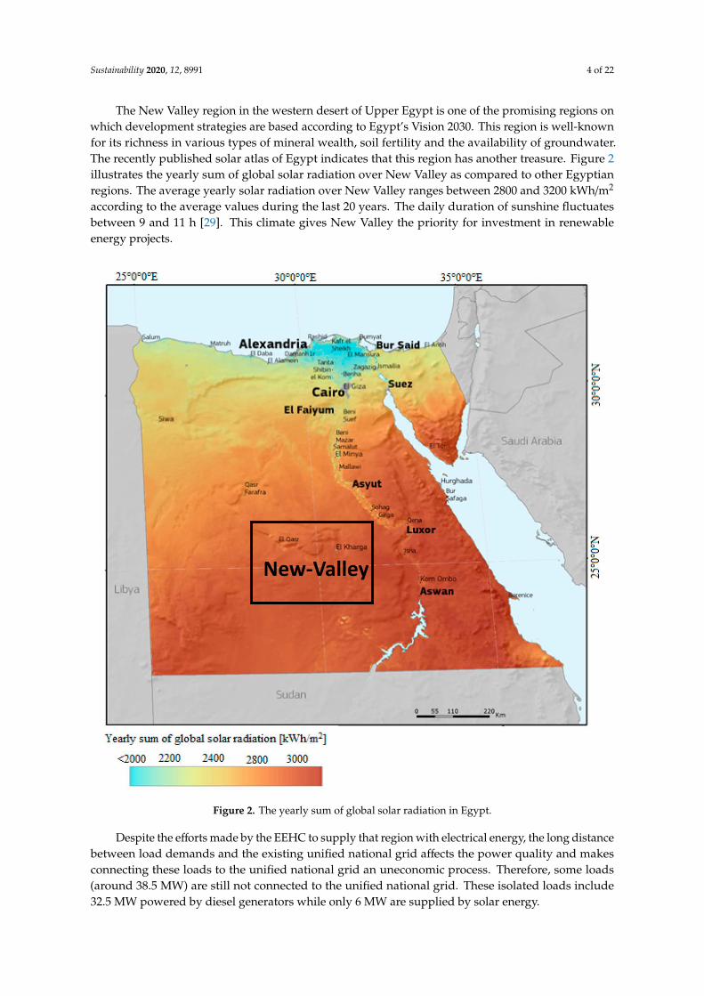
The New Valley region in the western desert of Upper Egypt is one of the promising regions onwhich development strategies are based according to Egypt’s Vision 2030. This region is well-knownfor its richness in various types of mineral wealth, soil fertility and the availability of groundwater.The recently published solar atlas of Egypt indicates that this region has another treasure. Figure 2illustrates the yearly sum of global solar radiation over New Valley as compared to other Egyptianregions. The average yearly solar radiation over New Valley ranges between 2800 and 3200 kWh/m2

according to the average values during the last 20 years. The daily duration of sunshine fluctuatesbetween 9 and 11 h [29]. This climate gives New Valley the priority for investment in renewableenergy projects.

New-Valley

Figure 2. The yearly sum of global solar radiation in Egypt.

Despite the efforts made by the EEHC to supply that region with electrical energy, the long distancebetween load demands and the existing unified national grid affects the power quality and makesconnecting these loads to the unified national grid an uneconomic process. Therefore, some loads(around 38.5 MW) are still not connected to the unified national grid. These isolated loads include32.5 MW powered by diesel generators while only 6 MW are supplied by solar energy.

Sustainability 2020, 12, 8991 5 of 22

Two far demand areas (Arbien and Max) located in the New Valley region were selected as acase study. The two areas are electrically fed by the same DN. Figure 3 illustrates the location of thisUpper Egypt distribution network (UEDN) compared to the path of the Egyptian unified electricalgrid. The single-line diagram of the existing network that supplies these areas with electrical energy isshown in Figure 4. The selected areas are supplied from the Kharja substation through the transformer5T of capacity 25 MVA with a transformation ratio of 66/22 kV. The Kharja substation is connected tothe extra-high-voltage grid through the Abo Tartor substation 220/66 kV by two circuits. Each circuit isconstructed by an overhead line of aluminum conductors steel reinforced (ACSR) with a cross-sectionalarea of 380/50 mm2 and 48 km in length. A detailed description of the studied network and its loaddistribution is given in Section 5.2.

Sustainability 2020, 12, x FOR PEER REVIEW 6 of 24

Figure 3. Case study location compared to the Egyptian unified national grid. “TH. POWER ST.” is referred to thermal power stations, “HY. POWER ST.” is referred to Hydraulic Power Station and “SS” is referred to Substation.

Figure 3. Case study location compared to the Egyptian unified national grid. “TH. POWER ST.” isreferred to thermal power stations, “HY. POWER ST.” is referred to Hydraulic Power Station and “SS”is referred to Substation.

Sustainability 2020, 12, 8991 6 of 22Sustainability 2020, 12, x FOR PEER REVIEW 7 of 24

Figure 4. Single-line diagram of the case-study supply system.

3. Modeling of DN Components

The realization of any power-flow algorithm requires first an establishment of a model for each component of the DN. A component model is mainly built with physical and electrical specifications given in the manufacturing catalogs. Figure 5 shows a simplified single-line diagram and an electric equivalent of an ADN portion containing DG, distribution transformer, SCB and AVR connected to node k. The following subsections describe the modeling of each element in this segment [30].

Figure 5. Electric equivalent of an active distribution network (ADN) segment. AVR: automatic voltage regulator; DG: distributed generation.

1−kZ k

kLS

kTSkCQ

1−ksegS

kVksegSb

bV

AVR

DG

1−ksegI1−kdropVksegI

kinjS

kinjIkgS

Figure 4. Single-line diagram of the case-study supply system.

3. Modeling of DN Components

The realization of any power-flow algorithm requires first an establishment of a model for eachcomponent of the DN. A component model is mainly built with physical and electrical specificationsgiven in the manufacturing catalogs. Figure 5 shows a simplified single-line diagram and an electricequivalent of an ADN portion containing DG, distribution transformer, SCB and AVR connected tonode k. The following subsections describe the modeling of each element in this segment [30].

Sustainability 2020, 12, x FOR PEER REVIEW 7 of 24

Figure 4. Single-line diagram of the case-study supply system.

3. Modeling of DN Components

The realization of any power-flow algorithm requires first an establishment of a model for each component of the DN. A component model is mainly built with physical and electrical specifications given in the manufacturing catalogs. Figure 5 shows a simplified single-line diagram and an electric equivalent of an ADN portion containing DG, distribution transformer, SCB and AVR connected to node k. The following subsections describe the modeling of each element in this segment [30].

Figure 5. Electric equivalent of an active distribution network (ADN) segment. AVR: automatic voltage regulator; DG: distributed generation.

1−kZ k

kLS

kTSkCQ

1−ksegS

kVksegSb

bV

AVR

DG

1−ksegI1−kdropVksegI

kinjS

kinjIkgS

Figure 5. Electric equivalent of an active distribution network (ADN) segment. AVR: automatic voltageregulator; DG: distributed generation.

Sustainability 2020, 12, 8991 7 of 22

3.1. Modeling of Distribution Line

The typical π-model has been generally used to implement the modeling of a distribution linesegment connecting two nodes. The series impedance matrix Z of any three-phase line segment isrepresented as [16]:

Z = l·

z11 z12 z13

z21 z22 z23

z31 z32 z33

(1)

where l is the segment length. Element zii along the diagonal of the series impedance matrix isthe self-impedance of conductor i per unit length. Element zi j along the off-diagonal is the mutualimpedance between conductors i and j per unit length. Equations (2) and (3) use the modified Carson’sequations [16] to represent the self and mutual impedances, respectively.

zii = rd + Rre f(1 + α

(T − Tre f

))+ j

[(2π f )

(0.2× 10−3

)ln

( De

GMR

)](2)

zi j = rd + j[(2π f )

(0.2× 10−3

)ln

( De

GMD

)](3)

where rd, α, T and f are the resistance of dirt in Ω/km, the temperature coefficient of conductor material,the operating temperature in °C and the system frequency in Hertz, respectively. The referenceresistance Rre f in Ω/km of conductor i is given by the manufacturer at a reference temperatureTre f = 20 °C. The distances De, GMR and GMD in meters are, respectively, the distance from conductori to dirt, the geometric mean radius of conductor i and the geometric mean distance between the threeconductors. Although the shunt admittance at the distribution voltage level is small enough to beneglected, the model has the flexibility to include that effect.

3.2. Modeling of Transformer Losses

A three-phase distribution transformer converts the consumed or generated power at thelow-voltage network to the medium voltage network, along with the real and reactive power dissipatedby that transformer. The power dissipated inside the distribution transformer shown in Figure 5 isgiven by [31–33]:

STk =

Po

(VkVr

)2+ Pcβ

2(

Vr

Vk

)2+ j

IoSr

(VkVr

)2+ UxSrβ

2(

Vr

Vk

)2 (4)

where STk is the apparent power that dissipated inside the transformer, Vr is the rated voltage,and Vk is the node voltage. Sr and β are the transformer-rated power and the transformer loadingpercentage, respectively. Po, Pc and Io are the no-load losses, full-load losses and percentage of no-loadcurrent, respectively. The parameter Ux in Equation (4) represents the reactive part of the percentageshort-circuit voltage, which can be expressed as [31–33]:

Ux =

√Us2 −

(100Pc

Sr

)2(5)

where Us is the percentage of short-circuit voltage given by the transformer manufacturer.

3.3. Modeling of AVR

AVR is a normal auto-transformer equipped with an automatic tap-changing mechanism [34–39].Standard AVR provides ±10% voltage regulation in 32 steps of approximately 5/8% each. The tap ofmaximum raise position is 16R, while 16L is the tap of minimum lower position. The AVR has anautomatic tap-changer able to switch from 16R to 16L and vice versa in less than 10 s.

Sustainability 2020, 12, 8991 8 of 22

According to the IEEE Std. C57.15-2009 (IEC60076-21:2011) standard [36], AVR is manufacturedin one of two types: ANSI type-A and ANSI type-B. Figure 6 shows the overall functional diagram of asingle-phase type-A regulator unit. Commonly, distribution utilities prefer to use three individualsingle-phase regulators rather than a single compact three-phase unit because the practical unbalancein voltage requires controlling each phase individually. The presence of more than one winding insidethe same tank raises the winding and oil temperature, which means more losses. Additionally, the sizeof a single-phase AVR unit is much smaller as compared to a compact three-phase unit; this facilitatesthe processes of transportation, installation and maintenance. Moreover, in case of damage or fault in asingle-phase AVR unit, the remaining two units can be reconnected as an open-delta configuration tocontinue voltage regulation during the period of repairing or replacing the damaged unit.

Sustainability 2020, 12, x FOR PEER REVIEW 9 of 24

3.3. Modeling of AVR

AVR is a normal auto-transformer equipped with an automatic tap-changing mechanism [34–39]. Standard AVR provides ±10% voltage regulation in 32 steps of approximately 5/8% each. The tap of maximum raise position is 16R, while 16L is the tap of minimum lower position. The AVR has an automatic tap-changer able to switch from 16R to 16L and vice versa in less than 10 s.

According to the IEEE Std. C57.15-2009 (IEC60076-21:2011) standard [36], AVR is manufactured in one of two types: ANSI type-A and ANSI type-B. Figure 6 shows the overall functional diagram of a single-phase type-A regulator unit. Commonly, distribution utilities prefer to use three individual single-phase regulators rather than a single compact three-phase unit because the practical unbalance in voltage requires controlling each phase individually. The presence of more than one winding inside the same tank raises the winding and oil temperature, which means more losses. Additionally, the size of a single-phase AVR unit is much smaller as compared to a compact three-phase unit; this facilitates the processes of transportation, installation and maintenance. Moreover, in case of damage or fault in a single-phase AVR unit, the remaining two units can be reconnected as an open-delta configuration to continue voltage regulation during the period of repairing or replacing the damaged unit.

Figure 6. Overall functional diagram of the AVR.

Since the common configuration of a primary DN is delta, single-phase AVR units are typically grouped in one of two connections [16]: closed-delta or open-delta. Figure 7 shows the closed-delta connection where three single-phase units are required to provide up to 15% voltage regulation. In an open-delta connection, only two units can be used to provide up to 10% voltage regulation as illustrated in Figure 8.

Figure 6. Overall functional diagram of the AVR.

Since the common configuration of a primary DN is delta, single-phase AVR units are typicallygrouped in one of two connections [16]: closed-delta or open-delta. Figure 7 shows the closed-deltaconnection where three single-phase units are required to provide up to 15% voltage regulation. In anopen-delta connection, only two units can be used to provide up to 10% voltage regulation as illustratedin Figure 8.

Sustainability 2020, 12, 8991 9 of 22Sustainability 2020, 12, x FOR PEER REVIEW 10 of 24

Figure 7. Closed-delta connection of AVR units.

Figure 8. Open-delta connection of AVR units.

The relationship between the source voltage and current (𝑉 and 𝐼 ) to the load voltage and current (𝑉 and 𝐼 ) are governed by [16,37–39]:

For Type-A Regulator:

𝑉 = ∙ 𝑉 ,𝐼 = 𝑎 ∙ 𝐼 (6)

where

𝑎 = 1 + 𝑁 ∙ 𝑇𝑎𝑝 for raise taps1 − 𝑁 ∙ 𝑇𝑎𝑝 for lower taps (7)

For Type-B Regulator:

ba

c

SL

SL SL

SL

1 2

Shun

t Ar

rest

er

Shun

t Ar

rest

er

Bypass Switch

Bypass Switch

Disconnects

Sour

ce

ABC

Load

Figure 7. Closed-delta connection of AVR units.

Sustainability 2020, 12, x FOR PEER REVIEW 10 of 24

Figure 7. Closed-delta connection of AVR units.

Figure 8. Open-delta connection of AVR units.

The relationship between the source voltage and current (𝑉 and 𝐼 ) to the load voltage and current (𝑉 and 𝐼 ) are governed by [16,37–39]:

For Type-A Regulator:

𝑉 = ∙ 𝑉 ,𝐼 = 𝑎 ∙ 𝐼 (6)

where

𝑎 = 1 + 𝑁 ∙ 𝑇𝑎𝑝 for raise taps1 − 𝑁 ∙ 𝑇𝑎𝑝 for lower taps (7)

For Type-B Regulator:

ba

c

SL

SL SL

SL

1 2

Shun

t Ar

rest

er

Shun

t Ar

rest

er

Bypass Switch

Bypass Switch

Disconnects

Sour

ce

ABC

Load

Figure 8. Open-delta connection of AVR units.

The relationship between the source voltage and current (VSource and ISource) to the load voltageand current (VLoad and ILoad) are governed by [16,37–39]:

For Type-A Regulator:

VSource =1

aR·VLoad, I Sou

6rce

= aR·ILoad (6)

where

aR =

1 + NR·Tap for raise taps1−NR·Tap for lower taps

(7)

For Type-B Regulator:

VSource = aR·VLoad, ISource =1

aR·ILoad (8)

where

aR =

1−NR·Tap for raise taps

1 + NR·Tap for lower taps(9)

Sustainability 2020, 12, 8991 10 of 22

In Equations (7) and (9), NR is the per unit regulation of single step (NR = 0.00625 for a step-typeAVRs), and Tap is the tap position of the current step.

3.4. Modeling of DG Unit

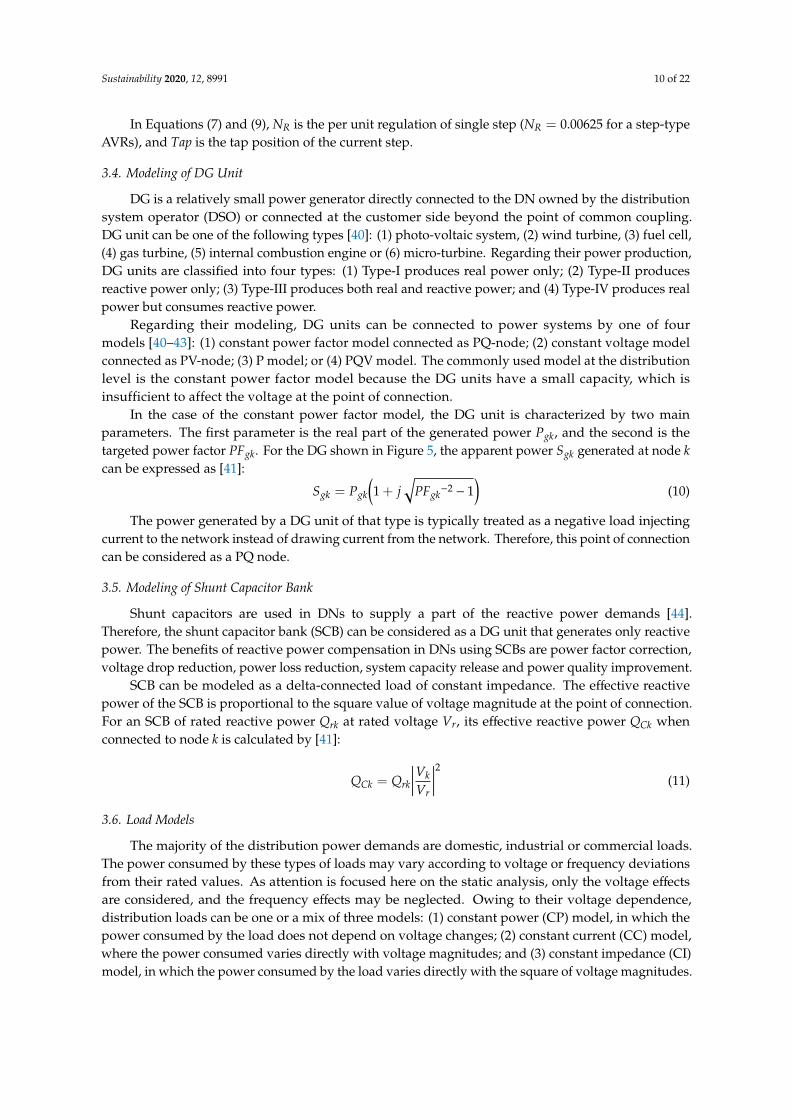
DG is a relatively small power generator directly connected to the DN owned by the distributionsystem operator (DSO) or connected at the customer side beyond the point of common coupling.DG unit can be one of the following types [40]: (1) photo-voltaic system, (2) wind turbine, (3) fuel cell,(4) gas turbine, (5) internal combustion engine or (6) micro-turbine. Regarding their power production,DG units are classified into four types: (1) Type-I produces real power only; (2) Type-II producesreactive power only; (3) Type-III produces both real and reactive power; and (4) Type-IV produces realpower but consumes reactive power.

Regarding their modeling, DG units can be connected to power systems by one of fourmodels [40–43]: (1) constant power factor model connected as PQ-node; (2) constant voltage modelconnected as PV-node; (3) P model; or (4) PQV model. The commonly used model at the distributionlevel is the constant power factor model because the DG units have a small capacity, which isinsufficient to affect the voltage at the point of connection.

In the case of the constant power factor model, the DG unit is characterized by two mainparameters. The first parameter is the real part of the generated power Pgk, and the second is thetargeted power factor PFgk. For the DG shown in Figure 5, the apparent power Sgk generated at node kcan be expressed as [41]:

Sgk = Pgk

(1 + j

√PFgk

−2 − 1)

(10)

The power generated by a DG unit of that type is typically treated as a negative load injectingcurrent to the network instead of drawing current from the network. Therefore, this point of connectioncan be considered as a PQ node.

3.5. Modeling of Shunt Capacitor Bank

Shunt capacitors are used in DNs to supply a part of the reactive power demands [44].Therefore, the shunt capacitor bank (SCB) can be considered as a DG unit that generates only reactivepower. The benefits of reactive power compensation in DNs using SCBs are power factor correction,voltage drop reduction, power loss reduction, system capacity release and power quality improvement.

SCB can be modeled as a delta-connected load of constant impedance. The effective reactivepower of the SCB is proportional to the square value of voltage magnitude at the point of connection.For an SCB of rated reactive power Qrk at rated voltage Vr, its effective reactive power QCk whenconnected to node k is calculated by [41]:

QCk = Qrk

∣∣∣∣∣VkVr

∣∣∣∣∣2 (11)

3.6. Load Models

The majority of the distribution power demands are domestic, industrial or commercial loads.The power consumed by these types of loads may vary according to voltage or frequency deviationsfrom their rated values. As attention is focused here on the static analysis, only the voltage effectsare considered, and the frequency effects may be neglected. Owing to their voltage dependence,distribution loads can be one or a mix of three models: (1) constant power (CP) model, in which thepower consumed by the load does not depend on voltage changes; (2) constant current (CC) model,where the power consumed varies directly with voltage magnitudes; and (3) constant impedance (CI)model, in which the power consumed by the load varies directly with the square of voltage magnitudes.

Sustainability 2020, 12, 8991 11 of 22

The power dependency of a certain load to voltage changes can be expressed in a general exponentialform as [45]:

SLk = Srk

(VkVr

)n(12)

where SLk is the consumed apparent power, Vk is the node voltage, Srk is the rated apparent power ofthe load, Vr is the rated voltage, and n is the model exponent. By setting n to 0, 1 or 2, the load typecan be turned into CP, CC or CI, respectively [45].

4. Proposed Power-Flow Algorithm

To describe the proposed power-flow algorithm, a general scheme of a three-phase distributionnetwork is considered. The network is assumed to contain a total number of nodes Nn and segmentsNs. Typically, Ns = Nn − 1 for radial DNs. The voltage V1 at the slack node 1 (main substation) isgenerally taken as a base voltage. All other successive nodes are sequentially numbered. Figure 9illustrates the program flow-chart. As shown, the algorithm consists of four modules: initialization,matrices construction, BFS iterations and losses calculations. The following subsections describe thealgorithm sequence.

4.1. Module 1: Initialization

• Input the network data (specifications and locations of the network components).• Input the loads data (locations, consumptions and types of all load points).• Select the solution accuracy (ε) and the maximum number of iterations (max_itr).• Recall the required parameters related to network components from the database library.

4.2. Module 2: Matrices Construction

• Construct the connection matrix (CONMAT) [30], the series impedance matrix (Z) and the shuntadmittance matrix (Y).

4.3. Module 3: BFS Iterations

• Calculate the power injected at each node Sinj assuming a flat voltage profile. Sinj is the resultantof the load apparent power SL (Equation (12)), the transformer dissipated power ST (Equation (4)),the apparent power generated by DG unit Sg (Equation (10)) and the effective reactive power ofcapacitor bank QC (Equation (11)) if any.

• Repeat the following BFS iterations:

4.3.1. Backward Sweep Calculations:

• Correct Sinj considering the load models, DG, SCB and transformer losses.

• Find the current injected to each node using: Iinj =(Sinj/V

)∗.

• Find the current flowed through each segment using: Iseg = [CONMAT][Iinj

].

• Find the voltage drop across each segment using: Vdrop =[Iseg

][Z].

• Denote the calculated voltage distribution matrix V of the current iteration as Vold.

Sustainability 2020, 12, 8991 12 of 22

Sustainability 2020, 12, x FOR PEER REVIEW 14 of 24

Figure 9. Flow-chart of the power-flow algorithm. SCB: shunt capacitor bank. Figure 9. Flow-chart of the power-flow algorithm. SCB: shunt capacitor bank.

Sustainability 2020, 12, 8991 13 of 22

4.3.2. Forward Sweep Calculations

• Update the matrix V according to the voltage drop Vdrop formerly determined in the backwardsweep. Considering the voltage at any arbitrary node k (Vk shown in Figure 5) is the voltage at itspredecessor node b (Vb) minus the voltage drop across the segment connecting them (Vdropk−1).

• Recalculate both voltage and current matrices according to the AVR model.• Update the loop counter.• Terminate the loop if each element in the matrix (Vold – V) is less than the solution accuracy ε,

or the loop counter exceeds the maximum number of iterations (max_itr).

4.4. Module 4: Losses Calculations

• Find the power flowed through each segment using: Sseg = [V][Iseg

]∗• Find the conductor losses using

[Vdrop

][Iseg

]∗• Find the total losses by adding the conductor losses to the transformer losses.• Print the outputs.

5. Simulation Results and Discussions

5.1. Case I: Unbalanced IEEE 37-Node Feeder

The unbalanced IEEE 37-node standard feeder is a PDN prepared to evaluate and benchmarkdistribution system models [46]. The proposed algorithm was applied first to this test feeder in itsoriginal PDN state. The algorithm was coded under MATLAB platform version R2016b. A laptopwith an Intel (core i5 2.9 GHz) processing unit and 4 GB RAM was used to execute the algorithm.The execution time was 0.19 s. Table 2 presents the obtained results. Our results were found to be veryclose to the results published in [46]. By selecting a solution tolerance ε equals 10−6, the maximumfounded deviation in the voltage magnitudes as compared to those given in [46] is less than 0.006%.The maximum deviation of the calculated power losses from those of [46] is less than 0.005%. This testasserted the effectiveness of the presented algorithm to analyze unbalanced DNs.

Table 2. Voltage behavior of the ADN as compared to the passive distribution network (PDN) in case I.

Network PDN ADN

Line-to-line A-to-B B-to-C C-to-A A-to-B B-to-C C-to-A

Min. Voltage (pu) 0.998 0.995 0.985 1.006 1.002 0.999

at Node 741 722 741 741 722 741

Max. Voltage (pu) 1.044 1.025 1.035 1.031 1.019 1.025

at Node 701 701 701 701 701 701

Tap of AVR 7R 4R - 5R 3R -

To convert this test system to an ADN, the network was divided into three zones. Each zone has alocal area control center (LACC) to monitor and control the corresponding area. Each zone is supposedto have a constant power factor DG unit of type-III. The three DG units were assumed to have thesame rated active power of 500 kW at 0.958 power factor for each. The DG units were located at nodes720, 744 and 734. Figure 10 compares the line-to-line voltage profile along with the PDN nodes to thatalong with the ADN nodes. As shown, the conversion to ADN improves voltage unbalance. The shapeof the voltage profile also appears to become more flattened in the case of the ADN.

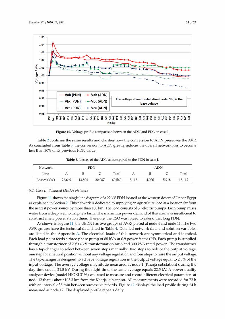
Sustainability 2020, 12, 8991 14 of 22

Sustainability 2020, 12, x FOR PEER REVIEW 16 of 24

Figure 10. Voltage profile comparison between the ADN and PDN in case I.

5.2. Case II: Balanced UEDN Network

Figure 11 shows the single line diagram of a 22 kV PDN located at the western desert of Upper Egypt as explained in Section 2. This network is dedicated to supplying an agriculture load at a location far from the nearest power source by more than 100 km. The load consists of 39 electric pumps. Each pump raises water from a deep well to irrigate a farm. The maximum power demand of this area was insufficient to construct a new power station there. Therefore, the DSO was forced to extend that long PDN.

As shown in Figure 11, the UEDN has two groups of AVRs placed at node 4 and node 11. The two AVR groups have the technical data listed in Table 4. Detailed network data and solution variables are listed in the Appendix A. The electrical loads of this network are symmetrical and identical. Each load point feeds a three-phase pump of 88 kVA at 0.9 power factor (PF). Each pump is supplied through a transformer of 20/0.4 kV transformation ratio and 300 kVA rated power. The transformer has a tap-changer to select between seven steps manually: two steps to reduce the output voltage, one step for a neutral position without any voltage regulation and four steps to raise the output voltage. The tap-changer is designed to achieve voltage regulation in the output voltage equal to 2.5% of the input voltage. The average voltage magnitude measured at node 1 (Kharja substation) during the day-time equals 21.5 kV. During the night-time, the same average equals 22.5 kV. A power quality analyzer device (model HIOKI 3196) was used to measure and record different electrical parameters at node 12 that is about 103.3 km from the Kharja substation. All measurements were recorded for 72 hours with an interval of 5 min between successive records. Figure 12 displays the load profile during 24 h measured at node 12. The displayed profile repeats daily.

Table 4. Specifications and sittings of the AVR groups in the Upper Egypt distribution network (UEDN).

Location Node

ANSI Type

Rated Current (A)

Connection Type Voltage Level Setting (V) 𝟒 𝐵 300 Closed Delta 120 𝟏𝟏 𝐵 300 Closed Delta 115

Figure 10. Voltage profile comparison between the ADN and PDN in case I.

Table 2 confirms the same results and clarifies how the conversion to ADN preserves the AVR.As concluded from Table 3, the conversion to ADN greatly reduces the overall network loss to becomeless than 30% of its previous PDN value.

Table 3. Losses of the ADN as compared to the PDN in case I.

Network PDN ADN

Line A B C Total A B C Total

Losses (kW) 26.669 13.804 20.087 60.560 8.118 4.076 5.918 18.112

5.2. Case II: Balanced UEDN Network

Figure 11 shows the single line diagram of a 22 kV PDN located at the western desert of Upper Egyptas explained in Section 2. This network is dedicated to supplying an agriculture load at a location far fromthe nearest power source by more than 100 km. The load consists of 39 electric pumps. Each pump raiseswater from a deep well to irrigate a farm. The maximum power demand of this area was insufficient toconstruct a new power station there. Therefore, the DSO was forced to extend that long PDN.

As shown in Figure 11, the UEDN has two groups of AVRs placed at node 4 and node 11. The twoAVR groups have the technical data listed in Table 4. Detailed network data and solution variablesare listed in the Appendix A. The electrical loads of this network are symmetrical and identical.Each load point feeds a three-phase pump of 88 kVA at 0.9 power factor (PF). Each pump is suppliedthrough a transformer of 20/0.4 kV transformation ratio and 300 kVA rated power. The transformerhas a tap-changer to select between seven steps manually: two steps to reduce the output voltage,one step for a neutral position without any voltage regulation and four steps to raise the output voltage.The tap-changer is designed to achieve voltage regulation in the output voltage equal to 2.5% of theinput voltage. The average voltage magnitude measured at node 1 (Kharja substation) during theday-time equals 21.5 kV. During the night-time, the same average equals 22.5 kV. A power qualityanalyzer device (model HIOKI 3196) was used to measure and record different electrical parameters atnode 12 that is about 103.3 km from the Kharja substation. All measurements were recorded for 72 hwith an interval of 5 min between successive records. Figure 12 displays the load profile during 24 hmeasured at node 12. The displayed profile repeats daily.

Sustainability 2020, 12, 8991 15 of 22Sustainability 2020, 12, x FOR PEER REVIEW 17 of 24

Figure 11. Single-line diagram of the UEDN.

Figure 12. Daily load profile of the UEDN measured at node 12.

123

456789

1011

12 33 34

37

36 39

35 38

40 41 42

44

45

46

48 49 50 5152

606162636465

54

55

5356575859

13

15

1614

1718

2019

212223

2425

28293032

31

26 27

43

47

Load PointAVR

0.00

0.50

1.00

1.50

2.00

2.50

3.00

00.0

000

.55

01.5

002

.45

03.4

004

.35

05.3

006

.25

07.2

008

.15

09.1

010

.05

11.0

011

.55

12.5

013

.45

14.4

015

.35

16.3

017

.25

18.2

019

.15

20.1

021

.05

22.0

022

.55

2350

Active Power (MW)Apparent Power (MVA)

Hour

Load

Figure 11. Single-line diagram of the UEDN.

Table 4. Specifications and sittings of the AVR groups in the Upper Egypt distribution network (UEDN).

Location Node ANSI Type Rated Current (A) Connection Type Voltage Level Setting (V)

4 B 300 Closed Delta 120

11 B 300 Closed Delta 115

Sustainability 2020, 12, x FOR PEER REVIEW 17 of 24

Figure 11. Single-line diagram of the UEDN.

Figure 12. Daily load profile of the UEDN measured at node 12.

123

456789

1011

12 33 34

37

36 39

35 38

40 41 42

44

45

46

48 49 50 5152

606162636465

54

55

5356575859

13

15

1614

1718

2019

212223

2425

28293032

31

26 27

43

47

Load PointAVR

0.00

0.50

1.00

1.50

2.00

2.50

3.00

00.0

000

.55

01.5

002

.45

03.4

004

.35

05.3

006

.25

07.2

008

.15

09.1

010

.05

11.0

011

.55

12.5

013

.45

14.4

015

.35

16.3

017

.25

18.2

019

.15

20.1

021

.05

22.0

022

.55

2350

Active Power (MW)Apparent Power (MVA)

Hour

Load

Figure 12. Daily load profile of the UEDN measured at node 12.

Sustainability 2020, 12, 8991 16 of 22

5.2.1. PDN Performance

The passive form of the UEDN is analyzed under two operating modes: the day-time mode andthe night-time mode, as follows:

(a) Day-time Mode

During the day-time, irrigation pumps draw their maximum rated power. At that time, the voltagemagnitude at the Kharja substation is 21.5 kV. The output results confirm that the two voltage regulatorsoperate at tap 16R. However, some pumps suffer from the operation below their permissible voltagelimit. Therefore, these loads draw currents more than their rated values. This operation conditionleads to an increase in power losses and reduces the motor lifetime. The minimum voltage magnitudecalculated at node 65 equals 18.2 kV. The percentage of voltage regulation equals 17.4%, which exceedsthe allowable operating limits. The load at node 63 is found to operate in a critical condition.Its calculated voltage equals 364 V (9% below its rated value). The calculated power losses equal1.337 MW, i.e., 29.74% of the total supplied real power are losses.

(b) Night-time Mode

During the night-time, loads vanish. The only flowed power is the losses resulted from unloadedtransformers in-service. At that time, the voltage at the Kharja substation is 22.5 kV which is higherthan its rated value. Therefore, the calculated results confirm that the voltage regulator located at node4 operates at step 3L while the other regulator located at node 11 operates at step 4L. This operationalstatus of the two AVR groups maintains the voltage magnitudes at essential safe values. The calculatedpower losses equal 23.6 kW, i.e., all the supplied real power are losses.

5.2.2. ADN Performance

To convert the passive UEDN to an ADN, the network was divided into three zones. (1) The firstzone extends from node 1 to node 12 without load points; hence, there is no need to install DG unitsor LACCs in this zone. (2) The second zone is the Max area, which extends from node 13 to node 32and contains 13 load points. Therefore, it is useful to install a DG unit and LACC at the zone center,node 21. (3) The third zone is the Arbien area, which extends from node 33 to node 65 and contains26 load points. A suggested DG unit and LACC is required at the zone center, node 46. Rates andtypes of the suggested DG units are given in Table 5.

Table 5. Required DG units to turn the passive UEDN into an ADN.

Location(at Node)

DGType Rated Active Power (kW) Specified Power Factor

21 III, PQ 900 0.9

46 III, PQ 1800 0.9

Because of the following reasons, it is highly recommended to select the DG units as on-grid solarpower stations:

• The daily repeated load profile, shown in Figure 12, is similar to the solar power irradiancecurve [47]; load vanishes by sunset and returns by sunshine.

• The required lands to construct solar power stations are available.• The annual mean insolation [48] is high at the case study location as explained in Section 2.

The conversion of the UEDN from a PDN to an ADN improves the overall behavior of the networkas concluded from Table 6. This improvement is noticed in the total losses reduction, the voltage

Sustainability 2020, 12, 8991 17 of 22

correction and the convenient operation of AVR groups. Figure 13 confirms the reduction in the totalnetwork losses from 1.34 MW (29.74% of the total consumed power in the PDN) to 85.3 kW (2.63%of the total consumed power in the ADN). This reduction is mainly due to the great reduction inconductors’ losses while the transformers’ losses remain the same.

Table 6. ADN performance as compared to the PDN in the UEDN under different loading conditions.

Network PDN ADN

Operation Mode Day-Time(Full Load)

Night-Time(No Load)

Day-Time(Full Load)

Night-Time(No Load)

Substation Voltage (kV) 21.5 22.5 21.5 22.5

Min. Load Voltage Magnitude (kV) 18.17 20.83 20.65 20.83

Location Node 65 65 65 65

Max. Load Voltage Magnitude (kV) 19.14 20.86 20.99 20.86

Location Node 15 15 18 15

Conductors′ LosseskW 1301.3 1.2 50.1 1.2

% 28.95 4.97 1.55 4.97

Transformers′ losseskW 35.28 22.46 35.28 22.46

% 0.79 95.03 1.10 95.03

Total LosseskW 1336.7 23.65 85.33 23.65

% 29.74 100 2.63 100

Tap Position of AVR at node 4 16R 3L 7R 3L

Tap Position of AVR at node 11 16R 4L 3L 4L

Sustainability 2020, 12, x FOR PEER REVIEW 19 of 24

Table 6. ADN performance as compared to the PDN in the UEDN under different loading conditions.

Network PDN ADN

Operation Mode Day-Time (Full Load)

Night-Time (No Load)

Day-Time (Full Load)

Night-Time (No Load) 𝐒𝐮𝐛𝐬𝐭𝐚𝐭𝐢𝐨𝐧 𝐕𝐨𝐥𝐭𝐚𝐠𝐞 (𝐤𝐕) 21.5 22.5 21.5 22.5 𝐌𝐢𝐧. 𝐋𝐨𝐚𝐝 𝐕𝐨𝐥𝐭𝐚𝐠𝐞 𝐌𝐚𝐠𝐧𝐢𝐭𝐮𝐝𝐞 (𝐤𝐕) 18.17 20.83 20.65 20.83 𝐋𝐨𝐜𝐚𝐭𝐢𝐨𝐧 𝐍𝐨𝐝𝐞 65 65 65 65 𝐌𝐚𝐱. 𝐋𝐨𝐚𝐝 𝐕𝐨𝐥𝐭𝐚𝐠𝐞 𝐌𝐚𝐠𝐧𝐢𝐭𝐮𝐝𝐞 (𝐤𝐕) 19.14 20.86 20.99 20.86 𝐋𝐨𝐜𝐚𝐭𝐢𝐨𝐧 𝐍𝐨𝐝𝐞 15 15 18 15 𝐂𝐨𝐧𝐝𝐮𝐜𝐭𝐨𝐫𝐬′ 𝐋𝐨𝐬𝐬𝐞𝐬

kW 1301.3 1.2 50.1 1.2 % 28.95 4.97 1.55 4.97 𝐓𝐫𝐚𝐧𝐬𝐟𝐨𝐫𝐦𝐞𝐫𝐬′ 𝐥𝐨𝐬𝐬𝐞𝐬

kW 35.28 22.46 35.28 22.46 % 0.79 95.03 1.10 95.03 𝐓𝐨𝐭𝐚𝐥 𝐋𝐨𝐬𝐬𝐞𝐬

kW 1336.7 23.65 85.33 23.65 % 29.74 100 2.63 100 𝐓𝐚𝐩 𝐏𝐨𝐬𝐢𝐭𝐢𝐨𝐧 𝐨𝐟 𝐀𝐕𝐑 𝐚𝐭 𝐧𝐨𝐝𝐞 𝟒 16R 3L 7R 3L 𝐓𝐚𝐩 𝐏𝐨𝐬𝐢𝐭𝐢𝐨𝐧 𝐨𝐟 𝐀𝐕𝐑 𝐚𝐭 𝐧𝐨𝐝𝐞 𝟏𝟏 16R 4L 3L 4L

Figure 13. Losses reduction by converting the UEDN from a PDN to an ADN.

Figure 14 compares the voltage profile along the ADN length to that of the PDN during different operating modes. As shown, the ADN moves the operating voltage at load points from a near-critical limit (18 kV) to a safe operation state (21 kV). It is also clear that the ADN narrows the wide gap between day-time and night-time voltage profiles. Narrowing this gap removes the daily repeated thermal and electrical stresses on network insulations. Obviously, the ADN also decreases the daily-accumulated number of AVR steps. Therefore, the ADN leads to the convenient operation of AVR groups and extends the AVR lifetime.

Figure 13. Losses reduction by converting the UEDN from a PDN to an ADN.

Figure 14 compares the voltage profile along the ADN length to that of the PDN during differentoperating modes. As shown, the ADN moves the operating voltage at load points from a near-critical

Sustainability 2020, 12, 8991 18 of 22

limit (18 kV) to a safe operation state (21 kV). It is also clear that the ADN narrows the wide gap betweenday-time and night-time voltage profiles. Narrowing this gap removes the daily repeated thermal andelectrical stresses on network insulations. Obviously, the ADN also decreases the daily-accumulatednumber of AVR steps. Therefore, the ADN leads to the convenient operation of AVR groups andextends the AVR lifetime.

Sustainability 2020, 12, x FOR PEER REVIEW 20 of 24

Figure 14. Voltage profile along the UEDN as an ADN compared to PDN under different loading

conditions.

The algorithm presented in this paper considers only one DG model—the constant power factor model. Modeling other DG types is planned to be covered in future work. In addition, our future work will include harmonic effects and sub-transient network states.

6. Conclusions

A new algorithm for power-flow calculations based on the BFS method was developed in this paper. Modeling of the commonly used medium voltage components including distribution line, AVR, DG unit and SCB was presented. Moreover, different load models and the power dissipated inside distribution transformers were also considered. The proposed models were integrated with the developed power-flow algorithm to form a comprehensive tool valid to simulate balanced or unbalanced ADNs. The proposed algorithm was tested on the standard IEEE 37-node feeder as an unbalanced network. The validation test confirmed the effectiveness of the presented algorithm to simulate unbalanced DNs. A remote PDN located in the western desert of Upper Egypt was highlighted as a practical balanced application of the proposed algorithm. The examined situation of the Egyptian electricity sector imposes the need to increase the future contribution of renewable energies. The passive 22 kV UEDN is suggested to be turned into an ADN by the installation of two DG units with two LACCs. The conversion of the UEDN from a PDN to an ADN improves the overall behavior of the network. The total network losses are reduced from 1.34 MW (29.74% of the total consumed power in the PDN) to 85.3 kW (2.63% of the total consumed power in the ADN). ADN moves the operating voltage at load points from a near-critical limit (18 kV) to a safe operation state (21 kV). ADN also narrows the wide gap between day-time and night-time voltage profiles which removes the daily repeated thermal and electrical stresses on network insulations. Moreover, ADN decreases the daily-accumulated number of AVR steps. This leads to the convenient operation of AVR groups and extends the AVR lifetime.

Author Contributions: Conceptualization, A.A.R., A.A.Z.D. and A.-H.M.E.; methodology, A.A.R., A.A.Z.D. and A.-H.M.E.; software, A.A.R. and A.A.Z.D.; validation, A.A.R., A.A.Z.D. and H.H.A.; formal analysis, A.A.R., A.A.Z.D. and H.H.A.; investigation, P.S. and A.A.Z.D.; resources, H.H.A., P.S. and A.A.Z.D.; data curation, A.A.R., A.A.Z.D. and A.-H.M.E.; writing—original draft preparation, A.A.R., A.A.Z.D. and A.-H.M.E.; writing—review and editing, A.A.R., P.S. and A.A.Z.D.; visualization, A.A.Z.D.; supervision, A.A.Z.D. and A.-H.M.E.; project administration, A.A.Z.D., H.H.A., P.S. and A.-H.M.E.; funding acquisition, H.H.A., P.S. and A.A.Z.D. All authors have read and agreed to the published version of the manuscript.

Figure 14. Voltage profile along the UEDN as an ADN compared to PDN under different loading conditions.

The algorithm presented in this paper considers only one DG model—the constant power factormodel. Modeling other DG types is planned to be covered in future work. In addition, our futurework will include harmonic effects and sub-transient network states.

6. Conclusions

A new algorithm for power-flow calculations based on the BFS method was developed in thispaper. Modeling of the commonly used medium voltage components including distribution line,AVR, DG unit and SCB was presented. Moreover, different load models and the power dissipatedinside distribution transformers were also considered. The proposed models were integrated withthe developed power-flow algorithm to form a comprehensive tool valid to simulate balanced orunbalanced ADNs. The proposed algorithm was tested on the standard IEEE 37-node feeder asan unbalanced network. The validation test confirmed the effectiveness of the presented algorithmto simulate unbalanced DNs. A remote PDN located in the western desert of Upper Egypt washighlighted as a practical balanced application of the proposed algorithm. The examined situationof the Egyptian electricity sector imposes the need to increase the future contribution of renewableenergies. The passive 22 kV UEDN is suggested to be turned into an ADN by the installation of twoDG units with two LACCs. The conversion of the UEDN from a PDN to an ADN improves the overallbehavior of the network. The total network losses are reduced from 1.34 MW (29.74% of the totalconsumed power in the PDN) to 85.3 kW (2.63% of the total consumed power in the ADN). ADN movesthe operating voltage at load points from a near-critical limit (18 kV) to a safe operation state (21 kV).ADN also narrows the wide gap between day-time and night-time voltage profiles which removes thedaily repeated thermal and electrical stresses on network insulations. Moreover, ADN decreases thedaily-accumulated number of AVR steps. This leads to the convenient operation of AVR groups andextends the AVR lifetime.

Sustainability 2020, 12, 8991 19 of 22

Author Contributions: Conceptualization, A.A.R., A.A.Z.D. and A.-H.M.E.; methodology, A.A.R., A.A.Z.D. andA.-H.M.E.; software, A.A.R. and A.A.Z.D.; validation, A.A.R., A.A.Z.D. and H.H.A.; formal analysis, A.A.R.,A.A.Z.D. and H.H.A.; investigation, P.S. and A.A.Z.D.; resources, H.H.A., P.S. and A.A.Z.D.; data curation,A.A.R., A.A.Z.D. and A.-H.M.E.; writing—original draft preparation, A.A.R., A.A.Z.D. and A.-H.M.E.;writing—review and editing, A.A.R., P.S. and A.A.Z.D.; visualization, A.A.Z.D.; supervision, A.A.Z.D. andA.-H.M.E.; project administration, A.A.Z.D., H.H.A., P.S. and A.-H.M.E.; funding acquisition, H.H.A., P.S. andA.A.Z.D. All authors have read and agreed to the published version of the manuscript.

Funding: This research received no external funding

Conflicts of Interest: The authors declare no conflict of interest.

Appendix A

Conductor types and lengths of the case II UEDN are given in Table A1. Table A2 presents thesolution variables. The required parameters to simulate the underground cables and overhead lines ofthe UEDN are given in Tables A3 and A4, respectively. Table A5 lists the parameters of the UEDNdistribution transformer.

Table A1. Conductor types and conductor lengths of the UEDN.

Fromnode

Tonode Code a Length

(km)Fromnode

Tonode Code a Length

(km)Fromnode

Tonode Code a Length

(km)

01 02 2401 0.1 21 24 1502 2 40 46 1502 0.5

02 03 2403 35 24 25 1502 3 46 47 1502 5

03 04 4001 0.05 25 26 0702 1 47 48 0702 0.5

04 05 4001 0.05 26 27 0702 1 48 49 0702 0.5

05 06 2403 5 27 28 0702 1 49 50 0702 1

06 07 1502 25 28 29 0702 1.5 50 51 0702 1

07 08 1502 23 28 30 0702 4 47 52 1502 5

08 09 2401 3 25 31 1502 0.5 52 53 0702 1

09 10 1502 12 31 32 1502 4 53 54 0702 0.2

10 11 4001 0.05 12 33 2401 0.3 53 55 0702 0.2

11 12 4001 0.05 33 34 1502 1 53 56 0702 1

12 13 1502 0.5 34 35 1502 1 56 57 0702 2

13 14 1502 2.5 35 36 0702 0.5 57 58 0702 0.5

14 15 0701 0.1 35 37 0702 0.5 58 59 0702 0.5

14 16 0701 0.1 35 38 1502 10 52 60 1502 2

13 17 1502 2 38 39 0702 2 60 61 1502 2

17 18 0701 0.5 38 40 1502 4 61 62 0702 1.5

17 19 1502 1 40 41 0702 1 62 63 0702 0.3

19 20 0702 0.3 41 42 0702 1 63 64 0702 1.5

19 21 1502 0.5 42 43 0702 3 64 65 0702 0.3

21 22 0702 3 43 44 0702 0.5

22 23 0702. 9 43 45 0702 1.5a Codes 4001, 2401 and 0701 denote three-core aluminum cables of nominal cross-sectional areas of 400 mm2,240 mm2 and 70 mm2, respectively. Codes 1502 and 0702 denote overhead ACSR of cross-sectional areas of150/25 mm2 and 70/12 mm2, respectively. Code 2403 denotes an overhead all aluminum alloy conductor (AAAC) ofa cross-sectional area of 240 mm2.

Table A2. Solution variables and UEDN parameters.

Solution Variables

max_itr 100 iterations

ε 10−6 -

f 50 Hz

Sustainability 2020, 12, 8991 20 of 22

Table A3. Cable parameters of the UEDN.

Utility Grid (UG) Cable Parameters (Codes 701, 2401 and 4001)

Code zii (Ω/km)

0701 0.5683 + j 0.11624

2401 0.1618 + j 0.09676

4001 0.102 + j 0.090164

Table A4. Overhead line parameters of the UEDN.

Overhead Transmission Lines (OHTL) Network Parameters (Codes 702, 1502 and 2403)

T 70 °C

rd 0.04935 Ω/km

De 931.76 m

GMD 1151.15 mm

Code Rre f (Ω/km) GMR (mm) α(/°C)

0702 0.4130 4.75020.00404

1502 0.1939 6.9426

2403 0.1373 7.8358 0.00347

Table A5. Parameters of the UEDN distribution transformer.

Distribution Transformer Parameters

Sr 300 kVA

Po 576 Watt

Pc 3815 Watt

Us 4 %

References

1. Dunstan, L.A. Machine computation of power network performance. Trans. Am. Inst. Electr. Eng. 1947, 66,610–624. [CrossRef]

2. Dunstan, L.A. Digital load flow studies. Trans. Am. Inst. Electr. Eng. III-PAS 1954, 73, 825–832. [CrossRef]3. Ward, J.; Hale, H. Digital computer solution of power flow problems. Trans. Am. Inst. Electr. Eng. III-PAS

1956, 75, 398–402. [CrossRef]4. Tinney, W.F.; Hart, C.E. Power flow solution by Newton’s method. IEEE Trans. Power Appar. Syst. 1967, 86,

1449–1460. [CrossRef]5. Stagg, G.W.; El-Abiad, A.H. Computer Methods in Power System Analysis; International Student, Ed.;

McGraw Hill Kogakusha Ltd.: Tokyo, Japan; Auckland, New Zealand; Beirut, Liban, 1968.6. Stott, B. Decoupled Newton load flow. IEEE Trans. Power Appar. Syst. 1972, 91, 1955–1959. [CrossRef]7. Alsac, O.; Stott, B. Optimal load flow with steady-state security. IEEE Trans. Power Appar. Syst. 1974, 93,

745–751. [CrossRef]8. Stott, B.; Alsac, O. Fast decoupled load flow. IEEE Trans. Power Appar. Syst. 1974, 93, 859–869. [CrossRef]9. Kersting, W. A method to teach the design and operation of a distribution system. IEEE Trans. Power

Appar. Syst. 1984, 103, 1945–1952. [CrossRef]10. Cheng, C.S.; Shirmohammadi, D. A three-phase power flow method for real-time distribution system

analysis. IEEE Trans. Power Syst. 1995, 10, 671–679. [CrossRef]11. Teng, J.H. A direct approach for distribution system load flow solutions. IEEE Trans. Power Deliv. 2003, 18,

882–887. [CrossRef]

Sustainability 2020, 12, 8991 21 of 22

12. AlHajri, M.; El-Hawary, M. Exploiting the radial distribution structure in developing a fast and flexible radialpower flow for unbalanced three-phase networks. IEEE Trans. Power Deliv. 2010, 25, 378–389. [CrossRef]

13. Hamouda, A.; Zehar, K. Improved algorithm for radial distribution networks load flow solution. Int. J. Electr.Power Energy Syst. 2011, 33, 508–514. [CrossRef]

14. Abul’Wafa, A.R. A network-topology-based load flow for radial distribution networks with composite andexponential load. Electr. Power Syst. Res. 2012, 91, 37–43. [CrossRef]

15. Shakarami, M.; Beiranvand, H.; Beiranvand, A.; Sharifipour, E. A recursive power flow method for radialdistribution networks: Analysis, solvability and convergence. Int. J. Electr. Power Energy Syst. 2017, 86,71–80. [CrossRef]

16. Kersting, W.H. Distribution System Modeling and Analysis, 4th ed.; CRC Press Taylor & Francis Group:Boca Raton, FL, USA, 2017; ISBN 978-1-3151-20782.

17. Jayamohan, M.; Drisya, K.; Bindumol, E.; Babu, C. Improved BFSA for computation of power loss andvoltage profile in radial distribution system. In Proceedings of the IEEE International Conference on Electrical,Electronics, and Optimization Techniques ICEEOT, Tamil Nadu, India, 3–5 March 2016; pp. 3247–3250. [CrossRef]

18. Alinjak, T.; Pavic, I.; Stojkov, M. Improvement of backward/forward sweep power flow method by usingmodified breadth-first search strategy. IET Gener. Transm. Distrib. 2017, 11, 102–109. [CrossRef]

19. Hameed, F.; Al-Hosani, M.; Zeineldin, H.H. A Modified Backward/Forward Sweep Load Flow Method forIslanded Radial Microgrids. IEEE Trans. Smart Grid 2017. [CrossRef]

20. Theo, W.L.; Lim, J.S.; Ho, W.S.; Hashim, H.; Lee, C.T. Review of distributed generation (DG) systemplanning and optimisation techniques: Comparison of numerical and mathematical modelling methods.Renew. Sustain. Energy Rev. 2017, 67, 531–573. [CrossRef]

21. Salman, S.; Tan, S. Investigation into protection of active distribution network with high penetration ofembedded generation using radial and ring operation mode. In Proceedings of the IEEE InternationalUniversities Power Engineering Conference UPEC, Northumbria University, Newcastle, UK, 6–8 September2006. [CrossRef]

22. D’adamo, C.; Abbey, C.; Baitch, A. Development and operation of active distribution networks: Results ofCIGRE C6.11 working group. In Proceedings of the International Conference and Exhibition on ElectricityDistribution CIRED, Frankfurt, Germany, 6–9 June 2011. Paper 0311.

23. Yu, W.; Liu, D.; Huang, Y.; Abbey, C. Operation optimization based on the power supply and storage capacityof an active distribution network. Energies 2013, 6, 6423–6438. [CrossRef]

24. Pilo, F.; Jupe, S.; Silvestro, F.; El Bakari, K.; Abbey, C.; Celli, G.; Taylor, J.; Baitch, A.; Carter-Brown, C.Planning and optimisation of active distribution systems-An overview of CIGRE Working Group C6.19activities. In Proceedings of the CIRED Workshop, Lisbon, Portugal, 29–30 May 2012. [CrossRef]

25. Mohammed, N.; Ciobotaru, M.; Town, G. Online parametric estimation of grid impedance under unbalancedgrid conditions. Energies 2019, 12, 4752. [CrossRef]

26. Hoffmann, N.; Fuchs, F.W. Minimal invasive equivalent grid impedance estimation in inductive–resistivepower networks using extended Kalman filter. IEEE Trans. Power Electron. 2013, 29, 631–641. [CrossRef]

27. Mohammed, N.; Ciobotaru, M.; Town, G. Fundamental grid impedance estimation using grid-connectedinverters: A comparison of two frequency-based estimation techniques. IET Power Electron. 2020, 13,2730–2741. [CrossRef]

28. Xiang, Y.; Liu, J.; Li, F.; Liu, Y.; Liu, Y.; Xu, R.; Su, Y.; Ding, L. Optimal active distribution network planning:A review. Electr. Power Compon. Syst. 2016, 44, 1075–1094. [CrossRef]

29. Sultan, H.M.; Diab, A.A.Z.; Kuznetsov, O.N.; Ali, Z.M.; Abdalla, O. Evaluation of the Impact of HighPenetration Levels of PV Power Plants on the Capacity, Frequency and Voltage Stability of Egypt’s UnifiedGrid. Energies 2019, 12, 552. [CrossRef]

30. Radwan, A.A.; Foda, M.O.; Elsayed, A.M.; Mohamed, Y.S. Modeling and Reconfiguration of Middle EgyptDistribution Network. In Proceedings of the 19th IEEE International Middle East Power Systems ConferenceMEPCON, Cairo, Egypt, 19–21 December 2017. [CrossRef]

31. Wu, P.; Gu, J.; Qun, X.; Tao, Y. Distribution power flow calculation based on the load monitoring system.In Proceedings of the IEEE China International Conference on Electricity Distribution CICED, Shanghai, China,5–6 September 2012. [CrossRef]

32. Wu, A.; Ni, B. Line Loss Analysis and Calculation of Electric Power Systems; John Wiley& Sons Singapore PteLtd.: Singapore, 2016; ISBN 978-1-1188-6727-3.

Sustainability 2020, 12, 8991 22 of 22

33. Huang, J.; Liu, M.; Zhang, J.; Dong, W.; Chen, Z. Analysis and field test on reactive capability of photovoltaicpower plants based on clusters of inverters. J. Mod. Power Syst. Clean Energy 2017, 5, 283–289. [CrossRef]

34. Hill, L. Step type feeder voltage regulators. Trans. Am. Inst. Electr. Eng. 1935, 54, 154–158. [CrossRef]35. Bishop, M.; Foster, J.D.; Down, D.A. The application of single-phase voltage regulators on three-phase

distribution systems. In Proceedings of the IEEE Rural Electric Power Conference, Colorado Springs,CO, USA, 24–26 April 1994. [CrossRef]

36. International Electrotechnical Commission. IEC Standard 60076-21, Power Transformers—Part 21:Standard Requirements, Terminology, and Test Code for Step-Voltage Regulators; International ElectrotechnicalCommission: Geneva, Switzerland, 2011.

37. Kersting, W.H. The modeling and application of step voltage regulators. In Proceedings of the IEEE PowerSystems Conference and Exposition PSCE, Seattle, WA, USA, 15–18 March 2009. [CrossRef]

38. Yan, R.; Li, Y.; Saha, T.; Wang, L.; Hossain, M. Modelling and Analysis of Open-Delta Step Voltage Regulatorsfor Unbalanced Distribution Network with Photovoltaic Power Generation. IEEE Trans. Smart Grid 2016, 9,2224–2234. [CrossRef]

39. González-Morán, C.; Arboleya, P.; Mojumdar, R.R.; Mohamed, B. 4-Node Test Feeder with Step VoltageRegulators. Int. J. Electr. Power Energy Syst. 2018, 94, 245–255. [CrossRef]

40. Moghaddas-Tafreshi, S.; Mashhour, E. Distributed generation modeling for power flow studies anda three-phase unbalanced power flow solution for radial distribution systems considering distributedgeneration. Electr. Power Syst. Res. 2009, 79, 680–686. [CrossRef]

41. Teng, J.-H. Modelling distributed generations in three-phase distribution load flow. IET Gener. Transm. Distrib.2008, 2, 330–340. [CrossRef]

42. Elsaiah, S.; Benidris, M.; Mitra, J. Analytical approach for placement and sizing of distributed generation ondistribution systems. IET Gener. Transm. Distrib. 2014, 8, 1039–1049. [CrossRef]

43. Tah, A.; Das, D. Novel analytical method for the placement and sizing of distributed generation unit ondistribution networks with and without considering P and PQV buses. Int. J. Electr. Power Energy Syst. 2016,78, 401–413. [CrossRef]

44. Baran, M.E.; Wu, F.F. Optimal capacitor placement on radial distribution systems. IEEE Trans. Power Deliv.1989, 4, 725–734. [CrossRef]

45. Jagtap, K.M.; Khatod, D.K. Loss allocation in radial distribution networks with various distributed generationand load models. Int. J. Electr. Power Energy Syst. 2016, 75, 173–186. [CrossRef]

46. Kersting, W.H. Radial distribution test feeders. In Proceedings of the IEEE Power Engineering SocietyWinter Meeting, Columbus, OH, USA, 28 January–1 February 2001; Volume 2, pp. 908–912. Available online:http://sites.ieee.org/pes-testfeeders/resources/ (accessed on 29 June 2019). [CrossRef]

47. Messenger, R.A.; Ventre, J. Photovoltaic Systems Engineering, 3rd ed.; CRC Press Taylor & Francis Group:Boca Raton, FL, USA, 2010; ISBN 978-1-4398-0293-9.

48. Lynn, P.A. Electricity from Sunlight: An Introduction to Photovoltaics; John Wiley & Sons: New York, NY, USA,2011; ISBN 978-1-119-96503-9.

Publisher’s Note: MDPI stays neutral with regard to jurisdictional claims in published maps and institutionalaffiliations.

© 2020 by the authors. Licensee MDPI, Basel, Switzerland. This article is an open accessarticle distributed under the terms and conditions of the Creative Commons Attribution(CC BY) license (http://creativecommons.org/licenses/by/4.0/).