arX

iv:1

012.

0346

v1 [

astr

o-ph

.SR

] 1

Dec

201

0Draft version December 3, 2010Preprint typeset using LATEX style emulateapj v. 8/13/10

TEMPERATURE DISTRIBUTION OF A NON-FLARING ACTIVE REGION FROM SIMULTANEOUS HinodeXRT AND EIS OBSERVATIONS

Paola Testa1, Fabio Reale2,3, Enrico Landi4, Edward E. DeLuca1, Vinay Kashyap1

Draft version December 3, 2010

ABSTRACT

We analyze coordinated Hinode XRT and EIS observations of a non-flaring active region to inves-tigate the thermal properties of coronal plasma taking advantage of the complementary diagnosticsprovided by the two instruments. In particular we want to explore the presence of hot plasma innon-flaring regions. Independent temperature analyses from the XRT multi-filter dataset, and theEIS spectra, including the instrument entire wavelength range, provide a cross-check of the differ-ent temperature diagnostics techniques applicable to broad-band and spectral data respectively, andinsights into cross-calibration of the two instruments.The emission measure distribution, EM(T ), we derive from the two datasets have similar width and

peak temperature, but show a systematic shift of the absolute values, the EIS EM(T ) being smallerthan XRT EM(T ) by approximately a factor 2. We explore possible causes of this discrepancy,and we discuss the influence of the assumptions for the plasma element abundances. Specifically, wefind that the disagreement between the results from the two instruments is significantly mitigatedby assuming chemical composition closer to the solar photospheric composition rather than the oftenadopted “coronal” composition (Feldman 1992).We find that the data do not provide conclusive evidence on the high temperature (logT [K] & 6.5)

tail of the plasma temperature distribution, however, suggesting its presence to a level in agreementwith recent findings for other non-flaring regions.Subject headings: Sun: activity; Sun: corona; Sun: UV radiation; Sun: X-rays, gamma rays; Sun:

abundances; Techniques: spectroscopic

1. INTRODUCTION

Understanding how solar and stellar coronae areheated to high temperatures is one of the most importantopen issues in astrophysics. Coronal heating is clearlyrelated to the strong magnetic fields that fill the atmo-spheres of the Sun and solar-like stars, but the mech-anism that converts magnetic energy into thermal en-ergy remains unknown. Theoretical models based onsteady heating failed to explain the physical propertiesobserved in coronal structures. A promising and widelystudied framework for understanding coronal heating isthe nanoflare model proposed by Parker (1972). Inthis model, convective motions in the photosphere leadto the twisting and braiding of coronal magnetic fieldlines. This topological complexity ultimately leads tothe formation of current sheets, where the magneticfield can be rearranged through the process of mag-netic reconnection. This model has been further re-fined and adapted to a scenario where nanoflares occurin unresolved strands in coronal loops, below the spa-tial resolution of available instrumentation (Parker 1988;Cargill 1994; Cargill & Klimchuk 1997; Klimchuk 2006;Warren et al. 2003; Parenti et al. 2006).

1 Smithsonian Astrophysical Observatory, 60 Garden street,MS 58, Cambridge, MA 02138, USA; ptesta@cfa.harvard.edu

2 Dipartimento di Scienze Fisiche ed Astronomiche, Sezionedi Astronomia, Universita di Palermo, Piazza del Parlamento 1,90134, Italy

3 INAF-Osservatorio Astronomico di Palermo, Piazza del Par-lamento 1, 90134 Palermo, Italy

4 Department of Atmospheric, Oceanic and Space Sciences,University of Michigan 2455 Hayward St., Ann Arbor MI 48109USA

Nanoflare models predict the presence of very hotplasma with temperatures in excess of 3 MK in nonflaring solar regions; depending on the energy of thenanoflare, temperatures may reach or even exceed10 MK. Unambiguous detection of such extreme temper-atures in non-flaring solar regions can provide convincingevidence for the presence of nanoflares. However, suchdetection is not easy, as the amount of very hot plasmaproduced by nanoflares is expected to be very small. Re-cent studies have provided some evidence of the presenceof hot plasma in the non-flaring Sun. McTiernan (2009)carried out an analysis of the temperature and emissionmeasure determined from quiescent plasma during the2002-2006 decay phase of solar cycle 23, as derived fromGOES and RHESSI observations. He found a persis-tent faint plasma component with temperatures approxi-mately constant during the entire 2002-2006 interval, andapproximately between 5 and 10 MK. However, GOESand RHESSI provided different values of such temper-ature, and their results were not necessarily well corre-lated; also, this analysis relied on the isothermal plasmaassumption.Other studies tried to identify the hot plasma through

the X-ray emission observed by the X-ray Telescope(XRT; Golub et al. 2007) onboard Hinode (Kosugi et al.2007). Reale et al. carried out a temperature analysis ofa non-flaring active region, first with only XRT multi-filter data (Reale et al. 2009b) and then combining XRTand RHESSI observations (Reale et al. 2009a). Theirfindings point to the presence of small amounts of veryhot plasmas, with temperatures of ≃ 5 − 10 MK, andemission measure of the order of few percent of the dom-

2 Testa et al.

inant cool component. These characteristics of the emis-sion measure distribution are compatible with the predic-tions of nanoflare models. However, they spelled out anddiscussed the main limitations of their study and similaranalyses. First, XRT is also sensitive to plasma at nor-mal active region temperatures (2-3 MK) and thus con-tamination from the colder active region plasma is a con-siderable obstacle to the detection of the much smalleramounts of hot plasma; also, the limited temperature res-olution ofXRT prevents a detailed study of the cold com-ponent. Second, RHESSI sensitivity makes it very hardto even detect the quiescent active region plasma. Third,instrumental calibration is an issue for both instruments.Schmelz et al. (2009b) also detected a faint hot temper-ature tail to the emission measure distribution of activeregion plasma, and determined its temperature to bearound 30 MK. Subsequent analyses by Schmelz et al.(2009a) included RHESSI data and, while confirming thepresence of such hot material, could not reconcile theXRT and RHESSI observations using the standard cal-ibration of both instruments. A self-consistent solutionwas only found if a series of instrumental parameters andthe plasma element abundances were adjusted, and thetemperature of the hot plasma decreased.Ample efforts have been devoted to the accurate

determination of the thermal structuring of coronalplasma to derive robust observational constraints tothe mechanism(s) of coronal heating. The plasma tem-perature distribution of the quiet corona and of activeregions has been investigated through imaging dataand spectroscopic observations (e.g., Brosius et al.1996; Landi & Landini 1998; Aschwanden et al.2000; Testa et al. 2002; Del Zanna & Mason 2003;Reale et al. 2007; Landi et al. 2009; Shestov et al.2010; Sylwester et al. 2010). Several recent workshave focused on EUV spectra obtained with the Hin-ode Extreme Ultraviolet Imaging Spectrometer (EIS;Culhane et al. 2007 ) which provides good temperaturediagnostic capability, together with higher spatialresolution and temporal cadence than previously avail-able (e.g., Watanabe et al. 2007; Warren et al. 2008;Patsourakos & Klimchuk 2009; Brooks et al. 2009;Warren & Brooks 2009).In the present work, we address the issue of determin-

ing the temperature distribution of coronal plasma froma different perspective: we investigate thermal proper-ties of coronal plasma in non-flaring active regions usingsimultaneous Hinode observations with XRT and withEIS, which provide complementary diagnostics for theX-ray emitting plasma. The multi-filter XRT datasettogether with EIS spectra, including its entire wave-length range, allow to accurately determine the thermalstructure of the active region plasma, and to explorethe presence of hot plasma in non-flaring regions. Weuse spectroscopic observations from the Hinode/EIS in-strument of a quiescent active region to constrain theemission measure distribution of the bulk of the activeregion plasma with the spectral lines observed by EISin the 171-212A and 245-291A spectral ranges (see alsoe.g., Young et al. 2007; Doschek et al. 2007). Since EISis most sensitive to plasma with temperatures of 0.6-2 MK, EIS spectra allow us to accurately determine theemission measure distribution of the quiescent active re-

gion plasma, to evaluate the fraction of the observedXRT count rates that it emits, and thus investigate thetrue amount of emission from the nanoflaring plasma.Thus, the combination of XRT and EIS observationsof the same active region allows us to characterize theplasma temperature distribution with better detail thanin previous studies. In fact, while some previous stud-ies have made use of data from both imaging and spec-troscopic data to constrain the properties of the emit-ting plasma (e.g., Warren et al. 2010; Landi et al. 2010;O’Dwyer et al. 2010), to our knowledge no previous workhas carried out a determination of the temperature dis-tribution by combining XRT and EIS data, nor a quan-titative comparison of the independent analysis from thedifferent instruments, as we do here. Independent tem-perature analysis from the two datasets provide a cross-check of the different temperature diagnostics techniquesapplicable to spectral and broad-band data respectively,and insights into cross-calibration of the two instruments.The observations are described in Section 2. The data

analysis and results of the determination of the plasmatemperature distribution are presented in Section 3. Ourfindings are discussed in Section 4 and summarized inSection 5.

2. OBSERVATIONS

We observed the non-flaring NOAA active region 10999close to disk center, beginning on June 20 2008 around23 UT for several hours with both the X-ray Telescopeand the Extreme Ultraviolet Imaging Spectrometer on-board Hinode. The details of the observations are pre-sented in Table 1.XRT observed AR 10999 in several filters, with a field

of view (FOV) of 384′′×384′′, for about 4 hours start-ing June 20 2008 at 23:27 UT, with a cadence of about5 minutes in each filter. We analyze observations in thefollowing filters: Al poly, C poly, Ti poly, Be-thin, Be-med, Al-med. The XRT data were processed with thestandard routine xrt prep, available in SolarSoft to re-move the CCD dark current, and cosmic-ray hits. Fig-ure 1 shows the images of XRT observations in Al-poly,Be-thin and Be-med, integrated over the entire observingtime (see also Table 1 for details).The FOV of the EIS observations analyzed here is

128′′×128′′ and was built up by stepping the 1′′ slit fromsolar west to east over a 3.5 hr period from 23:03 UTof June 20th to 02:19 UT of June 21st. The study in-cludes full spectra on both the EIS detectors from 171-212A and 245-291A. The exposure time was 90 s andthe study acronym is HPW001 FULLCCD RAST. Theobservations were carried out during eclipse season andthey were not paused during eclipses: the black stripes ofmissing data in Figure 2 correspond to Hinode eclipses.The EIS data are processed with the eis prep routineavailable in SolarSoft to remove the CCD dark current,cosmic-ray strikes on the CCD, and take into accounthot, warm, and dusty pixels. In addition, the radiomet-ric calibration is applied to convert the data from photonevents to physical units. The EIS routine eis ccd offsetis then used to correct for the wavelength dependentrelative offset of the two CCDs of 1-2 pixels in the X-direction, and ∼ 18 pixels in the Y-direction. Figure 2shows images obtained from EIS observations by inte-grating over narrow wavelength ranges each dominated

Active Region Plasma Diagnostics with Hinode 3

TABLE 1Details of Hinode XRT and EIS observations analyzed in this paper, and shown in

Figures 1, and 2.

XRT EISAl-poly C-poly Ti-poly Be-thin Be-med Al-med 171-212A, 245-291A

FOV 384′′×384′′ 128′′×128′′

START OBS 2008-06-20T23:27:30 2008-06-20T23:03:39END OBS 2008-06-21T03:38:50 2008-06-21T02:19:14texp [s] 4.1 8.2 8.2 23 33 46 90

Fig. 1.— XRT images of AR 10999, obtained summing all the images taken in a given filter over the ∼ 3 hr observation (see Table 1):Al-poly (left; total integration time tint ∼ 131 s), Be-thin (center; tint ∼ 828 s), and Be-med filter (right; tint ∼ 1155 s).

by a single line with different characteristic temperatureof formation. We also show three small areas of the activeregion which have been selected for the detailed analysisof thermal structuring (see next section for details).

3. ANALYSIS METHODS AND RESULTS

Inspection of the XRT observations, in all filters, indi-cate that the active region is characterized by a modestlevel of variability over a wide range of temperatures (seeFigure 3). Therefore, in order to increase S/N, we haveanalyzed the XRT dataset obtained by coaligning theimages taken in each filter at different times, and thensumming them up.In order to carry out a direct and detailed comparison

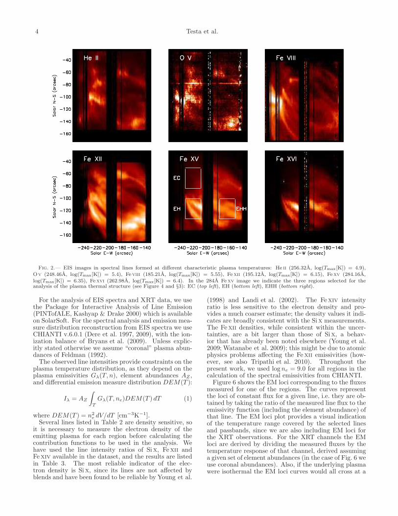
of thermal analysis from XRT and EIS data, we havethen selected a few subregions. To select these regionswe have first obtained maps of temperature and emissionmeasure over the whole active region, by using estimatesderived with the so-called combined improved filter ra-tio method, devised by Reale et al. (2007). The result-ing temperature map is shown in Figure 4. We selectedthree regions, of area approximately 30′′×30′′: EC, whichin the temperature map homogeneously appears as rela-tively cool, and two hotter regions (EH, EHH). The val-ues of temperature mean and standard deviation derivedfor these three regions from the CIFR diagnostics are:1.5±0.1 MK (EC), 1.9±0.2 MK (EH), and 2.0±0.2 MK(EHH). When selecting the boundaries of region EHHin the XRT data, we slightly modified the shape (how-ever maintaining the area value) in order to avoid thecontamination spots clearly visible in the temperaturemap as bright blobs immediately to the east and north

of the selected area. Figure 2 shows the selected regionsin the EIS Fexv 284A image. For the temperature anal-ysis presented in the rest of the paper we integrated theXRT and EIS signals over each of these regions, over thetime intervals when the two instruments were simultane-ously observing the selected region. Figure 3 shows thatthe XRT light curves of each region changed little overthe time period when EIS was observing the same areas.

Figure 5 shows the EIS full spectra in the three re-gions selected for the analysis, with the identification ofthe brightest lines. The EIS exposure time (90 s at eachlocation) yields high signal in the strongest lines, mostlyproduced in a temperature range logT [K] ∼ 5.8 − 6.3.Hotter lines present in the EIS wavelength range havegenerally low intensities, in typical solar non-flaring con-ditions, and are difficult to detect. We have selected alist of lines which are suitable for an accurate derivationof the plasma thermal properties. This list (see Table 2)includes strong lines, unblended and with reliable atomicdata, and we also included hot lines for which howeverwe can only derive upper limits from the EIS observa-tions of this non-flaring active region. These upper limitsare nevertheless useful to constrain the high temperaturecomponent (logT [K] & 6.5).In the following we will describe in detail the analy-

sis methods and results obtained for one of the selectedregions, EHH. Then we will discuss our findings for allthree regions.

3.1. Thermal Structuring from EIS spectra

4 Testa et al.

Fig. 2.— EIS images in spectral lines formed at different characteristic plasma temperatures: He ii (256.32A, log(Tmax[K]) = 4.9),Ov (248.46A, log(Tmax[K]) = 5.4), Feviii (185.21A, log(Tmax[K]) = 5.55), Fe xii (195.12A, log(Tmax[K]) = 6.15), Fexv (284.16A,log(Tmax[K]) = 6.35), Fexvi (262.98A, log(Tmax[K]) = 6.4). In the 284A Fe xv image we indicate the three regions selected for theanalysis of the plasma thermal structure (see Figure 4 and §3): EC (top left), EH (bottom left), EHH (bottom right).

For the analysis of EIS spectra and XRT data, we usethe Package for Interactive Analysis of Line Emission(PINTofALE, Kashyap & Drake 2000) which is availableon SolarSoft. For the spectral analysis and emission mea-sure distribution reconstruction from EIS spectra we useCHIANTI v.6.0.1 (Dere et al. 1997, 2009), with the ion-ization balance of Bryans et al. (2009). Unless explic-itly stated otherwise we assume “coronal” plasma abun-dances of Feldman (1992).The observed line intensities provide constraints on the

plasma temperature distribution, as they depend on theplasma emissivities Gλ(T, n), element abundances AZ ,and differential emission measure distribution DEM(T ):

Iλ = AZ

∫T

Gλ(T, ne)DEM(T ) dT (1)

where DEM(T ) = n2edV/dT [cm−3K−1].

Several lines listed in Table 2 are density sensitive, soit is necessary to measure the electron density of theemitting plasma for each region before calculating thecontribution functions to be used in the analysis. Wehave used the line intensity ratios of Six, Fexii andFexiv available in the dataset, and the results are listedin Table 3. The most reliable indicator of the elec-tron density is Six, since its lines are not affected byblends and have been found to be reliable by Young et al.

(1998) and Landi et al. (2002). The Fexiv intensityratio is less sensitive to the electron density and pro-vides a much coarser estimate; the density values it indi-cates are broadly consistent with the Six measurements.The Fexii densities, while consistent within the uncer-tainties, are a bit larger than those of Six, a behav-ior that has already been noted elsewhere (Young et al.2009; Watanabe et al. 2009); this might be due to atomicphysics problems affecting the Fexii emissivities (how-ever, see also Tripathi et al. 2010). Throughout thepresent work, we used logne = 9.0 for all regions in thecalculation of the spectral emissivities from CHIANTI.Figure 6 shows the EM loci corresponding to the fluxes

measured for one of the regions. The curves representthe loci of constant flux for a given line, i.e. they are ob-tained by taking the ratio of the measured line flux to theemissivity function (including the element abundance) ofthat line. The EM loci plot provides a visual indicationof the temperature range covered by the selected linesand passbands, since we are also including EM loci forthe XRT observations. For the XRT channels the EMloci are derived by dividing the measured fluxes by thetemperature response of that channel, derived assuminga given set of element abundances (in the case of Fig. 6 weuse coronal abundances). Also, if the underlying plasmawere isothermal the EM loci curves would all cross at a

Active Region Plasma Diagnostics with Hinode 5

TABLE 2Identification and measured fluxes of EIS spectral lines used forreconstructing the DEM of the three regions selected for the

analysis and shown in Figure 2.

λ [A] Ion log(Tmax[K]) flux [erg cm−2 s−1] Notesa

EC EH EHH

171.0755 Fexix 5.9 8494.52 16757.8 9238.51174.5340 Fex 6.0 7310.57 12152.6 7888.11177.2430 Fex 6.0 4231.15 7555.12 4736.85180.4080 Fexi 6.1 10609.4 16354.4 11523.8182.1690 Fexi 6.1 1784.80 3021.49 1914.51186.8520 Fexii 6.2 694.141 1099.68 426.001186.8840 Fexii 6.2 3129.81 5212.59 3902.01188.2320 Fexi 6.1 5613.69 8863.01 6469.60192.0285 Fexxiv 7.3 310.929 539.337 304.685 u192.3930 Fexii 6.2 4107.59 5858.81 4550.20195.1180 Fexii 6.2 14092.9 21301.2 16415.0202.0440 Fexiii 6.2 11240.2 15845.5 14868.5204.6542 Fe xvii 6.7 37.2628 60.1331 44.5043 u208.6040 Caxvi 6.7 5.61904 17.4814 38.7130 u246.0200 Si vi 5.6 76.5847 91.3415 28.2609249.1240 Si vi 5.6 29.2495 38.8003 15.6522249.1780 Nixvii 6.5 20.5272 277.752 312.949253.1702 Fe xxii 7.1 3.55755 9.38507 9.47460 u253.7880 Si x 6.1 379.199 578.696 436.514258.3710 Si x 6.1 2737.30 4175.65 3144.01261.0440 Si x 6.1 1151.82 1731.62 1318.26262.9760 Fexvi 6.4 173.934 968.696 1036.80263.7657 Fexxiii 7.2 14.5618 12.5289 9.42194 u264.2310 Sx 6.2 925.718 975.778 899.526264.7900 Fexiv 6.3 2784.31 5570.13 4768.17265.0010 Fexvi 6.4 19.6691 105.484 99.7671270.5220 Fexiv 6.3 1356.52 3060.05 2607.03272.0060 Si x 6.1 1117.27 1592.69 1191.82272.6390 Si vii 5.8 134.686 237.159 99.4883275.3540 Si vii 5.8 456.285 706.011 317.491284.1630 Fe xv 6.3 10317.8 28644.9 27965.3

a “u” indicates upper limits of fluxes of hot lines which are not actuallydetected in the EIS spectra.

TABLE 3Electron density diagnostic results for each

region. The density adopted throughout the studyis logne = 9.0. Densities are in cm−3.

Ion Line ratio logne

EC EH EHH

Six 261.0/253.8 8.95+0.30−0.20 9.00±0.25 8.95+0.30

−0.20

Fexii 186.8/195.1 9.15+0.15−0.20 9.20±0.20 9.10±0.15

Fexiv 264.8/270.5 9.5±0.4 9.3+0.3−0.5 9.3+0.3

−0.5

single points, therefore this plot also provides some indi-cation for the characteristics of temperature distributionof the plasma.The method of reconstruction of the differential emis-

sion measure distribution that we adopt for the analysisof EIS data runs a Markov-chain Monte Carlo (MCMC)algorithm on a set of line fluxes (intensities in broadbandpasses can also be used, as for instance in thecase of XRT datasets; see §3.2), and it returns an es-timate of the DEM that generates the observed fluxes(see Kashyap & Drake 1998 for details on assumptionsand approximations). With respect to other methods forreconstructing the plasma emission measure distributionfrom a set of fluxes, the MCMC method we adopt hasthe main advantage of providing an estimate of the uncer-

tainties in the derived DEM. The problem of determiningthe emission measure distribution and its confidence lim-its is notoriously challenging (e.g., Craig & Brown 1976;Judge et al. 1997; Judge 2010). Part of the reason isthat the emission measure at a given temperature cannotbe determined independently of temperatures at otherbins, and therefore the corresponding errors are also cor-related. The MCMC method works around this funda-mental problem by sampling solutions from the full prob-ability distribution of the DEM given the data. It is afeature of the MCMC chain that regardless of the con-ceptual complexity of the solution space, it can be fullyexplored numerically at a relatively low computationalcost. Thus, the sampled solutions include the effects ofstatistical noise from the measured data as well as corre-lations across temperatures that arise due to overlaps be-tween the individual contribution functions of the differ-ent lines. From the set of solutions thus obtained, we candepict the uncertainty range at temperatures of interest.Since it is difficult to display correlations, for purposesof clarity, we only show the error ranges computed sepa-rately at each temperature bin in the figures. Error barscomputed for predicted fluxes, and thus abundances, areuncorrelated and thus have the usual meaning. Anotherproblem with DEM reconstruction is that the derivedcurves are solutions to a Fredholm integral equation ofthe first kind, and are thus subject to high-frequency in-stability. These instabilities are typically suppressed by

6 Testa et al.

Fig. 3.— Lightcurves of XRT observations in all analyzed filters,for the three selected regions: EC (top), EH (middle), EHH (bot-tom). For each filter the signal is normalized to the intensity inthe first image. The solid line at the bottom of the plot indicatesthe time interval when EIS was observing the selected region.

imposing a global smoothness criterion. In the case of theMCMC method adopted here however, this restriction isrelaxed. Smoothing is more physically based, is locallyvariable, and is limited by the width and number of theline contribution functions used. This leads to solutionsthat individually have more fluctuations, but on averagethe ensemble of solutions produce an envelope that reli-ably determines features that are statistically significant.As uncertainties on the measured line fluxes listed in

-300 -250 -200 -150 -100X (arcsec)

-200

-150

-100

-50

0

Y (

arcs

ec)

6.400

6.100

Fig. 4.— Temperature map obtained from the combined im-proved filter ratio from the XRT images of AR 10999 shown inFigure 1. The three regions selected for the detailed tempera-ture analysis are indicated: EC (top left), EH (bottom left), EHH(bottom right). When selecting the boundaries of region EHH wemodified the shape (however maintaining the area value) in orderto avoid the contamination spots clearly visible in the tempera-ture map as bright blobs immediately to the east and north of theselected area.

Table 2 we combine in quadrature the statistical uncer-tainties which are typically very small (of the order offew percent), with the uncertainty in the absolute radio-metric calibration for EIS which is estimated to be 22%(Lang et al. 2006).Figure 7 shows the results of the MCMC method to

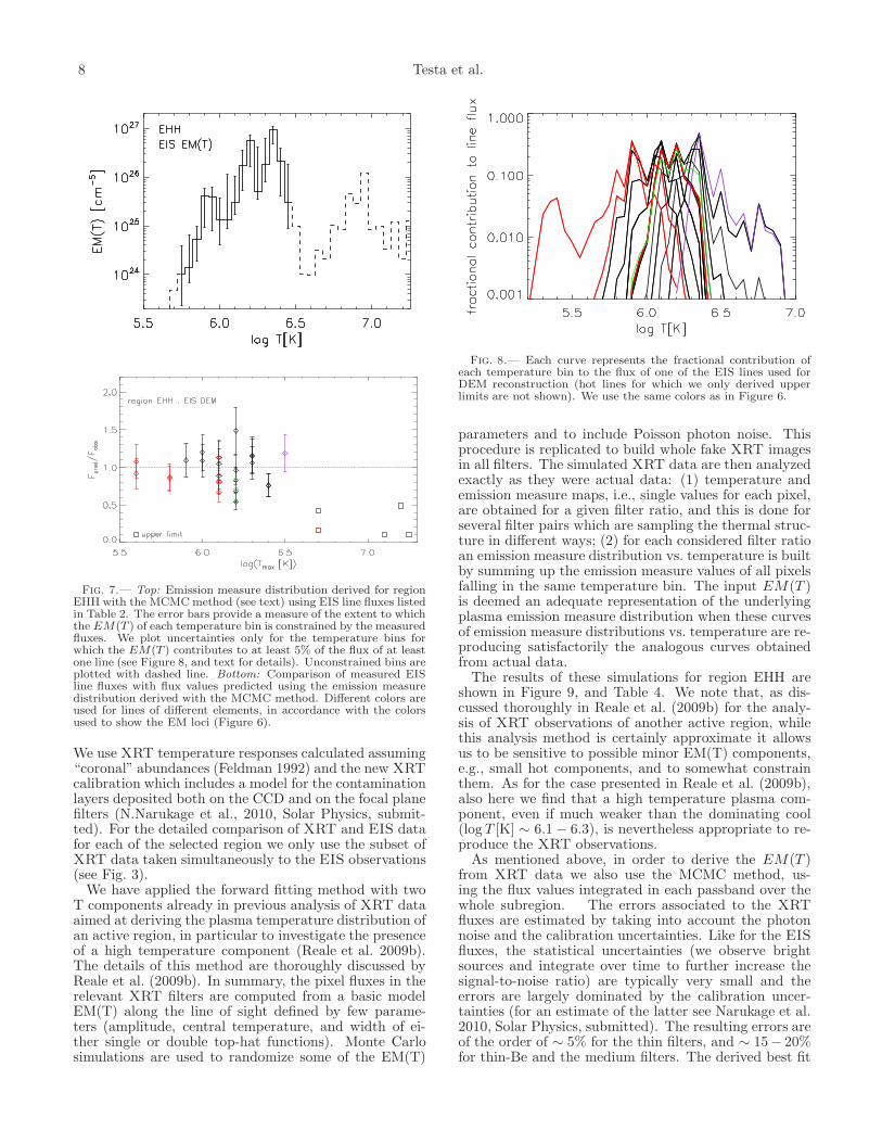
derive the emission measure distribution, applied to theEIS fluxes measured for the EHH region. In this case, asin the rest of the paper, we will plot the emission measuredistribution EM(T ) which is obtained by integrating thedifferential emission measure distribution DEM(T ) ineach temperature bin (here we use a temperature gridwith constant ∆ logT = 0.05). The upper panel showsthe emission measure distribution that reproduces themeasured fluxes; the associated uncertainties estimatedas described at the beginning of this section are also plot-ted. The bottom panel shows the ratios of predicted toobserved fluxes for the EIS lines. The comparison ofmeasured fluxes with predictions based on the emissionmeasure distribution shows that all fluxes are reproducedwithin about 50%, and that the fluxes predicted for thehot lines, for which the spectra only provide upper limit,are all lower than the upper limits.We can investigate the compatibility of this derived

EM(T ) with the XRT observations by computing thepredictedXRT fluxes and comparing them with the mea-sured ones. It is worth noting however that when deriv-ing the EM(T ) using exclusively the information con-tained in the EIS spectra, not all temperature bins arewell constrained. In particular for these EIS datasetswhich lack measured lines in the high temperature range

Active Region Plasma Diagnostics with Hinode 7

Fig. 5.— EIS spectra of the three regions selected for the analysis:EC (top), EH (middle), EHH (bottom). The identification of thespectral lines used for the analysis of the plasma thermal properties(listed in Table 2) are shown in the spectrum in the top panel.

(logT [K] & 6.5) the hot tail of the EM(T ) is poorlyconstrained, but XRT is very sensitive to it, having tem-perature responses which peak around logT [K] ∼ 7 forall filters. Therefore some caution must be applied toperform this cross-check. To determine in which temper-ature bins the EM(T ) is constrained by EIS data we lookat the contribution of each bin to the line fluxes. Foldingthe EM(T ) with the line emissivity we can investigatethe relative weight of each temperature bin for each line,as shown in Figure 8. We then consider as constrainedthe temperature bins where the EM(T ) contributes morethan a threshold (percentage) value to at least one of theEIS lines. The choice of the threshold value is somewhatarbitrary and we chose a rather conservative 5%.Considering the EM(T ) in the temperature bins satis-

fying our selection criterium, we calculate the predictedfluxes in the XRT filters (which therefore are strictlyspeaking lower limits to the values predicted by the as-sumed EM(T )) which are listed in Table 4, together withthe measured fluxes. The comparison of the two sets in-dicates that the EM(T ) derived from EIS underpredictsthe XRT fluxes by a factor ∼ 2, the discrepancy be-ing slightly larger for the thinner filters (Al-poly, C-poly,Ti-poly) which are more sensitive to the cooler plasma

Fig. 6.— EM loci obtained for the measured EIS line fluxes,including upper limits (dotted lines) for hot lines in EIS passbands.The dashed lines indicate the EM loci for XRT measured fluxes.We use different colors for lines of different elements, as indicatedin the inset.

TABLE 4For region EHH, comparison of XRT measured

fluxes with the values predicted using the EM(T )derived from EIS line fluxes (and shown in theupper panel of Figure 7), and from the forwardmodeling with two temperature components (see

§3.2), assuming coronal abundances.

XRT filter Fobs Fpred,EISa Fpred,fm

b

[DN/s] [DN/s] [DN/s]

Al-poly 122.0 57.8 (41.8-70.2) 123.2C-poly 95.8 44.5 (32.8-53.4) 101.1Ti-poly 69.1 31.0 (23.0-36.9) 65.94Be-thin 11.1 5.85 (3.69-7.61) 9.82Be-med 1.59 1.06 (0.66-1.38) 1.42Al-med 0.730 0.483 (0.301-0.628) 0.673

a XRT fluxes predicted using the emission measure dis-tribution derived using EIS line fluxes only. The valuesin parentheses represent the range of fluxes predicted bythe Monte Carlo simulations of the EM(T) which are theacceptable emission measure distributions, defining theerror bars shown in Figure 7.b XRT fluxes predicted using the EM(T ) derived fromthe forward modeling with 2T, and using coronal abun-dances.

which is better characterized by the EIS data.

3.2. Thermal Structuring from XRT data

We then derive the thermal distribution of the coronalplasma exclusively from XRT data, by using two differ-ent methods:

• Forward fitting of distributions of filter ratios ofseveral filter pairs, through pixel-by-pixel MonteCarlo simulations of the observations, using twotemperature components (2T);

• MCMCmethod, as for the analysis of the EIS spec-tra (see §3.1).

8 Testa et al.

Fig. 7.— Top: Emission measure distribution derived for regionEHH with the MCMCmethod (see text) using EIS line fluxes listedin Table 2. The error bars provide a measure of the extent to whichthe EM(T ) of each temperature bin is constrained by the measuredfluxes. We plot uncertainties only for the temperature bins forwhich the EM(T ) contributes to at least 5% of the flux of at leastone line (see Figure 8, and text for details). Unconstrained bins areplotted with dashed line. Bottom: Comparison of measured EISline fluxes with flux values predicted using the emission measuredistribution derived with the MCMC method. Different colors areused for lines of different elements, in accordance with the colorsused to show the EM loci (Figure 6).

We use XRT temperature responses calculated assuming“coronal” abundances (Feldman 1992) and the new XRTcalibration which includes a model for the contaminationlayers deposited both on the CCD and on the focal planefilters (N.Narukage et al., 2010, Solar Physics, submit-ted). For the detailed comparison of XRT and EIS datafor each of the selected region we only use the subset ofXRT data taken simultaneously to the EIS observations(see Fig. 3).We have applied the forward fitting method with two

T components already in previous analysis of XRT dataaimed at deriving the plasma temperature distribution ofan active region, in particular to investigate the presenceof a high temperature component (Reale et al. 2009b).The details of this method are thoroughly discussed byReale et al. (2009b). In summary, the pixel fluxes in therelevant XRT filters are computed from a basic modelEM(T) along the line of sight defined by few parame-ters (amplitude, central temperature, and width of ei-ther single or double top-hat functions). Monte Carlosimulations are used to randomize some of the EM(T)

Fig. 8.— Each curve represents the fractional contribution ofeach temperature bin to the flux of one of the EIS lines used forDEM reconstruction (hot lines for which we only derived upperlimits are not shown). We use the same colors as in Figure 6.

parameters and to include Poisson photon noise. Thisprocedure is replicated to build whole fake XRT imagesin all filters. The simulated XRT data are then analyzedexactly as they were actual data: (1) temperature andemission measure maps, i.e., single values for each pixel,are obtained for a given filter ratio, and this is done forseveral filter pairs which are sampling the thermal struc-ture in different ways; (2) for each considered filter ratioan emission measure distribution vs. temperature is builtby summing up the emission measure values of all pixelsfalling in the same temperature bin. The input EM(T )is deemed an adequate representation of the underlyingplasma emission measure distribution when these curvesof emission measure distributions vs. temperature are re-producing satisfactorily the analogous curves obtainedfrom actual data.The results of these simulations for region EHH are

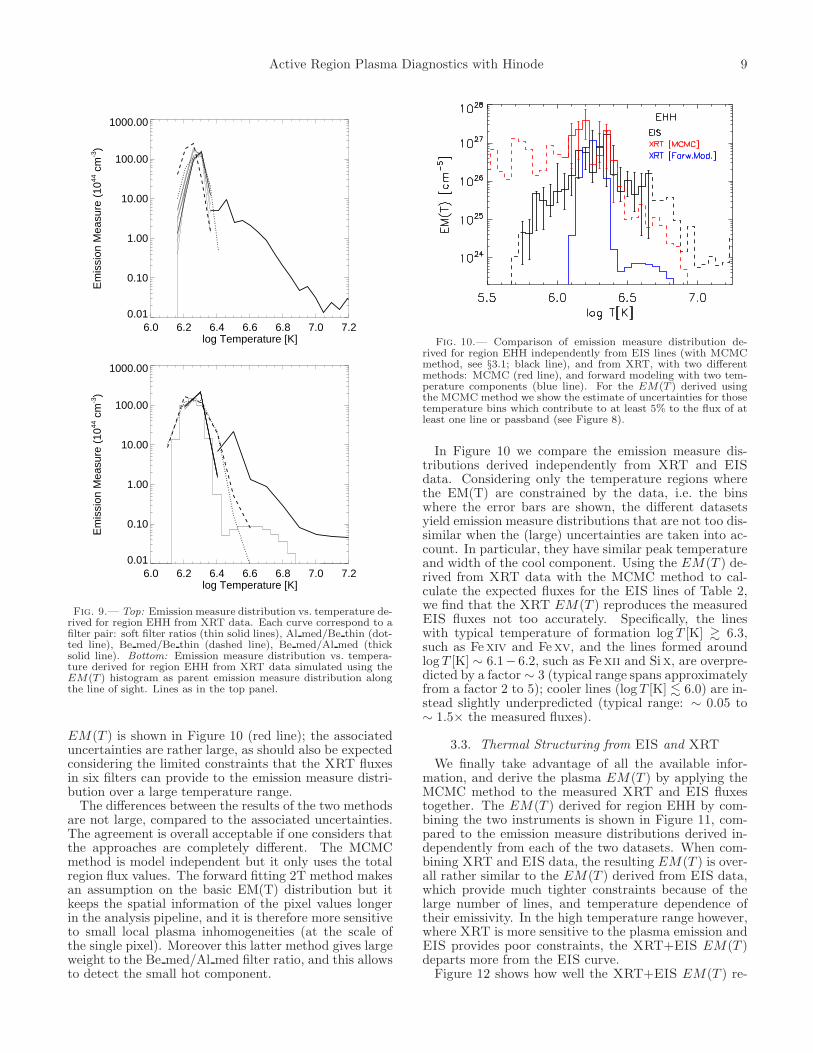
shown in Figure 9, and Table 4. We note that, as dis-cussed thoroughly in Reale et al. (2009b) for the analy-sis of XRT observations of another active region, whilethis analysis method is certainly approximate it allowsus to be sensitive to possible minor EM(T) components,e.g., small hot components, and to somewhat constrainthem. As for the case presented in Reale et al. (2009b),also here we find that a high temperature plasma com-ponent, even if much weaker than the dominating cool(logT [K] ∼ 6.1− 6.3), is nevertheless appropriate to re-produce the XRT observations.As mentioned above, in order to derive the EM(T )

from XRT data we also use the MCMC method, us-ing the flux values integrated in each passband over thewhole subregion. The errors associated to the XRTfluxes are estimated by taking into account the photonnoise and the calibration uncertainties. Like for the EISfluxes, the statistical uncertainties (we observe brightsources and integrate over time to further increase thesignal-to-noise ratio) are typically very small and theerrors are largely dominated by the calibration uncer-tainties (for an estimate of the latter see Narukage et al.2010, Solar Physics, submitted). The resulting errors areof the order of ∼ 5% for the thin filters, and ∼ 15− 20%for thin-Be and the medium filters. The derived best fit

Active Region Plasma Diagnostics with Hinode 9

6.0 6.2 6.4 6.6 6.8 7.0 7.2log Temperature [K]

0.01

0.10

1.00

10.00

100.00

1000.00

Em

issi

on M

easu

re (

1044

cm

-3)

6.0 6.2 6.4 6.6 6.8 7.0 7.2log Temperature [K]

0.01

0.10

1.00

10.00

100.00

1000.00

Em

issi

on M

easu

re (

1044

cm

-3)

Fig. 9.— Top: Emission measure distribution vs. temperature de-rived for region EHH from XRT data. Each curve correspond to afilter pair: soft filter ratios (thin solid lines), Al med/Be thin (dot-ted line), Be med/Be thin (dashed line), Be med/Al med (thicksolid line). Bottom: Emission measure distribution vs. tempera-ture derived for region EHH from XRT data simulated using theEM(T ) histogram as parent emission measure distribution alongthe line of sight. Lines as in the top panel.

EM(T ) is shown in Figure 10 (red line); the associateduncertainties are rather large, as should also be expectedconsidering the limited constraints that the XRT fluxesin six filters can provide to the emission measure distri-bution over a large temperature range.The differences between the results of the two methods

are not large, compared to the associated uncertainties.The agreement is overall acceptable if one considers thatthe approaches are completely different. The MCMCmethod is model independent but it only uses the totalregion flux values. The forward fitting 2T method makesan assumption on the basic EM(T) distribution but itkeeps the spatial information of the pixel values longerin the analysis pipeline, and it is therefore more sensitiveto small local plasma inhomogeneities (at the scale ofthe single pixel). Moreover this latter method gives largeweight to the Be med/Al med filter ratio, and this allowsto detect the small hot component.

Fig. 10.— Comparison of emission measure distribution de-rived for region EHH independently from EIS lines (with MCMCmethod, see §3.1; black line), and from XRT, with two differentmethods: MCMC (red line), and forward modeling with two tem-perature components (blue line). For the EM(T ) derived usingthe MCMC method we show the estimate of uncertainties for thosetemperature bins which contribute to at least 5% to the flux of atleast one line or passband (see Figure 8).

In Figure 10 we compare the emission measure dis-tributions derived independently from XRT and EISdata. Considering only the temperature regions wherethe EM(T) are constrained by the data, i.e. the binswhere the error bars are shown, the different datasetsyield emission measure distributions that are not too dis-similar when the (large) uncertainties are taken into ac-count. In particular, they have similar peak temperatureand width of the cool component. Using the EM(T ) de-rived from XRT data with the MCMC method to cal-culate the expected fluxes for the EIS lines of Table 2,we find that the XRT EM(T ) reproduces the measuredEIS fluxes not too accurately. Specifically, the lineswith typical temperature of formation logT [K] & 6.3,such as Fexiv and Fexv, and the lines formed aroundlogT [K] ∼ 6.1− 6.2, such as Fexii and Six, are overpre-dicted by a factor ∼ 3 (typical range spans approximatelyfrom a factor 2 to 5); cooler lines (logT [K] . 6.0) are in-stead slightly underpredicted (typical range: ∼ 0.05 to∼ 1.5× the measured fluxes).

3.3. Thermal Structuring from EIS and XRT

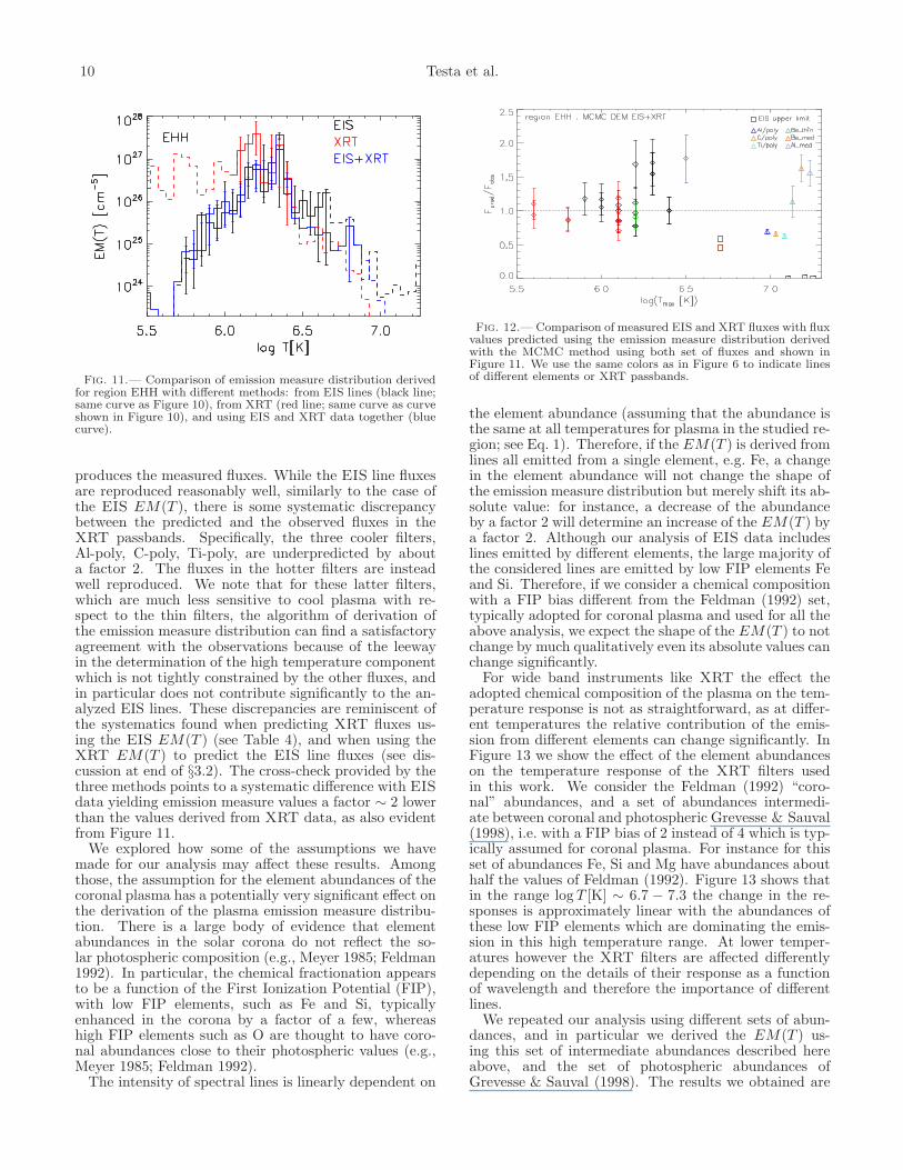
We finally take advantage of all the available infor-mation, and derive the plasma EM(T ) by applying theMCMC method to the measured XRT and EIS fluxestogether. The EM(T ) derived for region EHH by com-bining the two instruments is shown in Figure 11, com-pared to the emission measure distributions derived in-dependently from each of the two datasets. When com-bining XRT and EIS data, the resulting EM(T ) is over-all rather similar to the EM(T ) derived from EIS data,which provide much tighter constraints because of thelarge number of lines, and temperature dependence oftheir emissivity. In the high temperature range however,where XRT is more sensitive to the plasma emission andEIS provides poor constraints, the XRT+EIS EM(T )departs more from the EIS curve.Figure 12 shows how well the XRT+EIS EM(T ) re-

10 Testa et al.

Fig. 11.— Comparison of emission measure distribution derivedfor region EHH with different methods: from EIS lines (black line;same curve as Figure 10), from XRT (red line; same curve as curveshown in Figure 10), and using EIS and XRT data together (bluecurve).

produces the measured fluxes. While the EIS line fluxesare reproduced reasonably well, similarly to the case ofthe EIS EM(T ), there is some systematic discrepancybetween the predicted and the observed fluxes in theXRT passbands. Specifically, the three cooler filters,Al-poly, C-poly, Ti-poly, are underpredicted by abouta factor 2. The fluxes in the hotter filters are insteadwell reproduced. We note that for these latter filters,which are much less sensitive to cool plasma with re-spect to the thin filters, the algorithm of derivation ofthe emission measure distribution can find a satisfactoryagreement with the observations because of the leewayin the determination of the high temperature componentwhich is not tightly constrained by the other fluxes, andin particular does not contribute significantly to the an-alyzed EIS lines. These discrepancies are reminiscent ofthe systematics found when predicting XRT fluxes us-ing the EIS EM(T ) (see Table 4), and when using theXRT EM(T ) to predict the EIS line fluxes (see dis-cussion at end of §3.2). The cross-check provided by thethree methods points to a systematic difference with EISdata yielding emission measure values a factor ∼ 2 lowerthan the values derived from XRT data, as also evidentfrom Figure 11.We explored how some of the assumptions we have

made for our analysis may affect these results. Amongthose, the assumption for the element abundances of thecoronal plasma has a potentially very significant effect onthe derivation of the plasma emission measure distribu-tion. There is a large body of evidence that elementabundances in the solar corona do not reflect the so-lar photospheric composition (e.g., Meyer 1985; Feldman1992). In particular, the chemical fractionation appearsto be a function of the First Ionization Potential (FIP),with low FIP elements, such as Fe and Si, typicallyenhanced in the corona by a factor of a few, whereashigh FIP elements such as O are thought to have coro-nal abundances close to their photospheric values (e.g.,Meyer 1985; Feldman 1992).The intensity of spectral lines is linearly dependent on

Fig. 12.— Comparison of measured EIS and XRT fluxes with fluxvalues predicted using the emission measure distribution derivedwith the MCMC method using both set of fluxes and shown inFigure 11. We use the same colors as in Figure 6 to indicate linesof different elements or XRT passbands.

the element abundance (assuming that the abundance isthe same at all temperatures for plasma in the studied re-gion; see Eq. 1). Therefore, if the EM(T ) is derived fromlines all emitted from a single element, e.g. Fe, a changein the element abundance will not change the shape ofthe emission measure distribution but merely shift its ab-solute value: for instance, a decrease of the abundanceby a factor 2 will determine an increase of the EM(T ) bya factor 2. Although our analysis of EIS data includeslines emitted by different elements, the large majority ofthe considered lines are emitted by low FIP elements Feand Si. Therefore, if we consider a chemical compositionwith a FIP bias different from the Feldman (1992) set,typically adopted for coronal plasma and used for all theabove analysis, we expect the shape of the EM(T ) to notchange by much qualitatively even its absolute values canchange significantly.For wide band instruments like XRT the effect the

adopted chemical composition of the plasma on the tem-perature response is not as straightforward, as at differ-ent temperatures the relative contribution of the emis-sion from different elements can change significantly. InFigure 13 we show the effect of the element abundanceson the temperature response of the XRT filters usedin this work. We consider the Feldman (1992) “coro-nal” abundances, and a set of abundances intermedi-ate between coronal and photospheric Grevesse & Sauval(1998), i.e. with a FIP bias of 2 instead of 4 which is typ-ically assumed for coronal plasma. For instance for thisset of abundances Fe, Si and Mg have abundances abouthalf the values of Feldman (1992). Figure 13 shows thatin the range logT [K] ∼ 6.7 − 7.3 the change in the re-sponses is approximately linear with the abundances ofthese low FIP elements which are dominating the emis-sion in this high temperature range. At lower temper-atures however the XRT filters are affected differentlydepending on the details of their response as a functionof wavelength and therefore the importance of differentlines.We repeated our analysis using different sets of abun-

dances, and in particular we derived the EM(T ) us-ing this set of intermediate abundances described hereabove, and the set of photospheric abundances ofGrevesse & Sauval (1998). The results we obtained are

Active Region Plasma Diagnostics with Hinode 11

Fig. 13.— Ratio of XRT responses, as a function of temperature,calculated using intermediate abundances (FIP bias = 2), to theresponses calculated using coronal abundances (Feldman 1992). Adifferent color is used for each filter used in this work, as indicatedin the inset.

shown in Figure 14, also compared to the EM(T ) derivedwith Feldman abundances. The curves have very similarshape and are overall compatible within the uncertain-ties. However it is clear that, as expected in the lightof the above discussions, the EM(T ) obtained for inter-mediate abundances (which are lower than the “coronal”abundances) is systematically larger than the one foundfor “coronal” abundances, and the EM(T ) derived forthe photospheric abundances case are even larger. In themiddle panel of Figure 14 we show the comparison of theobserved fluxes with the predictions using the EM(T )derived for intermediate abundances. Comparing thesefindings with the analogous results of Figure 12 we notethat although the overall results are not changed dra-matically, the fluxes predicted for the XRT thin filtersare closer to the observations when using intermediateabundances. The increases by about 20-35% are com-patible with expectations: the predicted fluxes shouldrise accordingly to the increase of the cool component ofthe EM(T ) but be reduced by a factor corresponding tothe decrease of the XRT response (see Figure 13). Theanalogous plot for the case of photospheric abundances(bottom panel of Figure 14) shows that using these abun-dance values the agreement between EIS and XRT im-proves even further.The values assumed for the element abundances can in

principle be checked with the EIS spectra. As discussedabove, the DEM obtained from EIS has been determinedusing almost exclusively lines from low-FIP ions, whosecoronal abundances are enhanced by a factor of ∼ 3− 4over the photospheric values. Therefore, any change inthe actual abundance of the low-FIP elements from theassumed value will result in a systematic shift betweenthe observed intensities of the lines from Sx to Sxiii,whose coronal abundance is expected to be close to thephotospheric one, and their values predicted with theDEM. There are ten S lines in the EIS spectra, emittedby Sx to Sxiii, and we have compared their predictedand observed intensities to check the corrections to thecoronal abundances. We found no unambiguous evidenceof systematic differences in the observed to predicted in-

Fig. 14.— Top panel: Comparison of emission measure distribu-tions derived with the MCMC method using simultaneously EISand XRT fluxes, and three different sets of abundances: coronalabundances (Feldman 1992; black line), intermediate abundances(red line; see text for definition of intermediate abundances), andphotospheric abundances (Grevesse & Sauval 1998; blue line). Forintermediate abundances, for which Fe and Si have roughly halfthe abundance as in the coronal set, the EM(T ) accordingly in-creases; the EM(T ) increases even further for photospheric abun-dances. Middle and bottom panels: Comparison of measured EISand XRT fluxes with flux values predicted by the emission measuredistribution derived with the MCMCmethod (XRT+EIS) and: (a)intermediate abundances (middle), or (b) photospheric abundances(bottom; Grevesse & Sauval 1998).

tensity ratios. Moreover, recent estimates of the S ab-solute abundance have been revised by Lodders (2003)and by Caffau & Ludwig (2007), who decreased them bya factor 1.5 from the Grevesse & Sauval (1998) value.Since this change is of the same order of the revision

12 Testa et al.

of the low-FIP element abundances we propose, we feelthat the uncertainties in the S predicted line intensitiesare so large that these ions can not be used to confirmthe abundance change made necessary by the XRT chan-nels in this work. S is in any case a borderline elementfor FIP effect studies, and abundances of other low FIPelements are difficult to determine. While oxygen lines ofO iv,v,vi are present in the EIS wavelength range, theyare formed at low temperature (log(T [K]) . 5.5) withrespect to the hotter coronal EIS lines considered in ouractive region study. In that temperature range the ther-mal distribution is not well constrained and therefore theabundances cannot be accurately determined.While the results shown in Figure 14 seem to suggest

that the photospheric abundances might be a more ap-propriate choice for the active region we studied here,we note that the data we have used do not allow us todetermine the abundances and therefore do not allow usto disentangle between the abundance effects and cross-calibration issues. We also note that this active regionwas already several days old at the time of the obser-vation, and therefore it is reasonable to expect somesignificant effect of chemical fractionation to have oc-curred producing departures from the photospheric com-position (see e.g., Widing & Feldman 2001; however, seealso Del Zanna 2003).We have presented the complete analysis carried out

for one of the selected regions, providing insights intothe thermal distribution of the plasma, limitations of themethods, and cross-calibration of the Hinode XRT andEIS. Before discussing in details these findings in §4 webriefly present and discuss the analogous results found forthe other two selected regions, EC and EH, comparingthem with the results obtained for region EHH.Carrying out the same analysis described above (§3.1,

3.2, 3.3) on the other two regions, we find results quali-tatively similar to our findings for region EHH discussedabove, in particular in terms of the comparison betweendifferent analysis methods and systematic discrepanciesbetween XRT and EIS.In Figure 15 we show the emission measure distribu-

tions obtained for the three regions, using the MCMCalgorithm applied to XRT and EIS data together (toppanel), or forward fitting the XRT observations usingtwo temperature components (bottom panel). We notethat despite the forward fitting 2T model adopts consid-erable simplifying assumptions for the underlying emis-sion measure distribution the results we obtain with thismethod are qualitatively in good agreement with theMCMC approach which does not impose constraints onthe shape of the DEM. On the other hand, we notethat the forward fitting 2T model has the advantage ofalso taking into account the spatial information, whilethe MCMC method only uses the information containedin the integrated fluxes in each passband. The twohotter regions, EH and EHH, have very similar under-lying EM(T ): their cool components have analogouspeak temperature (logT [K] ∼ 6.2− 6.3) and amounts ofplasma, whereas the hot component of EHH is of weightcomparable to the high temperature component of EHbut it appears shifted towards slightly higher tempera-tures. For region EC the cool component is character-ized by a peak temperature slightly cooler than the othertwo regions, and in particular its EM(T ) falls off faster

on the high temperature side of the cool peak; the hotcomponent of EC is much weaker than the other twocomponents, if at all present.

Fig. 15.— Emission measure distributions for the three selectedregions: EC (red line), EH (blue line), EHH (black line). Top:EM(T ) curves derived with MCMC method, using EIS and XRTfluxes. Bottom: EM(T ) derived from XRT data through the for-ward fitting 2T method (see §3.2 for details), using photosphericabundances.

4. DISCUSSION

We have presented the results of a detailed analysisof Hinode XRT and EIS observations of a non-flaringactive region to diagnose the temperature distribution ofthe coronal plasma. In this work we carried out indepen-dent temperature analysis from measurements of eitherinstruments, and use the derived thermal distributionsto make prediction for the fluxes observed with the otherinstrument and then compare them with actual measure-ments. Then we combine the information from bothinstruments and compare the results with the findingsbased on XRT or EIS data only. This approach allowedus to explore the limitations of the data and analysismethods in providing constraints to the plasma temper-ature distribution, and investigate the cross-calibrationof the two Hinode instruments. With respect to previousworks using both XRT and EIS data to study the ther-mal properties of the coronal plasma (e.g., Landi et al.

Active Region Plasma Diagnostics with Hinode 13

2010), in this work we provide a quantitative cross-checkbetween the diagnostics of the two instruments.When using the two datasets separately the derived

EM(T ) curves have overall similar width and peak tem-perature. However, the emission measure derived fromEIS is systematically smaller, by a factor ∼ 2 − 3, thanthe emission measure derived from XRT fluxes, for eachof the three studied regions. We note that even if theuncertainties in the derived EM(T ) are rather large thesystematic discrepancy appears to be significant. We findthat the extent of the discrepancy betweenXRT and EISdepends in part on the assumptions made for the chem-ical composition of the X-ray emitting plasma: it canbe mitigated by assuming abundances intermediate be-tween the typical “coronal” abundances (Feldman 1992)and the photospheric values Grevesse & Sauval (1998),and it almost disappears when using photospheric abun-dances. This interesting finding encourages further in-vestigations to search for similar evidence in other activeregions, in an active region at different epochs, and indifferent kinds of coronal structures (quiet sun, brightpoints, coronal holes). While our study provides no ro-bust constraints on the element abundances we stress theimportance of the assumed values in the analysis of Hin-ode observations. The detailed EM(T ) reconstructionand the instrument cross-calibration are significantly af-fected by the assumed abundances: EIS spectra allowthe determination of “abundance independent” EM(T )e.g. using exclusively Fe lines (Watanabe et al. 2007),but its absolute values depend on the abundances; theXRT passbands include significant contribution of sev-eral elements, both high-FIP and low-FIP, and thereforethe dependence of the EM(T ) on abundances is morecomplicated and temperature dependent.For the analysis of XRT data we use two different

methods for deriving the emission measure distribution.We find that the Markov-chain Monte Carlo methodyields results in good qualitative agreement with the for-ward fitting 2T method which makes rather simplifyingassumptions on the emission measure distribution buthas the advantage of making use also of the spatial in-formation. This finding lends further confidence to theresults obtained previously by applying this method tothe study of XRT observations of another active region(Reale et al. 2009b).We find that the EIS spectra allow an accurate deter-

mination of the cool (logT [K] . 6.5), most prominent,component, but when used alone the EIS data are unableto constrain the hotter emission due to the lack of stronghot lines in the spectra. The combination with XRTdata provide much tighter constraints on the emissionmeasure distribution on a wider temperature range. Ouranalysis shows that the studied active region is character-ized by bulk plasma temperatures of ∼ 2 MK, which arerather low for active region plasma. The EM(T ) of thethree selected regions are very similar for log T [K] . 6.2,but for the two hotter regions, EH and EHH, the coolcomponent is broader and with a peak shifted towardshigher T. The high temperature tail of the emission mea-sure distribution is not strongly constrained by the data.However, the EM(T ) derived at least for the two hotterregions, EH and EHH, suggests the presence of a hottercomponent (logT [K] & 6.5) about two orders of magni-tude weaker than the dominant cool component, in good

agreement with the findings of Reale et al. (2009b) foranother, hotter, active region.

5. CONCLUSIONS

We analyzed Hinode XRT multi-filter data and EISspectral observations of a non-flaring active region tostudy the temperature distribution of coronal plasma,EM(T ), and to carry out a detailed investigation of thecross-calibration of the two instruments. We selectedthree subareas of the active region, and for each of themwe derived the emission measure distribution EM(T )by: (1) using EIS measured line fluxes; (2) using XRTfluxes in six of the instrument’s filters; (3) combining thedatasets for the two instruments.We find a good consistency in the qualitative character-

istics – peak temperature and width of dominant temper-ature component– of the EM(T ) derived with differentmethods. However, the emission measure distributionsderived by the two instruments XRT and EIS indicatea systematic discrepancy between the two instruments,with EIS data yielding EM(T ) consistently smaller, byabout a factor 2, than the EM(T ) compatible with XRTdata. We discuss the possible origin of the disagreementand find that the assumptions for the element abun-dances significantly influence the plasma temperature di-agnostics. In particular we find that a chemical compo-sition intermediate between the usually adopted coro-nal abundances by Feldman (1992) and the solar pho-tospheric abundances improves the comparison betweenthe results obtained with the two instruments. Whenadopting photospheric abundances the discrepancy be-tween EIS and XRT decreases further. However we notethat it seems unlikely that the observed plasma, in an ac-tive region which is not newly emerged, has photosphericcomposition. Furthermore, the used data do not allow adefinite determination of the abundances, and thereforedo not allow us to robustly assess of the cross-calibrationof the instruments.One of the main aims of this work was to exploit

the complementary diagnostics for the X-ray emittingplasma provided by XRT and EIS, to investigate thepresence of hot plasma in non-flaring regions and testnanoflare heating models. We find that the derivedEM(T ) are characterized by an expected dominant coolcomponent (typically logT [K] ∼ 6.3), and a much weakeramount of plasma at higher temperature. While theamount of hot plasma is in general in agreement withrecent findings for other non-flaring active regions, andit is compatible with expectations from nanoflare mod-els, we find that within the uncertainties these results arenot conclusive.

We thank P. Grigis, and J. Drake, for useful dis-cussions. Hinode is a Japanese mission developed andlaunched by ISAS/JAXA, with NAOJ as domestic part-ner and NASA and STFC (UK) as international part-ners. It is operated by these agencies in co-operationwith ESA and the NSC (Norway). P.T. and E.E.D.were supported by NASA contract NNM07AB07C to theSmithsonian Astrophysical Observatory. F.R. acknowl-edges support from Italian Ministero dell’Universita eRicerca and Agenzia Spaziale Italiana (ASI), contractI/015/07/0. The work of Enrico Landi is supported

14 Testa et al.

by the NNH06CD24C, NNH09AL49I and other NASA grants.

REFERENCES

Aschwanden, M. J., Nightingale, R. W., & Alexander, D. 2000,ApJ, 541, 1059

Brooks, D. H., Warren, H. P., Williams, D. R., & Watanabe, T.2009, ApJ, 705, 1522

Brosius, J. W., Davila, J. M., Thomas, R. J., & Monsignori-Fossi,B. C. 1996, ApJS, 106, 143

Bryans, P., Landi, E., & Savin, D. W. 2009, ApJ, 691, 1540Caffau, E., & Ludwig, H. 2007, A&A, 467, L11Cargill, P. J. 1994, ApJ, 422, 381Cargill, P. J., & Klimchuk, J. A. 1997, ApJ, 478, 799Craig, I. J. D., & Brown, J. C. 1976, A&A, 49, 239Culhane, J. L., Harra, L. K., James, A. M., Al-Janabi, K.,

Bradley, L. J., Chaudry, R. A., Rees, K., Tandy, J. A.,Thomas, P., Whillock, M. C. R., Winter, B., Doschek, G. A.,Korendyke, C. M., Brown, C. M., Myers, S., Mariska, J., Seely,J., Lang, J., Kent, B. J., Shaughnessy, B. M., Young, P. R.,Simnett, G. M., Castelli, C. M., Mahmoud, S.,Mapson-Menard, H., Probyn, B. J., Thomas, R. J., Davila, J.,Dere, K., Windt, D., Shea, J., Hagood, R., Moye, R., Hara, H.,Watanabe, T., Matsuzaki, K., Kosugi, T., Hansteen, V., &Wikstol, Ø. 2007, Sol. Phys., 243, 19

Del Zanna, G. 2003, A&A, 406, L5Del Zanna, G., & Mason, H. E. 2003, A&A, 406, 1089Dere, K. P., Landi, E., Mason, H. E., Monsignori Fossi, B. C., &

Young, P. R. 1997, A&AS, 125, 149Dere, K. P., Landi, E., Young, P. R., Del Zanna, G., Landini, M.,

& Mason, H. E. 2009, A&A, 498, 915Doschek, G. A., Mariska, J. T., Warren, H. P., Culhane, L.,

Watanabe, T., Young, P. R., Mason, H. E., & Dere, K. P. 2007,PASJ, 59, 707

Feldman, U. 1992, Phys. Scr, 46, 202Golub, L., Deluca, E., Austin, G., Bookbinder, J., Caldwell, D.,

Cheimets, P., Cirtain, J., Cosmo, M., Reid, P., Sette, A.,Weber, M., Sakao, T., Kano, R., Shibasaki, K., Hara, H.,Tsuneta, S., Kumagai, K., Tamura, T., Shimojo, M.,McCracken, J., Carpenter, J., Haight, H., Siler, R., Wright, E.,Tucker, J., Rutledge, H., Barbera, M., Peres, G., & Varisco, S.2007, Sol. Phys., 243, 63

Grevesse, N., & Sauval, A. J. 1998, Space Science Reviews, 85,161

Judge, P. G. 2010, ApJ, 708, 1238Judge, P. G., Hubeny, V., & Brown, J. C. 1997, ApJ, 475, 275Kashyap, V., & Drake, J. J. 1998, ApJ, 503, 450—. 2000, Bulletin of the Astronomical Society of India, 28, 475Klimchuk, J. A. 2006, Sol. Phys., 234, 41Kosugi, T., Matsuzaki, K., Sakao, T., Shimizu, T., Sone, Y.,

Tachikawa, S., Hashimoto, T., Minesugi, K., Ohnishi, A.,Yamada, T., Tsuneta, S., Hara, H., Ichimoto, K., Suematsu,Y., Shimojo, M., Watanabe, T., Shimada, S., Davis, J. M., Hill,L. D., Owens, J. K., Title, A. M., Culhane, J. L., Harra, L. K.,Doschek, G. A., & Golub, L. 2007, Sol. Phys., 243, 3

Landi, E., Feldman, U., & Dere, K. P. 2002, ApJS, 139, 281Landi, E., & Landini, M. 1998, A&A, 340, 265Landi, E., Miralles, M. P., Curdt, W., & Hara, H. 2009, ApJ, 695,

221Landi, E., Raymond, J. C., Miralles, M. P., & Hara, H. 2010,

ApJ, 711, 75

Lang, J., Kent, B. J., Paustian, W., Brown, C. M., Keyser, C.,Anderson, M. R., Case, G. C. R., Chaudry, R. A., James,A. M., Korendyke, C. M., Pike, C. D., Probyn, B. J.,Rippington, D. J., Seely, J. F., Tandy, J. A., & Whillock,M. C. R. 2006, Appl. Opt., 45, 8689

Lodders, K. 2003, ApJ, 591, 1220McTiernan, J. M. 2009, ApJ, 697, 94Meyer, J. 1985, ApJS, 57, 173O’Dwyer, B., Del Zanna, G., Mason, H. E., Sterling, A. C.,

Tripathi, D., & Young, P. R. 2010, A&A, in pressParenti, S., Buchlin, E., Cargill, P. J., Galtier, S., & Vial, J. 2006,

ApJ, 651, 1219Parker, E. N. 1972, ApJ, 174, 499—. 1988, ApJ, 330, 474Patsourakos, S., & Klimchuk, J. A. 2009, ApJ, 696, 760Reale, F., McTiernan, J. M., & Testa, P. 2009a, ApJ, 704, L58Reale, F., Parenti, S., Reeves, K. K., Weber, M., Bobra, M. G.,

Barbera, M., Kano, R., Narukage, N., Shimojo, M., Sakao, T.,Peres, G., & Golub, L. 2007, Science, 318, 1582

Reale, F., Testa, P., Klimchuk, J. A., & Parenti, S. 2009b, ApJ,698, 756

Schmelz, J. T., Kashyap, V. L., Saar, S. H., Dennis, B. R., Grigis,P. C., Lin, L., De Luca, E. E., Holman, G. D., Golub, L., &Weber, M. A. 2009a, ApJ, 704, 863

Schmelz, J. T., Saar, S. H., DeLuca, E. E., Golub, L., Kashyap,V. L., Weber, M. A., & Klimchuk, J. A. 2009b, ApJ, 693, L131

Shestov, S. V., Kuzin, S. V., Urnov, A. M., Ul’Yanov, A. S., &Bogachev, S. A. 2010, Astronomy Letters, 36, 44

Sylwester, B., Sylwester, J., & Phillips, K. J. H. 2010, A&A, 514,A82+

Testa, P., Peres, G., Reale, F., & Orlando, S. 2002, ApJ, 580, 1159Tripathi, D., Mason, H. E., Del Zanna, G., & Young, P. R. 2010,

A&A, 518, A42+Warren, H. P., & Brooks, D. H. 2009, ApJ, 700, 762Warren, H. P., Kim, D. M., DeGiorgi, A. M., & Ugarte-Urra, I.

2010, ApJ, 713, 1095Warren, H. P., Ugarte-Urra, I., Doschek, G. A., Brooks, D. H., &

Williams, D. R. 2008, ApJ, 686, L131Warren, H. P., Winebarger, A. R., & Mariska, J. T. 2003, ApJ,

593, 1174Watanabe, T., Hara, H., Culhane, L., Harra, L. K., Doschek,

G. A., Mariska, J. T., & Young, P. R. 2007, PASJ, 59, 669Watanabe, T., Hara, H., Yamamoto, N., Kato, D., Sakaue, H. A.,

Murakami, I., Kato, T., Nakamura, N., & Young, P. R. 2009,ApJ, 692, 1294

Widing, K. G., & Feldman, U. 2001, ApJ, 555, 426Young, P. R., Del Zanna, G., Mason, H. E., Dere, K. P., Landi,

E., Landini, M., Doschek, G. A., Brown, C. M., Culhane, L.,Harra, L. K., Watanabe, T., & Hara, H. 2007, PASJ, 59, 857

Young, P. R., Landi, E., & Thomas, R. J. 1998, A&A, 329, 291Young, P. R., Watanabe, T., Hara, H., & Mariska, J. T. 2009,

A&A, 495, 587