Quantitative Modeling in Practice: Applying Optimization Techniques to a Brazilian Consumer Packaged...
20
Quantitative Modeling in Practice: Applying Optimization Techniques to a Brazilian Consumer Packaged Goods (CPG) Company Distribution Network Design Gustavo Corrêa Mirapalheta Fundação Getulio Vargas - EAESP [email protected] Flavia Junqueira de Freitas Fundação Getulio Vargas - EAESP fl[email protected] ABSTRACT: This article aims presenting an example of quantitative modeling and optimization techniques application to the design of the distribution network of a consumer packaged goods com- pany in São Paulo, Minas Gerais and Paraná states, Brazil. This study shows that economies of 5% to 10% (which represent in absolute terms, approximately R$10 million) can be quickly achieved by the application of linear optimization technics showing a vast area of improvement for Brazilian economy, with minimal investments, on a macroeconomic scale. First, it is made a brief review of quantitative modeling techniques as they are applied in the modeling and optimization of network problems. In the second section it is depicted the company’s distribution problem.. The model is then optimized through a series of software so the methodologies and results can be compared. The article finishes with the results that the company got from the model deployment, presenting a clear case of optimiza- tion techniques in a real world application, showing the viability of easily using such techniques in a broad range of distribution and logistics problems. Keywords: logistics, network design, optimization, quantitative modeling Volume 6• Number 2 • July - December 2013 74 DOI: hp://dx.doi.org/10.12660/joscmv6n2p74-93
Transcript of Quantitative Modeling in Practice: Applying Optimization Techniques to a Brazilian Consumer Packaged...
Quantitative Modeling in Practice: Applying Optimization Techniques to a Brazilian Consumer
Packaged Goods (CPG) Company Distribution Network Design
Gustavo Corrêa MirapalhetaFundação Getulio Vargas - EAESP
Flavia Junqueira de FreitasFundação Getulio Vargas - [email protected]
ABSTRACT: This article aims presenting an example of quantitative modeling and optimization techniques application to the design of the distribution network of a consumer packaged goods com-pany in São Paulo, Minas Gerais and Paraná states, Brazil. This study shows that economies of 5% to 10% (which represent in absolute terms, approximately R$10 million) can be quickly achieved by the application of linear optimization technics showing a vast area of improvement for Brazilian economy, with minimal investments, on a macroeconomic scale. First, it is made a brief review of quantitative modeling techniques as they are applied in the modeling and optimization of network problems. In the second section it is depicted the company’s distribution problem.. The model is then optimized through a series of software so the methodologies and results can be compared. The article finishes with the results that the company got from the model deployment, presenting a clear case of optimiza-tion techniques in a real world application, showing the viability of easily using such techniques in a broad range of distribution and logistics problems.
Keywords: logistics, network design, optimization, quantitative modeling
Volume 6• Number 2 • July - December 2013
74
DOI: http://dx.doi.org/10.12660/joscmv6n2p74-93
Mirapalheta, G. C., Freitas, F. J.: Quantitative Modeling in Practice: Applying Optimization Techniques...ISSN: 1984-3046 • Journal of Operations and Supply Chain Management Volume 6 Number 2 pp 74 – 9375
1. INTRODUCTION
The usage of quantitative modeling to describe problems in the area of supply chain management is an intense research subject (McGarvey & Han-non, 2004). Several linear (and nonlinear as well) optimization techniques have been specifically tai-lored to them, allowing managers and researchers to have them applied in a variety of different situa-tions (Geunes & Panos, 2005); (Winston, 2003). The usage of these techniques by a broad, non-technical audience have been much increased through the dissemination of spreadsheet software, like Micro-soft Excel, and Excel’s Add-In package Solver from Frontline Systems (Ragsdale, 2008). Full scale, in-dustrial models have been studied and solved in microcomputers, through the usage of numerical simulation and optimization software like Math-works Matlab (Radhakrishnan, Prasad, & Gopalan, 2009), (Huang, 2012), (Huang & Kao, 2012), (Esh-laghy & Razavi, 2011), Opti Optimization Toolbox (Wilson, Young, Currie, & Prince-Pike, 2008-2013) and IBM CPLEX (Ding, Wang, Dong, Qiu, & Ren, 2007), (Goetschalckx, Vidal, & Dogan, 2002). More recently, the limitations of Frontline Solver Standard package that is shipped together with Microsoft Ex-cel have been overcome with the release of freeware add-ins like OpenSolver (Perry, 2012), (Aeschbach-er, 2012) which are capable of solving linear models of almost unlimited size.
The problem that is analyzed and solved, through a series of different methods in this paper, is the redesign of the logistic network of a Brazilian com-pany, from the consumer packaged goods sector (CPG), with headquarters and factory located in São Paulo city and a customer and distribution network spreading over São Paulo state. Its solution was part of a consulting project engaged by the undergradu-ate students company from Escola de Adminstração de Empresas de São Paulo (namely EAESP/FGV’s
Empresa Júnior). EAESP/FGV is the leading busi-ness school in Brazil. From now on the CPG com-pany which is the study object of this article will be just called “company”. The objective is to minimize the overall distribution costs through the adequate choice of distribution centers, DCs (“centros de distri-buição” as they are called in Portuguese), transport routes from factories to DCs and the appropriate assignment of customers (mainly wholesale com-panies and supermarkets) to each DC, based on de-mand and costs levels.
At first the company decided to choose the DCs only by the criterion of proximity from its customers. Due to volume increase, coupled with stiff competi-tion, the logistics costs started representing a con-siderable percentage of the company profits. This prompted the upper management to try alternatives to the selection process, which would be based not only in one but in several factors. It was hoped that this way, besides getting an optimal solution for the problem at hand, the model could let managers think about the implications of their decisions allowing a continuous improvement process to be deployed, and letting the spread of this quantitative based de-cision process to be spread over other regions.
Another factor that runs in parallel with the analysis is the environmental implications of this redesign. Since the model aims a total cost reduction and the problem at hand deals with the movement of goods by carretas, trucks, and other kinds of diesel ve-hicles, there’s a carbon dioxide emission reduction that could also have a net positive impact in the company’s results.
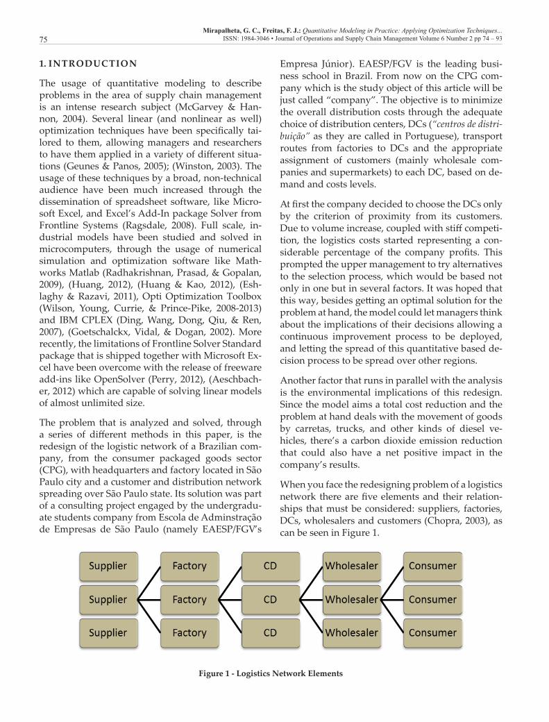
When you face the redesigning problem of a logistics network there are five elements and their relation-ships that must be considered: suppliers, factories, DCs, wholesalers and customers (Chopra, 2003), as can be seen in Figure 1.
4
Another factor that runs in parallel with the analysis is the environmental
implications of this redesign. Since the model aims a total cost reduction and the
problem at hand deals with the movement of goods by carretas, trucks, and other kinds
of diesel vehicles, there’s a carbon dioxide emission reduction that could also have a net
positive impact in the company’s results.
When you face the redesigning problem of a logistics network there are five
elements and their relationships that must be considered: suppliers, factories, DCs,
wholesalers and customers (Chopra, 2003), as can be seen in Figure 1.
Figure 1 - Logistics Network Elements
Since there´s just one factory in the company´s structure and the company itself
doesn´t sell directly to consumers, the model from Figure 1 was simplified from four
levels and five different elements to two levels and three different elements (as can be
seen in Figure 2) when applying it to this specific problem.
Figure 1 - Logistics Network Elements

Mirapalheta, G. C., Freitas, F. J.: Quantitative Modeling in Practice: Applying Optimization Techniques...ISSN: 1984-3046 • Journal of Operations and Supply Chain Management Volume 6 Number 2 pp 74 – 9376
Since there´s just one factory in the company´s struc-ture and the company itself doesn´t sell directly to consumers, the model from Figure 1 was simplified
from four levels and five different elements to two levels and three different elements (as can be seen in Figure 2) when applying it to this specific problem.
5
Figure 2 - Company's Model Logistic Network Elements
In order to minimize the total operational cost of a network, the relationships
among the elements and their constraints are modeled with linear functions. This is
done in order to guarantee the existence of only one optimal solution or no solution at
all. The decision variables are the DCs location, the customers that will be assigned to
each DC and the transportation routes that will be chosen to fulfill the customer´s
demands. The last cost factor is the fixed cost to operate a DC, which due to its
nonlinear relationship with the amount that will be moved (since it can be either zero or
a fixed amount) requires a linearization procedure in the modeling (Sitek & Wikarek,
2012).
In the next section it will be presented a brief review of network modeling and
optimization procedures as they relate to the process of optimizing and redesigning a
logistic network.
Literary Review
Figure 2 - Company’s Model Logistic Network Elements
In order to minimize the total operational cost of a network, the relationships among the elements and their constraints are modeled with linear functions. This is done in order to guarantee the existence of only one optimal solution or no solution at all. The decision variables are the DCs location, the custom-ers that will be assigned to each DC and the trans-portation routes that will be chosen to fulfill the customer´s demands. The last cost factor is the fixed cost to operate a DC, which due to its nonlinear rela-tionship with the amount that will be moved (since it can be either zero or a fixed amount) requires a linearization procedure in the modeling (Sitek & Wi-karek, 2012).
In the next section it will be presented a brief review of network modeling and optimization procedures as they relate to the process of optimizing and rede-signing a logistic network.
2. LITERARY REVIEW
The area of logistics optimization through linear programming methods, have undergone a strong development, especially after the 80’s (Sitek & Wi-karek, 2012). From an historical perspective the op-timization of goods transportation had been studied as early as 1930, as part of the USSR railway network management (Schrijver, 2002). Its development had a major boost in the late 40’s, with the development of the Simplex Method by Dantzig and its applica-tion to various problems either in specific engineer-ing application or in the solution of broad classes of managerial problems (Dantzig, 1963) and another one with the development of combinatorial optimi-zation (i.e. integer programming methods) in the be-ginning of the 60’s (Schrijver, 2005). Due to the linear
relationship between transportation cost, distance and transported weight, around the problem of min-imizing the cost of moving products from factories to distribution centers and there to customers have evolved a whole class of different solutions, each tai-lored to a specific piece of the logistic network (Ber-wick & Mohammad, 2003), (Kropf & Sauré, 2011), (Nagourney, 2007).
On a theoretical point of view, a network system consists of a series of nodes interconnected by arcs representing the transportation routes available (Nagourney, 2010). As in a real distribution network there are nodes which supply products to the net-work and there are nodes which demand them. The challenge is to move the products from the supply nodes to the demand nodes in the least costly pos-sible way (Tsao & Lu, 2012) . Most of these prob-lems can be solved by assigning a different variable cost to each arc in the network, supposing that the amount to be moved in each route are the decision variables and trying to minimize the linear combi-nation of amounts to be moved and variable costs in each arc. This solution must satisfy a series of more or less standard constraints . The amount to be moved out of a supply node must not exceed the amount available to be moved and the amount to be moved into a demand node should at least satisfy it (Hockey & Zhou, 2002). The flux of products in each intermediary node must be kept smooth, in other words, the amount coming to the node must equal the amount that leaves it minus the amount of products that will remain in the node, besides that, the arcs can be submitted to a maximum flux constraint (Cui, Ouyang, & Shen, 2010). Finally to simplify things when the problem is being deployed in a spreadsheet, the supplies are considered to be

Mirapalheta, G. C., Freitas, F. J.: Quantitative Modeling in Practice: Applying Optimization Techniques...ISSN: 1984-3046 • Journal of Operations and Supply Chain Management Volume 6 Number 2 pp 74 – 9377
negative values (as opposed to the demands, which will be considered positive). This allows all flux con-straints in the nodes to be thought of having the fol-lowing structure:
Arrivals – Departures >= Supply(-) or Demand(+)
If the optimization problem under development re-quires also decisions regarding the availability of a specific network structure (like having available or not a distribution center or a specific route), binary variables can be used to model this kind of decision. As long as these binaries variables are kept adding or subtracting their values within each other, the problem will be kept linear and so, entitled to have an unique solution which will be able to be found by the simplex method (Altiparmak, Gen, Lin, & Pak-soy, 2006).
Besides the Simplex Method, integer program-ming problems (when the decision variables must be found among the integers) can be addressed through the Branch-and-Bound algorithm (Land & Doig, 1960) (Yuan, 2013), and the selection of differ-ent options can be modeled through the usage of bi-nary variables, which are in fact a subset of the inte-ger programming methods (Winston, 2003) (Amin, 2012)
All this theory must now be coded in some pro-gramming language and presented to a computer so the specific problem at hand can be solved. Through the years, since the development of the simplex method, the computer has been used in this kind of problem, first by programming each problem in a high-level broad purpose programming language like FORTRAN or C (Press, Teukolsky, Vetterling, & Flannery, 2007) , than in specific software packages, tailored to solve linear programming problems like LINDO (Copado-Mendez & Blum, 2013) and final-ly as a toolbox embedded in another software de-signed to make calculations in general like Microsoft Excel (Ravindran & Warsing Jr., 2013) or Mathworks MATLAB (Ko, Tiwari, & Mehnen, 2010) . It was as an embedded package in Microsoft Excel, called Solver and developed by Frontline Systems, that LP problems and the Simplex Method achieved wide-spread usage, especially in non-technical audiences (Godfrey & Manikas, 2012). The problem that will be described in this paper is presented and solved in a simplified version through problem modeling in a spreadsheet using Microsoft Excel and Front-line Solver. The full scale problem is solved by three different procedures. The first procedure is a com-
bination of Matlab, Opti Toolbox (Currie & Wilson, 2012) and CPLEX (Goetschalckx, Vidal, & Hernan-dez, 2012). The second one is done by using Open-Solver Add-in and the third one by calling CPLEX from within Microsoft Excel as if it was an Add-in.
3. METHODOLOGY
As stated in the previous section, the problem that will be analyzed here was solved as part of a con-sulting project developed by EAESP/FGV’s Empresa Júnior. Therefore the project was conducted from the onset as a case study of logistic network opti-mization through the usage of linear programming.
The consultants (business administration under-graduate students from EAESP/FGV) conducted a series of meetings with the company’s upper man-agement to understand the strategic choices avail-able to them when redesigning and optimizing company’s logistic network and with middle-level managers to understand which kind of problem they were facing, due to the lack of optimization on their network.
In fact, there happened a total of eight meetings. Three of them with the upper management, one of them (the first one) an introductory meeting where EAESP/FGV´s Empresa Junior was presented, fol-lowed by a second meeting where the upper man-agement described what they would like to get from the project in terms of managerial decision support and the third one to present the results, upon project completion. In these three meetings the company´s national logistics and distribution director and two of his senior staff members were always present.
The other five meetings were conducted among the mid-level managers at the company´s distribution center in São Paulo, were they presented to Empre-sa Junior´s consultants the companie´s distribution network, their decision system (which was in fact a best guess system) and provided the consultants with the information needed to develop and deploy the optimization model,
After this series of meetings (which includes the last meeting with upper management), the consul-tants presented to the company’s managers (in three workshops) a series of choices, not only to optimize the structure in place but also to give advice on how to modify the network structure in order to bet-ter manage it. All these choices were backed up by quantitative analysis done with linear programming

Mirapalheta, G. C., Freitas, F. J.: Quantitative Modeling in Practice: Applying Optimization Techniques...ISSN: 1984-3046 • Journal of Operations and Supply Chain Management Volume 6 Number 2 pp 74 – 9378
and made possible by the flexibility and power of the packages above mentioned. Although the free version of Solver that comes bundled with Micro-soft Excel is not capable of handling more than one hundred and fifty variables and constraints, Micro-soft Excel can manipulate matrices of a huge size. Besides that Mathworks Matlab, IBM CPLEX or OpenSolver can handle an almost unlimited num-ber of variables when solving a problem through the Simplex Method.
The specific problem that will be first described and solved is a simplified version of the original one. This way it can be reproduced and the results pre-sented here replicated using only the Standard Solv-er. The full scale problem will require a different software packages and when being solved by Mat-lab an entirely different approach than just creat-ing a spreadsheet depicting the overall calculations that are being made, and these processes will also be described in detail. After that, the models will be solved in a number of different scenarios, so the so-lutions, methodologies and managerial options can be presented and properly evaluated.
The objective of the model is to minimize the total logistic cost when moving goods from the compa-ny’s main distribution center to cities in São Paulo, Minas Gerais and Paraná states, where the retailers are located. This model has three levels : a factory (which is considered the main distribution center), distribution hubs (DCs) and retailers. This means that the products are first moved from the factory in São Paulo to the distribution hubs. There the prod-ucts undergo a cross docking process and then are moved to the retailers. This model therefore is fo-cused in the supply chain middle levels, ignoring suppliers and consumers. The objective function is composed of three costs: a) the cost of moving the goods from the factory to the transportation hubs, b) the operational cost of executing the cross docking in the transportation hubs themselves and c) the cost of moving the goods from the transportation hubs to the retailers. The decision variables are the number and location of the distribution hubs and the retail-ers that will be assigned to each distribution hub. The model constraints are the minimum and maxi-mum quantities of products that can be transported from a distribution hub, and the demand of goods in each retailer. As parameters, the model uses: a) the distance between each pair of city, b) the vehi-cle capacity and c) the cost per km per ton moved, which depends on the transportation modal being
employed and the retailer demand.
From a purely algebraic point of view the model can be represented as follows:
Variables
Xij = amount of goods moved from transportation hub j to retailers located in the city i.
Tj = transportation hub in location j. Binary variable, if city j is chosen to host a transportation hub, Tj = 1, if not Tj = 0.
Di = quarterly demand of retailers in city j.
Hj = unit cost (in Brazilian Reais per km per ton) of goods moved from distribution center (factory) to transportation hub located in city j.
Since the unit cost depends on the modal used to move goods from one point to another and the movement of goods from the factory to the trans-portation hubs is done only by large trucks (carre-tas in Brazilian Portuguese), this cost is fixed in R$ 0,714 per km per ton moved. This amount is based on historical data provided by the company and is the average of several different transportation costs with fully loaded large trucks (28 tons) on different distances, ranging from fifty to two hundred and fifty kilometers.
Cij = unit cost (in Brazilian Reais per km per ton) of goods moved from transportation hub located in city j to retailers in city i.
In this case, the unit cost will depend on the trans-portation modal used to move goods from transpor-tation hub j to retailers in city i. These costs can be: a) R$ 1,865 for vans, which will be used for demands of less than two tons of goods per month, b) R$ 1,557 for “3/4 s”, which will be used for demands of more than 2 tons and less than 3,5 tons a month, c) R$ 0,810 for “tocos”, which will be used for demands of more than 3,5 tons a month and less than 7 tons and d) R$ 0,851 for “trucks” (small trucks, not to be confused with large trucks which are called carretas) which will be used for demands of more than 7 tons a month. These trucks have a capacity of 12 tons.
It could be argued that demands of more than 12 tons a month (which are the capacity of a truck) should be fulfilled using a carreta (which has a capacity of 28 tons), but this is not the case. Maneuvering a carreta within a city neighborhood is a tough task (some-times it is not possible), so trucks must be used, even
Mirapalheta, G. C., Freitas, F. J.: Quantitative Modeling in Practice: Applying Optimization Techniques...ISSN: 1984-3046 • Journal of Operations and Supply Chain Management Volume 6 Number 2 pp 74 – 9379
if it is needed more than one truck to fulfill the task at hand.
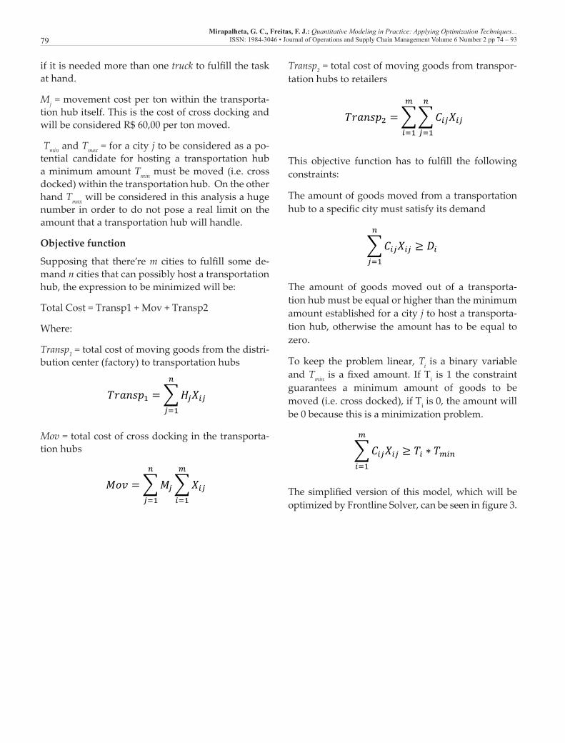
Mj = movement cost per ton within the transporta-tion hub itself. This is the cost of cross docking and will be considered R$ 60,00 per ton moved.
Tmin and Tmax = for a city j to be considered as a po-tential candidate for hosting a transportation hub a minimum amount Tmin must be moved (i.e. cross docked) within the transportation hub. On the other hand Tmax will be considered in this analysis a huge number in order to do not pose a real limit on the amount that a transportation hub will handle.
Objective function
Supposing that there’re m cities to fulfill some de-mand n cities that can possibly host a transportation hub, the expression to be minimized will be:
Total Cost = Transp1 + Mov + Transp2
Where:
Transp1 = total cost of moving goods from the distri-bution center (factory) to transportation hubs
13
Transp1 = total cost of moving goods from the distribution center (factory) to
transportation hubs
∑
Mov = total cost of cross docking in the transportation hubs
∑ ∑
Transp2 = total cost of moving goods from transportation hubs to retailers
∑∑
This objective function has to fulfill the following constraints:
The amount of goods moved from a transportation hub to a specific city must
satisfy its demand
∑
The amount of goods moved out of a transportation hub must be equal or higher
than the minimum amount established for a city j to host a transportation hub, otherwise
the amount has to be equal to zero.
Mov = total cost of cross docking in the transporta-tion hubs
13
Transp1 = total cost of moving goods from the distribution center (factory) to
transportation hubs
∑
Mov = total cost of cross docking in the transportation hubs
∑ ∑
Transp2 = total cost of moving goods from transportation hubs to retailers
∑∑
This objective function has to fulfill the following constraints:
The amount of goods moved from a transportation hub to a specific city must
satisfy its demand
∑
The amount of goods moved out of a transportation hub must be equal or higher
than the minimum amount established for a city j to host a transportation hub, otherwise
the amount has to be equal to zero.
Transp2 = total cost of moving goods from transpor-tation hubs to retailers
13
Transp1 = total cost of moving goods from the distribution center (factory) to
transportation hubs
∑
Mov = total cost of cross docking in the transportation hubs
∑ ∑
Transp2 = total cost of moving goods from transportation hubs to retailers
∑∑
This objective function has to fulfill the following constraints:
The amount of goods moved from a transportation hub to a specific city must
satisfy its demand
∑
The amount of goods moved out of a transportation hub must be equal or higher
than the minimum amount established for a city j to host a transportation hub, otherwise
the amount has to be equal to zero.
This objective function has to fulfill the following constraints:
The amount of goods moved from a transportation hub to a specific city must satisfy its demand
13
Transp1 = total cost of moving goods from the distribution center (factory) to
transportation hubs
∑
Mov = total cost of cross docking in the transportation hubs
∑ ∑
Transp2 = total cost of moving goods from transportation hubs to retailers
∑∑
This objective function has to fulfill the following constraints:
The amount of goods moved from a transportation hub to a specific city must
satisfy its demand
∑
The amount of goods moved out of a transportation hub must be equal or higher
than the minimum amount established for a city j to host a transportation hub, otherwise
the amount has to be equal to zero.
The amount of goods moved out of a transporta-tion hub must be equal or higher than the minimum amount established for a city j to host a transporta-tion hub, otherwise the amount has to be equal to zero.
To keep the problem linear, Ti is a binary variable and Tmin is a fixed amount. If Ti is 1 the constraint guarantees a minimum amount of goods to be moved (i.e. cross docked), if Ti is 0, the amount will be 0 because this is a minimization problem.
14
To keep the problem linear, Ti is a binary variable and Tmin is a fixed amount. If
Ti is 1 the constraint guarantees a minimum amount of goods to be moved (i.e. cross
docked), if Ti is 0, the amount will be 0 because this is a minimization problem.
∑
The simplified version of this model, which will be optimized by Frontline
Solver, can be seen in figure 3.
Figure 3 - Logistics Model - Simplified Version
In this version, there are four possible locations to be chosen as transportation
hubs and sixteen locations where the demand must be fulfilled. The values presented
above are already the optimal solution values for the simplified model. This version was
developed so the modeling process errors could be easily located. Once the reduced
The simplified version of this model, which will be optimized by Frontline Solver, can be seen in figure 3.

Mirapalheta, G. C., Freitas, F. J.: Quantitative Modeling in Practice: Applying Optimization Techniques...ISSN: 1984-3046 • Journal of Operations and Supply Chain Management Volume 6 Number 2 pp 74 – 9380
14
To keep the problem linear, Ti is a binary variable and Tmin is a fixed amount. If
Ti is 1 the constraint guarantees a minimum amount of goods to be moved (i.e. cross
docked), if Ti is 0, the amount will be 0 because this is a minimization problem.
∑
The simplified version of this model, which will be optimized by Frontline
Solver, can be seen in figure 3.
Figure 3 - Logistics Model - Simplified Version
In this version, there are four possible locations to be chosen as transportation
hubs and sixteen locations where the demand must be fulfilled. The values presented
above are already the optimal solution values for the simplified model. This version was
developed so the modeling process errors could be easily located. Once the reduced
Figure 3 - Logistics Model - Simplified Version
In this version, there are four possible locations to be chosen as transportation hubs and sixteen locations where the demand must be fulfilled. The values pre-sented above are already the optimal solution values for the simplified model. This version was devel-oped so the modeling process errors could be eas-ily located. Once the reduced model version started giving correct results, the model structure was de-ployed over the entire volume of possible DCs and retailers locations.
The complete model on the other hand deals with four hundred and sixteen cities where the demand must be fulfilled and thirty three locations to choose as pos-sible candidate for a transportation hub. Therefore it has to handle approximately fourteen thousand vari-ables. Due to its size, for purposes of presentation, it is divided in three spreadsheets, one for parameters, another just for the distances matrix and another for the model itself, as can be seen below. It must be not-ed that to show the whole tables (i.e. spreadsheets), several lines have been hided from view.
Figure 4 - Full Model - Parameters Spreadsheet

Mirapalheta, G. C., Freitas, F. J.: Quantitative Modeling in Practice: Applying Optimization Techniques...ISSN: 1984-3046 • Journal of Operations and Supply Chain Management Volume 6 Number 2 pp 74 – 9381
Figure 5 - Full Model - Distance Matrix
Figure 6 - Full Model - Objective, Variables and Constraints View

Mirapalheta, G. C., Freitas, F. J.: Quantitative Modeling in Practice: Applying Optimization Techniques...ISSN: 1984-3046 • Journal of Operations and Supply Chain Management Volume 6 Number 2 pp 74 – 9382
As stated earlier, to deal with the full scale model, an industrial class optimization environment is re-quired. Three choices will be used to optimize the full scale model: a) Matlab, Opti Toolbox and Cplex, b) Excel, Cplex and Cplex Excel Connector and c) Excel and OpenSolver Add-in.
The first option is Matlab, Opti Toolbox and Cplex. The main reason is the numerical features and avail-ability of Matlab (especially in academic environ-ments) and the possibility of using Opti Toolbox and CPLEX in their academic versions without any performance constraint.
Matlab is an environment that was originally de-veloped to handle matrices, and to use it effective-ly everything must be converted to this modeling paradigm. As an example suppose that one wants to solve the following optimization problem:
Find x>=0 that minimizes : f(x) = -5x1 - 4x2 -6x3,
subject to :
x1 + x2 + x3 <= 20
3x1 + 2x2 + 4x3 <= 42
3x1 + 2x2 <= 30
In Matlab it would be necessary to issue to following set of commands :
f = [-5; -4; -6]; A = [ 1 -1 1; 3 2 4 ; 3 2 0]; b = [20; 42; 30];
lb = zeros(3,1); [x,fval,exitflag,output,lambda] = linprog(f,A,b,[],[],lb); x
This happens because the problem to be solve (i.e. optimised) needs to be put in matrix form A.x <= b (the constraints) and f.x (the objective function). After that the function linprog is called to produce the output vector x with the solution. The function linprog (as most Matlab optimization functions) re-quires the matrices f, A, b (as described above), Aeq, beq, if there are constraints of the form Aeq.x = beq (equality constraints), and lower and upper bounds vectors, lb and ub (if there are such limits) for the solution vector x.
The outputs are: the solution vector x, the value of the objective function f, named fval, the output flag (+1 if the process finished ok, -1 if not, etc…) and some process and optimization parameters that are of no interest for this paper.
This example illustrates the standard that the LP problem structure must adhere to, so it can be solved in Matlab. If, for example, the problem requires the variables all to be of binary type, another solver should be called, bintprog, but the overall structure of the parameters and outputs remains the same.
Next, it is needed to include a mix of continuous and binary variables in the problem, something that the standard optimization packages of Matlab are not able to do. To overcome this limitation it was used the Opti Toolbox, a free Matlab Toolbox developed by the Industrial Information and Control Centre from the Auckland University of Technology, New Zealand. This toolbox can be freely downloaded from http://www.i2c2.aut.ac.nz/Wiki/OPTI/index.php/DL/DownloadOPTI and includes a variety of solvers, but most important than that, as will be seen later in this section, is the ability to encapsulate sev-eral other solvers in its command framework. This way, the standard optimization functions of Matlab for instance, can be called as opti_linprog and opti_bintprog.
The Opti Toolbox has a function called opti_lpsolve that is called with the exact same parameters as de-scribed for linprog above, plus an extra parameter that describes if the variable will be of continuous, integer or binary type. This parameter is just a string with the chars “C”, “I” and “B” listed in the same order as the variables appear in the objective func-tion. Therefore if the variable is not normally present in the objective function expression, a 0 (zero) must be added so it can be “understood” by the function that it “exists”.
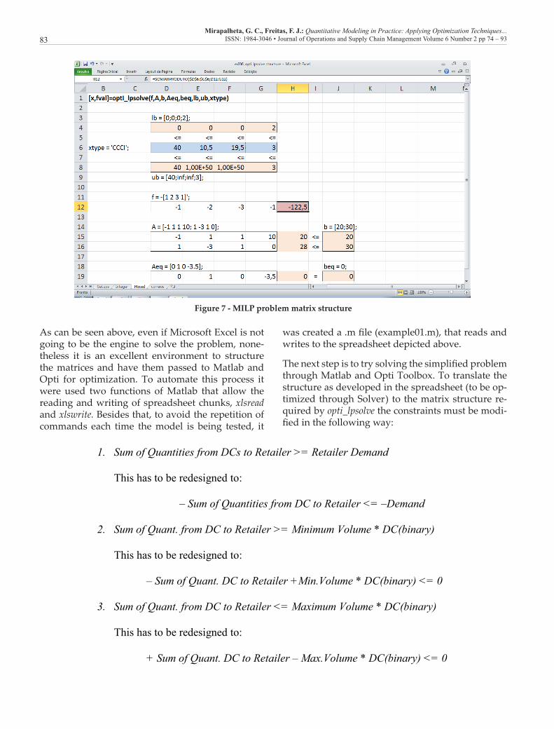
In the picture below it can be seen a MILP (Mixed Integer Linear Programming problem) structure in a spreadsheet, where the matrices have been prepared to be passed to opti_lpsolve.
Mirapalheta, G. C., Freitas, F. J.: Quantitative Modeling in Practice: Applying Optimization Techniques...ISSN: 1984-3046 • Journal of Operations and Supply Chain Management Volume 6 Number 2 pp 74 – 9383
Figure 7 - MILP problem matrix structure
As can be seen above, even if Microsoft Excel is not going to be the engine to solve the problem, none-theless it is an excellent environment to structure the matrices and have them passed to Matlab and Opti for optimization. To automate this process it were used two functions of Matlab that allow the reading and writing of spreadsheet chunks, xlsread and xlswrite. Besides that, to avoid the repetition of commands each time the model is being tested, it
was created a .m file (example01.m), that reads and writes to the spreadsheet depicted above.
The next step is to try solving the simplified problem through Matlab and Opti Toolbox. To translate the structure as developed in the spreadsheet (to be op-timized through Solver) to the matrix structure re-quired by opti_lpsolve the constraints must be modi-fied in the following way:
20
chunks, xlsread and xlswrite. Besides that, to avoid the repetition of commands each
time the model is being tested, it was created a .m file (example01.m), that reads and
writes to the spreadsheet depicted above.
The next step is to try solving the simplified problem through Matlab and Opti
Toolbox. To translate the structure as developed in the spreadsheet (to be optimized
through Solver) to the matrix structure required by opti_lpsolve the constraints must be
modified in the following way:
1. Sum of Quantities from DCs to Retailer >= Retailer Demand
This has to be redesigned to:
– Sum of Quantities from DC to Retailer <= –Demand
2. Sum of Quant. from DC to Retailer >= Minimum Volume * DC(binary)
This has to be redesigned to:
– Sum of Quant. DC to Retailer +Min.Volume * DC(binary) <= 0
3. Sum of Quant. from DC to Retailer <= Maximum Volume * DC(binary)
This has to be redesigned to:
+ Sum of Quant. DC to Retailer – Max.Volume * DC(binary) <= 0
Also, in each constraint expression, every variable must be present (if it is not
supposed to be there, it has to be multiplied by 0). This makes the coefficient matrix A
huge and sparse. Besides that, the Maximum Volume parameter, since it multiplies a
binary variable and is then compared with variables values that can be much smaller
than itself, has the potential to make the solution numerically unstable. In fact, the Opti
Toolbox was capable of handling a maximum of 4.000.000 for this parameter, before
starting producing results that were wrong. Nonetheless, using a maximum of four
million for the maximum volume that can be handled by a DC still produces a valid

Mirapalheta, G. C., Freitas, F. J.: Quantitative Modeling in Practice: Applying Optimization Techniques...ISSN: 1984-3046 • Journal of Operations and Supply Chain Management Volume 6 Number 2 pp 74 – 9384
Also, in each constraint expression, every variable must be present (if it is not supposed to be there, it has to be multiplied by 0). This makes the coef-ficient matrix A huge and sparse. Besides that, the Maximum Volume parameter, since it multiplies a binary variable and is then compared with vari-ables values that can be much smaller than itself, has the potential to make the solution numerically unstable. In fact, the Opti Toolbox was capable of
handling a maximum of 4.000.000 for this param-eter, before starting producing results that were wrong. Nonetheless, using a maximum of four mil-lion for the maximum volume that can be handled by a DC still produces a valid result. On the other hand, if this solver is to be used in the full scale model this volume should be much greater. The overall structure of the problem matrices can be seen in the following picture:
Figure 8 - Simplified Problem Matrix Structure
As can be seen, the spreadsheet structure is correct, since the solutions from Matlab – Opti Toolbox and Excel – Solver are in agreement with each other. Now the problems that remain are: how to over-come the scaling problem and how to replicate the matrix structure presented in the picture above in the full scale model, where the number of columns and lines in the matrix will be incredibly high.
The scaling problem was solved in a twofold way. First, the total demand of goods in each retailer was divided by ten, something that could be done only be-cause de model is linear. Therefore, the results present-ed by the spreadsheet must be multiplied by ten, so one can know the real quarterly logistics cost. Second, the solver was changed from the Opti Toolbox stan-dard solver to IBM’s CPLEX. Opti Toolbox, as noted before, has the ability to encapsulate other solvers, from different vendors, and this is no different with CPLEX. All it is needed to be done is to install IBM’s
CPLEX and let Matlab know where it is installed. From that moment own, if someone wants to use the power-ful IBM solver, he/she has just to call it using the func-tion wrapper opti_cplex with the parameter structure : [x,fval,exitflag] = opti_cplex([],f,A,[],b,lb,[],xtype). CPLEX solver was able to optimize the simplified model with a maximum value on the volume that could be han-dled by a DC as high as two billion tons.
The matrix structure was deployed in a somewhat automatic manner, by using Excel’s functionalities of copy and paste to create the sparse matrix A. The resulting spreadsheet can be seen next (take special attention to the number of columns that matrix A has, it spreads over almost fourteen thousand columns, one for each variable, to be more precise thirteen thousand, seven hundred and sixty one columns and four hundred and eighty one lines, making it a matrix with approximately six point seven million elements, most of them zeros, since it is a sparse matrix):
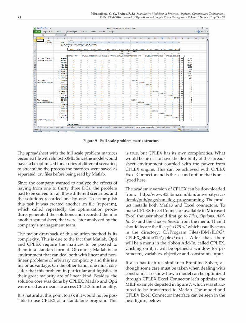
Mirapalheta, G. C., Freitas, F. J.: Quantitative Modeling in Practice: Applying Optimization Techniques...ISSN: 1984-3046 • Journal of Operations and Supply Chain Management Volume 6 Number 2 pp 74 – 9385
Figure 9 - Full scale problem matrix structure
The spreadsheet with the full scale problem matrices became a file with almost 50Mb. Since the model would have to be optimized for a series of different scenarios, to streamline the process the matrices were saved as separated .csv files before being read by Matlab.
Since the company wanted to analyze the effects of having from one to thirty three DCs, the problem had to be solved for all these different scenarios, and the solutions recorded one by one. To accomplish this task it was created another .m file (report.m), which called repeatedly the optimization proce-dure, generated the solutions and recorded them in another spreadsheet, that were later analyzed by the company’s management team.
The major drawback of this solution method is its complexity. This is due to the fact that Matlab, Opti and CPLEX require the matrices to be passed to them in a standard format. Of course, Matlab is an environment that can deal both with linear and non-linear problems of arbitrary complexity and this is a major advantage. On the other hand, one must con-sider that this problem in particular and logistics in their great majority are of linear kind. Besides, the solution core was done by CPLEX. Matlab and Opti were used as a means to access CPLEX functionality.
It is natural at this point to ask if it would not be pos-sible to use CPLEX as a standalone program. This
is true, but CPLEX has its own complexities. What would be nice is to have the flexibility of the spread-sheet environment coupled with the power from CPLEX engine. This can be achieved with CPLEX Excel Connector and is the second option that is ana-lyzed here.
The academic version of CPLEX can be downloaded from: http://www-03.ibm.com/ibm/university/aca-demic/pub/page/ban_ilog_programming. The prod-uct installs both Matlab and Excel connectors. To make CPLEX Excel Connector available in Microsoft Excel the user should first go to Files, Options, Add-In, Go and the choose Search from the menu. Than it should locate the file cplex125.xll which usually stays in the directory: C:\Program Files\IBM\ILOG\CPLEX_Studio125\cplex\excel. After that, there will be a menu in the ribbon Add-In, called CPLEX. Clicking on it, it will be opened a window for pa-rameters, variables, objective and constraints input.
It also has features similar to Frontline Solver, al-though some care must be taken when dealing with constraints. To show how a model can be optimized through CPLEX Excel Connector let’s optimize the MILP example depicted in figure 7, which was struc-tured to be transferred to Matlab. The model and CPLEX Excel Connector interface can be seen in the next figure, below:

Mirapalheta, G. C., Freitas, F. J.: Quantitative Modeling in Practice: Applying Optimization Techniques...ISSN: 1984-3046 • Journal of Operations and Supply Chain Management Volume 6 Number 2 pp 74 – 9386
Figure 10 - CPLEX Excel Connector Interface
As can be seen in the picture above, instead of trans-ferring the matrices to the solution engine, one only needs to express the relationships in the spreadsheet and have the cell’s addresses transferred to the inter-face. As stated above, some care must be taken when modeling the constraints and variables. The variables can have lower and upper bounds, but they must be passed together with the variables cells themselves and not as a separated constraint. The interface has a minor ‘bug’, which is, the integer variable mark is written as ‘integral’ but this doesn’t seem to af-fect the performance of the environment. About the constraints, CPLEX must receive fixed numbers as lower and upper bounds. The variable cells are the constraint cells themselves. Therefore if one wants to deploy in the spreadsheet a constraint like x1 < x2,
where x1 and x2 are variables themselves, this con-straint has to be deployed in a cell as x1 - x2 < 0. If there are no lower or upper bound, there’s no need to indicate that in the interface. Leaving the field as blank will make CPLEX assume that the constraint (or the variable) is unbounded. Besides that, all the values that are going to be needed to solve a model (be they variables or parameters), must be placed in the same sheet. As will be shown later in this sec-tion, CPLEX Excel Connector was not able to handle a model when a parameter as being transferred from another sheet. Therefore, when solving the full scale model, the distance, demand and parameters matri-ces will have to be put next to the model itself.
The next figures depict the spreadsheet full scale model deployment.

Mirapalheta, G. C., Freitas, F. J.: Quantitative Modeling in Practice: Applying Optimization Techniques...ISSN: 1984-3046 • Journal of Operations and Supply Chain Management Volume 6 Number 2 pp 74 – 9387
Figure 11 - CPLEX Excel Connector Full Scale Model Deployment
Figure 12 - CPLEX Excel Connector Full Scale Model Parameters
Mirapalheta, G. C., Freitas, F. J.: Quantitative Modeling in Practice: Applying Optimization Techniques...ISSN: 1984-3046 • Journal of Operations and Supply Chain Management Volume 6 Number 2 pp 74 – 9388
As can be seen above, the parameters have been transferred to the same spreadsheet that will handle the model itself. If this is not done, CPLEX loops around the problem without being able to stabilize it and never finishing its job. When this happens, pressing ESC or CTRL+C keys will be of no avail, having the user to shut Excel itself down by press-ing CTRL+ALT+DELL and selecting Excel from the Windows Task Manager. Although this is something that should be addressed by IBM, as long as the user saves its spreadsheet before running CPLEX, there’s no problem with the file and the procedure can be started again.
The performance is impressive. Starting from a null solution (where all variables are set equal to zero) it sets up the model and optimizes the model in less than one minute and thirty seconds, when using a modest Sony Vaio laptop with Intel Centrino with 2 cores of 2.1GHz and 3GB of RAM memory.
On the downside, although stated by CPLEX’s documentation that CPLEX engine can be called by VBA, the methods are complex and are not well documented, so it was not possible to gener-ate automatically the report with the minimum cost based on the number of DCs. Besides that, al-though impressive in its speed and sophistication when handling linear problems, CPLEX is not well suited for non-linear problems. It can only handle quadratic problems and the software is designed to test the problem looking for other kinds of func-tions, which when found made CPLEX stop the op-timization process.
So far, CPLEX engine coupled with its Excel Con-nector has the speed and flexibility needed to be used by a manager on a daily basis but it lacks easy VBA programming features and of course, if it is
to be used in an industrial (non-academic environ-ment) it will have a non-negligible cost.
The third option to be tested is OpenSolver. Open-Solver can be downloaded from http://opensolver.org and is developed as a freeware by Prof.Andrew Mazon from The Faculty of Engineering from Uni-versity of Auckland. It also can handle only linear problems but has an interface more similar to Front-line Solver than CPLEX Excel Connector, where the constraints don’t need to be put in a specific format. Besides that, as will be shown in this section, it can easily be called from VBA. More important than that, it can handle an almost unlimited number of variables and constraints, making it an excellent op-tion when one have to deal with linear problems of considerable size.
To install it, after downloading the .zip package from the authors website, all is needed to be done is to unpack the .zip file in a suitable directory and fol-low the same procedure already followed to include CPLEX Excel Connector Add-In. Usually the default directory for third-party Add-Ins installed by the user itself is the directory C:\Users\gustavo\Ap-pData\Roaming\Microsoft\Suplementos. In this case it was created an specific subdirectory (Open-Solver21) to receive the unpacked files. After that all is needed is to include the file opensolver.xla in the Add-In menu of Excel and OpenSolver will be avail-able as part of the Data ribbon.
The model structure itself was pretty similar to the reduced model (only bigger), and the OpenSolver interface also pretty similar to Frontline Solver. As a matter of fact, OpenSolver captures any model that has been developed previously in the spreadsheet by Frontline Solver and can exchange changes with Frontline Solver.

Mirapalheta, G. C., Freitas, F. J.: Quantitative Modeling in Practice: Applying Optimization Techniques...ISSN: 1984-3046 • Journal of Operations and Supply Chain Management Volume 6 Number 2 pp 74 – 9389
Figure 13 - OpenSolver Parameters Interface
The first time OpenSolver was put to optimize the full scale model (see figure below), the spreadsheet was designed with parameters being passed from other sheets, since this way the problem can be broke in smaller pieces. This way the optimization process took of a model starting from a null solution and having to choose up to thirty three DCs took almost thirty minutes. At first it was taught that this was happening because the algorithms deployed in OpenSolver were less efficient than the CPLEX simi-lar ones. It was noted however that the spreadsheet took a long time setting up de model and, more important than that, used to present intermediate results similar to the ones CPLEX presented when looping without finding a solution. This was an in-dication that the problem was not in the OpenSolver algorithms but in the model structure itself.
The spreadsheet was then redesigned without the external links. In fact, OpenSolver was applied in the CPLEX sheet which was already running in stand-alone mode (i.e. without external links). Considering that OpenSolver is a freeware developed by an engi-neering department in an university, seeing it solve
the full scale model, with thirty three DCs to choose in the same amount of time that it took CPLEX to accomplish the same task (ninety seconds) was be-yond impressive.
The next task was to develop a way to call this model thirty three times, so the full managerial report could be generated. If OpenSolver had equaled CPLEX on the matter of performance here it surpassed its professional counterpart. It was decided to write a small report in three parts of eleven lines. In each part there was going to be put the number of DCs and the total cost obtained after the optimization process had been run. To automate this task it was created a command button that called a small VBA program (the listing can be seen in Appendix A). Of special interest is the easiness with which one can call OpenSolver from VBA. Once the model is de-signed and objective, variables and restrictions are set in the OpenSolver Model interface, there are only two VBA functions that are required: initializequick-solve and runquicksolve, which are called from VBA without any special argument. The spreadsheet with the report result can be seen in the next figure.

Mirapalheta, G. C., Freitas, F. J.: Quantitative Modeling in Practice: Applying Optimization Techniques...ISSN: 1984-3046 • Journal of Operations and Supply Chain Management Volume 6 Number 2 pp 74 – 9390
Figure 14 - OpenSolver Managerial Report
4. RESULTS
Both the simplified and the full versions of the model run smoothly, although the full version required ei-ther the transfer of the model to the Matlab environ-ment where the Simplex method could be applied to the huge matrices involved or the usage of Microsoft Excel, CPLEX and CPLEX Excel Connector or Micro-soft Excel with OpenSolver Add-In.
The simplified version, using the Simplex Method, re-quired less than 5 seconds when running the Standard Solver. On the other hand, the full scale model required almost 2 minutes for each optimization scenario.
Matlab, Opti Toolbox and CPLEX were the most sophisticated group of software used to solve the full scale model. There´s no doubt that this trio has the biggest amount of resources, its performance is excellent and should be considered especially if the optimization procedure would require a non-linear feature. On the other hand, since Matlab has to deal with matrices in an almost raw form and its optimi-zation routines require a fixed input format, it can be cumbersome to generate them, as became obvi-ous in this problem. Therefore, if one is looking for a flexible interface that can be easily manipulated by non-technical personnel, other options should be considered. That is even more the case if the model will be of linear type.
CPLEX and CPLEX Excel Connector are the next choice. Since CPLEX was the real power horse be-
hind the trio Matlab, Opti and CPLEX itself, and IBM has released an Excel Connector it would be an excellent candidate for being the preferred option. This is even more the case because IBM is a name that provides a solid guarantee for whoever decides to use its products. The problem with CPLEX was the difficult way with which one had to deal if trying to call the optimization procedure from VBA. Be-sides that, CPLEX requires some specificities in the spreadsheet design, especially when dealing with constraints, which make him a not so flexible option.
The third option, and its performance and flexibil-ity, was a big surprise. OpenSolver demonstrated having the same performance as CPLEX and is structured in a way that is as flexible as Frontline Solver itself. Besides that, its VBA interface is simple enough for a non-technical person to use it, as long as he/she has some basic programming knowledge. When you consider that OpenSolver is a freeware, it becomes an obvious choice. Therefore the model and the managerial report were presented to the company´s management in Microsoft Excel with OpenSolver Add-In.
The management team wanted to analyze what was the effect on the total logistics cost of increasing from one to thirty three the number of DCs spread in the distribution network. The results are presented below, where the total cost is the total quarterly lo-gistic cost in Brazilian Reais. Full details can be seen in the spreadsheets “report.xls” (for the environment

Mirapalheta, G. C., Freitas, F. J.: Quantitative Modeling in Practice: Applying Optimization Techniques...ISSN: 1984-3046 • Journal of Operations and Supply Chain Management Volume 6 Number 2 pp 74 – 9391
Matlab, Opti Toolbox and CPLEX) and “opensolver & cplex.xls” (for the other two environments).
N.DCs Total Cost N.DCs Total Cost N.DCs Total Cost1 R$ 31.070.534 12 R$ 26.787.013 23 R$ 26.260.6712 R$ 30.016.453 13 R$ 26.710.367 24 R$ 26.235.9843 R$ 29.180.240 14 R$ 26.633.644 25 R$ 26.212.5284 R$ 28.565.673 15 R$ 26.566.322 26 R$ 26.194.9475 R$ 28.045.175 16 R$ 26.508.863 27 R$ 26.176.8336 R$ 27.752.740 17 R$ 26.456.825 28 R$ 26.162.2507 R$ 27.480.289 18 R$ 26.414.672 29 R$ 26.150.7448 R$ 27.291.289 19 R$ 26.374.946 30 R$ 26.139.6059 R$ 27.115.694 20 R$ 26.341.173 31 R$ 26.133.512
10 R$ 26.971.041 21 R$ 26.312.369 32 R$ 26.133.71611 R$ 26.871.384 22 R$ 26.284.127 33 R$ 26.133.716
Considering that the company’s total logistic cost was approximately R$ 45M, with a total of 5 DCs, based on the results presented above the company would be able to achieve a total cost reduction of about 28%, representing a total of R$ 17M in econo-mies, on a quarterly base, just by redesigning their distribution network.
Other interesting result can be seen if one looks at the total cost reduction from one number of DCs to the next number. If one goes from four DCs to five DCs the total cost reduction is approximately R$ 520.000 per quarter. When increasing the num-ber of DCs from five to six the cost reduction is ap-proximately R$ 290.000 per quarter. If the number of DCs is increased beyond seven, the total optimal cost keeps reducing but the marginal reduction is increasingly smaller. The total number of five DCs is the transition point from more than half a mil-lion reais per quarter to almost half of this amount. Somehow, when the management team had first de-cided to choose in having five DCs they had chosen the number of DCs that would provide the best mar-ginal cost reduction.
5. CONCLUSIONS
Although being a practical application of a theoreti-cal framework, the work presented in this paper can be tough of having one major theoretical implica-tion, which is the possibility of applying linear op-timization techniques in large scale within Brazilian companies to achieve large economies of scale in
distribution networks. This application can have not only a quantitative impact in the operations of Bra-zilian companies but also a qualitative impact that could generate new levels of operation efficiency leading to new supply chain models when applying them to emerging markets operations.
Before this project, the company used to choose the DCs locations by following the competition deci-sions, even knowing that its direct competitor had a product portfolio somewhat different from its own. With the decision process now based also on quan-titative data it is now possible to analyze what will be the consequences in terms of cost of choosing one location versus another. The logistics director stated that this has allowed the logistics division to be bet-ter integrated in the company’s strategic planning and to get a fair share of recognition in the results. The next step is to spread this decision process to other regions in Brazil, especially in other the south-ern states (Santa Catarina and Rio Grande do Sul).
When it comes to the results that the full scale model produced, they were both reassuring and challeng-ing for the company’s management. As can be seen in the Results section, the marginal cost reduction that was calculated with the full scale pointed to a maximum marginal optimal cost reduction in the region of five DCs. Since this was the number that the management team had chosen previously, this fact was highly reassuring for the company’s past decisions and for the model validity is general. After that, there was no doubt that the options offered by it were not something “purely theoretical stuff from

Mirapalheta, G. C., Freitas, F. J.: Quantitative Modeling in Practice: Applying Optimization Techniques...ISSN: 1984-3046 • Journal of Operations and Supply Chain Management Volume 6 Number 2 pp 74 – 9392
a group of academics” but real stuff that could be used to really reduce the company’s total logistics cost. This fact is reflected in the company’s decision to have workshops with middle level managers to explain how this model could be deployed in other regions and in a smaller base or in different con-texts. The consultant perception was that suddenly the company’s middle level management team had realized that “there’s a practical side on this theo-retical stuff”.
6. LIMITATIONS AND SUGGESTIONS FOR FUTURE RESEARCH
When talking about the scope of this study, it is ob-vious that it is a very limited application of linear optimization techniques. More work should be done to determine if this case represents a distribution network tipical situation of a company in the Brazil-ian CPG´s sector or if it was a very specific individ-ual case, although one can argue that cases where the improvements are achieved in a way so quick and straighforward as this one cannot be a statistical anomaly. This is even more so if one considers that this company is a leading CPG manufacturer and distributor.
Nonetheless, this study opens some areas for future research. As can be seen from the example presented here, the modeling of a logistics network of a consid-erable size can be done with spreadsheet resources and its optimization be accomplished with the sup-port of software running in microcomputers.
What is even more interesting, and could be further analyzed in the future, is the amount of optimiza-tion that companies in Brazil use when designing their logistic infrastructure. It was a surprise for the consultants of EAESP/FGV Empresa Júnior the in-terest and willingness to cooperate that the logistics management team have received the results and the efforts that they took to understand how the opti-mization process was achieved and how it could be improved.
This is an indication that even classroom examples, when properly applied, can have a huge impact in the competitiveness of well established companies of considerable size in Brazil.
Regarding the environmental implications of this network redesign, specifically in this project the to-tal carbon dioxide emissions where not calculated, although it is a matter of logic to think that if one is
reducing the total goods movement cost, there will be a positive impact in the emissions by the com-pany. This is something that management will be addressing in a future analysis, because it can add an impact in the company’s results in a way that is not usually offered by a logistics department (where the net impact is felt mainly by cost reductions and not by revenue increase).
REFERENCES
Aeschbacher, B. (2012, 08 23). Solving a Large Scale Integer Pro-gram with Open-Source-Software Master thesis Submitted at the University of Zurich. Retrieved 04 19, 2013, from University of Zurich: http://ufpr.dl.sourceforge.net/project/opensolver/OtherResources/Aeschbacher%20Masters%20Thesis%20Solving%20a%20Large%20Scale%20Integer%20Program.pdf
Berwick, M., & Mohammad, F. (2003). Truck Costing Model for Transportation Managers. North Dakota, USA: Upper Great Plains Transportation Institute.
Chopra, S. (2003). Designing the Distribution Network in a Sup-ply Chain. Transportation Research, pp. 39(2):123-140.
Dantzig, G. B. (1963). Linear Programming and Extensions. Santa Monica, California: The RAND Corporation.
Ding, H., Wang, W., Dong, J., Qiu, M., & Ren, C. (2007). IBM Sup-ply-Chain Network Optimization Workbench: An Integrated Optimization and Simulation Tool for Supply Chain Design. Proceeding of the 2007 Winter Simulation Conference, (pp. 1940-1946).
Eshlaghy, A. T., & Razavi, M. (2011). Modeling and Simulating Supply Chain Management. Applied Mathematical Sciences, pp. vol.5, no.17, 817-828.
Geunes, J., & Panos, P. M. (2005). Supply Chain Optimization. New York, NY: Springer Science.
Goetschalckx, M., Vidal, C., & Dogan, K. (2002, Nov 16). Model-ing and design of global logistics systems: A review of inte-grated strategic and tactical models and design algorithms. European Journal of Operational Research, pp. Vol.143, Issue 1, pags 1-18.
Huang, C.-H., & Kao, H.-Y. (2012, 12). A Design of Supply Chain Management System with Flexible Planning Capabil-ity. International Journal of Human and Social Sciences, pp. 5, pags.775-779.
Huang, L. (2012, 07). Modeling and Planning on Urban Logistics Park Location Selection Based on the Artificial Neural Net-works. Journal of Computers, pp. Vol.7, no.3, 792-797.
Kropf, A., & Sauré, P. (2011). Fixed Cost per Shipment. Retrieved March 25, 2013, from http://www.eui.eu/Personal/JMF/Phil-ipSaure/KropfSaure_2011_12_16.pdf
Land, A., & Doig, A. (1960). An automatic method of solving discrete programming problems. Econometrica, pp. 28 (3). pp. 497–520.

Mirapalheta, G. C., Freitas, F. J.: Quantitative Modeling in Practice: Applying Optimization Techniques...ISSN: 1984-3046 • Journal of Operations and Supply Chain Management Volume 6 Number 2 pp 74 – 9393
McGarvey, B., & Hannon, B. (2004). Dynamic Modeling for Busi-ness Management: An Introduction. New York, NY: Springer-Verlag.
Nagourney, A. (2007). Mathematical Models of Transportation and Networks. Retrieved March 25, 2013, from http://supernet.is-enberg.umass.edu/articles/EOLSS.pdf
Perry, K. M. (2012, 04 27). The Call Center Scheduling Problem us-ing Spreadsheet Optimization and VBA A thesis submitted in partial fulfillment of the requirements for the degree of Master of Science at Virginia Commonwealth University. Retrieved 04 18, 2013, from Virginia Commonwealth University: https://diz-zyg.uls.vcu.edu/bitstream/handle/10156/3746/PerryThesis.pdf?sequence=1
Press, W. H., Teukolsky, S. A., Vetterling, W. T., & Flannery, B. P. (2007). Numerical Recipes 3rd Edition: The Art of Scientific Com-puting. Cambridge University Press.
Radhakrishnan, P., Prasad, V. M., & Gopalan, M. R. (2009, Jan). Inventory Optimization in Supply Chain Management using
Genetic Algorithms. International Journal of Computer Science and Network Security, pp. vol.9, no.1, pags 33-40.
Ragsdale, C. T. (2008). Spreadsheet Modleing and Decision Analysis, 5th Revised Edition. Mason, OH: Thomson South-Western.
Sitek, P., & Wikarek, J. (2012). Cost optimization of supply chain with multimodal transport. IEEE Processdings of the Federated Conference on Computer Science and Information Systems, (pp. pp.1111-1118).
Wilson, D. I., Young, B. R., Currie, J., & Prince-Pike, A. (2008-2013). Industrial Information & Control Centre (I2C2) Home Page. Retrieved 04 17, 2013, from Industrial Information & Control Centre (I2C2): http://www.i2c2.aut.ac.nz/
Winston, W. (2003). Operations Research: Applications and Algo-rithms. Pacific Grove, CA: Duxbury Press.
Winston, W., & Albright, S. (2009). Practical Management Science, 3rd revised ed. Mason, OH: South Western - Cengage Learning.
Gustavo Mirapalheta is Electrical Engineer (UFRGS), Dsc in Business Administration (EAESP/FGV) and prof.of Quantitative Modeling and Decision Analysis at EAESP/FGV. Gustavo´s research interests lay in the areas of Operations Research, Simulation and Big Data. Currently works as business diretor at Inventive Solutions, a sales optimization and improvement consulting company. Previously worked as software direc-tor at Sun Microsystems and business manager at IBM Brasil
Flávia Junqueira de Freitas is majoring in Business Administration at Fundação Getulio Vargas (FGV-EAESP). She has experience in Consulting due to her two-year job at Empresa Junior FGV (EJ-FGV). She is currently at A.T. Kearney