This article appeared in a journal published by Elsevier. The attachedcopy is furnished to the author for internal non-commercial researchand education use, including for instruction at the authors institution

and sharing with colleagues.

Other uses, including reproduction and distribution, or selling orlicensing copies, or posting to personal, institutional or third party

websites are prohibited.

In most cases authors are permitted to post their version of thearticle (e.g. in Word or Tex form) to their personal website orinstitutional repository. Authors requiring further information

regarding Elsevier’s archiving and manuscript policies areencouraged to visit:

http://www.elsevier.com/copyright

Author's personal copy

Agricultural Water Management 110 (2012) 94– 108

Contents lists available at SciVerse ScienceDirect

Agricultural Water Management

jo u rn al hom epag e: www.elsev ier .com/ locate /agwat

Modeling the impacts of climate change on irrigated corn production in theCentral Great Plains

Adlul Islama,1, Lajpat R. Ahujaa,∗, Luis A. Garciab, Liwang Maa, Anapalli S. Saseendrana,c, Thomas J. Troutd

a USDA-ARS Agricultural Systems Research Unit, 2150 Centre Avenue, Bldg D., Fort Collins, CO 80526, United Statesb Department of Civil and Environmental Engineering, Colorado State University, Fort Collins, CO, United Statesc Department of Soil and Crop Sciences, Colorado State University, Fort Collins, CO, United Statesd USDA-ARS, Water Management Research Unit, Fort Collins, CO, United States

a r t i c l e i n f o

Article history:Received 21 February 2012Accepted 3 April 2012Available online 27 April 2012

Keywords:Climate changeCorn yieldEvapotranspirationWater use efficiencyClimate changeMulti-model scenarios

a b s t r a c t

The changes in temperature and precipitation patterns along with increasing levels of atmospheric car-bon dioxide (CO2) may change evapotranspiration (ET) demand, and affect water availability and cropproduction. An assessment of the potential impact of climate change and elevated CO2 on irrigated corn(Zea mays L.) in the Central Great Plains of Colorado was conducted using the Root Zone Water QualityModel (RZWQM2) model. One hundred and twelve bias corrected and spatially disaggregated (BCSD) cli-mate projections were used to generate four different multi-model ensemble scenarios of climate change:three of the ensembles represented the A1B, A2, and B1 emission scenarios and the fourth comprised ofall 112 BCSD projections. Three different levels of irrigation, based on meeting 100, 75, and 50% of thecrop ET demand, were used to study the climate change effects on corn yield and water use efficiency(WUE) under full and deficit irrigation. Predicted increases in mean monthly temperature during the cropgrowing period varied from 1.4 to 1.9, 2.1 to 3.4, and 2.7 to 5.4 ◦C during the 2020s, 2050s, and 2080s,respectively, for the different climate change scenarios. During the same periods, the projected changes inmean monthly precipitation varied in the range of −4.5 to 1.7, −6.6 to 4.0 and −11.5 to 10.2%, respectively.Simulation results showed a decrease in corn yield, because the negative effects of increase in tempera-ture dominated over the positive effects of increasing CO2 levels. The mean overall decrease in yield forthe four different climate change scenarios, with full irrigation, ranged from 11.3 to 14.0, 17.1 to 21.0,and 20.7 to 27.7% during the 2020s, 2050s, and 2080s, respectively, even though the CO2 alone increasedyield by 3.5 to 12.8% for the scenario representing ensembles of 112 projections (S1). The yield decreasewas linearly related to the shortening of the growing period caused by increased temperature. Underdeficit irrigation, the yield decreases were smaller due to increased WUE with elevated CO2. Because ofthe shortened crop growing period and the CO2 effect of decreasing the ET demand, there was a decreasein the required irrigation. Longer duration cultivars tolerant to higher temperatures may be one of thepossible adaptation strategies. The amount of irrigation water needed to maintain the current yield fora longer duration corn cultivar, having the same WUE as the current cultivar, is projected to change inthe range of −1.7 to 6.4% from the current baseline, under the four different scenarios of climate changeevaluated in this research.

Published by Elsevier B.V.

1. Introduction

Global climate change induced by increasing concentrations ofgreenhouse gasses (GHG) in the atmosphere is likely to increasetemperatures, change precipitation patterns and increase the fre-quency of extreme events. Agricultural crop production might

∗ Corresponding author. Tel.: +1 970 492 7315; fax: +1 970 492 7310.E-mail address: Laj.Ahuja@ars.usda.gov (L.R. Ahuja).

1 Now at: ICAR Research Complex for Eastern Region, PO Bihar Veterinary College,Patna 800 014, India.

be significantly affected by changes in climate and rising CO2levels. Changes in temperature and precipitation may either ben-efit or harm agricultural systems depending on the location inthe world (Peiris et al., 1996; Rosenzweig and Hillel, 1998). Theincreased CO2 levels enhance photosynthesis rates (i.e., CO2 enrich-ment effect), yields in some crops (Kimball et al., 2002; Parryet al., 2004; Tubiello and Ewert, 2002) and water use efficiency(WUE) under water stress conditions (Chaudhuri et al., 1990;Kimball et al., 1995). Therefore, the overall effect of increased CO2levels and climate change on crop yields will depend on local cli-matic conditions as well as cropping systems and managementpractices.

0378-3774/$ – see front matter. Published by Elsevier B.V.http://dx.doi.org/10.1016/j.agwat.2012.04.004

Author's personal copy

A. Islam et al. / Agricultural Water Management 110 (2012) 94– 108 95

Irrigated crop production in the arid and semi-arid regions ofthe world is critical to sustaining the increasing human population.According to the recent report of the Inter-Governmental Panel onClimate Change (IPCC, 2007), there will be decreasing water avail-ability in many semi-arid and arid areas due to climate change.This is expected to lead to decreased food security and increasedvulnerability of poor rural farmers, especially in the arid and semi-arid tropics. The cereal productivity will tend to decrease in spite ofsome beneficial effects of increased CO2 levels. Hence, the effects offuture climate change in these regions are a serious concern. Lobellet al. (2011) estimated that the yields of cereal crops (maize, rice,and wheat) has already declined in the last three decades between2.5 and 3.8% globally due to climate change, much of it in the aridand semi-arid regions.

Numerous studies have been conducted using crop models toproject the effects of climate change on the production of vari-ous crops in different regions of the world, with inputs of futureclimate projections obtained from several Global Circulation Mod-els (GCMs). These studies are contained in the IPCC report (IPCC,2007) and described in a number of publications (Anderson et al.,2001; Hillel and Rosenzweig, 2011; Izaurralde et al., 2003; Ko et al.,2011; Parry et al., 2004; Phillips et al., 1996; Reilly et al., 2003;Rosenzweig and Parry, 2004; Thompson et al., 2005; Tubiello andEwert, 2002). The results of different simulation studies showedthat the effect of climate change on crop production varied withthe GHG emission scenario, time, current climate, cropping systemsand management practices from region to region. Accelerated cropgrowth and maturation under warmer climate will not only reducecorn yield, but would also decrease seasonal evapotranspirationand hence irrigation demands (Guerena et al., 2001; Meza et al.,2008; Tao and Zhang, 2011; Tubiello et al., 2000). However, thereare only a few studies of the effects of climate change on irrigatedcrops in arid/semi-arid regions. None of these studies included theeffects of both temperature and increasing CO2 levels on evapotran-spiration and irrigation demands. This study explores the effects ofchanges in temperature and precipitation and increases in CO2 con-centrations on corn production in relation to potential ET demandand actual ET, and irrigation water use in the semi-arid CentralGreat Plains of Colorado using the Root Zone Water Quality Model(RZWQM2).

The General Circulation Models are the primary tools that esti-mate changes in climate due to increased greenhouse gases ina physically consistent manner. There are a number of GCMsdeveloped by different organizations around the world whichcontributed to the Third Coupled Model Intercomparison Project(CMIP3; Meehl et al., 2007). Based on the likely profile of GHGemissions arising from contrasting patterns of economic devel-opment and population growth for the period 2000–2100, IPCC’sSpecial Report on Emission scenarios (SRES) defined a range offuture greenhouse gas emission scenarios (IPCC, 2000). The FourthAssessment Report (AR4) of the IPCC (IPCC, 2007) focused on mod-eling of four main scenarios (i.e., A1, A2, B1 and B2). A1 scenariois characterized by rapid economic growth, a global populationthat reaches a peak in mid-century and then gradually declines,the quick spread of new and efficient technologies, and a conver-gent world. Based on the alternative directions of the technologicalchanges in the energy systems, the A1 scenario family is grouped asA1FI (fossil intensive), non-fossil energy source (A1T) and a balanceacross all sources (A1B). The A2 family of scenarios is characterizedby a world of independently operating, self-reliant nations, con-tinuously increasing population and regionally oriented economicdevelopment. The B1 scenarios describe a convergent world withpopulation rising to a peak in mid-century and then declining asin the A1 scenario but with rapid changes toward a service andinformation economy, reductions in material intensity, introduc-tion of clean and resource efficient technologies, and an emphasis

on global solutions to economic, social and environmental stability.The B2 storyline and scenario family describes a world in which theemphasis is on local solutions to economic, social, and environmen-tal sustainability. It is a world with continuously increasing globalpopulation at a rate lower than the A2 scenario, intermediate levelsof economic development, and less rapid and more diverse tech-nological change than in the B1 and A1 storylines. Thus, climateprojections from several GCMs are available for different emissionscenarios.

Selection of the GCM outputs that would most likely repre-sent the region of interest is important in climate change impactassessment studies. One common issue in regional impact assess-ment studies is that the GCM outputs are generally available ata coarse resolution. Therefore, spatial downscaling to scales morerepresentative of local areas of interest is required (Christensenand Lettenmaier, 2007). Furthermore, as the outputs of differentGCMs vary considerably for some regions, selection of the bestGCM becomes an issue. In recent years, there has been growinginterest in use of multiple GCMs and emission scenarios to accountfor the uncertainty associated with individual GCM predictions inimpact assessment studies. Reifen and Toumi (2009) concludedthat the multi-model ensemble mean of all available AR4 modelsprovides the most reasonable basis for obtaining the best projec-tions of future climate change. Raff et al. (2009) selected a subset of9 GCM projections, from the 112 Coupled Model IntercomparisonProject phase 3 (CMIP3) projections, that encapsulates the variabil-ity of temperature and precipitation and hence showing the rangeof risk that may exist. In this study, 112 bias corrected and spatiallydisaggregated (BCSD) projections from the World Climate ResearchProgram’s (WRCP) Coupled Model Intercomparison Project phase 3(CMIP3) climate projections archive (Maurer et al., 2007) were usedto generate four multi-model ensemble climate scenarios. The firstscenario comprised all 112 projections, and the other three com-prised of 36, 39 and 37 projections representing the B1, A1B andA2 emission paths respectively, which represent low, medium andhigh emission conditions.

The main objective of this paper was to evaluate the effects ofdifferent climatic change scenarios on the production of irrigatedcorn in relation to ET and water demand in the Central Great Plainsof Colorado. The RZWQM2 model combined with four multi-modelensemble climate change scenarios was used for this purpose. Inaddition, the effect of elevated CO2 levels on potential ET demandand on growth and yield of corn was also studied for CO2 lev-els representing the B1, A1B and A2 emission paths. Simulationswere also made using three different irrigation levels (meeting100, 75 and 50% of ET demand) to study the effect of climatechange on water use and corn production under full and deficitirrigation.

2. Material and methods

2.1. The Root Zone Water Quality Model (RZWQM2)

The Root Zone Water Quality Model (RZWQM2, version 2.0) withthe Decision Support Systems for Agrotechnology Transfer (DSSAT,version 4.0) crop modules was used in this study. The RZWQM2 isa process-oriented agricultural systems model that integrates var-ious physical, chemical and biological processes and simulates theimpacts of soil-crop-nutrient management practices on soil water,crop production, and water quality under different climate condi-tions (Ahuja et al., 2000). The crop simulation modules (CSM) inthe DSSAT 4.0 package facilitate detailed growth and developmentsimulations of 16 different crops (Jones et al., 2003). The soil andwater routines of RZWQM are linked with the CSM-DSSAT 4.0 cropmodules in the current version RZWQM2 (Ma et al., 2009).

Author's personal copy

96 A. Islam et al. / Agricultural Water Management 110 (2012) 94– 108

RZWQM2 uses the Green–Ampt equation for infiltration andthe Richards’ equation for redistribution of water in the soilprofile (Ahuja et al., 2000). Potential evapotranspiration is calcu-lated using the extended Shuttleworth–Wallace equation, whichis the Penman–Monteith equation modified to include partial cropcanopy and the surface crop residue dynamics on aerodynamicsand energy fluxes (Farahani and DeCoursey, 2000) such that:

�ET = CC(PMC) + CS(PMS) + CR(PMR) (1)

where �ET is the total flux of the latent heat above the canopy, CC, CSand CR are coefficients based upon the fractions of the area coveredby the canopy, bare soil, and residue, respectively, and the corre-sponding aerodynamic and surface resistances; and PMC, PMS andPMR are the Penman–Monteith equations applied to the canopy,bare soil, and residue, respectively.

The soil carbon/nitrogen dynamic module contains two surfaceresidue pools, three soil humus pools and three soil microbial pools.N mineralization, nitrification, denitrification, ammonia volatiliza-tion, urea hydrolysis, and microbial population processes aresimulated in detail (Shaffer et al., 2000). Management practicessimulated in the model include tillage, applications of irrigation,application of manure and fertilizer at different rates and times bydifferent methods, planting and harvesting operation, and surfacecrop residue dynamics (Rojas and Ahuja, 2000).

The DSSAT 4.0-CERES (Crop Environment Resource Synthesis)crop plant growth module for corn was used in this study. TheDSSAT 4.0-CERES plant growth module in RZWQM2 simulates phe-nological stage, vegetative and reproductive growth, and crop yieldand its components. This module calculates net biomass produc-tion using the radiation use efficiency (RUE) approach. Biomassproduction per day is a product of photosynthetic active radiationintercepted by the canopy and the RUE. The effects of elevated CO2on RUE are modeled empirically using curvilinear multipliers (Allenet al., 1987; Peart et al., 1989). A y-intercept term in a modifiedMichaelis–Menten equation was used to fit crop responses to CO2concentration as below:

RUE = RUEm · CO2

CO2 + Km+ RUEi (2)

where RUEm is the asymptotic response limit of (RUE − RUEi) athigh CO2 concentration, RUEi is the intercept on the y-axis whenCO2 = 0, and Km is the value of the substrate concentration, i.e.,CO2 at which (RUE − RUEi) = 0.5 RUEm; the units of RUE, RUEm,and RUEi are g MJ−1 and Km and CO2 are in ppm. Water stresseffects on photosynthesis are simulated by CERES using empiricallycalculated stress factors, with respect to potential transpirationand crop water uptake (Ritchie and Otter-Nacke, 1985). Enhance-ment in CO2 concentration also decreases stomatal conductance(increases stomatal resistance) in the equation for calculatingpotential transpiration in the Shuttleworth–Wallace equation usedin RZWQM2-DSSAT package, based on relationships publishedin the literature (Allen, 1990; Rogers et al., 1983). The decreasein potential transpiration demand, in turn, decreases root wateruptake and actual transpiration, and reduces plant water stress.

2.2. Data

Daily weather data on minimum and maximum temperature,wind speed, and solar radiation for the Greeley, Colorado (40.45◦N,104.64◦W) for the period 1992–2010 were obtained from theColorado Agricultural Meteorological Network (CoAgMet) websitehttp://ccc.atmos.colostate.edu/∼coagmet/. These data were sup-plemented by data for minimum and maximum temperature andprecipitation from a nearby National Climatic Data Center weatherstation at the University of Northern Colorado for the period of1950–1991 to create a 50-year baseline period for studying climatic

change impacts. Daily gridded observed data (1/8◦ resolution)available from the World Climate Research Program’s (WCRP’s)Coupled Model Intercomparison Project phase 3 (CMIP3) dataset(Maurer et al., 2007) was also used to fill the gaps in the basedata. For future climate projections, bias corrected and spatially dis-aggregated (BCSD) WCRP’s CMIP3 climate projections were used.CMIP3 archive includes projections made from climate models thatinclude coupled atmospheric and ocean general circulation models(Meehl et al., 2007). Each of these models simulates global responseto various future greenhouse gas emission paths.

2.3. Model parameterization and calibration

The minimum driving variables for RZWQM2 simulations aremaximum and minimum temperature, precipitation, daily solarradiation, soil texture, and initial soil nitrogen and soil water status.Typical crop management practices include planting dates, plant-ing depth, plant population, and amount and method of irrigationand fertilizer applications. An irrigated corn experiment was con-ducted from 2008 to 2010 in the Greeley, Colorado, to study theeffects of deficit irrigation on corn water use efficiency. In the exper-iment, five levels of irrigation were scheduled based on meeting acertain percentage (100%, 85%, 70%, 55%, and 40%) of the poten-tial crop evapotranspiration demand during the growing season.Soil water content was measured in the field with a portable timedomain reflectometry (TDR) moisture meter for the 0–15 cm soillayer and with a neutron attenuation moisture meter between15 cm and 200 cm below the soil surface at 30 cm intervals. Forlaboratory measurement, three intact soil profile cores were takenin the experimental area to 182 cm depth. Soil water retentioncurves (SWRC) and bulk densities were measured for eight differ-ent depths in the laboratory using pressure plates at 10, 33, 50,100, and 1500 kPa suction. The Brooks–Corey equation was fittedto these groups of soil layers to obtain the SWRC (Ma et al., 2012).Field measured water contents after a big storm also allowed esti-mates of field capacity, assumed equivalent to 0.33 MPa soil watercontent, and wilting point, assumed 1.5 MPa soil water content,which along with laboratory-measured bulk densities were usedto estimate field SWRCs (Ma et al., 2012).

The RZWQM2 model was calibrated for yield, biomass, leaf areaindex (LAI), and soil moisture under five irrigation treatments inall the 3 years. The model was first manually calibrated for bothlaboratory-measured and field-estimated SWRCs by matching sim-ulated results with measured soil water, anthesis and maturitydates, maximum LAI, and final biomass and yield. After man-ual calibration, automated calibration with field-estimated SWRCswas also done to optimize the plant parameters. The step-by-stepRZWQM2 model calibration procedure for corn is described in Maet al. (2012). In this study, the calibrated model (Ma et al., 2012) wasused for simulating crop growth and yield under different climatechange scenarios.

2.4. Climate change scenario generation

The Delta change or Perturbation factor method (Hay et al.,2000; Ragab and Prudhomme, 2002) is the most commonly usedapproach for generating future climate scenarios in impact assess-ment studies. In this method, the differences between (or theratio of) the control and future climate simulations are appliedto historical observations by simply adding (or multiplying) thechange factor to daily observed data. This method ignores poten-tial changes in the variance or time series behavior in the futureprojections. Hamlet et al. (2010) developed a new downscalingtechnique called the Hybrid Delta Method which utilizes biascorrected and spatially disaggregated precipitation and tempera-ture data downscaled to fine-scale grids (1/8◦). The statistical bias

Author's personal copy

A. Islam et al. / Agricultural Water Management 110 (2012) 94– 108 97

Table 1General Circulation Models (GCMs) and SRES emission scenarios considered in this study.

Modeling group, country WCRPa CMIP3 I.D. SRESb A2 runs SRES A1B runs SRES B1 runs

1 Bjerknes Centre for Climate Research BCCR-BCM2.0 1 1 12 Canadian Centre for Climate Modeling & Analysis CGCM3.1 (T47) 1,. . .,5 1,. . .,5 1,. . .,53 Meteo-France/Centre National de Recherches Meteorologiques, France CNRM-CM3 1 1 14 CSIRO Atmospheric Research, Australia CSIRO-Mk3.0 1 1 15 US Dept. of Commerce/NOAA/Geophysical Fluid Dynamics Laboratory, USA GFDL-CM2.0 1 1 16 US Dept. of Commerce/NOAA/Geophysical Fluid Dynamics Laboratory, USA GFDL-CM2.1 1 1 17 NASA/Goddard Institute for Space Studies, USA GISS-ER 1 2, 4 18 Institute for Numerical Mathematics, Russia INM-CM3.0 1 1 19 Institute Pierre Simon Laplace, France IPSL-CM4 1 1 1

10 Center for Climate System Research (The University of Tokyo), NationalInstitute for Environmental Studies, and Frontier Research Center forGlobal Change (JAMSTEC), Japan

MIROC3.2 (medres) 1,. . .,3 1,. . .,3 1,. . .,3

11 Meteorological Institute of the University of Bonn, MeteorologicalResearch Institute of KMA

ECHO-G 1,. . .,3 1,. . .,3 1,. . .,3

12 Max Planck Institute for Meteorology, Germany ECHAM5/MPI-OM 1,. . .,3 1,. . .,3 1,. . .,313 Meteorological Research Institute, Japan MRI-CGCM2.3.2 1,. . .,5 1,. . .,5 1,. . .,514 National Center for Atmospheric Research, USA CCSM3 1,. . .,4 1,. . .,3, 5,. . .,7 1,. . .,715 National Center for Atmospheric Research, USA PCM 1,. . .,4 1,. . .,4 2,. . .,316 Hadley Centre for Climate Prediction and Research/Met Office, UK UKMO-HadCM3 1 1 1

Total 36 39 37

a WCRP CMIP3, World Climate Research Programme Coupled Model Inter-comparison Project phase 3.b SRES, Special Report on Emission Scenario.

correction employs a quantile mapping technique (Wood et al.,2002) to remove the systematic bias in the GCM simulations.Quantile mapping is one-to-one mapping between two cumulativedistribution functions (CDFs) – one for the GCM simulated data andanother for the observed historical data. In the quantile mapping,the probability of non-exceedance for a given temperature (T) orprecipitation (P) is first selected from the GCM simulated CDF of Tor P and then corresponding to that non-exceedance probability,the T or P value is selected from the observed CDF, which repre-sents the bias corrected GCM value. In the Hybrid Delta Method,BCSD monthly data for the selected location (grid point) are dividedinto individual calendar months and a probability distribution func-tion for each month is generated. Then quantile mapping is doneto re-map the observations onto the bias corrected GCM data toproduce a set of transformed observations reflecting the futurescenario. Thus, in this method for each month 50 factors are gen-erated (one for each year for the period 1950–1999) as against onefactor for each month in the case of delta change method. Thus,this method allows for consideration of inter-annual variability foreach month. For creating an ensemble of ‘n’ projections, ‘n’ num-ber of BCSD projections are considered while constructing a CDFfor future and historical time series. In this study, the Hybrid DeltaEnsemble method was adopted for generation of different climatechange scenarios by varying the number of ensemble members.

One hundred and twelve BCSD projections were obtained fromthe WRCP archive, which are available at 1/8◦ spatial resolution,for the period 1950–2099 for the latitude–longitude coordinate ofthe study area. The 112 BCSD climate projections are comprised of16 different CMIP3 models simulating three different GHG emissionpaths of B1 (low), A1B (middle), and A2 (high) (Table 1). The follow-ing climate change scenarios were generated for use in this studyusing the Hybrid Delta Ensemble Method to model their effect oncorn production:

1. Ensemble of 112 projections combining all emission scenarios(referred as S1);

2. Ensemble of 37 projections representing lower (B1) emissionpath (S2);

3. Ensemble of 39 projections representing middle (A1B) emissionpath (S3); and

4. Ensemble of 36 projections representing higher (A2) emissionpath (S4).

Approximate CO2-equivalent concentrations corresponding tothe computed radiative forcing due to anthropogenic GHGs andaerosols in 2100 for the SRES B1, A1B, and A2 illustrative markerscenarios are about 600, 850, and 1250 ppm, respectively (IPCC,2007). For studying the effect of increasing CO2 concentrations oncrop yield, CO2 levels of 600, 850 and 1250 ppm by 2100 were usedfor the B1, A1B and A2 emission paths, respectively (IPCC, 2007).For the ensemble of 112 projections, an average CO2 level of thethree emission paths (900 ppm) was used.

To simulate the projected climate change impacts on growthand yield of corn, the temperature and precipitation changescorresponding to the climate change scenario (S1–S4) were super-imposed on the observed baseline data series. The initial conditionsfor the soil water and nitrogen levels for the simulations were setequal to an average field measured value. For studying the effect ofirrigations under changing climate scenarios, three different levelsof irrigation, i.e., 100ET, 75ET and 50ET (irrigation is applied to meet100, 75 or 50% evapotranspiration demand) were considered. Theeffects of climate change on crops were evaluated by comparingthe crop yield, potential and actual ET, and needed irrigation underfuture climate and under baseline scenarios, and hence baseline(without change in climate) simulations were also made with threedifferent irrigation levels. Simulation runs were made for threefuture periods, 2020s (2010–2039), 2050s (2040–2069) and 2080s(2070–2099) to estimate the projected changes in corn production.The results in each case were expressed as percentage change withrespect to the baseline and as cumulative distribution functions(CDFs). To obtain a CDF, the yearly simulated yields were orderedaccording to their value from the smallest to the largest. Then, theprobability of obtaining a yield is computed as the ratio of its rankto the total number of values in the set. A nonparametric test, theKolmogorov–Smirnov (K–S) test, was also conducted to determineif the baseline CDF and each of the projection period CDFs differsignificantly.

3. Results and discussion

3.1. Temperature and precipitation change

Mean monthly changes in temperature and precipitation underdifferent climate change scenarios during the corn growth periodfrom May to October are presented in Fig. 1. Mean changes in

Author's personal copy

98 A. Islam et al. / Agricultural Water Management 110 (2012) 94– 108

Fig. 1. Mean changes in temperature and precipitation during May–October (corn growing season) under different climate change scenarios (S1–S4).

temperature during the months of May to October varied from 1.4to 1.9, 2.1 to 3.4, and 2.7 to 5.4 ◦C during the 2020s, 2050s, and2080s, respectively. Change in precipitation varied in the range of−4.5 to 1.7, −6.6 to 4.0 and −11.5 to 10.2% during the 2020s, 2050sand 2080s, respectively. As projected by different GCMs, in most ofthe months precipitation decreased during the 2020s and increasedduring the 2050s and 2080s. In the month of May the precipitationdecreased in all the scenarios during all the three time periods.During June, July and August, the precipitation increased duringthe 2050s (except S4 scenario in August) and the 2080s, but thisincrease was only 4.0 and 10.2%, respectively.

3.2. Temperature changes with respect to optimum and basetemperatures of corn

Temperature has a significant effect on the growth and devel-opment of plants. Each crop species has an optimum temperature

range for its development, and deviation from this temperaturerange can affect its production. The base temperature for vegeta-tive development (at which growth commences) and the optimumtemperature (best plant growing conditions) for corn are 8 and34 ◦C, respectively (Hatfield et al., 2011; Kiniry and Bonhomme,1991). Under the S1 scenarios the average number of days withmaximum temperature (Tmax) greater than 34 ◦C, increased from17 days (baseline years 1950–1999) to 34, 44, and 50 days duringthe 2020s, 2050s, and the 2080s, respectively (Table 2); and thenumber of days with minimum temperature (Tmin) less than thebase temperature (i.e., 8 ◦C) decreased from 27 (baseline years) to11, 6 and 4 days during the 2020s, 2050s and 2080s, respectively.As shown in Table 2, during the 2020s the number of days with Tmax

greater than 34 ◦C almost doubled and varied in the range of 34–35days under different climate change scenarios. During the 2050sand 2080s, the increase in the number of days with Tmax greaterthan 34 ◦C was higher under the A1B and A2 emission scenarios

Author's personal copy

A. Islam et al. / Agricultural Water Management 110 (2012) 94– 108 99

Table 2Average number of days with Tmax > 34 ◦C in future years for different scenarios.

Scenarios Number of days with Tmax > 34 ◦C Number of days with Tmin < 8 ◦C

2020s 2050s 2080s 2020s 2050s 2080s

Base 17 17 17 27 27 27S1 34 44 50 11 6 4S2 34 40 44 11 8 6S3 35 46 50 11 6 4S4 34 46 54 11 6 3

S1, ensemble of 112 projections; S2, ensemble of 37 projections representing B1 emission path; S3, ensembles of 39 projections representing A1B emission path; S4, ensembleof 36 projections representing A2 emission path.

as compared to the B1 emission scenario. Under the A2 emissionscenario, during the 2080s the average number of days with tem-perature greater than 34 ◦C increased to 54 (218% increase) from17 days (baseline). This increase in days with maximum tempera-ture exceeding the optimum temperature limit will have a negativeeffect on crop growth and development. Another effect of the highertemperatures is to speed up the crop development. Several experi-mental and modeling studies have reported decreases in corn grainyield with increasing temperature due to a shortened life cycle andreproductive phase (Badu-Apraku et al., 1983; Hatfield et al., 2011;Muchow et al., 1990).

3.3. Climate change impact on yield and water use under fullyirrigated condition

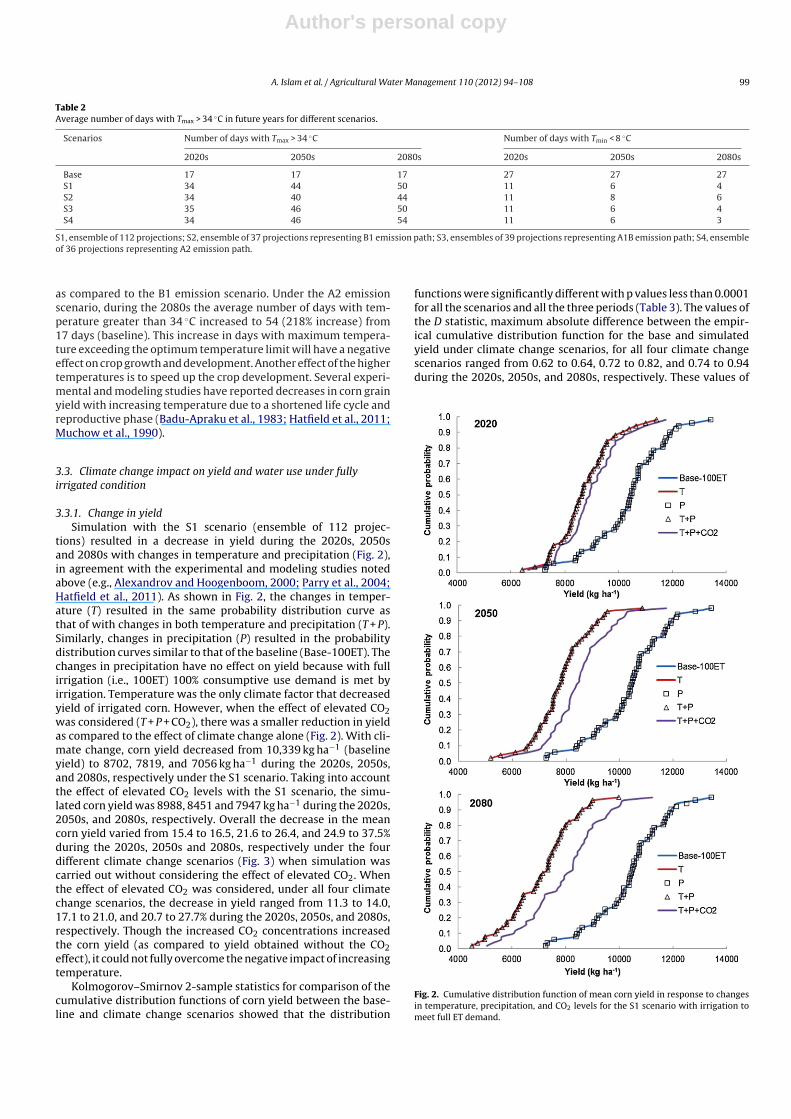
3.3.1. Change in yieldSimulation with the S1 scenario (ensemble of 112 projec-

tions) resulted in a decrease in yield during the 2020s, 2050sand 2080s with changes in temperature and precipitation (Fig. 2),in agreement with the experimental and modeling studies notedabove (e.g., Alexandrov and Hoogenboom, 2000; Parry et al., 2004;Hatfield et al., 2011). As shown in Fig. 2, the changes in temper-ature (T) resulted in the same probability distribution curve asthat of with changes in both temperature and precipitation (T + P).Similarly, changes in precipitation (P) resulted in the probabilitydistribution curves similar to that of the baseline (Base-100ET). Thechanges in precipitation have no effect on yield because with fullirrigation (i.e., 100ET) 100% consumptive use demand is met byirrigation. Temperature was the only climate factor that decreasedyield of irrigated corn. However, when the effect of elevated CO2was considered (T + P + CO2), there was a smaller reduction in yieldas compared to the effect of climate change alone (Fig. 2). With cli-mate change, corn yield decreased from 10,339 kg ha−1 (baselineyield) to 8702, 7819, and 7056 kg ha−1 during the 2020s, 2050s,and 2080s, respectively under the S1 scenario. Taking into accountthe effect of elevated CO2 levels with the S1 scenario, the simu-lated corn yield was 8988, 8451 and 7947 kg ha−1 during the 2020s,2050s, and 2080s, respectively. Overall the decrease in the meancorn yield varied from 15.4 to 16.5, 21.6 to 26.4, and 24.9 to 37.5%during the 2020s, 2050s and 2080s, respectively under the fourdifferent climate change scenarios (Fig. 3) when simulation wascarried out without considering the effect of elevated CO2. Whenthe effect of elevated CO2 was considered, under all four climatechange scenarios, the decrease in yield ranged from 11.3 to 14.0,17.1 to 21.0, and 20.7 to 27.7% during the 2020s, 2050s, and 2080s,respectively. Though the increased CO2 concentrations increasedthe corn yield (as compared to yield obtained without the CO2effect), it could not fully overcome the negative impact of increasingtemperature.

Kolmogorov–Smirnov 2-sample statistics for comparison of thecumulative distribution functions of corn yield between the base-line and climate change scenarios showed that the distribution

functions were significantly different with p values less than 0.0001for all the scenarios and all the three periods (Table 3). The values ofthe D statistic, maximum absolute difference between the empir-ical cumulative distribution function for the base and simulatedyield under climate change scenarios, for all four climate changescenarios ranged from 0.62 to 0.64, 0.72 to 0.82, and 0.74 to 0.94during the 2020s, 2050s, and 2080s, respectively. These values of

Fig. 2. Cumulative distribution function of mean corn yield in response to changesin temperature, precipitation, and CO2 levels for the S1 scenario with irrigation tomeet full ET demand.

Author's personal copy

100 A. Islam et al. / Agricultural Water Management 110 (2012) 94– 108

Fig. 3. Relative changes in the mean corn yield under different climate change scenarios (S1–S4) with and without CO2 effect under full irrigation.

the p (<0.0001) and D statistic indicate that the cumulative distri-bution functions are significantly different as compared to those ofthe baseline yield. The differences between the baseline and futuresimulated yields increased from the 2020s to the 2080s, as indicatedby the higher D values. When the effect of elevated CO2 concentra-tions was considered, the D values were lower; ranging from 0.52to 0.62, 0.58 to 0.70, and 0.66 to 0.78 during the 2020s, 2050s, and2080s, respectively and the p values remained less than 0.0001.These lower values of D, in the case of the elevated CO2, also indi-cate that changes in yield are lower as compared to the changes inyield obtained when effect of elevated CO2 was not considered.

3.3.2. Change in crop duration, evapotranspiration and water useefficiency

Increased temperature may accelerate crop growth and devel-opment and shorten the crop growing period, as evidenced by theseveral experimental studies (Badu-Apraku et al., 1983; Muchowet al., 1990). Simulation results showed a substantial decrease incrop maturity time (shortened crop growing period) during the2020s, 2050s and 2080s under all four climate change scenarios.In the case of the S1 scenario, the crop growing duration changedfrom 133 (baseline) to 117, 109, and 104 days during the 2020s,2050s and 2080s, respectively (Table 4 and Fig. 4a). Climate changescenarios representing the higher emission path (A2) resulted in

comparatively more decrease in crop duration as compared to themiddle (A1B) and low emission (B1) scenarios during the 2080s,whereas during the 2020s the crop duration remained almost thesame for all three emission scenarios (Table 4). Further, the meancrop duration decreased linearly with mean increase in temper-ature for all climate change scenarios (Fig. 4b). Every 1 ◦C rise inmean temperature resulted in shortening of crop growing dura-tion by about 5 days. The mean grain yield decreased linearly withreduction in the crop growth period (Fig. 4c) because of the reducedseasonal light interception and photosynthesis due to the shortercrop growing period. This result indicates that the shortening ofthe crop maturity duration caused by increased temperature wasan important factor in the yield reduction.

The reduction in the crop growing period due to rise in temper-ature resulted in a decrease in actual seasonal evapotranspirationas compared to the baseline (Table 4) under all four climate changescenarios. However, the daily evapotranspiration rate increaseddue to the increase in temperature (Table 4). The change in sea-sonal crop evapotranspiration remained almost the same for allthe four scenarios during the 2020s and 2050s when simula-tion was made without considering elevated CO2 levels. Therewere approximately a 6 and 10% decreases in the actual evapo-transpiration demand during the 2020s and 2050s, respectively(Fig. 5a); whereas during the 2080s this decrease ranged from 9.4 to

Table 3Mean corn yield under different climate change scenarios with full irrigation.

Scenarios Without CO2 effect With CO2 effect

Mean (kg ha−1) SD (kg ha−1) D statistic Mean (kg ha−1) SD (kg ha−1) D statistic

Base 10339.0 1333.62020s

S1 8701.5 (−15.8) 1028.1 0.62a 8988.4 (−13.1) 1060.6 0.58a

S2 8708.4 (−15.8) 1039.9 0.62 8886.8 (−14.1) 1057.9 0.60S3 8633.2 (−16.5) 991.9 0.64 8896.1 (−14.0) 1023.4 0.58S4 8744.6 (−15.4) 1074.0 0.62 9167.8 (−11.3) 1130.6 0.52

2050sS1 7819.2 (−24.4) 1043.8 0.74 8451.0 (−18.3) 1130.7 0.62S2 8102.6 (−21.6) 902.4 0.72 8413.1 (−18.6) 936.9 0.68S3 7609.2 (−26.4) 1017.0 0.76 8164.1 (−21.0) 1092.2 0.68S4 7607.5 (−26.4) 1042.6 0.74 8568.3 (−17.1) 1176.2 0.58

2080sS1 7056.2 (−31.8) 1209.4 0.84 7946.7 (−23.1) 1366.2 0.68S4 7767.4 (−24.9) 974.5 0.74 8202.5 (−20.7) 1028.0 0.66S3 7059.8 (−31.7) 1089.4 0.84 7880.7 (−23.8) 1217.4 0.72S2 6457.6 (−37.5) 1288.2 0.90 7476.1 (−27.7) 1499.2 0.78

S1, ensemble of 112 projections; S2, ensemble of 37 projections representing B1 emission path; S3, ensemble of 39 projections representing A1B emission path; S4, ensembleof 36 projections representing A2 emission path; SD, standard deviation; D stats, Kolmogorov–Smirnov 2-sample statistics; terms in the parenthesis indicates percentagechange from baseline period.

a p values less than 0.0001 for all the four scenarios and all the three time periods (2020s, 2050s, and 2080s).

Author's personal copy

A. Islam et al. / Agricultural Water Management 110 (2012) 94– 108 101Ta

ble

4C

han

ge

in

crop

grow

ing

per

iod

and

seas

onal

wat

er

bala

nce

com

pon

ents

un

der

dif

fere

nt

clim

ate

chan

ge

scen

ario

s

wit

h

full

irri

gati

on.

Scen

ario

s

Cro

p

du

rati

on,

day

sA

ct

evap

(cm

)A

ct

tran

(cm

)Po

t

evap

(cm

)Po

t

tran

(cm

)S–

W

ET(c

m)

Act

ET(c

m)

WU

E(k

g

m−3

)A

ct

evap

(cm

)A

ct

tran

(cm

)Po

t

evap

(cm

)Po

t

tran

(cm

)S–

W

ET(c

m)

Act

ET(c

m)

WU

E(k

g

m−3

)

Bas

e

133

23.7

47.2

28.0

47.8

75.8

(5.7

)a71

.0

(5.3

)

1.46

23.7

47.2

28.0

47.8

75.8

(5.7

)

71.0

(5.3

)

1.46

Wit

hou

t

CO

2W

ith

CO

2

2020

sS1

117

21.3

45.4

25.1

45.7

70.7

(6.1

)

66.7

(5.7

)

1.31

21.9

41.6

25.6

41.9

67.5

(5.8

)

63.4

(5.4

) 1.

42S2

117

21.3

45.3

25.1

45.7

70.7

(6.1

)

66.6

(5.7

)

1.31

21.5

43.0

25.4

43.3

68.7

(5.9

)

64.5

(5.5

)

1.38

S3

116

21.4

45.3

25.0

45.6

70.6

(6.1

)

66.6

(5.7

)

1.30

21.7

41.8

25.5

42.1

67.6

(5.8

)

63.5

(5.5

)

1.40

S4

117

21.2

45.4

25.1

45.7

70.9

(6.0

)

66.6

(5.7

)

1.31

22.1

39.8

26.0

40.1

66.1

(5.6

) 61

.9

(5.3

)

1.48

2050

sS1

109

20.0

44.3

23.9

44.4

68.3

(6.3

)

64.2

(5.9

)

1.22

21.2

36.1

25.1

36.2

61.3

(5.6

)

57.3

(5.2

)

1.48

S2

112

20.4

44.6

24.3

44.8

69.1

(6.2

)

65.0

(5.8

)

1.25

21.1

40.4

24.9

40.6

65.5

(5.9

)

61.4

(5.5

)

1.37

S3

108

19.9

44.2

23.6

44.3

67.9

(6.3

)

64.1

(5.9

)

1.19

21.1

36.7

24.8

36.8

61.6

(5.7

)

57.8

(5.4

)

1.41

S4

108

20.0

44.2

23.7

44.3

68.0

(6.3

)

64.2

(5.9

)

1.18

21.7

32.4

25.5

32.5

58.0

(5.4

)

54.1

(5.0

)

1.58

2080

sS1

104

19.4

43.7

23.0

43.8

66.8

(6.4

)

63.1

(6.1

)

1.12

21.1

32.3

24.8

32.3

57.1

(5.5

)

53.3

(5.1

)

1.49

S2

109

20.0

44.2

23.7

44.4

68.2

(6.3

)

64.3

(5.9

)

1.21

21.0

38.1

24.7

38.2

63.0

(5.8

)

59.2

(5.4

)

1.39

S3

104

19.4

43.7

22.9

43.8

66.7

(6.4

)

63.1

(6.1

)

1.12

20.9

32.9

24.6

33.0

57.5

(5.6

)

53.8

(5.2

)

1.46

S410

0

18.7

43.4

22.3

43.4

65.7

(6.6

)

62.1

(6.2

)

1.04

20.6

31.2

24.2

31.2

55.4

(5.5

)

51.8

(5.2

)

1.44

S1, e

nse

mbl

es

of

112

pro

ject

ion

s;

S2, e

nse

mbl

es

of

37

pro

ject

ion

s

rep

rese

nti

ng

B1

emis

sion

pat

h; S

3,

ense

mbl

es

of

39

pro

ject

ion

s

rep

rese

nti

ng

A1B

emis

sion

pat

h; S

4,

ense

mbl

es

of

36

pro

ject

ion

s

rep

rese

nti

ng

A2

emis

sion

pat

h;

S–W

ET, S

hu

ttle

wor

th–W

alla

ce

evap

otra

nsp

irat

ion

;

WU

E,

wat

er

use

effi

cien

cy;

Act

evap

, act

ual

evap

orat

ion

, Pot

evap

, pot

enti

al

evap

orat

ion

;

Act

tran

, act

ual

tran

spir

atio

n;

Pot

tran

s,

pot

enti

al

tran

spir

atio

n.

aTe

rms

in

the

par

enth

esis

ind

icat

es

aver

age

rate

of

evap

otra

nsp

irat

ion

du

rin

g

crop

per

iod

in

mm

/day

.

Fig. 4. Effect of climate change on crop growing duration of corn: (a) cumulativedistribution functions of crop duration for the S1 scenario; (b) relationship betweenchange in temperature and crop growing period for all scenarios; and (c) relationshipbetween mean decrease in crop duration and mean decrease in yield for all scenarios,under full irrigation.

12.6%. The seasonal potential evapotranspiration decreased byabout 7% during the 2020s. During the 2050s and 2080s, thedecrease in potential evapotranspiration ranged from 8.9 to 10.4and 10.1 to 13.3%, respectively. When effect of elevated CO2 wasconsidered, the decrease in the seasonal crop evapotranspirationwas higher, ranging from 9.0 to 12.8, 13.4 to 23.8, and 16.7 to 27.0%during the 2020s, 2050s, and 2080s, respectively, under differentclimate change scenarios (Fig. 5b).

The water use efficiency (WUE) (yield per unit of actualevapotranspiration) also decreased due to the decrease in yield.With increasing CO2 concentrations, due to the decrease in stoma-tal conductance, there was a decrease in transpiration and henceevapotranspiration, along with an increase in grain yield. Thus, theincreased CO2 levels resulted in higher WUE values as compared tothe WUE values obtained without considering the effect of elevated

Author's personal copy

102 A. Islam et al. / Agricultural Water Management 110 (2012) 94– 108

Fig. 5. Change in seasonal actual evapotranspiration, potential evapotranspiration and water use efficiency for the S1–S4 scenarios with and without CO2 effect under fullirrigation.

CO2. The WUE varied from 1.1 to 1.3 kg m−3 in case of the S1 sce-nario without the considering the effect of elevated CO2, and 1.4 to1.5 kg m−3 when the effect of elevated CO2 was considered. Theseresults suggest that with the elevated CO2 levels, WUE remainscloser to the baseline WUE values and partly mitigate the negativeeffect of increasing temperature.

Fig. 6 depicts the changes in seasonal irrigation water require-ments to meet the ET demand under different climate changescenarios. Simulation results showed an increase in seasonal irriga-tion water use when effect of elevated CO2 was not considered, butthe increase was less than 3%. This increase in irrigation water use isdue to a decrease in precipitation and an increase in ET demand dur-ing the crop growing period. When the effect of elevated CO2 wasconsidered, the irrigation water use decreased as compared to thebaseline conditions for all the scenarios during the 2020s, 2050s and2080s respectively. This decrease ranged from 2.0 to 6.8, 5.2 to 16.0and 8.1 to 15.5% during the 2020s, 2050s and 2080s, respectively.

This decrease was primarily due to decrease in actual evapotran-spiration demand with increasing CO2 levels and a shortened cropgrowing period.

Several studies have suggested longer duration hybrids of cornas one of the possible adaptation strategies to counterbalance theaccelerated phenology due to warmer climate (Kapetanaki andRosenzweig, 1997; Tao and Zhang, 2011; Tubiello et al., 2000).Assuming a longer duration hybrid corn having the same WUEas the current hybrid, the amount of water required to main-tain the baseline yield was estimated. When the effect of elevatedCO2 was not considered the estimated increase in irrigation waterdemand to maintain the baseline yield (100ET) under different cli-mate change scenarios (S1–S4) ranged from 11.0 to 12.4, 16.9 to23.0 and 20.6 to 40.0% during the 2020s, 2050s and 2080s, respec-tively. When the effect of elevated CO2 was considered, these valuesranged from −1.7 to 5.8, −8.1 to 6.4 and −2.2 to 5.1% during the2020s, 2050s and 2080s, respectively. These estimates indicate that

Author's personal copy

A. Islam et al. / Agricultural Water Management 110 (2012) 94– 108 103

Fig. 6. Changes in seasonal precipitation and irrigation water use from the baselineperiod under different climate change scenarios (S1–S4) during the 2020s, 2050sand 2080s, with irrigation to meet full ET demand.

with elevated CO2 levels, total seasonal irrigation water demandmay not change significantly under the projected climate changescenarios even when longer duration hybrids are used to maintainyield potential.

3.4. Climate change impact on yield and water use efficiencyunder deficit irrigation

As a management strategy to meet the challenges of reducedwater availability, two deficit irrigations levels (i.e., 75ET, 50ET)were also simulated. Table 5 presents the comparison of the effectof changes in temperature, precipitation, CO2 on yield under dif-ferent irrigation levels for S1 scenario. For the baseline period(1950–99), average corn yields for 100ET, 75ET and 50ET simula-tions were 10,339, 8441 (18.4% decrease) and 4817 (53.4% decrease)kg ha−1, respectively. As expected with only CO2 increase (withoutany change in P or T) there was an increase in yield as comparedto the corresponding baseline yield for each irrigation level. Thegain in yield due to elevated CO2 was marginal in case of full irri-gation (100ET); there was 3. 5, 8.1 and 12.8% increase in yield ascompared to the baseline yield for 100ET during 2020s, 2050s, and2080s, respectively. For deficit irrigation level of 75ET, the gain inyield (as compared to the baseline yield for 75ET) due to the effectof increased CO2 concentrations was about 7.3, 18.7 and 28.5% dur-ing 2020s, 2050s, and 2080s, respectively; whereas for irrigationlevel of 50ET the increase (as compared to the baseline yield for50ET) in yield was 10.6, 27.0, and 43.0% during 2020s, 2050s, and2080s, respectively. Thus, the positive effect of CO2 was higherunder water stress conditions and these results are in agreementwith other previous results (Boote et al., 2011; Chun et al., 2011;Leakey, 2009; Ruane et al., 2011; Wechsung et al., 2000; Xionget al., 2007). However, the simulation with increasing CO2 con-centrations coupled with precipitation and temperature changes,resulted in decrease in corn yield for all the three irrigation levelsand for all the three periods (2020s, 2050s, and 2080s). As maize isC4 plant, elevated CO2 enrichment alone would not benefit maizeproduction significantly, especially for irrigated maize (Alexandrovand Hoogenboom, 2000). Based on the experimental results in theopen air and within the Corn Belt using Free-Air ConcentrationEnrichment (FACE) technology, Leakey et al. (2006) reported thatphotosynthesis and yield of maize might be unaffected by risingCO2 in the absence of water stress.

Under deficit irrigation (75ET and 50ET), decreases in yield (rela-tive to the baseline yield for the corresponding irrigation level) dueto climate change were lower (Fig. 7) as compared to the decrease in Ta

ble

5C

omp

aris

on

of

clim

ate

chan

ge

effe

ct

on

corn

yiel

d

wit

h

dif

fere

nt

irri

gati

on

leve

ls

un

der

S1

scen

ario

.

Scen

ario

Cro

p

du

rati

on(d

ays)

T min

◦ C

T max

◦ C

Prec

ipit

atio

n,

cm10

0ET

75ET

50ET

Irri

gati

onap

pli

ed, c

mY

ield

,(k

g

ha−

1)

Ch

ange

inyi

eld

(%)

Irri

gati

onap

pli

ed, c

mY

ield

,(k

g

ha−

1)

Ch

ange

inyi

eld

(%)

Irri

gati

onap

pli

ed, c

mY

ield

,(k

g

ha−

1)

Ch

ange

inyi

eld

(%)

Bas

e

133

11.3

5

28.5

6

17.9

3

53.3

3

1033

9.00

–

35.6

1

8441

.30

–

18.4

6

4816

.88

–20

20 P13

311

.35

28.5

6

17.7

3

53.5

0

1034

2.06

0.03

35.7

8

8417

.18

−0.2

9

18.7

0

4868

.43

1.07

CO

213

3

11.3

5

28.5

6

17.9

3

50.0

8

1069

5.74

3.45

33.1

9

9056

.84

7.29

17.0

7

5328

.18

10.6

1T

117

13.4

6

30.5

6

16.0

6

54.0

0

8699

.58

−15.

86

36.2

8

7383

.70

−12.

53

19.0

4

4263

.98

−11.

48T

+

P

117

13.4

6

30.5

6

15.8

9

54.3

8

8701

.48

−15.

84

36.5

3

7392

.22

−12.

43

19.1

5

4263

.52

−11.

49T

+

P

+

CO

211

7

13.4

6

30.5

6

15.8

9

51.1

6

8988

.40

−13.

06

34.2

1

7854

.14

−6.9

6

17.9

3

4682

.52

−2.7

920

50 P

133

11.3

5

28.5

6

18.0

0

53.2

2

1034

1.58

0.02

35.5

4

8426

.34

−0.1

8

18.4

4

4877

.06

1.25

CO

213

3

11.3

5

28.5

6

17.9

3

46.1

0

1118

0.68

8.14

30.1

1

1001

5.84

18.6

5

15.0

5

6123

.40

27.1

2T

109

14.7

4

31.7

4

15.6

9

54.2

7

7818

.42

−24.

38

36.5

7

6674

.62

−20.

93

19.4

3

3820

.12

−20.

69T

+

P

109

14.7

4

31.7

4

15.7

5

53.9

2

7819

.24

−24.

37

36.6

3

6654

.14

−21.

17

19.2

1

3858

.56

−19.

90T

+

P

+

CO

210

9

14.7

4

31.7

4

15.7

5

47.4

3

8450

.98

−18.

26

31.6

3

7705

.88

−8.7

1

16.0

4

4782

.72

−0.7

120

80 P

133

11.3

5

28.5

6

18.2

8

53.0

1 10

349.

60

0.10

35.2

5

8439

.66

−0.0

2

18.1

3

4887

.66

1.47

CO

213

3

11.3

5

28.5

6

17.9

3

42.8

2 11

662.

02

12.8

0

27.6

9

1085

0.82

28.5

4

13.3

8

6889

.56

43.0

3T

104

15.8

1

32.7

7

15.2

4

54.3

8 70

56.3

0

−31.

75

37.2

3

6029

.62

−28.

57

19.7

1

3434

.82

−28.

69T

+

P

104

15.8

1

32.7

7

15.5

7

54.5

1

7056

.20

−31.

75

36.8

5

6068

.14

−28.

11

19.4

3

3480

.56

−27.

75T

+

P

+

CO

210

4

15.8

1

32.7

7

15.5

7

45.0

8

7946

.72

−23.

14

30.0

5

7604

.64

−9.9

1

14.9

0

4722

.76

−1.9

5

P,

scen

ario

wit

h

chan

ges

in

pre

cip

itat

ion

only

;

T,

scen

ario

wit

h

chan

ges

in

tem

per

atu

re

only

;

CO

2, s

cen

ario

wit

h

chan

ges

in

CO

2on

ly;

T

+

P,

scen

ario

wit

h

chan

ges

in

tem

per

atu

re

and

pre

cip

itat

ion

;

T

+

P

+

CO

2, s

cen

ario

wit

hch

ange

s

in

tem

per

atu

re, p

reci

pit

atio

n

and

CO

2;

T min

, ave

rage

min

imu

m

air

tem

per

atu

re

du

rin

g

crop

grow

ing

per

iod

(50

year

s

aver

age)

;

T max

, ave

rage

max

imu

m

air

tem

per

atu

re

du

rin

g

crop

grow

ing

per

iod

(50

year

s

aver

age)

;p

reci

pit

atio

n, t

otal

pre

cip

itat

ion

du

rin

g

crop

grow

ing

per

iod

(50

year

s av

erag

e);

irri

gati

on, t

otal

irri

gati

on

wat

er

app

lied

du

rin

g

crop

grow

ing

per

iod

(50

year

s

aver

age)

.

Author's personal copy

104 A. Islam et al. / Agricultural Water Management 110 (2012) 94– 108

Fig. 7. Comparison of change in yield from the baseline for different levels of irrigation under different climate change scenarios (S1–S4) with and without CO2 effect.

yield for full irrigation (relative to the baseline yield for the full irri-gation). Simulation results for the 75ET deficit irrigation with the S1scenario and elevated CO2 levels, showed a decrease of 7.0, 8.7 and9.9% in yield during the 2020s, 2050s and 2080s, respectively whencompared to the baseline yield simulated with 75ET. In the case of50ET, the decrease in average yield was about 2.8, 0.7 and 1.95%,during the 2020s, 2050s and 2080s, respectively when comparedto the baseline yield simulation with 50ET. With increased CO2concentrations, the maximum change (increase/decrease) in cornyield for all scenarios (S1–S4) remained below 10 and 15% for the50ET and 75ET treatments, respectively (Fig. 7). Relatively smallerdecreases in yields under deficit irrigations could be explained bythe combination of accelerated crop maturity due to higher tem-peratures combined with more positive effects of higher CO2 undersoil water deficit conditions (Ruane et al., 2011). Under elevatedCO2, reduced stomatal conductance reduces evapotranspirationand crop water use, and thereby ameliorates short-term waterstress by conserving soil moisture (Leakey, 2009). The number of

days with above-optimum or below-optimum temperatures dur-ing crop period was the same for all irrigation levels for any givenclimate change scenario, and therefore, relative effect of the above– or below-optimum temperatures on growth was the same underall irrigation levels.

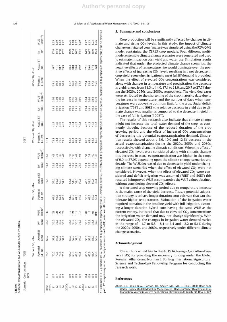
The WUE for 75ET remained almost the same as that of 100ETwith the elevated CO2 concentrations (Table 6). The WUE rangedfrom 1.40 to 1.52 kg m−3 in the case of the S1 scenario. But withthe 50ET there was a decrease in the WUE and it ranged from 1.15to 1.27 kg m−3 in the case of the S1 scenario. Comparison of theWUE obtained with and without the elevated CO2 concentrations,indicated an improved WUE under deficit irrigation when the effectof increased CO2 concentrations was considered (Fig. 8).

4. Limitations

The crop growth simulation models are frequently usedby researchers to understand the complexity of climate–crop

Author's personal copy

A. Islam et al. / Agricultural Water Management 110 (2012) 94– 108 105

Fig. 8. Changes in water use efficiency with different levels of irrigation under different climate change scenarios (S1–S4) with and without CO2 effect.

interactions, and probably the only practical approach for assess-ing climate change impact on agro-ecosystems. Like most studieson climate change impact on crop production using crop simulationmodels, there are several sources of uncertainty and limitations inthis study. Some uncertainties are inherent in the model structureand some are due to model calibration and parameterization. Themodel has been calibrated using three years of field measured datafor different levels of irrigations. The effect of increasing CO2 con-centrations on growth and yield of corn has been simulated usingstandard relationships/methodology as published in the literature.However, these relationships were derived from a limited num-ber of experiments, often in controlled environments, and were,therefore, not fully tested, particularly for warmer and more vari-able climate change conditions. Lack of field measured data on theeffect of CO2 on growth and yield of corn under different temper-ature regimes and different irrigation levels, is one of the majorlimitations for validation of simulation results in climate change

impact assessment studies, including this study. Thus, considerabledebate over whether the simulation results obtained using cropmodels are accurate will remain until more definitive field resultsare incorporated in the simulation studies. Further, in this simu-lation study it was assumed that insect pests, diseases, and weedspose no limitation on crop growth and yield under both current andfuture climate scenarios. The agronomic practices, e.g., fertilizationrates, sowing dates, irrigation applications etc. were assumed to besame in future. Technological development and land use were alsoassumed to be constant. Thus, the effects of climatic change on cropproduction under the natural and future field conditions may be dif-ferent from those obtained using the crop models. However, thesesimulation studies provide valuable information on possible impactof climate change on crop production, and guideline for adaptationstrategies through simulation of different agronomical (changingof planting dates, varieties/cultivars, cropping sequences, irrigationlevels etc.) management options.

Author's personal copy

106 A. Islam et al. / Agricultural Water Management 110 (2012) 94– 108

Tab

le

6Se

ason

al

evap

otra

nsp

irat

ion

and

WU

E

un

der

defi

cit

irri

gati

on.

Scen

ario

Cro

p

du

rati

on,

day

s75

ET

50ET

Wit

hou

t

CO

2ef

fect

Wit

h

CO

2ef

fect

Wit

hou

t

CO

2ef

fect

Wit

h

CO

2ef

fect

Pote

nti

alET

(cm

)A

ctu

al

ET(c

m)

IW (cm

)W

UE

(kg

m−3

)Po

ten

tial

ET

(cm

)A

ctu

al

ET(c

m)

IW (cm

)W

UE

(kg

m−3

)Po

ten

tial

ET

(cm

)A

ctu

al

ET(c

m)

IW (cm

)W

UE

(kg

m−3

)Po

ten

tial

ET

(cm

)A

ctu

al

ET(c

m)

IW (cm

)W

UE

(kg

m−3

)

Bas

e

133

75.5

60.2

35.6

1.40

75.8

43.4

18.5

1.11

2020

sS1

117

70.5

57.8

36.5

1.28

67.3

55.6

34.2

1.41

71.1

41.9

19.2

1.02

68.1

40.7

17.9

1.15

S2

117

70.5

57.8

36.5

1.28

68.5

56.6

35.1

1.35

71.1

41.9

19.3

1.02

69.3

41.1

18.4

1.10

S311

670

.4

57.7

36.2

1.27

67.4

55.6

33.9

1.39

70.9

41.9

19.1

1.00

68.1

40.7

17.8

1.12

S4

117

70.7

57.8

36.3

1.28

65.8

54.8

33.0

1.48

71.3

41.9

19.3

1.01

66.8

39.9

17.2

1.22

2050

sS1

109

68.0

57.0

36.6

1.17

61.0

52.3

31.6

1.47

68.6

41.3

19.2

0.93

61.7

38.3

16.0

1.25

S211

268

.9

57.2

36.2

1.21

65.2

54.9

33.7

1.35

69.4

41.4

19.0

0.96

66.0

40.0

17.4

1.10

S3

108

67.7

57.0

36.6

1.14

61.3

52.6

31.9

1.42

68.2

41.2

19.1

0.90

62.0

38.6

16.2

1.17

S4

108

67.8

57.0

36.9

1.14

57.6

50.2

29.9

1.63

68.3

41.2

19.5

0.91

58.3

36.9

14.8

1.39

2080

sS1

104

66.6

56.9

36.9

1.07

56.8

49.9

30.1

1.52

66.9

41.2

19.4

0.84

57.4

37.1

14.9

1.27

S210

967

.9

56.9

36.3

1.16

62.7

53.6

32.5

1.38

68.4

41.3

19.1

0.92

63.4

39.0

16.7

1.13

S310

4

66.4

56.7

36.8

1.06

57.2

50.4

30.3

1.49

66.8

41.1

19.2

0.85

57.8

37.4

15.0

1.23

S410

0

65.6

56.7

37.9

0.99

55.1

49.1

30.7

1.48

65.9

41.2

20.1

0.79

55.6

36.8

15.3

1.26

S1, e

nse

mbl

e

of

112

pro

ject

ion

s;

S2, e

nse

mbl

e

of

37

pro

ject

ion

s

rep

rese

nti

ng

the

B1

emis

sion

pat

h;

S3, e

nse

mbl

es

of

39

pro

ject

ion

s

rep

rese

nti

ng

A1B

emis

sion

pat

h;

S4, e

nse

mbl

e

of

36

pro

ject

ion

s

rep

rese

nti

ng

the

A2

emis

sion

pat

h;

ET, e

vap

otra

nsp

irat

ion

;

IW, i

rrig

atio

n

wat

er

use

d;

WU

E,

wat

er

use

effi

cien

cy.

5. Summary and conclusions

Crop production will be significantly affected by changes in cli-mate and rising CO2 levels. In this study, the impact of climatechange on irrigated corn (maize) was simulated using the RZWQM2model containing the CERES crop module. Four different multi-model ensemble climate change scenarios were generated and usedto estimate impact on corn yield and water use. Simulation resultsindicated that under the projected climate change scenarios, thenegative effects of temperature rise would dominate over the pos-itive effects of increasing CO2 levels resulting in a net decrease incrop yield, even when irrigation to meet full ET demand is provided.When the effect of elevated CO2 concentrations was consideredalong with changes in temperature and precipitation, the decreasein yield ranged from 11.3 to 14.0, 17.1 to 21.0, and 20.7 to 27.7% dur-ing the 2020s, 2050s, and 2080s, respectively. The yield decreaseswere attributed to the shortening of the crop maturity date due tothe increase in temperature, and the number of days when tem-peratures were above the optimum limit for the crop. Under deficitirrigation (75ET and 50ET) the relative decrease in yield due to cli-mate change was smaller as compared to the decrease in yield inthe case of full irrigation (100ET).

The results of this research also indicate that climate changemight not increase the total water demand of the crop, as com-monly thought, because of the reduced duration of the cropgrowing period and the effect of increased CO2 concentrationsof decreasing the potential evapotranspiration demand. Simula-tion results showed about a 6.0, 10.0 and 12.6% decrease in theactual evapotranspiration during the 2020s, 2050s and 2080s,respectively, with changing climatic conditions. When the effect ofelevated CO2 levels were considered along with climatic changesthis decrease in actual evapotranspiration was higher, in the rangeof 9.0 to 27.0% depending upon the climate change scenarios anddecade. The WUE decreased due to decrease in yield under chang-ing climate scenarios when the effect of elevated CO2 were notconsidered. However, when the effect of elevated CO2 were con-sidered and deficit irrigation was assumed (75ET and 50ET) thisresulted in improved WUE as compared to the WUE values obtainedwithout considering elevated CO2 effects.

A shortened crop growing period due to temperature increaseis the major cause of the yield decrease. Thus, a potential adapta-tion strategy is to have longer duration corn cultivars that can alsotolerate higher temperatures. Estimation of the irrigation waterrequired to maintain the baseline yield with full irrigation, assum-ing a longer duration hybrid corn having the same WUE as thecurrent variety, indicated that due to elevated CO2 concentrationsthe irrigation water demand may not change significantly. Withthe elevated CO2, the changes in irrigation water demand variedin the range of −1.7 to 5.8, −8.1 to 6.4 and −2.2 to 5.1% duringthe 2020s, 2050s, and 2080s, respectively under different climatechange scenarios.

Acknowledgment

The authors would like to thank USDA Foreign Agricultural Ser-vice (FAS) for providing the necessary funding under the GlobalResearch Alliance and Norman E. Borlaug International AgriculturalScience and Technology Fellowship Program for conducting thisresearch work.

References

Ahuja, L.R., Rojas, K.W., Hanson, J.D., Shafer, M.J., Ma, L. (Eds.), 2000. Root ZoneWater Quality Model: Modeling Management Effects on Water Quality and CropProduction. Water Resources Publications, LLC Highlands Ranch, CO, USA, p. 372.

Author's personal copy

A. Islam et al. / Agricultural Water Management 110 (2012) 94– 108 107

Alexandrov, V.A., Hoogenboom, G., 2000. Vulnerability and adaptation assessmentsof agricultural crops under climate change in the Southeastern USA. Theoreticaland Applied Climatology 67, 45–63.

Allen, L.H., 1990. Plant response to rising carbon dioxide and potential interactionwith air pollutants. Journal of Environment Quality 19, 15–34.

Allen, L.H., Boote, K.J., Jones, J.W., Valle, R.R., Acock, B., Rogers, H.H., Dahlman, R.C.,1987. Response of vegetation to rising carbon dioxide: photosynthesis, biomass,and seed yield of soybean. Global Biogeochemical Cycles 1, 1–14.

Anderson, J.A., Alagarswamy, G., Rotz, C.A., Ritchie, J.T., LeBaron, A.W., 2001. Weatherimpacts on maize, soybean, and alfalfa production in the Great Lakes region,1895–1996. Agronomy Journal 93, 1059–1070.

Badu-Apraku, B., Hunter, R.B., Tollenaar, M., 1983. Effect of temperature during grainfilling on whole plant and grain yield in maize. Canadian Journal of Plant Science63, 357–363.

Boote, K.J., Allen, L.H., Vara Prasad, P.V., Jones, J.W., 2011. Testing effects of climatechange in crop models. In: Hillel, D., Rosenzweig, C. (Eds.), Handbook of ClimateChange and Agroecosystems: Impacts, Adaptation, and Mitigation. ICP Serieson Climate Change Impacts, Adaptation, and Mitigation, vol. 1. Imperial CollegePress, pp. 109–129.

Chaudhuri, U.N., Kirkam, M.B., Kanemasu, E.T., 1990. Root growth of winter wheatunder elevated carbon dioxide and drought. Crop Science 30, 853–857.

Christensen, N.S., Lettenmaier, D.P., 2007. A multimodel ensemble approach toassessment of climate change impacts on the hydrology and water resources ofthe Colorado River Basin. Hydrology and Earth System Sciences 11, 1417–1434.

Chun, J.A., Wang, Q., Timlin, D., Fleisher, D., Reddy, V.R., 2011. Effect of elevatedcarbon dioxide and water stress on gas exchange and water use efficiency incorn. Agricultural and Forest Meteorology 151, 378–384.

Farahani, H.J., DeCoursey, D.G., 2000. Potential evapotranspiration processes in thesoil–crop-residue system. In: Ahuja, L.R., Rojas, K.W., Hanson, J.D., Shafer, M.J.,Ma, L. (Eds.), Root Zone Water Quality Model: Modeling Management Effects onWater Quality and Crop Production. Water Resources Publications, LLC, High-lands Ranch, CO, pp. 51–80.

Guerena, A., Ruiz-Ramos, M., Diaz-Ambrona, C.H., Conde, J.R., Minguez, M.I., 2001.Assessment of climate change and agriculture in Spain using climate models.Agronomy Journal 93, 237–249.

Hamlet, A.F., Salathe, E.P., Carrasco, P., 2010. Statistical downscaling tech-niques for global climate model simulations of temperature andprecipitation with application to water resources planning studies.http://www.hydro.washington.edu/2860/report/ (accessed 18.05.11).

Hatfield, J.L., Boote, K.J., Kimball, B.A., Ziska, L.H., Izaurralde, R.C., Ort, D., Thom-son, A.M., Wolfe, D., 2011. Climate impacts on agriculture: implications for cropproduction. Agronomy Journal 103, 351–370.

Hay, L.E., Wilby, R.L., Leavesley, G.H., 2000. A comparison of delta change and down-scaled GCM scenarios for three mountainous basins in the United States. Journalof the American Water Resources Association 36 (2), 387–397.

Hillel, D., Rosenzweig, C., 2011. Handbook of Climate Change and Agroecosystems:Impacts, Adaptation, and Mitigation. ICP Series on Climate Change Impacts,Adaptation, and Mitigation, vol. 1. Imperial College Press, 440 pp.

Intergovernmental Panel on Climate Change (IPCC), 2000. IPCC Special Report onEmission Scenarios. A Special Report of IPCC Working Group III. Report of theIntergovernmental Panel on Climate Change, Cambridge University Press, UK,570 pp.

Intergovernmental Panel on Climate Change (IPCC), 2007. Climate Change 2007:The Physical Science Basis. Contribution of Working Group I to the FourthAssessment Report of the Intergovernmental Panel on Climate Change (IPCC).Cambridge University Press, Cambridge, UK, 881 pp.

Izaurralde, R.C., Rosenberg, N.J., Brown, R.A., Thompson, A.M., 2003. Integratedassessment of Hadley Centre (HadCM2) climate change projections on agri-cultural productivity and irrigation water supply in the conterminous UnitedStates. Part II. Regional agricultural production in 2030 and 2095. Agriculturaland Forest Meteorology 117, 97–122.

Jones, J.W., Hoogenboom, G., Porter, C.H., Boote, K.J., Batchelor, W.D., Hunt, L.A.,Wilkens, P.W., Singh, U., Gijsman, A.J., Ritchie, J.T., 2003. The DSSAT croppingsystem model. European Journal of Agronomy 18, 235–265.

Kapetanaki, G., Rosenzweig, C., 1997. Impact of climate change on maizeyield in central and northern Greece: a simulation study with Ceres-Maize.Mitigation and Adaptation Strategies for Global Change 1 (3), 251–271,http://dx.doi.org/10.1023/B:MITI.0000018044.48957.28.

Kimball, B.A., Pinter Jr., P.J., Garcia, R.L., LaMorte, R.L., Wall, G.W., Hunsaker, D.J.,Wechsung, G., Wechsung, F., Kartschall, T., 1995. Productivity and water use ofwheat under free-air CO2 enrichment. Global Change Biology 1, 429–442.

Kimball, B.A., Kobayashi, K., Bindi, M., 2002. Responses of agricultural crops to free-air CO2 enrichment. Advances in Agronomy 77, 293–368.

Kiniry, J.R., Bonhomme, R., 1991. Predicting maize phenology. In: Hodges, T. (Ed.),Predicting Crop Phenology. CRC Press, Boca Raton, pp. 115–131.

Ko, J., Ahuja, L.R., Saseendran, S.A., Green, T.R., Ma, L., Nielsen, D.C., Walthall, C.L.,2011. Climate change impacts on dryland cropping systems in the CentralGreat Plains, USA. Climatic Change, http://dx.doi.org/10.1007/s10584-011-0175-9(published online, August 09, 2011).

Leakey, A.D.B., 2009. Rising atmospheric carbon dioxide concentration and thefuture of C4 crops for food and fuel. Proceedings of the Royal Society B: BiologicalSciences 276, 2333–2343.

Leakey, A.D.B., Uribelarrea, M., Ainsworth, E.A., Naidu, S.L., Rogers, A., Ort, D.R., Long,S.P., 2006. Photosynthesis, productivity, and yield of maize are not affectedby open-air elevation of CO2 concentration in the absence of drought. PlantPhysiology 140, 779–790.

Lobell, D.B., Schlenker, W., Costa-Roberts, J., 2011. Climate trends andglobal crop production since 1980. Science 333 (6042), 616–620,http://dx.doi.org/10.1126/science.1204531.

Ma, L., Hoogenboom, G., Saseendran, S.A., Bartling, P.N.S., Ahuja, L.R., Green,T.R., 2009. Effect of estimating soil hydraulic properties and root growthfactors on soil water balance and crop production. Agronomy Journal 101,http://dx.doi.org/10.2134/agronj2008.0206x.

Ma, L., Trout, T.J., Ahuja, L.R., Bausch, W.C., Saseendran, S.A., Malone, R.W., Nielsen,D.C., 2012. Calibrating RZWQM2 model for maize responses to deficit irrigation.Agricultural Water Management 103, 140–149.

Maurer, E.P., Brekke, L., Pruitt, T., Duffy, P.B., 2007. Fine-resolution climate pro-jections enhance regional climate change impact studies. Eos Transactions,American Geophysical Union 88 (47), 504.

Meehl, G.A., Covey, C., Delworth, T., Latif, M., McAvaney, B., Mitchell, J.F.B., Stouf-fer, R.J., Taylor, K.E., 2007. The WRCP CMIP3 multi-model dataset: a new era inclimatic change research. Bulletin of the American Meteorological Society 88,1383–1394.

Meza, F.J., Silva, D., Vigil, H., 2008. Climate change impacts on irrigated maize inMediterranean climates: evaluation of double cropping as an emerging adapta-tion alternative. Agricultural Systems 98, 21–30.

Muchow, R.C., Sinclair, T.R., Bennett, J.M., 1990. Temperature and solar radiationeffects on potential maize yield across locations. Agronomy Journal 82, 338–343.

Parry, M.L., Rosenzweig, C., Iglesias, A., Livermore, M., Fischer, G., 2004.Effects of climate change on global food production under SRES emis-sions and socio-economic scenarios. Global Environmental Change 14, 53–67,http://dx.doi.org/10.1016/j.gloenvcha.2003.10.008.

Peart, R.M., Jones, R.B., Curry, K., Boote, K.J., Allen, L.H., 1989. Impacts of climatechange on crop yield in the Southern U.S.A. In: Smith, J.B., Tirpak, D.A. (Eds.),The Potential Effects of Global Climate Change on the United States, Report toCongress. U.S. Environmental Protection Agency, EPA-230-05-89-050, Washing-ton, DC.

Peiris, D.R., Crawford, J.W., Grashoff, C., Jefferies, R.A., Porter, J.R., Marshall, B., 1996.A simulation study of crop growth and development under climate change.Agricultural and Forest Meteorology 79, 271–287.

Phillips, D.L., Lee, J.J., Dodson, R.F., 1996. Sensitivity of the US corn belt to climatechange and elevated CO2: I. corn and soybean yields. Agricultural Systems 52,481–502.

Raff, D.A., Pruitt, T., Brekke, L.D., 2009. A framework for assessing flood frequencybased on climate projection information. Hydrology and Earth System Sciences13, 2119–2136.

Ragab, R., Prudhomme, C., 2002. Climate change and water resources management inarid and semi-arid regions: prospective and challenges for 21st century. Biosys-tems Engineering 81 (1), 3–34.

Reifen, C., Toumi, R., 2009. Climate projections: past performance noguarantee of future skill? Geophysical Research Letters 36, L13704,http://dx.doi.org/10.1029/2009GL038082.

Reilly, J., Tubiello, F., McCarl, B., Abler, D., Darwin, R., Fuglie, K., Hollinger, S., Izau-rralde, C., Jagtap, S., Jones, J., Mearns, L., Ojma, D., Paul, E., Paustian, K., Riha, S.,Rosenberg, N., Rosenzweig, C., 2003. US agriculture and climate change: newresults. Climatic Change 57 (1–2), 43–67.

Ritchie, J.T., Otter-Nacke, S., 1985. Description and performance of CERES-Wheat: auser-oriented wheat yield model. USDA-ARS, ARS-38, pp. 159–175.

Rogers, H.H., Bingham, G.E., Cure, J.D., Smith, J.M., Suran, K.A., 1983. Responses ofselected plant species to elevated carbon dioxide in the field. Journal of Envi-ronmental Quality 12, 569–574.

Rojas, K.W., Ahuja, L.R., 2000. Management practices. In: Ahuja, L.R., Rojas, K.W.,Hanson, J.D., Shafer, M.J., Ma, L. (Eds.), Root Zone Water Quality Model. ModelingManagement Effects on Water Quality and Crop Production. Water ResourcesPublications, LLC, Highlands Ranch, CO, pp. 245–280.

Rosenzweig, C., Hillel, D., 1998. Climate Change and the Global Harvest. OxfordUniversity Press, Oxford, UK, pp. 135–154.

Rosenzweig, C., Parry, M.L., 2004. Potential impact of climate change on world foodsupply. Nature 367, 133–138.

Ruane, A.C., Cecil, L.D., Horton, R.M., Gordón, R., McCollum, R., Brown, D.,Killough, B., Goldberg, R., Greeley, A.P., Rosenzweig, C., 2011. Climatechange impact uncertainties for maize in Panama: farm information, cli-mate projections, and yield sensitivities. Agricultural and Forest Meteorology,http://dx.doi.org/10.1016/j.agrformet.2011.10.015.

Shaffer, M.J., Rojas, K.W., DeCoursey, D.G., Hebson, C.S., 2000. Nutrient chemistryprocess-OMNI. In: Ahuja, L.R., Rojas, K.W., Hanson, J.D., Shafer, M.J., Ma, L. (Eds.),Root Zone Water Quality Model. Modeling. Management Effects on Water Qual-ity and Crop Production. Water Resources Publications, LLC, Highlands Ranch,CO, USA, pp. 119–144.

Tao, F., Zhang, Z., 2011. Impacts of climate change as a function of global meantemperature: maize productivity and water use in China. Climatic Change 105,409–432, http://dx.doi.org/10.1007/s10584-010-9883-9.

Thompson, A.M., Brown, R.A., Rosenberg, N.J., Izaurralde, R.C., Benson, V., 2005. Cli-mate change impacts for the conterminous USA: an integrated assessment.Part. 3. Dryland production of grain and forage crops. Climatic Change 69,43–65.

Tubiello, F.N., Ewert, F., 2002. Simulating the effects of elevated CO2 on crops:approaches and applications for climate change. European Journal of Agronomy18, 57–74.

Tubiello, F.N., Donatelli, M.C., Rosenzweig, C., Stockle, C.O., 2000. Effects of climatechange and elevated CO2 on cropping systems: model predictions at two Italianlocations. European Journal of Agronomy 13, 179–189.

Author's personal copy

108 A. Islam et al. / Agricultural Water Management 110 (2012) 94– 108

Wechsung, F., Garcia, R.L., Wall, G.W., Kartschall, T., Kimball, B.A., Michaelis, P., PinterJr., P.J., Wechsung, G., Grossman-Clarke, S., Lamorte, R.L., Adamsen, F.J., Leav-itt, S.W., Thompson, T.L., Matthias, A.D., Brooks, T.J., 2000. Photosynthesis andconductance of spring wheat ears: field response to free-air CO2 enrichmentand limitations in water and nitrogen supply. Plant Cell and Environment 23,917–929.

Wood, A.W., Maurer, E.P., Kumar, A., Lettenmaier, D.P., 2002. Long range experimen-tal hydrologic forecasting for the eastern U.S. Journal of Geophysical Research107 (D20), 4429.

Xiong, W., Matthews, R., Holman, I., Lin, E., Xu, Y., 2007. Modelling China’s potentialmaize production at regional scale under climate change. Climatic Change 85,433–451.