Modeling sequence evolution in acute HIV1 infection

Modeling Sequence Evolution in Acute HIV-1 Infection

Ha Youn Lee1,2,*, Elena E. Giorgi1,3,*, Brandon F. Keele4, Brian Gaschen1, Gayathri S.Athreya1, Jesus F. Salazar-Gonzalez4, Kimmy T. Pham4, Paul A. Goepfert4, J. MichaelKilby4, Michael S. Saag4, Eric L. Delwart5, Michael P. Busch5, Beatrice H. Hahn4, George M.Shaw4, Bette T. Korber1,6, Tanmoy Bhattacharya1,6, and Alan S. Perelson1,§1Theoretical Biology and Biophysics, Los Alamos National Laboratory, Los Alamos, NM 87545, USA2Department of Biostatistics and Computational Biology, University of Rochester Medical Center,Rochester, NY 14642, USA3University of Massachusetts, Amherst MA 010024University of Alabama at Birmingham, Birmingham, AL 35223, USA5Blood Systems Research Institute, San Francisco, CA 94118, USA6Santa Fe Institute, Santa Fe, NM 87501, USA

AbstractWe describe a mathematical model and Monte-Carlo (MC) simulation of viral evolution during acuteinfection. We consider both synchronous and asynchronous processes of viral infection of new targetcells. The model enables an assessment of the expected sequence diversity in new HIV-1 infectionsoriginating from a single transmitted viral strain, estimation of the most recent common ancestor(MRCA) of the transmitted viral lineage, and estimation of the time to coalesce back to the MRCA.We also calculate the probability of the MRCA being the transmitted virus or an evolved variant.Excluding insertions and deletions, we assume HIV-1 evolves by base substitution without selectionpressure during the earliest phase of HIV-1 infection prior to the immune response. Unlikephylogenetic methods that follow a lineage backwards to coalescence, we compare the observed datato a model of the diversification of a viral population forward in time. To illustrate the applicationof these methods, we provide detailed comparisons of the model and simulations results to 306envelope sequences obtained from 8 newly infected subjects at a single time point. The data from6/8 patients were in good agreement with model predictions, and hence compatible with a single-strain infection evolving under no selection pressure. The diversity of the samples from the othertwo patients was too great to be explained by the model, suggesting multiple HIV-1-strains weretransmitted. The model can also be applied to longitudinal patient data to estimate within-host viralevolutionary parameters.

KeywordsHIV-1; population dynamics; viral evolution

*Contributed equally§Corresponding Author: [email protected], MS K710, Los Álamos National Laboratory, Los Álamos NM 87544, Phone: +1 505 667 6829FAX: +1 505 665 3493Publisher's Disclaimer: This is a PDF file of an unedited manuscript that has been accepted for publication. As a service to our customerswe are providing this early version of the manuscript. The manuscript will undergo copyediting, typesetting, and review of the resultingproof before it is published in its final citable form. Please note that during the production process errors may be discovered which couldaffect the content, and all legal disclaimers that apply to the journal pertain.

NIH Public AccessAuthor ManuscriptJ Theor Biol. Author manuscript; available in PMC 2010 November 21.

Published in final edited form as:J Theor Biol. 2009 November 21; 261(2): 341–360. doi:10.1016/j.jtbi.2009.07.038.

NIH

-PA Author Manuscript

NIH


NIH


IntroductionThe HIV-1 population in a chronically infected individual is subject to continuous immuneselection (Richman et al., 2003; Wei et al., 2003), and evolves to become a complex set ofrelated viruses, often referred to as a quasispecies, through the course of an infection (Lee etal., 2009; Shankarappa et al., 1999; Wolinsky et al., 1996). A reduction in viral complexity attransmission was originally noted in the context of mother to infant transmission (Wolinskyet al., 1992), and has been extensively studied in recent years (Derdeyn et al., 2004; Dickoveret al., 2006; Edwards et al., 2006; Painter et al., 2003). During sexual transmission of HIV-1,a genetic bottleneck usually occurs since a limited number of viral strains are transmitted fromthe complex quasispecies typically found in a donor (Delwart et al., 2001; Derdeyn et al.,2004; Zhang et al., 1993), although other studies have found multiple transmitted variants ata relatively high frequency (Long et al., 2002; Ritola et al., 2004; Sagar et al., 2004; Vernazzaet al., 1999). Infection with multiple genetic variants has been associated with genital tractulcers and use of hormonal contraceptives (Sagar et al., 2004). Recent studies have identifiedpatients in the earliest weeks of infection, many prior to the selective pressure imposed by thenewly infected host’s initial immune response (Abrahams et al., 2009; Keele et al., 2008;Salazar-Gonzalez et al., 2008). Sequence data from the HIV-1 env gene collected during acuteHIV-1 infection in 102 subjects by Keele et al. (2008) show a wide range of diversity, with theaverage number of bases differing between pairs of sequences from the same patient varyingbetween 0.01% and 2.18%, suggesting that both single and multiple viral strain transmissionsmay have occurred in this cohort.

In this paper, we develop simple models of HIV-1 evolution early in infection with the aim ofquantitatively assessing whether infections were established by single or multiple viral strains.Further, in the case of single strain, i.e., homogeneous, infections we aim to identify the most-likely initiating strain or a close descendent that gave rise to the observed lineage.

We derive analytical results and approximate formulas. We used Monte Carlo (MC)simulations to capture the randomness in early HIV-1 evolution and to compare with ouranalytical results. The analytical results were derived from idealized models whereas the MCsimulations allowed for more accurate models that incorporate unequal base composition andan evolutionary based substitution matrix that defines the frequency at which base i is replacedby base j during a mutation event. Previously, Monte Carlo methods have been used to studythe within-host dynamics of HIV-1 infection (Heffernan and Wahl, 2005; Kamina et al.,2001; Ribeiro and Bonhoeffer, 1999; Ruskin, 2002; Tan and Wu, 1998; Tuckwell and LeCorfec, 1998), but here our focus is on sequence evolution and not viral and T cell dynamicsas in these earlier works. Keele and colleagues applied a variant of this model to the analysisof 102 B-clade infected patients (Keele et al., 2008) and of 18 experimentally SIV-infectedrhesus macaques (Keele, 2009). Abrahams et al. (2009) have used the same techniques toanalyze a set of 69 C-clade infected subjects.

In this study we provide a complete mathematical description of the model, and explore theimplications of varying the baseline assumptions, the input parameters, as well as purelyanalytical versus computational outcomes. We use just 8 of the patients described in Keele etal. (Keele et al., 2008) to illustrate nuances in the application of our model. These 8 subjectswere chosen to be representative of the full set of 102 patients with 80% being characterizedas having homogenous infection and 20% heterogeneous infections.

The main problem we focus on here is developing a systematic, reasoned way to determinewhether a single strain or multiple stains of HIV-1 infected an individual. This is not straight-forward; even if an individual is infected by a single strain, with time this transmitted viruswill diversify. Thus, given a set of sequences one needs to compute how much diversity would

Lee et al.

J Theor Biol. Author manuscript; available in PMC 2010 November 21.

NIH


NIH


NIH


be expected by a given time from infection. For sequences collected early after infection, ifthe diversity is much greater than what is expected from a homogeneous infection, then multiplestrain infection is a likely explanation. Other signatures of multiple strain infection might alsobe present, e.g., the sequences cluster into groups with very different most recent commonancestors. Our model also provides an estimate of the time from the origin of the most recentcommon ancestor (MRCA) of the sampled variants. If the sampled variants are representativeof a lineage that was initiated by the infecting strain, the time to the MRCA should correspondto the time of infection; if the lineage arose in the donor, the time to the MRCA would be longerthan the infection; if the lineage arose post-infection in the newly infected individual as aconsequence of selection, the time estimated to the MRCA would be less than the time frominfection.

To characterize HIV-1 evolution in samples in the earliest weeks of infection, we have modeledthe events that occur between virus transmission and peak replication, approximately 21-35days later. Our model assumes random drift prior to the initial immune response andexponential viral expansion prior to peak viremia. We ignored the effects of selection—basedon the premise that the sequences we analyze were obtained sufficiently early in infection thatimmune responses would not yet provide substantial selective pressure. Although other sourcesof selection may be present, these also are ignored in our model. The effects of recombinationwere not modeled either. Comparing the expectations based on the mathematical model andthe simulations to observed acute infection sequence data enables us to explore the validity ofthese assumptions in real infections. We show that under the hypothesis of exponential growthin the infected cell population the frequency distribution of the genetic distances between pairsof HIV-1 sequences follow an approximate Poisson distribution and star-phylogeny topology.This was first shown by Slatkin and Hudson in the context of the evolution of mitochondrialDNA (Slatkin and Hudson, 1991).

Since the precise time of initial HIV-1 infection cannot usually be known with certainty, thestatus of acute/early subjects can be classified using the “Fiebig” staging system (Table 1),which is based on an orderly appearance of viral RNA, antigen and antibodies in plasma duringearly infection (Fiebig et al., 2005;Fiebig et al., 2003). Prior to stage I, where plasma viral RNAfirst becomes detectable, is the eclipse phase. The length of this period can be roughly estimatedbased on clinical histories from a series of studies (Clark et al., 1991;Gaines et al.,1988;Lindback et al., 2000a;Lindback et al., 2000b;Schacker et al., 1996) and suggests anaverage length of about 10 days (range 7-21 days, see Table 1). For each patient in our datasetthe Fiebig stage is known. This provides a rough estimate of the time since infection, whichcan be compared with the estimated time since the MRCA computed with our models fromthe sampled sequences.

Coalescent theory can also be used to find common ancestors and estimate the time tocoalescence. Further, results have been obtained using coalescent theory for the type of linearbirth death process that underlies the model described in this paper (Kuhner et al., 1998;Rannala, 1997). When the infection is indeed homogeneous and it meets our modelassumptions (exponential viral growth, no selection, etc.), we are under a very particularevolutionary scenario that allows us to use more direct and computationally efficient methodsto derive the approximate time to the MRCA. Even though appropriate, Bayesian estimationmethods (Drummond et al., 2005; Drummond et al., 2006; Kuhner and Smith, 2007), as theones provided by the software BEAST by (Drummond and Rambaut, 2007), arecomputationally intensive even when the number of sequences is small as they perform a wholesuite of additional tests that are redundant for our particular evolutionary scenario. The methodspresented below are computationally efficient, and our model results can be obtained in minutesfor the entire dataset, while in our hands BEAST runs for a single patient took over 3 hours.Further, as we shall show, the estimated time to the MRCA using BEAST and using our method

Lee et al.


NIH


NIH


NIH


are very similar. Thus, we believe the methods we present below enable a rapid exploration ofthe implications of a forward evolution model, provide consistent results with a coalescencemodel, and allow us to compare the model to the data to infer biologically interestinginformation from the sample.

ResultsMathematical Models and Monte-Carlo Simulations

HIV-1 can be transmitted from one individual to another either through the transmission ofvirus particles or infected cells. Since transmission of virus will quickly generate infected cells,we describe the transmission as if it occurred through infected cells.

In the case of sexually transmitted HIV-1, most often only a single viral sequence initiates thenew infection, or only a single sequence grows out to yield a detectable level of viremia{Delwart, 2001 #61; Derdeyn, 2004 #20; Zhang, 1993 #59; Abrahams, 2009 #185}. Thus, weshall model the case in which infection is initiated by a single HIV-1 sequence. The simplestimplementation of this hypothesis is to assume that a single cell, carrying this sequence as aprovirus, starts the infection. We shall also examine the case in which multiple cells carryingidentical sequences start the infection. When the predictions of these models fail to explain theextent of sequence heterogeneity observed, this is evidence that either multiple sequences havebeen transmitted, or that immune or other selective pressures are driving the observed level ofdiversification (Long et al., 2002; Ritola et al., 2004; Sagar et al., 2004; Vernazza et al.,1999).

We assume that the initial infected cell produces virus; most are cleared, but some successfullyinfect a new generation of cells. The number of secondary infections caused by one infectedcell placed in the population of cells of an uninfected individual and fully susceptible toinfection is called the basic reproductive ratio, R0. While data on early viral kinetics in humansis limited, the available data in humans infected with HIV-1 and in monkeys infected with SIVand SHIV show that the virus grows exponentially until a viral load peak is attained a fewweeks after infection (Little et al., 1999; Nowak et al., 1997; Stafford et al., 2000). Followingthe peak, viral levels decline and establish a set-point. At the set-point each infected cell, onaverage, successfully infects one other cell during its lifetime. If it infected more than one othercell viral levels would increase, whereas if it infected less than one cell viral levels would fall.Thus, once the set-point is established we can assume that the number of infected cells remainsconstant.

In our model we assume a homogeneous infection in which the virus grows exponentially withno selection pressure, no recombination, no occurrence of back mutations and a constantmutation rate across positions and across lineages. We also assume the virus grows with a fixedgeneration length and that each infected cell produces the same number of progeny. Clearly,the approximation of exponential growth must break down as target cells become limited andthe number of cells infected per generation must decrease from R0, stabilizing at 1 when theviral set point is established. However, we present evidence indicating that what is importantin determining viral diversity is the number of reverse transcription events that have occurredalong a lineage, i.e., the number of generations that separate the initial infection from the timeat which sequences were obtained, and not the number of cells infected at each generation. Inour first, simplest model, we also assume that the infection is synchronous, and thus can becharacterized by discrete generations, with the virus infecting exactly R0 new cells at eachgeneration.

Let all genomes be of same length NB, let ε be the reverse transcriptase point mutation rate,which we assume to be constant throughout the genome, and let s0 denote the infecting strain.

Lee et al.


NIH


NIH


NIH


Then, after the first replication cycle, the R0 daughter cells will each differ from the infectingstrain at exactly n bases (positions) with a probability given by

(1)

After the second replication cycle, the total number of mutations in the new generation ofinfected cells will follow the probability distribution given by

In other words, n mutations in the second generation are the result of all possible combinationsof k mutations occurring in the first replication, and n-k occurring in the second, for all integersk between 0 and n. Mathematically, this is given by the convolution of two Binomialdistributions with the same probability parameter (ε, in our case), which is in turn a Binomialdistribution (Casella and Berger, 1990). One can see that after a replication cycles,

Let HD0 denote the Hamming distance, i.e., the number of base differences from the infectingstrain s0. In general, given n mutations, we have HD0 ≤ n , as some of the n mutations mayoccur at the same site. However, after a replication cycles, the probability that one site hasmutated at most once is

(2)

Therefore, the probability that at least one site across the entire genome has mutated more than

once is Q = 1-PNB , which is approximately when ε is small.

For the HIV-1 base substitution rate ε, we use the value of 2.16 × 10-5 base substitutions perreplication cycle. The base substitution rate we use is derived from the results of (Mansky andTemin, 1995), where after a single round of HIV-1 replication they found an overall mutationrate of 3.4 × 10-5, but this included insertions and deletions. Restricting their results to onlybase substitutions, we calculated from their data a base substitution rate of 2.16 × 10-5 per baseper replication. The sequences that we analyze later are envelope gene sequences with NB~2600 bases. Substituting these values into Q, we find that the probability of two or moremutations at the same site increases with the number of replication cycles, yet even for a=50one finds Q < 0.0015. Hence we expect that we can ignore back mutations when we analyzepatient sequence data obtained early in infection.

Under this assumption, HD0 coincides with the number of mutations and hence it follows thesame Binomial distribution:

(3)

Lee et al.


NIH


NIH


NIH


Notice that this formula assigns a nonzero probability to the Hamming distance being largerthan the total number of bases NB, and this is an artifact of our approximations. In fact, usingChebyshev’s inequality (Feller, 1957), one can show (see Materials and Methods) that

, and thus indeed, within our approximation, P(mutations> NB) ≈ 0.

Synchronous Infection, Mathematical ModelIn the synchronous model, we assume that each cell infects R0 other cells at the end of its lifecycle. At generation a from the infection event, there will be infected cells, each one carryingone HIV-1 genome. Further, at generation a

(4)

In order to analyze single time point data, it is useful to compute the intersequence HDdistribution rather than HD0 (since for the latter we would need to assume that we know theinfecting sequence s0). In other words, rather than comparing any given sequence to the foundersequence, we take all possible sequence pairs in the sample and compute their relative HD.Given two sequences, s1 and s2, picked at random at time t, that have evolved independentlyfrom the common ancestor s0, the distribution of HD[s1, s2] is

(5)

The assumption of independent evolution of sequences s1 and s2 from the common ancestors0 is equivalent to assuming that the phylogeny of these sequences is star-like with s0 beingthe only common ancestor. However, it is also conceivable that the common ancestor of s1 ands2 is not the transmitted sequence s0 but rather a sequence that evolved from s0. This is animportant issue, as the identity of the transmitted sequence is generally not known. Asillustrated in Figure 1, the probability of s1 and s2 coalescing m generations from the ancestor,with m < a, is the number of all sequences coalescing m generations from the ancestor (minusthe one we have already picked), divided by the total number of sequences at generation a(again, minus the one we picked already)

(6)

As shown in Material and Methods, this probability approaches zero rapidly as a and m getlarge.

We can use Eq. (6) to determine the probability that two sequences from a given individualcoalesce at a time point other than at the transmitted sequence. For example, for samplesobtained a few weeks into the infection and under no selective pressure, e.g. a=5 and R0=6(see below) the probability of coalescence later than generation 0, from Eq. (6) is 0.167 form=1, 0.028 for m=2 and 0.0045 for m=3. For greater values of a, the probability of coalescingat generation 3 or higher is < 0.005. Thus, we expect that use of Eq. (5) and the assumption of

Lee et al.


NIH


NIH


NIH


a star-like phylogeny to hold for all patient samples in which a single viral strain wastransmitted. However, even for large a, the probability of coalescing 1 or 2 generations awayfrom the founder strain still remains non-negligible: even at generation 40, the probability ofcoalescence later than generation 0, is still 0.167 for m=1, and 0.028 for m=2. In a set ofsequences from an individual, these estimates of less than a 0.5% chance of being 3 generationsaway from the actual founder, a 3% chance of being 2 generations away, and a 17% chance ofbeing 1 generation away hold for each independent pair of comparisons.

Samples that diverge from a star phylogeny often show patterns of shared mutations acrosssequences. The above calculation shows that coalescence not at the founder strain is most likelyone generation away from the actual founder. Therefore, a mutation observed very early in theinfection, could possibly carry on and develop as a second lineage. Also, we can not rule outthat the founders of these two lineages were simply transmitted from the donor and hencecoalesced in the donor. For infections transmitted during the acute phase before muchdiversification occurred in the donor this may even be likely. Lastly, we observe that since thebase substitution rate ε is so small it is very likely that the sequences at a=0 and a=1 are thesame. In fact, with probability (1-ε)RoNB all R0 proviruses at generation 1 are identical to thefounder; e.g., with R0=6 and NB=2600 this probability is 0.71.

For ease of notation, let the intersequence Hamming distance distribution be denoted HDI .Thus,

(7)

We also define some basic quantities based on the calculated Hamming distance distributionfrom the initial strain and the intersequence Hamming distance distribution between all possiblesequence pairs. The divergence at generation a is defined as the average Hamming distanceper base from the initial founder strain. From Eq. (4), this can be estimated as the mean of thebinomial distribution divided by the number of bases, and is εa . The diversity at generationa is the average intersequence Hamming distance per base between sequence pairs and fromEq. (7), diversity = 2εa. The variance of the intersequence HD distribution at generation adivided by the number of bases is 2εa(1-ε). We also introduce the % sequence identity, definedas the proportion of sequences identical to the sequence, s0, of the infecting strain. As the virusevolves, the population diversifies from the founder strain and the proportion of the totalpopulation that is identical to the MRCA decays exponentially. By setting d = 0 in Eq. (4), wehave % sequence identity = Binom(0;aNB,ε) = (1-ε)aNB .

Finally, we wish to compute the expected maximum HDI. This is motivated by the observationthat more extensive diversity is seen in some transmission cases, presumably the result ofinfections established by two or more distinct HIV-1 strains (Long et al., 2002; Ritola et al.,2004; Sagar et al., 2004; Vernazza et al., 1999). Thus, a strategy for systematic classificationof homogeneous, single strain infections versus heterogeneous infections is needed. To addressthis, we ask what is the maximum diversity that one would expect in a single strain infectionwithin a time frame compatible with the subject’s Fiebig stage at the time of sampling. Themaximum diversity expected depends on the sample size: the larger the sample, the higher theexpected maximum, as outliers become more likely to be sampled.,The expected maximumHD at generation a is computed in the Materials and Methods.

Monte Carlo Simulation of the Synchronous Infection ModelThe mathematical model derived above assumes that all mutations have equal probability.However, in HIV-1 the four bases are not equally frequent and the rates of base substitutionare not all equal. Further, we neglected more than one mutation occurring at the same site,

Lee et al.


NIH


NIH


NIH


although this potentially can occur. To examine the influence of these biological details on thepredictions of HIV-1 sequence evolution, and to capture stochastic effects, we developed asimple Monte Carlo simulation and compared its predictions with those of the mathematicalmodel.

The simulation starts at “generation 0” with one cell infected with a single HIV-1 sequenceNB bases long. The initial sequence is generated randomly with base frequencies of 0.19 (Tand C), 0.37 (A) and 0.24 (G), based on typical frequencies measured in the full-length envelopegene (see Materials and Methods). We assume that the initially infected cell infects R0 othercells synchronously. We chose R0 =6, representing the average value of R0 across 10 differentpatients studied by (Stafford et al., 2000). During the infection of these cells mutations canoccur. In the simulation, the sites for the occurrence of the base substitutions are chosenrandomly from the NB bases. The probability that base i is replaced by j is given by a 4×4transition matrix deduced from a maximum likelihood General Time Reversible (GTR) modelof substitutions that occur in the full length HIV-1 envelope gene (for the matrix and the detailssee Materials and Methods). Unlike in our analytical model, we allow the same site to mutatemore than once. For a given sample size NS, the MC simulation produces an HD frequencydistribution for each generation step within a certain time frame chosen by the user. At eachgeneration exactly NS sequences are sampled (with replacement) and the intersequence HDdistribution is thus constructed.

We implemented the MC code so that the user has the option of running either one or multipleiterations. When multiple iterations are done, the HD frequencies computed at each generationstep are averaged over all iterations, thus retrieving the mean field description described bythe analytical method. On the other hand, when not averaging over all iterations, one capturesthe stochastic effects due to rare mutations, e.g. the run-to-run variance, which, in real life,corresponds to the host-to-host variation. This is completely neglected in the analytical method,which is a mean field description.

In the synchronous model the population of infected cells grows exponentially as . Once thenumber of infected cells reaches 104, which is close to some estimates of the effectivepopulation size Ne of the virus in a mature infection (Achaz et al., 2004; Leigh Brown, 1997;Wakeley, 2008), there is no need to expand the population further in order to study the diversityof genetic sequences as long as we allow the proviral sequences contained in these 104 tocontinue to evolve. We thus cap the total population of infected cells at 104 and let those cellsproduce 104 R0 progeny. We then randomly sample 104 cells out of the 104 R0, and continuethe simulation. In this way, we are able to maintain the population of infected cells constantover the rest of the simulation, which is equivalent to what occurs when the viral set-point isreached. We confirmed that our simulation results (i.e., means and 95% CIs) did not dependon the cutoff value of infected cells as long as it is above 103 (data not shown).

Using the MC simulation, we computed divergence, diversity, maximum HD and % sequenceidentity (defined in the previous section) as functions of time, and confirmed that theirdependence on the number of generation steps matched the dependency found analytically.Figure 2 shows this comparison as well as 95% confidence intervals computed from 1,000 MCsimulations using a typical number of sampled sequences, NS=30.

Asynchronous InfectionThe synchronous infection model is a simplification. In reality, cell infections occur at randomtimes by the viruses released from an infected cell. Viral production starts on average about24 hours after a cell is initially infected (Perelson et al., 1996), and most likely continues untilcell death. In order to understand the dependence of our results on the synchronousapproximation, we devised a second model in which infections are asynchronous. Again we

Lee et al.


NIH


NIH


NIH


will assume each cell infects R0 others during its lifetime. While each of the R0 infections couldoccur at different times, here we take a first step in assessing the role of asynchrony by assumingthe infections occurs at two times. Each infected cell infects α cells at an intermediate time,and the rest at the end of its life-time. Even though this scenario is again a simplification, it isuseful to analyze the differences from the previous model, and as we shall show below itpreserves the same basic mathematical structure as before. However, because an infected cellcontributes progeny to the next generation before the end of its life there is now a faster growthrate of the infected cell population.

Let τa and 2τa be the times at which a newly infected cell infects other cells, and suppose itinfects α cells at τa, and γ at 2τa, with α+γ=R0, the total number of cells one cell infected duringits lifetime. Notice that if γ=0, then infections only occur at one time, α=R0, and τa is thegeneration time. Hence this model reduces to the synchronous model with generation timeτs= τa, where τs denotes the duration of a single generation step in the synchronous model.

Denote by I(a,t) the number of infected cells of age a at time t. Here, by age, we mean the ageof the infecting genome, measured in terms of the number of times the viral genome hasundergone reverse transcription, rather than the cell’s physical age. Thus, a is equivalent to thegeneration variable we used in the synchronous model. As a consequence, at any given timet, under the synchronous model all cells belong to the same age group, whereas in the

asynchronous model, the infecting genomes have undergone a minimum of replication

cycles, and a maximum of (see Figure 3), where ⌈ ⌉ and ⌊ ⌋ are the ceiling and floorfunctions defined as ⌈x⌉ = max {n ∈ Z | n ≤ x} and ⌈x⌉ = min {n ∈ Z | n ≤ x}, where Z is theset of integers.

Let I0 denote the initial number of infected cells and let , i.e., n represents time measuredin units of τa. In the following we shall use n as the time variable. A general expression for I(a,n) is derived in Materials and Methods, and is given by

(8)

As illustrated in Figure 3, at any given time n, the HIV-1 strains in an individual have undergone

a minimum of and a maximum of n replication cycles. Then, as a function of time, therandom variable HD0 follows the probability distribution

(9)

In Materials and Methods we show the following relationship

(10)

Lee et al.


NIH


NIH


NIH


where and . By substituting Eq. (10) into Eq. (9) weobtain

(11)

with mean μn = λnεNB and variance , where

(12)

Notice, as one would expect, that in neither the synchronous nor the asynchronous model, doesthe probability distribution depend on the initial number of infected cells, I0.

We show in Materials and Methods that up to terms in O(ε2) P(HD0 =d | n) is a Poissondistribution with mean μn = λnεNB, in other words

(13)

As a consequence, given that the intersequence HD distribution, HDI, is to a goodapproximation the self-convolution of the HD0 distribution, we get that HDI also follows aPoisson distribution with parameter 2λnεNB . Therefore, analogously to the synchronous model,divergence = λnεNB , diversity = 2λnεNB = variance and % sequence identity = Exp(-2λnεNB) .The expected maximum HD is calculated as in the synchronous infection model, Eq. (8) and

(9), except we now insert from Eq. (11).

In the synchronous model, the intersequence Hamming distance, Eq. (5), follows a binomialdistribution, which is also well approximated by a Poisson distribution with equal mean since2aNB is large, ε is small and λ = 2aNBε is of reasonable size (Casella and Berger, 1990). Hencein both scenarios the HD follows essentially the same probability distribution, but with differentdivergence and diversity, implying a different rate of evolution due to the asynchrony ininfection.

Let N(n) be the total number of newly infected cells at time n. For I0=1 and R0 >> 1 , we show

in Material and Methods that , whereas for the same time t,in the synchronous model, , where τs denotes the generation time in thesynchronous model. Notice that τa ≠ τs see Materials and Methods), hence the two scenariosboth provide descriptions of an exponentially growing infected cell population but withdifferent exponents.

We also devised a partially randomized model, in which the α, instead of being a fixedparameter, is a random number uniformly distributed with mean R0/2, and then γ is alwayschosen to be R0-α. This introduces an additional variability the effect of which is inverselyproportional to the total population size. Therefore, large fluctuations from the abovedescription will occur within the first 2-3 generation steps, but will be negligible after that,thus recovering the above mean field description.

Lee et al.


NIH


NIH


NIH


An important difference between the asynchronous and synchronous models is in thedependence on R0. In both models, divergence and diversity depend linearly on the number ofgeneration steps. In the synchronous model, the slope of the diversity is 2ε does not depend onR0 and it. In the asynchronous model, the slope has the additional factor

(14)

with and γ+α=R0. One sees that in the asynchronous model there is a dependenceon R0. Let α=ηR0 for some 0<η≤1, and γ=R0(1-η). Then, one gets the expression of the slopein diversity as

(15)

Notice that the when η=1, we retrieve as a special case the synchronous model, and indeed Eq.(15) yields exactly 2ε. However, when η≠1, the above expression is strictly smaller than 2ε,and approaches 2ε as R0 increases. Figure 4 illustrates the dependence of the slope of thediversity as a function of the number of generation steps on R0.

Table 2 summarizes the above formulas for both the synchronous and the asynchronous models.In both models, divergence, diversity, and variance increase linearly as a function of time.Diversity and variance are expressed by the same mathematical formula, which is aconsequence of the fact that the intersequence HDs follow a Poisson distribution. Divergence,diversity, and HDI variance do not depend on the number of bases per sequence. In contrast,the maximum HD and the % sequence identity depend on the sequence length NB. In thesynchronous infection model, all the quantities are independent of the basic reproductive ratio,while in the asynchronous model, they do depend on the R0, as discussed above. Quantitatively,however, the asynchronous infection model provides minor corrections compared to thesynchronous infection model.

Monte Carlo simulation of the asynchronous infection modelWe keep the basic framework used for the synchronous MC simulation, and choose parametersR0=6, ε=2.16×10-5, and τa=1.5 days (see Materials and Methods). Furthermore, we simulatethe situation where I0=1 and each infected cells infects R0/2 cells at τa, and the remainingR0/2 at time 2τa. We also devised a second scenario under which each infected cells infects αcells at time τa, where α is drawn from a random uniform distribution with mean R0/2, andR0-α at time 2τa. We confirmed that both types of simulations, after generation step 4, are inexcellent agreement, and also confirmed our analytical results described in the previous section.Furthermore, both % divergence and % diversity grow linearly with time (in units of τa) atrates of 1.79 × 10-5 and 3.57 × 10-5, respectively (i.e., 1.2 ×10-5 and 2.4 ×10-5 per day,respectively).

At times τa, 2τa, 3τa, and so on, we sample NS sequences, construct the HD distribution andcompute the divergence, diversity, HDI variance, % sequence identity and the expectedmaximum HD. As for the synchronous model, we find that the MC results agree well with theanalytical results given in Table 2 (Figure 5).

Lee et al.


NIH


NIH


NIH


We examined the dependency of our results on the values chosen for the parameters τ, R0, I0and ε (Figure 6). In agreement with our calculations (Table 2), the diversity increases linearlywith time (not shown) at a rate proportional to ε , inversely proportional to τa (Figures 6A and6B), dependent on R0 (Figure 6C) and independent of I0 (not shown). The mutation rate controlsthe rate of increase of the divergence and the diversity. The larger the mutation rate, the fasterthe genomes mutate, hence the steeper the growth of the diversity (Figure 6A). The greater thegeneration time, the slower the genomes diversify, hence the smaller the growth in diversity(Figure 6B). The computed diversity depends on R0 (Figure 6C). At low values there is a strongdependence, e.g., from R0=2 to R0=6 there is 15.9% increase in the slope of the diversity. Onthe other hand, for larger values of R0, the dependence is much weaker (Figure 6C).

Sample Size DependenceWhen patients are sampled, only a limited number of sequences are obtained. The Monte Carlosimulations provide a means of assessing the variability introduced by limited sequencing andcan be used to choose the number of samples to be sequenced based on the trade-offs betweencost and accuracy. Figure 7 shows the variation in the HD frequency distribution as the samplesize NS varies. Clearly, the larger the sample size, the smaller the variation.

We also asked what is the probability of erroneously classifying an infection as homogeneousdue to poor sampling. In other words, what is the chance of missing a second lineage thatrepresents a small percentage of the entire population when NS sequences are sampled. Weassumed a range of hypothetical low population prevalence, from 0.1% to 20%, and computedthe probability that, out of a sample size NS, all sequences come from the dominant lineage.This is given by a binomial probability of getting zero “successes” out of NS trials, where a“success” is defined as a sequence belonging to the minor lineage, and the probability p ofsuccess is given by its population prevalence

(16)

Thus, for example, for NS ≥30, we can be 95% confident that any missed variant wouldcomprise less than 10% of the total viral population (see Fig. pS9 in (Keele et al., 2008)). Thenumber of sequences sampled from our 8 patients ranged from 16 to 50. When NS =16, we are95% certain that we have sampled all lineages that represent at least 20% of the population.On the other hand, when NS =50, we are 95% confident that any missed lineage would haveto represent 5% or less of the total population.

Analysis of Sequence Data from 8 Acute PatientsPlasma samples were obtained from 8 subjects with acute or very recent HIV-1 subtype Binfection. Laboratory testing showed that 7 subjects were in Fiebig stage II, both viral RNAand p24 antigen were detected, and one subject was in Fiebig stage III, HIV-1 IgM in additionto viral RNA and p24 was detected (see Table 1). Detailed information of each subject issummarized in Table 3. Furthermore, samples were analyzed using the Hypermut tool (LANL)to test for overall enrichment of G-to-A hypermutation patterns with APOBEC3G/F signatures(Bourara et al., 2007;Harris and Liddament, 2004;Simon et al., 2005). Because these mutationalpatterns occur at a faster rate than ordinary mutations, they violate one of our modelassumptions (constant mutation rate across sites and lineages). Only one sample, SUMA,presented mutations (three) that were found to carry the APOBEC3G/F signature. When allmutations were kept, the sample did not fit the Poisson model (χ2 goodness of fit p-value =0.04, where a p<0.05 represents significant departure from the Poisson distribution), whereasa good fit was restored upon removing the APOBEC signatures (χ2 goodness of fit p-value =0.243) (Keele et al., 2008).

Lee et al.


NIH


NIH


NIH


For each of the 8 samples we computed the HD0 and HDI frequencies, as well as the divergence,diversity, HDI variance, % sequence identity and maximum HDI. All quantities are summarizedin Table 4. In order to compute the HD0 distribution, we used the LANL tool ConsensusMaker (LANL) to compute a consensus sequence for each of the homogeneous samples, andthen assumed that the consensus sequence was the founder sequence s0. We then proceeded toanalyze the data in two steps: first, we used our models to infer what the expected maximumHD would be under a homogeneous infection, and used this to distinguish homogeneousinfections from heterogeneous ones. Then, we applied our models to the homogeneous samplesin order to infer a plausible time since the infection.

The eight early infection samples presented two distinct behaviors: either overall low diversity(max HD below 0.5%) and unimodal intersequence HD distribution, or overall high diversity(max HD above 2.5%; patients 1051 and BORI) and multimodal intersequence HD distribution(see Table 4 and Figure 8). We hypothesized that the underlying difference between the twopatterns was whether a single HIV-1 strain entered the host or if multiple distinct strainsentered. In order to exclude single strain infection in the high diversity samples, we computedthe maximum HD one could reasonably expect to achieve at a given point in the infection andcompared this to predictions based on the Fiebig stage. To do this, we used the maximum HDprobability distribution computed in the asynchronous model, Eq. (22) and (23), with P takenfrom equation (13), using the patient specific base length NB and sample size NS given in Table3. To be conservative, we then computed the combined weight in the upper 2.5% tail that wouldbe achieved at each generation step a. The maximum HD at generation step a is less than orequal to this value 97.5% of the time. For patient 1051 (Fiebig stage III), with probability 0.975a minimum of 241 generation steps would be needed to achieve the observed maximum HDof 71 if the infection were homogeneous. This is not compatible with Fiebig stage III, whichcorresponds to a maximum of 37 days since infection (Table 1). Similarly, patient BORI (Fiebigstage II) yielded 261 generation steps for a maximum HD of 77, again incompatible with theFiebig stage. We thus conclude that the high diversity samples were from multiple straininfections, whereas the low diversity samples were compatible with a single strain infection.

An alternative way for distinguishing between homogeneous and heterogeneous infections canbe obtained by looking at both the mean diversity and the variance of each sample. Accordingto our analytical results, when the infection is truly homogeneous, the measured averagediversity and its variance should be approximately equal, which is one of the basic propertiesof a Poisson distribution. However, since measured mean HD and variance are affected bysample size and stochastic effects in early evolution, they may differ. Thus, for a homogeneousinfection we can require that the mean (diversity) and variance be located between the upperand lower 95% confidence limits computed from MC simulations based on the number ofsequences sampled per patient (Figure 9). All of the six low diversity subjects (WEAU, WITO,TRJO, SUMA, 1054, 1056) satisfy this condition, while subjects 1051 and BORI violate it.Thus we classify subjects 1051 and BORI as ”heterogeneous” infections (i.e., infectionsinitiated by two or more founder strains) and the other 6 subjects as “homogeneous” infections.The limitation of this classification is the assumption that the sequence population diversifieswithout any selection, e.g. under neutral evolution. This assumption does not hold for Fiebigstage III or higher, and this classification becomes problematic. The area outside the cone inFigure 9 indicates deviations from a Poisson distribution. In early Fiebig stages this suggestsa heterogeneous infection, whereas in later stages it indicates either immune selection or aheterogeneous infection or both. Also due to purifying selection, samples from a heterogeneousinfection could be located inside the cone in later Fiebig stages. However, to be classified ashomogenous we also require that the average % diversity in these samples be less than thatexpected based on the upper limit of the cumulative duration for the Fiebig stage, i.e., day 34for Fiebig stage II (Figure 9, vertical dashed line)

Lee et al.


NIH


NIH


NIH


The above classification was also confirmed by visual inspection through the LANL toolHighlighter (LANL). The visualization tool represents each sequence in the sample with ahorizontal line, and places a mark whenever the sequence presents a mutation from theconsensus. Figure 9 shows two exemplary behaviors found in acute infection samples: thehomogeneous sample SUMA has few randomly distributed mutations, whereas theheterogeneous sample 1051 presents a majority of sequences that are similar to the consensusand a second group of sequences that not only have many more mutations relative to theconsensus, but these mutations are shared, indicative of a second lineage.

Examining Neutral Evolution: Star-like PhylogenyDuring rapid exponential growth in the absence of selection, small samples of sequences arelikely to have evolved from the founder sequence following a star-like phylogeny, i.e., they allcoalesce at the founder (Wakeley, 2008). When this is the case, the intersequence HD frequencydistribution, HDI, coincides with the self-convolution of the HD0 frequency distribution. Totest whether this is the case and hence if the observed samples evolved following a star-likephylogeny, we compared the observed HDI frequencies from those computed assuming a star-like phylogeny. Given HD0 frequencies X0, X1, ... Xm, where Xi is the number of sequenceswith HD0=i, we constructed the theoretical HDI frequencies by computing the HD self-convolution frequencies Ȳ0,Ȳ1,...,Ȳn, where n=2m, as follows

(17)

The above formula is derived from the arithmetic convolution of the frequencies Xk withthemselves. For example, , Ȳ1 = X0X1, , and so on.

Figure 10 compares the theoretical frequencies Ȳ0,Ȳ1,...,Ȳn (red lines), with the observed ones(the histograms). For 4 out of the 6 low diversity samples there was a perfect agreement betweenthe calculated frequencies and the actual intersequence HD frequency. For the other two(WEAU and TRJO) a 5% and 15% difference was found, respectively. These very lowdifferences, if any, in observed and computed frequencies suggest that all 6 samples evolvedfollowing an approximate star-like phylogeny.

Estimating Time Since the MRCAWe applied the synchronous and asynchronous models to characterize early homogeneousinfections and estimate the time since the MRCA. We did this using both the theoretical Poissonmodel and the output from the MC simulations.

In a homogeneous infection we expect the intersequence HD to follow a Poisson distribution,as in Eq. (13). We used a maximum likelihood method to fit a Poisson distribution to theobserved HDI frequencies and estimate the Poisson parameter λ, which is proportional to thetime or the number of generations since the most recent common ancestor. Given the vectorof observed frequencies Y = (Y0,..., Yn), where Yi is the number of sequence pairs with HD=i,the log likelihood function is defined as

(18)

By minimizing the log likelihood function, we obtain

Lee et al.


NIH


NIH


NIH


(19)

the mean of the intersequence Hamming distance distribution.

We then used λ to estimate the number of generation steps, n, since the most recent commonancestor (MRCA), using the following:

(20)

where n=a in the synchronous model, and in the asynchronous model. Then t, the timesince the MRCA, is given by t=nτs for the synchronous model, and t=nτa for the asynchronousmodel. As illustrated in Materials and Methods, we chose values of 2 and 1.5 days for τs andτa, respectively.

We assessed the goodness of the fit using a χ2 goodness-of-fit test statistic calculated from asingular value decomposition of the covariance matrix (see Materials and Methods). In agoodness of fit test the null hypothesis is that the two distributions being tested are statisticallythe same, hence a low p-value rejects the null hypothesis. All 6 low-diversity samples yieldeda goodness-of-fit p-value of 0.1 or higher, suggesting that the observed distribution is consistentwith a Poisson.

We fixed the values of base length NB and sample size NS appropriate for each patient andthen, under either the synchronous or the asynchronous model, we generated the HDintersequence distribution for generation steps n1 through n2. For example, a typical outputcould be generated by choosing NB=2,600, NS=30 and generation steps 1 through 100. At eachgeneration step, NS sequences were randomly sampled from it and the intersequence HDdistribution of the sample was calculated. From the set of n2-n1+1 intersequence HDdistributions generated, we used a Kolmogorov-Smirnov statistic (Casella and Berger, 1990)to pick the HD distribution that best fit the HD distribution computed from the observedsequence data. We repeated this 103 times. From n*, the average of generation step of the103 best-fitting distributions, we estimate the time since the MRCA, as done above for thePoisson model.

For all 6 low-diversity samples the time of infection could be estimated based on patients’Fiebig stage. Table 4 summarizes the estimates both from fitting the Poisson distribution andthe MC output using the asynchronous model. The computed estimated time since infectionestimated by each patient’s Fiebig stage were within the 95% CIs predicted by the MCsimulations. In contrast, the Poisson fit yielded slightly lower estimates (with respect to thegiven Fiebig stage) for subjects SUMA and 1056. All Poisson estimates were systematicallylower than the MC ones. This is due to the fact that run-to-run variation, while accounted forin the MC fitting, is neglected when fitting the Poisson distribution. To understand this,consider for example a base length of NB=2600. From Eq. (12), under the asynchronous model,the average Hamming distance from the founder strain, after one generation step will be 0.05.In this time, only 3 infected cells are produced, and, on average there will correspondingly be0.15 mutations. However, in any given run, we can only have a discrete number of mutations.

Lee et al.


NIH


NIH


NIH


In particular, the first three cells will be identical 85% of the time (hence a mean HD of 0),14% of the time there will be exactly one mutation across all three sequences (hence a meanHD of 0.333), and so on. Thus, though averaging over enough runs will lead to the correctmean value, most of the runs (85%) will have less than the expected number of mutations (afterthe first reverse transcription), and the rest will have more. This initial difference will persistthrough the generations and appear as an offset in a plot of mean HD versus generations (notshown). Averaging over 1,000 MC runs one finds that a sample of sequences with mean HDfrom the founder of 0.8 coalesce at a MRCA that is always 17 generation steps back (or 25.5days) when fitting the Poisson distribution, but in the MC method 85% of the time the inferrednumber of generation steps will be higher (19 or 20 instead of 17) leading to a mean of 18.2generation steps (or 27.3 days) Thus explaining the roughly 2 day discrepancy in the time toMRCA between these methods as shown in Table 4. Because the variation in the MC isequivalent to host-to-host variation, the MC 95% CIs are more likely to capture the true timeestimates than the Poisson fits.

DiscussionEarly HIV-1 infection tends to be characterized by a viral population with limited sequencediversity in many but not all individuals. A recent study examined sequence data obtained from102 individuals (Keele et al., 2008), and using the methods developed in this papercharacterized the infections as being consistent with a single transmitted strain in 78 cases andmultiple strains in 21 cases with 3 being borderline. In order to do this classification the authorsused the model of early HIV-1 infection developed in this paper. Even though the biologicalconclusion that some people are infected by multiple strains and others by one strain only hasalready been published (Delwart et al., 2001; Derdeyn et al., 2004; Long et al., 2002; Sagar etal., 2004; Zhang et al., 1993), our goal here was to provide, in a self-contained manner, themathematical underpinnings for the analysis of sequences obtained by single genomeamplification methods.

Our goals were not novel in the sense that coalescent and Bayesian inference methods(Drummond et al., 2005; Drummond et al., 2006; Kuhner and Smith, 2007; Kuhner et al.,1998; Rannala, 1997), when restricted to homogeneous infections, can provide the same results.In fact, comparing the estimated time to the MRCA using BEAST (Drummond and Rambaut,2007) and using our method on the 53 patients that had a homogeneous infection and no overtenrichment for APOBEC3 mutations from Keele et al. (Keele et al., 2008), we found the resultsto be similar (correlation coefficient = 0.973, best fitting slope = 1.036, see Figure 11).However, the main difference between these methods and ours is that whereas the formersimulate genealogies, under similar assumptions, our simulation models follow the entirepopulation. While for most of the problems studied in the literature simulating genealogies isthe correct approach, what one gives up in that approach is simplicity when other processeslike recombination and selection need to be modeled. A forward simulation like ours, on theother hand, is usually not feasible because of the problem size, for example for studying HIV-1at the population level, but is readily applied to the important problem of modeling theevolutionary events in early infection and characterization of viral transmission. Because ofthe small number of generations since the extreme bottleneck, we can follow the entirepopulation in a simulation as well as provide analytical calculations for various quantitiessummarizing viral evolution. In this paper, we set up a basic framework in which we neglectrecombination and selection, but it is easy to see that with our methods these pose no problemsof principle, whereas the analysis involving ancestral recombination graphs (Minichiello andDurbin, 2006), or ancestral selection graphs (Sharma, 1977) or both combined would beprohibitive for this data.

Lee et al.


NIH


NIH


NIH


For cases of a single strain infection, our model suggests that the consensus sequence, whichcorresponds to our best estimate of the MRCA given the Poisson model described here, is eitherthe transmitted strain or a strain one to two mutations away from the transmitted strain (Keeleet al., 2008). Identifying the transmitted/founder strain has great biological significance as onecan then determine if it has particular properties that allowed it to be transmitted. Even if ouridentification is only accurate to within one or two base accuracy this will still provide anenormous advance as it is the virus that selectively expands, and we can use this informationto search for particular attributes of the virus that allowed it to expand. For example, preliminaryexamination of putative transmitted viruses suggests that they may generally be more uniformlyrefractive to neutralization than viruses obtained at the chronic stage of infection, which showheterogeneity in susceptibility to antibodies directed at their receptor binding surfaces (Keeleet al., 2008). Also there are subtype specific attributes in terms of variable loop lengths andthe number of glycosylation sites (the loops appear to be shorter and less glycosylated in thetransmitted viruses of A and C clade infections (Chohan et al., 2005; Derdeyn et al., 2004;Sagar et al., 2006), but not B clade transmitted viruses (Frost et al., 2005)). Data is justbeginning to accrue that will enable further exploration of potential viral transmissionsignatures and phenotypic traits, and the models described in this paper allow one to easilydetermine whether or not the MRCA or consensus sequence of an early sample is indeed areasonable estimate of the transmitted virus.

Another important issue that our model addressed is the number of viruses from a single patientthat one must sequence to determine if the infection is homogeneous within some confidenceband and the number of sequences needed to obtain a reasonable estimate of the time to theMRCA. In order to achieve this, we computed pairwise Hamming distance frequencies of eachgiven sample. Other types of statistical analyses that involve pairwise Hamming distances havebeen devised elsewhere (Gilbert et al., 2005), however the focus there was to simply comparetwo different populations, not to infer time estimates. Furthermore, we showed that under thehomogeneous infection hypothesis, the HD frequencies follow a star-phylogeny and Poissondistribution. This was also shown in (Slatkin and Hudson, 1991), where the Poisson was usedto calculate a population growth rate. Here we used it to test the homogeneity of the sample,and then to get time estimates since the MRCA. The probability of misclassifying an infectionas homogeneous is easily calculable from our model. For example, we showed that with asample of 30 sequences the probability of mistakenly classifying an infection as homogeneousdue to not detecting a second minor lineage (less than 10% of the population) is at most 5%.However, now with deep sequencing methods, such as 454 technology (Margulies et al.,2005), 100,000 or more sequences of limited length can be obtained. Such technology mayindeed show examples of what we have called homogeneous infections that are not trulyhomogenous, and could enable us to discern if minor lineages exist at very low frequencies.

The model assumes that the viral population grows exponentially with no selection pressureand no recombination. These are reasonable assumptions to make early in the infection, beforethe host’s immune response begins and while the infected cell population is still much smallerthan the population of target cells. Further, early in infection derived from a single strain viraldiversity is low and recombination may have only a small effect — as recombination betweenidentical sequences leaves the sequences unchanged. Later in the infection, the exponentialgrowth phase stops and selection pressure from the host environment gets established, both ofwhich break the star-phylogeny evolution and hence our model is no longer valid.

In our mathematical models we neglect the occurrence of a mutation occurring more than onceat the same site since it occurs with probability O(a2ε2NB). For our values of ε = 2.16×10-5 andNB ~ 2,600, this probability remains below 0.006 throughout the first 100 replication cycles.After that, the model assumptions may fail because of immune pressure.

Lee et al.


NIH


NIH


NIH


We assumed that the viral diversity evolves under a star-like phylogeny, and that all genomescoalesce at the founder strain. We used this assumption to construct the intersequence HDdistribution and compute sample diversity. The probability of not coalescing at the founder

strain is , where R0 is the basic reproductive ratio and m is the number of generationsaway from the founder strain. So, for example, if we sample after 10 generation steps, theprobability of any two randomly chosen sequences to coalesce one generation step back is ~R0

-9. However, the probability of coalescing 1 or 2 generations earlier than the actual founderstrain is not negligible. Even though we assumed that any two sequences coalesce at the founderstrain, there is in fact less than a 0.5% chance of being 3 generations away from the actualfounder, a 3% chance of being 2 generations away, and a 17% chance of being 1 generationaway. For a set of 20 to 50 sequences, the probability of at least one pair coalescing after theactual founder is virtually certain, but the exponential growth of the infected cell populationwill severely limit the violation of star phylogeny.

It has been estimated that a free virus has a half-life of less than an hour (Ramratnam et al.,1999), whereas an infected cell has an average lifespan of ~2 days (Markowitz et al., 2003;Perelson et al., 1996). Therefore, the virus present in plasma in a given sample is a reflectionof the viral genomes contained in HIV-1 producing cells. Thus, as a simplification, we chosein our models to follow the infected cell population and not the virus. At each generation step,we assumed that an infected cell successfully infects R0 other cells. In effect, we are followingthe integrated HIV-1 provirus rather than viral particles. The experimental data we analyzedwas obtained by sequencing virus and not provirus. On average, each cell produces as manyas 5 × 104 virions (Chen et al., 2007), which makes the viral population at any given time pointmuch larger than the infected cell population. Sampling with replacement of the provirus poolis therefore a good approximation, introducing a fractional error on the estimated probabilitiesof O(10-4 NS), where NS is the number of sequences sampled. Because we never sample over60 sequences, this is a negligible correction.

Finally, we assumed the mutation rate is constant across different lineages and along the entiregenome. This assumption is violated if APOBEC3G/F causes G-to-A mutation at an enhancedrate even in sequences that are not overtly hypermutated. Keele et al. (Keele et al., 2008)showed that overall APOBEC enriched samples follow our evolutionary model upon removingthe G-to-A mutations with APOBEC3G/F signature. For the point mutation rate, we used thevalue 2.16×10-5 per base per replication cycle. (Mansky and Temin, 1995) estimated a mutationrate of 3.14×10-5 per base per replication cycle, but their estimate counted all types ofmutations, including gaps. Because we exclude gaps throughout our analyses, we removedtheir contribution from the Mansky calculation and obtained the value 2.16×10-5. The valuefrom Mansky et al. was obtained in vitro from HeLa cells and reproduced in two different celllines (Mansky, 1996; Mansky and Temin, 1995). More recent in vitro studies found a slightlysmaller point mutation rate of 2.2 × 10-5 (including deletions and insertions) in one case (Huangand Wooley, 2005), and a larger rate of 5.4 × 10-5 in another (Gao et al., 2004). The use of abase substitution rate different from 2.16×10-5 would result in larger estimates for the numberof days to the MRCA than obtained in Table 4, if the rate were smaller, and shorter if it werelarger.

Within both the analytical and the MC model descriptions, we have envisioned two scenarios,one in which all infection events are synchronous, and one in which they are asynchronous andoccur at two distinct times. Again, the advantage of the former is its simplicity. It yields astraightforward mathematical description, a population that grows exponentially in time withbase R0. However, it is biologically unrealistic that each cell would infect all other cells in ata single time. To explore how the synchronicity affects the model, we broke this assumptionin the simplest possible way, e.g. by allowing infections to happen at two times. Even though

Lee et al.


NIH


NIH


NIH


this second scenario is still biologically unrealistic, nonetheless, it shows that the intersequenceHD distributions do not change nature: they are still essentially Poisson distributions, and theincrease in diversity is again driven by the number of RT cycles that have occurred. However,whereas in the synchronous model the increase in diversity depends on the base substitutionrate ε and the generation time expressed in days, in the asynchronous model it also dependson R0. This poses an additional difficulty in estimating time since MRCA, as studies haveshown the wide variability in estimates of R0 across patients (Little et al., 1999; Stafford et al.,2000).

For the six patients that we classified as having been infected by a single viral strain, weestimated time since the MRCA by computing the divergence (i.e. the mean Hamming distanceper base pair) from the founder strain. Because we do not know the actual founder strain, weconstructed the sample consensus sequence and assumed it to be identical to the MRCA. Indoing this, we are implicitly assuming no bottleneck after the virus has entered the host. Shoulda sublineage prevail over the rest of the population after entering the host, this would cause theconsensus to represent the dominant sublineage rather than the actual infecting strain; anestimate to that MRCA that is statistically less than the minimal time from infection based onFiebig stage would point to such a scenario, and suggest selection. All these caveats factor intoour time since MRCA estimates, and would similarly impact the use coalescent methods insuch estimates.

We have presented a simple description of an early homogeneous infection. This restricts thevalidity of our model to early infections, before selection pressure can be detected and whilethe infected cell population is still small with respect to the target cell population. Furthermore,in some cases there may be evidence of purifying selection even early in the infection, whichcould explain why for some of the samples we get too early time estimates, suggesting abottleneck in viral evolution posterior to infection. Using the SNAP program (LANL), welooked at the dS/dN ratios of all 6 low diversity patients. Four out 6 (1054, SUMA, TRJO,WEAU) had ratios greater than 1, suggesting purifying selection (to be published elsewhere).Future developments of our model could allow correction for such a scenario, for example byusing a modified base substitution rate.

Despite its limitations, our model successfully distinguishes homogenous from heterogeneousinfections, and predicts the time evolution of divergence, diversity, maximum diversity and %sequence identity in single-strain HIV-1-infections.

Materials and MethodsSequence Data Analysis

Plasma samples were obtained from 8 subjects with acute or very recent HIV-1 subtype Binfection. All subjects gave informed consent, and plasma collections were performed withinstitutional review board and other regulatory approvals. Blood specimens were generallycollected in acid citrate dextrose and plasma separated and stored at -20 to -70°C. To determinehow the far into the acute phase the of infection the samples were taken, they were tested forHIV-1 RNA, p24 antigen, quantitative Chiron bDNA 3.0 or Roche Amplicor viral RNA assays;Coulter or Roche p24 Ag assays; Genetic Systems Anti-HIV-1/2 Plus O and AbbottAntiHIV-1/2 3rd Generation EIAs; and Genetic Systems HIV-1 Western Blot Kit. Based onthese test results, subjects were staged according to the Fiebig laboratory classification systemfor acute and early HIV-1 infection (see Table 1).

We employed single genome amplification (SGA) of plasma HIV-1 RNA followed by directsequence analysis of uncloned env amplicons (Keele et al., 2008) as described in Salazar etal. (Salazar-Gonzalez et al., 2008). The number of env sequences, ranging from 16 to 50,

Lee et al.


NIH


NIH


NIH


analyzed per subject, their GenBank accession numbers are given in Keele et al. (Keele et al.,2008), and the subjects’ Fiebig stages are shown in Table 1. Sequences were aligned withGeneCutter (LANL) and the alignment was hand-checked. We removed insertions anddeletions using the “Gap StripTool” (http://www.hiv.lanl.gov/content/sequence/GAPSTREEZE/strip_ready.html), whichremoves all columns that contain one or more gaps from a nucleotide alignment.

Mathematical DerivationsNumber of mutations

We show that . Chebyshev’s inequality (Feller, 1957)states that, given a random variable X with mean μ and variance σ2, for any positive integerk one has

Let X be the number of mutations. Then μ = aεNB and σ2 = aεNB (1-ε). We pick k such thatkσ + μ = NB + 1, from which it follows that:

CoalescenceTo see that the probability of coalescence before generation 0 approaches zero exponentially

as a and m get large, i.e. the expression in Eq. (6) is , recall that

Therefore

The Expected Maximum HDIGiven a sample of NS sequences drawn from the viral population at generation a derived froma single strain infection, and a positive integer M, we examine how the NS HD0 values shouldbe distributed so that the maximum intersequence Hamming distance is exactly M. Notice thatHDI = M if, for any given k ≥ 0, there is at least one sequence such that HD0 = k and another

one such that HD0 = M -k . Now, if , where ⌊ x ⌋ is the floor functions defined as themaximum integer less than or equal to x, and there is more than one sequence with HD0 = k ,then for two such sequences their relative Hamming distance will be HDI = 2k > M , assumingthat for a single strain infection the MRCA is s0. Therefore, for the maximum to be exactly

Lee et al.


NIH


NIH


NIH


http://www.hiv.lanl.gov/content/sequence/GAPSTREEZE/strip_ready.html

M, there can be only one sequence with , and at least one with HD0 = M -k ,and all the others with HD0 ≤ M -k. Using the abbreviated notation

, the probability that the maximum HDI = M is thus multiplied by the probability of having all the other NS-1 sequences with HD0 ≤ M -k and atleast one with HD0 = M -k , yielding:

In the special case when M is even and , we need at least two sequences such that

, which is expressed in the following

(21)

Putting everything together, we obtain

(22)

when M is odd, and

(23)

when M is even. Here we are assuming that a>0 and that any two sequences coalesce atgeneration 0. Therefore, the expected maximum HD at generation a is given by

Asynchronous Model, Eq. (8)Of all infected cells I(a+1,n+1) at time n+1, α I(a,n) were infected by cells of age a that were“born” at time n, whereas γI(a,n-1) were infected by cells of age a that were born at time n-1.In other words, we have the following relationship

(24)

Lee et al.


NIH


NIH


NIH


Using the binomial expansion , one can verify that for

the expression satisfies Eq. (24) as shown below:

Asynchronous Model, Eq. (10)Let

(25)

By taking the summations on both side of Eq. (24), one obtains that N(n) satisfies N(n+1) =

αN(n)+γN(n-1). Let , and , where . Then, for any integersa and b, the function so defined: is such that for every n it satisfies the identityNa,b(n+1) = αNa,b(n)+γNa,b(n-1). In fact, because λ1 and λ2 are the roots of the second degreeequation x2 = αx + γ, it follows that for i=1,2 we have . In particular, for every n >1, , and as a consequence

Therefore, we need to find a and b such that N(0)=I0 and N(1)=αI0, which are the boundary

conditions. This yields a linear system with solutions: and . Hence,substituting these values into the expression of Na,b(n), we get

. As a side result, notice that if we let

then it follows that . Finally, notice that

for large values of , and therefore .

Asynchronous Model, Eq. (13)In order to show that the HD0 probability distribution is such that P(d,n) ≈ Pois(d,λ) + O(ε2)for some suitable parameter λ, we show that up to terms in ε2, all cumulants of this distributionare equal, which is a property that uniquely characterizes a Poisson distribution. The cumulantgenerating function is given by

Lee et al.


NIH


NIH


NIH


(26)

where is the moment generating function

In Eq. (26), pj(ε) is a polynomial in ε of degree j-1 such that pj(0) = 1 for all j’s. Let

. One can show that for sufficiently large n, the following

holds . This can be shown by first noticing that because of the identity

(27)

And since , it follows that . Given

, for n >> 1, we have . In fact, let

. Then

As a consequence, . Dividing both side by Fncompletes the proof.

Given this notation, we can write . As a consequence, forlarge n, we can approximate the m-th cumulant as

and up to terms in O(ε2NB), all cumulants are equal (the m-th cumulant does not depend onm but only on n), which proves that the distribution is approximately Poisson.

Lee et al.


NIH


NIH


NIH


Generation times τs and τaThe times at which cells are infected differ in the synchronous and asynchronous models.However, the growth rate of the infected cell population in the two models should both bechosen equal to the best estimate of the actual growth rate. Setting these growth rates equalwill lead to a relationship between τs and τa. Current estimates for the generation time areroughly two days (Markowitz et al., 2003). Thus, lets assume τs=2 days. In order to derive theduration of τa, notice that LogR0 (N(n)) is linear in n for sufficiently large n, where N(n) is thequantity defined in Eq. (25). In particular, this quantity grows linearly with a rate per τa givenby

In the synchronous model, at any time t=a, the total number of newly infected cells is. Therefore, the synchronous growth rate ρs in the logarithmic scale is 1, i.e.,

If the mean generation time is 2 days, it follows that the average growth rate is 0.5/day.Comparing the rate of increase per day between the two models, we get

where τs=2 days. Hence . In particular, when , τa=1.5 daysand the total number of newly infected cells at time t=nτa is given by

where . We could also assume given the data that the average generation time inan asynchronous model is 2 days and then use the procedure given above to deduce acorresponding τs. In using a τa of 1.5 days half the infected cells are implicitly assumed to livefor 3 days. While the average measured lifetime is 2 days the variance around the mean is notknown and hence it is unclear if this value of τa is realistic.

Chi square test for dependent data cellsDefine

(28)

where Y is the vector of intersequence HD frequencies of length n=max(HD), E denotes theexpectation operator E(Y)=(E(Y0),...E(Yn)), and Σ-1 is calculated by inverting the covariancematrix Σi,j = σi,j = E(YiYj)-E(Yi)E(Yj) on its non-singular space using Singular ValueDecomposition. This is motivated by the non-independence of our observations, since they are

Lee et al.


NIH


NIH


NIH


drawn from a convolution of two identical Poisson distributions with mean λ. In particular

, where c is a normalization constant and k=0, ... ,n. Since the convolution

operation imposes linear constraints on Σ’s columns, the degrees of freedom of the χ2

statistic are .

Monte Carlo SimulationsThe number of bases that undergo mutation is determined by the mutation rate ε. However,once a base is chosen to be mutated a matrix of base transitions is then used to determine whichbase it is mutated into. This same method is used in both the synchronous and asynchronousmodels. The base frequencies and substitution matrix employed in the MC simulations wereobtained from a general time reversible (GTR) evolutionary model (Yang, 1994) optimized inconjunction with a maximum likelihood phylogenetic tree. Relative base substitutionfrequencies are listed in Table 5; these were based on the GTR probability matrix (Korber etal., 2000) and a maximum likelihood estimate of rate variation per site, and indicate theprobability of change of one nucleotide to another per unit time, assuming a branch length of1 (there is extensive change with a branch length of 1). In the MC simulation the equilibriumbase frequencies for this model were A=0.373, G=0.241, C=0.193, and T=0.192. The transitionmatrix was computed from Table 5 by setting the diagonal elements to zero and renormalizingeach row.

The maximum likelihood tree used to derive this matrix in Table 5 included 445 HIV-1 cladeB Envelope sequences from the Los Alamos database (LANL) combined with sequences fromKeele et al. (Keele et al., 2008) (code described in (Korber et al., 2000)). While this model wasused for the simulations presented in this paper, the use of the HIV-1 specific GTR modelturned out to have little impact on the simulation results; a neutral model with an even basedistribution and equal substitution rates yielded essentially the same results for the simulations(data not shown).

AcknowledgementsPortions of this work were done under the auspices of the U. S. Department of Energy under contract DE-AC52-06NA25396 and supported in part by the Center for HIV/AIDS Vaccine Immunology (AI67854), the Bill &Melinda Gates Foundation Grand Challenges program (37874), the University of Alabama at Birmingham Center forAIDS Research (AI27767), the University of Rochester Developmental Center for AIDS Research (P30-AI078498)and NIH grants AI083115, AI028433, and RR0655. We thank Marcus Daniels for technical assistance.

ReferencesAbrahams MR, Anderson JA, Giorgi EE, Seoighe C, Mlisana K, Ping LH, Athreya GS, Treurnicht FK,

Keele BF, Wood N, Salazar-Gonzalez JF, Bhattacharya T, Chu H, Hoffman I, Galvin S, Mapanje C,Kazembe P, Thebus R, Fiscus S, Hide W, Cohen MS, Karim SA, Haynes BF, Shaw GM, Hahn BH,Korber BT, Swanstrom R, Williamson C. Quantitating the multiplicity of infection with humanimmunodeficiency virus type 1 subtype C reveals a non-poisson distribution of transmitted variants.J Virol 2009;83:3556–67. [PubMed: 19193811]

Achaz G, Palmer S, Kearney M, Maldarelli F, Mellors JW, Coffin JM, Wakeley J. A robust measure ofHIV-1 population turnover within chronically infected individuals. Mol Biol Evol 2004;21:1902–12.[PubMed: 15215321]

Bourara K, Liegler TJ, Grant RM. Target cell APOBEC3C can induce limited G-to-A mutation in HIV-1.PLoS Pathog 2007;3:1477–1485. [PubMed: 17967058]

Casella, G.; Berger, RL. Statistical inference. Brooks/Cole Pub. Co.; Pacific Grove, Calif.: 1990.

Lee et al.


NIH


NIH


NIH


Chen HY, Di Mascio M, Perelson AS, Ho DD, Zhang L. Determination of virus burst size in vivo usinga single-cycle SIV in rhesus macaques. Proc Natl Acad Sci U S A 2007;104:19079–84. [PubMed:18025463]

Chohan B, Lang D, Sagar M, Korber B, Lavreys L, Richardson B, Overbaugh J. Selection for humanimmunodeficiency virus type 1 envelope glycosylation variants with shorter V1-V2 loop sequencesoccurs during transmission of certain genetic subtypes and may impact viral RNA levels. J. Virol2005;79:6528–6531. [PubMed: 15858037]

Clark SJ, Saag MS, Decker WD, Campbell-Hill S, Roberson JL, Veldkamp PJ, Kappes JC, Hahn BH,Shaw GM. High titers of cytopathic virus in plasma of patients with symptomatic primary HIV-1infection. N. Engl. J. Med 1991;324:954–960. [PubMed: 1900576]

Delwart EL, Magierowska M, Royz M, Foley B, Peddada L, Smith R, Heldebrand C, Conrad A, BuschMP. Homogeneous quasispecies in 16 out of 17 individuals during very early HIV-1 primary infection.AIDS 2001;15:1–7. [PubMed: 11192849]

Derdeyn CA, Decker JM, Bibollet-Ruche F, Mokili JL, Muldoon M, Denham SA, Heil ML, Kasolo F,Musonda R, Hahn BH, Shaw GM, Korber BT, Allen S, Hunter E. Envelope-constrained neutralization-sensitive HIV-1 after heterosexual transmission. Science 2004;303:2019–2022. [PubMed: 15044802]

Dickover R, Garratty E, Yusim K, Miller C, Korber B, Bryson Y. Role of maternal autologous neutralizingantibody in selective perinatal transmission of human immunodeficiency virus type 1 escape variants.J. Virol 2006;80:6525–33. [PubMed: 16775339]

Drummond AJ, Rambaut A. BEAST: Bayesian evolutionary analysis by sampling trees. BMC Evol Biol2007;7:214. [PubMed: 17996036]

Drummond AJ, Rambaut A, Shapiro B, Pybus OG. Bayesian coalescent inference of past populationdynamics from molecular sequences. Mol. Biol. Evol 2005;22:1185–1192. [PubMed: 15703244]

Drummond AJ, Ho SY, Phillips MJ, Rambaut A. Relaxed phylogenetics and dating with confidence.PLoS Biol 2006;4:e88. [PubMed: 16683862]

Edwards CT, Holmes EC, Wilson DJ, Viscidi RP, Abrams EJ, Phillips RE, Drummond AJ. Populationgenetic estimation of the loss of genetic diversity during horizontal transmission of HIV-1. BMCEvol Biol 2006;6:28. [PubMed: 16556318]

Feller, W. An introduction to probability theory and its applications. John Wiley and Sons, Inc.; 1957.Fiebig EW, Heldebrant CM, Smith RI, Conrad AJ, Delwart EL, Busch MP. Intermittent low-level viremia

in very early primary HIV-1 infection. J Acquir Immune Defic Syndr 2005;39:133–7. [PubMed:15905727]

Fiebig EW, Wright DJ, Rawal BD, Garrett PE, Schumacher RT, Peddada L, Heldebrant C, Smith R,Conrad A, Kleinman SH, Busch MP. Dynamics of HIV viremia and antibody seroconversion inplasma donors: implications for diagnosis and staging of primary HIV infection. AIDS2003;17:1871–1879. [PubMed: 12960819]

Frost SD, Liu Y, Pond SL, Chappey C, Wrin T, Petropoulos CJ, Little SJ, Richman DD. Characterizationof human immunodeficiency virus type 1 (HIV-1) envelope variation and neutralizing antibodyresponses during transmission of HIV-1 subtype B. J. Virol 2005;79:6523–7. [PubMed: 15858036]

Gaines H, von Sydow M, Pehrson PO, Lundbegh P. Clinical picture of primary HIV infection presentingas a glandular-fever-like illness. BMJ 1988;297:1363–8. [PubMed: 3146367]

Gao F, Chen Y, Levy DN, Conway JA, Kepler TB, Hui H. Unselected mutations in the humanimmunodeficiency virus type 1 genome are mostly nonsynonymous and often deleterious. J Virol2004;78:2426–33. [PubMed: 14963138]

Gilbert PB, Rossini AJ, Shankarappa R. Two-sample tests for comparing intra-individual geneticsequence diversity between populations. Biometrics 2005;61:106–17. [PubMed: 15737083]

Harris RS, Liddament MT. Retroviral restriction by APOBEC proteins. Nat. Rev. Immunol 2004;4:868–877. [PubMed: 15516966]

Heffernan JM, Wahl LM. Monte Carlo estimates of natural variation in HIV infection. J Theor Biol2005;236:137–53. [PubMed: 16005307]

Huang KJ, Wooley DP. A new cell-based assay for measuring the forward mutation rate of HIV-1. JVirol Methods 2005;124:95–104. [PubMed: 15664056]

Kamina A, Makuch RW, Zhao H. A stochastic modeling of early HIV-1 population dynamics. MathBiosci 2001;170:187–98. [PubMed: 11292498]

Lee et al.


NIH


NIH


NIH


Keele B, Li H, Learn GH, Hraber PT, Giorgi EE, Grayson T, Sun C, Chen Y, Yeh WW, Letvin NL,Mascola JR, Nabel GJ, Hayens BF, Bhattacharya T, Perelson AS, Korber BT, Hahn BH, Shaw GS.Low Dose Rectal Inoculation of Rhesus Macaques by SIVsmE660 or SIVmac251 RecapitulatesHuman Mucosal Infection by HIV-1. J Exp Med To appear. 2009

Keele BF, Giorgi EE, Salazar-Gonzalez JF, Decker JM, Pham KT, Salazar MG, Sun C, Grayson T, WangS, Li H, Wei X, Jiang C, Kirchherr JL, Gao F, Anderson JA, Ping LH, Swanstrom R, Tomaras GD,Blattner WA, Goepfert PA, Kilby JM, Saag MS, Delwart EL, Busch MP, Cohen MS, Montefiori DC,Haynes BF, Gaschen B, Athreya GS, Lee HY, Wood N, Seoighe C, Perelson AS, Bhattacharya T,Korber BT, Hahn BH, Shaw GM. Identification and characterization of transmitted and early foundervirus envelopes in primary HIV-1 infection. Proc Natl Acad Sci U S A. 2008

Korber B, Muldoon M, Theiler J, Gao F, Gupta R, Lapedes A, Hahn BH, Wolinsky S, Bhattacharya T.Timing the ancestor of the HIV-1 pandemic strains. Science 2000;288:1789–96. [PubMed:10846155]

Kuhner MK, Smith LP. Comparing likelihood and Bayesian coalescent estimation of populationparameters. Genetics 2007;175:155–65. [PubMed: 16510781]

Kuhner MK, Yamato J, Felsenstein J. Maximum likelihood estimation of population growth rates basedon the coalescent. Genetics 1998;149:429–34. [PubMed: 9584114]

LANL. Hypermut. http://www.hiv.lanl.gov/content/sequence/HYPERMUT/hypermut.htmlLANL. Consensus Maker. http://www.hiv.lanl.gov/content/sequence/CONSENSUS/consensus.htmlLANL. Highlighter. http://www.hiv.lanl.gov/content/sequence/HIGHLIGHT/highlighter.htmlLANL. SNAP. http://www.hiv.lanl.gov/content/sequence/SNAP/SNAP.htmlLANL. GeneCutter. http://www.hiv.lanl.gov/content/sequence/GENE_CUTTER/cutter.htmlLANL. Los Alamos Database. http://www.hiv.lanl.gov/content/indexLee HY, Topham DJ, Park SY, Hollenbaugh J, Treanor J, Mosmann TR, Jin X, Ward BM, Miao H,

Holden-Wiltse J, Perelson AS, Zand M, Wu H. Simulation and prediction of the adaptive immuneresponse to influenza a virus infection. J Virol 2009;83:7151–65. [PubMed: 19439465]

Leigh Brown AJ. Analysis of HIV-1 env gene sequences reveals evidence for a low effective number inthe viral population. Proc Natl Acad Sci U S A 1997;94:1862–5. [PubMed: 9050870]

Lindback S, Karlsson AC, Mittler J, Blaxhult A, Carlsson M, Briheim G, Sonnerborg A, Gaines H,Karolinska Institutet Primary HIV Infection Study Group. Viral dynamics in primary HIV-1infection. AIDS 2000a;14:2283–2291. [PubMed: 11089616]

Lindback S, Thorstensson R, Karlsson AC, von Sydow M, Flamholc L, Blaxhult A, Sonnerborg A,Biberfeld G, Gaines H, Karolinska Institute Primary HIV Infection Study Group. Diagnosis ofprimary HIV-1 infection and duration of follow-up after HIV exposure. AIDS 2000b;14:2333–2339.[PubMed: 11089621]

Little SJ, McLean AR, Spina CA, Richman DD, Havlir DV. Viral dynamics of acute HIV-1 infection. J.Exp. Med 1999;190:841–850. [PubMed: 10499922]

Long EM, Rainwater SM, Lavreys L, Mandaliya K, Overbaugh J. HIV type 1 variants transmitted towomen in Kenya require the CCR5 coreceptor for entry, regardless of the genetic complexity of theinfecting virus. AIDS Res. Hum. Retroviruses 2002;18:567–576. [PubMed: 12036486]

Mansky LM. Forward mutation rate of human immunodeficiency virus type 1 in a T lymphoid cell line.AIDS Res Hum Retroviruses 1996;12:307–14. [PubMed: 8906991]

Mansky LM, Temin HM. Lower in vivo mutation rate of human immunodeficiency virus type 1 than thatpredicted from the fidelity of purified reverse transcriptase. J. Virol 1995;69:5087–5094. [PubMed:7541846]

Margulies M, Egholm M, Altman WE, Attiya S, Bader JS, Bemben LA, Berka J, Braverman MS, ChenYJ, Chen Z, Dewell SB, Du L, Fierro JM, Gomes XV, Godwin BC, He W, Helgesen S, Ho CH, IrzykGP, Jando SC, Alenquer ML, Jarvie TP, Jirage KB, Kim JB, Knight JR, Lanza JR, Leamon JH,Lefkowitz SM, Lei M, Li J, Lohman KL, Lu H, Makhijani VB, McDade KE, McKenna MP, MyersEW, Nickerson E, Nobile JR, Plant R, Puc BP, Ronan MT, Roth GT, Sarkis GJ, Simons JF, SimpsonJW, Srinivasan M, Tartaro KR, Tomasz A, Vogt KA, Volkmer GA, Wang SH, Wang Y, Weiner MP,Yu P, Begley RF, Rothberg JM. Genome sequencing in microfabricated high-density picolitrereactors. Nature 2005;437:376–80. [PubMed: 16056220]

Lee et al.


NIH


NIH


NIH


http://www.hiv.lanl.gov/content/sequence/HYPERMUT/hypermut.html

http://www.hiv.lanl.gov/content/sequence/CONSENSUS/consensus.html

http://www.hiv.lanl.gov/content/sequence/HIGHLIGHT/highlighter.html

http://www.hiv.lanl.gov/content/sequence/SNAP/SNAP.html

http://www.hiv.lanl.gov/content/sequence/GENE_CUTTER/cutter.html

http://www.hiv.lanl.gov/content/index

Markowitz M, Louie M, Hurley A, Sun E, Di Mascio M, Perelson AS, Ho DD. A novel antiviralintervention results in more accurate assessment of human immunodeficiency virus type 1 replicationdynamics and T-cell decay in vivo. J. Virol 2003;77:5037–5038. [PubMed: 12663814]

Minichiello MJ, Durbin R. Mapping trait loci by use of inferred ancestral recombination graphs. Am JHum Genet 2006;79:910–22. [PubMed: 17033967]

Nowak MA, Lloyd AL, Vasquez GM, Wiltrout TA, Wahl LM, Bischofberger N, Williams J, Kinter A,Fauci AS, Hirsch VM, Lifson JD. Viral dynamics of primary viremia and antiretroviral therapy insimian immunodeficiency virus infection. J Virol 1997;71:7518–25. [PubMed: 9311831]

Painter SL, Biek R, Holley DC, Poss M. Envelope variants from women recently infected with clade Ahuman immunodeficiency virus type 1 confer distinct phenotypes that are discerned by competitionand neutralization experiments. J Virol 2003;77:8448–61. [PubMed: 12857914]

Perelson AS, Neumann AU, Markowitz M, Leonard JM, Ho DD. HIV-1 dynamics in vivo: virionclearance rate, infected cell life-span, and viral generation time. Science 1996;271:1582–6. [PubMed:8599114]

Ramratnam B, Bonhoeffer S, Binley J, Hurley A, Zhang L, Mittler JE, Markowitz M, Moore JP, PerelsonAS, Ho DD. Rapid production and clearance of HIV-1 and hepatitis C virus assessed by large volumeplasma apheresis. Lancet 1999;354:1782–5. [PubMed: 10577640]

Rannala B. Gene genealogy in a population of variable size. Heredity 1997;78(Pt 4):417–23. [PubMed:9134707]

Ribeiro RM, Bonhoeffer S. A stochastic model for primary HIV infection: optimal timing of therapy.AIDS 1999;13:351–7. [PubMed: 10199225]

Richman DD, Wrin T, Little SJ, Petropoulos CJ. Rapid evolution of the neutralizing antibody responseto HIV type 1 infection. Proc Natl Acad Sci U S A 2003;100:4144–9. [PubMed: 12644702]

Ritola K, Pilcher CD, Fiscus SA, Hoffman NG, Nelson JA, Kitrinos KM, Hicks CB, Eron JJ Jr. SwanstromR. Multiple V1/V2 env variants are frequently present during primary infection with humanimmunodeficiency virus type 1. J. Virol 2004;78:11208–11218. [PubMed: 15452240]

Ruskin HJ, Pandey RB, Liu Y. Viral load and stochastic mutation in a Monte Carlo simulation of HIV.Physica A 2002;293:315–323.

Sagar M, Wu X, Lee S, Overbaugh J. Human immunodeficiency virus type 1 V1-V2 envelope loopsequences expand and add glycosylation sites over the course of infection, and these modificationsaffect antibody neutralization sensitivity. J Virol 2006;80:9586–98. [PubMed: 16973562]

Sagar M, Kirkegaard E, Long EM, Celum C, Buchbinder S, Daar ES, Overbaugh J. Humanimmunodeficiency virus type 1 (HIV-1) diversity at time of infection is not restricted to certain riskgroups or specific HIV-1 subtypes. J Virol 2004;78:7279–83. [PubMed: 15194805]

Salazar-Gonzalez JF, Bailes E, Pham KT, Salazar MG, Guffey MB, Keele BF, Derdeyn CA, Farmer P,Hunter E, Allen S, Manigart O, Mulenga J, Anderson JA, Swanstrom R, Haynes BF, Athreya GS,Korber BT, Sharp PM, Shaw GM, Hahn BH. Deciphering human immunodeficiency virus type 1transmission and early envelope diversification by single-genome amplification and sequencing. JVirol 2008;82:3952–70. [PubMed: 18256145]

Schacker T, Collier AC, Hughes J, Shea T, Corey L. Clinical and epidemiologic features of primary HIVinfection. Ann. Intern. Med 1996;125:257–264. [PubMed: 8678387]

Shankarappa R, Margolick JB, Gange SJ, Rodrigo AG, Upchurch D, Farzadegan H, Gupta P, RinaldoCR, Learn GH, He X, Huang XL, Mullins JI. Consistent viral evolutionary changes associated withthe progression of human immunodeficiency virus type 1 infection. J. Virol 1999;73:10489–502.[PubMed: 10559367]

Sharma JC. Inheritance of defective extremities. Indian J Med Res 1977;66:120–6. [PubMed: 924577]Simon V, Zennou V, Murray D, Huang Y, Ho DD, Bieniasz PD. Natural variation in Vif: differential

impact on APOBEC3G/3F and a potential role in HIV-1 diversification. PLoS Pathog 2005;1:e6.[PubMed: 16201018]

Slatkin M, Hudson RR. Pairwise comparisons of mitochondrial DNA sequences in stable andexponentially growing populations. Genetics 1991;129:555–62. [PubMed: 1743491]

Stafford MA, Corey L, Cao Y, Daar ES, Ho DD, Perelson AS. Modeling plasma virus concentrationduring primary HIV infection. J. Theor. Biol 2000;203:285–301. [PubMed: 10716909]

Lee et al.


NIH


NIH


NIH


Tan WY, Wu H. Stochastic modeling of the dynamics of CD4+ T-cell infection by HIV and some MonteCarlo studies. Math Biosci 1998;147:173–205. [PubMed: 9433062]

Tuckwell HC, Le Corfec E. A stochastic model for early HIV-1 population dynamics. J Theor Biol1998;195:451–63. [PubMed: 9837702]

Vernazza PL, Eron JJ, Fiscus SA, Cohen MS. Sexual transmission of HIV: infectiousness and prevention.AIDS 1999;13:155–66. [PubMed: 10202821]

Wakeley, J. Coalescent Theory, an Introduction. Roberts & Co.; 2008.Wei X, Decker JM, Wang S, Hui H, Kappes JC, Wu X, Salazar-Gonzalez JF, Salazar MG, Kilby JM,

Saag MS, Komarova NL, Nowak MA, Hahn BH, Kwong PD, Shaw GM. Antibody neutralizationand escape by HIV-1. Nature 2003;422:307–312. [PubMed: 12646921]

Wolinsky SM, Wike CM, Korber BT, Hutto C, Parks WP, Rosenblum LL, Kunstman KJ, Furtado MR,Munoz JL. Selective transmission of human immunodeficiency virus type-1 variants from mothersto infants. Science 1992;255:1134–7. [PubMed: 1546316]

Wolinsky SM, Korber BT, Neumann AU, Daniels M, Kunstman KJ, Whetsell AJ, Furtado MR, Cao Y,Ho DD, Safrit JT. Adaptive evolution of human immunodeficiency virus-type 1 during the naturalcourse of infection. Science 1996;272:537–42. [PubMed: 8614801]

Yang Z. Estimating the pattern of nucleotide substitution. J Mol Evol 1994;39:105–11. [PubMed:8064867]

Zhang LQ, MacKenzie P, Cleland A, Holmes EC, Brown AJ, Simmonds P. Selection for specificsequences in the external envelope protein of human immunodeficiency virus type 1 upon primaryinfection. J. Virol 1993;67:3345–56. [PubMed: 8497055]

Lee et al.


NIH


NIH


NIH


Figure 1. Probability of early coalescence when R0=2Let s1 be the randomly picked sequence at generation a=3. The common ancestor betweens1 and any of the sequences represented by the blue dots is indeed s0 (the founder strain),whereas the common ancestor between s1 and any of the sequences represented by the red dotssits at generation a=1. There are 22-1 “red” sequences out of a total of 23-1 sequences we couldchoose s2 from at generation 3. Therefore, the probability of s1 and s2 coalescing at generation

m =1 instead of generation 0 is . This probability decreases exponentially asm gets larger. Indeed, by generalizing the above argument, one can see that if s1 is picked atrandom at generation a, there are exactly sequences that coalesce m generations afterthe founder strain, out of the total of sequences s2 could be picked out of. Hence theprobability of coalescing a-m generations back, with 1 ≤m < a , is given by

, and the probability of coalescing at the founder strain is

. So, the larger R0, the smaller the error in assuming that everything coalescesat the founder.

Lee et al.


NIH


NIH


NIH


Figure 2. Synchronous Infection ModelDynamics of (A) divergence, (B) diversity, (C) maximum HDI, and (D) the % sequence identityfor sequences of length 2600, derived from mathematical model (blue line) and from 103

Monte-Carlo simulations. The coprresponding values for the 6 homogeneous patients are alsogiven (filled circles). In each Monte-Carlo simulation a sample of NS =30 randomly drawnsequences was used to generate the plot and the 95% confidence intervals (black lines). Thegeneration time was assumed to be 2 days in order to convert the results to days since infection.

Lee et al.


NIH


NIH


NIH


Figure 3. Schematic diagrams of the synchronous and asynchronous MC infection modelsEach circle represents one infected cell, and the number within the circle represents the age ofthe infected cells’ viral genome measured in terms of the number of times it has been reversetranscribed since the founder strain. The generation time in the synchronous model is τs andτa denotes the time the first infected progeny are produced in the asynchronous model (definedin the text).

Lee et al.


NIH


NIH


NIH


Figure 4. The slope of the diversity versus time for different values of η and R0The diversity depends linearly on the number of generation steps, i.e., diversity = εf(η,R0)n,where n is the number of generation steps and 0<η≤1. As R0 increases, the slope of the diversityversus time plot increases, and f approaches 2 as R0 increases.

Lee et al.


NIH


NIH


NIH


Figure 5. Asynchronous infection modelDynamics of (A) divergence, (B) diversity, (C) maximum HDI, and (D) the % sequence identityfor sequences of length 2600, derived from mathematical model (blue line) and from 103

Monte-Carlo simulations. The coprresponding values for the 6 homogeneous patients are alsogiven (filled circles). In each Monte-Carlo simulation a sample of NS =30 randomly drawnsequences was used to generate the plot and the 95% confidence intervals (black lines).

Lee et al.


NIH


NIH


NIH


Figure 6. Parameter dependence (Asynchronous infection model)The dependence of the slope of the mean diversity, computed from a sample of NS=30sequences at each time, on (A) the base substitution rate, ε, (B) the generation time, τ, and (C)the basic reproductive number R0. The vertical bars indicate 95% confidence intervals.

Lee et al.


NIH


NIH


NIH


Figure 7. Sample size dependence of the Poisson fitPairwise HD distribution from the asynchronous MC simulation with different numbers ofsampled sequences, Ns, from 10 to 100 at day 20. The average frequency of each HD (blackdot) and the 95% confidence interval from 103 MC runs (blue lines) are plotted as a functionof HD.

Lee et al.


NIH


NIH


NIH


Figure 8. Poisson fit of intersequence Hamming distance distributionThe intersequence HD distributions of 8 acute HIV-1 subjects (black boxes) with the best fittingPoisson distribution (red lines) with parameter λ given by Eq. (21) below. Heterogeneoussubjects 1051 and BORI clearly do not present a Poisson behavior. The vertical axis scalesdiffer among patients due to difference in the number of sequences per individual. The threepatients in the top row probably represent older infections than those in the middle row (Table4) reflected in their having a greater mean HD.

Lee et al.


NIH


NIH


NIH


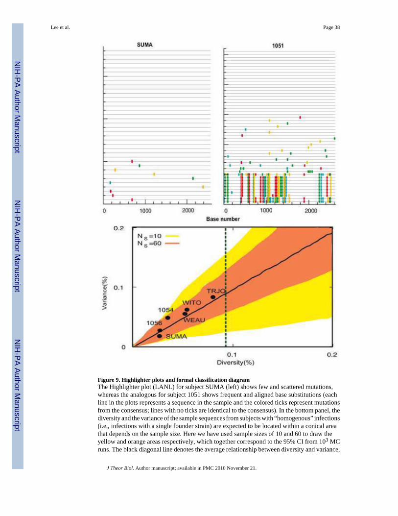
Figure 9. Highlighter plots and formal classification diagramThe Highlighter plot (LANL) for subject SUMA (left) shows few and scattered mutations,whereas the analogous for subject 1051 shows frequent and aligned base substitutions (eachline in the plots represents a sequence in the sample and the colored ticks represent mutationsfrom the consensus; lines with no ticks are identical to the consensus). In the bottom panel, thediversity and the variance of the sample sequences from subjects with “homogenous” infections(i.e., infections with a single founder strain) are expected to be located within a conical areathat depends on the sample size. Here we have used sample sizes of 10 and 60 to draw theyellow and orange areas respectively, which together correspond to the 95% CI from 103 MCruns. The black diagonal line denotes the average relationship between diversity and variance,

Lee et al.


NIH


NIH


NIH


and the dashed vertical line denotes the average % diversity expected at day 34, which is theupper limit of the cumulative duration for Fiebig stage II (see Table 1). Samples 1051 andBORI are classified as “heterogeneous” infections since there diversities are 0.73% and 1.7%(Table 4), respectively, which places them outside this window.

Lee et al.


NIH


NIH


NIH


Figure 10. Comparison between observed intersequence HD frequencies and the theoreticalfrequencies calculated from Eq. (19)The histograms are of the observed intersequence HD frequencies, whereas in red are thefrequencies computed according to Eq. (19). The two match perfectly except for WEAU, forwhich an overall 5% difference was found, and TRJO, for which the overall difference was15%.

Lee et al.


NIH


NIH


NIH


Figure 11. Comparison between BEAST results and Poisson model resultsThe number of generations per sample obtained fitting the Posson model (x-axis) and the onesobtained running the BEAST analysis (y-axis) over a set of 53 patients (Keele et al., 2008).

Lee et al.


NIH


NIH


NIH


NIH


NIH


NIH


Lee et al.

Table 1Fiebig stage classification for sub-stages of HIV-1 primary infection, and the average and cumulative duration of eachphase. The duration of each stage is presented in Keele et al. (Keele et al., 2008). We obtained 95% CIs, shown inparenthesis, by recalculating the confidence intervals presented by Fiebig et al. (Fiebig et al., 2003), through aquadrature method in the following manner. We assume that errors in estimating the length of each stage areuncorrelated, and that they add in quadrature in the cumulative, where the result of adding the numbers a and b isdefined as (Taylor, 1982). We use 7-21 days as the duration of the eclipse phase (Keele et al., 2008), and add 2 dayswith no further error to the duration of the first Fiebig stage because of the increased sensitivity of current assays overthe ones available when Fiebig et al. published their work

Stage Duration of each phase (days) Cumulative duration (days)

Eclipse 10 (7,21) 10 (7,21)

I (vRNA+) 7 (5,10) 17 (13,28)

II (p24Ag+) 5 (4,8) 22(18,34)

III (ELISA+) 3 (2,5) 25 (22,37)

IV (Western Blot +/-) 6 (4,8) 31 (27,43)

V (Western Blot +, p31-) 70 (40,122) 101 (71,154)

VI (Western Blot +, p31+) open-ended


NIH


NIH


NIH


Lee et al.

Table 2Analytical formulas for the basic quantities in the synchronous and asynchronous infection models. The expression forλn is given by Eq. (14)

Synchronous Infection Model Asynchronous Infection Model

Divergence εa ελn

Diversity 2εa 2ελn

Variance 2εa(1-ε)≃2εa 2ε(1-ε)λn≃2ελn

Maximum∑M=0

NB M × Psyn(H Dmax = M ∣ a) ∑M=0NB M × Pasyn(H Dmax = M ∣ n)

% Sequence Identity (1-ε)aNB e-λnεNB


NIH


NIH


NIH


Lee et al. Ta

ble

3Pa

tient

cha

ract

eris

tics a

t tim

e of

sam

plin

g, n

umbe

r of e

nvel

ope

sequ

ence

s obt

aine

d an

d th

eir l

engt

h, a

nd G

enB

ank

acce

ssio

n nu

mbe

rs

Subj

ect

Gen

der

Fieb

ig S

tage

Num

ber

of S

eque

nces

**B

ase

Len

gth

Vir

al L

oad

(cop

ies/

ml)

CD

4 C

ount

(cel

ls/m

l)G

enB

ank

Acc

essi

on N

umbe

r

WEA

U05

75M

II43

2581

216,

415

714

EU57

7344

-EU

5773

87

WIT

O41

60M

II16

2550

325,

064

247

EU57

7388

-EU

5774

03

TRJO

4551

MII

1625

748,

121,

951

336

EU57

7101

-EU

5771

18

SUM

A08

74M

II35

2568

939,

260

760

EU57

7039

-EU

5770

73

1054

MII

3625

6232

0,00

0N

AEU

5752

44-E

U57

5282

1056

MII

4625

8914

0,00

0N

AEU

5752

83-E

U57

5328

1051

FII

I50

2619

280,

000

NA

EU57

5134

-EU

5751

83

BO

RI0

637

MII

2926

072,

400,

000

902

EU57

6274

-EU

5763

02**

Num

ber o

f seq

uenc

es u

sed

in o

ur a

naly

sis.

Patie

nts W

EAU

, TR

JO a

nd 1

054

had

1, 2

and

3 a

dditi

onal

sequ

ence

s, re

spec

tivel

y, th

at w

ere

rem

oved

from

the

anal

yses

bec

ause

of l

arge

inte

rnal

del

etio

ns.


NIH


NIH


NIH


Lee et al. Ta

ble

4A

naly

sis o

f 8 H

IV-1

acut

e seq

uenc

e sam

ples

usin

g the

asyn

chro

nous

infe

ctio

n mod

el. F

or ea

ch su

bjec

t, w

e cal

cula

ted d

iver

genc

e, di

vers

ityan

d m

axim

um in

ters

eque

nce H

D. T

he p

aram

eter

λ o

f the

bes

t fitt

ing

Pois

son

dist

ribut

ion

is g

iven

for t

he 6

low

div

ersi

ty su

bjec

ts, t

oget

her

with

95%

con

fiden

ce in

terv

als.

Day

s sin

ce in

fect

ion

are

calc

ulat

ed fr

om th

e Po

isso

n fit

bas

ed o

n th

e va

lue

of λ

usi

ng E

q. (2

2) w

ith τ a

=1.

5 da

ys (K

eele

et a

l., (K

eele

et a

l., 2

008)

use

d τ a

=1.6

day

s, gi

ving

slig

htly

diff

eren

t est

imat

es).

In th

e M

C m

etho

d w

e co

mpu

ted

the

HD

I dis

tribu

tion

for e

ach

time

n an

d th

en u

sed

the

Kol

mog

orof

f-Sm

irnov

sta

tistic

to p

ick

the

dist

ribut

ion

that

bes

t fit

each

pat

ient

’sH

DI d

istri

butio

n (r

esul

ts s

how

n fo

r asy

nchr

onou

s m

odel

onl

y). T

he m

ean

time

sinc

e th

e M

RC

A a

nd 9

5% c

onfid

ence

inte

rval

s fo

r the

MC

bes

t fit

are o

btai

ned

from

103 s

imul

atio

ns. T

he fi

rst 6

subj

ects

, all

of w

hom

wer

e cha

ract

eriz

ed as

hav

ing

had

a hom

ogen

ous i

nfec

tion

wer

e in

Fie

big

stag

e II

, im

plyi

ng th

at th

eir e

stim

ated

tim

e fr

om in

fect

ion

had

a m

ean

of 2

2 da

ys a

nd ra

nged

bet

wee

n 18

and

34

days

(Tab

le 1

)

Subj

ect

Div

erge

nce

Div

ersi

tyV

aria

nce

Max

. HD

Sequ

en Id

entit

yλ

(95%

CIs

)E

stim

ated

tim

e (d

ays)

to M

RC

A fr

om P

oiss

onfit

(95%

CIs

)E

stim

ated

tim

e (d

ays)

to M

RC

A fr

om M

C(9

5% C

Is)

WEA

U05

750.

026

%0.

052

%0.

055

%6

51 %

1.34

(1.2

8,1.

40)

22 (1

7, 2

9)25

(14,

36)

WIT

O41

600.

027

%0.

054

%0.

062

%5

56 %

1.38

(1.3

2, 1

.43)

23 (1

2, 3

6)26

(12,

44)

TRJO

4551

0.04

1 %

0.08

0 %

0.08

3 %

644

%2.

06 (1

.99,

2.1

4)34

(22,

49)

37 (2

1,54

)

SUM

A08

740.

011

%0.

022

%0.

015

%2

71 %

0.57

(0.5

4, 0

.65)

10 (6

, 13)

14 (3

,21)

1054

0.01

7 %

0.03

5 %

0.04

8 %

572

%0.

89 (0

.84,

0.9

4)15

(9, 2

2)16

(6,2

6)

1056

0.01

3 %

0.02

7 %

0.02

7 %

471

%0.

70 (0

.66,

0.7

4)11

(7, 1

6)13

(5,2

1)

1051

0.42

%0.

73 %

22.4

%71

42 %

NA

NA

NA

BO

RI0

637

1.2

%1.

7 %

24.9

%77

19 %

NA

NA

NA


NIH


NIH


NIH


Lee et al.

Table 5Transition Matrix. Rows are “from”, columns are “to”

A G C T

A 0.5450 0.2475 0.1137 0.0937

G 0.3836 0.4357 0.0891 0.0915

C 0.2192 0.1108 0.4274 0.2425

T 0.1823 0.1149 0.2448 0.4581


Modeling sequence evolution in acute HIV1 infection

Documents

Transcript of Modeling sequence evolution in acute HIV1 infection