437

Modeling of water temperatures based onstochastic approaches: case study of theDeschutes River

Loubna Benyahya, André St-Hilaire, Taha B.M.J. Ouarda, Bernard Bobée, andBehrouz Ahmadi-Nedushan

Abstract: Water temperature is an important physical variable in aquatic ecosystems. It can affect both chemical andbiological processes such as dissolved oxygen concentration and both the metabolism and growth of aquatic organisms.For water resource management, stream water temperature models that can accurately reproduce the essential statisticalcharacteristics of historical data can be very useful. The present study deals with the modeling in the Deschutes River ofaverage weekly maximum temperature (AWMT) series using univariate stochastic approaches. Autoregressive (AR) andperiodic autoregressive (PAR) models were used to model AWMT data. The AR model consisted of decomposing watertemperature data into a long-term annual component and a residual component. The long-term annual component wasmodeled by fitting a sine function to the time series, while the residuals representing the departure from the long-termannual component were modeled using a Markov chain process. The PAR model was applied to the standardized dataobtained by subtracting the AWMT series from interannual mean of each period. To test the performance of the abovemodels, the leave-one-out (Jackknife) technique was used. The results indicated that both models have good predictiveability for a relatively large system such as the Dechutes River. On an annual basis from 1963 to 1980, the average rootmean square error varied between 0.81 and 0.90 ◦C for AR(1) and PAR(1), respectively, and the mean bias remained near0 ◦C. Averaged Nash-Sutcliffe coefficient of efficiency (NSC) values obtained by AR (0.94) and PAR (0.92) models wereclose and comparable. Of the two models, the PAR(1) model seemed the most promising based on its performance andability to model periodicity in autocorrelations. Since no exogenous variables such as air temperatures and streamflowwere incorporated, the use of the PAR model limits the managerial decisions in natural streams and rivers.

Key words: average weekly maximum temperature, stochastic model, PAR, AR.

Résumé : La température de l’eau est une variable physique importante des écosystèmes aquatiques. Elle peut affecterles procédés chimiques et biologiques, tels que les concentrations en oxygène dissous et le métabolisme et la croissancedes organismes aquatiques. Les modèles de température de l’eau des ruisseaux qui peuvent reproduire précisémentles caractéristiques statistiques essentielles des données historiques peuvent être très utiles en gestion de la ressourcehydrique. La présente étude traite de la modélisation d’une série de températures maximales hebdomadaires moyennes(AWMT) utilisant les approches stochastiques univariées pour la rivière Deschutes (Orégon, États-Unis). Deux différentsmodèles ont été utilisés pour modéliser les données de AWMT : un modèle autorégressif (AR) et un modèle autorégressifpériodique (PAR). Le modèle AR décompose les données de températures de l’eau en une composante annuelle à longterme et une composante résiduelle. La composante annuelle à long terme a été modélisée en ajustant une fonctionsinusoïdale à la série temporelle, alors que les résidus, qui étaient un écart par rapport à la composante annuelle à longterme, ont été modélisés en utilisant un processus de chaîne de Markov. Le modèle PAR a été appliqué aux donnéesnormalisées obtenues en soustrayant la série AWMT d’une moyenne interannuelle pour chaque période. La méthodedu « jackknife » a été utilisée pour valider les modèles ci-dessus. Les résultats indiquent que les deux modèles ont unebonne capacité prédictive pour des systèmes relativement gros tels que celui de la rivière Deschutes. Entre 1963 et 1980,l’erreur quadratique moyenne variait annuellement entre 0,81 ◦C et 0,90 ◦C pour AR(1) et PAR(1) respectivement. Lebiais demeurait près de 0 ◦C. Les moyennes des valeurs NSC obtenues par les modèles sont proches et donc comparables(respectivement 0,94 et 0,92). Des deux modèles, le modèle PAR(1) semblait le plus prometteur selon ses performanceset sa capacité à modéliser la périodicité dans les autocorrélations. Puisque aucune variable exogène (c.-à-d. températuresde l’air, débit du ruisseau) n’a été incorporée, l’utilisation du modèle PAR limite les décisions de gestion concernant lesrivières et les ruisseaux naturels.

Received 26 September 2005. Revision accepted 8 November 2006. Published on the NRC Research Press Web site at http://jees.nrc.ca/ on28 June 2007.

L. Benyahya,1 A. St-Hilaire, T.B.M.J. Ouarda, B. Bobée, and B. Ahmadi-Nedushan. Statistical Hydrology, National Institute of ScientificResearch (INRS)-ETE, Université du Québec, 490 de la Couronne Street, Québec, QC G1K 9A9, Canada.

Written discussion of this article is welcomed and will be received by the Editor until 30 November 2007.

1 Corresponding author (e-mail: Benyahyal@dfo-mpo.gc.ca).

J. Environ. Eng. Sci. 6: 437–448 (2007) doi: 10.1139/S06-067 © 2007 NRC Canada

438 J. Environ. Eng. Sci. Vol. 6, 2007

Mots-clés : température maximale hebdomadaire moyenne, modèle stochastique, modèle autorégressif périodique, modèleautorégressif.

[Traduit par la Rédaction]

Introduction

Water temperature is an important physical variable in aquaticecosystems. It can affect both chemical and biological processessuch as dissolved oxygen concentration and the metabolism andgrowth of aquatic organisms. In stream ecosystems, water tem-perature may influence stream fish (Li et al. 1994; Peterson andRabeni 1996) and aquatic insects (Vannote and Sweeney 1980;Ward and Stanford 1982). If a stream reach becomes increas-ingly warm and water temperature exceeds a certain tolerablelimit, cold water fish (e.g., Salmonids) will leave their habitatand search for thermal refuge (Eaton and Scheller 1996). If norefuge exists, temperature extremes may cause stress and evenfish mortality (Bjornn and Reiser 1991). For instance, Hodgsonand Quinn (2002) have demonstrated that during the spawn-ing season some species of Pacific salmon will suspend theirspawning activity when water temperature exceeds 19 ◦C.

The thermal regime of a watercourse is governed by the inter-action of natural environmental processes and human activities.Examples of the latter include thermal pollution (e.g., plant ef-fluents) and deforestation, which has been linked to temperaturerises in certain cases (Brown and Krygier 1970).

Given the importance of water temperature on lotic ecosys-tems, it is essential to provide efficient predictive tools to waterresource managers. Deterministic and stochastic temperaturemodeling approaches have been used in the past (Marceau etal. 1986). Deterministic approaches are based on the mathemat-ical representation of physical processes and the calculation ofan energy budget to predict stream water temperature. Depend-ing on the complexity of the model, the budget equations mayrequire numerous input parameters such as meteorological fac-tors (e.g., air temperature, solar radiation, and wind velocity)and physical characteristics of the stream (e.g., depth of water,flow, and forest cover). Examples of deterministic models in-clude those of Morin and Couillard (1990), Bartholow (1999),and St-Hilaire et al. (2003). One potential limitation of thismodeling approach results from the fact that some input vari-ables can be difficult and (or) expensive to measure. However,deterministic models are efficient tools when the user wants tosimulate modifications to some components of the heat budget(St-Hilaire et al. 2000). Consequently, they are very useful foranalyzing and comparing different impact scenarios because ofanthropogenic sources such as presence of reservoirs, thermalpollution, and deforestation.

Alternatively, stochastic approaches are based on statisticalfunctions that estimate water temperature with a limited numberof independent variables (e.g., water temperature of previousdays and air temperature). However, the disadvantage of theseapproaches is that they require long time series of water tem-perature for a particular stream. Examples of stochastic modelsinclude those of Pilgrim et al. (1998), who examined linear re-lationships between stream water temperature and air tempera-

ture for a number of sites in Minnesota. This study showed thatthe slope of the regression increased with increasing time scale(daily, weekly, and monthly). Mohseni et al. (1998) developeda nonlinear logistic function to predict average weekly streamtemperatures from air temperature at different locations in theUnited States that account for heat storage effects (hysteresis).More recently, Bélanger et al. (2005) modeled water tempera-tures in Catamaran Brook, a small (51 km2) stream catchmentin New Brunswick, Canada. They developed a neural networkand a multiple linear regression to relate water temperature toair temperature and discharge. They concluded that both ap-proaches are equally adequate in predicting stream water tem-peratures.

The so-called stochastic models are generally applied forsmaller time steps (e.g., daily). In this approach, the annualcomponent of the water temperatures is first removed and timeseries models are then fitted to water temperature residuals.For instance, Caissie et al. (1998, 2001) modeled mean andmaximum daily water temperatures in Catamaran Brook usingair temperatures as the independent variable. Their preferredmethodology involved estimating an annual component in watertemperatures by fitting a sinusoidal function and (or) Fourierseries to the data and a second order Markov process to theresiduals (Cluis 1972).

It can be seen from this brief literature review that stochasticmethods can be successfully applied to model water temper-atures at different time scales. However, to assess changes infish habitat and growth conditions, the weekly time scale isdeemed most appropriate (Eaton and Scheller 1996; Oliver andFidler 2001). Therefore, the general objective of this study wasto develop stochastic approaches to accurately predict averageweekly maximum temperatures (AWMT) at one site in the De-schutes River, a relatively large water course in the state ofOregon.

The timescale is an important deciding factor of time se-ries models. For example, many hydrological time series areperiodic and show seasonal variation. In many cases, seasonal-ity of the data cannot be removed by simple deseasonalizationto achieve stationary residuals because the correlation struc-ture of the series may be dependent on the period. In suchsituations, periodic models are more suitable because they areable to model periodicity in autocorrelations. Two popular peri-odic models are the periodic autoregressive (PAR) and periodicautoregressive-moving average (PARMA) models, which arebasically a group of autoregressive moving average (ARMA)models (Box and Jenkins 1976) that allow periodic parameters.Such models have been widely used in economic applications(Osborn and Smith 1989; Novales and de Frutto 1997) as well asin the field of hydrology (Salas et al. 1980; Vecchia 1985; Bar-tolini et al. 1988; Rasmussen et al. 1996, Ula and Smadi 1997).However, to our knowledge, the periodic models have not been

© 2007 NRC Canada

Benyahya et al. 439

previously used for water temperature modeling. Therefore, thepresent study was undertaken to study the suitability of an au-toregressive (AR) model and a PAR model to predictAWMT ona relatively large water course, to compare results of the mod-els, and to verify the efficiency of the two models to simulatewater temperature.

Methods

AR modelIn the present study, the AR model consists first of separat-

ing the water temperatures, Tw(t), into two different compo-nents: the long-term annual component, TA(t), and the short-term component or residuals, Rw(t), such as:

[1] Tw(t) = TA(t) + Rw(t)

where t represents the week of the year (e.g., t = 18 for the firstweek of May).

Each term in eq. [1] is modeled separately. The long-termannual component is computed by using the approach suggestedby Cluis (1972); i.e., fitting a sinusoidal function to the AWMTseries:

[2] TA(t) = a + b sin

[2π

52(T + t0)

]

where a and b are fitted coefficients so as to minimize the sumof squared errors and t0 is the mean time of departure from 0 ◦Cin the water temperature. The annual variation in water temper-atures can also be calculated by using an empirical interannualmean value.

The stationary residual component, which is obtained fromthe difference between the original time series and TA(t), ismodeled by using first- and second-order Markov Chains. Forinstance, the second-order Markov Chain is given by:

[3] Rw(t) = A1Rw(t − 1) + A2Rw(t − 2) + ε(t)

where Rw(t), Rw(t – 1), and Rw(t - 2) are, respectively, theresiduals of water temperature at time t, t −1, and t −2, and A1and A2 are regression coefficients, which are estimated usingthe least square method and ε(t) is the error term.

In the remainder of this article, the symbolsAR(1) andAR(2)represent the AR model with, respectively, first- and second-order Markov Chain as models of residuals.

PAR modelGiven Twν,τ an AWMT series, in which ν defines the year

with ν = 1, . . . , N , and τ defines the period with τ = 1, . . . , ω,the Twν,τ series can be written in the following matrix form:

[4]

Tw1,1 Tw1,2 . . . Tw1,ω

Tw2,1 Tw2,2 . . . Tw2,ω

......

...

TwN,1 TwN,2 . . . TwN,ω

where the process may be represented by a PAR(p) model (Salas1993) expressed as:

[5] Twν,τ = µτ +p∑

i=1

φi,τ

(Twν,τ−i − µτ−i

) + εν,τ

where p represents the order of the model. The model param-eters φi,τ and the mean µτ are functions of τ , and εν,τ is theerror term which is not included in the comparative study.

Since the autocorrelations vary for each period, the identi-fication of the appropriate PAR model order from the plot ofperiodic autocorrelation can become complicated. In such sit-uations, the simplest PAR models can be used. In the presentstudy, two PAR models, namely PAR(1) and PAR(2), were ad-justed to the stationary data. Low-order PAR models have beenwidely used in hydrology. Indeed, the PAR(1) model was orig-inally introduced by Thomas and Fiering (1962) for modelingmonthly streamflows.

Before applying the above models, it is necessary to ensurethat the original data conforms to the hypothesis of normality.Otherwise, the original series should be transformed. In thepresent study, the Shapiro-Wilk test (Shapiro and Wilk 1965)is used to test the normality of the data. This test is appropriatewhen the sample size is lower than 50.

PAR model parameters may be estimated by several methodssuch as the method of moments, the least squares method, orthe method of maximum likelihood (Salas 1993). In this study,the least squares (LS) method was adopted. Generally, estimatesobtained by this method have optimal statistical properties: theyare consistent, unbiased, and efficient (Hsia 1977). Hence, theparameters {φi,τ } of the model (eq. [5]) are independently esti-mated for each period by minimizing the sum of squared errors(ε2

ν,τ ):

[6]N∑

ν=1

ω∑τ=1

ε2ν,τ =

N∑ν=1

ω∑τ=1

[ (Twν,τ − µτ

)

−p∑

i=1

φi,τ

(Twν,τ−i − µτ−i

) ]2

Model evaluation and validationStochastic approaches require long time series of water tem-

perature for a particular stream or river. However, such tempo-rally prolonged water temperature series are scarce. Althoughthe time series used in this study can be considered relativelylong (18 years), it was deemed too short to validate the modelusing separate calibration and validation periods. Instead, theleave-one-out (Jackknife) technique (Quenouille 1949) wasused to test the performance of the above models. This methodconsists of removing one year (e.g., {X1,1 . . . X1,2 . . . . . . X1,ω})from the data set of matrix eq. [4] and estimating the model pa-rameters using the rest of data set. This allows the model to beused to estimate the temperature for the left-out year, with theestimated values being compared with measurements. The ideaof this method is to test if the model is able to make a correctprediction for the removed year.

© 2007 NRC Canada

440 J. Environ. Eng. Sci. Vol. 6, 2007

To evaluate the performance of AR(p) and PAR(p) models,three criteria are used. The first is the root mean square error(RMSE) (Janssen and Heuberger 1995), which is a combinedmeasure of bias and variance. It is given as:

[7] RMSE =√√√√1

n

n∑i=1

(Pi − Oi)2

where Pi and Oi are the predicted and observed weekly watertemperatures, respectively, and n is the number of data points.

The second criterion is the bias error (B), which is computedsimply as the sum of the differences between predicted andobserved values divided by n:

[8] B = 1

n

n∑i=1

(Pi − Oi)

where n is the number of data points.The third criterion is the Nash-Sutcliffe coefficient of effi-

ciency (NSC) (Nash and Sutcliffe 1970), which is <1 (equal to1 when P = 0), and is defined as:

[9] NSC = 1 −

n∑i=1

(Pi − Oi)2

n∑i=1

(O − Oi)2

where O is the average of observed weekly water temperaturevalues.

These criteria are calculated for each year left out for inter-annual comparison and then for each period for interperiodiccomparison.

Case study area and data set

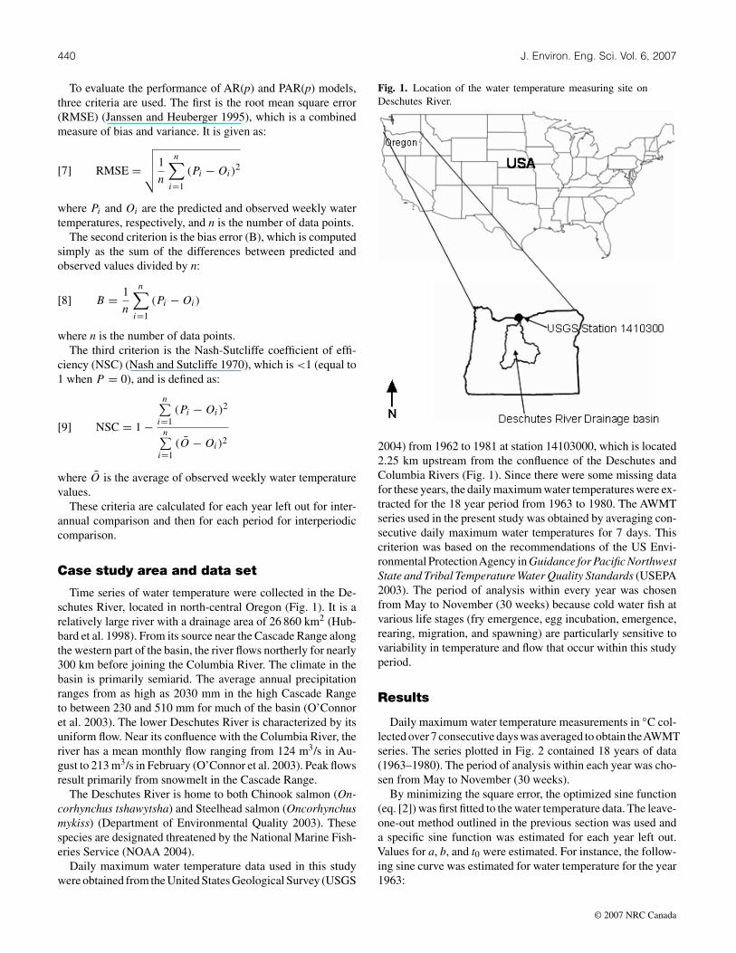
Time series of water temperature were collected in the De-schutes River, located in north-central Oregon (Fig. 1). It is arelatively large river with a drainage area of 26 860 km2 (Hub-bard et al. 1998). From its source near the Cascade Range alongthe western part of the basin, the river flows northerly for nearly300 km before joining the Columbia River. The climate in thebasin is primarily semiarid. The average annual precipitationranges from as high as 2030 mm in the high Cascade Rangeto between 230 and 510 mm for much of the basin (O’Connoret al. 2003). The lower Deschutes River is characterized by itsuniform flow. Near its confluence with the Columbia River, theriver has a mean monthly flow ranging from 124 m3/s in Au-gust to 213 m3/s in February (O’Connor et al. 2003). Peak flowsresult primarily from snowmelt in the Cascade Range.

The Deschutes River is home to both Chinook salmon (On-corhynchus tshawytsha) and Steelhead salmon (Oncorhynchusmykiss) (Department of Environmental Quality 2003). Thesespecies are designated threatened by the National Marine Fish-eries Service (NOAA 2004).

Daily maximum water temperature data used in this studywere obtained from the United States Geological Survey (USGS

Fig. 1. Location of the water temperature measuring site onDeschutes River.

2004) from 1962 to 1981 at station 14103000, which is located2.25 km upstream from the confluence of the Deschutes andColumbia Rivers (Fig. 1). Since there were some missing datafor these years, the daily maximum water temperatures were ex-tracted for the 18 year period from 1963 to 1980. The AWMTseries used in the present study was obtained by averaging con-secutive daily maximum water temperatures for 7 days. Thiscriterion was based on the recommendations of the US Envi-ronmental ProtectionAgency in Guidance for Pacific NorthwestState and Tribal Temperature Water Quality Standards (USEPA2003). The period of analysis within every year was chosenfrom May to November (30 weeks) because cold water fish atvarious life stages (fry emergence, egg incubation, emergence,rearing, migration, and spawning) are particularly sensitive tovariability in temperature and flow that occur within this studyperiod.

Results

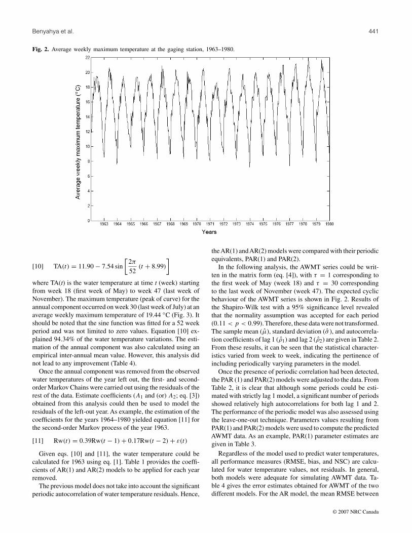
Daily maximum water temperature measurements in ◦C col-lected over 7 consecutive days was averaged to obtain theAWMTseries. The series plotted in Fig. 2 contained 18 years of data(1963–1980). The period of analysis within each year was cho-sen from May to November (30 weeks).

By minimizing the square error, the optimized sine function(eq. [2]) was first fitted to the water temperature data. The leave-one-out method outlined in the previous section was used anda specific sine function was estimated for each year left out.Values for a, b, and t0 were estimated. For instance, the follow-ing sine curve was estimated for water temperature for the year1963:

© 2007 NRC Canada

Benyahya et al. 441

Fig. 2. Average weekly maximum temperature at the gaging station, 1963–1980.

[10] TA(t) = 11.90 − 7.54 sin

[2π

52(t + 8.99)

]

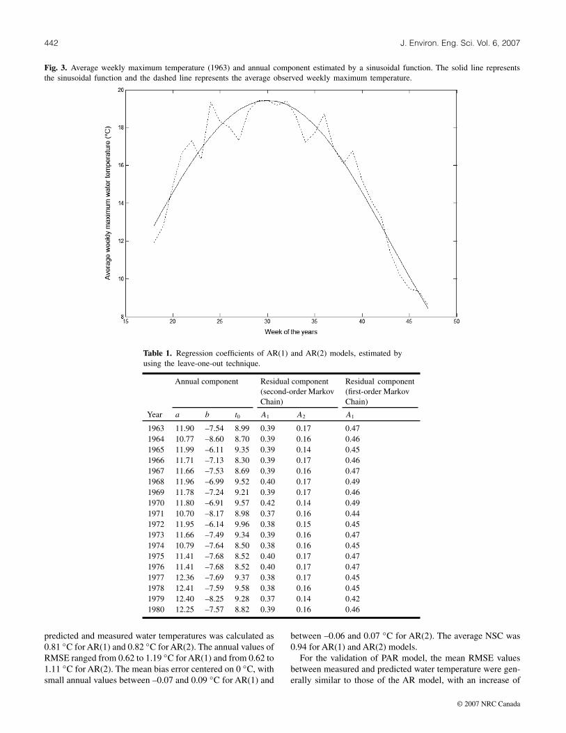
where TA(t) is the water temperature at time t (week) startingfrom week 18 (first week of May) to week 47 (last week ofNovember). The maximum temperature (peak of curve) for theannual component occurred on week 30 (last week of July) at anaverage weekly maximum temperature of 19.44 ◦C (Fig. 3). Itshould be noted that the sine function was fitted for a 52 weekperiod and was not limited to zero values. Equation [10] ex-plained 94.34% of the water temperature variations. The esti-mation of the annual component was also calculated using anempirical inter-annual mean value. However, this analysis didnot lead to any improvement (Table 4).

Once the annual component was removed from the observedwater temperatures of the year left out, the first- and second-order Markov Chains were carried out using the residuals of therest of the data. Estimate coefficients (A1 and (or) A2; eq. [3])obtained from this analysis could then be used to model theresiduals of the left-out year. As example, the estimation of thecoefficients for the years 1964–1980 yielded equation [11] forthe second-order Markov process of the year 1963.

[11] Rw(t) = 0.39Rw(t − 1) + 0.17Rw(t − 2) + ε(t)

Given eqs. [10] and [11], the water temperature could becalculated for 1963 using eq. [1]. Table 1 provides the coeffi-cients of AR(1) and AR(2) models to be applied for each yearremoved.

The previous model does not take into account the significantperiodic autocorrelation of water temperature residuals. Hence,

theAR(1) andAR(2) models were compared with their periodicequivalents, PAR(1) and PAR(2).

In the following analysis, the AWMT series could be writ-ten in the matrix form (eq. [4]), with τ = 1 corresponding tothe first week of May (week 18) and τ = 30 correspondingto the last week of November (week 47). The expected cyclicbehaviour of the AWMT series is shown in Fig. 2. Results ofthe Shapiro-Wilk test with a 95% significance level revealedthat the normality assumption was accepted for each period(0.11 < p < 0.99). Therefore, these data were not transformed.The sample mean (µ), standard deviation (σ ), and autocorrela-tion coefficients of lag 1 (ρ1) and lag 2 (ρ2) are given in Table 2.From these results, it can be seen that the statistical character-istics varied from week to week, indicating the pertinence ofincluding periodically varying parameters in the model.

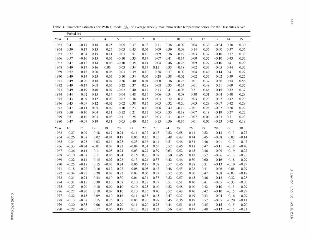
Once the presence of periodic correlation had been detected,the PAR (1) and PAR(2) models were adjusted to the data. FromTable 2, it is clear that although some periods could be esti-mated with strictly lag 1 model, a significant number of periodsshowed relatively high autocorrelations for both lag 1 and 2.The performance of the periodic model was also assessed usingthe leave-one-out technique. Parameters values resulting fromPAR(1) and PAR(2) models were used to compute the predictedAWMT data. As an example, PAR(1) parameter estimates aregiven in Table 3.

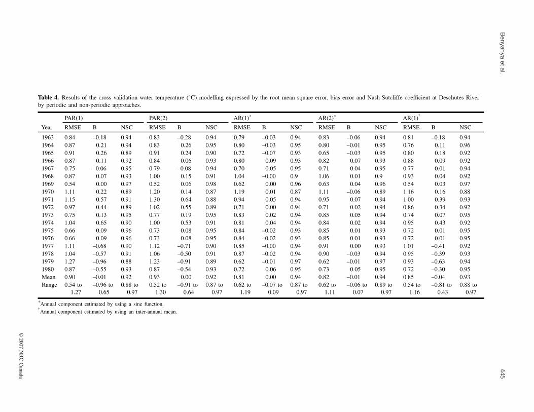
Regardless of the model used to predict water temperatures,all performance measures (RMSE, bias, and NSC) are calcu-lated for water temperature values, not residuals. In general,both models were adequate for simulating AWMT data. Ta-ble 4 gives the error estimates obtained for AWMT of the twodifferent models. For the AR model, the mean RMSE between

© 2007 NRC Canada

442 J. Environ. Eng. Sci. Vol. 6, 2007

Fig. 3. Average weekly maximum temperature (1963) and annual component estimated by a sinusoidal function. The solid line representsthe sinusoidal function and the dashed line represents the average observed weekly maximum temperature.

Table 1. Regression coefficients of AR(1) and AR(2) models, estimated byusing the leave-one-out technique.

Annual component Residual component(second-order MarkovChain)

Residual component(first-order MarkovChain)

Year a b t0 A1 A2 A1

1963 11.90 –7.54 8.99 0.39 0.17 0.471964 10.77 –8.60 8.70 0.39 0.16 0.461965 11.99 –6.11 9.35 0.39 0.14 0.451966 11.71 –7.13 8.30 0.39 0.17 0.461967 11.66 –7.53 8.69 0.39 0.16 0.471968 11.96 –6.99 9.52 0.40 0.17 0.491969 11.78 –7.24 9.21 0.39 0.17 0.461970 11.80 –6.91 9.57 0.42 0.14 0.491971 10.70 –8.17 8.98 0.37 0.16 0.441972 11.95 –6.14 9.96 0.38 0.15 0.451973 11.66 –7.49 9.34 0.39 0.16 0.471974 10.79 –7.64 8.50 0.38 0.16 0.451975 11.41 –7.68 8.52 0.40 0.17 0.471976 11.41 –7.68 8.52 0.40 0.17 0.471977 12.36 –7.69 9.37 0.38 0.17 0.451978 12.41 –7.59 9.58 0.38 0.16 0.451979 12.40 –8.25 9.28 0.37 0.14 0.421980 12.25 –7.57 8.82 0.39 0.16 0.46

predicted and measured water temperatures was calculated as0.81 ◦C for AR(1) and 0.82 ◦C for AR(2). The annual values ofRMSE ranged from 0.62 to 1.19 ◦C for AR(1) and from 0.62 to1.11 ◦C for AR(2). The mean bias error centered on 0 ◦C, withsmall annual values between –0.07 and 0.09 ◦C for AR(1) and

between –0.06 and 0.07 ◦C for AR(2). The average NSC was0.94 for AR(1) and AR(2) models.

For the validation of PAR model, the mean RMSE valuesbetween measured and predicted water temperature were gen-erally similar to those of the AR model, with an increase of

© 2007 NRC Canada

Benyahya et al. 443

Table 2. Sample mean, standard deviation, andautocorrelation coefficients of lag 1 and lag 2 ofaverage weekly maximum temperature series for theDeschutes River.

Period (τ ) µ σ ρ1(τ ) ρ2(τ )

1 13.00 1.08 –0.23 0.202 13.78 0.89 0.17 0.143 14.41 1.33 0.36 0.234 14.95 0.91 0.40 –0.035 15.95 1.38 0.31 0.506 16.44 1.30 0.66 0.377 16.90 1.19 0.37 0.328 17.61 1.24 0.22 0.499 17.72 1.10 0.58 0.47

10 18.65 1.14 0.13 0.2811 18.92 0.93 0.42 0.5312 19.49 1.23 0.60 0.1113 19.91 0.80 0.67 0.5314 19.61 0.84 0.58 0.5315 19.51 0.80 0.62 0.6616 18.60 1.02 0.52 0.2717 18.00 0.72 0.44 0.3618 17.48 0.78 –0.09 –0.1719 17.29 1.03 0.15 –0.1220 16.46 0.90 0.67 –0.1021 15.75 0.92 0.47 0.6122 15.30 1.13 0.64 0.4823 14.07 1.02 0.53 0.4424 13.34 0.72 0.64 0.3725 12.43 0.88 0.48 0.2926 11.40 0.90 0.51 0.2227 10.83 0.81 0.41 0.2428 9.94 0.73 0.54 0.3129 9.15 0.88 0.54 0.1830 8.50 0.55 0.25 0.36

0.09 ◦C for PAR(1) and 0.11 ◦C for PAR(2) (Table 4). The an-nual values of RMSE ranged from 0.54 to 1.27 ◦C for PAR(1)and varied between 0.52 and 1.30 ◦C for PAR(2). The meanbias errors centered on 0 ◦C, while the annual values rangedfrom –0.96 to 0.65 ◦C for PAR(1) and from –0.91 to 0.64 ◦Cfor PAR(2). Also, the results presented in Table 4 indicate thatthe PAR models were more negatively biased between 1977and 1980. The average NSC was 0.92 for PAR(1) and PAR(2)models.

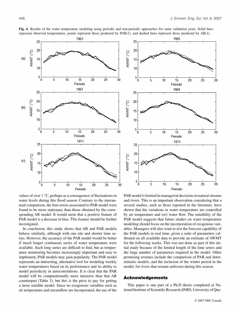
The slightly better performance of AR(1) and PAR(1) is anindication that parsimony should remain a guiding criterionwhen choosing a model. These results also suggest that there isno need to consider higher order AR and PAR models. The effi-ciency of the AR (1) and PAR(1) fit for some years is illustratedin Fig. 4. It can be seen that both models generally reproducedthe annual cycle and followed weekly data very closely.

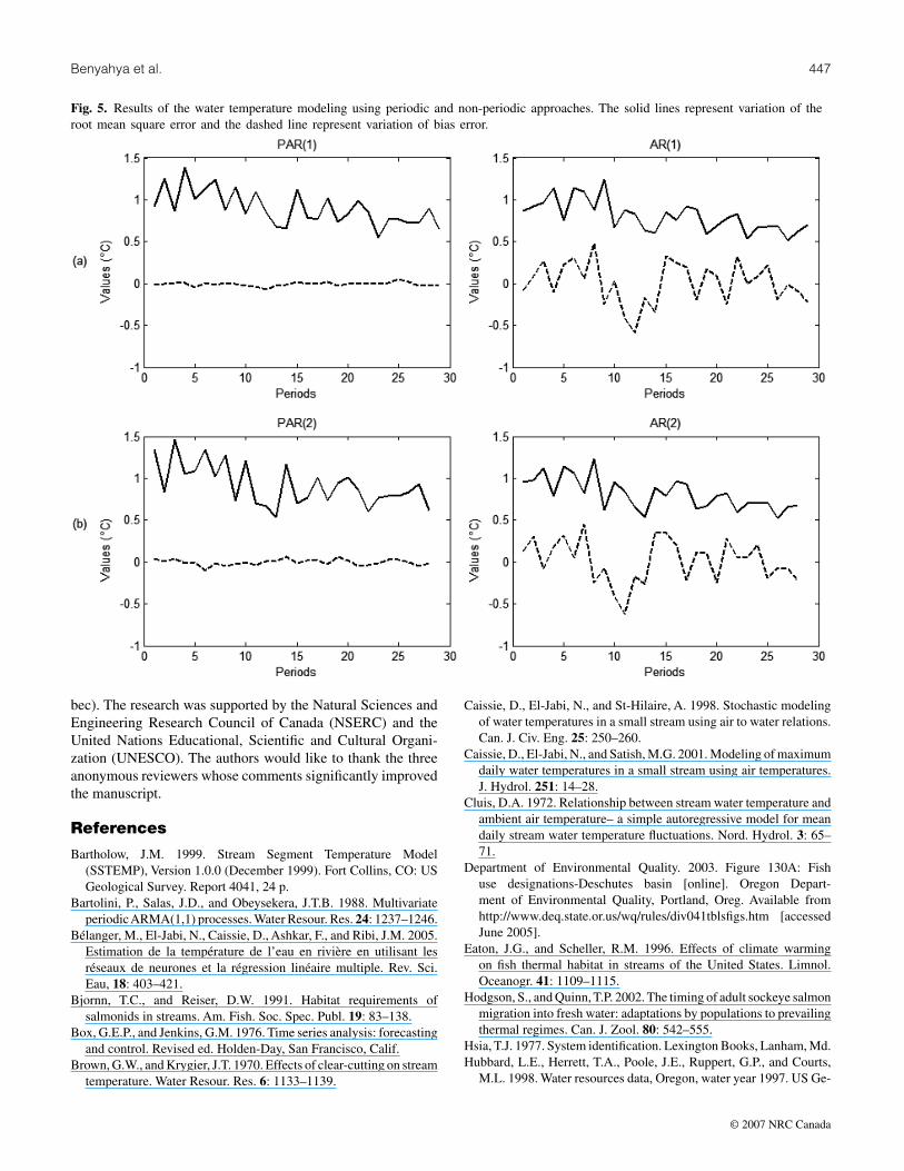
The performance measures (RMSE and bias) also variedfrom week to week and the overall results of the AR and PARmodels showed that the highest values of RMSE were observedduring the spring, with values of over 1 ◦C (Fig. 5). A higher

value of RMSE in the spring was likely owing to higher varia-tion in water levels during that season. Inversely to interannualcomparison, it was also observed from this figure that the biaserrors associated to PAR model centered on 0 ◦C, while thoseobtained by AR model showed the highest variation, rangingfrom –0.59 to 0.48 ◦C for AR(1) and from –0.62 to 0.45 ◦C forAR(2). This was expected, as the PAR model adds an importantcomponent to the corresponding AR model.

Discussion and conclusions

The prediction of water temperature data is important for theadequate management of water resources systems. Given theimportance of water temperature to lotic ecosystems, it is essen-tial to provide water resources managers with simple and goodpredictive models. For this purpose, the present study dealswith the modeling of AWMT series using univariate stochasticapproaches in Oregon’s Deschutes River. Two different mod-els were used to model AWMT data: an AR model and a PARmodel.

In the present study, the analysis of water temperatures viathe AR model consisted first of calculating the long-term an-nual component by fitting a sinusoidal function to water tem-peratures. After the annual component was removed from thetime series, the residuals series could be used to model wa-ter temperatures using first and second order Markov Chains.However, AR tools suffer from a drawback that their applica-tion requires that a fixed sinusoidal function be fitted to the timeseries. It can be argued that this may result in non-stationaryresiduals from year to year. On the other hand, this approachdoes not take into account the periodic autocorrelation in theweekly water temperature series, which is significant. To allevi-ate this problem, the PAR model was used. However, this modelalso suffers from the assumption that the distributions are nor-mal; therefore, the PAR model cannot be applied to fit periodictime series where density functions depart from a Gaussian dis-tribution. The PAR model is applied to the standardized data.To better compare models presently, the RMSE and bias errorwere calculated for each validation year (Table 4) and when theyears are predicted, these criteria were recalculated for eachweek (Fig. 5) of the analysis.

The results based on the RMSE, bias, and NSC criteria in-dicate that both models are equally good in predicting AWMTon a relatively large watercourse such as the Deschutes River.This is important, as AR models have been mostly developedfor smaller water courses (e.g., Caissie et al. 1998). For the ARmodel, mean RMSE values ranged from 0.81 to 0.82 ◦C. Themean bias errors centered on 0 ◦C with the smallest annual val-ues. The AR model led to a NSC of 0.94 on average. Comparedto the AR model, the PAR model showed an increase in meanRMSE less than 0.12 ◦C, which is minimal. The mean bias er-rors also centered on 0 ◦C, while the annual values showed thehighest variation. In terms of NSC, the average value was 0.92.When studying the model performances from week to week,it was found that periodic model and non-periodic model bothshowed the highest values of RMSE during the spring, with

© 2007 NRC Canada

444J.E

nviron.Eng

.Sci.Vol.6,2007

Table 3. Parameter estimates for PAR(1) model (φ1) of average weekly maximum water temperature series for the Deschutes River.

Period (τ )

Year 1 2 3 4 5 6 7 8 9 10 11 12 13 14 15

1963 0.41 –0.17 0.18 0.25 0.05 0.37 0.33 0.11 0.38 –0.09 0.04 0.30 –0.04 0.38 0.301964 0.39 –0.17 0.15 0.25 0.03 0.45 0.03 0.09 0.39 –0.09 0.14 0.36 0.00 0.37 0.351965 0.37 0.04 0.15 0.11 0.03 0.51 0.10 0.09 0.36 –0.19 –0.03 0.37 –0.10 0.37 0.331966 0.57 –0.10 0.15 0.07 –0.10 0.33 0.14 0.07 0.41 –0.14 0.00 0.32 –0.10 0.43 0.321967 0.47 –0.12 0.14 0.06 –0.10 0.35 0.14 0.04 0.46 –0.26 0.09 0.27 –0.10 0.41 0.291968 0.49 –0.17 0.16 0.06 0.03 0.34 0.14 0.15 0.35 –0.18 0.02 0.33 –0.05 0.44 0.321969 0.52 –0.13 0.20 0.06 0.03 0.39 0.10 0.28 0.37 0.02 0.04 0.40 –0.14 0.41 0.271970 0.49 0.14 0.23 0.07 0.10 0.34 0.05 0.28 0.38 –0.02 0.02 0.33 0.02 0.39 0.271971 0.49 –0.20 0.18 0.07 0.36 0.40 0.04 –0.00 0.36 –0.23 0.01 0.37 0.36 0.54 0.581972 0.49 –0.17 0.08 0.05 0.22 0.37 0.28 0.08 0.35 –0.24 0.01 0.48 0.21 0.69 0.371973 0.49 –0.19 0.40 0.07 –0.02 0.40 0.17 0.13 0.41 –0.06 0.31 0.46 0.15 0.52 0.371974 0.44 0.02 0.15 0.14 0.04 0.48 0.15 0.06 0.34 –0.08 0.30 0.31 –0.04 0.40 0.281975 0.43 –0.09 0.12 –0.02 0.02 0.38 0.15 0.03 0.32 –0.20 0.03 0.29 –0.07 0.42 0.291976 0.43 –0.09 0.12 –0.02 0.02 0.38 0.15 0.03 0.32 –0.20 0.03 0.29 –0.07 0.42 0.291977 0.47 –0.11 0.05 0.09 0.10 0.23 0.10 0.06 0.42 –0.12 –0.01 0.28 –0.07 0.28 0.221978 0.50 –0.10 0.04 0.11 –0.12 0.21 0.12 0.05 0.35 –0.18 –0.07 0.18 –0.19 0.27 0.221979 0.51 –0.10 0.03 0.03 –0.11 0.25 0.13 0.03 0.31 –0.16 –0.07 –0.00 –0.23 0.31 0.231980 0.47 –0.09 0.19 0.11 0.05 0.40 0.15 0.13 0.36 –0.16 0.01 0.03 –0.23 0.42 0.19

Year 16 17 18 19 20 21 22 23 24 25 26 27 28 29 301963 –0.27 –0.09 0.18 0.17 0.24 0.11 0.32 0.47 0.52 0.58 0.41 0.52 –0.13 –0.13 –0.271964 –0.26 0.08 0.02 –0.04 0.19 0.05 0.13 0.35 0.48 0.48 0.44 0.45 –0.08 0.02 –0.141965 –0.24 –0.23 0.03 0.14 0.23 0.25 0.36 0.41 0.51 0.46 0.34 0.46 –0.01 –0.17 –0.421966 –0.33 –0.24 –0.01 0.09 0.21 –0.04 0.34 0.65 0.52 0.46 0.41 0.47 –0.11 –0.19 –0.401967 –0.26 –0.11 0.11 0.05 0.24 –0.03 0.27 0.39 0.63 0.52 0.45 0.46 –0.09 –0.19 –0.221968 –0.10 –0.08 0.11 0.06 0.24 0.16 0.25 0.38 0.50 0.46 0.43 0.52 –0.06 –0.13 –0.251969 –0.22 –0.14 0.15 –0.02 0.28 0.13 0.24 0.37 0.42 0.46 0.30 0.60 –0.16 –0.18 –0.291970 –0.25 –0.18 0.15 –0.03 0.24 0.06 0.19 0.38 0.57 0.46 0.28 0.31 –0.13 –0.10 –0.291971 –0.18 –0.22 0.16 0.12 0.22 0.08 0.05 0.42 0.48 0.45 0.28 0.41 0.06 0.08 –0.291972 –0.34 –0.25 0.20 0.07 0.22 0.03 0.06 0.37 0.52 0.35 0.30 0.47 0.08 –0.02 –0.181973 –0.21 –0.21 0.24 0.10 0.30 0.04 0.34 0.37 0.52 0.57 0.45 0.46 –0.12 –0.32 –0.281974 –0.31 –0.15 0.30 0.10 0.38 0.10 0.28 0.37 0.51 0.51 0.40 0.41 –0.05 –0.33 –0.301975 –0.27 –0.20 0.10 0.09 0.10 0.10 0.25 0.40 0.52 0.48 0.40 0.42 –0.10 –0.15 –0.291976 –0.27 –0.20 0.10 0.09 0.10 0.10 0.25 0.40 0.52 0.48 0.40 0.42 –0.10 –0.15 –0.291977 –0.22 –0.15 0.09 0.10 0.16 0.11 0.33 0.43 0.47 0.37 0.49 0.43 –0.04 –0.16 –0.291978 –0.13 –0.08 0.15 0.26 0.35 0.05 0.20 0.28 0.45 0.36 0.49 0.52 –0.05 –0.20 –0.111979 –0.30 –0.35 0.06 0.03 0.20 0.11 0.20 0.23 0.44 0.51 0.43 0.45 –0.15 –0.15 –0.201980 –0.28 –0.36 0.17 0.06 0.19 0.13 0.22 0.22 0.56 0.47 0.47 0.48 –0.13 –0.15 –0.21

©2007

NR

CC

anada

Benyahya

etal.445

Table 4. Results of the cross validation water temperature (◦C) modelling expressed by the root mean square error, bias error and Nash-Sutcliffe coefficient at Deschutes Riverby periodic and non-periodic approaches.

PAR(1) PAR(2) AR(1)* AR(2)* AR(1)†

Year RMSE B NSC RMSE B NSC RMSE B NSC RMSE B NSC RMSE B NSC

1963 0.84 –0.18 0.94 0.83 –0.28 0.94 0.79 –0.03 0.94 0.83 –0.06 0.94 0.81 –0.18 0.941964 0.87 0.21 0.94 0.83 0.26 0.95 0.80 –0.03 0.95 0.80 –0.01 0.95 0.76 0.11 0.961965 0.91 0.26 0.89 0.91 0.24 0.90 0.72 –0.07 0.93 0.65 –0.03 0.95 0.80 0.18 0.921966 0.87 0.11 0.92 0.84 0.06 0.93 0.80 0.09 0.93 0.82 0.07 0.93 0.88 0.09 0.921967 0.75 –0.06 0.95 0.79 –0.08 0.94 0.70 0.05 0.95 0.71 0.04 0.95 0.77 0.01 0.941968 0.87 0.07 0.93 1.00 0.15 0.91 1.04 –0.00 0.9 1.06 0.01 0.9 0.93 0.04 0.921969 0.54 0.00 0.97 0.52 0.06 0.98 0.62 0.00 0.96 0.63 0.04 0.96 0.54 0.03 0.971970 1.11 0.22 0.89 1.20 0.14 0.87 1.19 0.01 0.87 1.11 –0.06 0.89 1.16 0.16 0.881971 1.15 0.57 0.91 1.30 0.64 0.88 0.94 0.05 0.94 0.95 0.07 0.94 1.00 0.39 0.931972 0.97 0.44 0.89 1.02 0.55 0.89 0.71 0.00 0.94 0.71 0.02 0.94 0.86 0.34 0.921973 0.75 0.13 0.95 0.77 0.19 0.95 0.83 0.02 0.94 0.85 0.05 0.94 0.74 0.07 0.951974 1.04 0.65 0.90 1.00 0.53 0.91 0.81 0.04 0.94 0.84 0.02 0.94 0.95 0.43 0.921975 0.66 0.09 0.96 0.73 0.08 0.95 0.84 –0.02 0.93 0.85 0.01 0.93 0.72 0.01 0.951976 0.66 0.09 0.96 0.73 0.08 0.95 0.84 –0.02 0.93 0.85 0.01 0.93 0.72 0.01 0.951977 1.11 –0.68 0.90 1.12 –0.71 0.90 0.85 –0.00 0.94 0.91 0.00 0.93 1.01 –0.41 0.921978 1.04 –0.57 0.91 1.06 –0.50 0.91 0.87 –0.02 0.94 0.90 –0.03 0.94 0.95 –0.39 0.931979 1.27 –0.96 0.88 1.23 –0.91 0.89 0.62 –0.01 0.97 0.62 –0.01 0.97 0.93 –0.63 0.941980 0.87 –0.55 0.93 0.87 –0.54 0.93 0.72 0.06 0.95 0.73 0.05 0.95 0.72 –0.30 0.95Mean 0.90 –0.01 0.92 0.93 0.00 0.92 0.81 0.00 0.94 0.82 –0.01 0.94 0.85 –0.04 0.93Range 0.54 to

1.27–0.96 to

0.650.88 to

0.970.52 to

1.30–0.91 to

0.640.87 to

0.970.62 to

1.19–0.07 to

0.090.87 to

0.970.62 to

1.11–0.06 to

0.070.89 to

0.970.54 to

1.16–0.81 to

0.430.88 to

0.97

*Annual component estimated by using a sine function.†Annual component estimated by using an inter-annual mean.

©2007

NR

CC

anada

446 J. Environ. Eng. Sci. Vol. 6, 2007

Fig. 4. Results of the water temperature modeling using periodic and non-periodic approaches for same validation years. Solid linesrepresent observed temperatures, points represent those predicted by PAR(1), and dashed lines represent those predicted by AR(1).

values of over 1 ◦C, perhaps as a consequence of fluctuations inwater levels during this flood season. Contrary to the interan-nual comparison, the bias errors associated to PAR model werefound to be more stationary than those obtained by the corre-sponding AR model. It would seem that a positive feature ofPAR model is a decrease in bias. This feature should be furtherinvestigated.

In conclusion, this study shows that AR and PAR modelsbehave similarly, although with one site and shorter time se-ries. However, the accuracy of the PAR model would be betterif much longer continuous series of water temperature wereavailable. Such long series are difficult to find, but as temper-ature monitoring becomes increasingly important and easy toimplement, PAR models may gain popularity. The PAR modelrepresents an interesting, alternative tool for modeling weeklywater temperatures based on its performance and its ability tomodel periodicity in autocorrelations. It is clear that the PARmodel will be computationally more intensive than that ARcounterpart (Table 3), but this is the price to pay for gettinga more suitable model. Since no exogenous variables such asair temperature and streamflow are incorporated, the use of the

PAR model is limited in managerial decisions in natural streamsand rivers. This is an important observation considering that aseveral studies, such as those reported in the literature, haveshown that the variations in water temperature are controlledby air temperature and (or) water flow. The suitability of thePAR model suggests that future studies on water temperaturemodeling should focus on the incorporation of exogenous vari-ables. Managers will also want to test the forecast capability ofthe PAR models in real time, given a suite of parameters cal-ibrated on all available data to provide an estimate of AWMTfor the following weeks. This was not done as part of this ini-tial study because of the limited length of the time series andthe large number of parameters required in the model. Otherpromising avenues include the comparison of PAR and deter-ministic models, and the inclusion of the winter period in themodel, for rivers that remain unfrozen during this season.

Acknowledgements

This paper is one part of a Ph.D thesis completed at Na-tional Institute of Scientific Research (INRS, University of Que-

© 2007 NRC Canada

Benyahya et al. 447

Fig. 5. Results of the water temperature modeling using periodic and non-periodic approaches. The solid lines represent variation of theroot mean square error and the dashed line represent variation of bias error.

bec). The research was supported by the Natural Sciences andEngineering Research Council of Canada (NSERC) and theUnited Nations Educational, Scientific and Cultural Organi-zation (UNESCO). The authors would like to thank the threeanonymous reviewers whose comments significantly improvedthe manuscript.

References

Bartholow, J.M. 1999. Stream Segment Temperature Model(SSTEMP), Version 1.0.0 (December 1999). Fort Collins, CO: USGeological Survey. Report 4041, 24 p.

Bartolini, P., Salas, J.D., and Obeysekera, J.T.B. 1988. MultivariateperiodicARMA(1,1) processes. Water Resour. Res. 24: 1237–1246.

Bélanger, M., El-Jabi, N., Caissie, D., Ashkar, F., and Ribi, J.M. 2005.Estimation de la température de l’eau en rivière en utilisant lesréseaux de neurones et la régression linéaire multiple. Rev. Sci.Eau, 18: 403–421.

Bjornn, T.C., and Reiser, D.W. 1991. Habitat requirements ofsalmonids in streams. Am. Fish. Soc. Spec. Publ. 19: 83–138.

Box, G.E.P., and Jenkins, G.M. 1976. Time series analysis: forecastingand control. Revised ed. Holden-Day, San Francisco, Calif.

Brown, G.W., and Krygier, J.T. 1970. Effects of clear-cutting on streamtemperature. Water Resour. Res. 6: 1133–1139.

Caissie, D., El-Jabi, N., and St-Hilaire, A. 1998. Stochastic modelingof water temperatures in a small stream using air to water relations.Can. J. Civ. Eng. 25: 250–260.

Caissie, D., El-Jabi, N., and Satish, M.G. 2001. Modeling of maximumdaily water temperatures in a small stream using air temperatures.J. Hydrol. 251: 14–28.

Cluis, D.A. 1972. Relationship between stream water temperature andambient air temperature– a simple autoregressive model for meandaily stream water temperature fluctuations. Nord. Hydrol. 3: 65–71.

Department of Environmental Quality. 2003. Figure 130A: Fishuse designations-Deschutes basin [online]. Oregon Depart-ment of Environmental Quality, Portland, Oreg. Available fromhttp://www.deq.state.or.us/wq/rules/div041tblsfigs.htm [accessedJune 2005].

Eaton, J.G., and Scheller, R.M. 1996. Effects of climate warmingon fish thermal habitat in streams of the United States. Limnol.Oceanogr. 41: 1109–1115.

Hodgson, S., and Quinn, T.P. 2002. The timing of adult sockeye salmonmigration into fresh water: adaptations by populations to prevailingthermal regimes. Can. J. Zool. 80: 542–555.

Hsia, T.J. 1977. System identification. Lexington Books, Lanham, Md.Hubbard, L.E., Herrett, T.A., Poole, J.E., Ruppert, G.P., and Courts,

M.L. 1998. Water resources data, Oregon, water year 1997. US Ge-

© 2007 NRC Canada

448 J. Environ. Eng. Sci. Vol. 6, 2007

ological Survey, Water-Data Rep. OR-97-1, Oregon Water ScienceCenter, Portland, Oreg.

Janssen, P.H.M., and Heuberger, P.S.C. 1995. Calibration of processoriented models. Ecol. Model. 83: 55–66.

Li, H.W., Lamberti, G.A., Pearsons,T.N., Tait, C.K., Li, J.L., and Buck-house, J.C. 1994. Cumulative effects of riparian disturbances alonghigh desert trout streams of the John Day Basin, Oregon. Trans.Am. Fish. Soc. 123: 627–640.

Marceau, P., Cluis, D., and Morin, G. 1986. Comparaison des perfor-mances relatives à un modèle déterministe et à un modèle stochas-tique de température de l’eau en rivière. Can. J. Civ. Eng. 13: 352–364.

Mohseni, O., Stefan, H.G., and Erickson, T.R. 1998. Nonlinear regres-sion model for weekly stream temperatures. Water Resour. Res. 34:2685–2692.

Morin, G., and Couillard, D. 1990. Predicting river temperatures witha hydrological model. Chapter 5. Encyclopedia of Fluid Mechanics:Surface and Groundwater Flow Phenomena. Volk Gulf PublishingCompany, Houston, Tex. pp. 171–209.

Nash, J.E., and Sutcliffe, J.V. 1970. River flow forecasting throughconceptual models. Part A. Discussion of principles. J. Hydrol. 10:282–290.

NOAA. 2004. Endangered species act: status reviews and listing infor-mation [online]. National Marine Fisheries Service, NOAA, Seattle,Wash. Available from http://www.nwr.noaa.gov [updated 12 June2007].

Novales,A., and de Fruto, R.F. 1997. Forecasting with periodic models:a comparison with time invariant coefficient models. Int. J. Forecast.13: 393–405.

O’Connor, J.E., Grant, G.E., and Haluska, T.L. 2003. Overview ofgeology, hydrology, geomorphology, and sediment budget of theDeschutes River basin, Oregon. In A peculiar river: geology, geo-morphology, and hydrology of the Deschutes River, Oregon. Editedby J.E. O’Connor and G.E. Grant. American Geophysical Union,Washington, D.C. Water Sci. Appl. Ser. 7: 7–30. Available fromwww.fsl.orst.edu/wpg/pubs/OConnor_Paper.01.pdf [accessed June2005].

Oliver, G.G., and Fidler, L.E. 2001. Towards a water qualityguideline for temperature in the province of British Columbia.Ministry of Environment, Lands and Parks, Water ManagementBranch, Water Quality Section, Victoria, B.C. Available fromwww.env.gov.bc.ca/wat/wq/BCguidelines/temptech/index.html[accessed June 2005].

Osborn, D., and Smith, J. 1989. The performance of periodic autore-gressive models in forecasting seasonal UK consumption. J. Bus.Econ. Stat. 7: 117–127.

Peterson, J.T., and Rabeni, C.F. 1996. Natural thermal refugia for tem-perate warm water stream fishes. N. Am. J. Fish. Manag. 16: 738–746.

Pilgrim, J.M., Fang, X., and Stefan, H.G. 1998. Stream temperaturecorrelations with air temperature in Minnesota: implications forclimate warming, 1998. J. Am. Water Res. Assoc. 34: 1109–1121.

Quenouille, M. 1949. Approximate tests of correlation in time series.J. R. Stat. Soc. Ser. B. 11: 18–84.

Rasmussen, P.F., Salas, J.D., Fagherazzi, L., and Rassam, J.C. 1996.Estimation and validation of contemporaneous PARMA models forstreamflow simulation. Water Resour. Res. 32: 3151–3160.

Salas, J.D. 1993. Analysis and modelling of hydrologic time series.Chap. 19. In Handbook of hydrology. Editor-in-Chief D.R. Maid-ment. McGraw-Hill, New York.

Salas, J.D., Delleur, J.W., Yevjevich, V., and Lane, E.L. 1980. Appliedmodeling of hydrological time series. Water Resources Publica-tions, Littleton, Colo.

Shapiro, S.S., and Wilk, M.B. 1965. An analysis of variance test fornormality (complete samples). Biometrika, 52: 591–611.

St-Hilaire, A., Morin, G., El-Jabi, N., and Caissie, D. 2000. Watertemperature modeling in a small forested stream: implication offorest canopy and soil temperature. Can. J. Civ. Eng. 27: 1095–1108.

St-Hilaire, A., Morin, G., El-Jabi, N., and Caissie, D. 2003. Sensitiv-ity analysis of a deterministic water temperature model to forestcanopy and soil temperature in Catamaran Brook (New Brunswick,Canada). Hydrol. Process. 17: 2033–2047.

Thomas, H.A., and Fiering, M.B. 1962. Mathematical synthesis ofstreamflow sequences for analysis of river basins by simulation. InThe design of water resources systems. Edited by A. Maas, M.M.Hufschmidt, R. Dorfman, H.A. Thomas, S.A. Marglin, and G.M.Fair. Harvard University Press, Cambridge, Mass.

Ula, T.A., and Smadi, A.A. 1997. Periodic stationarity conditions forperiodic autoregressive moving average processes as eigen-valueproblems. Water Resour. Res. 33: 1929–1934.

USEPA. 2003. Region 10 guidance for Pacific Northwest state andtribal temperature water quality standards. US Environmental Pro-tection Agency, Portland, Oreg. Available from www.epa.gov [up-dated 30 May 2007].

US Geological Survey (USGS). 2004. USGS water data for the nation[online]. National Water Information System (NWIS), US Geolog-ical Survey, Reston, Va. Available from waterdata.usgs.gov/nwis[modified 24 November 2003].

Vannote, R.L., and Sweeney, B.W. 1980. Geographic analysis of ther-mal equilibria: a conceptual model for evaluating the effect of nat-ural and modified thermal regimes on aquatic insect communities.Am. Nat. 115: 667–695.

Vecchia, A.V. 1985. Periodic autoregressive-moving average(PARMA) modeling with applications to water resources. Water.Resour. Bull. 21: 721–730.

Ward, J.V., and Stanford, J.A. 1982. Thermal responses in the evolu-tionary ecology of aquatic insects. Ann. Rev. Entomol. 27: 97–117.

© 2007 NRC Canada