STOCHASTIC STRONG-MOTION SIMULATION OF THE

UMBRIA- MARCHE EARTHQUAKE OF SEPTEMBER 1997 (Mw 6):

COMPARISON OF DIFFERENT APPROACHES

R.R. Castro, F. Pacor, G. Franceschina, D. Bindi , G. Zonno and L. Luzi

ABSTRACT

We simulated strong motion records from the Umbria-Marche, Central Italy earthquake (Mw 6)

of September 1997 using a frequency-dependent S-wave radiation function. We compared the

observed acceleration spectra, from strong-motion instruments located in the near field and at

regional distances, with those simulated using the stochastic modeling technique of Beresnev

and Atkinson (1997, 1998), and modified to account for a frequency dependent radiation pattern

correction. By using the frequency-dependent radiation function previously obtained by Castro

et al. (2006) we reduced the overall fitting error of the acceleration spectra by about 9%. In

general, we observed that the frequency-dependent radiation pattern correction has a small

effect on the spectral amplitudes compared with site effects, which is an important factor

controlling the strong-motion records generated by the 1997 Umbria-Marche earthquake. In

addition, we modeled the observed ground-motion records using the dynamic corner frequency

model of Motazedian and Atkinson (2005) to reproduce the directivity effects, reducing the

average error of the spectral amplitudes by 24%. We concluded that although the frequency-

dependent radiation pattern correction affects the frequency content of the spectral amplitudes

simulated, site and directivity effects are more relevant.

1

Introduction

Stochastic modeling techniques for finite faults (e.g. Beresnev and Atkinson, 1997) simulate the

high-frequency ground-motion amplitudes by summing stochastic point sources. In this process

the S-wave radiation pattern is considered as independent of frequency and a constant average

value is used to model the source spectra. However, recent studies of S-wave radiation pattern,

using local earthquakes in Japan (Takenaka et al., 2003) and Central Italy (Castro et al., 2006),

show that at low frequencies (f<0.5 Hz) the observed radiation pattern is similar to that expected

from a double-couple source. However, at higher frequencies (f>0.5 Hz) the S-wave radiation

pattern varies randomly with frequency.

Several source studies have pointed out that the S-wave radiation pattern is not constant at high

frequencies (e.g. Liu and Helmberger, 1985; Vidale, 1989; Takenaka et al., 2003). These studies

suggest that the complexity of the source rupture process and the heterogeneity of the crust may

contribute to the frequency-dependent radiation pattern.

Because the stochastic modeling techniques simulate high-frequency ground-motion amplitudes

assuming that the radiation pattern is constant, we evaluate in this paper the effect of

incorporating a frequency-dependent S-wave radiation function in the stochastic finite-fault

technique of Beresnev and Atkinson (1997). We also analyze the dynamic corner frequency

model introduced by Motazedian and Atkinson (2005) to simulate ground motion. In this model

the energy radiated by each subfault is controlled by the rupture history and the corner

frequency is a function of time.

In particular, we simulated strong-motion records from the Umbria-Marche, Central Italy

earthquake (Mw6) of September 1997 using a frequency-dependent S-wave radiation function

determined empirically by Castro et al. (2006). We choose this event because the source

parameters are well known from previous studies. This earthquake, also known as the 1997

Colfiorito earthquake, ruptured a fault segment nearly 12 km long (De Martini and Valensise,

2

1999; Hunstad et al., 1999, Salvi et al., 2000; Stramondo et al., 1999; Zollo et al., 1999;

Capuano et al., 2000). The extent of the rupture area of nearly 50 km was determined by Amato

et al. (1998) and Deschamps et al. (2000). The normal faulting focal mechanism was well

constrained using long-period wave forms (Ekstrom et al., 1998), and the slip distribution

obtained by forward and inverse modeling of GPS measurements and SAR interferograms

(Stramondo et al., 1999; Hunstad et al., 1999; Salvi et al., 2000). Based on the distribution of

PGA at the triggered strong-motion stations, Castro et al. (2001) reported evident effects of

rupture directivity toward the northwest from the epicenter. In particular, the PGA at Nocera

Umbra (NOC), located in the direction of rupture propagation, is more than a factor of two the

value predicted by the empirical regression model proposed by Sabetta and Pugliese (1987).

The strong-motion records from stations located in the near field have been also previously

modeled by Berardi et al. (2000) and Castro et al. (2001) using a stochastic simulation

approach. Figure 1 shows the location of the main event of the 1997-1998 Umbria-Marche

sequence and the distribution of strong-motion stations used by Castro et al. (2001) and also in

this paper. The acceleration time records were corrected for baseline, instrument response and

band-pass-filtering to avoid long-period biases and high-frequency noise with band-pass

frequencies ranging between 0.05 and 27 Hz. Thus, at low frequencies the acceleration spectra

are reliable above 0.05 for station NOC, above 0.18 for CLF, ASI and BVG and above 0.55 for

MNF and MAT.

Frequency Dependent Radiation Pattern

Castro et al. (2006) used local earthquakes registered during the 1997-1998 Umbria-Marche

aftershock sequence to analyze the frequency dependence of the S-wave radiation pattern. Most

of the earthquakes analyzed are normal fault events that occurred at shallow depths (H<6.3 km).

They separated source and path effects using a spectral inversion technique and then the

3

radiation pattern was isolated from other source related effects by calculating the fraction of

SH-wave contribution to the total S-wave energy following the same procedure used by

Takenaka et al., (2003).

)()()()( 22

2

fSfSfSfR

SHSV

SHSH +

= ( 1 )

Where SSH(f) and SSV(f) are the amplitudes of the SH- and SV-waves source functions,

respectively, obtained from the spectral inversion. RSH(f) can be considered a measure of the

radiation pattern of SH waves.

Castro et al. (2006) found that in general the low frequency SH energy approaches that

expected from a double-couple source. In particular, at 0.34 Hz the fraction of SH energy is

about the same, but at higher frequencies (f > 0.5 Hz) the radiation pattern varies randomly with

frequency.

Figure 2 shows the average SH radiation pattern function obtained by Castro et al. (2006) using

22 aftershocks of the sequence with magnitudes ranging between 3.3 and 5.6. This function

shows a maximum between 2 and 4 Hz and then varies randomly with frequency. It is also

interesting to note that the mean value in the frequency band shown (0.3-24 Hz) is 0.6,

consistent with previous estimates of the average S-wave radiation pattern (Boore and

Boatwright, 1984).

The average fraction of SH energy estimated by Castro et al. (2006) can be projected on the NS-

EW directions using the take-off angle of the strong-motion station to be modeled. We did that

to be able to model the observed NS and EW spectral components. Figure 3 shows the projected

SH-wave energy for the six stations modeled. These functions represent the S-wave radiation

pattern at each recording site. In general, the values of RSH vary between 0.5 and 0.9.

4

Stochastic Finite-Fault Modeling

Frequency Dependent Radiation Pattern

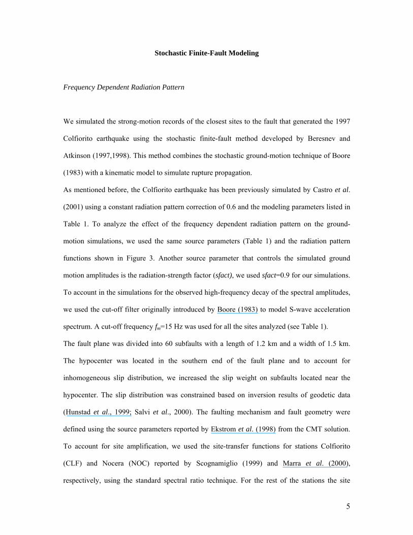
We simulated the strong-motion records of the closest sites to the fault that generated the 1997

Colfiorito earthquake using the stochastic finite-fault method developed by Beresnev and

Atkinson (1997,1998). This method combines the stochastic ground-motion technique of Boore

(1983) with a kinematic model to simulate rupture propagation.

As mentioned before, the Colfiorito earthquake has been previously simulated by Castro et al.

(2001) using a constant radiation pattern correction of 0.6 and the modeling parameters listed in

Table 1. To analyze the effect of the frequency dependent radiation pattern on the ground-

motion simulations, we used the same source parameters (Table 1) and the radiation pattern

functions shown in Figure 3. Another source parameter that controls the simulated ground

motion amplitudes is the radiation-strength factor (sfact), we used sfact=0.9 for our simulations.

To account in the simulations for the observed high-frequency decay of the spectral amplitudes,

we used the cut-off filter originally introduced by Boore (1983) to model S-wave acceleration

spectrum. A cut-off frequency fm=15 Hz was used for all the sites analyzed (see Table 1).

The fault plane was divided into 60 subfaults with a length of 1.2 km and a width of 1.5 km.

The hypocenter was located in the southern end of the fault plane and to account for

inhomogeneous slip distribution, we increased the slip weight on subfaults located near the

hypocenter. The slip distribution was constrained based on inversion results of geodetic data

(Hunstad et al., 1999; Salvi et al., 2000). The faulting mechanism and fault geometry were

defined using the source parameters reported by Ekstrom et al. (1998) from the CMT solution.

To account for site amplification, we used the site-transfer functions for stations Colfiorito

(CLF) and Nocera (NOC) reported by Scognamiglio (1999) and Marra et al. (2000),

respectively, using the standard spectral ratio technique. For the rest of the stations the site

5

amplification factors were estimated using horizontal to vertical spectral ratios (Castro et al.,

2001). The amplification factors displayed by these site functions vary from about 14 for station

NOC, located on alluvial deposits, to 1.6 for station MNF, which is on rock (Figure 4). Station

ASI is also on rock, CLF and BVG on lacustrine deposits, and MAT on alluvial deposits (Luzi

et al., 2005). The records simulated were also corrected for attenuation using the relation

Q(f)=77 f 0.6 obtained by Castro et al. (2000 and 2002) with earthquakes from the 1997 Umbria-

Marche sequence and a geometrical spreading function of the form G(r)=1/r, where r is the

hypocentral distance. For consistency we used the same geometrical spreading function for the

simulations.

The distance-dependent duration was also estimated in the previous study for each site by

calculating the observed average duration of both horizontal components records from

aftershocks of the sequence.

Dynamic Corner Frequency

Motazedian and Atkinson (2005) introduced a new approach to the stochastic finite-fault model

of Beresnev and Atkinson (1998) based on a dynamic corner frequency. In this new model the

frequency content of the simulated ground motion of each subfault is controlled by the rupture

history and the corner frequency is a function of time. The main advantage of the dynamic

corner frequency model is that the high frequency energy radiated is conserved, regardless of

subfault size, and consequently it is possible to use an arbitrary constant subfault size. Thus, the

new method has a wider magnitude range of application than previous versions of the stochastic

finite-fault models. There are two main model parameters: the stress drop that controls the high-

frequency spectral amplitude level and the percentage of pulsing area that controls the level of

spectra at low frequencies. The pulsing area parameter controls the percentage of active

subfaults during the rupture process and thus contributing to the dynamic corner frequency.

6

We used this new model to simulate the strong-motion records generated by the 1997 Colfiorito

earthquake. We used the same model parameters as before (see table 1) and try different values

of stress drop. Figure 5 shows the observed acceleration spectra at CLF, the closest station to

the source, and the spectral amplitudes calculated using a constant radiation pattern (left frame)

and using the frequency dependent radiation pattern (Figure 3). We made the same calculations

for all stations to calculate the model bias and the average error.

To quantify the fit between observed and simulated acceleration spectra, we define a model bias

as:

∑=

⎟⎟⎠

⎞⎜⎜⎝

⎛=

n

i isim

obs

fSfS

nfE

1 )()(

log1)( ( 2 )

Where n is the number of stations modeled and S(f) the acceleration spectra. We also define the

average error within the frequency band used to simulate the spectra as:

∑=

=m

jjfE

m 1

)(1ε ( 3 )

Where m is the number of frequencies considered in the analysis.

Figure 6 and Table 2 show the values E(f) and ε obtained for different values of stress drop.

When using a constant radiation pattern we have to reduce the stress drop to 100 bars to fit the

observed high-frequency amplitude level and to 50 bars when we use the frequency dependent

radiation pattern (see right frame of Figure 5). We also try different values of the percentage of

pulsing area, finding the best fit with a value of 35%, consistent with the slip distribution

reported by Hunstad et al. (1999).

7

Results

Figure 7 compares the observed (solid line) and the simulated acceleration spectra

(discontinuous lines). We also compare the spectral amplitudes simulated using a constant

radiation pattern for both the standard finite-source model of Beresnev and Atkinson (1997,

1998) (dotted lines) and the dynamic corner frequency model of Motazedian and Atkinson

(2005) (black dots) with those obtained using the frequency-dependent radiation pattern

functions in the standard finite-source technique (dashed lines). In general, the dynamic corner

frequency model provides the best fit, particularly at low frequencies (0.1-0.5 Hz) for stations

CLF, BVG and MAT. It is also interesting to note that for NOC, located in the direction of

rupture propagation, neither model reproduce the observed amplitudes that well, suggesting the

need of an additional directivity correction, as reported by Castro et al. (2001).

Figure 8 shows the model bias calculated with Equation (2) for the static corner frequency

model of Beresnev and Atkinson (1997) with constant radiation pattern (dotted line) and using

the frequency dependent functions (dashed line). In this model the corner frequency remains

constant during the whole rupture history. For the first the average error calculated with

Equation (3) equals 0.194 and for the latter 0.176. Although the overall error is smaller when a

frequency-dependent radiation is used, at high frequencies (f> 4 Hz) the constant radiation

pattern value of 0.55 gives a better fit. The dots in Figure 8 are the model bias calculated using

the dynamic corner frequency model with constant radiation pattern. As explained above, in this

model the corner frequency is a function of time. Note that at low frequencies this model

provides better fit than the frequency-dependent radiation model and at high frequencies a better

fit than the static corner frequency model with constant radiation pattern. We calculated an

average error of 0.146 using the dynamic corner frequency which is also smaller than that of the

other two models.

8

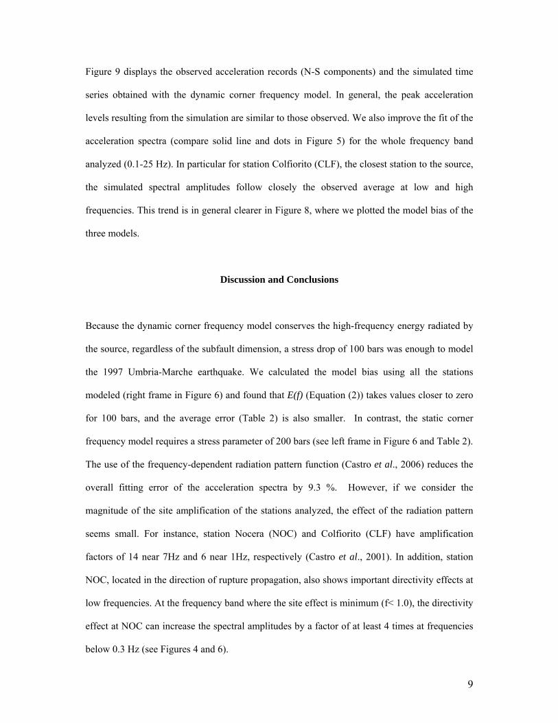
Figure 9 displays the observed acceleration records (N-S components) and the simulated time

series obtained with the dynamic corner frequency model. In general, the peak acceleration

levels resulting from the simulation are similar to those observed. We also improve the fit of the

acceleration spectra (compare solid line and dots in Figure 5) for the whole frequency band

analyzed (0.1-25 Hz). In particular for station Colfiorito (CLF), the closest station to the source,

the simulated spectral amplitudes follow closely the observed average at low and high

frequencies. This trend is in general clearer in Figure 8, where we plotted the model bias of the

three models.

Discussion and Conclusions

Because the dynamic corner frequency model conserves the high-frequency energy radiated by

the source, regardless of the subfault dimension, a stress drop of 100 bars was enough to model

the 1997 Umbria-Marche earthquake. We calculated the model bias using all the stations

modeled (right frame in Figure 6) and found that E(f) (Equation (2)) takes values closer to zero

for 100 bars, and the average error (Table 2) is also smaller. In contrast, the static corner

frequency model requires a stress parameter of 200 bars (see left frame in Figure 6 and Table 2).

The use of the frequency-dependent radiation pattern function (Castro et al., 2006) reduces the

overall fitting error of the acceleration spectra by 9.3 %. However, if we consider the

magnitude of the site amplification of the stations analyzed, the effect of the radiation pattern

seems small. For instance, station Nocera (NOC) and Colfiorito (CLF) have amplification

factors of 14 near 7Hz and 6 near 1Hz, respectively (Castro et al., 2001). In addition, station

NOC, located in the direction of rupture propagation, also shows important directivity effects at

low frequencies. At the frequency band where the site effect is minimum (f< 1.0), the directivity

effect at NOC can increase the spectral amplitudes by a factor of at least 4 times at frequencies

below 0.3 Hz (see Figures 4 and 6).

9

In conclusion, the frequency-dependent radiation pattern correction proposed in this study has a

small effect on the simulated spectral amplitudes, compared to site and directivity effects, which

are the most important factors controlling the strong-motion records generated by the 1997

Umbria-Marche earthquake.

Acknowledgments

We are grateful to Dariush Motazedian and Gail Atkinson for providing us with their computer

code EXSIM. This research was partially supported by the Mexican National Council of

Science and Technology (CONACYT) and the Istituto Nazionale di Geofisica e Vulcanologia

(INGV). We thank the Associate Editor Art McGarr, Basil Margaris and the anonymous

reviewer whose comments improved the quality of this paper.

10

References

Amato, A., R. Azzara, C. Chiarabba, G.B. Cimini, M. Cocco, M. DiBona, L. Margheriti, S.

Mazza, F. Mele, G. Selvaggi, A. Basili, E. Boschi, F. Courboulex, A. Deschamps, S.

Gaffet, G. Bittarelli, L. Chiaraluce, D. Piccinini, M. Ripepe (1998). The 1997 Umbria-

Marche, Italy, earthquake sequence: a first look of the main shock and aftershock,

Geophys. Res. Lett., 25, 2861-2864.

Berardi, R., M.J. Jiménez, G. Zonno, M. García-Fernández (2000). Calibration of stochastic

finite-fault ground motion simulations for the 1997 Umbria-marche, Central Italy,

earthquake sequence, Soil Dynam. and Earthq. Eng., 20, 315-324.

Beresnev, I.A. and G.M. Atkinson (1997). Modeling finite-fault radiation from the

spectrum, Bull. Seism. Soc. Am., 87, 67-84.

nω

Beresnev, I.A. and G.M. Atkinson (1998). FINSIM a Fortran program for simulating stochastic

acceleration time histories from finite faults, Seism. Res. Lett., 69, 27-32.

Boore, D.M. (1983). Stochastic simulation of high-frequency ground motions based on

seismological models of the radiated spectra, Bull. Seism. Soc. Am. 73, 1865-1894.

Boore, D.M., and J. Boatwright (1984). Average body-wave radiation coefficients, Bull. Seism.

Soc. Am., 74, 1615-1621.

Capuano P., A. Zollo, A, Emolo, S. Marcucci and G. Milana (2000). Rupture mechanism and

source parameters of Umbria-Marche mainshocks from strong motion data, J. of

Seismology, 4, 501-516 .

Castro, R.R., A. Rovelli, M. Cocco, M. Di Bona, and F. Pacor (2001). Stochastic simulation of

strong-motion records from the 26 September 1997 (Mw 6), Umbria-Marche (Central

Italy) earthquake, Bull. Seism. Soc. Am., 91, 27-39.

11

Castro, R.R., G. Franceschina, F. Pacor, D. Bindi, and L. Luzi (2006). Análisis of the frequency

dependence of the S-wave radiation pattern from local earthquakes in Central Italy,

Bull. Seism. Soc. Am. 96, 415-426.

De Martini, P.M. and G. Valensise (1999). Pre-seismic slip on the 26 September 1997, Umbria-

Marche earthquake fault? Unexpected clues from the analysis of 1951-1992

elevation changes, Geophys. Res. Lett., 26, 1953-1956.

Deschamps, A., F. Courboulex, S. Gaffet, A. Lomax, J. Virieux, A. Amato, R. Azzara, B.

Castello, C. Chiarabba, G.B. Cimini, M. Cocco, M. Di Bona, L. Margheriti, F.

Mele, G. Selvaggi, G. Bittarelli, L. Chiaraluce, D. Piccinini and M. Ripepe (1997).

The spatio-temporal distribution of seismic activity during the Umbria-Marche

crisis, (accepted on J. of Seismology).

Ekstrom, G., A. Morelli, E. Boschi and A.M. Dziewonski (1998). Moment tensor analysis of the

Central Italy earthquake sequence of September-October 1997, Geophys. Res. Lett., 25,

1971-1974.

Hunstad, I., M. Anzidei, M. Cocco, P. Baldi, A. Galvani and A. Pesci (1999). Modeling

coseismic displacements during the 1997 Umbria-Marche earthquake (Central Italy),

Geophys. J. Int., 139, 283-295.

Liu, H.L. and D.V. Helmberger (1985). The 23:19 aftershock of the 15 October 1979 Imperial

Valley earthquake: more evidence for an asperity, Bull. Seism. Soc. Am. 75, 689-708.

Luzi, L., D. Bindi, G. Franceschina, F. Pacor, and R.R. Castro (2005). Geotechnical site

characterisation in the Umbria-Marche area and evaluation of earthquake site-response,

Pure appl. Geophys. 162, 2133-2161.

Marra, F., R. Azzara, F. Bellucci, A. Caserta, G. Cultera, G. Mele, B. Palombo, A. Rovelli and

E. Boschi (2000). Large amplification of ground motion at rock sites within a fault zone

in Nocera Umbra (Central Italy), J. of Seismology, 4, 543-554.

12

Motazedian, D. and G. M. Atkinson (2005). Stochastic finite-fault modeling based on a

dynamic corner frequency, Bull. Seism. Soc. Am. 95, 995-1010.

Sabetta, F., and A. Pugliese (1987). Attenuation of peak horizontal acceleration and velocity

from Italian strong-motion records, Bull. Seism. Soc. Am. 77, 1491-1513.

Salvi, S., S. Stramondo, M. Cocco, M. Tesauro, I. Hunstad, M. Anzidei, P. Briole, P. Baldi, E.

Sansosti, G. Fornaro, R. Lanari, F. Doumaz, A. Pesci and A. Galvani (2000). Modeling

coseismic surface displacements resulting from SAR interferometry and GPS

measurements during the 1997 Umbria-Marche seismic sequence, J. of Seismology 4,

479-499.

Scognamiglio, L. (1999). Caratteri del moto di superficie in un bacinointramontano durante i

terromoti: il caso di Colfiorito, Thesis, University of Rome “Rama Tre”, Rome, Italy.

Stramondo S., M. Tesauro, P. Briole, E. Sansosti, S. Salvi, G. Lanari, M. Anzidei, P. Baldi, G.

Fornaro, A. Avallone, M.F. Buogiorno, R. Franceschetti and E. Boschi (1999). The

September 26, 1997 Colfiorito, Italy earthquakes: modeled coseismic surface

displacement from SAR interferometry and GPS, Geophys. Res. Lett., 26, 883-886.

Takenaka, H., Y. Mamada, and H. Futamure (2003). Near-source effect on radiation pattern of

high-frequency S waves: strong SH-SV mixing observed from aftershocks of the 1997

northwestern Kagoshima, Japan, earthquakes, Phys. Earth and Plan. Int., 137, 31-43.

Vidale, J.E. (1989). Influence of focal mechanism on peak accelerations of strong motions of

the Whittier Narrows, California, earthquake and an aftershock, Jour. Geophys. Res. 94,

9607-9613.

Zollo, A., S. Marcucci, G. Milana, G. Bongiovanni, P. Capuano, A. Emolo and A. Herrero

(1999). The 1997 Umbria-Marche (central Italy) earthquake sequence: Insights on the

mainshock ruptures from near source strong motion records Geoph. Res. Lett., 26,

3165-3168.

13

Centro de Investigación Científica y de Educación Superior de Ensenada (CICESE)

División Ciencias de la Tierra

Departamento de Sismología

km 107 Carretera Tijuana-Ensenada

22860 Ensenada, Baja California, México

raul@cicese.mx

(R.R.C.)

Istituto Nazionale di Geofisica e Vulcanologia,

Sezione di Milano,

Via Bassini 15, 20133 Milano, Italia

pacor@mi.ingv.it

(F.P., G.F., D.B., G.Z.,L.L.)

14

TABLE 1. Input Modeling Parameters

Fault orientation strike 1420 , dip 39 0 **

Fault dimensions length 12 km, width 9 km

Focal depth 6 km

Number of subfaults along strike 10, along dip 6

Shear wave velocity 3.2 km/s

Density 2.9 gr/cm3

Stress parameter 200 bars

Radiation-strength factor 0.9

fmax 15.0 Hz

Q(f) 77 f 0.6

Subfault corner frequency 0.91 Hz

Subfault rise time 0.50 s

Seismic Moment 1.14 x 10 25 dyne-cm

Magnitude 6.0

** Ekstrom et al. (1998)

15

TABLE 2. Estimates of average error (see Equation (3)) obtained using a constant radiation

patters (Rsh=0.55) and using the frequency dependent function shown in Figure 2.

Radiation Pattern Stress drop

50 bars 100 bars 200 bars

Rsh=0.55 0.191 0.146 0.188

Rsh(f) 0.121 0.132 0.231

16

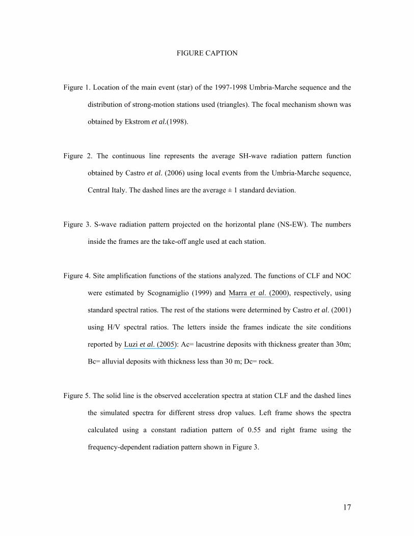
FIGURE CAPTION

Figure 1. Location of the main event (star) of the 1997-1998 Umbria-Marche sequence and the

distribution of strong-motion stations used (triangles). The focal mechanism shown was

obtained by Ekstrom et al.(1998).

Figure 2. The continuous line represents the average SH-wave radiation pattern function

obtained by Castro et al. (2006) using local events from the Umbria-Marche sequence,

Central Italy. The dashed lines are the average ± 1 standard deviation.

Figure 3. S-wave radiation pattern projected on the horizontal plane (NS-EW). The numbers

inside the frames are the take-off angle used at each station.

Figure 4. Site amplification functions of the stations analyzed. The functions of CLF and NOC

were estimated by Scognamiglio (1999) and Marra et al. (2000), respectively, using

standard spectral ratios. The rest of the stations were determined by Castro et al. (2001)

using H/V spectral ratios. The letters inside the frames indicate the site conditions

reported by Luzi et al. (2005): Ac= lacustrine deposits with thickness greater than 30m;

Bc= alluvial deposits with thickness less than 30 m; Dc= rock.

Figure 5. The solid line is the observed acceleration spectra at station CLF and the dashed lines

the simulated spectra for different stress drop values. Left frame shows the spectra

calculated using a constant radiation pattern of 0.55 and right frame using the

frequency-dependent radiation pattern shown in Figure 3.

17

Figure 6. Values of model bias estimated with all stations using a constant radiation pattern

correction of 0.55 (left frame) and using the frequency dependent radiation pattern

(right frame) for different values of stress drop. Solid line corresponds to 50 bars, dotted

lines to 100 bars and dashed line to 200 bars.

Figure 7. Acceleration spectra obtained at the stations analyzed. Solid lines are the observed

amplitudes, dashed lines are simulated amplitudes using the finite-source model of

Beresnev and Atkinson (1997,1998) and the radiation pattern functions shown in figure

3; dotted lines are simulated amplitudes using the same model but with a constant

radiation pattern of 0.55; and the black dots are the simulated amplitudes using constant

radiation pattern and the dynamic corner frequency model of Motazedian and Atkinson

(2005).

Figure 8. Model bias calculated for the three models: the static corner frequency model with a

constant radiation pattern of 0.55 (dotted line), that with the frequency-dependent

radiation pattern (dashed line) and the dynamic corner frequency model with constant

radiation pattern (dots).

Figure 9. Ground acceleration time series. On the left are the observed North-South components

and on the right side the simulated ground acceleration obtained using the dynamic

corner frequency model.

18

MAT

MNFCLF

NOC

ASI

BVG

12 30’0"E

12 30’0"E

13 0’0"E

13 0’0"E43

0’0"

N

430’

0"N

0 10 205Km

1997/09/2609:40.26 GMT

FIGURE 1

19

FIGURE 2

20

FIGURE 3

21

FIGURE 4

22

FIGURE 5

23

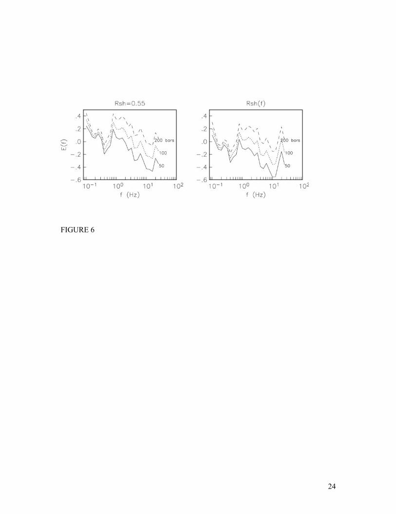
FIGURE 6

24

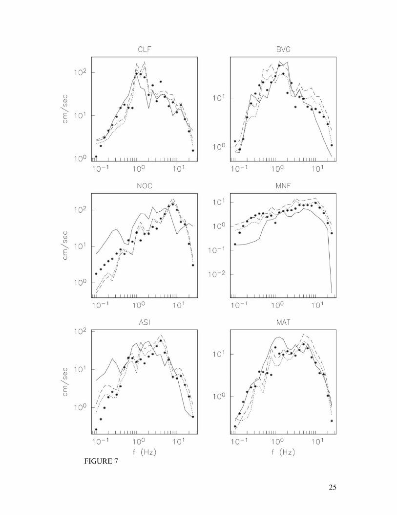
FIGURE 7

25

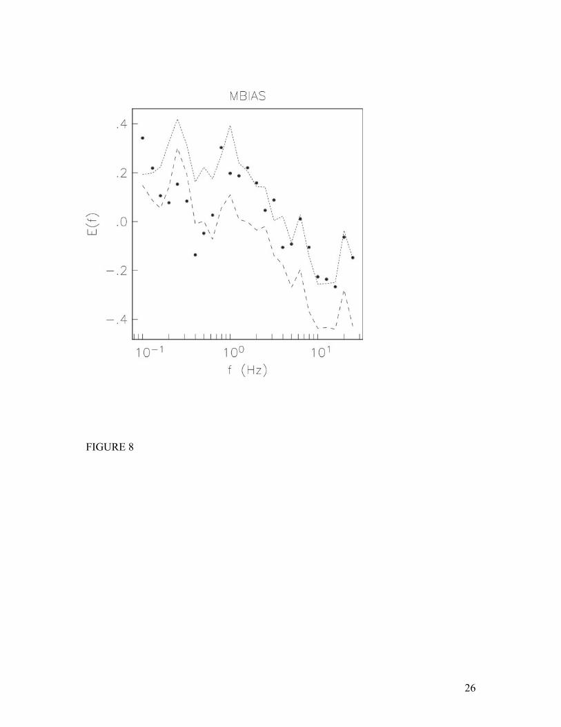
FIGURE 8

26

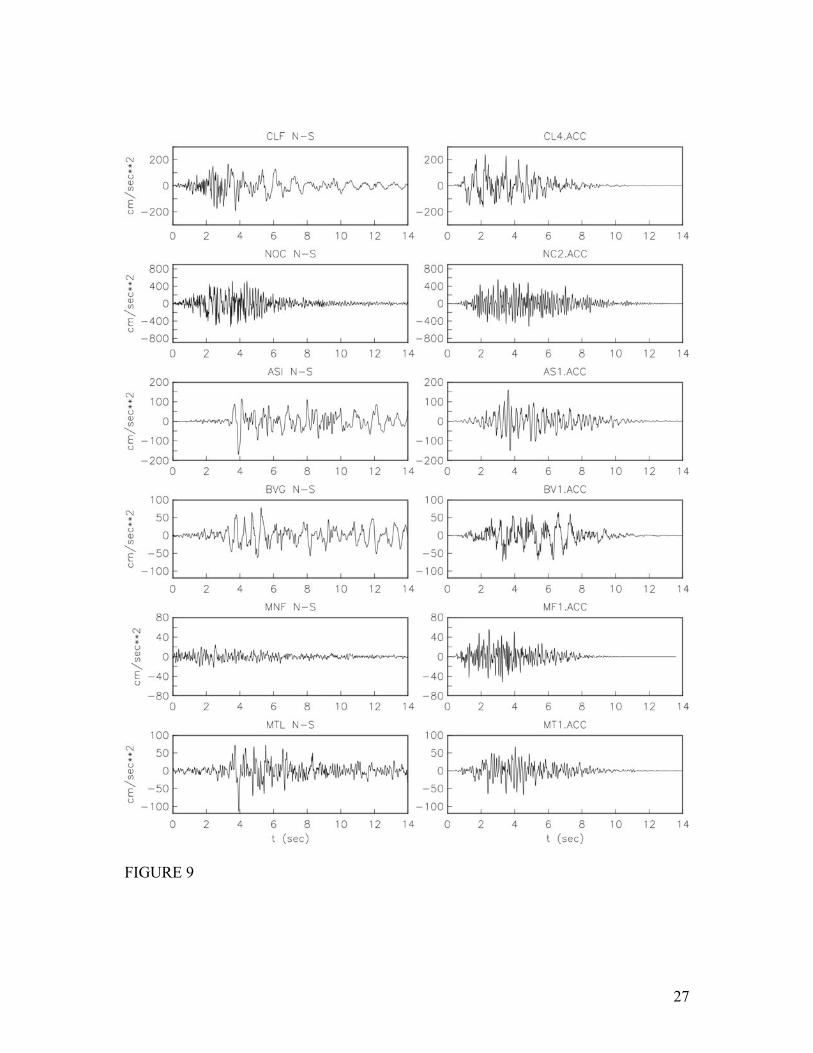
FIGURE 9

27