Modeling of Power Spectral Density using Correlated Double ...

1

Modeling of Power Spectral Density using

Correlated Double Ring Channel Model with

OFDM for High Mobility User on Vehicular

Network

Anggun Fitrian Isnawati1, Jans Hendry2, Wahyu Pamungkas3, Titiek Suryani4 1,2,3 Fakultas Teknik Telekomunikasi dan Elektro

Institut Teknologi Telkom

Purwokerto, Indonesia 4Department of Electrical Engineering, Faculty of Electrical Technology

Institut Teknologi Sepuluh Nopember,

Surabaya, Indonesia

[email protected], [email protected], [email protected], [email protected]

Abstract— Channel modeling using the correlated

double ring concept on Vehicular Network

communications systems has been developed previously.

However, no such model has been incorporated into the

OFDM multi-carrier system to simulate the effect of the

transmitter and receiver velocity on the received signal

quality. User velocity on the transmitter and receiver

side produces a Doppler effect that damages the signal

orthogonality on OFDM. In addition, the speed of the

transmitter and receiver also affect the Power Spectral

Density of the received signal. This paper used the

Correlated Double Ring channel modeling to simulate

the transmitter and receiver movement against the

Power Spectral Density parameter with non-moving

scatterers. The IFFT output of the OFDM transmitter b

is consonant with the Channel Impulse Response (CIR)

of the channel modeling output and coupled with the

AWGN noise. Simulation is done by dividing the

movement of sender and receiver into 3-speed regions,

i.e. low speed, medium and high speed. Simulation

results show the faster movement of the sender and

receiver cause Doppler Shift larger and make the value

of power spectral density parameters become getting

muffled.

Keywords—Doppler, OFDM, Power Spectral Density,

Channel Impulse Response, Correlated Double Ring.

I. INTRODUCTION

Modeling mobile user movement between the transmitter and the recipient (mobile to mobile) has been widely used in wireless-based communications systems. One paper that dealt with this model used urban and suburban areas. The modeling used the probability density function (PDF) parameter of the received signal envelope, spatial correlation function, and power spectral density (PSD) of complex envelope signals on the receiving end. The result of this model shows that the channel will act as a symmetrical Narrow-band Gaussian Process on its spectrum [1].

Furthermore, the same authors developed the modeling with different parameter statistical properties, i.e., level crossing rate (LCR), automatic fade duration (AFD), PDF of random (FM), power spectrum from random FM, and the expected number of crossings of the random phase and random FM of the channel. The results show that the LCR value

increases with the parameter ( )2

2 11 /V V+ and the

AFD value decreases with the same parameter factor [2].

One of the channel modeling used to model radio communication channels, especially the frequency nonselective Rayleigh fading channels, is Jake's model. Furthermore, Xiao Chengsan developed Rician fading channel modeling with a stochastic sinusoid zero-mean pattern under LOS conditions. This modeling differs from the previous modeling which assumes that the signal received in the Rician Fading Channel condition always has a non-zero-mean stochastic sinusoid pattern [3]. Furthermore, the same author also developed Rician Fading Channel with the pattern of a pre-chosen angle of arrival and a random initial phase. The results show that the parameters of the autocorrelation function, PDF from the signal envelope and LCR approximate the theoretical value even though the sum of the sinusoidal signal is infinite [4].

The mobile transmitter and receiver movement concerning the number of surrounding reflecting factors also developed by [5]. The transmitter and receiver regions were modeled like a ring that correlates with each other. The correlation modeled in the paper was the scatterer correlation of the same number and characteristics between the transmitter and receiver. The parameters of the autocorrelation function and PDF were based on the number of reflections on the transmitter and receiver side with

2

unequal Rician Factor (K) values were used, these parameters were also used in validation and accuracy test. However, the simulated transmitter and receiver movement in the paper only accommodated for slow user movement resulting in a small Doppler effect.

The same author developed further modeling by testing the validity and accuracy of the system through different statistical parameters. High order statistic parameters such as level crossing rate and automatic fade duration (AFD) were used to test the validity and accuracy of correlated double ring modeling. In addition, the validity test was done in the single ring on the transmitter side only or the recipient only with results that could approach the theoretical values [6].

The correlated double ring channel for V2V applications is then developed by adding a moving scatter. The simulation results show different ACF parameters for near and far scattering with the transmitter and receiver [7]. Nevertheless, this modeling has not been developed further to be combined with multi-carrier. Afterwards, this double ring channel modeling is combined with a layered ellipse model to illustrate the bounced signal paths [8]. Real traffic density is used to simulate vehicle movement and Doppler effects. Next, Power Spectral Density parameter is determined to know the effect of Inter-Carrier Interference (ICI) due to the dynamic Doppler spectrum on OFDM. The phenomenon of ICI is overcome by Phase Rotated Aided (PRA) method compared with the previous method that is Pre Coding Based Cancelation (PBC).

This paper used the correlated double ring modeling applied to the vehicular network with a high transmitter and receiver mobility and the static surrounding reflective object. To authors’ best knowledge, the use of correlated double ring channel modeling combined with multi-carrier OFDM has never been done before. The high transmitter and receiver mobility generates a large Doppler effect that may affect the orthogonality of the carrier signal used in multi-carrier OFDM. The Doppler effect validity test on a high transmitter and receiver mobility using correlated double ring channel with result approaching the theoretical values [9]. The same author also validates the Rayleigh and Rician distribution conditions at low speeds up to high speed with valid results. The OFDM parameters used to conform to the IEEE 802.11p specification as a technology standard for vehicle ad-hoc network (VANET). Furthermore, the channel impulse response parameter is determined by assuming the ring diameter on the transmitter and receiver to be very small compared to the distance between the transmitter and receiver. At the receiving end, for various transmitter and receiver velocities, the spectral density power parameter is determined to see the effect of velocity on the power density values.

The next sections of this paper will be divided as follows. Chapter II discusses the channel modeling characteristics using the correlated double ring, Chapter III contains the concept of combining the

channel with OFDM, Chapter IV presents the results and analysis, and Chapter V presents the conclusions.

II. SYSTEM MODEL

Channel modeling in this study used the correlated double ring combined with OFDM. The correlated double ring channel modeling is usually applied to a single carrier, but this study applied it to a multi-carrier system to accommodate multi-user condition. The correlated double ring model for high mobility user communications on the vehicular network can be described as follows:

N

Scatterers

M

ScatterersScattering paths

LOSTX RX

V1 V2

ᶱ ψ

Figure 1. Model of V2V communication using correlated double

ring channel

Figure 1 shows the mobile-to-mobile

communication system where the transmitter and

receiver move at the velocity of V1 and V2. There are

N and M scatters spread surrounding the transmitter

and the receiver. Parameter n shows the angle of V1

and the path of the n-th scattering, with n = 1, 2, 3…,

N. Meanwhile, m is the angle of arrival between V2

and the m-th scattering path, with m = 1, 2, 3…, M.

The n and m are assumed to be independent and

uniformly distributed in the range of [-π,π). The LOS

component gives the high correlation between the

transmitter and the receiver. Therefore, the cellular-to-

cellular scattering channel model is named the

Correlated Double Ring channel model.

LOS

shift

ᶱdiff

ᶱsend

V1 V2 V2

TX RX

LOSᶱ31diff

θ'

V1

-V2

TX

V3

Figure 2. Definition of the angle parameters

Figure 2 displays the relative velocity of a transmitter

V3 after the receiver’s speed is reduced to zero. As

can be seen in Figure 2, ' is the angle between V3

and the LOS component. The V3 relative velocity can

3

be derived using geometry and trigonometry as

follows:

( )( ) ( )( )2 2

3 1 2 1.cos .sindiff diffV V V V = − + (1)

'

31send diff = + (2)

2 2 21 1 3 2

31

1 3

cos2 .

diff

V V V

V V − + −

= (3)

V1 and V2 are the respective transmitters and receiver

velocity at M2M. diff

the parameter is the angle

between V1 and V2 vectors; send is the angle

between the V1 vector and the LOS component;

31diff is the angle between V3 and V1 vector.

Therefore, the LOS component can be formulated as

follows:

( )( )( )'3 0exp 2 cosLOS K j f t = +

(4)

K is the ratio of the specular power to the scattering

power while 0 is the initial phase that is equally

distributed at [-π, π).

Initially, in the implementation of correlated double ring scattering model, Rayleigh fading channel in M2M is calculated based on the following formula:

( ) ( ) ( )( )( ),

1 2

, 1

1exp 2 cos 2 cos

N M

n m nm

n m

Y t j f t f tNM

=

= + +

(5) 11

vf

= and 2

2

vf

= are the maximum Doppler

frequencies generated from the Tx and Rx mobility, N and M are the numbers of scatterers surrounding Tx

and Rx, nm is the independent random phase that is

uniformly distributed in the range of [-π, π), with

2

4

nn

n

N

− +=

(6)

and

( )2 2

4

m

m

m

M

− +=

(7)

With n and m are independent and uniformly

distributed in the range of [-π,π). The antenna is assumed to be an omnidirectional antenna with isotropic scattering. Due to the total independent path of NM, then the total Doppler frequency in the receiver is the total Doppler frequency induced by Tx and Rx mobility on each path. The complex autocorrelation method can be formulated as follows.

( )( ) ( )0 1 0 22 2

2YY

J f J fR

=

(8)

0 (.)J is the zero-order Bessel function. The

Rayleigh equation and the LOS component are used to formulate the Rician fading channel method as follows.

( )( ) ( )( )( )'

1 0exp 2 cos

1

Y t K j f tZ t

K

+ +=

+ (9)

III. CORRELATED DOUBLE RING CHANNEL MODEL

WITH MULTI-CARRIER OFDM

A. OFDM

Orthogonal frequency division multiplexing (OFDM) is a special technique of multi-carrier modulation which is transmitted through several subcarriers with low symbol rate. Bandwidth efficiency is obtained by overlapping subcarrier and utilizing the orthogonality properties between subcarriers. Orthogonality between subcarriers will not cause interference problems because the frequency of each subcarrier is harmonic. OFDM is built using multiple subcarriers which are obtained by generating some oscillator frequency. Generation of the oscillator in a great quantity to realize an OFDM will cause complexity in hardware implementation. Therefore, to simplify the problem, the FFT/IFFT technology is added to the OFDM communication system.

Serial to

Parallel

(S/P)

Modulation IFFT

Cyclic

Prefix

(CP)

Parallel to

Serial

(P/S)

Noise

Correlated

Double

Ring

Channel

Serial to

Parallel

(S/P)

Remove

Cyclic

Prefix

(CP)

FFTDe-

modulation

Parallel to

Serial

(P/S)

Input

Output

Figure 3. OFDM using correlated double ring channel model

The use of correlated double ring channel model on OFDM is intended to accommodate the user's mobility on both the transmitter and receiver and the presence of a scatterer factor. Figure 3 shows the use of correlated double ring on OFDM for vehicular communication. The type of modulation used in this simulation is QPSK with 4 subcarriers and 256 bits of transmitted data. This signal is then transformed in the time domain using IFFT and adding some bits as Cyclic Prefix. When the signal mix with the channel it will be exposed to a disturbance noise AWGN.

In multi-carrier OFDM, the IFFT output signal

that will be integrated is:

( ) ( )1

0exp 2

Nkk

s t X j k ft=

== −

(10)

with N is the number of IFFT nodes, Xk is the symbol

data, and f is frequency.

4

B. Channel Impulse Response

If the complex envelope value Z(t) in Equation (9) is elaborated to the real and imaginary parts, then the resulting equation is as follows:

( ) ( ) ( )Z t x t jy t= + (11)

with x(t) is the real part while y (t) is the imaginary

part. The absolute value of the complex envelope can

be calculated using the following equation:

2 2( ) ( ) ( ) ( )R t Z t x t y t= = + (12)

Meanwhile, the phase angle is:

1 ( )tan

( )t

y t

x t − =

(13)

Therefore, the real, imaginary, and absolute parts

can be expressed as follows:

( )( ) Re ( ) ( )cos tx t Z t R t = = (14)

( )( ) Im ( ) ( )sin ty t Z t R t = = (15)

( ) ( ). tjZ t R t e

= (16)

Determining the channel impulse response value

for the above channel condition can be done using the

following equation:

( ) ( )1

, ( ) . k

Nj

k

k

h k R t e

=

= − (17)

The obtained channel impulse response values

are used to determine the received signal value after

the signal is convoluted with s(t) as the output of

IFFT OFDM as follows:

*( ) ( ) ( ) ( )G t s t R t n t= + (18)

with n(t) is the AWGN noise added to the

channel. Power spectral density of received signal

G(t) can be calculated as follows:

221

( ) lim ( )2

T j ftx TT

S f E G t e dtT

−

−→

=

(19)

IV. SIMULATION RESULTS

Predetermined parameters in this study are shown

in Table 1 as follows: Table 1. Simulation Parameters

Parameters Value

Carrier Frequency 5.8 GHz

Number of Scatterers 3

Intial Phase 0°

K 2.5

Bandwidth 40 MHz

Sampling Frequency 100 Hz

Transmitted Data 64 bit

Modulation QPSK

No of Sub Carriers 4

The simulation results were focused on the velocity change and the effect on power spectral

density (PSD) of the transmitted signal. The study was classified into three user’s velocity scheme, i.e., low, medium, and high velocity as depicted in Table 2. The angle of the direction of V1 and V2 is set 10º. This classification of speed is adopted from [10] to represent the condition of urban and suburban driving behavior in busy hours and less traffic jam.

Table 2. The study schemes based on the user velocity

Scheme Type Velocity (km/hour) 1 Low 5 10 15

2 Medium 30 40 50

3 High 60 80 100

The simulation results of the three schemes are displayed in Figures 4 – 6.

Figure 4 depicts the PSD of a signal transmitted in the low-velocity scheme. As can be seen in Figure 4, the 5 km/hour velocity had the highest PSD compared with 10 km/hour and 15 km/hour velocity, with the number reached 3.31 dB/Hz. As frequency increased until 13 Mhz, the PSD of 10 km/hour decreased linearly until -18 dB/Hz then slowly increased in frequency 15 MHz. Meanwhile, the other two schemes keep decreasing in PSD as the frequency increased.

Figure 4. PSD of signals transmitted in the low-velocity

Meanwhile, Figure 5 displays the PSD of a signal transmitted in the medium-velocity scheme. As shown in Figure 5, the 30 km/hour velocity had the highest PSD compared with 40 km/hour and 50 km/hour velocity, with the number reached -0.1655 dB/Hz. All the schemes velocity decreases when the frequency higher, and for the scheme velocity 30 km/hour and 50 km/hour are slowly increasing starts from frequency 13 MHz.

5

Figure 5. PSD of signals transmitted in the medium velocity

Figure 6 shows the PSD of a signal transmitted in the high-velocity scheme. As can be seen in Figure 6, the 60 km/hour velocity had the highest PSD compared with 80 km/hour and 1000 km/hour velocity, approximately -3.448 dB/Hz. All of the schemes of velocity tend to decrease in PSD when the frequency is getting higher until reach one point of frequency and go back up. Scheme velocity 60 km/hour and 80 km/hour tend to go back up frequency 15 MHz, and another scheme tends to raise in PSD when reaching frequency 11 MHz.

Figure 6. PSD of signals transmitted in the high velocity

The implementation of the correlated double ring in this study was related to the varied velocity schemes. The results obtained in each velocity scheme are displayed in Table 3.

Table 3. The comparison of PSD based on user’s velocity

Scheme Type Velocity (km/hour)

PSD (dB/Hz)

1 Low 5 3.31

2 Medium 30 -0.1655

3 High 60 -3.448

Table 3 shows that as the user’s velocity increased, the generated PSD was decreased or damped. This is caused by the higher Doppler effects that occur.

Figure 7. PSD of the signals transmitted on the three schemes

The results are displayed in the graphic form as can be seen in Figure 7, which compares the PSD of signals transmitted on the three schemes. The results show that the low-velocity scheme, represented by the 20 km/hour velocity had the highest PSD compared to the medium (60 km/hour) and high (100 km/hour) velocity schemes.

V. CONCLUSIONS

The correlated double ring channel modeling on the vehicular network communication system has been described and integrated with multi-carrier OFDM for a various transmitter and receiver velocity. The power spectral density shows valid results for three velocity schemes, which was low, medium, and high velocity. The results show that the user’s velocity is inversely proportional to the PSD value because the users with high velocity will receive higher Doppler effects than the users with low velocity.

FUTURE WORK

In this stage, the channel model used in V2V communication was determined. In the future, Power Spectral Density as the result of this study will be used further to determine the performance parameters which are SNR (signal to noise ratio), BER (bit error rate), and channel capacity. Furthermore, providing a solution to the substandard performance, for example, noise or interference mitigation, Doppler effects, and beamforming are also becoming our concern.

REFERENCES

[1] C. Channel, “A Statistical Model of Mobile-to-Mobile

Land,” vol. V, no. 1, pp. 2–7, 1986.

[2] A. S. Akki, “Statistical Properties of Mobile-to-Mobile

Land Communication Channels Vff ;,” vol. 43, no. 4, pp.

826–831, 1994.

[3] C. Xiao, Y. R. Zheng, and N. C. Beaulieu, “Statistical

simulation models for Rayleigh and Rician fading,”

Commun. 2003. ICC ’03. IEEE Int. Conf., vol. 5, pp.

3524–3529, 2003.

[4] C. Xiao and Y. R. Zheng, “A Statistical Simulation

Model for Mobile Radio Fading Channels,” 2003.

[5] L. Wang and Y. Cheng, “A Statistical Mobile-to-Mobile

Rician Fading Channel Model,” Veh. Technol. Conf., vol.

00, no. c, pp. 63–67, 2005.

[6] L.-C. Wang, W.-C. Liu, and Y.-H. Cheng, “Statistical

Analysis of a Mobile-to-Mobile Rician Fading Channel

Model,” IEEE Trans. Veh. Technol., vol. 58, no. 1, pp.

32–38, 2009.

6

[7] S. Yoo, “An improved temporal correlation model for

vehicle-to-vehicle channels with moving scatterers,” in

2016 URSI Asia-Pacific Radio Science Conference,

2016, p. 2.

[8] X. Cheng, Q. Yao, M. Wen, C. X. Wang, L. Y. Song,

and B. L. Jiao, “Wideband channel modeling and

intercarrier interference cancellation for Vehicle-to-

Vehicle communication systems,” IEEE J. Sel. Areas

Commun., vol. 31, no. 9, pp. 434–448, 2013.

[9] W. Pamungkas and T. Suryani, “Correlated Double Ring

Channel Model at High Speed Environment in Vehicle to

Vehicle Communications,” Int. Conf. Inf. Commun.

Technol., pp. 600–605, 2018.

[10] W. Alasmary and W. Zhuang, “Ad Hoc Networks

Mobility impact in IEEE 802 . 11p infrastructureless

vehicular networks,” Ad Hoc Networks, vol. 10, no. 2,

pp. 222–230, 2012.

7

Clustering and Classification of Twitter

Indonesian Text Status to Capture Corruption

Commission Performance Opinion

Aviv Yuniar Rahman1, Istiadi1, Feddy Wanditya Setiawan2, April Lia Hananto3,4 1Department of Informatics Engineering, Universitas Widyagama, Malang, Indonesia

2Department of Automotive Mechanical Technology, Politeknik Hasnur, Barito Kuala, Indonesia 3Faculty of Computing, Universiti Teknologi Malaysia, Skudai Johor, Malaysia

4Faculty of Technology and Computer Science, Universitas Buana Perjuangan, Karawang, Indonesia

[email protected], [email protected], [email protected], [email protected]

Abstract—Indonesia's corruption commission laws on

corruption every period of government are evaluated to

support a better eradication of corruption. The revision of

the law for corruption eradication committees is based

solely on the input of the legislature. The community is

not given space to provide input for revision of the anti-

corruption commission law. Therefore, We propose

performance measurement for corruption eradication

committees using twitter text status with K-Means based

and Support Vector Machine (SVM). So the opinions of

the public on the twitter text status can be used for input

to the legislature in the measurement of performance.

Twitter status text data used in the performance

measurement of corruption binding commissions in the

case of new building KPK as much as 19880. The method

used to measure performance is K-Means and Support

Vector Machine (SVM). Accuracy results obtained by K-

Means by 87% support and 13% reject the new building.

The best SVM classification accuracy is 91.93% at 90:10

split ratio. So the corruption commission is still

performing well and revision of legislation is not required

based on K-Means and SVM measurement results in the

case of twitter status of new building.

Keywords—measurement; eradication of corruption;

twitter text; k-means; svm

I. INTRODUCTION

KPK are urgently needed in the State of Indonesia

[1][2][3]. since corruption cases found after the 1998

reforms are numerous [3]. KPK was founded on

demands for reform in 2003 and its supporting legislation [4][5] was established. Every turn of the

government period, KPK laws had changed [6].

Evaluations were made to produce better performance

of KPK [6]. Over time, much of the performance of

KPK has been weakened [7]. due to reform of KPK

based on input only from the House of Representatives,

government, social institutions and the political

interests of a group [8].

Every corruption case found by the KPK will be

publicly announced [9][10][11]. Many people are

responding through social media accounts like Twitter

[12][13][14]. Opinions of people are diverse, some are

supportive and some are counter on Twitter statuses

[15][16][17]. This research uses the case of opinion of

new building of KPK. Daily Twitter status data multiply

with public opinion about corruption [18]. For

clustering and classification of the Twitter text statuses

requires a method [19][20][21][22]. Therefore, we propose K-Means and Support Vector Machine (SVM).

K-Means is used to categorize Twitter text status data

automatically [23][24][25]. While SVM is used for the

classification of Twitter text [26][27][28].

The results of K-means clustering are used to measure

the performance of KPK based on public opinion on

Twitter. So the clustering results are used for

classification training data. This research uses SVM to

classify Twitter's status sentiments against the topic of a

new building of KPK.

II. RELATED WORKS

This section describes the research that has been

achieved in previous research. Related research contains

an explanation of KPK and methods used to process

twitter text status data to resolve this research problem.

A. Corruption Eradication Commission (KPK)

The country of Iraq has a major challenge to

corruption. Law enforcement officers try to solve this

problem, but the result is less than the maximum. Information technology is present to overcome the

problem of corruption with Open Government Data

notation. The proposed system for government policy on

data becomes more transparent to the public thereby

reducing corruption in the Iraqi state [29].

mailto:[email protected]


8

Figure 1: The performance measurement system of KPK

B. Twitter Text Clustering

Twitter text sentiment analysis is faster using

clustering because the results obtained maximum

without the need to create training data first with K-

means optimization [19]. Twitter text status

sentiments are often encountered every day on

Twitter. Topics covered vary according to current

issues. The result of sentiment on a particular topic

is positive or negative [23]. In addition, clustering

twitter has the advantage to connect tweets based on

polarity and subjectivity [30]. Tweet clustering can be used for geotagging information [31].

C. Twitter Text Classification

The classification of Twitter text status is

required for identification, extraction,

characterization and filtration the system on data

that has not been processed [32]. The methods

usually proposed for the classification of Twitter

text status are Naive Bayes, Support Vector

Machine (SVM), and Maximum Entropy (MaxEnt)

to improve the most important classification

accuracy in text feature selection [21]. In addition, there is a method for detecting Twitter status topics

based on a score matrix. This method is called a

dynamic matrix to reduce faster computation time

[22].

III. RESEARCH METHODOLOGY

Figure 1 is a picture of the performance

measurement system of KPK proposed in this study.

The system has eight sections consisting of Twitter

Status Data, Tokenization, Stopword, Stemming, Weighting Words, K-means, SVM and Evaluation.

Each part of the system will be described in

subsequent chapters.

A. Twitter Status Data

Twitter statuses were taken from the process of adding

data on the scraperwiki page. Twitter status data contains

the theme of the corruption eradication commission.

Collecting Data was done by entering the keyword of new

building of corruption eradication commission. The data

obtained as much as 19880 twitter status.

B. Tokenization

Tokenization is the process used to cut the status of

Twitter into every word. The result of the tokenization

process is stored in the array. Tokenization is used for subsequent pre-processing.

C. Stopword

Stopword is used to remove word features that are

considered not to affect clustering or classification results

on Twitter statuses. The dictionary used for the stopword

process is referring to the lucene library. The omitted word

feature consists of a subject or a conjunctive word.

D. Stemming

Stemming is part of pre-processing to take the word base

on Twitter statuses. The related word is considered not to affect clustering results or better classification. In addition

to this, stemming is used to minimize the number of word

features used. So when using stemming process pre-

processing time is faster.

E. Word Weighting

Word weighting is a major part of the proposed system.

Word weighting is used to convert words into numeric

form. The method used to convert text to numerical form

in this research is the term (tf) of the word i in document j

as in Eq.1, term Invers Document Frequency (tf-IDF) in Eq.2, Term Frequency Inverse Document Frequency (TF-

IDF) on Eq.3. Parameter |D| is the total amount of the

document file. For parameter |d:Wiɛd| in the inverse

document frequency is the number where the document

(term/word) Wi appears.

Word

Weighting

K-means Evaluation SVM

Twitter

Status Data

Pre-

Processing

Tokenization

Stopword

Stemming

9

Table 1

The result of cluster testing of twitter status

Weighting

Method

Twitter Data Without Pre-Processing

Full Data Cluster

SSE 0 1

tf 19880

(100%)

570

( 3%)

19310

( 97%)

67347.43

tfIDF 19880

(100%)

570

( 3%)

19310

( 97%)

67347.43

TFIDF 19880

(100%)

17249

( 87%)

2631

( 13%)

34934.03

Table 2

The result of cluster testing of twitter status with stopword

Weighting

Method

Twitter Data Through Stop Word

Full Data Cluster

SSE 0 1

tf 19880

(100%)

570

( 3%)

19310

( 97%)

56279.60

tfIDF 19880

(100%)

570

( 3%)

19310

( 97%)

56279.60

TFIDF 19880

(100%)

1027

( 5%)

18853

( 95%)

30027.43

jiji Wotf = ()

|:|

||log

dwd

DtftfIDF

i

jiji

= ()

|:|

||log

dwd

D

tf

tftfIDF

ii ji

ji

ji

= ()

F. K-means

K-means is used for the clustering process of this

system because of the data status of Twitter mined a

number of 19880. This much data requires the process

of grouping status to support or refuse in the case of a

new building of KPK. Eq.4 is the K-means equation used for clustering. Parameter K is a clustered output

symbol, fxn is centroid center, fyn is a word feature of

Twitter text status. K-means clustering results into

clusters 0 and cluster 1. Clustering results require

interpretation with the help of humans containing

support or rejection of new buildings. K-means result

data is used for training data on SVM process.

22

22

2

11 ..min nn fyfxfyfxfyfxK −++−+−=

()

G. SVM SVM is used for the Twitter text classification process

that consists of supporting or rejecting a new building.

SVM is part of the supervised learning process. SVM

works by using data training and testing. Training data is

taken from K-means. Data testing with a ratio of 10-

90% of the 19880 total data tested.

Table 3

The result of cluster testing of twitter status with stop word and

stemming

Weighting

Method

Twitter Data Through Stop Word and Stemming

Full Data Cluster

SSE 0 1

tf 19880

(100%)

570

( 3%)

19310

( 97%)

45424.95

tfIDF 19880

(100%)

570

( 3%)

19310

( 97%)

45424.95

TFIDF 19880

(100%)

1198

( 6%)

18682

(94%)

23900.54

Table 4

The result of manual evaluation

Twitter Data with Manual Evaluation

Full Data Cluster

Rejected Supported

19880

(100%)

3269

( 16.44%)

16611

( 83.56 %)

Eq.5. is an SVM equation that has parameters Eq.5 is an

SVM equation that has parameters for optimization,

K( iX , jX )= ( ) ( )ji XX is a linear kernel and b

is a constant.

( ) ( ) bXXxf ji += )( ()

H. Evaluation

Evaluations used to measure the performance of the

corruption eradication commission consist of Error Sum

of Squares (SSE) and accuracy. SSE is used to measure

performance in the clustering process of twitter status

using K-means. While the classification of Twitter text

using accuracy. Eq.6 is an equation for measuring the

performance results of clustering based on K-means.

Eq.7 is used for evaluation of SVM-based Twitter

classification accuracy.

=

−=n

i

ni xxSSE1

2)( ()

iiii

iii

FNFPTNTP

TNTPAc

+++

+= ()

SSE has parameter xi called observation value, while

xn is mean. The output of accuracy (Ac) with parameters TP, TN, FP, and FN. TP is true positive value of

supporting new building, while TN is true negative

value from rejecting new building. For FP is the false

positive value of supporting the new building, whereas

FN is the false negative value of rejecting the new

building.

10

Figure 2: The result of the classification of Twitter status using the

weighting method tf

IV. RESULT AND DISCUSSION

Table 1 is the result of cluster testing of Twitter text

status without pre-processing. Twitter text statuses

were tested with three weighting methods consisting

of tf, tfIDF and TFIDF. The number of Twitter Text

statuses tested in this table 1 is 19880 tweets. Twitter

text statuses were grouped as much as two, which

consists of supporting and rejecting new building of

KPK automatically. The result of grouping Twitter

text status consists of 0 and 1. To interpret the support

or reject twitter statuses required manual interpretation. For number 0 after reading is rejected

new building, while number 1 is supporting new

building for method of weighting tf and tfIDF. While

the interpretation of TFIDF levers method is the

opposite, the number 1 is to support the new building,

while the number 0 is to reject the new building. The

evaluation applied to test this system used SSE. The

result of the evaluation that has the largest SSE on the

tf and IDF weighting method is 67347.43, while the

smallest SSE when using TFIDF method is 34934.03.

The next Twitter text statuses test is with pre-

processing stop word in Table 2. Twitter text statuses via stop word process were tested by three weighting

methods consisting of tf, tfIDF and TFIDF. The

number of Twitter text statuses tested with the stop

word process as much as 19880 tweet. Twitter text

statuses were grouped as much as two that consists of

supporting and rejecting new buildings. The test

results shown in Table 2, the numbers 0 and number 1

are the result of automatic grouping, which consists of

supporting new or rejected buildings. The result of the

manual interpretation by reading for the number 0 is

to reject the new building, while the number 1 is in favor of the new building. The result of evaluation

using SSE shows that the method of weighting tf and

tfIDF is bigger than TFIDF. The value of tf and tfIDF

is 56279.60, while the TFIDF value is 30027.43.

Twitter text statuses were tested with pre-processed

stopword and stemming in Table 3. The weighting

method for testing clustering of Twitter text statuses

consists of tf, tfIDF, and TFIDF. Clustering consists

of supportive status of new or rejected buildings. The results from Table 2 show the numbers 0 and 1. For

the number 0 is the Twitter text statuses that rejected

the new building,


weighting method tfIDF

while the number 1 is in favor of the new building.

The amount of data used in this third test is 19880

tweets. The smallest SSE result when using the

TFIDF weighting method is 23900.54, while the

largest SSE result when using the tf and tfIDF method

is 45424.95. The clustering result using pre-

processing stop word and stemming is better than pre-processing only using stop word or without using pre-

processing.

Clustering test results on Twitter text statuses in

Table 1, Table 2 and Table 3 is to measure the

performance of KPK policy by unsupervised learning.

Table 1 results show the percentage of supporting new

KPK’s building is 87% -97%, while those who refuse

new building is 6% -13%. For the results of Table 2 it

is apparent that the public tends to support the new

KPK’s building of 95% -97%, while those who reject

the new building are 3% -5%. Furthermore, for the

results of Table 3 shows that Twitter text statuses to support the new KPK’s building of 94% -97%, while

those who refused the new building of 3% -6%.

Opinion evaluation of Twitter text statuses with

manual way is by reading per tweet. The results of

manual evaluation in Table 4 shows that Twitter

statuses supported the new KPK’s building amounted

to 83.56%, while those who rejected the new building

amounted to 16.44%. The result of manual evaluation

on clustering process of Twitter statuses opinion

shows that Table 1 is closer to the result of manual

evaluation, but for the smallest SSE value in Table 3 with TFIDF weighting method.

Clustering results of Twitter text statuses are used

for training data in the classification process using

11

SVM. The classification of Twitter text status using a

comparison of split ratio training with testing of

(10:90)% to (90:10)%. Classification testing of

Twitter text statuses in Figure 2 is with Twitter

statuses without pre-processing, Twitter text statuses via pre-processing stop word, twitter text statuses via

pre-processing stop word and stemming. The result of

Twitter text classification accuracy shows that when

comparison of training with testing at 90:10 split ratio,

maximum accuracy result is 91.30% without going

through pre-processing.


weighting method TFIDF

Testing text classification of Twitter through pre-

processing stop word has seen maximum of 91.37% at 90:10 split ratio. Testing of subsequent Twitter text

classification was via pre-processing stop word and

stemming. Maximum accuracy results of 91.25%

through pre-processing stop word and stemming at

50:50 split ratio.

Twitter text statuses were further tested by tfIDF

weighting method with variations of twitter text

statuses without pre-processing, Twitter text status via

stop word, and Twitter text status via stop word and

stemming. Twitter text statuses were tested with split

ratio training variation compared with testing from 10:90 to 90:10. The result of classification testing of

twitter text statuses with variation without pre-

processing is seen in split ratio training compared to

90:10 testing, 90.60% accuracy. The next attempt to

classify the text of Twitter with pre-processing

variation was via stop word with split ratio training

compared to testing is 90:10 to 10:90. The results of

testing the classification of Twitter text statuses with

variations of pre-processing through the stop word

appeared a maximum accuracy of 90.73 at 90:10 split

ratios. For testing the next classification of Twitter statuses were with variations of pre-processing stop

word and stemming. The results of testing the

classification of Twitter statuses with split ratio

training compared to testing of 90:10 to 10:90

appeared optimum accuracy of 91.93% at 90:10 split

ratio through pre-processing stop word and stemming.

The test result of the tfIDF weighting method can be

seen in Figure 3.

The next Twitter statuses classification test used

TFIDF weighting method with variations of Twitter text status without pre-processing, Twitter text status

via stop word and Twitter text statuses via stop word

and stemming. The experimental variations as in the

previous classification tests on Figure 2 and Figure 3

are with the ratio of split ratio training and testing of

90:10 to 10:90. The results of accuracy testing

classification of Twitter text statuses with variations

without pre-processing of 91.53% at 90:10 split ratios.

The result of maximum accuracy of subsequent

Twitter text classification with variation of pre-

processing stop word is 91.53% at 90:10 split ratios.

For Twitter text classification with variations of pre-processing stop word and stemming 91.33% at 60:40

split ratios. The result of comparison of text

classification of Twitter with three variations

consisting of Twitter statuses without pre-processing,

Twitter statuses through pre-processing via stop word,

Twitter statuses through pre-processing stop word and

stemming is on Figure 4.

The results of the classification of Twitter text status

on the opinion of the KPK’s new building can be seen

in Figure 2, Figure 3 and Figure 4 with variations of

pre-processing. The result of classification of Twitter text statuses using tf weighting method with pre-

processing variation shows that the classification of

the best Twitter text statuses when using variation of

pre-processing stop word is 91.37% at 90:10 split

ratios. To classify the text of Twitter using tfIDF

weighting method with pre-processing variation can

be seen that the accuracy of maximal twitter text

classification in pre-processing stop word and

stemming is 91.93% at 90:10 split ratios while for

testing the classification of Twitter text using TFIDF

weighting method the maximum accuracy without

pre-processing or pre-processing stop word is 91.53% at 90:10 split ratio.

V. CONCLUSION AND FURTHER WORKS

Measuring the performance of KPK using Twitter

statuses clustering with the tf weighting method and without pre-processing is closer to manual results. The percentage of Twitter's clustering statuses uses K-means with the tf drainage method of 87% -97% for supporting the KPK’s new building, while those who refuse the new building are 3% -6%.

The smallest SSE values use the TFIDF levers method with pre-processing stop word and stemming. From the clustering percentage of Twitter statuses can be seen that the performance of KPK is still better and the revision of the KPK’s law is not necessary based

12

on the opinion of Twitter statuses that supports the new building.

Classification of Twitter status using SVM with training data from the clustering results looks maximum accuracy. The result of classification of text status of Twitter using tfIDF weighting method shows that the accuracy reaches 91.93% with split ratio training compared to testing of 90:10. The result of Twitter text classification accuracy used tfIDF weighting with pre-processing stop word and stemming.

SSE values to measure the performance of KPK need to be lowered again so that the results of clustering accuracy with the results manually be better. To improve the performance of clustering requires research by different clustering methods and replace the metric on K-means such as Mahalanobis or Minkowski so that K-means measurement performance is more maximum than the previous metric.

ACKNOWLEDGMENT

The authors would like to thank the scrapper wiki

who have provided data mining facilities for Twitter text status for free. Secondly, the author would like to

thank LPPM Universitas Widyagama Malang for

PERINTIS grant. Not forgetting we say thank you to

friend from the University of Buana Perjuangan

Karawang for this research collaboration. from the

Department of Info

matn Systesitas Buana Perjuangan Karawang for

hiREFERENCES

[1] A. Education, “Peranan Komisi Pemberantasan Korupsi

( KPK ) dalam Mendesain Kelembagaan Pendidikan

Antikorupsi,” vol. 9, 2016.

[2] T. International, “Peranan komisi pemberantasan korupsi

(kpk) sebagai lembaga anti korupsi di indonesia,” vol.

18, no. 1, pp. 84–96, 2011.

[3] D. A. N. Regulasi, “POLITIK HUKUM

PEMBERANTASAN KORUPSI DI ERA

REFORMASI ; KONSEP,” vol. 16, no. 1, pp. 2805–

2834, 2015.

[4] “UNDANG-UNDANG REPUBLIK INDONESIA

NOMOR 30 TAHUN 2002 TENTANG KOMISI

PEMBERANTASAN TINDAK PIDANA KORUPSI

UNDANG-UNDANG REPUBLIK INDONESIA

NOMOR 30 TAHUN 2002 TENTANG KOMISI

PEMBERANTASAN TINDAK PIDANA KORUPSI.

Presiden Republik Indonesia,” 2002.

[5] “EKSISTENSI KOMISI PEMBERANTASAN

KORUPSI (KPK) SEBAGAI LEMBAGA NEGARA

PENUNJANG DALAM SISTEM

KETATANEGARAAN INDONESIA Oleh: Fitria.”

[6] R. Online, E. Martianawulansari, P. Tindak, and P.

Korupsi, “Politik hukum perubahan kedua uu kpk,” no.

April, 2016.

[7] “POLITIK HUKUM PERUBAHAN KEDUA UU KPK

No Title,” 2016.

[8] D. P. D. D. A. N. Dprd, “DEGRADASI

KEWENANGAN LEGISLASI BADAN LEGISLASI

DPR RIPASCA REVISI UU NO 27 TAHUN 2009

TENTANG MPR ,” vol. 1, no. 1, pp. 11–16, 2016.

[9] T. T. P. Non-conviction, S. Anakan, and R. Di, “Nomor

1, Maret 2017,” 2017.

[10] K. Korupsi and G. Halomoan, “Upaya komisi

pemberantasan korupsi dalam menangani kasus korupsi

gayus halomoan p tambunan ,” no. September 2013.

[11] R. Nazriyah, “Kewenangan Komisi Pemberantasan

Korupsi dalam Penyidikan Kasus Simolator SIM (

Kapolri VS KPK ),” vol. 19, no. 4, pp. 586–606, 2012.

[12] H. Chen and D. Zimbra, “AI and Opinion Mining,”

2010.

[13] F. Ren, S. Member, and Y. Wu, “Predicting User-Topic

Opinions in Twitter with Social and Topical Context,”

vol. 4, no. 4, pp. 412–424, 2014.

[14] T. K. Das, D. P. Acharjya, and M. R. Patra, “Opinion

Mining about a Product by Analyzing Public Tweets in

Twitter,” pp. 3–6, 2014.

[15] P. Barnaghi, J. G. Breslin, I. D. A. B. Park, and L.

Dangan, “Opinion Mining and Sentiment Polarity on

Twitter and Correlation Between Events and Sentiment,”

2016.

[16] R. Fernandes, “Analysis of Product Twitter Data though

Opinion Mining,” 2016.

[17] V. R. Prasetyo, “Rating Of Indonesian Sinetron Based

On Public Opinion In Twitter Using Cosine Similarity,”

2016.

[18] K. Kpk, D. A. N. Kepolisian, and R. Indonesia, “Opini

publik di media sosial twitter konflik politik antara

komisi pemberantasan korupsi (kpk) dan kepolisian

republik indonesia (polri),” 2017.

[19] H. Suresh, “An Unsupervised Fuzzy Clustering Method

for Twitter Sentiment Analysis,” pp. 80–85, 2016.

[20] X. Dai, M. Bikdash, and B. Meyer, “From Social Media

to Public Health Surveillance : Word Embedding based

Clustering Method for Twitter Classification,” no. Table

I, 2017.

[21] N. Chamansingh and P. Hosein, “P ( clt ) P ( c ) P ( c ) P

( tlc ) jp ( t ),” no. February 2012, 2016.

[22] D. Milioris, “Towards Dynamic Classification

Completeness in Twitter,” pp. 1098–1102, 2016.

[23] A. Alsayat, “Social Media Analysis using Optimized K-

Means Clustering,” 2016.

[24] S. K. Jain, “Using Mahout for clustering similar Twitter

Users,” pp. 29–33, 2014.

[25] K. Nur, I. Najahaty, L. Hidayati, H. Murfi, and S.

Nurrohmah, “Combination of Singular Value

Decomposition and K-means Clustering Methods for

Topic Detection on Twitter,” pp. 123–128, 2015.

[26] B. M. Jadav and M. E. Scholar, “Sentiment Analysis

using Support Vector Machine based on Feature

Selection and Semantic Analysis,” vol. 146, no. 13, pp.

26–30, 2016.

[27] R. Bouchlaghem, A. Elkhelifi, and R. Faiz, “SVM based

approach for opinion classification in Arabic written

tweets,” pp. 1–4, 2016.

[28] I. Dilrukshi and K. De Zoysa, “Twitter News

Classification : Theoretical and Practical comparison of

SVM against Naive Bayes Algorithms,” no. December,

p. 2013, 2013.

[29] M. N. Al-ajwad and L. Carr, “An Open Public E-

Procurement Solution to Tackle Corruption in Iraq.”

[30] S. Ahuja, “Clustering and Sentiment Analysis on Twitter

Data,” pp. 1–5, 2017.

[31] N. Garg and R. Rani, “k-means Clustering,” pp. 670–

675, 2017.

[32] A. K. Soni and I. I. N. H. Eading, “Multi-Lingual

Sentiment Analysis of twitter data by using classification

algorithms.”

13

Microstrip Patch Antenna with Double-Fed for

Anti Collision System

N. Ab Wahab, N. N. Naim, S. Subahir, Z. Ismail Khan, M. N. Hushim Applied Electromagnetic Research Center

Faculty of Electrical Engineering

Universiti Teknologi MARA

Shah Alam, Selangor, Malaysia

[email protected], [email protected]

Abstract—A single element rectangular microstrip

patch antenna topology is presented. Based on this

topology, the performance of the rectangular patch

antenna is investigated using different microstrip

feeding techniques which are inset-fed and double-

fed. These antennas are designed at 10 GHz on

microstrip FR-4 substrate, with dielectric constant Ԑr

= 4.3, tan 𝛿 = 0.012 and thickness of h =1.6mm. The

responses are compared in terms of return loss, gain,

directivity and efficiency. The results show that the

antenna with doubled-fed achieved best performance

in terms of return loss, gain, directivity and

efficiency. To prove the concept, the rectangular

patch antenna with double-fed antenna is fabricated

and measured. The measured return loss of this

antenna attenuated more than 40dB, achieved gain of

6.363 dBi, directivity of 8.023 dBi with efficiency of

68.23%. Based on this finding, this rectangular patch

double-fed antenna can be considered as suitable to

be applied in anti-collision safety system of vehicle

besides enriching the antenna bank.

Index Terms—Anti-collision system; Double-fed;

FR-4; Inset-fed, microstrip; Patch antenna

I. INTRODUCTION

An anti-collision system is a vehicle security system

intended to reduce the seriousness of an impact. It is otherwise called a pre-crash system or forward

crash cautioning system. It utilizes radar (all-

climate) and some of the time laser and camera

(utilizing picture acknowledgment) to recognize a

fast approaching accident. Numerous investigations

and improvements have been conducted to address

society's issues in terms of security for vehicles.

These include the inhabitant insurance system such

as airbags, created and acquainted all together

which ultimately reduced occupant wounds of the

vehicle that encounter with accidents, making huge commitments to wellbeing[1]. To further enhance

the security system of a vehicle, anti-collision

system is introduced. This system is basically a

programmed-stopping-mechanism that works under

basic conditions. However, it is difficult to build a

system that able to function in a speedy manner

when dealing with a moving vehicle especially in

shocking crises[2-3].

In order to overcome this problem, Radar

technology has been suggested. This is due to the

fact that the radar system embraced a few detecting

and handling techniques for deciding the position

and speed of the vehicles ahead[4]. Normally car

producers are exceptionally hesitant to change the

state of the vehicles to install any sensors, so

designers are obliged to design systems that can

housed the system in the available existing space of

the car's front grille. With this constraint, flexible

and compact size devices is crucial without sacrificing the specification of the anti-collision

system of vehicle [4].

Antenna, as one of the main component to act as

a sensor is an imperative part in the field of remote

correspondences. It has become as the spine and the

main impetus behind the current advances in remote

correspondence innovation of radar system. The

antenna can be built using well known technologies

and designs such as microstrip antennas, parabolic

reflectors, and collapsed dipole reception

apparatuses with each sort having their own particular properties and application. [5]. In terms of

costing, microstrip antenna is the most popular

technology for its low cost, robustness and

reliability. Microstrip antenna can be considered as

a set up kind of antenna that is unquestionably

utilized by designers around the world, particularly

when application required low profile reception

apparatus. There is numerous type of microstrip

substrates, and one has to make proper plan in

choosing the reasonable dielectric substrate with

proper thickness and loss tangent. The dielectric

constants are usually in the range of 2.2≤ Ԑr ≤12. The ones that are most desirable for antenna

performance are thick substrate whose dielectric

constant is in lower end because they provide better

performance compared to thin substrate[6].

Other than microstrip substrate, the shape of the

antenna also influenced the performance of antenna

itself. Most of the popular shapes are ring, patch,

elliptic to name a few but patch antenna is the most

popular due to its simplicity in design. The patch

antenna can be in rectangular, square or circular

shapes with different type of feeding depending on


14

the desired characteristics and applications. The

feeding technique can be divided into two classes

which are contacting feed and non-contacting feed.

The feeding role is very important in the case of

efficient operation of antenna, to improve the antenna input impedance. In the contacting feed

method, it is commonly used in Microstrip Feed and

Coaxial Feed where the patch is directly being fed

with RF power using contacting element [8-11].

In this paper, a single element rectangular

microstrip patch antenna topology is proposed.

Based on this topology, three antenna designs using

different technique of feeding are investigated.

These antennas are designed at 10 GHz to suit for

anti-collision application system. Based on three

different techniques of feeding method, the antennas

are simulated and the performances are evaluated in terms of return loss, gain, directivity and efficiency.

It is found that, the microstrip rectangular patch

antenna with double-fed technique gives the best

performance of high gain, directivity and efficiency.

Hence, this antenna may be suitable for vehicle anti-

collision system. To proof the concept, this antenna

is fabricated using microstrip substrate on FR-4

substrate with dielectric constant Ԑr = 4.3, tan 𝛿 =

0.012 and thickness of h =1.6 mm. Even though the

dielectric of the substrate is low, it is sufficient for the purpose of this investigation to build an antenna

that radiates in directional manner having small

angular width that is suitable for anti-collision

system of vehicle.

II. ANTENNA DESIGN

The design of the antenna is based on rectangular

patch antenna. To suit for the application in anti-

collision system, the size of the microstrip patch

antenna should be compact and light. Hence, the

height or thickness of the dielectric substrate must

be small. Therefore, for realization, microstrip

technology is used. FR-4 substrate is chosen as a material which is well known as suitable material

for antenna; given dielectric constant with

permittivity of Ԑr = 4.3, tan 𝛿 = 0.012 and thickness

of h =1.6 mm. The antenna is designed using CST

Microwave Studio software. The specification of

the antenna should be high in gain and radiate more

directional or forward in order to achieve high

signal strength, which is very crucial in anti-

collision system. For validation of concept, the best

antenna performance is fabricated and the prototype

of the antenna is tested to measure its performance.

For reflection coefficient or return loss, , of the

antenna is tested by using VNA while gain,

directivity and radiation pattern are tested in a

Chamber Room.

Figure. 1 Chamber Room to measure the performance of the

antenna.

A. Microstrip antenna characteristic calculation

The single element rectangular patch antenna is

designed based on the well-known parameters. To

calculate the dimensions of the antenna, the width,

wp, and length, lp are obtained by using Equations (1) and (2). The transmitting edge , patch width

is normally kept to such an extent that it exists in

the range of for proficient

radiation[9].

Thus, the width of patch is calculated by using this

following formula:

Width of patch, wp is defined as,

(1)

The effective dielectric constant is calculated by the formula below:

(2)

The genuine length of patch, is computed

utilizing the accompanying formula:

(3)

(4)

As stated in theory, the distance between the edge

of patch and substrate must be more than in order

to avoid the signal to radiate more to ground. Thus, the length of substrate, and the width of substrate,

been computed by using these formulas:

(5)

(6)

While the width of the quarter-wave line is obtained by [7][10]:

15

(7)

Where ZT is calculated as [7][10]:

(8)

The length of quarter line is calculated by [7][10]:

(9)

And the width of the 50 Ω microstrip feed is found using the well-known equation below:

(10)

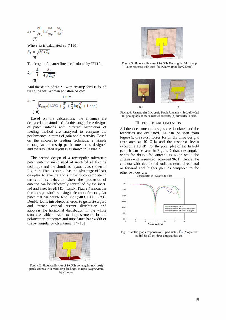
Based on the calculations, the antennas are

designed and simulated. At this stage, three designs

of patch antenna with different techniques of

feeding method are analyzed to compare the

performance in terms of gain and directivity. Based

on the microstrip feeding technique, a simple

rectangular microstrip patch antenna is designed

and the simulated layout is as shown in Figure 2.

The second design of a rectangular microstrip patch antenna make used of inset-fed as feeding

technique and the simulated layout is as shown in

Figure 3. This technique has the advantage of least

complex to execute and simple to contemplate in

terms of its behavior where the properties of

antenna can be effectively controlled by the inset-

fed and inset length [13]. Lastly, Figure 4 shows the

third design which is a single element of rectangular

patch that has double feed lines (50Ω, 100Ω, 75Ω).

Double-fed is introduced in order to generate a pure

and intense vertical current distribution and

suppress the horizontal distribution in the whole structure which leads to improvements in the

polarization properties and impedance bandwidth of

the rectangular patch antenna [14- 15].

Figure. 2: Simulated layout of 10 GHz rectangular microstrip patch antenna with microstrip feeding technique (wig=0.2mm,

lig=2.5mm).

Figure. 3: Simulated layout of 10 GHz Rectangular Microstrip Patch Antenna with inset-fed (wig=0.2mm, lig=2.5mm).

(a) (b)

Figure. 4: Rectangular Microstrip Patch Antenna with double-fed (a) photograph of the fabricated antenna, (b) simulated layout.

III. RESULTS AND DISCUSSION

All the three antenna designs are simulated and the responses are evaluated. As can be seen from

Figure 5, the return losses for all the three designs

attenuated at 10 GHz and the response levels

exceeding 10 dB. For the polar plot of the farfield

gain, it can be seen in Figure. 6 that, the angular

width for double-fed antenna is 63.8° while the

antenna with insert-fed, achieved 96.4°. Hence, the

antenna with double-fed radiates more directional

or forward with higher gain as compared to the

other two designs.

Figure. 5: The graph responses of S-parameter, [Magnitude

in dB] for all the three antenna designs.

16

(a)

(b)

Figure 6: The polar plot of farfield gain abs (Phi=0); (a)

Rectangular Microstrip Patch with insert-fed (b) Rectangular

Microstrip Patch with double-fed

Table 1

Simulated Results for the Antenna Designs

Parameter

Rectangular

Microstrip

Patch

Rectangular

Microstrip

Patch with

Inset-gap

Rectangular

Microstrip

Patch with

Double-feed

S-parameter,

S11 (dB)

53.0184 40.1853 40.7033

Gain (dBi) 3.216 3.839 6.363

Directivity

(dBi)

5.997 6.716 8.023

Antenna

efficiency (%)

52.7% 51.55% 68.23%

Table 1 tabulated the simulated performance for

all the three designs. It shows that all the three

designs achieved antenna’s requirement in terms of return loss. The rectangular microstrip patch

antenna with double-fed achieved the best

performance compared to the other two designs in

terms of gain, directivity and efficiency. Based on

these findings, the Rectangular Microstrip Patch

antenna with double-fed is chosen and to prove the

concept this antenna is fabricated and measured.

The measurement results are compared with

simulated results for validation.

A. Measurement Process

Figure. 7: The graph of S-parameter, [Magnitude in dB] of

the proposed Rectangular Microstrip Patch antenna with double-

fed

Figure. 8: The Normalized Polar Plot of Farfield Gain Abs

(Phi=0) of the proposed Rectangular Microstrip Patch antenna

with double-fed.

(a) (b) (c)

Figure. 9: The 3D Plot of Farfield Gain Rectangular Microstrip

Patch antenna with double-fed

During measurement process, the fabricated

Rectangular Microstrip Patch antenna with double-

fed was tested inside the chamber lab to measure its performances. The results are compared with

simulated in terms of return loss, gain, directivity

and efficiency. As can be seen in Figure 7, the

measured return loss is slightly shifted from 10

GHz to 9.8 GHz. The attenuation level shows more

than 10 dB.

While Figure 8 shows the polar plot of farfield

gain abs (Phi=0) after been normalized and Figure

9 shows the plot of farfield gain in 3D pattern in

three perspectives; (a) up view, (b) down view and

(c) front view. From these views, it can be seen that

the radiation of the antenna is directional and forward as simulated.

17

Table 2

Comparison Between Measurement and Simulation Results

Parameter Simulation Measurement

S-parameter,

(dB)

40.703 33.931

Gain (dBi) 6.36 6.66

Directivity (dBi) 8.02 8.74

Antenna

efficiency (%)

68.23% 61.94%

Finally, all the measured results for Rectangular

Microstrip Patch antenna with double-fed are

summarized and tabulated in Table 2. The

measurement results are compared with simulation

results to validate the concept. The results proved

that this proposed design achieved high gain,

improve directivity and antenna’s efficiency as

compared to the other two antenna designs, meeting the requirement for anti-collision safety

system.

IV. CONCLUSION

The aims of this project is to study and

investigate the suitable antenna design that can be

used as an object sensing for vehicle anti-collision

system. Three single element of rectangular patch

antennas with different technique of feeding

methods were investigated. The performances of the

antennas were compared and it was found that the

rectangular patch antenna with double-fed performed the best in terms of gain, directivity and

efficiency. For validation, this antenna was

fabricated and measured using microstrip

technology. The results were measured and were

found agreeable with simulations. The results of the

rectangular patch antenna with double-fed showed

that, the measured return loss attenuated more than

40dB, with gain of 6.363 dBi, directivity of 8.023

dBi and efficiency of 68.23%. With this simple

design and concept, this antenna should be fairly

easy to be mass-produced owing to their simplicity and compatibility. In addition, this antenna is also

easy to fabricate and compact in size. Besides

enriching the antenna bank, the design can be

considered as suitable to be applied in anti-collision

safety system of vehicle.

ACKNOWLEDGMENT

This work was supported by the Ministry of

Education Malaysia, under Niche Research Grant

Scheme (NRGS) [600-RMI/NRGS 5/3 (3/2013)]

and the Faculty of Electrical Engineering, Universiti

Teknologi MARA (UiTM), Shah Alam, Malaysia.

REFERENCES

[1] S. Tokoro, K. Kuroda, T. Nagao, T. Kawasaki, and T.

Yamamoto, “Pre-Crash Sensor for Pre-Crash Safety,” Esv,

pp. 1–6, 2003.

[2] T. Shinde, “Car Anti-Collision and Intercommunication

System using Communication Protocol,” vol. 2, no. 6, pp.

187–191, 2013.

[3] Taieba Taher, R. U. Ahmed, M. A. Haider, Swapnil. Das,

M. N.Yasmin, Nurasdul Mamun,"Accident Prevention

Smart Zone Sensing System," IEEE Region 10

Humanitarian Technology Conference (R10-HTC), 2017.

[4] F. Baselice, G. Ferraioli, S. Lukin, G. Matuozzo, V.

Pascazio, and G. Schirinzi, “A New Methodology for 3D

Target Detection in Automotive Radar Applications,”

Sensors, vol. 16, no. 5, p. 614, 2016.

[5] A. Majumder, “Rectangular microstrip patch antenna

using coaxial probe feeding technique to operate in S-

band,” Int. J. Eng. Trends Technol., vol. 4, no. April, pp.

1206–1210, 2013.

[6] Y. S. H. Khraisat, “Design of 4 elements rectangular

microstrip patch antenna with high gain for 2.4 GHz

applications,” Mod. Appl. Sci., vol. 6, no. 1, pp. 68–74,

2012.

[7] A. De, C. K. Chosh, and A. K. Bhattacherjee, “Design and

Performance Analysis of Microstrip Patch Array Antennas

with different configurations,” Int. J. Futur. Gener.

Commun. Netw., vol. 9, no. 3, pp. 97–110, 2016.

[8] D. Shashi Kumar and S. Suganthi,"Performance Analysis

of Optimized Corporate-fed Microstrip Array for ISM

Band Applications," IEEE WiSPNET 2017.

[9] A. Arora, A. Khemchandani, Y. Rawat, S. Singhai, and G.

Chaitanya, “Comparative study of different feeding

techniques for rectangular microstrip patch antenna,” Int.

J. Innov. Res. Electr. Electron. Instrum. Control Eng., vol.

3, no. 5, pp. 32–35, 2015.

[10] Manotosh Biswas, Mausumi Sen,” Design and

Development of Coax-Fed Electromagnetically Coupled

Stacked Rectangular Patch Antenna for Broad Band

Application,” Progress In Electromagnetics Research B,

vol. 79, 21–44, 2017.

[11] A. Verma, O. P. Singh, and G. R. Mishra, “Analysis of

Feeding Mechanism in Microstrip Patch Antenna,” Int. J.

Res. Eng. Technol., vol. 3, no. 4, pp. 786–792, 2014.

[12] Wong, K. L, Wu, C. H, Su, S. S. W, “Ultrawide-Band

Square Planar Metal-Plate Monopole Antenna with

Trident-Shaped Feeding Strip” IEEE, vol. 53, no. 4, 2005.

[13] V. Samarthay, S. Pundir and B. Lal, “Designing and

Optimization of Inset Fed Rectangular Microstrip Patch

Antenna (RMPA) for Varying Inset Gap and Inset

Length,” Int. J. Eng. Vol. 7, no. 9, pp. 1007-1013, 2014.

[14] H. Eriffi, A. Baghdad and A. Badri, “Design and

Simulation of Microstrip Patch Array Antenna with High

Directivity for 10 GHz Applications” Fac. Sc and. Tech.

Morocco, 2010.

[15] E. A. Daviu, M. C. Febres, M. F. Bataller and A.V.

Nogueira, “Wideband double-fed planar monopoles

antennas” IEE, vol. 39, no. 23, 2003.

18

OpenCL-Based FPGA Implementation of Plant

Identification Application Noel B. Linsangan1, Rodrigo S. Pangantihon, Jr.2

1School of Electrical, Electronics and Computer Engineering, Mapua University, Manila, Philippines

2College of Engineering Education, Computer Engineering Program, University of Mindanao, Davao City,

Philippines [email protected]

[email protected]

Abstract— This paper is exploring the use of high-level

synthesis (HLS) tool implemented in field programmable

gate array (FPGA) device for plant identification

application. HLS for FPGAs has the capability of compiling

from high-level programs to low level register-transfer-level

(RTL) specifications. This study utilized the Altera Cyclone

V DE1-SoC board and Intel SDK for OpenCL v16.1 as the

HLS tool. The open-source PipeCNN generic framework, as

hardware accelerator for convolutional neural network

(CNN) in FPGAs, was also used and integrated in plant

identification application. In the initial testing, the plant

identification system has achieved an accuracy rate of

89.52%.

Index Terms— High-level synthesis; convolutional

neural network; FPGA; OpenCL; plant identification

I. INTRODUCTION

The field programmable gate array (FPGA) provided

programmable and massively parallel architecture, thus,

certainly appropriate to perform neural network

configurations [1]. The strength of FPGAs came from the

fact that hardware developers can program it to deliver

exactly what they need for their design. In the past,

FPGAs were programmed through the use of a hardware

description language (HDL), the most popular of those

being VHDL and Verilog. An HDL is used to implement a register-transfer-level (RTL) abstraction of a design [2].

Productivity gap between algorithm development and

hardware development has surfaced. It may also be stated

as a productivity gap between development of simulation

models in software and their efficient real- time

implementation on custom hardware platforms. High-

Level Synthesis (HLS) has been looked at as a remedy to

this problem [3].

In time, the process of creating RTL abstractions was made easier through the use of reusable IP blocks,

speeding the design-flow process. As designs became

more complex and the time-to-market pressures

increased, developers and the vendor community have

strived to provide more software-based tool chains to

help reduce development times. One of these techniques

was “high level synthesis” (HLS). HLS can be thought of

as a productivity tool for hardware designs. It typically

uses C/C++ source files to generate RTL that is, in most

cases, optimized for a particular target FPGA device [2].

Further, the high-level synthesis tools offer faster hardware development cycle and software friendly

program interfaces that can be easily integrated with user

applications [4]. The High-Level Synthesis (HLS) design

flow has steadily grown to the point of now being widely

adopted for current hardware designs to reduce both

design and verification costs. In [5], HLS needed only 1/2

to 1/10 the design time compared to the traditional RTL

design flow.

High-level synthesis tools for FPGAs will lessen the

time and intricacy of the design procedures. Since proficient level knowledge was not mandatory to be able

to develop and design applications on FPGAs, this

resulted to substantial acceptance of FPGA technology

among domain developers [6].

The number of applications using FPGAs were on the

rise. They have long been used for avionics and digital

signal processing (DSP) based applications, and many

new applications in which their flexible and configurable

compute capabilities were much in demand. These

applications included accelerating large compute-

intensive workloads, within wireless based control and management functions, and already look set to play a

major role in vision processing in autonomous driving

systems [7].

The general objective of this study is to use high-level

synthesis tool to be implemented in field programmable

gate array (FPGA) device for developing plant

identification system. In order to achieve this, specific

objectives are laid: (1) to utilize PipeCNN generic


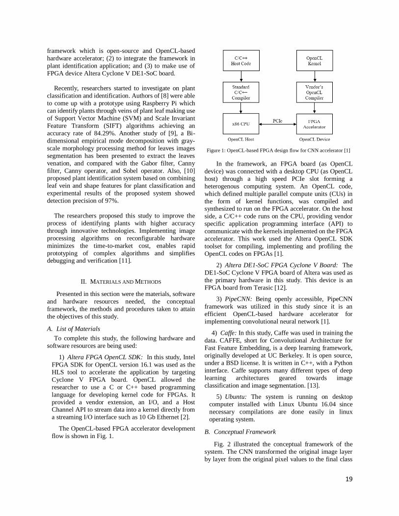
19

framework which is open-source and OpenCL-based

hardware accelerator; (2) to integrate the framework in

plant identification application; and (3) to make use of

FPGA device Altera Cyclone V DE1-SoC board.

Recently, researchers started to investigate on plant

classification and identification. Authors of [8] were able

to come up with a prototype using Raspberry Pi which

can identify plants through veins of plant leaf making use

of Support Vector Machine (SVM) and Scale Invariant

Feature Transform (SIFT) algorithms achieving an

accuracy rate of 84.29%. Another study of [9], a Bi-

dimensional empirical mode decomposition with gray-

scale morphology processing method for leaves images

segmentation has been presented to extract the leaves

venation, and compared with the Gabor filter, Canny

filter, Canny operator, and Sobel operator. Also, [10] proposed plant identification system based on combining

leaf vein and shape features for plant classification and

experimental results of the proposed system showed

detection precision of 97%.

The researchers proposed this study to improve the

process of identifying plants with higher accuracy

through innovative technologies. Implementing image

processing algorithms on reconfigurable hardware

minimizes the time-to-market cost, enables rapid

prototyping of complex algorithms and simplifies debugging and verification [11].

II. MATERIALS AND METHODS

Presented in this section were the materials, software

and hardware resources needed, the conceptual

framework, the methods and procedures taken to attain

the objectives of this study.

A. List of Materials

To complete this study, the following hardware and

software resources are being used:

1) Altera FPGA OpenCL SDK: In this study, Intel

FPGA SDK for OpenCL version 16.1 was used as the

HLS tool to accelerate the application by targeting

Cyclone V FPGA board. OpenCL allowed the

researcher to use a C or C++ based programming

language for developing kernel code for FPGAs. It

provided a vendor extension, an I/O, and a Host Channel API to stream data into a kernel directly from

a streaming I/O interface such as 10 Gb Ethernet [2].

The OpenCL-based FPGA accelerator development

flow is shown in Fig. 1.

Figure 1: OpenCL-based FPGA design flow for CNN accelerator [1]

In the framework, an FPGA board (as OpenCL

device) was connected with a desktop CPU (as OpenCL

host) through a high speed PCIe slot forming a

heterogenous computing system. An OpenCL code,

which defined multiple parallel compute units (CUs) in

the form of kernel functions, was compiled and synthesized to run on the FPGA accelerator. On the host

side, a C/C++ code runs on the CPU, providing vendor

specific application programming interface (API) to

communicate with the kernels implemented on the FPGA

accelerator. This work used the Altera OpenCL SDK

toolset for compiling, implementing and profiling the

OpenCL codes on FPGAs [1].

2) Altera DE1-SoC FPGA Cyclone V Board: The

DE1-SoC Cyclone V FPGA board of Altera was used as

the primary hardware in this study. This device is an

FPGA board from Terasic [12].

3) PipeCNN: Being openly accessible, PipeCNN

framework was utilized in this study since it is an

efficient OpenCL-based hardware accelerator for

implementing convolutional neural network [1].

4) Caffe: In this study, Caffe was used in training the

data. CAFFE, short for Convolutional Architecture for

Fast Feature Embedding, is a deep learning framework,

originally developed at UC Berkeley. It is open source,

under a BSD license. It is written in C++, with a Python

interface. Caffe supports many different types of deep

learning architectures geared towards image

classification and image segmentation. [13].

5) Ubuntu: The system is running on desktop

computer installed with Linux Ubuntu 16.04 since

necessary compilations are done easily in linux

operating system.

B. Conceptual Framework

Fig. 2 illustrated the conceptual framework of the

system. The CNN transformed the original image layer

by layer from the original pixel values to the final class

20

scores. The input of the system is a leaf image which will

be analyzed and processed to come up with the desired

result which is the identity of the plant. The leaf veins of

a sampled plant leaf served as the main data of the system

for the implementation of convolution neural network in FPGA device using PipeCNN generic framework.

The input image of plant leaf contained the pixel

values of the raw image bearing three color channels R,

G, B. In Fig. 3, the processing stages of the convolutional

neural network layer of the input image is shown. The

convolution layer performed computation of the output

of neurons that were being connected to the input local

regions. A dot product of their respective weights and a

certain region in which they were joined was then

computed. Then, the elementwise activation function was

conducted by the rectified linear unit layer. Likewise, the pooling layer performed downsampling operation which

reduced the sampling rate for spatial dimensions, such as

width and height. Fully-connected layer computed the

plant class scores and classification of the plant shall be

based on the computed scores.

Figure 2: Conceptual Framework

A. Methods and Procedures

The following procedures were taken to complete the

study:

1. Specimen collection: A corpus of two hundred fifty

leaf images were collected from fifty different Philippine

plant species. For each specie, five (5) leaf images were

collected. The letters from A to E were appended to the

species name to differentiate various images of the same

species. For example, Durian A, Durian B, Durian C,

Durian D and Durian E were the five different leaves collected from the Durian tree. From each specie, one

image will be considered as the query image and the other

four images shall be kept as reference images.

Figure 3: Convolution Neural Network Layer

2. Preparing the Data Before Training: Before

training the network using the gathered data, the

collected images were converted into the format that the

networks can read. For the data conversion, LMDB

format was chosen. Two files called train.txt and text.txt

were created. These files tell the network where to look

for each image and its corresponding class. After

converting data into LMDB format, the mean image was

created. Fig. 4 showed samples of leaf dataset used in this study.

Figure 4: Sample Local Leaf Dataset

3. Training the data: After preparing the images of plant

leaves, training of the network was made possible in

Caffe. Necessary tools were provided by Caffe in

creating the local dataset. The goal of the training phase

was to learn the network's weights. Two elements were

needed to train the artificial neural network, namely:

training data and loss function. The training data was composed of plant leaf images and the corresponding

plant name labels while the loss function measured the

inaccuracy of predictions. Training set was used to

21

estimate and pre-select promising model and filter out

bad models.

4. Installing necessary applications: Before starting to

use PipeCNN, there was a need to install Altera OpenCL

SDK toolset on a Linux desktop computer, on which a

supported FPGA board was also correctly installed. The

Intel SoC FPGA Embedded Development Suite (EDS) must also be installed. It contained development tools,

utility programs, run-time software, and application

examples to enable embedded development on the SoC

hardware platform [14].

5. Testing and Validation Phase: Captured leaf images

were inputted into the system to test the performance.

Validation was used to authenticate the final network

model specification.


Presented in this section were the discussion on the

gathering, collection, and analysis of data, as well as the

findings and results of the study.

A. Data Gathering and Collection

The training and testing of data was done using a locally created dataset consisting of plants endemic in the

Philippines, specifically in Davao City. The Agri-Expo

Community in SM Ecoland, Davao City allowed the

researcher to perform image gathering and classification

process of the needed samples.

The test sample used per plant for the training set was

5 leaves. Fifty plant species were used for local dataset,

49 known leaves and 1 unknown. Two hundred images

were used for training and 50 images were used for

testing, for a total of 250 images. The images were

captured using white background.

Table 1 showed the Confusion Matrix reflecting the

output of the functionality test using the DE1-SoC

Cyclone V FPGA board through the implementation of

convolution neural network. Twenty-one (21) plants

were being sampled and given codes P1 to P20 for plant

classification while the PU code was a given sample of

an unknown plant. Plant leaves were subjected for testing in the system five (5) times. From the gathered data, some

deviations in the prediction surfaced due to factors that

may affect the quality of the input images. Using data in

Table 1, the accuracy of the system was determined by

making use of Equation 1 and the error rate was

calculated using Equation 2 [15]. The system has

achieved an accuracy rate of 89.52% and error rate of

10.48%.

Accuracy = (TP+TN

TP+TN+FN+FP) X 100

(1)

Error = (FP+FN

TP+TN+FN+FP) X 100

(2)

Where:

TP = number of correct prediction that an instance is

positive

FP = number of incorrect prediction that an instance is

positive

FN= number of incorrect prediction that an instance is negative

TN = number of correct prediction than an instance is

negative.

22

Table I

Results and Confusion Matrix

Actual/

PredictedP1 P2 P3 P4 P5 P6 P7 P8 P9 P10 P11 P12 P13 P14 P15 P16 P17 P18 P19 P20 PU

P1 3 1 1 0 0 0 0 0 0 0 0 0 0 0 0 0 0 0 0 0 0

P2 0 5 0 0 0 0 0 0 0 0 0 0 0 0 0 0 0 0 0 0 0

P3 0 1 4 0 0 0 0 0 0 0 0 0 0 0 0 0 0 0 0 0 0

P4 0 0 0 5 0 0 0 0 0 0 0 0 0 0 0 0 0 0 0 0 0

P5 0 0 0 0 5 0 0 0 0 0 0 0 0 0 0 0 0 0 0 0 0

P6 0 0 0 0 0 5 0 0 0 0 0 0 0 0 0 0 0 0 0 0 0

P7 0 0 0 0 0 0 4 1 0 0 0 0 0 0 0 0 0 0 0 0 0

P8 0 0 0 0 0 0 0 5 0 0 0 0 0 0 0 0 0 0 0 0 0

P9 0 0 0 0 0 0 0 0 4 0 1 0 0 0 0 0 0 0 0 0 0

P10 0 0 0 0 0 0 0 0 0 5 0 0 0 0 0 0 0 0 0 0 0

P11 0 0 0 0 0 0 1 0 1 0 3 0 0 0 0 0 0 0 0 0 0

P12 0 1 0 0 1 0 0 0 0 0 0 3 0 0 0 0 0 0 0 0 0

P13 0 0 0 0 0 0 0 0 0 0 0 0 5 0 0 0 0 0 0 0 0

P14 0 0 0 0 0 0 0 0 0 0 0 0 0 4 1 0 0 0 0 0 0

P15 0 0 0 0 0 0 0 0 0 0 0 0 0 0 5 0 0 0 0 0 0

P16 0 0 0 0 0 0 0 0 0 0 0 0 0 0 0 5 0 0 0 0 0

P17 0 0 0 0 0 0 0 0 0 0 0 0 0 0 0 0 5 0 0 0 0

P18 0 0 0 0 0 0 0 0 0 0 0 0 0 0 0 0 0 5 0 0 0

P19 0 0 0 0 0 0 0 0 0 0 0 0 0 0 0 0 0 0 5 0 0

P20 0 0 0 0 0 0 0 0 0 0 0 0 0 0 0 0 0 0 1 4 0

PU 0 0 0 0 0 0 0 0 0 0 0 0 0 0 0 0 0 0 0 0 5

B. Actual Hardware Components Setup

Fig. 5 showed the demonstration setup of the

hardware components. The Altera FPGA Cyclone

V DE1-SoC board was interfaced to the host

computer through USB ports. Likewise, the

minicom terminal installed in the computer has

provided avenue to access the FPGA device. The

kernel codes in OpenCL were being compiled

through Intel SDK for OpenCL version 16.1. The plant leaf images from SD card were loaded by the

host programs. Then, these input images were

forwarded to the hardware accelerator to perform

computationally-intensive image processing of

plant leaves. The convolution neural network was

implemented by the system and final class score

was generated.

Figure 5: Setup of the system

C. Sample Test Result

Shown in Fig. 6 was a sample test result of a

sampled plant leaf. The FPGA board is accessed

through minicom terminal. The board has micro

SD card installed which contained the program

and images to be tested. The system has identified

the sampled plant leaf as Piper nigrum (scientific name), or Black Pepper (English name) or

Paminta (Philippine common name). The testing

has a total kernel runtime of 154.403 ms.

23

Figure 6: Sample Test of Plant Leaf

D. System Flow Summary

Generated from the log report of FPGA board was the flow summary report of the system. It has generated

logic utilization of 83% (26,724 / 32,070). The total

registers used were 64, 218 and total pins utilized was

23%. The total block memory bits consumed was 54%.

Also, the total PLLs was 33%, DLLs was 25% and DSP

Blocks was 83%.

IV. CONCLUSIONS AND FUTURE WORKS

After conducting the study, a plant identifier

application was developed using high-level synthesis

(HLS) tool implemented in field programmable gate

array (FPGA) device. PipeCNN opensource framework

was successfully utilized and played significant role as

hardware accelerator for performing convolutional

neural network. The Altera Cyclone V DE1-SoC board

was used. The system has achieved an accuracy rate of

89.52%. High level synthesis provided by the Intel SDK

for OpenCL is instrumental for substantial speedups of

convolution neural network and image processing when compared to other computing practices. The Intel SDK

for OpenCL has afforded this study the needed tools to

take a compute-intensive processing of plant leaf

classification.

The FPGA device used is consisting of 85K logic

elements (LE) only which somehow constrained the

resources of the system. For future works in image

processing projects using FPGA, DE10-nano and DE5-

net are worthy to be considered since these boards have

higher resource capacity.

REFERENCES

[1] Dong Wang, Ke Xu and Diankun Jiang (2017). PipeCNN: An

OpenCL-Based open-source FPGA accelerator for convolution

neural networks. 2017 International Conference on Field

Programmable Technology (ICFPT), Melbourne, VIC,

Australia.

[2] Tom Hill (2015). Myths About High-Level-Synthesis

Techniques for Programming FPGAs.

[3] Aydın Emre Güzel et. al (2016). Using High-Level Synthesis for

Rapid Design of Video Processing Pipes. 2016 IEEE East-West

Design & Test Symposium (EWDTS).

[4] U. Aydonat, S. O’Connell, D. Capalija, A.C. Ling and G.R.

Chiu, “An OpenCL Deep Learning Accelerator on Arria 10” in

Proc. ACM/SIGDA International Symposium on Field-

Programmable Gate Arrays (FPGA ’17), 2017.

[5] Qiang Zhu & Masato Tatsuoka (2016). High Quality IP Design

using High-Level Synthesis Design Flow. 2016 21st Asia and

South Pacific Design Automation Conference (ASP-DAC).

[6] Ian Janik, Qing Tang & Mohammed Khalid (2015). An overview

of Altera SDK for OpenCL: A user perspective. 2015 IEEE 28th

Canadian Conference on Electrical and Computer Engineering

(CCECE), 3-6 May 2015, Halifax, NS, Canada.

[7] Razvan Nane et. al (2016). A Survey and Evaluation of FPGA

High-Level Synthesis Tools. IEEE transactions on computer-

aided design of integrated circuits and systems, vol. 35, no. 10,

October 2016.

[8] Selda, J., Ellera, R., Cajayon II, L. and Linsangan, N. (2017).

Plant identification by image processing of leaf veins. 2017

International Conference on Imaging, Signal Processing and

Communication (ICISPC 2017), July 26–28, 2017, Penang,

Malaysia.

[9] Wenshuang Yin, Changcheng Xiang, Liming Tang and Shiqiang

Chen (2015). Venation extraction of leaf image by bi-

dimensional empirical mode decomposition and morphology.

2015 IEEE Advanced Information Technology, Electronic and

Automation Control Conference (IAEAC).

[10] Heba F. Eid, Aboul Ella Hassanien and Tai-Hoon Kim (2015).

Leaf plant identification system based on hidden naive bays

classifier. 4th International Conference on Advanced

Information Technology and Sensor Application (AITS), IEEE,

At Harbin, China.

[11] Muthukumar Venkatesan and Daggu Venkateshwar Rao (2004).

Hardware Acceleration of Edge Detection Algorithm on FPGAs.

[12] Altera (2015). DE1-SoC.

[13] Jia, Yangqing and Shelhamer, Evan and Donahue, Jeff and

Karayev, Sergey and Long, Jonathan and Girshick, Ross and

Guadarrama, Sergio and Darrell, Trevor (2014). Caffe:

Convolutional Architecture for Fast Feature Embedding. 2014

Proceedings of the 22nd ACM international conference on

Multimedia, pages 675-678.

[14] Hamid Mahmoodi, Arturo Montoya et. al (2012). Hands-on

teaching of embedded systems design using FPGA-Based tPad

development kit. 2012 2nd Interdisciplinary Engineering Design

Education Conference (IEDEC), 19 March 2012, Santa Clara,

CA, USA

[15] Thomas G. Dietterich (1998). Special issue on applications of

machine learning and the knowledge discovery process. Journal

Machine Learning archive, Kluwer Academic Publishers

Norwell, MA, USA, Volume 30 Issue 2-3, Feb./March, 1998,

ISSN:0885-6125.

24

A-Eye: An Intrusive Load Monitoring System

for Appliance Classification Jobenilita R. Cuñado1 and Noel B. Linsangan2

Department of Engineering Education, Computer Engineering Program, University of Mindanao, Tagum City

School of Electrical, Electronics and Computer Engineering, Mapua University, Manila, Philippines [email protected]

[email protected]

Abstract— Interest in power consumption management

has grown over time with the limitation of energy resources.

The need for a load identification infrastructure is central

to energy usage management applications, with control over

devices only possible if a means by which devices can be

identified is available. This study is aimed to develop an

individual appliance meter with appliance classification

capability based on time-dependent power consumption

features drawn and with remote access facility. An

individual appliance meter is developed and is used to

create a library of load signatures, with an appliance

classification capability and a provision for remote access

based on time-dependent power features drawn by an

appliance, from power-up to its steady state. An increase in

classification accuracy is achieved and the load library

derived from this work can be used in other ILM

endeavours. Results showed accuracy of 92%, hence, the

appliance classification infrastructure developed can be

useful in energy management applications to reduce

wastage in energy usage.

Index Terms— Intrusive Load Monitoring, smart meter,

Raspberry Pi, appliance classification, power signature

I. INTRODUCTION

With ever increasing demands but with limited

available resources, mitigation of energy wastage is a

societal need.

One of the answers to this need is through load

monitoring, through which, awareness among consumers

can be heightened and thereby propel them to conserve.

To date, meters are commercially available for monitoring of electricity consumption. However, this

type of monitoring devices cannot isolate an individual

appliance with their lack of appliance identification

capability. The researcher proposed to develop a device

using an intrusive load monitoring system. With its

capability to identify a plugged appliance, remote access

can be made possible.

Appliance load monitoring (ALM) intends to sense

electric consumption. ALM has been divided in two

approaches: Intrusive Load Monitoring (ILM) and Non-

Intrusive Load Monitoring (NILM); the former utilizes

sensors and wireless technologies to detect every single

appliance while the latter discerned devices based from

the data acquired from a single point of measurement [1].

Present works on ILM have been focused on approaches

on appliance classification alone. A study by Paradiso et al proposed artificial neural network approach [2].

Reinhardt et al offered another solution using time series

pattern matching [3]. Both Reddy et al [4] and Ridi et al

[5], on the other hand, presented the use of machine

learning to process signals from appliances.

Identification of power waveforms has been proposed by

Ito [6]. Moreover, a work by Lee et al focused on the

development of signal rocessing techniques for load

identification [7]. Ganu et al has developed an actual load

monitoring device: SocketWatch [8]. This device detects

appliance malfunctions by learning behavioural model of appliances using unsupervised learning techniques. It

solely focused on energy leakage monitoring and has no

communication infrastructure for intervention. Other

researchers explored high frequency and low-frequency

measurements. Reinhardt et al sampled current flow of

appliances at a rate of 1.6 kHz [9]. Fitta et al proposed to

recognize switch-on and –off events from signatures

sampled at 6.4 kHz [10] while Englert et al sampled the

power consumption of a connected device at 96 kHz

sampling rate [11]. However, since high-frequency

sampling is resource demanding, Abbas [12] and

Zufferey et al [13] sampled electric consumptions every 10 seconds with promising results.

Though ILM has been a point-of-interest of researches

and many approaches have come forward as a result, the

availability of commercial metering device with an

appliance classification capability is not yet prevalent.

Also, the availability of public ILM datasets is very

limited, with very limited appliance types, which

significantly affects the reported performance of

scientific works. Moreover, ILM systems have not been

implemented in the Philippines. With the limited availability of smart plugs with load identification

25

capability, remote load monitoring and access are still

seen wanting intervention.

In an attempt to address these needs, the researcher

endeavoured to develop an individual appliance metering device which can be used to 1) create a library of

appliance load signatures; 2) classify appliances based on

their power signatures using a supervised learning

technique; and, 3) access appliances remotely.

The limitations in resources and increasing demand for

energy justify the need of intelligent load monitoring

devices. The development of a load identification

infrastructure will contribute to energy conservation

innovations from which the society, in general, can

benefit. Also, with the availability of a metering device

which can be used to capture load power signatures, ILM

libraries can be expanded to include additional appliance class of various models to significantly increase the

identification accuracy of ALM-related scientific works.

This study was conducted with the purpose of

developing a metering device for appliance

classification. The appliances being considered are those

common appliances for the ten identified offices of UM

Tagum College and are also assumed to be in good

working conditions. They are classified into five types:

computer set, printer, laptop (via charger), electric fan

and cellular phone (via charger). The researcher considers the sampling period from the time an appliance

is switched on until its steady state.

II. METHODOLOGY

A. System Design

Figure 1: System Block Diagram

Figure 1 showed the block diagram of the system. The

smart meter was placed between the home outlet and the appliance. The meter’s internal structure was comprised

of latches, potential and current transformers, Analog-to-

Digital Converter and Raspberry Pi. The power and

current transformers were necessary to step down actual

values to match parameters of digital circuitries. After

voltage and current levels were stepped down, the ADC

performed conversion. The Raspberry Pi was used as the

main processor of the smart meter with its low cost and

reliability, making it well-suited for wireless sensor

network monitoring system [14]. The Raspberry Pi

sampled data received from ADC and used these samples

for feature extraction and appliance classification. As a

microcomputer, the PI had its own Ethernet and WIFI

ports which make communication to network possible;

thereby, providing information views and control using mobile device. The mobile device sent signal for a user

to turn off the plugged appliance through the Raspberry

Pi, which responded by providing trigger to the latches to

accomplish the required function.

B. System Flow

The whole system, as shown in Figure 2, was

constructed with the objectives to develop a metering

device with appliance classification capabilities, store

data for load library of power signatures and provide remote access and intervention.

1) Data Acquisition: Data acquisition necessary for

classification had to be done first by stepping down

current and voltage levels. Once they were stepped down,

the analog signals must be converted to digitalized ones

before the Raspberry Pi can take samples. For this study,

the researchers were able to sample two thousand

samples per appliance at a rate of 100 samples per

second. The sampling period covered the time the

plugged appliance was turned on until its steady state.

The Raspberry Pi was programmed using Python language to read current and voltage levels while

computing the time difference of their zero crossings.

The difference of current and voltage crossings was

necessary to accurately measure the power factor which

was a vital factor for classification. Once these were

done, electrical quantities considered as parameters for

power signatures were derived. These parameters include

real power (P), peak current (IPEAK), RMS current

(IRMS), and the power factor (PF).

26

Figure 2: System Flowchart

2) Appliance Classification: Appliance was

identified and classified using their power signatures.

This was done using the k-Nearest Neighbors algorithm.

The algorithm worked by comparing the data to the

training set and then returning the class label [15]. This training set was in the classification model, an appended

library of appliance power signatures. The load library of

appliance power signatures to be used for classification

was local to the meter. This load library was a collection

of records from data sets of seventy five plug loads from

five appliance classes, fifteen of each class, including

computer set, electric fan, laptop (via charger), printer,

and mobile phone (via charger).

3) Remote Access and Intervention: After an

appliance was classified, the result is communicated to a

network i.e. stored to a cloud where the user can also view the results. Using a mobile device, the user can

install an Android-based application to remotely control

the switching on or off of a plugged appliance.

C. Hardware Configuration

The value of the line voltage from the distribution lines

varied depending on diverse load consumption

conditions. As such, actual line voltage values were

measured at different times in a day, especially

considering peak and off-peak power usage hours, to

determine the maximum possible voltage that the meter

will capture to ensure that the circuitry remains safe even with voltage fluctuations. The maximum possible input

voltage to the meter, based on several observations is

approximately 230 V. This value had to be stepped down

to 2.048 V, the selected GAIN setting for the selected

ADC input channels that will capture the voltage value to

be digitized. A voltage divider circuit was used, shown in

Figure 1, with R1 and R2 values computed to achieve the

required ratio.

Figure 3: Voltage Divider Circuit

With a 230V input and R1 and R2 being 4.2MΩ and

2.2kΩ, respectively, the maximum possible RMS voltage

output (VOUT) of the circuit is 1.31979 V, which still has

a safety net of 0.7282 V in case the line voltage will go

beyond 230 V.

For current sensing, ACS712, a fully integrated, hall effect-based linear current sensor IC, was used. The

output voltage of the current sensor can reach up to 5V

depending on the input voltage and the current drawn by

a load. The output voltage of the current sensor that was

equivalent to zero current (no load) is ½ of the input

voltage, e.g. for a 5 V input, a 2.5 V output is equivalent

to zero current. An increment of 100mV was added to the

output of the current sensor for every ampere of current

drawn.

The ADS1115 was used for analog-to-digital conversion. The ADS1115 has four input channels.

Channels 0 and 2 capture the output of the current sensor

while the outputs of the voltage divider circuit were

captured by Channels 1 and 3. The selected GAIN setting

for the channels that captured the sensed current was 2/3

to read voltages ranging from -6.144 V to +6.144 V to

accommodate the maximum possible voltage output of

the current sensor which was 5 V. The ADS1115 was set

to perform conversions at 860 samples per second. With

its 16-bit precision, the voltage and current steps were

27

0.0000625 V and 0.001875 V, respectively, based on the

selected GAIN settings. The ADS1115 communicated

the outputs of conversion to the Raspberry Pi via the I2C

interface, with the default address, 0x48, selected.

Python was used to program the Raspberry Pi to

perform its three major tasks: data acquisition, feature

extraction and appliance classification. The Raspberry Pi

was configured as master and the ADS1115 as slave.

III. RESULTS AND DISCUSSIONS

After the data were collected, the required power

features were extracted. Table I showed the comparison of the approximate maximum appliance power

consumption at start-up against at steady state of the five

appliances gathered by the developed meter.

Table I

Comparison of Appliance Power Consumption at Start-up and at

Steady State

Appliance

Class

Power Consumption (Max) Steady State to

Peak Current

Ratio Start-Up Steady State

Computer Set 106 W 94 W 0.88679

Electric Fan 86 W 83 W 0.96512

Laptop 188 W 107 W 0.56915

Mobile Phone 20 W 21 W 1.05

Printer 865 W 13 W 0.01503

It can be observed that the printer drew a much bigger

current during start-up compared to the other appliances

under study; however, during steady state the power

consumption remarkably dropped and became the lowest

from among the five appliances. The steady state to peak

current ratio based on the results was unique for each

appliance class.

Table II

Comparisons of Power Feature Sets of Electric Fan at Different

Settings

Fan

Speed

Setting

Real

Power

(Steady

State)

Peak IRMS

Mean

IRMS

(Steady

State)

Power

Factor

Slow 61.317184 0.322175 0.265562 0.9999915

Medium 64.967736 0.340074 0.280146 0.9999917

Fast 66.209614 0.371893 0.286842 0.9999938

The power consumption of the electric fan was

specifically investigated. Table II showed the

comparison of power feature sets of an electric fan at

different speed settings. It can be observed that power

consumption was highest at the maximum setting.

However, it is worth noting that at the maximum setting

the electric fan was most efficient with the power factor

closest to unity.

Table III

Power Feature Sets of Electric Fan at Maximum Speed Setting

Trial

Real

Power

(Steady

State)

Peak

IRMS

Mean

IRMS

(Steady

State)

Power

Factor

1 68.818094 0.360624 0.295592 0.99999127

2 58.562131 0.353995 0.258469 0.99999252

3 71.741695 0.372556 0.308121 0.99999283

4 75.783824 0.382500 0.325821 0.99999264

5 66.209614 0.371893 0.286842 0.9999938

To investigate more the behaviour of the electric fan,

five trials were conducted for the maximum fan speed

setting to determine the consistency of the gathered data.

Table III showed that in the second trial the gathered

feature set was closer to the feature set of the fan at the

lowest setting as can be observed in Table II. Also, each

trial generated results which, when compared to the

results of the other trials, were not equivalent for the same

setting.

Table IV

Comparison of Power Feature Sets of Mobile Phones of the

Same Brand but of Different Models

Model

Real Power

(Steady

State)

Peak IRMS Mean

IRMS

(Stead

y

State)

Power

Factor

Samsung

Keystone 3

15.584834 0.070931 0.0678

15

0.9999

9884

Samsung

Galaxy J1

Mini

17.289824 0.086178 0.0746

43

0.9999

9873

Samsung S6 18.184310 0.092144 0.0792

18

0.9999

8673

The data shown in Table IV were gathered while the

phone was charging. It can be observed that the power

drawn by the different models of the same brand of

mobile phone were different yet comparable.

The accuracy of the readings was verified using

commercial meters. The readings were approximately

equivalent, with the difference attributed to precision.

After the training set was prepared, the kNN classifier

was tested on the data set and the estimated error rate was

0%, with k = 3.

Actual testing revealed an overall accuracy of 92%,

based on Equation 1 as shown in Table V. Three

appliances, in all instances, were correctly classified. The printer was incorrectly classified when the classification

process was initiated and the printer was not turned on

28

immediately, significantly affecting the extracted

features of the testing data.

Accuracy = (TP+TN

TP+TN+FN+FP) X 100

(1)

Where: TP = number of correct prediction that an

instance is positive

TN = number of correct prediction than an

instance is negative

FP = number of incorrect prediction that an


FN = number of incorrect prediction that an


Table V

Confusion Matrix

Predicted/

Actual

Computer

Set

Electric

Fan

Laptop Mobile

Phone

Printer Unknown

Appliance

Computer

Set 15

Electric

Fan 15

Laptop 1 14

Mobile

Phone 15

Printer 1 14

Unknown

Appliance 2 1 1 11


This study was aimed to develop an individual

appliance meter with appliance classification capability

based on time-dependent power consumption features

drawn and with remote access facility. The developed

meter can be used to create a library of load signatures,

classify appliances based on their power signatures using a supervised learning technique, and access an appliance

remotely. With the limited ILM datasets, there are still

so much to explore considering different appliance

categories and different types of measurements that can

result to an increase in classification accuracy. The load

library derived from this work can be used to expand the

ILM datasets which can be used by other researchers.

Results showed accuracy of 92%, hence, the appliance

classification infrastructure developed can be useful in

energy management applications to reduce wastage in

energy usage.

Future works should consider the effects of varied load

conditions. Also, the load library has to be further

populated to include other appliance classes of different

brands and models to enhance the classification range and accuracy of the system.

REFERENCES

[1] A. Ridi, C. Gisler, and J. Hennebert, “A Survey on Intrusive

Load Monitoring for Appliance Recognition,” IEEE, 2014.

[2] F. Paradiso, F. Paganelli, A. Luchetta, D. Giuli, and P.

Castrogiovanni, “ANN-Based Appliance Recognition from

Low-frequency Energy Monitoring Data,” IEEE, 2013.

[3] A. Reinhardt, D. Christin, and S. Kanhere, “Predicting the Power

Consumption of Electric Appliances through Time Series Pattern

Matching,” in Proceedings of the 5th ACM Workshop on

Embedded Systems for Energy-Efficient Buildings (BuildSys),

pp. 1-2, ACM Press, Nov. 2013.

[4] R.S. Reddy, N. Keesara, V. Pudi, and V. Garg, “Plug load

identification in Educational Buildings Using Machine Learning

Algorithms,” in Proc. BS2015: 14th Conference of International

Building Performance Simulation Association, 2015.

[5] A. Ridi, C. Gisler, and J. Hennebert, “Automatic Identification

of Electrical Appliances Using Smart Plugs,” IEEE, 2013.

[6] M. Ito, R. Uda, S. Ichimura, K. Tago, T. Hoshi, and Y.

Matsushita, “A Method of Appliance Detection Based on

Features of Power Waveform,” IEEE, 2004.

[7] W.K. Lee, G.S.K. Fung, H.Y. Lam, F.H.Y. Chan, and M.

Lucente, “Exploration on Load Signatures,” in Proc. of

International Conference on Electrical Engineering, 2004.

[8] T. Ganu, D. Rahayu, D. Seetharam, R. Kunnath, A.P. Kumar, V.

Arya, S. Husain, and S. Kalyanaraman, “Socketwatch: An

Autonomous Appliance Monitoring System,” IEEE, 2014.

[9] A. Reinhardt, D. Burkhardt, M. Zaheer, and R. Steinmetz,

“Electric Appliance Classification Based on Distributed High

Resolution Current Sensing,” IEEE, 2012.

[10] M. Fitta, S. Biza, M. Lehtonen, T. Nieminen, and G. Jacucci,

“Exploring Techniques for Monitoring Electric Power

Consumption in Households,” in Proceedings of the 4th

International Conference on Mobile Ubiquitous Computing,

Systems, Services and Technologies (UbiComm), 2010, pp. 471–

477.

[11] F. Englert, S. Kobler, A. Reinhardt, and R. Steinmetz, “How to

Auto-Configure Your Smart Home? High-Resolution Power

Measurements to the Rescue,” ACM, 2013.

[12] D. Zufferey, C. Gisler, O.A. Khaled, and J. Hennebert, “Machine

Learning Approaches for Electric Appliance Classification,”

IEEE, 2012.

[13] F.K. Zaidi Adeel Abbas and P. Palensky, “Load Recognition for

Automated Demand Response in Microgrids,” in Proceedings of

the 36th IEEE Annual Conference on Industrial Electronics

Society (IECON), 2010, pp. 2442–2447.

[14] C.N. Cabaccan, F.R.G. Cruz, and I.C. Agulto, “Wireless Sensor

Network for Agricultural Environment Using Raspberry Pi

Based Sensor Nodes,” IEEE, 2017.

[15] P. Harrington, Machine Learning in Action, New York: Manning

Publications Co., 2012

29

Price Calculator of Dry-Fermented Cacao Beans

Using k-NN Algorithm Randy E. Angelia1, Noel B. Linsangan2

1College of Engineering Education, Computer Engineering Program, University of Mindanao, Davao City 2School of Electrical, Electronics and Computer Engineering, Mapua University

Manila, Philippines [email protected]

[email protected]

Abstract— From a basic economic point of view, good

quality harvests were mostly entwined to high market value

but some conventional methodologies on trading somehow

deprived either the traders or the farmers of the real value

of the goods due to erroneous practices and at some point,

subjective decision making. Knowing these issues at hand

the proponents were inspired to propose a solution of

automating the calculation of fermented cacao beans based

on its fermentation quality using digital image processing.

Three hundred cross cut cacao beans were pre-classified by

a qualified human cacao quality assurance officer and

visually characterized them based on color features and

classified as well-fermented, under-fermented and over-

fermented. RGB features of pre-identified beans were

extracted and enlisted as part of the classifier data sets. The

created device sampled the cross-cut beans for visual

analysis through image capturing and classification via its

image processing chamber. The image feature extraction

was done through processes such as grayscaling,

thresholding and outlining of regions of interest.

Classification was done on the generated RGB features of

each object and using k-Nearest Neighbour prediction

techniques the classification of each beans was attained.

Using the standard price matrix multiplier of cacao traders

along with the base price data, trading price of cacao beans

was determined. Initial data revealed a 97.5 percent overall

accuracy in determining the quality of cacao beans which

basically led to true positive fermented cacao beans price

appraisal.

Index Terms— beans price appraisal, cacao beans, image

processing, k-NN Algorithm, confusion matrix.

I. INTRODUCTION

As world’s population continues to grow, food

security is always put into balance. As a nation, the

higher production in agricultural products the better for

the economy since not all nations has the capacity to

produce food. Theobroma cacao generally known as

cacao, the raw material for making chocolate, cocoa

powder, cocoa liquor and many more is experiencing

shortage in terms of supply with respect to the world’s

demand. The global demand for cacao has tripled from

1970 to 2000 from nearly 900 thousand tons to 3 million

tons in year 2000. United States of America and

European countries like Germany, France and United

Kingdom ware the front runner in cacao consumptions

[1]. Such development is a big opportunity to cacao

farmers to improve yields and quality. However, in the

Philippines, a country known to produce great quality of

cacao due to its appropriate weather conditions; only

25% of the total domestic demand has been produce

yearly [2]. Things like industry support, upgrading of

knowledge in modern cacao farming, availability of

technology and government support programs were some of the obvious reasons such low production. Philippine

scenario was not far from Ghana, Africa where targeted

yields and quality were constantly not been reached

yearly due to lack of government support though 4

percent of its Gross Domestic Product (GDP) came from

cacao production [3]. Another interesting part in cacao

industry was the quality of beans since compared to other

crops, after harvest procedures lowering the moisture

content was the only requirement in order to preserve and

to market such as corn, rice, coffee, copra, etc. Cacao

beans needed to be fermented for the acid build-up which was necessary to generate aroma to the chocolates [4].

During trading, prices differed according to its quality

wherein the prime indicator was the fermentation quality.

Grading procedure of fermented cacao beans was based

on the percent of slaty or under-fermented, over-

fermented and the presence of foreign objects. Test

involved counting of cacao beans, cutting in lengthwise

and examining by visual inspection [5]. This method of

inspection turned to be erroneous and somehow

subjective due to different standard of every human

examiners. Integration of modern technology is likely

applicable in this kind of challenges like image processing techniques that analyse ordinary photographs

through its color and images features [6]. Several studies

in image processing intended for agricultural products

were recorded using different approaches appropriate to

different scenarios. Classification of rice grains using

neural network to extract the characteristics of rice grains

30

using thirteen morphological features, six color features,

and fifteen texture features were recorded with high

acceptable rate [7]. Artificial Neural Network or ANN

was also implemented in classifying green coffee beans

transformation model using the Bayes classifier algorithm with a remarkable 100 percent accuracy in

classifying four classifications of beans [8]. ANN was

also implemented in cacao beans classification in

Indonesia [9]. A prominent name in image classification

was k-Nearest Neighbor’s Algorithm or k-NN because of

its simplicity and accuracy in analysis [10]. Numerous

implementations of k-NN algorithm produced

remarkable results, one example was for skin disease

identification system using Gray-Level Co-Occurrence

Matrix as its feature extraction while k-NN as its

classifier [11]. Also, k-NN was implemented in

identifying and quality of rice grains with gained positive accuracy result [12]. Features extraction was another

essential part in image processing since there is nothing

to be classified if extraction of image features or

information does not occur. Red, Green and Blue or RGB

feature extraction is one of the most used since every

image has visible RGB differences [13]. This type of

processing is implemented in India in colour feature

extraction of different fruits [14]. In Iran, identification

of bean varieties was done according to color features

using ANN which yielded extremely high results [15].

This study focused only in determining prices of cacao

beans based on its fermentation quality through image

processing. For the realization of the study, the

construction of hardware and development of software

was necessary to process the image captured.

Specifically, the researchers shall develop an image

capturing chamber for gathering cross-cut cacao images,

classify cacao beans images to well, under and over

fermented and lastly, generate the buying price of cacao

beans.

Quality food is the main importance of the study. The integration of modern technology to agricultural

application will hopefully give cacao famers particularly

in the Mindanao area fair market price for their produce.

This study will also serve as reference for future

researchers of cacao beans. The success of the study may

enhance farmers’ outputs that may lead to positive impact

to the economy.

The study is limited only in classifying well, under and

over fermented cacao beans and disregards other possible

classifications. It only considers cacao varieties common to Mindanao specifically in Davao region. All samples,

training data and standards considered are based on the

standards of Auro Chocolates.

II. METHODOLOGY

The following steps were implemented to realize the

objectives of this study. The first step was the review of

related literatures. Various study in image analyses were

read especially those studies that were implemented in

agriculture. Conventional and modern way cacao

farming methodologies were studied in order to

formulate accurate solutions to the identified gap.

Activities like post-harvest processes such as

fermentation, drying and even proper storage were

observed including trading procedures. With the help of

cacao farming guides, the researchers were able to craft

the conceptual framework of the study as shown in Fig. 1. As presented in the figure, the required inputs to the

system were the parameters such as dry-fermented bean

images and the price matrix multiplier from the identified

cacao buyer.

The images will undergo several processes like,

binarization, gray-scaling and thresholding followed by

the image classification using image classifier, and

analytics in identifying the price multiplier of cacao

beans in kilogram. The expected output would be the

accurate pricing of cacao beans according to its fermentation quality.

Figure 1: Conceptual Framework

In order to produce the fair price of the fermented

cacao beans, the creation of image chamber was necessary. This chamber contained the camera for image

capturing and fluorescents lamps installed strategically

for equal illumination during the image capturing of the

subject beans. The image chamber is a sealed chamber

to control the luminance inside. The chamber has the

capacity to take forty cacao beans at a time with an

average size of 1.2 to 1.8 centimetres in width and 2.3 to

3.0 centimetres in length. The camera that captured

images was directly connected to the computer with

developed application program. The design of the

graphic user interface of the system was shown in Fig. 8.

And was written in Visual Basic.Net. Python programming and OpenCV libraries were for the pre-

processing and image prediction.

*Beans

Images

* Price

multiplie

r

*Pre-processing

*Feature

Extraction

*Image Prediction

* Price

computation

Identifie

d price

of cacao

beans

Input Process Output

31

Testing procedures were done to determine if the

created system was working according to its identified

functions. Creation of data sets using the pre-classified

samples containing the Red, Green and Blue or RGB characteristics were added to the data bank of the

classifier which will be used later as the basis in

predicting the quality of the beans. RGB features are

usually in three 8-bits numerical value of the images that

represent the density of the three colors. The system is

now ready for actual use. For data gathering, samples of

100 grams per sack of dry-fermented cacao beans of

approximately 80-120 beans were randomly picked from

the sack, cut into half then loaded to the imaging chamber

for the image capturing and classification. The results of

the classification together with the use of Table I, the

application program shall compute for the fair market price of the beans. Confusion matrix was used in

analysing the accuracy of the identification of the beans

quality.

As mentioned earlier, the development of the graphic

user interface or GUI was done using VB.NET while Python programming and OpenCV was used for the

application program. Image analysis procedures started

with the extraction of the RGB feature of the beans as

shown in Figure 2. Original image would have to

undergo a pre-processing to prepare the image for classification. The first step of image feature extraction

pre-processing was to convert the original RGB image to

grayscale. The second pre-processing step was the image

thresholding. In this step, two thresholding methods were

applied: Otsu’s method and the binary inverse method.

The Otsu method was used to determine the threshold

value that would be used to compare the pixels in the

images. The threshold value extracted from the Otsu

method would be was used for the binary inverse method

which would then compare the threshold value to the

pixels in the image.

Figure 2: Image analysis process flow

After pre-processing, the classification process

followed by getting the corresponding features of the

images. The classification process started by marking the

Region of Interest or ROI fitting each object within a bounding rectangle. The average Red, Green Blue values

of each bounded bean is extracted and underwent k-NN

classification using the classification of the 5 nearest

neighbours.

Table I

Price Multiplier

Number of

beans every

100 grams

Percentage of

Over-

fermented

Percentage of

Under-

fermented

Price

Multiplier

80 beans 3% 19% 1.54

80 beans 3% 40% 1.47

80 beans 6% 19% 1.35

80beans 6% 40% 1.29

81-90 beans 2% 18% 1.47

81-90 beans 2% 37% 1.40

81-90 beans 6% 18% 1.29

81-90 beans 6% 37% 1.23

91-100 beans 2% 16% 1.44

91-100 beans 2% 34% 1.37

91-100 beans 5% 16% 1.26

91-100 beans 5% 34% 1.20

101-110 beans 5% 30% 1.00

111-120 beans 4% 28% 0.90

Marking of the

Region of Interest

(ROI)

Extraction of RGB

Features

Beans

Classification

Image

Classification

Image Feature

Extraction

RGB to Grayscale

Conversion

Image

Thresholding

Object Tracking

Display the Price

of Cacao Beans Pre-Processing

32

Table I showed the price of multiplier in buying

cacao beans. The pricing of cacao beans shall depend

upon its quality based on size and fermentation quality results. Price of cacao beans varies according to size

which means the bigger the cacao beans the higher the

price. Also, the lower the number of over and under

fermented beans in a sample resonate to higher

multiplier. To determine the buying price, the price

multiplier will be multiplied to the base price. The base

price usually varies according to the economic demands

of the goods. Table 1 will serve as the lookup table for

the price multiplier.

Beans that exceeded the acceptable percentages of

under and over fermented were considered as rejected beans by high end buyers and available to other buyers

for other end products like cocoa powder, low-quality

chocolate bars and others.

The accuracy of the whole system will be

computed based on the actual prediction of the system

versus the predicted classification and being computed as

shown in Equation 1.

𝐴𝑐𝑐 = 𝑇𝑃 + 𝑇𝑁

𝑇𝑃 + 𝑇𝑁 + 𝐹𝑃 + 𝐹𝑁

Where: Acc = accuracy

TP = number of correct prediction that an instance is positive

FP = number of incorrect prediction that an


FN = number of incorrect prediction that an


TN = number of correct prediction than an

instance is negative.


Figures 3-5 showed the image feature extraction

results of the study. As mentioned in the methodology,

the classification process followed the standard

classification procedure of the industry where sampled

beans were cut into halves then arranged in the image

chamber for image capturing. Figure 3 exhibited the

original image taken inside the chamber before grayscale

conversion and thresholding occurred.

Figure 3: Original Image

Figure 4 showed the grayscaling results of the

subjects. The conversion of images from RGB to

grayscale was applied for easy thresholding and

determination of boundaries needed in the next procedure.

Figure 4: RGB to Grayscale Image

Figure 5 showed the image thresholding results of the

subjects. Thresholding was necessary in determining the

background to the objects from the subject images. This

segmentation procedure turned the object color into

white while the background into black. The thresholding

procedure was implemented using Otsu technique and

inverse binary method. Results from such procedure were preparatory in tracing the region of interest of the image.

(1)

33

Figure 5: Image Thresholding

After the required pre-processing procedures were

completed, the image undergone object tracking or

contour finding of the images. This can be done by

finding the region of interest or ROI of each object as

shown in Figure 6. Defining the ROI was considered with

bounding rectangle, important step in determining the

average RGB values of the image in classifying since

only those within the bounded area will be subjected to

analysis.

Figure 6: Tracing of ROI

After defining the ROI of the images, the original

image was loaded back to identify the average values of

red, green and blue colors with values ranging from 0-

127 in decimal as shown Figure 7. These values served

as inputs to the k-NN where data sets were also loaded.

The classifier located the 5 nearest neighbours based on its RGB values together with its individual

classifications. The greatest number of classifications out

of the 5 nearest neighbours will be the classification of

the particular sample.

From Figure 7, the images inside the green rectangles

were the regions of interest of the images where RGB values were extracted. The marking written such as over,

under and well were the results of the classification.

Figure 7: Classification Result

Table II showed the result of the test conducted with

120 beans using confusion matrix. The device correctly

classified all 40 well fermented beans, 38 of the 40 under

fermented beans were classified correctly while for the

third classification, 39 out of 40 were correctly classified

as over fermented. Using Equation 1, the accuracy of the

device was 97.5%. Before the beans were subjected to the classification prediction by the device, they were already

manually classified by an expert human cacao classifier.

Forty (40) beans were classified as well-fermented,

another 40 were classified as under-fermented and the

last set of 40 were classified as over-fermented.

Table II

Data Analysis Results

Predicted/

Actual

Well

Fermented

Under

Fermented

Over

Fermented

Well Fermented 40 2 1

Under

Fermented 38

Over Fermented 39

Figure 8 showed the sample screenshot of the application

created to calculate the price of the fermented cacao

beans. Price multiplier in the figure was a value used as

34

a multiplier to the base price of the cacao to get the beans’

buying price. Base price was the suggested price of the

beans per kilogram and a user-input information. The

basis of these values were presented Table 1 in in Section

II. Table 1 serve as the lookup table for identifying the price multiplier and base price of the fermented cacao

beans. In this particular trial, the software detected 78

well fermented beans, 1 over fermented bean and 1 under

fermented bean which yielded to less than 2 percentage

respectively in the last two categories. Therefore, with

the base price of 120.00 pesos per kilogram, the buying

price is calculated by multiplying the base price to the

price multiplier of 1.54 that resulted to 184.40 pesos per

kilo

Figure 8: Graphic User Interface Screenshot


Based on the data gathered the study was successful

in creating a system that has the ability to calculate the

price cacao beans. Also, the system was successful in

classifying accurately cacao beans according to its

fermentation quality through image analysis. The results

of the comparison of actual and predicted data using the

confusion matrix yielded 97.5% accuracy, justifying the

correctness of the methods adopted.

For the future endeavours of the study, the inclusion

of damage beans such as germinated, moldy and wet

beans are highly recommended as well as the ability of the system to detect the variety of the beans since a lot

new cacao variety were being recorded in the Philippines

with ample of unique color and size characteristics. The

use of other image classifying techniques like artificial

neural network classifier and other image feature

extraction methods are highly recommended since this

study was solely relying on the RGB of the images.

REFERENCES

[1] (2017) Cacao Industry Development Association of Mindanao

Inc. Website [Online]. Available: http://www.cidami.org.

[2] (2017) Bureau of Agricultural Statistics website [Online].

Available: http://www.psa.ph.

[3] W. Quarmine, “Incentives for Cacao Beans Production in Ghana:

Does Quality Matter?” NJAS-Wageningen Journal of Life

Sciences, pp 7-14, Sep. 2012.

[4] I. Ganeswari, K, Bariah and A. Sim, “Effect of Different

Approaches on the Microbiological and Physicochemical

Changes during Cocoa Bean Fermentation”, International Food

Research Journal, pp 70-7, 2015.

[5] (2017) International Cocoa Organization website [Online].

Available: www.icco.org.

[6] I. Young, J. Gerbrands, and L.van Vliet, Fundamentals of Image

Processing,Delft University of Technology, 2007.

[7] C. Silva and U. Sonnadara, “Classification of Rice Grains Using

Neural Networks”, Technical Sessions Institute of Physics, pp 9-

14, 2013.

[8] Emanuelle Morais de Oliveira et.al, “A Computer Vision System

for Coffee Beans Classification Based on Computational

Intelligence Techniques”, Journal of Food Engineering 2016,

pp. 22-27,2016.

[9] W. Astika, M. Solahudin, A.Kurniawan, and Y. Walandari,

“Determination of Cocoa Beans Quality with Image Processing

and Artificial Neural Network,” AFITA International

Conference,2010.

[10] I.Moise, E. Pournaras, and D. Helbing. (2017) ETH Zurich page.

[Online]. Available: http://www.ethz.ch.

[11] J. Aglibut, N. Linsangan, L. Alonzo, M. Coching, and J Torres,

“Skin Disease Identification System using Gray Level Co-

occurrence Matrix”, International Conference on Computer and

Automation Engineering, pp. 136-140, 2017.

[12] V. Kolkure, and B. Shaikh, “Identification and Quality Testing

of Rice Grains Using Image Processing and Neural Network”,

International Journal of Recent Trends in Engineering and

Reaserch, volume 3, pp. 130-135, 2016.

[13] R. Chary, R. Lakshmi, and K. Sunitha, “Feature Extraction

Methods for Color Image Similarity”, Advanced Computing: An

International Journal, 2012.

[14] A. Vyas, B. Talati, and S. Naik, “Color Feature Extraction

techniques of Fruits: A Survey”, International Journal of

Computer Application, 2013.

[15] A. Nasirahmadi, and N. Behroozi-Khazaei, “Identification of

Beans Varieties According to Color Features Using Artificial

Neural Network” Spanish Journal of Agricultural Research, pp

670-677, 2013

35

Performance of (15, 11) Linear Block Code with

SCM Transmission over MMF at Low-

Frequency Passbands

Jaruwat Patmanee and Surachet Kanprachar Department of Electrical and Computer Engineering

Faculty of Engineering, Naresuan University

Phitsanulok, Thailand.

[email protected]

Abstract— Low-frequency passbands of multimode

fibers have been shown recently to be possible channels to

convey many subcarrier signals so that the total data rate

can be increased comparing to the data rate obtained

solely from the 3-dB modal bandwidth of the fiber. The

challenge in using these passbands is that they are

frequency-selective with many nulls; thus, putting a

subcarrier signal in the vicinity of these nulls can result in

errors at the receiving end. In this paper, to overcome such

problem, a (15, 11) linear block code has been adopted.

Using subcarrier multiplexing (SCM) technique, 4 low-

frequency passbands and the 3-dB band of the multimode

fiber are used as channels for transmitting a high data-rate

signal. From the simulation result, with 1-km multimode

fibers, it is shown that the data rate of 396 Mbps, which is

almost twice the data rate obtained from the 3-dB modal

bandwidth, is achieved with a bit-error-rate (BER) lower

than 10-9. It is shown that applying the (15, 11) linear block

code with SCM technique, the low-frequency passbands of

multimode fibers can be used in increasing the data rate

effectively, which can be applied in practice without

replacing the fiber.

Index Terms — Bit-error-rate; Linear block code; Low-

frequency passbands; Multimode fibers; Subcarrier

Multiplexing.

I. INTRODUCTION

The frequency response of multimode fibers at the

frequency higher than the 3-dB modal band of the fiber has been studied and used as channels in transmitting

signals. To use such high frequency region of

multimode fibers effectively, a technique called

Orthogonal Frequency Division Multiplexing or OFDM

has been adopted [1 – 4]. This technique is related to

subcarrier multiplexing (SCM) technique at which a

high data rate signal is divided into many low data rate

signals and these signals are sent by modulating to

different subcarrier frequencies. This technique was

adopted in order to reduce the effects of frequency-

selective nature of the high frequency region of

multimode fibers. Additionally, to overcome such

nature of the channels, forward-error-correcting codes can be used in order to undo what channels do to the

signals. Linear block codes are one possible family of

forward-error-correcting technique used in practice.

These error-correcting codes have been used in wireless

communications with a problem of Rayleigh and Rician

fading channels [5, 6]. These kinds of channels in

wireless applications are similar to what has been shown

in multimode fibers at the high frequency region; that is,

there are many possible passbands with many deep

nulls.

The frequency response of the multimode fiber at

frequency higher than the 3-dB modal band has been studied. It has shown [7] that at the low-frequency

region, defined as the frequency at which just above the

3-dB modal band of the fiber, there are many possible

passbands and the peak frequencies of these passbands

are somewhat predictable. The formulae for predicting

the peak frequencies has been given and tested. These

passbands at low-frequency were also used as channels

in transmitting a high data rate signal via SCM

technique [8, 9]. It was shown that a BER lower than

10-6 has been achieved with a data rate of 500 Mbps,

which is 2.5 times larger than the data rate obtained from the 3-dB modal bandwidth. Noted that the length

of the multimode fiber chosen is 1 km. However, it is

seen that the BER of 10-6 is quite large to be used in

practice, especially in Optical fiber transmission, hence,

a (7, 4) linear block code was adopted [10] in order to

lessen the obtained BER. It was shown that a BER

lower than 10-8 with a data rate of 392 Mbps is obtained.

This achieved BER is lower than the case without using

a linear block code. Thus, it is seen that applying a

linear block code to the SCM multimode fiber

transmission can help reducing the BER of the system.

To further reduce the obtained BER while keeping

the total data rate at least identical to that from [10], in

this paper, another linear block code is adopted; that is,

(15, 11) linear block code. Similar to the code in [10],

36

with this kind of block code, only one-bit errors can be

corrected. A high data rate signal is transmitted over

many low-frequency passbands and the 3-dB modal

band of the multimode fiber. Two different kinds of bit

allocation in the transmission will be studied. The received signals and the obtained BERs will be studied.

The organization of this paper is done as follow. In

Section I, the importance of the research and the review

of the related work are described. The low-frequency

passbands of multimode fibers and linear block code

will be given in Section II. And, in Section III, the SCM

with multimode fiber transmission system used in the

work and the bit allocation in linear block code are

shown. The obtained results in terms of BER are given

and discussed in Section IV. Finally, in Section V, the

work done in this paper is summarized.

II. LOW-FREQUENCY PASSBANDS AND LINEAR BLOCK

CODES

A. Low-Frequency Passbands

As described previously, the frequency response of

multimode fibers at the frequency higher that the 3-dB

modal band is frequency-selective; that is, there are

many possible passbands available. The peak amplitude

of these passbands is lower than that of the zeroth-

frequency of the multimode fiber; that is, attenuation is

introduced. Also, the peak frequencies seem to be

random in general. Hence, to make use of these passbands in SCM signal transmission, it is possible that

one of the subcarrier signals can be significantly

degraded if such signal is located at the null or in the

vicinity of the null. The whole BER obtained will then

be high and not be able to make use in practice.

However, at the frequency next to the 3-dB modal

band, the characteristics of these passbands are fairly

predictable, especially, the peak frequencies. Examples

of 3 magnitude responses of multimode fiber are shown

in Figure 1.

Figure 1: Magnitude response of three diffent multimode fibers: each

with 100 guided modes, average delay of 5 s, and delay deviation of

2.5 ns.

From Figure 1, it is seen that the 3-dB modal

bandwidth of these 3 multimode fiber responses is 200

MHz. At the frequency higher than 200 MHz, there are

many possible passbands with approximately 10-dB

attenuated from the zeroth-frequency. These passbands have been analyzed and shown to be somewhat

predictive [7], especially, at the first two passbands. The

3-dB modal band and the next 6 passbands (that is, the

passbands at low-frequency region between 0.2 to 1.6

GHz) have been shown to be promising in transmitting

a high data-rate signal. It should be noted that the

bandwidth of each possible passband is identical to that

of the 3-dB modal band; for this case, is 200 MHz.

B. Linear Block Codes

Forward-error-correction code or FEC is one

important technique used in digital communication systems. It is used generally for correcting the errors

done by the channel to the signal without requesting a

retransmission from the sender. Linear block codes are

one important family of FEC used in practice. The

ability of correcting error is done by adding parity check

bits to the original bits [11 – 12]. The original bits are

divided into blocks of k bits (that is, m0, m1, to mk-1) as

shown in (1) by a vector m. Also, the encoded n bits,

which include the original k bits and (n – k) parity bits,

are determined by multiplying between the vector m

and the generator matrix, G, as shown by (2).

0 1 1km m m −=m (1)

0,0 0,1 0, 1

1,0 1,1 1, 1

1,0 1,1 1, 1

n

n

k k k n

g g g

g g g

g g g

−

−

− − − −

= =

c mG m(2)

Considering (2), it is seen that linear block codes are

generally defined by two parameters; that is, n and k, or

called (n, k) linear block code. There are many possible

kinds of linear block codes. One important code is the

code at which one error can be corrected at the receiving

end. Possible codes are (7, 4), (15, 11), (31, 26), and so

on. For (15, 11) linear block code, the generator matrix,

G, can be determined from a generator polynomial [11] shown in (3).

( ) 4 1g x x x= + +

(3)

After applying (15, 11) code to a set of 11 original

input bits (that is, m1, m2, …, m10), 15 encoded bits are

generated. These bits are described in Figure 2. It is

seen that there are 4 parity bits added shown by p1, p2,

37

p3, and p4. Additionally, the output bits as seen in the

figure is arranged systematically; that is, the parity bits

are located in front of the original input bits. Once the

decoding process has been done at the receiving end and

if there is no error found, these 4 parity bits can then be disregarded easily.

m0 m1 m2 m3 m4 m5 m6 m7 m8 m9 m10

(15, 11) Encoder

m0 m1 m2 m3 m4 m5 m6 m7 m8 m9 m10p1 p2 p3 p4

Figure 2: Diagram for original and encoded bits for (15, 11) linear

block code.

III. SCM TRANSMISSION OVER MULTIMODE FIBER

WITH (15, 11) LINEAR BLOCK CODE

To utilize the passbands of multimode fibers, an SCM

transmission system is adopted here in order to separate

a high data-rate signal into many lower data-rate signals

(also called subcarrier signals) and transmit these

signals via different subcarrier frequencies. These

subcarrier frequencies are selected at the peak

frequencies of the low-frequency passbands studied in

[7] with some adjustments. All subcarrier signals are

combined and transformed into an optical signal so that it can be transmitted over a multimode fiber. At the

receiving end, the received optical signal is transformed

back into an electrical signal and demodulated via

different subcarrier frequencies as used at the

transmitting end.

Considering the low-frequency passbands, it has been

shown [10] that the 3rd low-frequency passband is not

suitable for being used in SCM transmission since it

varies drastically from fiber to fiber. Additionally, the

4th low-frequency passband is not quite suitable for

transmitting a subcarrier signal; hence, in this work, only the 3-dB modal band (called passband#0) and 4

passbands (called passband#1, #2, #5, and #6) of

multimode fibers are used in SCM transmission. The

peak frequencies of the 4 passbands are at 300, 528,

1,311, and 1,572 MHz, respectively.

To be able to correct one error at any original block

of 11 bits, 4 parity bits are added to the block, resulting

in a total block of 15 bits; that is, the (15, 11) linear

block code. In this work, two different bit allocations

for these 15 bits are defined as shown in Figure 3. It

should be noted that the number of encoded bits transmitted via the 3-dB modal band is twice the

number of encoded bits transmitted via a passband since

the bandwidth of the 3-dB modal band and that of a

passband are identical. Hence, in Figure 3, two bits are

assigned to passband#0.

Passband No.

#0 #0 #2 #5 #6#1

m0 m1p1 p2 p3 p4

m2 m3 m4 m5 m6 m7

m8 m9 m10 p1 p2 p3

m0 m1 m2 m3 m4p4

m5 m6 m7 m8 m9 m10

Passband No.

#0 #0 #2 #5 #6#1

m0 m1p1 p2 p3 p4

m2 m3 m4 m5 m6 m7

m8 m9 m10

m0 m1p1 p2 p3 p4

m2 m3 m4 m5 m6 m7

m8 m9 m10

(a) Type I (b) Type II

Figure 3: Two types of bit-allocation for (15, 11) linear block code

to be transmitted via different passbands: (a) Type I and (b) Type II.

From Figure 3, two blocks of encoded bits (that is,

totally 30 bits) are assigned to passband#0, 1, 2, 5, and

6, respectively. For Type I bit-allocation shown in Figure 3(a), it is seen that the encoded bits are assigned

to all slots without leaving any slots vacant. The bit-

allocation pattern is repeated every two blocks of

encoded bits. With this type of bit-allocation, the

bandwidth of each passband can be fully utilized; thus,

the total transmitted data rate is high. Considering Type

II bit-allocation, as shown in Figure 3(b), it is seen that

there are 3 slots for passbands#2, 5, and 6 unoccupied

by any encoded bits since all 15 encoded bits is already

assigned. The next block of encoded bits is assigned

using the same bit-allocation pattern. For this type of

bit-allocation, the transmitted data rate is slightly lower than that of Type I bit-allocation because of those 3

unoccupied slots.

To determine the bit-error-rate or BER of each

received subcarrier signal, Q-parameter [13] is adopted

and shown in (4).

( )1 0

1 0

sub subBER K K Q

−= =

+

(4)

Where 1 and 0 are the averages for the received bit

1 and

bit 0, respectively

1 and 0 are the standard deviations of the

received

bit 1 and bit 0, respectively

and K(x) is the probability of a zero-mean unit-variance Gaussian random variable exceeding x.

From (4), it is seen that the BER of each subcarrier

signal or BERsub,i can be determined once all 4 related

parameters are known. This can be done by getting the

data from the received signal at the particular ith

subcarrier. The probability of bit error for a particular

38

bit transmitted over the ith subcarrier will then identical

to BERsub,i.

Considering Type I bit-allocation, it is seen that there

are two different patterns in transmitting the encoded

bits (15 bits) as seen in Figure 3(a); that is, Pattern-1 (shown by the blue letters) and Pattern-2 (shown by the

red letters). The probability of no error in transmitting a

15-bit block over the multimode fiber is the average

between the probabilities of no error from these two

patterns; that is,

( ) ( )

15 15

1,Pattern-1 1,Pattern-2

Type I

1 1

no error2

i j

i j

p p

P= =

− + −

=

(5)

where pi is the probability of bit error the the ith bit

in the 15-bit block transmitted,

pj is the probability of bit error the the jth bit

in the 15-bit block transmitted.

Similarly, the probability of having 1-bit error in

transmitting a 15-bit block over the multimode fiber is

determined by

2

Type I Pattern-1

11-bit error 1-bit error

2 kk

P P=

= (6)

where

( )1515

Pattern- 1 1,Pattern-

1-bit error 1 i jkj i i j

k

P p p= =

= −

(7)

Keeping in mind that now a (15, 11) linear block

code is applied and any one-bit error in a 15-bit

transmitted block can be corrected; hence, from (5) to

(7), the system BER of Type-I bit-allocation (BERType I)

can then be determined by

Type I Type I

Type I

1 Prob no error Prob 1-bit error

15BER

− −=

(8)

It is seen from (8) that the probability of wrong

decision in a received block (of 15 bits) is the

complement of the combined probabilities of no error

and 1-bit error. Dividing this block error rate by 15, the

system BER can then be obtained. Noted that a similar

calculation can be done in order to obtain the system

BER for Type II bit-allocation with a less complexity since in Type II bit-allocation, there is only one pattern

in transmitting the encoded bits over the multimode

fiber.

IV. RESULTS AND DISCUSSION

In this section, the resulting BER for different cases

are given. The comparison and discussion from these

cases are also given. In order to obtain a general

performance of the proposed system; that is, the (15, 11)

linear block code SCM transmission system over the

multimode fiber using its low-frequency passbands, the

BER is averaged from the BERs achieved from 10 different realizations of multimode fibers. The

frequency response of these multimode fibers is

determined from the multimode fiber with 100 guided

modes, an average group delay of 5 s, and a delay

deviation of 2.5 ns.

A. BER of Type I bit allocation: for different data

rates

Considering Figure 3(a) and the information shown in

Figure 1 about the available bandwidth of the 3-dB

modal band and the passbands, it can be estimated that

the highest data rate transmitted over the 3-dB modal

band and 4 low-frequency passbands is 200 + 4×100 =

600 Mbps; thus, resulting in a real data rate of 440

Mbps. The average BER from sending this amount of

data rate over multimode fibers via SCM transmission

with the 3-dB modal band and the passbands#1, 2, 5,

and 6 is shown in Figure 4. Also, the obtained BERs

from other values of the data rate are given.

Figure 4: Average BER of Type I bit allocation: for different data

rates. It is seen from Figure 4 that with a total data rate of

440 Mbps (shown by black dash line with circle

markers), the average BER becomes approximately

constant at 10-8 as the received optical power is larger

than -15 dBm. This value of BER is quite high and

might not be suited for being used in practice. To lessen

the achieved BER, the data rate transmitted over each

channels should be reduced. This means that the total

data rate transmitted must also be reduced. In Figure 4,

other two average BERs for data rates of 418 Mbps and

396 Mbps are displayed. It is seen that for the 418-Mbps data rate transmission (shown by the dotted green line

39

with diamond markers), the average BER is lower than

that of the 440-Mbps data rate transmission. However,

this average BER is still slightly larger than 10-9 in some

value of the received optical signal power. To get a

better (or lower BER) BER, the case of transmitting 396 Mbps of data rate (shown by red solid line with star

markers) is considered. It is seen that for this particular

case, the obtained BER is lower than 10-9.

B. BER of Type I bit allocation: for different drop-

off passband

From Figure 4, it is seen that the average BER lower than 10-9 is obtained for the case of 396-Mbps data rate

transmission. This performance is achieved from the

case of not using passbands#3 and 4, at which the

carrier frequencies are at 789 and 1,050 MHz,

respectively. One might wonder whether about the

performance if passband#4 is selected instead of the

other passbands. Noted that passband#3 is not chosen

since it has been shown [9] that it is strongly fluctuated

from fiber to fiber. Using such passband in the SCM

transmission can severely degrade the whole system

performance. In this part, the average BER will be studied for the case of using the 3-dB modal band,

passband#1, and the other 3 passbands selecting from

passbands#2, 4, 5, and 6. The performance in terms of

the average BER is shown in Figure 5.

Figure 5: Average BER of Type I bit-allocation: for different drop-off

passband.

It is seen from Figure 5 that dropping passband#2

(shown by the dash black line with black-filled circle

markers) or 6 (shown by the dash pink line with pink

circle markers) seems to give us a high BER. At a high received optical power (that is, higher than -20 dBm),

the obtained BER from these two cases is varying

between 10-10 and 10-7, which should not be used in the

SCM transmission since it is not guarantee to have the

obtained BER to be lower than 10-9, which is the

preferred BER used in practice. Considering the cases

of dropping passband#4 and 5 (that is, shown by the

solid red line with star markers and the dotted green line

with diamond markers, respectively), it is seen that the

BERs from these two cases are better than the previous

two. Also, comparing between the case of dropping

passband#4 and the case of dropping passband#5, it is

clearly seen that dropping passband#4 gives a better

performance; that is, a lower BER on average. From this figure, it is confirmed then that dropping passband#4 is

suitable for being adopted in the SCM transmission over

the low-frequency passbands of multimode fibers. In the

next sub-section, the case of dropping passband#4 will

be further studied by using different types of bit-

allocation.

C. BER Comparisons: Type I and Type II bit

allocations

Considering the average BER from Figure 4 for the

case of transmitting a 396-Mbps signal, it is seen that

the BER is lower than 10-9 and slightly larger than 10-10.

This achieved BER is from Type I bit-allocation, at

which, the data rate transmitted over all 4 passbands are

identical as seen from Figure 3(a). Since the variation of

the passbands from fiber to fiber is quite large as the

frequency increases, to lessen this effect to the whole

system performance, Type II bit-allocation (as shown in Figure 3(b)) is considered. With this type of bit-

allocation, it is seen that the data rates transmitted over

passbands#2, 5, and 6 are identical and are 2/3 of the

data rate transmitted over passband#1; that is, the

subcarrier signal bandwidth occupied by these

subcarrier signals is reduced. This then results in less

effect from these higher passbands to the system

performance. The obtained average BERs for these two

types of bit-allocation with (15, 11) linear block code

are shown in Figure 6. Also, the obtained BER from the

case of using (7, 4) linear block code [10] is given in the

figure.

Figure 6: Average BER: for different types of linear block code and

bit-allocation. From Figure 6, using (15, 11) linear block code, there

are two cases shown; that is, the case of using Type I

bit-allocation (shown by the solid red line with star

40

markers) and the case of using Type II bit-allocation

(shown by the dash pink line with pink circle markers).

It is seen that the average obtained BER from both cases

is lower than 10-9 as the received optical power is larger

than -20 dBm). Additionally, the superiority, in terms of BER, is delivered from the case of using Type II bit-

allocation at which the average BER of lower than 10-10

is obtained. Noted that with this case, the total data rate

transmitted is reduced to 363 Mbps, which is

approximately 1.8 times the data rate that can be

transmitted if only the 3-dB modal band is adopted.

Comparing these two cases with the case of using (7,

4) linear block code (shown by the dash blue line with

triangle markers) [10], it is seen that the average BER

obtained from the proposed (15, 11) linear block code

(for both cases of bit-allocation) is superior. More

importantly, the (15, 11) linear block code system gives approximately 7 dB coding gain at the BER of 10-9

comparing to the (7, 4) linear block code system.

V. CONCLUSION

In this work, a (15, 11) linear block code is adopted in

order to combat with the frequency selective nature of

the low-frequency passbands of multimode fibers. A

high data rate signal is sent through a multimode fiber

with SCM transmission using the fiber’s 3-dB modal

band and other 4 low-frequency passbands. It is shown

that an average BER of lower than 10-9 is obtained with

a data rate of 396 Mbps, which is approximately twice the data rate offered by using the 3-dB modal band only.

Additionally, with a careful bit- allocation, an average

BER of lower than 10-10 is obtained with a data rate of

363 Mbps, which is approximately 1.8 times the data

rate achieved from the 3-dB modal band of the

multimode fiber. A significant coding gain is also

achieved with the proposed (15, 11) linear block code

SCM system when compared to the previous work using

(7, 4) linear block code.

ACKNOWLEDGMENT

This work was supported by Naresuan University, Phitsanulok, Thailand.

REFERENCES

[1] Giacoumidis, E., et al., “Experimental and Theoretical Investigations of Intensity-Modulation and Direct-Detection Optical Fast-OFDM over MMF-Links,” IEEE Photonics Tech. Letters 24(1), 52-54 (2012).

[2] Hugues-Salas, E., et al., “Adaptability-enabled record-high and robust capacity-versus-reach performance of real-time dual-band optical OFDM signals over various OM1/OM2 MMF systems [invited],” IEEE/OSA Journal of Optical Communications and Networking 5(10), A1-A11 (2013).

[3] Rahim, A., et al., “16-channel O-OFDM demultiplexer in silicon photonics,” Proc. Optical

Fiber Communications Conference and Exhibition (OFC), 1-3 (2014).

[4] Tsai, C.T., et al., “Multi-Mode VCSEL Chip with High-Indium-Density InGaAs/AlGaAs Quantum-Well Pairs for QAM-OFDM in Multi-Mode Fiber,” IEEE Journal of Quantum of Electronics 53(4), (2017).

[5] Sidhu K. K. and Kaur G., “Performance Evaluation of Multilevel Linear Block Codes on Rayleigh Fading Channel,” 2016 International Conference on Electrical, Electronics, and Optimization Techniques (ICEEOT), 2192-2196 (2016).

[6] Kamala, P. R. and Satyanarayana R. V. S., “Optimal Linear Block Code Modeling and Performance Analysis over Various Channels for use in Wireless Communications,” 2016 International Conference on Emerging Trends in Engineering, Technology and Science (ICETETS), 1-6 (2016).

[7] Patmanee, J. and Kanprachar, S., “Analysis of the Multimode Fiber at Low-Frequency Passband Region,” Journal of Telecommunication, Electronic and Computer Engineering 9(2-6), 37-41 (2017).

[8] Patmanee, J., Pinthong, C. and Kanprachar, S., “Performance of Subcarrier Multiplexing Transmission over Multimode Fiber at Low-Frequency Passbands,” Proc. The 8th Annual International Conference on Information and Communication Technology for Embedded Systems (IC-ICTES2017), 160-164 (2017).

[9] Patmanee, J., Pinthong, C. and Kanprachar, S., “BER Performance of Multimode Fiber Low-Frequency Passbands in Subcarrier Multiplexing Transmission,” The 3rd International Conference on Photonics Solutions (ICPS2017).

[10] Patmanee, J., Pinthong, C. and Kanprachar, S., “Performance of Linear Block Code with Subcarrier Multiplexing System on a Multimode Fiber using Low Frequency Passbands,” The 1st International Conference on Photonics Solutions (ECTI-NCON2018), 74-79 (2018).

[11] Lin, S. and Costello D. J., [Error Control Coding], Peason Prentice Hall, United States of America, 66-95 (2004).

[12] Proakis J. G. and Salehi M., [Digital Communication], McGraw-Hill, United States of America, 400-482 (2008).

[13] Keiser, G., [Optical Fiber Communications], McGraw Hill, United States of America, 285-286 (2004).

https://sslvpn2.nu.ac.th/search/searchresult.jsp?searchWithin=%22Authors%22:.QT.R.%20V.%20S.%20Satyanarayana.QT.&newsearch=true

41

Nevanlinna’s Algortihm in Designing A

Robust Controller For Precision Motion

Control of A Ladder-Secondary Double-Sided

Linear Induction Drive

Mochammad Rusli1 ,2 , I. N. G. Wardana2 , Rudy Yuwowno1, Sigit Kusmaryanto

1,

Moch Agus Choiron2 and Muhammad Aziz Muslim 1

1 Electrical Engineering Dept. Faculty of Engineering Brawijaya University Malang INDONESIA

2Mechanical Engineering Dept. Faculty of Engineering Brawijaya University Malang INDONESIA

[email protected]

Abstract: The Nevanlinna’s algorithm for matching

solution on calculation of Robust controller in a double-

sided linear induction motor (DLIM) with ladder

secondary member are presented. The ferro magnetic-

core secondary consists of copper bars as ladder

conductive lines and as end connector-rings Equations

of two-dimensional magnetic-flux-density distribution in

the secondary and the airgap are derived. Formulas for

resistance and reactance of the ladder secondary and

the thrust of DLIM are obtained. The end effect caused

by the open-end of the airgap is taken into account. For

specific purpose, the matching solution will be

implemented in calculating of digital robust controller

for a double-sided linear induction motors to achieve

precise position tracking. A nonlinear transformation

with decouple modification is proposed to facilitate

controller design. In addition, the very unique end effect

of the linear induction motor is also considered and is

well taken care of in step of the controller design. Also,

the computer simulations is conducted to demonstrate

the performance of some various controller design. The

control algorithm of vector control will be also

implemented in the closed loop system.

Keywords—Double-Sided Linear Induction Motor,

2DOF Robust Controller.

I. INTRODUCTION

A design of a control system is aimed for providing solutions on two kind of problems: reference tracking problem and disturbance rejection. Those problems are commonly based on the corresponding Sensitivity and Comple-mentary Sensitivity - closed loop system. The disturbance rejection problem is solved by a feedforward control staregies (unknown disturbances can only be decreased by the use of feedforward tartegies). The other side for the reference tracking problem and stability are referred to an closed-loop perfromance. Usually both controllers is solved easily by separated

methods. However for disturbance in kind of cogging force (periodical disturbance) which is shown low frequancy caharsteristic is difficult to calculate both controllers separately. Therefore both controllers can be solved simulataneous and more advantageously startegies with the use of a Two Degree of Freedom (2-DOF) control configuration [1].

Several researches have taken more attention in designing controllers for such a robust controller. Those are shown in the literature from a wide spectrum of approaches[2], [3]. However eventhough the robust configurations provide more advantages compared to the nomal configuration, a robust controller design algorithm of the reference tracking problem in related to the influence of plant model uncertainty and cogging force as disturbance has not been completely conducted This is the main reason of this research for implementing nevanllinna’s algorithm for ronust-controller design using matching concept.

Currently, precision motion control especially in automated mechanical systems, such as machining processes tool, often need high-speed/ high-accuracy linear motions. These linear precision motions are drived by rotary motors with linear transmission mechanisms such as conversion gears and lead screw. Such mechanical transmissions not only significantly decrease linear motion speed and dynamic response, but also introduce backlash,large frictional and inertial loads, and structural flexibility. Therefore the direct drive linear motors can be as alternative device for linear motion, which eliminate the use of mechanical transmissions, and also provide a better performance for widespread use in high-speed/high-accuracy positioning systems [4]. Linear induction motors (LIMs) are widely used in many industrial applications, including transportation, conveyor systems, actuators, material handling,

42

pumping of liquid metal, sliding door closers, etc., with satisfactory performance.

The double-sided linear induction motor (DLIM) with squirrel-cage secondary produces thrust by means of an interaction between the primary field and the eddy currents induced in the secondary bars. A single-sided linear induction motor with a squirrel-cage reaction rail has been tested by Eastham and Katz [5]. The thrust forces indicate that the cage-rail single-sided linear induction motor performance is similar to that traditionally associated with the conventional squirrel-cage induction motor with frequency- ndependent rotor resistance. The DSLIM have beeen designed and manufactured by Author [5],[6],[7],[8] and [9.

The control startegies for controlling a precision linear induction motor is not new. However the robust-controller using Nevanlinna’s algortihm for matching solution and the cogging forces as disturbance for a ladder secondary double sided linear induction motor have not still be done. The constribution of this reasearch is design Robust controller algorithm using matching consept for a ladder secondary double-sided linear induction motor.

II. PROBLEM FORMULATION

A three-phases double-sided linear induction motors is considered in this research. The secondary part of motor consist of some bars, which are arranged in ladder form. In orde to achieve the high performance conditions, the mathematical model for simulation is inserted by most nonlinear effects like friction and ripple forces. According to type of signal-shape, the ripple force can be divided into two shape: periodical and non-periodical signals. This paper focuses only to the periodic ripple force – cogging forces. In the derivation of the model, the current dynamics is neglected in comparison to the mechanical dynamics due to the much faster electric response. The mathematical model of the system can be described by the following equations 1.

FyM −= ..

(1a)

drf FFFF ++=

(1b)

where y represents the position load, M is the

mass of the load plus the all of windings. is the

input voltage to the motor, F is the normalized effects of uncertain components that can be figured out as nonlinearities such as friction

fF , ripple forces rF ,

and external disturbances dF might be clasified as

disturbance components. The one of ripple force is cogging force. The cogging force equation is commonly derived using the “tooth overlap” technique. Without considering fringing effects, the energy loss due to cogging is:

2

7)(

.10.2

.2...93.2

p

tmtmsmtusumps

cg

NDIF

−=

(2)

where: su and tu are the moving part slot

and tooth width respectively; sm and tm are

the stationary part slot and tooth widths respectively; Is is the rms current in one stator

slot; p is the slot pitch; Dp is the depth of the

primary core; Nm is the number of coil-turns per phase and g is the actual air-gap length.

12

3 4 5

1 2 3 4 5 6

umm NN −

2

Mechanical Degree

pu

tu su

dmovable part

Stationary part tmsm

pm

Figure 1 Schematic of overlap process

Acording to equation (2) cogging force is

proportional to current source and opposite to the airgap length (g). Commonly, designers assume that the air gap length, dimensions and current source are constant. So the magnitude of cogging force is not changed while the moving parts moves. However, as it moves, there are reluctance magnetic in the ar gap is varied. The problem is finding the algortihm of controller design with considering the cogging force as disturbance.

III. MATHEMATICAL MODEL OF DSLIM

Mathematical model of DSLIM have been described on previous paper by author[5,6,7]. The model of DSLIM proposed in this paper having 9 ladder-bars and 10 winding slots in moving part. The designed and manufactured DSLIM is shown by figure 3. The physical design of this motor has been conducted by author [8,9,10,11]. This DSLIM have two kind of magnetic circuit: moving and stationary part. There are two moving part and one statinonary part. The coils are placed on slots of moving parts. The three-phases of AC signals are flowed into coils with paralel configuration betweem both part of moving parts.

43

Figure 2 Physical DSLIM

The simulation of dynamic equation describing a DSLIM in the reference frame u , moving with

any velocity k have the below equations that have

been conducted in laboratory of control system – Brawijaya University Malang Indonesia. The dynamic equaton are shown by equation 3-5.

12

'

1

'

11 ++−=

kurssussu

u Kdt

d

ukrssss Kdt

d12

'

1

'

11 ++−=

ukusrsursu K

dt

d21

'

2

'2 )( −++−=

ukrrsrs Kdt

d22

'

1

'2 ++−=

(3)

)(2

321122

2

−= uu

s

rs

X

KF

(4)

( )dt

dxFF

mdt

dext =−=

;

1

(5)

Where:

gs

sXX

R

X

R

+==

1

11

gr

rXX

R

X

R

+==

2

22

rs

rs

gKK

XX

X−=−= 11

2

r

g

r

s

g

sX

XK

X

XK == ;

)( 1

1'

g

ss

XX

R

+==

)( 2

2'

g

rr

XX

R

+==

The force equation that is shown by equation 5 for

one degree of freedom D=0 and K=0, and

extFFtf −=)( . The coeficients

,,,, ''

rsrs KK and gX in equation 3 can be

obtained by parameter identification of a DSLIM during starting and braking.

The closed loop position control system used for the simulation verification in this paper is handled by a Closed Vector Control Scheme configured in the Commercial Digital servo controller. Maintaining a constant maximum force in Linear Induction Motor in induction motors involves monitoring the linear speed of the motor, controlling the three phase current, and keeping the magnetizing current vector at a maximum. This produces the Magneto-motive Force (MMF) that is always at a 90 degree angle to the magnetizing current vector.

The movement of the DSLIM can be controlled easily by using the standard control process concept employed in common rotary induction motors, which involves adjusting the three phase currents. By controlling the current flowing into the coils of the moving part of the DSLIM, the continuous linear

movement of the moving part is produced. If is

defined as the angle between the stationary part and the magnetizing current vector, so the three phase current flowing into the stator coils can be described by d-q coordination do you mean in d-q coordinates

qdj jiiei +=− .

(6)

In equation 6, di and qi are the direct and

quadrature currents respectively. The details of relationship between current in moving part and magnetizing current are shown in figure 3. Based on figure 3the direct and quadrature component of stator current can be obtained by The park-transformation,

44

Stator axis

Rotor axis

)(tim

1

m

)(tis

di

qi

Figure 3 Field Coordinate Systems

Based on figure 3 the direct and quadrature

component of stator current can be obtained by The park-transformation,

cosRe sj

sd ieii == −

(6)

sin. sj

sq ieiimi == −

(7)

The relationship between controlling variables – stator and rotor current to torque of motors can be written in the vector form:

( ) ( ) *)(.sinsin* j

RsmRs eiiIKiiK ==

(8) Where:

03

2MK = ; 0M → the coefficient of mutual

inductivity inductance.

In order to obtain high dynamic performance of the three pahses DSLIM, the same strategy as with the DC motor seems appropiate. The magnetizing current

)(timR should be maintained at maximum value and

limited below base speed by saturation of the iron core, while useful thrust should be controlled the quafrature current.

Inverse of d-q

Coordinate

Transformation

Phase

Transformation

d-q Coordinate

System

Transformation

Inverse of

Phase

Transformation

Converter

supported by

Current Control

Dynamic of

Linear

Induction

Motor

2si

3si

sai

sbi

sqi

sdi

1si

)(2 refsi

)(3 refsi

)(1 refsi)(refsai

)(refsbi

)(refsqi

)(refsdiController

Algorithms

Set-up Signals

)(tFth

)();();)()((.

txttta

(max)thF (max)

gnalsFeedbackSi

Converter

Dynamic LIM in field

Coordinate System

Algorithm

Controllers

12 3

4 5 6 Output Variables

This diagram blocks neglected for controller design purposes

Figure 4 Vector Controlling Cocept for DSLIM

IV. DECOUPLING PROCESS

Decoupling process has aim to separate process of coupling diagram block, so the diagram block can be analyzed easily. Principally, the decoupling algorithm can be illustrated as controller paars

22211211 ,,, RRRR , so that coupling diagram block

can be divided into two direction-path of diagram blocks. Figure 5 shows the decoupling process.

For simplicity, diagram block shown in figure 5 is

simbolised into a simple capital letters. Figure 6 shows the modification of diagram block in figure 5.

Based on the diagam block shown in figure 6, the

some value controllers are 22211211 ,,, RRRR must

be calcultaed, so the coupling diagram block can be divided into two loop structures. It is aimed to separte two path of sontrol into two path of systems.

In order to 4R-controllers can cancel coupling-factor in block diagram, each R-controller should be defined in certain values that it lead to a zero-transfer function in between direct path of block diagram. Figure 9 shows detail calculation of 4R-Controllers.

SR1

SR1

11R

12R

21R

22R

1

1

+STs1e

2e

12G

21G

1

1

+STs

1xisq =

2xisd =

11R

12R

21R

22R

1e

2e

22B

22B

12G

21G

11G

22G

1xisq =

2xisd =

1RG

2RG

11G

22G

1e

2e

1xisq =

2xisd =

)( 2112221122

2211111

GGGGB

GGGR R

+=

)( 1221112222

2211222

GGGGB

GGGR R

+=

22

11

`2121 R

G

GR −=

22

11

`2112 R

G

GR =

Figure 5 Decoupling Process

Figure 6 Diagram Block Modification

Figure 7 Un-coupled Diagram Blocks

45

V. MATCHING AND NEVANLINNA PICK PROBLEM

The model matching problem in this case is finding a stabile transfer function C(s) as controller, so that difference between real plant and model is as minimum as possible. The finding of minimum difference is required a NORM mathematic process. The mathematical expression of this problem is to make minimum the equation :

min

− CTT 21 =

(9)

where the minimum is taken over all stable Cs. 1T

describes a proposed model and 2T is controlled

system which are a DSLIM and its driver. To solve this problem, it is required some theoritical mathemetics that is intrapolated from several input output data of a function with some requirement. The one method that can be used is the nevalinna Pick Problem.

The Nevanlinna pick problem is the one method for intrapolation cases. This method is aimed for

finding a function G in c space – stand for the space

of stable, proper, complex rational function. It must be satisfying two condition:

,1

G and

(10)

nibaG ii ,......1,)( ==

(11)

The latter equation expalins that G is to interpolate

the value ib at the point ia or a function of G have to

pass through poimts ( ii ba , ). The constraint of this

algorithm is important: G have to be stable, proper and

satisfy 1G .

For controller-design using matching concept, the closed loop control system should be arranged in suitable closed loop appropiate system. Plant (controlled system) is considered in a uncertainty structures. Uncertainty means the plant-mathematics is combined with the This structures consist of some whighting functions and nominal plant. The reel plant is described by nominal plant with error model which is represented by weighting function.

Based on the mathematical model of DSLIM with

Decoupling process, the algorithm of Nevanlinna-Matching problem consist two procedures:

Nevanlinna Pick procedure and controller design

procedure.

For Nevalinna Pick Problem are:

1. Arrangement of data-data ia and bi into a

matrix is called the PICK matrix. Those

parameters come from zeros of 2T in

0Re s - ,.....1: nizi = and

parameter b is calculated in satisfying

)(1 ii zTb = , and form the matrices:

+=

ji zzA

1;

+=

ji

ji

zz

bbB

2. Calculate opt as sqaure root of largest

eigenvalue 2/12/1 −− BAA .

3. Define G(s) use the nevallinna Pick Problem

(NP) by arrange the following table:

iz ............ nz

............. .............. ...............

1bopt ............ noptb

4. Check pick matrix is Hermitian matrix, if it

is not, the problem is unsolvable.

5. Set controllers as:

)(

)()()(

2

1

sT

sGsTsC

opt−=

VI. CONTROLLER DESIGN BY NEVALLINNA PICK

PROBLEM

Speed controller design of DSLIM is based on the

uncertainty plant or portubated plant )(sPg . The one

factor in designing speed controller is directed to

guarantie the robust stability. Also to achieve the

robust performance. The both objectives can be

formulated into NORM-equation, which is shown by

equation 9.

2 2

1 2S T

+

(9)

Problem formulation can be defined as finding robust controller , so closed loop system achieve internally stabil and fullfill the inequality equation, which s shown by equation 10.

( )gP s ( )nP s

2 ( )s

0

1( )s

46

2 2

1 2 1S T

+

(10)

The problem equation is shown by equation 9 can not be solved, so that equation should be modified into the circle equation [6]. The problem equation is changed into:

2 2

1 2

1

2S T

+

(11)

Figure 7: Closed loop system with uncertainty plant

Equation 11 can be solved if it is provided some

assumtions: (a) Nominal-Plant have to be strictly proper and stabil; (b) there are no imajiner-poles and have no zero in the imajiner axes. Equation 12 provide the formulation of plat-factorizations.

; 1; , , ,n

NP NX MY N M X Y

M= + =

(12)

So the real plant )(sPg is:

( ) ;g

X MQP s Q

Y NQ

+=

− (13)

Based on the equation 13, sensitivity and system

equation can be written into:

( )S M Y NQ= −

(14)

( )T N X MQ= +

(15)

If both equation 13 and 14 are subtited into equation

10, the problem formulation is defined in equation 16.

2 2

1 2 1 2

1

2R R Q S S Q

+ + +

(16)

For simplicity of equation, it is defined some

parameters. Equation 17 and 18 show those

parameters.

1 1 1 2R MY S NX = =

(17)

1 1 2 2R MN S MN = = −

(18)

Equation 16 can not be solved by matching model

approximation. In order for finding a soltion of

matching model, the unequality equation shown by

equation 16 should be replaced by kuadratic equation

is shown by equation 19.

2 2

1 2 3

1

2U U Q U

− +

(19)

The nominal plant is

( )( )/

( ) ;1 1

T mn

e m

K BP s

sT sT=

+ +

(20)

With :

0,48; 0,53; 0,17; 0,83T m e mK B T T= = = =

It is obtained the equation:

2

0,91( ) ;

0,14 1nP s

S S=

+ +

(21)

And:

2

2,5(0,33 1)( )

0,1 1

Ss

S

+=

+ ; 1( )

1

as

s =

+

(22)

Based on the three above equations, Model-

matching equation is:

2 2 2

3 4 2 2

0,681 6,25

0,681 6,941 (6,25 )

a S aU

S S a

+=

− + + (23)

Determination of a-value is obtained by calculating

Norm-of 3U , the next step is doing

factorization. For this case, factorization terms are

N=P;M=1;X=0;Y=1. The parameters can be defined

as:

11

aR

S=

+ ;

2

0,91

( 1)(0,17 1)(0,83 1)

aR

S S S=

+ + + (24)

Figure 8 Closed Loop System with

Uncertainty Plant

47

Figure 9 Controlled Systems with Damping Ratio Variations

1 2

2,275(0,33 1)0;

(0,1 1)(0,17 1)(0,83 1)

SS S

S S S

+= = −

+ + + (25)

By using value of a=0,7, it will be obtained the

equation:

4 2

8 6 4 2

0,0057 0,062 0,456

0,0002 0,027 0,755 1,728 1

S S

S S S S

− +

− + − + (26)

Based the equation 28, can be achieved spectral equation:

)1)(20,1)(96,5)(85,9(

34,59785,8)(

2

++++

++=

ssss

sssFsf

(27)

With the equation 27, U-fuction can be obtained in

some beow eauations:

)34,598,8)(183,0)(117,0)(1(

)20,1)(96,5)(85,9(91,02

2

12121

sssss

sssa

F

SSRRU

sf+++++

+−+−+−=

+=

(28)

)34,598,8)(183,0)(117,0)(1(

)34,598,8)(183,0)(117,0(2

2

2sssss

ssssU

+++++

+−+−+−=

(29)

74,694,6681,0

43,680,3341,024

24

4+−

+−=

ss

ssU

(30)

)44,1)(34,598,8)(183,0)(117,0)(1(

)0427,1)(0427,1)(96,5)(85,9(91,02

2

1++++++

+−−−=

ssssss

ssssaT

(31)

)44,1)(183,0)(117,0)(1)(20,1)(96,5)(85,9(

)34,598,8)(0427,1)(0427,1)(96,5)(88,5(14,0 2

2+++++++

+−+−−−=

sssssss

ssssssT

(32)

−

−

−

−

−−

=

010100000

001010000

8,5238,402,11001000

000010100

000001010

0008,528,402,11001

8,52008,40002,1110

08,52008,40002,111

008,520038,408,5238,404,22

cL

−

−

−−

−

−

=

008,520008,5200

1038,4000008,520

012,11000008,52

100008,5238,4000

0101038,40038,400

001012,110038,40

0001002,1108,52

00001012,1138,40

000001014,22

0L

(33)

With the both matrixes – equation 37 and 38,

crobust controller can be calculated by model

matching approximation. The controller is:

(34)

778,06,34,455,324,1

56,01,332,034,2)(

234

23

++++

+++=

SSSS

SSSsPg

2

0,91( ) ;

0,14 1nP s

S S=

+ +

setting)(0

aktual)(

0

qsi

Beban motor

Figure 8 Designed closed Loop System

VII. RESULTS AND ANALYSIS

Mathematical model of plant – controlled system was assumed that it has variety of damping ratio values. The observation of controlled system response aimed to evaluate magnitude of overshoot of linear speed variable if motor currents is changed. Fig. 10 shows that response of controlled system is widely varied.

sss

ss

sss

sssPg

++

++=

++

++=

23

2

041,000015,0

1847,0014,046,1

)1004,0)(1037,0(

)1017,0)(183,0(46,1)(

48

Fig. 11 and 12 show that the actual linear speed

response follows the speed reference trajectory accurately. It illlustrates also that the results of Matching 2-DOF controllers has been compared to response with only one DOF controller. Furthermore, it reaches the desired final linear speeed at the specified settling time. The inset of the figure shows a close up view of the tracking with a linear speed resolution of 2 mm/s per division. The speed curve in Fig. 11 shows that the actual motion trajectory follows very well with the desired motion profile. From both Figs. 11 and 12, we observe that the achievable error speed reaches 0.01% for 2-DOF structure and 2.2% for 1-DOF structure. The evaluate of closed loop system using 2DOF controllers, investigations has been conducted for set-point of exponential signals. Fig 12 shows response system for 2-DOF and 1-DOF structure for exponential set-point. It illustrate that the 1-DOF structure generate more error linear speed than using the 2-DOF structure by matching solution method. The 2-DOF precision linear speed for setpoint exponential is less than 1-DOF structure. The erroe-transient of trayectory for 2-DOF is 0.002%, for 2-Dof 2.12%.

VIII. CONCLUSION

In this paper, a precision linear speed control using Matching solution strucutre with combination with cacscade controller have been successfully implemented for a Ladder-Secondary Double-Sided Linear Induction drive applications. High precision motion performance has been verificated by MATLAB-simulation. Design-algorithm guarantee the existence of the variety of parameter model (Robustness performance). Furthermore, it is illustrated that the desired matching scheme, in which the feedforward controller is calculated using directly trajectory information only, provided several implementation advantages such as less on-line computation time, reduced effect of measurement noise, a separation of robust control design from parameter adaptation, and a faster adaptation rate in implementation. The results shown that the system provided a good tracking and steady state performance for both sinusoidal and exponential variation of set-point. Even though the damping ratio parameter of model have been changed from 0.9 to 1.5, the closed loop system show a stable condition and have good performance.

Figure 11 Exponential Responses

IX. ACKNOWLEDGMENTS

The authors would like to thank to High Educational Directorate Of the National Education Ministerium of Republic of Indonesia for financial support for this project.

X. REFERENCES

[1] Kittaya Somsai and Thanatchai Kulwo-rawanichpong, itus

Voraphonpiput, Design of Decoupling Current Control with

Symmetrical Optimum Method for D-TATCOM, IEEE,

2012.

[2] V. M. Alfaro, R. Vilanova, O. Arrieta, A Single-Parameter

Robust Tuning Approach for Two-Degree-of-Freedom PID Controllers, Proceedings of the European Control Conference

2009 • Budapest, Hungary, August 23–26, 2009

[3] Fayez F .M. EL-Sousymplementation Of 2DOF I-PD Controller For inndirect Field Orientation Control Induction

Machine and System, ISIE 2001, Pusan, KOREA, 2001.

[4] Ming-Chang Chou and Chang-Ming Liaw, Development of

Robust Current 2-DOF Controllers for a Permanent Magnet Synchronous Motor Drive With Reaction Wheel Load, IEEE

TRANSACTIONS ON POWER ELECTRONICS, VOL. 24,

NO. 5, MAY 2009

[5] Mochammad Rusli, Christopher Cook, Design of Geometric

Parameters of A Double-Sided LIM with ladder Secondary (DSLIM) and a Consideration for Reducing Cogging Force,

ARPN Journal of Engineering and applied Sciences, Vol. 10,

2015

[6] Mochammad Rusli, I.N.G. Wardana, Mochammad Agus

Choiron, Muhammad Aziz Muslim, Design, manufacture and Finite Element Analysis of a small Double-sided Linear

Induction Motor, advanced Sceince Letters, Vol. 23, May

2017.

[7] Mochammad Rusli, An Analytical Method for Prediction of

Cogging Forces in Linear Induction Motor, The eight’s

LDIA, Edhoven, Netherland, 2011.

[8] Mochammad Rusli, Zero Cogging Force in Linear Induction

Motor by Shifting the one side of Double-sided Linear

Induction Motor, EECCIS,2012.

[9] Mochammad Rusli, Moch Agus Choiron, Muhammad Aziz

Muslim, I.N.G. Wardana, The Effect of Ladder-Bar Shape Variation for A Ladder-Secondary Double-Sided Linear

Induction Motor (LSDSLIM) Design to Cogging Force and Useful Thrust Performances, Journal of Telecommunication, Electronic and Computer Engineering (JTEC), 2018.

[10] M. Caruso, G. Cipriani, V. Di Dio, R. Miceli and C. Spataro, “ Speed control of double-sided linear induction motor for automated manufacturing systems, IEEE International Energy Conference (ENERGYCON), pp 33-38 2014.

[11] G. Agnelio, M. Caruso, V. Di Dio, R. Miceli, C. Nevoloso, C. Spataro, “ Speed control of tubular linear induction motor for industry automated application”,

Figure 10 Sinusoidal Responses

49

renewable Energy Research and Applications (ICRERA) 2016 IEEE International Conference on pp. 1196-1201, 2016.

[12] M. S. Manna, S. Marwaha, A. Marwaha, N. Garg and S. Singh, “ Computations of Electromagnetic forces and fields in double-sided linear induction motors (Dlim) using Finite Element method”, In 3rd Int. Conf. On Advances in Recent Technologies in Communication and Computing, pp 96-100, 2011

50

Design of combined separate ground system protection for

wind energy power plant

Muhammad Galvanir Noor1,2,a ) Muhammad Bachtiar Nappu1, 2, b) and Ardiaty Arief 1, 2,c )

1Centre for Research and Development on Energy and Electricity, Hasanuddin University, Makassar 90245,

Indonesia.

2Electricity Market and Power System Research Group, Dept. of Electrical Engineering, Faculty of Engineering,

Hasanuddin University, Gowa 92119, Indonesia.

a)Corresponding author: [email protected]

b) [email protected] c) [email protected]

Abstract. This paper presents a combined-protection of earth system that can be applied for wind energy power plants. The proposed prototype design is a combination of the ferrite ring technique, surge arrester models as well as voltage

surge protector impacts to dampen tension more effectively by building a dedicated line with a separate model. The proposed model is 100 meters width with a depth of 2 meters from the soil which is based on IEC-61643-12 study. Transmission line approach model is used to obtain a description of the behavior of lightning occurring in the soil. The simulation results show the proposed design can be applied effectively.

Keywords—wind energy power plant; wind turbine; transmission line; voltage surge protection; surge arrester; system grounding, ground potential rise.

INTRODUCTION

Wind energy is a renewable energy that is ideal for reducing the use of fossil fuels in electricity generation,

which plays a very important role in life in this modern era [1]. One of the problems faced by this renewable energy generation is a natural phenomenon that cannot be predicted such as lightning strikes. By considering the condition

of wind energy power plants (WEPPs) that are usually located up in the mountains, high earth resistance and an

open location that makes it very vulnerable to be hit by direct lightning strike and may further cause system’s

instability and potential load shedding in some areas[2]. In addition, if the system is currently working on its

stability limit, more attention should be given to avoid potential transmission congestion [3-7].

Generally, when wind turbine is hit by a direct transient current which passes through each part of the turbine, it

propagates throughout the equipment with a high voltage and current capacity. These events can aggravate the

energy distribution system and causing total damage to WEPP equipment [8]. Therefore it is necessary to design a

superior protection. Another problem that arises is when the high current passes through the blade and tower. Voltages and currents

accumulated beneath the feet of the wind turbine (WT) tower propagate in a direction and can infect other adjacent WTs. Induction produced by lightning with a very large capacity leads to an increase in the soil potential that can trigger a backflow. This situation can be worsen since the surge arrester (SA) that is earthed around the WT can operate in a reverse direction. To avoid this, the protection system should be designed effectively by prioritizing the separate ground, dampening the voltage surge protector (VSP) feedback as well as the proper use of the arrester model. In the literature, many authors have been discussing the risk of direct strikes on WEPPs and evaluation of grounding system [9][10][11]. In this research the transient behavior with the incorporation of various methods of transmission line (TL) approach, ferrite ring, pincetti model and VSP is assumed. The purpose of this research is to design the combination of ferrite ring, pinceti model, VSP to reduce equipment failure due to direct strike of lightning, dampen over voltage and limit backflow with separate grounding method.

51

WT 2 WT 1

Transformator

Lightning

Inductive Loop

100 m

WT 2 WT 1

Transformator

Lightning

Inductive Loop

Transient

current

a b

Protect

equipment

c

PROBLEM FORMULATIONS

This simulation is performed one wind generator distributed on the final substation shown in Fig. 1, with a

ground value of 10 Ω and 100 Ω and WEPP placements are assumed in mountainous and rocky locations. All

WEPP is connected with a 6.6 kV / 66 kV grid transformer [12], with SAs inserted between the primary and

secondary sides. Fig. 2 shows a specially constructed (proposed) route method to remove more voltage when a direct

strike occurs by lightning. This method is proposed because of the magnitude of the light current at lightning which

can induce a large induction of the WEPP grounding system beneath the foot of the tower.

(a)

(b)

FIGURE 1. (a). The lightning direct strike lightning causes more stress on the basic foundation of WEPP (b). implementation of separated land from WT [13]

As an approach to strengthen the lightning phenomenon protection in the case of strikes, for the first case usually

more tension can be absorbed without much damage, in the second case after the occurrence of an over-voltage

strike which is reversed due to the integrated grounding system around the WT and the more discharged high

voltage this can be expressed in the equation.

(1)

Voltage Surge Protector For WEPP (VSP)

This equipment is used as part of WEPP protection, for additional special grounding combinations that is

proposed as protection methods. Usually this tool is used to provide installation protection on high buildings.

Because its ability to work like a breaker circuit (CB), hence this tool serves as an over voltage breaker when there

is a lightning strike [14]. The performance of VSP can be seen in Fig 2.

FIGURE 2. VSP working system. (a) before transient overvoltage (b) during overvoltage (c) after overvoltage.

The Arrester Model

The arrester’s selection to be used is based on its maximum operating voltage which can be seen in the electrical data of the ABB [15]. Is expected to work continuously to protect the transformer from over voltage [16].

The modified pinceti et.al model of the IEEE is employed in the form of an equivalent circuit consists of 2 non-

linear resistances A0 and A1, separated by 2 inductances arranged in series with L1 and L0 [17]. A parallel resistance

is added as a function of avoiding numerical errors in circuit system, where R is 1 MΩ [12,18]. To calculate the

value of L1 and L0, we use this following equations.

(2)

52

ΔRV0(t) V1(t)

Δl

ΔL

ΔG/2 ΔC/2 ΔG/2 ΔC/2

I0(t)

k(t)

X=0 X=1

(3)

Where is Vn is the arrester voltage on kV, Ur1/T2 is the residual voltage at 10 kA and fast front current surge (1/T2µ).

Ur8/20µs is the residual voltage at 10 kA current surge with 8/20µs time referring to Ur8/20 selected based on

electrical data of ABB [15].

WEPP Grounding Model System

The main basis of the WEPP grounding system consist of conductors buried in the ground with a very strong

concrete foundation. The outline of the conductor is connected to the electrical system in WEPP as the grounding

system [19]. The simplified transmission line (TL) approach used is shown in Fig 3.

FIGURE 3. Equivalent circuit of the each conductor segment of Δl length.

Where ΔR is horizontal resistance in unit, ΔL is horizontal the inductance in unit, ΔG and ΔC is the conductance

with capacitance in per-unit. The distributions of parameter are based on the state of the location and space. More

details of the expression of the distributed parameters can be seen in [9][20] and the cable parameters are referring

[21].

RESULTS AND DISCUSSIONS

This study compares the simulations result between the conventional design and the proposed design method.

The simulated response is a 51 kA direct lightning strike hit the transformer between WT 1 and WT 2, then

observing the ground potential response after the strike by assuming the soil resistance of 10 Ω and 100 Ω.

The simulation result showed a very significant difference by using the combination of protection, as can be seen

in Fig. 4 and Fig. 5. Fig. 4 shows the simulation result using the conventional design with a combination of

protection, which only use SA and VSP. The voltage on the recorded equipment system for WT 1 reaches up to 170

kV and for WT 2 reaches to 4.5 kV. With earthing-centered at the foot of the tower, the potential value of soil

caused by lightning recorded reaches 2.1 MV at 100 Ω and 650 kV soil resistance values at soil resistance value 10

Ω. This may trigger a backflow for the grounding case between WT protections in one segment.

(a) (b) FIGURE 4. (a) lightning strike reaction to turbine control equipment (b) ground potential rises stricken around WEPP

Fig. 5 shows the recorded over voltage on WT 1 that reaches to only 1.1 kV and for WT 2 to 670 V. The soil potential drops from 2.1 MV to 128 V in case of soil resistance value of 100 Ω and 170 kV to 15 V at resistance 10 Ω. The results achieved are based on the combination of protection capabilities consisting of ferrite, VSP, SA's and separate grounding systems. The interesting result is that the failure of each protection to cover each other and serve according to the capabilities of each separate earth system is expected as the main point to overcome the effects of backflow caused by lightning. Further research can be done in improving system’s stability with this protection systems combination, such as assessing the voltage drop in the system [22-23] and voltage stability enhancement with reactive power compensators [24-25].

53

(f ile Exa_55.pl4; x-v ar t) v :X0001A v :X0021A

0 10 20 30 40 50[us]

300

400

500

600

700

800

900

1000

1100

[V]

(f ile Exa_55.pl4; x-v ar t) v :XX0568-

0 10 20 30 40 50[us]

-40

-10

20

50

80

110

140

[V]

100 ohm

(f ile Exa_55.pl4; x-v ar t) v :XX0604-

0 1 2 3 4 5 6 7 8[us]-25

-20

-15

-10

-5

0

5

10

15

[V]

10 ohm

(a) (b) FIGURE 5. (a) lightning strike reaction to WT’s control equipment by using protection combination (b) Respons GPR

using a combination of protection

CONCLUSIONS

This combination of protection is designed to protect all existing equipment in WEPP against overcurrent

voltage and current well as the lightning reverse currents from soil. The proposed soil resistance role leads to a soil

resistivity response and refers to a high voltage wave peak increase with some fluctuations in the grounding system

that may cause transient radiation effects to some nearby point. Restricting this separate earth path in line with VSP

based on equation 1 can reduce the 99% radiation effects of transients. Other planned protection such as ferrite rings

and SAs can reduce the voltage and current by about 98%. With this combination technique the performance of the

protection is not emphasized on the SA's alone, but rather centered to a more effective transient disposal line.

ACKNOWLEDGMENTS

M.B.Nappu and A.Arief gratefully thank the Indonesia Ministry of Research, Technology and Higher Education

for providing the research grant and their support in this work.

REFERENCES

[1] E. Shulzhenko, M. Krapp, M. Rock, S. Thern, and J. Birkl, “Investigation of lightning parameters occurring

on offshore wind farms,” 2017 Int. Symp. Light. Prot. XIV SIPDA 2017, no. October, pp. 169–175, 2017.

[2] A. Arief, Z. Y. Dong, M. B. Nappu, and M. Gallagher, Under voltage load shedding in power systems with

wind turbine-driven doubly fed induction generators, vol. 96. 2013.

[3] M. B. Nappu, R. C. Bansal, and T. K. Saha, “Market power implication on congested power system: A case

study of financial withheld strategy,” Int. J. Electr. Power Energy Syst., vol. 47, pp. 408–415, 2013.

[4] M. Bachtiar Nappu, A. Arief, and R. C. Bansal, “Transmission management for congested power system: A

review of concepts, technical challenges and development of a new methodology,” Renew. Sustain. Energy

Rev., vol. 38, pp. 572–580, 2014.

[5] M. B. Nappu and A. Arief, “Network Losses-based Economic Redispatch for Optimal Energy Pricing in a

Congested Power System,” Energy Procedia, vol. 100, pp. 311–314, 2016.

[6] M. B. Nappu, “LMP-lossless for congested power system based on DC-OPF,” Proceeding - 2014 Makassar Int. Conf. Electr. Eng. Informatics, MICEEI 2014, vol. pp. 194-19, no. Makassar International conference,

pp. 194–199, 2014.

[7] M. B. Nappu and A. Arief, “Economic redispatch considering transmission congestion for optimal energy

price in a deregulated power system,” in 2015 International Conference on Electrical Engineering and

Informatics (ICEEI), 2015, pp. 573–578.

[8] S. Abdullah, N. Mohamad Nor, N. Agbor, M. Reffin, and M. Othman, “Influence of remote earth and

impulse polarity on earthing systems by field measurement,” IET Sci. Meas. Technol., vol. 12, no. 3, pp.

308–313, 2018.

[9] O. Kherif, S. Chiheb, M. Teguar, and A. Mekhaldi, On the Analysis of Lightning Response of Interconnected

Wind Turbine Grounding Systems. 2017.

[10] B. Nekhoul, B. Harrat, L. Boufenneche, M. Chouki, D. Poljak, and K. Kerroum, A simplified apporoach to the study of electromagnetic transients generated by lightning stroke in power network. 2014.

[11] Y. Yasuda, N. Uno, H. Kobayashi, and T. Funabashi, “Surge Analysis on Wind Farm When Winter

Lightning Strikes,” IEEE Trans. Energy Convers., vol. 23, no. 1, pp. 257–262, 2008.

54

[12] A. M. Abd-Elhady, N. A. Sabiha, and M. A. Izzularab, “Overvoltage investigation of wind farm under

lightning strokes,” IET Conf. Renew. Power Gener. (RPG 2011), pp. P40–P40, 2011.

[13] J. C. Das, Transients in Electrical Systems, Analysis, Recognition and mitigation. 2010.

[14] “Protection against lightning effects,” in POWER GUIDE 2009 / BOOK 07, 2009, p. 40.

[15] “surge Arrester,Data Sheet,” Www.abb.com/arresteronline. [16] Joint CIRED/CIGRE Working Group 05, “Lightning protection of distribution networks. Part II:

Application to MV networks,” 14th Int. Conf. Exhib. Electr. Distrib. Birmingham, U.K, vol. 199, 1997.

[17] M. C. Magro, M. Giannettoni, and P. Pinceti, “Validation of ZnO surge arresters model for overvoltage

studies,” IEEE Trans. Power Deliv., vol. 19, no. 4, pp. 1692–1695, 2004.

[18] M. Abdullah, M. ALI, and A. Said, Towards an Accurate Modeling of Frequency-dependent Wind Farm

Components under Transient Conditions, vol. 9. 2014.

[19] N. Malcolm and R. Aggarwal, “Analysis of transient overvoltage phenomena due to direct lightning strikes

on wind turbine blade,” in 2014 IEEE PES General Meeting | Conference & Exposition, 2014, pp. 1–5.

[20] E. D. Sunde, “Earth Conduction Effets in Transmission Systems, Bell Telephone, Laboratories

incorporated,” New York, 1968.

[21] X. Li et al., “Lightning transient characteristics of cable power collection system in wind power plants,” IET

Renew. Power Gener., vol. 9, no. 8, pp. 1025–1032, 2015. [22] A. Arief and M. B. Nappu, “Voltage drop simulation at Southern Sulawesi power system considering

composite load model,” in 2016 3rd International Conference on Information Technology, Computer, and

Electrical Engineering (ICITACEE), 2016, pp. 169–172.

[23] A. Said, M. N. Ali, and M. A. Abd-Allah, “A novel lightning protection technique of wind turbine

components,” J. Eng., no. December, 2015.

[24] A. Arief, Antamil, and M. B. Nappu, “An Analytical Method for Optimal Capacitors Placement from the

Inversed Reduced Jacobian Matrix,” Energy Procedia, vol. 100, pp. 307–310, 2016.

[25] A. Arief, M. B. Nappu, and A. Antamil, Analytical Method for Reactive Power Compensators Allocation,

vol. 9. 2018.

55

CMOS Design of a Low Voltage AC-DC

Switched-Mode Power Supply for Energy

Harvesting Applications

Malcolm.Kwok, Roderick.Yap Department of Electronics and Communications Engineering, De La Salle University

Manila, Philippines

[email protected]

Abstract— A design of a low voltage AC-DC Switched-

Mode Power Supply (SMPS) using 0.35um CMOS

technology is presented in this paper. The objective of this

research is to simulate the conversion and regulation of the

small AC power from low-voltage microgenerators. While

a standard 0.35um CMOS is typically operated with 3.3 V,

this paper proposes a low voltage design operating with AC

input as low as 1.3 Vpk. Using a digital pulse frequency

modulation (DPFM) control for the SMPS, a regulated

output of 3V and 3 mA load is achieved. Key elements in the

AC-DC SMPS are the CMOS rectifier, formed by a

negative voltage converter (NVC) and an active diode, and

the DPFM booster circuit operating up to 40 kHz. The chip

reaches a maximum of 87% efficiency at 3 mA load. The

chip performance is evaluated across the five corner

libraries of the standard 0.35um CMOS.

Index Terms— AC-DC power conversion; Boost-

converter; Energy harvesting; Low voltage

I. INTRODUCTION

The Internet of Things (IoT) is an emerging technology

that will greatly change our lifestyle in the years to come.

In this technology, smartphones, appliances, sensors, and biomedical devices belong to a wireless network and

communicate with each other using a small amount of

power in the microwatt to milliwatt range. In the

progression of recent years, it was observed that the

energy density of batteries developed in a relatively slow

rate compared to the development of computing and

semiconductor technologies, implying the need to

migrate to different forms of energy. Various ambient

energy sources have been explored, such as energy from

direct sunlight, thermoelectrics, and vibration [1].

Among these, vibrations from piezoelectric [2] [3] [4] [5] [6] and electromagnetic microgenerators [7] [8] have

been widely researched today as they produce high

energy density. These sources have been observed to

produce low AC voltages and varying output power

depending on the material, construction, and size of the

microgenerator. To store the power from the

microgenerator, the storage element usually comes in the

form of a supercapacitor or battery, which is charged

using a DC voltage. The energy harvesting circuit then

needs to be AC-DC converter.

The first problem that needs to be solved in energy

harvesting from vibration microgenerators is the low

voltage that it produces. To increase its voltage, a voltage multiplier can be used. However, voltage multipliers

require more diodes or specifically-timed CMOS

circuitry, more capacitors, and have poor line regulation.

On the other hand, AC-DC conversion can be

implemented through a two-stage system consisting of a

rectifier and a DC-DC converter. With the typical full-

wave bridge rectifiers, the disadvantage, on the other

hand, is the relatively large voltage drop of the pn-

junction diodes or even Schottky diodes. Additionally,

the second problem of AC-DC converters for the low

voltage and low power AC sources is the power

efficiency of the overall system. While maintaining good regulation, the system has to minimize on power losses.

In this research, a proposed solution to the

aforementioned problems is to design an efficient AC-

DC SMPS, which considers the low power loads in

energy harvesting systems and the low voltage AC input,

using a standard 0.35um CMOS process.

II. LITERATURE REVIEW

In this chapter, existing low power AC-DC converters,

rectifiers, and DC-DC converters are reviewed.

A. Low power AC-DC converters

For piezoelectric sources, [5] has made an extensive

research regarding the modeling of the piezoelectric

transducer and proposed a novel inductor sharing

architecture. For piezoelectric sources, the research

showed that it can be modeled as an AC current source in

56

parallel with a parasitic capacitance and resistance. The

parasitic capacitance was showed to greatly affect the

overall efficiency of the system, as the charging and

discharging of the parasitic capacitance limits the transfer

of the charge to the storage capacitor. It is for this reason that [5] proposed a switch-only rectifier, wherein a

switch is placed in parallel with the piezoelectric

transducer which conducts shortly at the zero-crossings

of the AC current to instantly discharge the parasitic

capacitance, making the voltage across the parasitic

capacitance equal to zero as it starts to be charged again

in the negative half-cycle. The research further improved

this scheme by proposing a bias-flip architecture,

wherein an inductor is in series with the same switch, but

the operation is now improved because the inductor

effectively “flips” the voltage at the zero-crossings of the

AC current to maximize the power stored at the storage capacitor. This is the same inductor used in the booster

stage, highlighting the circuit’s component-saving

feature.

On the other hand, [8] proposed a dual-polarity boost

converter with split-capacitor topology. This topology

removes the rectifier block, as it has a boost converter for

the positive half-cycle and another boost converter for the

negative half-cycle. The output voltage is regulated

through the use of PI controller, which changes the duty

cycle of the system.

B. Rectifiers

To maximize the voltage harvested low voltage AC

sources, [2] [6] [9] proposed some new rectifier

topologies. [2] and [6] proposed a negative voltage

converter (NVC) with active diode topology, which was

also adapted for this research. An active diode was

composed of a comparator and a PMOS. It was used to block the current from the storage capacitor whenever its

voltage is higher than the output of the NVC. On the other

hand, [9] proposed an active cross-coupled rectifier

although unlike the NVC with active diode, it requires

two PMOS, and two active switches comprised of a

comparator and an NMOS.

C. DC-DC Converters

For DC-DC converters, topologies featuring low

power modes, particularly PFM topologies were

reviewed. [10] presented a “burst-mode” PFM circuit,

boosting a 1.5 V source to power a 2.7 – 5.1 V LED load

operating around 20 mA. In its operation, a feedback

comparator set at the target voltage enables and disables

the clock generator, which oscillates through the use of a

hysteretic comparator and a capacitor that charges and

discharges. This circuit was able to achieve an 88%

efficiency. [11] presents a dual-mode digital pulse width modulation (DPWM) and digital pulse frequency

modulation (DPFM) control applied to a buck converter.

The DPWM is formed through programmable delay

cells, and a multiplexer, while the DPFM was made with

the DPWM, more programmable delay cells, and SR flip-

flops. The advantage of the dual-mode control is the

increased efficiency across a wide range of loads. Their

work resulted to quiescent currents as low as 3 uA for the DPFM mode, while 4.5 uA/MHz was the quiescent

current for DPWM.

III. THEORY

A. Block Diagram

Fig. 1 shows the block diagram of the entire system. Enclosed within the polygon are the components to be implemented in 0.35 um CMOS, which include the CMOS rectifier, the DPFM control circuit, and the switching power transistor for the boost converter. In the system’s operation, the CMOS rectifier

Fig. 1 Block Diagram of the Low Voltage AC-DC SMPS

Fig. 2 Negative Voltage Converter with Active Diode Rectifier [2] [6]

rectifies the low AC voltage Vin and converts it into a pulsating DC voltage Vdd filtered and stored in Cin. Vdd is then used to power supply of the booster circuit, and is the input to be boosted to a regulated output Vout of 3 V.

B. Rectifier

In the design of the rectifier, this research made use of

the NVC with active diode architecture [2] [6] as shown

in Fig. 2. This architecture cross couples the NMOS and

PMOS. During the positive half cycle where vacp has a

positive voltage relative to vacn, MP1 and MN2 allow

current to pass through. On the other hand, at the negative

half cycle, MP2 and MN1 are active. Due to the reversible

current characteristic of MOSFETs, it is necessary to

place a diode after the NVC to block the backflow

current. In this case, an active diode comprised of a

comparator and a PMOS is used. At start-up, the gate of MP_main is low, therefore allowing current to pass

through from the NVC. After a while, Cin increases to an

57

operational amount of voltage for the low voltage

comparator. When the NVC output is greater than the

stored voltage across Cin, the comparator outputs a low

and MP_main allows current to pass through it. When the

NVC output is lower than the voltage across Cin, the comparator outputs a high, blocking the backflow current

coming from the capacitor. The inverters added to the

architecture shown in Fig. 2 are simply to drive the gate

of MP_main using the output of the comparator.

C. Op Amp / Comparator

The op amp or comparator used for the low voltage bandgap reference, the feedback comparator, and the

active diode is based on the NMOS Differential Pair

Folded Cascode 2-Stage Differential Amplifier. For low

voltage power supply, [10] presents a resistor-less op

amp / comparator topology, as shown in Fig. 3. The

minimum supply voltage of this op amp / comparator is

1.2 V.

Fig. 3 Low Voltage Opamp / Comparator [10]

D. DC-DC Boost Converter

Fig. 4 shows the block diagram of the DC-DC booster

circuit. In operation, the feedback resistors will return a

voltage proportional to the output. When the output

voltage is less than 3 V, the fed back voltage is less than

the reference voltage vref produced by the low voltage

bandgap generator. The feedback comparator will output

a high en, which enables boosting by the DPFM modulator. The comparator output en is also the active

low input to the preset of the down counter, which starts

at fpf=11, the minimum regulation state, and counts

down to 00, the maximum regulation state. These states

are the frequency control bits fpf that vary the off time of

the DPFM modulator’s output boosting signal boost. As

long as the output voltage is not achieved, the down

counter counts down with each clock signal from the

DPFM modulator. When the output voltage is above 3 V,

the feedback comparator outputs a low en, which disables

the boosting signal of the DPFM modulator, and presets the down counter to 11. When the output voltage drops

again, the cycle repeats.

For low power loads, discontinuous conduction mode

(DCM) is preferred. The downside of using DCM is in its

design, as it uses a more complex formula for the

modulation index M, which is the voltage gain of the

circuit.

𝑀(𝐷, 𝐾) =1+√1+4𝐷2/𝐾

2 (1)

𝐾𝑐𝑟𝑖𝑡(𝐷) = 𝐷(1 − 𝐷)2 (2)

𝐾 =2𝐿

𝑅𝑇𝑠 (3)

Operating in DCM requires K to be less than Kcrit,

where D is the duty cycle, L is the inductance, R is the load resistance, and Ts is the switching period. Table 1

shows the design specifications of the boost converter.

Fig. 4 DC-DC Boost Converter Block Diagram

TABLE 1. BOOST CONVERTER DESIGN SPECIFICATIONS

Design Variable Variable Name Value

Output Voltage V 3 V

Minimum Input Voltage Vg 1.3 V

Schottky Diode drop Vd 0.25 V (+0.1

V allowance)

Minimum Resistance

(Maximum Output

Current)

R

(I)

1 kΩ

(3 mA)

Maximum Duty Cycle D 40%

Inductance L 820 uH

Using (1) (2) and (3) and the design specifications in

Table 1, an absolute minimum for Ts is 11.4 us or

maximum of 87 kHz.

E. DPFM Modulator / Clock Generator

The DPFM modulator, which also acts as the clock of

the whole system, is presented in Fig. 5. It is inspired by

the DPFM/DPWM Modulator racing ring [11].

58

Fig. 5 DPFM Modulator / Clock Generator

In this architecture, the constant on time is caused by the buffer, while the variable off time is controlled by the

two frequency control bits fpf connected to the delayed

inverter. The SR latches in this architecture are NOR-

based, and the ~Q pin is avoided for correct and simpler

timing of the modulator. The only input to this module is

the fpf, while the only output is t_on which is also the

clock pulse. This t_on, together with the enable en from

the feedback comparator, are inputs to an AND gate, of

which the output is the boosting signal to the power

transistor. The oscillation is generated as follows:

1. When all the latches are reset (Q=0), the t_off node sets the 3rd latch which outputs to the node buf_in.

2. buf_in sets the 1st latch, producing the positive edge

of the clock pulse t on. t on also sets the output of the

2nd latch, t_off (and disables the set for buf_in).

3. After on time, the buffer outputs buf_out, which is

the delayed positive edge of buf_in earlier, resetting

t_on. This consequently resets buf_in.

4. After the off time determined by the fpf, the delayed

inverter output inv_out resets t_off, which

consequently (disables the reset of the 3rd latch

and_out) sets buf_in once again for another cycle.

Delay Cells

To introduce delays, the DPFM Modulator makes use

of the BUFFER and Delayed_INV blocks. Fig. 6 shows

the schematic of a programmable delay cell.

BUFFER uses a similar architecture, but does not have

inputs as it produces a fixed on time. On the other hand,

Delayed_INV makes use of digital frequency control bits

fpf. It can be seen that there are three biases for the current

source / mirror. The longest off time is achieved when

fpf=11, since only MPB and MNB are biasing the current

mirror. The fastest switching period is produced with fpf=00, because more current passes through MNB, as it

mirrors a proportional amount of current to MNST. The

sizing here is critical, as the off time is linearly varied

with the saturating current as determined by the

MOSFET current equation in saturation.

Fig. 6 Programmable Delay Cell of Delayed Inverter [11]

IV. TESTING AND ANALYSIS

In the characterization of the circuits, LTSpice was

used as a simulator. For the DPFM, it was characterized through measuring the produced on and off time under

different frequency control inputs. Its power

consumption is also measured. The entire AC-DC SMPS

was characterized under different input voltages, varying

resistive loads, and their corresponding power efficiency,

which is simply the ratio of its output power to the input

power, given by the equation

𝑃𝑒𝑓𝑓 =∫ 𝑉𝑜𝑢𝑡(𝑡)∗𝐼𝑜𝑢𝑡(𝑡)𝑡1+𝑇𝑡1

∫ 𝑉𝑖𝑛(𝑡)∗𝐼𝑖𝑛(𝑡)𝑡1+𝑇𝑡1

(4)

where Vout(t) and Iout(t) is the instantaneous output

voltage and current and Vin(t) and Iin(t) is the

instantaneous input voltage and current evaluated across a period of time T.

V. RESULTS AND DISCUSSIONS

A. DPFM

TABLE 2. RESULTANT DUTY CYCLE AS A FUNCTION OF THE

FREQUENCY CONTROL INPUT OF THE DPFM

Frequency Control Bits (fpf) Duty Cycle (%)

11 15

10 26

01 35

00 42

Table 2 shows the output duty cycle of the DPFM depending on the frequency control input. Varying the

Vdd from 1.3 to 2 V across the five corner libraries, the

output duty cycle is consistent with its corresponding

frequency control input fpf.

For the power consumption of the DPFM at its

maximum regulation state fpf=00, Fig. 7 shows the

power consumption across corner libraries as the power

supply voltage Vdd is increased. The circuit quickly

59

increases its power consumption at higher power supply

voltages, which causes a decrease in the overall circuit

efficiency, especially at the ff corner library.

Fig. 7 Power consumption of the DPFM at maximum regulation state

as the power supply voltage is increased across process corners

B. AC-DC SMPS

Fig. 8 shows a steady-state simulation of the AC-DC.

From the simulation, it can be observed that output is

regulated at 3 V through the operation described by the

enabling and disabling by en of the boosting signal boost

and the changing of frequency control bits fpf_1 and

fpf_0.

Fig. 8 LTSpice steady-state simulation result of the AC-DC SMPS

displaying the change of frequency control input and the pulse width

Fig. 9 Load Regulation of the AC-DC SMPS

As shown in Fig. 9 illustrating the load regulation of

the AC-DC SMPS, it can be observed that the output

voltage is held close to the 3 V for inputs from 1.3 to 2

Vpk with a load range of up to 3 mA. However, beyond

3 mA, the 1.3 Vpk input struggles to maintain a 3 V

output beyond 3 mA.

On the other hand, Fig. 10 displays the power

efficiency trend of the AC-DC SMPS as the load is increased. With loads below 1 mA, the efficiency of the

circuit quickly drops. Nevertheless, it is notable that the

1.5 Vpk input maintains an efficiency above 80% even

with a 0.5 mA load.

Fig. 10 Efficiency of the AC-DC SMPS

Fig. 11 Full-Chip Layout of the AC-DC SMPS

The full-chip layout and its IO pads is implemented in

Tanner Tools and is illustrated in Fig. 11. It has the

dimensions 2028 um x 715 um.

VI. CONCLUSION

This research designed, simulated, and characterized a

low voltage AC-DC SMPS with a DPFM control. Layout

implementation was done through Tanner Tools, while

simulations were performed using LTSpice. At typical

conditions (Vin = 1.5 Vpk, Iout= 3 mA), a power

efficiency of 87% can be achieved. The circuit can

operate as low as 1.3 Vpk, but it struggles in sustaining a

3 V output beyond a 3 mA load. In rectifying the AC

input, a NVC with active diode topology was used as a

rectifier, and it had a minimal voltage drop and power consumption. From the designs to the simulations, the

DPFM operating up to 40 kHz proved to be an

architecture with a controllable behavior even in low

voltage supply. The digital control to the DPFM provided

by the feedback comparator, the bandgap reference, and

60

the down counter was able to regulate the output at the 3

V target. For future researches on AC-DC SMPS with

low power applications, it is recommended that the

DPFM architecture be further optimized and be utilized

together with popular control algorithms like digital PID control and fuzzy logic to decrease the output ripple

voltage, without compromising much on the quiescent

power consumption. A higher frequency using the same

architecture may also be used to reduce the output ripple

from this research. The actual experimentation of an AC-

DC SMPS with piezoelectric and electromagnetic

microgenerators is also a recommended as a future

directive of this research.

ACKNOWLEDGEMENT

This research is fully funded by the Engineering

Research and Development for Technology (ERDT) led

by the Department of Science and Technology (DOST)

of the Philippines.

REFERENCES

[1] J. A. Paradiso and T. Starner, "Energy scavenging for mobile

and wireless electronics," IEEE Pervasive Computing, pp. 18-

27, 2005.

[2] C. Peters, O. Kessling, F. Henrici, M. Ortmanns and Y. Manoli,

"CMOS Integrated Highly Efficient Full Wave Rectifier," in

2007 IEEE International Symposium on Circuits and Systems,

2007.

[3] R. Radzuan, M. A. A. Raop, M. K. M. Salleh, M. K. Hamzah

and R. A. Zawawi, "The designs of low power AC-DC

converter for power electronics system applications," in 2012

International Symposium on Computer Applications and

Industrial Electronics (ISCAIE), 2012.

[4] M. A. Rongi, M. K. M. Salleh, E. Noorsal, R. Radzuan and A.

K. Halim, "CMOS bridge rectifier boost converter with internal

ASIC DPWM," in 2016 IEEE Asia-Pacific Conference on

Applied Electromagnetics (APACE), 2016.

[5] Y. K. Ramadass and A. P. Chandrakasan, "An Efficient

Piezoelectric Energy Harvesting Interface Circuit Using a Bias-

Flip Rectifier and Shared Inductor," IEEE Journal of Solid-

State Circuits, vol. 45, no. 1, pp. 189-204, 2010.

[6] Q. Li, J. Wang and Y. Inoue, "A Two-stage CMOS Integrated

Highly Efficient Rectifier for Vibration Energy Harvesting

Applications," Journal of International Council on Electrical

Engineering, 2014.

[7] R. Dayal, S. Dwari and L. Parsa, "Design and Implementation

of a Direct AC-DC Boost Converter for Low-Voltage Energy

Harvesting," IEEE Transactions on Industrial Electronics, vol.

58, no. 6, pp. 2387-2396, 2011.

[8] X. Cao, W. Chiang, Y. King and Y. Lee, "Electromagnetic

Energy Harvesting Circuit With Feedforward and Feedback

DC-DC PWM Boost Converter for Vibration Power Generator

System," IEEE Transactions on Power Electronics, vol. 22, no.

2, pp. 679-685, 2007.

[9] Y. Sun, I. Y. Lee, C. J. Jeong, S. K. Han and S. G. Lee, "An

comparator based active rectifier for vibration energy

harvesting systems," in 13th International Conference on

Advanced Communication Technology (ICACT2011), 2011.

[10] R. Yap, A Low Voltage Dynamic Power Saving Pulse

Frequency Modulated Boost Converter Design for Driving a

White LED, 2009.

[11] N. Rahman, A. Parayandeh, K. Wang and A. Prodic,

"Multimode digital SMPS controller IC for low-power

management," in 2006 IEEE International Symposium on

Circuits and Systems, 2006.

[12] P. Allen and D. Holberg, CMOS Analog Circuit Design, Third

Edition, Oxford University Press, 2011.

61

A System Dynamics Simulation Model to

Increase Paddy Productivity and Rice

Production

E.Suryani1, R.A. Hendrawan1, I. Muhandhis2, L.P. Dewi3, A.S. Nisafani1 , and Damanhuri4 1Information Systems, Institut Teknologi Sepuluh Nopember, Kampus ITS Sukolilo - Surabaya 60111

2Informatics, Universitas Wijaya Putra, Surabaya, Indonesia. 3Informatics Department, Petra Christian University, Surabaya, Indonesia, 60236

4Agricultural Cultivation, Universitas Brawijaya, Malang, Indonesia

[email protected]

Abstract— Currently, rice production growth continues

to decline due to destruction of irrigation networks,

conversion of agricultural land to non-agricultural sectors,

declining soil fertility, poor quality of paddy seeds, and

traditional cultivation so that the results depend on natural

factors. Therefore, in this research we proposed a system

dynamics simulation model to analyze the productivity and

production of paddy fields based on the existing condition

as well as to develop several scenarios to increase rice

productivity and production through the use of superior

seeds, the implementation of Jajar Legowo planting system,

balanced fertilization, irrigation improvements, integrated

nutrient as well as integrated pest management. As a

method used to develop the model, we utilized system

dynamics because it has some advantages such as the ability

to analyze a complex system behavior as a feedback process

of reinforcing and balancing loops and provides some

qualitative and quantitative analysis in a computer

program. From the scenario results, it was found that that

the productivity of irrigated rice land could be increased

from 6.5 tons to 9.2 tons / ha. The productivity of non-

irrigated rice field could be increased from 3.6 tons to 6.3

tons / ha and productivity in dry land area could be

increased from 4.8 tons to 7.2 tons / ha. With the increasing

productivity of all type areas, rice production in East Java

is projected would be increased to be 14.4 M tons in 2035.

Index Terms— Productivity; System Dynamics;

Simulation; Model; Scenarios.

I. INTRODUCTION

Rice is one of main commodities of food crops that have

an important and strategic role in food security.

Currently, paddy productivity is around 5-6 tons/ha [1].

Several problems related to rice production include [1]:

conversion of agricultural land, limited agricultural

facilities and infrastructure, business inefficiency. Based

on the Master Plan for the Development of Food Crops

and Horticultural Areas of East Java in 2015 - 2019 [2],

there are some basic problems in the development of food

crops for rice commodities: 1) the lack of ownership of

agricultural land (0.39 hectares), 2) the declining

carrying capacity of natural resources, 3) the lack of

optimal agricultural infrastructure, 4) the loss of yield

still high enough and low competitiveness to imported

products.

The slow growth of rice production in East Java needs to get priority to be addressed immediately. The slow

production is due to the decreasing of harvested area until

2005 and stagnant growth of productivity. In the period

of 1998-2008, the effect of productivity on rice

production is greater than the impact of harvested area

[3]. Increased productivity per unit area is still possible

to do. From the interviews with farmer groups in Malang

district, the application of balanced fertilizer, paddy

productivity can achieve 11 tons/ ha, while the average

production was around 5-6 tons/ ha [4].

This paper is organized as follows. Section 2 provides the literature review and Section 3 presents the research

objectives and methodology. Section 4 describes the

model development. Results and discussion are provided

in Section 5. Finally, in Section 6, conclusion and further

research are presented.

II. LITERATURE REVIEW

The section demonstrates several literature reviews

that have some contributions to the model development

such as harvested area of paddy, land productivity, and

rice production.

A. Harvested Area of Paddy

The area of harvest in East Java is getting bigger

(although with the growth tends to stagnate) in contrast

to land area. This can happen because the area of harvest is influenced by land area and planting intensity. The

decreasing of land area and the increasing of harvested

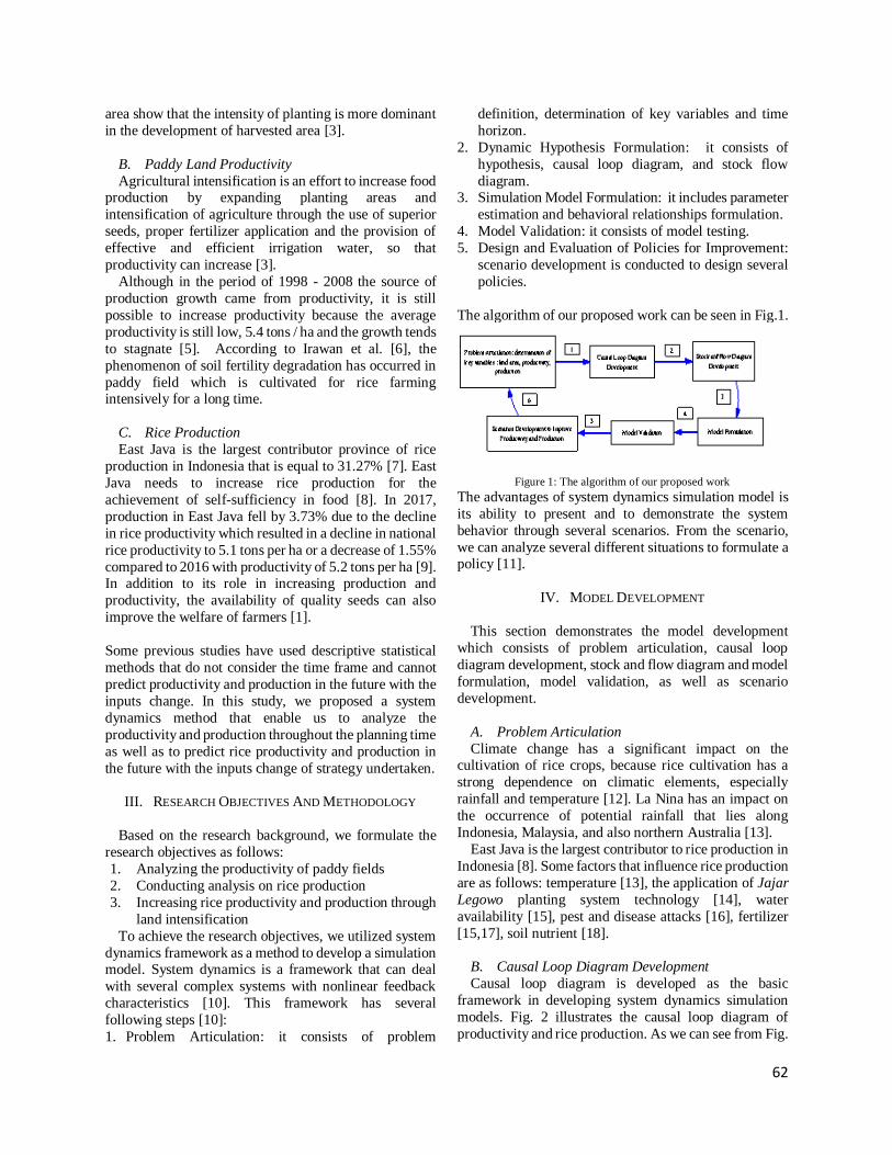
62

area show that the intensity of planting is more dominant

in the development of harvested area [3].

B. Paddy Land Productivity

Agricultural intensification is an effort to increase food production by expanding planting areas and

intensification of agriculture through the use of superior

seeds, proper fertilizer application and the provision of

effective and efficient irrigation water, so that

productivity can increase [3].

Although in the period of 1998 - 2008 the source of

production growth came from productivity, it is still

possible to increase productivity because the average

productivity is still low, 5.4 tons / ha and the growth tends

to stagnate [5]. According to Irawan et al. [6], the

phenomenon of soil fertility degradation has occurred in

paddy field which is cultivated for rice farming intensively for a long time.

C. Rice Production

East Java is the largest contributor province of rice

production in Indonesia that is equal to 31.27% [7]. East

Java needs to increase rice production for the

achievement of self-sufficiency in food [8]. In 2017,

production in East Java fell by 3.73% due to the decline

in rice productivity which resulted in a decline in national

rice productivity to 5.1 tons per ha or a decrease of 1.55%

compared to 2016 with productivity of 5.2 tons per ha [9]. In addition to its role in increasing production and

productivity, the availability of quality seeds can also

improve the welfare of farmers [1].

Some previous studies have used descriptive statistical

methods that do not consider the time frame and cannot

predict productivity and production in the future with the

inputs change. In this study, we proposed a system

dynamics method that enable us to analyze the

productivity and production throughout the planning time

as well as to predict rice productivity and production in

the future with the inputs change of strategy undertaken.

III. RESEARCH OBJECTIVES AND METHODOLOGY

Based on the research background, we formulate the

research objectives as follows:

1. Analyzing the productivity of paddy fields

2. Conducting analysis on rice production

3. Increasing rice productivity and production through

land intensification

To achieve the research objectives, we utilized system

dynamics framework as a method to develop a simulation model. System dynamics is a framework that can deal

with several complex systems with nonlinear feedback

characteristics [10]. This framework has several

following steps [10]:

1. Problem Articulation: it consists of problem

definition, determination of key variables and time

horizon.

2. Dynamic Hypothesis Formulation: it consists of

hypothesis, causal loop diagram, and stock flow

diagram. 3. Simulation Model Formulation: it includes parameter

estimation and behavioral relationships formulation.

4. Model Validation: it consists of model testing.

5. Design and Evaluation of Policies for Improvement:

scenario development is conducted to design several

policies.

The algorithm of our proposed work can be seen in Fig.1.

Figure 1: The algorithm of our proposed work

The advantages of system dynamics simulation model is

its ability to present and to demonstrate the system

behavior through several scenarios. From the scenario,

we can analyze several different situations to formulate a policy [11].

IV. MODEL DEVELOPMENT

This section demonstrates the model development

which consists of problem articulation, causal loop

diagram development, stock and flow diagram and model

formulation, model validation, as well as scenario

development.

A. Problem Articulation

Climate change has a significant impact on the cultivation of rice crops, because rice cultivation has a

strong dependence on climatic elements, especially

rainfall and temperature [12]. La Nina has an impact on

the occurrence of potential rainfall that lies along

Indonesia, Malaysia, and also northern Australia [13].

East Java is the largest contributor to rice production in

Indonesia [8]. Some factors that influence rice production

are as follows: temperature [13], the application of Jajar

Legowo planting system technology [14], water

availability [15], pest and disease attacks [16], fertilizer

[15,17], soil nutrient [18].

B. Causal Loop Diagram Development

Causal loop diagram is developed as the basic

framework in developing system dynamics simulation

models. Fig. 2 illustrates the causal loop diagram of

productivity and rice production. As we can see from Fig.

63

2, there are several factors that affect paddy productivity,

those are the availability of water, temperature, rainfall,

seed quality, pest and disease, cropping system, and soil

nutrient. Rice production depends on productivity,

harvested area, rendement, and after harvest handling.

Figure 2: Causal Loop Diagram of Paddy Productivity and Production

C. Stock and Flow Diagram and Model Formulation

From the causal loop diagram (CLD) developed at the

beginning of the model development, the CLD is

converted into a stock flow diagram (SFD). SFD is a

technique that represents a precise quantitative specification of all systems of its components and their

interrelation [19].

C1. Harvested Area

In rice farming there are three types of harvest area that

is irrigated harvest area, non-irrigated harvested area, and

dry land harvest area. The model structure in these three

types of harvested area is almost the same, the difference

lies in the cropping intensity on irrigated rice fields are

affected by the availability of water. Harvested area is

affected by land area and planting intensity. The area of paddy land is affected by land expansion and land

conversion into residential or industrial areas. Model

formulation of harvested area can be seen in Eq. (1) as

follows:

Rice Area = Initial Rice Area +

∫ 𝑒𝑥𝑝𝑎𝑛𝑠𝑖𝑜𝑛 𝑓𝑎𝑐𝑡𝑜𝑟 − 𝑐𝑜𝑛𝑣𝑒𝑟𝑠𝑖𝑜𝑛 𝑓𝑎𝑐𝑡𝑜𝑟

(1)

C2. Rice Productivity

The productivity of rice in irrigated rice area is

influenced by several factors such as the availability of water, rainfall, temperature, seed quality, planting

methods, soil nutrients, soil fertility, and pest and disease,

as seen in Fig. 3.

Figure 1: Stock and Flow Diagram for Paddy Productivity

Model formulation of rice productivity of irrigated rice

area can be seen in Eq. (2):

Productivity of Irrigated Rice Area = Initial Productivity

+ ∫ 𝑟𝑎𝑡𝑒 𝑖𝑛 𝑝𝑟𝑜𝑑𝑢𝑐𝑡𝑖𝑣𝑖𝑡𝑦 − 𝑟𝑎𝑡𝑒 𝑜𝑢𝑡 𝑝𝑟𝑜𝑑𝑢𝑐𝑡𝑖𝑣𝑖𝑡𝑦

(2)

C3. Productivity of Non-Irrigated Rice Area

The structure of productivity model is similar with the

irrigated rice field. The difference lies in the formulation

of the impact of water availability on non-irrigated rice

area.

C4. Productivity of Dry Land Area.

The structure of productivity model is similar with the

irrigated rice field. The only difference lies in the

formulation of the impact of water availability on dry

land.

C5. Production Total rice production is determined by rice production

in irrigated rice, non-irrigated rice, and dry rice areas.

D. Model Validation

Model validation is required to checked the model

accuracy and constitutes a very important step in system

dynamics simulation model development. In this process,

we utilized historical data during the time horizon

starting from the year 2000 to 2017. We consider the time

frame based on the data availability and system behavior.

Barlas (1996) explained that a model will be valid if the error rate is less than 5% and the error variance is less

than 30% [20]. We validate some variables that have

significant contribution to rice productivity and

64

production such as harvested area, productivity, and

production of irrigated land. The formulations of the

error rate and error variance are defined in Eq. 3-4.

Error Rate = ⌈S− A⌉

A

(3)

Error Variance = ⌈Ss−Sa⌉

Sa

(4)

Where:

= the average rate of simulation

= the average rate of data

A= Data at time t

S = Simulation Result at time t

𝑆𝑠= the standard deviation of simulation

𝑆𝑎= the standard deviation of data

Error rate of some variables of harvested area,

productivity, and production of irrigated land are as

follows:

Error rate of “harvested area of irrigated land”

=[ 1522660.74 − 1535028.91]

1535028.91= 0.008

Error rate of “productivity of irrigated land”

=[ 6.02 − 6.10]

6.10= 0.014

Error rate of “paddy production of irrigated land”

=[ 9218901.86 − 9414509.60 ]

9414509.60= 0.0208

Error variance of some variables of harvested area, productivity, and production of irrigated land are as

follows:

Error variance of “harvested area of irrigated land”

=[ 214589.35 − 191501.63 ]

191501.63= 0.121

Error variance of “productivity of irrigated land”

=[ 0.27 − 0.35 ]

0.35= 0.213

Error variance of “paddy production of irrigated land”

=[ 1712758.19 − 1595120.95]

1595120.95= 0.073

Based on the above calculation, all the error rates are

less than 5% and error of variances are less than 30%

which means that our model is valid.

E. Scenarios Development Scenario is a strategic planning method that aims to

analyze and project the potential developments of a

certain system in the future [21]. We may utilize a valid

model to develop several scenarios by modifying the

model structure and parameter. Simulation models built

with the system dynamics framework can provide a

reliable forecast and can develop several scenarios as a

basis for decision making [22]. It provides a framework

for developing several long-term strategies for testing

future alternatives [23]. In this study we have developed

several scenarios to improve rice productivity and

production for irrigated land, non-irrigated land as well

as dry land areas to increase rice production.

E1. Increasing Productivity of Irrigated Land Area

This scenario was developed to increase the

productivity of irrigated land area through the use of

superior seeds, the implementation of Jajar Legowo

planting system, and balanced fertilization. It is expected

that with the application of superior seeds, the productivity will increase and the pest attack can be

reduced by 10-20% [24]. The application of Jajar

Legowo planting system provides an opportunity to

maintain without disturbing the plants [14]. With the

target of productivity increase of 3.5 tons/ha, fertilizer

application should use 2 tons of manure [18]. For K

fertilization it is necessary to add 5 tons of fresh straw per

hectare to reduce the fertilizer dose by 50% [18].

E2. Increasing Productivity of Non-Irrigated Land

Area

Total irrigated rice land in 2010 reached 7.23 M ha. From the total area, as much as 230,000 ha of irrigated

land is damaged [25] and caused the irrigated land areas

turned into rain fed area. To increase the productivity of

non-irrigated land area, some of the strategies required

are similar to irrigated rice land, such as the use of

superior seeds, balanced fertilization, Jajar Legowo

implementation, and irrigation improvements.

E3. Increasing Productivity of Dry Land Area

Based on research conducted by Widyantoro and Toha,

(2010), some recommended strategies to boost dry land

productivity are: the use of high quality seed, the

implementation of Jajar Legowo, integrated nutrient

management, as well as integrated pest and disease [26].

65

E4. Increasing the Production

With the increasing productivity in each type of land

area, the overall production is also increasing as total

production is the summation of Production of Irrigated

Land, Non-Irrigated land and Dry Land as shown in Eq.

5.

Total production = Production of Irrigated Land +

Production of Non-Irrigated Land + Production of Dry

Land (5)

V. RESULTS AND DISCUSSION

In this section we demonstrates results and discussion

for harvested area, productivity of irrigated land area,

productivity of non-irrigated land area, productivity of

dry land area, production based on the existing condition,

and several scenarios results to increase land productivity

and production.

A. Productivity of Irrigated Land Area

Productivity of irrigated land area continues to increase, so that in 2017 productivity reached 6.6 tons /

ha. This productivity value although increased over time,

but still below the potential of 11 tons / ha.

B. Productivity of Non-Irrigated Land Area

Land productivity of non-irrigated land area also

continues to increase slightly so that in 2017 reached 3.65

tons / ha, however

this value was still far below the productivity of irrigated land that has reached 6.6 tons / ha.

C. Productivity of Dry Land Area

The productivity of dry land area also continues to

increase slightly, so that in 2017 reached 4.84 tons / ha,

however this value is still far below the productivity of

irrigated land that has reached 6.6 tons / ha.

D. Production Rice production also increased by 3.6% / year, so that

in 2017 the production reached 14.2 Million tons.

E. Scenarios

By implementing several strategies discussed in

scenario development, the productivity of irrigated rice

land could be increased up to 9.2 tons/ha as seen in Fig.4,

non-irrigated land productivity could be increased to 6.3 tons / ha and the productivity in dry land area could be

increased up to 7.2 tons/ha. Rice production is projected

would be increased, so that by the year 2035, the

projected rice production in East Java is projected to be

14.5 M tons.

Figure 4. Productivity Improvement of Irrigated Land

VI. CONCLUSION AND FURTHER RESEARCH

This research is designed to analyze and improve rice

productivity and production through several scenarios

development. To achieve the research objectives, we

utilized system dynamics due to several advantages such as the availability of functions and facilities to analyze a

complex system behavior as a feedback process of

reinforcing and balancing loops as well as provides

qualitative and quantitative analysis in a computer

program.

Several models based on the existing condition have

been developed to analyze the existing condition of

productivity and production. We may utilize a valid

model to develop several scenarios by modifying the

model structures and parameters.

The productivity of irrigated rice land could be

increased from 6.5 tons to 9.2 tons / ha. The productivity of non-irrigated rice field could be increased from 3.6

tons to 6.3 tons / ha and the productivity in dry land area

could be increased from 4.8 tons to 7.2 tons / ha. With the

increasing productivity in all type areas, rice production

in East Java is projected would be increased to be 14.5 M

tons in 2035. Further research is required to analyze and

increase the value of rice supply chain by considering the

internal and external factors that influence the rice supply

chain.

ACKNOWLEDGMENT

This research is supported by Directorate of Research

and Community Service of RistekDikti, Institut

Teknologi Sepuluh Nopember (ITS), ITS Research

Center, Enterprise Systems Laboratory, Information

Systems Department, Department of Agriculture in East

Java, as well as Faculty of Information and

Communication Technology of ITS.

Nomenclature

CLD causal loop diagram

SFD stock and flow diagram

66

REFERENCES

[1] Dinas Pertanian dan Ketahanan Pangan Provinsi Jawa Timur,

“Performance Report of Agricultural Service of East Java in

2014 (Laporan Kinerja Dinas Pertanian Provinsi Jawa Timur

Tahun 2014),” Pemerintah Provinsi Jawa Timur, 2015.

[2] Dinas Pertanian dan Ketahanan Pangan Provinsi Jawa Timur,

“Strategic Issues and Policy Direction: Master Plan for the

Development of Food Crops and Horticultural Areas of East Java

in 2015 - 2019 (Isu Strategis dan Arah Kebijakan: Master Plan

Pengembangan Kawasan Tanaman Pangan dan Hortikultura Jawa

Timur Tahun 2015 – 2019),” unpublished.

[3] F. Hasan, " The Role of Harvested Area and Productivity on Food

Plant Growth in East Java (Peran Luas Panen Dan Produktivitas

Terhadap Pertumbuhan Produksi Tanaman Pangan di Jawa

Timur," Embryo, vol. 7 no.1, pp. 3–8, 2010.

[4] W. Sudana, S.Sudiono, Sujatmo, “Rice Behavior in East Java

(Perilaku Perberasan di Jawa Timur),” Jurnal Soca. vol 2 no.2,

2002.

[5] M. Maulana, “The Role of Land, Intensity of Cultivation, and

Productivity as a Source of Rice Growth in Indonesia in 1980-

2001 (Peranan Luas Lahan, Intensitas Pertanaman, dan

Produktivitas Sebagai Sumber Pertumbuhan Padi Sawah

di Indonesia 1980-2001,”Jurnal Agro Ekonomi,vol 22 no.1, pp.

74-95, 2004.

[6] B. Irawan, B. Winarso, I. Sadikin, G.S. Hardono, Factor Analysis

Causes Slowing Production of Main Plant Commodities (Analisis

Faktor Penyebab Perlambatan Produksi Komoditas Tanaman

Utama.: Pusat Penelitian dan Pengembangan Sosial

Ekonomi Pertanian, Bogor, 2003.

[7] Bulog, “Java is a National Rice Mill (Jawa Masih Jadi Lumbung

Padi Nasional)“ news, okezone.com, 2012. Available at

https://economy.okezone.com/read/2012/07/04/320/658712/jawa

-masih-jadi-lumbung-padi-nasional.

[8] M. Ishaq, A.T. Rumiati, E.O. Permatasari, "Analysis of Factors

Affecting Paddy Production in East Java Province with

Semiparametric Spline Regression Method (Analisis Faktor-

Faktor yang mempengaruhi Produksi Padi di Provinsi Jawa Timur

menggunakan Regresi Semiparametrik Spline),” Jurnal Sains dan

Seni ITS, vol. 5 no. 2, pp. 420-425, 2016.

[9] CNBC, “Price of Rice and Unhusked Rice Rise Due to Weaken

Rice Production (Harga Beras dan Gabah Naik Akibat Produksi

Padi Melemah),” news, 2018. Available at

https://www.cnbcindonesia.com/news/20180110141538-4-

1118/harga-beras-dan-gabah-naik-akibat-produksi-padi-

melemah

[10] J. D. Sterman, Business Dynamics: Systems Thinking and

Modeling for a Complex World, McGraw-Hill Education, Boston,

Massachusetts, 2004.

[11] M. Kljajić1, A. Škraba, and Č. Rozman, “Methodology of system

dynamics for decision support in agriculture,” Agricultura vol. 9,

pp. 7-16, 2012.

[12] I. Yasin, I., M. Ma'shum, Y. Abawi, and L. Hadiawaty, “The use

of Early Summer Rain through Flowcast and Strategy

Development of Land Rice Cultivation of Rainwater in Lombok

Island (Penggunaan Flowcast untuk menentukan Awal Musim

Hujan dan Menyusun Strategi Tanam di Lahan Sawah Tadah

Hujan di Pulau Lombok),” in Proc. Seminar Nasional

Peningkatan Pendapatan Petani melalui Penerapan Teknologi

Tepat Guna. BPTP NTB, 2002.

[13] Ruminta, "Analysis of the decrease of rice production due to

climate change in Bandung Regency, West Java (Analisis

penurunan produksi tanaman padi akibat perubahan iklim di

Kabupaten Bandung Jawa Barat)," Jurnal Kultivasi vol. 15, no. 1,

pp. 37–45, 2016.

[14] S. Abdulrachman, M.J. Mejaya, N. Agustiani, I. Gunawan, P.

Sasmita and A. Guswara Besar, Legowo Planting System (Sistem

Tanam Legowo), Badan Penelitian dan Pengembangan Pertanian

Kementerian Pertanian, Sukamandi, 2013.

[15] W.E. Putra, and A. Ishak,”The effect of Production Factors on

Wetland Rice Productivity in Bengkulu City (Case Study in

Semarang Village, Sungai Serut Sub-district) (Pengaruh Faktor-

Faktor Produksi Terhadap Produktivitas Padi Sawah Di Kota

Bengkulu (Studi Kasus Di Kelurahan Semarang, Kecamatan

Sungai Serut))” Litbang Pertanian Bengkulu, unpublished.

[16] A.Z. Siregar, “Plant Rice Pests (Hama-hama Tanaman Padi,”

article, 2007. Available at

http://library.usu.ac.id/download/fp/07004376.pdf

[17] C. Rahma,” Still Want to Use Chemical Fertilizer? Check out the

danger (Masih Mau Pakai Pupuk Kimia? Yuk Intip Bahayanya),”

article, 2014. Available at

http://library.usu.ac.id/download/fp/07004376.pdf

[18] Kementrian Pertanian, References on the Recommendation of

Fertilizer N, P and K on Specific Wetland Location Per District

(Acuan Penetapan Rekomendasi Pupuk N, P dan K Pada Lahan

Sawah Spesifik Lokasi Per Kecamantan), Kementerian Pertanian,

Jakarta 2007.

[19] Transentis Consulting,” Step-By-Step Tutorials: Introduction to

System Dynamics: Stock and Flow Diagrams,” articles, 2018.

Available at https://www.transentis.com/step-by-step-

tutorials/introduction-to-system-dynamics/stock-and-flow-

diagrams/

[20] Y. Barlas “Formal aspects of model validity and validation in

system dynamics,” System Dynamics Review, vol. 12 no. 3, pp.

183-210, 1996.

[21] A. Brose, a. Fugenschuh, P. Gausemeier, I. Vierhaus, and G.

Seliger. “A System Dynamic Enhancement for the Scenario

Technique,” Technical Report, 2014.

[22] E. Suryani, S.Y. Chou,and C.H. Chen, “Dynamic simulation

model of air cargo demand forecast and terminal capacity

planning,” Simulation Modelling Practice and Theory 28, pp. 27-

41, 2012.

[23] Federal Highway Administration, “Scenario Planning Trends and

Transitions,” Webinar, 2013.

[24] Badan Litband Pertanian, “Superior Rice Varieties Agricultural

Research Agency (Varietas Padi Unggulan Badan Litbang

Pertanian),” in Tabloid Sinar Tani Edisi 25-31 no. 3341, Jakarta.

2012.

[25] Kementrian Pekerjaan Umum., “Support Ministry of Public

Works Against Achieving Self-Sufficiency (Dukungan

Kementrian Pekerjaan Umum Terhadap Pencapaian Swasembada

Berkelanjutan),” Jakarta: Kementrian Pekerjaan Umum, 2013.

[26] Widyantoro, and H.M. Toha, "Optimization of Rainfed Rice

Paddy Management through Integrated Crop Management

Approach (Optimalisasi Pengelolaan Padi Sawah Tadah Hujan

melalui Pendekatan Pengelolaan Tanaman Terpadu),” in

Prosiding Pekan Serealia Nasional, pp. 648-657, 2010.

https://www.cnbcindonesia.com/news/20180110141538-4-1118/harga-beras-dan-gabah-naik-akibat-produksi-padi-melemah



http://bbpadi.litbang.pertanian.go.id/index.php

http://bbpadi.litbang.pertanian.go.id/index.php

67

Microstrip Patch Wearable

Antenna for body Centric

Wireless Communication

Muhammad Fauzan bin Fisal, Ahmad

Rashidy Razali, Alhan Farhanah Abd

Rahim, Rosfariza Radzali, Emilia

Noorsal,Mohd Syazwan Osman, Aslina

Abu Bakar Faculty of Electrical Engineering

Unversiti Teknologi MARA (Pulau

Pinang) Malaysia

13500 Permatang Pauh, Pulau

Pinang, Malaysia. e-mail:

[email protected]

Abstract—This paper introduces an investigation on

microstrip patch antenna designed with copper radiating

patch and Polydimethylsiloxane as a substrate. Highly

conductive copper is embedded in flexible and durable

PDMS elastomer. The antenna is constructed to be

wearable for application in body-centric wireless

communication (BCWCs). The designed antenna is aimed

to be operated at 2.4 GHz Industrial, Scientific, and

Medical (ISM) band. The radiation pattern and return loss

result are simulated using Computer Simulation

Technology (CST) Microwave Studio. The return loss was

shifted to a resonance frequency when the antenna is laid

flat. However when the antenna is bent at 30 degree the

resonance frequency is at the desired frequency of 2.4 GHz

and thus imitates the real condition as the antenna will be

worn on human’s arm.

Index Terms – Microstrip Patch, Poydimethylsiloxane

(PDMS), body centric.

I. INTRODUCTION

In recent years, textile electronics have been acknowledged and earned a high demand in technology growth due to its many variable purposes in application[1]. Antenna is one of the most crucial element in wireless communication. It can be implemented in many ways for wireless communication such as mobile communication, medical and textile. The microstrip patch antenna is great option for wireless communication due to its fundamental properties such as small size, light weight, low cost, ease of installation with other RF equipment or component[2].

The common microstrip patch antennas resonates at single frequency and functioning in small frequency range and thus, able to transmit or receive electromagnetic wave for a single wireless communication application. The drawbacks of this type of antenna is its narrow bandwidth and low gain[3]. To overcome this problem, cutout were inserted on both

side of the patch in order to obtain 2.4 GHz resonant frequency, while cut-off the unwanted frequency as well as improving the bandwidth[4].

Wearable antenna demand the capability to operate under different mode of structural deformation while being applied to clothing. The traditional antennas are fabricated by printing or etching conductor patterns on solid substrates, where it has the probability of failure function accordingly once subjected to mechanical deformation such as stretching, bending and twisting. One of the major analysis in antennas for BCWCs application is wearable, fabric-based antennas. These textile material antennas are identified to be sensitive to environment such as humidity and temperature. Their performance could also be affected significantly or maybe fail to function under specific situation. Even though there are a lot of other polymer materials such as Liquid Crystal Polymers (LCP), Polyetherimide (PEI) or Polyethyleneterephalate (PET)[1], PDMS also known as one of the substrate that is commonly used as a substrate material for flexible antennas. PDMS is a silicon-based elastomer, known for its characteristic such as chemically inert, thermally stable, permeable to gases, easy to handle, and exhibit isotropic and homogenous properties. The initial form of the PDMS which is fluid allows the substrate to be manipulated during the fabrication process[5]. Furthermore, the liquid state of the PDMS also allow the substrate thickness to be manipulated and there is probability of the antenna to be immersed inside the substrate[6]. There are many samples of wearable antennas introduced in the research [7-10]. In this paper, a microstrip patch antenna with inset-fed were inserted on both sides of the patch element based on polymer being proposed with good conducting element metal, copper. This paper will

68

focus on parametric study and material capability to produce the best performance of the microstrip patch antenna with inset-fed prototype. All the simulation results obtained were measured using CST software and the prototype results were measured by using Vector Network Analyzer.

II. ANTENNA DESIGN

In this section, the antenna design of a microstrip patch with inset-fed has been introduced. The radiating patch element and the ground plane uses copper. The substrate for this antenna will be PDMS elastomer. The dielectric substrate will isolate the radiating patch from the ground plane. The antenna operates at Industrial Scientific and Medical (ISM) band where the operating frequency must be around 2.45 GHz. The proposed antenna constructed with it radiating plate alienated from substrate by layers of PDMS.

A. Simulation Using CST

First, Computer Simulation Technology (CST) Studio

provides a 3D electromagnetics simulation that deals

with precise, effective computational solutions for

electromagnetics design and analysis for this project. To

obtain the specific dimension, numerical analysis is

important for prior before performing the antenna

fabrication. The dimension are the first to be considered

and calculated using formula that will be discussed in

the next section. The numerical analysis will involve several stages which are creating the ground plane,

creating the substrates layer and creating the radiating

patch element and perform the antenna analysis using

CST. Once the dimension of the antenna had been

determined as required according to the specification,

the next step that need to be perform is molding and

fabrication process. Lastly, the antenna that had been

fabricated will be measure using Vector Network

Analyzer (VNA) and the results will be compared with

simulation results.

Figure 1. The dimension of copper microstrip patch

antenna on PDMS substrate with optimized dimension.

Figure 1 shows the geometry of copper

microstrip patch antenna on PDMS substrate. The

dimension of this antenna was optimized. Some adjustment were made to the calculation in order to

achieve optimized performance. The amount of

fringing fields produce are affected by the geometry of

the patch and the height of the substrate[11].

B. Substrates

The relative permittivity of PDMS is 2.7 with none inclusion with magnitude tangent beneath constant conductivity, tan δ =0.02 with waveguide method [5]. Silgard-184 kit was used for the PDMS, where it will be in liquid states initially then will become solid when proper polymerized was added. In order to get a good harden condition, the polymerization method will lasts one day and could be speed up by adding curing agent. The proposed design will use 1.5mm as the thickness of the substrates showed the frequency references stated was 2.4261 GHz but the increase in thickness will affect the bandwidth, return loss, gain, directivity and frequency reference.

C. Conductive Material

In this paper, the conductive material proposed

are copper due to its characteristic which is high conductivity in microwave application. This material

will also be used as the ground plane with the

thickness of 0.5mm. Effectiveness of antenna

matching by inset feed method can be achieved with

50Ω by varying the inset feed length.

Figure 2. Cross section of the antenna

Figure 2 shows the cross section of the microstrip patch antenna. The copper radiating patch (at the top) and ground plane (at the bottom) have the same thickness which is 0.5mm. The thickness of the substrate layer (at the middle), PDMS is 1.5mm. The thickness is optimized in order to achieve the best

69

performance for the antenna.

Table 1. ANTENNA SIMULATION PARAMETERS

Parameter

Dimension

(mm)

Patch Length, Lp 36

Patch Width, Wp 44

Patch Height, Hp 0.5

Ground Length, Lg 43

Ground Width, Wg 53

Ground Height, Hg 0.5

Substrate Length, Ls 43

Substrate Width, Ws 53

Substrate Height, Hs 1.5

Inset Feed Length,

Yo

4.67

Inset Feed Width, Xo 3

Feed Width, Wf 1.4

Feed Length, Lf 8.17

D. Design Equation To determine the dimension of the antenna, the

resonant frequency, fres need to be decided. The resonant frequency is a width’s function W, the patch element’s length L and the substrate’s thickness, h. The formula for computing the is

(1)

Where

c = speed of light L = microstrip patch’s length

εreff = microstrip patch’s relative permittivity

The aim of the resonant frequency is 2.45 GHz. The current research on PDMS dielectric properties

disclosed the relative permittivity of 2.7 to 3.0 [12].

The planned antenna was designed with relative

permittivity of 2.7.

A width of practical patch, W, for effective

radiator to obtain a high radiation efficiency is

calculated using

(2)

Where

W= microstrip patch’s width fres = resonant frequency

εr = microstrip patch’s relative permittivity

and the patch antenna actual length, L is calculated by

(3)

Where

ΔL= microstrip patch’s extended length

fres = resonant frequency

εreff = microstrip patch’s relative permittivity

The effective relative permittivity εreff and the microstrip

patch’s extended lentgh, ΔL can be determined by using

(4)

(5)

Where h is the substrate’s height. Equation (5) shows a

possible estimated of normalized length extension ΔL,

which is a function of effective dielectric constant and

the width-to-height ration (W/h). The microstrip patch antenna seems to be bigger electrically than its physical

measurement due to the fringing fields at patch corner.

The copper patch layer and ground plane

thickness is 0.5 mm. The radiating patch element is

isolated from the ground plane by a layer of PDMS

substrate with thickness of 1.5 mm. Inset-fed were

inserted on both edges of the radiating patch elements

to obtain 2.45 GHz resonant frequency. The inset

slot dimension and the microstrip line’s width, Wf

were correct using CST to achieve optical

performance.

III. ANTENNA DESIGN

The efficiency of the PDMS antenna was analyzed

through simulation and measurement where copper act

as radiating patch and ground plane.

A. Return Loss or Reflection Coefficient

The simulated S11 result of the antennas were found to be good in agreement. The antennas were found to have a measured of return loss of -15dB as shown in Figure 3. But the bandwidth is too narrow to

70

contain the 2.45 GHz ISM band.

Figure 3. Return loss comparison of microstrip patch antenna

Figure 3 shows the comparison result of microstrip patch antenna return loss using MATLAB. The red graph represent the simulation result while the blue graph represent the measured result. The return loss for the simulation is 15dB and the frequency references stated 2.42 GHz. Whereas the return loss for the measured is 14.54dB at the resonance frequency of 2.38 GHz. The difference in the result is due to the dimension of the patch which is slightly different from the simulation due to some fabrication imperfection.

B. S11 During Bending

Figure 4. Return loss comparison during bending

Figure 4 shows the return loss comparison during bending at 30 degree. , the measure return loss falls nearly 2.4 GHz and has a better return loss compared to the simlation. The

fabricated antenna was bent on the arm during measurement, while in the simulation, the antenna was bent n lies on a cylinder imitate the tissue of human body. The wearable antenna have shown that when the antenna having a contact with human body, the performance of the antenna will be improved. That is the explanation why the antenna measured has better return loss compared to the simulation. To avoid the antenna from crack, it only able to be bend to 30°. For both simulation and measurement. max angle of 30° was used for bending.

C. Radiation Pattern

Figure 4. Simulated radiation pattern of microstrip patch antenna

Figure 5. 3D simulation of radiation pattern of the microstrip patch antenna

71

Figure 6. Measured radiation pattern of the fabricated microstrip patch antenna.

Figure 4 and figure 5 shows the microstrip patch antenna’s radiation pattern. The major lobe have the highest power density of 6.15dB with magnitude of 6.0°. The measured radiation pattern is as shown in Figure 6. It has the highest density of 6.0 dB and magnitude of 270°. Both of the result shows the result of omnidirectional radiation pattern.

IV. CONCLUSION

A 2.45 GHz inset-fed rectangular patch wearable

antenna integrate with copper radiating patch and

ground plane while PDMS elastomer substrate is

presented in this paper. The fabricated antenna has

shown a good near field and far field radiation pattern. The measured result of the return loss is 14.54dB and

resonates at 2.4 GHz. The return loss when bent on the

human arm is better compared to the simulation as the

antenna is affected by the human presence.

V. ACKNOWLEDGEMENT

The authors acknowledge the financial support from

Universiti Teknologi MARA and Ministry of Higher

Education Malaysia under Grant No: 600-RMI/FRGS

5/3(14/2015) entitled “Wearable Flexible Polymer Based

Antenna Design Incorporates Highly Conductive

Radiating Element for Body Centric Wireless

Communication”.

REFERENCES

[1] C.-P. Lin, C.-H. Chang, Y. Cheng, and C. F. Jou, "Development of a flexible SU-8/PDMS-based antenna," IEEE Antennas and wireless propagation letters, vol. 10, pp. 1108-1111, 2011.

[2] D. Sanchez-Hernandez and I. D. Robertson, "Analysis and design of a dual-band circularly polarized microstrip patch antenna," IEEE Transactions on Antennas and Propagation,

vol. 43, pp. 201-205, 1995. [3] S. Tripathi, S. R. Patre, S. Singh, and S. Singh,

"Triple-band microstrip patch antenna with improved gain," in Emerging Trends in Electrical Electronics & Sustainable Energy Systems (ICETEESES), International Conference on, 2016, pp. 106-110.

[4] M. A. Murad, A. A. Bakar, A. R. Razali, M. A. I. M. Hasli, and M. F. A. J. Khan, "Bending Effects on Wearable Antenna with Silver Nanowires and Polydimethylsiloxane," in Advanced Computer and Communication Engineering Technology, ed: Springer, 2016, pp. 771-781.

[5] J. Trajkovikj, J.-F. Zürcher, and A. K. Skrivervik, "PDMS, a robust casing for flexible W-BAN antennas

EurAAP corner]," IEEE Antennas and

Propagation Magazine, vol. 55, pp. 287-297, 2013.

[6] E. Apaydin, "Microfabrication Techniques for Printing on PDMS Elastomers for Antenna and Biomedical Applications," Ohio State University, 2009.

[7] I. Locher, M. Klemm, T. Kirstein, and G. Trster, "Design and characterization of purely textile patch antennas," IEEE Transactions on advanced packaging, vol. 29, pp. 777-788, 2006.

[8] C. Hertleer, H. Rogier, L. Vallozzi, and L. Van Langenhove, "A textile antenna for off-body communication integrated into protective clothing for firefighters," IEEE Transactions on Antennas and Propagation, vol. 57, pp. 919-925, 2009.

[9] N. Chahat, M. Zhadobov, and R. Sauleau, "Wearable textile patch antenna for BAN at 60 GHz," in Antennas and Propagation (EuCAP), 2013 7th European Conference on, 2013, pp. 217-219.

[10] P. J. Soh, G. Vandenbosch, X. Chen, P.-S. Kildal, S. L. Ooi, and H. Aliakbarian, "Wearable textile antennas' efficiency characterization using a reverberation chamber," in Antennas and Propagation (APSURSI), 2011 IEEE International Symposium on, 2011, pp. 810-813.

[11] C. A. Balanis, "Antenna Theory: Analysis and Design” Third edition John Wiley & Sons," Inc. ISBN 0-471-60639-1, p. 28, 2005.

[12] G. J. Hayes, J.-H. So, A. Qusba, M. D. Dickey, and G. Lazzi, "Flexible liquid metal alloy (EGaIn) microstrip patch antenna," IEEE Transactions on Antennas and Propagation, vol. 60, pp. 2151-2156, 2012.

72

Comparison of Modification of Key Matrices

Cryptography Algorithm Playfair Cipher

and Linear Feedback Shift Register (LFSR)

in Data Security

April Lia Hananto1,2, Bayu Priyatna2, Ahmad Fauzi2, Aviv Yuniar Rahman3 1Faculty of Computing, Universiti Teknologi Malaysia, Skudai Johor, Malaysia

2Faculty of Technology and Computer Science, Universitas Buana Perjuangan, Karawang, Indonesia 3Department of Informatics Engineering, Universitas Widyagama, Malang, Indonesia

[email protected], [email protected], [email protected],

[email protected]

Abstract— Playfair cipher is a classic encryption method

that is difficult to manually manipulate but apart from the

advantages found in Playfair cipher there are also many

shortcomings, can be solved by using the information

frequency of occurrence bigram, cannot enter lowercase

letters, numbers and special characters at the time of

encryption. This study modifies the key matrix of Playfair

cryptography algorithms and combines with the Linear

Feedback Shift Register (LFSR) algorithm, by changing

the size of the 13x13 key matrix the Playfair cipher is able

to insert characters as many as 196 characters consisting

of capital letters, lowercase letters. The result of

calculation by avalanche effect method got average value

45,59% at Playfair cipher done by modification of matrix

key 13x13 and combined with generator LFSR, 36,12% at

Playfair cipher key matrix 10x10 combined with LFSR,

32,41% at Playfair classic 5x5 combined with LFSR. That

the Playfair cipher that has been modified and combined

with the LFSR generator is stronger than the previous

Playfair cipher. The results of testing the complexity of

encryption time and decryption of these three methods are

still relatively fast.

Keywords: LFSR, playfair cipher, modification,

cryptography, encryption, description

I. INTRODUCTION

Using Data will be important if it produces useful

information for a person or an institution or company, in

general, important information will always generate high-value validation in accordance with the principle

of the information itself that is reliable and authenticity

of the source. It does not rule out that very important

and high-value information can be targeted by

criminals, who deliberately want to exploit the

weaknesses of both conventional and modern systems

such as theft and data destruction. The techniques that

can be used to maintain the contents of a data is very

diverse one of them is by using cryptography techniques

(Cryptography). Cryptography itself comes from the Greek word "cryptós" which means secret, while

"gráphein" means writing, so if combined into "secret

writing". Currently, cryptography is often used in many

ways, especially to maintain information security such

as confidentiality/privacy, data integrity, authentication

and nonrepudiation used for authentication (Simbolon,

2016).

Examples of cryptographic techniques used both

classical and modern, such as Vigenere, Playfair, AES,

RSA and many others. According to Bhat [1], the

results of a comparison analysis between AES, RSA and

Playfair Cipher cryptography, that Playfair Cipher excels in securing data efficiently and unambiguously.

According to Mahyudin [2], Playfair Cipher should be

used to disguise important messages needed quickly.

Then [3], Playfair Cipher is a classic encryption

method that is difficult to manually analyze. An

important component of the Playfair algorithm is the

cipher table used for encrypting and decrypting the

default table introduced by Playfair is a table that has a

matrix of size (5x5) containing the capital letters of AZ

by omitting the letter J. Although the text security on

the Playfair cipher algorithm this is very difficult to analyze, it can still be solved by using the information

frequency of occurrence bigram.

In addition to these problems [4], the classic Playfair

cipher algorithm still has a number of weaknesses such

as not being able to enter lowercase letters, numbers and



73

special characters while encrypting. The resultant

ciphertext of the Playfair algorithm is easily solved

when a cryptanalysis knows the ciphertext and its cipher

table, although cryptanalysis only knows its ciphertext

without knowing that the cryptanalyst chipper table can guess the bigram by meaningful letters from a word [5].

Although by modifying the contents of the squares key

by simply shifting according to the number of columns,

then actually the key is repeated every 5 times. Thus

this will result in a gap in conducting cryptanalysis [6].

Looking at these problem factors, the authors are

interested in modifying the key matrix of the Playfair

cryptography algorithm and combining it with other cryptographic algorithms, then comparing some

modified algorithms.

Figure 2.1: Sample Key Matrix [9].

Encryption 1

Using the Playfair Modified Matrix table

(13 x 13)

Key 1

Data / File (Plain Text 1)

Data/File (Cipher Text 1)

Encryption 2

8-bit LFSR Key Formation

Key 2

Data/File (Cipher text 2)

Description 2

8-bit LFSR Key Formation

Key 1

Data/File (Cipher Text 1)

Description 1

Key 2

Data/File (Plain Text 1)

Using the Playfair Modified Matrix table

(13 x 13)

Figure 3.1: Flow of Data Security System

II. THEORETICAL BASIS

A. Cryptography

Cryptography in Greek is divided into two terms

namely "cryptós" which has a secret meaning, while

"gráphein" means writing, of the two terms combined

into "secret writing" [7]. The beginning of cryptography is the science and art of keeping the message

confidential by encoding into meaningless forms. Then

along with the development of cryptography is no

longer limited to encrypt messages, but also provides a

security aspect against attacks from password readings.

Therefore, the idea of cryptography turns into science as

well as art to maintain message security [8].

B. Playfair Cipher Cryptography

Playfair Cipher is asymmetric substitution key substitution. Techniques used in conventional Playfair

ciphers split plaintext into sets of two characters each

known as digraphs. Namely is composed of the alphabet

74

as identification. The Playfair password algorithm is

formed using the 5 × 5 matrices of 25 letters created as

shown in Figure

2.1. The key matrix required for the encryption and

description process is built by placing letters of the

keyword without repetition from left to right and from

top to bottom in the matrix, and then the remaining

matrix complete with the remaining alphabets in

alphabetical order. And change the letter "J" to "I" if it

is on plaintext [9].

C. Playfair Cipher Encryption Algorithm

Before performing the encryption process, the

plaintext to be encrypted is set first as follows

[10]:

1. All characters and spaces that do not belong to

the alphabet must be removed first from

plaintext (if any).

2. If there is a letter J on the plaintext do the

changes with the letter I.

3. Plaintext into the original message done arrangement according to the letter pair

(bigram).

4. When there is a pair of the same letter then do

change one letter of the letter pair with the letter

Z or X insert

Figure 3.2: Playfair 13x13 Matrix

Figure 3.3: Key Formation Process

it by using the letter X because the letter X is

very minimal in the same bigram, unlike the

letter Z, for example, is the word FUZZY.

5. If the letters on the plaintext have an odd number

then select an additional letter then add at the end of the plaintext. Additional letters can be selected

for example the letter Z or X.

D. Algorithm Description Playfair Cipher

Here is the stage of the Playfair cipher algorithm:

1. If there are two letters located on the same key row then each letter is changed using the letters

on the left.

2. If there are two letters located on the same

column then each letter is changed with the letter

above it.

3. If two letters are not on the same row and

column, change them to the letter in the first line

intersection with the two-letter columns. Then

next the second letter is changed using letters at

the fourth vertex of the rectangle formed from

the letters used [3].

E. Linear Feedback Shift Register (LFSR)

LFSR is a register that shifts with a certain amount,

the output is selected and added modulo 2. Also fed back to the input register at each clock cycle. LFSR

itself consists of N storage elements called stages. An

N-stage LFSR is characterized by an N × N matrix,

called TSR. The format and size of the TSR are based

on the feedback stage dependence. Furthermore, the

state is a linear function of the previous state [10].

Figure 3.4: Establishment of LFSR Keys

75

III. SYSTEM DESIGN

The research methodology used in this research is

engineering, Theoretical Computer Science where the

researcher uses a cryptographic technique with modification method of Playfair algorithm table using

13x13 matrix and combining it with Linear Feedback

Shift Register (LFSR) 8 bits. The process flow of the

systematic process from this research is poured in

Figure 3.1 as follows :

A. Playfair 13x13 Matrix

The establishment of a 13 x 13 Playfair matrix table

of keys entered, in the formation of keys consisting of

letters, numbers, and symbols Suppose the key example

"IM @ Ululu5". The first step is a key consisting of

numbers, letters or symbols should not have more than

one appearance if there is such thing then remove the

numbers, letters or symbols that have in common. So

the key of "AkuM @ Ululu5" becomes "AkuM @ Ul5".

In Figure 3.2 is a matrix formed from the key "AkuM @

U15":

B. Linear Feedback Shift Register (LFSR)

The step in the data encryption method using linear

feedback Shift Register (LFSR) 8 bits, is the formation of the key matrix. Here is an illustration of the key

formation process of LFSR key

In the illustration Figure, 3.3 illustrates the stage or

process flow in key formation with 8 bit LFSR. Where

b1, b2, .... b8 represent an input bit b1 xor b8 then b8 is

shifted and placed in the output bit. Here are the results

of the LFSR key building process :

In the Figure 3.4 table enter initial input 10011001

then the resulting output is 10011001 then the next

output is 00010001 and so on until (n). Then the resulting output compiles into a matrix of size (2 × n)

where length (n) is based on the length of the row

contained in ciphertexts which have been generated

from the 1st encryption process, using Playfair cipher.

Figure 4.1: Main Interface Application and Encryption

Figure 4.2: Interface Description

76


A. Construction User Interface

The built application user interface can be seen in

Figure 4.1 and Figure 4.2 :

B. The results of the 13x13 Playfair Cipher Matrix

Cryptography Test and merged with LFSR

In the test of ciphertexts, randomness is done as

much as 30 experiments with different sample

parameters that are based on the size of the file, the length of ciphertext characters and the same key.

Results obtained from experiments using the application

is calculated using the Avalanche Effect method with

the formula : 𝐴𝑣𝑎𝑙𝑎𝑛𝑐ℎ𝑒 𝐸𝑓𝑓𝑒𝑐𝑡

=number of bit changes

the total number of chip load bit x 100% (4.1)

Where Where the number of bit changes obtained

from the results of XOR calculation between plaintext

with

ciphertext first converted into binner number, then to

prove that the modification of Playfair algorithm with

13x13 key matrix and combined with LFSR have a

higher value of ciphertext randomness, then made a

comparison with the previous method. Here is the result

of the comparison of ciphertext randomness test can be

seen in Table 4.1 :

C. Time Complexity Testing

In this time complexity testing was done 30 times

experiment with different sample parameters that are

based on the size of the file and the length of the

character ciphertext. This time complexity testing is

obtained from the application during the encryption

process and description. After that do the average

calculation time of encryption and description. Here is

the result of time complexity test between Playfair 13x3

key matrix and merged with LFSR, Playfair classic

matrix lock 5x5 and Playfair 10x10 key matrix can be

seen in Figure 4.3, Figure 4.4, Figure 4.5 and Figure 4.6

:

Table 4.1

Comparison of Ciphertext Randomness Test Results

No Data Plaintext

length (bit)

Avalanche Effect

Playfair 5x5 & LFSR Playfair 10x10 & LFSR Playfair 13x13 & LFSR

1 Experiment 1 112 26.79 31.25 40.18

2 Experiment 2 472 30.93 35.17 41.31

3 Experiment 3 943 28.74 33.19 45.07

4 Experiment 4 1247 29.35 34.64 41.06

5 Experiment 5 1.961 29.73 35.90 46.51

6 Experiment 6 2.232 32.21 32.39 39.87

7 Experiment 7 3.480 31.75 33.33 45.34

8 Experiment 8 3.680 31.30 36.88 47.31

9 Experiment 9 4.224 32.15 36.65 44.96

10 Experiment 10 5.320 32.05 33.59 45.15

11 Experiment 11 5.904 32.57 36.26 46.93

12 Experiment 12 6.816 32.42 31.41 45.77

13 Experiment 13 7.872 31.40 35.71 41.92

14 Experiment 14 8.376 31.40 33.82 45.01

15 Experiment 15 18.696 31.61 33.62 45.97

16 Experiment 16 10.840 39.18 30.50 38.81

17 Experiment 17 16.480 40.18 29.78 43.62

19 Experiment 19 31.592 38.17 30.82 44.94

20 Experiment 20 19.440 38.11 30.95 39.61

21 Experiment 21 33.472 38.18 29.24 40.14

22 Experiment 22 35.896 37.09 30.74 39.96

23 Experiment 23 25.592 36.42 31.06 44.40

24 Experiment 24 38.600 36.67 30.33 44.80

25 Experiment 25 58.256 37.72 35.09 44.48

26 Experiment 26 70.112 37.25 39.91 40.10

27 Experiment 27 95.880 37.21 39.32 44.73

28 Experiment 28 121.648 37.21 39.35 39.49

29 Experiment 29 138.880 37.80 39.76 44.15

30 Experiment 30 141.368 37.37 40.26 44.63

Avalanche Effect Average Score 32.41 36.12 45.59

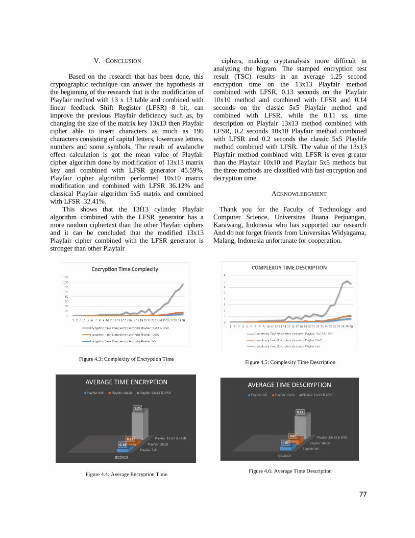
77

V. CONCLUSION

Based on the research that has been done, this

cryptographic technique can answer the hypothesis at the beginning of the research that is the modification of

Playfair method with 13 x 13 table and combined with

linear feedback Shift Register (LFSR) 8 bit, can

improve the previous Playfair deficiency such as, by

changing the size of the matrix key 13x13 then Playfair

cipher able to insert characters as much as 196

characters consisting of capital letters, lowercase letters,

numbers and some symbols. The result of avalanche

effect calculation is got the mean value of Playfair

cipher algorithm done by modification of 13x13 matrix

key and combined with LFSR generator 45.59%,

Playfair cipher algorithm performed 10x10 matrix modification and combined with LFSR 36.12% and

classical Playfair algorithm 5x5 matrix and combined

with LFSR 32.41%.

This shows that the 13f13 cylinder Playfair

algorithm combined with the LFSR generator has a

more random ciphertext than the other Playfair ciphers

and it can be concluded that the modified 13x13

Playfair cipher combined with the LFSR generator is

stronger than other Playfair

ciphers, making cryptanalysis more difficult in

analyzing the bigram. The stamped encryption test

result (TSC) results in an average 1.25 second

encryption time on the 13x13 Playfair method combined with LFSR, 0.13 seconds on the Playfair

10x10 method and combined with LFSR and 0.14

seconds on the classic 5x5 Playfair method and

combined with LFSR, while the 0.11 ss. time

description on Playfair 13x13 method combined with

LFSR, 0.2 seconds 10x10 Playfair method combined

with LFSR and 0.2 seconds the classic 5x5 Playlife

method combined with LFSR. The value of the 13x13

Playfair method combined with LFSR is even greater

than the Playfair 10x10 and Playfair 5x5 methods but

the three methods are classified with fast encryption and

decryption time.

ACKNOWLEDGMENT

Thank you for the Faculty of Technology and

Computer Science, Universitas Buana Perjuangan,

Karawang, Indonesia who has supported our research

And do not forget friends from Universitas Widyagama,

Malang, Indonesia unfortunate for cooperation.

Figure 4.3: Complexity of Encryption Time

Figure 4.4: Average Encryption Time

Figure 4.5: Complexity Time Description

Figure 4.6: Average Time Description

78

REFERENCES

[1] K. Bhat, D. Mahto, and D. K. Yadav, “Vantages of Adaptive Multidimensional Playfair Cipher

over AES-256 and RSA-2048,” vol. 8, no. 5, pp.

2015–2018, 2017.

[2] K. Bhat, D. Mahto, and D. K. Yadav, “A NOVEL

APPROACH TO INFORMATION SECURITY

USING FOUR DIMENSIONAL ( 4D )

PLAYFAIR CIPHER FUSED WITH LINEAR,”

vol. 8, no. 1, pp. 15–32, 2017.

[3] E. H. Nurkifli, “MODIFIKASI ALGORITMA

PLAYFAIR DAN MENGGABUNGKAN

DENGAN LINEAR FEEDBACK SHIFT

REGISTER ( LFSR ),” vol. 2014, no. Sentika, 2014.

[4] H. Tunga and S. Mukherjee, “A New

Modified Playfair Algorithm Based On

Frequency Analysis,” vol. 2, no. 1, 2012.

[5] J. Choudhary, “A generalized version of play

fair cipher,” vol. 2, no. Vi, pp. 176–179,

2013.

[6] E. Andriana, “Algoritma Enkripsi Playfair

Cipher,” no. May, pp. 0–5, 2016.

[7] D. Mardhatillah, “Universitas sumatera

utara,” 2017. [8] G. H. Ekaputri, “Super-Playfair , Sebuah

Algoritma Varian Playfair Cipher dan Super

Enkripsi.”

[9] T. Nafis, M. Sadiq, and N. Siddiqui,

“Addendum of Playfair Cipher in Hindi,”

vol. 10, no. 5, pp. 977–983, 2017.

[10] I. Pomeranz, “LF SR -Based Generation of

Multicycle Tests,” vol. 70, no. c, pp. 1–5,

2016.

79

Overview and Practical Use of Web APIs for

Improving User Experience

P.Filip and L.Čegan University of Pardubice

[email protected]

Abstract—How websites are perceived by a user is called

user experience (UX). UX is not exactly measurable because

it is influenced by many factors. However, one of the

measurable constituents is page-loading speed, which is

part of the usability factor. Companies such as Google or

Facebook bring new technologies and frameworks for

better and faster web applications such PWA and APIs.

This paper introduce new and current web APIs that can

help to improve user experience. A real-life experiment with

interfaces is introduced. This showed results of utilization

of APIs for lazy loading of contents such as media files.

Index Terms—User Experience; Web API; Web

Browser; Web Performance.

I. INTRODUCTION

Every year, the worldwide number of Internet users is

growing. Actually more than 50% of the world

population use the Internet [1]. Due to this trend, for

thousands of companies, the Internet has become the

main sales channel. They offer services and products via

web pages, and their revenues are influenced by UX of

the website. One of the many parts of UX is “page speed”. The page

speed is also influenced by many factors. From the

technical point of view elements such as connection type,

transfer protocols, total size of a web pages, count of

HTTP requests, performance of a target devices, web-

server performance and others can be considered [2, 3].

According to the statistics, the median web page has a

sum of transferred data of around 1500 KB [4]. Loading

on mobile devices is crucial. Time to load and parse a

HTML document takes 7 seconds and after 17 seconds,

all resources are downloaded [5].

Long loading time is the reasons why more and more emphasis is placed on web page performance and its

optimization. Resource compression, caches usage,

resource loading optimization and usage of protocols

such as HTTP2, SPDY or QUIC [6, 9], are all factors

which can lead to improvement. The consequence of the

aforementioned was that page speed become a crucial

part of the ranking factor for Google search [10].

A few years ago, PWA (progressive web application)

was introduced as a new way to create cross-platform

mobile web applications. It combines the best features of

native applications with the characteristics of web

applications [11, 12].

In the next sections are described selected APIs, which

are followed by an experiment, which uses the mentioned

APIs for improving web page loading speed. The paper

finishes with a discussion.

II. WEB APIS

In this section, new and current web APIs for improving

of web performance are introduced. Each API has

described practical use cases, which can help to increase

UX.

A. Network Information API

This API provides information about connection such

as connection type (e.g., ‘wifi’, ‘cellular’, ‘ethernet’, etc),

bandwidth estimate (Mb/s), estimate of the average

round-trip time (ms) and other information. The network

quality is based on the before mentioned properties and it

is defined by the following strings: slow-2g, 2g, 3g or 4g.

This kind of network quality is called ‘effective

connection type’ (ECP), but it is not a connection type,

but rather, how the user perceive resource loading [13, 14]. For example, a fast WiFi connection is usually 4g. A

more detailed explanation of the ECPs is described in the

following table 1.

Table 1

Effective Connection Type Explanation [13]

ECT Minimum

RTT(ms)

Maximum

(Kbps)

downlink

Explanation

slow-

2g 2000 50

The network is suited for

small transfers only such

as text-only pages.

2g 1400 70 The network is suited for

transfers of small images.

3g 270 700

The network is suited for

transfers of large assets

such as high resolution

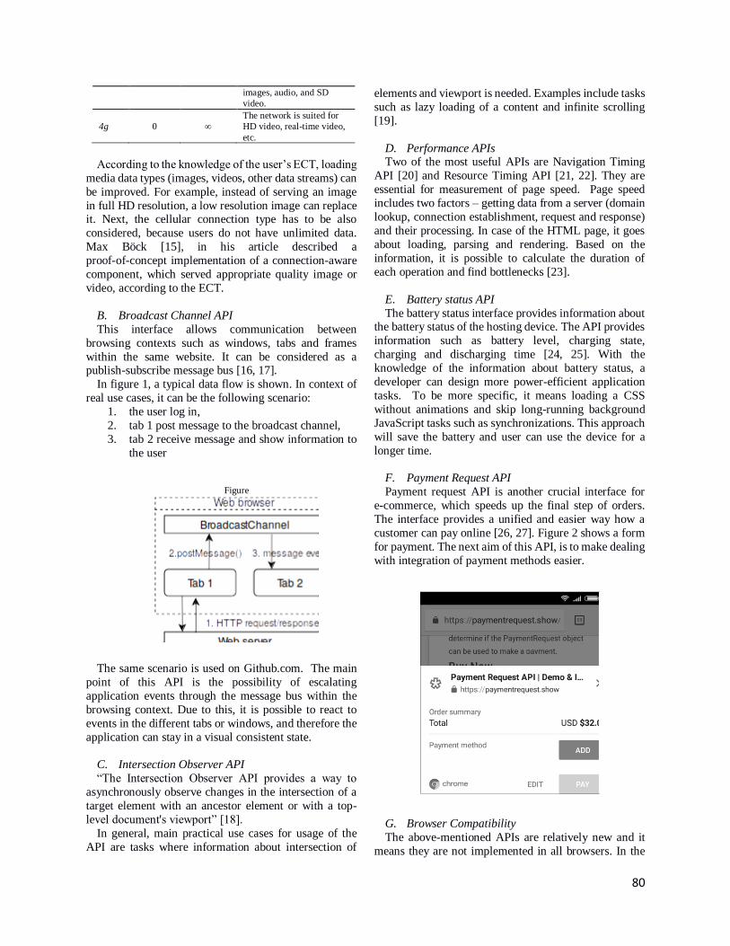
80

images, audio, and SD

video.

4g 0 ∞ The network is suited for

HD video, real-time video,

etc.

According to the knowledge of the user’s ECT, loading

media data types (images, videos, other data streams) can

be improved. For example, instead of serving an image

in full HD resolution, a low resolution image can replace it. Next, the cellular connection type has to be also

considered, because users do not have unlimited data.

Max Böck [15], in his article described a

proof-of-concept implementation of a connection-aware

component, which served appropriate quality image or

video, according to the ECT.

B. Broadcast Channel API

This interface allows communication between

browsing contexts such as windows, tabs and frames

within the same website. It can be considered as a publish-subscribe message bus [16, 17].

In figure 1, a typical data flow is shown. In context of

real use cases, it can be the following scenario:

1. the user log in,

2. tab 1 post message to the broadcast channel,

3. tab 2 receive message and show information to

the user

The same scenario is used on Github.com. The main

point of this API is the possibility of escalating

application events through the message bus within the

browsing context. Due to this, it is possible to react to

events in the different tabs or windows, and therefore the

application can stay in a visual consistent state.

C. Intersection Observer API

“The Intersection Observer API provides a way to

asynchronously observe changes in the intersection of a

target element with an ancestor element or with a top-

level document's viewport” [18].

In general, main practical use cases for usage of the

API are tasks where information about intersection of

elements and viewport is needed. Examples include tasks

such as lazy loading of a content and infinite scrolling

[19].

D. Performance APIs Two of the most useful APIs are Navigation Timing

API [20] and Resource Timing API [21, 22]. They are

essential for measurement of page speed. Page speed

includes two factors – getting data from a server (domain

lookup, connection establishment, request and response)

and their processing. In case of the HTML page, it goes

about loading, parsing and rendering. Based on the

information, it is possible to calculate the duration of

each operation and find bottlenecks [23].

E. Battery status API

The battery status interface provides information about the battery status of the hosting device. The API provides

information such as battery level, charging state,

charging and discharging time [24, 25]. With the

knowledge of the information about battery status, a

developer can design more power-efficient application

tasks. To be more specific, it means loading a CSS

without animations and skip long-running background

JavaScript tasks such as synchronizations. This approach

will save the battery and user can use the device for a

longer time.

F. Payment Request API

Payment request API is another crucial interface for

e-commerce, which speeds up the final step of orders.

The interface provides a unified and easier way how a

customer can pay online [26, 27]. Figure 2 shows a form

for payment. The next aim of this API, is to make dealing

with integration of payment methods easier.

G. Browser Compatibility

The above-mentioned APIs are relatively new and it

means they are not implemented in all browsers. In the

Figure

1: Use Case for Broadcast Channel

Figure 2 :Example of Unified Payment Form

81

following tables, supporting of implementation each

APIs for each major browser is marked.

Table 2

Overview of Compatibility of APIs on Desktop Browsers [28]

Desktop environment

Network Information

Broadcast Channel

Battery Status

Payment Request

Intersection Observer

Navigation Timing

Resource Timing

Table 3

Overview of Compatibility of APIs on Mobile Browsers [28]

Mobile environment

Network Information

Broadcast Channel

Battery Status

Payment Request

Intersection Observer

Navigation Timing

Resource Timing

III. EXPERIMENT

For the purposes of the experiment, which

demonstrates three strategies for content loading, three

web pages were created. Every page contains nine images, which are placed to one column. Every image has

different resolution and size. The images have another

three copies with different lower resolution and quality.

• First page use strategy “no lazy loading”, which

requests all nine full resolution images

immediately after DOM is loaded.

• Second page use Intersection Observer API for

lazy loading and page requests only for images

that are intersected with the viewport. In the test

cases, two images are loaded.

• Third page combines Intersection Observer API

with Network Information API. According to the ECT, an image with a suitable resolution is

requested.

Every test was repeated and final values represent an

attempt average when measured values were stabilized.

Time of domContentLoadedEventStart and

domComplete events was established as performance

metrics.

• domContentLoadedEventStart – event is fired

when HTML document is loaded and parsed.

Images can be still loading at that moment.

• domComplete – event is fired when the whole

page is loaded. It includes CSS and images.

For greater information value, the measured times are

shown without network delays. Testing configuration

was as follows: Dell E5470 (i5-6200), Debian 9.5, local

Apache web server 2.4.25 and Google Chrome 68.0.3440.75. The web browser was running in developer

mode and desktop mode, with disabled cache and the

transfer protocol was HTTP/1.1. For simulation of type

network such as 4g, 3g and 2g, default presets were used.

For testing purpose of slow-2g ECT, a custom preset was

created. The pages include JavaScript code (based on

performance interface) for capturing and sending (via

AJAX) gathered information to a PHP script, which

writes data to a file. Source codes and measured data are

placed in a public git repository:

https://github.com/petrfilip/.

Table 4

Results of the Experiments

No Lazy

loading Observer

Observer

and ECT

Requests 14 7

Data

transfered 5.9 MB 2 MB

4g = 2MB

3g = 126 KB

2g = 48 KB

slow-2g = 10

KB

4g (in ms)

domContentL

oaded 368 240 196

domComplete 955 642 591

3g (in ms)

domContentL

oaded 833 696 660

domComplete 33444 12565 1877

2g (in ms)

domContentL

oaded 2294 2156 2162

domComplete 123037 45659 5136

slow-2g (in ms)

domContentL

oaded 3165 2617 2606

domComplete 1128628 27084 6159

As was expected, the combination of lazy loading and

information about the network (ECT) achieved the best

page loading performance (see table 4). However, in case

of the scenario with applied ECT, image quality

decreased and it can be perceived as decreasing of UX.

It is more like a placeholder, which can be replaced

during the user staying with an image in higher

resolution. When the applied ECT was equal to slow-2g, images with an average size 3 KB were requested.

Consideration about the quality and resolution of images

depends on the nature of the web and the user’s

requirements. For websites, where the text content is

essential, and images are only for illustration, it can be an

acceptable approach.

82

IV. DISCUSSION

At the beginning of the paper, the current state of web

applications was mentioned. It included a new PWA

approach which takes the best from the current web environment and native applications.

Next, an overview of the web APIs which can be used

for improving of UX, is provided. As the most important

API, Network Information API can be considered, which

provides data about user connection such as ECT. It

brings new opportunities for web developers who can

care more about their web users who do not have a stable

and quality Internet connection, and provide them with a

faster website, which increases UX.

In the experiment, how effectively Intersection

Observer API can be used for lazy loading was shown. In

addition, there are many more opportunities, such as combination of a data from Battery Status API. For

improving of performance, we need to begin with

empirical measurements. For this, APIs, which gather

information about page loading and its resources, are

prepared. According to this measurement, it is possible to

improve the situation. The problem of the UX, is that

there is not only one metric which fits to all use cases;

and the page loading speed is only one factor which

influences the level of user satisfaction.

For faster payment on e-commerce websites Request

Payment API is available, which provides a unified checkout process. In addition, after the payment, the state

of the application has to be consistent, which can be done

through the Broadcast Channel API.

Web applications are still evolving and it brings new

challenges for all participants of the web development

environment. Involved people need to watch how trends

are changing which includes learning modern

technologies, frameworks and patterns.

ACKNOWLEDGMENT

The work has been supported by the Funds of University of Pardubice, Czech Republic. This support is

very gratefully acknowledged.

REFERENCES

[1] StatCounter, “Mobile Browser Market Share Worldwide”,

online: http://gs.statcounter.com/browser-market-

share/mobile/worldwide [2] Scott W. H. Young, “Speed Matters: Performance Enhancements

for Library Websites”, in Weave, vol. 1 , 2016, DOI :

10.3998/weave.12535642.0001.401, online:

https://quod.lib.umich.edu/

w/weave/12535642.0001.401?view=text;rgn=main [3] J. Avery, “Watching your (image) weight”, 2017, online:

https://responsivedesign.is/articles/watching-your-image-weight/ [4] HTTP Archive, “State of the Web | 2018_07_01”, 2018, online:

https://httparchive.org/reports/state-of-the-

web?start=2018_07_01 [5] HTTP Archive, “Loading speed | 2018_07_01”, 2018, online:

https://httparchive.org/reports/loading-speed?start=2018_07_01

[6] J. Alakuijala, R. Obryk, O. Stoliarchuk, Z. Szabadka, L.

Vandevenne, J. Wassenberg, “Guetzli: Perceptually Guided JPEG

Encoder”, 2017, online: https://arxiv.org/pdf/1703.04421.pdf [7] H. Leventić, K. Nenadić, I. Galić and Č. Livada, "Compression

parameters tuning for automatic image optimization in web

applications," in 2016 International Symposium ELMAR, Zadar,

2016, pp. 181-184. DOI: 10.1109/ELMAR.2016.7731782, 2016 [8] Y. Liu, Y. Ma, X. Liu and G. Huang, “Can HTTP/2 Really Help

Web Performance on Smartphones?,” in 2016 IEEE International

Conference on Services Computing (SCC), San Francisco, CA,

2016, pp. 219-226. doi: 10.1109/SCC.2016.36 [9] C. Gaetano, L. D. Cicco, S. Mascolo, “HTTP over UDP: an

experimental investigation of QUIC.” in SAC, 2015, online:

https://c3lab.poliba.it/images/3/3b/QUIC_SAC15.pdf [10] Z. Wang, D. Phan, “Using page speed in mobile search ranking”

in Webmaster Central Blog, 2018, online:

https://webmasters.googleblog.com/2018/01/using-page-speed-

in-mobile-search.html [11] A. Osmani, “Getting started with Progressive Web Apps”, 2015,

online: https://addyosmani.com/blog/getting-started-with-

progressive-web-apps/ [12] A. Biørn-Hansen, T. A. Majchrzak, T. Grønli. "Progressive web

apps: The possible web-native unifier for mobile development."

in Proceedings of the 13th International Conference on Web

Information Systems and Technologies (WEBIST), 2017, online:

http://www.scitepress.org/Papers/2017/63537/63537.pdf [13] Web Incubator Community Group, “Network Information API”,

2018, online: https://wicg.github.io/netinfo/ [14] Mozilla, “NetworkInformation”, in MDN Web Docs, 2017,

online: https://developer.mozilla.org/en-

US/docs/Web/API/NetworkInformation [15] M. Böck, “Connection-Aware Components”, in MXB, 2018,

online: https://mxb.at/blog/connection-aware-components/ [16] Mozzila, “Broadcast Channel API”, in MDM Web Docs, 2018,

online: https://developer.mozilla.org/en-

US/docs/Web/API/Broadcast_Channel _API [17] E. Bidelman, “BroadcastChannel API: A Message Bus for the

Web”, 2016, online:

https://developers.google.com/web/updates/2016/09/

broadcastchannel [18] Mozzila, “Intersection Observer API”, in MDM Web Docs, 2018,

online: https://developer.mozilla.org/en-US/docs/Web/API/

Intersection_Observer_API [19] Web Platform Working Group, “Intersection Observer”, 2018,

online: https://w3c.github.io/IntersectionObserver/ [20] Web Performance Working Group, “Navigation Timing”, 2012,

online: https://www.w3.org/TR/navigation-timing/ [21] Web Performance Working Group, “Resource Timing Level 1”,

2017, online: https://www.w3.org/TR/resource-timing/ [22] Mozilla, “Using the Resource Timing API”, 2018, online:

https://developer.mozilla.org/en-US/docs/Web/API/

Resource_Timing_API/Using_the_Resource_Timing_API [23] I. Grigorik, “Critical Rendering Path”, online:

https://developers.google.com/web/fundamentals/performance/cr

itical-rendering-path/ [24] Device and Sensors Working Group, “Battery Status API”, 2018,

online: https://www.w3.org/TR/battery-status/ [25] Mozilla, “Battery Status API”, 2017, online:

https://developer.mozilla.org/en-

US/docs/Web/API/Battery_Status_API [26] Web Payments Working Group, “Payment Request API” , 2018,

online: https://www.w3.org/TR/payment-request/ [27] E. Kitamura, D. Gash, Z. Koch, “Introducing the Payment

Request API”, 2018, online:

https://developers.google.com/web/fundamentals/payments/ [28] A. Deveria, “Can I use... Support tables for HTML5, CSS3, etc”,

2018, online: https://caniuse.com/

https://developer.mozilla.org/en-US/docs/Web/API/

https://developers.google.com/web/fundamentals/payments/

83

Online Posture Strategy on Irregular Terrain for

“T-FLoW” Humanoid Robot

R. Dimas Pristovani1, Dewanto. Sanggar2, Pramadihanto. Dadet3 EEPIS Robotics Research Center (ER2C)

1Electronics Engineering Department, 2Mechatronics Engineering Department, 3Computers Engineering

Department,

Electronics Engineering Polytechnic Institute of Surabaya (EEPIS) / Politeknik Elektronika Negeri Surabaya

(PENS)

St. Raya ITS, Keputih, Sukolilo, Surabaya, Indonesia, 60111

[email protected]

Abstract—Human has several natural behaviors when

they are walking or just stand up. The one of the behavior

is adaptive posture of legs including ankle placement during

stand up in uneven area (irregular terrain with certain

angle). This paper describes the implementation of adaptive

posture of human into T-FLoW humanoid robot during

stand up in the irregular terrain with certain angle. The

strategy to finish this implementation is how to arrange the

legs posture of the robot to avoid the falling state caused by

angle changes. The inverse kinematics analysis is used to

arrange the legs part based on global position reference.

This kinematics analysis makes the process of calculation is

in the cartesian space. The strategy control is built based on

the dynamics system approach by using quasi dynamics

system with single body zero moment point analysis. The

result of dynamics analysis is position vector of zero

moment point. To maintain the posture of the robot

(kinematics input), the PI controller is used to arrange the

compensation of the cartesian data input of kinematics

analysis. From the experimental result, the T-FLoW

humanoid robot successfully complete the task but still has

some limitations.

Index Terms— inverse kinematics; quasi dynamics

system; online posture stabilization; robot in irregular

terrain; PI controller.

I. INTRODUCTION

A lot of humanoid robots were made to adapt one or

several human behaviors. This condition was happened

because the human behaviors are an ideal characteristic

for all system of bipedal or humanoid system. The most basic behavior which adapted by humanoid robot is stand

up posture models. When human in the stand-up

condition, a lot of posture models are happened in there.

More specifics are when human stand up in the uneven

area, they will naturally adapt and change their stand-up

behavior based on the environment. If the human stands

up in irregular terrain with certain angle, the human will

adapt the legs height and ankle joint rotation based on the

direction vector between irregular terrain angle and

human direction (Figure 1). This paper describes about the process to solve a main

problem that is caused by irregular terrain which is

falling condition of the robot. From several researches in

the reference [2-12], they are using several methods to

solve the main problems such as dynamic dynamics

control model, dynamic statics control model, direct

control to kinematics, artificial intelligent, and lookup

table. This research is proposing a combination between

2 steps of analysis to solve the main problem which are

using geometry analysis for 1st step and analysis of

dynamics system approach by using quasi dynamics system with single body zero moment point analysis for

2nd step. The plant is joint in the legs part. To simplify it,

the inverse kinematics analysis is used to covering the

angle control of each joint in legs part. Because of it, the

calculation in this system is using cartesian space data (x,

y, z-Axis).

Figure 1: Human behavior in the legs part during stand up on the

irregular terrain with certain angle with (A) right, (B) left, (C)

backward, and (D) forward of human direction.

84

Figure 2: T-FLoW humanoid robot mechanical design with 28 DoF

The plant which is used in this research is T-FLoW

humanoid robot. From previous research of T-FLoW

humanoid robot [14, 15], this research is future work with

implementation plant and different plan. The mechanism

of T-FLoW humanoid robot can be seen in Figure 2. II. INVERSE KINEMATICS ANALYSIS

The kinematics in the legs mechanism had been solved

by using an analytical solution with complex

trigonometry and reflection models. The design of Legs

mechanism can be seen in Figure 2 and the configuration

of DoF in both legs is shows in Table 1. T-FLoW

humanoid robot using parallelogram mechanism system

to generate more torque. Because of it, the knee joint is

calculated with a special condition.

Table 1

Joint configuration of legs mechanism (translational and rotational)

No Joint Translation

Rotational x y z

1 (𝑅𝐿|𝐿𝐿)0 0 (𝑑𝑅𝐿,𝑦,0, −𝑑𝐿𝐿,𝑦,0) 0 0

2 (𝑅𝐿|𝐿𝐿)1 0 0 −𝑑(𝑅𝐿|𝐿𝐿),𝑧,1 𝑅𝑧(𝜃(𝑅𝐿|𝐿𝐿),1)

3 (𝑅𝐿|𝐿𝐿)2 0 0 −𝑑(𝑅𝐿|𝐿𝐿),𝑧,2 𝑅𝑥(𝜃(𝑅𝐿|𝐿𝐿),2)

4 (𝑅𝐿|𝐿𝐿)3 0 0 −𝑑(𝑅𝐿|𝐿𝐿),𝑧,3 𝑅𝑦(𝜃(𝑅𝐿|𝐿𝐿),3)

5 (𝑅𝐿|𝐿𝐿)4 0 0 −𝑑(𝑅𝐿|𝐿𝐿),𝑧,4 𝑅𝑦(𝜃(𝑅𝐿|𝐿𝐿),4)

6 (𝑅𝐿|𝐿𝐿)5 0 0 −𝑑(𝑅𝐿|𝐿𝐿),𝑧,5 𝑅𝑦(𝜃(𝑅𝐿|𝐿𝐿).5)



9 (𝑅𝐿|𝐿𝐿)8 0 0 −𝑑(𝑅𝐿|𝐿𝐿),𝑧,8 𝑅𝑥(𝜃(𝑅𝐿|𝐿𝐿).8)

The cartesian space data is position vector of 𝐸𝑜𝐸(𝑅𝐿

(𝑃(𝑅𝐿|𝐿𝐿),(𝑥,𝑦,𝑧)) and the orientation angel (𝜃(𝑅𝐿|𝐿𝐿),(𝜙)).

The inverse kinematics analysis can be seen in Figure

3(A), Figure 3(B), and Figure 4 and the calculation is

shown in Equation (1~15).

(A)

(B)

Figure 3: (A) Transversal plane analysis of right leg mechanism

and (B) Frontal plane analysis of right leg mechanism

𝜃(𝑅𝐿,𝐿𝐿),1 = 𝜃(𝑅𝐿|𝐿𝐿),(𝜙) (1)

𝑅0(𝑅𝐿,𝐿𝐿) = √𝑃(𝑅𝐿,𝐿𝐿),(𝑥)2 + 𝑃(𝑅𝐿,𝐿𝐿),(𝑦)

2 (2)

𝜃(𝑅𝐿,𝐿𝐿),𝛽 = 𝑡𝑎𝑛−1 (𝑃(𝑅𝐿,𝐿𝐿),(𝑦)

𝑃(𝑅𝐿,𝐿𝐿),(𝑥)⁄ ) − 𝜃(𝑅𝐿,𝐿𝐿),1

(3)

𝑃′(𝑅𝐿,𝐿𝐿),(

𝑦𝑥

)= 𝑅0(𝑅𝐿,𝐿𝐿) (

sin 𝜃(𝑅𝐿,𝐿𝐿),𝛽

cos 𝜃(𝑅𝐿,𝐿𝐿),𝛽) (4)

Where 𝜃(𝑅𝐿|𝐿𝐿),1 is joint angle in the 𝑅𝐿1 joint.

𝜃(𝑅𝐿|𝐿𝐿),𝛽 is angle deviation between present position

vector of 𝐸𝑜𝐸(𝑅𝐿|𝐿𝐿) (𝑃(𝑅𝐿|𝐿𝐿),(𝑥,𝑦)) with the next position

vector of 𝐸𝑜𝐸(𝑅𝐿|𝐿𝐿) (𝑃(𝑅𝐿|𝐿𝐿),(𝑥,𝑦)′ ).

𝑃(𝑅𝐿,𝐿𝐿)8,(𝑧) = 𝑃(𝑅𝐿,𝐿𝐿),(𝑧) − (𝑑(𝑅𝐿,𝐿𝐿),𝑧,1 + 𝑑(𝑅𝐿,𝐿𝐿),𝑧,8)

(5)

𝜃(𝑅𝐿,𝐿𝐿),2 = −𝜃(𝑅𝐿,𝐿𝐿),8 = tan−1 (𝑃′(𝑅𝐿,𝐿𝐿),(𝑦)

𝑃(𝑅𝐿,𝐿𝐿)8,(𝑧)) (6)

85

𝑅1(𝑅𝐿,𝐿𝐿) = √𝑃′(𝑅𝐿,𝐿𝐿),(𝑦)2

+ 𝑃(𝑅𝐿,𝐿𝐿)8,(𝑧)2 (7)

Where 𝑃(𝑅𝐿|𝐿𝐿)8,(−𝑧) is new height for inverse

kinematics calculation. 𝜃(𝑅𝐿|𝐿𝐿),8 is reflection of

𝜃(𝑅𝐿|𝐿𝐿),2. 𝑅1𝑅𝐿is resultant that occurs because existence

of 𝑃𝑅𝐿6 ,(−𝑧)and 𝑃′(𝑅𝐿,𝐿𝐿),(𝑦).

Figure 4: Sagittal plane analysis of right leg mechanism with

simplification from parallel mechanism into serial mechanism

∆𝑅1(𝑅𝐿,𝐿𝐿) = 𝑅1(𝑅𝐿,𝐿𝐿) − (𝑑(𝑅𝐿,𝐿𝐿),𝑧,2 + 𝑑(𝑅𝐿,𝐿𝐿),𝑧,4

+ 𝑑(𝑅𝐿,𝐿𝐿),𝑧,6 + 𝑑(𝑅𝐿,𝐿𝐿),𝑧,7) (8)

𝑅2(𝑅𝐿,𝐿𝐿) = √𝑃′(𝑅𝐿,𝐿𝐿),(𝑥)2

+ ∆𝑅1(𝑅𝐿,𝐿𝐿)2 (9)

𝜃(𝑅𝐿,𝐿𝐿),𝛾𝑐 =

𝑐𝑜𝑠−1 ((𝑑(𝑅𝐿,𝐿𝐿),𝑧,3)

2+ (𝑑(𝑅𝐿,𝐿𝐿),𝑧,5)

2− 𝑅2(𝑅𝐿,𝐿𝐿)

2

2 𝑑(𝑅𝐿,𝐿𝐿),𝑧,3𝑑(𝑅𝐿,𝐿𝐿),𝑧,5

) (10)

𝜃(𝑅𝐿,𝐿𝐿),𝛾𝑎 = 𝑡𝑎𝑛−1 (𝑃′(𝑅𝐿,𝐿𝐿),(𝑥)

∆𝑅1(𝑅𝐿,𝐿𝐿)

) (11)

𝜃(𝑅𝐿,𝐿𝐿),𝛾𝑏 =

𝑡𝑎𝑛−1 (𝑑(𝑅𝐿,𝐿𝐿),𝑧,3 𝑠𝑖𝑛 𝜃(𝑅𝐿,𝐿𝐿),𝛾𝑐

(𝑑(𝑅𝐿,𝐿𝐿),𝑧,3) + (𝑑(𝑅𝐿,𝐿𝐿),𝑧,5 𝑐𝑜𝑠 𝜃(𝑅𝐿,𝐿𝐿),𝛾𝑐))

(12)

𝜃(𝑅𝐿,𝐿𝐿),3 = −𝜃(𝑅𝐿,𝐿𝐿),4 = (𝜃(𝑅𝐿,𝐿𝐿),𝛾𝑎 + 𝜃(𝑅𝐿,𝐿𝐿),𝛾𝑏) (13)

𝜃(𝑅𝐿,𝐿𝐿),5 = −𝜃(𝑅𝐿,𝐿𝐿),6 = 0 − ((180 − 𝜃(𝑅𝐿,𝐿𝐿),𝛾𝑐) −

𝜃(𝑅𝐿,𝐿𝐿),3) (14)

𝜃(𝑅𝐿,𝐿𝐿),7 = 0 (15)

Where 𝜃(𝑅𝐿|𝐿𝐿),4 is reflection of 𝜃(𝑅𝐿|𝐿𝐿),3. 𝜃(𝑅𝐿|𝐿𝐿),6 is

reflection of 𝜃(𝑅𝐿|𝐿𝐿),6. 𝜃(𝑅𝐿|𝐿𝐿),7 is joint angle in the

joint 𝑅𝐿7 (ankle pitch angle) and has default value as much as 0 degree.

III. QUASI DYNAMICS ANALYSIS

In the humanoid robot, the dynamics system analysis

is approached by using zero moment point analysis. Because of that, the dynamics analysis became a quasi-

dynamics analysis.

A. Classic Zero Moment Point (Multi-Body)

The general concept of ZMP is analyzing non-vertical

force and momentum when momentum (𝑀𝐴) and the

action force (𝐹𝐴) is equal with zero because it is damped

by momentum (𝑀𝐵) and reaction force (𝐹𝐵) (action force

and momentum = reaction force and momentum / 3rd newton’s law) [13]. This concept was published in

January 1968 by Miomir Vukobratović [1].

Figure 5: Condition Type of zero moment point (ZMP)

The ZMP has 3 conditions based on the event which is

ZMP equal with center of pressure (CoP), ZMP inside

support polygon (SP), and ZMP outside SP as seen in

Figure 5. The main calculation of classic ZMP is

explained in Equation (18).

(𝑥,𝑦,𝑧) = 𝐶𝑜𝑀,(𝑥,𝑦,𝑧) = 𝑚𝑡𝑜𝑡𝐶𝑜𝑀,(𝑥,𝑦,𝑧) (16)

ℒ(𝑥,𝑦,𝑧) = ℒ𝐶𝑜𝑀,(𝑥,𝑦,𝑧) = 𝑃𝐶𝑜𝑀,(𝑥,𝑦,𝑧) × 𝑚𝑡𝑜𝑡𝐶𝑜𝑀,(𝑥,𝑦,𝑧)

(17)

𝑃𝑧𝑚𝑝,(𝑥,𝑦) = 𝑃𝐶𝑜𝑀,(𝑥,𝑦)𝑚𝑡𝑜𝑡𝑔𝑧 + 𝑃𝑧𝑚𝑝,𝑧(𝑥,𝑦) − ℒ(𝑦,𝑥)

𝑚𝑡𝑜𝑡𝑔𝑧 + 𝑧

(18)

B. Simplified Zero Moment Point (Single-Body)

The calculation of classic ZMP is derived by using

Single Linear Inverted Pendulum Model (SLIPM)

approach [16]. The calculation of simplified ZMP is

explained in Equation (19).

𝑃𝑧𝑚𝑝,(𝑥,𝑦) = 𝑃𝐶𝑜𝑀,(𝑥,𝑦) −𝑃𝐶𝑜𝑀,𝑧

𝑔𝑧𝐶𝑜𝑀,(𝑥,𝑦) (19)

In the simplified model, the linear acceleration in Z

axis is equal to zero (𝑃𝐶𝑜𝑀,𝑧 = 0). Each component in

vertical composition (Z axis) such as angular velocity,

linier velocity, angular acceleration and linier

86

acceleration is removed.

IV. ONLINE POSTURE STRATEGY

Online Posture Strategy (OPS) is strategy which is

used to solve the problems caused by irregular terrain.

OPS are divided into 2 part which are OPS – legs position

correction and OPS – position of center of mass (COM)

correction. The output from those OPS control is

combined and controlled in the PI controller to generate

a simple trajectory for IK of legs. The process of control

system is shown in Figure 6.

Figure 6: Subdivision of Zero Moment Point (ZMP)

A. OPS - Legs Position Correction (LPC)

OPS – Legs Position Correction (LPC) is used to

calculate the differences between position vector of CoM

in normal condition with position vector of CoM after

influenced with angle caused by irregular terrain. This

strategy is the first step to solve the main problem caused

by irregular terrain which is falling condition because

position vector of ZMP is outside SP.

Figure 7: Process during OPS - LPC (A) Angle direction similar

with roll angle (Y axis), (B) angle direction similar with pitch angle

(X axis)

OPS – LPC are divided into 2 conditions based on robot direction with angle of irregular terrain. The 1st

condition is when the angle direction of irregular terrain

is similar with roll angle of the robot (Y axis) (Figure

7(A)) and the 2nd condition is when the angle direction of

irregular terrain is similar with pitch angle of the robot

(X axis) (Figure 7(B)). The 1st and 2nd condition are

explained in the Equation (20) and Equation (21).

𝑃(

𝑅𝐿𝐿𝐿

),(𝑧)

𝐿𝑃𝐶 = (−𝑑𝑅𝐿,𝑦 sin−1 ∅(𝐷𝑒𝑠−𝑅𝑒𝑓),(𝑟)

𝑑𝐿𝐿,𝑦 sin−1 ∅(𝐷𝑒𝑠−𝑅𝑒𝑓),(𝑟)

) (20)

𝑃(

𝑅𝐿𝐿𝐿

),(𝑥)

𝐿𝑃𝐶 = 𝑃𝐶𝑜𝑀,(𝑧) sin−1 ∅(𝐷𝑒𝑠−𝑅𝑒𝑓),(𝑝) (21)

𝑃(

𝑅𝐿𝐿𝐿

),(𝑦)

𝐿𝑃𝐶 = 0 | Normal Condition (22)

𝑃𝐹𝐶,(

𝑅𝐿𝐿𝐿

),(𝑥𝑦𝑧

)= 𝑃

(𝑅𝐿𝐿𝐿

),(𝑥𝑦𝑧

)+ 𝑃

(𝑅𝐿𝐿𝐿

),(𝑥𝑦𝑧

)

𝐿𝑃𝐶 (23)

B. OPS – Position of CoM Correction (PCC)

OPS – Position of CoM Correction (PCC) is used to

calculate the differences between position vector of CoM after normalized with OPS – LCC with position vector of

CoM after calculated by using ZMP calculation. This

strategy is the second step to solve the main problem

caused by irregular terrain.

Figure 8: Process during OPS - PCC (A) Angle direction similar

with roll angle (Y axis), (B) angle direction similar with pitch angle

(X axis)

Similar with OPS – LPC, OPS – PCC are divided into

2 conditions based on robot direction with angle of

irregular terrain. Similar with condition in OPS – LPC

above. The 1st (Figure 8(A)) and 2nd (Figure 8(B)) condition is explained in the Equation (24) and Equation

(25).

𝑃(

𝑅𝐿𝐿𝐿

),(𝑦)

𝑃𝐶𝐶 = 𝑃𝑧𝑚𝑝,(𝑦) + 𝑃𝐹𝐶,(

𝑅𝐿𝐿𝐿

),(𝑦) (24)

𝑃(

𝑅𝐿𝐿𝐿

),(𝑥)

𝑃𝐶𝐶 = 𝑃𝑧𝑚𝑝,(𝑥) + 𝑃𝐹𝐶,(

𝑅𝐿𝐿𝐿

),(𝑥) (25)

𝑃(

𝑅𝐿𝐿𝐿

),(𝑧)

𝑃𝐶𝐶 = 0 | Normal Condition (26)

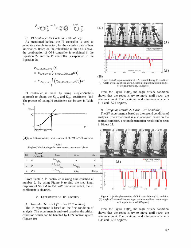
87

𝑃𝑆𝐶,(

𝑅𝐿𝐿𝐿

),(𝑥𝑦𝑧

)= 𝑃

𝐹𝐶,(𝑅𝐿𝐿𝐿

),(𝑥𝑦𝑧

)+ 𝑃

(𝑅𝐿𝐿𝐿

),(𝑥𝑦𝑧

)

𝑃𝐶𝐶 (27)

C. PI Controller for Cartesian Data of Legs

As mentioned before, the PI controller is used to

generate a simple trajectory for the cartesian data of legs

kinematics. Based on the calculation in the OPS above,

the combination of OPS controller is explained in the

Equation 27 and the PI controller is explained in the Equation 28.

𝑃𝑃𝐼,(𝑅𝐿,𝐿𝐿),(𝑥,𝑦,𝑧)(𝑡)

= 𝐾𝑝,𝑃𝐼,(𝑥,𝑦,𝑧) (𝑃𝑆𝐶,(𝑅𝐿,𝐿𝐿),(𝑥,𝑦,𝑧)(𝑡))

+ 𝐾𝑖,𝑃𝐼,(𝑥,𝑦,𝑧) ∫ (𝑃𝑆𝐶,(𝑅𝐿,𝐿𝐿),(𝑥,𝑦,𝑧)(𝜏)) 𝑑𝜏

𝜏

0

(28)

PI controller is tuned by using Ziegler-Nichols

approach to obtain the 𝐾𝑝,𝑃𝐼 and 𝐾𝑖,𝑃𝐼 coefficient [16].

The process of tuning PI coefficient can be seen in Table

2.

Figure 9: S-shaped step input response of SLIPM in T-FLoW robot

Table 2

Ziegler-Nichols tuning rule based on step response of plants

No Type of

Controller 𝐾𝑝,𝑃𝐼 𝐾𝑖 ,𝑃𝐼 𝐾𝑑,𝑃𝐼

1 𝑃 𝛾𝑍𝐿

𝛽𝑍𝐿⁄ ∞ 0

2 𝑃𝐼 0.9𝛾𝑍𝐿

𝛽𝑍𝐿⁄ 𝛽𝑍𝐿

0.3⁄ 0

3 𝑃𝐼𝐷 1.2𝛾𝑍𝐿

𝛽𝑍𝐿⁄ 2𝛽𝑍𝐿 0.5𝛽𝑍𝐿

From Table 2, PI controller is using tune equation at number 2. By using Figure 9 to find the step input

response of SLIPM in T-FLoW humanoid robot, the PI

coefficient is obtained.

V. EXPERIMENT OF OPS CONTROL

A. Irregular Terrain 1 (Y axis – 1st Condition)

The 1st experiment is based on the first condition of

analysis. The experiment is analyzed based on the critical

condition which can be handled by OPS control system

(Figure 10).

Figure 10: (A) Implementation of OPS control during 1st condition

(B) Angle offside condition during experiment until maximum angle

of irregular terrain (25 Degrees)

From the Figure 10(B), the angle offside condition

shows that the robot is try to move until reach the

reference point. The maximum and minimum offside is

6.11 and -6.21 degrees.

B. Irregular Terrain 2 (X axis – 2nd Condition)

The 2nd experiment is based on the second condition of

analysis. The experiment is also analyzed based on the

critical condition. The implementation result can be seen

in Figure 11.

Figure 11: (A) Implementation of OPS control during 2nd condition

(B) Angle offside condition during experiment until maximum angle

of irregular terrain (25 Degrees)

From the Figure 11(B), the angle offside condition

shows that the robot is try to move until reach the

reference point. The maximum and minimum offside is

1.35 and -2.36 degrees.

(𝐴)

(𝐵)

(𝐴)

(𝐵)

88

C. Irregular Terrain 3 (Combination X axis and Y

axis)

The 3rd experiment is based on the combination of 1st

and 2nd condition. The critical condition which can be

handled by OPS control system can be seen in Figure 12.

Figure 12: Implementation of OPS control during combination

condition

VI. CONCLUSION

The main problem which shows in this paper research

is falling condition of T-FLoW humanoid robot caused

by irregular terrain. During the 1st condition, OPS

controller is successfully handled the maximum and

minimum angle of irregular terrain from 28 degrees until

–28 degrees. During the 2nd condition, the maximum and

minimum angle of irregular terrain is from 34 degrees

until –32 degrees. During combination condition (1st and

2nd condition), the maximum and minimum angle of

irregular terrain is from 26 degrees until –24 degrees.

ACKNOWLEDGMENT

Gratefulness to Ministry of Research, Technology and

Higher Education of the Republic of Indonesia for

financial support and EEPIS Robotics Research Center

(ER2C) laboratory.

REFERENCES

[1] Vukobratović, Borovac, “Zero-Moment Point - Thirty Five Years

of Its Life”, Int. J. Humanoid Robotics, Vol. 1 No. 1, pp. 161–

162, 2004

[2] Changjiu Zhou, Pik Kong Yue, Jun Ni, Shan-Ben Chan,

“Dynamically Stable Gait Planning for a Humanoid Robot to

Climb Sloping Surface”, In Proc. the 2004 IEEE Conference on

Robotics, Automation and Mechatronics, Singapore, 2004, PP.

341–346.

[3] Zhibin Li, Nikos G. Tsagarakis, and Darwin G. Caldwell,

“Stabilizing Humanoids on Slopes Using Terrain Inclination

Estimation”, In Proc. 2013 IEEE/RSJ International Conference on

Intelligent Robots and Systems (IROS), Tokyo, Japan, 2013, pp.

4124–4129.

[4] Amir Massah B, Arman Sharifi K, Yaser Salehinia, Farid Najafi,

“Open Loop Walking on Different Slopes for NAO Humanoid

Robot”, In International Symposium on Robotics and Intelligent

Sensors 2012 (IRIS 2012), Procedia Engineering, Vol. 41, pp.

296–304, 2012.

[5] Edoardo Farnioli, Marco Gabiccini, Antonio Bicchi, “Optimal

Contact Force Distribution for Compliant Humanoid Robots in

Whole-Body Loco-Manipulation Tasks”, In Proc. 2015 IEEE

International Conference on Robotics and Automation (ICRA),

Seattle, Washington, 2015, pp. 5675–5681.

[6] Kitti Suwanratchatamanee,Student, Mitsuharu Matsumoto, and

Shuji Hashimoto, “Haptic Sensing Foot System for Humanoid

Robot and Ground Recognition With One-Leg Balance”, In IEEE

Transactions On Industrial Electronics, Vol. 58, No. 8, pp. 3174–

3186, 2009,

[7] Fariz Ali, Ahmad Zaki Hj. Shukor, Muhammad Fahmi Miskon,

Mohd Khairi Mohamed Nor and Sani Irwan Md Salim, “3-D

Biped Robot Walking along Slope with Dual Length Linear

Inverted Pendulum Method (DLLIPM)”, In International Journal

of Advanced Robotic Systems, Vol 10, No 11, pp. 1–12, 2013.

[8] Luis Sentis, Josh Petersen, and Roland Philippsen, “Experiments

with Balancing on Irregular Terrains using the Dreamer Mobile

Humanoid Robot”, In Proc. Robotics: Science and Systems,

Sydney, NSW, Australia, 2012.

[9] K. Nagasaka, M. Inaba, H. Inoue, “Dynamic Walking Pattern

Generation for Humanoid Robot based on Optimal Gradient

Method”, In Proc. of the IEEE International Conference on

Systems, Man and Cybemetics, 1999, pp. 908–913.

[10] Jung-Shik Kong, Eung-Hyuk Lee, Bo-Hee Lee, and Jin-Geol

Kim, “Study on the Real-Time Walking Control of a Humanoid

Robot Using Fuzzy Algorithm”, In International Journal of

Control, Automation, and Systems, Vol. 6, No. 4, pp. 551–558,

2008.

[11] Kensuke Harada, Mitsuharu Morisawa, Shin-ichiro Nakaoka,

Kenji Kaneko, and Shuuji Kajita, “Kinodynamic Planning for

Humanoid Robots Walking on Uneven Terrain”, In Journal of

Robotics and Mechatronics, Vol. 21, No. 3, pp. 311–316, 2009

[12] Seung-Joon Yi, Byoung-Tak Zhang, and Daniel D. Lee, “Online

Learning of Uneven Terrain for Humanoid Bipedal Walking”, In

Proceedings of the Twenty-Fourth AAAI Conference on Artificial

Intelligence (AAAI-10), 2010, pp. 1639–1644.

[13] R. Dimas Pristovani, W. M. Rindo, B. Eko Henfri, Kh. Achmad

S, and Pramadihanto. D, “Basic walking trajectory analysis in

FLoW ROBOT”, In Proc. 2016 International Electronics

Symposium (IES), Bali, Indonesia, 2016, pp 333–338.

[14] R. Dimas Pristovani, Ajir, B. Eko Henfri, K. Achmad Subhan, D.

Raden Sanggar, and Pramadihanto. Dadet, “Implementation of

direct pass strategy during moving ball for “T-FLoW” Humanoid

Robot”, in Proc. 2017 2nd International Conferences on

Information Technology, Information Systems and Electrical

Engineering (2nd ICITISEE), Yogyakarta, Indonesia, 2017, pp.

223–228.

[15] R. Dimas Pristovani, B. Eko Henfri, D. Raden Sanggar, and

Pramadihanto. Dadet, “Walking Strategy Model based on Zero

Moment Point with Single Inverted Pendulum Approach in “T-

FLoW” Humanoid Robot”, in Proc. 2017 2nd International

Conferences on Information Technology, Information Systems

and Electrical Engineering (2nd ICITISEE), Yogyakarta,

Indonesia, 2017, pp. 217–222.

[16] R. Dimas Pristovani, D. Raden Sanggar, and Pramadihanto. Dadet

“Implementation of Push Recovery Strategy using Triple Linear

Inverted Pendulum Model in “T-FloW” Humanoid Robot”, in

IOP Journal of Physics: Conference Series, vol. 1007, pp. 1–13,

2018.

89

A Logic Scoring of Preference Algorithm for

Quality Performance Evaluation of Moodle and

Wordpress Aaron Don M. Africa

Department of Electronics and Communications Engineering

De La Salle University, Manila

2401 Taft Ave Manila 1004, Philippines

[email protected]

Abstract— Moodle and Wordpress are the most

commonly used Open Source applications. Moodle is

used for education purposes while Wordpress to create

websites. These programs are open source software

meaning they are free to download and their source code

are freely available and can be modified by anyone.

Logic Scoring of Preference is a multi-criteria decision

making process with theoretical foundations in advance

optimization techniques and continuous logic. This

research proposes a standard method to evaluate the two

programs using the Logic Scoring of Preference

Algorithm. Focus will be will be given on the criteria of

Performance Efficiency and Reliability to follow the

International Standard ISO/IEC 25010:2011. If these

programs are designed to follow the International

Standard their optimization will improve.

Index Terms—Information Technology; Open Source

Software; Moodle; Wordpress; Logic Scoring of

Preference.

I. INTRODUCTION

Ever since the dawn of the internet, programmers have

been creating web applications [1]. One category of

Applications are Open Source Web Applications [2].

In these types of Applications, the source code is freely

available [3]. This means that programmers has access

to it so they can modify the program to their liking [4].

Moodle and Wordpress are Open Source Web

Applications [5]. Moodle is used for creating

educational Websites [6] while Wordpress [7] is used for creating different types of Web content. These

programs have communities that develops them. One

problem is creating a standard for the different types

of programmers that does the contribution [8].

A good reference is the ISO/IEC 25010:2011. This

ISO Standard is about Systems and Software

Engineering quality [9]. This research creates an

algorithm that incorporates the ISO/IEC 25010:2011

to the Logic Scoring of Preference [10] to create a way of checking the quality of Open Source Web

Applications. Focus was given to the two parameters

of the ISO standard that is Performance Efficiency and

Reliability [11]. Rough Set Theory can be used to find

the missing components of the two parameters if it

existed [12,13]. The Fuzzy Logic Algorithm can also

be applied if there are uncertain parameters [14,15]. In

performing the test via quality requirement tree the

Neural Network algorithm can be applied [16,17].

Spatial Algorithm can also be applied in making the

tree [18]. An algorithm was developed to test these

parameters. This research can aid programmers in

optimizing Moodle and Wordpress because it adheres

to the ISO/IEC 25010:2011 standard.

II. METHODOLOGY

A. Performance Efficiency

In this research it is the performance of the Open

Source web application is in terms of speed. The speed

of the data transfer is measured using website

monitoring service applications. This software is used

to determine the speed of the web download. In this

test the elementary criteria are a multi-variable

criterion. The formula that will be used is [19]:

100*) )(X / ) 0.8X 0.4X- (X ( X 1321=

Where Xn represents the number of pages that

satisfies the range given in the download time. The download time references are X1 4 Mbps and above,

90

X2 3-3.999 Mbps and X3 is 2.999 Mbps and below.

The percentages 0.4 and 0.8 was suggested as a metric.

B. Reliability

In this research Reliability defines the links found

that lead to broken links or destination URLs that are

not present. Reliability can be computed by using a

link checker tool. This tool will be used to determine

the broken links and the total number of links. The

formula used to determine this is:

100) * TL) / ((BL - 100 = X

In the equation:

TL = number of total site links

BL = number of broken links found by the

link checker tool.

III. DATA AND RESULTS

A. Performance Efficiency

To test the Performance Efficiency the software

Pingdom [20] was used.

Figure 1: Website of Pingdom

Figure 1 shows the Website of Pingdom. The free

version was used to conduct the test.

Figure 2: Performance insights for the test server of

Moodle and Wordpress

The program Pingdom can give the performance

insights of the server. Figure 2 shows the Performance

insights for the test server of Moodle and Wordpress.

Test can also be done from different servers around the

globe. For this test the server in San Jose United States was used.

The formula:

100*) )(X / ) 0.8X 0.4X- (X ( X 1321=

was used to conduct the test. The speed used as a

reference is X1 4 Mbps and above, X2 3-3.999 Mbps

and X3 is 2.999 Mbps and below.

For Moodle:

100*) ) (310 / ) 0.8(5) 0.4(11)- (310 ( X = =

98.4%

For Wordpress:

100*) ) (390 / ) 0.8(15) 0.4(21)- (390 ( X = =

94.76 %

B. Reliability

The test for Reliability was done for and Moodle

and Wordpress. The software W3C Link Checker [21]

was used to test the result. The speed of the connection

will greatly affect the transfer [22].

91

Figure 3: Screenshot of W3C Link Checker Tool

Figure 3 shows the Screenshot of the W3C Link

Checker Tool

Figure 4: Broken links of the test server

Figure 5 : Parse Code of the test server

The W3C Link Checker Tool is useful in finding the

broken links of the test servers for Moodle and

Program as shown in figures 4 and 5. These data are placed in a database Information Systems

configuration [23]. Custom Database can also be used

[24].

The equation:

100) * TL) / ((BL - 100 = X

Was used to compute for the performance Efficiency.

For Moodle there are a total of 310 links where 4 are

broken based on the test. Plugging it in the equation

we have:

100) * 310) / ((4 - 100 = X = 98.7%

For Worpress there are 390 Links and a total of 8 was

broken. The result is:

100) * 390) / ((8 - 100 = X = 97.94%

IV. CONCLUSION AND RECOMMENDATIONS

This paper presented a new algorithm that can be

used to evaluate Moodle and Wordpress. Focus was

given on the parameter Performance Efficiency and

Reliability. A test website was created to do the

assessment. For measuring the Performance

Efficiency, the software Pingdom was used. This

program is a free to use website to know the speed of web pages. This software was used to know the speed

of the pages and if it satisfies the required speed. For

92

this test the result was 98.4 % for Moodle and 94.76%

for Wordpress.

In the test for reliability the W3C validator was

used. The W3C Validator is a free website used for checking broken links of target web pages. The result

was 98.7 % for Moodle and 97.94 % for Wordpress.

The test developed was to make it compatible with the

International Standard ISO/IEC 25010:2011.

The test was only performed in a test server. To

further improve the results, it is recommended to use a

commercial webserver. Increasing the specifications

of the webserver will greatly improve the speed and

performance of the system.

REFERENCES

[1] Z. Hemel, D. Groewenegen, L. Kats, and E. Visser, “Static

consistency checking of Web applications with Web DSL, ”

Journals of Symbolic Computation, vol. 46 no. 2 pp. 150-182,

2011.

[2] N. Swain, K. Latu, S. Kristensen, N. Jones, E. Nelson, D.

Ames, and G. Williams, “A review of open source software

solutions for developing water resources web applications, ”

Environmental Modelling and Software, vol. 67 no. 1 pp. 108-

117, 2015.

[3] E. Gomez-Garcia, J. Azevado, and F. Perez-Rodriguez, “A

compiled project and open-source code to generate web-based

forest modelling simulators, ” Computer and Electronics in

Agriculture, vol. 147 no. 1 pp. 1-5, 2018.

[4] P. Gleeson, A. Davinson, R. Silver, and G. Ascoli, “A

Commitment to Open Source in Neuroscience, ” Neuron, vol.

96 no. 5 pp. 964-965, 2017.

[5] R. Phunsuk, C. Viriyavejakul, and T. Ratanaolarn,

“Development of a problem-based learning model via a virtual

learning environment, ” Kasetsart Journal of Social Sciences,

vol. 38 no. 3 pp. 297-306, 2017.

[6] Moodle. https://www.moodle.org/. 2018.

[7] Wordpress. https://www.wordpress.com/. 2018.

[8] D. Mason, “Data Programming for Non-programmers,”

Procedia Computer Science, vol. 21 no. 1 pp. 68-74, 2013.

[9] ISO/IEC 25010:2011.

https://www.iso.org/standard/35733.html 2011

[10] J. Dujmovic, “LSP method and its use for evaluation of Java

IDEs,” International Journal of Approximate Reasoning, vol.

41 no. 1 pp. 3-22, 2006.

[11] ISO/IEC 25010:2011 en 2011.

https://www.iso.org/obp/ui/#iso:std:iso-iec:25010:ed-1:v1:en

2011.

[12] A. Africa, and M. Cabatuan, “A Rough Set Based Data Model

for Breast Cancer Mammographic Mass Diagnostics, ”

International Journal of Biomedical Engineering and

Technology, vol. 18 no. 4 pp. 359-369, 2015.

[13] A. Africa, “A Rough Set-Based Expert System for diagnosing

information system communication networks,” International

Journal of Information and Communication Technology, vol.

11 no. 4 pp. 496-512, 2017.

[14] A. Africa, “A Rough Set Based Solar Powered Flood Water

Purification System with a Fuzzy Logic Model,” ARPN

Journal of Engineering and Applied Sciences, vol. 12 no. 3 pp.

638-647, 2017.

[15] A. Africa, “A Mathematical Fuzzy Logic Control Systems

Model Using Rough Set Theory for Robot Applications,”

Journal of Telecommunication, Electronic and Computer

Engineering, vol. 9 no. 2-8 pp. 7-11, 2017.

[16] S. Brucal, A. Africa, and E. Dadios “Female Voice

Recognition using Artificial Neural Networks and MATLAB

Voicebox Toolbox,” Journal of Telecommunication,

Electronic and Computer Engineering, vol. 10 no. 1-4 pp. 133-

138, 2018.

[17] A. Africa, and J. Velasco, “Development of a Urine Strip

Analyzer using Artificial Neural Network using an Android

Phone,” ARPN Journal of Engineering and Applied Sciences,

vol. 12 no. 6 pp. 1706-1712, 2017.

[18] P. Loresco, and A. Africa, “ECG Print-out Features Extraction

Using Spatial-Oriented Image Processing Techniques,”

Journal of Telecommunication, Electronic and Computer

Engineering, vol. 10 no. 1-5 pp. 15-20, 2018.

[19] A. Africa, “A Logic Scoring of Preference Algorithm using

ISO/IEC 25010:2011 for Open Source Web Applications

Moodle and Wordpress,” ARPN Journal of Engineering and

Applied Sciences, vol. 13 no. 15, 2018.

[20] Pingdom. https://www.pingdom.com/. 2018.

[21] W3C Link Checker. https://validator.w3.org/. 2018

[22] A. Africa, and A. Mesina, J. Izon, and B. Quitevis,

“Development of a Novel Android Controlled USB File

Transfer Hub,” Journal of Telecommunication, Electronic and

Computer Engineering, vol. 9 no. 2-8 pp. 1-5, 2017.

[23] A. Africa, S. Bautista, F. Lardizabal, J. Patron, and A. Santos,

“Minimizing Passenger Congestion in Train Stations through

Radio Frequency Identification (RFID) coupled with Database

Monitoring System,” ARPN Journal of Engineering and

Applied Sciences, vol. 12 no. 9 pp. 2863-2869, 2017.

[24] A. Africa, J. Aguilar, C. Lim Jr., P. Pacheco, and S. Rodrin,

“Automated Aquaculture System that Regulates Ph,

Temperature and Ammonia,” 9th International Conference on

Humanoid, Nanotechnology, Information Technology,

Communication and Control, Environment, and Management

(HNICEM), 2017.

93

Microcontroller-based Blood Agglutination

Detector and Coagulation Analyzer Gel Ann S. Divino, Patricia Mae M. Manuel, Dejeannie Gayle B. Tieng, Roderick Yap

De La Salle University

Manila, Philippines

[email protected]

Abstract— Blood typing involves categorizing a person’s

blood into a group according to antigens present in it. Blood

coagulation, on the other hand, is the subsequent dissolution

of blood to repair injured tissues. An abnormal coagulation

time could lead to bruising and excessive bleeding. Current

testing methods for blood typing and coagulation are

inconvenient. In this study, a microcontroller-based device

that is able to determine a person’s blood type and

coagulation time is constructed. This is implemented using

a simple photodiode light sensor and LED circuit. For blood

typing, the device mixes two separate drops of blood on a

glass slide with two different reagents, which triggers an

agglutination reaction that is detected by the photodiode

and LED circuit. The microcontroller then analyzes the

result and classifies the blood sample into one of four types

(A, B, AB, and O). For coagulation analysis, the photodiode

and LED circuit detects the appearance of a light, yellowish

serum at the top of a blood sample in a test tube, which

indicates that the blood has already coagulated. The device

is low-cost, automated, accessible, and portable, making it

advantageous for efficient and accurate on-site blood

testing.

Index Terms— –Blood Agglutination, Blood

Coagulation, Photodiode Spectrophotometry;

I. INTRODUCTION

A lot of studies have been conducted to pave the way

for biomedical applications through electronics. One study from Chua (2014) shows a method of non-invasive

glucose level measurement using a LED pair sensor

which eliminates the pain of everyday pricking [1]. Dy

Perez (2016), on the other hand, used ISFET as the active

component for a glucose sensor, which is integrated into

a WiFi module for easy visibility and management for the

doctors [2]. Nakamachi (2010) designed an automatic

operated blood sampling system to satisfy accurate and

quick blood collection and blood glucose measurement.

They adopted near infrared light transmitting scheme as

a human blood vessel visualization methodology [3].

Blood comprises of the ABO and Rh(D) systems.

Classifications of blood types can be determined by the

presence or absence of certain antigens. The chemical

reaction of blood if an antigen is mixed and is used for blood grouping is called Agglutination [4]. Agglutination

has two different types of antigens which are type A and

type B [5]. A person should know his or her blood type

because it is needed for emergencies, calamities and

transfusions because not all blood types are compatible

with each other.

On the other hand, coagulation, also known as clotting, is the process wherein blood changes from a liquid to

form a clot [6]. It also measures the ability of the blood

of a person to clot and the amount of time to do so. The

normal coagulation time range is from 2-15 minutes and

normal activity means normal clotting function while low

activity of coagulation factor means impaired clotting

ability that can lead to the detections of different types of

diseases.

Over the past few years, studies were made regarding

Blood Agglutination and Blood Coagulation. Razo

(2003) did a study that involved using image processing

to be able to detect blood agglutination [7]. To overcome

the tedious and laborious operation, Chang (2014) used

microfluidic chips for blood typing. This allows the

operation sequence to be conducted automatically

through the manipulation of micro fluids [8]. In order for

microfluidic devices to be used in remote, rural or in

private clinics, they should be cheap, low power

consuming and easy to operate. This implies that such

devices are essential in the health care departments. Zia (2016) developed a device that is capable of providing

point-of-care diagnostics for various medical test by

providing a platform to run microfluidic lab-on-disc [9].

Fernandes (2015) used of the concept of

spectrophotometry to be able to determine the blood type

of a person [10] while Li (2009) conducted a study about

measuring the coagulation time of a person using too the concept of spectrophotometry [11]. Spectrophotometry

can be defined as the measure of the different intensities

of light in the different spectrums. Another

spectrophometric approach to blood typing was

conducted by Anthony (2005) in which a discrete array

94

of LED/IRED and photodiode pairs are used as sensors

to determine red blood cell agglutination [12].

Despite the prior studies that were made, both blood

agglutination and coagulation in many laboratories are

still carried out using manual procedure and thus human

error is possible. The result of a patient can also take time

to be released because of personnel or equipment

availability. Laboratories may not also be accessible to

everyone especially in remote areas and in times of

calamites. The main objective of this study is to construct

a microcontroller-based device that is able to detect

agglutination in a patient’s blood sample as well as

analyze its coagulation process using the concept of spectrophotometry to be able to help solve the problems

mentioned above.

Fig. 1 System Block Diagram

II. DESIGN CONSIDERATION

A. Block Diagram

The block diagram of the prototype for blood coagulation

analyzer and agglutination detector is seen on Fig. 1. The

user first turns on the prototype and selects from three switches namely switch A, B and C. Switch A is for

coagulation, switch B is for agglutination while switch C

is for both. When the user chooses switch A, the LEDs

for coagulation illuminates the blood sample from the test

tube. The photodiode also reads a voltage reading which

is also converted to a current value through the use of a

current to voltage converter. The current to voltage

converter is connected to a low pass filter to eliminate

noise and erratic readings. As blood coagulates, the

voltage value reading of the photodiode increases. The

output of the low pass filter is then connected to the

microcontroller to analyze and output the results. When

the user chooses switch B, the syringe plunger, which is driven by a stepper motor, will drop reagents A and B.

Motors A and B will then turn on one at a time and these

motors will be used to stir the blood samples with

reagents and this blood sample is then illuminated by the

LEDs by which these LEDs is powered by the

microcontroller. The LEDs also illuminate the

photodiode at the same time and the photodiode obtains

a voltage reading which is then converted to current with

the use of a current to voltage converter. These are also

connected to low pass filter circuit to eliminate noise and

erratic results. The output of the low pass filter is

connected to the microcontroller to analyze and output the results. When the user chooses Switch C, the

prototype performs both agglutination and coagulation

separately, coagulation being first.

Fig. 2. Current to Voltage Converter

Fig. 3. Illumination Circuit

B. Sensor Circuit

In order to implement the sensor circuit, a current to

voltage converter as seen in Fig. 2 is used to convert the intensity of light into a voltage value. A photodiode

conducts current when light is applied to the junction.

The operational amplifier is LM741 and a commercial

95

photodiode is used for this circuit. For the illumination

circuit as seen in Fig. 3, the light source is based on three

LEDs for higher light intensity.

Fig. 4. Setup for Coagulation

For agglutination, the light source is a common cathode

tricolor LED. The specific wavelengths are 650 nm, 536

nm and 475 nm. The colors of these LEDs are red, green

and blue, respectively. The specified wavelengths were chosen to maximize the spectral differences between

agglutinated and non-agglutinated samples for blood

typing. There are values obtained for each color that

lights up for comparison in agglutination.

For blood coagulation as seen on Fig. 4, having a high

intensity source will produce accurate results due to

clearer opacity so four super bright white LEDs are used.

The circuit is the same for agglutination and coagulation, only the LEDs differ. Tricolor LEDs are not used in

coagulation because the comparison of values for the

color does not apply wherein time here is an important

factor.

Both the circuits of agglutination and coagulation

method need proper alignment of the LEDs with respect

to the photodiode circuit. This is to produce higher light

absorption and the samples should be in proper place.

The placement of blood on the glass slide is important for

all the samples so that the photodiode read the samples in the correct position. For coagulation, the height of the

blood on the test tube is maintained for all the samples

because the circuits of photodiode and LEDs are aligned.

C. Low Pass Filters

A low pass filter circuit is used to filter signals with

frequency lower than a certain cut-off frequency. The input voltage for the circuit seen on Fig. 5 is from the

output of current to voltage circuit of the photodiode

while the output voltage is to the microcontroller.

Without the low pass filter, the microcontroller does not

read the correct output values from the photodiode circuit

and produces erratic values. When the output of

photodiode circuit is connected to a low pass filter then

to the microcontroller, it produces a more stable and

accurate values. It is used for conditioning signals prior

to analog-to-digital conversion.

Fig. 5. Low Pass Filter Circuit

Fig. 6. Plunger Setup

D. Syringe Plunger Set Up

For the reagent dropping, a syringe plunger circuit is

developed. The plunger circuit has a 3 mL syringe loaded

with reagent operated by a stepper motor. The actual

setup is seen on Fig. 6. The stepper motor is connected to a bearing block coupler and threaded rods to push the

syringe. If the syringe is pushed, the reagent will drop to

the sample. The blocks for the plunger setup are made up

of black acrylic plastic designed by the group.

E. Conveyor Belt

In the automation of the reagent dropper and stirrer for

agglutination, a conveyor belt is implemented to hold the

glass slide with blood samples. The gears are driven by a

DC motor and the driver is L293D that provides

bidirectional operation for the motor. The design is seen

on Fig. 7. It is made up of rubber silicon to avoid slipping

of the glass slide and the gears are made up of acrylic

plastic.

96

Fig. 7. Conveyor Belt

F. Reagent Mixer

After the dropping of reagent from the plunger circuit,

the blood sample is mixed with reagent by simply stirring the sample slowly. The reagent mixer seen on Fig. 8

should be slow but accurate to avoid spilling of the

samples. An improvised mixer is made using rubber. The

mixer should be soft so that the glass slides will still slip

through. The setup for the mixer is equipped with

magnets for convenient placement.

Fig. 8. Reagent Mixer

Fig. 9. Coagulated Blood Sample

III. DATA AND RESULTS

A. Coagulation

Twenty samples were gathered for coagulation and

agglutination testing with each of the ABO blood group

present. When the test tube is placed on the prototype, the

program starts to count with a 24-second delay and the

recorded output voltage is the initial voltage. For every 12 seconds, the output voltage is checked if it is higher

than the initial voltage with voltage difference (Vd) of

0.012 V. When the serum is present as seen on Fig. 9,

there is a change in the color of the blood and it suddenly

becomes clear so there is a change in the light absorbance

of the photodiode. The photodiode should be able to read a higher voltage value because the serum is seen and

more light would be able to penetrate. The result from

laboratory testing is used as the ideal value. The voltage

difference is determined through a series of testing

wherein the trend of the values are observed. If the

voltage difference (Vd) reaches 0.012 V, the timer will

then stop and record the total time. The results are seen

on Table 1. In the table, Vi(V) and Vf(V) are the output

voltages for the initial and final values. ADCi and ADCf

are the initial and final ADC values read by the

microcontroller. CT(min) is the coagulation time

obtained from the prototype while CTL(min) is the coagulation time via slide method from the laboratory

tests and is usually used by medical technologists. Lastly,

the %E is the percentage error of the data.

For coagulation, to be able to output accurate readings,

the blood sample quantity should not exceed 1.0-1.2ml

and should not be lower than 0.9ml. If the blood sample

exceeds 1.2ml or is lower than 0.9 ml, the height of the

serum when it separates from the blood will be different

if the blood sample height is higher or lower, thus the

photodiode will still be able to read a different value. In order for an exact blood measurement to be obtained, a guide while placing the blood into the test tube will be

followed.

B. Agglutination

In Table 2, the threshold voltage for reagent A is shown

while Table 3 is for reagent B. The threshold values were

determined by using 2 blood samples for each blood type.

The ideal results are seen on the left of Fig. 10. This was done for all three LED colors and two reagents. The right

picture from Fig. 10 shows the results obtained through

the prototype in which it does dropping and mixing of

reagents automatically.

Fig. 10. Blood Typing

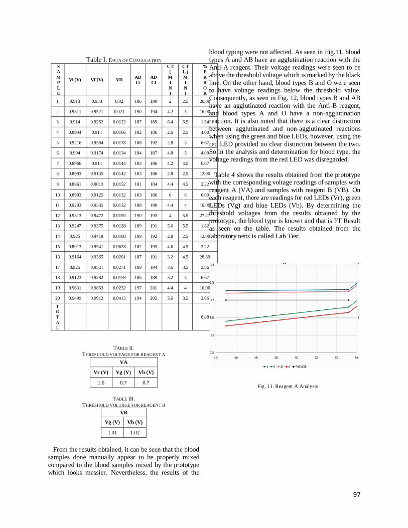
97

Table I. DATA OF COAGULATION S

A

M

P

L

E

Vi (V) Vf (V) VD AD

Ci

AD

Cf

CT

(

M

I

N

)

CT

L (

M

I

N

)

%

E

R

R

O

R

1 0.913 0.933 0.02 186 190 2 2.5 20.00

2 0.9311 0.9521 0.021 190 194 4.2 5 16.00

3 0.914 0.9262 0.0122 187 189 6.4 6.5 1.54

4 0.8944 0.911 0.0166 182 186 2.6 2.5 4.00

5 0.9216 0.9394 0.0178 188 192 2.8 3 6.67

6 0.904 0.9174 0.0134 184 187 4.8 5 4.00

7 0.8966 0.911 0.0144 183 186 4.2 4.5 6.67

8 0.8993 0.9135 0.0142 183 186 2.8 2.5 12.00

9 0.8861 0.9013 0.0152 181 184 4.4 4.5 2.22

10 0.8993 0.9125 0.0132 183 186 6 6 0.00

11 0.9203 0.9335 0.0132 188 190 4.4 4 10.00

12 0.9313 0.9472 0.0159 190 193 4 5.5 27.27

13 0.9247 0.9375 0.0128 189 191 5.6 5.5 1.82

14 0.925 0.9418 0.0168 189 192 2.8 2.5 12.00

15 0.8913 0.9541 0.0628 182 195 4.6 4.5 2.22

13 0.9164 0.9365 0.0201 187 191 3.2 4.5 28.89

17 0.925 0.9521 0.0271 189 194 3.6 3.5 2.86

18 0.9123 0.9282 0.0159 186 189 3.2 3 6.67

19 0.9631 0.9863 0.0232 197 201 4.4 4 10.00

20 0.9499 0.9912 0.0413 194 202 3.6 3.5 2.86

T

O

T

A

L

8.88

TABLE II.

THRESHOLD VOLTAGE FOR REAGENT A

VA

Vr (V) Vg (V) Vb (V)

1.6 0.7 0.7

TABLE III.

THRESHOLD VOLTAGE FOR REAGENT B

VB

Vg (V) Vb (V)

1.01 1.02

From the results obtained, it can be seen that the blood

samples done manually appear to be properly mixed

compared to the blood samples mixed by the prototype

which looks messier. Nevertheless, the results of the

blood typing were not affected. As seen in Fig.11, blood

types A and AB have an agglutination reaction with the

Anti-A reagent. Their voltage readings were seen to be

above the threshold voltage which is marked by the black

line. On the other hand, blood types B and O were seen to have voltage readings below the threshold value.

Consequently, as seen in Fig. 12, blood types B and AB

have an agglutinated reaction with the Anti-B reagent,

and blood types A and O have a non-agglutination

reaction. It is also noted that there is a clear distinction

between agglutinated and non-agglutinated reactions

when using the green and blue LEDs, however, using the

red LED provided no clear distinction between the two.

So in the analysis and determination for blood type, the

voltage readings from the red LED was disregarded.

Table 4 shows the results obtained from the prototype with the corresponding voltage readings of samples with

reagent A (VA) and samples with reagent B (VB). On

each reagent, there are readings for red LEDs (Vr), green

LEDs (Vg) and blue LEDs (Vb). By determining the

threshold voltages from the results obtained by the

prototype, the blood type is known and that is PT Result

as seen on the table. The results obtained from the

laboratory tests is called Lab Test.

Fig. 11. Reagent A Analysis

98

Fig. 12. Reagent B Analysis

For agglutination, for the prototype to be able to read

the voltage values accurately, the blood drops and

reagent drops should be dropped in the proper positions

and thus, a guide is made in the glass slide. The blood and

reagent should also be mixed well by the reagent dropper.

Having the blood drops and reagents drop dropped in

different parts of the glass resulted to different readings and also, if not stirred properly by the reagent stirrer will

thus also produce different voltage readings and output a

blood type that is not accurate. The glass slide should also

be placed exactly above the photodiode and for this to

happen, a small acrylic was utilized to block the glass

slide from exceeding the photodiode’s exact location. If

the glass slide exceeds the exact location of the

photodiode, the photodiode will then read a different

voltage reading that will also output a different blood

type.

Table IV: Results of Agglutination

Sample VA VB PT

Resul

t

Lab

Tes

t Vr Vg Vb Vr Vg Vb

1 1.6

3

0.6

6

0.6

3

1.8

4

0.9

9

0.9

8 O O

2 1.5

9

0.7

2

0.7

2

1.8

1

1.0

2

1.0

3 AB AB

3 1.6

2

0.6

8

0.6

5

1.8

1

0.9

9

0.9

8 O O

4 1.6

3

0.6

5

0.6

1

1.8

8

0.9

5

0.9

2 O O

5 1.6

8

0.6

9

0.6

6

1.9

1

1.0

5

1.0

6 B B

6 1.5

6

0.7

1 0.7

1.8

2

0.9

9

0.9

8 A A

7 1.5

8

0.7

3

0.7

2

1.7

5

1.0

1

1.0

2 AB AB

8 1.7

4

0.6

8

0.6

4

1.9

8

1.0

3

1.0

5 B B

9 1.5

6

0.6

8

0.6

3

1.8

7

0.9

9

0.9

8 O O

10 1.6

7

0.6

8

0.6

6

1.8

9

1.0

3

1.0

5 B B

11 1.6

5

0.6

8

0.6

4

1.8

4

1.0

1

1.0

2 B B

12 1.6

4

0.6

4 0.6

1.9

2

0.9

5

0.9

2 O O

13 1.8

1

0.7

6

0.7

6

1.8

3

0.9

9

0.9

7 A A

14 1.6

1

0.7

2

0.7

2

1.8

2

0.9

9

0.9

7 A A

15 1.5

6

0.6

7

0.6

4

1.8

3

0.9

9

0.9

9 O O

16 1.6

1

0.6

7

0.6

3

1.8

3

0.9

9

0.9

8 O O

17 1.7

4

0.6

9

0.6

5

1.8

5

1.0

1

1.0

5 B B

18 1.6

5

0.6

9

0.6

7

1.8

9

1.0

4

1.0

6 B B

19 1.5

8

0.6

6

0.6

4

1.8

7

0.9

6

0.9

2 O O

20 1.6 0.6

8

0.6

2

1.8

2

0.9

9

0.9

8 O O

%ERRO

R 0

IV. CONCLUSION

In this paper, an automated microcontroller-based device

is designed to determine a person’s blood type and

coagulation time using the concept of spectrophotometry.

The blood type of a person is determined by mixing Anti-

A and Anti-B reagents to two separate blood samples and

detecting an agglutination reaction in either sample. The dropping of these reagents and the consequent mixing

with the blood sample were achieved using a stepper

motor plunger system and two dc motors, respectively.

Agglutination was detected using a sensor circuit

consisting of a photodiode connected to a current to

voltage converter, and an illumination circuit consisting

of three RGB LEDs. The microcontroller was then able

to analyze and display the results on an LCD screen.

The coagulation time measured in this prototype started

from inserting the blood sample into the device until the

presence of a serum was detected. The presence of this serum was successfully detected using the same sensor

circuit, and an illumination circuit consisting of four

white LEDs. The microcontroller was able to measure the

time, interpret it as either normal or abnormal, and output

the results on an LCD screen. Additionally, three

functions were made available to the user in which they

may choose among Agglutination Detection,

Coagulation Analysis, or both. The prototype was

constructed in an 8.5x11x8.5-inch acrylic casing, and

was powered using an AC power source.

REFERENCES

[1] C. Chua, I. Gonzales, E. Manzano and M. Manzano, "Design and

Fabrication of a Non-Invasive Blood Glucometer Using Paired

Photo-Emitter and Detector Near-Infrared LEDs", DLSU Research

Congress 2014, 2014.

[2] J. Dy Perez, W. Misa, P. Tan, R. Yap and J. Robles, "A wireless

blood sugar monitoring system using ion-sensitive Field Effect

Transistor - IEEE Region 10 Conference (TENCON) , 2016.

[3] E. Nakamachi, “Development of automatic operated blood

sampling system for portable type Self-Monitoring Blood Glucose

99

device” - Annual International Conference of the IEEE

Engineering in Medicine and Biology, 2010. pp. 335-338

[4] H. Ashiba, M. Fujimaki, K. Awasu, M. Fu, Y. Ohki, T. Tanaka, and

M. Makishima, “Hemagglutination detection for blood typing

based on waveguide-mode sensors.,” Sensing and Bio-Sensing

Research, n.d.

[5]"Blood Types", Redcrossblood.org. [Online]. Available:

https://www.redcrossblood.org/donate-blood/how-to-

donate/types-of-blood-donations/blood-types.html. [Accessed: 21-

Aug- 2018].

[6]"Blood Clots", Hematology.org. [Online]. Available:

http://www.hematology.org/Patients/Clots/. [Accessed: 16- Feb-

2016].

[7] R. Razo, V. Recto, D. Regullano, and M. Salvador, “A portable

electronic blood typing device,” Master’s thesis, De La Salle

University, 2003.

[8] Y. Chang, W. Hong-Shong Chang, and Y. Lin “Detection of RBC

agglutination in blood typing test using integrated Light-Eye-

Technology (iLeyeT)” , IEEE International Symposium on

Bioelectronics and Bioinformatics (IEEE ISBB 2014), 2014, pp 1-

4

[9] A. Zia, M. Ali, M. Zeb, U. Shafiq, S. Fida, and N. Ahmed,

“Development of microfluidic lab-on-disc based portable blood

testing point-of-care diagnostic device”. IEEE EMBS Conference

on Biomedical Engineering and Sciences (IECBES), 2016, pp

142-145

[10] J. Fernandes, S.Pimenta, F. Soares, G, Minas, “A complete blood

typing device for automatic agglutination detection based on

absorption spectrophotometry,” IEEE transactions on

instrumentation and measurement, 2015. Pp. 112-119

[11] B. Li, S. Ong, and V. Pollard, “Microcontroller-based human blood

coagulation and erythrocyte sedimentation rate analyzer,”

Master’s thesis, De La Salle University, 2009.

[12] S. Anthony and M. Ramasubramanian, "Visible/Near-Infrared

Spectrophotometric Blood Typing Sensor for Automated Near-

Patient Testing“- IEEE Engineering in Medicine and Biology

27th Annual Conference, 2005, pp 1980-1983

https://ieeexplore.ieee.org/xpl/mostRecentIssue.jsp?punumber=5608545








100

Embedded System Based

Reconfigurable General Controller Board

for Home Automation System

Ismail1, Agung Nugroho Jati2, Fairuz Azmi3 1,2,3School of Electrical Engineering, Telkom University

Bandung, Indonesia

[email protected]

Abstract— In this research, an embedded system

based controller board is made to control electrical

appliances, such as lights, air conditioners, TVs, and

others, automatically according to the user

configuration. The configuration example is to switch

on lights for a certain clock range or when a light sensor

detects dark condition. The controller board consists of

a microcontroller, RTC, Wi-Fi module, Bluetooth

module, eight input ports for sensors, and eight output

ports for switching on and off home electrical

appliances. This research is implemented on a home

model that has been prepared according to the test

requirements. The controller board can be configured

by using a desktop application which is connected via

Bluetooth at the maximum distance of 4.8 meters

without obstacles. The controller board is designed to

be able to connect to a Wi-Fi network at the maximum

distance of 18 meters to send the I/O status to the

server for monitoring purpose. The findings indicated

that the controller board is 100% configurable and

work according to the configuration. It can also send

the I/O status to the server with 100% data accuracy.

Index Terms—Controller board; Embedded system;

Home automation system.

I. INTRODUCTION

Home automation system is a system that

integrates and controls home electrical appliances

such as lights, TVs, fans, air conditioners, etc. The

home automation system provides convenience,

energy efficiency, and comfort. Currently, the home automation system is growing rapidly and supported

by the number of companies engaged in this field

such as Control4, Crestron, Dynalite, and others.

Generally, a home automation systems consist of

sensors, a controller as the brain of the system, and

actuators such as relay, motor, or solenoid, and

usually focus on a single function or a single home

condition, such as door locking system [1], smoke

and fire alarm [2], or automation of lights only, so for

the other home conditions, the system or the

controller must be redesigned or reprogrammed. The

development of embedded system technology allows

a controller to support general home conditions,

which means that the controller is not required to be

redesigned or reprogrammed to support a new home

condition, but simply configured using a desktop

application.

A controller board is an electronic board based on microcontroller or microprocessor which is

programmed to control another systems or devices. A

controller board typically consists of a controller unit

and I/O unit. The controller unit may be

microcontroller based such as PIC family [3, 4, 5],

ATMEL [6, 7, 8], MCS51 [9], microprocessor based

as ARM [10, 11], or FPGA based. The advantages of

using FPGA are flexibility, accuracy, cost-

effectiveness, and rapid development [12]. The I/O

unit can be made to be onboard with the controller

unit [3, 13] or separated [4, 6, 7]. Some separated

ones use the other microcontroller in the I/O unit so they can work independently and flexibly [6]. In the

output unit is usually installed drivers to amplify the

current from microcontroller such as IC ULN2003

and IC L293D. The IC ULN2003 is used to amplify

the trigger current on relays [4, 7], while the IC

L293D is used to gain the current of DC motors [7].

In the input unit is usually installed op-amps

(operational amplifier) as IC LM358N to amplify the

voltage of sensors for maximum reading in the

microcontroller [4]. There are also use comparators

as IC LM339 to compare the voltage of a sensor with a threshold voltage, so the signal that are read by the

microcontroller is HIGH or LOW [3].

II. SYSTEM DESIGN

Overall system design is shown in Fig. 1 and the

focus of this research is the controller board.

101

Figure 1: Overall system diagram

The controller board is connected to the desktop application via Bluetooth. In the desktop application,

there are some configuration for the controller board,

for example is to switch on an output port for a

certain clock range or switch on when an input port

(sensor) is detected HIGH signal. It is also connected

to the server in internet via Wi-Fi network to send

I/O status. The I/O status can be monitored via the

mobile application.

A. Hardware Design

The controller board is based on microcontroller with eight input ports, eight output ports, a Real-

Time Clock, a Wi-Fi module, a Bluetooth module,

and four LED indicators. Fig. 2 shows the block

diagram of the hardware design.

Figure 2: Controller board diagram

1) The microcontroller is used as the brain,

process and control unit. It will be operated at

5-volt DC and 16 MHz clock. 2) Eight input ports that can read digital signal up

to 5-volt DC and are connected to the

microcontroller pin directly. 3) Eight output ports, relays, which is controlled

by a driver. The driver itself is controlled by

the microcontroller. 4) RTC to provide a real-time clock data. It is

connected to the microcontroller via I2C communication.

5) Wi-Fi module to connect the controller board

to a Wi-Fi network. It is connected to the

microcontroller via serial UART

communication. 6) Bluetooth module to connect the controller

board to the desktop application. It is

connected to the microcontroller via serial

UART communication. 7) Four LED indicators to indicate the working

status of the controller board: powering,

working, configuring, and Wi-Fi connection

status.

B. Operating System Design

There are two main process of this operating

system design, they are main program and Bluetooth

reception interruption. The main program starts with

initialization of ports and modules, then check each

input port signal and activate relay based on the

configuration, and then send the I/O status to the

server. The Bluetooth reception interruption starts with selection of port to be configured, then parse the

configuration data, and store them to the EEPROM of

the microcontroller. These two are shown in the flow

process in Fig. 3.

Figure 3: Flow process of operating system

III. REALIZATION AND IMPLEMENTATION

The controller board consists of two PCBs, main

board and I/O board that are shown in Fig. 4.

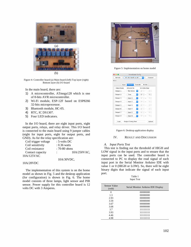
102

(a)

(b)

Figure 4: Controller board (a) Main board (left) Top layer (right)

Bottom layer (b) I/O board

In the main board, there are:

1) A microcontroller, ATmega128 which is one

of 8-bits AVR microcontroller. 2) Wi-Fi module, ESP-12F based on ESP8266

32-bits microprocessor. 3) Bluetooth module, HC-05. 4) RTC, IC DS1307. 5) Four LED indicators.

In the I/O board, there are eight input ports, eight

output ports, relays, and relay driver. This I/O board

is connected to the main board using 9 jumper cables

(eight for input ports, eight for output ports, and

GND). As for the relay specification are:

Coil trigger voltage : 5-volts DC Coil sensitivity : 0.36 watts

Coil resistance : 70-80 ohms

Contact capacity : 10A/250VAC,

10A/125VAC

10A/30VDC,

10A/28VDC

The implementation of this system is on the home

model as shown in Fig. 5 and the desktop application

(for configuration) is shown in Fig. 6. The home

model consists of three lamps, light sensor and PIR

sensor. Power supply for this controller board is 12 volts DC with 3 Amperes.

Figure 5: Implementation on home model

Figure 6: Desktop application display


A. Input Ports Test

This test is finding out the threshold of HIGH and

LOW signal in the input ports and to ensure that the

input ports can be used. The controller board is

connected to PC to display the read signal of each

input port in the Serial Monitor Arduino IDE with

value 1 or 0 (HIGH or LOW). So, there will be eight

binary digits that indicate the signal of each input

port. Table 1

Input Test

Sensor Value

(volt) Serial Monitor Arduino IDE Display

0 00000000

1.3 00000000

2.93 00000000

3.59 00000000

3.67 00000000

3.68 00000000

3.7 11111111

3.93 11111111

4.46 11111111

4.98 11111111

103

Based on the Table 1, it can be ascertained that the

input port can be used well and the microcontroller

can read the sensor values and process them. The

conclusion is LOW signal that are read are in range

0-3.68 volts, while HIGH signal that are read are in range 3.7-4.98 volt.

B. Output Ports Test

In this test, the controller board is programmed to

activated all relays to ensure that all relays can be

triggered to active. There is an LED in each output

port to indicates that the relay is active or not. A

voltage measuring in the relay coil is also done to

ensure that the relay is triggered.

Table 2

Input Test

Port

No.

First Test Second Test

Program

LED Indicator,

Coil Voltage

(volt)

Program

LED Indicator,

Coil Voltage

(volt)

1 ON On, 4.07 ON On, 4.13

2 ON On, 4.05 OFF Off, 0

3 ON On, 4.04 ON On, 4.12


5 ON On, 4.04 ON On, 4.12


7 ON On, 4.03 ON On, 4.12


Table 2 shows that all the relays can be controlled.

The average voltage of relay coil when all relays are

activated is 4.04 volts, while when a half number of

relays are activated is 4.12 volts.

C. HC-05 Bluetooth Module Test

This test is for finding out the maximum distance

of the connection between Bluetooth module and PC.

At any distance, the connection and data request are done to test data transmission at that distance. Time

between data request until data is displayed in PC is

also measured.

Table 3

Connection and Data Transmission Test of Bluetooth Module

Distance

(m)

Without Obstacles With Obstacles (Wall

and Door)

Connection Response

Time (s) Connection

Response

Time (s)

1.2 Connected 0.48 Connected 0.61

2.4 Connected 0.86 Connected 0.79

3.6 Connected 1.46 -

4.8 Connected 0.99 -

6.0 Connected - -

7.2 Not Connected - -

8.1 Not Connected - -

Table 3 shows that the Bluetooth module, HC-05,

can be connected well at the maximum distance of

4.8 meters without obstacles and 2.4 meters with

obstacles. At distance of 6 meters can be connected

but no data transmission.

D. Configuration Data Transmission Test

In this test, the microcontroller is programmed to receive a string, the configuration data, then parse

and display them in the Serial Monitor Arduino IDE.

Table 4

Configuration Data Transmission Test

Test

No. Configuration Data Sent

Serial Monitor Arduino

IDE

1 “setinp;11110000” setinp

11110000

2

“setout;2,17,5,0;2,17,5,1;

1,17,18,0; 1,18,5,0;

0,17,5,0;0,17,5,0;

0,17,5,0;0,17,5,0”

setout

2,17,5,0

2,17,5,1

1,17,18,0

1,18,5,0

0,17,5,0

0,17,5,0

0,17,5,0

0,17,5,0

Result that is shown in Table 4 is the Bluetooth

module successfully receive all configuration data

sent and parse them with 100% data accuracy. By this test, can be conclude that the controller board is

ready to be configurable using desktop application

via Bluetooth communication. The configuration data

itself are stored in the microcontroller EEPROM, so

that the configuration data will not be lost even if the

power supply is turned off.

E. ESP-12F Wi-Fi Module Test

This test is for finding out the maximum distance

of the connection between Wi-Fi module and Wi-Fi

network (in this case using smartphone Hotspot). At any distance, the connection is checked.

Table 5

Connection Test of Wi-Fi Module

Distance

(m)

Connection

Without Obstacles With Obstacles (Wall

and Door)

1.2 Connected Connected








24.0 Not Connected Not Connected

104

Table 5 shows that the Wi-Fi module, ESP-12F,

can be connected well at the maximum distance of

18 meters with or without obstacles.

F. I/O Status Sending Test

In this test, the microcontroller is programmed to get status of each input and output ports, then make

them as a string, then send them to the server using

HTTP GET protocol.

Table 6

I/O Status Sending Test

Test

No. Microcontroller Data Stored Data in Server

1

time: 2018-7-11+1:9:19

id: HS0001

data: 0000000000010000

time: 2018-07-11 01:09:19

id: HS0001

data: 0000000000010000

2

time: 2018-7-11+1:16:48

id: HS0001

data: 1100000011010000

time: 2018-07-11 01:16:48

id: HS0001

data: 1100000011010000

3

time: 2018-7-11+1:21:19

id: HS0001

data: 0000000000010000

time: 2018-07-11 01:21:19

id: HS0001

data: 0000000000010000

4

time: 2018-7-11+3:3:48

id: HS0001

data: 0000000000010000

time: 2018-07-11 03:03:48

id: HS0001

data: 0000000000010000

5

time: 2018-7-11+9:18:52

id: HS0001

data: 0000000000000000

time: 2018-07-11 09:18:52

id: HS0001

data: 0000000000000000

Result that is shown in Table 6 is the Wi-Fi module

successfully receive send all the I/O status to the

server with 100% data accuracy. This I/O status are

stored in database server for monitoring purpose via

mobile application. V. CONCLUSION

Based on the design, implementation, and test, the

conclusion is the controller board can be made based

on embedded system technology. It can read digital

signal from each input port in range 0-3.68 volts for

LOW and 3.7-4.98 for HIGH and also can control all

relays in output port well. It can be configured using

a desktop application via Bluetooth at maximum

distance of 4.8 meters. It also can send the I/O status

to the server via Wi-Fi network at maximum distance

of 18 meters with 100% data accuracy.

VI. REFERENCES

[1] Y. T. Park, P. Sthapit and J.-Y. Pyun, "Smart Digital Door Lock for

the Home Automation," in IEEE Region 10 Conference, 2009.

[2] I. Kaur, "Microcontroller Based Home Automation System with

Security," International Journal of Advanced Computer Science and

Applications, vol. I, no. 6, pp. 60-65, 2010.

[3] S. Mohyuddin, Z. Anwar and M. M. Ashraf, "A Programmable Logic

Controller Based Power Factor Controller for Single Phase Induction

Motor," International Journal of Engineering Science and

Computing, pp. 4688-4690, 2017.

[4] P. Visconti, P. Constantini and G. Cavalera, "Design of

electronic programmable board with user-friendly touch

screen interface for management and control of thermosolar

plant parameters," in International Conference on

Environment and Electrical Engineering, 2015.

[5] M. Bharani, S. Elango, S. M. Ramesh and R. Preetilatha, "An

Embedded System Based Smart Sensor Interface for

Monitoring Industries using Real Time Operating System

(RTOS)," International Journal of Advanced Information and

Communication Technology, pp. 496-498, 2014.

[6] M. E. Rida, F. Liu and Y. Jadi, "Design Mini-PLC based on

ATxmega256A3U-AU Microcontroller," in International

Conference on Information Science, Electronics and

Electrical Engineering, 2014.

[7] M. Avhad, V. Divekar, H. Golatkar and S. Joshi,

"Microcontroller based Automation system using Industry

standard SCADA," in Annual IEEE India Conference, 2013.

[8] S. Anwaarullah and S. V. Altaf, "RTOS based Home

Automation System using Android," International Journal of

Advanced Trends in Computer Science and Engineering, pp.

480-484, 2013.

[9] W. HuiJiao, Z. Wang and H. Jie, "An Embedded

Environmental Control System Based on Small RTOS," in

IEEE International Conference on Intelligent Computing and

Integrated Systems, 2011.

[10] S. S. Pawar and P. C. Bhaskar, "Design and Development of

ARM based Real-Time Industry Automation System using

GSM," International Research Journal of Engineering and

Technology, pp. 800-805, 2015.

[11] S. Pinto, J. Pereira, D. Oliveira, F. Alves, E. Qaralleh, M.

Ekpanyapong, J. Cabral and A. Tavares, "Porting SLOTH

System to FreeRTOS running on ARM Cortex-M3," in

International Symposium on Industrial Electronics, 2014.

[12] D. Gawali and V. K. Sharma, "FPGA Based Micro-PLC

Design Approach," in International Conference on Advances

in Computing, Control, and Telecommunication

Technologies, 2009.

[13] J.-H. Su, C.-S. Lee and W.-C. Wu, "The Design and

Implementation of a Low-cost and Programmable Home

Automation Module," IEEE Transactions on Consumer

Electronics, pp. 1239-1244, 2006.

[14] V. N, H. K. S, N. M. S, R. Umesh and S. A. A. Kumar, "A

Low Cost Home Automation System Using Wi-Fi Based

Wireless Sensor Network Incorporating Internet of Things

(IoT)," in International Advance Computing Conference,

2017.

105

Development of Synthesizable VHDL Library

Modules for a Small Scale Convolutional

Neural Network with Weight Quantization

using K-Means Clustering

Roderick Yap, Lawrence Materum Department of Electronics and Communications Engineering, De La Salle University

Manila, Philippines

[email protected]

Abstract— Convolutional Neural Network (CNN) has

evolved as a very popular tool in the field of artificial

intelligence. In many instances, CNN is implemented using

the software approach. Hardware approach of

implementation likewise, has made use of Field

Programmable Gate Array (FPGA), in many applications,

equipped with embedded processors in it. In many cases,

CNN is used in applications that normally involve large

volume of data. In this paper, a set of synthesizable VHDL

library modules is designed. The modules developed can be

used as one possible guide for building a small scale CNN

for a small set of input data. The goal is to implement the

CNN and allow it to train by itself. The system will use

fixed point binary numbers. A synthesizable hardware

model of a programmable K-means clustering is also

designed for CNN weights quantization. The K-Means

clustering can be used for various values of K with

maximum of K in this paper set at 36. As part of

experimentation, the CNN module and the K-means

clustering module were integrated and the results were

evaluated.

Index Terms— Convolutional Neural Network; K-Means

Clustering; Hardware Model; VHDL Library Modules

I. INTRODUCTION

CNN is a popular tool used for many image recognition

applications. A lot has been done on its various forms of

implementation and application. One research focused

on automatic HDL code generation for CNN in Verilog

[1]. In [2] FPGA based CNN using the Caffe framework

was implemented. In [3], CNN was used for processing

moving images. The system was able to perform super

resolution on up to 1920x1080 pixels in no less than 48

frames per second with a latency of less than 1 ms. Use

of Open Computer Language (Open CL) was highlighted in [4] for an FPGA based CNN with emphasis on CNN

acceleration. An FPGA based CNN was developed in

[5]. The paper proposed a faster method for computing

hyperbolic tangent activation function.

A lot of researches Clustering has also been published.

One paper focused on fast determination of cluster center

and including fast determination of optimal density

radius [6]. Pattern recognition involving binary sketch

template image is another area that has found application

for clustering [7]. In [8], collaborative clustering, which

focused on several clustering method done in parallel was proposed. Other applications on clustering that have

found publication included SAR image segmentation [9],

multi task clustering [10] and even on bioinformatics

[11].

When CNN and clustering are combined in one

research, deep neural network can be one application. In

[12], the concept of deep compression was introduced. In this paper, the weights of a neural network can be

quantized using K-means clustering. With quantization,

the system enforced weight sharing. With weight sharing,

the system can save memory resources as this will reduce

the number of memory spaces for holding of unique

weight values. In addition, the system also proposed the

elimination of weights which are too insignificant due to

its very low value.

Hardware Description Language (HDL) is a popular

entry tool for digital IC design. Two popular HDLs

widely used are Verilog and VHDL. With HDL, large

digital system design can be carried by mere coding using

HDL. However, the success of coding largely depends on

the synthesizability of the code. In synthesis, the code is

translated to a hardware equivalence based on a library

prescribed by the user. The target library can be an FPGA

based library or for mass production, a standard cell

based library.

106

II. THEORETICAL CONSIDERATION

In CNN, the input data, e.g. pixel information from an

image, is processed in several stages with an intention to

reach a target output set by the designer. Figure 1 shows one possible scenario. The input data is first convolved

with the filter weights. The number of filters is decided

by the designer. The initial filter weight values can be

randomly assigned. After convolution, user applies

activation function. One option is to apply ReLU to the

data. ReLU is used to convert all negative values

obtained from convolution to zero. Another option is to

apply Pooling. The goal of pooling is to reduce the data

size in case it gets too big. One possible effect of pooling

is to get the maximum value only from a spatial area

within the input data. This spatial area can be defined by

the user. Some other popular activation function includes Sigmoid and Tanh.

Fig. 1: A Possible Data Flow for CNN

The outputs of the activation function enter the fully

connected layer block as its inputs. In the Fully

Connected Layer block are layers of neurons. The user

decides on how many layers are needed based on his

requirements. The first layer would normally be the

inputs. As for example, let there be 4 neurons in the

second layer. Every input will form a connection to every

neuron of the second layer. If there are 4 inputs, then

there would be 16 connections. Every connection carries a numerical weight with it. Quantifying this block is a

series of “Sum Of Product” (SOP) terms for every layer.

The result of the SOP expression is then fed to another

activation. The outputs from the fully connected layer

are then compared to a set of target values. If the output

is not yet equal to the target, then back propagation

procedure is carried out. A back-propagation procedure

is applied to update the weight values of the fully

connected. A back-propagation procedure is likewise

applied to update the filter weights. And then, the next

iteration is executed. The iteration is executed repeatedly

until the desired outputs are achieved.

Fig. 2: Flowchart for K-Means Clustering

K-means clustering is a form of unsupervised

learning. With K-means clustering, a set of data can be

classified into K groups. Figure 2 shows the behavioral

flow of K-means clustering algorithm [13]. At first, the user specifies into how many groups does he wish to

classify a given set of data. A random search for the

initial centroid values is then carried out. The number of

centroid values corresponds to the value of K. Each

member of the given set of data will have its Euclidean

distance from each centroid computed. The member is

then classified to belong to the group of the centroid that

provided the minimum Euclidean distance value. After

one iteration, all members belonging to the same centroid

form 1 group. A new set of centroid values will then be

computed for every group. The new value is based on the

average of all members comprising the group. And the iteration continues until all the centroid values have

converged and have stopped changing for successive

iterations.

III. SIGNIFICANCE AND LIMITS OF THE STUDY

The design highlighted in this paper explores to a

certain degree the concept of parallelism. Because

VHDL supports parallelism, by allowing several data to

be updated in just 1 clock cycle, parallel updating of a

number of variables is adopted in the design. The advantage of parallel computation is faster processing

time to reach the target output. Both CNN and K-means

clustering use a lot of variables; and these variables are

constantly updated for every iteration. Instead of

updating each variable one at a time, parallel

computation will obviously allow faster processing time,

hence, faster convergence to the set target. However,

the drawback of parallel computation is larger circuit

size. The synthesizable VHDL code done in this research

can pave the way for standard cell-based Application

Specific Integrated Circuit (ASIC) design in the future.

Alternatively, on the part of FPGA implementation, if one FPGA is not large enough to contain the entire

107

circuit, one can look at partitioning it into several sub

blocks for several interconnected FPGAs for

implementation.

IV. DESIGN CONSIDERATION FOR CNN

The hardware model design of the entire system is

divided into 2 main circuit blocks namely the

Convolutional Neural Network block and the K-Means

clustering block. In designing the hardware model of the

CNN block, figure 1 serves as basis for the structural

modeling. In doing the Register Transfer Level hardware

model, a python code was first written for the CNN. It

was important to have a working python code to ensure

that the mathematical procedure adopted for the

hardware model will work effectively.

A. The Convolution Block

The input image adopted for the design is a 4x4 matrix.

Let A represent the 4 x 4 matrix. Three pieces of 3x3 filter

matrix are used for this design. Each filter weight is

represented as 10 bits signed number. Of the 10 bits, 7

bits are allotted for the fractional part. Let the 3 filters be

represented by B, C and D respectively. B, C and D

accept the filter weight inputs. For this design each filter

will convolve with the input image using single stride. As

for example, convolving B with the image A, equation

(1) represents a sample output, E1. Matrix B then moves down to continue the convolution process until the entire

matrix A has been covered. Similar approach is done for

matrix C and D. After the convolution procedure, the

system would have produced 12 outputs, E1 to E12

E1 = A(0,0) * B(0,0) + A(0, 1)* B(0,1) + A(0,2) * B(0,2) +

A(1,0) * B(1,0) + A(1,1) * B(1,1) + A(1,2) * B(1,2) + A(2,0) *B(2,0) + A(2, 1) * B(2,1) + A(2,2) * B(2,2) + bias (1)

In hardware modeling the convolutional block, one can

normally rely on the multiplier and adder circuits that are

readily synthesizable. Use of operators * and + in VHDL

are synthesizable. In this research, the image used is a

black and white image that can be represented as 1 or 0

for every pixel. Instead of using a multiplier,

multiplexers which are more component saving can be

used to replace the multiplier. Figure 3 shows the circuit

representation for one multiplication operation. With

multiplexers used, the only mathematical operation left

for the convolutional block is addition. Looking at (1) and (2), there are still too many addition operations

carried out at a time. This can lead to too much hardware

consumption. One way to reduce the number of adders

needed is to divide the entire convolution procedure into

several states using Finite State Machines (FSM). The

reader has the option to limit the operation to 1 just adder

per state or he can add a few more additions. Limiting to

just 1 addition has a draw back of increasing the latency

i.e. it will take several clock cycles before the entire

operation is completed. Figure 4 shows the abstract view

of the Convolutional block. Clk and res represent the

clock and reset input which are normally found in any sequential circuit. Start, when asserted high will begin

the convolution. Change, when asserted high, will

replace the filter weights values inside the block with

those coming from the inputs. The output signal, Finish

asserts high for one clock cycle when the convolution

operation is completed.

Fig. 3: Multiplication Replaced with Mutliplexing

Fig.4: Convolution Block Abstract View

B. The Sigmoid Block

In this design, the activation function adopted right

after the convolution operation is the sigmoid function.

Equation (2) shows the mathematical expression [14]. Hardware modeling of the sigmoid function has several

options. In carrying out the exponential part of the

formula, one can use the Maclaurin’s series [15].

Another option is to use Coordinate Rotation Digital

Computer (CORDIC) specifically the hyperbolic

trigonometric function [16]. Still a 3rd option is to use

lookup table. Lookup table could be memory intensive,

but it is the easiest approach. One advantage of using

lookup table is the faster time to obtain the answer. In

the best case, the answers are readily available in just 1

clock cycle. Using CORDIC would normally take

considerable number of clock pulses since this method is based on repeated iteration. Using Maclaurin’s series on

the other hand would involve a number of

multiplications, addition and division operations. In this

paper, look up table using VHDL function declaration is

adopted for the sigmoid function.

108

𝑆𝑖 =1

1+𝑒−𝐸𝑖 (2)

As shown in equation (2), Si represents one activation

function output while Ei represents one of the outputs of

the convolution operation. Figure 5 shows the abstract

view of the Sigmoid Block. It only takes 2 clock cycles

for the output to be readily available. The first clock cycle

is allotted for the waiting state i.e. waiting for the start signal to go high. In the 2nd clock cycle, the outputs, set

at 9 bits signed number, are delivered. The releasing of

the outputs can be gradual by using FSM with only one

output computed for every clock pulse. This option is

chosen for saving hardware components.

Fig 5: Sigmoid Block Abstract View

C. The Fully Connected Layer Block

After the Sigmoid block, the signals enter the fully

connected layer block. This block is a pure multiply and

accumulate operation block for every layer.

Mathematically, it is a Sum of Product terms. If there are

more than 2 layers in this block, an activation would be

needed before proceeding to the 3rd layer. For this

design, this block has a total of 12 inputs with each input

at 9 bits signed number. The inputs come from the

Sigmoid block. It depends on the user requirement to set the number of outputs. As for example, based on the

previous discussion on figure 1, assuming there are 4

neurons in the layer following the inputs, with 12 inputs

and 4 neurons, there would be 48 weights present.

Figure 6 shows an abstract view of this block

Fig 6: Fully Connected Layer Abstract View

For this design, the weights are assigned as 10 bits each. The outputs are set at 20 bits. As for example, let

Sg1 to Sg12 serve as inputs, let SOP1 represent a neuron.

SOP1 can be expressed as shown in equation (3).

SOP1 = Sg1*W1 + Sg2*W2 + Sg3*W3 + Sg4*W4 + Sg5*W5 + Sg6*W6 + Sg7 * W7 + Sg8 * W8 + Sg9 * W9 + Sg10* W10+Sg11*W11+Sg12*W12

(3)

Where W1 to W12 represent the corresponding weight from

each input to SOP1.

As shown in figure 6, the Fully Connected Layer Block

has a clock input, a reset input, a start input and Weight

inputs for updating the block weights for every iteration.

There are also weight outputs that represent the current

set of weights. These outputs are fed to another module

which is responsible for updating the weights. The

“Change” input when asserted high, will allow the

external weight inputs to replace the weights inside the

block.

D. The Softmax Block

For classification, one option for activating the last

layer neurons of the fully connected layer block is to use

the Softmax function. Softmax is adopted for this design.

If the user does not want to use softmax, other activation

functions can be adopted depending on the choice of the

user. Softmax is popularly used for classification. The mathematical behavior of the Softmax block is shown in

equation (4) [17].

𝑆𝑓𝑡𝑚𝑎𝑥𝑖

=𝑒(𝑆𝑂𝑃𝑖−𝑆𝑂𝑃𝑚𝑎𝑥)

∑ 𝑒(𝑆𝑂𝑃𝑖−𝑆𝑂𝑃𝑚𝑎𝑥)𝑁𝑖

(4)

Where SOPmax is the maximum among the main

output signals coming from the Fully Connected Layer

blocks of figure 6. The output of the Softmax block

indicates probability which in this case is the official output of the CNN. Figure 7 shows the abstract view of

the Softmax block. Four main inputs are adopted for this

design. The 4 inputs are also fed to the “Get Max” block

which determines the maximum among the 4 inputs. The

outputs of this block, together with the “Get Max” output

form the main inputs to the Softmax block. A look up

table for e-x is constructed inside this block to evaluate

the exponential functions of (4). After obtaining all the

exponential terms and performing the necessary addition

processes, a division process is carried out using an

embedded divider inside the block. The main outputs of this block are set at 20 bits each. As seen in figure 1, the

output of the softmax module are fed to an Error

Calculator Block. In this block, the difference between

each Softmax block output and a corresponding set

target value is computed. The difference is termed as the

error.

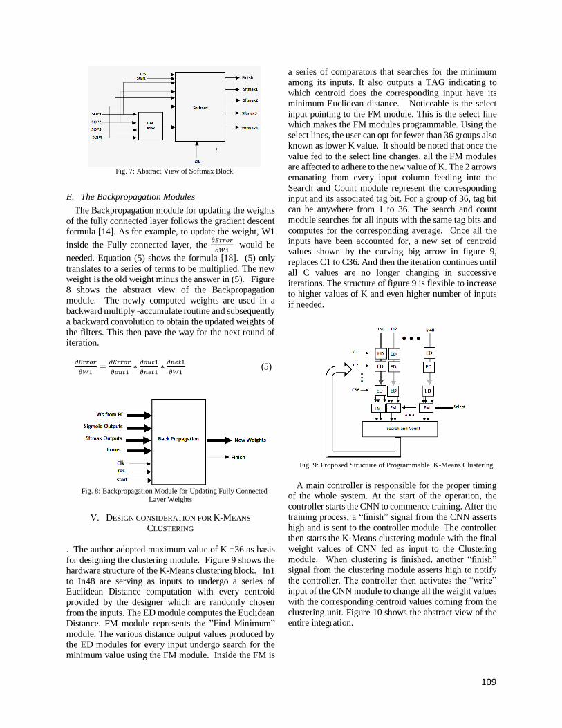
109

Fig. 7: Abstract View of Softmax Block

E. The Backpropagation Modules

The Backpropagation module for updating the weights

of the fully connected layer follows the gradient descent

formula [14]. As for example, to update the weight, W1

inside the Fully connected layer, the 𝜕𝐸𝑟𝑟𝑜𝑟

𝜕𝑊1 would be

needed. Equation (5) shows the formula [18]. (5) only

translates to a series of terms to be multiplied. The new

weight is the old weight minus the answer in (5). Figure

8 shows the abstract view of the Backpropagation

module. The newly computed weights are used in a

backward multiply -accumulate routine and subsequently

a backward convolution to obtain the updated weights of

the filters. This then pave the way for the next round of iteration.

𝜕𝐸𝑟𝑟𝑜𝑟

𝜕𝑊1=

𝜕𝐸𝑟𝑟𝑜𝑟

𝜕𝑜𝑢𝑡1∗

𝜕𝑜𝑢𝑡1

𝜕𝑛𝑒𝑡1∗

𝜕𝑛𝑒𝑡1

𝜕𝑊1 (5)

Fig. 8: Backpropagation Module for Updating Fully Connected

Layer Weights

V. DESIGN CONSIDERATION FOR K-MEANS

CLUSTERING

. The author adopted maximum value of K =36 as basis

for designing the clustering module. Figure 9 shows the

hardware structure of the K-Means clustering block. In1

to In48 are serving as inputs to undergo a series of Euclidean Distance computation with every centroid

provided by the designer which are randomly chosen

from the inputs. The ED module computes the Euclidean

Distance. FM module represents the ”Find Minimum”

module. The various distance output values produced by

the ED modules for every input undergo search for the

minimum value using the FM module. Inside the FM is

a series of comparators that searches for the minimum

among its inputs. It also outputs a TAG indicating to

which centroid does the corresponding input have its

minimum Euclidean distance. Noticeable is the select

input pointing to the FM module. This is the select line which makes the FM modules programmable. Using the

select lines, the user can opt for fewer than 36 groups also

known as lower K value. It should be noted that once the

value fed to the select line changes, all the FM modules

are affected to adhere to the new value of K. The 2 arrows

emanating from every input column feeding into the

Search and Count module represent the corresponding

input and its associated tag bit. For a group of 36, tag bit

can be anywhere from 1 to 36. The search and count

module searches for all inputs with the same tag bits and

computes for the corresponding average. Once all the

inputs have been accounted for, a new set of centroid values shown by the curving big arrow in figure 9,

replaces C1 to C36. And then the iteration continues until

all C values are no longer changing in successive

iterations. The structure of figure 9 is flexible to increase

to higher values of K and even higher number of inputs

if needed.

Fig. 9: Proposed Structure of Programmable K-Means Clustering

A main controller is responsible for the proper timing of the whole system. At the start of the operation, the

controller starts the CNN to commence training. After the

training process, a “finish” signal from the CNN asserts

high and is sent to the controller module. The controller

then starts the K-Means clustering module with the final

weight values of CNN fed as input to the Clustering

module. When clustering is finished, another “finish”

signal from the clustering module asserts high to notify

the controller. The controller then activates the “write”

input of the CNN module to change all the weight values

with the corresponding centroid values coming from the

clustering unit. Figure 10 shows the abstract view of the entire integration.

110

Figure 10: Integrating the CNN and K-Means Clustering

VI. DATA AND RESULTS

In implementing a CNN, there are many possibilities as

to the number of filters used, size of filters adopted and

even on the choice of the activation function. Even the

number of layers inside the fully connected block can

vary depending on the need of the user. A simple small

size integration of the different modules developed was

done in this paper to see how the system works. A test

image (4 x4) was fed to the convolution block. A python

code was also tested for the given image. Figure 11 shows

the sample image as input. The image is adopted as black

and white. The yellow is assigned a value of 1 while the

violet is assigned a value of 0. Figure 12 shows the 3

filters structure after around 10000 iterations of the

python code. The 3 filters, as seen in the figures have

adopted to the pattern of the input image. The brighter

the color, the higher is the corresponding value of the cell

in the filter.

The VHDL bit-level code was then simulated using the

same image of figure 10. The result obtained after around

1 million clock cycles are shown Table I-1 to I-3. The

result of the VHDL simulation appeared similar to the

python code simulation result. The binary results from

the VHDL simulation were manually converted to

decimal. In testing the effect of clustering, the authors

have made some observations on weight values relation

to the output. A total of 48 weights were fed to the

clustering module. Table II shows the result of the CNN

performance with clustering. The target outputs when

training the CNN was 100%, 0%, 0% 0%. It shows that

even with great reduction in number of unique weight

values, the performance of the CNN is still more than

satisfactory. Tables III and IV show the synthesis result

for the CNN and Clustering respectively.

Fig. 11: The Sample Image Trained

Fig 12: The 3 Filters after the training

Table I -1 Filter B Results in VHDL

0.95 0.95 1.46

0 0 1.01

0 0 1.01

Table I -2 Filter C Results in VHDL

1.17 1.17 1.67

0 0 0.97

0 0 0.97

Table I -3 Filter D Results in VHDL

1.06 1.06 1.51

0 0 0.98

0 0 0.98

Table II. Result for Clustering Weights

Clustering Outputs

24 groups 98%, 0.09% 0.34% , 0.58%

15 groups 98% , 0.09%, 0.39%, 0.68%

5 groups 98%, 0.19%, 0.43%, 0.58%

111

Table III: CNN Module Synthesis Result

MAC (Multiply -accumulate) 77

Multipliers 115

Adder / Subtractor 113

Registers 3633

Comparators 7

Table IV: Clustering Module Synthesis Result

ROM 36

Multipliers 36

Adders / Subtractors

(minimum)

1736

Registers (minimum) 441

Comparators (minimum) 3408

VII. CONCLUSION

In this paper, a set of library modules written in VHDL

for CNN and K-means Clustering were presented.

Integrating the modules for a simple CNN training

proved to be working when compared to a python code.

The training was carried out using solely the library

modules developed. Exponential mathematical functions

were implemented using lookup tables. K-means

clustering proved effective for weight quantization. The

timing for the entire system’s operation was implemented

using a controller module which acts like a director to the

system. Although only a small scale is adopted for this

design, the algorithm used is flexible enough to increase

to higher data sizes

ACKNOWLEDGEMENT

The authors wish to thank Engineering Research and

Development for Technology (ERDT) led by the

Department of Science and Technology (DOST) -Science and Education Institute (SEI), Philippines for the

funding provided in this research.

REFERENCES

[1] Z. Liu, Y. Dou, J. Jiang, and J. Xu, “Automatic code generation

of convolutional neural networks in FPGA implementation,” in 2016 International Conference on Field-Programmable

Technology (FPT) [8], pp. 61–68

[2] R. DiCecco, G. Lacey, J. Vasiljevic, P. Chow, G. Taylor, and S.

Areibi, “Caffeinated FPGAs:FPGA framework for convolutional neural networks,” in 2016 International Conference on Field-

Programmable Technology (FPT) [9], pp. 265–268.

[3] T. Manabe, Y. Shibata, and K. Oguri, “FPGA implementation of a real-time super-resolution system using a convolutional neural

network,” in 2016 International Conference on Field-Programmable Technology (FPT) [10], pp. 249–252.

[4] Z. Wang, F. Qiao, Z. Liu, Y. Shan, X. Zhou, L. Luo, and H. Yang,

“Optimizing convolutional neural network on FPGA under

heterogeneous computing framework with opencl,” in 2016 IEEE

Region 10 Conference (TENCON) [5], pp. 3433–3438

[5] S. Ghaffari and S. Sharifian, “FPGA-based convolutional neural network accelerator design using high level synthesize,” in 2016

2nd International Conference of Signal Processing and Intelligent

Systems (ICSPIS) [6], pp. 1–6.

[6] C. Jinyin, L. Xiang, Z. Haibing, and B. Xintong, “A novel cluster

center fast determination clustering algorithm,” Applied Soft

Computing, vol. 57, pp. 539 – 555, 2017. [7] X. Mei, “Object clustering by k-means algorithm with binary

sketch templates,” in 2016 International Conference on Progress in Informatics and Computing (PIC) [49], pp. 360–363.

[8] A. Cornujols, C. Wemmert, P. Ganarski, and Y. Bennani, “Collaborative clustering: Why,when, what and how,”

Information Fusion, vol. 39, pp. 81 – 95, 2018.

[9] T.Xing, Q.Hu, J.Li and G. Wang, “Refined SAR Image Segmentation Algorithm Based on K-means Clustering”, 2016

CIE International Conference on Radar, Oct., 2016

[10] ] A. Sokhandan, P. Adibi, and M. Sajadi, “Multitask fuzzy bregman co- clustering approach for clustering data with

multisource features,” Neurocomputing, vol. 247, pp. 102 – 114,

2017.

[11] L.V. Bijuraj, “Clustering and its Applications”, Proceedings of

National Conference on New Horizon in IT (NCNHIT), 2013

[12] H. M. .W. D. Song Han, “Deep compression: Compressing deep

neural networks with pruning, trained quantization and huffman

coding,” https://arxiv.org/pdf/1510.00149.pdf, 2016 .

[13] K. Teknomo, “K-Means Clustering Tutorial”,

http://people.revoledu.com/kardi/tutorial/kMean/Algorithm.htm

[14] Tariq Rashid, “Make Your Own Neural Network” .

[15] Weisstein, Eric W. "Maclaurin Series." From MathWorld--A Wolfram Web

Resource. http://mathworld.wolfram.com/MaclaurinSeries.html

[16] A. Dulay, R.Yap, L.Materum, “Hardware Modelling of a PLC Multipath Channel Transfer Function”, Journal of

Telecommunications, Electronics and Compter Engineering, Vol

9, No. 2-7, 2017

[17] How to implement the Softmax function in Python

[Available Online:]https://stackoverflow.com/questions/34968722/how-to-

implement-the-softmax-function-in-python

[18] M. Mazur, “A step by step backpropagation example,”[Available Online:] https://mattmazur.com/2015/03/17/a-step-by-step-

backpropagation-example/

http://mathworld.wolfram.com/about/author.html

http://mathworld.wolfram.com/

http://mathworld.wolfram.com/MaclaurinSeries.html

https://stackoverflow.com/questions/34968722/how-to-implement-the-softmax-function-in-python



112

Cooperative Spectrum Sensing with Obstacles

on both Sensing and Reporting Channels

Abdul Haris Junus Ontowirjo1, Wirawan2, Adi Soeprijanto3 1,2,3Department of Electrical Engineering, Faculty of Electrical Technology

Institut Teknologi Sepuluh Nopember,

Surabaya, Indonesia 1Jurusan Teknik Elektro, Fakultas Teknik

Universitas Sam Ratulangi Manado, Indonesia

[email protected], [email protected], [email protected]

Abstract- The performance of cooperative spectrum

sensing is investigated over channels with obstacles on

both sensing and reporting channels. With weighted sum

at the fusion center, the detection and false alarm

probabilities are derived. Our analysis is validated by

numerical and simulation results.

Index of Terms-About; Cooperative Spectrum Sensing;

False Alarm; Obsctacles; Receiver Operating

Characteristic; Probability of Detection.

I. INTRODUCTION

Cooperative Spectrum Sensing is a technology that

can be used to overcome the effects of multipath fading on the side of the environmental performance in the

detection of the cognitive radio network. On the other

hand, the lack of availability of frequency spectrum

allocation is currently the most important issue for a

wireless communication system when setting placement

in static frequency allocation makes the frequency

spectrum becomes inefficient [1,2]. Cognitive Radio has

become the latest phenomenon to be able to overcome

the lack of spectrum allocation along with the user

settings. Spectrum Sensing is one of the important

functions for technology users Cognitive Radio (CR) to detect the presence of the Primary User (PU) and

exploit the unused frequency spectrum without causing

interference to PU [3,4].

Today's wireless communication systems have grown

rapidly and had a very large number of users. The

number of users using the frequency spectrum

allocation has been set for the communication system.

Wireless communication system environments are

experiencing the phenomenon of multipath fading due

to obstructions (obstacles) has resulted in the

distribution of the received signal will be Rayleigh,

while the absence of a barrier in wireless

communication systems resulted in the distribution of

the received signal into nature Rician. The study

discusses the effects of multipath fading channels

affected has been done before. Assuming the channel is

with Nakagami fading, has submitted a method for

exploiting the spectrum by Secondary User (SU)

allocated to PU when not being used [3]. SU will

continue to monitor the channels to decide whether to

use or not. To determine priorities for the use of the

spectrum allocation from use by PU and SU,

predetermined parameter limit SNR. Paper discusses other channel modeling and

parameter limit to determine the allocation of spectrum

that can be used by SU. In this paper, the channel is

assumed to be Nakagami and Rician and made a two-

level parameter limits [5-7]. Both of these parameters

limit use logic 2 ratios and 1 ratio that produces better

incorporation mechanism on the channel with nature

Nakagami and Rician distribution. When all the

parameters are set optimally, the result of a reduction in

the energy used in a trade between detection

performance and excessive use of spectrum.

II. CHANNEL AND SYSTEM MODELS

In this paper discussed cognitive radio network

described by Figure 1, with a number of L cognitive

relays (named SU1, SU2,..., SUL). In the first phase, all

relays observe cognitive user primary signal. In the

second phase of each cognitive relay amplifies and

forward the received signal to the fusion center. We

assume relays communication channels between

cognitive fusion center and independently of one

another. In the free channels, the fusion center receives

signals that are free of cognitive relays. The fusion center is a combination of the selection combiner and

energy detector that compares the output signal

combiner selection and a predetermined threshold λ.

113

A. Single Cognitive Relay Network

We review the single-cognitive relay network. In this

case, we have three nodes, PU, SU, and Fusion Center

(FC). SU continuously monitors the signals received

from the PU, as embodied in the Figure 1:

Fig.1 Cooperative Spectrum Sensing with Obstacles

1

0

:

:

s sk k

k sk

h x n w n Hy n

w n H

+=

(1)

1

0

:

:

r rk k k k

k r s rk k k k

g h y n w n Hz n

g h w n w n H

+=

+

(2)

( )

1

0

1

0

1

0

:

:

:

:

:

:

r s s rg h h x n w n w nk k k k kk r s rg h w n w nk k k k

r s r s rg h h x n g h w n w nk kk k k k kr s rg h w n w nk k k k

k k

k

Hz n

H

H

H

Hh x n w n

Hw n

+ +

+

+ +

+

=

=

+=

(3)

Fusion Center (FC) consists of Diversity Combining

(DC) and Detector. While the other parameters of its

belonging signals are x[n], the signal transmitted by PU

(unknown deterministic with the power of 𝐸𝑠), 𝑦𝑘[𝑛], the signal received by 𝑆𝑈𝑘, 𝑧𝑘[𝑛] the signal received by

the FC from 𝑆𝑈𝑘. For parameters that belong to the

channels ares

hk which is a sensing channel gain between

PU and SUk, r

hk is reporting channel gain between 𝑆𝑈𝑘

and FC,s

wk a noise in sensing channels between PU and

𝑆𝑈𝑘, r

wk a noise in reporting channel between 𝑆𝑈𝑘 and

FC.

For the parameter on the relay, gk an amplification

factor of 𝑆𝑈𝑘, and 𝐸𝑟 is the power budget of 𝑆𝑈𝑘.

Parameters related to the Cooperative quantities are

r sk k k kh g h h= which is the equivalent channel gain

between PU and FC through Suk and

r sk k k kw n g h w n= which is the effective noise

between PU and FC through suk. The value of n is

determined by 1,2, ..., 𝜏𝑠𝑓𝑠. The signal received by 𝑆𝑈𝑘 at time t, denoted as

𝑦𝑘[𝑛], is given by:

( )sk ky n h x n= (4)

θ reflects the PU activities that will be worth 1 in the

presence of PU and is 0 for other possibilities. Thus the

above formula can be written as:

1

0

:

:

s sh x n w nk k

k sw nk

Hy n

H

+=

(5)

Where x[n] is the signal emitted from power PU with

𝐸𝑠,s

hk is flat fading channel sensing gain (between PU

and 𝑆𝑈𝑘), and sw nk is AWGN at SU with variance

0sN , Let gk be the amplification factor at the cognitive

relay. Thus, the received signal at the decision maker

(ie, the fusion center), denoted kz n , is given by:

r rk k k k k

r s s rk k k k k

r s r s rk k k k k k k

k k

z n h g y n w n

h g h x n w n w n

g h h x n g h w n w n

h x n w n

= +

= + +

= + +

= +

(6)

where rkh is the reporting channel gain between the

relay and the fusion center, and rkw n is the AWGN at

the FC. Furthermore, s rk k k kh g h h= and

r s rk k k k kw n g h w n w n= + can be interpreted as the

equivalent channel gain between the primary user and

the fusion center and the effective noise at the fusion

center, respectively.

1) Amplification Factor

In amplify-and-forward (AF) relay communications,

it can be assumed that the relay node has its own power

budget Er, and the amplification factor is designed

accordingly. First, the received signal power is

normalized, and then it is amplified by 𝐸𝑟. The CSI

requirement depends on the AF relaying strategy, in the

114

which two types of relays have been Introduced in the

literature [8-9].

Non-coherent power coefficient meaning that the

relay has knowledge of the average fading power of the

channel between the primary user and itself, ie,

2skE h

, And uses it to constrain its average to

transmit power. Therefore, 𝑔𝑘 is given as:

2

0

rk

ss k

Eg

N E E h

=

+

For Coherent power coefficient meaning the relay has

knowledge of the instantaneous CSI of the channel

between the primary user and itself, ie,skh , And uses it

to constrain its average to transmit power. Therefore, 𝑔𝑘

is given as:

2

0

rk

ss k

Eg

N E h

=

+

An advantage of the non-coherent power coefficient

over the coherent one is in its less overhead Because it

does not need the instantaneous CSI, the which requires

training and channel estimation at the relay. In this

research, we use the noncoherent coefficient power

roommates is also called as fixed gain relays. The

amplification factor 𝑔𝑘 can also be written as

( ) ( )2

0/k r kg E C N= where

2

01 /sk s kC E E h N

= +

which is a constant.

( )0, 0,s rk kw w CN N (7)

With such an assumption, the SNR of the received

signal from the primary user for the k-th secondary user

can be denoted as 𝛾𝑘 with its mean k , The distribution

of the which is subject to the PDF 𝑓𝛾𝑘(𝛾𝑘). The k-th

secondary user measures the normalized energy

statistics of the signal it has received as Ek, the which

has a central chi-square distribution under the hypothesis H0 as inactive primary user and non-central

chi-square distribution with a center parameter 2γk

under the hypothesis H1 as the primary active user.

( )

2 : 0222 2 : 1

X Hu

kX

u Hk

E

(8)

For Rayleigh fading channels, the local SNR of

secondary users is subject to an exponential distribution

given by:

1( ) exp , 0k

k k

k k

f

−=

( (9)

For Rician fading channels, each user's local

secondary SNR is subject to a weighted non-central chi-

square distribution with two degrees of freedom given

by:

( )( ) ( )

0

1 11exp 2 , 0

k k k k kkk k k

k k k

K K KKf K I

+ + + = − −

(10)

where Kk is the Rician factor for the k-th channel. In

this article, we concentrate on energy detection due to

its ability to detect PU without prior information. Based

on the energy detection, the test statistic of the k-th SU

received signal energy on the channel can be expressed

as

2

1

1 s sf

k k

ns s

Z z nf

=

=

(11)

For a large 𝜏𝑠𝑓𝑠, Zk can be approximated as the

following Gaussian distribution according to the central

limit theorem:

( ) ( )

2

0 0 0

2

0 0 1

1, :

11 , 1 2 :

s s

k

k k

s s

N N Hf

Z

N N Hf

+ +

(12)

B. Multiple Cognitive Relay Network

A multiple-cognitive relay network is shown in Fig.

1. We have L cognitive relays between the primary user

and the fusion center, andskh ,

rkh denote the sensing

channel gains from the primary user to the k-th relay

cognitive SUk and the reporting channel gains from the

k-th relay cognitive SUk to the fusion center

respectively. All cognitive relays the user's primary

receive signals through independent fading channels

simultaneously. Each cognitive relay, let say SUk relay

amplifies the received primary signal by an

amplification factor kg given as ( )20/k k kg E C N= ,

Where 𝐸𝑘 is the power budget at the relay 𝑆𝑈𝑘,

115

2

01 /sk s kC E E h N

= +

, and N0 is the AWGN

power at the relay SUk and forwards to the fusion center

over mutually orthogonal channels. We apply a

weighted sum fusion rule as:

1

L

k k

k

Z Z=

=

(13)

where k is the number of SUS assigned to cooperate

to sense the PU channel. Without loss of generality, we

assume that2

1

1L

k

K

=

= Then Z is Gaussian distributed

as:

( ) ( )

2

0 0 0

2 2

0 0 11 1

1,

11 , 1 2

s s

L L

k k k kk ks s

N N Hf

Z

N N Hf

= =

+ +

(14)

If we choose the decision threshold as λ, the

probabilities of false alarm and detection are given by:

0 1

0

L

kkf s s

NP Q f

N

=

− =

(15)

( )

( )

0 1

2

0 1

1

1 2

L

k kkd s s

L

k kk

NP Q f

N

=

=

− + =

+

(16)

where Q (.) is the complementary distribution

function of the standard Gaussian.

( )21

exp22 x

tQ x dt

= −

(17)

III. SIMULATION RESULTS

Figure 2 is generated from the formula (15) with the

parameters of the sampling frequency and the sampling

period are normalized. The simulation results show the

relationship between the probability of a false alarm with threshold limit values in dB. The simulated signal

parameters will be compared to the condition of Noise

by 0 dB and 2 dB. False alarm probability value will be

drastically reduced the threshold limit of 5-10 dB noise

value by 0 dB. The same thing applies to the value of 2

dB noise that would decrease the value of its probability

of false alarm in the range of 10-20 dB. At the threshold limit value of 10 dB occurs largest difference in value

between the probability of a false alarm noise value of 0

dB and 2 dB for the threshold limit value of 20-50 dB

false alarm probability value is the same for both noises.

Fig. 2 Probability of False Alarm

Figure 3 shows the results of simulation in the form

of analysis of the relationship between the probability of

detection as mentioned in the formula (16) with a

threshold parameter ranges between 0-50 dB. The value

of the sampling frequency with the period of

normalization and weighting parameters do

1

1L

k

K

=

= ,

Noise parameter values are included for comparison

results on this simulation was set at N0 = 0 dB and N0 =

2 dB. The simulation results show that the threshold

value range between 10-35 dB decreases the probability

of detection value quite dramatically with N0 = 0 dB

values are always greater than N0 = 2 dB. If the limit of detection probability value used is 0.3 dB then the

threshold value for N0 = 0 dB that can be used is 25 dB

and for N0 = 2 dB generating threshold value of 30 dB.

116

Fig 3. Probability of Detection

Fig 4. Receiver Operating Characteristic

The simulation results of multiple cognitive two-hop

relay network with noise AWGN channel affected by 0

and 2 dB presented in Figure 4. Parameter receiver

operating characteristic (ROC) shows the true positive

rate (TPR) and false positive rate (FPR) in the range of

the threshold value have been determined. The

simulation results show the 0 dB noise conditions on

threshold probability of false alarm = 0 has the best

detection probability value nearly ideal. This will decrease when the value rises to 2 dB noise where only

able to approach the ideal conditions on the value of 𝑃𝑓

greater than 0.7.

IV. CONCLUSION

Cooperative spectrum sensing performance with

obstacles is studied. A set of results for average

detection probability and false alarm probability and

related receivers operating characteristics are derived. The secondary users i.e. the cognitive relays use of

independent channels to be forwarded signal to the

fusion center. The results of numerical simulations and

analytical results show sufficient closeness.

REFERENCES

[1] S. Haykin. "Cognitive radio: brain-empowered,"

vol. 23, no. 2, pp. 201-220, 2005.

[2] IC Surveys. "A survey of spectrum sensing

algorithms for cognitive radio applications," vol. 11, no. 1, pp. 116-130, 2009.

[3] O. El Bashir and M. Abdel-hafez. "Opportunistic

spectrum access using collaborative sensing in

Nakagami- m with real fading channel parameters,"

pp. 472-476, 2011.

[4] IM Sharifi, S. Alirezaee, and R. Heydari. "A double

detection threshold energy cooperative spectrum

sensing scheme over Nakagami and Rician fading

channels."

[5] S. Atapattu, C. Tellambura, and H. Jiang. “Energy

detection based cooperative spectrum sensing in

cognitive radio networks”. IEEE Transactions on Wireless Communications, 10(4):12321241, April

2011.

[6] O. El Bashir and M. Abdel-Hafez. “Opportunistic

spectrum access using collaborative sensing in

Nakagami-m fading channel with real fading

parameter”. In 2011 7th International Wireless

Communications and Mobile Computing

Conference, pages 472476, July 2011.

[7] M. O. Hasna and M. S. Alouini. “A performance

study of dual-hop transmissions with xed gain

relays”. IEEE Transactions on Wireless Communications, 3(6):19631968, Nov 2004.

[8] J. N. Laneman, D. N. C. Tse, and G. W. Wornell.

“Cooperative diversity in wireless networks:

Eficient protocols and outage behavior”. IEEE

Transactions on Information Theory,

50(12):30623080, Dec 2004.

[9] Y. C. Liang, Y. Zeng, E. C. Y. Peh, and A. T.

Hoang. “Sensing-throughputt radio for cognitive

radio networks”. IEEE Transactions on Wireless

Communications, 7(4):13261337, April 2008

117

Violation of Uniform Partner Ranking

Condition in Two-way Flow Strict Nash

Networks

Banchongsan Charoensook Department of International Business, Keimyung University, Republic of Korea

[email protected]

Abstract– The paper of [1] extends the results of the

original model of two-way flow information sharing network

of [2], given that a condition called Uniform Partner Ranking

is satisfied. In this technical report, we study what happen to

these results when this condition is violated. By providing

some examples, we conclude that a certain degree of agent

homogeneity needs to exist in order that the results of [1]

remains satisfied.

Index Terms– Agent Heterogeneity; Information

Network; Network Formation; Strict Nash Network

I. INTRODUCTION

Nonrival information refers to information that agents are willing to share with one another without concerns that

by so doing their benefits may decline. Such information

is that of product prices, users’ reviews, hotels’ phone

numbers and the like. It traverses through social networks

from one agent to another. How rapid such information

reaches agents depends largely on network structure,

which shows how they are located in the network. This

raises the question of how a network structure can be

predicted.

A game-theoretic model of network formation

assumes that networks are formed based upon self-interest agents who choose to establish costly

connections or links with each other in order to exchange

some benefits (eg., his private information) . The well-

cited two-way flow model of [2] envisages a situation in

which each agent pays for all information that he wishes

to acquire by solely bears the cost of link establishment

used for communication, given that he promises to share

his own private piece of information with others. Since

this model assumes that all agents are identical, there has

been literature that extends this model by allowing the

existence of agent heterogeneity. Specifically for agent heterogeneity in link formation cost, the paper of [1]

generalizes the results of [2], [3] and [4]. Importantly, the

generalization of [1] is achieved through imposing a

condition called Uniform Partner Ranking on the

characteristics of the structure of link establishment cost

in order that the shapes of Strict Nash networks can be

predicted.

Apparently, an unanswered question in this literature

is how a strict Nash network can be predicted when such

a restriction is completely removed. In this technical

report, we contribute to the literature by providing a

partial answer to this question. It achieves this goal by

studying what happen when the aforementioned

condition - Uniform Partner Ranking - is violated.

Specifically, we provide some examples that show that (i) the results of [1] can still hold even if the Uniform

Partner Ranking condition, UPR henceforth, is violated,

(ii) only partial results still hold, and (iii) even partial

results do not hold. Through these examples we conclude

that a certain degree of agent homogeneity needs to exist

in order that the results of [1] remain to hold.

An introduction to related literature is given as

follows. The literature in game-theoretic model of

network formation is invented by two papers - [5] and

[2]. These two papers are quite different in terms of basic

assumptions on the nature of benefits that each agent

possesses. On one hand, [5] assumes the benefits that each agent possess may not necessarily be nonrival.

Therefore, a link is formed and the benefits are shared

only if both agents agree. On the other hand, the model

of network formation of [2] assumes that each agent

owns a piece of information that is non-rival. He can

independently chooses to establish a link with any other

agent in the network by bearing a link establishment cost

on his own. In this paper, Nash and Strict Nash

equilibrium in pure strategies are adopted to predict the

appearance of equilibrium networks which are called

Nash networks and Strict Nash networks, SNNs henceforth, respectively. An important assumption is that

link establishment cost is assumed to be identical across

all agents. Thus, agent homogeneity is assumed in [2].

See [6] and [7] for more literature review on network

formation.

Several works in the literature extend this BG model

to cases at which link formation cost is heterogeneous

118

across agents. How this heterogeneity is imposed,

though, varies among existing literature. A paper that is

of our concern is that of [1] since it establishes a result

that generalizes the results of [2], [3], and [4]. This

generalization assumes that link formation cost satisfies the UPR condition. Intuitively this condition requires that

agents may pay different levels of link formation cost, yet

each of them has the same ranking in terms of partner

preference. This condition results in the fact that every

non-empty component of an SNN has at most one agent

who receives more than one link. A question that follows

is what happen to shape of SNN when this UPR condition

is violated. Our technical report, therefore, contributes to

the literature by seeking to answer this question.

This technical report proceeds as follows. In the next

two sections, model specifications and the definition of

SNN as an equilibrium prediction criterion are introduced. We then proceed to the main results section

by giving examples of SNNs that violate the Uniform

Partner Ranking condition. Finally, in the conclusion

section we discuss on insights from these examples.

II. THE MODEL

A. Basic Setting

𝑁 = 1, . . . , 𝑛 denotes the set of all agents in the

network. For any agent 𝑖 ∈ 𝑁, i establishes a link with

another agent j by paying the link formation cost 𝑐𝑖,𝑗. The

incentive of 𝑖 is to acquire the information of 𝑗. Note that

𝑐𝑖,𝑗 depends on both the identity of 𝑖 and𝑗. This is where

agent heterogeneity is introduced in our model.

Whenever a link to 𝑗 is established by 𝑖, we say that 𝑖 is a link sender and 𝑗 is a link receiver. Alternatively, it is

said that 𝑖 accesses 𝑗.

Strategies of agents and network representation.

Let 𝑔𝑖,𝑗 = 1 represents the fact that 𝑖 accesses 𝑗 and

𝑔𝑖,𝑗 = 0 represents the fact that 𝑖 does not access 𝑗. A

strategy of 𝑖, represented by 𝑔𝑖, is 𝑔𝑖 =𝑔𝑖,1, . . . , 𝑔𝑖,𝑖−1. . . 𝑔𝑖,𝑛. A strategy profile is, therefore,

𝑔 = (𝑔1, . . . , 𝑔𝑛). Since all links constitute the network, g

refers to both a strategy profile and a network.

Graphically we let an agent 𝑖 be presented by a node 𝑖. An arrow from node 𝑖 to node 𝑗 then represents the fact

that i accesses 𝑗.

Structure of information flow. Information flow is

two-way in the sense that if 𝑖 has an inlet to the

information j then j also has an inlet to the information of

𝑖. 𝑖 has an inlet to the information of 𝑗 whenever a chain

between i and 𝑗 exists. Formally, let 𝑖𝑗 = 𝑚𝑎𝑥𝑔𝑖𝑗 , 𝑔𝑗𝑖.

A chain between 𝑖 and 𝑗 in a network g or 𝑖,𝑗(𝑔) is then

defined as a sequence 𝑖,𝑗1, 𝑗1𝑗2

, . . . , 𝑗𝑚𝑗 such that each

element in this sequence is 1. If a chain between 𝑖 and 𝑗

exists, we say that to 𝑖 observes 𝑗. A path from 𝑖 to 𝑗 or

𝑃𝑖,𝑗(𝑔) is defined in a similar manner as 𝑖 to j except that

link sponsorship matters. That is, a path from 𝑖 to 𝑗 is a

sequence 𝑔𝑖,𝑗1, 𝑔𝑗1𝑗2

, . . . , 𝑔𝑗𝑚𝑗 such that each element in

this sequence is 1.

Network decay, minimality and connectedness. A

natural question that arises is whether information decays

as it traverses through multiple links. In this technical

report, we assume that the decay is completely absent,

which is also assumed in [1], [3], [4], and [2]. This implies that different chains between the same pair of

agents alway provide the same informational benefits.

Hence, an agent has no incentive to establish a link to

another agent if a chain to that agent already exists.

Consequently in equilibrium there exists at most one path

between a pair of agents. A network that has this feature

is called minimal network. In addition, if there is exactly

one path between any pair of agents, a network is said to

be minimally connected. Individual’s payoff. Let 𝑁𝑑(𝑖; ) and 𝑁(𝑖; ) be the

set of all agents that 𝑖 accesses and observes

respectively. Let 𝑉𝑖,𝑗 be the value of information of 𝑗

that 𝑖 receives. Then, the payoff of 𝑖 in a minimal

network 𝑔 is defined as: Π𝑖(𝑔) = ∑𝑗∈𝑁(𝑖;𝑔) 𝑉𝑖,𝑗 − ∑𝑗∈𝑁𝑑(𝑖;𝑔) 𝑐𝑖,𝑗

Graph-theoretic notations. Consider a network 𝑔. A

network is connected if 𝑖 observes 𝑗 for for all 𝑖, 𝑗 ∈ 𝑁

and 𝑖 ≠ 𝑗. A subnetwork 𝑔′ is a subset of a network 𝑔,

ie., 𝑔′ ⊂ 𝑔. A component of a network is a subnetwork

that is maximally connected. That is, 𝑖 observes 𝑗 if and

only if 𝑖 and 𝑗 belong to the same component. A network

is said to be minimal if every chain between 𝑖 and 𝑗 is

unique. An agent who observes no other agent is said to

be isolated. If all agents in the network are isolated, the

network is said to be an empty network. 𝑩𝒊 and branching networks. The definitions of these

terms are borrowed from [4]. A branching network is a

minimally connected such that there is a unique agent 𝑖 who receives no link and every other agent receives

exactly one link. That is, a branching network rooted at 𝑖 is a minimally connected network such that |𝐼𝑖(𝑔)| = 0

and |𝐼𝑗(𝑔)| = 1 for all 𝑗 ≠ 𝑖 and 𝑗 ∈ 𝑁, where 𝐼𝑖(𝑔) and

𝑂𝑖(𝑔) denote the set of agents who access 𝑖 and the set of

agents who are accessed by 𝑖 respectively. To define 𝐵𝑖 network, we first introduce the following

notations. Let 𝑄𝑁′ = 𝑁′ ∪ 𝑗 ∈ 𝑁|apathfromi𝑡𝑜j𝑒𝑥𝑖𝑠𝑡.

A point contrabasis of a network 𝑔, 𝐵(𝑔), is a minimal

set of players such that 𝑄𝐵(𝑔) = 𝑁. 𝑄𝐵(𝑔) carries the

intuition that there is a set of agents that can be used to

reach all other agents through the existence of a path from

an agent in this set to an agent outside this set. An 𝑖-point

contrabasis, 𝐵𝑖(𝑔), is a point contrabasis of 𝑔 such that

all players 𝑗 ∈ 𝐵𝑖(𝑔) accesses 𝑖. Finally, A network 𝑔 is

a 𝐵𝑖-network if |𝐼𝑖(𝑔)| ≥ 2, |𝐼𝑗(𝑔)| < 2 for all 𝑗 ≠ 𝑖, and

119

𝐼𝑖(𝑔) = 𝐵𝑖(𝑔).

B. The Definition of Nash Network

Consider a network 𝑔. Let 𝑔−𝑖 be the set of all links in

𝑔 that 𝑖 does not establish. Put differently, a union of 𝑔−𝑖

and 𝑔𝑖 is precisely the network 𝑔.

Definition 1 (Best response) A strategy 𝑔𝑖 is a best

response of 𝑖 to 𝑔−𝑖 if Π𝑖(𝑖; 𝑔𝑖 ⊕ 𝑔−𝑖) ≥ Π𝑖(𝑖; 𝑔𝑖′ ⊕ 𝑔−𝑖) for all gi′ ∈ Gi

Definition 2 (Nash network) A network 𝑔 is a Nash

network if 𝑔𝑖 is a best response to 𝑔−𝑖 for every agent

𝑖 ∈ 𝑁.

Moreover, if the inequality is strict for all i ∈ N ,

Nash network is a Strict Nash Network.

C. Cost Structure and the Uniform Partner Ranking

Condition

A cost structure 𝒞 is defined as a collection of all link

formation costs 𝒞 = 𝑐𝑖,𝑗 : 𝑖, 𝑗 ∈ 𝑁, 𝑖 ≠ 𝑗. Similarly a

value structure 𝒱 is defined as a collection of values of

information 𝒱 = 𝑉𝑖,𝑗 : 𝑖, 𝑗 ∈ 𝑁, 𝑖 ≠ 𝑗. We use these

definition to define the following two terms, which are

borrowed from [1].

Definition 3 (Better Partner) Consider a set 𝑋 ⊂ 𝑁

and agents 𝑗, 𝑘 ∈ 𝑋, 𝑗 is at least as good a partner as 𝑘

with respect to the set 𝑋 if 𝑐𝑖,𝑗 ≤ 𝑐𝑖,𝑘 for any 𝑖 ∈ 𝑋, 𝑖 ≠

𝑗 ≠ 𝑘. Moreover, if the inequality is strict then 𝑗 is said

to be a better partner than 𝑘 with respect to the set 𝑋.

Definition 4 (Uniform Partner Ranking) A cost

structure 𝒞 is said to satisfy Uniform Partner Ranking

condition if for any distinct pair 𝑗, 𝑘 ∈ 𝑁 it holds true that

𝑗 is at least as good a partner as 𝑘 or 𝑘 is at least as a

good a partner as 𝑗 with respect to the set 𝑁.

Definition 5 (Common Best Partner) An agent 𝑖∗ is

said to be Common Best Partner if 𝑖∗ is at least as good

a partner as 𝑖′ with respect to the set 𝑁, where 𝑖′ ≠ 𝑖∗.

III. MAIN ANALYSES

In this section, we analyze what happen to the shapes of

SNNs when the UPR condition in [?] is violated. To do so we first restate the results of [1] below. Proposition 1 ([1], Proposition 1, p. 25) Let 𝒞 satisfy

Uniform Partner Ranking Condition, 𝑉𝑖,𝑗 flow freely, and

the payoff function satisfy Equation 1, then every non-

empty component in SNN is a branching or 𝐵𝑖∗.

Conversely, given that the payoff satisfies Equation 2, a

network of which each non-empty component is a

branching or 𝐵𝑖 network can be supported as SNN by a

pair of 𝒱 and 𝒞, where 𝒞 satisfies Uniform Partner

Ranking Condition. That is, if UPR holds then SNN consists of non-empty

components that are either branching or 𝐵𝑖∗. In what

follows, we divide our analyses as to what happen when

UPR is violated into three cases: (i) UPR is violated but

the result of [1] that every non-empty component in SNN

is a branching or 𝐵𝑖∗ still holds, (ii) UPR is violated and

the result of [1] disappears in the sense that none of non-

empty components of SNN are either branching or 𝐵𝑖∗, and (iii) UPR is violated but the result of [1] only partially

holds in the sense that only some non-empty components

of are either branching or 𝐵𝑖∗.

A. Case 1: UPR is violated but the results of [1] still

hold

Table 1: Cost structure for Example 1

Figure 1: Example 1

Example 1 Let 𝑉𝑖,𝑗 = 1 for all 𝑖, 𝑗 ∈ 𝑁 and 𝑖 ≠ 𝑗. Let

the cost structure be represented by the above table,

where each row represents an agent 𝑖, each column

represents an agent 𝑗, and each number in the table

represents the cost 𝑐𝑖,𝑗 . This cost structure divides agents

into two groups, where agents 1 to 7 belong to group I

and agents 8 to 10 belongs to group II. Accordingly, the table is divided into four quadrants at agent 7. Observe

further that link formation costs between agents from the

same group are at most 0.6, while the link formation costs

between agents across groups are set at 20. Hence,

accessing an agent from the other group is never a best

response. This cost structure, therefore, is reminiscent of

the insider-outsider model of [3]. A major difference,

though, is that in this example link formation cost 𝑐𝑖,𝑗 is

not identical among agents in the same group. It is straightforward to show that this cost structure violates UPR, yet every non-empty SNNs consists of non-

empty components that are either branching or 𝐵𝑖. To

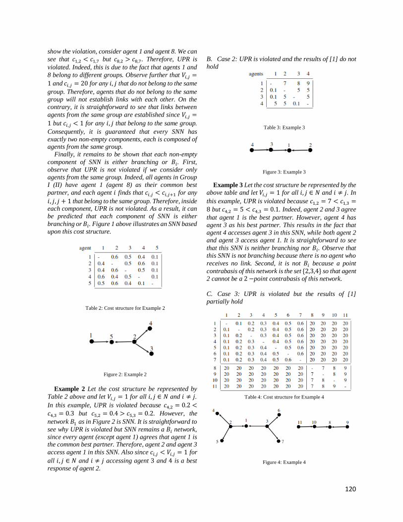
120

show the violation, consider agent 1 and agent 8. We can

see that 𝑐1,2 < 𝑐1,7 but 𝑐8,2 > 𝑐8,7. Therefore, UPR is

violated. Indeed, this is due to the fact that agents 1 and

8 belong to different groups. Observe further that 𝑉𝑖,𝑗 =

1 and 𝑐𝑖,𝑗 = 20 for any 𝑖, 𝑗 that do not belong to the same

group. Therefore, agents that do not belong to the same

group will not establish links with each other. On the

contrary, it is straightforward to see that links between

agents from the same group are established since 𝑉𝑖,𝑗 =

1 but 𝑐𝑖,𝑗 < 1 for any 𝑖, 𝑗 that belong to the same group.

Consequently, it is guaranteed that every SNN has

exactly two non-empty components, each is composed of agents from the same group. Finally, it remains to be shown that each non-empty

component of SNN is either branching or 𝐵𝑖. First,

observe that UPR is not violated if we consider only

agents from the same group. Indeed, all agents in Group

I (II) have agent 1 (agent 8) as their common best

partner, and each agent 𝑖 finds that 𝑐𝑖,𝑗 < 𝑐𝑖,𝑗+1 for any

𝑖, 𝑗, 𝑗 + 1 that belong to the same group. Therefore, inside each component, UPR is not violated. As a result, it can

be predicted that each component of SNN is either

branching or 𝐵𝑖. Figure 1 above illustrates an SNN based

upon this cost structure.


Figure 2: Example 2

Example 2 Let the cost structure be represented by

Table 2 above and let 𝑉𝑖,𝑗 = 1 for all 𝑖, 𝑗 ∈ 𝑁 and 𝑖 ≠ 𝑗.

In this example, UPR is violated because 𝑐4,2 = 0.2 <𝑐4,3 = 0.3 but 𝑐5,2 = 0.4 > 𝑐5,3 = 0.2. However, the

network 𝐵1 as in Figure 2 is SNN. It is straightforward to

see why UPR is violated but SNN remains a 𝐵𝑖 network,

since every agent (except agent 1) agrees that agent 1 is the common best partner. Therefore, agent 2 and agent 3

access agent 1 in this SNN. Also since 𝑐𝑖,𝑗 < 𝑉𝑖,𝑗 = 1 for

all 𝑖, 𝑗 ∈ 𝑁 and 𝑖 ≠ 𝑗 accessing agent 3 and 4 is a best

response of agent 2.

B. Case 2: UPR is violated and the results of [1] do not

hold

Table 3: Example 3

Figure 3: Example 3

Example 3 Let the cost structure be represented by the

above table and let 𝑉𝑖,𝑗 = 1 for all 𝑖, 𝑗 ∈ 𝑁 and 𝑖 ≠ 𝑗. In

this example, UPR is violated because 𝑐1,2 = 7 < 𝑐1,3 =8 but 𝑐4,2 = 5 < 𝑐4,3 = 0.1. Indeed, agent 2 and 3 agree

that agent 1 is the best partner. However, agent 4 has

agent 3 as his best partner. This results in the fact that

agent 4 accesses agent 3 in this SNN, while both agent 2

and agent 3 access agent 1. It is straightforward to see

that this SNN is neither branching nor 𝐵𝑖. Observe that

this SNN is not branching because there is no agent who

receives no link. Second, it is not 𝐵𝑖 because a point

contrabasis of this network is the set 2,3,4 so that agent

2 cannot be a 2 −point contrabasis of this network.

C. Case 3: UPR is violated but the results of [1]

partially hold


Figure 4: Example 4

121

Example 4 The cost structure of this example is simply

a combination of Example 1 and Example 3. Observe that

the link formation costs of agent 1 to agent 7 is identical

to that of example 1 and that the link formation costs of agent 8 to agent 11 is identical to that of example 3 (agent

1 to agent 4 in Example 3). We therefore divide agents

into two groups, where agent 1 to agent 7 belong to the

group I and agent 8 to agent 11 belong to group II.

Observe further that link formation cost 𝑐𝑖,𝑗 is set to be

20 if 𝑖 and 𝑗 belong to different groups. Similar to

Example 1, we have an SNN that consists of two non-

empty components, each is composed of agents from the

same group. Moreover, the shape of each component is precisely that of Example 1 and Example 3.

Consequently, we have an SNN such that one of its

components is 𝐵𝑖 and the other is neither branching or

𝐵𝑖. This entails that UPR is violated and the results of [?]

hold only partially.

IV. DISCUSSION AND CONCLUSION

This technical report shows various effects of the

violation of UPR condition on Strict Nash networks. We

summarize these effects below

1. If it can be predicted that SNN consists of multiple

components and which agents belong to which

components, then the shape of each component depends

merely on the cost structure pertaining to agents in that

component. This insight can be seen from Example 1 and

Example 4. 2. Consequently even if UPR is violated when

considering the cost structure of all agents, the result of

[1] - each component of minimal SNN being 𝐵𝑖 or

branching - still holds. This is possible if UPR is satisfied

when considering the cost structure pertaining to agents

in each component. Such possibility is illustrated by

Example 1. 3. Alternatively it is also possible that this result of [1]

holds partially in the sense that only some components of

minimal SNN - but not all - are 𝐵𝑖 or branching, if the cost structure pertaining to agents in each of these

components satisfies UPR while the violation of UPR

emerges in other components. This possibility is

illustrated by Example 4. 4. Whenever UPR is violated when considering the

cost structure pertaining to agents in the same

component, there are cases in which the component

remains 𝐵𝑖 or branching as well as cases in which the

component is neither 𝐵𝑖 or branching. These cases are

illustrated by Example 2 and Example 3 respectively We further provide an important observation from

point (3) and point (4) above as follows. First, note that

although Example 2 and Example 3 UPR is violated, only

SNN in Example 3 remains 𝐵𝑖 while SNN in Example 2

is neither 𝐵𝑖 nor branching. What explain this difference?

In Example 2, all agents (except agent 1) agree that agent

1 is their best common partner. However, this form of

agreement between agents does not exist in Example 3, where agent 4 does not agree with agent 2 and agent 3

that agent 1 is the best partner. Therefore, we conclude

that some forms of preferential agreement among agents

inside the component are required in order that the results

of [1] - a component of SNN guaranteed to be branching

or 𝐵𝑖 - continue to hold. Indeed, a similar analogy applies to point 1 and 2

above. Since the satisfaction of UPR in a component

requires that all agents in the component agree on which

agent is superior as a partner than which in terms of link

formation cost, the same interpretation emerges: some forms of agreement among agents inside the component

are required in order that the results of the results of [1] -

a component of SNN being branching or 𝐵𝑖 - continue to

hold. Finally, these examples raise a question of what a

necessary and sufficient condition for a component of

SNN to be branching or 𝐵𝑖 is. We leave this question as

a research to be explored in the future.

ACKNOWLEDGMENT

This research is sponsored by a Keimyung University

Outstanding Research Grant. I thank my research

assistant – Kwon Yun Heon – for his excellent assistance,

which helps save the time for conducting this research.

REFERENCES

[1] Bala, V. and Goyal, S. (2000). A noncooperative model of

network formation. Econometrica, 68(5):1181–1229.

[2] Billand, P., Bravard, C., and Sarangi, S. (2011). Strict nash

networks and partner heterogeneity. International Journal of

Game Theory, 40(3):515–525.

[3] Charoensook, B. (2015). On the Interaction between Player

Heterogeneity and Partner Heterogeneity in Two-way Flow Strict

Nash Networks. Journal of Economic Theory and Econometrics,

26(3).

[4] Galeotti, A., Goyal, S., and Kamphorst, J. (2006). Network

formation with heterogeneous players. Game and Economic

Behavior, 54(2):353–372.

[5] Goyal, S. (2012). Connections: an introduction to the economics

of networks. Princeton University Press.

[6] Jackson, M. O. and Wolinsky, A. (1996). A strategic model of

social and economic networks. Journal of Economic Theory,

71(1):44–74.

[7] Vannetelbosch, V. and Mauleon, A. (2016). Network formation

games. In Bramoullè, Y., Galeotti, A., and Rogers, B., editors,

The Oxford Handbook of the Economics of Networks. Oxford

University Press.

122

Design of Collision Prevention based on Wall

Following Mechanism on Multi-Robot System

Joao Amaral de Fatima Pereira, Agung Nugroho Jati, Randy Erfa Saputra School of Electrical Engineering, Telkom University

Indonesia

[email protected]

Abstract— Wall following mechanism is mostly used for

finding a way out in the maze or room on the single robot

cases, but in this paper, it will be demonstrated a multi-

robot system by applying collision avoidance based on wall

following mechanism to solve an unknown maze. Fuzzy

logic will be implemented on right wall following

algorithm to avoid the collision while the robots are in a

maze, and at the same time robots will recognize which are

the wall of maze, junctions, and other robot. Based on the

results, shown that the robots could recognize the

junctions, wall and other robots. Based on the result of all

testing, robots might solve the complicated maze for 2 until

5 minutes, with 86% of solution without any collision.

Index Terms— Collision Prevention, Fuzzy logic; Multi-

Robot; Maze Solver; Tremaux’s Algorithm.

I. INTRODUCTION

Collision avoidance is a fundamental problem in

robotics. Problems are generally defined in the context

of autonomous mobile robots which navigate in

environments with barriers and/or other mobile entities,

where robots use continuous sensing and action cycles.

Solving a maze with more than 2 robots, such a serious

problem that we need to concern because collision

avoidance may occur during the robots are running inside it. Robots have a goal it is to reach the endpoint,

then probably collision will happen if the robots face the

wall of a maze or with another robot. In this problem,

we found out that ebbed an algorithm for each robot is

the key to avoiding those problems. And there are a lot

of algorithms have used to solve the maze easily, like

flood fill[1], tremaux's algorithm, wall followers[12],

random mouse[2] algorithm, dead-end filling maze-

routing algorithm and etc. but most of those algorithms

have already implemented in mobile robot, and it

worked very well. Here, we will use one of those algorithms for solving a maze faster and no collisions

happened while the robots are searching for a goal.

As we all know maze is a common unknown arena,

needs to find its short way to solve the maze. And in

this paper will tell you about using one of the mazes

solving algorithm, take a good decision when the robots

facing the arena and find the short path, during the

seeking of the shortest path, there are no collisions

occurred between robots and arena or with another

Robots.

A single robot may use those algorithms to solve a

maze, instead of it multi-robot also has an occasion to

use those algorithms, but the differences in time to reach

the goal or end-point[10]. A single robot solves a maze fast, but multi-robot will make it faster with the same

algorithm. Regarding to this problem of maze solving, a

necessary and applicable algorithm is needed, and we

prefer using wall follower algorithm. Wall follower has

2 types, those are Right Wall Follower(RWF) and Left

wall follower(LWF) it depends on application of both

algorithm, Left Wall follower(LWF) is the most one

used, but in this research, we chose Right Wall Follower

(RWF).

Basically, ultrasonic and IR sensors are mostly used

to apply the wall follower algorithm, right here we are

used 4 ultrasonic sensors, as it demonstrated using Right Wall Follower means ultrasonic sensors are located in

each side instead of back side[3][5]. An ultrasonic

sensor will be located in the front side, 2 ultrasonic

sensors in the right side, each ultrasonic are located in

front and back of right sides of a robot, and the other

one is in the left sides of the robot. The combination of

that ultrasonic sensors is able to respond as quickest

when the robots are in the junction, corridor or in the

dead-end.

To apply the right wall follower algorithm,

actually fuzzy logic is allowed to work on it, take the range on a measurement of each ultrasonic sensors are

keys to implementing the fuzzy logic in right wall

follower.

The algorithm which will be used in this paper is right

wall follower algorithm, and inside of the RWF

actually, there is the implementation of fuzzy logic

applied. To use those algorithms, we need to embed it in

sensors as everyone one knows, it would be possible

using the camera, IR sensors, ultrasonic sensors and

others. After all of this, because we're implemented

123

these algorithms on Robots using Arduino, we chose the

ultrasonic sensors as a parameter for writing and

embedding the algorithms.

This paper is organized as follows: Section I will

show the introduction, backgrounds, and problems about this research. Then, section II discusses about

other related researches used as references in this

research. In the section III, shown the conducted method

and configuration of this research while section IV

shown the results and analysis. The last section is a

conclusion of the research.

II. RELATED WORKS

There are many algorithms can be used to solve the

maze such as random mouse, wall follower, and flood

fill algorithms[2][13]. The wall follower algorithm mostly is used when the arena or place the robots face

are unknown and only have one purpose to reach the

end point. The end point basically is set by giving a

sign. On the other hand, the flood fill algorithm is

commonly used when the position of end point is

recognized by the robot through some identification and

from that sign robot must be find the shortest path[2].

Flood Fill Algorithm is one of the most efficient

algorithms to be used[1][2]. This algorithm may solve

complex and difficult maze without having any

troubles/collisions by receiving the value of all cells in a maze, which those values shows the steps from any cell

to reach the end point. At the same time, mostly this

algorithm is used by count the every passed grid and the

next grid, means that solving the maze by recording the

number of grid.

Pulse Width Modulation “PWM” is a simple method

by controlling analog values through the digital signal

by changing or modulating the pulse width. This is a

well applicable algorithm using electricity[1][14]. By

tuning an analog device with a pulse wave changes

between HIGH with “5V” and LOW with "0V" at a fast

rate the device will behave as it getting a steady voltage somewhere between 0V and 5V. Figure-1 shows an

example of a PWM with a duty cycle of 0% - 100&,

which gives a voltage value of for 0V until 5V. The

term of duty cycle explains the amount of time in the

period that the pulse is on or HIGH and off or LOW. It

will be specified as a percentage of the full period of

time . 0% duty cycle means that the PWM wave is off

or LOW and 100% means waves is fully on or

HIGH[1].

Figure 1: PWM of 0% - 100% duty cycle [1]

Table 1

Right And Left Wall Following Routes

The wall following algorithm is one of the simplest

and most used algorithm to solve a maze. The robot will

heading any direction to reach the end point by

following the right side of wall or it might be left

wall[12][4][14]. Robot will recognize any junction by

the value of the input sensors, and robot will sense the open wall also by detecting using sensors. And the robot

will follow the priority wall. By consider the wall as a

main key to reach the end point, the robot doesn’t need

to find the shortest path to reach the end point. From fig.

2 bellow it shows how wall follower algorithm works

for both right and left side, it depends of how we prefer

which one is better and useable to solve and unknown

maze.

From all those related works we take the Right Wall

Follower algorithm as the main part, but inside of the

Right Wall Follower algorithm itself, there an existence of PWM that will actually controlling the wheel to

explore and shows how fuzzy logic works[3][6][9].

Briefly, Right Wall Follower Algorithm used

can be seen in the following pseudocode:

124

Pseudocode above shows the decision making of

robot to follow the wall, by receiving the data from the

input value of 4 ultrasonic sensors where located in

every Robot.

III. SYSTEM IMPLEMENTATION

Before we describe for further about algorithms, first

we need to know where those mentioned sensors placed

in robot, then it would be easier to understand better the

algorithm.

Figure 2: Implementation of Robots

Figure 3: Design Scheme of Robot

Right wall Follower as an algorithm is used to avoid

collision between robots and walls[11], but inside of it,

we need to add some system to let this RWF algorithm

working better. Fuzzy logic will be established, to make

the RWF algorithm works and keep making a good

decision and knows where the robot is located. The

algorithm for robot will be different depends on the

location of the robot, it means that when the robots are in corridor or junction will certainly check all the time.

In figure 4 below shows us how robots taking the

decision when they are in the corridor.

For the RWF Algorithm will combine with PWM

controlling. But those algorithms are combined using

the Fuzzy logic. Fig 4 demonstrates that the RWF is

working with the PWM and controlled by the inputs of

data decided by fuzzy logic[6].

Flowchart bellow will show, how we implement the

Right Wall Follower algorithm on Multi-Robot. And

this flowchart also shows the certain value of ultrasonic

to make any decision for robot such follow the wall, turn left, turn right or turn around. The purposes of this

flowchart is to find the end point by implementing the

Right wall follower algorithm, and at the same time

there are no collisions for robots and maze, also with

other robots.

Before this algorithm works, it took some decision

making to run it, like what sensors will do if the data

they have from the inputs, and how it works. Fuzzy

logic implementation led the robot to make its own

decision to run the designing algorithm[7][12]. As the

flow-chart demonstrated that, there are only 3 ultrasonic used to show how RWF work. The table below has

shown that the inputs of every three sensors will tell the

While not Reach Goal

If frontside is open

If Right1 > 10

Turn_Right Slowly

If Right2 > 10

Turn_Left Slowly

Else if right1 is open then

Turn _right

Else if left side is open then

Turn_left

Else

Turn_around

Loop

125

motors by controlling using PWM. Actually, using

PWM to controlling the motor such a good

implementation, because PWM would be worked well if

a microcontroller received the data from more than 2

sensors.

Figure 4: Flow-chart for Right Wall Follower Algorithm for Multi-

Robot

In the next table, shown how the turn left slowly and

turn right slowly work and the combination of PWM for

two motors making a decision, while the Right Wall

Follower algorithm is running, but no collision

happened.

Table 2

Motor Rotation Speed based on Distance from Wall

Front

sensor

Right1

sensor

Right2

sensor Left motor Right motor

X > 10 X > 10 X > 10 *PWM=110 *PWM=90

X > 10 X < 10 X > 10 *PWM=60 *PWM=90

X > 10 X > 10 X < 10 *PWM=90 *PWM=60

X > 10 X < 10 X < 10 *PWM=90 *PWM=110

X < 10 X > 10 X > 10 *PWM=0 *PWM=0

X < 10 X < 10 X > 10 *PWM=0 *PWM=0

X < 10 X > 10 X < 10 *PWM=0 *PWM=0

X < 10 X < 10 X < 10 *PWM=0 *PWM=0

Beside of Right Wall Follower algorithm as you see in TABEL II, at the same time there is an existence of

another algorithm to recognize the junctions[13]. In this

paper describes that the robot will consider another

robot as a junction, but the decision making of each

robot for maze solving actually different. When the

robot is facing the others are different, those differences

are the embedded of the delay and PWM of turning

around. For the delay, every robot has 10 seconds

bigger from another when they are in the junctions[8].

In the table below, also will be demonstrated, when

the robot will make a decision to choose the paths. Paths here are mentioned to the heading points of a robot, turn

left, turn right, turn around or moving forward.

Table 3

Decision Making For Motors

Direction Left Sensor Right

Sensor

Front

Sensor

TURN LEFT X > 15 X < 15 X < 10

TURN RIGHT X < 15 X > 15 X < 10

TURN AROUND X < 15 X < 15 X < 10

Table 4

Heading Directions Of Motors

Direction Left Motor Right Motor

TURN LEFT Backward Forward

TURN RIGHT Forward Backward

TURN AROUND Forward Backward

The table 3 shows that every robot’s direction

depends on its input of ultrasonic sensors. On the other

side, fig 6 shows how both motors work after robot

make a decision of the heading direction. And the next

table will show you the implementation of PWM for the

Direction of the robot.

126

Table 5

Speed Motors For Heading Directions

Direction Left Motor Right Motor

Forward Backward Forward Backward

TURN

LEFT PWM=0 PWM=55 PWM=110 PWM=0

TURN

RIGHT PWM=110 PWM=0 PWM=0 PWM=55

TURN

AROUN

D

PWM=110 PWM=0 PWM=0 PWM=55

Robot considers the junction by the inputs data of

three ultrasonic sensors located on front side of the

robot (Front, left and Right1). When those three

ultrasonic detect some several data, they found out the junction. Then, it will automatically choose its own

decision. Flow-chart bellow demonstrates how robot

knows that he's facing the junction.

Before we end this part of discussing the algorithm,

here a picture that shows how the decision making of

the robot in maze arena to avoid the collision between

the maze and another robot.

Figure 5: Flow-Chart For Facing The Junction/other Robot

In fig 7, shown that when the robot in the arena, and if

the inputs of ultrasonic sensors in the front side detect

that it is a junction, and it will automatically turn

around, by the right side. The robot will find the endpoint if three ultrasonic sensors in front sides detects

in a certain distance with the certain timing.

Figure 6: Robots Run in the Environment

(a)

127

(b)

Figure 6: (a) Example of How Robot will Make a Decision, (b) RWF

based Robot’s Movements

IV. DISCUSSION

The movements of each robots depend on the location

of each sensors. Based on the result of the test, found

that the main point in collision prevention on robot

which uses ultrasonic sensors, are value of every

ultrasonic sensors. It can be seen as follows:

(a)

(b)

(c)

Figure 7: (a) Frontside US Sensor (b) Leftside US Sensor (c)

Rightside US Sensor

Based on test shown on the graph, there are error

values arround 5% between distance captured by sensor

and real distance. It was caused by different material

used as wall. Furthermore, it happened because of signal

reflection. Different materials influence the spped of

signal reflection received by robot, so that they defined different value of distance eventough it’s similar in real

condition.

The condition above, can lead to collision of robots or

robot because robot wll make a late and/or wrong

decision caused by invalid distance value from sensor.

To avoid them, all of sensor should be callibrated before

use. Moreover, perfect input value of ultrasonic sensors

will be automatically validated, and rate of collision will

be decrease significanly.

According to the experiment, robots can avoid the

Real distance

Real distance

Real distance

Front US

Left US

Right US

128

collision between them in arround 86% success rate. It

is taken after 10 times experiment in the environment

maze. Besides, robots can prevent to face each other by

defining their range and orientation in the maze.

In addition, communication between robot to share its location based on their sensor values can prevent more

significant to collide. However, there were delay

communication arround 0.75 s can be tolerated. Robot

can communicate in range approximately 2.95 m.

Table 6

Result of Test in Decision Making to Avoid Collision

N

o.

Real

Distance

Robot 1 Robot 2 Decision Result

1 F:9

L:80

R:90

F:9.43

L:88.23

R:95.22

F:9.15

L:81.95

R:95.22

Turn

Right

Turn

Right

Success

2 F:45

L:78

R:19

F:44.24

L:75.33

R:17.02

F:43.13

L:77.06

R:18.55

Move

Forward

Move

Forward

Success

3 F:9

L:50

R:87

F:9.57

L:51.63

R:127.98

F:10.01

L:53.81

R:85.05

Turn

Right

Turn

Right

Success

4 F:10

L:19

R:12

F:10.06

L:19.29

R:12.45

F:14.28

L:20.33

R:14.26

Turn

Arround

Move

Forward

Success

5 F:40

L:25

R:15

F:40.01

L:25.04

R:15.89

F:39.32

L:24.29

R:15.19

Move

Forward

Move

Forward

Success

6 F:8

L:12

R:70

F:9.15

L:4.22

R:63.56

F:9.66

L:9.08

R:0

Turn

Right

Error Failed

7 F:30

L:52

R:12

F:31.11

L:49.39

R:12.44

F:32.02

L:51.45

R:15.12

Turn

Right

Move

Forward

Success

8 F:30

L:10

R:40

F:30.35

L:9.21

R:41.60

F:30.44

L:10.22

R:39.82

Error Turn

Right

Failed

9 F:60

L:70

R:70

F:58.12

L:68.09

R:98.22

F:57.91

L:69.12

R:71.49

Turn

Right

Move

Forward

Success

1

0

F:8

L:15

R:15

F:8.76

L:15.77

R:15.98

F:9.07

L:21.53

R:15.62

Turn

Arround

Turn

Left

Success

V. CONCLUSION

Collision avoidance on multi-robot system is such a

complicated problem which can be solved by mixing

more than one algorithm. In advance, it can be

improved to collision prevention to reduce the

possibility for robots to collide. However, it needs

sensor fusion system, such as combining ultrasonic sensor as range finder and compass to define robot’s

orientation.

Each area have to be marked by the robots by using

values of various sensors in order to determine the well

path of every single robot. To overcome them, fuzzy

logic control can be added to the system, especially in

right wall following mechanism. Right wall following is

used to simplify the movement model of robot system.

Furthermore, communication between robots is

established to share the location of each robot.

On the other hand, some problems are still happened

in the system. It is mostly caused by inaccuray of sensor

values. Somehow, it can make robot moves unproperly.

Since multi-robot system involves more than a robot in

the environment, timing is very considered as an

important parameters. For example, robot can collide

when they face each others if a robot make a late decision to turn arround even another can make a well

decision.

In the next research, it will be added a mapping

system in order to know exact location of the explored

environment. It also can be used to defined the path of

each robot. In advance, it can be developed to coverage

the area.

REFERENCES

[1] Angelo Martinez, Eddie Tunstel1, and Mo Jamshidi “ Fuzzy

Logic Based Collision Avoidance For a Mobile Robot”. CAD

Laboratory for Intelligent and Robotic Systems, 1994.

[2] Reinhard Braunstingl, Pedro Sanz, Jose Manuel Ezkerra “Fuzzy

Logic Wall Following of a Mobile Robot Based on the Concept

of General Perception”. ICAR ‘95, 7th International Conference

on Advanced Robotics, Sant Feliu de Guixols, Spain, PP.367-

376, SEPT., 1995.

[3] I. Gavrilut, V. Tiponut, A. Gacsadi, L. Tepelea" Wall-following

Method for an Autonomous Mobile Robot using Two IR Sensors

"University of Timisoara, B-dul Vasile Parvan No. 2, 300223

Timisoara, Romania.

[4] Reinhard Braunstingl, Jose Manuel Ezkerra, Pedro Sanz “Fuzzy

Logic Wall Following of a Mobile Robot Based on the Concept

of General Perception” ICAR ‘95, 7th international conference

on advanced robotics, sant Feliu De Guixols, Spain, PP.367-376,

SEPT., 1995.

[5] Michael G. Murphy, Ph.D. "Fuzzy Logic Path Planning system

for collision Avoidance by an Autonomous Rover vehichle",

NASA/ASEE Summer Faculty Fellowship Program, 1991.

[6] C.G. Rusu, I.T. Birou “Obstacle Avoidance Fuzzy System for

Mobile Robot with IR Sensors “,10th International Conference

on DEVELOPMENT AND APPLICATION SYSTEMS,

Suceava, Romania, May 27-29, 2010.

[7] David Llorca, Vicente Milanés, Ignacio Parra, Miguel Gavilán,

Iván García Daza, Joshué Pérez Rastelli, M.A. Sotelo, “

Autonomous Pedestrian Collision Avoidance Using a Fuzzy

Steering Controller”, IEEE Transactions on Intelligetn

Transportation System, VOL. 12, No. 2, June 2011.

[8] Akib Islam, Farogh Ahmad, P.Sathya, “ Shortest Distance Maze

Solving Robot”, International Journal of Research in

Engineering and Technology, eISSN: 2319-1163 | pISSN: 2321-

7308.

[9] Marco A. C. Simões, Helder Guimarães Aragão, Victor Souza,

Simon Viegas, “ Using Fuzzy Logic to Build a Heterogeneous

Multiagent System for the Robotics Soccer Problem ” Computer

Architecture and Operating Systems Group(ACSO) State

University of Bahia (UNEB).

[10] Yee Mon Nyein, Nu Nu Win, “Path Finding and Turning with

Maze Solving Robot”, International Journal of Science,

Engineering and Technology Research (IJSETR) Volume 5,

Issue 9, September 2016, ISSN: 2278 – 7798.

[11] Yuan Zhou, Hesuan Hu, Yang Liu, and Zuohua Ding, “Collision

and Deadlock Avoidance in Multirobot Systems: A Distributed

Approach “IEEE Transaction on Systems, man and Cybernetics

Systems. 2017.

[12] Dali Sun, Alexander Kleiner, Bernhard Nebel, “Behavior-based

Multi-Robot Collision Avoidance”, 2014 IEEE International

Conference on Robotics & Automation (ICRA), Hong Kong

Convention and Exhibition Center May 31 - June 7, 2014. Hong

Kong,China.

129

[13] Aulian Miftahul Fathan, Agung Nugroho Jati, Randy Erfa

Saputra, “ Mapping Algorithm Using Ultrasonic And Compass

Sensor On Autonomous Mobile Robot,” ICCEREC, September

2016.

[14] NT AlGhifari, AN Jati, RE Saputra, “Coordination Control for

Simple Autonomous Mobile Robot ”, International Conference

on Instrumentation Control and Automation, pp 93-98, August

2017.

[15] Agung Nugroho Jati, Randy Erfa Saputra, Muhammad Ghozy

Nurcahyadi, Nasyan Taufiq Al Ghifary,“A Multi-Robot System

Coordination Design and Analysis On Wall Follower Robot

Group”, IJECE, Vol 8 (6), Dec 2018.

130

A Robotic Image Sensor System for an

Octocopter Drone

Rainier Jo-Matthew Baring, Yen-Wei Chang, Calvin Leader Tiu, Tung Haang Yen, Alvin Chua Unmanned Aerial Vehicle Research Laboratory, Mechanical Engineering Department,

De La Salle University, Manila, Philippines

Corresponding Author: [email protected]

Abstract-The study focuses on design of a robotic image

sensor system attached on an octocopter drone, which will

be utilize in surveying activities. This is composed of a

3DOF robotic manipulator with camera system. This is to

address the limited camera view of the current

technologies on a drone system. The robotic image sensory

system uses a pro-trinket microcontroller to manipulate its

movements. During pre-set mode, the robotic manipulator

has two positions: retracted and extracted position. The

retracted position activates during storage while the

extracted position actuates during surveying. The

experimental results shows that the new image sensor

system is able to capture images in different viewpoints

that would benefit for the drone user.

Index Terms—sensor; drone, image octocopter

I. INTRODUCTION

There are more and more researches on how to

add a manipulator to an UAV to maximize the usage of

the drone, This also helped achieve a wide variety of

usage in multiple fields. For example, there is the

ARCAS project that is now ongoing in the European

nations. According to Loos (2014), ARCAS project

helps researchers build robotic manipulators for the

UAV that may serve different functions. One of their

current project on ARCAS has the ability to pick up an

object autonomously without the control of the user. On

the commercial side, the most common manipulators

usually seen are the camera manipulators. An example

would be the DJI Phantom series which has a gimbal

manipulator for the camera. This gives the user a more

steady view while recording.

The most concerning of all would be

limitations in angles when taking the shot. Since the

drone camera is usually fixed, it is hard to take photos

that include angles that may be important in cases such

as car chases or bridge surveying. In addition, it cannot

view the scenery on the top side of the multirotor

because components such as the flight controller is

blocking it. An example of this problem would be

surveying a bridge, examining an inaccessible tunnel or

other unreachable places. A possible solution to this is

applying a 360 rotation for the camera around the

structure of the drone or applying a robotic manipulator

to the camera allowing it to rotate around the drone

giving a 360 like view as output.

By creating a manipulator that provides the

octocopter a multidirectional view, it can decrease the

common blind spots that the cameras on the drones

today. With this research, it will be able to benefit for

the users which needs to view an object which is located

somewhere high and at the top of the infrastructure.

Sample of places like these are the top of the lower side

of the bridge, or the high ceiling of a factory which

requires inspection on its structure or safety.

This study will focus on the development of a

new robotic image sensor system for an octocopter

drone. The design of the arm should consider the shape

of the arm, material of the arm and its location for

maximum image capture. The controller should be

light so as not to affect the flight of the octocopter while

having the capability of manipulating the joints.

II. ROBOTIC IMAGE MANIPULATOR DESIGN

To compute for the best dimensions for the

frame of the robotic camera manipulator, the

dimensions of the octocopter must be considered. The

first dimension of the octocopter, Tarot 1000, to be

considered would be the position where the camera

would be placed in between the shafts of the octocopter.

The position must be where least of the camera’s view

131

is covered by the shafts of the octocopter and the

propellers of the octocopter (see Figure 1)

Figure 1. Robotic Image Manipulator camera location

Based from the specification sheet of the

octocopter, the diamter of the octocopter is 287.54mm

thus the radius of the octocopter body is 143.77mm.

The length of the propellers are 400mm. After

measuring the length of the shaft from the center of

octocopter to the propellers which is 445mm, the

length from the tip of the center body of octocopter to

the middle of the rotational area of the propellers is

approximately 190mm.

The second part of the dimension

computation is to know the distance of the octocopter

body to the floor. In considering the octocopter stand,

the length of TL100B05-02 stand must be considered.

The total length of octocopter stand is 400mm as

found in Figure 2.

Fig.

2.

Mea

sur

eme

nt

of

the

Oct

oco

pter

stand

Thus, from the different dimensions collected

from the octocopter parts, the vertical length of the

robotic camera must not exceed 400mm, else it will hit

the floor when it is operating on the ground. The

horizontal length of the manipulator fully extended

must not exceed 443.77mm, that is the sum from the

point where the camera robotic manipulator would be

attached to the optimal location to place the camera.

The camera robotic manipulator would be

divided into three different parts. Link A would be the

part that is designed with a 90 degree angled link.

This would be able to create an extension effect. Link

B will be the part where the arm could retract and

extend 160 degrees by using a servo motor. Link C

would be the part that would rotate 180 degree the

camera. This would provide more vision for the

camera. Figure 3 shows the dimensions of the link C

after considering the restrictions in the design.

Fig. 3. Drawing of Link C

III. MECHANICAL STRESS ANALYSIS

To test if the design for the frame of the

manipulator is feasible, Solidworks’ simulation

software to test the effect of the loads to the

manipulator frame. For Link A, the maximum stress

is 2.894MPA. The force applied to the Link A is

3.5512N. The value of 3.5512N came from the total

weight of the Servo motors A and B, Links B and C

and the weight of GoPro with its case.

Fig. 4. Stress Simulation of Link C

132

For Link B, the maximum stress encountered is

7.183MPa. The load or force applied to the link is

1.5598N. It is consisted of the link C , servo B and

Gopro with its case. In the simulation of Link C (see

Figure 4), the maximum stress experienced by the

Link is 0.651 MPa. The load applied to the link is

1.8149N. The load consists of the weight of Gopro and

Gopro case.

Based from the stress simulation of the three

designed links, its maximum stress is still below the

yield stress of ABS. Thus, the designed links camera

robotic manipulator frame will not break apart when

the loads were attached.

IV. ELECTRONICS AND PROGRAMMING OF THE

ROBOTIC SENSORY SYSTEM

The Hitec HS-311 motor was used to control

the movement of Link B of the manipulator arm. It

has a torque range of 3.0 kg/cm to 3.7 kg/cm

depending on the voltage output. This is more than

the torque required. It is to ensure the safety of the

robotic manipulator for further unforeseen

circumstances. The KST DS113MG is a standard

plastic servo with great performance. It was used to

control the movement of the GoPro Holder or Link C.

It has a torque output of 1.8 kg/cm to 2.2 kg/cm,

depending on the set operating voltage.

The microcontroller used to program the

servomotor is the Pro Trinket 5V. It has been the

chosen microcontroller due to its capacity to calculate

as well as its size that measures only 1.5”x0.7”x0.2”. It

is also cheaper compared to other microcontrollers

due to its size and how the overall built was optimized

to provide the desired performance. It is also easy to

program through the Arduino IDE as well as through

the use of a micro-USB jack for power and USB

uploading. The turnigy 9x was used as the radio

transmitter in this study.

Fig. 5. Flowchart of Robotic Arm Software Control

The program (Figure 5) starts off by stating

the required values and assigning pins of the

microcontroller as either outputs for servo or inputs

for the receiver. It then initializes and determines

whether the robotic arm must be extended or not

based on the positioning of the designated control

knob in the remote controller. Inside the loop that

determines whether the arm is being extended or not,

it contains 2 sub-programs which control the camera

position and the panning position of the overall

octorotor stand.

V. RESULTS

Servomotor Test

This test would test the effect of load on the servo

motor’s angular speed. The first part of the test would

be no load and the second part would be with load.

The servo motors tested would be servo motors A and

B. A stop watch was used to time how long would the

servo motors rotate from its initial position to the

final position.

Fig. 6. Timer used (left) and Setup(right) in the

Servomotor Speed Test

133

A camera would be also used to check is the servo

motor had reached its desired position. The camera

must also be set up the same way as the servo motor

test where the camera must be positioned

perpendicular to the centerline.

Figure. 7. Servomotor A Speed Test

Figure 8 Servomotor B Speed Test

Based from the collected data, for servomotor A,

there is a 18.88% difference in the travel time of a

loaded and an unloaded servo; However, for

servomotor B, there is a 78.61% difference in the time.

This may be due to the processing delay starting from

the receiver to the microcontroller (see Figure 7 and

8).

Camera Test

The camera test would show how many percent

the camera or Gopro’s vision would be covered by the

octocopter’s shaft when the lens is extended and

pointing upward. The test would be separated into

two sections. The first part of the test would be the

GoPro capturing photo without the cover of

octocopter. The second part of the test would be GoPro

capturing photo with the cover of the octocopter.

The first part of the test, the GoPro of the camera

robotic manipulator would be turned at the 180 or

pointing upward position and first capture an image

without the cover of octocopter. A white board would

be placed 800mm above the camera, to minimize the

noise created by the light straight above the GoPro

In the second part of the test, the rest of the

octocopter would be placed above the camera robotic

manipulator. Servo motor C would position the

camera robotic manipulator in the middle of the two

shafts of the octocopter. This is to increase space for

the camera’s lens angle. The same procedure where a

white board would be placed 800mm above the GoPro,

then a picture would be taken afterwards.

Fig. 9. Robotic Image Sensor at the Center of Two

Shafts

Based from the data collected, the difference

between the covered and uncovered by the octocopter

is 14.5833%. This showed that there is a large portion

of area that was covered by the octocopter. However,

the extend arm function still provided a wide portion

of uncovered view for the GoPro, there is still more

than 73.9239% that is uncovered by the octocopter.

This is more efficient than the target of having 40% of

the covered area when the camera manipulator is

attached to the arm.

Flight Test

Before performing the flight test, the initial setup

of the programming the APM 2.6 must be done

through the mission planner. After performing

programming section of the APM 2.6 using the

134

mission planner setup wizard, the accelerometer must

be calibrated.

Next step of calibration would be the radio

calibration. This step of calibration would determine

the control value of each function. After the

calibration, the red line would indicate the maximum

and minimum value of the transmitter. These values

would be then used to program the microcontroller for

the robotic arm

Last part of the calibration would be the compass

attached to the APM 2.6 flight controller. This part of

test would let the controller know the direction of the

octocopter.

After all part were done, the octocopter would be

ready to have its test flight. The flight of the

octocopter was stable, since there were less

unnecessary movement in the flight during the test

flight. The flight controller also has a quick response

to the change of direction coming from the flight

controller. Thus, the calibrations of the mission

planner are essential to achieve a safer flight.

VI. CONCLUSION

The research study was able to design a robotic

image sensor system which provides a multi-

directional view to a rotorcraft unmanned

autonomous vehicle.

In order to design a camera robotic manipulator,

different theoretical factors were considered namely

material properties especially the ultimate and yield

strength of the materials of choice. Through the use of

Solidworks, the best material was chosen given the

restrictions in weight and size of the robotic arm due

to the payload that the rotorcraft can carry. The

design was optimized especially when it comes to its

weight to provide the least strain to the flight of the

rotorcraft.

In order to simulate the manipulator to

understand its behavior, different pre-fabrication

familiarization and testing was done. The servos were

studied with the use of different pre-set programs.

The receiver connection and configuration was also

studied in order to be able to retrieve serial data that

is required for it to allow the transmitter and the

servos to communicate. Lastly, the transmitter

function was altered based on the control

requirements of the manipulator setup up namely the

gear switch, the throttle cut switch and the hover-

throttle knob while still keeping the controller capable

of flying the rotorcraft.

Finally, the whole robotic manipulator was

attached to the Tarot-frame Octorotor powered by the

Ardupilot flight controller. Both octocopter system

and robotic image system setup can be simultaneously

controlled through the Turnigy 9x controller.

ACKNOWLEDGMENT

The authors would like to acknowledge the funding support

of the Department of Science and Technology – PCIEERD. Also, the Mechanical Engineering Department of DLSU for supporting the study

REFERENCES

[1] Airbornedrones long range flight systems with Direct Vision

Feed. (n.d.). Retrieved July 14, 2016, from

http://www.airbornedrones.co/

[2] Aeryon SkyRanger the benchmark for VTOL sUAS – Aeryon

Labs Inc. (n.d.). Retrieved from

https://www.aeryon.com/aeryon-skyranger

[3] Bouabdallah, S., & Siegwart, R. (2007). Full control of a

quadrotor. 2007 IEEE/RSJ International Conference on

Intelligent Robots and Systems. doi:10.1109/iros.2007.4399042

[4] Dollosa, C.M., Gavinio, S., Hermoso, G., Laco, N., Roberto,

L.A. (2013). Implementation of speed and torque control on

quadrotor altitude and attitude stability (Undergraduate Thesis).

De La Salle University, Manila.

[5] Experimental Characterization of the Mechanical Properties of

3D-Printed ABS and Polycarbonate Part. (2016). Retrieved June

22, 2017, from

http://cimar.mae.ufl.edu/rapid_proto/pages/3D%20Printing%20P

aper%20Final%20Manuscript.pdf

[6] Fatan, M., Sefidgari, B. L., & Barenji, A. V. (2013). An adaptive

neuro PID for controlling the altitude of quadcopter robot. 2013

18th International Conference on Methods & Models in

Automation & Robotics (MMAR).

doi:10.1109/mmar.2013.6669989

[7] Gameros, A. (2015, July 20). The Use of Composite Materials in

Unmanned Aerial Vehicles (UAVs). Retrieved July 22, 2016,

from http://www.azom.com/article.aspx?ArticleID=12234

[8] Kelly, H. (2013, May 23). Drones: The future of disaster

response - CNN.com. Retrieved February 04, 2016, from

http://edition.cnn.com/2013/05/23/tech/drones-the-future-of-

disaster-response/index.html

[9] Kucuk, S., & Bingul, Z. (2006). Robot Kinematics: Forward and

Inverse Kinematics. Industrial Robotics: Theory, Modelling and

Control. doi:10.5772/5015

[10] Lippiello, V., & Ruggiero, F. (2012). Cartesian Impedance

Control of a UAV with a Robotic Arm. IFAC Proceedings

Volumes, 45(22), 704-709. doi:10.3182/20120905-3-hr-

2030.00158

[11] Loos, R. (2014, September 18). ARCAS Develops Flying

Robots With Arms | Robotics Today. Retrieved July 14, 2016,

from http://www.roboticstoday.com/news/arcas-flying-robots-

have-arms-3044

[12] Mendoza-Mendoza, J., Sepulveda-Cervantes, G., Aguilar-

Ibanez, C., Mendez, M., Reyes-Larios, M., Matabuena, P., &

Gonzalez-Avila, J. (2015). Air-arm: A new kind of flying

manipulator. 2015 Workshop on Research, Education and

135

Development of Unmanned Aerial Systems (RED-UAS).

doi:10.1109/red-uas.2015.7441018

[13] Pros and Cons of Drone Cameras - Soaring Sky Academy.

(2015, November 25). Retrieved July 04, 2016, from

http://soaringskyacademy.com/drone-cameras/

[14] Radhesh. (2008, May 11). PID Controller Simplified | My

Weblog. Retrieved July 18, 2016, from

https://radhesh.wordpress.com/2008/05/11/pid-controller-

simplified/

[15] Robotshop. (2013). Tarot IRON MAN 1000 Carbon Fiber

Octocopter Frame. Retrieved July 20,2016, from

http://www.robotshop.com/media/files/pdf/user-manual-

tl100b01.pdf

[16] SenseFly's eXom Drone Uses Vision and Ultrasound to Fly

Precisely, Safely - IEEE Spectrum. (2014, November 6).

Retrieved from

http://spectrum.ieee.org/automaton/robotics/drones/sensefly-

exom-drone-vision-and-ultrasonic-sensors

[17] Vanian, J. (2016, July 22). 7-Eleven and Flirtey Delivered a

Sandwich and Slurpees via Drone Fortune. Retrieved July 13,

2016, from http://fortune.com/2016/07/22/7-eleven-drone-

flirtey-slurpee/

136

Design of a Programmable Fixed-Wing

Drone System

Lanz Gaffud, Carlos Guinto, Starl Mallari. Alvin Chua

Unmanned Aerial Vehicle Research Laboratory, Mechanical Engineering Department,

De La Salle University, Manila, Philippines

Corresponding Author: [email protected]

Abstract- The study presents the design, simulation and

testing of a programmable fixed-wing drone system for the

enhancement of teaching and development of fixed-wing

drones. The fixed-wing uses a Pixhawk flight controller to

stabilize flight and provide autonomous features. A

Skywalker Carbon Fiber Tail Version 1880mm serves as

the frame to house the important parts such as the flight

controller, battery, electronic speed controller and RC

receiver for proper flight. An on-line website was

developed to serve as a teaching tool in the different

theories and procedures to operate the fixed- The online

manual was evaluated through the students'

comprehension of the discussion of each experiment using

quizzes and survey. Actual flight test was done to verify

the air worthiness of the fixed wing drone developed.

Index Terms—fixed wing, drone, programmable

I. INTRODUCTION

The use of Unmanned Aerial Vehicles (UAVs) are

becoming more and more apparent in our daily lives. It

has many applications that can make human lives easier. UAVs are classified in two categories, fixed wing and

rotary wing. These categories possess different

advantages and limitations on specific applications of

the drone. The advantages of the rotary winged UAVs

are: the ability to hover; Vertical Takeoff and Landing

(VTOL) and; to maneuver through tight spaces.

However, it only has a low flight duration and slow

speeds around 60 kph compared to fixed wing UAVs

which has a longer flight duration and faster speed

around 80 kph. Although, most fixed wing UAVs need

a runway to take off and land.[1][2].

As the UAVs are now introduced as the new

emerging technology used by many, people are taking

steps to learn how the UAV works, operates and how to

fly it. The programmable fixed wing system will not

only help users learn how to fly the fixed wing UAV but

it will also help them learn the assembly and software

needed by the fixed wing UAV. The training module

will also provide the capabilities and limits of the fixed

wing UAV, so that the users would be able to

understand how they can maximize the use of the UAV.

They will also learn the safety and different measures to avoid any kind of accident when the users are operating

the fixed wing UAV.

This study is about the development of a new

programmable fixed wing drone system with an

autopilot system. The system is composed of a fixed

wing frame, electronic components, programmable

software and website. It uses an online software

management system that allows the user to create online

courses. The website contains the detailed process of

setting up the drone and the autopilot software that will control the drone. Moreover, this online training module

will demonstrate the different capabilities of the fixed

wing drone that was developed. It would also contain

the specifications and parts of the aircraft as well as a

guide on how to calibrate and assemble the drone.

II. METHODOLOGY

This section discusses the methodology used in

conducting the study. Figure 1 shows the flowchart of

the major phases done for the study. The flowchart of

the study consists of four major processes as indicated

in Figure 1:

(1) Development of a fixed wing training module

with autopilot system,

137

(2) setting up an autopilot software to control the

drone,

(3) creating an online training module for the fixed

wing training module developed, and

(4) testing the effectiveness of the developed drone and training materials to university students.

In the development of the fixed wing training

drone with an autopilot system, The researchers chose

the 1880 mm Skywalker Carbon Fiber tail version with

T-tail, 1880 mm wingspan of the aircraft due to its

availability and versatility.

Figure 1. Flowchart of Methodology

For the remote controller, FrSky Taranis X9D

Plus 2.4GHz Transmitter with X8R Receiver was

chosen. It has a good review from actual users, great

range for the flight and has a lot of channels that can be

programmed to do different flight modes available for

the fixed-wing UAV.

After assembling the fixed-wing UAV and

knowing the safety precautions, the operator should

undergo training with the use of a simulator. This will

help the operator have an experience on flying a UAV

before flying an actual UAV. While learning how to fly

the UAV on the simulator, the operator will also learn

how the different parts work, e.g. aileron, rudder and

elevator. Also, after learning how to fly the UAV, the

different fly modes can also be explored. Different fly

modes are circle, loiter, return-to-launch (RTL) and

many other more.

In the set up an autopilot software to control

the drone, the autopilot system uses Ardupilot, This

autopilot features controls over a wide variety of

autonomous systems from rotorcraft, fixed wings and

even submarines. It has versatile features that provide

stability in its application and expandability to new

features. (see Figure 2).

Figure 2. Ardupilot Installation Screen

(http://ardupilot.org/ardupilot)

The creation of the online module shows the capability

of the fixed-wing drone developed. This online module

uses a learning management system that lets users create

their own private website. The training module aims to

provide more knowledge about the fixed wing UAV,

such as parts, flight modes and others, to the users. This

training module will show how to assemble the drone

and how to operate it with and without the autopilot

system. The module will also include the factors behind

on how the aircraft flies. The researchers developed the

following modules:

Module 1: Introduction to Fixed Wing UAV (History

and Difference to other types of UAV), Parts of the

Plane, Flight Dynamics and the Pixhawk

Module 2: Electronic Assembly, Plane Assembly (Part

1 and 2) and Final Assembly

Module 3: Take-off and Landing, Practice, Flight

Proper and Mechanical Trimming

Module 4: Programming with Custom Flight Mode

Figure 3 shows a sample of the on-line module created.

138

Figure 3 Sample of on-line module

Finally, to test the effectiveness of the developed drone

and training materials, several university students were

asked to evaluate it. They would access the training

module provided and learn how to operate the drone. It

is expected that after going through thoroughly to the

training module, they will have more knowledge on

how to assemble, operate and use the autopilot system.

However, it is recommended that the students should

first use a realistic simulator before flying an actual

fixed wing drone. After, the students were asked to

evaluate the training module and which areas of module

needs improvement.

III. RESULTS

This section discusses the results acquired in the

study. The researchers was able to develop the 1880 mm

Skywalker Carbon Fiber tail version with T-tail. (see

Figure 4)

Figure 4 Fixed-Wing Drone

To gather more data from the plane, the researchers

added an air speed sensor. The researchers also

equipped the plane with a fiberglass underside to ensure

rigidity during landing, hinge tape to prolong the life of

the wing flaps and lead weight to provide as

counterweight to level the fixed-wing.

The mission planner was initially used to install the firmware of the drone and calibrate the accelerometer,

radio receiver, rudder arming, and the electronic speed

controller. It’s also used as the ground station

application for Ardupilot and the team used Windows

OS (Operating System) since it’s the only OS that

mission planner can be compatible with. The

researchers setup, configured, and tuned the fixed-wing

drone using mission planner. Since it’s used as the

ground station, it monitored the status of the drone,

recorded telemetry logs, and operated the vehicle in a

first-person view.

There are four servos mounted on the plane. 2

servos are for the ailerons, 1 for the rudder and another

1 for the elevator. It is connected through wires to the

Pixhawk. The servos are connected to the different

channels of the Pixhawk to individually control the

wings. The 2 servos for the ailerons are connected to

channel 1, the servo for the elevator to channel 2 and the

servo for the rudder to channel 4. Figure 5 shows the

fuselage with the buzzer, safety switch and RGB light.

Figure 5. Fuselage Left Wall with Buzzer, Safety

Switch and RGB Light

Online Training Module

The researchers used Wix, a cloud-based web

development platform to create the training module. The

training module consists of a home page where the

plane is featured in a video and an overview on what the

website is all about. It also consists of a safety

operations page where a video of the Civil Aviation

Authority of the Philippines Rules and Regulations on

Drones is featured, as well as a What’s in the kit page to

139

feature the contents of the training kit. The website

consists of 4 modules where experiment 1 introduces

the fixed wing drone to the users. It also discusses the

parts of the plane and its uses as well as the flight

dynamics and the pixhawk. Experiment 2 shows videos made by the group on how to build and assemble a fixed

wing drone. Experiment 3 discusses pre-flight checks,

flight proper, take-off and landing as well as discusses

the concepts of mechanical trimming. Experiment 4

shows a video on how to program the fixed wing drone

using a custom flight mode named OFFSET.

Programming Results

The group developed a new flight mode named

OFFSET. OFFSET is a flight mode that when triggered,

the plane will move at a distance to be specified by the operator and loiter around it. For example, if the offset

parameters is changed so that the plane will move 500

meters going North after being triggered, anytime

during the flight, the OFFSET flight mode can be

triggered and the plane will move to the heading for the

given distance. The operators may change the distance

of offset, direction of offset, home location, loiter radius

and direction of loiter. The Software in the loop (SITL)

implementation of the program is found in Figure 6.

Figure 6 OFFSET SITL Result

Training Module Efficiency Rate

After testing the online training module for the

fixed wing UAV, a survey was conducted through

survey monkey to test the efficiency of the online

training module. This gave direct feedback from the

first users of the training module. Moreover, the quiz

results of the participants were analyzed.

Quiz Results

Thirty students were tasked to go through the

website. The survey was conducted online. After the

activity, each student evaluated the site through an

online survey using Survey Monkey. The survey aims to evaluate the effectiveness of the developed training

module.

Some of the questions that are included in the quiz

are based from the legitimate quizzes given by the

Federal Aviation Administration (FAA), an agency in

the United States Department of Transportation, in-

charge of the regulation and oversight of civil aviation

in the US. The sample questions that were available in

the FAA website are suitable study materials for the

Remote Pilot Certificate and these questions can be

found on all Unmanned Aircraft General tests. The basis of the remaining questions was gotten from Ardupilot,

the developers of Mission Planner, the software used to

calibrate, operate, and control the UAV.

From the thirty respondents that answered, the

results are shown below. The highest score for

Experiment 1 is 14 out of 15 and the lowest score is 10

out of 15.(see Figure 7)

Figure 7. Experiment 1 Results

For Experiment 2, the highest score is 14 out of 15 and the lowest score is 5 out of 15 (see Figure 8).

Figrue 8. Experiment 2 Results

140

For Experiment 3, the highest score is a perfect 10 out

of 10 and the lowest score is 6 out of 10. Finally, for

Experiment 4, the highest score is a perfect 5 out of 5

and the lowest score is 1 out of 5.

The quizzes were helpful for the researchers since

based on these results, we can see what experiment the

students had trouble with and we can therefore improve

and make the online training module better so that they

can understand better the experiments.

Survey Results

A sample of 30 mechanical engineering students

from De La Salle University were selected. The sample

was a combination of the different year levels with no

specific number of participants from each year level.

The students had no or minimal knowledge about the

fixed-wing drone. To evaluate the effectiveness of the

online training module developed, the group designed a

survey through the Kirkpatrick evaluation model. Six

survey questions constructed to gather insights from the

sample together with the quiz in the online training

module. These were made to evaluate the reaction,

learning, behavior and results from the online training

module. From the data gathered from the sample,

63.33% of the sample strongly agrees that the objective

was clearly stated and 56.67% strongly agrees that the

experiments effectively presented the theories and

concepts needed in the experiment (see Figure 9 and

10). On the other hand, 76.67% of the sample think that

the assembly of the fixed-wing is presented in an

organized manner and almost the same percentage,

73.33% strongly agrees that the questions in the quizzes

are relevant to the topic. Moreover, from the 8

participants of the actual training, 100% of the students

were able to build and calibrate the plane in 2 days.

Figure 9. Survey Question 1 Results

Figure 10. Survey Question 2 Results

IV. CONCLUSIONS

This study was able to design a fixed wing

drone system as well as an online training module to be

used for online teaching of a fixed-wing drone. It

contains an introduction to the drone, the parts as well

as basic flight theories. It also contains modules which

users can follow to build and assemble their own fixed-

wing drone. Take off, flight and landing are also

discussed so that the user can be guided on the proper

way to operate a fixed-wing drone. The quizzes on the training module are used to assess if users are able to

differentiate the parts of the drone and know their uses.

It is also used to assess if the users are able to

understand the concepts and theories behind the fixed-

wing drone.

The efficiency of the online module was tested

through quizzes after every module and a survey after

the whole session. The results showed that the

participants gained knowledge and scored high on the

overall quiz. Moreover, the participants rated that the

experiment clearly and efficiently presented the theories and concept regarding the assembly and operation of the

fixed-wing drone.

With all the visual aids attached in the online

training module, it is recommended to make it more

interactive with the users. It is also recommended to

conduct similar research and training module for other

types of UAV systems..

ACKNOWLEDGMENT

The authors would like to acknowledge the funding

support of the Department of Science and Technology

– PCIEERD. Also, the Mechanical Engineering

Department of DLSU for supporting the study.

141

REFERENCES

[1] Airbornedrones long range flight systems with Direct Vision

Feed. (n.d.). Retrieved July 14, 2016, from


[2] Advantages of Fixed Wing UAV than Rotary Wing. (n.d.).

Retrieved June 01, 2017, from

http://www.cleverdronemaps.com/advantages-of-fixed-wing-

uav-than-rotary-wing/?lang=en

[3] Chao, Y., & Xiao, L. (2013). Design of UAV Flight Simulation

Software Based on Simulation Training Method. WSEAS

Transaction On Information Science And Applications, 10(2).

Retrieved from

http://www.wseas.org/multimedia/journals/information/2013/57

09-117.pdf

[4] Cook, M. V. (2017). Flight Dynamic Principles. S.l.:

Butterworth-Heinemann LTD.

[5] D. Ito and J. Valasek, ‘‘Robust dynamic inversion controller

design and analysis for the X-38,’’ in Proc. AIAA Guid.,

[6] Fahlstrom, P. G., & Gleason, T. J. (2012). Introduction to UAV

systems. Chichester: Wiley.

[7] Gaum, D. (2009). Agressive flight control techniques for a fixed

wing unmanned aerial vehicle. SUNScholar Research

Repository. Retrieved 9 July 2017, from

http://scholar.sun.ac.za/handle/10019.1/3112

[8] H. B. Duan, Y. X. Yu, and Z. Y. Zhao, ‘‘Parameters

identification of UCAV flight control system based on predator-

prey particle swarm optimization,’’ Sci. China Inf. Sci., vol. 56,

no. 1, pp. 1–12, Jan. 2013

[9] J. Li and H. Duan, ‘‘Simplified brain storm optimization

approach to control parameter optimization in F/A-18 automatic

carrier landing system,’’ Aerosp. Sci. Technol., vol. 42, pp. 187–

195, Apr./Mar. 2015.

[10] Levin, J. M., Nahon, M., & Paranjape, A. A. (2016). Aggressive

Turn-Around Manoeuvres with an Agile Fixed-Wing UAV.

IFAC-PapersOnLine,49(17), 242-247.

doi:10.1016/j.ifacol.2016.09.042

[11] Marianandam, P. A., & Ghose, D. (2014). Vision Based

Alignment to Runway during Approach for Landing of

Fixed wing UAVs. IFAC Proceedings Volumes,47(1),

470-476. doi:10.3182/20140313-3-in-3024.00197

[12] Mberia, H. (2011). Communication Training Module.

International Journal of Humanities and Social Science, 1(20).

[13] Midori, M., Hideo, T., & Kazutoshi, I. (2009). Development of

Skill-Free Manual Control Module for Easy and Safe Flight of

UAV.

[14] National Aeronatucs and Space Administration. (n.d.). General

Thrust Equation. Retrieved from Glenn Research Center -

NASA: https://www.grc.nasa.gov/WWW/k-

12/VirtualAero/BottleRocket/airplane/thrsteq.html

[15] National Aeronautics and Space Administration. (2015, May 5).

The Drag Equation. Retrieved from Glenn Research Center -

NASA: https://www.grc.nasa.gov/www/k-

12/airplane/drageq.html

[16] National Aeronautics and Space Administration. (2015, May 5).

The Lift Equation. Retrieved from Glenn Research Center -

NASA: https://www.grc.nasa.gov/www/k-

12/airplane/lifteq.html


http://www.cleverdronemaps.com/advantages-of-fixed-wing-uav-than-rotary-wing/?lang=en

http://www.cleverdronemaps.com/advantages-of-fixed-wing-uav-than-rotary-wing/?lang=en

http://www.wseas.org/multimedia/journals/information/2013/5709-117.pdf

http://www.wseas.org/multimedia/journals/information/2013/5709-117.pdf

http://scholar.sun.ac.za/handle/10019.1/3112

142

Disaster Multi-robot Communication with

MQTT and CoAP Protocol Muhammad Ikrar Yamin1, Son Kuswadi2 and Sritrusta Sukaridhoto3

1 Politeknik Elektronika Negeri Surabaya, Surabaya, Indonesia 2Mechatronics Study Program, Mechanical and Energy Engineering Department, Politeknik Elektronika Negeri

Surabaya, Surabaya, Indonesia 3 Multimedia Creative Department, Politeknik Elektronika Negeri Surabaya, Surabaya,Indonesia.

[email protected], sonk ,[email protected]

Multi-robot can take an important role in a disaster

area to search and rescue victims. It needs good

communication among the robots to perform their tasks

quickly and efficiently. Communication can be used

between the operator and multi-robot or among the

multi-robot themselves. This relates to the queue

message protocol system. In this research, we

implemented the queue message protocol on mesh

topology. As we know, the development of

communication protocol grows fast like the development

of IoT (Internet of Things) Technology. MQTT and

CoAP are among the communication protocols used for

IoT needs. Both protocols were used and implemented

into disaster multi-robot and their performances were

compared. The result shows that MQTT protocol is

easier to be implemented on to disaster multi-robot user

interface on mesh topology than CoAP, and that data

transfer rate, the throughput of MQTT protocol is

higher than CoAP.

Keywords: Disaster; Mesh; Robot; Communication

Protocol; CoAP; MQTT; Internet of Things

I. INTRODUCTION

Indonesia is a country that frequently disasters happen either natural disasters and disasters caused by human neglect. Natural disasters that most often hit Indonesia are the earthquake like the earthquake in Lombok that happens recently in 2018[1]. This cannot be avoided considering that Indonesia is located right above the meeting of three earth plates. The earthquake that occurred in Indonesia several times caused very fatal damage. Not infrequently, these disasters cause the collapse of buildings. Even in large-scale disasters, the ruins that occur can take human casualties. Victims are often difficult to be found because they are trapped in rubble so the SAR (Search And Rescue) Team need a lot of energy and time for to carry out the process of searching for victims.

Using multi-robot is one of the solutions to save time and minimize the risk of the SAR team to search victims trapped in the rubble. Multi-robot that can do many tasks is needed in order to cover all of the disaster area and do the search and rescue task [2]. Multi-robots design with embedded system offers easiness due to its easy operation, lightweight, less power, reliability, real-time and inexpensive cost[3]. In addition, effective communication inter-robot will

bring successful control and cuoordination of group multi-robot[4].

There are many wireless technologies that are used to control the mobile robot remotely like bluetooth, 3G and Wi-Fi. Selection of wireless technologies in physical layer of communication depends on the type of application to be developed considering the following; range, frequency and data rate[5]. In transport layer, an appropriate communication protocol is needed to considered that related to battery usage and one-to-many communication. Development of internet of things concept achieve emergence of lightweight protocol communication like MQTT, CoAP, AMQP, etc that can be applied to constrained devices, especially for robot. Communication between robots will transfer data stream from sensor, actuator, camera, etc

This research implemented MQTT over Wi-Fi Mesh-Networking for remotely control multi-robot and will be compared with CoAP over Wi-Fi Mesh-Networking to know their performance.

II. RELATED WORK

Robot’s design for disaster areas considers many

aspects including field, mechanisms and mobility,

obstacles, missions and more. Some research has been

done to overcome these things by making robots with

wheels that match the uneven terrain[6], robots that

can learn to avoid obstacles with certain

algorithms[7], robots that can maneuver by adaptation

by changing themselves (see Figure 1)[8], remote-

controlled robot and equipped with navigation

capabilities[9], another study about multi-robot

cooperation to rescue disaster victims[10].

Figure 1: Adaptive Morphology-based Design of Multi-

Locomotion Flying and Crawling Robot “PENS-FlyCrawl”

143

A research about light communication protocols

such as MQTT to control the robot and GPS tracking

has also been done by integrating it into the cloud

platform. But the study is only for one robot[11].

There are some papers that have discussed the difference between CoAP and MQTT and compare

the performance between both of them. As been

discussed earlier, CoAP and MQTT use different

transport layer (UDP vs TCP). Previous experiment

shows that MQTT better than CoAP in

communication delay if loss rate of network is 20%

and verse versa CoAP better than MQTT if loss rate is

25%[12].

A study show MQTT faster and more power

efficient than HTTP[13] and another paper shows that

CoAP more power efficient compared to MQTT[14].

MQTT and CoAP also consume low bandwith[15]. Among them is also research to compare

communication protocol MQTT-SN and COAP in

internet network using LAN ethernet cable for

robot.MQTT-SN is a protocol using similar transport

layer with CoAP[16]

Communication connection between the robots in

the disaster area is needed to be maintained and the

loss of the connection also should ibe predicted for

multi-robot control need and to make data

transmission can continue so that mesh network

topology management in multi-robot network is necessary. There is a study of wireless mesh network

implementation between nodes (laptops) using

applications[17].

This paper will discuss the comparison of disaster

multi-robot communication performance in wireless

mesh network using MQTT and CoAP protocol.

III. MULTI-ROBOT COMMUNICATION

A. MQTT AND COAP

MQTT is a publish/subscribe messaging protocol

designed for lightweight M2M communications in

constrained networks [15]. MQTT need a topic to

connect between nodes We can arrange

communication between nodes or robots by arranging

this topic. MQTT offered three kinds of modes which

are called Quality of Service (QoS). They are QoS 0,

1 and 2 based on how MQTT give confirmation

message and guarantee the messages are delivered.

For MQTT, TCP is used for the transport

protocol[16].

CoAP is a lightweight M2M protocol from the

IETF CoRE (Constrained RESTful Environments)

Working Group. CoAP supports both

request/response and resource/observe (a variant of

publish/subscribe) architecture[15]. CoAP was

developed for devices constrained by capabilities and

power. CoAP uses UDP as the underlying transport

layer. CoAP uses Representational State Transfer

(REST) which is a communication model shared with

HTTP. In the standard installation, CoAP supports

two modes, reliable and non-reliable.

Reliability in CoAP is handled by using

Confirmable (CON) messages. For every CON

message sent to the server, this will be replied by Acknowledge (ACK) packages to the client. CoAP

also supports “Piggybacked Response” ACK

message. This means that an ACK can be included in

the response message of another message to further

reduce communication[16].

B. Mesh Network

Wireless mesh networks (WMN) are self-

organized wireless networks in which component

parts (nodes) can all connect to each other via

multiple hops. Each node operates not only as a host

but also as a router, forwarding packets on behalf of

other nodes that may not be within direct wireless

transmission range of their destinations[18].Wireless

mesh network is very flexible and more efficient

energy to cover large area. Wireless mesh network

needs routing protocol to determine route from

transmitter to receiver.Wireless mesh network has two model routing protocol, reactive and proactive routing

protocol.

Batman-adv is one of proactive routing protocol

and uses distance vector mechanism to determine the

best route.It makes Batman-adv has high

mobility[19].

IV. SYSTEM DESIGN

A. Hardware Setup

In this research, we used multi-robot consisting of 3 robots, in which each had their own special task.

This research use multi-robot which consists of 3

robots with their specializations, that is, 1 robot as the

leader and 2 robots as the followers. The multi-robot

will do search and simple rescue to human victims in

the experimental field. All robots can detect fire and

human based on thermal. When one or more robots

found a fire spot in a location, they send signal to the

operator or other robots, then order the robot equipped

with fire extinguisher toward the location to

extinguish the fire. And when they found or detect a human, they will send signal for robot equipped with

water tube toward the victim and giving water

controlled by the operator.

Figure 2 show multi-robot for this research. 2

Followers have arm to complete their tasks.

a) b) c)

Figure 2: (a) Leader; (b) Follower1 (Fire Extinguisher); (c)

Follower2 (WaterProvider)

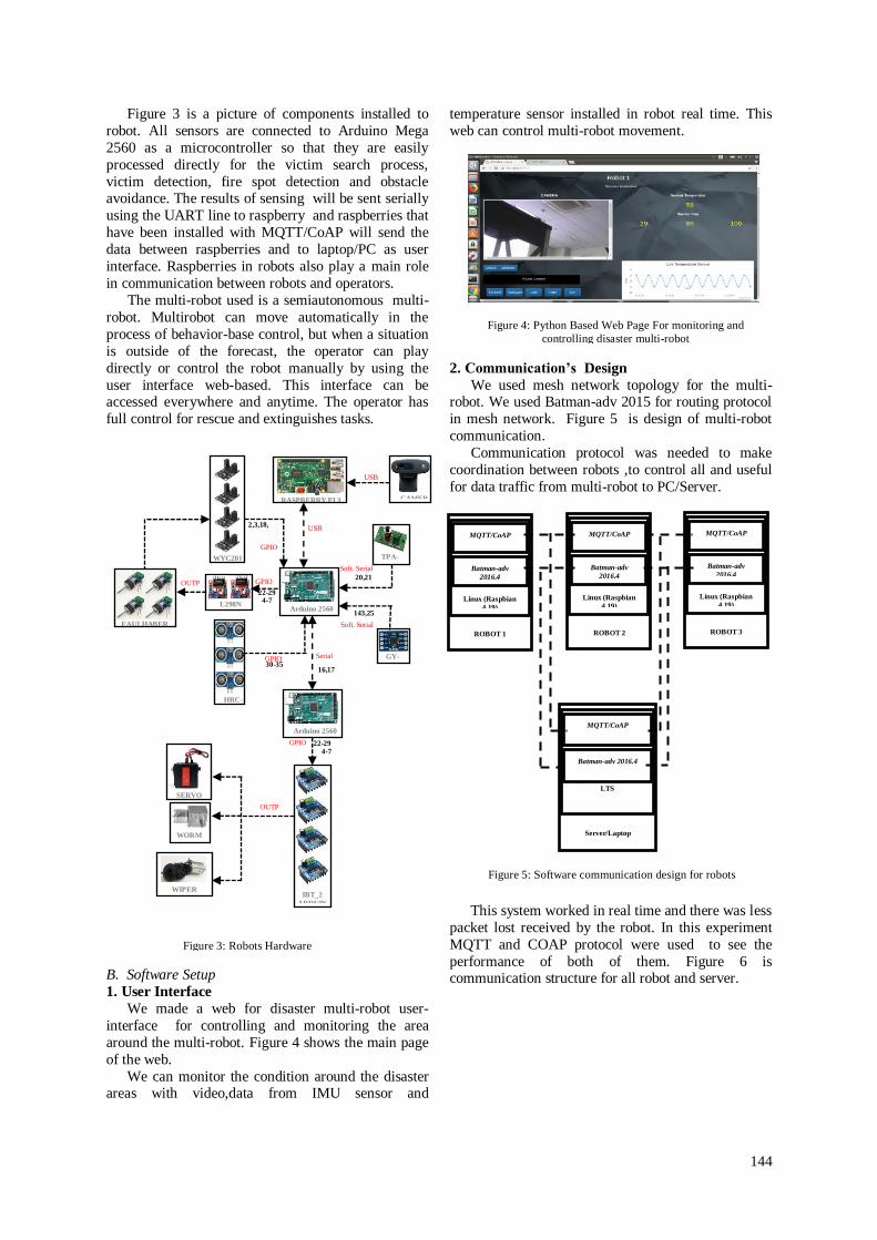
144

Figure 3 is a picture of components installed to

robot. All sensors are connected to Arduino Mega

2560 as a microcontroller so that they are easily

processed directly for the victim search process,

victim detection, fire spot detection and obstacle avoidance. The results of sensing will be sent serially

using the UART line to raspberry and raspberries that

have been installed with MQTT/CoAP will send the

data between raspberries and to laptop/PC as user

interface. Raspberries in robots also play a main role

in communication between robots and operators.

The multi-robot used is a semiautonomous multi-

robot. Multirobot can move automatically in the

process of behavior-base control, but when a situation

is outside of the forecast, the operator can play

directly or control the robot manually by using the

user interface web-based. This interface can be accessed everywhere and anytime. The operator has

full control for rescue and extinguishes tasks.

B. Software Setup

1. User Interface

We made a web for disaster multi-robot user-

interface for controlling and monitoring the area

around the multi-robot. Figure 4 shows the main page

of the web.

We can monitor the condition around the disaster areas with video,data from IMU sensor and

temperature sensor installed in robot real time. This

web can control multi-robot movement.

2. Communication’s Design

We used mesh network topology for the multi-robot. We used Batman-adv 2015 for routing protocol

in mesh network. Figure 5 is design of multi-robot

communication.

Communication protocol was needed to make

coordination between robots ,to control all and useful

for data traffic from multi-robot to PC/Server.

This system worked in real time and there was less

packet lost received by the robot. In this experiment

MQTT and COAP protocol were used to see the

performance of both of them. Figure 6 is communication structure for all robot and server.

Figure 5: Software communication design for robots

Figure 3: Robots Hardware

Figure 4: Python Based Web Page For monitoring and

controlling disaster multi-robot

GPIO

USB

143,25

22-29

TPA-

81

GY-

25

RASPBERRY PI 3

SERVO

MOTOR

CAMER

A

HRC-

04

FAULHABER

MOTOR

WYC201

0

L298N Arduino 2560

WIPER

MOTOR

WORM

GEAR

22-29

USB

GPIO 30-35

OUTP

UT

4-7

2,3,18,

19

GPIO

Soft. Serial

Soft. Serial

20,21

Arduino 2560

Serial

16,17

IBT_2

ARDUIN

O

OUTP

UT

GPIO

4-7

Linux (Raspbian

4.19)

Batman-adv

2016.4

ROBOT 1

MQTT/CoAP

Linux Ubuntu 16.0 4

LTS

Batman-adv 2016.4

Server/Laptop

MQTT/CoAP

Linux (Raspbian

4.19)

Batman-adv

2016.4

ROBOT 2

MQTT/CoAP

Linux (Raspbian

4.19)

Batman-adv

2016.4

ROBOT 3

MQTT/CoAP

145

V. EXPERIMENT RESULT

Personal computer used for this experiment was

Lenovo G40-30 Laptop, which was based on Intel

Celeron N2840 processor unit as the server. Each

robot was equipped with raspberry pi 3 Model B V1.2

as the clients. All devices used wifi module on board

to support wifi mesh network. The server or laptop

would send data to all 3 robots and the performance of

communications protocols could be monitored by

using Wireshark. The experiment environment is

summarized in Table 1.

Parameter Value

Wireless 802.11n

Linux (Robot) Raspbian 4.19

Linux (Server/PC) Ubuntu 16.04 LTS

Batman-Adv 2016.4 version

Wireshark

(Server/PC)

2..9.0 version

Tcpdump

(Raspberry)

4.9.2

Paho-mqtt 1.3.1

CoAPthon 4.0.2

The system needed to be configured to see the

performance of MQTT and Wifi-Mesh. Figure 7-9

shows the design of the system for MQTT Protocol.

In this research, the laptop was used as the broker and

publisher because the user interface was installed in it.

All systems were set with Python-based script. The

arrows show Wifi-Mesh that built for communication.

The server/PC sent 988-byte string data for all robots within 1 hour to see its performance. This

experiment was conducted in stages by sending data

to 1 robot (Figure 7), then to 2 robots(Figure 8), and

finally to 3 robots(Figure 9). It is necessary to

determine the topic to send data with MQTT protocol.

In this research one topic was used because all robots

received the same data. The topic in this case was

“robotmonitoring”. To find out data flow received by

the three robots and all raspberries in robots, tcpdump

software was installed.

For CoAP protocol and mesh-wifi did not require a special configuration same with MQTT

configuration but with change PC/Laptop as server

and robots as clients.

The result of experiment for 1, 2 and 3 robots was

plotted in a graphic for MQTT and CoAP protocol.

Figure 10 shows MQTT and CoAP performance in

this experiment. It can be seen from Figure 10 that for

MQTT protocol, with any numbers of robots, all

robots receive almost same amount of data because

MQTT works on the TCP /IP layer where it cannot

broadcast data in parallel to all clients in same time.

Figure 10: Received data in multi-robot with MQTT and

CoAP protocol

Wate

r

FE

Mesh Network

-WebserverTornado

Framework

-Using websocket to get

data and control all robot

Fire Extinguisher (FE) Water Provider Leader

Cam

Table 1: Experiment environment

Figure 7: MQTT design for 1 robot

Figure 8: MQTT design for 2 robots

PC/Laptop Robot 1 Mesh

Broker/Publisher Subscriber 2 m

Mesh

Robot 1 Robot 2

PC/Laptop Broker/Publisher

Subscriber

Subscriber

2 m

2 m

2 m

PC/Laptop

Mesh

Broker

/Publisher

Subscriber

Subscriber Subscriber

Robot 1

Robot 2 Robot 3

2 m

2 m 2 m

2 m

3.4 m

2 m

Figure 9: MQTT design for 3 robots

Figure 6: Communication Structure among the robots

146

For CoAP, the total received data is greater for

more number of robots. However, the total data that

using the CoAP protocol is fewer than using MQTT.

Comparison on error packet data between MQTT

and CoAP is shown in Figure 11. CoAP has no error data. But it doesn’t mean CoAP better than MQTT in

data accuration. It happen because data transfer rate of

CoAP under MQTT. Error in this case can be caused

by data traffic in MQTT protocol.

Figure 11: Error Packet Data in MQTT and CoAP Protocol

In our experiment, it is easy to use MQTT to send

data to the targeted robots. MQTT uses topics to connect the sender and data receiver. So data

communication lines can be set easily. CoAP needs

combination of GET/PUT method for data

communication. This method must be prepared before

executing in a python script. For integration with web

as GUI (Graphical User Interface), MQTT protocol is

easier than CoAP .

Figure 12: Comparison Data Transfer Rate between MQTT

and CoAP

From Figure 12, data transfer rate for MQTT

protocol is higher than CoAP. Therefore, multi-robot

using MQTT protocol receives more data in 1 hour

than multi-robot using CoAP protocol. This result

shows that the MQTT protocol can be used for real

time communication rather than CoAP. For communication test between robots, we tried

to send data from 1 robot to other while moves with

configuration that shown in Figure 13.

Robot 1 sent 988-bytes of data string to Robot 2

through a laptop as a broker in MQTT configuration

and as a server in CoAP Configuration. Distance

between robots was 1 m and position of laptop was

fixed. 2 robots moved forward together and left

laptop in its position. Figure 14 shows the results of

the experiment.

Figure 14: Comparison of MQTT vs CoAP throughput when 2

robots move

Then, we tried to change distance between robots

with position of a server/broker and 1 robot were

fixed as in Figure 15. And the result is shown in

Figure 16.

Figure 14 and 16 show that the performance of the

MQTT protocol was better in throughput and stable

than CoAP although the multi-robot moved within the

range of distance that we set.

Figure 13: Communication Scheme between 2 robots with MQTT

& CoAP

Server/Lapto

p

Robot 1 Robot 2 5m

Figure 15: Communication Scheme between 2 robots with

different

distance between of them

Figure 16: Comparison of MQTT and CoAP Throughput for

Communication between Robots when 1 robot move

Publisher/Client

Robot 1

Robot 2

Server/Laptop Broker

Subscriber/Client

1m

147

VI. CONCLUSION

This research has compared MQTT and CoAP

communication protocols to remotely control disaster

multi-robot. MQTT Protocol is good for real time communication for Disaster Multi-robot because it

has higher data transfer rate than CoAP in sending

data. Moreover, MQTT is more simple to use for

Disaster Multirobot communication and integrate in

user interface. MQTT has throughput bigger than

CoAP in different distances of Disaster Multi-robot

positions.

REFERENCES [1] “Magnitude 7.0 earthquake hits Lombok.” [Online].

Available:

http://www.thejakartapost.com/multimedia/2018/08/10/magn

itude-7-0-earthquake-hits-lombok.html. [Accessed: 15-Aug-

2018].

[2] H. Kitano, “RoboCup Rescue: A grand challenge for multi-

agent systems,” in Proceedings - 4th International

Conference on MultiAgent Systems, ICMAS 2000, 2000, pp.

5–12.

[3] J. Liu, H. Zhang, B. Fan, G. Wang, and J. Wu, “A Novel

Economical Embedded Multi-mode Intelligent Control

System for Powered Wheelchair,” 2010 Int. Conf. Comput.

Control Ind. Eng., pp. 156–159, 2010.

[4] X. Long, J. Jiang, and K. Xiang, “Towards Multirobot

Communication,” 2004 IEEE Int. Conf. Robot. Biomimetics,

pp. 307–312, 2004.

[5] S. Kahar, R. Sulaiman, A. S. Prabuwono, and N. A. Ahmad,

“A Review of Wireless Technology Usage for Mobile Robot

Controller,” vol. 34, no. Icsem, pp. 7–12, 2012.

[6] T. Sun, X. Xiang, W. Su, H. Wu, and Y. Song, “A

transformable wheel-legged mobile robot: Design, analysis

and experiment,” Rob. Auton. Syst., vol. 98, pp. 30–41, 2017.

[7] A. R. A. Besari, R. Zamri, A. S. Prabuwono, and S.

Kuswadi, “The study on optimal gait for five-legged robot

with reinforcement learning,” Lect. Notes Comput. Sci.

(including Subser. Lect. Notes Artif. Intell. Lect. Notes

Bioinformatics), vol. 5928 LNAI, pp. 1170–1175, 2009.

[8] S. Kuswadi, M. N. Tamara, D. A. Sahanas, G. I. Islami, and

S. Nugroho, “Adaptive morphology-based design of multi-

locomotion flying and crawling robot ‘PENS-FlyCrawl,’”

2016 Int. Conf. Knowl. Creat. Intell. Comput. KCIC 2016,

pp. 80–87, 2017.

[9] B. Doroodgar, Y. Liu, and G. Nejat, “A learning-based semi-

autonomous controller for robotic exploration of unknown

disaster scenes while searching for victims,” IEEE Trans.

Cybern., vol. 44, no. 12, pp. 2719–2732, 2014.

[10] J. S. Jennings, G. Whelan, and W. F. Evans, “Cooperative

search and rescue with a team of mobile robots,” 1997 8th

Int. Conf. Adv. Robot. Proceedings. ICAR’97, pp. 193–200,

1997.

[11] N. Aroon, “Study of using MQTT cloud platform for

remotely control robot and GPS tracking,” 2016 13th Int.

Conf. Electr. Eng. Comput. Telecommun. Inf. Technol. ECTI-

CON 2016, 2016.

[12] D. Thangavel, X. Ma, A. Valera, H. X. Tan, and C. K. Y.

Tan, “Performance evaluation of MQTT and CoAP via a

common middleware,” IEEE ISSNIP 2014 - 2014 IEEE 9th

Int. Conf. Intell. Sensors, Sens. Networks Inf. Process. Conf.

Proc., no. April, pp. 21–24, 2014.

[13] N. Stephen, “Power Profiling: HTTPS Long Polling vs.

MQTT with SSL, on Android,” 2012. .

[14] N. De Caro, W. Colitti, K. Steenhaut, G. Mangino, and G.

Reali, “Comparison of two lightweight protocols for

smartphone-based sensing,” in IEEE SCVT 2013 -

Proceedings of 20th IEEE Symposium on Communications

and Vehicular Technology in the BeNeLux, 2013.

[15] S. Bandyopadhyay and A. Bhattacharyya, “Lightweight

Internet protocols for web enablement of sensors using

constrained gateway devices,” in 2013 International

Conference on Computing, Networking and

Communications, ICNC 2013, 2013, pp. 334–340.

[16] M. H. Amaran, N. A. M. Noh, M. S. Rohmad, and H.

Hashim, “A Comparison of Lightweight Communication

Protocols in Robotic Applications,” Procedia Comput. Sci.,

vol. 76, no. Iris, pp. 400–405, 2015.

[17] H. Yuliandoko, S. Sukaridhoto, U. H. Al Rasyid, and N.

Funabiki, “Performance of Implementation IBR-DTN and

Batman-Adv Routing Protocol in Wireless mesh Networks,”

Emit. Int. J. Eng. Technol., vol. 3, no. 1, 2015.

[18] L. M. Cortés-peña, “Wireless Mesh Network

Implementation,” Comput. Eng., 2007.

[19] Davinder Singh Sandhu and Sukesha Sharma, “Performance

Evaluation of BATMAN, DSR, OLSR Routing Protocols - A

Review,” Int. J. Emerg. Technol. Adv. Eng., vol. 2, no. 1, pp.

184–188, 2012.

Modeling of Power Spectral Density using Correlated Double ...

Documents

Transcript of Modeling of Power Spectral Density using Correlated Double ...