Simulation of a planar micro Ion Mobility Spectrometer for security applications
Upload
khangminh22Category
view
0download
0
HAL Id: tel-01469871https://tel.archives-ouvertes.fr/tel-01469871
Submitted on 16 Feb 2017
HAL is a multi-disciplinary open accessarchive for the deposit and dissemination of sci-entific research documents, whether they are pub-lished or not. The documents may come fromteaching and research institutions in France orabroad, or from public or private research centers.
L’archive ouverte pluridisciplinaire HAL, estdestinée au dépôt et à la diffusion de documentsscientifiques de niveau recherche, publiés ou non,émanant des établissements d’enseignement et derecherche français ou étrangers, des laboratoirespublics ou privés.
Modeling and simulation of multi-fluid systems.Applications to blood flows
Vincent Doyeux
To cite this version:Vincent Doyeux. Modeling and simulation of multi-fluid systems. Applications to blood flows. Physics[physics]. Université de Grenoble, 2014. English. NNT : 2014GRENY017. tel-01469871

THESE
Pour obtenir le grade de
DOCTEUR DE L’UNIVERSITE DE GRENOBLESpecialite : Physique
Arrete ministeriel : du 7 aout 2006
Presentee par
Vincent Doyeux
These dirigee par Mourad Ismail
preparee au sein du laboratoire Interdisciplinaire de Physiqueet de l’ecole doctorale de Physique de Grenoble
Modelisation et simulationde systemes multi-fluides.Application aux ecoulementssanguins.
These soutenue publiquement le 28 Janvier 2014,devant le jury compose de :
M. George BirosProfesseur, University of Texas at Austin, Rapporteur
M. Jeffrey MorrisProfesseur, City University of New York, Rapporteur
M. Emmanuel MaitreProfesseur, Grenoble Institute of Technology, Examinateur
M. Bertrand MauryProfesseur, Universite Paris Sud, Examinateur
M. Mourad IsmailMaıtre de Conferences, Universite Joseph Fourier, Directeur de these
M. Christophe Prud’hommeProfesseur, Universite de Strasbourg, Co-Directeur de these
M. Philippe PeylaProfesseur, Universite Joseph Fourier, Co-Directeur de these

2
Table of Contents
Table of Contents . . . . . . . . . . . . . . . . . . . . . . . . . . . . . . . . . . . 3Aknowlegments . . . . . . . . . . . . . . . . . . . . . . . . . . . . . . . . . . . . 7Notations . . . . . . . . . . . . . . . . . . . . . . . . . . . . . . . . . . . . . . . 11
Introduction 13i Introduction . . . . . . . . . . . . . . . . . . . . . . . . . . . . . . . . . . . 14
Francais . . . . . . . . . . . . . . . . . . . . . . . . . . . . . . . . . 14English . . . . . . . . . . . . . . . . . . . . . . . . . . . . . . . . . . 16
ii Vesicles as a model for red blood cells . . . . . . . . . . . . . . . . . . . . . 18iii State of the art of the simulation of vesicles . . . . . . . . . . . . . . . . . 19
The pure Lagrangian methods . . . . . . . . . . . . . . . . . . . . . 19The Lagrangian / Eulerian methods . . . . . . . . . . . . . . . . . . 21The pure Eulerian methods . . . . . . . . . . . . . . . . . . . . . . 22
iv Contributions and outline of this thesis . . . . . . . . . . . . . . . . . . . . 24First part : the numerical methods . . . . . . . . . . . . . . . . . . 24Second part : the implementation . . . . . . . . . . . . . . . . . . . 26Third part : Flow of object in micro capillary and rheology . . . . . 27
v The finite element library Feel++ . . . . . . . . . . . . . . . . . . . . . 28The library Feel++ . . . . . . . . . . . . . . . . . . . . . . . . . 28How does this work fit in Feel++ ? . . . . . . . . . . . . . . . . . 28
I Numerical Methods 29
1 The level set method 311.1 Principle of the method . . . . . . . . . . . . . . . . . . . . . . . . . . . . 32
1.1.1 The level set method . . . . . . . . . . . . . . . . . . . . . . . . . . 321.1.2 The level set function . . . . . . . . . . . . . . . . . . . . . . . . . . 33
1.2 Advection . . . . . . . . . . . . . . . . . . . . . . . . . . . . . . . . . . . . 361.2.1 Discretization of the advection reaction equation . . . . . . . . . . . 361.2.2 Stabilization methods . . . . . . . . . . . . . . . . . . . . . . . . . . 37
1.3 Reinitialization methods . . . . . . . . . . . . . . . . . . . . . . . . . . . . 401.3.1 The advection by an extended velocity . . . . . . . . . . . . . . . . 411.3.2 The interface local projection . . . . . . . . . . . . . . . . . . . . . 411.3.3 Reinitialization by solving a Hamilton Jacobi problem . . . . . . . . 421.3.4 The fast marching method . . . . . . . . . . . . . . . . . . . . . . . 44
1.4 Solid rotation of a slotted disk . . . . . . . . . . . . . . . . . . . . . . . . . 501.4.1 Presentation of the benchmark . . . . . . . . . . . . . . . . . . . . . 50
3

Table of Contents Table of Contents
1.4.2 Time convergence . . . . . . . . . . . . . . . . . . . . . . . . . . . . 52
1.4.3 Space convergence . . . . . . . . . . . . . . . . . . . . . . . . . . . 53
1.5 Active contours . . . . . . . . . . . . . . . . . . . . . . . . . . . . . . . . . 57
1.5.1 Principle of active contours method . . . . . . . . . . . . . . . . . . 57
1.5.2 Implementation . . . . . . . . . . . . . . . . . . . . . . . . . . . . . 58
1.5.3 Detection tests . . . . . . . . . . . . . . . . . . . . . . . . . . . . . 60
2 Multi-fluid flows simulation 63
2.1 Fluid equations . . . . . . . . . . . . . . . . . . . . . . . . . . . . . . . . . 64
2.1.1 Stokes equations . . . . . . . . . . . . . . . . . . . . . . . . . . . . 64
2.1.2 Navier-Stokes equations . . . . . . . . . . . . . . . . . . . . . . . . 70
2.2 Coupling fluid and level set equations . . . . . . . . . . . . . . . . . . . . . 72
2.2.1 Two-fluid flow . . . . . . . . . . . . . . . . . . . . . . . . . . . . . . 72
2.2.2 Multi-fluid flow . . . . . . . . . . . . . . . . . . . . . . . . . . . . . 73
2.3 Benchmarks and tests . . . . . . . . . . . . . . . . . . . . . . . . . . . . . 76
2.3.1 Rising of a bubble in a viscous fluid . . . . . . . . . . . . . . . . . . 76
2.3.2 Rising of different fluid bubbles . . . . . . . . . . . . . . . . . . . . 85
2.4 Oscillations of a bubble . . . . . . . . . . . . . . . . . . . . . . . . . . . . . 90
2.4.1 Motivation . . . . . . . . . . . . . . . . . . . . . . . . . . . . . . . . 90
2.4.2 Description of the simulation . . . . . . . . . . . . . . . . . . . . . 90
2.4.3 Results . . . . . . . . . . . . . . . . . . . . . . . . . . . . . . . . . . 91
3 Simulation of solid objects in flow 95
3.1 Existing methods . . . . . . . . . . . . . . . . . . . . . . . . . . . . . . . . 96
3.2 FPD and penalty methods . . . . . . . . . . . . . . . . . . . . . . . . . . . 99
3.2.1 A similar formulation for FPD and penalty method . . . . . . . . . 99
3.2.2 Particle motion in FPD/penalty methods . . . . . . . . . . . . . . . 101
3.3 FPD in Level set framework . . . . . . . . . . . . . . . . . . . . . . . . . . 102
4 Simulation of vesicles 105
4.1 Bending force in level set context . . . . . . . . . . . . . . . . . . . . . . . 106
4.1.1 High order derivative by increasing polynomial approximation order 107
4.1.2 High order derivative by smooth projections . . . . . . . . . . . . . 109
4.1.3 Test on the curvature of a circle . . . . . . . . . . . . . . . . . . . . 111
4.2 Inextensibility by elastic force . . . . . . . . . . . . . . . . . . . . . . . . . 113
4.2.1 Principle of the method . . . . . . . . . . . . . . . . . . . . . . . . 113
4.2.2 Record the stretching information . . . . . . . . . . . . . . . . . . . 115
4.2.3 Equations and dimensionless numbers . . . . . . . . . . . . . . . . . 117
4.3 Inextensibility by Lagrange multiplier . . . . . . . . . . . . . . . . . . . . . 119
4.3.1 Introduction of the Lagrange Multiplier . . . . . . . . . . . . . . . . 119
4.3.2 Discretization . . . . . . . . . . . . . . . . . . . . . . . . . . . . . . 120
4.4 Validation . . . . . . . . . . . . . . . . . . . . . . . . . . . . . . . . . . . . 122
4.4.1 Equilibrium shape . . . . . . . . . . . . . . . . . . . . . . . . . . . 122
4.4.2 Dynamics of single vesicle under shear flow . . . . . . . . . . . . . . 124
4

Table of Contents Table of Contents
II Implementation 137
5 Contributions to Feel++ 139
5.1 Projection operator as a C++ class . . . . . . . . . . . . . . . . . . . . . . 140
5.1.1 Motivation . . . . . . . . . . . . . . . . . . . . . . . . . . . . . . . . 140
5.1.2 Usage of the Projector class . . . . . . . . . . . . . . . . . . . . . . 141
5.1.3 Projector class used to compute the derivative of a field . . . . . . . 142
5.2 The Advection class . . . . . . . . . . . . . . . . . . . . . . . . . . . . . . 144
5.2.1 Description of the class . . . . . . . . . . . . . . . . . . . . . . . . . 145
5.2.2 Example on Hamilton-Jacobi equation for reinitialization . . . . . . 146
5.3 LevelSet class . . . . . . . . . . . . . . . . . . . . . . . . . . . . . . . . . 147
5.3.1 The public part . . . . . . . . . . . . . . . . . . . . . . . . . . . . . 147
5.3.2 The markers . . . . . . . . . . . . . . . . . . . . . . . . . . . . . . . 148
5.3.3 The external options . . . . . . . . . . . . . . . . . . . . . . . . . . 150
5.3.4 The protected part . . . . . . . . . . . . . . . . . . . . . . . . . . . 151
5.4 The MultiLevelSet class . . . . . . . . . . . . . . . . . . . . . . . . . . . . 151
5.4.1 From LevelSet to MultiLevelSet . . . . . . . . . . . . . . . . 151
5.4.2 Specific MultiLevelSet methods . . . . . . . . . . . . . . . . . . 152
6 Development for Vesicle application 155
6.1 Lagrange multiplier construction . . . . . . . . . . . . . . . . . . . . . . . . 156
6.1.1 A size problem . . . . . . . . . . . . . . . . . . . . . . . . . . . . . 156
6.1.2 Extract the submesh . . . . . . . . . . . . . . . . . . . . . . . . . . 156
6.1.3 Creating the Lagrange Multiplier contribution . . . . . . . . . . . . 158
6.1.4 The global matrix assembly . . . . . . . . . . . . . . . . . . . . . . 159
6.1.5 Performance test . . . . . . . . . . . . . . . . . . . . . . . . . . . . 159
6.2 A Python interface . . . . . . . . . . . . . . . . . . . . . . . . . . . . . . . 162
6.2.1 Why an interface is needed? . . . . . . . . . . . . . . . . . . . . . . 162
6.2.2 An example: the vesicle in a shear flow application . . . . . . . . . 163
III Rheology and flows of solid disks 167
7 Disks at a bifurcation 169
7.1 The splitting of a suspension at a bifurcation . . . . . . . . . . . . . . . . . 170
7.1.1 The Zweifach-Fung effect . . . . . . . . . . . . . . . . . . . . . . . . 170
7.1.2 The bifurcation without particles . . . . . . . . . . . . . . . . . . . 170
7.1.3 Particle distribution with the simplest model . . . . . . . . . . . . . 171
7.1.4 Effect of the free particle zone . . . . . . . . . . . . . . . . . . . . . 172
7.1.5 Hydrodynamic force . . . . . . . . . . . . . . . . . . . . . . . . . . 173
7.1.6 Finding the separating line of particles . . . . . . . . . . . . . . . . 174
The Zweifach–Fung effect . . . . . . . . . . . . . . . . . . . . . . . . . . . . . . 174
7.2 Suspension of vesicle in a bifurcation . . . . . . . . . . . . . . . . . . . . . 205
7.2.1 Entry and exit of vesicles . . . . . . . . . . . . . . . . . . . . . . . . 205
7.2.2 Quantity of interest: the flux of vesicles . . . . . . . . . . . . . . . . 206
7.2.3 Extension to two different kinds of vesicles . . . . . . . . . . . . . . 208
5

Table of Contents Table of Contents
8 Rheology of solid disks 2138.1 Measurement of the viscosity . . . . . . . . . . . . . . . . . . . . . . . . . . 214
8.1.1 Some methods to compute the effective viscosity . . . . . . . . . . . 2158.1.2 Convergence to the Einstein’s viscosity . . . . . . . . . . . . . . . . 216
8.2 Semi-dilute suspensions . . . . . . . . . . . . . . . . . . . . . . . . . . . . . 2198.2.1 The viscosity of a confined dilute suspension of solid disks . . . . . 2238.2.2 The contribution to the viscosity of the pair interaction . . . . . . . 2278.2.3 Extension to the simulation of a semi dilute suspension . . . . . . . 229
9 Conclusion and perspectives 235
Appendices 245A Stokes variational formulation . . . . . . . . . . . . . . . . . . . . . . . . . 247B Finding the axes of an ellipse . . . . . . . . . . . . . . . . . . . . . . . . . 248C Distance to parametrized curve . . . . . . . . . . . . . . . . . . . . . . . . 249
The method . . . . . . . . . . . . . . . . . . . . . . . . . . . . . . . 249Example of use . . . . . . . . . . . . . . . . . . . . . . . . . . . . . 251
D Simulation of rigid disk by direct method . . . . . . . . . . . . . . . . . . . 254E Bilinear forms of Projector . . . . . . . . . . . . . . . . . . . . . . . . . . . 258F A configuration file . . . . . . . . . . . . . . . . . . . . . . . . . . . . . . . 260G Indexes notations . . . . . . . . . . . . . . . . . . . . . . . . . . . . . . . . 261H Viscosity from energy dissipation . . . . . . . . . . . . . . . . . . . . . . . 263
Bibliography 265
6

Remerciements
Tout au long de la realisation de cette these, j’ai pu compter sur le soutien de nombreusespersonnes tant au niveau professionnel que personnel. Je tiens a les remercier ici.
Je voudrais tout d’abord remercier Mourad Ismaıl pour m’avoir fait confiance et pro-pose un stage en premiere annee de master dans ce labo que je n’ai finalement plus vouluquitte. Merci pour m’avoir propose une these des ce moment la alors que je ne n’avaisjamais imagine cette option, puis, pour m’avoir accompagne jusqu’a la fin de mon doc-torat en cherchant toujours a m’aider a faire les bons choix pour mon avenir professionnel.J’espere que nous pourrons nous revoir dans le futur pour prendre un verre ensemble, pourparler un peu de maths et beaucoup de tout le reste... J’en profite aussi pour remercierAlice, Gabriel, et Leonore que j’ai eu plaisir a croiser pendant ces 4 ans, sans oublier Mayaque je connais depuis le debut grace a ses incursions au labo !
Je remercie aussi Christophe Prud’homme pour m’avoir suivi durant ma these, pouravoir ete disponible tres souvent pour repondre a mes questions et me guider face auxdifficultes que j’ai pu rencontrer. Merci pour son enthousiasme qui a ete un moteur cer-tain pour moi. Merci aussi de m’avoir integre dans l’equipe Feel++ . Grace a lui j’aipu acquerir une experience extremement enrichissante en maths appli, programmation,elements finis et en conception de logiciels, quelques uns des elements de ma these quim’ont le plus passionnes.
Merci aussi a Philippe Peyla pour les discussions scientifiques que nous avons pu avoiret pour lesquelles il a toujours ete disponible. Merci aussi pour ses conseils d’ordre generaldurant le master.
Je remercie egalement les rapporteurs de cette these, Jeffrey Morris et George Biros,ainsi que les examinateurs Emmanuel Maitre et Bertrand Maury qui ont pris le tempsde s’interesser a mon travail et m’ont fait d’interessantes suggestions. Je les remercieegalement d’avoir ete presents, physiquement ou virtuellement le jour de ma soutenance.
Je tiens a remercier toute l’equipe DYFCOM, qui est une equipe dans laquelle j’aieu beaucoup de plaisir a travailler. Etre dans une equipe dynamique dans laquelle secotoient experimentateurs, theoriciens et numericiens venant principalement du mondede la physique mais aussi des mathematiques et de la biologie, donne lieu a de tres bellescollaborations ainsi qu’a des discussions extremement riches. J’espere pouvoir retrouverdes environnements aussi diversifies que cette equipe dans le futur.
7

Table of Contents Table of Contents
Je voudrais egalement remercier particulierement les personnes qui m’ont aidees apreparer l’oral pour obtenir ma bourse de these. En effet, dix jours apres mon retourde stage aux Etats-Unis, il me fallait presenter un projet sous forme d’oral tres court,un exercice difficile pour lequel j’etais un peu perdu au depart. Je suis reconnaissanta l’equipe d’avoir fait bloc et de m’avoir apporte une aide extremement precieuse a cemoment la. Pour cela, je remercie particulierement Salima, Philippe, Gwennou, Thomas,Pierre-Yves, et Mourad.
Merci aussi a Thomas, Gwennou, Chaouqi, Marine et Alexander chercheurs et postdocs du laboratoire avec qui j’ai pu avoir de nombreuses discussions scientifiques interessantestout au long de ma these. J’en profite pour remercier egalement Silvia Bertoluzza et Em-manuel Maitre avec qui j’ai pu egalement discuter de mon sujet a plusieurs reprises et quim’ont donne de precieux conseils.
Une these de simulation s’effectue difficilement sans un bon support technique infor-matique. Je remercie Philippe Beys pour sa patience, sa reactivite et sa gentillesse pourtoutes les (nombreuses) fois ou je suis venu lui demander d’installer des paquets manquantpour faire tourner mes applications.
Une des grandes forces de cette equipe est aussi son nombre important de thesards etpost-docs. Il est tellement important de ne pas se sentir seul dans les moments de galerequ’on connaıt tous durant une these, et pouvoir partager ses doutes et ses difficultes avecdes personnes ayant les memes preoccupations est souvent un grand soulagement. J’aibeaucoup apprecie la bonne ambiance entre les thesards et post-docs du laboratoire toutle temps de ma these. Un grand merci aux doctorants de l’equipe DYFCOM ainsi qu’aceux du LIPHY en general que j’ai pu croiser et qui m’ont beaucoup apporte, pour lesbons moments passes a la cafet, durant les repas, un match de foot, ou autour d’unechartreuse en Chartreuse... Ils sont trop nombreux pour que je les nomme tous ici, je saisqu’ils se reconnaıtront, alors encore une fois, un grand merci a eux tous.
Pour continuer avec les personnes m’ayant aide moralement tous les jours au labo, jeveux absolument remercier les personnes avec qui j’ai partage le bureau 330, ou, le bureaudu fond pendant ces quelques annees. Les pauses cafe / the, les pauses potins avec eux,ou simplement leur bonne humeur ont rendu ma these agreable au jour le jour. Pour toutca, un grand merci a (dans leur ordre d’apparition au bureau) Aparna, Najim, Maeva,Xavier, Vassanti et Marie Cecilia.
Et pour finir avec mes remerciements au laboratoire, je me dois d’avoir une penseespeciale pour les couchers de soleils sur la grande lance de Domene et le grand Colonenneiges. Il sera difficile dans mes futurs environnements professionnels de trouver uncadre aussi beau dans lequel travailler.
Je remercie egalement toute l’equipe Feel++ avec qui j’ai eu plaisir a interagir du-rant ces annees, des petits coups de mains rapides instantanes aux longues recherches debugs, j’ai toujours pu trouver une aide precieuse venant des autres developpeurs. Merciaussi pour les bons moment passes lors de conferences, du CEMRACS, et de nos voyagesa Strasbourg. Un grand merci a Vincent C., Christophe P., Abdoulaye, Cecile, Stephane
8

Table of Contents Table of Contents
V., Gonzalo, Ranine, Vincent H., Alexandre, Jean-Baptiste, Guillaume, Christophe T.,Marcella et Stephane P.
Je remercie mes colocs et amis Benj, Mariya et Mathilde avec qui j’ai pu passer detres bons moments. Merci aussi a mes amis de facs souvent devenus thesards eux aussi.Merci en particulier a Guillaume, Jeanne, Benj et Mariya (encore), autres labos, autresproblematiques, differentes difficultes, mais qu’il est agreable de se plaindre autour d’unebonne biere ! Un grand merci aussi a Emilie, pour son amitie et son ecoute. Apres lesparcs du Texas, les Ecrins, les Calanques, la Corse, j’espere qu’on creera de nouveauxsouvenirs dans ton Colorado ou autour d’un concert de Blues dans mon Texas !
Je remercie egalement mes copains d’avant cette periode, en particulier les cond’laB200qui m’ont toujours encourage, en particulier pour mes moments de procrastination. J’esperequ’on pourra continuer encore longtemps les discussions cinema et les sorties montagne.
Je dois un tres grand merci a Sandrine qui m’a portee (et supporte) durant ces annees.Je suis conscient de la patience qu’il faut certains jours pour vivre avec un geek qui passeautant de temps devant son pc au sacrifice quelques fois des loisirs communs. Merci deme rappeler de sortir la tete du travail et merci pour tous les bons moments qu’on apasses durant nos annees de these, en esperant que ceux qui nous attendent soient encoremeilleurs.
Enfin un enorme merci a toute ma famille qui m’a supporte et pousse tout au long demes etudes et particulierement durant les moments difficiles que nous avons pu connaıtredurant la periode de ma these. Jamais je n’aurais pu arriver jusqu’ici sans ce soutieninconditionnel. Merci encore.
9

Table of Contents Table of Contents
10

Notations
The Level set related quantities
Symbol Description Page
φ : the level set function 33φh : the discrete level set function 36ε : the half interface thickness 33Hε : the smoothed Heaviside function of thickness 2ε 33δε : the smoothed delta function of thickness 2ε 33n : the normal of the level set field 35κ : the curvature of the level set field 35σ,β, f : the coefficients of the advection equation 36
The fluid, vesicles and flow related quantities
Symbol Description Page
Re : the Reynolds number 64u, p : the velocity and pressure of the fluiduh, ph : the discrete versions of the velocity and pressureσ : the stress tensor 64D(u) : the strain tensor 64µ : the viscosity of the fluid 64ρ : the density of the fluid 70µφ : the viscosity of the fluid defined according to the level set function 72ρφ : the density of the fluid defined according to the level set function 72σ : the surface tension 76fφ : the external forces defined according to the level set function 72Eb : vesicle bending energy 106kb : bending modulus 106Fb : bending force 106Eel : the elastic energy of the membrane 114Fel : the elastic force 115λ : Lagrange multiplier insuring the inextensibility of the membrane 120α : reduced area 122Cn : the confinement 91, 133Qi : the flow rate in the branch i 170Ni : the particle flow rate in the branch i 172
11
Table of Contents Table of Contents
yf : the fluid separating line 170yp : the particles separating line 174Φ : the volume fraction of a suspension 217µeff : effective viscosity of a suspension 217(L, l) : size of the box where the effective viscosity is computed 223
Domains and spaces
Symbol Description Page
Ω : the whole domain 33∂Ω : the boundary of ΩΩ1 : the outside domain, in which φ > 0 33Ω2 : the inside domain, in which φ < 0 33Γ : the interface φ = 0 33L2(Ω) : the square-integrable function space 65[L2(Ω)]d : the square-integrable function space of dimension d 65L20(Ω) : the square-integrable function space with null mean pressure 65
H1(Ω) : the Sobolev function space 65[H1(Ω)]d : the Sobolev function space of dimension d 65H1
0 (Ω) : the Sobolev function space with vanishing value at boundary 65C0 : the set of the continuous functionsRk
h : the discrete finite element space depending on mesh size h and spannedby Lagrange polynomials of degree k
36
Mathematical and numerical symbols
Symbol Description Page
Sgn : the sign function[[f ]] : the jump of the function f across the face of an element 40πL2 : the L2 projection 107[µ] : the physical dimensions of the quantity µt(v) : the transposed of the vector vId : the identity matrix 262∇s ·u : the surfacic divergence of u 262δ : the Dirac functionχ : the characteristic function 51h : the mesh sizedt : the time stepd : the space dimension, in this work, d = 2 or 3
12

Introduction
Contentsi Introduction . . . . . . . . . . . . . . . . . . . . . . . . . . . . . 14
Francais . . . . . . . . . . . . . . . . . . . . . . . . . . . . . . . 14
English . . . . . . . . . . . . . . . . . . . . . . . . . . . . . . . 16
ii Vesicles as a model for red blood cells . . . . . . . . . . . . . . 18
iii State of the art of the simulation of vesicles . . . . . . . . . . 19
The pure Lagrangian methods . . . . . . . . . . . . . . . . . . 19
The Lagrangian / Eulerian methods . . . . . . . . . . . . . . . 21
The pure Eulerian methods . . . . . . . . . . . . . . . . . . . . 22
iv Contributions and outline of this thesis . . . . . . . . . . . . . 24
First part : the numerical methods . . . . . . . . . . . . . . . . 24
Second part : the implementation . . . . . . . . . . . . . . . . 26
Third part : Flow of object in micro capillary and rheology . . 27
v The finite element library Feel++ . . . . . . . . . . . . . . . . 28
The library Feel++ . . . . . . . . . . . . . . . . . . . . . . . 28
How does this work fit in Feel++ ? . . . . . . . . . . . . . . . 28
13

i. Introduction Table of Contents
i Introduction
Francais
Le sang est un fluide au comportement complexe. Il est compose de plasma, un fluide danslequel baignent des cellules : globules rouges, globules blancs et plaquettes. Ces differentesentites ayant des proprietes mecaniques riches, conferent au sang des comportements tresvaries. Depuis tres longtemps, les scientifiques essayent de decrire les ecoulements du sang.Au 19eme siecle, Poiseuille etudiait l’ecoulement du sang dans les veines et les capillaires.Il tenta de decrire le sang comme un fluide homogene, ce qui le conduisit a decouvrir, enmeme temps que Hagen, la loi qui porte desormais leurs noms.
Cette loi decrit la vitesse d’un fluide dans une conduite cylindrique lorsqu’on lui ap-plique une difference de pression. De plus, pour un rayon de tube donne, le rapport entrela difference de pression appliquee au tube et la vitesse maximum acquise par le fluidedonne une definition de la viscosite. Meme si cette loi est encore utilisee de nos jours pourdes fluides homogenes, elle n’est pas suffisante pour decrire l’ecoulement du sang dans depetits vaisseaux.
Plus tard, Fahræus et Lindqvist decouvrirent que la viscosite d’un meme echantillon desang etait plus faible lorsqu’il circulait dans des vaisseaux de tres petite taille. Cet effet aete explique par le fait que les globules rouges ont une tendance a migrer vers le centre desvaisseaux, creant une zone proche des parois dans laquelle le flux sanguin peut s’ecoulerfacilement, ce qui reduit la resistance globale de l’ecoulement et fait apparaıtre la viscositeplus faible que dans de grands vaisseaux ou cette zone sans globules est negligeable. Ceteffet tres connu illustre parfaitement le probleme de l’etude de l’ecoulement du sang.
Les proprietes telles que la viscosite ou la vitesse d’ecoulement dans un vaisseau sontgrandement influencees par les proprietes mecaniques individuelles des globules rouges(99% des cellules presente dans le sang), les interactions entre les globules, les interac-tions des globules avec la paroi des vaisseaux sanguins, et meme les interactions entre lesglobules rouges et les autres cellules. De nos jours, une grande partie des etudes realiseespour la comprehension des ecoulements sanguins s’attache a comprendre ces phenomenesau niveau microscopique pour ensuite les appliquer a une description a plus grande echelle.De plus, l’interet grandissant pour les ecoulements de fluides biologiques dans des microcanaux artificiels dans le but de creer des laboratoires sur puce augmente encore le besoinde connaissance des comportements microscopiques de ces fluides. Pour cela, de nom-breuses experiences, theories et simulations sont developpees. C’est dans cette dernierecategorie que s’inscrit cette these. En effet, depuis la fin du 20eme siecle la simulationnumerique a pris une importance croissante dans tous les domaines de la physique etdes mathematiques. L’evolution constante de la puissance des ordinateurs conduit lesphysiciens et mathematiciens a repenser constamment leurs modeles et les faire evolueren consequence. S’il paraissait impossible il y a une dizaine d’annee de resoudre en memetemps les equations regissant un fluide, les coupler avec les equations gouvernant les pro-prietes mecaniques d’un globule rouge, le tout dans une geometrie complexe, l’arrivee desuper calculateurs et la democratisation du calcul parallele rendent aujourd’hui ces simu-lations possibles dans certaines mesures. La recherche de nouvelles methodes numeriquescouplee a des codes de calculs performants est donc un des defis auquel se confrontentles scientifiques aujourd’hui. De plus l’utilisation de ces codes de calcul pour extraire denouvelles lois physique est aussi un axe de recherche prenant une importance grandis-
14

i. Introduction Table of Contents
sante dans les laboratoire et conduit physiciens et mathematiciens a travailler en etroitecollaboration.
C’est dans ce contexte que se place cette these. L’objectif est de developper un cadrede calcul generique pour la modelisation et la simulation d’ecoulements sanguins, et del’utiliser dans un contexte de simulation en interaction avec des experiences. Le butd’avoir un environnement de calcul tres generique est qu’il ne soit pas simplement un outilde simulation, mais aussi un “laboratoire d’experimentation de methodes numeriques”.En effet, l’objectif est de pouvoir tester quelques-unes des methodes de calcul les plusinteressantes et les differents modeles d’ecoulement sanguins. Lors de ce travail, deuxstrategies differentes ont par exemple ete testees pour assurer l’inextensibilite de la mem-brane des objets en suspension. Par soucis de genericite, un effort particulier a ete faitdurant le developpement pour que le meme code de calcul soit utilisable en deux et troisdimensions, sur une machine de bureau ou un cluster de calcul, sur un seul ou plusieursprocesseurs. Ceci est rendu possible par l’utilisation d’une librairie d’elements finis util-isant les avancees des dernieres technologies informatiques (1MPI, meta-programmationet derniere norme du C++).
Durant ce travail, les methodes numeriques developpees ont ete verifiees grace a dessimulations tests dans lesquelles la solution numerique est connue. Elles ont egalementete validees sur des simulations dans lesquelles les resultats physiques etaient connus parexperiences, theories ou d’autres simulations.
Bien que les parties numeriques de ce travail fassent partie du projet Feel++ in-teractions fluide structure, les problemes physiques etudies sont lies aux recherches del’equipe Dynamique des fluides complexes (DYFCOM) du laboratoire interdisciplinairede physique dans lequel ce travail a ete effectue. Le champ de recherche de cette equipeest le comportement des fluides complexes en general et celui des fluides complexes bi-ologiques en particulier. Dans ce contexte, l’equipe etudie entre autre la rheologie etl’ecoulement du sang par l’intermediaire d’experiences, de developpements theoriques etbien entendu de simulations. Les travaux numeriques effectues dans cette these, avaientcomme but, l’application a des problemes etudies au sein de l’equipe DYFCOM.
Ainsi, l’etude de l’influence du confinement sur la frequence des oscillations d’unebulle a ete guidee par les experiences d’O.Vincent [111] sur la cavitation de bulles dansun hydrogel.
Puis, une methode de simulation d’objets rigides a ete applique au probleme de larepartition d’une suspension diluee de particules rigides lors de son passage dans unebifurcation micro-fluidique. En collaboration avec les experimentateurs G.Coupier etT.Podgorski, l’effet de l’accroissement de la concentration de particules dans la brancherecevant le plus grand debit a ete explique par un effet geometrique de la repartition desparticules dans le canal d’entree. De plus, nous avons mis a jour l’existence d’une forcepoussant les particules vers la branche de plus bas debit et entrant en concurrence avecle precedent effet.
Enfin, la rheologie d’une suspension de disques rigides dans un ecoulement de ci-saillement confine a ete etudiee. Nous avons pu confirmer l’influence decroissante del’interaction entre les particule sur la viscosite pour des grands confinements. Cet effetavait deja ete observe en 3D numeriquement et experimentalement et est maintenant con-
1http://fr.wikipedia.org/wiki/Message_Passing_Interface
15

i. Introduction Table of Contents
firme en 2D. Durant ce travail, l’influence de la position des particules d’une suspensiondiluee relativement aux bords du domaine a aussi ete explore.
Tous les problemes etudies en utilisant la methode de simulation d’objets rigides onete adaptes a l’etude de d’objets deformables. Dans un futur proche, ces methodes serontutilisees pour explorer l’influence de la deformabilite sur ces differents phenomenes.
English
Blood is a fluid having a complex behavior. It is composed of plasma, a fluid in which areflowing cells: red blood cells, white blood cells and blood platelets. These different cellshaving rich mechanical properties, confer to blood diverse behaviors. For a long time,scientists have tried to describe blood flows. In the 19th century, Poiseuille studied bloodflow in veins and capillaries. He tried to describe blood as a homogeneous fluid, whichled him to discover, at the same time as Hagen, the law which carries their names.
This law describes the velocity of a fluid in a cylindrical channel when one appliesa pressure different at the extremities. Moreover, for a given channel radius, the ratiobetween the pressure difference and the maximum velocity of the fluid gives a measureof the viscosity. Even if this law is still used nowadays for homogeneous fluids, it is notsufficient to describe the flow of blood in very small vessels.
Later, Fahræus and Lindqvist discovered that the viscosity of a given sample of bloodis smaller when it flows in very small vessels. This effect has been explained by the factthat red blood cells tend to migrate toward the center of the channel, making a cell freelayer around the vessel walls in which the plasma can circulate more easily. This reducesthe global resistance of the flow and makes the viscosity appear smaller than in largechannels in which the free layer zone impact is negligible. This famous effect illustratesthe problem of the study of blood flow.
The properties such as the viscosity or the flowing velocity in a channel are greatlyinfluenced by the individual mechanical properties of red blood cells (99% of the cellspresent in the blood), the interaction between the red blood cells, the interaction betweenthe cells and the vessel walls, and even the interactions between the red blood cells andthe other cells. Nowadays, a large part of the study devoted to the understanding ofblood flow is trying to understand these phenomenons at a microscopic scale to applythem to a macroscopic one. Moreover, the increasing interest for the biological flows inartificial microfluidic devices with the goal to create lab on chip tools increases the needof knowledge of the microscopic behaviors of these fluids.
To this goal, many experiments, theories and simulations have been developed. Thisthesis is consecrated to this last category. Indeed, since the end of the 20th centurythe numerical simulation took an increasing importance in all the fields of physics andmathematics. The constant evolution of computers leads physicists and mathematiciansto re-think their models and make them evolve. Although it seemed impossible ten yearsago to solve at the same time the equations governing a fluid, couple them with the one ofthe mechanical properties of red blood cells and do so in a complex geometry, the rise ofsuper computers and the ready availability of parallel computing make these simulationspossible today in some measure. The research of new numerical methods coupled topowerful codes is thus one of the challenge faced by scientists today. Moreover the useof these codes to extract new physical laws is also a research axis growing in laboratoriesand leads physicists and mathematicians to work in close collaboration.
16

i. Introduction Table of Contents
It is in this context that belongs this thesis. The objective is to develop a genericnumerical framework for the model and simulation of blood flows, and to use it in acontext of simulation in close collaboration with experiments. The goal to have a verygeneric framework environment is that it is not simply a numerical tool to make simulation,but also a laboratory to experiment new numerical methods. Indeed, the objective is tobe able to test some of the most promising techniques and different models for blood flowsimulation. For example, during this work, two different strategies have been tested toinsure the inextensibility of the cells membrane. For general purposes, a particular carehas been taken during the development in order to be able to use the same code in 2D or3D, on a cluster or on a single computer, on a single or several processors. This has beenpossible thanks to the use of a finite element library using some of the latest programmingtools (2MPI, meta-programming, and recent C++ norms).
During this work, the numerical methods have been verified thanks to test simulationsin which the numerical solution is known. They have also been validated on simulationsfor which the physical result was known by experiment, theory or other simulations.
Although the numerical part of this thesis takes place in the context of the Feel++
fluid structure interaction project, the physical problems studied are related to the re-searches of the Dynamics of Complex Fluids (DYFCOM) team of the interdisciplinarylaboratory of Physics in which this work has been made. The research subject of thisteam is the behavior of complex fluids in general and the one of biological related fluidsin particular. In this context, blood rheology and circulation are studied in the team, ex-perimentally, theoretically and of course numerically. The numerical developments madein this work had as goals applications in the fields of interest of the DYFCOM team.
As a matter of fact, the study of the influence of the confinement on the oscillation fre-quency of a bubble has been suggested by the experiments of O.Vincent [111] on cavitationof bubbles in an hydrogel.
Then, a solid disk simulation method has then been applied to the problem of thesplitting of a suspension of particles when flowing in a micro fluidic bifurcation. Incollaboration with the experimenters by G.Coupier and T.Podgorski, the effect of theincreasing concentration of particles in the high flow rate branch has been explained bythe geometrical distribution of particles in the inlet channel. Moreover, a force pushingparticles toward the low flow rate branch balancing the previous effect has been discovered.
Finally, the rheology of a suspension of solid disks in a confined shear flow has beenmade. We were able to confirm the effect of the decreasing influence of the interactionsbetween particles on the viscosity for strong confinements. This effect has already beenseen in 3D numerically and experimentally and is now also confirmed in 2D. During thiswork, the influence of the position of the particles of a dilute suspension relative to thewalls of a confined shear flow has also been explored.
All the problems studied with the solid disk simulation method have been adaptedto soft object simulations and will be used in a near future to explore the influence ofdeformability on these phenomenons.
2http://fr.wikipedia.org/wiki/Message_Passing_Interface
17

ii. Vesicles as a model for red blood cells Table of Contents
ii Vesicles as a model for red blood cells
Red blood cells (RBCs) are cells measuring about 7 µm of diameter and having no nu-cleus. The inside of a RBC is principally composed of hemoglobin and a cytoskeleton.The surrounding membrane is a bi-layer of phospholipids. Many proteins compose themembrane in a minor manner compared to the phospholipids as one can see in figure 1. A
Figure 1: Scheme representing the membrane of a red blood cell.
common simple model of red blood cell (RBC) is a vesicle. A vesicle is a fluid drop sur-rounded by a bi-layer phospholipidic membrane as shown in figure 2. Generally, artificialvesicles are of the order of 10 µm. A vesicle does not include the cytoskeleton which adds
Figure 2: Scheme of a vesicle. The scale is not correct, the phospholipids are about 5 nmwhereas the diameter of an artificial vesicle is about 10 µm
some elastic properties to the RBC. Nevertheless, a big part of the mechanical behaviorof the RBCs can be reproduced by vesicles. Indeed, both vesicles and RBC membranesare resist strongly to stretching and both have the same curvature energy expression. Oneof the first theoretical works trying to model the vesicle goes back to 1982 with Kellerand Skalak [99], and the first simulation arrived more than 10 years after that with [61]followed by the first experimental work one year after that [23]. Since then, many workshave been done to understand the behaviors of these objects. From the numerical point
18

iii. State of the art of the simulation of vesicles Table of Contents
of view, the system of a single vesicle in a shear or Poiseuille flow has been studied widelyand scientists start to get interested in many vesicle interacting systems or flowing incomplex geometries. Many efforts are done in this sense, and many works are done tomodify existing techniques. We give a short overview of the existing methods to simulatevesicles and their advantages or drawbacks.
iii State of the art of the simulation of vesicles
The simulation of a vesicle is a difficult task. It is part of the large field of the fluidstructure interactions. Indeed, one has to deal at the same time with the fluid equationsand the membrane of the vesicle having its own properties. Two fluids are involved inthis kind of simulation. The fluids inside and outside the vesicle which are in the generalcase different. Thus, the fluid solver has to be able to deal with a viscosity ratio. Theequations involved are the incompressible Navier-Stokes equations in the general case,which are nonlinear. Most of the time, in microcapillaries, one can consider the limit ofthe vanishing Reynolds number and solve the Stokes equations which are linear and thuseasier to handle.The model for the vesicle has three main properties. The first one is that the membraneresists stretching. It is modeled as inextensible, its local surface is conserved. The totalvolume of the vesicle is also conserved. The membrane can let solvent particles passthrough it, but the osmotic pressure balance insures that in a small time scale, the sameamount of particle is going in and out. Thus in a continuous description, the total volumeof fluid inside the vesicle is conserved. The last property needed to be incorporated inthe models is the fact that it costs some energy to bend the membrane. This energy hasbeen derived by Canham and Helfrich respectively in [16, 43] and it is proportional to thesquare of the curvature of the membrane. Many different methods have been developed todeal with the membrane and the fluids. One can put them in three categories of methods.In the pure Lagrangian methods, only the membrane is discretized and one follows eachdiscretization point individually. In Lagrangian / Eulerian methods, the membrane isdiscretized in a Lagrangian manner but the fluid has an Eulerian treatment. And finally,in the pure Eulerian methods both the membrane and the fluid are seen from an Eulerianpoint of view. Let us give a brief overview of some of these methods.
The pure Lagrangian methods
Principle of the boundary integral method
Under the pure Lagrangian methods, we can name all the variants of the boundary integralmethods. They have been introduced for the vesicle problem by Pozrikidis in 2001 [85].The principle is to use the Green tensor G of the Stokes equation and couple it to aforce giving to the membrane all its properties. The Helfrich energy is derived to givethe curvature force. A tension force is added with a huge energy value which makes themembrane unstreatchable, in other implementations, a Lagrange multiplier enforces thelocal area conservation exactly. A typical expression for the membrane force in 2D isgiven by:
f = kB
(d2κ
ds2+κ3
2
)
n− ξκn+dξ
dst
19

iii. State of the art of the simulation of vesicles Table of Contents
with κ the curvature of the membrane, n and t the normal and tangent unit vector tothe membrane, s the arc-length coordinate and kB the membrane bending rigidity. ξ isa tension accounting for the inextensibility. The velocity for a given point of the domaincan be computed as an integral over the membrane boundary. Thus for each point x0 onwhich one wants to compute the velocity u(x0), it is given by:
u(x0) = u0(x0) +1
µ
∫
membrane
G(x− x0)fds
where u0 is the imposed velocity flow without vesicle. Here, G(x − x0)f is the productmatrix-vector resulting in a vector. A more general formulation exists providing the abil-ity to deal with a different viscosity inside and outside of the vesicle.
To have the evolution of a vesicle in a flow, one has to compute the velocity of eachpoint of the membrane which depends on an integral of all the other points of the mem-brane. Then, the membrane position is updated by integration of the velocity. One ofthe advantages of this method is that for a 2D problem, the problem is reduced to onlya 1D problem (since only the membrane has to be discretized) and only integrals have tobe calculated. However, the fact that the velocity of each point of the membrane dependson all the other points makes the complexity of algorithms vary as N2 where N is thenumber of discretization points. However, this complexity can be decreased to N log(N)thanks to a fast multi-pole method [96].
The tensor G can be given for an infinite Stokes fluid, or simple geometry cases like asemi-infinite fluid (with one wall). This does not make impossible to add other walls, butone has to integrate over all the walls by addition to the integration over the membranewhich can be costly in the case of a geometry with many walls. The method is well suitedfor simulations where the positions and shapes of the particles are important since theyare computed at every time step. They are also good to do rheology since the viscosity ofa suspension can be computed with only the knowledge of the velocity on the walls of thedomain. However, in a simulation where one would like to see for example the velocityfield in all the domain in a complex geometry, one would have to compute an integral foreach point of the domain, running on all points of the complex geometry boundary and allpoints of the membrane. This is one of the limitation of this method. It is however veryaccurate and efficient for simulation in simple flows and is probably the method whichgave the most numerical results on vesicles until now. Let us present briefly some of theimplementations and results obtained with this method.
The use of the boundary integral method in the literature
In 2009, Veerapaneni et al. [108] have used the boundary integral method where theFourier transform of the arc-length is used to compute derivatives of the shape (normaland curvature). They performed a 2D simulation of 256 highly deformable vesicles in anunbounded Poiseuille flow. The method has been extended to the 3D case in [109] and[117, 116]. The boundary integral method has been one of the most used methods andled to many progress in the understanding of vesicle behaviors. In [54] the authors used a2D boundary integral method to explore the lateral migration of a vesicle in a Poiseuilleflow. In [57] the authors explored the different shapes of a vesicle in Poiseuille flow and
20
iii. State of the art of the simulation of vesicles Table of Contents
the influence of the relevant parameters. They were able to construct a phase diagram outof these simulations. The differences between 2D and 3D calculations in Poiseuille flowhave been explored in [55]. The rheology of a single vesicle in a shear flow has also beenexplored in [37] where some comparisons with the phase field method have been made.The rheology of a dilute suspension of vesicles in a curved flow have been studied in [38].
Some other works have been using the Lagrangian point of view for both the fluidand the membrane. For example, in [79], the authors use a particle collision dynamics toexplore the shapes of vesicles in capillary flows. In this method, the fluid is seen as manyparticles interacting by collision and the membrane is meshed independently.
The Lagrangian / Eulerian methods
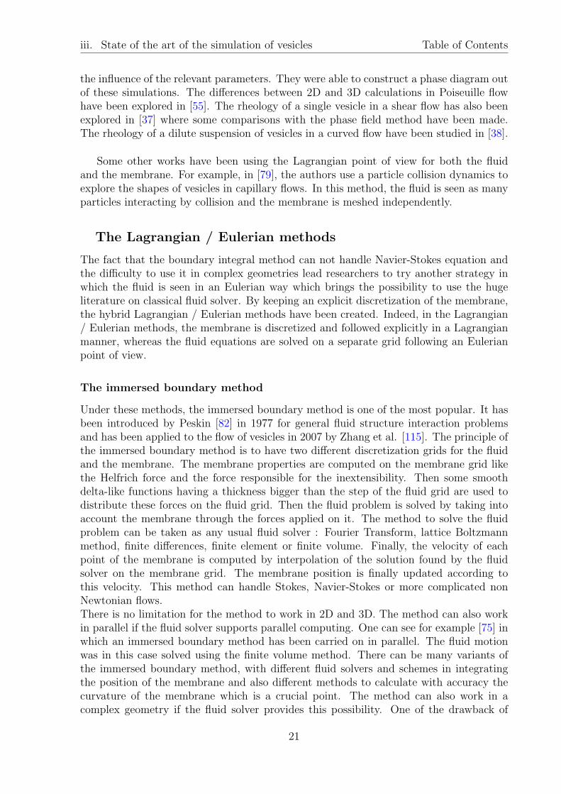
The fact that the boundary integral method can not handle Navier-Stokes equation andthe difficulty to use it in complex geometries lead researchers to try another strategy inwhich the fluid is seen in an Eulerian way which brings the possibility to use the hugeliterature on classical fluid solver. By keeping an explicit discretization of the membrane,the hybrid Lagrangian / Eulerian methods have been created. Indeed, in the Lagrangian/ Eulerian methods, the membrane is discretized and followed explicitly in a Lagrangianmanner, whereas the fluid equations are solved on a separate grid following an Eulerianpoint of view.
The immersed boundary method
Under these methods, the immersed boundary method is one of the most popular. It hasbeen introduced by Peskin [82] in 1977 for general fluid structure interaction problemsand has been applied to the flow of vesicles in 2007 by Zhang et al. [115]. The principle ofthe immersed boundary method is to have two different discretization grids for the fluidand the membrane. The membrane properties are computed on the membrane grid likethe Helfrich force and the force responsible for the inextensibility. Then some smoothdelta-like functions having a thickness bigger than the step of the fluid grid are used todistribute these forces on the fluid grid. Then the fluid problem is solved by taking intoaccount the membrane through the forces applied on it. The method to solve the fluidproblem can be taken as any usual fluid solver : Fourier Transform, lattice Boltzmannmethod, finite differences, finite element or finite volume. Finally, the velocity of eachpoint of the membrane is computed by interpolation of the solution found by the fluidsolver on the membrane grid. The membrane position is finally updated according tothis velocity. This method can handle Stokes, Navier-Stokes or more complicated nonNewtonian flows.There is no limitation for the method to work in 2D and 3D. The method can also workin parallel if the fluid solver supports parallel computing. One can see for example [75] inwhich an immersed boundary method has been carried on in parallel. The fluid motionwas in this case solved using the finite volume method. There can be many variants ofthe immersed boundary method, with different fluid solvers and schemes in integratingthe position of the membrane and also different methods to calculate with accuracy thecurvature of the membrane which is a crucial point. The method can also work in acomplex geometry if the fluid solver provides this possibility. One of the drawback of
21

iii. State of the art of the simulation of vesicles Table of Contents
the immersed boundary method is that the interpolation step of the velocity on theinterface grid leads to numerical error. This can cause a loss of mass of the vesicle.Special care has also to be taken when some particles are entering or leaving the domain.Indeed, since there is a Lagrangian knowledge of the interface, they have to be destroyedor reconstructed explicitly at the boundaries. The last drawback of this method is thedifficulty of the method to handle a different viscosity inside and outside a vesicle. Insuch case, one has to explicitly locate the points of the fluid mesh being inside or outsidethe vesicle. This method gives a lot of results and many different implementations of ithave been made.In the first implementation [115] the authors used a lattice Boltzmann method as fluidsolver and shown 2D simulations of a vesicle in Poiseuille and shear flows. Kim [60] usedan immersed boundary method in which the fluid was solved using Fourier transformswhich limits the simulation to periodic boundaries. They validated their results on theequilibrium shapes of vesicles and on the simulation of vesicles in a shear flow. They alsoperformed simulation with 56 vesicles. In [35], the authors used a finite element solverand shown the ability of their code to work properly in 3D. In [53] the authors used alattice Boltzmann method to solve the fluid equations in 2D and validated their code onthe equilibrium shapes on vesicles. They have also shown the dependency of the tanktreading angle on the confinement of the vesicle.
The other methods
There exist also some other methods, which can be classified as Lagrangian / Eulerianmethods. In [11], a deformation field for the membrane is introduced and advected intime. The problem of finding the coupled velocity, pressure and deformation field whiletaking into account the particle is solved in an Eulerian manner. But at each time step,the interface is localized and the mesh is adapted so that mesh points are always presentat the exact location of it. In this sense, one can say that there is a Lagrangian handling ofthe interface. In other works [107, 47], the coupling between the fluid and the membraneis not done by the forces exerted on the fluid, but by a force acting on the membranediscretization points. That is to say, at the step of updating the membrane points, aforce is added to mimic the membrane properties. This is different from the immersedboundary method in which the force is also computed on the membrane points but istransmitted to the fluid thanks to the delta-like functions. In such implementation, themembrane points have generally some thickness and are seen as rigid particles embeddedin the fluid. The membrane is thus seen as a particle necklace.
The pure Eulerian methods
To avoid the interpolation problem of the velocity at membrane points introduced by theimmersed boundary method, to have the possibility to handle easily a viscosity ratio andto handle also more easily the vesicles at the boundary of the domain, researchers haveintroduced some pure Eulerian methods in which both the fluid and the membrane arelying on the same grid.
22

iii. State of the art of the simulation of vesicles Table of Contents
Phase field and level set methods
The two pure Eulerian methods which have been adapted to the simulation of vesicles arethe phase field method and the level set methods. They both present many similarities.The principle is to define a field on the mesh which accounts for the position of theinterfaces. From this field, delta-like and Heaviside-like functions are defined which makepossible to differentiate the inner and outer fluid, distribute interfacial forces, and definedifferent viscosities for each fluid. The normal and curvature of the interfaces are alsocomputed from this position field.The fluid equations are solved on the same mesh and the membrane is taken into accountthanks to the forces added on it. The difference between the phase field method and thelevel set method resides on the choice of the function representing the position of theinterfaces. In the phase field method, the function representing the two fluids is equal to1 in one fluid, −1 in the other one and varies smoothly from one to the other. Whereasfor the level set method, the representation of the interface is made by a signed distancefunction to the interface. The level set function carries more information than the phasefield one, but it needs to be reset to a distance function often because the advection doesnot preserve the distance function property of the field. The methods can work in 2Dand 3D and can be carried in principle on multiple processors. The fluid solver can beStokes, Navier-Stokes or more complicated non-Newtonian solver. Complex geometriescan be also handled since the fluid solver is able to deal with it. However, one of thedrawbacks of pure Eulerian methods is that, since the membrane is not independentlymeshed, the number of discretization points around it might be low. Indeed, if the meshsize is the same everywhere in the domain, one has to use very small mesh size to have alot of discretization points around the membrane which might be costly. An alternativeis to use a mesh adaptation algorithm but the need to project a solution from a mesh toanother one arises. Usually, to obtain a projection with a good accuracy, a multi stepprediction - projection is needed [12, 62]. Another drawback which is in general attributedto the level set methods is that the advection and procedure to reset the level set to asigned distance field leads to some mass loss. This can be reduced by improving thediscretization or using conservative schemes but it might still be an issue for long timesimulations.
Eulerian methods for the simulation of vesicles
A phase field method to do simulation of vesicles has been introduced by Biben andMisbah in [7] for 2D simulations. It has been then extended to three dimensions in [8].In these works, a tension field is searched to penalize the extensibility of the membrane.The problems were solved using finite difference methods. Later, in [20, 21], Cottet etal. used a level set field to simulate an inextensible object in flow. They showed that thestretching of the interface was recorded in the level set field and derived a force out of it toinsure the inextensibility of the membrane. This force has been used in the PhD thesis ofMilcent [76] combined with a force accounting for the curvature to simulate vesicles. Thesimulations have been made both in 2D and 3D. A comparison between level set and phasefield methods for the simulation of vesicles has then been made in [70] showing all thesimilarities between them. Another level set strategy has been developed by Laadhari [62]during his PhD where the inextensibility of the membrane where insured by a Lagrangemultiplier. The simulations were made in 2D with a finite element method for which a
23
iv. Contributions and outline of this thesis Table of Contents
mesh adaptation have been developed to follow more precisely the interface. A level setmethod in which both the level set and its gradient are advected has been presented in[92]. Moreover the authors presented a 4 step projection solving Navier Stokes equationwhile searching for a surface tension term imposing the inextensibility of the membrane.
iv Contributions and outline of this thesis
The goal of this thesis was to develop a generic framework for the simulation of vesiclesin flow with a maximum of generality to be able to test different models in the futureand compare them. A special care was also taken to make the framework efficient andeasy to handle in order to be applied to real physical problems. Several verifications andvalidations have been made. The second goal of the thesis was to prepare some physicalstudies on a simpler model of rigid circular particle with the goal to be applied in thefuture to vesicles and red blood cells.
First part : the numerical methods
The first part of this thesis is dedicated to the description and the tests of the numericalmethods we used.
First chapter
The numerical framework for the simulation of vesicles had to be able to capture vesicleswith non-unit viscosity ratio, to be easily coupled with Stokes, Navier Stokes or otherfluid solver, and to be easy to run in complex geometries. Following the previous stateof the art on the numerical methods available for vesicles, we choose a level set methodwhich includes all these ingredients. We also choose a finite element method because ofthe great number of theoretical results available in the literature compared to the finitedifference or finite volume methods. Moreover, the finite element method allows us to usecomplex geometries. The promising work of A. Laadhari [62] on the simulation of a vesi-cle with level set method solved by finite element has also been an ingredient for our choice.
Consequently, the first chapter of this thesis is dedicated to the level set method. Wepresent the strategy we used to create the level set framework, particularly the stabi-lization methods that we used for the advection of the level set field. We also presentthe different strategies of reinitialization of the level set field to a distance function, theirlimitations and advantages. We then show our results on a verification test which is afamous numerical benchmark: the solid rotation of a slotted disk. Finally we show asimple application of the level set which does not need any fluid solver: the detection ofboundaries in an image.
Second chapter
For the sake of generality, we choose to decouple the fluid solver and the level set advec-tion solver. That is to say, instead of solving the fluid equations and the advection of thelevel set field in the same problem (i.e in the same matrix for the algebraic point of view),
24
iv. Contributions and outline of this thesis Table of Contents
we choose to solve them one after the other. On the coding part, both fluid and level setframework are independent and separate C++ classes that we can plug into each otherat will. The goal of having this separation is to be able to couple any fluid solver which isimplemented in our library to the level set framework. For example during this thesis, twodifferent fluid solvers have been used, a simple Stokes solver and a Navier-Stokes solver.Thus, in the second chapter, we introduce the fluid equation and their discretization withthe finite element method. Then we show how the coupling between the fluid frameworkand the level set framework is done to create a two fluid flow system. We extend thiscoupling to a multi-level set framework to show that it is also possible to have an N-fluidflow system with N greater than two. After that, we present a verification on a precisenumerical benchmark for two fluid flow: the rising of a viscous drop in a fluid. Finally,we show a validation on a physical problem which is also a problem suggested by exper-imental physicists in our group: the oscillation frequency of a bubble in a fluid viscousfluid. Indeed, we have shown that the oscillation frequency of a bubble in a fluid is notinfluenced by its confinement.
Third chapter
Although the goal of this thesis was the simulation of vesicles, we wanted to show that it isalso possible to deal with simpler objects with the same framework. Indeed, in a physicalapplications context, most of the time, to understand the precise role of the deformabilityof the vesicles, one would have to understand first the phenomenon with rigid spheresor disks. Thus, being able to simulate efficiently these kind of objects is a nice featureoffered by our framework.This is why the third chapter is dedicated to the simulation of solid objects in flow. Wefirst make a brief review of the existing methods dedicated to this kind of simulations.Then we show that two of them are closely linked: the fluid particle dynamics and thepenalty method. Finally we show that the two fluid flow framework presented in chap-ter two can be easily used for the simulation of solid objects. We also show that, fromthe fluid solver point of view, the method is equivalent to a fluid particle dynamics or apenalty method which brings all the theoretical development made for these methods toour framework. The only difference with these methods is that with level set method, theparticles are followed in an Eulerian point of view. We then discuss the advantages anddrawbacks compared to the classical Lagrangian point of view used in this context.
Fourth chapter
The fourth chapter is dedicated to our simulation method for vesicles. We start by de-scribing the curvature force and show that it needs the knowledge of the curvature andits derivatives with a good accuracy. Thus, we present two strategies to obtain this in-formation in finite element / level set context which are: increasing the polynomial orderof approximation of the finite element bases, or smoothing the derivative fields. We thenpresent in detail two different strategies to insure the inextensibility of the membranewhich have been found in the literature and adapted to our framework. We finally makevalidation simulations on known results of vesicles which are the equilibrium shapes in
25
iv. Contributions and outline of this thesis Table of Contents
a fluid at rest, the tank treading motion, and the tumbling motion. Finally we compareboth methods.
Second part : the implementation
The implementation of the numerical methods presented in the first part was an importantpiece of this work. The second part of this thesis is dedicated to the implementation ofsome particular ingredients needed to achieve the simulation of vesicles under flow.
Fifth chapter
The numerical framework that we developed has been based on the finite element libraryFeel++ . A special care has been taken to make all the different ingredients needed forthe simulation of vesicles as general as possible both on the methodology and implemen-tation level. By generality on the methodology level, we mean that we tried as much aspossible to keep every development valid both in 2D and 3D, at order one and higher,and valid on a single or several CPU’s. The library Feel++ being developed in thisspirit, most of the time, the proper use of the standard features of the library leads tosuch genericity. However on few occasions, some specific development had to be made tokeep the code valid. By generality at the implementation level, we mean that we tried tomake the codes as re-usable as possible. In this spirit, most of the tools developed for thisapplication are meant to become some part of the Feel++ library. Thus, a special designneeded to be done properly to ease the usability and future maintainability of the codes.To this goal, the object oriented paradigm included in C++ has been a powerful tool. Forexample the solution of the advection equation framework, the level set framework, thefluid framework are all C++ classes. Moreover some special tools helped to build reallyindependent frameworks, like the 3boost::program options which allows each level setor fluid solver object to have its own external options when such object is created.The fifth chapter is dedicated to the implementation tools needed for the simulation ofvesicles in flow and which have been designed to be included in Feel++ . We firstdescribe the projection operator, which is a small useful tool to ease the use of severalprojection methods. Then we explain how the level set class works, what are the essentialfeatures and how to use them in a two fluid flow context. Finally, we explain how wecreated the multi-level set class which derives from the level set class making it easy topool the resources of the many level set fields for a maximum efficiency.
Sixth chapter
In the sixth chapter, a description is made of some development done for the simulationof vesicles which can not be transposed directly to other works. In this chapter we firstdescribe the problem of constructing efficiently the Lagrange multiplier in the methodwhere the inextensibility of vesicles is insured by it. We also describe how we interfacedthe vesicle application. Indeed, because of the high generality spirit of the development,many parameters have been allowed to be set by the user as external options. Thus, at
3http://www.boost.org/doc/libs/1_54_0/doc/html/program_options.html
26

iv. Contributions and outline of this thesis Table of Contents
the user point of view, it might be useful to have a small interface to deal at least withthe inter dependent options.
Third part : Flow of object in micro capillary and rheology
The last part of this thesis is dedicated to the physical applications of the flow of objectsin microcapillaries and their rheology. In order to understand the precise role of thedeformability of the particles in such systems, it is important to start with the simplercase of rigid bodies. This is why, in this part, most of the applications are made on rigiddisks.
Seventh chapter
One of the building blocks of any microfluidic or biological micro-circulation is the splittingof a channel into two daughter channels having different flow rates. Understanding thebehavior of a suspension of particles in such a configuration is a big step forward in theunderstanding of the micro-circulation in general. The seventh chapter adresses studyof the suspension in splitting channels. We started by the most simple case: a dilutesuspension of rigid disks in a bifurcation. In collaboration with experimental physicists, wewere able to explain the effect of the increasing concentration of the higher flow rate branchalready known for several years as the Zweifach-Fung effect and often miss interpreted.We then show the possibility to extend this work to deformable particles and the way tomeasure properly the interesting quantities.
Eighth chapter
In the future, one issue we want to study is the rheology of a confined suspension of vesicles.To this goal, once again, it is necessary to understand the basic behaviors of rigid disksin order to be able to extract the role of the deformability of the particles. Moreoverrheology study requires measurement of the viscosity of a suspension with a controlledaccuracy. Finally, even if it has been studied for a long time, the basic behaviors of asuspension of rigid disks in a confined environment still have many open questions and itsstudy is interesting to many groups in the world. For these reasons, the eighth chapteris dedicated to the study of the rheology of solid disks. We first show three methods tomeasure the effective viscosity of a suspension. We show that two of them always convergeto the theoretical effective viscosity and explain the condition for the last one to converge.The errors made on the viscosity are also quantified as a function of the mesh size.In the second part of the chapter, we study the contribution of a single particle to theeffective viscosity and the contribution of a pair of particles. We finally use the studyof these contributions to recover the effective viscosity of a suspension of semi diluteparticles in a confined shear flow. We show that with this method, we are able to simulatethe effective viscosity of a great number of different configurations for every suspensionconcentration studied in a relatively small time. Finally, we show that the phenomenonof the decrease of the second order viscosity of a suspension with the confinement whichwas a known effect of a 3D suspension still holds in 2D.
27
v. The finite element library Feel++ Table of Contents
v The finite element library Feel++
The library Feel++
This work has been done using the library Feel++ which stands for Finite ElementEmbedded Library in C++ [86, 87]. This is a C++ library solving partial differentialequation (PDE) by finite element method. The goal of Feel++ is to provide a languageclose to the mathematical one to solve complex PDEs. The idea is to provide to scientistsa framework in which they can express in a language close to the mathematics the strategythey propose for solving complex systems of PDE and generate a high performance code.Feel++ can be classified as a domain specific embedded language (DSEL), that is tosay, it is a C++ code but provides a language which makes the interface between themathematics written by the user of the library and the lower level high performancescomputer science domain. To this goal, Feel++ uses the last standards of C++ andmeta-programming (through the template and boost meta-programming library) to havea maximum of generality. Indeed, the code written using the standard formulation ofFeel++ is valid in 1D, 2D and 3D and works with an arbitrary polynomial order sincethe mathematical formulation allows it. Moreover, the code can run on a single or severalprocessors [17]. It also uses external libraries as for example the mesh generator Gmsh
[36], or the library Petsc [3] which provides a large class of method to solve numericalproblems.
How does this work fit in Feel++ ?
Within Feel++ , this work is a part of the fluid structure interaction (FSI) project.The goal of this project is to develop strategies toward the simulation of complex bloodcirculation system. Blood flow is a complex subject and to simulate whole its complexity,one would have to deal with a complex geometry, the interaction between the elastic vesselwalls and the blood plasma, and include the red blood cells and possibly other objectsdealing with the plasma. During his PhD, Vincent Chabannes developed an arbitraryLagrangian Eulerian (ALE) method [18] able to deal with the coupling between an elasticwall and a Newtonian fluid. Moreover, flows in complex geometries such as part of thecerebrovenous system, the aorta or an artery with an aneurysm have been investigatedwith Stokes flow in [15, 17]. This work is dedicated to the simulation of the blood vessels.It could be in the future coupled with the Eulerian part of the ALE method created todeal with the vessel walls to simulate realistic blood flows.
The tools created for the simulation of vesicles can be used to other purposes. Forexample, we have shown that our two fluid flow system can handle drop suspensions.Future development can be made using the large existing literature on level set methods[98] to create many different applications based on this framework.
28

Part I
Numerical Methods
29


Chapter 1
The level set method
Contents1.1 Principle of the method . . . . . . . . . . . . . . . . . . . . . . 32
1.1.1 The level set method . . . . . . . . . . . . . . . . . . . . . . . . 32
1.1.2 The level set function . . . . . . . . . . . . . . . . . . . . . . . 33
1.2 Advection . . . . . . . . . . . . . . . . . . . . . . . . . . . . . . . 36
1.2.1 Discretization of the advection reaction equation . . . . . . . . 36
1.2.2 Stabilization methods . . . . . . . . . . . . . . . . . . . . . . . 37
1.3 Reinitialization methods . . . . . . . . . . . . . . . . . . . . . . 40
1.3.1 The advection by an extended velocity . . . . . . . . . . . . . . 41
1.3.2 The interface local projection . . . . . . . . . . . . . . . . . . . 41
1.3.3 Reinitialization by solving a Hamilton Jacobi problem . . . . . 42
1.3.4 The fast marching method . . . . . . . . . . . . . . . . . . . . . 44
1.4 Solid rotation of a slotted disk . . . . . . . . . . . . . . . . . . 50
1.4.1 Presentation of the benchmark . . . . . . . . . . . . . . . . . . 50
1.4.2 Time convergence . . . . . . . . . . . . . . . . . . . . . . . . . 52
1.4.3 Space convergence . . . . . . . . . . . . . . . . . . . . . . . . . 53
1.5 Active contours . . . . . . . . . . . . . . . . . . . . . . . . . . . . 57
1.5.1 Principle of active contours method . . . . . . . . . . . . . . . 57
1.5.2 Implementation . . . . . . . . . . . . . . . . . . . . . . . . . . . 58
1.5.3 Detection tests . . . . . . . . . . . . . . . . . . . . . . . . . . . 60
31

1.1. Principle of the method Chapter 1. The level set method
In this chapter we will present the level set numerical methods we have used and someverification results. We will firstly remind some basic principles of level set methods. Thenwe will detail the formulations of the stabilization methods that we developed to stabilizethe transport of the level set function. We will also detail the reinitialization methodsavailable, especially the reinitialization by solving a Hamilton Jacobi equation and thefast marching method. We will discuss our strategy to make the fast marching methodvalid for high order polynomial approximations. The results of the famous benchmark ofthe rotation of a slotted disk will be presented. Both time and space convergence willbe addressed. Finally, an application of the level set method which does not require acoupling with fluid equations will be presented to show the genericity of the method. Thisapplication is the contour detection of an image.
1.1 Principle of the method
1.1.1 The level set method
Many domains in scientific computing require knowledge of the position of an interfacebetween two regions. The method called level set proposes a solution to this problem.It has been introduced by Sethian during his PhD on propagating flames in 1982 [97]. Hehas then kept developing the method and pushed its application fields. His book [98] andOsher’s [101] are two major references for the introduction to the method and overviewits possible applications. The principle of the method is the following: it defines a scalarfunction on all the computing space so that the 0 value of this function defines the inter-face between the two domains. This function is then transported respecting the equationsof the system. At each moment, the value where this function is 0 represents the interface.This method, for which the interface is known implicitly, thanks to a function, is classifiedas an Eulerian method. This classification is made by opposition to Lagrangian methodsin which the points on the interface are known explicitly. In the level set method, findingthe interface is equivalent to find the 0 value of a function. This function is often taken asa signed distance function to the interface. Then, the function can be seen as the altitudeon a map for which the interface would be the sea level. One can easily see where thename level set comes from.
One of the advantages using an implicit function to follow the interface is that themethod can handle naturally topological changes. Indeed, if the velocity imposed to thelevel set field induces a sign change in a region, this leads naturally to the creation of a newinterface. It is also possible to have an interface disappearing during a simulation. This isautomatically taken into account in a level set context which is not the case in Lagrangianpoint of view. Another big advantage is that it is possible to handle many interfaces withthe same level set function. Indeed, the two domains can be spread in many differentplaces on the domain. Nothing forbids the level set function to have the value 0 at manydifferent connected components. The computing time is then not necessarily impactedby the number of interfaces, as opposed to Lagrangian methods in which following oneinterface or several generally makes a difference from the computational cost point of view.
The method only introduces a scalar field and to use it, one needs to be able to solve
32

1.1. Principle of the method Chapter 1. The level set method
partial differential equations (PDE). It is often used in applications which already needPDE solvers (fluid mechanics, combustion, solid mechanics ...) and offers then a solutionto follow interfaces without introducing a new tool. It can be used in finite differenceFD, finite volume FV or finite element FE frameworks and going from two to threedimensions does not lead to methodological problems. For all these reasons the levelset method has been adopted in the multi-fluid flows simulation community for example,but its application fields are much larger. In the book [98], it is applied to combustion,deposition and etching of thin layers on surfaces, noise removal and shape recognition inimages, shape optimization, optimal path search, solidification and grid generation.
1.1.2 The level set function
Let us describe in detail the principle of the method. As already explained, the maincharacteristic of the level set function is that it has to be negative in one domain, positivein the other and vanishes between them. Any function satisfying this property could beused as a level set function. In practice, the function almost always used is the signeddistance function to the interface. The choice of this function implies by definition thatit has a unit gradient magnitude. As this quantity is used during the advection of thefunction, it is appreciable to have this property. Moreover, the signed distance functionhas the property to be regular at each side of the interface. Since the level set functionis used as support for Dirac and Heaviside functions, it is important to have also thisproperty. Let us define a function φ on a domain Ω composed of two subdomains Ω1 andΩ2. The interface between Ω1 and Ω2 is denoted Γ. The definition of the function φ isthe following:
φ(x) =
dist(x,Γ), x ∈ Ω1
0, x ∈ Γ− dist(x,Γ), x ∈ Ω2
(1.1)
withdist(x,Γ) = min
y ∈ Γ(|x− y|). (1.2)
This function is represented in the figure 1.1. As we explained previously, this function hasby definition the property |∇φ| = 1. We also define the regularized Heaviside function:
Hε(φ) =
0, φ ≤ −ε,
1
2
1 +
φ
ε+
sin
(πφ
ε
)
π
, −ε ≤ φ ≤ ε,
1, φ ≥ ε
(1.3)
and the regularized Dirac function:
δε(φ) =
0, φ ≤ −ε,1
2ε
(
1 + cos
(πφ
ε
))
, −ε ≤ φ ≤ ε,
0, φ ≥ ε.
(1.4)
These two functions are the smoothed versions of the classical Heaviside and Dirac func-tions. They have a thickness of 2ε. That is to say, the thickness of the zone in which
33

1.1. Principle of the method Chapter 1. The level set method
(a) Level set function on the plane. The color isthe value of the level set. The iso 0 is representedin red. The iso values are represented as black line.
(b) Level set function represented in elevation. Theelevation corresponds to the value of φ. The 0 planeis represented in grey. The iso 0 of φ is representedas a red line. Every points above the 0 plane are inΩ1, every points below are in Ω2.
Figure 1.1: Representations of the level set function φ.
the Heaviside goes from 0 to 1 and the one in which the Dirac function is not 0 is 2ε.This value has to be taken sufficiently small to approach the real functions and has tobe large enough not to induce very brutal jumps in the quantities they define. A typicalvalue often found in the literature is ε = 1.5h with h the typical size of the mesh. Anexample of the regularized Heaviside function is given by figure 1.2 and an example of theregularized delta function is given figure 1.3. Both are represented for an interface beinga circle.
(a) Hε function represented in the plane. (b) Hε function represented in elevation.
Figure 1.2: Representation of the regularized Heaviside function.
The function Hε is used to define quantities having different values on each side ofthe interface. Let µ be a function having a value µ1 in Ω1 and µ2 in Ω2. In level setformulation, µ is defined as:
µ = µ2 + (µ1 − µ2)Hε. (1.5)
34

1.1. Principle of the method Chapter 1. The level set method
(a) δε function represented in the plane. (b) δε function represented in elevation.
Figure 1.3: Representation of the regularized delta function.
The function δε is used to define quantities having a non 0 value only at the interface (forexample interfacial forces). A function f which needs to be distributed on the interfacecan be distributed on all the domain Ω. Its action is restricted to the interface thanks tothe function δε: ∫
Γ
f ≃∫
Ω
f δε. (1.6)
Thanks to these functions, one can also define the volume (area in 2D) inside each domain,so as the surface (perimeter in 2D) of the interface. The volume inside a domain definedaccording to the level set is often called the mass because of its use in fluid mechanics inwhich the volume inside the domain and the mass are proportional. One can thus definethe regularized volume and a surface:
V +ε =
∫
Ω
Hε (1.7)
SΓε =
∫
Ω
δε. (1.8)
One also defines the unit outward normal vector to the interface as well as the curvature.These two quantities are given by:
n =∇φ
|∇φ| (1.9)
κ = ∇ ·n = ∇ ·(
∇φ
|∇φ|
)
. (1.10)
The evolution of the level set function under the incompressible velocity field u is theadvection equation:
∂tφ+ u ·∇φ = 0. (1.11)
This hyperbolic equation is a particular form of the advection reaction equation andpresents some numerical difficulties to be solved. These issues are presented theoreticallyin [67]. Few schemes for its resolution are presented in [98] for finite difference methods.
35

1.2. Advection Chapter 1. The level set method
We will present in section 1.2 the method we used to solve this equation in a finite elementframework. The advection velocity u has to be equal to the velocity of the interface on Γ.It is thus given by the problem to solve (Navier-Stokes, combustion, shape detection inimages). There is no a priori restriction to its value on the rest of the domain except itsdivergence has to vanish. We will see that usually there is a natural extension for u awayfrom the interface, and if not, one can construct an extension making to advection easyto solve. The equation (1.11) does not conserve φ as a distance function which can bringsome numerical problems. One needs then a way to bring regularly φ close to a distancefunction. The methods that we used are presented section 1.3.
1.2 Advection
In this section, we will describe how to handle the transport of the function φ. Thegoverning equation is the advection equation (1.11) that we recall here:
∂tφ+ u ·∇φ = 0.
This is an hyperbolic equation. After time discretization, this equation can be seen as aparticular form of the advection reaction equation:
σφ+ β ·∇φ = f. (1.12)
We choose to treat the general equation (1.12) and to apply it to the advection (1.11). Inthis manner, any time discretization scheme can be treated the same way, by discretizingthe time derivative and make the terms depending on the previous iterations in the righthand side f . It is also possible to treat the case of other advection reaction equationslike for example the one appearing in the reinitilization by Hamilton Jacobi equationframework (see section 1.3).
1.2.1 Discretization of the advection reaction equation
Spatial discretization
The variational formulation of the equation (1.12) is found by multiplying it by a testfunction ψ and integrating it on Ω. The problem becomes: find φ ∈ H1(Ω) so that∀ψ ∈ H1(Ω): ∫
Ω
σφψ +
∫
Ω
(β ·∇φ)ψ =
∫
Ω
fψ. (1.13)
Dirichlet boundary conditions are added at the boundary of the domain. Let us introducethe discrete finite element space Rk
h depending on mesh size h and spanned by Lagrangepolynomials of degree k. We also introduce (φh, ψh) ∈ (Rk
h,Rkh) the discrete versions of
(φ, ψ). The discrete form of the equation (1.13) becomes: find φh ∈ Rkh so that ∀ψh ∈ Rk
h:∫
Ω
σφhψh +
∫
Ω
(β ·∇φh)ψh =
∫
Ω
fψh. (1.14)
The advection equation being numerically unstable when solved by finite element (or finitedifference), a stabilization term has to be added to the variational formulation. We willgive more details about this term in section 1.2.2.
36

1.2. Advection Chapter 1. The level set method
Temporal discretization
A framework to solve the problem (1.14) is implemented in Feel++ and will be pre-sented in section 5.2. To be able to use the equation (1.11), one needs to do a temporaldiscretization of (1.11) and identify the coefficients in this equation to the coefficients(σ,β, f). The time derivative of the level set function is discretized by both Euler schemeof order 1 (1.15) and a Backward Differentiation Formula of order 2 BDF2 (1.16). Let∆t be the time discretization step so that, at the iteration n : tn = n∆t, we approximatethe temporal derivative by:
Euler : ∂tφ ≈φn+1 − φn
∆t(1.15)
BDF2 : ∂tφ ≈3φn+1 − 4φn + φn−1
2∆t(1.16)
where φn is an approximation of φ(tn). By multiplying the equation (1.11) by a testfunction, integrating over Ω, and replacing the time derivative by the approximations(1.15) and (1.16), we obtain, for the Euler scheme: find φ ∈ H1(Ω) so that ∀ψ ∈ H1(Ω):
∫
Ω
φn+1
∆tψ +
∫
Ω
(un+1 ·∇φn+1)ψ =
∫
Ω
φn
∆tψ (1.17)
and for the BDF2 scheme: find φ ∈ H1(Ω) so that ∀ψ ∈ H1(Ω):
∫
Ω
3φn+1
2∆tψ +
∫
Ω
(un+1 ·∇φn+1)ψ =
∫
Ω
4φn − φn−1
2∆tψ. (1.18)
By identifying in these equations the coefficients of the equation (1.14), we find the coef-ficients given in table 1.1. When BDF2 is used, the first step is an Euler step since φ−1
does not exist. A similar special care has to be taken when a reinitialization is performed.Indeed, if a reinitialization has been made at iteration n, there is a break in the regu-larity between φn−1 and φn. Thus, if a reinitialization step occurs at iteration n, φn+1 isobtained by an Euler step.
σ β f
Euler1
∆tun+1 φn
∆t
BDF23
2∆tun+1 4φn − φn−1
2∆t
Table 1.1: Identification of the terms in equations (1.17, 1.18) to those of the advectionreaction equation (1.14)
1.2.2 Stabilization methods
The transport equation (1.12) is difficult to solve numerically. More generally the resolu-tion of the advection-reaction-diffusion equation:
σφ+ β ·∇φ+ ε∆φ = f (1.19)
37

1.2. Advection Chapter 1. The level set method
sees some spurious oscillations appearing in the convection dominated regime when no careis taken to stabilize the discretized problem. The equation (1.19) is general and the rangeof fields where it appears goes from propagating acoustic waves, shallow water equations,Navier-Stokes with incompressibility constraint or not, noise removal in images [98] andof course propagating interfaces. Thus, a lot of effort has been spent to stabilize thisequation. In finite volume and finite difference methods, some special schemes have beenwritten to overcome these oscillations. They are called Essentially non-oscillatory (ENO)or Weighted ENO (WENO) schemes [68] and are efficient to solve hyperbolic equationsin FV and FD methods. The idea of these methods is to solve the equation using stencilsso that the derivative is always taken in a upwind manner (in the same direction of theflow). One can show [10] that it is equivalent to add a small artificial diffusion term onlyin the direction of the flow. However, these methods are designed for regular grids anddo not apply directly for finite element formulations. Many other methods have beenwritten to stabilize equation (1.19) in finite element. We have implemented four of themwith Feel++ . In this section we describe all these methods, that we separated in twodifferent classes. First, we will show three methods in which a perturbation term is addedto the elements of the computational domain. Secondly, we will present a more recentmethod based on the stabilization of the internal faces of the domain.
Elements stabilization
In 1982, Brooks [10] introduced the streamline upwind Petrov Galerkin method (SUPG)in which one adds a perturbation term to each element of the domain. The perturbationhas a weight depending on the upstream values of the flow and on the advection coeffi-cients terms. The method is applied in [10] on 1D advection equation and 2D convectiondominated Navier Stokes. One can actually see this perturbation as a way to modifythe test functions so that the upstream values are favored compared to the downstreamones. In this sense, it is close to the methods used by finite difference to stabilize theconvection dominated problem. Later, Hughes and Franca [44] proposed a formulationin which the advection equation was re-written as a minimization problem. The leastsquare minimization leads to a new formulation of an element stabilization called theGalerkin Least Square formulation (GLS). Finally Hauke [42] presented a complete studyof the sub-grid scale method SGS in which he developed an idea of Hughes and appliedit to more general cases (negative source term f). A Matlab implementation of the SGSmethod is also given in [42]. Good reviews and presentations of those techniques are givenin [34, 89, 9]. The way we present the stabilization methods follows these reviews (byusing an operator L). In the cited references, the authors present the way to stabilizeequation (1.19) with a parameter ε very small compared to |β| (convection dominatedregime). In the following, we will focus on the pure advection equation and thus we setε = 0.
The advantage of using element stabilization is that it does not introduce new elementsto the matrix associated to the algebraic representation of the discretized problem. Thus,the size of the stabilized problem is the same as without stabilization.To have a general view of these methods, let us introduce the operator L and its adjoint
38
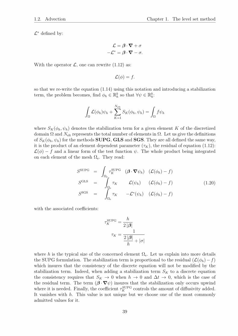
1.2. Advection Chapter 1. The level set method
L∗ defined by:
L = β ·∇+ σ
−L∗ = β ·∇− σ.
With the operator L, one can rewrite (1.12) as:
L(φ) = f.
so that we re-write the equation (1.14) using this notation and introducing a stabilizationterm, the problem becomes, find φh ∈ Rk
h so that ∀ψ ∈ Rkh:
∫
Ω
L(φh)ψh +
Nelt∑
K=1
SK(φh, ψh) =
∫
Ω
fψh
where SK(φh, ψh) denotes the stabilization term for a given element K of the discretizeddomain Ω and Nelt represents the total number of elements in Ω. Let us give the definitionsof SK(φh, ψh) for the methods SUPG, GLS and SGS. They are all defined the same way,it is the product of an element dependent parameter (τK), the residual of equation (1.12):L(φ) − f and a linear form of the test function ψ. The whole product being integratedon each element of the mesh Ωe. They read:
SSUPG =
∫
Ωe
τSUPGK (β ·∇ψh) (L(φh)− f)
SGLS =
∫
Ωe
τK L(ψh) (L(φh)− f)
SSGS =
∫
Ωe
τK −L∗(ψh) (L(φh)− f)
(1.20)
with the associated coefficients:
τSUPGK =
h
2 |β|
τK =1
2 |β|h
+ |σ|
where h is the typical size of the concerned element Ωe. Let us explain into more detailsthe SUPG formulation. The stabilization term is proportional to the residual (L(φh)− f)which insures that the consistency of the discrete equation will not be modified by thestabilization term. Indeed, when adding a stabilization term SK to a discrete equationthe consistency requires that SK → 0 when h → 0 and ∆t → 0, which is the case ofthe residual term. The term (β ·∇ψ) insures that the stabilization only occurs upwindwhere it is needed. Finally, the coefficient τSUPG
K controls the amount of diffusivity added.It vanishes with h. This value is not unique but we choose one of the most commonlyadmitted values for it.
39

1.3. Reinitialization methods Chapter 1. The level set method
Internal faces stabilization
Another kind of method has been proposed for the first time by Douglas and Dupont in1976 [25] and a convergence study has been made long time after that (2004) by Burmanand Hansbo in [13] on the advection-diffusion-reaction problem and has been applied toNavier Stokes by the same authors in [14]. The precise error analysis at high order hasbeen made in [100]. Two implementations in the context of level set advection can befound in [81, 112]. The idea is to add a penalty term on the jump of the gradient of thesolution. This avoids artificial higher gradients to appear. The advantage of this methodis that it stays consistent even for higher order finite element. The drawback is that itadds new non-zero entries in the matrix and leads to a more difficult problem to solve.Let us denote the internal faces of the mesh by ΓI, being all the lines (surfaces in 3D)which are not on a boundary. We also need to define the jump of a quantity across twoelements called K0 and K1. The jump of a scalar quantity f is a vector defined by:
[[f ]] = f0N0 + f1N1 (1.21)
where Ni denotes the normal of the concerned face pointing outward from the elementKi. And the jump of a vector f is a scalar defined by:
[[f ]] = f0 ·N0 + f1 ·N1 (1.22)
Thus, in a configuration where K0 and K1 are neighbors, N0 = −N1 as shown infigure 1.4. The CIP stabilization consists of adding the following term to the discretized
Figure 1.4: Normal of the touching faces of two neighbors elements.
weak formulation (1.14), with (φ, ψ) ∈ (H1(Ω), H1(Ω)):
SCIP =
∫
ΓI
γh2fk3.5|β ·N | [[∇φ]][[∇ψ]] (1.23)
with γ a small factor, hf the length of the edge and N the outward normal of the edge.
1.3 Keeping the level set function close to a distance
function: the reinitialization methods
The function φ transported by the equation (1.11) does not conserve the property to bea signed distance function (|∇φ| = 1). In the areas where the velocity u goes from a
40

1.3. Reinitialization methods Chapter 1. The level set method
big value to a smaller one, one sees an accumulation of the iso lines or iso surface of thelevel set function. The gradient magnitude of the function increases and the Heavisideand Dirac function supports are getting thinner. These functions can even have no moremesh element on which they are supported if |∇φ| is too large. At the opposite, an areawhere u goes roughly from a small value to a big one sees the support of these functionsgetting larger and the extension of the interface becoming too large. Several solutionsexist to this problem.
1.3.1 The advection by an extended velocity
As explained previously, the velocity u used in the equation (1.11) has to be equal tothe velocity of the interface on Γ but no particular restriction on the rest of the domainis needed. It is then possible to define an extended velocity uext equal to the velocity ofthe interface on Γ and being defined elsewhere in a way so that the advection of φ withthis velocity does not change the property |∇φ| = 1. An example of extended velocityis the one we have used in section 1.5. This velocity is defined by the equation (1.24),that is to say that the value of uext on a point of the domain is equal to its value on theclosest point in Γ. In practice, searching for each point in the domain the closest point toit on the interface is costly and we choose not to use an extended velocity for multi-fluidapplications.
uext(x) =
u(x) if x ∈ Γu(x∗) else
(1.24)
with
dist(x,x∗)x∗∈Γ
= dist(x,Γ)
Other ways exist to create extensional velocities, many are described in [98]. Nevertheless,they all must be calculated at every time iteration and for performance purposes we chooseother methods for multi-fluid applications. This method could be really interesting whenthere is no obvious definition of the velocity in all the domain. For example, for a multi-fluid application, taking the velocity of the fluid on all the domain as the advection velocityis an obvious choice. For contour detection on an image (see section 1.5), such a velocitydoes not exist, thus an extended velocity is well suited for this application.
1.3.2 The interface local projection
When φ is not too irregular, it has been shown in [81, 21] that the functionφ
|∇φ| isclose to a distance function where φ vanishes, that is to say near the interface. So it is
possible to useφ
|∇φ| as support for the functions Hε and δε which will then have a regular
extension at each side of the interface. Nevertheless, for a long time simulation with avelocity field u(t) irregular, |∇φ| can take extreme values. If |∇φ| becomes too big, it is
possible thanφ
|∇φ| tends to 0 and with the numerical error changes of sign. In this case,
a new artificial interface appears and is advected by the equation (1.11) as if it was a realinterface. This method is not completely sufficient to solve the problem of keeping φ asa distance function but it is extremely useful for two purposes: i) it maintains a relative
41

1.3. Reinitialization methods Chapter 1. The level set method
regularity of the functions Hε and δε for a simulation time longer than if one uses theclassical φ as a support. ii) It can be used as an exact value for a distance function close tothe interface. This last advantage is particularly valuable in the case of a reinitializationby a fast marching method as we will see in section 1.3.4.
1.3.3 Reinitialization by solving a Hamilton Jacobi problem
Hamilton Jacobi equation leading φ to a distance function
It is possible to reset the function φ regularly to a signed distance function. The positionof the 0 value of the new function has to be the same as the previous one, in this way,the interface does not move. A method based on an idea of [91], modified in [104] andused several times since (a non-exhaustive list is given by [103, 106, 31, 78, 110]) consistsin solving a Hamilton Jacobi equation of the form:
∂tφ = Sgn(φ)(1− |∇φ|) (1.25)
Sgn being the sign function. When this equation is solved to equilibrium (∂tφ = 0) thesolution is a signed distance function (one has |∇φ| = 1). One can rewrite the equation(1.25) as:
∂tφ− Sgn(φ)(1−∇φ
|∇φ| ·∇φ) = 0. (1.26)
Equation (1.26) is a transport equation with a velocity equal to Sgn(φ)∇φ
|∇φ| . One can
then see this reinitialization as a front propagating and resetting φ to a distance function.
The velocity∇φ
|∇φ| is normal to the interface and is pointing out from the interface. The
reinitialization front with such a velocity would always go from the interface Γ to theexterior of the domain Ω1 (i.e toward φ > 0). This is the reason for the introductionof the sign function as a factor to this velocity. This way, the front always goes fromthe interface Γ to both the domains Ω1 and Ω2. Thus, the areas close to the interfaceare always reinitialized first. This can be useful since the need of having a distancefunction is stronger close to the interface. Moreover, generally the initial function φ is nottoo far away from a signed distance function, the equation (1.25) is not too far from theequilibrium. One can generally use a large pseudo time step and few iterations are neededto reach the equilibrium state. The sign function is smoothed so that the numerical errordoes not make the front go to the wrong side. It is often found on the form initially givenby [104]:
Sgn(φ) =φ
√
φ2 + ε2(1.27)
with ε a small smoothing parameter. In our case, we prefer to use the formula given in[63] using the function Hε. Thus, the smoothing parameter ε is the interface thickness.So we use:
Sgn(φ) = 2Hε −1
2. (1.28)
The advantage of using this formulation, is that it does not need a new parameter ε, theinterface thickness is used and the sign function is defined the same way as the Heavisideand Delta functions.
42

1.3. Reinitialization methods Chapter 1. The level set method
Discretization and resolution of the problem
The equation (1.25) is discretized in time using an Euler scheme and linearized by taking
the velocity term as being the value of∇φ
|∇φ| at the previous iteration. We obtain the
equation:φn+1
∆τ+Sgn(φ
n)∇φn
|∇φn| ·∇φn+1 = Sgn(φn) +
φn
∆τ(1.29)
with ∆τ the pseudo time step. The weak formulation associated is obtained by multiplyingby the test function ψ and integrating the equation (1.29) on all the space. The problemobtained is then: find φ ∈ H1(Ω) so that ∀ψ ∈ L2(Ω):
∫
Ω
φn+1
∆τψ +
∫
Ω
(Sgn(φ
n)∇φn
|∇φn| ·∇φn+1
)
ψ =
∫
Ω
(
Sgn(φn) +
φn
∆τ
)
ψ. (1.30)
One recognizes an equation of the form (1.14) with the coefficients given by:
σ =1
∆τ
β =Sgn(φ
n)∇φn
|∇φn|
f = Sgn(φn) +
φn
∆τ
One understands that the great advantage of this method is that it is simple to implementsince it does not need other tools than the one already implemented for the advectionof the function φ. Moreover, this formulation is very generic and no hypothesis hasbeen done for the dimension of the spaces or the polynomial order of the finite elementfunctions. It also works on one or many processors since the PDE solver used providesthis possibility (as opposed to the fast marching, for which a special care has to be takenin the algorithm).It is possible to create an indicator to know at each iteration if one needs to reinitializeor not. An example of indicator is the distance to a distance function. It measures therelative distance of φ to a signed distance function. It is given by:
edist to dist =1
V
∫
Ω
√
(|∇φ| − 1)2 (1.31)
with V the volume of the domain. One can then choose a stop criterion for the reinitial-ization thanks to this indicator.In practice, we prefer to fix a reinitialization frequency. At this frequency, we solve the
equation (1.30) until we obtain|φn+1 − φn||φn| < εtol, with εtol a numerical tolerance imposed
according to the needs of the application.
The reinitialization requires choosing correctly the parameters: reinitialization fre-quency, ∆τ and εtol. These parameters depend on the space discretization h, on thetime step ∆t, on the precision needed for the application. Even if one can find relationsbetween these parameters, there does not exist any absolute formula working for every
43

1.3. Reinitialization methods Chapter 1. The level set method
application, and, in practice, one needs to do many tests before finding optimal parame-ters. It is the principal drawback that one can find to this method. The other drawbackis that in general, the interface slightly moves during the first iteration of (1.30), and forlong time simulations, one can see large variations of the volume of the domains due tothe implied numerical errors.
An example: the signed distance function to an ellipse
The figure 1.5 shows different iterations of the equation (1.30). The example is takenfrom chapter 2.4 for which this reinitialization method has been used. We do not knowan analytic expression for a signed distance function to an ellipse. To initialize a level setfunction to an ellipse, we have to use the following function:
φellipse0 =
√(x− x0a
)2
+
(y − y0b
)2
− 1 (1.32)
with (x0, y0) the position of the center of the ellipse and a and b its semi-axes. This
function is not a signed distance function, one can easily show that∣∣∣∇φellipse
0
∣∣∣ 6= 1, but
the iso surface of value 0 and the sign of each side of the interface are well positioned. φ0
is an acceptable approximation of a distance function when the 1eccentricity of the ellipseis very small. If one starts the simulation with this function, one sees that the Diracand Heaviside functions will have a different thickness along the interface. Thus, we needto reinitialize this function to a signed distance function. The initial reinitialization isthe one taking the longest time since, after that, we never let φ be so different from adistance function. Moreover, since we do not want to lose too much mass at the beginningof the simulation, a small pseudo time step is chosen. In this example, the mesh size ish = 0.025, the time step for the simulation is ∆t = 0.0125 and the pseudo time step hasbeen taken as ∆τ = 0.08. The equation is stabilized by a SUPG method. We see on thefigure 1.5 the state of φellipse
0 every 10 iterations.
1.3.4 The fast marching method
Basic principle of the fast marching
Another way to reinitialize φ to a distance function is to modify one by one every degree offreedom of the system by calculating the new value of φ. Such a method has already beendescribed in [98] and with more details in [72]. The method is named the fast marchingmethod (FMM). This method is a way to efficiently iterate over the degrees of freedomand updating the visited points.
The idea is the following: it starts by an initialization phase, let us suppose that onealready knows the value of φ as a distance function on a few degrees of freedom. Onemarks these points as being accepted, they will never be changed again during the reini-tialization step. Then, one searches for all the closest neighbors to the accepted pointsand we mark them as close. All the other points are marked as far. A new value φ is
1The eccentricity is defined as
√
1−(b
a
)2
. At the limit of a vanishing eccentricity, the ellipse is a
circle.
44

1.3. Reinitialization methods Chapter 1. The level set method
(a) iteration 0 (b) iteration 10 (c) iteration 20
(d) iteration 30 (e) iteration 40 (f) iteration 50
Figure 1.5: Successive iterations of the discretized Hamilton Jacobi equation for thereinitialization of the function φellipse
0 . The line φellipse0 = 0 is represented in red and
other values of level lines equally separated are represented in black. The background
color represents∣∣∣∇φellipse
0
∣∣∣. One can see that
∣∣∣∇φellipse
0
∣∣∣ expands to a value of 1 while the
shape of the iso 0 stay preserved.
calculated for each point marked as close, this value is computed by using the values of φof the points marked accepted for which one knows that φ is a correct distance function.
The elements in close are then sorted by their values of∣∣∣φ∣∣∣. They are stored in a heap so
that the one having smallest value is on the top. Then follows the real marching proce-dure, it is reported in the algorithm 1.
With this method, we are sure that one point is accepted every iteration and thealgorithm 1 has a complexity of O(N). The fact that the elements close are in a sortedheap is important, indeed, once the heap is sorted, it is easy to find the smallest value ofφ and update the heap. The initialization procedure has a complexity of O(log(N)).One understands the term marching. Indeed, the idea is never to modify an already ac-cepted point. Thus, the algorithm always goes from known points to the unknowns. Themethod requires that some points are already known at the initialization step. For that,one uses the interface local projection method presented above 1.3.2. Thus, the elementsclose to the interface are known at the beginning of the marching algorithm. The way tocalculate the new value of φ using the known values of φ is given in detail in [112] bothfor 2D and 3D, but it assumes monotonicity of φ between the nodes (only P1 elements).The fast marching method for Feel++ has already been implemented during the PhDthesis of Christophe Winkelmann [112]. We used it without changes except adding thepossibility to handle periodic boundary conditions. This implementation has been done
45
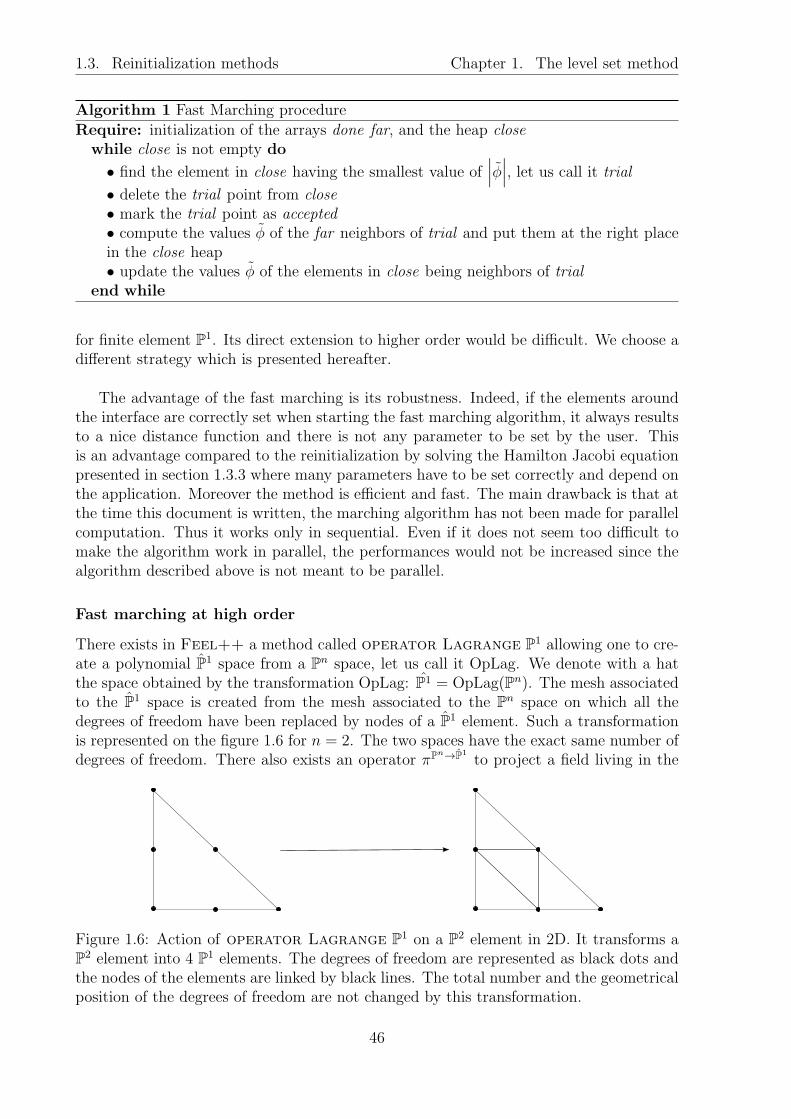
1.3. Reinitialization methods Chapter 1. The level set method
Algorithm 1 Fast Marching procedure
Require: initialization of the arrays done far, and the heap closewhile close is not empty do
• find the element in close having the smallest value of∣∣∣φ∣∣∣, let us call it trial
• delete the trial point from close• mark the trial point as accepted• compute the values φ of the far neighbors of trial and put them at the right placein the close heap• update the values φ of the elements in close being neighbors of trial
end while
for finite element P1. Its direct extension to higher order would be difficult. We choose adifferent strategy which is presented hereafter.
The advantage of the fast marching is its robustness. Indeed, if the elements aroundthe interface are correctly set when starting the fast marching algorithm, it always resultsto a nice distance function and there is not any parameter to be set by the user. Thisis an advantage compared to the reinitialization by solving the Hamilton Jacobi equationpresented in section 1.3.3 where many parameters have to be set correctly and depend onthe application. Moreover the method is efficient and fast. The main drawback is that atthe time this document is written, the marching algorithm has not been made for parallelcomputation. Thus it works only in sequential. Even if it does not seem too difficult tomake the algorithm work in parallel, the performances would not be increased since thealgorithm described above is not meant to be parallel.
Fast marching at high order
There exists in Feel++ a method called operator Lagrange P1 allowing one to cre-ate a polynomial P1 space from a Pn space, let us call it OpLag. We denote with a hatthe space obtained by the transformation OpLag: P1 = OpLag(Pn). The mesh associatedto the P1 space is created from the mesh associated to the Pn space on which all thedegrees of freedom have been replaced by nodes of a P1 element. Such a transformationis represented on the figure 1.6 for n = 2. The two spaces have the exact same number ofdegrees of freedom. There also exists an operator πPn→P1
to project a field living in the
Figure 1.6: Action of operator Lagrange P1 on a P2 element in 2D. It transforms aP2 element into 4 P1 elements. The degrees of freedom are represented as black dots andthe nodes of the elements are linked by black lines. The total number and the geometricalposition of the degrees of freedom are not changed by this transformation.
46

1.3. Reinitialization methods Chapter 1. The level set method
Pn space onto the P1 space. The opposite projector also exists πP1→Pn
. We emphasizethe fact that an element created by the operator πPn→P1
has the exact same number ofdegrees of freedom that the element in the Pn space used to create it. Moreover, bothelements have the exact same values at degrees of freedom having the same geometricalcoordinates. Of course the same remark holds for πP1→Pn
. We use this transformation tocreate a temporary level set function φ being in a P1 space φ = πPn→P1
(φ). Then φ isreinitialized using the fast marching method, let us call it φ∗ after reinitialization. Finally,the inverse transformation is used φ∗ = πP1→Pn
(φ∗) and one obtains a function φ∗ being adistance function in a Pn space. We summarized this transformation on the scheme 1.7.We present an example of reinitialization using the proposed high order fast marching
Figure 1.7: Scheme of the transformations used to do a reinitialization using the fastmarching method for an element being in a space of polynomials of order greater than 1.The P1 space is created from the Pn space: P1 = OpLag(Pn).
method. The level set function is set on a unit square by the equation (1.32) for whichwe put a = 0.3 and b = 0.1. With this equation, we can show easily that |∇φ| 6= 1 thusφ is not a distance function. We use a space of polynomials of order 2 as space for φ andtest the procedure below. Figure 1.8(a) shows the mesh associated to the P2 space andfigure 1.8(b) shows the mesh associated to the P1 space created from the P2 mesh usingOpLag. The faces which already existed in the initial mesh are reported in red so that itbecomes clear which faces and points have been added.
Figures 1.9(a) and 1.9(b) represent the value of φ before and after the reinitializationprocedure on a mesh thinner than the one used in figure 1.8. The iso 0 is represented ingreen and 30 iso lines are represented as black lines. The color is given by |∇φ|. We seeclearly that |∇φ| becomes close to 1 and that the iso lines are equally spaced.
Finally, figure 1.10 shows the same reinitialization procedure but taking φ ∈ P5. Wehave also plotted a close up of the intermediate mesh constructed with Operator LagrangeP1 on the mesh associated to the P5 space.
47

1.3. Reinitialization methods Chapter 1. The level set method
(a) Mesh associated to the P2 space. (b) Mesh associated to the P1 space after using Op-erator Lagrange P1. The edges which were alreadypresent in the previous mesh are represented in red.
Figure 1.8: Action of Operator Lagrange P1 on a mesh associated to a P2 space.
(a) φ before reinitialization procedure. (b) φ after reinitialization procedure.
Figure 1.9: Value of φ ∈ P2 before and after the reinitialization procedure by fast marchingmethod. The iso 0 is represented in green and 30 iso lines are represented as black lines.The color is given by |∇φ|.
The distance to the boundaries of a domain
The fast marching has been designed to reinitialize the level set field to a distance function,but it can also be used in another context: to get the distance to the closest boundary ofa domain. Indeed, some applications need the information of the distance to the closestboundary as for example turbulence models where a boundary layer model is used. Al-though it is trivial to get the distance to the boundary when the geometry is a rectangle,
48
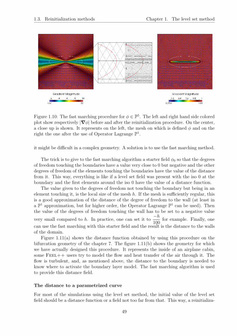
1.3. Reinitialization methods Chapter 1. The level set method
Figure 1.10: The fast marching procedure for φ ∈ P5. The left and right hand side coloredplot show respectively |∇φ| before and after the reinitialization procedure. On the center,a close up is shown. It represents on the left, the mesh on which is defined φ and on theright the one after the use of Operator Lagrange P1.
it might be difficult in a complex geometry. A solution is to use the fast marching method.
The trick is to give to the fast marching algorithm a starter field φ0 so that the degreesof freedom touching the boundaries have a value very close to 0 but negative and the otherdegrees of freedom of the elements touching the boundaries have the value of the distancefrom it. This way, everything is like if a level set field was present with the iso 0 at theboundary and the first elements around the iso 0 have the value of a distance function.
The value given to the degrees of freedom not touching the boundary but being in anelement touching it, is the local size of the mesh h. If the mesh is sufficiently regular, thisis a good approximation of the distance of the degree of freedom to the wall (at least ina P1 approximation, but for higher order, the Operator Lagrange P1 can be used). Thenthe value of the degrees of freedom touching the wall has to be set to a negative value
very small compared to h. In practice, one can set it to−h100
for example. Finally, one
can use the fast marching with this starter field and the result is the distance to the wallsof the domain.
Figure 1.11(a) shows the distance function obtained by using this procedure on thebifurcation geometry of the chapter 7. The figure 1.11(b) shows the geometry for whichwe have actually designed this procedure. It represents the inside of an airplane cabin,some Feel++ users try to model the flow and heat transfer of the air through it. Theflow is turbulent, and, as mentioned above, the distance to the boundary is needed toknow where to activate the boundary layer model. The fast marching algorithm is usedto provide this distance field.
The distance to a parametrized curve
For most of the simulations using the level set method, the initial value of the level setfield should be a distance function or a field not too far from that. This way, a reinitializa-
49

1.4. Solid rotation of a slotted disk Chapter 1. The level set method
(a) Bifurcation geometry. (b) Airplane cabin.
Figure 1.11: Distance to the boundaries of two geometries computed by the fast marchingmethod.
tion procedure can be applied and the simulation can start with a distance function field.Writing a distance function to a line or a circle is easy. Distance functions of shapes beinga combination of lines and circles can be written with min and max functions of distanceto lines and circles. Distance function to more complicated shapes are impossible to writeanalytically. To be able to start with more complicated shapes, we built a method tocreate a distance function to a parametrized curve.
Once again, the key is to create a distance function to the first elements touching thecurve. Since this field is created, it can be given as a starter to the fast marching methodwhich gives as a result a nice distance field. The procedure to create a distance functionto a parametrized curve is given in appendix C.
1.4 Benchmark, solid rotation of a slotted disk
1.4.1 Presentation of the benchmark
This test has been initially proposed by Zalesac in [114]. It has become one of the mostcommon tests for interface propagation. It has been used for example in [59, 12, 78, 29] totest numerical frameworks. The test consists of the rotation of a slotted disk in a squaredomain. The geometry of the domain is represented in figure 1.12(a). The domain Ωis the square [0, 1] × [0, 1]. The center of the slotted disk is initially in (0.5, 0.75). Theimposed velocity is a solid rotation of center (0.5, 0.5). The angular velocity is chosenso that the disks makes one round every tf = 628. The velocity has the following form
u =( π
314(50− y), π
314(x− 50)
)
, it is represented on the domain in the figure 1.12(b).
50
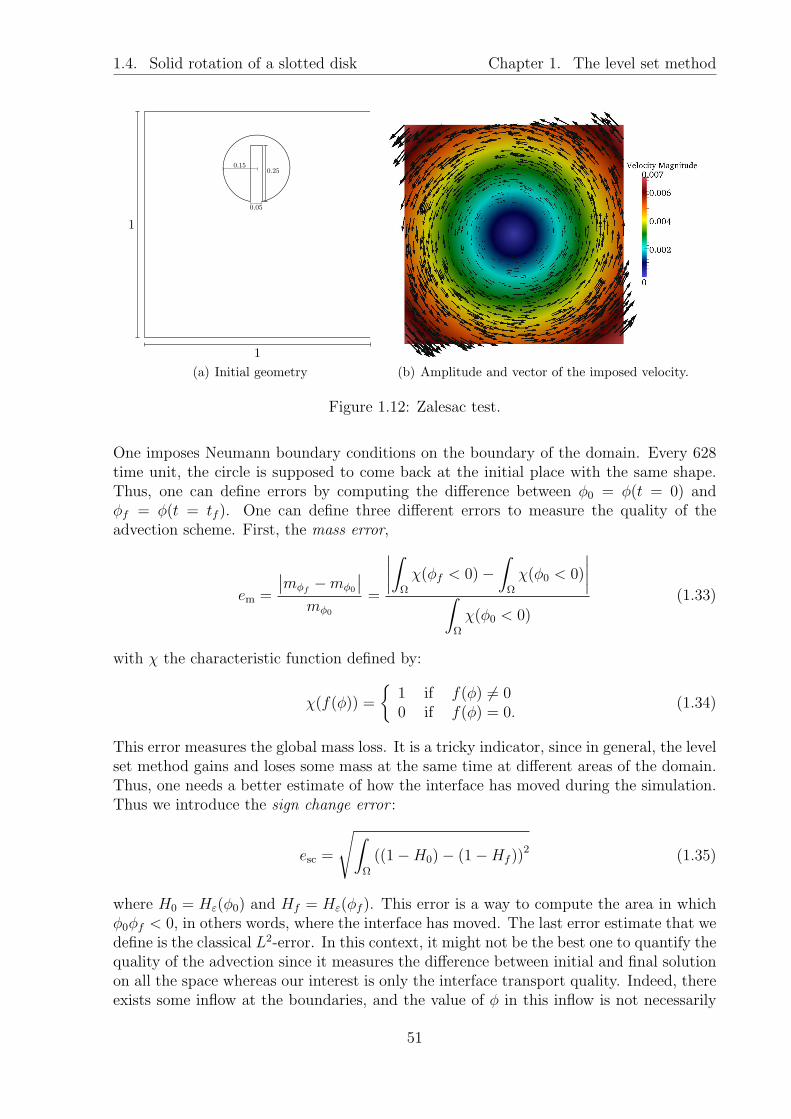
1.4. Solid rotation of a slotted disk Chapter 1. The level set method
(a) Initial geometry (b) Amplitude and vector of the imposed velocity.
Figure 1.12: Zalesac test.
One imposes Neumann boundary conditions on the boundary of the domain. Every 628time unit, the circle is supposed to come back at the initial place with the same shape.Thus, one can define errors by computing the difference between φ0 = φ(t = 0) andφf = φ(t = tf ). One can define three different errors to measure the quality of theadvection scheme. First, the mass error,
em =
∣∣mφf
−mφ0
∣∣
mφ0
=
∣∣∣∣
∫
Ω
χ(φf < 0)−∫
Ω
χ(φ0 < 0)
∣∣∣∣
∫
Ω
χ(φ0 < 0)(1.33)
with χ the characteristic function defined by:
χ(f(φ)) =
1 if f(φ) 6= 00 if f(φ) = 0.
(1.34)
This error measures the global mass loss. It is a tricky indicator, since in general, the levelset method gains and loses some mass at the same time at different areas of the domain.Thus, one needs a better estimate of how the interface has moved during the simulation.Thus we introduce the sign change error :
esc =
√∫
Ω
((1−H0)− (1−Hf ))2 (1.35)
where H0 = Hε(φ0) and Hf = Hε(φf ). This error is a way to compute the area in whichφ0φf < 0, in others words, where the interface has moved. The last error estimate that wedefine is the classical L2-error. In this context, it might not be the best one to quantify thequality of the advection since it measures the difference between initial and final solutionon all the space whereas our interest is only the interface transport quality. Indeed, thereexists some inflow at the boundaries, and the value of φ in this inflow is not necessarily
51
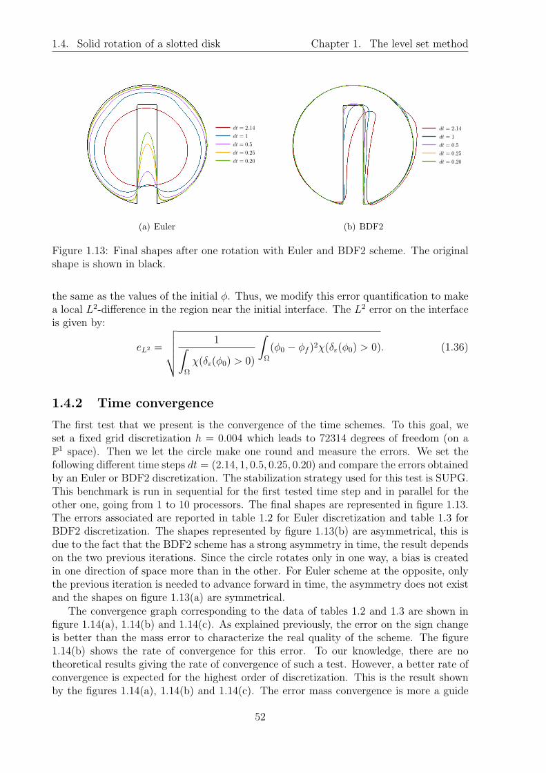
1.4. Solid rotation of a slotted disk Chapter 1. The level set method
(a) Euler (b) BDF2
Figure 1.13: Final shapes after one rotation with Euler and BDF2 scheme. The originalshape is shown in black.
the same as the values of the initial φ. Thus, we modify this error quantification to makea local L2-difference in the region near the initial interface. The L2 error on the interfaceis given by:
eL2 =
√√√√√
1∫
Ω
χ(δε(φ0) > 0)
∫
Ω
(φ0 − φf )2χ(δε(φ0) > 0). (1.36)
1.4.2 Time convergence
The first test that we present is the convergence of the time schemes. To this goal, weset a fixed grid discretization h = 0.004 which leads to 72314 degrees of freedom (on aP1 space). Then we let the circle make one round and measure the errors. We set thefollowing different time steps dt = (2.14, 1, 0.5, 0.25, 0.20) and compare the errors obtainedby an Euler or BDF2 discretization. The stabilization strategy used for this test is SUPG.This benchmark is run in sequential for the first tested time step and in parallel for theother one, going from 1 to 10 processors. The final shapes are represented in figure 1.13.The errors associated are reported in table 1.2 for Euler discretization and table 1.3 forBDF2 discretization. The shapes represented by figure 1.13(b) are asymmetrical, this isdue to the fact that the BDF2 scheme has a strong asymmetry in time, the result dependson the two previous iterations. Since the circle rotates only in one way, a bias is createdin one direction of space more than in the other. For Euler scheme at the opposite, onlythe previous iteration is needed to advance forward in time, the asymmetry does not existand the shapes on figure 1.13(a) are symmetrical.
The convergence graph corresponding to the data of tables 1.2 and 1.3 are shown infigure 1.14(a), 1.14(b) and 1.14(c). As explained previously, the error on the sign changeis better than the mass error to characterize the real quality of the scheme. The figure1.14(b) shows the rate of convergence for this error. To our knowledge, there are notheoretical results giving the rate of convergence of such a test. However, a better rate ofconvergence is expected for the highest order of discretization. This is the result shownby the figures 1.14(a), 1.14(b) and 1.14(c). The error mass convergence is more a guide
52

1.4. Solid rotation of a slotted disk Chapter 1. The level set method
dt eL2 esc em2.14 0.0348851 0.202025 0.2020251.00 0.0187567 0.147635 0.1476350.50 0.0098661 0.10847 0.108470.25 0.008791 0.0782569 0.07825690.20 0.00803373 0.0670677 0.0670677
Table 1.2: Errors on the time convergence of Euler scheme for Zalesac benchmark.
dt eL2 esc em2.14 0.0118025 0.0906617 0.04927751.00 0.00436957 0.0445275 0.01634940.50 0.00173637 0.0216359 0.01006210.25 0.001003 0.0125971 0.003546440.20 0.000949343 0.0117449 0.00317368
Table 1.3: Errors on the time convergence of BDF2 scheme for Zalesac benchmark.
for the eyes since, as we already explained, the loss of mass in a region is sometimescompensated by a gain of mass in another region, making the mass error a poor errorestimate. Thus this error might not be relevant in this case. The sign change error showsa gain of around half an order going from Euler discretization scheme to BDF2 whereasin the same case, the L2 error shows a gain of one order.
1.4.3 Space convergence
The goal of the second test is to verify the space convergence. We set a relation between
the time step and the space discretization. The time step, is usually taken as dt = Ch
Umax
,
where C is a constant smaller than one and Umax the maximum velocity on the domain.In our case we set C = 0.8 and the maximum velocity is obtained for the points havingthe highest distance from the center. With the velocity imposed, we have Umax = 0.007.
Thus the time step is taken as dt = 0.8h
0.007. A BDF2 time scheme is chosen for the
time discretization. Different mesh sizes are taken: h = 0.32, 0.16, 0.08, 0.04. The testis run in parallel from 2 processors, for h = 0.32 to 10 processors for h = 0.04. All thestabilization methods at our disposal are tested, namely, CIP, SUPG, GLS, SGS. Thefinal shapes obtained are represented in figure 1.15. The numerical errors are representedin table 1.4. The sign change error is represented in figure 1.16(a). All the stabilizationmethods show a rate of convergence of 0.6 and all the errors are almost equivalent. TheL2 error convergence is represented in figure 1.16(b) and the convergence of this error isnot as clear as the previous one. All the element stabilization show a rate of convergenceof 0.9, whereas the CIP stabilization only shows a rate of convergence of 0.6.
53

1.4. Solid rotation of a slotted disk Chapter 1. The level set method
10−1 100
dt
10−2
10−1e m
Euler
slope = 0.80
BDF2
slope = 1.20
(a) Mass error as a function of time step for Zalesac benchmark.
10−1 100
dt
10−2
10−1
e sc
Euler
slope = 0.50
BDF2
slope = 0.90
(b) Sign change error as a function of time step for Zalesac bench-mark.
10−1 100
dt
10−3
10−2
e L2
Euler
slope = 0.60
BDF2
slope = 1.10
(c) L2 local error as a function of time step for Zalesac bench-mark.
Figure 1.14: Convergence of the errors measured in the benchmark for the time discretiza-tion methods Euler and BDF2.
54

1.4. Solid rotation of a slotted disk Chapter 1. The level set method
Figure 1.15: Final shapes of the Zalesac circle after a whole revolution for different meshsizes. The initial shape is also depicted.
stab h eL2 esc em
CIP
0.32 0.0074 0.072 0.000290.16 0.0046 0.055 0.002020.08 0.0025 0.033 0.000490.04 0.0023 0.020 0.00110
SUPG
0.32 0.012 0.065 0.016320.16 0.008 0.049 0.070520.08 0.004 0.030 0.000730.04 0.001 0.018 0.00831
GLS
0.32 0.013 0.066 0.024990.16 0.008 0.051 0.051800.08 0.004 0.031 0.008050.04 0.001 0.019 0.00672
SGS
0.32 0.012 0.065 0.011030.16 0.008 0.050 0.075700.08 0.004 0.030 0.000840.04 0.001 0.018 0.00850
Table 1.4: Errors for different mesh sizes and stabilization methods.
55

1.4. Solid rotation of a slotted disk Chapter 1. The level set method
10−2
h
10−2
10−1
e sc
CIP
slope = 0.6
GALS
slope = 0.6
SGS
slope = 0.6
SUPG
slope = 0.6
(a) Error and rate of convergence of the sign change error as a function of the spacediscretization.
10−2
h
10−3
10−2
e L2
CIP
slope = 0.6
GALS
slope = 0.9
SGS
slope = 0.9
SUPG
slope = 0.9
(b) Error and rate of convergence of the L2 error as a function of the space discretiza-tion.
Figure 1.16: Space convergence of the measured errors for the four stabilization methodstested.
56

1.5. Active contours Chapter 1. The level set method
1.5 An application : the active contours
The level set method can be used in different domains than multi-fluids simulations, forexample it can be used in image analysis to find systematically the boundaries of objects.This technique has been used for the first time by Malladi [72]. Many improvements havebeen made, and a good review of those enhancements is given in [102]. This method isoften used in image analysis. One can find it for example as a plugin for the free imageanalysis software imageJ 2. An image being organized in pixels, it is easy to representit on a regular grid. Thus, the finite difference method is often used for this kind ofapplication and most of the schemes presented in the cited references are written forthe finite difference method. However, the method naturally extends to finite elementmethod. We were interested to implement the active contours method not for a researchpurpose but to test the generality of the LevelSet class implemented in Feel++ .Indeed, the LevelSet class has to be totally decoupled from the fluid part and has tobe usable for totally different applications than multi-fluid simulations. Moreover, if theclass interface is correctly designed, a basic active contours application has to be easy andsimple to implement. This part shows that, as for the level set method, the LevelSet
class implemented can be used for other goals than multi-fluids simulations, and it hasbeen a guide to design the LevelSet interface.
1.5.1 Principle of active contours method
The principle of the active contours method is to see an image as a scalar function ofgray level (the method can be extended to colored images by using a vectorial function,but we will not go into the details in this description). Let us call I(x) the functionrepresenting the gray level of an image. Finding a boundary in an image is equivalent tofinding the part in the image where there exists a strong contrast. In other words, findingthe boundary of an object in an image, is equivalent to find the set of x so that |∇I|is big. A possible solution could be to calculate the gradient of gray level everywhere inthe image and define the boundary as being the set of x for which |∇I| > Imax. Thedrawback of this method, is that if the image is noisy, all the noise will be included in theboundary. Malladi has then proposed to define a scalar level set field in the image and toinitialize it as a small circle inside the area in which the boundary is searched. The ideais then to make evolve the iso 0 of the level set (called the front) by applying a velocityfield u. This velocity is normal to the front and depends on the function I. The goal isthat at the end of the simulation, the front fits the contour of the object in the image.This front is called the active contour. The velocity u has to vanish when |∇I| is bigenough. Such a velocity is given by :
u =1
1 + α |∇I|∇φ
|∇φ| (1.37)
where α is a parameter. Let us now imagine what happens in a noisy region. In such aregion, a lot of small regions exists where |∇I| is big, making the front stop around them.These regions being small, the curvature of the front around it should very high. Thus,one can add to the velocity term, a component proportional to the curvature of the front.
2 Module maintained by Erwin Frise http://fiji.sc/Level_Sets
57
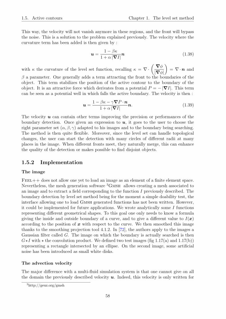
1.5. Active contours Chapter 1. The level set method
This way, the velocity will not vanish anymore in these regions, and the front will bypassthe noise. This is a solution to the problem explained previously. The velocity where thecurvature term has been added is then given by :
u =1− βκ
1 + α |∇I|n (1.38)
with κ the curvature of the level set function, recalling κ = ∇ ·(
∇φ
|∇φ|
)
= ∇ ·n and
β a parameter. One generally adds a term attracting the front to the boundaries of theobject. This term stabilizes the position of the active contour to the boundary of theobject. It is an attractive force which derivates from a potential P = − |∇I|. This termcan be seen as a potential well in which falls the active boundary. The velocity is then :
u =1− βκ− γ∇P ·n
1 + α |∇I| n. (1.39)
The velocity u can contain other terms improving the precision or performances of theboundary detection. Once given an expression to u, it goes to the user to choose theright parameter set (α, β, γ) adapted to his images and to the boundary being searching.The method is then quite flexible. Moreover, since the level set can handle topologicalchanges, the user can start the detection with many circles of different radii at manyplaces in the image. When different fronts meet, they naturally merge, this can enhancethe quality of the detection or makes possible to find disjoint objects.
1.5.2 Implementation
The image
Feel++ does not allow one yet to load an image as an element of a finite element space.Nevertheless, the mesh generation software 3Gmsh allows creating a mesh associated toan image and to extract a field corresponding to the function I previously described. Theboundary detection by level set method being for the moment a simple doability test, theinterface allowing one to load Gmsh generated functions has not been written. However,it could be implemented for future applications. We wrote analytically some I functionsrepresenting different geometrical shapes. To this goal one only needs to know a formulagiving the inside and outside boundary of a curve, and to give a different value to I(x)according to the position of x with respect to the curve. We then smoothed this imagethanks to the smoothing projection tool 4.1.2. In [72], the authors apply to the images aGaussian filter called G. The image on which the boundary is actually searched is thenG⋆I with ⋆ the convolution product. We defined two test images (fig 1.17(a) and 1.17(b))representing a rectangle intersected by an ellipse. On the second image, some artificialnoise has been introduced as small white disks.
The advection velocity
The major difference with a multi-fluid simulation system is that one cannot give on allthe domain the previously described velocity u. Indeed, this velocity is only written for
3http://geuz.org/gmsh
58
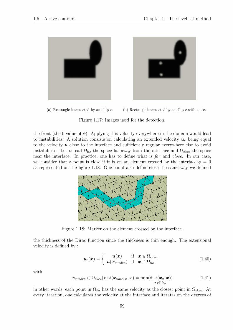
1.5. Active contours Chapter 1. The level set method
(a) Rectangle intersected by an ellipse. (b) Rectangle intersected by an ellipse with noise.
Figure 1.17: Images used for the detection.
the front (the 0 value of φ). Applying this velocity everywhere in the domain would leadto instabilities. A solution consists on calculating an extended velocity ue being equalto the velocity u close to the interface and sufficiently regular everywhere else to avoidinstabilities. Let us call Ωfar the space far away from the interface and Ωclose the spacenear the interface. In practice, one has to define what is far and close. In our case,we consider that a point is close if it is on an element crossed by the interface φ = 0as represented on the figure 1.18. One could also define close the same way we defined
Figure 1.18: Marker on the element crossed by the interface.
the thickness of the Dirac function since the thickness is thin enough. The extensionalvelocity is defined by :
ue(x) =
u(x) if x ∈ Ωclose,
u(xmindist) if x ∈ Ωfar(1.40)
withxmindist ∈ Ωclose| dist(xmindist,x) = min(dist(x2,x)
x2∈Ωfar
) (1.41)
in other words, each point in Ωfar has the same velocity as the closest point in Ωclose. Atevery iteration, one calculates the velocity at the interface and iterates on the degrees of
59

1.5. Active contours Chapter 1. The level set method
freedom far from the interface. One associates to each degree of freedom the velocity of theclosest point in the interface. This should be done by iterating on the degrees of freedomin an optimized way, for example using a fast marching method as for the reinitializationstep. Our goal for this application being the workable and not the performance, we onlyimplemented a simple non optimized iterative process.
Stop criterion
The velocity never totally vanishes since |∇I| is never infinite. Thus, it is important todefine a threshold below which the velocity is considered as 0. This minimum velocityumin is another parameter the user has to monitor. The real velocity advecting the levelset function is thus :
u′
e(x) = ue(x) χ (|ue(x)| > umin) (1.42)
In the following, we will intentionally forget the apostrophe and consider that ue is thevelocity on which the threshold has been applied. We can now write a stop criterion forthe simulation. The program stops when the active contour does not move anymore, thuswhen ∫
Ωclose
ue(x) = 0, (1.43)
we integrate on Ωclose which is the real matter of interest, but since the extended velocityfollows the velocity of the interface, it would be equivalent to integrate on all the domain.
1.5.3 Detection tests
The first and the simplest detection is done on the noiseless image. It is done withoutcurvature term and with a very weak attractive force. This test being easy, a relativelybig time step is used and few iterations are necessary to reach the final state. The resultsare presented in the figure 1.19. The second test (figure 1.20) is done on the noisy imagebut keeping the parameter β = 0. Thus, the noisy areas are detected as boundaries.The image resolution chosen being rough so as the time step, these boundaries are onlyapproximately described. Finally the last test (figure 1.21) is done on the same noisy imagebut by choosing a β parameter big enough to overstep the noisy areas but sufficiently smallin order not to modify the image boundary at the corners where the curvature is high.
60

1.5. Active contours Chapter 1. The level set method
Figure 1.19: Active boundary detecting the boundary on a noiseless image.
Figure 1.20: Active boundary moving on a noisy image with a velocity independent onits curvature.
61

1.5. Active contours Chapter 1. The level set method
Figure 1.21: Active boundary moving on a noisy image with a velocity depending of itscurvature to overstep the noise.
62

Chapter 2
Multi-fluid flows simulation
Contents2.1 Fluid equations . . . . . . . . . . . . . . . . . . . . . . . . . . . . 64
2.1.1 Stokes equations . . . . . . . . . . . . . . . . . . . . . . . . . . 64
2.1.2 Navier-Stokes equations . . . . . . . . . . . . . . . . . . . . . . 70
2.2 Coupling fluid and level set equations . . . . . . . . . . . . . . 72
2.2.1 Two-fluid flow . . . . . . . . . . . . . . . . . . . . . . . . . . . 72
2.2.2 Multi-fluid flow . . . . . . . . . . . . . . . . . . . . . . . . . . . 73
2.3 Benchmarks and tests . . . . . . . . . . . . . . . . . . . . . . . . 76
2.3.1 Rising of a bubble in a viscous fluid . . . . . . . . . . . . . . . 76
2.3.2 Rising of different fluid bubbles . . . . . . . . . . . . . . . . . . 85
2.4 Oscillations of a bubble . . . . . . . . . . . . . . . . . . . . . . . 90
2.4.1 Motivation . . . . . . . . . . . . . . . . . . . . . . . . . . . . . 90
2.4.2 Description of the simulation . . . . . . . . . . . . . . . . . . . 90
2.4.3 Results . . . . . . . . . . . . . . . . . . . . . . . . . . . . . . . 91
63
2.1. Fluid equations Chapter 2. Multi-fluid flows simulation
In this chapter, we will present the fluid equations, the strategy we used to solvethem and their coupling with the level set method presented previously. We will start byrecalling the Stokes and Navier-Stokes equations and show how they are solved in finiteelement context. Then we will show how we can couple the level set method and the fluidsolver to have a two-fluid flow and extend this method to a multi-fluid flow. A verificationon a precise benchmark on two-fluid flow will be done and a test of a 9 fluid flow will bepresented. Finally, we will use this framework to answer a physical question proposed byexperimental physicists: does the theoretical frequency of oscillations of a bubble in aninfinite fluid still hold in a very confined environment?
2.1 Fluid equations
2.1.1 Stokes equations
Derivation of the Stokes equation
The Stokes equation is used to describe the behavior of a fluid when the viscosity domi-nates the flow. A way to determine the relative strength of the inertia and the viscosityis to compute the Reynolds number. This number gives a typical value of the ratio of theinertial and the viscous terms. It is given by:
Re =ρUL
µ(2.1)
with ρ the density of the fluid, µ its viscosity, L a typical length of the flow and U atypical velocity magnitude of the flow. When the effect of inertia is negligible comparedto the viscous terms ( Re << 1 ), the momentum equation can be written as:
∇ ·σ = −f . (2.2)
With σ the fluid stress and f the volume forces exerted to the fluid. The expression of σcan be complicated and the rheology is the science dedicated to the study of this object.Nevertheless, it is known for common fluids that the stress is proportional to the rate ofstrain being defined by:
D(u) =∇u+t(∇u)
2. (2.3)
A fluid for which the strain rate and stress tensors are proportional is called a Newtonianfluid. For these fluids, the stress tensor can be expressed as:
σ = −pId + 2µD(u) (2.4)
with p the pressure, Id the identity matrix, u the fluid velocity and µ the viscosity of thefluid. When the velocities and forces involved are not too high and for a common liquid,one can usually admit that the liquid is incompressible. This results in:
∇ ·u = 0 (2.5)
by taking the divergence of the equation (2.4) and using equation (2.5) one can re-writes(2.2) as:
− µ∆u+∇p = f (2.6)
64
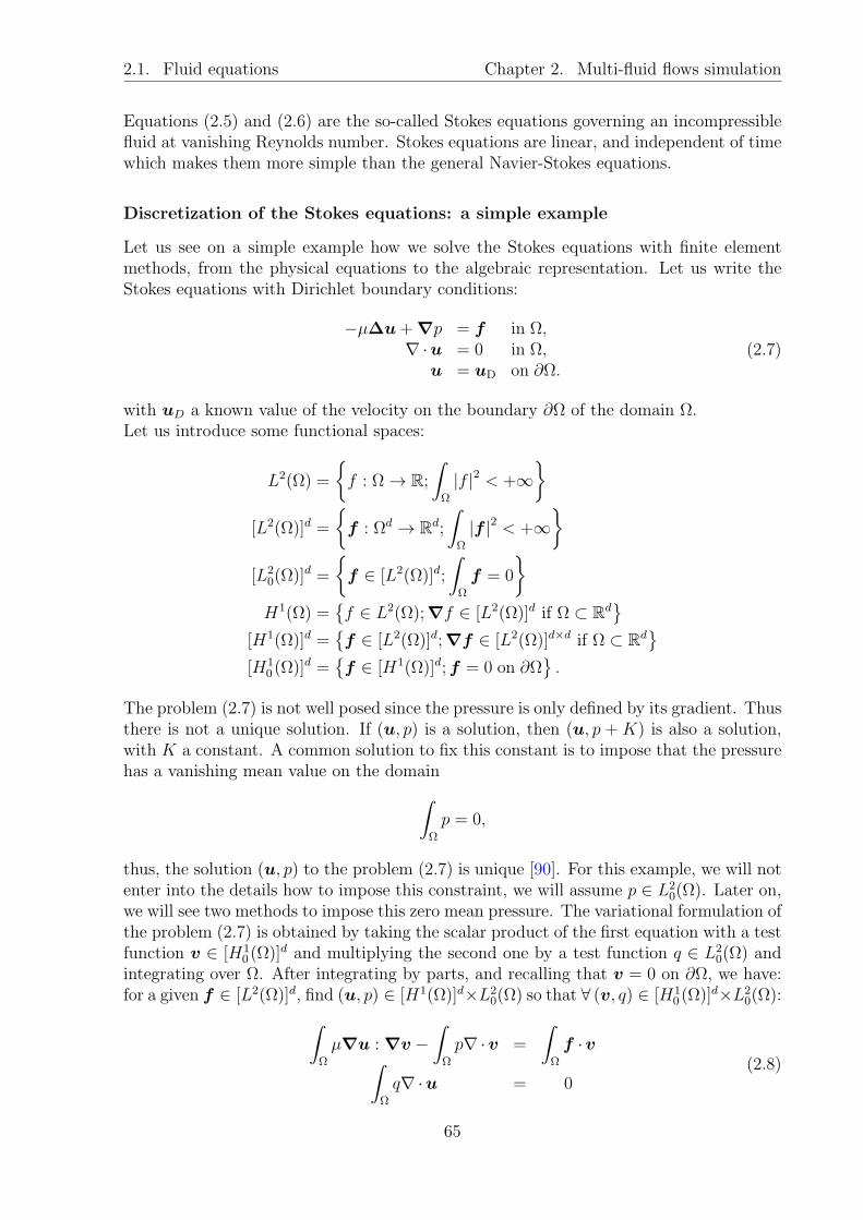
2.1. Fluid equations Chapter 2. Multi-fluid flows simulation
Equations (2.5) and (2.6) are the so-called Stokes equations governing an incompressiblefluid at vanishing Reynolds number. Stokes equations are linear, and independent of timewhich makes them more simple than the general Navier-Stokes equations.
Discretization of the Stokes equations: a simple example
Let us see on a simple example how we solve the Stokes equations with finite elementmethods, from the physical equations to the algebraic representation. Let us write theStokes equations with Dirichlet boundary conditions:
−µ∆u+∇p = f in Ω,∇ ·u = 0 in Ω,
u = uD on ∂Ω.(2.7)
with uD a known value of the velocity on the boundary ∂Ω of the domain Ω.Let us introduce some functional spaces:
L2(Ω) =
f : Ω→ R;
∫
Ω
|f |2 < +∞
[L2(Ω)]d =
f : Ωd → Rd;
∫
Ω
|f |2 < +∞
[L20(Ω)]
d =
f ∈ [L2(Ω)]d;
∫
Ω
f = 0
H1(Ω) =f ∈ L2(Ω);∇f ∈ [L2(Ω)]d if Ω ⊂ Rd
[H1(Ω)]d =f ∈ [L2(Ω)]d;∇f ∈ [L2(Ω)]d×d if Ω ⊂ Rd
[H10 (Ω)]
d =f ∈ [H1(Ω)]d;f = 0 on ∂Ω
.
The problem (2.7) is not well posed since the pressure is only defined by its gradient. Thusthere is not a unique solution. If (u, p) is a solution, then (u, p +K) is also a solution,with K a constant. A common solution to fix this constant is to impose that the pressurehas a vanishing mean value on the domain
∫
Ω
p = 0,
thus, the solution (u, p) to the problem (2.7) is unique [90]. For this example, we will notenter into the details how to impose this constraint, we will assume p ∈ L2
0(Ω). Later on,we will see two methods to impose this zero mean pressure. The variational formulation ofthe problem (2.7) is obtained by taking the scalar product of the first equation with a testfunction v ∈ [H1
0 (Ω)]d and multiplying the second one by a test function q ∈ L2
0(Ω) andintegrating over Ω. After integrating by parts, and recalling that v = 0 on ∂Ω, we have:for a given f ∈ [L2(Ω)]d, find (u, p) ∈ [H1(Ω)]d×L2
0(Ω) so that ∀ (v, q) ∈ [H10 (Ω)]
d×L20(Ω):
∫
Ω
µ∇u : ∇v −∫
Ω
p∇ ·v =
∫
Ω
f ·v∫
Ω
q∇ ·u = 0(2.8)
65

2.1. Fluid equations Chapter 2. Multi-fluid flows simulation
with : the double contraction (see appendix G for details). Let us now introduce the finiteelement spaces:
Un+1h ⊂ [H1(Ω)]d, Un+1
h = wh|wh =
NUhdof∑
i=1
wiΦi
Pnh ⊂ L2(Ω), Pn
h = rh|rh =
NPhdof∑
i=1
riψi
with:
NUh
dof and NPh
dof the total number of degrees of freedom of respectively Un+1h and Pn
h.
Φi and ψi the finite element basis functions, Lagrange polynomials of order n + 1and n.
One can remark that the basis functions associated to the pressure are not constructedwith the null mean constraint. In practice, this constraint is added by Lagrange multiplieror penalty method as we will see in the next section.
It can be proven theoretically that the Stokes equations solved with the formulation(2.9) are not stable if the same polynomial order is used for the velocity and for the pres-sure. These instabilities can be avoided by using the stabilization techniques describedin section 1.1 and adapted to the Stokes problem. We choose another approach whichconsists of using the so-called Taylor-Hood finite element. They are defined by elementswith polynomial approximations of order n for the pressure and n+ 1 for the fluid. Thisexplains our space discretization choice Un+1
h × Pnh. In practice, Lagrange basis functions
are used.
Let us introduce now (uh, ph) ∈ Un+1h × Pn
h and (vh, qh) ∈ Un+1h × Pn
h the discreteversions of (u, p) and (v, q). The problem (2.8) discretized reads now, for a given fh, find(uh, ph) ∈ Un+1
h × Pnh so that ∀ (vh, qh) ∈ Un+1
h × Pnh:
∫
Ω
µ∇uh : ∇vh −∫
Ω
ph∇ ·vh =
∫
Ω
fh ·vh∫
Ω
qh∇ ·uh = 0(2.9)
As the problem (2.9) stands for all (vh, qh), it stands in particular for vh =
NUhdof∑
i=1
Φi and
qi =
NPhdof∑
i=1
ψi the basis functions. Thus we can re-write the problem (2.9) in an algebraic
representation by introducing the matrices
A, Aij =
∫
Ω
µ(∇Φj : ∇Φi),
B, Bij =
∫
Ω
−ψj∇ ·Φi,
66

2.1. Fluid equations Chapter 2. Multi-fluid flows simulation
and the vectors
U, uj
P , pj
F , fj.
The problem (2.9) can be written as(
A BBT 0
)
︸ ︷︷ ︸
D
(UP
)
︸ ︷︷ ︸
U
=
(F0
)
︸ ︷︷ ︸
F
(2.10)
Finally, a sparse problem DU = F is obtained and can be solved numerically.
Impose vanishing mean pressure
The problem (2.7) is not posed correctly because when only Dirichlet boundary conditionsare prescribed on ∂Ω, the pressure is only defined by its gradient and thus exists with aninfinity of possible solutions. The usual solution consists of imposing
∫
Ω
p = 0.
There are two ways to impose this constraint, and both of them are implemented in ourframework. The first method consists of adding a Lagrange multiplier λ to impose theconstraint. The Lagrange multiplier is a single constant since the pressure only needsone constant to fix its value. The pressure no longer belongs to L2
0(Ω) but L2(Ω) sincethe zero mean value constraint is now imposed by λ. The variational formulation readsthen, for a given f ∈ [L2(Ω)]d, find (u, p, λ) ∈ [H1(Ω)]d × L2(Ω)× R so that ∀(v, q, ν) ∈[H1
0 (Ω)]d × L2(Ω)× R:
∫
Ω
µ∇u : ∇v −∫
Ω
p∇ ·v =
∫
Ω
f ·v∫
Ω
q∇ ·u+
∫
Ω
λ q = 0∫
Ω
p ν = 0
(2.11)
The discretizations of (u, p) are the same as in the previous formulation and give (uh, ph) ∈Un+1
h × Pnh. The discretized Lagrange multiplier λh is taken in a space L0
h for which thebasis functions are continuous polynomials of degree 0. That is to say a single constantfor all Ω, this constant is simply 1. Let us name the vector associated to the couplingbetween the pressure and the Lagrange multiplier, which is simply the integral of thebasis functions associated to the pressure:
Sj =
∫
Ω
ψj. (2.12)
The algebraic representation of the discretized problem then reads:
A B 0BT 0 S0 ST 0
UPλh
=
F00
(2.13)
67

2.1. Fluid equations Chapter 2. Multi-fluid flows simulation
The main advantage of this method is that only one degree of freedom is added to thesystem and the constraint is fulfilled exactly. The drawback is that in Feel++ , thechoice to construct the solution U either in a composite space U ∈ Un+1
h × Pnh × L0
h orU ∈ Un+1
h × Pnh has to be made at compilation time. Thus, for a very general application
for which the boundary conditions have to be changed by the user without recompilingthe code, two options remain: i) compile two versions of the code and choose at executiontime the one to run according to the needs. ii) Use a penalty term to impose the zeromean pressure.
Indeed, the second method to impose the zero mean pressure is to add a penalty termto the second equation of (2.7) insuring that the mean value of p is very small. Theweak problem reads, for a given f ∈ [L2(Ω)]d, find (u, p) ∈ [H1(Ω)]d × L2(Ω) so that∀(v, q) ∈ [H1
0 (Ω)]d × L2(Ω):
∫
Ω
µ∇u : ∇v −∫
Ω
p∇ ·v =
∫
Ω
f ·v∫
Ω
q∇ ·u+
∫
Ω
ε p q = 0(2.14)
with ε a small scalar. The corresponding algebraic representation is given by:(
A BBT εId
)(UP
)
=
(F0
)
(2.15)
The advantage of this method is that it does not change the composite space in whichbelongs the solution U . Thus, the choice to impose or not the null mean pressure canbe done automatically in the code without recompiling. As a drawback, the constraintis only imposed approximately whereas it was exact with a Lagrange multiplier. Anadded drawback is that the penalty term deteriorates the matrix conditioning makingthe system more difficult to solve. Finally, the tolerance of the iterative solver used tosolve the algebraic system has to be tuned with respect to the penalty term, which canbe tricky.
Boundary conditions
The boundary conditions have been purposefully left apart previously. Let us now describehow we treat them in our framework. First of all, let us re-write the problem (2.7) byadding both Neumann and Dirichlet boundary conditions. The boundary having Dirichletconditions is called ∂ΩD and the one having Neumann ∂ΩN. The Neumann boundaryconditions for Stokes equations impose the normal stress at the boundary. Thus, wewill re-write (2.7) in a form making appear σ and the strain D. Of course this is notcompulsory, and one can use the form (2.7) and get the same results. The problem reads:
−∇ ·σ = f in Ω,∇ ·u = 0 in Ω,
u = uD on ∂ΩD,σ = σN = −pNId + 2µD(uN) on ∂ΩN.
(2.16)
With uD and σN some known functions on the boundary. One multiplies (2.16) by testfunctions, integrate by parts and remark that ∇v can be replaced by D(v) (see appendix
68
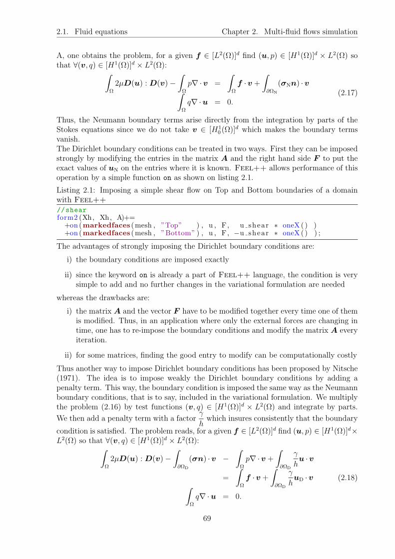
2.1. Fluid equations Chapter 2. Multi-fluid flows simulation
A, one obtains the problem, for a given f ∈ [L2(Ω)]d find (u, p) ∈ [H1(Ω)]d × L2(Ω) sothat ∀(v, q) ∈ [H1(Ω)]d × L2(Ω):
∫
Ω
2µD(u) : D(v)−∫
Ω
p∇ ·v =
∫
Ω
f ·v +
∫
∂ΩN
(σNn) ·v∫
Ω
q∇ ·u = 0.(2.17)
Thus, the Neumann boundary terms arise directly from the integration by parts of theStokes equations since we do not take v ∈ [H1
0 (Ω)]d which makes the boundary terms
vanish.The Dirichlet boundary conditions can be treated in two ways. First they can be imposedstrongly by modifying the entries in the matrix A and the right hand side F to put theexact values of uN on the entries where it is known. Feel++ allows performance of thisoperation by a simple function on as shown on listing 2.1.
Listing 2.1: Imposing a simple shear flow on Top and Bottom boundaries of a domainwith Feel++
//shearform2 (Xh, Xh, A)+=
+on (markedfaces (mesh , ”Top” ) , u , F , u shear ∗ oneX ( ) )+on (markedfaces (mesh , ”Bottom” ) , u , F , −u shear ∗ oneX ( ) ) ;
The advantages of strongly imposing the Dirichlet boundary conditions are:
i) the boundary conditions are imposed exactly
ii) since the keyword on is already a part of Feel++ language, the condition is verysimple to add and no further changes in the variational formulation are needed
whereas the drawbacks are:
i) the matrix A and the vector F have to be modified together every time one of themis modified. Thus, in an application where only the external forces are changing intime, one has to re-impose the boundary conditions and modify the matrix A everyiteration.
ii) for some matrices, finding the good entry to modify can be computationally costly
Thus another way to impose Dirichlet boundary conditions has been proposed by Nitsche(1971). The idea is to impose weakly the Dirichlet boundary conditions by adding apenalty term. This way, the boundary condition is imposed the same way as the Neumannboundary conditions, that is to say, included in the variational formulation. We multiplythe problem (2.16) by test functions (v, q) ∈ [H1(Ω)]d × L2(Ω) and integrate by parts.
We then add a penalty term with a factorγ
hwhich insures consistently that the boundary
condition is satisfied. The problem reads, for a given f ∈ [L2(Ω)]d find (u, p) ∈ [H1(Ω)]d×L2(Ω) so that ∀(v, q) ∈ [H1(Ω)]d × L2(Ω):
∫
Ω
2µD(u) : D(v)−∫
∂ΩD
(σn) ·v −∫
Ω
p∇ ·v +
∫
∂ΩD
γ
hu ·v
=
∫
Ω
f ·v +
∫
∂ΩD
γ
huD ·v
∫
Ω
q∇ ·u = 0.
(2.18)
69

2.1. Fluid equations Chapter 2. Multi-fluid flows simulation
The parameter γ has to be set strong enough to impose correctly the condition and lowenough not to create instabilities. A typical value lies between 1 and 20. The advantagesof this method are
i) in the common case discussed previously where only the vector F changes duringsuccessive iterations, the boundary conditions in the matrix A are set once for allthe simulation
ii) every boundary conditions (Neumann and Dirichlet) can be treated the same way.
The drawbacks are
i) the parameter γ has to be fixed by hand. But the range of γ for which the boundaryconditions are correctly imposed can be quite large and usually a value between 10and 20 is satisfying
ii) the boundary conditions are not imposed exactly. However, the formulation is stillconsistent and optimal convergence rates are still obtained.
2.1.2 Navier-Stokes equations
The Navier-Stokes equation
The Navier-Stokes equations govern fluid motion when neither the viscosity neither theinertia is negligible. We will only deal with the incompressible Navier-Stokes equationswhen the density is constant; hence we deal with incompressible fluid flow. This equationis obtained by writing the momentum conservation:
ρDu
Dt= ∇ ·σ + f (2.19)
where ρ is the density of the fluid. By expressing the stress tensor for a Newtonian fluid,developing the divergence as done previously, and developing the Lagrangian derivativeD
Dt, one obtains:
ρ(∂tu+ (u ·∇)u)− µ∆u+∇p = f , (2.20)
∇ ·u = 0, (2.21)
which are the Navier-Stokes incompressible equations. The framework we used to solvethese equations has been developed by Vincent Chabannes during his PhD [17]. In thissection, we will describe briefly the method used. For more details, the interested readershould see [17].
Temporal discretization
The time is discretized by a time step ∆t so that at iteration n, t = n∆t. The timederivative is discretized by a finite difference scheme of arbitrary high order. We usethe backward differentiation formulation BDF. For a given order q, the BDFq scheme isgiven by:
∂tun+1 ≈ β−1
∆tun+1 −
q−1∑
j=0
βj∆t
un−j. (2.22)
The coefficients βj for BDFq schemes up to order q = 4 are given in the table 2.1.
70

2.1. Fluid equations Chapter 2. Multi-fluid flows simulation
q β−1 β0 β1 β2 β31 1 12 3/2 2 -1/23 11/6 3 -3/2 1/34 25/12 4 -3 4/3 -1/4
Table 2.1: BDFq schemes up to order q = 4
Spatial discretization
The variational formulation is given by find (un+1, pn+1) ∈ [H1(Ω)]d × L2(Ω) so that∀(v, q) ∈ [H1(Ω)]d × L2(Ω):
∫
Ω
ρ∂tun+1 ·v +
∫
Ω
ρ((un+1 ·∇)un+1) ·v −∫
Ω
µ∇un+1 : ∇v
+
∫
Ω
pn+1∇ ·v =
∫
Ω
f ·v, (2.23)∫
Ω
q∇ ·un+1 = 0.
One introduces then (uh, ph) ∈ Un+1h × Pn
h and (vh, qh) ∈ Un+1h × Pn
h the discrete versionsof (u, p) and (v, q) has for equation (2.9). The problem finally reads: find (uh, ph) ∈Un+1
h × Pnh so that ∀(vh, qh) ∈ Un+1
h × Pnh:
∫
Ω
ρ∂tun+1h ·vh +
∫
Ω
ρ((un+1h ·∇)un+1
h ) ·vh−∫
Ω
µ∇un+1h : ∇vh
+
∫
Ω
pn+1h ∇ ·vh =
∫
Ω
f ·vh, (2.24)∫
Ω
qh∇ ·un+1h =0.
One obtains an algebraic representation of (2.24). Once again, the problem (2.24) issolved as one problem, i.e. both equations are solved at the same time. This strategyis called monolithic. The advantage of a monolithic strategy is that the solution fulfillsall the equations at the same time. The drawback is that the algebraic problem can bedifficult to solve numerically. Other ways exist where one splits the equations and solvesthem separately, they are called projection methods [41]. The advantage of projectionmethods is that they are simple to implement and the algebraic problems obtained by thedifferent equations are simpler to solve than the one given by the monolithic method. Thedrawback of projection methods is that at each projection, the solution does not fulfill allthe equations at the same time. In our framework, Navier-Stokes equations are alwayssolved using a monolithic strategy.
Non linear solver
The equation (2.24) is non-linear. A non-linear solver is used to find its solution. Twodifferent non linear solvers are available in the Navier-Stokes framework. A fixed pointmethod and a Newton method. In general, we use the Newton method which requires
71
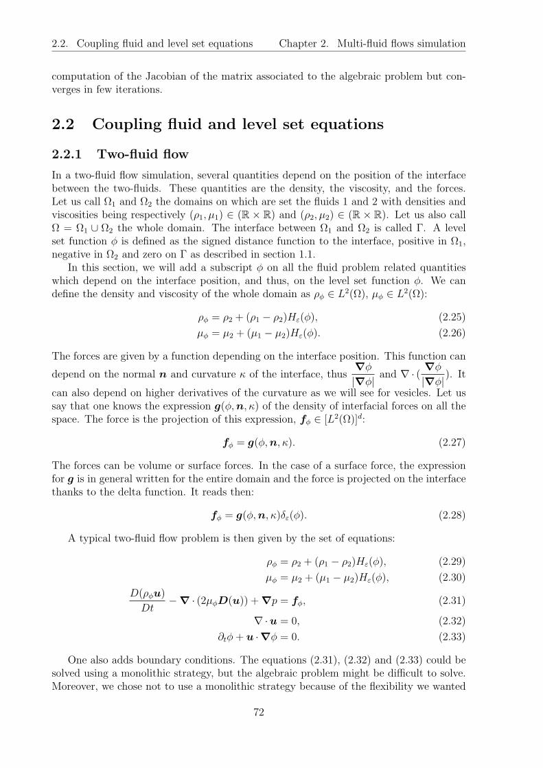
2.2. Coupling fluid and level set equations Chapter 2. Multi-fluid flows simulation
computation of the Jacobian of the matrix associated to the algebraic problem but con-verges in few iterations.
2.2 Coupling fluid and level set equations
2.2.1 Two-fluid flow
In a two-fluid flow simulation, several quantities depend on the position of the interfacebetween the two-fluids. These quantities are the density, the viscosity, and the forces.Let us call Ω1 and Ω2 the domains on which are set the fluids 1 and 2 with densities andviscosities being respectively (ρ1, µ1) ∈ (R × R) and (ρ2, µ2) ∈ (R × R). Let us also callΩ = Ω1 ∪ Ω2 the whole domain. The interface between Ω1 and Ω2 is called Γ. A levelset function φ is defined as the signed distance function to the interface, positive in Ω1,negative in Ω2 and zero on Γ as described in section 1.1.
In this section, we will add a subscript φ on all the fluid problem related quantitieswhich depend on the interface position, and thus, on the level set function φ. We candefine the density and viscosity of the whole domain as ρφ ∈ L2(Ω), µφ ∈ L2(Ω):
ρφ = ρ2 + (ρ1 − ρ2)Hε(φ), (2.25)
µφ = µ2 + (µ1 − µ2)Hε(φ). (2.26)
The forces are given by a function depending on the interface position. This function can
depend on the normal n and curvature κ of the interface, thus∇φ
|∇φ| and ∇ · (∇φ
|∇φ|). It
can also depend on higher derivatives of the curvature as we will see for vesicles. Let ussay that one knows the expression g(φ,n, κ) of the density of interfacial forces on all thespace. The force is the projection of this expression, fφ ∈ [L2(Ω)]d:
fφ = g(φ,n, κ). (2.27)
The forces can be volume or surface forces. In the case of a surface force, the expressionfor g is in general written for the entire domain and the force is projected on the interfacethanks to the delta function. It reads then:
fφ = g(φ,n, κ)δε(φ). (2.28)
A typical two-fluid flow problem is then given by the set of equations:
ρφ = ρ2 + (ρ1 − ρ2)Hε(φ), (2.29)
µφ = µ2 + (µ1 − µ2)Hε(φ), (2.30)
D(ρφu)
Dt−∇ · (2µφD(u)) +∇p = fφ, (2.31)
∇ ·u = 0, (2.32)
∂tφ+ u ·∇φ = 0. (2.33)
One also adds boundary conditions. The equations (2.31), (2.32) and (2.33) could besolved using a monolithic strategy, but the algebraic problem might be difficult to solve.Moreover, we chose not to use a monolithic strategy because of the flexibility we wanted
72

2.2. Coupling fluid and level set equations Chapter 2. Multi-fluid flows simulation
to keep. Indeed, this framework is meant to be very generic, and its goal is to keepindependent as much as possible the level set from the fluid. This way, many fluid modelscould be coupled with the level set framework without much change in the code. Thus,the framework we present decouples the definition of density, viscosity, and forces, thesolution of the Navier-Stokes problem, and the advection of the level set. The associatedalgorithm is given by algorithm 3. One can note that the FluidSolver could be also a
Algorithm 2 Coupling between Fluid solver and Level Set solver.
Require: φ0
φ0 ← φ0
for n = 0 to Ntf do
ρn+1φ = UpdateDensity(φn), eq (2.25)
µn+1φ = UpdateViscosity(φn), eq (2.26)
fn+1φ = UpdateForces(φn,n(φn), κ(φn)), eq (2.27)
(un+1, pn+1) = FluidSolver(ρn+1φ , µn+1
φ ,fn+1φ ), eq (2.31) and (2.32)
φn+1 = AdvectionSolver(un+1), eq (2.33)end for
Stokes solver or another fluid model. The forces can take many forms, volume forces orinterfacial forces. Thus, this strategy is very generic and many models can be tested withit.
2.2.2 Multi-fluid flow
As we have shown previously, one level set field can handle two-fluids. The two-fluids canhave many interfaces but there are still only two different fluids. Some applications mayneed more than only two fluids in the domain. For example, one wants to simulate thebehavior of a mixture of immiscible fluids. For a blood flow purpose, it can be interestingto have two different kind of red blood cells, with some cells very rigid to simulate diseaseslike drepanocitosis. It may also be interesting for a low number of objects, to have a sortof Lagrangian information on each objects. Indeed, in an application where one looks atthe interaction between few vesicles, it can be useful to have the independent informationof the position, velocity, surface and volume of each object which is impossible if only onelevel set is involved. In these cases, it is necessary to define more than one level set field.Each field will define the interface between two fluids. All the level set fields have to beadvected, thus the equation (2.33) has to be solved for each level set field which can becomputationally costly. However, from an implementation point of view, we will see insection 5.4 that many features can be shared between all the level set fields to enhancethe performance of the application, like the matrix associated to the discretized equation(2.33) or the reinitialization framework.In our many-fluid flow, each level set represents the interface between one domain and itsexterior called domain 0. The domain 0 does not need a proper level set since it will bedefined by the area in which there is no level set having a negative value.From a fluid application point of view, one can say that we need to define a level set foreach embedded fluid. The solvent being simply defined by the area in which there is noother fluid. That is to say that for an N fluid flow, we need N − 1 level set fields.
73

2.2. Coupling fluid and level set equations Chapter 2. Multi-fluid flows simulation
Link fluids and level set fields
Let us call NLS the number of level set fields in a multi-fluid application and φ1, ..., φNLS
the different level set fields. We start intentionally the numbering by 1 to keep the number0 for the ambient fluid defined according to the others. We define φ0 in eq (2.34) as beingthe min value of all the other level set fields. This way, φ0 is a field being negative ifone of the other φ is negative, and positive else. This function has also the informationof the positions of all the interfaces and can be used to distribute common values on theinterface or compute general information like the area of the total interfaces.
φ0 = min(φ1, ..., φNLS) (2.34)
The density and viscosity of such a multi-fluid system can be defined by using the factthat the function Hε(φ0) vanishes in the regions where one other fluid is supposed to be.Thus, the value ρ0 and µ0 has to be set in the area where Hε(φ0) = 1. They are definedby:
ρφ = ρ0Hε(φ0) +
NLS∑
i=1
ρi(1−Hε(φi)), (2.35)
µφ = µ0Hε(φ0) +
NLS∑
i=1
µi(1−Hε(φi)). (2.36)
We emphasize the fact that the previous definitions hold for a mixture of immisciblefluids. It can be the case for example of drops of fluids immiscible or any object witha membrane (vesicle, red blood cell, white blood cell, capsule ...). More precisely, thedefinitions hold when the inner domains (φi < 0) are not intersecting which is the casein figure 2.1(a). In the case of an intersection between the inner domains, like in figure2.1(b), the definitions of the density and viscosity cannot be given by equations (2.35)and (2.36). The correct equations have to be given by the physics one wants to express.Anyway, it should not be too difficult since the intersected areas are easy to identifythanks to the sign of the different level set fields.
(a) No intersection between the inner domains ofthe level set fields.
(b) Intersection exists between the inner domainsof the level set fields.
Figure 2.1: Intersection or not of the inner domains of the level set fields in a multi levelset context.
74
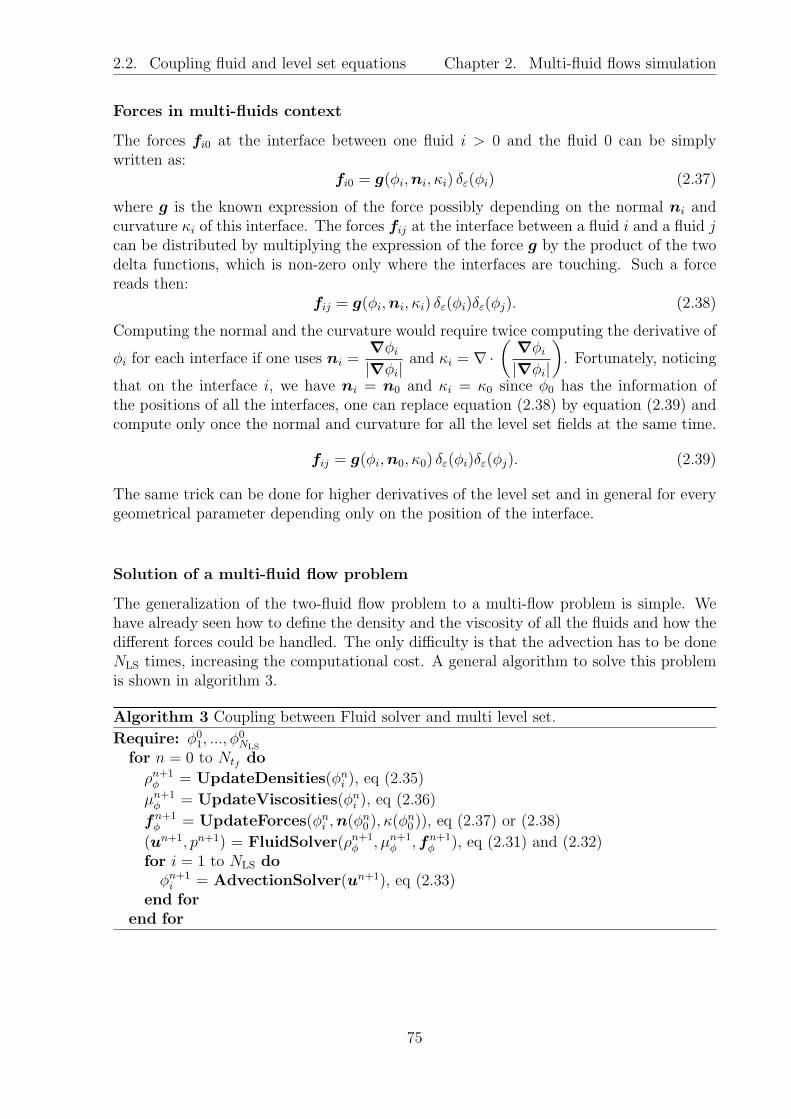
2.2. Coupling fluid and level set equations Chapter 2. Multi-fluid flows simulation
Forces in multi-fluids context
The forces fi0 at the interface between one fluid i > 0 and the fluid 0 can be simplywritten as:
fi0 = g(φi,ni, κi) δε(φi) (2.37)
where g is the known expression of the force possibly depending on the normal ni andcurvature κi of this interface. The forces fij at the interface between a fluid i and a fluid jcan be distributed by multiplying the expression of the force g by the product of the twodelta functions, which is non-zero only where the interfaces are touching. Such a forcereads then:
fij = g(φi,ni, κi) δε(φi)δε(φj). (2.38)
Computing the normal and the curvature would require twice computing the derivative of
φi for each interface if one uses ni =∇φi
|∇φi|and κi = ∇ ·
(∇φi
|∇φi|
)
. Fortunately, noticing
that on the interface i, we have ni = n0 and κi = κ0 since φ0 has the information ofthe positions of all the interfaces, one can replace equation (2.38) by equation (2.39) andcompute only once the normal and curvature for all the level set fields at the same time.
fij = g(φi,n0, κ0) δε(φi)δε(φj). (2.39)
The same trick can be done for higher derivatives of the level set and in general for everygeometrical parameter depending only on the position of the interface.
Solution of a multi-fluid flow problem
The generalization of the two-fluid flow problem to a multi-flow problem is simple. Wehave already seen how to define the density and the viscosity of all the fluids and how thedifferent forces could be handled. The only difficulty is that the advection has to be doneNLS times, increasing the computational cost. A general algorithm to solve this problemis shown in algorithm 3.
Algorithm 3 Coupling between Fluid solver and multi level set.
Require: φ01, ..., φ
0NLS
for n = 0 to Ntf do
ρn+1φ = UpdateDensities(φn
i ), eq (2.35)
µn+1φ = UpdateViscosities(φn
i ), eq (2.36)
fn+1φ = UpdateForces(φn
i ,n(φn0 ), κ(φ
n0 )), eq (2.37) or (2.38)
(un+1, pn+1) = FluidSolver(ρn+1φ , µn+1
φ ,fn+1φ ), eq (2.31) and (2.32)
for i = 1 to NLS doφn+1i = AdvectionSolver(un+1), eq (2.33)
end forend for
75

2.3. Benchmarks and tests Chapter 2. Multi-fluid flows simulation
2.3 Benchmarks and tests
2.3.1 Rising of a bubble in a viscous fluid
We will present a benchmark which has been proposed in [45] and simulates the rising ofa bubble of a viscous fluid in another viscous fluid. This benchmark is a good verificationof the level set code, the Navier-Stokes solver and the coupling between both of them.The Navier-Stokes code that we used has been written and verified by Vincent Chabannesduring his PhD [17]. We will show that we found a good agreement between the resultsof other groups and ours. We published these results in [26].
The benchmark objective is to simulate the rising of a 2D bubble in a Newtonian fluid.The idea is to put a fluid as a bubble in another fluid of a higher density. Both fluidsare initially at rest. Because of the gravity, the bubble having the lower density rises.The equations solved are the incompressible Navier-Stokes equations for the fluid and theadvection for the level set as described in section 2.2. To simulate the rising of a bubble,one adds a gravity force fg and a surface tension force fst defined by:
fg = ρφg (2.40)
fst =
∫
Γ
σκn (2.41)
with g =t (0, 0.98) the gravity acceleration and σ the surface tension. We recall that
n =∇φ
|∇φ| is the normal to the interface and κ = ∇ · ( ∇φ
|∇φ|) is its curvature.The computational domain is Ω×]0, T ] where Ω = (0, 1)×(0, 2) and T = 3. We denote
Ω1 the domain outside the bubble Ω1 = x|φ(x) > 0, Ω2 the domain inside the bubbleΩ2 = x|φ(x) < 0 and Γ the interface Γ = x|φ(x) = 0. On the lateral walls, slipboundary conditions are imposed, i.e. u ·n = 0 and t · (∇u +t∇u) ·n = 0 where n isthe unit normal to the interface and t the unit tangent. No slip boundary conditions areimposed on the horizontal walls i.e. u = 0. The initial bubble is circular with a radiusr0 = 0.25 and centered on the point (0.5, 0.5). The figure 2.2 taken from [45] shows theinitial configuration of the simulation. We denote with indices 1 and 2 the quantitiesrelative to the fluid in respectively in Ω1 and Ω2. The parameters of the benchmark areρ1, ρ2, µ1, µ2 and σ and we define two dimensionless numbers. The first dimensionlessnumber is the Reynolds number which is the ratio between inertial and viscous terms andis defined in this simulation by :
Re =ρ1√
|g|(2r0)3µ1
. (2.42)
The second one, is the Eotvos number which represents the ratio between the gravityforce and the surface tension, it takes the form :
E0 =4ρ1|g|r20
σ. (2.43)
The table 2.2 reports the values of the parameters used for the two different test casesproposed in [45]. The quantities measured are Xc the position of the center of mass of
76

2.3. Benchmarks and tests Chapter 2. Multi-fluid flows simulation
Figure 2.2: Initial configuration taken from [45]. In this notation u = (u, v).
Tests ρ1 ρ2 µ1 µ2 σ Re E0
Test 1 (ellipsoidal bubble) 1000 100 10 1 24.5 35 10Test 2 (squirted bubble) 1000 1 10 0.1 1.96 35 125
Table 2.2: Numerical parameters taken for the benchmarks.
the bubble defined by
Xc =
∫
Ω2
x
∫
Ω2
1=
∫
Ω
x(1−Hε(φ))∫
Ω
(1−Hε(φ)), (2.44)
the velocity of the center of mass Uc :
Uc =
∫
Ω2
u
∫
Ω2
1=
∫
Ω
u(1−Hε(φ))∫
Ω
(1−Hε(φ)), (2.45)
and the circularity defined as the ratio between the perimeter of a circle which has the
77

2.3. Benchmarks and tests Chapter 2. Multi-fluid flows simulation
same area and the perimeter of the bubble :
c =
(
4π
∫
Ω2
1
) 12
∫
Γ
1=
(
4π
∫
Ω
(1−Hε(φ))
) 12
∫
Ω
δε(φ). (2.46)
The results of both test cases are represented in figure 2.3 for test case 1 and in figure2.4 for test case 2. One can see with the arrows and colors that the boundary conditionsare correctly imposed, especially the slip boundary conditions on the left and right sides.Three different groups have done the same benchmark and the results are presented in
[45] and are available online 1. The name of the codes, the institutions and the authors ofthe tests are reported in the table 2.3 taken from [45] in which we added our own code.
Group and affiliation Code/Method
TU Dortmount, Inst. of Applied Math. TP2DS. Turek, D. Kuzmin, S. Hysing FEM-Level Set
EPFL Lausanne, Inst. of Analysis ans Sci. Comp. FreeLIFEE.Burman, N.Parolini FEM-Level Set
Uni. Magdeburg, inst. of Analysis and Num. Math. MooNMDL. Tobiska, S. Ganesan FEM-ALE
Univ. Joseph Fourier, LIPhy. Feel++V.Doyeux, Y.Guyot, V.Chabannes, C.Prud’homme, M.Ismail FEM-Level Set
Table 2.3: Summarize of the different groups having done the benchmark and the methodused.
In the first test case, the energy cost to deform the bubble is strong enough to keep theshape of the bubble close to an ellipsoid. We will call this bubble the ellipsoidal bubble,whereas in the second test, the surface tension is weak and not sufficient to keep the bubblein one piece. The bottom part of the bubble lets appear some squirts, thus, this bubblewill be called the squirted bubble. The quantities Xc and Uc are calculated directly fromFeel++ using the discretized Heaviside function. Whereas the circularity c is calculatedboth by integrating the discretized Dirac function in Feel++ and by post processingusing an interpolation tool of the software Paraview . Both circularity computationmethods give the same results but we only show the post processed one. Indeed it showsalmost no noise since thanks to Paraview we are able to reconstruct an iso 0 level setline by interpolation and integrate over Γ without the use of the delta function whichalways has some thickness. The final shapes of the bubbles are also monitored. We onlyplot the better approximation shape for the comparison. All the groups did not use thesame approximations; the best approximation used for each group is reported in table2.4.
The curves of the shape of the bubble, Xc, Uc and c as functions of time are plotted onthe same graph for different mesh sizes respectively in figures 2.5(a), 2.6(a), 2.7(a), 2.8(a)for the ellipsoidal bubble and 2.9(a), 2.10(a), 2.11(a), 2.12(a) for the squirted bubble.
1http://www.featflow.de/en/benchmarks/cfdbenchmarking/bubble.html
78
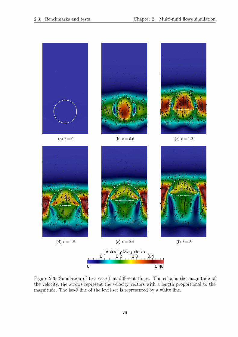
2.3. Benchmarks and tests Chapter 2. Multi-fluid flows simulation
(a) t = 0 (b) t = 0.6 (c) t = 1.2
(d) t = 1.8 (e) t = 2.4 (f) t = 3
Figure 2.3: Simulation of test case 1 at different times. The color is the magnitude ofthe velocity, the arrows represent the velocity vectors with a length proportional to themagnitude. The iso-0 line of the level set is represented by a white line.
79

2.3. Benchmarks and tests Chapter 2. Multi-fluid flows simulation
(a) t = 0 (b) t = 0.6 (c) t = 1.2
(d) t = 1.8 (e) t = 2.4 (f) t = 3
Figure 2.4: Simulation of test case 2 at different times. The color is the magnitude ofthe velocity, the arrows represent the velocity vectors with a length proportional to themagnitude. The iso-0 line of the level set is represented by a white line.
80

2.3. Benchmarks and tests Chapter 2. Multi-fluid flows simulation
Group h Nelt
FEEL++ 0.00625 120174TP2 0.003125 204800
FreeLIFE 0.00625 102400MooNMD 8066
Table 2.4: Summary of the best spatial approximation for all the groups. h is the meshsize and Nelt is the number of elements. MooNMD has no typical mesh size. Since it usedan adaptive mesh, the mean mesh size would not be a representative value.
The same parameters are plotted versus the 3 different group results in figures 2.5(b),2.6(b), 2.7(b), 2.8(b) for the ellipsoidal bubble and 2.9(b), 2.10(b), 2.11(b), 2.12(b) forthe squirted bubble. The curves can be compared by eye. Ones see that all the groupsagree on the ellipsoidal bubble results whereas all groups have varying results for thesquirted bubble. The difference comes from the squirts appearing on the bottom of thebubble which are difficult to resolve. In our case, the squirts are quite large and do notbreak from the bubble, this might be due to the reinitialization frequency set quite high(one reinitialization every 5 time step) which always make the bubble difficult to break.These part having a low velocity, the overall velocity of the bubble is lowered by the largeamount of squirts in our simulation. This explains why our velocity curve in figure 2.11(b)is below the other curves. A more quantitative comparison uses few remarkable pointsthat are quantitatively monitored. The quantitative points that are measured for the firsttest case are cmin the minimum of the circularity, tcmin
the time to attain this minimum,ucmax
the maximum velocity, tucmaxthe time to reach it, and yc(t = 3) the position of the
bubble at final time (t = 3).
For the second test, we monitor the same quantities and add the second maximumvelocity ucmax2
, and the time to reach it tucmax2. The simulations are run for different mesh
sizes and the benchmark quantities are reported in table 2.5 for the first case and table 2.6for the second case with, for reference, the max and min values found by the groups in [45].
h cmin tcminucmax
tucmaxyc(t = 3)
lower bound 0.9011 1.8750 0.2417 0.9213 1.0799upper bound 0.9013 1.9041 0.2421 0.9313 1.0817
0.02 0.8981 1.925 0.2400 0.9280 1.07870.01 0.8999 1.9 0.2410 0.9252 1.0812
0.00875 0.89998 1.9 0.2410 0.9259 1.08140.0075 0.9001 1.9 0.2412 0.9251 1.08120.00625 0.9001 1.9 0.2412 0.9248 1.0815
Table 2.5: Results comparison between benchmark values (lower and upper bounds) andours for the ellipsoidal bubble.
81

2.3. Benchmarks and tests Chapter 2. Multi-fluid flows simulation
h cmin tcminucmax1
tucmax1ucmax2
tucmax2yc(t = 3)
lower bound 0.4647 2.4004 0.2502 0.7281 0.2393 1.9844 1.1249upper bound 0.5869 3.0000 0.2524 0.7332 0.2440 2.0705 1.1380
0.02 0.4744 2.995 0.2464 0.7529 0.2207 1.8319 1.08100.01 0.4642 2.995 0.2493 0.7559 0.2315 1.8522 1.1012
0.00875 0.4629 2.995 0.2494 0.7565 0.2324 1.8622 1.10470.0075 0.4646 2.995 0.2495 0.7574 0.2333 1.8739 1.11110.00625 0.4616 2.995 0.2496 0.7574 0.2341 1.8828 1.1186
Table 2.6: Results comparison between benchmark values (lower and upper bounds) andours for the squirted bubble
(a) Comparison of different mesh sizes.
0.0 0.2 0.4 0.6 0.8 1.0
Y
0.7
0.8
0.9
1.0
1.1
1.2
1.3
X
FEEL++
FreeLIFE
TP2D
MooNMD
(b) Comparison with other codes.
Figure 2.5: Final shape (t = 3) of the ellipsoidal bubble.
0.0 0.5 1.0 1.5 2.0 2.5 3.0
t
0.5
0.6
0.7
0.8
0.9
1.0
1.1
y c
h = 0.02
h = 0.01
h = 0.00875
h = 0.0075
h = 0.00625
(a) Comparison of different mesh sizes.
0.0 0.5 1.0 1.5 2.0 2.5 3.0
t
0.5
0.6
0.7
0.8
0.9
1.0
1.1
y c
FEEL++
FreeLIFE
TP2D
MooNMD
(b) Comparison with other codes.
Figure 2.6: y position of the ellipsoidal bubble versus time.
82

2.3. Benchmarks and tests Chapter 2. Multi-fluid flows simulation
0.0 0.5 1.0 1.5 2.0 2.5 3.0
t
0.00
0.05
0.10
0.15
0.20
Uy
h = 0.02
h = 0.01
h = 0.00875
h = 0.0075
h = 0.00625
(a) Comparison of different mesh sizes.
0.0 0.5 1.0 1.5 2.0 2.5 3.0
t
0.00
0.05
0.10
0.15
0.20
Uy
FEEL++
FreeLIFE
TP2D
MooNMD
(b) Comparison with other codes.
Figure 2.7: Velocity magnitude the ellipsoidal bubble versus time
0.0 0.5 1.0 1.5 2.0 2.5 3.0
t
0.90
0.92
0.94
0.96
0.98
1.00
c
h = 0.02
h = 0.01
h = 0.00875
h = 0.0075
h = 0.00625
(a) Comparison of different mesh sizes.
0.0 0.5 1.0 1.5 2.0 2.5 3.0
t
0.90
0.92
0.94
0.96
0.98
1.00
cFEEL++
FreeLIFE
TP2D
MooNMD
(b) Comparison with other codes.
Figure 2.8: Circularity of the ellipsoidal bubble versus time
(a) Comparison of different mesh sizes.
0.0 0.2 0.4 0.6 0.8 1.0
Y
0.6
0.7
0.8
0.9
1.0
1.1
1.2
1.3
1.4
X
FEEL++
FreeLIFE
TP2D
MooNMD
(b) Comparison with other codes.
Figure 2.9: Final shape (t = 3) of the squirted bubble.
83

2.3. Benchmarks and tests Chapter 2. Multi-fluid flows simulation
0.0 0.5 1.0 1.5 2.0 2.5 3.0
t
0.5
0.6
0.7
0.8
0.9
1.0
1.1
1.2
y c
h = 0.02
h = 0.01
h = 0.00875
h = 0.0075
h = 0.00625
(a) Comparison of different mesh sizes.
0.0 0.5 1.0 1.5 2.0 2.5 3.0
t
0.5
0.6
0.7
0.8
0.9
1.0
1.1
1.2
y c
FEEL++
FreeLIFE
TP2D
MooNMD
(b) Comparison with other codes.
Figure 2.10: y position of the squirted bubble versus time.
0.0 0.5 1.0 1.5 2.0 2.5 3.0
t
0.00
0.05
0.10
0.15
0.20
0.25
Uy
h = 0.02
h = 0.01
h = 0.00875
h = 0.0075
h = 0.00625
(a) Comparison of different mesh sizes.
0.0 0.5 1.0 1.5 2.0 2.5 3.0
t
0.00
0.05
0.10
0.15
0.20
0.25
Uy
FEEL++
FreeLIFE
TP2D
MooNMD
(b) Comparison with other codes.
Figure 2.11: Velocity magnitude the squirted bubble versus time
0.0 0.5 1.0 1.5 2.0 2.5 3.0
t
0.5
0.6
0.7
0.8
0.9
1.0
c
h = 0.02
h = 0.01
h = 0.00875
h = 0.0075
h = 0.00625
(a) Comparison of different mesh sizes.
0.0 0.5 1.0 1.5 2.0 2.5 3.0
t
0.5
0.6
0.7
0.8
0.9
1.0
c
FEEL++
FreeLIFE
TP2D
MooNMD
(b) Comparison with other codes.
Figure 2.12: Circularity of the squirted bubble versus time
84

2.3. Benchmarks and tests Chapter 2. Multi-fluid flows simulation
2.3.2 Rising of different fluid bubbles
This test is made to test the method described in section 2.2.2 in which one uses manylevel set fields to describe different fluids flowing in the domain. It consists of having8 bubbles of fluids with different densities rising in another fluid. It is inspired by thebenchmark presented in section 2.3.1, the bubbles are set in a fluid at rest and rise bygravity. We denote with a subscript number, the quantities related to the different fluids.The subscript 0 is kept for the surrounding fluid, which is not defined by a negative valueof its own level set, but by the area where all the other level sets are not negative, asexplained in section 2.2.2. The gravity force is given by :
fg =
(
ρ0Hε(φ0) +8∑
i=1
ρi(1−Hε(φi))
)
g (2.47)
with g =t (0, 0.98) the gravity acceleration.The surface tension force is naturally given by the sum of the surface tension forces
acting on all the interfaces :
fst =8∑
i=0
8∑
j>i
∫
Γij
σij κij nij (2.48)
with Γij the interface between fluid i and fluid j, κij and nij the curvature and normalrelated to this interface. As already explained in section 2.2.2 with the equation (2.37),the interface between the ambient fluid and any other fluid can be handled by :
∫
Γ0i
1 ≈∫
Ω
δε(φi), with i > 0 (2.49)
and the interface between the other fluids is handled by the equation (2.38) that is to say∫
Γij
1 ≈∫
Ω
δε(φi)δε(φj) with i > 0 and j > i. (2.50)
The surface tension σij is an intrinsic property related to the interaction between twofluids (i and j). Consequently, the case of each fluid i interacting with any other fluid jby surface tension should be considered and all the σij should be set. Of course σij = σji,this would make 36 different surface tensions to handle. There is no methodologicalproblem to handle this, but for the sake of simplicity, in this particular application, wewill only deal with the interaction with the surrounding fluid 0. Indeed, we allow a spacebetween the bubbles large enough so that the bubbles do not touch each other. Thus, theonly surface tensions to handle are σ0i with i = (1, ..., 8). Since only the interactions withinterface 0 are considered, there is no ambiguity and the subscript 0 can be omitted. Inwhat follows, we will denote Γi, κi, ni, σi the quantities Γ0i, κ0i, n0i, σ0i. The surfacetension reads then :
fst =8∑
i=1
∫
Ω
σi κi ni δε(φi) =8∑
i=1
∫
Ω
σi κ(φi)n(φi) δε(φi). (2.51)
The quantities ni and κi could be naturally calculated using ni = n(φi) and κi = κ(φi).But an improvement is made recalling that φ0 = min(φ1, ..., φ8) contains the information
85

2.3. Benchmarks and tests Chapter 2. Multi-fluid flows simulation
of the positions of all the interfaces at the same time. Thus n(φ0) has the same value asn(φi) on the interface i. Hence the following equality stands :
∫
Ω
n(φi)δε(φi) =
∫
Ω
n(φ0)δε(φi) for all 1 < i < 8. (2.52)
The equivalent for κi is also true. The equality (2.52) is important when one recalls thatone needs to differentiate the level set function to get the normal and differentiate onemore time to get the curvature. Thus, for each time step, one can calculate n(φ0) andκ(φ0) and economize the computing of 8 derivatives of the fields φi and 8 derivatives ofni. The expression of the force becomes :
fst =8∑
i=1
∫
Ω
σi κ(φ0)n(φ0) δε(φi)
fst =8∑
i=1
∫
Ω
σi∇ ·(
∇φ0
|∇φ0|
)∇φ0
|∇φ0|δε(φi) (2.53)
The equation (2.53) is the form of the surface tension force used in this test.The computational domain is Ω×]0, T [ with Ω = (0, 8) × (0, 2) and T = 4.5. On the
lateral walls, slip boundary conditions are imposed, u ·n = 0 and t · (∇u +t∇u) ·n = 0where n is the unit normal to the interface and t the unit tangent. No slip boundaryconditions are imposed on the horizontal bottom wall, u = 0. And Neumann homogeneousboundary conditions are imposed on the horizontal top wall, σ ·n = 0. The initialparameters given for each bubble are reported in table 2.7 and a scheme of the initialconfiguration is given in figure 2.13. The parameters of the fluids for the bubbles are
Bubble 1 2 3 4 5 6 7 8r0 0.25 0.25 0.25 0.25 0.25 0.25 0.25 0.25x0 0.5 1.5 2.5 3.5 4.5 5.5 6.5 7.5y0 0.5 0.5 0.5 0.5 0.5 0.5 0.5 0.5σ 50 50 50 50 50 50 50 50µ 1 1 1 1 1 1 1 1ρ 800 700 600 500 400 300 200 100
Table 2.7: Initial parameters given for the 8 bubbles, r0 being the radius, (x0, y0) theinitial position, σ the surface tension with the surrounding fluid, µ the viscosity, and ρthe density.
identical except the density. This makes the bubbles rise at different velocities. The localReynolds number for a single bubble varies slightly since the densities and the velocities ofeach bubble are different, but all of them are of the same order. The quantities monitoredare the same as for the benchmark presented in section 2.3.1, that is to say the center ofmass Xc (and in particular its y component yc), the mean velocity Uc and the circularityc given by respectively equations (2.44), (2.45) and (2.46). The simulation has been runon the super computer SuperMUC on 10 processors. The time step was set to dt = 0.01,the final time to 4.5 and the mesh size to h = 0.03. With this mesh size, the number ofelements in the mesh was 41902, and all simulations lasted 50 minutes. This makes one
86

2.3. Benchmarks and tests Chapter 2. Multi-fluid flows simulation
Figure 2.13: Initial geometry, boundary conditions and densities of the different bubbles.
total iteration last for about 7 seconds. The figure 2.14 shows the colored results for 4different times. The densities of the bubbles decrease from the left to the right. Thusthe first bubble moves very slowly compared to the last one. The color on backgroundrepresents the velocity magnitude of the fluid. One sees that as for the single bubble,the velocity is the highest on the sides of the bubbles where the fluid is pushed down.In figure 2.15 we have plotted the position of the center of mass of the bubbles as afunction of time. As we can see, the shapes seem similar to the single bubble. We cansee clearly a difference between all the bubbles, which attains a higher position for thelower density ones as expected. We can add that due to the other bubbles, the system isnot symmetrical in the x direction at the opposite of the single bubble simulation, andthis symmetry breaking induces a movement of the center of mass of the bubble in the xdirection. The figure 2.16 shows the velocities of the center of mass of the bubbles. Thefastest bubble is the bubble 8, its velocity attains a maximum, then, decreases to a localminimum and finally increases again. The bubbles 7, 6, 5 follow almost the same behaviorthan the single bubbles, being that the velocity increases quickly and attains a maximumthen decreases and finally increases again to attain a second maximum. The bubbles 4,3, 2, and 1 have a velocity increasing to attain a kind of plateau, the maximum velocityattained is smaller for the higher densities. Finally the figure 2.17 shows the circularitiesof the bubbles. The circularities show a noise which is approximately of the order ofmagnitude of the mesh. This is due to the fact that for this simulation, the circularityis computed directly by integrating the perimeter and the surface of the bubbles on themesh without any post processing. Thus, the perimeter being very sensitive to the meshsize, the circularities show a bigger noise that the one post processed in the previoussection. We recall that one advantage of using a multi-level set method is that it ispossible to do such a computation directly in the simulation. Computing the circularityof many interfaces with only one level set is not possible in general since there is no wayto differentiate the interfaces. We can see that the bubbles 8 to 4 show the same behavioras the single bubble with local variation stronger for the lower density bubbles. This canbe explained by the fact that, this bubble going faster, the hydrodynamical forces actingon it are stronger and thus lead to more deformation. Finally, the higher density bubblesshow weak deformations which can be directly seen on the graph since the circularity isroughly unchanged.
87

2.3. Benchmarks and tests Chapter 2. Multi-fluid flows simulation
(a) t = 0.2
(b) t = 1.6
(c) t = 3
(d) t = 4.5
Figure 2.14: Rising of 8 bubbles of different fluids. Velocity magnitude |u| is representedin color outside the bubbles. The bubbles are colored by their density ρ.
88

2.3. Benchmarks and tests Chapter 2. Multi-fluid flows simulation
0.0 0.5 1.0 1.5 2.0 2.5 3.0 3.5 4.0 4.5
t
0.4
0.6
0.8
1.0
1.2
1.4
1.6
1.8
y c
ρ8 = 100
ρ7 = 200
ρ6 = 300
ρ5 = 400
ρ4 = 500
ρ3 = 600
ρ2 = 700
ρ1 = 800
Figure 2.15: Position of each bubble as a function of time.
0.0 0.5 1.0 1.5 2.0 2.5 3.0 3.5 4.0 4.5
t
0.00
0.05
0.10
0.15
0.20
0.25
0.30
0.35
Uy
ρ8 = 100
ρ7 = 200
ρ6 = 300
ρ5 = 400
ρ4 = 500
ρ3 = 600
ρ2 = 700
ρ1 = 800
Figure 2.16: Velocity of each bubble as a function of time.
0.0 0.5 1.0 1.5 2.0 2.5 3.0 3.5 4.0 4.5
t
0.92
0.93
0.94
0.95
0.96
0.97
0.98
0.99
1.00
1.01
c
ρ8 = 100
ρ7 = 200
ρ6 = 300
ρ5 = 400
ρ4 = 500
ρ3 = 600
ρ2 = 700
ρ1 = 800
Figure 2.17: Circularity of each bubble as a function of time.
89

2.4. Oscillations of a bubble Chapter 2. Multi-fluid flows simulation
2.4 Oscillations of a bubble in a fluid at rest
2.4.1 Motivation
A validation of our code has been suggested to us by Philippe Marmottant and OlivierVincent, experimental physicists in our laboratory. In the context of his PhD, OlivierVincent [111] studied the cavitation of a bubble in a hydrogel. His experimental subjectwas composed of a hydrogel with many holes in it, these holes are called inclusions. Theseinclusions are filled with water. The hydrogel is then dried letting the water evaporateslowly toward the exterior of the inclusions. The water is then under tension, its pressureis strongly negative, that is to say that it pulls on the walls of the inclusions. At somepressure, a bubble forms very quickly, the pressure relaxes to a positive value. It is thecavitation phenomenon. The bubble formation is done in two different steps: i) the bubblesize increases very quickly and compresses the fluid and the hydrogel. The Reynoldsnumber of this step is relatively high (Re ∼ 100). The initially empty bubble is filled withvapor. ii) In the second step, the bubble is formed but its shape is out of equilibrium.It oscillates around its equilibrium shape. The oscillations come from the surface tensionwhich exists between the vapor and the liquid water. The Reynolds number of this stepis lower (Re ∼ 5), the fluid can be considered as incompressible. We were interestedin reproducing this last phenomenon. The oscillation frequency of a bubble in a fluidis known theoretically since 1932 by Lamb [64]. It depends on the surface tension, thedensities and the effective radius of the bubble. When Olivier Vincent compared hisexperimental data to the theoretical ones, he showed that an effective surface tensionof about 30% lower than the one given for the water fitted well his data. Two mainexplanations were possible for that. The first one is that some chemical contaminationcould have happened during the polymerization of the hydrogel, which could have changedthe surface tension of the solvent. The second one is that the confinement could have animpact on the oscillation frequency of the drops. It is this last point that we tried to figureout with our simulations. Indeed, the Lamb theory has been made with the assumptionthat the drop is in an infinite fluid. The goal of this study was to see if there exists astrong influence of the confinement on the oscillation frequency of the bubble. As wewill see, our simulations have shown that the Lamb theory still holds even in a confineddomain. Indeed, we have recovered the Lamb frequency with a good precision evenwith our strongest confinement. Consequently, as a first conclusion we can say that theinfluence of the confinement on the oscillation frequency of a bubble is relatively small.The second conclusion is that since we are able to recover the theoretical frequency of theoscillation, this test was a good validation for our model of two fluid flow. A similar testhas already been done to validate a two fluid flow system with level set method [81].
2.4.2 Description of the simulation
Let us define a circular domain Ω, the fluid and the pressure are governed by the Navier-Stokes equations. No gravity force is added to the system. The only force added in theright hand side of the Navier Stokes equations is the surface tension force given by:
FSurfTens =
∫
Ω
σκnδε (2.54)
90

2.4. Oscillations of a bubble Chapter 2. Multi-fluid flows simulation
where σ is the surface tension between the two fluids. No-slip boundary conditions areadded on the boundary of Ω. The bubble is initially at the center of the domain with-out any initial velocity. The initial shape given to the bubble is an ellipse. The non-dimensional characteristic numbers for this flow are the Reynolds number:
Re =ρUL
µ
and the Weber number:
We =ρU2L
σ(2.55)
which characterizes the relative importance of the inertia on the surface tension. Ex-perimentally, the rigid inclusion size is of the order of 40 µm, the size of a bubble isabout 10 µm. The densities of the liquid water and vapor at the experimental conditionsare respectively ρ1 = 103 kg/m3 and ρ2 = 2× 10⁻² kg/m3, the viscosities are given byµ1 = 10−3 Pa · s and µ2 = 2× 10⁻² Pa · s. The surface tension between the two waterphases is σ = 70× 10−3 N/m. For this experiment, the Reynolds and Weber numbershave been estimated as Re ∼ 5 andWe ∈ [0.3, 2]. The numerical parameters are simplifiedto ease the numerical simulation and to see a good number of oscillations in a short time.We choose ρ1 = 10, ρ2 = 103, µ1 = µ2 = 1. The surface tension is σ = 12.5. The area istaken as A = 4.87. The effective radius R0 is defined as the radius of a circle having the
same area as the bubble, R0 =
√
A
π= 0.775. With these parameters, the Weber number
is estimated to We = 1.4 and the Reynolds number to Re = 100. The Reynolds number istaken larger than the experimental one to be able to see many oscillations in a reasonabletime. If it is taken too low, the oscillations are overly damped and the frequency is difficultto measure. The domain radius has been taken to the following values RΩ = [2, 4, 6, 8],
giving a confinement Cn =RΩ
R0
of respectively
[1
2,1
4,1
6,1
8
]
.
2.4.3 Results
The shapes that the bubbles take during their oscillations are represented in figure 2.18.The resolution of the experiments being done in our lab cannot give us the clear shapeof the bubble. Nevertheless, Apfel et al. [2] did picture these shapes during a microgravity experiment led in the Columbia space shuttle. In this experiment, the bubbleshave been excited with an acoustic field, giving them a non equilibrium shape. Afterstopping the acoustic field, the bubbles did oscillate around their equilibrium shapes asin our simulations. In the same paper, some simulations by boundary integral methodare compared to experiments. The results of these experiments and simulations are givenin figure 2.19. The Reynolds number for these simulations is 600. One can see that werecover correctly the experimental shapes in our own simulations, even if the Reynoldsnumber is 6 times lower. The only shape that we can not recover is the 8 shape at time3.05 in figure 2.19 which needs a high Reynolds number.
The oscillation frequency of a bubble has been given by Lamb in 1932 [64] for a 3Dbubble in an infinite fluid. Later, the oscillation frequency of an infinite cylinder in thez direction under surface tension has been given by Chandrasekhar [19]. The oscillation
91

2.4. Oscillations of a bubble Chapter 2. Multi-fluid flows simulation
Figure 2.18: Our simulation of the shape oscillations of a bubble during time. Theconfinement is 1
2and we have taken Re = 50, We = 1. Only half a period is represented
since the following shapes are of the same type with different amplitudes.
frequency ωn of a mode n is given by:
ω2n = n(n− 1)(n+ 1)
σ
ρ1R3(2.56)
where R is the radius of the bubble at equilibrium. The excited mode in our simulation isn = 2. The theoretical frequency that we obtain with the numerical parameters we usedis w2 = 0.40.The simulations have been carried out on 6 processors. The mesh sizes have been takento 0.135 away from the bubble and to 0.045 around and inside it. The time step is takento 0.025. The reinitialization has been done by solving the Hamilton Jacobi equationpresented in section 1.3.3 every 5 iterations. To measure the frequency of the oscillations,we choose to measure ylength the y long axis of the bubble. That is to say, the length of thebubble in the y direction at the center of the bubble. At equilibrium, this is equal to thediameter. Out of equilibrium, it oscillates around this value. We then do a fit of ylength(t).For this fit, we use a model of damped oscillation for which we add a corrective termaccounting for the loss of area due to the reinitialization of the level set. We modeled theloss of area by a linear loss of perimeter in time. At the end of the simulation, around 1%of the total mass has been lost, which is an acceptable result when taking into accounthow long last the simulation in time. The fits are done by the mean square method
92

2.4. Oscillations of a bubble Chapter 2. Multi-fluid flows simulation
Figure 2.19: Figure taken from [2]. The first line represents the oscillation shape simula-tion of a bubble with an integral boundary method for a Reynolds number of 600. Thetwo other lines are the views from two different axes of the oscillations of a bubble in themicro gravity experiment.
implemented in MINPACK 2 and interfaced by scipy 3 [51] that we used as a black box.The formula used has been given by:
ylength = a sin(ωt+ ψ)e−tτ − 2R0 − bt (2.57)
where a is the amplitude of the oscillations, ω the frequency we are seek, τ a character-istic time and b accounts for the loss of mass. The whole equation has subtracted theequilibrium value 2R0. The figure 2.20 represents the oscillations of ylength as a function oftime. The curves with the parameters taken from the fit are represented as dashed lines.An offset is given to each curve so that we can plot them all on the same graph. Table 2.8gives the values of the fit parameters for all the curves of figure 2.20. It turns out that the
Cn a ω τ b1/2 0.86 0.40 54 0.00141/4 0.81 0.40 61 0.00131/6 0.79 0.40 62 0.00131/8 0.78 0.42 57 0.0018
Table 2.8: Parameters taken from the fit of the simulation curves with the model equation2.57.
frequency is equal to the theoretical frequency up to the second decimal for the three firstbubbles. The bubble with the lowest confinement has a slightly higher value, but it canbe explained by the fact that the error for this simulation is also slightly higher than theother ones. Indeed, the value of the linear loss of area is much higher for this simulation
2 http://www.netlib.org/minpack3 http://www.scipy.org
93

2.4. Oscillations of a bubble Chapter 2. Multi-fluid flows simulation
40 60 80 100 120 140time
0.0
0.5
1.0
1.5
2.0
2.5
3.0
3.5
y−
len
gth
c = 12
c = 14
c = 16
c = 18
Figure 2.20: Results of the simulations of the oscillation of a drop around its equilibriumposition for different confinements. The parameter being monitored, ylength is the lengthof the y axis of the bubble. An offset is added to each curve for the sake of visibility. Thedashed lines are the curves of equation (2.57) with the parameters obtained from the fitof the simulation curves. The first period of the oscillations has been cut to see the actualoscillations without the initial excitation.
than the others. Anyway, in the experiments, a surface tension about 30% higher thanthe theoretical one is observed. If we compute how important should be the frequencygap with the theoretical one in our simulation to get the same percentage difference, wefound that the frequency difference ∆ω = ω − ωth should be of the order of 0.1. Thuswe can say that we do not see a significant effect of the confinement on the oscillationfrequency and that the Lamb formula still holds at such confinements. Moreover, thetheoretical frequency is obtained with a good accuracy and this simulation was a goodvalidation of our two-fluid flow framework.
94

Chapter 3
Simulation of solid objects in flow
Contents3.1 Existing methods . . . . . . . . . . . . . . . . . . . . . . . . . . 96
3.2 FPD and penalty methods . . . . . . . . . . . . . . . . . . . . . 99
3.2.1 A similar formulation for FPD and penalty method . . . . . . 99
3.2.2 Particle motion in FPD/penalty methods . . . . . . . . . . . . 101
3.3 FPD in Level set framework . . . . . . . . . . . . . . . . . . . . 102
95
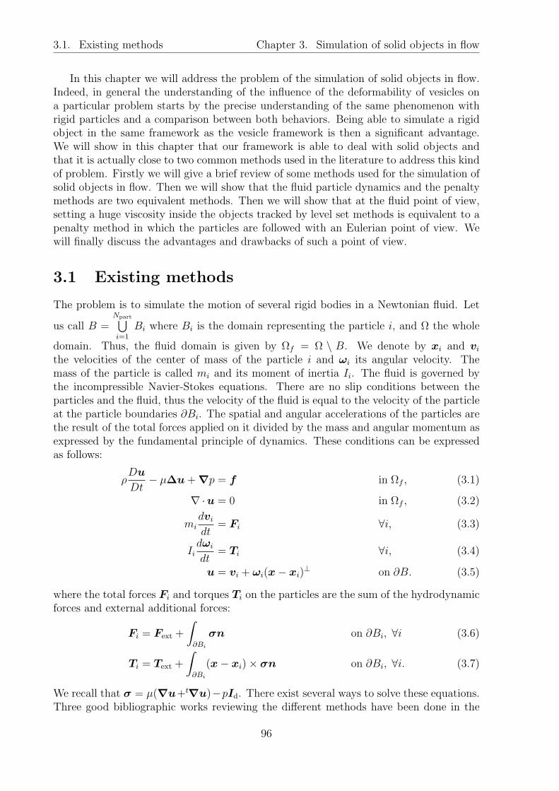
3.1. Existing methods Chapter 3. Simulation of solid objects in flow
In this chapter we will address the problem of the simulation of solid objects in flow.Indeed, in general the understanding of the influence of the deformability of vesicles ona particular problem starts by the precise understanding of the same phenomenon withrigid particles and a comparison between both behaviors. Being able to simulate a rigidobject in the same framework as the vesicle framework is then a significant advantage.We will show in this chapter that our framework is able to deal with solid objects andthat it is actually close to two common methods used in the literature to address this kindof problem. Firstly we will give a brief review of some methods used for the simulation ofsolid objects in flow. Then we will show that the fluid particle dynamics and the penaltymethods are two equivalent methods. Then we will show that at the fluid point of view,setting a huge viscosity inside the objects tracked by level set methods is equivalent to apenalty method in which the particles are followed with an Eulerian point of view. Wewill finally discuss the advantages and drawbacks of such a point of view.
3.1 Existing methods
The problem is to simulate the motion of several rigid bodies in a Newtonian fluid. Let
us call B =Npart⋃
i=1
Bi where Bi is the domain representing the particle i, and Ω the whole
domain. Thus, the fluid domain is given by Ωf = Ω \ B. We denote by xi and vi
the velocities of the center of mass of the particle i and ωi its angular velocity. Themass of the particle is called mi and its moment of inertia Ii. The fluid is governed bythe incompressible Navier-Stokes equations. There are no slip conditions between theparticles and the fluid, thus the velocity of the fluid is equal to the velocity of the particleat the particle boundaries ∂Bi. The spatial and angular accelerations of the particles arethe result of the total forces applied on it divided by the mass and angular momentum asexpressed by the fundamental principle of dynamics. These conditions can be expressedas follows:
ρDu
Dt− µ∆u+∇p = f in Ωf , (3.1)
∇ ·u = 0 in Ωf , (3.2)
midvi
dt= Fi ∀i, (3.3)
Iidωi
dt= Ti ∀i, (3.4)
u = vi + ωi(x− xi)⊥ on ∂B. (3.5)
where the total forces Fi and torques Ti on the particles are the sum of the hydrodynamicforces and external additional forces:
Fi = Fext +
∫
∂Bi
σn on ∂Bi, ∀i (3.6)
Ti = Text +
∫
∂Bi
(x− xi)× σn on ∂Bi, ∀i. (3.7)
We recall that σ = µ(∇u+t∇u)−pId. There exist several ways to solve these equations.
Three good bibliographic works reviewing the different methods have been done in the
96

3.1. Existing methods Chapter 3. Simulation of solid objects in flow
PhD theses [46, 66] and [32] (all in french). We will name briefly the main methods beforecomparing the penalty and fluid particle dynamic methods.
The conform methods
The simplest method to solve this problem is to create a conforming mesh to the domainΩf , in which the domains Bi are represented as holes in Ωf . The velocities vi andpositions xi are defined independently of the mesh. The equations (3.1) and (3.2) with thecondition (3.5) are solved on the mesh by a PDE solver. Then the velocities and positionsare updated solving the equations (3.3) and (3.4). The domain is finally re-meshed toconform to the new positions xi and the loop is closed. A simple implementation of such amethod is made with the software FreeFem++ in appendix D. This method suffers fromseveral issues. Indeed, the re-meshing procedure can be computationally costly. Moreover,if one actually solves the Navier-Stokes equations, the solution to the previous iterationis needed at the current iteration. The problem is that the previous solution belongsto a different mesh and a projection procedure has to be employed which induces someerror. An alternative to the systematic re-meshing is to move slightly the points of themesh around the particles to their new positions. These methods are called ArbitraryLagrangian Eulerian methods. This way, since the displacement of the mesh is not toohigh, the re-meshing procedure can be avoided. Such a method is used for example in[50] and an implementation of an ALE method for Feel++ has been done by VincentChabannes during his PhD [17].
Fictitious domain methods
The fictitious domain methods are a set of methods in which the fluid is defined onall the space Ω which is a domain larger than Ωf but simpler. A rigid body constraintis applied to the fluid on the space which belongs to the particles. These methods havethe advantage of not having to handle a changing mesh as done with the direct methods.There are two main ways to impose the no slip boundary condition (3.5). In a finiteelement context, one can impose the rigid body motion of the particles by adding aLagrange multiplier to the equations as done in [40, 39]. The Lagrange multiplier is avector which can be seen as the volume force needed to impose the rigid body constraint.The advantage of this method is to impose exactly the constraint and it does not changethe conditioning of the matrix to invert. The drawback is that it can be difficult toimplement. The other method, that we will develop in this section, consists of addinga penalty term to force the rigid body motion; as a shortcut name, we will call thesemethods penalty methods. This method has been introduced for the problem of rigidparticles in a fluid in [49] and a precise analysis has been made in [73]. The method hasalso been studied during the PhD thesis of A.Lefebvre-Lepot [66]. It has the advantageof being simple to implement. However, the drawback is that the penalty term generallydeteriorates the conditioning of the matrix, making the problem more difficult to solvenumerically. Moreover, both methods induce a discontinuity in the normal derivative ofthe solution at the boundary of the particles. Some methods called control methods tryto get a better regularity by changing the value of the forces inside the particle. Indeed,the value of the right hand side of the Stokes equation is usually extended by zero in theparticle, but since this value has no physical meaning or natural value, it can be extended
97

3.1. Existing methods Chapter 3. Simulation of solid objects in flow
to a value making the solution of the problem smoother. Such a method has been thesubject of study of the PhD of B. Fabreges [32].
The fat boundary method
The fat boundary method (FBM) has been introduced in [74] and study during thePhD thesis of M.Ismail [46]. It consists of writing the problem on two different meshes.A first mesh, called global mesh being defined on all the domain, having a relatively largediscretization step. This mesh can possibly be structured in order to use fast solvers onit. A second mesh is defined around the particles, it is called the local mesh. It is thinner,and can move with the particles if they are motile. The problems written on the globaland local meshes are coupled. The solution is obtained by an iterative procedure which,at convergence, imposes that the solution on both meshes match. A condition is addedto impose the continuity of the normal derivative. Thus, the spatial error obtained withthis method has a better rate of convergence than the previous one. An implementationof the FBM for Feel++ has been made in [17] and a mathematical analysis has beendone in [6].
The immersed boundary method
The immersed boundary method has been introduced by C.Peskin [82]. A generaldescription of this method is given in [83]. It has been initially written for a finite differencescheme but it can be extended to finite element. The idea is to write the structureboundary (here the particle boundary) as a collection of Lagrangian points. The velocityand pressure of the fluid are discretized on a fixed grid. The forces acting on the interfaceare calculated off the grid, since they usually depend only on the positions of the pointsof the interface (the normal, its curvature, or higher derivatives of the curvature). Theforces obtained are defined only on the boundary, which do not belong to the grid points,thus it is projected on the grid thanks to a regularized delta-like function (with a formequivalent to the one used in a level set context). The thickness of the delta function istaken large enough so that few grid points are always intersected. Then the fluid equationsare solved on the grid with the forces due to the boundary as right hand side. The solutionis then interpolated to the Lagrangian points of the boundary which are advected at thefluid velocity. This method has been written for arbitrary interface force, but it has beenextended to the rigid body motion in [113].
The fluid particle dynamics method
An other method comes from the physics community whereas all the methods presentedabove arise from the applied mathematics one. It has been introduced by H. Tanaka[105] for the simulation of colloids. It has been also used in [22, 84] in the context ofrheology of rigid spheres and in the PhD of L. Jibuti [48] and [88] for the rheology ofmicro-swimmers. The idea is once again to have a Lagrangian approach for the particles.Then, the coupling with the fluid is made by fixing the fluid viscosity to a huge valuewhere the particles are. The huge viscosity induces a rigid body motion of the fluid inthis region. In [105], the flow field was solved by inverse Fourier transform. In [22, 84, 48]the method was written in a finite difference context, we will see that its extension to a
98

3.2. FPD and penalty methods Chapter 3. Simulation of solid objects in flow
finite element context makes this method very similar to the fictitious domain where therigid body constraint is imposed by a penalty term.
3.2 Penalty method vs Fluid Particle Dynamics method
3.2.1 A similar formulation for FPD and penalty method
We propose to show that the finite element version of fluid particle dynamics [105] isexactly equivalent to the penalty fictitious domain method [49]. Let us describe themethods following both points of view and show that at the end, the same equationsare solved. We start by the penalty method, for the sake of simplicity. To make theproblem unique, we impose the Dirichlet boundary conditions (3.8), but the problem canbe extended to any type of boundary condition.
u = 0 on ∂Ω. (3.8)
Let us introduce the space:
KB =u ∈ [H1
0 (Ω)]d,D(u) = 0 in B
. (3.9)
As we have already shown in section 2.1.1, the problem (3.1) (3.2) (3.3) (3.4) (3.5) (3.8)can be written in a variational form as, for a given f ∈ [L2(Ω)]d, find (u, p) ∈ KB×L2(Ω)so that ∀(v, q) ∈ KB × L2(Ω):
∫
Ω
ρDu
Dt·v +
∫
Ω
2µD(u) : D(v)−∫
Ω
p∇ ·v =
∫
Ω
f ·v∫
Ω
q∇ ·u = 0,(3.10)
where the problem has been written on all the domain Ω instead of Ωf by imposing theconstraint that the solution belongs to KB. This is the principle of the fictitious domainmethod. Now let us relax the constraint on the space by adding a penalty term, theformulation reads, for a given f ∈ [L2(Ω)]d find (u, p) ∈ [H1
0 (Ω)]d × L2(Ω) such that
∀(v, q) ∈ [H10 (Ω)]
d × L2(Ω):∫
Ω
ρDu
Dt·v +
∫
Ω
2µD(u) : D(v) +
∫
B
2
εD(u) : D(v)−
∫
Ω
p∇ ·v =
∫
Ω
f ·v∫
Ω
q∇ ·u = 0,
(3.11)
with ε << 1 to impose correctly the constraint. We can notice at this point that1
εhas
the physical dimension of a viscosity
[1
ε
]
= [µ]. The space discretization of this equation
is made as done previously, by introducing (uh, ph) ∈ Un+1h × Pn
h the discrete versionsof (u, p) and their test functions (vh, qh) ∈ Un+1
h × Pnh. A special treatment has to be
done for the penalty integral. Indeed, it is defined on the space B which depends on thepositions of the particles B = B(xi(t)). The simplest way to treat this integral is to definea characteristic function χ(xi):
χ(x) =
1 if x ∈ B,0 else.
(3.12)
99

3.2. FPD and penalty methods Chapter 3. Simulation of solid objects in flow
This characteristic function can be defined analytically for simple shapes like a sphereof radius r: χ(x) = |x− xi| < r or an ellipsoid of parameters (a, b, c): χ(x, y, z) =(x− xi)2
a2+
(y − yi)2b2
+(z − zi)2
c2< 1, but it would be more difficult to handle a problem
in which the rigid bodies have complicated shapes. Then one replaces the integral overB by an integral over Ω thanks to the characteristic function. The problem reads, find(uh, ph) ∈ Un+1
h × Pnh so that ∀(vh, qh) ∈ Un+1
h × Pnh:
∫
Ω
ρDuh
Dt·vh +
∫
Ω
2µD(uh) : D(vh) +
∫
Ω
2χ(xi)
εD(uh) : D(vh)−
∫
Ω
ph∇ ·vh =
∫
Ω
fh ·vh∫
Ω
qh∇ ·uh = 0.
(3.13)Finally, the time discretization is performed if one considers a non zero Reynolds number.Our goal is now to show that a term similar to the third integral of equation 3.13 will beapplied in the FPD method.In [105] the authors propose to impose the rigid body constraint on the particle by solvingthe Navier-Stokes equations with a space dependent viscosity having a huge value insidethe particle. Such a problem reads:
ρDu
Dt− µ(xi)∆u−∇p = f
∇ ·u = 0(3.14)
with, µp >> µ if one call µ the viscosity of the fluid and µp the viscosity inside theparticles. We also call ∆µ = µp − µ the viscosity difference. With these notations wedefine the viscosity µ as:
µ(xi) = µ+ Ξ(xi)∆µ, (3.15)
Ξ(xi) =
Npart∑
i=1
1
2
tanh
(r − |x− xi|
ζ
)
+ 1
(3.16)
where r is the radius of the rigid particle and ζ an interface thickness. The function Ξimposes the shape of the particles to be spherical, and the viscosity varies continuously(but sharply) from µ to µp. If the problem is solved in a finite element context, theequations are put on a variational form and spatially discretized on finite element bases.The problem reads, find (uh, ph) ∈ Un+1
h × Pnh so that ∀(vh, qh) ∈ Un+1
h × Pnh:
∫
Ω
ρDuh
Dt·vh +
∫
Ω
2 µ(xi)D(uh) : D(vh)−∫
Ω
ph∇ ·vh =
∫
Ω
fh ·vh∫
Ω
qh∇ ·uh = 0,(3.17)
which reads if one replace µ by its expression (3.15):∫
Ω
ρDuh
Dt·vh +
∫
Ω
2µD(uh) : D(vh) +
∫
Ω
2Ξ(xi)∆µD(uh) : D(vh)−∫
Ω
ph∇ ·vh =
∫
Ω
fh ·vh∫
Ω
qh∇ ·uh = 0.
(3.18)
100

3.2. FPD and penalty methods Chapter 3. Simulation of solid objects in flow
We see clearly with this expression that the two formulations are actually similar. Theyboth introduce an additional term to the classical formulation defined as the integral overall the domain of 2D(u) : D(v) times a factor being the product of a term equivalent toa viscosity and having a huge value, and a term representing the shape and distributionof the particles. The only difference lies in the fact that one of the characteristic functionis sharp and the other is continuous. However, Ξ→ χ when ζ → 0, . Thus we have shownthat both methods are actually completely similar in a finite element context.
3.2.2 Particle motion in FPD/penalty methods
We have shown that FPD solved by finite element and penalty methods are the samemethods for the fluid equations. The particle motion is actually also handled the sameway in both methods. The particles are seen in a Lagrangian point of view. That is tosay that one keeps the information of the position and velocity of each particle. We willsee how the coupling is done between the fluid velocity and the particle velocities andpositions.
First of all, one has to define the initial positions and velocities of the rigid inclusions.Then one solves the fluid equations with the rigid body constraint and possibly externalforces depending on the positions of the particles (electrostatic forces for example). Then,from the solution u, one needs to compute the velocity of each particle vi. To this end,the velocity vi is simply taken as the mean velocity of u in B:
vi =1
volume(Bi)
∫
Bi
u. (3.19)
Finally, the velocities are integrated to get the new positions. A classical BDF integrationscheme can be employed. For the example, let us take the simple Euler scheme:
xn+1i = xn
i + vni δt. (3.20)
An algorithm for FPD or penalty method is presented in algorithm 4.
Algorithm 4 FPD method or fictitious domain with penalty term method for the simu-lation of rigid inclusions in a fluid
Require: x0i ,v
0i
for n = 0 to Ntf doχn = ComputeCharacteristicFunction(xn
i ) eq (3.12) or (3.16)(un, pn) = SolveFluidProblem(χn,xn
i ) eq (3.13) or (3.18)vni = MeanVelocities(un, χn) eq (3.19)
xn+1i = UpdatePositions(xn
i ,vni ) eq (3.20)
end for
This Lagrangian point of view has the advantage of being simple to implement. More-over, in a context of a physical problem in which one needs the individual trajectories ofthe particles (as the bifurcation problem presented in section 7.1), the Lagrangian point ofview is also the best. We will show that it is not the only option available and that in somecases, seeing the particles in an Eulerian point of view can also have some advantages.
101
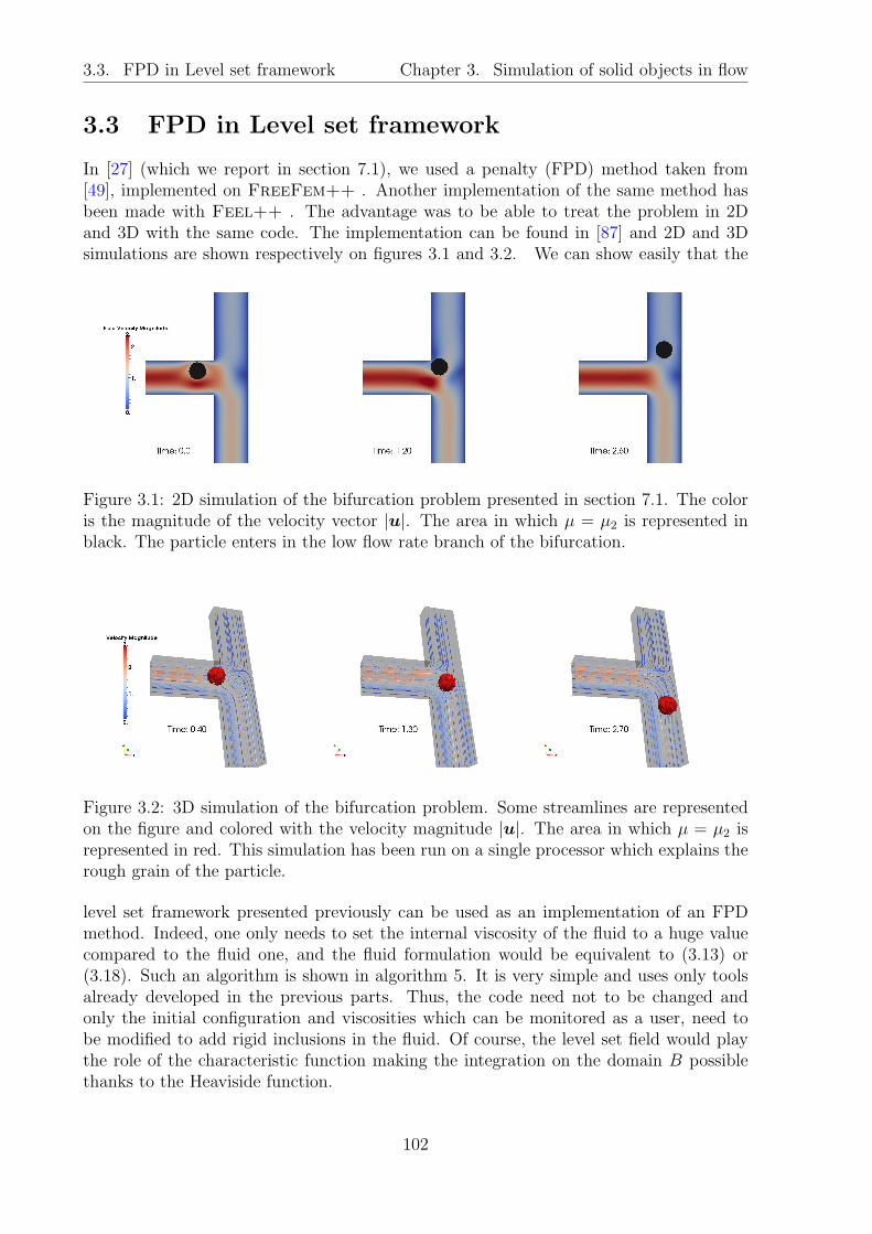
3.3. FPD in Level set framework Chapter 3. Simulation of solid objects in flow
3.3 FPD in Level set framework
In [27] (which we report in section 7.1), we used a penalty (FPD) method taken from[49], implemented on FreeFem++ . Another implementation of the same method hasbeen made with Feel++ . The advantage was to be able to treat the problem in 2Dand 3D with the same code. The implementation can be found in [87] and 2D and 3Dsimulations are shown respectively on figures 3.1 and 3.2. We can show easily that the
Figure 3.1: 2D simulation of the bifurcation problem presented in section 7.1. The coloris the magnitude of the velocity vector |u|. The area in which µ = µ2 is represented inblack. The particle enters in the low flow rate branch of the bifurcation.
Figure 3.2: 3D simulation of the bifurcation problem. Some streamlines are representedon the figure and colored with the velocity magnitude |u|. The area in which µ = µ2 isrepresented in red. This simulation has been run on a single processor which explains therough grain of the particle.
level set framework presented previously can be used as an implementation of an FPDmethod. Indeed, one only needs to set the internal viscosity of the fluid to a huge valuecompared to the fluid one, and the fluid formulation would be equivalent to (3.13) or(3.18). Such an algorithm is shown in algorithm 5. It is very simple and uses only toolsalready developed in the previous parts. Thus, the code need not to be changed andonly the initial configuration and viscosities which can be monitored as a user, need tobe modified to add rigid inclusions in the fluid. Of course, the level set field would playthe role of the characteristic function making the integration on the domain B possiblethanks to the Heaviside function.
102

3.3. FPD in Level set framework Chapter 3. Simulation of solid objects in flow
The only difference from the FPD and penalty method is that in a level set contextone does not follow the position of each rigid inclusion independently. Indeed, one wouldadvect one level set field and lose the information of the position of each rigid inclusion.Moreover, this advection step takes generally more computational time than to do theintegration of the positions of the particles (3.20). However, in a simulation where onlyone rigid inclusion is present (bifurcation in [27]) the position of the particle would notbe lost by using a level set function instead of integrating the position x of the particle.On the other hand, for a very large number of rigid particles, one generally does not careabout the exact position of each particle, and only mean values are monitored (viscosity,density of particles in a region) which are accessible by the level set field. In these cases,only the computational time could be a drawback for the use of level set instead of indi-vidual coordinates for the particles.Nevertheless, two main advantages can be found for the use of level set field. The first one,is that the shape of the rigid particles has to be given once and for all at the beginning ofthe simulation. Then, there is no need to re-use any shape function and the initial shapewill be advected correctly by the velocity of the fluid. The shape can be given by analyticdistance functions (or close to it), as for spheres, lines or ellipses. It can also be givenanalytically by combination of min and max of these functions, as it has been done forthe slotted disk in section 1.4. Or, for more complicated shapes, it can be given by theparametrization of a curve as explained in appendix C. Instead, for the FPD method, theshape function has to be easy to express since it is used at any time step to update thecharacteristic function.Moreover, we only considered in this section spherical or disk shapes for which the incli-nation angle of the object has no influence. But to use ellipsoidal particles in an FPDcontext for example, one would have to add new sets of variables accounting for the anglesof the objects (αi, βi, γi) (in 3d) and the rotational velocities wi as it is done for examplein [48]. At each time step, the positions and angles have to be updated which can start tobe heavy in a 3D simulation where 3 angles are needed to describe the rotation. This iscompletely transparent in a level set context and only the initial shape has to be changedto go from spherical particles to other asymmetric particles.The second advantage of the use of level set instead of classical explicit following of theparticles resides in the fact that it can be easily coupled with deformable objects. In-deed, by using the multi level sets framework introduced in section 2.2.2, one can set aviscosity to a huge value for rigid inclusion and softer values to model vesicles, bubblesor other objects. In conclusion, we can say that using level set for the simulation of rigidinclusions might not be optimal for a simple simulation but it brings more flexibility likethe possibility to handle easily the rotation and complex forms or to couple it with softobjects.
Algorithm 5 FPD method or fictitious domain with penalty term method using a levelset field.Require: φ0, µ2 >> µ1
for n = 0 to Ntf do(un, pn) = SolveFluidProblem(Hε(φ
n)) eq (2.31) and (2.32)φn+1 = SolveAdvection(un) eq (2.33)
end for
103

3.3. FPD in Level set framework Chapter 3. Simulation of solid objects in flow
104
Chapter 4
Simulation of vesicles : comparisonof two models
Contents4.1 Bending force in level set context . . . . . . . . . . . . . . . . . 106
4.1.1 High order derivative by increasing polynomial approximationorder . . . . . . . . . . . . . . . . . . . . . . . . . . . . . . . . . 107
4.1.2 High order derivative by smooth projections . . . . . . . . . . . 109
4.1.3 Test on the curvature of a circle . . . . . . . . . . . . . . . . . 111
4.2 Inextensibility by elastic force . . . . . . . . . . . . . . . . . . . 113
4.2.1 Principle of the method . . . . . . . . . . . . . . . . . . . . . . 113
4.2.2 Record the stretching information . . . . . . . . . . . . . . . . 115
4.2.3 Equations and dimensionless numbers . . . . . . . . . . . . . . 117
4.3 Inextensibility by Lagrange multiplier . . . . . . . . . . . . . . 119
4.3.1 Introduction of the Lagrange Multiplier . . . . . . . . . . . . . 119
4.3.2 Discretization . . . . . . . . . . . . . . . . . . . . . . . . . . . . 120
4.4 Validation . . . . . . . . . . . . . . . . . . . . . . . . . . . . . . . 122
4.4.1 Equilibrium shape . . . . . . . . . . . . . . . . . . . . . . . . . 122
4.4.2 Dynamics of single vesicle under shear flow . . . . . . . . . . . 124
105

4.1. Bending force in level set context Chapter 4. Simulation of vesicles
In this chapter we will describe our strategy for the simulation of vesicles in flow. Firstwe will recall the expression of the bending force and its level set expression. This forcerequires the knowledge of the 4th derivative of the level set field. Two strategies will bedescribed to get this high order derivative, the increase of the polynomial approximationorder of the level set field and the smoothing of the fields during each differentiation.Then we will present our implementation of two different methods used in the literatureto impose the inextensibility of the vesicle membrane. The first one uses the informationof the stretching of the interface recorded in the level set field to derive a force opposed toit (this is a penalty method). The other one uses a Lagrange multiplier to impose that thesurface divergence is zero on the membrane. We finally present some validation tests onthe behavior of a vesicle in a simple shear flow including its equilibrium shape, and showthat the Lagrange multiplier method gives a better accuracy and is more stable than thepenalty method.
4.1 Bending force in level set context
The energy associated to the bending of a vesicle membrane has been addressed by Can-ham and Helfrich, respectively, in [16, 43]. They have shown that this energy variesas:
Eb =kB2
∫
Γ
κ2 (4.1)
where kB is the bending modulus of the vesicle (a typical value is 10−19 J), and κ isthe curvature of the membrane. In the context of phase field simulation, the authors of[8] used the principle of virtual works to derive this energy and get a force. The sameprocedure has been done in the level set context in [71]. We used the force formulationgiven in [71]. A comparison between level set and phase field methods has been madein [70] where the authors have shown that equivalent results can be obtained with bothmethods. The curvature force given in [71] can be written as:
Fb =
∫
Ω
kB∇ ·(−κ2
2
∇φ
|∇φ| +1
|∇φ|
(
Id −∇φ⊗∇φ
|∇φ|2)
∇|∇φ|κ)
δε∇φ (4.2)
where
(
Id −∇φ⊗∇φ
|∇φ|2)
is the orthogonal projector operator, often called P⊥ and can be
simplified in 2D by the expression P2D⊥(v) = t(t ·v), with t = n⊥. An index expression of
the orthogonal projector operator is given in appendix G. One can see that the expression(4.2) leads to some numerical difficulties. Indeed, it consists of the divergence of a functionof the gradient of the curvature, the curvature being itself the divergence of the gradient
of the level set field (κ = ∇ ·n = ∇ · ∇φ
|∇φ|). Thus the curvature force requires taking
four times the derivative of the field φ. This problem is not specific to the level set orphase field methods as all the methods involving a force derived from the bending energyof the form (4.1) need the fourth-order derivative of the shape function of the membranewith a good accuracy. To overcome this issue different techniques have been used. In thecontext of spectral boundary integral methods [108, 33, 116, 117, 109] the shape is usuallyrepresented as a function of the spherical coordinates and time r(θ1, θ2, t) (in 3D) and isdiscretized using finite spherical harmonics. The fourth order derivative of the shape can
106

4.1. Bending force in level set context Chapter 4. Simulation of vesicles
be obtained with a good accuracy by using high order spherical harmonics. In a finiteelement context, Laadhari during his PhD [62] used L2 projection with quadrature orderof 1 (mass lumping).
In this section, we will present two different strategies that we developed to be ableto obtain the derivatives of the curvature. The first one is done by increasing the poly-nomial order of the discretized level set field. This method gives the better accuracy. Itcan be difficult to derive all the coefficients we talked about in this work for high orderapproximations. Indeed, all the parameters depending on the mesh size should, for ahigh order simulation, also depend on the polynomial approximation order used. Thesecoefficients are: the interface thickness and the stabilization coefficients for the elementstabilization (the CIP method already includes high order finite element). Moreover, tokeep a reasonable computational time, one would need to decrease the mesh size, thus,the polynomial approximation for the fluid and pressure should also be increased in conse-quence to keep the overall approximation accurate. This is already included in our modeland should work satisfactorily. Increasing the polynomial order of approximation for thevesicle application is thus possible and a few tests have been made in this way. However,we wanted also to derive a method working at low order (order 1). The goal was to beable to keep the classical level set parameters and simplify the method. Consequently,we also derived a projection method in which we smooth the projected field by adding asmall Laplacian term to the left hand side of a projection. This method has a much worseaccuracy but is enough to get an approximation of the curvature and its derivatives.
4.1.1 High order derivative by increasing polynomial approxi-mation order
Let us define a function u ∈ H1(Ω) for which we want to find the gradient ∇u. One wayto get this gradient is to do a L2 projection of ∇u. Such a projection reads, for a givenu ∈ H1(Ω), find g ∈ [L2(Ω)]d such that ∀v ∈ [L2(Ω)]d:
∫
Ω
g ·v =
∫
Ω
∇u ·v. (4.3)
One discretizes this equation by introducing the continuous finite element spaces Ukh and
Glh, respectively scalar and vectorial finite element spaces based on a mesh of typical size
h and Lagrange polynomials of order k and l. Let us introduce the discrete version ofu and g, uh ∈ Uk
h and gh ∈ Glh. The discretized equation (4.3) reads then, for a given
uh ∈ Ukh, find gh ∈ Gl
h such that ∀vh ∈ Glh:
∫
Ω
gh ·vh =
∫
Ω
∇uh ·vh. (4.4)
Let us write this projection in a more general form. We introduce the vectorial finiteelement space Am
h ⊂ L2(Ω) and Bnh ⊂ L2(Ω)∩C0 based on a discretization mesh of size h
and Lagrange polynomials of order respectively m and n. Let us introduce ah ∈ Amh and
bh ∈ Bnh elements of those spaces. We define the L2 projection operator on space Bn
h asfollows:
πBnh
L2 : Amh → Bn
h
ah(4.6)7→ bh
(4.5)
107

4.1. Bending force in level set context Chapter 4. Simulation of vesicles
find bh ∈ Bnh so that ∀vh ∈ Bn
h:∫
Ω
bh ·vh =
∫
Ω
ah ·vh(4.6)
Thus, the projection (4.4) can be rewritten as:
g = πGl
h
L2 (∇uh) (4.7)
Since uh is discretized on polynomials of order k, its gradient∇uh has only the informationof polynomials of order k − 1. If one wants to derive a quantity n times by this method(let us say one needs ∇nu), this limitation requires taking uh in a finite element space oforder k >= n to have at least ∇nu as polynomial of degree 0.
In the case where one projects the gradient of a P1 field, the field to project (ah in theformulation (4.6)) is a discontinuous piecewise polynomials of order 0. Since the solutionof the problem (4.6) is searched in a continuous space (we recall that Bn
h ⊂ L2(Ω)∩C0), thesolution is continuous; consequently, in this case, the projection is equivalent to project adiscontinuous field on a continuous one.
Feel++ allows use of a basis with arbitrarily high polynomial order. Consider agraphical example taken from the test presented in section 4.1.3 in which we define a levelset field as a circle of radius r = 0.5. We want to compute the curvature of the level setfield on the iso 0 of the field, and the gradient of the curvature (called ih). It requiresthen to differentiate 3 times the level set field φh. The quantities are computed this way,for a level set field φh ∈ Rk
h, we compute:
nh = π(Rk
h×Rk
h)
L2 (∇φh
|∇φh|)
κh = πRkh
L2 (∇ ·nh)
ih = π(Rk
h×Rk
h)
L2 (∇κh)
What is the expected result? The curvature field of the level set has the form of concentriccircles and has the value 2 where the level set field is 0. The gradient of the curvaturefield is supposed to be a vector field for which each vector is pointing to the center ofthe domain. On this graphical example, we plot the iso value 2 of the curvature κh, andsome vectors of ih on this iso line. The figure 4.1(a) represents these values for a levelset field taken in R2
h. The approximation is not sufficient to get a correct value of ih.One can see on the figure that κh which carries the information of a field of degree 0 hassome oscillations. If one needs only the value of the curvature (as for a surface tensionforce for example), this approximation could be enough. But if one needs the gradient ofκh, the result is completely wrong as we can see from the vectors plotted on the graph.On the figure 4.1(b) by contrast, we plotted the same values but by taking an initialapproximation φh ∈ R3
h. This way, the curvature field κh is differentiable and its gradientcan be calculated correctly. This method of increasing the approximation order to getthe proper derivative is very precise as we will see in the convergence test made in section4.1.3, even though it suffers a few drawbacks.No hypothesis has been made on the approximation order of the level set framework andconsequently it can work at high order. Nevertheless, a special care has to be taken at thereinitialization step if the fast marching method is used as explained in section 1.3.4. Thestabilization methods of the elements presented in section 1.2.2 has also been derived only
108

4.1. Bending force in level set context Chapter 4. Simulation of vesicles
(a) φh ∈ R2h (b) φh ∈ R3
h
Figure 4.1: The iso 0 line of the level set field φh is represented in black. The iso value2 of the curvature κh is represented as the red line, and its gradient ih as black vectorsrandomly distributed on the curvature line.
for first order finite elements. These methods also work for high order finite elements butthe stabilization factor has to be set by hand and to our knowledge no theoretical relationexists which includes the polynomial order (as for the CIP stabilization for example).Moreover, the thickness of the interface ε usually set as 1.5h might depend on the poly-nomial order. Indeed, since high order finite elements method are computationally costly,the mesh size is usually increased compared to low order finite elements. Consequently, ifthe thickness is kept to few mesh size, it can be too large, once again the parameter mustbe prescribed according to the needs of the simulation. An added drawback with the useof high order finite elements is that not all the visualization software are able to handlethem. For example, Paraview that we used in this work can not plot such elements. Itis then necessary to use the operator described in section 1.3.4 which creates a first orderspace out of a high order one. The visualization of a high order field can then be made,but this operation has a cost. Finally, not every finite elements software or library canprovide an arbitrary high order finite element basis. Some numerical methods coupledwith the level set framework added in the future could also work only at first order (forexample some interface localization algorithm). For these reasons, we found necessary todevelop a method able to get high order derivative of a low order field. This method isdeveloped in section 4.1.2.
4.1.2 High order derivative by smooth projections
We saw in section 4.1.1 that one can differentiate a finite element field since the numberof derivative is lower or equal to the polynomial order of the initial field. But whatis happening if one takes a field in a low polynomial approximation set, let us say 1and differentiate it twice by the method of derivation / projection explained previously?After the first derivation, the derivative is discretized by construction on a continuouspolynomial set of order 1 even if it carries only the information of a piecewise discontinuouspolynomial set of order 0. The missing information is filled by unpredictable values,
109

4.1. Bending force in level set context Chapter 4. Simulation of vesicles
leading to oscillations (as seen in the curvature of figure 4.1(a)) making the differentiatedfield impossible to differentiate once again. The idea of the method presented here is toadd artificial diffusion to the projection (4.3) to minimize the oscillations happening whenderiving a variable discretized on a low order polynomial set. One adds a small termproportional to ∆g which smooths the oscillations and makes the obtained derivativepossible to derivate. The continuous formulation of such a smoothed projection, afterintegrating by parts is the following, for a given u ∈ H1(Ω), find g ∈ [H1(Ω)]d ∩ [C0]d sothat ∀v ∈ [H1(Ω)]d:
∫
Ω
g ·v +
∫
Ω
ε1 ∇g : ∇v −∫
∂Ω
ε1 (∇g n) ·v =
∫
Ω
∇u ·v (4.8)
with ε1 a sufficiently small parameter. To be precise, ∇g n is the classical product of thematrix ∇g and the vector n, thus it is a vector. One remarks that for ε1 = 1, we obtain aclassical H1 projection. One needs to impose boundary conditions to the equation (4.8).The third integral could be passed to the right hand side and ∇gn replaced by ∇(∇u)nto impose Neumann boundary conditions but this would require that u ∈ H2(Ω) and wedo not want to impose such a strong regularity on u. Instead, we impose weakly Dirichletboundary conditions to fix the value of g at the boundary using the Nitsche method. Firstwe symmetrize the equation by adding the symmetric of the third integral on both sidesof the equation. Then we impose the value of g on the boundary by adding a penaltyterm. Finally the projection reads, for a given u ∈ H1(Ω), find g ∈ [H1(Ω)]d ∩ [C0]d sothat ∀v ∈ [H1(Ω)]d:
∫
Ω
g ·v +
∫
Ω
ε1 ∇g : ∇v −∫
∂Ω
ε1 (∇g n) ·v −∫
∂Ω
ε1 (∇v n) · g
+γ1
∫
∂Ω
g ·v =
∫
Ω
∇u ·v −∫
∂Ω
ε1 (∇v n) ·∇u+ γ1
∫
∂Ω
∇u ·v(4.9)
with γ1 a big enough parameter. The discrete version reads, for a given ∇uh ∈ Uk−1h , find
gh ∈ Gkh so that ∀vh ∈ Gk
h:
∫
Ω
gh ·vh +
∫
Ω
ε2h
k∇gh : ∇vh −
∫
∂Ω
ε2h
k(∇ghn) ·vh −
∫
∂Ω
ε2h
k(∇vhn) · gh
+γ2h
∫
∂Ω
gh ·vh =
∫
Ω
∇uh ·vh −∫
∂Ω
ε2h
k(∇vhn) ·∇uh +
γ2h
∫
∂Ω
∇uh ·vh
(4.10)
with h the element mesh size as a factor of a small parameter ε2 to insure consistency andγ2 a penalty parameter strong enough to impose the boundary conditions. Once againwe can write this projection in a more general form, it reads:
πGk
hsm : Uk−1
h → Gkh
∇uh(4.10)7→ gh
(4.11)
Of course, this projection also works to get the divergence of a vector by replacing thedouble contracted product (:) by a scalar product ( · ), and the scalar products of vectorsby simple products of scalars. The πsm projection smooths the information, thus it mightmodify the initial field that one wants to project. Let us test graphically the method on
110

4.1. Bending force in level set context Chapter 4. Simulation of vesicles
the same example as in section 4.1.1. The calculated quantities are the same except thatthis time, we use the following projections:
nh = π(Rk
h×Rk
h)
sm (∇φh
|∇φh|)
κh = πRkh
sm(∇ ·nh)
ih = π(Rk
h×Rk
h)
sm (∇κh)
The results are presented in figure 4.2. The figure 4.2(a) is the same than 4.1(a) that wereported here to compare more easily the methods. We recall that it uses L2 projectionsand that the level set space is R2
h making impossible to differentiate twice φh by thismethod, consequently, the gradient of the curvature vectors is wrong. We can see nowon the figure 4.2(b) that with a smooth projection method, it is indeed possible to derivethe level set field in R2
h. However, the interface moved slightly during the smoothingprojections (the red curve representing the iso line 2 of the curvature is not exactly onthe iso 0 of φ). Thus this method works to get high order curvature but the smoothingparameter ε2 has to be tuned to get a value strong enough to smooth the field but smallenough to keep the approximation correct.
(a) φh ∈ R2h, projectors used: π
R2
h
L2 and
π(R2
h×R
2
h)
L2
(b) φh ∈ R2h, projectors used: π
R2
h
sm and
π(R2
h×R
2
h)
sm
Figure 4.2: The iso 0 line of the level set field φh is represented in black. The iso value2 of the curvature κh is represented as the red line, and its gradient ih as black vectorsrandomly distributed on the curvature line.
4.1.3 Test on the curvature of a circle
We choose to test the order of the curvature that we can get with this method. The testis simple consisting in taking the curvature of a function φ ∈ Pn for which we know anexact value for the curvature and compute the error. The domain Ω is taken as a squareof dimensions (−1, 1)× (−1, 1). The level set function φ is taken so that the interface Γis a circle centered in the domain with a radius equal to 0.5, thus φ =
√
x2 + y2 − 0.5.
111

4.1. Bending force in level set context Chapter 4. Simulation of vesicles
The level set lines of the function φ are concentric circles of radii r =√
x2 + y2. The
curvature of a circle of radius r is equal to1
r. Thus the iso lines of the function curvature
defined by κ = ∇ · ( ∇φ
|∇φ|) are concentric circles of radii1
√
x2 + y2. The goal of the test
is to compute with the best accuracy possible the curvature of Γ. Theoretically, one hasκexact = 2 for any point (x, y) ∈ Γ but numerically, the integral over Γ is replaced by anintegral over Ω by multiplying the expression by δε(φ). Since δε(φ) has a given thicknessequal to 2ε, assuming that κexact = 2 on all Γ is only first order accurate. The exact value
of the curvature for a point (x, y) ∈ Γ is κexact =1
√
x2 + y2. Thus, for this test, the L2
error will be defined as follow:
eL2 =
∫
Ω
(
κ(φ)− 1√
x2 + y2
)2
δε(φ)
∫
Ω
δε(φ)
12
(4.12)
The simulation is run on a single processor Intel(R) Xeon(R) CPU E5-2670, 2.60GHz.The initial mesh size is set to h = 0.12 and divided by 2 at each iteration. We haveperformed 6 iterations for polynomial approximation P1 and P2, 5 iterations for P3 and 4iterations for P4 and P5 because of the increase in computational time.Figure 4.3 shows the results obtained by the method in which we increase the polynomialorder of the initial function φ and project each derivative on the same space withoutsmoothing the solution. We can see clearly that the logarithmic slope of the error asa function of the mesh size is increased by one when the polynomial approximation inincreased by one as well. Two major consequences can be given from this error analy-sis. Firstly, it confirms that it is impossible to get a good value of the curvature for apolynomial approximation of 1 by using this method. The error is bigger than unity andnever decreases with the mesh size. Secondly, this method can give very high precisionto compute the curvature for higher order. Indeed, at the best polynomial approximationthat we tried, which is 5, the error decreases as h4, and we were able to get an errordown to 2 · 10−8 on a single processor. Of course, the computational cost for such anapproximation is very high. But for an application for which the approximation of thebending forces has to be really good (for steady shape study, for example), one mightconsider using high order polynomial approximation. The computational time could bedecreased by increasing the number of processors on which running the application.The figure 4.4 shows the same simulation for which we used the smooth projection as
described in (4.10) by taking a factor ε2 =1
3. We see that for any polynomial order
approximation we get a rate of convergence of 1. This convergence at order one is reachedwhen the number of degrees of freedom is high enough. Thus, the two first points of theP1 and P2 approximations do not respect this behavior. Thus, two main conclusions canbe found from this simulation. Firstly, the absolute error at high order is big. Even at apolynomial approximation of order 5, the best error we get with the smallest mesh size isbigger than 10−2. Secondly, the only configuration for which the multiple derivation bysmooth projection is better than without smooth projection is for a polynomial approxi-
112
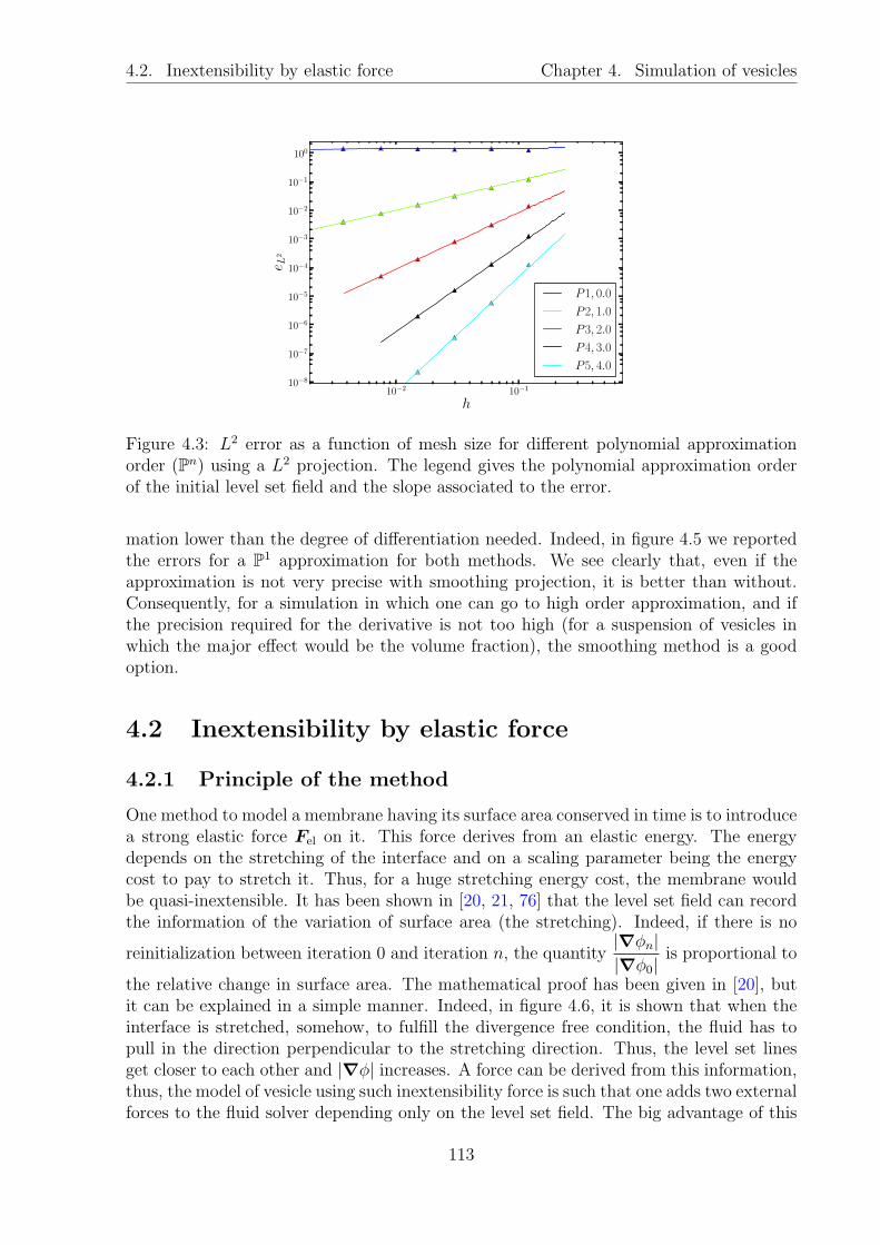
4.2. Inextensibility by elastic force Chapter 4. Simulation of vesicles
10−2 10−1
h
10−8
10−7
10−6
10−5
10−4
10−3
10−2
10−1
100
e L2
P1, 0.0
P2, 1.0
P3, 2.0
P4, 3.0
P5, 4.0
Figure 4.3: L2 error as a function of mesh size for different polynomial approximationorder (Pn) using a L2 projection. The legend gives the polynomial approximation orderof the initial level set field and the slope associated to the error.
mation lower than the degree of differentiation needed. Indeed, in figure 4.5 we reportedthe errors for a P1 approximation for both methods. We see clearly that, even if theapproximation is not very precise with smoothing projection, it is better than without.Consequently, for a simulation in which one can go to high order approximation, and ifthe precision required for the derivative is not too high (for a suspension of vesicles inwhich the major effect would be the volume fraction), the smoothing method is a goodoption.
4.2 Inextensibility by elastic force
4.2.1 Principle of the method
One method to model a membrane having its surface area conserved in time is to introducea strong elastic force Fel on it. This force derives from an elastic energy. The energydepends on the stretching of the interface and on a scaling parameter being the energycost to pay to stretch it. Thus, for a huge stretching energy cost, the membrane wouldbe quasi-inextensible. It has been shown in [20, 21, 76] that the level set field can recordthe information of the variation of surface area (the stretching). Indeed, if there is no
reinitialization between iteration 0 and iteration n, the quantity|∇φn||∇φ0|
is proportional to
the relative change in surface area. The mathematical proof has been given in [20], butit can be explained in a simple manner. Indeed, in figure 4.6, it is shown that when theinterface is stretched, somehow, to fulfill the divergence free condition, the fluid has topull in the direction perpendicular to the stretching direction. Thus, the level set linesget closer to each other and |∇φ| increases. A force can be derived from this information,thus, the model of vesicle using such inextensibility force is such that one adds two externalforces to the fluid solver depending only on the level set field. The big advantage of this
113

4.2. Inextensibility by elastic force Chapter 4. Simulation of vesicles
10−2 10−1
h
10−2
10−1e L
2
P1, 1.1
P2, 1.1
P3, 1.1
P4, 1.2
P5, 1.1
Figure 4.4: L2 error as a function of mesh size for different polynomial approximationorders (Pn) using a smooth projection method. The legend gives the polynomial approx-imation order of the initial level set field and the slope associated to the error.
method is that the fluid solver can be seen as a black box taking as entry an externalforce field, and giving as output the velocity and pressure solutions. This is an advantageif one wants to test different numerical techniques to solve a fluid equation or even testdifferent fluid models. Another advantage is that the time cost to solve such a problemwould be almost independant of the number of vesicles in the flow. As a matter of facts,the total number of elements in the final problem is always the same if one increases thenumber of vesicles. Only the number of non-zero entries in the force vector is increased.This is a big advantage compared to the method described in section 4.3 in which theLagrange multiplier increases the number of unknowns to find. This method can be seenas a penalty method to restrict surface area change. It is not an exact method and suffersfrom some technical difficulties that we will describe later on. First, let us describe themethod in detail. The elastic energy Eel is defined as:
Eel =
∫
Ω
E(|∇φ|)δε, (4.13)
where E(|∇φ|) is a constitutive law for the membrane such that E(1) = 0 meaningthat there is no initial stretching. Different models could be used for E(|∇φ|), usuallywe prefer to describe E ′(|∇φ|) the derivative of E(|∇φ|) which is directly used in theexpression of the elastic force Fel. A simple expression usually sufficient to get most ofthe effects is a linear law E ′(|∇φ|) = Λ(|∇φ| − 1) with Λ the energy cost per unit ofsurface to stretch the membrane. For this expression, the energy would be a quadraticlaw E(|∇φ|) = Λ
2(|∇φ| − 1)2 making the membrane modeled as a spring, pulling when
it is stretched and pushing back when it is compressed. A more realistic model is to cutthe force when the membrane is compressed, making the membrane more like a tensile ora balloon, the derivative of the energy would be then E ′(|∇φ|) = Λmin (|∇φ| − 1, 0). Ithas been shown in [20] that after having derived the energy (4.13), the elastic force takes
114

4.2. Inextensibility by elastic force Chapter 4. Simulation of vesicles
10−2 10−1
h
10−3
10−2
10−1
100
101
e L2
nodal, 0.0
smooth, 1.1
Figure 4.5: Comparison of the L2 error on the curvature as a function of mesh size for apolynomial approximation of first order.
the form:
Fel =
∫
Ω
∇E ′(|∇φ|)−∇ ·[
E ′(|∇φ|) ∇φ
|∇φ|
]∇φ
|∇φ|
δε. (4.14)
If we re-write this equation by replacing∇φ
|∇φ| by n and E ′(|∇φ|) by the spring like
model, we obtain:
Fel = Λ
∫
Ω
∇(|∇φ| − 1)−∇ · [(|∇φ| − 1)n] δεn. (4.15)
4.2.2 Record the stretching information
Several difficulties arise when using this method. The first one has already been seen in theprevious section: the high order derivative of the level set field. Indeed, the formulation(4.15) leads to a 2nd derivative of the level set field. This problem has already beenaddressed in section 4.1. Another difficulty is that for a given simulation, one needs to
keep the information∇φ
|∇φ| during all the simulation time. Thanks to the elastic force
Fel, this quantity is supposed to stay close to 1 on the membrane. The problem is thatit can reach really high values away from the membrane. For example, for a simulationof one vesicle at the center of a shear flow, the velocity induced by the wall forces thelevel set field to move in one direction since its value has to be 0 on the membrane. Thisresults in an accumulation of level set lines on one side of the vesicle and a depletion inthe other side. The gradient magnitude of the level set takes extremes values, leading toinstabilities when solving the advection equation 1.11. For other level set simulations, thereinitialization resets |∇φ| to values close to 1 and the problem is solved. But doing so inthis context would lose the stretching information. A way to overcome this last problem
115

4.2. Inextensibility by elastic force Chapter 4. Simulation of vesicles
Figure 4.6: Scheme explaining how the divergence free velocity implies that |∇φ| recordsthe stretching of the interface. If the interface is stretched it means that the velocity fieldis pulling on it from two sides as shown on the left scheme. Since the velocity is divergencefree, it has to push in the other direction to fulfill this condition. Thus, the level set linesare getting closer, consequently, the gradient magnitude of φ increases.
is to introduce e = |∇φ|, an alternative field being governed by the equation:
∂te+ u ·∇e = −e∇φ⊗∇φ
|∇φ|2: D(u). (4.16)
This field is set initially to e0 = |∇φ0| and then advected as an independent field. Itcan be solved numerically by the numerical framework presented in sections 1.2 and 5.2as for the advection of the level set, by changing the right hand side f . This methodof taking the gradient magnitude of the level set field as an independent field is knownas the gradient augmented level set method in [78], it has also been used in the vesiclesimulation context in [92]. A first advantage of using this method is that it reduces thedegree of derivation of equation (4.14) by one. Indeed, replacing |∇φ| by e in equation(4.15) leads to only one differentiation of the field e. This field e is usually discretized onthe same polynomial set as the level set field.The problem of the extremes values of |∇φ| is still here. The solution that we propose isto reinitialize the level set field and the field e, but to keep the information of the field ebefore reinitialization around the interface.
By doing so, after reinitializing, φ is equal to a distance function, e is almost equalto the unit everywhere and we reset e to its value before the reinitialization around theinterface. This does not lead to a huge discontinuity of e since it is supposed to stay closeto one thanks to the strong elastic force. Moreover, the discontinuity can be smeared outby using a Heaviside like function.
Let us call e∗ and e respectively the values of e before and after the reinitialization step(e is almost equal to 1 everywhere). We call e the value of e for which we reincorporatedthe information of the stretching before reinitialization. The value of e can be obtainedby:
e = e+ e∗Rε2(φ) (4.17)
with Rε2 the smoothed rectangular function being equal to one in a thickness ε2 aroundthe interface. It can be defined by:
Rε2 = Hε(φ+ ε2)−Hε(φ− ε2). (4.18)
116
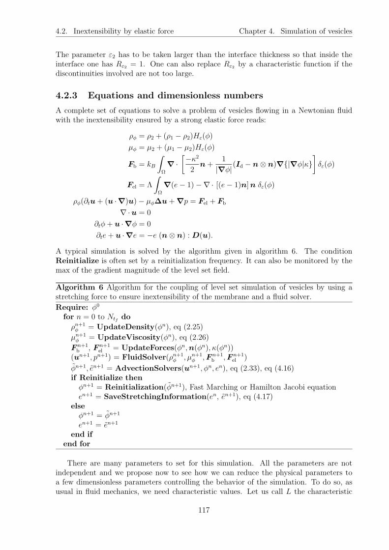
4.2. Inextensibility by elastic force Chapter 4. Simulation of vesicles
The parameter ε2 has to be taken larger than the interface thickness so that inside theinterface one has Rε2 = 1. One can also replace Rε2 by a characteristic function if thediscontinuities involved are not too large.
4.2.3 Equations and dimensionless numbers
A complete set of equations to solve a problem of vesicles flowing in a Newtonian fluidwith the inextensibility ensured by a strong elastic force reads:
ρφ = ρ2 + (ρ1 − ρ2)Hε(φ)
µφ = µ2 + (µ1 − µ2)Hε(φ)
Fb = kB
∫
Ω
∇ ·[−κ2
2n+
1
|∇φ|(Id − n⊗ n)∇|∇φ|κ]
δε(φ)
Fel = Λ
∫
Ω
∇(e− 1)−∇ · [(e− 1)n]n δε(φ)
ρφ(∂tu+ (u ·∇)u)− µφ∆u+∇p = Fel + Fb
∇ ·u = 0
∂tφ+ u ·∇φ = 0
∂te+ u ·∇e = −e (n⊗ n) : D(u).
A typical simulation is solved by the algorithm given in algorithm 6. The conditionReinitialize is often set by a reinitialization frequency. It can also be monitored by themax of the gradient magnitude of the level set field.
Algorithm 6 Algorithm for the coupling of level set simulation of vesicles by using astretching force to ensure inextensibility of the membrane and a fluid solver.
Require: φ0
for n = 0 to Ntf do
ρn+1φ = UpdateDensity(φn), eq (2.25)
µn+1φ = UpdateViscosity(φn), eq (2.26)
F n+1b , F n+1
el = UpdateForces(φn,n(φn), κ(φn))(un+1, pn+1) = FluidSolver(ρn+1
φ , µn+1φ ,F n+1
b ,F n+1el )
φn+1, en+1 = AdvectionSolvers(un+1, φn, en), eq (2.33), eq (4.16)if Reinitialize thenφn+1 = Reinitialization(φn+1), Fast Marching or Hamilton Jacobi equationen+1 = SaveStretchingInformation(en, en+1), eq (4.17)
elseφn+1 = φn+1
en+1 = en+1
end ifend for
There are many parameters to set for this simulation. All the parameters are notindependent and we propose now to see how we can reduce the physical parameters toa few dimensionless parameters controlling the behavior of the simulation. To do so, asusual in fluid mechanics, we need characteristic values. Let us call L the characteristic
117
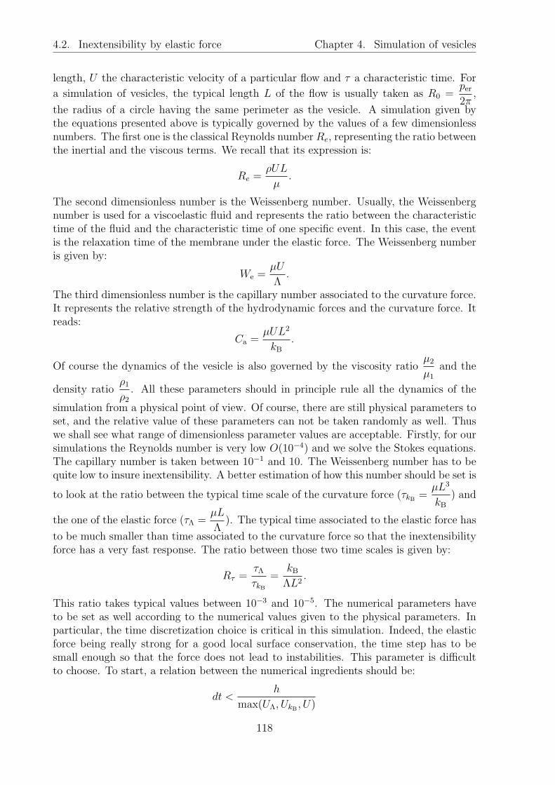
4.2. Inextensibility by elastic force Chapter 4. Simulation of vesicles
length, U the characteristic velocity of a particular flow and τ a characteristic time. For
a simulation of vesicles, the typical length L of the flow is usually taken as R0 =per2π
,
the radius of a circle having the same perimeter as the vesicle. A simulation given bythe equations presented above is typically governed by the values of a few dimensionlessnumbers. The first one is the classical Reynolds number Re, representing the ratio betweenthe inertial and the viscous terms. We recall that its expression is:
Re =ρUL
µ.
The second dimensionless number is the Weissenberg number. Usually, the Weissenbergnumber is used for a viscoelastic fluid and represents the ratio between the characteristictime of the fluid and the characteristic time of one specific event. In this case, the eventis the relaxation time of the membrane under the elastic force. The Weissenberg numberis given by:
We =µU
Λ.
The third dimensionless number is the capillary number associated to the curvature force.It represents the relative strength of the hydrodynamic forces and the curvature force. Itreads:
Ca =µUL2
kB.
Of course the dynamics of the vesicle is also governed by the viscosity ratioµ2
µ1
and the
density ratioρ1ρ2
. All these parameters should in principle rule all the dynamics of the
simulation from a physical point of view. Of course, there are still physical parameters toset, and the relative value of these parameters can not be taken randomly as well. Thuswe shall see what range of dimensionless parameter values are acceptable. Firstly, for oursimulations the Reynolds number is very low O(10−4) and we solve the Stokes equations.The capillary number is taken between 10−1 and 10. The Weissenberg number has to bequite low to insure inextensibility. A better estimation of how this number should be set is
to look at the ratio between the typical time scale of the curvature force (τkB =µL3
kB) and
the one of the elastic force (τΛ =µL
Λ). The typical time associated to the elastic force has
to be much smaller than time associated to the curvature force so that the inextensibilityforce has a very fast response. The ratio between those two time scales is given by:
Rτ =τΛτkB
=kBΛL2
.
This ratio takes typical values between 10−3 and 10−5. The numerical parameters haveto be set as well according to the numerical values given to the physical parameters. Inparticular, the time discretization choice is critical in this simulation. Indeed, the elasticforce being really strong for a good local surface conservation, the time step has to besmall enough so that the force does not lead to instabilities. This parameter is difficultto choose. To start, a relation between the numerical ingredients should be:
dt <h
max(UΛ, UkB , U)
118

4.3. Inextensibility by Lagrange multiplier Chapter 4. Simulation of vesicles
where UΛ and UkB are the typical velocities induced by the elastic force and the curvatureforce, and U is the typical velocity of the flow. Replacing the velocities by their valuesleads to the relation:
dt <h
max
(kBµL2
,Λ
µ, U
) .
This relation is a good starting point to check the range in which should be dt, however,usually one has to try different values to find the optimal one not leading to instabilitieswhile keeping a reasonable computational time. In the previous formulation, usually theleading term is the velocity due to the inextensibility force. Indeed, if it is not the case,the membrane has some extensibility.
4.3 Inextensibility by Lagrange multiplier
4.3.1 Introduction of the Lagrange Multiplier
A more stable way than having a force to impose inextensibility of the membrane is toimpose this constrain by adding a Lagrange multiplier to the equations. This method hasbeen employed in [62] and we propose to see in this section its implementation within ourframework. The idea is to insure that the velocity of the membrane is divergence free.Since in this model, the membrane is a part of the fluid, we can write this constraint asthe fact that in the fluid, the surface divergence on the interface Γ has to vanish, that isto say:
∇s ·u = 0 on Γ (4.19)
where ∇s ·u is the surface divergence, it can be written as: ∇s ·u = (Id−n⊗n) : ∇u =∇ ·u − (∇u n) ·n. One can see appendix G for the indexes notation of the surfacedivergence. This constraint on the fluid is added to the fluid system of equation. For thesake of simplicity, we will only write the incompressible Stokes equations for this part butthere is no problem to extend it to the Navier-Stokes equations. The system of equationreads now:
−2µ∇ ·D(u) +∇p = f in Ω
∇ ·u = 0 in Ω
∇s ·u = 0 on Γ.
Boundary conditions are also applied depending on the type of flow needed, for the sake ofsimplicity, in this example we will consider that we impose Dirichlet boundary conditionson ∂Ω. The variational formulation of the Stokes equations are classically obtained asfor the problem 2.17 by using the strain tensor D(u). A Lagrange multiplier λ is alsoadded to insure the constraint (4.19). The problem reads: for a given f ∈ [L2(Ω)]d, find
119
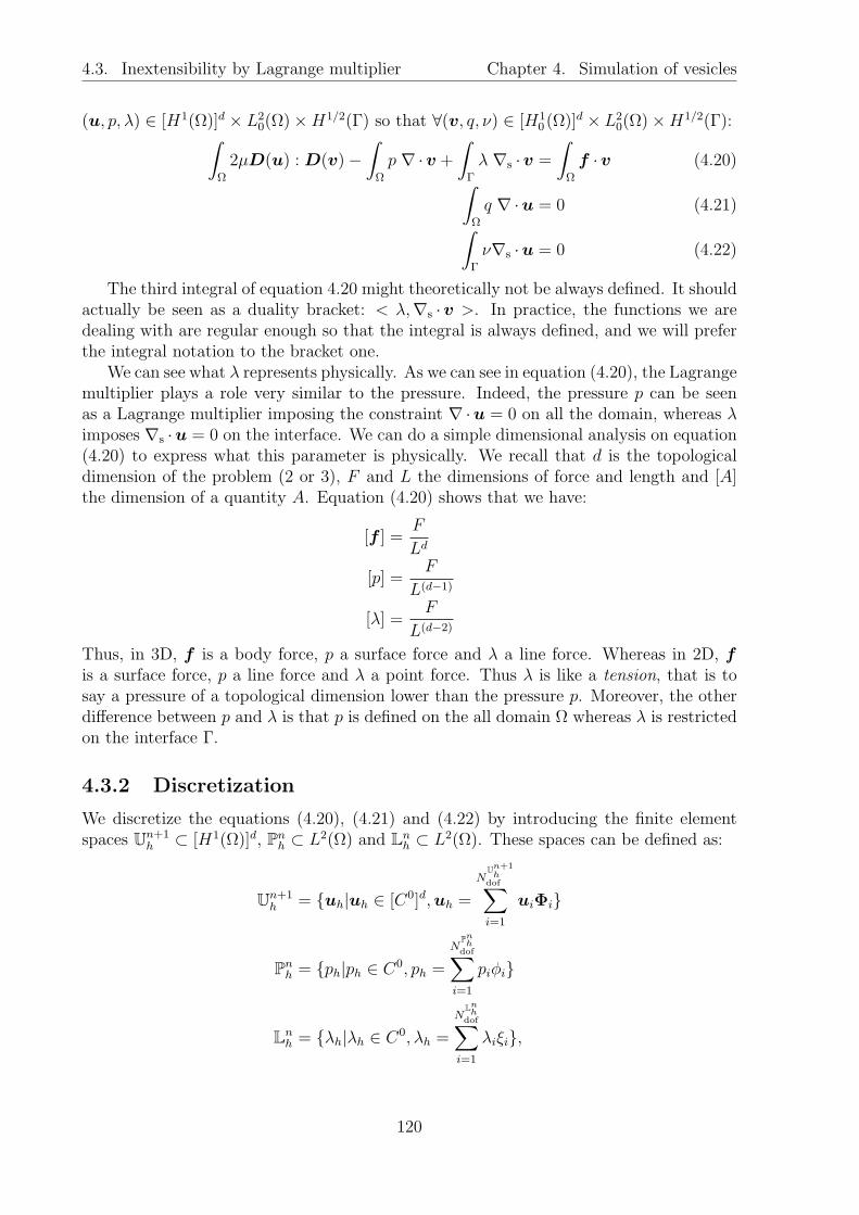
4.3. Inextensibility by Lagrange multiplier Chapter 4. Simulation of vesicles
(u, p, λ) ∈ [H1(Ω)]d × L20(Ω)×H1/2(Γ) so that ∀(v, q, ν) ∈ [H1
0 (Ω)]d × L2
0(Ω)×H1/2(Γ):∫
Ω
2µD(u) : D(v)−∫
Ω
p ∇ ·v +
∫
Γ
λ ∇s ·v =
∫
Ω
f ·v (4.20)∫
Ω
q ∇ ·u = 0 (4.21)∫
Γ
ν∇s ·u = 0 (4.22)
The third integral of equation 4.20 might theoretically not be always defined. It shouldactually be seen as a duality bracket: < λ,∇s ·v >. In practice, the functions we aredealing with are regular enough so that the integral is always defined, and we will preferthe integral notation to the bracket one.
We can see what λ represents physically. As we can see in equation (4.20), the Lagrangemultiplier plays a role very similar to the pressure. Indeed, the pressure p can be seenas a Lagrange multiplier imposing the constraint ∇ ·u = 0 on all the domain, whereas λimposes ∇s ·u = 0 on the interface. We can do a simple dimensional analysis on equation(4.20) to express what this parameter is physically. We recall that d is the topologicaldimension of the problem (2 or 3), F and L the dimensions of force and length and [A]the dimension of a quantity A. Equation (4.20) shows that we have:
[f ] =F
Ld
[p] =F
L(d−1)
[λ] =F
L(d−2)
Thus, in 3D, f is a body force, p a surface force and λ a line force. Whereas in 2D, fis a surface force, p a line force and λ a point force. Thus λ is like a tension, that is tosay a pressure of a topological dimension lower than the pressure p. Moreover, the otherdifference between p and λ is that p is defined on the all domain Ω whereas λ is restrictedon the interface Γ.
4.3.2 Discretization
We discretize the equations (4.20), (4.21) and (4.22) by introducing the finite elementspaces Un+1
h ⊂ [H1(Ω)]d, Pnh ⊂ L2(Ω) and Ln
h ⊂ L2(Ω). These spaces can be defined as:
Un+1h = uh|uh ∈ [C0]d,uh =
NUn+1h
dof∑
i=1
uiΦi
Pnh = ph|ph ∈ C0, ph =
NPnh
dof∑
i=1
piφi
Lnh = λh|λh ∈ C0, λh =
NLnh
dof∑
i=1
λiξi,
120

4.3. Inextensibility by Lagrange multiplier Chapter 4. Simulation of vesicles
where Φi, ψi and ξi are the finite element basis functions being Lagrange polynomials oforders n+1, n and n respectively. We introduce (uh, ph, λh) ∈ Un+1
h ×Pnh×Ln
h the discreteversions of (u, p, λ). The discrete version of equations (4.20), (4.21) and (4.22) reads, fora given fh find (uh, ph, λh) ∈ Un+1
h × Pnh × Ln
h so that ∀(vh, qh, νh) ∈ Un+1h × Pn
h × Lnh:
∫
Ω
2µφD(uh) : D(vh)−∫
Ω
ph ∇ ·vh +
∫
Ω
λh ∇s ·vh δε(φ) =
∫
Ω
fh ·vh (4.23)∫
Ω
qh ∇ ·uh = 0 (4.24)∫
Ω
νh∇s ·uh δε(φ) = 0, (4.25)
where we replaced the integral on Γ by an integral on Ω thanks to the delta function. Thisis important from the point of view of the dimensional analysis we performed previously.Indeed, as opposed to λ, λh is defined on the domain Ω even if most of its values are 0on it. Thus it is defined on a space with the same topological dimension as the space ofp. If we perform a dimensional analysis of equation (4.23), we can show that
[λh] = [ph] =F
Ld−1.
Consequently, by discretizing the Lagrange multiplier and projecting it on a space oftopological dimension superior to the one where it belongs, we changed its physical di-mensions and transformed it to a pressure. It can be seen as a pressure acting on a verysmall portion of the fluid trying to keep the surface divergence free. Thus, the pressureph and the Lagrange multiplier λh are the same kind of objects. To put this problem inan algebraic form, we introduce the following matrices:
A,Aij =
∫
Ω
2µD(Φj) : D(Φi)
B,Bij =
∫
Ω
−ψj∇ ·Φi
C,Cij =
∫
Ω
δε ξj∇s ·Φi
and the following vectors:
U,uj
P , pj
Q, λj
F ,fj.
Then, the problem (4.23) (4.24) (4.25) can be written as:
A B CBT 0 0CT 0 0
UPQ
=
F00
(4.26)
This algebraic system can be solved by a direct solver. The same method can be appliedfor the Navier-Stokes equation, for which a non-linear solver is used (Newton).
121

4.4. Validation Chapter 4. Simulation of vesicles
4.4 Validation
In this section we will try to validate our two different methods on several known behaviorsof vesicles. The first one is the equilibrium shape of a vesicle in a fluid at rest. The otherones are the behaviors of vesicles under shear flow. In this system two remarkable motionsare well known: the tank-treading and the tumbling motions. We will show that we canrecover them easily with the Lagrange multiplier method and explain why it is difficultto do the same with the forces methods.
4.4.1 Equilibrium shape
The first validation of the model that we address is the equilibrium shapes of the vesicles.If one puts a vesicle in a fluid at rest in a shape which does not minimize the Helfrichenergy (4.1), the bending force is not zero and leads to a movement of the membrane whichcauses a motion of the fluid as well. The force and the velocity vanish when the membraneattains its equilibrium shape. When the inner of two fluids is a drop, the surface energyis proportional to the curvature which leads to a minimization of the shape of a sphere.The case is different for a vesicle, indeed, the surface energy is proportional to the squareof the curvature which leads to a different minimal energy shape. It has been shown[24, 95, 94, 1] that the equilibrium shape depends strongly on a geometrical parameterbeing given by the ratio between the volume and the area of the vesicle. A dimensionlessparameter has been defined to quantify this ratio. It is called the reduced volume, it isdefined as the ratio of the volume of the vesicle and the volume of a sphere having thesame area as the vesicle. In two dimensions, the parameter is the reduced area α which isthe ratio between the area of the vesicle and the area of a disk having the same perimeter.Its definition is
α =4πA
p2er, (4.27)
where A is the area of the vesicle and per its perimeter. This coefficient measures howmuch the vesicle is swollen or deflated. A reduced area of 1 means that the vesicle iscircular, thus completely swollen. If one considers a vesicle for which α < 1, it meansthat the vesicle is deflated. It has been shown that a deflated vesicle tends to take abi-concave shape as shown in figure 4.7 taken from [95]. This test will mostly validate theexpression of the bending force Fb since the equilibrium shape is totally dependent on it.The inextensibility is not too difficult to achieve in this simulation. Indeed, the initialshape that we set is not too far away from the equilibrium shape and the movement thatthe vesicle has to do is relatively small. Thus, the vesicle is not stretched too much. Thedifficulties of this test are, firstly to calculate precisely the bending force. Secondly, sincethis force vanishes close to the equilibrium, the time for which the equilibrium shape isreached can be long. Thus the numerical error, especially the loss of mass induced bythe level set advection, has to be controlled. We chose to compare our results to those ofBadr Kaoui obtained during his PhD [56] and published in [53].
In [53], Kaoui used a Lattice Boltzmann method to compute the equilibrium shapes ofthe vesicles that he compared to the one he obtained with the Boundary Integral Method.Both methods showed the same results. The numerical data being available to us, wechose to compare our results to it. Another possibility could have been to solve coupledEDO as shown in [62]. Since the inextensibility of the membrane is not the most critical
122

4.4. Validation Chapter 4. Simulation of vesicles
Figure 4.7: Scheme taken from [95] of the equilibrium shapes of a vesicle for differentreduced volumes. The values of the reduced volumes are indicated at the bottom of eachvesicle. One can see clearly the transition from a quasi circular vesicle to a bi-concaveone, from right to left.
point of this simulation, it is insured by the inextensibility force seen in section 4.2 and wedid not performed the same study with the Lagrange multiplier method which would havelead to a similar result. For this simulation, the domain has been taken as a square of 8×8,the mesh size was h = 0.16 away from the center and a box with a better mesh aroundthe vesicle has been taken with h = 0.064. The fluid equations are the incompressibleNavier-Stokes equations with Dirichlet boundary conditions. The zero mean pressure isimposed by a Lagrange multiplier. The viscosities inside and outside are µ1 = µ2 = 1and the volumic mass ρ1 = ρ2 = 10−5. The vesicles are taken initially as ellipses withmajor and minor axes a and b, since this shape is not the equilibrium shape, the vesicle’smembrane will start to move. We have already seen in section 1.3.3 that we can put thefollowing field as initial level set field:
φ0 =
√(x− x0a
)2
+
(y − y0b
)2
− 1
which is not a signed distance function but has the property to be an ellipse on theiso-0 and positive outside and negative inside the ellipse. Thus we can start with thisfunction, and the reinitialization procedure resets it to a distance function quickly. Forthis simulation, the fast marching method presented in section 1.3.4 has been used asreinitialization procedure. The chosen reduced areas go from 1 to 0.6. The perimeter peris fixed to 8, the equivalent radius is R0 = 1.27. A simple numerical way to find a andb when α and per (or A) are fixed is presented in appendix B. The parameters for theforces are fixed to kB = 0.01 and Λ = 400 giving a time ratio Rτ = 1.5 × 10⁻⁵, thus theinextensibility of the membrane should be correctly maintained. With this parameter,if we consider the previous study of the relevant velocity, the time step should be reallysmall. But in this particular case, the membrane will move smoothly and slowly andwill not be too much stretched. Thus, the inextensibility force should stay small andthe time step can rather be set according to the time scale of the bending force. Taking
the previous scaling, the time step should follow: dt <hµR2
0
kB= 0.64. We chose a time
step dt = 0.01, one order of magnitude smaller. The time discretization was BDF2 andthe stabilization method GALS. The simulations have been run on a single processor.Figure 4.8 shows the result of the simulation for 4 different reduced areas that we already
123

4.4. Validation Chapter 4. Simulation of vesicles
presented in [28]. The results of our simulations are represented by blue dots and the oneof Kaoui by red lines. One can see that there is a small difference in the results due tothe error on the total surface conservation by the level set method. The relative variationof area is lower than 4%, this value is already large but enough to validate shape of thevesicles and thus the curvature force.
4.4.2 Dynamics of single vesicle under shear flow
The behavior of a vesicle which has been the most studied and therefore the one which isthe most understood is probably the dynamics of a single vesicle in a shear flow. A shearflow is a simple kind of flow in which the velocity has only the x component different fromzero, and this component is a linear value of the y position. The coefficient linking they position and the x velocity is called the shear rate (γ) and has the dimension of theinverse of a time. To summarize, in 2d:
ushear = γ
(0 10 0
)
x. (4.28)
It has been shown by the theory of Keller and Skalak [99] that when an ellipsoidal particlelike a vesicle is placed at the center of a shear flow, it undergoes a kind of solid rotationif the viscosity of the internal fluid is high enough compared to the external one. Thismotion is called the tumbling motion (see figure 4.9). If the viscosity ratio decreases be-low a critical value λc, the vesicle takes a steady angle and the membrane of the vesiclerotates like a tank-tread. Thus, this behavior has been called the tank-treading motion(see figure 4.10). The authors have shown that the critical viscosity ratio depends onthe reduced volume α. Later on, this transition between tank-treading and tumbling hasbeen studied numerically in detail [7, 5]. Experimentally, the tank-treading motion hasbeen obtained on vesicles by Kantsler et al. in [52]. The transition to tumbling has alsobeen studied experimentally by Mader and Podgorski [69]. A state transition betweenthe tank-treading and the tumbling has been found at the same time by Misbah et al.[77] and Kantsler et al. [52], it has been called the vacillating breathing or the swingingmode. In this motion, the vesicle’s angle oscillates around its equilibrium value. Theangle the a vesicle takes in a shear flow is defined as the angle between the horizontalline and the larger axis of the vesicle. Numerical investigations has been made to clarifythe role of the different parameters and the associated regime in which the vesicle shouldbe [58] and quantitative details about the phase diagram (represented schematically infigure 4.11) have been found. In [53], the effect of the confinement on the tank-treadingregime has also been studied. The goal of the following tests will be to reproduce thetank-treading and tumbling motions to be sure that we are able to capture this physicswith our framework.
Tank-Treading motion of a vesicle with inextensibility force
The first test that we have done is getting the tank-treading motion using the methodpresented in section 4.2. In this method, the inextensibility is obtained thanks to a forceapplied on the membrane and depending on the stretching of the level set field (recordedby a field e).
124
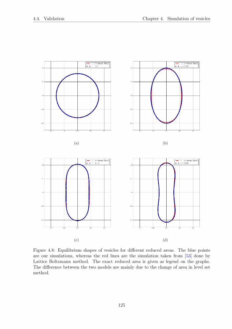
4.4. Validation Chapter 4. Simulation of vesicles
(a) (b)
(c) (d)
Figure 4.8: Equilibrium shapes of vesicles for different reduced areas. The blue pointsare our simulations, whereas the red lines are the simulation taken from [53] done byLattice Boltzmann method. The exact reduced area is given as legend on the graphs.The difference between the two models are mainly due to the change of area in level setmethod.
125
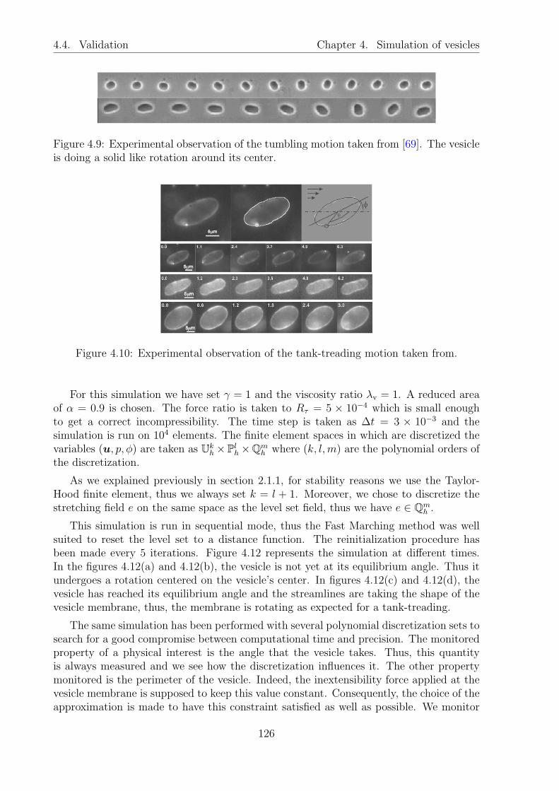
4.4. Validation Chapter 4. Simulation of vesicles
Figure 4.9: Experimental observation of the tumbling motion taken from [69]. The vesicleis doing a solid like rotation around its center.
Figure 4.10: Experimental observation of the tank-treading motion taken from.
For this simulation we have set γ = 1 and the viscosity ratio λv = 1. A reduced areaof α = 0.9 is chosen. The force ratio is taken to Rτ = 5 × 10⁻⁴ which is small enoughto get a correct incompressibility. The time step is taken as ∆t = 3 × 10⁻³ and thesimulation is run on 104 elements. The finite element spaces in which are discretized thevariables (u, p, φ) are taken as Uk
h×Plh×Qm
h where (k, l,m) are the polynomial orders ofthe discretization.
As we explained previously in section 2.1.1, for stability reasons we use the Taylor-Hood finite element, thus we always set k = l + 1. Moreover, we chose to discretize thestretching field e on the same space as the level set field, thus we have e ∈ Qm
h .
This simulation is run in sequential mode, thus the Fast Marching method was wellsuited to reset the level set to a distance function. The reinitialization procedure hasbeen made every 5 iterations. Figure 4.12 represents the simulation at different times.In the figures 4.12(a) and 4.12(b), the vesicle is not yet at its equilibrium angle. Thus itundergoes a rotation centered on the vesicle’s center. In figures 4.12(c) and 4.12(d), thevesicle has reached its equilibrium angle and the streamlines are taking the shape of thevesicle membrane, thus, the membrane is rotating as expected for a tank-treading.
The same simulation has been performed with several polynomial discretization sets tosearch for a good compromise between computational time and precision. The monitoredproperty of a physical interest is the angle that the vesicle takes. Thus, this quantityis always measured and we see how the discretization influences it. The other propertymonitored is the perimeter of the vesicle. Indeed, the inextensibility force applied at thevesicle membrane is supposed to keep this value constant. Consequently, the choice of theapproximation is made to have this constraint satisfied as well as possible. We monitor
126

4.4. Validation Chapter 4. Simulation of vesicles
Figure 4.11: Scheme taken from [58] representing the phase diagram of the vesicle dynam-ics under shear flow. The y axis represents the viscosity ratio and the x axis the capillarynumber
the percentage of loss of perimeter defined as:
∆per = 100× per − per0per0
(4.29)
where per0 is the perimeter at the initial time.We first checked that changing the polynomial approximation of the fluid velocity and
pressure does change neither the perimeter conservation nor the measure of the angle.Indeed, the perimeter conservation is mainly a consequence of the stretching force. Bylooking at the expression (4.15) we see that the force is the sum of two terms involving the
first derivative of the level set field (n =∇φ
|∇φ|) and the first derivative of the stretching
(e− 1).When the polynomial order of discretization of the level set field and the stretching
field is taken as m = 1, the derivatives of φ and e are discontinuous piecewise constants.Thus, even by projecting on a P1 space, the inextensibility force carries only this infor-mation. This is in fact the biggest limitation of this model for the inextensibility, and theapproximation error on the velocity and the pressure are dominated by the error broughtby the inextensibility force. Figure 4.13(a) shows the percentage of loss of perimeter asa function of time and figure 4.13(b) the angle dependency as a function of time for twodifferent polynomial approximations for the fluid being (k = 2, l = 1) and (k = 4, l = 3).
We see clearly that the increase of the polynomial approximation has almost no effecton the loss of perimeter and on the evolution of the angle during time. By contrast, figure
127

4.4. Validation Chapter 4. Simulation of vesicles
(a) (b)
(c) (d)
Figure 4.12: Vesicle in shear flow under tank-treading regime. The inside fluid of thevesicle (where φ < 0) is represented in red, whereas the outside fluid (φ > 0) is representedin blue. The streamlines are represented as black lines.
128

4.4. Validation Chapter 4. Simulation of vesicles
(a) Percentage of loss of perimeter. No effect is seenby increasing the fluid polynomial approximation.
(b) Angle evolution in time.
Figure 4.13: Loss of perimeter and angle as a function of time for different polynomialapproximation for the fluid: U2
h × P1h and U4
h × P3h.
4.14(a) and 4.14(b) show the same simulation in which only the level set (and stretching)polynomial approximation has been raised from 1 to 3. We see in figure 4.14(a) that theloss of perimeter is greatly improved by increasing the polynomial order of the level setfrom 1 to 2. Indeed, this makes the inextensibility force carry the information of a P1
continuous field which improves a lot the perimeter conservation (gain of almost 2%) forthis particular simulation. Increasing again the approximation ameliorates slightly theperimeter conservation but the gain is small.
The angle dependency in figure 4.14(b) is not greatly affected by the change of poly-nomial approximation. This could be understood by the fact that the vesicle perimeterdecreases almost symmetrically. Thus, the overall shape of the vesicle is almost the sameand the angle with respect to the horizontal does not change much even if the globalperimeter decreases. Of course, for a long time simulation this loss of perimeter would becritical.
Let us discuss the quality of this method. Even for the better approximation, the lossof perimeter is of the order of 3% for a simulation time which is not so long. This is arelatively bad result.
Moreover, we see some instabilities appearing around the vesicle if the time step is notsmall enough. This is because the inextensibility force has to be very strong to have goodperimeter conservation. Thus, a relatively big local change in the stretching introduces ahuge response of the inextensibility force. If the time step is not very small, this responseintroduces a local movement of the interface which possibly brings more stretching andmakes the simulation completely unstable.
This stability issue makes this method unsuitable for difficult simulations of long timefor now. Even if the advantage of having a vesicle completely defined only by adding aright hand side term in the fluid solver is really attractive, we did not go further than thistest and the previous one with this method.
Moreover, keeping the stretching information might be difficult in the context of thesimulation of a suspension of vesicles. When two particles get very close to each other,the level set has to be reinitialized often to avoid the merging of the two interfaces. In the
129

4.4. Validation Chapter 4. Simulation of vesicles
(a) Percentage of loss of perimeter. (b) Angle of the vesicle in time. The effect on theangle dependency in time is not significant.
Figure 4.14: Loss of perimeter and angle as a function of time for different polynomialapproximation of the level set and stretching fields: Q1
h, Q2h and Q3
h.
context of inextensibility forces many mesh elements between two vesicles are needed todo the computation of the stretching and the force, and to distribute the force on severalelements.
In the future, this method might be improved to overcome those issues, maybe witha different formulation of the force or a mesh adaptation making the local approximationof the force very precise.
Tank-treading motion of a vesicle with inextensibility imposed by Lagrangemultiplier
We will see that the Lagrange multiplier method gives better results and brings a betterstability for this simulation. We take the model described in section 4.3 and put a vesiclein the conditions for a tank-treading motion.
The viscosity ratio is set to λv = 1. The vesicle is in the center of a box where the topand bottom walls are moving in opposite directions at speed U = 1. On the lateral walls,a linear velocity is imposed. The velocities of the walls are imposed by strong Dirichletboundary conditions. The vesicles are chosen to have a fixed area A = π2. The capillary
number defined as Ca =µUL2
kBis equal to π. The quantities (u, p, λ, φ) are discretized
on finite element spaces Uk+1h × Pk
h × Lkh × Qk
h, where we choose the Lagrange multiplierand the level set field to be discretized on a finite element basis of the same order as thepressure field. For this simulation, we have set k = 1.
We show a first simulation in which we set a box of [30 × 8]2, the mesh size is fixedat hmin = 0.06 in a box centered on the vesicle of size [1× 7]2 and hmax = 0.4 elsewhere.This mesh has 36144 elements. The simulations are run in parallel on 5 processors.
A picture of the computational domain, the associated mesh and the mesh partitionsis represented in figure 4.15. The time step is taken as dt = 0.008 and the final time isset to 40 which makes this simulation relatively long.
Since the simulation is run in parallel and since the Fast Marching method is not a
130

4.4. Validation Chapter 4. Simulation of vesicles
Figure 4.15: A vesicle in tank-treading simulation in the computational domain. Themesh has been added with its refinement around the vesicle. The sub domains associatedto different processors are represented with different colors.
parallel algorithm, the reinitialization procedure has been made by solving the HamiltonJacobi equation as explained in section 1.3.3. The reinitialization procedure is made every5 iterations.
As expected, the vesicle rotates to attain a steady angle and a steady shape in whichthe curvature forces (shown in figure 4.16) and the hydrodynamic one are equilibrated.The tank-treading motion is obtained as we can see in figure 4.19(a) in which the stream-
Figure 4.16: Curvature forces exerted on the vesicle at steady state.
lines are represented as black lines.One can see that the streamlines are along the membrane, which implies that the
membrane (as well as the internal fluid) is rotating. The velocity of the fluid is almostzero at the middle abscissa of the channel, but the continuity of the velocity imposes thestreamlines to close.
On figure 4.19(b) we have plotted the magnitude of the perturbation field induced bythe presence of the vesicle. This magnitude is defined by |u− ushear|, where ushear is theshear velocity as defined in equation (4.28).
We can see clearly on this figure that the disturbance of the velocity field is local and
131

4.4. Validation Chapter 4. Simulation of vesicles
that after two or three vesicle sizes on the lateral sides it has completely vanished. Thedisturbance is higher on the top right and bottom left sides of the vesicle. This can beunderstood by the fact that at these locations, the vesicle causes the fluid to go in theopposite direction that it would go in a pure shear flow.
At the top and bottom of the vesicle, one sees a blue spot where the perturbation flowseems to quickly vary. This is a numerical artifact due to the fact that the mesh becomesrough in this area.
Figure 4.19(c) shows the pressure field around the vesicle. We recall that a zero meanpressure is imposed to fix the pressure constant which is defined only by its gradient inStokes flow with Dirichlet boundary conditions.
We see that the vesicle is compressed on its lateral sides whereas it is elongated alongits long axis. The pressure inside the vesicle is higher than outside and is almost constant.
An interesting point is to look at the high variations of the pressure which arise insidethe membrane area. To emphasize this, we have drawn two black lines representing thearea in which the delta function is higher than 0.1.
Inside this region, the Lagrange multiplier is defined and the curvature force is applied.These additional terms to the Stokes equation make the pressure vary significantly in thatsmall region. For this particular case, we wanted to show explicitly the variations, thusan interface thickness of 6 mesh elements has been chosen. In general, only 3 or 4 meshelements are sufficient to distribute correctly the forces and the Lagrange multiplier.
The perimeter conservation is obtained with a better accuracy than in the case of thesimulations by inextensibility forces. The stability issue that we had with the forces doesnot exist since the Lagrange multiplier is distributed on a sufficient number of elementsacross the interface. Figures 4.17 and 4.18 show the loss of perimeter and surface as afunction of time for this simulation.
5 10 15 20 25 30 35 40t
0.0
0.2
0.4
0.6
0.8
1.0
∆p(%
)
(a) Loss of perimeter (in percent) for the wholesimulation.
20.2 20.4 20.6 20.8 21.0 21.2 21.4t
0.380
0.385
0.390
0.395
0.400
∆p(%
)
(b) Close up of the loss of perimeter. The stepsare due to the reinitialization procedure.
Figure 4.17: Perimeter conservation (in percent) as a function of time for the tank-treadingsimulation.
We recall that since the velocity chosen for this simulation is low U = 1, the shearrate is also weak γ = 0.2, and the time necessary to attain a steady state in tank-treadingmotion is long (4000 iterations for the whole simulation). This makes this simulation hardin the sense of perimeter and surface conservation. Thus, regarding the simulation time,the conservation of these quantities is good.
132

4.4. Validation Chapter 4. Simulation of vesicles
5 10 15 20 25 30 35 40t
0.0
0.5
1.0
1.5
2.0∆s(%
)
(a) Loss of surface (in percent) for the whole sim-ulation.
20.2 20.4 20.6 20.8 21.0 21.2 21.4t
0.94
0.95
0.96
0.97
0.98
0.99
1.00
∆s(%
)
(b) Close up of the loss of surface. The steps aredue to the reinitialization procedure.
Figure 4.18: Surface conservation (in percent) as a function of time for the tank-treadingsimulation.
We also emphasize the fact that much of the loss of perimeter and surface is lostduring the reinitialization procedure. Indeed, the figures 4.17(b) and 4.18(b) show someclose up of the figures 4.17(a) and 4.18(a) in which we see that at each reinitializationstep (every 5 iterations), the errors increase quickly compared to the error added by thesimple advection without reinitialization.
The angle that the vesicle takes is measured between the long axis and the horizontalline. We call this angle Θ.
The variation of Θ as a function of time is represented in figure 4.20(a). On this graph,we have plotted the same information for different reduced areas. We can see that thesteady angle decreases with the reduced area. In the limit case, where the vesicle is almosttotally swollen (circular), the angle tends to the value 45 and of course, the steady stateis obtained almost instantaneously.
The figure 4.20(b) shows the steady angle as a function of the reduced volume for twodifferent confinements. We define the confinement as the ratio between twice the radiusof a circle having the same area than the vesicle and the length of the channel:
Cn =2R0
L. (4.30)
In our case, we have R0 =√π. We see that when the confinement increases, the steady
angle decreases.At the limit, one can imagine that when the length of the channel is really small,
there is no space for the vesicle to rotate, and the angle has to go to 0. The behaviorsshown in figure 4.20(a) and 4.20(b) are in good agreement with what was expected. Theresults are slightly different from those of [53] but it can be attributed to the differenceof parameters chosen (capillary number and shear rate). However, the behavior is good.
133

4.4. Validation Chapter 4. Simulation of vesicles
(a) Velocity of the fluid for a vesicle in tank-treading regime. The color is the magnitude of the velocity.The streamlines are represented with black lines. The vesicle is at steady state, the streamlines arealong the membrane which is rotating.
(b) Magnitude of the perturbation velocity |u− ushear|. The perturbation field vanishes away fromthe vesicle. It is higher in the regions where the vesicle membrane forces the fluid to go in the oppositedirection that the unperturbed one.
(c) Pressure field. We can see that the vesicle is elongated in the direction of its axis andcompressed in the other direction. Because of the Lagrange multiplier, the pressure inside themembrane has values varying quickly. The membrane boundary are represented in black lines.
Figure 4.19: Results of the simulation of a tank-treading motion.
134

4.4. Validation Chapter 4. Simulation of vesicles
0 5 10 15 20 25 30 35 40t
0
5
10
15
20
25
30
35
Θ
α = 0.9
α = 0.8
α = 0.7
α = 0.6
(a) Angle as a function of time for different re-duced areas.
0.55 0.60 0.65 0.70 0.75 0.80 0.85 0.90 0.95α
16
18
20
22
24
26
28
30
32
34
Θ
Cn = 0.35
Cn = 0.59
(b) Steady angle as a function of reduced area, fordifferent confinements.
Figure 4.20: Angle behaviors with respect to different parameters.
Tumbling motion
We also wanted to check that we can obtain the tumbling motion. To reproduce thisbehavior, we set initially a vesicle as an ellipse in a box of size [14, 5]2, discretized with7218 elements. We chose a time step of δt = 3 × 10⁻². These parameters are not asrefined as in the previous section in order to get long time simulations in a reasonablecomputational time. The other parameters of the simulation were: Ca = 6 × 10⁻²,Cn = 0.25 and α = 0.8. Figure 4.21 shows 3 snapshots of a vesicle tumbling motion.
Increasing the viscosity ratio increases the rotation frequency of the tumbling as canbe seen in figures 4.22(a) and 4.22(b). Moreover, as described in [37], when one increasesthe viscosity ratio, the rotation frequency of the vesicle reaches a steady value whichcorresponds to the steady rotation of a solid object in a shear flow. We can see thisphenomenon in figure 4.22(b).
We can understand the fact that the rotation frequency decreases with decreasingviscosity as the egg theorem: take a raw egg and a cooked egg. Make them rotate withthe same torque, the cooked egg rotates faster than the other one, because the differentlayers of fluid inside the raw egg are sheared and dissipate some energy.
(a) t = 1.0 (b) t = 1.1 (c) t = 6.0
Figure 4.21: Tumbling of a vesicle
135

4.4. Validation Chapter 4. Simulation of vesicles
(a) Tumbling angle as a function of time for two different viscosity ratios.One can see that the higher viscosity ratio exibits a higher rotation fre-quency.
(b) Tumbling frequency for different viscosity ratios. The frequency in-creases with the viscosity ratio. It reaches the limit of a solid object rota-tion.
Figure 4.22: Tumbling angle and frequency.
136

Part II
Implementation
137


Chapter 5
Contributions to the library Feel++
Contents5.1 Projection operator as a C++ class . . . . . . . . . . . . . . . 140
5.1.1 Motivation . . . . . . . . . . . . . . . . . . . . . . . . . . . . . 140
5.1.2 Usage of the Projector class . . . . . . . . . . . . . . . . . . . . 141
5.1.3 Projector class used to compute the derivative of a field . . . . 142
5.2 The Advection class . . . . . . . . . . . . . . . . . . . . . . . . . 144
5.2.1 Description of the class . . . . . . . . . . . . . . . . . . . . . . 145
5.2.2 Example on Hamilton-Jacobi equation for reinitialization . . . 146
5.3 LevelSet class . . . . . . . . . . . . . . . . . . . . . . . . . . . . . 147
5.3.1 The public part . . . . . . . . . . . . . . . . . . . . . . . . . . . 147
5.3.2 The markers . . . . . . . . . . . . . . . . . . . . . . . . . . . . 148
5.3.3 The external options . . . . . . . . . . . . . . . . . . . . . . . . 150
5.3.4 The protected part . . . . . . . . . . . . . . . . . . . . . . . . . 151
5.4 The MultiLevelSet class . . . . . . . . . . . . . . . . . . . . . . 151
5.4.1 From LevelSet to MultiLevelSet . . . . . . . . . . . . . . 151
5.4.2 Specific MultiLevelSet methods . . . . . . . . . . . . . . . . 152
139

5.1. Projection operator as a C++ class Chapter 5. Contributions to Feel++
In this chapter, we will present some development made for the vesicle application butwhich can be useful in other ones. Thus, a special care has to be taken to make theseapplications as generic and re-usable as possible. We first present a projection tool whichhas been of great use in writing the bending forces in the vesicle context but which canbe used in many applications. Then, we present the framework for solving the advectionequation which is used to transport the level set function and reinitialize it by solving theHamilton Jacobi equation previously presented. We explain in this chapter how the C++templates can be used to make a class solving this equation for any coefficient expression.Then the LevelSet class is presented and the MultiLevelSet class derived from it isalso introduced.
5.1 Projection operator as a C++ class
5.1.1 Motivation
In Feel++ , a projection operator exists. It is a useful tool to do nodal projections. Thefunction is a part of the language, its arguments are the following:
p r o j e c t ( space=<nodal f unc t i on space in which the i n t e r p o l an t l i v e s>range=<domain range i t e r a t o r s >,expr=<exp r e s s i on to be in t e rpo l a t ed >, . . . . )
Note that this function uses the 1boost parameter library which allows passing ofarguments independently and in any order by name (prefixed with an underscore). Thisfunction calculates the expression given in expr at every quadrature point in the rangerange which is a part of the domain on which is defined the space space. The resultingfunction is thus exact at quadrature points of range. We have seen in section 4.1 thatthe vesicle application requires L2 and smooth projections rather than nodal projections.These projections were already supported in Feel++ since they require solving a simplePDE problem. But each application requiring it had to create its own projector frameworkby providing the bilinear forms of the projection and solving the final problem. Since theapplication we were interested in required many of these projections, we created a C++class which was able to handle all the types of projections (L2, H1, smooth,CIP) neededfor this application. Then, other types of projection needed in other applications havebeen added to complete this tool like Hdiv, Hcurl or the LIFT operator. The advantage tohave a single model object for all these projections is that they are all handled the sameway, the declarations of these objects are the same and only a parameter has to be givento differentiate the projector type. The project function itself takes exactly the sameexpression for any projector which brings more clarity in the different codes. Moreover,some optimization can be done (like keeping the bilinear form as it will be explainedbelow) and the optimizations are completely hidden in the projector class, making theoptimization systematic. Finally, the bilinear form projections are written and testedonce and for all and there is no need to re-write them for each application.The basic idea of this class is to construct projector objects. Each object can do a givenprojection. For the construction of such an object, one only need the type of projection,and the space in which the projection is done. Providing this information, one can createthe matrix associated to the bilinear form (the left hand side of the projection equation)
1http://www.boost.org/doc/libs/
140
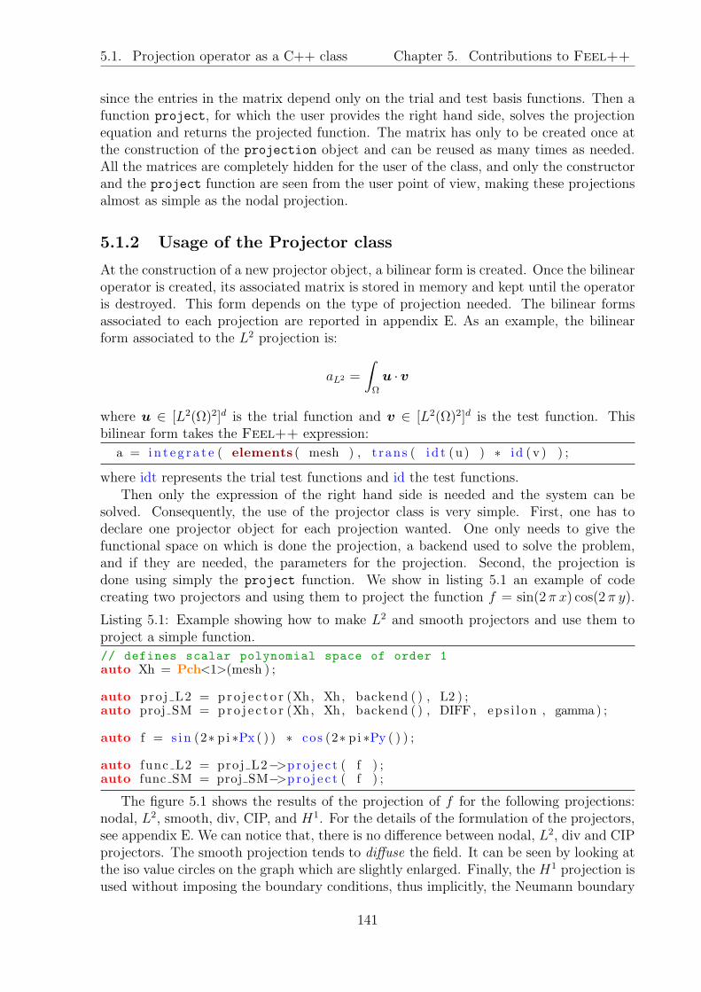
5.1. Projection operator as a C++ class Chapter 5. Contributions to Feel++
since the entries in the matrix depend only on the trial and test basis functions. Then afunction project, for which the user provides the right hand side, solves the projectionequation and returns the projected function. The matrix has only to be created once atthe construction of the projection object and can be reused as many times as needed.All the matrices are completely hidden for the user of the class, and only the constructorand the project function are seen from the user point of view, making these projectionsalmost as simple as the nodal projection.
5.1.2 Usage of the Projector class
At the construction of a new projector object, a bilinear form is created. Once the bilinearoperator is created, its associated matrix is stored in memory and kept until the operatoris destroyed. This form depends on the type of projection needed. The bilinear formsassociated to each projection are reported in appendix E. As an example, the bilinearform associated to the L2 projection is:
aL2 =
∫
Ω
u ·v
where u ∈ [L2(Ω)2]d is the trial function and v ∈ [L2(Ω)2]d is the test function. Thisbilinear form takes the Feel++ expression:
a = in t e g r a t e ( elements ( mesh ) , t rans ( i d t (u) ) ∗ id ( v ) ) ;
where idt represents the trial test functions and id the test functions.Then only the expression of the right hand side is needed and the system can be
solved. Consequently, the use of the projector class is very simple. First, one has todeclare one projector object for each projection wanted. One only needs to give thefunctional space on which is done the projection, a backend used to solve the problem,and if they are needed, the parameters for the projection. Second, the projection isdone using simply the project function. We show in listing 5.1 an example of codecreating two projectors and using them to project the function f = sin(2 π x) cos(2 π y).
Listing 5.1: Example showing how to make L2 and smooth projectors and use them toproject a simple function.
// defines scalar polynomial space of order 1auto Xh = Pch<1>(mesh ) ;
auto pro j L2 = pro j e c t o r (Xh, Xh, backend ( ) , L2 ) ;auto proj SM = pro j e c t o r (Xh, Xh, backend ( ) , DIFF , eps i l on , gamma) ;
auto f = s i n (2∗ pi ∗Px ( ) ) ∗ cos (2∗ pi ∗Py ( ) ) ;
auto func L2 = proj L2−>p r o j e c t ( f ) ;auto func SM = proj SM−>p r o j e c t ( f ) ;
The figure 5.1 shows the results of the projection of f for the following projections:nodal, L2, smooth, div, CIP, and H1. For the details of the formulation of the projectors,see appendix E. We can notice that, there is no difference between nodal, L2, div and CIPprojectors. The smooth projection tends to diffuse the field. It can be seen by looking atthe iso value circles on the graph which are slightly enlarged. Finally, the H1 projection isused without imposing the boundary conditions, thus implicitly, the Neumann boundary
141

5.1. Projection operator as a C++ class Chapter 5. Contributions to Feel++
condition ∇f ·n = 0 is imposed. Consequently, there is no gradient of the function inthe normal direction close to the boundaries, this makes the iso values perpendicular tothe borders of the domain as we can see in figure 5.1(f).
(a) Nodal projection (b) L2 projection (c) smooth projection
(d) Hdiv projection (e) CIP projection (f) H1 projection
Figure 5.1: Results of the projection of f using different projectors. The color is theamplitude of the projected function f . The deepest red is 1, the deepest blue is -1. 10iso values are reported in black.
5.1.3 Projector class used to compute the derivative of a field
Let us consider that we want u ∈ [L2(Ω)]d as the projection of the gradient of a knownscalar field f ∈ H1(Ω). We can write this expression on the weak form (5.1) which is theclassical L2 projection of the gradient of f . We can also integrate by parts this equation,which leads to the formulation (5.2). This formulation requires that the test functionv ∈ [H1(Ω)]d.
∫
Ω
u ·v =
∫
Ω
∇f ·v (5.1)∫
Ω
u ·v = −∫
Ω
f∇ ·v +
∫
∂Ω
f v ·n (5.2)
The formulation (5.2) has the advantage of never computing directly the gradient of thefunction f since the derivatives are on the test functions. We remark also that the lefthand side is exactly the same as for a classical L2 projection. Thus by changing only
142

5.1. Projection operator as a C++ class Chapter 5. Contributions to Feel++
the form of the right hand side term, we can provide an operator which computes theprojection of the gradient of an expression. We called such a method derivate.
If we take the previous example, and we want the projection of g = ∇f , we onlyneed to create a projector in a vectorial space (since g is a vector), and use the derivatefunction on the expression f . The listing 5.2 gives an example of such a code. In thisexample, we also show an alternative to get the derivative of a field, by projecting theexpression on the vectorial space, and doing a nodal projection of its gradient on the samespace.
Listing 5.2: Create a projector and compute the projection of ∇f
// Vectorial functionspaceconst int order = 1 ;auto Xhv = Pchv<order>(mesh ) ;
// defines the expression to deriveauto f = s i n (2∗ pi ∗Px ( ) ) ∗ cos (2∗ pi ∗Py ( ) ) ;
// compute the derivative using the projector classauto pro j L2 vec = p r o j e c t o r (Xhv , Xhv , backend ( ) , L2 ) ;auto g = pro j L2 vec−>de r i v a t e ( f ) ;
// compute the derivative of a nodal projection of fauto f n oda l = p r o j e c t (Xhv , elements (mesh ) , f ) ;auto g nodal = p ro j e c t (Xhv , elements (mesh ) , gradv ( f noda l ) ) ;
We made this test by taking a discretization of f as polynomials of order 1 and 3 and u
has been taken in vectorial spaces of the same polynomial order.
The results of the nodal projection have been plotted in figure 5.3 and the result of theprojection using the method derivate has been plotted in figure 5.4. Since the theoreticalresult is known, the L2 error has been computed. We can see on figures 5.2(a) and 5.2(b)that we obtain one order of convergence higher using the derivate method compared tothe nodal projection of ∇f on the same space.
10−2 10−1
h
10−3
10−2
10−1
100
e L2
nodale proj, slope = 1.0
derivate(f ), slope = 2.0
(a) f and u taken as polynomials of order 1
10−2 10−1
h
10−9
10−8
10−7
10−6
10−5
10−4
10−3
10−2
10−1
e L2
nodale proj, slope = 3.0
derivate(f ), slope = 4.0
(b) f and u taken as polynomials of order 3
Figure 5.2: Comparison between the derivative using the derivate method and a nodalprojection of the derivative.
143

5.2. The Advection class Chapter 5. Contributions to Feel++
(a) X component of ∇f (b) Y component of ∇f
Figure 5.3: Gradient of f computed using a nodal projection.
(a) X component of g (b) Y component of g
Figure 5.4: Gradient of f computed using 5.2.
5.2 The Advection class
Solving the advection equation (1.12) is a key point for this work. Indeed, it is usedevery time step for the evolution of the level set field that we have seen in section 1.2and it is also used to reinitialize the level set front in the context of a reinitialization bysolving a Hamilton-Jacobi equation as seen in section 1.3.3. Thus, the need of a generalframework to solve this equation arises. A C++ class has been created during the PhDof Christophe Winkelmann [112]; we updated this to fit our needs and we added thestabilization methods presented in section 1.2.2. We will present in this section someaspects of the implementation of this class.
144

5.2. The Advection class Chapter 5. Contributions to Feel++
5.2.1 Description of the class
A simplified view of the Advection class is given in listing 5.3
Listing 5.3: Simplified view of the Advection class.
public :enum s t ab i l i z a t i onMethod NO, GALS, CIP , SUPG, SGS ;
Advection ( space type space , s t ab i l i z a t i onMethod sMeth ) ;
// update the coefficients to solve the equation:// σφ+ β ·∇φ = f in Ω// φ = g on ∂Ωtemplate <typename SigmaT , typename BetaT , typename FT, typename GT>void update (SigmaT sigma , BetaT beta , FT f , GT g ) ;
e l ement type phi ( ) ;
private :spa r s e mat r ix D;v e c t o r p t r t ype F ;
s t ab i l i z a t i onMethod stabMethod ;
The matrix D associated to the discretization of the equation and the right hand side Fare created at the construction of the object once and for all. Of course, the matrix has tobe reassembled at each resolution of the equation, but for a given problem, the test andtrial functions of the problem do not change at each new resolution. Thus, creating thenon null entries of the matrix once and for all is an optimization. From the user point ofview, when solving the equation (1.12), one only has to give the values of σ,β, f and someDirichlet boundary conditions g which are applied at the inflow boundaries. The methodupdate is meant for that. The types of σ,β, f, g might be complicated. Indeed, we wantto allow the possibility for the user to enter expressions for these values and not simplyelement of the space. The type of an expression in Feel++ depends on the expression.Thus, it is impossible to write explicitly the types of these parameters. It is not a problemsince C++ handles meta-programming thanks to the template feature. Thus, the updatefunction is a template function and the SigmaT, BetaT, FT, GT which are the types ofrespectively σ,β, f, g are computed automatically at compilation time depending on theexpression that have been given to the function. In the update function, the matrix Dand the vector F are assembled according to the variational formulation (1.14) as one cansee on listing 5.4.
Listing 5.4: Assembly of the matrix D and the vector F in the update function
// trial function φauto phi = space−>element ( ) ;// test function ψauto p s i = space−>element ( ) ;
//∫
Ω fψform1 ( space , F)= i n t e g r a t e (elements (mesh ) , f ∗ id ( p s i ) ) ;
//∫
Ω(σφ+ β ·∇φ)ψform2 ( space , space , D)= i n t e g r a t e (elements (mesh ) ,
( sigma ∗ i d t ( phi ) + gradt ( phi ) ∗ beta ) ∗ id ( p s i ) ) ;
145

5.2. The Advection class Chapter 5. Contributions to Feel++
As one can see on listing 5.4, there are obviously some restrictions on the types of the pa-rameters given to this method. But the restrictions are more related to the mathematicalobjects that represent the parameters σ,β, f than to the C++ types. More precisely, themethod can work since σ and f are of a type representing a scalar function or a scalarnumber, and β a line vector. If these conditions are not respected, an error will be thrownduring the compilation.
The stabilization method is chosen by the user. It has to be picked as one of theenumeration stabilizationMethod elements. Then the algebraic representation of thecorresponding terms of equations (1.20) or (1.23) is added to the matrix D and the vectorF . Listing 5.5 gives an example of such terms for the SUPG stabilization.
Listing 5.5: SUPG stabilization added to the matrix D and vector F
// β ·∇ψauto supg term = grad ( p s i ) ∗ beta ;
// τSUPG
auto tau supg = h ( ) / (2 ∗ s q r t ( t rans ( beta )∗ beta ) ) ;
// L(φ)auto L op = gradt ( phi ) ∗ beta + sigma ∗ i d t ( phi ) ;
form2 ( space , space , D)+=in t e g r a t e (elements (mesh ) ,tau supg ∗ supg term ∗ L op ) ;
form1 ( space , F)+=in t e g r a t e (elements (mesh ) ,tau supg ∗ supg term ∗ f ) ;
Finally the method phi solves the equation and returns the solution.
5.2.2 Example on Hamilton-Jacobi equation for reinitialization
As an example of the use of Advection class we could give the advection equation (1.11)used for the motion of the level set field, but we chose to present the Hamilton Jacobiequation used for the reinitialization as presented in section 1.3.3. This is a bit morecomplicated. We have shown that the signed distance function can be obtained from afield being not too far from a distance function by solving the equation (1.26) which is anadvection equation of the form (1.12) for which the coefficients are:
σ =1
∆τ,
β =Sgn(φ
n)∇φn
|∇φn| ,
f = Sgn(φn) +
φn
∆τ,
with the same notations that we used in section 1.3.3. Given the Advection class, theimplementation of the reinitialization by solving the Hamilton Jacobi equation is simple.An example is given in listing 5.6.
146

5.3. LevelSet class Chapter 5. Contributions to Feel++
Listing 5.6: Hamilton Jacobi equation for the reinitialization of the level set field solvedby using the Advection class.
// max_iter and dtau are taken from user options// create an Advection objectadvec t i on h j = advec t i on type : : New( space , SUPG ) ;
for ( int i =0; i<=max iter ; ++i )
// update the Heaviside function according to (1.3)auto H = vf : : p r o j e c t ( space , elements (mesh ) ,ch i ( phi< −ep s i l o n ) ∗ 0 .+ ch i ( phi >= −ep s i l o n )∗ ch i ( phi <= ep s i l o n )∗ 1/2∗(1 + phi / ep s i l o n + s i n ( p i ∗phi / ep s i l o n ) / p i )+ ch i ( phi > ep s i l o n ) ∗ 1 . ) ;
// expressions of Sgn(φ), σ, β, fauto sgn = 2 ∗ ( idv (H) − 0 .5 ) ;auto sigma = 1 / dtau ;auto beta = sgn ∗ t rans ( gradv ( phi ) )/ sq r t ( gradv ( p h i r e i n i t )∗ t rans ( gradv ( p h i r e i n i t ) ) ) ;auto f = idv ( p h i r e i n i t ) / dtau + s i gne ;
// update the matrices D and fadvect i on h j−>update ( sigma , beta , f , true ) ;
// solve the equation and save into phiphi = advect ion h j−>phi ( ) ;
5.3 Design of the Level Set class
In this section, we will explain how we structured the Level Set class. This class has beenmade with the goal of a maximum generality and ease re-use.
5.3.1 The public part
Let us describe how we designed the LevelSet class in order to make it as generic aspossible. The core of the level set class should provide methods to initialize a level set fieldand advect it with respect to the advection equation since the user provides a velocity.The advection equation should also contain the possibility to reinitialize the level set fieldif needed. The advection and the reinitialization should be the only two ways to modifythe level set field and the C++ encapsulation is used to make sure it happens this way.The class should also provide some accessors to the Dirac and Heaviside fields whichshould be automatically updated after each modification of the level set fields. Thus, thebasic components of the public level set class are the following:
Listing 5.7: Simplified part of the core of the public part of the LevelSet class.
public :
/* constructor and initialization*/Leve lSet ( mesh ptrtype mesh ) ;
147

5.3. LevelSet class Chapter 5. Contributions to Feel++
void i n i t i a l i z e ( e l ement ptr type phio , bool doF i r s tRe in i t ) ;
/* advection method */template <typename Tu> bool advect ( Tu& u ) ;
/* getters */const e l ement ptr type phi ( ) ;const e l ement ptr type H( ) ;const e l ement ptr type D( ) ;
where the suffix ptrtype represents the fact that the given type is actually a smart pointertype, the 2boost::shared ptr is used. The initialize method is used to set the initiallevel set φ0 to the given phio field. If we are not able to provide an exact distance functionfor phio, the parameter doFirstReinit can be set to true and then a reinitializationis performed. The methods phi(), H() and D() are accessors to the values of respec-tively φ, δε, and Hε. They could be used directly in an expression, for example if onehas to define the viscosity of a two fluids system, we have seen that the viscosity fieldhas to be defined as: µφ = µ2 + (µ1 − µ2)Hε(φ). If one has an instance levelset of theclass LevelSet , providing the values of µ1 and µ2, the formulation simply takes the form:
mu2 + ( mu1 − mu2 ) ∗ idv ( l e v e l s e t−>H() ) ;
where idv is the Feel++ keyword to have access to the values of an element of a functionspace.The advect method is used to advect the level set field with the given velocity u, checkif the reinitialization is needed, do it if necessary, and update the quantities φ, Hε andδε. The advect method has to be a template method since the type of the velocity is notknown a priori. The type will be deduced at the compilation time according to the typeof the velocity given when the method is used. By introducing this template parameter,every velocity type for which the operator * is implemented can be used in this method.Indeed, only this operation is needed in the advection equation.The type of an element of a functional space depends on its polynomial order of ap-proximation. The * operator is implemented between elements of different polynomialorders. Thus, providing this template function advect allows coupling the level set witha velocity of an arbitrarily high order. Since in the level set framework the coupling withthe fluid only appears at the level of the advection equation, making this method genericleads to a generic LevelSet class which will be easy to couple to any type of fluid velocity.
5.3.2 The markers
We also created other useful methods that we did not report in the listing 5.7, like sev-eral markers calculated from the level set field. A marker is a P0 element defined on allthe space and having integer values at different regions of the domain. It is possible inFeel++ to do operations only on the area on which a marker has a specific value. Weprovide the following markers:
2 http://www.boost.org/doc/libs/1_54_0/libs/smart_ptr/shared_ptr.htm
148
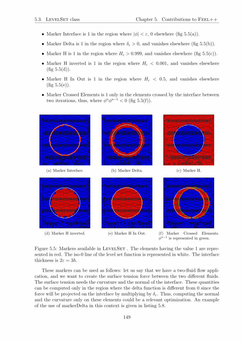
5.3. LevelSet class Chapter 5. Contributions to Feel++
• Marker Interface is 1 in the region where |φ| < ε, 0 elsewhere (fig 5.5(a)).
• Marker Delta is 1 in the region where δε > 0, and vanishes elsewhere (fig 5.5(b)).
• Marker H is 1 in the region where Hε > 0.999, and vanishes elsewhere (fig 5.5(c)).
• Marker H inverted is 1 in the region where Hε < 0.001, and vanishes elsewhere(fig 5.5(d)).
• Marker H In Out is 1 in the region where Hε < 0.5, and vanishes elsewhere(fig 5.5(e)).
• Marker Crossed Elements is 1 only in the elements crossed by the interface betweentwo iterations, thus, where φnφn−1 < 0 (fig 5.5(f)).
(a) Marker Interface. (b) Marker Delta. (c) Marker H.
(d) Marker H inverted. (e) Marker H In Out. (f) Marker Crossed Elements.φn−1 is represented in green.
Figure 5.5: Markers available in LevelSet . The elements having the value 1 are repre-sented in red. The iso-0 line of the level set function is represented in white. The interfacethickness is 2ε = 3h.
These markers can be used as follows: let us say that we have a two-fluid flow appli-cation, and we want to create the surface tension force between the two different fluids.The surface tension needs the curvature and the normal of the interface. These quantitiescan be computed only in the region where the delta function is different from 0 since theforce will be projected on the interface by multiplying by δε. Thus, computing the normaland the curvature only on these elements could be a relevant optimization. An exampleof the use of markerDelta in this context is given in listing 5.8.
149
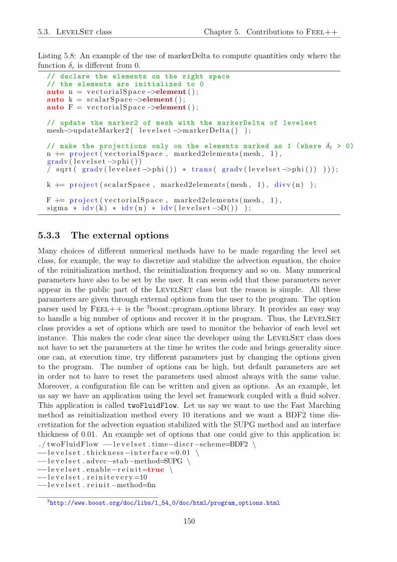
5.3. LevelSet class Chapter 5. Contributions to Feel++
Listing 5.8: An example of the use of markerDelta to compute quantities only where thefunction δε is different from 0.
// declare the elements on the right space// the elements are initialized to 0auto n = vec to r i a lSpace−>element ( ) ;auto k = sca larSpace−>element ( ) ;auto F = vec to r i a lSpace−>element ( ) ;
// update the marker2 of mesh with the markerDelta of levelsetmesh−>updateMarker2 ( l e v e l s e t−>markerDelta ( ) ) ;
// make the projections only on the elements marked as 1 (where δε > 0)n += pro j e c t ( vec to r i a lSpace , marked2elements (mesh , 1 ) ,gradv ( l e v e l s e t−>phi ( ) )/ sq r t ( gradv ( l e v e l s e t−>phi ( ) ) ∗ t rans ( gradv ( l e v e l s e t−>phi ( ) ) ) ) ) ;
k += pro j e c t ( sca larSpace , marked2elements (mesh , 1 ) , divv (n) ) ;
F += pro j e c t ( vec to r i a lSpace , marked2elements (mesh , 1 ) ,sigma ∗ idv (k ) ∗ idv (n) ∗ idv ( l e v e l s e t−>D( ) ) ) ;
5.3.3 The external options
Many choices of different numerical methods have to be made regarding the level setclass, for example, the way to discretize and stabilize the advection equation, the choiceof the reinitialization method, the reinitialization frequency and so on. Many numericalparameters have also to be set by the user. It can seem odd that these parameters neverappear in the public part of the LevelSet class but the reason is simple. All theseparameters are given through external options from the user to the program. The optionparser used by Feel++ is the 3boost::program options library. It provides an easy wayto handle a big number of options and recover it in the program. Thus, the LevelSet
class provides a set of options which are used to monitor the behavior of each level setinstance. This makes the code clear since the developer using the LevelSet class doesnot have to set the parameters at the time he writes the code and brings generality sinceone can, at execution time, try different parameters just by changing the options givento the program. The number of options can be high, but default parameters are setin order not to have to reset the parameters used almost always with the same value.Moreover, a configuration file can be written and given as options. As an example, letus say we have an application using the level set framework coupled with a fluid solver.This application is called twoFluidFlow. Let us say we want to use the Fast Marchingmethod as reinitialization method every 10 iterations and we want a BDF2 time dis-cretization for the advection equation stabilized with the SUPG method and an interfacethickness of 0.01. An example set of options that one could give to this application is:. / twoFluidFlow −− l e v e l s e t . time−d i s c r−scheme=BDF2 \−− l e v e l s e t . th i cknes s−i n t e r f a c e =0.01 \−− l e v e l s e t . advec−stab−method=SUPG \−− l e v e l s e t . enable−r e i n i t=true \−− l e v e l s e t . r e i n i t e v e r y=10−− l e v e l s e t . r e i n i t−method=fm
3http://www.boost.org/doc/libs/1_54_0/doc/html/program_options.html
150

5.4. The MultiLevelSet class Chapter 5. Contributions to Feel++
5.3.4 The protected part
The protected part of the level set function is by definition not accessible for the user ofthe class but its attribute are accessible from a class derived from it. These parametersand methods are important for the multi level set framework, thus, it is important todescribe it. A simplified list of the protected part of the LevelSet class is given inlisting 5.9
Listing 5.9: Simplified list of protected parameters and methods of the LevelSet class
protected :
e l ement ptr type p t r ph i ;e l ement ptr type ptr h ;e l ement ptr type ptr d ;
void updateHeavis ide ( ) ;void updateDirac ( ) ;
The parameters ptr phi, ptr h and ptr d are pointers on the elements representing thelevelset, Heaviside and Delta fields. The methods updateHeaviside and updateDirac
are used just after the advection step to update the fields pointed by ptr h and ptr d
according to the new value of the field pointed by ptr phi.
5.4 The MultiLevelSet class
5.4.1 From LevelSet to MultiLevelSet
To handle several level set fields at the same time, one could think at first to create anarray of LevelSet instances. This could work but would be dramatically costly in termsof computational time and memory. Indeed, this would copy all the internal ingredientsof LevelSet such as for example the bilinear matrices for the advection. It wouldalso copy the reinitialization framework which contains some features possibly heavy inmemory. For example, the bilinear matrix for the reinitialization by solving HamiltonJacobi equation or the table of the closest degree of freedom needed for the fast marchingmethod.Consequently, it is essential to think differently and try to share at maximum everythingwhich can be constructed once and reused for all the different level set. For example,the non-stabilized part of the bilinear matrix associated to the advection equation onlydepends on the given velocity u. Thus, in a context of multi-fluid flow, the velocity is thesame for all the level sets and this matrix could be computed once and for all and reusedto advect all the level set fields. The table of the first neighbors used for the fast marchingreinitialization depends only on the mesh, this can also be used for all the level sets. Thus,we created a MultiLevelSet class which allows to handle an arbitrary high number ofdifferent level sets fields. The MultiLevelSet class derives from the LevelSet class.It defines in addition, a vector of elements phis, hs, and ds meant to contain severalelements φ, Hε and δε. It also provides a method called switchPhi(i) which takes aninteger i as argument. This method is essential. It makes the pointers ptr phi, ptr h
and ptr d that we described previously, point on the ith element of phis, hs, and ds.This way, the methods advect, updateHeaviside and updateDirac will act on the ith
151

5.4. The MultiLevelSet class Chapter 5. Contributions to Feel++
level set element since they act on the value pointed by ptr phi, ptr h and ptr d. Weemphasize the fact that switchPhi(i) only changes the value of a few pointers, thus itdoes not cost anything in term of performance. Thanks to this method, it is possible todo operations on a single chosen level set field without duplicating all the attributes ofthe LevelSet class since by inheritance, MultiLevelSet has these attributes once.A scheme representing the effect of switchPhi(i) is given on figure 5.6. The advect
Modifies the value
pointed by
Figure 5.6: Action of switchPhi() on the pointers inherited from LevelSet .
method in a multi-level set context takes new arguments being the number of the levelset to advect. Then one only needs to switch to the desired level set and advect it. Thecode is given in listing 5.10
Listing 5.10: The advect method in multilevelset context. super represents the motherclass (here LevelSet )
template < typename Tu >bool advect (Tu& u , int i )
switchPhi ( i ) ;return super : : advect (u ) ;
5.4.2 Specific MultiLevelSet methods
The MultiLevelSet class provides accessors to individual φ, δε or Hε fields by themethods called phi(i), H(i) and D(i) accepting one argument being the number of thefield wanted. The class also provides interesting methods such as minPhi(), globH()and globD(). The first method returns a field corresponding to the minimum of all thelevel set fields (that we called φ0 in section 2.2.2, equation (2.34)). Indeed, as explainedin section 2.2.2, in the context of a multi-fluid application, this can be useful since thenormal and curvature depend only on the geometry of the iso 0 and are not specific toeach level set field. Thus, if the level sets are not interpenetrating, one could computethe geometrical fields (normal and curvature) once and finally use the delta function to
152

5.4. The MultiLevelSet class Chapter 5. Contributions to Feel++
differentiate the areas of the different level sets.The two other methods are simply the delta and Heaviside functions applied to the fieldφ0. The globH() function can be used to describe the regions inside any interface oroutside every interface. The globD() function can be used to distribute a quantity on allthe interfaces regardless of which individual level set it is. We give an example to illustratethe use of these functions. In section 5.3, we have seen how to define the viscosity andthe surface tension force in the context of a two-fluid flow. Let see how this works for amore than two-fluid flow. We already showed that the viscosity of such a system is givenby the equation (2.36). The surrounding fluid is represented by the area in which all thelevel set fields are positive, it has a given viscosity mup. The other fluids have differentviscosities stored in an array mum. Let us say we have an instance multilevelset of theclass MultiLevelSet . The viscosity of such a system can be given by:
auto mu = pro j e c t ( sca larSpace , elements (mesh ) ,mup ∗ idv ( mu l t i l e v e l s e t−>globH ( ) ) ) ;
for ( int i =0; i<mu l t i l e v e l s e t−>getNbPhi ( ) ; i++)
mu += pro j e c t ( sca larSpace , elements (mesh ) ,mum[ i ] ∗ (1 − idv ( mu l t i l e v e l s e t−>H( i ) ) ) ) ;
If the number of different fluids is known at the compilation time, one could avoid thefor loop and directly write the viscosity in one single projection. We wrote here the moregeneral way to do it where the number of different fluids is not known at compilation time,but only at execution. Let us see now how to write the surface tension force between thedifferent interfaces and the surrounding fluid. We will not describe here the general casewhere all the interfaces can be interacting with each other. Such a force is given byequation (2.37). As explained in section 2.2.2, we will use the fact than the min of all thelevel sets contains the geometrical information (normal and curvature) of all the interfacesat the same time. The different surface tension coefficients are given in an array calledsigma. The surface tension force reads:
// expression of |∇φ|auto modgradphi = sq r t ( gradv ( mu l t i l e v e l s e t−>minPhi ( ) )∗ t rans ( gradv ( mu l t i l e v e l s e t−>minPhi ( ) ) ) ) ;
// normalauto n = pro j e c t ( ve c to r i a lSpace , elements (mesh ) ,
gradv ( mu l t i l e v e l s e t−>minPhi ( ) )/ modgradphi ) ;
// curvatureauto k = pro j e c t ( sca larSpace , elements (mesh ) , divv (n) ) ;
// surface tension forceauto F = vec t o r i a l Spa c e ()−>element ( ) ;for ( int i =0; i<mu l t i l e v e l s e t−>getNbPhi ( ) ; i++)
F += pro j e c t ( vec to r i a lSpace , elements (mesh ) ,− sigma [ i ] ∗ idv (k ) ∗ idv (n) ∗ idv ( mu l t i l e v e l s e t−>D( i ) ) ) ;
153

5.4. The MultiLevelSet class Chapter 5. Contributions to Feel++
154

Chapter 6
Specific development for the Vesicleapplication
Contents6.1 Lagrange multiplier construction . . . . . . . . . . . . . . . . . 156
6.1.1 A size problem . . . . . . . . . . . . . . . . . . . . . . . . . . . 156
6.1.2 Extract the submesh . . . . . . . . . . . . . . . . . . . . . . . . 156
6.1.3 Creating the Lagrange Multiplier contribution . . . . . . . . . 158
6.1.4 The global matrix assembly . . . . . . . . . . . . . . . . . . . . 159
6.1.5 Performance test . . . . . . . . . . . . . . . . . . . . . . . . . . 159
6.2 A Python interface . . . . . . . . . . . . . . . . . . . . . . . . . 162
6.2.1 Why an interface is needed? . . . . . . . . . . . . . . . . . . . . 162
6.2.2 An example: the vesicle in a shear flow application . . . . . . . 163
155

6.1. Lagrange multiplier construction Chapter 6. Development for Vesicle application
We present in this chapter a few developments which have been made specially for thevesicle application. The first one is the problem of constructing the Lagrange multiplierwhich insures that the vesicle is unstretchable. This requires creating a subspace definedon a submesh around the vesicle. The Lagrange multiplier is defined only in this subspacewhich reduces substentially the number of total degrees of freedom in the final problem.Then we explain our strategy to make user-friendly simulations. Indeed, the vesicle codeis made to be very generic and many options have to be set by the user. For real physicallsimulation in which we only want to see the physically relevant parameters, we created aPython interface which allows us to concentrate on the physics of the problem, makingtransparent all the inter-dependent options.
6.1 Lagrange multiplier construction
6.1.1 A size problem
We have seen in section 4.3 that the constraint of the inextensibility of the membranecan be satisfied by adding a Lagrange multiplier to the variational formulation of theproblem. This Lagrange multiplier is supposed to act on the membrane of the vesicle (i.e.in the area where δε > 0). If we look at the expression (4.23), the discretized Lagrangemultiplier λh is defined on all the domain Ω and its action is restricted to the interfaceby multiplying by the function δε. Thus, from the algebraic point of view, the matrix C,which corresponds to the contribution of the variables in the trial space Lk
h(Ω) associatedto the Lagrange multiplier and the test space Uk+1
h (Ω) associated to the velocity, has itscoefficients defined by
Cij =
∫
Ω
δεξj∇s ·Φi =
∫
Ω
δεξj(Id − n⊗ n) : ∇Φi.
The sparse matrix C has as many entries as there are non-vanishing pairs (ξj,∇s ·Φi) inall the domain Ω. Of course, most of these entries are set to 0 thanks to the delta function,but they are still created. The size of this matrix is large. It makes the global matrix heavyto store in memory and the problem (4.26) is at best difficult, at worst impossible to solve.
An optimization has been made which consists of adding in the matrix C only theentries which are not vanishing because of the delta function. This optimization is madeby changing the space in which is defined the Lagrange multiplier Ln
h(Ω) by Lnh(ΩI). The
domain ΩI is a sub domain of Ω which corresponds to the elements of Ω for which |φ| < ε.In other words, ΩI corresponds to the domain of the interface, where δε 6= 0. Doing sorequires extracting the submesh associated to these elements in an optimized manner.Then create the matrix C which counts a much lower number of entries than with thenon optimized construction. Finally, one has to assemble the global matrix.
6.1.2 Extract the submesh
There is a method in Feel++ to extract a submesh from another mesh. The methodmakes sure that the daughter and the mother meshes keep the information of their rela-tionship. It is always possible to project a variable which belongs to a space defined on a
156

6.1. Lagrange multiplier construction Chapter 6. Development for Vesicle application
(a) Initial mesh, the different partitions are rep-resented in color. The area in which δε > 0 isrepresented in grey. The iso 0 of the level set isrepresented in white.
(b) Extracted submesh. The partitions are thesame than the one of the original mesh. The levelset position did not change during the extraction.
Figure 6.1: Extraction of a sub mesh.
mesh, on a space defined on another mesh. The degrees of freedom of the space owningthe variable are localized on the mesh on which it is projected. This localization takestime. By keeping the information of the relationship between the meshes, we are able toavoid the localization since the two meshes perfectly match. This optimization has beenmade by the Feel++ developers in the context of the vesicle application but can be nowused for many purpuses. Moreover, the submesh keeps the information of the partition ofthe mesh. Thus, there is no need to repartition it, to find again the ghost cells and so on.Extracting the submesh is then a relatively costless operation. The method used to createthe submesh is called createSubmesh, which needs the original mesh and an iterator onthe elements to be extracted. In the context of the Lagrange multiplier acting on theinterface, we can use the marker described in section 5.3: markerDelta which marks theelements for which δε > 0. The figure 6.1(a) shows a mesh on which is defined a level setfield for which the 0 represents a circle centered on the domain. The different partitionsare represented in color. The area in which markerDelta is 1 is grey tone. The figure6.1(b) represents the sub mesh extracted from the initial one. The colors are the differentpartitions. We can check that the partitions are exactly the same as the position of theiso 0 of the level set.
The code to create the associated submesh to the elements around the interface isreally simple. We give an example doing so in listing 6.1
Listing 6.1: Extracting the submesh around the interface.
// mark the elements to extractmesh−>updateMarker2 ( ∗ l e v e l s e t−>markerDelta ( ) ) ;// extract the submesh and store itauto submesh = createSubmesh (mesh , marked2elements (mesh , 1) ) ;
157

6.1. Lagrange multiplier construction Chapter 6. Development for Vesicle application
6.1.3 Creating the Lagrange Multiplier contribution
For clarity reasons, in section 4.2 we expressed the matrices as if all the spaces associated tothe velocity, the pressure and the Lagrange multiplier were completely separated. In fact,in the implementation that we did, the velocity and the pressure are actually embeddedin a composite space being the product of the velocity space and the pressure space. Letus call this space Dk
h(Ω) = Uk+1h (Ω) × Pk
h(Ω). This way, the matrix associated to thepure fluid problem is assembled in one block. We can call this matrix D, and it is simplydefined as the contributions of the velocity and the pressure in the same matrix. Withthe notation of section 4.2, it reads:
D =
(A BBt 0
)
.
We can remark by looking at the equations (4.23), (4.24) and (4.25) that since the equa-tions solved are the Stokes equations, the only time dependent parameter is the positionof the interface. Thus in these equations, only the viscosity µφ is time dependent. Conse-quently, if one makes a simulation with a viscosity ratio between the inner and outer fluidequal to 1, the whole matrix D can be created once and for all at the beginning of thesimulation and reused every time step. If the viscosity is changing, we can optimize bychanging only the elements which have been crossed by the interface (which are accessibleby the marker crossedelements).
Then a matrix associated to the trial space Lkh(ΩI) and the test space Dk
h(Ω) is as-sembled. Let us call this matrix E. Of course, since there is no coupling between thepressure and the Lagrange multiplier, the corresponding entries are null. The matrix Eis thus expressed as:
E =
(C0
)
At the opposite of D for which the construction might be optimized from an iterationto the other, the matrix E has to be recreated every time step. Moreover, this matrixdoes not have the same number of elements at each iteration since the size of ΩI dependson how many elements are in the area where δε > 0. A typical example of the wayto construct this matrix is given in listing 6.2. It assumes that we already provided asubmesh associated to the elements of the interface. Then it creates the space Lk
h(ΩI)and assembles the associated matrix.
Listing 6.2: Creation and assembly of the matrix E.
// fluidSpace represents Dkh(Ω)
// create Lkh(ΩI)
lagMultSpace = lagMultSpace type : : New( mesh=submesh ) ;
// get basis functions associated to λ and uauto lam = lagMultSpace−>element ( ) ;auto u = D−>element<0>();
// identity matrix Idauto Id = Id<Dim, Dim>() ;// n⊗ nauto nxn = idv (n)∗ t rans ( idv (n ) ) ;
158

6.1. Lagrange multiplier construction Chapter 6. Development for Vesicle application
//surfacic divergence: (Id − n⊗ n) : ∇uauto d ivs = t ra c e ( ( Id−nxn ) ∗ t rans ( grad (u ) ) ) ;
E = M backend−>newMatrix( lagMultSpace , f l u i dSpac e ) ;form2 ( t r i a l=lagMultSpace , test=f lu idSpace , matrix=E)=//
∫
ΩIδε λ∇s ·u
i n t e g r a t e ( elements ( submesh ) , i d t ( lam ) ∗ d ivs ∗ idv ( l e v e l s e t−>D( ) ) ) ;E−>c l o s e ( ) ;
The transpose of E will also be needed in the final assembled matrix. It can simply beconstructed by doing:
Et = M backend−>newMatrix( f lu idSpace , lagMultSpace ) ;E−>transpose (Et ) ;
6.1.4 The global matrix assembly
At this stage, we dispose of the matrix associated to the fluid problem D, and the oneassociated to the Lagrange multiplier E and its transpose Et. The final global matrix (letus call it G) is then the assembly of the different blocks:
G =
(D EEt Z
)
.
The last matrix Z corresponds to the coupling between the test and trial functions of theLagrange multiplier space; since such terms do not exist in the variational formulation,all these entries are vanishing but the matrix still needs to be created.
During his PhD, Vincent Chabannes [17] created a tool to assemble some matricesblock by block. This algorithm is fully parallel. We used this framework to assembletogether the different contributions. In listing 6.3 we have put an example of how tocreate the matrix G.
Listing 6.3: Creation of the matrix G block by block.
// creation of the 0 matrixauto Z = backend()−>newMatrix( test=lagMultSpace type ,
t r i a l=lagMultSpace type ) ;Z−>zero ( ) ;
// assemble the blocksBlocksBaseSparseMatrix<double> myblockMat ( 2 , 2 ) ;myblockMat (0 , 0 ) = D; // fluid (velocity + pressure)myblockMat (0 , 1 ) = E; // lagrange multiplier / velocity couplingmyblockMat (1 , 0 ) = Et ; // transposed of EmyblockMat (1 , 1 ) = Z ; // the zero matrix
// create the matrix Gauto G = backend()−>newBlockMatrix( block=myblockMat , copy va lue s=true ) ;
6.1.5 Performance test
A small performance test has been made in order to show how important was this op-timization. The setup is close to the one presented in section 4.4.2. A vesicle with areduced area of 1 and a perimeter equal to 2π is centered in a box of (10 × 10). The
159

6.1. Lagrange multiplier construction Chapter 6. Development for Vesicle application
viscosity ratio is equal to 1 as well. The interface thickness is set to ε = 2h, where his the mesh size. The polynomial order has been taken to k = 1. A shear flow is im-posed. The goal of the test is simply to compute the size of the matrices associated tothis problem by taking the non-optimized method L1
h(Ω) or the optimized one L1h(ΩI).
We also performed one resolution of the final linear system and recorded the time to do it.
The table 6.1 shows the results for the non-optimized version of the test while thetable 6.2 gives the results of the optimized one. We reported in the table the mesh size,the number of non-zero entries (nnz) of the different matrices of the problem and thetime to solve the resulting linear problem. We emphasize the fact that nnz representsthe number of entries which are non-zero by construction since the product of their basisfunctions does not vanish. All the entries which are in this case are taken into account innnz, even the ones for which their value is set to 0 after the construction of the matrix(else the matrix Z would always have nnz(Z) = 0). Consequently, nnz gives how muchinformation is stored in memory for each sparse matrix.
The simulations have been run separately on a single processor Intel(R) Core(TM)
i7-2820QM CPU @ 2.30GHz. If the time to solve the final problem exceeded 6 minutes,the program was killed and a cross × is reported in table 6.1.
We report in the figure 6.2 some values taken in the tables which emphasize how muchthe optimization is essential. One can see in figure 6.2(a) that the slope of the logarithmiccurve of the number of degrees of freedom in the space L1
h as a function of the mesh sizeis better for the optimized version than for the non optimized one.Moreover, the absolute value of the number of degrees of freedom is always one or twoorders of magnitude lower for the optimized version. The same remark can be madefor the number of non-zero entries in the matrices E and Z. Finally, the time costincreases dramatically when decreasing the mesh size in the non-optimized version. Evenfor this simple problem, the time was too long to solve the problem for the two bestapproximations. The optimized version, at the opposite, is solved in a reasonable timeand shows a slope 3 order lower on the graph 6.2(d).
h NL1h(Ω)
dof ND1h(Ω)
dof nnz(E) nnz(D) nnz(Z) nnz(G) time (s)
0.2 5076 45178 197072 1.32853 106 35026 1.62518 106 8.160.15 9008 80398 351488 2.36947 106 62382 2.8994 106 38.960.10 20046 179408 785418 5.29902 106 139316 6.48066 106 357.760.08 31500 282242 1.23654 106 8.34389 106 219242 1.02041 107 ×0.06 55626 498960 2.18792 106 1.47635 107 387708 1.80572 107 ×
Table 6.1: Results of the test without the optimization. In this test, λ ∈ L1h(Ω). We
denote nnz(M) the number of non zero entries of a matrix M .
160

6.1. Lagrange multiplier construction Chapter 6. Development for Vesicle application
h NL1h(ΩI)
dof ND1h(Ω)
dof nnz(E) nnz(D) nnz(Z) nnz(G) time (s)
0.2 198 45178 7869 1.32853 106 1242 1.33913 106 0.720.15 263 80398 10525 2.36947 106 1651 2.3843 106 1.510.10 382 179408 15166 5.29902 106 2378 5.31921 106 4.020.08 501 282242 20023 8.34389 106 3133 8.37059 106 7.490.06 652 498960 25966 1.47635 107 4064 1.47977 107 15.81
Table 6.2: Results of the test with the optimization. In this test, λ ∈ L1h(ΩI). We denote
nnz(M) the number of non zero entries of a matrix M .
10−1
h
102
103
104
105
NL1 h
dof
Non Optimized
Optimized
(a) NL1
h
dof(Ω) and NL1
h
dof(ΩI) as a function of h.
10−1
h
104
105
106
107
nnz(E
)
Non Optimized
Optimized
(b) Number of entries in the sparse matrix E.
10−1
h
103
104
105
106
nnz(Z
)
Non Optimized
Optimized
(c) Number of entries in the sparse matrix Z.
10−1
h
100
101
102
103
time
Non Optimized, slope = -5
Optimized, slope = -2
(d) Time to solve the linear system (in second) as afunction of the mesh size. The slopes of the lines arereported in the legend.
Figure 6.2: Some results taken from tables 6.1 and 6.2 comparing the optimized and nonoptimized methods. We can see that the non zero entries in the matrices increases slowerwhen the mesh size decreases with the optimization than without. Moreover, the absolutevalue of the number of non zero entries in the optimized version is one or two order ofmagnitude lower than the non optimized one.
161

6.2. A Python interface Chapter 6. Development for Vesicle application
6.2 A Python interface
6.2.1 Why an interface is needed?
A lot of parameters have been presented in this work which have to be set by the useraccording to the needs of the simulation. All the design of the different programs pre-sented in this work has been made with the goal of a maximum of generality. Thus, allthe parameters arising from the numerical models are never set in the code to a value, butleft as an external option to the user. In section 5.3 we briefly presented the options auto-matically present when one creates a LevelSet object. To give a few examples of whatare these options, let us just cite the thickness of the interface, the advection stabilizationmethod, the coefficient for the stabilization, the reinitialization frequency, the reinitializa-tion method; if the Hamilton Jacobi equation reinitialization is chosen, the pseudo timestep, the maximum iteration, the tolerance, the stabilization for this advection equationand so on. With these options, come the Feel++ standard options, like the format inwhich the data are exported, the directory to export the data and many others. Otheroptions come from other Feel++ classes, as for example the fluid solver which is coupledto the level set or the backend options. The backend options are the options which aregiven to Petsc [3], the algebra solver that Feel++ uses. Thus it controls by whichmethod a particular algebraic system is solved, consequently, if one wants a control toevery system solved in his program, one needs as many copy of the backend options thatit exists different types of system to solve in the problem. All these added options makea huge number of options to set. Feel++ uses the 1boost::program options library asoption parser. This library provides the possibility to set default options. Thus, whenan option is frequently used to a common value, the default value can be set and thereis, most of the time, no need to change it. This reduces the number of options to beset by the user. Another feature that boost::program options provides is the possibilityto handle configuration files. Thus, the options do not need to be given directly in thecommand line but can be set in a file.The backend and test applications presented in section 2.3 have a precise set of param-eters which are defined when the test is designed and almost never changed. Thus, forthese applications, a configuration file have been set and no more options than the nameof this file has to be given. Launching the application is then very simple, it looks like:application name --config-file=a config file.cfg.For the vesicles or rigid disk applications, things are more complicated. Indeed, theseapplications are meant to explore some physical parameters which are not necessarilyknown when creating the application and the numerical parameters have to be adaptedto the particular simulation. Moreover, the options are generally inter-dependent. As anexample, the interface thickness depends on the mesh size, as well as the time step. Thereinitialization frequency depends on the time step, the pseudo time for reinitializationdepends on the mesh size and the time step as well... The physical parameters are alsointer-dependent or might at least be defined thanks to dimensionless numbers (Reynolds,capillary) that a physicist user prefers to give instead of direct parameters (velocity, rigid-ity).For all these reasons, we usually created an interface to our programs which handles the
1http://www.boost.org/doc/libs/1_54_0/doc/html/program_options.html
162
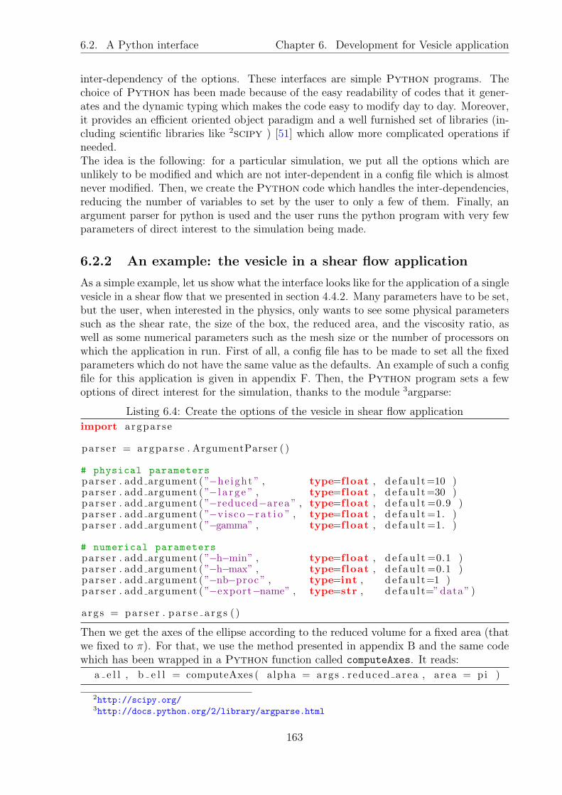
6.2. A Python interface Chapter 6. Development for Vesicle application
inter-dependency of the options. These interfaces are simple Python programs. Thechoice of Python has been made because of the easy readability of codes that it gener-ates and the dynamic typing which makes the code easy to modify day to day. Moreover,it provides an efficient oriented object paradigm and a well furnished set of libraries (in-cluding scientific libraries like 2scipy ) [51] which allow more complicated operations ifneeded.The idea is the following: for a particular simulation, we put all the options which areunlikely to be modified and which are not inter-dependent in a config file which is almostnever modified. Then, we create the Python code which handles the inter-dependencies,reducing the number of variables to set by the user to only a few of them. Finally, anargument parser for python is used and the user runs the python program with very fewparameters of direct interest to the simulation being made.
6.2.2 An example: the vesicle in a shear flow application
As a simple example, let us show what the interface looks like for the application of a singlevesicle in a shear flow that we presented in section 4.4.2. Many parameters have to be set,but the user, when interested in the physics, only wants to see some physical parameterssuch as the shear rate, the size of the box, the reduced area, and the viscosity ratio, aswell as some numerical parameters such as the mesh size or the number of processors onwhich the application in run. First of all, a config file has to be made to set all the fixedparameters which do not have the same value as the defaults. An example of such a configfile for this application is given in appendix F. Then, the Python program sets a fewoptions of direct interest for the simulation, thanks to the module 3argparse:
Listing 6.4: Create the options of the vesicle in shear flow application
import argparse
par s e r = argparse . ArgumentParser ( )
# physical parameterspar s e r . add argument ( ”−he ight ” , type=f loat , d e f au l t=10 )par s e r . add argument ( ”− l a r g e ” , type=f loat , d e f au l t=30 )par s e r . add argument ( ”−reduced−area ” , type=f loat , d e f au l t =0.9 )par s e r . add argument ( ”−v i sco−r a t i o ” , type=f loat , d e f au l t =1. )par s e r . add argument ( ”−gamma” , type=f loat , d e f au l t =1. )
# numerical parameterspar s e r . add argument ( ”−h−min” , type=f loat , d e f au l t =0.1 )par s e r . add argument ( ”−h−max” , type=f loat , d e f au l t =0.1 )par s e r . add argument ( ”−nb−proc ” , type=int , d e f au l t=1 )par s e r . add argument ( ”−export−name” , type=str , d e f au l t=”data” )
args = par s e r . p a r s e a r g s ( )
Then we get the axes of the ellipse according to the reduced volume for a fixed area (thatwe fixed to π). For that, we use the method presented in appendix B and the same codewhich has been wrapped in a Python function called computeAxes. It reads:
a e l l , b e l l = computeAxes ( alpha = args . reduced area , area = pi )
2http://scipy.org/3http://docs.python.org/2/library/argparse.html
163

6.2. A Python interface Chapter 6. Development for Vesicle application
The mesh is also created from the interface. Actually, Feel++ provides interfaces tocreate several meshes which are really useful for testing applications (unit square, unitcircle or sphere). But if we want a precise control of the mesh, like having a part of themesh with a smaller typical size, once again, a Python interface can be useful. Thus, wemade several functions which generate scripts for Gmsh and call it to create the mesh ofthe application. As examples, functions creating the following meshes are available:
• simple rectangular mesh
• rectangular mesh with one rectangular area in the middle having a different meshsize
• rectangular mesh having an arbitrary number of rectangular areas with differentmesh sizes
• circular mesh having a circular area with different mesh size
• the bifurcation mesh used in section 7.1 as well as the 3D version [87]
We use for this application the rectangular mesh with a smaller mesh size at the middle:
mesh name = makeMeshBox( l a r g e = L , he ight = l ,largeBand = 3∗ a e l l , heightBand = 3∗ b e l l ,hmin = args . h min , hmax = args . h max ,name=”mesh” , p e r i o d i c=True , p a r t i t i o n s=args . nb proc )
We then create the command to run and compute at the same time the dependentparameters. The command is put in an array in which each argument is an element. Andfinally, the command is launched by the module 4subprocess of Python .
l = args . he ightL = args . l a r g ecommand = [# mpi command to run on multiple processors”mpirun” ,”−np” ,str ( args . nb proc ) ,”−bind−to−core ” ,
# -- application options --# name of the executableExeName ,”−−con f i g− f i l e=”+Config ,”−−expor te r . d i r e c t o r y=”+args . export name ,”−−meshFile=”+mesh name ,
# -- numerical parameters --”−−bdf . time−s tep=”+str ( args . h min / 4 . ) ,”−− l e v e l s e t . th i cknes s−i n t e r f a c e=”+str ( args . h min ∗ 1 . 5 ) ,”−−dif fnum=”+str ( args . h min /50 . ) ,
# -- physical parameters --# µ2 = λ ∗ µ1”−−mum=”+str ( 10 ∗ v i s c o r a t i o ) ,”−−a e l l=”+str ( a e l l ) ,
4http://docs.python.org/2/library/subprocess.html
164

6.2. A Python interface Chapter 6. Development for Vesicle application
”−−b e l l=”+str ( b e l l ) ,”−−x0=”+str (L/ 2 . ) ,”−−y0=”+str ( l / 2 . ) ,”−−s t oke s . sh ea rVe l o c i t y=”+str ( l ∗ gamma / 2 . ) ]
c a l c = subproces s . Popen (command)c a l c . wait ( )
The user can now concentrate on the physics and has only few arguments to set. Asan example, we can now do a simulation of vesicle under shear flow by calling:vesInShearFlow.py -reduced-area=0.8 -gamma=2 -visco-ratio=3 -nb-proc=5
165

6.2. A Python interface Chapter 6. Development for Vesicle application
166
Part III
Rheology and flows of solid disks
167

Chapter 7
Flow of disks at a microfluidicbifurcation
Contents7.1 The splitting of a suspension at a bifurcation . . . . . . . . . 170
7.1.1 The Zweifach-Fung effect . . . . . . . . . . . . . . . . . . . . . 170
7.1.2 The bifurcation without particles . . . . . . . . . . . . . . . . . 170
7.1.3 Particle distribution with the simplest model . . . . . . . . . . 171
7.1.4 Effect of the free particle zone . . . . . . . . . . . . . . . . . . . 172
7.1.5 Hydrodynamic force . . . . . . . . . . . . . . . . . . . . . . . . 173
7.1.6 Finding the separating line of particles . . . . . . . . . . . . . . 174
The Zweifach–Fung effect . . . . . . . . . . . . . . . . . . . . . . . . . 174
7.2 Suspension of vesicle in a bifurcation . . . . . . . . . . . . . . 205
7.2.1 Entry and exit of vesicles . . . . . . . . . . . . . . . . . . . . . 205
7.2.2 Quantity of interest: the flux of vesicles . . . . . . . . . . . . . 206
7.2.3 Extension to two different kinds of vesicles . . . . . . . . . . . 208
169

7.1. The splitting of a suspension at a bifurcation Chapter 7. Disks at a bifurcation
In this chapter, we present some results on the physical problem of the splitting of asuspension of particles in a microfluidic bifurcation. We first start by a simplified problem:a dilute suspension of hard disks. With this simplified model, we are able, in collaborationwith experimenters, to explain the known phenomenon of the increasing concentration ofparticles in the higher flow rate branch. These explanations have been published inJournal Of Fluid Mechanics [27] and we reported the publication in this chapter. Wefinally show that it will be possible in the near future to do the same simulation withvesicles. We show that it is possible to measure the flux of vesicles in each branch andpresent a preliminary result. Finally we extend this simulation to the simulation of asuspension of two different kind of vesicles.
7.1 The splitting of a suspension at a bifurcation
7.1.1 The Zweifach-Fung effect
When a dilute suspension of particles reaches a geometrically symmetric bifurcation inwhich the branches do not have the same flow rate, the branch which has the higher flowrate always sees its concentration of particles increase. This phenomenon is called theZweifach-Fung effect. It has often been interpreted as a consequence of the existence ofan hydrodynamical force pushing particles toward the high flow rate branch. In otherwords, some particles in the inlet channel which have their center of mass in a regionwhere the fluid goes to the low flow rate branch would actually go in the high flow ratebranch. The goal of this work was to figure out if such a force exists. We have actuallyshown that there is no need for an hydrodynamical force to have an increase of the volumefraction of particles in the high flow rate branch. Indeed, this effect is a consequence of ageometrical effect of the distribution of particles in the inlet channel. Then, experimentsin our group combined with our numerical simulations have shown that, at the opposite,there exists a force pushing particles toward the low flow rate branch. This force is notstrong enough to overcome the geometrical distribution effect; this is why one sees anincrease of the volume fraction of particles in the high flow rate branch. Let us explainin more detail this phenomenon.
7.1.2 The bifurcation without particles
We consider a fluid flow governed by the Stokes equations in a 2D bifurcation for whichthe inlet channel makes a 90 angle with the two daughter branches. A different flow rateexists in the two daughter branches. We call the branch having the lower flow rate branch1 and its flow rate Q1, the other one is branch 2 and its flow rate Q2. Finally the motherbranch is branch 0 and its flow rate Q0 = Q1 + Q2. The velocity profile of the fluid ineach branch away from the bifurcation is a parabolic profile. Thus we can calculate theposition yf in the inlet channel separating the fluid regions going to the branch 1 or 2 bysimply writing the flow rate ratio:
Q1
Q0
=
∫ L/2
yf
u0 ·n0
∫ L/2
−L/2
u0 ·n0
(7.1)
170
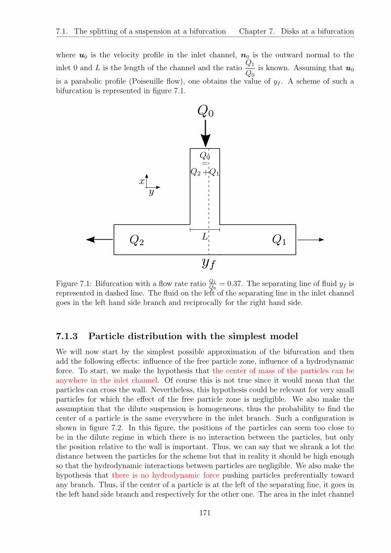
7.1. The splitting of a suspension at a bifurcation Chapter 7. Disks at a bifurcation
where u0 is the velocity profile in the inlet channel, n0 is the outward normal to the
inlet 0 and L is the length of the channel and the ratioQ1
Q0
is known. Assuming that u0
is a parabolic profile (Poiseuille flow), one obtains the value of yf . A scheme of such abifurcation is represented in figure 7.1.
Figure 7.1: Bifurcation with a flow rate ratio Q1
Q0= 0.37. The separating line of fluid yf is
represented in dashed line. The fluid on the left of the separating line in the inlet channelgoes in the left hand side branch and reciprocally for the right hand side.
7.1.3 Particle distribution with the simplest model
We will now start by the simplest possible approximation of the bifurcation and thenadd the following effects: influence of the free particle zone, influence of a hydrodynamicforce. To start, we make the hypothesis that the center of mass of the particles can beanywhere in the inlet channel. Of course this is not true since it would mean that theparticles can cross the wall. Nevertheless, this hypothesis could be relevant for very smallparticles for which the effect of the free particle zone is negligible. We also make theassumption that the dilute suspension is homogeneous, thus the probability to find thecenter of a particle is the same everywhere in the inlet branch. Such a configuration isshown in figure 7.2. In this figure, the positions of the particles can seem too close tobe in the dilute regime in which there is no interaction between the particles, but onlythe position relative to the wall is important. Thus, we can say that we shrank a lot thedistance between the particles for the scheme but that in reality it should be high enoughso that the hydrodynamic interactions between particles are negligible. We also make thehypothesis that there is no hydrodynamic force pushing particles preferentially towardany branch. Thus, if the center of a particle is at the left of the separating line, it goes inthe left hand side branch and respectively for the other one. The area in the inlet channel
171

7.1. The splitting of a suspension at a bifurcation Chapter 7. Disks at a bifurcation
Figure 7.2: Distribution of particles in a bifurcation when the finite size of the particles isnot taken into account and when no force pushed them to a particular branch. The centerof mass of the particles are represented as red dots. The area in the inlet channel for whichthe particles present will go in the high flow rate branch is represented in blue. The areato go in the other branch is in green. In this configuration, there is no concentrationincrease in any branch.
in which particles will go in channel 1 is represented in green in figure 7.2 and the one inwhich the particles are going in branch 2 is represented in blue. The line separating thetwo areas is yf , because of the no force assumption. We call N1 and N2 the particle flowrate in branches, respectively, 1 and 2.
With the previous hypotheses, we can say that the ratio between the number of par-
ticles going in each branch is the same as the flow rate ratio (N1
N2
=Q1
Q2
). Indeed the
area in the inlet branch determining the destination branch is the same for the particlesand the fluid. Thus, the volume fraction, which is the ratio between the number of par-
ticles going in a branch and the flow rate in the same branchN
Q, is the same for the two
daughter branches (N1
Q1
=N2
Q2
). With this relation and recalling that Q0 = Q1 + Q2 and
N0 = N1 +N2, we obtain thatN0
Q0
=N1
Q1
=N2
Q2
. Consequently, under the hypotheses that
we formulated, the volume fraction is the same in all the branches. This is actually thecase for very small particles for which our hypotheses are correct.
7.1.4 Effect of the free particle zone
Let us now consider that the particles are big enough so that the hypothesis saying thatthe center of mass of the particle can be everywhere in the inlet channel is not correctanymore. The particle’s center cannot be closer to the wall than their radii. Thus, there
172

7.1. The splitting of a suspension at a bifurcation Chapter 7. Disks at a bifurcation
Figure 7.3: Distribution of particles in a bifurcation when the finite size of the particleis taken into account. The free particle layer in the inlet channel is marked in red. Thenumber of particles entering in the low flow rate branch has been decreased more thanthe one entering in the other one. Consequently, there is an increase in the concentrationof particles in the high flow rate branch.
exists a particle free zone in the inlet channel having a thickness equal to the radius of theparticles in both sides of the channel. A scheme of the bifurcation with the free particlezone represented in red is shown in figure 7.3. A consequence of this free particle layeris that the area in the inlet channel in which the particles would enter the branch 1 ispenalized compared to the other one. Indeed, an equal area (the free layer) is deletedfrom two non equal areas, thus relatively to their size, the smallest area is much morelowered than the other. In other words, N1 decreases more than N2. In a mean time,the fluid flow rate is not affected by the free layer zone, thus Q1 and Q2 stay the same
than in figure 7.2. This breaks the previous equality and one hasN2
Q2
>N1
Q1
, which means
that there is an increase in the concentration of the particles in the high flow rate branch.Thus, only a geometrical consideration on the distribution of particles in the inlet channelis enough to explain the concentration increase in the high flow rate branch.
7.1.5 Hydrodynamic force
Even if we have shown that there is no need for an hydrodynamical force pushing particlestoward the high flow rate branch to increase its concentration, it does not mean that sucha force does not exist. Thus we compared the results found in the literature and theconcentration of particles expected under the assumption that no hydrodynamical forcesuch as described earlier exists. We have found that all the results in literature hadactually a concentration of particles in the high flow rate branch lower than it should beif only the geometrical effect were present. This led us to think that there could at by
173

7.1. The splitting of a suspension at a bifurcation Chapter 7. Disks at a bifurcation
Figure 7.4: Scheme of the bifurcation when the finite size of the particle is taken intoaccount so as a force pushing particles toward the low flow rate branch. The line separatingthe areas for which the particles go in each branch is represented as a black dotted line(at position yp).
contrast exist a force pushing particles toward the low flow rate branch. We have shownby experiments and simulations that this force actually exists. The consequence of sucha force is represented in figure 7.4. The line separating the areas where the fluid goesin each branch is no longer the same as the line separating the areas where the particlesgoes in each branch. The position of the separating line of particles is yp. Subsequently,there exists a zone in the inlet channel, between yp and yf in which a solid particle wouldgo to the low flow rate branch whereas a fluid particle would go to the higher flow rateone. The fact that particles are pushed toward the low flow rate branch implies that N1
increases compare to the no force assumption. However, this force is never strong enough
to invert the inequalityN2
Q2
>N1
Q1
.
7.1.6 Finding the separating line of particles
The position of the separating line of particles (yp) was the key to understand the wholephenomenon. Hence, our goal was to find this position. The experimenters ThomasPodgorski, Sarah Peponas and Gwennou Coupier designed an experiment in which theycontrol with precision the position of an inlet particle in a bifurcation and explored thedifferent trajectories until they found the separating line of particles. They did thisexperiment for several flow rate ratios and different sizes of particles. For the simulationpart, we used the penalty method presented in section 3.1. The code has been writtenwith the software FreeFem++ . Later, it has been re-written with Feel++ [87] to beable to handle 3D simulations. We searched for the separating line for different flow rateratio, radii of particles, and sizes of channels. All the results, and their consequences onthe Zweifach-Fung effect are published in [27] that we give hereafter.
174

J. Fluid Mech. (2011), vol. 674, pp. 359–388. c© Cambridge University Press 2011
doi:10.1017/S0022112010006567
359
Spheres in the vicinity of a bifurcation:elucidating the Zweifach–Fung effect
V. DOYEUX, T. PODGORSKI, S. PEPONAS,
M. ISMAIL AND G. COUPIER†Universite Grenoble 1 / CNRS, Laboratoire Interdisciplinaire de Physique / UMR 5588,
Grenoble, F-38041, France
(Received 8 July 2010; revised 26 October 2010; accepted 21 December 2010;
first published online 17 March 2011)
The problem of the splitting of a suspension in bifurcating channels divided into twobranches of non-equal flow rates is addressed. As has long been observed, in particularin blood flow studies, the volume fraction of particles generally increases in the high-flow-rate branch and decreases in the low-flow-rate branch. In the literature, thisphenomenon is sometimes interpreted as the result of some attraction of the particlestowards this high-flow-rate branch. In this paper, we focus on the existence of suchan attraction through microfluidic experiments and two-dimensional simulations andshow clearly that such an attraction does not occur but is, on the contrary, directedtowards the low-flow-rate branch. Arguments for this attraction are given and adiscussion on the sometimes misleading arguments found in the literature is given.Finally, the enrichment of particles in the high-flow-rate branch is shown to be mainlya consequence of the initial distribution in the inlet branch, which shows necessarilysome depletion near the walls.
Key words: blood flow, microfluidics, particle/fluid flows
1. Introduction
When a suspension of particles reaches an asymmetric bifurcation, it is well-knownthat the particle volume fractions in the two daughter branches are not equal; basically,for branches of comparable geometrical characteristics, but receiving different flowrates, the volume fraction of particles increases in the high-flow-rate branch. Thisphenomenon, sometimes called the Zweifach–Fung effect (see Svanes & Zweifach1968; Fung 1973), has been observed for a long time in the blood circulation. Understandard physiological circumstances, a branch receiving typically one fourth of theblood inflow will see its haematocrit (volume fraction of red blood cells) drop down tozero, which will have obvious physiological consequences. The expression ‘attractiontowards the high-flow-rate branch’ is sometimes used in the literature as a synonymfor this phenomenon. Indeed, the partitioning not only depends on the interactionsbetween the flow and the particles, which are quite complex in such a geometry, butalso on the initial distribution of particles.
Apart from the huge number of in vivo studies on blood flow (see Pries, Secomb &Gaethgens 1996 for a review), many other papers have been devoted to this effect,either to understand it, or to use it in order to design sorting or purification devices.
† Email address for correspondence: [email protected]

360 V. Doyeux, T. Podgorski, S. Peponas, M. Ismail and G. Coupier
In the latter case, one can play at will with the different parameters characterizingthe bifurcation (widths of the channels and relative angles of the branches), in orderto reach a maximum efficiency. As proposed in many papers, focusing on rigidspheres has already given some keys to understand or control this phenomenon (seeBugliarello & Hsiao 1964; Chien et al. 1985; Audet & Olbricht 1987; Ditchfield &Olbricht 1996; Roberts & Olbricht 2003, 2006; Yang, Undar & Zahn 2006; Barberet al. 2008). In vitro behaviour of red blood cells has also attracted some attention(see Dellimore, Dunlop & Canham 1983; Fenton, Carr & Cokelet 1985; Carr &Wickham 1990; Yang et al. 2006; Jaggi, Sandoz & Effenhauser 2007; Fan et al. 2008;Zheng, Liu & Tai 2008). The problem of particle flow through an array of obstacles,which can be considered as somewhat similar, has also been studied recently (seeEl-Kareh & Secomb 2000; Davis et al. 2006; Balvin et al. 2009; Frechette & Drazer2009; Inglis 2009).
All the studies mentioned above have focused on the low-Reynolds-number limit,which is the relevant limit for applicative purposes and the biological systems ofinterest. Therefore, this limit is also considered throughout this paper.
In most studies, as well as in in vivo blood flow studies, which are for historicalreasons the main sources of data, the main output is the particle volume fractionin the two daughter branches as a function of the flow rate ratio between them.Such data can be well described by empirical laws that still depend on some ad hocparameters but allow some rough predictions (see Dellimore et al. 1983; Fenton et al.1985; Pries et al. 1989), which have been exhaustively compared recently (see Guibert,Fonta & Plouraboue 2010).
On the other hand, measuring macroscopic data such as volume fraction does notallow identification of the relevant parameters and effects involved in this phenomenonof asymmetric partitioning.
For a given bifurcation geometry and flow rate ratio between the two outletbranches, the final distribution of the particles can be straightforwardly derivedfrom two sets of data: first, their spatial distribution in the inlet and, second, theirtrajectories in the vicinity of the bifurcation, starting from all possible initial positions.If the particles follow their underlying unperturbed streamlines (as a sphere would doin a Stokes flow in a straight channel), their final distribution can be easily computed,although particles near the apex of the bifurcation require some specific treatment,since they cannot approach it as closely as their underlying streamline does.
The relevant physical question in this problem is thus to identify the hydrodynamicphenomenon at the bifurcation that would make flowing objects escape from theirunderlying streamlines and, as a consequence, a large particle would be driven towardsone branch while a tiny fluid particle located at the same position would travel to theother branch.
In order to focus on this phenomenon, we need to identify more precisely theother parameters that influence the partitioning, for a given choice of flow rate ratiobetween the two branches.
(i) The bifurcation geometry. Audet & Olbricht (1987) and Roberts & Olbricht(2003) made it clear, for instance, that the partitioning in Y-shaped bifurcationsdepends strongly on the angles between the two branches (see figure 1a). For instance,while the velocity is mainly longitudinal, the effective available cross-section to entera perpendicular branch is smaller than in the symmetric Y-shaped case. Even in thelatter case, the position of the apex of the bifurcation relative to the separation linebetween the fluids travelling in the two branches might play a role, due to the finitesize of the flowing objects.
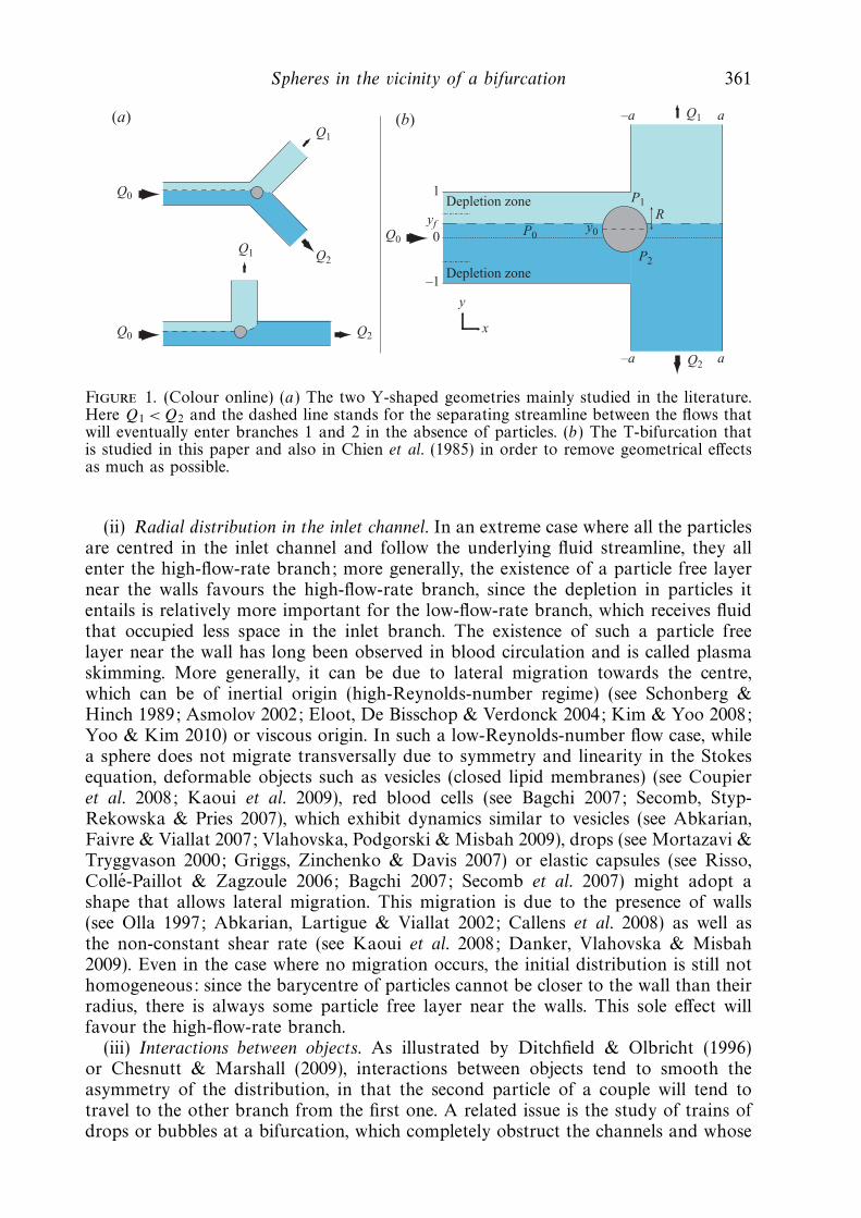
Spheres in the vicinity of a bifurcation 361
(b)(a)
Depletion zone1
0
–1
Q0
Q0
P1
P0
P2
y0
R
Q0
Q1
Q1
Q2–a a
–a a
y
yf
x
Q1
Q2
Q2
Depletion zone
Figure 1. (Colour online) (a) The two Y-shaped geometries mainly studied in the literature.Here Q1 < Q2 and the dashed line stands for the separating streamline between the flows thatwill eventually enter branches 1 and 2 in the absence of particles. (b) The T-bifurcation thatis studied in this paper and also in Chien et al. (1985) in order to remove geometrical effectsas much as possible.
(ii) Radial distribution in the inlet channel. In an extreme case where all the particlesare centred in the inlet channel and follow the underlying fluid streamline, they allenter the high-flow-rate branch; more generally, the existence of a particle free layernear the walls favours the high-flow-rate branch, since the depletion in particles itentails is relatively more important for the low-flow-rate branch, which receives fluidthat occupied less space in the inlet branch. The existence of such a particle freelayer near the wall has long been observed in blood circulation and is called plasmaskimming. More generally, it can be due to lateral migration towards the centre,which can be of inertial origin (high-Reynolds-number regime) (see Schonberg &Hinch 1989; Asmolov 2002; Eloot, De Bisschop & Verdonck 2004; Kim & Yoo 2008;Yoo & Kim 2010) or viscous origin. In such a low-Reynolds-number flow case, whilea sphere does not migrate transversally due to symmetry and linearity in the Stokesequation, deformable objects such as vesicles (closed lipid membranes) (see Coupieret al. 2008; Kaoui et al. 2009), red blood cells (see Bagchi 2007; Secomb, Styp-Rekowska & Pries 2007), which exhibit dynamics similar to vesicles (see Abkarian,Faivre & Viallat 2007; Vlahovska, Podgorski & Misbah 2009), drops (see Mortazavi &Tryggvason 2000; Griggs, Zinchenko & Davis 2007) or elastic capsules (see Risso,Colle-Paillot & Zagzoule 2006; Bagchi 2007; Secomb et al. 2007) might adopt ashape that allows lateral migration. This migration is due to the presence of walls(see Olla 1997; Abkarian, Lartigue & Viallat 2002; Callens et al. 2008) as well asthe non-constant shear rate (see Kaoui et al. 2008; Danker, Vlahovska & Misbah2009). Even in the case where no migration occurs, the initial distribution is still nothomogeneous: since the barycentre of particles cannot be closer to the wall than theirradius, there is always some particle free layer near the walls. This sole effect willfavour the high-flow-rate branch.
(iii) Interactions between objects. As illustrated by Ditchfield & Olbricht (1996)or Chesnutt & Marshall (2009), interactions between objects tend to smooth theasymmetry of the distribution, in that the second particle of a couple will tend totravel to the other branch from the first one. A related issue is the study of trains ofdrops or bubbles at a bifurcation, which completely obstruct the channels and whose

362 V. Doyeux, T. Podgorski, S. Peponas, M. Ismail and G. Coupier
passage in the bifurcation greatly modifies the pressure distribution in its vicinity, andthus influences the behaviour of the following element (see Engl et al. 2005; Jousseet al. 2006; Schindler & Ajdari 2008; Sessoms et al. 2009).
In spite of the large body of literature on this subject, but perhaps because ofthe applicative purpose of most studies, the relative importance of these differentparameters is seldom discussed quantitatively, although most authors are fully awareof the different phenomena at stake.
Since we focus here on the question of cross-streamline migration in the vicinity ofthe bifurcation, we will consider rigid spheres, for which no transverse migration inthe upstream channel is expected. These spheres are in the vanishing concentrationlimit and flow through symmetric bifurcations, that is the symmetric Y-shaped andT-shaped bifurcations shown in figure 1, where the two daughter branches have thesame cross-section and are equally distributed relative to the inlet channel.
Indeed, the case of rigid spheres is still quite unclear in the literature. In thefollowing, first we briefly review previous studies that consider a geometricallysymmetric situation and thoroughly re-analyse their results in order to determinewhether the Zweifach–Fung effect they see is due to initial distribution or due to someattraction in the vicinity of the bifurcation, which generally has not been done (§ 2).
Then, we present in §§ 3 and 4 our two-dimensional simulations and quasi-two-dimensional experiments (in the sense that the movement of three-dimensional objectsis planar). We mainly focus on the T-shaped bifurcation, in order to avoid as muchas possible the geometric constraint due to the presence of an apex.
Our main result is that there is some attraction towards the low-flow-rate branch(§ 4.1). This result is then analysed and explained through basic fluid mechanicsarguments, which are compared with those previously discussed in the literature.
Secondly, we discuss consequences of this drift on the final distribution in thedaughter branches. To do so, we focus on particle concentrations possible at theoutlets in the simplest case, where particles are homogeneously distributed in the inletchannel, with the sole (and unavoidable) constraint that they cannot approach thewalls closer than their radius (termed depletion effect below, see figure 1b). This hasbeen done through simulations, which allow us to easily control the initial distributionin particles (§ 4.2). Consequences for the potential efficiency of sorting or purificationdevices are discussed. We finally recall, in § 4.3, some previous studies from theliterature for quantitative comparisons to check the consistency between them andour results.
Before discussing the results from the literature and presenting our data, weintroduce useful common notation (see figure 1b).
The half-width of the inlet branch is set as the length scale of the problem. Theinlet channel is divided into two branches of width 2a (the case a = 1 is mainlyconsidered here by default, unless otherwise stated) and spheres of radius R 1. Theflow rate at the inlet is denoted by Q0, and Q1 and Q2 are the flow rates at the upperand lower outlets (Q0 = Q1 + Q2). In the absence of particles, all the fluid particlessituated initially above the line y = yf eventually enter branch 1. This line is calledthe (unperturbed) fluid separating streamline. Here y0 is the initial transverse positionof the considered particle long before it reaches the bifurcation (|y0| 1 − R). N1
and N2 are the numbers of particles entering branches 1 and 2 in unit time, whileN0 = N1 + N2 have entered the inlet channel. The volume fractions in the branchesare Φi = V Ni/Qi , where V is the volume of a particle.
With this notation, we can reformulate our question: if y0 = yf , does the particleexperience a net force in the y-direction (e.g. a pressure difference) that would push

Spheres in the vicinity of a bifurcation 363
it towards one of the branches, while a fluid particle would remain on the separatingstreamline (by definition of yf )? If so, for which position y∗
0 does this force vanish,so that the particle follows the streamlines and eventually hits the opposite wall andreaches an (unstable) equilibrium position? If Q1 Q2 and y∗
0 <yf , then one will talkabout attraction towards the low-flow-rate branch.
Following this notation, we have
N1 =
∫ 1
y∗0
n(y)u∗x(y) dy, (1.1)
Q1 =
∫ 1
yf
ux(y) dy, (1.2)
where n(y) is the mean density of particles at height y in the inlet branch, and u∗x
and ux are respectively particle and flow longitudinal upstream velocities. Note thatN0 and Q0 are given by the same formula with y∗
0 = yf = −1.The Zweifach–Fung effect can then be written as follows: if Q1/Q0 < 1/2 (branch
1 receives less flow than branch 2), then N1/N0 <Q1/Q0 (branch 1 receives even lessparticles than fluid) or equivalently Φ1 <Φ0 (the particle concentration decreases inthe low-flow-rate branch).
2. Previous results in the literature
In the literature, the most common symmetric case that is considered is the Y-shaped bifurcation with daughter branches leaving the bifurcation with a 45 anglerelative to the inlet channel, and cross-sections identical as those of the inlet channel(figure 1a) (see Audet & Olbricht 1987; Ditchfield & Olbricht 1996; Roberts &Olbricht 2003, 2006; Yang et al. 2006; Barber et al. 2008). The T-shaped bifurcation(figure 1b) has attracted little attention (see Yen & Fung 1978; Chien et al. 1985).All studies but Yen & Fung (1978) showed results for rigid spherical particles, whilesome results for deformable particles are given by Yen & Fung (1978) and Barberet al. (2008). Explicit data on a possible attraction towards one branch are scarce andcan only be found in a recent paper dealing with two-dimensional simulations (seeBarber et al. 2008). In three other papers, dealing with two-dimensional simulations(see Audet & Olbricht 1987) or experiments in square cross-sectional channels (seeRoberts & Olbricht 2006; Yang et al. 2006), the output data are the concentrations Φi
at the outlets. In this section, we re-analyse their data in order to discuss the possibilityof an attraction towards one branch. Experiments in circular cross-sectional channelswere also performed (see Yen & Fung 1978; Chien et al. 1985; Ditchfield & Olbricht1996; Roberts & Olbricht 2003), on which we comment later in the text.
In the two-dimensional simulations presented by Audet & Olbricht (1987), sometrajectories around the bifurcation are shown; however, the authors focused on anasymmetric Y-shaped bifurcation. In addition, some data for N1/N0 in a symmetricY-shaped bifurcation and R = 0.5 are presented. Yang et al. (2006) performedexperiments with balls of similar size (R =0.46) in a symmetric Y-shaped bifurcationwith a square cross-section and showed data for N1/N0 as a function of Q1/Q0 (seeYang et al. 2006). Experiments with larger balls (R = 0.8) in square cross-sectionalchannels were carried out by Roberts & Olbricht (2006). Once again, the outputdata are the ratios N1/N0. In both experiments, the authors made the assumptionthat the initial ball distribution is homogeneous, as also considered in a paper onsimulation by Audet & Olbricht (1987). In these three papers, although the authors

364 V. Doyeux, T. Podgorski, S. Peponas, M. Ismail and G. Coupier
0.1 0.2 0.3 0.4 0.5 0.6 0.7 0.8 0.9 1.00
0.2
0.4
0.6
0.8
1.0
Medium size
Yang et al. (2006)
Experiments, R = 0.46
Audet & Olbricht (1987)
Simulations, R = 0.5
No-attraction assumption,
R = 0.48
N1/N
0
Q1/Q0
Large size
Roberts & Olbricht (2006)
experiments, R = 0.8
No-attraction assumption,
R = 0.8
Figure 2. Comparison between data from the literature and theoretical distribution under theassumption of no attraction, which would indicate some previously unseen attraction towardsthe low-flow-rate branch. Rigid spheres distribution N1/N0 is shown as a function of the flowdistribution Q1/Q0 in a symmetric Y-shaped bifurcation and a homogeneous distribution atthe inlet (but the unavoidable depletion effect). Symbols: data extracted from previous papers:, Yang et al. (2006, figure 3), experiments, R = 0.46; , Audet & Olbricht (1987, figure 8),two-dimensional simulations, R = 0.5; , Roberts & Olbricht (2006, figure 5A), experiments,R = 0.8. Dotted and full lines, theoretical distribution for R = 0.48 and R = 0.8 in the casewhere the particles follow their underlying streamline (y∗
0 = yf : no-attraction assumption) andu∗
x given by our simulations; dashed line, fluid distribution (N1/N0 = Q1/Q0).
were sometimes conscious that the depletion and attraction effects might screen eachother, the relative weight of each phenomenon has not been discussed. However, Yanget al. (2006) explicitly considered that there must be some attraction towards the high-flow-rate branch and gave some qualitative arguments for this. This opinion, initiallyintroduced by Fung (see Fung 1973; Yen & Fung 1978; Fung 1993), is widespreadin the literature (see El-Kareh & Secomb 2000; Jaggi et al. 2007; Kersaudy-Kerhoaset al. 2010). We shall come back to the underlying arguments in the following.
In figure 2, we present the data of N1/N0 as a function of Q1/Q0 taken fromAudet & Olbricht (1987) for R = 0.5 (two-dimensional simulations), Yang et al. (2006)for R = 0.46 (experiments) and Roberts & Olbricht (2006) for R = 0.8 (experiments).It is instructive to compare these data with the corresponding values calculated witha very simple model based on the assumption that no particular effect occurs atthe bifurcation, that is, the particles follow their underlying streamline (no-attractionassumption). To do so, we consider the two-dimensional case of flowing spheresand calculate the corresponding N1 according to (1.1). The no-attraction assumptionimplies that y∗
0 = yf and, as in the considered papers, the density n(y) is consideredconstant for |y| 1 − R. The particle velocity u∗
x is given by the simulations presentedin § 4.2. Since we consider only flow ratios, this two-dimensional approach is a goodenough approximation to discuss the results of the three-dimensional experiments, asthe fluid separating plane is orthogonal to the plane where the channels lie; moreover,the position of this plane differs only by a few per cent from that of the separatingline in two dimensions.
In all curves, it is seen that, if Q1/Q0 < 1/2, then N1/N0 < Q1/Q0, which is preciselythe Zweifach–Fung effect. Note that this effect is present even under the no-attraction
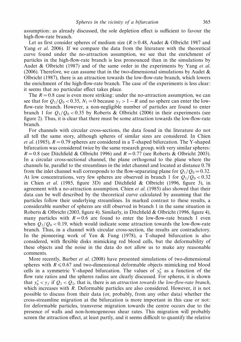
Spheres in the vicinity of a bifurcation 365
assumption: as already discussed, the sole depletion effect is sufficient to favour thehigh-flow-rate branch.
Let us first consider spheres of medium size (R ≃ 0.48, Audet & Olbricht 1987 andYang et al. 2006). If we compare the data from the literature with the theoreticalcurve found under the no-attraction assumption, we see that the enrichment ofparticles in the high-flow-rate branch is less pronounced than in the simulations byAudet & Olbricht (1987) and of the same order in the experiments by Yang et al.(2006). Therefore, we can assume that in the two-dimensional simulations by Audet &Olbricht (1987), there is an attraction towards the low-flow-rate branch, which lowersthe enrichment of the high-flow-rate branch. The case of the experiments is less clear:it seems that no particular effect takes place.
The R = 0.8 case is even more striking: under the no-attraction assumption, we cansee that for Q1/Q0 < 0.35, N1 = 0 because yf > 1−R and no sphere can enter the low-flow-rate branch. However, a non-negligible number of particles are found to enterbranch 1 for Q1/Q0 < 0.35 by Roberts & Olbricht (2006) in their experiments (seefigure 2). Thus, it is clear that there must be some attraction towards the low-flow-ratebranch.
For channels with circular cross-sections, the data found in the literature do notall tell the same story, although spheres of similar sizes are considered. In Chienet al. (1985), R = 0.79 spheres are considered in a T-shaped bifurcation. The Y-shapedbifurcation was considered twice by the same research group, with very similar spheres:R = 0.8 (see Ditchfield & Olbricht 1996) and R = 0.77 (see Roberts & Olbricht 2003).In a circular cross-sectional channel, the plane orthogonal to the plane where thechannels lie, parallel to the streamlines in the inlet channel and located at distance 0.78from the inlet channel wall corresponds to the flow-separating plane for Q1/Q0 = 0.32.At low concentrations, very few spheres are observed in branch 1 for Q1/Q0 < 0.32in Chien et al. (1985, figure 3D) and Ditchfield & Olbricht (1996, figure 3), inagreement with a no-attraction assumption. Chien et al. (1985) also showed that theirdata can be well described by the theoretical curve calculated by assuming that theparticles follow their underlying streamlines. In marked contrast to these results, aconsiderable number of spheres are still observed in branch 1 in the same situation inRoberts & Olbricht (2003, figure 4). Similarly, in Ditchfield & Olbricht (1996, figure 4),many particles with R = 0.6 are found to enter the low-flow-rate branch 1 evenwhen Q1/Q0 < 0.19, which would indicate some attraction towards the low-flow-ratebranch. Thus, in a channel with circular cross-section, the results are contradictory.In the pioneering work of Yen & Fung (1978), a T-shaped bifurcation is alsoconsidered, with flexible disks mimicking red blood cells, but the deformability ofthese objects and the noise in the data do not allow us to make any reasonablecomments.
More recently, Barber et al. (2008) have presented simulations of two-dimensionalspheres with R 0.67 and two-dimensional deformable objects mimicking red bloodcells in a symmetric Y-shaped bifurcation. The values of y∗
0 as a function of theflow rate ratios and the spheres radius are clearly discussed. For spheres, it is shownthat y∗
0 <yf if Q1 <Q2, that is, there is an attraction towards the low-flow-rate branch,which increases with R. Deformable particles are also considered. However, it is notpossible to discuss from their data (or, probably, from any other data) whether thecross-streamline migration at the bifurcation is more important in this case or not:for deformable particles, transverse migration towards the centre occurs due to thepresence of walls and non-homogeneous shear rates. This migration will probablyscreen the attraction effect, at least partly, and it seems difficult to quantify the relative

366 V. Doyeux, T. Podgorski, S. Peponas, M. Ismail and G. Coupier
contribution of both effects. In particular, y∗0 depends on the (arbitrary) initial distance
from the bifurcation. In Chesnutt & Marshall (2009), attraction towards the low-flow-rate branch is also quickly evoked, but considered as negligible since the focus wason large channels and interacting particles.
Finally, from our new analysis of previous results from the literature (and despitesome discrepancies) it appears that there should be some attraction towards thelow-flow-rate branch, although the final result is an enrichment of the high-flow-ratebranch due to the depletion effect in the inlet channel. This effect was seen by Barberet al. (2008) in their simulations. On the other hand, if one considers the flow aroundan obstacle, as simulated in El-Kareh & Secomb (2000), it seems that sphericalparticles are attracted towards the high-flow-rate side.
From the above discussion, we conclude that the different effects occurring atthe bifurcation level are neither well identified nor explained. Moreover, to date, nodirect experimental proof of any attraction phenomenon exists. In § 4.1, we showexperimentally that attraction towards the low-flow-rate branch takes place andconfirm this through numerical simulations.
It is then necessary to discuss whether this attraction has important consequenceson the final distributions in particles in the two daughter channels. This was not doneexplicitly in Barber et al. (2008); however, in § 4.2 through simulations we discuss therelative weight of the attraction towards the low-flow-rate branch and the depletioneffect, which have opposite consequences.
3. Method
3.1. Experimental set-up
We studied the behaviour of hard balls as a first reference system. Since the potentialmigration across streamlines is linked to the way the fluid acts on the particles, wealso studied spherical fluid vesicles. These are closed lipid membranes enclosing aNewtonian fluid. The lipids that we used are in liquid phase at room temperature,so that the membrane is a two-dimensional fluid. In particular, it is incompressible(so that spherical vesicles will remain spherical even under stress, unlike drops), butit is easily sheared: this means that a torque exerted by the fluid on the surface ofthe particle can imply a different response depending on whether it is a solid ball ora vesicle. Moreover, since vesicle suspensions are polydisperse, it is a convenient wayto vary the radius R of the studied object.
The experimental set-up is a standard microfluidic chip made of polydimethylsilox-ane bonded on a glass plate (figure 3). We wish to observe what happens to an objectlocated around position yf , that is, in which branch it goes at the bifurcation. Inorder to determine the corresponding y∗
0 , we need to scan different initial positionsaround yf . One solution would be to let a suspension flow and hope that some of theparticles are close enough to the region of interest. In the meantime, as we shall see,the cross-streamline effect is weak and requires precise measurement, and noticeableeffects appear only at high radius R, typically R > 0.5. Clogging is unavoidable withsuch objects, which would modify the flow rates ratio, and if a very dilute suspensionis used, it is likely that the region of interest will only partly be scanned.
Therefore, we designed a microfluidic system that allowed us to use only oneparticle, which would go through the bifurcation with a controlled initial positiony0, would be taken back, its position y0 modified, would flow again through thebifurcation, and so on. Moreover, we allowed continuous modification of the flowrate ratio between the two daughter branches. The core of the chip is the five branch

Spheres in the vicinity of a bifurcation 367
The focusing section The studied bifurcation
a
b
100 µm
c
a
h0
–h0
–H – h –H + h
c
b2
1
Figure 3. (Colour online) Scheme of the microfluidic device. The photograph shows thetrajectory of a particle from branch a to branch 1 after having been focused on a givenstreamline thanks to flows from lateral branches b and c.
crossroad shown in the inset to figure 3. These five branches have different lengthsand are linked to reservoirs placed at different heights, in order to induce flow by ahydrostatic pressure gradient. A focusing device (branches a–c) is placed before thebifurcation of interest (branches 1 and 2), in order to control the lateral position ofthe particle. Particles are initially located in the central branch a, where the flow isweak and the incoming particles are pinched between the two lateral flows. In orderto modify the position y0 of the particle, the relative heights of the reservoirs linked tothe lateral branches are modified. The total flow rate and the flow rate ratios betweenthe two daughter branches after the bifurcation are controlled by varying the heightsof the two outlet reservoirs. Note that the flow rate ratio also depends on the heightsof the reservoirs linked to inlet branches a, b and c. Since the latter two must becontinuously modified to vary the position y0 of the incoming particle in order to findy∗
0 for a given flow rate ratio, it is convenient to place them on a pulley so that theirmean height is always constant (resistances of branches b and c being equal). If thetotal flow rate is a relevant parameter (which is not the case here since we consideronly Stokes flow of particles that do not deform), one can do the same with the twooutlet reservoirs. In such a situation, if the reservoir of branch a is placed at height0, reservoirs of branches b and c at heights ±h0, and reservoirs of branches 1 and 2at heights −H + h and −H − h, the flow rate ratio is governed by setting (h, H ) andh0 can be modified independently in order to control y0. Once the particle has gonethrough the bifurcation, height H and the height of reservoir a are modified so thatthe particle comes back to branch a, and h0 is modified in order to get closer andcloser to the position y∗
0 . Note that Q1/Q0 (or equivalently yf ) is a function of H ,h, and the flow resistances of the five branches of rectangular cross-sections, which

368 V. Doyeux, T. Podgorski, S. Peponas, M. Ismail and G. Coupier
100 µ
m
(a) (b)
Figure 4. Photographs showing the different positions of a vesicle of radius R = 0.60 startingjust above and just below its separating line. No clear difference between these two startingpositions can be seen by eye, which illustrates the accuracy we get in the measurement of y∗
0 .Here Q1/Q0 is set to 0.28.
are known functions of their lengths, widths and thicknesses (see White 1991). Theaccuracy of the calculation of this function was checked by measuring y∗
0 for smallparticles, which must be equal to yf .
Note that the length of the channel is much more important than the size of asingle flowing particle, so that we can neglect the contribution of the latter in theresistance to the flow: hence, even though we control the pressures, we can considerthat we work at fixed flow rates.
Finally, as can be seen in figure 4, our device allows us to scan very precisely thearea of interest around the sought y∗
0 , so that the uncertainty associated with it isvery low.
At the bifurcation level, channels widths are all equal to 57 ± 0.2 µm. Their thicknessis 81 ± 0.3 µm. We used polystyrene balls of maximum radius 40.5 ± 0.3 µm insoapy water (therefore R 0.71) and fluid vesicles of size R 0.60. The vesiclemembrane is a dioleoylphosphatidylcholine lipid bilayer enclosing an inner solutionof sugar (sucrose or glucose) in water. Vesicles are produced following the standardelectroformation method (see Angelova et al. 1992). Maximum flow velocity at thebifurcation level was around 1 mm s−1, so that the Reynolds number Re ≃ 10−1.
3.2. The numerical model
In the simulations, we focus on the two-dimensional problem (invariance along thez-axis). Our problem is a simple fluid/structure interaction and can be modelledby Navier–Stokes equations for the fluid flow and Newton–Euler equations for thesphere. These two problems can be coupled in a simple manner.
(i) The action of fluid on the sphere is modelled by the hydrodynamic force andtorque acting on its surface. They are used as the right-hand sides of Newton–Eulerequations.
(ii) The action of the sphere on fluid can be modelled by no-slip boundaryconditions on the sphere (in the Navier–Stokes equations).However, this explicit coupling can be numerically unstable and its resolution oftenrequires very small time steps. In addition, as we have chosen to use the finite elementmethod (FEM) (for accuracy) and since the position of the sphere evolves in time,we have to remesh the computational domain at each time step or in best cases everyfew time steps.

Spheres in the vicinity of a bifurcation 369
For these reasons, we chose another strategy to model our problem. Instead ofusing Newton–Euler equations for modelling the sphere motion and Navier–Stokesequations for the fluid flow, we use only the Stokes equations in the entire domain ofthe bifurcation (including the interior of the sphere). The use of Stokes equations isjustified by the small Reynolds number in our case and the presence of the sphere isrendered by a second fluid with a ‘huge’ viscosity on which we impose a rigid bodyconstraint. Such a strategy is widely used in the literature under different names, e.g.the so-called fluid particle dynamics (FPD) method (see Tanaka & Araki 2000; Peyla2007), but we can group them generically as penalty-like methods. The method usedhere was mainly developed by Lefebvre et al. (see Janela, Lefebvre & Maury 2005;Lefebvre 2007) and we can find a mathematical analysis of such methods in Maury(2009).
In what follows, we briefly describe the basic ingredients of the FEM and thepenalty technique applied to the problem.
The fluid flow is governed by Stokes equations written as follows:
−νu + ∇p = 0 in Ωf , (3.1)
∇ · u = 0 in Ωf , (3.2)
u = f on ∂Ωf , (3.3)
where the variables(i) ν, u and p are respectively the viscosity, velocity and pressure fields of the fluid;(ii) Ωf is the domain occupied by the fluid; typically Ωf = Ω\B if we denote by
Ω the whole bifurcation and by B the rigid particle;(iii) ∂Ωf is the border of Ωf ;(iv) f is some given function for the boundary conditions.
It is known that under some reasonable assumptions the problem (3.1)–(3.3) has aunique solution (u, p) ∈ H 1(Ωf )2 × L2
0(Ωf ) (see Girault & Raviart 1986). Below, weuse the following functional spaces:
L2(Ω) =
f : Ω → ;
∫
Ω
|f |2 < +∞
, (3.4)
L20(Ω) =
f ∈ L2(Ω);
∫
Ω
f = 0
, (3.5)
H 1(Ω) = f ∈ L2(Ω); ∇f ∈ L2(Ω), (3.6)
H 10 (Ω) = f ∈ H 1(Ω); f = 0 on ∂Ω. (3.7)
As we use the FEM for the numerical resolution of the problem (3.1)–(3.3), weneed to rewrite this in a variational form (an equivalent formulation of the initialproblem). For the sake of simplicity, we start by writing it in a standard way(fluid without sphere), then we modify it using the penalty technique to take intoaccount the presence of the particle. In what follows, we briefly describe these twomethods, the standard variational formulation for the Stokes problem and the penaltytechnique.
3.2.1. Variational formulation
First recall the deformation tensor τ , which is useful in what follows
τ (u) = 12(∇u + (∇u)t ) . (3.8)

370 V. Doyeux, T. Podgorski, S. Peponas, M. Ismail and G. Coupier
Thanks to the incompressibility constraint ∇ · u = 0, we have
u = 2∇ · τ (u). (3.9)
Hence, the problem (3.1)–(3.3) can be rewritten as follows: find (u, p) ∈H 1(Ωf )2 L2
0(Ωf ) such that
−2ν∇ · τ (u) + ∇p = 0 in Ωf , (3.10)
∇ · u = 0 in Ωf , (3.11)
u = f on ∂Ωf . (3.12)
By simple calculations (see the Appendix for details) we show that problem (3.10)–(3.12) is equivalent to the following: find (u, p) ∈ H 1(Ωf )2 × L2
0(Ωf ) such that
2ν
∫
Ωf
τ (u) : τ (v) −∫
Ωf
p∇ · v = 0, ∀v ∈ H 10 (Ωf )2, (3.13)
∫
Ωf
q∇ · u = 0, ∀q ∈ L20(Ωf ), (3.14)
u = f on ∂Ωf , (3.15)
where ‘:’ denotes the double contraction.
3.2.2. Penalty method
We chose to use the penalty strategy in the framework of FEM, described herebriefly (see Janela et al. 2005 and Lefebvre 2007 for more details).
The first step consists in rewriting the variational formulation (3.13)–(3.15) byreplacing the integrals over the real domain occupied by the fluid (Ωf = Ω \ B) bythose over the whole domain Ω (including the sphere B). This means that we extendthe solution (u, p) to the whole domain Ω . More precisely, by the penalty methodwe replace the particle by an artificial fluid with huge viscosity. This has been madepossible by imposing a rigid-body motion constraint on the fluid that replaces thesphere (τ (u) = 0 in B). Obviously, the divergence-free constraint is also ensured in B .
The problem (3.13)–(3.15) is then modified as follows: find (u, p) ∈ H 1(Ω)2 L20(Ω)
such that
2ν
∫
Ω
τ (u) : τ (v) +2
ε
∫
B
τ (u) : τ (v)
−∫
Ω
p∇ · v = 0, ∀v ∈ H 10 (Ω)2, (3.16)
∫
Ω
q∇ · u = 0, ∀q ∈ L20(Ω), (3.17)
u = f on ∂Ω, (3.18)
where ε ≪ 1 is a given penalty parameter.Finally, if we denote the time discretization parameter by tn = nδt , the velocity and
the pressure at time tn by (un, pn), the velocity of the sphere at time tn by V n and itscentre position by Xn, we can write our algorithm as
V n =1
volume(B)
∫
B
un, (3.19)
Xn+1 = Xn + δtV n, (3.20)

Spheres in the vicinity of a bifurcation 371
where (un +1, pn+1) solves
2ν
∫
Ω
τ (un+1) : τ (v) +2
ε
∫
B
τ (un+1) : τ (v)
−∫
Ω
pn+1∇ · v = 0, ∀v ∈ H 10 (Ω)2, (3.21)
∫
Ω
q∇ · un+1 = 0, ∀q ∈ L20(Ω), (3.22)
un+1 = f on ∂Ω. (3.23)
The implementation of algorithm (3.19)–(3.23) is done with a user-friendly finiteelement software Freefem++ (see Hecht & Pironneau 2010).
Finally, we consider the bifurcation geometry shown in figure 1(b) and impose no-slip boundary conditions on all walls and prescribe parabolic velocity profiles at theinlets and outlets such that, for a given choice of flow rate ratio, Q0 = Q1 + Q2. Fora given initial position y0 of the sphere of radius R at the outlet, the full trajectoryis calculated until it definitely enters one of the daughter branches. A dichotomyalgorithm is used to determine the key position y∗
0 . Spheres of radius R up to 0.8 areconsidered.
Remark 1. In practice, the penalty technique may deteriorate the pre-conditioning ofour underlying linear system. To overcome this problem, one can regularize (3.22) byreplacing it with the following:
−ε0
∫
Ω
pn+1q +
∫
Ω
q∇ · un+1 = 0, ∀q ∈ L20(Ω), (3.24)
where ε0 ≪ 1 is a given parameter.
4. Results and discussion
4.1. The cross-streamline migration
4.1.1. The particle-separating streamlines
In figure 5, we show the position of the particle-separating line y∗0 relative to
the position of the fluid-separating line yf when branch 1 receives less fluid thanbranch 2 (see figure 1b), which is the main result of this paper. For all particlesconsidered, in the simulations or in the experiments, we find that the particle-separating line lies below the fluid-separating line, the upper branch being the low-flow-rate branch. These results clearly indicate an attraction towards the low-flow-ratebranch: while a fluid element located below the fluid-separating streamline will enterinto the high-flow-rate branch, a solid particle can cross this streamline and enterinto the low-flow-rate branch, provided it is not too far away initially. It is also clearthat the attraction increases with the sphere radius R.
In particular, in the experiments (figure 5a), particles of radius R 0.3 behavelike fluid particles. Note that R =0.52 balls show a slight attraction towards thelow-flow-rate branch, while the effect is more marked for big balls of radius R = 0.71.Vesicles show a comparable trend and it seems from our data that solid particles orvesicles with fluid membrane behave similarly in the vicinity of the bifurcation.
In the simulations (figure 5b), we clearly see that for a given R, the discrepancybetween the fluid and particle behaviour increases when Q1/Q0 decreases. On thecontrary, in the quasi-two-dimensional case of the experiments, the difference between

372 V. Doyeux, T. Podgorski, S. Peponas, M. Ismail and G. Coupier
0.1 0.2 0.3 0.4 0.5
0
0.1
0.2
0.3
0.4
0.5
0.6(a)
(b)
Fluid 2D Fluid 3D Balls and vesicles, R = 0.26–0.3 Balls, R = 0.71 Balls, R = 0.52 Vesicles, R = 0.6 2D balls (simulations), R = 0.71
0.1 0.2 0.3 0.4 0.5
0
0.1
0.2
0.3
0.4
0.5
0.6
Q1/Q0
Fluid (2D) R = 0.25 R = 0.42 R = 0.48 R = 0.53 R = 0.60 R = 0.67 R = 0.71
y0*
y0*
Figure 5. Position of the particle-separating line y∗0 . The T-bifurcation with branches of equal
widths is considered. Branch 1 receives flow from high y values, so y∗0 < yf for Q1/Q0 < 1/2
indicates attraction towards the low-flow-rate branch (see also figure 1b). (a) Data fromquasi-two-dimensional experiments and comparison with the two-dimensional case for oneparticle size. The two-dimensional and three-dimensional fluid-separating lines are shown toillustrate the low discrepancy between the two cases, as required to validate our new analysisof the literature in § 2. The horizontal dotted line shows the maximum position y0 = 1 − R forR = 0.71 spheres. Its intersection with the curve y∗
0 (Q1/Q0) yields the critical flow rate ratioQ1/Q0 below which no particle enters branch 1, the low-flow-rate branch. These expectedcritical flow rates for the two- and three-dimensional cases are shown by arrows. (b) Datafrom two-dimensional simulations.
the flow and the particle streamlines seems to be rather constant in a wide rangeof Q1/Q0 values. Finally, for small enough values of Q1/Q0, the attraction effect ismore pronounced in the two-dimensional case than in the quasi-two-dimensional case,as shown in figure 5(a) for R = 0.71. This result was expected, since this effect hassomething to do with the non-zero size of the particle, and the real particle to channelsize ratio is lower in the experiments for a given R, due to the third dimension. In allcases, below a given value of Q1/Q0, the critical position y∗
0 would enter the depletionzone y0 > 1 − R, so that no particle will eventually enter the low-flow-rate branch.

Spheres in the vicinity of a bifurcation 373
The corresponding critical Q1/Q0 is much lower in the two-dimensional case than inthe experimental quasi-two-dimensional situation (see figure 5a).
4.1.2. Discussion
The first argument for some attraction towards one branch was initially given byFung (see Fung 1973; Yen & Fung 1978; Fung 1993) and strengthened by recentsimulations (see Yang & Zahn 2004): a sphere in the middle of the bifurcation isconsidered (y0 = 0) and it is argued that it should go to the high-flow-rate branchsince the pressure drop P0 − P2 is higher than P0 − P1 because Q2 >Q1 (see figure 1bfor notation). This is true (we also found y∗
0 > 0 when Q1 <Q2) but this is not thepoint to be discussed: if one wishes to discuss the increase in volume fraction inbranch 2, therefore to compare the particles and fluid fluxes N2 and Q2, one needs tofocus on particles in the vicinity of the fluid-separating streamline (to see whether ornot they behave like the fluid) and not in the vicinity of the middle of the channel.On the other hand, this incorrectly formulated argument by Fung has led to the ideathat there must be some attraction towards the high-flow-rate branch in the vicinityof the fluid-separating streamline (see Yang et al. 2006), which appears now in theliterature as a well-established fact (see Jaggi et al. 2007; Kersaudy-Kerhoas et al.2010).
In Barber et al. (2008), Fung’s argument has been rejected, although it is notexplained why. Arguments for attraction towards the low-flow-rate branch (that is,P2 > P1 in figure 1b) are given, considering particles in the vicinity of the fluidseparating streamline. The authors’ main idea was, first, that some pressure differenceP0 − Pi builds up on each side of the particle because it travels more slowly thanthe fluid. Then, as the particle intercepts a relatively more important area in the low-flow-rate branch region (yf <y < 1) than in the high-flow-rate region, they considerthat the pressure drop is more important in the low-flow-rate region, so that P2 >P1.The authors called this effect ‘daughter vessel obstruction’.
However, it is not clear in Barber et al. (2008) where the particles must be for thisargument to be valid: they could be at the entrance of the bifurcation, in the middle ofit or close to the opposite wall, since their arguments are used to explain what happensin the case of daughter branches of different widths. Indeed, we shall see that theeffects can be quite different according to this position and, furthermore, the notionof ‘relatively larger part intercepted’ is not the key phenomenon to understand thefinal attraction towards the low-flow-rate branch, even though it clearly contributesto it.
To understand this, let us focus on the simulated trajectories starting around y∗0
shown in figure 6(a) (R = 0.67, Q1/Q0 = 0.2). These trajectories must be analysed incomparison with the unperturbed flow streamlines, in particular the fluid separatingstreamline, starting at y = yf and ending against the front wall at a stagnation point.
Particles starting around y∗0 <yf show a clear attraction towards the low-flow-
rate branch (displacement along the y-axis) as they enter the bifurcation. Moreprecisely, there are three types of motions: for low initial position y0 (in particulary0 = 0), particles travel directly into the high-flow-rate branch. Similarly, above y∗
0 , theparticles travel directly into the low-flow-rate branch. Between some y∗∗
0 > 0 and y∗0 ,
the particles first move towards the low-flow-rate branch, but finally enter the high-flow-rate branch: the initial attraction towards the low-flow-rate branch becomesweaker and the particles eventually follow the streamlines entering the high-flow-ratebranch. This non-monotonic variation of y0 for a particle starting just below y∗
0 isalso seen in experiments, as shown in figure 4(b): the third position of the vesicle is

374 V. Doyeux, T. Podgorski, S. Peponas, M. Ismail and G. Coupier
(c)
(a)
yf
yf
yf
y0*
y0*
y0*
a = 2.5a = 1
a = 7.5
(b)
Figure 6. Comparison between fluid and particle trajectories in the vicinity of thebifurcation. Grey lines, some trajectories of an R =0.67 particle when Q1/Q0 = 0.2 for(a) branches of equal widths, (b) daughter branches 2.5 times wider than the inlet branchand (c) daughter branches 7.5 times wider than the inlet branch. The unperturbed fluidseparating streamline starting at y = yf is shown in black. The particle is shown approximatelyat its stagnation point.
characterized by a y0 slightly higher than the initial one. Returning to the simulations,note that, at this level, there is still some net attraction towards the low-flow-ratebranch: the particle stagnation point near the opposite wall is still below the fluid-separating streamline (that is, on the high-flow-rate side). This two-step effect iseven more visible when the width 2a of the daughter branches is increased, so thatthe entrance of the bifurcation is far from the opposite wall, as shown in figure6(b, c). The second attraction is, in such a situation, more dramatic: for a = 7.5, theparticle stagnation point is even on the other side of the fluid-separating streamline,that is, there is some attraction towards the high-flow-rate branch. Thus, there areclearly two antagonistic effects along the trajectory. In the first case of branches ofequal widths, where the opposite wall is close to the bifurcation entrance, the secondattraction towards the high-flow-rate branch coexists with the attraction towards thelow-flow-rate branch and finally only diminishes it.
These two effects occur in two very different situations. At the entrance of thechannel, an attraction effect must be understood in terms of streamlines crossing:does a pressure difference build up orthogonally to the main flow direction? Near theopposite wall, the flow is directed towards the branches and being attracted means

Spheres in the vicinity of a bifurcation 375
(b)(a)
Q0 Q0
Q2
Q2
Q1
Q1
RR
–a a
–a a
1
0
–1
yf
P′
0
P′
2
P′
1
P1
P2
P0
hh~
Figure 7. (Colour online) Schematic of the geometry considered for the two effects occurringin the bifurcation. (a) Entrance to the bifurcation showing attraction towards the low-flow-ratebranch (P1 <P2). (b) Opposite wall showing attraction towards the high-flow-rate branch(P ′
1 > P ′2).
flowing upstream or downstream. In both cases, in order to discuss whether somepressure difference builds up or not, the main feature is that, in a two-dimensionalStokes flow between two parallel walls, the pressure difference between two pointsalong the flow direction scales like P ∝ Q/h3, where Q is the flow rate and h isthe distance between the two walls. This scaling is sufficient to discuss in a first-orderapproach the two effects at stake.
The second effect is the simplest one: the sphere is placed in a quasi-elongational,but asymmetric, flow. As shown in figure 7(b), around the flow stagnation point,the particle movement is basically controlled by the pressure difference P ′
2 − P ′1,
which can be written (P ′0 − P ′
1) − (P ′0 − P ′
2). Focusing on the y-component of thevelocity field, which becomes all the more important as a is larger than 1, we haveP ′
0−P ′i ∝ Qi/(a−R)3. Around the flow stagnation point, the pressure difference P ′
2−P ′1
has then the same sign as Q1–Q2 and is thus negative, which indicates attractiontowards the high-flow-rate branch. For wide daughter branches, when this effect isnot screened by the first one, this implies that the stagnation point for particles isabove the fluid separating line, as seen in figure 6(c). The argument that we use hereis similar to that introduced by Fung (see Fung 1993; Yang et al. 2006) but resolvesonly one part of the problem. Following these authors, it can also be pointed outthat the shear stress on the sphere is non-zero: in a two-dimensional Poiseuille flowof width h, the shear rate near a wall scales as Q/h2, so the net shear stress on thesphere is directed towards the high-flow-rate branch, making the sphere roll along theopposite wall towards this branch.
Finally, this situation is similar to that of a flow around an obstacle, which wasconsidered by El-Kareh & Secomb (2000) as a model situation to understand whathappens at the bifurcation. Indeed, the authors found that spheres are attractedtowards the high-velocity side of the obstacle. However, we show here that thismodelling is misleading, as it neglects the first effect, which eventually governs the neteffect.

376 V. Doyeux, T. Podgorski, S. Peponas, M. Ismail and G. Coupier
This first effect leads to an attraction towards the low-flow-rate branch. Tounderstand this, let us consider a sphere located in the bifurcation with transverseposition y0 = yf . The exact calculation of the flow around it is much too complicated,and simplifications are needed. Just as we considered the large a case to understandthe second mechanism eventually leading to attraction towards the high-flow-ratebranch, let us consider the small a limit to understand the first effect: as soon as theball enters the bifurcation, it hits the front wall. On each side, we can write in a firstapproximation that the flow rate between the sphere and the wall scales as Q ∝ Ph3,where P =P0 − Pi is the pressure difference between the back and the front of thesphere, and h is the distance between the sphere and the wall (see figure 7a).
Since the ball touches the front wall, the flow rate Q is either Q1 or Q2 and is,by definition of yf , the integral of the unperturbed Poiseuille flow velocity between
the wall and the y = yf line, so Q ∝ h2 − h3/3, where h = 1 ± yf (see figure 7a fornotation).
We have then, on each side,
P ∝ h2 − h3/3
h3. (4.1)
To make things clear, let us consider the extreme case of a flat particle: h = h. Then,P ∝ 1/h − 1/3 is a decreasing function of h, that is, a decreasing function of Q.Therefore, the pressure drop is more important on the low-flow-rate side, and finallyP1 < P2: there is an attraction towards the low-flow-rate branch. This is exactly theopposite result from the simple view claiming that there is some attraction towardsthe high-flow-rate branch since P scales as Q/h3 so as Q. Since one has to discusswhat happens for a sphere in the vicinity of the separating line, Q and h are notindependent. This is the key argument. Note finally that there is no need for someobstruction arguments to build up a different pressure difference on each side. It onlyincreases the effect since the function h → (h2 − h3/3)/(h − R)3 decreases faster thanthe function h → (h2 − h3/3)/h3. One can be even more precise and take into accountthe variations in the gap thickness as the fluid flows between the sphere and the wallto calculate the pressure drop by lubrication theory. Still, it is found that P is adecreasing function of h.
In the more realistic case a ≃ 1, the flow repartition becomes more complex, andthe particle velocity along the x-axis is not zero. Yet, as it reaches a low-velocityarea (the velocity along the x-axis of the streamline starting at yf drops to zero),its velocity is lower than its velocity at the same position in a straight channel. Inaddition, as the flow velocities between the sphere and the opposite wall are low, andsince the fluid located e.g. between yf and the top wall will eventually enter the topbranch by definition, we can assume that it will mainly flow between the sphere andthe top wall. Note that this is not true in a straight channel: there are no reasons forthe fluid located between one wall and the y = y0 line, where y0 is the sphere lateralposition, to enter completely, or to be the only fluid to enter, between the wall andthe particle. Therefore, we can assume that the arguments proposed to explain theattraction towards the low-flow-rate branch remain valid, even though the net effectwill be weaker.
Note, finally, that contrary to what we discussed for the second effect, the particlerotation probably plays a minor role here, as in this geometry the shear stress exertedby the fluid on the particle will mainly result in a force acting parallel to the x-axis.

Spheres in the vicinity of a bifurcation 377
Finally, this separation into two effects can be used to discuss a scenario forbifurcations with channels of different widths: if the inlet channel is broadened, thefirst effect becomes less strong while the second one is not modified, which resultsin a weaker attraction towards the low-flow-rate branch. If the outlet channelsare broadened, as in figure 6(b, c), it becomes more subtle. Let us start againwith the second effect (migration upstream or downstream) before the first effect(transverse migration). As seen in figure 6, the position of the particle stagnation point(relative to the flow-separating line) is an increasing function of a, so the second effectis favoured by the broadening of the outlets: for a → ∞, we end up with the problemof flow around an obstacle, while for small a, one cannot write that the width of thegap between the ball and the wall is just a − R, therefore independent from Qi , as italso depends on the y-position of the particle relative to y ′
0. In other words, in sucha situation, the second effect is screened by the first effect. On the other hand, as a
increases, the distance available for transverse migration becomes larger, which couldfavour the first effect, although the slowdown of the particle at the entrance of thebifurcation becomes less pronounced.
Finally, it appears difficult to predict the consequences of an outlet broadening:for instance, in our two-dimensional simulations presented in figure 6 (R = 0.67,Q1/Q0 = 0.2), y∗
0 varies from 0.27 when the outlet half-width a is equal to 1, to 0.31when a is equal to 2.5 and drops down to 0.22 for a = 7.5. Note that the net effect isalways an attraction towards the low-flow-rate branch (y∗
0 <yf ).For daughter branches of different widths, it was illustrated in Barber et al. (2008)
that the narrower branch is favoured. This can be explained through the second effect(see figure 7b): the pressure drop P ′
0 − P ′i ∝ Qi/(a − R)3 increases when the channel
width decreases, which favours the narrower branch even in the case of equal flowrates between the branches.
4.2. The consequences for the final distribution
As there is some attraction towards the low-flow-rate branch, we could expect someenrichment of the low-flow-rate branch. However, as already discussed, even in themost uniform situation, the presence of a free layer near the walls will favour thehigh-flow-rate branch. We discuss now, through our simulations, the final distributionthat results from these two antagonistic effects.
As in most previous papers in the literature, we focus on the case of uniformnumber density of particles in the inlet (n(y) = 1 in (1.1)). In order to compute thefinal splitting N1/N0 of the incoming particles as a function of flow rate ratio Q1/Q0,one needs to know, according to (1.1), the position y∗
0 of the particle-separatingline and the velocity u∗
x of the particles in the inlet channel. From figure 5, we seethat y∗
0 depends roughly linearly on (Q1/Q0–1/2), so we will consider a linear fit ofthe calculated data in order to get values for all Q1/Q0. The longitudinal velocityu∗
x was computed for all studied particles as a function of transverse position y0.As shown in figure 8, the function u∗
x(y0) is well described by a quartic functionu∗
x(y0) = αy40 +βy2
0 + γ , which is an approximation also used in Barber et al. (2008).Values for the fitting parameters for this velocity profile and for the linear relationshipy∗
0 = ξ × (Q1/Q0 − 1/2) are given in table 1.The evolution of N1/N0 as a function of Q1/Q0 for two-dimensional rigid spheres
is shown in figure 9 for two representative radii. By symmetry, considering Q1 < Q2 issufficient. In order to discuss the enrichment of particles in the high-flow-rate branch(branch 2 then), it is also convenient to consider directly the volume fraction variationΦ2/Φ0 = (N2/Q2)/(N0/Q0).

378 V. Doyeux, T. Podgorski, S. Peponas, M. Ismail and G. Coupier
R 0 0.25 0.42 0.48 0.53 0.60 0.67 0.71 0.80α 0 −0.96 −3.45 −4.77 −6.33 −9.52 −11.6 −12.6 –β −1 −0.85 −0.65 −0.70 −0.64 −0.61 −0.71 −0.73 –γ 1 0.96 0.91 0.89 0.87 0.84 0.81 0.79 0.75ξ – −1.35 −1.25 −1.17 −1.09 −1.01 −0.90 −0.81 –
Table 1. Values for the fitting parameters (α, β, γ ) for the longitudinal velocityu∗
x(y0) = αy40 + βy2
0 + γ of a two-dimensional sphere of radius R in a Poiseuille flow ofimposed velocity at infinity ux(y) = 1 − y2; for R = 0.80, the velocity profile is too flat tobe reasonably fitted by a three-parameter law, since all velocities are equal to 0.75 ± 0.005 inthe explored interval y0 ∈ [−0.15; 0.15]. We also give the values for the fitting parameter ξof the linear relationship between the particle separating line position y∗
0 and flow rate ratios:y∗
0 = ξ × (Q1/Q0 − 1/2). For R = 0.8, the strong confinement leads to numerical problems asthe sphere approaches the walls.
0 0.1 0.2 0.3 0.4 0.5 0.6 0.7
0.3
0.4
0.5
0.6
0.7
0.8
0.9
1.0
ux*
y0
Fluid
R = 0.25
R = 0.42
R = 0.53
R = 0.60
R = 0.71
Fits to quartic law
Figure 8. Some longitudinal velocity profiles u∗x(y0) for two-dimensional spheres of different
radii R in the inlet channel, where a Poiseuille flow of velocity ux(y) = 1 − y2 is imposed atinfinity. The full lines show the fits by the quartic law u∗
x(y0) = αy40 + βy2
0 + γ .
When Q1/Q0 = 1/2, the particle flow splits equally into the two branches: N1 = N0
and Φ2 = Φ0. For all explored sizes of spheres, when the flow rate in branch 1 decreases,there is an enrichment of particles in branch 2, which is precisely the Zweifach–Fungeffect: N1/N0 <Q1/Q0 or Φ2/Φ0 > 1. Then, even in the most homogeneous case, theattraction towards the low-flow-rate branch is not strong enough to counterbalancethe depletion effect that favours the high-flow-rate branch. However, this attractioneffect cannot be considered as negligible, in particular for large particles: while, whenthe particles follow their underlying fluid streamline, the maximum enrichment in thehigh-flow-rate branch would be around 40 % for R =0.71, it drops down to less than17 % in reality. Similarly, the critical flow rate ratio Q1/Q0 below which no particleenters into branch 1 is greatly shifted: from around 0.29 to around 0.15 for R =0.71.For smaller spheres (R =0.42), this asymmetry in the distribution between the two
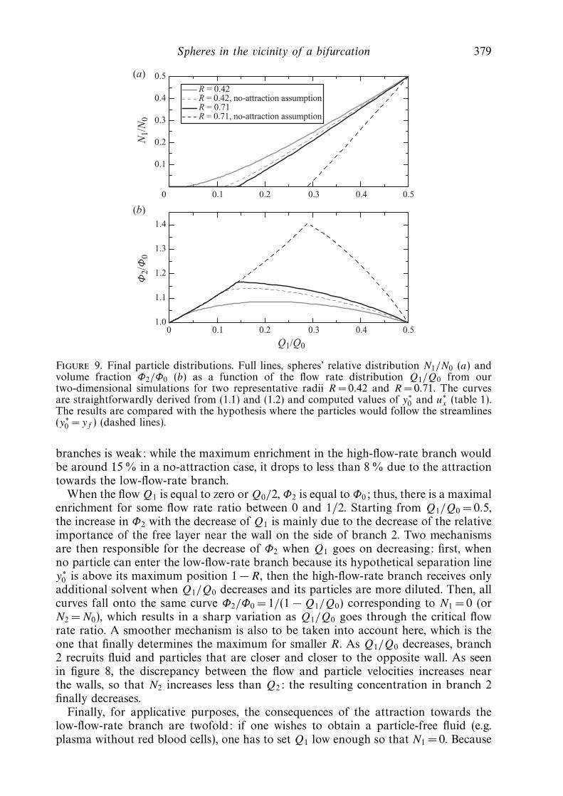
Spheres in the vicinity of a bifurcation 379
0 0.1 0.2 0.3 0.4 0.5
0.10 0.2 0.3 0.4 0.5
0.1
0.2
0.3
0.4
0.5(a)
(b)
1.0
1.1
1.2
1.3
1.4
N1/N
0Φ
2/Φ
0
Q1/Q0
R = 0.42 R = 0.42, no-attraction assumption R = 0.71 R = 0.71, no-attraction assumption
Figure 9. Final particle distributions. Full lines, spheres’ relative distribution N1/N0 (a) andvolume fraction Φ2/Φ0 (b) as a function of the flow rate distribution Q1/Q0 from ourtwo-dimensional simulations for two representative radii R = 0.42 and R = 0.71. The curvesare straightforwardly derived from (1.1) and (1.2) and computed values of y∗
0 and u∗x (table 1).
The results are compared with the hypothesis where the particles would follow the streamlines(y∗
0 = yf ) (dashed lines).
branches is weak: while the maximum enrichment in the high-flow-rate branch wouldbe around 15 % in a no-attraction case, it drops to less than 8 % due to the attractiontowards the low-flow-rate branch.
When the flow Q1 is equal to zero or Q0/2, Φ2 is equal to Φ0; thus, there is a maximalenrichment for some flow rate ratio between 0 and 1/2. Starting from Q1/Q0 =0.5,the increase in Φ2 with the decrease of Q1 is mainly due to the decrease of the relativeimportance of the free layer near the wall on the side of branch 2. Two mechanismsare then responsible for the decrease of Φ2 when Q1 goes on decreasing: first, whenno particle can enter the low-flow-rate branch because its hypothetical separation liney∗
0 is above its maximum position 1 − R, then the high-flow-rate branch receives onlyadditional solvent when Q1/Q0 decreases and its particles are more diluted. Then, allcurves fall onto the same curve Φ2/Φ0 = 1/(1 − Q1/Q0) corresponding to N1 = 0 (orN2 =N0), which results in a sharp variation as Q1/Q0 goes through the critical flowrate ratio. A smoother mechanism is also to be taken into account here, which is theone that finally determines the maximum for smaller R. As Q1/Q0 decreases, branch2 recruits fluid and particles that are closer and closer to the opposite wall. As seenin figure 8, the discrepancy between the flow and particle velocities increases nearthe walls, so that N2 increases less than Q2: the resulting concentration in branch 2finally decreases.
Finally, for applicative purposes, the consequences of the attraction towards thelow-flow-rate branch are twofold: if one wishes to obtain a particle-free fluid (e.g.plasma without red blood cells), one has to set Q1 low enough so that N1 = 0. Because

380 V. Doyeux, T. Podgorski, S. Peponas, M. Ismail and G. Coupier
of attraction towards the low-flow-rate branch, this critical flow rate is decreased andthe efficiency of the process is lowered. If one prefers to concentrate particles, thenone must find the maximum of the Φ2/Φ0 curve. This maximum is lowered andshifted by the attraction towards the low-flow-rate branch (see figure 9). Note that forsmall spheres (e.g. R = 0.42), the position of the maximum does not correspond to thepoint at which N1 vanishes; in addition, the shift direction of the maximum positiondepends on the sphere size: while it shifts to lower Q1/Q0 values for R =0.71, it shiftsto higher values for R = 0.42.
The choice of the geometry, within our symmetric frame, can also greatly modifythe efficiency of a device. Since the depletion effect eventually governs the finaldistribution, narrowing the inlet channel is the first requirement. On the other hand,it also increases the attraction towards the low-flow-rate branch, but one can tryto diminish it. As discussed in the preceding section, this can be done by wideningreasonably the daughter branches. For instance, if their half-width is not 1 but 2.5,as in figure 6(b), the slope ξ in the law y∗
0 = ξ × (Q1/Q0 − 1/2) increases by around15 % for R = 0.67. The critical Q1/Q0 below which no particle enters the low-flow-rate branch increases from 0.13 to 0.19, which is good for fluid–particle separation,and the maximum enrichment Φ2/Φ0 that can be reached is 22 % instead of 15 %.Alternatively, since the attraction is higher in two dimensions than in three, we canalso infer that considering thicker channels, which does not modify the depletioneffect, can greatly improve the final result. Note that this conclusion would have beencompletely different in the case of the high-flow-rate branch enrichment due to someattraction towards it, as claimed in some papers: in such a case, confining as much aspossible would have been required, as it increases all kinds of cross-streamline drifts.
4.3. Consistency with the literature
We now come back to the previous studies already discussed in § 2 in order to checkthe consistency between them and our results.
The only paper that dealt with the position of the particle-separating streamlinewas by Barber et al. (2008), where a symmetric Y-shaped bifurcation was studied(branches leaving the bifurcation with a 45 angle relative to the inlet channel,see figure 1a). In figure 10(a), we compare their results with our simulations in asimilar geometry. The agreement between the two simulations (based on two differentmethods) is very good, except for large particles (R =0.67) and low Q1/Q0. Note thatBarber et al. (2008) have chosen to consider branches whose widths follow the laww3
0 = w31 +w3
2 , where w0 is the width of the inlet branch and w1 and w2 are the widthsof the daughter branches. This law has been shown to describe approximately therelationship between vessel diameters in the arteriolar network (see Mayrovitz & Roy1983). With our notation, they thus consider a = 3
√1/2 ≃ 0.79, while we focused on
a =1 in order to compare with the T-shaped bifurcation. In addition, their apex hasa radius 0.75 (for the R = 0.67 case) while ours is sharper (with radius of 0.1). Thesedifferences seem to impact only partly on the results, as discussed above. We canexpect this slight discrepancy to be due to the treatment of the numerical singularitiesthat appear when the particle is close to one wall. For R = 0.67, the maximum positiony0 is 0.33, which is close to the separating streamline position.
It is also interesting to compare our results in the Y-shaped bifurcation with theresults in the T geometry, which was chosen to make the discussion easier. We cansee that, for low enough Q1/Q0, the attraction towards the low-flow-rate branch isslightly higher. This can be understood by considering a particle with initial positiony0 slightly below the critical position y∗
0 found in the T geometry: in the latter

Spheres in the vicinity of a bifurcation 381
(a) (b)
Q1/Q0
y0*
y0* (T)
y0* (Y)
0.1 0.2 0.3 0.4 0.5
0
0.1
0.2
0.3
0.4
R = 0.67 Barber et al., Y geometry Our simulations, Y geometry Our simulations, T geometry
R = 0.53 Barber et al., Y geometry Our simulations, Y geometry Our simulations, T geometry
Figure 10. (a) Position of the particle separation line y∗0 in a symmetric Y-shaped bifurcation:
according to Barber et al. (2008) (data extracted from their figure 4) and according to oursimulations. The results for similar spheres in our T geometry are also shown. (b) Trajectoriesfrom our simulations in the T- and Y-shaped bifurcations, for similar sphere size (R =0.67)and flow rate ratio (Q1/Q0 =0.2). Full lines, T geometry; dashed lines, Y geometry. Thecorresponding separating streamline positions (respectively y∗
0 (T ) and y∗0 (Y )) are also indicated.
The sphere shown is located at its stagnation point y ′0 (see figure 6) in the Y geometry.
geometry, it will eventually enter the high-flow-rate branch, by definition of y∗0 . As
shown in figure 10(b), in the Y geometry, this movement is hindered by the apexsince the final attraction towards the high-flow-rate branch occurs near the oppositewall (the second effect discussed in § 4.1.2). Finally, from this comparison we seethat comparing results in T and symmetric Y geometry is relevant but for highlyasymmetric flow distributions.
In § 2, the analysis of the two-dimensional simulations for R = 0.5 spheres inAudet & Olbricht (1987) showed that there should be some attraction towards thelow-flow-rate branch. Our simulations for R =0.48 showed that this effect is non-negligible (figure 5b) and modifies significantly the final distribution (figure 9). Finally,we can see in figure 11 that our simulations give results similar to those of Audet &Olbricht (1987).
As for the experiments presented in Yang et al. (2006) for R =0.46, we showed thatthe final distribution was consistent with a no-attraction assumption. As we showedin figure 5(a), in a three-dimensional case, the attraction towards the low-flow-rateregion is weak for spheres of radius R ≃ 0.5 or smaller, which is again consistent withthe results of Yang et al. (2006). Note that, while their results were considered by theauthors as a basis to discuss some attraction effect towards the high-flow-rate branch,we see that their final distributions are just reminiscent of the depletion effect in theinlet channel.
The other consistent set of studies in the literature deals with large balls in three-dimensional channels. We have studied balls of radius R = 0.71 that stop enteringbranch 1 when Q1/Q0 0.22 (figure 5a), while this critical flow rate would be around0.29 if they followed the fluid streamlines. This critical flow rate is expected to beslightly higher for larger balls of radius R ≃ 0.8, but far lower than 0.35, which

382 V. Doyeux, T. Podgorski, S. Peponas, M. Ismail and G. Coupier
0 0.1 0.2 0.3 0.4 0.5 0.6 0.7 0.8 0.9 1.0
0.2
0.4
0.6
0.8
N1/N
0
Q1/Q0
R = 0.48, no-attraction assumption
R = 0.48, our 2D simulations
R = 0.50, Audet & Olbricht
Figure 11. Particle distribution as a function of flow rate ratios for spheres of medium size,according to simulations of this paper and Audet & Olbricht (1987) (same data as plotted infigure 2).
would be the no-attraction case. In the experiments of Roberts & Olbricht (2006),some balls are still observed in branch 1 when Q1/Q0 ≃ 0.22 (figure 2), indicating astronger attraction effect towards the low-flow-rate branch, which can be associatedwith the fact that the authors considered a square cross-sectional channel, while theconfinement in the third direction is 0.5 < 0.71 in our case. The experiments withcircular cross-sectional channels lead to contradictory results: in Chien et al. (1985)and Ditchfield & Olbricht (1996), the results were consistent with a no-attractionassumption; therefore, they are in contradiction with our results. On the contrary, inRoberts & Olbricht (2003), the critical flow rate for R = 0.77 is around 0.2, whichwould show a stronger attraction than in our case. Note that all these apparentlycontradictory observations are to be considered keeping in mind that the data ofN1/N0 as a function of Q1/Q0 are sometimes very noisy in the papers cited.
5. Conclusion
In this paper, we have focused explicitly on the existence and direction of somecross-streamline drift of particles in the vicinity of a bifurcation with different flowrates in the daughter branches. A new analysis of some previous unexploited resultsfrom the literature first gave us some indications on the possibility of an attractiontowards the low-flow-rate branch.
Then, the first direct experimental proof of attraction towards the low-flow-ratebranch was shown and arguments for this attraction were given with the help of two-dimensional simulations. In particular, we showed that this attraction is the resultof two antagonistic effects: the first effect, which takes place at the entrance of thebifurcation, induces migration towards the low-flow-rate branch, while the secondeffect takes place near the stagnation point and induces migration towards the high-flow-rate branch but is not strong enough, in standard configurations of branches ofcomparable sizes, to counterbalance the first effect.
Only the second effect was previously considered in most papers in the literature,which has led to the misleading idea that the enrichment of particles in the high-flow-rate branch is due to some attraction towards it. On the contrary, it had been arguedby Barber et al. (2008) that there should be some attraction towards the low-flow-ratebranch. By distinguishing the two effects mentioned above, we have tried to clarifytheir statements.

Spheres in the vicinity of a bifurcation 383
In the second step, we have discussed the consequences of such an attraction onthe final distribution of particles. It appears that the attraction is not strong enough,even in a two-dimensional system where it is stronger, to counterbalance the impactof the depletion effect. Even in the most homogeneous case where the particles areequally distributed across the channel but cannot approach the wall closer than theirradius, the existence of a free layer near the walls favours the high-flow-rate branch,which eventually receives more particles than fluid.
However, these two antagonistic phenomena are of comparable importance, andneither can be neglected: the increase in the particle volume fraction in the high-flow-rate branch is typically divided by two because of the attraction effect. On theother hand, the initial distribution is a key parameter for the prediction of the finalsplitting. For deformable particles, initial lateral migration can induce a narrowingof their distribution, which will eventually favour the high-flow-rate branch. Forinstance, Barber et al. (2008) had to adjust the free layer width in their simulationsin order to fit experimental data on blood flow. On the other hand, in a network ofbifurcations, the initially centred particles will find themselves close to one wall afterthe first bifurcation, which can favour a low-flow-rate branch in a second bifurcation.
Note, finally, that as seen in Enden & Popel (1992), these effects become weakerwhen the confinement decreases. Typically, as soon as the sphere diameter is lessthan half the channel width, the variations of volume fraction do not exceed a fewper cent.
For applicative purposes, the consequences of this attraction have been discussedand some prescriptions have been proposed. Of course, one can go further than oursymmetric case and modify the angle between the branches, or consider many-branchbifurcations, and so on. However, the T-bifurcation case allowed us to distinguishbetween two goals: concentrating a population of particles or obtaining a particle-free fluid. The optimal configuration can be different according to the chosen goal.Similar considerations are also valid regarding sorting in polydisperse suspensions,which is an important activity (see Pamme 2007): getting an optimally concentratedsuspension of large particles might not be compatible with getting a suspension ofsmall particles free of large particles.
Now that the case of spherical particles in a symmetric bifurcation has beenstudied and the framework well established, we believe that quantitative discussionscould be made in the future about the other parameters that we put aside here. Inparticular, discussing the effect of the deformability of the particles is a challengingtask if one only considers the final distribution data, as the deformability modifiesthe initial distribution, but most probably also the attraction effect. In a network,the importance of these contributions will be different according, in particular, to thedistance between two bifurcations, so they must be discussed separately.
Considering concentrated suspensions is of course the next challenging issue.Particles close to each other will obviously hydrodynamically interact, but so willdistant particles, through the modification of the effective resistance to flow of thebranches. In such a situation, considering pressure-driven or flow-rate-driven fluidswill be different.
For concentrated suspensions of deformable particles in a network, like blood inthe circulatory system, the relevance of a particle-based approach can be questioned.Historical models for the major blood flow phenomena are continuum models withsome ad hoc parameters, which must be somehow related to the intrinsic mechanicalproperties of the blood cells (for a recent example, see Obrist et al. 2010). Buildingup a bottom-up approach in such a system is a long quest. For dilute suspensions,

384 V. Doyeux, T. Podgorski, S. Peponas, M. Ismail and G. Coupier
some links between the microscopic dynamics of lipid vesicles and the rheology ofa suspension have been recently established (see Danker & Misbah 2007; Vitkovaet al. 2008; Ghigliotti, Biben & Misbah 2010). For red blood cells, which exhibitqualitatively similar dynamics (see Abkarian et al. 2007; Deschamps et al. 2009;Dupire, Abkarian & Viallat 2010; Farutin, Biben & Misbah 2010; Noguchi 2010),we can hope that such a link will soon be established, following Vitkova et al.(2008). For confined and concentrated suspensions, the distribution is known tobe non-homogeneous, which has direct consequences on the rheology (the Fahraeus–Lindquist effect). Once again, while empirical macroscopic models are able to describethis reality, establishing the link between the viscosity of the suspension and the localdynamics is still a challenging issue. The final distribution of the flowing bodies isthe product of a balance between migration towards the centre, as discussed in theIntroduction, and interactions between them that can broaden the distribution (seeKantsler, Segre & Steinberg 2008; Podgorski et al. 2010). The presence of deformableboundaries also needs to be taken into account, as shown in Beaucourt et al. (2004).In the meantime, the development of simulation techniques for quantitative three-dimensional approaches is a crucial task, which is becoming more and more feasible(see McWhirter, Noguchi & Gompper 2009; Biben, Farutin & Misbah 2011).
The authors thank G. Ghigliotti for his final reading and acknowledge financialsupport from ANR MOSICOB and CNES.
Appendix. Derivation of the variational formulation
In this appendix, details of the derivation of (3.13)–(3.15) from (3.10)–(3.12) aregiven.
First, we introduce the scalar product in L2(Ωf )2 as follows:
∀ f , g ∈ L2(Ωf )2, 〈 f , g〉L2(Ωf )2 =
∫
Ωf
f · g. (A 1)
The variational formulation of the problem (3.10)–(3.12) is obtained by taking thescalar product of (3.10) in L2(Ωf )2 with a test function v ∈ H 1
0 (Ωf )2 and we multiply(3.11) by a test function q ∈ L2
0(Ω). It leads to the following problem: find (u, p) ∈H 1(Ωf )2 × L2
0(Ωf ) such that
−2ν
∫
Ωf
(∇ · τ (u)) · v +
∫
Ωf
∇p · v = 0, ∀v ∈ H 10 (Ωf )2, (A 2)
∫
Ωf
q∇ · u = 0, ∀q ∈ L20(Ωf ), (A 3)
u = f on ∂Ωf . (A 4)
Applying Green’s formula to (A 2), we obtain
2ν
∫
Ωf
τ (u) : ∇v − 2ν
∫
∂Ωf
τ (u)n · v
−∫
Ωf
p∇ · v +
∫
∂Ωf
pv · n = 0, (A 5)
where n denotes the outer unit normal on ∂Ωf . Taking into account the fact thatv vanishes on ∂Ωf (recall that we have chosen the test function v ∈ H 1
0 (Ωf )2), the
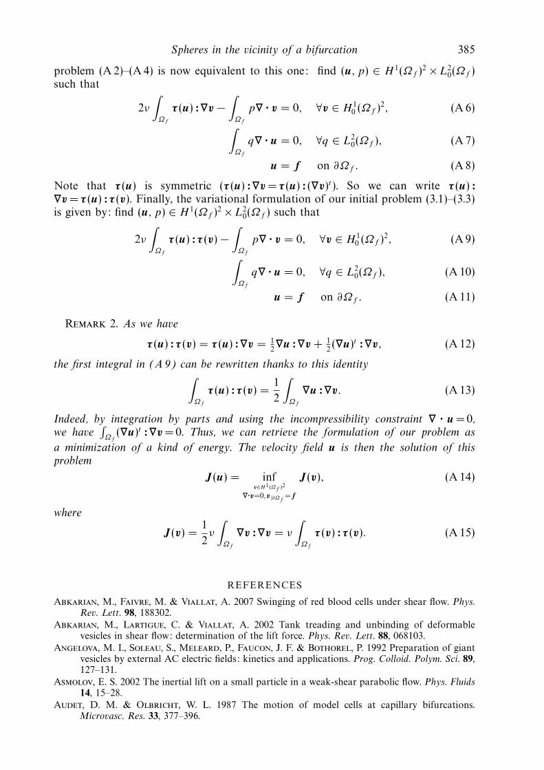
Spheres in the vicinity of a bifurcation 385
problem (A 2)–(A 4) is now equivalent to this one: find (u, p) ∈ H 1(Ωf )2 × L20(Ωf )
such that
2ν
∫
Ωf
τ (u) : ∇v −∫
Ωf
p∇ · v = 0, ∀v ∈ H 10 (Ωf )2, (A 6)
∫
Ωf
q∇ · u = 0, ∀q ∈ L20(Ωf ), (A 7)
u = f on ∂Ωf . (A 8)
Note that τ (u) is symmetric (τ (u) : ∇v = τ (u) : (∇v)t ). So we can write τ (u) :∇v = τ (u) : τ (v). Finally, the variational formulation of our initial problem (3.1)–(3.3)is given by: find (u, p) ∈ H 1(Ωf )2 × L2
0(Ωf ) such that
2ν
∫
Ωf
τ (u) : τ (v) −∫
Ωf
p∇ · v = 0, ∀v ∈ H 10 (Ωf )2, (A 9)
∫
Ωf
q∇ · u = 0, ∀q ∈ L20(Ωf ), (A 10)
u = f on ∂Ωf . (A 11)
Remark 2. As we have
τ (u) : τ (v) = τ (u) : ∇v = 12∇u : ∇v + 1
2(∇u)t : ∇v, (A 12)
the first integral in (A 9) can be rewritten thanks to this identity∫
Ωf
τ (u) : τ (v) =1
2
∫
Ωf
∇u : ∇v. (A 13)
Indeed, by integration by parts and using the incompressibility constraint ∇ · u = 0,we have
∫
Ωf(∇u)t : ∇v = 0. Thus, we can retrieve the formulation of our problem as
a minimization of a kind of energy. The velocity field u is then the solution of thisproblem
J(u) = infv∈H1(Ωf )2
∇·v=0,v|∂Ωf= f
J(v), (A 14)
where
J(v) =1
2ν
∫
Ωf
∇v : ∇v = ν
∫
Ωf
τ (v) : τ (v). (A 15)
REFERENCES
Abkarian, M., Faivre, M. & Viallat, A. 2007 Swinging of red blood cells under shear flow. Phys.Rev. Lett. 98, 188302.
Abkarian, M., Lartigue, C. & Viallat, A. 2002 Tank treading and unbinding of deformablevesicles in shear flow: determination of the lift force. Phys. Rev. Lett. 88, 068103.
Angelova, M. I., Soleau, S., Meleard, P., Faucon, J. F. & Bothorel, P. 1992 Preparation of giantvesicles by external AC electric fields: kinetics and applications. Prog. Colloid. Polym. Sci. 89,127–131.
Asmolov, E. S. 2002 The inertial lift on a small particle in a weak-shear parabolic flow. Phys. Fluids14, 15–28.
Audet, D. M. & Olbricht, W. L. 1987 The motion of model cells at capillary bifurcations.Microvasc. Res. 33, 377–396.
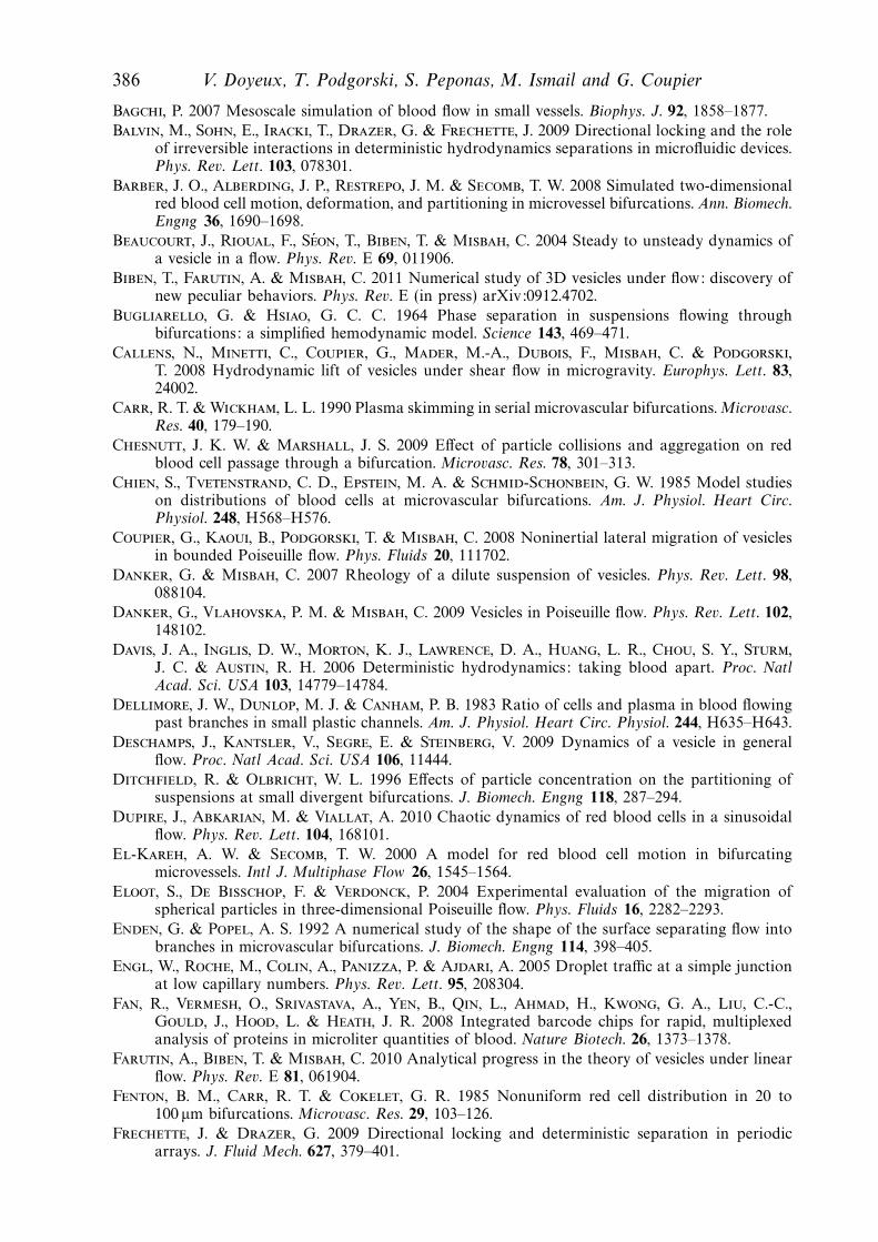
386 V. Doyeux, T. Podgorski, S. Peponas, M. Ismail and G. Coupier
Bagchi, P. 2007 Mesoscale simulation of blood flow in small vessels. Biophys. J. 92, 1858–1877.
Balvin, M., Sohn, E., Iracki, T., Drazer, G. & Frechette, J. 2009 Directional locking and the roleof irreversible interactions in deterministic hydrodynamics separations in microfluidic devices.Phys. Rev. Lett. 103, 078301.
Barber, J. O., Alberding, J. P., Restrepo, J. M. & Secomb, T. W. 2008 Simulated two-dimensionalred blood cell motion, deformation, and partitioning in microvessel bifurcations. Ann. Biomech.Engng 36, 1690–1698.
Beaucourt, J., Rioual, F., Seon, T., Biben, T. & Misbah, C. 2004 Steady to unsteady dynamics ofa vesicle in a flow. Phys. Rev. E 69, 011906.
Biben, T., Farutin, A. & Misbah, C. 2011 Numerical study of 3D vesicles under flow: discovery ofnew peculiar behaviors. Phys. Rev. E (in press) arXiv:0912.4702.
Bugliarello, G. & Hsiao, G. C. C. 1964 Phase separation in suspensions flowing throughbifurcations: a simplified hemodynamic model. Science 143, 469–471.
Callens, N., Minetti, C., Coupier, G., Mader, M.-A., Dubois, F., Misbah, C. & Podgorski,T. 2008 Hydrodynamic lift of vesicles under shear flow in microgravity. Europhys. Lett. 83,24002.
Carr, R. T. & Wickham, L. L. 1990 Plasma skimming in serial microvascular bifurcations. Microvasc.Res. 40, 179–190.
Chesnutt, J. K. W. & Marshall, J. S. 2009 Effect of particle collisions and aggregation on redblood cell passage through a bifurcation. Microvasc. Res. 78, 301–313.
Chien, S., Tvetenstrand, C. D., Epstein, M. A. & Schmid-Schonbein, G. W. 1985 Model studieson distributions of blood cells at microvascular bifurcations. Am. J. Physiol. Heart Circ.Physiol. 248, H568–H576.
Coupier, G., Kaoui, B., Podgorski, T. & Misbah, C. 2008 Noninertial lateral migration of vesiclesin bounded Poiseuille flow. Phys. Fluids 20, 111702.
Danker, G. & Misbah, C. 2007 Rheology of a dilute suspension of vesicles. Phys. Rev. Lett. 98,088104.
Danker, G., Vlahovska, P. M. & Misbah, C. 2009 Vesicles in Poiseuille flow. Phys. Rev. Lett. 102,148102.
Davis, J. A., Inglis, D. W., Morton, K. J., Lawrence, D. A., Huang, L. R., Chou, S. Y., Sturm,J. C. & Austin, R. H. 2006 Deterministic hydrodynamics: taking blood apart. Proc. NatlAcad. Sci. USA 103, 14779–14784.
Dellimore, J. W., Dunlop, M. J. & Canham, P. B. 1983 Ratio of cells and plasma in blood flowingpast branches in small plastic channels. Am. J. Physiol. Heart Circ. Physiol. 244, H635–H643.
Deschamps, J., Kantsler, V., Segre, E. & Steinberg, V. 2009 Dynamics of a vesicle in generalflow. Proc. Natl Acad. Sci. USA 106, 11444.
Ditchfield, R. & Olbricht, W. L. 1996 Effects of particle concentration on the partitioning ofsuspensions at small divergent bifurcations. J. Biomech. Engng 118, 287–294.
Dupire, J., Abkarian, M. & Viallat, A. 2010 Chaotic dynamics of red blood cells in a sinusoidalflow. Phys. Rev. Lett. 104, 168101.
El-Kareh, A. W. & Secomb, T. W. 2000 A model for red blood cell motion in bifurcatingmicrovessels. Intl J. Multiphase Flow 26, 1545–1564.
Eloot, S., De Bisschop, F. & Verdonck, P. 2004 Experimental evaluation of the migration ofspherical particles in three-dimensional Poiseuille flow. Phys. Fluids 16, 2282–2293.
Enden, G. & Popel, A. S. 1992 A numerical study of the shape of the surface separating flow intobranches in microvascular bifurcations. J. Biomech. Engng 114, 398–405.
Engl, W., Roche, M., Colin, A., Panizza, P. & Ajdari, A. 2005 Droplet traffic at a simple junctionat low capillary numbers. Phys. Rev. Lett. 95, 208304.
Fan, R., Vermesh, O., Srivastava, A., Yen, B., Qin, L., Ahmad, H., Kwong, G. A., Liu, C.-C.,Gould, J., Hood, L. & Heath, J. R. 2008 Integrated barcode chips for rapid, multiplexedanalysis of proteins in microliter quantities of blood. Nature Biotech. 26, 1373–1378.
Farutin, A., Biben, T. & Misbah, C. 2010 Analytical progress in the theory of vesicles under linearflow. Phys. Rev. E 81, 061904.
Fenton, B. M., Carr, R. T. & Cokelet, G. R. 1985 Nonuniform red cell distribution in 20 to100 µm bifurcations. Microvasc. Res. 29, 103–126.
Frechette, J. & Drazer, G. 2009 Directional locking and deterministic separation in periodicarrays. J. Fluid Mech. 627, 379–401.

Spheres in the vicinity of a bifurcation 387
Fung, Y. C. 1973 Stochastic flow in capillary blood vessels. Microvasc. Res. 5, 34–48.
Fung, Y. C. 1993 Biomechanics: Mechanical Properties of Living Tissues . Springer.
Ghigliotti, G., Biben, T. & Misbah, C. 2010 Rheology of a dilute two-dimensional suspension ofvesicles. J. Fluid Mech. 653, 489–518.
Girault, V. & Raviart, P.A. 1986 Finite Element Methods for Navier–Stokes Equations: Theory andAlgorithms . Springer.
Griggs, A. J., Zinchenko, A. Z. & Davis, R. H. 2007 Low-Reynolds-number motion of a deformabledrop between two parallel plane walls. Intl J. Multiphase Flow 33, 182–206.
Guibert, R., Fonta, C. & Plouraboue, F. 2010 A new approach to model confined suspensionsflows in complex networks: application to blood flow. Trans. Porous Med. 83, 171–194.
Hecht, F. & Pironneau, O. 2010 A finite element software for PDEs: freeFEM++. Available at:http://www.freefem.org/.
Inglis, D. W. 2009 Efficient microfluidic particle separation arrays. Appl. Phys. Lett. 94, 013510.
Jaggi, R. D., Sandoz, R. & Effenhauser, C. S. 2007 Microfluidic depletion of red blood cells fromwhole blood in high-aspect-ratio microchannels. Microfluid Nanofluid 3, 47–53.
Janela, J., Lefebvre, A. & Maury, B. 2005 A penalty method for the simulation of fluid-rigid bodyinteraction. In ESAIM: Proc (ed. E. Cances & J.-F. Gerbeau), vol. 14, pp. 115–123. ESAIM.
Jousse, F., Farr, R., Link, D. R., Fuerstman, M. J. & Garstecki, P. 2006 Bifurcation of dropletflows within capillaries. Phys. Rev. E 74, 036311.
Kantsler, V., Segre, E. & Steinberg, V. 2008 Dynamics of interacting vesicles and rheology ofvesicle suspension in shear flow. Europhys. Lett. 82, 58005.
Kaoui, B., Coupier, G., Misbah, C. & Podgorski, T. 2009 Lateral migration of vesicles inmicrochannels: effects of walls and shear gradient. Houille Blanche 5, 112–119.
Kaoui, B., Ristow, G., Cantat, I., Misbah, C. & Zimmermann, W. 2008 Lateral migration of atwo-dimensional vesicle in unbounded Poiseuille flow. Phys. Rev. E 77, 021903.
Kersaudy-Kerhoas, M., Dhariwal, R., Desmulliez, M. P. Y. & Jouvet, L. 2010 Hydrodynamicblood plasma separation in microfluidic channels. Microfluid Nanofluid 8, 105–114.
Kim, Y. W. & Yoo, J. Y. 2008 The lateral migration of neutrally-buoyant spheres transportedthrough square microchannels. J. Micromech. Microengng 18, 065015.
Lefebvre, A. 2007 Fluid–particle simulations with FreeFem++. In ESAIM: Proc., vol. 18, pp. 120–132. ESAIM.
Maury, B. 2009 Numerical analysis of a finite element/volume penalty method. SIAM J. Numer.Anal. 47 (2), 1126–1148.
Mayrovitz, H. N. & Roy, J. 1983 Microvascular blood flow: evidence indicating a cubic dependenceon arteriolar diameter. Am. J. Physiol. 255, H1031–H1038.
McWhirter, J. L., Noguchi, H. & Gompper, G. 2009 Flow-induced clustering and alignment ofvesicles and red blood cells in microcapillaries. Proc. Natl Acad. Sci. USA 106, 6039–6043.
Mortazavi, S. & Tryggvason, G. 2000 A numerical study of the motion of drops in Poiseuilleflow. Part 1. Lateral migration of one drop. J. Fluid. Mech. 411, 325–350.
Noguchi, H. 2010 Dynamic modes of red blood cells in oscillatory shear flow. Phys. Rev. E 81,061920.
Obrist, D., Weber, B., Buck, A. & Jenny, P. 2010 Red blood cell distribution in simplified capillarynetworks. Phil. Trans. R. Soc. Lond. A 368, 2897–2918.
Olla, P. 1997 The lift on a tank-treading ellipsoidal cell in a shear flow. J. Phys. II Paris 7,1533–1540.
Pamme, N. 2007 Continuous flow separations in microfluidic devices. Lab Chip 7, 1644–1659.
Peyla, P. 2007 A deformable object in a microfluidic configuration: a numerical study. Europhys.Lett. 80, 34001.
Podgorski, T., Callens, N., Minetti, C., Coupier, G., Dubois, F. & Misbah, C. 2010 Dynamicsof vesicle suspensions in shear flow between walls. Microgravity Sci. Technol. 23, 263–270.
Pries, A. R., Ley, K., Claassen, M. & Gaethgens, P. 1989 Red cell distribution at microvascularbifurcations. Microvasc. Res. 38, 81–101.
Pries, A. R., Secomb, T. W. & Gaethgens, P. 1996 Biophysical aspects of blood flow in themicrovasculature. Cardiovasc. Res. 32, 654–667.
Risso, F., Colle-Paillot, F. & Zagzoule, M. 2006 Experimental investigation of a bioartificialcapsule flowing in a narrow tube. J. Fluid. Mech. 547, 149–173.

388 V. Doyeux, T. Podgorski, S. Peponas, M. Ismail and G. Coupier
Roberts, B. W. & Olbricht, W. L. 2003 Flow-induced particulate separations. AIChE J. 49,2842–2849.
Roberts, B. W. & Olbricht, W. L. 2006 The distribution of freely suspended particles at microfluidicbifurcations. AIChE J. 52, 199–206.
Schindler, M. & Ajdari, A. 2008 Droplet traffic in microfluidic networks: a simple model forunderstanding and designing. Phys. Rev. Lett. 100, 044501.
Schonberg, J. A. & Hinch, E. J. 1989 Inertial migration of a sphere in a Poiseuille flow. J. FluidMech. 203, 517–524.
Secomb, T. W., Styp-Rekowska, B. & Pries, A. R. 2007 Two-dimensional simulation of red bloodcell deformation and lateral migration in microvessels. Ann. Biomed. Engng 35, 755–765.
Sessoms, D. A., Belloul, M., Engl, W., Roche, M., Courbin, L. & Panizza, P. 2009 Droplet motionin microfluidic networks: hydrodynamic interactions and pressure-drop measurements. Phys.Rev. E 80, 016317.
Svanes, K. & Zweifach, B. W. 1968 Variations in small blood vessel hematocrits produced inhypothermic rats by micro-occlusion. Microvasc. Res. 1, 210–220.
Tanaka, H. & Araki, T. 2000 Simulation method of colloidal suspensions with hydrodynamicinteractions: fluid particle dynamics. Phys. Rev. Lett. 85 (6), 1338–1341.
Vitkova, V., Mader, M.-A., Polack, B., Misbah, C. & Podgorski, T. 2008 Micro–macro link inrheology of erythrocyte and vesicle suspensions. Biophys. J. 95, 33–35.
Vlahovska, P. M., Podgorski, T. & Misbah, C. 2009 Vesicles and red blood cells in flow: fromindividual dynamics to rheology. C. R. Physique 10, 775–789.
White, F. M. 1991 Viscous Fluid Flow . McGraw-Hill.Yang, S., Undar, A. & Zahn, J. D. 2006 A microfluidic device for continuous, real time blood
plasma separation. Lab Chip 6, 871–880.Yang, S. & Zahn, J. D. 2004 Particle separation in microfluidic channels using flow rate control. In
Proc. ASME Conf. International Mechanical Engineering Exp Fluids Engineering (IMECE),Anaheim, CA.
Yen, R. T. & Fung, Y. C. 1978 Effect of velocity distribution on red cell distribution in capillaryblood vessels. Am. J. Physiol. Heart Circ. Physiol. 235, H251–H257.
Yoo, J. Y. & Kim, Y. W. 2010 Two-phase flow laden with spherical particles in a microcapillary. IntlJ. Multiphase Flow 36, 460–466.
Zheng, S., Liu, J.-Q. & Tai, Y.-C. 2008 Streamline-based microfluidic devices for erythrocytes andleukocytes separation. J. Microelectromech. Syst. 17, 1029–1038.

7.2. Suspension of vesicle in a bifurcation Chapter 7. Disks at a bifurcation
7.2 Suspension of vesicle in a bifurcation
In the future we would like to continue the work previously done for dilute suspension ofspheres and expand it to the simulation of soft objects and suspensions. In this section,we will show the ability of our framework to handle a complete suspension of vesicles ina bifurcation. We will explain some technical aspects and how to obtain the quantitiesof interest and show a few results. Then we will show that it is also possible to handlesuspensions with two different kinds of vesicles.
7.2.1 Entry and exit of vesicles
The goal is to simulate the entry of a continuous flow of vesicle in a bifurcation and mea-sure the out flux in each branch. As opposed to what has been done in the previous studyfor dilute suspension, the goal is not to follow the trajectory of an individual particle butto have a global information. First of all let us explain how it is possible to deal with theentry and exit of vesicles.
As all the vesicles are of the same kind (same viscosity and rigidity), a single level setfield φ is defined and handles all the interfaces. The geometry of the bifurcation is thesame as in the previous study, as are the fluid equations and boundary conditions. A firstvesicle is set as an ellipse in the inlet boundary. Since a Poiseuille flow is imposed at theentrance of the channel, the vesicle moves forward. To have a continuous flow of vesiclesit is necessary to add new vesicles in the inlet channel. One way to do it could be to addnew vesicles periodically in time, but this might not be the way which most representsthe reality. Indeed, if the vesicles at the bifurcation slow down the flow of vesicle, newvesicles would still be added and the concentration in the inlet branch would increase.Consequently, we choose to add a new vesicle only when the one before it has left an inletregion that we define. Indeed, we define a band of size Lin in the x direction and of thesize of the inlet channel in the y direction, we call it Ωin. We compute the amount ofvesicles in this region Ain as:
Ain =
∫
Ωin
(1−Hε(φ)). (7.2)
When Ain is smaller than a certain value, a new vesicle is added in Ωin or a bit upstreamof it as shown on the scheme 7.2.1. The length Lin, the position of the new vesicle, aswell as the threshold of Ain under which a new vesicle is added are the three parameterson which one can vary to change the concentration of particles in the inlet.Let us explain now how we can add a new vesicle in the system. Since we are in a Stokesregime, the solution of Stokes equations does not need the previous one. Thus, no specialcare has to be taken at the fluid point of view and we can simply add a new object inthe inlet, the Stokes equations will take it into account instantaneously. We only need tobe careful to put the particle far enough from the center of interest of the physical studyto avoid modifying the behavior we want to observe. In this case, it is sufficient to addthe new particles at the very beginning of the inlet to be sure that the physics of thebifurcation point is not modified. Consequently, the procedure of adding a new vesiclesimply consists of modifying the level set function φ to a new one, φ∗ containing the new
205

7.2. Suspension of vesicle in a bifurcation Chapter 7. Disks at a bifurcation
Figure 7.5: Scheme of the inlet of the bifurcation. The domain Ωin is represented in green.The area where (1−Hε(φ)) 6= 0 is represented in red. On the left hand side, the quantityAin is too high for a new vesicle to be added. On the right hand side, the vesicle justexited the domain Ωin, this makes Ain vanishing, thus a new vesicle is added.
vesicle. This is done by computing a field which represents the distance function to thenew vesicles, φves and set:
φ∗ = min(φves, φ). (7.3)
This way, the interfaces already present in the bifurcation are not lost, and the new vesicleis added. Nevertheless, even if the fluid equations are independent of the time since weare concerned about the Stokes flow, the time evolution of the advection equation of thelevel set might by of order two. If so, we need to impose a first order scheme when a newparticle is added in order to avoid the need of the previous value of φ which would inducean unwanted jump.
We discussed the choice of the x position of the new vesicle added in the channel, butthe y position is also an important parameter. From the numerical point of view, there isno restriction for the vesicle to be set at any y position in the inlet channel, the choice isguided by the physics we want to represent. To represent a homogeneous suspension inthe inlet branch, a random choice of the position y with the same probability in all theaccessible y can be done. One can also take into account that the vesicles tend to migrateto the center and pick the new y position in a distribution taking into account this effect.
The exit of vesicles at the outlet channels is not difficult to handle. The only carewhich might have to be taken is because the curvature and its higher order derivativesmight not be captured correctly when the vesicle is cut at the outlet. The vesicle is not aclosed shape anymore and its normal, curvatures and higher derivatives have unpredictablevalues creating huge force points. This can be avoided simply by making vanish the forcesfew mesh sizes away from the exit. This way, from the fluid point of view, the vesicleoutlet is a few mesh sizes before the geometric outlet, and at this point, the curvature isstill defined.
7.2.2 Quantity of interest: the flux of vesicles
For a simulation of a semi-dilute or concentrated suspension, the quantities of interestare not anymore the trajectories of individual particles but the flux of particles in eachbranch. To measure these fluxes, we define three very small bands of about 2h size inlength that we call ΩN0
, ΩN1and ΩN2
. The fluxes of particles are computed through these
206

7.2. Suspension of vesicle in a bifurcation Chapter 7. Disks at a bifurcation
domains as :
Ni =
∫
ΩNi
(u ·ni)(1−Hε(φ))
∫
ΩNi
1with i = 0, 1, 2 (7.4)
where u is the fluid velocity and ni is the normal to the domain ΩNi. More precisely,
n0 = (1, 0), n1 = (0, 1), and n2 = (0,−1). The different domains are disposed as in figure7.6, not too far from the outlets.
Figure 7.6: Scheme representing the positions of the domains in which the fluxes aremeasured.
The figure 7.8 shows a simulation made on 12 processors. The time step has been fixedto 2 · 10−3 and the mesh size h = 0.05. The flow forces are assumed to be much strongerthan the membrane forces, thus the parameter kB has been set to a value close to 0. The
flow rate ratio has been set toQ1
Q2
=2
3. In this simulation we choose to pick the new y
position of the vesicle in the inlet channel randomly, with an equal probability of each y tooccur. The resulting fluxes are shown in figure 7.7(a). We also made another simulationfor which all the vesicles were set at the center of the inlet channel. This could simulatethe fact that a focusing device has been used upstream. The result of this simulation isshown in figure 7.7(b). We can see on the figure 7.7(b) that the inlet channel presents anice regular periodicity. This comes from the fact that the vesicles are all at the centerof the channel initially and thus pass through Ω0 all the same way. Whereas, in figure7.7(a), the vesicles which are closer to a wall see a local shear and incline which mightresult in a larger flux peak. Moreover, these particles are moving faster than the one atthe center, thus, they also exhibit a slightly higher peak.
We can also guess only from the flux graphs which branch is the high or low flow rateone. Indeed, one sees clearly that the top branch sees a smaller flux of particles and more-over, the peaks are large which means that the vesicles spend a long time in the domainΩ1 and the height is low which also means they are going slowly. It is the opposite in thebranch 2. Furthermore, we see clearly that the first particles are entering in this branch.
The kind of information that we would like to extract in the future is the influence ofthe many parameters that we can change on the mean fluxes in each branch. We define
207

7.2. Suspension of vesicle in a bifurcation Chapter 7. Disks at a bifurcation
the mean fluxes as:
< Ni >=1
tf − ti
∫ tf
ti
Ni (7.5)
where ti and tf are respectively the initial and final time of the simulation. Thus, byintegrating the fluxes in the branches we can compare the ratio of particle fluxes and
the ratio of fluid fluxes. We obtained for this particular case:< N1 >
< N2 >= 0.48 for the
simulation where the y inlet positions were random, and< N1 >
< N2 >= 0.46 for the other
one. We can see that there is still a concentration increase in the high flow rate branch
since the initial flow rate ratio wereQ1
Q2
=2
3.
This value should be studied by varying many parameters in this problem and wehope to be able to extract general laws out of such simulations on the general repartitionof the cells in vivo and in vitro.
0 2 4 6 8 10 12 14t
0.00
0.05
0.10
0.15
0.20
0.25
0.30
0.35
0.40
Ni
N0 (in)
N1 (top)
N2 (bot)
(a) Fluxes in each branch when the y position ofthe vesicle is randomly set.
0 2 4 6 8 10 12t
0.00
0.05
0.10
0.15
0.20
0.25
0.30
0.35
0.40
Ni
N0 (in)
N1 (top)
N2 (bot)
(b) Fluxes in each branch when the y position of thevesicle is always at the center of the inlet channel.
Figure 7.7: Fluxes measured in each branch of a bifurcation. An offset of 0.9 have beenused to separate all the curves.
7.2.3 Extension to two different kinds of vesicles
In the future we want to address the problem of the splitting of a suspension of differentkinds of vesicles. It happen in some diseases like drepanocitosis, also called sickle celldisease, that some red blood cells become very rigid. This property makes their flowin microcapillaries very difficult and leads to dramatic effects on patients. A better un-derstanding of the flow of suspensions with objects of different rigidity or viscosity ratiocould also lead to a better knowledge of these diseases. During this work, we set up thesimulation of such a problem and checked that we were able to measure the different fluxes.
The method to simulate vesicles is the one described in chapter 4 and the multi-levelset framework presented in section 2.2.2 is used to deal with the two different kinds ofvesicles. For this test, we call a kind of vesicles the vesicles 0 and the other one the
208

7.2. Suspension of vesicle in a bifurcation Chapter 7. Disks at a bifurcation
Figure 7.8: Suspension of vesicles in a bifurcation.
209
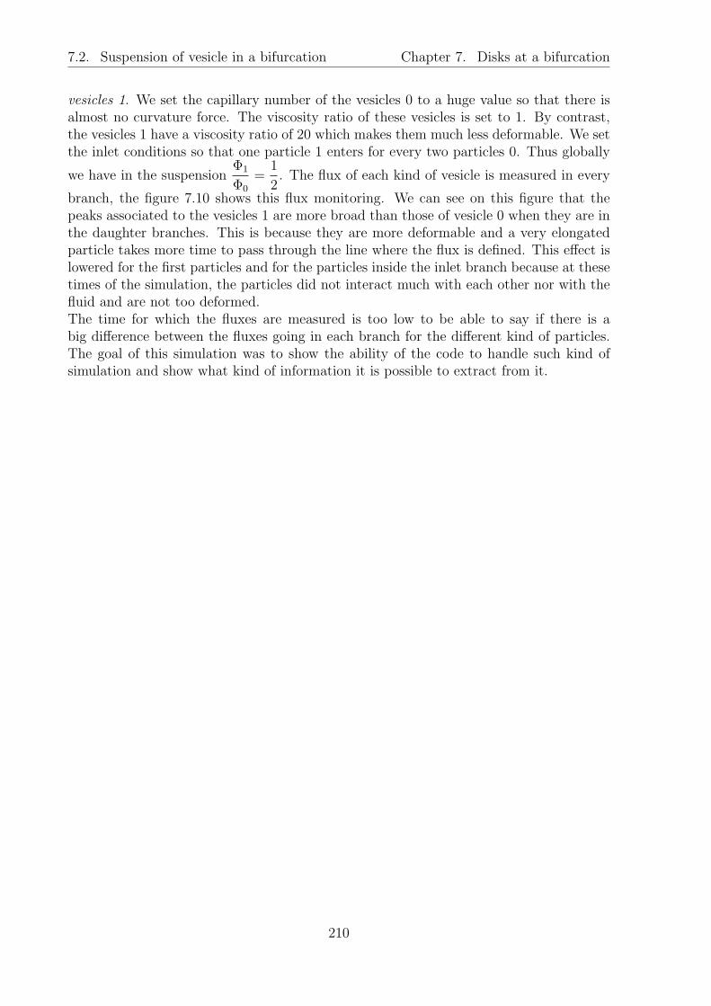
7.2. Suspension of vesicle in a bifurcation Chapter 7. Disks at a bifurcation
vesicles 1. We set the capillary number of the vesicles 0 to a huge value so that there isalmost no curvature force. The viscosity ratio of these vesicles is set to 1. By contrast,the vesicles 1 have a viscosity ratio of 20 which makes them much less deformable. We setthe inlet conditions so that one particle 1 enters for every two particles 0. Thus globally
we have in the suspensionΦ1
Φ0
=1
2. The flux of each kind of vesicle is measured in every
branch, the figure 7.10 shows this flux monitoring. We can see on this figure that thepeaks associated to the vesicles 1 are more broad than those of vesicle 0 when they are inthe daughter branches. This is because they are more deformable and a very elongatedparticle takes more time to pass through the line where the flux is defined. This effect islowered for the first particles and for the particles inside the inlet branch because at thesetimes of the simulation, the particles did not interact much with each other nor with thefluid and are not too deformed.The time for which the fluxes are measured is too low to be able to say if there is abig difference between the fluxes going in each branch for the different kind of particles.The goal of this simulation was to show the ability of the code to handle such kind ofsimulation and show what kind of information it is possible to extract from it.
210
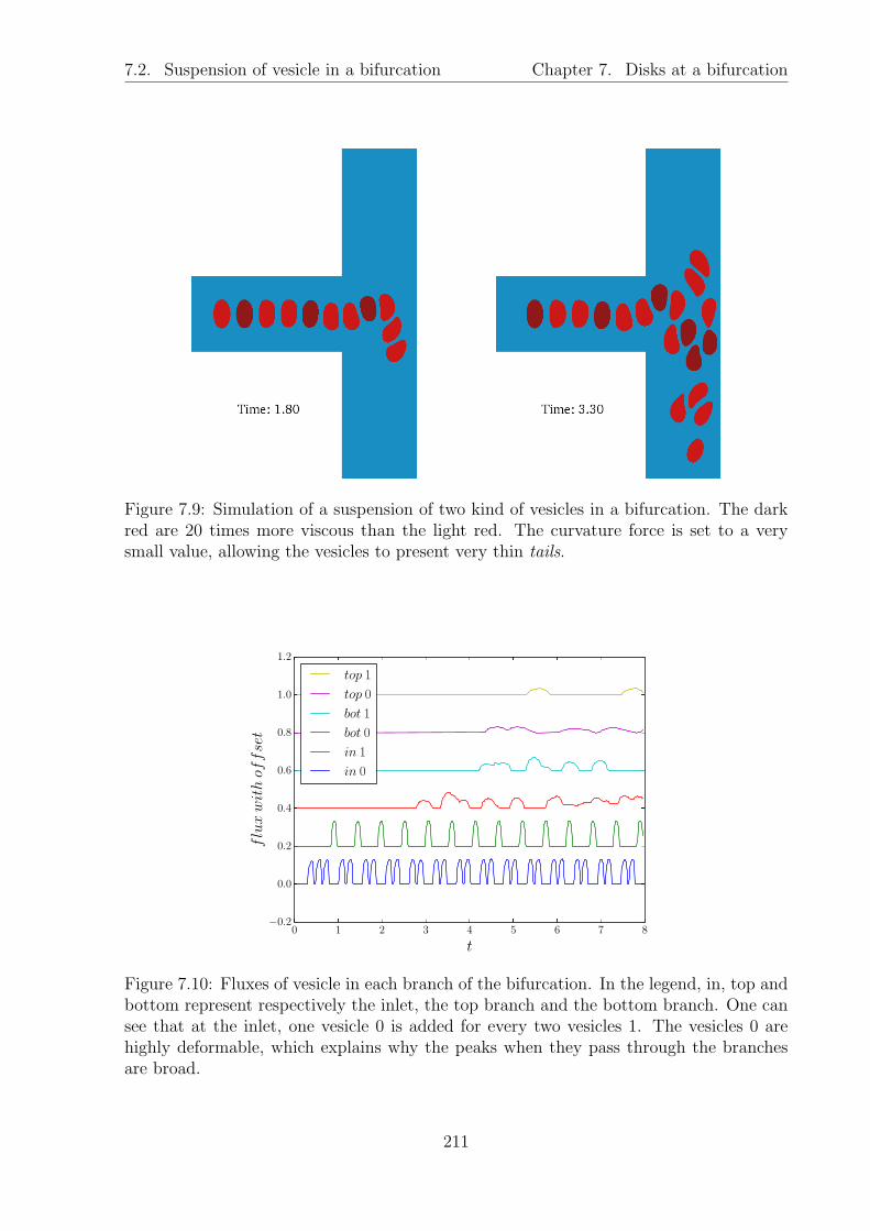
7.2. Suspension of vesicle in a bifurcation Chapter 7. Disks at a bifurcation
Figure 7.9: Simulation of a suspension of two kind of vesicles in a bifurcation. The darkred are 20 times more viscous than the light red. The curvature force is set to a verysmall value, allowing the vesicles to present very thin tails.
0 1 2 3 4 5 6 7 8
t
−0.2
0.0
0.2
0.4
0.6
0.8
1.0
1.2
fluxwithoffset
top 1
top 0
bot 1
bot 0
in 1
in 0
Figure 7.10: Fluxes of vesicle in each branch of the bifurcation. In the legend, in, top andbottom represent respectively the inlet, the top branch and the bottom branch. One cansee that at the inlet, one vesicle 0 is added for every two vesicles 1. The vesicles 0 arehighly deformable, which explains why the peaks when they pass through the branchesare broad.
211

7.2. Suspension of vesicle in a bifurcation Chapter 7. Disks at a bifurcation
212
Chapter 8
Rheology of solid disks
Contents8.1 Measurement of the viscosity . . . . . . . . . . . . . . . . . . . 214
8.1.1 Some methods to compute the effective viscosity . . . . . . . . 215
8.1.2 Convergence to the Einstein’s viscosity . . . . . . . . . . . . . . 216
8.2 Semi-dilute suspensions . . . . . . . . . . . . . . . . . . . . . . . 219
8.2.1 The viscosity of a confined dilute suspension of solid disks . . . 223
8.2.2 The contribution to the viscosity of the pair interaction . . . . 227
8.2.3 Extension to the simulation of a semi dilute suspension . . . . 229
213

8.1. Measurement of the viscosity Chapter 8. Rheology of solid disks
The goal of this chapter is to show results that we obtained in preparation for therheology study of semi dilute suspensions of vesicles within our framework. To be ableto perform quantitative study of such a system, some work needs to be done to makesure that we are able to recover the basic known results of rheology. Moreover, a preciseunderstanding of the rheology of deformable objects in flow requires the knowledge ofthe behavior of simple non-deformable objects. This is why we will start this chapter byshowing the system used to measure the viscosity of a suspension. Then we will show thatwe are able to recover the Einstein viscosity of a dilute suspension of 2D rigid disks andcontrol the accuracy of the measure of the viscosity. We will then measure the viscosityof a single particle in a confined shear flow, explore the possible parameters and compareour results with an analytical model. We extend the same method to the viscosity of twointeracting particles. Finally, we will use these results to derive a method to measurethe viscosity of a semi dilute suspension of particles for different configurations. We willshow with this method that we can recover a behavior already known in 3D which is thedecrease of the influence of the pair interactions at high confinement.
8.1 Numerical measurement of the viscosity of a sus-
pension of particles
We compared three different methods to compute the effective viscosity of a suspensionof rigid disks confined between two moving walls. The configuration of the problem isshown in figure 8.1. The fluid is governed by the Stokes equations. As in section 3.1, wedenote Ω the whole computational domain, Ωf the fluid domain and Bi the rigid disks.
We recall the definition of the flow rate γ =2U
l.
Figure 8.1: Suspension of rigid disks between two moving walls.
214

8.1. Measurement of the viscosity Chapter 8. Rheology of solid disks
8.1.1 Some methods to compute the effective viscosity
Computing the forces on the walls
A possible way to compute the effective viscosity, is to compute the forces exerted by thefluids on the walls. It is equivalent to what is done experimentally with a rheometer. Itis also the intuition that one has of viscosity: if you put a liquid between your fingersand move your fingers in opposite directions, you will say the liquid is more viscous if itcauses a higher resistance.
Let us show that in a fluid where no particles are present, this is a way to get theviscosity. The force acting on the upper wall (called ft) is defined as :
ft =
∫
Top Wall
σn (8.1)
where, in this case, n = (0, ny) is the outward normal of the wall. Let us consider nowonly the x component of this force, that we will call ft. We have, for a flow withoutparticles:
ft =
∫
Top Wall
µ0(∂xuy + ∂yux)ny. (8.2)
Which can be re-written for a pure shear flow:
ft = µ0γL.
Thus, using the x component of the bottom force (that we will call fb) defined the sameway and having opposite sign, one has a relation between the force difference and theviscosity:
ft − fb = 2µ0γL. (8.3)
By substitution, a definition of the effective viscosity of a suspension µeff can be given as:
µeff =ft − fb2Lγ
=l (ft − fb)
4LU(8.4)
The advantage of this definition is that one has only to integrate the velocity field over thetop and bottom walls to get the effective viscosity. Thus, it can be done really quickly.Moreover, this method is valid for vesicles as well as for rigid disks or other objects.This method is very close to the experimental one. Indeed, an experimental rheometeris measuring the force needed to impose a given velocity. The drawbacks of having tointegrate only on few elements of the boundary of the domain is that the effective viscositycan be more sensitive to numerical noise than in other methods integrating in the wholevolume.
Computing the mean of the stress tensor
Another way to compute the effective viscosity of a suspension of rigid disks is to integratethe off-diagonal part of the stress tensor. Let us call it σxy. Once again, we start byshowing that we can recover the viscosity of a Newtonian fluid without particles with this
215

8.1. Measurement of the viscosity Chapter 8. Rheology of solid disks
information and then extend the definition to the effective viscosity of a suspension. Themean of the off-diagonal part of the stress tensor reads:
< σxy >=1
V
∫
Ω
µ0(∂xuy + ∂yux)
with V the volume of Ω. It becomes for a pure shear flow of a Newtonian fluid:
< σxy >= µ0γ
The viscosity is thus given by: µ0 =< σxy >
γ. Consequently, a way to define the effective
viscosity is:
µeff =µ0
γV
∫
Ω
∂xuy + ∂yux. (8.5)
The advantage compared to the previous method is that we integrate over the wholedomain, which tends to smooth more the numerical error. The method is valid for solidparticles and can be extended to vesicles if one recalls that the stress to integrate is thetotal stress and not only the one induced by the fluid. Thus the stress coming from themembrane forces have also to be incorporated in the computation of the viscosity.
Computing the dissipation rate
It as been shown in [65] that the effective viscosity of a suspension can also be calculated byintegrating the dissipation in the fluid. We have reported the ways to do this calculationin appendix H. The expression of the effective viscosity is:
µeff =µ0 l
8LU2
∫
Ωf
|∇u+t∇u|2. (8.6)
This integral is defined on the fluid domain. This is an advantage when only the fluiddomain is defined and the inclusions are seen as holes on the mesh, as in the conformmethod or the fat boundary method (see section 3.1 for more details). In our case, withthe penalty method presented in algorithm 5, we can access the fluid domain thanks tothe Heaviside like function. Since the integrand vanishes inside the particles, we can alsointegrate over the whole domain without changing the result.
8.1.2 Convergence to the Einstein’s viscosity
We made a simple test in order to compare the three different ways to compute theviscosity. It consists in putting a single solid particle of radius R = 1 at the center of arectangular domain Ω of size (L, l) and imposing a shear flow of shear rate γ = 1. Theviscosity has been fixed to µ0 = 10. The method used to simulate the fluid and the particleis the one described in algorithm 5 of chapter 3, that is, a penalty method for which theposition of the particle is tracked by level set method. The thickness of the interface isdefined as 1.5 h with h the discretization step of the domain around the particle. Whenthe wanted mesh size becomes too small, the domain is meshed with a thin mesh size hin a vertical band of size (5R, l) and with a bigger mesh size of 5 h everywhere else. The
216

8.1. Measurement of the viscosity Chapter 8. Rheology of solid disks
viscosity is computed using the three different methods exposed above. The theoreticalviscosity of a dilute suspension of particles has been calculated by Einstein in 1905 [30].We recall that the hypothesis of a dilute suspension means that each particle does notinteract hydrodynamically with its neighbors. This theory has also been made for aninfinite fluid. In our case, we only consider one particle, thus there is no possible mutualinfluence, and the walls are sufficiently far away for us to be able to neglect their influenceon the particle. Thus, we normally are in the range where the Einstein’s viscosity formulashould work. The Einstein law for the viscosity of a dilute suspension is:
µeff = µ0(1 + αΦ) (8.7)
where µ0 is the viscosity of the solvent, α is a coefficient, one has α = 2.5 for 3D spheresand α = 2 for 2D disks. Here Φ is the volume fraction of particles. Note that it isunrelated to the level set field φ which is denoted by a minor φ. The volume fraction Φis defined as the volume (surface in 2D) occupied by the particles divided by the totalvolume of the suspension.
Computing the numerical volume fraction
In penalty / FPD methods, the following question arises: were is exactly the limit betweenthe particle and the fluid? Since the particle is seen as part of the fluid having a hugeviscosity, and since the transition from the viscosity of the fluid to the one of the particleis smooth, it is not obvious where the precise boundary of the particle should be defined.The simplest answer that one could give is that, in our case, the particle is defined thanksto the level set function by the region where φ < 0. Doing this simple approximationleads to an underestimate of the real value of the volume fraction, the particle seen bythe system is actually slightly bigger than that. This problem as been addressed byL.Jibuti [48] in his thesis for a 3D particle, where he did two numerical experiments forwhich the result is known to calibrate the real size of the particle. The first experimentwas to compute the Stokes force on a sphere moving in a fluid at rest. This problem hasno analytic solution in 2D (Stokes paradox) and was not accessible to us. The secondone was the same simulation that we are concerned with here, i.e recovering the Einsteinviscosity. We did similar tests and found that a correct behavior is obtained by setting the
particle region as the region in which φ <ε
2, that is to say for this simulation φ < 0.75 h.
Thus we compute the numerical volume fraction as:
Φh =1
V
∫
Ω
χ(φ < 0.75 h). (8.8)
A consequence is that for a given radius, the size of the mesh has influence on the volumefraction of the suspension.
Results of the test
The test has been made for several mesh sizes. For h < 0.1, the refinement in the bandaround the particle explained previously has been used. The following error has beencalculated:
evisco = |µeff − µ0(1 + 2Φh)| (8.9)
217
8.1. Measurement of the viscosity Chapter 8. Rheology of solid disks
which is the absolute error of the effective viscosity compared to the theoretical viscosityat this numerical volume fraction. The length of the box in the x direction has been takenequal to L = 50 and two different channel widths have been tested: l = 30 and l = 8.To differentiate the methods, we will call the force method the method using expression(8.4) to compute the effective viscosity, the stress method the one using (8.5) and finallythe dissipation method the one using equation (8.6).
We have reported in figure 8.2 the effective viscosity computed by each method forboth channel widths. The theoretical value of the viscosity using the volume fraction ofa particle with a fixed radius R = 1 has been represented as a red line, it is simply given
in this problem by: µ0 (1 + 2π
L l). The viscosity calculated using the numerical volume
fraction is also represented as red squares. It is given by: µ0 (1 + 2 Φh). Of course, sinceΦh → Φ when h → 0, the theoretical effective viscosity computed with Φh tends to theabsolute theoretical one for small h.
We have also reported in figure 8.3 the values of evisco for the different methods. Theerrors are plotted in logarithmic scale and the slope of the fit with a linear law has beengiven in the legend.
We see in figures 8.2(a) and 8.3(a) that for the problem with l = 8, the viscositiescomputed by the force method and the stress method are giving exactly the same resultsand we can almost not distinguish the different points on the graphs. This can be ex-plained by the fact that the same components of the stress tensor is used to computeboth of them whereas the dissipation method uses all the components of the stress tensor.Anyway, all the methods are giving comparable results and the rate of convergence tothe theoretical value is 1 for all of them. The absolute value of the error can seem highcompared with the system l = 30. This can be explained by the fact that the unconfinedhypothesis starts to be false at this confinement. The theoretical value of the viscosityshould be slightly higher than the one that we took, and then, the absolute value of theerror should be of the same order as for the system l = 30.
The figures 8.2(b) and 8.3(b) show the results for the problem l = 30. We see thatcontrary to the previous result, the effective viscosity computed by the force method iscompletely wrong. It does not converge to the theoretical value. Whereas the othermethods still have a rate of convergence of 1. This can be explained by the fact thatthe influence of the particle on the walls decreases with the distance. Theoretically, eventhe small influence that the particle exerts on the walls should be enough to measure theviscosity of the system. But in practice, at a certain distance, the disturbance induced bythe particle on the values of the forces exerted on the walls are too small to be capturednumerically. To emphasize this phenomenon, we have reported in figure 8.4 the followingcoefficient:
Mf = |µ0(∂xupy + ∂yu
px)|
where up = (upx, upy) is the perturbation velocity defined by up = u − ushear. Here, Mf
has been chosen this way because at the boundary, it gives directly the magnitude of theperturbation on the force induced by the particle. We see clearly in figure 8.4(a) thatfor a box with l = 8, the boundaries see a non-negligible perturbation whereas in figure8.4(b), for l = 30, the perturbation almost vanishes at the boundaries. The two other
218

8.2. Semi-dilute suspensions Chapter 8. Rheology of solid disks
methods, for which we integrate over the whole domain Ω or the whole fluid domain Ωf
do not suffer from this drawback.
Consequently, we can say that we validated our numerical method to measure theeffective viscosity of a suspension by recovering a rate of convergence of 1 of the numericalerror when compared to the Einstein viscosity of a suspension. We also showed a limitationof the method of the forces that we are able to explain. We can now do rheological studiesof 2D disks with a controlled error in the effective viscosity.
8.2 A simulation method for confined semi-dilute sus-
pension
We have shown in section 8.1 that our code was able to recover the Einstein viscosity whichhas been derived under the hypotheses that the suspension is dilute i.e. the particles arenot interacting with each other and the fluid is infinite that is to say that the effects of theboundaries of the domain are negligible. A long time after Einstein’s theory, Batchelorand Green [4] extended the formula to a suspension of semi-dilute particles. In this work,they were considering pair interactions in an infinite fluid. They found that the effectiveviscosity of a semi-dilute suspension should obey the expression:
µeff = µ0(1 + αΦ + βΦ2) (8.10)
where β is a coefficient which is β = 5.2 for a homogeneous suspension of 3D, non Brow-nian, neutrally buoyancy particles under shear flow.Finding the β coefficient is not a simple task, even numerically. Indeed, getting theviscosity of a suspension of hard disks in pure shear flow is not so difficult, but each con-figuration of the suspension corresponds to a different viscosity. Thus the β factor shouldrepresent the value for the more probable configuration and thus it is usually a mean ona great number of simulations with a random configuration.To our knowledge, the value of the factor β has not been derived for a 2D suspension.Recently, some work has been done to incorporate the effects of the confinement on thecoefficients α and β in 3D. Davit and Peyla [22] have shown that the α coefficient increases
when the confinement Cn =2R
lis greater than about
1
6. They have also shown that the
coefficient β decreases for a confinement greater than 0.2 and even becomes negative forconfinements greater than 0.4. These results have been confirmed experimentally [84]and the decrease of the influence of the particle-particle interaction (the coefficient β) hasbeen investigated in [93], still in 3D.
There are two main goals in this section. The first one is to show a numerical methodfor the fast simulation of the viscosity of a great number of different configurations. Itconsists of creating some maps of the mean stress tensor thanks to finite element solutionsof a simplified system, and re-use these maps to obtain the viscosity of a suspension ofparticles. Indeed, since the Stokes equations are linear, the mean xy component of thestress tensor of a system of two particles interacting in a shear flow can be decomposedas:
< σxy >=< σshearxy > +Φ1 < σpart 1
xy > +Φ2 < σpart 2xy > +(Φ1Φ2) < σ2 part
xy > (8.11)
219

8.2. Semi-dilute suspensions Chapter 8. Rheology of solid disks
0.0 0.1 0.2 0.3 0.4 0.5h
10.1
10.2
10.3
10.4
10.5
10.6
µeff
forces
stress
dissipation
theory with Φh
theory with Φ
(a) l = 8
−0.1 0.0 0.1 0.2 0.3 0.4 0.5h
10.00
10.02
10.04
10.06
10.08
10.10
10.12
µeff
forces
stress
dissipation
theory with Φh
theory with Φ
(b) l = 30
Figure 8.2: Effective viscosity computed by three different methods as a function of themesh size. The theoretical value of the viscosity using the volume fraction of a particlewith a fixed radius R = 1 is represented as a red line. The theoretical value computedusing the numerical volume fraction is represented as red squares. This value naturallyconverges to the other theoretical value for small h.
220

8.2. Semi-dilute suspensions Chapter 8. Rheology of solid disks
10−1
h
10−2
10−1
100
e vis
co
forces
slope = 1
stress
slope = 1
dissipation
slope = 1
(a) l = 8
10−1
h
10−3
10−2
10−1
e vis
co
forces
slope = 0
stress
slope = 1
dissipation
slope = 1
(b) l = 30
Figure 8.3: Error on the viscosity (evisco) computed with different methods as a functionof the mesh size in logarithmic scale. A fit of each line with a linear relation is shown asdashed lines and each slope is reported in the legend.
221

8.2. Semi-dilute suspensions Chapter 8. Rheology of solid disks
(a) l = 8
(b) l = 30
Figure 8.4: Representation of Mf on all the domain for l = 8 and l = 30. One can seethat the walls of the larger domain do not experience a sensible perturbation due to thepresence of the particle.
222

8.2. Semi-dilute suspensions Chapter 8. Rheology of solid disks
where < σshearxy > is the contribution of the pure shear flow (< σshear
xy >= µ0γ), < σpart 1xy >
and < σpart 2xy > are respectively the contributions of the first and second particle and
< σ2 partxy > is the contribution of the interaction between particles 1 and 2 together. Φ1
and Φ2 are respectively the volume fractions of particles 1 and 2. For the decomposition,we extract from the mean tensor the volume fraction corresponding to each contribution.It is thus possible to create a map of the contribution of a single particle in a shearflow for every possible position in a channel. Then, we can use this map to extract thecontribution of the interaction of two particles. Finally, for any random configuration ofsuspension, it is possible to search in the map the value of the contribution of each particleand each pair of particles. This way, a fast solution of the viscosity of a suspension of sucha system can be obtained as long as the hypothesis of neglecting higher order interactionthan pair interactions is enough. The method will be applied here for suspensions of soliddisks but it can be extended to vesicles or drops easily.
The second objective of this section is to determine the behaviors of suspension ofconfined disks. Indeed, as we already explained, the understanding of the effect of thedeformability of the vesicles on the viscosity of 2D suspensions starts by the knowledgeof the behaviors of disks. Nothing indicated clearly that the effects found in [22, 84, 93]should still be true in 2D.
8.2.1 The viscosity of a confined dilute suspension of solid disks
The first step is to study and get a precise map of the effective viscosity of a rigid particlein a confined shear flow. We made the simulation represented in figure 8.5. The shearrate γ has been kept equal to 1 for all the simulations. The box was taken large enough(L = 60) so that no boundary effects were present in the x direction, and the wall distancel has been varied in order to study the effect of the confinement. The mesh size was takenequal to h = 0.13, the radius R = 1, the viscosity of the fluid µ0 = 10 and the thicknessof the interface ε = 1.5h. Since the x direction is very long compared to the y one,
Figure 8.5: Scheme of the simulation of a single particle in a shear flow.
223

8.2. Semi-dilute suspensions Chapter 8. Rheology of solid disks
the viscosity of this system should depend only on the confinement Cn and the distancebetween the particle and the wall (that we called yp). Following equation (8.11), thecontribution of the particle to the viscosity is obtained by:
< σ1 partxy > (yp, Cn) =
< σxy > − < σshearxy >
Φ1 part(8.12)
< σxy > is measured during the simulation, we have < σshearxy >= γµ0 = µ0 = 10 and
Φ1 part =πR2
(l L)=π(1 + 0.75h)2
(l L). The problem is symmetric with respect to the center of
the channel. Thus, we can restrict our interest on the range:l
2< yp < l −R.
The simulation consists in setting a particle at different yp in the channel in the rangegiven above and measuring of the viscosity. Since the Stokes equation does not dependon time, the measure is obtained instantaneously. The figure 8.6 shows the result of sucha simulation for several confinements. The result is that when the particle approachesthe wall, the viscosity of the system increases. The rate of increase is higher when theparticle is closer to the wall. In the figure, we can see that for a small confinement, werecover the Einstein formula, which gives, for this simulation: < σ1 part
xy >= 2µ0 = 20.For medium confinement, the viscosity is high near the wall and decreases to the Einsteinviscosity when approaching the center of the channel. It is interesting to see that forstrong confinements, the viscosity never decreases to the Einstein limit. This is due tothe fact that at these confinements, the presence of the walls is still important at the
distancel
2.
In [93] the authors used theory coupled with numerical results to show that the viscos-ity of a 3D particle in the center of the channel increases when the confinement increases.They have also shown that the viscosity of a uniform dilute suspension of particles in-creases with the confinement. The direct simulation of < σ1 part
xy > (yp, Cn) was not donebut the two limiting cases: very confined and particle not too confined with the positionnear the center of the channel were studied and gave results similar to the one obtainedfigure 8.6.
Alexander Farutin, a physicist in our group, made a development similar to the onedone in [93] where he considered the problem of a single circular particle near a singlewall. The fluid is then infinite in one direction. One can write the velocity in a complexform (ux + iuy) and develop it as a series of integer powers of complex coordinate (x −xp) + i(y − yp) and its complex conjugate. The reflection method is employed to satisfythe null boundary conditions at the wall (one considers that there is another particle onthe other side of the wall at the same distance). He found the solution u and derived themean stress; developped as series of integer powers of the distance from the center of theparticle to the wall (l − yp). The result is, if one cuts the expansion at the 6th order andnormalizes by the viscosity of the fluid:
< σ1 part thxy > (yp)
µ0
= 2 +2
(l − yp)2− 1
4 (l − yp)4+
15
16 (l − yp)6. (8.13)
We have plotted in figure 8.7 the same data as in figure 8.6 and added the values ofequation (8.13) for the different confinements. An offset has been added to separate thecurves and we have split the high and low confinements for more visibility.
224
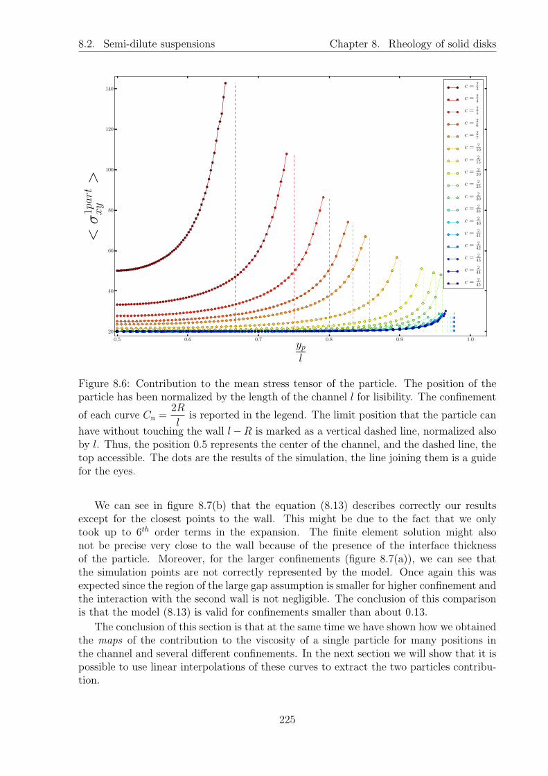
8.2. Semi-dilute suspensions Chapter 8. Rheology of solid disks
0.5 0.6 0.7 0.8 0.9 1.0ypl
20
40
60
80
100
120
140<σ1part
xy
>c = 2
3
c = 24
c = 25
c = 26
c = 27
c = 210
c = 215
c = 220
c = 225
c = 230
c = 236
c = 240
c = 241
c = 242
c = 243
c = 244
c = 245
Figure 8.6: Contribution to the mean stress tensor of the particle. The position of theparticle has been normalized by the length of the channel l for lisibility. The confinement
of each curve Cn =2R
lis reported in the legend. The limit position that the particle can
have without touching the wall l−R is marked as a vertical dashed line, normalized alsoby l. Thus, the position 0.5 represents the center of the channel, and the dashed line, thetop accessible. The dots are the results of the simulation, the line joining them is a guidefor the eyes.
We can see in figure 8.7(b) that the equation (8.13) describes correctly our resultsexcept for the closest points to the wall. This might be due to the fact that we onlytook up to 6th order terms in the expansion. The finite element solution might alsonot be precise very close to the wall because of the presence of the interface thicknessof the particle. Moreover, for the larger confinements (figure 8.7(a)), we can see thatthe simulation points are not correctly represented by the model. Once again this wasexpected since the region of the large gap assumption is smaller for higher confinement andthe interaction with the second wall is not negligible. The conclusion of this comparisonis that the model (8.13) is valid for confinements smaller than about 0.13.
The conclusion of this section is that at the same time we have shown how we obtainedthe maps of the contribution to the viscosity of a single particle for many positions inthe channel and several different confinements. In the next section we will show that it ispossible to use linear interpolations of these curves to extract the two particles contribu-tion.
225

8.2. Semi-dilute suspensions Chapter 8. Rheology of solid disks
0.50 0.55 0.60 0.65 0.70 0.75 0.80 0.85 0.90 0.95ypl
0
50
100
150
200
250
300
<σ1part
xy
>+
off
set
c = 23
c = 24
c = 25
c = 26
c = 27
c = 210
c = 215
c = 220
(a) High confinements: 220 ≤ Cn ≤ 2
3
0.5 0.6 0.7 0.8 0.9 1.0ypl
20
25
30
35
40
45
50
55
<σ1part
xy
>+
off
set
c = 230
c = 236
c = 240
c = 241
c = 242
c = 243
c = 244
c = 245
c = 250
(b) Low confinements: 230 ≤ Cn ≤ 2
50
Figure 8.7: Contribution to the viscosity of a single particle displaced from the centerof a channel. The points are representing the same data as in figure 8.6 except that weadded an offset to separate the curves from each other. The lines represent the values ofequation (8.13) with the same offset, which is the model of a particle near a single wall.For lisibility reasons, the high and low confinements have been split into two differentgraphs.
226

8.2. Semi-dilute suspensions Chapter 8. Rheology of solid disks
In the same time, we explored the behavior of the contribution to the viscosity of a solidcircular particle in presence of walls. We can already extend this work on the viscosityof dilute suspensions. Indeed, for a dilute suspension of particles, the contribution ofeach particle is simply added. Thus, for a suspension of Np similar particles of the samevolume where the position of each one is known, one can express the viscosity of the wholesuspension as:
< σxy >=< σshearxy > +Φ1 part
Np∑
n=1
< σ1 partxy > (yn) (8.14)
where yn is the vertical position of the particle n. For a large number of particles, one candrop the sum to integrate over the length l of the channel and multiply by the probabilitydensity P (y) of finding a particle at the vertical position y. The equation 8.14 becomes:
< σxy > =< σshearxy > +Φ1 part
∫ l−R
R
< σ1 partxy > (y)P (y)Npdy (8.15)
=< σshearxy > +ΦN part
∫ l−R
R
< σ1 partxy > (y)P (y)dy (8.16)
where ΦN part = NpΦ1 part is the volume fraction of all the particles, and we recall the
property of a probability density :
∫ l
0
P (y)dy = 1. With the expression (8.16), we see
clearly the different influences of the distribution of particles and the intrinsic function ofcontribution to the viscosity.
From this formula, we can also extract the minimum and maximum viscosity valuesthat a confined dilute suspension of a given volume fraction can have. Indeed, the min-imum effective viscosity is obtained by a distribution where all the particles are alignedon the center of the channel. The probability density of such configuration is given by
P (y) = δ(y− l
2) where δ is the Dirac function (the real one, not the smoothed δε used in
the level set framework of course). On the contrary, the maximum viscosity is obtainedat the opposite when all the particles are almost touching the wall: P (y) = δ(y − R) orP (y) = δ(y − (l −R)). A common configuration is the random distribution, in this case,there is the same probability to find a particle for any accessible position in the channel.
Such a configuration is given by P (y) =1
l − 2R.
8.2.2 The contribution to the viscosity of the pair interaction
Since we are able to get the contribution of a single vesicle in a confined shear flow, itis also possible to extract the contribution to the viscosity of the pair interaction of twoparticles. It is given by:
< σ2 partxy >=
< σxy > −Φ1 < σ1 partxy > (y1)− Φ2 < σ1 part
xy > (y2)
Φ1Φ2
(8.17)
where y1 and y2 are the positions of the two particles. The contribution of one particle< σ1 part
xy > can be either taken as the interpolation of the curves of the previous studyor recomputed by solving the same system but taking into account only one particle. Wemade the following simulation: for a given confinement, we start a simulation with two
227

8.2. Semi-dilute suspensions Chapter 8. Rheology of solid disks
Figure 8.8: Three remarkable configurations at the points of view of the effective viscosityand their probability densities. The first and last one are respectively the configurationsgiving the lowest and highest effective viscosity. The middle one is the one often consid-ered: a homogeneous suspension. In these schemes, the x direction has been shrunk for abetter representation, but the particles should be separated of at least 5 radii to considerthe suspension as dilute.
particles far away from each other in the x direction. Then, by keeping the y positionof each particle the same, we measure the viscosity of the fluid when approaching thetwo particles. This simulation is repeated for many different y positions and differentconfinements. The two particles are located symmetrically to the center of the channel.Consequently, for a given confinement, the quantity < σ2 part
xy > depends only on ∆x =|x1 − x2| and ∆y = |y1 − y2|. The range in which ∆y varies is 0 < ∆y < l − 2R. Themaximum value given for ∆x is 15R, for ∆x higher than this value, the contributionis small enough to be neglected. The minimum values that ∆x and ∆y can have is 0(particles aligned) or higher if the particles are too close (contact is avoided). The schemeof such a simulation and the corresponding notations are shown in figure 8.9. The resultof the simulation is shown in 2D for the different ∆y in figure 8.11(a) and in 3D forall the (∆x,∆y) in figure 8.11(b). We also reported in figure 8.10 the snapshots of thevalue of σ2 part
xy for three different ∆x showing characteristic behaviors. The 2D plot ofthe contribution is also given in figure 8.12 for a confinement twice greater than the oneof figure 8.11(a).We can see that, as expected, when the distance between the particles is large enough(∼ 10R), the contribution of the pair interaction vanishes. This can be seen graphicallywith the very low values of σ2 part
xy in figure 8.10(a), the plateau on the 3D surface of figure8.11(b) and the systematic 0-value of the curves in 8.11(a) for large ∆x.
It is also interesting to see that on the other hand, when the two particles are on thetop of each other (∆x = 0), the contribution of the pair to the viscosity is negative. Thisis illustrated by the figure 8.10(c), the negative values at (∆x = 0) in figure 8.11(a) andthe negative gradient of the 3D surface.
Finally, we observe a maximum of the contribution to the viscosity for sufficiently
228

8.2. Semi-dilute suspensions Chapter 8. Rheology of solid disks
Figure 8.9: Scheme of the simulation of the two particles interaction in shear flow.
close particles with a certain disposition. This peak can be large and have a great value.It appears when the particles are aligned with an angle of around 45 with respect to thedirection of the flow as we can see in figure 8.10(b).
It is interesting to see how evolve these behaviors for higher confinements. We havereported in figure 8.12 the contribution to the viscosity of a pair of particles in a channelhaving a confinement twice higher than the one of graph 8.11(a). The first obvious thing isthat the high interaction occurring when the particles are close to each other is enhancedby the confinement. But this actually happens only for relatively high ∆y, since, for lower∆y the particles would touch at the same ∆x.
The other important remark to make is that from medium to low ∆x at this confine-ment, almost all the curves are negative on a large domain. Thus, at high confinement,adding a pair of particles at a random place in the box would in general add a negativecontribution to the overall viscosity.
The same simulation has been done for different confinement in the range 0.04 < Cn <0.33. The maps generated are used to compute the viscosity of a semi-dilute suspension.
8.2.3 Extension to the simulation of a semi dilute suspension
We will show that the previous information can be used to compute the viscosity of asemi-dilute suspension of mono-disperse rigid disks. Indeed, for a given random configu-ration of positions, the contribution of each particle to the viscosity can be computed byinterpolating the curves presented in section 8.2.1. Then, for each pair of particles, doinga 2D interpolation of the information presented in section 8.2.2 leads to the second orderterm of the effective viscosity. Two remarks have to be made about the accuracy of themethod. The first one is that higher order interactions are neglected. These interactionscan be dominant for high concentration, thus we limit our study to the semi-dilute case(φ < 0.2).
229

8.2. Semi-dilute suspensions Chapter 8. Rheology of solid disks
(a) The particles are far away and almost do not interact.
(b) The pair interaction is at its maximum when the particles are aligned at around 45 with respect tothe shear direction.
(c) The interaction is at its minimum when the particles are aligned along their y axis (∆x = 0).
Figure 8.10: The value of the field σ2 partxy for a confinement Cn = 0.1 and a given ∆y at
three different ∆x.
The second hypothesis made and which might be a source of error is that we willconsider that for a given confinement, the pair interaction only depends on ∆x and ∆y.Thus we do not take into account the fact that the absolute distance of the pair of particlesto the wall might change its viscosity contribution.
Effect of the confinement on the viscosity of a 2D semi dilute suspension
The processes to compute the viscosity of a suspension of a given confinement at a givenvolume fraction Φ is first to compute the number of particles needed to achieve such avolume fraction:
Npart = int
(ΦlL
πR2
)
(8.18)
where “int” represents the closest integer of the argument. Then Npart coordinates (x, y)are generated randomly in the range ([R,L−R], [R, l−R]). The viscosity of this config-
230

8.2. Semi-dilute suspensions Chapter 8. Rheology of solid disks
0 2 4 6 8 10 12 14
∆x
−0.1
0.0
0.1
0.2
0.3
0.4
0.5
0.6
<σxy>
∆y = 0.0
∆y = 0.4
∆y = 0.8
∆y = 1.2
∆y = 1.6
∆y = 2.0
∆y = 2.4
∆y = 2.8
∆y = 3.2
∆y = 3.6
∆y = 4.0
∆y = 4.4
∆y = 4.8
∆y = 5.2
∆y = 5.6
∆y = 6.0
∆y = 6.4
∆y = 6.8
∆y = 7.2
∆y = 7.6
(a) 2D representation of the simulation of the contribution to the viscosity of apair of particles. For each different ∆y, the quantity < σ2 part
xy > is measured formany ∆x. The curves are represented with an offset to avoid their overlapping. Adashed line represents the value of the offset for each curve. The color representsthe value of ∆y for each curve which are reported in the legend.
∆x
24
68
10
∆y
12
34
56
7
<σxy>
−5
0
5
10
l = 10
(b) The quantity < σ2 partxy > represented in elevation. The bottom plane represents the values
of ∆x and ∆y. The color represent the value of < σ2 partxy >. This quantity has been measured
for every point represented on the 3D surface. The lines between the points are just a guide forthe eyes.
Figure 8.11: The value of < σ2 partxy > represented in 2D and 3D for a confinement of
Cn = 0.2.
231

8.2. Semi-dilute suspensions Chapter 8. Rheology of solid disks
0 2 4 6 8 10 12
∆x
0.0
0.2
0.4
0.6
0.8
1.0
1.2
1.4
<σxy>
∆y = 0.0
∆y = 0.1
∆y = 0.3
∆y = 0.4
∆y = 0.5
∆y = 0.7
∆y = 0.8
∆y = 1.0
∆y = 1.1
∆y = 1.2
∆y = 1.4
∆y = 1.5
∆y = 1.6
∆y = 1.8
∆y = 1.9
∆y = 2.0
∆y = 2.2
∆y = 2.3
∆y = 2.4
∆y = 2.6
Figure 8.12: This figure represents the same graph as in figure 8.11(a), the contributionto the viscosity of a pair of particles, except that it is done for a higher confinement:Cn = 0.4.
uration is computed using the formula:
< σxy >=< σshxy > +Φ1
Npart∑
i=1
< σ1 partxy > (yi)+Φ2
1
Npart−1∑
i=1
Npart∑
j=i+1
< σ2 partxy > (|xi−xj|, |yi−yj|)
(8.19)where the values of < σ1 part
xy > (yi) and < σ2 partxy > (|xi−xj|, |yi− yj|) are extracted from
the data presented in sections 8.2.1 and 8.2.2 thanks to the interpolation tools of scipy[51].
Since each configuration has its own effective viscosity, this process is repeated on agreat number of different configurations. Finally the mean value of all these viscosities istaken as the value for this particular volume fraction and the standard deviation is takenas the error bars.
The result of such simulation is shown in figure 8.13 where three different confinementshave been plotted. They have been fitted with the expression (8.10). The coefficients ofthese fits and some other confinements are shown in figure 8.14.
The figure 8.14 shows a similar behavior as [22] which confirms that the same decreaseof the interaction between the particles for high confinement also occurs in 2D.
Link with the two particle interaction effect
Thanks to the work done in the previous section, we can try to explain qualitatively whatis happening. At low confinement, when a pair of particles is added, if the particles arenot too far from each other, by addition to the linear single particle contributions, theinteraction contribution exists. If we look at the figure 8.11(a), we see that there are large
232
8.2. Semi-dilute suspensions Chapter 8. Rheology of solid disks
areas where this contribution is positive. Moreover, the values where the contributionhas a high negative value are obtained for high ∆y. There are fewer possibility to obtainlarge ∆y than small ones. For example, in the extreme case, to obtain a ∆y of l− 2R theonly possibilities are to have (y1 = R, y2 = l −R) and (y1 = l −R, y2 = R).
Thus, we can say that globally, for this confinement, a pair of particles randomlydisposed will add a positive contribution to the viscosity. Consequently, we expect thesecond order viscosity coefficient viscosity to be positive.
At the opposite, the figure 8.12 shows that for a strong confinement, a randomly chosenpair of particle will add a negative contribution to the linear viscosity. Indeed, thereare large regions where the pair contribution is negative. Moreover these contributionsare more probable since they exist at low ∆y. At the contrary, the areas where thecontribution is positive are happening for large ∆y which have few chances to happen.Consequently, we can say that adding a particle in such a system would add a negativevalue to the second order viscosity, thus one can expect that the second order coefficientviscosity of such a confinement is negative.
Discussion about the method
The drawback of this method is the systematic errors that are added to the problem.Making the maps and extracting their data by interpolation are error prone and thecoefficients obtained from the fits of the simulation of a large number of objects mightnot be very precise.
The whole simulation to obtain the figure 8.14 took only few minutes since we alreadyhad the maps of the single particle and pair contribution. This is one of the advantages ofthis method, since the maps are calculated, the rest of the simulation is done in a reallyshort time.
The other advantage of not simulating directly a large number of particles as solutionof the finite element problem, is that we are able to explain the behavior of a collectionof objects thanks to their individual contributions.
233

8.2. Semi-dilute suspensions Chapter 8. Rheology of solid disks
0.00 0.05 0.10 0.15 0.20
Φ
0.0
0.1
0.2
0.3
0.4
0.5
0.6
0.7
0.8
µ−µ0
µ0
Cn =24, α = 4.2, β = −2.1
Cn =28, α = 2.7, β = 2.8
Cn =225, α = 2.2, β = 3.1
Figure 8.13: Reduced viscosity of a suspension for different volume fraction and differentconfinement. The points are the mean of 200 different configuration viscosities. Theerror bar are the standard deviation of the set of viscosities. The lines are the fits ofthese curves with a second order polynomial as given in equation (8.10). The coefficientsobtained from the fit are given in the legend.
0.1 0.2 0.3 0.4 0.5
Cn
−2
−1
0
1
2
3
4
5
α,β
α
β
Figure 8.14: The coefficients of the fit of the viscosity curves as the one given in figure 8.13for different confinement. The values of the α coefficient are represented as red squareswhereas the β values are blue triangles. One can see that the α coefficient convergestoward the Einstein’s value for smaller confinement. The β factor decreases for strongerconfinement and even becomes negative.
234

Chapter 9
Conclusion and perspectives
235

Chapter 9. Conclusion and perspectives
Francais
Dans cette these, nous avons presente un cadre methodologique et numerique de simu-lation d’objets rigides et deformables sous ecoulement. Notre approche est totalementEulerienne et est basee sur la methode de level set. Nous avons ensuite utilise ce cadrepour explorer des problemes ouverts de mecanique des fluides.
Premiere Partie
La premiere partie de cette these a ete consacree a l’expose des methodes mathematiqueschoisies et a leur validation et verification. Nous avons commence par exposer la methodedes level set et les choix que nous avons fait la concernant. En particulier, nous avonsexpose les methodes de stabilisations utilisees pour son transport, et les methodes dereinitialisation implementees. Pour chacune de ces methodes, nous avons precise si ellessont applicables pour des calculs paralleles, en deux comme en trois dimensions, et si untraitement special etait necessaire pour qu’elle soit aussi valable avec une discretisationspatiale d’ordre elevee. Nous avons ensuite verifie ces methodes sur des cas tests.
Nous avons ensuite decrit notre strategie pour la simulation d’un systeme multi-fluides,qui est la brique de base de la simulation d’une suspension de globules rouges. Le systemeclassique bi-fluides a ete decrit et verifie sur un cas test. Puis nous avons presente notremethode pour passer d’un systeme bi-fluides a un systeme contenant un nombre arbi-traire de fluides. Nous avons montre un exemple d’un tel systeme avec la simulations dela montee de huit bulles de fluides differents dans un neuvieme fluide.
Nous avons aussi utilise cette methode de calcul pour montrer que les oscillationsd’une bulle autour de sa forme d’equilibre ne dependent pas du confinement auquel elleest soumise. Ce resultat a aussi une valeur de validation puisque nous sommes capablede retrouver la frequence d’oscillations theorique d’une bulle avec une bonne precision.
Nous avons ensuite montre que notre methode de simulation a deux fluides pouvaitetre utilisee pour simuler l’ecoulement d’objets rigides dans un fluide. Nous avons fait lelien entre cette methode de simulation et des methodes deja existantes dans la litterature.Nous avons enfin discute de l’interet et des inconvenients d’utiliser une methode de levelset pour ce genre de simulation.
La fin de notre premiere partie est consacree a la simulation de vesicules. Nousavons presente deux methodes differentes pour calculer la force de courbure appliqueeaux vesicules qui depend de la derivee seconde de la courbure de la membrane. Les avan-tages et inconvenients de ces methodes ont aussi ete discutes.
Nous avons aussi teste deux methodes tirees de la litterature pour appliquer la con-trainte d’inextensibilite de la membrane des vesicules. Une methode basee sur la penalisationde l’etirement de la membrane par l’intermediaire d’une force elastique, l’autre utilise unmultiplicateur de Lagrange forcant la contrainte voulue. Nous avons ensuite montre unevalidation de ces methodes sur des comportements connus de vesicules et avons conclusque la methode utilisant le multiplicateur de Lagrange est bien plus stable que la methode
236

Chapter 9. Conclusion and perspectives
de penalisation. Bien qu’elle necessite un developpement numerique plus complexe, nousutiliserons la methode du multiplicateur de Lagrange dans le futur pour nos simulations.
Futurs developpements methodologiques
Dans le futur, certains aspects methodologiques pourraient etre explores en prenantcomme base le travail effectue durant cette these. Il serait par exemple interessant dedevelopper un cadre de methodes de stabilisation a l’ordre eleve. Une telle adaptation adeja ete faite pour la stabilisation des faces internes (CIP), neanmoins elle reste inconnuepour la stabilisation des elements (SUPG, SGS, GLS).
Sauf indication contraire, toutes les methodes que nous avons presente sont utilisableen deux et trois dimensions. La librairie Feel++ a ete concue de telle sorte qu’un codesoit aussi valable en deux et trois dimensions grace a la meta-programmation. La plupartdes tests presentes dans cette these sont donc deja prets a fonctionner en 3 dimensions.Neanmoins, les simulations 3D sont peu nombreuses dans ce travail. Bien que les codessoient valable en 3D, la simulation d’objets 3D necessite de passer a un grand nombre dedegres de liberte. Elle necessite aussi la parallelisation des codes de calculs ainsi que le ra-patriement des donnees depuis le cluster de calcul sur lequel elles ont ete obtenues et enfinle traitement du grand nombre de donnees ainsi generees. Tous ces elements necessitantun certain temps de developpement, ils ne sont pas tous operationnels aujourd’hui maisle seront dans un futur tres proche.
Enfin, durant cette these, seul les cas de suspensions diluees ou semi-diluees ont etetraites. Dans le futur, une extension a des suspensions concentrees pourrait etre envisagee.Il se poserait alors le probleme de la gestion des contacts entre les vesicules.
En theorie, les forces hydrodynamiques dues au fluide se trouvant entre deux vesiculesdevrait eviter leur contact. Cet effet a ete suffisant pour eviter le contact entre les vesiculespour toutes les concentrations que nous avons teste jusqu’a present (jusqu’a une fractionvolumique de 25%). En pratique, cela necessite de toujours avoir un certain nombre depoints de discretisation entre deux membranes. Il est possible que pour des suspensionsde vesicules tres concentrees, la force hydrodynamique ne soit plus suffisante pour eviterle contact faute d’un nombre suffisant de points de discretisation entre les vesicules. Dansce cas, plusieurs strategies pourraient etre imaginees.Une methode de raffinement de maillage pourrait etre utilisee pour s’assurer qu’il y aittoujours assez d’elements entre deux membranes. Un pas de temps adaptatif pourraitalors etre mis en place pour garder une coherence entre les discretisations spatiale ettemporelle.Une force de contact dependant de la distance a l’interface la plus proche pourrait aussietre developpee. Une telle force est assez simple a implementer dans le cas d’interfacesetant suivies par des champs de level set differents.Neanmoins, il n’est pas trivial de trouver l’expression d’une force de contact pour desinterfaces suivies par le meme champ de level set. Ces questions pourraient faire le sujetde futurs travaux.
237

Chapter 9. Conclusion and perspectives
Deuxieme partie
Les developpements numeriques apportes durant cette these s’inscrivent dans le projet in-teractions fluide structure de la librairie Feel++ dediee a la resolution d’equations auxderivees partielles. Ainsi certains codes developpes dans le cadre de cette these pourraientetre utiles dans d’autres contextes. Nous avons donc essaye de separer un maximum lessolutions apportees aux differents problemes de facon a pouvoir les reutiliser et les faireevoluer dans le futur. La programmation orientee objet ayant ete en grande partie inventeedans ce but, differentes classes ont ete crees et seront incluses dans la partie publique deFeel++ dans le futur.
Ainsi, le debut de notre seconde partie a ete consacre a la description des classespouvant etre integrees a Feel++ dans le futur et utilisees dans different contextes desimulation.
La premiere de ces classes, propose un cadre pour creer different operateurs de pro-jections necessitant la solution d’une equation aux derivees partielles (projection L2, H1,etc ...). Elle propose aussi la possibilite de deriver une expression mathematiques de faconefficace.
La deuxieme classe, propose de resoudre l’equation d’advection utilisee par la methodesdes level set dans deux contextes differents (transport de la fonction et reinitialisation).Cette classe inclue toutes les methodes de stabilisation decrites en premiere partie.
La troisieme classe presentee est la classe LevelSet , qui contient tous les developpementsnumeriques necessaires a la mise en place d’une methode de level set.
Enfin, la derniere classe est une generalisation de la precedente, elle propose de mu-tualiser certains elements de la classe LevelSet pour proposer une classe multi levelsetcapable de gerer efficacement plusieurs champs de level set a la fois.
La fin de notre seconde partie est consacree a la presentation de developpements creespour les applications liees a cette these et qui ne sont pas directement applicable a d’autrescontextes.
Nous avons ainsi presente les details de la construction du multiplicateur de Lagrangeassocie a la contrainte d’inextensibilite de la membrane. Puis nous avons decrit l’interfacePython que nous avons developpe pour lancer un grand nombre de simulation assez facile-ment.
Troisieme Partie
La derniere partie de cette these est consacree au comportement de disques rigides dansdes geometries complexes et a leur rheologie. Les problemes etudies dans cette parties’inscrivent dans la thematique d’etude de l’equipe Dynamique des fluides complexes ausein de laquelle a ete preparee cette these.
Le premier probleme auquel cette partie est dediee est l’etude du comportement d’unesuspension diluee de particules rigides lorsqu’elle atteint une bifurcation micro-fluidique.L’hypothese de faible concentration de particule nous a conduit a ne considerer qu’uneparticule a la fois dans le systeme etudie. Nous avons explore un grand nombre detrajectoires possibles pour les particules en fonction de divers parametres (rayons, rapportde debits dans les branches ...). Enfin, en comparant nos resultats avec des experiencesrealisees dans notre laboratoire, nous avons pu expliquer l’effet connu d’accroissement de
238

Chapter 9. Conclusion and perspectives
la concentration de particule dans la branche recevant le plus grand debit. De plus, nousavons mis a jour l’existence d’une force hydrodynamique inconnue jusqu’alors poussant lesparticules vers la branche de bas debit et entrant en concurrence avec l’effet precedemmentmentionne.
Enfin, nous avons etendu cette methode a la simulation d’une suspension de vesiculesdans une bifurcation. Nous avons aussi montre qu’il etait possible d’effectuer la simula-tion d’une suspension de deux types de vesicules different, c’est a dire ayant des rapportsde viscosite ou des forces de courbure differents.
Dans le futur, un grand nombre de questions peuvent encore etre posees a propos deces systemes. Des simulations de bifurcations dans lesquels deux particules sont presentesont ete menees depuis notre travail [80]. Il serait maintenant interessant de voir commentla concentration en particules dans la branche de depart influe sur la repartition dans lesbranches d’arrivee.
L’influence de la deformabilite des particules sur la repartition dans les differentesbranches est aussi une suite logique a ce travail. Finalement, des simulations de suspen-sions dans lesquels quelques vesicules se comportent comme de longues particules quasi-rigide pourraient etre menee et representeraient une avancee dans la comprehension demaladies telles que la drepanocytose dans laquelle un certain nombre de globules rougesse rigidifient et genent la circulation sanguine lors du passage dans de petits vaisseaux.
La fin de cette troisieme partie a ete consacree a la rheologie d’une suspension dedisques rigides dans un ecoulement de cisaillement confine. De precedents travaux ontmontres que lorsqu’une suspension de particules rigides est suffisamment confinee, l’effetde l’interaction entre les particules sur la viscosite effective de la suspension diminuegrandement. Ces resultats on ete obtenus en trois dimensions. Un des objectifs de cetravail etait de verifier si cet effet etait un effet purement 3D ou si il etait aussi present endeux dimensions. Pour cela nous nous sommes d’abord interesses a la viscosite effectived’une suspension diluee confinee, ce qui nous a permis de mettre en evidence l’influencede la position d’une particule par rapport au bord du domaine cisaille.
Puis, nous avons explore la viscosite d’un systeme de deux particules dans un ecoulementde cisaillement confine. En combinant les deux differentes etudes, nous avons pu montrerque l’effet connus a 3D etait aussi present en 2D bien que les phenomenes soient quanti-tativement differents.
Ce genre d’etude pourrait aussi etre generalisee a une suspension de vesicules. Ainsi,l’influence de la deformabilite sur la viscosite effective d’une vesicule proche d’une paroispourrait etre etudiee. Il est connu que les vesicules ont une tendance a migrer vers le centredu canal dans lequel elles evoluent. Connaıtre la dependance de la viscosite effective parrapport a la position des vesicules dans le canal pourrait alors faire un lien entre lesphenomenes de migration et la viscosite effective.
239

Chapter 9. Conclusion and perspectives
English
In this thesis, we have presented a numerical and methodological framework for the sim-ulation of rigid and deformable objects in flow. Our approach is totally Eulerian and isbased on the level set method. We then used this framework to explore open problems influid mechanics.
Part I
The first part of this thesis was dedicated to the overview of the mathematical methodschosen and their validation and verification. We explained the level set method and thechoices that we made for it. Indeed, we have explained the stabilization methods used forits transport, and the implemented reinitialization methods. For each of these methods,we made precise if they are directly applicable to parallel computation, in 2 or 3 dimen-sions, and, if a special treatment is needed for high order polynomial approximation. Wethen verified these methods on test cases.
We then described our strategy concerning the simulation of a multi-fluid flow, whichis the building block for the simulation of a red blood cell suspension. The classical two-fluid system has been described and verified on a test case. After what, we presented ourmethod to adapt the two-fluid system to a system with an arbitrary number of fluids. Wehave shown an example of such a system with the simulation 8 rising bubbles of differentfluids in a 9th fluid.
We have used the two-fluid flow framework to show that the oscillations of a bubblearound its equilibrium shape are not dependent on its confinement. This result has alsoa validation value since we are able to recover the theoretical oscillation frequency of thebubbles with a good accuracy.
Next, we have shown that our two-fluid flow simulation method can be used to sim-ulate rigid object flows. We made a link between this simulation method and alreadyexisting ones. Finally, we discussed the advantages and drawbacks of using the level setmethod for this kind of simulations.
The end of our first part was dedicated to the simulation of vesicles. We have pre-sented two different methods to compute the curvature force applied on the membraneof the vesicles. This force is complex since it requires the second derivative of the cur-vature of the membrane. We discussed the advantages and drawbacks of the two methods.
We also tested two methods taken from the literature to apply the inextensibility con-straint on the membrane. One of them penalizes the stretching by using an elastic force,while the other one requires use of a Lagrange multiplier to enforce the constraint. Wethen showed a validation of these methods on known behaviors of vesicles and concludedthat the method using the Lagrange multiplier is more stable than the penalty one. Al-though it necessitates a more complex numerical development, we will use the Lagrangemultiplier method in the future for our vesicles simulations.
240

Chapter 9. Conclusion and perspectives
Future methodological developments
In the future, some methodological aspects could be explored taking this work as a basis.It would be interesting for example to develop a high order stabilization framework. Suchadaptation has already been made for the internal faces stabilization (CIP), but it is stillunknown for the elements stabilization (SGS, SUPG, GLS).
Unless we specifically mentioned it, all the methods that we presented are valid in 2and 3 dimensions. The Feel++ library has been made so that the same code is valid in2 and 3 dimensions thanks to the meta-programming concept. Most of the tests presentedin this thesis are then ready to work in 3D. Nevertheless, 3D simulations are very rarein this work. Although the codes are valid in 3D, the simulation of 3D object necessi-tates a large number of degrees of freedom. It also necessitates making the code work inparallel as well as the downloading and treatment of the data from the cluster on whichthe simulations are made. All these features are time consuming to prepare and are notall operational to this date but they will be in a near future and the 3D versions of oursimulations will be made.
Finally, during this thesis, only dilute or semi-dilute suspensions have been studied. Inthe future, an extension to more concentrated suspensions could be made. The problemof handling the contacts between the vesicles would arise.
Theoretically, the hydrodynamical forces due to the fluid being in between the vesiclesshould be sufficient to avoid their contact. This effect has been strong enough to avoidcontact in every concentration we have tested (until a volume fraction of 25%). In practice,it necessitates always having several discretization points between two membranes. It ispossible that for highly concentrated vesicles, the hydrodynamical force is not sufficientto avoid contact because of a lack of discretization points between two interfaces. In thiscase, several strategies could be used.A mesh refinement method could be used to be sure that there are always enough elementsbetween the membranes. An adaptive time step could also be set to keep coherent thespatial and temporal discretizations.A contact force depending on the distance to the closest interface could also be developed.Such a force is simple to implement in the case of interfaces tracked by different level setfields.Nevertheless, it is non-trivial to find an expression of this force for interfaces tracked bythe same level set field. These questions could be the subject of future works.
Part II
The numerical developments made in this thesis take place in the Feel++ fluid structureinteraction project of the library. Consequently, several codes developed for this thesispurpose could be used in other contexts. Thus, we tried to separate the solutions thatwe made to the different problems in order to re-use them and make them evolve in thefuture. The object oriented programming paradigm being created to this goal, differentclasses have been made and will be included in the public part of Feel++ in the future.
In this way, the beginning of our second part has been dedicated to the descriptionof the classes which can be integrated in Feel++ in the future and used in other context.
241

Chapter 9. Conclusion and perspectives
The first of these classes proposes a framework to create different projection operatorwhich necessitate to solve a partial differential equation (L2 or H1 projections ...).The second one proposes solving the advection equation used by the level set method intwo different contexts (transport and reinitialization). This class includes all the stabi-lization methods described in the first part.The third class presented is the LevelSet class. It contains all the numerical develop-ments necessary to setting up of a level set method.
Finally, the last class is a generalization of the previous one. It proposes to share severalelements of the level set class to make a multi-level set class able to handle efficiently manylevel set fields at the same time.
The end of this second part, was dedicated to the developments made to create appli-cations linked to this thesis by which are not directly applicable to other contexts.
We presented the details of the construction of the Lagrange multiplier associated tothe inextensibility constraint. Then we described the Python interface that we developedto run easily a large number of simulations.
Part III
The last part of this thesis was dedicated to the behavior of rigid disks in complex ge-ometries and their rheology. The problems studied in this part take place in the field ofthe studies of the Dynamics of Complex Fluids team in which this thesis has been done.
The first problem addressed in this part was the study of the behavior of a dilutesuspension of particles when it reached a bifurcation. The low concentration hypothesisled us to only consider one particle in the system. We studied a large number of possibletrajectories for the particles as a function of the different parameters (radius, flow rateratio ...). Finally, by combining our results to experimental ones, we have explained theknown effect of the increasing concentration of particles in the high flow rate branch.Moreover, we have discovered a hydrodynamic force pushing the particles toward theother branch balancing the first effect.
Finally, we have shown that our simulation framework was adapted to the simulationof a suspension of vesicles in a bifurcation. We also have shown that it is possible to useit for the simulation of a suspension having two types of different vesicles, that is to sayhaving different viscosity ratio or curvature force intensities.
In the future, a large number of questions can be addressed. Simulations in which twoparticles are present have been made since our work [80]. It would be interesting to seehow the concentration of the suspension in the inlet branch changes the repartition in theoutlet branches.
The influence of the deformability of the particles on the concentration in the differ-ent branches could also be a relevant continuation of this work. Finally, simulations ofsuspension in which several vesicles behave as long rigid particles could be done. Thiswould represent a step ahead in the understanding of diseases like drepanocitosis for whichfew red blood cells are getting rigid which hindrances the blood flow in circulatory system.
242

Chapter 9. Conclusion and perspectives
The end of this third part was dedicated to the rheology of a suspension of rigid disksin a confined shear flow. Previous works have shown that when a suspension of particles issufficiently confined, the interaction effect between the particles is lowered. These resultshave been obtained in 3D. One of the objectives of this work was to check if this effectis purely 3D or if it is also present in 2D. To this goal, we first addressed the problem ofthe effective viscosity of a a dilute suspension, which allowed us to show the importanceof the position of the particle relatively to the walls of the domain.
Then we explored the viscosity of a system of two particles in a confined shear flow.By combining the two studies, we were able to show that the known 3D effect was indeedpresent in 2D even if the results are quantitatively different.
This kind of study could also be generalized to a vesicle suspension. This way, theinfluence of the deformability on the effective viscosity of a vesicle near a wall could bestudied. The vesicles having the property to lift toward the center of the channel, oneunderstands the interest to study the influence of the distance to the wall on the viscosity.
243

Chapter 9. Conclusion and perspectives
244

Appendices
245

A. Stokes variational formulation Chapter 9. Conclusion and perspectives
A Stokes variational formulation
Let us prove that:
∫
Ω
−(∇ ·σ) ·v =
∫
Ω
2µD(u) : D(v)−∫
Ω
p∇ ·v −∫
∂Ω
(σn) ·v (1)
First of all, let us integrate by part the first term and develop σ following the Newtonianfluid law:
∫
Ω
−(∇ ·σ) ·v
=
∫
Ω
σ : ∇v −∫
∂Ω
(σn) ·v
=
∫
Ω
2µD(u) : ∇v −∫
Ω
p∇ · v −∫
∂Ω
(σn) ·v
Now let us remark that D(u) is a symmetrical, thus when taking the contracted productwith ∇v, the same results can be obtained if we invert the anti-symmetrical part of ∇v
(i.e taking t(∇v), we have then:
D(u) : ∇v = D(u) :t (∇v)
Thus we can write:
D(u) : ∇v
=D(u) : ∇v
2+
D(u) :t (∇v)
2
=D(u) : 2D(v)
2= D(u) : D(v)
Thus, by replacing this expression we get:
∫
Ω
−∇ ·σ ·v =
∫
Ω
2µD(u) : D(v)−∫
Ω
p∇ ·v −∫
∂Ω
(σn) ·v
247

B. Finding the axes of an ellipse Chapter 9. Conclusion and perspectives
B Finding the axes of an ellipse
We will show in this appendix how to find easily the minor and major axes (a, b) of anellipse for a given reduced area (α) and a fixed area A. The problem could be modifiedto find these parameters for a fixed perimeter P . Let us recall that the area of an ellipseis given by:
A = π a b.
The perimeter of an ellipse does not have a simple exact analytic expression but a goodapproximation is given by the Srinivasa Ramanujan formula:
P ≈ π(
3 (a+ b)−√
(3 a+ b)(a+ 3 b))
.
We recall that the reduced area is given by the ratio between the area of the ellipse andthe area of a circle having the same perimeter:
α =4πA
P 2.
The problem is to find (a, b) for a given A = A0 and α = α0. Thus it can be re-writtenas, for a given (A0, α0), find (a, b) so that:
π a b− A0 = 0
π(
3 (a+ b)−√
(3 a+ b)(a+ 3 b))
−√
4 π A0
α0
= 0.
The problem is of the form F (U ) = 0, with U = (a, b). It can be solved by the NewtonKrylov non linear solver of scipy [51] that we use as a black box. We give as initialguess of the solution the radius of a circle having the area A0 plus and minus an epsilon:
U0 =
(√
A0
π+ ε,
√
A0
π− ε)
. With this guess, the non linear solver always converges in
the range of α0 and A0 we are looking at. An example of such code, searching for theparameters (a, b) for a list of different α0 is given in listing 1.
Listing 1: Finding minor and major axes of an ellipse given the area and reduced areafrom pylab import ∗from s c ipy . opt imize import newton krylov as nk
# define equations on perimeter P (a, b), area A(a, b) and the residual F (a, b)P = lambda a , b : p i ∗ (3∗ ( a+b)− s q r t ( (3∗ a+b )∗ ( a+3∗b ) ) ) − s q r t (4∗ pi ∗A0/alpha )A = lambda a , b : p i ∗ a ∗ b − A0F = lambda x : ( P(x [ 0 ] , x [ 1 ] ) , A(x [ 0 ] , x [ 1 ] ) )
# define the fixed values of A0 and a list of different α0A0 = 1 .a l p h a l i s t = 1 . , 0 . 95 , 0 . 9 , 0 . 85 , 0 . 8 , 0 . 75 , 0 . 6 , 0 . 5 , 0 . 4
# initial guessX0 = sq r t (A0/ p i )+0.2 , s q r t (A0/ p i )−0.2
for alpha in a l p h a l i s t :a , b = nk (F , X0)print ” alpha = %f , a=%f , b=%f ”%(alpha , a , b )
248

C. Distance to parametrized curve Chapter 9. Conclusion and perspectives
C Create a distance function to a parametrized curve
The level set field φ has to be initialized to a value on all the domain: φ0. This value hasto be a signed distance function or a function close to that. Indeed, if the reinitializa-tion method used for the application is the reinitialization by solving a Hamilton Jacobiequation as presented in section 1.3.3, the method converges only if the initial function isnot too far from the solution. In the case of a reinitialization by fast marching method aspresented in section 1.3.4, φ0 has to be a distance function in the first elements crossed bythe iso 0 of φ0. There are only few cases where the distance function to a curve is knownanalytically. For example, the distance function to a single line, or to a circle. A functionclose to a signed distance function to an ellipse is given by equation (1.32). Some shapescan be constructed by a combination of min and max function of the previous curves andthus, a distance function to these curves is known. It is the case for example of the slotteddisk used in section 1.4 which is a combination of a signed distance to a circle and threesigned distances to lines. For more complicated shapes, it is not possible to have a signeddistance function. However, it might be useful to be able to describe more shapes thancircles or lines and one might want to have directly the distance function to an ellipseand do not need to reinitialize it even before the first advection. Thus, we created a toolwhich provides a signed distance function to a parametrized curve. Parametrized curveis one of the better way to describe analytically a shape. We will present in this section,the method and the algorithm used to create such a distance function. Finally we willshow how to use this method which is included in the level set framework and show someexamples.
The method
The idea is to create a starter state for the fast marching method. That is to say, tohave a distance function φ0 to a parametrized curve only in the first elements crossedby the curve. Then, all the other elements are initialized by using the fast marchingmethod presented in section 1.3.4. A brief explanation of the principle of the method isthe following: we discretized the parametrized curve into a set of points. For each point,we locate the element to which it belongs, we store this information and we mark thiselement. Then, for all the degrees of freedom of all the marked elements (all the elementscontaining points), we compute the distance between the degree of freedom position andeach point contained in this element. If the closest distance computed is smaller than theabsolute value of φ0 at this degree of freedom, φ0 takes this value. The sign is determinedthanks to the direction of the parametrized curve. Let us show into details how such amethod is implemented.To simplify, we will assume that we are in 2D even if the method can be extended to 3D.The curve is given by a parametrization s(θ) = (x(θ), y(θ)). We assume that the user ofthe method provides the functions x(θ) and y(θ), the parametrized equations for the xand y positions of a point of the curve. The curve s has to be a closed curve. The user alsoprovides the range in which is defined the parameter θ ∈ [θmin, θmax] and a discretizationstep dθ which will be used to discretize s(θ). Indeed, the first step of the method consistson creating a discretization of the curve s(θ). A set of points pi is computed. It is adiscretization of s defined as pi = (x(θi), y(θi)) for all θi ∈ [θmin, θmax] being multiple ofdθ. For each point pi, we locate the element on the mesh to which it belongs. The global
249

C. Distance to parametrized curve Chapter 9. Conclusion and perspectives
index of the element (called id) is a way to differentiate and access each element of themesh. Thus, for each point pi, we search for the id of the element in which it is lying.We store all these information in a map for which the keys are the ids of the elements andthe value are vectors containing all the (θi,pi) present in the element id. Let us call thismap map points at index. We also mark all the elements which contain at least one pointin order to be able to iterate on it. A scheme of the mesh and the discretized curve isgiven in section 1(a) and the associated map is given in figure 1(b). Then, starts the most
1
2
3
4
56
7
8
9
10
11
12
13
14
15
16
17
18
19
20
23
4
5
6
7
8
9
10
1112
13141516
17
18
19
20
21
22
2324
25
1
(a) Scheme of the first step of the discretization ofthe parametrized curve. The indexes of the ele-ments are represented in black. The parametrizedcurve is a circle and its discretization points arerepresented in red. The value of the parameter θ isgiven below the discretization points. We assumedθ = 1. We represented in gray the marked ele-ments, that is to say, the elements in which at leastone discretization point is present.
17
19
6
23
15
15
16
16
17
18
18
20
21
22
7
24
25
8
1
11
7
12
8
9
10
13
11
12
14
13
14
9
2
3
4
10
5
6
(b) Representation of the mapmap points at index.Each element of the map is composed of a key anda value. The key is the index (id) of the consideredelement. The value is a vector of pairs (θi,pi), thevalue of the parameter and the coordinates of theconsidered point. Thanks to this map, all the infor-mation concerning the discretization points whichbelong to an element are easily accessible.
Figure 1: First step of the creation of a distance function to a parametrized curve.
computationally costly part. For all the degrees of freedom of all the marked elements(all the elements crossed by the interface), we compute the distance between the positionof the degree of freedom (let us call these points pdof
j ) and all the points pi contained inthis element (they can be accessed easily via the map map points at index. We search forthe point pi having the smallest distance to pdof
j , we call it pmin. If the distance to pmin
is smaller than the value of φ0 at this degree of freedom (called φdof0 ), then φdof
0 takes thisvalue. The sign of φdof
0 is given by the vectorial product of the vector v = pmin − pdofj
and the normal to the curve ns at the point pmin. That is to say, Sgn(φdof0 ) = Sgn(v×ns)
The normal to the curve at the point pmin is given by the difference between pmin and theposition of the next point on the curve. In other words, if pmin corresponds to a valueof the parameter θ = θpmin
, that is to say pmin = p(θpmin) then the vector ns is given by:
ns = p(θpmin+ dθ)− p(θpmin
). An example of these vectors is given in figure 2 for a givenelement. This whole algorithm gives a good approximation of a distance function to theparametrized curve s on the elements crossed by it. Then this function can be given tothe fast marching algorithm which makes a distance function on all the domain from it.The method as we presented it is valid also at high order. But in the case of an high orderapproximation, making a loop on all the degrees of freedom of all the elements crossed bythe curve can be computationally costly. We also recall that even at high order, the fast
250

C. Distance to parametrized curve Chapter 9. Conclusion and perspectives
1 2
3
Figure 2: Representation of the second part of the algorithm. One element in representedand the considered degree of freedom is the number 3. Its coordinates are given by pdof
3 .The curve is represented in red dotted line, and its discretization points in this elementare represented as the three red squares. In this scheme, one has |pdof
3 −p3| < |pdof3 −p4| <
|pdof3 −p2|. Thus pdof
3 = pmin. The approximation of the normal ns = p4−p3 is representedin blue. The vector v = pdof
3 − pmin is represented in green. One sees that the vectorv × ns is pointing toward the z positive.
marching method requires the field being reinitialized to be in a P1 space as explained insection 1.3.4. In practice, it is better to use the algorithm 7 directly in the same P1 spacethan the one used for the fast marching. It increases a bit the number of elements crossedby the curve, but decreases the number of degree of freedom to iterate in each element.It is usually benefit in term of computational cost to do it in this order.
Example of use
The previous algorithm has been embedded in the LevelSet class. To use it, one simplyhas to call the method makeDistFieldFromParametrizedCurve of the LevelSet class.We will show a simple example of use of this method. Let us say that we want a distancefunction to an 1epitrochoid. The shape of the latter can be defined thanks to the followingparametrization :
x(θ) = (1 + a) cos(a θ)− a b cos((1 + a) θ) + x0
y(θ) = (1 + a) sin(a θ)− a b sin((1 + a) θ) + y0
where θ is the parameter, a and b are parameters used to change the shape and thenumber of branches of the epitrochoid, finally x0 and y0 define the center of the shape.If we have defined a mesh and a level set object, we simply need to define the previousfunctions and start the algorithm. The function x(θ) and y(θ) are given as argumentto makeDistFieldFromParametrizedCurve. Their types are 2std::function which is afeature present in the standard C++11. The functions have to take one double argumentas entry (θ) and returns one double. A very convenient way to define these functions isto use another C++11 feature, the 3lambda functions which allow to create a function
1http://en.wikipedia.org/wiki/Epitrochoid2http://en.cppreference.com/w/cpp/utility/functional/function3http://en.cppreference.com/w/cpp/language/lambda
251

C. Distance to parametrized curve Chapter 9. Conclusion and perspectives
Algorithm 7 Algorithm making a distance function to a parametrized curve in theelements crossed by the curve.
Require: θmin, θmax, dθ, x(θ), y(θ) givenRequire: φ0(x) = HugeValuefor θi = θmin to θmax doid= index of element containing point(pi = x(θi), y(θi))if map points at index contains key id thenadd pi to map points at index at key id
elsecreate key id in map points at index and add the value pi
end ifcreate key θi in map point param with the value pi
mark the element idend forfor id i in (ids of all marked elements) dofor dofj in dof(id i) dopdofj = position of dofj
minDistToDof = HugeValuefor pk in (all points in map points at index at index id i ) dodistToDof = compute distance(pk, p
dofj )
if distToDof < minDistToDof thenminDistToDof = distToDofpmin = pk
end ifend forif minDistToDof < |φdof
0 | thenns =map point param(θ + dθ)− pmin
v = pdofj − pmin
φdof0 = Sgn(v × ns) minDistToDof
end ifend for
end for
252

C. Distance to parametrized curve Chapter 9. Conclusion and perspectives
embedded in another function in a very simple way. The code 2 shows on the example ofthe epitrochoid how to define these functions and use them as initial level set field.
Listing 2: Example showing how to define the functions x(θ), y(θ) and create a distancefunction from a parametrized curve using the algorithm present in LevelSet .
double a=0.1 , b=0.8 ;double x0=5, y0=5;double t min=0, t max=20∗pi , dt =0.0001;
auto x = [& ] (double t ) return (1+a ) ∗ cos ( a∗ t ) − a∗b ∗ cos ( (1+a ) ∗ t ) + x0 ; ;auto y = [& ] (double t ) return (1+a ) ∗ s i n ( a∗ t ) − a∗b ∗ s i n ( (1+a ) ∗ t ) + y0 ; ;
auto phio = l e v e l s e t−>makeDistFieldFromParametrizedCurve (x , y , t min , t max , dt ) ;
The resulting field is shown in figure 3(a). We also show in figure 3(b) the result ofthe parametrization of an ellipse having a relatively big eccentricity, for which our usualapproximation equation (1.32) is far from a distance function. One can see that in bothcases, the gradient magnitude is around 1 almost every where and that the shape is welldefined.
(a) Distance function from a epitrochoid with 10branches.
(b) Distance function from an ellipse with a rela-tively big eccentricity.
Figure 3: Distance function from parametrized curves. The iso 0 is represented in green,some iso lines are represented in white and the color represents the gradient magnitude|∇φ0|.
253

D. Simulation of rigid disk by direct method Chapter 9. Conclusion and perspectives
D Simulation of rigid disk by direct method
We present in this appendix a toy code which simulates the flow of a rigid disk in a2D Stokes fluid by a direct method. The equations solved are the Stokes equations, theparticle is seen as a hole in the mesh as shown in figure 4. There are no slip boundary
Figure 4: Mesh of a bifurcation in the case of a direct method for the simulation of asolid particle. One can see that the mesh is conform to the particle. The density oftriangles around the particle can be increased to have a better accuracy when computingthe hydrodynamical forces exerted on it.
conditions between the particle and the fluid and between the fluid and the walls. Thegeometry is the bifurcation studied in chapter 7. At each time step, the stokes equationis solved, the forces and torque are computed on the boundary of the particle. Then,the position and velocity of the particle are updated. Finally the domain is re-meshedaccording to the new position of the particle. Since the Stokes equations are independentof time, there is no need to project the solution of the previous step on the mesh ofthe current step. The Stokes equations are solved by finite element method using thevariational formulation (2.14) where the null mean pressure is imposed by a penaltyterm. The finite element software chosen to solve this problem is FreeFem++ whichis a Domain Specific Language dedicated for the solutions of PDE, that is to say thatthe software has its own language (with a syntax close to the one of C++). The useof FreeFem++ for this particular application is made because it integrates a meshgenerator. Thus re-meshing the domain at each time step is very simple at the user point
254

D. Simulation of rigid disk by direct method Chapter 9. Conclusion and perspectives
of view. The update of the velocities and positions of the particle is made by a simpleexplicit Euler integration which is first order. This is one of the limitation of this method.A very small time step has to be taken to keep the system stable. And since the remeshing is time costly this method might not be adapted for long time simulations. Forthe case of the bifurcation problem, we finally chose a fictitious domain method. However,it is interesting to see how simple can be the implementation of such method if the PDEand meshing tools are provided.
Listing 3: Direct method for the simulation of a rigid disk with FreeFem++
// pressure penalty parameterreal ep s i l o n =0.0000001;// viscosityreal nu=666.67 ;// radius of the particlereal R=1.2 ;// mass of the particlereal M=10 ;// intertial momentum of a diskreal I = M∗0 .5∗Rˆ2 ;
string FileName=”Forces ” ;
// time parametersreal dt =0.0003;real f ina lTime = 3 ;
// mesh parametersint n=3;real m=2;
// geometrical parameters of the bifurcationreal H1=4;real L1=6;real H2=6;real L2=4;
// flow rate imposed to the branches Q=Qh+Qbreal Q = 150 ;real Qratio =2 ./3 . ; // Qb/Qhreal Qh = Q/(1+Qratio ) ;real Qb = Qh∗Qratio ;
// Poiseuille flow velocities imposed with respect to the flow ratesfunc V = −(6∗Q /H1ˆ3)∗ ( y+H1/2)∗ ( y−H1/2 ) ; // V_inlet vx(y)func Vh = −(6∗Qh/L2ˆ3)∗ ( x−L1 )∗ ( x−(L1+L2 ) ) ; // V_outlet top vy(x)func Vb = (6∗Qb/L2ˆ3)∗ ( x−L1 )∗ ( x−(L1+L2 ) ) ; // V_outlet bottom vy(x)
// create the borders of the bifurcationborder b1 ( t=H1/2. ,−H1/2 . ) x=0; y=t ; l a b e l =1; ;border b2 ( t=0,L1) x=t ; y=−H1/2 ; l a b e l =2; ;border b3 ( t=−H1/2 . , −(H1/2.+H2) ) x=L1 ; y=t ; l a b e l =3; ;border b4 ( t=L1 , L1+L2) x=t ; y=−(H1/2+H2 ) ; l a b e l =4; ;border b5 ( t=−(H1/2.+H2) , (H1/2.+H2) ) x=L1+L2 ; y=t ; l a b e l =5; ;border b6 ( t=L1+L2 , L1) x=t ; y=H1/2+H2 ; l a b e l =6; ;border b7 ( t=H1/2.+H2 , H1/2 . ) x=L1 ; y=t ; l a b e l =7; ;border b8 ( t=L1 , 0 ) x=t ; y=H1/2 ; l a b e l =8; ;
255

D. Simulation of rigid disk by direct method Chapter 9. Conclusion and perspectives
ofstream f f ( FileName ) ;f f<<”#time x1 y1 t e ta vx1 vy1 w1 fx fyC”<<endl ;
// initial positions and velocities of the center of the particlereal x1=3, y1=−0.1, t e t a =0;real w1=0;real vx1=0;real vy1=0;
func X=x−x1 ;func Y=y−y1 ;
for ( real t t =0; tt<f ina lTime ; t t+=dt )
// define the particle boundaryborder Part1 ( t=0 ,2∗ pi )
x=R∗ cos ( t)+x1 ;y=R∗ s i n ( t)+y1 ;l a b e l =100; ;
// build the meshmesh Th=buildmesh ( b1 ( int (n ∗ H1) )
+b2 ( int (n ∗ L1 ) )+b3 ( int (n ∗ H2) )+b4 ( int (n ∗ L2 ) )+b5 ( int (n ∗ (H1+H2) ) )+b6 ( int (n ∗ L2 ) )+b7 ( int (n ∗ H2) )+b8 ( int (n ∗ L1 ) )+Part1(− int (5 ∗ n ∗ 2 ∗ pi ) ) ) ;
//----------------------------------------------------// spaces for velocity and pressurefespace Esp (Th, P2 ) ;fespace Pre (Th, P1 ) ;Esp ux , uy , vx , vy , modU;Pre p , pp ;//----------------------------------------------------
//----------------------------------------------------// define the bilinear form and impose boundary conditionsproblem Stokes ( [ ux , uy , p ] , [ vx , vy , pp ])=
int2d (Th) ( // bilinear form// µ(∇u : ∇v)
−nu∗( dx (ux )∗dx ( vx)+dy (ux )∗dy ( vx)+dx (uy )∗dx ( vy)+dy (uy )∗dy ( vy ) )−dx ( vx )∗p − dy ( vy ) ∗ p // p∇ ·v−dx (ux )∗pp − dy (uy ) ∗ pp // q∇ ·u+ep s i l o n ∗ p ∗ pp ) // ε p q
// boundary conditions// no slip conditions on walls+on (2 , 3 , 5 , 7 , 8 , ux=0, uy=0)// velocities imposed at outlet+on (1 , ux=V, uy=0)+on (6 , ux=0, uy=Vh)+on (4 , ux=0, uy=Vb)// no slip condition on the particle
256
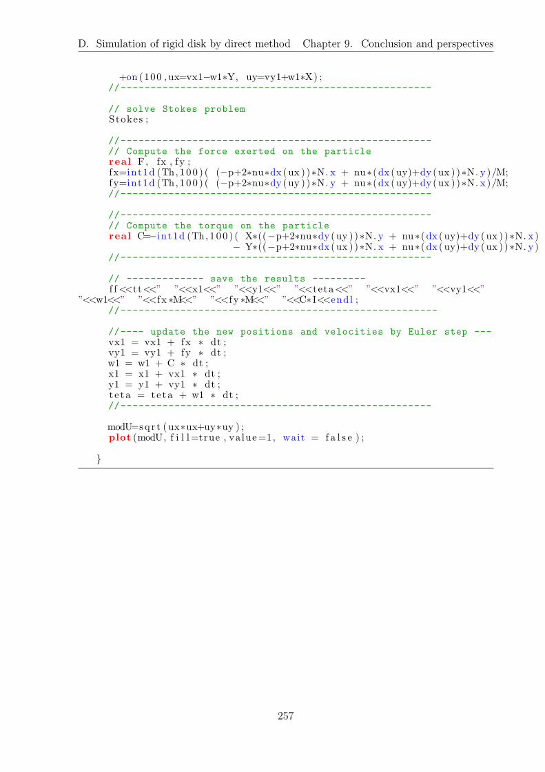
D. Simulation of rigid disk by direct method Chapter 9. Conclusion and perspectives
+on (100 , ux=vx1−w1∗Y, uy=vy1+w1∗X) ;//----------------------------------------------------
// solve Stokes problemStokes ;
//----------------------------------------------------// Compute the force exerted on the particlereal F, fx , fy ;fx=int1d (Th, 1 0 0 ) ( (−p+2∗nu∗dx (ux ) )∗N. x + nu∗( dx (uy)+dy (ux ) )∗N. y )/M;fy=int1d (Th, 1 0 0 ) ( (−p+2∗nu∗dy (uy ) )∗N. y + nu∗( dx (uy)+dy (ux ) )∗N. x )/M;//----------------------------------------------------
//----------------------------------------------------// Compute the torque on the particlereal C=−in t1d (Th, 1 0 0 ) ( X∗((−p+2∗nu∗dy (uy ) )∗N. y + nu∗( dx (uy)+dy (ux ) )∗N. x )
− Y∗((−p+2∗nu∗dx (ux ) )∗N. x + nu∗( dx (uy)+dy (ux ) )∗N. y )//----------------------------------------------------
// ------------- save the results ---------f f<<tt<<” ”<<x1<<” ”<<y1<<” ”<<teta<<” ”<<vx1<<” ”<<vy1<<”
”<<w1<<” ”<<fx ∗M<<” ”<<fy ∗M<<” ”<<C∗ I<<endl ;//-----------------------------------------------------
//---- update the new positions and velocities by Euler step ---vx1 = vx1 + fx ∗ dt ;vy1 = vy1 + fy ∗ dt ;w1 = w1 + C ∗ dt ;x1 = x1 + vx1 ∗ dt ;y1 = y1 + vy1 ∗ dt ;t e t a = te ta + w1 ∗ dt ;//----------------------------------------------------
modU=sqr t ( ux∗ux+uy∗uy ) ;plot (modU, f i l l =true , va lue=1, wait = f a l s e ) ;
257

E. Bilinear forms of Projector Chapter 9. Conclusion and perspectives
E Bilinear forms of the different projection operators
implemented in Projector
Here are the different expression of the bilinear forms implemented in the class Projec-tor and the corresponding code. The Feel++ expression are valid for u and u vectorsor scalar.
• L2 projection Bilinear form:
aL2 =
∫
Ω
u ·v
Feel++ expression:
a = in t e g r a t e ( elements ( mesh ) , t rans ( i d t (u) ) ∗ id ( v ) ) ;
• H1 projection Bilinear form:
aH1 =
∫
Ω
u ·v +
∫
Ω
∇u : ∇v
Feel++ expression:
a = in t e g r a t e ( elements ( mesh ) ,t rans ( i d t (u) ) ∗ id ( v )+ t ra c e ( gradt (u) ∗ t rans ( grad (v ) ) ) ) ;
• Hdiv projection Bilinear form:
aHdiv =
∫
Ω
u ·v +
∫
Ω
(∇ ·u)(∇ ·v)
Feel++ expression:
a = in t e g r a t e ( elements ( mesh ) ,t rans ( i d t (u) ) ∗ id ( v )+ trans ( d iv t (u) ) ∗ div (v ) ) ;
• Smooth projection A special care has to be taken to impose the boundary conditionsin a weak manner. The bilinear form reads:
asmooth =
∫
Ω
u ·v +
∫
Ω
ε∇u : ∇v −∫
∂Ω
ε(∇u n) ·v −∫
∂Ω
ε(∇v n) ·u+
∫
∂Ω
εγ
hu ·v
Feel++ expression:
a = in t e g r a t e ( elements ( mesh ) ,t rans ( i d t (u) ) ∗ id ( v )+ ep s i l o n ∗ t r a c e ( gradt (u) ∗ t rans ( grad (v ) ) ) ) ;
a += in t e g r a t e ( boundaryfaces ( mesh ) ,e p s i l o n ∗ ( − t rans ( id (v ) ) ∗ gradt (u) ∗ N() )
+ep s i l o n ∗ ( − t rans ( i d t (u ) ) ∗ grad (v ) ∗ N() )+ep s i l o n ∗ ( gamma ∗ t rans ( i d t (u) ) ∗ id ( v ) / vf : : hFace ( ) ) ) ;
258
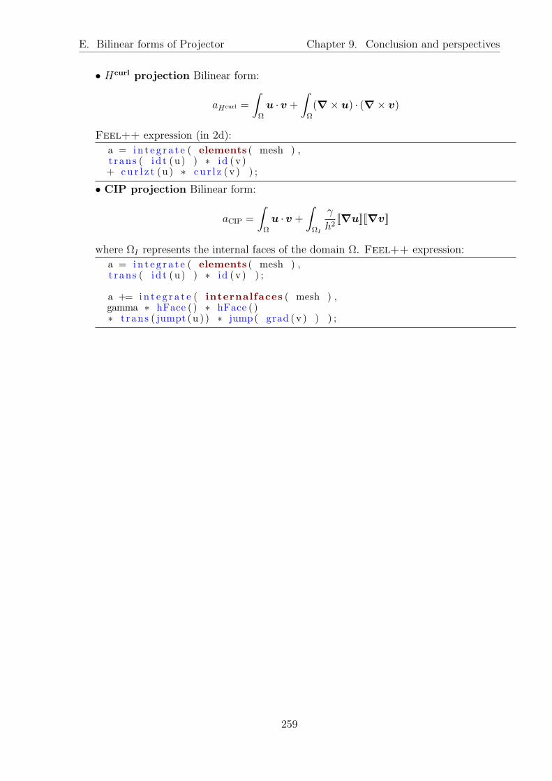
E. Bilinear forms of Projector Chapter 9. Conclusion and perspectives
• Hcurl projection Bilinear form:
aHcurl =
∫
Ω
u ·v +
∫
Ω
(∇× u) · (∇× v)
Feel++ expression (in 2d):
a = in t e g r a t e ( elements ( mesh ) ,t rans ( i d t (u) ) ∗ id ( v )+ cu r l z t (u) ∗ cu r l z ( v ) ) ;
• CIP projection Bilinear form:
aCIP =
∫
Ω
u ·v +
∫
ΩI
γ
h2[[∇u]][[∇v]]
where ΩI represents the internal faces of the domain Ω. Feel++ expression:
a = in t e g r a t e ( elements ( mesh ) ,t rans ( i d t (u) ) ∗ id ( v ) ) ;
a += in t e g r a t e ( internalfaces ( mesh ) ,gamma ∗ hFace ( ) ∗ hFace ( )∗ t rans ( jumpt (u ) ) ∗ jump( grad (v ) ) ) ;
259

F. A configuration file Chapter 9. Conclusion and perspectives
F A configuration file
In this appendix we present a configuration file. This file is used to give the static optionsof the simulation of a vesicle in a shear flow.
Listing 4: Configuration file for a simple simulation of vesicle in a shear flow. Theoptions set in this files are the option usually not changed and do not depend on changingparameters. The other options are handled in a Python interface.
# -- application options --mup=10k=10.i n i t i a l −s t a t e=0export−plus=1save−every=10
# -- levelset options --[ l e v e l s e t ]time−d i s c r−scheme=BDF2advec−stab−method=GALSenable−r e i n i t=1r e i n i t e v e r y=5r e i n i t−method=hjhj−max−i ter=5hj−dtau=0.01hj−t o l =0.05
# -- fluid options --[ s t oke s ]c l t y p e=strongf l ow type=shear
# -- time options --[ bdf ]time− i n i t i a l =0time− f i n a l =40
# -- backend options --# advection system[ l s−advec ]reuse−prec=0ksp−a t o l =0.0000000001pc−f a c to r−mat−so l v e r−package−type=mumps
# fluid system[ f l u i d ]pc−f a c to r−mat−so l v e r−package−type=mumpsreuse−prec=1ksp−monitor=1
# projectors (L2, smooth)[ p r o j e c t o r s ]ksp−monitor=1reuse−prec=0pc−f a c to r−mat−so l v e r−package−type=mumpspc−type=lupc−gasm−over lap=1
260

G. Indexes notations Chapter 9. Conclusion and perspectives
G Indexes notations
In this work, we have choose to write all the equations using vectors and matrices. Inother works, one can find the same equations written in component form. We will givein this appendix some equivalent forms between the vector and indexes notations. Weassume the space has ND dimensions. The position of a point is given by
x = xi, i = 1, ..., ND.
The partial derivative of a scalar s in the direction xi is given by,∂s
∂xiand will be written
in our notations ∂xis.
For each vector v, one can write its components as
v = vi, i = 1, ..., N
with N the number of component of the vector. The same way, we can write the compo-nents of any matrix A as:
A = aij, i = 1, ..., N and j = 1, ...,M
with N the number of columns and M the number of lines of A.The scalar product of two vectors u and v is given by:
u ·v = uivi
with the Einstein summation convention, which stands that we sum over all the repeatedindexes. In the following, we will always use the Einstein convention.The double contraction product between a matrix A and a matrix B is a scalar given by:
A : B = aijbij.
The product of a matrix A and a vector v is a vector given by:
A v = aijvj, i = 1, ..., N.
The gradient of a scalar, let us say p is a vector given by:
∇p = ∂xip, i = 1, ..., ND.
The gradient of a vector v is a matrix given by:
∇v = ∂xivj, i = 1, ..., ND and j = 1, ..., N.
The divergence of a vector v is a scalar given by:
∇ ·v = ∂xivi
261

G. Indexes notations Chapter 9. Conclusion and perspectives
The laplacian of a vector v is a vector given by:
∆v = ∂xj∂xj
vi, i = 1, ..., N
The Navier-Stokes equation which we have written in the vectorial form:
ρ(∂tu+ (u ·∇)u)− µ∆u+∇p = f
∇ ·u = 0
ρ(∂tui + (uj∂xj)ui)− µ∂xm
∂xmui + ∂xi
p = fi, i = 1, ..., ND
∂xlul = 0.
The surface divergence:
∇s ·u = (Id − n⊗ n) : ∇u = ∇ ·u− (∇u n) ·n (2)
∇s ·u = (δij − njni)∂xjui = ∂xi
ui − ((∂xiuj)nj)ni (3)
with δij the Kronecker symbol. We emphasize the fact that (∇u n) is the product ofthe matrix ∇u by the vector n, thus it is a vector. We can denote its components by(∇u n)i. Consequently (∇u n)i ni is a scalar which is expected.
The same way, we can re-write:
D(u) : D(v)
(∂xiuj + ∂xj
ui)(∂xivj + ∂xj
vi).
262

H. Viscosity from energy dissipation Chapter 9. Conclusion and perspectives
H Derive the effective viscosity from energy dissipa-
tion
In this section, we will explicit the expression given in [65] where the viscosity of a suspen-sion of rigid spheres or disks is given as a function of the energy dissipation |∇u+t
∇u|2.In this appendix, all the notations are the same than in section 8.1. We will show thatthe energy dissipation in the fluid domain can be related to the forces applied on thetop and bottom walls. Then we can use the definition of the effective viscosity given inequation (8.4). In this problem, we only consider a pure shear flow which is infinite in thex direction (or with periodic boundary conditions). Consequently, the boundaries ∂Ωf
are only the top and bottom moving walls.The Stokes equation (2.6) without external forces can be re-written as:
− 2µ0∇ ·D(u) +∇p = 0 (4)
since ∇ ·u = 0. We multiply the equation (4) by the velocity u and integrate over thefluid domain Ωf . Integration by part gives:
−2µ0
∫
∂Ωf
[D(u)n] ·u+ 2µ0
∫
Ωf
D(u) : ∇u+
∫
∂Ωf
p(u ·n)−∫
Ωf
p∇ ·u = 0
• Thanks to the symmetry of 2D(u) = (∇u+t∇u), the second term becomes:
(∇u+t
∇u)
: ∇u
=(∇u+t
∇u) : ∇u+ (∇u+t∇u) :t∇u
2
=(∇u+t
∇u) : (∇u+t∇u)
2
=|∇u+t
∇u|22
= 2 |D(u)|2
• The third term can be re-written as [(pId)n] ·u so that we can factorize it with thefisrt term.
• The last term vanishes since ∇ ·u = 0.
Factorization of the first and third term leads to:
2µ0
∫
Ωf
|D(u)|2 −∫
∂Ωf
[(−p Id + 2µ0D(u))n] ·u = 0
2µ0
∫
Ωf
|D(u)|2 −∫
∂Ωf
(σn) ·u = 0
Finally, computing the last integral, which is done on the top and bottom boundariesgives:
2µ0
∫
Ωf
|D(u)|2 = (ft − fb) U
263

H. Viscosity from energy dissipation Chapter 9. Conclusion and perspectives
The forces difference applied on the walls is related to the definition of the effectiveviscosity given in equation (8.4), it reads:
(ft − fb) =4 L U µeff
l
Replacing this term in the previous equation leads to the definition of the effective viscosityusing the dissipation in the fluid domain:
µeff =µ0 l
2LU2
∫
Ωf
|D(u)|2.
264

Bibliography
[1] D Andelman, T Kawakatsu, and K Kawasaki. Equilibrium shape of two-componentunilamellar membranes and vesicles. EPL (Europhysics Letters), 19(1):57, 1992.
[2] Robert E Apfel, Yuren Tian, Joseph Jankovsky, Tao Shi, X Chen, R Glynn Holt,Eugene Trinh, Arvid Croonquist, Kathyrn C Thornton, Albert Sacco, Jr, et al. Freeoscillations and surfactant studies of superdeformed drops in microgravity. Physicalreview letters, 78(10):1912–1915, 1997.
[3] Satish Balay, Jed Brown, Kris Buschelman, William D. Gropp, Dinesh Kaushik,Matthew G. Knepley, Lois Curfman McInnes, Barry F. Smith, and Hong Zhang.PETSc Web page, 2013. http://www.mcs.anl.gov/petsc.
[4] GK Batchelor and JT Green. The determination of the bulk stress in a suspensionof spherical particles to order c2. J. Fluid Mech, 56(3):401–427, 1972.
[5] J. Beaucourt, F. Rioual, T. Seacuteon, T. Biben, and C. Misbah. Steady to unsteadydynamics of a vesicle in a flow. Phys. Rev. E, 69(1):011906–, January 2004.
[6] Silvia Bertoluzza, Mourad Ismail, and Bertrand Maury. Analysis of the fully discretefat boundary method. Numerische Mathematik, 118(1):49–77, 2011.
[7] T. Biben and C. Misbah. Tumbling of vesicles under shear flow within an advected-field approach. Phys. Rev. E, 67(3):031908, Mar 2003.
[8] Thierry Biben, Klaus Kassner, and Chaouqi Misbah. Phase-field approach to three-dimensional vesicle dynamics. Phys. Rev. E, 72:041921, Oct 2005.
[9] R.P. Bonet Chaple. Numerical stabilization of vonvection-diffusion-reaction prob-lems. Technical report, 2006.
[10] Alexander N Brooks and Thomas JR Hughes. Streamline upwind/petrov-galerkinformulations for convection dominated flows with particular emphasis on the in-compressible navier-stokes equations. Computer methods in applied mechanics andengineering, 32(1):199–259, 1982.
[11] Cuc Bui, Vanessa Lleras, and Olivier Pantz. Dynamics of red blood cells in 2d.ESAIM: Proceedings, 28:182–194, 2009.
[12] Thi Thu Cuc Bui, P. Frey, and B. Maury. A coupling strategy based on anisotropicmesh adaptation for solving two-fluid flows. International Journal for NumericalMethods in Fluids, pages n/a–n/a, 2010.
265
Bibliography Bibliography
[13] Erik Burman and Peter Hansbo. Edge stabilization for galerkin approximations ofconvection-diffusion-reaction problems. Computer Methods in Applied Mechanicsand Engineering, 193(15-16):1437 – 1453, 2004.
[14] Erik Burman and Peter Hansbo. Edge stabilization for the generalized stokes prob-lem: A continuous interior penalty method. Computer Methods in Applied Mechan-ics and Engineering, 195(19-22):2393–2410, April 2006.
[15] Celine Caldini Queiros, Vincent Chabannes, Mourad Ismail, Goncalo Pena,Christophe Prud’Homme, Marcela Szopos, and Ranine Tarabay. Towards large-scalethree-dimensional blood flow simulations in realistic geometries. pp. 17, Acceptedin ESAIM: Proc, CEMRACS 2012, 2012.
[16] P.B. Canham. The minimum energy of bending as a possible explanation of thebiconcave shape of the human red blood cell. Journal of Theoretical Biology, 26(1):61– 81, 1970.
[17] Vincent Chabannes. Vers la simulation des ecoulements sanguins. PhD thesis,Universite de Grenoble, 2013.
[18] Vincent Chabannes, Goncalo Pena, and Christophe Prud’Homme. High-orderfluid-structure interaction in 2D and 3D. Application to blood flow in arteries.Journal of Computational and Applied Mathematics, 246:1–9, July 2013. FifthInternational Conference on Advanced COmputational Methods in ENgineering(ACOMEN 2011).
[19] S. Chandrasekhar. Hydrodynamic and Hydromagnetic Stability. Courier Dover Pub-lications., 1981.
[20] Georges-Henri Cottet and Emmanuel Maitre. A level-set formulation of immersedboundary methods for fluid–structure interaction problems. Comptes Rendus Math-ematique, 338(7):581 – 586, 2004.
[21] Georges-Henri Cottet and Emmanuel Maitre. A level set method for fluid-structureinteractions with immersed surfaces. Mathematical Models and Methods in AppliedSciences, 2010.
[22] Y Davit and P Peyla. Intriguing viscosity effects in confined suspensions: A numer-ical study. EPL (Europhysics Letters), 83(6):64001, 2008.
[23] KH De Haas, C Blom, D Van den Ende, MHG Duits, and J Mellema. Deformationof giant lipid bilayer vesicles in shear flow. Physical Review E, 56(6):7132, 1997.
[24] HJ Deuling andWHelfrich. The curvature elasticity of fluid membranes: a catalogueof vesicle shapes. Journal de Physique, 37(11):1335–1345, 1976.
[25] Jim Douglas and Todd Dupont. Interior penalty procedures for elliptic and parabolicgalerkin methods. Computing Methods in Applied Sciences, 58:207–216, 1976.
266
Bibliography Bibliography
[26] V. Doyeux, Y. Guyot, V. Chabannes, C. Prud’homme, and M. Ismail. Simulation oftwo-fluid flows using a finite element/level set method. application to bubbles andvesicle dynamics. Journal of Computational and Applied Mathematics, 246(0):251– 259, 2013.
[27] V. Doyeux, T. Podgorski, S. Peponas, M. Ismail, and G. Coupier. Spheres in thevicinity of a bifurcation: elucidating the zweifach-fung effect. Journal of FluidMechanics, 674:359–388, 2011.
[28] Doyeux, Vincent, Chabannes, Vincent, Prud´homme, Christophe, and Ismail,Mourad. Simulation of vesicle using level set method solved by high order finiteelement. ESAIM: Proc., 38:335–347, 2012.
[29] V. Ducrot and P. Frey. Anisotropic level set adaptation for accurate interface cap-turing. In RaoV. Garimella, editor, Proceedings of the 17th International MeshingRoundtable, pages 159–176. Springer Berlin Heidelberg, 2008.
[30] Albert Einstein. Eine neue bestimmung der molekuldimensionen. Annalen derPhysik, 324(2):289–306, 1906.
[31] Douglas Enright, Ronald Fedkiw, Joel Ferziger, and Ian Mitchell. A hybrid par-ticle level set method for improved interface capturing. Journal of ComputationalPhysics, 183(1):83–116, November 2002.
[32] Benoit Fabreges. Une methode de prolongement regulier pour la simulationd’ecoulements fluide / particules. PhD thesis, Universite Paris XI, 2012.
[33] Alexander Farutin, Thierry Biben, and Chaouqi Misbah. Analytical progress in thetheory of vesicles under linear flow. Physical Review E, 81(6):061904, 2010.
[34] Leopoldo P. Franca, Sergio L. Frey, and Thomas J.R. Hughes. Stabilized finiteelement methods: I. application to the advective-diffusive model. Computer Methodsin Applied Mechanics and Engineering, 95(2):253–276, March 1992.
[35] Thomas Franke, Ronald HW Hoppe, Christopher Linsenmann, Lothar Schmid, Ca-rina Willbold, and Achim Wixforth. Numerical simulation of the motion of redblood cells and vesicles in microfluidic flows. Computing and visualization in sci-ence, 14(4):167–180, 2011.
[36] Christophe Geuzaine and Jean-Francois Remacle. Gmsh: A 3-d finite element meshgenerator with built-in pre-and post-processing facilities. International Journal forNumerical Methods in Engineering, 79(11):1309–1331, 2009.
[37] Giovanni Ghigliotti, Thierry Biben, and Chaouqi Misbah. Rheology of a dilutetwo-dimensional suspension of vesicles. Journal of Fluid Mechanics, 653:489–518,2010.
[38] Giovanni Ghigliotti, Abtin Rahimian, George Biros, and Chaouqi Misbah. Vesiclemigration and spatial organization driven by flow line curvature. Physical ReviewLetters, 106(2):028101, 2011.
267

Bibliography Bibliography
[39] R Glowinski, TW Pan, TI Hesla, DD Joseph, and J Periaux. A fictitious domainapproach to the direct numerical simulation of incompressible viscous flow pastmoving rigid bodies: application to particulate flow. Journal of ComputationalPhysics, 169(2):363–426, 2001.
[40] Roland Glowinski, T-W Pan, Todd I Hesla, and Daniel D Joseph. A distributedlagrange multiplier/fictitious domain method for particulate flows. InternationalJournal of Multiphase Flow, 25(5):755–794, 1999.
[41] J.L. Guermond, P. Minev, and Jie Shen. An overview of projection methods forincompressible flows. Computer Methods in Applied Mechanics and Engineering,195(44-47):6011–6045, September 2006.
[42] G. Hauke. A simple subgrid scale stabilized method for the advection-diffusion-reaction equation. Computer Methods in Applied Mechanics and Engineering,191(27-28):2925–2947, April 2002.
[43] W Helfrich. Elastic properties of lipid bilayers: theory and possible experiments. ZNaturforsch C, 28(11):693–703–, 1973.
[44] Thomas JR Hughes, Leopoldo P Franca, and Gregory M Hulbert. A new finite ele-ment formulation for computational fluid dynamics: Viii. the galerkin/least-squaresmethod for advective-diffusive equations. Computer Methods in Applied Mechanicsand Engineering, 73(2):173–189, 1989.
[45] S. Hysing, S. Turek, D. Kuzmin, N. Parolini, E. Burman, S. Ganesan, and L. To-biska. Quantitative benchmark computations of two-dimensional bubble dynamics.International Journal for Numerical Methods in Fluids, 60(11):1259–1288, 2009.
[46] Mourad Ismail. Methode de la frontiere elargie pour la resolution de problemeselliptiques dans des domaines perfores. Application aux ecoulements fluides tridi-mensionnels. PhD thesis, Universite Paris VI, 2004.
[47] Mourad Ismail and Aline Lefebvre-Lepot. A” necklace” model for vesicles simula-tions in 2d. arXiv preprint arXiv:1202.3034, 2012.
[48] Levan Jibuti. Locomotion et ecoulements dans les fluides complexes confines. PhDthesis, Universite de Grenoble, 2011.
[49] Joao Janela, Aline Lefebvre, and Bertrand Maury. A penalty method for the sim-ulation of fluid - rigid body interaction. ESAIM: Proc., 14:115–123, 2005.
[50] AA Johnson and TE Tezduyar. Simulation of multiple spheres falling in a liquid-filled tube y. 1995.
[51] Eric Jones, Travis Oliphant, Pearu Peterson, et al. SciPy: Open source scientifictools for Python, 2001–.
[52] Vasiliy Kantsler and Victor Steinberg. Orientation and dynamics of a vesicle intank-treading motion in shear flow. Phys. Rev. Lett., 95:258101, Dec 2005.
268

Bibliography Bibliography
[53] B. Kaoui, J. Harting, and C. Misbah. Two-dimensional vesicle dynamics undershear flow: Effect of confinement. pre, 83(6):066319, june 2011.
[54] B. Kaoui, G. H. Ristow, I. Cantat, C. Misbah, and W. Zimmermann. Lateral migra-tion of a two-dimensional vesicle in unbounded Poiseuille flow. pre, 77(2):021903–+,February 2008.
[55] B. Kaoui, N. Tahiri, T. Biben, H. Ez-Zahraouy, A. Benyoussef, G. Biros, and C. Mis-bah. Complexity of vesicle microcirculation. Phys. Rev. E, 84:041906, Oct 2011.
[56] Badr Kaoui. Modelisation de vesicules en geometrie etendue et dans des systemesmicro-fluidiques. PhD thesis, Universite Joseph-Fourier - Grenoble I, LSP - Labo-ratoire de Spectrometrie Physique, 2009.
[57] Badr Kaoui, George Biros, and Chaouqi Misbah. Why do red blood cells haveasymmetric shapes even in a symmetric flow? Phys. Rev. Lett., 103:188101, Oct2009.
[58] Badr Kaoui, Alexander Farutin, and Chaouqi Misbah. Vesicles under simpleshear flow: Elucidating the role of relevant control parameters. Phys. Rev. E,80(6):061905, Dec 2009.
[59] C.E. Kees, I. Akkerman, M.W. Farthing, and Y. Bazilevs. A conservative levelset method suitable for variable-order approximations and unstructured meshes.Journal of Computational Physics, 230(12):4536 – 4558, 2011.
[60] Yongsam Kim and Ming-Chih Lai. Simulating the dynamics of inextensible vesiclesby the penalty immersed boundary method. Journal of Computational Physics,229(12):4840–4853, 2010.
[61] M. Kraus, W. Wintz, U. Seifert, and R. Lipowsky. Fluid Vesicles in Shear Flow.Physical Review Letters, 77:3685–3688, October 1996.
[62] Aymen Laadhari. Modelisation numerique de la dynamique des globules rouges parla methode des fonctions de niveau. PhD thesis, Universite de Grenoble, 2011.
[63] Aymen Laadhari, Pierre Saramito, and Chaouqi Misbah. Computing the dynamicsof biomembranes by combining conservative level set and adaptive finite elementmethods. CNRS, June 2011.
[64] H LAMB. Hydrodynamics. Cambridge University Press., 1932.
[65] Aline Lefebvre and Bertrand Maury. Apparent viscosity of a mixture of a newtonianfluid and interacting particles. Comptes Rendus Mecanique, 333(12):923 – 933, 2005.
[66] Aline Lefebvre-Lepot. Modelisation numerique d’ecoulements fluide/particules. PhDthesis, Universite Paris XI, 2007.
[67] Randall J. LeVeque. Numerical Methods for Conservation Laws. Birkhauser, 1992.
[68] Xu-Dong Liu, Stanley Osher, and Tony Chan. Weighted essentially non-oscillatoryschemes. Journal of Computational Physics, 115(1):200 – 212, 1994.
269

Bibliography Bibliography
[69] M. Mader, V. Vitkova, M. Abkarian, A. Viallat, and T. Podgorski. Dynamics ofviscous vesicles in shear flow. The European Physical Journal E: Soft Matter andBiological Physics, 19(4):389–397, 2006-04-01.
[70] E. Maitre, C. Misbah, P. Peyla, and A. Raoult. Comparison between advected-field and level-set methods in the study of vesicle dynamics. Physica D: NonlinearPhenomena, 241(13):1146 – 1157, 2012.
[71] Emmanuel Maitre, Thomas Milcent, Georges-Henri Cottet, Annie Raoult, and YvesUsson. Applications of level set methods in computational biophysics. Mathematicaland Computer Modelling, 49(11-12):2161–2169, June 2009.
[72] Ravikanth Malladi, JamesA. Sethian, and BabaC. Vemuri. A fast level set basedalgorithm for topology-independent shape modeling. Journal of Mathematical Imag-ing and Vision, 6(2-3):269–289, 1996.
[73] B. Maury. Numerical analysis of a finite element/volume penalty method. SIAMJournal on Numerical Analysis, 47(2):1126–1148, 2009.
[74] Bertrand Maury. A fat boundary method for the poisson problem in a domain withholes. Journal of Scientific Computing, 16(3):319–339, 2001.
[75] S. Mendez, E. Gibaud, and F. Nicoud. An unstructured solver for simulations of de-formable particles in flows at arbitrary reynolds numbers. Journal of ComputationalPhysics, 2013.
[76] Thomas MILCENT. Une approche eulerienne du couplage fluide-structure, anal-yse mathematique et applications en biomecanique. PhD thesis, Universite JosephFourier, 2009.
[77] Chaouqi Misbah. Vacillating breathing and tumbling of vesicles under shear flow.Phys. Rev. Lett., 96(2):028104, Jan 2006.
[78] Jean-Christophe Nave, Rodolfo Ruben Rosales, and Benjamin Seibold. A gradient-augmented level set method with an optimally local, coherent advection scheme.Journal of Computational Physics, 229(10):3802 – 3827, 2010.
[79] Hiroshi Noguchi and Gerhard Gompper. Shape transitions of fluid vesicles and redblood cells in capillary flows. Proceedings of the National Academy of Sciences ofthe United States of America, 102(40):14159–14164, 2005.
[80] Santtu TT Ollila, Colin Denniston, and Tapio Ala-Nissila. One-and two-particledynamics in microfluidic t-junctions. Physical Review E, 87(5):050302, 2013.
[81] Nicola Parolini. Computational fluid dynamics for naval engineering problems. PhDthesis, Politecnico di Milano, 2004.
[82] Charles S Peskin. Numerical analysis of blood flow in the heart. Journal of Com-putational Physics, 25(3):220 – 252, 1977.
[83] Charles S Peskin. The immersed boundary method. Acta numerica, 11(0):479–517,2002.
270

Bibliography Bibliography
[84] Philippe Peyla and Claude Verdier. New confinement effects on the viscosity ofsuspensions. EPL (Europhysics Letters), 94(4):44001, 2011.
[85] C Pozrikidis. Effect of membrane bending stiffness on the deformation of capsulesin simple shear flow. Journal of Fluid Mechanics, 440:269–291, 2001.
[86] C. Prud’homme, V. Chabannes, and G. Pena. Feel++: Finite Element EmbeddedLanguage in C++. Free Software available at http://www.feelpp.org. Contributionsfrom A. Samake, V. Doyeux, M. Ismail and S. Veys.
[87] Prud´homme, Christophe, Chabannes, Vincent, Doyeux, Vincent, Ismail, Mourad,Samake, Abdoulaye, and Pena, Goncalo. Feel++ : A computational frameworkfor galerkin methods and advanced numerical methods. ESAIM: Proc., 38:429–455,2012.
[88] Salima Rafaı, Levan Jibuti, and Philippe Peyla. Effective viscosity of microswimmersuspensions. Phys. Rev. Lett., 104:098102, Mar 2010.
[89] Codina Ramon. Comparison of some finite element methods for solving the diffusion-convection-reaction equation. Computer Methods in Applied Mechanics and Engi-neering, 156(1-4):185–210, April 1998.
[90] PA Raviart and V Girault. Finite element approximation of the navier-stokes equa-tions. Lecture notes in mathematics, Springer-Verlag, 1979.
[91] Elisabeth Rouy and Agnes Tourin. A viscosity solutions approach to shape-from-shading. SIAM Journal on Numerical Analysis, 29(3):867–884, 1992.
[92] D. Salac and M. Miksis. A level set projection model of lipid vesicles in generalflows. Journal of Computational Physics, 230(22):8192–8215, September 2011.
[93] Ashok S. Sangani, Andreas Acrivos, and Philippe Peyla. Roles of particle-wall andparticle-particle interactions in highly confined suspensions of spherical particlesbeing sheared at low reynolds numbers. Physics of Fluids, 23(8):–, 2011.
[94] Udo Seifert. Configurations of fluid membranes and vesicles. Advances in Physics,46(1):13–137, 1997.
[95] Udo Seifert, Karin Berndl, and Reinhard Lipowsky. Shape transformations of vesi-cles: Phase diagram for spontaneous- curvature and bilayer-coupling models. Phys.Rev. A, 44(2):1182–, July 1991.
[96] Hassib Selmi, Lassaad Elasmi, Giovanni Ghigliotti, and Chaouqi Misbah. Boundaryintegral and fast multipole method for two dimensional vesicle sets in poiseuille flow.Discrete and Continuous Dynamical Systems-Series B (DCDS-B), 15(4):1065–1076,2011.
[97] J.A. Sethian. Analysis of flame propagation. PhD thesis, Lawrence Berkeley Lab.,CA (USA), 1982.
[98] J.A. Sethian. Level Set Methods and Fast Marching Methods. Cambridge UniversityPress, 1996.
271
Bibliography Bibliography
[99] Richard Skalak. Motion of a tank-treading ellipsoidal particle in a shear flow. Jour-nal of Fluid Mechanics, 120:27–47, 1982.
[100] Benjamin Stamm. Stabilization strategies for discontinuous Galerkin methods. PhDthesis, Ecole Polytechnique Federale de Lausanne, 2008.
[101] Ronald Fedkiw Stanley Osher. Level Set Methods and Dynamic Implicit Surfaces.Springer, S.S. Antman, J.E. Marsden, L. Sirovich.
[102] Jasjit S. Suri, Sameer Singh, Swamy Laxminarayan, Xiaolan Zeng, Kecheng Liu,and Laura Reden. Shape recovery algorithms using level sets in 2-d/3-d medicalimagery: A state-of-the-art review. IEEE Transactions on information technologyin biomedicine, 2001.
[103] Mark Sussman, Ann S. Almgren, John B. Bell, Phillip Colella, Louis H. Howell, andMichael L. Welcome. An adaptive level set approach for incompressible two-phaseflows. Journal of Computational Physics, 148(1):81–124, January 1999.
[104] Mark Sussman, Peter Smereka, and Stanley Osher. A level set approach for comput-ing solutions to incompressible two-phase flow. Journal of Computational Physics,114(1):146 – 159, 1994.
[105] Hajime Tanaka and Takeaki Araki. Simulation method of colloidal suspensionswith hydrodynamic interactions: Fluid particle dynamics. Physical review letters,85(6):1338–1341, 2000.
[106] Anna-Karin Tornberg and Bjorn Engquist. A finite element based level-set methodfor multiphase flow applications. Computing and Visualization in Science, 3:93–101,2000. 10.1007/s007910050056.
[107] Ken-ichi Tsubota and Shigeo Wada. Effect of the natural state of an elastic cellularmembrane on tank-treading and tumbling motions of a single red blood cell. PhysicalReview E, 81(1):011910, 2010.
[108] Shravan K. Veerapaneni, Denis Gueyffier, Denis Zorin, and George Biros. A bound-ary integral method for simulating the dynamics of inextensible vesicles suspendedin a viscous fluid in 2d. Journal of Computational Physics, 228(7):2334 – 2353,2009.
[109] Shravan K Veerapaneni, Abtin Rahimian, George Biros, and Denis Zorin. A fastalgorithm for simulating vesicle flows in three dimensions. Journal of ComputationalPhysics, 230(14):5610–5634, 2011.
[110] Paul Vigneaux. Methodes Level Set pour des problemes d’interface en microfluidique.PhD thesis, Universite Bordeaux I, 2007.
[111] Olivier Vincent. Dynamique de bulles de cavitation dans de l’eau micro-confinee soustension. Application a l’etude de l’embolie dans les arbres. PhD thesis, Universitede Grenoble, 2012.
272

Bibliography Bibliography
[112] Christophe Winkelmann. Interior penalty finite element approximation of Navier-Stokes equations and application to free surface flows. PhD thesis, Ecole polytech-nique federale de Lausanne EPFL, 2007.
[113] Sheng Xu. The immersed interface method for simulating prescribed motion ofrigid objects in an incompressible viscous flow. Journal of Computational Physics,227(10):5045–5071, 2008.
[114] Steven T Zalesak. Fully multidimensional flux-corrected transport algorithms forfluids. Journal of Computational Physics, 31(3):335 – 362, 1979.
[115] Junfeng Zhang, Paul C Johnson, and Aleksander S Popel. An immersed boundarylattice boltzmann approach to simulate deformable liquid capsules and its applica-tion to microscopic blood flows. Physical biology, 4(4):285, 2007.
[116] Hong Zhao, Amir HG Isfahani, Luke N Olson, and Jonathan B Freund. A spectralboundary integral method for flowing blood cells. Journal of Computational Physics,229(10):3726–3744, 2010.
[117] Hong Zhao and Eric SG Shaqfeh. The dynamics of a vesicle in simple shear flow.Journal of Fluid Mechanics, 674:578, 2011.
273
Copyright © 2022 FDOKUMEN