�����������������

Citation: Acorsi, R.L.; De Giovanni,

M.Y.G.; Olivo, J.E.; Andrade, C.M.G.

Modeling and Simulation of Batch

Sugarcane Alcoholic Fermentation

Using the Metabolic Model.

Fermentation 2022, 8, 82. https://

doi.org/10.3390/fermentation8020082

Academic Editor: Kurt A. Rosentrater

Received: 31 January 2022

Accepted: 9 February 2022

Published: 16 February 2022

Publisher’s Note: MDPI stays neutral

with regard to jurisdictional claims in

published maps and institutional affil-

iations.

Copyright: © 2022 by the authors.

Licensee MDPI, Basel, Switzerland.

This article is an open access article

distributed under the terms and

conditions of the Creative Commons

Attribution (CC BY) license (https://

creativecommons.org/licenses/by/

4.0/).

fermentation

Article

Modeling and Simulation of Batch Sugarcane AlcoholicFermentation Using the Metabolic ModelRenam Luis Acorsi, Matheus Yuri Gritzenco De Giovanni , José Eduardo Olivoand Cid Marcos Gonçalves Andrade *

Departamento de Engenharia Química, Universidade Estadual de Maringá, Av. Colombo 5790,Maringá 87020-900, PR, Brazil; rnmacorsi@gmail.com (R.L.A.); matheusdegiovanni@gmail.com (M.Y.G.D.G.);olivo@deq.uem.br (J.E.O.)* Correspondence: cidmga@yahoo.com.br

Abstract: The present work sought to implement a model different from the more traditional ones forthe fermentation process of ethanol production by the action of the fungus Saccharomyces cerevisiae,using a relevant metabolic network based on the glycolytic Embden–Meyerhof–Parnas route, alsocalled “EMP”. We developed two models to represent this phenomenon. In the first model, weused the simple and unbranched EMP route, with a constant concentration of microorganismsthroughout the process and glucose as the whole substrate. We called this first model “SR”, regardingthe Portuguese name “sem ramificações”, which means “no branches”. We developed the secondmodel by simply adding some branches to the SR model. We called this model “CR”, regarding thePortuguese name “com ramificações”, which means “with branches”. Both models were implementedin MATLABTM software considering a constant temperature equal to 32 ◦C, similar to that practicedin sugar and ethanol plants, and a wide range of substrate concentrations, ranging from 30 to 100 g/L,and all the enzymes necessary for fermentation were already expressed in the cells so all the enzymesshowed a constant concentration throughout the fermentation. The addition of common branches tothe EMP route resulted in a considerable improvement in the results, especially predicting ethanolproduction closer to what we saw experimentally. Therefore, the results obtained are promising,making adjustments consistent with experimental data, meaning that all the models proposed here area good basis for the development of future metabolic models of discontinuous fermentative processes.

Keywords: Saccharomyces cerevisiae; alcohol fermentation; metabolic models; fermentation process

1. Introduction

A wide range of fermented products are still produced by batch or sequential batchprocesses using easily accessible raw materials. In the case of ethanol production, biofuelis of interest to compete with fossil fuels, since its use brings a reduction in the emissionof harmful gases, such as SOx and NOx. This is similar to the use of one of the mostwidely used processes in the production of this alcohol, the Melle-Boinot process, a form offed-batch fermentation developed by Fermin Boinot, in the town of Melle, located in theNouvelle-Aquitaine region of France, in the first half of the 20th century. Furthermore, inthe production of ethanol, the yeast Saccharomyces cerevisiae is the most used microorganism,even if other microorganisms have a better potential in laboratory situations, such as thebacterium Zymomonas mobilis [1–4].

Due to the importance of this type of process, from the second half of the 20th century,a series of works seeking to understand these interactions began to be developed, especiallyafter Gaden [5], who developed an empirical analysis (black box) of batch fermentationprocesses, verifying whether it was possible to associate the production of a metabolitewith cell growth or not. This relatively simple approach had good results, despite ignoringa large part of the interactions that occur inside the cells. Because of this, numerous works

Fermentation 2022, 8, 82. https://doi.org/10.3390/fermentation8020082 https://www.mdpi.com/journal/fermentation

Fermentation 2022, 8, 82 2 of 18

were developed based on the work of Gaden and the kinetic model of Monod, makingadditions that sought to insert any metabolic knowledge.

Among the models that began seeking to insert these metabolic details, we can men-tion the model developed by Sonnleitner and Käppeli [6], developed based on a quasi-idealMonod kinetic model. In such a model, Sonnleitner and Käppeli simplified the relevantmetabolism into three stoichiometric relationships: two containing purely oxidative rela-tionships, and one reductive. Furthermore, this model already considered the possibility ofalcoholic fermentation not being fueled by a single substrate: it considered the possibility ofmultiple substrates, such as the possibility of ethanol being used by Saccharomyces cerevisiaeas a carbon source. Despite the relevant results achieved in such a model, it still consideredthe great metabolic complexity in an extremely simplified way.

In addition to the model by Sonnleitner and Käppeli [6], several other relevant modelsfor alcoholic fermentation were developed in a black box or with the addition of somemetabolic details. Among such models, we can cite the work of Birol et al. [7], Kostovet al. [8], Sainz et al. [9], and Freitas et al. [10]. The works by Birol et al. [7] and Kostovet al. [8] have the merit of analyzing a large number of black box models for alcoholicfermentation, highlighting the Monod, Andrews, Naock, and Hinshelwood models. Fer-mentation processes conducted in batch and fed-batch form generate a considerably com-plex dynamic interaction between microorganisms and the environment around them, asstudied by Freitas et al. [10] using genetic algorithms, differential evolution, and real-timedynamic optimization. These interactions have been generally studied and well analyzedin the form of black box analyses for some decades, as highlighted by Sainz et al. [9], butthey fail to consider that each of the cells of a microorganism is capable of carrying outhundreds of reactions simultaneously. It was fair to the model proposed by Sainz et al. [9]that such interactions began to be considered. Each of these reactions is extremely wellcontrolled by the action of substances that generate the expression of or inhibit very specificbiocatalysts—enzymes [11,12].

Among the most important metabolic routes for numerous fermentative processes,we can mention the Embden–Meyerhof–Parnas route, or the EMP route. Completelydescribed in the 1940s, the EMP pathway is present in a large number of organisms anddescribes a series of spontaneous reactions that convert glucose to pyruvate. The pyru-vate generated in this sequence can be converted into a wide range of other substances,including ethanol, which can be produced under anaerobic conditions by reducingpyruvate [11,13–15].

Considering the importance of ethanol in the current economic and environmentalscenario, as well as the development of models that are more faithful to reality, thepresent work sought to model a batch alcoholic fermentation process. We used kineticequations derived from the EMP route of Saccharomyces cerevisiae, considering substrateconcentrations lower than those used industrially to avoid the appearance of significantinhibitory effects. The production of ethanol still needs further clarification at themetabolic level. Thus, we propose two distinct models: the SR model, built only with thereactions present in the EMP route followed by alcoholic fermentation, and the CR model,which consists of using the SR model as a basis, adding the ramifications of trehalose,glycerol, succinate, and acetate. Furthermore, the development of models based on asmuch metabolic information as possible can benefit countless other industrial sectorsbesides sugar and alcohol: an understanding of the behavior of possible ramificationsis something that would greatly benefit the food and pharmaceutical industries, forexample. In the case of the food industry, this knowledge would make better controlof the processes and the selection and development of new strains of microorganismspossible, making it possible to obtain larger amounts of specific substances, especiallythose involved in aromas and flavors.

Fermentation 2022, 8, 82 3 of 18

2. Method and Experimental Procedures

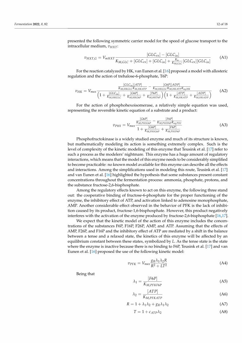
Figure 1 below shows the sequence of reactions selected for the composition of themodel. In short, there are the transport of the substrate from the extracellular environmentto the intracellular environment, the EMP route, and alcoholic fermentation. Additionally,highlighted are the enzymes responsible for each of the reactions, in blue; products orresulting secondary reagents, in green; and the intracellular energy molecules ADP, ATP,NAD+, and NADH, in red. A list of symbols and meanings is available in the end of thispaper.

Fermentation 2022, 8, x FOR PEER REVIEW 3 of 18

2. Method and Experimental Procedures Figure 1 below shows the sequence of reactions selected for the composition of the

model. In short, there are the transport of the substrate from the extracellular environment to the intracellular environment, the EMP route, and alcoholic fermentation. Additionally, highlighted are the enzymes responsible for each of the reactions, in blue; products or resulting secondary reagents, in green; and the intracellular energy molecules ADP, ATP, NAD+, and NADH, in red. A list of symbols and meanings is available in the end of this paper.

1 GLCexAmbiente extracelular

Membrana da Saccharomyces cerevisiae

HXT

1 GLCin

HK

1 G6P

T6PATP

ADP

PHI

1 F6PFK

ATP ADP

1 FRUin

T6P

HXT1 FRUex

PFK

1 DHAP + 1 GAP

TPI

2 GAP

GAPDH

2 BPG

PGK

2 P3GPGM2 P2G

ENO

2 PEP

PYK

ATP ADP

1 F16P

ALD

2 PYR

PDC

2 ACA

ADH

2 EtOH

Ambiente intracelular2 NAD+

2 NADH

2 Pi (não ATP)

2 ADP

2 H2O

2 CO2

2 ATP

2 NAD+

2 NADH

1 GlicerolG3PDH

NADHNAD+

Succinato

3 NADH3 NAD+

Acetato

NADHNAD+

F26P

Trealose

ATP ADP

ADP

AMP ATP

2 ADP

2 ATP

Figure 1. Stoichiometric representation of the selected metabolic route consisting of the EMP route followed by alcoholic fermentation. Source: prepared by the authors. Figure 1. Stoichiometric representation of the selected metabolic route consisting of the EMP routefollowed by alcoholic fermentation. Source: prepared by the authors.

Fermentation 2022, 8, 82 4 of 18

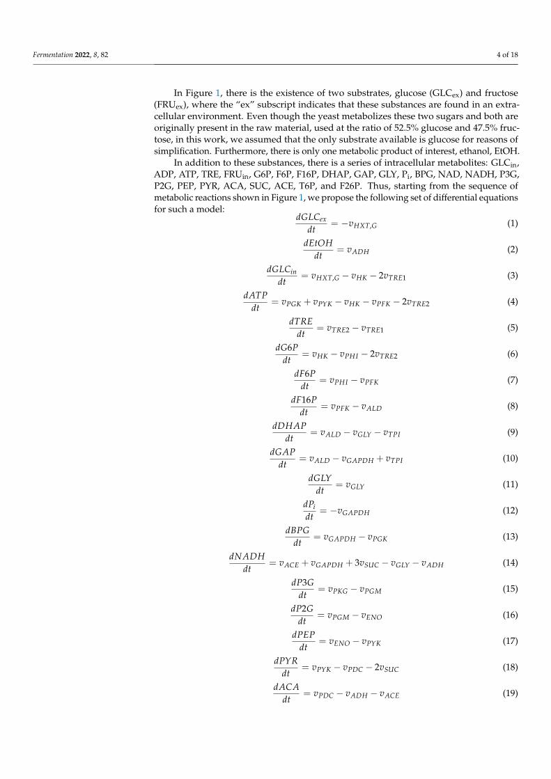
In Figure 1, there is the existence of two substrates, glucose (GLCex) and fructose(FRUex), where the “ex” subscript indicates that these substances are found in an extra-cellular environment. Even though the yeast metabolizes these two sugars and both areoriginally present in the raw material, used at the ratio of 52.5% glucose and 47.5% fruc-tose, in this work, we assumed that the only substrate available is glucose for reasons ofsimplification. Furthermore, there is only one metabolic product of interest, ethanol, EtOH.

In addition to these substances, there is a series of intracellular metabolites: GLCin,ADP, ATP, TRE, FRUin, G6P, F6P, F16P, DHAP, GAP, GLY, Pi, BPG, NAD, NADH, P3G,P2G, PEP, PYR, ACA, SUC, ACE, T6P, and F26P. Thus, starting from the sequence ofmetabolic reactions shown in Figure 1, we propose the following set of differential equationsfor such a model:

dGLCex

dt= −vHXT,G (1)

dEtOHdt

= vADH (2)

dGLCindt

= vHXT,G − vHK − 2vTRE1 (3)

dATPdt

= vPGK + vPYK − vHK − vPFK − 2vTRE2 (4)

dTREdt

= vTRE2 − vTRE1 (5)

dG6Pdt

= vHK − vPHI − 2vTRE2 (6)

dF6Pdt

= vPHI − vPFK (7)

dF16Pdt

= vPFK − vALD (8)

dDHAPdt

= vALD − vGLY − vTPI (9)

dGAPdt

= vALD − vGAPDH + vTPI (10)

dGLYdt

= vGLY (11)

dPidt

= −vGAPDH (12)

dBPGdt

= vGAPDH − vPGK (13)

dNADHdt

= vACE + vGAPDH + 3vSUC − vGLY − vADH (14)

dP3Gdt

= vPKG − vPGM (15)

dP2Gdt

= vPGM − vENO (16)

dPEPdt

= vENO − vPYK (17)

dPYRdt

= vPYK − vPDC − 2vSUC (18)

dACAdt

= vPDC − vADH − vACE (19)

Fermentation 2022, 8, 82 5 of 18

dSUCdt

= vSUC (20)

dACEdt

= vACE (21)

The model generated from Equations (1)–(21) constitutes what will be called the CRmodel, that is, the most complete model that considers the existence of ramifications inthe EMP route followed by alcoholic fermentation. On the other hand, the simplest model,called the SR model, is the model for which the velocities of Equations (5), (11), (20), and(21) will be equal to zero, that is, the SR model is the model where the EMP route andalcoholic fermentation occur directly and without deviations. Furthermore, as the focusof the present work is the development of a model for alcoholic fermentation, and cellreproduction in alcoholic fermentation in an anaerobic medium is low, we opted for thesimplified use of kinetic relationships for cell growth, as will be discussed later.

A problem that may occur when using all these reactions in a metabolic model relatesto the concentrations of energetic molecules, such as AMP, ADP, ATP, T6P, and NAD. Thesesubstances are used in numerous other reactions that occur in cell metabolism, being gener-ated and consumed, thus maintaining such substances at approximately constant levels inhealthy cells. Therefore, as chosen in the model proposed by van Eunen et al. [16], we de-cided to maintain the levels of these substances as constant in the present work. In additionto these substances, F26P is also another substance of importance in the metabolic networkin question, but it is difficult to measure and ended up having its concentration consideredas constant as well. In Table 1, we list the fixed concentrations for such substances.

Table 1. Substances with constant concentrations in the model application. Source: van Eunenet al. [16].

Substance Concentration (mM) Substance Concentration (mM)

ATP 3 T6P 0.2ADP 1 F26P 0.014AMP 0.3 NAD 1.59

In addition to constant concentrations, we need to employ a series of initial concentra-tions for the relevant metabolites in order to solve the model. The use of good initial valuesis essential for a good model response; however, finding practical values for the initialconcentration of metabolites is complex. Teusink [17] and van Eunen [16] used a similarset of initial concentrations of substances, but some concentrations used by them wereconsiderably high compared to the data presented in other works, such as Sato et al. [18],Ruoff et al. [19], Casei et al. [20], and Peeters et al. [21]. Thus, based on the data presentedin such studies, we list the initial concentrations of metabolites in Table 2 below.

Table 2. Initial concentrations of the substrate, [i]0, product, and internal metabolites from alcoholicfermentation. Source: van Eunen et al. [16]; Sato et al. [18]; Teusink et al. [17]; Ruoff et al. [19]; Caseiet al. [20]; Peeters et al. [21].

Substance (mM) [i]0 (mM) Substance (mM) [i]0 (mM)

GLCex * P3G 1.09GLCin 0.1213 P23G 0.15G6P 0.50 PEP 0.11F6P 0.20 PYR 0.25

F16P 1.80 ACA 0.04TRIO 0.50 EtOH 0.00BPG 0.05 NADH 0.29

* The initial value to be chosen.

Fermentation 2022, 8, 82 6 of 18

The importance of choosing the initial values used for solving the systems of differen-tial equations found in the present work should be highlighted. The system of differentialequations proposed to solve the problem treated in the present work consists of a set of stiffdifferential equations, which generates a highly nonlinear system of differential equations.That said, the initial conditions used in solving the problem are extremely important, sincea set of initial values can easily lead to non-convergence of values or even to mathemati-cally correct results that are unrealistic in practice. Thus, a search was carried out in otherworks in the literature for initial concentration values for the various substances found inthe system proposed here, looking for those that produced more stable and biologicallyviable results. Therefore, a series of initial values for the substances was tested in themodel proposed here, noticing three types of behaviors, used as groups. The first group ofvalues included values of the initial concentration of certain metabolites, such as fructose-6-phosphate and pyruvate, which presented a very abrupt drop in concentrations in theinitial periods of fermentation, generating instability in the resolution, including negativeconcentrations. The second group of values included initial values that presented the oppo-site behavior, with an abrupt growth, generating concentrations biologically impossible tosee inside a cell—in the case of glucose-6-phosphate, fructose-1,6-bisphosphate, and trioses.The third group of values generated a more stable response consistent with data found inthe literature.

The initial substrate concentration in the present work varied between 30 g/L, 75 g/L,and 100 g/L. Another point we considered in this type of modeling is related to the cellconcentration. Under anaerobic conditions with low substrate concentrations, Saccharomycescerevisiae does not reproduce as much as under aerobic conditions. This considerationmakes it common for the cell concentration to be set as constant in such fermentationassays; however, as the cell concentration relates directly to the enzyme concentration, theconsideration of a variable amount of cells certainly enriches the model. Therefore, in thepresent model, we considered the cell concentration to follow the Andrews and Noackmodel, a simple model derived from the Monod model that showed a good predictivecapacity according to the work of Kostov et al. [8].

µ =1X

dXdt

= µ0[S]

1 + KSXS + S

KiS

(22)

This Andrews and Noack model is a black box model, that is, it does not consider pe-culiarities regarding the fungus metabolism. The growth metabolism is extremely complexand not addressed in the present work. The purpose of inserting this growth model is justto add dynamic behavior to the cell concentration. Furthermore, the Andrews and Noackmodel takes into account a possible inhibitory effect on cell growth due to excess substratein the culture medium, something important to take into account, since inhibitory effectson growth tend to appear even at lower levels of the substrate concentration.

With this, it is possible to start solving the system of equations. Both the kinetic equa-tions and the parameters used are in the Appendices A and B. The values of the kineticparameters for the action of the enzymes hexokinase (HK), phosphohexoisomerase (PHI),phosphofructokinase (PFK), fructose-bisphosphate aldolase (ALD), triose-phosphateisomerase (TPI), glyceraldehyde-3-phosphate dehydrogenase (GAPDH), bisphospho-glycerate mutase (PGK), phosphoglycerate mutase (PGM), enolase (ENO), pyruvatok-inase (PYK), pyruvate decarboxylase (PDC), and alcohol dehydrogenase (ADH) weretaken from Teusink et al. [22], Berthels et al. [23], van Eunen et al. [16], and Smallboneet al. [24].

Fermentation 2022, 8, 82 7 of 18

For HXT, there is the limiting step of the fermentation process: that is, it is expectedthat this step presents a greater variety of possible values than the other steps. Thus, wecarried out a manual search within a range of possible values for the kinetic constants,coming from the same works mentioned above. These constants are called apparent, as theyvary with the initial conditions of the fermentation process, and the model proposed heredoes not aim to incorporate repression or expression terms into the behavior of proteins.

The models were validated using data from Acorsi et al. [25]. In the batch fermentationcarried out in such works, the culture media used were prepared based on diluted finalsugarcane honey and inverted at 50 ◦C with the addition of 1 mL of invertase solution foreach 100 mL of the desired medium, where the enzyme solution contained 4 mg/mL ofinvertase. The raw material was provided by “Usina Santa Terezinha Iguatemi Unit” andcollected directly from the output of the continuous honey centrifuge B, being the sameraw material that supplies the plant’s fermentation vats.

We carried out fermentation tests from 30 to 100 g/L in a BIOSTAT® B reactor, abioreactor with a 5 L-capacity vessel with built-in mechanical agitation and temperaturecontrol, with the temperature controlled by the water distribution. In addition, this bioreac-tor features an automatic sampler, which makes sample collection possible, considerablyreducing the risk of contamination during sampling. The other fermentations used smallerKitasato-type reactors. We carried out the fermentation tests at a temperature of 32 ◦C [25].

For the quantification of sugars present in the fermentation medium at a given moment,as the wort used presented its sugars in the form of glucose and fruit, a DNS methodologymodified for a wavelength of 600 nm was used [26–28]. For the quantification of ethanol, aVARIAN 330 with a Porapak Q column was used. The inlet and detector were kept at 120◦C, and the column was kept at 100 ◦C. Helium was used as a carrier gas, at a flow rate of18.75 mL/min. Finally, 1 µL samples were injected to obtain the amount of ethanol present.

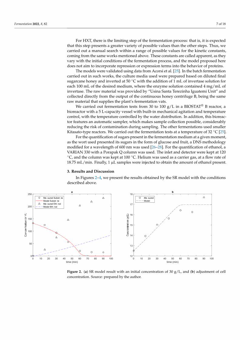
3. Results and Discussion

In Figures 2–4, we present the results obtained by the SR model with the conditionsdescribed above.

Fermentation 2022, 8, x FOR PEER REVIEW 7 of 18

they vary with the initial conditions of the fermentation process, and the model proposed here does not aim to incorporate repression or expression terms into the behavior of proteins.

The models were validated using data from Acorsi et al. [25]. In the batch fermentation carried out in such works, the culture media used were prepared based on diluted final sugarcane honey and inverted at 50 °C with the addition of 1 mL of invertase solution for each 100 mL of the desired medium, where the enzyme solution contained 4 mg/mL of invertase. The raw material was provided by “Usina Santa Terezinha Iguatemi Unit” and collected directly from the output of the continuous honey centrifuge B, being the same raw material that supplies the plant’s fermentation vats.

We carried out fermentation tests from 30 to 100 g/L in a BIOSTAT® B reactor, a bioreactor with a 5 L-capacity vessel with built-in mechanical agitation and temperature control, with the temperature controlled by the water distribution. In addition, this bioreactor features an automatic sampler, which makes sample collection possible, considerably reducing the risk of contamination during sampling. The other fermentations used smaller Kitasato-type reactors. We carried out the fermentation tests at a temperature of 32 °C [25].

For the quantification of sugars present in the fermentation medium at a given moment, as the wort used presented its sugars in the form of glucose and fruit, a DNS methodology modified for a wavelength of 600 nm was used [26–28]. For the quantification of ethanol, a VARIAN 330 with a Porapak Q column was used. The inlet and detector were kept at 120 °C, and the column was kept at 100 °C. Helium was used as a carrier gas, at a flow rate of 18.75 mL/min. Finally, 1 µL samples were injected to obtain the amount of ethanol present.

3. Results and Discussion In Figures 2–4, we present the results obtained by the SR model with the conditions

described above.

Figure 2. (a) SR model result with an initial concentration of 30 g/L, and (b) adjustment of cell con-centration. Source: prepared by the author.

0 10 20 30 40 50 60 70 80 90 100time (min)

0

50

100

150

200

250a

Measured SubstrateModel SubstrateMeasured EthanolModel Ethanol

0 10 20 30 40 50 60 70 80 90 100time (min)

12

13

14

15

16

17

18b

MeasuredModel

Figure 2. (a) SR model result with an initial concentration of 30 g/L, and (b) adjustment of cellconcentration. Source: prepared by the author.

Fermentation 2022, 8, 82 8 of 18Fermentation 2022, 8, x FOR PEER REVIEW 8 of 18

Figure 3. (a) SR model result with an initial concentration of 75 g/L, and (b) adjustment of cell concentration. Source: prepared by the author.

Figure 4. (a) SR model result with an initial concentration of 100 g/L, and (b) adjustment of cell concentration. Source: prepared by the author.

In the three cases analyzed, we obtained a good fit for both the cell concentration and substrate consumption. However, for product formation, the results found were very poor: in none of the cases was product formation minimally close to the experimental values.

When we added the ramifications to the model, that is, when we run the model with branches, we obtained the results shown in Figures 5–7.

0 20 40 60 80 100 120 140 160 180time (min)

0

100

200

300

400

500

600

700a

Measured SubstrateModel SubstrateMeasured EthanolModel Ethanol

0 20 40 60 80 100 120 140 160 180time (min)

13.5

14

14.5

15

15.5

16

16.5

17

17.5

18b

MeasuredModel

0 50 100 150 200 250 300time (min)

0

200

400

600

800

1000

1200a

Measured SubstrateModel SubstrateMeasured EthanolModel Ethanol

0 50 100 150 200 250 300time (min)

13

13.5

14

14.5

15

15.5

16b

MeasuredModel

Figure 3. (a) SR model result with an initial concentration of 75 g/L, and (b) adjustment of cellconcentration. Source: prepared by the author.

Fermentation 2022, 8, x FOR PEER REVIEW 8 of 18

Figure 3. (a) SR model result with an initial concentration of 75 g/L, and (b) adjustment of cell concentration. Source: prepared by the author.

Figure 4. (a) SR model result with an initial concentration of 100 g/L, and (b) adjustment of cell concentration. Source: prepared by the author.

In the three cases analyzed, we obtained a good fit for both the cell concentration and substrate consumption. However, for product formation, the results found were very poor: in none of the cases was product formation minimally close to the experimental values.

When we added the ramifications to the model, that is, when we run the model with branches, we obtained the results shown in Figures 5–7.

0 20 40 60 80 100 120 140 160 180time (min)

0

100

200

300

400

500

600

700a

Measured SubstrateModel SubstrateMeasured EthanolModel Ethanol

0 20 40 60 80 100 120 140 160 180time (min)

13.5

14

14.5

15

15.5

16

16.5

17

17.5

18b

MeasuredModel

0 50 100 150 200 250 300time (min)

0

200

400

600

800

1000

1200a

Measured SubstrateModel SubstrateMeasured EthanolModel Ethanol

0 50 100 150 200 250 300time (min)

13

13.5

14

14.5

15

15.5

16b

MeasuredModel

Figure 4. (a) SR model result with an initial concentration of 100 g/L, and (b) adjustment of cellconcentration. Source: prepared by the author.

In the three cases analyzed, we obtained a good fit for both the cell concentration andsubstrate consumption. However, for product formation, the results found were very poor:in none of the cases was product formation minimally close to the experimental values.

When we added the ramifications to the model, that is, when we run the model withbranches, we obtained the results shown in Figures 5–7.

Note that the prediction of product formation improves considerably with the additionof branches, even using extremely simple expressions such as those assumed in the presentwork. Thus, there is an indication that the addition of well-described ramifications to themetabolic model can further improve the results.

Fermentation 2022, 8, 82 9 of 18Fermentation 2022, 8, x FOR PEER REVIEW 9 of 18

Figure 5. (a) Result of the CR model with an initial concentration of 30 g/L, and (b) adjustment of cell concentration. Source: prepared by the author.

Figure 6. (a) Result of the CR model with an initial concentration of 75 g/L, and (b) adjustment of cell concentration. Source: prepared by the author.

Figure 7. (a) Result of the CR model with an initial concentration of 100 g/L, and (b) adjustment of cell concentration. Source: prepared by the author.

Note that the prediction of product formation improves considerably with the addition of branches, even using extremely simple expressions such as those assumed in the present work. Thus, there is an indication that the addition of well-described ramifications to the metabolic model can further improve the results.

0 10 20 30 40 50 60 70 80 90 100time (min)

0

50

100

150

200

250a

Measured SubstrateModel SubstrateMeasured EthanolModel Ethanol

0 10 20 30 40 50 60 70 80 90 100time (min)

12

13

14

15

16

17

18b

MeasuredModel

0 20 40 60 80 100 120 140 160 180time (min)

0

100

200

300

400

500

600

700

800a

Measured SubstrateModel SubstrateMeasured EthanolModel Ethanol

0 20 40 60 80 100 120 140 160 180time (min)

13.5

14

14.5

15

15.5

16

16.5

17

17.5

18b

MeasuredModel

0 50 100 150 200 250 300time (min)

0

200

400

600

800

1000

1200a

Measured SubstrateModel SubstrateMeasured EthanolModel Ethanol

0 50 100 150 200 250 300t (min)

13

13.5

14

14.5

15

15.5

16

Con

cent

raçã

o (g

/L)

b

Figure 5. (a) Result of the CR model with an initial concentration of 30 g/L, and (b) adjustment ofcell concentration. Source: prepared by the author.

Fermentation 2022, 8, x FOR PEER REVIEW 9 of 18

Figure 5. (a) Result of the CR model with an initial concentration of 30 g/L, and (b) adjustment of cell concentration. Source: prepared by the author.

Figure 6. (a) Result of the CR model with an initial concentration of 75 g/L, and (b) adjustment of cell concentration. Source: prepared by the author.

Figure 7. (a) Result of the CR model with an initial concentration of 100 g/L, and (b) adjustment of cell concentration. Source: prepared by the author.

Note that the prediction of product formation improves considerably with the addition of branches, even using extremely simple expressions such as those assumed in the present work. Thus, there is an indication that the addition of well-described ramifications to the metabolic model can further improve the results.

0 10 20 30 40 50 60 70 80 90 100time (min)

0

50

100

150

200

250a

Measured SubstrateModel SubstrateMeasured EthanolModel Ethanol

0 10 20 30 40 50 60 70 80 90 100time (min)

12

13

14

15

16

17

18b

MeasuredModel

0 20 40 60 80 100 120 140 160 180time (min)

0

100

200

300

400

500

600

700

800a

Measured SubstrateModel SubstrateMeasured EthanolModel Ethanol

0 20 40 60 80 100 120 140 160 180time (min)

13.5

14

14.5

15

15.5

16

16.5

17

17.5

18b

MeasuredModel

0 50 100 150 200 250 300time (min)

0

200

400

600

800

1000

1200a

Measured SubstrateModel SubstrateMeasured EthanolModel Ethanol

0 50 100 150 200 250 300t (min)

13

13.5

14

14.5

15

15.5

16

Con

cent

raçã

o (g

/L)

b

Figure 6. (a) Result of the CR model with an initial concentration of 75 g/L, and (b) adjustment ofcell concentration. Source: prepared by the author.

Fermentation 2022, 8, x FOR PEER REVIEW 9 of 18

Figure 5. (a) Result of the CR model with an initial concentration of 30 g/L, and (b) adjustment of cell concentration. Source: prepared by the author.

Figure 6. (a) Result of the CR model with an initial concentration of 75 g/L, and (b) adjustment of cell concentration. Source: prepared by the author.

Figure 7. (a) Result of the CR model with an initial concentration of 100 g/L, and (b) adjustment of cell concentration. Source: prepared by the author.

Note that the prediction of product formation improves considerably with the addition of branches, even using extremely simple expressions such as those assumed in the present work. Thus, there is an indication that the addition of well-described ramifications to the metabolic model can further improve the results.

0 10 20 30 40 50 60 70 80 90 100time (min)

0

50

100

150

200

250a

Measured SubstrateModel SubstrateMeasured EthanolModel Ethanol

0 10 20 30 40 50 60 70 80 90 100time (min)

12

13

14

15

16

17

18b

MeasuredModel

0 20 40 60 80 100 120 140 160 180time (min)

0

100

200

300

400

500

600

700

800a

Measured SubstrateModel SubstrateMeasured EthanolModel Ethanol

0 20 40 60 80 100 120 140 160 180time (min)

13.5

14

14.5

15

15.5

16

16.5

17

17.5

18b

MeasuredModel

0 50 100 150 200 250 300time (min)

0

200

400

600

800

1000

1200a

Measured SubstrateModel SubstrateMeasured EthanolModel Ethanol

0 50 100 150 200 250 300t (min)

13

13.5

14

14.5

15

15.5

16

Con

cent

raçã

o (g

/L)

b

Figure 7. (a) Result of the CR model with an initial concentration of 100 g/L, and (b) adjustment ofcell concentration. Source: prepared by the author.

Fermentation 2022, 8, 82 10 of 18

Considering the difference obtained between the models, we can compare the kineticconstants that most interfere in the response of the models, starting with the kinetic con-stants of the limiting step of alcoholic fermentation, i.e., the transport of glucose from theextracellular medium to the intracellular medium. Starting with the saturation constantKGLC, we noticed that the increase in the concentration of the substrate in the mediumdecreased the microorganism’s affinity for glucose: in the analyzed fermentations, medium-to low-affinity transporters were found, with this constant varying from 6.95 to 54 mM. Inboth models, we found the highest affinity in the situation with the lowest substrate concen-tration, matching the need for yeast cells to facilitate substrate entry under nutrient-scarceconditions. Furthermore, we noted that the CR model needed slightly higher saturationconstants, except in the fermentation with a higher initial substrate concentration. Fur-thermore, in the more concentrated fermentation, the saturation constant for the two caseswith a greater availability of microorganisms in the CR model was repeated, something notseen in the SR model. This point may also indicate the need to investigate whether yeastcan express different transport proteins at different stages of fermentation, according tothe availability of the substrate in the medium: in the present work, the concentrationsof relevant enzymes and proteins were constants, since including kinetic expressions fortheir expression in different phases of the fermentation process is a future step for thedevelopment of metabolic models.

As for the maximum substrate conversion speed, there was an increase in this parame-ter with increasing concentration, and in the case of the CR model, the maximum glucosetransport speed was reached at a lower concentration of substrate available in the medium.Better results for substrate consumption can eventually be obtained by working withoutconsidering a very simple substrate composed only of glucose.

4. Conclusions

The present work aimed to propose a model for a batch alcoholic fermentation processusing a series of kinetic equations derived from the metabolism of Saccharomyces cerevisiae.Considering the ease and efficiency of the fungus Saccharomyces cerevisiae in carrying outalcoholic fermentation, in addition to the fact that this fungus is a quasi-model organism, wesuccessfully assembled a model capable of predicting sugar consumption and the formationof ethanol using the relevant metabolic network. This setup was certainly simple becausethe fungus considered in the present study is a quasi-model microorganism, and the centralmetabolic route, the EMP route, is well studied. The biggest difficulties arose with theramifications of this route, which have not been sufficiently studied and lack information.However, even the simplified use of these ramifications showed an improvement in theresults of the proposed models, especially for the formation of ethanol, which was closer toreality with the CR model. This work can still be improved by giving more detail to thekinetics of the relevant branches. Andrews and Noack’s model sufficiently represents cellgrowth, but it is a black box model; if we add the kinetic relationships from metabolism, itscontribution would be improved. Thus, we have in our hands a basic metabolic model thatshows promise for the representation and study of batch alcoholic fermentation, which canbe improved and optimized in the future.

Author Contributions: Conceptualization, R.L.A. and M.Y.G.D.G.; methodology, R.L.A., J.E.O. andC.M.G.A.; software, R.L.A. and C.M.G.A.; validation, R.L.A.; formal analysis, R.L.A.; investigation,R.L.A. and M.Y.G.D.G.; resources, R.L.A. and M.Y.G.D.G.; data curation, R.L.A., J.E.O.; writing—original draft preparation, R.L.A. and M.Y.G.D.G. and C.M.G.A.; writing—review and editing,R.L.A. and M.Y.G.D.G.; visualization, R.L.A. and J.E.O.; supervision, J.E.O. and C.M.G.A.; projectadministration, R.L.A. and J.E.O.; funding acquisition, R.L.A. and M.Y.G.D.G. All authors have readand agreed to the published version of the manuscript.

Funding: This study was funded by the Coordenação de Aperfeiçoamento de Pessoal de NívelSuperior-Brasil (CAPES)-Finance Code 001-and by Conselho Nacional de Desenvolvimento Científicoe Tecnológico-CNPq (Grant Number 162382/2018-9). The APC was funded by This work was

Fermentation 2022, 8, 82 11 of 18

partially supported by Conselho Nacional de Desenvolvimento Científico e Tecnológico-CNPq (GrantNumber 162382/2018-9).

Conflicts of Interest: The authors declare no conflict of interest.

List of Acronyms and Abbreviations

ACA AcetaldehydeACE AcetateADH Alcohol dehydrogenaseADP Adenosine diphosphateALD AldolaseART Total reducing sugarsATP Adenosine triphosphateBPG 1,3-bisphosphoglycerateDHAP Dihydroxyacetone-phosphateEMP Embden–Meyerhof–Parnas RouteENO EnolaseEtOH Ethanolex When used as a subscript, it indicates an extracellular substanceFK FructokinasesF16P β-D-fructose-1,6-bisphosphateF26P Fructose-2,6-bisphosphateF6P β-D-fructose-6-phosphateFRU FructoseG1P α-D-Glucose-1-phosphateG3PDH Glycerol-3-Phosphate DehydrogenaseG6P α-D-Glucose-6-phosphateGAP Glyceraldehyde-3-phosphateGAPDH Glyceraldehyde-3-phosphate dehydrogenaseGLCex α-D-Extracellular glucoseGLCin α-D-Intracellular glucoseGLY Glycerolgr Kinetic parameter of the PFK enzymeHK HexokinaseHXT Large family of hexose transportersin When used as a subscript, it indicates an intracellular substancePDC Pyruvate decarboxylaseP2G 2-phosphoglycerateP3G 3-phosphoglyceratePEP PhosphoenolpyruvatePF Pentose-phosphate routePFK PhosphofructokinasePGK Phosphoglycerate KinasePGM PhosphoglyceratomutasePHI PhosphohexoisomerasePYR PyruvatePYK PyruvatokinaseSUCC SuccinateT6P Trehalose-6-phosphateTPI Triose-phosphate-isomeraseTRE TrehaloseTRIO or Trio-P Triose-phosphateΓ Ratio for the mass action

Appendix A. Kinetic Equations Used

Since it is expected that this process of GLC entry into the intracellular environment issimilar to an enzymatic process, as it is a process of facilitated diffusion, Teusink et al. [17]

Fermentation 2022, 8, 82 12 of 18

presented the following symmetric carrier model for the speed of glucose transport to theintracellular medium, vHXT :

vHXT,G = VmHXT[GLCex]− [GLCin]

KM,GLC + [GLCex] + [GLCin] +Kic

KM,GLC[GLCex][GLCin]

(A1)

For the reaction catalyzed by HK, van Eunen et al. [16] proposed a model with allostericregulation and the action of trehalose-6-phosphate, T6P:

vHK = Vmax

[GLCin ][ATP]KM,HKGLCKM,HKATP

− [G6P][ADP]KM,HKGLCKM,HKATPKeq,HK(

1 + [GLCin ]KM,HKGLC

+ [G6P]KM,HKG6P

+ [T6P]KM,HKT6P

)(1 + [ATP]

KM,HKATP+ [ADP]

KM,HKADP

) (A2)

For the action of phosphohexoisomerase, a relatively simple equation was used,representing the reversible kinetic equation of a substrate and a product:

vPHI = Vmax

[G6P]KM,PHIG6P

− [F6P]KM,PHIF6PKeq,PHI

1 + [G6P]KM,PHIG6P

+ [F6P]KM,PHIF6P

(A3)

Phosphofructokinase is a widely studied enzyme and much of its structure is known,but mathematically modeling its action is something extremely complex. Such is thelevel of complexity of the kinetic modeling of this enzyme that Teusink et al. [17] refer tosuch a process as the modelers’ nightmare. This enzyme has a huge amount of regulatoryinteractions, which means that the model of this enzyme needs to be considerably simplifiedto become practicable: no known model available for this enzyme can describe all the effectsand interactions. Among the simplifications used in modeling this route, Teusink et al. [17]and van Eunen et al. [16] highlighted the hypothesis that some substances present constantconcentrations throughout the fermentation process: ammonia, phosphate, protons, andthe substance fructose-2,6-bisphosphate.

Among the regulatory effects known to act on this enzyme, the following three standout: the cooperative binding of fructose-6-phosphate for the proper functioning of theenzyme, the inhibitory effect of ATP, and activation linked to adenosine monophosphate,AMP. Another considerable effect observed in the behavior of PFK is the lack of inhibi-tion caused by its product, fructose-1,6-bisphosphate. However, this product negativelyinterferes with the activation of the enzyme produced by fructose-2,6-bisphosphate [16,17].

We expect that the kinetic model of the action of this enzyme includes the concen-trations of the substances F6P, F16P, F26P, AMP, and ATP. Assuming that the effects ofAMP, F26P, and F16P and the inhibitory effect of ATP are mediated by a shift in the balancebetween a tense and a relaxed state, the kinetics of this enzyme will be affected by anequilibrium constant between these states, symbolized by L. As the tense state is the statewhere the enzyme is inactive because there is no binding to F6P, Teusink et al. [17] and vanEunen et al. [16] proposed the use of the following kinetic model:

vPFK = VmaxgRλ1λ2RR2 + LT2 (A4)

Being that

λ1 =[F6P]

KM,PFKF6P(A5)

λ2 =[ATP]

KM,PFKATP(A6)

R = 1 + λ1λ2 + gRλ1λ2 (A7)

T = 1 + cATPλ2 (A8)

Fermentation 2022, 8, 82 13 of 18

L = L0

(1 + Ci,ATPα1

1 + α1

)2(1 + Ci,AMPα2

1 + α2

)2(1 + Ci,F2,6Pα3 + Ci,F1,6Pα4

1 + α3 + α4

)2(A9)

α1 =[ATP]

KPFK,ATP(A10)

α2 =[AMP]

KPFK,AMP(A11)

α3 =[F26P]

KPFK,F26P(A12)

α4 =[F16P]

KPFK,F16P(A13)

Of the constants to be used in this model, we have gR = 5, 12 and L0 = 0.66, accordingto Teusink et al. [17] and van Eunen et al. [16].

For the action of the ALD enzyme, it is generally assumed to be a “uni–bi”-orderedkinetics, and this mechanism is represented by the following equation:

vALD = Vmax

aKa

(1 − Γ

Keq,ALD

)1 + a

KM,F16p+ p

Kp+ q

Kq+ aq

KaKiq+ pq

KpKq

(A14)

In (A14), it represents the F16P concentration, the DHAP concentration, and the GAPconcentration. Furthermore, Ki indicates the saturation constant of this enzyme for each ofthe substances involved, and Kiq indicates an inhibition constant. This equation expandsin a particular way, which we show below, taking into account a different way of writingthe GAP concentration [16,17,24].

There are not many studies of this enzyme from Saccharomyces cerevisiae contributingthe kinetic data of the model presented in (A14). The parameter with the most values foundin the literature is the saturation constant for F16P, which is around 0.30 mM [16,17,24].

For the glycerol branch, Teusink et al. [17] indicated that the flux is completely con-trolled by the action of the G3PDH enzyme. The mechanism of action of this enzyme isnot very well known yet, and some modeling works use a model similar to the action ofHK, that is, a reversible reaction model with two substrates and two products, shown byEquation (A2), DHAP and NADH being the substrates, and glycerol-3-phosphate, GLY,and NAD+ the products.

To close the glycolysis preparation step, DHAP must be converted into GAP. Thisreaction is also mediated by a single enzyme, TPI. The kinetics of this TPI enzyme present,according to Smallbone et al. [24], direct the inhibition of DHAP in a particular way:

vTPI = Vmax[DHAP]

KM,TPIDHAP[DHAP](

1 +([DHAP]

4

)4) (A15)

However, it is common for this reaction to be considered in equilibrium, so it iscustomary not to consider the action of this enzyme in the glycolytic model. For such acondition, the equilibrium constant is used:

Keq,TPI =[GAP][DHAP]

(A16)

Since the value of the constant is around 0.045, the total amount of triose-phosphate,TRIO, in the cell is defined as

[TRIO] = [GAP] + [DHAP] (A17)

Fermentation 2022, 8, 82 14 of 18

As a mathematical model for the GAPDH enzyme, a relationship similar to that ofthe action of HK can be used. However, van Eunen et al. [16] suggested improving thisrelationship with the use of two distinct maximum speeds, one for the direct reaction, V+

max,and one for the reverse reaction, V−

max:

vGAPDH =V+

max[GAP]([NAD]−[NADH])

KM,GADPHGAPKM,GADPHNAD− V−

max[BPG][NADH]

KM,GADPHBPGKM,GADPHNADH(1 + [GAP]

KM,GADPHGAP+ [BPG]

KM,GADPHBPG

)(1 + [NAD]

KM,GADPHNAD+ [NADH]

KM,GADPHNADH

) (A18)

The next enzyme, PGK, presents a complicated kinetic study, according to Teusinket al. [17], because the BPG substrate is very unstable. Thus, it is more common to have datafrom the reverse reaction catalyzed by PGK, which is where most of the kinetic data forthis reaction are taken from. Thus, it is customary to use the kinetic model of the reversiblereaction with two substrates and two products for this enzyme, the substrates being BPGand ADP, and the products P3G and ATP, as shown in Equation (A19):

vPGK = Vmax

Keq,PGK [BPG][ADP]KM,PGKBPGKM,PGKADP

− [P3G][ATP]KM,PGK3PGKM,PGKATP(

1 + [BPG]KM,PGKBPG

+ [P3G]KM,PGK3PG

)(1 + [ADP]

KM,PGKADP+ [ATP]

KM,PGKATP

) (A19)

In the next reaction, we have the action of PGM, an enzyme that is dependent on theconcentration of 2,3-diphosphoglycerate. To circumvent this dependence, thus reducing themodel’s variables, some authors simply assume that the enzyme is already saturated withthis substance at concentrations at micromolar levels. Even with these considerations, thereis considerable variability in the values of the saturation constants of this reaction for P3G.Therefore, such a reaction can be modeled using a simple reversible reaction mechanism,with one substrate and one product only, as shown in the reaction below:

vPGM = Vmax

[P3G]KM,PGMP3G

− [P2G]KM,PGMP3GKeq,PGM

1 + [P2G]KM,PGMP3G

+ [P2G]KM,PGMP2G

(A20)

The conversion of P2G to PEP is one of the last reactions of glycolysis, a reactioncatalyzed, under conditions of low growth, by only one enzyme, enolase (ENO). Kinetically,the model used to assess the action of this enzyme is similar to that used in PGM modeling,that is, a reversible reaction model with a substrate and a product:

vENO = Vmax

[P2G]KM,ENOP2G

− [PEP]KM,ENOPEPKeq,ENO

1 + [P2G]KM,ENOP2G

+ [PEP]KM,ENOPEP

(A21)

Finally, closing the glycolysis, the last reaction consists of the conversion of PEP toPYR by a reaction catalyzed by the PYK enzyme. A striking feature of this enzyme is thestrong dependence on F16P for its activation: under conditions of high concentrations ofF16P, it exhibits hyperbolic behavior and a good affinity with PEP. This condition of a highF16P concentration was determined to be around 0.5 mM F16P, which is 10 times lowerthan the common value of such a metabolite in a cell under normal fermentative conditions.Therefore, hyperbolic modeling may prove adequate for this enzyme, the reaction beingreversible, with two substrates and two products, and with F16P presenting an allostericregulation, as shown in the equation below, proposed by van Eunen et al. [16]:

vPYK = Vmax

[PEP]KM,PYKPEP

([PEP]

KM,PYKPEP+ 1)n−1

L0,PYK

([ATP]

KM,PYKATP+1

[F16P]KM,PYKF16P

+1

)n

+(

[PEP]KM,PYKPEP

+ 1)n

ADPADP + KM,PYKADP

(A22)

Fermentation 2022, 8, 82 15 of 18

Now, the alcoholic fermentation begins. This step consists of only two reactions thatwill lead to pyruvate being converted to ethanol, and the first metabolite to appear inthis phase is acetaldehyde, produced by a reaction catalyzed by the PDC enzyme. Thisenzyme has cooperative kinetics, linked to the concentration of PYR in the medium, beinga relatively simple model:

vPDC = Vmax[PYR]nPDC

KM,PDCPYR

([PYR]nPDC

KM,PDCPYRnPDC + 1

) (A23)

Finally, there is the last reaction of the metabolic network under study: the conversionof ACA into ETOH and carbon dioxide by the action of ADH enzymes, whose kineticbehavior is considerably complex, being a bi-ordered mechanism with binding by a cofactorfirst:

vADH = −VmaxαADH

1 + βADH + γADH + δADH + εADH(A24)

αADH =([NAD]− [NADH])[EtOH]

Ki,ADHNADKM,ADHEtOH− [NADH][ACA]

Ki,ADHNADKM,ADHEtOHKeq,ADH(A25)

βADH =[NAD]− [NADH]

Ki,ADHNAD+

KM,ADHNAD[EtOH]

Ki,ADHNADKM,ADHEtOH+

KM,ADHNADH [ACA]

Ki,ADHNADKM,ADHACA(A26)

γADH =([NAD]− [NADH])[EtOH]

Ki,ADHNADKM,ADHEtOH+

KM,ADHNADH([NAD]− [NADH])[ACA]

Ki,ADHNADKi,ADHNADHKM,ADHACA(A27)

δADH =[NADH]

Ki,ADHNADH+

KM,ADHNAD[NADH][EtOH]

Ki,ADHNADKi,ADHNADHKM,ADHEtOH+

[NADH][ACA]

Ki,ADHNADHKM,ADHACA(A28)

εADH =([NAD]− [NADH])[EtOH][ACA]

Ki,ADHNADKM,ADHEtOHKi,ADHACA+

[NADH][EtOH][ACA]

Ki,ADHEtOHKi,ADHNADHKM,ADHACA(A29)

ADH lacks data for inhibition constants in the literature, but there are several studieson the saturation constant for different substrates at a pH of around 9.0 and differenttemperatures, ranging from 10 to 30 ◦C.

Appendix B. Tables with Kinetic Parameters Used in the Model

Table A1. Apparent turnover numbers (nmol min−1 mg−1s ) of the SR and CR models according to

the initial fermentation concentration.

Protein 30 (g L−1) 75 (g L−1) 100 (g L−1)

HXT 128,929 165,200 167,980HK 377,554 354,849 370,000PHI 874,243 877,000 877,000PFK 208,993 209,980 210,000ALD 535,408 535,170 535,500

GAPDH+ 1,973,459 2,084,595 2,090,000GAPDH− 912,296 840,000 840,000

PGK 2,125,000 2,090,000 2,160,000PGM 748,124 840,000 854,609ENO 345,772 384,832 439,400PYK 646,674 718,020 755,000PDC 172,954 172,062 172,000ADH 143,204 143,000 143,000

Fermentation 2022, 8, 82 16 of 18

Table A2. Apparent saturation constants K (mM), equilibrium constants, and other constants of the SRand CR models as a function of the substance i according to the initial concentration of fermentationin g L−1.

9 i 30 75 100

KM,HXT GLC 15,552 2735 5750KiC,HXT GLC 0.9081 0.9081 0.9081KM,HK GLC 0.02 0.018 0.02KM,HK ATP 0.25 0.25 0.25KM,HK G6P 30.00 30.00 30.00KM,HK ADP 0.24 0.24 0.24KM,HK T6P 0.20 0.20 0.15Keq,HK - 3800 3800 3800KM,PHI G6P 1.00 1.01 1.00KM,PHI F6P 0.31 0.31 0.31Keq,PHI - 0.314 0.314 0.314KM,PFK F6P 0.10 0.10 0.10KM,PFK ATP 0.71 0.71 0.71KPFK ATP 0.65 0.65 0.65KPFK AMP 0.0995 0.0995 0.0995KPFK F16P 0.111 0.111 0.111KPFK F26P 6.82·10−4 6.82·10−4 6.82·10−4

ci,PFK ATP 3 3 3Ci,PFK ATP 100 100 100Ci,PFK AMP 0.0845 0.0845 0.0845Ci,PFK F16P 0.397 0.397 0.397Ci,PFK F26P 0.0174 0.0174 0.0174gR,PFK - 5.12 5.12 5.12L0,PFK - 0.66 0.66 0.66

KM,ALD F16P 0.055 0.055 0.055KM,ALD GAP 2.00 2.00 2.00KM,ALD DHAP 2.40 2.40 2.40Ki,ALD GAP 10 10 10Keq,ALD - 0.069 0.069 0.069

KM,GAPDH GAP 0.21 0.21 0.21KM,GAPDH NAD 0.09 0.09 0.09KM,GAPDH BPG 1.18 1.18 1.18KM,GAPDH NADH 0.1 0.1 0.1

KM,PGK BPG 3.00·10−3 3.00·10−3 3.00·10−3

KM,PGK ADP 0.49 0.49 0.49KM,PGK 3PG 0.53 0.53 0.53KM,PGK ATP 0.30 0.30 0.30Keq,PGK - 3200 3200 3200KM,PGM P3G 1.08 1.09 1.10KM,PGM P2G 0.10 0.10 0.10Keq,PGM - 0.19 0.19 0.19KM,ENO P2G 0.050 0.050 0.050KM,ENO PEP 0.50 0.50 0.50Keq,ENO - 6.7 6.7 6.7KM,PYK PEP 0.021 0.021 0.021KM,PYK ADP 0.16 0.16 0.20KM,PYK F16P 0.2 0.2 0.2KM,PYK ATP 1.5 1.5 1.5

nPYK - 4 4 4L0,PYK - 60,000 60,000 60,000

Fermentation 2022, 8, 82 17 of 18

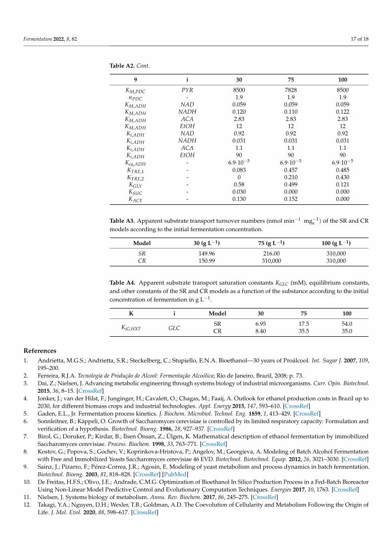
Table A2. Cont.

9 i 30 75 100

KM,PDC PYR 8500 7828 8500nPDC - 1.9 1.9 1.9

KM,ADH NAD 0.059 0.059 0.059KM,ADH NADH 0.120 0.110 0.122KM,ADH ACA 2.83 2.83 2.83KM,ADH EtOH 12 12 12Ki,ADH NAD 0.92 0.92 0.92Ki,ADH NADH 0.031 0.031 0.031Ki,ADH ACA 1.1 1.1 1.1Ki,ADH EtOH 90 90 90Keq,ADH - 6.9·10−5 6.9·10−5 6.9·10−5

KTRE,1 - 0.083 0.457 0.485KTRE,2 - 0 0.210 0.430KGLY - 0.58 0.499 0.121KSUC - 0.030 0.000 0.000KACE - 0.130 0.152 0.000

Table A3. Apparent substrate transport turnover numbers (nmol min−1 mg−1s ) of the SR and CR

models according to the initial fermentation concentration.

Model 30 (g L−1) 75 (g L−1) 100 (g L−1)

SR 149.96 216.00 310,000CR 150.99 310,000 310,000

Table A4. Apparent substrate transport saturation constants KGLC (mM), equilibrium constants,and other constants of the SR and CR models as a function of the substance according to the initialconcentration of fermentation in g L−1.

K i Model 30 75 100

KiG,HXT GLCSR 6.95 17.5 54.0CR 8.40 35.5 35.0

References1. Andrietta, M.G.S.; Andrietta, S.R.; Steckelberg, C.; Stupiello, E.N.A. Bioethanol—30 years of Proálcool. Int. Sugar J. 2007, 109,

195–200.2. Ferreira, R.J.A. Tecnologia de Produção de Alcool: Fermentação Alcoólica; Rio de Janeiro, Brazil, 2008; p. 73.3. Dai, Z.; Nielsen, J. Advancing metabolic engineering through systems biology of industrial microorganisms. Curr. Opin. Biotechnol.

2015, 36, 8–15. [CrossRef]4. Jonker, J.; van der Hilst, F.; Junginger, H.; Cavalett, O.; Chagas, M.; Faaij, A. Outlook for ethanol production costs in Brazil up to

2030, for different biomass crops and industrial technologies. Appl. Energy 2015, 147, 593–610. [CrossRef]5. Gaden, E.L., Jr. Fermentation process kinetics. J. Biochem. Microbiol. Technol. Eng. 1859, 1, 413–429. [CrossRef]6. Sonnleitner, B.; Käppeli, O. Growth of Saccharomyces cerevisiae is controlled by its limited respiratory capacity: Formulation and

verification of a hypothesis. Biotechnol. Bioeng. 1986, 28, 927–937. [CrossRef]7. Birol, G.; Doruker, P.; Kirdar, B.; Ilsen Önsan, Z.; Ülgen, K. Mathematical description of ethanol fermentation by immobilized

Saccharomyces cerevisiae. Process. Biochem. 1998, 33, 763–771. [CrossRef]8. Kostov, G.; Popova, S.; Gochev, V.; Koprinkova-Hristova, P.; Angelov, M.; Georgieva, A. Modeling of Batch Alcohol Fermentation

with Free and Immobilized Yeasts Saccharomyces cerevisiae 46 EVD. Biotechnol. Biotechnol. Equip. 2012, 26, 3021–3030. [CrossRef]9. Sainz, J.; Pizarro, F.; Pérez-Correa, J.R.; Agosin, E. Modeling of yeast metabolism and process dynamics in batch fermentation.

Biotechnol. Bioeng. 2003, 81, 818–828. [CrossRef] [PubMed]10. De Freitas, H.F.S.; Olivo, J.E.; Andrade, C.M.G. Optimization of Bioethanol In Silico Production Process in a Fed-Batch Bioreactor

Using Non-Linear Model Predictive Control and Evolutionary Computation Techniques. Energies 2017, 10, 1763. [CrossRef]11. Nielsen, J. Systems biology of metabolism. Annu. Rev. Biochem. 2017, 86, 245–275. [CrossRef]12. Takagi, Y.A.; Nguyen, D.H.; Wexler, T.B.; Goldman, A.D. The Coevolution of Cellularity and Metabolism Following the Origin of

Life. J. Mol. Evol. 2020, 88, 598–617. [CrossRef]

Fermentation 2022, 8, 82 18 of 18

13. Keller, M.A.; Turchyn, A.V.; Ralser, M. Non-enzymatic glycolysis, and pentosentation phosphate pathway-like reactions in aplausible Archean ocean. Mol. Syst. Biol. 2014, 10, 12. [CrossRef] [PubMed]

14. Nilsson, A.; Nielsen, J.; Palsson, B.O. Metabolic models of protein allocation call for the kinome. Cell Syst. 2017, 5, 4.15. Davidi, D.; Milo, R. Lessons on enzyme kinetics from quantitative proteomics. Curr. Opin. Biotechnol. 2017, 46, 81–89. [CrossRef]16. van Eunen, K.; Bakker, B.M. The importance and challenges of in vivo-like enzyme kinetics. Perspect. Sci. 2014, 1, 126–130.

[CrossRef]17. Teusink, B.; Passarge, J.; Reijenga, C.A.; Esgalhado, M.; van der Weijden, C.C.; Schepper, M.; Walsh, M.C.; Bakker, B.M.; Van Dam,

K.; Westerhoff, H.V.; et al. Can yeast glycolysis be understood in terms of in vitro kinetics of the constituent enzymes? Testingbiochemistry. JBIC J. Biol. Inorg. Chem. 2000, 267, 5313–5329. [CrossRef]

18. Sato, K.; Yoshida, Y.; Hirahara, T.; Ohba, T. On-line measurement of intracellular ATP of Saccharomyces cerevisiae and pyruvateduring sake mashing. J. Biosci. Bioeng. 2000, 90, 294–301. [CrossRef]

19. Ruoff, P.; Christensen, M.K.; Wolf, J.; Heinrich, R. Temperature dependency and temperature compensation in a model of yeastglycolytic oscillations. Biophys. Chem. 2003, 106, 179–192. [CrossRef]

20. Casei, E.; Mosier, N.S.; Adamec, J.; Stockdale, Z.; Ho, N.; Sedlak, M. Effect of salts on the Co-fermentation of glucose and xyloseby a genetically engineered strain of Saccharomyces cerevisiae. Biotechnol. Biofuels 2013, 6, 10. [CrossRef]

21. Peeters, K.; Van Leemputte, F.; Fischer, B.; Bonini, B.M.; Quezada, H.; Tsytlonok, M.; Haesen, D.; Vanthienen, W.; Bernardes, N.;Gonzalez-Blas, C.B.; et al. Fructose-1,6-bisphosphate couples glycolytic flux to activation of Ras. Nat. Commun. 2017, 8, 922.[CrossRef] [PubMed]

22. Teusink, B.; Diderich, J.A.; Westerhoff, H.V.; van Dam, K.; Walsch, M.C. Intracellular glucose concentration in derepressed yeastcells consuming glucose is high enough to reduce the glucose transport rate by 50%. J. Bacteriol. 1998, 180, 556–562. [CrossRef][PubMed]

23. Berthels, N.J.; Otero, R.R.C.; Bauer, F.F.; Pretorius, I.S.; Thevelein, J.M. Correlation between glucose/fructose discrepancy andhexokinase kinetic properties in different Saccharomyces cerevisiae wine yeast strains. Appl. Microbiol. Biotechnol. 2008, 77,1083–1091. [CrossRef] [PubMed]

24. Smallbone, K.; Messiha, H.L.; Carroll, K.M.; Winder, C.L.; Malys, N.; Dunn, W.B.; Murabito, E.; Swainston, N.; Dada, J.O.; Khan, F.;et al. A model of yeast glycolysis based on a consistent kinetic cha of all its enzymes. FEBS Lett. 2013, 587, 2832–2841. [CrossRef][PubMed]

25. Acorsi, R.L.; Moraes, F.F.; Olivo, J.E. Estudo da Fermentação Alcoólica Descontínua de Mel Invertido; VII EPCC: Maringá, Brasil, 2013.26. Sumner, J.B. Dinitrosalicylic acid reagent for the estimation of sugar in normal and diabetic urine. J. Biol. Chem. 1959, 47, 5–9.

[CrossRef]27. Dove, G.B., III; Wilke, C.R.; Blanch, H.W. Process Development Studies for the Enhanced Recovery of Cellulase in Cellulose

Hydrolysis. Master’s Thesis, Lawrence Berkeley Laboratory, University of California, Berkeley, CA, USA, 1981.28. Zanin, G.M.; Moraes, F.F. Tecnologia de Imobilização de Células e Enzimas Aplicada à Produção de Álcool de Biomassas. Relatório

1987, 2, 315–321.