AN INTEGRATED SUGARCANE SUPPLY CHAIN MODEL: DEVELOPMENT AND DEMONSTRATION

PETER STUTTERHEIM

Submitted in partial fulfilment of the requirements

for the degree of MSc Engineering

School of Bioresources Engineering and Environmental Hydrology

University of KwaZulu-Natal

Pietermaritzburg

South Africa

2006

DISCLAIMER

I wish to certify that the work reported in this dissertation is my own original and

unaided work except where specific acknowledgement is made.

Signed: Date:

P. Stutterheim

Supervisors:

Signed: Date:

C.N. Bezuidenhout

Signed: Date:

P.W.L. Lyne

ACKNOWLEDGEMENTS

I extend my sincere gratitude and appreciation to all those who made this masters

dissertation possible.

• Dr CN Bezuidenhout, School of Bioresources Engineering and Environmental Hydrology, University of KwaZulu-Natal, for his commitment to supervising the project, ensuring that a suitable standard was met and the work was also enjoyed.

• Prof PWL Lyne, South African Sugarcane Research Institute (SASRI), for his support and guidance throughout the project.

• Mr Steve Davis, Sugar Milling Research Institute (SMRI), for readily assisting in providing technical insight and guidance on modelling sugar milling processes.

• Dr Adrian Wynne, South African Canegrowers Association (SACGA), for providing technical assistance and access to a model which compares the economics of trashing and burning of sugarcane.

• Richard Loubser, SMRI, for providing technical information on sugarcane deterioration and access to a model for estimating the effects of sugarcane quality on factory output.

• The Department of Transport via the Eastern Centre of Transport Development for funding the project.

• The School of Bioresources Engineering for hosting the project and providing infrastructure and support.

• The following people involved at TSB Malelane and Komati Mills: Mr Roelf Venter for organising the case study, Mr Schalk Krieg, Mr Alan Williamson, Mr Clint Vermulen, Mr Nico Stoltz and Mrs Lynie van Staden.

• To the other members of the project steering committee, namely, Dr Abraham Singles (SASRI), Mr Arnoud Wienese (SMRI), Dr Brian Purchase (SMRI), Mr Eddie Meyer (SASRI), Mr Erik Dube (UND), Mr Francois Oberholzer (ICFR), Mr Mark Smith (SASRI), Dr Maurits van den Berg (SASRI) and Mr Paul Schorn (Hullets Sugar LTD).

• To family and friends for encouragement.

ii

ABSTRACT

The South African sugar industry is a large industry which relies on expensive capital

equipment to harvest, transport and process sugarcane. An average of 23 million tons of

sugarcane are annually supplied to 14 mills from over 2 000 large-scale commercial

growers and 48 000 small-scale growers. Supply chain stakeholders can benefit if

operations are successfully streamlined. Computer-based mathematical models have

been used in other industries to improve supply chains, especially in forestry, and are

expected to play an increasingly important role in future planning and management.

Management of sugar supply chains has historically focussed on generating competitive

individual supply chain components. However, inter-component optimisation generally

disregards many important intra-component interactions. Hence, efficiency

improvements may be significantly limited. Integrated supply chain modelling provides

a suitable approach for addressing this problem. The aim of this project was to develop

and demonstrate, in concept, an integrated supply chain model for the sugar industry.

Such a model could be used to address various integrated planning and management

problems throughout the supply chain. A review of existing integrated agri-supply chain

models was conducted followed by the development of CAPCONN, an integrated sugar

supply chain model framework, that incorporate all steps from field to mill back end.

CAPCONN estimates sugarcane quality, mill recovery, capacity utilisation and

production costs. Bottlenecks are highlighted and the model could contribute towards

capacity manipulation for efficiency improvements under different harvesting scenarios.

CAPCONN was demonstrated by analysing a number of scenarios in a mechanisation

case study at Komati Mill where sugarcane is currently burned and manually cut. A

total of twelve scenarios were compared, including variations in cropping system and

time of year. The model framework predicted that a decrease in sugarcane quality and

sugar recovery would occur under mechanical harvesting scenarios. Estimated

production costs were also higher, even though the transport fleet was significantly

reduced. A manually cut green (unburned) harvesting scenario showed a further

decrease in sugarcane quality and sugar recovery. Mechanical harvesting during wet

weather caused a substantial reduction in supply chain capacity and an increase in

m

production costs. CAPCONN output trends compared favourably with measured and

observed data, though the magnitude of the trends should be viewed with caution, since

the CAPCONN framework is only a prototype. This shows that it may be a suitable

diagnostic framework for analysing and investigating the sugarcane supply chain as a

single entity. With further development to a model, the CAPCONN model framework

could be used as a strategic planning tool although, one drawback is that a relatively

large number of technical inputs are required to run the model.

IV

NOTATION FOR SUPPLY CHAIN COMPONENTS AND

VARIABLES

Component

Harvest

Loading

Transport

Off loading

Preparation

Extraction

Boiler

Exhaustion

Symbol

H

L

T

OL

P

E

B

X

Variable

Sucrose

Non-sucrose

Fibre

Ash

Tops

Trash

Stalk

Quality or compound % of total produce mass

Truck payload

Weekly throughput capacity

SC constricting capacity

Throughput rate capacity

Operational throughput rate

Capacity utilisation

Effective hours operated

Unavailable operational time

Cost

Symbol

S

NS

F

A

TS

TSH

ST

a

P

C

^-min

7

y

cu t

u Tt

Units

%

%

%

%

%

%

%

%

tons

Lwk"'

t.wk"1

t.hr"1; t.day"1

t.hf'; t.day"1

%

hr.wk"1

hr.wk"

R

Note: Component and variable symbols were combined in the format Vc where V

represents the variable symbol and C represents the component symbol.

v

TABLE OF CONTENTS

DISCLAIMER i

ACKNOWLEDGEMENTS ii

ABSTRACT iii

NOTATION FOR SUPPLY CHAIN COMPONENTS AND

VARIABLES v

LIST OF TABLES ix

LIST OF FIGURES xi

1 INTRODUCTION 1 2 AN OVERVIEW OF AGRI-FORESTRY SUPPLY CHAIN

MODELS 3 2.1 Introduction 3

2.2 Agri-Forestry Supply Chains 3

2.3 Types of Models Used in Supply Chain Planning 4

2.4 Model Planning Horizon 6

2.5 Modelling in Agri-Forestry Industries 7

2.5.1 Forestry supply chain models 8

2.5.2 Agricultural supply chain modelling 9

2.6 Conclusions 11

3 A REVIEW OF SUGAR SUPPLY CHAIN MODELS 13 3.1 Introduction 13

3.2 A Review of the South African Sugar Supply Chain Physical

System 13

3.2.1 Field to mill components 14

3.2.2 A description of mill processes 18

3.3 Models for Individual Sugar Supply Chain Components 20

3.3.1 Modelling of sugarcane growth 21

3.3.2 Optimisation of sugarcane harvesting 21

3.3.3 Optimisation of sugarcane transport 23

3.3.4 Optimisation of sugarcane milling 24

3.4 Integrated Sugar Supply Chain Models 25

3.5 Conclusions 33

4 THE DEVELOPMENT OF A SUGAR SUPPLY CHAIN MODEL FRAMEWORK 34

VI

4.1 Introduction 34

4.2 Model Framework Conceptualisation 35

4.2.1 Determination of significant variables 35

4.2.2 CAPCONN operating principles 37

4.2.2.1 Symbol notation 38

4.2.2.2 Estimating component throughput capacity 40

4.2.2.3 CAPCONN's constrictor and utilisation principles 41

4.3 Model Formulation 42

4.3.1 Representing sugarcane quality and modelling deterioration in CAPCONN 43

4.3.2 Modelling different components of the supply chain 45

4.3.3.1 Harvesting (H) 47

4.3.3.2 Loading and transloading (L) 47

4.3.3.3 Extraction and road transport (T) 48

4.3.3.4 Offloading (OL) 48

4.3.3.5 Preparation (P) 48

4.3.3.6 Extraction (E) 49

4.3.3.7 Boiler (B) 50

4.3.3.8 Exhaustion (X) 51

4.3.3 Modelling economics in CAPCONN 45

4.4 Model Construction in MS Excel 54

A SUPPLY CHAIN CASE STUDY: MECHANISATION AT KOMATI MILL; METHODOLOGY AND MODEL INPUTS 56 5.1 Introduction 56

5.2 Scenarios 56

5.3 CAPCONN Configuration for Komati Mill 57

5.3.1 Cane quality 57

5.3.2 General inputs 58

5.3.3 Operational inputs 59

5.3.3.1 Harvesting impacts on sugarcane quality 59

5.3.3.2 Loading, offloading and mill yard impacts on harvested sugarcane quality 60

5.3.3.3 Harvest capacity determination 61

5.3.3.4 Loading capacity determination 62

vn

5.3.3.5 Transport capacity determination 63

5.3.3.6 Offloading capacity determination 64

5.3.3.7 Mill component capacity determination 64

5.3.3.8 Extraction and exhaustion component inputs 64

5.3.4 Cost Inputs 65

5.3.4.1 Harvest, loading and transport costing 65

5.3.4.2 Offloading costing 66

5.3.4.3 Mill costing 67

5.3.4.4 Determination of component dual price 69

6 MODEL EVALUATION 71

6.1 Model Configuration and Integrity 71

6.1.1 Transport capacity configuration 71

6.1.2 Assessment of mill performance 72

6.1.3 Assessment of economic outputs 77

6.2 Model Sensitivity Analysis 78

6.2.1 Field to mill and production cost sensitivity to trash content 79

6.2.2 Mill performance sensitivity to sugarcane quality and HTCD 81

6.3 Conclusions 84

7 A SUPPLY CHAIN CASE STUDY: MECHANISATION AT KOMATI MILL; RESULTS AND DISCUSSION 86

7.1 General Observations of Dry Weather Scenarios 86

7.1.1 Capacity utilisation in dry weather scenarios 94

7.1.2 Process performance and cost under dry weather scenarios 96

7.2 Capacity Utilisation, Processing and Costs Under Wet Weather Scenarios 97

7.3 Case Study Conclusions 98

8 DISCUSSION, CONCLUSIONS AND RECOMMENDATIONS FOR FUTURE RESEARCH 100

8.1 Discussion and Conclusions 100

8.2 Recommendations for Future Research 102

9 REFERENCES 105

10 APPENDIX 111

2005 SMRI Observed Data for Komati Mill 111

vin

LIST OF TABLES

Table 2.1

Table 2.2

Table 3.1

Table 4.1

Table 4.2

Table 4.3

Table 4.4

Table 4.5

Table 5.1

Table 5.2

Table 5.3

Table 5.4

Table 5.5

Table 5.6

Table 5.7

Table 5.8

Table 5.9

Table 5.10

Table 6.1

Table 6.2

Table 7.1

Table 7.2

Table 7.3

Different planning horizons in forest related supply chains (Ronnqvist,

2003)

Characteristics of forest related decision problems (Mitchell, 2004)

Model simulation parameters and variables (Guilleman et al, 2003)

28

39

39

43

Notation for supply chain components

Notation for supply chain variables

An example of CAPCONN's sugarcane quality representation

Sugarcane compositions assumed after the loading stage for burned

sugarcane 46

Supply chain components included in the economic assessment 52

Average pre-milling sugarcane composition in the early, mid and late

season at Komati Mill (% of total sugarcane mass) (pers. comm.9) 57

Assumed levels of tops and trash (pers. comm. 10) 58

Summary of inputs for the harvesting component 60

Summary of inputs for the loading component 60

Soil and trash reduction values for the rock and trash removal system

61

Summary of calculated harvesting capacities 62

Summary of calculated loading capacities 63

Summary of calculated transport capacities 63

Summary of costing inputs for harvest, load, transport and offloading

operations 67

Komati Mill costing based on a 2.2 million ton season (pers. comm.24) 69

Changes in CAPCONN outputs for a 10% variation in trash % sugarcane

79

Changes in model milling outputs for a 10% variation in model inputs 81

Capacity utilisation (%) based on the current system at Komati Mill 86

General outputs based on the current system at Komati Mill 87

Individual component costing (FC + VC + Stock cost) based on the

IX

current system at Komati Mill 88

Table 7.4 Capacity utilisation (%) based on an adjusted system for Komati Mill 89

Table 7.5 General outputs based on an adjusted system for Komati Mill 90

Table 7.6 Individual component costing (FC + VC + Stock cost) based on an

adjusted system for Komati Mill 91

x

LIST OF FIGURES

Figure 2.1 The timber supply chain components modelled by Bredstrom et al.

(2004) 9

Figure 2.2 An example of an agricultural pea supply chain (Apaiah et al., 2005) 9

Figure 3.1 Main sugar supply chain components (Higgins et al., 2004) 14

Figure 3.2 Simplified sugar mill process diagram (Villani et al, 2004) 24

Figure 3.3 Model harvest and delivery system structure (Barnes et al., 2000) 26

Figure 3.4 Modelling framework showing modules and key links in a sugar supply

chain in Australia (Higgins et al, 2004) 27

Figure 3.5 A MAGI representation of mill supply area structure (le Gal et al, 2003)

32

Figure 4.1 CAPCONN development process 35

Figure 4.2 CAPCONN visualisation of sugarcane flow in terms of driver variables

37

Figure 4.3 CAPCONN's capacity visualisation methodology 41

Figure 4.4 CAPCONN's utilisation visualisation methodology showing harvesting

100% utilised with a capacity equal to Cmi„ 42

Figure 4.5 An example of CAPCONN's transport component worksheet which

calculates fleet capacity and costing 54

Figure 4.6 An example of CAPCONN's mill front end worksheet which calculates

component capacity and costing 55

Figure 4.7 An example of CAPCONN's calculation worksheet which determines

the minimum component capacity 55

Figure 6.1 Comparison of CAPCONN and observed extraction and exhaustion

ranges 73

Figure 6.2 The 2005 Komati Mill observed sugarcane quality information 74

Figure 6.3 2005 Komati Mill observed extraction % data and CAPCONN extraction

% data 75

Figure 6.4 2005 Komati Mill observed exhaustion % data and CAPCONN

exhaustion % data 75

Figure 6.5 CAPCONN exhaustion % vs. CAPCONN non-sucrose % 76

xi

Figure 6.6 Plot of 2005 observed exhaustion % vs. CAPCONN non-sucrose % 76

Figure 6.7 Capacity and production cost sensitivity to a 10% trash variation 80

Figure 6.8 Sensitivity of extraction % to a 10% variation of trash and soil 81

Figure 6.9 Sensitivity of extraction to a 10% variation of non-sucrose % and HTCD

82

Figure 6.10 Sensitivity of sugar production rate to a 10% variation of sucrose, non-

sucrose and soil content, and HTCD 83

Figure 6.11 Sensitivity of boiler capacity utilisation to a 10% variation of soil % 83

xn

1 INTRODUCTION

A supply chain describes the physical flow of resources from procurement through to

the consumer. The sugar supply chain is an agri-supply chain, that is comprised of the

physical flow of sugarcane between growing, transport and processing components, as

well as the processes within individual components (Gigler et al, 2002). According to

Creamer (2006), the South African sugar industry generates an average annual revenue

of over R5 billion, and this could be increased if operations were successfully

streamlined. Streamlining refers to component optimisation which improves sugar

quantity and quality, and reduces production costs, and ultimately increases profit.

However, co-ordination of South African sugar supply chains, is complicated by the

existence of a high number of independent growers, which makes centralised logistic

planning solutions difficult (Gaucher et al, 2004). Computer models have been used in

many industries to visualise complicated supply chain systems and improve

profitability, and are expected to play an increasingly important role in future planning

and management.

Management of sugar supply chains worldwide tends to focus on generating

competitive individual supply chain components. This inter-component optimisation

generally does not consider all the important interactions between components and

hence the efficiency of the supply chain may be limited (CSIR, 2004). Integrated supply

chain modelling has been recognised as a suitable tool for supply chain planning and

system improvement, considering the supply chain as a single entity (Ronnqvist, 2003).

Integration refers to the interlinking of individual supply chain components to form a

single component.

This project's hypothesis is that an integrated supply chain model is a suitable and

feasible tool for representing supply chain processes and improving efficiencies. The

aim of this dissertation is to demonstrate, in concept, that an integrated supply chain

model, from the point of harvest to the production of raw sugar, could be developed for

the South African sugar industry. The research involved three primary objectives. The

first objective was a brief review of existing integrated agri-supply chain models, with a

focus on the sugar supply chain. The second objective was the integration of current

1

fragmented knowledge of sugar supply chains into a suitable analytical framework from

harvest to raw sugar production. The third objective was to demonstrate this framework

as part of a mechanisation case study, which facilitated a theoretical test for the model

as well as the investigation of a new and complex industry issue. Depending on the

success of the project, the theoretical model framework may later be developed into a

model for industry use, by refining inputs and algorithms. The time step for the model

was chosen to be one week, therefore the effects of management decisions and system

considerations at less than a weekly time step were not included.

2

2 AN OVERVIEW OF AGRI-FORESTRY SUPPLY CHAIN

MODELS

2.1 Introduction

There is a worldwide trend towards greater competitiveness and deregulation in the

production and sale of agricultural commodities (Gigler et al, 2002). Existing

management methods are not achieving sufficient performance levels, hence new forms

of co-ordination are required to improve efficiencies and profitability (Gaucher et al,

2004). There is currently an increased interest in modelling integrated agricultural

supply chains, since competitiveness in the world market is more easily achieved by

developing a single competitive supply chain unit, compared to the development of

competitive individual components (CSIR, 2004). This chapter discusses the use of

models in the management and planning of agri-forestry supply chains. Model types and

the influence of a planning horizon are reviewed, followed by an overview of existing

models for forestry and for agricultural supply chains (other than the sugar supply

chain).

2.2 Agri-Forestry Supply Chains

Agri-forestry supply chains describe supply chains for usually perishable produce of

agricultural origin (Gigler et al, 2002). Agri-forestry industries typically follow a

pyramidal supply structure with many producers supplying raw materials to a few

processing facilities (Ainsley Archer et al., 2005). According to Ronnqvist (2003) every

supply chain planning problem needs a model to capture important processes and

facilitate system optimisation.

Modelling problems and techniques in agri-supply chains are expected to develop

rapidly in the near future as a result of increased pressure for supply chain improvement

(CSIR, 2004). Agri-forest supply chain models address management and planning

problems over various planning horizons, integrating different combinations of

components at different levels of detail (Ronnqvist, 2003). Components are usually

modelled sequentially due to the high level of variable interaction between components.

3

Numerical models are most commonly used to evaluate different methods for increasing

productivity (increasing efficiencies, production and net profit) without expensive and

time consuming experimentation, which may not be practically feasible (Barnes et al,

2000). Economic models are usually used to analyse supply chain stakeholder

interactions, while Operations Research models optimise physical supply chain

problems through mathematical modelling (Gaucher et al, 2004). The disadvantages of

mathematical models are that skilled people are required to formulate and interpret them

(Thompson, 1997) and that accuracy is limited when physical systems are simplified to

a practical modelling level (Loubser, 2002).

2.3 Types of Models Used in Supply Chain Planning

According to Mitchell (2004) the choice of the supply chain model type depends on the

nature and complexity of the problem and the required output. The simplest models

used in supply chain planning simulate the physical system, while more complex

models optimise systems and identify critical factors. Spreadsheet based models are

used for simple algebraic modelling and basic optimisation. Scenarios that are too

complex to be solved or optimised by a spreadsheet can be formulated into equations

and solved by a mathematical solver. Linear programming (LP), integer programming

(IP) and non-linear programming (NLP) techniques are used to optimise such equation

sets. Mixed integer programming (MIP) combines LP and IP. Simulation models are

used to model systems which are too complex to be represented algebraically.

Spreadsheet models make use of a spreadsheet to serve as a framework to store and run

algebraic equations, and graph outputs if required. The algebraic processing capability

of these models is limited to that of the spreadsheet used. The most popular spreadsheet

platform worldwide is MS Excel®. MS Excel® offers convenient data entry and editing

and a LP solving option called Solver has recently been included (MacDonald, 2005).

Spreadsheets are, however, not considered to be user friendly if they do not have a

graphical user interface (Thompson, 1997).

Mathematical solvers are applications that offer a range of advanced algebraic

processing and plotting capabilities. An example of a mathematical solver is Matlab®

(MathWorks®), which is a high generation computing language and interactive

4

programming environment. Matlab , an abbreviation of "matrix laboratory", is based on

the use of matrices, making it well suited for linear algebra computations. It is used for

algorithm development, data analysis and visualization and numerical computation.

LP, IP, MIP and NLP models make use of a specific algebraic solving technique to

solve problems of a specific nature. The problem is entered into the model as a series of

equations and the model is set to determine the maximum or minimum of the solution

space. LP models maximise or minimise a linear objective function subject to

constraints (Ioannou, 2004). This technique allows the user to determine the optimal

allocation of scarce resources. An advantage of LP models is that risk can be accounted

for, allowing a problem to be solved according to a preferred risk level. One of the most

popular commercial LP models is LINDO® (Lindo Systems Inc., 2005); (MacDonald,

2005). Linear programming models can include integer variables allowing activities to

be either selected or omitted. This process is called integer programming (IP). This is

useful for choosing optimal activities and for sequencing activities, which allows

phenomena such as economies of scale to be modelled (Lyne, 2005). Integer

programming can cope with non-linear inputs, but problems are difficult to solve and

often require an additional procedure called column generation to account for large

numbers of input variables. Mixed Integer Programming (MIP) is a combination of LP

and IP (Ronnqvist, 2003). Dynamic Programming (DP) is a modelling approach used to

solve sequential or multi-stage decision problems. An example of a DP is a series of LP

models, where the output of each model becomes the input for the next model. This

allows future scenarios to be evaluated and accounted for. Linear programming requires

both the objective function and the constraints to be linear. Non-linear programming

(NLP) techniques are available for solving LP problems involving non-linear

relationships (Lyne, 2005).

Simulation models provide a framework for capturing a physical system as a series of

components, allowing the user to view the physical characteristics of the system which

are lost in a purely algebraic model. They provide a quick and reliable way of

comparing different scenarios in the supply chain, often providing an animation of

operations. Parameters such as time delays can be input in histogram form, producing a

distribution of outputs, which improves the representation of the system. Models are

available for the simulation of discrete and continuous systems or a combination of the

5

two, called hybrid systems (Villani et al, 2004). Higher generation simulation models

are capable of optimisation. Simulation helps stakeholders to make decisions by

enhancing common knowledge and finding solutions which take all concerns into

account (Guilleman et al, 2003). Heuristic procedures can be incorporated into a

simulation or optimisation model to obtain a solution quickly. Heuristic procedures

generate and search within critical parts of the solution space to reduce solution time,

but solutions are near-optimal, rather than exact (Barnes, 1998). One disadvantage of

simulation modelling is that it can be difficult to identify which factors produce

differences in results (Sonesson and Berlin, 2003).

2.4 Model Planning Horizon

The model planning horizon or timeline refers to the time period over which modelling

outputs are generated. It is an important aspect of integrated modelling, as the planning

horizon in each component of the supply chain should be matched for the model to be

realistic. Table 2.1 shows the terminology for different planning horizons and gives

examples of activities within a forestry supply chain context. These terminologies differ

between countries (Ronnqvist, 2003).

Table 2.1 Different planning horizons in forest related supply chains (Ronnqvist, 2003)

Planning level

Strategic planning

> 5 years

Tactical planning

6 months to 5 years

Operative planning

1 day to 6 months

Online planning

< 1 day

Category of activity

Management

and harvest

Planting

Harvest plan

Crew scheduling

Harvesting

Windrowing

Stacking

Transport and

routing

Road construction

and management

Road upgrade

Machinery

utilisation

Scheduling

Truck dispatching

Production

Investment

planning

Annual

production

planning

Scheduling

Process control

6

Mitchell (2004) states that forest related planning operations are commonly divided into

a hierarchy of strategic, tactical and operational plans. Table 2.2 shows the

characteristics of each planning horizon. The plans all begin with the current period as

the starting point, differing in resolution, accuracy and planning horizon outlook.

Table 2.2 Characteristics of forest related decision problems (Mitchell, 2004)

Characteristics

Objective

Time Horizon

Level of

Management

Scope

Information

Source

Level of Detail

Degree of

Uncertainty

Degree of Risk

Strategic Planning

Resource

Long

Top

Broad

External and

Internal

Highly Aggregated

High

High

Tactical Planning

Resource

acquisition

Middle

Middle

Medium

External and

Internal

Moderately

Aggregate

Moderate

Moderate

Operational

Planning

Execution

utilisation

Short

Low

Narrow

Internal

Very Detailed

Low

Low

2.5 Modelling in Agri-Forestry Industries

Examples of major agricultural and forestry supply chains in South Africa are those

which supply fruit, grains, sugar, cotton, meat, wool, forest products and flowers.

Production systems in these industries are composed of, at a minimum, a primary

production component, a processing component and a wholesale component (Ainsley

Archer et al, 2005). Forestry and agri-supply chain models are discussed in the

following two sections.

7

2.5.1 Forestry supply chain models

R6nnqvist (2003) and Mitchell (2004) describe a variety of optimisation models used in

the European, Chilean, New Zealand and Australian forestry industries for operative,

tactical and strategic planning. Large amounts of data are required for the formulation

of these models, which are usually obtained from GIS databases. Typically, the models

only describe a small portion of the supply chain. A wide array of software tools are

used, and there is not, as yet, an industry standard.

Linear Programming (LP) models are used for strategic planning of planting, harvesting

and scheduling. Dynamic Programming (DP) has been used extensively in operational

planning of activities, such as bucking (logging), where information from markets and

production plants controls harvesting operations (Ronnqvist, 2003). MIP is used for

tactical planning of harvest and road building and upgrading activities, where both

integer and non-integer variables are involved. Forestry problems are also often

modelled using IP models, while LP models and heuristics are used in produce

transportation planning at an operational level. Simulation modelling is most commonly

used for truck scheduling. Moving into the mill, production optimisation models are

used to evaluate scenarios, but not to make strategic and tactical decisions, due to the

complexity of interactions. Operational planning in sawmills is performed by LP and

DP. Pulp and paper mill tactical and operative planning are usually integrated with

transport. Online planning of process control is usually done by single loop optimisation

models (Ronnqvist, 2003).

While most models only consider a small portion of the supply chain, some attempts

have been made at integrating the full supply chain into a single model. According to

Ronnqvist (2003) there is a general opinion in the forestry industry that efficiency

improvements lie in improved integration between wood flow components with a focus

on customer orientation. Bredstrom et al. (2004) modelled the harvest, transport,

production, storage and distribution of a large pulp producer with five mills using a

large MIP model. A layout of the timber supply chain model is shown in Figure 2.1. A

column generation component was used for network planning while another component

considers daily decisions. Bredstrom and Ronnqvist (2002) developed a logistic support

system for a large Swedish pulp producer. They divided the supply chain into a pulp

8

production component and a distribution component. MIP was used to optimise partial

problems within these two components. According to Carlsson and Ronnqvist (2005),

integrated frameworks such as these are essential for identifying the rank of importance

of factors in effective supply chain operation.

Forest districts

u n

,Sloragc pulp at milts

Domestic D D

customers a

Pulp production Storage pulp at harbours

I _ _ D C / o c

Import Export customers

t n

D

Figure 2.1 The timber supply chain components modelled by Bredstrom et al. (2004)

2.5.2 Agricultural supply chain modelling

The literature shows that modelling is applied to a variety of agri-supply chain problems

(Gigler et al, 2002). These range from models of individual components to models of a

series of integrated components. Figure 2.2 is an example of a pea supply chain.

%

Primary Processing

Flow of product

Ingredient Processing

Product Processing

Distribution and Retail

Flow of information

Figure 2.2 An example of an agricultural pea supply chain (Apaiah et al, 2005)

Models for agri-supply chains most commonly consist of crop models, scheduling

models, and overall supply chain models. Crop growth models are usually stand-alone

due to the complexity of biological systems. Simulation modelling is most commonly

used when there is a need to capture complex system interactions. Examples of

commercial models are APSIM (APSRU, 2005), ACRU (Schulze, 2005) and The

9

Decision Support System for Agrotechnology Transfer (DSSAT) (ICASA, 2005), are

used for systems analysis on a range of crops. ACRU is used to simulate crop yield

while APSIM includes additional features of optimisation procedures and an economic

module (McCown et al, 1994). DSSAT is a crop simulation model used in over 100

countries for over 15 years and uses the CANEGRO model to simulate sugarcane

growth (Hartkamp et al, 2004), (Inman-Bamber and Kiker, 1997).

Customised simulation models have been developed for unique applications. An

example is the model developed by Haverkort and van Haren (1998) for potato growth

simulation. The model determined worldwide optimum production based on optimal

variety and location combinations. MIP has also been used for the optimisation of

animal product operations, which typically involve fewer variables compared to crop

operations. Wade and Fadel (1995) used a MIP to optimise caviar and meat production.

The model was moderately complex demonstrating economic feasibility and generating

an optimal production schedule.

Scheduling models usually run from farm gate to production or consumption. Modelling

is most commonly done by MIP and DP. Gigler et al. (2002) describe a range of MIP's

developed to optimise agri-supply routes in the Netherlands. They present a method to

optimise agri-chains using DP. The model determines the least integral cost routes

defining which process (e.g. harvest, transport, and factory) is assigned to the available

resources (produce, vehicles) under required constraints. Applications to banana and

willow chip agri-chains are also discussed. The banana supply chain model includes

harvest, transport, wholesale activities, truck distribution and retail activities to meet the

consumer at target ripeness.

Supply chain problems, such as economic and environmental sustainability analysis

have been addressed by LP (van Calker et al, 2004) and simulation modelling

(Sonesson and Berlin, 2003). Various models have been used in supply chain

infrastructure capacity evaluation. CSIR (2004) used multiple models to assess capacity

in a National Fruit Logistics Infrastructure Study in South Africa. Simulation models

were used for capacity utilisation investigations of the Durban and Cape Town fresh

produce terminals. A multi-commodity produce flow optimisation model was used to

determine the national network flow and storage capacities.

10

In the future, modelling is expected to play a greater role in supply chain planning as

pressures on supply chain performance increase. A wide range of models is available.

Model selection depends on the nature of the problem, complexity and the required

output. The planning horizon needs to be considered in order to synchronise supply

chain components. Relatively simple problems are modelled by spreadsheet

applications while more complex problems, involving many variables, are simulated.

Optimisation models such as LP, DP, MIP and mathematical solvers determine optimal

variable combinations. Trends in the literature show that the agronomic component is

most commonly simulated and MIP is used for transport scheduling. No models of agri-

supply chain processing plants were reviewed. Furthermore, no comprehensive models

of integrated agri-supply chains, from primary production through to the consumer,

were found. Value chain models account for human impacts on the supply chain. Those

used in agri-chains were generally supply chain models adapted to include factors such

as management decisions (Yaibuathet et al, 2001).

2.6 Conclusions

Mathematical models provide a basis for system evaluation and decision support.

Models are used for dealing with a range of planning problems. Operational and online

planning problems are usually solved by stand-alone models that consider only the

process of concern. Strategic and tactical planning problems have previously been

solved by models that tend to focus on individual supply chain components, often at the

expense of overall optimisation and therefore international competitiveness of the

industry.

A range of models are used in agri-forest operations. These models address planning

problems in physical systems with a range of complexity, different planning horizons

and various levels of integration. Models are primarily used to represent physical

systems and more advanced models are used to optimise and identify critical factors.

The choice of model depends on the nature of the supply chain problem, the required

modelling complexity and output. Simple problems are usually formulated into

spreadsheet and algebraic models. This includes problems which are straightforward by

nature and those which have been simplified by considering only the dominant factors

and variables. Such models would typically be applicable for single component analysis

11

or estimating solutions to large scale strategic and tactical planning problems. More

complex problems requiring optimisation are solved by LP and DP. These methods

have been used extensively in forestry industries worldwide (Ronnqvist, 2003), and are

applicable for optimisation scenarios such as optimising capacity investment subject to

cost. Simulation models are used for modelling systems involving a high level of

variable interaction and would be suitable for an operational transport analysis and

integrated component analysis.

12

3 A REVIEW OF SUGAR SUPPLY CHAIN MODELS

In Chapter 2 some modelling concepts and a range of agri-forest supply chains were

reviewed. This chapter covers modelling of the sugar supply chain. A description of the

sugar supply chain system was firstly provided and a range of sugar supply chain

models were then discussed. The models ranged from individual component models to

integrated models of the full supply chain.

3.1 Introduction

Supply chain management in the sugar industry is concerned with co-ordinating

stakeholders to regulate the quantity and quality of produce flow from the farmer to the

miller and onto the consumer. Management is under increasing pressure to increase

productivity due to factors such as the drop in the international sugar price over the past

few years (Guilleman et al, 2003).

According to Salassi et al. (1999), increasing input costs are narrowing profit margins

and the future sustainability of sugar industries lies in finding ways to produce sugar

more economically. Noqueira et al. (2000) states that a major factor causing the sugar

price drop is the substitution of natural sugar by artificial or laboratory produced sugar.

Cox (2005) states that the use of modern technology and the advantage of high yields

and economies of scale enable major producers, such as Brazil, to sell sugar at a

relatively low price while ensuring market security through diversification into

activities such as ethanol production. Noqueira et al. (2000) and Cox (2005) argue that

investigations into diversification options in the sugar industry are required in order to

remain globally competitive. Diversification options include the production of green

energy and ethanol. Animal feed options have also been researched.

3.2 A Review of the South African Sugar Supply Chain Physical System

The sugar supply chain is a non-integrated system. However, the activities in each

component often interact significantly with the operation of components following on

from the respective component. Processes need to be effectively streamlined and

13

integrated in order to achieve a reliable and efficient sugarcane flow. This can only be

achieved through a sound understanding of the full system. Figure 3.1 shows the main

components of a simplified sugar supply chain.

The planning horizons for sugarcane production correspond to those shown in Table

2.1. Variations are expected in the actual length of planning horizons as the ratoon

lengths of sugarcane are significantly less than those characteristic of the forestry

industry.

Growing — •

Harvesting — •

Transport — •

Milling — •

Marketing

Figure 3.1 Main sugar supply chain components (Higgins et al, 2004)

3.2.1 Field to mill components

The sugar supply chain essentially begins with the growing of sugarcane. Various

sugarcane varieties are used depending on climate and soil conditions. In South Africa

areas north of the Umfolozi River generally require irrigation, while southern areas

generally support rain fed sugarcane or a combination of both.

The composition of sugarcane varies throughout the plant life cycle, and also

throughout the harvest season, which runs for roughly 10 months from April to

December. Commercial sugarcane entering the mill is typically composed of soluble

sucrose ±12%, non-sucrose ±2%, insoluble fibre ±14% and ash ±2% as well as water

±70%. Normally, fibre content is at its maximum in the early season (April - May),

sucrose content peaks at midseason in winter (July - August), and non-sucrose peaks at

the end of the season (November to December). The term ash refers to insoluble non-

carbon compounds of which the major component is usually soil.

The most important components of non-sucrose are those which reduce sucrose

recovery. These are largely soluble non-carbons (also termed soluble ash), which limit

crystal formation. Non-sucrose also includes viscosity enhancing substances, generally

known as gums, starches and dextrans. Once harvested, sugarcane rapidly deteriorates,

14

during which sucrose decomposes to form other compounds. Deterioration is

accompanied by an increase in non-sucrose which is generally proportional to the loss

of sucrose (pers. comm}). It is therefore desirable to minimise the harvest to crush delay

(HTCD). Deterioration is largely a function of time, temperature, humidity, variety and

degree of sugarcane damage (billet or whole stalk) (Lionnet, 1998). Non-sucrose is also

inherent to drought stressed sugarcane and sugarcane with split stalks. Two other

processes which occur after harvesting are a loss in mass due to water loss (mainly

evaporation), and respiration, which refers to the oxidation of sugars to produce heat,

water and CO2.

Sugarcane age at harvest ranges from 12 to 24 months, depending on the climatic

potential and attempts to mitigate against pests. Worldwide, it is estimated that 50% of

sugarcane is burned before harvest (Meyer et al., 2005). According to Meyer and

Fenwick (2003) 80% of sugarcane in South Africa is burned before harvesting. This

reduces mill trash levels and improves harvest rate, although burning is believed to

significantly increase maintenance costs in mechanical harvesting due to the abrasive

nature of carbon (pers. comm.2). The use of mechanical harvesting is expected to

increase worldwide. This is largely due to a decrease in the availability and productivity

of manual cutters (de Beer and Purchase, 1999). Burning enables higher utilisation of

transport equipment as sugarcane bulk densities are higher and less money is spent on

carting trash. Burning, however, impacts on sugarcane deterioration as it lengthens the

HTCD. Burning, especially under hot conditions, causes tissue damage by cracking

open stalks. As a result, deterioration is more rapid. For delays under 20 hours

deterioration is similar to that of green sugarcane since spores and bacteria are

destroyed in burning, which delays the onset of deterioration (Lionnet, 1996). After 20

hours, however, the deterioration rate of burned sugarcane is significantly higher

compared to green sugarcane. In South Africa the current average HTCD is ±160 hours

(pers. comm. ).

According to Meyer (1999) 80% of sugarcane worldwide is cut manually. In South

Africa 98% of sugarcane is manually harvested and a variety of manual harvesting

1 S. Davis, Mill Process Engineer, SMRI, Durban, South Africa, January 2006 L. van Staden, Harvesting contractor, Komatipoort, South Africa, March 2006

3 P.W. Lyne, Agricultural Engineer, SASRI, Mount Edgecombe, South Africa, November 2006

15

techniques have been implemented (Langton, 2005). A small proportion of the industry

is mechanised, using chopper harvesters which are able to load while cutting, and hence

eliminate the need for loading equipment. Different sugarcane varieties have different

degrees of hardness, which impacts on the ease and rate of cutting. Manually cut

sugarcane is laid in windrows, stacked or bundled and then extracted by haulage

vehicles (Langton, 2005). "Lodging" refers to the case when mature sugarcane falls

over, often as a result of wind, high rainfall, structural weakness or saturated soils.

Lodged sugarcane is difficult to cut manually and is more easily harvested

mechanically. Manually harvested lodged sugarcane will also reduce payloads as the

stalks are usually curved which reduces the bulk density of the product.

The composition of the harvested product has a significant impact on components

further down the chain. Prior to the mill, sugarcane composition mainly impacts on

harvesting, loading rate and payload as trash occupies volume hence displacing stalks.

In the mill, different processes become more significant and complicated.

Approximately 75% of the plant is stalk, which contains sucrose, non-sucrose, fibre and

ash, and the remainder consists of tops and trash. Tops carry a high colour content that

darkens the colour of sugar and also have low sucrose content which makes them non

profitable to transport. Most tops are therefore removed during harvesting. Trash also

adds a significant amount of colour and fibre to sugarcane (Purchase and de Boer,

1999). Research by Scott (1977) in Australia showed a 1% increase in trash caused a

2.75% increase in fibre content. Fibre has a significant impact on the mill and is the

primary regulator of throughput in the mill front end (Kent et al, 1999). Purchase and

de Boer (1999) showed that crushing sugarcane with tops and trash reduced sucrose

throughput from 25 to 16 tons per hour. The reduction in throughput described above is

a result of a combination of processes in different parts of the mill. Fibre will reduce

throughput, it will carry sucrose away in extraction where it acts as a sponge, and its

colour and impurities will create processing difficulties in the mill back end (ESR,

2005).

One of the most significant determinants of product composition is the performance of

the harvesting method. Hence it is important to have well trained labour. Mechanical

harvesters can pick up large amounts of soil, especially in wet conditions with infield

ridging. Trash levels also increase when mechanical harvesting is used, and a loss of

16

harvested sugarcane occurs in the cleaning system (ESR, 2005). A compromise between

sugarcane losses and trash levels needs to be met as higher extractor fan speeds remove

more trash, but also increases sugarcane losses as billets are blown out with the trash

(Meyer, 1999). Deterioration of mechanically harvested sugarcane is higher as a result

of a greater surface area of sugarcane exposed to air. Lionett (1998) showed that cleanly

cut burned billets on average lost 0.14% of sucrose per hour, while mutilated billets

from older and un-serviced machines lost 0.23%. Furthermore, poor operation and stool

damage of mechanically harvested sugarcane reduces the long term yield. Soil

compaction can be significant for both harvesters and haulage vehicles travelling

infield. Meyer (1999) outlines the impacts of soil compaction on yield, showing that

yields can be halved in cases of severe row and inter-row compaction.

Transport in the South African sugar industry generally involves a primary and

secondary component. Tractors are used for primary and tracks for secondary haulage.

Some operators do haul directly from field to mill, depending on haulage distance and

field grades. In the field, windrowed sugarcane is loaded mechanically by infield

loaders. Bundled sugarcane is loaded by hand or stacked and loaded by self loading

trailers. Transloading zones typically use mechanical bell loaders or transloading

cranes. Transport involves a significant proportion of the total supply chain production

cost (Giles, 2004). The main objective of the loading and transport components is to

maintain a constant supply to the mill at minimal expense. This is achieved through

capacity planning to determine the required capacity of equipment. Scheduling is a tool

for the use of equipment. System delays arise due to the difference in the cycle times of

harvest, load and transport operations. In order to minimise delays, cycle times need to

be matched (Barnes et al, 2000). Unscheduled and overcapitalised systems both result

in inconsistent throughput, low equipment utilisation and high cost.

Sugarcane receiving systems differ between mills. Trucks arriving at the mill are

weighed and then offloaded. At most mills, offloading occurs directly onto the mill

spiller table, which feeds sugarcane into the mill front end. Some mills may use a

sugarcane stockpile as a buffer to ensure consistent supply into the mill, especially on

Sundays and during no-cane stops.

17

3.2.2 A description of mill processes

Pillay, 2005 describes the two stage preparation process. Once on the spiller table, the

sugarcane is conveyed to a set of knives. The knives billet the sugarcane and a shredder

then pulverises the billets. Shredding breaks open cells, which allows brix (sucrose and

non-sucrose) to be extracted. Some mills include a rock and trash removal system as

rocks can damage preparation equipment and soil and trash impact significantly on mill

preparation and extraction efficiency. Sugarcane preparation may become a bottleneck

in the beginning of the season, when fibre levels are high. Sugarcane hardness, which

varies with varieties, lowers the throughput capacity and increases maintenance costs of

mill preparation equipment. Similarly, billeted sugarcane is more easily crushed,

provided trash levels are not significantly increased. Hence it can increase throughput

capacity and possibly decrease equipment maintenance cost.

After preparation, a sample of sugarcane is taken to estimate the sugarcane composition

and calculate the value of the sugarcane using the Recoverable Value (RV) formula,

(Murray, 2002). The RV formula accounts for the effect of non-sucrose and fibre on

extraction. Losses to bagasse are a function of fibre level and losses to molasses are a

function of non-sucrose level.

Extraction technology has moved from mill tandems to diffusers, which wash out brix

(soluble sucrose and non-sucrose) using water. This process is called imbibition. Older

mills use mill tandems to squeeze out brix and use imbibition as well. Mill tandem

maintenance costs are 75% higher than that of a diffuser. Once extracted the brix enters

a mixed juice tank while the remaining fibre (bagasse) is stored or burned to heat the

boilers. Sucrose extraction efficiency is a function of many variables. Major regulators

are fibre %, imbibition %, sucrose % and produce throughput rate. The Corrected

Reduced Extraction (CRE) formula calculates changes in a reference extraction due to

variations in fibre and sucrose. Other factors impacting on extraction are soil and trash

(Cardenas and Diez, 1993). Diffuser throughput capacity is usually limited by the

dewatering mill's fibre throughput capacity, which removes water from bagasse (fibre)

18

before it exits the dewatering mill (pers. comm. ). However, diffusers do require a

minimum fibre amount to operate effectively (Pillay, 2005).

Processes after extraction are primarily driven by steam (pers. comm. ) which is

provided by the boilers which are started on coal and then often run on bagasse. In some

mills high soil levels regulate mill throughput capacity by extinguishing boiler fires.

Purchase and de Boer (1999) state that in milling tandems, 50% of the soil entering the

mill passes through into the boiler, while in a diffuser this amounts to 90%. Boilers

involve a high maintenance cost of which a large component entails removing soil. It

can be concluded that soil has a significant effect on the mill front end capacity. Soil

also increases maintenance costs associated with gear boxes and wear on chains

(Purchase and de Boer, 1999). Purchase and de Boer (1999) estimate a maintenance cost

of 100 R.ton"' of soil passing through the mill. Soil levels are largely related to weather

conditions and the harvest and loading methods used. This indicates the integrated

relationship between supply chain components.

The first process after extraction is the heating and liming of the mixed juice to remove

part of the soluble ash and to manage the pH level. Once in the mill the sucrose

deterioration process is primarily in the form of inversion to non-sucrose, which is

managed through pH management. The mixed juice enters a clarifier, which removes

mud to form a clear neutral juice. Thereafter, the juice enters the evaporator which boils

off water, and hence increases the brix concentration. The following components are the

pans, crystallisers and centrifuges which usually operate in three stages, namely the A,

B and C stations. The pans grow sugar crystals under boiling, the crystallisers continue

crystal growth under cooling and the centrifuges separate crystals from the molasses.

The A-Pan extracts the majority of the sugar (approx 34%) and usually forms the

bottleneck in the mill during the mid season, when sucrose content peaks. The B-Pan is

used to form seed crystals which are fed back into the A-Pan. Once the mixture reaches

the C-Pan the sucrose content has been significantly reduced. Here viscous enhancing

substances such as starches gums and dextrans limit crystallisation and may even cause

solidification. The C-Pan therefore often forms the bottleneck in the mill when non-

sucrose peaks and this normally occurs in late season (Pillay, 2005).

4 S. Davis, Mill Process Engineer, SMRI, Durban, South Africa, January 2006

19

The conversion of sucrose to crystals in the A, B and C stations is termed exhaustion.

This process is primarily affected by soluble ash and viscous enhancing substances.

These substances prevent crystallisation by bonding to crystal surfaces. Relatively high

viscosities created by certain non-sucrose compounds also retard crystal formation and

crystal extraction. Crystals are often washed to reduce colour, which increases value at

the expense of sugar loss.

As in all businesses, sugar mills seek to maximise profit. This is normally achieved

through managing three key principles, namely throughput, sugar recovery and quality.

Throughput needs to be consistent as the mill is most efficient under an even

throughput. Higher recovery values mean that more sugar is extracted. Hence, it is

desirable to maximise recovery. Quality refers to both produce and sugar quality.

Produce quality describes impurity levels in the produce, which ultimately determines

sugar quality. Sugar quality refers to the properties (crystal size and colour) of the final

product. A balance needs to be found between throughput, recovery, and quality, the

ratio of which depends on the cost and ultimately the profit involved.

This section has provided insight into the integrated systems comprising the sugar

supply chain. Harvesting, loading, transport and mill yard management practices can

significantly influence downstream processes. The problem concerning optimisation is

complex and requires an integrated material handling systems analysis, supported by

sound economic and sustainable management approaches. Mathematical modelling

provides a suitable platform to address the problem and the remainder of this chapter

discusses models developed for the sugar supply chain.

3.3 Models for Individual Sugar Supply Chain Components

Models developed for individual supply chain components generally fall into one of

three categories; growth, transport and milling. They are usually developed to address

particular planning problems within each component and therefore simplify the physical

system to involve key variables and processes of the specific problem. Although these

models are not strictly supply chain models as they do not integrate components, they

do form a supply chain model when linked. Modelling of the full supply chain has been

described as an intractable task due to high complexity and component interaction.

20

Running sub-models in parallel as a single application is seen as the best integrated

modelling approach (Terzi and Cavalieri, 2003).

3.3.1 Modelling of sugarcane growth

Existing sugarcane growth models are most commonly simulation models. Agronomic

planning problems addressed by these models include optimal variety location,

determination of optimal harvest time and growth simulation for sustainability and yield

estimation, le Gal (2005) describes a modelling project to determine an optimal harvest

plan for the Sezela sugar mill region using simulation, based on the seasonal quality

variation of coastal and inland sugarcane. The model could also aid in assessing new

strategic issues, such as variety selection for diversification into cogeneration and

ethanol production. The MAGI simulation software package described in Section 3.4

was used. Historical yield and sugarcane quality curves obtained from Sezela mill data

are the primary inputs. Cheeroo-Nayamuth et al. (2000) developed a model to estimate

sugar yields in the Mauritian sugar industry. An assessment of potential and attainable

yield (potential yield being attainable yield limited by water availability) was needed for

management and irrigation investment decisions, as high spatial and temporal climate

variability were hindering optimal decision making. The APSIM-Sugar model was used

to show the difference between actual and attainable yield and to provide a means to

reduce the difference between the two. Complex crop growth simulation models, such

as APSIM, are composed of sub models or modules which simulate specific

environmental processes or cycles. These modules are often updated, an example being

the simulation of the nitrogen cycle by Thorburn et al. (2005). Nitrogen is fundamental

to the formation of biomass and forms a substantial input cost for commercial sugarcane

farms. The complex nitrogen cycle was simulated to gain insight into the effects of

climate, soil and plant characteristics on nitrogen accumulation. The model provided

new insight into nitrogen dynamics and may be incorporated into growth simulations.

3.3.2 Optimisation of sugarcane harvesting

Sugarcane harvesting involves the cutting and removal of burned or green sugarcane.

The harvesting method depends on the terrain, harvesting cost and whether the

sugarcane is burned or trashed. The literature shows that mechanical harvesting (billeted

21

and whole stalk) is the principal technology used by sugar producers such as The USA

and Australia (Salassi and Champagne, 1998) (Higgins et al, 2004).

Optimising harvest schedules is a well researched field. It involves a high level of

interaction with transport schedules and mill operation. Higgins et al. (1998) developed

an LP model which determines the optimum harvest schedule, considering spatial and

temporal yield variations in Australia. These variations make it difficult to determine

functional relationships between yield and a harvest date. The model's objective

function is to maximise net revenue over a planning horizon subject to capacity and cost

constraints. The results showed there are potential gains for optimising harvest date.

Higgins and Muchow (2003) continued with the concept by developing an IP model to

optimise the harvest date and ratoon cycle with a whole industry approach. The model

investigated the potential benefits of an optimal harvest plan accounting for spatial and

temporal sugarcane quality variation. The model suggested that substantial savings

could be made without any capital investment.

A similar study was made by Salassi et al. (1999) in Louisiana, USA. A complex LP

model was developed to predict stalk mass and sucrose content based on present and

historic climatic and crop data. The sucrose prediction component showed that sucrose

content was highest when the plant was mature and that sucrose content curves differed

between varieties and ratoon cycles. Older ratoon cycles typically reach maturity faster

than newly planted sugarcane and should therefore be harvested at a younger age.

Chemical ripeners add a new dynamic to sucrose curves and the feasibility of the

technology can be assessed with such a model. With consistent and accurate sucrose

curves the harvest schedules can be optimised. The modelling concept was obtained

from agronomic LP, IP, Bayesian and Tabu search models used in the forestry industry

and is economically based. Yield is predicted and an optimal single-season daily

harvesting schedule is selected by minimising harvest cost. Reasonable sucrose yield

estimates were obtained in a case study. Future development plans include the

implementation of Geographic Information Systems (GIS) which could also be used for

fertility programs, weed control programs and replanting decisions.

Once a harvest plan has been formulated the next planning problem is the optimisation

of the harvesting process. Salassi and Champagne (1998) describe a spreadsheet model

22

developed to estimate equipment requirements and costs for mechanical harvesting in

the Louisiana sugar industry. The model consists of a multi page spreadsheet with

macros for user input and output. The model considers whole stalk and chopper

harvesters. The loading and transport costs associated with each harvester are also

included. The inter-connected nature of the model indicates that harvest and transport

are interlinked and that they should not be considered separately.

3.3.3 Optimisation of sugarcane transport

Sugarcane transport from field to mill is costly and involves many interlinked variables.

According to Milan et al. (2005) sugarcane transport costs are the largest single

component costs in raw sugar production. In the Australian and South African sugar

industries transport costs amount to 25% and 20% of total production costs, respectively

(Higgins and Muchow, 2003); (Giles, 2004).

Infrastructure design addresses road network layout and zone positioning. Ronnqvist et

al. (1999) used IP to determine optimum facility location, a principle which could be

applied to sugarcane loading zone positioning in South Africa. Mathematical algorithms

have been used by Bezuidenhout et al. (2004) to solve a similar problem. He

determined optimal loading zone positions based on fixed and variable road costs for

tractor and truck transport.

Scheduling is concerned with finding the least cost combination of transport units,

routes and departure times. A variety of commercial scheduling programs are available

and various programs have been developed for specific industries. Giles et al. (2005)

uses a computer based vehicle scheduling program to assess transport capacity

requirements at a sugar mill in Sezela, South Africa. The model showed that the

transport system was 60% overcapitalised.

An LP model was formulated by loannou (2004) for determining the optimal sugar

distribution practices for a large sugar producer in Greece. The model is economically

based with an objective function of cost minimisation. A substantial number of

variables were considered including storage capacities, production and distribution

facilities and actual flow patterns. The model showed that significant savings were

23

attainable through optimal planning of internode transfers, without drastic restructuring

of logistic operations. The model, combined with MS Excel procedures, forms part of a

Decision Support System.

3.3.4 Optimisation of sugarcane milling

Sugar milling involves the processing of sugarcane into raw sugar. A simplified process

diagram is shown in Figure 3.2. A variety of models are used for planning and

management of sugar mill operations. Mill optimisation is difficult due to the system

complexity involving feedbacks and the presence of both discrete and continuous

processes (Villani et al, 2004).

Reception Sulphate adtftion

Figure 3.2 Simplified sugar mill process diagram (Villani et al, 2004)

Simulation models are often used in mill planning and management. An example is the

Sugars™ model which was developed in the ASPENTECH platform specifically for

sugar mills (Alvarez et al, 2001). A mill is constructed through a drag-drop process

providing a means of quick customised model construction. The model simulates heat

24

and mass balances and assesses the impacts of process modification. Sugars was

developed in the US and has been used worldwide. Another mill modelling approach is

equation based simulation using programs such as the ASPENTECH Speedup

platform. This has the advantage of flexibility, but requires knowledge of the program

and investigations to formulate inter-process relationships. Speedup™ has the option of

dynamic modelling (Thompson, 1997). Models of specific mill components are

developed to gain insight into operation and if required, control the processes. An

example of such a model is the mathematical model developed by Cadet et al. (1999)

for mill evaporators. Evaporator control is considered to be of highest importance due to

its effect on sugar quality and high energy consumption. The model was validated and

implemented in a non-linear control structure.

3.4 Integrated Sugar Supply Chain Models

Stakeholders in the sugar supply chain are starting to recognise the importance of

integrated supply chain management, which considers growing, harvesting, transport

and processing as a single entity. This enables fundamental strategic and tactical

planning problems to be addressed. Gaucher et al. (2004) note that joint decision

making between several sugar supply chain stakeholders yields higher profits for the

whole chain. According to Higgins et al. (2004), integrated modelling creates new

opportunities for efficiency gains. Higgins and Muchow (2003) state that a whole-

system approach needs to be made as component based improvements limit industry

profitability. However, the increase in complexity when integrating supply chain

components limits the construction of a rigorous model representing all processes in

detail. According to Loubser (2002) caution should be taken when integrating

components so that simplifications do not reduce the reliability of the model. For

operational planning, growing and milling are usually modelled as stand alone

components while harvesting and transport are often integrated due to the high

interaction between them and high losses resulting from inefficiencies.

The literature shows that integrated harvest and transport models commonly consist of

simulation models used for harvester and truck scheduling. For example, an integrated

harvest and transport MIP model was developed by Milan et al. (2005) for the Cuban

sugar industry. The objective function represented sugarcane extraction and transport

25

costs. The model dimensions included a continuous mill supply, harvester selection,

vehicle selection and routing. The model proved to be effective in reducing transport

cost, combining road and rail, and provided daily harvest and transport schedules.

Barnes et al. (2000) describe a discrete simulation model developed to evaluate methods

to reduce HTCD in the Sezela mill supply region in South Africa. Altered burning

schedules, harvesting groups and delivery schedules were investigated using the

ARENA simulation model. All combinations of operations from cutting through to mill

feed were stochastically simulated. The various operations are shown in Figure 3.3.

Farm 1

Burn i Cut

d Load Into

Infield Transport

, *"»""""' Transport

T; Unload Infield

Transport Farm 1 Transloading I 2one

Farm 2

Bum * Cut

• d Load Mo

Road Transport

Load Road Transport

I Farm 3

Bum * Cut i Farm 100

D : Etc.

Stack

n* Load into

Infield Transport

Cut

• d Load into

Road Transport

Transport

Transport

Weigh In ^>j Cleaning)

Farm 3 Transloadi Zone

Unload Infield

Transport

"9 I Load Road Transport

Note: 1. Some storage or travel time generaity occurs l>etween process weeks 2. Diffsrert equipment and systems may be used to perform she same processes on afferent farms

Etc.

Spiller Offload ->» Weigh Out j

Mill f Legend \

Dummy Spiller Offload

Transport to Ground Store Shute Feed Crush

Offload into Bundle Store

Gantry Feed

Cane Process

" I Area

| Empty Transport Process

f. Empty Transport J \ Route /

Figure 3.3 Model harvest and delivery system structure (Barnes et al., 2000)

The model was validated by a comparison between simulated and observed data. It

proved to be successful, showing that the largest delays occur when burnt sugarcane

stands uncut and in transloading and mill stockpiles. One advantage of simulation

models, such as this one, is that the model can be adjusted to simulate other mill areas.

Higgins et al. (2004) developed an integrated model of sugarcane harvest and transport

processes in the Australian sugar industry. Industry regulations were limiting

efficiencies (e.g. machinery overcapitalisation) and a model was needed to estimate

26

production cost reduction. Previously, research had only been done on specific

components, resulting in technical efficiency for individual components (i.e. variety

selection, farming practice, harvesting and transport). Research into the integration of

harvesting and transport components is now regarded as one of the highest priorities in

the Australian sugar industry (Higgins et al, 2004). The first step in the construction of

the model was to identify the key drivers and links within the chain. This revealed

components representing key activities, major managerial decisions and those

conducive to being modelled. These were combined into interrelated modules which

could be optimised as one system, shown in Figure 3.4. A financial module was used to

keep decisions focused on cost reduction, for example by ensuring transport costs are

minimised, but not at the expense of mill delivery rate. The model was applied in two

mill areas. The results justified further model development and additional research into

change management.

Harvest Group and Siding Location

Model

T

Number and .^location of _

sidings

Number erf groups arid hours of *™

Haulout distance harvest

Upfront and on-going costs of harvesting and transport

M ± I f l Financial Module

1 Siding and

toeo upgrade

Harvester and Siding Rosters

Harvest Haul Model

Row length Harva

Hsrmting • * eosts

Delays to J .

Location of K harvesters*

harvesters

Locos, shifts and bins required

I Transport

Capacity Model

©stjng equipment t Bin and locos fleet

Figure 3.4 Modelling framework showing modules and key links in a sugar supply

chain in Australia (Higgins et al, 2004)

Higgins and Davies (2005) describe the harvesting and haulage component of die above

model in further detail. They state that optimisation of the full harvest system with such

a model is an intractable task. The model harvesting component determines the required

haulage capacity. Smaller harvest times place larger demands on harvest capacity and

transport systems, and result in longer queuing times. This queuing time reduces me

utilisation of transport units. The model determines the number of locomotives and

27

shifts required, the number of bins to deliver from field to railway siding and the

harvesting delay while waiting for bins. It is a stochastic simulation model which has

the advantages of flexibility and ease of application and integration over optimisation

models which produce transport schedules. The model was used for medium to long

term (tactical to strategic) planning, running with fifteen minute time steps for

simulation of harvester and bin activity. The model was applied to a case study region

and the results motivated an increase in harvest time window from 12 to 18 hours and a

staggered harvest start time. Further developments will be made by integrating the

model with other harvest transport models to simulate impacts on other industry

scenarios.

Sugarcane supply scheduling was modelled in MS Excel by Guilleman et al. (2003) at a

relatively low technical level to assess the potential to improve mill area profitability in

the Sezela region, South Africa. This shows that the complex system can be represented

by a few key variables, summarised in Table 3.1.

Table 3.1 Model simulation parameters and variables (Guilleman et al, 2003)

Parameters

Variables

Production units Total crop

Harvest capacity

RV curves

Weekly DRD

Hauliers

Transport capacity: • Tracks per day • Trips per day • Days worked per

week • Average payload

Mill

Crush capacity: • Scheduled stops • Breakdown rate • Cane handling capacity • Fibre handling capacity • Non-sucrose handling capacity • Brix handling capacity

Opening or closing date

The model represented a demand driven system, beginning with the mill crushing

capacity which is then used to determine the sugarcane delivery rate. Crush capacity is

based on sugarcane handling capacity, which ignores quality variations. Crush capacity

can also be based on fibre, non-sucrose and brix handling capacities which are quality-

dependent. The number of trucks required was estimated by summing the tons per

vehicle per trip per day. Sugarcane was sourced from production units, which represent

homogenous supply zones characterised by rainfall and temperature. These are linked to

mill sugarcane quality records. The model results showed that supply zoning and

28

making delivery schedules according to quality could increase total production, with a

profit for both growers and millers.

Most of the models reviewed optimise transport schedules and vehicle requirements

with the objective of minimising cost. However, efficiencies can only be determined if

vehicle utilisation is known. A model was developed by Arjona et al. (2001) for this

purpose in the Mexican sugar industry. A discrete event simulation model of harvest

and transport systems was developed to assess the problem of machinery

overcapitalisation and underutilisation. Mill operations were also simulated to gain

insight into mill yard bottlenecks. The model showed that less machinery, operated

more efficiently, could maintain production levels and that the inefficiencies result

mainly from an inability to manage the complex system.

Integrated modelling of growing, transport and milling involves the development of a

single simplified model or the integration of sub models. Ainsley Archer et al. (2005)

integrated sub models in a sugar supply chain model framework for the Australian sugar

industry. They state that the Australian sugar industry was investigating avenues for

diversification in order to reduce risk and increase sustainability as a result of a general

devaluation of the Australian dollar. Leading sugar industries, such as Brazil, have

shown the advantages of diversification into ethanol production, which enables them to

sell either sugar or ethanol depending on international market prices. The biophysical,

logistical and processing domains are integrated into one model. The model was used to

address the issues of reducing risks of quality and quantity, capturing efficiencies,

controlling costs and meeting consumer needs. Three important factors for effective

component integration are outlined in the paper. These are the generation of a

hierarchical model structure, representation of the system environment and knowledge

of the impact of spatial and temporal factors on the system. A value chain model

overlays the physical supply chain model. Product value is modelled and agent-based

simulation of manager decisions are incorporated, forming a functional value chain

model. A model was used to identify processes, material flows, information and

financial flows. The model was customised or calibrated to mill areas and case studies

were carried out. Results showed that the success of the model depends largely on the

input from reference groups. Future plans are to implement dynamic inputs to replace

the manual controls.

29

Another example of an integrated supply chain model is the Global Model developed by

Loubser (2002) to assess the effect of delivered sugar on factory output. The model

integrates existing models of harvesting and milling. Detailed modelling of individual

components would require expertise and a significant investment of capital and time,

hence the processes were significantly simplified. The model begins by calculating

sugarcane properties (i.e. pol %, brix %, fibre %, ash % and water %) from historical

mill records. Harvesting methods are represented by a purity factor, which is a function

of burn or green harvest practice, trash levels and delay (converted into deterioration).

Transport is represented by a delay factor and spillage losses, effectively representing a

loss of pol %. Processing is represented as a single equation for target purity, which

determines the maximum sugar recovery. The model is currently used for benchmarking

and indicating trends, but not for predicting output, due to many over simplifications.

Determination of the optimum length of milling season (LOMS) is a complex task

which seeks to balance the increase in profits from harvesting in the peak sucrose

window, with increased equipment and infrastructure costs. Such an investigation

requires consideration of the supply chain and is ultimately an economic exercise,

balancing capital invested into capacity gains against economic returns. Hildebrand

(1998) developed a model to optimise LOMS for a fixed mill capacity and varying

sugarcane supply in the South African sugar industry. The model is based on LP

principles and is formulated in an MS Excel spreadsheet. Three approaches are

considered, namely to vary both sugarcane supply and milling capacity, or varying only

one of these at a time. The approach of varying sugarcane supply for a fixed mill

capacity was selected as the industry was experiencing an expanding sugarcane supply.

The model considers the supply chain as a single business entity by ensuring a fixed

division of proceeds between millers and growers. Beginning with the growing

component, the CANEGRO simulation model is used to predict yield. Milling revenue

is calculated by an estimated recoverable crystal formula and three driver costs are

considered, namely seasonal, weekly crushing and throughput related costs. The model

determines at what time marginal losses to growers and millers are matched by the

benefits of mill utilisation. The model has been used as a guideline during negotiations

to determine the LOMS. Mill capacity design was not considered in the model

discussed above. It is complicated by seasonal sugarcane quality variation. Mills are

30

usually designed to crush sugarcane of average quality, which results in bottlenecks in

different components during the season (Hildebrand, 1998).

Nguyen and Prince (1995) developed a model to reduce the cost of ethanol production,

which is more expensive than that of sugar in the Australian industry. The model

optimises ethanol plant capacity by balancing transport costs, which increase with plant

size, against production costs, which decrease due to economies of scale. The model

uses algebraic equations to determine the unit cost per mass of sugarcane and integrates

the unit cost over the transport distance. An algebraic equation representing total factory

cost was derived to determine the optimum ratio of transport to production cost.

Environmental authorities are putting growers under increasing pressure to trash

sugarcane. The choice between trashing and burning requires an integrated evaluation

of impacts on grower, transport and milling components. Such a study was done by

Cock et al. (2000) who developed a simple spreadsheet model to compare the

profitability of different sugarcane treatments in the Columbian industry. Harvesting,

transport and milling costs per ton are represented algebraically. The model facilitates

assessing the impact of variety, burning and irrigation (which determine trash levels) on

transport efficiency and sugarcane payment, and can easily be adapted for other crops.

A similar model was developed by Wynne and van Antwerpen (2004) for the South

African industry. They developed a spreadsheet based model to determine if trashing or

burning is more economical within a given area. The model includes the full supply

chain from field production through transport to raw sugar production. Production cost

figures and deterioration rates (using the Loubser (2002) model) are used to calculate

production costs and miller income. The model shows that there are areas where

trashing is more economical. There is room for further development in areas such as

cogeneration, which supports trashing.

Another simulation model representing the full sugar supply chain is the MAGI model

developed by le Gal et al. (2003). The model was designed for the management of sugar

supply from growing to mill crushing in La Reunion and it was later adapted to the

South African industry. MAGI can be used to assist millers and growers to manage the

supply chain through restructuring of mill areas, changing delivery allocation rules, the

31

length of milling season and the division of different areas according to variations in

sugarcane quality. The model structure is shown in Figure 3.5.

The model runs at a weekly time step and therefore does not consider machinery

scheduling. This approach was seen to be more practical than an optimization approach

as it would be impractical to find optimal solutions with such a high level of integration.

Simulation also provides a basis for negotiations between millers and growers, serving

as a decision support tool. The model was initially formulated in a spreadsheet and later

converted into MS Access format.

PUl Area under cane

Cane tonnage Harvest capacity

Sucrose curve

PU2 Area under cane

Cane tonnage Harvest capacity

Sucrose curve

/ Transloading Zone 1

Transfer capacity

PU3 Area under cane

Cane tonnage Harvest capacity

Sucrose curve

PU4 Area under cane

Cane tonnage Harvest capacity

Sucrose curve

\ /

Transloading Zone 2 Transfer capacity

Mill Crushing capacity

Maintenance duration Breakdown rate

PUn Area under cane

Cane tonnage Harvest capacity

Sucrose curve

Figure 3.5 A MAGI representation of mill supply area structure (le Gal et ah, 2003)

Figure 3.5 shows how large farms or zones of similar sugarcane quality are represented

by production units. Each unit is characterised by its area, yield, harvest and transport

capacity and sucrose curve, which excludes the impact of harvesting procedures. The

production unit data are mill based. As explained in Section 3.3.3 transport is a critical

component as it involves high costs and the quantity and quality of the sugarcane

delivered impacts the total sugar produced. The variables associated in this component

are harvest, transport and mill capacities, delivery allocation rules and varying (spatially

and temporally) sugarcane quality. Sugarcane is delivered from the production units via

the relevant infrastructure to the mill. Each transport entity has a capacity. The mill

32

capacity is calculated by multiplying the mill crush rate by weekly operating hours and

a mill delay factor. Unforeseen delivery and mill delays can be input facilitating

sensitivity analysis.

3.5 Conclusions

A range of models used in sugar supply chain planning have been reviewed. Generally,

crop growth is simulated, harvest and transport are modelled using LP, IP or MIP and

milling is simulated. Modelling techniques used for integrated supply chain problems

ranged from simplified spreadsheets to complex simulation models.

There is a general opinion in international sugar industries that models of the full supply

chain are required to investigate new avenues for production and efficiency

improvements. Such models serve to evaluate the impact of factors which affect the full

supply chain and ultimately determine best practices for the profitability of the supply

chain as a single entity. The need for integrated management has been met with the

development of various integrated supply chain models. Trends in the literature showed

that crop growth is usually simulated, harvest and transport are modelled by linear,

integer and mixed integer programming, and milling is most commonly simulated.

Relatively simple integrated systems have been formulated into single models, while

complex integrated models are run as series of separate models in parallel. It is believed

that, in future, supply chain models will achieve higher technical integration. To date

relatively simplified models have been used to address integrated planning problems in

the South African sugar industry in comparison to those used in other sugar supply

chain industries worldwide.

33

4 THE DEVELOPMENT OF A SUGAR SUPPLY CHAIN MODEL

FRAMEWORK

4.1 Introduction

In Chapters 2 and 3 a range of models developed for agri-forest supply chains (SC)

were discussed with a focus on the sugarcane SC. A detailed description of the

sugarcane SC was included (Section 3.2), describing variable changes and their impacts

on processes as sugarcane moves through each component.

The overall aim of this project was to develop and verify the suitability and feasibility

of an integrated SC model for the South African sugar industry. Such a model should

serve as a tool for representing SC processes and improving system efficiencies in the

context of the SC as a single business entity.

Few integrated SC models for addressing planning problems in the sugarcane SC were

found in the literature. Some simplified models have been developed for specific

problems, such as optimising the length of milling season (Hildebrand, 1998). These

models provide insight into useful modelling techniques and model input information.

However, the operational principles of the CAPCONN model framework were

developed from first principles, independent of the literature reviewed, and hence they

have no connection to Chapters 2 and 3.

The main objective of this chapter is to present an integrated sugarcane SC model

framework based on the pipe flow relationship between capacity and throughput. This

operational principle is referred to as capacity constricted conveyance (CAPCONN).

The development process is summarised in Figure 4.1. The overall conceptualisation,

formulation and construction are firstly discussed (Sections 4.2, 4.3 and 4.4,

respectively). Conceptualisation involved identifying the significant capacity driving

variables and the operational principles. The operational principles refer to the

theoretical approach of representing the physical system. Model framework formulation

involved representing each SC component by the operational principles. Model

construction refers to how the model was developed in an MS Excel spreadsheet and is

34

discussed in Section 4.4. The means of data acquisition and system evaluation are dealt

with in Chapters 5 and 6.

• Model framework conceptualisation

• Significant variable identification (Section 4.2.1)

• Definition of operational principles (Section 4.2.2)

• Model framework formulation

• CAPCONN representation of each SC component

(Section 4.3.3)

• Model framework construction

• Software development of CAPCONN (Section 4.4)

Figure 4.1 CAPCONN development process

4.2 Model Framework Conceptualisation

The first step undertaken to develop the CAPCONN modelling concept is variable

identification, which aims to identify the twenty percent of variables that control

approximately eighty percent supply chain operations. The variables identified

determine which of the processes described in Section 3.2 are included in CAPCONN.

Thereafter, the fundamental operational principles of the model framework are

proposed. This includes component capacity, process performance, quality and cost.

Section 4.4 explains which components are included in the economics calculations.

4.2.1 Determination of significant variables

The integration of the SC from field to mill requires significant simplification, but also

the inclusion of certain fundamental aspects. Although very important, the reason for

excluding a growing component in CAPCONN is that the nature of the crop growth

process is unique, and not easily included in an integrated model of mechanical

operations. Crop growth would best be included as a sub-model running in parallel with

an integrated model, as mentioned in Section 3.3. Similarly, beyond raw sugar

production, supply chain operations would best be modelled by a value chain model,

accounting for management decisions.

35

According to Higgins and Davies (2005) the optimisation of the full sugarcane harvest

system using a mathematical model is an intractable task owing to the complexity of the

various processes. It is therefore necessary to simplify the system to a level of

complexity that can be sufficiently modelled, while maintaining a level of accuracy and

representation of the actual system.

The variables identified in this section are those variables (termed driver variables) that

were perceived to drive SC processes by regulating capacity and quality properties.

Numerous other inputs are required to calculate coefficients and sugarcane composition,

which are discussed in Section 4.2.2. A range of possible driver variables were sourced

from the literature, through industry consultation and analysing the algorithms of

previously developed models. Driver variables were selected according to their impact

on sugarcane quality, SC capacity and process efficiency.

The driver variables used in CAPCONN are the sugarcane composition descriptive

variables, namely sucrose, non-sucrose, fibre and ash (primarily soil) contents. These

variables describe sugarcane quality and often regulate mill component throughput

capacities. Mill separation efficiency is often a function of some of these sugarcane

quality variables. The mass flow rate of sugarcane is also considered to be a driver

variable.

Sucrose is the primary income generator for the sugar industry, hence process impacts

on sucrose content and ultimately sugar recovery need to be considered. The throughput

capacity of a mill is often regulated by high sucrose contents in the A-Pan, often during

the midseason when sucrose levels naturally peak (Pillay, 2005).

Fibre was selected since it is often the regulator for preparation and extraction

throughput capacity. It also reduces sucrose extraction efficiency (Kent et al, 1999).

Mill capacity is usually regulated by fibre levels during the early season (Pillay, 2005).

Non-sucrose is also an important regulator of mill component capacity, often during late

season when high non-sucrose contents limit C-Pan throughput capacity (Pillay, 2005).

Although non-sucrose contains many compounds, these are not easily disaggregated and

it was therefore most suitable to view non-sucrose as a single variable.

36

Soil levels were included as they regulate mill operation through the potential to

extinguish boiler fires and hence stop the mill {pers. comm. ). Soil levels have also been

shown to significantly impact sugar recovery and mill maintenance costs (ESR, 2005).

As described above, the primary sugarcane composition variables were selected to

estimate sugarcane quality and the effects on SC capacity. Figure 4.2 shows sugarcane

flow through the SC viewed in terms of these primary sugarcane composition variables.

From the field to mill gate sugarcane components remain combined while undergoing

deterioration. The modelling of these components is discussed in Section 4.3.1.

Deterioration includes sucrose deterioration, non-sucrose generation and mass loss.

Once in the mill, separation occurs during the extraction process. Fibre and ash exit the

SC as bagasse, while the remainder of the produce is transferred to the mixed juice tank.

Sucrose and non-sucrose are the primary compounds transferred to the mill back end

where they are separated by the A, B and C stations.

Figure 4.2 CAPCONN visualisation of sugarcane flow in terms of driver variables

4.2.2 CAPCONN operating principles

After identifying the significant variables in Section 4.2.1, it was necessary to determine

how they would be interlinked when conceptualising the SC. The SC is viewed in terms

of four fundamental concepts listed below:

• Component throughput capacity,

5 S. Davis, Mill Process Engineer, SMRI, Durban, South Africa, January 2006

37

• Sugarcane quality,

• Mill process separation efficiency, and

• Cost

Sugarcane quality and process separation efficiency are indirectly related to throughput

capacity as efficiencies determine the quality of produce exiting a process. Various mill

process capacities are regulated by quality (pers. comm.6). The fourth concept is cost,

which ultimately drives SC planning and management decisions.

A weekly time step was selected because comprehensive weekly mill performance

reports were available from SMRI. This information can be used to determine

relationships between processes and to serve as modelling inputs. A weekly time step

simplifies the model framework, omits operational factors, such as scheduling, and

allows the user to focus on strategic and tactical planning issues.

Sugarcane conveyance through the SC is limited by the throughput capacity of each

component. For example, the transport component can only move sugarcane as fast as

the number of trucks available allow, while the sugarcane shredder in the mill can only

handle a specific quantity of fibre per hour. The SC can only process sugarcane at a

capacity equal to or less than the single most constricting component. Fixed costs are

considered to be constant throughout the season.

4.2.2.1 Symbol notation

For the purpose of simplicity, SC components and variables were represented by

standardised symbols, shown in Tables 4.1 and 4.2.

The notation was used to represent components and variables individually, as well as

variable values within each component. For example Sx represents the sucrose content

after the exhaustion component and Csx represents the weekly sucrose throughput

capacity of the exhaustion component.

6 S. Davis, Mill Process Engineer, SMRI, Durban, South Africa, January 2006

38

Table 4.1 Notation for supply chain components

Component

Harvest

Loading

Transport

Offloading

Preparation

Extraction

Boiler

Exhaustion

Symbol

H

L

T

OL

P

E

B

X

Table 4.2 Notation for supply chain variables

Variable

Sucrose

Non-sucrose

Fibre

Ash

Tops

Trash

Stalk

Quality or compound % of total produce mass

Truck payload

Weekly throughput capacity

SC constricting capacity

Throughput rate capacity

Operational throughput rate

Capacity utilisation

Effective hours operated

Unavailable operational time

Cost

Symbol

S

NS

F

A

TS

TSH

ST

a

P

C

r •

y

y

cu t

u %

Unit

%

%

%

%

%

%

%

%

tons

t-wk-1

t.wk_1

t.hr"1; tday"'

t.hr"1; tday"1

%

hr.wk"1

hr.wk"1

R

39

4.2.2.2 Estimating component throughput capacity

Only those components likely to form bottlenecks were included in the capacity

modelling component of CAPCONN. Field to mill capacities are solely a function of

sugarcane mass and volume and all the components involved were included as possible

bottlenecks. These are the harvesting, loading, transloading and transport components.

Only the components that could be potential bottlenecks in the mill were included.

These are preparation, extraction, the boilers and the A-Pan and C-Pan. Preparation and

extraction are limited by fibre levels and boiler capacity is limited by soil levels. A-Pan

and C-Pan capacities are limited by sucrose and non-sucrose contents, respectively.

CAPCONN represents each component's capacity in terms of weekly processing

capacity C. In order to determine the weekly throughput capacity of a respective

component, t and y are multiplied as shown in Equation 4.1.

C,-t,*Y, (4.1)

where i can reflect any SC component as summarised in Table 4.1.

Within a one week time step t is considered to be a constant, referring to the actual time

in the week that a component operated at its capacity. It does not represent the time that

the component was available for use. Hence, operational efficiency and equipment

utilisation are assumed to be 100%. If the operational efficiency was sub optimal, it

must be accounted for by reducing either t or y. The concepts of operational efficiency

and equipment utilisation are of interest in operative (1 day to 6 months) and online (1

day) planning and are addressed by more specific models which include factors such as

scheduling and buffer capacity. For visualisation purposes t and y were set on the x and

y axes as shown in Figure 4.3.

40

Figure 4.3 CAPCONN's capacity visualisation methodology

The surface area of each component equals C of that particular component. Since the

various sugarcane plant compounds are separated in the mill it was necessary to convert

the ys, yMs, yp, y^, Y& JNS, JF and yA to an effective ysugarcane and ysugarcane respectively.

Note yJugarca„e represents the smallest component ysugarcane in the SC.

4.2.2.3 CAPCONN's constrictor and utilisation principles

The flow through the SC is analogous to pipe flow. On a daily operational level,

sugarcane flows are expected to vary between components but on a weekly time step v

was assumed to be constant in all components. In CAPCONN the SC is considered to

operate at a rate equal to Cmin. Cmin equals the minimum C of all the components in the

SC as shown in Equation 4.2.

Cm„ = ™n(Ci,C2-"G...C,!) (4.2)

A y greater than the y corresponding to Cmin will create a bottleneck at the component

with C = Cmin. Figure 4.4 shows C and Cmin plotted on the same axes with CH = Cmin.

Since t was considered to be constant over time, y is adjusted to y so that C in each

component equals Cmin.

41

Figure 4.4 CAPCONN's utilisation visualisation methodology showing harvesting

100% utilised with a capacity equal to Cm,-„

When using a weekly time step the feedback systems involved on an operative and

online planning horizon are excluded. Significantly more detailed information on

process cycle times are required in order to determine the impacts such as the delays in

each component resulting from a bottleneck or mill stoppage.

Capacity utilisation (CU) indicates the percentage of available capacity used in each

component when the SC is operating at Cmm. The capacity utilisation of each component

is calculated according to Equation 4.3.

C U ' ^ (4.3)

4.3 Model Formulation

This section describes the process of applying the theoretical principles outlined above

to each component of the SC. The modelling of sugarcane quality was firstly discussed

followed by the modelling of deterioration and component operations.

42

4.3.1 Representing sugarcane quality and modelling deterioration in CAPCONN

CAPCONN models sugarcane quality through the use of a sugarcane composition table

after Wynne and van Antwerpen (2004). The composition table represents pre-harvest

composition, as illustrated in Table 4.3. Input values are displayed in italics. Inputs

included the TS %, TSH % and ST % in the sugarcane, within which the proportion of

sucrose, non-sucrose, fibre and ash is provided.

An additional row was included to calculate the mass proportions of the sugarcane

supplied, shown in the last row of Table 4.3. This row calculated the changes in the total

seasonal harvest mass, a constant model input, in each component from the field to the

mill. The addition of soil, increases the sum of the % mass of sugarcane. Hence, the

sum of the total sugarcane composition column may rise above 100%, showing the

composition of sugarcane material is higher than the infield composition. The total mass

may however be lower as a result of evaporation and other mass losses.

Table 4.3 An example of CAPCONN's sugarcane quality representation

Sugarcane composition

before harvest

% fresh mass

Sucrose

Non-sucrose

Fibre

Insoluble Ash

Moisture

Total

Mass (Mtseason"1)

Tops

17.62%

0.2%

3.8%

16.0%

0.5%

79.5%

100.0%

0.49

Trash/Leaves

6.95%

0.0%

1.0%

89.0%

0.5%

9.5%

100.0%

0.19

Stalk

75.43%

12.60%

2.87%

11.40%

0.50%

72.6%

100.0%

2.11

Total

100.00%

9.5%

2.90%

17.6%

0.5%

69.5%

100.0%

2.80

The composition table facilitates integrated modelling as it links the sugarcane quality

in each component to the quality in the following component. This is achieved by

passing the quality to the following component after adjusting the quality values

according to the operation and time delay incurred between the components. For

example, if trash is increased, transport will be directly affected as truck payloads will

43

contain a higher proportion of trash and hence less stalk. The mill will also receive less

sugar per unit sugarcane mass as a lower proportion of the sugarcane processed is stalk.

Deterioration, in this report, refers to the natural processes of sucrose inversion to non-

sucrose and sugarcane mass loss due to evaporation and respiration. All three processes

have a dependence on the time delay from harvest and temperature.

Mass loss is modelled using a time based mass loss coefficient, according to Wynne and

van Antwerpen (2004) shown in Equation 4.7. Mass loss is only considered up to the

mill front end, thereafter the process was assumed to no longer occur.

ML = ClxD ( 4 ? )

where:

ML = mass loss (%),

c\ = daily mass loss (0.291% and 0.814% for green and burned

whole stalk sugarcane respectively) and

D = delay from time of harvest (hr).

Sucrose loss up to the mill front end is modelled as a function of hourly delay and the

ambient temperature in Kelvin after Wynne and van Antwerpen (2004), shown in

Equation 4.8.1. The coefficient C2 was assumed to be 2 for burned whole stalk and green

billeted sugarcane (pers. comm. ). The sucrose loss is applied to the sucrose within the

stalk, tops and trash. The non-sucrose formation is assumed to be proportional to the

sucrose loss, hence non-sucrose levels are increased by the SL.

SL = c2x(\- EXP(-h) x EXP(-(9498/(K) + 24.1)))) (4.8.1)

where:

SL = sucrose loss before the mill (%) and

K = temperature (K).

C2 - 1 for green whole stalk sugarcane and 2 for burned whole stalk

7 S. Davis, Mill Process Engineer, SMRI, Durban, South Africa, January 2006

44

and green billeted sugarcane and

h = delay since harvest (hr).

The term "inversion" is used to represent the loss of sucrose to non-sucrose in the mill.

Since there is a negligible formation of viscous enhancing non-sucrose compounds in

the mill, no adjustments were made to non-sucrose levels (pers. comm.1). This is

because viscous enhancing non-sucrose compounds limit Cy. The Vucov equation is

used by the SMRJ to estimate inversion losses (pers. comm.1). Theoretical inversion loss

percentages for each component are estimated from research or consultation. Inversion

losses were calculated using Equation 4.8.2.

SL = c3xS (4-8-2)

where:

SL = sucrose loss in the mill (%),

cj = component sucrose loss (%) and

S = sucrose content (%).

4.3.2 Modelling different components of the supply chain

CAPCONN calculates three aspects of operational processes; (1) component capacity

(y), (2) component impacts on sugarcane quality and (3) operational performance. The

value of y of all components is based on data in scientific literature as well as

consultation. The value of / for each component can be obtained through consultation

with experts in the field.

Before the product enters the mill, component capacities are dependent on ySUgarame-

Inside the mill, however, component capacities are functions of both throughput and

sugarcane quality. Using data organised as in Table 4.3, y of each mill component was

converted to ySUgarcane, allowing all component capacities to be inter-comparable

(Equation 4.13).

Y =y +a (4-13) / sugarcane I i

45

where:

J sugarcane - mill component sugarcane throughput capacity (t.hr" ),

ji = mill component sugarcane compound throughput capacity (t.hr" )

and

a = compound % of total produce mass.

Changes in a (i.e. TS, TSH and ST) were recorded in the sugarcane composition table

described in Table 4.3. Table 4.4 shows the composition table transferred between

components from harvesting to offloading. Three additional data points were added to

components between harvest and the mill front end, to account for deterioration effects

and changes in ash levels. Changes in ash levels were applied to the ash levels within

the stalk, tops and trash columns. Constant stalk, tops and trash mass ratios were used,

hence sugarcane mass varied proportionally to change in ash levels. Table 4.4 shows a

sample of these data, in this case for the point after cane is loaded for transport.

Table 4.4 Sugarcane compositions assumed after the loading stage for burned sugarcane

% fresh mass

Sucrose

Non-sucrose

Fibre

Insol Ash

Moisture

Total

Mass component (Mt / season)

Sucrose loss, non-sucrose

increase (%)

Mass loss (%)

Ash percentage increase (%)

Total

100.0%

10.7%

2.7%

16.0%

2.5%

70.0%

102.0%

2.13

0.03%

0.03%

2.0%

Tops

0.0%

0.2%

3.8%

16.0%

0.5%

79.5%

100.0%

0

Trash/Leaves

4.0%

0.0%

1.0%

89.0%

0.5%

9.5%

100.0%

0.0845

Stalk

96.0%

11.2%

2.8%

13.0%

0.5%

72.5%

100.0%

2.03

46

4.3.2.1 Harvesting (H)

The value of JH was calculated from the number of harvest units (HU) and yUmt, shown

in Equation 4.14. Harvest units refer to the number of cutters and are in units of men or

mechanical harvesters.

=/n/xv <4-14> y =HUxy

where:

JH = harvest capacity (tday"1),

HU = number of harvest units and

junit = unit harvest rate (tday"1 .unit"1).

The HU was calculated from the seasonal sugarcane crush mass (SM), the length of

milling season (LOMS) and harvest yunit. Equation 4.15 was used for manual and

mechanical harvesting.

HU = (SM + LOMS) +V (4A5^ ' • unit

where:

SM - seasonal crush mass (tons),

LOMS - length of milling season (days) and

junit = unit harvest rate (tday"1 .unit"1).

4.3.2.2 Loading and transloading (L)

The value of % was calculated using Equation 4.16. The number of loading units (LU)

is determined through industry consultation. The value of loader yunit is determined from

literature or consultation. This method applies to both field and zone transloading.

V =LUxy (4-16) I L J mil

where:

LU = number of loading units and

unit

47

yunit = unit load rate ( t .hf l) .

4.3.2.3 Extraction and road transport (T)

Similar to loading, yT was calculated by multiplying the actual number of transport units

(777), obtained through consultation, by the vehicle yu„u- Vehicle y m i t was calculated

from payload (p) and vehicle turnaround time (<p) (hr), shown in Equation 4.18. The

value of <p was calculated using Equation 4.19, the input values were obtained from

industry consultation. The delay times are weekly averages which are obtained from

measured industry data.

v-IVxv T J unit

where:

(4.17)

(4.18) y =p + <p •/ unit

where:

where:

dj = field queue time (hr),

cfc = field load time (hr),

di = inbound travel time (hr),

d4 = outbound travel time (hr),

ds = offload, cleaning and shift change time (hr),

p = payload (tons) and

q> = turnaround time (hr).

4.3.2.4 Offloading (OL)

The value of yOL indicates the offloading capacity at the mill yard and is obtained from

consultation with mill engineers. This value considers offloading directly onto the

spiller tables, onto mill stockpiles or a combination of the two, depending on the mill.

4.3.2.5 Preparation (P)

The value of preparation throughput capacity (jp) was estimated solely as a function of

F. The seasonal ypmax and jpmj„ were plotted against the seasonal range of fibre content,

48

v-Fmax and aFmin, as shown in Equation 4.20. All values are obtained through consultation

with mill engineers.

i \ (v - v ) (4-2°) v =v - c — F x max °"D

/ p /max \ T m a X * / ( E 1 - Z T ) VZ max •* mhr

where:

Y/> = preparation throughput capacity (t-hr"1),

Fmax = maximum seasonal dp (%),

Fmin = minimum seasonal a? (%),

F = actual fibre content CIF (%),

Jpmax = maximum seasonal y (thr1) and

ypmin = minimum seasonal y (thr"1).

4.3.2.6 Extraction (E)

The value of YE was represented by the dewatering mill fibre handling capacity. This

value was obtained through consultation with mill engineers.

CAPCONN models extraction efficiency (aE) as a function of F and A levels, where F

is largely determined by the amount of trash. These two parameters were selected after

Meyer (1999) who outlined that the two most significant impacts on the mill when

changing to mechanical harvesting were increased soil and trash levels. This subject is

well researched. Kent et al. (1999) undertook an extensive literature survey into the

subject and concluded an average increase in OCE of 0.4 units for a 5% decrease in trash.

Such relationships are not useful when deriving an aE function since they do not apply

to a wide range of soil and trash level combinations.

The CAPCONN aE function was derived by determining the average range of aE over

the season from mill records and industry consultation. Cardenas and Diez (1993)

showed that a 1% increase in soil and trash contents decreased aE by 0.91% and 0.37%

respectively. A two dimensional range for aE (i.e aE is a function of two variables) for a

specific mill was used, according to the 0.91% and 0.37% proportions, shown in

Equation 4.21. Soil and trash levels controlled 60% and 40% of the extraction range

respectively. Amax and Ami„ (ash was assumed to be primarily composed of soil) were

49

linearly correlated to 60% of the measured industry extraction range. The maximum and

minimum trash levels were correlated linearly against 40% of the measured industry

extraction range. Ranges of soil and trash were obtained from literature or consultation.

In this way, CCE was formulated into a function of soil and trash while remaining within

the measured industry maximum to minimum range. The calculated loss resulting from

fibre and soil was then subtracted from the maximum ag level, shown in Equation 4.21.

ry =F -r[A - A yEm*.~h,<J>_ lp _ g, )(£„,»"iSnJ I. • > KAiE I - /max L*4 VT-max / l ' ( A —A \ ^ * » " " a * •* ' ( J? — J7 ~\

^•AM-max - / imi iK ^-i max -i min'

where:

<XE

t-'tnax

J^min

1 max

F • 1 mm

F

•Amax

A

•"•min

C4

C5

= extraction efficiency (%),

= maximum seasonal OCE(%),

= minimum seasonal «£(%),

= maximum seasonal OF (%),

= minimum seasonal dp (%),

= actual aF (%),

= maximum seasonal aA (%),

= actual aA (%),

= minimum seasonal aA (%),

= proportion of OCE loss due to soil (60%) and

= proportion of ag loss due to trash (40%).

4.3.2.7 Boiler (B)

The next throughput capacity regulator in the SC is the boiler station. The boiler

capacity (yB) is obtained through consultation with mill engineers. In CAPCONN the

diffuser transfers 100% of the soil entering the mill to the furnace, based on the

assumption that the mill recycles the clarifier mud. This is based on the observation that

10% of soil which typically enters the mixed juice tank returns to the diffuser when the

mud is recycled (Pillay, 2005).

50

4.3.2.8 Exhaustion (X)

Constant values for ys and y^s in the A-Pan and in the C-Pan were assumed. These

values are mill specific and obtained through consultation with mill engineers.

CAPCONN estimates exhaustion efficiency (ax) in the A, B and C stations as a

function of NS, shown in Equation 4.22. Xmax and Xmin were plotted linearly against

NSmax and NSmin, which were obtained from literature or consultation. This function

does not consider soil and trash impacts on ax, only NS impacts. This may need to be

taken into account when analysing exhaustion as soil and trash considerably reduce

purity and therefore exhaustion (Cardenas and Diez, 1993).

ct = Y -(N<\ -N<\) ^™* ^"^ v4-22)

where:

ax ~ exhaustion efficiency (%),

= maximum seasonal ax(%),

= minimum seasonal ax{%),

NSmax = maximum seasonal NS (%),

NSmi„ - minimum seasonal NS (%) and

NS = actual NS (%).

4.3.3 Modelling economics in CAPCONN

CAPCONN calculates the weekly cost of operating the supply chain by summing the

costs of each component. Each component cost is split up into its component fixed cost

(FC) and variable cost (VC), and a stock cost (STC) is also assigned to each component.

A total of 15 components were included in the economic assessment, shown in Table

4.5.

51

Table 4.5 Supply chain components included in the economic assessment

Field to mill

Harvest

Load

Transload

Transport

Mill front end

Preparation

Extraction

Boiling

Mill back end

Heating

Clarification

Evaporation

A-Pan

A-Crystaliser

C-Pan

C-Crystaliser

Centrifuges

The total production cost (TC) is calculated by summing the total cost of each

component, shown in Equation 4.9.

TC=YFC+VC+STC (4.9)

where:

TC

FQ

STCt

= total production cost of supply chain (R.wk_1),

= fixed cost of component i (R.wk_1),

= variable cost of component i (R.wk_1) and

= stock cost of component i (R.wk_1).

The FC is represented by R.wk'.unit"1 of capital. The VC is represented by R.f! of

sugarcane for each component. Prior to the mill, the VC is in R-t"1 of sugarcane while in

the mill, costs are represented by R.t"1 of fibre, ash or sucrose, depending on the

particular component. The only VC that is not given on a "per ton" basis is the cost of

milling soil, which was represented by a single combined value accounting for VC in all

front end components. Variable costs are calculated by multiplying the SC throughput

rate Cmi„ by the R.f' per unit sugarcane or sugarcane compound, shown in Equation

4.10.

VC = CniBxvcx0 mm /

(4.10)

where:

52

VC = variable cost (Rwk"1),

vc = component throughput cost of sugarcane compound (R-t"1),

/? = sugarcane compound percentage mass of total sugarcane mass (%)

and

Cmin = minimum C of all supply chain components.

The STC represented the opportunity cost associated with the time and value of

sugarcane at each position in the SC. As sugarcane travels through the SC the STC

value compounds. The STC, in units of Rwk 1 , was calculated from growing through to

the mill back end, hence an additional agronomic VC was required. The equation used

to calculate the STC per component cycle is shown in Equation 4.11 below. The OC rate

represents the rate at which financial loss occurs as a result of funds lying idle in stock.

STC = RxCBMxVxOC = MPxVxOC ( 4 1 1 )

where:

STC = stock cost (R. week"1),

R = produce residence time in component (weeks),

Cmin = minimum C of all supply chain components (t.wk" ),

V = product value (Rt"1),

OC = the opportunity cost (%.wk_1) and

MP = mass of produce resident in component at any given time (tons).

The dual price (DP) is the required input cost to increase or decrease the throughput

capacity of a SC component, or a series of components. This cost is not used in

CAPCONN as it is only useful for optimisation purposes, however it was included in

this chapter as it would be useful were CAPCONN to be developed into a model with

optimisation capabilities. The DP was calculated by Equation 4.12.

DP = TC + y (4.12)

where:

DP = seasonal dual price per component (R),

53

TC = seasonal cost per component unit (e.g. harvester, truck) (R.unif )

and

y = operational throughput rate (t.hr"1).

4.4 Model Construction in MS Excel

CAPCONN was developed in MS Excel as series of worksheets, within a single file.

User-friendly entry sheets capture general and operational inputs. A calculation sheet

reads the capacities from all the input sheets. The C of each component is calculated as

well as Cmin. A diagnostics sheet calculates and displays capacity utilisation (CU), fixed

cost (FC), variable cost (VC), stock cost (STC) and total cost (TC) are calculated.

Figure 4.5 shows the transport component entry worksheet and Figure 4.6 shows the

entry worksheet for the mill front end components. Figure 4.7 shows the calculation

worksheet which determines the minimum component capacity. Only the sucrose

calculation sheet is shown. Specialist understanding may be required to run this version

of CAPCONN since some of the modelling concepts differ from mill to mill. For

example, modelling a mill that uses a stockpile system would require an adaptation of

the current Komati Mill modelling setup, which has not stockpile component.

3 } F>« £ * Vtew Insert Format Toots Data ^ i d o w t r *

D G* o *» a a y x •*. a • <? *> • * z • a u tuggiys^ • ®.

*« . i o . B / i i e u i s x , a a t s * D - » - i -gjffl" >5 r m -i « SM& !* M £ AI3

Tabls 13: Road transport jnputx Number of units Payload (tons) Loading zone queuing time (hrs) Loading time (hrs) Distance to mill (km) Averaqe speed (truck loaded) (km/hour) Average speed (truck empty (km/hour) Mill queuing time (hrs) Mill offloading time (hrs) Capacity per unit (t/hr/unit) Total capacity (t/rtr) Road transport time (hrsAvk)

65 27.6

0.2 1

18 40 45

1 0.5

7.77 505.35

138

19 Table 14: Road transport cost 20 21 Method 1 (unit costs) 22

15 R/hr/unit R/week

502775

" * > M \ scenarios / Inputs / Harvest / In-few load / Extraction transport / Long, haul toadmg \Road transport/ Mi yard / Mi front end / Mi back er | < j | i

t*»- ts Autost»r»s- \ -« • o SB 4 o si is » • ,z • A. - = ^ a a • . RMOV MJM

I

Figure 4.5 An example of CAPCONN's transport component worksheet which

calculates fleet capacity and costing

54

J E « E I * tie* N r t Format loos C«a Widow He*

D E r i ^ S a ? I « i »>|« » z • *l II (US)"* - ©.

Arti • « • i j g i l i i V x , e i . 1 W • • > , • ! • 51 P B j e a a / H S A H » .

Mill front »nd

dcwat-ying ml capaely (tfibre*ir)

j £

. T«M» » t UfraciMm ulc MleMwia

Maintenance cost (other titan prep) due to ash (Mon ash)

_J

Bcatr ash capacity IIASJMTT)

Qwrtgwwlfl itn fart requgcnaot (t>>) Effective mi delay when ash txls tires oU (hra;

TaWe: Beter WC VC UoMtwh

|

vc M e n fibre

6

FC Wweatuwntt

K"< • » / Inputs / Harvest / In-fk*fbad / Extraction transport / Long haul loadhg / Road transport ^Mlyard \l*t*

dan- k «i*o5i>«»»- \ x n o H ' S O L l L a .•s> • ,#* - A. - = ss g • & . Ready

« and /H I back end / Catula|«| I i | P

Figure 4.6 An example of CAPCONN's mill front end worksheet which calculates

component capacity and costing

J [ » [ * tfaw Inwrt FgriMt T.K*) D*<« UAMw

LJ ffa £a I f * 4 ?j N »d *.:- » • • . - . . » - ,

P30 * J&

ten

A B C 2

3 4 5

e 7 Harvest S Load 9 I xlr Trans 10 Transload 11 Transport 12 M«l yard 13 Preparation 14 Extraction 15 Boiler 18 Juke heating 17 Clarification 18 Evaporator 19 A Pan 20 ACrystaKsar 21 CPan 22 C Crystallise! 23 Centrifuge 2 4 rows tor working:

25 26 27 min chain capacity (l/week)

time (hrs/wk)

48 168

0 0

138 150 150 150 150 150

150 150 150 150 150 150 150

60000 28 Final Individual chain values: (.H-Jrhrf

mass chain capacity tl/hrl

1250 660

0 0

505 660

not applicable not applicable not applicable

not applicable not applicable not applicable not applicable not applicable not applicable not applicable

- _ a

D 1 K I M

actual (tfhr>

1250 357

435 400

minimum capacity:

600001

Mass chain iiAvkr: 29

"3V 32 _ ^ _ _ ^ .

w < » -/ In-Mdbad / Extracton tHroport / LaxrhalbadriQ / BaM tiansor.:

60OO0

capacity ff/hr)

not applicable not applicable not applicable not applicable not applicable not applicable not applicable not applicable not applicable not applicable not applicable not applicable

70.66 not applicable not applicable not applicable not applicable

actual <t/hr) sucrose 7.

EXTRACTION % at drftoser 98.76%

Sucrose inversion within m.m%) 0.39%

Sucrose value before Pans: 62.77' 98.37%

Amount of sugar (t/hr): 54.74

minimum capacity:

60000.03

Sucrose chain torn per hour

3 « i .

•

•

•

Figure 4.7 An example of CAPCONN's calculation worksheet which determines the

minimum component capacity

55

5 A SUPPLY CHAIN CASE STUDY: MECHANISATION AT

KOMATI MILL; METHODOLOGY AND MODEL INPUTS

5.1 Introduction

Chapter four describes the development of the CAPCONN sugarcane supply chain

model framework. This chapter describes a mechanisation case study at Komati Mill,

located in Mpumalanga, South Africa. The case study serves as an evaluation scenario

for CAPCONN. As a result of a significant reduction in labour availability and

performance for harvesting, and pressure to harvest green cane, contractors have begun

to investigate the feasibility of implementing mechanical harvesting in the area.

Mechanically harvesting sugarcane has a significant operational and financial impact on

the supply chain, and the objectives of the case study were to quantify the effects on

supply chain capacity and ultimately production costs. CAPCONN could also be used to

identify problem areas and determine the feasibility of adjusting component capacity

and performance.

It should be noted mat the mill component algorithms described in Chapter 4 have been

developed specifically for a mechanisation case study, focussing on the impacts of soil

and trash on the mill as explained in Section 4.3.3. Chapter 6 discusses the evaluation of

CAPCONN and Chapter 7 discusses the case study results.

5.2 Scenarios

Twelve scenarios were simulated at Komati Mill to compare the integrated SC impacts

of manual and mechanical harvesting. The scenarios were (1) manually harvested burnt,

(2) manually harvested green and (3) mechanically harvested green sugarcane in the

early, mid and late season (3x3=9 runs). In addition, a wet scenario in the late season

was also considered for all three harvesting scenarios (3 additional runs). The wet

season was assumed to have higher trash and soil levels that enter the mill. Manually

harvested burnt and green sugarcane are termed Scenario 1 and 2, respectively and

mechanically harvested green sugarcane is termed Scenario 3. The Komati Mill area

currently practices Scenario 1 to the largest extent.

56

5.3 CAPCONN Configuration for Komati Mill

Modelling inputs were obtained from literature and consultation with members involved

in the harvesting, transport and milling SC components. Where necessary, inputs were

sourced from research done in other mill areas worldwide. This section describes the

modelling inputs used for this case study. These include sugarcane quality inputs and

general and operational modelling inputs.

5.3.1 Cane quality

Since sugarcane quality varies over the course of the season, inputs to the model for

sugarcane composition were varied for the early, mid and late season scenarios.

Average sucrose (S), fibre (F) and non-sucrose (NS) levels were obtained from Komati

Mill staff and assumed to be representative of sugarcane delivered to the mill (pers.

comm}). The values are shown in Table 5.1.

Table 5.1 Average pre-milling sugarcane composition in the early, mid and late season

at Komati Mill (% of total sugarcane mass) (pers. comtn.9)

Sucrose (%)

Fibre (%)

Non-sucrose (%)

Insoluble ash (%)

Early season

(April to June)

11.0

14.5

2.8

1.5

Mid season

(July to September)

16.0

12.5

2.6

1.5

Late season

(October to December)

12.0

14.5

2.8

1.5

While the data in Table 5.1 are for sugarcane quality in the mill yard, inputs for

CAPCONN need to be for conditions at the time of harvest. Therefore a back

calculation had to be made to obtain the sugarcane quality at the time of harvest. This

was achieved by manually adjusting the sucrose and non-sucrose values in Table 4.3,

Scenario 1, till the same sugarcane quality parameters as shown in Table 5.1 were

achieved. Values for tops (TS), trash (TSH) and stalk (ST) were taken from Table 4.3

and the tops and trash composition in Table 5.2 was assumed. These inputs were

A. Williamson, Mill Manager, Komati Mill, Komatipoort, South Africa, March 2006

57

obtained from the Trashing Model (pers. comm.9) and were assumed to remain constant

throughout the season.

Table 5.2 Assumed levels of tops and trash {pers. comm. j

Sucrose (%)

Fibre (%)

Non-sucrose (%)

Insoluble ash (%)

Tops %

0.2%

16.0%

3.8%,

0.5%

Trash %

0.0%

89.0%

1.0%

0.5%

5.3.2 General inputs

A number of general model inputs are described in Chapter 4, the values of which are

discussed below. The option of harvesting burnt or green sugarcane indicates which

deterioration equation to use, which was explained in Section 4.3.1.2. Estimated mean

ambient temperatures for the early (April), mid (July) and late (October) seasons were

assumed to be 14°C, 10°C and 16°C, respectively. A HTCD of 45 hours and 33 hours

were used for burnt and green manual harvesting respectively (pers. comm.i0). The

HTCD for mechanical harvesting was assumed to be 3 hours (pers. comm.11). A daily

mass loss of 0.291% was assumed for green whole stalk sugarcane and 0.814% for

burnt whole stalk and green billets. These coefficients were obtained from the Trashing

Model (pers. comm}2).

Agronomic variable costs (VC) of 18 R.t"' and 22 R.t_1 for green and burnt sugarcane,

respectively, were obtained from the Trashing Model. A seasonal infield sugarcane

mass of 2.8 million tons was used. Under the current harvest and transport methods, this

reduced to 2.09 million tons of milled sugarcane, which corresponds to the 2005 Komati

season tonnage (Anon, 2005). The difference between the two tonnages represents

losses from topping, trashing, transport and deterioration. A theoretical opportunity cost

of 20% was assumed.

A. Wynne, Agricultural Economist, Canegrowers, Mt Edgecombe, Durban, South Africa, February 2006 L. van Staden, Harvest contractor, Komatipoort, Mpumalanga, South Africa, March 2006

11 S. Krieg, Procurement Manager, Komati Mill, Komatipoort, Mpumalanga, South Africa, March 2006 12 S. Davis, Mill Process Engineer, SMRI, Durban, South Africa, January 2006

58

5.3.3 Operational inputs

This section describes the inputs for determining operational impacts on harvested

sugarcane quality and the inputs for capacity calculations. Harvested sugarcane quality

inputs for each component of the supply chain are firstly discussed, followed by a

description of the capacity determination of each component. The inputs required for

extraction (E) and exhaustion (X) are then discussed.

Impacts on harvested sugarcane quality, in each component, were simulated by

adjusting the values of the sugarcane composition table (Tables 4.3 and 4.5) from one

component to the next. After harvest, tops (75) and trash (TSH) were combined in the

trash (TSH) column. This is considered to be a reasonable assumption as most of the

literature reviewed used a combined tops and trash value (e.g. Kent et ah, 1999).

5.3.3.1 Harvesting impacts on sugarcane quality

de Beer et ah (1989) measured a mass fraction of 0.5% tops (75) and 2.7% trash (TSH)

for manually cut and burnt sugarcane and 2.8 % 75 and 6.9 % TSH for manually cut

green sugarcane. The combined tops and trash were assumed to be 4% and 10% for

manually cut burnt and green sugarcane, respectively. According to Meyer (1999), 5-

20% of tops and trash are removed in green sugarcane mechanical harvesting. Meyer

(1999) describes a study in which tops and trash of mechanically harvested green

sugarcane were found to range between 7.4% and 10.6%. Tops plus trash were therefore

assumed to be 8% for mechanically harvested green sugarcane.

Wet weather causes a significant increase in soil and trash levels in sugarcane (ESR,

2005). For the wet period scenarios, manually harvested burnt sugarcane, 75 + TSH was

increased from 4% to 6%, an assumption based on literature by Rein (2005). The value

of 75 + 7577 for manually harvested green sugarcane was increased from 10% to 14%,

after Rein (2005). Tops and trash levels of mechanically harvested green sugarcane

were increased from 8% to 12% as moisture reduces the effectiveness of the trash

removal system. This is a relatively conservative assumption compared to the 5% to

20% range stated by Meyer (1999).

59

Manual harvesting was assumed to have no impact on soil content. Mechanical

harvesting impacts on soil levels were based on research by ESR (2005). Values of 8%

and 30% inorganic solids were reported for best case and wet scenarios, respectively.

CAPCONN assumes AH to be 10% and 15% for dry and wet periods, respectively, as

more soil is retained in the harvested sugarcane in wet conditions. Table 5.3 provides a

summary of the inputs used.

Table 5.3 Summary of inputs for the harvesting component

Harvest method

Harvest treatment

Tops and trash (%) (Dry weather)

Tops and trash (%) (Wet weather)

Ash content change (%) (Dry weather)

Ash content change (%) (Wet weather)

Manual

Burn

4

6

0

0

Manual

Green

10

14

0

0

Mechanical

Green

8

12

10

15

5.3.3.2 Loading, offloading and mill yard impacts on harvested sugarcane quality

Mechanical loading is practiced in the Komati Mill area, in the form of non-slewing and

excavator type slewing loaders. A 2% and 6% increase in At was assumed for manually

harvested burnt and green sugarcane in dry and wet weather, respectively. These values

were obtained from Neethling (1982) who found At to be 1.7% and 6% for Bell loaders

in dry and wet weather, respectively. Table 5.4 provides a summary of the inputs used.

Table 5.4 Summary of inputs for the loading component

Harvest method

Harvest treatment

Ash content change (%) (Dry weather)

Ash content change (%) (Wet weather)

Manual

Burn

2

6

Manual

Green

2

6

Mechanical

Green

0

0

Komati Mill has a rock and trash removal system prior to preparation, the performance

of which is unknown. Percentages of soil and trash removal were assumed by the

author, based on the amount of soil and trash present and weather conditions. Table 5.5

shows the values used. The general trends in all scenarios were that (1) higher soil and

60

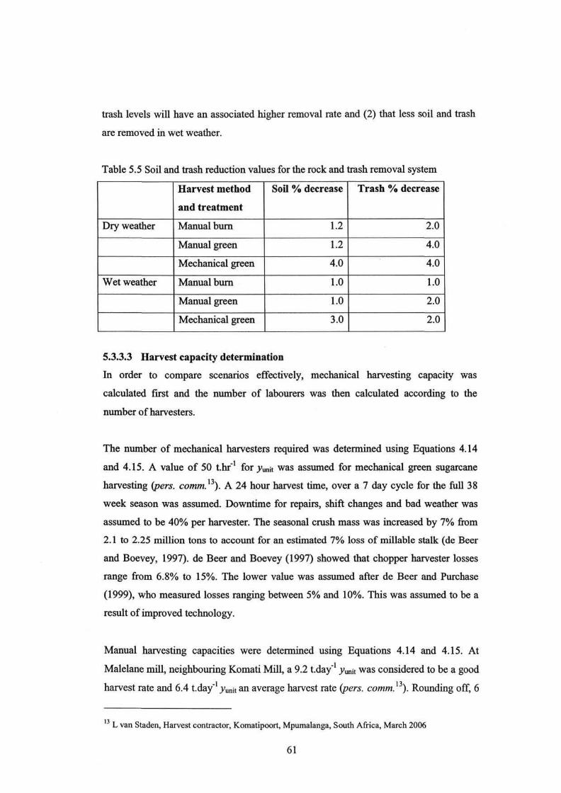
trash levels will have an associated higher removal rate and (2) that less soil and trash

are removed in wet weather.

Table 5.5 Soil and trash reduction values for the rock and trash removal system

Dry weather

Wet weather

Harvest method

and treatment

Manual burn

Manual green

Mechanical green

Manual burn

Manual green

Mechanical green

Soil % decrease

1.2

1.2

4.0

1.0

1.0

3.0

Trash % decrease

2.0

4.0

4.0

1.0

2.0

2.0

5.3.3.3 Harvest capacity determination

In order to compare scenarios effectively, mechanical harvesting capacity was

calculated first and the number of labourers was then calculated according to the

number of harvesters.

The number of mechanical harvesters required was determined using Equations 4.14

and 4.15. A value of 50 thr"1 for y^n was assumed for mechanical green sugarcane

harvesting (pers. comm.u). A 24 hour harvest time, over a 7 day cycle for the full 38

week season was assumed. Downtime for repairs, shift changes and bad weather was

assumed to be 40% per harvester. The seasonal crush mass was increased by 7% from

2.1 to 2.25 million tons to account for an estimated 7% loss of millable stalk (de Beer

and Boevey, 1997). de Beer and Boevey (1997) showed that chopper harvester losses

range from 6.8% to 15%. The lower value was assumed after de Beer and Purchase

(1999), who measured losses ranging between 5% and 10%. This was assumed to be a

result of improved technology.

Manual harvesting capacities were determined using Equations 4.14 and 4.15. At

Malelane mill, neighbouring Komati Mill, a 9.2 t.day" yunit was considered to be a good

harvest rate and 6.4 tday"1 yunn an average harvest rate (pers. comm.13). Rounding off, 6

L van Staden, Harvest contractor, Komatipoort, Mpumalanga, South Africa, March 2006

61

t.day" was used as the average unit capacity for burnt whole stalk sugarcane, de Beer

and Boevey (1997) showed that manual harvesting incurs a 2.1% loss of millable

sugarcane. This loss was not added to SM as the harvest rate of 6 tday"1 was assumed to

be a significant simplification in itself. Adding 2.1% to the harvest throughput would

not improve the accuracy of representation of the system. The calculation of the number

of manual harvesters began with matching the exact rate of 60000 t.wk_1cut by the

mechanical harvesting system. It was assumed that cutting takes place for 7 hours a day,

7 days a week and that the cutter rate is 6 tday"1.

The same method was used to determine the number of harvesters required for green

sugarcane harvesting, de Beer et al, (1989) and Meyer and Fenwick (2003) showed

that junit was reduced by between 20% and 30% when harvesting green sugarcane. A

30% reduction in capacity was applied to the yunit used for burnt sugarcane harvesting.

Table 5.6 provides a summary of the inputs used.

Table 5.6 Summary of calculated harvesting capacities

Harvest method

Mechanical harvesting

Manual harvest of burned sugarcane

Manual harvest of green sugarcane

Number of harvest

units

12

1429

2144

Unit capacity

(t.hr'.unit1)

50

0.87

0.58

5.3.3.4 Loading capacity determination

Loading inputs are only used for manually harvested sugarcane because mechanical

harvesters automatically load sugarcane as part of their harvesting operation. Values

were obtained through consultation with Komati Mill supply management. Currently

there are 25 machines of which 16 are non-slewing and 9 are excavator type slewing

loaders. It was assumed that 1 excavator performed the equivalent work of 1.5 Bell

loaders. Hence, there were effectively 30 Bell loaders (16 + 9 x 1.5). A load capacity of

22 t.hr"1.unif1 was obtained from the Trashing Model. According to de Beer et al.

(1989), this rate decreases by 23% when loading green harvested sugarcane as a result

of the density decrease of green sugarcane. Hence a 20% reduction in capacity was

used. At Komati Mill loaders are available to operate 24 hours a day, 7 days a week

62

with an estimated utilisation time of 30% (pers. comtn. ). Table 5.7 provides a

summary of the inputs used.

Table 5.7 Summary of calculated loading capacities

Harvest method and treatment

Manual harvest of burned sugarcane

Manual harvest of green sugarcane

Number of loading

units

16

16

Unit capacity

(t.hr'.unif1)

22

17.6

5.3.3.5 Transport capacity determination

Transport inputs were obtained through consultation. There were an estimated 65 units

of which 65% were trucks and 35% tractor-trailer units. The use of different loading and

transport equipment necessitated additional cohorts (as outlined in the recommendations

for future research). Cohorts refer to zones of similar sugarcane quality. For manual cut

and burnt sugarcane, trucks were assigned a payload of 29 tons and tractor-trailer units

25 tons hence a mean punjt of 27.6 tons (0.65 x 29 + 0.35 x 25) was used. For green

whole stalk sugarcane payload was decreased by 25%. According to de Beer et al.

(1989) a 44% payload reduction occurs under no topping, while a 25% reduction occurs

with green topped sugarcane, as a result of the density decrease. Payloads increase in

the case of mechanical harvesting, resulting from a higher density associated with

billets. Olwage (2000) showed a 6 ton increase in payload with billeted sugarcane at

Komati Mill, hence the existing 27.6 ton payload was increased by 6 tons. Transport

units operate 24 hours a day, 7 days a week with an estimated 18% downtime (pers.

comrn.15). Hence tT equals 138 hours / week (7 x 24 x 0.82). Table 5.8 provides a

summary of the inputs used.

Table 5.8 Summary of calculated transport capacities

Harvest method

Manual harvesting burned sugarcane

Manual harvesting green sugarcane

Mechanical harvesting green sugarcane

Number of units

65

65

65

Payload (tons)

27.6

20.7

32.6

S. Krieg, Procurement Manager, Komati Mill, Mpumalange, South Africa, March 2006 R. Venter, Procurement Manager, Malelane Mill, Mpumalange, South Africa, March 2006

63

5.3.3.6 Offloading capacity determination

Offloading capacity was based on the maximum offloading rate at the mill. For a

minimum offloading time of 5 minutes per truck, 12 loads could be offloaded on each

of the two offloading lines, generating an offload capacity of 660 thr"1 (2 x (12 x 27.6)

tons). The capacity was increased by 18% to 780 t.hr"1 for billeted sugarcane based on

the 6 ton increase in payload explained in section 5.3.3.5. Offloading was assumed to

occur whenever the mill was functioning.

5.3.3.7 Mill component capacity determination

Preparation capacity was modelled using Equation 4.20. The fibre (F) range was

assumed to be 10% to 16%. These values were obtained from tops (TS) and trash (TSH)

values of 7% and 3% in Table 4.3, after Kent et al. (1999). These levels were used in

the sugarcane composition table to obtain the corresponding F levels. For billeted

sugarcane the throughput range at Komati Mill was estimated to be between 550 to 630

t.hr"1, while for whole stalk sugarcane a range of 460 to 520 thr"1 was assumed (pers.

comm.17). Diffuser throughput is limited by the dewatering mill fibre throughput

capacity, which was estimated to be 79 t fibre.hr" (pers. comm. I7). Ash levels (A) were

estimated to be roughly 2% of the total mass of sugarcane, ranging from 1.7 % in dry

weather to 4% in wet weather (pers. comm.17). A 30 t ash.hr"1 capacity was assumed.

Since Komati Mill recycles the clarifier mud, all the sand was expected to enter the

boiler. The remaining two potential capacity constrictors are the A and C-Pans for

which the throughput capacities were estimated to be 70 tons pol (sucrose equivalent)

and 13 t non-pol hour"1, respectively (pers. comm.17). Table 5.9 provides a summary of

the inputs used.

5.3.3.8 Extraction and exhaustion component inputs

The two major mill components modelled by CAPCONN are extraction (E) and

exhaustion (X). Extraction was modelled using Equation 4.21. Values of 96% and 99%

were used for Emax and Emin (pers. comm. 16). Values of 10% and 16%, 1% and 10%

were used for Fmax> Fmin, Amax and Ami„, respectively. These values were based on the

sugarcane composition table input information discussed in Section 5.3.

16 A. Williamson, Mill Manager, Komati Mill, Komatipoort, South Africa, March 2006

64

Exhaustion was modelled using Equation 4.22. Values of 86% and 88% were used for

Xmwc andXmi„, respectively (Anon, 2005). Non-sucrose (NS) values of 1% and 5% were

used for NSmox and NSmi„, based on the sugarcane composition table input information

discussed in Section 5.3.

Inversion was modelled using Equation 4.9. Values of 0.1%, 0.24% and 0.05% were

used for c? in the clarifier, evaporator and A, B and C-Pans respectively (Shaffler,

1994). In general, a smoother flow of produce in the mill reduces total sucrose inversion

losses to between 1.0% and 1.5% while a few start-stops would raise it to between 3.0%

and 4.0% (pers. comm.11).

5.3.4 Cost Inputs

This section summarises the fixed cost (FC) and variable cost (VC) inputs for each

component of the Komati Mill supply chain. The derivation of dual price is also

discussed. Two general cost inputs are the agronomic input costs and the cost of dealing

with soil in the mill. Agronomic costs of R 8 t"1 and R 22 t for green and burnt

sugarcane, respectively, were obtained from the Trashing Model. These values were

later estimated to be in the order of R 100 t"1 (pers. comm.n) and hence could be

significantly underestimated. The maintenance cost for the milling of soil was assumed

to be R 1001"1 as estimated by Purchase and de Boer (1999).

5.3.4.1 Harvest, loading and transport costing

Three types of mechanical harvesters are most commonly used in South Africa, namely

the Case IH, Claas and Cameco. The Cameco is considered to be the most suitable for

use by harvest contractors in Malelane (pers. comm.19), costing approximately R 2.2

million per unit. The transport component of the Trashing Model was used to estimate

the mechanical harvester FC. For a purchase price of 2.2 million, a machine operator

cost of R 86 000 pa and R 71 200 licence fees, the FC was 10 177 R.wk"\ per harvester.

17 S. Davis, Mill Process Engineer, SMRI, Durban, South Africa, January 2006 18 B. Purchase, Retired SMRI Manager, SMRI, Durban, South Africa, April 2006 19 L van Staden, Harvest contractor, Komatipoort, Mpumalanga, South Africa, March 2006

65

A mechanical harvesting VC of R 20 t"1 and R 17 t"1 were used for green and burnt

sugarcane respectively (pers. comm. ) .

Manual harvesting costing involves both FC and VC. The FC includes UIF, rations,

housing, electricity, water, working equipment and transport. FC can be estimated as

roughly equal to 50% of the VC (pers. comm21). A VC of R 11.13 t"1 and R 4.53 t"1 was

used for green and burnt sugarcane respectively, obtained from the Trashing Model.

This corresponds to a wage of R 30 and R 38 per day. Assuming 7 days of the week are

worked, and a FC of R 30 day"1 .man , the weekly FC = R 105 man"1. Overtime

payments were not considered.

A loading VC of R 1.93 t"1 and FC of R 2 342 week"1 were obtained from the Trashing

Model. The FC was based on a machine price of R 330 000. Transport costing was

estimated using the Trashing Model, which makes use of an extensive spreadsheet to

calculate transport costs accounting for depreciation and interest. A combined purchase

price of R 1.4 million was used for the truck and trailer unit (pers. comm?1). Other FC

included a machine operator cost of R 86 000 pa and a R 71 200 licence fee. This

resulted in a FC of R 7 735 week"1 and VC of R 10 t"1. The VC was increased from R 10

t" to R 15 t", proportionally to the FC increase of the initial Trashing Model truck cost

to the current estimated cost of R 1.4 million. Table 5.9 provides a summary of the

costing inputs described in this section, as well as offloading costing.

5.3.4.2 Offloading costing

The FC of all the mill offloading equipment was assumed to be R 50 million and the

equipment was assumed to have a hfespan of 10 years. Dividing by 520 weeks, the FC

is roughly R 100 000 week"1. A VC of R 0.01 t"1 was assumed for maintenance and

electricity based on a Komati Mill maintenance cost report (pers. comm}2).

E. Meyer, Agricultural Engineer, SASRI, Mt Edgecombe, Durban, South Africa, August 2005 R. Giles, Agricultural Engineer, Crickmay and Associates, Pietermaritzburg, South Africa, April 2006

22 A. Williamson, Mill Engineer, Komati Mill, Komatipoort, Mpumalanga, South Africa, March 2006

66

Table 5.9 Summary of costing inputs for harvest, load, transport and offloading

operations

Component

Agronomic component

Agronomic component

Mechanical harvesting

Mechanical harvesting

Manual harvesting

Manual harvesting

Loading

Transport

Mill offloading equipment

Harvest

treatment

Burn

Green

Burn

Green

Burn

Green

-

-

-

Fixed cost

(R-wk^unif1)

-

-

10 177

10 177

105

105

2 342

7 735

100 000

Variable cost

(R-f1)

22

8

17

20

4.53

11.13

1.93

15

0.01

5.3.4.3 Mill costing

Mill costing information is generally confidential and for the purposes of this case

study, mill costing values were based largely on assumptions. Each component in the

mill was considered to have the same FC of R 200 000 week-1. This was estimated by

assuming each component costs R 100 million and operates for 10 years. The

theoretical value of R 100 million was based on the cost of R 130 million to install a

new boiler at Komati Mill (pers. comm.23).

It was estimated that 80% of mill VC were attributed to the mill front end (pers.

comm.23). The VC of preparation, extraction and boiling should therefore be 80% of the

total mill operational cost.

A Komati Mill maintenance cost report showed a maintenance cost range for

preparation of between R 1.4 million and R 2 million pa from 2001 to 2005. It was

assumed that billets have a lower VC as they can be prepared faster than whole stalk

sugarcane. For a 2.2 million ton season the whole stalk VC was assumed to be R 1 t"1,

increased by 10% to account for operational VC. The billet cost was based on the lower

maintenance cost of R 1.4 million, and was increased by 10% to R 0.7 t"1 to account for

23 S. Davis, Mill Process Engineer, SMRI, Durban, South Africa, January 2006

67

operational VC. The average diffuser maintenance cost from 2001 to 2005 was R 5

million. The diffuser VC used was R 2.271"1 (R 5 million + 2.2 million tons per season).

The mill maintenance cost report showed boiler ash handling amounting to R 320 000

pa which is equivalent to R 0.145 t"1 of sugarcane for 2.2 million tons of sugarcane per

season. For an average A of 2.5%, the VC of processing ash amounts to R 9 t" of ash.

The mill maintenance cost report shows boiler maintenance cost amounts to R 2.8

million. This cost was assumed to be a function of the amount of bagasse burnt. For a

2.2 million ton season it costs R 1.27 R.t"' of sugarcane and for a fibre content of 20%,

this is equivalent to R 6 t"1 of fibre. The total VC is the sum of the ash and fibre costs.

The Komati Mill maintenance cost report was also used to estimate mill back end costs.

The juice heating, clarification and evaporation costs were based on the R.t_1 sugarcane,

not on the R.t_1 mixed juice. This simplified the effects of sugarcane quality and

imbibition variation. The A, B and C-Pan VC was converted from R.t_1 sugarcane to R.t" 1 brix (sucrose + non-sucrose). The cost of the B-Pan was included in the A and C-Pan

costs. Similarly, the crystalliser cost of R 0.055 t"1 sugarcane was converted to R 0.36 t"1

brix (for 15% brix). The cost for the A and C crystallisers was therefore R 0.2 t"1 brix,

which included the B crystalliser cost. A single figure was used to represent the

combined cost of centrifuging in the A, B and C stations. The cost units described above

were selected in order to simplify costing calculations.

Produce residence times within each component were obtained in order to calculate the

stock cost, described by Equation 4.11. Estimated values were used for the purposes of

this project, which were obtained from consultation, shown in Table 5.10 (pers.

comm.26). Table 5.10 shows the mill costing for a 2.2 million ton season.

68

Table 5.10 Komati Mill costing based on a 2.2 million ton season (pers. comm. )

Preparation of

billeted

sugarcane

Preparation of

wholestalk

sugarcane

Diffuser

extraction

Boiler furnace

Juice heating

Clarification

Evaporation

Pans

Crystallisers

Centrifuging

FC

(R.week"x)

200 000

200 000

200 000

200 000

200 000

200 000

200 000

200 000

200 000

200 000

vc (R.t_1

sugarcane)

0.7

1

2.27

0.145

0.030

0.040

0.20

0.20

0.055

0.23

Equivalent cost

(R.t_1 sugarcane

compound)

-

-

-

-

0.66 R.t"' brix per

station

0.2 R.t"' brix per

station

1.5 R-t"1 brix

Component

residence time

(minutes)

12

18

24

30

54

24

5.3.4.4 Determination of component dual price

The dual price (DP) has been defined as the required input cost to increase or decrease

the throughput capacity of a SC component, or a series of components. The dual price

for each component was calculated as follows:

• Manual harvesters were assumed to work for 6 hours a day, 7 days a week over a

38 week season, totalling 1596 seasonal hours. For a yunit of 1 thr"1 each labourer

cuts 1596 t season" . Multiplying the t season"1 by a R 4 t"1 gave the seasonal VC.

For a FC of R 105 week"1 the TC per labourer was R 10 374 season", which

equaled the dual price.

A. Williamson, Mill Engineer, Komati Mill, Komatipoort, Mpumalanga, South Africa, March 2006

69

• As a result of the larger yunit of mechanical harvesters, the y# could only be

increased in relatively large increments. The following inputs were assumed. The

Yunit = 60 thr"1, VC = R 17 t"1 and FC = R 10 177 week"1. For a 40% downtime,

TC was 29 913 398 harvester \ The Dual price was R 49857 f'.hr"1 (R 29 913 398

harvester" .season ') / (60 thr"1).

• The same principle used to calculate the mechanical harvesting dual price, was

used for the loading and transport components. The seasonal TC was divided by

the t"!iff"1 .unit*1, which gave R 140624 t"1.hr"1and R153704 f 1.hr"1 for the loading

and transport components, respectively.

• Offloading and mill costing was based on theoretical cost figures. An initial

estimate of the dual price was estimated at 300 000 $ per ton sugarcane per hour

(Kent et al, 1999). This is equivalent to Rl 320 000 t'l.bfl. This value was

divided equally between each of the milling components included in CAPCONN.

The required modelling inputs were sourced from literature, consultation and where

necessary they were assumed. The modelling algorithms for mill process were

developed specifically to assess mechanisation impacts.

70

6 MODEL EVALUATION

Chapter 5 described the development of the modelling algorithms and the sourcing of

modelling inputs. This chapter discusses three main topics: (1) configuring the model

with inputs obtained from industry, (2) validating the integrity of the model through a

sensitivity analysis and (3) where possible, verifying model outputs with observed data.

As a result of the complexity of this model, configuration and integrity validation were

handled together. It was decided that the best means of validating CAPCONN's inputs

and verifying CAPCONN's outputs was to use an independent data source of Komati

Mill values. This is because sugarcane quality and mill performance characteristics are

highly mill specific. Hence CAPCONN transport and mill data were compared to SLIP

and SMRI data.

6.1 Model Configuration and Integrity

This section assesses how well the model represents the physical system by confirming

input data and comparing output data with independent observed data. Confirming input

data provides an indication of data integrity, while comparing output data indicates

model accuracy. Both input and output data need to be compared with external data that

are independent of any data used in the model. Unfortunately, there was a limited

availability of observed data for field to mill output verification.

6.1.1 Transport capacity configuration

Loading and transport operations were assessed based on transport utilisation

information from the Sugar Logistics Improvement Programme (SLIP) (pers. comm. ) .

An average load time of 0.59 hours was measured at Komati Mill, which was lower

than the 1 hour per truck assumed in the model. The average load rate has been

measured as 1.31 minutes.t", which corresponds to 45.8 t.hr"1. This is significantly

higher than the 22 and 33 thr"1 assumed in the model, for non-slewing and excavator

type slewing loaders respectively (See Section 5.3.3.4).

R. Giles, Bioresources Engineer and Logistics Consultant, Crickmay and Associates, Pietermaritzburg, South Africa, April 2006

71

Inconsistencies may exist between the 2003 and 2005 SLIP data, which measured 88

trucks in 2003 and 65 trucks in 2005 respectively. The CAPCONN transport capacity of

7.77 thr"1 .truck"1 corresponded well with the 2003 SLIP recorded industry average of

7.7 thr"1 .truck"1. CAPCONN input values were obtained through consultation at Komati

Mill. The 2003 SLIP transport capacity for Komati Mill was measured at 6.69 thr"1,

which implied that CAPCONN overestimated transport utilisation by 10%.

6.1.2 Assessment of mill performance

CAPCONN mill process trends were compared to measured data recorded by SMRI in

2005. (The complete Komati Mill report is shown in the Appendix). CAPCONN

outputs were compared to observed data of (1) CAPCONN input and output data ranges

and (2) seasonal trends in CAPCONN input and output data. The comparison of

modelled and observed model input and output data ranges served to evaluate the

accuracy of the CAPCONN outputs.

"Input data" for the model consist primarily of sugarcane composition data. The 2005

observed data shows a seasonal sucrose range of 11.60% to 15.52%, which was

encompassed by the CAPCONN input range of 11.0% to 16.0%. The CAPCONN fibre

range was 12.5% to 14.5%, while the observed range was 12.14% to 15.97%, hence the

CAPCONN range was narrower. Similarly the CAPCONN non-sucrose range of 2.6%

to 2.8% was narrower than the measured observed non-sucrose range of 2.41% to

3.69%. Although some of the input ranges do not match the observed data, the

CAPCONN inputs are, in the author's opinion, of suitably similar magnitude.

CAPCONN ash levels were significantly over-estimated at 1.3%, while the SMRI data

show an actual range of 0.21% to 0.59%. This overestimation could be a result of

incorrect assumptions of the performance of the rock and trash removal system and that

soil levels in the Komati Mill region are not as significant as in KwaZulu-Natal. The

difference in soil level may be a result of differing harvest practice, soil type and/ or

rainfall.

"Output data" for the model consist of mill component performance coefficients. Figure

6.1 shows the CAPCONN and measured industry extraction and exhaustion ranges.

72

Equations 4.21 and 4.22 require a maximum and minimum range in extraction and

exhaustion. A seasonal extraction range of 96% to 99% was used in Equation 4.21 and

the model output range was 98.6% to 98.8%. The observed data of 97.6% to 98.5%

showed a greater seasonal variation compared to CAPCONN. The CAPCONN

extraction model input range was suitable, but the output range was too narrow. An

86% to 88% range in exhaustion was assumed for the exhaustion equation, based on

seasonal averages. The model output rage was 87.06% to 87.20% compared to the

observed data range of 81.73% to 88.97%. This shows that the CAPCONN range may

have been too narrow, especially overestimating the lower values of the range. The

CAPCONN output range was widiin the SMRI data range, but it was significantly

narrower. Therefore, CAPCONN output data for the Komati analysis are probably not

accurate.

Figure 6.1 Comparison of CAPCONN and observed extraction and exhaustion ranges

The comparison of seasonal data trends served to evaluate the authenticity of

CAPCONN outputs. Figure 6.2 shows the observed sucrose, non-sucrose and fibre

contents for the Komati Mill 2005 season. The sucrose trend corresponded with the

trend shown in Table 5.1, peaking in the midseason. The observed fibre levels followed

a linearly increasing seasonal trend. The CAPCONN fibre input trend was inversely

correlated to the sucrose trend and therefore underestimated the fibre contents in the late

season. The CAPCONN non-sucrose seasonal trend sufficiently represents the actual

trend shown in Figure 6.2 since non-sucrose reduces from early to mid season and then

rises to a maximum in the late season. Seasonal ash level trends were not included as

73

the observed ash levels are highly variable and significantly lower than the CAPCONN

ash levels.

Figure 6.3 shows the observed seasonal extraction trend and CAPCONN extraction

estimates. The observed extraction trend exhibited a steady decreasing extraction rate,

which corresponds to the linearly increasing fibre levels. Similarly, in CAPCONN the

seasonal extraction efficiency, is concave which corresponds with the concave fibre

trend used in CAPCONN.

Figure 6.4 shows the observed exhaustion at Komati Mill in 2005 as well as CAPCONN

exhaustion estimates. The observed data peak at mid-season, and are lowest in the late

season. This trend corresponds to that in the CAPCONN seasonal exhaustion efficiency.

The seasonal trend in the CAPCONN calculated exhaustion efficiency is inversely

correlated to the non-sucrose % trends in Table 5.1, which is the expected trend

described by Equation 4.2.2. Figure 6.5 shows the plot of the CAPCONN exhaustion

efficiency vs. CAPCONN non-sucrose %. The correlation coefficient for both of the

two lines is -1 which confirms linearity. The reason for the existence of two lines is that

the exhaustion data is not symmetrical on either side of the mid-season values, while the

non-sucrose data is. The correlation coefficient between the 2005 observed exhaustion

efficiency and the CAPCONN non-sucrose %, Figure 6.6, is -0.83 which indicates a

significant degree of linear correlation. This correlation reinforces the validity of

Equation 4.2.2, showing exhaustion efficiency is comprehensively modelled as a

function of non-sucrose % alone.

74

18.00

~ 16.00

~ 14.00 c I 12.00 | 10.00 E

8 8.00

I 6.00 4.00

2.00

0.00

3

10 20

Milling week

30 40

H— Sucrose %

- •—Non-sucrose %

-•— Fibre %

Figure 6.2 The 2005 Komati Mill observed sugarcane quality information

10 20 30

Milling week

40

H— Observed extraction %

• CAPCONN extraction output

Linear (Observed extraction %)

Figure 6.3 2005 Komati Mill observed extraction % data and CAPCONN extraction %

data

75

90.00

89.00

88.00

87.00

86.00

85.00

84.00

83.00

82.00

81.00

, t\ff\f\ jt/if^^TiR t 7 vri i \ \ VI \ \ v WK t

/ \j\i\ + ¥ \

\ \

1 1 1

10 20

Milling week

30 40

-i— Observed ejdiaustion

-•— CAPCONN erfiaustion output Poly. (Observed e?diaustion)

Figure 6.4 2005 Komati Mill observed exhaustion % data and CAPCONN exhaustion %

data

87.2

87.18

5> 87.16 w 87.14 C

& 87.12 M

S 87.1 -• "fl 87.08 -W 87.06 -

87.04 -

87.02 -87-

2.

• , I •

• *

• • • • • -• • • - . ,

• • •

•

•

•

•

•

55 2.6 2.65 2.7 2.75 2.8

Non-sucrose (%)

2.85 2 9

• Exhaustion efficiency vs. non-sucrose (%)

Figure 6.5 CAPCONN exhaustion efficiency vs. CAPCONN non-sucrose %

76

• Exhaustion efficiency vs. non-sucrose (%)

— Poly. (Exhaustion efficiency vs.

2.55 2.6 2.65 2.7 2.75 2.8 2.85 2.9

Non-sucrose (%)

Figure 6.6 Plot of 2005 observed exhaustion (%) vs. CAPCONN non-sucrose (%)

6.1.3 Assessment of economic outputs

A comparison of total production cost provides a means of assessing CAPCONN's

representation of the economics of the integrated supply chain. The best available

estimate of production cost was the industry average sugar price, used to determine the

recoverable value (RV) (pers. comm.26). The 2005 sugar price increased consistently

throughout the season. However, the sugar price does not provide an indication of the

cost to produce each ton of sugar in the mill and therefore cannot be compared to

CAPCONN production cost estimates. CAPCONN estimated that sugar production

costs (Rt"1) were highest at the start of the season when sucrose content was lowest and

at a minimum during the mid season when sucrose content peaked. This is because total

production costs (R) are consistent throughout the season while sugar production (thr"1)

varies.

Another means of verifying CAPCONN's economic outputs is to compare cost outputs

to those obtained through other studies. Ahmadi et al. (2000) conducted a trial to

evaluate agronomic and cost factors related to mechanical burned and green sugarcane

harvesting in Swaziland, a neighbouring region to Komati Mill. The results showed that

VC for both mechanical harvesting scenarios were slightly lower than for the existing

manual cut system. The CAPCONN VC of mechanical harvesting was higher than that

26 S. Davis, Mill Process Engineer, SMRI, Durban, South Africa, January 2006

77

of manual harvesting, the reason for the difference is attributed to a difference between

the labour rates and fuel price in Swaziland, and those used by CAPCONN in this study.

This difference in output is purely attributed to the CAPCONN inputs used, and is

independent of the functionality of the CAPCONN model framework.

CAPCONN estimated the total production cost of sugar to be half of the actual value of

around 1500 R.t_1 (pers. comm.27). The major reasons for this difference are that (1) the

profits of the growers and hauliers, which increase production costs, are not included in

CAPCONN (2) most of the mill FC and VC were assumed and (3) the agronomic cost

in CAPCONN was only included in the stock cost calculation. The agronomic cost

should be added to the VC in order to compare production costs with industry values.

Agronomic operations and associated costs are outside of the scope of this dissertation

and have therefore at this stage been omitted.

6.2 Model Sensitivity Analysis

A sensitivity analysis was used to assess the integrity of CAPCONN by testing the

operational principles. This was done by assessing the sensitivity of CAPCONN outputs

to changes in the driver variable inputs. A case study is not adequate to do this, as the

model is run once for each scenario, providing no insight into variable sensitivity. One

method to assess the integrity of a model is to perform sensitivity analysis. The response

of CAPCONN output with respect to changes in selected variables by various

increments was investigated. The late season (dry weather) manual harvesting of burnt

sugarcane was selected for the sensitivity analysis, and outputs were intuitively

evaluated against real expectations.

Trash (TSH) was selected as a suitable variable for evaluating field to mill components,

having an impact on harvest (y#), loading (yi) and transport (yr) capacity. It should be

noted that TSH was used to represent the combined tops and trash value as explained in

Section 5.3.3 The sensitivities of manual v#, VL, vr and production cost to a 10%

variation in TSH were assessed. The results are discussed in Section 6.2.1.

A. Williamson, Mill Manager, Komati Mill, Komatipoort, Mpumalanga, South Africa, March 2006

78

Five sugarcane composition variables were selected for sensitivity analysis of mill

component operation. These were sucrose (5), non-sucrose (NS), TSH, soil (A) and

HTCD. The sensitivities of extraction (E), exhaustion (X), sugar production (thr"1) and

boiler capacity utilisation (CC/B) were assessed. The S and NS in the stalk were varied

by 10%, and trash % and soil % were adjusted by 10% after harvest and loading,

respectively. The results are discussed in Section 6.3.2.

6.2.1 Field to mill and production cost sensitivity to trash content

The impacts of varying trash amounts (TSH) were simulated throughout the supply

chain. In this section the relationships of manual harvest, load and transport component

capacity to TSH are firstly derived. The trends in the relationships are then discussed.

Before any processing occurs, the stalk percentage of sugarcane and sugarcane density

are inversely correlated to TSH. The unit v# is inversely correlated to TSH. The harvest

stalk throughput rate is therefore affected by two factors relating to TSH, namely

composition and harvest rate. CAPCONN accounts for trash impacts on manual harvest

capacity as discussed in Section 4.3.3. Since a TSH of 4% and 10% was used for manual

burnt and green sugarcane harvesting respectively, a linear relationship was used to

approximate trash impacts on the unit yn- The burnt harvest rate and green harvest rate

are 6 tday"1 and 4 tday"1, respectively. Equation 6.1 was used to determine the

sensitivity of yu to TSH.

Ay = -ATSH + l00x(6-4) + (lQ-4) ( 6 1 )

Loading (yi) and transport (yr) component capacities are inversely correlated to

sugarcane density. Density impacts on vi and payload (p) were assumed to be linear.

Based on information from Section 4.3.3 j>z and p sensitivities were estimated by

Equations 6.2 and 6.3 below. Values of 22 and 17.6 thr"1 .unit"1 were used for burnt and

green sugarcane loading, respectively. A 27.7 ton and 20.7 ton p were used for burnt

and green sugarcane, respectively. A 4% to 10% trash range was assumed for loading

and transport. The effect of lodging on density was not included.

79

Ay =-A7SH>100x(22-17.6)+(10-4)

Ay =-A7Sff+100x(27.6-20.7)+(10-4)

(6.2)

(6.3)

Table 6.1 and Figure 6.7 show the sensitivity of harvest, load and transport capacity to a

10% change in TSH. This corresponded to a 0.06 unit change in magnitude of trash for

the default value of 6% trash.

Table 6.1 Changes in CAPCONN outputs for a 10% variation in trash % sugarcane

Normal case

Trash %

Model

value

4%

%

change

10%f

io%|

Harvest

rate

(t/day)

6.0

-0.33

+0.33

Loader

rate

(t/hr)

22.0

-0.20

+0.20

Payload

(tons)

27.6

-0.25

+0.25

Transport

(t/hr)

7.77

-0.12

+0.25

R/t

sugarcane

483.0

+0.41

-0.41

The trends are as expected for each scenario, with increasing TSH reducing system

capacity by reducing sugarcane density and increasing biomass. The yn was most

sensitive to TSH, followed by p and finally yi. The sensitivity of yr to TSH was assessed

by determining the sensitivity of the unit yr to p. The only variable that showed a non­

linear sensitivity was transport unit capacity (t.hr'.unit"1).

Figure 6.7 Capacity and production cost sensitivity to a 10% trash variation

80

The sugar production cost (R.f') was obtained from the diagnostics output sheet, the

calculation of which is explained in Section 4.4. The production cost was seen to be

inversely correlated to TSH. This is because TSH occupies sugarcane mass, effectively

displacing S, and TSH furthermore reduces S extraction. TSH did not impact on FC and

VC, however the decrease in S throughput decreased the Rf' production cost.

6.2.2 Mill performance sensitivity to sugarcane quality and HTCD

Table 6.2 and Figures 6.8, 6.9, 6.10 and 6.11 show mill operation sensitivity to a 10%

variation in sucrose (S), non-sucrose (NS), trash (TSH), ash (A) and harvest to crush

delay (HTCD).

Figure 6.6 shows that simulated E % was more sensitive to TSH than to A. The results

correspond to the trends concluded by Cardenas and Diez (1993) which are discussed in

4.3.2.2. The reason E % was less sensitive to A although A carries a greater weight in

Equation 4.20, is that TSH occupies a higher proportion of the harvested sugarcane

composition. Hence a 10% change in TSH will be proportionally larger than a 10%

change in A. Changes in S and NS in Table 4.3 impact on the moisture content and do

not reduce the percentages of F and A. Hence a variation in S has no impact on E % or

X %, E % being a function of F and A, and X a function of NS. E % is not sensitive to

HTCD which only influences NS %.

0.0250 -i

I 0.

0

•a o 0 •2 0 S 2 o

C

0200

0150

0100

0050

.0000

0050

.0100

0150

0200

-0.0250

10%TSH-decrease

I » t ' t » - ; i

se—10% A decrease

Figure 6.8 Sensitivity of extraction % to a 10% variation of trash and soil

81

Table 6.2 Changes in model milling outputs for a 10% variation in model inputs

Normal case

Sucrose %

Non-sucrose

%

Trash %

Soil %

Harvest to

crush delay

Model

value

12.6%

2.87%

4%

2%

45

hours

10%t

10%i

10%t

10%i

10%T

io%i

io%T

10%i

10%t

io%|

Extraction

%

0.9860

-

-

-

-

0.9860

0.9864

0.9861

0.9863

-

"

Exhaustion

%

0.8706

-

-

0.8692

0.8721

-

-

-

-

0.8706

0.8707

t/hour

sugar

41.64

45.80

37.47

41.57

41.71

-

-

41.64

41.65

41.58

41.70

Boiler

capacity

utilisation

17.3%

-

-

-

-

-

-

20.0%

14.7%

-

-

Figure 6.9 shows the sensitivity of X % to NS and the HTCD of 45 hours. The simulated

X % was inversely correlated to NS which is an expected trend (pers. comm.28). It is

evident that a 10% change in HTCD generated a significantly lower change to NS. It is

also evident that NS was insensitive to S, TSH and A changes.

e o

••a 3

I u a a

J= u *

0.2

0.15

0.1

0.05

0

-0.05

-0.1

-0.15

-0.2

;ase 10% NS decrease 10% HTCD 10% delay

increase decrease

Figure 6.9 Sensitivity of extraction to a 10% variation of non-sucrose % and HTCD

S. Davis, Mill Process Engineer, SMRI, Durban, South Africa, October 2005

82

Figure 6.10 shows the sensitivity of the sugar production rate (t.hr") to changes in

sugarcane quality and the HTCD. S impacted significantly on sugar production, relative

to NS, A and HTCD. The sugar production rate was correlated to S and was inversely

correlated to NS, A and HTCD which were the expected trends. Sugar production was

inversely proportional to A and NS as a result of the associated impacts of these

compounds on E % and X %.

S

4

3

2

1

0

-1

-2

-3

-4

-5

10% S increase d

10% NS 10% NS 10% A 10% A 10% 10% se increase decrease increase decrease HTCD HTCD

increase decrease

Figure 6.10 Sensitivity of sugar production rate to a 10% variation of sucrose, non-

sucrose and soil content, and HTCD

Figure 6.11 shows that the simulated boiler capacity utilisation (CUB) was sensitive to

A, changing by 15% for a 10% change in soil %. CUB was not sensitive to S, NS, TSHox

HTCD, being solely a function of A alone.

83

u M « u •- s Ol o

"s « -S S « 3 Ml S es

43 w

20.00

15.00

10.00

5.00

0.00

-5.00

-10.00

-15.00

-20.00 J

10% A increase 10% A decrease

Figure 6.11 Sensitivity of boiler capacity utilisation to a 10% variation of soil %

6.3 Conclusions

CAPCONN inputs and outputs have been compared to industry measured data, termed

observed data. Relatively few data comparisons were available for field to mill

processes, and no comprehensive means of evaluating production cost trends were

available. According to SLIP observed data, CAPCONN overestimated transport

capacity by 10%. CAPCONN output data was compared to the observed 2005 SMRI

data in terms of seasonal data range and trend. The simulated extraction % and

exhaustion % ranges were within the observed range and the seasonal trends did not

correspond well to SMRI data. However, CAPCONN output trends and observed

operational trends corresponded to sugarcane quality trends. This suggests that if the

same quality curves were used, the same mill performance curves may have been

obtained. The costing evaluation was inconclusive, as the available industry costs did

not include the same cost variables used in CAPCONN.

The sensitivity trends of all simulated variables followed intuitive expectations. The

equation for transport unit capacity exhibited a non-linear relationship with transport

capacity, as shown in Figure 6.7. All other variable changes were equal in magmtude

and opposite in sign, showing the linearity of CAPCONN variable relationships. The

magnitude and direction of harvest, load and transport capacity change are perceived to

be representative as these components were significantly simpler to model compared to

mill processes. In the mill, the trends of changes in component capacity and

84

performance variables are perceived to be accurate. Further refinement of the algorithms

used by CAPCONN would allow mill component capacity and performance to be more

accurately determined. Knowing the cost associated with changes in component

capacity or performance would allow comparison of the financial significance of

variable sensitivity.

85

7 A SUPPLY CHAIN CASE STUDY: MECHANISATION AT

KOMATI MILL; RESULTS AND DISCUSSION

This chapter discusses the results of the case study which are presented in table form.

Table 7.1 shows CAPCONN estimates of capacity utilisation (CU) for the existing

system (Scenario 1) inputs used in all three scenarios. The loading and transport

component capacities for Scenarios 2 and 3 were adjusted to run with a suitable truck

fleet size. For green whole stalk harvesting, the truck fleet capacity was increased by 22

trucks and for mechanical harvesting it was decreased by 25 trucks. Table 7.4 shows

estimates of CU after these system adjustments had been made.

Table 7.2 shows general model outputs representing the existing system. These include

the estimated maximum throughput twk"1, a total cost breakdown, estimated diffuser

recovery and exhaustion. A t.hr"1 of sugar and a R.t_1 sugar value were calculated. The

thr"1 of sugar was calculated by multiplying the sugarcane throughput rate with sucrose

content and the E and X coefficients. The R.f' sugar was then calculated by dividing the

total cost R-hr"1 by the thr"1. Table 7.5 shows the general outputs after making the

system capacity adjustments described above.

Tables 7.3 and 7.6 show the total cost (FC + VC + STC) for each component in the SC.

The tables show the unadjusted and adjusted inputs respectively, the system capacity

adjustments being those described above.

7.1 General Observations of Dry Weather Scenarios

The required weekly flow of 58 000 twk"1 (for a 38 week milling season crushing 2.2

million tons of sugarcane) has been met for the current systems of manual burnt

sugarcane harvesting, shown in Table 7.2. This was confirmed by TSB employees

during consultation, who stated Komati Mill has an over-designed sugarcane throughput

capacity. It is further confirmed by Enslin (2003), who stated that by 2006, Komati Mill

is planned to have a 2.6 million ton seasonal crush capacity.

86

Table 7.1 Capacity utilisation (%) based on the current system at Komati Mill

Scenario Season

Harvest Treatment Harvest Load Transport Offloading Preparation Extraction Boiler

A-Pan C-Pan

1 Early season

Manual Burn

100% 54% 86% 61% 65% 74% 17%

61% 85%

2 Mid season

Manual Burn

100% 54% 86% 61%

65% 63% 17%

89% 80%

3a Late season Dry Manual Burn

100% 54% 86% 61% 65% 74% 17% 68% 88%

3b Late season Wet Manual Burn

100% 54% 86% 61%

65% 85% 47% 65% 87%

7 Early season

Manual Green

87% 59%

100% 53% 61% 78% 15%

51% 72%

8 Mid season

Manual Green

87% 59%

100% 53% 61% 69% 15%

75% 68%

9a Late season Dry Manual Green

87% 59%

100% 53% 61% 78% 15% 57% 75%

9b Late season Wet Manual Green

87% 59%

100% 53%

61% 98% 41%

53% 71%

4 Early season

Mech Green

100%

54% 51% 54% 81%

87% 60% 83%

5 Mid season

Mech Green

100%

54% 51% 54% 71% 87% 87% 79%

6a Late season Dry Mech Green

100%

54% 51% 54% 81% 87% 67% 86%

6b Late season Wet Mech Green

60%

33% 31% 32% 63%

100%

37% 50%

87

Table 7.2 General outputs based on the current system at Komati Mill

Scenario Season

Harvest Treatment Total cost FC + VC + Stock Cost (R.wk"1) FC (R.wk'')

VC (R.wk"')

Stock Cost (R.wk"') Cost of soil (R.wk"1) (Included in total cost) Maximum throughput before bottleneck (t.wk"1) Estimated extraction (%)

Estimated sugar exhaustion (%) Estimated sugar recovery (tons.hr"1) R.ton" sugar produced

1 Early season

Manual Burn

4697870

3023080

1532004

64786

78000

60000

98.62%

87.12%

37.46

746

2 Mid season

Manual Burn

4698759

3023080

1532915

64764

78000

60000

98.76%

87.20%

54.74

511

3a Late season Dry

Manual Burn

4700356

3023080

1534487

64789

78000

60000

98.62%

87.06%

41.64

672

3b Late season Wet Manual Burn

4853106

3023080

1555153

64872

210000

60000

98.33%

87.09%

40.24

718

7 Early season

Manual Green

4572404

3098155

1345901

60353

67995

52304

98.42%

87.16%

31.46

865

8 Mid season

Manual Green

4573143

3098155

1346659

60334

67995

52304

98.55%

87.23%

45.86

594

9a Late season Dry Manual Green

4574512

3098155

1348006

60356

67995

52304

98.42%

87.11%

35.01

778

9b Late season Wet Manual Green

4715371

3098155

1373692

60460

183064

52304

97.98%

87.17%

32.65

860

4 Early season

Mech Green

5721076

2924899

2376263

29914

390000

60000

98.21%

87.15%

36.98

921

5 Mid season

Mech Green

5722297

2924899

2377504

29894

390000

60000

98.34%

87.22%

53.78

633

6a Late season Dry Mech Green

5723580

2924899

2378764

29917

390000

60000

98.21%

87.10%

41.19

827

6b Late season Wet Mech Green

4853768

2924899

1456752

22117

450000

36000

97.54%

87.16%

23.03

1255

88

Table 7.3 Individual component costing (FC + VC + Stock cost) based on the current system at Komati Mill

Scenario Season

Harvest

Treatment Harvest Load Transport Offloading Preparation Extraction Boiler Juice heating Clarification Evaporator A-Pan A Crystalliser C-Pan C Crystalliser Centrifuge

1 Early season

Manual

Burn 445070 188631

1416764 102287 208717 338850 259292 202983 204256 214587 208800 205852 206886 203911 212983

2 Mid season

Manual

Burn 445070 188631

1416764 102287 207488 338850 251919 202981 204252 214583 210716 206429 208806 204492 217492

3a Late season Dry

Manual

Burn 445070 188631

1416764 102287 208717 338850 259292 202983 204256 214587 209329 206013 207415 204072 214090

3b Late season Wet

Manual

Burn 445070 188631

1416764 102287 210085 338851 279380 202989 204264 214599 209172 205977 207249 204028 213760

7 Early season

Manual Green

483560 173585

1300234 102114 209189 321196 261227 202679 203838 212901 207756 205369 205953 203539 211268

8 Mid season

Manual Green

483560 173585

1300234 102114 208162 321195 255062 202677 203835 212897 209359 205852 207558 204025 215034

9a Late season Dry

Manual Green

483560 173585 1300234 102114 209189 321196 261227 202679 203838 212901 208204 205505 206400 203676 212209

9b Late season Wet

Manual Green

483560 173585 1300234 102114 211574 321198 285894 202686 203849 212915 207924 205436 206109 203596 211634

4 Early season

Mech Green

1323725

1405058 101587 206742 339166 292844 203118 204458 214857 209072 206237 206955 204094 213162

5 Mid season

Mech Green

1323725

1405058 101587 205900 339165 285621 203116 204455 214853 210949 206802 208835 204663 217568

6a Late season Dry

Mech

Green 1323725

1405058 101587 206742 339166 292844 203118 204458 214857 209603 206398 207486 204255 214282

6b Late season Wet

Mech

Green 843117

1044295 101029 205195 283800 284996 202042 202963 209341 206142 204545 204563 202939 208801

89

Table 7.4 Capacity utilisation (%) based on an adjusted system for Komati Mill

Scenario Season

Harvest Treatment Harvest Load Transport Offloading Preparation Extraction Boiler A-Pan C-Pan

7 Early season

Manual Green

100% 68% 86% 61% 70% 89% 17% 59% 82%

8 Mid season

Manual Green

100% 68% 86% 61% 70% 79% 17% 85% 78%

9a Late season Dry

Manual Green

100% 68% 86% 61% 70% 89% 17% 65% 85%

9b Late season Wet Manual Green

89% 60% 77% 54% 63%

100% 42% 54% 73%

4 Early season

Mech Green

100%

88% 51% 54% 81% 87% 60% 83%

5 Mid season

Mech Green

100%

88% 51% 54% 71% 87% 87% 79%

6a Late season Dry Mech

Green 100%

88% 51% 54% 81% 87% 67% 86%

6b Late season Wet Mech

Green 60%

53% 31% 32% 63%

100% 37% 50%

1 Early season

Manual Burn

100% 54% 86% 61% 65% 74% 17% 61% 85%

2 Mid season

Manual Burn

100% 54% 86% 61% 65% 63% 17% 89% 80%

3a Late season Dry Manual Burn

100% 54% 86% 61% 65% 74% 17% 68% 88%

3b Late season Wet Manual Burn

100% 54% 86% 61% 65% 85% 47% 65% 87%

Note: Transport capacity was increased by 22 trucks for Scenario 2 and decreased by 25 trucks for Scenario 3.

90

Table 7.5 General outputs based on an adjusted system for Komati Mill

Scenario Season

Harvest Treatment Total cost FC + VC + Stock Cost (R.wk"1) FC (R.wk"')

VC (R.wk'')

Stock Cost (R.wk"') Cost of soil (R.wk-') (Included in total cost) Maximum throughput before bottleneck (t.wk"1) Estimated extraction (%) Estimated sugar exhaustion (%) Estimated sugar recovery (tons.hr'1) R.ton" sugar produced

7 Early season

Manual Green

4958506

3268325

1543939

68243

78000

60000 98.42%

87.16%

36.09

818

8 Mid season

Manual Green

4959354

3268325

1544808

68221

78000

60000 98.55%

87.23%

52.61

561

9a Late season Dry

Manual Green

4960924

3268325

1546353

68246

78000

60000 98.42%

87.11%

40.16

735

9b Late season Wet Manual Green

4925904

3268325

1406981

63098

187500

53571 97.98%

87.17%

33.44

877

4 Early season

Mech Green

5526657

2731524

2376263

28870

390000

60000 98.21%

87.15%

36.98

890

5 Mid season

Mech Green

5527877

2731524

2377504

28849

390000

60000 98.34%

87.22%

53.78

612

6a Late season Dry Mech

Green

5529161

2731524

2378764

28873

390000

60000 98.21%

87.10%

41.19

799

6b Late season Wet Mech

Green

4659349

2731524

1456752

21073

450000

36000 97.54%

87.16%

23.03

1204

1 Early season

Manual Burn

4697870

3023080

1532004

64786

78000

60000 98.62%

87.12%

37.46

746

2 Mid season

Manual Burn

4698759

3023080

1532915

64764

78000

60000 98.76%

87.20%

54.74

511

3a Late season Dry Manual Burn

4700356

3023080

1534487

64789

78000

60000 98.62%

87.06%

41.64

672

3b Late season Wet Manual Bum

4853106

3023080

1555153

64872

210000

60000 98.33%

87.09%

40.24

718

Note: Transport capacity was increased by 22 trucks for Scenario 2 and decreased by 25 trucks for Scenario 3.

91

Table 7.6 Individual component costing (FC + VC + Stock cost) based on an adjusted system for Komati Mill

Scenario Season

Harvest

Treatment Harvest Load Transport Offloading Preparation Extraction Boiler Juice heating Clarification Evaporator A-Pan A Crystalliser C-Pan C Crystalliser Centrifuge

7 Early season

Manual Green

521146 188731

1587964 102451 210541 339015 270236 203052 204359 214725 208786 206001 206768 203958 212774

8 Mid season

Manual Green

521146 188731 1587964 102451 209362 339014 263163 203050 204356 214720 210624 206555 208610 204515 217094

9a Late season Dry

Manual Green

521146 188731 1587964 102451 210541 339015 270236 203052 204359 214725 209299 206157 207282 204114 213853

9b Late season Wet

Manual Green

489750 176080 1490362 102264 211855 324227 287975 202786 203992 213292 208192 205656 206285 203723 211966

4 Early season

Mech

Green

1323725

1211567 101535 206742 339037 292844 203067 204381 214754 208943 206082 206904 204016 213059

5 Mid season

Mech

Green

1323725

1211567 101535 205899 339036 285621 203064 204378 214750 210820 206648 208784 204585 217465

6a Late season Dry Mech

Green 1323725

1211567 101535 206742 339037 292844 203067 204381 214754 209474 206243 207435 204178 214179

6b Late season Wet Mech

Green 843117

850804 100978 205195 283671 284996 201990 202886 209238 206013 204390 204511 202861 208698

1 Early season

Manual

Burn 445070 188631 1416764 102287 208717 338850 259292 202983 204256 214587 208800 205852 206886 203911 212983

2 Mid season

Manual

Burn 445070 188631 1416764 102287 207488 338850 251919 202981 204252 214583 210716 206429 208806 204492 217492

3a Late season Dry

Manual

Burn 445070 188631

1416764 102287 208717 338850 259292 202983 204256 214587 209329 206013 207415 204072 214090

3b Late season Wet

Manual

Burn 445070 188631

1416764 102287 210085 338851 279380 202989 204264 214599 209172 205977 207249 204028 213760

Note: Transport capacity was increased by 22 trucks for Scenario 2 and decreased by 25 trucks for Scenario 3.

92

The reason why the weekly SC capacity is expressed as 60 000 t.wkf1, and not 58 000

t.wk"1, is because the number of mechanical harvesters required was rounded up to the

nearest whole number. The manual cutting capacity was, therefore, increased to match

the mechanical harvester capacity for equal comparison of the two harvesting scenarios.

A typical mill in KwaZulu-Natal has the following trend in capacity constriction areas

throughout the season:

• fibre Cmm in the mill front end in early season

• sucrose Cmin in the A-Pan over midseason

• non-sucrose Cmi„ in C-Pan at the end of the season

The seasonal CU trends correspond for manual and mechanical harvesting scenarios

during average weather conditions. Once enough sugarcane is grown for the mill to run

at 100% utilisation, CAPCONN estimates that Komati Mill will have the following

potential bottlenecks:

• non-sucrose Cmin in C-Pan in early season

• sucrose Cmi„ in the A-Pan over midseason

• non-sucrose Cmin in C-Pan at the end of the season

The trends were confirmed during consultation wim Komati Mill managers. Possible

reasons for the unusual C-Pan bottleneck in the early season at Komati Mill are:

• Preparation and dewatering equipment has been over designed to accommodate

the expected future increase in crush rate.

• Billeted sugarcane can be seen to have a higher crush rate capacity, hence this

trend may be greater under mechanical harvesting.

• The fibre content in Mpumalanga may be lower than in KwaZulu-Natal. Different

varieties are suited to different rainfall and soil types and can have significantly

different fibre contents

• The rock and trash removal system significantly lowered trash and therefore fibre

levels.

93

Table 7.2 shows that in the case of manual green sugarcane harvesting the required

sugarcane throughput rate is limited by the transport fleet capacity. Were the industry to

change to green sugarcane harvesting, the transport fleet capacity would need to be

increased. The decrease in transport throughput capacity results from the lower density

of green sugarcane with high levels of tops and trash. Under mechanical green

sugarcane harvesting the required sugarcane throughput is met although the transport

fleet has excess capacity. This is a result of an increase in payload and decrease in

turnaround time, which both increase the capacity of the fleet.

The transport fleet capacity was increased by 22 trucks for the green manual scenario

and decreased by 25 trucks for the mechanical scenario in order to achieve the same

capacity use compared to the current system.

7.1.1 Capacity utilisation in dry weather scenarios

Dry season scenarios were based on average sugarcane quality, hence produce average

results while the wet season scenarios represent extreme cases of poor sugarcane

quality. The following section discusses the components which are most highly utilised

and those under utilised for each of the three scenarios. The cost of loading and

transport components are also discussed.

It should be noted that in comparing scenarios, the adjusted scenario input values,

discussed in the introduction to Chapter 7, are used as they represent a more realistic

system for Scenarios 2 and 3.

The harvest component capacity, for all scenarios under the existing harvest method,

equalled Cm,„ throughout the season. Harvest units were sourced according to the

available seasonal sugarcane mass, hence the amount of sugarcane drives the harvest

capacity. Harvest capacity cannot essentially be viewed as Cmi„ as it was assumed there

will always be sufficient harvest units. Looking at the next highest CU for each system

provides insight into the actual and possible future capacity constrictors.

94

For Scenario 1 the SC capacity was constricted next in the transport and mill back end

components. The CU of these components ranged from 80% to 89%, which showed that

the system capacity is possibly over designed for a manually harvested burnt sugarcane

system. If the seasonal tons were increased, these components would first form

bottlenecks. Of the components which are potential bottlenecks, the most underutilised

are loading at 54% and preparation at 65% throughout the season.

For Scenario 2 an addition of 22 trucks raised the transport capacity to handle 60000

t.wk"1. The second highest utilisation was in the dewatering mill in early and late

season at 89% utilisation, and the transport component at 86% utilisation. During the

mid season the transport and A-Pan CU are highest at 86% and 85%, respectively.

Similarly to the manually cut burnt sugarcane scenario, the most underutilised

components are loading at 59% and preparation at 61% throughput the season. The

increase in CUp utilisation from 65% to 70% when moving from Scenario 1 to Scenario

2 is as a result of the higher fibre levels in green sugarcane.

In Scenario 3 the second highest CU after transport (which is at 88%), is the boiler at

87% throughout the season and the A-Pan at 87% during the midseason. Preparation

was the most unutilised component, at 54% throughout the season. The decrease in

preparation CU from 65% to 54% when moving from Scenario 1 to Scenario 3 is as a

result of the higher throughput capacity when crushing billets.

Loading and transport utilisations are seen to be significantly different in the existing

system at 54% and 86%, respectively. The reason for the large difference in the two

utilisations is believed to be related to the cost of equipment. CAPCONN estimates the

cost of transport constitutes 30% of the total production cost of sugar, from growing to

milling, which is over seven times that of loading. Since loaders are cheaper, it is

logical to overcapitalise on loaders to reduce truck delays. CAPCONN estimates that

transport is 14% overcapitalised. However, a more detailed investigation would be

required to determine whether this excess capacity is needed as a buffer. Decreasing

turnaround time (through scheduling software) would increase the thr"1 throughput of

each truck and hence increase fleet efficiency.

95

7.1.2 Process performance and cost under dry weather scenarios

Tables 7.2 and 7.5 show the general operational outputs for the unadjusted and adjusted

scenarios, respectively. Scenario 1 was compared with the adjusted versions of

Scenarios 2 and 3. The major production differences between these scenarios are

discussed followed by a discussion of trends within each scenario.

The most significant observation from Tables 7.3 and 7.6 is that the production cost

(R.t_1 sugar) for Scenario 2 is 10% higher compared to Scenario 1. This trend is as a

result of sugarcane quality and cost levels. Inverse trends in cost and recovery patterns

result in the increasing R.f' cost from Scenario 1 to 3. The quality and cost trends are

further discussed below.

The sugarcane quality parameters impacting on recovery are soil (A) and trash (TSH).

Higher soil and trash levels in Scenarios 2 and 3 are shown in the mass of sugarcane

milled in Table 5.4. The difference in the mass of sugarcane is largely due to different

soil and trash compositions.

Table 5.4 Comparison of seasonal SC milled mass during the early season

Field mass (Mt)

Seasonal mass milled (Mt)

Scenario 1

Manual cut

burnt sugarcane

2.80

2.08

Scenario 2

Manual cut

green

sugarcane

2.80

2.18

Scenario 3

Mechanically

cut green

sugarcane

2.80

2.16

For each ton of sugarcane there is effectively less sucrose in Scenarios 2 and 3, Scenario

2 having the highest F levels followed by Scenario 3. F has a compounding effect on

reducing sugar production rate, not only occupying a mass component, but it also

increases losses to bagasse. The third effect of F is in purity reduction, which has not

been included in CAPCONN. The combined E % and X % is highest for Scenario 1 and

lowest for Scenario 3, which is explained by the F, A and NS levels. X % is highest for

manually harvested green sugarcane (Scenario 2) and then mechanically harvested

green sugarcane (Scenario 3) showing the NS levels are highest in Scenario 1 and

96

lowest in Scenario 2. The sugar recovery pattern (t.hr~) is inversely proportional to the

total cost pattern. Scenario 3 has a 20% higher production cost. Scenario 3 has the

lowest FC, but significantly higher VC, and the stock cost is almost 1/3 of that of

Scenario 1 and 2. This is a result of the lower HTCD. Soil milling costs are highest

under Scenario 3.

After comparing quality, throughput and cost trends in each scenario, some operational

trends within each scenario are now discussed. In all scenarios the highest E % occurs

in mid season, when F levels are lowest. The equal outputs of E % in early and late

season corresponds to the equal F levels shown in Table 5.1 above, and equal A levels

which is reflected by the equal early and late season soil maintenance cost in Table 7.2.

CAPCONN provided insight into the costs associated with each component of the SC.

The effect of adding trucks in Scenario 2 and reducing trucks in Scenario 3 can be seen

with the 13% increase and 7% decrease in transport costs respectively. An investigation

of the diagnostics sheet showed the ratio of mill front end to back end costs are 83% to

17 % which corresponds to the 80% to 20% relationship mentioned in section 5.3.4.3.

7.2 Capacity Utilisation, Processing and Costs Under Wet Weather Scenarios

As mentioned in the introduction of this chapter, wet weather scenarios represent

extreme sugarcane quality situations.

Tables 7.1 and 7.4 show the capacity of Scenario 1 was not affected in wet periods, and

that Scenario 2 and 3 are limited by E% (fibre levels) and boiler (soil levels) capacity.

This is a result of the increase in trash and soil levels which is described in Section 3.1.

Table 7.2 shows a 15% increase in mill maintenance costs in Scenario 3 as a result of

the increase in soil levels. In all three scenarios E % decreased with higher soil and trash

levels. X% remained constant or increased with lower non-sucrose levels, as the

sugarcane had significant levels of soil and trash which contain no non-sucrose. This

would not occur in reality as during wet weather exhaustion levels can be as low as half

of the average X% levels (ESR, 2005). Higher fibre and soil content and lower E%

reduced the sugar recovery in all scenarios. The increase in VC and decrease in sugar

97

production rate resulted in a significant increase in production costs, up to 50% in

Scenario 3.

An important aspect of mechanical harvesting is that the harvester cannot operate in wet

fields and does not effectively cut wet sugarcane. Hence, under a large mechanical

harvesting fleet the industry may be forced to shut down during periods of high rainfall.

A general rule is that for every millimetre of rain, one hour of harvest time is lost (pers.

comm.29). The impact of weather conditions on harvesting capacity is not included as it

is desirable to compare scenarios under the same harvest throughput rate. This issue is

further discussed in the recommendations for future research section.

7.3 Case Study Conclusions

CAPCONN provided insight into SC operations at Komati Mill on a strategic and

tactical planning level, allowing the SC to be viewed as a single business entity. The

output trends correspond to those described by TSB employees after consultation. The

model framework provided insight into the current system and the implications of

practicing manual and mechanical green sugarcane harvesting were highlighted. The

integrated impacts of sugarcane quality on the system were demonstrated and the

implications could be assessed in terms of throughput impacts and production cost.

CAPCONN estimated that Komati Mill was between 11% and 14% overcapitalised

throughout the season, viewed on a strategic planning level. This corresponded to

reports that the mill is designed for a 2.6 million ton season, but to date had averaged

2.2 million tons per season.

One of the most significant observations is that the R.t_1 is lowest for current system of

burned manual harvesting and highest for green mechanical harvesting. This is a result

of an increasing trend in total production cost and decreasing trend in recovery when

moving from burned manual to green mechanical harvesting. Mechanical harvesting of

green sugarcane is estimated to increase production cost by 20% whereas manually

harvesting green sugarcane increases production cost by 10% throughout the season.

S. Davis, Mill Process Engineer, SMRI, Durban, South Africa, January 2006

98

Scenarios 2 and 3 showed significant impacts on transport capacity. When the system

was changed from burnt to green sugarcane harvesting, the transport capacity was

reduced by 34% as a result of the density decrease in sugarcane. Likewise, under

mechanical harvesting, truck utilisation increased by 39% as a result of greater payload

and quicker turnaround time. This decrease in transport costs may compensate for the

increase in harvesting costs. Mechanical harvesting is seen to involve higher risks in

wet weather conditions. High soil and trash levels result in high production costs and

low sugar yields. Under green whole stalk harvesting, high fibre levels may limit mill

throughput during wet periods.

As quoted from a mill engineer, sugar milling is no exact science. Hence mill processes

have been conservatively modelled. It is believed that the effect of trash and soil on

milling processes has been handled conservatively.

99

8 DISCUSSION, CONCLUSIONS AND RECOMMENDATIONS

FOR FUTURE RESEARCH

8.1 Discussion and Conclusions

Integrated modelling of the sugarcane supply chain was investigated through the

development and demonstration of the CAPCONN model framework. The suitability of

computer models for such applications was demonstrated, facilitating the capture,

visualisation and manipulation of a complicated system. Furthermore, the effectiveness

of integrated modelling was highlighted, capturing the cascading intra-component

impacts of a relatively non-integrated system.

The literature review provided insight into the available modelling techniques and their

application in industry. Since none of the models reviewed were believed to be suitable

for use in this project, and no techniques were particularly applicable, CAPCONN was

derived from first principles using the concepts of capacity and constriction. The

algorithms used in CAPCONN were based on pipe flow dynamics, in which

conveyance is restricted to the lowest throughput capacity in the pipeline, analogous to

a chain being as strong as its weakest link. The variable relationships within and

between components, especially in the mill, are generally complicated and were often

difficult to model. It was decided to base the modelling algorithms only on the

significant variables, which are the twenty percent of all the supply chain variables that

control approximately eighty percent of supply chain process operation. CAPCONN

was specifically configured to assess the impact of mechanical harvesting on the supply

chain. Hence, mill process performances were modelled as functions of trash %, soil %

and non-sucrose %, which are the variables that are sensitive to the harvesting practice

used. Furthermore these variables have a significant impact on mill process operation.

CAPCONN calculates the capacity of each component in the supply chain and then

identifies the lowest throughput capacity. The cost of operating each component at this

throughput capacity is then calculated. Sugarcane quality, operational and naturally

occurring (e.g. sucrose deterioration) processes are used to determine capacity and

costing. In general, a significant amount of inputs are required, which are obtainable

100

through measurement, from the literature, consultation and, where necessary,

theoretically assumed. Prior to the case study, CAPCONN was evaluated through a

variable assessment and a sensitivity analysis. The results showed that CAPCONN's

output trends are reliable, though the magnitude of the trends should be viewed with

caution, which is expected since the inputs and algorithms used were often simplified or

assumed. The reliability of the output trends confirms that the model framework is

functional.

CAPCONN was demonstrated through a mechanisation study at Komati Mill. The

integrated impacts of different harvesting methods were assessed. CAPCONN

confirmed that the supply chain was overcapitalised. It was estimated that the total

production cost would rise by 20% should the harvest practice move from burned

manual harvesting to green mechanical harvesting. The transport fleet size was reduced

by 40% to maintain the existing truck utilisation. The utilisation increase is a result of

increased payload and lower turnaround time, which may compensate for the increase in

harvesting costs. Under manual harvesting of green sugarcane, the total production cost

increased by 10% and it was necessary to increase transport fleet size by 34% to achieve

the current truck utilisation value. Here, transport capacity decreased due to a decrease

in produce density. These trends were greater during wet weather, especially under

mechanical harvesting, resulting in a reduction of supply chain capacity below the

required weekly capacity. The problems associated with wet weather caution against a

fully mechanised harvesting strategy.

This project has demonstrated that there is sufficient information and expertise in the

South African sugar industry to develop an integrated supply chain model. It has shown

that an integrated modelling approach provides improved insight and problem solving

capabilities. Revisions to modelling inputs and algorithms would transform the model

framework into a full scale model, which may in time become a valuable tool for the

sugar industry.

101

8.2 Recommendations for Future Research

CAPCONN applications

The CAPCONN model framework has been developed in this study. It is envisioned

that the model framework will be developed into a model for use by the South African

sugar industry. The first steps in transforming the framework into a model are to further

develop all modelling relationships used, and to obtain accurate input data. The

elements of the CAPCONN model framework believed to have the highest priority of

adaptation are outlined in the modelling adaptations section below. It is intended for

these to serve as a starting point for the transformation of the model framework into a

model.

CAPCONN was configured to represent one week's supply of sugarcane from field to

mill back end. The next step in the development of a CAPCONN model would be to

replicate this to resent a full milling season. Different supply lines can be represented by

different cohorts that converge at the mill. This will enable CAPCONN to be used as a

strategic planning tool. Problems, such as optimising the length of milling season

(LOMS), can be addressed by selecting the number of milling weeks by minimising the

total seasonal cost. Other problems such as optimising variety selection and mill

location can be optimised. It should be noted that such optimisation capabilities would

run parallel to the existing CAPCONN simulation model framework.

CAPCONN can be used as a capacity planning tool. The optimal supply capacity

distribution can be determined by selecting the capacity in each component subject to

minimising production cost. The cost of increasing or decreasing the capacity of a

component can be represented by the dual price (R.f Jri ).

CAPCONN serves as a tool to identify problem areas in the supply chain. The cost for

the mill to purchase sugarcane is currently 80% of the total milling cost. Therefore in

order to reduce production cost of sugar the majority of focus needs to be on field to

mill operations (pers. comm.30).

S. Davis, Mill Process Engineer, SMRI, Durban, South Africa, January 2006

102

Modelling adaptations

A number of simplifications have been made in the modelling of supply chain

components. The following list represents the improvements that should be made to the

CAPCONN model framework as part of an ongoing research and development process.

1. The mechanical harvesting scenario assumed that trucks are loaded infield.

Mechanical harvesting operations may include tractor-trailer units which are

loaded during harvesting and transfer the produce to trucks alongside the field.

2. Field inaccessibility and compaction are significant problems associated with

mechanical harvesting, especially during periods of rain. This should be

accounted for in the harvesting hrs.wk"1.

3. Agronomic problems associated with converting to a mechanised harvesting

system are outlined by Meyer et al. (2005), and should be considered.

4. The mass loss of the sugarcane plant when burnt was not accounted for and may

be significant when comparing burnt and green harvesting scenarios.

5. Sugarcane deterioration has been modelled. The use of more advanced

deterioration equations for each type of harvest method would improve the

accuracy of deterioration determination. Furthermore in the conversion of

sucrose to non-sucrose, the non-sucrose must be increased proportionally to the

amount of sucrose vs. non-sucrose and not just by the % deterioration as there is

more sucrose than non-sucrose.

6. Theoretical coefficients have been used for the rock and trash removal system

which must be replaced by tested values.

7. Mill extraction and exhaustion processes have been highly simplified and should

be improved.

8. The Vucov Equation discussed in Section 4.3.1 should be used to determine mill

inversion losses.

9. Simplified FC and VC figures have been used in all components and theoretical

values have been used for mill processes. These values need to be improved in

further development stages of the model.

10. The supply chain costing does not include the opportunity cost of land which

may be significant when assessing whether to convert to other activities (Cock et

al, 2000). The agronomic cost used must be added to the VC in order to

103

calculate the TC (R-t"1) and the CAPCONN value needs to be updated, being

approximately one fifth of the industry value of 100 R.t" (pers. comm. ).

11. The weekly time step significantly simplifies the modelling detail of the supply

chain. Were the model adapted to handle smaller time steps, through sub-models

within each component, the component processing time and delay per component

cycle could be determined. A knowledge of component cycle time (e.g. vehicle

turnaround time) and the sugarcane capacity per cycle (e.g. vehicles x p) would

be required to model smaller time steps. Knowing the component processing time

and the delay per component cycle would be useful in finding the time taken for

each unit of produce to travel through the supply chain. This time would be used

to calculate the HTCD and SC.

31 B. Purchase, Retired SMRI Manager, SMRI, Durban, South Africa, April 2006

104

9 REFERENCES

Ahmadi, R, Shipley, DJ and Uys, EJ. 2000. Mechanical Harvesting in the Ubombo Sugar Context. International Society of Sugar Cane Technologists' Agricultural Engineering Workshop, Malelane, RSA. July 23-28 2000.

Ainsley Archer, A, Higgins, A, Thorburn, PJ, Hobson, P, Antony, G and Andrew, B. 2005. Employing participatory methods and agent-based systems modelling to implement agricultural supply chain systems. CSIRO Sustainable Ecosystems Supply Chain Management Symposium, Sugar Research Systems, Queensland, AU. September 30 - October 1 2004.

Alvarez, JF, Baez-Smith, CY and Weiss, LW. 2001. Modelling the new technology raw sugar factory refinery using SUGARS™ for Windows. Sugars International Ltd, Colarado, USA.

Anon. 2005. Komati Mill 2005 Season Review, TSB Sugar Ltd.

Apaiah, RK, Hendrix, MT, Meerdink, G and Linnemann, R. 2005. Qualitative methodology for efficient food chain design. Trends in Food Science and Technology 16 (5): 204-214.

APSRU. 2005. APSIM. [Internet]. APSRU, Available from: http://www.apsim.info. [Accessed: 28 June 2006].

Arjona, E, Bueno, G and Salazar, L. 2001. An activity simulation model for the analysis of the harvesting and transportation systems of a sugarcane plantation. Computers and Electronics in Agriculture 32: 247-246.

Barnes, A. 1998. Simulation modelling of sugarcane harvest-to-crush delays. Unpublished MscEng Dissertation, School of Bioresources Engineering and Environmental Hydrology, University of Natal, Pietermaritzburg, RSA.

Barnes, A, Meyer, E and Schmidt, E. 2000. Evaluation of methods to reduce harvest-to-crush delays using a simulation model. Proceedings of the South African Sugar Technologists' Association, Durban, RSA 74: 25-28.

Bezuidenhout, CN, Lusso, CD, Lyne, PWL and Meyer, E. 2004. Minimising transport costs through optimal upgrading of roads and loading zones. Proceedings of the South African Sugar Technologists' Association, Durban, RSA 78: 103-112.

Bredstrom, D, Lundgren, JT, Ronnqvist, M, Carlsson, D and Mason, A. 2004. Supply chain optimization in the pulp mill industry - IP models, column generation and novel constraint branches. European Journal of Operational Research 156: 2-22.

Bredstrom, D and Ronnqvist, M. 2002. Integrated production planning and route scheduling in pulp mill industry. IEEE Computer Society 3:1606-1614.

105

Cadet, C, Toure, Y, Gilles, G and Chabriat, JP. 1999. Knowledge modeling and nonlinear predictive control of evaporators in cane sugar production plants. Journal of Food Engineering 40: 59-70.

Cardenas, GJ and Diez, OA. 1993. Influence of mechanization of sugarcane harvesting on the industrial process. Avance Agroindustrial 13 (53): 11-14.

Carlsson, D and Ronnqvist, M. 2005. Supply chain management in forestry - case studies at Sodra Cell AB. European Journal of Operational Research 163: 589-616.

Cheeroo-Nayamuth, FC, Robertson, MJ, Wegener, MK and Nayamuth, ARH. 2000. Using a simulation model to assess potential and attainable sugar cane yield in Mauritius. Field Crops Research 66: 225-243.

Cock, JH, Luna, CA and Palma, A. 2000. The trade-off between total harvestable production and concentration of the economically useful yield component: cane tonnage and sugar content. Field Crops Research 67: 257-262.

Cox, D. 2005. Industry challenges for policy and resource management. Outlook Conference, AUSTCANE, AU. March 2005.

Creamer, M. 2006. 2,7m tons of sugar milled a year, Engineering News, Creamer Media (Pty) Ltd, RSA.

CSIR. 2004. Transportek Summary Document for FruitLog Study. CSIR Transportek, Stellenbosch, RSA.

de Beer, AG, Boast, MMW and Worlock, B. 1989. The agricultural consequences of harvesting sugarcane with various amounts of tops and trash. Proceedings of the South African Sugar Technologists' Association, Durban, RSA 63: 107-110.

de Beer, AG and Boevey, TMC. 1997. Field efficiency of chopper harvesters. Proceedings of the South African Sugar Technologists' Association, Durban, RSA 51: 19-21.

de Beer, AG and Purchase, BS. 1999. Field mechanisation and factory performance Part 1: Field operations. International Society of Sugar Cane Technologists' 22: 119-128.

Enslin, S. 2003. TSB plans to expand sugar mill, TSB Sugar Ltd.

ESR. 2005. Making waste our greatest resource. [Internet]. ESR International, Available from: http://esrint.com/agro-sugar. [Accessed: 15 March 2006].

Gaucher, S, Le Gal, P-Y and Soler, L-G. 2004. Modelling supply chain management in the sugar industry. Sugar Cane International 22 (2): 8-16.

Gigler, JK, Hendrix, EMT, Heesen, RA, van den Hazelkamp, VGW and Meerdink, G. 2002. On optimisation of agri chains by dynamic programming. European Journal of Operational Research 139: 613-625.

106

Giles, R. 2004. A review of vehicle routing and scheduling problems with industry examples. Unpublished MScEng Seminar, School of Bioresources Engineering and Environmental Hydrology, University of KwaZulu-Natal, Pietermaritzburg, RSA.

Giles, R, Bezuidenhout, CN and Lyne, PWL. 2005. A simulation study on cane transport system improvements in the Sezela mill area. Proceedings of the South African Sugar Technologists' Association, Durban, RSA 79: 402-408.

Guilleman, E, Le Gal, P-Y, Meyer, E and Schmidt, E. 2003. Assessing the potential for improving mill area profitability by modifying cane supply and harvest scheduling: A South African Case Study. Proceedings of the South African Sugar Technologists' Association, Durban, RSA 77: 566-579.

Hartkamp, AD, White, JW, Rossing, WAH, van Ittersum, MK, Bakker, EJ and Rabbinge, R. 2004. Regional application of a cropping systems simulation model: Crop residue retention in maize production systems of Jalisco, Mexico. Agricultural Systems 84: 117-138.

Haverkort, AJ and van Haren, RJF. 1998. The application of modelling in the potato production chain. In: Hertog, MLATM, International Symposium on Applications of Modelling as Innovative Technique in the Agri-Food Chain, ISHS, Wageningen, Netherlands. November 1998.

Higgins, A, Antony, G, Sandell, G, Davies, I, Prestwidge, D and Andrew, B. 2004. A framework for integrating a complex harvesting and transport system for sugar production. Agricultural Systems 82: 99-115.

Higgins, A and Davies, I. 2005. A simulation model for capacity planning in sugarcane transport. Computers and Electronics in Agriculture 47: 85-102.

Higgins, A and Muchow, RC. 2003. Assessing the potential benefits of alternative cane supply arrangements in the Australian sugar industry. Agricultural Systems 76: 623-638.

Higgins, A, Muchow, RC, Rudd, AV and Ford, AW. 1998. Optimising harvest date in sugar production: A case study for the Mossman mill region in Australia: Development of operations research model and solution. Field Crops Research 57: 153-162.

Hildebrand, QL. 1998. Maximising profits from sugar through optimising the length of milling season. Proceedings of the South African Sugar Agronomists' Association Annual General Meeting, SASEX, Mount Edgecombe, RSA. 27 October 2006.

ICASA. 2005. DSSAT. Available from: www.icasa.net/dssat. [Accessed: 28 June 2006].

Inman-Bamber, N.G., Kiker,G., 1997, CANEGRO 3.10. DSSAT version 3.1 1998 distribution software. IBSNAT, University of Hawaii, Honolulu, Hawaii, USA.

107

Ioannou, G. 2004. Streamlining the supply chain of the Hellenic sugar industry. Journal of Food Engineering 70:323-332.

Kent, GA, Allen, WJ, Hoare, CP and Dixon, TF. 1999. The effect of extraneous matter on throughput and performance. Proceedings of the Australian Society of Sugar Cane Technologists'2\: 38-43.

Langton, M. 2005. Sugarcane harvesting methods, ergonomics and changing management systems. Unpublished Seminar, School of Bioresources Engineering and Environmental Hydrology, University of KwaZulu-Natal, Pietermaritzburg, RSA.

Le Gal, P-Y. 2005. Improving sugarcane supply chain management in the South-African sugar industry. Departement territoires environnement et acteurs Cirad-Tera, Montpellier, France.

Le Gal, P-Y, Lejars, C and Auzoux, S. 2003. MAGI: A Simulation Tool to Address Cane Supply Chain Managament. Proceedings of the South African Sugar Technologists' Association, Durban, RSA 7: 555-565.

Lindo. 2005. Lindo Systems Inc, Available from: www.lindo.com. [Accessed: 28 June 2006].

Lionnet, G. 1996. Cane deterioration. Proceedings of the South African Sugar Technologists' Association, Durban, RSA 70: 287-289.

Lionnet, G. 1998. The deterioration of billeted cane: A literature survey. Literature review, SMRI, Durban, RSA.

Loubser, RC. 2002. Model for estimating effects of harvesting practices on factory output. Proceedings of the South African Sugar Technologists' Association, Durban, RSA 76: 42-50.

Lyne, M. 2005. Applied Linear Programming Honours Course Notes. School of Agricultural Economics, University of KwaZulu-Natal, Pietermaritzburg, RSA.

MacDonald, Z. 2005. Teaching Linear Programming using Microsoft Excel Solver. University of Leicester, England, Available from: http://www.economics.ltsn.ac.uk/. [Accessed 27 June 2006].

MathWorks®. 2005. MATLAB 7.0.4. Available from: www.mathworks.com. [Accessed: 30 March 2005].

McCown, RL, Hammer, GL, Hargreaves, JNG, Holzworth, DP and Freebairn, DM. 1994. APSIM: a Novel Software System for Model Development, Model Testing and Simulation in Agricultural Systems Research. Agricultural Systems 50: 255-271.

Meyer, E. 1999. Issues to consider when implementing a mechanical harvesting system. International Society of Sugar Cane Technologists' 2: 147-154.

108

Meyer, E and Fenwick, LJ. 2003. Manual sugarcane cutter performances in the southern african region. Proceedings of the South African Sugar Technologists' Association, Durban, RSA 7: 150-157.

Meyer, E, Norris, CP, Jacquin, E, Richard, C and Scandaliaris, J. 2005. The impact of green cane production systems on manual and mechanical farming operations. International Society of Sugar Cane Technologists' 25: 500-510.

Microsoft®. 2005. Excel. Available from: www.microsoft.com. [Accessed: 26 June 2005].

Milan, EL, Fernandez, SM and Aragones, LMP. 2005. Sugar cane transportation in Cuba, a case study. European Journal of Operational Research 174: 374-. 386.

Mitchell, SA. 2004. Operational Forest Harvest Scheduling Optimisation. PhD, Department of Engineering Science, University of Auckland, Auckland, AU.

Murray, T. 2002. Derivation of the RV formula. Proceedings of the Farming for RV Workshop. South African Sugar Technologists' Association, Mount Edgecombe, RSA. 5pp.

Neethling, MV. 1982. Different loading systems and their effect on soil in cane. Proceedings of the South African Sugar Technologists' Association, Durban, RSA 56: 4-7.

Nguyen, MH and Prince, RGH. 1995. A simple rule for bioenergy conversion plant size optimisation: Bioethanol from sugar cane and sweet sorghum. Biomass and Bioenergy 10: 361-365.

Noqueira, LAH, Horseman, JMG, Silva, ED, Arrieta, FP and Carrasco, RC. 2000. Alternative study of sugarcane as a nutritional and power resource. International Multidimensional Agenda on Sugarcane, Brazil, SA. March 2000.

Olwage, DC. 2000. Acceptance of billeted cane at Komati Mill. Proceedings of the South African Sugar Technologists' Association, Durban, RSA 74: 295-297.

Pillay, JV. 2005. Essential sugar technology. SMRI, Durban, RSA.

Purchase, BS and de Boer, AG. 1999. Field mechanisation and factory performance Part 2: Factory operations. International Society of Sugar Cane Technologists' 22: 157-167.

Rein, P. 2005. The effect of green cane harvesting on a sugar mill. International Society of Sugar Cane Technologists' 25: 513-520.

Ronnqvist, M. 2003. Optimisation in Forestry. Mathematical Programming Journal 97: 267-284.

Ronnqvist, M, Tragantalemgsak, S and Holt, J. 1999. An exact algorithm for the capacitated facility location problems with single sourcing. European Journal of Operational Research 116: 51-68.

109

Salassi, ME and Champagne, LP. 1998. A spreadsheet-based cost model for sugarcane harvesting systems. Computers and Electronics in Agriculture 20: 215-227.

Salassi, ME, Champagne, LP and Legendre, BL. 1999. Maximizing Economic Returns from Sugarcane Production Through Optimization of Harvest Schedule. Louisiana State University Agricultural Center, Louisiana, USA.

Schulze, R.E. 1995. Hydrology and Agrohydrology: A Text to Accompany the ACRU 3.00 Agrohydrological Modelling System. Report No. TT 69/9/95. Water Research Commission, Pretoria, RSA.

Scott, RP. 1977. The limitations imposed on crushing rate by tops and trash. Proceedings of the South African Sugar Technologists' Association, Durban, RSA 51: 164-166.

Shaffler, K. 1994. Example of a Vucov model for estimating inversion losses in Sezela evaporators. SMRI, Durban, RSA.

Sonesson, U and Berlin, J. 2003. Environmental impact of future milk supply chains in Sweden: a scenario study. Journal of Cleaner Production 11: 253-266.

Terzi, S and Cavalieri, S. 2003. Simulation in the supply chain context: a survey. Computers in Industry 53: 3-16.

Thompson, P. 1997. The Engineers' Toolbox: A review of modelling and analysis tools. International Sugar Journal 99: 1-10.

Thorburn, PJ, Meier, EA and Probert, ME. 2005. Modelling nitrogen dynamics in sugarcane systems: Recent advances and applications. Field Crops Research 92: 337-351.

van Calker, KJ, Berensten, PBM, de Boer, IMJ, Giesen, GWJ and Huirne, RBM. 2004. An LP-model to analyse economic and ecological sustainability on Dutch dairy farms: model presentation and application for an experimental farm. Agricultural Systems 82: 139-160.

Villani, E, Pascal, JC, Miyagi, PE and Valette, R. 2004. Object oriented approach for cane sugar production: modelling and analysis. Control Engineering Practice 12 (10): 1279-1289.

Wade, EM and Fadel, JG. 1995. Optimization of caviar and meat production from white sturgeon (Acipenser transmontanus). Agricultural Systems 54: 1-21.

Wynne, AT and van Antwerpen, R. 2004. Factors affecting the economics of trashing. Proceedings of the South African Sugar Technologists Association, Durban, RSA 78: 207-214.

Yaibuathet, K, Toncich, D and Ng, C. 2001. The development of a supply chain measurement framework for the milk products industry. Industrial Research Institute, Swinburne, AU.

110

10 APPENDIX

2005 SMRI data for Komati Mill

Week

1 2 3 4

5 6 7 8 9

10 11 12

13 14

15 16 17 18

19 20 21 22

23 24 25 26 27 28 29 30 31 32 33 34 35

Max Min

Fibre %

sugarcane

12.87 12.14 12.51

12.69 12.61 12.76 12.48 12.76 12.60 13.13 13.09 13.94 13.40 12.91

12.94

13.49 13.65

13.69 13.94 13.74

13.78 13.68

13.54 13.49 13.68 13.95 14.13 14.07 14.97 14.79 15.16 15.78 15.35 14.72 15.97

15.97 12.14

Sucrose %

sugarcane

11.80 12.46 12.98 13.03 12.98 13.96 13.34 13.99 13.79 14.28 14.00 14.35 14.43 14.22

14.50 14.60 14.50 14.72

14.92 15.13

14.99 15.52

15.28 14.94 14.79 14.81 14.87 15.11

13.79 13.90 12.72 12.12 11.81 12.43

11.60 15.52

11.60

Non-sucrose

% sugarcane

3.01

2.96 2.88

2.89 2.86 2.63 3.02 2.84 3.07 2.76 2.69 2.42

2.41 2.69

2.55 2.59 2.66 2.84

2.95 2.99

3.00 2.91

3.30 3.55 3.59 3.68 3.69 3.34 3.07 3.20 3.35 3.03 2.87 2.81 2.95

3.69 2.41

Ash %

sugarcane

0.45 0.46 0.59 0.54

0.51 0.55 0.48 0.50 0.53 0.50 0.48 0.54 0.56

0.45 0.57 0.54 0.51

0.50 0.54 0.38

0.32 0.38 0.21

0.43 0.48 0.48 0.36 0.50 0.50 0.50 0.52 0.56 0.38 0.36

0.59

0.21

Extraction

%

98.38 98.32 98.16

98.29 98.09 98.13 98.24 98.24 98.04 98.50 98.20 98.29 98.24

98.13 97.97

98.25 97.94 98.27

98.40

98.45 98.44 98.37 98.20 98.44 98.22

98.43 98.42 98.36 97.95 98.09

98.10 97.66 98.11 98.17 97.92

98.50 97.66

Overall

recovery or

exhaustion %

81.73 81.94 85.69 86.12 87.64 87.58 85.75 88.28

86.51 87.53 87.78 88.90 88.68 87.62

88.25

88.97 88.18 88.86

88.74

86.38 88.42 88.43 87.20 86.19 84.95 85.38 83.85 85.71 84.55 83.26

83.75 83.44

85.27 84.33

88.97

81.73

Sugar

price

(R.ton')

2175.49 2175.49 2175.49 2175.49 2175.49 2117.47 2117.47 2117.47

2117.47 2133.00 2133.00

2133.00 2133.00

2188.31 2188.31 2188.31

2188.31 2188.31

2211.99 2211.99 2211.99 2211.99 2214.11 2214.11 2214.11 2214.11 2214.11 2226.82 2226.82 2226.82

2226.82 2241.18

2241.18 2241.18

2241.18