MULTIPLE REACTIONS IN BATCH REACTORS

CHAPTER 2

MULTIPLE REACTIONS INBATCH REACTORS

Chapter 1 treated single, elementary reactions in ideal reactors. Chapter 2broadens the kinetics to include multiple and nonelementary reactions.Attention is restricted to batch reactors, but the method for formulating thekinetics of complex reactions will also be used for the flow reactors ofChapters 3 and 4 and for the nonisothermal reactors of Chapter 5.

The most important characteristic of an ideal batch reactor is that the con-tents are perfectly mixed. Corresponding to this assumption, the component bal-ances are ordinary differential equations. The reactor operates at constant massbetween filling and discharge steps that are assumed to be fast compared withreaction half-lives and the batch reaction times. Chapter 1 made the furtherassumption of constant mass density, so that the working volume of the reactorwas constant, but Chapter 2 relaxes this assumption.

2.1 MULTIPLE AND NONELEMENTARYREACTIONS

Multiple reactions involve two or more stoichiometric equations, each with itsown rate expression. They are often classified as consecutive as in

Aþ B �!kI

C R I ¼ kI ab

C þD �!kII

E R II ¼ kII cd

ð2:1Þ

or competitive as in

Aþ B �!kI

C R I ¼ kIab

AþD �!kII

E R II ¼ kIIad

ð2:2Þ

35

or completely independent as in

A �!kI

B R I ¼ kIa

C þD �!kII

E R II ¼ kIIcd

ð2:3Þ

Even reversible reactions can be regarded as multiple:

Aþ B �!kI

C R I ¼ kI ab

C �!kII

Aþ B R II ¼ kII c

ð2:4Þ

Note that the Roman numeral subscripts refer to numbered reactions andhave nothing to do with iodine. All these examples have involved elementaryreactions. Multiple reactions and apparently single but nonelementary reactionsare called complex. Complex reactions, even when apparently single, consist ofa number of elementary steps. These steps, some of which may be quite fast,constitute the mechanism of the observed, complex reaction. As an example,suppose that

A �!kI

Bþ C R I ¼ kIa

B �!kII

D R II ¼ kIIb

ð2:5Þ

where kII � kI . Then the observed reaction will be

A ! C þD R ¼ ka ð2:6Þ

This reaction is complex even though it has a stoichiometric equation andrate expression that could correspond to an elementary reaction. Recall theconvention used in this text: when a rate constant is written above the reactionarrow, the reaction is assumed to be elementary with a rate that is consistentwith the stoichiometry according to Equation (1.14). The reactions inEquations (2.5) are examples. When the rate constant is missing, the reactionrate must be explicitly specified. The reaction in Equation (2.6) is anexample. This reaction is complex since the mechanism involves a short-livedintermediate, B.

To solve a problem in reactor design, knowledge of the reaction mechanismmay not be critical to success but it is always desirable. Two reasons are:

1. Knowledge of the mechanism will allow fitting experimental data to a theo-retical rate expression. This will presumably be more reliable on extrapolationor scaleup than an empirical fit.

2. Knowing the mechanism may suggest chemical modifications and optimiza-tion possibilities for the final design that would otherwise be missed.

36 CHEMICAL REACTOR DESIGN, OPTIMIZATION, AND SCALEUP

The best way to find a reaction mechanism is to find a good chemist. Chemicalinsight can be used to hypothesize a mechanism, and the hypothesized mechan-ism can then be tested against experimental data. If inconsistent, the mechanismmust be rejected. This is seldom the case. More typically, there are severalmechanisms that will fit the data equally well. A truly definitive study of reactionmechanisms requires direct observation of all chemical species, including inter-mediates that may have low concentrations and short lives. Such studies arenot always feasible. Working hypotheses for the reaction mechanisms mustthen be selected based on general chemical principles and on analogous systemsthat have been studied in detail. There is no substitute for understanding thechemistry or at least for having faith in the chemist.

2.2 COMPONENT REACTION RATES FORMULTIPLE REACTIONS

The component balance for a batch reactor, Equation (1.21), still holds whenthere are multiple reactions. However, the net rate of formation of the compo-nent may be due to several different reactions. Thus,

R A ¼ �A, IR I þ �A, IIR II þ �A, IIIR III þ � � � ð2:7Þ

Here, we envision component A being formed by Reactions I, II, III, . . . , each ofwhich has a stoichiometric coefficient with respect to the component. Equivalentto Equation (2.7) we can write

R A ¼X

Reactions

�A, IR I ¼X

I

�A,IR I ð2:8Þ

Obviously, �A, I ¼ 0 if component A does not participate in Reaction I.

Example 2.1: Determine the overall reaction rate for each component inthe following set of reactions:

Aþ B �!kI

C

C �!kII

2E

2A �!kIII=2

D

Solution: We begin with the stoichiometric coefficients for each componentfor each reaction:

�A, I ¼ �1 �A, II ¼ 0 �A, III ¼ �2�B, I ¼ �1 �B, II ¼ 0 �B, III ¼ 0�C, I ¼ þ1 �C, II ¼ �1 �C, III ¼ 0

MULTIPLE REACTIONS IN BATCH REACTORS 37

�D, I ¼ 0 �D, II ¼ 0 �D, III ¼ þ1�E, I ¼ 0 �E, II ¼ þ2 �E, III ¼ 0

The various reactions are all elementary (witness the rate constants over thearrows) so the rates are

R I ¼ kIab

R II ¼ kIIc

R III ¼ ðkIII=2Þa2

Now apply Equations (2.7) or (2.8) to obtain

R A ¼ �kI ab� kIII a2

R B ¼ �kIab

R C ¼ þkI ab� kII c

R D ¼ ðkIII=2Þa2

R E ¼ þ2kII c

2.3 MULTIPLE REACTIONS INBATCH REACTORS

Suppose there are N components involved in a set of M reactions. ThenEquation (1.21) can be written for each component using the rate expressionsof Equations (2.7) or (2.8). The component balances for a batch reactor are

dðVaÞ

dt¼ VR A ¼ Vð�A,I R I þ �A,II R II þ �A,III R III þ � � � þM termsÞ

dðVbÞ

dt¼ VR B ¼ Vð�B,I R I þ �B,IIR II þ �B,III R III þ � � �Þ

dðVcÞ

dt¼ VR C ¼ Vð�C,IR I þ �C,IIR II þ �C,IIIR III þ � � �Þ

ð2:9Þ

This is a set of N ordinary differential equations, one for each component. Thecomponent reaction rates will have M terms, one for each reaction, althoughmany of the terms may be zero. Equations (2.9) are subject to a set of N initialconditions of the form

a ¼ a0 at t ¼ 0 ð2:10Þ

The number of simultaneous equations can usually be reduced to fewer than Nusing the methodology of Section 2.8. However, this reduction is typically moretrouble than it is worth.


Example 2.2: Derive the batch reactor design equations for the reaction setin Example 2.1. Assume a liquid-phase system with constant density.

Solution: The real work has already been done in Example 2.1, whereR A,R B,R C, . . . were found. When density is constant, volume is constant,and the V terms in Equations (2.9) cancel. Substituting the reaction rates fromExample 2.1 gives

da

dt¼ �kIab� kIIIa

2 a ¼ a0 at t ¼ 0

db

dt¼ �kIab b ¼ b0 at t ¼ 0

dc

dt¼ þkI ab� kII c c ¼ c0 at t ¼ 0

dd

dt¼ ðkIII=2Þa

2 d ¼ d0 at t ¼ 0

de

dt¼ þ2kIIc e ¼ e0 at t ¼ 0

This is a fairly simple set of first-order ODEs. The set is difficult to solve ana-lytically, but numerical solutions are easy.

2.4 NUMERICAL SOLUTIONS TO SETS OFFIRST-ORDER ODEs

The design equations for multiple reactions in batch reactors can sometimesbe solved analytically. Important examples are given in Section 2.5. However,for realistic and industrially important kinetic schemes, the component balancessoon become intractable from the viewpoint of obtaining analytical solutions.Fortunately, sets of first-order ODEs are easily solved numerically. Sophisti-cated and computationally efficient methods have been developed for solvingsuch sets of equations. One popular method, called Runge-Kutta, is describedin Appendix 2. This or even more sophisticated techniques should be used ifthe cost of computation becomes significant. However, computer costs willusually be inconsequential compared with the costs of the engineer’s personaltime. In this usual case, the use of a simple technique can save time andmoney by allowing the engineer to focus on the physics and chemistry of theproblem rather than on the numerical mathematics. Another possible way tosave engineering time is to use higher-order mathematical programming systemssuch as Mathematica�, Matlab�, or Maple� rather than the more funda-mental programming languages such as Fortran, Basic, or C. There is somerisk to this approach in that the engineer may not know when either he or thesystem has made a mistake. This book adopts the conservative approach of


illustrating numerical methods by showing programming fragments in thegeneral-purpose language known as Basic. Basic was chosen because it can besight-read by anyone familiar with computer programming, because it iswidely available on personal computers, and because it is used as theprogramming component for the popular spreadsheet Excel�.

The simplest possible method for solving a set of first-order ODEs—subjectto given initial values—is called marching ahead. It is also known as Euler’smethod. We suppose that all concentrations are known at time t¼ 0. Thisallows the initial reaction rates to be calculated, one for each component.Choose some time increment, �t, that is so small that, given the calculated reac-tion rates, the concentrations will change very little during the time increment.Calculate these small changes in concentration, assuming that the reactionrates are constant. Use the new concentrations to revise the reaction rates.Pick another time increment and repeat the calculations. Continue until thespecified reaction time has been reached. This is the tentative solution. It istentative because you do not yet know whether the numerical solution hasconverged to the true solution with sufficient accuracy. Test for convergenceby reducing �t and repeating the calculation. Do you get the same results tosay four decimal places? If so, you probably have an adequate solution. If not,reduce �t again. Computers are so fast that this brute force method of solvingand testing for convergence will take only a few seconds for most of theproblems in this book.

Euler’s method can be illustrated by the simultaneous solution of

da

dt¼ R Aða, bÞ

db

dt¼ R Bða, bÞ

ð2:11Þ

subject to the usual initial conditions. The marching equations can be written as

anew ¼ aold þR Aðaold , bold Þ�t

bnew ¼ bold þR Bðaold , boldÞ�t

tnew ¼ told þ�t

ð2:12Þ

The computation is begun by setting aold ¼ a0, bold ¼ b0, and told ¼ 0: Rates arecomputed using the old concentrations and the marching equations are used tocalculate the new concentrations. Old is then replaced by new and the marchtakes another step.

The marching-ahead technique systematically overestimates R A when com-ponent A is a reactant since the rate is evaluated at the old concentrations wherea and R A are higher. This creates a systematic error similar to the numericalintegration error shown in Figure 2.1. The error can be dramatically reducedby the use of more sophisticated numerical techniques. It can also be reducedby the simple expedient of reducing �t and repeating the calculation.


Example 2.3: Solve the batch design equations for the reaction ofExample 2.2. Use kI ¼ 0.1mol/(m3Eh), kII¼ 1.2 h–1, kIII ¼ 0.6mol/(m3Eh).The initial conditions are a0 ¼ b0 ¼ 20mol/m3. The reaction time is 1 h.

Solution: The following is a complete program for performing the calcula-tions. It is written in Basic as an Excel macro. The rather arcane statementsneeded to display the results on the Excel spreadsheet are shown at the end.They need to be replaced with PRINT statements given a Basic compilerthat can write directly to the screen. The programming examples in this textwill normally show only the computational algorithm and will leave inputand output to the reader.

DefDbl A-ZSub Exp2_3()

k1¼0.1k2¼1.2k3¼0.06tmax¼1

dt¼2

For N¼1 To 10

aold¼20bold¼20cold¼0dold¼0eold¼0

t¼0

= Error

Rat

e

Time

FIGURE 2.1 Systematic error of Euler integration.


dt¼dt/4

Do

RA¼–k1 * aold * Bold – k3 * aold ^2RB¼–k1 * aold * BoldRC¼k1 * aold * Bold – k2 * coldRD¼k3/2 * aold ^2RE¼2 * k2 * coldanew¼aold þ dt * RAbnew¼bold þ dt * RBcnew¼cold þ dt * RCdnew¼dold þ dt * RDenew¼eold þ dt * RE

t¼t þ dt

aold¼anewbold¼bnewcold¼cnewdold¼dneweold¼enew

Loop While t<tmax

Sum¼aoldþboldþcoldþdoldþeold

‘The following statements output the results to the‘Excel spreadsheetRange("A"& CStr(N)).SelectActiveCell.FormulaR1C1¼dtRange("B"& CStr(N)).SelectActiveCell.FormulaR1C1¼aoldRange("C"& CStr(N)).SelectActiveCell.FormulaR1C1¼boldRange("D"& CStr(N)).SelectActiveCell.FormulaR1C1¼coldRange("E"& CStr(N)).SelectActiveCell.FormulaR1C1¼doldRange("F"& CStr(N)).SelectActiveCell.FormulaR1C1¼eoldRange("G"& CStr(N)).SelectActiveCell.FormulaR1C1¼Sum

Next N

End Sub


The results from this program (with added headers) are shown below:

�t a(tmax) b(tmax) c(tmax) d(tmax) e(tmax) Sum

0.5000000 �16.3200 0.0000 8.0000 8.1600 24.0000 23.84000.1250000 2.8245 8.3687 5.1177 2.7721 13.0271 32.11020.0312500 3.4367 8.6637 5.1313 2.6135 12.4101 32.25520.0078125 3.5766 8.7381 5.1208 2.5808 12.2821 32.29840.0019531 3.6110 8.7567 5.1176 2.5729 12.2513 32.30950.0004883 3.6195 8.7614 5.1168 2.5709 12.2437 32.31230.0001221 3.6217 8.7625 5.1166 2.5704 12.2418 32.31300.0000305 3.6222 8.7628 5.1165 2.5703 12.2413 32.31310.0000076 3.6223 8.7629 5.1165 2.5703 12.2412 32.31320.0000019 3.6224 8.7629 5.1165 2.5703 12.2411 32.3132

These results have converged to four decimal places. The output requiredabout 2 s on what will undoubtedly be a slow PC by the time you read this.

Example 2.4: Determine how the errors in the numerical solutions inExample (2.3) depend on the size of the time increment, �t.

Solution: Consider the values of a(tmax) versus �t as shown below. Theindicated errors are relative to the fully converged answer of 3.6224.

�t a(tmax) Error

0.5000000 �16.3200 19.94240.1250000 2.8245 �0.79720.0312500 3.4367 �0.18530.0078125 3.5766 �0.04580.0019531 3.6110 �0.01140.0004883 3.6195 �0.00290.0001221 3.6217 �0.00070.0000305 3.6222 �0.0002

The first result, for�t¼ 0.5, shows a negative result for a(tmax) due to the verylarge value for �t. For smaller values of �t, the calculated values for a(tmax)are physically realistic and the errors decrease by roughly a factor of 4 as thetime step decreases by a factor of 4. Thus, the error is proportional to �t.Euler’s method is said to converge order �t, denoted O(�t).

Convergence order�t for Euler’s method is based on more than the empiricalobservation in Example 2.4. The order of convergence springs directly from theway in which the derivatives in Equations (2.11) are calculated. The simplestapproximation of a first derivative is

da

dt

anew � aold

�tð2:13Þ


Substitution of this approximation into Equations (2.11) gives Equations (2.12).The limit of Equation (2.13) as �t! 0 is the usual definition of a derivative.It assumes that, locally, the function a(t) is a straight line. A straight line is afirst-order equation and convergence O(�t) follows from this fact. Knowledgeof the convergence order allows extrapolation and acceleration of convergence.This and an improved integration technique, Runge-Kutta, are discussed inAppendix 2. The Runge-Kutta technique converges O(�t5). Other things beingequal, it is better to use a numerical method with a high order of convergence.However, such methods are usually harder to implement. Also, convergenceis an asymptotic property. This means that it becomes true only as�t approacheszero. It may well be that the solution has already converged with adequateaccuracy by the time the theoretical convergence order is reached.

The convergence of Euler’s method to the true analytical solution is assuredfor sets of linear ODEs. Just keep decreasing �t. Occasionally, the word lengthof a computer becomes limiting. This text contains a few problems that cannotbe solved in single precision (e.g., about seven decimal digits), and it is goodpractice to run double precision as a matter of course. This was done inthe Basic program in Example 2.3. Most of the complex kinetic schemes giverise to nonlinear equations, and there is no absolute assurance of convergence.Fortunately, the marching-ahead method behaves quite well for most nonlinearsystems of engineering importance. Practical problems do arise in stiffsets of differential equations where some members of the set have characteristictimes much smaller than other members. This occurs in reaction kinetics whensome reactions have half-lives much shorter than others. In free-radical kinetics,reaction rates may differ by 3 orders of magnitude. The allowable time step, �t,must be set to accommodate the fastest reaction and may be too small to followthe overall course of the reaction, even for modern computers. Special numericalmethods have been devised to deal with stiff sets of differential equations.In free-radical processes, it is also possible to avoid stiff sets of equations throughuse of the quasi-steady-state hypothesis, which is discussed in Section 2.5.3.

The need to use specific numerical values for the rate constants and initialconditions is a weakness of numerical solutions. If they change, then the numer-ical solution must be repeated. Analytical solutions usually apply to all values ofthe input parameters, but special cases are sometimes needed. Recall the specialcase needed for a0¼ b0 in Example 1.4. Numerical solution techniques do nothave this problem, and the problem of specificity with respect to numericalvalues can be minimized or overcome through the judicious use of dimensionlessvariables. Concentrations can be converted to dimensionless concentrationsby dividing by an initial value; e.g. a ¼ a=a0, b ¼ b=a0, and so on. Thenormal choice is to normalize using the initial concentration of a stoichiometri-cally limiting component. Time can be converted to a dimensionless variable bydividing by some characteristic time for the system. The mean residence time isoften used as the characteristic time of a flow system. In a batch system, wecould use the batch reaction time, tbatch, so that t ¼ t=tbatch is one possibilityfor a dimensionless time. Another possibility, applicable to both flow and


batch systems, is to base the characteristic time on the reciprocal of a rate con-stant. The quantity k�11 has units of time when k1 is a first-order rate constantand ða0k2Þ

�1 has units of time when k2 is a second-order rate constant. Moregenerally, ðaorder�1

0 korderÞ�1 will have units of time when korder is the rate constant

for a reaction of arbitrary order.

Example 2.5: Consider the following competitive reactions in a constant-density batch reactor:

Aþ B! P ðDesired productÞ R I ¼ kI ab2A! D ðUndesired dimerÞ R II ¼ kIIa

2

The selectivity based on component A is

Selectivity ¼Moles P produced

Moles A reacted¼

p

a0 � a¼

p

1� a

which ranges from 1 when only the desired product is made to 0 when only theundesired dimer is made. Components A and B have initial values a0 and b0respectively. The other components have zero initial concentration. On howmany parameters does the selectivity depend?

Solution: On first inspection, the selectivity appears to depend on five para-meters: a0, b0, kI, kII, and tbatch. However, the governing equations can be castinto dimensionless form as

da

dt¼ �kI ab� 2kIIa

2 becomesda

dt¼ �ab � 2KII ða

Þ2

db

dt¼ �kI ab becomes

db

dt¼ �ab

dp

dt¼ kIab becomes

dp

dt¼ ab

dd

dt¼ kIIa

2 becomesdd

dt¼ KII ða

Þ2

where the dimensionless time is t ¼ kII a0t: The initial conditions area ¼ 1; b ¼ b0=a0; p ¼ 0; d ¼ 0 at t ¼ 0. The solution is evaluated att ¼ kII a0tbatch: Aside from the endpoint, the numerical solution depends onjust two dimensionless parameters. These are b0=a0 and KII ¼ kII=kI : Thereare still too many parameters to conveniently plot the whole solution on asingle graph, but partial results can easily be plotted: e.g. a plot for afixed value of KII ¼ kII=kI of selectivity versus t with b0=a0 as the parameteridentifying various curves.


2.5 ANALYTICALLY TRACTABLE EXAMPLES

Relatively few kinetic schemes admit analytical solutions. This section is con-cerned with those special cases that do, and also with some cases where prelimin-ary analytical work will ease the subsequent numerical studies. We begin withthe nth-order reaction.

2.5.1 The nth-Order Reaction

A! Products R ¼ kan ð2:14Þ

This reaction can be elementary if n¼ 1 or 2. More generally, it is complex.Noninteger values for n are often found when fitting rate data empirically,sometimes for sound kinetic reasons, as will be seen in Section 2.5.3. For anisothermal, constant-volume batch reactor,

da

dt¼ �kan a ¼ a0 at t ¼ 0 ð2:15Þ

The first-order reaction is a special case mathematically. For n¼ 1, the solutionhas the exponential form of Equation (1.24):

a

a0¼ e�kt ð2:16Þ

For n 6¼ 1, the solution looks very different:

a

a0¼ 1þ ðn� 1Þ an�1

0 kt� �1=ð1�nÞ

ð2:17Þ

but see Problem 2.7. If n>1, the term in square brackets is positive and the con-centration gradually declines toward zero as the batch reaction time increases.Reactions with an order of 1 or greater never quite go to completion. In con-trast, reactions with an order less than 1 do go to completion, at least mathema-tically. When n<1, Equation (2.17) predicts a¼ 0 when

t ¼ tmax ¼a1�n0

ð1� nÞkð2:18Þ

If the reaction order does not change, reactions with n < 1 will go to completionin finite time. This is sometimes observed. Solid rocket propellants or fuses usedto detonate explosives can burn at an essentially constant rate (a zero-orderreaction) until all reactants are consumed. These are multiphase reactions lim-ited by heat transfer and are discussed in Chapter 11. For single phase systems,a zero-order reaction can be expected to slow and become first or second orderin the limit of low concentration.


For n<1, the reaction rate of Equation (2.14) should be supplemented bythe condition that

R ¼ 0 if a � 0 ð2:19Þ

Otherwise, both the mathematics and the physics become unrealistic.

2.5.2 Consecutive First-Order Reactions, A ! B ! C ! � � �

Consider the following reaction sequence

A �!kA

B �!kB

C �!kC

D �!kD� � � ð2:20Þ

These reactions could be elementary, first order, and without by-products asindicated. For example, they could represent a sequence of isomerizations.More likely, there will be by-products that do not influence the subsequentreaction steps and which were omitted in the shorthand notation of Equation(2.20). Thus, the first member of the set could actually be

A �!kA

Bþ P

Radioactive decay provides splendid examples of first-order sequences of thistype. The naturally occurring sequence beginning with 238U and ending with206Pb has 14 consecutive reactions that generate � or � particles as by-products.The half-lives in Table 2.1—and the corresponding first-order rate constants, seeEquation (1.27)—differ by 21 orders of magnitude.

Within the strictly chemical realm, sequences of pseudo-first-order reactionsare quite common. The usually cited examples are hydrations carried outin water and slow oxidations carried out in air, where one of the reactants

TABLE 2.1 Radioactive Decay Series for 238U

Nuclear Species Half-Life

238U 4.5 billion years234Th 24 days234Pa 1.2 min234U 250,000 years230Th 80,000 years226Ra 1600 years222Rn 3.8 days218Po 3 min214Pb 27 min214Bi 20 min214Po 160�s210Pb 22 years210Bi 5 days210Po 138 days206Pb Stable


(e.g., water or oxygen) is present in great excess and hence does not change appre-ciably in concentration during the course of the reaction. These reactions behaveidentically to those in Equation (2.20), although the rate constants over thearrows should be removed as a formality since the reactions are not elementary.

Any sequence of first-order reactions can be solved analytically, although thealgebra can become tedious if the number of reactions is large. The ODEs thatcorrespond to Equation (2.20) are

da

dt¼ �kAa

db

dt¼ �kBbþ kAa

dc

dt¼ �kCcþ kBb

dd

dt¼ �kDd þ kCc

ð2:21Þ

Just as the reactions are consecutive, solutions to this set can be carried out con-secutively. The equation for component A depends only on a and can be solveddirectly. The result is substituted into the equation for component B, which thendepends only on b and t and can be solved. This procedure is repeated until thelast, stable component is reached. Assuming component D is stable, the solu-tions to Equations (2.21) are

a ¼ a0e�kAt

b ¼ b0 �a0kA

kB � kA

� �e�kBt þ

a0kA

kB � kA

� �e�kAt

c ¼ c0 �b0kB

kC � kBþ

a0kAkB

ðkC � kAÞðkC � kBÞ

� �e�kCt

þb0kB

kC � kB�

a0kAkB

ðkC � kBÞðkB � kAÞ

� �e�kBt þ

a0kAkB

ðkC � kAÞðkB � kAÞ

� �e�kAt

d ¼ d0 þ ða0 � aÞ þ ðb0 � bÞ þ ðc0 � cÞ

ð2:22Þ

These results assume that all the rate constants are different. Special forms applywhen some of the k values are identical, but the qualitative behavior of the solu-tion remains the same. Figure 2.2 illustrates this behavior for the case ofb0 ¼ c0 ¼ d0 ¼ 0. The concentrations of B and C start at zero, increase to max-imums, and then decline back to zero. Typically, component B or C is thedesired product whereas the others are undesired. If, say, B is desired, thebatch reaction time can be picked to maximize its concentration. Settingdb/dt¼ 0 and b0 ¼ 0 gives

tmax ¼lnðkB=kAÞ

kB � kAð2:23Þ


Selection of the optimal time for the production of C requires a numericalsolution but remains conceptually straightforward.

Equations (2.22) and (2.23) become indeterminate if kB¼ kA. Special formsare needed for the analytical solution of a set of consecutive, first-order reactionswhenever a rate constant is repeated. The derivation of the solution can berepeated for the special case or L’Hospital’s rule can be applied to the generalsolution. As a practical matter, identical rate constants are rare, except formultifunctional molecules where reactions at physically different but chemicallysimilar sites can have the same rate constant. Polymerizations are an importantexample. Numerical solutions to the governing set of simultaneous ODEs haveno difficulty with repeated rate constants, but such solutions can becomecomputationally challenging when the rate constants differ greatly in magnitude.Table 2.1 provides a dramatic example of reactions that lead to stiff equations.A method for finding analytical approximations to stiff equations is described inthe next section.

2.5.3 The Quasi-Steady State Hypothesis

Many reactions involve short-lived intermediates that are so reactive that theynever accumulate in large quantities and are difficult to detect. Their presenceis important in the reaction mechanism and may dictate the functional formof the rate equation. Consider the following reaction:

A ��! ��

kf

kr

B �!kB

C

0

0.25

0.5

0.75

1

Time

Dim

ensi

onle

ss c

once

ntra

tion

D

CB

A

FIGURE 2.2 Consecutive reaction sequence, A! B! C! D:


This system contains only first-order steps. An exact but somewhat cumbersomeanalytical solution is available.

The governing ODEs are

da

dt¼ �kf aþ krb

db

dt¼ þkf a� krb� kBb

Assuming b0¼ 0, the solution is

a ¼kf a0

S1� S21�

kB

S1

� �e�S1t � 1�

kB

S2

� �e�S2t

� �

b ¼kf a0

S1 � S2e�S2t � e�S1t� ð2:24Þ

where

S1,S2 ¼ ð1=2Þ kf þ kr þ kB �

ffiffiffiffiffiffiffiffiffiffiffiffiffiffiffiffiffiffiffiffiffiffiffiffiffiffiffiffiffiffiffiffiffiffiffiffiffiffiffiffiffiffiffiffiffiffiffiffiffiðkf þ kr þ kBÞ

2� 4kf kB

q� �

Suppose that B is highly reactive. When formed, it rapidly reverts back to A ortransforms into C. This implies kr � kf and kB � kf . The quasi-steady hypo-thesis assumes that B is consumed as fast as it is formed so that its time rateof change is zero. More specifically, we assume that the concentration of Brises quickly and achieves a dynamic equilibrium with A, which is consumedat a much slower rate. To apply the quasi-steady hypothesis to component B,we set db/dt¼ 0. The ODE for B then gives

b ¼kf a

kr þ kBð2:25Þ

Substituting this into the ODE for A gives

a ¼ a0 exp�kf kBt

kf þ kB

� �ð2:26Þ

After an initial startup period, Equations (2.25) and (2.26) become reasonableapproximations of the true solutions. See Figure 2.3 for the case of kr ¼

kB ¼ 10kf : The approximation becomes better when there is a larger differencebetween kf and the other two rate constants.

The quasi-steady hypothesis is used when short-lived intermediates areformed as part of a relatively slow overall reaction. The short-lived moleculesare hypothesized to achieve an approximate steady state in which they arecreated at nearly the same rate that they are consumed. Their concentrationin this quasi-steady state is necessarily small. A typical use of the quasi-steady


hypothesis is in chain reactions propagated by free radicals. Free radicals aremolecules or atoms that have an unpaired electron. Many common organic reac-tions, such as thermal cracking and vinyl polymerization, occur by free-radicalprocesses. The following mechanism has been postulated for the gas-phasedecomposition of acetaldehyde.

Initiation

CH3CHO �!kI

CH3. þ .CHO

This spontaneous or thermal initiation generates two free radicals by breaking acovalent bond. The aldehyde radical is long-lived and does not markedly influ-ence the subsequent chemistry. The methane radical is highly reactive; but ratherthan disappearing, most reactions regenerate it.

Propagation

CH3. þ CH3CHO �!

kIICH4 þ CH3

.CO

CH3.CO �!

kIIICH3

. þ CO

These propagation reactions are circular. They consume a methane radical butalso generate one. There is no net consumption of free radicals, so a single initia-tion reaction can cause an indefinite number of propagation reactions, each oneof which does consume an acetaldehyde molecule. Ignoring any accumulationof methane radicals, the overall stoichiometry is given by the net sum of thepropagation steps:

CH3CHO! CH4 þ CO

The methane radicals do not accumulate because of termination reactions. Theconcentration of radicals adjusts itself so that the initiation and termination

1.2

1

0.8

0.6

0.4

0.2

0

0.05

0.04

0.03

0.02

0.01

0Time

Com

pone

nt A

Com

pone

nt B

Approximate b (t)

True b (t)

Approximate a (t)

True a (t)

FIGURE 2.3 True solution versus approximation using the quasi-steady hypothesis.


rates are equal. The major termination reaction postulated for the acetaldehydedecomposition is termination by combination.

Termination

2CH3. �!

kIVC2H6

The assumption of a quasi-steady state is applied to the CH3. and CH3

.COradicals by setting their time derivatives to zero:

d½CH3. �

dt¼ kI ½CH3CHO� � kII ½CH3CHO�½CH3

. �

þ kIII ½CH3.CO� � 2kIV ½CH3

. �2¼ 0

and

d½CH3.CO�

dt¼ kII ½CH3CHO�½CH3

. � � kIII ½CH3.CO� ¼ 0

Note that the quasi-steady hypothesis is applied to each free-radical species. Thiswill generate as many algebraic equations as there are types of free radicals. Theresulting set of equations is solved to express the free-radical concentrationsin terms of the (presumably measurable) concentrations of the long-lived species.For the current example, the solutions for the free radicals are

½CH3. � ¼

ffiffiffiffiffiffiffiffiffiffiffiffiffiffiffiffiffiffiffiffiffiffiffiffiffiffiffiffikI ½CH3CHO�

2kIV

s

and

½CH3.CO� ¼ ðkII=kIII Þ

ffiffiffiffiffiffiffiffiffiffiffiffiffiffiffiffiffiffiffiffiffiffiffiffiffiffiffiffiffiffikI ½CH3CHO�3

2kIV

s

The free-radical concentrations will be small—and the quasi-steady statehypothesis will be justified—whenever the initiation reaction is slow comparedwith the termination reaction, kI � kIV ½CH3CHO�.

Acetaldehyde is consumed by the initiation and propagation reactions.

�d½CH3CHO�

dt¼ kI ½CH3CHO� þ kII ½CH3CHO�½CH3

. �

The quasi-steady hypothesis allows the difficult-to-measure free-radical concen-trations to be replaced by the more easily measured concentrations of the long-lived species. The result is

�d½CH3CHO�

dt¼ kI ½CH3CHO� þ

k2IIkI

2kIV

� �1=2

½CH3CHO�3=2


The first term in this result is due to consumption by the initiation reactionand is presumed to be small compared with consumption by the propagationreactions. Thus, the second term dominates, and the overall reaction hasthe form

A! Products R ¼ ka3=2

This agrees with experimental findings1 on the decomposition of acetaldehyde.The appearance of the three-halves power is a wondrous result of the quasi-steady hypothesis. Half-integer kinetics are typical of free-radical systems.Example 2.6 describes a free-radical reaction with an apparent order of one-half,one, or three-halves depending on the termination mechanism.

Example 2.6: Apply the quasi-steady hypothesis to the monochlorinationof a hydrocarbon. The initiation step is

Cl2 �!kI

2Cl.

The propagation reactions are

Cl. þRH �!kII

R. þHCl

R. þ Cl2 �!kIII

RClþ Cl.

There are three possibilities for termination:

ðaÞ 2Cl. �!kIV

Cl2

ðbÞ Cl. þR. �!kIV

RCl

ðcÞ 2R. �!kIV

R2

Solution: The procedure is the same as in the acetaldehyde example. ODEsare written for each of the free-radical species, and their time derivatives areset to zero. The resulting algebraic equations are then solved for the free-radical concentrations. These values are substituted into the ODE governingRCl production. Depending on which termination mechanism is assumed, thesolutions are

ðaÞ R ¼ k½Cl2�1=2½RH�

ðbÞ R ¼ k½Cl2�½RH�1=2

ðcÞ R ¼ k½Cl2�3=2


If two or three termination reactions are simultaneously important, an analy-tical solution for R is possible but complex. Laboratory results in suchsituations could probably be approximated as

R ¼ k½Cl2�m½RH�n

where 1/2 < m < 3/2 and 0 < n < 1.

Example 2.7: Apply the quasi-steady hypothesis to the consecutivereactions in Equation (2.20), assuming kA � kB and kA � kC:

Solution: The assumption of a near steady state is applied to components Band C. The ODEs become

da

dt¼ �kAa

db

dt¼ �kBbþ kAa ¼ 0

dc

dt¼ �kCcþ kBb ¼ 0

The solutions are

a ¼ a0e�kAt

b ¼kAa

kB

c ¼kBb

kC

This scheme can obviously be extended to larger sets of consecutive reactionsprovided that all the intermediate species are short-lived compared with theparent species, A. See Problem 2.9

Our treatment of chain reactions has been confined to relatively simple situa-tions where the number of participating species and their possible reactionshave been sharply bounded. Most free-radical reactions of industrial importanceinvolve many more species. The set of possible reactions is unbounded in poly-merizations, and it is perhaps bounded but very large in processes such asnaptha cracking and combustion. Perhaps the elementary reactions can bepostulated, but the rate constants are generally unknown. The quasi-steadyhypothesis provides a functional form for the rate equations that can be usedto fit experimental data.

2.5.4 Autocatalytic Reactions

As suggested by the name, the products of an autocatalytic reaction acceleratethe rate of the reaction. For example, an acid-catalyzed reaction may produce


acid. The rate of most reactions has an initial maximum and then decreases asreaction proceeds. Autocatalytic reactions have an initially increasing rate,although the rate must eventually decline as the reaction goes to completion.A model reaction frequently used to represent autocatalytic behavior is

A! Bþ C

with an assumed mechanism of

Aþ B �!k

2Bþ C ð2:27Þ

For a batch system,

da

dt¼ �kab ¼ �kaðb0 þ a0 � aÞ ð2:28Þ

This ODE has the solution

a

a0¼½1þ ðb0=a0Þ� expf�½1þ ðb0=a0Þ�a0ktg

ðb0=a0Þ þ expf�½1þ ðb0=a0Þ�a0ktgð2:29Þ

Figure 2.4 illustrates the course of the reaction for various values of b0=a0.Inflection points and S-shaped curves are characteristic of autocatalytic beha-vior. The reaction rate is initially low because the concentration of the catalyst,B, is low. Indeed, no reaction ever occurs if b0 ¼ 0. As B is formed, the rateaccelerates and continues to increase so long as the term ab in Equation (2.28)is growing. Eventually, however, this term must decrease as component Ais depleted, even though the concentration of B continues to increase. The inflec-tion point is caused by depletion of component A.

Autocatalytic reactions often show higher conversions in a stirred tank thanin either a batch flow reactor or a piston flow reactor with the same holdingtime, tbatch ¼ �tt: Since aa ¼ aout in a CSTR, the catalyst, B, is present at the

0

0.25

0.5

0.75

1

0 5 10Dimensionless reaction time

15 20

Frac

tion

conv

erte

d

0.2 5 × 10_4

2 × 10_6

FIGURE 2.4 Conversion versus dimensionless time, a0kt, for an autocatalytic batch reaction. Theparameter is b0=a0:


same, high concentrations everywhere within the working volume of the reactor.In contrast, B may be quite low in concentration at early times in a batch reactorand only achieves its highest concentrations at the end of the reaction. Equiva-lently, the concentration of B is low near the inlet of a piston flow reactor andonly achieves high values near the outlet. Thus, the average reaction rate in theCSTR can be higher.

The qualitative behavior shown in Figure 2.4 is characteristic of many sys-tems, particularly biological ones, even though the reaction mechanism maynot agree with Equation (2.27). An inflection point is observed in most batch fer-mentations. Polymerizations of vinyl monomers such as methyl methacrylateand styrene also show autocatalytic behavior when the undiluted monomersreact by free-radical mechanisms. A polymerization exotherm for a methylmethacrylate casting system is shown in Figure 2.5. The reaction is approxi-mately adiabatic so that the reaction exotherm provides a good measure ofthe extent of polymerization. The autocatalytic behavior is caused partially byconcentration effects (the ‘‘gel effect’’ is discussed in Chapter 13) and partiallyby the exothermic nature of the reaction (temperature effects are discussed inChapter 5). Indeed, heat can be considered a reaction product that acceleratesthe reaction, and adiabatic reactors frequently exhibit inflection points withrespect to both temperature and composition. Autoacceleration also occurs inbranching chain reactions where a single chain-propagating species can generatemore than one new propagating species. Such reactions are obviously importantin nuclear fission. They also occur in combustion processes. For example, theelementary reactions

H. þO2 ! HO. þO.

H2 þO. ! HO. þH.

are believed important in the burning of hydrogen.

100

80

60

40

20

0Induction

period

6 7

Time, min

8 9 10

Tem

perature,°C

FIGURE 2.5 Reaction exotherm for a methyl methacrylate casting system.


Autocatalysis can cause sustained oscillations in batch systems. This idea ori-ginally met with skepticism. Some chemists believed that sustained oscillationswould violate the second law of thermodynamics, but this is not true.Oscillating batch systems certainly exist, although they must have some externalenergy source or else the oscillations will eventually subside. An importantexample of an oscillating system is the circadian rhythm in animals. A simplemodel of a chemical oscillator, called the Lotka-Volterra reaction, has theassumed mechanism:

RþG �!kI

2R

LþR �!kII

2L

L �!kIII

D

Rabbits (R) eat grass (G) to form more rabbits. Lynx (L) eat rabbits to formmore lynx. Also, lynx die of old age to form dead lynx (D). The grass is assumedto be in large excess and provides the energy needed to drive the oscillation. Thecorresponding set of ODEs is

dr

dt¼ kI gr� kII lr

dl

dt¼ kII lr� kIII l

These equations are nonlinear and cannot be solved analytically. They areincluded in this section because they are autocatalytic and because this chapterdiscusses the numerical tools needed for their solution. Figure 2.6 illustrates onepossible solution for the initial condition of 100 rabbits and 10 lynx. This modelshould not be taken too seriously since it represents no known chemistry or

Rabbits

Lynx

Time

150

100

50

0

Popu

latio

n

FIGURE 2.6 Population dynamics predicted by the Lotka-Volterra model for an initial populationof 100 rabbits and 10 lynx.


ecology. It does show that a relatively simple set of first-order ODEs can lead tooscillations. These oscillations are strictly periodic if the grass supply is notdepleted. If the grass is consumed, albeit slowly, both the amplitude and thefrequency of the oscillations will decline toward an eventual steady state of nograss and no lynx.

A conceptually similar reaction, known as the Prigogine-Lefver orBrusselator reaction, consists of the following steps:

A �!kI

X

BþX �!kII

YþD

2XþY �!kIII

3X

X �!kIV

E

This reaction can oscillate in a well-mixed system. In a quiescent system,diffusion-limited spatial patterns can develop, but these violate the assumptionof perfect mixing that is made in this chapter. A well-known chemical oscillatorthat also develops complex spatial patterns is the Belousov-Zhabotinsky orBZ reaction. Flame fronts and detonations are other batch reactions that violatethe assumption of perfect mixing. Their analysis requires treatment of massor thermal diffusion or the propagation of shock waves. Such reactions arebriefly touched upon in Chapter 11 but, by and large, are beyond the scope ofthis book.

2.6 VARIABLE VOLUME BATCH REACTORS

2.6.1 Systems with Constant Mass

The feed is charged all at once to a batch reactor, and the products are removedtogether, with the mass in the system being held constant during the reactionstep. Such reactors usually operate at nearly constant volume. The reason forthis is that most batch reactors are liquid-phase reactors, and liquid densitiestend to be insensitive to composition. The ideal batch reactor considered sofar is perfectly mixed, isothermal, and operates at constant density. We nowrelax the assumption of constant density but retain the other simplifyingassumptions of perfect mixing and isothermal operation.

The component balance for a variable-volume but otherwise ideal batch reac-tor can be written using moles rather than concentrations:

dðVaÞ

dt¼

dNA

dt¼ VR A ð2:30Þ


where NA is the number of moles of component A in the reactor. The initial con-dition associated with Equation (2.30) is that NA ¼ ðNAÞ0 at t¼ 0. The case ofa first-order reaction is especially simple:

dNA

dt¼ �Vka ¼ �kNA

so that the solution is

NA ¼ ðNAÞ0e�kt ð2:31Þ

This is a more general version of Equation (1.24). For a first-order reaction, thenumber of molecules of the reactive component decreases exponentially withtime. This is true whether or not the density is constant. If the density happensto be constant, the concentration of the reactive component also decreases expo-nentially as in Equation (1.24).

Example 2.8: Most polymers have densities appreciably higher than theirmonomers. Consider a polymer having a density of 1040 kg/m3 that isformed from a monomer having a density of 900 kg/m3. Suppose isothermalbatch experiments require 2 h to reduce the monomer content to 20% byweight. What is the pseudo-first-order rate constant and what monomercontent is predicted after 4 h?

Right Solution: Use a reactor charge of 900 kg as a basis and applyEquation (2.31) to obtain

YA ¼NA

ðNAÞ0¼

0:2ð900Þ=MA

ð900Þ=MA¼ 0:2 ¼ expð�2kÞ

This gives k¼ 0.8047 h�1. The molecular weight of the monomer, MA, is notactually used in the calculation. Extrapolation of the first-order kinetics toa 4-h batch predicts that there will be 900 exp(–3.22)¼ 36 kg or 4% byweight of monomer left unreacted. Note that the fraction unreacted, YA,must be defined as a ratio of moles rather than concentrations because thedensity varies during the reaction.

Wrong Solution: Assume that the concentration declines exponentiallyaccording to Equation (1.24). To calculate the concentration, we need thedensity. Assume it varies linearly with the weight fraction of monomer.Then �¼ 1012 kg/m3 at the end of the reaction. To calculate the monomerconcentrations, use a basis of 1m3 of reacting mass. This gives

a

a0¼

0:2ð1012Þ=MA

900=MA¼ 0:225 ¼ expð�2kÞ or k ¼ 0:746

This concentration ratio does not follow the simple exponential decay offirst-order kinetics and should not be used in fitting the rate constant. Ifit were used erroneously, the predicted concentration would be 45.6/MA


(kgEmol)/m3 at the end of the 4 h reaction. The predicted monomer contentafter 4 h is 4.4% rather than 4.0% as more properly calculated. The differenceis small but could be significant for the design of the monomer recovery andrecycling system.

For reactions of order other than first, things are not so simple. For a second-order reaction,

dðVaÞ

dt¼

dNA

dt¼ �Vka2 ¼ �

kN2A

V¼ �

kN2A�

�0V0ð2:32Þ

Clearly, we must determine V or � as a function of composition. The integrationwill be easier if NA is treated as the composition variable rather than a since thisavoids expansion of the derivative as a product: dðVaÞ ¼ Vdaþ adV . Thenumerical methods in subsequent chapters treat such products as compositevariables to avoid expansion into individual derivatives. Here in Chapter 2,the composite variable, NA ¼ Va, has a natural interpretation as the numberof moles in the batch system. To integrate Equation (2.32), V or � must be deter-mined as a function of NA. Both liquid- and gas-phase reactors are considered inthe next few examples.

Example 2.9: Repeat Example 2.8 assuming that the polymerization issecond order in monomer concentration. This assumption is appropriate fora binary polycondensation with good initial stoichiometry, while thepseudo-first-order assumption of Example 2.8 is typical of an additionpolymerization.

Solution: Equation (2.32) applies, and �must be found as a function of NA.A simple relationship is

� ¼ 1040� 140NA=ðNAÞ0

The reader may confirm that this is identical to the linear relationship basedon weight fractions used in Example 2.8. Now set Y ¼ NA=ðNAÞ0: Equation(2.32) becomes

dY

dt¼ �k0Y2 1040� 140Y

900

� �

where k0 ¼ kðNAÞ0=V0 ¼ ka0: The initial condition is Y¼ 1 at t¼ 0. An analy-tical solution to this ODE is possible but messy. A numerical solutionintegrates the ODE for various values of k0 until one is found that givesY¼ 0.2 at t¼ 2. The result is k0 ¼ 1.83.

Example 2.10: Suppose 2A �!k=2

B in the liquid phase and that the densitychanges from �0 to �1¼ �0þ�� upon complete conversion. Find ananalytical solution to the batch design equation and compare the resultswith a hypothetical batch reactor in which the density is constant.


Solution: For a constant mass system,

�V ¼ �0V0 ¼ constant

Assume, for lack of anything better, that the mass density varies linearly withthe number of moles of A. Specifically, assume

� ¼ �1 ��NA

ðNAÞ0

� �

Substitution in Equation (2.32) gives

dNA

dt¼ �kN2

A

�1 ��NA=ðNAÞ0

�0V0

� �

This messy result apparently requires knowledge of five parameters: k,V0, (NA)0, �1, and �0. However, conversion to dimensionless variablesusually reduces the number of parameters. In this case, set Y ¼ NA=ðNAÞ0(the fraction unreacted) and ¼ t=tbatch (fractional batch time). Then algebragives

dY

d¼�KY2 �1 ��Y

�0

This contains the dimensionless rate constant, K ¼ a0ktbatch, plus the initialand final densities. The comparable equation for reaction at constant density is

dY 0

d¼ �KY 02

where Y 0 would be the fraction unreacted if no density change occurred.Combining these results gives

dY 0

Y 02¼ �Kd ¼

�0dY

�1 ��YY2

or

dY 0

dY¼

�0Y02

�1 ��YY2

and even K drops out. There is a unique relationship between Y and Y 0

that depends only on �1 and �0. The boundary condition associatedwith this ODE is Y¼ 1 at Y 0 ¼ 1. An analytical solution is possible, butnumerical integration of the ODE is easier. Euler’s method works, but note


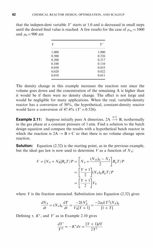
that the indepen-dent variable Y 0 starts at 1.0 and is decreased in small stepsuntil the desired final value is reached. A few results for the case of �1¼ 1000and �0¼ 900 are

Y Y 0

1.000 1.0000.500 0.5260.200 0.2170.100 0.1100.050 0.0550.020 0.0220.010 0.011

The density change in this example increases the reaction rate since thevolume goes down and the concentration of the remaining A is higher thanit would be if there were no density change. The effect is not large andwould be negligible for many applications. When the real, variable-densityreactor has a conversion of 50%, the hypothetical, constant-density reactorwould have a conversion of 47.4% (Y 0 ¼ 0.526).

Example 2.11: Suppose initially pure A dimerizes, 2A �!k=2

B, isothermallyin the gas phase at a constant pressure of 1 atm. Find a solution to the batchdesign equation and compare the results with a hypothetical batch reactor inwhich the reaction is 2A! Bþ C so that there is no volume change uponreaction.

Solution: Equation (2.32) is the starting point, as in the previous example,but the ideal gas law is now used to determine V as a function of NA:

V ¼ ½NA þNB�RgT=P ¼ NA þðNAÞÞ0 �NA

2

� �RgT=P

¼Y þ 1

2

� �ðNAÞ0RgT=P

¼Y þ 1

2

� �V0

where Y is the fraction unreacted. Substitution into Equation (2.32) gives

dNA

dt¼ ðNAÞ0

dY

dt¼�2kN2

A

V0½Y þ 1�¼�2a0kY2ðNAÞ0

½1þ Y �

Defining , K, and Y 0 as in Example 2.10 gives

dY 0

Y 02¼ �Kd ¼

½Y þ 1�dY

2Y2


An analytical solution is again possible but messy. A few results are

Y Y 0

1.000 1.0000.500 0.5420.200 0.2630.100 0.1500.050 0.0830.020 0.0360.010 0.019

The effect of the density change is larger than in the previous example, butis still not major. Note that most gaseous systems will have substantialamounts of inerts (e.g. nitrogen) that will mitigate volume changes at constantpressure.

The general conclusion is that density changes are of minor importance inliquid systems and of only moderate importance in gaseous systems at constantpressure. When they are important, the necessary calculations for a batchreactor are easier if compositions are expressed in terms of total moles ratherthan molar concentrations.

We have considered volume changes resulting from density changes in liquidand gaseous systems. These volume changes were thermodynamically determinedusing an equation of state for the fluid that specifies volume or density as afunction of composition, pressure, temperature, and any other state variablethat may be important. This is the usual case in chemical engineeringproblems. In Example 2.10, the density depended only on the composition.In Example 2.11, the density depended on composition and pressure, but thepressure was specified.

Volume changes also can be mechanically determined, as in the combustioncycle of a piston engine. If V¼V(t) is an explicit function of time, Equationslike (2.32) are then variable-separable and are relatively easy to integrate,either alone or simultaneously with other component balances. Note, however,that reaction rates can become dependent on pressure under extreme conditions.See Problem 5.4. Also, the results will not really apply to car engines sincemixing of air and fuel is relatively slow, flame propagation is important, andthe spatial distribution of the reaction must be considered. The cylinder headis not perfectly mixed.

It is possible that the volume is determined by a combination of thermo-dynamics and mechanics. An example is reaction in an elastic balloon. SeeProblem 2.20.

The examples in this section have treated a single, second-order reaction,although the approach can be generalized to multiple reactions with arbitrary


kinetics. Equation (2.30) can be written for each component:

dðVaÞ

dt¼

dNA

dt¼ VR Aða, b, . . .Þ ¼ VR AðNA,NB, . . . ,VÞ

dðVbÞ

dt¼

dNB

dt¼ VR Bða, b, . . .Þ ¼ VR BðNA,NB, . . . ,VÞ

ð2:33Þ

and so on for components C, D, . . . . An auxiliary equation is used to determineV. The auxiliary equation is normally an algebraic equation rather than anODE. In chemical engineering problems, it will usually be an equation ofstate, such as the ideal gas law. In any case, the set of ODEs can be integratednumerically starting with known initial conditions, and V can be calculated andupdated as necessary. Using Euler’s method, V is determined at each time stepusing the ‘‘old’’ values for NA,NB, . . . . This method of integrating sets of ODEswith various auxiliary equations is discussed more fully in Chapter 3.

2.6.2 Fed-Batch Reactors

Many industrial reactors operate in the fed-batch mode. It is also called the semi-batch mode. In this mode of operation, reactants are charged to the system atvarious times, and products are removed at various times. Occasionally, a heelof material from a previous batch is retained to start the new batch.

There are a variety of reasons for operating in a semibatch mode. Some typi-cal ones are as follows:

1. A starting material is subjected to several different reactions, one after theother. Each reaction is essentially independent, but it is convenient to usethe same vessel.

2. Reaction starts as soon as the reactants come into contact during the chargingprocess. The initial reaction environment differs depending on whether thereactants are charged sequentially or simultaneously.

3. One reactant is charged to the reactor in small increments to control thecomposition distribution of the product. Vinyl copolymerizations discussedin Chapter 13 are typical examples. Incremental addition may also be usedto control the reaction exotherm.

4. A by-product comes out of solution or is intentionally removed to avoid anequilibrium limitation.

5. One reactant is sparingly soluble in the reaction phase and would be depletedwere it not added continuously. Oxygen used in an aerobic fermentation isa typical example.

6. The heel contains a biocatalyst (e.g., yeast cells) needed for the next batch.


All but the first of these has chemical reaction occurring simultaneouslywith mixing or mass transfer. A general treatment requires the combination oftransport equations with the chemical kinetics, and it becomes necessary tosolve sets of partial differential equations rather than ordinary differential equa-tions. Although this approach is becoming common in continuous flow systems,it remains difficult in batch systems. The central difficulty is in developing goodequations for the mixing and mass transfer steps.

The difficulty disappears when the mixing and mass transfer steps are fastcompared with the reaction steps. The contents of the reactor remain perfectlymixed even while new ingredients are being added. Compositions and reactionrates will be spatially uniform, and a flow term is simply added to the massbalance. Instead of Equation (2.30), we write

dNA

dt¼ ðQaÞin þ VR AðNA,NB, . . . ,VÞ ð2:34Þ

where the term ðQaÞin represents the molar flow rate of A into the reactor. A fed-batch reactor is an example of the unsteady, variable-volume CSTRs treated inChapter 14, and solutions to Equation (2.34) are considered there. However,fed-batch reactors are amenable to the methods of this chapter if the chargingand discharging steps are fast compared with reaction times. In this specialcase, the fed-batch reactor becomes a sequence of ideal batch reactors that arereinitialized after each charging or discharging step.

Many semibatch reactions involve more than one phase and are thus classi-fied as heterogeneous. Examples are aerobic fermentations, where oxygen is sup-plied continuously to a liquid substrate, and chemical vapor deposition reactors,where gaseous reactants are supplied continuously to a solid substrate.Typically, the overall reaction rate will be limited by the rate of interphasemass transfer. Such systems are treated using the methods of Chapters 10and 11. Occasionally, the reaction will be kinetically limited so that the trans-ferred component saturates the reaction phase. The system can then be treatedas a batch reaction, with the concentration of the transferred component beingdictated by its solubility. The early stages of a batch fermentation will behave inthis fashion, but will shift to a mass transfer limitation as the cell mass and thusthe oxygen demand increase.

2.7 SCALEUP OF BATCH REACTIONS

Section 1.5 described one basic problem of scaling batch reactors; namely, itis impossible to maintain a constant mixing time if the scaleup ratio is large.However, this is a problem for fed-batch reactors and does not pose a limitationif the reactants are premixed. A single-phase, isothermal (or adiabatic) reactionin batch can be scaled indefinitely if the reactants are premixed and preheatedbefore being charged. The restriction to single-phase systems avoids mass


transfer limitations; the restriction to isothermal or, more realistically, adiabatic,systems avoids heat transfer limitations; and the requirement for premixing elim-inates concerns about mixing time. All the reactants are mixed initially, the reac-tion treats all molecules equally, and the agitator may as well be turned off.Thus, within the literal constraints of this chapter, scaleup is not a problem.It is usually possible to preheat and premix the feed streams as they enter thereactor and, indeed, to fill the reactor in a time substantially less than the reac-tion half-life. Unfortunately, as we shall see in other chapters, real systems canbe more complicated. Heat and mass transfer limitations are common. If there isan agitator, it probably has a purpose.

One purpose of the agitator may be to premix the contents after they arecharged rather than on the way in. When does this approach, which violatesthe strict assumptions of an ideal batch reactor, lead to practical scaleup pro-blems? The simple answer is whenever the mixing time, as described inSection 1.5, becomes commensurate with the reaction half-life. If the mixingtime threatens to become limiting upon scaleup, try moving the mixing step tothe transfer piping.

Section 5.3 discusses a variety of techniques for avoiding scaleup problems.The above paragraphs describe the simplest of these techniques. Mixing, masstransfer, and heat transfer all become more difficult as size increases. To avoidlimitations, avoid these steps. Use premixed feed with enough inerts so thatthe reaction stays single phase and the reactor can be operated adiabatically.This simplistic approach is occasionally possible and even economical.

2.8 STOICHIOMETRY AND REACTIONCOORDINATES

The numerical methods in this book can be applied to all components in thesystem, even inerts. When the reaction rates are formulated using Equation(2.8), the solutions automatically account for the stoichiometry of the reaction.We have not always followed this approach. For example, several of the exam-ples have ignored product concentrations when they do not affect reaction ratesand when they are easily found from the amount of reactants consumed. Also,some of the analytical solutions have used stoichiometry directly to ease thealgebra. This section formalizes the use of stoichiometric constraints.

2.8.1 Stoichiometry of Single Reactions

The general stoichiometric relationships for a single reaction in a batch reactorare

NA � ðNAÞ0

�A¼

NB � ðNBÞ0

�B¼ � � � ð2:35Þ


where NA is the number of moles present in the system at any time. DivideEquation (2.35) by the volume to obtain

aa� a0�A¼

bb� b0�B¼ � � � ð2:36Þ

The circumflex over a and b allows for spatial variations. It can be ignored whenthe contents are perfectly mixed. Equation (2.36) is the form normally used forbatch reactors where aa ¼ aðtÞ. It can be applied to piston flow reactors by settinga0 ¼ ain and aa ¼ aðzÞ, and to CSTRs by setting a0 ¼ ain and aa ¼ aout:

There are two uses for Equation (2.36). The first is to calculate the concentra-tion of components at the end of a batch reaction cycle or at the outlet of a flowreactor. These equations are used for components that do not affect the reactionrate. They are valid for batch and flow systems of arbitrary complexity if thecircumflexes in Equation (2.36) are retained. Whether or not there are spatialvariations within the reactor makes no difference when aa and bb are averagesover the entire reactor or over the exiting flow stream. All reactors satisfyglobal stoichiometry.

The second use of Equations (2.36) is to eliminate some of the compositionvariables from rate expressions. For example, R Aða, bÞ can be converted toR AðaÞ if Equation (2.36) can be applied to each and every point in the reactor.Reactors for which this is possible are said to preserve local stoichiometry. Thisdoes not apply to real reactors if there are internal mixing or separation processes,such as molecular diffusion, that distinguish between types of molecules. Neitherdoes it apply to multiple reactions, although this restriction can be relaxedthrough use of the reaction coordinate method described in the next section.

2.8.2 Stoichiometry of Multiple Reactions

Consider a system with N chemical components undergoing a set of M reactions.Obviously, N > M: Define the N �M matrix of stoichiometric coefficients as

l ¼

�A,I �A,II . . .�B,I �B,II

..

. . ..

0BBB@

1CCCA ð2:37Þ

Note that the matrix of stoichiometric coefficients devotes a row to each of the Ncomponents and a column to each of the M reactions. We require the reactionsto be independent. A set of reactions is independent if no member of the set canbe obtained by adding or subtracting multiples of the other members. A set willbe independent if every reaction contains one species not present in the otherreactions. The student of linear algebra will understand that the rank of lmust equal M.


Using l, we can write the design equations for a batch reactor in very com-pact form:

dðaVÞ

dt¼ lRV ð2:38Þ

where a is the vector (N � 1 matrix) of component concentrations and R is thevector (M � 1 matrix) of reaction rates.

Example 2.12: Consider a constant-volume batch reaction with thefollowing set of reactions:

Aþ 2B! C R I ¼ kI a

Aþ C! D R II ¼ kII ac

Bþ C! E R III ¼ kIII c

These reaction rates would be plausible if B were present in great excess,say as water in an aqueous reaction. Equation (2.38) can be written out as

d

dt

abcde

0BBBB@

1CCCCA ¼

�1 �1 0�2 0 �1þ1 �1 �10 þ1 00 0 þ1

0BBBB@

1CCCCA

kIakIIackIII c

0@

1A

Expanding this result gives the following set of ODEs:

da

dt¼ � kI a� kII ac

db

dt¼ � 2kIa � kIII c

dc

dt¼ þ kI a� kII ac � kIII c

dd

dt¼ kII ac

de

dt¼ þ kIII c

There are five equations in five unknown concentrations. The set is easilysolved by numerical methods, and the stoichiometry has already been incor-porated. However, it is not the smallest set of ODEs that can be solved todetermine the five concentrations. The first three equations contain only a,b, and c as unknowns and can thus be solved independently of the othertwo equations. The effective dimensionality of the set is only 3.

Example 2.12 illustrates a general result. If local stoichiometry is preserved,no more than M reactor design equations need to be solved to determine all


N concentrations. Years ago, this fact was useful since numerical solutions toODEs required substantial computer time. They can now be solved in literallythe blink of an eye, and there is little incentive to reduce dimensionality insets of ODEs. However, the theory used to reduce dimensionality also givesglobal stoichiometric equations that can be useful. We will therefore present itbriefly.

The extent of reaction or reaction coordinate, e is defined by

NN� NN0 ¼ le ð2:39Þ

where NN and NN0 are column vectors ðN � 1 matricesÞ giving the final and initialnumbers of moles of each component and e is the reaction coordinate vectorðM � 1 matrixÞ. In more explicit form,

NNA

NNB

..

.

0BBB@

1CCCA�

NNA

NNB

..

.

0BBB@

1CCCA

0

¼

�A,I �A,II . . .�B,I �B,II

..

. . ..

0BBB@

1CCCA

"I

"II

..

.

0BB@

1CCA ð2:40Þ

Equation (2.39) is a generalization to M reactions of the stoichiometricconstraints of Equation (2.35). If the vector e is known, the amounts of allN components that are consumed or formed by the reaction can be calculated.

What is needed now is some means for calculating e: To do this, it is useful toconsider some component, H, which is formed only by Reaction I, which doesnot appear in the feed, and which has a stoichiometric coefficient of �II , I ¼ 1for Reaction I and stoichiometric coefficients of zero for all other reactions. Itis always possible to write the chemical equation for Reaction I so that a realproduct has a stoichiometric coefficient of þ1. For example, the decompositionof ozone, 2O3! 3O2, can be rewritten as 2=3O3! O2: However, you mayprefer to maintain integer coefficients. Also, it is necessary that H not occur inthe feed, that there is a unique H for each reaction, and that H participatesonly in the reaction that forms it. Think of H as a kind of chemical neutrinoformed by the particular reaction. Since H participates only in Reaction I anddoes not occur in the feed, Equation (2.40) gives

NH ¼ "I

The batch reactor equation gives

dðVhÞ

dt¼

dðNHÞ

dt¼

d"I

dt¼ VR I ðNA,NB, . . . ,VÞ ¼ VR I ð"I , "II , . . . ,VÞ ð2:41Þ

The conversion from R I ðNA,NB, . . . ,VÞ to R I ð"I , "II , . . . ,VÞ is carried outusing the algebraic equations obtained from Equation (2.40). The initial


condition associated with Equation (2.41) is each "I¼ 0 at t¼ 0. We now con-sider a different H for each of the M reactions, giving

dedt¼ V R where e ¼ 0 at t ¼ 0 ð2:42Þ

Equation (2.42) represents a set of M ODEs in M independent variables,"I , "II , . . . . It, like the redundant set of ODEs in Equation (2.38), will normallyrequire numerical solution. Once solved, the values for the e can be used tocalculate the N composition variables using Equation (2.40).

Example 2.13: Apply the reaction coordinate method to the reactions inExample 2.12.

Solution: Equation (2.42) for this set is

d

dt

"I

"II

"III

0@

1A ¼ V

kI akII ackIII c

0@

1A ¼ kI NA

kI NANC=VkIIINC

0@

1A ð2:43Þ

Equation (2.40) can be written out for this reaction set to give

NA � ðNAÞ0 ¼ �"I � "II

NB � ðNBÞ0 ¼ �2"I � "III

NC � ðNCÞ0 ¼ þ"I � "II � "III

ND � ðNDÞ0 ¼ þ"II

NE � ðNEÞ0 ¼ þ "III

ð2:44Þ

The first three of these equations are used to eliminate NA, NB, and NC fromEquation (2.43). The result is

d"I

dt¼ kI ½ðNAÞ0 � "I � "II �

d"II

dt¼

kII

V½ðNAÞ0 � "I � "II �½ðNCÞ0 þ "I � "II � "III �

d"III

dt¼ kIII ½ðNCÞ0 þ "I � "II � "III �

Integrate these out to time tbatch and then use Equations (2.44) to evaluateNA, . . . ,NE . The corresponding concentrations can be found by dividing byVðtbatchÞ:


In a formal sense, Equation (2.38) applies to all batch reactor problems.So does Equation (2.42) combined with Equation (2.40). These equations areperfectly general when the reactor volume is well mixed and the various compo-nents are quickly charged. They do not require the assumption of constantreactor volume. If the volume does vary, ancillary, algebraic equations areneeded as discussed in Section 2.6.1. The usual case is a thermodynamicallyimposed volume change. Then, an equation of state is needed to calculatethe density.

PROBLEMS

2.1. The following reactions are occurring in a constant-volume, isothermalbatch reactor:

Aþ B �!kI

C

Bþ C �!kII

D

Parameters for the reactions are a0¼ b0¼ 10mol/m3, c0¼ d0¼ 0,kI¼ kII¼ 0.01m3/(mol Eh), tbatch¼ 4 h.(a) Find the concentration of C at the end of the batch cycle.(b) Find a general relationship between the concentrations of A and C

when that of C is at a maximum.2.2. The following kinetic scheme is postulated for a batch reaction:

Aþ B! C R I ¼ kI a1=2b

Bþ C! D R II ¼ kIIc1=2b

Determine a, b, c and d as functions of time. Continue your calculationsuntil the limiting reagent is 90% consumed given a0¼ 10mol/m3,b0¼ 2mol/m3, c0¼ d0¼ 0, kI¼ kII¼ 0.02m3/2/(mol1/2 E s).

2.3. Refer to Example 2.5. Prepare the plot referred to in the last sentence ofthat example. Assume kII=kI ¼ 0:1.

2.4. Dimethyl ether thermally decomposes at temperatures above 450�C. Thepredominant reaction is

CH3OCH3! CH4 þH2 þ CO

Suppose a homogeneous, gas-phase reaction occurs in a constant-volumebatch reactor. Assume ideal gas behavior and suppose pure A is chargedto the reactor.


(a) Show how the reaction rate can be determined from pressure mea-surements. Specifically, relate R to dP/dt.

(b) Determine P(t), assuming that the decomposition is first order.2.5. The first step in manufacturing polyethylene terephthalate is to react

terephthalic acid with a large excess of ethylene glycol to form diglycolterephthalate:

HOOC�f�COOHþ 2HOCH2CH2OH!

HOCH2CH2OOC�f�COOCH2CH2OHþ 2H2O

Derive a plausible kinetic model for this reaction. Be sure your modelreflects the need for the large excess of glycol. This need is inherent inthe chemistry if you wish to avoid by-products.

2.6. Consider the liquid-phase reaction of a diacid with a diol, the first reac-tion step being

HO�R�OHþHOOC�R0�COOH! HO�ROOCR0�COOHþH2O

Suppose the desired product is the single-step mixed acidol as shownabove. A large excess of the diol is used, and batch reactions are conductedto determine experimentally the reaction time, tmax, which maximizesthe yield of acidol. Devise a kinetic model for the system and explainhow the parameters in this model can be fit to the experimental data.

2.7. The exponential function can be defined as a limit:

Limm!1

1þz

m

� �m

¼ ez

Use this fact to show that Equation (2.17) becomes Equation (2.16) in thelimit as n !1.

2.8. Determine the maximum batch reactor yield of B for a reversible, first-order reaction:

A ��! ��

kf

kr

B

Do not assume b0¼ 0. Instead, your answer will depend on the amount ofB initially present.

2.9. Start with 1 mol of 238U and let it age for 10 billion years or so. Refer toTable 2.1. What is the maximum number of atoms of 214Po that will everexist? Warning! This problem is monstrously difficult to solve by bruteforce methods. A long but straightforward analytical solution is possible.See also Section 2.5.3 for a shortcut method.

2.10. Consider the consecutive reactions

A �!k

B �!k

C

where the two reactions have equal rates. Find bðtÞ.


2.11. Find the batch reaction time that maximizes the concentration of compo-nent B in Problem 2.10. You may begin with the solution of Problem 2.10or with Equation (2.23).

2.12. Find c(t) for the consecutive, first-order reactions of Equation (2.20)given that kB ¼ kC:

2.13. Determine the batch reaction time that maximizes the concentration ofcomponent C in Equation (2.20) given that kA¼ 1 h�1, kB¼ 0.5 h�1,kC¼ 0.25 h–1, kD¼ 0.125 h–1.

2.14. Consider the sequential reactions of Equation (2.20) and supposeb0¼ c0¼ d0¼ 0, kI¼ 3 h�1, kII¼ 2 h�1, kIII¼ 4 h�1. Determine the ratiosa/a0, b/a0, c/a0, and d/a0, when the batch reaction time is chosensuch that(a) The final concentration of A is maximized.(b) The final concentration of B is maximized.(c) The final concentration of C is maximized.(d) The final concentration of D is maximized.

2.15. Find the value of the dimensionless batch reaction time, kf tbatch, thatmaximizes the concentration of B for the following reactions:

A ��! ��

kf

kr

B �!kB

C

Compare this maximum value for b with the value for b obtained usingthe quasi-steady hypothesis. Try several cases: (a) kr ¼ kB ¼ 10kf , (b)kr ¼ kB ¼ 20kf , (c) kr ¼ 2kB ¼ 10kf :

2.16. The bromine–hydrogen reaction

Br2 þH2 ! 2HBr

is believed to proceed by the following elementary reactions:

Br2 þM ��! ��

kI

k�I

2Br. þM ðIÞ

Br. þH2��! ��

kII

k�II

HBrþH. ðIIÞ

H. þ Br2 �!kIII

HBrþ Br . ðIIIÞ

The initiation step, Reaction (I), represents the thermal dissociation ofbromine, which is brought about by collision with any other molecule,denoted by M.


(a) The only termination reaction is the reverse of the initiation step andis third order. Apply the quasi-steady hypothesis to ½Br. � and ½H. � toobtain

R ¼k½H2� ½Br2�

3=2

½Br2� þ kA½HBr�

(b) What is the result if the reverse reaction (I) does not exist and termi-nation is second order, 2Br. ! Br2?

2.17. A proposed mechanism for the thermal cracking of ethane is

C2H6 þM �!kI

2CH3. þM

CH3. þ C2H6 �!

kIICH4 þ C2H5

.

C2H5. �!

kIIIC2H4 þH.

H.þC2H6 �!kIV

H2 þ C2H5.

2C2H5. �!

kVC4H10

The overall reaction has variable stoichiometry:

C2H6 ! �BC2H4 þ �CC4H10 þ ð2 � 2�B � 4�CÞCH4

þ ð�1þ 2�B þ 3�CÞH2

The free-radical concentrations are small and are ignored in this equationfor the overall reaction.(a) Apply the quasi-steady hypothesis to obtain an expression for the

disappearance of ethane.(b) What does the quasi-steady hypothesis predict for �B and �C?(c) Ethylene is the desired product. Which is better for this gas-phase

reaction, high or low pressure?2.18. The Lotka-Volterra reaction described in Section 2.5.4 has three initial

conditions—one each for grass, rabbits, and lynx—all of which mustbe positive. There are three rate constants assuming the supply of grassis not depleted. Use dimensionless variables to reduce the number ofindependent parameters to four. Pick values for these that lead to a sus-tained oscillation. Then, vary the parameter governing the grass supplyand determine how this affects the period and amplitude of the solution.

2.19. It is proposed to study the hydrogenation of ethylene

C2H4 þH2! C2H6


in a constant-pressure, gas-phase batch reactor. Derive an expression forthe reactor volume as a function of time, assuming second-order kinetics,ideal gas behavior, perfect stoichiometry, and 50% inerts by volume att¼ 0.

2.20. Suppose a rubber balloon is filled with a gas mixture and that one of thefollowing reactions occurs:

2A �!k

B

Aþ B �!k

C

A �!k

Bþ C

Determine V(t).Hint 1: The pressure difference between the inside and the outside

of the balloon must be balanced by the stress in the fabric of the balloonso that �R2 �P ¼ 2�Rh where h is the thickness of the fabric and isthe stress.

Hint 2: Assume that the density of the fabric is constant so that4�R2h ¼ 4�R2

0h0:Hint 3: Assume that the fabric is perfectly elastic so that stress is pro-

portional to strain (Hooke’s law).Hint 4: The ideal gas law applies.

2.21. A numerical integration scheme has produced the following results:

�z Integral

1.0 0.237490.5 0.201080.25 0.192980.125 0.191040.0625 0.19056

(a) What is the apparent order of convergence?(b) Extrapolate the results to �z¼ 0. (Note: Such extrapolation should

not be done unless the integration scheme has a theoretical order ofconvergence that agrees with the apparent order. Assume that itdoes.)

(c) What value for the integral would you expect at �z¼ 1/32?2.22. See Example 2.14 in Appendix 2.

(a) Write chemical equations that will give the ODEs of that example.(b) Rumor has it that there is an error in the Runge-Kutta calculations

for the case of �t¼ 0.5. Write or acquire the necessary computercode and confirm or deny the rumor.


2.23. The usual method of testing for convergence and of extrapolating to zerostep size assumes that the step size is halved in successive calculations.Example 2.4 quarters the step size. Develop an extrapolation techniquefor this procedure. Test it using the data in Example 2.15 in Appendix 2.

REFERENCE

1. Boyer, A., Niclause, M., and Letort, M., ‘‘Cinetique de pyrolyse des aldehydes aliphatiquesen phase gazeuse,’’ J. Chim. Phys., 49, 345–353 (1952).

SUGGESTIONS FOR FURTHER READING

Most undergraduate texts on physical chemistry give a survey of chemicalkinetics and reaction mechanisms. A comprehensive treatment is provided in

Benson, S. W., Foundations of Chemical Kinetics, McGraw-Hill, New York, 1960.

A briefer and more recent description is found in

Espenson, J. H., Ed., Chemical Kinetics and Reaction Mechanisms, McGraw-Hill, New York,1995.

A recent, comprehensive treatment of chemical oscillators and assorted esotericais given in

Epstein, I. R. and Pojman, J. A., Eds., An Introduction to Nonlinear Chemical Dynamics:Oscillations, Waves, Patterns, and Chaos, Oxford University Press, New York, 1998.

A classic, mathematically oriented work has been reprinted as a paperback:

Aris, R., Elementary Chemical Reactor Analysis, Dover, Mineola, NY, 2000.

An account of the reaction coordinate method as applied to chemical equili-brium is given in Chapter 14 of

Smith, J. M., Van Ness, H. C., and Abbott, M. M., Introduction to Chemical EngineeringThermodynamics, 6th ed., McGraw-Hill, New York, 2001.

The Internet has become a wonderful source of (sometimes free) software fornumerical analysis. Browse through it, and you will soon see that Fortranremains the programming language for serious numerical computation. Oneexcellent book that is currently available without charge is

Press, W. H., Teukolsky, S. A., Vetterling, W. T., and Flannery, B. P., Numerical Recipes inFortran 77: The Art of Scientific Computing, Vol. 1, 2nd ed., Cambridge University Press,New York, 1992.

This book describes and gives Fortran subroutines for a wide variety of ODEsolvers. More to the point, it gives numerical recipes for practically anythingyou will ever need to compute. Volume 2 is also available online. It discussesFortran 90 in the context of parallel computing. C, Pascal, and Basic versionsof Volume 1 can be purchased.


APPENDIX 2: NUMERICAL SOLUTION OFORDINARY DIFFERENTIAL EQUATIONS

In this chapter we described Euler’s method for solving sets of ordinary differ-ential equations. The method is extremely simple from a conceptual and pro-gramming viewpoint. It is computationally inefficient in the sense that a greatmany arithmetic operations are necessary to produce accurate solutions. Moreefficient techniques should be used when the same set of equations is to besolved many times, as in optimization studies. One such technique, fourth-order Runge-Kutta, has proved very popular and can be generally recommendedfor all but very stiff sets of first-order ordinary differential equations. The set ofequations to be solved is

da

dt¼ R Aða, b, . . . , tÞ

db

dt¼ R Bða, b, . . . , tÞ

ð2:45Þ

..

. ...

A value of �t is selected, and values for �a, �b, . . . are estimated by evaluatingthe functions R A,R B . . . . In Euler’s method, this evaluation is done at theinitial point (a0, b0, . . . , t0) so that the estimate for �a is just �tR Aða0,b0, . . . , t0Þ ¼ �tðR AÞ0: In fourth-order Runge-Kutta, the evaluation is done atfour points and the estimates for �a, �b, . . . are based on weighted averagesof the R A, R B, . . . at these four points:

�a ¼ �tðR AÞ0 þ 2ðR AÞ1 þ 2ðR AÞ2 þ ðR AÞ3

6

�b ¼ �tðR BÞ0 þ 2ðR BÞ1 þ 2ðR BÞ2 þ ðR BÞ3

6ð2:46Þ

..

. ...

where the various R s are evaluated at the points

a1 ¼ a0 þ�tðR AÞ0=2

a2 ¼ a0 þ�tðR AÞ1=2

a3 ¼ a0 þ�tðR AÞ2

ð2:47Þ

with similar equations for b1, b2, b3, and so on. Time rarely appears explicitly inthe R , but, should it appear,

t1 ¼ t0 þ�t=2

t2 ¼ t1

t3 ¼ t0 þ�t

ð2:48Þ


Example 2.14: Use fourth-order Runge-Kutta integration to solve thefollowing set of ODEs:

da

dt¼ �k1a

2

db

dt¼ þk1a

2 � k2bc

dc

dt¼ �k2bc

Use a0¼ c0¼ 30, b0¼ 0, k1 ¼ 0:01, k2¼ 0.02. Find a, b, and c for t¼ 1.

Solution: The coding is left to the reader, but if you really need a workedexample of the Runge-Kutta integration, check out Example 6.4. The follow-ing are detailed results for �t¼ 1.0, which means that only one step was takento reach the answer.

j ai bi ci (R A)j (R B)j (R C)j

0 30.000 0 30.000 �18.000 9.000 01 21.000 4.500 30.000 �8.820 1.710 �2.7002 25.590 0.855 28.650 �13.097 6.059 �0.4903 16.903 6.059 29.510 �5.714 �0.719 �3.576

Final : 18:742 3:970 28:341

For �t¼ 0.5, the results for a, b, and c are

Final : 18:750 4:069 28:445

Results accurate to three places after the decimal are obtained with �t¼ 0.25:

Final : 18:750 4:072 28:448

The fourth Runge-Kutta method converges O(�t5). Thus, halving the stepsize decreases the error by a factor of 32. By comparison, Euler’s method con-verges O(�t) so that halving the step size decreases the error by a factor ofonly 2. These remarks apply only in the limit as �t ! 0, and either methodcan give anomalous behavior if �t is large. If you can confirm that the dataare converging according to the theoretical order of convergence, the conver-gence order can be used to extrapolate calculations to the limit as �t ! 0.

Example 2.15: Develop an extrapolation technique suitable for the first-order convergence of Euler integration. Test it for the set of ODEs inExample 2.3.


Solution: Repeat the calculations in Example 2.3 but now reduce �t bya factor of 2 for each successive calculation rather than by the factor of4 used in the examples. Calculate the corresponding changes in a(tmax) anddenote these changes by �. Then � should decrease by a factor of 2 foreach calculation of a(tmax). (The reader interested in rigor will note that theerror is halved and will do some algebra to prove that the � are halved aswell.) If � was the change that just occurred, then we would expect thenext change to be �/2, the one after that to be �/4, and so on. The totalchange yet to come is thus �/2þ�/4þ�/8þ � � �. This is a geometric seriesthat converges to �. Using Euler’s method, the cumulative change yet tocome is equal to the single change that just occurred. Thus, the extrapolatedvalue for a(tmax) is the value just calculated plus the � just calculated. Theextrapolation scheme is illustrated for the ODEs in Example 2.3 in thefollowing table:

Numberof steps a(tmax) �

Extrapolateda(tmax)

2 �16.32004 1.5392 17.8591 19.39388 2.8245 1.2854 4.109916 3.2436 0.4191 3.662632 3.4367 0.1931 3.629864 3.5304 0.0937 3.6241128 3.5766 0.0462 3.6228256 3.5995 0.0229 3.6225512 3.6110 0.0114 3.62241024 3.6167 0.0057 3.62242048 3.6195 0.0029 3.62244096 3.6210 0.0014 3.62248192 3.6217 0.0007 3.622416384 3.6220 0.0004 3.622432768 3.6222 0.0002 3.622465536 3.6223 0.0001 3.6224131072 3.6223 0.0000 3.6224

Extrapolation can reduce computational effort by a large factor, but compu-tation is cheap. The value of the computational reduction will be trivial for mostproblems. Convergence acceleration can be useful for complex problems or forthe inside loops in optimization studies. For such cases, you should also considermore sophisticated integration schemes such as Runge-Kutta. It too can beextrapolated, although the extrapolation rule is different. The extrapolatedfactor for Runge-Kutta integration is based on the series

1=32þ 1=322 þ 1=323 þ � � � ¼ 0:03226


Thus, the total change yet to come is about 3% of the change that just occurred.As a practical matter, your calculations will probably achieve the required accu-racy by the time you confirm that successive changes in the integral really aredecreasing by a factor of 32 each time. With modern computers and Runge-Kutta integration, extrapolation is seldom needed for the solution of ODEs.It may still be useful in the solution of the second-order, partial differential equa-tions treated in Chapters 8 and 9. Ordinary differential equation solvers areoften used as part of the solution technique for PDEs. Extrapolation is usedin some highly efficient ODE solvers. A variety of sophisticated integration tech-niques are available both as freeware and as commercial packages. Their usemay be justified for design and optimization studies where the same set of equa-tions must be solved repetitively or when the equations are exceptionally stiff.The casual user need go no further than Runge-Kutta, possibly with adaptivestep sizes where �t is varied from step to step in the calculations based onerror estimates. See Numerical Recipes by Press et al., as cited in the‘‘Suggestions for Further Reading’’ section for this chapter, for a usable exampleof Runge-Kutta integration with adaptive step sizes.


MULTIPLE REACTIONS IN BATCH REACTORS

Documents

Transcript of MULTIPLE REACTIONS IN BATCH REACTORS