POLITECNICO DI MILANOScuola di Ingegneria Industriale e dell’Informazione

Corso di Laurea Magistrale in Ingegneria Energetica

Modeling Liquid-Droplet Evaporation in a

Direct Contact Heat Exchanger

Politecnico di Milano, Ecole Polytechnique de Montreal

“Altan Tapucu” Thermohydraulic Laboratory

Montreal, Canada

Tesi di Laurea di:

Franco Cascella (771139)

Relatore: Andrea Lucchini (PhD)

Anno Accademico 2012-2013

c© Franco Cascella, 2013.

ne dolcezza di figlio, ne la pietadel vecchio padre, ne ’l debito amorelo qual dovea Penelope far lieta, 96

vincer potero dentro a me l’ardorech’i’ ebbi a divenir del mondo esperto,e de li vizi umani e del valore; 99

ma misi me per l’alto mare apertosol con un legno e con quella compagnapicciola da la qual non fui diserto. 102

Dante, Inferno, Canto XXVI, vv 94-102

To the people I lovenothing else matters. . .

iv

ACKNOWLEDGEMENTS

This thesis is the result of two years of trying work. Even though its realization has been

strenuous, the feeling of accomplishment I have now in fulfilling it is limitless. However, this

accomplishment could not have been reached without the help and mostly the trust of the

people who supported me over the past two years.

I would like to thank the two universities, the Ecole Polythecnique de Montreal and the

Politecnico di Milano, that allowed me to do the double degree programs between these two

institutions. I was not the ideal student to do this, thus, I’ve always worked hard in order to

gain their confidence. I hope to have achieved this task.

Professor Alberto Teyssedou has had a significant role in these two years. His economic

help was essential, but not as much as the trust he has had for me from the beginning of

my Master’s. Though he did not know me two years ago, he accepted me as his student.

Since then, he has never stopped believing in me, in my knowledge and in my ability. For

this reason, he has always encouraged me – even my ideas that could have been considered

unattainable – and never stopped providing me with precious suggestions and advice (not

necessarily limited to my work). Thanks to him, I was able to present my project at the

Canadian Nuclear Society in Toronto on June 12th and to write a scientific paper.

My thanks also go to my family whose presence has always been strong, in spite of the

seven thousand kilometers that divide us. I thank my sister Cinzia, who has forgiven for not

being as present in her life as I would like be, to my mother Lidia, who keeps on bearing me

showing infinite tolerance, and to my father Cosimo, who has understood my need to leave

Bari, even if he would have preferred me to stay.

I thank my relatives in Vancouver, for making me feel less alone in this country; they

have always helped me in the moments of need. Thanks to Filomena, Nicla and Generoso

Vitucci for their supporting Skype calls, and to my beloved uncle Girolamo Vitucci, whose

absence is harder to handle day by day.

I cannot forget to emphasize the help of the people I have met over the past two years.

I thank Giovanniantonio Natale, who is not only a colleague who has patiently analyzed

my work providing valuable suggestions, but mostly a friend. The moments we have spent

together (inside and outside the school) are a significant part of my experience in Montreal. I

thank my closest friends, Valeria Galluccio in Montreal and Alessandra Azzena in Milan, for

their unconditional moral support. And I thank all those people I am simply grateful to have

met here: Giovanni, the first and best roommate ever, Cecilia for our pleasant runs in Mount

Royal Park, Paul and Thomas for improving my French by revising everything I wrote and

v

correcting my pronunciation, Daniel Del Balso for showing how important our friendship was

even on Christmas holidays, Madeleine for being by my side in the most difficult moment

of my life, Lidia, Elsa, Rami, Rosario, Linda and all the people I am forgetting. A special

thanks go to my friends in Bari, who have never forgotten me: seeing them waiting for me

at the airport in Bari was one of the most touching moments of my life.

My final thanks go to the person who uncovered my weaknesses, showing how selfish,

touchy and insecure I can be. In other words, she saw how afraid I am to fail in life.

Nevertheless, she was always close to me and appreciated me in a way I could never have

imagined.

vi

ABSTRACT

In the last thirty years, Direct Contact Heat Exchangers (DCHX) have found success in

different power engineering applications. In fact, due to their configuration, which allows the

direct contact between the hot and cold fluids, it is possible to reach very high mass and

energy transfer efficiencies. Despite their high performance, it remains, to this day, difficult

to correctly predict the thermal power as a function of plant operation conditions. In fact,

this problematic constitutes a fundamental parameter to correctly operate heat exchangers.

In order to study super-critical water choked flow in a super-critical water loop, a heat

exchanger of this type has been recently installed in the “Altan Tapucu” Thermo-hydraulic

Laboratory. It consists of a fluid mixer called “quenching chamber”, i.e. a vessel where super-

heated steam coming from a test section (where choked flow conditions occur) mixes with

sub-cooled water. This component can safely work in a wide range of pressures (5 bar < p <

40 bar). However, on the top of the vessel, a nozzle is set so that the cooling water is sprayed

into the chamber under the form of tiny droplets (i.e., about 200 µm in diameter).

Within the frame work of this Master’s thesis, we developed a thermodynamic model

capable of describing the thermal power in the aforementioned DCHX for different working

conditions. The main idea is to apply an energy balance to every single droplet in order

to evaluate the total heat transfer. In order to do that, we focused our attention on two

problems:

–Droplet size: to perform any energy balance, it is necessary to know the droplet size,

however, the quenching chamber working conditions affect this parameter. That is, the

droplet dimensions vary depending on steam pressure, liquid flow rate and temperature.

Moreover, for a given condition, droplets are expected to have non-uniform dimensions.

This means that firstly, a statistical distribution describing the droplet size is to be

found, and secondly, the working conditions have to be considered when evaluating this

statistical law.

–Heat transfer: Since there is a mutual interaction between the sub-cooled liquid (dis-

perse phase) and the super-heated steam (continuous phase), we analyzed two heat

transfer modes: convection and evaporation. However, this study cannot be performed

without a preliminary evaluation of the droplet velocity. That is, the velocity field

needs to be known since it affects the amount of energy released.

In this work, the experimental data collected at Ecole Polytechnique de Montreal are

compared with the predictions of our model. We found a very good agreement for steam

vii

pressures of 1.6 and 2.1 MPa however, at higher pressures, it over estimates the experimental

trends. Hence, we performed an analysis in order to explain the model behavior. Thus, we

have justified the observed over predictions at high pressure due to physical variables which

are not taken into account in the model (such as droplet collision and break-up).

Despite the fact that our modeling approach may be questionable on several points, it

gives us the possibility to analyze the quenching chamber behavior by linking the dynamics

of liquid droplets to the total thermal power. This way, we are able to predict some working

conditions that may optimize the thermal power in our DCHX. However, this aspect has not

been proven yet and should be the research subject of a future work.

viii

RESUME

Negli ultimi 30 anni gli scambiatori di calore a contatto diretto (Direct Contact Heat Ex-

changer, DCHX) hanno riscontrato grande successo in diverse applicazioni ingegneristiche.

Infatti, in questi scambiatori vi e contatto diretto tra il fluido caldo e fluido freddo, il che

permette di ottenere elevati rendimenti energetici. Nonostante le loro elevate prestazioni,

e ancora molto difficile valutare gli scambi termici in funzione delle condizioni di funziona-

mento dello scambiatore di calore; questa valutazione risulta quindi necessaria per garantire

il corretto funzionamento dei suddetti DCHX.

Per studiare l’evoluzione fluidodinamica del vapore supercritico e supersonico in una stroz-

zatura (comunemente chiamata choked flow in letteratura), un DCHX e stato recentemente

installato nel laboratorio di termo-idraulica“Altan Tapucu”dell’Ecole Polytechnique de Mon-

treal. Questo componente, comunemente chiamato quenching chamber, consiste in un con-

dotto dove vapore surriscaldato proveniente da una sezione di prova (in cui si verificano le

condizioni supersoniche) e mescolato con acqua sotto raffreddata. Questo componente puo

lavorare in tutta sicurezza in una vasto gamma di pressioni (5 bar < p < 40 bar). Inoltre,

sulla parte superiore dello scambiatore, e presente un nebulizzatore (spray nozzle) che con-

sente il cambio di fase dell’acqua da continua a dispersa; le gocce d’acqua cosı formate hanno

un diametro dell’ordine di 200 µm.

Negli ultimi due anni abbiamo sviluppato un modello termodinamico per descrivere lo

scambio termico nel DCHX per diverse condizioni di lavoro. L’idea principale e quella di

applicare un bilancio energetico per ogni goccia al fine di valutare la potenza termica totale

scambiata. Per fare questo, abbiamo focalizzato la nostra attenzione su due questioni:

–Determinazione della dimensione delle gocce: per effettuare il bilancio energetico,

e necessario conoscere la dimensione delle gocce. Tuttavia, le condizioni di lavoro della

camera influenzano questo parametro; infatti la dimensione delle gocce variera a sec-

onda di determinate variabili, quali la tensione di vapore, la portata e la temperatura

del liquido. Inoltre, per una data condizione, e impossibile (o perlomeno poco proba-

bile) aspettarsi che gocce abbiano dimensione uniforme. Quindi, bisogna introdurre una

distribuzione statistica (Droplet Distribution Function, DDF) che da un lato descriva la

dimensione delle gocce, dall’altro, tenga conto dell’influenza che le condizioni di lavoro

del DCHX hanno sulla suddetta distribuzione.

–Soluzione del problema di scambio termico: Dal momento che vi e una mutua in-

terazione tra il liquido sotto-raffreddato (fase dispersa) e vapore surriscaldato (fase

continua), abbiamo analizzato due modalita trasmissione del calore: convezione ed

ix

evaporazione. Tuttavia, questo studio non puo essere eseguito senza una precedente

valutazione della velocita delle gocce. In altre parole, la soluzione del problema di

scambio termico non puo precludere la valutazione del campo di velocita delle gocce,

visto che quest’ultimo influenza il trasferimento di calore.

In questo lavoro, i dati sperimentali raccolti presso i laboratori dell’Ecole Polytechnique de

Montreal sono confrontati con le previsioni del nostro modello. Abbiamo trovato un ottimo

accordo per le pressioni della camera di 1.6 e 2.1 MPa, ma a pressioni piu elevate il modello

sovrastima sensibilmente i dati sperimentali. Pertanto, abbiamo effettuato un’analisi per

capire le ragioni di questo comportamento: i fenomeni che non sono stati considerati e che

possono influire sul modello sono legati alle mutue interazioni fisiche e dinamiche fra le gocce

(ovvero la collisione e il breakup delle suddette).

Anche se il nostro approccio teorico puo essere discutibile su diversi punti, questo modello

ci da la possibilita di analizzare il comportamento dello scambiatore di calore, correlando la

dinamica delle gocce alla potenza termica totale scambiata. Nonostante ci siano ancora ampi

margini di miglioramento, possiamo ritenerci piu che soddisfatti dei risultati ottenuti.

x

TABLE OF CONTENTS

DEDICATION . . . . . . . . . . . . . . . . . . . . . . . . . . . . . . . . . . . . . . . . iii

ACKNOWLEDGEMENTS . . . . . . . . . . . . . . . . . . . . . . . . . . . . . . . . . iv

ABSTRACT . . . . . . . . . . . . . . . . . . . . . . . . . . . . . . . . . . . . . . . . . vi

RESUME . . . . . . . . . . . . . . . . . . . . . . . . . . . . . . . . . . . . . . . . . . . viii

TABLE OF CONTENTS . . . . . . . . . . . . . . . . . . . . . . . . . . . . . . . . . . x

LIST OF TABLES . . . . . . . . . . . . . . . . . . . . . . . . . . . . . . . . . . . . . . xii

LIST OF FIGURES . . . . . . . . . . . . . . . . . . . . . . . . . . . . . . . . . . . . . xiii

LIST OF APPENDICES . . . . . . . . . . . . . . . . . . . . . . . . . . . . . . . . . . . xv

LIST OF ACRONYSMS AND SYMBOLS . . . . . . . . . . . . . . . . . . . . . . . . . xvi

CHAPTER 1 INTRODUCTION . . . . . . . . . . . . . . . . . . . . . . . . . . . . . 1

1.1 Direct Contact Heat Exchangers (DCHX) . . . . . . . . . . . . . . . . . . . . 1

1.2 Problem Studied . . . . . . . . . . . . . . . . . . . . . . . . . . . . . . . . . . 2

1.3 Research Objectives . . . . . . . . . . . . . . . . . . . . . . . . . . . . . . . . . 4

1.4 Thesis Plan . . . . . . . . . . . . . . . . . . . . . . . . . . . . . . . . . . . . . 5

CHAPTER 2 LITERATURE REVIEW . . . . . . . . . . . . . . . . . . . . . . . . . 7

2.1 Droplet Size Evaluation . . . . . . . . . . . . . . . . . . . . . . . . . . . . . . 7

2.1.1 The Atomization Process . . . . . . . . . . . . . . . . . . . . . . . . . . 8

2.1.2 Droplet Distribution Function (DDF) . . . . . . . . . . . . . . . . . . . 9

2.2 Heat and Mass Transfer from Liquid Droplets . . . . . . . . . . . . . . . . . . 11

CHAPTER 3 THE EXPERIMENTAL FACILITY . . . . . . . . . . . . . . . . . . . . 14

3.1 The Super Critical Water Loop (SCWL) . . . . . . . . . . . . . . . . . . . . . 14

3.2 The Test Section . . . . . . . . . . . . . . . . . . . . . . . . . . . . . . . . . . 16

3.3 The Quenching Chamber . . . . . . . . . . . . . . . . . . . . . . . . . . . . . . 18

xi

CHAPTER 4 DEVELOPMENT OF A STATISTIC DISRIBUTION FUNCTION FOR

THE DROPLET SIZE . . . . . . . . . . . . . . . . . . . . . . . . . . . . . . . . . . 21

4.1 The Sauter Mean Diameter . . . . . . . . . . . . . . . . . . . . . . . . . . . . 21

4.1.1 Lefebvre’s Correlation (1989) . . . . . . . . . . . . . . . . . . . . . . . 24

4.2 The Droplet Distribution Function . . . . . . . . . . . . . . . . . . . . . . . . 25

4.2.1 The Rosin-Rammler Equation . . . . . . . . . . . . . . . . . . . . . . . 26

4.3 Considerations on Statistical Methodology . . . . . . . . . . . . . . . . . . . . 27

CHAPTER 5 HEAT TRANSFER STUDY . . . . . . . . . . . . . . . . . . . . . . . . 30

5.1 The Steam Temperature . . . . . . . . . . . . . . . . . . . . . . . . . . . . . . 30

5.2 The Solution of the Heat Transfer Problem . . . . . . . . . . . . . . . . . . . . 32

5.2.1 Droplet Convective Heat Transfer . . . . . . . . . . . . . . . . . . . . . 33

5.2.2 Droplet Evaporation Heat Transfer . . . . . . . . . . . . . . . . . . . . 36

5.3 Thermal Power Transferred in DCHX Systems . . . . . . . . . . . . . . . . . . 37

5.4 Final Remarks on the Presented Procedure . . . . . . . . . . . . . . . . . . . . 38

CHAPTER 6 RESULTS . . . . . . . . . . . . . . . . . . . . . . . . . . . . . . . . . . 40

6.1 Model Methodology . . . . . . . . . . . . . . . . . . . . . . . . . . . . . . . . . 40

6.1.1 Analysis of a DCHX Thermal Condition . . . . . . . . . . . . . . . . . 43

6.2 Comparison of Model with Experimental Data . . . . . . . . . . . . . . . . . . 47

6.3 Parametric Study . . . . . . . . . . . . . . . . . . . . . . . . . . . . . . . . . . 52

6.4 Other Correlation Approach . . . . . . . . . . . . . . . . . . . . . . . . . . . . 55

6.4.1 Definition of f . . . . . . . . . . . . . . . . . . . . . . . . . . . . . . . . 55

6.4.2 Definition of ψ . . . . . . . . . . . . . . . . . . . . . . . . . . . . . . . 57

6.5 Final Remarks . . . . . . . . . . . . . . . . . . . . . . . . . . . . . . . . . . . . 59

CHAPTER 7 CONCLUSION . . . . . . . . . . . . . . . . . . . . . . . . . . . . . . . 60

7.1 General Objectives . . . . . . . . . . . . . . . . . . . . . . . . . . . . . . . . . 60

7.2 Limits of the Proposed Model . . . . . . . . . . . . . . . . . . . . . . . . . . . 61

7.3 Result Discussion . . . . . . . . . . . . . . . . . . . . . . . . . . . . . . . . . . 62

7.4 Usefulness of the Proposed Model . . . . . . . . . . . . . . . . . . . . . . . . . 63

7.5 Future Work . . . . . . . . . . . . . . . . . . . . . . . . . . . . . . . . . . . . . 64

REFERENCES . . . . . . . . . . . . . . . . . . . . . . . . . . . . . . . . . . . . . . . . 66

APPENDIX . . . . . . . . . . . . . . . . . . . . . . . . . . . . . . . . . . . . . . . . . . 68

xii

LIST OF TABLES

4.1 Experimental correlations available in scientific literature . . . . . . . . 22

6.1 Parameters used to generate Figures 6.2, 6.3 and 6.5 . . . . . . . . . . 43

6.2 Ratios between predictions and data for three working pressures . . . . 57

xiii

LIST OF FIGURES

1.1 Example of a DCHX: in a cooling tower, the warm liquid mixes with

ambient air. A portion of the water brings the air to saturation, and

the rest goes in a container at the bottom of the cooling tower (cooling

tower in Dresden, Germany) . . . . . . . . . . . . . . . . . . . . . . . . 2

1.2 Scheme of the quenching chamber: water at conditions 1 passes through

the spray nozzle and mixes with steam at conditions 2. Finally, satu-

rated water exits at conditions 3 . . . . . . . . . . . . . . . . . . . . . . 3

1.3 Thesis plan . . . . . . . . . . . . . . . . . . . . . . . . . . . . . . . . . 6

2.1 Atomization process: formation of ligaments and droplets (adapted

from N. Dombowsky and W. R. Johns, Chem. Eng. Sci., 18, 203–214,

1963) . . . . . . . . . . . . . . . . . . . . . . . . . . . . . . . . . . . . . 8

3.1 Flow Diagram . . . . . . . . . . . . . . . . . . . . . . . . . . . . . . . . 15

3.2 Test section . . . . . . . . . . . . . . . . . . . . . . . . . . . . . . . . . 17

3.3 Test section scheme . . . . . . . . . . . . . . . . . . . . . . . . . . . . . 18

3.4 (a) Photo of the quenching chamber (b) scheme of the quenching chamber 18

3.5 Spray System catalogue . . . . . . . . . . . . . . . . . . . . . . . . . . 19

3.6 Spray nozzle components and flow pattern (Spray System Catalog) . . 20

4.1 Location of the characteristic diameters on a given Droplet Distribution

Function (DDF) . . . . . . . . . . . . . . . . . . . . . . . . . . . . . . . 22

4.2 D32 as a function of Pqch and Vliq . . . . . . . . . . . . . . . . . . . . . 25

4.3 Statistical methodology used to evaluate the DDF . . . . . . . . . . . . 27

4.4 Examples of the DDF . . . . . . . . . . . . . . . . . . . . . . . . . . . 28

5.1 Thermodynamic process into the test section . . . . . . . . . . . . . . . 31

5.2 Choked flow experimental data (Muftuoglu and Teyssedou, 2013) . . . 32

5.3 Droplet control volume . . . . . . . . . . . . . . . . . . . . . . . . . . . 34

5.4 Comparison between the real velocity trend and the approximation . . 35

6.1 Model flow diagram . . . . . . . . . . . . . . . . . . . . . . . . . . . . . 41

6.2 Parametric velocity (in m/s) as a function of time and droplet size . . 44

6.3 Temperature field . . . . . . . . . . . . . . . . . . . . . . . . . . . . . . 45

6.4 Energy released from droplets as a function of residence time . . . . . . 45

6.5 Energy released from droplets as a function of size . . . . . . . . . . . . 47

6.6 Comparison of model predictions with data . . . . . . . . . . . . . . . . 48

6.7 Model predictions (Pqch = 1.6 MPa) . . . . . . . . . . . . . . . . . . . . 49

xiv

6.8 Model predictions (Pqch = 2.1 MPa) . . . . . . . . . . . . . . . . . . . . 50

6.9 Model predictions (Pqch = 3.1 MPa) . . . . . . . . . . . . . . . . . . . . 51

6.10 Heat transfer rate as a function of DCHX pressure Pqch and q . . . . . 52

6.11 Heat transfer as a function of quenching chamber pressure Pqch and

volumetric flow rate Vliq . . . . . . . . . . . . . . . . . . . . . . . . . . 52

6.12 Influence of volumetric flow rate Vliq on predictions . . . . . . . . . . . 53

6.13 Influence of quenching chamber pressure Pqch on predictions . . . . . . 54

6.14 Analysis of the coefficients a, b and c . . . . . . . . . . . . . . . . . . . 56

6.15 Evaluation of the correction coefficient (Equation 6.5) . . . . . . . . . . 58

6.16 Experimental data and proposed correction on predictions . . . . . . . 58

.1 Atomization Process . . . . . . . . . . . . . . . . . . . . . . . . . . . . 68

.1 Quenching chamber scheme . . . . . . . . . . . . . . . . . . . . . . . . 76

xv

LIST OF APPENDICES

APPENDIX A . . . . . . . . . . . . . . . . . . . . . . . . . . . . . . . . . . . . . . . . 68

APPENDIX B . . . . . . . . . . . . . . . . . . . . . . . . . . . . . . . . . . . . . . . . 71

APPENDIX C . . . . . . . . . . . . . . . . . . . . . . . . . . . . . . . . . . . . . . . . 74

APPENDIX D . . . . . . . . . . . . . . . . . . . . . . . . . . . . . . . . . . . . . . . . 76

xvi

LIST OF ACRONYSMS AND SYMBOLS

Alphabet Letters

As Surface area [m2]

Bi = hDkl

Biot number

cp Heat capacity [J/(kgK)]

CD Drag coefficient

D Droplet diameter [m]

D0.1 Diameter such that 10% of total liquid volume is in drops of smaller

diameter [m]

Dpeak Value of D corresponding to the peak of F (D) [m]

D0.5 Diameter such that 50% of total liquid volume is in drops of smaller

diameter [m]

D0.632 Diameter such that 63.2% of total liquid volume is in drops of smaller

diameter [m]

D0.999 Diameter such that 99.9% of total liquid volume is in drops of smaller

diameter [m]

D32 Sauter mean diameter [m]

∆P Pressure differential [Pa]

f Drag Factor

F (D) Cumulative distribution function for droplet size

Fo = αtR2 Fourier number

FN Flow Number [m2]

g Gravitational acceleration [9.81m/s2]

h Convective heat transfer coefficient [W/(m2K)]

hfg Difference between vapor and liquid saturation enthalpies [J/kg]

k Conductivity [W/(m3K)]

i Summation index

L Nozzle length [m]

m Flow Rate [kg/s]

Nu = hDkv

Nusselt Number

r Radius [m]

Re = ρDvµ

Reynolds number

p, P Pressure [bar]

xvii

Pr = cpk

µPrandtl number

t Sheet thickness in Equation 4.6 [m]

t Time in Equation 5.2 [m]

T Temperature [◦C]

u Droplet velocity [m/s]

v Droplet velocity [m/s]

v Relative velocity [m/s]

V Volume [m3]

Greek Letters

α Diffusivity [m2/s]

Γ Gamma function

ζn Infinite solutions of Equation 5.9

θ Spray nozzle cone angle [o]

ρ Density [kg/m3]

µ Dynamic viscosity [Ns/m2]

ν Kinematic viscosity (ν = µρ) [m2/s]

σ Surface tension [J/m2]

τ Surface shear stress [Pa]

Subscripts

cr Critic

D Droplet

evap Evaporation

conv Convection

g Gas phase

h Constant enthalpy

l Liquid phase

qch Quenching chamber

s Constant entropy

sat Saturation

v Gas phase

xviii

Acronyms

DCHX Direct Contact Heat Exchanger

DDF Droplet Distribution Function

SCWL Super Critical Water Loop

1

CHAPTER 1

INTRODUCTION

1.1 Direct Contact Heat Exchangers (DCHX)

The use of DCHX is common in modern industries. In fact, compared with ordinary heat

exchangers, the energy and mass transfer efficiencies reachable with DCHXs are considerably

higher. Their first application dates back to the Industrial Revolution, when James Watt

developed a direct contact condenser to be used in his steam engine (Jacobs, 2011). Since

then, DCHXs have found great success in many engineering fields.

The reason of this success lies in their configuration: conventional heat exchangers are

designed in such a way that the heat is forced to pass through a wall which decreases the

overall efficiency. As for in DCHXs, hot and cold working fluids mix together to reach

maximum heat and mass transfers. In fact, when studying the heat transfer, because of

the lack of a wall that divides the two streams, a thermal resistance related to this wall

should not be considered. In effect, this provokes a lower entropy losses than conventional

heat exchangers. Also, the heat transfer rate is enhanced by the large contact surface area

due to fluid mixing and to phase change, as the case may be. DCHXs are economically

competitive too. Their capital cost is low since these heat exchangers do not present any

kind of constructive complexity (a DCHX can be simply a vessel, as the one in our laboratory)

and, in most cases, they have very compact dimensions. Even the maintenance cost is low;

it is sufficient to think of a shell and tube heat exchanger, in which the large contact surface

area comes from the high number of tubes crossed together in a complex geometry; during

its service, if a replacement part is needed, the cost related to this change may be high. The

absence of this complexity in DCHXs clearly explains their low maintenance costs (Jacobs,

2011).

It is possible to find several DCHX configurations, depending on the two phases that

the working fluids present. That being said, the heat transfer can occur between gas and

liquid phases, between solid and liquid (or gas) phases or between two liquid phases. Another

distinction is related to the presence of the phase change of one or both streams. However,

the most common configuration involves the heat transfer between gas and liquid phases

(Saunders, 1988) with phase change (i.e., evaporative condensers). This kind of DCHXs

finds numerous applications in nuclear power plants (cooling towers, Figure 1.1), air-cooling

and in petrochemical engineering (Takahashi et al., 2001).

2

Figure 1.1 Example of a DCHX: in a cooling tower, the warm liquid mixes with ambient air.A portion of the water brings the air to saturation, and the rest goes in a container at thebottom of the cooling tower (cooling tower in Dresden, Germany)

Despite their common use, gas-liquid DCHXs present disadvantages. In fact, on one hand,

the mixing of the stream to be cooled and a cooling fluid leads to high heat transfer rates,

on the other, it causes some problems. First of all, fluid mixing is not always acceptable; in

certain conditions, the hot working fluid must be preserved and it cannot be contaminated

by the cooling fluid. Another problematic concerns the choice of the cooling fluid, which

has to be done regarding the fact that it cannot be recovered (or separated after mixing).

Thus, the use of a DCHX requires a cooling liquid to be available in large quantities and, for

this reason, at a low cost (i.e., water). Finally, another difficult problem is the prediction of

heat transfer; despite the fact that DCHXs have been used for more than two hundred years,

the physical phenomena pertaining to the mixing process are not well understood yet (i.e.,

different heat transfer modes may occur simultaneously). To this day, reliable heat transfer

calculations remain difficult to achieve and in turn, reduces the usage of DCHXs to a few

applications.

1.2 Problem Studied

In May 2012, renovations took place in the Thermo-Hydraulic Laboratory of Ecole Poly-

technique de Montreal in order to update the thermal loop for which the main purpose is

to study super-critical water choked flow (this fluid-dynamic condition will be analyzed in

Section 3.2). Presently, this facility is under operation.

3

At the time of the loop design, regarding the need to cool steam, it was decided to

include a DCHX similar to the ones described above. The design consists of a quenching

chamber in which super-critical water mixes with sub-cooled liquid droplets (i.e., of about

200 µm in diameter) coming from a spray nozzle (Figure 1.2). Consequently, a control system

Figure 1.2 Scheme of the quenching chamber: water at conditions 1 passes through the spraynozzle and mixes with steam at conditions 2. Finally, saturated water exits at conditions 3

able to predict the optimum cooling-liquid flow rate is needed. Although it is a mandatory

requirement to insure an appropriate operation of the DCHX, the development of the control

system is not an easy task. This difficulty is not only caused by the problems related to their

design, as mentioned in the previous section, but also due to different phenomena related to

the operation of the quenching chamber. To this aim it is necessary to know:

– Steam conditions not exactly known before entering in the quenching chamber,

the super-critical water passes through a test section, in which choked flow is performed

(Figure 1.2). Since the nature of the transformation occurring in the test section is not

thermodynamically known, it is not possible to exactly predict the conditions of the

steam at the quenching chamber inlet (even if its conditions are accurately known at

the test section inlet).

– Difficulties in predicting droplet size the spray nozzle present in the quenching

chamber is a fundamental component. In fact, it converts the cooling liquid from a

continuous to a disperse phase in a complex process called atomization. That being

said, the water enters into the DCHX under the form of droplets (Figure 1.2). In order

4

to evaluate the droplet dimension, a parameter needed to find the heat transfer, a deep

knowledge of the factors that influence the atomization quality (which are geometric

characteristics of the nozzle, liquid flow rate, quenching chamber pressure and steam

temperature) is needed (Schick, 2006). Moreover, even if a qualitative analysis on

atomization is made, it is not realistic to expect droplets with uniform sizes. Thus,

a procedure that takes into account the complexity of the atomization process and is

capable of finding a statistical distribution for droplet size is needed.

– Heat transfer since sub-cooled water blends with super-critical water, it is natural to

think that two heat transfer modes occur, i.e. convection (until the liquid and/or steam

temperatures reach saturation conditions) and phase change (liquid evaporation and/or

steam condensation). Convection heat transfer is not easy to estimate because an

analysis on heat transfer yields two kinds of convection. The first one occurs through the

steam boundary layer, on the surface of the droplet, and the second occurs in the droplet

itself, since the temperature gradient inside it gives rise to convective liquid movements

(Celata et al., 1991). Even the phase change problem is not easy to solve; because of

the mutual exchange of heat between hot and cold fluids (due to the mixing), it is not

possible to predict what kind of phase change will predominate. It may be evaporation

of liquid droplets or condensation of steam. Moreover, convection heat transfer and

phase change may happen simultaneously, making the heat transfer problem that much

more difficult to solve.

These are only a few of the problems that can occur when predicting the thermal power

exchanged in the quenching chamber. Some of them can be encountered for other configu-

rations of DCHXs, which adequately explains why, the use of these heat exchangers is not

common despite their great performance.

In this work, a thermodynamical and physical model able to describe the DCHX is pre-

sented. The aim of this model is to evaluate the heat exchange in order to find the cooling-

liquid flow rate. The aforementioned phenomena have been studied, but, since taking them

into account leads to a highly complex problem, simplifying hypotheses have been made and

will be presented through the course of this thesis.

1.3 Research Objectives

Over the past two years, a model for the quenching chamber showed in Figure 1.2 has

been developed at Ecole Polytechnique de Montreal. Its main goal is to evaluate the heat

transfer rate for different working conditions. In order to do that, it is implemented with

5

MatLab 1, to compute:

1. The Droplet Distribution Function (DDF), considering that the atomization depends

firstly, on the geometrical characteristics of the nozzle (fixed, since the spray nozzle

cannot be changed), and secondly, on the working conditions (variables such as the

liquid flow rate, the quenching chamber pressure and the steam temperature);

2. The heat transfer problem, since the initial droplet size is known; the following infor-

mation is needed: the droplet size (i.e., when phase change occurs), the drag coefficient,

the droplet velocity, the heat transfer coefficient, the temperature and the evaporation

rate. These properties have been studied considering that they are functions of the

droplet size and of the residence time in the DCHX;

3. The power and the total energy exchanged into the DCHX for a given set of conditions.

Last but not least, an important task is the validation of the code; thus, the predictions

are compared with experimental data collected at the Thermo-Hydraulic Laboratory and the

results are listed in this thesis as well.

It is important to underline that choked flow has not been analyzed along this work. Even

if this phenomenon has a great influence on steam temperature (parameter that is needed to

study the heat transfer), choked flow is too complex. In fact, this fluid dynamic condition

has been studied by a PhD student and in this work, we use a portion of his research results

to validate our hypotheses (Muftuoglu and Teyssedou, 2013) as it will be seen through the

course of this work.

1.4 Thesis Plan

The thesis can be divided into three main parts. First of all, a “Theoretic Background”

section containing the basic information needed to understand the problems addressed in

this document. Secondly, a “Model Description” section in which the code is developed.

And thirdly, a “Final Remarks” section where we will draw the conclusions of this study

(Figure 1.3). Each chapter of this thesis belongs to one of these sections. In the first part

(“Theoretic background”), we find the first three chapters. The literature revue is presented

(Chapter 2) divided into two parts: the first concerning the evaluation of the parameters

that describe the DDF, and the second concerning the solution of the heat transfer problem.

Then, after a brief description of the experimental facility of the laboratory (Chapter 3), we

step into the second portion of this document, that is, the modeling approach in which we

explain the experimental correlations necessary to evaluate the DDF (Chapter 4) and the

1. Trade Mark of MathWorks

6

Theoretic Background Model Description Result Discussion

Ch. 1: Introduction

Ch. 2: Literature Review

Ch. 3: The Experimental Facility

Ch. 4: The Development of a DDF

Ch. 5: Heat Transfer Study

Ch. 6: Results

Ch. 7: Conclusion

Figure 1.3 Thesis plan

solution of the droplet heat transfer problem (Chapter 5). Finally, in the last part of this

document, a comparison between the predictions of the code and the experimental data is

presented (Chapter 6), followed by the limitations of our code and the future work necessary

to improve the developed program (Chapter 7).

7

CHAPTER 2

LITERATURE REVIEW

DCHXs are extensively used in numerous power applications: nuclear power stations, cool-

ing towers, petroleum, thermal and chemical plants (Marshall, 1955; Takahashi et al., 2001):

for this reason, the complex phenomena happening during the DCHX operation (some of

them already explained in Chapter 1) have been studied by many researchers. Nevertheless,

it seems that in the scientific literature there is not a complete model capable of correlating

these phenomena and the overall thermal power exchanged for a given thermodynamic con-

dition. Since our purpose is to find this correlation, the literature review lists many research

works concerning these phenomena. In order to be clear, the literature review is divided into

two parts, each of which focuses on the following basic aspects of our research:

– the droplet size evaluation, the atomization process and the development of a statistical

function (Section 2.1);

– the heat and mass transfer from liquid droplets in a gaseous environment (Section 2.2).

2.1 Droplet Size Evaluation

Since spray systems find many applications (i.e., air cooling, fire protection, combustion),

the need of evaluating their efficiency is justifiable. The most common way to characterize

the efficiency is to provide the dimensions of droplets coming from the nozzles. This goal can

be reached by using droplet-size analyzers.

There are different types of analyzers and they differ by the method to measure spray

droplets. Two main methods are available, imaging and scattering optical methods. The

former analyzes the light recorded by a camera while the spray is operating (optical imaging

analyzers). Instead, the latter measures the scattered light intensity caused by falling droplets

(laser diffraction analyzers or optical array probes). We point out that these methods are

non-intrusive, hence the spray behavior is not influenced and the measurements are very

accurate (Schick, 2006).

In our thermal facility we do not have any of these devices, so, to evaluate the size of

droplets issuing from the spray nozzle, we studied scientific works made by other researchers

on this theme. Most of these can be found in combustion research field, since in many

ignition chambers, liquid fuel is sprayed through a nozzle. In spite of that, to understand

these works, it is necessary to have a clear idea about the fundamental process happening in

8

nozzle systems, the atomization. Thanks to this process, liquid passes from a continuous to

a disperse phase: since this process deeply affects the droplet size, a brief summary about

atomization is necessary.

2.1.1 The Atomization Process

Atomization is the conversion of bulk liquid into droplets (Lefebvre, 1989); this process

can be reached in several ways (mixing liquid with air, forcing the liquid to pass through an

orifice, etc.) depending on the type of nozzle used. Usually, two stages of atomization are

defined; the former takes place close to the spray nozzle and is named first atomization. As its

name suggests, in the first atomization there is the first formation of liquid droplets. Liquid

coming from the nozzle is still in a continuum phase, but it is highly unstable (because of

the high relative velocity between liquid and gas) so, the instabilities firstly make the liquid

to convert into ligaments and then into droplets, as showed in Figure 2.1 (Crowe, 2005).

However, droplets are not yet in a stable condition; as a matter of fact, larger droplets

traveling at high velocities are subject to deformations, and if the surface tension is not high

enough to hold them, droplets break-up and the secondary atomization takes place (Crowe,

2005).

Figure 2.1 Atomization process: formation of ligaments and droplets (adapted from N. Dom-bowsky and W. R. Johns, Chem. Eng. Sci., 18, 203–214, 1963)

As it can be easily understood, atomization is difficult to study, since both types depend

on geometric characteristics of the nozzle and on thermodynamic conditions of the liquid

(Lefebvre, 1989; Schick, 2006). In the scientific literature, it is possible to find several models

describing atomization; even if all of them have been collected by Ashgriz (2011) into his

9

handbook, we did not include any of them in our modeling approach. Instead, we focused

our research on the influence that those factor may have on the final droplet size.

The factors affecting the final atomization quality are of different natures: they may refer

to the features of the nozzle, as the type of spray (hydraulic, twin-fluid, rotary, ultrasonic

or electrostatic nozzle), their size (orifice diameter and axial length), the flow pattern they

provide (flat, hollow or full cone) and the cone angle at the nozzle exit. Another factor is the

temperature of the sprayed fluid, since it affects the thermodynamic properties (we will see

later that the droplet size is a function of these properties, among all viscosity and surface

tension). Finally, the working conditions that have to be considered are the liquid flow rate

in the nozzle, the temperature and the pressure of the environment in which the fluid is

sprayed.

In order to understand how these parameters influences the atomization, the qualitative

study made by Schick (2006) can be used. In fact, he has proved that a high atomization

quality (droplets with low size), can be reached by increasing the chamber pressure, the liquid

temperature (viscosity and surface tension decrease with increasing temperature) and, if it

is possible, the spray cone angle; on the other side, an increment in liquid flow rate has the

effect of degrading the atomization quality (i.e., big size droplets are expected).

2.1.2 Droplet Distribution Function (DDF)

The latter qualitative analysis is not enough; in fact, it helps to understand how the single

factor acts on droplet size, while all of them simultaneously affect the atomization process.

For this reason, from the beginning of ‘80s to the end of ‘90s, researchers analyzed spray

behavior in order to develop experimental correlations linking the aforementioned factors

and the droplet size.

This is a complex task because the physical variables affecting the atomization process are

numerous and it is not easy to consider all of them in a unique correlation (in fact, the more

variables that are considered, the less accurate the correlation becomes). Moreover, it is not

easy to define the droplet size: how can we define the droplet size when, independently from

the working conditions, a spray nozzle always provides a range of drops of different physical

dimensions? For these reasons, researchers studied the statistical distributions describing

droplet size and developed correlations that evaluate the characteristic diameters of these

distributions.

Let us assume F (D) (i.e., DDF) to be the cumulative probability of having droplets with

diameter lower than D; the aforementioned correlations can estimate (Lefebvre, 1989):

– D0.1, the diameter that gives 0.1 when used in the cumulative distribution F (D);

10

– Dpeak, the diameter corresponding to the peak of the F (D) curve;

– D0.5, which is the mass median diameter of F (D);

– D0.632, the diameter that gives 0.632 when used in the cumulative distribution F (D);

– D0.999, the maximum droplet diameter predicted by F (D);

– D32, or SMD, the Sauter mean diameter, defined as

D32 =

N∑i=1

niD3i

n∑i=1

niD2i

(2.1)

Unlike other parameters, the Sauter mean diameter (Equation 2.1) has not a statistical

meaning; instead, it represents the ratio between the total volume occupied by droplets

and the total surface area.

In the scientific literature, several correlations are available and these have been collected

by Ashgriz (2011); among others, Lefebvre (1989) developed a considerable number of these

experimental correlations which are still used today (Semiao et al., 1996).

Nevertheless, the knowledge of the statistical diameters is not enough and F (D) (i.e.,

DDF) has to be found. Ashgriz (2011) collected the available methods to estimate droplet

size distributions; some of them are complex, as the use of the Maximum Entropy Formalism,

others are easier, as the use of empirical distributions. One of the first distributions on this

topic has been proposed by Rosin and Rammler (1933), who used the Weibull distribution

to describe coal-particle sizes. This law is still used because of its simplicity. In spite of that,

other statistical functions are available, such as the normal and the log-normal, the upper-

limit, the root-normal and the Nukiyama-Tanasawa distribution (Lefebvre, 1989; Gonzales-

Tello et al., 2008; Ashgriz, 2011); these laws require experimental observations to find the

parameters describing those distributions.

Once the characteristic diameters are defined and a statistical distribution for droplet size

is chosen, it is possible to use closure equations to find the DDF for given working conditions

(i.e., liquid temperature, flow rate, chamber pressure, etc.). For instance, Zhao et al. (1986)

developed the closure equations for a Rosin-Rammler distribution and the characteristic

diameters.

From a broader prospective, the elements necessary to evaluate a DDF have been pre-

sented. In fact, the use of experimental correlations allows the evaluation of one, or more,

statistical laws. In spite of that, two weak points must be highlighted:

1. The use of these correlations is not always straightforward. In fact, despite the extensive

literature on this topic, their use should be limited to applications where the working

11

conditions are similar to the laboratory conditions in which these correlations were

developed. As it can be easily understood, it is hard to respect this constraint.

2. The statistical approach presented here does not take into consideration two phenomena

pertaining to the dynamics of liquid droplets. The first one has been already mentioned,

it concerns the secondary atomization: as said before, bigger droplets are subject to

break-up (this phenomenon obviously affects the real statistic distribution). The second

concerns the mutual interaction of liquid droplets. In fact, it may happen that two (or

more) droplets collide to form a bigger droplet, or a large number of relatively smaller

droplets. Despite the complexity of droplet break-up and collision, in scientific literature

models describing these two phenomena are available (Crowe, 2005; Beck and Watkins,

2002; Ashgriz, 2011).

For these reasons, the use of empirical correlations to find the DDF is questionable. That

being said, the DDF obtained by following this approach is valid only at a first approximation

and can be far from the actual distribution; this aspect will be discussed through the course

of this thesis.

2.2 Heat and Mass Transfer from Liquid Droplets

The second important problematic studied in this work is the heat and mass transfer from

liquid droplets. Some of the questions concerning this topic have already been presented in

Chapter 1; here we provide a more detailed explication on this problem and some possible

solutions found in the scientific literature. In particular, our research focuses on two main

heat transfer modes: convection and phase change (i.e., evaporation).

Convection from liquid droplets in a gaseous environment is not easy to understand be-

cause phenomena such as the liquid circulation inside droplets (Celata et al., 1991) or droplet

deformation (Ashgriz, 2011; Crowe, 2005) affect the convection and can be difficult to predict.

For these reasons, it is common to find in the literature the hypothesis of considering liquid

droplets as solid spheres. These approximations help to simplify the problem in order to eval-

uate the energy and mass exchanges. Moreover, it has been proven that these assumptions

do not lead to significantly high errors (Celata et al., 1991).

One of the most detailed works on this topic has been presented by Sripada et al. (1996)

and Huang et al. (1996). These authors developed a model by writing the conservation

equations in spherical coordinates for falling water droplets in a steam environment (i.e.,

cylindrical control volume). Also, based on their modeling approach, Sripada et al. (1996)

and Huang et al. (1996) added the effect of steam condensation on spray droplets (considered

as solid spheres). Sripada et al. presented the conservation equations (mass, momentum and

12

energy), the corresponding boundary conditions and some assumptions (such as Re number

of the order of 100, uniformly spaced droplets in the control volume) necessary to solve

the problem. Instead, Huang et al. (1996) analyzed the results obtained by Sripada et al.

and, consequently, estimated the behavior of key physical properties, i.e., surface tangential

velocity (ug,θ|r=1), condensation velocity (ug,r|r=1), Nusselt (Nu) and Sherwood (Sh) numbers

and surface shear stress (τ), as a function of time, droplet angular position and radius. For

instance, they showed that Nu (and Sh, using the Reynolds analogy) and ug,r|r=1 reach the

highest value on the stagnation point, no matter the considered time.

Since Sripada et al. (1996) and Huang et al. (1996) solved the two dimension conservation

equations in spherical coordinates, the solution is a function of the time t, the radius r and

the polar angle θ. If we neglect the dependence on θ and we limit our study only on r and

t, the solution becomes easier to find. For instance, let us assume that we want to find the

temperature variation of a free-falling liquid droplet T ; then, the heat conduction equation

to be solved is∂2T

∂r2+

2

r

∂T

∂r=

1

α

∂T

∂t(2.2)

where α is the thermal diffusivity of the liquid droplet. Depending on the boundary condi-

tions, the solution of this problem can be found using the method of separation of variables,

a topic well analyzed in Carslaw (1959) and in Ozisik (1993), or even much more easily with

the lumped capacitance method, whenever it is applicable (Incropera et al., 2007).

Celata et al. (1991) solved the previous differential equation in order to study the behavior

of droplet temperature established in a condensing steam environment. As initial conditions,

they assumed the droplets at sub-cooled liquid condition and the vapor at saturation. As-

suming conduction heat transfer inside the droplet, Celata et al. (1991) have calculated the

spray-droplet mean temperature by averaging the solution on the radial coordinate. That

is, the mean temperature is only a function of time. Furthermore, to take into account the

effect of liquid circulation inside the droplet, they introduced a coefficient as a function of

Peclet number, which permitted a better agreement of model predictions with experimental

data to be achieved. Takahashi et al. (2001) have compared the predictions of Celata et al.

model with their own experimental data. Thus, they were able to show that the model was

not adequate to evaluate the liquid temperature for non-dimensional distances lower than 6

(the non-dimensional distance is defined as X = x/D, where x is the distance from the nozzle

and D is the droplet diameter).

The second main phenomenon, the phase change, is not any less easier to study. Sripada,

Huang and Celata imposed steam condensation as a boundary condition, but elsewhere re-

searchers studied droplet evaporation, phenomenon occurring in air-cooling systems. A de-

tailed work on this aspect has been presented by Marshall (1955), who studied the heat and

13

mass transfer from a liquid spray to air during air-drying processes by including the effect of

the size of droplets. In order to do that, Marshall used the Rosin-Rammler equation. In his

modeling approach, he applied the energy balance to liquid droplets, supposing the droplet

evaporation rate equates to the convection heat transfer rate. From this, he was able to

calculate the mass evaporation rate. Moreover, Marshall (1955) used a correlation for the

Nusselt number (Nu) as a function of the Reynolds (Re) and Prandtl (Pr) numbers; using

the Reynolds analogy, the correlation links the Sherwood number (Sh) with Reynolds and

Schmidt (Sc). This correlation, proposed in a previous work (Ranz and Marshall, 1952), is

necessary to estimate the convective heat and the mass transfer coefficients.

As it can be understood, the phase change problem is not easy to handle. In fact, since

in DCHXs there is a mutual contact between liquid and steam, it is hard to predict if liquid

evaporation will predominate on steam condensation. Furthermore, the scientific literature

is not helpful: first of all, we have works that impose steam condensation on liquid droplets

(Sripada et al., 1996; Huang et al., 1996; Celata et al., 1991; Takahashi et al., 2001). On the

other hand, we must face the fact that the working conditions in our DCHX may allow liquid

evaporation instead of steam condensation, as it happens in air-cooling system (Marshall,

1955). We opted for studying liquid evaporation. However, the question is still open and not

yet solved.

14

CHAPTER 3

THE EXPERIMENTAL FACILITY

Before describing the modeling approach, it is necessary to present the experimental setup

in the“Altan Tapucu”Thermo-Hydraulic laboratory. It consists in two coupled thermal loops;

one working at pressures lower than 40 bar and one working at pressures ranging from 220 to

240 bar. Note that these two loops will not be described in detail, however, their description

can be found in Muftuoglu and Teyssedou (2013).

After a brief but necessary explanation of its operation (Section 3.1), we present in a

more detailed way two components of the thermal loop, the test section (Section 3.2) and the

quenching chamber (Section 3.3). The former is the key element of the whole facility, since

choked flow conditions occur here. However, steam coming from the test section is at a high

temperature, so a heat exchanger (i.e., DCHX) is needed in order to cool down the steam.

Since our aim is to analyze the heat transfer in the DCHX, a description of the quenching

chamber shown in Figure 3.1 is required.

3.1 The Super Critical Water Loop (SCWL)

The main purpose of the steam-water loop is to study super-critical steam choked flow

(Muftuoglu and Teyssedou, 2013). In order to reach this fluid-dynamic condition, a large

pressure drop is needed. In fact, coupling two thermal loops working at different pressures

can satisfy this constraint. As already mentioned, two loops are present, one working with

pressure lower than 40 bar, while the other can support pressures between 220 and 240

bar (super-critical water pressure). In spite of this, to understand the experimental facility

operation, it is not necessary to describe the low pressure water loop in detail, but it is

sufficient to focus on the Super Critical Water Loop (SCWL) shown in Figure 3.1.

Let us analyze the flow diagram given in this figure: the isolation valve identified with

“V-1” acts as the first conjunction between the two loops; in fact, water coming from the low

pressure loop enters into the SCWL through this valve. This means that the water has a low

pressure (pH2O < 40 bar) and a temperature close to saturation. Since these conditions are

too high and they may affect the operation of certain components in the thermal loop, a heat

exchanger (“Cooler” technical designation in Figure 3.1) is needed to cool the water down.

Moreover, since solid particles dispersed in the water degree may affect the operation of other

components, a filter (“Filter”) is installed next to the cooler. Thanks to the cooler and the

15

Coo

ler

Filte

r

Test

Sec

tion

S.SC

H

TS

PC

Pum

p

PR

Puls

atio

nD

ampe

rH

eate

r

PTr-

1

TTr-

1

TTr-

5

TTr-

7C

alm

ing

Cha

mbe

r

C.W

. out

TC

C.W

. in

FTr-

1

FTr-

2

FC

Flow

met

er

#

2

Rec

ircul

atin

gflo

w c

ontr

ol

CV-

1

CV-

2

CV-

3

Flow

met

er

#

1

SV

Isol

atio

nVa

lve

Stra

iner

Que

nchi

ngC

ham

ber

RD

Pres

sure

relie

f dev

ices

TTr-

6

Che

ck v

alve

M

M

STEA

M D

RU

M

To 2

" M

ain

Exha

ust L

ine

ÉCO

LE P

OLT

YTEC

HN

IQU

EIN

STIT

UT

DE

GÉN

IE N

UC

LÉA

IRE

unio

n

Isol

atio

nVa

lve

V-1

V-2

V-5

V-4

Supe

rcrit

ical

Cho

ked

Flow

Pro

ject

Exis

ting

Blo

ck V

alve

Loop

Sta

rt-u

p B

ypas

s

vent

TTr-

8

PTr-

2

TTr-

9

Hyd

rote

stPo

rt

Che

ck v

alve

unio

n

Star

t-up

Blo

ck V

alve

V-3

T46a

& T

46b

Px-1

Px-2

12-A

ug-0

4R

ev 1

9 : 9

-Oct

-201

2

FLO

W D

IAG

RA

M

Fig

ure

3.1

Flo

wD

iagr

am

16

filter, the subsequent water loop elements can safely work. One of the key equipment is a

six pistons variable-speed pump, in which the maximum allowable inlet water temperature

is 65oC. Since the water must reach the super-critical pressure, the pressure drop in the

pump can be higher than 200 bar. To avoid any fluctuation in water pressure due to the six

pistons, a damper is installed next to the pump. This component can be seen as a chamber

containing nitrogen at high pressure (pN2 = 206.8 bar): the nitrogen and the water never

come into contact, because they are separated by a natural rubber membrane. In order to

reach super-critical conditions, thermal power is needed in such a way to increase the water

temperature. This task is performed by the “Heater” (Figure 3.1), that consists of a 11.2-

m-long tube where water at high pressure (pH2O > 220 bar) flows. The heater can transfer

to the water a power of up to 550 kW via a difference in electric potential of 110 V and an

electrical current of 5000 A.

At the outlet of the heater, water has reached super-critical conditions (pcr > 220.6 bar,

Tcr > 373.9oC ), however, the flow coming from the heater can be highly unstable because at

the critical point the thermodynamic properties change abruptly in a short period of time (for

instance, the density becomes 800 times lower). To avoid instabilities due to super-critical

water stratification, the “Calming Chamber” (Figure 3.1) is used. Then, super-critical water

in a stable condition enters into the test section where choked flow condition occurs. In

the “Test Section” (Figure 3.1) the pressure decreases, so we can say that this component

acts as the second conjunction between the two loops. In spite of the pressure reduction,

steam temperature is still too high, thus it must be cooled down in the “Quenching Chamber”

(Figure 3.1) where mixing between steam and water coming from the isolation valve “V-1”

takes place. A more detailed description of the test section and the quenching chamber is

given in the following sections.

3.2 The Test Section

Before presenting the test section, it is necessary to characterize the water flow present in

this component. As aforementioned, the super-critical water reaches choked flow conditions

in the test section; a brief explanation on this fluid dynamic condition is necessary in order

to understand the geometric characteristics of our test section.

When a fluid flows from a high-pressure to a low-pressure environment through a choke,

its velocity increases, thus, causing an increase in fluid velocity proportional to the pressure

differential between the two environments. This is generally true until the pressure ratio

17

reaches a critical value, defined as (isoentropic transformation)

poutpin

=

(2

γ + 1

) γγ−1

(3.1)

where γ is the ratio of specific heats. In fact, if the pressure ratio is higher than the critical

one, the fluid velocity becomes sonic, giving rise to a choked (or critical) flow. At these

conditions, any increase in upstream pressure (or decrease in downstream pressure) does not

affect the flow velocity, which is constant (hence, the name of choked flow). This means that

if the velocity does not increase anymore, at first approximation (neglecting any change in

fluid density), the mass flux becomes independent of the pressure ratio and is consequently

constant (Muftuoglu and Teyssedou, 2013).

Figure 3.2 Test section

As already mentioned, the test section used in the laboratory has been designed in order

to study super-critical water choked flow; Figure 3.2 shows two views of this key component.

It is a tube manufactured from a solid Hastelloy C-276 cylinder equipped with eight pressure

taps (three upstream and five downstream). On the left side of Figure 3.2 we can see how

the test section is installed in the loop, while on the right hand side of the same figure, we

highlight the orifice plate located inside into this component. In order to be more clear,

Figure 3.3 shows the schematics of the test section; in fact, when steam enters into this

element, at the beginning it flows in a 4-mm-diameter channel (here the pressure is super-

critical). Afterwards, it is forced to pass through a restriction of 1 mm in diameter and 3.17

mm in length and finally it discharges into a 23.7-mm-diameter channel, where the pressure

decreases rapidly.

It is difficult to define, from a thermodynamic standpoint, the flow evolution taking place

in the test section (Muftuoglu and Teyssedou, 2013). The orifice plate shown in Figure 3.3

18

φ 4.00 φ 23.7

1.00

1

Figure 3.3 Test section scheme

is not a valve which means the transformation is not necessary isoenthalpic. Obviously, it

cannot be considered isoentropic as well. Experimental data shows that the flow evolution

along the discharge lies between the isoenthalpic and the isoentropic line (for more details,

see Section 5.1). Nevertheless, steam leaving from the test section has a temperature that

can be too high and for the maximal design value of the low pressure loop (i.e., 250oC) it is

cooled down in the quenching chamber.

3.3 The Quenching Chamber

The task of cooling steam coming from the test section is performed in the quenching

chamber (DCHX). Here, super heated steam mixes with sub-cooled water coming form the

valve “V-1” in Figure 3.1 (in fact, steam and water have the same pressure). The direct

(a) (b)

Figure 3.4 (a) Photo of the quenching chamber (b) scheme of the quenching chamber

19

contact between hot and cool fluid takes place in the quenching chamber, that is a pipe (Def.

4”SCH-80-PIPE-CAP) for which dimensions are 0.9144 m (3 feet) in length and 0.1143 m

(4.5inches) in diameter. These dimensions allow the pipe to work with pressures lower than

40 bar (Cascella and Teyssedou, 2013). The left hand side of Figure 3.4 shows a picture of the

quenching chamber before adding the thermal insulation. Sub-cooled water enters into the

heat exchanger through the duct “1”, while steam enters through the duct “2”. Thereafter,

a mixture of steam and liquid exits from duct “3” and is finally sent to the “Steam Drum”

as shown in Figure 3.1. The right hand side of Figure 3.4 shows a scheme of the DCHX.

Particularly, in this figure we highlight the presence of a spray nozzle in the quenching

chamber (hidden component in the photo). This component, placed at 4 cm below the top

of the pipe, sprays water inside the vessel under the form of tiny droplets, maximizing the

contact surface area and, in turn, the heat transfer.

Figure 3.5 Spray System catalogue

The spray nozzle is manufactured by Spray Systems 1. This component is manufactured in

stainless steel and belongs to the UniJet family. Moreover, the Spray System catalog (Figure

1. Trade Mark of Spray Systems

20

3.5) puts our nozzle under the Type D, which means “Full Cone Spray Nozzle, Disc and Cone

Type”. As the name says, this nozzle provides a full cone pattern (left side of Figure 3.6)

and the assembly includes six elements (right side of Figure 3.6): a female and a male body,

which form the nozzle body, a slotted strainer, a core, a disc and finally a tip retainer.

In the Spray System catalog, the nozzle body codes are 14TD4-56 for the female body and

14TTD4-56 for the male one, which characterize the working conditions. For instance, they

affect the choice of the disc and core, leading to a disc orifice diameter of 1.6 mm (0.063”).

Moreover, using these nozzle components, the maximum allowable flow rate and spray angle

become functions of the discharge pressure through the nozzle. In the present case, we have

a discharge pressure of 2.76 bar and, accordingly, a maximum flow rate of 0.035 l/s and a

spray angle of 26o.

We must point out that this information is needed, because the aforementioned parameters

have a strong influence on the atomization process. Furthermore, as it will be seen in Chapter

4, the dimensions of sprayed droplets have to be known to evaluate DCHX performances,

however, the manufacturer’s catalog does not provide this information; it is limited to a note

which says “a finely atomized uniform spray pattern” is provided. This lack of information

related to the droplet size made the task of evaluating quenching chamber behavior quite

difficult. Therefore, the information available in the catalog has been used in order to estimate

the droplet size, and consequently to build one of the basis of the model as it will be seen in

the next chapter.

Figure 3.6 Spray nozzle components and flow pattern (Spray System Catalog)

21

CHAPTER 4

DEVELOPMENT OF A STATISTIC DISRIBUTION FUNCTION FOR THE

DROPLET SIZE

The droplet size is a fundamental parameter that affects the droplet-velocity field and,

in turn, the heat transfer. However, as previously mentioned, the droplet size depends on a

large set of independent variables, such as the geometrical characteristics of the nozzle and

the thermodynamic conditions of the cooling liquid (Section 4.2).

Here we present the methodology to evaluate a statistical distribution function for the

droplet size: we present the Sauter mean diameter (already defined in Equation 2.1), its

meaning (Section 4.1) and how to calculate it with experimental correlations (Section 4.1.1).

Afterwards, we collect the different DDFs available in literature (Section 4.2), focusing on

the Rosin-Rammler distribution function (Section 4.2.1).

4.1 The Sauter Mean Diameter

The topic of the droplet size evaluation has been studied by many in depth researchers

because this parameter affects the spray system efficiency. In spite of that, it is not easy to

define the droplet size when a nozzle sprays droplets of various diameters; one could evaluate

the DDF by directly measuring the droplet dimensions (if it is possible) or by using empirical

correlations. Moreover, for the latter, it is necessary to define characteristic diameters that

describe the DDF; hence, these are:

– D0.1, the diameter that gives 0.1 when used in the cumulative distribution F (D);

– Dpeak, the diameter corresponding to the peak of F (D) curve;

– D0.5, which is the mass median diameter of F (D);

– D0.632, the diameter that gives 0.632 when used in the cumulative distribution F (D);

– D0.999, the maximum droplet diameter predicted by F (D);

– D32, or SMD, the Sauter mean diameter.

In order to better understand the meaning of these characteristic values, Figure 4.1 shows

their location on a given DDF. Probably the most used of these characteristic values is the

Sauter mean diameter (SMD or D32), defined as:

22

0 1 2 3 4 5 6

x 10−4

0

0.5

1

1.5

2

2.5x 10

−3

Diameter (m)

Pro

babili

ty D

ensity F

unction (

m

−1)

DDF

D0.1

D32

Dpeak

D0.5

D0.632

D0.999

Figure 4.1 Location of the characteristic diameters on a given DDF

D32 =

N∑i=1

niD3i

N∑i=1

niD2i

(4.1)

where N is the total number of droplets and ni is the number of droplet with diameter Di.

The reason for its common use in this research field lies in its meaning; Lefebvre (1989)

defines D32 as “the diameter of the drop whose ratio of volume to surface area is the same as

that of the entire spray”.

Because of its importance, researchers analyzed D32 for different spray nozzles, in order

to find a relationship between the nozzle working conditions and the Sauter mean diameter.

Doing so is not an easy task since a satisfactory correlation should take into account differ-

Table 4.1 Experimental correlations available in scientific literature

Correlation Application Source

D32 = 31t+Cρl4σ

[U2a

(mAmL

)+U2

l

] Pre-filmingair-blast nozzles

Barreras and Eduardo (2006)

D32 = Ad 0.120 d 0.56

inµ0.12L

µA

(mLmA

)0.3 Plain jetair-blast nozzles

Broniarz-Press et al. (2009)

D32 = 64.73d0Re(Ld0

)− 0.014d0We0.533 Plain orifice

nozzlesCleary et al. (2007)

D32 = 2.25σ0.25µ0.25L m0.25

L ∆P−0.5ρ0.25A Swirl nozzles Lefebvre (1989)

23

ent parameters, i.e., the geometrical characteristic of the nozzle (spray cone angle, length of

the initial liquid sheet), the ambient pressure, the thermodynamic conditions of the liquid

(Lefebvre, 1989; Schick, 2006). In addition, the more parameters are considered, the less the

correlation is accurate (Ashgriz, 2011). Nowadays, many experimental correlations are avail-

able in literature (Table 4.1 shows some of them). Ashgriz (2011) collected many relationships

encountered in industrial applications into his handbook, which simplifies the complex task

of choosing the suitable correlation for our case. In particular, since the spray nozzle falls

into the swirl and plain orifice categories, we focus our attention on four correlations provided

into recent Ashgirz’s handbook:

D32 = 52mL∆P−0.−0.397ν0.204 (4.2)

D32 = 64.73 d0Re

(L

d0

)− 0.014 d0We0.533 (4.3)

D32 = 2.25σ0.25µ0.25L m0.25

L ∆P−0.5ρ0.25A (4.4)

D32 = 4.52

(σµ2

l

ρv∆P 2l

)0.25

(t cos θ)0.25 + 0.39

(σρlρv∆Pl

)0.25

(t cos θ)0.75 (4.5)

Equation 4.2 has been developed by Orzechowski (1976), Equation 4.3 has been developed

by Cleary et al. (2007) and Equation 4.4 and 4.5 has been developed by Lefebvre (1989).

The reason why we chose these equations is because all of them have been developed using

water as the working liquid. In fact, since most of the research done in this field is available

in combustion literature, the major part of these correlations has been developed using liquid

fuel (i.e., kerosene, glycerin) instead of water. It is well known that the thermodynamic

properties of fuels are greatly different from water. In particular, liquid fuels have a surface

tension smaller than that of water. Thus, using a correlation developed for liquid fuels leads

to an underestimation of droplet size of about one order of magnitude.

The use of the aforementioned correlations is not straightforward. Equation 4.2 has

not been used because it was impossible to analyze the working conditions in which this

correlation has been developed since the reference is in Polish (Orzechowski, 1976). Equation

4.3 (Cleary et al., 2007) has been developed using a nozzle that provides a full cone pattern,

however, when increasing the pressure, it predicts an increment of droplet size, and is in

disagreement with most of the works done in this field. Equations 4.4 and 4.5, developed by

Lefebvre (1989), seem to be valid but Equation 4.4 was found seven years before Equation

4.5. Consequently, in our work we used Equation 4.5 to estimate D32.

We point out that the use of Equation 4.5 is still questionable. In fact, Lefebvre (1989)

used six spray nozzles very different from ours. Also, he used nozzles that provided a hollow

24

cone flow pattern as the cone angle varied between 60o and 90o, while in our case we have a

full cone pattern and the spray cone angle is 26o. So, predictions using Equation 4.5 may be

far from the real droplet size. Nevertheless, the correlation is based on theoretical aspects

of the atomization process that are valid for every nozzle (see Appendix A). In effect, we

think that this correlation is always valid so long as we change the two constants present in

Equation 4.5 (4.52 and 0.39) which come form Lefebvre’s experiments. However, since we

did not have the instrumentation needed to evaluate the droplet size (Schick, 2006), we did

not change the value of the constants in front of the two terms and we used Equation 4.5 as

it has been presented by Lefebvre (1989).

4.1.1 Lefebvre’s Correlation (1989)

Several correlations are available in the open literature that allow D32 to be determined.

We introduced Equation 4.5 in our modeling approach to evaluate the Sauter mean diameter.

In this equation σ is the surface tension [N/m], µl is the dynamic viscosity of the liquid

[Ns/m2], ρl and ρv are the density of the liquid and the steam respectively [kg/m3], ∆Pl is

the pressure difference in the nozzle chamber [Pa], t is the sheet film-thickness outside of the

discharge orifice [m] and θ is half the spray cone angle. The sheet film-thickness is calculated

as (Lefebvre, 1989):

t = 2.7

[d0FNµl

(ρl∆Pl)0.5

]0.2

(4.6)

where d0 is the discharge orifice diameter and FN is the flow number defined as:

FN =ml

(ρl∆Pl)0.5(4.7)

with ml defined as the liquid flow rate [kg/s]. More details on this correlation are listed in

Appendix A.

Equation 4.5 shows that D32 depends both on the thermodynamic properties and on the

geometric characteristics of the spray nozzle. Since the geometric characteristics are fixed and

the thermodynamic working conditions are variable, we present in Figure 4.2 the influence

of the pressure and the volumetric flow rate on D32. As it can be seen from this figure,

D32 increases when increasing the liquid flow rate and decreasing the quenching chamber

pressure; this result is in agreement with the results presented by Schick (2006). However,

when the effect of the pressure is compared to that of the liquid flow rate, the former seems

to have a more remarkable influence on D32.

25

0

1

2

3

x 10−5

0

20

403

4

5

6

7

x 10−5

Vl iq [m3/s]Pq ch [bar ]

D32[m

]

Figure 4.2 D32 as a function of Pqch and Vliq

4.2 The Droplet Distribution Function

Characteristic diameters provide a general idea about the droplet size but these should

be used to evaluate the actual DDF (Figure 4.1). For this reason, several statistical laws

have been studied in order to find the one that best describes the droplet size. These laws

are listed by Lefebvre (1989) and Ashgriz (2011):

f(D) =1

D lnσ√

2πexp

{−1

2

[lnD/D

lnσ

]2}

(4.8)

f(D) =δDmax√

πD(Dmax −D)exp

{−δ2 ln

[aD

(Dmax −D)

]2}

(4.9)

f(D) =1

2σ√

2πDexp

−

1

2

[√D −

√D

σ

]2 (4.10)

f(D) = aDp exp(−bDq) (4.11)

F (D) = 1− exp[−(

D

D0.632

)q](4.12)

In the equations listed above, f represents the probability density function, while F is the

cumulative density function. Moreover, D is the droplet diameter, D is the mean diameter,

26

σ is the distribution width and Dmax is the maximal allowable diameter. In Equation 4.9,

the parameters a and δ are defined as follows:

a =Dmax

D, δ =

1√2 lnσ

(4.13)

The log-normal (Equation 4.8), the upper-limit (Equation 4.9) and the root-normal (Equation

4.10) distributions depend on only two parameters, which areD (log-normal and root-normal)

or Dmax (upper-limit) and σ. We point out that Dmax, D and σ require a direct measure of

the droplets size during spraying process (unreachable in our case), which makes it difficult to

evaluate these quantities. In addition, it is even more difficult to use the Nukiyama-Tanasawa

distribution (Equation 4.11), even if it is reliable (Ashgriz, 2011), because it depends on

four parameters. Finally, the Rosin-Rammler equation (Equation 4.12) depends on two

experimental parameters (q and D0.632). However, because this was the first statistical laws

used to describe particle sizes (Rosin and Rammler, 1933), it has been deeply studied and

nowadays it is possible to use this law even if experimental data is not available.

4.2.1 The Rosin-Rammler Equation

One of the simplest laws available is the Rosin-Rammler cumulative distribution function,

where the probability of having the volume fractions for droplets with diameters smaller than

a given D is defined by (Rosin and Rammler, 1933):

F (D) = 1− exp[−(

D

D0.632

)q](4.14)

where q is a measure of the distribution width (i.e., skewness of the distribution function).

It is apparent that applying Equation 4.14 requires a preliminary computation of D0.632 and

q, which should come from experimental data. However, studies performed by Lefebvre

(1989) have shown that for most types of spray nozzles, the value of q varies between 2 and

2.8. Furthermore, Zhao et al. (1986) have demonstrated that D0.632 can be determined as a

function of Sauter mean diameter (Equation 4.1) and q :

D0.632

D32

= Γ

[1− 1

q

](4.15)

where Γ is the gamma function. Hence, choosing a value for q between 2 and 2.8 and using

one of the experimental correlations to evaluate D32 (i.e., Equation 4.5), it is possible to

calculate a statistical distribution for droplet size.

Since Equation 4.14 is a cumulative function, its derivative evaluated for a given Di is the

27

probability of finding a droplet within the interval D < Di < D + dD :

f(Di) =dF (D)

dD

∣∣∣∣D=Di

≥ 0,

∫ ∞

0

f(D)dD = 1 (4.16)

Note that the limits zero and infinity used for the droplet size do not have a physical meaning.

Thus, we used the limits provided from Zhao et al. (1986) who have shown that the lower

and the upper limits of the distribution function can be estimated respectively by:

D0.1 = D0.632(0.1054)1/q (4.17)

D0.999 = D0.632(6.9077)1/q (4.18)

At this point, we have enough information to develop a reliable method to calculate the

DDF. As it can be understood, the elements on which it is based are D32 and q (Cascella

and Teyssedou, 2013).

4.3 Considerations on Statistical Methodology

In order to be more clear, Figure 4.3 summarizes the methodology used to develop the

DDF. In this methodology, D32 becomes the factor that takes into account the thermody-

namic conditions of the liquid and the geometrical characteristics of the nozzle. By choosing

a value of q 1, the use of Equations 4.14, 4.15, 4.17 and 4.18 is straightforward (Cascella and

Teyssedou, 2013).

Thermodynamic Conditionsof Cooling Water

Geometric Characteristicsof the Nozzle

2 ≤ q ≤ 2.8

D32 fromLefebvre’s correlation

D0.632

D32= Γ

[1− 1

q

]

F (D) = 1− exp[−(

DD0.632

)q]

Figure 4.3 Statistical methodology used to evaluate the DDF

To show how the DDF may be affected by D32 and q, Figure 4.4 presents four examples

1. The value of q will be chosen later; in fact, in Chapter 6 we will chose this value in order to minimizethe difference between predictions and experimental data

28

of statistical distributions in which the liquid flow rate is kept constant and equal to 2.25×10−5 m3/s. We evaluated the DDFs for two values of quenching chamber pressures (Pqch =

10 bar and Pqch = 30 bar) and q (q = 2.1 and q = 2.8). For each distribution, the liquid

temperature is 30 oC lower than the saturation temperature (149.9 oC and 200.3 oC for Pqch =

10 bar and Pqch = 30 bar, respectively). We can draw two conclusions from this figure.

The first aspect concerns the influence of the pressure on the DDF; in agreement with

Equation 4.5, when pressure increases, the droplet size decreases (see Figure 4.2). This result

can be forecasted since an increment in pressure causes an increment in liquid temperature

(since it grows with pressure), which causes a decrease in surface tension and, consequently,

into a decrease in droplet size.

0 0.1 0.2 0.3 0.4 0.5 0.6 0.7 0.8 0.9 1

x 10−3

0

1

2

3

4

5

6

7x 10

−3

Diameter [m]

ProbabilityDen

sity

Function[

m−1]

V l iq= 2.25x10−5m3/s

q = 2.1, Pqch

= 10 bar

q = 2.8, Pqch

= 10 bar

q = 2.1, Pqch

= 30 bar

q = 2.8, Pqch

= 30 bar

Figure 4.4 Examples of the DDF

Secondly, it is important to underline the effect of q (i.e., skewness); in fact, when q

changes, the distribution width significantly changes. From a physical standpoint, this means

that for a high value of q, the DDF predicts a spray pattern with uniformly sized droplets. On

the other hand, a low value of q makes the DDF predicts a spray pattern having nonuniform

droplet sizes.

Limitations of the statistical methodology Finally, it is important to highlight two

limitations of the current methodology:

– Because of the lack of instruments able to measure the droplet size (see Section 2.1),

the presented methodology has not been completely validated in the laboratory. This

means that the method presented here may calculate an incorrect distribution. Also,

29

we are limited to correctly using Equation 4.5 in order to obtain reliable values for D32.

These values have been compared with Schick (2006) and Lefebvre (1989) measurements

and were found to be qualitatively in agreement with our data.

– The presented methodology does not take into account the phenomena of droplet col-

lision (i.e., interactions) and droplet break-up. It is clear that these factors affect the

DDF but it is hard to integrate them into the proposed model. For this reason, droplet

collision and break-up have not been taken into account. Moreover, this hypothesis

assumes that the number of droplets in the chamber is low enough. Therefore, the

probability of their mutual interaction is very low. Furthermore, their diameter is so

small and the velocity of the steam is so low that the surface tension overwhelms any

probability of breaking them up.

As it can be seen, there is still work to be done in order to ameliorate the presented method-

ology, however, we used it to find the droplet size distribution. Because of these limitations,

the presented methodology should be considered valid only as a first approximation since it

most probably provides a DDF far from the real droplet-size distribution.

30

CHAPTER 5

HEAT TRANSFER STUDY

The main purpose of this work is to develop a thermodynamic model that best describes

the DCHX shown in Figure 3.4. This intent has been reached by analyzing the hardest

way possible, since we studied the behavior of every droplet for any given size in a super-

critical steam environment. Hence, given the fact that the steam temperature at the test

section exit is known (Section 5.1), the solution of the heat transfer problem from sub cooled

liquid droplets (considered as spherical) must be found. Two heat exchange modes have been

considered, i.e., convection (Section 5.2.1) and evaporation (Section 5.2.2). Then, knowing

the heat exchange from droplets, we propose a procedure that links the heat transfer solution

with the statistical study in order to find the total thermal power exchanged into the DCHX

(Section 5.3).

5.1 The Steam Temperature

In order to study the energy released from the droplets, the parameters that affect the

heat transfer must be known. One of these variables is the droplet size which has already

studied (Chapter 4) and the other one is the steam temperature.

The evaluation of the latter when entering into the quenching chamber requires a deep

knowledge of the thermodynamic transformation occurring in the test section (Figure 3.3),

however choked flow conditions are difficult to analyze (Muftuoglu and Teyssedou, 2013).

Moreover, at the beginning of this project, the experimental facility was undergoing reno-

vations, and there was not enough available data to completely characterize fluid dynamic

conditions. Because of this situation, the evaluation of steam temperature was difficult. Nev-

ertheless, we can still figure out how the transformation will look like. Let us assume water

at super-critical conditions at test section inlet, where the thermodynamic conditions are

accurately known. If the discharge pressure is also known, it is possible to study two kinds of

transformations, i.e., one at constant enthalpy and another at constant entropy. Assuming

that the fluid conversion in the test section undergoes one of these two transformations, the

steam temperature at test section outlet can be accurately evaluated for these two conditions.

However, we do not know if the real transformation is isoenthalpic or isoentropic (Muftuoglu

and Teyssedou, 2013), for this reason, we assume that this temperature can be approximated

31

by the average value calculated as

T2 =T2s + T2h

2(5.1)

where T2s is the final temperature of an isoentropic expansion and T2h is the final temperature

of an isoenthalpic one. As an example, let us assume the following water condition at the test

section inlet: T1 = 500oC and p1 = 240 bar (i.e., super-critical conditions); if the discharge

pressure is p2 = 40 bar, the isoenthalpic temperature is T2h = 386.1oC, the isoentropic tem-

perature is T2s = 250.4oC and the temperature found from Equation 5.1 is T2 = 318.2oC.

This example becomes clearer in Figure 5.1 where we show the three transformations: the

isoenthalpic (green line), the isoentropic (red line) and the one we obtain linking the ther-

modynamic points 1 and 2. It is important to note that the aforementioned hypotheses have

0 2 4 6 8 100

100

200

300

400

500

600

700

800

Entropy [kJ/kgK]

Tem

pera

ture

[°C

]

Tc

p =

240 b

ar

p =

40 b

ar

1

2s

2h

2

Figure 5.1 Thermodynamic process into the test section

a foundation; if the temperature of the steam that enters into the quenching chamber is not

known a priori, the conditions of super-critical water at the test section inlet are accurately

known (see Figure 3.1, “TTr-5”, visible on the calming chamber, consists of thermocouple

with a low response time). Thus, knowing this information is sufficient to calculate T2s and

T2h. Moreover, since T2s < T2 < T2h, Equation 5.1 yields a good approximation of T2.

Finally, when available, experimental data has been used to validate the suggested hy-

pothesis. What we observed from experimental data (Muftuoglu and Teyssedou, 2013) is that

choked flow transformation is highly complex. Figure 5.2 shows the studied thermodynamic

32

conditions of the critical flow before the test section (blue points). In particular, we analyzed

two conditions (p1 =236.64 bar, T1 = 499.93oC and p1 =239.43 bar, T1 = 470.16oC) and,

knowing the discharging pressure (p2 = 7.8 bar), we studied either the isoenthalpic (dash-

dotted green lines) and the isoentropic (dashed red lines) transformations. Thereafter, we

compared our calculation with the effective temperature at the test section outlet (star in the

end of the dotted black line). As it can be seen, the transformation is neither isoenthalpic

nor isoentropic, which means that the thermodynamic conditions of the steam cannot be

described solely by one of these transformations. In effect, we conclude that with the infor-

mation in our possession, it is not possible to formulate any hypothesis, other than the one

proposed, to evaluate the steam temperature, since the choked flow transformation is not

well defined.

0 2 4 6 8 100

100

200

300

400

500

600

700

800

Entropy [kJ/kgK]

Tem

pera

ture

[°C

]

Tc

p =

300

bar

p =

220.

1 ba

r

p =

7.8

bar

École Polytechnique Data

Figure 5.2 Choked flow experimental data (Muftuoglu and Teyssedou, 2013)

5.2 The Solution of the Heat Transfer Problem

Thus, for a given value of the liquid flow rate, the knowledge of the initial water temper-

ature, the steam temperature given by Equation 5.1 and the droplet size distribution from

Equation 4.14 should make it possible to determine the heat transfer between the steam and

droplets. The overall procedure consists in analyzing droplets which varies in size between

D0.1 (Equation 4.17) and D0.999 (Equation 4.18). Hence, for each droplet, we study the behav-

33

ior of the variables (which are functions of time) that affect the heat transfer. These variables

are the droplet size (i.e., when evaporation occurs), the drag coefficient, the droplet velocity,

the residence time, the heat transfer coefficient, the temperature and the evaporation rate.

More details about the methodology are given in the following sections.

5.2.1 Droplet Convective Heat Transfer

The water entering into the quenching chamber (Figure 3.1) is at sub-cooled state while

the steam may be at saturation or super-heated. Therefore, during the first interaction of

droplets with the steam, heat is transferred to the liquid only by convection (Cascella and

Teyssedou, 2013). Let us assume that the temperature distribution inside a spherical droplet

of radius R can be determined from a conduction heat transfer equation written in spherical

coordinates as (Ozisik, 1993):∂2T

∂r2+

2

r

∂T

∂r=

1

α

∂T

∂t(5.2)

where the temperature depends on the droplet radius r and on time t (i.e., the effects of

others spatial coordinates are neglected). To solve this equation, the following boundary

conditions are imposed:

– Uniform initial temperature distribution inside the droplet, T (r, 0) = Ti;

– Continuity of the heat flux at the droplet surface, −kl ∂T∂r∣∣r=R

= h[T (R, t)− T∞];

– Symmetry at the center of the droplet, ∂T∂r

∣∣r=0

= 0.

Figure 5.3 shows the droplet control volume and the aforementioned boundary conditions.

The convective heat transfer coefficient h is estimated using the Ranz and Marshall cor-

relation expressed as (Marshall, 1955):

Nu =hD

k= 2 + 0.6Re1/2

v Pr1/3 (5.3)

where Rev is the steam Reynolds number based on an observer moving with respect to the

steam at the velocity of the droplets.

Equation 5.3 requires a previous knowledge of the droplet velocity (i.e., value of Rev) that

is obtained by solving the following problem (Takahashi et al., 2001):

{ρlπD3

6dvDdt

= 3πµvDfv + ρlπD3

6g t > 0

vD =Vliqπd20/4

t = 0(5.4)

where vD is the droplet velocity, v is the relative velocity, f is a drag factor and g is the

acceleration of gravity. Assuming that the steam velocity is close to zero, we considered that

vD ∼= v. As usual, the drag factor is calculated as a function of the drag coefficient CD and

34

−kl∂T

∂r

∣∣∣r=R

= h[T∞ − T (R, t)]

r

O

∂T

∂r

∣∣∣r=0

= 0

T (r, 0) = Ti

Figure 5.3 Droplet control volume

the Reynolds number Rev, as:

f =CDRev

24(5.5)

Ashgriz (2011) provides an experimental correlation for spray droplets given by:

{CD = 24

Rev(1 + 0.15Re0.687

v ) Rev ≤ 103

CD = 0.44 Rev > 103(5.6)

Only close to the nozzle the Reynolds number Rev is higher than 103 (Beck and Watkins,

2002). The iterative method used to study Equation 5.4 (i.e., Runge-Kutta) slowly converges

to the solution. Thus, instead of solving Equation 5.4, we assume that the droplet quickly

reaches the terminal velocity. That is, the droplet velocity can be estimated as:

vD =gτvf, τv =

ρlD2

18µv(5.7)

where τv is defined as the velocity response time. In Figure 5.4 we validate this hypothesis

by studying the velocity trend of a 100 µm freely falling droplet in a super heated steam

environment (the droplet has constant temperature and evaporation has not been considered).

The velocity trend is calculated solving Equation 5.4 and 5.7. As we can see, the error

committed using the approximation is remarkable only at the initial time and it rapidly goes

to zero.

35

0.1 0.2 0.3 0.4 0.5

0.02

0.04

0.06

0.08

0.1

0.12

Time [s]

Dro

ple

t V

elo

city [m

/s]

Approximation

Real Velocity

0 0.1 0.2 0.3 0.4 0.5

0

2

4

Time [s]

Absolu

te E

rror

[−]

Figure 5.4 Comparison between the real velocity trend and the approximation

Knowing the boundary conditions, Equation 5.2 is now solved using the method of sep-

aration of variables (the details are given in Appendix B), which gives (Incropera et al.,

2007):

T (r, t)− T∞Ti − T∞

=∞∑

n=1

4[sin ζn − ζn cos ζn]

2ζn − sin 2ζne−ζ

2nFo

sin ζnr

ζnr(5.8)

where r is the dimensionless diameter defined as r = r/R, Fo is the Fourier number and ζn

are the roots of the following equation:

1− ζn cot ζn = Bi (5.9)

and Bi the Biot number. However, we are not interested in the temperature profile but we

want to know the mean temperature of the droplets. Schneider (1955) provides the space-

averaged solution of the heat transfer problem with the mean temperature obtained from:

T =1

43πR3

∫ R

0

4πr2T, dr (5.10)

36

The complete solution of Equation 5.2 is expressed as (Schneider, 1955):

T − T∞Ti − T∞

=∞∑

n=1

6

ζ2n

[sin ζn − ζn cos ζn]2

ζn − sin ζn cos ζne−ζ

2nFo (5.11)

In this work, we have used only the first five roots of Equation 5.9 (listed in Appendix C)

taken from the Schneider (1955). The energy transferred by convection in time t∗ can be

estimated as:

Qconv(t∗) =

πD3

6

∫ T (t∗)

Ti

ρl(T )cp,l(T ) dT (5.12)

It is obvious that under a particular set of experimental conditions, the heat transfer

problem can be simplified. For instance, when Fo> 0.2, the solution of Equation 5.2 can be

approximated by considering only the first term of Equation 5.11 which leads to:

T − T∞Ti − T∞

=6

ζ21

[sin ζ1 − ζ1 cos ζ1]2

ζ1 − sin ζ1 cos ζ1

e−ζ21Fo

with ζ1 the first root of Equation 5.9. In turn, if Bi << 0.1, the lumped parameter approach

can be applied and gives (Incropera et al., 2007):

T − T∞Ti − T∞

= e− tτT

with

τT =ρlVDcp,lhAs

(5.13)

5.2.2 Droplet Evaporation Heat Transfer

When droplets reach saturation conditions, they start evaporating (Cascella and Teysse-

dou, 2013). Marshall (1955) has studied the evaporation of sub-cooled droplets in a hot-air

environment. Assuming that the heat transferred to a droplet from steam by convection

vaporizes the droplet itself, then for a single droplet the following energy balance equation

can be written:

hπD2[Tv − Ts]dt = dmevaphfg

with hfg the latent heat of vaporization. This equation allows the rate of mass transferred

to the steam to be calculated as:

mevap =dmevap

dt=hπD2[Tv − Ts]

hfg(5.14)

37

It is apparent that this mass transfer plays an important role in the physics of the problem.

In fact, the value of mevap provides a direct indication of the amount of thermal energy that

is transferred along the phase change process taking place in the droplets. Equation 5.14

shows that mevap depends on the diameter of the droplet D which decreases whit increasing

the evaporation rate, and the heat transfer coefficient h, both of which are functions of time.

Therefore, it cannot be assumed that the evaporation rate will be the same for each droplet

at each time step. Hence, the droplet-mass variation can be expressed as a function of time

t:

∆m(t) =

∫ t

ti

h(t)πD(t)2[Tv − Ts]hfg

dτ (5.15)

where τ is the temporal variable of integration. Knowing the mass variation, the calculation

of the energy released by phase change in the interval tf − ti is straightforward:

Qevap =

∫ tf

ti

mevap(t)hfgdt (5.16)

5.3 Thermal Power Transferred in DCHX Systems

For a droplet having known dimensions and thermal conditions, the knowledge of the

thermal energy transferred by a single droplet comes from Equations 5.12 and 5.16:

Qi = Qconv +Qevap =πD3

i

6

∫ T (t∗)

Ti

ρl(T )cp,l(T ) dT +

∫ tf

t∗mevap(t,Di)hfgdt (5.17)

However, we are not interested in the energy released but rather in the total power exchanged

under a set of given conditions (i.e., the conditions are studied in Section 6.1). This parameter

can be found as follows:

QTOT =n∑

i=1

NiQi (5.18)

where QTOT is the total thermal power exchanged in the DCHX, Ni is the rate of droplet

population having diameter Di and Qi is the thermal energy found using Equation 5.17. For

a given droplet diameter, the droplet population is determined by:

Ni = fi(Di)NTOT (5.19)

where Ni is the number of droplets with diameter Di, NTOT is the total number of analyzed

droplets (both at steady state conditions) and fi is the probability density function expressed

38

as:

fi(Di) =dF (D)

dD

∣∣∣∣D=Di

(5.20)

It is obvious that this probability density function corresponds to the derivative of the cu-

mulative probability given by Equation 4.14 and can be evaluated by assuming steady state

conditions as (Cascella and Teyssedou, 2013):

fi(Di) =Ni

NTOT

=Niδt

NTOT δt(5.21)

The total flow rate of droplets can be estimated by the following expression:

NTOT =6VliqπD3

m

(5.22)

where Dm is the mean statistical diameter of the droplets. Then, from Equation 5.18, the

total thermal power becomes:

QTOT =n∑

i=1

NiQi = NTOT

n∑

i=1

fi(Di)Qi (5.23)

where n is the number of droplets from Equation 6.1 (Cascella and Teyssedou, 2013).

5.4 Final Remarks on the Presented Procedure

In this chapter the heat transfer procedure has been presented. In developing it, we tried

to follow as much as possible a clear and rigorous method to calculate the thermal power. In

spite of that, this procedure can be questionable.

First of all, the evaluation of steam temperature is not precise; experience shows that our

hypothesis (Equation 5.1) can be, in some situations, completely unsubstantiated (Figure

5.2). However, the phenomena concerning the choked flow make the task of evaluating this

temperature quite difficult. Moreover, the latter is assumed constant during the direct contact

with liquid droplets; of course, this cannot be true. This hypothesis has been used since it

is highly difficult to characterize the heat transfer between two mixing fluids: therefore, we

must point out that this assumption will lead to an overestimation of the experimental data.

Another questionable point is related to the study of droplet evaporation. In fact, when

a droplet reaches saturation conditions, the surrounding steam may condensate on its sur-

face. This problem has been studied in detail; nevertheless, the choice of choosing droplet

evaporation instead of steam condensation is based on the following considerations:

39

– If evaporation occurs, the droplet needs energy in order to change its phase, since it is

an endothermic process and this energy can come only from steam. Thus, the rate of

evaporation corresponds to Equation 5.14;

– If condensation occurs, this means that the steam is transferring energy to the droplets.

Since it is an exothermic process, also the rate of steam condensation can be approxi-

mated as:

mcond =dmcond

dt=hπD2[Tv − Ts]

hfg(5.24)

it is obvious that the use of this equation will increase the droplet sizes, instead of

decreasing them.

We did our calculations assuming that these two scenarios were valid and we discovered

that the final evaluated thermal power does not change at all. For this reason, we chose the

scenario that corresponds to evaporation, which according to us was more plausible. However,

this topic still remains open to discussions.

Finally, the assumption of matching the probability density function to the droplet flow

rate ratio (Equation 5.21) is valid only under steady state conditions, where the DDF does

not change in time. Since the conditions of steam coming from the test section were not

stable, the liquid flow rate is never constant and, from a theoretical standpoint, Equation

5.21 should not be used.

In the next chapter, we will analyze the data collected under the experimental facility .

Further, the predictions of our model are compared the data.

40

CHAPTER 6

RESULTS

The experimental data collected in our laboratory has been used to validate the modeling

approach presented in Chapter 4 and 5. For this reason, we present here a comparison

between the experimental data and the predictions of the model. However, we do not limit

ourselves to this task.

The chapter begins by explaining how the model works and also presents its flow dia-

gram (Section 6.1). Afterwards, we focus our attention on how it implements the properties

necessary to evaluate the total thermal power for a prescribed set of thermodynamic condi-

tions. Also, we will highlight how the droplet dimensions may affect the quenching chamber

behavior. In turn, the predictions are compared with the experimental data collected for

three different quenching chamber pressures (Section 6.2). Since there are discrepancies be-

tween predictions and data, it is essential to understand where these differences come from.

In effect, a parametric study which focuses on how two parameters, the quenching chamber

pressure and the liquid flow rate, influence the prediction of the model is performed (Sec-

tion 6.3). From this, we will draw our conclusions by providing a corrective coefficient that

improves the model.

6.1 Model Methodology

The methodology presented in Chapter 4 and 5 has been used to develop a computer

model for which the flow diagram is presented in Figure 6.1. As it can be seen, to perform

our simulations, it is necessary to provide the variables that describe the DCHX working

conditions, i.e., the steam temperature at the test section inlet Tv, the quenching chamber

pressure Pqch, the cooling liquid temperature Tliq,i,j1 and its volumetric flow rate Vliq. Know-

ing this information, it is possible to evaluate the Sauter mean diameter D32 from Equation

4.5 and, for a given value of q, the DDF from Equation 4.14. Thus, Equations 4.17 and 4.18

have been used in order to generate n droplets having diameters ranging from D0.1 to D0.999:

n =D0.999 −D0.1

dD(6.1)

1. Here, the index i stands for the time variable, while j for the droplet dimension; this aspect will becomeclearer, when the matrix Pm,n will be presented

41

TvPqch

Tliq,i,jVliq

D32

Eq.

4.5

DD

FE

q.

4.14

qNTOT

v i,j

Eq.

5.4

t i

free

pat

h<Lqch

Tliq,i,j<Ts

Con

vect

ion

Eva

por

atio

n

Tliq,i

+1,j

QTOT

Eq.

5.17

yes

no

yes

no

Fig

ure

6.1

Model

flow

dia

gram

42

with dD = 10−6m. Consequently, the probability of having a diameter Dj (with D0.1 <

Dj < D0.999) is evaluated differentiating the cumulative distribution function. Thereafter, a

temporal scale with a time step of 10 ms is applied in such a way that for each diameter and

time increment the droplet velocity vi,j is calculated (Equation 5.4). In effect, this is necessary

not only to predict convection heat transfer but also to calculate the droplet residence time

in the chamber. In fact, since the size affects their velocity, the biggest droplets will reach

the bottom of the quenching chamber faster than smaller and mean ones. For instance, if a

droplet of diameter Dj has a velocity vi,j and a residence time in the chamber ti, the droplet

free path is si,j = vi,jti, and if this quantity is higher than the quenching chamber length (Lqch

in Figure 6.1), the model will stop to analyze the droplet of size Dj to study the droplet of

size Dj+1. After this analysis, the heat transfer study is performed starting by the evaluation

of the droplet temperature. In fact, until it reaches saturation, convection heat transfer is

considered, according to the methodology presented in Section 5.2.1. However, if the droplet

temperature is equal to the saturation temperature Ts, evaporation heat transfer is studied

(Section 5.2.2). Finally, the knowledge of the statistical distribution, the total rate of droplets

NTOT and the heat exchanged by convection/evaporation makes it possible to determine the

total power exchanged in the DCHX.

In order to perform the heat transfer study, the behavior of the properties presented in

Sections 5.2.1 and 5.2.2 must be known; these are the drag factor, the heat transfer coefficient,

the non-dimensional numbers (Nu, Re, Pr) and the evaporation rate. For this reason, the

calculations has been developed in such a way that, as the simulation is running, the trend

of each property is stored in a m × n matrix, namely Pm,n, where m is the length of the

temporal scale and n is the number of droplets:

Pm,n =

P (D1, t1) P (D2, t1) · · · P (Dn, t1)

P (D1, t2) P (D2, t2) · · · P (Dn, t2)...

.... . .

...

P (D1, tm) P (D2, tm) · · · P (Dn, tm)

(6.2)

It is important to mention that not all the elements of the matrix Pm,n contains a physical

value. In fact, the residence time of a droplet Dj, as 1 < j < n, is tk, with 1 < k < m. Also,

this time is always lower than tm and it is not equal for all droplets since the residence time

depends on the thermodynamic conditions and size. For instance, because of its limited mass,

a small droplet quickly vaporizes and so its residence time is shorter. However, a big droplet

subjected to a low drag force (Equation 5.6) travels at high velocity, which means that it

has a little residence time also. Finally, mean size droplets have a size which allows them to

slowly vaporize and travel at mean velocity. However, if the residence time of a droplet Dj is

43

tk, the element P (i, j) of the matrix Pm,n is a finite value for i < k. Consequently, it is not

defined for i > k (i.e., it is zero).

In order to understand not only the aforementioned aspects but also the behavior of

different droplets (roughly mentioned previously), a thermodynamic DCHX condition will be

analyzed and the predictions will be presented in the next section.

6.1.1 Analysis of a DCHX Thermal Condition

Here we analyze the DCHX working condition summarized in Table 6.1. In particular, we

highlight the choice of a mean value for q (q = 2.4) in Equation 4.14. For these conditions,

we will analyze the velocity, the temperature and finally the energy released as a function of

the droplet dimension and residence time.

Table 6.1 Parameters used to generate Figures 6.2, 6.3 and 6.5

Quenching Chamber Working ConditionsChamber pressure Pqch = 30bar

Liquid flow rate Vliq = 2× 10−5m3/sq value of Equation 4.14 q = 2.4Steam temperature at test section inlet Tv = 340oC

Figure 6.2 shows the droplet velocity as a function of time and droplet size. As we

can see, small droplets have an initial low velocity, while increasing the size their initial

velocity increases; in fact, the drag force acting on droplets diminishes with increasing the

size. Moreover, it is clear from Figure 6.2 that the residence time of small droplets is low

(in fact, until the droplet does not vaporize the model keeps on evaluating the velocity). As

their size increases, the droplet residence time also increases (in fact, the model evaluates

the velocity of mean size droplets at times greater then 0.5s). Finally, when the droplet

dimension reaches a critical value (i.e., 320 µm), its residence time decreases with the size.

This behavior can be explained in the following way. Small size droplets have a low mass,

this means that they rapidly vaporize. Thus, the fact that these droplets travel at a low

velocity (which comes from the high drag coefficient from Equation 5.6) is not a sufficient

condition to augment the residence time. Increasing the size brings up the mass and leads

to a higher time needed to vaporize. However, if the droplet has a diameter higher than the

critical value (i.e., Dcr = 320µm), it will have a low residence time because their velocity is

too high (Figure 6.2). In fact, for bigger droplets, the influence of the velocity is too strong

and the drop in size due to evaporation is not enough to increase the residence time. This

means that big droplets travel at a high enough velocity to rapidly reach the bottom of the

44

quenching chamber without completely vaporizing. Thus, the trade-off between droplet size

and velocity which maximizes the residence time with Dcr = 320µm is obvious.

0.1

0.1

0.1

0.2

0.2

0.2

0.3

0.3

0.4

0.4 0.5

0.5

0.6

Diameter [m]

Tim

e [

s]

1 1.5 2 2.5 3 3.5 4 4.5

x 10−4

0

0.5

1

1.5

2

2.5

Dcrit = 320µm

tres ↓−→ CD ↑ phase change tres ↓ v ↑

Figure 6.2 Parametric velocity (in m/s) as a function of time and droplet size

This apparent trade-off is shown as a function of the droplet temperature, size and time

in Figure 6.3. In this case, the temperature is evaluated as a function of the residence time.

Because small size droplets vaporize faster, the temperature change within short periods of

times. The droplet residence time increases with droplet size. It reaches critical value and

then start decreasing. For instance, for a droplet of diameter Dj at time ti, if the model is

not able to provide the residence time for the temperature Tliq,i,j, this means that one of the

following situations occur:

– The droplet mass is completely vaporized (Dj < Dcr),

– The droplet has reached the bottom of the quenching chamber (Dj > Dcr).

Several aspects can be highlighted from Figure 6.3. First of all, every single droplet reaches

the constant temperature of saturation (the plateau clearly shown in figure). Secondly, it

is possible to distinguish both aforementioned heat transfer modes, namely convection and

evaporation. In fact, if the droplet of diameter Dj is subjected to an increase in temperature

during the time interval ti+1 − ti, this means that convection is taking place. On the other

hand, if the temperature stops changing, the heat transfer mechanism is driven by evapora-

tion. In particular, it is clearly shown the effect of droplet size on convection: small droplets

rapidly reach saturation temperature while the bigger ones undergo a smoother change in

45

Figure 6.3 Temperature field

temperature. This aspect could be predicted even before simulations are performed. Let us

define the energy capacity of a droplet C as the product of its mass mD and the heat capacity

at constant pressure cp

C = mDcp

At first glance, for a given set of thermodynamic liquid conditions, the droplet energy

capacity depends only on the mass i.e., the higher the mass, the higher the capacity of a

10−2

10−1

100

101

0

1

2

3

4

5

6

7

8x 10

−4

Time [s]

Energ

y [J]

Evaporation

Convection

440 µm

320 µm

50 µm

Figure 6.4 Energy released from droplets as a function of residence time

46

droplet of exchanging energy becomes. For this reason, bigger size droplets need more time

to reach saturation, when compared with smaller size droplets. This is the reason why the

temperature change is smoother for large droplets (even if the initial temperature is the same

for all droplets).

Since droplets exchange energy both by convection and evaporation, it is useful to show

the respective weight of these two contributions. In Figure 6.4 we plot the energy absorbed

by three different size droplets as a function of the residence time (on a logarithmic-time

scale). For a small size droplet, the energy is negligible but becomes more significant as

the dimension increases. Moreover, it is possible to discern convection and evaporation heat

transfer modes for big and mean size droplets. At the beginning, when the temperature

difference between the liquid and the gas is considerable, the energy absorbed by convection

is also important but decreases when the droplet temperature approaches saturation. Once

the saturation is reached, evaporation occurs and leads to a larger heat transfer due to the

mass transfer. From Figure 6.4, we must point out that not only the difference in residence

time due to droplet dimension but even the time at which evaporation occurs increases with

increasing the size. In fact, as mentioned in the previous paragraph, big size droplets reach

saturation later than small size ones, due to higher convection contributions from big size

droplets.

Finally, Figure 6.5 shows the absorbed energy QTOT (Equation 5.17) as a function of

the droplet size. Here we can see how this parameter increases with increasing the droplet

dimension (as already shown in Figure 6.4). However, this growth is not constant. At the

beginning, it seems that QTOT ∝ D2, which is equivalent to say that QTOT ∝ SD where SD

is the droplet surface area. This means that the energy increases with increasing the contact

surface area (which is obvious). But, after a certain point, this growth become linear, i.e.,

QTOT ∝ D which means that there is a phenomena taking place that makes the energy

transfer to decrease. Comparing Figure 6.5 with Figure 6.2 and 6.3, it is possible to conclude

that this change of behavior happens exactly at the critical size value of Dcr = 320µm, where

the a high droplet velocity enable vaporization to occur. As already mentioned, droplets

with a diameter larger than the critical value reach the bottom of the chamber before their

complete vaporization. In fact, for high velocity, droplets have not enough time to transfer

all their energy, leading to a decrease in the amount of energy. Based on this figure, we can

draw our first conclusion about the DCHX efficiency; even if big droplets have higher energy

capacity (C ) than small droplets, they do not necessarily improve the overall quenching

chamber efficiency. The highest efficiency has to be found in the optimum droplet velocity

or, in other words, in the optimum volumetric flow rate that does not make any of the droplets

reach the bottom of the quenching chamber before their complete vaporization occurs. That

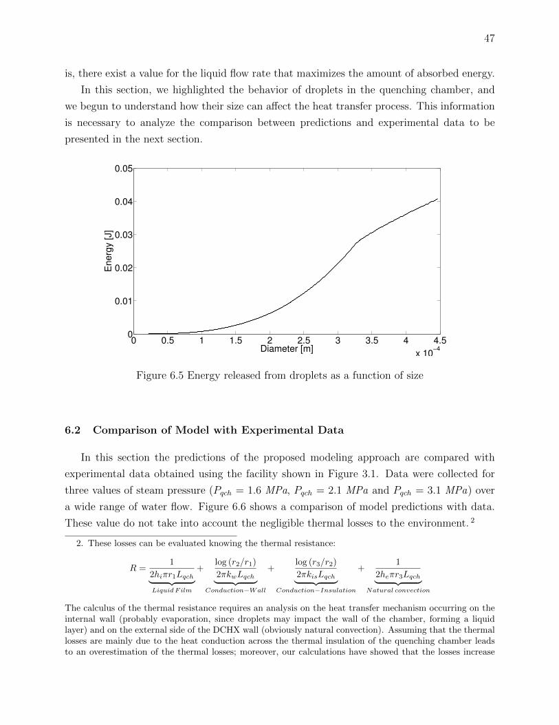
47

is, there exist a value for the liquid flow rate that maximizes the amount of absorbed energy.

In this section, we highlighted the behavior of droplets in the quenching chamber, and

we begun to understand how their size can affect the heat transfer process. This information

is necessary to analyze the comparison between predictions and experimental data to be

presented in the next section.

0 0.5 1 1.5 2 2.5 3 3.5 4 4.5

x 10−4

0

0.01

0.02

0.03

0.04

0.05

Diameter [m]

Energ

y [J]

Figure 6.5 Energy released from droplets as a function of size

6.2 Comparison of Model with Experimental Data

In this section the predictions of the proposed modeling approach are compared with

experimental data obtained using the facility shown in Figure 3.1. Data were collected for

three values of steam pressure (Pqch = 1.6 MPa, Pqch = 2.1 MPa and Pqch = 3.1 MPa) over

a wide range of water flow. Figure 6.6 shows a comparison of model predictions with data.

These value do not take into account the negligible thermal losses to the environment. 2

2. These losses can be evaluated knowing the thermal resistance:

R =1

2hiπr1Lqch︸ ︷︷ ︸Liquid Film

+log (r2/r1)

2πkwLqch︸ ︷︷ ︸Conduction−Wall

+log (r3/r2)

2πkisLqch︸ ︷︷ ︸Conduction−Insulation

+1

2heπr3Lqch︸ ︷︷ ︸Natural convection

The calculus of the thermal resistance requires an analysis on the heat transfer mechanism occurring on theinternal wall (probably evaporation, since droplets may impact the wall of the chamber, forming a liquidlayer) and on the external side of the DCHX wall (obviously natural convection). Assuming that the thermallosses are mainly due to the heat conduction across the thermal insulation of the quenching chamber leadsto an overestimation of the thermal losses; moreover, our calculations have showed that the losses increase

48

The results presented in Figure 6.6 show that for low steam pressure (Pqch = 1.6 MPa,

Pqch = 2.1 MPa), the agreement of the model with the data is very good. In spite of that,

this is not necessarily true at high pressure (Pqch = 3.1 MPa) where the proposed model

significantly overestimates the thermal power.

0.5 1 1.5 2 2.5 3 3.5

x 10−5

10

20

30

40

50

60

70

Volumetric Flow Rate (m3/s)

Th

erm

al P

ow

er

(kW

)

Exp. Data Pch

= 1.5 MPa

Exp. Data Pch

= 2.1 MPa

Exp. Data Pch

= 3.1 MPa

Model (q = 2.8)

Model (q = 2.1)

Model (q = 2.8)

Figure 6.6 Comparison of model predictions with data

Several phenomena which are not taken into account in the present model can probably

explain this behavior. One of these aspects has been mentioned in the previous section,

where we highlighted how some droplets reach the bottom of the quenching chamber before

their complete vaporization occurs, leading to a drop in the DCHX performance. However,

droplets may impact even the inner wall of the quenching chamber. This kind of interaction

may contribute to the formation of a liquid film on the inner side of the DCHX. This layer

should move downward and, assuming steady conditions, it is continuously supplied by liquid

droplets. Moreover, if the assumptions made in Section 5.4 are correct, the formed layer

should evaporate. In this situation, the contact surface area is greatly reduced because a non

negligible portion of the droplets feeds this inner water layer. On the other hand, the surface

available to exchange heat is lower compared to a situation in which none of the droplets

with the DCHX working pressure. So, we evaluated them for Pqch = 40 bar :

QDiss =Tv − Tamblog(r3/r2)2πkisLqch

which gives 240 W transferred to the environment. That is, the thermal losses are always lower than thisvalue, and neglecting them does not provide any considerable error in our calculation.

49

are deposited over the wall (in fact, for a given liquid mass, the contact area is higher if this

mass is under the form of tiny droplets instead of being an unique liquid sheet). It is obvious

that a decrease in the total contact surface area leads to a decrease in heat transfer since the

latter is proportional to the surface area 3. The fact that our model overestimates the data

at high pressures (Figure 6.6 and 6.9) can be explained because it does not take into account

this possible droplet deposit over the wall. In fact, it has a greater probability of occurring

at high pressures than at lower ones. This aspect is confirmed by the fact that increasing

the pressure, also increases the liquid flow rate and yields an augmentation of the total rate

of droplets NTOT (Equation 5.22). In other words, this means that the probability that a

droplet reaches the cylindrical wall is higher at high pressure, and leads to a non-negligible

loss in heat transfer that has not been included in the model.

0.9 1 1.1 1.2 1.3 1.4 1.5 1.6

x 10−5

10

15

20

25

30

Volumetric Flow Rate (m3/s)

Th

erm

al P

ow

er

(kW

)

Pqch

= 1.6 MPa

q = 2.1 q = 2.4 q = 2.8Exp. Data

Figure 6.7 Model predictions (Pqch = 1.6 MPa)

Another possible factor concerns the skewness of the DDF shown in Figure 4.4. In order

to achieve a good agreement, the skewness has been optimized in Figure 6.6. However, this

is not sufficient to reduce the gap at high pressures. Thus, a further analysis is needed to

properly model this phenomena. Figure 4.4 indicates that for a constant skewness coefficient

q, the pressure strongly affects the overall shape of the DDF. For instance, for a constant

value of the Sauter mean diameter D32 (Equation 4.5), D0.632 decreases with increasing q

3. This result should not be confused with what is shown in Figure 6.5. This figure states that the biggerthe droplet size, the bigger the energy released becomes. Here we point out that increasing the total surfacecontact area (so, the sum of the areas of all the droplets), the heat transfer increases too.

50

(Equation 4.15). Consequently, the probability of obtaining droplets with small diameters

increases (Equation 4.14). Recalling Figure 6.5, small size droplets exchange a negligible

quantity of heat in contrast to big size droplets. However, for a fixed flow rate, the total

number of droplets changes depending on the size of them. Indeed, the total number of

droplet NTOT is higher if their sizes are low (i.e., high value of q) and vice versa (i.e., low

value of q). From Equation 5.23, we can argue that when q is increased (situation in which

there is a large number of small size droplets), the heat transfer does not necessarily increases.

1.4 1.45 1.5 1.55 1.6 1.65 1.7 1.75 1.8 1.85

x 10−5

24

26

28

30

32

34

36

38

Volumetric flow rate (m3/s)

Th

erm

al P

ow

er

(kW

)

Pqch

= 2.1 MPa

q = 2.1

q = 2.4

q = 2.8

Exp. Data

Figure 6.8 Model predictions (Pqch = 2.1 MPa)

To better understand this aspect, the calculations shown Figure 6.6 were repeated using

three values of q (q = 2.1, q = 2.4 and q = 2.8,). These results are shown in Figures 6.7,

6.8 and 6.9. As it can be seen from these figures, at low pressures (Pqch = 1.6 MPa, Pqch =

2.1 MPa, where the agreement is good), increasing q increases the heat transfer. However,

the same behavior is not observed at high pressure (Figure 6.9). To understand this change

of behavior, we analyze the thermal power as a function of the quenching chamber pressure

for the three different values of q (with the flow rate and the thermodynamic conditions of

the water are fixed). In Figure 6.10, it is clearly shown that the thermal power does not

increase linearly but, depending on q, there is a pressure that maximizes the heat transfer.

Moreover, it seems that increasing q makes the maximal thermal power to shift to the right

which explains the aforementioned trade-off between the droplet size (which decreases with

pressure) and the total rate of droplets generation (which increases).

51

2.4 2.5 2.6 2.7 2.8 2.9 3 3.1 3.2

x 10−5

40

45

50

55

60

65

70

75

Volumetric flow rate (m3/s)

Th

erm

al P

ow

er

(kW

)

Pqch

= 3.1 MPa

q = 2.1

q = 2.4

q = 2.8

Exp. Data

Figure 6.9 Model predictions (Pqch = 3.1 MPa)

The fact that the thermal power is not a linear function of the pressure confirms analyses

performed from Figure 6.5, where it is assumed the existence of a condition that maximizes

the DCHX performance. In fact, it has been argued that for a given pressure, there is a value

of the volumetric flow rate that optimizes the energy transferred from the droplets (it is the

value that makes all the droplets completely vaporize before they reach the bottom of the

chamber). Calculations shown in Figure 6.10 provide further information; for a given flow

rate, the heat transfer does not linearly increase with pressure and, if the value of q is known,

there is a DDF capable to maximize the heat transfer. Hence, to reach high heat transfer

efficiencies, increasing the cooling flow rate may not be sufficient, therefore, it is necessary

to find working conditions (i.e., a combination of flow rate and pressure) which provides

the DDF that optimizes the quenching chamber performances. For this reason, in the next

section we will neglect the influence of q to focus more on the effects of the volumetric flow

rate and the quenching chamber pressure. However, as it has been shown, the effects of

statistics (i.e., q) have a strong influence on heat transfer predictions, and this fact should

never be forgotten.

52

10 15 20 25 30 351

2

3

4

5

6x 10

4

Pqch(bar)

Ther

malP

ower

(W)

Vl iq= 2 × 10−5m3/s

q = 2.1

q = 2.4

q = 2.8

Figure 6.10 Heat transfer rate as a function of DCHX pressure Pqch and q

6.3 Parametric Study

If, on one hand, the behavior shown in Figure 6.10 highlights the effects of the droplet size

distribution on heat transfer, on the other hand it represents an unrealistic situation. In fact,

as said before, this figure has been evaluated keeping the volumetric flow rate constant and

equal to a mean value. As shown in Figure 6.6, this situation never occurs and increasing the

pressure requires an increment in the liquid flow rate in order to reach a good operation of

the DCHX. The analysis made in the previous sections has shown that there are at least two

1020

3040

0

5

x 10−5

0

5

10

x 104

Pqch

[bar]

Thermal Power [W] q = 2.4

Vliq

[m3/s]

1

2

3

4

5

6

7

8

9

x 104

(a)

10000

20000

2000020000 20000

30000

30000

30000 30000

40000

40000

40000 40000

50000

5000050000

60000

6000060000

70000

70000

80000

80000

90000

Vliq

[m

3/s

]

Pqch

[bar]

Thermal Power (W) q = 2.4

10 15 20 25 30 35

1

1.5

2

2.5

3

3.5

4x 10

−5

(b)

Figure 6.11 Heat transfer as a function of quenching chamber pressure Pqch and volumetricflow rate Vliq

53

parameters that are more important than others that affect the behavior of the quenching

chamber. For this reason, we focus our attention on the influence that the pressure and flow

rate have on heat transfer predictions. Even though the statistics of the liquid droplets have

a key role, calculations have been carried out by keeping q constant.

Figure 6.11 shows the DCHX thermal power as a function of the flow rate and the pressure

for a constant value of q. Figure 6.11a shows that power increases with increasing these two

variables. However, if we plot the contour curves of the thermal power as shown in Figure

6.11b, we deduce that the increase in power is not constant. In fact, it seems that under

certain conditions, one of the two parameters has a greater effect on the calculations. For

instance, whit increasing the pressure, the influence on the heat transfer decreases. This is

just one of the aspects that can be argued. However, in order to make a critical analysis of

the results in Figure 6.11, a different representation is still needed.

Figure 6.12 presents the behavior of the thermal power for different values of the flow

rate, as a function of the pressure. Obviously, increasing the cooling flow rate leads to

a larger exchange in the thermal power. However, it is interesting to point out that, for

low volumetric flow rates, the heat transfer is almost independent of the pressure while,

increasing the liquid flow rate, the quenching chamber behavior changes, and is subjected

to a remarkable dependence on pressure. Moreover, for each value of volumetric flow rate,

the heat transfer does not grow linearly. That is, for a given flow rate, the thermal power

increases with pressure; however, this growth is considerable at low pressures and not at high

ones. Based on Figure 6.10, it can be argued that a maximum value for the heat transfer can

be reached at high pressure.

10 15 20 25 30 350

1

2

3

4

5

6

7

8

9

10x 10

4

Pqch[bar]

QTOT[W

]

q = 2.4

Vl iq

Figure 6.12 Influence of volumetric flow rate Vliq on predictions

54

The same aspects can be seen in Figure 6.13, which shows the behavior of the ther-

mal power for different values of working pressures. Again, the working pressure affects the

quenching chamber behavior and, as aforementioned, the thermal power increases with in-

creasing the pressure. However, it seems that, for a fixed flow rate, when certain values of

pressure are reached (in this case, the highest ones), the thermal power does not increase

anymore. That is, for a given volumetric flow rate, there exists a maximum thermal power

that can be exchanged in the DCHX.

1 1.5 2 2.5 3 3.5 4

x 10−5

2

4

6

8

x 104

Vl iq [m3/s]

QTOT[W

]

q = 2.4

Pqch

Figure 6.13 Influence of quenching chamber pressure Pqch on predictions

Figure 6.12 and 6.13 give us the directives to reach high heat transfer efficiencies. These

two figures show that, in any case, an increment in the cooling water flow rate leads to an

increment in heat transfer. But this increment depends on the chamber pressure as well,

since an increment in heat transfer due to the flow rate seems to be higher if the pressure is

high as well (Figure 6.12). This observation does not necessarily mean that an increment in

pressure always results in a significant increase of the amount of heat transferred. In fact,

this contribution becomes lower with increasing the pressure (Figure 6.13). The reasons of

this behavior should be found in the effects that these two variables have on the droplet

size. That is, increasing the pressure and decreasing the cooling water flow rate leads to a

decrease in droplet size (Figure 4.2). It is obvious that the droplet size affects the heat transfer

calculations; however, the model predictions have shown that under certain conditions, the

heat transfer seems to be constant. This behavior can be justified by assuming that at these

conditions, the cooling water flow rate and the quenching chamber pressure does not affect

the droplet size at all. Consequently, the heat transfer predictions will be slightly influenced

by these variables.

55

6.4 Other Correlation Approach

To improve our model, we decided to analyze Figure 6.13 in order to evaluate a generic

function able to describe the predictions for q = 2.4. That is, this generic function f should

have the quenching chamber pressure Pqch and the volumetric flow rate Vliq as independent

variables, and the thermal power QTOT as a dependent variable. Then, using the experimental

data, we will try to define a correction factor ψ which is a function of the pressure in order

to achieve a better agreement. Let us define

ψ = ψ (p) , p =p

pmax(6.3)

where p is the non-dimensional pressure which is defined as the ratio between the quenching

chamber pressure and the maximum allowable pressure, worth 40 bar in this case. Once this

correction factor has been defined, the thermal power will be evaluated as

QTOT = ψ (p) f(Pqch, Vliq

)(6.4)

The determination of f and c is presented in the two following subsections.

6.4.1 Definition of f

Let us assume that the curves in Figure 6.13 can be characterized by the following second-

degree polynomial:

QTOT = f(Pqch, Vliq

)= aV 2

liq + bVliq + c

where the coefficients a, b and c depend on pressure as follows

a = a (p) b = b (p) c = c (p)

The trend of a, b and c can be found by evaluating the coefficients of the second-degree

polynomial describing the lines in Figure 6.13 and finally analyzing their dependence in

pressure. Assuming that third-degree polynomials can describe the trend of a, b and c, we

computed the following expressions:

a (p) = −8.8454× 108p3 + 9.371× 1010p2 − 2.6305× 1012p+ 1.2883× 1013

b (p) = −2.5258× 104p3 − 2.2061× 106p2 + 2.0845× 108p− 1.0860× 109

c (p) = 0.7813p3 − 55.5p2 + 1.0853× 103p− 3.5098× 103

56

0.5

11

.52

2.5

33

.54

4.5

x 1

0−

5

0123456789

10

x 1

04

Vliq[m

3/s]

ThermalPower[W]

(a)

10

15

20

25

30

35

−10

−9

−8

−7

−6

−5

−4

−3

−2

x 1

01

2

Pqch[bar]

Coefficient[Js/m6]

a=

a(p)

a(p

olynomials)

a(rea

ltren

d)

(b)

10

15

20

25

30

35

0.51

1.52

2.53

x 1

09

Pqch[bar]

Coefficient[J/m3]

b=

b(p)

b(p

olynomials)

b(rea

ltren

d)

(c)

10

15

20

25

30

35

−5000

500

1000

1500

2000

2500

3000

Pqch[bar]

Coefficient[W]

c=

c(p)

c(p

olynomials)

c(rea

ltren

d)

(d)

Fig

ure

6.14

Anal

ysi

sof

the

coeffi

cien

tsa,

ban

dc

57

The units for a, b and c are Js/m6, J/m3 and W, respectively. The validity of these ex-

pressions is shown at Figure 6.14 in which four graphics are present: Figure 6.14a shows the

thermal power as a function of the cooling water flow rates; the interpolation poles needed

to define f (green circles) are highlighted. Figures 6.14b to 6.14d compare the coefficient

behavior estimated from our predictions with the same behavior evaluated from the devel-

oped third-degree polynomials. As it can be seen, the behavior of the coefficients a, b and c

is close to the one evaluated using the polynomials, which allow as to argue that the error

committed in using these expressions is negligible.

6.4.2 Definition of ψ

Let us define a coefficient ψ as a multiplicative factor which corrects the predictions of

the developed model. Since it is a multiplicative coefficient, it can be also defined as the ratio

between the predictions and the experimental data for given pressure and flow rate.

An analysis of Figure 6.7 to 6.9 clearly shows that, for a given quenching chamber pressure,

the difference between the predictions and the experimental data is approximately constant

and does not depend on the cooling water flow rate. For this reason, we assumed that the

correction factor is a function of the quenching chamber pressure:

ψ = ψ (p) , p =p

pmax

In Table 6.2 we summarize the ratio between the predictions and the data for three

quenching chamber pressures. Knowing these values, it is possible to find the second degree

Table 6.2 Ratios between predictions and data for three working pressures

Pressure RatiosPqch = 1.6MPa 1.09Pqch = 2.1MPa 0.881Pqch = 3.1MPa 0.7549

polynomial which interpolates the aforementioned ratios. This operation is shown in Figure

6.15 and the mathematical expression given by:

ψ (p) = 3.0933p2 − 4.5253p + 2.4041 (6.5)

Finally, in order to validate the proposed methodology, we plotted in Figure 6.16 the

experimental data and the predictions using the correction factor. As it can be seen, the

agreement is satisfactory. However, it is important to underline the limits of validity of the

58

presented expressions. Since we used polynomial interpolation, the aforementioned expres-

sions should not be used for pressure lowers than 16 bar or higher than 31 bar. That is, using

the polynomial interpolations in the range of pressure in which these have been evaluated

will avoid interpolation errors which raise close to the interpolation end nodes (where the

error get worse).

0 0.2 0.4 0.6 0.8 10.5

1

1.5

2

2.5

Non−dimensional pressure [−]

ψ =

ψ (

p)

Interpolation points

ψ = 3.0933p2−4.5253p+2.4041

Figure 6.15 Evaluation of the correction coefficient (Equation 6.5)

0.5 1 1.5 2 2.5 3 3.5

x 10−5

1

2

3

4

5

6x 10

4

Vliq

[m3/s]

Therm

al P

ow

er

[W]

CorrectionData P

qch = 1.6 MPa

Data Pqch

= 2.1 MPa

Data Pqch

= 3.1 MPa

Figure 6.16 Experimental data and proposed correction on predictions

59

6.5 Final Remarks

The analysis made in this chapter gave us the possibility to review the modeling approach

presented in Chapter 4 and 5. First, we have analyzed a single working condition in order to

understand the physics of liquid droplets and we noted that a non-negligible portion of the

droplets (i.e., the biggest ones) do not exchange all their energy. We justified this behavior by

considering that they rapidly reach the bottom of the quenching chamber without completely

vaporizing. Then, we compared the predictions with the experimental data and we found a

good agreement at low pressures and an over estimation at higher ones. In effect, we assumed

the occurrence of a other interactions between droplets and the quenching chamber. That

is, droplets impact the inner wall of the chamber, forming a liquid layer that decreases the

contact surface area and in turn, the heat transfer. Thereafter, we analyzed the possibility

of having a combination of the flow rate and pressure that maximizes the performance of the

DCHX. Studying the effects of these two parameters, we discovered that working at high

pressures may not be advisable. Finally, in order to use our results, we computed polynomials

capable of describing the model behavior and a factor which corrects the predictions. In this

way, it will be possible to test our model for different values of the pressure and flow rate.

60

CHAPTER 7

CONCLUSION

During these two years, the quenching chamber used in a super-critical water loop facility

installed at the “Altan Tapucu” Thermo-hydraulic Laboratory has been studied. The main

function of this component is to cool down steam coming from the test section where super-

critical choked flow conditions occur.

Here we summarize the main aspects of this study, in particular, the methodology used

to solve the problems and its validation. In the end, we will present the utility of the results

and the further works needed to improve our modeling approach.

7.1 General Objectives

Since the quenching chamber is a direct contact heat exchanger, this component does not

present any particular complexity, because of the lack of a wall that divides both streams. In

fact, it is a vertical vessel in which steam flows mixing with sub-cooled liquid. However, this

equipment cases a nozzle located on the top of the tube. Due to this component, the cooling

liquid enters into the chamber under the form of tiny droplets. This way, the contact surface

area and, consequently, the thermal power, are maximized. The major problem analyzed in

this work was the evaluation of the thermal power for given set of thermodynamic conditions

of both streams (liquid and vapor). The solution was found by analyzing each of the following

sub problems:

– The thermodynamic evolution in the test section the super-critical water pass-

ing through the test section is subjected to a considerable change in thermodynamic

properties. This fact makes it difficult to evaluate the steam conditions entering the

quenching chamber. In order to solve this problem, we assumed that the steam tem-

perature is equal to the average between the temperature coming from an isoentropic

transformation and the one evaluated if the test section is an isoenthalpic valve (Equa-

tion 5.1).

– The evaluation of a statistical distribution for droplet size the DDF is a pa-

rameter difficult to compute since it is a function of the working conditions (liquid

temperature, steam pressure and volumetric flow rate) and of the geometric character-

istics of the nozzle (the orifice diameter and the swirl-chamber length). All these vari-

ables have been taken into account by using an experimental correlation for the Sauter

61

mean diameter (D32). This parameter is needed in order to use the DDFs available in

the scientific literature. Among all, the easiest DDF to handle is the Rosin-Rammler

distribution which depends on D32 (Equation 4.5) and the exponent q of Equation 4.14.

– Solution of the heat transfer problem for a single droplet the evaluation of the

droplet size is mandatory to perform the heat transfer study. Since there is a mutual

interaction between super-heated steam and sub-cooled water, two heat transfer modes

have been analyzed: convection and evaporation.

– Evaluation of the exchanged thermal power finally, the results provided by the

statistical and heat transfer studies (respectively in Chapter 4 and 5) have been used

to compute the total power exchanged for a given DCHX condition. It was assumed

that the latter quantity is equal to the total energy released by the droplets multiplied

by the rate of droplets (Equation 5.18).

All these considerations have been used to develop a Matlab R© script capable of not only

computing the thermal power exchanged into the DCHX but also able to describe the behavior

of droplets having different sizes and in a gaseous environment.

7.2 Limits of the Proposed Model

In the proposed modeling approach, some assumptions have been made to simplify the

calculations. Their validity has been explained in the course of this work and shall be reca-

pitulated here.

The methodology used to evaluate the DDF is questionable on several points. First of

all, the experimental correlation used to evaluate the Sauter mean diameter (Equation 4.5)

was found by Lefebvre (1989) under laboratory conditions extremely different form ours.

For instance, Lefebvre used six different hollow-cone nozzles instead of a full cone nozzle.

However, the theoretical assumptions used to develop this correlation were found to be always

valid and independent from the type of nozzle considered (see Appendix A). This encouraged

us to use Lefebvre’s correlation. Secondly, even the use of the Rosin-Rammler equation may

not be advisable since in the course of this work, we mentioned other statistical laws available

in the scientific literature and it has been proven that these laws are more powerful than the

Rosin-Rammler equation (Ashgriz, 2011). However these laws are also more difficult to use

since they require the search of more than two statistical parameters. In effect, the lack of

experimental data forces us to use the easiest statistical law available.

The heat transfer study was implemented following the theory as much as possible. In fact,

if the convective heat transfer study is rigorous, the phase change solution is questionable since

we did not provide any satisfactory reasons to explains the occurrence of liquid evaporation

62

instead of steam condensation. Moreover, even if the hypothesis of liquid evaporation is

verified, we cannot exclude other phase change phenomena as, for instance, the evaporation

of a liquid layer on the inner wall of the chamber. However, as it has been shown, taking

into account these phenomena leads to a problem difficult to solve (Cascella and Teyssedou,

2013) and, at the same time, impossible to validate since there are no instruments capable of

validating these assumptions. For these reasons, we limited ourselves to droplet evaporation

only.

There are two more phenomena, namely the droplet break-up and collision that have not

been considered in the model but we think that this assumption has a great influence on the

model. Indeed, it affects the DDF shape since adding the two aforementioned phenomena

increases the probability of having littler droplets. That is, in our work we considered only

the decreases in droplet size due to evaporation, and not the ones due to break-up and

collision. Moreover, they affect even the heat transfer calculations since break-up and collision

are disruptive phenomena (Cascella and Teyssedou, 2013) which should increase the energy

exchanged by the droplets. In scientific literature, we did not find any satisfactory model

predicting these two phenomena and for this reason, we decide to neglect them. However,

this decision is questionable.

Finally, we mentioned how the total rate of droplets may influence the thermal power

calculations (Equation 5.18). Equation 5.22 shows that the total number of droplets can

be evaluated by assuming all the droplets to have a diameter equal to the mean diameter

associated to the DDF (Equation 4.14). Obviously, this assumption brings an error of which

we cannot quantify the magnitude because of the lack of an instrument capable to measure

the effective mean droplet size.

7.3 Result Discussion

As shown in Figure 6.6, our code describes well the heat exchange in the quenching

chamber at low pressures but it over predicts the data at high pressures. We tried to justify

this behavior by analyzing the dynamics of liquid droplets. Thus, we looked for all the

phenomena that can influence our calculations.

Before performing the code, we were well aware of the fact that neglecting droplet break-

up and collision affects the calculations. However, a preliminary analysis on these phenomena

may help to understand their influence on the numerical predictions. Let us consider droplet

break-up, which occurs when the surface tension is not high enough to contain the liquid

instabilities. Recalling that the surface tension decreases with temperature, we can assume

that the probability that a droplet will break up is higher at higher temperatures (and,

63

indeed, at higher pressures). Moreover, since break-up is a disruptive phenomenon, it should

increase the heat transfer and this augmentation must be higher at higher pressures. The

fact that we have an overestimation of the data at high pressures (Figure 6.6) brings us to

conclude that including the break-up process may not necessarily improve the calculations.

A similar analysis can be done for collision: the collision between two (or more) droplets

leads to the formation of smaller droplets or of a larger droplet. Neglecting the last scenario,

we can assume that the collision process augments the heat exchange since it increases the

formation of tinier droplets. Hence, including collision process may not improve our model.

This preliminary analysis leads us to consider other phenomena that may explain the behavior

shown in Figure 6.6.

Another aspect affecting the model is the choice of q in Equation 4.14. We have shown that

this parameter describes the shape of the DDF and has a great influence on the calculations.

To understand how this variable affects the predictions, we have repeated the calculations

for three values of q. In effect, we have found that the error increases whit increasing q at

low pressures but not at high ones. As shown in Figure 6.6, q has been chosen in such a way

as to minimize the error between experimental data and numerical predictions. However,

this is not a sufficient condition that can completely explain the discrepancy between the

predictions and the data.

For these reasons, we have analyzed the behavior of droplets in the quenching chamber.

we have assumed that they could impact the inner wall of our cylindrical vessel, forming a

liquid layer which moves downward. Assuming this layer to be at saturation temperature,

it should evaporate. In this scenario, the contact droplet surface area available to exchange

heat decreases. Moreover, in Figure 6.5 we have stated that the heat transfer is a linear

function of the surface area. If both of these hypotheses are correct, we can assume that

the thickness of the liquid layer increases with pressure which in turn leads to a decrease in

the total droplet-surface area (and so, the heat transfer). Finally, we can assume that this

behavior is more important at high pressures, and not at low ones, which may explain the

gap between the predictions and the data shown in Figure 6.6.

7.4 Usefulness of the Proposed Model

Even if we were not able to propose a satisfactory model (i.e., which well describes the

quenching chamber behavior over a wide range of pressures), doing so gave us the possibility

to better understand the dynamics of liquid droplets in a steam environment. In fact, in this

model, the physical parameters linked to the droplet (i.e., the size, the residence time and

the velocity) have been used to evaluate the overall heat transfer.

64

based on the proposed theoretical approach, we were able to demonstrate that the quench-

ing chamber (and probably all DCHXs of this type) admits a set of working conditions which

maximize its performance. This aspect has been exposed in different sections of this docu-

ment

In Figure 6.5 we have analyzed the heat transfer as a function of droplet size; two aspects

have been highlighted. Firstly, the energy released grows linearly with the contact surface

area (which is obvious). Secondly, there is a decrease in the amount of energy released due

to the impact of some droplets (i.e., the bigger ones) on the bottom of the chamber. In fact,

their velocity is too high and they are not able to completely vaporize. Hence, we assumed

the existence of a minimal volumetric flow rate that makes all the droplets change their phase

and, consequently, maximizes the amount of heat transferred. In Figure 6.10, the effect of

q on Equation 4.14 has been analyzed for a given volumetric flow rate. Even in this case,

we found a pressure which maximize the heat transfer. Because of that, a further analysis

on the statistics of liquid droplets should be done, in order to compute the real value of q

to be used. Finally, the analysis of Figure 6.12 and Figure 6.13 leads us to conclude that

two parameters, namely the chamber pressure and volumetric flow rate affect significantly

our calculations. The parametric study shows that the heat transfer grows linearly with the

flow rate but not with the pressure. In fact, increasing the latter for a given flow rate leads

to an asymptotic value of the heat transfer. For this reason, we stated that working at high

pressures is not advisable since the only way to increase the heat transfer is by increasing

the water rate.

This analysis has helped to understand the behavior of a DCHX. Obviously, we cannot

forget that the predictions may not always be true but, if the code forecasts the right trends

(i.e., there is a working condition maximizing the performances), the way of designing these

heat exchangers will be revised. We underline that these systems find applications not only in

heat exchangers, chemical reactors and agriculture factories, but even in nuclear engineering

(depressurizers) and fire extinguishers, fields in which safety is a mandatory requirement. If

our assumptions are correct, the implementation of this code (and any future improvement)

will help to increase the efficiency of these systems and in turn their safety.

7.5 Future Work

In the course of this work we have often highlighted the weak points of our modeling

approach. For this reason, any future improvement of the presented methodology cannot

neglect these points.

It is obvious that further work is needed to provide a better way to compute the DDF.

65

The equation used to estimate D32 must be adapted to the type of spray nozzle and the use

of other DDFs should be considered as well. It is clear that this kind of improvement requires

the use of additional experimental data (i.e., the direct measure of the droplet sizes).

We often mentioned droplet break-up and collision. In fact, they have been neglected in

our work but these phenomena have a great influence on the quenching chamber behavior and

any improvement of the code cannot neglect these factors. At first glance they may deteriorate

the performances of the proposed model. However, the results obtained by introducing these

phenomena will be different from the ones showed here and their analysis may be easier to

explain.

Another assumption is the formation of a liquid layer on the inner wall of the quenching

chamber. Since droplets feed this layer, these will impact the wall at different locations. This

means that another information should be evaluated which is the moving directions of the

droplets. Knowing their size should make it possible to evaluate the direction under which

droplets move and consequently, determine those droplets that impact the cylindrical wall of

the DCHX.

We highlighted certain aspects that were neglected and the relation they have on the

dynamics of the liquid droplets. We can underline another aspect related to the behavior of

the quenching chamber. In fact, our calculations have shown the existence of a set of working

conditions that can maximize the performance. It would be interesting to prove this fact since,

once achieved, it will have a great influence on the way these type of thermal equipment are

designed. For these reasons, further ad hoc experiments should be implemented in order to

validate the behavior shown in Figure 6.12 and 6.13.

Finally, we underlined that, when developing the proposed model, several assumptions

have been made because of the lack of an optical instrument capable of showing the droplet

behavior within the quenching chamber. For instance, we assumed the droplet size to be

described by the Rosin-Rammler distribution or the formation of an evaporating liquid layer

on the inner wall of the DCHX. All these assumptions, including the others not listed here,

can easily be validated by the introduction of a measurement instrument such as a camera

or an image analyzer.

66

REFERENCES

ASHGRIZ, N. (2011). Handbook of Atomization and Sprays: Theory and Applications.

Springer.

BARRERAS, F. and EDUARDO, L. (2006). Experimental Characterization of Industrial

Twin-Fluid Atomizers. Atomization Spray J. Inst. Liq. Atomization Spray Syst., vol. 16,

pp. 127–145.

BECK, J. C. and WATKINS, A. P. (2002). On the Development of Spray Submodels Based

on Droplet Size Moments. Journal of Computational Physics, vol. 182, pp. 586–621.

BRONIARZ-PRESS, L., OCHOWIAK, M., ROZANSKI, J. and WOZIWODZKI, S. (2009).

The Atomization of Water-Oil Emulsions. Exp. Thermal Fluid Sci., vol. 20, pp. 631–637.

CARSLAW, H. S. (1959). Conduction of Heat in Solids. Oxford : Clarendon Press.

CASCELLA, F. and TEYSSEDOU, A. (2013). Modeling a direct contact heat exchanger

for supercritical water loop. Proceedings of the 2013 Canadian Nuclear Society Annual

Conference, Toronto, 12/06/2013.

CELATA, G. P., CUOMO, M., D’ANNIBALE, F. and FARELLO, G. E. (1991). Direct

Contact Condensation of Steam on Droplets. Int. J. Multiphase Flow, vol. 17, pp. 191–211.

CLEARY, V., BOWEN, P. and WITLOX, H. (2007). Flashing Liquid Jets and Two-Phase

Droplet Dispersion: 1. Experiments for derivation of droplet Atomization Correlation. J.

Hazard. Mater., vol. 142, pp. 786–796.

CROWE, C. T. (2005). Multiphase Flow Handbook. CRC Press.

GONZALES-TELLO, P., CAMACHO, F., VICARIA, J. M. and GONZALES, P. A. (2008).

A Modified Nukiyama-Tanasawa Distribution Function and a Rosin-Rammler Model for the

Particle-Size-Distribution Analysis. Powder Technology, vol. 186, pp. 278–281.

HUANG, L. J., AYYASWAMY, P. S. and SRIPADA, S. S. (1996). Condensation on a Spray

of Water Drops: a Cell Model Study–II. Transport Quantities. Int. J.Heat Mass Transfer,

vol. 39, pp. 3791–3797.

INCROPERA, F. P., DEWITT, D. P., BERGMAN, T. L. and LAVINE, A. S. (2007).

Fundamentals of Heat and Mass Transfer. Wiley.

JACOBS, H. R. (2011). Direct Contact Heat Exchangers. Thermopedia. http://www.

thermopedia.com/content/700/.

LEFEBVRE, A. H. (1989). Atomization and Sprays. Hemisphere Publishing Corp.

67

MARSHALL, W. R. (1955). Heat and Mass Transfer in Spray Drying. Transaction of

ASME, pp. 1377–1385.

MUFTUOGLU, A. and TEYSSEDOU, A. (2013). Experimental study of water flow at su-

percritical pressures. Proceedings of the 2013 Canadian Nuclear Society Annual Conference,

Toronto, 12/06/2013.

ORZECHOWSKI, A. (1976). Liquid Atomization. WNT, Warsaw.

OZISIK, M. N. (1993). Heat Conduction. John Wiley & Sons, Inc.

RANZ, W. E. and MARSHALL, W. R. (1952). Evapotation from Drops. Chemical Engi-

neering Progress, vol. 48, pp. 141–146,173–180.

ROSIN, P. and RAMMLER, E. (1933). The Laws Governing the Fineness of Powdered

Coal. Journal of the Institute of Fuel, vol. 7, pp. 29–36.

SAUNDERS, E. A. (1988). Heat Exchanges: Selection, Design and Construction. Longman

Scientific and Technical.

SCHICK, R. J. (2006). Spray Technology Reference Guide: Understanding Drop Size. Spray-

ing Systems Co. http://de.spray.com/Portals/0/pdf/B459c.pdf.

SCHNEIDER, P. J. (1955). Conduction Heat Transfer. Addison-Wesley Publishing Com-

pany, Inc.

SEMIAO, V., ANDRADE, P. and DE GARCA CARVALHO, M. (1996). Spray Characteri-

zation: Numerical Prediction of Sauter Mean Diameter and Droplet Size Distribution. Fuel,

vol. 75, pp. 1707–1714.

SRIPADA, S. S., AYYASWAMY, P. S. and HUANG, L. J. (1996). Condensation on a spray

of water drops: A cell model study–I. Flow description. Int. J.Heat Mass Transfer, vol. 39,

pp. 3781–3790.

TAKAHASHI, M., NAYAK, A. K., KITAGAWA, S. and MURAKOSO, H. (2001). Heat

Transfer in Direct Contact Condensation of Steam to Subcooled Water Spray. Journal of

Heat Transfer, vol. 123, pp. 703–710.

ZHAO, Y. H., HOU, M. H. and CHIN, J. S. (1986). Dropsize Distributions for Swirl and

Airblast Atomizers. Atomization Spray Technol., vol. 2, pp. 3–15.

68

APPENDIX A

Development of an experimental correlation for D32 (Lefebvre, 1989)

In Chapter 4, we showed that the knowledge of the Sauter mean diameter defined as

SMD =

N∑i=1

niD3i

N∑i=1

niD2i

is fundamental to evaluate the DDF. In our modeling approach, we used the experimental

correlation found by Lefebvre (1989). We summarize here the theory behind the development

of this correlation.

The droplet size is strictly correlated to the atomization process defined as“ the conversion

of bulk liquid issuing from a nozzle into a dispersion of small droplets ranging in size from sub

micron to several hundred microns in diameter” (Jacobs, 2011). In Figure .1 this conversion

is showed: the liquid gets out from the nozzle but it is in a continuous phase; then, because

of the aerodynamic and hydrodynamic instabilities, the liquid sheet breaks up into ligaments

and then into droplets.

Figure .1 Atomization Process

The main idea explained in Lefebvre (1989) is to develop an experimental correlation for

D32 which is the sum of two terms:

– the first term is related to the first stage of atomization, where hydrodynamic and

aerodynamic forces generate instabilities into the liquid sheet;

69

– the second term is related to second stage of atomization where the liquid passes from a

continuous to a disperse phase (conversion of the liquid sheets into ligaments and then

into droplets).

That is, an expression of the following form is to be found

D32 = D32,1 +D32,2 (1)

Respectively, D32,1 and D32,2 are function of the two aforementioned stages.

1st atomization In the first stage, the disruptive forces take place into the liquid sheet:

this force is related to the volumetric flow and consequently to the initial liquid velocity.

The stronger the force, the lower the droplet size becomes. Moreover, in order to have a

better atomization quality, the liquid viscosity must decrease. These considerations allow us

to write a dependence of the Reynolds number Re on D32,1

D32,1

ts∝ Re−x Re =

ρL vL tsµL

ts is the liquid sheet length and vL the liquid velocity. Another aspect affecting the droplet

size is the ratio between the aerodynamic forces acting on liquid surface to the surface tension.

That is, D32,1 is inversely proportional to the Weber number:

D32,1

ts∝ We−0.5x We =

ρv ts v2R

σ

with vR the relative velocity between the liquid and the gaseous media. The first term of

Equation 1 can be written as

D32,1

ts∝(Re√We)−x

→ D32,1 ∝(

σ0.5µLρ0.5v ρLvRvL

)x(t cos θ)1−1.5x

θ is half the cone spray angle and ts = t cos θ.

2nd atomization In order to have a finer atomization, the surface tension σ must be low,

and the relative velocity vR must by high:

D32,2

ts∝ We−y =

(σ

ρv ts v2R

)y→ D32,2 ∝

(σ

ρv v2R

)y(t cos θ)1−y

70

Recalling Equation 1, we can write

D32 = A

(σ0.5µL

ρ0.5v ρLvRvL

)x(t cos θ)1−1.5x + B

(σρLρv v2

R

)y(t cos θ)1−y

Assuming vR ' vL and ∆PL = 0.5ρLv2L

D32 = A

(σ0.5µLρ0.5v ∆PL

)x(t cos θ)1−1.5x + B

(σρLρv∆PL

)y(t cos θ)1−y

Lefebvre (1989) analyzed the behavior of six simplex hollow-cone atomizers of different size

and spray-cone angle (60 < θ < 90); the working fluids were water, diesel oil and blend

of diesel oil with polybutene. Experiments performed by Lefebvre allowed him to find the

following constants:

x = 0.5, y = 0.25, A = 4.52, B = 0.39

Finally, Lefebvre (1989) proposed a correlation to find the normal liquid sheet length,

necessary parameter to compute D32:

t = 2.7

[d0FNµl

(ρl∆Pl)0.5

]0.2

where d0 is the discharge orifice diameter and FN is the flow number:

FN =ml

(ρl∆Pl)0.5

ml is the liquid flow rate [kg/s].

71

APPENDIX B

Solution of the Heat Transfer Problem – Convection

The conduction equation in spherical coordinates has been used in order to find the droplet

mean temperature. The complete three–dimensional (r, θ, φ) homogeneous equation is

∂2T

∂r2+

2

r

∂T

∂r+

1

r2 sin θ

∂

∂θ

(sin θ

∂T

∂θ

)+

1

r2 sin2 θ

∂2T

∂φ2=

1

α

∂T

∂t

Neglecting the effect of the polar angle θ and the azimuth angle φ, the dependence of the

radius r on T can be written as

∂2T

∂r2+

2

r

∂T

∂r=

1

α

∂T

∂t

or1

r

∂2

∂r2(rT ) =

1

α

∂T

∂t(2)

with the following boundary conditions

∂T

∂r

∣∣∣∣r=0

= 0

T (r, 0) = Ti

−kl∂T

∂r

∣∣∣∣r=R

= h[T∞ − T (R, t)]

To solve this problem, the following change of variable is applied. This leads to a differential

equation easier to handle

Θ (r, t) = rT (r, t)

So, Equation 2 becomes∂2Θ (r, t)

∂r2=

1

α

∂Θ (r, t)

∂t(3)

The new boundary conditions to solve Equation 3 are

∂Θ

∂r

∣∣∣∣r=0

= limr→0

Θ (r, t)

r

Θ (r, 0) = rTi = Θi

−kl∂Θ

∂r

∣∣∣∣r=R

= Θ (R, t)

(h+

klR

)

72

Where the limit of the first boundary condition exists and is finite. Following the method of

the separation of variables, we assume that the function Θ (r, t) can be written as

Θ (r, t) = ρ (r) τ (t)

leading the the search of the functions ρ and τ . Introducing these two functions, Equation 3

becomes1

ρ (r)

d2ρ(r)

dr2=

1

ατ (t)

dτ (t)

dt= −ζ2 (4)

So, the following equation can be written

dτ (t)

dt+ αζ2τ (t) = 0

which has a solution of the form

τ (t) = Ae−αζ2t

with A a constant to be determined. Here we understand the negative sign before ζ2 in

Equation 4 : that way, we avoid a solution for τ that diverges to infinity since α, ζ2 and t

are always positive quantities. The function ρ (r) comes from

d2ρ (r)

dr2+ ζ2ρ (r) = 0

The solution has the following form

ρ (r) = C1 cos (ζr) + C2 sin (ζr) (5)

where the two constants have to be determined from the boundary conditions. So,

∂Θ

∂r

∣∣∣∣r=0

= limr→0

Θ (r, t)

r= lim

r→0

τ (t)

r[C1 cos (ζr) + C2 sin (ζr)] = lim

r→0τ (t)

[C1

r+ C2ζ

sin (ζr)

ζr

]

The limit goes to infinity for r → 0; in order to avoid a prediction of an infinite temperature

in the center of the droplet, we impose C1 = 0. So, the solution of the problem has the form

ρ (r) = ρ (ζ, r) = C2 sin (ζr)

Applying the boundary condition of the heat transfer on the droplet surface we obtain

1−Rζ cotRζ =hR

kl= Bi

73

with Bi the Biot number. Equation 7.5 has infinite roots so, ζ = ζn. Introducing C = AC2,

the solution of the problem is

Θ (r, t) =∞∑

n=1

τ (t, ζn) ρ (r, ζn) =∞∑

n=1

Ce−αζ2nt sin (ζnr)

The evaluation of C comes from the application of the initial constant temperature to the

obtained solution:

Θi = rTi =∞∑

n=1

C sin (ζnr)

leading to

Cn =1

N (ζn)

∫ R

0

ρ (r, ζn) rTidr since ∀ n ∃| Cn

With N (ζn) the norm, defined as

N (ζn) =

∫ R

0

ρ (r, ζn) ρ (r, ζm) dr

which is different of zero for m = n. So, Cn becomes

Cn =1

R∫0

sin (r, ζn) dr

R∫

0

sin (r, ζn) rTidr =4ζn [Ti sin ζnR− ζnR cos ζnR]

2Rζn − sin 2ζnR

The final solution of the equation is

Θ (r, t) =∞∑

n=1

e−αζ2t4ζn [Ti sin ζnR− ζnR cos ζnR]

2Rζn − sin 2ζnRsin (ζnr)

Or, introducing the non-dimensional temperature T (r,t)−T∞Ti−T∞ , the Fourier number Fo = αt

R2 and

the non-dimensional radius r = rR

, we obtain the temperature trend in a more elegant form:

T (r, t)− T∞Ti − T∞

=∞∑

n=1

4[sin ζn − ζn cos ζn]

2ζn − sin 2ζne−ζ

2nFo

sin ζnr

ζnr

74

APPENDIX C

First Five Roots of Transcendental Equation 5.9 (Schneider, 1955)

1− ζn cot ζn = Bi

Bi ζ1 ζ2 ζ3 ζ4 ζ5

0 0 4.4934 7.7253 10.9041 14.0662

0.005 0.1224 4.4945 7.7259 10.9046 14.0666

0.01 0.173 4.4956 7.7265 10.905 14.0669

0.02 0.2445 4.4979 7.7278 10.906 14.0676

0.03 0.2991 4.5001 7.7291 10.9069 14.0683

0.04 0.345 4.5023 7.7304 10.9078 14.069

0.05 0.3854 4.5045 7.7317 10.9087 14.0697

0.06 0.4217 4.5068 7.733 10.9096 14.0705

0.07 0.4551 4.509 7.7343 10.9105 14.0712

0.08 0.4860 4.5112 7.7356 10.9115 14.0719

0.09 0.515 4.5134 7.7369 10.9124 14.0726

0.1 0.5423 4.5157 7.7382 10.9133 14.0733

0.2 0.7593 4.5379 7.7511 10.9225 14.0804

0.3 0.9208 4.5601 7.7641 10.9316 14.0875

0.4 1.0528 4.5822 7.777 10.9408 14.0946

0.5 1.1656 4.6042 7.7899 10.9499 14.1017

0.6 1.2644 4.6261 7.8028 10.9591 14.1088

0.7 1.3525 4.6479 7.8156 10.9682 14.1159

0.8 1.432 4.6696 7.8284 10.9774 14.123

0.9 1.5044 4.6911 7.8412 10.9865 14.1301

1 1.5708 4.7124 7.8540 10.9956 14.1372

1.5 1.8366 4.8158 7.9171 11.0409 14.1724

2 2.0288 4.9132 7.9787 11.0856 14.2075

3 2.2889 5.087 8.0962 11.1727 14.2764

4 2.4557 5.2329 8.2045 11.256 14.3434

5 2.5704 5.354 8.3029 11.3349 14.408

6 2.6537 5.4544 8.3914 11.4086 14.4699

75

7 2.7165 5.5378 8.4703 11.4773 14.5288

8 2.7654 5.6078 8.5406 11.5408 14.5847

9 2.8044 5.6669 8.6031 11.5994 14.6374

10 2.8363 5.7172 8.6587 11.6532 14.687

11 2.8628 5.7606 8.7083 11.7027 14.7335

16 2.9476 5.908 8.8898 11.8959 14.9251

21 2.993 5.9921 9.0019 12.025 15.0625

31 3.0406 6.0831 9.1294 12.1807 15.238

41 3.0651 6.1311 9.1987 12.2688 15.3417

51 3.0801 6.1606 9.242 12.3247 15.409

∞ 3.1105 6.2211 9.3317 12.4426 15.5537

76

APPENDIX D

Determination of the experimental data

In Figure 6.6 we compared the thermal power predicted by our code and measured in the

thermal facility (Figure 3.1). The data we plotted in Figure 6.6 have been indirectly evaluated

applying an energy balance to the quenching chamber, i.e., the decrease in enthalpy at which

the steam is subjected must be equal to the water enthalpy increase. Neglecting the thermal

losses to the environment, we can write (Figure .1)

Qqc,exp = m2 (h2 − h3) = m1 (h3 − h1) (6)

where mi is the mass flow rate and hi is the enthalpy. The resolution of Equation 6 makes

it possible to compute the thermal power exchanged Qqc,exp, evaluating either the enthalpy

variation of the steam or the enthalpy variation of the liquid (expect for a sign change).

In order to use Equation 6, all the stream temperatures and flow rates (Figure .1) have

to be estimated. This task is done by the measure instruments present in the experimental

facility:

Figure .1 Quenching chamber scheme

– Stream 1: The thermodynamic conditions 1 can be exactly determined: in fact, a

flow meter (technical designation “Flowmeter#2” in Figure 3.1) makes it possible to

77

measure the liquid flow rate, while the temperature comes form the measure of the

thermocouple present at SCWL inlet (“TTr-8” technical designation in Figure 3.1).

– Stream 2: The conditions 2 of the steam entering in the DCHX are less easier to

predict: the fact that the transformation occurring in the test section isn’t thermody-

namically known makes it difficult to evaluate the steam flow rate and temperature.

As it can be seen in Figure 3.1, there isn’t a flow meter at test section outlet. This

means that any evaluation on steam flow rate should came from the flow meter iden-

tified with “Flowmeter#1” (Figure 3.1). However, choked flow conditions occurring in

the test section makes this task hard. On the other hand, a thermocouple is set at

test section outlet (“TTr-6” technical designation in Figure 3.1). However, this last has

a time constant lower than other thermocouples present in the SCWL (i.e., “TTr-7”

and “TTr-8”, which are electrical thermocouples). That is, using the information from

“TTr-6” leads to an error in steam temperature evaluation, as it may happen in tran-

sient conditions (for instance, when the heater is turned off, the steam temperature

decreases, but the thermocouple predicts an increase in steam temperature: obviously,

this is meaningless).

– Stream 3: The conditions 3 at quenching chamber outlet can be partially determined:

the stream temperature comes from the thermocouple identified with the “TTr-7” tech-

nical designation (Figure 3.1), while the lack of any flow meter at quenching chamber

outlet makes difficult an evaluation on the mass flow rate.

Finally, an other important parameter to be known is the quenching chamber pressure: ne-

glecting the pressure drop in the quenching chamber, we can assume that it is equal to the

pressure at test section exit, where a pressure traducer is installed (not shown in Figure 3.1).

As it can be argued, only the liquid conditions are accurately known: for this reason, we

used the last hand of Equation 6 to estimate Qqc,exp:

Qqc,exp = m1︸︷︷︸Flowmeter#2

( h3︸︷︷︸TTr−7

− h1︸︷︷︸TTr−8

)

We point out that the measurement from “TTr-7” isn’t necessary in our calculations: in fact,

recalling the procedure presented in Chapter 5, the liquid change its phase to became vapor;

this means that h3 is equal to saturated-steam enthalpy hv at the quenching chamber pressure

Pqch. This assumption is supported by the fact that “TTr-7” provides always the saturation

temperature at the working pressure Pqch.