Model Based Approach for AutonomicAvailability Management

Kesari Mishra and Kishor S. Trivedi

Dept. of Electrical and Computer Engineering, Duke UniversityDurham, NC 27708-0294, USA : {km,kst}@ee.duke.edu

Abstract. As increasingly complex computer systems have started play-ing a controlling role in all aspects of modern life, system availability andassociated downtime of technical systems have acquired critical impor-tance. Losses due to system downtime have risen manifold and becomewide-ranging. Even though the component level availability of hardwareand software has increased considerably, system wide availability stillneeds improvement as the heterogeneity of components and the complex-ity of interconnections has gone up considerably too. As systems becomemore interconnected and diverse, architects are less able to anticipateand design for every interaction among components, leaving such issuesto be dealt with at runtime. Therefore, in this paper, we propose an ap-proach for autonomic management of system availability, which providesreal-time evaluation, monitoring and management of the availability ofsystems in critical applications. A hybrid approach is used where analyticmodels provide the behavioral abstraction of components/subsystems,their interconnections and dependencies and statistical inference is ap-plied on the data from real time monitoring of those components andsubsystems, to parameterize the system availability model. The modelis solved online (that is, in real time) so that at any instant of time,both the point as well as the interval estimates of the overall systemavailability are obtained by propagating the point and the interval esti-mates of each of the input parameters, through the system model. Theonline monitoring and estimation of system availability can then lead toadaptive online control of system availability.

1 Introduction

Growing reliance upon computer systems in almost all the aspects of modernlife has made things more manageable and controllable but at the same timehas imposed stricter requirements on the dependability of these systems. Sys-tem availability and associated downtime of technical systems have acquiredcritical importance as losses due to downtime have risen manifold. The natureof losses due to downtime vary, depending upon the field of deployment. In e-commerce applications like online brokerages, credit card authorizations, onlinesales etc., system downtime will directly translate into financial losses due tolost transactions in the short term to a loss of customer base in the long term.In the infrastructure field, a downtime of the controlling systems may lead to

Fig. 1. A high availability data storage setup

disruption of essential services. In safety-critical and military applications, thedependability requirements are even higher as system unavailability would mostoften result in disastrous consequences. In such critical systems, there is a needto continuously monitor the availability of various components in the system andto take corrective/control actions in a timely manner, to maximize the systemavailability.

While the availability of hardware and software has significantly improvedover time, the heterogeneity of systems, the complexity of interconnections andthe dependencies between components has grown manifold. As a result, thoughthe node level availability has improved, system level availability still needs im-provement. Figure 1 shows a commonly deployed high availability data storagesetup. In this common setup, the switches, the fire-wall (h/w or s/w), the en-cryption engines, file servers, disk arrays, backup system, anti-virus servers, fiberchannel loops etc. are all interconnected with very complex dependencies. Mostlikely, all of these components will be from different manufacturers, followingdifferent best-practices guides and behaving differently, making it extremely dif-ficult to plan for and anticipate every interaction between these components inthe design phase of the setup.

The heterogeneity of system components(both hardware and software) andthe complexity of their interconnections now makes the task of availability mon-itoring and management even more important as it will be more difficult topredict and design for all the interactions between these diverse components inthe design phase and these interactions will need to be handled at runtime.

Therefore, in this paper we propose an approach for autonomic [11] manage-ment of system availability, which provides real-time evaluation, monitoring andmanagement of the availability of systems in critical applications.

In this approach, an analytic model captures the interactions between sys-tem components and the input parameters of the model are inferred from dataobtained by online (realtime) monitoring of the components of the system. Thesystem availability model is solved online using these estimated values, therebyobtaining a realtime estimate of the system availability. The confidence intervalfor the overall system availability is obtained by propagating the confidence in-tervals of the individual parameter estimates through the system model, using ageneric Monte-Carlo approach. Based on the parameter estimates and the overallsystem availability, control strategies such as alternate hardware and softwareconfigurations [17, 10] or load balancing schemes can be decided. Optimal pre-ventive maintenance schedules can also be computed [16, 18]. This automatesthe whole process of availability management to ensure maximum system avail-ability, making the system autonomic.

This paper is organized as follows: Section 2 discusses the background andrelated work in the field of availability evaluation, section 3 describes realtimeavailability estimation for a system viewed as a black box (when the wholesystem can be monitored from a single point). Section 4 discusses the stepsin implementing autonomic availability management for a system (viewed as agrey box) with many hardware and software components, Section 5 illustratesthis concept with the help of a simple prototype system and Section 6 finallyconcludes the paper.

2 Background and Related Work

Availability of a system can be defined as the fraction of time the system isproviding service to its users. Limiting or steady state availability of a (non-redundant) system is computed as the ratio of mean time to failure (MTTF) ofthe system to the sum of mean time to failure and mean time to repair (MTTR).It is the steady state availability that gets translated into other metrics likeuptime or downtime per year. In critical applications, there also needs to bea reasonable confidence in the estimated value of system availability. In otherwords, the quality or precision of the estimated values needs to be known too.Therefore, computing the interval estimates (confidence interval) of availabilityis also essential.

Availability evaluation has been widely researched and can be broadly clas-sified into two basic approaches, measurement-based and model-based. In themodel-based approach, availability is computed by constructing and solving ananalytic or simulation model of the system. In the model-based approach, thesystem availability model is prepared (offline), based on the system architectureto capture the system behavior taking into account the interaction and depen-dencies between different components/subsystems, and their various modes offailures and repairs. Model-based approach is very convenient in the sense that it

can be used to evaluate several what-if scenarios (for example, alternate systemconfigurations), without physically implementing those cases. However, for theresults to be reasonably accurate, the model should capture the system behavioras closely as possible and the failure-repair data of the system components isneeded as inputs. In measurement-based approach, availability can be estimatedfrom measured failure-repair data (data comes from a real system or its proto-type) using statistical inference techniques. Even though the results would bemore accurate than using the availability modeling approach, elaborate mea-surements need to be made and the evaluations of what-if scenarios would bepossible only after implementing each of them. Direct measurements may alsoprovide lesser insight into the dependencies between various components in thesystem. Furthermore it is often more convenient to make measurements at theindividual component/subsystem level rather than on the system as a whole[13]. The availability management approach advocated in this paper, combinesboth measurement based and model based availability evaluation approaches tocomplement each other’s deficiencies and makes use of the advantages of boththe approaches.

Traditionally, availability evaluation has been an offline task using either themodel based or the measurement based approach. A few projects combined avail-ability modeling with measurements, but they did not produce the results in anonline manner [4, 19, 7]. In other words, these previous approaches were goodonly for a post-mortem type analysis. In today’s complex and mission-criticalapplications, there is a need to continuously evaluate and monitor system avail-ability in real-time, so that suitable control actions may be triggered. The grow-ing heterogeneity of systems and complexity of their interconnections indicatethe need for an automated way of managing system availability. In other words,the system should ultimately self-manage its availability to some degree (auto-nomic system). Kephart et. al. [11, 31] suggest that an autonomic system needsto comprise of the following key components : a continuous monitoring system,automated statistical analysis of data gathered upon monitoring, a behavioralabstraction of the system (system model) and control policies to act upon theruntime conditions. This paper describes ways to implement each of these keycomponents and hence outlines a way for autonomic availability management oftechnical systems.

3 Realtime Availability Estimation for a System Viewedas a Black Box

Availability evaluation addresses the failure and recovery aspects of the system.In cases where it is possible to ascertain the operational status of the wholesystem by monitoring at a single point (thus considering the system as a black-box), the availability of such systems can be computed by calculating the meantime to failure (MTTF) and mean time to repair (MTTR) from direct mea-surements of times to failure(TTF) and times to repair(TTR) of the system.To monitor the status of a system, two approaches can be followed. Either the

system under observation sends heartbeat messages to the monitoring stationor the monitoring station polls the monitored system for its status. Each pollwill either return the time of the last boot up or an indication of the system’sfailure. The heartbeat message will also contain similar information. In eithercase the information about the monitored system is stored as the tuple (currenttime stamp, last boot time, current status). The ith time to failure is calculatedas the difference between ith failure time and the (i− 1)st boot up time, (as-suming the system came up for the first time at i = 0). The ith repair time iscalculated as the difference between ith boot up time and the ith failure time. Atany observation i , the time to failure(ttf) and time to repair(ttr) are calculatedas

ttf [i] = failure time[i]− bootup time[i− 1]ttr[i] = bootup time[i]− failure time[i]

The sample means of mean time to failure and mean time to repair are calculatedas the averages of these measured times to failure and times to repair. If at thecurrent time of observation, the system is in an up interval, the last time to failurewill be an incomplete one and the point estimate of MTTF can be obtained as

ˆMTTF =∑n

i=1 ttf [i] + xn+1

n

where, xn+1 is the current(unfinished) time to failure. The point estimate ofMTTR can be obtained as

ˆMTTR =∑n

i=1 ttr[i]n

Similarly, if the system is in a down state at the current time of observation, thelast time to repair will be an incomplete one and in this case, the MTTR can beestimated as

ˆMTTR =∑n−1

i=1 ttr[i] + yn

n− 1

where, yn is the current(unfinished) time to repair. The point estimate of MTTFcan be obtained as

ˆMTTF =∑n

i=1 ttf [i]n

The point estimate of the steady state availability of the system is thenobtained as A = ˆMTTF

ˆMTTF+ ˆMTTR. It can be shown that the point estimate of

steady state availability depends only on the mean time to failure and meantime to repair and not on the nature of distributions of the failure times andrepair times [1]. However, the nature of distributions of the failure and repairtimes will govern the interval estimates of availability.

Assuming the failure and repair times to be exponentially distributed, boththe two sided and the upper one-sided confidence interval of the system avail-ability can be obtained with the help of Fischer-Snedecor F distribution. If atthe current time of observation, the system is in an up state, the 100(1 − α)%upper one-sided confidence interval for availability (AL, 1), can be obtained as

AL =1

1 + 1/A−1f2n,2n;1−α

where f2n,2n;1−α is a critical value of the F distribution with (2n, 2n) degrees offreedom. The 100(1− α)% two-sided confidence interval (AL, AU ) for this case,can be computed as

AL =1

1 + 1/A−1f2n,2n;1−α/2

AU =1

1 + 1/A−1f2n,2n;α/2

where f2n,2n;α/2 and f2n,2n;1−α/2 are critical values of the F distribution with(2n, 2n) degrees of freedom.

If the system is in the down state at the time of the current observation, the100(1− α)% upper one-sided confidence for availability (AL, 1) is computed as:

AL =1

1 + 1/A−1f2n,2n−2;1−α

The 100(1 − α)% two-sided confidence interval (AL, AU ) for this case, can becomputed as

AL =1

1 + 1/A−1f2n,2n−2;1−α/2

AU =1

1 + 1/A−1f2n,2n−2;α/2

where, f2n,2n−2;1−α, f2n,2n−2;α/2 and f2n,2n−2;1−α/2 are critical values of the Fdistribution with (2n, 2n− 2) degrees of freedom [1, 3].

Figure 2 shows a screenshot of the online point and interval estimates ofavailability of a system viewed as a black-box, with exponentially distributedtime between failures and repairs. The monitored system was forced to crashand bootup at exponentially distributed times and the boot up and crash timeswere recorded at the monitoring station. As the number of samples increases,the confidence interval for the system availability, becomes tighter. In cases,where calculation of exact confidence intervals is time consuming (and hence,non-feasible for an online application), approximate confidence intervals are cal-culated using normal distribution assumptions [19]. Fricks and Ketcham [21] have

Fig. 2. Point and Interval Estimates of Steady State Availability of a Black box System

proposed the method of Cumulative Downtime Distribution(CDD) that makesuse of the sample means of the cumulative system outage time and providesboth the point estimate as well as confidence intervals for the system availabilitywithout a need to make any assumption about the lifetime or time to repairdistributions of the system being monitored.

4 Availability Management for a Complex System

High availability systems in critical applications have diverse and redundanthardware and software components configured together into a system with thehelp of complex interconnections. Availability/unavailability of these compo-nents affects the overall system availability. It might be difficult to ascertain thestatus of the whole system by monitoring a single point [13]. In this section, weoutline the basic steps needed to implement autonomic availability managementfor such systems. The steps in its implementation can be summarized as:

1. Development of System Availability model (Behavioral Abstraction of theSystem)Based on the system architecture, the system availability model is con-structed to capture the system behavior with respect to the interaction anddependencies between different components/subsystems, and their variousmodes of failures and repairs [22]. State-space, non-state space or hierar-chical models are chosen based on the level of dependency in failure and

Optimal

Preventive

Maintenance

Schedule

Continuous

Log

Monitoring

Watch

Dogs

Active

Probing

Health

Checking

Statistical

Inference

Engine

Model

evaluator/

SHARPEDecision

/Control

No Action

System. Reconfig

Monitoring Tools

Availability Estimator

Confidence Intervals

Graphics

System Availability

Sensors

Other Control

Actions

Optimal

Preventive

Maintenance

Schedule

Continuous

Log

Monitoring

Watch

Dogs

Active

Probing

Health

Checking

Statistical

Inference

Engine

Model

evaluator/

SHARPEDecision

/Control

No Action

System. Reconfig

Monitoring Tools

Availability Estimator

Confidence Intervals

Graphics

System Availability

Sensors

Other Control

Actions

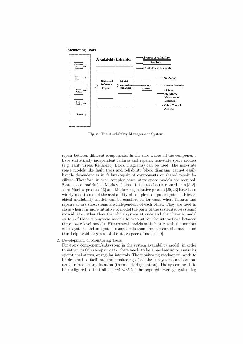
Fig. 3. The Availability Management System

repair between different components. In the case where all the componentshave statistically independent failures and repairs, non-state space models(e.g. Fault Trees, Reliability Block Diagrams) can be used. The non-statespace models like fault trees and reliability block diagrams cannot easilyhandle dependencies in failure/repair of components or shared repair fa-cilities. Therefore, in such complex cases, state space models are required.State space models like Markov chains [1, 14], stochastic reward nets [5, 8],semi-Markov process [18] and Markov regenerative process [20, 23] have beenwidely used to model the availability of complex computer systems. Hierar-chical availability models can be constructed for cases where failures andrepairs across subsystems are independent of each other. They are used incases when it is more intuitive to model the parts of the system(sub-systems)individually rather than the whole system at once and then have a modelon top of these sub-system models to account for the interactions betweenthese lower level models. Hierarchical models scale better with the numberof subsystems and subsystem components than does a composite model andthus help avoid largeness of the state space of models [9].

2. Development of Monitoring ToolsFor every component/subsystem in the system availability model, in orderto gather its failure-repair data, there needs to be a mechanism to assess itsoperational status, at regular intervals. The monitoring mechanism needs tobe designed to facilitate the monitoring of all the subsystems and compo-nents from a central location (the monitoring station). The system needs tobe configured so that all the relevant (of the required severity) system log

messages are directed to the monitoring station. Some of the steps neededin developing a monitoring mechanism have been summarized below.– The system event logging mechanism in the monitored systems, should

be configured so that the messages of required severity, from componentsbeing monitored are directed to the monitoring station. The monitoringstation needs to be configured also as the log server for the log messagesfrom all the monitored systems. Tools need to be developed to contin-uously inspect these log messages for error messages from I/O devices,hard disk, memory, CPU and related components like caches and buses,daemons and user processes, fans and power supplies. These tools canbe either one of the available log monitoring tools like Epylog [25] or alight-weight custom developed one, running at the monitoring station.In Unix or Linux based systems, hardware failures like memory failure(uncorrectable ECC error), hard disk errors, I/O device errors, cacheparity errors, bus errors etc. can be kept track of, by keeping a watchon emergency, alert, critical, error and warning level messages from thekernel [32].

– Polling agents need to be developed to poll the system regularly to deter-mine the status of some components (e.g. sending periodic ICMP echomessages for network status, probing the sensor monitoring tools forstatus of fans and power supplies [28]).

– In cluster systems, watchdog processes need to be developed to listen forheartbeat messages from applications running on the cluster elements.Available redundancy (both process and hardware) in the cluster sys-tems, provides additional mechanisms for monitoring by peer clusterelements [24, 29, 30]. Heart beat messages and Watch dog processes [29,30] and hardware [24] help detect processor and application failures.

– If SNMP (Simple Network Management Protocol) based monitoring isused, then periodic queries need to be sent from the monitoring station[26].

3. Development of the Statistical Inference EngineOnce the monitoring tools have begun their task of data collection, parame-ters of the system availability model need to be estimated from the data byusing methods of statistical inference. The tasks of the statistical inferenceengine are :– The statistical inference engine should first perform goodness of fit tests

(Kolmogorov-Smirnov test and probability plot) upon the failure andrepair data of each monitored component or subsystem. The parametersof the closely fitting distribution need to be calculated next.

– The point estimate of limiting availability for any component or subsys-tem will be calculated as the ratio of mean time to failure and sum ofmean time to failure and mean time to repair.

– Depending upon the distribution of time to failure and time to repair,exact or approximate confidence intervals are calculated for the limitingavailability of each component as discussed in the case of availabilityestimation for the non-redundant system.

4. Evaluation of the System Availability ModelThe point estimates of the parameter values are used to solve the systemavailability model using the software package SHARPE [2] to obtain thepoint estimate of the overall system availability. The confidence interval foroverall system availability is calculated as discussed in section 5.

5. Deciding the Control ActionSome of the possible control actions that may be suggested online, based onthe estimated parameter values are :– At any set of parameter values, for system availability below a threshold,

the availability of the system in different possible configurations can becalculated by evaluating the system availability models for those configu-rations at the current set of parameter values. The system configurationwith maximum availability at that set of parameter values, could besuggested as an alternative.

– Optimal preventive maintenance schedule (repair/replacement schedulefor ageing components, scrubbing interval for memory or memory-typeelements, rejuvenation schedule to avoid software ageing ) can be ob-tained in terms of the parameters of the maintenance model [18, 20]. Inthis case, since the parameter values are being constantly updated, thereis a need to recalculate these schedules at each set of parameter values.

– Diagnostics are performed to increase system availability by detectinglatent faults(for example, failure of a standby component). The avail-ability of the system as a function of period between diagnostics hasbeen obtained in [1]. For a required availability and at the current setof parameter values, the schedule for diagnostics to detect failures instandby components can be adjusted.

The flow diagram in figure 4 summarizes the above described steps.

5 Illustration with a Specific System Model

In this section, the availability management approach is illustrated with an ex-ample. A simple online transaction processing system with two back end nodesfor transaction processing and one front end machine forwarding the incomingrequests to the backend nodes based on some load balancing scheme, is set up inour laboratory. The backend machines have apache servers running on them andthe frontend machine has the load generator httperf [33] running on it, whichsends requests to each of the backend machines. All the machines have the Red-hat Linux 9 as their operating system. The setup is shown in figure 5. The stepsin the availability management of the above described setup is discussed next.

– Development of system modelBased on the conditions for the system to be available, the system availabilitymodel is constructed as a two level hierarchy. The lower level model being atwo-state Markov chain for each of the components and the upper level is afault tree shown in figure 6. The events considered are failures of network,

Fig. 4. Flow Diagram of the Autonomic Availability Management Approach

hard disk drive, memory, cpu and the application, on each of the systems.The system is up as long as the front end machine and at least one of thetwo backend machines are working. Each of the machines is considered upwhen their network, memory, hard disk and the application software are allup.

– Development of monitoring toolsThe monitoring system is designed as• The Linux system event logging mechanism known as syslog provides

flexibility in selectively directing log messages from a source (known asfacility) and of a given severity to any remote location (the log server).The monitoring station is configured as the log server for all the ma-chines. On each of the monitored system, the messages from facilitykernel and of severity error, critical and emergency are forwarded to themonitoring station.

• A log-parser at the monitoring station continuously inspects the incom-ing log messages for error messages from all the three machines’ memory(ECC errors), hard disk and CPU related errors.

• The network status is obtained by probing the machines at regular inter-vals. To ensure that lack of response from a machine is due to networkfailure, a redundant network has been provided in the system.

• The applications on each of the machines, send periodic heartbeat mes-sages to the monitoring station. A watchdog process on the monitoringstation looks out for these heartbeat messages and considers the appli-cation down on the absence of any heartbeat for a specific duration.

• For each component, at any observation i (assuming the component cameup for the first time at i = 0), the time to repair(ttr) and time to

Fig. 5. The Experimental Setup

failure(ttf) are calculated as

ttr[i] = time component came up[i]− time component went down[i]ttf [i] = time comp. went down[i]− time comp. came up[i− 1]

– Statistical InferenceThe availability of each component is calculated as the ratio of mean timeto failure and sum of mean time to repair and mean time to failure. Theavailability of each component serves as input to the fault tree and thepoint estimate of overall system availability is calculated by evaluating thefault tree using SHARPE. The time to failure and time to repair data arefitted to some known distributions (e.g. Weibull, lognormal, exponential)and the parameters for the best fitting distribution are calculated. Usingexact or approximate methods, the confidence intervals for these parame-ters are calculated. The estimators of each of the input parameters in thesystem model themselves being random variables, have their own distribu-tion and hence their point estimates have some associated uncertainty whichis accounted for, in the confidence intervals. The uncertainty expressed inconfidence intervals of the parameter needs to be propagated through thesystem model to obtain the confidence interval of the overall system avail-ability. We follow a generic Monte Carlo approach for uncertainty [15]. Thesystem availability model can be seen as a function of input parameters. IfΛ = {λi, i = 1, 2, . . . , k} be the set of input parameters, the overall availabil-ity can be viewed as a function g such that A = g(λ1, λ2, . . . , λk) = g(Λ).Suppose the joint probability density function of all the input parameters isf(Λ) then A can be calculated through a simple simulation:

Fig. 6. Fault Tree for the setup

• Draw Samples Λ(j) from f(Λ), where j = 1, 2, . . . , J , J being the totalnumber of samples

• Compute A(j) = g(Λ(j))• Summarize A(j)

In the case when λis are mutually independent and so the joint probabilitydensity function f(Λ) can be written as the product of marginal densityfunctions, samples can be drawn independently. Drawing enough numberof samples from the distributions of the input parameters, the confidenceinterval for the overall system availability is computed from values obtainedby evaluating the system availability model at each of these sample values.

– Suggesting Control ActionsWhen the availability drops below a threshold, the possible reconfigurationsmay be done by making the frontend redundant or adding one more backendmachines, after evaluating the system availability model for those configura-tions at current parameter values. Optimal preventive maintenance schedulefor components that age (e.g., the hard disk), software rejuvenation schedulefor the backends (as the web server Apache has been shown to display aging[12]) or scrubbing interval may also be obtained.

Figure 7 shows a snapshot of the online availability estimation of this setup.Hardware failures are emulated by injecting kernel level messages for hardwarefailures like uncorrected ECC, cache parity error, bus error etc. at each of themonitored stations. These messages get forwarded to the monitoring station ,where they are inspected by the log parser. Software failures are injected bykilling of the processes. Absence of heartbeat messages is detected by the watch-dog process on the monitoring station as a failure. The times between failure

0.6

0.65

0.7

0.75

0.8

0.85

0.9

0.95

2 4 6 8 10 12 14 16 18

Ava

ilabi

lity

Number of Samples

Realtime Availability EstimationUpper Bound of 90% conf. interval

Point Estimate of System AvailabilityLower Bound of 90% conf. interval

Fig. 7. Realtime Availability Estimation of the experimental setup

and repair injections are exponentially distributed. As the number of samples in-creases from observation to observation, the confidence interval becomes tighter.

6 Conclusion

In this paper, an autonomic availability management approach for complex sys-tems in critical applications is presented. The approach consists of monitoringthese systems to continuously estimate their availability and its confidence inter-vals by exercising their availability model. Based on their availability and otherinferred lifetime characteristics, appropriate control actions to increase the sys-tem availability may be suggested, in real time. The approach combines boththe measurement based and model based approaches of availability estimationand at the same time provides continuous realtime monitoring and control ofthe system availability. This automates the whole process of availability man-agement to ensure maximum system availability, making the system autonomic.

References

1. Trivedi, K.S. (2001),Probability and Statistics with Reliability, Queuing and Com-puter Science Applications, John Wiley & Sons, New York.

2. Sahner R.A., Trivedi K.S. and Puliafito A. (1996),Performance and ReliabilityAnalysis of Computer Systems: An Example-Based Approach Using the SHARPESoftware Package, Kluwer Academic Publishers.

3. Leemis, L.M. (1995),Reliability. Probabilistic Models and Statistical Methods, Pren-tice Hall, New Jersey.

4. Tang, D. and Iyer, R.K. (1993), Dependability Measurement and Modeling of aMulticomputer System, IEEE Transactions on Computers, 42 (1), 62–75.

5. Malhotra, M. and Trivedi, K.S.(1995), Dependability Modeling Using Petri NetBased Models, IEEE Transactions on Reliability, 44 (3), 428–440.

6. Cristian, F., Dancey, B. and Dehn J. (1996), Fault Tolerance in Air Traffic ControlSystems, ACM Transactions on Computer Systems, 14, 265–286.

7. Morgan, P., Gaffney, P., Melody, J., Condon, M., Hayden, M. (1990), SystemAvailability Monitoring, IEEE Transactions on Reliability, 39 (4), 480–485.

8. Ibe, O., Howe, R., and Trivedi, K.S. (1989), Approximate availability analysis ofVAXCluster systems, IEEE Transactions on Reliability, R-38 (1), 146–152.

9. Blake, J.T. and Trivedi, K.S. (1989), Reliability analysis of interconnection net-works using hierarchical composition, IEEE Transactions on Reliability, 32, 111–120.

10. Albin, S.L.. and Chao, S. (1992), Preventive Replacement in Systems with Depen-dent Components, IEEE Transactions on Reliability, 41 (2), 230–238.

11. Kephart., J.O. and Chess, D.M. (Jan. 2003), The Vision of Autonomic Computing,Computer magazine, 41–50.

12. Li, L., Vaidyanathan, K. and Trivedi, K.S. (2002), An Approach for Estimation ofSoftware Aging in a Web Server, Proc. of Intl. Symposium on Empirical SoftwareEngineering (ISESE-2002).

13. Garzia, M.R. (2003), Assessing the Reliability of Windows Servers, Proc. of De-pendable Systems and Networks, (DSN-2002).

14. Hunter, S.W. and Smith, W.E. (1999), Availability modeling and analysis of atwo node cluster, Proc. of 5th Int. Conf. On Information Systems, Analysis andSynthesis.

15. Yin, L., Smith, M.A.J. and Trivedi, K.S. (2001), Uncertainty Analysis in ReliabilityModeling, Proc. of the Annual Reliability and Maintainability Symposium, (RAMS-2001).

16. Dohi, T., G.-Popstojanova,K., Trivedi, K.S. (2000), Statistical Non-ParametricAlgorithms to estimate the Optimal Software Rejuvenation Schedule, Proc. ofPacific Rim Intl. Symposium on Dependable Computing, (PRDC).

17. Garg, S., Huang, Y., Kintala, C.M.R., Trivedi, K.S. and Yajnik S. (1999), Per-formance and Reliability Evaluation of Passive replication Schemes in ApplicationLevel fault Tolerance, Proc. of 29th Annual Intl. Symposium on Fault TolerantComputing (FTCS).

18. Chen, D.Y. and Trivedi, K.S. (2001), Analysis of Periodic Preventive Mainte-nance with General System Failure Distribution, Pacific Rim Intl Symposium onDependable Computing (PRDC).

19. Long, D., Muir, a., and Golding, R. (1995), A Longitudinal Survey of InternetHost Reliability, Proc. of the 14th Symposium on Reliable Distributed Systems.

20. Garg, S., Puliafito, A., Telek, M. and Trivedi, K.S. (1995), Analysis of SoftwareRejuvenation using Markov Regenerative Stochastic Petri Net, Proc. of Intl. Sym-posium on Software Reliability Engineering (ISSRE).

21. Fricks, R.M. and Ketcham, M. (2004), Steady State Availability Estimation Us-ing Field Failure Data, Proc. Annual Reliability and Maintainability Symposium(RAMS-2004).

22. Sathaye, A., Ramani, S., Trivedi, K.S. (2000), Availability Models in Practice,Proc. of Intl. Workshop on Fault-Tolerant Control and Computing (FTCC-1).

23. Logothetis, D. and Trivedi, K. (1995), Time-dependent behavior of redundantsystems with deterministic repair, Proc. of 2nd International Workshop on theNumerical Solution of Markov Chains.

24. G. Hughes-Fenchel (1997), A Flexible Clustered Approach to High Availability,27th Int. Symp. on Fault-Tolerant Computing (FTCS-27).

25. Epylog Log Analyzer, http://linux.duke.edu/projects/epylog.26. Sun SNMP Management Agent Guide for Sun Fire B1600,

http://docs.sun.com/source/817 -1010-10/SNMP intro.html.27. Simple Network Management Protocol, http://www.cisco.com/univercd/cc/

td/doc/cisintwk/ito doc/snmp.htm.28. Hardware Monitoring by lm sensors, http://secure.netroedge.com/lm78/info.html.29. Windows 2000 Cluster Service Architecture, www.microsoft.com/serviceproviders

/white papers/win2k.30. SwiFT for Windows NT, http://www.bell-labs.com/project/swift.31. IBM Research — Autonomic Computing, http://www.research.ibm.com/autonomic

/index.html.32. Linux Syslog Man Page, http://www.die.net/doc/linux/man/man2/ syslog.2.html.33. Mosberger, D. and Jin, T., httperf—A Tool for Measuring Web Server Perfor-

mance, http://www.hpl.hp.com/personal/David Mosberger/httperf.html.