IEEE JOURNAL ON SELECTED AREAS IN COMMUNICATIONS, VOL. 23, NO. 12, DECEMBER 2005 2305

Data Dissemination in AutonomicWireless Sensor Networks

Max do Val Machado, Olga Goussevskaia, Raquel A. F. Mini, Cristiano G. Rezende, Antonio A. F. Loureiro,Geraldo Robson Mateus, and José Marcos S. Nogueira, Member, IEEE

Abstract—In this paper, a new data dissemination algorithm forwireless sensor networks is presented. The key idea of the proposedsolution is to combine concepts presented in trajectory-based for-warding with the information provided by the energy map of thenetwork to determine routes in a dynamic fashion, according tothe energy level of the sensor nodes. This is an important featureof an autonomic system, which must have the capacity of adaptingits behavior according to its available resources.

Simulation results revealed that the energy spent with the datadissemination activity can be concentrated on nodes with high-en-ergy reserves, whereas low-energy nodes can use their energy onlyto perform sensing activity or to receive information addressed tothem. In this manner, partitions of the network due to nodes thatran out of energy can be significantly delayed and the network life-time extended.

Index Terms—Data dissemination, energy map, trajectory-based forwarding (TBF), wireless sensor networks (WSNs).

I. INTRODUCTION

ONE OF THE MOST important challenges in the designof wireless sensor networks (WSNs) is to deal with the

dynamics of such networks. The physical world where the sen-sors are embedded is dynamic. Over time, the operating condi-tions and the associate tasks to be performed by the sensors canchange. Some of the causes that may trigger these changes arethe events occurring in the network, amount of resources avail-able at nodes, particularly, energy and reconfiguration of nodes.Furthermore, it is important that sensors adapt themselves to theenvironment since manual configuration may be unfeasible oreven impossible. In summary, the kind of distributed system weare dealing with calls for new data communication, coordina-tion, and control algorithms for large scale, highly dynamic, andunattended WSN.

“Autonomic computing is an approach to self-managedcomputing systems with a minimum of human interference”[6]. Given this definition, the challenge is to design WSNs

Manuscript received October 18, 2004; revised May 5, 2005. This work wassupported in part by CNPq, Brazil, under Process Number 55.2111/2002-3, Sen-sornet Project (http://www.sensornet.dcc.ufmg.br), and in part by Scholarshipsfrom CAPES, Ministry of Education, Brazil.

M. do Val Machado, O. Goussevskaia, C. G. Rezende, A. A. F. Loureiro,G. R. Mateus, and J. M. S. Nogueira are with the Department of Computer Sci-ence, Federal University of Minas Gerais, Belo Horizonte 30123-970, Brazil(e-mail: maxm@dcc.ufmg.br; olga@dcc.ufmg.br; rezende@dcc.ufmg.br;loureiro@dcc.ufmg.br; mateus@dcc.ufmg.br; jmarcos@dcc.ufmg.br).

R. A. F. Mini is with the Department of Computer Science, PontificalCatholic University of Minas Gerais, Belo Horizonte 30535-610, Brazil(e-mail: raquel@dcc.ufmg.br).

Digital Object Identifier 10.1109/JSAC.2005.857209

that are self-managing, self-diagnostic, and transparent to themonitoring entity. This new computing paradigm, when appliedto a WSN, means that the design of such a network should aimto embed autonomic capabilities in sensor nodes.

In WSNs, data communication, from the point of view ofthe communicating entities, can be divided into three cases, asdepicted in Fig. 1: from sensors to a monitoring node, amongneighboring sensors, and from a monitoring node to sensors.The first is used to send the sensed data to a monitoring applica-tion. The second often happens when some kind of cooperationamong nodes is needed. The last, called data dissemination, isnormally used to disseminate a piece of information that is im-portant to sensor nodes. Reliable data dissemination is crucial toWSN since a monitoring node has to perform some specific ac-tivities, such as to change the operational mode of part or the en-tire WSN, broadcast a new interest to the network, activate/de-activate one or more sensors, and send queries to the network.

In this work, an energy-efficient data dissemination protocolfor WSNs, called trajectory and energy-based data dissemi-nation (TEDD), is proposed. The key idea is to combine con-cepts presented in trajectory-based forwarding (TBF)1 [15] withthe information provided by the energy map2 [12] to determineroutes in a dynamic fashion. TEDD is comprised of two mainparts. The first one is an algorithm for generating trajectoriesthat pass through regions with higher energy reserves and avoidlow-energy areas. The main idea is to select a set of nodes thatare most suitable for disseminating information and to find thebest set of curves passing through or near these selected points.The second part of TEDD is a new packet forwarding mech-anism which is a receiver-based approach. This characteristicintroduces two improvements to the TBF process. First, it elim-inates the need of neighbor table maintenance, which is veryexpensive in terms of radio transmissions. Second, it presentsa more robust behavior in dynamic topology scenarios, such asWSNs.

The rest of this paper is organized as follows. Section II dis-cusses the related work. The two parts of TEDD are describedin Sections III and IV, respectively. In Section V, we analyze theexperimental results. Finally, in Section VI, we present the con-clusion and the future directions.

1Data dissemination technique in which packets are disseminated from amonitoring node to a set of nodes along a predefined curve. The main idea is toembed a trajectory in the packet, and then let the intermediate nodes forward itin a unicast manner to those nodes that lie close to the trajectory.

2Energy map is the information about the amount of energy available at eachpart of the network.

0733-8716/$20.00 © 2005 IEEE

2306 IEEE JOURNAL ON SELECTED AREAS IN COMMUNICATIONS, VOL. 23, NO. 12, DECEMBER 2005

Fig. 1. Data communication schemes in WSNs. (a) Data communication from a sensor node to a monitoring node. (b) Data communication among neighboringnodes. (c) Data communication from a monitoring node to sensor nodes.

II. RELATED WORK

Several different routing protocols for WSNs have been pro-posed in the literature [1], [3], [7], [9]. Among all algorithmsalready proposed in the literature, the closest to the one pre-sented in this work is the TBF [15], that is a technique to dis-seminate messages in dense wireless networks. The key idea isto embed a curve (trajectory) in the packet to be disseminatedfrom a monitoring node to sensor nodes [Fig. 1(c)], and then letthe intermediate nodes forward it in a unicast manner to thosenodes that lie close to the curve. TBF is a sender-based algo-rithm since the current node systematically chooses the next hopof the route. This forwarding decision is based on the curve and aneighboring table. To update this table, nodes exchange beaconpackets periodically. TBF is a source routing protocol since theentire trajectory is defined by the data dissemination source. Intraditional source routing protocols for mobile ad hoc networks[8], the source node inserts all nodes of the path into the packetas a discrete set of points, generating a considerable overheadand making impracticable its use in WSNs. Two main advan-tages of TBF are compact representation of a route, since curvescan be described using few parameters, and node independence,since no particular node address is specified in the trajectory.

Algorithm 1 shows the basic operation of TBF.3 When a nodereceives a beacon packet, it updates its neighbor table. If thereceived packet is not a beacon, but a data packet, this nodechecks if it is the node elected to forward this packet. If it isnot the case, the node drops the packet, otherwise it chooses thenext node in the trajectory defined by the curve. This choice ismade based on its neighbor table and a predefined forwardingpolicy (e.g., minimum deviation). After choosing the next node,the current node transmits the packet.

Algorithm 1: TBF—Receiving packetinput: the received packetif the packet is a beacon thenUpdate my neighbor table

else/ The received packet is a datapacket /if I am the node elected to forwardthis received data packet thenChoose the next node in thetrajectory

3Since TBF is a source routing protocol, its basic operation is similar to thetraditional source routing protocols. The main difference to them is that TBFdefines the routes as curves.

Insert the chosen node as the nexthopTransmit the packet

elseDrop the packet

endifendif

Despite its advantages, TBF has two main drawbacks. First,the overhead required to update the neighbor tables increasesthe number of transmitted packets, and consequently, the totalenergy spent. In dynamic topology environments, such as WSNsin which nodes frequently enter a sleep mode to save energy,mechanisms for neighbor table maintenance have a prohibitivecost. Second, TBF is not fault tolerant in scenarios in whichtopological changes are faster than the neighbor table updates.In this case, broken trajectories happen when the selected nodeis unavailable (e.g., the node is sleeping). Therefore, we notea tradeoff between the neighbor table update overhead and theprotocol robustness.

III. DYNAMIC TRAJECTORY GENERATION

In this section, we discuss the problem of generating trajec-tories for data dissemination. First, the problem is defined and,afterward, the proposed solution is presented.

A. Problem Definition

As input to this problem, we have a data forwarding protocol,a set of nodes distributed in an ad hoc manner over the WSN,and a monitoring node that disseminates data. The problem ofgenerating routing trajectories asks for the ideal number oftrajectories and the parameters (we suppose a continuousmodel, describing a curve using parameters), such that theobjectives of the routing protocol are achieved or maximized.

Despite providing several insights into the problems thatmight arise during the process of specifying a forwardingtrajectory, the authors of TBF [15] do not present solutionsto the curve generation problem, specially to the problem ofhow and based on what kind of information the trajectoriesshould be generated for the routing. In Cartesian routing [5],the route is defined as a straight line between the router and thedestination. In source-based routing [8], the route is specifiedas a discrete set of points. In other protocols [3], [7], the routeis “discovered” instead of being defined. Therefore, to the bestof our knowledge, the solution proposed in this work is pioneer.

DO VAL MACHADO et al.: DATA DISSEMINATION IN AUTONOMIC WIRELESS SENSOR NETWORKS 2307

Fig. 2. Process of trajectory generation.

The problem of generating trajectories can be divided intoseveral subproblems. In the following, we discuss and proposesolutions to each subproblem.

B. Input: The Energy Map

The first question that arises when solving the problem ofcurve generation is: what kind of information should the pro-cedure be based on. In this work, we use the energy map as ourinput, since energy is an important constraint in WSNs. In [12],the authors analyze the cost of obtaining this map using a pre-diction-based approach and show that it is viable in WSNs. It isworth mentioning that the cost of obtaining the energy map canbe amortized among different network applications, and, thus,neither of them has to pay for this information itself.

C. Point/Node Selection

Having defined the input to the procedure (i.e., the energymap), a subset of points4 from the WSN has to be selected toserve as input data for the fitting process. Several strategies canbe used to select this subset. The main criterion for this selec-tion is the energy available at each of these points. The idea isto force the trajectories to pass through points with greater en-ergy reserves, in order to avoid nodes with little energy to par-ticipate in the forwarding process. Another criterion is the nodedensity in each part of the network. The denser the region thetrajectory passes, the greater the network connectivity is, andthe better the chances of the packet to be delivered successfully.This occurs because nodes are frequently programmed to turnoff their radios in order to save energy. Therefore, there is al-ways a possibility of the trajectory to break, in case there are nonodes “awake” to propagate the packet.

In this work, the points are selected using a combination ofenergy and density criteria. For every node, the sum of energiesof all its neighbors, together with its own is calculated. After-wards, the nodes are sorted in decreasing order of this factor,

4We can study a WSN as a set of points where each point can be a node inthe network graph or a pixel in the image of the energy map.

and the first half of the nodes is selected to be the input to thefitting procedure.5 In this manner, the trajectories are “forced”to pass through regions of higher densities and energy reserves.The main concern here is to avoid that low-energy nodes partic-ipate in forwarding activities and to minimize packet losses dueto broken trajectories.

D. Curve Representation and Curve Fitting

The second question that arises when solving the problem oftrajectory generation is: which model should be used to repre-sent the trajectories. In this work, we use a polynomial repre-sentation that offers a compact encoding, allowing to controlthe number of parameters by limiting the degree of the polyno-mial. Moreover, the value of the dependent variable is directlycomputed for any value of the independent variable . Based onexperiments, we could observe that this type of representationis flexible and expressive enough to generate trajectories thatavoid low-energy and low-density areas.

Having defined the model to represent the trajectories, acurve-fitting algorithm has to be determined. Due mainly to itssimplicity, we use multiple linear regression [10], [14] to fit thecurves into a set of points and, in particular, we use the LSQRalgorithm6 [17].

E. Architecture

Having discussed the previous subproblems, some questionsrelated to the architecture of the curve generation process haveto be answered. The architecture proposed in this work is illus-trated in Fig. 2 and is described in the following.

The process has some variations depending on the dissemina-tion type. As showed in Fig. 2 (Point A), the first step is to selectpoints from the dissemination target area. If the dissemination is

5The reason to select only 50% of nodes is purely empirical. Experimentswere made with different percentages, and better results were obtained by elim-inating 50% of nodes from the fitting procedure.

6The computational requirements of LSQR are: storage (n+2p), and numberof floating-point multiplications per iteration (3n+5p). The maximum numberof iterations was set to 4np.

2308 IEEE JOURNAL ON SELECTED AREAS IN COMMUNICATIONS, VOL. 23, NO. 12, DECEMBER 2005

Fig. 3. Maximum number of sectors depends on the position of the monitoring node. (a) Network sectoring with monitoring node in the center. (b) Networksectoring with monitoring node at the corner.

a broadcast, the points are selected from the whole map, whichis the target area. If the dissemination is a multicast (the targetarea is a subset of the map), two sets of points are selected: oneinside the area between the monitoring node and the target area,and the other inside the target area. The former set is used tofit a special curve, called delivery curve [Fig. 2 (Point B)], thatis used as a tunnel between the monitoring node and the targetarea. The latter set is used to fit curves inside the target area. Thedelivery curve must intersect the monitoring node at one end,and the target area at another. To not overload the nodes locatedat the point of intersection between the delivery curve and thetarget area, this point must be defined dynamically, based on en-ergy/density. It means that, given all points located on the targetarea boundary, the intersection point is the one with greater en-ergy/density factor. Inside the target area, the origin of the gener-ated curves is the intersection point. A procedure called networksectoring is used to define the ideal number of curves inside thetarget area [Fig. 2 (Point C)], as explained in this next section.

1) Network Sectors: Given a set of points that we wouldlike to force to participate in the forwarding process and giventhe curve type (polynomial), we have to decide how manycurves/trajectories would be sufficient to achieve a certain goal.The goal could be to disseminate information to a particulararea of the network or just perform a broadcast to all nodes.

By introducing the concept of network sectors, which dividethe network area in identical angular sectors centered at themonitoring node, the problem of determining the best number ofcurves can be viewed as the problem of finding the best numberof network sectors and placing a unique trajectory at each net-work sector. The curve corresponding to each network sector isfitted based solely on the points located inside that sector [Fig. 2(Point D)].

An arbitrary number of network sectors could be used. How-ever, it is not reasonable to have a large value, since this wouldresult in an unacceptably high number of parameters to be trans-mitted with each packet and an unacceptably low number ofpoints at each sector, compromising the quality of the fittingprocedure. A maximum limit can, therefore, be defined for thenumber of network sectors. This limit depends on the positionof the monitoring node. If it is located at one of the corners ofthe target area, the sectoring is made within a 90 angle. If it is

located at the center, the sectoring is made within a 360 angle,allowing the greatest possible number of sectors. These situa-tions are illustrated in Fig. 3.

Besides the number of sectors, the degree of the polynomialalso has influence on the quality of the fitting procedure. There-fore, the curve fitting is not only performed for different num-bers of network sectors, but also for different polynomial de-grees. The maximum polynomial degree used in this work isfour, since the higher the degree of the polynomial, the greaterthe complexity of calculating the distance between each nodeand the curve.

Given a maximum number of network sectors and a max-imum polynomial degree, all possible curve sets are generated.By selecting the curve set with the “best” average quality, wedetermine the boundaries and the angles of the sectors, as is ex-plained in the next section.

2) Best Curve Set Selection: The last step in the curve gen-eration process is the selection of the best curve set, as shownin Fig. 2 (Point E). This selection can be made by calculatingthe average quality for each set and simply choosing the onewith the best average quality. The average quality of one setcan be calculated as the sum of the qualities of each curveparticipating in the set, divided by the number of networksectors in the set. The quality of one curve can be calculatedbased on different criteria, depending on the application re-quirements. In this work, the following fit evaluation criteriawere used: maximum average energy, which maximizes theaverage energy of the nodes within the covering range of thecurve , andmaximum coverage, which maximizes the total number ofnodes within the covering range of the curve. Finally, the “best”fit quality is determined by calculating the average criteriaof each set, and selecting the one with the highest average fitquality.

In the following section, we provide examples of networksectoring and curve fitting in different network scenarios.

3) Examples of Network Sectoring: Fig. 4(a) and (b) illus-trates two sets of broadcast curves, selected for two differentenergy maps, using the maximum average energy criterion.Fig. 4(c) and (d) illustrates the same scenarios, however, usingthe maximum coverage criterion. It can be observed that when

DO VAL MACHADO et al.: DATA DISSEMINATION IN AUTONOMIC WIRELESS SENSOR NETWORKS 2309

Fig. 4. Curve sets to perform broadcasts. Energy map of an area of 35� 35 m with one and two low-energy areas. (a) Maximum energy. (b) Maximum energy.(c) Maximum coverage. (d) Maximum coverage.

Fig. 5. Curve sets to perform multicasts. Energy map 35�35m with one and two low-energy areas. Target area = (20; 20)�(35;35). (a) Maximum energy.(b) Maximum energy. (c) Maximum coverage. (d) Maximum coverage.

the first criterion is used, a set with fewer sectors is selected,and the curves avoid the low-energy areas. When the secondcriterion is applied, the maximum number of sectors is selected,and the curve inside each sector is fitted closer to the nodeswith greater energy reserves.

Fig. 5(a) and (b) illustrates two sets of curves generated to per-form a multicast, using the maximum average energy criterion.The target area is determined as a rectangle with coordinates(20,20)–(35,35). Fig. 5(c) and (d) illustrates the same scenarios,however using the maximum coverage criterion. It can be ob-served that the delivery curve avoids low-energy areas. Whenthe first criterion is used, less sectors are used inside the targetarea. When second criterion is applied, more sectors are used.

F. Some Remarks

It is important to point out that the trajectory generationstrategy proposed here is not restricted to the illustrated net-work scenarios. An energy map of a network with an arbitraryshape and an arbitrary number of randomly distributed mon-itoring nodes can be used as input to this procedure. In thissituation, each node would be able to participate in more thanone trajectory, possibly forwarding packets originated by dif-ferent monitoring nodes. This solution presents two importantfeatures of an autonomic system: flexibility and adaptability.

Another relevant consideration is about the process of en-coding the trajectories. Curve parameters can be embedded inthe packet header or can be preconfigured in the nodes beforedelivering them. However, in the latter case, the monitoringnode should be able to update those values periodically.

IV. PACKET FORWARDING POLICY

In this section, we present the second part of our solution thatconsists of the data dissemination model of TEDD, whose goalis to discover the best energy-efficient routes.

A. Proposed Improvements

TEDD extends the principles of TBF by incorporating theusage of the energy map. The proposed protocol defines a re-ceiver-based data dissemination policy, i.e., each node upon re-ceiving a packet decides itself whether to relay it or not, as op-posed to TBF that is a sender-based data dissemination policy.In TEDD, the decision to forward a packet or not is based onthe node geographical location and the packet information. Theforwarding decision process uses a temporization policy: beforerelaying a packet, the current node waits a small time interval.After this time, if no neighbor has relayed the packet, the nodetransmits it. The key idea of this technique is how to estimatethe delay time, based only on the distance between the currentnode and a point ahead on the curve called reference point.

Using the temporization policy, TEDD overcomes the draw-backs of TBF. First, TEDD avoids both the necessity of neighbortables and beacon transmissions, and consequently, spends lessenergy in the forwarding process. In TBF, the neighbor table isfundamental to the process of choosing the next hop of the tra-jectory. Second, TEDD is more robust than TBF because nodesare not selected by the previous elected node. TEDD is a re-ceiver-based protocol and, thus, avoids situations where the for-warding process is interrupted because the selected node is un-

2310 IEEE JOURNAL ON SELECTED AREAS IN COMMUNICATIONS, VOL. 23, NO. 12, DECEMBER 2005

Fig. 6. Reference points.

available. Another important advantage of TEDD is the possi-bility of disseminating data only to a target area, as shown inFig. 5. In this case, the protocol avoids nodes not interested inthis data (outside the target area).

B. Temporization Policy and Forwarding Modes

The proposed temporization policy is based on the distancefrom the current node to a point ahead on the curve, called ref-erence point. In particular, the reference point is the point (notnecessarily a node) closest to the curve localized at the circum-ference with center at the current node and radius equals to thenode communication radius (Fig. 6). In each relay, the selectionof the reference point is determined by the previous hop of thetrajectory. Each node that receives a packet adjusts its delay timeusing its distance to the reference point sent in the packet.

Based on this policy, TEDD defines two different forwardingmodes: one data flow and two data flows. In the first one, thedata is disseminated using only one flow, in a way that only onenode decides to forward the packet. In the second forwardingmode, two flows are used to disseminate the data, in a way thattwo nodes end up forwarding the packet. As illustrated in Fig. 6,when one flow is used, the node closer to reference point Brelays the packet; and when two flows are used, the node closerto reference point A and the one closer to reference point C relaythe packet. As an example, in Fig. 5(a)–(d), TEDD uses one flowin the delivery curve and two flows in the target area.

The choice between one or two flows depends on the goalof the dissemination. In data dissemination protocols, there is atradeoff between minimizing the number of transmissions andmaximizing the coverage. In situations in which the first goalis the most important requirement, only one data flow shouldbe used. On the other hand, when maximizing the coverage isthe main goal, two data flows should be used. Its important topoint out that independently of the number of data dissemina-tion flows, the previous trajectory node always selects only onereference point. In the two flows forwarding mode, nodes thatreceive a packet calculate the two reference points also using thereference point present in the packet.

C. Basic Operation

Algorithm 2 presents the basic operation of TEDD. When anode receives a packet, it verifies whether it is inside the re-ceived network sector. If it is not, it drops the packet. If it isinside the network sector, the node verifies if its distance to thereference point (calculated by the previous hop) is higher thanthe communication range. When the forwarding mode with twoflows is used, the node calculates the two new reference pointsand its distance to both points, and then selects the closest pointas the reference point. If the calculated distance is higher thanthe communication range, the node drops the packet. If it is not,the node waits a delay time that is calculated according to itsdistance to the reference point. The smaller the distance, thesmaller the delay. After the node waits the delay time, it verifieswhether any of its neighbors retransmitted the packet. If this isthe case, the node drops the packet. Otherwise, the node selectsthe reference point and, then, forwards the packet. The processof selecting the reference point is presented in the next section.

Algorithm 2: TEDD—Receiving packetinput: the received packetif I am inside the received networksector thenCalculate my distance to thereference pointif this distance vale is less orequal to the communication range thenCalculate the delay timeWait the delay time

if any of my neighbors retransmittedthis packet thenDrop the packet

elseCalculate the reference point(Algorithm 3)Forward the packet

endifelseDrop the packet

endifelseDrop the packet

endif

D. Selecting the Reference Point

The process of selecting a reference point is described in Al-gorithm 3 and it is determined by the previous hop in the tra-jectory. Before forwarding the packet, the node calculates twospecial points on the curve, and , where

and . In thiscase, and are, respectively, the

-coordinate and the communication range of the node that isselecting the reference point. Similarly, the same holds for thevalues of and . If the data dissemination is from left toright, , otherwise, if it isfrom right to left, . In thesecond step, the algorithm defines the straight line

DO VAL MACHADO et al.: DATA DISSEMINATION IN AUTONOMIC WIRELESS SENSOR NETWORKS 2311

TABLE IDEFAULT VALUES USED IN SIMULATIONS

Fig. 7. Possible reference points.

that passes through and . This equation is used by theproposed algorithm instead of the curve equation because thealgorithm has to calculate the distance from a curve to a point.The evaluation of the curve/point distance is not trivial, mainlyconsidering the limited resources of sensor nodes. On the otherside, the distance from a straight line to a point is easier to becalculated. This heuristic presents good results, since the gen-erated curves do not present a great variation inside the nodecommunication radius. In the third step, the node determinesthe quadrant where the reference point is localized. The quad-rant of a reference point is an important concept because it re-duces the amount of possible reference points to examine. Thecommunication radius has four quadrants, the first one is lo-cated at the northeast and the others are, respectively, locatedat the northwest, the southwest, and the southeast. Moreover,this concept is the same one used in the plain geometry for theCartesian plan, except that the source is the current node. Thequadrant of a reference point is obtained using Algorithm 4 andit is detailed below. In the last step, the node selects the refer-ence point among some points located in the selected quadrant.In Fig. 7, the points of each quadrant are, respectively: (N, NNE,NE, ENE, E); (N, NNW, NW, ENW, W); (W, WSW, SW, SSW,S); and (E, ESE, SE, SSE, S).

Algorithm 3: TEDD—Selecting the referencepointinput: the received packetCalculate points and whereand

Calculate the straight line thatpasses through points and

Call the procedure to discover the quad-rant of the reference point (Algorithm4)

Select the reference point using the quad-rant and the straight line .

Return the reference point

The process of discovering the quadrant of the referencepoint is described in Algorithm 4 and it is the third step ofAlgorithm 3. Using quadrants, TEDD reduces the amountof possible reference points, and consequently, the cost ofselecting this point. As illustrated in Fig. 7, the use of quadrantsreduces this value from sixteen to five. The proposed processconsiders two scenarios: 1) the curve intercepts the “commu-nication circle” and 2) it does not intercept. In the former, thedesired quadrant is the one that contains the reference point; inthe latter, the desired quadrant is the one nearest to the curve.To identify whether the curve intercepts the communicationradius, TEDD uses the following procedure. The node verifiesif the point is inside its communication radius. If it is, theselected quadrant is the one where is inside. In this case,TEDD knows that the circumference is intercepted by the line

and is inside the quadrant of the referencepoint. On the other hand, if is outside the communicationcircle, TEDD evaluates the inclination of the straight line

, and the values of (the -coordinate of point) and (the -coordinate of the node that is selecting

the reference point). TEDD selects the first quadrant whenand . The other quadrants are, respectively,

selected when: and (second); and(third); and and (fourth).

Algorithm 4: TEDD—Discover the quadrant ofthe reference pointinput points and , and straightline ;if is localized inside mycommunication circle thenI select the quadrant where pointis localized.

elseif thenif thenI select the first quadrant.

elseI select the third quadrant.

2312 IEEE JOURNAL ON SELECTED AREAS IN COMMUNICATIONS, VOL. 23, NO. 12, DECEMBER 2005

Fig. 8. Energy map and network coverage evolutions for one instance of each protocol evaluated (TBF, TEDD with one flow forwarding mode and flooding) ina broadcast scenario. (T =time, C =coverage, E =mean energy). (a) TBF, T = 0 s: C = 100%, E = 100%. (b) TBF, T = 500 s: C = 39%, E = 48%.(c) TBF, T = 1000 s: C = 0%, E = 1:3%. (d) TEDDc(1F), T = 0 s: C = 100%, E = 100%. (e) TEDD(1F), T = 500 s: C = 51%, E = 60%.(f) TEDD(1F), T = 1000 s: C = 46%, E = 23%. (g) Flooding, T = 0 s: C = 100%, E = 100%. (h) Flooding, T = 500 s: C = 79%, E = 38%.(i) Flooding, T = 1000 s: C = 0%, E = 0%.

end ifelseif thenI select the second quadrant.

elseI select the fourth quadrant.

end ifend if

end if

E. Some Remarks

The goal of TEDD is to reduce the number of transmittedpackets so that only nodes closer to the reference point relaypackets. Moreover, TEDD maintains a good network coveragesince nodes closer to the reference point are exactly those thatreach the highest number of yet unreached nodes. Using this al-gorithm, we are able to reach our goals and, thus, increase thereceived/transmitted ratio, which is an important metric to in-dicate the quality of a data dissemination technique. One draw-back of this approach is a higher latency to deliver data. This

DO VAL MACHADO et al.: DATA DISSEMINATION IN AUTONOMIC WIRELESS SENSOR NETWORKS 2313

Fig. 9. Performance parameters (TEDD, TBF, and flooding) in a broadcast scenario. (a) Percentage of reached nodes. (b) Number of transmitted packets. (c) Meanenergy. (d) Percentage of dead nodes. (e) Received/transmitted ratio. (f) Latency.

and other metrics are evaluated using simulations, as discussedin the next section.

V. SIMULATION RESULTS

In this section, we show the behavior of TEDD in two sce-narios of data dissemination in a WSN. In the first one, the

monitoring node disseminates data to the entire network. Inthe second one, it disseminates data to a target area located atthe right top corner of the sensing field, which has an initiallow-energy area in the center of it. The remainder of this sectionis organized as follows. Section V-A presents the simulation pa-rameters. Sections V-B and V-C show our protocol performancein both data dissemination scenarios.

2314 IEEE JOURNAL ON SELECTED AREAS IN COMMUNICATIONS, VOL. 23, NO. 12, DECEMBER 2005

TABLE IIAVERAGE NUMBER OF OPERATIONS, TRANSMISSIONS, AND NETWORK COVERAGE AT EACH DATA

DISSEMINATION FOR TEDD, TBF, AND GOSSIPING IN A MULTICAST SCENARIO

A. Scenarios

In this section, we present the scenarios used throughout thesimulations. We consider a dynamic topology, where nodes arestatic but periodically go into a sleeping mode to save energy,which leads frequently to topology changes. In [4], Hill et al.state that a WSN should embrace the philosophy of getting thework done as quick as possible and going to sleep. The bestway to save energy is to turn off parts of the sensor that are notneeded, as modeled by a state-based energy dissipation model(SEDM) presented in [13]. In order to analyze the performanceof TEDD, we use the ns-2 simulator [16].

We consider a WSN with static and homogeneous nodeswith a finite amount of energy. Nodes are deployed randomly,forming a high-density flat topology. It is assumed that eachnode knows its own location and the monitoring node knowsthe coordinates of all nodes. One monitoring node with noenergy, memory or processor restrictions is placed at thebottom left corner of the network and performs a series of datadisseminations. In each data dissemination, a new set of curvesis recalculated based on the current energy map that is obtainedusing a prediction-based approach [12]. The cost of obtainingthis map is not considered in the results since it is expectedto be distributed among different network activities. The costof generating the curves is also not considered since they aregenerated in the monitoring node. The numerical values chosenfor the simulations can be seen in Table I.

B. Dissemination to the Entire Network

In this section, a scenario where the monitoring node dissemi-nates information to the entire network is studied. The behaviorof TEDD is analyzed using both forwarding modes: one andtwo flows, presented in Section IV. Its performance is comparedto the TBF and to the flooding-based dissemination schemes.Both TBF and TEDD use the same trajectory generation proce-dure, described in Section III. The maximum coverage criterionwas used to select the best set of curves. In Fig. 8, we show thenetwork energy map evolution during the network lifetime. To-gether with the energy available at each node, the network cov-erage is shown. White squares represent nodes that receive thedisseminated packets and the black ones indicate nodes that donot receive packets at that particular moment. Since the max-imum number of network sectors was set to five, this was thenumber of network sectors selected to maximize the networkcoverage.7

7In this work, the term network coverage is used to designate the number ofnodes that receive the disseminated data.

When we compare a flooding-based dissemination schemeto TEDD, we can see that its energy consumption is signifi-cantly higher [Fig. 8(d)–(i)]. Although flooding starts with abetter network coverage, after approximately 750 s of simu-lation, the average node energy becomes insufficient to guar-antee network connectivity. As result, network coverage dropsto zero and no more packets are transmitted. This behavior is il-lustrated in more detail in Fig. 9(a)–(d), which show the numberof reached nodes, the number of transmitted packets, the av-erage node energy, and the number of dead nodes, respectively.The number of transmitted packets by flooding remains constantafter 800 s, since no packets can be transmitted in a disconnectednetwork. Moreover, in Fig. 9(a), we observe that flooding coversonly about 80% of the network. It happens because of the dy-namic topology, i.e., nodes periodically go into sleeping modeto save energy.

Comparing the energy consumption of TBF and TEDD(both forwarding modes: one and two flows) [Fig. 8(a)–(f) andFig. 9(c)], the cost of neighbor table maintenance becomesevident. In average, TEDD consumes 22% less energy thanTBF. In this scenario, after approximately 600 s, if TBF isused, nodes located near the monitoring node begin to die.After 950 s, TBF is not able to perform broadcasts anymore,since the monitoring node becomes disconnected from thenetwork. When TEDD is used, however, more than 98% (oneflow) and 82% (two flows) of nodes remain alive, with morethan 21% (one flow) and 16% (two flows) of their initial energy[Fig. 9(c)–(d)] and more than 45% of network coverage, evenafter 1000 s of simulation [Fig. 9(a)]. The number of trans-mitted packets by the TBF does not remain constant after 950 sin Fig. 9(b), since beacon packets continue to be transmittedeven in a disconnected network.

When one flow and two flow modes of TEDD are compared,we observe that one flow minimizes the number of transmis-sions and two flows maximize the coverage. It can be seen that,when two flows are used, TEDD achieves a 10% greater networkcoverage [Fig. 9(a)]. On the other side, when one flow mode isused, TEDD sends twice less packets and spends 9% less energy[Fig. 9(b) and 9(c)].

In Fig. 9(c), the received/transmitted ratio of all four ap-proaches is shown. It can be seen that TEDD using one flowmode achieves the best result, followed by TEDD using twoflows. Flooding-based dissemination presents a ratio equal toone, which was already expected, since every packet that isreceived by a node is forwarded with probability one. TBFpresents the worst received/transmitted ratio, due to the over-head of beacon transmission.

DO VAL MACHADO et al.: DATA DISSEMINATION IN AUTONOMIC WIRELESS SENSOR NETWORKS 2315

Fig. 10. Energy map and network coverage evolutions for one instance of each protocol evaluated (TBF, TEDD, and flooding) in a multicast scenario. (T =time,Ct =coverage inside the target area, Elea = mean energy inside the low-energy area, and En = mean energy in the entire network). (a) TEDD, T = 0 s:Ct = 78%, Elea = 44%, En = 93%. (b) TEDD, T = 500 s: Ct = 46%, Elea = 11%, En = 58%. (c) TEDD, T = 1000 s: Ct = 36%, Elea = 0%,En = 27%. (d) TBF, T = 0 s: Ct = 70%, Elea = 44%, En = 93%. (e) TBF, T = 500 s: Ct = 30%, Elea = 0%, En = 43%. (f) TBF, T = 1000 s:Ct = 2%, Elea = 0%, En = 2%. (g) Gossiping dynamic, T = 0 s: Ct = 89%, Elea = 44%, En = 93%. (h) Gossiping dynamic, T = 500 s: Ct = 34%,Elea = 6%, En = 53%. (i) Gossiping dynamic, T = 1000 s: Ct = 23%, Elea = 0%, En = 21%.

In Fig. 9(f), the latency for TEDD, TBF and flooding are an-alyzed. The latency is calculated as the time elapsed for eachpacket sent by the monitoring node until it reaches nodes lo-cated at different distances from the monitoring node. It can beseen that TEDD presents a significantly greater latency than theother approaches. This is due to its timing mechanism, whichestablished delays for nodes to forward packets. The delays, asdescribed in Section IV, are used in order to guarantee that onlythe nearest nodes to the reference points of each disseminationcurve forward the packets. This might be the main drawback of

TEDD, what means that it has to be adapted for environmentswhere latency is crucial.

Table II compares the number of operations and radiotransmissions performed by TEDD, TBF and flooding. It canbe seen that TEDD (one flow) covers less nodes than TEDD(two flows), however, TEDD (one flow) performs significantlyless computational operations and transmits twice less packetsthan the others. Comparing TEDD (both flows) and TBF,the former performs more arithmetic operations, althoughit realizes less comparisons and assignments, transmits less

2316 IEEE JOURNAL ON SELECTED AREAS IN COMMUNICATIONS, VOL. 23, NO. 12, DECEMBER 2005

Fig. 11. Performance parameters (TEDD, TBF, and gossiping) in a multicast scenario. (a) Percentage of reached nodes inside the target area. (b) Number ofpackets transmitted in the entire network. (c) Received (target area)/transmitted (entire network) ratio. (d) Number of packets transmitted inside the low-energyarea. (e) Mean energy in the entire network. (f) Mean energy inside the low-energy area.

packets and covers more nodes. Comparing TEDD (bothflows) and flooding, the protocol proposed in this work per-forms more arithmetic operations and assignments, and coversless nodes, however, it transmits less packets and performs lesscomparisons. This happens because when a node transmits apacket, each one of its neighbors has to process the packet

(e.g., in flooding, each neighbor evaluates whether it hasalready received the packet). The flooding protocol transmitssignificantly more packets than TEDD, and performs morecomparisons. Finally, considering that the cost of a radiotransmission is higher than the cost of a processor operation,TEDD makes an excellent tradeoff.

DO VAL MACHADO et al.: DATA DISSEMINATION IN AUTONOMIC WIRELESS SENSOR NETWORKS 2317

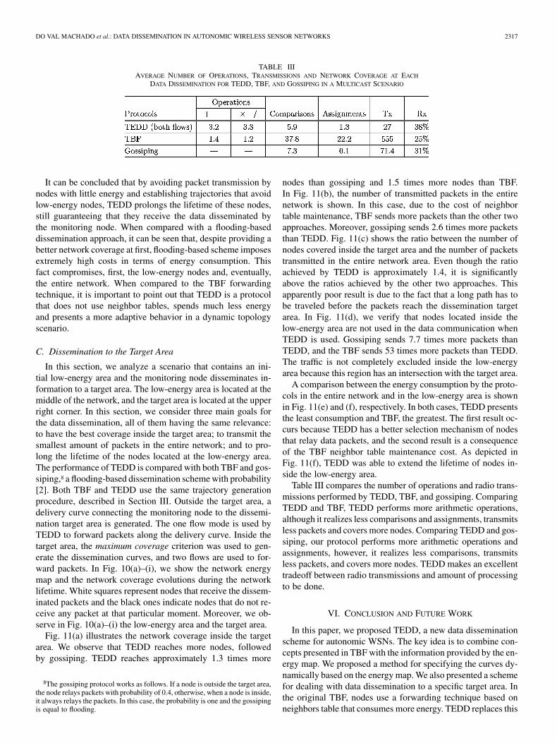
TABLE IIIAVERAGE NUMBER OF OPERATIONS, TRANSMISSIONS AND NETWORK COVERAGE AT EACH

DATA DISSEMINATION FOR TEDD, TBF, AND GOSSIPING IN A MULTICAST SCENARIO

It can be concluded that by avoiding packet transmission bynodes with little energy and establishing trajectories that avoidlow-energy nodes, TEDD prolongs the lifetime of these nodes,still guaranteeing that they receive the data disseminated bythe monitoring node. When compared with a flooding-baseddissemination approach, it can be seen that, despite providing abetter network coverage at first, flooding-based scheme imposesextremely high costs in terms of energy consumption. Thisfact compromises, first, the low-energy nodes and, eventually,the entire network. When compared to the TBF forwardingtechnique, it is important to point out that TEDD is a protocolthat does not use neighbor tables, spends much less energyand presents a more adaptive behavior in a dynamic topologyscenario.

C. Dissemination to the Target Area

In this section, we analyze a scenario that contains an ini-tial low-energy area and the monitoring node disseminates in-formation to a target area. The low-energy area is located at themiddle of the network, and the target area is located at the upperright corner. In this section, we consider three main goals forthe data dissemination, all of them having the same relevance:to have the best coverage inside the target area; to transmit thesmallest amount of packets in the entire network; and to pro-long the lifetime of the nodes located at the low-energy area.The performance of TEDD is compared with both TBF and gos-siping,8 a flooding-based dissemination scheme with probability[2]. Both TBF and TEDD use the same trajectory generationprocedure, described in Section III. Outside the target area, adelivery curve connecting the monitoring node to the dissemi-nation target area is generated. The one flow mode is used byTEDD to forward packets along the delivery curve. Inside thetarget area, the maximum coverage criterion was used to gen-erate the dissemination curves, and two flows are used to for-ward packets. In Fig. 10(a)–(i), we show the network energymap and the network coverage evolutions during the networklifetime. White squares represent nodes that receive the dissem-inated packets and the black ones indicate nodes that do not re-ceive any packet at that particular moment. Moreover, we ob-serve in Fig. 10(a)–(i) the low-energy area and the target area.

Fig. 11(a) illustrates the network coverage inside the targetarea. We observe that TEDD reaches more nodes, followedby gossiping. TEDD reaches approximately 1.3 times more

8The gossiping protocol works as follows. If a node is outside the target area,the node relays packets with probability of 0.4, otherwise, when a node is inside,it always relays the packets. In this case, the probability is one and the gossipingis equal to flooding.

nodes than gossiping and 1.5 times more nodes than TBF.In Fig. 11(b), the number of transmitted packets in the entirenetwork is shown. In this case, due to the cost of neighbortable maintenance, TBF sends more packets than the other twoapproaches. Moreover, gossiping sends 2.6 times more packetsthan TEDD. Fig. 11(c) shows the ratio between the number ofnodes covered inside the target area and the number of packetstransmitted in the entire network area. Even though the ratioachieved by TEDD is approximately 1.4, it is significantlyabove the ratios achieved by the other two approaches. Thisapparently poor result is due to the fact that a long path has tobe traveled before the packets reach the dissemination targetarea. In Fig. 11(d), we verify that nodes located inside thelow-energy area are not used in the data communication whenTEDD is used. Gossiping sends 7.7 times more packets thanTEDD, and the TBF sends 53 times more packets than TEDD.The traffic is not completely excluded inside the low-energyarea because this region has an intersection with the target area.

A comparison between the energy consumption by the proto-cols in the entire network and in the low-energy area is shownin Fig. 11(e) and (f), respectively. In both cases, TEDD presentsthe least consumption and TBF, the greatest. The first result oc-curs because TEDD has a better selection mechanism of nodesthat relay data packets, and the second result is a consequenceof the TBF neighbor table maintenance cost. As depicted inFig. 11(f), TEDD was able to extend the lifetime of nodes in-side the low-energy area.

Table III compares the number of operations and radio trans-missions performed by TEDD, TBF, and gossiping. ComparingTEDD and TBF, TEDD performs more arithmetic operations,although it realizes less comparisons and assignments, transmitsless packets and covers more nodes. Comparing TEDD and gos-siping, our protocol performs more arithmetic operations andassignments, however, it realizes less comparisons, transmitsless packets, and covers more nodes. TEDD makes an excellenttradeoff between radio transmissions and amount of processingto be done.

VI. CONCLUSION AND FUTURE WORK

In this paper, we proposed TEDD, a new data disseminationscheme for autonomic WSNs. The key idea is to combine con-cepts presented in TBF with the information provided by the en-ergy map. We proposed a method for specifying the curves dy-namically based on the energy map. We also presented a schemefor dealing with data dissemination to a specific target area. Inthe original TBF, nodes use a forwarding technique based onneighbors table that consumes more energy. TEDD replaces this

2318 IEEE JOURNAL ON SELECTED AREAS IN COMMUNICATIONS, VOL. 23, NO. 12, DECEMBER 2005

mechanism with a new forwarding technique: when a node re-ceives a packet, it decides whether it should forward the packetbased solely on its own location and the equation embedded inthe packet. All these features, when put together, present an au-tonomic solution to data dissemination in a WSN.

The simulations showed that when TEDD is used, the routingprocess becomes more adaptive to topology changes. Moreover,the energy spent with the routing activity can be concentrated onthose nodes that have high-energy reserves, whereas low-energynodes can be left to use their energy only to perform the sensingactivity or to receive information addressed to them, showing inthis way the autonomic characteristics of our solution.

There are several improvements that we are planning to in-troduce. One aspect to be explored is the way of interpreting thenetwork. Currently, we are representing the network as a set ofsensors, whose coordinates are used as input to the curve fittingprocedure. Another interesting manner of performing the map-ping is by viewing the network as a set of geographic points,whose energy reserves are calculated as an interpolation of theenergy of those sensor nodes that cover each point. Another fu-ture work is to introduce other techniques to avoid transmissionsinside the low-energy region. For example, we can use a energythreshold to allow nodes that have less energy than a certain pre-defined amount to not forward data.

REFERENCES

[1] I. F. Akyildiz, W. Su, Y. Sankarasubramaniam, and E. Cayirci, “Wirelesssensor networks: A survey,” Comput. Netw., vol. 38, pp. 393–422, 2002.

[2] Z. Haas, J. Halpern, and L. Li, “Gossip-based ad hoc routing,” in Proc.IEEE 21st Annu. Joint Conf. IEEE Comput. Commun. Soc., vol. 3, 2002,pp. 1707–1716.

[3] W. R. Heinzelman, J. Kulik, and H. Balakrishnan, “Adaptive protocolsfor information dissemination in wireless sensor networks,” in Proc. Mo-biCom, Seattle, WA, 1999, pp. 174–185.

[4] J. Hill, R. Szewczyk, A. Woo, S. Hollar, D. Culler, and K. Pister, “Systemarchitecture directions for networked sensors,” in Proc. 9th Int. Conf.Arch. Support Programming Languages and Operating Systems, Nov.2000, pp. 93–104.

[5] L. Hughes, O. Banyasad, and E. Hughes, “Cartesian routing,” Comput.Netw., vol. 34, pp. 455–466, 2000.

[6] IBM. (2004) Autonomic computing. [Online]. Available: http://www.ibm.com/research/autonomic

[7] C. Intanagonwiwat, R. Govindan, and D. Estrin, “Directed diffusion: Ascalable and robust communication paradigm for sensor networks,” inProc. 6th Annu. Int. Conf. Mobile Comput. Netw., Boston, MA, 2000,pp. 56–67.

[8] D. Johnson, D. A. Maltz, and J. Broch, “Dynamic source routing in adhoc wireless networks,” in Mobile Computing, J. Imielinski and J. Korth,Eds. Norwell, MA: Kluwer, 1996, vol. 353.

[9] J. Kulik, W. R. Heinzelman, and H. Balakrishnan, “Negotiation-basedprotocols for disseminating information in wireless sensor networks,” inProc. ACM/IEEE Int. Conf. Mobile Comput. Netw., Seattle, WA, Aug.1999, pp. 200–209.

[10] C. L. Lawson and R. J. Hanson, Solving Least Squares Problems. En-glewood Cliffs, NJ: Prentice-Hall, 1974.

[11] MTS/MDA Sensor and Data Acquisition Boards User’s Manual, 2004.www.xbow.com.

[12] R. A. F. Mini, M. do Val Machado, A. A. F. Loureiro, and B. Nath,“Prediction-based energy map for wireless sensor networks,” Ad HocNetw. J., vol. 3, pp. 235–253, 2005.

[13] R. A. F. Mini, A. A. F. Loureiro, and B. Nath, “A state-based energydissipation model for wireless sensor networks,” in Proc. 10th IEEE Int.Conf. Emerging Technol. Factory Autom., 2005.

[14] D. C. Montgomery, E. A. Peck, and G. G. Vining, Introduction to LinearRegression Analysis. New York: Wiley, 2001.

[15] D. Niculescu and B. Nath, “Trajectory-based forwarding and its appli-cations,” in MobiCom, 2003, pp. 260–272.

[16] (2002) ns2. The Network Simulator. [Online]. Available: www.isi.edu/nsnam/ns

[17] C. C. Paige and M. A. Saunders, “LSQR: Sparse linear equations andleast squares problems,” ACM Trans. Math. Softw., vol. 8, pp. 195–209,1982.

Max do Val Machado received the B.S. degreein computer science from the Pontifical CatholicUniversity of Minas Gerais, Belo Horizonte, Brazil,in 2002, and the M.S. degree in computer sci-ence from the Federal University of Minas Gerais(UFMG), Belo Horizonte, Brazil, in 2005. Currently,he is working towards the Ph.D. degree in computerscience at UFMG.

His research interests are routing and cross-layerdesign in wireless sensor networks and mobile ad hocnetworks.

Olga Goussevskaia received the M.S. degree in com-puter science from the Federal University of MinasGerais (UFMG), Belo Horizonte, Brazil, in 2005.

Her current research interests are primarily inrouting and control protocols for wireless sensornetworks. Her other interests include optimizationmodels and algorithms for mobile telecommunica-tion systems.

Raquel A. F. Mini received the B.Sc., M.Sc., andPh.D. degrees in computer science from FederalUniversity of Minas Gerais (UFMG), Belo Hori-zonte, Brazil.

Currently, she is an Associate Professor of Com-puter Science at the Pontifical Catholic University ofMinas Gerais, Belo Horizonte, Brazil. Her main re-search areas are sensor networks, distributed algo-rithms, and mobile computing.

Cristiano G. Rezende received the B.Sc. degreein computer science from the Federal University ofMinas Gerais, Belo Horizonte, Brazil.

His research areas area sensor networks and mo-bile computing.

Antonio A. F. Loureiro received the B.Sc. andM.Sc. degrees in computer science from the Fed-eral University of Minas Gerais (UFMG), BeloHorizonte, Brazil, and the Ph.D. degree in computerscience from the University of British Columbia,Vancouver, BC, Canada.

Currently, he is an Associate Professor of Com-puter Science at UFMG. His main research areasare wireless sensor networks, mobile computing,distributed algorithms, and network management.

DO VAL MACHADO et al.: DATA DISSEMINATION IN AUTONOMIC WIRELESS SENSOR NETWORKS 2319

Geraldo Robson Mateus received the M.S. andPh.D. degrees in computer science from the FederalUniversity of Rio de Janeiro, Rio de Janeiro, Brazil,in 1980 and 1986, respectively.

He is a Full Professor of Computer Science at theFederal University of Minas Gerais, Belo Horizonte,Brazil. He spent 1991 and 1992 at the Universityof Ottawa, Ottawa, ON, Canada, as a VisitingResearcher. He has published over 100 scientificpapers and is a leader of several national and interna-tional projects. His research interests span network

optimization, combinatorial optimization, algorithms, and telecommunications.Dr. Mateus is a member of the Institute for Operations Research and the

Management Sciences (INFORMS), the International Federation of OperationalResearch Societies (IFORS), and the Society for Industrial and Applied Math-ematics (SIAM).

José Marcos S. Nogueira (M’94) received the B.S.degree in electrical engineering and the M.S. degreein computer science from the Federal University ofMinas Gerais (UFMG), Belo Horizonte, Brazil, in1979, and the Ph.D. degree in electrical engineeringfrom the University of Campinas, Campinas, Brazil,in 1985.

He is an Associate Professor of Computer Scienceat UFMG. He held a Postdoctoral position at the Uni-versity of British Columbia, Vancouver, BC, Canada(1988–1989), and currently is on a sabbatical year at

the universities of Evry and Paris VI/LIP 6. He headed the Department of Com-puter Science, UFMG from 1998 to 2000. Currently, he heads the ComputerNetwork Group, UFMG. He has supervised a number of Ph.D. and Master’sstudents, He was the Technical Coordinator of the System for the Integrationof Supervision (SIS) Project, where a complex and distributed system for themanagement of telecommunications networks was developed. He has served invarious roles, including General Chair (1985) and TPC Chair (1999 and 2004) ofthe Brazilian Symposium on Computer Networks (SBRC), and General Chair ofLANOMS 2001. He publishes regularly in international conferences and jour-nals. His areas of interest and research include computer networks, wirelesssensor networks, telecommunications and network management, and softwaredevelopment.

Dr. Nogueira has been a TPC member in IEEE/IFIP NOMS (2000, 2002, and2004), IEEE/IFIP IM 2003, IEEE LANOMS (1999, 2001, 2003, and 2005),IEEE/IFIP MMNS (2000, 2001, 2002, and 2003), IPOM 2002, SBRC (from1990 to 2005), and IEEE/IFIP DSOM (2003, 2004, and 2005). He is a member ofthe Brazilian Computer Society (SBC) and Brazilian Telecommunications So-ciety (SBrT). He also participates in the IEEE ComSoc CNOM Interest Group.Currently, he is a Secretary of the IEEE ComSoc TCII.