InterestCast: Adaptive Event Dissemination for Interactive ...

InterestCast: Adaptive EventDissemination for InteractiveReal-Time ApplicationsZur Erlangung des akademischen Grades Doktor-Ingenieur (Dr.-Ing.)genehmigte Dissertation von Max Lehn, M.Sc. aus Groß-GerauTag der Einreichung: 16.12.2015, Tag der Prüfung: 26.02.2016Darmstadt 2016 — D 17

1. Gutachten: Prof. Alejandro Buchmann, Ph.D.2. Gutachten: Prof. Klara Nahrstedt, Ph.D.

Fachbereich InformatikDatenbanken und Verteilte Systeme

InterestCast: Adaptive Event Dissemination for Interactive Real-Time Applications

Genehmigte Dissertation von Max Lehn, M.Sc. aus Groß-Gerau

1. Gutachten: Prof. Alejandro Buchmann, Ph.D.2. Gutachten: Prof. Klara Nahrstedt, Ph.D.

Tag der Einreichung: 16.12.2015Tag der Prüfung: 26.02.2016

Darmstadt — D 17

Bitte zitieren Sie dieses Dokument als:URN: urn:nbn:de:tuda-tuprints-53982

URL: http://tuprints.ulb.tu-darmstadt.de/id/eprint/5398

Dieses Dokument wird bereitgestellt von tuprints,E-Publishing-Service der TU Darmstadthttp://tuprints.ulb.tu-darmstadt.de

[email protected]

Die Veröffentlichung steht unter folgender Creative Commons Lizenz:Namensnennung – Keine kommerzielle Nutzung – Keine Bearbeitung 3.0 Deutschlandhttp://creativecommons.org/licenses/by-nc-nd/3.0/de/

AcknowledgmentsThis work would not have been possible without the many discussions, help, and motivating sup-

port by several people.

First and foremost, I would like to thank my advisor, Prof. Alejandro Buchmann for his uncondi-

tional support over all the years and for the freedom he gave me to work on a variety of interesting

topics. I am also grateful to Prof. Klara Nahrstedt, who did not only host me and give advise during

the time I worked on the initial concepts for this thesis, but also accepted to become my second

referee.

Further thanks go to the numerous colleagues who accompanied me on my academic career, of

whom many became close friends. First, there is the whole DVS group. Particular thanks go to

Christof Leng and Wesley Terpstra, who acted as my academic mentors in the early days of my

research; the other two peer-to-peer office mates Robert Rehner and Alex Frömmgen; but also

Stefan Appel, Sebastian Frischbier, Tobias Freudenreich, and Daniel Bausch who were regularly

available for chats and discussions during lunch or coffee.

The research projects QuaP2P and MAKI gave me the opportunity to collaborate with many

more researchers. Particular thanks go to Christian Groß, who was not only project colleague, but

also longtime friend and companion since the beginning of our studies. The QuaP2P project work

also laid the foundations for this work; I would like to thank Tonio Triebel and Prof. Wolfgang

Effelsberg for their initiating contributions to the Planet PI4 prototype. Of those who helped me

with discussions and feedback, I would further like to highlight Boris Koldehofe, Sabrina Müller,

and Kai Habermehl. Thanks also go to the several undergraduate students assisting in my research,

most notably Marcel Blöcher, who were a great help not only with several implementation tasks.

The two DFG-funded projects I worked on would not exist without Prof. Ralf Steinmetz, as well as

all other involved PIs.

Last not least, I am grateful to my family, Irmi, Thomas, and Robert who always lovingly sup-

ported me over the years, and my grandma Elli who had to ask after my progress for such a

long time. Finally, loving thanks to Katrin, who greatly supported me with a lot of affection and

patience, especially in the final stages of my thesis.

i

AbstractMany networked applications use push-based many-to-many communication. Especially real-time

applications, such as online games and other virtual reality applications, need to synchronize state

between many participants under strict latency requirements. Those applications typically ex-

change frequent state updates and therefore require an appropriate dissemination mechanism.

Centralized and server-based solutions do not minimize latency, since they always need an extra

round-trip to the server. In addition, a server infrastructure constitutes a potential performance

bottleneck and thus a scalability limitation. Direct communication between event source and des-

tination is often latency-minimal but quickly exceeds the capacities especially of poorly connected

participants because each one needs to communicate individually with many others.

Our proposed solution, InterestCast, provides a decentralized event dissemination mechanism

that uses peer-to-peer event forwarding, allowing powerful participants to help weak participants

with the event multiplication and dissemination. To obtain forwarding configurations that best fit

the current situation and application needs, InterestCast adapts them dynamically and continu-

ously during runtime. The application’s needs are passed as utility functions, which determine the

utility of events with a given latency for a given interest level. Interest levels serve as an abstrac-

tion for the importance of events from a specific source, allowing a more fine-grained prioritization

than an all-or-nothing subscription model. This is particularly useful if the importance of updates

depends on virtual reality distance or another application-specific metric.

InterestCast runs an incremental local optimization algorithm that repeatedly evaluates all pos-

sible rerouting operations from the point of view of the respective local node. In each iteration,

the best operation is chosen based on the application’s utility functions and a system model that

predicts the effects of a given operation. As this optimization process is run on each node indepen-

dently, it scales well with the number of participants. The prediction only uses local knowledge

as well as information from the local neighborhood in up to two hops, which is provided by a

neighborhood information exchange protocol.

Our evaluation shows that the results of InterestCast’s distributed optimization are close to the

global optima computed by a integer program solver. Computing the optimum for a given situ-

ation globally at runtime, however, is infeasible due to its computational complexity, even with

a highly simplified network model. In detailed network simulations, we further demonstrate the

superiority of InterestCast over a purely direct event dissemination in online gaming scenarios.

In comparison with the direct dissemination, InterestCast significantly reduces the traffic of weak

nodes and almost quadruples the possible number of participants for the same average delivery

latency of high-interest events.

ii

ZusammenfassungViele Netzwerkanwendungen verwenden push-orientierte Kommunikation zwischen vielen An-

wendern. Insbesondere Echtzeitanwendungen, wie etwa Onlinespiele und andere Virtual-Reality-

Anwendungen bedürfen der Synchronisierung des Anwendungszustands zwischen vielen Teil-

nehmern unter engen Latenz-Voraussetzungen. Solche Anwendungen tauschen typischerweise

regelmäßig Zustands-Updates aus und benötigen einen dafür geeigneten Verteilungsmechanis-

mus. Zentralisierte, serverbasierte Lösungen minimieren Latenz insofern nicht, als sie immer

einen separaten Round-Trip zum Server benötigen. Hinzu kommt, dass die Serverinfrastruktur

einen potentiellen Performance-Engpass darstellt und damit die Skalierbarkeit einschränkt. Direkte

Kommunikation zwischen Quelle und Ziel ist meist Latenz-minimal, führt aber schnell zur Über-

schreitung der Netzwerkkapazität, insbesondere bei schwach angebundenen Teilnehmern. Denn

so muss jeder mit vielen anderen Teilnehmern individuell kommunizieren.

Die in dieser Arbeit vorgestellte Lösung, InterestCast, bietet einen dezentralen Mechanismus zur

Verteilung von Ereignissen, welcher eine Peer-to-Peer-Weiterleitung von Ereignissen verwendet und

so starken Teilnehmern erlaubt, schwachen bei der Vervielfältigung und Verbreitung von Ereignis-

Meldungen zu helfen. Um die Weiterleitungskonfiguration zu erhalten, die in der momentanen

Situation am besten für die jeweiligen Anforderungen der Anwendung geeignet sind, passt In-

terestCast diese zur Laufzeit kontinuierlich an. Die Anforderungen der Anwendung werden als

Nutzenfunktionen spezifiziert, die den Nutzen von Ereignissen mit einer gegebenen Ausliefer-

ungsverzögerung bewertet, abhängig vom Interesse am jeweiligen Ereignis. Interessensniveaus

dienen als eine Abstraktion für die Wichtigkeit von Ereignissen von einer bestimmten Quelle und

erlauben eine Priorisierung der Auslieferung von Ereignis-Benachrichtigungen. Dies ist besonders

nützlich wenn die Wichtigkeit von Ereignissen z.B. vom Abstand der Teilnehmer in der virtuellen

Realität oder von sonstigen anwendungsspezifischen Metriken abhängt.

InterestCast führt einen inkrementellen lokalen Optimierungsalgorithmus aus, der wieder-

holt alle möglichen Veränderungen der Weiterleitungen aus Sicht des jeweils lokalen Knotens

auswertet. In jedem Durchlauf wird anhand der Nutzenfunktionen und einem Systemmodell die

Operation ausgewählt, von der die größte Verbesserung des Gesamtzustands erwartet wird. Da

dieser Optimierungsprozess auf jedem Knoten unabhängig ausgeführt wird, skaliert er gut mit der

Teilnehmerzahl. Die Vorhersage verwendet nur lokales Wissen sowie Informationen aus der Nach-

barschaft in bis zu zwei Schritten, welche über ein entsprechendes Austauschprotokoll gewonnen

werden.

Unsere Auswertungen zeigen, dass die Ergebnisse der verteilten Optimierung von InterestCast

nahe an den globalen Optima liegen, welche wir anhand der verwendeten Modelle mit Hilfe eines

Solvers für Integer-Programme ermitteln. Die Lösung des globalen Optimums zur Laufzeit ist

jedoch unpraktikabel, da die Komplexität des Problems selbst mit einem stark vereinfachten Net-

zwerkmodell zu äußerst langen Berechnungszeiten führt. In detaillierten Netzwerksimulationen

zeigen wir außerdem die Überlegenheit von InterestCast über eine rein direkte Verteilung der

iii

Ereignisse in Online-Spiel-Szenarien. Im Vergleich mit der direkten Verteilung reduziert Inter-

estCast die nötige Datenmenge bei schwachen Knoten erheblich und vervierfacht beinahe die

mögliche Teilnehmerzahl bei gleichbleibender durchschnittlicher Auslieferungszeit von Ereignis-

sen von hohem Interesse.

iv Zusammenfassung

Contents

1. Introduction 11.1. Challenges . . . . . . . . . . . . . . . . . . . . . . . . . . . . . . . . . . . . . . . . . . . . . 3

1.2. Problem Statement . . . . . . . . . . . . . . . . . . . . . . . . . . . . . . . . . . . . . . . . 5

1.3. Approach . . . . . . . . . . . . . . . . . . . . . . . . . . . . . . . . . . . . . . . . . . . . . . 6

1.4. Methodology and Thesis Outline . . . . . . . . . . . . . . . . . . . . . . . . . . . . . . . . 7

2. Background: Applications and Use Cases 92.1. Online Gaming . . . . . . . . . . . . . . . . . . . . . . . . . . . . . . . . . . . . . . . . . . . 9

2.2. Mobile Augmented Reality Gaming . . . . . . . . . . . . . . . . . . . . . . . . . . . . . . 13

2.3. Robotics and Vehicular Networks . . . . . . . . . . . . . . . . . . . . . . . . . . . . . . . . 16

2.4. Air Traffic Control . . . . . . . . . . . . . . . . . . . . . . . . . . . . . . . . . . . . . . . . . 17

2.5. Requirements and Challenges . . . . . . . . . . . . . . . . . . . . . . . . . . . . . . . . . . 18

3. State of the Art 213.1. Interfacing Event Dissemination . . . . . . . . . . . . . . . . . . . . . . . . . . . . . . . . 21

3.2. Multicast . . . . . . . . . . . . . . . . . . . . . . . . . . . . . . . . . . . . . . . . . . . . . . 21

3.2.1. IP Multicast . . . . . . . . . . . . . . . . . . . . . . . . . . . . . . . . . . . . . . . . 22

3.2.2. Application-Layer Multicast . . . . . . . . . . . . . . . . . . . . . . . . . . . . . . 22

3.3. Delay Optimization in Multicast . . . . . . . . . . . . . . . . . . . . . . . . . . . . . . . . 24

3.4. Publish/Subscribe . . . . . . . . . . . . . . . . . . . . . . . . . . . . . . . . . . . . . . . . . 26

3.5. Adaptive Overlay Topologies . . . . . . . . . . . . . . . . . . . . . . . . . . . . . . . . . . 29

3.6. Interest Management and Application-tailored Multicast . . . . . . . . . . . . . . . . . 30

4. Approach and Design Decisions 374.1. Decomposition and Interfacing . . . . . . . . . . . . . . . . . . . . . . . . . . . . . . . . . 37

4.1.1. Decomposing Interest Management and Event Dissemination . . . . . . . . . 38

4.1.2. Interfacing . . . . . . . . . . . . . . . . . . . . . . . . . . . . . . . . . . . . . . . . . 40

4.2. Adaptability . . . . . . . . . . . . . . . . . . . . . . . . . . . . . . . . . . . . . . . . . . . . 42

4.2.1. Network Conditions . . . . . . . . . . . . . . . . . . . . . . . . . . . . . . . . . . . 42

4.2.2. Application Requirements . . . . . . . . . . . . . . . . . . . . . . . . . . . . . . . 43

4.2.3. Utility vs. Cost . . . . . . . . . . . . . . . . . . . . . . . . . . . . . . . . . . . . . . 44

4.2.4. Composition of the Target Function . . . . . . . . . . . . . . . . . . . . . . . . . 45

4.2.5. Specifying and Updating Utility Functions . . . . . . . . . . . . . . . . . . . . . 46

4.3. Topology and Routing . . . . . . . . . . . . . . . . . . . . . . . . . . . . . . . . . . . . . . 46

4.3.1. Topology Construction . . . . . . . . . . . . . . . . . . . . . . . . . . . . . . . . . 48

v

4.4. Optimization Strategy . . . . . . . . . . . . . . . . . . . . . . . . . . . . . . . . . . . . . . 49

4.4.1. System Performance Model . . . . . . . . . . . . . . . . . . . . . . . . . . . . . . 50

4.4.2. Optimization Objective . . . . . . . . . . . . . . . . . . . . . . . . . . . . . . . . . 51

5. System Model and Problem Formalization 535.1. Basic System Model . . . . . . . . . . . . . . . . . . . . . . . . . . . . . . . . . . . . . . . . 53

5.1.1. Event Delivery Paths . . . . . . . . . . . . . . . . . . . . . . . . . . . . . . . . . . . 55

5.2. Event Classes . . . . . . . . . . . . . . . . . . . . . . . . . . . . . . . . . . . . . . . . . . . . 55

5.2.1. Update Events . . . . . . . . . . . . . . . . . . . . . . . . . . . . . . . . . . . . . . 55

5.2.2. Instant Events . . . . . . . . . . . . . . . . . . . . . . . . . . . . . . . . . . . . . . . 57

5.3. Application Utility Functions . . . . . . . . . . . . . . . . . . . . . . . . . . . . . . . . . . 57

5.4. Performance Model . . . . . . . . . . . . . . . . . . . . . . . . . . . . . . . . . . . . . . . . 58

5.4.1. Queuing Delay . . . . . . . . . . . . . . . . . . . . . . . . . . . . . . . . . . . . . . 58

5.4.2. Update Event Loss . . . . . . . . . . . . . . . . . . . . . . . . . . . . . . . . . . . . 59

5.5. Optimization Problem . . . . . . . . . . . . . . . . . . . . . . . . . . . . . . . . . . . . . . 60

5.6. Global Solutions Using Integer Programming . . . . . . . . . . . . . . . . . . . . . . . . 61

5.6.1. ILP Problem . . . . . . . . . . . . . . . . . . . . . . . . . . . . . . . . . . . . . . . . 61

5.6.2. MINLP Problem . . . . . . . . . . . . . . . . . . . . . . . . . . . . . . . . . . . . . . 63

6. Incremental Optimization Algorithm 656.1. Basic Algorithm . . . . . . . . . . . . . . . . . . . . . . . . . . . . . . . . . . . . . . . . . . 65

6.2. Utility Estimation . . . . . . . . . . . . . . . . . . . . . . . . . . . . . . . . . . . . . . . . . 66

6.2.1. Link Utilization . . . . . . . . . . . . . . . . . . . . . . . . . . . . . . . . . . . . . . 67

6.2.2. Path Latency . . . . . . . . . . . . . . . . . . . . . . . . . . . . . . . . . . . . . . . . 69

6.2.3. Utility Estimation Algorithm . . . . . . . . . . . . . . . . . . . . . . . . . . . . . . 70

6.3. Neighbor Information Exchange . . . . . . . . . . . . . . . . . . . . . . . . . . . . . . . . 72

6.4. Measuring Network Capabilities . . . . . . . . . . . . . . . . . . . . . . . . . . . . . . . . 73

6.4.1. Link Usage and Capacity . . . . . . . . . . . . . . . . . . . . . . . . . . . . . . . . 73

6.4.2. Route Throughput . . . . . . . . . . . . . . . . . . . . . . . . . . . . . . . . . . . . 74

6.4.3. Latency . . . . . . . . . . . . . . . . . . . . . . . . . . . . . . . . . . . . . . . . . . . 75

6.5. Utility Functions . . . . . . . . . . . . . . . . . . . . . . . . . . . . . . . . . . . . . . . . . . 75

6.5.1. Latency Utility . . . . . . . . . . . . . . . . . . . . . . . . . . . . . . . . . . . . . . 76

6.5.2. Bandwidth Demand Utility . . . . . . . . . . . . . . . . . . . . . . . . . . . . . . . 78

6.5.3. Utility Weights . . . . . . . . . . . . . . . . . . . . . . . . . . . . . . . . . . . . . . 79

7. Prototype 817.1. High-Level Architecture . . . . . . . . . . . . . . . . . . . . . . . . . . . . . . . . . . . . . 81

7.2. InterestCast Components and Layers . . . . . . . . . . . . . . . . . . . . . . . . . . . . . 81

7.3. Routing . . . . . . . . . . . . . . . . . . . . . . . . . . . . . . . . . . . . . . . . . . . . . . . 85

7.3.1. Route Operations . . . . . . . . . . . . . . . . . . . . . . . . . . . . . . . . . . . . . 87

7.3.2. Route Measurements . . . . . . . . . . . . . . . . . . . . . . . . . . . . . . . . . . 89

7.4. Scheduling . . . . . . . . . . . . . . . . . . . . . . . . . . . . . . . . . . . . . . . . . . . . . 90

vi Contents

7.5. Aggregation and Deduplication . . . . . . . . . . . . . . . . . . . . . . . . . . . . . . . . . 91

7.6. Protocol Headers . . . . . . . . . . . . . . . . . . . . . . . . . . . . . . . . . . . . . . . . . 92

8. Evaluation Platform 958.1. The Game Planet PI4 . . . . . . . . . . . . . . . . . . . . . . . . . . . . . . . . . . . . . . . 95

8.2. The Planet PI4 Evaluation Platform . . . . . . . . . . . . . . . . . . . . . . . . . . . . . . 95

8.2.1. Workload Generation . . . . . . . . . . . . . . . . . . . . . . . . . . . . . . . . . . 96

8.2.2. Game Network Components . . . . . . . . . . . . . . . . . . . . . . . . . . . . . . 97

8.2.3. System and Network Environment . . . . . . . . . . . . . . . . . . . . . . . . . . 99

8.3. Experiment Workflow and Data Model . . . . . . . . . . . . . . . . . . . . . . . . . . . . 100

9. Evaluation 1039.1. Evaluation Modes . . . . . . . . . . . . . . . . . . . . . . . . . . . . . . . . . . . . . . . . . 104

9.2. Important Factors and Metrics . . . . . . . . . . . . . . . . . . . . . . . . . . . . . . . . . 106

9.2.1. Factors . . . . . . . . . . . . . . . . . . . . . . . . . . . . . . . . . . . . . . . . . . . 106

9.2.2. Metrics . . . . . . . . . . . . . . . . . . . . . . . . . . . . . . . . . . . . . . . . . . . 106

9.3. Graph-Based Model . . . . . . . . . . . . . . . . . . . . . . . . . . . . . . . . . . . . . . . . 107

9.3.1. Virtual Reality Scenario . . . . . . . . . . . . . . . . . . . . . . . . . . . . . . . . . 108

9.3.2. The Basic Optimization Process . . . . . . . . . . . . . . . . . . . . . . . . . . . . 109

9.3.3. Comparison with Global Optimization . . . . . . . . . . . . . . . . . . . . . . . . 110

9.3.4. Node Density . . . . . . . . . . . . . . . . . . . . . . . . . . . . . . . . . . . . . . . 114

9.3.5. Utility Weights . . . . . . . . . . . . . . . . . . . . . . . . . . . . . . . . . . . . . . 114

9.3.6. Clustering . . . . . . . . . . . . . . . . . . . . . . . . . . . . . . . . . . . . . . . . . 115

9.4. Prototype . . . . . . . . . . . . . . . . . . . . . . . . . . . . . . . . . . . . . . . . . . . . . . 116

9.4.1. Node Density . . . . . . . . . . . . . . . . . . . . . . . . . . . . . . . . . . . . . . . 117

9.4.2. Interest Dynamics . . . . . . . . . . . . . . . . . . . . . . . . . . . . . . . . . . . . 120

9.4.3. Traffic Overhead . . . . . . . . . . . . . . . . . . . . . . . . . . . . . . . . . . . . . 123

9.4.4. Planet PI4 Bot Workload . . . . . . . . . . . . . . . . . . . . . . . . . . . . . . . . 125

9.5. Discussion . . . . . . . . . . . . . . . . . . . . . . . . . . . . . . . . . . . . . . . . . . . . . . 126

10.Conclusion and Outlook 12910.1.Future Work . . . . . . . . . . . . . . . . . . . . . . . . . . . . . . . . . . . . . . . . . . . . 130

A. Global Optimization Integer Programs 133A.1. ILP Problem . . . . . . . . . . . . . . . . . . . . . . . . . . . . . . . . . . . . . . . . . . . . 133

A.2. MINLP Problem . . . . . . . . . . . . . . . . . . . . . . . . . . . . . . . . . . . . . . . . . . 135

B. InterestCast Routing Update Handling 139

C. Prototype Evaluation Results 143

Contents vii

Simply Explained: Latency.Oliver Widder, http://geek-and-poke.com/, CC BY 3.0

viii Contents

http://geek-and-poke.com/

1 IntroductionThere is an old network saying:

Bandwidth problems can be cured with

money. Latency problems are harder

because the speed of light is fixed—you

can’t bribe God.

David Clark

The major trends of the Internet in the 1990s and 2000s have been on the globalization of data,

making services available independently from the consumer’s location. This led to the huge success

of the Internet. The assumption, however, was that applications could work with moderate net-

work bandwidths and be mostly insensitive to network latencies. With its success, more and more

demanding applications became part of the Internet. New web technologies enabled new classes of

interactive applications such as Google Docs1, more and more business logic with increasing real-

time demands is run over the Internet (e.g., real-time business intelligence [12]), and applications

based on virtual environments, especially large real-time online multiplayer games have become

ever more popular [160]. In contrast to most conventional Internet applications like newsgroups,

the web, or web services, which use mostly pull-based communication, interactive and real-time

applications need push-based communication schemes to inform participants about events as they

happen. Further, interaction is often multilateral, in contrast to applications like one-to-one chats,

voice, or video calls. Certain events or actions are relevant for a potentially large group of users,

and each user may have a unique set of interests. Online games are in particular prototypical for

this set of properties.

From the network perspective, those applications have increasing demands in terms of network

bandwidths as well as latencies. Bandwidth increases due to network developments and large

scale investment and is, therefore, becoming less of an issue nowadays, at least in fixed networks

of well-developed regions [58]. Latencies, however, remain limited by the speed of light. There

are ambitious initiatives to bring latencies close to what is possible at the speed of light on lin-

ear distance, e.g., using microwave links [145]. Such approaches, however, are associated with

high costs and therefore only available to selected services, like high-frequency trading [39]. An

alternative approach is to bring the services closer to the consumer. One of the first and largest

deployments of such an approach was made by Akamai [126], bringing static content close to the

consumer with the goal of a faster, more reliable, and more efficient delivery. Such solutions are

application-specific in that the distribution of service functionality must be selected in accordance

with application needs. Static content, for instance, can be arbitrarily replicated, while the directinteraction between two users is still constrained by the network latency between them.

1 Google Docs. http://www.google.com/docs/about/

1

http://www.google.com/docs/about/

If interacting parties are geographically distant from each other, the possibly significant speed-

of-light latency is inevitable. On the other hand, if they are close, geographically or in terms of

network distance, there is a huge potential for making their communication more direct. Indeed,

many applications, even though they are globally available, have a large ratio of regionalized

communication. One example are online social networks, where locality refers to the network of

friends. News or posts from close sources in terms of the social graph tend to have more impor-

tance and are treated with a higher priority [89]. The algorithms behind online social networks

therefore mimic the natural human behavior regarding information valuation. The increasing us-

age of mobile Internet services also results in a trend to information locality, most explicitly in the

form of location-based services [142].

Another example for localized communication are machine-to-machine communication net-

works, such as wireless sensor networks or vehicular (ad-hoc) networks. Having started with

communication technologies and protocols tailored for their specific application needs, these ap-

plication areas increasingly adopt Internet technologies. Using Internet protocols, all the billions of

devices can theoretically talk to each other, which is part of what the ‘Internet of Things’ [165, 8]

and the ‘Internet of Everything’ [55] stand for. Actual applications, however, often need localized

communication. A brightness sensor most likely adapts local lamps, not those on the other side

of the planet. Further, machine-to-machine communication often has to deal with high-frequency

event streams. Such events may have small payloads, but sending each event individually using

Internet protocols may induce a significant communication overhead due to protocol headers.

An application class with similar requirements are interactive real-time applications, such as

online games, or more generally multiuser virtual environments. To keep the users’ views syn-

chronous, the clients regularly exchange update events, often several events per second. Interac-

tive real-time applications further depend on low event delivery latencies. Their scale reaches from

a handful of participants up to several ten thousands [53], and the distribution of users ranges from

a single room to worldwide.

Most of today’s online services rely on server infrastructures acting as mediators between the

participating clients. This has the benefits of a central authority and maintenance, as well

as lightweight client-side applications. With cloud infrastructures, server management became

cheaper and scalable, as virtual servers can be dynamically allocated in large data centers. The

cloud economy is based on a small number of such large data centers. Although large operators

maintain multiple data centers in different parts of the world, the typical distance to the user is still

between a few hundred to several thousand kilometers [107]. Amazon, one of the largest cloud

service providers, for instance, has at the time of writing eleven data centers worldwide [5].

While many use cases still require central synchronization, e.g., for data consistency or account-

ing, interactive applications can still profit from unmanaged high-frequency, low latency updates.

Consider a real-time multiplayer game where players navigate and interact in a common virtual

world with their avatars. Awareness of the activities of their avatars’ surroundings is an impor-

tant factor for a good gaming experience. Therefore, a high view synchronicity is desirable, which

generally requires a high frequency and low latency of position updates among players.

2 1. Introduction

Virtual/interest space

Physical/network space

A

A

B

B

C

D

C

D

Figure 1.1.: Illustration of the physical space and virtual space in which participants are located.The virtual space is defined by the application and determines the interest of the par-ticipants in each other. The physical space is determined by the physical location of theparticipants’ devices and the connecting network. In some cases, the virtual and phys-ical locations correlate (participants A and B), while in other cases, they are completelyindependent (C and D).

We therefore argue that the dissemination of such time-critical update events should be done

using direct communication where suitable. Despite its potential for significantly lowering dis-

semination latency, aiming for direct communication results in several challenges that must be

overcome.

Their composition of properties makes online games a well-suited use case for this thesis.

1.1 Challenges

Our targeted applications have a push-based many-to-many communication pattern. This means

that each participant’s updates are of interest to multiple other participants and vice versa that

each participant is interested in the updates of multiple others. Considering only network latencies,

delivering each event as a direct message from source (i.e., participant of interest) to destination

(i.e., interested participant) is the fastest option in most cases. This approach becomes more

and more suitable with today’s bandwidths. Nevertheless, we have to be able to deal with nodes

whose bandwidth is the limiting factor. As soon as the spare bandwidth becomes scarce, queuingdelays can significantly increase the total delivery latency, and especially weak nodes may not be

able to serve all destinations at all. This problem is amplified by the fact that event messages,

which are transmitted frequently but often have only small payload data, are inflated by network

protocol header overhead. As a consequence, the effective net bandwidth in terms of event payload

is diminished.

Application-level multicast approaches can mitigate this problem by using stronger nodes as

message forwarders and multipliers. By taking network latencies into account, the additional la-

tency introduced by the extra hop(s) can be minimized. Figure 1.1 illustrates the mapping between

physical (network) and virtual (interest) space. While the latter determines who needs to commu-

nicate with whom, the former determines the latencies between the participants. Both need to be

1.1. Challenges 3

taken into account to optimize latencies depending on interest in the virtual world based on the

network conditions in the physical world.

Most existing multicast solutions do not consider multi-source deployments. Although a multi-

source problem can be modeled as multiple single-source problems, this does not take into account

the potential for aggregating multiple messages from different sources to reduce the relative net-

work packet header overhead. Other approaches, such as distributed publish/subscribe broker

networks, assume the available additional infrastructure. In addition, there is a delay due to the

publish/subscribe mechanism that relies on multicast or in the worst case on sequential unicast.

To keep the solution cheap and easily deployable, we strive for a decentralized and self-managing

solution.

From the application perspective, on the other hand, there can be interest gradations in the

sense that update events from a particular source are more important for some receivers than for

others. An example are virtual spaces in which the perception of events depends on distance.

While actions in the close proximity of a participant are critical, peripheral events may be of less

importance. This should be considered by the dissemination solution. Since different applications

have different needs in this respect, the application should be able to determine the goal for which

the dissemination is optimized. Such option is not available in existing multicast systems, especially

in decentralized solutions. On the other hand, there are special-purpose approaches for multiplayer

online games and virtual environments that incorporate mechanisms for the differentiation of

fidelity levels for neighbors, e.g., depending on their distance and interaction. Those, however, are

not generalizable for different applications.

Additionally, the distribution of load among participants should be fair. Fairness can be mea-

sured in different ways, and existing systems considering fairness usually select some more or less

reasonable way for measuring and optimizing fairness. Different applications may have different

goals with respect to load distribution. Therefore, the application should also have means for in-

fluencing the way the system distributes load. This includes the option of trading the load of the

participants for the performance of the system.

Finally, using best effort networks like the Internet, the system must cope with varying network

conditions. The solution should, therefore, be adaptive to both the network conditions and the

application load.

A promising option for tackling adaptiveness with respect to both application requirements and

network conditions in a generalizable way is the use of utility functions. They allow the application

to define high-level utility indicators without the need for dealing with low-level decisions and

thereby leaving the system room for self-optimization. Furthermore, they allow the consideration

of costs on the underlying system, i.e, the network and node resource usage.

Though being powerful, for an effective application of utility functions, several challenges have

to be overcome. The first is to find an appropriate specification level. Applications should only be

faced with the parameters that are relevant on the application level. If the system internally deals

with lower-level parameters, there should be a translation to application-level metrics. Ideally,

there should be no need to provide heuristics in the utility functions. Instead, the system model

should be capable of predicting the system response in terms of the utility function well enough

4 1. Introduction

so that the optimization goal can be directly encoded in the utility function(s). Finally, in our

case, the system optimization needs to be performed in a distributed setting. In a system with

decentralized control, there is no entity with full knowledge about the system state. The utility

prediction, therefore, has to work with the limited knowledge available locally.

1.2 Problem Statement

In this thesis, we focus on application use cases requiring timely many-to-many event dissemination.

Many-to-many refers to the fact that each participant is both an event producer and consumer.

Further, each participant has its own individual interest set, making conventional group commu-

nication inefficient. Since latency is critical for interactive applications, it is the core optimization

objective with respect to application performance. Building on top of Internet infrastructure only

allows best-effort guarantees, a fact that is considered throughout this work. Besides performance,

it is necessary to consider capabilities and costs of the underlying network infrastructure. We

assume bandwidth availability and link utilization as the main factors that determine the costs.

Latency can be minimized using direct connectivity among participants. Hence, this option

should be preferred where feasible. Heterogeneous connectivity and device capabilities, how-

ever, limit the possible direct fan-out. To mitigate this limitation, participants can help each other

by forwarding and multiplying each other’s event messages. This distributes load amongst the

participants and also yields savings in data traffic due to aggregation.

A dynamic trade-off between the two goals, latency and traffic minimization, is a core objective

of this thesis. Such a dynamic trade-off calls for an adaptive solution based on both application

demands and network environment capabilities.

Based on the above challenges, we derive the following set of research questions to be addressed

in this thesis.

• We have identified the need for an efficient many-to-many event dissemination in decentral-

ized settings. Therefore, the top level question addressed here is:

How can a decentralized many-to-many event dissemination be solved efficiently and with aparticular regard to dissemination latencies?

• To evaluate and improve possible solutions, it is necessary to identify the criteria based on

which the goodness can be quantified. This is of particular importance for a self-optimizing

solution. Hence, the question is:

What are the goodness criteria to be considered for the targeted class of applications?

• Application-level utility functions promise to be a flexible way for defining application needs

for an adaptive system. In the context of the targeted application the following research

question is posed:

How can application demands and adaptivity goals for a many-to-many dissemination infras-tructure, such as interest gradations and bandwidth-latency trade-offs, be formulated as utilityfunctions?

1.2. Problem Statement 5

• From the engineering perspective, there is the need to define an appropriate application

interface, based on the goals and the requirements identified in the application use cases.

The corresponding research question is:

What is a suitable decomposition and interfacing for a many-to-many event dissemination mech-anism providing application-defined optimization goals?

• Having the goal of providing a solution that requires no central coordination, the utility-based

optimization has to be able to run in a decentralized setting:

Can the optimization of the dissemination topology be effectively performed with a local op-timization algorithm, i.e., by evaluating the utility function on each node based on its localknowledge?

• Given the targeted application scenarios, there are opportunities to leverage properties spe-

cific to those applications. Most importantly:

How can the clustering of interest be exploited to reduce bandwidth usage with little impact onlatency?

1.3 Approach

We introduce InterestCast, a decentralized opportunistic many-to-many message dissemination

middleware, following the introduced concepts. InterestCast introduces the concept of interestlevels, which determine the importance of update events of one participant to another. Setting

interest levels is comparable to subscriptions in publish/subscribe terminology, but adds the no-

tion of priorities. This concept further provides an interface for decomposing existing overlays for

networked virtual environments.

InterestCast adapts to both the application load and the underlying network properties (Fig-

ure 1.2). Further, it allows the application to specify utility functions, giving the application control

over the desired trade-offs. While the first two factors are determined at runtime, the latter pro-

vides variability at design time. The utility functions consider event dissemination metrics, most

importantly their end-to-end latency, as well as the nodes’ load in terms of link utilization. The

application specifying the utility functions can benefit in several ways: varying application require-

ments can be expressed as utility function changes, the utility functions have an influence on the

load and performance distribution among nodes and therefore the overall fairness, and they allow

tuning the trade-off between performance (low latencies) and cost (bandwidth usage).

For the adaptation, InterestCast runs a continuous and incremental local optimization algorithmof message forwarding rules between nodes. All participating nodes repeatedly evaluate and rank

possible optimization operations based on their local views and using the application-defined utility

functions. In each iteration, the option with the highest expected change in utility is executed,

provided the change in utility is positive.

Finally, to minimize message overhead and therefore maximize the effective bandwidth while

keeping delays low, a message scheduling and aggregation mechanism reduces the transmission of

redundant data.

6 1. Introduction

Network

InterestCastMiddleware

Application

Utilityfunctions

Capabilities, utilization

Workload, interest levels

Figure 1.2.: InterestCast’s optimization acts upon three main factors: application-defined utilityfunctions, the application workload, and the network infrastructure capabilities andutilization.

1.4 Methodology and Thesis Outline

To set the detailed goals of this thesis, we must first identify the possible target applications. As

introduced, the main target application group in this thesis are real-time online games due to their

relatively clear set of requirements and conditions. We do, however, consider further application

groups: the special case of mobile and augmented reality games, robotics and vehicular networks,

as well as air traffic control. Those applications and their particularities are analyzed in Chapter 2.

Based on this, the set of requirements is identified.

In Chapter 3, the state of the art of the related work is discussed. Starting with a general

introduction to interfacing approaches for event dissemination, publish/subscribe and different

multicast incarnations are compared. We further look into specific approaches to adaptive overlays,

delay optimization, and peer-to-peer gaming overlays.

Based on the identified requirements, Chapter 4 derives the main design principles for the solu-

tion proposed in this thesis. They include basic design decisions such as component decompositions

and adaptability approaches, as well as more detailed discussions on topology, routing, and their

optimization.

Subsequently, we define the formal system model in Chapter 5. This model provides the nec-

essary abstraction for analyzing and predicting current and future system state. The chapter fur-

thermore carves out the underlying optimization problem. The global optimization problem is

formulated as an integer programming problem to be solvable from a global point of view using a

standard solver. This allows a comparison between the distributed solutions using local knowledge

and the global optimum.

InterestCast incremental optimization algorithm is described in Chapter 6. This includes the

basic local optimization algorithm as well as the local utility estimation. The chapter further

elaborates on the various options and considerations for selecting appropriate utility functions

and presents possible utility functions.

1.4. Methodology and Thesis Outline 7

To be able to evaluate and fine-tune InterestCast under realistic network conditions, a proto-

type is developed, which is described in Chapter 7. The prototype contains the full software stack

including connection management, routing, monitoring, optimization, and the application-level

interface. The prototype implementation shows the effective cost of the necessary local knowl-

edge, effects of real networking, overhead, and aggregation, and can be used as a basis for real

applications.

The prototype implementation is integrated into the Planet PI4 evaluation platform, which is

described in Chapter 8. The platform’s core is the game Planet PI4, which serves as a workload

generator. Alternatively, it provides a workload generation using abstracted mobility models. It

allows the execution of the prototype on different network simulators as well as on a real network.

It further provides several testing and evaluation facilities like logging, tracing, and analysis tools.

Chapter 9 presents and discusses the evaluation results. We start with a graph-based implemen-

tation based on an abstracted network model, showing the basic behavior and the comparison with

the global solutions. Subsequently, a more detailed analysis is performed based on the prototype.

Finally, Chapter 10 discusses the overall results and concludes this thesis.

8 1. Introduction

2 Background: Applications and Use CasesThis chapter introduces the main target applications and use cases that set the goals of this thesis.

We discuss their relevant properties and implications for this work. The set of applications shown

here is not intended to be exhaustive, but exemplifies the need for low latency many-to-many

communication.

We begin with and put most emphasis on the application domain of online gaming, since this is

the primary scenario throughout this work. Mobile and augmented reality gaming is then intro-

duced as a special case of online gaming. Afterwards we briefly examine the application domains

of robotics and vehicular networks as well as air traffic control systems.

The chapter concludes with a list of requirements and challenges derived from the discussed

applications, which serves as a basis for the design of InterestCast.

2.1 Online Gaming

Since the emergence of the first computer games in the 1970s, there has been a long and successful

story of advancements, which has led to a ubiquity of computer games in our lives, driven by a

multi-billion-dollar industry [7]. Although computers enable attractive single-user games, which in

fact make a significant part of the games market, multiplayer gaming has been a compelling factor

from the beginning. Like in conventional games, their main aspect is the competition between

human players.

Multiplayer games started as dedicated arcade machines, such as Atari’s popular Pong [87, 121].

Games for two players were usually played using two controls on the same machine with a shared

screen. Home computers adopted this concept, as do modern game consoles. With the prevalence

of computer networks, however, computer games made use of them by distributing the games

across multiple computers, providing each player a dedicated device. Early approaches for desktop

PCs used direct serial cables or modem connections between two machines. Later came local

networks, e.g., using Ethernet.

The Internet created new opportunities by bringing thousands, later millions, and now billions of

potential players together. This is when online games grew large. Online games range from single-

digit to five-digit numbers of simultaneous players playing in a single virtual universe. Games

with small and short-lived sessions often use one participant as the master (or server) node. The

selection usually happens explicitly in that the player who opens the game session runs the master

node. Alternatively, all nodes replicate and process the whole game state and synchronize in a

peer-to-peer fashion.

Large and long-lasting games, such as massively multiplayer online games (MMOG), typically use

dedicated server infrastructures. MMOG worlds are persistent and continuously active, and players

9

can join and leave at any time. EVE Online1 is an MMOG with one of the largest game worlds. Its

number of simultaneous online players regularly exceeds 50,000 in a single universe [53].

The broader technical term also used in this context is the networked virtual environment (NVE),

which includes, in addition to online games, social virtual worlds and military simulations [28].

We use the term virtual world as the simulated content of the game or virtual environment. In most

games, the perception of the virtual world for an individual participant is limited to her immedi-

ately surrounding environment. In the simplest case, this is modeled by a circular or spherical areaof interest (AOI), limited by the vision range (VR); sometimes, these are also referred to as aura,

focus, and nimbus [19].

The responsibilities of the game server can be coarsely decomposed in collecting updates from

the clients, managing (persistent) game objects, selecting relevant game updates for each player

(interest management), and delivering game updates to each player (event dissemination).2 The

largest part of the network traffic is caused by position updates [35, 34], which in their most basic

form contain the current position of the player. To keep the views of all players synchronous, it is

necessary to exchange those updates regularly. Typical update frequencies are between 5 and 10

Hz [35, 34, 151].

To achieve a high degree of synchronicity among the views of each player and a high reactivity

to user actions, a low dissemination latency of update messages is crucial [44, 43]. While for

relatively slow-paced role-playing games, latencies of one second can still be acceptable [61],

player performance of fast-paced shooter games starts suffering from latencies above 100ms [18]

or even less [134]. Omitting the intermediate server for the events between clients, i.e., passing

update messages directly between the clients, therefore, helps reduce end-to-end (i.e., client-to-

client) latencies. This is where peer-to-peer approaches come into play.

For this purpose, it is unnecessary to fully replace the game server(s) using peer-to-peer tech-

nology. Aspects requiring central control, such as authorization, persistent storage, or conflict

resolution can remain server-supported, while opportunistic low-latency updates are disseminated

in a peer-to-peer fashion.

In the past one and a half decades, research has resulted in a variety of peer-to-peer approaches

for the different aspects. An overview on contributions specific to interest management and event

dissemination can be found in Section 3.6 of this work. Yahyavi and Kemme [167] provide a recent

survey covering a broader range of peer-to-peer online gaming aspects, which go beyond the scope

of this thesis.

Packet OverheadAs indicated above, online games use frequent update messages to keep the game state syn-

chronous among participants. Since these messages only need to contain metadata, e.g., player

position or object states, they are typically small. Measurements on network traces of real online

games show that typical update packet sizes are between 20 and 60 bytes [150, 34, 35]. The

1 EVE Online. https://www.eveonline.com/2 A similar decomposition has been proposed by Fan et al. specifically for peer-to-peer gaming [56]. They dis-

tinguish between interest management, game event dissemination, NPC host allocation, game state persistence,

cheating mitigation, and incentive mechanisms.

10 2. Background: Applications and Use Cases

https://www.eveonline.com/

Position3x4=12 bytes

Direction3x4=12 bytes

Rotation3x4=12 bytes

ID/State8 bytes

UDP8 bytes

IPv420+ bytes

TCP20 bytes

IPv420+ bytes

Payload44 bytes

Payload44 bytes

TCP20 bytes

IPv640+ bytes

Payload44 bytes

Payload: 44 bytes

UDP+IPv4: ≥72 bytes

TCP+IPv4: ≥84 bytes

TCP+IPv6: ≥104 bytes

Figure 2.1.: Illustration of network packet sizes for transmitting position updates. Only consideringLayers 3 and 4 (network and transport), protocol header overhead is between 50%and more than 100% of the payload size.

average throughput for the activity of a single participant in terms of bytes per second is therefore

rather low. 50-byte messages at 10 Hz result in 500 bytes/s or 4 kbit/s net traffic, which has been

confirmed by measurements [150, 151, 35].

This traffic profile is distinct from most other common Internet applications. Although the traffic

seems low, Internet protocols induce a significant overhead. For example, consider a multiplayer

game in which each player’s current position has to be regularly disseminated to all interested

neighbors. The payload of such update is position data, e.g., a triple of floating point coordinates,

plus a player ID and possibly some additional state. To minimize traffic, these high-frequency

updates contain as little data as necessary. A typical payload can thus consist of just 20 bytes (e.g.,

3×4 bytes coordinates plus 8 bytes player ID). Even a more sophisticated position update packet, as

illustrated in Figure 2.1, has a size of just 44 bytes. Sending such an update over the Internet, even

using the most lightweight transport protocol UDP, adds another 28 bytes (8 bytes UDP header,

20 bytes IPv4 header). This results in 48-byte and 72-byte packets on the link layer, respectively.

Hence, if only a single update event is transmitted in a UDP packet, the size of network protocol

headers can exceed the size of the actual payload—and this calculation ignores any protocol below

the network layer. Using TCP (20 bytes header) instead of UDP, or IPv6 (40 bytes or more) instead

of IPv4 makes the situation even worse: 20 bytes of application payload would be blown up to 80

bytes on the link layer.

Protocol overhead therefore easily adds more than 100% overhead, i.e., more than doubles the

necessary bandwidth. And this does not even include further overhead of Layer 2 and potential ad-

ditional encapsulation techniques such as VPN. Prosad et al. [133] exemplify the Layer 2 overhead

by showing that the capacity of a 10BaseT Ethernet link is only 7.24 Mb/s for 100-byte packets

versus 9.75 Mb/s for 1500-byte packets.

So far, we only considered events from one player. In the client/server case, this is what each

client sends to the server. The server returns an aggregated view of all relevant events for the

respective client, consisting of larger, but equally frequent packets. Measurements show around ten

times higher server-to-client traffic, strongly depending on the game situation [150]. With larger

packets, the relative overhead is smaller, which is why server-based approaches work reasonably

well with today’s Internet infrastructure.

In contrast, using peer-to-peer event dissemination to minimize latencies requires each client to

send its updates to each interested peer individually, and vice versa each client receives updates

2.1. Online Gaming 11

from many individual peers. In this case, clients have to send each of their updates more than

once, and the packet header overheads become highly significant. Miller and Crowcroft conducted

a simulation study on this issue [114], in which they conclude that pure peer-to-peer MMOG

messaging is not feasible with residential broadband. In their peer-to-peer model, peers subscribe

for updates among each other based on a constant-size area of interest (AOI) and deliver updates

directly.

Intuitively, the upstream traffic of each peer induced with direct update delivery grows linearly

with the fan-out, i.e., the number of subscribers. Inversely, the downstream traffic is linear with

the fan-in. Since most residential Internet connections have asymmetric up- and downstream

bandwidths, with a significantly lower upstream bandwidth, we will focus on the peers’ fan-out.

Typical upstream bandwidths of residential connections range from 100 kbps to 10 Mbps. Using

the 4 kbps per subscriber from the example above, peers could theoretically serve 25 up to 2,500

subscribers. In practice, however, when saturating the uplink, latencies will skyrocket due to

queuing3, not even considering cross traffic. The simulation by Miller and Crowcroft [114] suggests

that already an average bandwidth usage of less than 50% significantly increases transmission

latencies. On the other hand, a 10 Mbps connection has a lot of spare capacity in such situations.

In this thesis, the described packet overhead problem is addressed twofold. First, we strive

for combining direct message delivery where possible with aggregation of update messages by

dynamically using forwarder nodes. Those nodes receive updates from potentially multiple sources

and can therefore forward aggregated packets. Second, we strive to be adaptive with respect to

node heterogeneity. When powerful nodes participate, e.g., one with a 10 Mbps uplink, it is

possible to shift load from weaker nodes.

Opportunities: Clustering and InterestWith the challenges described above, online gaming scenarios show important properties that

we aim to exploit for improvement. The first is the clustering of interest among participants. Since

interest is mostly based on virtual world proximity, it is typically highly clustered.4 This clustering

has a direct effect on the number of options for aggregation and load shifting, because forwarding

of events can be performed most efficiently using nodes with common interests.

Secondly, the interests of participants in each other typically have gradations. This means that,

while some neighbors in the virtual world are of high interest, e.g., because they are close by, others

further away, might be visible, but of low interest. Studies from cognitive sciences indicate that

the human brain can only focus on a small and constant number of objects simultaneously [157,

138]. The number of neighbors of highest priority is therefore very limited. Updates from the

other neighbors are still needed for a reasonable awareness of the environment. Low-interest

nodes, however, need lower update frequencies and tolerate higher latencies. Hence, the update

dissemination can be optimized based on interest, therefore serving highly interested neighbors

with high priority and less interested neighbors on a best-effort basis.

3 The effect of excessive delays caused by large buffer sizes throughout the Internet has gained attention under the

term bufferbloat [68].4 We have measured clustering coefficients of around 60% in typical scenarios. Refer to Section 9.3.1 for more

details.


We have chosen online games as the primary scenario not only because of their popularity,

but also because they reflect a unique combination of the different properties and requirements

described above. This allows us to study interdependencies between these properties, specifically

with respect to latency sensitivity, dynamism, and heterogeneity of both interest and resources.

Using the knowledge we have about properties and requirements of specific mobile game types,

we can define benchmarks that serve as representative and reproducible standard tests [99, 103]

to compare networking approaches.

2.2 Mobile Augmented Reality Gaming

A subclass of the above discussed online games are online augmented reality (AR) games. Aug-

mented reality games in general augment the real world with virtual objects, which shape the

game play. The game therefore is embedded into the real world, giving a new perspective of gam-

ing. This class of games has gained a lot of potential with the ubiquity of powerful enough mobile

devices, most notably smartphones.

Augmented reality technologies and applications, however, had been on the research agenda al-

ready one and a half decades before the emergence of smartphones [11, 10]. Using special-purpose

hardware, the use of augmented reality was explored in various application domains beyond enter-

tainment, including manufacturing and maintenance, education, medical, and military. According

to Azuma [11], an augmented reality system must have the following three characteristics: (i)

combines real and virtual, (ii) is interactive in real time, and (iii) is registered in 3D. Azuma’s def-

inition is limited in that it focuses on the computer graphics domain, where the term augmented

reality relates to graphical augmentation, e.g., adding rendered 3D objects to live video recorded

by a camera. A recent example from computer games that fits this definition is the Android-based

game DroidShooting5.

Putting less emphasis on the graphical representation, an important aspect of augmented reality

is the mapping of the virtual space onto the physical space. Large scale, or massively multiplayer,

augmented reality games often use the users’ GPS-based positions to place them on the virtual map.

To ease navigation, the virtual map reflects the real world to a certain degree, usually by using a

street map underlay (e.g., Google Maps6 or OpenStreetMap7) for the virtual world map. The most

popular example of this class of games is Ingress8 (Figure 2.2a). TowerWorld [97] (Figure 2.2b) is

a prototype of a similar game which was developed for the evaluation of mobile publish/subscribe

solutions is this application class.

Local CommunicationBy mapping the virtual world onto the physical world, interest within the virtual world becomes

directly related with physical proximity. Interest-based communication (e.g., position updates,

player actions) is therefore highly localized with respect to the physical world. Figure 2.3 shows

5 DroidShooting. https://play.google.com/store/apps/details?id=jp.co.questcom.droidshooting6 Google Maps. https://maps.google.com/7 OpenStreetMap. http://www.openstreetmap.org/8 Ingress. https://www.ingress.com/

2.2. Mobile Augmented Reality Gaming 13

https://play.google.com/store/apps/details?id=jp.co.questcom.droidshooting

https://maps.google.com/

http://www.openstreetmap.org/

https://www.ingress.com/

(a) Ingress (b) TowerWorld

Figure 2.2.: Screen shots of two typical mobile augmented reality multiplayer games. Both use thephysical location of the player as the in-game position and show the local street mapas an underlay of the virtual world.

that a large part of the communication traffic of an augmented reality game has a target of only a

few dozens of meters away. This raises the question about keeping traffic local even more than for

stationary network games. Yet, today’s mobile applications are largely cloud-based, meaning that

the network sees only communication between the devices and cloud servers.

The mobile devices’ cellular network connectivity is often the limiting—and most expensive—

factor for online applications, particularly for interactive ones. Beyond the dependency on a rea-

sonable infrastructure coverage, cellular communication is expensive in terms of energy usage

because the connection needs to stay permanently in high power mode despite the low uti-

lization [14, 125]. Furthermore, although low in throughput, the accumulated data volume of

long-lasting sessions easily exceeds the volume of inexpensive data plans, jeopardizing the users’

desire for playing the game. In a test session, the prototype TowerWorld [97] used around 10 MB

per 15 minutes. Users of Ingress, which is less interactive and more optimized than TowerWorld,

report varying values of 200 to 600 MB per month for typical usage.9 Finally, cellular networks

often induce higher latencies than wired broadband connections.

Opportunity: Wireless Ad-Hoc Communication

Given those facts, the use of opportunistic ad-hoc networks for a low-latency local communica-

tion offload has a great potential [98]. Today’s basic technologies that qualify for such connectivity

on consumer devices are Bluetooth and WiFi (IEEE 802.11). In the Bluetooth protocol stack, the

Bluetooth Network Encapsulation Protocol (BNEP) [23] provides an Ethernet emulation, which

9 Based on user reports on Reddit. “How much data are you using? How active are you?” http://www.reddit.com/

r/Ingress/comments/18u5k7/how_much_data_are_you_using_how_active_are_you/. Accessed 2014-04-09.


http://www.reddit.com/r/Ingress/comments/18u5k7/how_much_data_are_you_using_how_active_are_you/

http://www.reddit.com/r/Ingress/comments/18u5k7/how_much_data_are_you_using_how_active_are_you/

0

20

40

60

0 10 20 30 40 50

%directcommunicationdata

max. direct communication range in meters

Data that could have been send directlyas a function of the maximal direct communication range

Figure 2.3.: Ratio of data that could have been sent directly depending on the direct communi-cation range, measured in a test session with the augmented reality game prototypeTowerWorld [97]. Almost half of the data is sent to a destination less than 20 metersaway from the source.

can serve as the base for an IP stack. The need for explicit device pairing, however, limits Blue-

tooth’s suitability for dynamic ad-hoc networks. IEEE 802.11 [79] specifies the Independent Basic

Service Set (IBSS) that allows for an ad-hoc communication mode without a coordinating ac-

cess point. Wi-Fi Direct [166] is an alternative WiFi ad-hoc connection standard that has been

promoted by the industry lately. Unlike IBSS, it uses software access points on the participating

devices and focuses on easy and secure connection setup. Yet, the dynamically allocated access

points, make Wi-Fi Direct less flexible in group size and range. On the other hand, Wi-Fi Direct

is available on many recent smartphones and tablets, while IBSS is rarely activated on consumer

devices. Hence today, the perfect ad-hoc communication technology that is available on a large

number of mobile devices is still lacking. Nevertheless, for this work, we assume the availability of

an IEEE-802.11-IBSS-like wireless ad-hoc protocol on all mobile devices.

Wireless multi-hop routing protocols, such as AODV [131] and OLSR [42], enable nodes to

communicate with each other even if they are not in direct wireless transmission range. This

works as long as there is a chain of intermediate nodes that are in each other’s range to forward

the messages. Hence, given a sufficient device density, these protocols can extend the effective

communication range by orders of magnitude. For augmented reality games, only a small number

of hops can be sufficient (Figure 2.4).

Forwarding nodes, however, have to bear additional load. The use of a simple application-level

multicast mechanism, e.g., using direct overlay connections from source to destinations, can lead to

a multiplication of forwarding traffic. If multiple source-destination pairs use a common forwarder,

the forwarder has to carry the same information multiple times. Network-level broadcasts, on the

other hand, might be too unbounded in larger ad-hoc networks.

InterestCast can mitigate this problem by aggregating common data on common forwarding

links. Provided that forwarder nodes are also participants of the InterestCast overlay, the mea-

surement of overlay link properties (most importantly latency) gives hints about the forwarders in

2.2. Mobile Augmented Reality Gaming 15

0

20

40

60

0 1 2 3 4

%saveddata

max. # of hops

max. direct range 3

max. direct range 5

max. direct range 10



Data that could have been send over multiple hopsas a function of the maximal hop count

Figure 2.4.: Accumulated ratio of data that could have been sent over a number of hops depend-ing on the single-hop transmission range (meters), measured in a test session with theaugmented reality game prototype TowerWorld [97]. A large amount of data requiresonly a small number of hops.

the underlay. The forwarding function can then be pulled up into the overlay, where the necessary

information for message aggregation is available. This allows for keeping a general-purpose ad-

hoc routing protocol, while at the same time fitting the overlay routing structure to the underlying

topology.

Mobile games can benefit even more from localized communication than conventional multi-

player games. Although not yet deployed on a large fraction of mobile devices, the basic necessary

wireless ad-hoc connectivity and routing technology is available. InterestCast provides an overlay

routing mechanism that adapts to the underlying topology.

2.3 Robotics and Vehicular Networks

Multi-Robot SystemsMulti-robot systems [110] have become an important research field in the robotics domain

since the early 2000s. Multi-robot systems can be seen as a subclass of multi-agent systems [59],

which, as a research discipline, has relations to distributed systems, artificial intelligence, human-

computer interaction, and ubiquitous computing. Most practical multi-robot systems considered

in research consist of only a small number of robots [17], and most work considering coordina-

tion [57] deals with the aspects of interaction languages, semantics, and higher-level coordination

tasks.

Basic communication for the low-level real-time coordination, however, is nevertheless needed.

Deployments of self-sustaining autonomous robots, e.g., for rescue missions [90], typically use mo-

bile, and possibly ad-hoc communication to be infrastructure-independent. Particularly in rescue

missions, the projected number of independent agents is larger (100 or more), control is mostly

distributed, and real-time planning is in the order of seconds [90]. Furthermore, robot teams


moving in a real-world space need the concept of positioning and proximity, and coordination is

most time-critical where agents are close to each other or form a group. Finally, agent behavior

and coordination should be adaptive to their environment. For example, simple situations might

be covered with a fast local coordination, while complex situations require tighter interaction and

more planning [85]. With the adaptation of planning schemes, communication requirements, such

as delay bounds, may also change. With these properties, the concept of InterestCast appears to

be a good fit to be used as the low-level distributed status and coordination message exchange

mechanism.

Vehicular NetworksSimilarly to multi-robot networks, vehicular networks [119, 127] are built among physical, mo-

bile entities—in this case cars and trucks. Due to their participants’ mobility, they emerged as

a variation of Mobile Ad-hoc Networks (MANETs), named Vehicular Ad-hoc Networks (VANETs).

Besides vehicle-to-vehicle (V2V) communication, there is vehicle-to-infrastructure (V2I) commu-

nication, which uses cellular or WiFi infrastructure. Among the most prominent applications of

vehicular networks are safety and traffic optimization applications such as accident, congestion,

and road condition warnings [162], which are propagated locally in real-time. More recently,

entertainment applications, including distributed gaming gained increasing interest [127].

The immediately critical but rare communication, e.g., accident alerts, will most likely use lower

layer forwarding mechanisms to achieve the best reactivity and reliability without any trade-offs.

On the other hand, regular monitoring and control information dissemination, as well as mobile

entertainment applications, such as mobile gaming discussed in the previous section, could benefit

from a system like InterestCast. Those non-safety-critical applications require trade-offs in the re-

source usage between applications with different communication requirements, e.g., with respect

to bandwidth and latency. Local traffic safety monitoring, for instance, uses periodic messages

containing vehicle speed, position, and direction [4]. In addition, event-driven messages are sent

once unsafe situations are detected. Especially vehicle data like position and speed is most rele-

vant for other close-by vehicles, while more distant vehicles in the same traffic flow might still be

interested, but timeliness is less critical. Furthermore, information from vehicles ahead in traffic is

more informative than from following vehicles. Finally, groups of vehicles moving in the same flow

have the highest interest in each other’s information and therefore form clusters. Those interest

distributions are similar to those discussed in the context of virtual game worlds above.

2.4 Air Traffic Control

A timely and scalable event dissemination is a core requirement also for modern aeronautical

control systems [70]. Much data is produced and consumed on a spatio-temporal basis, i.e.,

with respect to location and time. Trajectories can be modeled using 4D coordinates (longi-

tude, latitude, altitude, time) [156]. For example, up-to-date airplane positioning information

allows making route planning more dynamic to meet near-term needs. Information about detailed

weather conditions, which are scarce across oceans, can be observed in real-time by airplanes and

disseminated to following airplanes.

2.4. Air Traffic Control 17

Much of this data might be of little immediate interest to central control authorities and particu-

larly to other air traffic participants that are not in close range to the reference location, supporting

the case for localized dissemination. Generally, air traffic control currently aims for a more decen-

tralized coordination, for which a decentralized event dissemination system could be an important

part.

2.5 Requirements and Challenges

From the targeted applications and use cases detailed above, we identify the following set of

requirements and challenges. They are used as a basis for the selection of potential approaches

and design decisions, which are discussed in Chapter 4 of this thesis.

Latency sensitivity. The targeted applications are sensitive to latency. In many cases, this means

that the goal is to minimize delivery latency. When disseminating events to multiple re-

ceivers, minimizing can refer to the average latency but also the maximum latency among

the receivers. Depending on the particular application, there might be fixed upper bounds

for event delivery. For particular reasons, such as fairness among participants, it might also

be desirable to minimize the latency variance among receivers.

Best-effort adaptation. There are physical bounds on the latency and throughput the underlying

network can provide. Since typical network infrastructures, such as the Internet, do not give

latency guarantees or predictions, overlays can only provide best-effort guarantees.

The dissemination overlay should therefore (1) be prepared for different—and possibly

changing—application needs and (2) adapt to changing conditions of the underlying net-

work to provide the best possible performance in all situations.

Many-to-many communication. Every participant is an event producer and has an individual set of

interested participants. This many-to-many communication scheme generally does not lend

itself for an efficient clustering into a fixed set of multicast groups or channels. Instead, each

participant needs a separate dissemination structure.

Many scenarios, however, show a strong clustering in the participants’ interests, induced by

the interest locality. This fact can be used to facilitate the maintenance of the individual

dissemination structures.

Dynamics. Locations and interests of participants are highly dynamic. In particular, the interest sets

can change constantly. The reorganization of dissemination structures should thus generate

little overhead.

Rebuilding the dissemination structure from scratch on each change is not an option. Fur-

thermore, a quick fallback mechanism should compensate failing nodes or connections.

Packet overhead. Update events are often small, because they either contain incremental updates

or very limited state (such as coordinates of a position). This results in high relative over-

heads from packet headers of the different network layers. A low ratio between actual pay-

load and the gross traffic unnecessarily reduces achievable node fan-out.


The dissemination system should therefore aggregate packets where possible to maximize

efficiency.

Interest gradations. Interest among participants often has gradations. While some (e.g., close

players, close friends) are of high priority, delay or message loss from others might be toler-

able.

The interface should therefore provide means for specifying the interest priority to be able to

tune event delivery to meet the needs of the highest-priority participants first.

Scalability. The total number of nodes in the network can be very large, while only relatively small

subsets are of interest for a certain participant. The algorithmic complexity should therefore

only depend on the number of interested participants, not on the total system size.

Some participants may be of particularly high interest, causing heterogeneous fan-outs. For

instance, in online games, areas with a high player density require many connections between

the players. This can easily exhaust the available connection bandwidth of single nodes.

Resource heterogeneity. The participants’ resources are heterogeneous. While some nodes, e.g.,

those on mobile networks, may have extremely constrained connection bandwidths, other

nodes have a lot of spare capacity. Ideally, all participants should get the same service quality,

independent of their connection and location.

Infrastructure. Dedicated infrastructure (e.g., multicast servers) might or might not be available.

The system should, therefore, be able to work independently of dedicated servers. However,

if such options are available, it should be possible to leverage them.

2.5. Requirements and Challenges 19

3 State of the ArtIn this chapter, we discuss and categorize important existing work with respect to event dissem-

ination and the application-specific challenges identified in the previous chapter. We start with

the conceptual high-level view, exploring approaches how applications can interface with the dis-

semination infrastructure. Subsequently, we dive deeper into the lower-level message multicast

implementations and further provide an overview of publish/subscribe systems. Finally, we move

towards more specialized systems and look into the aspect of interest management and integrated

approaches for interest management and event dissemination.

3.1 Interfacing Event Dissemination

Although the concept of delivering events in the form of messages to a multitude of receivers is

intuitively comprehensible, a closer investigation of possible options and features poses a multi-

tude of questions regarding design decisions. Early approaches were simple multicast solutions

with multicast groups, such as IP multicast [48]. Messages could be sent to a group so that all

registered group members receive it. When only unicast is available, the most primitive solution

is obviously to send the message to each receiver individually. This requires each sender to know

all receivers, but on the other hand allows an individual selection of receiver groups for each mes-

sage. Such approach, however, limits scalability with respect to the receiver set size. Scalability

and implementation aspects are further discussed in Section 3.2. Here, we want to concentrate

on what information the application needs to manage and what can be hidden behind the event

dissemination facade.

A basic distinction criterion with respect to the interface is the way the receivers for a particular

message are selected. The selection can be sender-initiated (i.e., the sender has the information

who shall receive the message), receiver-initiated (receivers join a certain sender, channel, or

group), or implicit and based on the content of a message. Simple unicast-based dissemination

belongs to the first category; group-based multicast solutions (e.g., IP multicast) belong to the

second. The third category is largely covered by a variety of publish/subscribe systems.

3.2 Multicast

When it comes to the simple but efficient dissemination of data to a set of receivers, multicast proto-

cols are the means of choice. In contrast to the unselective broadcast (e.g., [65]), multicast uses an

explicit selection of the set of desired receivers. By running multiple protocol instances, in principle

any number of multicast groups can be created. This allows for a basic channel-based publish/sub-

scribe implementation with little effort, but omits some decoupling of the participants, especially

with respect to time (cf. Section 3.4), because messages are not stored for offline participants.

21

There is a plethora of protocols, especially in the area of application layer overlays, aiming

to solve multicast efficiently. Many of them have been analyzed for different application do-

mains [168, 96, 66]. This section therefore provides only a brief overview, focusing on the issues

relevant for this work.

3.2.1 IP Multicast

IP multicast [48] is an extension to the Internet Protocol that allows sending IP datagrams to

multicast groups. Datagram delivery is defined as best-effort, analogous to IP unicast. Membership

in multicast groups is dynamic in that hosts can join and leave groups at any time. Multicast

groups (named host groups) are identified with IP addresses from a specific range (224.0.0.0 to

239.255.255.255). Sending a datagram to a multicast address delivers the datagram to all hosts

is the corresponding group. To do so, the sender does not even need to be member of the group.

This way, IP multicast can work as both single-source and multi-source multicast.

Host groups are not limited in size, but, since they are addressed using IP addresses, their

number is limited. The most important practical limitation, however, is that IP multicast has never

been widely deployed on the Internet. Without such, it is of little use for large-scale Internet

applications. The main reasons are considered to be limitations in access control, security, address

allocation, and network management [51]. It is also argued that the end-to-end principle [140],

stating that application-specific functions should be implemented on the end hosts rather than in

the network, prevails over the efficiency benefit of IP multicast [41].

3.2.2 Application-Layer Multicast

Due to the limitations of IP multicast, a lot of research focus has been put on application-layer mul-

ticast (ALM), on which we concentrate in the following. ALM only employs the end systems for

data multiplication, therefore it is sometimes called end system multicast. An advantage of ALM

over IP multicast is its greater flexibility. While IP multicast has to concentrate on core features

to keep in-network complexity low, ALM can incorporate more sophisticated, and therefore more

complex, approaches. These include application-specific extensions and optimizations, which ex-

plains the large number of variations. In the following, we first give an overview of general-purpose

application-layer multicast solutions, before looking more specifically at topology optimization and

delay minimization.

Overcast [83] is an early approach for replacing IP multicast. It builds overlay trees, focusing on

organizing nodes to build high-bandwidth channels. Fast joining of nodes is an explicit goal, but

latency is explicitly not an optimization target. Joining nodes start at the root of the distribution

tree and try to move downwards towards the leaves as long as they do not observe bandwidth

degradation. This leads to particularly deep trees and therefore high maximum latencies.

The Banana Tree Protocol (BTP) [77] provides a multicast service with best-effort delivery, on

top of which a group communication as well as a file sharing protocol are defined. Nodes can

switch their positions in the tree to optimize the metrics latency, degree, and total tree cost. The

optimization process is performed in a distributed fashion by switching siblings. The authors,

22 3. State of the Art

however, do not explain based on which information the selection of options is performed. Al-

though the basic algorithm takes latency into account, the further analysis is only done with cost

minimization in mind.

ALMI [130] targets small multicast groups and employs a central session controller for node

registration and building the spanning tree. The session controller communicates directly with all

members using unicast messages to propagate tree updates. Each pair of nodes regularly sends

pings to each other to measure the link delay. To reduce the O(n2)measurement cost necessary for

a full mesh, nodes use a fixed degree and regularly replace known bad edges to converge to the

optimum mesh.

Chu et al. present Narada [41, 40], an End System Multicast protocol, explicitly designed as

an IP multicast replacement. Narada maintains an overlay mesh among the participating nodes

on top of which multicast spanning trees are constructed. The mesh is continuously updated to

optimize for latency by adding links where latency is significantly reduced and by removing links

that are least utilized. Spanning trees are constructed using a distance vector protocol similar to

DVMRP [49]. The authors suggest application-specific customizations with respect to bandwidth

and latency prioritization, but only really consider one scheme. Available bandwidth is discretized

into a few classes. Links are first selected based on the bandwidth class, and if there are several

options left, latency is minimized. Hence, the authors explicitly address the latency vs. bandwidth

issue, but always prioritize bandwidth over latency.

NICE [15] targets low-bandwidth applications with large receiver sets and focuses on constrain-

ing control overhead, node degree, and latency stretch1. Nodes are organized into a hierarchy

of layers, in which they are grouped in clusters. Clusters are based on inter-node latencies to

minimize forwarding latency stretch. NICE differentiates between the distribution topology, which

must be loop-free, and the control topology, which is denser. Nodes join by connecting to the high-

est layer in the hierarchy and subsequently finding close-by neighbors in one of the lower-layers

clusters. Clusters have a minimum and a maximum size. To stay within these bounds, they are

merged and split respectively. Although considering latency for the optimization, average path

lengths beyond 20 hops with 128 nodes are hardly suitable for latency-critical applications.

OMNI [16] is designed for real-time applications, such as media streaming. It tries to mini-

mize latency with bounded out-degrees, but it assumes dedicated Mulicast Service Nodes (MSN)

deployed by service providers. The authors first present linear programming solutions to the NP-

hard minimum average-latency and minimum maximum-latency degree-bounded spanning tree

problems. The spanning tree only refers to the MSN topology. They then present a decentralized

heuristic algorithm to build a spanning tree among the MSNs that converges to the optimum. The

algorithm is adaptive with respect to the network latencies and the number of clients at each MSN,

but the MSNs themselves are assumed to be mostly static and stable.

SplitStream [32] is a multicast system building on top of Scribe [33]. It builds a forest of multiple

trees, each transporting a stripe of the data, so that nodes can decode the data even if a fraction

of the stripes is missing. Furthermore, all nodes are both leaves and inner nodes of the different

trees, leading to a good load fairness. This system therefore aims at heavy traffic data streams,

1 Latency stretch is defined as the ratio between the latency accumulated over multiple hops from source to desti-

nation and the direct latency between source and destination.

3.2. Multicast 23

such as media content. The trees are built and maintained as separate Scribe trees. To deal with

nodes whose out degree is exceeded, SplitStream adds a child rejection mechanism. For children

that find no new parent, SplitStream maintains a spare capacity group of nodes that can handle

additional children.

A similar approach is taken by Bullet [94]. It also splits the data into disjoint encoded blocks,

which are distributed via a mesh over an overlay tree. The overlay tree is constructed and main-

tained by any of the existing algorithms. The delivery through the mesh is probabilistic, but the

block encoding scheme (e.g., using erasure codes) allows reconstructing the data even if a few

blocks are missing. Disjoint content is located using the RanSub algorithm [93]. Like SplitStream,

Bullet aims for high bandwidth traffic, and delivery latency is not a primary concern.

Chainsaw [128] builds on an unstructured topology and completely replaces trees with a mesh.

Based on a random mesh topology, peers get notified upon arrival of new sequence-numbered

packets and request ranges of sequence numbers. Unlike the previous systems, Chainsaw thus

uses a pull-based approach, which is similar to the BitTorrent distribution strategy. Obviously,

this concept is rather suitable for bulk data streaming than for low-latency control information

dissemination.

Most of the presented approaches use node degree or bandwidth as the primary factor determin-

ing the dissemination structure. Many optimize for high throughput and assume a single source.

Latency is also considered, but the average number of hops is usually too high for sub-second

end-to-end latencies. They further provide no prioritization, but rather rely on a simple multicast

group interface. Further, an adaptation to application needs is barely considered. A comparison of

the discussed approaches based on their properties is provided in Table 3.1.

3.3 Delay Optimization in Multicast

Although multicast and in particular application layer multicast has been a research topic for more

than two decades, only recently there have been new approaches dedicated to the analysis and

optimization of the delay in message dissemination. An important novelty is the explicit consider-

ation and modeling of queuing delay on each node, caused by bandwidth limitation. When a node

that forwards a message to several neighbors “simultaneously”, the last of the messages may have

to wait for a significant amount of time to be actually transmitted, depending on fan-out, message

size, and bandwidth availability. To exemplify, a 1 kB packet takes about 12 ms to be transmitted

on a 1 Mbps line. With a fan-out of 10, the last packet has a delay of 100 ms before even being put

on the line. The fan-out but also the message transmission order therefore have a significant im-

pact on the individual message delays, which has been largely ignored in the previously described

works.

Mokhtarian and Jacobsen [116, 117] propose algorithms that optimize the delay of multicast

trees. In their model, they include the time messages are delayed on the nodes before getting sent

out. The authors consider the two problems of minimizing average and maximum latency. They

show that the problems are NP-hard and propose heuristic approaches to solve them efficiently.

Their first paper [116] only covers constructing whole trees, incremental updates are added in


App

roac

hSi

ngl

e-vs

.

mu

lti-

sou

rce

Tree

con

stru

ctio

nC

onsi

dere

dn

ode/

net

wor

kfe

atu

res

Del

iver

yA

dapt

atio

n

(en

viro

nm

ent)

Ada

ptat

ion

(app

lica

tion

)

Fail

ure

fall

-bac

k

Ove

rcas

t[8

3]si

ngle

rece

iver

node

band

wid

thde

term

inis

tic

rece

iver

-bas

ed

relo

cati

on

nore

ceiv

er-b

ased

relo

cati

on

BTP

[77]

mul

tidi

stri

bute

dno

dede

gree

,

node

-to-

node

late

ncy,

tree

cost

dete

rmin

isti

csi

blin

gsw

itch

ing

poss

ibly

re-c

onne

ctto

root

ALM

I[1

30]

mul

tice

ntra

l(se

ssio

n

cont

rolle

r)

node

-to-

node

late

ncy

dete

rmin

isti

cce

ntra

l

reco

mpu

tati

on

noce

ntra

lrec

ompu

tati

on,

mem

ber-

or

cont

rolle

r-in

itia

ted

NIC

E[1

5]si

ngle

dist

ribu

ted,

clus

ter-

hier

arch

y

node

-to-

node

late

ncy,

node

degr

ee

dete

rmin

isti

ccl

uste

r-ba

sed

refin

emen

t

nocl

uste

r-ba

sed

OM

NI

[16]

sing

ledi

stri

bute

d(a

mon

g

MSN

s)

late

ncy,

node

degr

eede

term

inis

tic

dist

ribu

ted

(am

ong

MSN

s)

nono

ne/

mov

eon

ech

ild

upth

etr

ee

Scri

be[3

3]m

ulti

(sin

gle

rend

ezvo

us)

DH

T-ba

sed

(Pas

try)

Past

rylo

calit

y

(lat

ency

)

dete

rmin

isti

cdi

stri

bute

d,Pa

stry

loca

lity

(lat

ency

)

noD

HT-

base

d(P

astr

y)

Split

Stre

am[3

2]si

ngle

mul

tipl

eSc

ribe

tree

sPa

stry

loca

lity

(lat

ency

),no

dede

gree

dete

rmin

isti

cno

tbe

yond

Past

ryno

Scri

be,c

odin

gfa

ult

tole

ranc

e

Bul

let

[94]

sing

lem

esh

ontr

eenu

mbe

rof

send

ers/

rece

iver

s

prob

abili

stic

dist

ribu

ted

peri

odic

re-e

valu

asio

n

nono

spec

ific,

codi

ng

faul

tto

lera

nce

Cha

insa

w[1

28]

sing

lera

ndom

mes

hba

ndw

idth

dete

rmin

isti

cno

nom

ulti

-sou

rce

pull

Nar

ada

[41]

sing

ledi

stan

ceve

ctor

span

ning

tree

on

mes

h

band

wid

th,l

aten

cyde

term

inis

tic

cont

inuo

usm

esh

opti

miz

atio

n

vari

atio

nof

late

ncy-

band

w.

trad

eoff

neig

hbor

failu

re

dete

ctio

n,pa

rtit

ion

dete

ctio

n&

repa

ir

Mok

htar

ian

2013

/14

[116

,117

]

sing

leso

urce

node

band

wid

th,

inte

r-no

dede

lay

dete

rmin

isti

cno

min

-avg

-lat

vs.

min

-max

-lat

sour

ce-b

ased

Li20

13[1

08]

mul

tice

ntra

lwit

hdi

stri

b.

heur

isti

cup

date

node

band

w.

(pac

kets

),in

ter-

node

dela

y

dete

rmin

isti

cdi

stri

bute

d

refin

emen

t

nopo

ssib

lydi

stri

bute

d

Stre

amlin

e[1

13]

sing

leso

urce

node

band

wid

thde

term

inis

tic

tree

reca

lcul

atio

non

chan

ges

none

wpa

rent

sele

ctio

n

wit

hgl

obal

know

ledg

e

Tabl

e3.

1.:C

ompa

rison

ofa

sele

ctio

nof

appl

icat

ion

laye

rmul

ticas

talg

orith

ms

3.3. Delay Optimization in Multicast 25

their follow-up version [117]. The trees are calculated at the source nodes and encoded in the

data packets, so that intermediate nodes do not need to keep state. Additionally, this gives the

source node the best possible flexibility in selecting the tree structure. While in certain cases

the path information can be encoded economically using bloom filters, other cases require an

overhead of up to O(n) with n being the number of nodes in the tree, which is significant. For

small payloads, this option seems infeasible. Furthermore, the information each node needs to

exchange with others to run the optimization algorithm is O(DLN), where N is the total number

of nodes, L is the pairwise shortest path hop count, and D is the node degree. Especially the linear

dependency on the network size N is critical for large networks. For small receiver sets compared

to the network size, there might be an option to prune the information without overly restricting

the optimization process. Finally, all intermediate node or link failures must be quickly reported to

the source node because only the source node is able to rebuild the tree. Other intermediate nodes

that are first notified about the failure are therefore unable to react independently.

A very similar investigation was performed by Li et al. [108]. They also argue that the delay

incurred on the nodes due to queuing is a significant source of latency and must be included in the

optimization model. The authors distinguish between transmission and waiting time and model

waiting time using queuing theory. They define two problems to be solved incrementally. The first

is to build a multicast tree for each peer so that all receivers can be reached and total (i.e., aver-

age) delay is minimized. The second is to find multicast trees that reach all receivers and satisfy

node bandwidth constraints. NP-completeness is proven for both problems. The main algorithm

is designed to run on a central server, which needs to know all nodes’ capacities and latencies

and which disseminates the results to the nodes. The authors do not explain what information

each node needs to perform the forwarding and they do not analyze the necessary communication

overhead. To add or remove nodes from an existing multi-tree, the authors propose distributed

operations that can be initiated by all nodes. The same holds for a refinement operation that is

supposed to react on environment changes. It remains, however, unclear what exact information

each single node needs to perform these operations and how the information is exchanged. Fur-

thermore, distributed operations and updates are barely evaluated. In a follow-up paper [109], Li

et al. present a genetic algorithm for the central multi-tree computation.

3.4 Publish/Subscribe

A main motivation for the publish/subscribe paradigm is the decoupling of sender and receiver, as

pointed out by Eugster et al. [54]. In its core concept, participants that are interested in a par-

ticular kind of information can subscribe to receive corresponding event notifications. The senders

(publishers) do not need to know their receivers; this is transparently handled by the publish/sub-

scribe system, often implemented as a publish/subscribe middleware. The middleware might also

be able to store events for subscribers that are offline at the time a message is published. This con-

cept decouples senders (publishers) and receivers (subscribers) in space and time. Furthermore,

publishers can pass events asynchronously to the middleware and therefore do not need to handle

or care about the delivery process (synchronization decoupling [54]).


Publish/subscribe systems are commonly distinguished by the way they express interest in sub-

scriptions. The most basic option is channel-based publish/subscribe, providing fixed channels in

which events are placed and which can be subscribed. Conceptually, this is similar to group-based

multicast. A slight extension of channel-based publish/subscribe is topic-based publish/subscribe,

which allows additional filters on message header fields. Subject-based publish/subscribe pro-

vides a hierarchically structured name space and allows subscriptions on different levels on the

hierarchy. For example, the hierarchy “news/sports” can be subscribed as “news/sports”, or less

selectively as “news”, which could also include events on “news/business”. The most expressive

scheme is content-based publish/subscribe. It allows subscriptions with a logic term of predicates

based on event properties, such as “type = ‘sensor’ AND temperature > 30”. Finally, special pur-

pose publish/subscribe types provide subscription criteria tailored to certain kinds of applications.

A prominent example is the class of spatial publish/subscribe systems, which is implemented by

many of the virtual reality overlays presented in Section 3.6.

The degree of expressiveness has an impact on the performance and/or the cost of the system.

While channel associations can be matched with little effort, especially if the number of channels

is limited, content-based publish/subscribe requires matching each event against each subscription

individually in the extreme case. Specialized types (e.g, spatial publish/subscribe) have the poten-

tial to be more efficient because they reduce the subscription space while at the same time fitting

the application needs, but on the other hand are limited to a smaller number of applications.

Traditional distributed publish/subscribe systems use broker-based architectures. All partici-

pants connect as clients to one of possibly multiple brokers, which distributes the client’s publi-

cations and notifies the client based on its subscriptions. If the system consists of more than one

broker, the brokers build a network, forming an overlay topology.

Essentially, a publish/subscribe system fulfills two main purposes: filtering and multiplication of

events. Event filtering makes sure that clients only receive the events that match their subscriptions

and therefore minimizes network traffic and client load. Event multiplication is necessary because

potentially multiple clients have to be notified of a single publication. In broker-based systems,

these two tasks are handled by the brokers, which are running on reliable and well-connected

servers.

There are several commercial implementations of message oriented middleware supporting the

publish/subscribe paradigm. Some of the most prominent examples are TIBCO Rendezvous2 and

Apache ActiveMQ3. With Java Message Service (JMS) [76] and Advanced Message Queuing Proto-col (AMQP) [161], a few standard protocols for message oriented middleware have emerged,

which allow inter-operation across products. These systems aim at performance and scalability,

but assume stable and managed server environments.

Some of the popular research prototypes are Hermes [132], Padres [60], Rebeca [120, 6], and

SIENA [31]. They commonly employ a distributed broker architecture, building spanning trees for

message distribution on arbitrary broker topologies. An important question addressed by these

systems is how filters can be efficiently moved as close to the source as possible in order to filter

2 TIBCO Rendezvous. http://www.tibco.com/products/soa/messaging/rendezvous/default.jsp3 Apache ActiveMQ. http://activemq.apache.org/

3.4. Publish/Subscribe 27

http://www.tibco.com/products/soa/messaging/rendezvous/default.jsp

http://activemq.apache.org/

out messages as early as possible, saving communication overhead. Filter merging minimizes the

number of filters at the brokers to reduce computation effort.

All conventional broker-based solutions require dedicated infrastructure, which has to be man-

aged and maintained, inducing non-negligible costs to run the system. Additionally, requirements

for low latencies demand optimized broker and subscriber placements [36]. This increases deploy-

ment costs further.

Peer-to-Peer Publish/Subscribe

Peer-to-peer-based approaches do not require dedicated brokers and instead use the partici-

pants (peers) to perform event filtering and multiplication. Hence, they waive the distinction

between clients and brokers. Being peer-to-peer systems, they are based on the assumption that

any participant can leave the system or fail at any time. They use mechanisms for redundancy and

decentralized organization to achieve an increased resilience against failures.

There are numerous approaches to build publish/subscribe functionality on top of peer-to-peer

overlay networks. An early peer-to-peer system for application-layer multicast (cf. Section 3.2)

is Scribe [33] by Castro et al., based on which a simple channel-based publish/subscribe can be

implemented. Scribe is built on top of Pastry [139], a generic peer-to-peer routing overlay, which

provides a certain degree of resilience against failures. With Meghdoot [72], Gupta et al. present a

content-based publish/subscribe approach based on the distributed hash table (DHT) CAN [135].

Also based on a DHT, in this case Chord [148], is the system Mercury [22] by Bharambe et al.

Meghdoot projects its attribute space onto CAN’s n-dimensional Cartesian space. Mercury uses

one Chord ring for each attribute. Like Scribe, both inherit their reliability properties from the

underlying DHT. Terpstra et al. [154] propose a content-based publish/subscribe solution on top

of Chord as well, by combining a broker network with the DHT. For this, the broker network is

extended to handle more general topologies than just trees, while maintaining its expressiveness.

The DHT routing guarantees an O(n) routing depth.

DHTs achieve high scalability by requiring only O(log n) (Chord, Pastry) or O(dn1/d) (CAN)

overlay hops for routing, where n is the network size and d is CAN’s number of dimensions. On

the other hand, when latencies matter, even O(log n) overlay hops can be far too much. Consider a

Chord network with n= 1.000 nodes. On average, a Chord message takes 12 log2 n≈ 5 hops. With

typical Internet latencies, a message transmission can thus easily take more than one second. DHT

nodes build the topology only based on their node IDs, which does not allow clustering participants

with similar interests (i.e., subscriptions) for an accelerated event delivery.

This problem is partially tackled by the two content-based publish/subscribe approaches

Sub-2-Sub [163] and Mirinae [38]. In Mirinae, the peers arrange in a virtual hypercube, in

which published events are routed. The position of each node in the cube is determined by its

subscription predicates. Sub-2-Sub uses an unstructured network in which peers continuously ex-

change subscription information and form clusters based on this information. This reduces the

involvement of peers in the propagation of events they are not interested in and therefore also

reduces total transmission overhead. The number of hops for message dissemination, however,

remains significant. In the Sub-2-Sub experiment with 10.000 nodes, many events take more than


ten hops to be disseminated to all subscribers. At the end of the day, this is the cost to be paid for

a generic content-based publish/subscribe.

Another approach to generic publish/subscribe on peer-to-peer overlays is to use rendezvous

systems [105] like BubbleStorm [153]. Rendezvous systems allow for an efficient and scalable

search based on arbitrary attributes and in an analogous manner publish/subscribe functionality

based on arbitrary matching criteria. A lookup or subscription matching, however, still requires

multiple hops to reach O(p

n) nodes in the system. While this works well enough for a timely

neighbor discovery [112], it would induce too much overhead and dissemination latency, if used

for the propagation of all regular update messages.

Subscription DynamicsFor applications with dynamic interests, such as virtual worlds with moving avatars, an ad-

ditional challenge for publish/subscribe is the regular update of subscriptions. Performing full

re-subscriptions can be very costly as filters may have to be re-optimized each time. This issue is

addressed by context-aware and parametric publish/subscribe. Context-aware publish/subscribe,

as described by Cugola et al. [46], explicitly takes into account the “situation in which the infor-

mation to be communicated is produced or consumed.” [46] An example for this situation (i.e.,

context) is the positioning of publishers and subscribers. The authors argue that keeping such in-

formation in a separate context is preferable to encoding it into the publications and subscriptions

for different reasons. Beyond the filter update efficiency indicated above and a better separation

of concerns, the main argument is the matching inversion that is necessary to model cases where

events should have a limited range: In such cases, the position of the subscriber, i.e., data, needs

to be encoded in the filter condition. This conflicts with the original concept that subscriptions do

not hold data, but only constraints on the data.

Parametric publish/subscribe [84] is a further generalized variant that introduces parameters

in subscriptions that can be updated separately, avoiding frequent re-subscriptions. Additionally,

using approximation techniques, the system can mitigate parameter update rates that are too

high to be handled directly. As above, examples for such parameters are dynamically changing

coordinates, but also target prices in trading systems.

Especially the general parametric context-based publish/subscribe is a powerful and highly ex-

pressive model for dynamic subscriptions. Being a general-purpose solution, however, parametric

publish/subscribe still requires the parameters to be updated, and thus communicated, directly. In

cases where the main or the only subscription criterion depends on parameters, the optimization

potential shrinks. This is where application-aware solutions, with constrained functionality but

with more knowledge about data semantics, can bring further improvements.

3.5 Adaptive Overlay Topologies

There are a few approaches to build adaptive overlays with different dissemination strategies. They

explicitly focus on changing conditions, but apart from that follow the concepts of application layer

multicast.

3.5. Adaptive Overlay Topologies 29

With Hyphen [3], Allani et al. present a middleware protocol for a generic construction of

overlay trees. Targeting ALM, content distribution, and media streaming, it is designed for single-

tree, multi-tree, and mesh topologies. The topologies are constructed using gossip messages in the

peers’ local neighbor sets, which are selected based on the Streamline [113] concept. Topologies

are constructed by forwarding control messages from the source and by selecting the best paths

according to a generic path quality function. The path quality can be composed from the three

components bandwidth, latency, and reliability. Peers are limited to connections to neighbors from

their local neighbor set. Therefore, the algorithm cannot leverage low-latency and high-bandwidth

links between peers, unless they are represented in their neighbor sets.

Streamline [113], proposed by Malekpour et al., decomposes the data dissemination problem

into two parts, which are implemented as two layers. The first is the construction and maintenance

of a mesh overlay. Using a gossip-based protocol, starting from their local view, nodes select

peering nodes (neighbors) based on a selection function that keeps the node degree between a

certain minimum and maximum. The second layer builds an optimized diffusion tree for data

propagation. Tree construction is based on a global network view including each nodes’ peer set

and bandwidth that each node gathers using a gossiping mechanism. The reliability of updates is

estimated using a distortion factor that is increased in each gossiping step. The multicast source

node uses the global network view to build an optimized propagation tree. Each newly calculated

tree is embedded in full in a multicast message to be disseminated to all relevant nodes. To react

promptly to node departures and failures, a node in the tree detecting the departure of its parent

searches for an alternative parent based on its global network view and the tree information it has

received.

Although the gossiping reduces the necessary overhead compared to a full broadcast of updates

by trading off accuracy against overhead, maintenance of global state severely limits the scalability

of this approach. Furthermore, piggy-backing the full propagation tree on each change causes a

high overhead in dynamic networks.

3.6 Interest Management and Application-tailored Multicast

For the purpose of enabling peer-to-peer multiplayer online games (MMOGs), a significant amount

of research has been conducted to find bespoke solutions. In many cases, the aspect of event dis-

semination is tightly coupled with interest management. Interest management determines which

participant requires which part of the game world information. This function is necessary when-

ever the total number of participating players or world size do not allow sending updates for

the full state to all players, which is the case for MMOGs. Usually, the basic concept of interest

management is the area of interest, which is bounded by the player’s vision range. Assuming an

omnidirectional vision range, the area of interest is often treated as a circle around the player in

the virtual (2D) game world.

The event dissemination within each player’s vision range can be translated into multicast group

memberships or receiver sets. By combining the two aspects, efficiency gains can be obtained,

e.g., by sharing neighborhood information. Furthermore, the event dissemination can be fit to

special needs, such as different priority levels. On the downside, however, a tight coupling reduces


flexibility because it becomes harder to exchange single components, e.g., only the dissemination

algorithm.

In the remainder of this section, we look at such approaches. Section 4.1 provides further

discussion on the composition of interest management and event dissemination.

DHT-based Online GamingSoon after the emergence of distributed hash tables (DHTs), which pushed the peer-to-peer

paradigm forward in the early 2000s, steps were taken to use DHTs for enabling MMOGs on a

peer-to-peer basis.

One of the first is SimMud [91] by Knutsson et al. The game world is split into regions whose size

is based on the players’ vision range. Interest management is performed by distributing information

only within a region. Thus, each region forms an interest group. Player’s positions are multicast

in fixed intervals to all other players within the region. SimMud also supports mutable objects.

Each object is assigned to a coordinator, a node that is responsible for resolving conflicts when

the object is manipulated. Updates to objects are multicast to all players in the containing region.

The system builds on top of the Pastry DHT [139]. Each region has an ID assigned and is mapped

onto the DHT. The node responsible for a region’s ID is responsible for that region. To achieve a

better load balancing when certain regions are under heavy load, the authors propose to create a

different region ID for each object type. Fault tolerance is achieved by replicating the game state

objects over several nodes so that one of the secondary copies can take over when the primary

copy holder fails.

As discussed for DHT-based publish/subscribe systems (Section 3.4), DHTs are not well suited

for use cases where a low update dissemination latency is of importance. DHT-based games are

therefore limited to slow-paced games where latencies in the order of one second are acceptable.

Further, fixed-size regions like those used in SimMud have the downside that there remains the

trade-off between small regions that have to be switched frequently and large regions that become

overloaded in crowded places. Dynamically adjusting region sizes can be complex and expensive,

depending on the used DHT. These problems are tackled by the dynamic overlays that we discuss in

the following. They build the topology based on the virtual world coordinates, so that close players

have direct overlay links. This reduces routing overhead and message dissemination delays.

pSensepSense [143] is an unstructured and dynamic peer-to-peer network specialized for MMOGs.

Based on locality within the game world, it provides interest management and efficient multicast

in a highly dynamic game world. Unlike many other peer-to-peer gaming approaches, pSense does

not split the world into static regions. Instead, every node (i.e., player) keeps track of its neighbors

in the game world proximity and only exchanges information with those. Therefore, each node is

immediately informed about activities nearby and almost completely unaware of everything that

happens outside its vision range.

The main task of the pSense topology is to keep the network connected, as there is no underlay-

ing system like a DHT or super peers with global knowledge to do this. Each node maintains two

lists, a near node list and a sensor node list. The near node list contains all nodes in the circular

3.6. Interest Management and Application-tailored Multicast 31

vision range. pSense assumes that vision ranges are symmetric, i.e., that all neighbors in a given

node’s near node list have the node in their list. The sensor node list contains nodes that are just

outside the vision range. The area around the vision range is partitioned into eight sections for the

different directions (Figure 3.1a). In each of those sections, the node closest to the vision range

(but still outside) is selected as sensor node. The sensor node list is maintained by periodically

sending sensor node request messages to all nodes in the sensor node list, returning new sensor

node suggestions. When joining the network, the new node connects to some arbitrary node that

is already in the network. That node provides information about nodes closer to the joining node

via a sensor node request. The new node then repeatedly sends sensor node requests, and its posi-

tion updates are forwarded by the sensor nodes, so that the node eventually finds all vision range

neighbors.

Messages (position updates) are sent directly to all nodes in near node and sensor node list.

If the outbound bandwidth capacity is exceeded, a random subset of messages is dropped. To

make sure that all nodes in the vision range receive the message, receivers forward messages to all

known nodes which are within the vision range of the originator but not in the message’s receiver

list, as long as a certain hop count has not been exceeded.

pSense’s interest management scheme is simple but effective and has shown to be stable in highly

dynamic situations [69]. Yet, it is in its original version not prepared to be adaptive to changing

loads. While player discovery works well in crowded environments, the direct transmission of

events between players can exhaust the available bandwidth. We have shown [69] that pSense’s

forwarding scheme quickly exhausts the participants’ node bandwidths. One of the reasons is

that the whole receiver set has to be sent with each message. This is particularly expensive for

small payloads, even with moderate receiver set sizes. Therefore, an improved and adaptive event

dissemination system can be a highly beneficial complement.

nSensenSense [137] is a proposed extension to the pSense overlay that aims at generalizing inter-

est management to higher numbers of dimensions. The circular area of interest becomes an

n-dimensional ball, whose (n − 1)-dimensional sphere is divided into a variable number of sec-

tors. Beyond a better selectivity for three-(and even higher-)dimensional game worlds, this can be

used to provide visibility layers, wormhole portals, or the like. The event dissemination mecha-

nism, however, remains unchanged and thus has the same shortcomings as pSense’s.

VONThe core idea of VON [78] is to build a Voronoi diagram [71] from the players’ positions, which

are scattered on a 2D plane, the NVE/game world. Using the Voronoi diagram, each node can find

all enclosing and boundary neighbors. Enclosing neighbors are nodes that have a common edge with

the node in the Voronoi diagram. Boundary neighbors are those whose areas are cut by the node’s

area of interest border. The Voronoi diagram is not built globally, but every node builds its own

for its proximity (Figure 3.1b). Position updates are sent to all recorded neighbors in the Voronoi

diagram. Boundary neighbors inform the node when there is a new node overlapping the area

of interest boundary. For joining the network, the new node contacts some node in the network


a) pSense b) VON c) QuON

area-of-interest node sensor/binding node outer node (no connection)

Figure 3.1.: Typical decentralized interest management topologies: VON, pSense, and QuON. Apartfrom the different ways of structuring neighbors, they work very similarly. All use acircular area of interest and have direct connections to all neighbors within the areaof interest. Connectivity of the overlay is maintained using sensor nodes (pSense) orbinding nodes (QuON). VON only uses inner-area-of-interest nodes to inform aboutnew neighbors based on the Voronoi structure. With up to eight sensor nodes, pSenserequires the most extra connections to nodes outside the area of interest. This increasestraffic, but also improves robustness.

who forwards the join request to the node whose region contains the desired position of the new

node. This acceptor node sends the list of neighbor nodes to the new node which then builds up its

Voronoi diagram. Before leaving the network, a node informs all of its enclosing neighbors, which

may then decide to notify neighbors about changes where necessary.

Messages are transmitted directly from the sender to all enclosing and boundary neighbors. To

avoid bandwidth bottlenecks in crowded areas where nodes have many neighbors, the authors

propose a dynamic area of interest adjustment. Nodes shrink their area of interest radius when a

certain connection limit is exceeded and restore it when the number of connections falls below that

limit. This adaptation concept on the interest management layer effectively treats outer neighbors

in the vision range with lower priority.

Voronoi diagrams allow for efficient and completely decentralized overlay topology manage-

ment. There is no global knowledge necessary, and nodes only communicate with neighbors in

their vision range. Direct communication causes low delays and thus a good awareness of the

surrounding players. However, the Voronoi diagrams need to be maintained. Especially in very

crowded places this causes a high transmission and computation overhead as well as topology in-

consistencies due to the frequent changes of the Voronoi diagram [69]. Direct communication may

overburden the connection capacities of some nodes. A dynamic area of interest limits the required

bandwidth, but this will not help for heterogeneous networks as a node cannot disconnect from

nodes whose area of interest cover its position. Message forwarding approaches such as described

in this work can help overcoming this problem.


QuON

QuON [13] follows an approach similar to pSense and VON, but uses point quad-trees to struc-

ture neighboring nodes in the virtual space. Each participant builds a local point quad-tree cen-

tered at its own position. Known neighbors are sorted into the four regions, each one splitting

the region into four sub-regions (Figure 3.1c). Like pSense and VON, QuON maintains a set of

direct neighbors that are located in the area of interest and to which messages are sent directly. To

maintain connectivity, one binding neighbor outside of the area of interest is selected per quadrant.

Neighbor discovery works similarly to pSense. Upon movement, all neighbors notify about new

neighbors that are located in the new but not in the old area of interest. Additionally, the list

of binding neighbors and their positions is sent to all binding neighbors so that they can suggest

better binding neighbors. As a backup mechanism against inconsistencies due to delayed messages

and failures, QuON increases the effective area of interest by a certain factor and therefore stays

connected to a larger number of direct neighbors.

Like pSense and VON, QuON lays the focus on an efficient distributed interest management. The

dissemination of messages within the area of interest using direct communication, however, is as

simple as pSense’s and VON’s with the discussed drawbacks.

Donnybrook

Donnybrook [21] by Bharambe et al. uses the idea that in multiplayer games, a coherent view on

the virtual world is not necessarily needed. Instead of sending high precision updates to all players

in vision range, Donnybrook’s interest management identifies the five most relevant neighbors

for that player, the player’s interest set. This approach is based on the insight that humans can

only concentrate on a constant number of objects at once—studies found numbers between 4 and

7 [45, 138]. The importance of a particular neighboring player is based on three factors: proximity,

aim, and interaction recency. Interest set neighbors are subscribed for high frequency updates,

while the remaining neighbors only send guidance information once a second. This guidance is

used by artificial intelligence players (bots), the so-called doppelgängers, that run on each player’s

machine to approximate the neighbors’ actions. The purpose of the doppelgängers is therefore to

make the neighbors that are not focused by the player look plausible, even if they do no behave

identical to their real counterpart.

Donnybrook has two different message dissemination schemes for update messages and for guid-

ance messages. Interest sets limit the traffic caused by incoming updates, however, there may be

nodes that are of interest for many others but whose outgoing bandwidth does not suffice for sat-

isfying subscribers. To mitigate this problem, nodes with spare capacity can help disseminating

these updates. If a node’s available bandwidth is greater than a certain reserved amount, it joins a

forwarding pool serving those with scarce bandwidth. Nodes whose outgoing update messages ex-

ceed their available bandwidth build a probabilistic forwarding tree by choosing a random subset

from the forwarding pool, whose total capacity suffices the requirement. This is done separately

in each frame where necessary. As the selection from the forwarding pool is made randomly, the

nodes in the pool advertise only half of their capacity to be able to cope with being selected twice

in one frame.


Guidance messages of nodes with a low outgoing bandwidth are also forwarded by a set of for-

warder nodes. The assignment of these forwarder nodes is done at the beginning of the game.

Guidance forwarders are nodes that are not in the update forwarding pool and have spare in-

bound capacity. Depending on that spare capacity, a node can forward guidance messages for a

certain amount of other nodes. The guidance messages are always sent to all other players. Nodes

forwarding guidance information for multiple nodes may reduce traffic by aggregating guidance

messages. Failed forwarder nodes are detected via timeouts. Replacement forwarders are dis-

covered using a bit in each guidance packet, indicating that the sending node still has unused

forwarding capacity.

The principle of Donnybrook’s interest sets includes game semantics to estimate the importance

of certain objects to a particular player. This is a very powerful feature effectively reducing net-

work traffic without compromising the user’s view of the game. On the other hand, this feature

requires specific adjustments for each game, maybe even for each gameplay mode. Replacing less

important players with doppelgängers is an advancement of the dead reckoning [129] technique.

Its strength, of course, depends on the predictability of player actions. Reducing the high fidelity

interest set to a fixed size of five is only feasible assuming that the predictions on the importance of

the individual players is very reliable and that five is sufficient even for experienced players. There

is evidence that playing video games can increase the capacity of tracking multiple objects [158].

Further, Donnybrook’s messaging scheme, which disseminates guidance info to all players, is not

particularly scalable. The same applies for the static guidance forwarding and per-message proba-

bilistic forwarding. We believe that Donnybrook could also benefit from using InterestCast as the

message dissemination layer.


4 Approach and Design DecisionsIn this chapter, we highlight the major design decisions for the development of InterestCast. By

discussing possible options and their consequences, we argue why we choose certain options and

thereby lay the foundations for the design of InterestCast. We follow a top-down approach, starting

with the fundamental architectural issues and move towards the more technical and implementa-

tion details.

We begin with a decomposition of functionality into the two components interest managementand event dissemination and discuss their interfaces. We afterwards dive into the topic of adaptabil-

ity, first presenting universal concepts with a focus on utility functions and subsequently narrowing

down to the application for our use case of event dissemination. In the third part, we take a closer

look at topology construction and event routing schemes. After that, we derive an optimization

strategy based on the discussed adaptability concepts. Finally, we identify an optional extension

for using dedicated helper nodes supporting the operation.

4.1 Decomposition and Interfacing

The first aspects to discuss here are the decomposition of the application level protocol stack and

the interfacing between the components and the application. The goals are to maximize flexibilitywith respect to application demands, reusability of protocol components, and runtime efficiency,

which includes minimization of protocol overhead and provision of adaptation capabilities.

As introduced in Section 3.1, the publish/subscribe paradigm provides a good abstraction for

a decoupled event dissemination to the application. In particular, many of the applications con-

sidered in this work require a spatial publish/subscribe model, e.g., with respect to the virtual or

physical world. Although conceptually similar, the applications have differences in their models

of representation and therefore need slightly different publish/subscribe filter criteria to fit their

native representation. One example for such case is the number of dimensions of the virtual world.

Overlays for virtual environments usually assume a 2D world and therefore only support 2D coor-

dinates, because most games have a 2D or quasi-2D world. There are, however, good reasons to

allow more than two dimensions, e.g., for full 3D or even 4D space simulations1, fast portal effects,

or game unit type layers [136, 137]. Another example is the asymmetry between longitude/lati-

tude and height in air traffic. Height is measured in much smaller units because of the thinness of

the atmosphere, and the space is vertically separated in a different way than horizontally [70].

A generic content-based publish/subscribe solution can in principle cover all those cases. Such

approach, however, would at least harm efficiency. First, the subscriptions might not be defined

as precisely as needed by the application. For instance, circular range-based subscriptions might

1 Examples of 4D games are Adanaxis [122], a space shooter in 4D euclidean space, and Miegakure [152], a puzzle

game in a 4D block world.

37

Interest Management(e.g., pSense)

Event Dissemination(InterestCast)

Application

Network

Periodic update eventsAperiodic events

Neighbor management (add/remove)Interest level assignment

Interest-utility-based disseminationRouting topologyScheduling & aggregation

Messaging

Event

dis

sem

inati

on

mid

dle

ware

ED Interface

Figure 4.1.: Layering of the basic components in the interaction with InterestCast. Together with aninterest management implementation such as pSense, InterestCast provides the eventdissemination middleware.

have to be extended to a rectangle to be specified in a way compatible with attributes used in

content-based publish/subscribe. Such reduced precision increases the amount of false positive

matches and therefore introduces overhead through unnecessarily delivered events. Second, filter-

ing and delivery can be more effectively optimized the more domain knowledge is available in the

middleware, e.g., by prioritizing events using implicit application knowledge or making domain-

specific assumptions about the need for certain events. This is particularly the case for distributed

peer-to-peer solutions.

We therefore follow a more specialized approach. As a common abstraction, we use interest.Entities, such as users and possibly other application objects, have interest in each other. From the

generalization of peer-to-peer gaming overlays [56], we adopt the aspects of interest management

and event dissemination. Unlike in most existing gaming overlays, however, we explicitly separate

the two concerns to provide both flexibility and reusability.

4.1.1 Decomposing Interest Management and Event Dissemination

For a decomposition, we need a clear separation of concerns as well as an interface between the

two components. The first aspect is subject of this section, the second is approached in the next

section.

Figure 4.1 illustrates the basic composition and interaction of interest management and event

dissemination, which together provide the application-specific event dissemination middleware.

The application-specific parts are contained in the interest management part, whereas the event

dissemination part, which is provided by InterestCast, is reusable for a wider range of applications.

38 4. Approach and Design Decisions

Interest ManagementInterest management determines which entities are of interest for a given entity. An entity

interested in another entity has to receive state updates of that other entity. State can include

position, battery life, current task, etc., depending on the application. There might be multiple

classes of state with different interest assignments. In our consideration, without loss of generality,

we assume a single state type. Multiple classes can be implemented, e.g., by using multiple interest

management instances in parallel. Furthermore, in the following, we assume a single entity (e.g.,

user) on each node. Multiple entities per node can be achieved by introducing virtual nodes, one

for each entity.2

Interest can be binary, meaning that an entity is either of interest or is not. This corresponds

to a regular subscription. In such case, all interested entities are handled the same way. Interest,

however, can also have gradations. The interest level quantifies the degree of interest and therefore

the importance or urgency of state updates. This is particularly useful where some nodes might

not have enough capacity to serve all interested nodes with the highest fidelity. Interest levels

allow prioritizing update delivery. Donnybrook [21] (cf. Section 3.6), for example, distinguishes

two classes of update fidelity, corresponding to three interest levels (none, low, high). Instead

of providing two separate classes, the factors that Donnybrook uses for classification (distance,

direction, interaction) can likewise be used to determine a continuous interest value. We therefore

model interest as a continuous value to cover all of the described options.

In addition to interest level assignment, interest management is also responsible for managing

the set of neighbors that are of interest or interested, respectively. This particularly includes adding

new neighbors of interest. The need for this arises from the fact that an interest value can only be

assigned to existing neighbors. In the simplest case, all nodes in the system are added as neighbors,

with only a subset having an interest value of greater than zero assigned. Maintaining connections

to all other participants, however, imposes a serious limitation to the scalability of the system. It is,

therefore, the task of the interest management to preselect the set of interested participants so that

each node has to maintain connections to only a subset of all nodes. This selection can possibly

be done by a central instance that is informed about all participants’ positions. Alternatively, a

more decentralized approach is to agree on fixed regions based on which participants can form

groups. This is a common technique also for server selection in large game worlds, such as Second

Life [111]. More fine-grained distributed interest management specifically for virtual environments

in an euclidean 2D space is provided by the overlay algorithms VON [78] and pSense [143] (cf.

Section 3.6).

The interest management scheme in many cases depends on the application or application type.

This manifests itself in the multitude of overlays that are designed specifically for games and vir-

tual environments. Generic solutions, e.g., using general-purpose attributes and matching criteria

as seen in content-based publish/subscribe solutions, can fit the needs of such applications as well.

More specific solutions, however, can improve performance and/or efficiency. A good example

is the euclidean space, which can be modeled with coordinates being represented as generic at-

2 Using virtual nodes can lead to unnecessarily receiving redundant messages for multiple entities. Using an ap-

propriate deduplication mechanism as we will introduce for InterestCast, however, duplicates can be effectively

avoided.

4.1. Decomposition and Interfacing 39

tributes. A selection for a rectangular (more generally: orthotopic) subspace can be formulated as

a simple n-dimensional range query (e.g., x ≥ xA ∧ x ≤ xB ∧ y ≥ yA ∧ y ≤ yB). When circular

shapes are to be selected for a direction-independent constant vision range, more complex selec-

tion operations are required (e.g., x2 + y2 ≤ r2). Such queries are often not supported or hardly

efficient to implement generically in a distributed fashion. An option is to use bounding rectangles

(othotopes), but this implies false positive results, in turn reducing efficiency. The higher efficiency

can therefore be reached with interest management solutions designed for a certain domain.

To sum up, the interest management part is responsible for discovering neighbors of interest

and assigning interest values to the neighbors. The rules based on which this is done are mostly

application-specific and can therefore vary.

Event DisseminationThe purpose of the event dissemination part is to disseminate the events generated by the ap-

plications to the interested neighbors according to the assigned interest levels. Unlike interest

management, the event dissemination is mostly application agnostic.

Since interest management primarily takes application needs into account, the event dissem-

ination has to serve as a moderator between the application needs and the network properties.

The latter include first and foremost the available bandwidths as well as the network latencies

between the nodes. Hence, the event dissemination should optimize to fit the application needs

to the underlying network reality as well as possible. This includes the selection of the network

paths on which event messages are transmitted, their aggregation, and scheduling, among others.

By abstracting the application needs, the event dissemination can perform this self-optimization

without built-in application domain knowledge.

Many existing works have a very primitive event dissemination mechanism strongly coupled to

the interest management. Server-based approaches, including publish/subscribe broker networks,

assume that the servers have sufficient capacity to aggregate information and send it to each of its

clients individually. In most peer-to-peer-based approaches (cf. Section 3.6), peers send all their

updates to their neighbors directly. Capacity shortages are mitigated with simple forwarding tech-

niques, e.g., probabilistic forwarding (pSense [143]) or global forwarder pools (Donnybrook [21]).

For this reason, InterestCast focuses on the event dissemination part.

4.1.2 Interfacing

The interface between interest management and event dissemination should on the one hand be

specific enough to incorporate the benefits that the integrated solutions (pSense, Donnybrook, etc.)

provide, and on the other hand should be generic enough to be application agnostic. Application

agnostic means that it is not dependent on the representation of the virtual space and the topology

or neighbor selection strategy, respectively.

The main abstraction that InterestCast introduces for this purpose is the concept of interest levels.Interest levels are assigned by participants to other participants and express their interests in each

other. Interest levels are normalized to the interval [0, 1]. A value of 0 indicates no interest, i.e.,

no information has to be delivered from the respective neighbor at all, and 1 indicates maximum


interest. A threshold greater than zero can be defined for the minimum interest that is necessary

for delivering information from a given neighbor. With the participants as nodes and interest levels

that participants have assigned to each other as directed edges, it is possible to derive the interestgraph. In this model, interest is only defined among participants. Applications requiring interest-

based event dissemination from objects that are not immediately assigned to a participant, can

implement those as virtual participants in the network [115].

The assignment of interest levels can be done by the interested node, by the node of interest,

or both. When the interest level is set by the interested node, we call it a subscription, since the

receiver-based determination of interest corresponds to the publish/subscribe model. The receiver

often has the best knowledge about its interest at a given time. Hence, this is the most precise inter-

est determination. On the downside, an explicit subscription requires dedicated communication.

This is particularly costly when subscriptions, i.e., interest assignments, are updated frequently.

Given that using application-specific knowledge, the node of interest (i.e., the sender node) can

estimate the interest level, it is possible to react more quickly on interest changes. Additionally,

this reduces the necessary amount of subscription messages. To achieve this, the application can

provide interest hints with interest estimates for neighboring nodes.

Whenever a node has an update on its state to be delivered to interested neighbors, it invokes

the disseminate function. This function corresponds to the publish function in publish/subscribe.

Dissemination of the update event is then performed according to the current interest- and utility-

based routing configuration. For application state that is updated continuously, such as positions

of moving objects, the update dissemination frequency has to be limited to some maximum value.

This can be done by the application. The application can also couple the frequency to a dead reck-

oning scheme [129], with predicts future positions to show a smoother movement. Alternatively,

InterestCast provides a pull-based dissemination that automatically retrieves the current state from

the application. This option allows for potential further optimization, such as a fine-grained adap-

tation of update rates to the current network availabilities or piggy-backing updates for a better

utilization when there is a message to be transmitted anyways. Pull-based dissemination, how-

ever, cannot take into account application-specific information that is used for dead reckoning. In

addition to the dissemination function, messages can be sent to single nodes individually. This

point-to-point communication can be useful when information is only relevant for a single neigh-

bor. Instead of being sent directly to the destination, however, point-to-point messages also use the

current routing configuration. This way they are piggy-backed with other data where possible.

Hence, the interface between interest management and event dissemination (‘ED Interface’ in

Figure 4.1) has to provide for the following main functions:

Neighbor introduction The event dissemination component is notified of new neighbors of interest

by the interest management component.

Interest assignment For each neighbor, the interest management component assigns and updates

interest values. This can be done in both directions: by the interested node (subscriber) and

by the node of interest (application-specific interest estimation). The removal of obsolete

neighbors is handled by the event dissemination component autonomously based on the

interest assignments.

4.1. Decomposition and Interfacing 41

Event dissemination Periodic update events are pushed by the application or interest management

component or regularly pulled by the event dissemination component. Aperiodic events must

be pushed. Further, the same event dissemination mechanism can be used to send events to

neighbors individually. The interest management component can use the event dissemination

for its own purposes. It is responsible for dispatching incoming events either for its own use

or deliver them to the application.

The implementations of the interest management and event dissemination components together

provide the event dissemination middleware.

4.2 Adaptability

A major contribution of this work is the adaptivity of the event dissemination middleware. Adap-

tivity relates to two aspects. First, there is adaptivity with respect to changes in the environment.

In a networked application, the most important environmental factors include node capacities

(throughput, processing power, memory) and properties of their inter-connectivity, such as net-

work bandwidths and latencies. These factors effectively determine the cost of network operations,

such as transmitting a network packet. Second, there is adaptivity with respect to the application.

This includes both static properties and requirements, which only change when the application is

replaced by another, but also workloads and requirements that change dynamically during run-

time. Considering a multiuser virtual environment, such as an online game, the workload changes

with the number of participants or the degree of interactivity. Requirements can change depend-

ing on the users’ activities. For instance, the direct interaction between users involves tighter

latency constraints than users just moving by each other. Figure 4.2 illustrates the two aspects of

environment and application influences.

4.2.1 Network Conditions

Network conditions can be obtained by the middleware via measurements and from the operating

system or other information services. Information that we consider here are underlay network

latencies between pairs of nodes and individual node’s link capacities. Network latencies are

constantly measured as round-trip times (RTT) as two nodes communicate. Without a glob-

ally synchronized time, it is impossible to measure one-way latencies, so we assume symmetric

one-way latencies of 12 RTT.

The second important parameter is node and link capacities. On the network layer, each link and

each node (both end and intermediate nodes) have limited capacities with respect to maximum

throughput. Therefore, each network element can be the point of congestion, and the effective

throughput limits may vary greatly between each pair of nodes. In most real-world cases of nodes

connected to the Internet, however, the last hop to the node, usually using DSL, cable, UMTS,

or LTE technology, is the throughput bottleneck rather than the Internet backbone. With this

assumption, modeling and collection of capacities is simplified significantly.

Besides latencies and bandwidth limits, which imply costs from the application point of view, one

can also consider costs for the transmission of data between two nodes more explicitly. Those costs


Middleware

Application

Network

Workload & requirements:Bandwidth usage

Latency contraintsUtility functions

Conditions:Network latencies

Node capacitiesMeasurements

Figure 4.2.: Both the application and the network environment influence the conditions to whichthe system has to adapt. Environmental conditions are measured, whereas the applica-tion requirements are passed as utility functions.

could be obtained using a dedicated service. One such service is proposed by the ALTO [2] protocol,

which allows querying information on network properties, such as topology and network path

preferences. Availability of ALTO services, which are supposed to be provided by ISPs, however,

will not be available for regular end-users and their applications in the foreseeable future.3

We therefore stick to the two metrics that we can measure, latency and bandwidth for the adap-

tation decisions. If additional information is available, however, it can be considered with an

extension of our approach. More details on the measurement of network properties and condi-

tions can be found in Section 6.4.

4.2.2 Application Requirements

While the environment (i.e., network) conditions are mostly captured through measurements, the

second aspect, namely the application requirements, have to be specified more explicitly. The

application workloads can be measured and therefore do not require explicit notification, unless

the middleware provides means for resource reservation. Aiming for a best-effort service, we do

not consider the latter option further.

For the specification of non-functional, high-level application requirements, utility functions have

been shown to be a suitable option. In the autonomic systems community they have been used

as a higher-level alternative to action- or goal-oriented self-adaptation, e.g., for data center allo-

cation [164]. Quoting Walsh et al.: “[. . . ] truly autonomic computing system should not require

administrators to ascribe value to low-level resources. Instead, they should be able to specify utility

in terms of the service level attributes that matter to them [. . . ]” [164].

3 Source: personal communication with Thomas Dreibholz, 2011-11-16.

4.2. Adaptability 43

Utility functions are useful wherever trade-offs have to be made autonomously. They have the ad-

vantage that requirements or desires can be expressed directly based on application-level metrics,

such as response time or throughput, and conflicting needs can be purposefully traded off against

each other. This unburdens the developer from explicitly specifying adaptation rules, which re-

quires deep knowledge about the system. Utility functions do not specify hard constraints, i.e.,

things that must not happen such as ‘no request must have a response time of more than one sec-

ond’. Instead, assigning a low utility to responses taking more than a second, indicates that they

have little or no value and therefore should be avoided to maximize overall utility. Hence, this

representation is well suited for a best-effort service that cannot provide hard guarantees anyways.

Using utility functions for conventional Internet routing has been proposed already two decades

ago by Scott Shenker [144]. This idea has been continued by Gvozdiev et al. with the system

FUBAR [74], proposing flow utility based routing in software-defined networks. Both consider

the two factors flow bandwidth and latency. Other approaches for using utility functions can be

found in the application areas of service selection [9, 75], mobile ad-hoc networks [29, 146], and

distributed systems in general [62].

4.2.3 Utility vs. Cost

Besides the utility, i.e., the usefulness of a given service to the application, it is necessary to consider

costs. Costs in general are investments of resources. Depending on the application, use case, and

particular resource, resources can be modeled as finite or infinite. Infinite resources still have

a value, so that their use is to be minimized, but they do not put constraints on the possible

configurations. Examples are electrical power, which may be practically unlimited, processing time,

as long as there are no timing constraints, or even servers in a large data center. Finite resources

could be CPU cores, memory, or network link capacities. A finite resource may be associated

with no extra usage costs, meaning that using none or all that is available does not make a cost

difference. In such case, the resource only implies constraints, but no costs to be minimized. As

indicated, resources that are in fact limited can in certain cases be modeled as infinite to simplify

the model.

There are different ways for relating the costs with utility. One option is to calculate utility and

cost separately and to use the difference or quotient between utility and cost. Another option is

to treat utility and costs in an integrated way, with costs being the inverse or negation of utility.

This way, costs are traded off against utility in the same manner as different utilities. Further,

costs can be accounted using non-linear cost functions on resource usage, like utility functions on

application-level metrics. Another dimension in the modeling of utility and cost is the matter of

different stakeholders, such as the service provider and the end user. In the following, we only

consider utility and costs on a purely technical level, i.e., omitting monetary or user perception

metrics.

The model we use in this work assumes the utility to be related to the application performance,

i.e., it can be measured at the application interface. Costs, on the other hand, arise at the envi-

ronment interface of the respective node, as depicted in Figure 4.3. In our particular use case,

application performance is the latency of the event dissemination, i.e., the time from source to


Environment

Middleware

Application

Interface

Interface

Node

Utility

Cost

Figure 4.3.: Illustration of the generic utility/cost-based middleware adaptation concept. We modelutility as the performance on the application interface and cost as the usage at theenvironment interface.

destination of each delivery. To trade off utility (latency) against cost (bandwidth demand), they

must be made comparable. We achieve this by treating the costs as a negative utility and therefore

unifying the concept of cost and utility functions.

4.2.4 Composition of the Target Function

For the optimization, it is necessary to combine the individual utilities for bandwidth demands and

latencies to a total utility, or objective function. There are different ways to do this, most common

are addition, multiplication, and minimum. The most important difference between them is in

the trade-off between the individual utilities. For both the product and the minimum, single low

utilities have a high impact on the total utility. Hence, there is a particular focus on fairness.

Maximizing the minimum is also called max-min fairness. The downside of those objectives is

that with a single low partial utility that cannot be increased, there is little or no potential to

improve the overall utility by increasing other individual utilities. We therefore argue that they are

unsuitable because the fulfillment of the partial needs cannot simply be shifted among each other,

as it would be the case, e.g., in a single shared medium.

For this reason, we use an additive objective function. By itself, an additive objective does not

consider fairness at all. Increasing an already high utility component is as good as increasing a low

utility by the same amount. A consideration of fairness can, however, be added by using sublinear

functions for the individual utilities. Let us assume a utility function U(m), where m is a higher-

is-better input metric, and an objective function Utotal =∑

m∈M U(m). With U being sublinear,

an increase of a low m adds more to the total utility than increasing a high m. Hence, there is a

reward for increasing fairness. If m is a lower-is-better metric, which is the case for both bandwidth

demand and latency, the relation needs to be inverted. U(m) then has to decrease superlinearly

with m.

4.2. Adaptability 45

4.2.5 Specifying and Updating Utility Functions

As discussed, utility functions provide a clear abstraction for the applications to specify their perfor-

mance demands. The concrete utility functions are specified, and possibly updated during runtime,

by the application in different ways. The first and most obvious option is to directly specify the

full utility function, which takes the relevant metrics as parameters. The programmatically sim-

plest way is to provide the function as a black box, which is evaluated by the adaptive system

at specific points. More efficient optimization may be achievable by providing the utility func-

tions in an analytic closed form with certain properties, such as continuous differentiability or

convexity. This, however, requires a representation of the analytical form that can be evaluated by

the optimizer, which causes a higher specification and implementation overhead than a black-box

function. Additionally, the system model that stands between the utility function and the actual

low-level optimization operation (cf. Section 6.1) will in many cases destroy the utility function’s

analytic properties (e.g., convexity [26, Section 1.1.2]) so that the optimizer can no longer bene-

fit from them. Finally, if the application can freely update the utility functions during runtime, a

distributed optimization approach may require exchanging the respective utility functions among

nodes to estimate each other’s utility. This introduces additional communication overhead.

Besides setting and updating the whole utility function, a second option is to use additional pa-

rameters to the utility function, which reflect application or system state that influences the overall

utility. An example for this is whether the application is being actively used in the foreground at

the moment or just idling in the background and waiting for incoming notifications. In such case,

an ‘active’ parameter could modify the utility function to set lower requirements to the notifica-

tion delay without the need for replacing the utility function. Additionally, such parameter can

be set by the system to distinguish different objects to which the utility relates. Where necessary

for the distributed optimization algorithm, those parameters, typically being scalar values, can be

exchanged among nodes with relatively little overhead.

For InterestCast, we use a combination of the two described approaches. The utility function

can be provided by the application as a black box function. It is assumed, however, to be con-

stant during runtime and that all nodes use the identical function. This allows nodes to predict

utility changes for a given node without the need for exchanging their respective utility functions.

Instead, adaptation of utility is achieved by introducing an additional parameter to the latency

utility function, the interest level. This interest level determines the urgency of the delivery of

events from a particular source. We therefore use the utility function Ulat(L , ι), with L being

the event delivery latency and ι the respective interest level. For more details on the modeling of

InterestCast’s utility functions, refer to Section 5.3.

4.3 Topology and Routing

InterestCast’s purpose is to provide many-to-many event dissemination among participants in the

network. As an application-level middleware, it builds an overlay topology on top of an existing

layer 3 (IP) network. The goal is to optimize event routing according to application needs and net-

work conditions. In its basic function, InterestCast is supposed to work in a peer-to-peer fashion


without any dedicated infrastructure. It is therefore necessary to distribute the required function-

ality, most importantly event multiplication and filtering as well as the optimization of this process,

among the peers in a scalable way.

Approaches assuming dedicated servers for their operation usually have both the filtering and

the multiplication on the servers, delivering the clients only their individual set of events. Typical

examples are broker-based publish/subscribe systems (cf. Section 3.4), where the brokers manage

the subscription filters and send notifications for all their events individually. In application-layer

multicast solutions (cf. Section 3.2) using dedicated multicast service nodes, those are responsible

for filtering based on multicast group membership and message delivery. All such centralized

approaches rely on server instances that need to have enough capacity to serve the desired number

of users.

With the simple direct delivery schemes used in many peer-to-peer overlays for virtual environ-

ments (cf. Section 3.6), the source node is responsible for filtering by managing the interest set

(i.e., receiver list) and multiplication by sending the event message to each receiver individually.

This works well and with low latencies as long as the respective sending node has enough uplink

capacity to dispatch its messages to all receivers within reasonable latency bounds. When a single

event is to be disseminated, the messages to the individual receivers instantaneously queue up.

The higher the number of receivers and the lower the sender capacity, the longer will it take to

dispatch all messages. To mitigate this problem, peer-to-peer multicast solutions distribute the

message multiplication, so that nodes with higher capacity or less load can take over part of the

work. In most cases, this is achieved by building a multicast tree. As already discussed in Sec-

tion 3.2, there are many options for how the tree is built with different trade-offs with respect to

group size, group and network dynamics, bandwidth and latency constraints, etc.

First of all, the tree can either be considered on its own or together with the trees from other

sources. Many application-layer multicast solutions assume a limited number of groups of which

each has a tree, and therefore only consider a single tree. InterestCast, however, assumes each

node to be a distinct source, so that the interaction of dissemination trees, particularly concerning

shared edges, must be taken into account. Edge sharing is relevant because it allows aggregating

packets thereby reducing packet overhead.

The construction, maintenance, and optimization of the tree can be performed either centrally

at the source or in a distributed way by the nodes in the tree. The main advantage of the source-

based construction is that it can be done efficiently using a central algorithm. The tree topology

information then has to be transmitted along with the data along the tree. This allows highly

dynamic trees as re-configurations are just propagated with the actual data. The encoding of the

whole topology, however, can cause significant overhead, especially when the payload is small and

the tree becomes large. More importantly, the central tree construction requires that all necessary

information is available at the source. While being informed about all receivers and their basic

properties can be reasonable, latency optimizations require knowledge about network latencies

between pairs of receivers, which is O(n2) state that needs to be updated regularly. Furthermore,

potential forwarders that are not in the receiver set might not be known to the source.

The alternative is to let the nodes in the tree optimize the routing based on their local knowledge.

This way, each node can choose to rearrange its position in the dissemination structure in certain

4.3. Topology and Routing 47

S Path

Messaging

Figure 4.4.: Virtually, InterestCast treats all paths from source (S) to the individual destinations sep-arately (red), while actual messages are only transmitted on the black arrows.

ways. In a tree structure, this could be moving up or down the tree, i.e., towards or away from

the source, or switching siblings like in BTP [77] (cf. Section 3.2). Doing so requires that the node

performing a local switching operation has the knowledge necessary for projecting the effects of

the change and the resulting performance impacts on the affected nodes. The easiest way is to

let the nodes act selfishly without considering impact on others, but optimizing the overall system

for certain requirements is only achievable under certain conditions.4 Forwarding nodes should

therefore be informed about the requirements and the fulfillment of those and take these into

consideration for their local decisions.

On the topology and routing level, InterestCast therefore treats each path from source to des-

tination as an individual unicast stream, as illustrated in Figure 4.4. This allows measuring the

end-to-end delay and optimizing each individually, even though this introduces some extra over-

head. On the plus side, application-level unicast messages and messages to subgroups can use the

same routing mechanism as the regular dissemination. The model and implementation details of

InterestCast’s routing can be found in Sections 5.1 and 7.3, respectively.

4.3.1 Topology Construction

Selecting appropriate forwarding configurations requires knowledge about the possible forwarders.

Considering all nodes in the network is too expensive in most cases, particularly because of the

aforementioned O(n2) inter-node latency state. Some application-layer multicast systems, such as

Narada [41] (cf. Section 3.2), use a reduced mesh overlay that is managed by an intermediate

layer. This mechanism limits the number of neighbors to a certain degree and therefore reduces

the neighbor state that has to be exchanged. Narada uses network latency as the criterion for

mesh neighbor selection. This way, the mesh can be fit to the underlay topology and therefore

4 In game theory, potential games [118] have the property that if each participant acts (rationally) selfishly, the

global optimum can be reached. This property, however, is in general not given in our case. One of the reasons is

that nodes manage flows of which they are neither source nor destination. Such flow would be of no interest for

a selfishly acting node and it would certainly just drop it to save costs. We therefore do not consider nodes acting

selfishly, but rather to be collaborative with a common goal.


reduces the forwarding options to the well-suited candidates. On the other hand, it introduces an

additional management layer, and changes in the mesh topology must be passed up to be reflected

in the dissemination tree. Furthermore, the mesh topology potentially constrains the options for

the most direct routes.

Assuming very dynamic group membership and network conditions, we take a different ap-

proach. InterestCast uses the neighbors with mutual interest as potential forwarding candidates.

This approach is promising with a high clustering of interest in the interest graph (cf. Section 5.1),

which is the case in virtual reality scenarios [101] (see also Section 9.3.1). Therefore, with nodes

knowing about their neighbors of interest as well as interested neighbors, those are likely to have

a high ratio of common interests. Common interests allow piggybacking update messages to each

other, making those neighbors well-suited forwarding candidates.

4.4 Optimization Strategy

Based on the utility functions discussed above, InterestCast optimizes its message routing config-

uration. Analogously to the tree construction, this optimization can be done either centrally, e.g.,

by the source node, or decentralized among all participating nodes. Consequently, our choice is

to allow all nodes on a path from source to destination (except for the destination node itself) to

adapt the path to increase the overall utility based on their local knowledge. This unburdens the

source node from the need for maintaining up-to-date state of all affected nodes.

As introduced above (Section 4.2), InterestCast uses two utility functions. First, there is the

utility for the end-to-end delivery latency that is applied to each individual path. Secondly, the

cost5 for bandwidth demand allows for a penalization of highly loaded nodes (with respect to their

link capacity). For the exact definition of the optimization objective, refer to Section 5.5.

Unlike heuristic tree building approaches such as Hyphen [3] (cf. Section 3.5), InterestCast

starts with an initial configuration that only uses direct routes from source to destination. The

idea behind this concept is that newly initiated connections are set up quickly without the need

for first being inserted into a dissemination tree, therefore providing best-effort delivery under

dynamic conditions. Subsequently, the routing is incrementally updated by inserting intermediate

forwarders wherever this increases the overall utility. The detailed description of the respective

operations can be found in Section 6.1.

The abstract distributed optimization algorithm used in this process is sketched in Algorithm 1.

Each node regularly invokes the OPTIMIZESTEP function, which selects at most one operation to

change the routing configuration. Since each node does this individually based on local knowledge,

it is a local greedy optimization approach.

In its basic version, each iteration of OPTIMIZESTEP first enumerates the possible configuration

changes (transitions). Each option is then evaluated with respect to the expected change in the

system (PREDICTSTATE) and the consequent change in the system behavior (PREDICTMETRICS) and

utility (UTILITY). Since the global state of the system is not known to the local node, the system

5 Recall that we do not strictly distinguish between utility and cost, assuming that one can be represented as the

negation of the other.

4.4. Optimization Strategy 49

Algorithm 1 The basic local greedy optimization algorithm used by InterestCast. In each iteration

the function OPTIMIZESTEP is invoked, which performs one routing change, if this is expected to

improve the utility.1: A← current system state

2: mA← measurements from current state

3: u−← transition cost/threshold

4: procedure OPTIMIZESTEP

5: T ← ENUMERATEPOSSIBLETRANSITIONS(A) . enumerate all possible local transitions

6: T ∗← ; . best transition (initialize with none)

7: ∆u∗← 0 . projected utility difference of best transition

8: for T ∈ T do

9: B← PREDICTSTATE(A, T ) . predict the system state after transition T10: mB ← PREDICTMETRICS(mA, B) . predict metrics changes after transition T11: ∆u← UTILITY(mB)−UTILITY(mA) . utility difference to current state

12: if ∆u>∆u∗ then . if this is the best option so far, select it

13: T ∗← T14: ∆u∗←∆u

15: if ∆u∗ − u− > 0 then . perform best transition, if any

16: EXECUTETRANSITION(A, T ∗)

behavior (mB) after the transition is estimated based on the current behavior (mA).6 The predicted

utility change ∆u is used to quantify the value of the respective option. The transition cost param-

eter u− can be used to set the minimum change in utility that is required to perform the transition.

Finally, the algorithm selects the transition that has the highest expected change in utility, if there

is at least one that is above zero.

4.4.1 System Performance Model

A prerequisite for the presented approach is the ability to predict the influence of the system

reconfiguration on the system behavior, i.e., on the performance metrics, with reasonable precision.

This implies that there is the need for a good system model to predict its performance. The utility

prediction process from Algorithm 1 is illustrated in Figure 4.5.

For InterestCast, the metrics to be predicted by the system model are end-to-end latency and

bandwidth demand. The main input factors of the system model are the nodes’ link capacities, their

usage, and network latencies between the nodes. As discussed in Section 4.2, network latencies

can only be measured by the nodes and are assumed to be load independent, though they may

vary over time. Link capacities are assumed to be known by the respective node, usually constant,

but possibly also varying over time.

The model for bandwidth demand is rather simplistic. We use the relative bandwidth demand,

which is computed as the ratio of bandwidth demand and link capacity. Predicting the usage of

6 We abstract the system behavior as a vector of performance metrics mS that is assumed to be measurable when

the system is in state S. Refer to Section 6.2 for more details.


SystemPerformance

ModelmA

TA→B

mB

UtilityFunctionU(m)

UtilityFunctionU(m)

uB

uA

Δu

Figure 4.5.: The basic prediction of utility changes caused by a transition TA→B from current stateA to a potential state B. m denotes the system performance metrics in a given state,U(m) is the corresponding utility value.

routing reconfigurations requires the averaged throughput of the respective path. Therefore, the

throughput of all paths needs to be monitored. The exact effect of message aggregation is hard

to predict because it depends on message content and timing. We therefore add a penalty for

additional links (i.e., a hop between two nodes that has not been used before) and inversely a

reward for the removal of a link. The intuition behind this is that any existing link can potentially

be used for aggregation.

End-to-end latency is modeled as a composition of network latencies between pairs of nodes on

each hop and the queuing delay on the nodes before each hop. The queuing delay is calculated

using standard queue models and depends on the corresponding node’s link utilization. Hence,

the relative bandwidth demand also affects the projected end-to-end latency and is considered as

a factor even if it is not directly associated with a cost by the application (cf. Section 4.2). The

concrete performance model for end-to-end latency can be found in Section 5.4.

4.4.2 Optimization Objective

In contrast to a global optimization algorithm, the local optimization approach restricts the possible

objectives to sums of utilities. Intuitively, this is due to the incremental steps towards any utility

improvement. Hence, the maximization of minimal utilities or other fairness-related aspects cannot

be covered. For a best-effort system, however, this appears to be a reasonable choice, because the

non-fulfillment of the utility of one participant should not penalize the utility of another.

Furthermore, since InterestCast allows for specifying utility functions for two aspects, that is

delivery latency and relative bandwidth demand, we have to take into account how to deal with

multiple objectives. One option is to consider them separately, prioritizing one. This is done, for

instance, by Narada [41] (cf. Section 3.2). Only if more than one alternative exists with the highest

value for the first factor, the second factor is considered. Depending on the concrete use case, this

may barely be the case. Another option is to treat the overall utility as a function of all factors, e.g.,

as a weighted sum. The weights allow trading different factors against each other, treating them

as linearly comparable. For InterestCast, we choose this approach. Delivery latency and relative

bandwidth demand are each included in the sum with a weight, see Section 5.5.

4.4. Optimization Strategy 51

5 System Model and Problem FormalizationIn this chapter, we introduce and explain the fundamental system model and discuss our considera-

tions and assumptions. Afterwards, we define the formalized problem and the overall optimization

problem.

5.1 Basic System Model

Definition 1. V denotes the set of nodes in the system.

Each node v ∈ V represents one participant in the system. We assume that each participant

(also referred to as user or player) uses an individual host in the system. The terms node, host,

participant, user, and player are therefore used interchangeably in this model.

Pairs of nodes communicate by sending messages over the underlying network.

Definition 2. `net(v , u) defines the underlay network latency for messages being sent from node

v to u.

The underlay network latency is usually assumed to be symmetric, i.e., `net(v , u) = `net(u, v ).For the algorithms presented in this thesis, this is generally not necessary. In a practical implemen-

tation, however, only the round-trip time (RTT) can be measured, so that the symmetry assumption

has to be made.

Definition 3. Bv defines the capacity, i.e., maximum bandwidth, of node v ’s uplink.

To keep the model simple, we only consider uplink capacity. Most consumer and residential

internet connections are asymmetric with much larger downlink than uplink capacities [52], so

that the downlink is rarely the bottleneck. Furthermore, we assume that the relevant bandwidth

bottleneck is close to the user rather than on the core network.

Definition 4. bv := bandwidth demand of vBv

≥ 0 denotes the relative uplink bandwidth demand of node

v .

The term bandwidth demand refers to the bandwidth that would be used to send all data in the

current configuration and with the given workload without loss of any event. Unlike the effective

uplink utilization, the relative bandwidth demand bv can exceed the value of 1. Therefore, if

bv > 1, v cannot send fast enough and has to drop events. This obviously should be avoided.

Values close to one usually imply heavy queuing and thus are undesired as well.

Each node generates events with updates from its own state. This could be a position update in

a virtual world or a status notification. Other nodes may be more or less interested in the updates

from a particular node:

53

(a) The graph induced through the

interest function applied on all

pairs of nodes.

(b) Applying the threshold of τ =0.5 determines the subscription

graph G.

(c) The resulting notification or

event flow graph.

Figure 5.1.: Example of a subscription graph being generated from a given interest function I

Definition 5. The interest function I : V × V → [0,1] quantifies the interest level of one node

in another. I(v , u) is the interest of node v in the updates of node u. Generally, the interest

level is continuous, but in simple cases, it can be binary. Then, the interest function is defined as

I : V × V → {0,1}.

Figure 5.1a shows an example of the interest between nodes.

Definition 6. The interest set Iv of a node v ∈ V is defined as

Iv := {u ∈ V | I(v , u)≥ τ},

where τ ∈ (0,1] is the interest threshold.

τ is thus the minimum interest level required for receiving any updates from the corresponding

node. For each node u ∈ Iv , v is subscribed for the updates of u. Interpreting Iv as adjacency

lists, we can define the subscription graph:

Definition 7. G = (V, E) is the directed interest or subscription graph, where

E := {(v , u) ∈ V × V | I(v , u)≥ τ}.

τ ∈ (0,1] is the interest threshold, i.e, the minimum interest level required for receiving updates

from the corresponding node. Therefore, v is subscribed to u’s updates iff (v , u) ∈ E (Figure 5.1b).

Although subscriptions are binary, i.e., a node is either subscribed to another or is not, the contin-

uous level of interest serves as an indicator for the delivery priority.

For each subscription (v , u), there will be a corresponding event flow from u to v (Figure 5.1c).

Events may be sent directly from u to v or via any number of intermediate forwarder nodes. In

this model, we assume that events are sent on a regular basis and do not exceed a predefined

maximum throughput per flow. The sequence of (forwarding) steps that messages of a particular

flow take is defined as their path.

Figure 5.2 shows an example of a virtual world where the players have a circular AOI. This

model can be extended in that the continuous interest level is determined by factors like distance,

focus, and interaction [21]. Thus, the updates of distant, hidden, or by other means less important

players are less critical. It also becomes apparent that the interest levels are highly dynamic over

time. A sudden interaction, for example, may instantly raise the interest in a particular player.

54 5. System Model and Problem Formalization

(a) Equally-sized AOI circles for all nodes. (b) The resulting subscription graph.

Figure 5.2.: An example of how a subscription graph is generated from positions in a 2-D virtualworld

5.1.1 Event Delivery Paths

Events can be routed via one or more intermediate nodes between their source and destination.

Definition 8. The ordered set of nodes Pv→u := (v0 = v , v1, . . . , vn = u) defines the path of length

n ∈ [1, |V | − 1] of events delivered from v to u.

The concrete instances of P depend on the nodes’ routing configurations, but are the same for

all events with the same source and destination.1 The set of events being routed along the same

path is called a flow.

The end-to-end delay of a given event is the sum of network transmission delays on each hop

(`net), and the queuing delay on the node before each hop (`q). The processing time on the nodes

is not modeled as a separate parameter because we assume it to be insignificant in comparison

with the other two components. Thus the end-to-end latency of a single n-hop event delivery is

calculated as

Lv→u =n−1∑

i=0

�

`q(vi) + `net(vi, vi+1)�

. (5.1)

5.2 Event Classes

We distinguish two classes of events: update events, which carry state updates, and instant events,which are triggered by actions at specific points in time. The two classes have slightly different

requirements and utilities.

5.2.1 Update Events

Update events serve the purpose of synchronizing state among entities. In our model, each entity

manages mutable state which is of potential interest for other entities.

1 To keep things simple, we do not distinguish different event types on potentially different paths. This could be

added to the model as additional instances of the optimization problem.

5.2. Event Classes 55

time

staleness

updateinterval network

latency

averagestaleness

updateinterval

Figure 5.3.: Illustration of staleness over time with periodic updates

The goal is to keep the information about the changing state of one entity as accurately as

possible at all interested entities. We use the metric staleness (the inverse of freshness) to quantify

the fulfillment of this goal. Staleness is the age of state available at a given node, assuming

constantly changing state. We assume that each network node manages exactly one entity and

each entity manages a single state variable. From the state Sv of node v , an interested node ukeeps a copy of the state, Su

v . The staleness of that state at time t is defined as

SSuv(t) :=min

�

∆t | Suv (t) = Sv (t −∆t)

,

i.e., the time difference ∆t between the time t and the last time for which the state available at

node u was current.

Staleness is influenced by two factors: update rate and update dissemination latency. With a

constant update rate the staleness over time has a sawtooth shape, as illustrated in Figure 5.3.

Intuitively, the average staleness can be calculated as

S =L +T2

, (5.2)

where T is the average update interval (i.e., 1T

is the update rate) and L is the average event

delivery latency. Hence, update events have two parameters that can be used to tune staleness.

Moreover, this model incorporates the effects of update message losses: T just has to be defined as

the effective update inter-arrival time at the destination.

Update events may contain the full state or the delta-encoded difference. For full update mes-

sages that are sent regularly, a message loss only transiently increases staleness. In such case,

messages can be transmitted using unreliable protocols and can be purposefully omitted in over-

load situations. With small state data, such as positions, delta encoding is usually of little benefit.

In the following, we therefore assume full state updates and with it the option to skip state update

events where necessary. This increases the staleness of the state at the receiver, which is counted

as a penalty in the staleness metric.

Some aspects of entity state can be predicted by other entities to a certain degree, in the sim-

plest case by just extrapolating the trajectory of a value. An example for this is position state. A

common technique for synchronizing player positions is dead reckoning [129], which uses inter-


and/or extrapolation of positions of neighboring players and omits position updates as long as the

extrapolations remain within certain bounds. Applying such a technique reduces the meaningful-

ness of the staleness metric. For those cases, either a position error metric [69] can be used or just

the event delivery like for instant events (see below).

5.2.2 Instant Events

Instant events are triggered upon actions at a specific point in time that are of relevance for other

entities. Those events can, but do not have to be coupled to a state change. Such events are

used for direct interaction in a virtual environment, like shooting in a multiplayer game or control

commands that need to be disseminated, for example. Since actions happen at one instant of time,

they should be delivered to the receivers as soon as possible. The metric to quantify this is the

delivery latency L .

5.3 Application Utility Functions

The primary objective from the application perspective is to optimize event dissemination latency

based on the application-specific end-to-end latency cost, i.e., the utility for meeting a certain

deadline. The major constraints are network latencies between the nodes (`net) and the nodes’

uplink capacities (B). In addition, we consider the cost of network usage in terms of bandwidth

demand. This can be used, for instance, where energy savings from reducing transmissions are

desired or spare capacity is to be used by other applications. Although considered a cost, the

network usage is also incorporated as a utility function to gain a consistent model.

The application objectives are handed over to the system as utility functions.

Definition 9. The application defines its utility function for event delivery latency as Ulat : R+0 ×[0,1]→ R.

Ulat(L , ι) returns the utility of events of interest ι being delivered with latency L . For most

applications, this function is monotonically decreasing, since lower latencies are usually considered

better. Furthermore, high interest values are considered to imply a stronger negative impact on

utility than low interest values. Concrete examples are given in Section 6.5.

For update events (Section 5.2.1), the application can alternatively specify a staleness-based

utility function Usta(S , ι), equivalent to the latency utility.

Definition 10. The application’s utility function for uplink bandwidth demand is defined as Ubw :

[0,1]→ R.

Ubw(b) returns the utility of the relative uplink demand b (Definition 4). For nodes with differ-

ent individual demand utilities, Ubw can be differentiated by node. We omit this in the following

for the purpose of simplicity, although it can be added to the model with little effort. Concrete

examples of bandwidth demand utility functions can be found in Section 6.5.

Even though the utility functions map to R, we only require utilities to be ordinal. That is, for

any two utility values, we can decide whether one is better (i.e., greater) than, worse (i.e., less)

5.3. Application Utility Functions 57

than, or equal to the other. In contrast to a cardinal utility, however, a doubled utility value does

not necessarily mean ‘twice as good’. This relaxation simplifies the definition of utility functions

for the developer.

Note that the image of the utility functions is defined in R with no constraints. For a reasonable

trade-off between the two, i.e., latency and bandwidth demand, it is, however, up to the application

developer to define functions with comparable images. This can be achieved by normalizing the

utility functions with respect to certain reference values, such as a target latency or critical points

of the relative demand. Refer to Section 6.5 for more details.

5.4 Performance Model

The application utility functions introduced in the previous section are supposed to give the ap-

plication developer the option to choose between trade-offs in abstracted and declarative fashion.

Ideally, this should be done without the need for knowing about the effects introduced by the un-

derlying network, such as interdependencies between link utilization and queuing delays. There-

fore, the system model should incorporate those effects where possible, so that they do not need to

be considered in the utility functions. This section provides the models for two effects considered

important for our system, namely queuing delay and update event loss.

5.4.1 Queuing Delay

As defined in Equation 5.1, the forwarding latency on each hop consists of the local queuing delay

`q and the underlay network latency `net. While `net is given as a system parameter, which is in the

real implementation measured by the system, `q depends on the sending node’s link utilization.

We use a queuing model to make estimates on the queuing delay.

Modeling the outgoing event scheduler on each node as an M/D/1 queue,2 the average queuing

time at a given node v being the sender for the respective hop is calculated as (cf. [24, pp. 245,

256])

`q(v ) = T v =W v +1µv

(5.3)

=Qv

λv+

1µv

(5.4)

=ρ2

v

2λv (1−ρv )+

1µv

(5.5)

=ρv

2µv (1−ρv )+

1µv

(5.6)

=2−ρv

2µv (1−ρv ), (5.7)

2 We assume an exponential arrival distribution and a constant service time, since the packet output is limited by

a constant rate limiter and packets are of similar size. This way, we are somewhat too optimistic with respect to

queue length, since the general queue length Q = ρ2

1−ρ ·1+c2

B2 [24, p. 256, Eq. (6.51)] increases with the service

time variance coefficient cB.


where T is the average time in the queuing system, W is the average waiting time in the queue,

Q is the average queue length, ρv =λvµv

is the uplink utilization of node v , and λv and µv are the

rate limiter’s effective packet input and output rates, respectively. ρv can be measured at the rate

limiter. µv is calculated as the current byte rate setting at the rate limiter divided by the average

packet size.

The overall utility function with respect to latency therefore also depends on the link capacities

and utilizations of all participating nodes. Given the application-level event latency utility function

Ulat, the effective event latency utility estimation evaluates as

U∗lat(P , ι) :=Ulat

∑

(v ,u)⊆P

`q(v ) + `net(v , u), ι

!

. (5.8)

5.4.2 Update Event Loss

In cases where the data volume that needs to be transmitted by a node exceeds its uplink capacity,

dropping messages is inevitable. The loss of update events, which we consider here, will lead to

an increase of staleness. Using a staleness-based utility function for update events, the expected

increase of staleness due to update loss can be incorporated.

With bv being the relative uplink bandwidth demand of node v (i.e., possibly bv > 1), we

approximate the loss probability of a single message outgoing from v with

Ploss(v ) =max§

1−1bv

, 0ª

. (5.9)

Assuming independent loss probabilities on each hop along path P , we obtain the loss probability

on the full path as

Ploss(P ) = 1−|P |−1∏

i=0

(1− Ploss(P (i))) (5.10)

= 1−|P |−1∏

i=0

min

�

1bP (i)

, 1

�

(5.11)

The effective update inter-arrival time (cf. Section 5.2.1) can therefore be approximated with

T (Ploss) = T ·1

1− Ploss(5.12)

and the expected staleness (cf. Equation 5.2) is modified as

Sv→u =Lv→u +T (Ploss(Pv→u))

2(5.13)

=Lv→u +T

2 ·∏

v ′∈Pv→u\umin

¦

1bv ′

, 1© (5.14)

=Lv→u +T2

∏

v ′∈Pv→u\u

max {bv ′ , 1}. (5.15)

5.4. Performance Model 59

We can therefore modify the staleness utility function such that

U∗sta(Pv→u, ι) :=Usta

Lv→u +T2

∏

v ′∈Pv→u\u

max {bv ′ , 1}, ι

!

. (5.16)

Combining this with the queuing model from above (Equation 5.8), we finally obtain

Usta(Pv→u, ι) :=Usta

T2

∏

v ′∈Pv→u\u

max {bv ′ , 1}+∑

(v ,u)⊆P

`q(v ) + `net(v , u), ι

!

. (5.17)

5.5 Optimization Problem

Finally, to define a single objective function for the optimization, it is necessary to combine the

utility functions for latency and bandwidth demand.

The factors wlat and wbw specify the weights of latency and bandwidth demand utility respec-

tively. They can be used to adjust the trade-off between the two. The total utility function (latency-

based) is consequently defined as

U(P ) := wlat ·∑

(v ,u)∈E

Ulat(Pu→v , I(v , u)) + wbw ·∑

v∈V

Ubw(bv ) (5.18)

and the staleness-based version as

U(P ) := wlat ·∑

(v ,u)∈E

Usta(Pu→v , I(v , u)) + wbw ·∑

v∈V

Ubw(bv ). (5.19)

Summing up the utilities of the nodes’ link utilizations and the latencies this way has the effect

that a changing ratio of interest graph edges and nodes ( |E||V |) will influence the weight ratio of the

two components. The ratio depends on the density of the interest graph and can therefore fluctuate

during runtime. An option would be to normalize the two components by using the factors wlat|E|

and wbw|V | instead of wlat and wbw, respectively. This would, however, decrease the weight of a single

edge’s staleness utility with the total number of edges. While this could be a reasonable decision

for some applications, we do not want to make such assumption here. Instead, the application can

reduce the interest levels from I(v , u) accordingly to achieve the same effect, if desired.

Based on the system model and utility functions described above, we can now formulate the

formal optimization problems considered in this thesis:

max wlat ·∑

(v ,u)∈E

Ulat(Pu→v , I(v , u)) + wbw ·∑

v∈V

Ubw(bv ), (5.20)

based on dissemination latencies, and the staleness-based version

max wlat ·∑

(v ,u)∈E

Usta(Pu→v , I(v , u)) + wbw ·∑

v∈V

Ubw(bv ). (5.21)

In words, we maximize the sum of utilities of the end-to-end latencies and stalenesses, respec-

tively, over all edges in the interest graph and the utilities of the nodes’ bandwidth demands. The

latency and staleness utility functions are further dependent on the interest level on the individual

interest graph edge.


5.6 Global Solutions Using Integer Programming

To gain insights about the best possible solutions for given static constellations, we first aim for

global solutions to the problem formulation described above (Section 5.5). These serve as refer-

ence solutions (benchmarks) for the results of the local optimization processes. Global optima,

being the best possible solutions, allow us to determine how close to the optimum we get using

the InterestCast’s local algorithm.

To efficiently find global optima for given static constellations, we use standard solver software.

For this, we transform the problem into an integer programming (IP) problem [123], more specif-

ically into an integer linear program (ILP) and a mixed integer nonlinear program (MINLP, [27]).

The ILP program serves as a reference that is easier to solve due to its linearity, while the MINLP

program considers non-linear utility functions.

To transform the problem into a linear program, we have to make certain simplifications. First

of all, we only consider static scenarios, i.e., a fixed interest graph, fixed event throughputs, fixed

inter-node latencies, and fixed node capacities. Further, we ignore all kinds of protocol and moni-

toring overhead that is necessary in a real implementation. We only consider path latencies rather

than dealing with staleness influenced by varying update rates and packet loss. With a globally

optimized solution, we can assume an ideal scheduling without packet drops. The event band-

width model is simplified so that each event flow (for each (v , u) ∈ E, Definition 7) has a cost of

one bandwidth unit and each overlay edge between two nodes that transports at least events from

one flow costs one additional unit. This model arises from the simplified assumption that packet

headers have roughly the same size as event payloads and that events from multiple streams can

be perfectly combined into one packet so that they share packet headers (cf. Section 2.1). Further-

more, events from one source are assumed identical for all destinations and therefore only count

as one when transmitted between two nodes.

We use the Zimpl [92] language to encode the problems programmatically and the SCIP

solver [64, 1] to find the solutions.

5.6.1 ILP Problem

We start with defining the simpler integer linear programming (ILP) problem. Its solution space is

defined as

yi, j,k,l =

¨

1 if events for flow from source k to destination l are forwarded from i to j,0 otherwise.

(5.22)

Therefore, for a given path Pk→l (where (k, l) ∈ E), for all pairs of nodes on the path, correspond-

ing entry must be set to one, i.e.,

yi, j,k,l =

¨

1 if (i, j) ⊆ Pk→l ,

0 otherwise.(5.23)

5.6. Global Solutions Using Integer Programming 61

For now, we ignore the spare capacity utility and only consider delivery latency. Node capacities

will be modeled as constraints. Given the utility function based on the event delivery latency L ,

Ulat(L ), we can define the objective function as

∑

(k,l)∈E

Ulat (Lk→l) =∑

(k,l)∈V×V

Ulat

∑

(i, j)∈V×V

yi, j,k,l ∗ `net(i, j)

!

. (5.24)

This expression using an arbitrary utility function, however, is not generally solvable using an

ILP solver. For this reason, we confine ourselves to linear utility functions and the special case

U(L ) = a · L . Being a constant factor, a can be moved outside of the sum. This way, the overall

utility function simplifies to

∑

(i, j,k,l)∈V×V×V×V

yi, j,k,l · a · Li, j = a ·∑


yi, j,k,l · Li, j. (5.25)

Since we want to minimize latency, a is assumed to be negative. Furthermore, being a constant

factor in the objective function, we can simply ignore its absolute value. The final objective is

therefore to minimize the sum of latencies of all paths:

min∑


yi, j,k,l ∗Li, j (5.26)

s.t.

∀i ∈ V,∑

( j,k)∈V×V

maxl∈V

yi, j,k,l +∑

j∈V

max(k,l)∈V×V

yi, j,k,l ≤BiNodes do not exceed their

link capacities.3

∀{(k, l) | l ∈ Ik} ,∀i ∈ V \ {k, l} ,∑

j∈V

y j,i,k,l =∑

j∈V

yi, j,k,lIn-degree = out-degree,

except for source and destination.

∀i ∈ V,∑

(k,l)∈V×V

yi,i,k,l = 0 Nodes do not route to themselves.

∀{(k, l) | l ∈ Ik} ,∑

j∈V

yk, j,k,l = 1 Source has exactly one outgoing flow.

∀{(k, l) | l ∈ Ik} ,∑

j∈V

y j,k,k,l = 0

∀{(k, l) | l ∈ Ik} ,∑

i∈V

yi,l,k,l = 1 Dest. has exactly one incoming flow.

∀{(k, l) | l ∈ Ik} ,∑

i∈V

yl,i,k,l = 0

The Zimpl [92] script of this problem formulation can be found in Appendix A. Since maximum

and minimum operations as used in the above description cannot be expressed directly in this

form, the script introduces the auxiliary variables x and z, which are constrained with respect to

y .

3 As described above, we count one bandwidth unit per overlay edge used (max(k,l)∈V×V yi, j,k,l) plus one unit per

outgoing flow of an individual source (maxl∈V yi, j,k,l).


5.6.2 MINLP Problem

To overcome the limitation to linear objective functions and constraints of the ILP formulation,

we extend it to a mixed integer nonlinear program (MINLP). The MINLP problem allows us to

use non-linear utility functions. Therefore, we can replace Equation 5.26 of the ILP problem with

the original objective function (Equation 5.20). In the Zimpl code (Appendix A), we work with

cost functions (Clat = −Ulat, Cbw = −Ubw) instead of utility functions, using simple negation for

the translation between utility and cost functions. We further omit the queuing model in this

formulation due to limitations of the SCIP solver. A polynomial approximation of the queuing

model can be provided with the link utilization cost function Cbw (see Appendix A).

Reusing the constraints from the ILP problem, we obtain the following optimization problem:

min wlat ·∑

(v ,u)∈E

Clat(Lu→v , I(v , u)) + wbw ·∑

v∈V

Cbw(bv ) (5.27)

s.t.

∀i ∈ V,∑

( j,k)∈V×V

maxl∈V

yi, j,k,l +∑

j∈V

max(k,l)∈V×V

yi, j,k,l ≤BiNodes do not exceed their

link capacities.

∀{(k, l) | l ∈ Ik} ,∀i ∈ V \ {k, l} ,∑

j∈V

y j,i,k,l =∑

j∈V

yi, j,k,lIn-degree = out-degree,

except for source and destination.

∀i ∈ V,∑

(k,l)∈V×V

yi,i,k,l = 0 Nodes do not route to themselves.

∀{(k, l) | l ∈ Ik} ,∑

j∈V

yk, j,k,l = 1 Source has exactly one outgoing flow.

∀{(k, l) | l ∈ Ik} ,∑

j∈V

y j,k,k,l = 0

∀{(k, l) | l ∈ Ik} ,∑

i∈V

yi,l,k,l = 1 Dest. has exactly one incoming flow.

∀{(k, l) | l ∈ Ik} ,∑

i∈V

yl,i,k,l = 0

The ILP problem solves the basic problem of minimizing the sum of latencies while keeping

bandwidth demand within the capacity bounds. The MINLP problem extends this by taking the

(non-linear) application-defined utility functions into account and therefore solves the Ineterest-

Cast optimization problem globally.

5.6. Global Solutions Using Integer Programming 63

6 Incremental Optimization AlgorithmIn this chapter, we present InterestCast’s incremental optimization algorithm. We further discuss

the core functionalities that are necessary to run the algorithm in a distributed setting: utility esti-

mation, neighbor information exchange, and network measurements. Finally, we discuss possible

application utility functions.

6.1 Basic Algorithm

As discussed in Section 4.4, we take the approach of a local algorithm by which each node man-

ages and incrementally optimizes its local event forwarding based on local knowledge. For that,

each node maintains a forwarding table containing an entry for every outgoing event flow (cf.

Section 5.1.1). Such a flow may either originate from this node, or the node is a forwarder. A for-

warding table entry consists of a reference to the next hop node as well as subscription metadata

like origin, destination, interest level, and the current path length and total delay.

For each new subscription, a direct path (i.e., using a direct connection between origin and

subscriber) is established. All nodes continuously run iterations of their local path optimization

algorithm. There are two basic operations for the optimization:

Redirect For an existing outgoing event flow, a node selects a forwarder from its local neighbor-

hood (i.e., its interest set), that will forward the events for the next hop (Figure 6.1). This

operation increases the respective path’s length by one.

Shortcut If the node is neither origin nor destination, it can take itself out of the path by cutting

the previous and next hop nodes short (Figure 6.2). This operation decreases the path length

by one.

The optimization algorithm, as presented in [101], works incrementally. In fixed time intervals,

each node repeatedly performs one iteration:

0. Let rv be the current forwarding configuration from the point of view of the local node v ,

consisting of its local routes. Let

Nv := {u ∈ V | (v , u) ∈ E ∨ (u, v ) ∈ E}

be its open neighborhood in the subscription graph G = (V, E) (cf. Definition 7 in Section 5.1).

(a) Initial Situation (b) S decides to route over U

Figure 6.1.: Redirect operation initiated by node S

65

(a) Initial Situation (b) U is no longer forwarder

Figure 6.2.: Shortcut operation initiated by node U

1. Enumerate all possible rerouting operations (redirect and shortcut). Let O be the set of all

options:

O := {SHORT(s, d) | (s, d) ∈ rv ∧ v /∈ {s, d}} ∪

{REDIR(s, d, u) | (s, d) ∈ rv ∧ u ∈ Nv ∧ (u, s) ∈ E}.

(s, d) ∈ V×V represents a subscription of node d for s’s events in v ’s forwarding configuration

rv .1 (s, d) ∈ rv means that v is a forwarder on the current path from s to d, or v = s.

Applying an operation o ∈ O will transform the current configuration r into r ′ = o(r). The

operation REDIR(s, d, u) will create a redirection of the path (s, d) via u (cf. Figure 6.1). The

operation SHORT(s, d) will remove v from the path (s, d) (cf. Figure 6.2). Note that node

v in this algorithm represents node S in the figures for the redirect case and node U in the

shortcut case.

2. Find the best option according to a utility function U : R→ R, with R being the configuration

space:

rmax := argmaxr′∈{o(r)|o∈O }

U(r ′).

3. If ∆u∗ = U(rmax)− U(r) ≥ ε, then activate rmax , otherwise do nothing. The threshold ε ≥ 0

accounts for the transition cost. Greater values of ε reduce the risk of oscillations.

6.2 Utility Estimation

As motivated in Section 4.4, the utility for a potential new state (r ′ in Item 2 of the above algorithm

sketch) cannot simply be computed, at least not without global knowledge. The PREDICTSTATE

function from Algorithm 1 in Section 4.4 can be trivially computed. The routing change according

to the chosen transition operation (o) immediately determines the new routing configuration (r ′).

The critical part is the PREDICTMETRICS equivalent, which is hidden in the utility function U(r) in

the above algorithm sketch.

Recalling the eventual objective function from Section 5.5, Equation 5.20, the relevant metrics in

our case are the nodes’ link utilizations (bv ) as well as the event delivery latencies (Lu→v ) and the

resulting stalenesses (Su→v ), respectively. With the global objective function being a sum of utility

functions, the effect of changes in the configuration can be predicted by adding deltas (positive or

negative) for those utility functions that are affected by the change. Therefore, if the overall utility

(i.e., the sum of utilities) in the current system configuration is known, the prediction of the effect

of a change only requires the knowledge about the metrics that are affected by the change.1 In a real implementation, a node’s forwarding table entry stores more than only source and destination, but this

is omitted here for simplicity.

66 6. Incremental Optimization Algorithm

6.2.1 Link Utilization

For the uplink utilization part (∑

v∈V Ubw(bv )), the differential estimation can be directly applied.

For both the redirect and the shortcut operation, the uplink utilization (bv ) is changed for nodes

S and U (cf. Figures 6.1 and 6.2). To predict the change in the respective utilities Ubw(bv ), it is

necessary to know the link utilizations for both nodes before and after the transition. The before

state is taken from measurements. The non-local values, i.e., those for U in the redirect case and

for S in the shortcut case, have to be communicated among the neighbors. The same applies to the

nodes’ link capacities. Finally, the throughput of the flow on the path to be changed determines

the amount by which the node utilizations are shifted.

In reality, however, the exact throughput change of the individual nodes is affected by further

parameters. When a node forwards multiple flows via the same neighbor, their messages may

be combined (cf. Section 7.5), depending on their synchronicity and deadlines. As motivated

in Section 2.1, the effective header-payload ratio, and therefore the combined gross throughput,

varies greatly with the payload size. Hence, adding a flow between a pair of nodes should be

considered less expensive if there is already at least one existing flow. Additionally, identical

data, i.e., data from the same source, may be deduplicated, resulting in even further reduction.

The exact impact of those effects in a concrete case is difficult to predict and requires detailed

statistics, which are costly at runtime in both computation and communication. We therefore limit

ourselves to estimates that can be achieved with reasonable effort as heuristics.

Factors of Utilization ChangeFor a redirect operation, the following set of conditions impact the change in utilization of the

involved nodes:

1. Does S need a new connection to U? A connection between two nodes means that there is

some regular communication between the two. This is equivalent to a transport protocol

(Layer 4) connection, but also applies if connectionless protocols such as UDP are used. The

cost we assume for a connection arises from (i) the regular neighbor state information ex-

change (cf. Section 6.3) and (ii) the fact that message exchanges introduce packet header

overhead. In the ideal case, where all messages on a connection can be aggregated into one,

the packet header overhead is almost constant and can therefore be treated as a connection

cost.

If S so far does not send events via U , either directly or to be forwarded, a new connec-

tion is needed. In most practical cases, S will only choose U as a forwarder if it already

has a connection; otherwise S will most likely not have the information about U necessary

for the operation (cf. Section 6.3). If there is no existing connection, a link usage penalty

corresponding to the expected additional connection has to be added.

2. Can S remove its connection to D? If after the redirect operation, S has no other event flow

that is forwarded via D, this connection can be removed. Consequently, the savings for that

connection can be counted as the inverse of the penalty above.

6.2. Utility Estimation 67

S

U

D S

U

D

1 3

24 6

5

Figure 6.3.: Illustration of the six conditions affecting the expected change in uplink utilization ofnodes S and U in the redirect case. The blue numbers correspond to the list items inthe text. Black lines are direct connections, red lines are paths that might start and/orend beyond the considered nodes. Dotted lines indicate potential connections/paths,each relevant for one of the items.

3. Does U need a new connection to D? If U did not have any event flow sent via D, it has to

create one. This is counted as a penalty like for the first condition. This case is more likely

than the first condition, as only the initiator S needs to know U and D. However, for the

path latency estimation (cf. Section 6.2.2) the latency between U and D has to be known,

requiring a caching of latencies for the occurrence of this case.

4. Does S have an existing flow from the same source via U? The previous conditions considered

cases where a connection is used for multiple flows, independently of their properties. If,

however, two or more flows from the same source, i.e., with the same content, are routed

via the same node, the aggregation potential is much higher than in the above cases. The

application payload, i.e., the identical part of the messages, can be completely deduplicated

to an almost constant size, independent of the number of receivers. Refer to Section 7.5

for details on the aggregation and deduplication algorithm. Only the individual parts of the

messages, such as timing information for latency measurements, remain of linear size with

the number of receivers.

Hence, if S already has a flow from the same source via the new forwarder U , the expected

outgoing traffic of S is reduced according to the flow payload in the estimation.

5. Does S have another flow from the same source via D? If S had more than one flow from the

same source via the previously next hop node D, the possible savings from the previous item

are canceled out. We therefore add the corresponding amount to the traffic expectation.

6. Does U have an existing flow from the same source via D? The same consideration as for node

S in Condition 4 can be made for node U . U ’s outgoing traffic increase from the additional

flow is lower if U already has at least one flow from the same source via D. However, the

estimation must be made by the initiating node S, for which this information is expensive to

obtain (cf. Section 6.3), because it would require detailed information on the current routing

configuration of U . We therefore omit this factor for the practical estimation.

The six cases are illustrated in Figure 6.3.


For shortcut operations, analogous considerations are made, but in the inverse effects and from

the point of view of the initiating node U:

1. Can S remove its connection to U? Inversely equivalent to Condition 1 for the redirect opera-

tion, if S has no other flows via U , it can remove this connection.

2. Does S need a new connection to D? Inversely equivalent to Condition 2 for the redirect oper-

ation, S needs a new connection to D, if there was none.

3. Can U remove its connection to D? Inversely equivalent to Condition 3 for the redirect opera-

tion, U can remove its connection to D if there are no other flows.

4. Does S have another flow from the same source via U? If U , that after the shortcut will no

longer be forwarder for the given flow, forwards other flows from the same source, the sav-

ings on the connection from S to U are low due to aggregation and deduplication. This has

to be considered as a penalty, inversely to Condition 4 for the redirect operation.

5. Does S have an existing flow from the same source via D? If, in turn, S has other flows from the

same source already routed via D, the same amount of traffic is saved. This case, however,

cannot be determined cheaply by the initiator U , like in Condition 6 for the redirect case.

We therefore omit this factor for the practical estimation. Although this reduces prediction

accuracy, we are pessimistic in all cases. Unlike too optimistic approximations, this has the

advantage of provoking no oscillations in the optimization process.

6. Does U have another flow from the same source via D? This is the inverse of Condition 6 for

the redirect case. In contrast to that, here U can easily determine whether this condition

holds. If it does, the expected traffic savings of U are reduced due to the aggregation and

deduplication in the current configuration.

6.2.2 Path Latency

For the delivery latency part (∑

(v ,u)∈E Ulat(Lu→v , I(v , u))), we need a little further decomposition.

As introduced in Section 5.1.1, the overall path latency is modeled as the sum of node-to-node

network latencies over all hops and the queuing delays on the nodes. Knowing the full path

latency (i.e., end-to-end latency), the effect with respect to network latency can be calculated by

adding and subtracting the latencies of the hops that are removed and added, respectively. For a

redirect, the initiator S thus has to know about the network latencies to D (the current next hop),

to U (the new next hop), and from U to D. Similarly, the initiator of a shortcut, U , has to know

the latency from S to itself, from itself to D, and from S to D.

The queuing delay is affected on those nodes along the path where the bandwidth utilization

changes, as addressed in the previous section. For queuing delays to be considered on the flow

that is modified by the operation, the queuing model from Section 5.4 is used. Hence, the resulting

latency prediction is defined as

L ′S→D :=LS→D − `net(S, D) + `net(S, U) + `net(U , D) (6.1)

− `q(S) + `′q(S) + `′q(U)


for redirect and

L ′S→D :=LS→D + `net(S, D) − `net(S, U) − `net(U , D) (6.2)

+ `′q(S) − `q(S) − `q(U)

for shortcut operations, where `q(v ) is the current queuing delay estimation for node v and `′q(v )is the estimated queuing delay after the utilization change of v expected from the operation.

6.2.3 Utility Estimation Algorithm

The estimation concepts for link utilization and latencies from the previous two sections can now

be put together into a single algorithm that predicts the change in utility (cf. ∆u in Algorithm 1,

Section 4.4) for a given redirect or shortcut operation. This algorithm is sketched as Algorithm 2.

With regard to the generic local optimization algorithm (Algorithm 1), the function UTILITYDELTA

combines the functions PREDICTSTATE, PREDICTMETRICS, and UTILITY to compute ∆u directly. The

function projects the three main factors affecting the utility change of an operation: the utilization

of node S (b′S), the utilization of node U (b′U), and the path latency of the the affected flow (L ′f low).

Lines 3 and 4 initialize the utilizations for the two nodes S and U with the current values. Then,

depending on the operation, the conditions from Section 6.2.1 are checked and the respective

utilization modifications are applied. The function THROUGHPUT returns the current throughput

measurement for the given flow. Utilizations are in all cases modified by adding the additional or

subtracting the removed traffic divided by the respective node’s link capacity Bv . HASCONN(v , u)

determines whether v has an active direct connection to u. NUMFLOWS(v , u) returns the number of

flows being routed by v via u. NUMFLOWSFROMSOURCEVIA(v , s, u) returns the number of flows from

source s that are routed by v via u. USAGEPERCONNECTION provides an estimation for the constant

traffic factor of a direct connection between two nodes, taking into account the regular node state

updates (cf. Section 6.3) and packet header overhead.

Lines 17 and 31 calculate the path latency change according to Section 6.2.2 for redirect and

shortcut, respectively. The following lines (18 and 32) project the queuing delays on the involved

nodes. The function QUEUINGDELAY estimates the queuing delay (`q) based on the respective node’s

link utilization, according to the model described in Section 5.4.

Finally, lines 33 and 34, calculate the expected utility difference for link utilization (∆ubw)

and path latency (∆ulat), respectively. This is done by taking the difference of the utilities of

the predicted values after the operation and the utilities of the current state. Those utilities are

then summed up, together with an optional REROUTEOFFSET. This offset is a negative number or

zero, allowing to consider rerouting costs as a constant factor, corresponding to u− in Algorithm 1

(Section 4.4).

Hence, the return value of the function UTILITYDELTA is the expected difference in the overall

utility of the system after applying the given operation op. A negative value indicates that the

given operation will degrade the overall system utility and is therefore not worth applying, while

a positive value indicates that an improvement is expected from the operation.


Algorithm 2 Algorithm sketch for the prediction of utility change for a given redirect or shortcut

operation.1: function UTILITYDELTA(op, f low, S, U , D)

2: src← SOURCENODE( f low) . Flow’s source node

3: b′S ← bS . Current uplink utilization of S4: b′U ← bU . Current uplink utilization of U

5: if op = REDIRECT then . Redirect operation

6: b′U ← b′U + THROUGHPUT( f low)/BU . U will have to forward the flow

7: if HASCONN(S, U) then . (cf. Section 6.2.1, Redirect Item 1)

8: b′S ← b′S +USAGEPERCONNECTION(S, f low)/BS

9: if NUMFLOWS(S, D) = 1 then . (cf. Section 6.2.1, Redirect Item 2)

10: b′S ← b′S −USAGEPERCONNECTION(S, f low)/BS

11: if HASCONN(U , D) then . (cf. Section 6.2.1, Redirect Item 3)

12: b′U ← b′U +USAGEPERCONNECTION(U , f low)/BU

13: if NUMFLOWSFROMSOURCEVIA(S, src, U)≥ 1 then . (cf. Section 6.2.1, Redirect Item 4)

14: b′S ← b′S − THROUGHPUT( f low)/BS

15: if NUMFLOWSFROMSOURCEVIA(S, src, D)> 1 then . (cf. Section 6.2.1, Redirect Item 5)

16: b′S ← b′S + THROUGHPUT( f low)/BS

17: L ′f low←L f low − `net(S, D) + `net(S, U) + `net(U , D) . Routing latency difference

18: L ′f low←L′f low −QUEUINGDELAY(bS) +QUEUINGDELAY(b′S) +QUEUINGDELAY(b′U)

. Projected queuing delays

19: else . Shortcut operation

20: b′U ← b′U − THROUGHPUT( f low)/BU . U will no longer forward the flow

21: if NUMFLOWS(S, U) = 1 then . (cf. Section 6.2.1, Shortcut Item 1)

22: b′S ← b′S −USAGEPERCONNECTION(S, f low)/BS

23: if HASCONN(S, D) then . (cf. Section 6.2.1, Shortcut Item 2)

24: b′S ← b′S +USAGEPERCONNECTION(S, f low)/BS

25: if NUMFLOWS(U , D) = 1 then . (cf. Section 6.2.1, Shortcut Item 3)

26: b′U ← b′U −USAGEPERCONNECTION(U , f low)/BU

27: if NUMFLOWSFROMSOURCEVIA(S, src, U)> 1 then . (cf. Section 6.2.1, Shortcut Item 4)

28: b′S ← b′S + THROUGHPUT( f low)/BS

29: if NUMFLOWSFROMSOURCEVIA(U , src, D)> 1 then . (cf. Section 6.2.1, Shortcut Item 6)

30: b′U ← b′U + THROUGHPUT( f low)/BU

31: L ′f low←L f low + `net(S, D)− `net(S, U)− `net(U , D) . Routing latency difference

32: L ′f low←L′f low +QUEUINGDELAY(b′S)−QUEUINGDELAY(bS)−QUEUINGDELAY(bU)

. Projected queuing delays

33: ∆ubw← Ubw(b′S) + Ubw(b′U)− Ubw(bS)− Ubw(bU)34: ∆ulat ← Ulat(L ′f low)− Ubw(L f low)35: return REROUTEOFFSET() +∆ubw +∆ulat


6.3 Neighbor Information Exchange

For the above estimations to be computed locally on the initiating node, the necessary information

must be available on that node. In the following, we briefly analyze what this information is and

what effort it takes to keep it up to date at the respective nodes.

• All connected neighbors, that is, the nodes known as senders and receivers as well as those

already used as forwarders, serve as potential forwarders. Of those, link utilizations andcapacities need to be exchanged. This information is in the order of O(n), where n is the

number of neighbors. It can be regularly piggy-backed on data that is sent between the

nodes anyway. Since it only needs to be updated when a value changes, its overhead is

negligible.

• When selecting forwarders, it is crucial that the forwarder is connected to the next-hop node.

Establishing a new connection on demand is possible, but the necessary handshake round-trip

prohibits an immediate switch of routes. Therefore, nodes need to be aware of their neigh-

bors’ neighbors, i.e., their two-hop neighborhood. Exchanging this information naively causes

O(n2) traffic (with n again being the number of neighbors). In addition, this information

may change regularly and thus requires regular updates.

In fact, however, we do not need the whole two-hop neighborhood, but only the set of

common neighbors in that neighborhood. This is due to the fact that in the redirect case, the

old next-hop node, D, is always known to the initiator S. S thus only needs to know whether

U is a common neighbor of S and D. Common neighborhood can be exchanged efficiently

using bloom filters. U sends the filter with its neighbors to S, which can test its neighbors

against the filter. This way, it finds out whether U is connected to D. Bloom filters reduce the

complexity of the exchanged information to O(n). False positives in the bloom filter test can

lead to S erroneously believing that a potential forwarder knows the next-hop node. In such

unlikely case, the selected neighbor just rejects the forwarding request.

• Besides the information whether a potential forwarder knows the next-hop node, it is also

relevant whether it has already existing flows to that node, as discussed above. Here, the

same technique is applied as for the common neighbors, using an additional bloom filter.

Hence, the resulting complexity is again O(n).

• For the prediction of path latency changes, the added and removed network latencies,`net(S, D), `net(S, U), and `net(U , D), have to be known. The connections adjacent to the

initiating node (`net(S, D) and `net(S, U) for redirect and `net(S, U), and `net(U , D) for short-

cut) are known to that node by monitoring the respective connections. As discussed in Sec-

tion 4.2, network latency is assumed to be half the round-trip time, which in turn is measured

by piggy-backing timing information onto the packets that are transmitted over the respective

connection, thus causing little overhead.

What remains is the third network latency component, `net(U , D) and `net(S, D), respec-

tively. For having the necessary information for all possible options available, each node


Communication m in Resulting

Information complexity InterestCast complexity

Neighbor (ID/existence/count) O(nm−1) 1 O(1)Neighbor properties (constant size) O(nm) 1 O(n)Common neighbors (naïve .. bloom filter) O(nm) .. O(nm−1) 2 O(n)Inter-neighbor properties (latency/weight) O(nm) 2 O(n2)

Table 6.1.: Overview of approximations for communication complexity of different types of infor-mation to be available in m-hop neighborhoods. n is the average number of neighborsper node.

needs the network latencies of all pairs of common neighbors, which is O(n2) in the worst

case, i.e., with an interest graph clustering coefficient of 1. With a lower clustering co-

efficient, the number of common neighbors and thereby the number of latency values is

lowered correspondingly. Note that n is still the number of neighbors, not the total number

of nodes. Moreover, in many cases, the network latency rarely varies significantly in short

time intervals, so that the update of latencies does not need to happen frequently.

• Finally, the path end-to-end latencies of the paths subject to change needs to be known to

predict the utility impacts with non-linear utility functions. This information is monitored by

the destination node of each path and propagated backwards along the path. This approach

involves that the routing tables contain backwards routing information, because all nodes on

the path need the information and it is not certain that there is an inverse path with the same

intermediate nodes.

Table 6.1 gives a more generic overview of the different types of information that are collected

in the nodes’ neighborhoods, as discussed above. The second column gives the communication

complexity parametrized with the desired neighborhood size in terms of number of hops (m). nis the average number of neighbors per node. The third and fourth columns show the values of mneeded for InterestCast and the resulting complexity, respectively.

6.4 Measuring Network Capabilities

Before exchanging the information with their neighbors, the nodes need to obtain it. Each node

therefore needs to measure the relevant data: the current link usage and its capacity, the through-

put of each individual path that is of relevance for the node, and the latencies to its neighbors.

6.4.1 Link Usage and Capacity

We consider the node’s local link as the bottleneck link, i.e., the last mile bandwidth as the limiting

factor, as introduced with the model (Section 5.1). The relevant parameters can be represented

in different ways, as total link capacity (in bytes per second), link usage (in bytes per second),

6.4. Measuring Network Capabilities 73

relative usage (utilization), and spare capacity (in bytes per second). Having values for two of the

four, estimates for the remaining two can be easily calculated. Depending on the particular use

case, different variations can be measured.

Measuring or estimating bandwidth is a common networking problem. Hence, there is already

a history of research work dealing with it [88, 30, 80], especially for the purpose of flow and

congestion control algorithms [88], but also with respect to dedicated tools [133]. Generally, one

can distinguish between active probing and passive measurements. Active probing injects traffic

into the network, while passive methods use the existing traffic to infer the available bandwidth.

Furthermore, different network models can be assumed [147]. The easiest and most direct way of

measuring spare capacity is to actively saturate the link and measure the throughput [147, 149].

Especially for latency-sensitive applications, however, this is harmful because saturating the link

introduces additional queuing delays. Therefore, less invasive techniques are preferred, such as

timing relationships between pairs or trains of packets [95, 133]. The corresponding tools like

nettimer [95] use packet traces to analyze the inter-arrival times to deduce the link bandwidth.

Alternatively, assuming that the available bandwidth is approximately constant, we can take it

as given, either measured externally or specified by the user. With this option, we just need to

measure the used bandwidth to get an estimate on the relative usage. Further, if the maximum

bandwidth to be used is given, the output rate should be limited. The rate limiter can then be used

to directly gain the relative usage, which is the ratio of the time the channel is free. We use this

option in our implementation, assuming that the available bandwidth is known a priori. Including

one of the existing bandwidth estimators is just an engineering task.

The usage measurements should be reasonably accurate so that the current state and change

predictions have the desired precision. With respect to total and spare capacity, the measurements

should not tend to overestimation to avoid overloading nodes. Conversely, the link usage should

rather be overestimated than underestimated to avoid actual overload situations. Furthermore, it is

necessary to find a good trade-off between agility and smoothness of the measurements. Changes

should be reflected quickly in the measurement values so that the system can react timely. On

the other hand, transient fluctuations should not disturb the system behavior. Hence, we use an

exponential averaging low pass filter.

6.4.2 Route Throughput

In addition to the nodes’ total throughput, the optimization requires information about the

throughput of each individual path (cf. Section 5.1.1) that is of relevance for the respective

node. Relevant paths are those that either start at or are routed via the particular node. This

information is needed to predict the usage change of the involved nodes for a given redirect or

shortcut operation (Section 6.1).

For each relevant path, a node manages a routing table entry, which can also store the

throughput-related information. Since it is of interest to provide estimates with respect to both

net payload throughput, which is relevant when packets can be aggregated, and gross throughput

including headers, which is relevant when packets are sent individually. We therefore measure the

packet rate and their sizes separately. Details can be found in Section 7.3.2.


6.4.3 Latency

Network latencies between pairs of nodes are of interest for predicting the effects of path opera-

tions on the path latency. Without perfectly synchronized clocks, it is easy to measure round-trip

times (RTT), while one-way latencies cannot be exactly determined. Despite some approaches to

estimate one-way latencies [73, 37], we assume the latencies to be symmetric and use RT T/2 as

the one-way latency. Round-trip times are measured by piggy-backing timestamps with the mes-

sages, similar to TCP’s extension for round-trip measurements [25]. This mechanism requires two

32-bit timestamps, resulting in a total overhead of 8 bytes per packet.

6.5 Utility Functions

The application-defined utility functions are a crucial part of InterestCast. Although in principle

freely chosen by the application, their properties influence how well the system can adapt to the ap-

plication’s needs. In this section, we discuss important aspects to consider regarding InterestCast’s

utility functions and give some examples.

As detailed in Chapter 5, InterestCast uses two utility functions,Ubw(bv ) for the node utilization

utility, and Ulat(L , ι) or Usta(S , ι) for interest-dependent latency or staleness utility, respectively.

Instead of utilities, applications can as well use costs, depending on their performance model.

Since we use additive utilities, costs are given as negative utilities.

The two utility functions provided by the application, although in principle freely defined, should

fulfill certain properties to be well suited for InterestCast’s optimization algorithm:

• They must be monotonic. Further, in areas where the solution is not considered ‘good

enough’, they should be strictly monotonic. InterestCast’s greedy local optimization uses

their gradient to decide which operation to perform in each iteration individually. If no sin-

gle operation (redirect or shortcut) changes the utility factors enough to make for a change

in utility, no operation is ever performed. It is, however, not necessary for the functions to be

convex.

• The utility functions should be defined on an appropriate domain, i.e., in a large enough

range. Even though a node’s link utilization can in principle not exceed 1, defining th corre-

sponding utility function in a range beyond 1 can be helpful for at least two reasons. First, a

node’s real link capacity might actually be higher than reported to InterestCast. In such case,

the capacity exceedance might be associated with a high penalty, but can sill be achievable.

Secondly, even if the capacity cannot be exceeded, the utility estimation can work with a

utilization that virtually grows beyond 1 to be able to trade off different ‘bad’ options against

each other. Over-utilized nodes will drop messages, according to the scheduling algorithm

(cf. Section 7.4).

• The value range (codomain) of the two utility functions should be comparable in that they

allow a trade-off between each other. Based on this, InterestCast decides which amount of

utilization reduction is needed to pay off for a certain latency increase or vice versa. The

utility weights wbw and wlat can be used to adjust the ratio between the individual functions.

6.5. Utility Functions 75

0

0.2

0.4

0.6

0.8

1

0 0.2 0.4 0.6 0.8 1

utilit

y

latency (s)

Ulat(l) = 1 - max(l - 0.2, 0)

(a) sectionwise constant and linear

0

0.2

0.4

0.6

0.8

1

0 0.2 0.4 0.6 0.8 1

utilit

y

latency (s)

Ulat(l) = (l <= 0.2) ? 1 - 0.5l : 1.1 - l

(b) sectionwise different slopes

0

0.2

0.4

0.6

0.8

1

0 0.2 0.4 0.6 0.8 1

utilit

y

latency (s)

Ulat(l) = (l <= 0.2) ? l + 0.8 : 1.2 - l

(c) inverse slope at low latencies

0

0.2

0.4

0.6

0.8

1

0 0.2 0.4 0.6 0.8 1

utilit

y

latency (s)

Ulat(l) = 1 - l

(d) linear

0

0.2

0.4

0.6

0.8

1

0 0.2 0.4 0.6 0.8 1

utilit

y

latency (s)

Ulat(l) = 1 - l2

(e) quadratic

0

0.2

0.4

0.6

0.8

1

0 0.2 0.4 0.6 0.8 1

utilit

y

latency (s)

Ulat(l) = 2 - 2l

(f) exponential

Figure 6.4.: Exemplary latency utility functions

• InterestCast does not consider fairness explicitly, e.g., by evaluating a dedicated fairness

function (Jain’s fairness index [82]) or by explicitly maximizing the minimum utility among

nodes (max-min fairness [20, ch. 6.5.2, pp. 524–529]). By defining the utility functions

appropriately, however, the system can be nudged to a fair distribution of performance and

load. Generally, this can be achieved by using superlinear cost functions (i.e., superlinear

negative utility functions), such as high-degree polynomials. With those, reducing perfor-

mance for a node that already achieves low performance or increasing load on an already

loaded node will be overproportionally costly and the system will tend to reduce other nodes’

performance or increase their load, respectively.

To conclude, it is to be noted that the utility functions do not indicate feasibility of a solution, but

only its value, therefore assuming every solution is feasible no matter how bad it is. This is due to

InterestCast’s best-effort guarantees. InterestCast does not have the concept of being ‘fully booked’.

Furthermore, there is no ‘zero’ utility, i.e., the utility value 0 has no special meaning. Utilities can

be all positive, all negative, or mixed, as long as they are comparable in that maximizing the sum

of all utilities maximizes the overall utility. In the following, we use as a convention a utility value

of one for the ‘ideal’ case and zero for ‘bad’ cases. Yet, utilities can fall to any value below zero,

representing the ‘worse’ cases.

6.5.1 Latency Utility

The purpose of the latency (or staleness) utility function is to directly express the application’s

performance requirements. As discussed in Chapter 2, different applications have different needs

with respect to latencies. The effects of latency to user experience have been particularly well

studied for the application class of online games [44, 43, 61, 18], see also Section 2.1. We first

consider the exemplary case of 200 ms being the critical limit, beyond which there is a negative

impact on the user experience. The corresponding utility function could be a sectionwise defined

function, assigning a constant value of one in the interval from 0 to 200 ms and afterwards falling

linearly (Figure 6.4a). If the latency is to be minimized even if it is already below the critical

value (200 ms in our example), the utility function may be defined to fall gradually in that interval

(Figure 6.4b). Conversely, to optimize for fairness, lower latencies could as well be penalized so

that the system tends to bring all latencies close to a target latency (Figure 6.4c).

Alternatively, if there is no clear threshold, a very simple utility function could be linear with a

negative slope (Figure 6.4d). To achieve better fairness, as discussed above, the function can be de-

fined with superlinear negative growth, e.g., quadratic (Figure 6.4e) or exponential (Figure 6.4f),

to increase the penalty for particularly high latencies. Finally, the latency utility function could be

sampled directly from measurements of specific applications, such as player performance in online

games [43].

InterestCast uses the interest level as a second parameter to the latency utility function, making it

bivariate. The interest level parameter allows modifying the utility for a given latency. Typical uses

are the variation of the critical limit of latency and the variation of the slope of the utility depending

on the latency. For example, the critical latency could range from 100 ms for the highest interest

level of one, to one second for an interest level close to zero. Like for the latency, the interest level

can be taken into account linearly, as a polynomial, or exponentially. Figure 6.5a shows an example

which is linear in both dimensions. A stepwise linear function is shown in Figure 6.5b, where the

critical latency threshold is dependent on the interest level. Here, too, a growth superlinear with

the latency is desirable if fairness is of concern. Furthermore, it may be desired that the interest

level has a sublinear impact; for instance, if the interest level is linear with the distance in a spatial

use case, events up to a certain distance may still be of high importance, while the importance

falls rapidly close to the vision range borders. An example for a resulting function is shown in

Figure 6.5c. Fulfilling all of the desired properties discussed in the beginning of this section,

such function appears promising with respect to a good optimization performance. In principle,

InterestCast also allows the specification of binary utility functions as exemplified in Figure 6.5d.

However, since such functions do not fulfill the desired properties, they do not seem particularly

promising.

The latency given as input to the utility function is a time value, which has been ignored so

far. We assume the unit of time to be seconds and keep omitting this unit in the following. There

remains, however, the problem of the normalization of the utility, especially in relation to the

link utilization utility to which the latency utility should be comparable. Unlike the latency, the

link utilization is already normalized with respect to the node’s capacity. This can be solved by

normalizing the latency with a reference latency, which can be the critical latency or some other

target latency. As before, the target latency can be dependent on the interest level. Figure 6.5e

shows an example with a quadratic dependency from the normalized latency. The normalization is

linear with the interest level so that a utility of zero is reached at a latency of 100 ms for an interest

level of one and 1 s for an interest level of zero.


0 0.2 0.4 0.6 0.8 1 0 0.2 0.4 0.6 0.8 1 0 0.2 0.4 0.6 0.8

1

utilit

yUlat(l, i) = 1 - l * i

latency (s) interest

utilit

y

(a) linear in latency and interest, product

0 0.2 0.4 0.6 0.8 1 0 0.2 0.4 0.6 0.8 1 0 0.2 0.4 0.6 0.8

1

utilit

y

Ulat(l, i) = 1 + min(0.1 + 0.4 * (1 - i) - l, 0)


utilit

y

(b) sectionwise linear

0 0.2 0.4 0.6 0.8 1 0 0.2 0.4 0.6 0.8 1 0 0.2 0.4 0.6 0.8

1

utilit

y

Ulat(l, i) = 1 + min(-l2 + 0.5 * 2-4 * i, 0)


utilit

y

(c) sectionwise, quadratic with latency, thresh-

old exponential with interest

0 0.2 0.4 0.6 0.8 1 0 0.2 0.4 0.6 0.8 1 0 0.2 0.4 0.6 0.8

1

utilit

y

Ulat(l, i) = (l <= 0.1 + 0.9 * (1 - i)) ? 1 : 0


utilit

y

(d) binary

0 0.2 0.4 0.6 0.8 1 0 0.2 0.4 0.6 0.8 1 0 0.2 0.4 0.6 0.8

1

utilit

y

Ulat(l, i) = 1 - (l / (0.1 + 0.9 * (1 - i)))2


utilit

y

(e) quadratic with latency, normalized linearly

with interest

Figure 6.5.: Exemplary bivariate latency-interest utility functions

6.5.2 Bandwidth Demand Utility

The bandwidth demand utility function accounts for the costs induced by the network traffic on

the participating nodes. Directly, this is not related to application performance, but it is up to the

application developer to decide on the trade-off between performance and cost. Hence, this utility

function is to be defined by the application on the same level as the latency utility function.

In addition to the direct use, the bandwidth demand utility function has important indirect

purposes. First, although the queuing model (cf. Section 5.4) accounts for utilization-induced

delays, it does not consider potential load changes. Expected queuing delays skyrocket when

the utilization reaches close to 100%, but remain insignificant below that. However, queuing of

instantaneous packets can lead to unwanted spikes in the queuing delay. The queuing model does

-0.2 0

0.2 0.4 0.6 0.8

1

0 0.2 0.4 0.6 0.8 1 1.2

utilit

y

relative bandwidth demand

Ubw(b) = 1 - b

(a) linear

-3-2.5

-2-1.5

-1-0.5

0 0.5

1

0 0.2 0.4 0.6 0.8 1 1.2

utilit

y


Ubw(b) = 1 - max(10 * (b - 0.8), 0)

(b) sectionwise linear

-25-20-15-10-5 0 5

0 0.2 0.4 0.6 0.8 1 1.2

utilit

y


Ubw(b) = 1 - max(4 * (b - 0.5), 0)3

(c) sectionwise polynomial

Figure 6.6.: Exemplary utility functions for bandwidth demand

not provision spare capacity to cope with those. The bandwidth demand utility function can be

used to achieve this by assigning a growing utility penalty to link utilizations going towards a

critical point that is located below 100%. Secondly, a superlinear bandwidth demand cost can

be used to trim the optimization process towards a more balanced load to improve cost fairness,

analogously to the latency fairness.

Figure 6.6 shows some exemplary bandwidth demand utility functions. A simple linear case is

given in Figure 6.6a. If we do not assume any costs associated with bandwidth demand but want

to penalize high utilizations, we can start reducing utility at a given threshold; Figure 6.6b uses

80%. Figure 6.6c shows a superlinear cost example, starting to decrease at a utilization of 50%.

6.5.3 Utility Weights

As already indicated in Chapter 5, the two utility functions for latency and bandwidth demand are

weighted using the factors wlat and wbw, respectively. In detail, there are three main purposes of

the weighting factors:

• They are used to fit the utility functions, if those are defined in different codomains. Although

the corresponding factors can be included directly in the utility functions, the separation

might improve clarity.

• They allow tuning the ratio between the two for influencing the trade-off between bandwidth

usage and latency without the need for updating the utility functions as a whole.


• Finally, as already discussed in Section 5.5, they compensate the different amount of nodes

versus paths and therefore the varying weights of their utility sums.

In this section we have shown and discussed several possible utility function designs. Utility

functions allow specifying optimization goals directly based on application needs on a best-effort

basis. However, as we have seen especially for the bandwidth demand utility functions, there re-

mains room and the need for engineering when defining the functions, including the consideration

of influencing factors and balancing trade-offs.


7 PrototypeThis chapter describes the prototypical implementation of the InterestCast algorithm. We first

introduce the high-level architecture describing the integration of InterestCast in the overall ap-

plication. Afterwards, we provide an overview of the InterestCast internals, following its internal

protocol layering. We then detail the important parts of the InterestCast implementation, which

go beyond the core algorithm that is discussed in Chapter 6. The implementation is integrated in

the Planet PI4 evaluation platform, which is described in Chapter 8.

7.1 High-Level Architecture

As discussed in Section 4.1.1, InterestCast is designed to work underneath an interest manage-

ment component, such as pSense. The interest management component is responsible for detect-

ing new neighbors, i.e., participants of interest, and passing them to InterestCast. InterestCast

does not bring its own neighbor discovery function, because this cannot be implemented in a fully

application-agnostic way. Therefore, this is part of the interest management. InterestCast, however,

manages the neighbors once they are connected and terminates obsolete connections. The inter-

est management is furthermore responsible for setting InterestCast’s interest levels. Optionally, it

may also give predictions or estimates for the interest of neighbors. This allows to react faster

to interest changes and the addition of new neighbors. The interest management module passes

application-level messages to InterestCast for their dissemination. It can use InterestCast’s mes-

saging functionality for its own management purposes, but does not have to. Figure 7.1 illustrates

this basic interaction.

7.2 InterestCast Components and Layers

Internally, InterestCast is split into several sub-components, which are illustrated in Figure 7.2. The

components are aligned as a layered stack. The top components provide the interfaces for the up-

per layers, including the respective functions for message dissemination and interest management.

The end-to-end layer provides messaging along the routing paths and end-to-end information such

as latencies. Routing and optimization interact closely in that the optimization component initiates

route updates. The hop layer keeps information on directly connected neighbors, which is used

mainly for the optimization process. Scheduling manages the outgoing message queue and creates

batches of messages for the same node to be aggregated and deduplicated by the aggregation com-

ponent, where possible. Finally, the connection management is a thin layer handling connections

to neighboring nodes and abstracting from the transport layer.

InterestCast’s internal component layering determines the internal message flow. Messages are

propagated downwards and upwards along the stack when being sent and received, respectively.

This process is illustrated in Figure 7.3. Generally, the upper layers use the lower layers, but there

81

Interest Management(e.g., pSense)

Application

Network

Update EventsNeighbors

Update EventsNew Neighbors,Interest Levels

Connections,Messages

Neighbors

InterestCast

Figure 7.1.: Illustration of the main interaction aspects between the high-level components of inter-est management and InterestCast as the event dissemination and their surroundings,application and network.

Application Interface

InterestCast

Interest Interface

End-to-End Messaging

SchedulingMessage Aggregation

& Deduplication

Connection Management, Messaging

Hop / Neighbor Information

Routing Optimization

Figure 7.2.: InterestCast’s internal components. The thickness of the boxes indicates the complexityof the components.

82 7. Prototype

are exceptions. Layers can be skipped for certain messages and functionality of layers further down

the stack can be used directly. While being propagated downwards, messages are kept as a linked

list of header blocks, allowing the aggregation and deduplication algorithm to efficiently remove

duplicate parts.

In the following, we briefly introduce the individual layers. More detailed discussions on impor-

tant aspects related to the respective layers are continued in the following sections.

Application LayerInterestCast’s application layer is a thin layer that primarily encapsulates application messages,

i.e., all messages that originate from a layer above InterestCast. It also multiplies messages to be

disseminated and passes them to the lower layer as individual messages for each recipient. This

allows processing, first and foremost the routing, to work on individual messages instead of sets

that have to be split according to different routing rules. Before going on the line, redundant

messages using the same connection are later deduplicated by the aggregation layer. In addition,

the automatic pull of update messages from the application is done by this layer.

Interest LayerThe interest layer is responsible for managing the interest levels of individual neighbors. The

interest level of one participant in another can be determined in two ways: explicitly by the inter-

ested participant (interest subscription) and implicitly by the participant of interest using interest

estimation based on application-specific information such as virtual world positions. This layer

integrates both sources, depending on what is provided by the application.

End-to-End LayerThe end-to-end layer encapsulates and monitors messages that are sent via possibly multiple

hops from source to destination via the routing layer. The monitored information includes general

activity (send, receive) of the respective neighbor, end-to-end latency, and jitter (i.e., the variation

of latency over time). This information is used by the optimizer to determine the utility of the used

paths. Furthermore, end-to-end path timeouts are detected on this layer, which trigger a fallback

to the direct route on the routing layer.

Optimization LayerThe optimization algorithm described in Section 6.1 is run in this component. It uses the infor-

mation collected by the routing, hop, and scheduling layers and regularly runs an iteration of the

optimization algorithm. Route update decisions are passed to the routing layer for execution.

Routing LayerThe routing layer is one of InterestCast’s core elements. It manages the routing tables including

the monitoring of path information as well as the re-routing operations. The routing determines the

path an event message takes from source to destination. Routing decisions are taken locally based

on the routing table, which is updated by the re-routing operations. In addition to the forward

routing, messages can also be routed backwards along a path. This is needed for path information

7.2. InterestCast Components and Layers 83

SP1

Pn

D

<AppMessa

ge>

EndToEndMessa

ge

RouteMessa

ge

<AppMessa

ge>

EndToEndMessa

ge

RouteMessa

ge

RouteMessa

ge

RouteMessa

ge

Messag

ing

AggregatedMessa

ge

Rou

ting

En

d-to

-En

d

Ap

plic

atio

nN

eig

hbor::d

issem

inate

()/ N

eig

hbor::se

ndM

essa

ge()

Neig

hbor::e

2eM

essa

ge()

Neig

hbor::ro

ute

Messa

ge()

/ Neig

hbor::fo

rward

Messa

ge()

Neig

hbor::se

ndM

essa

gesD

irect()

Neig

hbor::o

nM

essa

geD

irect()

Neig

hbor::o

nR

oute

Messa

ge()

Neig

hbor::o

nE2

EM

essa

ge()

Neig

hbor::o

nA

pplica

tionM

essa

ge(), ...

Neig

hbor::d

ispatch

Messa

ge()

Hop

/ Sch

ed

ulin

gN

eig

hbor::h

opM

essa

ge()

Sch

edu

ler::sch

edu

leM

essa

ge()

Neig

hbor::o

nH

opM

essa

ge()

AggregatedMessa

ge

AggregatedMessa

ge

AggregatedMessa

ge

Ag

gre

gatio

n

HopMessa

ge

==

==

HopMessa

ge

Figure7.3.:A

typicalmulti-hop

message

flowthrough

InterestCast’slayersfromsource

Sto

destinationD

viaP1

andPn.

84 7. Prototype

that is collected on the destination node and needed by all nodes on the path. Since paths are

not necessarily symmetric, the regular routing in the opposite direction cannot be used for this

purpose. The path information is used by the optimizer. In addition, the data throughput for each

route is measured, serving as an additional input to the optimizer. Details on the routing process

are explained in Section 7.3, and the route update operations are discussed in Section 7.3.1.

Hop LayerThe hop layer collects and manages information of direct neighbors, i.e., those with an active

direct connection. This includes the latencies to the direct neighbors and their activity, i.e., the last

interaction in terms of sending and receiving messages. Furthermore, direct neighbors regularly

exchange the fundamental information about each other that they need for the local optimization

(cf. Section 6.2): the node’s link capacity and its usage, directly connected neighbors, the subset

of active direct neighbors, and the latencies to the common neighbors.

Scheduling LayerThe scheduling layer is responsible for limiting the outgoing throughput to the amount set ac-

cording to the node’s link capacity or by other use case requirements. Besides the ability to limit

bandwidth to a rate lower than actually supported by the node, the primary purpose of the sched-

uler is to control queuing delays. Instead of having outgoing messages possibly buffered by the

operating system’s network stack, the scheduler limits the outgoing throughput to a rate that is

expected to be sent without significant buffering delay. The second important task of the scheduler

is to collect bunches of messages to be forwarded to the same node, so that the aggregation layer

can combine them. More details are provided in Section 7.4.

Aggregation LayerThe aggregation layer takes multiple messages to be transmitted to the same node and merges

them into a single message where possible. Individual data elements are simply concatenated,

while redundant data is deduplicated. The algorithm doing this is presented in Section 7.5. In-

coming messages are disassembled into possibly multiple individual messages, which are then

passed up the stack.

Connection and Messaging LayerThe connection and messaging layer is a thin layer providing basic connection management,

such as initiating and terminating direct connections between pairs of nodes. It provides a mes-

saging interface, abstracting from the actual transport protocol. InterestCast supports both reliable

transport protocols like TCP or CUSP [155] and unreliable protocols, most notably UDP.

7.3 Routing

InterestCast’s routing is designed with the goal of a low message header overhead. A route in

InterestCast is uniquely identified by the (source, destination) pair. Source and destination are

thereby identified by their node ID, typically a 64-bit integer. Each end-to-end message needs to be

7.3. Routing 85

S' D'PiPi-1 Pi+1

(RIDi-1, Msg) (RIDi, Msg)

Out-Routes

(S', D') → (Pi, RIDi-1)

Out-RoutesIn-Routes

(S', D') → (Pi+1, RIDi)(Pi-1, RIDi-1)

→ (S', D')

In-Routes

(Pi, RIDi) → (S', D')

Figure 7.4.: Illustration of the routing process of an event message from source S’ to destination D’between the nodes Pi-1, Pi, and Pi+1. The outgoing routing table (Out-Routes) is usedto obtain the route ID (RID) for the successor (via) node. That node uses its incomingrouting table (In-Routes) to get the (source, destination) pair identifying the path forfurther processing.

tagged with routing information so that a forwarder can process it accordingly. In the simplest case,

this information is the aforementioned (source, destination) pair. With 64-bit node IDs, this sums

up to 128 bits—a non-negligible overhead for small messages. InterestCast therefore introduces

a node-local 16-bit route ID that uniquely identifies a route. Node-local means that a given ID is

valid on the node that stores the respective routing table entry. Therefore, on each hop, a separate

route ID is generated and only shared between the sender and receiver for this hop. Even though

this approach complicates routing and requires synchronizing more state among the nodes, it saves

for small payloads a significant amount of space in the routing header, which is included in every

message.

Routing Tables

Each node therefore has two routing tables: one for incoming routes and one for outgoing

routes. The outgoing routing table maps from (source, destination) pairs to the via node (i.e., the

route successor), its route ID, and further path metadata. The path metadata is propagated back

along the path by the destination node and contains the number of hops, end-to-end delay and

jitter, and the interest of the receiver. Furthermore, the current message throughput is recorded

for each route and stored in the routing table. Finally, if there is a pending route update operation

for the route, it is stored so that conflicting update requests can be detected and rejected (cf.

Section 7.3.1).

The incoming routing table maps (predecessor, route ID) pairs to (source, destination) pairs,

which in turn identify the routing information for further processing.

Message Forwarding

Figure 7.4 illustrates the message routing process among multiple nodes. For the given route

from source S’ to destination D’ identified by the tuple (S’, D’), Pi-1 looks up the next node on the

path, Pi, and the corresponding route ID, RIDi-1. Together with the route ID, the message is then

forwarded to Pi. Pi looks up the route information (S’, D’) in its incoming routes table based on the

86 7. Prototype

S U D

redirectRoute(S′,D′,U)

setPendingOperation(UPDATE)

HOP ROUTE UPDATE(S′,D′,D,RIDS) onRouteUpdate(S′,D′,D,RIDS)

setPendingOperation(NOTIFY)

HOP ROUTE NOTIFY(S′,D′,RIDU ) onRouteNotify(S′,D′,RIDU )

updateIncoming(U ,RIDU ) ← (S′,D′)

HOP ROUTEACK(ACCEPT)

onRouteAck

route(S′,D′).setVia(D)

setPendingOperation(NONE)


onRouteAck

route(S′,D′).setVia(U)


Figure 7.5.: Sequence diagram of a successful route redirect operation initiated by node S, wherenode U is inserted into the path from source S’ to destination D’ between the nodes Sand D. Note that the path may start before S, i.e., the source S’ may be different fromS, and the path may end after D, i.e., the destination D’ may be different from D. Nodesother than S, U, and D, however, are not directly involved in the operation.

previous node Pi-1 and the route ID RIDi-1. Using the route information, it continues the routing

process as described for Pi-1.

A special case are direct routes without an intermediate forwarder. In this case, a special value

for the route ID is used, indicating that the previous node is the source node.

7.3.1 Route Operations

The reduced packet overhead due to the omission of source-destination pairs in the messages

comes with the trade-off of more complex route update processes for redirect and shortcut opera-

tions. Those operations are described in this section.

Figure 7.5 illustrates a redirect operation for a route from source S’ to destination D’ as a se-

quence diagram. Following the naming conventions from Chapter 6, the initiating node is named

S. S may be the source (i.e., S = S’) or any node on the path from S’ to D’, except the destination

D’. Initially, S forwards the messages for the given route to D. With the redirect operation, U is

inserted between S and D (cf. Figure 6.1).

The basic node interaction works as follows. First, S sends a HOP_ROUTE_UPDATE request

message to U, containing the route identification (S’, D’), new next-hop node for U, which is D,

and the route identifier RIDS that S will use for this route in the following. Consequently, U sends

7.3. Routing 87

S U D

shortcutRoute(S′,D′)

setPendingOperation(UPDATE)

HOP ROUTE UPDATE(S′,D′,D,RIDU )

onRouteUpdate(S′,D′,D,RIDU )

setPendingOperation(NOTIFY)

HOP ROUTE NOTIFY(S′,D′,RIDS) onRouteNotify(S′,D′,RIDS)

updateIncoming(S,RIDS) ← (S′,D′)


onRouteAck

route(S′,D′).setVia(D)


HOP ROUTEACK(ACCEPT) onRouteAck


removeRoute(S′,D′)

Figure 7.6.: Sequence diagram of a successful route shortcut operation initiated by node U, wherenode U is removed from the path from source S’ to destination D’ between the nodesS and D.

a HOP_ROUTE_NOTIFY to D to notify the takeover from S. This message contains the route ID

RIDU that U will use for sending messages on the corresponding route to D. D adjusts its incoming

route and responds with a HOP_ROUTEACK(ACCEPT). Upon receiving this message, U updates its

routing table and in turn responds to S with a HOP_ROUTEACK(ACCEPT).

A shortcut operation works analogously, but is initiated by node U, as shown in Figure 7.6. U

sends a HOP_ROUTE_UPDATE to its predecessor on the route, S. S sends a HOP_ROUTE_NOTIFY

to the successor D, which updates its incoming route. If successful, S updates its routing informa-

tion by setting D as the new forwarder for the given route. Finally, U can remove the routing table

entry as it is no longer on the corresponding path.

Since the whole operation takes some time, it is necessary to prevent concurrent updates for the

same route initiated by other nodes. Such colliding updates would result in inconsistent routing

states. Nodes waiting for a response therefore register the pending operation using the SETPENDIN-

GOPERATION function. If a pending operation is set, any further request that affects the respective

route will be refused1. The entry for the pending operation additionally stores metadata that is

used to handle responses for the same operation.

1 Due to the large number of paths and thus re-routing options and due to the usually short update completion

time compared to the update frequency, such collisions are expected to be rare. Yet, they have to be detected to

prevent routing inconsistencies.

88 7. Prototype

Route Update FailuresBesides a pending operation for the same route, nodes may reject route operations requested

using HOP_ROUTE_UPDATE for several reasons. Those include:

Unknown node If the request asks for forwarding via a node that is not known to the forwarder,

it cannot fulfill the request. Generally, the nodes keep each other up-to-date about their

neighbors. Therefore, this only happens if the respective neighbor has recently disconnected,

and the requesting node has not received the update yet.

Bandwidth exceeded Forwarding requests can be denied if the forwarder decides that it does not

have enough spare capacity to handle the additional load.

Already in route If a node that is asked to become forwarder finds out that it is already in the path,

it rejects to prevent a routing loop. The necessary information to anticipate this case is not

available at the initiating node.

Via reports error This status is reported when the HOP_ROUTE_NOTIFY has been rejected.

HOP_ROUTE_NOTIFY requests have only one fail state:

Unknown route The route to be modified is unknown. This indicates a routing inconsistency and

should not happen in normal operation.

Appendix B provides additional flowcharts detailing the operations for handling route update

messages.

To prevent an immediate repetition of a rejected route update request in the next iteration of

the optimizer, each node stores penalties for routes and neighboring nodes. Depending on the

fail state, different penalty values are added to the corresponding route and/or neighbor. The

incremental optimizer subtracts the penalties from the estimated utility deltas when evaluating

the possible operations (cf. Section 6.1). Therefore operations affecting penalized routes or nodes

are weakened. Penalties have an exponential decay so that failed operations can be repeated after

some time.

7.3.2 Route Measurements

As identified in Section 6.4, the incremental optimization algorithm needs an up-to-date through-

put measurement on each route. Therefore, each node monitors all routes on which it sends data.

Upon route operations (cf. Section 6.1) and interest changes, a node regularly gets new routes.

Therefore, for route measurements in particular, an important requirement is the prompt avail-

ability of measurement data, besides freshness for a quick reactivity and little fluctuation to avoid

misinterpretation.

The current throughput of each route is calculated based on the packets that are sent on the

respective route, smoothed using an exponential moving average. In its basic form, the exponential

moving average calculates a new average mi for each new sample x i with mi := α·mi−1+(1−α)·x i,

where α ∈ [0,1] is the smoothing factor.

7.3. Routing 89

Since new routes are created frequently, it is important to obtain a well smoothed value as soon

as possible. The exponential moving average requires a special case for the first value m0. Setting

m0 := x0 exaggerates the value of x0 for α > 0.5. Therefore, a common practice is to start with a

simple average and to switch to the exponential moving average after a few samples. The simple

average can be calculated in the same way as the exponential moving average, by just replacing

the constant α with α′i := 1 − 1i (which converges to 1 for i →∞). Instead of switching to the

exponential moving average after a certain number of samples, we define αi := α∞ · (1 −1

i+1),which converges to α∞ for i→∞.

While the above calculations assume a constant sampling rate, we can calculate a new through-

put sample for each transferred packet. Hence, we adjust the smoothing factor by the inter-arrival

time∆t of the corresponding packet (i.e., sample): αi(∆t) = αi∆t , where∆t is defined as t i− t i−1,

with t i being the arrival time of packet i (in seconds). Putting all together, we get

mi := αi ·mi−1 + (1−αi) · x i, (7.1)

αi :=�

α∞ ·�

1−1

i + 1

��ti−ti−1

. (7.2)

To be able to provide estimates on both net and gross throughput, i.e., with and without addi-

tional packet headers, the presented measurement method is used for packet size and packet rate

separately. The averaged throughput can then be calculated as the product of average rate and

size.

7.4 Scheduling

InterestCast’s scheduling has two main purposes. First, it limits the outgoing packet rate so that

it can perform its own queue management and avoid excessive buffering by the operating system

or network elements. Secondly, it collects bunches of messages to be passed to the aggregation at

once to be combined and compressed.

The scheduler therefore manages its own queue, a priority queue based on message deadline,

message type, and receiver interest level. This way, it prioritizes important and time-critical mes-

sages in the case of congestion. The output rate is limited using a token bucket limiter.

The queue further has the ability to dequeue arbitrary messages. Whenever a message is sent

out, the scheduler checks the queue for further messages directed to the same neighbor. Those are

then piggy-backed to the original message and passed to the aggregation at once. Piggy-backing

multiple small messages therefore saves bandwidth due to reduced packet header overhead and

due to the removal of duplicate data in the packets.

If the arrival rate of data to be transmitted exceeds the link capacity, i.e., in the case of link

congestion, messages need to be dropped to avoid an infinitely growing queue. Conventionally,

packets are dropped from the tail of the queue, which is a reasonable option if no further informa-

tion about the packets is available. In the case of update messages, however, for instance position

updates, an update message may be invalidated by a consequent message with more recent infor-

mation. In such situation, it is undesirable to drop the new message due to a full queue. Instead,

the new update should replace the outdated one. This is achieved by assigning update messages to

90 7. Prototype

ApplicationPayload

MessageReference(Layer 1)

HeaderLayer 1

HeaderLayer 2

HeaderLayer 3

Figure 7.7.: Illustration of a chained message. Each header is added as a separate block, pointingto the following block.

update slots, which indicate that messages in the same slot invalidate previous ones. The deadline-

based scheduling preserves fairness. When replacing an update message, the new message inherits

the old one’s deadline so that it gets a chance to be transmitted earlier.

7.5 Aggregation and Deduplication

As motivated in section Section 4.3, InterestCast treats each flow from one source to one destina-

tion separately on the routing and optimization level. Therefore, to achieve bandwidth savings, if

multiple messages are going out via the same neighbor node at the same time, they are aggregated.

It is the task of the scheduler to collect as many messages that can be aggregated and to push them

to the aggregation component at once.

There are two classes of aggregation, which are commonly handled by InterestCast’s aggregation

algorithm:

1. To save packet headers, multiple distinct messages are bundled into one. This corresponds

to a simple payload concatenation.

2. Event messages from the same source typically contain parts that are identical independent

from the destination. Such identical parts are stored only once and thus deduplicated.

A simple option to achieve this goal is to concatenate all messages and to use a standard com-

pression algorithm such as Lempel-Ziv [169] or one of its descendants to remove redundant in-

formation. Using InterestCast’s message structure, however, we propose an algorithm that directly

identifies identical blocks to store them only once. For this purpose, messages that are passed down

InterestCast’s network stack and augmented with additional headers are kept as a chain of message

parts. Each additional header is added as a new part. A single message is represented as a linked

list of data blocks, see Figure 7.7. If one message is to be disseminated to multiple nodes—which

is a common case—, several chains are built using the identical application payload block. This is

exemplified in Figure 7.8. The resulting data structure is like a tree, but with reversed edges.

Given a set of message references (‘Message A’, ‘Message B’, and ‘Message C’ in Figure 7.8),

InterestCast’s aggregation algorithm finds the roots of the inverse message part trees and builds

the serialized message based on those trees. Algorithm 3 sketches this algorithm. The two core

parts of the algorithm are invoked in Lines 4 and 5. Using the recursive TREEINSERT function,

all message parts of the messages in M are inserted into the multimap T , which serves as the

lookup for children of the non-inverse message part tree. All root message parts (i.e., typically the

message payload blocks) are handled as children of the common virtual root node ; (Line 12). The

7.5. Aggregation and Deduplication 91

ApplicationPayload

Message AHeaderLayer 1

HeaderLayer 2

HeaderLayer 3

Message BHeaderLayer 1

HeaderLayer 2

Message CHeaderLayer 1

HeaderLayer 2

Figure 7.8.: Exemplary messages with identical payload and Layer 3 header, but separate Layer 2and Layer 1 headers for different receivers.

InterestCast Layer Header fields bytes Header size (bytes)

End-to-End Message type 1 1

Route ID 2

Routing Hop count 2 6

Accumulated latency 2

Hop Type 1 1

Aggregation Tag 2∗ 2∗

Message size 2

Messaging Send timestamp 4 10

Timestamp delta 4

∗ per individual message part in aggregate

Table 7.1.: Overview of InterestCast’s layer headers and their sizes

SERIALIZE and SERIALIZEBRANCH functions recurse over this tree, starting from the root, to assemble

the serialized message in buffer B. Message parts with a common parent in the tree, i.e., siblings,

are stored as sequences. In the serialized form, message parts are separated with 16-bit tag fields,

which encode the length of the following block as well as markers for sequence start and sequence

end. A sequence start marker indicates that the following parts are a sequence of children, which

is terminated by an end marker. Single child cases (e.g., ‘Header Layer 1’ to ‘Header Layer 2’ in

Figure 7.8) are handled separately. To economize space needed for tags, they are concatenated into

a single block (Line 19). The serialization works in two intertwined phases. The SERIALIZE function

serializes the actual data of the message parts using the SERIALIZEDATA function, which is omitted

here for reasons of clarity. Message sequences are recursed by the SERIALIZEBRANCH function.

7.6 Protocol Headers

Table 7.1 shows an overview of the message headers of InterestCast’s layers. The lowest layer,

messaging, is not particular to InterestCast and used in a similar manner in the plain pSense con-

figuration. The timestamp fields allow for a round-trip time estimation. The aggregation layer

uses two bytes for each message part that is potentially deduplicated. The hop layer only adds

92 7. Prototype

Algorithm 3 InterestCast’s message packing algorithm1: M ← the set of message references to be packed

2: T ← empty multimap . T stores the tree of message parts as parent to child mappings

3: B← pointer to the destination buffer for the packed message

4: for m ∈ M do TREEINSERT(m) . build tree from all messages in set M

5: SERIALIZEBRANCH(;, B) . pack message (root is branch, go directly to branch serialization)

6: procedure TREEINSERT(m)

7: (data, nex t)← m . message m has a data block and optional reference to chained msg.

8: if nex t 6= ; then

9: T[nex t]← T[nex t]∪ {m} . insert as ‘child’ of next message

10: TREEINSERT(nex t) . recurse with next message

11: else

12: T[;]← T[;]∪ {m} . insert as root node (‘child’ of ;)

13: function SERIALIZE(m, b) . 1st phase message serialization (header, sequence)

14: C ← T[m] . get all children for message m from multimap

15: if C 6= ; then

16: size← SERALIZEDATA(m, b) . no children→ serialize message payload

17: return(size, False)

18: if |C |= 1 then

19: (size1, branchNex t)← SERIALIZE(c ∈ C , b) . exactly one child→ concatenate

20: size2← SERALIZEDATA(m, b+ size1) . serialize message payload

21: return(size1+ size2, branchNex t)

22: size← SERALIZEDATA(m, b) . multiple children (or root)→ serialize payload

23: return(size, True) . mark as branch-next

24: function SERIALIZEBRANCH(m, b) . 2nd phase message serialization (branching)

25: C ← T[m] . get all children for message m from multimap

26: if C 6= ; then

27: return b . no children→ nothing to do here

28: if |C |= 1 then

29: return SERIALIZEBRANCH(c ∈ C , b) . exactly one child, go ahead with this one

30: for c ∈ C do . more than one child→ branch

31: pTag ← b . copy current buffer position for later tag assignment

32: b← b+ TAGSIZE . increment buffer pointer to create space for tag

33: (size, branchNex t)← SERIALIZE(c, b) . 1st phase recursion

34: b← b+ size . increment buffer pointer by used size

35: TAGSIZE(∗pTag, size) . assign tag field with block size

36: if branchNex t then . if next block is branch, mark sequence start in tag

37: TAGSEQSTART(∗pTag)

38: SERIALIZEBRANCH(c, b) . 2nd phase recursion

39: TAGSEQEND(∗pTag) . end of branch, mark sequence end in tag

40: return b . return current buffer position

7.6. Protocol Headers 93

a type field to distinguish various hop message types and routed multi-hop messages. The rout-

ing layer needs a two-byte route ID whose function is detailed in Section 7.3 as well as a hop

counter and latency accumulator for determining path information. Finally, the end-to-end layer

adds another type field to distinguish end-to-end message types, such as application messages and

InterestCast-internal end-to-end messages.

94 7. Prototype

8 Evaluation PlatformIn this chapter, we describe the software platform in which the InterestCast prototype was imple-

mented and tested. This includes, first and foremost, the prototype multiplayer online game PlanetPI4, the network simulation environment, and experiment data model.

8.1 The Game Planet PI4

Planet PI4 is a third person spaceship shooter game. Each player navigates her ship through a

three dimensional space. The game is set in an asteroid field, with the solid asteroids providing

some structure in the space. Players join teams and play against the other team(s). The goals

are to destroy the other teams’ ships and to capture bases. Once a ship is destroyed, the player

respawns with a new ship at the team’s initial position. Bases are one among different types of

strategic points of interest and provide the possessing team with extra energy. To capture a base,

it is necessary to stay within the range of the base for an amount of time while keeping players of

other teams out. Other points of interest are recovery areas in which players can re-gain health

points. Figure 8.1 shows a screenshot of the game.

Planet PI4 was originally developed at the Lehrstuhl für Praktische Informatik IV at the Univer-

sity of Mannheim by Tonio Triebel [159] and has its origins in the SpoVNet project1. The game

was substantially extended during the QuaP2P project2 in cooperation of the Technische Univer-

sität Darmstadt and the University of Mannheim [102, 100] as well as for the work described in

this thesis.

Game WorldThe asteroid field determines the three-dimensional gameplay region. The region does not have

any explicit borders, but there is no incentive to move outside the asteroid field. Bases particularly

attract players, causing hotspots in player density. To evaluate scalability, the game map size

and player density must be variable. Therefore, the map is generated algorithmically, based on a

common random seed. The space is split into regions, so that only the region in which the player

is located and the immediately surrounding regions need to be generated and maintained. This

further increases scalability in the world size.

8.2 The Planet PI4 Evaluation Platform

The software architecture of the Planet PI4 evaluation platform was designed with the explicit goal

of an easy interchangeability of the main components, allowing for testing different compositions

of networking implementations under different workloads and network models.1 Spontaneous Virtual Networks (SpoVNet), http://www.spovnet.de/2 DFG Research Group 733 “QuaP2P”, http://www.quap2p.tu-darmstadt.de/

95

http://www.spovnet.de/

http://www.quap2p.tu-darmstadt.de/

Figure 8.1.: Screen shot of the Planet PI4 game UI. Centered in the foreground is the ship controlledby the local player. The brownish bodies are solid asteroids, the gray spheres representthe regions of influence associated with a base, and the purple lights are recovery areas.In the center in front of the local player’s ship a battle is going on; the purple dotsare the other player’s shots. The bar on the bottom indicates the local player’s statusinformation. On the top right is the radar screen with the player’s surroundings, andthe bottom right mini-map shows the teammates in the whole space. The top left textcontains technical information provided by the game and network engine.

Figure 8.2 shows a high-level view of the software architecture. On the highest abstraction level,

the software stack consists of three parts: the workload generation, which includes the Planet

PI4 game logic, the application-level (overlay) network components that are to be tested, and

the system and network environment, which can be embedded in a real network or as a network

simulation.

8.2.1 Workload Generation

The workload generation contains the game mechanics of Planet PI4 and, as alternative workload

providers, simplified mobility models that work without detailed game mechanics.

The block “PI4 Game Instance” contains the core game mechanics, including all game objects,

world generation, and the 3D geometry engine using the Irrlicht engine [67]. The geometry engine

provides object movement and collision detection. Irrlicht manages the 3D models and renders

the UI output, if enabled. The game instance provides an interface for the local ship control

(steering) and the local view of its surroundings, i.e., other ships, asteroids, etc. (“Game Control

Interface” in Figure 8.2). This interface is either used by the graphical user interface presented to

96 8. Evaluation Platform

System/Network Abstraction

NativeNetwork

OverlaySimulator

ns-3Simulator

Network Engine

PI4 Game Instance

SpatialMulticast

ObjectMgmt.

ChannelPub/Sub

GlobalState

GraphicalUser Interface

Bot

Mobility Model

WorkloadGeneration

Game NetworkComponents(Systemunder Test)

System &NetworkEnvironment

Game ControlInterface

Game NetworkInterfaces

SystemInterfaces

Figure 8.2.: The high-level architecture of the Planet PI4 evaluation platform. Slashes (/) indicatealternative configurations.

the human user, where the current view is rendered and mouse/keyboard input is taken from the

user. Alternatively, it can be used by a bot implementation (artificial intelligence player) that plays

the game autonomously. Several bot implementations are available, from very simple reactive

versions to more complex ones with tactics and strategic features. These bots can be tuned to

behave similarly to human players and can therefore be used to generate a realistic, interactive,

and repeatable gaming workload without the need for human players [103].

Running full game mechanics together with bots has the downside of being computationally and

memory intensive. This limits the number of game instances that can be run on a single machine

and iterations possible within a given time interval. Furthermore, bot tuning can become complex

because of their non-linear behavior [103]. For basic tests, it is therefore desirable to use a more

lightweight workload generation. For this purpose, the whole game instance can be replaced

with a mobility model infrastructure, which only simulates players moving in the virtual space.

Different mobility patterns are supported, like random way point, random point of interest and

simple swarm models. The implementation of further models is much easier than the development

of a new bot. The mobility model infrastructure allows sending synthetic game update messages.

Interaction like shooting each other, however, is not supported in this mode.

Both the game instance and the mobility models use the common set of game-specific network

interfaces provided by the game network components.

8.2.2 Game Network Components

The network engine is split into four functional parts. Each part can be implemented indepen-

dently by a separate network component, but a single component can as well provide all functions

together.

8.2. The Planet PI4 Evaluation Platform 97

Spatial Multicast is responsible for disseminating game updates among interested players. It incor-

porates the two aspects interest management and game event dissemination (cf. Section 4.1)

and is therefore the most relevant part for this thesis.

The basic interface for spatial multicast implementations, ISpatialMulticast, provides the

following set of functionalities:

• Getting and setting the local player ID. Player IDs are used to uniquely identify a player

in the network. The selection of an appropriate ID is left to the application, which in

turn can obtain an ID from the global state component (see below).

• Getting and setting the local vision range. The vision range determines the distance in

the virtual space up to which local events are disseminated.

• Updating the local player position. The local player’s movement is managed by the game

instance. Whenever the position changes, the spatial multicast component is updated

with the new position so that it can re-arrange its topology, add new neighbors, etc.,

whenever necessary.

• Neighbor list update notifications. The spatial multicast component manages the set

of neighboring players within the vision range. This set is used by the application to

display neighboring ships and allow interaction among them.

• Disseminating updates to all players in vision range. Any information that is relevant for

all players in proximity should use this mechanism. Typical updates are high-frequency

position updates, shooting events, or explosions.

• Sending messages to specific neighbors individually. This is useful where only a single

player is to be notified, e.g., when hit by a bullet. Sending to a single player is obviously

cheaper than a full dissemination.

The spatial multicast interface is typically provided by an interest management sub-

component (e.g., pSense), which can provide its own event dissemination algorithm or use

InterestCast.

Object Management maintains mutable game objects. Currently, only bases are handled as mu-

table objects; their object state consists of the possessing team ID. The object management

component may use the spacial multicast service, e.g., by handling objects as virtual partici-

pants that have their own area of interest [115].

Channel-based publish/subscribe provides a simple channel-based communication mechanism

that can be used, e.g., for team chats. This is particularly used by advanced bot imple-

mentations, which exchange team orders through this channel.

Global State manages global game statistics such as player scores and player ID assignment. Since

this is a low traffic component, it can most likely be implemented using a central server.


8.2.3 System and Network Environment

The system and network environment provides the necessary operating system abstraction for the

application to run both in a simulated network environment and as a prototype on a real network

without the need for changing the rest of the application.

The basic functionalities provided via the system interfaces are:

• To be able to run in a discrete event simulator, the application must be free of all kinds of

blocking operations. All timing-related operations are therefore handled by the task engine.

The task engine provides a simple scheduler for reoccurring and singular operations, such as

updating player positions, rendering a frame, and sending update messages.

• One reason to use simulations is the determinism in execution that they provide. To achieve

deterministic runs, the random generation used throughout the application(s) must be de-

terministic as well. Most network simulators provide facilities for deterministic random

generation. Those are made available though the IRandom interface. For prototype exe-

cution, a pseudo-random generator is used.

• The networking functionality is abstracted as a connection-oriented datagram protocol. This

abstraction allows for an exchangeability between different kinds of underlying transport

protocols, such as UDP, TCP, or CUSP [155]. This interfacing layer is furthermore needed

due to the fact that different network simulators provide incompatible network socket inter-

faces and therefore need to be translated. Connection orientation, i.e., explicit connection

initiation and teardown, is necessary to support connection-oriented protocols like TCP and

CUSP. Since the application protocols work with message packets instead of data streams

and to support datagram protocols (UDP) as the underlying transport, the interface uses the

datagram abstraction.

In addition, runtime-independent instrumentation for the testing and evaluation of the prototype

algorithms is facilitated through a set of additional common interfaces:

• A simple logging facility to output per-module log messages with different log levels. Using

the C++ logging framework log4cplus3, log messages can be output on the console dur-

ing runtime, forwarded to the respective simulator logging facility, or written directly to an

SQLite database. Persistent recording of log messages can be controlled based on module

name and log level to save storage space and execution time.

• The statistics facility is used for most measurement purposes. It is useful wherever numeric

metrics are to be recorded for an evaluation in the postprocessing phase. The statistics data

model is based on a previous testbed design [106]. Each statistic is identified with a name

and has additional meta-data like a unit and a human-readable label. Numeric values can ei-

ther be pushed or be pulled in regular intervals, typically one second. A statistic can either be

associated with a node, meaning that its measurement data stems from that node, or it can be

global, typically meaning that it contains an aggregate over several nodes. Statistics can build

3 log4cplus, Logging Framework for C++, http://sourceforge.net/projects/log4cplus/

8.2. The Planet PI4 Evaluation Platform 99

http://sourceforge.net/projects/log4cplus/

hierarchies, i.e., a statistic can have parents to which it propagates its measurement value in

each recording interval. A typical example is the instantiation of one statistic per node for

a given metric (e.g., number of neighbors), which all have a common parent statistic that

stores the global aggregates. Individual statistics can be set to persistent or non-persistent,

controlling whether their data is stored to the experiment database. Non-persistent statistics

can be used to just forward aggregated measurements to their parent(s). For each measure-

ment interval, each statistic stores an aggregate of the accumulated samples consisting of

the number of samples, their minimum and maximum value, their sum and sum of squares.

This way, the data amount is minimized while keeping the necessary information for statistic

evaluation (mean, variance) and further aggregation. Alternatively, where needed, the full

set of individual samples can be stored for more detailed analysis (e.g., the calculation of

quantiles) during postprocessing.

• For cases where the monitored data is structured in a way that it cannot be broken down

into statistics of numerical values (e.g., tables of related columns), or the data is simply non-

numeric, state dumps are an alternative way of persisting system state for postprocessing.

Like the statistics, dumps are identified by a name. Each dump regularly, typically once per

second, pulls its data in the form of a string from each node. The data can for example

be comma- or tab-separated lists of entries per node. Together with a header line stored

as the prefix in the dump metadata, the data from multiple nodes can later be joined and

processed as a combined structure. Since dumps are pulled synchronously in discrete-event

simulations, they provide a consistent view on the system state over all nodes.

Logging, statistics, and dump data can be directly written to an SQLite database or passed to the

corresponding simulator facilities, if available.

8.3 Experiment Workflow and Data Model

Config#1

Planet PI4Run #1

Logs

Statistics

Dumps

Logs

Statistics

Dumps

Config#n

Planet PI4Run #n

.

.

.

Post-processing Results

Figure 8.3.: The basic experimentation workflow. For each run, a configuration is specified for boththe Planet PI4 and network simulator settings. Each run generates a database of logs,statistics, and dumps, which are evaluated in the postprocessing phase.


Figure 8.3 shows an overview of the experimentation workflow. The configuration for each

run consists of the Planet PI4 game configuration and the network simulator configuration, de-

pending on whether and which simulation is used. Planet PI4’s configuration consists of a set of

configuration variables, which can be specified via a configuration file and the command line. The

configuration variables are available to all components throughout the application. This configura-

tion determines the selected network components and workload model, among others. In addition,

there is the network simulator configuration, which determines the random seed, network topol-

ogy, number of nodes, bandwidths, etc.

During each run, either in a simulation or in a real network, the Planet PI4 framework allows

all its components to write log messages, statistics, and dumps. This data is stored in a common

SQLite database for each experiment run. The outputs from multiple runs are integrated in the

postprocessing phase, comparing different configurations and for merging results of experiments

with different random seeds for statistical significance.

8.3. Experiment Workflow and Data Model 101

9 EvaluationIn this chapter we present the evaluation scenarios and results of the evaluation of InterestCast.

First, we elaborate on the main questions this evaluation aims to answer. For that, we start with

the more general and high-level questions and consequently move towards the details specific

to InterestCast. The high-level questions can be answered using macro metrics and higher net-

work abstractions, while the detail questions are answered using micro metrics and the more

fine-grained network models.

For all evaluations we use settings based on gaming or virtual environment scenarios, using

InterestCast as the spatial multicast solution. Since InterestCast purely relies on information from

the node’s local neighborhood, the total network size in terms of the number of nodes is not a

critical factor. On the contrary, the density of the network, i.e., the number of participants per area

in the virtual space, and therefore the density (as a graph metric) of the interest graph plays a

significant role, as it has a direct effect on the average number of neighbors in the interest graph.

Hence, we can use moderate numbers of participants (typically between 50 and 200) to achieve

the desired variations in density.

The evaluation aims for answering the following main questions:

How can the utility-based local optimization balance load and performance? This first question tar-

gets the general effects of the local optimization using utility functions. Initially, we want to

demonstrate the behavior of the optimization process. Further, we analyze the optimization

results depending on the network size, clustering, and with different utility function weights.

The analysis of these basic properties is conducted using a graph-based routing model, a

workload based on interest graphs, and a simple distance-based network model. Here, the

interest graph is synthetically generated using a vision-range based virtual reality model. The

network model includes end-to-end latencies between nodes and a static per-node bandwidth

model. Each message flow allocates a fixed amount of the nodes’ bandwidths. Hence, the

model abstracts from many network details, such as network dynamics and overload effects

such as queuing. This high abstraction allows for an analysis concentrating on the local

optimization without the need for dealing with many side effects.

The graph-based model and the basic optimization behavior are presented in Section 9.3.

How can the trade-off between bandwidth and latency be tuned? The utility weights (cf. Sec-

tion 5.5) provide the easiest tuning knob for the trade-off between bandwidth demand and

achieved latency. The effect of changing their ratio is demonstrated in Section 9.3.5.

What is the effect of interest clustering on InterestCast’s optimization capabilities? We expect In-

terestCast to profit from neighbors with common interests due to its forwarding and ag-

gregation concepts. This question aims for evaluating this potential. Here, we use the

103

same model and simulation as above, but with a different interest graph. To gain graphs

with specific clustering properties, the interest graph is built using a synthetic random graph

generator.

How close to the global optimum are the solutions of the local optimization algorithm? To answer

this question, we use the integer programs described in Section 5.6 and compare their results

with those of the local optimization algorithm. Again, we use the highly abstracted network

model, as the integer programs provide offline solutions restricted to the routing configura-

tion. They do not consider message scheduling, queuing, and other network dynamics at

runtime. This way, we can most directly compare the solutions of the two approaches. De-

spite the simplifications in the models, however, the main network properties are considered,

allowing us to view InterestCast’s results in relation to the global optima.

How does InterestCast perform in comparison with purely direct P2P connections? This question is

about the net performance of InterestCast compared to the alternative approach of simple

direct connections within the interest set, as used by gaming overlays like pSense [143]

and VON [78]. To analyze the net performance, we have to use the full InterestCast stack.

We therefore use the prototype implementation described in Chapter 7 and the Planet PI4

testbed (Chapter 8). We compare the plain pSense implementation from Planet PI4 with

the combination of pSense as the interest management component and InterestCast as the

event dissemination component. We use the overlay simulation mode of Planet PI4 to obtain

realistic results for gaming/NVE scenarios in fixed networks.

What is the overhead of the node state exchange necessary for local optimization? As discussed in

Section 6.2, InterestCast’s optimization process relies on measurement data from the nodes’

neighborhoods and the paths they are involved in. This question is about the effective com-

munication overhead caused by InterestCast’s state exchange protocol (cf. Section 6.3). We

measure this amount with the same simulation setup as above, but using micro metrics dif-

ferentiating the traffic generated by InterestCast’s message types.

To answer these questions, we first give an overview of the evaluation modes. We use a two-

staged model, a simple graph-based version for the general behavior and a detailed application

and network simulation for the full protocol evaluation. Then, we present the important factors

and metrics for the evaluation. Afterwards we first show the results of the graph-based model

evaluation, followed by the detailed protocol evaluation. Finally, we discuss the results.

9.1 Evaluation Modes

To answer the above questions, we need different ways for solving the InterestCast problem. Ac-

cordingly, we use three distinct setups:

1. Global solutions using a standard integer programming solver. Here we directly use the integer

programs for the global optimization problem, as derived in Section 5.6 and provided in

Appendix A. They are solved using the SCIP solver [64]. The integer problems consider a

104 9. Evaluation

1. Global solution 2. Graph-based local optimization 3. Full protocol implementation

Integer programming Custom graph model InterestCast protocol

SCIP + Zimpl Scala C++

Global optimum InterestCast’s incremental optimization

Interest graph Virtual reality scenario

No mobility Various mobility models

Simple delay/bandwidth model Network simulator or real network

Static event streams Gaming workload

Table 9.1.: Overview comparing the three evaluation modes

static scenario, which can be considered as the configuration at a given point in time. The

optimization finds the optimum for that configuration without considering any dynamics

such as transition costs. For being able to represent the problem as integer programs, we

use the simplified workload and network model. The interest graph is directly provided as

an input, as well as the node bandwidths. Inter-node latencies are calculated on a two-

dimensional geographical distance model.

2. Custom graph-based simulation. This mode runs InterestCast’s incremental local optimization

algorithm in a round-based simulation. The network and workload models are compati-

ble with those used for the global optimization. This way, their results can be compared

so that the global optimization serves as a benchmark for InterestCast’s algorithm. Further,

the simplified models allow analyzing the basic behavior without effects induced by net-

work dynamics and interdependencies. The detailed simulation setup is described below

(Section 9.3).

3. The full prototype implementation. Finally, using the full protocol implementation as described

in Chapter 7, we evaluate the system with network dynamics and all necessary overhead.

This provides the proof of concept from the systems perspective, i.e., that InterestCast can

run as a real distributed system. Embedded in the Planet PI4 evaluation environment (Chap-

ter 8), network simulators provide a realistic and reproducible network environment as well

as various workload scenarios.

Table 9.1 provides an overview and comparison of the three modes. Accordingly, we use two

stages with distinct models for the interest graph and the underlying network model. The first (Sec-

tion 9.3) is commonly used by the first two evaluation modes, making their solutions comparable.

The second (Section 9.4) provides a proof of concept for the full protocol implementation.

9.1. Evaluation Modes 105

9.2 Important Factors and Metrics

For the evaluation, it is important to consider an appropriate set of factors (i.e., relevant input

parameters) and metrics. This section provides an overview of the factors and metrics to be used

in the following.

9.2.1 Factors

Number of nodes. The number of nodes, or participants, is an important factor for almost every

distributed system. The state managed by InterestCast, however, does not directly depend on

the total number of nodes, but rather on the number of participants of interest, i.e., interest

set size.

Interest set size. In a virtual reality scenario, the interest set size can depend on the total number of

participants, but also on the virtual world size and the participant distribution in the virtual

world. With a uniform distribution and a fixed-size virtual world, the average interest set

size scales about linearly with the number of participants and can therefore be controlled via

the latter. We will use this method in the following.

The interest set size must further be considered in relation to the event throughput and node

capacities. The product of interest set size and event throughput gives the net bandwidth

demand for direct connections, which is a critical factor. We keep the event throughput per

participant constant while varying the interest set size.

Clustering. InterestCast’s event forwarding preferably chooses forwarders who are also interested

in the respective events to achieve maximum savings. The likelihood for finding such for-

warders depends on the clustering of the interest graph. A higher clustering coefficient in-

creases the number of potential forwarders with interest overlaps and therefore increases the

optimization potential.

Mobility. We consider mobility with respect to the virtual world. This mobility determines the

dynamics of the interest set as well as interest levels. An important aspect of the mobility is

the velocity of participants in the virtual world. In addition, the mobility patterns play a role,

such as the movements of participants with respect to each other. A completely independent

movement, such as that generated by simple uncoordinated random waypoint models, has

the fastest relative velocities and thus a high interest set change rate. Uncoordinated models

therefore provide the most challenging workload, making pessimistic assumptions with re-

spect to the mobility in real applications. A more coordinated and more realistic workload is

provided by using bots and the full Planet PI4 gameplay.

9.2.2 Metrics

Path latency. Considering latency-sensitive applications, the event delivery latency is one of the

primary metrics. Path latency refers to the accumulated latency incurred by the event delivery

106 9. Evaluation

over possibly multiple overlay hops, including queuing and network propagation delays, as

defined in Equation 5.1.

Since the latency can be measured for each individual event that is delivered, the latency

distribution is of interest. For a comparison, we have to use aggregate values. Important

aggregates are the mean value, maxima, and quantiles.

Path latency stretch. While the absolute latency is relevant for the application, it is highly depen-

dent on the latencies of the underlying network. The path latency stretch serves as a more

network-agnostic metric by taking the ratio of effective path latency and the network latency

for a direct connection between source and destination. Hence, for the direct dissemination

case, the latency stretch is always one, if we ignore queuing delays.

Missing neighbors. In extreme overload situations, connecting to neighbors may fail entirely. To

be aware of this case, we also consider missing neighbor ratio.1

Staleness. For events updating continuous state, staleness is the most relevant metric. In partic-

ular, staleness accounts for the loss of updates, in addition to the update rate. Staleness is

quantified as the average age of a piece of information, e.g., a position, from a neighboring

player.

Bandwidth demand. With bandwidth demand being the second optimization factor, the gross

bandwidth demand of the participants is an important metric as well. Depending on the sim-

ulation model, the gross bandwidth demand includes all additional communication needs,

such as monitoring and coordination overhead. We consider packet header overhead down

to Layer 3 (IP), but ignore any protocols below this layer. This avoids making assumptions

on the network technology on the lowest layers.

Like for latency, the bandwidth distribution among the nodes is of interest. Likewise, we

consider mean, maximum, and quantile aggregates for the analysis.

Total utility. Finally, the total utility, i.e., the optimization objective (cf. Equation 5.20), is a core

metric for comparing different solutions.

9.3 Graph-Based Model

The basic properties of InterestCast’s incremental optimization algorithm are evaluated using graph

based models for interest and routing, allowing us to focus on the algorithm’s behavior. The

interest graph model allows using interest graphs (cf. Section 5.1) directly, generated either based

on a concrete scenario or synthetically with desired properties. For the scenarios analyzed with

this model, we assume static interest graphs and static network properties. Results from the graph-

based model have been published earlier [101].

1 The interest set selection can be interpreted as a classification problem in which all nodes have to be classified

either as in the interest set or as of no interest. The missing neighbor ratio is then the inverse of the precision

metric for this classification problem.

9.3. Graph-Based Model 107

In each round of the round-based simulation, each node performs one optimization step of the

algorithm. The round-based model abstracts from the frequency of iterations, which can be ad-

justed to the application needs. A synchronization in rounds is in fact not needed for the algorithm,

but is used here for the simplicity of the evaluation.

The network and host model used for the simulations is based on abstracted geographical loca-

tions adapted from the Global Network Positioning (GNP) [124] model. Unlike the GNP model,

however, we use uniform node positioning. This is a pessimistic assumption compared to the more

clustered real-world global host distribution. Host upstream bandwidths are modeled in multiples

of the bandwidth required for a single event stream, while all event streams are assumed to have

equal bandwidth. We use a uniform upstream bandwidth distribution between 20 and 100 outgo-

ing streams. This corresponds to node uplink capacities ranging from 100 to 500 kbit/s, Assuming

a stream throughput of 512 bytes/s. This corresponds to, e.g., 10 messages/s of 50 bytes each. This

bandwidth distribution, again, is rather pessimistic, underestimating the heterogeneity of today’s

typical Internet uplink capacities, which range from 100 kbit/s to 10 Mbit/s. The local link latency

adds 10 ms to each hop. Further details, such as jitter, node churn, mobility, and firewalls, are

omitted in this model.

We assume messages to have an overhead from packet headers in the same order of magnitude

as the payload. For small messages, this assumption is realistic: using UDP transport, IPv4 and

UDP headers have a total size of 20+ 8 = 28 bytes. With TCP, this grows to 20+ 20 = 40 bytes,

and IPv6 makes it even worse (cf. Section 2.1).

9.3.1 Virtual Reality Scenario

In the virtual reality scenario, a variable number of nodes is placed randomly in a fixed-size region

of 1000× 1000 units. The interest function is a Gaussian of the Euclidean virtual world distance.

I(v , u) := e−‖v ,u‖2

2c2 , c := r�

2 ln1τ

�−0.5

.

c is calculated so that for a given threshold τ, I(v , u) comes below τ as the distance of v and uexceeds r. We choose τ= 0.1 and a default vision range of r = 250. This function is more complex

than a linear interest level decay with distance, but reflects the needs of a typical virtual reality

application better: Up to a certain distance, neighbors are well visible and thus of high interest.

More distant neighbors quickly become less interesting, and at the border of the vision range, i.e.,

at the tail of the Gaussian, they are barely visible and thus do not need to be presented with high

precision. At the end of the interest range, on the other hand, In addition, it increases the number

of high-interest neighbors compared to a simple linear function and thus leads to a more uniform

distribution of neighbors across interest levels.

As utility functions, we choose suitable candidates for the virtual reality scenario from the func-

tions discussed in Section 6.5:

Ulat(L , ι) := 1−�

L0.1+ 0.9 ∗ (1− ι)

�2

and Ubw(b) := 1−max (4 · (b− 0.5), 0)3

108 9. Evaluation

Nodes Avg. interest set size Clustering coefficient

50 7.64 0.642

100 14.93 0.637

150 23.90 0.645

200 30.57 0.642

Table 9.2.: Properties of the synthetic virtual environment interest graph

The latency utility functionUlat has a quadratic decrease with the latency. Further, it it normalized

with respect to a latency of 0.1 s for highest interest and 0.9 s for lowest interest. The bandwidth

demand utility function maps to a value of one up to a relative bandwidth demand of 0.5 and then

decreases cubically. The utility weights are set to

wlat := 1 and wbw := 10

to compensate the on average higher total number of subscriptions than nodes and therefore the

otherwise higher weight of Ulat in the sum of all utilities.

Basic Virtual Reality Interest PropertiesTable 9.2 details important properties of the interest graph of the given virtual reality scenario.

Keeping the world size fixed and varying the number of nodes between 50 and 200, the average

fan-out ranges from 7 to 31. Since the algorithm works on each node’s local view, the total number

of nodes does not play a significant role. The relevant factor is the fan-out, i.e, the interest set size.

Intuitively, with a fixed virtual world size, the fan-out grows linearly with the node density. The

clustering coefficient lies around 0.64, independent of density.

9.3.2 The Basic Optimization Process

The iteration process in an exemplary static scenario is illustrated in Figures 9.1 and 9.2, showing

the bandwidth demand, path length, and latencies after each iteration. Nodes do not change po-

sitions, capacities, or interest between the iterations. Latency stretch, interest-latency stretch, and

path length are normalized with respect to the initial direct dissemination configuration. Interest-

latency stretch is the average product of latency and interest level of all paths, therefore laying

a higher weight on high-interest paths. This metric shows that high-interest paths are penalized

significantly less than the average path. Figure 9.2 shows the distributions of relative bandwidth

demand and path latency stretch. The average bandwidth demand is reduced from almost 100%

to less than 75%. Initially, (line “0” in Figure 9.2), more than 35% of the nodes have a relative

bandwidth demand of greater than 100%, i.e., are overloaded. After 31 iterations, (line “31”), the

ratio is reduced to less than 3%. The plot illustrates the load shift: Overloaded nodes are relieved

(Figure 9.2a, top right) at the expense of sparsely utilized nodes (bottom left). Eventually, the

majority has a relative bandwidth demand between 60 and 80%.


0.7

0.75

0.8

0.85

0.9

0.95

1

1.05

1.1

1.15

0 5 10 15 20 25 30 35 1

1.05

1.1

1.15

1.2

1.25

1.3

1.35

1.4

1.45

1.5

bandw

idth

dem

and

rela

tive c

hange

# iterations

bandwidth demandlatency stretch

interest-latency stretchpath length (hops)

Figure 9.1.: Iterations of an InterestCast optimization process with 150 nodes.

0

0.2

0.4

0.6

0.8

1

0 0.5 1 1.5 2 2.5 3 3.5

P(X

≤ x

)

relative uplink bandwidth demand

iteration0123456789

10

1112131415161718192021

22232425262728293031

(a) CDF of relative bandwidth demand

0

0.2

0.4

0.6

0.8

1

1 1.2 1.4 1.6 1.8 2 2.2

P(X

≤ x

)

path latency stretch

iteration0123456789

10

1112131415161718192021

22232425262728293031

(b) CDF of path latency stretch ( L`net)

Figure 9.2.: Iterations of an optimization process with 150 nodes

9.3.3 Comparison with Global Optimization

In this section, we compare global solutions to the optimization problem with the results of the In-

terestCast algorithm. For the comparison, we use the graph-based model described in Section 9.3.

We vary the total number of nodes, with it the node density in the virtual reality scenario, and thus

the average node degree in the interest graph. Further, we stick to the static configuration, as the

global optimizer only provides solutions for one particular point in time.

We concentrate on two main aspects:

1. the time needed by the global optimizer to compute the solution (solve time), and

2. the comparison of the resulting solutions of the two approaches, especially with respect to

the global utilities.

For this test, we use the same virtual scenario settings as above, except that the vision range

is increased to 500 units. This is done to achieve a sufficiently high node density despite the

necessarily lower number of nodes due to the problem size limitations of the solver (see below).

The problem size is varied from 10 to 50 nodes. For each problem size, five scenarios are randomly

generated.

110 9. Evaluation

SCIP 3.1.0 gcc 4.8.2

SoPlex 2.0.0 Zimpl 3.3.2

Ipopt 3.11.7 CppAD 20140000.1

GMP 5.1.3 zlib 1.2.8

Table 9.3.: Versions of the software components used with the SCIP solver

We test both integer programming variants defined in Section 5.6 and detailed in Appendix A:

ILP The simplified linear version, which minimizes latency while keeping bandwidth bounds (cf.

Section 5.6.1).

MINLP The nonlinear version using utility functions and therefore the actual InterestCast opti-

mization problem (cf. Section 5.6.2).

The global solutions are computed using the SCIP solver [64] in version 3.1.0 on a 64-bit Linux

machine. SCIP is considered one of the fastest non-commercial solvers for mixed integer program-

ming (MIP) and mixed integer nonlinear programming (MINLP).2 The software version details

used for this evaluation are given in Table 9.3.

The solver is configured to stop at a relative gap between primal and dual problem3 of 1%

or less to speed up the optimization process while maintaining reasonable errors. Further, the

maximum solve time is limited to 24 hours (86,400 s). These settings can lead to suboptimal

solutions. As long as the time limit is not reached, however, the relative error of 1% is acceptable

for the comparison. Solutions taking more than 24 hours to compute seem infeasible for any

practical application. Suboptimal solutions can have inconsistent routes because duplicate routes

for a single subscription are not disallowed by the constraints of the given integer problems for

reasons of simplicity. Optimal solutions, however, usually do not contain such duplicates due to

their unnecessary costs. We therefore ignore those routes in the evaluation.

Solve TimeFigure 9.3 shows the solve times for the ILP and MINLP problems depending on the problem

size. The values represent the averages of the five runs per problem size. The numbers show an

exponential growth in solve time. The linear ILP problem is solved significantly faster but its solve

time also grows quickly with the problem size. Within 24 hours, not even all problem instances

with only 40 nodes were solvable to the 1% gap. The solve times further show a high variance as

indicated by the error bars in Figure 9.3.

Hence, even with moderate problem sizes, the optimal (or even close to optimal) global so-

lutions take infeasible amounts of time to be computed on demand. InterestCast’s incremental2 According to the MIPLIB2010 [63] benchmark results by H. Mittelmann (http://plato.asu.edu/ftp/milpc.

html, accessed 2015-06-03), graphically illustrated on http://scip.zib.de/ (accessed 2015-06-03). According

to the benchmark results, commercial products are up to one order of magnitude faster, which, however, is not

relevant for the purpose of comparing the results.3 The relative gap between primal and dual problem is computed as gap = |primal−dual|

min(|dual|,|primal| (http://scip.zib.de/

doc-3.0.1/html/PARAMETERS.shtml, accessed: 2015-06-09) and provides an estimation on the distance to the

lower bound of the solution for the optimization problem.


http://plato.asu.edu/ftp/milpc.html

http://plato.asu.edu/ftp/milpc.html

http://scip.zib.de/

http://scip.zib.de/doc-3.0.1/html/PARAMETERS.shtml

http://scip.zib.de/doc-3.0.1/html/PARAMETERS.shtml

10 15 20 25 30 35 4010−1

100

101

102

103

104

105

problem size (# nodes)

solv

eti

me

(s)

ILP MINLP

Size ILP MINLP

10 0.5 s 0.6 s

15 2.8 s 8.7 s

20 10.3 s 84.8 s

25 28.4 s 1151.6 s

30 68.4 s 9506.4 s

35 160.2 s 16845.4 s

40 20812.4 s 70396.2 s

Figure 9.3.: Integer programming solution times depending on the problem size (number of nodes)on an Intel Xeon E5-2650 at 2.0 GHz

optimization algorithm on the other hand only requires a small number of iterations, as shown in

Section 9.3.2.

Comparison of the Results

InterestCast’s faster optimization comes with the trade-off of a suboptimal solution. To find out

about the degree of suboptimality, we compare the solutions computed by the integer programming

solver (ILP and MINLP) with the results from the InterestCast incremental optimization algorithm.

For this purpose, the algorithm is run with the same static configurations as given as input to the

integer programming solver. The iterations are run until a convergence is reached, as visualized

in Figure 9.1. In addition, we provide the metrics of the pure direct communication mode, where

each node sends its updates to all receivers individually.

Figure 9.4 plots the latency stretch ( L`net) over the relative bandwidth demand for each individual

run. Hence, there are five bubbles for each problem size and each optimization mode. For the

direct communication, the latency stretch is always one. The bandwidth demand, however, is the

highest. The ILP mode uses message forwarding only to keep bandwidth within capacity limits

(i.e., a relative bandwidth demand of at most one for each node). The latency stretch is therefore

minimal. In contrast, the utility function based MINLP mode reduces bandwidth demand much

further, at the cost of a higher latency stretch. For the small scenarios considered here, the added

latency is still very low with less than 5%. The InterestCast optimization reduces the bandwidth

demand to about the same level, but with an even higher latency stretch of about up to 12%.

Figure 9.5 shows more aggregated results. Here, one can see that the absolute impact of the

higher latency stretch is rather marginal (Figure 9.5c). The total utility according to the utility

functions is shown in Figure 9.5d. The total utility is massively increased by all of the optimization

approaches compared to the direct communication case, mostly due to the bandwidth demand

reduction (cf. Figures 9.5a and 9.5b). With respect to bandwidth demand, the difference between

112 9. Evaluation

1.000

1.025

1.050

1.075

1.100

1.125

0.25 0.50 0.75Relative bandwidth demand average

Late

ncy

stre

tch

aver

age

Configurationdirect

ILP

MINLP

InterestCast

Size (# nodes)10

15

20

25

30

35

40

Figure 9.4.: Latency stretch over relative bandwidth demand for unoptimized direct communica-tion, ILP solution, MINLP solution, and the result of the InterestCast incremental opti-mization algorithm. The bubbles show the individual results of the five runs for eachproblem size, which is encoded as the bubble size.

0.0

0.2

0.4

0.6

0.8

10 15 20 25 30 35 40Size (# nodes)

Ave

rage

ban

dwid

th d

eman

d

Configuration direct ILP MINLP InterestCast

(a) Average bandwidth demand by problem size

0.0

0.5

1.0

1.5

2.0

10 15 20 25 30 35 40Size (# nodes)

Max

imum

ban

dwid

th d

eman

d


(b) Maximum bandwidth demand by problem size

0.00

0.05

0.10

0.15

10 15 20 25 30 35 40Size (# nodes)

Ave

rage

pat

h la

tenc

y


(c) Path latency by problem size

−400

−200

0

200

400

600

10 15 20 25 30 35 40Size (# nodes)

Tota

l util

ity


(d) Total utility by problem size

Figure 9.5.: Comparison of the three optimization approaches ILP, MINLP, and InterestCast as wellas the unoptimized direct communication.


0

0.5

1

1.5

2

2.5

3

50 100 150 200 0.9

1

1.1

1.2

1.3

1.4

1.5

1.6

bandw

idth

dem

and

stre

tch

total number of nodes

latency stretch afterpath length after

demand before (mean)demand after (mean)

demand before (90th)demand after (90th)

(a) Relative bandwidth demand before (i.e., direct com-

munication) and after the optimization

0

0.2

0.4

0.6

0.8

1

50 100 150 200

rati

o o

f nod

es

total number of nodes

demand ≥ 50% beforedemand ≥ 80% beforedemand ≥ 90% before

demand ≥ 100% beforedemand ≥ 50% afterdemand ≥ 80% afterdemand ≥ 90% after

demand ≥ 100% after

(b) Ratios of nodes exceeding a certain relative bandwidth

demand

Figure 9.6.: Bandwidth demand by varying number of nodes

the ILP and MINLP is notable. The ILP problem only considers the bandwidth cap and therefore

maxes out the available bandwidth (9.5b), while the utility-based MINLP considers the bandwidth

utility function and thus keeps the demand lower at the cost of some more latency stretch, as does

InterestCast.

The main result, however, is that InterestCast’s optimization can almost keep up with the global

integer programming solution. Hence, the incremental local optimization, which is targeted for a

completely distributed setting, achieves good results compared to the global optima, in particular

regarding the significantly lower solve time.

9.3.4 Node Density

In the following, we only look at InterestCast’s optimization properties. We now scale the number

of nodes beyond what is solvable using integer programming.

Figure 9.6a shows the initial and optimized uplink utilizations as well as path length and latency

stretch depending on the number of nodes. Both mean and 90th percentile of the initial relative

bandwidth demand grow linearly with the number of nodes, because the number of outgoing

message streams equals the fan-out (cf. Table 9.2). With 50 nodes, bandwidth demand is below

100%, hence, there is no need for further reduction. But the higher the density and therefore

bandwidth demand gets, the greater becomes the improvement in the optimized case. Especially

the most utilized nodes, represented by the 90th percentiles, profit the most. In return, reduction

of bandwidth demand in the denser cases is paid with an increased path length and latency stretch.

For the same scenarios, Figure 9.6b shows the ratios of nodes with a bandwidth demand over

50, 80, 90, and 100% respectively, before and after optimization.

9.3.5 Utility Weights

To demonstrate the trade-off between latency and bandwidth demand, Figure 9.7a shows the

results for 11 weight settings between “free” bandwidth (0.0 on the x-axis) and “free” latency

(1.0). The values at 0.0 represent the purely direct delivery configuration, since only latency has

114 9. Evaluation

0.4

0.6

0.8

1

1.2

1.4

1.6

1.8

2

2.2

2.4

0.0 0.1 0.2 0.3 0.4 0.5 0.6 0.7 0.8 0.9 1.0 1

1.1

1.2

1.3

1.4

1.5

1.6

1.7

1.8

1.9

bandw

idth

dem

and

stre

tch

x

latency stretchpath length

demand (mean)demand (90th)

(a) Path length, latency stretch, and average bandwidth

demand by weight factor

1

1.1

1.2

1.3

1.4

1.5

1.6

1.7

1.8

0.6 0.65 0.7 0.75 0.8 0.85 0.9 0.95 1 1.05

late

ncy

str

etc

h

bandwidth demand

(b) Latency stretch by average bandwidth demand, visual-

izing the trade-off

Figure 9.7.: Relative bandwidth demand and path lengths depending on weight factors of the util-ity function. wbw = 10 · x , wlat = 1− x .

1

1.5

2

2.5

3

3.5

4

4.5

5

0.1 0.2 0.3 0.4 0.5 0.6 0.7 0.8 0.9 1.2

1.3

1.4

1.5

1.6

1.7

1.8

1.9

2

2.1

2.2

bandw

idth

dem

and

stre

tch

clustering coefficient

latency stretch afterpath length after

demand before (mean)

demand after (mean)demand before (90th)

demand after (90th)

Figure 9.8.: Optimization potential depending on clustering coefficient

costs associated and the used delay model never violates the triangle inequality. At the other end,

when latency does not have any costs associated, the last bit of bandwidth saving is bought with

significantly added latency.

Between the extreme cases, the weights can be used to adjust the preference between bandwidth

demand and indirection latency. Figure 9.7b visualizes this trade-off by plotting the latency stretch

over the respective bandwidth demand for the data points of Figure 9.7a.

9.3.6 Clustering

To examine the optimization potential depending on the clustering, we use a synthetic graph gener-

ator to build connected subscription graphs. A variant of the random intersection graph algorithm

by Deijfen and Kets [50] allows us to generate random graphs with a predetermined degree distri-

bution and clustering coefficient. For the node degree generation, we use a Gaussian distribution.

The algorithm’s parameters are tuned to generate graphs with a Gaussian distributed node degree


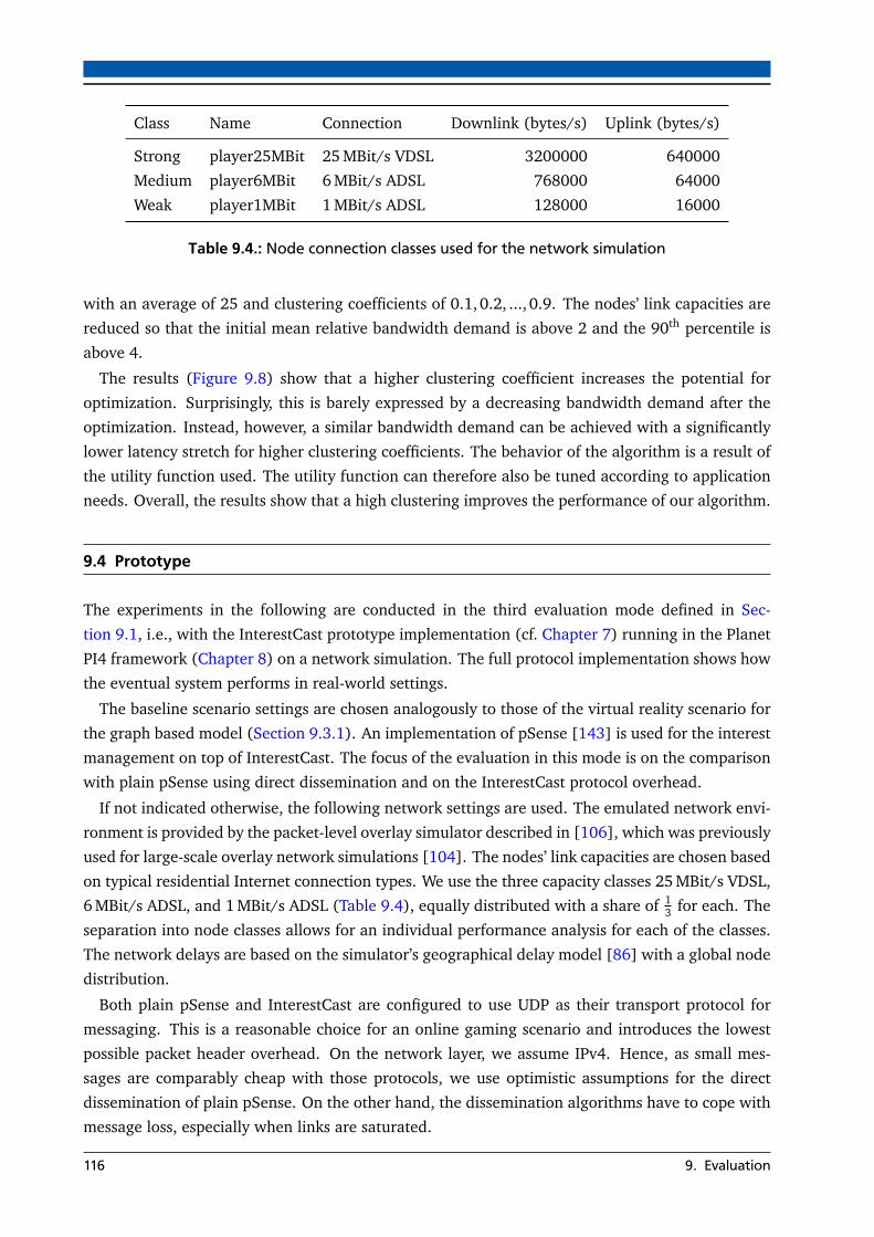
Class Name Connection Downlink (bytes/s) Uplink (bytes/s)

Strong player25MBit 25 MBit/s VDSL 3200000 640000

Medium player6MBit 6 MBit/s ADSL 768000 64000

Weak player1MBit 1 MBit/s ADSL 128000 16000

Table 9.4.: Node connection classes used for the network simulation

with an average of 25 and clustering coefficients of 0.1, 0.2, ..., 0.9. The nodes’ link capacities are

reduced so that the initial mean relative bandwidth demand is above 2 and the 90th percentile is

above 4.

The results (Figure 9.8) show that a higher clustering coefficient increases the potential for

optimization. Surprisingly, this is barely expressed by a decreasing bandwidth demand after the

optimization. Instead, however, a similar bandwidth demand can be achieved with a significantly

lower latency stretch for higher clustering coefficients. The behavior of the algorithm is a result of

the utility function used. The utility function can therefore also be tuned according to application

needs. Overall, the results show that a high clustering improves the performance of our algorithm.

9.4 Prototype

The experiments in the following are conducted in the third evaluation mode defined in Sec-

tion 9.1, i.e., with the InterestCast prototype implementation (cf. Chapter 7) running in the Planet

PI4 framework (Chapter 8) on a network simulation. The full protocol implementation shows how

the eventual system performs in real-world settings.

The baseline scenario settings are chosen analogously to those of the virtual reality scenario for

the graph based model (Section 9.3.1). An implementation of pSense [143] is used for the interest

management on top of InterestCast. The focus of the evaluation in this mode is on the comparison

with plain pSense using direct dissemination and on the InterestCast protocol overhead.

If not indicated otherwise, the following network settings are used. The emulated network envi-

ronment is provided by the packet-level overlay simulator described in [106], which was previously

used for large-scale overlay network simulations [104]. The nodes’ link capacities are chosen based

on typical residential Internet connection types. We use the three capacity classes 25 MBit/s VDSL,

6 MBit/s ADSL, and 1 MBit/s ADSL (Table 9.4), equally distributed with a share of 13 for each. The

separation into node classes allows for an individual performance analysis for each of the classes.

The network delays are based on the simulator’s geographical delay model [86] with a global node

distribution.

Both plain pSense and InterestCast are configured to use UDP as their transport protocol for

messaging. This is a reasonable choice for an online gaming scenario and introduces the lowest

possible packet header overhead. On the network layer, we assume IPv4. Hence, as small mes-

sages are comparably cheap with those protocols, we use optimistic assumptions for the direct

dissemination of plain pSense. On the other hand, the dissemination algorithms have to cope with

message loss, especially when links are saturated.

116 9. Evaluation

0.0

0.2

0.4

50 100 150 200# nodes

rela

tive

band

wid

th d

eman

d

Configuration plain pSense InterestCast

Average bandwidth demand

(a) All nodes

0.0

0.5

1.0

50 100 150 200# nodes

rela

tive

band

wid

th d

eman

d


Average bandwidth demand (weak nodes)

(b) Weak nodes only

Figure 9.9.: Relative bandwidth demand for a variation of node densities

The baseline application workload model is based on a gaming scenario, where each player

regularly disseminates a state update. If not stated otherwise, updates have a payload of 48 bytes

and are sent every 200 ms. This corresponds to a net data rate of 240 bytes/s per stream.

We stick to the same metrics as for the graph-based model wherever possible. Due to the dif-

ferent model, however, there are a few variations in the meaning of some metrics. Unlike in the

graph-based model, the network simulator limits the maximum bandwidth that a node can trans-

mit over its network link. To remain comparable with the graph-based model, the bandwidth

demand metric counts all UDP datagrams that are supposed to be sent, even if they are immedi-

ately dropped at the local link due to congestion. Therefore, bandwidth demand can still grow

beyond a value of 1. Yet, depending on the protocol, message loss can result in a reduced output

rate, so that it is not strictly comparable with its counterpart in the graph-based evaluation. Fur-

ther, latencies now include queuing delays in addition to the network propagation. With actual

state information being transmitted, we can now measure staleness.

For the sake of clarity, we only show plots of the most important evaluation results in this section.

Appendix C provides a collection of additional results.

9.4.1 Node Density

We first repeat the node density scenario from the graph-based model as described in Section 9.3.4.

The node density is therefore varied between experiments, of which each uses static interest and

network settings. We compare InterestCast together with pSense (‘InterestCast’) against plain

pSense with its purely direct dissemination (‘plain pSense’).

Each experiment has a run time of ten minutes. In the first nine minutes, the nodes join and

stabilize. At the same time, InterestCast’s optimization algorithm is already active. The last one

minute is used for measurements of the converged state. The long stabilization phase is chosen

pessimistically to work for all experiment sizes. In most situations, the system settles much quicker.

The distribution of participants in the virtual world and the resulting interest set sizes are on

average the same as for the graph-based scenario, see Table 9.2.

9.4. Prototype 117

0.00

0.05

0.10

0.15

50 100 150 200# nodes

late

ncy

(s)


Average latency

(a) All nodes

0.0

0.1

0.2

50 100 150 200# nodes

late

ncy

(s)


Average latency (weak nodes)

(b) Weak nodes only

Figure 9.10.: Average latency for a variation of node densities

0.00

0.05

0.10

0.15

50 100 150 200# nodes

late

ncy

(s)


Average latency for high interest (>= 0.75)

(a) High interest

0.00

0.05

0.10

0.15

50 100 150 200# nodes

late

ncy

(s)


Average latency for low interest (< 0.25)

(b) Low interest

Figure 9.11.: Average latency by density of high and low interest neighbors

Bandwidth DemandFigure 9.9 shows the bandwidth demand depending on the number of nodes. Like in the graph-

based simulation, Interest significantly reduces the needed bandwidth. Looking only at the weak

nodes (Figure 9.9b), the reduction is even more distinct. InterestCast almost allows doubling the

number of nodes with the same average bandwidth demand as plain pSense.

LatencyThe latency results (Figure 9.10) differ from the results of the graph-based model in that Inter-

estCast beats plain pSense, allowing about a factor of two in node density for the same latencies.

Although InterestCast uses longer paths, the reduced bandwidth demand, especially for the weak

nodes, leads to a reduction in queuing delays, with the consequence of overall lower event delivery

latencies. Queuing delays are not considered in the graph-based model. Again, the effect is most

significant for weak nodes (Figure 9.10b).

Figure 9.11 differentiates event delivery latencies for high (ι ≥ 0.75) and low (ι < 0.25) interest.

Here, we can see that high-interest event delivery latencies barely suffer from an increased load

118 9. Evaluation

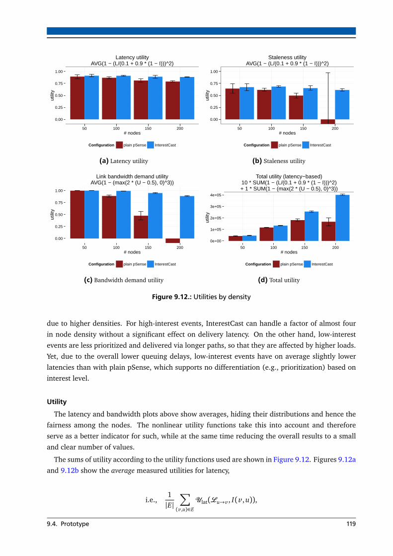
0.00

0.25

0.50

0.75

1.00

50 100 150 200# nodes

utili

ty


Latency utilityAVG(1 − (L/(0.1 + 0.9 * (1 − I)))^2)

(a) Latency utility

0.00

0.25

0.50

0.75

1.00

50 100 150 200# nodes

utili

ty


Staleness utilityAVG(1 − (L/(0.1 + 0.9 * (1 − I)))^2)

(b) Staleness utility

0.00

0.25

0.50

0.75

1.00

50 100 150 200# nodes

utili

ty


Link bandwidth demand utilityAVG(1 − (max(2 * (U − 0.5), 0)^3))

(c) Bandwidth demand utility

0e+00

1e+05

2e+05

3e+05

4e+05

50 100 150 200# nodes

utili

ty


Total utility (latency−based)10 * SUM(1 − (L/(0.1 + 0.9 * (1 − I)))^2)+ 1 * SUM(1 − (max(2 * (U − 0.5), 0)^3))

(d) Total utility

Figure 9.12.: Utilities by density

due to higher densities. For high-interest events, InterestCast can handle a factor of almost four

in node density without a significant effect on delivery latency. On the other hand, low-interest

events are less prioritized and delivered via longer paths, so that they are affected by higher loads.

Yet, due to the overall lower queuing delays, low-interest events have on average slightly lower

latencies than with plain pSense, which supports no differentiation (e.g., prioritization) based on

interest level.

Utility

The latency and bandwidth plots above show averages, hiding their distributions and hence the

fairness among the nodes. The nonlinear utility functions take this into account and therefore

serve as a better indicator for such, while at the same time reducing the overall results to a small

and clear number of values.

The sums of utility according to the utility functions used are shown in Figure 9.12. Figures 9.12a

and 9.12b show the average measured utilities for latency,

i.e.,1|E|

∑

(v ,u)∈E

Ulat(Lu→v , I(v , u)),

9.4. Prototype 119

and staleness,

i.e.,1|E|

∑

(v ,u)∈E

Ulat(Su→v , I(v , u)),

respectively. Figure 9.12c shows the average bandwidth utility

1|V |

∑

v∈V

Ubw(bv )

and Figure 9.12d shows the total weighted utility

wlat ·∑

(v ,u)∈E

Ulat(Lu→v , I(v , u)) + wbw ·∑

v∈V

Ubw(bv ).

Due to the definition of the utility functions, the average utilities have a maximum of one, while

the total utility is only bounded by the number of nodes and interest graph edges. Hence, the

averages allow for a comparison between different numbers of nodes, while the total utility sum

does not. There is no lower bound; in particular, utility sums can fall below zero. Such cases,

however, are cut off in the plots because they indicate really bad results.

Starting at 150 nodes, plain pSense’s bandwidth demands grow beyond the capacities, resulting

in a quick degradation of the respective utility. The effect of the saturation and the resulting

message loss becomes visible in the degrading staleness utility. InterestCast’s utilities, on the other

hand, remain much more stable.

9.4.2 Interest Dynamics

After analyzing InterestCast’s behavior depending on the node density, we now focus on interest

dynamics. Interest dynamics refer to both the change of interest levels as well as the consequent

change of interest sets. Those dynamics have an impact on mainly two factors with respect to

performance. First, the changes of neighbors and their interests require a continuous optimization,

which never converges due to the continuous change. Secondly, frequent neighbor set changes lead

to an increased rate of neighbor information updates and thus an increased management traffic

overhead. The latter is further analyzed in Section 9.4.3.

For this experiment, we use the virtual reality scenario from above, with a few modifications.

The interest dynamics are generated using a random waypoint mobility model. Each node selects

a random point destination in the virtual world and moves towards it on a straight line with

constant velocity. The destination points are uniformly distributed in the virtual world. This

mobility pattern makes very pessimistic assumptions for InterestCast. Since all participants move

totally independently, there are no groups that remain constant over a period of time, which would

be beneficial for the optimization. Instead, neighbors most of the time just pass by each other,

frequently entering and leaving each others’ vision range.

The virtual world size is slightly increased to 1200× 1200 units to compensate the fact that the

eventual distribution of participants moving on the world is not uniform in this case. A higher con-

centration towards the center of the virtual world leads to a higher average number of interest set

120 9. Evaluation

0.0

0.1

0.2

0.3

0.4

0 5 10 25velocity (units/s)

rela

tive

band

wid

th d

eman

d



(a) All nodes

0.0

0.3

0.6

0.9


rela

tive

band

wid

th d

eman

d



(b) Weak nodes only

Figure 9.13.: Relative bandwidth demand depending on virtual world velocity

neighbors. For a better comparability, the interest set sizes are therefore reduced to approximately

the same size as above by increasing the world size.

Keeping the number of nodes constant at 150, we scale the participants’ velocities in the steps

of 0, 5, 10, and 25 units per second. With a vision range of 150 units, a velocity of 25 units per

second is already very high: Crossing each others’ vision range takes at most 20 seconds.

As before, five experiments of ten minutes length each are run for each configuration. The

measurements are averaged over the last minute of each experiment run. Error bars show the

standard deviation between the experiment runs.

Bandwidth Demand

Figure 9.13 shows the bandwidth demand depending on the velocity. With higher interest dy-

namics, the distance to plain pSense shrinks. This is due to the management overhead of Inter-

estCast, including first and foremost the neighbor information exchange and the routing update

operations. Both need to be performed more frequently with higher velocities and therefore be-

come more expensive in terms of bandwidth overhead. For weak nodes, however, there remains a

significant reduction in bandwidth demand, improving load fairness.

Latency

The decrease of InterestCast’s efficiency with high dynamics is also visible in the latency mea-

surements (Figures 9.14 and 9.15). Yet, for weak nodes as well as for high interest neighbors, the

latencies remain significantly better than without InterestCast.

Utility

The utility sums based on the selected utility functions are shown in Figure 9.16. They as well

show the consistently better performance of InterestCast, except for very high dynamics.

9.4. Prototype 121

0.00

0.05

0.10


late

ncy

(s)


Average latency

(a) All nodes

0.0

0.1

0.2


late

ncy

(s)



(b) Weak nodes only

Figure 9.14.: Average latency depending on virtual world velocity

0.00

0.05

0.10


late

ncy

(s)


Average latency for high interest (>= 0.75)

(a) High interest

0.00

0.05

0.10


late

ncy

(s)


Average latency for low interest (< 0.25)

(b) Low interest

Figure 9.15.: Average latency by velocity of high and low interest neighbors

Missing Neighbors

As a final aspect of this section, we look at missing neighbors. Missing neighbors are those par-

ticipants that are of interest, i.e., are within the vision range, but are not visible to the application.

Although the discovery of neighbors is the job of the interest management, which is not in the

focus here, the reliability of the event dissemination plays an important role. In addition, missing

neighbors are not considered in the latency measurements. They further reduce the effective set

of participants to which the events are delivered. This reduces the bandwidth demand and must

therefore be considered.

Figure 9.17 shows the ratio of missing neighbors. It clearly shows that with InterestCast, the

missing neighbors ratio is drastically lower. The neighbor discovery and introduction process works

much more reliably with InterestCast, being a clear indication of the better capacity management.

Only with very high dynamics, a certain ratio of missing neighbors is inevitable due to the discovery

and introduction process, which delays the connection to new neighbors entering the vision range.

122 9. Evaluation

0.00

0.25

0.50

0.75

1.00


utili

ty


Latency utilityAVG(1 − (L/(0.1 + 0.9 * (1 − I)))^2)

(a) Latency utility

0.00

0.25

0.50

0.75

1.00


utili

ty


Staleness utilityAVG(1 − (L/(0.1 + 0.9 * (1 − I)))^2)

(b) Staleness utility

0.00

0.25

0.50

0.75

1.00


utili

ty


Link bandwidth demand utilityAVG(1 − (max(2 * (U − 0.5), 0)^3))

(c) Bandwidth demand utility

0e+00

1e+05

2e+05

3e+05


utili

ty


Total utility (latency−based)10 * SUM(1 − (L/(0.1 + 0.9 * (1 − I)))^2)+ 1 * SUM(1 − (max(2 * (U − 0.5), 0)^3))

(d) Total utility

Figure 9.16.: Utilities by velocity.

9.4.3 Traffic Overhead

A critical factor affecting the overall performance of InterestCast is the communication overhead

of management data. This management data includes route operation messages as well as the

neighbor information exchange messages for the mutual state monitoring. While the traffic gener-

ated by the former is marginal, the latter can have a significant impact. As analyzed in Section 6.3,

large neighbor sets and high ratios of common neighbors due to a high clustering lead to a growth

in neighbor state that needs to be exchanged. The exchange frequency demand further grows

with the interest dynamics. We therefore measure the traffic broken down by message type for the

relevant messages for varying virtual world velocities.

Figure 9.18 shows the traffic breakdown. The first four message types are InterestCast manage-

ment messages, while the last two are application messages from InterstCast’s point of view.

• BANDWIDTHMESSAGEs contain information on the nodes’ available and used bandwidth.

• Known neighbors are exchanged as bloom filters in NEIGHBORFILTERMESSAGEs.

• LATENCYMESSAGEs contain the latencies to common neighbors.

9.4. Prototype 123

0.00

0.05

0.10



Missing neighbors ratio

Figure 9.17.: Missing neighbors ratio (1− neighbors in vision rangeknown neighors ) of plain pSense and InterestCast de-

pending on the velocity

0

2000

4000

6000


byte

s/s

Message

BandwidthMessage

NeighborFilterMessage

LatencyMessage

PathInfoMessage

PSensePositionMessage

MobilityModelMessage

Traffic breakdown for selected messages

Figure 9.18.: Average per-node message traffic for a selection of important message types

• PATHINFOMESSAGEs are regularly transmitted backwards along each path to communicate the

number of hops and total latency.

• PSENSEPOSITIONMESSAGEs are low-frequency position updates of the pSense interest manage-

ment.

• The actual application payload, finally, is in this case transmitted as MOBILITYMODELMESSAGEs.

The average number of neighbors varies slightly depending on the velocity, which explains the

variations in application and interest management traffic. One can observe that the traffic vol-

ume of BANDWIDTHMESSAGE, NEIGHBORFILTERMESSAGE, and PATHINFOMESSAGE barely grow with the

velocity. LATENCYMESSAGEs, on the other hand, take a significant proportion of the total traffic in

cases of high velocities. This can be explained with the quadratic growth of latency information

depending on the number of common neighbors (cf. Section 6.3). Hence, for very high dynamics,

the management overhead can outgrow the bandwidth savings from the optimization. For medium

velocities, however, the overhead remains moderate.

124 9. Evaluation

0.0

0.1

0.2

0.3

20 40 60 80 100# nodes

mis

sing

nei

ghbo

rs r

atio


Missing neighbors

(a) Missing neighbors ratio

0

4000

8000

12000

20 40 60 80 100# nodes

posi

tion

erro

r (V

R d

ista

nce

units

)


Position error

(b) Position error

Figure 9.19.: Error metrics with Planet PI4 bot workload depending on virtual world density

0.0

0.3

0.6

0.9

20 40 60 80 100# nodes

rela

tive

band

wid

th d

eman

d



(a) All nodes

0.0

0.5

1.0

1.5

2.0

20 40 60 80 100# nodes

rela

tive

band

wid

th d

eman

d



(b) Weak nodes only

Figure 9.20.: Relative bandwidth demand with Planet PI4 bot workload depending on virtual worlddensity

9.4.4 Planet PI4 Bot Workload

So far, we have used synthetic workloads based on a mobility model because they allow fine-

grained control over the parameters and low-level metrics such as delivery latency and staleness.

To show the feasibility in a real gaming scenario, we use the Planet PI4 gameplay (cf. Chap-

ter 8) played by bots [47]. The bots provide a reproducible and scalable workload on top of the

game [103]. According to the higher-level workload, we also consider higher-level metrics. Most

important is the position error [69, 99], which measures the position difference of a player’s realposition and the positions of this player as they are perceived by its neighbors at a given point in

time. The real position is considered to be the position that the respective player perceives of itself.

Hence, the position error is the higher-level metric related to staleness and virtual world velocity.

In the experiments, we scale the number of players and thereby the virtual world density. Due to

the flocking behavior of the bots, the resulting density for a given number of players is higher than

9.4. Prototype 125

0.00

0.05

0.10

0.15

20 40 60 80 100# nodes

late

ncy

(s)


Average latency

(a) All nodes

0.0

0.1

0.2

0.3

20 40 60 80 100# nodes

late

ncy

(s)



(b) Weak nodes only

Figure 9.21.: Average latency with Planet PI4 bot workload depending on virtual world density

before. In addition, the events being generated are not only regular position updates, but also shot

and hit events. This results in a further workload increase.

Figure 9.19 shows the ratio of missing neighbors as well as the average position errors. As shown

above with a mobility model workload, the number of missing neighbors (Figure 9.19a) grows

rapidly with plain pSense due to the network overload. InterestCast is much more stable here. The

picture is similar for the position error (Figure 9.19b). Starting at 60 players, it grows dramatically

with plain pSense, only mitigated by the high numbers of missing neighbors. InterestCast, on the

other hand, only shows a moderate increase, thus handling the situation significantly better. Like

for the mobility model workloads, InterestCast’s bandwidth demand is lower (Figure 9.20) and the

latency of the events particularly from week nodes is significantly improved (Figure 9.21).

9.5 Discussion

For the evaluation of InterestCast, we chose a two-stage model. The first uses highly abstracted

graph-based models for interest and network properties. With those, our optimization problem is

solved in two variants: using a standard linear programming solver to obtain global optima and

with InterstCast’s incremental local optimization algorithm. In the second stage, the full protocol

implementation of InterestCast is tested in a detailed network simulation and compared against

plain pSense.

In the first stage we have shown that InterestCast’s incremental local optimization, although not

providing global optima, provides reasonably competitive solutions. In this context it needs to be

stressed that the global solutions can only serve as a benchmark. Implementing a global solver is

expensive in runtime, as we have shown, and would further require that all participants transmit

their state (bandwidth, latencies, etc.) to one single place where the optimization is done. The

advantages of the local algorithm therefore clearly outweigh the slightly suboptimal results.

The full protocol implementation tested in the second stage includes all the necessary monitoring

and route management infrastructure. Hence, the first thing that the evaluation shows is that the

concept can be practically implemented in a fully distributed system. More important, however, is

126 9. Evaluation

the comparison with plain pSense, which uses direct dissemination only but also gets along without

the additional monitoring and management overhead. In low demand situations, InterestCast

shows to be competitive, mostly relying on direct communication as well. In high load situations,

where especially weak nodes are overloaded with direct dissemination, InterestCast significantly

improves the results. The higher propagation delays due to the indirection are by far compensated

by the reduced queuing and message loss rates. Furthermore, InterestCast connects neighbors

more reliably by mitigating load peaks and thereby achieves significantly lower missing neighbor

rates.

With higher interest dynamics, it becomes harder to complete against the purely direct dissem-

ination. Interest dynamics lead to an increased overhead traffic due to InterestCast’s neighbor

information exchange, which is not needed for plain pSense. In addition, InterestCast’s incremen-

tal optimization does never converge due to the constant change and therefore does not reach its

best state. Both factors have a negative impact in InterestCast’s performance, so that at some point

the direct dissemination becomes the best choice. An option to improve the situation if very high

dynamics need to be supported could be to switch to a plain direct dissemination in such cases.

One final point that potentially adds to the reduced performance with dynamics is the greedy opti-

mization based on the redirect and shortcut operations. The optimization due to changed interest

may require to leap local optima much more often than the initial optimization starting from a

direct dissemination. Hence, the optimization might get stuck in the local optima more often.

It has to be noted, however, that the mobility model used to generate interest dynamics is a

very pessimistic choice. In many cases of virtual world scenarios, as represented in this evaluation

by the bot workloads, groups of participants move together such that intra-group dynamics are

significantly lower. In those cases, InterestCast is clearly superior to plain pSense, especially with

respect to the performance of weak nodes.

9.5. Discussion 127

10 Conclusion and OutlookIn this thesis, we have developed InterestCast, a fully distributed event dissemination system,

which adapts to both the application needs and network conditions. To achieve this, we first elab-

orated on potential target applications, focusing on online gaming. Based on those, we identified

the main requirements and challenges. After discussing existing solutions and their shortcom-

ings, we derived the basic design decisions: the decomposition of interest management and event

dissemination and their interfacing, the basic adaptation concepts, InterestCast’s routing, and its

optimization. Afterwards, we formalized our system model and formulated the optimization goal.

We detailed InterestCast’s core algorithm, the local incremental optimization. The full prototype

protocol implementation as well as the framework Planet PI4, in which the implementation and

evaluation took place, were described, before the evaluation with a two-staged model was pre-

sented.

The main goal of this work was a many-to-many event dissemination with a particular focus on

low dissemination latencies. Our proposed solution, InterestCast, is able to adapt with respect to

both application needs and network conditions. Further, it gains from heterogeneous environments

and needs no dedicated infrastructure, i.e., works in a decentralized and self-organizing manner.

InterestCast starts with a direct dissemination scheme and continuously runs a local optimization

algorithm that modifies event routes to use neighboring nodes as forwarders where suitable. This

way, it makes use of data aggregation and reduces the number of small packets with high packet

header overhead. Application needs are expressed as utility functions, which in the concrete case

consider bandwidth demand as well as latency depending on the interest level.

InterestCast provides a distributed event dissemination, while it relies on existing interest man-

agement solutions, such as pSense, which works fully decentralized as well. To make this possible,

we needed a clear separation of functionality between interest management and event dissemi-

nation. InterestCast’s interface to the interest management component uses interest levels as an

application-independent abstraction of interest gradations. This is an extension to the conventional

“interest or no interest” subscription model.

The optimization of the system state based on utility functions is a good fit for best-effort so-

lutions. Where no hard guarantees can be given, the utility-based optimization is able to make

trade-offs based on the particular application needs. Using additive utilities, it is possible to pre-

dict effects on overall utility based on local partial knowledge. Further, non-linear utility functions

allow considering fairness.

The comparison with global optima based on a graph-based network model has shown that the

local optimization provides good results compared to the global optima. Computing global optima

at runtime, on the other hand, is infeasible as it would require all information about the current

network and load situation at a single point. It has further shown to be too expensive to compute

for any relevant network size, despite the use of simplistic network models.

129

In detailed network simulations, the InterestCast prototype, which is suitable for real-world

deployments, has proven its superiority over a plain direct dissemination. Especially in situations

of high load, it significantly reduces the bandwidth demand of overloaded nodes and thereby also

decreases dissemination latencies. It allows doubling the node density and still provides the same

average latency than plain pSense. Hence, InterestCast’s performance is improved by the likely

heterogeneity of the participants’ devices and connections. Further, high-interest events have the

lowest latency penalty, demonstrating how the interest level can be used to prioritize events. For

high-interest events, the latency remains almost constant even with a node density factor of four.

InterestCast was evaluated with scenarios adopted from multiplayer online games. Those have

high demands particularly with respect to latency, which are well studied. This makes them well

suited for our evaluation purposes. The core results can be generalized to the other discussed

application scenarios as well. With respect to the workloads, the gaming scenarios have similar

magnitudes as expected in coordination tasks of robotics or vehicular networks. Ad-hoc networking

scenarios require an adapted system model and work in different latency ranges than global-scale

networks, but are otherwise comparable.

We have developed a fundamental concept for a decentralized utility-based optimization of a

many-to-many event dissemination middleware, which can be adapted to related problems using

factors beyond latency and bandwidth demand. With a system model that can be extended in a

modular fashion, it allows for further advances in the abstraction of the application utility functions

from the underlying system.

10.1 Future Work

With InterestCast, we have developed a fundamental concept for a decentralized utility-based

optimization of a many-to-many event dissemination middleware. Yet, there remains room for

future extensions and enhancement in several aspects. In this section, we discuss those, starting

with incremental additions and moving towards more sophisticated additions.

Computational EfficiencyThe current optimization algorithm was developed with the goal of a low communication and

state demand, but does not take into account the computational effort. Although this is not a

significant factor in many cases, the brute force enumeration of all possible transitions in each

optimization iteration can become a limiting factor with a large number of neighbors. Hence, a

more efficient algorithm that works without a full enumeration of options can improve the situation

in such case. One approach could be to use heuristics and to decide based on partial evaluation of

the utility impact of possible transitions. Other options are to parallelize the evaluation of possible

transitions or to re-compute only the options whose expected utility impact has changed.

Dynamic Optimization RateFor both reducing necessary computation and increasing optimization speed, a dynamic rate

adaptation for the incremental optimization can be introduced. With such, the optimization steps

would be invoked more frequently under high dynamics and less frequently under low dynamics.

130 10. Conclusion and Outlook

Since each node runs the optimization individually, there is no need for a coordination of optimiza-

tion rates. The rate adaptation could be done based on the interest and neighbor set dynamics or

the achieved utility improvements of the previous optimization steps.

Specializations for Update EventsThe delivery of update events, which contain updates of continuously changing state such as po-

sitions, can be improved by adding specific handling of those. In the current solution, for the sake

of generality, we assume that all events pushed by the application should be delivered instantly.

Update events on the other hand could be pulled from the application with fresh state whenever

the event dissemination decides to send one. This could be used to fill up existing packets, but also

allows the event dissemination mechanism to adapt the update rate. This allows further taking

into account the staleness utility in the optimization.

Utility-Based SchedulingA more generalized version of the above would be to consider the utility functions in the schedul-

ing algorithm for all events. This way, prioritization of events in high load situations could adapt

better to the application needs. The scheduler can use the accumulated latency that is already

included in every message to heuristically select the forwarding priority based on the remaining

timeframe. The interaction between the utility-based routing and scheduling, however, has to be

considered carefully to avoid unintended feedback loops.

Generalization of the Local Optimization ApproachInterestCast implements the local incremental optimization approach for a specific purpose. The

basic concept, however, is applicable in a much broader sense. A first extension would be the

addition of further route operations, such as directly switching a forwarder node instead of apply-

ing a shortcut and redirect operation. This can reduce the potential of local optima that hinder

the optimization. On the other hand, however, such operation requires neighbor information

to be exchanged one hop further, which introduces additional costs. Yet, the neighbor informa-

tion exchange algorithm can be generalized to support multiple hops where needed by the used

operations.

Additional Utility FactorsInterestCast works with the utility factors latency, interest, and bandwidth demand. The basic

optimization concept, however, makes it easy to add additional factors. For instance, a reliability

factor can be introduced, if the system allows for a redundant transmission of data or spare paths

for failover.

Consideration of Special Network PropertiesInterestCast’s current model only considers one network interface per node, which has been

the case for most end user Internet devices. Recently, however, an increasing number of devices

have multiple network interfaces, such as WiFi and cellular broadband. While they were initially

only used alternatively, using multiple interfaces at once opens a variety of new use cases. One

10.1. Future Work 131

example is mobile connection sharing [125]. Considering multiple interfaces and their individual

properties and costs separately, InterestCast could provide similar features, such as using certain

nodes as forwarding gateways between the cellular network and an ad-hoc WiFi network.

Inclusion of Active Network ElementsThe local optimization provides potential for the inclusion of locally available active network el-

ements, such as dynamically allocated virtual machines in network routers. Although they are still

uncommon in real network deployments, active research in cloudlets [141] and network function

virtualization (NFV) [81] may promote their future availability. With those, dedicated InterestCast

nodes could be dynamically deployed in the network, allowing for a more efficient yet flexible

event dissemination.

132 10. Conclusion and Outlook

A Global Optimization Integer ProgramsThis section lists and briefly explains the complete integer programs described in Section 5.6.

A.1 ILP Problem

The following listing contains the Zimpl program of the global optimization problem simplified to

an ILP program (cf. Section 5.6.1). Node IDs, link capacities, as well as X any Y coordinates for

the delay model are stored in the columns of file nodes.dat. Interest levels between pairs of nodes

are stored in interest.dat.

1 # nodes

2 set V := { read "nodes.dat" as "<1n>" comment "#" };

3

4 # node bandwidths in #flows

5 param bw[V] := read "nodes.dat" as "<1n> 2n" comment "#";

6

7 # nodes’ geo corrdinates

8 param geo_x[V] := read "nodes.dat" as "<1n> 3n" comment "#";

9 param geo_y[V] := read "nodes.dat" as "<1n> 4n" comment "#";

10

11 # interest of 1st node in 2nd node

12 param interest[V*V] := read "interest.dat" as "<1n, 2n> 3n" comment"#";

13

14 # minimum per-link latency

15 param baseLatency := 0.01;

16 # latency per geo-distance unit

17 param geoLatencyFactor := 0.002;

18

19 # subscription of l at k, i.e., flow from k to l

20 set subscriptions := { <k,l> in V*V with (k != l) and (interest[l,k] > 0) };

21

22 # latency model

23 defnumb latency(a,b) := sqrt((geo_x[a] - geo_x[b])^2 + (geo_y[a] - geo_y[b])

^2) * geoLatencyFactor + baseLatency;

24

25 # variables

26

27 # y[i,j,k,l] = 1 iff events for flow from k to l are routed from i to j

28 var y[V*V*V*V] binary;

29 # helper variables to achieve maximum operation:

30 # x[i,j,k] = 1 iff events for flow from k are routed from i to j

133

31 var x[V*V*V] binary;

32 # z[i,j] = 1 iff events are routed from i to j

33 var z[V*V] binary;

34

35 # objective function

36

37 minimize cost:

38 sum <i,j,k,l> in V*V*V*V: (y[i,j,k,l] * latency(i, j));

39

40 # constraints

41

42 # if at least one flow from k to some l is routed from i to j,

43 # there is a flow from k routed from i to j

44 subto x_y:

45 forall <i,j,k,l> in V*V*V*V:

46 x[i,j,k] >= y[i,j,k,l];

47 # if at least one flow from some k is routed from i to j,

48 # there is a flow routed from i to j

49 subto z_x:

50 forall <i,j,k> in V*V*V:

51 z[i,j] >= x[i,j,k];

52

53 # bandwidth limit

54 # counting all flows from individual sources (x) and connection overhead (z)

55 subto bwbound:

56 forall in V:

57 (sum <j,k> in V*V: x[i,j,k] + sum <j> in V: z[i,j]) <= 1.0 * bw[i];

58

59 # in-degree == out-degree, except for source and destination

60 subto path:

61 forall <k,l> in subscriptions:

62 forall in V without { <k>, <l> }:

63 (sum <j> in V: y[j,i,k,l]) == (sum <j> in V: y[i,j,k,l]);

64

65 # nodes don’t route to themselves

66 subto no_self_loop:

67 forall in V:

68 z[i,i] == 0;

69

70 # source has exactly one outgoing flow

71 subto source_out:


73 sum <j> in V: y[k,j,k,l] == 1;

74 subto source_no_in:


76 sum <j> in V: y[j,k,k,l] == 0;

134 A. Global Optimization Integer Programs

77

78 # destination has exactly one incoming flow

79 subto destination_in:


81 sum in V: y[i,l,k,l] == 1;

82 subto destination_no_out:


84 sum in V: y[l,i,k,l] == 0;

A.2 MINLP Problem

The following listing extends the ILP problem to a MINLP problem, as discussed in Section 5.6.2.

Due to limitations in the Zimpl language, the cost functions (Clat, Cbw) cannot be directly repre-

sented in the program code in all cases. Instead, it might be necessary to introduce additional

helper variables, e.g., for maximum and minimum operations.

Here, we use the exemplary cost functions (cf. Section 6.5)

Clat(L , ι) =�

L0.1+ 0.9 ∗ (1− ι)

�2

and

Cbw(b) =max (4 · (b− 0.5) , 0)3 .

1 # nodes

2 set V := { read "nodes.dat" as "<1n>" comment "#" };

3

4 # node bandwidths in #flows

5 param bw[V] := read "nodes.dat" as "<1n> 2n" comment "#";

6 param bw_factor := 1.0;

7

8 # nodes’ geo corrdinates

9 param geo_x[V] := read "nodes.dat" as "<1n> 3n" comment "#";

10 param geo_y[V] := read "nodes.dat" as "<1n> 4n" comment "#";

11

12 # interest of 1st node in 2nd node

13 param interest[V*V] := read "interest.dat" as "<1n, 2n> 3n" comment "#";

14 param interestThreshold := 0.1;

15

16 # minimum per-link (last mile) latency

17 param baseLatency := 0.01;

18 # latency per geo-distance unit

19 param geoLatencyFactor := 0.002;

20

21 param weightPathLatency := 1.0;

22 param weightBandwidth := 64.0;

23

A.2. MINLP Problem 135

24 # subscription of l at k, i.e., flow from k to l

25 set subscriptions := { <k,l> in V*V with (k != l) and (interest[l,k] >=

interestThreshold) };

26

27 defnumb latency(a,b) := sqrt((geo_x[a] - geo_x[b])^2 + (geo_y[a] - geo_y[b])

^2) * geoLatencyFactor + baseLatency;

28

29 # variables

30

31 # y[i,j,k,l] = 1 iff events for flow from k to l are routed from i to j

32 var y[V*V*V*V] binary;

33

34 # helper variables to achieve maximum operation:

35 # x[i,j,k] = 1 iff events for flow from k are routed from i to j

36 var x[V*V*V] binary;

37 # z[i,j] = 1 iff events are routed from i to j

38 var z[V*V] binary;

39

40 # helper variables for non-linear latency cost

41 # subscription latency cost (based on non-linear utility function)

42 var c_lat[subscriptions];

43 # node bandwidth cost (based on non-linear utility function)

44 var c_bw[V];

45 # node bandwidth maximum helper

46 var d_bw[V];

47 # relative node bandwidth demand

48 var u_bw[V];

49

50 # objective function

51

52 minimize cost:

53 (sum <k,l> in subscriptions: c_lat[k,l] * weightPathLatency)

54 + (sum in V: c_bw[i] * weightBandwidth);

55

56 # constraints

57

58 # c_lat: latency cost

59 # cost function: l / (0.1f + 0.9f * (1.0f - i))

60 subto c_lat:


62 c_lat[k,l] == (sum <i,j> in V*V: y[i,j,k,l] * latency(i, j)) / (0.1 + 0.9

* (1.0 - interest[k,l]));

63

64 # c_bw: bandwidth cost

65 # cost function: max(4 * (b - 0.5), 0)^3

66 subto c_bw:

67 forall in V:

68 c_bw[i] == d_bw[i]^3;

69 # max(4 * (b - 0.5), 0)

70 subto d_bw:

71 forall in V:

72 d_bw[i] >= 4 * (u_bw[i] - 0.5);

73 subto d_bw_gz:

74 forall in V:

75 d_bw[i] >= 0;

76 # relative bw demand

77 # counting all flows from individual sources (x) and connection overhead (z)

78 subto u_bw:

79 forall in V:

80 u_bw[i] == (sum <j,k> in V*V: x[i,j,k] + sum <j> in V: z[i,j]) / bw[i];

81

82 # if at least one flow from k to some l is routed from i to j,

83 # there is a flow from k routed from i to j

84 subto x_y:

85 forall <i,j,k,l> in V*V*V*V:

86 x[i,j,k] >= y[i,j,k,l];

87 # if at least one flow from some k is routed from i to j,

88 # there is a flow routed from i to j

89 subto z_x:

90 forall <i,j,k> in V*V*V:

91 z[i,j] >= x[i,j,k];

92

93 # in-degree == out-degree, except for source and destination

94 subto path:


96 forall in V without { <k>, <l> }:

97 (sum <j> in V: y[j,i,k,l]) == (sum <j> in V: y[i,j,k,l]);

98

99 # nodes don’t route to themselves

100 subto no_self_loop:

101 forall in V:

102 z[i,i] == 0;

103

104 # source has exactly one outgoing flow

105 subto source_out:


107 sum <j> in V: y[k,j,k,l] == 1;

108 subto source_no_in:


110 sum <j> in V: y[j,k,k,l] == 0;

111

112 # destination has exactly one incoming flow

A.2. MINLP Problem 137

113 subto destination_in:


115 sum in V: y[i,l,k,l] == 1;

116 subto destination_no_out:


118 sum in V: y[l,i,k,l] == 0;

B InterestCast Routing Update HandlingThis section details the operations performed for InterestCast’s route update operations, as de-

scribed in Section 7.3.1, using flowcharts. The flowcharts describe the basic operations upon re-

ception of update messages via the procedures ONROUTEUPDATE, ONROUTENOTIFY, and ONROUTEACK,

respectively, in Figures 7.5 and 7.6.

ONROUTEUPDATE, depicted in Figure B.1, handles HOP_ROUTE_UPDATE requests. In Figures 7.5

and 7.6, this procedure is invoked as the first operation on U and S, respectively. As parameters,

it gets the source-destination tuple (S′, D′), which identifies the route, as well as the new via node

(v ia) and the route ID RI D that will be used by the predecessor in the following. The procedure

checks the feasibility of the operation and, if successful, forwards a HOP_ROUTE_NOTIFY to the

new via node (v ia).

Subsequently, ONROUTENOTIFY (Figure B.2) is triggered on that via node. This proce-

dure checks the applicability from the point of view of the via node and replies with a

HOP_ROUTEACK(ACCEPT), if successful.

The HOP_ROUTEACK message is processed by ONROUTEACK (Figure B.3). HOP_ROUTEACK

messages serve as responses to both HOP_ROUTE_UPDATE and HOP_ROUTE_NOTIFY. The han-

dler therefore uses the pending operation registry to determine the operation associated with a

particular HOP_ROUTEACK message. A special case is the timeout (indicated as answer = TIME-

OUT), which is the absence of an acknowledgement within a certain time frame.

139

ONROUTEUPDATE

(S′, D′, v ia, RI D)

is v iaknown?

reject: reply

UNKNOWN_NODE

have

route(S′, D′)?

route.via

= sender

of update?

route has

pending

operation?

reject: reply

UPDATE_IN_PROGRESSS′ = sel f ?

reject: reply

ALREADY_IN_ROUTE

update incoming

route with RI D

send

HOP_ROUTE_NOTIFY

to v ia

yes

no

yes

yes

yesno

no

no

no

yes

Figure B.1.: Flowchart for the handling of a route update message

140 B. InterestCast Routing Update Handling

ONROUTENOTIFY

(S′, D′, RI D)

D′ = sel f ?

reply

HOP_ROUTEACK

(ACCEPT)

yes

have

route(S′, D′)?no

yes

reject: reply

HOP_ROUTEACK

(UNKNOWN_ROUTE)

no

update incoming

route with RI D

Figure B.2.: Flowchart for the handling of a route notify message

141

ONROUTEACK

(RI D, answer)

answer =TIMEOUT?

update routing,

use direct route

yes

answer =UNKNOWN

_ROUTE?

no

S′ = sel f ?yes update routing,

use direct route

notify predeces-

sor, drop route

yes

no

matching

pending route

update?

no

answer =ACCEPT?

yes update routing,

use new via

yes

abort

no

matching

pending route

notify?

no

answer =ACCEPT?

yesupdate routing, send

HOP_ROUTEACK

(ACCEPT) to issuer

yes

abort, send

HOP_ROUTEACK

(VIA_REPORTS_ERROR)

to issuer

no

ignore

no

Figure B.3.: Flowchart for the handling of a route update acknowledgement message

142 B. InterestCast Routing Update Handling

C Prototype Evaluation ResultsThis appendix section provides a more complete compilation of evaluation results of the Interest-

Cast prototype that were omitted for reasons of clarity in Chapter 9.

Figures C.1, C.2, C.3, and C.4 show the results of the virtual world density variation experiment,

systematically separated by node capacity class and interest level. The properties of the capacity

classes are listed in Table 9.4. The interest levels are classified into high ([0.75,1]), medium

([0.25, 0,75[), and low ([0, 0.25[). The respective results for the varied virtual world velocity

experiments are shown in Figures C.5, C.6 C.7, and C.8.

weak medium strong

0.0

0.5

1.0

50 100 150 200 50 100 150 200 50 100 150 200# nodes

rela

tive

band

wid

th d

eman

d


Average relative bandwidth demand by node class

Figure C.1.: Average relative bandwidth demand by node capacity class depending on virtual worlddensity. Error bars indicate the standard deviation of the measurements for five exper-iment runs.

143

weak medium strong

0.0

0.5

1.0

1.5

50 100 150 200 50 100 150 200 50 100 150 200# nodes

rela

tive

band

wid

th d

eman

d


90th quantile relative bandwidth demand by node class

Figure C.2.: 90th quantile relative bandwidth demand by node capacity class depending on virtualworld density. Error bars indicate the standard deviation of the measurements for fiveexperiment runs.

weak medium strong

0.0

0.1

0.2

0.0

0.1

0.2

0.0

0.1

0.2

high interestm

edium interest

low interest

50 100 150 200 50 100 150 200 50 100 150 200# nodes

late

ncy

(s)


Average latency by interest and node class

Figure C.3.: Average latency by node capacity and interest level class depending on virtual worlddensity. Error bars indicate the standard deviation of the measurements for five exper-iment runs.

144 C. Prototype Evaluation Results

weak medium strong

0.0

0.1

0.2

0.3

0.4

0.0

0.1

0.2

0.3

0.4

0.0

0.1

0.2

0.3

0.4

high interestm

edium interest

low interest

50 100 150 200 50 100 150 200 50 100 150 200# nodes

stal

enes

s (s

)


Average staleness by interest and node class

Figure C.4.: Average staleness by node capacity and interest level class depending on virtual worlddensity. Error bars indicate the standard deviation of the measurements for five exper-iment runs.

weak medium strong

0.0

0.3

0.6

0.9

0 5 10 25 0 5 10 25 0 5 10 25velocity (units/s)

rela

tive

band

wid

th d

eman

d


Average relative bandwidth demand by node class

Figure C.5.: Average relative bandwidth demand by node capacity class depending on virtual worldvelocity. Error bars indicate the standard deviation of the measurements for five exper-iment runs.

145

weak medium strong

0.0

0.5

1.0

1.5

0 5 10 25 0 5 10 25 0 5 10 25velocity (units/s)

rela

tive

band

wid

th d

eman

d


90th quantile relative bandwidth demand by node class

Figure C.6.: 90th quantile relative bandwidth demand by node capacity class depending on virtualworld velocity. Error bars indicate the standard deviation of the measurements for fiveexperiment runs.

weak medium strong

0.0

0.1

0.2

0.0

0.1

0.2

0.0

0.1

0.2

high interestm

edium interest

low interest

0 5 10 25 0 5 10 25 0 5 10 25velocity (units/s)

late

ncy

(s)


Average latency by interest and node class

Figure C.7.: Average latency by node capacity and interest level class depending on virtual worldvelocity. Error bars indicate the standard deviation of the measurements for five ex-periment runs.

146 C. Prototype Evaluation Results

weak medium strong

0.0

0.1

0.2

0.3

0.4

0.0

0.1

0.2

0.3

0.4

0.0

0.1

0.2

0.3

0.4

high interestm

edium interest

low interest

0 5 10 25 0 5 10 25 0 5 10 25velocity (units/s)

stal

enes

s (s

)


Average staleness by interest and node class

Figure C.8.: Average staleness by node capacity and interest level class depending on virtual worldvelocity. Error bars indicate the standard deviation of the measurements for five ex-periment runs.

147

List of Figures

1.1. Illustration of the physical space and virtual space in which participants are located 3

1.2. InterestCast’s optimization acting upon three main factors . . . . . . . . . . . . . . . . 7

2.1. Illustration of network packet sizes for transmitting position updates . . . . . . . . . 11

2.2. Screen shots of two typical mobile augmented reality multiplayer games . . . . . . . 14

2.3. Ratio of data that could have been sent directly depending on the direct communi-

cation range . . . . . . . . . . . . . . . . . . . . . . . . . . . . . . . . . . . . . . . . . . . . 15

2.4. Accumulated ratio of data that could have been sent over a number of hops depend-

ing on the single-hop transmission range . . . . . . . . . . . . . . . . . . . . . . . . . . . 16

3.1. Typical decentralized interest management topologies . . . . . . . . . . . . . . . . . . 33

4.1. Layering of the basic components in the interaction with InterestCast . . . . . . . . . 38

4.2. Influencing conditions for the system adaptation . . . . . . . . . . . . . . . . . . . . . . 43

4.3. Illustration of the generic utility/cost-based middleware adaptation concept . . . . . 45

4.4. InterestCast paths concept . . . . . . . . . . . . . . . . . . . . . . . . . . . . . . . . . . . . 48

4.5. The basic prediction of utility changes caused by a transition . . . . . . . . . . . . . . 51

5.1. Example of a subscription graph being generated from a given interest function I . 54

5.2. An example of how a subscription graph is generated from positions in a 2-D virtual

world . . . . . . . . . . . . . . . . . . . . . . . . . . . . . . . . . . . . . . . . . . . . . . . . 55

5.3. Illustration of staleness over time with periodic updates . . . . . . . . . . . . . . . . . 56

6.1. Redirect operation initiated by node S . . . . . . . . . . . . . . . . . . . . . . . . . . . . 65

6.2. Shortcut operation initiated by node U . . . . . . . . . . . . . . . . . . . . . . . . . . . . 66

6.3. Illustration of the six conditions affecting the expected change in uplink utilization 68

6.4. Exemplary latency utility functions . . . . . . . . . . . . . . . . . . . . . . . . . . . . . . 76

6.5. Exemplary bivariate latency-interest utility functions . . . . . . . . . . . . . . . . . . . 78

6.6. Exemplary utility functions for bandwidth demand . . . . . . . . . . . . . . . . . . . . 79

7.1. Illustration of the main interaction aspects between the high-level components . . . 82

7.2. InterestCast’s internal components . . . . . . . . . . . . . . . . . . . . . . . . . . . . . . . 82

7.3. A typical multi-hop message flow through InterestCast’s layers . . . . . . . . . . . . . 84

7.4. Illustration of the routing process of an event message . . . . . . . . . . . . . . . . . . 86

7.5. Sequence diagram of a successful route redirect operation . . . . . . . . . . . . . . . . 87

7.6. Sequence diagram of a successful route shortcut operation . . . . . . . . . . . . . . . . 88

7.7. Illustration of a chained message . . . . . . . . . . . . . . . . . . . . . . . . . . . . . . . 91

7.8. Exemplary messages . . . . . . . . . . . . . . . . . . . . . . . . . . . . . . . . . . . . . . . 92

149

8.1. Screen shot of the Planet PI4 game UI . . . . . . . . . . . . . . . . . . . . . . . . . . . . 96

8.2. The high-level architecture of the Planet PI4 evaluation platform . . . . . . . . . . . . 97

8.3. The basic experimentation workflow . . . . . . . . . . . . . . . . . . . . . . . . . . . . . 100

9.1. Iterations of an InterestCast optimization process with 150 nodes. . . . . . . . . . . . 110

9.2. Iterations of an optimization process with 150 nodes . . . . . . . . . . . . . . . . . . . 110

9.3. Integer programming solution times depending on the problem size . . . . . . . . . . 112

9.4. Latency stretch over relative bandwidth demand . . . . . . . . . . . . . . . . . . . . . . 113

9.5. Comparison of the optimization approaches . . . . . . . . . . . . . . . . . . . . . . . . . 113

9.6. Bandwidth demand by varying number of nodes . . . . . . . . . . . . . . . . . . . . . 114

9.7. Relative bandwidth demand and path lengths depending on weight factors of the

utility function . . . . . . . . . . . . . . . . . . . . . . . . . . . . . . . . . . . . . . . . . . . 115

9.8. Optimization potential depending on clustering coefficient . . . . . . . . . . . . . . . . 115

9.9. Relative bandwidth demand for a variation of node densities . . . . . . . . . . . . . . 117

9.10.Average latency for a variation of node densities . . . . . . . . . . . . . . . . . . . . . . 118

9.11.Average latency by density of high and low interest neighbors . . . . . . . . . . . . . 118

9.12.Utilities by density . . . . . . . . . . . . . . . . . . . . . . . . . . . . . . . . . . . . . . . . 119

9.13.Relative bandwidth demand depending on virtual world velocity . . . . . . . . . . . 121

9.14.Average latency depending on virtual world velocity . . . . . . . . . . . . . . . . . . . 122

9.15.Average latency by velocity of high and low interest neighbors . . . . . . . . . . . . . 122

9.16.Utilities by velocity. . . . . . . . . . . . . . . . . . . . . . . . . . . . . . . . . . . . . . . . 123

9.17.Missing neighbors ratio depending on the velocity . . . . . . . . . . . . . . . . . . . . . 124

9.18.Average per-node message traffic for a selection of important message types . . . . 124

9.19.Error metrics with Planet PI4 bot workload depending on virtual world density . . 125

9.20.Relative bandwidth demand with Planet PI4 bot workload depending on virtual

world density . . . . . . . . . . . . . . . . . . . . . . . . . . . . . . . . . . . . . . . . . . . 125

9.21.Average latency with Planet PI4 bot workload depending on virtual world density . 126

B.1. Flowchart for the handling of a route update message . . . . . . . . . . . . . . . . . . 140

B.2. Flowchart for the handling of a route notify message . . . . . . . . . . . . . . . . . . . 141

B.3. Flowchart for the handling of a route update acknowledgement message . . . . . . 142

C.1. Average relative bandwidth demand by node capacity class depending on virtual

world density . . . . . . . . . . . . . . . . . . . . . . . . . . . . . . . . . . . . . . . . . . . . 143

C.2. 90th quantile relative bandwidth demand by node capacity class depending on vir-

tual world density . . . . . . . . . . . . . . . . . . . . . . . . . . . . . . . . . . . . . . . . . 144

C.3. Average latency by node capacity and interest level class depending on virtual world

density . . . . . . . . . . . . . . . . . . . . . . . . . . . . . . . . . . . . . . . . . . . . . . . . 144

C.4. Average staleness by node capacity and interest level class depending on virtual

world density . . . . . . . . . . . . . . . . . . . . . . . . . . . . . . . . . . . . . . . . . . . . 145

C.5. Average relative bandwidth demand by node capacity class depending on virtual

world velocity . . . . . . . . . . . . . . . . . . . . . . . . . . . . . . . . . . . . . . . . . . . 145

150 List of Figures

C.6. 90th quantile relative bandwidth demand by node capacity class depending on vir-

tual world velocity . . . . . . . . . . . . . . . . . . . . . . . . . . . . . . . . . . . . . . . . 146

C.7. Average latency by node capacity and interest level class depending on virtual world

velocity . . . . . . . . . . . . . . . . . . . . . . . . . . . . . . . . . . . . . . . . . . . . . . . 146

C.8. Average staleness by node capacity and interest level class depending on virtual

world velocity . . . . . . . . . . . . . . . . . . . . . . . . . . . . . . . . . . . . . . . . . . . 147

List of Figures 151

List of Tables

3.1. Comparison of a selection of application layer multicast algorithms . . . . . . . . . . 25

6.1. Overview of approximations for communication complexity of different types of in-

formation to be available in m-hop neighborhoods . . . . . . . . . . . . . . . . . . . . . 73

7.1. Overview of InterestCast’s layer headers and their sizes . . . . . . . . . . . . . . . . . . 92

9.1. Overview comparing the three evaluation modes . . . . . . . . . . . . . . . . . . . . . . 105

9.2. Properties of the synthetic virtual environment interest graph . . . . . . . . . . . . . . 109

9.3. Versions of the software components used with the SCIP solver . . . . . . . . . . . . . 111

9.4. Node connection classes used for the network simulation . . . . . . . . . . . . . . . . 116

153

Bibliography[1] Tobias Achterberg. Constraint Integer Programming. PhD thesis, Technische Universität

Berlin, 2007. [Cited on page 61.]

[2] R. Alimi, R. Penno, Y. Yang, S. Kiesel, S. Previdi, W. Roome, S. Shalunov, and R. Woundy.

Application-layer traffic optimization (ALTO) protocol. RFC 7285 (Proposed Standard),

September 2014. [Cited on page 43.]

[3] Mouna Allani, Benoît Garbinato, and Peter Pietzuch. Hyphen: A hybrid protocol for generic

overlay construction in P2P environments. In 28th Annual ACM Symposium on AppliedComputing (SAC’13), pages 423–430, 2013. [Cited on pages 30 and 49.]

[4] Mohammad S. Almalag. Safety-related vehicular applications. In Vehicular networks: fromtheory to practice. CRC Press, 2010. [Cited on page 17.]

[5] Amazon Web Services, Inc. Products and services by region. http://aws.amazon.com/

about-aws/global-infrastructure/regional-product-services/. Accessed: 2015-03-

17. [Cited on page 2.]

[6] Jose Antollini, Mario Antollini, Pablo Guerrero, and Mariano Cilia. Extending REBECA

to support concept-based addressing. In Argentinean Symposium on Information Systems(ASIS’04), September 2004. [Cited on page 27.]

[7] Entertainment Software Association. Essential facts about the computer and video game

industry: 2013 sales, demographic and usage data. http://www.theesa.com/facts/pdfs/

esa_ef_2013.pdf, 2013. Accessed: 2014-03-19. [Cited on page 9.]

[8] Luigi Atzori, Antonio Iera, and Giacomo Morabito. The Internet of Things: A survey. Com-puter Networks, 54(15):2787–2805, October 2010. [Cited on page 2.]

[9] Alvin AuYoung, Laura Grit, Janet Wiener, and John Wilkes. Service contracts and aggregate

utility functions. 2006 15th IEEE International Conference on High Performance DistributedComputing, pages 119–131, 2006. [Cited on page 44.]

[10] Ronald Azuma, Yohan Baillot, Reinhold Behringer, Steven Feiner, Simon Julier, and B. Mac-

Intyre. Recent advances in augmented reality. IEEE Computer Graphics and Applications,21(6):34–47, 2001. [Cited on page 13.]

[11] Ronald T. Azuma. A survey of augmented reality. Presence, 4(August):355–385, 1997. [Cited

on page 13.]

[12] B. Azvine, Z. Cui, D. D. Nauck, and B. Majeed. Real time business intelligence for the

adaptive enterprise. In CEC/EEE 2006 Joint Conferences, 2006. [Cited on page 1.]

155

http://aws.amazon.com/about-aws/global-infrastructure/regional-product-services/

http://aws.amazon.com/about-aws/global-infrastructure/regional-product-services/

http://www.theesa.com/facts/pdfs/esa_ef_2013.pdf

http://www.theesa.com/facts/pdfs/esa_ef_2013.pdf

[13] Helge Backhaus and Stephan Krause. QuON: a quad-tree-based overlay protocol for dis-

tributed virtual worlds. In The 2nd International Workshop on Massively Multiuser VirtualEnvironments at IEEE Virtual Reality (MMVE’09), 2009. [Cited on page 34.]

[14] Niranjan Balasubramanian, Aruna Balasubramanian, and Arun Venkataramani. Energy

consumption in mobile phones: a measurement study and implications for network ap-

plications. 9th ACM SIGCOMM conference on Internet measurement conference (IMC’09),

pages 280–293, 2009. [Cited on page 14.]

[15] Suman Banerjee, Bobby Bhattacharjee, and Christopher Kommareddy. Scalable applica-

tion layer multicast. ACM SIGCOMM Computer Communication Review, 32(4):205, October

2002. [Cited on pages 23 and 25.]

[16] Suman Banerjee, Christopher Kommareddy, Koushik Kar, Bobby Bhattacharjee, and Samir

Khuller. OMNI: An efficient overlay multicast infrastructure for real-time applications. Com-puter Networks, 50(6):826–841, April 2006. [Cited on pages 23 and 25.]

[17] Maxim A. Batalin and Gaurav S. Sukhatme. Coverage, exploration, and deployment by a

mobile robot and communication network. In Feng Zhao and Leonidas Guibas, editors,

Information Processing in Sensor Networks, volume 2634 of Lecture Notes in Computer Sci-ence, pages 181–196. Springer Berlin Heidelberg, Berlin, Heidelberg, April 2003. [Cited on

page 16.]

[18] Tom Beigbeder, Rory Coughlan, Corey Lusher, John Plunkett, Emmanuel Agu, and Mark

Claypool. The effects of loss and latency on user performance in Unreal Tournament 2003®.

In Proceedings of 3rd ACM SIGCOMM workshop on network and system support for games(NetGames’04), pages 144–151. ACM, 2004. [Cited on pages 10 and 76.]

[19] Steve Benford and Lennart Fahlén. A spatial model of interaction in large virtual environ-

ments. In Third conference on European Conference on Computer-Supported Cooperative Work(ECSCW’93), pages 109–124, 1993. [Cited on page 10.]

[20] Dimitri P. Bertsekas, Robert G. Gallager, and Pierre Humblet. Data networks, volume 2.

Prentice-Hall International New Jersey, 1992. [Cited on page 76.]

[21] Ashwin Bharambe, John R. Douceur, Jacob R. Lorch, Thomas Moscibroda, Jeffrey Pang,

Srinivasan Seshan, and Xinyu Zhuang. Donnybrook: enabling large-scale, high-speed, peer-

to-peer games. SIGCOMM Comput. Commun. Rev., 38:389–400, 2008. [Cited on pages 34,

39, 40, and 54.]

[22] Ashwin Bharambe, Sanjay Rao, and Srinivasan Seshan. Mercury: A scalable publish-

subscribe system for internet games. In Workshop on Network and System Support for Games(NetGames), pages 3–9. ACM, 2002. [Cited on page 28.]

[23] Bluetooth SIG. Bluetooth network encapsulation protocol (BNEP) specification, 2003.

[Cited on page 14.]

156 Bibliography

[24] Gunther Bolch, Stefan Greiner, Hermann de Meer, and Kishor S. Trivedi. Queueing Networksand Markov Chains: Modeling and Performance Evaluation with Computer Science Applica-tions. John Wiley & Sons, Inc., second edition, 2006. [Cited on page 58.]

[25] D. Borman, B. Braden, V. Jacobson, and R. Scheffenegger. TCP extensions for high perfor-

mance. RFC 7323 (Proposed Standard), September 2014. [Cited on page 75.]

[26] Stephen Boyd and Lieven Vandenberghe. Convex Optimization. Cambridge University Press,


[27] Michael R. Bussieck and Stefan Vigerske. MINLP Solver Software. John Wiley & Sons, Inc.,


[28] Eliya Buyukkaya, Maha Abdallah, and Gwendal Simon. A survey of peer-to-peer overlay

approaches for networked virtual environments. Peer-to-Peer Networking and Applications,September 2013. [Cited on page 10.]

[29] J. Byers and G. Nasser. Utility-based decision-making in wireless sensor networks. FirstAnnual Workshop on Mobile and Ad Hoc Networking and Computing (MobiHOC’00), pages

143–144, 2000. [Cited on page 44.]

[30] Robert L. Carter and Mark E. Crovella. Measuring bottleneck link speed in packet-switched

networks. Performance Evaluation, 27-28(96):297–318, 1996. [Cited on page 74.]

[31] Antonio Carzaniga, David S. Rosenblum, and Alexander L. Wolf. Achieving scalability and

expressiveness in an internet-scale event notification service. In Symposium on Principlesof Distributed Computing (PODC), pages 219–227, New York, New York, USA, 2000. ACM.

[Cited on page 27.]

[32] Miguel Castro, Peter Druschel, Anne-Marie Kermarrec, Animesh Nandi, Antony Rowstron,

and Atul Singh. Splitstream: high-bandwidth multicast in cooperative environments. In

19th ACM symposium on Operating systems principles (SOSP’03), volume 37, pages 298–

313. ACM, 2003. [Cited on pages 23 and 25.]

[33] Miguel Castro, Peter Druschel, Anne-Marie Kermarrec, and Antony Rowstron. SCRIBE:

A large-scale and decentralized application-level multicast infrastructure. IEEE Journal onSelected Areas in communications, 20(8):1489–1499, 2002. [Cited on pages 23, 25, and 28.]

[34] F. Chang and J. Walpole. A traffic characterization of popular on-line games. IEEE/ACMTransactions on Networking, 13(3):488–500, June 2005. [Cited on page 10.]

[35] K. T. Chen, P. Huang, C. Y. Huang, and C. L. Lei. Game traffic analysis: an MMORPG

perspective. In International workshop on Network and operating systems support for digitalaudio and video (NOSSDAV’05), volume 50, pages 19–24. ACM, November 2005. [Cited on

pages 10 and 11.]

[36] Alex King Yeung Cheung and Hans-Arno Jacobsen. Publisher placement algorithms in

content-based publish/subscribe. In 30th International Conference on Distributed ComputingSystems (ICDCS’10), number 3, pages 653–664. IEEE, 2010. [Cited on page 28.]

Bibliography 157

[37] Jin-Hee Choi and Chuck Yoo. One-way delay estimation and its application. ComputerCommunications, 28(7):819–828, 2005. [Cited on page 75.]

[38] Yongjin Choi and Daeyeon Park. Mirinae: A peer-to-peer overlay network for content-based

publish/subscribe systems. In International Workshop on Network and Operating SystemsSupport for Digital Audio and Video (NOSSDAV’05), volume 89. ACM, June 2005. [Cited on

page 28.]

[39] Tarun Chordia, Amit Goyal, Bruce N. Lehmann, and Gideon Saar. High-frequency trading.

Journal of Financial Markets, 16:637–645, 2013. [Cited on page 1.]

[40] Yang-hua Chu, Sanjay Rao, Srinivasan Seshan, and Hui Zhang. Enabling conferencing ap-

plications on the internet using an overlay multicast architecture. ACM SIGCOMM ComputerCommunication Review, 31(4):55–67, October 2001. [Cited on page 23.]

[41] Yang-hua Chu, Sanjay G. Rao, Srinivasan Seshan, and Hui Zhang. A case for end system

multicast. IEEE Journal on Selected Areas in Communications, 20(8):1456–1471, October

2002. [Cited on pages 22, 23, 25, 48, and 51.]

[42] T. Clausen and P. Jacquet. Optimized link state routing protocol (OLSR). RFC 3626 (Exper-

imental), October 2003. [Cited on page 15.]

[43] Mark Claypool and Kajal Claypool. Latency and player actions in online games. Communi-cations of the ACM, 49(11):40–45, 2006. [Cited on pages 10, 76, and 77.]

[44] Mark Claypool and Kajal Claypool. Latency can kill: precision and deadline in online games.

In First annual ACM SIGMM conference on Multimedia systems (MMSys’10), pages 215–222,

New York, NY, USA, 2010. ACM. [Cited on pages 10 and 76.]

[45] Nelson Cowan. The magical number 4 in short-term memory: a reconsideration of mental

storage capacity. The Behavioral and brain sciences, 24(1):87–114; discussion 114–185,


[46] Gianpaolo Cugola, Alessandro Margara, and Matteo Migliavacca. Context-aware publish-

subscribe: Model, implementation, and evaluation. In IEEE Symp. on Computers and Com-munications (ISSC’09), pages 875–881, July 2009. [Cited on page 29.]

[47] Damian A. Czarny. Entwicklung einer game ai zur realistischen lasterzeugung in verteilten

massively multiplayer online games. Master’s thesis, Technische Universität Darmstadt,

September 2012. German. [Cited on page 125.]

[48] S. E. Deering. Host extensions for IP multicasting. RFC 1112 (Internet Standard), August

1989. Updated by RFC 2236. [Cited on pages 21 and 22.]

[49] Stephen E. Deering. Multicast routing in internetworks and extended lans. SIGCOMMComputer Communication Review, 18(4):88–101, 1988. [Cited on page 23.]

158 Bibliography

[50] Maria Deijfen and Willemien Kets. Random intersection graphs with tunable degree distri-

bution and clustering. Probability in the Engineering and Informational Sciences, 23(4):661–

674, October 2009. [Cited on page 115.]

[51] C. Diot, B. N. Levine, B. Lyles, H. Kassem, and D. Balensiefen. Deployment issues for the IP

multicast service and architecture. IEEE Network, 14(1):78–88, 2000. [Cited on page 22.]

[52] Marcel Dischinger, Andreas Haeberlen, Krishna P. Gummadi, and Stefan Saroiu. Char-

acterizing residential broadband networks. In 7th ACM SIGCOMM conference on Internetmeasurement (IMC’07), New York, New York, USA, 2007. ACM Press. [Cited on page 53.]

[53] Brendan Drain. EVE pushes over the 60,000 peak concurrent user mark. http:

//www.engadget.com/2010/06/07/eve-pushes-over-the-60-000-peak-concurrent-

user-mark/, June 2010. Accessed: 2015-05-08. [Cited on pages 2 and 10.]

[54] Patrick T. Eugster, Pascal A. Felber, Rachid Guerraoui, and Anne-Marie Kermarrec. The many

faces of publish/subscribe. ACM Computing Surveys, 35(2):114–131, June 2003. [Cited on

page 26.]

[55] Dave Evans. How the internet of everything will change the world... for the bet-

ter. http://blogs.cisco.com/ioe/how-the-internet-of-everything-will-change-

the-worldfor-the-better-infographic, 2013. Accessed: 2015-03-17. [Cited on

page 2.]

[56] Lu Fan, Phil Trinder, and Hamish Taylor. Design issues for peer-to-peer massively multiplayer

online games. International Journal of Advanced Media and Communication, 4(2):108–125,

2010. [Cited on pages 10 and 38.]

[57] Alessandro Farinelli, Luca Iocchi, and Daniele Nardi. Multirobot systems: A classification

focused on coordination. IEEE Transactions on Systems, Man and Cybernetics, Part B (Cyber-netics), 34(5):2015–2028, October 2004. [Cited on page 16.]

[58] FCC’s Office of Engineering and Technology and Consumer and Governmental Affairs Bu-

reau. A report on consumer wireline broadband performance in the u.s. https://www.fcc.

gov/reports/measuring-broadband-america-2014, 2014. Accessed: 2015-05-08. [Cited

on page 1.]

[59] Jacques Ferber. Multi-agent systems: an introduction to distributed artificial intelligence.

Addison-Wesley, 1999. [Cited on page 16.]

[60] E. Fidler, H. A. Jacobsen, G. Li, and S. Mankovski. The PADRES distributed publish/sub-

scribe system. In International Conference on Feature Interactions in Telecommunications andSoftware Systems (ICFI), pages 12–30, 2005. [Cited on page 27.]

[61] Tobias Fritsch, Hartmut Ritter, and Jochen Schiller. The effect of latency and network lim-

itations on MMORPGs: a field study of Everquest2. In Proceedings of 4th ACM SIGCOMMworkshop on Network and system support for games, page 9. ACM, 2005. [Cited on pages 10

and 76.]

Bibliography 159

http://www.engadget.com/2010/06/07/eve-pushes-over-the-60-000-peak-concurrent-user-mark/



http://blogs.cisco.com/ioe/how-the-internet-of-everything-will-change-the-worldfor-the-better-infographic

http://blogs.cisco.com/ioe/how-the-internet-of-everything-will-change-the-worldfor-the-better-infographic

https://www.fcc.gov/reports/measuring-broadband-america-2014

https://www.fcc.gov/reports/measuring-broadband-america-2014

[62] Alexander Frömmgen, Robert Rehner, Max Lehn, and Alejandro Buchmann. Fossa: Learn-

ing eca rules for adaptive distributed systems. In International Conference on AutonomicComputing (ICAC’15), 2015. [Cited on page 44.]

[63] Konrad-Zuse-Zentrum für Informationstechnik Berlin. MIPLIB – Mixed Integer Problem

Library. http://miplib.zib.de/. Accessed: 2015-06-03. [Cited on page 111.]

[64] Konrad-Zuse-Zentrum für Informationstechnik Berlin. SCIP – Solving Constraint Integer

Programs. http://scip.zib.de/. Accessed: 2015-06-03. [Cited on pages 61, 104,

and 111.]

[65] B. Garbinato, F. Pedone, and R. Schmidt. An adaptive algorithm for efficient message dif-

fusion in unreliable environments. In International Conference on Dependable Systems andNetworks (DSN’04), pages 507–516. Ieee, 2004. [Cited on page 21.]

[66] Benoît Garbinato, Hugo Miranda, and Luís Rodrigues. Application layer multicast. In Mid-dleware for Network Eccentric and Mobile Applications, volume 29, chapter 9, pages 191–218.

Springer Berlin Heidelberg, 2009. [Cited on page 22.]

[67] Nikolaus Gebhardt (project lead). The Irrlicht engine. http://irrlicht.sourceforge.

net/. Accessed: 2015-01-06. [Cited on page 96.]

[68] Jim Gettys and Kathleen Nichols. Bufferbloat: Dark buffers in the internet. ACM Queue,

9(11):40, November 2011. [Cited on page 12.]

[69] Christian Groß, Max Lehn, Christoph Münker, Alejandro Buchmann, and Ralf Steinmetz.

Towards a comparative performance evaluation of overlays for networked virtual envi-

ronments. In Eleventh International Conference on Peer-to-Peer Computing, pages 34–43,

September 2011. [Cited on pages 32, 33, 57, and 125.]

[70] Christian Grothe. An Aeronautical Publish/Subscribe System Employing Imperfect Spatiotem-poral Filters. PhD thesis, Technische Universität Darmstadt, 2010. [Cited on pages 17

and 37.]

[71] Leonidas Guibas and Jorge Stolfi. Primitives for the manipulation of general subdivisions

and the computation of Voronoi. ACM Transactions on Graphics, 4(2):74–123, 1985. [Cited

on page 32.]

[72] Abhishek Gupta, Ozgur D. Sahin, Divyakant Agrawal, and Amr El Abbadi. Meghdoot:

Content-based publish/subscribe over P2P networks. In ACM/IFIP/USENIX internationalconference on Middleware, pages 254–273, New York, NY, USA, 2004. Springer-Verlag New

York, Inc. [Cited on page 28.]

[73] Omer Gurewitz, Israel Cidon, and Moshe Sidi. One-way delay estimation using network-

wide measurements. IEEE Transactions on Information Theory, 52(6):2710–2724, 2006.

[Cited on page 75.]

160 Bibliography

http://miplib.zib.de/

http://scip.zib.de/

http://irrlicht.sourceforge.net/

http://irrlicht.sourceforge.net/

[74] Nikola Gvozdiev, Brad Karp, and Mark Handley. FUBAR. In 13th ACM Workshop on HotTopics in Networks (HotNets’14), pages 1–7, New York, New York, USA, 2014. ACM Press.

[Cited on page 44.]

[75] Chung Wei Hang and Munindar P. Singh. From quality to utility: Adaptive service selection

framework. Lecture Notes in Computer Science (LNCS), 6470:456–470, 2010. [Cited on

page 44.]

[76] M. Hapner, R. Burridge, R. Sharma, J. Fialli, and K. Stout. Java message service specifica-

tion, version 1.1, 2002. [Cited on page 27.]

[77] David A. Helder and Sugih Jamin. Banana tree protocol, an end-host multicast protocol.

Technical report, University of Michigan, CSE-TR-429-00, 2000. [Cited on pages 22, 25,

and 48.]

[78] Shun-Yun Hu, Jui-Fa Chen, and Tsu-Han Chen. VON: a scalable peer-to-peer network for

virtual environments. IEEE Network, 20(4):22–31, 2006. [Cited on pages 32, 39, and 104.]

[79] IEEE standard 802.11. Wireless LAN medium access control (MAC) and physical layer

(PHY) specifications, August 1999. [Cited on page 15.]

[80] Manish Jain and Constantinos Dovrolis. End-to-end available bandwidth: measurement

methodology, dynamics, and relation with TCP throughput. In Conference on Applications,technologies, architectures, and protocols for computer communications (SIGCOMM’02), pages

295–308, New York, New York, USA, 2002. ACM Press. [Cited on page 74.]

[81] Raj Jain and Subharthi Paul. Network virtualization and software defined networking

for cloud computing: a survey. IEEE Communications Magazine, 51(11):24–31, Novem-

ber 2013. [Cited on page 132.]

[82] Rajendra K. Jain, Dah-Ming W. Chiu, and William R. Hawe. A quantitative measure of

fairness and discrimination for resource allocation in shared computer systems. Technical

report, Digital Equipment Corporation, DEC-TR-301, 1984. [Cited on page 76.]

[83] J. Jannotti and D. K. Gifford. Overcast: reliable multicasting with an overlay network. In

4th Symposium on Operating System Design & Implementation (OSDI’00), pages 197–212.

USENIX Association, 2000. [Cited on pages 22 and 25.]

[84] K. R. Jayaram, Patrick Eugster, and Chamikara Jayalath. Parametric content-based pub-

lish/subscribe. ACM Transactions on Computer Systems, 31(2):1–52, May 2013. [Cited on

page 29.]

[85] Nidhi Kalra, Dave Ferguson, and Anthony Stentz. Hoplites: A market-based framework for

planned tight coordination in multirobot teams. In Proceedings of the 2005 IEEE Interna-tional Conference on Robotics and Automation, number April, pages 1170–1177. IEEE, 2005.

[Cited on page 17.]

Bibliography 161

[86] Sebastian Kaune, Konstantin Pussep, Aleksandra Kovacevic, Christof Leng, Gareth Tyson,

and Ralf Steinmetz. Modelling the internet delay space based on geographic locations.

In Proceedings of the 17th Euromicro International Conference on Parallel, Distributed, andNetwork-Based Processing (PDP’09), February 2009. [Cited on page 116.]

[87] Steven Kent. Ultimate History of Video Games, chapter And Then There Was Pong, pages

40–43. Three Rivers Press, 2001. [Cited on page 9.]

[88] Srinivasan Keshav. A control-theoretic approach to flow control. ACM SIGCOMM ComputerCommunication Review, 25(1):188–201, 1995. [Cited on page 74.]

[89] Jason Kincaid. EdgeRank: The secret sauce that makes Facebook’s news feed tick. http:

//techcrunch.com/2010/04/22/facebook-edgerank/, April 2010. Accessed: 2015-05-08.

[Cited on page 2.]

[90] Hiroaki Kitano and Satoshi Tadokoro. RoboCup Rescue: A grand challenge for multiagent

and intelligent systems. AI Magazine, 22(1):39–52, 2001. [Cited on page 16.]

[91] Björn Knutsson, Honghui Lu, Wei Xu, and Bryan Hopkins. Peer-to-peer support for mas-

sively multiplayer games. In Twenty-third Annual Joint Conference of the IEEE Computer andCommunications Societies (INFOCOM’04), pages 96–107. IEEE, 2006. [Cited on page 31.]

[92] Thorsten Koch. Rapid Mathematical Programming. PhD thesis, Technische Universität Berlin,

2004. ZIB-Report 04-58. [Cited on pages 61 and 62.]

[93] Dejan Kostic, Adolfo Rodriguez, and Jeannie Albrecht. Using random subsets to build scal-

able network services. 4th conference on USENIX Symposium on Internet Technologies andSystems (USITS’03), 2003. [Cited on page 24.]

[94] Dejan Kostic, Adolfo Rodriguez, Jeannie Albrecht, and Amin Vahdat. Bullet: High band-

width data dissemination using an overlay mesh. ACM SIGOPS Operating Systems Review,

37(5):297, December 2003. [Cited on pages 24 and 25.]

[95] Kevin Lai and Mary Baker. Nettimer: A tool for measuring bottleneck link bandwidth. In

The 3rd conference on USENIX Symposium on Internet Technologies and Systems (USITS’01),


[96] L. Lao, J.-H. Cui, M. Gerla, and D. Maggiorini. A comparative study of multicast protocols:

Top, bottom, or in the middle? In International Conference on Computer Communications(INFOCOM’06), pages 2809–2814. IEEE, 2006. [Cited on page 22.]

[97] Denis Lapiner. Design and implementation for an android based massively multiplayer

online augmented reality game. Master’s thesis, Technische Universität Darmstadt, February

2014. [Cited on pages 13, 14, 15, and 16.]

[98] Kyunghan Lee, Joohyun Lee, Yung Yi, Injong Rhee, and Song Chong. Mobile data offloading:

How much can WiFi deliver? IEEE/ACM Transactions on Networking, 21(2):536–550, April


162 Bibliography

http://techcrunch.com/2010/04/22/facebook-edgerank/

http://techcrunch.com/2010/04/22/facebook-edgerank/

[99] Max Lehn, Christian Groß, and Tonio Triebel. Benchmarking Peer-to-Peer Systems, volume

7847 of Lecture Notes in Computer Science, chapter Application Benchmarks for Peer-to-Peer

Systems: Peer-to-Peer Overlays for Online Games, pages 131–154. Springer, 2013. [Cited

on pages 13 and 125.]

[100] Max Lehn, Christof Leng, Robert Rehner, Tonio Triebel, and Alejandro Buchmann. An online

gaming testbed for peer-to-peer architectures. ACM SIGCOMM Computer CommunicationReview, 41(4):474–475, October 2011. [Cited on page 95.]

[101] Max Lehn, Robert Rehner, and Alejandro Buchmann. Distributed optimization of event

dissemination exploiting interest clustering. In Conference on Local Computer Networks(LCN’13), number 5, pages 328–331. IEEE, 2013. [Cited on pages 49, 65, and 107.]

[102] Max Lehn, Tonio Triebel, Christof Leng, Alejandro Buchmann, and Wolfgang Effelsberg. Per-

formance Evaluation of Peer-to-Peer Gaming Overlays. In IEEE Tenth International Confer-ence on Peer-to-Peer Computing (P2P’10), volume 79, pages 1–2. IEEE, August 2010. [Cited

on page 95.]

[103] Max Lehn, Tonio Triebel, Robert Rehner, Benjamin Guthier, Stephan Kopf, Alejandro Buch-

mann, and Wolfgang Effelsberg. On synthetic workloads for multiplayer online games: a

methodology for generating representative shooter game workloads. Multimedia Systems(MMSJ), February 2014. [Cited on pages 13, 97, and 125.]

[104] Christof Leng. BubbleStorm: Replication, Updates, and Consistency in Rendezvous InformationSystems. PhD thesis, Technische Universität Darmstadt, Darmstadt, Germany, August 2012.

[Cited on page 116.]

[105] Christof Leng. Large scale arbitrary search with rendezvous search systems. Peer-to-PeerNetworking and Applications, February 2014. [Cited on page 29.]

[106] Christof Leng, Max Lehn, Robert Rehner, and Alejandro Buchmann. Designing a testbed

for large-scale distributed systems. In ACM SIGCOMM Computer Communication Review,

volume 41, page 400. ACM, October 2011. [Cited on pages 99 and 116.]

[107] Ang Li, Xiaowei Yang, Srikanth Kandula, and Ming Zhang. CloudCmp: comparing public

cloud providers. In 10th annual conference on Internet measurement (IMC’10), pages 1–14,


[108] Yusen Li, Wentong Cai, and Xueyan Tang. Application layer multicast in p2p distributed in-

teractive applications. In 2013 International Conference on Parallel and Distributed Systems,pages 396–403. IEEE, December 2013. [Cited on pages 25 and 26.]

[109] Yusen Li, Jun Yu, and Dapeng Tao. Genetic algorithm for spanning tree construction in p2p

distributed interactive applications. Neurocomputing, April 2014. [Cited on page 26.]

[110] Pedro U. Lima and Luis M. Custódio. Multi-robot systems. In Srikanta Patnaik, Lakhmi C.

Jain, Spyros G. Tzafestas, Germano Resconi, and Amit Konar, editors, Innovations in Robot

Bibliography 163

Mobility and Control, volume 8 of Studies in Computational Intelligence, pages 1–64. Springer

Berlin Heidelberg, Berlin, Heidelberg, 2005. [Cited on page 16.]

[111] Linden Research, Inc. Second Life. http://secondlife.com/. Accessed: 2014-12-19.

[Cited on page 39.]

[112] Marcel Lucas. Implementation of a peer-to-peer spatial publish/subscribe system for net-

worked virtual environments using BubbleStorm. Master’s Thesis, Technische Universität

Darmstadt, May 2011. [Cited on page 29.]

[113] Amirhossein Malekpour, Fernando Pedone, Mouna Allani, and Benoît Garbinato. Stream-

line: An architecture for overlay multicast. In 2009 Eighth IEEE International Symposiumon Network Computing and Applications, pages 44–51. Ieee, July 2009. [Cited on pages 25

and 30.]

[114] John L. Miller and Jon Crowcroft. The near-term feasibility of P2P MMOG’s. In 9th An-nual Workshop on Network and Systems Support for Games (NetGames’10), pages 1–6. IEEE,

November 2010. [Cited on page 12.]

[115] Ragnar Mogk. Entwicklung eines ortsbezogenen Objekt-Management-Systems für Peer-to-

Peer-Onlinespiele. BSc. Thesis, Technische Universität Darmstadt, March 2013. [Cited on

pages 41 and 98.]

[116] Kianoosh Mokhtarian and Hans-Arno Jacobsen. Minimum-delay overlay multicast. In 32ndIEEE International Conference on Computer Communications (INFOCOM’13), pages 1771–

1779, 2013. [Cited on pages 24 and 25.]

[117] Kianoosh Mokhtarian and Hans-Arno Jacobsen. Minimum-delay multicast algorithms for

mesh overlays. IEEE/ACM Transactions on Networking, 2014. [Cited on pages 24, 25,

and 26.]

[118] Dov Monderer and Lloyd S. Shapley. Potential games. Games and Economic Behavior,14(1):124–143, 1996. [Cited on page 48.]

[119] Hassnaa Moustafa and Yan Zhang. Vehicular Networks: Techniques, Standards, and Applica-tions. Auerbach Publications, Boston, MA, USA, 1st edition, 2009. [Cited on page 17.]

[120] Gero Mühl. Large-Scale Content-Based Publish/Subscribe Systems. PhD thesis, Technische

Universität Darmstadt, Fachbereich Informatik, Darmstadt, Germany, 2002. [Cited on

page 27.]

[121] International Arcade Museum. Pong - Videogame by Atari. http://www.arcade-museum.

com/game_detail.php?game_id=9074. Accessed: 2014-03-19. [Cited on page 9.]

[122] Mushware. Adanaxis – a space shooter in four dimensions. http://www.mushware.com/.

Accessed: 2014-12-18. [Cited on page 37.]

[123] George L. Nemhauser and Laurence A. Wolsey. Integer and combinatorial optimization. Wi-

ley, 1988. [Cited on page 61.]

164 Bibliography

http://secondlife.com/

http://www.arcade-museum.com/game_detail.php?game_id=9074

http://www.arcade-museum.com/game_detail.php?game_id=9074

http://www.mushware.com/

[124] T. S. E. Ng and H. Zhang. Towards global network positioning. In 1st ACM SIGCOMM Work-shop on Internet Measurement (IMW’01), pages 25–29. ACM, 2001. [Cited on page 108.]

[125] Catalin Nicutar, Dragos Niculescu, and Costin Raiciu. Using cooperation for low power

low latency cellular connectivity. In 10th ACM International on Conference on emergingNetworking Experiments and Technologies (CoNEXT’14), pages 337–348, 2014. [Cited on

pages 14 and 132.]

[126] Erik Nygren, Ramesh K. Sitaraman, and Jennifer Sun. The Akamai network: A platform

for high-performance internet applications. ACM SIGOPS Operating Systems Review, 44:2,


[127] Stephan Olariu and Michele C. Weigle. Vehicular networks: from theory to practice. CRC

Press, 2010. [Cited on page 17.]

[128] Vinay Pai, Kapil Kumar, and Karthik Tamilmani. Chainsaw: Eliminating trees from overlay

multicast. Peer-to-Peer Systems IV, LNCS, 3640:127–140, 2005. [Cited on pages 24 and 25.]

[129] Lothar Pantel and Lars C. Wolf. On the suitability of dead reckoning schemes for games. In

1st workshop on Network and system support for games (NetGames’02), pages 79–84. ACM,

2002. [Cited on pages 35, 41, and 56.]

[130] D. Pendarakis, S. Shi, D. Verma, and M. Waldvogel. ALMI: An application level multicast

infrastructure. In 3rd USENIX Symposium on Internet Technologies and Systems (USITS’01),

pages 49–60, 2001. [Cited on pages 23 and 25.]

[131] C. Perkins, E. Belding-Royer, and S. Das. Ad hoc on-demand distance vector (AODV) routing.

RFC 3561 (Experimental), July 2003. [Cited on page 15.]

[132] Peter R. Pietzuch and Jean M. Bacon. Hermes: A distributed event-based middleware archi-

tecture. In International Conference on Distributed Computing Systems (ICDCS) Workshops,pages 611–618. IEEE, 2002. [Cited on page 27.]

[133] R. Prosad, C. Davrolis, M. Murray, and K. C. Claffy. Bandwidth estimation: metrics, mea-

surement techniques, and tools. IEEE Network, 17(6):27–35, 2003. [Cited on pages 11

and 74.]

[134] Kjetil Raaen and Tor-Morten Grønli. Latency thresholds for usability in games: A survey. In

Norsk Informatikkonferanse (NIK’14), 2014. [Cited on page 10.]

[135] Sylvia Ratnasamy, Paul Francis, Mark Handley, Richard Karp, and Scott Schenker. A scalable

content-addressable network. In Conference on Applications, technologies, architectures, andprotocols for computer communications (SIGCOMM’01), volume 31, pages 161–172. ACM,


[136] Robert Rehner, Max Lehn, and Alejandro Buchmann. nSense: Interest management

in higher dimensions. In Thirteenth International Conference on Peer-to-Peer Computing(P2P’13). IEEE, September 2013. [Cited on page 37.]

Bibliography 165

[137] Robert Rehner, Maribel Zamorano Castro, and Alejandro Buchmann. nSense: Decentralized

interest management in higher dimensions through mutual notification. In 13th AnnualWorkshop on Network and Systems Support for Games (NetGames’14). ACM, December 2014.

[Cited on pages 32 and 37.]

[138] J. G. Robson and Norma Graham. Probability summation and regional variation in contrast

sensitivity across the visual field. Vision Research, 21(3):409–418, January 1981. [Cited on

pages 12 and 34.]

[139] Antony Rowstron and Peter Druschel. Pastry: Scalable, decentralized object location, and

routing for large-scale peer-to-peer systems. In IFIP/ACM International Conference on Dis-tributed Systems Platforms (Middleware’01), pages 329–350, London, UK, 2001. Springer.


[140] J. H. Saltzer, D. P. Reed, and D. D. Clark. End-to-end arguments in system design. ACMTransactions on Computer Systems, 2(4):277–288, November 1984. [Cited on page 22.]

[141] Mahadev Satyanarayanan, Paramvir Bahl, Ramón Cáceres, and Nigel Davies. The case for

VM-based cloudlets in mobile computing. IEEE Pervasive Computing, 8(4):14–23, 2009.

[Cited on page 132.]

[142] Jochen Schiller and Agnès Voisard. Location-based services. Morgan Kaufmann Publishers,

Elsevier, 2004. [Cited on page 2.]

[143] Arne Schmieg, Michael Stieler, Sebastian Jeckel, Patric Kabus, Bettina Kemme, and Ale-

jandro P. Buchmann. pSense – maintaining a dynamic localized peer-to-peer structure for

position based multicast in games. In Eighth International Conference on Peer-to-Peer Com-puting, pages 247–256, 2008. [Cited on pages 31, 39, 40, 104, and 116.]

[144] Scott Shenker. Fundamental design issues for the future internet. IEEE Journal on SelectedAreas in Communications, 13(7):1176–1188, September 1995. [Cited on page 44.]

[145] Ankit Singla, Balakrishnan Chandrasekaran, P. Brighten Godfrey, and Bruce Maggs. The

internet at the speed of light. In 13th ACM Workshop on Hot Topics in Networks (HotNets’14),

pages 1–7, 2014. [Cited on page 1.]

[146] V. Srinivasan, C. F. Chiasserini, P. Nuggehalli, and R. R. Rao. Optimal rate allocation and

traffic splits for energy efficient routing in ad hoc networks. In Twenty-First Annual JointConference of the IEEE Computer and Communications Societies, volume 2, pages 950–957,


[147] Peter Steenkiste. Evaluation and characterization of available bandwidth probing tech-

niques. IEEE Journal on Selected Areas in Communications, 21(6):879–894, August 2003.

[Cited on page 74.]

[148] Ion Stoica, Robert Morris, David Karger, M. Frans Kaashoek, and Hari Balakrishnan.

Chord: A scalable peer-to-peer lookup service for internet applications. In Conference on

166 Bibliography

Applications, Technologies, Architectures and Protocols for Computer Communications (SIG-COMM’01), pages 149–160, New York, NY, USA, 2001. ACM. [Cited on page 28.]

[149] Richard Suselbeck, Gregor Schiele, Patricius Komarnicki, and Christian Becker. Efficient

bandwidth estimation for peer-to-peer systems. In IEEE International Conference on Peer-to-Peer Computing (P2P’11), pages 10–19. IEEE, August 2011. [Cited on page 74.]

[150] Mirko Suznjevic, Ognjen Dobrijevic, and Maja Matijasevic. MMORPG player actions: Net-

work performance, session patterns and latency requirements analysis. Multimedia Toolsand Applications, 45(1-3):191–214, May 2009. [Cited on pages 10 and 11.]

[151] P. Svoboda, W. Karner, and M. Rupp. Traffic analysis and modeling for World of Warcraft.

IEEE International Conference on Communications (ICC’07), pages 1612–1617, June 2007.


[152] Marc ten Bosch. Miegakure – a puzzle-platformer in four dimensions. http://miegakure.

com/. Accessed: 2014-12-18. [Cited on page 37.]

[153] Wesley Terpstra, Jussi Kangasharju, Christof Leng, and Alejandro Buchmann. BubbleStorm:

Resilient, Probabilistic, and Exhaustive Peer-to-Peer Search. In The 2007 conference onApplications, technologies, architectures, and protocols for computer communications (SIG-COMM’07), pages 49–60. ACM, 2007. [Cited on page 29.]

[154] Wesley W. Terpstra, Stefan Behnel, Ludger Fiege, Andreas Zeidler, and Alejandro P. Buch-

mann. A peer-to-peer approach to content-based publish/subscribe. In International Work-shop on Distributed Event-Based Systems (DEBS). ACM, June 2003. [Cited on page 28.]

[155] Wesley W. Terpstra, Christof Leng, Max Lehn, and Alejandro Buchmann. Channel-based

Unidirectional Stream Protocol (CUSP). In IEEE INFOCOM Mini Conference, pages 1–5, San

Diego, USA, 2010. [Cited on pages 85 and 99.]

[156] J. Teutsch and E. Hoffman. Aircraft in the future atm system – exploiting the 4d aircraft

trajectory. In The 23rd Digital Avionics Systems Conference, pages 3.B.2 – 31–22. IEEE, 2004.

[Cited on page 17.]

[157] J. Jay Todd and René Marois. Capacity limit of visual short-term memory in human posterior

parietal cortex. Nature, 428(6984):751–754, April 2004. [Cited on page 12.]

[158] Lana M. Trick, Fern Jaspers-Fayer, and Naina Sethi. Multiple-object tracking in children: The

“catch the spies” task. Cognitive Development, 20(3):373–387, 2005. [Cited on page 35.]

[159] Tonio Triebel, Benjamin Guthier, Richard Süselbeck, Gregor Schiele, and Wolfgang Effels-

berg. Peer-to-peer infrastructures for games. In 18th International Workshop on Networkand Operating Systems Support for Digital Audio and Video (NOSSDAV ’08), pages 123–124,

New York, NY, USA, 2008. ACM. [Cited on page 95.]

[160] Ibe Van Geel. MMOData.net. keeping track of the MMORPG scene. http://mmodata.

blogspot.de/. Archived. Accessed: 2015-03-16. [Cited on page 1.]

Bibliography 167

http://miegakure.com/

http://miegakure.com/

http://mmodata.blogspot.de/

http://mmodata.blogspot.de/

[161] Steve Vinoski. Advanced message queuing protocol. IEEE Internet Computing, 10(6):87–89,


[162] Volvo Car Group. Scandinavian cloud-based project for sharing road-condition infor-

mation becomes a reality. https://www.media.volvocars.com/global/en-gb/media/

pressreleases/157065/, 2015. Accessed: 2015-02-16. [Cited on page 17.]

[163] Spyros Voulgaris, Etienne Riviere, Anne-Marie Kermarrec, and Maarten Van Steen. Sub-

2-Sub: Self-organizing content-based publish and subscribe for dynamic and large scale

collaborative networks. In International Workshop on Peer-to-Peer Systems (IPTPS’06), 2006.

[Cited on page 28.]

[164] W. E. Walsh, G. Tesauro, J. O. Kephart, and R. Das. Utility functions in autonomic systems.

In International Conference on Autonomic Computing (ICAC’04), pages 70–77. IEEE, 2004.

[Cited on page 43.]

[165] Rolf H. Weber and Romana Weber. Internet of Things. Springer, Berlin, Heidelberg, 2010.

[Cited on page 2.]

[166] Wi-Fi Alliance. Wi-Fi peer-to-peer (P2P) technical specification v1.4. http://www.wi-fi.

org/discover-wi-fi/wi-fi-direct. Accessed: 2014-04-10. [Cited on page 15.]

[167] Amir Yahyavi and Bettina Kemme. Peer-to-peer architectures for massively multiplayer on-

line games: A survey. ACM Computing Surveys, 46(1), October 2013. [Cited on page 10.]

[168] C. K. Yeo, B. S. Lee, and M. H. Er. A survey of application level multicast techniques.

Computer Communications, 27(15):1547–1568, September 2004. [Cited on page 22.]

[169] Jacob Ziv and Abraham Lempel. A universal algorithm for sequential data compression.

IEEE Transactions on Information Theory, 23(3), 1977. [Cited on page 91.]

168 Bibliography

https://www.media.volvocars.com/global/en-gb/media/pressreleases/157065/

https://www.media.volvocars.com/global/en-gb/media/pressreleases/157065/

http://www.wi-fi.org/discover-wi-fi/wi-fi-direct

http://www.wi-fi.org/discover-wi-fi/wi-fi-direct

Wissenschaftlicher Werdegang des Verfassers2

10/2003 – 10/2009 Studium der Informatik an der TU Darmstadt

09/2006 Abschluss Bachelor of Science Informatik

Thema der Arbeit: Peer-to-Peer Instant Messaging mit SIP (Session Ini-

tiation Protocol)

Betreuer: Prof. Jussi Kangasharju

10/2009 Abschluss als Master of Science Informatik

Thema der Arbeit: Entwicklung eines Peer-to-Peer-Multiplayerspiels mit

Echtzeitanforderungen

Betreuer: Prof. Alejandro Buchmann

12/2009 – 08/2015 Wissenschaftlicher Mitarbeiter am Fachgebiet Datenbanken und

Verteilte Systeme im Fachbereich Informatik der TU Darmstadt

2 gemäß §20 Abs. 3 der Promotionsordnung der TU Darmstadt

169

InterestCast: Adaptive Event Dissemination for Interactive ...

Documents

Transcript of InterestCast: Adaptive Event Dissemination for Interactive ...