Mixing of Frenkel and Charge-Transfer Excitons and Their ...

Mixing of Frenkel and Charge-Transfer Excitonsand Their Quantum Confinement in Thin Films

Michael Hoffmann

Institut fur Angewandte Photophysik, Technische Universitat Dresden, 01062 Dresden, Germany,email: [email protected], web: www.iapp.de/∼mi-hoffm

This manuscript has been published as:Michael Hoffmann, ‘Mixing of Frenkel and Charge-Transfer Excitons and Their Quantum Con-finement in Thin Films’, in: V. M. Agranovich and G. F. Bassani (Eds.), Electronic Excitationsin Organic Multilayers and Organic Based Heterostructures, Elsevier, Amsterdam, 2003, pp.221–292, Chapter 5, (Thin Films and Nanostructures, Vol. 31).

Contents

1 Introduction 2

2 Electronic Frenkel and charge-transfer excitons in rigid one-dimensional crys-tals 72.1 Localized basis states in real and momentum space . . . . . . . . . . . . . . . . . 72.2 Model Hamiltonians for Frenkel and charge-transfer states . . . . . . . . . . . . . 92.3 Characters and transition dipoles of the eigenstates . . . . . . . . . . . . . . . . . 162.4 Direction of charge-transfer transition dipoles . . . . . . . . . . . . . . . . . . . . 20

3 Strong coupling of the electronic excitations with internal phonon modes 253.1 Exciton-phonon coupling in the isolated molecule . . . . . . . . . . . . . . . . . . 253.2 The Holstein-Hamiltonian for exciton-phonon coupling . . . . . . . . . . . . . . . 293.3 Basis functions for numerical diagonalization . . . . . . . . . . . . . . . . . . . . 303.4 Transition dipoles and phonon clouds of the eigenstates . . . . . . . . . . . . . . 343.5 Truncated phonon basis and symmetry adaptation . . . . . . . . . . . . . . . . . 383.6 The limit for weak intermolecular electronic coupling . . . . . . . . . . . . . . . . 403.7 Numerical solutions for various electronic coupling strengths . . . . . . . . . . . . 443.8 The Holstein Hamiltonian with charge-transfer states . . . . . . . . . . . . . . . . 47

4 Applications and consequences for quantum confinement 534.1 Description of PTCDA-derivatives . . . . . . . . . . . . . . . . . . . . . . . . . . 534.2 Inclusion of finite size and quantum confinement effects . . . . . . . . . . . . . . 59

5 Conclusion 65

6 Acknowledgments 66

1

1 Introduction

For opto-electronic applications of organic semiconductors, a microscopic understanding of thelowest excited states is essential for further developments. This chapter reviews a minimumset of phenomena that are relevant for one particular class of organic semiconductors: quasi-one-dimensional molecular crystals. It is based on the concepts of exciton theory for molecularcrystals and it therefore excludes polymers and amorphous molecular solids.

Within a one-dimensional theory, the major effects of Frenkel exciton transfer, mixing ofFrenkel and charge-transfer (CT) excitons and coupling to one intramolecular vibrational modeare described within a common framework. This framework was developed to model the excitonstates of PTCDA (3,4,9,10-perylenetetracarboxylic dianhydride, see Fig. 1) and related perylenepigment dyes.

To understand the optical properties of a semiconductor crystal, one can use two differentapproaches: One approach is to start from the viewpoint of one-particle states for charge car-riers (valence and conduction bands) and then to refine this picture by introducing correlationeffect. The correlated many-particle states (e.g. Wannier-Mott excitons) are called large-radiusexcitons. This approach is useful if the exciton formation is a small energetic effect compared tothe formation of the one-particle bands. For example, in GaAs, the one-particle bandwidths arein the order of 2 eV, whereas the binding energy of the Wannier-Mott exciton is only 4.2meV(cf. e.g. [1]).

The alternative approach starts from the correlated many-particle states of isolated moleculesand then introduces intermolecular interactions (small radius exciton theories). This approachis useful if the exciton binding energy is large compared to the one-particle bandwidths andthe optical spectra are more closely related to the molecular states than to one-particle crys-tal states. Such a situation is typical for molecular crystals, which are characterized by smallVan-der-Waals interactions between the molecules. Even for crystals with coplanar stackingand relatively strong interactions, e.g. PTCDA, the binding energy of the lowest excitons is inthe order of 1 eV,1 compared to estimated one-particle bandwidths in the order of 0.2 eV (seeSection 4.1).

The most basic small radius exciton theory considers only Frenkel excitons, i.e. crystalstates are described as superpositions of neutral molecular states. That means, all states inwhich electrons would be transferred from one molecule to another one are excluded, and theexciton radius defined as the mean separation between the excited electron and the remaininghole is necessarily smaller than one lattice constant. Frenkel exciton theory is now a standardtool described in many reviews and monographs (e.g. [3, 4, 5]). It was extensively applied in thethird quarter of the 20th century to describe optical properties of naphthalene and anthracenecrystals. In its mature versions, it tries to include as many interactions as possible to obtainquantitative predictions, in particular for the well defined phenomenon of Davydov splitting(see e.g. [6]).

Current interest in molecular crystals concentrates on materials with promising properties

1Binding energy of the lowest CT state in PTCDA from Ref. [2]. The lowest Frenkel exciton lies even 0.1 eVbelow, see Section 4.1.

2

for opto-electronics. Especially the demand for reasonably high charge-carrier mobilities leadsto materials with strong intermolecular interactions. In connection with the demand for excitonenergies in the visible range, this draws attention to aromatic dyes in which the molecules formstacks with a close coplanar arrangement of the aromatic system. Prominent examples arederivatives of the perylene tetracarboxylic acid or phthalocyanines. We will use two perylenederivatives as model compounds for this situation:MePTCDI(N-N′-dimethylperylene-3,4,9,10-dicarboximide)andPTCDA(3,4,9,10-perylenetetracarboxylic dianhydride), see Fig. 1).

��

� ��

��

��

!

" #$

��%

&

& &

&

& &

Figure 1:Chemical structures of the investigated molecules and definition of the molecular axes.MePTCDI = N-N′-dimethylperylene-3,4:9,10-dicarboximide, PTCDA = 3,4:9,10-perylene-tetracarboxylic dianhydride.

PTCDA has become a paradigm because it readily forms highly ordered films [7, 8], whilerelated perylene derivatives have solar cells applications [9, 10, 11]. Several works have soughtto understand the PTCDA absorption spectrum and related properties of its electronic excita-tions [12, 13, 14, 15, 16, 17, 18]. A whole class of PTCDA-derivatives is provided by varioussubstituents in place of the methyl group in MePTCDI. The crystal structures of such PTCDA-derivatives are always characterized by molecular stacks, as shown for MePTCDI in Fig. 2.The geometrical arrangement suggests that the interactions within the stacks will be muchstronger than inter-stack interactions. Therefore, we call such materials quasi-one-dimensional.An experimental evidence of the quasi-one-dimensional nature is given by the value of theDavydov splitting, which characterizes the inter-stack interaction between the translationallynon-equivalent molecules of the unit cell. In MePTCDI, this Davydov splitting was observed,and it is indeed much smaller than the effects related to interactions within the stacks [16].

A major advantage of PTCDA-derivatives is simple and accessible molecular behavior. Thelowest electronic excitation is a dipole allowed π-π∗ transition with a strong transition dipolealong the long molecular axis (e.g. [19, 20]). It couples predominantly to one effective vibrationalmode of the carbon-backbone (cf. Section 3.1), which causes the vibronic progression seen inthe absorption spectrum in Fig. 3a between 2.2 and 3.3 eV. The next higher allowed electronictransition is the small feature at 3.4 eV in Fig. 3a, which is related to an M -axis polarizedtransition [19, 20].

Since the optical spectra of the isolated molecule are determined by the conjugated systemthey are almost independent of the outer substituents [21]. However, the changes upon crystalformation depend sensitively on the actual crystal structure. Klebe et al. [21] discuss empirically

3

� � ��

� ��

Figure 2:Crystal structure of MePTCDI from data of Ref. [85]. We show the projections of 2×2 unitcells onto the b-c-plane (100), the a-b-plane (001) and onto the a-c-plane (010). The crystalstructure is monoclinic, space group P21/c, Z = 2 molecules per unit cell, a = 3.874 A,b = 15.580 A, c = 14.597 A, β = 97.65◦.

the relation between the crystal absorption spectra and the crystal geometry for a large set ofPTCDA derivatives. Because of the quasi-one-dimensional nature of the crystals, and becauseof the nearly constant distance between the molecular planes in the stacks, the crucial parameteris the lateral displacement of neighboring molecules. We illustrate this dependence for our twomodel compounds MePTCDI and PTCDA in Fig. 3b and 3c.

On a very rough scale, the crystal spectra in Fig. 3b and 3c still show similarities with themonomer spectrum, which corresponds to the nature of a molecular crystal and motivates theapproach by small radius exciton theories. However, on the scale of the vibronic progression(0.17 eV), the differences between the monomer and the crystal spectrum are pronounced. Thiseffect of the intermolecular interactions is much stronger than for the lowest transition in theearly model compound anthracene. These strong interactions require the inclusion of charge-

4

� � ��

� � � �

�� !" #$%&'#(&)*

+�,-� ./0 12 1*

� � ��

�

�

� � � �� 3 � 4 � 5 6

+ ,-� ./0 12 1*

7� !8 (&9: *

� � ��

�

�� 3 �

7� !8 (&9: *

� � �� ;<3 � 4 � 5 6

=?> � @�A

+ ,-� ./0 12 1*

B

B B

BC CD E F F D E

Figure 3:Absorption and emission spectra of the monomer unit compared to crystal spectra. (a) cwspectra of MePTCDI dissolved in chloroform at room temperature, absorption spectrum(at concenration 0.5µM) from [16], emission spectrum at concentration 0.3µM. (b) and(c): absorption spectra of thin polycrystalline films at 10 K, from [16], emission spectra ofsmall single crystals, MePTCDI from [106], PTCDA from [88]. The insets in (b) and (c)show the arrangment of nearest stack neighbors projected onto the molecular planes.

transfer states in the small radius exciton description.This chapter will present the basic models that are needed to describe the lowest exciton

states in such quasi-one-dimensional systems. In Section 2, we describe the purely electronic

5

problem for a small radius exciton theory in a one-dimensional molecular crystal. We emphasizethe relation between the general Merrifield Hamiltonian and minimum models involving justFrenkel and nearest-neighbor charge-transfer states. In Section 3, the tools for the inclusionof internal phonons are discussed. Section 4 demonstrates the path to quantitative applicationof these models. In Section 4.1, it is shown that the electronic Hamiltonian for Frenkel andCT excitons, together with coupling to internal phonons, can give a realistic description ofabsorption spectra of the model compounds. In Section 4.2, the implications of such models forfinite systems are discussed.

6

2 Electronic Frenkel and charge-transfer excitons in rigid one-

dimensional crystals

2.1 Localized basis states in real and momentum space

Let us first consider the purely electronic states of a one-dimensional molecular crystal. Thatmeans, we presume that the positions of all nuclei are fixed in space. In a molecular crystalthe constituting molecules retain their individuality to a high degree. This molecular structureprovides the basis for small radius exciton theories, in which the changes of the electronicstructure relative to a reference system of non-interacting molecules are considered.

In many cases, the problem can be conveniently posed in form of empirical model Hamilto-nians. That means, one defines the system by introducing a basis set of localized excited statesand by choosing the matrix elements between them. Then, the properties of the model can bestudied and compared to experiments. On this level, an explicit microscopic definition of thebasis states and matrix elements is not necessary.

Let |ϕfn〉 denote such an excited basis state localized at the lattice position n in the one-

dimensional crystal. In simple cases, this might be a localized neutral excitation (Frenkelexciton) or an ionized molecule (charge carrier). Generally, it might be a state with an arbitraryinternal structure, which has to be specified by further variables (e.g. the radius of a charge-transfer state). This set of internal variables shall be denoted by f . These states are assumedto form an orthonormal basis:

〈ϕgm|ϕf

n〉 = δmnδgf . (1)

We denote the electronic ground state of the crystal by |o〉 and introduce creation and annihi-lation operators as

X†nf |o〉 = |ϕf

n〉 (2)

Xnf |ϕfn〉 = |o〉 . (3)

The Hamiltonian in the representation of these localized basis states consists of on-siteenergies

εf = 〈ϕfn|H|ϕf

n〉 (4)

and transfer integralsJnf,mg = 〈ϕg

m|H|ϕfn〉 (n 6= m) . (5)

Because of the translational symmetry in the crystal, the on-site energies do not depend on thesite-index n and the transfer integrals only depend on the distance between the site indices:

Jnf,mg = J(n−m)f,0g . (6)

In second quantization, the Hamiltonian can be written as

H = εf∑

nf

X†nfXnf +

∑

nf

mg

′Jnf,mgX

†nfXmg . (7)

7

The prime at the summation symbol indicates that the terms for n = m are to be omitted. Inthis notation, the transfer terms can be visualized as a transfer of the exciton of type g at sitem into an exciton of type f at site n (“mg ⇒ nf”).

The translational symmetry of the crystal can be readily used to split the complete Hilbertspace of basis states |ϕnf 〉 into nonmixing subspaces of definite total momentum. We assume aperiodicity length of N and transform all operators into their momentum space representation:

Xkf =1√N

∑

n

e−iknXnf . (8)

Here, the coordinate k of the quasi-momentum takes the values

k =2π

Nl with l = . . . ,−1, 0,+1, . . . and − N

2< l ≤ +

N

2. (9)

The back-transformation is given by

Xnf =1√N

∑

k

eiknXkf . (10)

In this momentum space representation, operators with different k do not mix anymore:

X†kfXk′g = δkk′X†

kfXkg (11)

This can be proven by inserting the momentum space representation (8) into (11)

X†kfXk′g =

1

N

∑

nn′

ei(kn−k′n′)X†nfXn′g

and introducing a new summation index m = n′ − n. Because of the translational symmetryand the periodic boundary conditions, we can substitute X †

nfX(n+m)g ⇒ X†0fXmg and obtain

X†kfXk′g =

1

N

∑

n

e−i(k−k′)n∑

m

e−ikmX†0fXmg .

Using the identity∑

n

e−i(k−k′)n = Nδkk′ for all k,k′ from Eq. (9) , (12)

Eq. (11) is obtained.Now, the back-transformation (10) can be inserted into the real space representation of H

from Eq. (7). If the relation (11) as well as the arguments for its proof are used, the Hamiltoniantakes the form:2

H =∑

k

Hk (13)

Hk =∑

f

εfX†kfXkf +

∑

fg

Lfgk X†

kfXkg . (14)

2Cf. Ref. [4, p. 123] or [22] for the case of Frenkel excitons.

8

Here, the symbol Lfgk is used to abbreviate the lattice sum

Lfgk =

∑

m6=0

eikmJ0f,mg . (15)

Eq. (14) describes the mixing of the various momentum space basis states (8) within the subspaceof a given total momentum k. The dimension of this k-subspaces is determined by the numberF of localized basis states at a fixed position. The aim of an empirical small-radius excitonmodel is the identification of a small number of relevant basis states.

2.2 Model Hamiltonians for Frenkel and charge-transfer states

One of the simplest examples is the following Frenkel exciton Hamiltonian. As localized basisstates one considers states |n〉 in which molecule number n is in the first excited state whereasall other molecules are in the electronic ground state. A nearest-neighbor hopping model forFrenkel excitons can now be written as

HFENN = εFE

∑

n

a†nan + J∑

n

(a†nan+1 + a†n+1an) (16)

Here, εFE denotes the on-site energy of a localized Frenkel exciton and J the nearest-neighborexciton transfer integral (hopping integral). If introduced as an empirical model, Hamiltonian(16) reflects no more than heuristic assumptions about the physical situation. One assumesthat only one excited state of the molecule is important, one assumes that localized basis statescan be introduced corresponding to this excited molecular state and one assumes that onlythe nearest-neighbor matrix elements are important. A strict microscopic justification and aderivation of the precise meaning of the model parameters is another task on which we will notfocus here.

In the case of the Frenkel exciton Hamiltonian (16), the connection to microscopic theoryis well established (a widely available review is given in Ref. [4]). In this case, the localizedfunctions |n〉 are strictly identified with the eigenfunctions of the noninteracting case, and theirorthogonality has to be introduced as an approximation. From the analysis of the Schrodingerequation with the complete interaction Hamiltonian, the model parameters can be related toexact expressions using molecular wave functions. For example, it is seen that the on-site energyεFE deviates from the excitation energy of the noninteracting molecule by a solvent shift term.Furthermore, the nature of the involved approximations becomes clear. In this case, one isworking in the Heitler-London approximation, which is valid only for |J | � εFE.

Using the representation in momentum space, k-states according to Eq. (8) can be intro-duced:

ak =1√N

∑

n

e−iknan . (17)

Then, the Frenkel exciton Hamiltonian (16) takes the diagonal form

HFENN =

∑

k

Hk (18)

Hk = (εf + 2J cos k)a†kak . (19)

9

Thus, the momentum space Frenkel excitons a†k|o〉 are already eigenstates of the HamiltonianHFE

NN. They form an energy band

E(k) = εf + 2J cos k k ∈ [0, π] . (20)

The Frenkel exciton model from Eq. (16) can be directly extended to the case of a three-dimensional crystal with inclusion of arbitrary exciton transfer integrals Jn,m. Then, it reads

HFE3D = εFE

∑

n

a†nan +

∑

n,m

′Jn,ma

†nam . (21)

Here, the site indices n, m are three-dimensional vectors. The second sum runs over all pairsn, m with n 6= m, which is symbolized by the prime at the summation index. Such a type ofexciton model was already suggested by Frenkel in 1931 [23, 24] and first applied to molecularcrystals by Davydov in 1948 [25].

One way to extend the two-level model (21) is to include higher excited states of the molecule.For the one-dimensional crystal, this leads to model Hamiltonians of the form

H =∑

nf

εfa†nfanf +

∑

nfmg

′Jnf,mga

†nfamg , (22)

where a†nf now creates a localized Frenkel exciton in level f at molecule n with on-site energyεf and Jnf,mg denotes the hopping integrals between the various localized states. The prime atthe summation excludes the terms with n = m.

The interaction of various molecular excited states (mixing of molecular configurations) asin Eq. (22) was extensively investigated. It was first considered by Craig [26] to explain theexperimentally observed polarization ratios of the Davydov components in anthracene crystals.A general treatment in second quantization was given by Agranovich [27]. Reviews are availablein Refs. [28, 4, 5].

Another extension of the two-level model (21) is the inclusion of charge-transfer states (CTstates). In the one-dimensional crystal, a localized CT state can be written as

|n, f〉 = c†n,f |o〉 , (23)

meaning that an electron is transferred from molecule n, where it leaves a hole, to moleculen+f . If arbitrary electron-hole distances f are allowed, the complete set of the CT basis states|n, f〉 can describe not only bound CT states but also unbound states corresponding to freecharge carriers.

CT states are the lowest electronic excitations in so-called charge-transfer crystals, whichare mixed crystals containing donor and acceptor type molecules. Prominent example areanthracene-PMDA (anthracene as donor and pyromellitic dianhydride as acceptor) or TTF-TCNQ (tretrathiafulvalene as donor and tetracyano-p-quinodimethane as acceptor). The fun-damental optical properties of such crystals are reviewed e.g. in Ref. [29], and electronic model

10

Hamiltonians in second quantization are reviewed e.g. in Ref. [30]. In such charge-transfer crys-tals, the lowest electronic excitations are pure CT states and Frenkel excitons can be neglected.We are interested, however, in one-component molecular crystals. In this case, CT excitons areexpected to lie energetically above — but maybe close — to the lowest Frenkel excitons. Then,both types of states have to be included in model Hamiltonians, and the true eigenstates can beof mixed character. The possibility of such mixed states was first pointed out in 1957 by Lyons[31]. A detailed theoretical investigation of this general case was presented 1961 in the work ofMerrifield [32]. This model was extended for a description of absorption by Hernandez and Choi[33] and for the inclusion of several Frenkel excitons by Pollans and Choi [34]. In anthracenecrystals, CT states are essential to describe electro-absorption spectra [35, 36, 37, 38, 39] andcharge-generation mechanisms [40]. However, their effect on the low energy optical absorptionand emission spectra is still very small. In quasi-one dimensional crystals with close coplanararrangement of the molecules, Frenkel and CT states are considered to be strongly mixed evenin the lowest energy region [15, 16, 41, 17] and thus this mixing is an essential feature even forthe description of the linear absorption spectra.

The general one-dimensional Merrifield model for Frenkel-CT mixing [32] considers oneelectron (position ne) and one hole (position nh), which can perform nearest neighbor hopsindependently of each other. The corresponding transfer integrals are te and th, respectively.Electron-hole correlation is introduced by a Coulombic attraction potential V (ne − nh). Thespecial situation ne = nh is considered as a Frenkel exciton with an on-site energy εFE. ThisFrenkel exciton can perform arbitrary hops with hopping integrals Jn,m as in the Frenkel excitonHamiltonian (22).

In Merrifield’s work, the localized basis states are expressed by electron and hole positionsand the Frenkel exciton occurs just as a special position. Now, we will write down his Hamil-tonian in our notation of Frenkel and CT excitons. For Merrifield’s general case, our notationbecomes much less convenient but it reveals the path towards simplified small radius excitonHamiltonians. First, we explicitly split the Merrifield Hamiltonian into a Frenkel part H FE, aCT part HCT and a term that mixes Frenkel and CT states HFE−CT:

HMerri = HFEMerri +HCT

Merri +HFE−CTMerri (24)

The Frenkel part corresponds to the Frenkel exciton Hamiltonian (22) with just one molecularconfiguration:

HFEMerri = εFE

∑

n

a†nan +∑

nm

′Jn,ma

†nam (25)

The CT part treats the nearest-neighbor hopping of electrons and holes, which always meansthe transfer of a CT state with separation f into a CT state with separation f ± 1. Since f canbe arbitrarily large, these CT basis states can also describe the motion of an unbound (free)electron-hole pair. However, all Frenkel states (which correspond to an electron-hole separationf = 0) have to be excluded now, which we denote by primes at the summation symbols:

HCTMerri =

∑

nf

′V (f)c†n,fcn,f

11

+∑

nf

′

th c

†n+1,f−1cn,f︸︷︷︸

nh→n+1

+th c†n−1,f+1cn,f︸︷︷︸

nh→n−1

+h.c.

+∑

nf

′

te c

†n,f+1cn,f︸︷︷︸

n+fe→n+f+1

+te c†n,f−1cn,f︸︷︷︸

n+fe→n+f−1

+h.c.

(26)

The first sum in this notation covers the on-site energies of the CT states, which only depend

on the separation f . The second sum includes all nearest-neighbor hops of a hole (“nh→ n±1”),

and the third sum the corresponding hops of an electron (“n+ fe→ n+ f + 1 ± 1”).

Finally, the Frenkel-CT mixing part in Merrifield’s Hamiltonian can be expressed as:

HFE−CTMerri =

∑

n

te a

†ncn,+1︸︷︷︸

n+1e→n

+te a†ncn,−1︸︷︷︸

n−1e→n

+h.c.

+∑

n

th a

†ncn+1,−1︸︷︷︸

n+1h→n

+th a†ncn−1,+1︸︷︷︸

n−1h→n

+h.c.

(27)

Here, the first sum describes the processes in which a nearest neighbor CT state (separationf = 1) is transferred into a Frenkel exciton by a hop of the electron to the position of the hole(“n ± 1

e→ n”). The reverse transfer of a Frenkel into a CT state is included in the Hermitianconjugated part. The second sum describes the analogous process for the jump of the hole

(“n± 1h→ n”).

At this stage, the separation of the charge hopping processes into HCTMerri and HFE−CT

Merri seemslike an unnecessary complication. However, this separation makes an important point obvious:The charge hops in HCT

Merri and in HFE−CTMerri are not identical, since they connect different kinds

of states. Only in an uncorrelated one-particle picture, it would not make a difference forthe hopping integrals whether the final position is neutral or occupied by an opposite charge.Strictly speaking, even the hopping integrals that connect the various CT states in HCT

Merri mightbe different from each other. Using one value for all one-particle hopping integrals is a clearlydefinable approximation in the model. An explicit distinction of the various hops becomesmore important with the rising availability of computational methods that allow microscopiccalculations of both dissociation integrals and one-particle hopping integrals on highly correlatedlevels.

As a second important point, the separation into HCTMerri andHFE−CT

Merri allows the approximateseparation of low-lying small radius excitons. Let us first consider HCT

Merri. The basis states thatare mixed by this CT Hamiltonian have on-site energies V (f). In the simplest approximation,which was also used by Merrifield, the on-site energies follow Coulomb’s law V (f) = V1/|f |.

12

Then, the separation between the lowest CT states (|f | = 1) and the second lowest ones (|f | = 2)is V1/2. In our model compound PTCDA, the lowest CT states lie at approximately 2.3 eV (cf.Section 4.1) giving a separation of 1.2 eV. Detailed microscopic models predict a separation of0.5 eV [2].

The mixing of this states with the higher states is determined by the charge carrier hoppingintegrals t. In molecular crystals, these hopping integrals are small and even for quasi-one-dimensional materials such as PTCDA, values on the order of 0.05 eV are typically discussed(cf. Section 4.1). These values are much smaller than the separation from higher CT states.Thus, the lowest CT states will mix only weakly with the higher CT states. In contrast, theseparation of the higher CT states becomes smaller and tends to zero for f → ∞. Thus, thesehigher states will strongly mix with each other.

From this discussion we can derive the qualitative structure of the eigenstates of HCTMerri.

The lowest eigenstates will be dominated by the two lowest CT basis states (f = −1,+1). Inthe momentum space representation, the CT Hamiltonian for the lowest states becomes

HCTMerri(k) = V (1)(c†k,−1ck,−1 + c†k,+1ck,+1) (28)

Thus, the two lowest CT basis states |k,+1〉 and |k,−1〉 are two degenerate eigenstates. How-ever, these states do not yet represent the symmetry of the Hamiltonian for inversion about anysite n. Therefore, one can introduce symmetry adapted basis states

|k,+1〉 ± |k,−1〉√2

.

These symmetry adapted states are the simplest version of small radius CT states in a crystalwith translational and inversion symmetry. The mixing of such states with Frenkel excitons willbe the main topic of the following sections.

For the higher CT states, the matrix elements between CT states with different separation fwill be in the same order or larger than their decreasing energetic separation. Therefore, it is notpossible anymore to isolate weakly interacting subspaces in the Hamiltonian that correspond toCT states of a certain radius f . In Merrifield’s analytical solution [32], this situation is treatedexactly. Qualitatively, the situation now becomes similar to a Wannier-Mott exciton since forlarge exciton radii the discrete lattice structure of the molecular crystal can be replaced by acontinuum model with effective masses for the charge carriers.3

Now, we will consider the situation that only the lowest CT states |k,±1〉 can mix with theFrenkel states |k, 0〉. If we neglect all higher CT states in the Merrifield Hamiltonian (24), wearrive at a much simpler Hamiltonian that includes only nearest-neighbor CT states and mixingof these states with Frenkel excitons at the site of either the electron or the hole. If, as a furthersimplification, we also reduce the Frenkel exciton hopping to nearest neighbors, we arrive at a

3The equivalence between both models can be directly seen in the difference equations (18) of Ref. [32] for theexpansion coefficients α(n). For large radii n, (α(n−1)+α(n+1))/2 can be approximated by the second derivative∂2α/∂n2 and the difference equation transforms into the Schrodinger equation for the relative coordinate of anelectron-hole pair in a Coulomb potential.

13

nearest-neighbor Hamiltonian of the form

HNN = HFENN +HCT

NN +HFE−CTNN (29)

HFENN = εFE

∑

n

a†nan + J∑

n

(a†nan+1 + a†n+1an)

HCTNN = εCT

∑

nf

c†nfcnf

HFE−CTNN =

∑

n

te(a†ncn,+1︸︷︷︸

n+1e→n

+ a†ncn,−1︸︷︷︸

n−1e→n

) + th(a†ncn+1,−1︸︷︷︸

n+1h→n

+ a†ncn−1,+1︸︷︷︸

n−1h→n

) + h.c.

.

In this nearest-neighbor version of the Merrifield-Hamiltonian, the FE-CT mixing term is iden-tical with the original Eq. (27).

After Fourier transformation an → ak and cn → ck according to Eq. (8), the Hamiltonianbecomes:

HNN =∑

k

(

HFENN(k) +HCT

NN(k) +HFE−CTNN (k)

)

(30)

HFENN(k) = (εFE + 2J cos k)a†kak

HCTNN(k) = εCT

(

c†k,+1ck,+1 + c†k,−1ck,−1

)

HFE−CTNN (k) = a†k

[

(te + the−ik)ck,+1 + (te + the

ik)ck,−1

]

+ h.c.

Now, the Frenkel-CT mixing part in HFE−CTNN (k) can be further simplified by introducing sym-

metry adapted CT operators with even or odd symmetry with respect to change of the directionof the charge-transfer:4

ck± ≡ 1√2tk

[

(te + the−ik)ck,+1 ± (te + the

+ik)ck,−1

]

, (31)

where

tk ≡√

t2+ cos2k

2+ t2− sin2 k

2(32)

witht± ≡ te ± th . (33)

The Hamiltonian for the CT states then simplifies to:

HCTNN(k) = εCT

{

c†k+ck+ + c†k−ck−}

(34)

HFE−CTNN (k) =

√2 tka

†k ck+ + h.c. (35)

4ck+ is directly chosen as the term [. . .] multiplied with an - at first unknown - normalization constant. Thenormalization constant 1/(

√2tk) is then obtained by demanding the correct expression of HCT

NN(k) in Eq. (34).

14

Now, the odd operator ck− does not mix with the Frenkel operators ak anymore. The oddCT state c†k−|o〉 = |k, 1〉− is a non-mixing eigenstate of HCT

NN(k) and thereby of the completeFrenkel-CT Hamiltonian (30). It lies at the energy εCT of the localized CT states.

The remaining even part of the k-dependent Hamiltonian can be represented by the twoeven basis states |k, 0〉 = a†k|o〉 and |k, 1〉+ = c†k+|o〉. In this representation, it has the form of a2 × 2 matrix:

HNN+(k) =

(

εFE + 2J cos k√

2 tk√2 tk εCT

)

(36)

The two eigenstates |Ψj(k)〉 (j = 1, 2) of this problem are linear combinations

|Ψj(k)〉 = uFEj(k)|k, 0〉 + uCTj(k)|k, 1〉+ . (37)

The composition of the states is characterized by the squared coefficients |u|2 in terms of aFrenkel exciton character

FFEj(k) ≡ |uFEj(k)|2 = |〈Ψj(k)|a†k|o〉|2 (38)

and a CT characterFCTj(k) ≡ |uCTj(k)|2 = |〈Ψj(k)|c†k+|o〉|2 . (39)

From the matrix representation (36), one can directly see that the off-diagonal term betweenFrenkel and CT states is entirely given by tk. This term depends in a characteristically k-dependent way on the combination of the electron and hole transfer integrals. In particular,one has at the boundaries of the Brillouin zone:

tk=0 = t+ = te + th

tk=π = t− = te − th .

If one looks, e.g., only at absorption spectra (k = 0), the two parameters te and th are reducedto one effective parameter t+.

For illustration, we show several concrete exciton band structures of this Hamiltonian inFigs. 4 and 5. Since an additive constant in the on-site energies has no physical meaning inthis model, we always take εFE = 0. An example without FE-CT mixing is shown in Fig. 4a(te = th = 0). All other pictures demonstrate the situation for various mixing situations, asexplained in the figure captions. The characters of the bands (FE or CT) are always indicatedby the upper and lower stripes. The vertical height of each stripe is always proportional to thecharacter F (k).

The visualization scheme of Figs. 4 and 5 easily allows to realize the two main features thatdetermine the exciton band structure. The first important feature is the overall dispersion ofthe contributing Frenkel exciton. The pure Frenkel exciton band is a simple cosine function asseen in Fig. 4a. If this band is mixed with other bands, also the FE character is distributedover all mixed bands. However, the center of mass of the FE character

EFE(k) ≡∑

j

FFEj(k)Ej(k) (40)

15

exactly follows the dispersion of the pure FE band:

EFE(k) = εFE + 2J cos k . (41)

The same holds for the center of mass of the CT character:

ECT(k) ≡∑

j

FCTj(k)Ej(k) , (42)

andECT(k) = εCT . (43)

Both identities (41) and (43) follow directly from the theory of unitary transformations: IfU = (uij) is the transformation matrix that diagonalizes H by diag(Ej) = U †HU , then

∑

j

u2ijEj = Hii . (44)

The physical meaning of Eqs. (41) and (43) is very intuitive: No matter in which way the FEand CT states mix, the original dispersion of these states remains as a center of mass dispersionof the corresponding characters. Therefore, the upper stripes of the FE character will alwaysdisperse to lower energies and thus keep on average their original dispersion. This averagedispersion can easily be tracked by the eye. By the same token, the average position of thelower stripes represents the dispersion-less band of the pure CT state.

2.3 Characters and transition dipoles of the eigenstates

With knowledge of the eigenstates (37) of our considered Frenkel-CT Hamiltonian (29), we can

investigate the transition dipoles these states. Let ~P be the total transition dipole operator,which is a one-electron operator acting on all electrons in the system:

~P =∑

i

e~ri . (45)

First, we decompose the transition dipole into a Frenkel and CT component by means ofEq. (37):

~Pj = 〈Ψj(k)| ~P |o〉

= uFEj(k)〈k, 0| ~P |o〉︸︷︷︸

≡~PFEj

+uCTj(k)+〈k, 1| ~P |o〉︸︷︷︸

≡~PCTj

. (46)

The FE component ~PFEj becomes

~PFEj = uFEj(k)1√N

∑

n

eikn 〈n, 0| ~P |o〉︸︷︷︸

=~pFE

16

0 1

(a)te = 0th = 0

k / π

-0.6

-0.4

-0.2

0.0

0.2

0.4

0.6

E [e

V]

0 1

εFE = 0 εCT = 0.1 eV J = 0.1 eV

(b)te = 0.05 eVth = 0

CT character

FE character

Ej(k)

k / π0 1

(c)te = 0.05 eVth = 0.05 eV

k / π

Figure 4:Exciton bands for increasing charge-transfer parameters te, th and constant εFE, εCT, J .The FE character FFEj of each band is indicated by the upper stripe, the CT character FCTj

by the lower one (cf. Eqs. (38), (39)). (a) With te = 0 and th = 0, all interactions betweenthe FE and CT states are are turned off. The pure CT excitons form a dispersionlessband at εCT, the Frenkel excitons form a pure FE band with bandwidth 4J . (b) Withone charge-transfer integral (te) nonzero, FE and CT excitons can mix. Both bands havea mixed character and their crossing is avoided. The composition of the bands varies withk. For th > 0 and te = 0, the picture would be the same. (c) Now, both CT integralsare nonzero, which increases the overall mixing and repulsion of the bands. In the shownspecial case te = th, the bands are not mixed at k = π.

= uFEj(k)~pFE1√N

∑

n

eikn

︸︷︷︸

(12)= Nδk,0

= uFEj(k)δk,0

√N~pFE (47)

Here, we have introduced the transition dipole ~pFE of a localized Frenkel exciton basis state:

~pFE ≡ 〈n, 0| ~P |o〉 . (48)

17

0 1

(a)εCT = -0.1 eV

k / π

-0.6

-0.4

-0.2

0.0

0.2

0.4

0.6

εCT

E [e

V]

0 1

εCT

εFE = 0 J = 0.1 eV te = th = 0.05 eV

(b)εCT = 0.1 eV

CT character

FE character

Ej(k)

k / π0 1

εCT

(c)εCT = 0.3 eV

k / π

Figure 5:Exciton bands for varying CT on-site energy εCT and constant εFE, J , te = th. The FEcharacter FFEj of each band is indicated by the upper stripe, the CT character FCTj bythe lower one (cf. Eqs. (38), (39)). Because of te = th, the FE band and the CT bandmix strongly at k = 0 but do not mix at k = π (cf. Fig. 4). (a) With εCT = −0.1 eV, theCT state is energetically well below the FE band at k = 0 (cf. Fig. 4a) and strong mixingoccurs only for intermediate k. (b) With εCT = 0.1 eV, both bands are strongly mixed atk = 0. (c) With εCT = 0.3 eV, the CT band lies above the pure FE band and both statesare weakly mixed.

This local Frenkel exciton transition dipole represents the transition from the ground state of thecrystal to a localized Frenkel excitation at any position n. It corresponds to the transition dipoleof an isolated molecule, although it is not strictly identical with it due to the formal differencebetween the localized crystal functions and the wave functions of an isolated molecule.

The CT component in Eq. (46) becomes by means of Eq. (31)

~PCTj = uCTj(k)1√2tk

{

(te + theik)〈k,+1| ~P |o〉

+(te + the−ik)〈k,−1| ~P |o〉

}

18

= uCTj(k)1√2tk

(te + theik)

1√N

∑

n

eikn 〈n,+1| ~P |o〉︸︷︷︸

=~pCT/√

2

+(te + the−ik)

1√N

∑

n

eikn 〈n,−1| ~P |o〉︸︷︷︸

=~pCT/√

2

(49)

= uCTj(k)δk,0

√N~pCT√

2

1√2tk

{

(te + theik) + (te + the

−ik)}

︸︷︷︸

=√

2 for k=0

= uCTj(k)δk,0

√N~pCT (50)

In analogy to Eq. (48), we have used the transition dipole of a localized CT basis state, whichwill be discussed again in Eq. (71):

~pCT/√

2 ≡ 〈n,+1| ~P |o〉 = 〈n,−1| ~P |o〉 . (51)

Both in Eq. (47) for the Frenkel transition dipole and in Eq. (50) for the CT transition dipole,the k selection rule follows mathematically from identity (12). Combination of Eq. (47) andEq. (50) in Eq. (46) gives the final expression

~Pj = δk,0

√N [uFEj(k)~pFE + uCTj(k)~pCT] . (52)

The oscillator strength fj of a transition |o〉 → |Ψj〉 with transition dipole ~Pj is defined as

fj =2mEj

e2h2~P 2j , (53)

with m being the free electron mass and Ej the transition energy. In simple cases, e.g. formolecules in vacuum, fj directly determines the peak area in an absorption spectrum.

Typically, the CT transition dipole is very small compared to the Frenkel transition dipole.If we neglect the CT transition dipole, the FE part of the oscillator strength becomes:

fFEj =2mEj

e2h2 N~p2FE × FFEj(0) . (54)

In our case, we are always interested in a group of transitions that span an energy region givenby the order of magnitude of the interaction parameters and by the variation in the on-siteenergies. This relevant energy region is typically small compared to the total on-site energiesεFE and εCT. Furthermore, an arbitrary offset in the on-site energies would only appear as anadditive constant in our model Hamiltonians. Therefore, the factor Ej in Eq. (54) can be seenas a mere proportionality constant and the relation simplifies to

fFEj ∝ FFEj(0) . (55)

19

In this way, the Frenkel character introduced in Eq. (38) as the FE contents in the eigenstateobtains an additional meaning: The FE character at k = 0 directly gives the FE part of theoscillator strength of the corresponding state. This statement is very obvious for the case ofpurely electronic states, but it remains valid and becomes more valuable for vibronic states(exciton-phonon mixtures) in Section 3.

If Frenkel and CT basis-states are strongly mixed, both resulting eigenstates can have asignificant Frenkel character (see e.g. Figs. 4 and 5). This redistribution of the oscillatorstrength from the Frenkel state to all eigenstates is depicted by the notion that the CT statesborrow oscillator strength from the Frenkel states.

If the CT transition dipole has a significant size, it can contribute to the total transitiondipole (52) of the Frenkel-CT mixed eigenstates. Since the coefficients uCTj(k) vary for thedifferent eigenstates, not only the size but even the direction of the total transition dipole canbe different for the different eigenstates. The pure CT contribution to the oscillator strength isproportional to the CT character:

fCTj =2mEj

e2h2 N~p2CT × FCTj(0) . (56)

Typically, this CT contribution cannot be directly observed since it is masked by the muchstronger Frenkel contribution. But if ~pCT 6 ‖ ~pFE, this CT oscillator strength could be directlyprobed by light with polarization perpendicular to ~pFE.

As for the Frenkel part, the CT part of the oscillator strength is essentially given by the CTcharacter at k = 0:

fCTj ∝ FCTj(0) . (57)

Because of the proportionality of the oscillator strengths to the corresponding character, thecharacters are also named spectral weights.

2.4 Direction of charge-transfer transition dipoles

Let us now discuss the small CT transition dipole ~pCT from Eq. (51) in more detail. Forthis, we consider as the simplest model system a dimer of two identical closed-shell moleculesA and B. Let us assume that the molecules themselves have inversion symmetry and thatthere is an additional center of inversion between the molecules, which always holds if thedimer corresponds to translationally equivalent nearest-neighbor molecules from a crystal withinversion symmetry. The inversion symmetry is fulfilled in many typical examples of one-component molecular crystals, and it simplifies the situation considerably.

Let us further assume that the electronic structure of the isolated molecules can be rep-resented by just two molecular orbitals, the HOMO (highest occupied molecular orbital) andthe LUMO (lowest unoccupied molecular orbital). Thus, we have a one-particle basis set offour monomer orbitals (HA, HB, LA, LB) and we can construct many-particle configurationsby distributing the four electrons on these orbitals. Note that this monomer orbital set is notcompletely orthogonal since 〈HA|HB〉 and 〈LA|LB〉 can be nonzero. We only have

〈HA|LA〉 = 〈HB|LB〉 = 0 (58)

20

since the orbitals from each molecule are orthogonal by definition. Furthermore, from theinversion symmetry and the orthogonality (58), one can show that

〈HA|LB〉 = 〈HB|LA〉 = 0 . (59)

From the monomer orbitals HA/B, LA/B, we can directly construct the following localizedbasis states:5

|MEA〉 = |HA → LA〉

=1√2

{

|LAHAHBHB〉(−) + |HALAHBHB〉(−)}

(60)

|MEB〉 = |HB → LB〉

=1√2

{

|HAHALBHB〉(−) + |HAHAHBLB〉(−)}

(61)

|CTA→B〉 = |HA → LB〉

=1√2

{|LBHAHBHB〉(−) + |HALBHBHB〉(−)

}(62)

|CTB→A〉 = |HB → LA〉

=1√2

{|HAHALAHB〉(−) + |HAHAHBLA〉(−)

}(63)

The two molecular excitations |MEA/B〉 represent excited states of the isolated molecules.Furthermore, there are two charge-transfer excitations |CTA→B〉 and |CTB→A〉, which repre-sent the transfer of an electron to the other molecule. These configurations are depicted inFig. 6. They are all strictly orthogonal to the ground state, which is obvious for the molecularexcitations and which also follows from Eq. (59) for the CT excitations.6

However, there is no strict orthogonality between the molecular and the CT excitations,since the scalar products 〈MEA|CTA→B〉 and 〈MEB|CTB→A〉 include the overlap 〈LA|LB〉. Thismeans, the CT states |CTA→B〉 and |CTB→A〉 constructed from orbitals of isolated molecules areonly approximations for the CT basis states needed in the crystal Hamiltonian HNN in Eqs. (29).For a strict microscopic description of the CT crystal basis states, a further orthogonalizationof either the molecular orbitals (leading to Wannier orbitals) or of the localized many-electronconfigurations would be necessary.

For a qualitative discussion of the CT transition dipole, we will now ignore the differencebetween the true orthogonal crystal basis and the localized basis states derived from monomer

orbitals. Then, the transition dipole of the CT state ~pB→A = 〈CTB→A| ~P |o〉 can be related tothe molecular monomer orbitals. This problem was already discussed in detail by Mulliken [43],

5We use a quantum chemical notation for spin orbitals as e.g. in Ref. [42].6In order to calculate the overlap (−)〈HAHAHBHB|CTA→B〉 of the localized CT state with the ground state,

one has to represent the CT state in an orthogonal orbital basis, since for the nonorthogonal basis HA,B, LA,B

the standard rules for Slater determinants cannot be applied. A suitable orthogonalized orbital basis is given bysymmetric and antisymmetric linear combinations of the monomer orbitals.

21

��

� � � � � � � ��

��

�

��

��

�

��

��

�

��

�! " $#%��

��&�'�

�

(((((( )

�! "�*#! �� +�,�� -�

Figure 6:Scheme of the localized configurations for an idealized dimer with four monomer orbitals.All configurations represent excited singlet states and therefore no spin is indicated for theelectrons.

and we can use his expression7

~pB→A = −e〈LA|~r|HB〉 . (64)

Thus far, this result is very intuitive: The CT transition dipole is given as the dipole momentof the transition density

%AB(~r ) = LA(~r )HB(~r ) (65)

by

~pB→A = −e∫

d3r ~r × %AB(~r ) . (66)

The structure of the transition density cloud %AB(~r ), however, cannot be easily predicted forcomplicated molecules.

Mulliken and Person ([44], pp. 23ff) give a qualitative discussion for the case of a σ-typeoverlap between atomic orbitals. In this case, the transition density forms a small cloud withoutnodes and is localized between the two molecules. Then,

∫d3r ~r%AB can be approximated by

∫

d3r ~r%AB ≈ ~RAB

∫

d3r %AB = ~RABSAB , (67)

where SAB is the overlap 〈LA|HB〉 and ~RAB is the average position of the transition densitycloud. Based on this approximation, the CT transition dipole in a donor-acceptor complex is

7Mulliken actually considered a dimer of an electron donor B and a chemically different acceptor A, withoutinversion symmetry. Then, Eq. (59) does not hold and Mulliken had to consider the mixing with the ground stateas well as terms arising from the overlap 〈LA|HB〉. Eq. (64) is accordingly a simplified version for his expressionfor µ01.

22

derived as8

~pB→A = −e√

2SAB

√

1 + S2AB

(~RAB − ~RB) . (68)

This result is very intuitive: The CT transition dipole can be visualized as the transfer of anelectron from the donor (position ~RB) to the overlap region between donor and acceptor (position~RAB). The direction of ~pB→A is along the connection line between donor and acceptor.

We want to emphasize that this intuitive picture completely breaks down in our case of adimer with inversion symmetry. All effects included in Eq. (68) result from the nonzero overlapSAB between the donor HOMO and the acceptor LUMO, and they vanish for the symmetricdimer. The next nonzero term (Eq. (66)) in the symmetric dimer results not from the averageposition ~RAB of the transition density cloud %AB(~r ) but from its internal structure.

As another consequence of the inversion symmetry, the true eigenstates within the CTmanifold will also obey the symmetry. These symmetry adapted CT states are:

|CT±〉 ≡|CTA→B〉 ± |CTB→A〉√

2. (69)

The transition dipoles of these symmetry-adapted CT states are

~pCT± =~pB→A ± ~pA→B√

2. (70)

The two CT-transition dipoles ~pB→A and ~pA→B in Eq. (70) are equal because of the inversionsymmetry, which can also be seen from Eq. (64):

~pB→A = ~pA→B ≡ ~pCT/√

2 . (71)

Thus, Eq. (70) becomes:

~pCT+ = ~pCT (72)

~pCT− = 0 . (73)

In the case of coplanar stacked aromatic molecules, the structure of the transition densitycloud cannot be easily approximated. %AB is formed by two complicated π orbitals, whichoverlap in the region between the molecules. There it forms a flat, quasi-two dimensionalcloud with dimensions of the molecular size. Furthermore, like the contributing monomerorbitals, it has a complicated nodal structure with lobes of alternating sign. Therefore, itcan be expected that the transition dipole ~pB→A will lie approximately in the plane of thisquasi-two dimensional transition density cloud, i.e. parallel to the molecular planes. If thereare no additional symmetries, the actual direction cannot be estimated. As an illustration, weshow the monomer orbitals LA and HB and the resulting transition density for a MePTCDIdimer in Fig. 7. There, it is clearly visible how the transition density is formed in the planebetween the molecules. In conclusion, the direction the CT transition dipole and the underlyingleading terms are very different for a symmetric dimer compared to the classical donor-acceptorcomplexes studied by Mulliken [43].

8See [43], Eqs. (18) and(19). We give only the leading term for strong CT character of the excited state.

23

��

� ��

� ��

Figure 7:Formation of the transition density cloud in a dimer of MePTCDI molecules. a) LUMOLA. b) HOMO HB. c) Illustration of the transition density %AB = HB(~r ) × LA(~r ). Themolecular structure corresponds to nearest-neighbors along the stacking direction (a-axis)from the experimental crystal structure [85], see Figure 2. The molecular orbitals werecalculated with the ZINDO/S method as implemented by HyperChem [107], the transitiondensity was calculated from these orbitals. Its precise structure is not very accurate sincethe orthogonality relations are not exact in the ZINDO/S scheme, but the location betweenthe molecules can be illustrated. Calculations and pictures by K. Schmidt.

24

3 Strong coupling of the electronic excitations with internal

phonon modes

3.1 Exciton-phonon coupling in the isolated molecule

In Section 2, we have considered exciton states in a rigid lattice, which is a purely electronicproblem. Now, we want to include exciton-phonon coupling, i.e. coupling of the electronic statesto lattice vibrations. In this work, we consider only one type of exciton-phonon coupling, namelycoupling to internal phonon modes (vibrations along intramolecular nuclear coordinates). Thesevibrations occur already in the isolated molecule, and their effect is usually demonstrated by aFranck-Condon picture as in Fig. 8. If the exciton-phonon coupling constant (see below) is in theorder of one, the internal exciton-phonon coupling leads to a pronounced “vibronic progression”in the absorption and emission spectra of the isolated molecules. Such a progression is veryconspicuous in the monomer spectra of our model compounds MePTCDI and PTCDA, as canbe seen in Fig. 3a. In this section, we summarize the notation for exciton-phonon couplingin the isolated molecule, and in Sections 3.2-3.8 we deal with exciton-phonon coupling in one-dimensional systems.

Let us for simplicity assume that the isolated molecule has just one nuclear coordinate q. InBorn-Oppenheimer approximation, the molecular wave functions can be split into an electronicand a vibrational part:

ψfν(~r, q) = ϕf (~r, q) × χfν(q) , (74)

where f numbers the electronic and ν the vibrational levels. ϕf (~r, q) is the electronic wavefunction, which depends explicitly on all electron coordinates ~r and parametrically on the nuclearcoordinate q. χfν(q) are the vibrational wave functions in the electronic state f and vibrationallevel ν. They depend only on the nuclear coordinate q. In Born-Oppenheimer approximation,the Schrodinger equation for the molecule separates into an electronic problem at a fixed nuclearcoordinate q and a vibrational problem for the nuclear coordinate q.

From the electronic problem, the total energy of the molecule in electronic state f is givenas a function Vf (q) of the nuclear coordinate. Therefore, the vibrational Hamiltonian in statef becomes:

Hvibf = − h2

2Meff∇2 + Vf (q) . (75)

For small elongations from the equilibrium position, the vibrational potential becomes a har-monic potential

Vf (q) =1

2Meffω

2f (q − q0f )2 + vf , (76)

with effective mass Meff , angular frequency ωf and a total energy offset vf .Since the potential V1(q) in the excited state depends on all electrons but only a few electrons

take part in the excitation, the curvature of V1(q) differs not strongly from that of the potentialV0(q) in the ground-state. Hence, the vibronic spacing is very similar. For example, in thecase of MePTCDI in chloroform, the difference of hω derived from the absorption and emissionspectra amounts to 3meV compared to hω = 170meV (values from Fig. 3). We therefore make

25

the further approximation that the vibrational spacings hωf are identical for the ground andexcited state.

As an abbreviation, we introduce the dimensionless nuclear coordinate9

λ ≡√

Meffω

2h(q − q00) , (77)

which is centered around the equilibrium position q00 of the electronic ground state f = 0. Now,the vibrational potentials are in the electronic ground state

V0(λ) = hωλ2 + v0 (78)

and in the excited stateV1(λ) = hω(λ− g)2 + v1 . (79)

The exciton-phonon coupling constant g introduced here is the displacement of the exited statepotential V1 with respect to the ground state potential V0 along the dimensionless coordinateλ. Both potentials are illustrated in Fig. 8. If one introduces the vertical excitation energy

Evert ≡ V1(0) − V0(0) (80)

for the excitation energy in a rigid molecule (λ!= 0), the excited state potential can be written

asV1(λ) = hω(λ− g)2 + v0 +Evert −EFC . (81)

Here, the vibrational reorganization energy (Franck-Condon energy) EFC gives the energy gainfor the geometry relaxation of the electronically excited molecule after a “vertical excitation”into the new equilibrium geometry. The reorganization energy is trivially connected with theexciton-phonon coupling constant by

EFC = hωg2 . (82)

Optical absorption corresponds to the transitions |ψ00〉 → |ψ1ν〉, since for hω = 0.17 eV �kT only the lowest vibrational level of the electronic ground state is occupied. The transition

dipole moment is given by the matrix element with the dipole moment operator ~P :

~p ν = 〈ψ1ν | ~P |ψ00〉 (83)

This matrix element refers to integration over all electron and nucleus coordinates. In theproduct representation (74), the vibrational part χfν only depends on the nucleus coordinates,whereas the electronic part ϕf contains these nucleus coordinates as a variable that varies slowly

9In the literature, several ways are common to introduce dimensionless coordinates and exciton-phonon cou-pling constants.

26

� � � ��

E � �

(b-g)

(b-g)

b

b

V � (λ)

V � (λ)g

χ � �χ � �χ � �

χ � �χ � �χ � �

λ

Figure 8:Schematic energy diagram for the vibrational potentials of ground (V0) and excited (V1)state along the dimensionless coordinate λ. The excited-state potential is displaced onthe λ-axis by the exciton-phonon coupling constant g, which corresponds to a vibrationalreorganization energy EFC = hωg2. The vibrational wave functions χfν(λ) are shown forthe lowest three levels. The operators b† create phonons in the ground state potential, thedisplaced operators (b− g)† create phonons in the excited state potential.

compared to the electron coordinates. Therefore, the integration can be split into an electronicand a vibrational matrix element (e.g. [45], p. 305):

~p ν = 〈ϕ1| ~P |ϕ0〉︸︷︷︸

~pFE

×〈χ1ν |χ00〉︸︷︷︸

S(ν0 )

(84)

Here, we have introduced the electronic transition dipole moment of the lowest molecular ex-citation ~pFE and the vibronic overlap factors S( ν

0 ). The oscillator strength f for a transitionwith energy E is defined as f = 2mE|~p|2/(e2h2) (cf. Eq. (53)), where ~p is the transition dipolemoment. Thus, the oscillator strength (corresponding to the absorption peak area) of the ν-thtransition is

fν =2me

e2h2 ·Eν |~pFE|2 × S2(ν

0) . (85)

27

The squared values S2(ν0 ) are called the Franck-Condon factors. They determine the in-

tensity distribution in the vibronic progression. In the considered case of a single vibrationalcoordinate λ and two harmonic potentials displaced by g, the Franck-Condon factors can beanalytically expressed as (e.g. [46]):

S2(ν

0) = |〈χ1ν |χ00〉|2 =

g2ν

ν!e−g2

(86)

For large coupling constants g, the maximum intensity occurs at high vibrational levels, whereasfor g = 0 exclusively the lowest vibrational level is excited (fν = δ0ν). For a coupling constant ofg = 1, which is visualized in Fig. 8 and represents the order of magnitude in PTCDA-derivatives,the lowest and second lowest vibrational level obtain approximately the same oscillator strengths(f1 ≈ f0). This leads to the characteristic spectrum in Fig. 3a, where the areas of the 0-0 peakand of the 0-1 peak are on the same order of magnitude.

In order to extend the molecular vibrational Hamiltonian (75) to an aggregate Hamiltonian,the introduction of phonon creation and annihilation operators is very helpful:10

b† ≡ λ− 1

2

∂

∂λ, (87)

b ≡ λ+1

2

∂

∂λ. (88)

Then, the vibrational Hamiltonian in the electronic ground state becomes:

Hvib0 = hω

(

b†b+1

2

)

+ v0 . (89)

For the vibrational Hamiltonian in the excited state, it is more convenient to introducedisplaced operators because of the potential displacement in Eq. (81):

b† ≡ b† − g , (90)

b ≡ b− g . (91)

Then, from comparison with Eq. (89), the Hamiltonian in the excited state can be written as

Hvib1 = hω

(

b†b+1

2

)

+ v0 +Evert −EFC . (92)

After inserting relations (90), (91) and (82) for EFC, we can express the excited state Hamilto-nian with the undisplaced operators b†, b:

Hvib1 = hω

(

b†b− g(b† + b) +1

2

)

+ v0 +Evert . (93)

10A good summary can be found in Ref. [47], pp. 248-252; a comprehensive introduction is given e.g. inRef. [48].

28

Now, it is possible to combine the vibrational Hamiltonians for the ground and excited stateby introducing electronic operators. For this, we assume that the electronic problem is a stricttwo-level problem with the electronic ground state |φ0〉 and the exited state |φ1〉. We defineelectronic operators a† and a by

a†|φ0〉 ≡ |φ1〉 a|φ0〉 ≡ 0

a†|φ1〉 ≡ 0 a|φ1〉 ≡ |φ0〉 .(94)

That means, a† creates an exciton at the molecule, a destroys it and a†a is the exciton numberoperator.

Now, both operators Hvib0 and Hvib

1 can be combined by multiplying the additional termsin Hvib

1 with a†a. We obtain the monomer Hamiltonian

Hmono = hω

(

b†b+1

2

)

+ v0 + a†a×(

−hωg(b† + b) +Evert

)

. (95)

Here, the first term is the familiar Hamiltonian of the harmonic oscillator, which describes theinternal phonons in the molecule. The constant offset v0 for the total ground state energy of themolecule is not relevant here. a†a is zero for the electronic ground state but one for the excitedstate. In the excited state, the linear exciton-phonon coupling −hωg(b† + b) and the verticalexcitation energy Evert are added. The exciton-phonon coupling, which is the most interestingterm, entirely results from the displacement of the exited state vibrational potential.

3.2 The Holstein-Hamiltonian for exciton-phonon coupling

Now, we can extend the monomer Hamiltonian (95) to a one-dimensional chain. In the first step,we neglect intermolecular interactions and formally add the monomer Hamiltonians Hmono(n)of the molecules, which are numbered by the index n = 1 . . . N .

∑

n

Hmono(n) =∑

n

[

hω

(

b†nbn +1

2

)

+ v0

+a†nan

(

−hωg(b†n + bn) +Evert

)]

. (96)

We are exclusively interested in the one-exciton subspace of this problem (∑

n a†nan = 1). The

energy of the lowest state in this one-exciton subspace is given by the lowest vibrational level ofN − 1 molecules in the electronic ground state and the lowest vibrational level of one moleculein the excited state:

(N − 1) ×[

hω

(

0 +1

2

)

+ v0

]

+

[

hω

(

0 +1

2

)

+ v0 +Evert −EFC

]

= N ×[1

2hω + v0

]

+Evert −EFC

We want to use this state as the reference state and set the zero of the energy axis to its energy.Then, the Hamiltonian (96) in the non-interacting case becomes (with using EFC = g2hω)

Hnon−inter = Hph +HFE−ph , (97)

29

with the phonon partHph = hω

∑

n

b†nbn (98)

and the (Frenkel) exciton-phonon coupling part

HFE−ph = hω∑

n

a†nan

(

−g(b†n + bn) + g2)

. (99)

We call this non-interacting case the molecular limit.Now, we add to the non-interaction Hamiltonian (97) one of the simplest electronic interac-

tion terms, namely a nearest-neighbor Frenkel exciton hopping HFEelec as introduced in Eq. (16):

HFEelec = J

∑

n

(a†nan+1 + a†n+1an) , (100)

where J is the Frenkel exciton transfer integral. With this term, we obtain the classical HolsteinHamiltonian

HFEHol = HFE

elec +Hph +HFE−ph . (101)

This Hamiltonian is one of the simplest model systems for exciton-phonon coupling. HFEelec is a

purely electronic operator for Frenkel-exciton hopping, Hph is a purely vibrational operator forinternal phonons and HFE−ph is a linear coupling term, which couples excitons and phononslocally (i.e., if they occupy the same molecule).

The Hamiltonian (101) is commonly called Holstein Hamiltonian because of two fundamentalworks [49, 50] by Holstein on transport properties in this model system. The ground state ofthis Hamiltonian describes the states of free charge carriers or excitons that are responsible forelectric conduction or exciton diffusion. Therefore, the ground state has been extensively studiedby approximate analytical methods (reviews e.g. in Refs. [51, 52, 5, 53, 54]). Currently, mucheffort is also spent in obtaining numerical solutions for the full parameter range by variationalapproaches [55, 56, 57, 58, 59, 60, 61], direct diagonalization [62, 63, 64, 65, 66], quantumMonte-Carlo calculations [67, 68, 69, 70], and density-matrix renormalization-group techniques[71]. Compared to this, the properties of higher states have been much less investigated. Theseexcited vibronic states, however, are essential for an understanding of optical absorption spectra.The relevant issues were identified in the initial studies of molecular crystals and limiting caseswere analyzed (see e.g. [3, 72]). For intermediate cases, however, only a few quantitativestudies have been published. These include direct diagonalization studies of dimers [73, 15],variational and direct-diagonalization studies of aggregates [74, 75, 76, 77, 78], and a discussionof the second lowest vibronic state in an infinite chain [66]. Here, we will present the numericalapproach described in Ref. [41], which was specifically developed in the context of our work onPTCDA-related quasi-one-dimensional crystals.

3.3 Basis functions for numerical diagonalization

Our aim is to find the low energy eigenstates of the Holstein Hamiltonian (101) within theone-exciton manifold. For this, we use a numerical approach based on direct diagonalization.

30

At first, we define a set of basis functions for the Hilbert space on which the Hamiltonian acts.The basis functions should be close to the final solution. Then, already a small and finite subsetof functions can reasonably represent the solution.

In our case, we obtain the basis functions from the reference system given by the non-interacting case (J = 0, molecular limit). In a localized picture, the eigenstates in the molecularlimit are simple product functions of molecular vibronic states. One exciton is localized at siten is and the vibrational wave functions at this site are given by oscillator functions in thedisplaced potential V1. At all other sites, which we count relative to the position of the exciton,the vibrational wave functions are oscillator functions in the ground state potential V0. Theselocalized eigenstates can be used as basis functions for representing the solution of the completeHamiltonian.

Thus, the basis functions can be written as

|nν〉 ≡ |n〉 × | . . . ν−1ν0ν1 . . .〉≡ a†n|oel〉 × B†

nν |ovib〉 . (102)

Here, the first factor describes the electronic part of a localized Frenkel exciton at site n. Thesecond factor describes the vibrational wave function of the chain. It is created by the actionof the vibrational operator B†

nν on the vibrational ground state:

B†nν =

1√ν0!

(b†n)ν0 · e− g2

2 egb†n

︸︷︷︸

displaced on n

×∏

m6=0

1√νm!

(b†n+m)νm

︸︷︷︸

undisplaced otherwise

. (103)

Here, the first factor (“displaced”) describes internal phonons in the displaced potential at the

site n of the exciton, where the factor e−g2

2 egb†n transforms the undisplaced vibrational groundstate |on〉 into the displaced ground state |on〉 (e.g. [47, p. 249]). The second factor (“undis-placed”) describes internal phonons at all sites different from n in the undisplaced potential.

The phonon cloud state |ν〉 contains the phonon occupation numbers νm around the excitonfor all lattice sites. In the long notation | . . . ν−1ν0ν1 . . .〉, the special position of the exciton(m = 0) is denoted by the tilde. A complete phonon-cloud basis for a chain of N moleculesconsists of N -boson states and leads to huge basis sets even for small occupation numbers. Buta far smaller basis is sufficient to calculate the absorption spectrum.

In the molecular limit, optical absorption from the electronic and vibrational ground stateonly creates phonons at the site of the electronic excitation, i.e. only phonon clouds of the form| . . . 00ν000 . . .〉. We call such clouds joint configurations. In contrast, excited states with anyνm 6= 0 for m 6= 0 cannot be reached optically. We call these clouds separated configurations,since there is at least one phonon excitation separated from the exciton position. An exampleof a joint and of a separated configuration is illustrated in Fig. 9 and Fig. 10, respectively. Inthe molecular limit, the absorption spectrum can be explained by considering exclusively thejoint configurations since the separated configurations would not mix with the joint ones andthey have no transition dipole moment with the ground state on their own.

31

n-2n-1

nn+1

n+2

Fig

ure

9:

Illustra

tion

ofa

join

tco

nfigura

tion

(here:|ν〉

=|...0

020

0...〉).

n-2n-1

nn+1

n+2

Fig

ure

10:

Illustra

tion

ofa

separa

tedco

nfigura

tion

(here:|ν〉

=|...0

10 0

0...〉).

For|J|

>0,

the

separated

configu

rationscan

mix

with

the

jointcon

figu

rations.

That

mean

s,op

ticalab

sorption

createsa

statein

which

phon

ons

areex

citedat

arbitrary

distan

cefrom

the

exciton

site.H

owever,

the

contrib

ution

ofsep

aratedcon

figu

rations

decreases

with

increasin

gex

citon-p

hon

onsep

aration.

Thus,

the

photo-ex

citedex

citonw

illbe

surrou

nded

by

aloca

lizedphon

onclou

d.

The

localized

natu

reof

phon

onclou

ds

isth

em

otivationfor

our

choice

ofbasis

function

s.In

steadofN

-dim

ension

alclou

dstates|ν 〉,

afinite

range

|ν−

M...ν

0...ν

M〉,

with

Mden

oting

the

exten

sionof

the

phon

onclou

d,w

illbe

suffi

cient.

Num

erically,M

canbe

increased

until

convergen

ceis

reached

.Im

portan

tqualitative

insigh

tcan

already

be

obtain

edfrom

the

inclu

sionof

just

nearest-n

eighbor

phon

onclou

ds

(M=

1).T

he

choice

ofth

edisp

lacedbasis

function

sin

Eq.(102)

correspon

ds

toap

ply

ing

the

polaron

canon

icaltran

sformation

(Lan

g-Firsov

transform

ation)

toa

setof

basis

function

s,in

which

allvib

rational

function

s(in

cludin

gth

esite

nof

the

exciton

)are

oscillatorfu

nction

sin

the

ground

statepoten

tial([79

]or

seealso

e.g.[5

],p.

98,[53

],p.

25).W

ithth

erestriction

tolo

calphon

onclou

ds

around

the

exciton

,w

eFou

riertran

sformth

e

32

basis states (102):

|kν〉 ≡ 1√N

∑

n

eikn|nν〉 . (104)

These states represent an exciton “dressed” with a local phonon cloud. The index k givesthe quasi-momentum of the whole object, i.e. the dressed exciton, and k is a good quantumnumber due to translational symmetry. Thus, for any given k the basis set consists only of a setof phonon cloud configurations. We emphasize that in contrast to the real-space basis (102),the momentum-space basis functions (104) are not Born-Oppenheimer separable into a productof a purely electronic and a purely vibrational part.

Having specified the basis states, the Hamiltonian can be represented as a matrix. Applica-tion of HFE

Hol to the real space states from (102) yields the matrix elements:

〈mµ|HFEHol|nν〉 = δm,n〈µ|ν〉 ·

∑

i

νi

+ J

[

δm,n−1F−1

(µ

ν

)

+ δm,n+1F+1

(µ

ν

)]

. (105)

The first term in this compact notation results from the operators H ph and HFE−ph. Theycontain no interactions between different sites and thus simply count the phonons in the Lang-Firsov basis. The overlap factor 〈µ|ν〉 stands for the total overlap of two phonon clouds centeredat the same lattice site. It is nonzero only for identical clouds due to the orthogonality of theoscillator functions:

〈µ|ν〉 =∏

i

δµi,νi. (106)

The second term in Eq. (105) results from the purely electronic Frenkel transfer processHFE

elec. The vibrational part of the basis functions factors out and leads to the Franck-Condonoverlaps F±1 for the total vibronic overlap of the phonon cloud ν centered at n and the phononcloud µ centered at m = n± 1:

F−1 = S

(µ0

ν−1

)

· S(ν0

µ+1

)

·∏

i6=0,1

〈µi|νi−1〉 (107)

F+1 = S

(ν0

µ−1

)

· S(µ0

ν+1

)

·∏

i6=−1,0

〈µi|νi+1〉 . (108)

Here, S( νµ) is the overlap between a displaced oscillator function with quantum number ν and

an undisplaced function with quantum number µ [80]

S

(ν

µ

)

≡ 〈 1√µ!

(b†)µ o | 1√ν!

(b†)ν o〉 (109)

=e

−g2

2√µ!ν!

min(µ,ν)∑

i=0

(−1)ν−igµ+ν−2iµ!ν!

i!(µ− i)!(ν − i)!.

33

It is obvious that in the Lang-Firsov basis the strength g of the exciton-phonon coupling entersonly through the magnitude of the factors F±1 in the inter-site hopping term.

In the momentum space representation (104), the Hamiltonian matrix becomes

〈kµ|HFEHol|kν〉 = 〈µ|ν〉hω

∑

i

νi

+ J

[

e−ikF−1

(µ

ν

)

+ e+ikF+1

(µ

ν

)]

. (110)

For general momenta k, these matrix elements are complex numbers. For our intendedapplication to spectroscopy, the values at the Brillouin-zone edges (k = 0, π) are of interest, andthere the matrix elements are real. Representing the final eigenstates as

|Ψj(k)〉 =∑

ν

uν j(k)|kν〉 , (111)

we obtain the eigenvalue problem

∑

µ

〈kµ|HFEHol|kν〉 · uµ j = Ej · uν j (112)

for the real matrix 〈kµ|HFEHol|kν〉. Its eigenvalues Ej and eigenstates |Ψj(k)〉 are the stationary

solutions of the Holstein Hamiltonian (101).

3.4 Transition dipoles and phonon clouds of the eigenstates

The properties of the eigenstates (111) are easily computed. We start with the Frenkel excitoncharacter (FE character) defined as in Eq. (38) by the projection onto a purely electronic Frenkel

exciton state a†k|o〉:FFEj(k) ≡ |〈Ψj(k)|a†k|o〉|2 . (113)

By use of the explicit expression (111) for the basis state and the inverse Fourier transformations,one obtains:

FFEj(k) =

∣∣∣∣∣∣

∑

ν

u∗ν j(k)〈nν|a†n|o〉

∣∣∣∣∣∣

2

. (114)

The matrix element 〈nν|a†n|o〉 can be split into its electronic and vibrational components ac-cording to Eq. (102):

〈nν|a†n|o〉 = 〈a†nB†nνo|a†n|o〉

= 〈a†noel|a†n|oel〉︸︷︷︸

=1

×〈B†nνovib|ovib〉 .

The vibrational overlap factor in this equation can be formally evaluated by use of Eq. (103).Very obviously, it gives a factor S from position n, where the displaced vibrational wave function

34

of level ν0 overlaps with the undisplaced vibrational ground state. At all other lattice positionsn + r, we have the Kronecker symbol for the orthogonality of the wave functions in the sameundisplaced potential:

〈nν|a†n|o〉 = 〈B†nνovib|ovib〉 = S

(ν0

0

)∏

r 6=0

δνr ,0 . (115)

Thus, the Frenkel exciton character becomes:

FFEj(k) =

∣∣∣∣∣∣

∑

ν

u∗ν j(k)S

(ν0

0

)∏

r 6=0

δνr ,0

∣∣∣∣∣∣

2

. (116)

The characters obey the sum rule∑

j

F 2FEj(k) = 1 . (117)

since∑

j

F 2FEj(k) =

∑

j

|〈Ψj(k)|a†k|o〉|2

=∑

j

〈o|ak|Ψj(k)〉〈Ψj(k)|a†k|o〉

= 〈o|ak

∑

j

|Ψj(k)〉〈Ψj(k)|︸︷︷︸

=1

a†k|o〉

= 1 .

As in the electronic problem, the exciton character determines the oscillator strength of ak = 0 state. The transition dipole of state |Ψj(k)〉 is

~Pj = 〈Ψj(k)| ~P |o〉

=∑

ν

u∗ν j(k)〈kν| ~P |o〉

=∑

ν

u∗ν j(k)1√N

∑

n

eikn〈nν| ~P |o〉 . (118)

For the transition dipole of the basis state |nν〉, we have to use the approximate separabilityof the transition dipole moment into an electronic part and a vibrational overlap factor as inEq. (84) for the isolated molecule. Then, the transition dipole of each basis state |nν〉 becomes

〈nν| ~P |o〉 = 〈a†nB†nνo| ~P |o〉 (119)

= 〈a†noel| ~P |oel〉︸︷︷︸

~pFE

×〈B†nνovib|ovib〉

︸︷︷︸

Eq. (115)

(120)

= ~pFE × S

(ν0

0

)∏

r 6=0

δνr,0 . (121)

35

Thus, with identity (12) the transition dipole becomes

~Pj = δk,0

√N~pFE ×

∑

ν

u∗ν j(k)S

(ν0

0

)∏

r 6=0

δνr ,0

Comparison of this equation with the expression (116) for the Frenkel exciton character showsthat the squared transition dipole is given by the character

|~Pj |2 = δk,0N~p2FEFFEj(k) , (122)

and the oscillator strength (see Eq. (53)) of a k = 0 state is proportional to the Frenkel charac-ter:

fj =2mEj

e2h2 N~p2FE × FFEj(0) . (123)

This equation is identical to the corresponding expression (54) for the FE oscillator strength inthe electronic problem, since the transition dipole is a purely electronic operator and its actionon a vibronic state is only determined by the electronic character of this state.

As an illustration, we show in Fig. 11 the results of such a calculation for k = 0 and theparameters J = 0.5hω and g = 1. The energy levels Ej of the eigenstates are arranged at avertical energy axis in the left part. Their FE character FFEj is indicated by the horizontallength of each stick. The lowest state appears as a solitary stick at E1 = 0.0074hω. At higherenergies, the spectrum consists of many densely packed lines resulting from the mixture of thevarious phonon cloud configurations in the basis set. The numerical spectrum remains discreteonly since the basis is finite. To illustrate the dense vibronic manifold, we always convolve stickspectra with a Gaussian of constant standard derivation (σ = 0.15hω) and show the broadenedspectrum using a convenient scaling factor.

Another important property of a vibronic state |Ψj(k)〉 is the internal structure of its phononcloud. One measure to characterize it is the set of expectation values 〈Nm〉 for the occupationnumber operators:

〈Nm〉 ≡ 〈∑

n

a†nanb†n+mbn+m〉 . (124)

These occupation numbers show how many phonons are excited at the oscillator that is mlattice spacings apart from the exciton. Note that they depend on the displacement chosenfor the oscillator functions in the basis set. Thus, they are no observable quantities. They aremainly important for choosing a reasonable basis set: Since numerically for each relative site m,only states up to a predefined number νmax

m can be included in the basis set, it must be assuredthat 〈Nm〉 � νmax

m . These phonon occupation numbers are again illustrated in Fig. 11 for tworepresentative eigenstates of high spectral weight. For the lowest state at E1 = 0.0074hω, thereare 0.16 phonons at the exciton site (m = 0), and the total phonon number is

∑

m〈Nm〉 = 0.34.In the molecular limit, this state would be the zero-phonon state, but the hopping term J leadsto a nonzero phonon occupation number. At a higher state E41 = 2.28hω, the total phononnumber is 2.12 with a peak value of 〈N0〉 = 1.05. This state originates from the 2-phonon statein the molecular limit. Electronic delocalization leads to broad phonon clouds.

36

-2

-1

0

1

2

3

4

5

0.0 0.1 0.2 0.3

E /

(hω)

FFE

-5 0 5

0

1<Nm>

m

0

1<λm>

-5 0 5

0

1<Nm>

m

0

1<λm>

Figure 11:Illustration of the eigenstates and their properties for a numerical solution of the Holsteinmodel (101) with parameters J = 0.5hω and g = 1 at total momentum k = 0. In theleft panel, the optically active eigenstates are shown at a vertical energy axis. The sticksindicate the FE character FFEj of each state according to Eq. (116). For a visualizationof the resulting spectrum, the stick spectrum is convolved with a Gaussian (standardderivation σ = 0.15hω) and the broadened spectrum is scaled for easy superposition (here:area

∫f(E)dE = 0.5hω). In the right panels, the occupation number clouds 〈Nm〉 and

displacement clouds 〈λm〉 are shown for two particular eigenstates (cf. comments to Eqs.(124) and (125)).

A description of the phonon cloud that is independent of the basis set can be provided bythe expectation values of the displacement operators:

〈λm〉 ≡ 〈∑

n

a†nanb†n+m + bn+m

2〉 . (125)

This displacement cloud 〈λm〉 gives the average distortion from equilibrium (along the dimen-sionless normal coordinate λ) at a molecule which is m sites from the exciton. Note that theexciton itself is completely delocalized in real space and so is its displacement cloud. This delo-calization follows directly from the assumed perfect translational symmetry. The values 〈λm〉 as

37

a function of the distance m only show the spatial correlation between the electronic excitationand the lattice distortion.

With respect to the basis representation (102), the displacement cloud of a state |Ψj(k)〉(111) is obtained as:

〈λm〉 =∑

µ ν

u∗µ juν j ×

∏

r 6=m

δµr ,νr

×(√

νm + 1

2δµm ,νm+1 +

√νm

2δµm ,νm−1

+ g δm,0 δµ0,ν0

)

. (126)

Again, Fig. 11 may serve as an illustration. There, the displacement clouds are shown forthe same representative states that were analyzed in terms of occupation number clouds. Thenarrow clouds show that the actual lattice distortion is much more localized around the excitonthan the broad occupation number clouds might suggest. This difference results from the factthat the vibronic wavefunction in the actual eigenstates cannot be accurately represented bysingle oscillator functions of the special Lang-Firsov basis.

3.5 Truncated phonon basis and symmetry adaptation

By now, the formal tools for calculating and analyzing the eigenstates of the Holstein Hamil-tonian (101) have been collected. The only remaining issue is how to truncate the infinitephonon-cloud basis to a number that allows numerical diagonalization. For this, we first re-strict the basis to cloud states of the form

|νM 〉 = |ν−M . . . ν0 . . . ν+M 〉 , (127)

as motivated below Eq. (103). That means, only phonon clouds localized at the 2M+1 moleculesaround the exciton are included. Strongly delocalized or even free phonons can only be approx-imated using large M .

Second, for each position in the phonon-cloud we restrict the maximum occupation num-ber:

νm ≤ νmaxm . (128)

In this way, the localized nature of the phonon cloud can better be taken into account byconsidering only small occupation numbers νmax

m at sites far away from the exciton. A typicalcut-off vector as used for the calculation in Fig. 11 has M = 5 and looks like |12345654321〉.

Third, among these states we include only those for which the total number of phonons doesnot exceed a given maximum:

∑

m

νm ≤ νmaxtot . (129)

38

In this way, high energy basis states are excluded. Since the overlap factors for states with highvibrational excitation decrease rapidly, these states do not appear in the absorption spectrum.Condition (129) is only effective for νmax

tot <∑

m νmaxm , but typically it can be used as a strong

restriction (e.g. νmaxtot = 6 in Fig. 11).

Now, we have arrived at a fairly complex description for the cut-off conditions of the basisset, given by the numbers M , νmax, νmax

tot . However, this complex scheme allows to choose abasis just large enough to represent the optically active eigenstates of the Hamiltonian.

The minimum radius, M = 0, is an important special case of the phonon basis in whichelectronic and vibrational excitations are always at the same site, just as in the J = 0 limit.These joint exciton-phonon configurations (see illustration in Fig. 9) can be considered as dis-tinct molecular excited states and treated within the standard framework of Frenkel excitontheory. Following Broude, Rashba and Sheka ([47], p. 185), we call this the molecular vibronmodel:

M = 0 . (130)

The molecular vibron model follows naturally from the exciton concept and was successfully ap-plied to early interpretations of crystal spectra [26]. The approximation is additionally justifiedif — beyond the simplest Holstein Hamiltonian (101) — the phonon energy differs between theelectronic ground and excited state of the molecule (cf. Ref. [3], p. 87ff or Ref. [47], p. 198f).

To find a suitable phonon basis for concrete calculations, we start with the molecular vi-bron model and gradually increase the phonon basis until the obtained absorption spectrumconverges. This procedure is demonstrated in Ref. [41].

In addition to the general truncation scheme, in some cases the dimension of the phononbasis can be reduced by symmetry. For the Frenkel exciton problem in this section, we haveinversion symmetry about the exciton’s site. So we can introduce symmetry adapted basis states|kν〉± in which the phonon cloud is either symmetric (+) or antisymmetric (−) with respect toinversion about its center. Inversion of the phonon cloud in the non-adapted basis (104) shallbe denoted by a bar:

|ν〉 : νn = ν−n . (131)

Even the non-adapted basis contains some symmetric phonon-clouds (ν = ν). For all otherstates, a symmetry adaption has to be chosen. Thus, the symmetry adapted states can beobtained as:

|kν〉+ =

|kν〉 for ν = ν

1√2(|kν〉 + |kν〉) for ν 6= ν

|kν〉− = 1√2(|kν〉 − |kν〉) for ν 6= ν

(132)

Now, the symmetric subspace spanned by the |kν〉+ states does not mix with the antisymmetricsubspace spanned by the |kν〉− states and the diagonalization can be done separately for bothsubspaces. For a large cut-off radius of the the phonon cloud, the dimension of the two subspacesis roughly one half of the original basis. Furthermore, the transition dipoles of all antisymmetricstates vanish exactly and only the symmetric space is needed for the absorption spectrum.

39

3.6 The limit for weak intermolecular electronic coupling

In order to illustrate the qualitative effects that arise from exciton transfer, we will now applyperturbation theory for the limit of weak electronic coupling (J � ghω). The reference systemis given by the molecular limit (J = 0). Then, the molecular vibron model (130) gives an exactdescription of the optically active states, which form an equally spaced vibronic progression(cf. Fig. 11a). We consider the lowest (zero-phonon) and second lowest (one-phonon) molecularvibronic states.

The lowest state of the unperturbed system is |kν〉 with |ν〉 = | . . . 000 . . .〉. This state at

E(0)1 = 0 is non-degenerate, and application of first order perturbation theory gives immediately

E(1)1 = 〈kν|HFE

Hol|kν〉 = 2J cos(k) × S2(

0

0

)

= 2J cos(k) × e−g2. (133)

This result is well known from small polaron theory for zero temperature. The width 4J ofthe purely electronic band is renormalized by the overlap factor e−g2

since the exciton movestogether with its displacement cloud.

The second lowest state of the unperturbed system is, in the molecular vibron model, |kν〉with |ν〉 = | . . . 010 . . .〉. This is the molecular one-phonon state. Considering a complete phononbasis, the molecular one-phonon state is degenerate with with all other dark basis states thatcontain one phonon excitation at an arbitrary exciton-phonon separation n. A perturbationJ > 0 will mix all these states and lift their degeneracy.

This can be analyzed by writing down the matrix elements (110) for the states of the one-phonon manifold. We define the state |kν(n)〉 by a phonon cloud with the structure νi = δi,nand analogously for |kµ(m)〉: µi = δi,m. The matrix representation (110) then becomes

Hmn = 〈kµ(m)|HFEHol|kν(n)〉

= δm,nhω + Je−g2(Wmn + g2Vmn) , (134)

where

Wmn = δm,n+1 × e−ik + δm,n−1 × e+ik (135)

=

. . .

· · · 0 eik 0 0 0 · · ·· · · e−ik 0 eik 0 0 · · ·· · · 0 e−ik 0 eik 0 · · ·· · · 0 0 e−ik 0 eik · · ·· · · 0 0 0 e−ik 0 · · ·

. . .

,

40

and Vmn is a matrix that has nonzero-elements only for |m|, |n| ≤ 1:

Vmn =

. . .

· · · 0 0 0 0 0 · · ·· · · 0 0 −eik eik 0 · · ·· · · 0 −e−ik 2 cos k −eik 0 · · ·· · · 0 e−ik −e−ik 0 0 · · ·· · · 0 0 0 0 0 · · ·

. . .

. (136)

The non-diagonal contributions in Wmn and Vmn mix the joint configuration from the molecularvibron model with separated configurations. However, Vmn only mixes the states where thephonon is located either at the exciton site or at its nearest neighbor. Therefore, Wmn and Vmn

act in completely different ways.Let us first discuss the case of g � 1 and neglect Vmn in Eq. (134). For k = 0 or k = π,

Wmn is the Hamiltonian of a nearest-neighbor hopping particle on an infinite chain with openboundary. This gives a wave-like solution. In contrast to the ordinary hopping problem, theexact consideration of the specific boundary conditions is essential now. Only then, the correctamplitude at the special site n = 0 can be obtained; and this amplitude alone determines theexciton character. Thus, one obtains the eigenstates

|Ψj〉 =1√

M + 1

M∑

n=−M

sin

(n j π

2M + 2

)

|kν(n)〉 (137)

withj = 1, 2, . . . , 2M + 1 . (138)

Their energies are

E(1ph,g�1)j = hω ± 2Je−g2

cos

(j π

M + 1

)

, (139)

where ± refers to k = 0 and k = π, respectively. The FE character of state j at k = 0 followsfrom Eq. (116). It has only two values depending on the index j:

FFEj =

{1

M+1 · g2e−g2for odd j

0 for even j. (140)

The M states with even j and zero FE character belong to the subspace of the antisymmetricstates in the symmetry adapted basis (132). The M + 1 optically active states with odd j arethe symmetric states. These active states form a band of equally absorbing states with a totalwidth of 4Je−g2

. The total FE character of these active states sums up to g2e−g2representing

41

the value of the molecular limit. In all these states, the phonon cloud is not localized aroundthe exciton but consists of a standing phonon wave. We emphasize that this behavior is thelimit for small g. In this limit, the total FE character of the considered one-phonon band givesonly a small feature in the overall absorption spectrum since the major part of the FE characteris concentrated in the zero-phonon state.

Complementary, the Vmn part in the perturbation expression (134) mixes only the cloudstates with phonon excitations at or next to the exciton site. Therefore, in the limit of largeg, the basis set can be reduced to include only local phonon cloud configurations up the thenearest neighbor (M = 1). Using the symmetry adapted basis functions (132), the symmetricone-phonon subspace consists only of two phonon configurations: |Φ1(k)〉 = |k〉|010〉+ and|Φ2(k)〉 = |k〉|100〉+. The Hamiltonian in the representation of these two states takes the form

Hmn = δmnhω + 2Je−g2cos(k) ×

g2 1−g2√

2

1−g2√

212g

2

(141)

with eigenvalues

E(1ph,g�1)± = hω + 2J cos(k) × g2e−g2

×3

4

(

1 ±√

1 − 16

9g2+

8

9g4

)

. (142)

Thus, the zero-order energy E = hω splits into two bands E±(k). Similarly to the perturbation-in-J treatment of the lowest state (133), the electronic bandwidth 4J is multiplied by an overlapfactor g2e−g2

which corresponds to the interaction of the transition-dipole moments of themolecular one-phonon state. However, there are two states now. In the limit g → ∞, theirenergies tend to:

E(1ph,g→∞)+ → hω + 2J cos k · g2e−g2 × 3

4(143)

E(1ph,g→∞)− → hω (144)

In this limit, both states still have an FE character of FFE+ → 23 and FFE− → 1

3 .This splitting into two states which both carry spectral weight is entirely caused by the

delocalization of the phonon cloud. Such a delocalization is neglected in the simplest approach ofthe molecular vibron model (130), which would mean the neglect of state |Φ2(k)〉 in Hamiltonian(141). Looking at the non-diagonal term in Hamiltonian (141) suggests, and closer inspectionof the full one-phonon subspace Hamiltonian (134) confirms: For the special value g = 1, themolecular vibron state |kν(n = 0)〉 decouples from all other phonon cloud configurations. Onlyin this case, the molecular vibron model becomes exact (in the one-phonon subspace) and yieldsone energy band at

E(1ph,g=1) = hω + 2J cos k · g2e−g2(145)

which includes the complete FE character of the one-phonon state (g2e−g2).

42

To give an illustration of the phenomena in the one-phonon subspace and to show therelevance of the described limiting cases, we show a numerical solution in Fig. 12. For this, wesolved the Hamiltonian (134) numerically for a phonon cloud of radius M = 20 at the totalmomentum k = 0. For k = π, the spectra only have to be mirrored with respect to E = hω.

-2

-1

0

1

2

(E -

1)

/ J

0 0.02

3. m

olec

ular

vib

ron

1. exact

FFE

2. b

andw

idth

of W

mn

a) g = 0.5

0 0.2

FFE

mol

ecul

ar v

ibro

n =

exa

ct

b) g = 1

0 0.2F

FE

1. exact

c) g = 1.5

0 0.2

2.

M=

1 cl

oud

3. M

=0

mol

ecul

ar v

ibro

n

Figure 12:Perturbative treatment J → 0 of the one-phonon subspace for three coupling parameters g.The “exact” stick spectra are numerical solutions of the one-phonon Hamiltonian (134) fora phonon-cloud radius of M = 20. The envelopes are convolutions of the stick spectra withGaussians of appropriate width. Fig. 12a represents the small-g case, where a broad one-phonon sideband is formed. The “exact” solution in graph 1 is compared to the bandwidthof the free-phonon part (Wmn from Eq. (139)) in graph 2 and to the position of the singleactive state from the molecular vibron model (130) in graph 3. Fig. 12b represents theg = 1 case, where the molecular vibron model becomes exact. Fig. 12c represents thelarge-g case, in which the exciton interacts mainly with a nearest neighbor phonon cloud.The “exact” numerical solution in graph 1 resembles the approximate solution (141) for anearest neighbor cloud (M = 1) in graph 2. The single state from the molecular vibronmodel (M = 0) is shown in graph 3.

In Fig. 12a, the “exact” numerical results (graph 1) are shown for a relatively small g = 0.5.

43

The tendency of a broad band with constant FE character is clearly visible. This bandwidth iscompared to the width the free phonon part Wmn from Eq. (139) in graph 2. Both agree verywell. The molecular vibron model (M = 0) would give a single active sate at (E−hω)/J = 0.389(position indicated by graph 3). This state would represent the weighted center of the exactband but it would veil the large splitting (∆E/J ≈ 1.55).

In Fig. 12c, the numerical solution is shown for a rather large g = 1.5 (graph 1). It clearlyapproaches the two active states from the nearest neighbor cloud (radius M = 1) given byEq. (142), which is shown in graph 2. For comparison, the result of the molecular vibron model(M = 0) is also shown in graph 3. As for g < 1, the molecular vibron model can only representthe weighted center of the one-phonon states but not their qualitative splitting. Note that forboth cases g < 1 and g > 1 the correct splittings of the one-phonon states are on the sameorder as the perturbation parameter J .

The situation for energies above the one-phonon subspace becomes more complex and willnot be considered here. Already in the two-phonon subspace, which is spanned by all zero-order basis states with a total phonon number 2, there occurs a high degeneracy of variouscloud configurations. The numerical calculations in Ref. [41] confirm that for not too strong

electronic coupling (J<≈ 0.5hω) and g in the order of 1, the approximation of highly localized

phonon clouds or even the molecular vibron model yields a good description of the full absorptionspectrum.

3.7 Numerical solutions for various electronic coupling strengths

In this section, we want to give an impression of absorption spectra for various conditions.We always consider an electron-phonon coupling constant of g = 1, which is a typical orderof magnitude for the strongly coupled modes in π-conjugated systems. The numerical spectrawere calculated with phonon cloud radius M = 5, a maximum total phonon number νmax

tot = 6(cf. Eq. (129)) and a phonon cloud cut-off vector of |νmax〉 = |12345654321〉 (cf. Eq. (128))corresponding to 4485 symmetric basis states in the symmetry adapted basis (132). This ensuresa sufficient accuracy for all shown spectra (on the order of the graphic resolution) except forthe numerically demanding case J = 1hω, k = 0. In this case, deviations on the order of about10% might occur on the high energy side (E > 3hω).

As discussed in the previous section, for g = 1 the molecular vibron model (cf. Eq. (130))is a good approximation for weak electronic coupling (J � ghω). At first, we illustrate thequality of this approximation for intermediate positive J at k = 0 (top of the band). InFig. 13, we compare the discrete vibronic states resulting from the molecular vibron modelwith the complete numerical solutions. For J = 0.5hω, the molecular vibron model still gives aqualitatively reasonable description of the spectrum. The main effect of the delocalized cloudbasis in the high energy region is a broadening of the spectra. The lowest state, however, movesconsiderably from E1 = 0.229hω in the molecular vibron model to E1 = 0.0074hω in the largestbasis set. For J = 1hω, the deviations between the molecular vibron model and the exactsolution are already on the same order as all structures in the spectrum.

To give an overview about general trends, we show characters and electronic bands for g = 1

44

0 0.5

Holstein

FFE

-5 0 5

0

1

displacment cloud

m

<λm>

-2

-1

0

1

2

3

4

5

0 0.5

a) J = 0.5 hω

molecularvibron

FFE

E /

(hω

)

0 0.05

b) J = 1 hω

Holstein

FFE

-5 0 5

0

1

displacement cloud

m

<λm>

-2

-1

0

1

2

3

4

5

0 0.5

molecularvibron

FFE

E /

(hω

)

Figure 13:Comparison of the molecular vibron model (left panels) and the numerical solution for thecomplete Holstein problem (right panels) for two exciton transfer integrals: a) J = 0.5hω,b) J = 1hω. Exciton-phonon coupling is g = 1 and quasi-momentum is k = 0.

and various J in Fig. 14. The electronic bands Eelec(k) in this figure are the solutions of theelectronic Hamiltonian HFE

elec + g2hω (cf. Eq. (100)). The molecular Franck-Condon relaxationenergy g2hω has to be added to comply with our energy axis definition, in which the relaxedmolecular zero-phonon state lies at E = 0. The states and spectra resulting from the completeHolstein Hamiltonian HFE

Hol (Eq. (101)) are shown at k = 0 and k = π.In the non-interacting case J = 0 (Fig. 14a), the electronic dispersion is zero and the spectra

are the vibronic states of the isolated molecule. The molecular zero phonon state lies below theelectronic band by the amount of the Franck-Condon relaxation energy g2hω.

For a moderately small interaction J = 0.5hω (Fig. 14b), the spectrum still shows dis-tinct peaks reminding of the molecular vibronic states. However, the shape of the spectrumis changed. In particular, the spectrum loses one fingerprint of a vibronic progression in themolecular case, namely the constant energy spacing between the peaks. The centers of mass ofthe spectra are shifted upwards at the top of the band (k = 0) and downwards at the bottomof the band (k = π), corresponding to the dispersion of the electronic band. The bandwidth ofthe lowest dressed exciton state is ∆E = 0.62hω, which is still similar to the weak-electroniccoupling limit of 4Je−g2

= 0.74hω.For stronger interaction, J = 1hω (Fig. 14c), the spectra already show the tendency towards

the opposite limiting case. Instead of a number of vibronic peaks, just one major peak closeto the position of the electronic bands starts to emerge. Furthermore, there remains a small

45

-4

-3

-2

-1

0

1

2

3

4

5

6

7

0 0.5

E /

(hω)

k = 0

FFE

0 0.5

k = π

FFE

0 1

a) J = 0

Eelec(k)

k / π-4

-3

-2

-1

0

1

2

3

4

5

6

7

0 0.3E

/ (h

ω)

k = 0

FFE

0 0.8

k = π

FFE0 1

b) J = 0.5 hω

Eelec(k)

k / π

-4

-3

-2

-1

0

1

2

3

4

5

6

7

0 0.05

E /

(hω)

k = 0

FFE

0 0.8

k = π

FFE0 1

c) J = 1 hω

Eelec(k)

k / π-4

-3

-2

-1

0

1

2

3

4

5

6

7

0 1

1ph sideband

E /

(hω)

k = 0

FFE

0 1

1ph sideband

k = π

FFE

0 1

(J=2hω)

d) J >> hωschematic

Eelec(k)

k / π

Figure 14:Overview of band structures in the Holstein model for fixed exciton phonon coupling con-stant g = 1 and various exciton hopping integrals J . The vibronic spectra at k = 0 andk = π were calculated and represented as for Fig. 11. For the limiting case J � hω, weshow only schematic spectra at energy positions corresponding to the electronic bands forJ = 2hω.

one-phonon sideband approximately one vibrational quantum above the bottom of the bandstructure (at k = π). The one-phonon sideband at k = 0 corresponds to a mixture of the lowest

46

k = π dressed exciton and a k = −π phonon. For further increasing J , this one-phonon sidebandwill more and more lose its spectral weight. Nevertheless, there remains a low-lying k = 0 statewhich determines the overall dispersion of the lowest state to approximately one-vibrationalquantum, independently of the stronger and stronger electronic dispersion 4J .11

The limit of strong electronic coupling is schematically depicted in Fig. 14d. The electronicband is shown for the example of J = 2hω. The given absorption spectra, however, are notcalculated but only serve as a schematic illustration. In the strong coupling limit, the electronicbandwidth 4J is large compared to the molecular Franck-Condon relaxation energy g2hω, theexciton hopping is “fast” compared to the exciton-phonon coupling and the Born-Oppenheimerapproximation should be applied to the whole crystal as one object (cf. Ref. [81]). The totallattice displacement

∑〈λm〉 = g is now equally distributed over the N → ∞ molecules. There-fore, the total relaxation energy EFC = g2hω

∑〈λm〉2 tends to zero. Figuratively speaking,the very fast exciton loses its phonon cloud. Compared to the molecular limit (lowest state atE = 0), the lowest state will now be given by the purely electronic band at E = 2J cos k+g2hω.Because of the vanishing relaxation energy, higher vibronic states have no spectral weight andthe absorption spectrum consists of a narrow line at the electronic energy. The position of theone-phonon sidebands is also indicated, but these side-bands have vanishing spectral weight inthe limit J → ∞.

3.8 The Holstein Hamiltonian with charge-transfer states

The Holstein Hamiltonian for Frenkel excitons (101) can be very naturally extended to include

charge-transfer states (CT states). Let c†n,f be the creation operator for a nearest-neighborCT state in which an electron is transferred from lattice site n to site n + f (f = ±1). Themolecular limit is again defined as the case where no transfer interactions (neither Frenkelexciton transfer nor charge transfer nor Frenkel-CT interactions) are considered. Then, theelectronic CT Hamiltonian is

HCT = D∑

n,f

c†n,fcn,f , (146)

with D being the on-site energy of a CT state in the molecular limit (relative to the Frenkelexciton on-site energy at zero in our energy units).

The electron or hole excitation of the CT state are assumed to couple to the same effectivevibrational coordinate λ as the Frenkel exciton. With the electron-phonon coupling constant ge

and the hole-phonon coupling constant gh, the linear coupling between CT states and phononsis described by the Hamiltonian

HCT−ph = hω∑

n,f

c†n,fcn,f

11This behavior of the dispersion depends on the exciton-phonon coupling constant g. If the exciton-phononcoupling energy g2hω is large compared to the electronic bandwidth 4J , the bandwidth of the lowest dressed

sate takes the value of the weak-electronic coupling limit 4Je−g2

, which can be smaller than hω. For a detaileddiscussion, see e.g. Ref. [60].

47

×[

−gh(b†n + bn) − ge(b†n+f + bn+f ) + g2

h + g2e

]

. (147)

These expressions are analogous to the Frenkel-exciton-phonon coupling in Eq. (99). The term(g2

h + g2e )hω is the vibrational relaxation energy of a CT state in the molecular limit. As in

Eq. (99), this term is added to align the on-site energy D of the CT states to its value in themolecular limit.

For the electronic mixing between Frenkel and CT excitons, we use the corresponding partfrom the Merrifield Hamiltonian (27):

HFE−CT =∑

n

[

te(a†ncn,+1 + a†ncn,−1)+

+ th(a†ncn+1,−1 + a†ncn−1,+1) + h.c.

]

. (148)

Thus, the extended Holstein Hamiltonian for Frenkel and CT excitons becomes

HFCTHol = HFE

Hol +HCT +HCT−ph +HFE−CT . (149)

This Hamiltonian corresponds to the dimer Hamiltonian used in Ref. [15].A natural extension of the basis states |nν〉 from Eq. (102) is obtained by including the new

electronic degree of freedom f . The value f = 0 shall denote the former Frenkel exciton basisstates:

[ |nfν〉 ]f=0 ≡ |nν〉 . (150)

A Lang-Firsov-type basis for CT states (f = ±1) follows in complete analogy to Eqs. (102)and (103) for the Frenkel excitons:

[ |nfν〉 ]f=±1 ≡ c†n,f |oel〉 ×B†nfν |ovib〉 , (151)

with

B†nfν ≡ 1√

ν0!(b†n − gh)ν0 · e−

g2h2 eghb†n

︸︷︷︸

gh-disp. on n

× 1√νf !

(b†n+f − ge)νf · e−

g2e2 egeb

†

n+f

︸︷︷︸

ge-disp. on n+ f

×∏

m6=0,f

1√νm!

(b†n+m)νm

︸︷︷︸

undisp. otherwise

. (152)

Here, b†n − gh creates phonons in the gh displaced potential at the hole position n and b†n − gecreates phonons in the ge-displaced potential at the electron position n+ f . At all other sites,the vibrational potential is not displaced.

The real-space basis states from Eqs. (150),(151) can again be Fourier-transformed tomomentum-space basis states with total momentum k:

|kfν〉 ≡ 1√N

∑

n

eikn|nfν〉 . (153)

48

As for the Frenkel problem, the matrix elements of the Frenkel-CT Holstein Hamiltonian (149)can be derived in a straightforward way. The final expressions become lengthy due to variousoverlap factors and we omit them here. The basis can be reduced to a manageable size by atruncation scheme as for the Frenkel problem. Then, the eigenstates |Ψj(k)〉 at k = 0 or k = πcan again be obtained by standard diagonalization methods for real matrices in the form

|Ψj(k)〉 =∑

fν

ufνj(k)|kfν〉 (154)

As for the Frenkel exciton problem, the most important property for characterizing aneigenstate |Ψj(k)〉 is its electronic character. Since the states are now constructed from differentelectronic states (Frenkel and CT), we have to distinguish different electronic characters.

The Frenkel exciton character is given as in Definition (113) by the projection onto a Frenkelexciton:

FFEj(k) = |〈Ψj(k)|a†k|o〉|2 . (155)

Using the decomposition (154) into basis states, the FE character becomes:

FFEj(k) = |∑

fν

u∗fνj〈kfν|a†k|o〉|2 . (156)

The matrix element 〈kfν|a†k|o〉 is nonzero only for Frenkel-type basis states (f = 0). Then, itreduces to the same expression as for the Frenkel-only problem (see Eq. (116)) and we get:

FFEj(k) =

∣∣∣∣∣∣

∑

ν

u∗0νjS

(ν0

0

)∏

r 6=0

δνr ,0

∣∣∣∣∣∣

2

. (157)

For describing the CT character of the states, we use a projection onto the symmetric CTstates

c†k+|o〉 =1√2tk

{

(te + the+ik)c†k,+1 + (te + the

−ik)c†k,−1

}

|o〉 ,

which were introduced in Eq. (31) for the electronic problem. Then, the CT character becomes

FCTj(k) ≡ |〈Ψj(k)|c†k+|o〉|2 (158)

= |∑

fν

u∗fνj〈kfν|c†k+|o〉|2 . (159)

The matrix element can be decomposed into an electronic part and a vibrational overlap factor:

〈kfν|c†k+|o〉 =1√2tk

{

(te + theik)δf,+1 + (te + the−ik)δf,−1

}

×〈B†nfνovib|ovib〉 .

49

Naturally, the electronic part of the projection onto the symmetric CT state becomes zero for apure FE basis state (f = 0). The vibrational overlap factor contains two overlap terms for theelectron and hole displaced lattice site:

〈B†nfνovib|ovib〉 = Sgh

(ν0

0

)

× Sge

(νf

0

)

×∏

r 6=0,f

δνr ,0 .

At the important special points k = 0 and k = π, the electronic factor simplifies greatly andthe projection of the basis state becomes for both k:

〈kfν|c†k+|o〉 =1√2× Sgh

(ν0

0

)

× Sge

(νf

0

)

×∏

r 6=0,f

δνr ,0 . (160)

Inserting this matrix element into Eq. (159) gives the formula for the CT character of a numer-ically obtained eigenstate.

The transition dipole can be discussed similarly to the Frenkel-only case (see Eq. (118)), andone obtains a Frenkel and a CT transition dipole component as in the electronic problem (seeEq. (46)). For the experimental interpretation, we will later assume that the CT componentis a negligible contribution (pCT � pFE), and then the squared transition dipole becomesproportional to the Frenkel character at k = 0 as in Eq. (118):

|~Pj |2 ≈ |~PFEj |2 = δk,0N~p2FEFFEj(k) . (161)

A representative calculation is shown in Figs. 15 and 16 for the parameters J = 0.5hω,g = 1, D = 0, te = th = 0.5hω. The Frenkel part of this parameter set corresponds to thecalculation in Fig. 11. The basis cut-off vector for the phonon-space was |ν〉max = |123454321〉with νmax

tot = 5, resulting in 4332 basis states. An additional CT state is assumed at resonancewith the Frenkel state (D = 0). The charge-transfer integrals te and th are chosen equal to theFrenkel hopping integral to give an illustration for strong Frenkel-CT mixing.

For the electron and hole coupling parameters, we used ge = gh = g/√

2, which correspondsto equal relaxation energy for the CT state and the Frenkel exciton. In contrast to the Frenkelexciton-phonon coupling constant g, ge and gh are not easily accessible since absorption spectraof the ions would be needed. Alternatively, one might use quantum chemical calculationsor at least qualitative arguments: Perylene’s π-system is alternant. Simple Huckel theorythen gives equal and opposite charges in the cation and anion, with half-filled HOMO andLUMO, respectively, while both are half-filled in the excited state. We have ge = gh = g/2 fornoninteracting electrons. The Pariser-Parr-Pople model of interacting π-electrons yields ge = ghfor systems with electron-hole symmetry. The bond order changes and relaxation energy of thesinglet excitation in anthracene or trans-stilbene are now approximately half that of the triplet,which in turn is comparable to the relaxation energy of dication or dianion [82, 83]. Our initialchoice of equal relaxation energy for the Frenkel and CT excitation follows the correlated case,although this is a guess and PTCDA does not have e-h symmetry.

At the top of the band (k = 0, Fig. 15), the energetic degeneracy and the large charge-transfer integrals lead to a strong mixing of Frenkel and CT states throughout the whole spec-trum. The overall distribution of the spectral weights gives more Frenkel character to the higher

50

states as a result of the positive J . The FE character in Fig. 15 should be compared to theFrenkel-only problem from Fig. 11. In the Frenkel-only problem, the lowest state gave rise to asingle peak in the broadened spectrum at E ≈ 0. This peak is now split into two well separatedpeaks at E ≈ −1hω and E ≈ 0. In such a way, strong mixing with CT states can add newfeatures to the absorption spectrum even if their intrinsic transition dipoles are zero (~pCT = 0)as it was discussed for the electronic problem in Section 2.

0 0.3

FE character

FFE

-2

-1

0

1

2

3

4

5

0.3 0

CT character

k=0

FCT

E /

(hω)

Figure 15:Eigenstates of the extended Holstein model for Frenkel-CT mixing (149) at total momentumk = 0. Parameters: J = 0.5hω, g = 1, D = 0, te = th = 0.5hω, ge = gh = 1/

√2. The

Frenkel parameters and the illustration correspond to Fig. 11. FFE shows the spectralweights (Frenkel character) of the Frenkel-part, FCT shows the spectral weights of thesymmetric CT part. The broadened spectra are both normalized to an area of 0.5hω.

At the bottom of the band (k = π, Fig. 16), the symmetry of the CT integrals (te = th) inthis special case decouples the electronic Frenkel and CT states (cf. discussion below Eq. (39)).

51

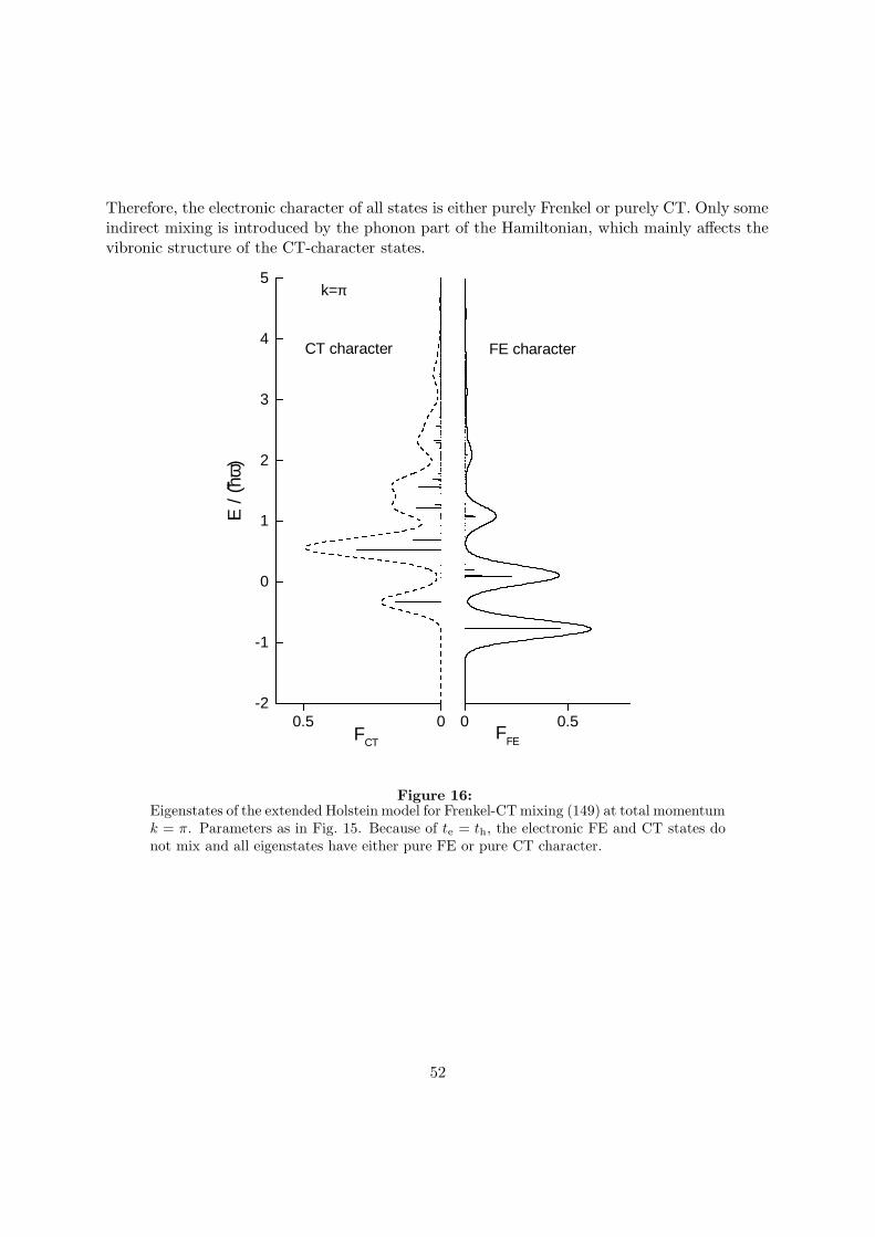
Therefore, the electronic character of all states is either purely Frenkel or purely CT. Only someindirect mixing is introduced by the phonon part of the Hamiltonian, which mainly affects thevibronic structure of the CT-character states.

0 0.5

FE character

FFE

-2

-1

0

1

2

3

4

5

0.5 0

CT character

k=π

FCT

E /

(hω)

Figure 16:Eigenstates of the extended Holstein model for Frenkel-CT mixing (149) at total momentumk = π. Parameters as in Fig. 15. Because of te = th, the electronic FE and CT states donot mix and all eigenstates have either pure FE or pure CT character.

52

4 Applications and consequences for quantum confinement

4.1 Description of PTCDA-derivatives

In Section 3.8, the energies Ej and transition dipoles Pj (Eq. (161)) of the eigenstates of theone-dimensional Holstein problem for mixed Frenkel-CT states were obtained. These quantitiesare essential but not yet sufficient for the description of a real absorption spectrum of a quasi-one-dimensional molecular crystal.

We still assume that all inter-stack interactions are on a much smaller energy scale than thein-stack interaction J . That means, the energy spectrum of the one-dimensional model is infirst approximation not affected. However, the direction of the transition dipoles is determinedby the complete three-dimensional crystal structure. In PTCDA and MePTCDI and manyother organic crystals, the unit cell contains two non-equivalent molecules. Then, the transitiondipoles of the non-equivalent molecules A and B couple and form two Davydov components(β = p, s) with orthogonal transition dipoles:

~Pjβ =~Pj(A) ± ~Pj(B)√

2. (162)

For the crystal structure of PTCDA and MePTCDI, the p-direction is given as the crystallo-graphic b axis. The s direction lies approximately in the (102) plane since the molecular planesof both inequivalent molecules are roughly parallel to the (102) plane (within 5◦ [84] for PTCDAand within 10◦ for MePTCDI, derived from [85]).

Knowing the transition dipoles per unit cell, the transverse dielectric constant for pertur-bation by an external light wave polarized along the β = p, s directions can be expressed as asum over the excited states (cf. e.g. [86, 4]):

ε0β(E) = 1 +8π

v

∑

j

~P 2jβEj

E2j −E2 − ihΓE

. (163)

Here, v is the volume of the unit cell and Γ−1 the life time of the excited states. Furthermore,the energies now have to be taken as the absolute energies with respect to the total ground state.Thus, the excitation energy E00 of our reference state (zero-phonon state of the molecular limit)has to be included.

Equation (163) is rigorous for any quantum system if all excited states are included. How-ever, we are considering only the lowest electronic excitation. Therefore, we include the contri-bution of the higher states (mixing of molecular configurations) by using a phenomenologicallymodified formula for the dielectric function:

εβ(E) = εbgβ +

8π

v

∑

j

(fbgβ~Pjβ)2Ej

E2j −E2 − ihΓE

. (164)

Here, εbgβ is a background dielectric constant that represents the value of εβ(0) correspond-

ing to a crystal in which the considered lowest electronic excitation would not exist. f bgβ is a

53

screening factor describing the modification of the acting field by the higher transitions. Fur-thermore, the higher transitions will modify the Frenkel exciton hopping integral J and therebyall the eigenstates of the system. Since we treat J as an effective fitting parameter anyway, theeffect of the higher transitions onto J is not important here but should be remembered in anymicroscopic interpretation of J . Such a background modification of the dielectric function wasdiscussed for a simple model system of one purely electronic Frenkel exciton in a cubic crystal inRef. [5]. In our general case, the effect of the higher transitions represented in the backgroundparameters is also anisotropic in nature.

The dielectric function (164) includes a Lorentzian broadening of the individual eigenstatesdue to a finite lifetime Γ−1. In a typical situation, however, there are several other sources ofa much larger broadening: (i) coupling to further low energy vibrations, (ii) splitting of thesingle effective vibrational mode, which actually consists of several nearly degenerate modes,and (iii) inhomogeneous broadening. To account for all these effects empirically, we replaceeach eigenstate of the Holstein model |Ψj〉 by a Gaussian distribution of states with standarddeviation σj as e.g. done in Ref. [87]. The individual broadenings σj have no microscopicmeaning and should be seen as no more than a convenient tool to compare the spectrum fromthe eigenstates of the Holstein model to an experimental spectrum. Practically, we assignedconstant values of σj for 4 separate regions of the spectrum in order to have only 4 differentbroadening parameters. The individual Lorentzian linewidth is assumed to be much smallerthan the σj and does not contribute anymore.

From the complex dielectric function (164), the complex refractive index (n + iκ)2 = εand the absorption coefficient α = 2E/(hc)κ can be calculated for the special light wavesthat propagate perpendicular to the p-s plane and are polarized along the p or s direction. Forgeneral directions, the complex rules of crystal optics would have to be considered. We note thatthe consideration of the absolute absorption coefficient is essential for describing the shape ofsolid state spectra. The microscopic models provide predictions only about the relative spectraldistribution of the transition dipoles, which determines the shape of the imaginary part ε2(E)of the dielectric function. The shape of the absorption spectrum α(E) however, is stronglyinfluenced by the variation of the refractive index in the absorption region (α = Eε2/(hcn)) andthe variation of n is again determined by the absolute absorption coefficient. Only if α is verysmall, as typically for spectroscopy of solutions (“dilute limit”), n does not vary and the shapeof the absorption spectrum is directly given by the distribution of the spectral weights (excitoncharacters).

For PTCDA and MePTCDI, it is possible to create vapor-deposited poly-crystalline filmswith a high preferential orientation such that the (102) crystal planes and thus approximatelythe p and s directions always lie parallel to the substrate. Only the azimuthal orientation, i.e.the orientation of the p and s directions within the substrate plane, is difficult to control.

In Ref. [41], low-temperature absorption spectra of such vapor deposited films were used toobtain model parameters for the Holstein Hamiltonian by fitting. The values for the monomerwere taken from the solution spectra (see Fig. 3): hω = 0.17 eV and g = 0.88 (for bothPTCDA and MePTCDI). For the electron and hole coupling parameters, ge = gh = g/

√2 was

used as in Section 3.8. Furthermore, only one value was used for the charge-transfer integrals:

54

t = te = th. This simplification is motivated, since for absorption only the value t+ = te + thenters the electronic problem (cf. the discussion below Eq. (39)) and since comparable values aresuggested by quantum chemical calculations (cf. Ref. [15]). Then, there remain four essentialparameters in the model Hamiltonian: Frenkel exciton transfer integral J , CT separation D,charge-transfer integral t, and the zero-point reference energy E00 of the molecular limit. Ithas to be noted that the electronic Frenkel-CT mixing at a given quasi-momentum k is onlydetermined by the absolute value of the transfer integrals (cf. Eqs. (32), (36)) and thus only|t| can be derived. The key-parameters obtained in Ref. [41] are for PTCDA:J = 42meV,D = 97meV, |t| = 42meV, E00 = 2.23 eV, and for MePTCDI:J = 46meV, D = 240meV,|t| = 57meV, and E00 = 2.13 eV.12

The structure of the corresponding eigenstate spectrum at k = 0 is best visualized by theFrenkel exciton character and the CT character of the states. We illustrate these characters inFigs. 17(b) and 18(b) in the same scheme as in Figs. 15 and 16. In these fits, the compositionof the optically active states at k = 0 shows a strong mixing of Frenkel and CT excitons. TheFrenkel character determines the absorption coefficient α. The comparison of the experimentalabsorption coefficient and the model fit is given in the panels (a). The characteristic differencebetween the absorption coefficient spectrum in (a) and the distribution of the Frenkel charactersin (b) is entirely caused by the spectral shape of the refractive index n, which becomes small atenergies above the major absorption region.

It has to be emphasized that the fitting parameters contain many uncertainties. In particularfor PTCDA, the absorption spectrum alone is not specific enough to determine the situationuniquely. Similarly good fits of the experimental spectra can be obtained for different parametersets with varying degree of CT mixing. Even total neglect of CT states would give a satisfactoryfit with a Frenkel transfer integral of 70meV. Such a value corresponds to the three-dimensionalFrenkel exciton model for PTCDA in Ref. [18] with a nearest-neighbor hopping of 82meV. ForMePTCDI, the absorption spectrum has a more characteristic shape with four main peaks. Thisspectrum can only be fitted within this framework by assuming a strong Frenkel-CT mixing.

The strongest support for the assumption of Frenkel-CT mixing is provided by the inter-pretation of electro-absorption rather than by linear absorption spectra [15, 17], since a pureFrenkel exciton model would not explain the strong response to electrical fields perpendicular tothe molecular planes. In Ref. [17], a three-dimensional version of a Frenkel-CT Hamiltonian (inthe molecular vibron approximation) was used to model electro-absorption spectra of PTCDA.The strongest effects were confirmed to arise from the one-dimensional stacks. Hamiltonianparameters could be obtained from fits and also confirmed by microscopic calculations. Theessential transfer parameters corresponding to our one-dimensional version were obtained asJ = 180meV, D = 130meV, t = −55meV [17]. These parameters from the electro-absorptionmodel essentially agree with our suggestion for the linear absorption spectra. The largest dis-crepancy is in the Frenkel exciton transfer integral J , where our smaller value mainly resultsfrom the use of a dielectric function.

Apart from the remaining uncertainty about the Frenkel-CT mixing, the obtained charge-

12In Ref. [41], the values of t+ were given.

55

transfer integrals would imply single-particle bandwidths 4te, 4th on the order of no more than0.2 eV, which is still smaller than the total exciton binding energy. Thus, the qualitative pictureis consistent with the approach of a small radius exciton theory (cf. discussion in Section 1).

We will now discuss following Ref. [88] what the proposed model for the absorbing states (k =0) means for the complete exciton band structure. In order to rationalize the k dependencies, wefirst concentrate on the purely electronic bands shown in Figs. 17(c) and 18(c). As in Section 3.7,the electronic bands are given by the purely electronic parts of the Holstein Hamiltonian (149):

Helec = HFEelec +HCT

elec +HFE−CTelec + g2hω . (165)

This electronic Hamiltonian corresponds to the electronic problem in Eq. (29), were the resultingbands and characters were visualized in Figs. (4) and (5). As for the Frenkel exciton case inSection 3.7, the Franck-Condon relaxation energy of the molecular zero-phonon state is addedbecause this state defines the reference energy. The electronic bands in the Holstein modelproposed for PTCDA and MePTCDI show that the electronic Frenkel character disperses tolower energies as a result of the positive Frenkel exciton hopping integral J . The center of massof the CT character remains at a constant position since a CT dispersion is not considered inthe model. Furthermore, for this special choice of charge-transfer integrals te = th, the Frenkeland CT states do not mix at k = π (see discussion below Eq. (39)).

The complete vibronic eigenstate structure at k = π is shown in Figs. 17(d) (PTCDA) and18(d) (MePTCDI). As at k = 0, the inclusion of exciton-phonon coupling at k = π transformsthe two electronic states into a broad vibronic spectrum. With the model parameters from theabsorption fit, the lowest k = π state lies at E = 2.18 eV for PTCDA and at E = 2.06 eV forMePTCDI.

56

0 51.4

1.6

1.8

2.0

2.2

2.4

2.6

2.8

abso

rptio

n

(a) (b) (c) (d) (e) (f)

exp

. fi

t

Exciton band structure scheme PTCDA

E [e

V]

α k=00 1

electronic bands

CT character

FE character

k/π k=π

04

03

02

01

00

Ej (k)

exp.

em

issi

on (

0...2

00 p

s)

emis

sion

from

k =

π

Iem

Figure 17:Suggested exciton band structure in PTCDA and experimental spectra. (a) solid line:experimental low temperature absorption spectrum of thin poly-crystalline film as reportedin Ref. [41], α in 105 cm−1; dotted line: α from model fit (plotted with offset +1×105 cm−1).(b) Vibronic model states at k = 0. The right side (dark shading) gives the Frenkelcharacter FFE j of the states j from Eq. (156), the left side the CT character FCT j fromEq. (158). Instead of the closely lying individual states, we show a broadened spectrum thatsummarizes the net contribution. The Frenkel character at k = 0 determines the oscillatorstrength and corresponds to the model absorption spectrum in (a). (c) Electronic bandsEj(k) corresponding to Eq. (165). These bands show the overall dispersion and the k-dependent Frenkel-CT mixing, which result from the electronic interaction parameters.(d) Vibronic model states for k = π. (e) Emission energies for transitions from the lowestk = π state to the vibrational levels of the electronic ground state. The highest transition(00) is strictly dipole-forbidden. (f) transient emission spectrum of a PTCDA single crystalat 10 K (time window 0 . . . 200 ps), from Ref. [88].

57

0 51.4

1.6

1.8

2.0

2.2

2.4

2.6

2.8

exp

. fi

t (a) (b) (c) (d) (e) (f)

Exciton band structure scheme MePTCDI

abso

rptio

n

E [e

V]

α k=00 1

CT character

FE character

electronic bands

k/π k=π

03

02

01

00

Ej (k)

exp.

em

issi

on (

0...2

00 p

s)

emis

sion

from

k =

π

Iem

Figure 18:Suggested exciton band structure in MePTCDI and experimental spectra. For detailedexplanations see Fig. 17. The experimental absorption spectrum in (a) is measured at 10 Kat a highly oriented poly-crystalline film with polarization parallel to the strong Davydovcomponent (crystallographic b-axis), cf. Ref. [16]. The transient emission spectrum in (f)is measured at 4 K at a single crystal, time window 0 . . . 200 ps, from from Ref. [88].

58

The band bottom of the exciton band structure is a starting point for the discussion ofemission spectra since all photo-excited states will rapidly relax to these lowest states. Thetransition from these k = π states to the total ground state is strictly dipole-forbidden, at leastin perfect crystals. However, transitions to k = π phonons in the electronic ground state areallowed. We indicate the resulting transition energies (including the forbidden 00-transition) inthe panels (e). For a qualitative comparison, these transition energies are compared to transientlow-temperature photoluminescence spectra of single crystals in the panels (f) of both figures.The comparison shows that the energetic positions of the 01 and 02 transition do approximatelyagree with the peaks in the emission spectra. This supports the order of magnitude of the modelparameters, especially the relatively small value of the Frenkel hopping J . A larger J , as couldbe expected from quantum chemical arguments and from models without dielectric function[15, 17], would give a larger separation between the lowest absorption peak and the 01-emissionpeak.

The assignment of the emission spectra still is very tentative, since the spectra do not showan exact vibronic progression and the decay times of the peaks are slightly different, whichbecomes much more pronounced at higher temperatures. Furthermore, the emission spectrasensitively depend on the concrete sample configurations, on the considered time scale (up tocw) and on the temperature. This leads to widely varying emission spectra and assignments.It is not clear at this stage to what extent extrinsic defects or further intrinsic effects determinethe emission behavior. In particular, a strong coupling to external phonon modes, correspond-ing to excimer emission, can be expected as an additional effect (cf. the explicit treatment forperylene in Ref. [89]). Such effects might be reasons for the discrepancies, which are particu-larly pronounced in the lowest PTCDA emission peak. A detailed discussion of time-resolvedPTCDA emission spectra was recently given in Refs. [90, 91]. These works are based on a pureFrenkel exciton band structure model within the molecular vibron approximation [18]. Thevarious spectral features and their temperature dependencies are explained by including thesmall interactions between the non-equivalent molecules, which leads to Davydov splitting ofthe exciton bands, and by considering vibrational relaxation along several different coordinates.

Since the fine details of the experimental emission spectra are very complex there is a largenumber of conceivable models for their interpretation. At present, there are not enough testsavailable that would allow independent confirmation of many model aspects. In particular,the complexity of model assumptions seems to be comparable to the complexity the explainedobservations. Therefore, it is very desirable to identify basic and unique features in the excitedstate structure of the considered class of materials. The exciton band structure within a Frenkel-CT-Holstein model provides such a unified framework for the description of absorption spectraand it is a starting point for a discussion of emission spectra and relaxation processes afterphoto-excitation.

4.2 Inclusion of finite size and quantum confinement effects

Up to here, the treatment of molecular crystals was presented for the case of an infinite chain.Real systems are always finite, and many systems of current interest cover the complete range of

59

one-dimensional chain lengths starting from a single molecule. For example, thin films consistingof one or just a few monolayers of PTCDA can be prepared by organic molecular beam epitaxy(OMBE) and they can be studied with spectroscopic methods (e.g. [7, 92]). Thus, it is importantto know down to which chain length N the picture of an infinite chain is still correct. It is evenmore important to investigate which qualitatively new effects can occur in finite systems. Wewill discuss these questions in the framework of the one-dimensional exciton models presentedin the previous sections.

The existence of a finite system size N affects all model descriptions at the very beginning.The starting point still is a model Hamiltonian expressed by on-site energies and interactionterms for localized excitations. However, the site index is restricted now (n = 1 . . . N) and theboundary conditions play a major role. Furthermore, the sites are not equivalent anymore andtherefore the on-site energies εFE and exciton transfer integrals J might have site-dependentvalues.

Let us illustrate the effects for the simplest example of the nearest-neighbor Frenkel excitonmodel from Eq. (16). In a finite chain, it can be written as:

HFENN(N) =

N∑

n=1

εFE(n)a†nan +N−1∑

n=1

J(n)(a†nan+1 + a†n+1an) . (166)

In this notation, the boundary conditions are expressed by the index range for the hoppingterm: Transfer from site n = 1 is only possible towards higher indices and transfer from siten = N only towards lower indices. Even if the site-dependence of εFE(n) and J(n) is neglected,the boundary conditions in Hamiltonian (166) do not allow the separation into non-mixingsubspaces with different quasi-momentum (Eq. (11)). Thus, a general diagonalization schemehas to work with basis states in real space. Even for a Frenkel-CT-Holstein model as in Eq. (149),a numerical diagonalization can be done in real-space along similar lines as presented for themomentum-space basis states, and only the number of basis states increases by a factor N .

The solutions of our example in Eq. (166) for constant εFE(n) = εFE and J(n) = J are wellknown (e.g. [93]). The N eigenstates have energies

Ej(N) = εFE + 2J cosπj

N + 1j = 1, 2, . . . N . (167)

The size dependence of the lowest and highest state energy is shown in Fig. 19. The differencebetween the highest and lowest state corresponds to the exciton bandwidth in the infinitesystem and it approaches its value ∆E = 4J for the limit N → ∞. For the dimer (N = 2),the bandwidth has already half of its maximum value. This size dependence results entirelyfrom the effect that the exciton is confined in its hopping motion by the system boundaries.Therefore, the effect can be approximately described by the picture of a ”particle in a box“.

We will illustrate this particle-in-a-box behavior by an alternative approach based on theeffective mass approximation (cf. also [94]): In the infinite system, the exciton states forHamiltonian (166) are entirely characterized by their dimensionless quasi-momentum k andtheir dispersion relation is (cf. Eq. (20))

Eeffk = εFE + 2J cos k . (168)

60

1 2 3 4 5 6

-2

-1

0

1

2

exact solution effective mass approx

(E -

εF

E )

/ J

N

Figure 19:Size dependence of the highest and lowest Frenkel exciton state in a linear nearest-neighborhopping model (Eq. (166)) for constant εFE and J . The “exact solution” shows the stateenergies from Eq. (167), the “effective mass approximation” shows the band edges fromEq. (171).

The effective mass of the exciton follows as

m−1eff =

a2

h2

∂2Eeffk

∂k2= −a

2

h2 × 2J cos k , (169)

where a is the lattice constant. We now treat this exciton as a real particle with mass meff ,which is confined within the chain. Thus, the wave function should be zero at the non-availablelattice positions n = 0 and n = N +1. This corresponds to a potential well of size L = (N+1)awith infinitely high boundaries. The ground state energy of the particle in such a well isπ2h2/(2meffL

2). This ground state energy corresponds to the energy shift ∆E eff that is inducedby the finite system size:

∆Eeff =π2h2

2meffL2. (170)

61

From Eqs. (168) and (170), the energy Eeffk (N) of the confined exciton follows as

Eeffk (N) = Eeff

k + ∆Eeff

= εFE + 2J cos(k) ×(

1 − 1

2

π2

(N + 1)2

)

(171)

We show this energy from the effective mass approximation for k = 0 and k = π in comparisonwith the exact energies in Fig. 19. The effective mass approximation works very good evendown to a chain length of N = 2, where the deviation is still only J(π2 − 9)/18 = 0.048J .

The comparison in Fig. 19 illustrates for the case of the one-dimensional Frenkel exciton:The effect of the finite system size can approximately be described by treating the exciton asa particle in a box, where the effective mass of the particle is given by the dispersion relation.This approach can be extended for the case that the exciton has a more complicated structure,i.e., if the localized basis states have additional internal degrees of freedom (cf. Section 2.1).Even in this case, the translational symmetry of the infinite system assures that the eigenstatescan be classified by their total momentum k and further quantum numbers for their internalstructure. The dispersion E(k) of a given state determines its effective mass and can therebycause a quantum size effect as given by Eq. (170). However, this simple picture obviously breaksdown if the internal structure of the exciton state is affected by changes of the system size. Sucha change must occur if the internal structure is related to a characteristic size (quantum length)of the exciton and the system size becomes comparable to or smaller than this intrinsic quantumlength.

For the simple Frenkel exciton in Fig. 19, there is no internal degree of freedom and thereforeno intrinsic quantum length. For the Merrifield model (see Eq. (24)) of one electron and one holeon a one-dimensional chain, the eigenstates do have an internal structure and a characteristiclength is given by the mean separation between electrons and holes. For the Holstein model(see Eq. (101)), an internal structure is introduced by the structure of the phonon cloud and acharacteristic quantum length follows from the extension of the lattice distortion 〈λm〉 aroundthe exciton (cf. Fig. 11). In all such cases with internal structure, one can therefore distinguishtwo finite size effects: (I) A quantum size effect according to Eq. (170) that results from theconfinement of the center-of-mass motion and (II) a quantum confinement effect that resultsfrom a confinement of the internal exciton structure.

A mathematically explicit version of the heuristic distinction between quantum size andquantum confinement effects is shown by Kayanuma for three dimensional Wannier-Mott exci-tons [95]. In this case, the intrinsic quantum length of the exciton is the electron-hole separationR. Kayanuma shows that for a system size L� R (“weak confinement” in the classification of

Kayanuma), the size dependence of the eigenstate energies is given by Eq. (170). For L<≈ R

(“strong confinement”), the internal structure of the exciton is drastically changed, and theeigenstates are rather characterized by the confinement of the single particles.

From this discussion we can conclude that the internal structure, more specifically theintrinsic quantum length R, of exciton states is crucial for estimating the effects of a finitesystem size. In the framework of the Frenkel-charge-transfer Holstein model (Eq. (149)) from

62

this chapter, there are three effects that give rise to an intrinsic quantum length:(I) Because of the CT states involved, one has a non-trivial electron-hole separation. How-

ever, since only nearest-neighbor CT states are included, this electron-hole separation has anupper limit of one lattice constant and quantum-confinement is of very limited interest.

(II) In a finite system, the subtle boundary conditions for CT states can lead to the ap-pearance of Tamm-like surface states [96]. These surface states have a decay length which isentirely given by the parameters in the Hamiltonian and which can be in the order of manylattice constants. Thus, this decay length has the nature of an intrinsic quantum length. Ifthe finite chain becomes smaller than the quantum length of the surface states, their internalstructure is changed, i.e. quantum-confinement occurs [97, 98].

(III) Exciton-phonon coupling leads to the appearance of phonon clouds, i.e., the excitonis surrounded by a lattice displacement 〈λm〉 (see Eq. (125)), which is illustrated for specificexamples in Figs. 11 and 13. For the scenario presented in Section 4.1, i.e., for the stronglycoupled internal vibrations in PTCDA derivatives, the phonon clouds have extensions not muchlarger than one lattice constant. However, one might also consider phonon modes which are notthat strongly coupled. With respect to such modes, one has the situation of strong electroniccoupling, and the approach of localized phonon clouds from Section 3 is not appropriate. Now,one can use the continuum model for large phonon clouds described by Rashba [99]. Thissituation was studied for Frenkel excitons by Agranovich et al. in Ref. [100]. The intrinsicquantum length (extension of the phonon cloud) in this case is R = Ja/(2g2hω),13 and Rcan easily become large for small coupling constants or small phonon energies. This results inquantum confinement effects, which are quantitatively discussed in Ref. [100].

In a realistic finite system, not only the quantum-size effect according to Eq. (170) and thequantum confinement effects (I)-(III) from above may occur, but also the possibility of site-dependent on-site and interaction energies should be considered as in Eq. (166). However, it isvery difficult to predict trends for the dependencies εFE(n), εCT(n), J(n), te/h(n).

A strong effect is expected for the variation of the on-site energy of the Frenkel exciton.For this case, at least some knowledge is available for the lowest transition in anthracene.The total gas-to-crystal shift is on the order of 2500 cm−1 (0.3 eV),14 whereas surface stateswere experimentally identified with energy differences to the bulk states of about 200 cm−1

(20meV) [101]. In Ref. [101], the energetic separation was interpreted as being mainly due tothe gas-to-crystal shift of the molecules from the outermost surface layer. The shift for thenext (sub-surface) layer was already considerably smaller. Thus, one can assume that εFE(n)is almost constant for n > 1, and even that the change at n = 1 is by far not as large as theupper limit given by the gas-to-crystal shift.

The on-site energy εCT of the CT states is strongly affected by the electronic polarizationof the surrounding molecules. Thus, close to the surface, strong changes of εCT(n) can beexpected. Modern microscopic calculations of polarization energies seem to allow estimationsfor this effect using a methodology that has already been applied for the polarization energy of

13This follows from Eq. (26) of Ref. [100]. Note that there the meaning of g is different.14The shift is given as the difference of the vapor-phase transition (27688 cm−1 taken from [101]) and the center

of the ‖ b and ⊥ b polarized crystal transitions (values taken from [4]).

63

ions in finite systems [102].The Frenkel transfer integral J is also strongly influenced by dielectric screening from the

surrounding molecules and therefore can be expected to change significantly close to the surface.Thus, one has to cope with a variety of different effects and unknown parameters and it is notsurprising that even for the experimentally well investigated case of PTCDA a coherent picturehas not been presented yet. Shifts in the absorptions spectra of PTCDA/NTCDA multilayerstructures [103] were initially interpreted as quantum-confinement (in the strict sense discussedabove) of Wannier-Mott excitons. However, a pure Wannier-Mott exciton picture seems not tobe adequate for PTCDA (see discussion in Section 4.1). An alternative interpretation for theshifts is given in terms of a varying contribution from the gas-to-crystal shift at the surface byAgranovich et al. in Ref. [104]. The situation becomes even more complicated due the possiblemixture of different crystal phases in thin layers [105]. Thus, a clear identification of quantumsize and quantum confinement effects in PTCDA-related quasi-one-dimensional crystals requiresconsiderably more information than currently available. In particular, one has to find ways inwhich the various contributing effects can be separately estimated from independent theoreticalor experimental methods.

64

5 Conclusion

In this chapter, we illustrated the application of basic exciton models for describing opticalspectra of quasi-one-dimensional molecular crystals. We concentrated on two essential effects:Mixing of electronic Frenkel and charge-transfer excitations and strong coupling to one internalmolecular vibration. For these models, we gave a comprehensive and self-contained discussionwith emphasis on illustrational examples.

In Section 2, the electronic states were described as one-dimensional collective excitationsconsisting of molecular excitations (Frenkel excitons) and nearest-neighbor charge-transfer ex-citations. This special case of the more general Merrifield model [32] seems to be suitable formolecular crystals that form stacks with close coplanar arrangement of the molecular planes.The essential parameters are given by the nearest-neighbor Frenkel transfer integral J , the sep-aration of the CT states from the molecular excitation D and the electron and hole transferintegrals te and th. The interplay of these parameters is illustrated in terms of band structureplots showing the two resulting bands and their mixed character. The mixing of two electronicstates can lead to two peaks in the absorption spectra — even if the CT states have a vanishingintrinsic transition dipole moment. This effect is one probable candidate for the explanationof broadening or peak-splitting in absorption spectra of quasi-one-dimensional crystals. Analternative explanation would be Davydov splitting due to Frenkel-type interactions of non-equivalent molecules. This Davydov splitting, however, is expected to be significantly smaller[16]. We also discussed the qualitative nature of the intrinsic CT transition dipole.

Section 3 considers strong coupling of the electronic excitations to internal molecular vi-brations, which is a typical feature in many molecules of current interest. This coupling ismost obvious in the vibronic progression in absorption spectra of isolated molecules. In aone-dimensional crystal, even the simplest model description for such exciton-phonon coupling(Holstein Hamiltonian) leads to a complicated many-particle problem that cannot be generallysolved. Here, we describe a numerical approach that is conceptually simple and allows thecalculation of optical spectra by standard numerical diagonalization tools. This approach isappropriate for weak electronic coupling and exciton-phonon coupling constants in the order ofone. This means in other words: The isolated molecules show a pronounced vibronic progression(0-0 and 0-1 peak of comparable height) and the spectral changes in the crystal concern onlyan energy range comparable to the range of the vibronic progression.

In Section 4, we outlined the application of the basic models to experimental spectra of thinorganic films. The first step is a realistic description of bulk optical constants. The capabilitesand limitations of the minium models are illustrated for spectra of two archetypal perylenederivatives. For very thin layers, a number of additional finite size and quantum confinementeffects can occur. We qualitatively discussed the nature of such effects in the framework ofour minimum model. A general distinction can be made on the basis of the internal excitonstructure. If, as in the pure electronic Frenkel case, the exciton has no internal structure,the finite system size leads to a simple particle-in-a-box behavior. This quantum size effectis still the leading effect if the system size is larger than any intrinsic length scale of a morecomplicated exciton. As soon as the system size affects the internal structure, we speak of

65

quantum confinement. Intrinsic quantum lengths responsible for quantum confinement canoccur in the idealized problem in two ways: (I) The electronic problem for Frenkel and CTstates can lead to surface states with a finite decay length. (II) Exciton-phonon coupling leadsto phonon clouds with finite extension around the electronic excitation. Further effects areexpected to arise from a site dependent modification of the Hamiltonian parameters.

At the present stage, there is still no general agreement about the specific interpretation ofexperimental spectra in terms of microscopic exciton models. Even in the case of bulk spectra,the available information is typically not sufficient for a unique parameterization. Furthermore,a comparison between different interpretations is often difficult since typically different aspectsare explained by different models. More certainty can be expected if not just single materialsare studied but general trends are investigated and described by a common framework.

6 Acknowledgments

Most of the material reviewed here is a result of fruitful collaborations that I enjoyed duringthe past years. The aspects of mixed Frenkel-CT excitons in Section 2 were developed togetherwith Vladimir M. Agranovich, Karin Schmidt and Karl Leo, and the exciton-phonon problemin Section 3 was investigated together with Zoltan G. Soos. I am very thankful to these col-laborators for their help and inspiration. To K. Schmidt I am also indebted for discussions onquantum confinement and for providing Fig. 7. I want to thank all members of the Institutfur Angewandte Photophysik at Technische Universitat Dresden for their support. Financialsupport by Deutsche Forschungsgemeinschaft is gratefully acknowledged.

References

[1] C. Kittel, Introduction to Solid State Physics, John Wiley & Sons, New York, 1996.

[2] E. V. Tsiper and Z. G. Soos, Phys. Rev. B 64 (2001) 195124.

[3] D. P. Craig and S. H. Walmsley, Excitons in Molecular Crystals, W. A. Benjamin, Inc.,New York, 1968.

[4] A. S. Davydov, Theory of Molecular Excitons, Plenum Press, New York, 1971.

[5] V. M. Agranovich and M. D. Galanin, Electronic Excitation Energy Transfer in CondensedMatter, North-Holland, Amsterdam, 1982.

[6] D. W. Schlosser and M. R. Philpott, J. Chem. Phys. 77 (1982) 1969.

[7] S. R. Forrest, Chem. Rev. 97 (1997) 1793.

[8] E. Umbach, K. Glockler, and M. Sokolowski, Surface Science 402-404 (1998) 20.

[9] C. W. Tang, Appl. Phys. Lett. 48 (1986) 183.

66

[10] P. Peumans, V. Bulovic, and S. R. Forrest, Appl. Phys. Lett. 76 (2000) 2650.

[11] D. Meissner and J. Rostalski, Synth. Met. 121 (2001) 1551.

[12] P. M. Kazmaier and R. Hoffmann, J. Am. Chem. Soc. 116 (1994) 9684.

[13] E. I. Haskal, Z. Shen, P. E. Burrows, and S. R. Forrest, Phys. Rev. B 51 (1995) 4449.

[14] V. Bulovic, P. E. Burrows, S. R. Forrest, J. A. Cronin, and M. E. Thompson, Chem. Phys.210 (1996) 1.

[15] M. H. Hennessy, Z. G. Soos, R. A. Pascal Jr., and A. Girlando, Chem. Phys. 245 (1999)199.

[16] M. Hoffmann, K. Schmidt, T. Fritz, T. Hasche, V. M. Agranovich, and K. Leo, Chem.Phys. 258 (2000) 73.

[17] G. Mazur, P. Petelenz, and M. Slawik, J. Chem. Phys. 118 (2003) 1423.

[18] I. Vragovic, R. Scholz, and M. Schreiber, Europhys. Lett. 57 (2002) 288.

[19] M. Sadrai, L. Hadel, R. R. Sauers, S. Husain, K. Krogh-Jespersen, J. D. Westbrook, andG. R. Bird, J. Phys. Chem. 96 (1992) 7988.

[20] M. Adachi, Y. Murata, and S. Nakamura, J. Phys. Chem. 99 (1995) 14240.

[21] G. Klebe, F. Graser, E. Hadicke, and J. Berndt, Acta Cryst. B45 (1989) 69.

[22] V. M. Agranovich, Theory of Excitons, Nauka, Moscow, 1968 (in Russian).

[23] J. Frenkel, Phys. Rev. 37 (1931) 17.

[24] J. Frenkel, Phys. Rev. 37 (1931) 1276.

[25] A. S. Davydov, Zh. Eksperim. i Teor. Fiz. 18 (1948) 210.

[26] D. P. Craig, J. Chem. Soc. (1955) 2302.

[27] V. Agranovich, Fizika Tverdogo Tela 3 (1961) 811 [Sov. Phys. - Solid State 3(1961), 592].

[28] V. M. Agranovich and Y. V. Konobeev, phys. stat. sol. 27 (1968) 435.

[29] D. Haarer and M. R. Philpott, ‘Excitons and polarons in organic weak charge transfercrystals’, in: V. M. Agranovich and R. M. Hochstrasser, (Eds.), Spectroscopy and Exci-tation Dynamics of Condensed Molecular Systems, North-Holland, Amsterdam, 1983, pp.27–82, Chapter 2.

[30] Z. G. Soos, Ann. Rev. Phys. Chem. 25 (1974) 121.

67

[31] L. E. Lyons, J. Chem. Soc. (1957) 5001.

[32] R. E. Merrifield, J. Chem. Phys. 34 (1961) 1835.

[33] J. P. Hernandez and S.-I. Choi, J. Chem. Phys. 50 (1969) 1524.

[34] W. L. Pollans and S.-I. Choi, J. Chem. Phys. 52 (1970) 3691.

[35] L. Sebastian and G. Weiser, Chem. Phys. 61 (1981) 125.

[36] L. Sebastian, G. Weiser, G. Peter, and H. Bassler, Chem. Phys. 75 (1983) 103.

[37] P. Petelenz, M. Slawik, K. Yokoi, and M. Z. Zgierski, J. Chem. Phys. 105 (1996) 4427.

[38] M. Slawik and P. Petelenz, J. Chem. Phys. 107 (1997) 7114.

[39] M. Slawik and P. Petelenz, J. Chem. Phys. 111 (1999) 7576.

[40] P. J. Bounds, P. Petelenz, and W. Siebrand, Chem. Phys. 63 (1981) 303.

[41] M. Hoffmann and Z. G. Soos, Phys. Rev. B 66 (2002) 024305.

[42] A. Szabo and N. S. Ostlund, Modern Quantum Chemistry, Dover Publications, Inc.,Mineola, New York, 1996.

[43] R. S. Mulliken, J. Amer. Chem. Soc. 74 (1952) 811.

[44] R. S. Mulliken and W. B. Person, Molecular Complexes. A Lecture and Reprint Volume,Wiley-Interscience, New York, 1969.

[45] H. Haken and H. C. Wolf, Molekulphysik und Quantenchemie, Springer-Verlag, Berlin,1994.

[46] D. B. Fitchen, ‘Zero-phonon transitions’, in: W. Fowler (Ed.), Physics of Color Centers,Academic Press, New York, 1968, pp. 294–350, , Chapter 5.

[47] V. L. Broude, E. I. Rashba, and E. F. Sheka, Spectroscopy of Molecular Excitons,Springer-Verlag Berlin, 1985.

[48] H. Haken, Quantum Field Theory of Solids, North Holland, Amsterdam, 1976.

[49] T. Holstein, Ann. Phys. 8 (1959) 325.

[50] T. Holstein, Ann. Phys. 8 (1959) 343.

[51] J. Appel, ‘Polarons’, in: F. Seitz, D. Trunbull, and H. Ehrenreich (Eds.), Solid StatePhysics. Advances in Research and Applications, Vol. 21, Academic Press, New York,1968, pp. 193–391, , Chapter 3.

68

[52] M. I. Klinger, Problems of Linear Electron (Polaron) Transport Theory, in: Semiconduc-tors, Pergamon Press, Oxford, 1979.

[53] H. Bottger and V. V. Bryskin, Hopping Conduction in Solids, VCH Weinheim, 1985.

[54] E. A. Silinsh and V. Capek, Organic Molecular Crystals. Interaction, Localization, andTransport Phenomena, AIP Press, New York, 1994.

[55] D. R. Yarkony and R. Silbey, J. Chem. Phys. 67 (1977) 5818.

[56] P. O. J. Scherer, E. W. Knapp, and S. F. Fischer, Chem. Phys. Lett. 106 (1984) 191.

[57] Y. Zhao, D. W. Brown, and K. Lindenberg, J. Chem. Phys. 106 (1997) 5622.

[58] A. H. Romero, D. W. Brown, and K. Lindenberg, Phys. Rev. B 60 (1999) 4618.



[61] A. H. Romero, D. W. Brown, and K. Lindenberg, J. Lum. 83-84 (1999) 147.

[62] A. S. Alexandrov, V. V. Kabanov, and D. K. Ray, Phys. Rev. B 49 (1994) 9915.

[63] G. Wellein, H. Roder, and H. Fehske, Phys. Rev. B 53 (1996) 9666.

[64] G. Wellein and H. Fehske, Phys. Rev. B 56 (1997) 4513.

[65] G. Wellein and H. Fehske, Phys. Rev. B 58 (1998) 6208.

[66] J. Bonca, S. A. Trugman, and I. Batistic, Phys. Rev. B 60 (1999) 1633.

[67] H. De Raedt and A. Lagendijk, Phys. Rev. Lett. 49 (1982) 1522.

[68] H. De Raedt and A. Lagendijk, Phys. Rev. B 27 (1983) 6097.

[69] H. De Raedt and A. Lagendijk, Phys. Rev. B 30 (1984) 1671.

[70] P. E. Kornilovitch and E. R. Pike, Phys. Rev. B 55 (1997) R8634.

[71] E. Jeckelmann and S. R. White, Phys. Rev. B 57 (1998) 6376.

[72] M. R. Philpott, J. Chem. Phys. 54 (1971) 111.

[73] R. E. Merrifield, Radiation Research 20 (1963) 154.

[74] P. O. J. Scherer and S. F. Fischer, Chem. Phys. 86 (1984) 269.

[75] N. Lu and S. Mukamel, J. Chem. Phys. 95 (1991) 1588.

69

[76] F. C. Spano and S. Siddiqui, Chem. Phys. Lett. 314 (1999) 481.

[77] F. C. Spano, J. Chem. Phys. 116 (2002) 5877.

[78] F. C. Spano, J. Chem. Phys. 118 (2003) 981.

[79] I. G. Lang and Y. A. Firsov, JETP (U.S.S.R.) 43 (1962) 1843.

[80] P. M. Morse and H. Feshbach, Methods of Theoretical Physics, McGraw-Hill, New York,1953.

[81] W. T. Simpson and D. L. Peterson, J. Chem. Phys. 26 (1957) 588.

[82] Z. G. Soos, S. Ramasesha, D. S. Galvao, and S. Etemad, Phys. Rev. B 47 (1993) 1742.

[83] S. Ramasesha, D. S. Galvao, and Z. G. Soos, J. Phys. Chem. 97 (1993) 2823.

[84] M. Mobus, N. Karl, and T. Kobayashi, J. Crystal Growth 116 (1992) 495.

[85] E. Hadicke and F. Graser, Acta Cryst. C 42 (1986) 189.

[86] F. Wooten, Optical Properties of Solids, Academic Press New York, 1972.

[87] R. Brendel, J. Appl. Phys. 71 (1992) 1.

[88] M. Hoffmann, Z. G. Soos, and K. Leo, Nonlinear Optics 29 (2002) 227.

[89] T.-W. Wu, D. W. Brown, and K. Lindenberg, Phys. Rev. B. 47 (1993) 10122.

[90] A. Y. Kobitski, R. Scholz, I. Vragovic, H. P. Wagner, and D. R. T. Zahn, Phys. Rev. B66 (2002) 153204.

[91] R. Scholz, I. Vragovic, A. Y. Kobitski, M. Schreiber, H. P. Wagner, and D. R. T. Zahn,phys. stat. sol. b 234 (2002) 402.

[92] E. Umbach, W. Gebauer, A. Soukopp, M. Bassler, and M. Sokolowski, J. Lum. 76-77(1998) 641.

[93] H. Fidder, J. Knoester, and D. A. Wiersma, J. Chem. Phys. 95 (1991) 7880.

[94] K. Schmidt, Electronic Excited States in Quasi-Onedimensional Organic Solids withStrong Coupling of Frenkel and Charge-Transfer Excitons, Ph. D. thesis, TU Dresden,2002.

[95] Y. Kayanuma, Phys. Rev. B 38 (1988) 9797.

[96] V. Agranovich, K. Schmidt, and K. Leo, Chem. Phys. Lett. 325 (2000) 308.

[97] K. Schmidt, Phys. Lett. A 293 (2002) 83.

70

[98] K. Schmidt, K. Leo, and V. M. Agranovich, ‘Surface states and quantum confinementin linear molecular chains with strong mixing of Frenkel and charge-transfer excitons’,in: V. M. Agranovich and G. C. L. Rocca (Eds.), Organic Nanostructures: Science andApplications. Proceedings of the International School of Physics ”Enrico Fermi”, CourseCXLIX, Varenna, 2001, IOS Press, Amsterdam, 2002, pp. 521–541.

[99] E. I. Rashba, ‘Self-trapping of excitons’, in: E. I. Rashba and M. D. Sturge (Eds.),Excitons, North-Holland, 1982, p. 543.

[100] V. M. Agranovich and A. M. Kamchatnov, Chem. Phys. 245 (1999) 175.

[101] J. M. Turlet, P. Kottis, and M. R. Philpott, Advan. Chem. Phys. 54 (1983) 303.

[102] E. V. Tsiper, Z. G. Soos, W. Gao, and A. Kahn, Chem. Phys. Lett. 360 (2002) 47.

[103] F. F. So, S. R. Forrest, Y. Q. Shi, and W. H. Steier, Appl. Phys. Lett. 56 (1990) 674.

[104] V. Agranovich, R. Atanasov, and G. Bassani, Chem. Phys. Lett. 199 (1992) 621.

[105] M. Leonhardt, O. Mager, and H. Port, Chem. Phys. Lett. 313 (1999) 24.

[106] T. W. Canzler, Ultrafast Dynamics in Quasi-One-Dimensional Organic Molecular Crys-tals. Self-Assembled Monolayers of Photochromic Molecules, Ph. D. thesis, TU Dresden,2002.

[107] HyperChem, Computational Chemistry (Manual), Hypercube, Inc., Waterloo, Ontario,Canada, 1996.

71

Mixing of Frenkel and Charge-Transfer Excitons and Their ...

Documents

Transcript of Mixing of Frenkel and Charge-Transfer Excitons and Their ...