Pattern Recognition 44 (2011) 330–349

Contents lists available at ScienceDirect

Pattern Recognition

0031-32

doi:10.1

� Corr

Box 823

E-m

adas.ge

journal homepage: www.elsevier.com/locate/pr

Mining data with random forests: A survey and results of new tests

A. Verikas a,b,�, A. Gelzinis b, M. Bacauskiene b

a Intelligent Systems Laboratory, Halmstad University, Box 823, S 301 18 Halmstad, Swedenb Department of Electrical & Control Equipment, Kaunas University of Technology, Studentu 50, LT-51368, Kaunas, Lithuania

a r t i c l e i n f o

Article history:

Received 18 December 2009

Received in revised form

2 August 2010

Accepted 7 August 2010

Keywords:

Random forests

Variable importance

Variable selection

Classifier

Data proximity

03/$ - see front matter & 2010 Elsevier Ltd. A

016/j.patcog.2010.08.011

esponding author at: Intelligent Systems Labo

, S 301 18 Halmstad, Sweden. Tel.: +46 35 16

ail addresses: antanas.verikas@hh.se (A. Verik

lzinis@ktu.lt (A. Gelzinis), marija.bacauskiene

a b s t r a c t

Random forests (RF) has become a popular technique for classification, prediction, studying variable

importance, variable selection, and outlier detection. There are numerous application examples of RF in

a variety of fields. Several large scale comparisons including RF have been performed. There are

numerous articles, where variable importance evaluations based on the variable importance measures

available from RF are used for data exploration and understanding. Apart from the literature survey in

RF area, this paper also presents results of new tests regarding variable rankings based on RF variable

importance measures. We studied experimentally the consistency and generality of such rankings.

Results of the studies indicate that there is no evidence supporting the belief in generality of such

rankings. A high variance of variable importance evaluations was observed in the case of small number

of trees and small data sets.

& 2010 Elsevier Ltd. All rights reserved.

1. Introduction

Growing size of data sets increases the variety of problemscharacterized by a large number of variables. Nowadays, it is notuncommon that the number of variables N is larger than thenumber of observations M. Microarray gene expression datais a characteristic example, where NbM most often. Traditionalstatistical techniques experience problems, when N4M.Therefore, machine learning-based techniques are usually appliedin such cases.

Support vector machine (SVM) [1,2], multilayer perceptron(MLP) [3], relevance vector machine (RVM) [4], and variousensembling approaches [5] are probably the most popularmachine learning techniques applied to create predictors. SVMand RVM make no assumptions about the data, are able to find theglobal minimum of the objective function, and can provide nearoptimal performance. Moreover, the complexity of these techni-ques depends on the number of support (relevance) vectors, butnot on the dimensionality of the input space. However, predictorsbased on these techniques provide too little insight as to theimportance of variables to the predictor derived. The transparencyis very important in some application areas, such as medicaldecision support or quality control, for example.

By contrast, classification and regression trees [6,7] are knownfor their transparency. However, decision trees are rather

ll rights reserved.

ratory, Halmstad University,

7140.

as),

@ktu.lt (M. Bacauskiene).

sensitive to small perturbations in the learning set. It has beendemonstrated that this problem can be mitigated by applyingbagging [8,9]. Random forests proposed by Breiman [10] andstudied by Biau et al. [11] is a combination of the randomsubspace method proposed by Ho [12] and bagging. RF have beenused for large variety of tasks, including: identification ofDNA-binding proteins [13], segmentation of video objects [14],classification of hyper-spectral data [15,16], prediction of thevegetation type occurrence in Belgian lowland valley based onspatially distributed measurements of environmental conditions[17,18], to predict distributions of bird and mammal speciescharacteristic to the eastern slopes of the central Andes [19],Czech language modeling in the lecture recognition task [20],diagnosing Alzheimer’s disease based on single photon emissioncomputed tomography (SPECT) data [21], genetic polymorphismsidentification [22], prediction of long disordered regions inprotein sequences [23], classification of agricultural practicesbased on Landsat satellite imagery [24], classification of aerialimages [25], analysis of phenolic antioxidants in chemistry [26],recognition of handwritten digits [27], categorizing time-depthprofiles of diving vertebrates [28], and many others.

2. Weak learners and random forests

Let us assume that given is a set of training dataX t ¼ fðxm,ymÞ,m¼ 1, . . . ,Mg, where xm is an input observationand ym is a predictor output. A weak learner can be created usingthe training set X t . A weak learner is a predictor f ðx,X tÞ having alow bias and a high variance [30]. By randomly sampling from the

A. Verikas et al. / Pattern Recognition 44 (2011) 330–349 331

set X t , a collection of weak learners f ðx,X t ,hkÞ can be created, withf ðx,X t ,hkÞ being the kth weak learner and hk is the random vectorselecting data points for the kth weak learner. By applyingbootstrap sampling to generate hk, for example, about two-thirdsof the data points are used by each weak learner. About one-thirdof the observations are out of the bootstrap sample or out-of-bag(OOB). The hk are independent and identically distributed, i.i.d.

It can be shown that combining i.i.d. randomized weaklearners into a committee by averaging, leaves the bias approxi-mately unchanged while reduces the variance by a factor ofrFthe mean value of the correlation between the weak learners[10]. Thus, if correlation and bias of i.i.d. randomized weaklearners are kept low, a big reduction in test set error can beobtained.

RF is a committee of weak learners for solving prediction (bothclassification and regression) problems. In RF, a decision tree, i.e.CART (classification and regression trees), is used as a weaklearner. When solving classification problems, the RF prediction isthe un-weighted majority of class votes. Fig. 1 presents a generalarchitecture of RF, where B is the number of trees in RF and k1, k2,kB, and k are class labels. As the number of trees in RF increases,the test set error rates converge to a limit, meaning that there isno over-fitting in large RFs [10]. Low bias and low correlation areessential for accuracy. To get low bias, trees are grown tomaximum depth. To achieve low correlation, randomization isapplied:

i.

Each tree of RF is grown on a bootstrap sample of the trainingset.

ii.

When growing a tree, at each node, n variables are randomlyselected out of the N available.

iii.

Usually, n5N. It is suggested starting with n¼ blog2ðNÞþ1c orn¼

ffiffiffiffiNp

and then decreasing and increasing n until theminimum error for the OOB data set is obtained. At eachnode, only one variable, providing the best split, is used out ofthe n selected.

In RF, n is the only parameter to be selected experimentally. RFcan handle thousands of variables of different types with manymissing values. For a tree grown on a bootstrap data, the OOB datacan be used as a test set for that tree. As the number of treesincreases, RF provides an OOB data-based unbiased estimate ofthe test set error. OOB data are also used to estimate importanceof variables. These two estimates (test set error estimate andvariable importance) are very useful byproducts of RF.

Fig. 1. A general architectu

2.1. Variable importance

There are four variable importance measures implemented inthe RF software code [29,30]. Two measures, based on the Giniindex of node impurity and classification accuracy of OOB data,are usually used.

Given a node t and estimated class probabilitiespðkjtÞ,k¼ 1, . . . ,Q , the Gini index is defined as [6]

GðtÞ ¼ 1�XQ

k ¼ 1

p2ðkjtÞ ð1Þ

where Q is the number of classes.To calculate the Gini index based measure, at each node the

decrease in the Gini index is calculated for variable xj used tomake the split. The Gini index-based variable importancemeasure Dj is then given by the average decrease in the Giniindex in the forest, where the variable xj is used to split a node.

The classification accuracy-based estimator of variable im-portance prevails in various studies. The measure computes themean decrease in classification accuracy of the OOB data. Havingbootstrap samples b¼1,y,B, the importance measure Dj forvariable xj is calculated as follows:

i.

re of

Set b¼1 and find the OOB data points Loobb .

ii.

Classify Loobb using the tree Tb and count the number of correct

classifications, Rboob.

iii.

For variables xj, j¼1,y,N:(a) permute the values of xj in Loob

b , the permutation resultsinto Loob

b,j ;(b) use Tb to classify Loob

b,j and count the number of correctclassifications, Rb,j

oob.

a ra

iv.

Repeat Steps i–iii for b¼2,y,B. v. The importance measure Dj for variable xj is then given by

Dj ¼1

B

XB

b ¼ 1

ðRoobb �Roob

b,j Þ ð2Þ

vi.

Compute the standard deviation sj of the decrease in correctclassifications and a z-score:

zj ¼Dj

sj=ffiffiffiBp ð3Þ

vii.

Assuming Gaussian distribution, covert zj to a significancevalue.

ndom forest.

A. Verikas et al. / Pattern Recognition 44 (2011) 330–349332

2.2. Data proximity matrix

The proximity matrix available from RF is a very usefulinformation source. To obtain the matrix, for each tree grown, thedata are run down the tree. If two observations xi and xj occupythe same terminal node of the tree, prox(i,j) is increased by one.When RF is grown, the proximities are divided by the number oftrees in RF. Data proximities can be used to replace missingvalues, to find outliers and mislabeled data, to visualize data byapplying the multidimensional scaling to the proximity matrix,for example.

3. Objectives of the study

Several researchers have found that RF error rates comparefavorably to other predictors, including logistic regression (LR), lineardiscriminant analysis (LDA), quadratic discriminant analysis (QDA),k-NN, MLP, SVM, classification and regression trees (CART), naiveBayes [10,31–33], and other techniques. However, contra-examplescan also be easily found [34], see Table 2. This is expected, sinceaccording to the No Free Lunch theorem [35], there is no singleclassifier model, which is best for all problems. In addition to aclassification or regression model, RF also provides an estimate ofvariable importance for the model. Variable importance estimates areoften used for data understanding. However, very few studies havebeen done to explore the adequacy of these estimates.

The objective of this work is twofold: to present a survey of RFapplications and to study some aspects related to variableimportance estimates available from RF. Four issues are consid-ered in the survey, namely, prediction accuracy, exploitation of RFto study variable importance, exploitation of RF data proximityestimates, and modifications of RF. Large scale studies includingRF we present in a separate section. Small scale studies aresummarized in several tables.

Our studies regarding variable importance evaluations arefocussed on the consistency and the generality of the variableimportance estimates provided by the measures Dj and Dj.Consistency reflects the stability of feature rankings uponvariations in parameters and procedure used to create RF. Bygenerality we mean the effectiveness of a set of featurescorresponding to highest values of the measures Dj and Dj inclassifiers of various types, including RF.

We also study the complexity of several classificationproblems providing diverse results when solved using RF andSVM. To assess the complexity, several measures of decisionboundary complexity studied in [36,37] are used. The aim of thesetests was to get some insights into ‘‘suitability’’ of a problem athand for RF-based classification.

4. Large scale studies including random forests

Meyer et al. investigated SVM performance and fulfilled a largescale comparison of 16 classification and nine regression techniques[38]. RF, SVM, MLP, and bagged ensembles of trees were among thetechniques compared. Hyper-parameters of RF, SVM, and MLP werecarefully selected. The classification benchmark was done on 21 datasets, while 12 data sets were used for the regression tests. Most ofthe data sets come from the UCI machine learning database. Theperformance was assessed using 10 times repeated 10-fold cross-validation. In the classification tasks, SVM always was ranked in thetop 3, except for two data sets. However, SVM was outperformed in10 out of 21 data sets. In the regression tasks, SVM was almost alwaysin the top 3. However, SVM was outperformed in all occasions, except2. The authors have found that MLP, RF, and projection pursuit

regression are good alternatives to SVM regression and often yieldedbetter performance than SVM.

Banfield et al. compared several decision tree ensemblecreation techniques against standard bagging [39]. Boosting[40], random subspaces [12], three types of random forests(exploiting 1, 2, and blog2ðNÞþ1c variables for node splitting) [10],and randomized C4.5 [9] have been used in the studies performedon 57 different data sets. For each technique, 1000 trees wereused to make an ensemble. The classification accuracy wasassessed using 10-fold and 5�2-fold [41] cross-validation. Thestatistical significance of differences in accuracy was assessedusing the t-test on results of the 10-fold cross-validation and theF-test for the 5�2-fold cross-validation. In addition to these tests,the techniques were compared on the multiple data sets bycomparing their average ranks [42]. The Friedman test [42] wasapplied to the ranks, to see if there is any statistically significantdifference between the algorithms for the data sets. For 37 of the57 data sets, none of the techniques showed statisticallysignificant improvement over bagging. Boosting with 1000 treesand RF with blog2ðNÞþ1c variables for node splitting appeared tothe best techniques (most wins over bagging and never losing).Boosting with only 50 trees was less accurate. RF with only twovariables showed the lowest average rank (the lower the rank thebetter the technique). The ranks of boosting with 1000 trees andRF with blog2ðNÞþ1c were close to the lowest rank.

Diaz-Uriarte and Alvarez de Andres [43] studied the ability of RF toselect a small set of genes retaining a high predictive accuracy. Geneselection was based on the OOB variable importance measureavailable from RF. The algorithm examined all forests resulting fromiterative elimination of a fraction of genes (0.2 for example) used inthe previous iteration. When tested on several microarray data setswith the number of genes ranging from 2000 to 9868, the algorithmwas able to find very small sets of genes and retain predictiveperformance. The classification accuracy obtained from RF wascomparable with that achieved by a linear SVM.

Inspired by work presented in [43], Statnikov et al. performedrigorous comparison of RF and SVM on 22 diagnostic andprognostic microarray data sets [34]. The data sets include50–308 samples and 2000–24,188 variables. RFs made of 500,1000, and 2000 trees were tested. The authors found that both onaverage and in the majority of the data sets SVM outperform RF,often by a large margin. The superiority of SVM was observed inboth settings: without gene selection and with several geneselection techniques. Classifier performance was evaluated usingreceiver operating curves (ROC) and area under the receiveroperating curves (AUC) for binary classification problems and therelative classifier information (RCI) [44] for multi-category tasks.RCI (entropy-based measure) evaluates how much the uncer-tainty in decision making is reduced by a classifier if comparedto classifying based only on the a priori class probabilities.Both AUC and RCI are not sensitive to unbalanced distributions.The average performance of SVMs was 0.775 AUC and 0.860 RCI,while the average performance of RFs was 0.742 AUC and 0.803RCI. The authors emphasize that the choice of RF parameters(the number of variables randomly selected at each node and thenumber of trees) creates large variation in RF performance. SVMwas much less sensitive to the choice of hyper-parameters.

5. Small scale studies including random forests

5.1. Accuracy related studies

There are a large number of small scale studies aiming tocompare the performance of several techniques on one or veryfew data sets. A large variety of application areas are explored.

A. Verikas et al. / Pattern Recognition 44 (2011) 330–349 333

Rigor of the comparisons varies greatly in different studies. Wesummarize results of these studies in two tables. Table 1 presentsa survey of studies where random forests outperformed or

Table 1A survey of studies where random forests outperformed or performed on the same lev

Area and techniques explored Study details & results

Customer churn prediction (RF, SVM, MLP, DT)

[45,46]

Data: from a Chinese b

smaller one contains ab

irrelevant or with mor

accuracy and AUC. The

Customer churn prediction (RF, LR, SVM) [47,48] Data: from a publishin

two classes, training se

both continuous and c

level) and accuracy

Credit card fraud detection (RF, SVM, kNN, LR,

QDA, CART, NB) [49]

Data: two data sets fro

contains about 30% of

training and 30% for te

Discrimination of fish populations using parasites

as biological tags (RF, MLP, LDA) [50]

Data: a set of 763 obse

Atlantic, 80% for trainin

of average accuracy, p

cross-validation

Automatic e-mail filing into folders (multi-class

problem) and spam e-mail filtering (two-class

problem) (RF CART, SVM, NB) [51]

Data: multi-class: five

6 very unbalanced clas

about 44% and 17% in

description, 256 contin

other techniques, in te

validation

Aircraft engine fault diagnosis (RF, MLP, SVM) [53] Data: a set of 19,635 o

continuous variables, s

features to split a node

when assessed by 5-fo

Bacterial species identification (RF, SVM, MLP) [54] Data: a set of 3012 ob

(961, 378, and 1673 ob

4 SVM and MLP in ter

by 10-fold stratified cr

Recognition of face images (RF, SVM) [55]. Data: a set of 2414 im

images) and evenly dis

accuracy of RF b SVM

Diagnosis of induction motor faults (RF, k-NN,

SVM, CART) [56]

Data: a set of 180 trai

classes), 63 continuous

accuracy. Best RF of 12

Classification of protein-localization patterns

within florescent microscope images (RF, SVM, DT)

[57]

Data: a set of 862 ima

Result: average accura

(56–86 trees) created u

20% were training and

Discrimination between acidic and alkaline

enzymes (RF, SVM, MLP, NB, k-NN, DT, Bayes net,

boosted ensemble, bagged ensemble) [58]

Data: a strictly screen

continuous variables c

all the other technique

validation

Forest areas prediction (RF, CART, MLP) [59] Data: a two-class (pres

continuous variables. Rlearning and 1/3 for te

Prediction of current and future tree distributions

(MARS, CART, BT, RF consisting of 1000 trees) [60]

Data: a regression (pre

characterized by 36 co

statistics, which measu

map B

Distinguishing between the chemical spaces of

metabolites and non-metabolites (RF, CART, CPNN)

[61]

Data: a two-class set o

continuous variables. Rby 10-fold cross-valida

Categorization of cancer cases (RF, multinomial

logit) [62]

Data: a four-class (4 c

proportions, collected

trees b multinomial l

Predicting the condition of vegetation across the

state of Victoria of Australia (RF, CART, MTRT, BT)

[63]

Data: a regression task

variables. Result: RF 4statistically significant

Friedman test [42]—te

Distinguishing between the diseased and non-

diseased eyes (RF, BT, boosted C4.5 trees) [64]

Data: a three-class (no

continuous variables g

techniques in terms of

Predicting partial defection by behaviorally loyal

clients (RF, ARDNN, LR) [65]

Data: two-class data c

categorical, but mainly

techniques in terms of

DT: decision tree; NB: naive Bayes; CCNN: cascade correlation neural network; 4: m

centroids [66]; MARS: multivariate adaptive regression splines; CPNN: counterpropa

relevance determination neural network [67,68]; and BT: bagged trees.

performed on the same level as other techniques. Table 2summarize studies where random forests were outperformed byother techniques.

el as other techniques.

ank, training and test sets each of 762 observations, two unbalanced classes, the

out 5% of the data, 27 continuous and categorical variables, 12 removed as being

e than 30% of missing values. Result: RF 4 all the other techniques in terms of

statistical significance not tested

g company on subscription renewal, training and test sets of 45,000 observations,

t is balanced, the smaller class of the test contains 11% of the data, 32 variables

ategorical [47]. Result: RF 4 SVM and LR in terms of AUC (significant at 95%

m two banks of about 47,000 observations each, two classes, the smaller class

the data, 87 and 91 continuous as well as categorical variables, 70% of data for

st. Result: RF 4 all the other techniques

rvations, � evenly distributed in five classes—different regions in the North East

g and 20% for test, 31 continuous variables. Result: RF 4 MLP and LDA, in terms

recision (specificity), and recall (sensitivity) when assessed by 10-fold stratified

users (data sets) with 545, 423, 888, 926, and 982 observations in 7, 6, 11, 19, and

ses, respectively; two-class: two data sets of 1099 and 2893 observations, with

the smaller class. IG technique [52] was used to select variables for text

uous variables. RF of 10 trees, 9 variables to split a node. Result: RF 4 all the

rms of accuracy, precision, and recall when assessed by 10-fold stratifiedcross-

bservations in 1 normal and 6 classes of faults, 2805 points in each class, 11

even binary classifiers one-against-all were used. Result: RF of 500 trees and 3

4 SVM, and CART, in terms of accuracy, false positive, and false negative rates

ld cross-validation, RF � MLP

servations represented by 105 continuous variables and coming from 3 classes

servations) or 213 classes. Result: RF of 1000–4000 trees (assessed on OOB data)

ms of AUC, sensitivity, and precision; performance of SVM and MLP was assessed

oss-validation

ages represented by 3584 or 3342 variables (gray values of pixels of resized

tributed in 38 classes. Training and test sets were of the same size. Result:

. Best RF consists of 500 trees and generated using 100 variables to split a node

ning samples, 90 test samples evenly distributed in 9 classes (normal an 8 fault

variables. Result: RF b than all the other techniques in terms of average

00 trees, 1 variable to split a node

ges approximately evenly distributed in 10 classes, 180 continuous variables.

cy of RF b than the other two techniques. Best were relatively small forests

sing a large number of variables (43–164) to split a node, 20/80, 50/50, and 80/

test set proportions explored

ed two-class data set of 105 acidic enzymes and 111 alkaline enzymes, 60

haracterizing the secondary structure of amino acid compositions Result: RF 4s in terms of accuracy, AUC, selectivity, and specificity, assessed by 10-fold cross-

ence and absence of given species) balanced data set of 16,510 observations, 14

esult: RF 4 MLP and CART in terms of AUC, when 2/3 of the data were used for

st. Best RF of 500 trees, 6 variables to split a node

dict the distribution of four tree species) data set of 9782 study cells

ntinuous variables. Result: RF and BT 4 CART and MARS, assessed by Kappa

res the level of agreement between the distribution of categories in map A and

f 6409 compounds, including 1811 metabolites and 4598 non-metabolites, 25

esult: RF of 1000 trees 4 CART and CPNN in terms of average accuracy, assessed

tion for CART and on OOB data for RF

ategories of cancer diagnosis) data set, with 54%, 34%, 7%, and 5% class

from 5608 subjects, 63 variables, many of which categorical. Result: RF of 500

ogit, in terms of average accuracy assessed by 8-fold stratified cross-validation

, 16,967 observations of ecological and remote-sensed data, 40 continuous

the other techniques. The difference in accuracy between RF and BT was not

according to the 10 times repeated 10-fold cross-validation and the corrected

st for the average ranks of the algorithms

rmal and 2 classes of diseases) set of 254 (119+36+99) observations, 15-121

iven by Zernike or pseudo-Zernike polynomials. Result: RF � the other

accuracy assessed by 10-fold cross-validation

ollected from 32,371 customers, the smaller class of 25%, 61 variables—several

continuous. Result: RF of 5000 trees and 8 variables to split a node � the other

accuracy and AUC assessed on a hold-out set of 50% of the data

ore accurate; � : approximately the same performance; NCS: nearest shrunken

gation neural network; MTRT: multi-target regression trees; ARDNN: automatic

Table 2A survey of small scale studies where random forests were outperformed by other techniques.

Area and techniques explored Study details & results

Recognition of five types of underwater plankton images (SVM, RF, C4.5, CCNN,

BT) [69]

Data: a 5-class problem (unbalanced classes) with 1285 binary images and a 6-class

problem (balanced classes) with 6000 binary images, 29 continuous variables

characterizing shape; Result: SVM 4 all the other techniques when assessed by

10-fold cross validation and a paired t-test at the 95% confidence level (for the 6-

class problem the difference between SVM and RF was not significant). BT and RF

consist of 100 trees and the default number of variables to split a node

Face recognition using Haar features (RF, SVM) [70] Data: a set of 464 images from 6 classes and a set of 40 images from 5 balanced

classes, 25 continuous features. Result: SVM 4 RF of 10 trees, in terms of

recognition accuracy, the way used to assess the accuracy not provided

Hyper-spectral remote sensing and geographic data classification (RF, ensemble

of SVMs) [71]

Data: a set of 2019 observations from 7 data channels (4 landsat channels, 1

elevation, 1 slope, and 1 aspect), 50% for training, 10 ground-cover classes,

continuous variables. Result: Ensembles of SVMs 4 RF in terms of average

accuracy

Spam email detection (CBART, LR, SVM, CART, NB, MLP, RF ranging from 10 to 500

trees) [72]

Data: a two-class problem, three data sets of 2893 (spam 16.6%), 1099 (spam

43.8%), and 4601 (spam 39.4%) observations, continuous variables—256 in the first

two sets and 57 in the third. Result: CBART 4 all the other techniques, in terms of

average error rate, confirmed by 10-fold cross-validation. The difference between

CBART and RF not significant. RF provided the highest AUC

Identification of strawberry cultivars from mass spectrometry data (RF, PDA,

DPLS) [73]

Data: a set of 233 observations, 9 classes (21 observations in the smallest class and

30 in the largest), 231 continuous variables. Result: Both techniques 4 RF with 15

variables to split a node, in terms of average accuracy assessed by LOO

Categorization of near infrared spectra of red grape homogenates (RF, PDA, MARS)

[74]

Data: a 3-class problem, a set of 284 spectra (original and transformed) made of

1024 sample wavelengths, 1024 continuous variables. Result: PDA and MARS 4 RF

in terms of accuracy. The number of trees in RF, the number variables used to split a

node, and the way to assess the accuracy not provided

Network intrusion detection (RF, ANFIS [75], LGP) [76] Data: a 5-class problem, a set of 5092 (1000+500+3002+27+563) training and

6890 test observations, 41 variables (categorical and continuous). Result: ANFIS

and LGP 4 RF generated by using 3 variables (a fixed number) to split a node, in

terms of accuracy. The number of trees in RF not provided

The task of diagnosing scrapie (disease) in sheep (18 classifiers including LDA, NB,

SVM, trees, BT, AdaBoost ensembles, RF) [77]

Data: a two-class data set of 3113 observations (83% in the scrapie class), 90% for

training and 10% for test, 100 random splits, 125 binary variables. Result: Pruned

J48 trees 4 RF and AdaBoost with unpruned J48 (significant difference at 95%

confidence level). Ensembles, including RF, were of 50 trees, the number of

variables used to split a node not provided

Rock glacier detection based on terrain analysis and multispectral remote sensing

data (LR, GLM, GAM, LDA, stabilized LDA, penalized LDA, SVM, BT, and RF) [78]

Data: a two-class problem, a data set of 2071 observations (only 86 in the rock

glacier class), 26 continuous variables. False-positive rates at sensitivity of 70% were

assessed by 100-repeated 5-fold cross-validation and compared. Result: PLDA,

GAM, GLM 4 RF of 200 trees, the number of variables used to split a node not

provided. Data over-fitting by RF was emphasized. A larger number of trees,

perhaps, could mitigate the problem

Customer loyalty prediction (RF, MLR, ARDNN) [79] Data: a regression task, a set of 878 observations, 35 variables several of them

categorical. Result: MLR with 4 variables 4 RF of 5000 trees and ARDNN (both

using all 35 variables), in terms of determination coefficient R2 and MSE, assessed

by the leave-one-out technique. MLR with 35 variables o RF with 35 variables

Predicting the chromatographic retention of basic drugs (RF, CART, TreeBoost,

PLS, GA-MLR) [80]

Data: a regression task, a set of 83 drugs, 1272 variables (molecular descriptors).

Result: Optimal RF of 600 trees, 382 variables to split a node. GA-MLR 4 RF, in

terms of determination coefficient R2, assessed by LOO or by using the OOB set (for

bagged and boosted models)

CBART: classification Bayesian additive regression trees; PDA: penalized discriminant analysis; PLS: partial least squares; DPLS: discriminant partial least squares; ANFIS:

adaptive-network-based fuzzy inference system; LGP: linear genetic programming; GLM: generalized linear models; GAM: generalized additive models; MLR: multiple

linear regression; GA-MLR: genetic algorithms-based multiple linear regression; and LOO: leave-one-out.

A. Verikas et al. / Pattern Recognition 44 (2011) 330–349334

It is interesting to note that in some cases, RF outperformed allother techniques used for comparisons, including SVM, by a largemargin. This was observed for problems characterized with bothrelatively large and small number of variables. The highestRF accuracy was sometimes achieved using the number ofvariables for node splitting, which deviated significantly, to bothdirections, from the approximate number, blog2ðNÞþ1c, suggestedby Breiman.

We found fewer examples, where RF were outperformed byother techniques. However, the variety of techniques outperformingRF was large, including multiple linear regression. It is worthmentioning that some comparisons may be biased, in the way thatwhen RF was applied for the first time in a specific application area,much effort was put to find the optimal forest size and the optimalnumber of variables used for node splitting, while selection ofparameters for other techniques was not so diligent.

5.2. Studies related to variable importance

In spite of the fact that variable importance measures availablefrom RF are widely used for data exploration, very few attemptswere made to study behavior of the measures. Below, we brieflysummarize the results of these studies.

Strobl et al. [81] studied the behavior of Dj, Dj, and the variableselection frequency-based measure on a set of artificial datawith one continuous and four categorical variables. The authorscame to a conclusion that the measures may give misleadingresults when variables are of different types or the number oflevels differ in different categorical variables. The Giniindex-based creation of classification trees is seen as the under-lying mechanism behind this deficiency. Gini index favorscontinuous variables or categorical variables with a large numberof levels.

A. Verikas et al. / Pattern Recognition 44 (2011) 330–349 335

Reif et al. [82] applied Dj of RF to identify relevant features insets of high-dimensional gene and protein data containing bothcategorical and continuous variables. A 100 data sets containingup to 1550 variables were generated for the studies. Randomforests of 10,000 trees were grown. In contrast to the findings ofStrobl et al. [81], the authors make a conclusion that randomforests are robust to noise and are able to identify relevantvariables of either type in high-dimensional data containingvariables measured on multiple scales.

Archer and Kimes [83] studied both Dj and Dj variableimportance measures using RF consisting of 2500 trees andmultivariate normal data generated by a linear regressionmodel. The degree of correlation between variables and thedegree of association of variables with the output were varied inthe study. The authors came to a conclusion that random forestsare attractive in settings with a large number of correlatedvariables. The authors indicate one drawback of the measure Dj inthe case of small data sets–a rather low resolution, which isapproximately equal to 3/M, with M being the number ofobservations.

In most of the studies surveyed in this article, evaluations ofvariable importance measures are directly used for data explora-tion, understanding, and interpretation. In some cases, suchinterpretations can be a point of contention, since correlationbetween variable rankings obtained using RF created underdifferent conditions can be rather low. For example, Okun andPriisalu [84] used RF for gene expression-based cancer classifica-tion and demonstrated that two forests, created using differentnumber of variables to split a node, may exhibit similar accuracyon the same data set, but correlation between the lists of variablesranked according to RF variable importance can be weak.Two very small data sets with 2000 and 822 genes (variables),and Gini index-based variable ranking were used in the experi-ment. The number of trees in the RF was set to 500. Table 3summarizes studies exploiting RF-based variable importanceevaluations.

5.3. Exploiting data proximity

Wang et al. [95] and Yang et al. [96] proposed an interestingdata classification approach based on the data proximity matrix.Classifier design and data classification proceeds as follows:

i.

Having a set XM�1 ¼ fx1, . . . ,xM�1g of training observations,create an RF.

ii.

Given an unknown observation xM, run a set XM ¼ fx1, . . . ,xM�1,xMg down the RF and create a proximity matrix prox(i,j)of size M�M.

iii.

Initialize the set of prediction classes Ge,tM ¼ |. iv. For j¼1 to Q (the number of classes) do:

(a) assume that j is the label of xM;(b) calculate scores a1,a2, . . . ,aM�1,aM for the set XM accord-

ing to the following rule:

ai ¼

PKk ¼ 1 prox�yi

ikPKk ¼ 1 proxyi

ik

, i¼ 1, . . . ,M ð4Þ

where yi is the class label of the observation xi, prox�yi

ik isthe jth largest proximity between xi and observationshaving different labels than yi, proxyi

ik is the jth largestproximity between xi and observations having label yi, andK is a user defined parameter;

(c) calculate py (confidence value) for the assumptionfxM Aclass jg according to the following equation:

py ¼jfi¼ 1, . . . ,M : ai4aMgjþtM jfi¼ 1, . . . ,M : ai ¼ aMgj

Mð5Þ

where tM is a uniformly distributed random number in[0,1].

(d) if py4e (significance level), Ge,tM :¼ Ge,tM [ j.

v. Output the classification result, Ge,tM .

Thus a set of possible classes and confidence values areobtained as a result of the classification. The authors applied theclassifier in the chronic gastritis diagnosis task, characterized by54 binary symptoms, using a data set collected from 709 subjects[95]. The number of trees included into the forest ranged from1000 to 10,000. A 10-fold cross-validation was used to assess theclassification accuracy. The technique significantly outperformedSVM, ordinary RF, and the Bayesian classifier.

Wiseman et al., aiming to visually explore data characterizingbenign and malignant thyroid tumors, applied multidimensionalscaling (MDS) to the data collected in the RF proximity matrix[97]. The MDS plot showed good separation between the benignand malignant cases. Spearman correlation between the Giniindex-based variable importance and the variable importanceevaluated with the Mann-Whitney U test [98] for the top 35variables (out of 57) was highly significant ðr¼ 0:764,po0:0001Þ.

Wu et al. [99] used RF to distinguish good chip delay testsignatures from bad chip delay test signatures as well as to detectoutliers in the post-silicon delay test data. The RF proximitymatrix was used to detect outliers. Gislason et al. [100] applied RFfor classification of remote sensing and geographic data, whereoutlier detection was also based on analysis of the RF proximitymatrix.

5.4. Modifications

There were several attempts to modify RF, aiming to increasethe prediction accuracy, to reduce the number of trees, or to makean online implementation. Gray and Fan [101] suggested usinggenetic algorithms (GA) for designing classification forests.Starting from randomly generated trees, genetic operations areapplied to evolve a forest with a low number of trees. Linearcombinations of two or three variables can be utilized for nodesplitting. Experimental tests on real data sets have shown that theforests evolved by GA are not as accurate as RF. Rodriguez et al.[102,103] proposed using rotation forests instead of RF. To createone of L base classifiers in a rotation forest, a feature set israndomly split into K (parameter of the technique) subsets, abootstrap sample set is selected for each subset and PCA isapplied. All PCs are retained and used as features to train theclassifier. It was found that rotation forests are more accuratethan RF and AdaBoost.

Tsymbal et al. [104] proposed using adaptive RF. Trees to beincluded into RF are dynamically selected for each observation.The proximity matrix is used to determine the trees to beincluded into RF. Voting and weighted voting aggregationschemes were explored. The local accuracy estimates are usedto determine weights in the case of weighted voting. Bothaggregation schemes showed rather similar performance andadaptive RFs were statistically significantly more accurate thanthe ordinary ones. Tripoliti et al. [105] used RF for diagnosingAlzheimer’s disease based on fMRI data. In addition to majorityvoting, different weighted voting schemes were explored.Weighted voting based on a distance between the unknown andtraining observations provided the best performance.

Leshem and Ritov suggested using RF as a weak learner in theAdaBoost algorithm [106]. The technique was applied to a trafficflow prediction task. However, no comparisons were performedwith an ordinary RF. Osman [107] proposed a technique for onlineRF design with incremental feature selection and demonstrated

Table 3A survey of studies exploiting random forests-based variable importance evaluations.

Techniques applied Task & results

Dj of RF applied to a set of 13 categorical variables [85] Task: ranking the importance of drivers, vehicles, and environment characteristics on crash

avoidance maneuvers of drivers; studied in a binary classification task—evasive actions or no

evasive actions of drivers. Result: rankings are useful for data exploration in 3 types of

collisions studied using three unbalanced data sets: rear-end collisions (10,867 observations),

head-on collisions (1105), and angle collisions (5878)

Based on Dj of RF applied to a set of 19 continuous and categorical

variables [86]

Task: discovering the most important factors for tooth loss/survival; studied in a binary

classification task. Result: obtained variable importance rankings make sense from a clinical

standpoint; data on 6463 teeth (from 355 subjects) were used, tooth loss observed for 17%

D j of RF, coefficients of MLR, and a of ARDNN (hyper-parameter for

each input variable reflecting variable importance) [79]

Task: Variable importance in the customer loyalty prediction task, 35 continuous and

categorical variables, see Table 2. Result: low correlation between variable importance values

obtained by the different techniques: the correlation coefficient r¼ 0:0886 between the MLR

and RF, and r¼ 0:1205 between the ARDNN and RF importance values

D j , Dj of RF applied to a set of 25 continuous variables [61] Task: variable importance for distinguishing between the chemical spaces of metabolites and

non-metabolites, see Table 1. Result: ‘‘the importance of descriptors was to a large extent in

accordance with the rules extracted by a single classification tree’’. Moderate agrement

between D j and Dj was observed

Dj of RF, multinomial logit-based backward and forward variable

selection [62]

Task: importance of 63 variables, many of which categorical, for categorizing cancer cases, see

Table 1. Result: seven of the top-ten variables were the same in both lists; the rank of

importance largely agreed with what could be expected based on experience and rationale

considerations

Dj of RF, a of ARDNN [65] Task: variable importance to predict partial defection by behaviorally loyal clients, 61

variables, several categorical, see Table 1. Result: the Spearman correlation coefficient

r¼ 0:313 between the rankings provided by the techniques. Six of the top-ten variables were

the same in both lists

Dj of RF [87,88] Task: variable selection in intrusion detection using a large balanced data set with 41

categorical and continuous variables. Result: elimination of 7 least important variables

allowed improving the detection accuracy. Selection result highly depends on a training set

D j of RF [89] Task: variable selection (from a set of 3629 wavelengthes) using a set of 641 observations for

hierarchical binary classification in infrared spectroscopy. Result: similarity of wavelength

regions selected by RF and regions selected by other authors using SVM and MLP was observed

Dj of RF [90] Task: variable selection for classification of mass spectrometry profiles in a prostate cancer

diagnosis task, 322 observations, thousands of variables. Result: iterative procedure to take

into account relations between variables, at each iteration 30% of the most important variables

were chosen

D j of RF [91] Task: variable importance evaluations to study issues affecting customer retention and

profitability, regression and binary classification tasks, 100,000 observations, 30 continuous

and categorical variables. Result: variable importance evaluations were found being useful for

exploring the data

Dj of RF [92] Task: identification of the most important identity markers when studying income

redistribution preferences across identity groups, 10 categorical variables, 13,024 observations.

Result: variable importance evaluations were found being useful for exploring the data

Dj of RF, Fisher’s Exact test [93] Task: identification of a small number of risk-associated single nucleotide polymorphisms

(SNPs) among large number of un-associated SNPs in complex disease models, two data sets of

1000 observations with 100 and 1000 ordinal variables. Result: when risk SNPs interact, Dj

significantly outperformed Fisher’s Exact test as an SNPs screening tool

Dj of RF [94] Task: to select features from a set of 304 continuous variables for electroencephalogram

classification, 98,160 observations. One-step feature selection was compared with recursive

feature elimination. Result: classification accuracy obtained from the recursive approach was

much higher than using the one-step procedure. The error rate decreased from 22.1%, when

using all variables, to 12.3%, when using 24 recursively selected variables

D j of RF [84] Task: a gene expression-based cancer detection task, a data set of 74 observations and 822

variables (genes) and a set of 62 observations and 2000 genes. Result: correlation between the

variable importance rankings obtained from RF, created using different number of variables to

split a node, can be weak

A. Verikas et al. / Pattern Recognition 44 (2011) 330–349336

that the online RF attains approximately the same performance asthe off-line counterpart.

6. New tests regarding variable importance measures

We used four public databases for these tests: Waveform,Satimage, Thyroid, and Wisconsin Diagnostic Breast Cancer—WDBC

(http://archive.ics.uci.edu/ml/).There are three classes of waves in the Waveform database [6]

with equal number of instances in each class, where each class isgenerated from a combination of 2 of 3 ‘‘base’’ waves. All of 40variables used include noise with mean 0 and variance 1. The later19 variables are all noise variables with mean 0 and variance 1.

The Satimage data set contains 6435 observations categorized intosix classes and represented by 36 features. The task in Thyroid

medical database is to decide whether the patient’s thyroidhas over-function, normal function, or under-function. It is a21-dimensional, three-class database containing 7200 examples.The class frequencies are 5.1%, 92.6%, and 2.3%, respectively. Thereare 30 real-valued features in the two-class WDBC problem.The features are computed from a digitized image of a fine needleaspirate of a breast mass and describe characteristics of the cellnuclei present in the image. There are 569 instances, 357 benignand 212 malignant.

The classification accuracy presented in this section is the averageaccuracy computed from 50 trials. In each trial, a data set wasrandomly split into learning—70% and test—30% subsets. The

A. Verikas et al. / Pattern Recognition 44 (2011) 330–349 337

statistical significance of difference in accuracy was assessed by usinga paired t-test at the 95% significance level.

We studied the consistency and generality of the variableimportance evaluations provided by Dj and Dj. In a finite samplecase, unimportant features usually degrade the performance of aclassifier. However, this sensitivity is different for differentclassifiers. It is well known that degradation in performanceoften accompanies addition of new, unimportant, equallyweighted features in k-NN classifiers. However, MLP and SVM,suffer from the ‘curse of dimensionality’ to a significantly lessextent than k-NN. The dependency of the test set classificationaccuracy on the number of features used by SVM and k-NNclassifiers to classify the Satimage data set, shown in Fig. 2,illustrates such behavior.

To create the plots, features were selected by the k-NN-basedforward selection and by taking features corresponding to the highestvalues of the Dj and Dj measures. Values of the measures werecomputed using RFs with the optimal number of trees and theoptimal number of features used for node splitting. Selected featureswere then used in k-NN and SVM classifiers. SVM was trained withthree different sets of features: selected by the k-NN, and according tothe Dj and Dj measures. Hyper-parameters of the SVM (regularizationconstant and width of the Gaussian kernel) were carefully selected bycross-validation. A mode can be clearly observed in the k-NN curve.However, there is no clear mode in the SVM plots. Therefore, wefocused on k-NN and RF classifiers, when studying the generality ofvariable importance evaluations provided by the Dj and Dj.

6.1. Results of the consistency studies

We assess the consistency by computing the width of theconfidence interval for the measures and by evaluating the averageSpearman correlation coefficients, rDj

and rDj, between rankings of

variables obtained in different experiments controlled by variousvalues of parameters governing the RF designing process.

6.1.1. Variance of the variable importance estimates

First, we studied the consistency using the artificial40-dimensional Waveform data. Previous tests of various variableselection techniques on this data set have shown that correctidentification of all the noise variables is not an easy task[108,109]. However, this was not the case for the Dj and Dj

10 15 288

88.5

89

89.5

90

90.5

91

91.5

92

92.5S

#

accu

racy

,%

SVM, features by

SVM, features by

k-NN, features b

SVM, features by

Fig. 2. The dependency of the test set classification accuracy of the SVM and k

rankings-based variable selection. Fig. 3 presents characteristicplots of average values of the Dj and Dj measures for the variableset. The plots were obtained by varying the number of trees in theforest from 900 to 1100, using 5000 observations to create RF, andusing blog2ðNÞþ1c variables to split a node. The figure alsoprovides the 95% confidence intervals for the measures, which arevery narrow and barely seen in the plots.

One can easily notice a clear difference between the variableimportance values computed for the pure noise and the relevantvariables. Observe that variables /1,2,20,21S are also almostequivalent to the noise variables. The measure Dj provides ahigher contrast between the pure noise and the relevant variablesthan Dj. The variance of the measures is very low. The variance ofthe measures remained low even when using a relatively smallnumber of trees in RF and/or a small number of observations.Fig. 4 (left) presents Dj computed by varying the number of treesin RF from 900 to 1100 and using 500 observations, while Fig. 4(right) plots Dj computed by varying the number of trees from50 to 150 and using 500 observations. As can be seen, the width ofthe confidence intervals remains very small even for smallnumber of trees and observations. The same behavior of themeasures was observed for the other data sets.

Next, we studied variability of the variable importance values byvarying the number of variables used to split a node when generatingRF. Fig. 5 plots the average values of Dj along with the 95% confidenceintervals computed for variables of the Satimage (left) and theWaveform (right) data sets when varying the number of variablesused to split a node. The number of features was varied from 4 to 20for the Satimage data set and from 6 to 25 for the Waveform data set.A 100 trees and 500 observations were used to create RFs.

As one can see, the confidence intervals are much wider and,for many variables of the Satimage data set, the difference invariable importance cannot be deemed as being statisticallysignificant. The same variability degree of the measures was alsoobserved for the other two data sets. Thus, variable importancerankings may, to a great extent, depend on the number ofvariables used to split a node when designing RF.

6.1.2. Correlation of the variable importance rankings

We studied correlation between rankings obtained by varyingthe number of trees in RF and the number of features used to splita node. Fig. 6 plots the average Spearman correlation coefficient

0 25 30 35

atimage

features

Dj, max AC = 92.14%

Δj : 92.13%

y k-NN, max AC = 91.36%

k-NN, max AC = 92.08%

-NN classifiers on the number of variables used for the Satimage data set.

0 10 20 30 400

0.01

0.02

0.03

0.04

0.05

0.06

0.07

feature

mag

nitu

de

0 10 20 30 400

50

100

150

200

250

300

350

400

feature

mag

nitu

de

Fig. 3. The average values of Dj (left) and D j (right) along with the 95% confidence intervals computed for variables of the Waveform data set using a large number of

observations and a large number of trees.

0 10 20 30 400

0.01

0.02

0.03

0.04

feature

mag

nitu

de

0 10 20 30 40

0

0.01

0.02

0.03

0.04

feature

mag

nitu

de

Fig. 4. The average value of Dj along with the 95% confidence intervals computed for variables of the waveform data set using a small number of observations (left) and a

small number of both trees and observations (right).

0 10 20 30

0

0.05

0.1

0.15

0.2

0.25

0.3

feature

mag

nitu

de

0 10 20 30 40

0

0.01

0.02

0.03

0.04

0.05

0.06

feature

mag

nitu

de

Fig. 5. The average values of Dj along with the 95% confidence intervals computed for variables of the Satimage (left) and the Waveform (right) data sets when varying the

number of variables used to split a node.

A. Verikas et al. / Pattern Recognition 44 (2011) 330–349338

400 800 1200 1600 200010

2030

0.88

0.9

0.92

0.94

0.96

0.98

1Satimage

# features

ρDj

# trees

Fig. 6. The average Spearman correlation coefficient rDjas a function of the number of trees in RF and the number of features used to split a node.

400800

12001600

20002400

051015202530

0.45

0.5

0.55

0.6

0.65

0.7

0.75

0.8

Satimage

# trees

ρ Dj

# features

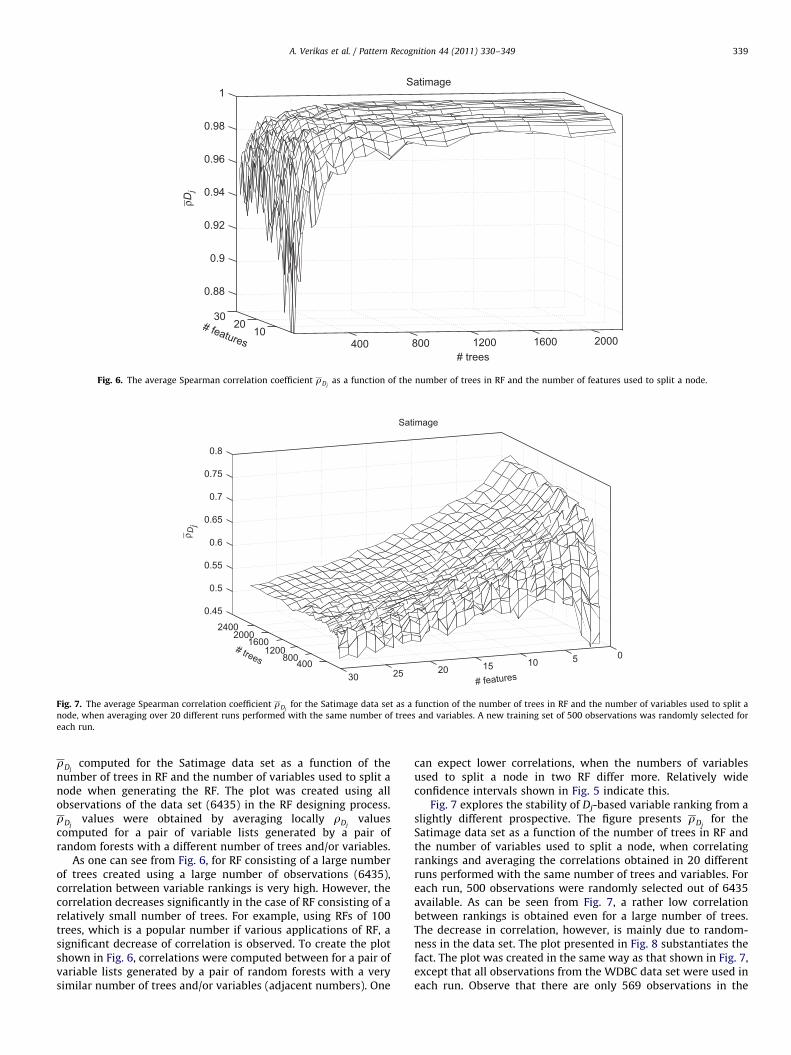
Fig. 7. The average Spearman correlation coefficient rDjfor the Satimage data set as a function of the number of trees in RF and the number of variables used to split a

node, when averaging over 20 different runs performed with the same number of trees and variables. A new training set of 500 observations was randomly selected for

each run.

A. Verikas et al. / Pattern Recognition 44 (2011) 330–349 339

rDjcomputed for the Satimage data set as a function of the

number of trees in RF and the number of variables used to split anode when generating the RF. The plot was created using allobservations of the data set (6435) in the RF designing process.rDj

values were obtained by averaging locally rDjvalues

computed for a pair of variable lists generated by a pair ofrandom forests with a different number of trees and/or variables.

As one can see from Fig. 6, for RF consisting of a large numberof trees created using a large number of observations (6435),correlation between variable rankings is very high. However, thecorrelation decreases significantly in the case of RF consisting of arelatively small number of trees. For example, using RFs of 100trees, which is a popular number if various applications of RF, asignificant decrease of correlation is observed. To create the plotshown in Fig. 6, correlations were computed between for a pair ofvariable lists generated by a pair of random forests with a verysimilar number of trees and/or variables (adjacent numbers). One

can expect lower correlations, when the numbers of variablesused to split a node in two RF differ more. Relatively wideconfidence intervals shown in Fig. 5 indicate this.

Fig. 7 explores the stability of Dj-based variable ranking from aslightly different prospective. The figure presents rDj

for theSatimage data set as a function of the number of trees in RF andthe number of variables used to split a node, when correlatingrankings and averaging the correlations obtained in 20 differentruns performed with the same number of trees and variables. Foreach run, 500 observations were randomly selected out of 6435available. As can be seen from Fig. 7, a rather low correlationbetween rankings is obtained even for a large number of trees.The decrease in correlation, however, is mainly due to random-ness in the data set. The plot presented in Fig. 8 substantiates thefact. The plot was created in the same way as that shown in Fig. 7,except that all observations from the WDBC data set were used ineach run. Observe that there are only 569 observations in the

400 800 1200 1600 2000 2400

0

10

20

300.85

0.9

0.95

1

Wisconsin Diagnostic Breast Cancer

# features

ρ Dj

# trees

Fig. 8. The average Spearman correlation coefficient rDjfor the WDBC data set as a function of the number of trees in RF and the number of features used to split a node,

when averaging over 20 different runs performed with the same number of trees and features.

0500

10001500

20002500

051015202530

0.75

0.8

0.85

0.9

0.95

1

Satimage

�Δj ↔

Dj

# trees# features

Fig. 9. The Spearmen correlation coefficient between variable rankings obtained by the two measures as a function of the number of trees in RF and the number of features

used to split a node for the Satimage data set.

A. Verikas et al. / Pattern Recognition 44 (2011) 330–349340

WDBC data set, but the correlation magnitude is much higher,especially for RF consisting of a large number of trees.

Plots presented in Figs. 9 and 10 explore correlation betweenvariable rankings based on the Dj and Dj variable importancemeasures. Fig. 9 plots the Spearmen correlation coefficientbetween variable rankings obtained by the two measures forthe Satimage data set. Fig. 9 shows that the two measures providevery similar variable rankings, especially when the number offeatures used to split a node is small. The same pattern ofcorrelations is also observed for the WDBC data set, see Fig. 10.

What observations can be made from the results of theconsistency studies?

i.

Variable importance rankings may, to a great extent, dependon the number of variables used to split a node when designingRF, especially when the number of trees in RF is small. This factshould not be forgotten when using variable importanceevaluations for data exploration and understanding. In manyapplications of RF, the number of variables used to split a node

is set to the default value given by blog2ðNÞþ1c orffiffiffiffiNp

and notoptimized. However, the optimal number of variables used tosplit a node may differ significantly from the default value.Thus, a rather different ranking of variables may be obtainedwhen using the optimal number of variables to split a nodeinstead of the default one.

ii.

Variable rankings obtained for the same data set from twolarge RFs designed using a similar number of variables to splita node are very similar.

iii.

For small data sets, variable importance evaluations obtainedfor unseen data can be rather different from those computedin the RF designing process.

iv.

Both measures, Dj and Dj, provide similar variable rankings.

6.2. Results of the generality studies

The effectiveness of a set of features corresponding to highestvalues of the measures Dj and Dj in SVM, k-NN, and RF classifierswas studied. Since variable rankings obtained using the two

05001000150020002500 051015202530

0.7

0.75

0.8

0.85

0.9

0.95

1

Wisconsin Diagnostic Breast Cancer

ρ Δj ↔

Dj

# trees # features

Fig. 10. The Spearmen correlation coefficient between variable rankings obtained by the two measures as a function of the number of trees in RF and the number of

features used to split a node for the WDBC data set.

10 15 20 25 30 3588

88.5

89

89.5

90

90.5

91

91.5Satimage

# features

accu

racy

, %

k-NN, features by k-NN, max AC = 91.36%k-NN, features by Dj elimination, max AC = 91.01%k-NN, features by Dj, max AC = 90.95%

Fig. 11. The dependency of the test set data classification accuracy of the k-NN classifier on the number of features selected by the different techniques for the Satimage

data set.

A. Verikas et al. / Pattern Recognition 44 (2011) 330–349 341

measures were highly correlated, we present here results only forthe Dj measure. Fig. 11 presents the dependency of the test setdata classification accuracy of the k-NN classifier on the numberof features selected by different techniques for the Satimage dataset. Three techniques have been applied for feature selection:k-NN-based forward selection (backward elimination providedsimilar results), selection by taking features corresponding tohighest values of the Dj measure, and recursive feature elimina-tion one-by-one based on Dj. The maximum achieved accuracy(AC) is also provided in the figure. As can be seen from Fig. 11, thek-NN-based forward feature selection outperformed the othertwo techniques. The difference in accuracy was statisticallysignificant for most of the feature sets. Similar results have alsobeen obtained for the WDBC and Thyroid data sets, presented inFigs. 12 and 13, respectively. Variables selected by the k-NNtechnique seems to be more general than the variables selectedaccording to the RF variable importance measure Dj. As can be

seen in Fig. 13, the accuracy of the k-NN classifier deterioratessignificantly when switching from feature sets selected by thek-NN technique to feature sets selected according to the variableimportance measure Dj.

One can expect the k-NN-based variable selection tooutperform the other variable selection techniques, sincein the case of k-NN, a classifier of the same type is used for bothvariable selection and classification. However, plots presented inFigs. 14–17 demonstrate that features selected by the k-NNtechnique are also efficient in SVM and RF classifiers.

Figs. 14 and 15 present the dependency of the test set dataclassification accuracy of the SVM classifier on the number offeatures selected by the different techniques for the WDBC andSatimage data sets, respectively. In the figures, ‘‘features by SVM’’refers to recursive forward feature selection based on SVMaccuracy. As can be seen from Figs. 14 and 15, for most of thefeature sets, SVM exploiting features selected using Dj performed

5 10 15 20 25 3088

90

92

94

96

98

100

#features

accu

racy

,%

Wisconsin Diagnostic Breast Cancer

k-NN, features by k-NN, max AC = 98.15%k-NN, features by Dj elimination, max AC = 97.51%k-NN, features by Dj, max AC = 97.44%

Fig. 12. The dependency of the test set data classification accuracy of the k-NN classifier on the number of features selected by the different techniques for the

WDBC data set.

2 4 6 8 10 12 14 16 18 2094.5

95

95.5

96

96.5

97

97.5

98

98.5

99Thyroid

# features

accu

racy

, % k-NN, features by k-NN, max AC = 98.92%

k-NN, features by Dj elimination, max AC = 98.53%

k-NN, features by Dj: 98.51%

Fig. 13. The dependency of the test set data classification accuracy of the k-NN classifier on the number of features selected by the different techniques for the

thyroid data set.

A. Verikas et al. / Pattern Recognition 44 (2011) 330–349342

significantly worse than the k-NN and SVM features-basedcounterparts.

In Figs. 16 and 17, ‘‘features by RF’’ refers to recursive featureelimination one-by-one based on RF accuracy. As expected, thiswas the best approach to feature selection when using RF as aclassifier. It is interesting to see that, for small feature sets, RFexploiting features selected by the k-NN technique was moreaccurate than the counterparts using features selected accordingto the Dj measure and the Dj measure-based recursive elimina-tion. For many of the feature sets the difference in accuracy wasstatistically significant.

SVM exploiting feature selected by the SVM provided thehighest classification accuracy for both Satimage and WDBCdata sets. Thus, it is interesting to see correlation betweenthe feature ranking obtained from the SVM-based featureselection and rankings produced by the Dj and Dj measures.

Fig. 18 presents the Spearman correlation coefficient ofsuch rankings for the Satimage data set as a function of thenumber of trees in RF and the number of features used to splita tree node. Though statistically significant, the correlations arenot high.

The following observations can be made from the generalitystudies:

i.

There is no evidence supporting the claim of high generality offeature subsets selected based on the Dj and Dj measures.

ii.

Feature subsets selected using the k-NN classifier-based forward or backward feature selection exhibit highergenerality and efficiency (in terms of classification accuracy)than feature subsets determined using the Dj and Dj

measures.

5 10 15 20 25 3092

93

94

95

96

97

98

99

# features

accu

racy

, %

Wisconsin Diagnostic Breast Cancer

SVM, features by SVM, max AC = 98.53%SVM, features by Dj elimination, max AC = 98.31%

SVM, features by Dj, max AC = 98.31% SVM, features by k-NN, max AC = 98.19%

Fig. 14. The dependency of the test set data classification accuracy of the SVM classifier on the number of features selected by the different techniques for the

WDBC data set.

10 15 20 25 30 3588

88.5

89

89.5

90

90.5

91

91.5

92

92.5Satimage

# features

accu

racy

, %

SVM, features by SVM, max AC = 92.19%SVM, features by Dj elimination, max AC = 92.19%SVM, features by Dj, max AC = 92.14%SVM, features by k-NN, max AC = 92.08%

Fig. 15. The dependency of the test set data classification accuracy of the SVM classifier on the number of features selected by the different techniques for the Satimage

data set.

A. Verikas et al. / Pattern Recognition 44 (2011) 330–349 343

iii.

The RF accuracy-based recursive feature selection is capable ofproviding a significantly higher classification accuracy thanfeature selection based on the Dj and Dj measures.

iv.

In problems where RF is outperformed by other techniques(by SVM for example), correlation between rankings offeatures in feature subsets providing the highest classificationaccuracy (feature subsets determined by SVM accuracy-basedrecursive forward feature selection, for example) and rankingsbased on the Dj and Dj measures can be rather low.

7. Tests concerning problem complexity

The aim of these studies is to get some insights into‘‘suitability’’ of a problem at hand for RF-based classification.To assess the problem complexity, several measures studied in[36,37] are used in this work. The measures are listed in Table 4.

The measures F1, F2, F3, and F4 reflect the degree of overlap ofindividual feature values, while the measures L1 and L2 assesslinear separability of classes. To compute values of the measuresL1, L2, and L3, a linear classifier is build. An SVM with a linearkernel trained by the sequential minimal optimization algorithm[110] is used to build the linear classifier in this work. Themeasures N1, N2, and N3 express mixture identifiability and areattributed to the class of measures reflecting separability ofclasses [37]. To describe geometry, topology, and density ofmanifolds spanned by different classes, measures L3, N4, T1, andT2 are used.

Fifteen data sets have been used in these studies. Three of thedata sets were used in our studies discussed in the previoussubsections, while the other twelve were taken from the literature[111,112]. Information on the data sets used in the experiment isgiven in Table 5. The table also provides the average test set dataclassification accuracy we obtained in the experiment for the SVM

10 15 20 25 30 3587.5

88

88.5

89

89.5

90

90.5

91

91.5Satimage

# features

accu

racy

, %

RF, features by RF, max AC = 91.49%RF, features by Dj elimination, max AC = 91.47%RF, features by Dj, max AC = 91.44%RF, features by k-NN, max AC = 91.49%

Fig. 16. The dependency of the test set data classification accuracy of the RF classifier on the number of features selected by the different techniques for the

Satimage data set.

5 10 15 20 25 3088

89

90

91

92

93

94

95

96

97

98

# features

accu

racy

, %

Wisconsin Diagnostic Breast Cancer

RF, features by RF, max AC = 97.54%RF, features by Dj elimination, max AC = 97.01%RF, features by Dj, max AC = 97.01%RF, features by k-NN, max AC = 96.66%

Fig. 17. The dependency of the test set data classification accuracy of the RF classifier on the number of features selected by the different techniques for the WDBC data set.

A. Verikas et al. / Pattern Recognition 44 (2011) 330–349344

and RF classifiers and the normalized difference in accuracy d. Theformalized difference is given by

d¼ASVM�ARF

100�Eð6Þ

where ASVM and ARF are the SVM and RF test set classificationaccuracy, and E is the average of the SVM and RF classificationerror. Hyper-parameters of SVM (width of the Gaussian kerneland the regularization parameter) and RF were carefully selectedwhen running the experiments. The RF accuracy was assessedusing the OOB data. To assess the SVM accuracy 80% of data wererandomly selected for training and 20% for validation. Theexperiment was repeated as many times as it was required toget 15,000 observations for validation in total. Then the averageclassification accuracy for these 15,000 observations was calcu-lated.

We have chosen to compare RF and SVM, since SVM is oftenconsidered as being one of the most successful types of classifiermodels. Values of the 13 problem complexity measures computed forthese data sets are given in Table 6. For multi-class problems, valuesof the measures were computed for pairwise binary classificationsand averaged. In the table are also given values of the correlationcoefficient R computed between the measures and the difference inaccuracy d. Values shown in bold indicate correlation significant atthe 90% confidence level. Thus, only four measures, F2, F3, N2, and T2out of 13 exhibit statistically significant correlations with thedifference in classification accuracy of the SVM and RF classifiers.The statistically significant negative correlation between the F3 and d

indicates that for problems with a large maximum efficiency ofindividual features, one can expect obtaining a higher accuracy fromRF than from SVM. The negative correlation of T2 and d shouldindicate that problems with a large number of observations per

01000

20003000 5 10 15 20 25

0.25

0.3

0.35

0.4

0.45

0.5

0.55

0.6

Satimage

ρ Δj ↔

SV

M, ρ

Dj ↔

SV

M

ρDj ↔ SVM

ρΔj ↔ SVM

# trees

# features

Fig. 18. The Spearman correlation coefficient between the feature ranking obtained from the SVM accuracy-based feature selection and rankings produced by the Dj and D j

measures as a function of the number of trees in RF and the number of features used to split a tree node.

Table 4A list of data complexity measures used.

F1: Maximum Fisher’s discriminant ratio

F2: Volume of overlap region

F3: Maximum (individual) feature efficiency

F4: Collective feature efficiency (sum of individual feature efficiencies)

N1: Fraction of points on class boundary

N2: Ratio of average intra/inter class nearest neighbor (NN) distance

N3: Leave-one-out error rate of 1-NN classifier

N4: Nonlinearity of 1-NN classifier

L1: Mean absolute training error of a linear classifier

L2: Error rate of a linear classifier

L3: Nonlinearity of a linear classifier

T1: Fraction of points with associated adherence subsets retained

T2: Average number of points per dimension

Table 5Test set data classification accuracy for the SVM and RF classifiers along with the normalized difference in accuracy.

N# Data set # Classes # Data # Features % SVM % RF Difference

1 Plankton [111] 5 8440 47 88.33 86.71 0.1299

2 Australian credit [112] 2 690 14 86.78 87.41 �0.0493

3 German credit [112] 2 1000 24 76.59 77.44 �0.0368

4 Pima diabetes [112] 2 768 8 77.26 76.68 0.0252

5 Vehicle silhouettes [112] 4 846 18 85.12 75.03 0.5063

6 Balance scale [112] 3 625 4 97.32 89.56 1.1828

7 Image segmentation [112] 7 2310 18 96.52 98.21 �0.6401

8 Optical digits [112] 10 5620 62 98.72 98.52 0.1480

9 WDBC original [38] 2 683 9 97.09 97.40 �0.1119

10 Heart disease [38] 2 296 13 82.21 82.22 �0.0009

11 Credit card [38] 2 653 15 87.20 87.90 �0.0562

12 Bupa liver [38] 2 345 6 72.27 74.17 �0.0710

13 Satimage 6 6435 36 92.12 91.49 0.0765

14 Thyroid 3 7200 21 98.16 99.66 �1.3768

15 WDBC 2 569 30 98.01 97.54 0.2102

A. Verikas et al. / Pattern Recognition 44 (2011) 330–349 345

dimension are more suitable for RF than SVM. However, the diverseresults obtained for the 6th and 14th data sets suggest that oneshould be careful with such a conclusion. Analysis of relation betweena linear combination of the four measures and the difference inaccuracy d does not provide much more insights into the results.

8. Discussion

Fast training, the possibility of obtaining the generalizationerror estimate without splitting the data set into learning andvalidation subsets, variable importance evaluations available as a

Table 6Values of the complexity measures computed for different data sets along with values of the correlation coefficient R between the measures and the difference

in accuracy d.

Data set F1 F2 F3 F4 N1 N2 N3 N4 L1 L2 L3 T1 T2

1 10.12 0.00 0.14 0.48 0.13 0.55 0.07 0.09 0.78 0.11 0.06 1.00 71.83

2 3.88 0.00 0.03 0.07 0.28 0.55 0.21 0.15 0.29 0.15 0.13 1.00 49.29

3 0.72 0.66 0.01 0.02 0.49 0.85 0.33 0.27 0.72 0.27 0.46 1.00 41.67

4 0.20 0.25 0.01 0.02 0.44 0.84 0.29 0.27 0.69 0.35 0.50 1.00 96.00

5 7.63 0.03 0.25 0.80 0.22 0.58 0.13 0.17 0.67 0.24 0.21 0.99 23.50

6 0.98 1.00 0.00 0.00 0.26 0.65 0.18 0.22 0.37 0.11 0.35 0.89 104.16

7 149.20 0.00 0.81 0.95 0.02 0.14 0.01 0.02 0.37 0.02 0.01 0.76 36.67

8 27.92 0.00 0.30 0.91 0.01 0.44 0.00 0.00 0.64 0.00 0.00 0.98 18.13

9 4.09 0.22 0.12 0.24 0.06 0.33 0.04 0.03 0.46 0.03 0.01 0.80 75.89

10 1.75 0.21 0.02 0.06 0.37 0.74 0.24 0.15 0.56 0.19 0.15 1.00 22.77

11 3.67 0.00 0.03 0.07 0.28 0.51 0.18 0.13 0.27 0.14 0.12 1.00 43.53

12 0.09 0.07 0.03 0.11 0.57 0.91 0.37 0.34 0.84 0.42 0.50 1.00 57.50

13 11.58 0.00 0.51 0.85 0.04 0.37 0.02 0.03 0.99 0.04 0.02 0.95 59.58

14 3.33 0.00 0.81 0.84 0.06 0.25 0.03 0.10 0.23 0.05 0.35 0.93 228.57

15 10.29 0.00 0.52 1.00 0.07 0.56 0.05 0.03 0.54 0.05 0.03 1.00 18.97

R �0.305 0.514 �0.573 �0.272 0.193 0.443 0.204 0.204 0.270 0.160 �0.010 0.222 �0.487

A. Verikas et al. / Pattern Recognition 44 (2011) 330–349346

byproduct of training, only one parameter to be tuned experi-mentally, make RF a very popular data mining technique.

8.1. Classification accuracy

Random forests have been applied in a variety of fields andtheir performance was compared to the performance of manyother popular techniques. As one can expect, both the few largescale comparisons and numerous small scale studies demonstratethat the superiority of RF over or loss to the other techniques isvery problem dependent. When studying the difference inaccuracy between RF and SVM classifiers, statistically significantcorrelations were found between several problem complexitymeasures and the difference in accuracy. However, the correla-tions are not very strong and do not allow making strongstatements.

8.2. Consistency of variable importance evaluations

Variable importance evaluations based on the variableimportance measures available from RF are widely used for dataexploration and understanding. Our experimental investigationshave shown that both measures, Dj and Dj, provide similarvariable rankings. The investigations have also shown that forlarge data sets, RF consisting of a large number of trees providesconsistent variable importance evaluations, exhibiting lowvariance and high correlation when varying the number of treesin RF. However, variable importance rankings may, to a greatextent, depend on the number of variables used to split a nodewhen designing RF, especially when the number of trees in RF issmall. This fact should not be forgotten when using variableimportance evaluations for data exploration and understanding.In many applications of RF found in the surveyed literature, thenumber of variables used to split a node is set to a default value,given by blog2ðNÞþ1c or

ffiffiffiffiNp

, without any further optimization.However, the optimal number of variables used to split a nodemay differ significantly from the default value. Thus, a ratherdifferent ranking of variables may be obtained when using theoptimal number of variables to split a node instead of the defaultone. On the other hand, one can expect obtaining very similarvariable rankings from two large RFs designed using the defaultand the optimal number of variables for node splitting,respectively, when the difference between these numbers issmall. One should also bear in mind that for small data sets, as it is

often the case with various RF applications, variable importanceevaluations obtained for unseen data can be rather different fromthose computed in the RF designing process.

8.3. Generality of variable importance evaluations

The results of experimental investigations concerning general-ity of variable importance evaluations indicate that there is noevidence supporting the belief in high generality of featuresubsets selected based on the Dj and Dj measures. In most ofthe cases, feature subsets selected using the k-NN classifier-basedforward or backward feature selection exhibited higher generalityand efficiency (in terms of classification accuracy) than featuresubsets determined using the Dj and Dj measures, especially forsmall feature subsets. Such superiority of the k-NN-based featureselection was observed even in the cases where RF was used as abase classifier. Thus, an unconditional belief in variable impor-tance evaluations available from RF seems to be not justified. Theexperimental tests have also shown that the RF accuracy-basedrecursive feature selection is capable of providing a significantlyhigher classification accuracy than feature selection based on theDj and Dj measures.

When studying feature subsets related to problems where RFwas outperformed by other techniques (by SVM for example), itwas found out that correlation between rankings of features infeature subsets providing the highest classification accuracy(feature subsets determined by SVM accuracy-based recursiveforward feature selection, for example) and rankings based on theDj and Dj measures can be rather low.

8.4. Designing issues

What issues are worth bearing in mind when designing and usingRF for solving a problem at hand? First, to avoid over-fitting, thenumber of trees in RF should be sufficiently large. The optimalnumber of features used for node splitting in the RF designing processis to be selected experimentally, rather than set to the default value,given by blog2ðNÞþ1c or

ffiffiffiffiNp

. Selection of salient variables for theproblem at hand should be based on advanced feature selectiontechniques, rather than on values of the Dj and Dj measures, availablefrom the RF designing process. The proximity matrix available fromRF is a very useful information source and can be used for dataexploration: to detect outliers and mislabeled data, to replace missingvalues, to visualize data by applying the multidimensional scaling to

A. Verikas et al. / Pattern Recognition 44 (2011) 330–349 347

the proximity matrix, for example. It is worth mentioning that noisyirrelevant features, which are not used in the final RF, do not have anyaffect on the proximity values.

Only one parameter to be tuned experimentally and thepossibility of obtaining the generalization error estimate withoutsplitting the data set into learning and validation subsets, makethe designing process of RF much faster than those of MLP or SVM.Computations in one grown tree are also very fast, since only onecomparison instruction is performed in each node of the tree. Thecomputation time in RF grows linearly with the increasingnumber of trees in RF. Computations in different trees of RF canbe easily parallelized, if required.

8.5. Challenges

Low correlation between RF trees and low RF bias are essential forRF accuracy. Thus, when aiming to improve the RF performance, RFdesigning techniques capable of reducing the average correlationbetween RF trees without increasing the RF bias is an interesting andchallenging research direction. Dynamic selection of relevant trees tobe included into RF of dynamic size can lead to RF, specific for eachobservation being analyzed and may help reducing the averagecorrelation. The proximity matrix available from RF can be animportant information source for designing data dependent RFs.Majority voting is the scheme applied in an ordinary RF to combinedecisions of single trees. Schemes for weighted voting using dynamic,data dependent aggregation weights is another promising area ofresearch aiming to improve the RF performance. The task of variableimportance evaluations, especially when variables of different typesare used to create RF, also needs more studies.

Bagging and random features are two types of randomnessusually used in the RF designing process. It is interesting toexplore other types of randomness, random Boolean combina-tions of features [10], for example. The size of bootstrap samplesin bagging does not necessary to be the same as that of theoriginal data set [11].

Acknowledgements

Useful suggestions from the referees are gratefully acknowl-edged. We acknowledge the support from the agency forInternational Science and Technology Development Programmesin Lithuania (COST Actions IC0602 and IC0806). The infrastructurefor parallel and distributed computing, and e-services (LitGrid)was used in the studies.

References

[1] V.N. Vapnik, Statistical Learning Theory, Wiley, New York, 1998.[2] J. Shawe-Taylor, N. Cristianini, Kernel Methods for Pattern Analysis,

Cambridge University Press, Cambridge, UK, 2004.[3] C.M. Bishop, Pattern Recognition and Machine Learning, Springer, Singa-

pore, 2006.[4] M.E. Tipping, Sparse bayesian learning and the relevance vector machine,

Journal of Machine Learning Research 1 (2001) 211–244.[5] A. Verikas, A. Lipnickas, K. Malmqvist, M. Bacauskiene, A. Gelzinis, Soft

combination of neural classifiers: a comparative study, Pattern RecognitionLetters 20 (1999) 429–444.

[6] L. Breiman, J.H. Friedman, R.A. Olshen, C.J. Stone, Classification andRegression Trees, Chapman & Hall, 1993.

[7] I.H. Witten, E. Frank, Data Mining: Practical Machine Learning Tools andTechniques with Java Implementations, Morgan Kaufmann, Los Altos, CA,1999 /http://www.cs.waikato.ac.nz/ml/wekaS.

[8] L. Breiman, Bagging predictors, Machine Learning 24 (2) (1996) 123–140.[9] T.G. Dietterich, An experimental comparison of three methods for

constructing ensembles of decision trees: bagging, boosting, and randomi-zation, Machine Learning 40 (2) (2000) 139–157.

[10] L. Breiman, Random forests, Machine Learning 45 (2001) 5–32.

[11] G. Biau, L. Devroye, G. Lugosi, Consistency of random forests and otheraveraging classifiers, Journal of Machine Learning Research 9 (2008)2015–2033.

[12] T.K. Ho, The random subspace method for constructing decision forests,IEEE Transactions on Pattern Analysis and Machine Intelligence 20 (8)(1998) 832–844.

[13] G. Nimrod, A. Szilagyi, C. Leslie, N. Ben-Tal, Identification of DNA-bindingproteins using structural, electrostatic and evolutionary features, Journal ofMolecular Biology 387 (4) (2009) 1040–1053.

[14] H.T. Chen, T.L. Liu, C.S. Fuh, Segmenting highly articulated video objectswith weak-prior random forests, in: A. Leonardis, H. Bischof, A. Pinz (Eds.),ECCV 2006, Part IV, Lecture Notes in Computer Science, vol. 3954, Springer-Verlag, Berlin, Heidelberg2006, pp. 373–385.

[15] J. Ham, Y. Chen, M.M. Crawford, J. Ghosh, Investigation of the random forestframework for classification of hyperspectral data, IEEE Transactions onGeoscience and Remote Sensing 43 (3) (2005) 492–501.

[16] M.M. Crawford, J. Ham, Y. Chen, J. Ghosh, Random forests of binaryhierarchical classifiers for analysis of hyperspectral data, in: 2003 IEEEWorkshop on Advances in Techniques for Analysis of Remotely Sensed Data,IEEE, Greenbelt, MD, USA2004, pp. 337–345.

[17] J. Peters, B. De Baets, N.E.C. Verhoest, R. Samson, S. Degroeve, P. De Becker,W. Huybrechts, Random forests as a tool for ecohydrological distributionmodelling, Ecological Modelling 207 (2007) 304–318.

[18] J. Peters, N.E.C. Verhoest, R. Samson, M. Van Meirvenne, L. Cockx, B. DeBaets, Uncertainty propagation in vegetation distribution models based onensemble classifiers, Ecological Modelling 220 (2009) 791–804.

[19] P.A. Hernandez, I. Franke, S.K. Herzog, V. Pacheco, L. Paniagua, H.L. Quintana,A. Soto, J.J. Swenson, C. Tovar, T.H. Valqui, J. Vargas, B.E. Young, Predictingspecies distributions in poorly-studied landscapes, Biodiversity and Con-servation 17 (2008) 1353–1366.

[20] I. Oparin, O. Glembek, L. Burget, J. Cernocky, Morphological random forestsfor language modeling of inflectional languages, in: 2008 IEEE Workshop onSpoken Language Technology, SLT 2008, IEEE, Goa, India2008, pp. 189–192.

[21] J. Ramirez, J.M. Gorriz, R. Chaves, M. Lopez, D. Salas-Gonzalez, I. Alvarez, F.Segovia, SPECT image classification using random forests, ElectronicsLetters 45 (12) (2009) 604–605.

[22] A.G. Heidema, J.M.A. Boer, N. Nagelkerke, E.C.M. Mariman, D.L. van der A,E.J.M. Feskens, The challenge for genetic epidemiologists: how to analyzelarge numbers of SNPs in relation to complex diseases, Accident Analysisand Prevention 7 (23) (2006) 1–15.

[23] P. Han, X. Zhang, R.S. Norton, Z.P. Feng, Large-scale prediction of longdisordered regions in proteins using random forests, BMC Bioinformatics 10(8) (2009) 1–9.

[24] J.D. Watts, R.L. Lawrence, P.R. Miller, C. Montagne, Monitoring of croplandpractices for carbon sequestration purposes in north central montana bylandsat remote sensing, Remote Sensing of Environment 113 (2009)1843–1852.

[25] S.R. Joelsson, J.A. Benediktsson, J.R. Sveinsson, Feature selection formorphological feature extraction using random forests, in: Seventh NordicSignal Processing Symposium, IEEE, New York, Reykjavik, Iceland2006, pp.138–141.

[26] S. Gupta, S. Matthew, P.M. Abreu, J.A. de Sousa, QSAR analysis of phenolicantioxidants using MOLMAP descriptors of local properties, Bioorganic &Medicinal Chemistry 14 (2006) 1199–1206.

[27] S. Bernard, L. Heutte, S. Adam, Using random forests for handwritten digitrecognition, ICDAR 2007: Ninth International Conference on DocumentAnalysis and Recognition, vol. 1–2, Curitiba, Brazil2007, pp. 1043–1047.

[28] M. Thums, C.J.A. Bradshaw, M.A. Hindell, A validated approach forsupervised dive classification in diving vertebrates, Journal of ExperimentalMarine Biology and Ecology 363 (2008) 75–83.

[29] A. Liaw, M. Wiener, Classification and regression by random forest, R News2 (3) (2002) 18–22.

[30] L. Breiman, RFtools—for predicting and understanding data, TechnicalReport, Berkeley University, Berkeley, USA /http://oz.berkeley.edu/users/breiman/RandomForests/cc.papers.htmS, 2004.

[31] V. Svetnik, A. Liaw, C. Tong, J.C. Culberson, R.P. Sheridan, B.P. Feuston,Random forest: a classification and regression tool for compoundclassification and QSAR modeling, Journal of Chemical Information andComputer Sciences 43 (6) (2003) 1947–1958.

[32] V. Svetnik, T. Wang, C. Tong, A. Liaw, R.P. Sheridan, Q.H. Song, Boosting:an ensemble learning tool for compound classification and QSARmodeling, Journal of Chemical Information and Modeling 45 (3) (2005)786–799.

[33] A. Folleco, T.M. Khoshgoftaar, J. Van Hulse, L. Bullard, Software qualitymodeling: the impact of class noise on the random forest classifier, 2008IEEE Congress on Evolutionary Computation, vol. 1–8, IEEE, Hong Kong, PRChina2008, pp. 3853–3859.

[34] A. Statnikov, L. Wang, C.F. Aliferis, A comprehensive comparison of randomforests and support vector machines for microarray-based cancer classifica-tion, BMC Bioinformatics 9 (319) (2008) 1–10.

[35] R.O. Duda, P.E. Hart, D.G. Stork, Pattern Classification, second ed., JohnWiley & Sons, New York, 2001.

[36] T.K. Ho, A data complexity analysis of comparative advantages ofdecision forest constructors, Pattern Analysis and Applications 5 (2002)102–112.

A. Verikas et al. / Pattern Recognition 44 (2011) 330–349348

[37] T.K. Ho, M. Basu, Complexity measures of supervised classificationproblems, IEEE Transactions on Pattern Analysis and Machine Intelligence24 (3) (2002) 289–300.

[38] D. Meyer, F. Leisch, K. Hornik, The support vector machine under test,Neurocomputing 55 (1–2) (2003) 169–186.

[39] R.E. Banfield, L.O. Hall, K.W. Bowyer, W.P. Kegelmeyer, A comparison ofdecision tree ensemble creation techniques, IEEE Transactions on PatternAnalysis and Machine Intelligence 29 (1) (2007) 173–180.

[40] Y. Freund, R.E. Schapire, Experiments with a new boosting algorithm, in:Proceedings of the 13th International Conference on Machine Learning,1996, pp. 148–156.

[41] E. Alpaydin, Combined 5�2 cv F test for comparing supervised classifica-tion learning algorithms, Neural Computation 11 (8) (1999) 1885–1892.

[42] J. Demsar, Statistical comparisons of classifiers over multiple data sets,Journal of Machine Learning Research 7 (2006) 1–30.

[43] R. Diaz-Uriarte, S. Alvarez de Andres, Gene selection and classification ofmicroarray data using random forest, BMC Bioinformatics 7 (3) (2006)1–13.

[44] V. Sindhwani, P. Bhattacharyya, S. Rakshit, Information theoretic featurecrediting in multiclass support vector machines, in: R. Grossman, V. Kumar(Eds.), Proceedings of the First SIAM International Conference on DataMining, SIAM, Chicago, USA2001, pp. 1–18.

[45] Y. Xie, X. Li, E.W.T. Ngai, W. Ying, Customer churn prediction usingimproved balanced random forests, Expert Systems with Applications 36(2009) 5445–5449.

[46] W. Ying, X. Li, Y. Xie, E. Johnson, Preventing customer churn by usingrandom forests modeling, in: IEEE International Conference on InformationReuse and Integration (IRI-2008), IEEE, Las Vegas, USA2008, pp. 429–434.

[47] K. Coussement, D. Van den Poel, Churn prediction in subscription services:an application of support vector machines while comparing two parameter-selection techniques, Expert Systems with Applications 34 (2008) 313–327.

[48] K. Coussement, D. Van den Poel, Improving customer attrition prediction byintegrating emotions from client/company interaction emails and evaluat-ing multiple classifiers, Expert Systems with Applications 36 (2009)6127–6134.

[49] C. Whitrow, D.J. Hand, P. Juszczak, D. Weston, N.M. Adams, Transactionaggregation as a strategy for credit card fraud detection, Data Mining andKnowledge Discovery 18 (1) (2009) 30–55.

[50] D. Perdiguero-Alonso, F.E. Montero, A. Kostadinova, J.A. Raga, J. Barrett,Random forests, a novel approach for discrimination of fish populationsusing parasites as biological tags, International Journal for Parasitology 38(2008) 1425–1434.

[51] I. Koprinska, J. Poon, J. Clark, J. Chan, Learning to classify e-mail, InformationSciences 177 (2007) 2167–2187.

[52] C. Manning, H. Schutze, Foundations of Statistical Natural LanguageProcessing, MIT Press, Cambridge, MA, USA, 1999.

[53] W. Yan, Application of random forest to aircraft engine fault diagnosis, in:IMACS Multiconference on Computational Engineering in Systems Applica-tions (CESA), IEEE, Beijing, PR China2006, pp. 468–475.

[54] B. Slabbinck, B. De Baets, P. Dawyndt, P. De Vos, Towards large-scale FAME-based bacterial species identification using machine learning techniques,Systematic and Applied Microbiology 32 (2009) 163–176.

[55] A.Z. Kouzani, Faceparts for recognition, in: TENCON 2006–2006 IEEE Region10 Conference, IEEE, Hong Kong, PR China2006, pp. 1232–1235.

[56] B.S. Yang, X. Di, T. Han, Random forests classifier for machine faultdiagnosis, Journal of Mechanical Science and Technology 22 (2008)1716–1725.

[57] A.Z. Kouzani, Subcellular localisation of proteins in fluorescent microscopeimages using a random forest, 2008 IEEE International Joint Conference onNeural Networks, vol. 1–8, IEEE, Hong Kong, PR China2008, pp. 3926–3932.

[58] G. Zhang, H. Li, B. Fang, Discriminating acidic and alkaline enzymes using arandom forest model with secondary structure amino acid composition,Process Biochemistry 44 (2009) 654–660.

[59] M.B. Garzon, R. Blazek, M. Neteler, R.S. de Dios, H.S. Ollero, C. Furlanello,Predicting habitat suitability with machine learning models: the potentialarea of Pinus sylvestris L. in the Iberian peninsula, Ecological Modelling 197(2006) 383–393.

[60] A.M. Prasad, L.R. Iverson, A. Liaw, Newer classification and regression treetechniques: bagging and random forests for ecological prediction, Ecosys-tems 9 (2006) 181–199.

[61] S. Gupta, J. Aires-deSousa, Comparing the chemical spaces of metabolitesand available chemicals: models of metabolite-likeness, Molecular Diversity11 (1) (2007) 23–36.

[62] S. Tognazzo, B. Emanuela, F.A. Rita, G. Stefano, M. Daniele, S.C. Fiorella, Z.Paola, Probabilistic classifiers and automated cancer registration: anexploratory application, Journal of Biomedical Informatics 42 (2009) 1–10.

[63] D. Kocev, S. Dzeroski, M.D. White, G.R. Newell, P. Griffioen, Using single- andmulti-target regression trees and ensembles to model a compound index ofvegetation condition, Ecological Modelling 220 (2009) 1159–1168.

[64] K. Marsolo, M. Twa, M.A. Bullimore, S. Parthasarathy, The support vectormachine under test, IEEE Transactions on Information Technology inBiomedicine 11 (2) (2007) 203–212.

[65] W. Buckinx, D. Van den Poel, Customer base analysis: partial defection ofbehaviourally loyal clients in a non-contractual FMCG retail setting,European Journal of Operational Research 164 (2005) 252–268.

[66] R. Tibshirani, T. Hastie, B. Narasimhan, G. Chu, Class prediction by nearestshrunken centroids, with applications to DNA microarrays, StatisticalScience 18 (1) (2003) 104–117.

[67] D.J. MacKay, Bayesian interpolation, Neural Computation 4 (1992) 415–447.[68] D.J.C. MacKay, The evidence framework applied to classification networks,

Neural Computation 4 (5) (1992) 720–736.[69] T. Luo, K. Kramer, D.B. Goldgof, L.O. Hall, S. Samson, A. Remsen, T. Hopkins,

Recognizing plankton images from the shadow image particle profilingevaluation recorder, IEEE Transactions on Systems, Man, and Cybernetic-s—Part B: Cybernetics 34 (4) (2004) 1753–1762.

[70] V. Belle, T. Deselaers, S. Schiffer, Randomized trees for real-time one-stepface detection and recognition, in: 19th International Conference on PatternRecognition, vol. 1–6, Tampa, FL, USA, 2008, pp. 3547–3550.

[71] J.A. Benediktsson, J. Chanussot, M. Fauvel, Multiple classifier systemsin remote sensing: from basics to recent developments, in: M. Haindl,J. Kittler, F. Roli (Eds.), Multiple Classifier Systems, Lecture Notes inComputer Science, vol. 4471, Springer-Verlag, Berlin, Heidelberg2007,pp. 501–512.

[72] S. Abu-Nimeh, D. Nappa, X. Wang, S. Nair, Bayesian additive regressiontrees-based spam detection for enhanced email privacy, in: The ThirdInternational Conference on Availability, Reliability and Security, IEEEComputer Society, Barcelona, Spain2008, pp. 1044–1051.

[73] P.M. Granitto, F. Biasioli, E. Aprea, D. Mott, C. Furlanello, T.D. Mark, F.Gasperi, Rapid and non-destructive identification of strawberry cultivars bydirect PTR-MS headspace analysis and data mining techniques, Sensors andActuators B 121 (2007) 379–385.

[74] D. Donald, D. Coomans, Y. Everingham, D. Cozzolino, M. Gishen, T. Hancock,Adaptive wavelet modelling of a nested 3 factor experimental design in NIRchemometrics, Chemometrics and Intelligent Laboratory Systems 82 (2006)122–129.

[75] J.R. Jang, ANFIS: adaptive-network-based fuzzy inference system, IEEETransactions on Systems, Man, and Cybernetics 23 (1993) 665–685.

[76] A. Zainal, M.A. Maarof, S.M. Shamsuddin, A. Abraham, Ensemble of one-classclassifiers for network intrusion detection system, in: Fourth InternationalSymposium on Information Assurance and Security, IEEE Computer Society,Napoli, Italy2008, pp. 180–185.

[77] L.I. Kuncheva, V.J. del Rio Vilas, J.J. Rodriguez, Diagnosing scrapie in sheep: aclassification experiment, Computers in Biology and Medicine 37 (2007)1194–1202.

[78] A. Brenning, Benchmarking classifiers to optimally integrate terrain analysisand multispectral remote sensing in automatic rock glacier detection,Remote Sensing of Environment 113 (1) (2009) 239–247.

[79] W. Buckinx, G. Verstraeten, D. Van den Poel, Predicting customer loyaltyusing the internal transactional database, Expert Systems with Applications32 (2007) 125–134.

[80] T. Hancock, R. Put, D. Coomans, Y.V. Heyden, Y. Everingham, A performancecomparison of modern statistical techniques for molecular descriptorselection and retention prediction in chromatographic QSRR studies,Chemometrics and Intelligent Laboratory Systems 76 (2005) 185–196.

[81] C. Strobl, A.L. Boulesteix, A. Zeileis, T. Hothorn, Bias in random forestvariable importance measures: illustrations, sources and a solution, BMCBioinformatics 8 (25) (2007) 1–21.

[82] D.M. Reif, A.A. Motsinger, B.A. McKinney, J.E. Crowe, J.H. Moore, Featureselection using a random forests classifier for the integrated analysis ofmultiple data types, in: Proceedings of the 2006 IEEE Symposium onComputational Intelligence in Bioinformatics and Computational Biology,IEEE, Toronto, Canada2006, pp. 171–178.

[83] K.J. Archer, R.V. Kimes, Empirical characterization of random forest variableimportance measures, Computational Statistics & Data Analysis 52 (4)(2008) 2249–2260.

[84] O. Okun, H. Priisalu, Random forest for gene expression based cancerclassification: overlooked issues, in: J. Marti et al.(Ed.), IbPRIA 2007, Part II,Lecture Notes in Computer Science, vol. 4478, Springer-Verlag, Berlin,Heidelberg2007, pp. 483–490.

[85] R. Harb, X. Yan, E. Radwan, X. Su, Exploring precrash maneuvers usingclassification trees and random forests, Accident Analysis and Prevention 41(2009) 98–107.

[86] J. Fan, M.E. Nunn, X. Su, Multivariate exponential survival trees and theirapplication to tooth prognosis, Computational Statistics and Data Analysis53 (2009) 1110–1121.

[87] J. Zhang, M. Zulkernine, A. Haque, Random-forests-based network intrusiondetection systems, IEEE Transactions on Systems, Man, and Cybernetics—

Part C: Applications and Reviews 38 (5) (2008) 649–659.[88] J. Zhang, M. Zulkernine, A hybrid network intrusion detection technique

using random forests, in: Proceedings of the First International Conferenceon Availability, Reliability and Security (ARES’06), IEEE Computer Society,Vienna, Austria2006, pp. 262–269.

[89] B.H. Menze, W. Petrich, F.A. Hamprecht, Multivariate feature selection andhierarchical classification for infrared spectroscopy: serum-based detectionof bovine spongiform encephalopathy, Analytical and Bioanalytical Chem-istry 387 (5) (2007) 1801–1807.

[90] D. Donald, T. Hancock, D. Coomans, Y. Everingham, Bagged super waveletsreduction for boosted prostate cancer classification of seldi-tof massspectral serum profiles, Chemometrics and Intelligent Laboratory Systems82 (2006) 2–7.

A. Verikas et al. / Pattern Recognition 44 (2011) 330–349 349

[91] B. Lariviere, D. Van den Poel, Predicting customer retention and profitabilityby using random forests and regression forests techniques, Expert Systemswith Applications 29 (2005) 472–484.

[92] L.C. Keely, C.M. Tan, Understanding preferences for income redistribution,Journal of Public Economics 92 (2008) 944–961.

[93] K.L. Lunetta, L.B. Hayward, J. Segal, P. Van Eerdewegh, Screening large-scaleassociation study data: exploiting interactions using random forests, BMCGenetics 5 (32) (2004) 1–13.

[94] K.Q. Shen, C.J. Ong, X.P. Li, Z. Hui, E.P.V. Wilder-Smith, A feature selectionmethod for multilevel mental fatigue EEG classification, IEEE Transactionson Biomedical Engineering 54 (7) (2007) 1231–1237.

[95] H. Wang, C. Lin, F. Yang, X. Hu, Hedged predictions for traditional Chinesechronic gastritis diagnosis with confidence machine, Computers in Biologyand Medicine 39 (2009) 425–432.

[96] F. Yang, H.Z. Wang, H. Mi, A novel classification method of microarray withreliability and confidence, Proceedings of the Seventh InternationalConference on Machine Learning and Cybernetics, vol. 1–7, IEEE, Kunming,PR China2008, pp. 1726–1733.

[97] S.M. Wiseman, A. Melck, H. Masoudi, F. Ghaidi, L. Goldstein, A. Gown, S.J.M.Jones, O.L. Griffith, Molecular phenotyping of thyroid tumors identifies amarker panel for differentiated thyroid cancer diagnosis, Annals of SurgicalOncology 15 (10) (2008) 2811–2826.

[98] G.W. Corder, D.I. Foreman, Nonparametric Statistics for Non-Statisticians: AStep-by-Step Approach, Wiley, New Jersey, 2009.

[99] S.H. Wu, B.N. Lee, L.C. Wang, M.S. Abadir, Statistical analysis andoptimization of parametric delay test, IEEE International Test Conference,vol. 1–2, IEEE, Santa Clara, CA, USA2007, pp. 613–622.

[100] P.O. Gislason, J.A. Benediktsson, J.R. Sveinsson, Random forests for landcover classification, Pattern Recognition Letters 27 (2006) 294–300.

[101] J.B. Gray, G. Fan, Classification tree analysis using TARGET, ComputationalStatistics & Data Analysis 52 (2008) 1362–1372.

[102] J.J. Rodrguez, C.J. Alonso, Rotation-based ensembles, Current Topics inArtificial Intelligence, Lecture Notes in Computer Science, vol. 3040,Springer-Verlag2003, pp. 498–506.

[103] J.L. Rodrguez, L.I. Kuncheva, C.J. Alonso, Rotation forest: a new classifierensemble method, IEEE Transactions on Pattern Analysis and MachineIntelligence 28 (10) (2006) 1619–1630.

[104] A. Tsymbal, M. Pechenizkiy, P. Cunningham, Dynamic integration withrandom forests, in: J. Furnkranz, T. Scheffer, M. Spiliopoulou (Eds.), ECML2006, Lecture Notes in Artificial Intelligence, vol. 4212, Springer-Verlag,Berlin, Heidelberg2006, pp. 801–808.

[105] E.E. Tripoliti, D.I. Fotiadis, M. Argyropoulou, An automated supervisedmethod for the diagnosis of Alzheimer’s disease based on fMRI datausing weighted voting schemes, in: IEEE International Workshopon Imaging Systems and Techniques—IST 2008, IEEE, Chania, Greece2008,pp. 338–343.

[106] G. Leshem, Y. Ritov, Traffic flow prediction using adaboost algorithmwith random forests as a weak learner, in: Proceedings of World Academyof Science, Engineering and Technology, vol. 19, Bangkok, Thailand, 2007,pp. 193–198.

[107] H.E. Osman, Online random forests based on CorrFS and CorrBE, in: 2008IEEE Computer Society Conference on Computer Vision and PatternRecognition, IEEE, Anchorage, AK, USA2008, pp. 863–869.

[108] A. Verikas, M. Bacauskiene, Feature selection with neural networks, PatternRecognition Letters 23 (11) (2002) 1323–1335.

[109] A. Verikas, M. Bacauskiene, D. Valincius, A. Gelzinis, Predictor outputsensitivity and feature similarity-based feature selection, Fuzzy Sets &Systems 159 (2008) 422–434.

[110] J.C. Platt, Fast training of support vector machines using sequential minimaloptimization, in: B. Scholkopf, C.J.C. Burges, A.J. Smola (Eds.), Advances inKernel Methods: Support Vector Learning, MIT Press, Cambridge, MA1998,pp. 185–208.

[111] T. Luo, K. Kramer, D.B. Goldgof, L.O. Hall, A.R.S. Samson, T. Hopkins, Activelearning to recognize multiple types of plankton, Journal of MachineLearning Research 6 (2005) 589–613.

[112] S.J. Wang, A. Mathew, Y. Chen, L.F. Xi, L. Mab, J. Lee, Empirical analysis ofsupport vector machine ensemble classifiers, Expert Systems with Applica-tions 36 (2009) 6466–6476.

Antanas Verikas is currently holding a Professor position at both Halmstad University Sweden and Kaunas University of Technology, Lithuania. His research interestsinclude image processing, pattern recognition, artificial neural networks, fuzzy logic, and visual media technology. He is a member of the International Pattern RecognitionSociety, European Neural Network Society, International Association of Science and Technology for Development, Swedish Society of Learning Systems, and a member ofthe IEEE.

Adas Gelzinis received the M.S. degree in Electrical Engineering from Kaunas University of Technology, Lithuania, in 1995. He received the Ph.D. degree in ComputerScience from the same university, in 2000. He is a Senior Researcher in the Department of Electrical and Control Equipment at Kaunas University of Technology. Hisresearch interests include artificial neural networks, kernel methods, pattern recognition, signal and image processing, texture classification.

Marija Bacauskiene is a Senior Researcher in the Department of Electrical and Control Equipment at Kaunas University of Technology, Lithuania. Her research interestsinclude artificial neural networks, image processing, pattern recognition, and fuzzy logic. She participated in various research projects and published numerous papers inthese areas.