Forests 2015, 6, 2545-2559; doi:10.3390/f6082545

forests ISSN 1999-4907

www.mdpi.com/journal/forests

Article

An Improved Weise’s Rule for Efficient Estimation of Stand

Quadratic Mean Diameter

Róbert Sedmák 1,2,*, Ľubomír Scheer 1, Róbert Marušák 2, Michal Bošeľa 2,3,

Denisa Sedmáková 4 and Marek Fabrika 1

1 Faculty of Forestry, Technical University in Zvolen, Zvolen 96053, Slovakia;

E-Mails: scheer@tuzvo.sk (L.S.); fabrika@tuzvo.sk (M.F.) 2 Faculty of Forestry and Wood Sciences, Czech University of Life Sciences Prague,

Prague 6 165 21, Czech Republic; E-Mail: marusak@fld.czu.cz 3 National Forest Centre––Forest Research Institute in Zvolen, Zvolen 96053, Slovakia;

E-Mail: bosela@nlcsk.org 4 Institute of Forest Ecology, Slovak Academy of Sciences, Zvolen 96053, Slovakia;

E-Mail: sedmakova@savzv.sk

* Author to whom correspondence should be addressed; E-Mail: robert.sedmak@tuzvo.sk;

Tel.: +421-455-206-305, Fax: +421-455-332-654.

Academic Editor: Maarten Nieuwenhuis

Received: 1 June 2015 / Accepted: 22 July 2015 / Published: 27 July 2015

Abstract: The main objective of this study was to explore the accuracy of Weise’s rule of

thumb applied to an estimation of the quadratic mean diameter of a forest stand. Virtual

stands of European beech (Fagus sylvatica L.) across a range of structure types were

stochastically generated and random sampling was simulated. We compared the bias and

accuracy of stand quadratic mean diameter estimates, employing different ranks of

measured stems from a set of the 10 trees nearest to the sampling point. We proposed

several modifications of the original Weise’s rule based on the measurement and averaging

of two different ranks centered to a target rank. In accordance with the original formulation

of the empirical rule, we recommend the application of the measurement of the 6th stem in

rank corresponding to the 55% sample percentile of diameter distribution, irrespective of

mean diameter size and degree of diameter dispersion. The study also revealed that the

application of appropriate two-measurement modifications of Weise’s method, the 4th and 8th

ranks or 3rd and 9th ranks averaged to the 6th central rank, should be preferred over the

classic one-measurement estimation. The modified versions are characterised by an

OPEN ACCESS

Forests 2015, 6 2546

improved accuracy (about 25%) without statistically significant bias and measurement

costs comparable to the classic Weise method.

Keywords: quadratic mean diameter; diameter dispersion, sample quantile; rule of thumb;

simulation; European beech; forest inventory

1. Introduction

Exact mathematical descriptions of stand diameter distributions are one of the important tasks of

forest growth modelling [1]. Diameter structure is a basic modelling component of many complex

forest growth and yield models linking individual tree characteristics with stand variables [2,3];

therefore, modelling stand diameter distribution is a rapidly evolving research field [4–7]. Several

probability density functions based on statistical probability theory are used as a mathematical model of

diameter distributions. Normal distribution modified by Gramm-Charlier expansion [8], Weibull

distribution [9,10], Beta distribution [11], Johnson’s SB distribution [12,13], and logit-logistic

distribution [14] are popular probability density functions.

Principally, four main approaches are used for parameter estimation of diameter distributions:

(i) the parameter prediction method [15]; (ii) the parameter recovery and percentile-based parameter

recovery method [16]; (iii) the non-parametric percentile-based distribution-free method [17]; and (iv) the

quantile regression method [18]. In particular, the quantile regression method has gained increased

attention in the last few years [19].

Effective, unbiased, and accurate determination of stand mean diameter in the field is an important

task for forest inventory and empirical modeling. Arithmetic and quadratic mean diameters (QMD) are

the most important descriptive characteristics of diameter distributions, as derived from the 1st and 2nd

non-central moments. They are often used for the estimation of parameters of the selected distribution

model for the application of parameter recovery or percentile-based parameter recovery approaches [18].

Stand QMD is a basic input variable for the calculation of growing stock at a particular stand age.

However, the errors associated with mean diameter determination have four times greater impact on

the accuracy of growing volume calculations than errors of mean height determination [20].

An efficient method to quickly estimate the QMD in the field is an empirical rule known as Weise’s

rule [21]. It is a rule of thumb for estimating QMD using the 60th percentile from the visually ordered

set of diameters selected at a given sampling point. A practical procedure of estimation is based on the

visual ranking of 10 trees nearest to the sampling point according to their size (smallest to largest) and

measurement of diameter of the 6th stem in rank order. Stand QMD is then calculated as an arithmetic

mean from the appropriate number of sampling point estimates (approximately 1 sampling point ha−1 is

empirically suggested). Weise’s rule of thumb is widely used within Slovak and Czech forest state

surveys and precedes the elaborate forest management plans obligatory for all forest owners in both

countries [22]. From a broader European perspective, the method has been almost forgotten in spite of

its rational approach and practical applicability.

Due to widespread utilization of QMD in forest planning and its empirical character, Weise’s rule has

become a subject of extensive validation in Slovak natural and forest management conditions [23,24].

Forests 2015, 6 2547

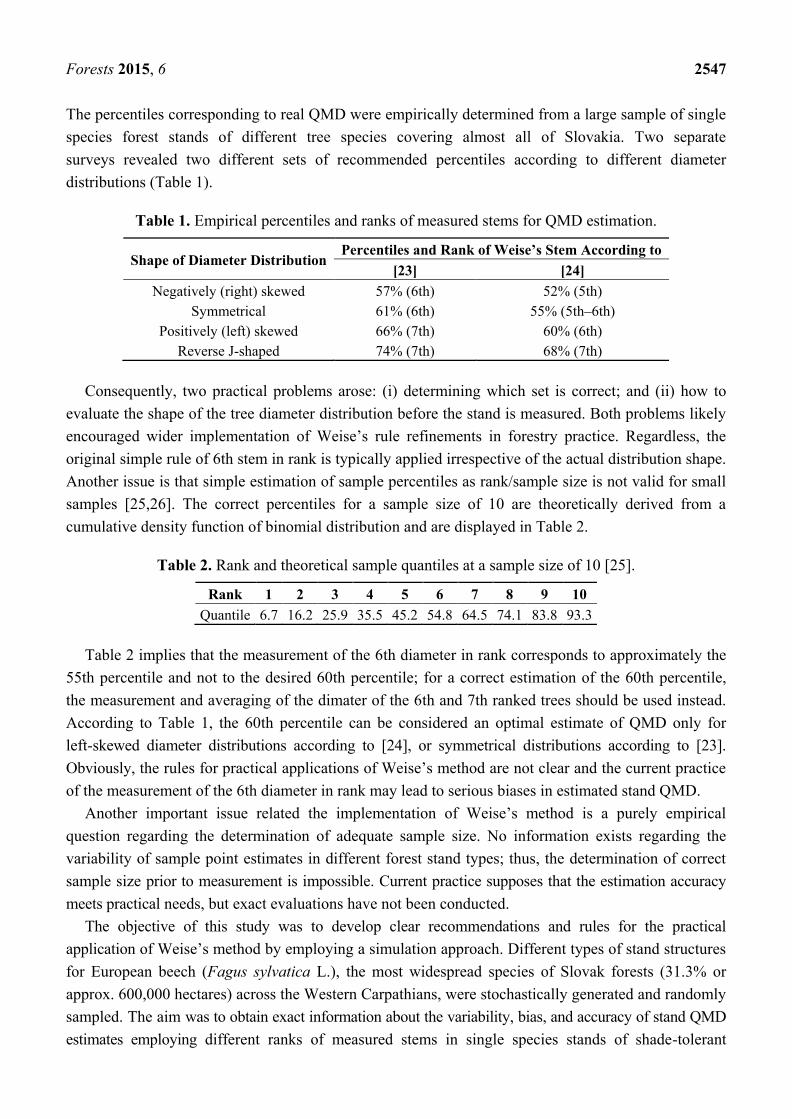
The percentiles corresponding to real QMD were empirically determined from a large sample of single

species forest stands of different tree species covering almost all of Slovakia. Two separate

surveys revealed two different sets of recommended percentiles according to different diameter

distributions (Table 1).

Table 1. Empirical percentiles and ranks of measured stems for QMD estimation.

Shape of Diameter Distribution Percentiles and Rank of Weise’s Stem According to

[23] [24]

Negatively (right) skewed 57% (6th) 52% (5th)

Symmetrical 61% (6th) 55% (5th–6th)

Positively (left) skewed 66% (7th) 60% (6th)

Reverse J-shaped 74% (7th) 68% (7th)

Consequently, two practical problems arose: (i) determining which set is correct; and (ii) how to

evaluate the shape of the tree diameter distribution before the stand is measured. Both problems likely

encouraged wider implementation of Weiseʼs rule refinements in forestry practice. Regardless, the

original simple rule of 6th stem in rank is typically applied irrespective of the actual distribution shape.

Another issue is that simple estimation of sample percentiles as rank/sample size is not valid for small

samples [25,26]. The correct percentiles for a sample size of 10 are theoretically derived from a

cumulative density function of binomial distribution and are displayed in Table 2.

Table 2. Rank and theoretical sample quantiles at a sample size of 10 [25].

Rank 1 2 3 4 5 6 7 8 9 10

Quantile 6.7 16.2 25.9 35.5 45.2 54.8 64.5 74.1 83.8 93.3

Table 2 implies that the measurement of the 6th diameter in rank corresponds to approximately the

55th percentile and not to the desired 60th percentile; for a correct estimation of the 60th percentile,

the measurement and averaging of the dimater of the 6th and 7th ranked trees should be used instead.

According to Table 1, the 60th percentile can be considered an optimal estimate of QMD only for

left-skewed diameter distributions according to [24], or symmetrical distributions according to [23].

Obviously, the rules for practical applications of Weise’s method are not clear and the current practice

of the measurement of the 6th diameter in rank may lead to serious biases in estimated stand QMD.

Another important issue related the implementation of Weise’s method is a purely empirical

question regarding the determination of adequate sample size. No information exists regarding the

variability of sample point estimates in different forest stand types; thus, the determination of correct

sample size prior to measurement is impossible. Current practice supposes that the estimation accuracy

meets practical needs, but exact evaluations have not been conducted.

The objective of this study was to develop clear recommendations and rules for the practical

application of Weise’s method by employing a simulation approach. Different types of stand structures

for European beech (Fagus sylvatica L.), the most widespread species of Slovak forests (31.3% or

approx. 600,000 hectares) across the Western Carpathians, were stochastically generated and randomly

sampled. The aim was to obtain exact information about the variability, bias, and accuracy of stand QMD

estimates employing different ranks of measured stems in single species stands of shade-tolerant

Forests 2015, 6 2548

species growing in Central Europe. In addition, we proposed several modifications of the original Weise’s

rule based on the measurement and averaging of two measured diameters with different ranks.

2. Materials and Methods

2.1. Data Generation and Simulation

Stochastic generation of adequate numbers, spatial distribution and dimensions of individual trees

growing at predefined site conditions was modelled for 27 virtual stands, each 9 ha in size. The virtual

list of tree values and their coordinates in each stand were stochastically generated by an original

modelling approach utilizing several existing submodels and equations constructed for single species

beech stands in Slovakia.

The modelling approach requires some basic predefined values, including site quality, defined by a

site index of 30 m (mean stand height at reference age of 100 years) commonly found in Slovak beech

stands, and the arithmetic mean and its degree of dispersion. Stands were differentiated by mean

diameter size intervals of 5 cm, from 10 to 50 cm, and three categories (low, medium, and high) of

degree of diameter dispersion (DoD). The DoD description is a qualitative measure of tree diameter

variability that can be easily estimated in the field by visual inspection of a stand. A low degree of

variability is typical for even-aged, single-species stands growing on homogenous sites managed by

silviculture approaches to encourage tree uniformity (e.g., understorey thinning). Conversely, high

DoD is characteristic of uneven-aged, highly-structured forest stands of variable site conditions tended by

close-to-nature approaches that preserve high variability of individual tree characteristics [20]. In total,

27 combinations of 9 mean diameters and 3 DoD yielded 27 virtual beech stands covering almost all

stand structure types of European beech that can be found in Slovakia on a single predefined site

quality. An effort was made to adequately capture the whole variety of stand types in order to secure a

wider generalization of the study results.

The virtual stands were generated through mathematical modelling using the following approach:

(1) Estimation of the stand age, number of trees per hectare, and mean height corresponding to

the selected mean diameter for a given height site index of 30 m from valid growth and yield

tables [27]; estimation of the diameters coefficients of variation and standard deviations from

the mean diameters according to different DoD categories through regression equations [28];

(2) Estimation of the diameter distribution skewness and curtosis corresponding to selected mean

diameters and DoD categories from results published by Halaj [23];

(3) Mathematical modelling of the diameter distributions based on predefined mean diameter,

DoD categories, and estimated coefficients of skewness and excess by means of normal

distribution modified by the second order Gram-Charlier expansion; and

(4) Stochastic generation of individual tree dimensions (tree diameter, height, and crown width)

and tree coordinates within the stand area.

An overview of input variables required for a simulation of virtual stands (results of steps (i)–(iii))

is given in Table 3.

Forests 2015, 6 2549

Table 3. Input variables for simulation of individual trees in virtual stands.

Stand Variables Degree of

Dispersion

Mean Diameter (cm)

10 15 20 25 30 35 40 45 50

Age (year) 35 45 60 75 90 110 135 155 180

Number of trees (ha−1) 3788 2160 1227 828 615 455 343 287 241

Mean height (m) 13.5 17.2 21.7 25.3 28.3 31.5 34.7 36.8 39

Coefficient of

variation (%)

Low 27.5 26.1 25.1 24.5 24.2 24.4 24.9 25.8 27.0

Medium 37.0 34.6 33.0 32.1 32.0 32.6 34.0 36.2 39.1

High 46.3 42.9 40.5 39.4 39.3 40.4 42.6 45.9 50.4

Skewness A

Low 0.45 0.50 0.60 0.65 0.68 0.65 0.60 0.48 0.30

Medium 0.40 0.48 0.52 0.55 0.60 0.55 0.50 0.30 0.10

High 0.30 0.40 0.48 0.52 0.60 0.58 0.50 0.35 0.10

Kurtosis E

Low –0.70 0.00 0.20 0.50 0.70 0.65 0.50 0.15 –0.10

Medium –0.70 –0.20 0.10 0.35 0.40 0.35 0.10 –0.30 –0.80

High –1.20 –0.50 –0.30 0.00 0.12 –0.05 –0.30 –1.00 –1.20

The diameter distributions were mathematically expressed by a probability density function of

normal distribution modified by the Gram-Charlier expansion [29]:

)36(24

)3(6

12

1)( 24

4

42

2

32

2

jj

d

jj

d

z

d

j zzs

zzs

es

dfj

(1)

where f (dj) is relative frequency for j-th diameter class with 1 cm width. Variable zj is a normalized

variable for j-th diameter class calculated as dgjj sddz )( , where dj is the central value of j-th

diameter class, and gd is QMD. κ3 and κ4 are the 3rd and 4th cumulated diameter distribution

modified symmetry and excess of normal distribution, respectively. The cumulants are functions of

central moments, m2, m3, m4; when κ3 = m3 and κ4 = m4 − 3 m2. The 2nd–4th central moments, mx are

calculated from estimated values of sd; A and E are listed in Table 3. An overview of all input

variables in Equation (1) is given in Table 4. The use of the modified normal distribution is justified by

its flexibility and by the possibility to obtain reliable estimates of its parameters for all considered

types of beech stands.

Table 4. Input variables for diameter distribution modelling.

Variable Degree of

Dispersion

Mean Diameter (cm)

10 15 20 25 30 35 40 45 50

sd

Low 2.8 3.9 5.0 6.1 7.3 8.5 10.0 11.6 13.5

Medium 3.7 5.2 6.6 8.0 9.6 11.4 13.6 16.3 19.5

High 4.6 6.4 8.1 9.8 11.8 14.1 17.0 20.7 25.2

κ3

Low 36 42 114 176 269 425 660 982 1111

Medium 50 108 215 336 627 952 1687 1982 3055

High 104 231 485 771 1474 2762 4836 9514 6227

κ4

Low −134 −94 −51 491 2123 3439 4904 1085 20024

Medium −934 −587 −510 1326 2796 5266 −3769 −47673 −244450

High −2530 −2785 −5271 −4588 −5789 −28267 −109209 −545833 −1407101

Forests 2015, 6 2550

After obtaining the mathematical representation of diameter distributions, the list of individual trees

and their dimensions for each modelled stand was generated (step iv). Initially, a list of individual

diameters was stochastically generated from the diameter distribution described by Equation (1). Two

numbers, r1 and r2 from uniform distribution (0.1), and the random diameter, dr from range 0.1–120 cm,

calculated using the formula dr = 0.1 + r1120, were determined. The random diameter, dr was assigned

corresponding to the 1 cm diameter class calculated by Equation (1) and the relative frequency of

diameters f (dj) in that particular class. The random diameter dr was stochastically accepted if r2 < f (dj);

otherwise, the stochastic generation was repeated with a new pair of random numbers [r1, r2] The

process was repeated until the number of accepted tree diameters equaled the expected number of trees

per hectare (Table 3).

Individual tree heights were estimated using a generalized height-diameter model [30] and the

generated tree diameter, d defined mean diameter, gd and corresponding mean height, gh variables

(Table 3); regression estimates of heights were stochastically modified. Normal distribution of height

residuals in a particular diameter class with 0 mean and variance were provided by Halaj [31]. Tree

crown widths were estimated by non-linear regression from known tree height and diameter [28], and

the distribution of trees was modelled across the stand area.

Tree distribution was simulated based on a model parameterised from long-term research plot data

from Slovak single-species beech stands [32]. This approach was based on the stochastic generation of

individual tree coordinates (x, y) from a uniform distribution of possible coordinates that was

stochastically verified by a probability, p (lr) determined by a generalized logistic equation using

relativised distance, lr. Relativised distance can be considered a special competition index calculated

from the crown widths and spatial distances between randomly selected pairs of trees. Tree coordinates

are accepted as long as the random number r generated from uniform distribution with range 0–1 is

r < p (lr); otherwise, the procedure is repeated with new random coordinates, and the procedure is

repeated until all generated trees are positioned within the stand area.

2.2. Methods

The average of simulated point samples of QMD estimates according to Weise’s rule determined

the estimated QMD in each virtual stand. For each virtual stand (Table 5), simple systematic sampling

was used with a sample size calculated to achieve an accuracy of Δ% = 5% at the confidence level

P = 95%, using the formula:

2

,2/

%

%

df stn (2)

where tα/2,f is a critical value of Student’s t distribution and sd% is the tree diameter coefficient of

variation (Table 3).

Forests 2015, 6 2551

Table 5. Number of sampling points for accuracy of Δ% = 5% at the 95% confidence level.

Degree of Dispersion Mean Diameter (cm)

10 15 20 25 30 35 40 45 50

Low 121 100 81 81 81 81 81 100 100

Medium 196 169 144 144 144 144 144 169 196

High 289 256 225 196 196 225 225 256 289

Several variants and modifications of Weise rule applied to QMD estimation were examined:

– Estimations based on the diameter measurement of the 5th, 6th, 7th, and 8th ranked largest

trees of the 10 individuals nearest to the sampling point

– Estimations based on the average of the two diameter measurements with appropriately

selected ranks:

Five rank combinations, [5. and 6.]––[4. and 7.]––[3. and 8.]––[2. and 9.]––[1. and 10.],

centered between the 5th and 6th rank (50% percentile according; Table 2)

Four rank combinations, [5. and 7.]––[4. and 8.]––[3. and 9.]––[2. and 10.], centered on

the 6th rank (55% percentile)

Four rank combinations, [6. and 7.]––[5. and 8.]––[4. and 9.]––[3. and 10.], centered on

between the 6th and 7th rank (60% percentile)

Three rank combinations, [6. and 8.]––[5. and 9.]––[4. and 10.], centered on the

7th rank (65% percentile)

Three rank combinations, [7. and 8.]––[6. and 9.]––[5. and 10.], centered between the

7th and 8th ranks (70% percentile)

Two rank combinations, [7. and 9.]––[6. and 10.], centered on the 8th rank

(75% percentile)

In principle, all ranks or combinations of ranks that have the potential to produce good estimates of

the QMD were explored. The two-measurement variants were applied at only half of the sampling

points to maintain the same number of diameter measurements and to approximate equal field

sampling time and measurement costs necessary for stand QMD estimation for comparisons between

one- and two-measurement variants.

The individual estimates of the QMD at each sampling point, jd were obtained using Weise’s

variants. The arithmetic mean of sampling point estimates, gd̂ provided the final estimate of real stand

QMD, gd and the relative standard deviation of sampling point estimates, %jds , provided a measure

of variability of sampling point estimates within the stand. The standard error of estimation, %es

describing the precision was determined using the equation:

1%% nssjde (3)

where n is the number of sampling points. Relative deviation of the final estimate gd̂ from known

mean stand diameter gd or the relative estimation bias was determined to be:

100)ˆ(% ggg ddde (4)

Forests 2015, 6 2552

Statistical significance of biases were tested by a t-test at the level of significance α = 5%. Final

measurements of estimated accuracy were calculated as:

%%eRMSE 22es (5)

where RMSE denotes the percent root mean square error.

The generation of virtual stands, the simulations of tree samples, and the application of different

QMD estimation methods associated with calculations of biases, precisions, and accuracies of applied

methods were done in the Borland Pascal programming environment [33].

3. Results

A trend of significant under-estimation to significant over-estimation of QMD was evident with

increasing rank for one-measurement variants of Weise’s rule (Figure 1A). The smallest, but still the

most significant negative bias (calculated as average of all examined stands differentiated by mean

diameter size and DoD), was achieved for the 6th rank. Because biases composed a substantial part of

the accuracy, the smallest average RMSE of 2.8% at 68% confidence level (i.e., approx. 5.6% at 95%)

was also achieved at the 6th rank. Still, the 6th rank was the most accurate and was higher than the

originally intended 5.0% at the 95% confidence level. On the other hand, the average precision, se%,

was rather high for all ranks (1.10%–1.26% at the 68% level) with only small and random variations

among them (Figure 1B).

Figure 1. Comparison of accuracy (A); and precision (B) for one-measurement variants of

Weise’s estimation averaged across all examined stands. The stacked accuracy bars

representing averaged proportions of bias (grey) and precision (white) in terms of

accuracy were calculated as ratios of squared bias/precision on squared RMSE. Signs in

the bias proportions shows the prevalent direction of original biases (under- or

overestimation). The signs denoted by an asterisk indicate the prevalence of statistically

significant biases at a p-value of 5%.

5th 6th 7th 8th

Rank of measured stem

0

2

4

6

8

10

12

14

16

18

Accu

racy R

MS

E in

%

Accuracy components

precision

bias

-*

5th 6th 7th 8th0,0

0,3

0,5

0,8

1,0

1,3

1,5

Pre

cis

ion

se %

-* +* +*

A

B

Forests 2015, 6 2553

More detailed analysis of the best accuracy results according to different mean diameter size and

degree of diameter dispersion confirms that the measurement of the 6th stem in rank is the best variant

in 24 out of 27 cases (Table 6). More than 90% (22 out of 24) of 6th rank RMSE% contained negative

biases of which approximately 60% (13 out of 22) are significant at a p-value of 5%. The influence of

different mean diameter size on RMSE was not unambiguous, but a weak tendency of RMSE to

decrease at larger mean diameters was observed.

Table 6. The optimal rank, accuracy, and bias of QMD estimation for the best

one-measurement variants of Weise’s rule (the values in column for each combination of

QMD and DoD are optimal rank followed by RMSE and bias in %).

Degree of

Dispersion

Real QMD in cm Mode

10 15 20 25 30 35 40 45 50 Mean/Mean

Low

6 6 6 6 6 6 6 6 6 6

1.38 3.01 1.21 2.08 2.36 1.94 3.00 2.61 2.02 2.18

−0.81 −2.82 * −0.32 −1.83 −2.16 * −1.70 −2.76 * −2.40 * −1.69 −1.83

Average

6 6 6 6 6 6 6 6 6 6

3.10 1.74 2.40 3.16 2.09 3.46 1.61 1.77 1.44 2.31

−2.91 * −1.34 −2.17 * −2.99 * −1.87 −3.29 * −1.26 −1.42 −0.90 −2.02

High

6 7 6 7 6 7 6 6 6 6

3.48 4.99 4.08 4.87 3.25 4.26 3.52 3.09 1.19 3.04 1

−3.31 * 4.89 * 3.95 * 4.77 * −3.07 * 4.16 * −3.35 * −2.88 * 0.14 −2.24

Mode 6 6 6 6 6 6 6 6 6

Mean/Mean 2.65 3.25 2.56 3.37 2.56 3.22 2.71 2.49 1.55

−2.34 0.25 −2.15 −0.02 −2.36 −0.28 −2.46 −2.23 −0.82

1 the averages for this DoD category are calculated only for optimal 6th rank values, * the statistically

significant biases at p-level 5%

The influence of DoD was more pronounced. The measurement of the 6th stem in rank was the

most accurate variant for stands with low and medium DoD with mean RMSE% of 2.2% and 2.3%,

respectively, at the 68% confidence level. In spite of the most significant negative biases, mean

RMSEs of these categories were smaller than the proposed accuracy of 2.5%. For the high DoD

category, the results were more complicated, although the 6th rank was generally still optimal.

However, measurement of the 7th stem in rank was the best option in some cases (particularly with

smaller mean diameters) because they had smaller RMSE% than the 6th stem in rank. Application of

7th stem in rank was accompanied by a significant overestimation of QMD in contrast to

underestimations characteristic of the 6th rank. The mean RMSE% (3.04%) was about 20% higher than

the proposed accuracy of 2.5%, which was not surprising considering the higher variability of diameters

in the generated stands of the high DoD category.

Modification of the classic Weiseʼs method based on averaging of two diameter measurements in

selected ranks on half the number of sampling points clearly improved the estimation accuracy

(Figure 2A). The most successful variants of the two-measurement modifications, the 6th rank centroid

obtained by averaging the measurements of the 4th and 8th stems in rank and the 6th rank centroid

obtained by averaging the measurements of the 3rd and 9th stems in rank, achieved average RMSE of

Forests 2015, 6 2554

2.17% and 2.12%, respectively, for all stands. They were approximately 15% lower than the planned

accuracy of 2.5% and approximately 25% lower than the accuracy at 2.8% of the best 6th rank’s variant

of the classic one-measurement Weiseʼs method. The 6th variant of 3–9 had a lower positive bias of

0.86% (on average) in comparison to the 6th variant of 4–8 with a larger negative bias of 1.25%

(i.e., 33%). Both biases were statistically non-significant at a p-level of 5% in most stands. Precisions

of the best two-measurement variants varied between 1.25 and 1.55% on average, which was slightly

worse than the precisions of one-measurement variants of Weise estimation (Figure 2B). More detailed

analysis of the best two-measurement variants according to different mean diameter sizes and DoD

revealed no significant differences (Table 7).

Figure 2. Comparison of accuracy (A); and precision (B) for two-measurement

modifications of Weise’s rule averaged across all stands. The stacked accuracy bars

representing averaged proportions of bias (grey) and precision (white) on accuracy were

calculated as ratios of squared bias/precision on squared RMSE. Signs in bias proportion

parts show the prevalent direction of original biases (under- or overestimation), and the

signs denoted by an asterisk indicate the prevalence of statistically significant biases at a

p-value of 5%).

Almost all biases of the best variants were not statistically significant and two variants identified

as optimal varied according to different mean diameters and DoD. The 6th variant of 3–9 was the best

in 13 of 27 cases, while the 6th variant of 4–8 was best in 14 of 27 cases. In general, negative bias was

prevalent amongst most estimations. The 6th variant of 4–8 had negative biases in 8 of 14 cases and

the 6th variant of 3–9 had negative biases in 9 of 13 cases. The slight statistically non-significant

tendency to underestimate existed if the two most accurate two-measurement variants were used for a

QMD estimation.

5-6th/1.-10. 6th/4.-8. 6th/3.-9. 6-7th/6.-7. 7th/6.-8. 7-8th/7.-8. 8th/7.-9.

Rank centroid/Combination of measured ranks

0

2

4

6

8

10

12

14

16

18

Accura

cy R

MS

E in %

Accuracy components precision bias

- - + +* +*+*+*

5-6th/1.-10.

6th/4.-8.

6th/3.-9.

6-7th/6.-7.

7th/6.-8.

7-8th/7.-8.

8th

/7.-9

.0,0

0,4

0,8

1,2

1,6

2,0

2,4

Pre

cis

ion

se %

A

B

Forests 2015, 6 2555

No clear pattern of optimal two-measurement variants was visible according to the mean diameter

size of the generated stands, but a weak pattern was detected according to DoD. The 6th variant of

4–8 occurred with a higher frequency in low DoD (7 of 9 cases), which was opposite to the high DoD

stands whereby the 6th variant of 3–9 prevailed (6 of 9 cases). Medium DoD was also consistent with

average frequency analysis, e.g., the 6th variant of 3–9 was identified and recommended due to its

slight prevalence (in 5 of 9 cases).

Table 7. The optimal centroid rank/combination of measured ranks, accuracy, and bias of

QMD estimation for the best two-measurement variants of Weise’s rule (the values in

columns for each combination of QMD and DoD are optimal rank centroid/combinations

of measured ranks followed by RMSE and bias in %).

Degree of

Dispersion

Real QMD (cm) Mode

10 15 20 25 30 35 40 45 50 Mean/Mean

Low

6/4–8 6/3–9 6/4–8 6/4–8 6/4–8 6/4–8 6/4–8 6/3–9 6/4–8 6/4–8

1.56 1.37 1.71 1.62 1.38 1.57 1.65 1.53 1.76 1.57

–0.77 –0.21 –0.15 –0.97 * –0.51 0.3 0.03 –0.53 1.21 –0.18

Medium

6/3–9 6/4–8 6/4–8 6/3–9 6/3–9 6/3–9 6/4–8 6/3–9 6/4–8 6/3–9

1.29 1.38 1.22 1.5 1.14 2.19 1.50 1.81 1.42 1.49

–0.06 –0.05 –0.32 –0.60 0.16 –1.68 * 0.01 1.18 0.38 –0.11

High

6/3–9 6/3–9 6/4–8 6/3–9 6/4–8 6/3–9 6/3–9 6/4–8 6/3–9 6/3–9

1.24 1.37 1.62 2.33 1.48 1.49 1.53 1.97 1.34 1.60

0.26 –0.21 –0.96 * –1.92 * 0.39 –0.32 0.77 –1.46 * –0.36 –0.42

Mode 6/3–9 6/3–9 6/4–8 6/3–9 6/4–8 6/3–9 6/4–8 6/3–9 6/4–8

Mean/Mean 1.36 1.38 1.52 1.82 1.34 1.75 1.56 1.77 1.51

–0.19 –0.16 –0.48 –1.16 0.01 –0.57 0.27 –0.27 0.41

* The statistically significant biases were at a p-level of 5%.

4. Discussion and Conclusions

A simple QMD estimation using an appropriate sample quantile is an efficient, practical solution to

quickly estimate the QMD of forest stands in the field. Although QMD estimation using Weise’s rule

is widely used in Czech and Slovak forest inventory practice, an evaluation of the accuracy of QMD

quantile estimations and exploration of different estimation alternatives has been missing until now.

Our study clearly demonstrates the usefulness of Weise’s method for a range of forest structure

types in the Western Carphatians, particularly for single-species beech forests. The advantage of

Weise’s method is the estimation of QMD at the sampling point using one diameter measurement;

systematic group sampling and measurement of ten trees are transformed into a single systematic

sampling of one specific tree. The inclusion of information about specific stem ranks into the

mathematical measurements provides variable sample point QMD estimates, similar to the variability

of sampling point estimates calculated as an average of ten measured diameters. Therefore, the number of

sampling points required for an arbitrarily selected accuracy and confidence level could remain equal,

but the number of diameter measurements at the sampling point is ten times smaller. Thus, it seems

reasonable to expect ten times lower time consumption and measurement costs in comparison to full

group sampling.

Forests 2015, 6 2556

This simulation study confirmed the recommendation to apply the 6th rank corresponding to the

55% percentile of diameter distribution in accordance with the original empirical rule. However, our

study also revealed that the application of the appropriate two-measurement variants of the modified

Weise’s method (measurement and averaging of 4th and 8th or 3rd and 9th diameters in rank centered

to the 6th rank) over a single measurement of the 6th diameter in rank should be preferred in beech

stands growing in the Western Carphatians. The accuracy of the best variants of the modified Weiseʼs

method was about 15% higher compared to the original accuracy of 5% at the 95% confidence

interval, and it was about 25% higher compared to the classic Weise method at comparable

measurement costs. One advantage of the two-measurement variants was the absence of significant

bias, which was notably decreased in the final accuracy of the single 6th rank estimation.

Recommendations for the two-measurement variant application differ according to DoD category.

The variant of the 6th diameter in rank of the 4th–8th rank measurements is recommended in stands

with low diameter dispersion, irrespective of the mean diameter size (e.g., artificially regenerated

even-aged beech stands tended by thinning from below growing on homogeneous sites). Averaging the

3rd and 9th ranks is suggested for stands with medium and high diameter dispersion, irrespective of the

mean diameter size (e.g., stands growing on less homogenous sites with more differentiated age

composition, or more variable spatial and vertical stand structure resulting from the application of

modern silviculture approaches, such as natural regeneration, intensive crown or target tree thinnings,

more close-to-nature management, etc.).

It should be noted that the explicit recommendation of the 6th rank is closely related to the

characteristics of the empirical material. According to [23], the tendency toward slightly left-skewed

diameter distributions persists in beech stands in general in the Western Carpathians. This is clearly

reflected in Table 3, where values of skewness (A) and kurtosis (E) varied between 0.1–0.68 and −1.2–0.7,

respectively. This indicates that most of the diameter distributions included in the study had a slight left

asymmetry and a nearly normal kurtosis distribution. In such cases, simple arithmetic and quadratic

mean diameters are always greater than the median and utilization of percentiles over 50% is to be

expected as a priori. Because of the slight deviation from normal symmetry, the 60% percentile and

the 6th rank of measured stem is a natural choice. These stand types were characteristic of managed

even-aged, normal age-classed stands favored in the past.

Changing environmental conditions and public demands have encouraged more close-to-nature

silviculture and management strategies supporting the diversification of tree age composition and stand

structure. Close-to-nature management of beech stands with natural regeneration under shelterwood

management supports the desired variability in shapes of diameter distribution curves, where highly

asymmetric or even reverse J-shaped distributions are becoming more frequent in forest practice.

Therefore, if it has been found that management approaches have favored practices that encourage a

divergence of stand structure from normal, even-aged forest structures, we suggest utilizing the

two-stage approach. In the first preliminary stage, measurements of a small preliminary set of diameters,

e.g., 10 trees, distributed across the stand area in a systematic fashion are recommended. Therefore,

sample ordering, estimation of sample quantiles corresponding to measured diameters (for example

according to Table 2), and the calculation of QMD from the preliminary diameter set are suggested.

Subsequently, regression estimation of parameters of a cumulative density function for a suitable

diameter distribution model (e.g., Weibull or SB distribution) according to the principles of

Forests 2015, 6 2557

percentile-based parameter recovery approaches, and the calculation of exact sample quantile

corresponding to preliminary QMD are suggested. Alternatively, the exact sample quantile

corresponding to preliminary QMD can be determined using simple interpolation between sample

quantiles reported in Table 2.

The calculation of QMD from a preliminary set of diameters and determination of corresponding

sample percentile (exact or aproximative) will determine the correct rank (or combination of ranks) of

measured stem(s) at sampling points in the second phase. The second phase has the character of

common presently applied approaches, which means: (i) the formation of representative systematic sample

of sampling points; (ii) visual ordering of ten nearest stems at each sampling point; (iii) measurement

of the specific proper rank(s) at each sampling point; and (iv) average QMD point estimates over the

whole stand.

A key part of all the above-described approaches is a simple non-parametric rank estimation of

sample quantiles. Different definitions of sample quantiles used in several statistical packages are

reviewed by [26]. Further research is needed in order to find the optimal definition of sample quantiles

from QMD estimation and/or growing stock calculation.

Overall, this study confirmed the usefulness of Weise’s rule of thumb. Original and modified

versions of Weise’s method attained almost invariant bias and accuracy according to different mean

diameter sizes, i.e., they achieved similar accuracy in stands with completely different age and site

quality. Only the degree of diameter dispersion significantly affected QMD accuracy; diameter dispersion

is easily determined from forest management information records, or on the basis of a simple visual

inspection of the stand. Two-stage sampling application of Weise’s method is recommended in beech

stands with very diversified structure, unmanaged or managed by more close-to-nature approaches, to

ascertain correct rank(s) of stems measured at a sampling point.

Empirical estimation of QMD by Weise’s method is a simple yet highly effective way to determine

mean diameter with reasonable accuracy. Moreover, two-measurement modifications of the original

rule show a tendency to remain unbiased and achieve a high accuracy of QMD estimation compared to

the original method. Therefore, they could be recommended for application in even- and uneven-aged

beech forests growing in Central Europe.

Acknowledgments

This study was supported by the Slovak Research and Development Agency under contracts

APVV-0069-12 and APVV-0111-10 also by the Scientific Grant Agency of the Ministry of Education,

Science, Research and Sport of the Slovak Republic under project 1/0953/13. Additional support was

received from the National Agency of Agricultural Research of the Czech Republic under the contract

No. QJ1320230.

Author Contributions

Róbert Sedmák and Ľubomír Scheer conceived and designed the study, processed and analysed the

data, and wrote the paper. Róbert Marušák and Michal Bošeľa contributed to the data analysis and

results interpretation. Denisa Sedmáková contributed to the discussion and language correction of the

paper. Marek Fabrika supervised and reviewed the manuscript.

Forests 2015, 6 2558

Conflicts of Interest

The authors declare no conflict of interest.

References

1. Pretzsch, H. Forest Dynamics, Growth and Yield. From Measurement to Model; Springer: Berlin,

Germany; Heidelberg, Germany, 2009; p. 664.

2. Burkhart, H.E.; Tomé, M. Modeling Forest Trees and Stands; Springer: Dordrecht, The Netherlands,

2012; p. 457.

3. Cao, Q.V. Linking individual-tree and whole-stand models for forest growth and yield prediction.

For. Ecosyst. 2014, 1, 18, doi:10.1186/s40663-014-0018-z.

4. Maltamo, M.; Kangas, A.; Uuttera, J.; Torniainen, T.; Saramäki, J. Comparison of percentile

based prediction methods and the Weibull distribution in describing the diameter distribution of

heterogenous Scots pine stands. For. Ecol. Manag. 2000, 133, 263–274.

5. Cao, Q.V. Predicting parameters of a Weibull function for modelling diameter distribution.

For. Sci. 2004, 50, 682–685.

6. Nord-Larsen, T.; Cao, Q.V. A diameter distribution model for even-aged beech in Denmark.

For. Ecol. Manag. 2006, 231, 218–225.

7. Fabrika, M.; Pretzsch, H. Forest Ecosystem Analysis and Modelling; Technical University in Zvolen:

Zvolen, Slovakia, 2011; p. 599.

8. Prodan, M. Die Verteilung des Vorrates gleichaltriger Hochwaldbestände auf Durchmesserstufen.

Allg. For. Jagdztg. 1953, 124, 93–106.

9. Bailey, R.L.; Dell, T.R. Quantifying Diameter Distributions with the Weibull Function. For. Sci.

1973, 19, 97–104.

10. Borders, B.E.; Patterson, W.D. Projecting Stand Tables: A Comparison of the Weibull Diameter

Distribution Method, a Percentile-Based Projection Method, and a Basal Area Growth Projection

Method. For. Sci. 1990, 36, 413–424.

11. Maltamo, M.; Puumalainen, J.; Päivinen, R. Comparison of beta and Weibull functions for

modelling basal area diameter distribution in stands of Pinus sylvestris and Picea abies. Scand. J.

For. Res. 1995, 10, 284–295.

12. Hafley, W.L.; Schreuder, H.T. Statistical distributions for fitting diameter and height data in

even-aged stands. Can. J. For. Res. 1977, 7, 481–487.

13. Rennolls, K.; Wang, M. A new parameterization of Johnson’s SB distribution with application to

fitting forest tree diameter data. Can. J. For. Res. 2005, 35, 575–579.

14. Wang, M.; Rennolls, K. Tree diameter distribution modelling: Introducing a logit-logistic

distribution. Can. J. For. Res. 2005, 35, 1305–1313.

15. Siipilehto, J. A comparison of two parameter prediction methods for stand structure in Finland.

Silv. Fenn. 2000, 34, 331–349.

16. Fonseca, T.F.; Marques, C.P.; Parresol, B.R. Describing maritime pine diameter distributions with

Johnson’s SB distribution using a new all-parameter recovery approach. For. Sci. 2009, 55, 367–373.

Forests 2015, 6 2559

17. Kangas, A.; Maltamo, M. Performance of percentile-based diameter distribution prediction

method and Weibull method in independent data sets. Silv. Fenn. 2000, 34, 381–398.

18. Mehtätalo, L.; Gregoire, T.G.; Burkhart, H.E. Comparing strategies for modelling tree diameter

percentiles from re-measured plots. Environmetrics 2008, 19, 529–548.

19. Bohora, S.B.; Cao, Q.V. Prediction of tree diameter growth using quantile regression and

mixed-effects models. For. Ecol. Manag. 2014, 319, 62–66.

20. Šmelko, Š. Forest Mensuration, 2nd ed.; Technical University in Zvolen: Zvolen, Slovakia, 2007;

p. 399. (In Slovak)

21. Van Laar, A.; Akca, A. Forest Mensuration, 2nd ed.; Springer: Berlin, Germany, 2007; p. 418.

22. Collective. Slovak Operational Instructions for Forest Management; National Forest Centre:

Zvolen, Slovakia, 2008; p. 147. (In Slovak)

23. Halaj, J. Mathematical and statistical survey of diameter structure of Slovak stands. Les. Čas.

For. J. 1957, 3, 39–74. (In Slovak)

24. Collective. Technical Guidelines for Forest Management; Institute for Forest Management:

Zvolen, Slovakia, 1984; p. 594. (In Slovak)

25. Hald, A. Statistical Theory with Engineering Applications; John Wiley & Sons, Inc.: New York,

NY, USA, 1952; p. 783.

26. Hyndman, R.J.; Fan, Y. Sample quantiles in statistical packages. Am. Stat. 1996, 50, 361–365.

27. Halaj, J.; Petráš R. Growth and Yield Tables of Main Tree Species in Slovakia; Slovak Academic

Press: Bratislava, Slovakia, 1998; p. 325. (In Slovak)

28. Fabrika, M. Growth simulator SIBYLA (conception, construction, software solution). Habilitation

Thesis, Technical University in Zvolen, Zvolen, Slovakia, 2005; p.187. (In Slovak)

29. Cramer, H. Mathematical Methods of Statistics, 19th ed.; Princeton University Press: Princeton,

NJ, USA, 1999; p. 571.

30. Šmelko, Š.; Pánek, F.; Zanvit, B. Mathematical formulation of system of unified height-diameter

curves for Slovak even-aged stands. Acta Fac. For. Zvolen 1987, 29, 151–174. (In Slovak)

31. Halaj, J. Height Growth and Structure of Forest Stands; Slovak Academic Press: Bratislava,

Slovakia, 1978; p. 283. (In Slovak)

32. Sedmák, R.; Hladík, M.; Brezina, L. Modeling the horizontal stem distribution in even-aged beech

stands. Les. Čas. For. J. 2000, 46, 145–153. (In Slovak)

33. Swan, T. Borland Pascal 7.0 Programming for Windows; Bantam Books, Inc.: New York, NY,

USA, 1973; p. 853.

© 2015 by the authors; licensee MDPI, Basel, Switzerland. This article is an open access article

distributed under the terms and conditions of the Creative Commons Attribution license

(http://creativecommons.org/licenses/by/4.0/).