Microstructural imaging of the human spinal cord with ... - CORE

Microstructural imaging of the humanspinal cord with advanced diffusion MRI

Francesco Grussu

Thesis submitted for the degree ofDoctor of Philosophy

of theUniversity College London

Field of study: Magnetic Resonance Physics

Department of Neuroinflammation,Institute of Neurology

1

I, Francesco Grussu confirm that the work presented in this thesis is my own.

Where information has been derived from other sources,I confirm that this has been indicated in the thesis.

2

Abstract

The aim of this PhD thesis is to advance the state-of-the-art of spinal cord magnetic resonanceimaging (MRI) in multiple sclerosis (MS), a demyelinating, inflammatory and neurodegenerativedisease of the central nervous system.

Neurite orientation dispersion and density imaging (NODDI) is a recent diffusion-weighted (DW)MRI technique that provides indices of density and orientation dispersion of neuronal processes.These could be new useful biomarkers for the spinal cord, since they could better characteriseoverall, widespread MS pathology than conventional metrics.

In this thesis, we test innovative clinically feasible acquisitions as well as signal analysis methodsto study the potential of NODDI for the spinal cord. We also design and run computer simulationsthat corroborate our in vivo findings. Furthermore, we compare NODDI metrics to quantitativehistological features, with the aim of validating their specificity.

The thesis is divided in two parts. In the first part, in vivo experiments are described. Specificobjectives are: i) to demonstrate the feasibility of performing NODDI in the spinal cord and in clinicalsettings; ii) to study the possibility of extracting with new approaches such as NODDI more specificmicrostructural information from standard DW acquisitions; iii) to assess how features typical ofspinal cord microstructure, such as presence of large axons, influence NODDI metrics.

In the second part of the thesis, ex vivo experiments are discussed. Their objective is the vali-dation of the specificity of NODDI metrics via comparison to quantitative histology in post mortemspinal cord tissue. The experiments required the implementation of high-field DW scans as well ashistological procedures and complex analysis pipelines.

The results of this thesis contribute to current scientific knowledge. They prove that NODDIoffers new opportunities to study how neurodegenerative diseases such as MS alter neural tissuecomplexity. We showed for the first time that NODDI can be performed in the spinal cord in vivoand in clinical scans. We also demonstrated that NODDI analysis of standard DW data is challeng-ing, and quantified how the presence of large axons in the spinal cord influences NODDI metrics.Lastly, our ex vivo data highlight that unlike routine DW MRI methods, NODDI can detect reliablypathological variations of neurite orientation dispersion. NODDI is also sensitive to the density ofaxons and dendrites, but can not fully resolve axonal loss and demyelination in MS.

We believe that the technique is a key element of a more general multi-modal MRI approach,which is necessary to obtain a complete description of complex diseases such as MS.

3

A babai, mamai e fradi miu

4

Acknowledgements

One of the major challenges I faced during the writing of this PhD thesis was to find an appropriateway of acknowledging the support of those without whom this PhD project would not have beencompleted. This section aims to demonstrate my warm and sincere gratitude to all of them.

I am thankful to my PhD supervisors, Professor Claudia Gandini Wheeler-Kingshott and Pro-fessor Daniel Alexander, for their excellent supervision during the past three years. I acknowledgetheir unconditional support, that never made me feel alone in the difficult world of MRI research.I thank them for their invaluable feedback, and for creating two wonderful research groups (thePhysics team within the NMR Research Unit and the MIG/POND groups) where working was agreat pleasure. I really believe that my supervisors taught me how to be a true scientist, and I willalways carry with me their useful lessons.

I am grateful to Doctor Torben Schneider. Torben was for me a true third supervisor, other thana good friend. I thank him for useful discussion and advice during the Monday morning meetings,for teaching me how to set up and control our 3T MRI scanner, for showing me how to performhigh-field ex vivo MRI experiments and for helping me keep the collaboration between London andOxford viable and fruitful. Working with Torben was very stimulating, indeed one of the nicest thingsthat happened during my PhD in London.

I would like to express sincere gratitude to Professor Gabriele DeLuca from the University ofOxford. He was a fantastic collaborator, and his invaluable expertise contributed heavily to thisPhD thesis. He made me feel an honorary member of his research team, and always showed kindhospitality when I went to Oxford. He made me feel at home even in his Canada, in Toronto, wherehe went with me through my ISMRM presentation. I really hope to have again the opportunity ofworking with him.

I am also thankful to Doctor Gary Hui Zhang. My work has focussed on NODDI, and certainlyhas benefited a lot of his useful suggestions and of his thorough reviews, which directed my choicestowards the simplest and most elegant solutions.

I would like to thank everyone else who was directly involved in the projects presented in thisthesis: Doctor Carmen Tur for her invaluable statistical expertise; Doctor Mohamed Tachrount forhis help with the high-field MRI acquisitions; Doctor Jia Newcombe for providing spinal cord tissuespecimens; Richard Yates and Janis Carter for their help with histological procedures; Doctor An-drada Ianus for her help with the implementation of the DTI-Dot model; Doctor Enrico Kaden for his

5

script drawing samples from a Watson distribution; Doctor Ferran Prados for his suggestions aboutspinal cord image registration.

I am grateful to Doctor Hugh Kearney, who gave me access to his data in 2012 to familiarisewith diffusion weighted images of the spinal cord, and to Doctor Marios Yiannakas, always ready toshare one of his MRI sequences for a quick test and willing to give a hand during the MRI sessions.

Many thanks go to Professor David Miller and to Professor Olga Ciccarelli, who led the NMRResearch Unit during my PhD and made it a stimulating research team.

Also, I would like to thank all members of the NMR Research Unit, of the Microstructure ImagingGroup and of the Progression of Neurodegenerative Disease team, for useful discussion and sug-gestions during our regular meetings and for being real friends. In particular, I would like to thankthose who offered to review individual chapters of my thesis: Carmen, Torben, Marco, Andrada,Becky, Neil and Viktor.

Thanks to radiographers Mr Luke Hoy and Ms Chichi Ugorji who often helped during my MRIscans, and to Mr Jon Steel for support with IT and software issues.

Thanks to everyone who volunteered to be a “second person” during my MRI sessions and tothose who ran MRI scans of myself for my studies.

Thanks to all my volunteers, who offered a bit of their time for me to have MRI data to work with.

Thanks to the UCL NeuroResource tissue bank and to the Oxford brain bank (Thomas Willisbrain collection) for providing spinal cord tissue specimens for my investigations.

Thanks to the UCL Grand Challenge Studentships program that funded my PhD.

Thanks to Ms Ifrah Iidow for helping me print my posters always so promptly.

Thanks to the examiners of my MPhil/PhD transfer and to the examiners of my final PhD vivafor taking some time to evaluate my scientific production.

Thanks to my friends Daniele Farris, Marco Caria, Giacomo Scheich, Emanuele Corriga andMarco Battiston, who were always ready to support me during the toughest periods of my PhD.

Thanks to wonderful Carmen, for supporting me so much during these last, stressful months,and for making my days better with her smile.

I conclude the acknowledgements thanking my family: my father Pietro, my mother Marisa andmy brother Giuseppe. In spite of the distance, they made me feel as if they were always here withme in London, celebrating my achievements and having a laugh together to forget about difficulties.Est su praghere prus mannu de totus a iscriere ca seis sa fortza mia!

Francesco

18th of December 2015

6

Contributors

The work presented in this thesis would not have been possible without the following contributions.

• Prof Claudia Gandini Wheeler-Kingshott (UCL): supervision; discussion and results interpre-tation.

• Prof Daniel Alexander (UCL): supervision; discussion and results interpretation.

• Dr Torben Schneider (UCL): help with MRI data acquisition (both in vivo and ex vivo) and withthe implementation of the MRI-histology pipeline; discussion and results interpretation.

• Prof Gabriele C. DeLuca (University of Oxford): carried out histological procedures; providedspinal cord tissue specimens; discussion and results interpretation.

• Dr Hui Zhang (UCL): discussion and results interpretation.

• Dr Mohamed Tachrount (UCL): help with ex vivo MRI data acquisition.

• Dr Carmen Tur (UCL): statistical advice and useful discussion.

• Dr Enrico Kaden, Dr Ferran Prados and Dr Andrada Ianus (UCL): provided useful suggestionsand some practical help with data synthesis and analysis.

• Dr Jia Newcombe (UCL): provided spinal cord tissue specimens.

• Mr Richard Yates and Ms Janis Carter (University of Oxford): contributed to the histologicalprocedures.

7

“B’a’ cosas chi pro las cumprendere bi chere’ tempus e isperienzia;e cosas chi cand’un’at isperienzia no las cumprende’ prusu.”

Mialinu Pira, Sos Sinnos

8

Contents

List of Figures 14

List of Tables 17

List of Abbreviations 18

List of Frequent Symbols 20

1 Introduction 221.1 Background . . . . . . . . . . . . . . . . . . . . . . . . . . . . . . . . . . . . . . . . . 221.2 Problem statement . . . . . . . . . . . . . . . . . . . . . . . . . . . . . . . . . . . . . 221.3 Aims . . . . . . . . . . . . . . . . . . . . . . . . . . . . . . . . . . . . . . . . . . . . . 221.4 Scientific relevance of the work . . . . . . . . . . . . . . . . . . . . . . . . . . . . . . 231.5 Structure of the thesis . . . . . . . . . . . . . . . . . . . . . . . . . . . . . . . . . . . 25

2 Neuroanatomy and multiple sclerosis: an overview 262.1 Neurons and neural tissue . . . . . . . . . . . . . . . . . . . . . . . . . . . . . . . . . 262.2 The human spinal cord . . . . . . . . . . . . . . . . . . . . . . . . . . . . . . . . . . . 272.3 Multiple sclerosis . . . . . . . . . . . . . . . . . . . . . . . . . . . . . . . . . . . . . . 28

3 Background 303.1 Introduction to magnetic resonance imaging . . . . . . . . . . . . . . . . . . . . . . . 303.2 Spins and magnetic moments . . . . . . . . . . . . . . . . . . . . . . . . . . . . . . . 31

3.2.1 Dynamics of a spin from classical mechanics . . . . . . . . . . . . . . . . . . 313.2.2 Larmor precession of a spin . . . . . . . . . . . . . . . . . . . . . . . . . . . . 323.2.3 The rotating reference frame . . . . . . . . . . . . . . . . . . . . . . . . . . . 33

3.3 Bloch equations and relaxation . . . . . . . . . . . . . . . . . . . . . . . . . . . . . . 343.3.1 The Bloch equations . . . . . . . . . . . . . . . . . . . . . . . . . . . . . . . . 353.3.2 Relaxation time constants . . . . . . . . . . . . . . . . . . . . . . . . . . . . . 353.3.3 Evolution of the magnetisation under a static field . . . . . . . . . . . . . . . . 373.3.4 Response of the magnetisation to on resonance excitation . . . . . . . . . . 383.3.5 Multicomponent relaxation . . . . . . . . . . . . . . . . . . . . . . . . . . . . . 393.3.6 Bloch-Torrey equations . . . . . . . . . . . . . . . . . . . . . . . . . . . . . . 40

9

3.4 Signal detection and imaging equation . . . . . . . . . . . . . . . . . . . . . . . . . . 403.4.1 From the magnetisation to a measurable signal . . . . . . . . . . . . . . . . . 403.4.2 The imaging problem . . . . . . . . . . . . . . . . . . . . . . . . . . . . . . . 41

3.5 Common MRI signal weightings . . . . . . . . . . . . . . . . . . . . . . . . . . . . . . 423.5.1 Free induction decay and gradient echo . . . . . . . . . . . . . . . . . . . . . 433.5.2 Inversion recovery . . . . . . . . . . . . . . . . . . . . . . . . . . . . . . . . . 433.5.3 Spin echo experiment . . . . . . . . . . . . . . . . . . . . . . . . . . . . . . . 443.5.4 Stimulated echo acquisition mode (STEAM) . . . . . . . . . . . . . . . . . . . 463.5.5 Repeated sequences . . . . . . . . . . . . . . . . . . . . . . . . . . . . . . . 47

3.6 Sampling methods . . . . . . . . . . . . . . . . . . . . . . . . . . . . . . . . . . . . . 483.6.1 Field-of-view and resolution . . . . . . . . . . . . . . . . . . . . . . . . . . . . 483.6.2 2D and 3D imaging . . . . . . . . . . . . . . . . . . . . . . . . . . . . . . . . . 503.6.3 Echo planar imaging . . . . . . . . . . . . . . . . . . . . . . . . . . . . . . . . 52

3.7 Noise and signal-to-noise ratio . . . . . . . . . . . . . . . . . . . . . . . . . . . . . . 533.8 Speeding up the MR experiment: parallel and multiband imaging . . . . . . . . . . . 543.9 Diffusion MRI . . . . . . . . . . . . . . . . . . . . . . . . . . . . . . . . . . . . . . . . 55

3.9.1 q-space imaging . . . . . . . . . . . . . . . . . . . . . . . . . . . . . . . . . . 573.9.2 Phenomenological models . . . . . . . . . . . . . . . . . . . . . . . . . . . . 573.9.3 Multi-compartment models . . . . . . . . . . . . . . . . . . . . . . . . . . . . 593.9.4 Alternative diffusion encoding approaches . . . . . . . . . . . . . . . . . . . . 59

3.10 Quantitative MRI of the spinal cord . . . . . . . . . . . . . . . . . . . . . . . . . . . . 603.10.1 Cardiac gating . . . . . . . . . . . . . . . . . . . . . . . . . . . . . . . . . . . 613.10.2 Reduced field-of-view acquisitions . . . . . . . . . . . . . . . . . . . . . . . . 623.10.3 Diffusion: DTI studies . . . . . . . . . . . . . . . . . . . . . . . . . . . . . . . 633.10.4 Diffusion: non-DTI studies . . . . . . . . . . . . . . . . . . . . . . . . . . . . . 63

3.11 Validation of quantitative MRI . . . . . . . . . . . . . . . . . . . . . . . . . . . . . . . 643.11.1 Phantom studies . . . . . . . . . . . . . . . . . . . . . . . . . . . . . . . . . . 643.11.2 Histological validation . . . . . . . . . . . . . . . . . . . . . . . . . . . . . . . 64

4 Demonstration of NODDI in the healthy spinal cord 684.1 Introduction . . . . . . . . . . . . . . . . . . . . . . . . . . . . . . . . . . . . . . . . . 684.2 Research dissemination . . . . . . . . . . . . . . . . . . . . . . . . . . . . . . . . . . 694.3 Theory: the NODDI model . . . . . . . . . . . . . . . . . . . . . . . . . . . . . . . . . 694.4 Methods . . . . . . . . . . . . . . . . . . . . . . . . . . . . . . . . . . . . . . . . . . . 70

4.4.1 Data acquisition . . . . . . . . . . . . . . . . . . . . . . . . . . . . . . . . . . 704.4.2 Motion correction . . . . . . . . . . . . . . . . . . . . . . . . . . . . . . . . . . 704.4.3 Segmentation . . . . . . . . . . . . . . . . . . . . . . . . . . . . . . . . . . . . 714.4.4 Model fitting . . . . . . . . . . . . . . . . . . . . . . . . . . . . . . . . . . . . . 724.4.5 Analysis . . . . . . . . . . . . . . . . . . . . . . . . . . . . . . . . . . . . . . . 73

4.5 Results . . . . . . . . . . . . . . . . . . . . . . . . . . . . . . . . . . . . . . . . . . . 764.5.1 Data acquisition and tissue segmentation . . . . . . . . . . . . . . . . . . . . 76

10

4.5.2 Model fitting . . . . . . . . . . . . . . . . . . . . . . . . . . . . . . . . . . . . . 774.5.3 Characterisation of the metrics . . . . . . . . . . . . . . . . . . . . . . . . . . 784.5.4 Reproducibility . . . . . . . . . . . . . . . . . . . . . . . . . . . . . . . . . . . 804.5.5 Relationship NODDI-DTI . . . . . . . . . . . . . . . . . . . . . . . . . . . . . 824.5.6 Quality of fit . . . . . . . . . . . . . . . . . . . . . . . . . . . . . . . . . . . . . 824.5.7 Effect of crossing fibres . . . . . . . . . . . . . . . . . . . . . . . . . . . . . . 84

4.6 Discussion . . . . . . . . . . . . . . . . . . . . . . . . . . . . . . . . . . . . . . . . . 864.7 Conclusion . . . . . . . . . . . . . . . . . . . . . . . . . . . . . . . . . . . . . . . . . 89

5 NODDI analysis of single-shell data: a feasibility study 905.1 Introduction . . . . . . . . . . . . . . . . . . . . . . . . . . . . . . . . . . . . . . . . . 905.2 Research dissemination . . . . . . . . . . . . . . . . . . . . . . . . . . . . . . . . . . 905.3 Methods . . . . . . . . . . . . . . . . . . . . . . . . . . . . . . . . . . . . . . . . . . . 91

5.3.1 Data acquisition . . . . . . . . . . . . . . . . . . . . . . . . . . . . . . . . . . 915.3.2 Motion correction . . . . . . . . . . . . . . . . . . . . . . . . . . . . . . . . . . 915.3.3 Segmentation . . . . . . . . . . . . . . . . . . . . . . . . . . . . . . . . . . . . 915.3.4 Model fitting . . . . . . . . . . . . . . . . . . . . . . . . . . . . . . . . . . . . . 91

5.4 Comparison between single-shell and two-shell analyses . . . . . . . . . . . . . . . 925.5 Results . . . . . . . . . . . . . . . . . . . . . . . . . . . . . . . . . . . . . . . . . . . 935.6 Discussion . . . . . . . . . . . . . . . . . . . . . . . . . . . . . . . . . . . . . . . . . 965.7 Conclusion . . . . . . . . . . . . . . . . . . . . . . . . . . . . . . . . . . . . . . . . . 98

6 Influence of axon diameter distribution on NODDI metrics 996.1 Introduction . . . . . . . . . . . . . . . . . . . . . . . . . . . . . . . . . . . . . . . . . 996.2 Research dissemination . . . . . . . . . . . . . . . . . . . . . . . . . . . . . . . . . . 1006.3 Methods . . . . . . . . . . . . . . . . . . . . . . . . . . . . . . . . . . . . . . . . . . . 100

6.3.1 In silico study . . . . . . . . . . . . . . . . . . . . . . . . . . . . . . . . . . . . 1006.3.2 In vivo study . . . . . . . . . . . . . . . . . . . . . . . . . . . . . . . . . . . . 106

6.4 Results . . . . . . . . . . . . . . . . . . . . . . . . . . . . . . . . . . . . . . . . . . . 1106.4.1 In silico study . . . . . . . . . . . . . . . . . . . . . . . . . . . . . . . . . . . . 1106.4.2 In vivo study . . . . . . . . . . . . . . . . . . . . . . . . . . . . . . . . . . . . 115


7 A pipeline for the histological validation of NODDI in the spinal cord 1257.1 Introduction . . . . . . . . . . . . . . . . . . . . . . . . . . . . . . . . . . . . . . . . . 1257.2 Research dissemination . . . . . . . . . . . . . . . . . . . . . . . . . . . . . . . . . . 1267.3 Methods . . . . . . . . . . . . . . . . . . . . . . . . . . . . . . . . . . . . . . . . . . . 126

7.3.1 Samples and MRI sessions . . . . . . . . . . . . . . . . . . . . . . . . . . . . 1267.3.2 Adaptation of NODDI analysis for ex vivo DW data . . . . . . . . . . . . . . . 1297.3.3 Strategy to determine the radiographic position of histological sections . . . . 132

7.4 Results . . . . . . . . . . . . . . . . . . . . . . . . . . . . . . . . . . . . . . . . . . . 134

11

7.4.1 Samples and MRI sessions . . . . . . . . . . . . . . . . . . . . . . . . . . . . 1347.4.2 Adaptation of NODDI analysis for ex vivo DW data . . . . . . . . . . . . . . . 1347.4.3 Strategy to determine the radiographic position of histological sections . . . . 136


8 Estimation of neurite orientation dispersion from histological images 1438.1 Introduction . . . . . . . . . . . . . . . . . . . . . . . . . . . . . . . . . . . . . . . . . 1438.2 Research dissemination . . . . . . . . . . . . . . . . . . . . . . . . . . . . . . . . . . 1448.3 Theory . . . . . . . . . . . . . . . . . . . . . . . . . . . . . . . . . . . . . . . . . . . . 144

8.3.1 Linear symmetry detection . . . . . . . . . . . . . . . . . . . . . . . . . . . . 1448.3.2 Patch-wise statistics of ST orientation . . . . . . . . . . . . . . . . . . . . . . 146

8.4 Methods . . . . . . . . . . . . . . . . . . . . . . . . . . . . . . . . . . . . . . . . . . . 1508.4.1 Data acquisition . . . . . . . . . . . . . . . . . . . . . . . . . . . . . . . . . . 1508.4.2 ST calculation . . . . . . . . . . . . . . . . . . . . . . . . . . . . . . . . . . . 1508.4.3 ST implementation efficiency . . . . . . . . . . . . . . . . . . . . . . . . . . . 1528.4.4 Variation of the local scale . . . . . . . . . . . . . . . . . . . . . . . . . . . . . 1528.4.5 Analysis . . . . . . . . . . . . . . . . . . . . . . . . . . . . . . . . . . . . . . . 153

8.5 Results . . . . . . . . . . . . . . . . . . . . . . . . . . . . . . . . . . . . . . . . . . . 1538.5.1 Data acquisition . . . . . . . . . . . . . . . . . . . . . . . . . . . . . . . . . . 1538.5.2 ST implementation efficiency . . . . . . . . . . . . . . . . . . . . . . . . . . . 1538.5.3 ST calculation on histological images . . . . . . . . . . . . . . . . . . . . . . 1558.5.4 Analysis . . . . . . . . . . . . . . . . . . . . . . . . . . . . . . . . . . . . . . . 160


9 Histological correlates of NODDI metrics 1689.1 Introduction . . . . . . . . . . . . . . . . . . . . . . . . . . . . . . . . . . . . . . . . . 1689.2 Research dissemination . . . . . . . . . . . . . . . . . . . . . . . . . . . . . . . . . . 1699.3 Methods . . . . . . . . . . . . . . . . . . . . . . . . . . . . . . . . . . . . . . . . . . . 169

9.3.1 Samples . . . . . . . . . . . . . . . . . . . . . . . . . . . . . . . . . . . . . . . 1699.3.2 High-field DW MRI . . . . . . . . . . . . . . . . . . . . . . . . . . . . . . . . . 1709.3.3 DW MRI signal model fitting . . . . . . . . . . . . . . . . . . . . . . . . . . . . 1729.3.4 Histological procedures . . . . . . . . . . . . . . . . . . . . . . . . . . . . . . 1729.3.5 Histological feature calculation . . . . . . . . . . . . . . . . . . . . . . . . . . 1749.3.6 MRI-histology registration . . . . . . . . . . . . . . . . . . . . . . . . . . . . . 1759.3.7 Visual inspection of quantitative maps . . . . . . . . . . . . . . . . . . . . . . 1769.3.8 Statistical analysis . . . . . . . . . . . . . . . . . . . . . . . . . . . . . . . . . 176

9.4 Results . . . . . . . . . . . . . . . . . . . . . . . . . . . . . . . . . . . . . . . . . . . 1789.4.1 Histological feature calculation . . . . . . . . . . . . . . . . . . . . . . . . . . 1789.4.2 Quantitative maps from NODDI, DTI and histology . . . . . . . . . . . . . . . 178

12

9.4.3 Statistical analysis . . . . . . . . . . . . . . . . . . . . . . . . . . . . . . . . . 1799.5 Discussion . . . . . . . . . . . . . . . . . . . . . . . . . . . . . . . . . . . . . . . . . 1879.6 Conclusion . . . . . . . . . . . . . . . . . . . . . . . . . . . . . . . . . . . . . . . . . 193

10 Conclusions 19410.1 Key findings . . . . . . . . . . . . . . . . . . . . . . . . . . . . . . . . . . . . . . . . . 19410.2 Summary . . . . . . . . . . . . . . . . . . . . . . . . . . . . . . . . . . . . . . . . . . 19410.3 General conclusions . . . . . . . . . . . . . . . . . . . . . . . . . . . . . . . . . . . . 19510.4 Specific conclusions from in vivo studies . . . . . . . . . . . . . . . . . . . . . . . . . 19610.5 Specific conclusions from ex vivo studies . . . . . . . . . . . . . . . . . . . . . . . . 19710.6 Future directions . . . . . . . . . . . . . . . . . . . . . . . . . . . . . . . . . . . . . . 198

A Example of SOP document used to plan histological procedures 202

B Fitting of linear regression models: relationship MRI-histology 209

Bibliography 220

13

List of Figures

2.1 Illustration of a neuron. . . . . . . . . . . . . . . . . . . . . . . . . . . . . . . . . . . . 262.2 Illustration of the anatomy of the human spinal cord. . . . . . . . . . . . . . . . . . . 27

3.1 Illustration of a spinning proton and of a current loop. . . . . . . . . . . . . . . . . . . 333.2 Dependence of relaxation times T1 and T2 on the correlation time τc for water. . . . . 373.3 Behaviour of the magnetisation under a static magnetic field. . . . . . . . . . . . . . 383.4 Behaviour of the magnetisation after on resonance RF excitation. . . . . . . . . . . . 393.5 Free induction decay signal for various flip angles. . . . . . . . . . . . . . . . . . . . 433.6 Effect of the ratio TI/T1 on the inversion recovery signal. . . . . . . . . . . . . . . . . 443.7 Magnitude of the spin echo signal in presence of magnetic field inhomogeneities. . . 463.8 Schematic describing the sequence of RF pulses employed in STEAM. . . . . . . . 463.9 Example of the impact of TR in a free induction decay experiment. . . . . . . . . . . 483.10 Example of two-dimensional k-space. . . . . . . . . . . . . . . . . . . . . . . . . . . 493.11 Toy example highlighting the importance of the design of the FOV. . . . . . . . . . . 503.12 Schematic of a 2D MRI experiment. . . . . . . . . . . . . . . . . . . . . . . . . . . . 513.13 Sampling of k-space in single-shot and multi-shot Cartesian EPI. . . . . . . . . . . . 523.14 Toy example of Gaussian-distributed and Rician-distributed noisy MRI images. . . . 543.15 Transmission electron micrograph of an axon and of its surrounding. . . . . . . . . . 553.16 Schematic of the PGSE sequence. . . . . . . . . . . . . . . . . . . . . . . . . . . . . 563.17 Schematic of the OGSE sequence. . . . . . . . . . . . . . . . . . . . . . . . . . . . . 603.18 Time intervals of the cardiac cycle exploited in cardiac gating. . . . . . . . . . . . . . 613.19 Schematic of ZOOM EPI. . . . . . . . . . . . . . . . . . . . . . . . . . . . . . . . . . 62

4.1 Illustration of the algorithm used to segment GM from DW images of the spinal cord. 724.2 Examples of DW and non-DW images of the human spinal cord in vivo. . . . . . . . 754.3 Tissue segmentation for the in vivo demonstration of NODDI. . . . . . . . . . . . . . 774.4 Examples of DW signals and NODDI fittings from one GM and one WM voxel in vivo. 774.5 NODDI metrics and DTI FA in the spinal cord of two healthy volunteers. . . . . . . . 784.6 Medians of NODDI and DTI metrics within GM, WM and at whole-cord level. . . . . 794.7 Contrast and contrast-to-noise ratio between GM and WM for NODDI and DTI metrics. 804.8 Relationships between NODDI indices vin and ODI and DTI metrics. . . . . . . . . . 834.9 Voxel-wise map of δBIC comparing the goodness of NODDI and DTI fits in vivo. . . . 84

14

4.10 Examples of WM voxels likely to contain crossing fibres. . . . . . . . . . . . . . . . . 844.11 Permutation test assessing the impact of crossing fibres on NODDI metrics. . . . . . 85

5.1 Voxel-wise percentage relative error for vr from single-shell analysis. . . . . . . . . . 945.2 Voxel-wise percentage relative error for ODI from single-shell analysis. . . . . . . . . 955.3 Scatter plots and distributions of errors characterising single-shell NODDI analysis. . 96

6.1 Illustration of the substrates employed in Monte Carlo simulations. . . . . . . . . . . 1026.2 Model of PGSE sequence employed to run simulations. . . . . . . . . . . . . . . . . 1046.3 Metric viso obtained from fitting NODDI to simulated data. . . . . . . . . . . . . . . . 1096.4 Metric vin obtained from fitting NODDI to simulated data. . . . . . . . . . . . . . . . . 1106.5 Metric vr obtained from fitting NODDI to simulated data. . . . . . . . . . . . . . . . . 1116.6 Metric ODI obtained from fitting NODDI to simulated data. . . . . . . . . . . . . . . . 1126.7 NODDI metrics in vivo as the diffusion time varies (first MRI session). . . . . . . . . 1136.8 NODDI metrics in vivo as the diffusion time varies (second MRI session). . . . . . . 1146.9 Distributions of NODDI metrics in WM as the diffusion time varies (first session). . . 1166.10 Distributions of NODDI metrics in GM as the diffusion time varies (first session). . . 1176.11 Distributions of NODDI metrics in WM as the diffusion time varies (second session). 1186.12 Distributions of NODDI metrics in GM as the diffusion time varies (second session). 120

7.1 Example of a manually drawn sketch used to plan the histological procedures. . . . 1317.2 Example of axial MRI views used to plan the histological procedures. . . . . . . . . . 1327.3 Examples of SNR maps calculated to compare DW MRI protocols ex vivo. . . . . . . 1357.4 Quantitative T2 map obtained from ex vivo spinal cord tissue. . . . . . . . . . . . . . 1357.5 Distributions of BIC for models NODDI and NODDI-Dot ex vivo (control cases). . . . 1367.6 Distributions of BIC for models NODDI and NODDI-Dot ex vivo (MS cases). . . . . . 1387.7 Distributions of BIC for models DTI and DTI-Dot ex vivo (control cases). . . . . . . . 1407.8 Distributions of BIC for models DTI and DTI-Dot ex vivo (MS cases). . . . . . . . . . 1407.9 Examples of the good correspondence between MRI and histological images. . . . . 141

8.1 Meaning of angle θ employed in Structure Tensor equations. . . . . . . . . . . . . . 1458.2 Polar diagram of the Watson distribution. . . . . . . . . . . . . . . . . . . . . . . . . . 1488.3 Bivariate weighted-Watson distribution. . . . . . . . . . . . . . . . . . . . . . . . . . 1518.4 Marginal distributions of θ and α from the bivariate weighted-Watson distribution. . . 1518.5 Examples of histological images employed to study Structure Tensor analysis. . . . 1548.6 Computational efficiency of the parallel implementation of Structure Tensor analysis. 1558.7 Hue-saturation-value encoding of the Structure Tensor in WM. . . . . . . . . . . . . 1568.8 Hue-saturation-value encoding of the Structure Tensor in GM. . . . . . . . . . . . . . 1578.9 Distributions of Structure Tensor orientations in WM. . . . . . . . . . . . . . . . . . . 1588.10 Distributions of Structure Tensor orientations in GM. . . . . . . . . . . . . . . . . . . 1598.11 Distributions of Structure Tensor anisotropy index in WM. . . . . . . . . . . . . . . . 1618.12 Distributions of Structure Tensor anisotropy index in GM. . . . . . . . . . . . . . . . . 162

15

8.13 Values of the maximised log-likelihood for the Watson and weighted-Watson models. 1638.14 Values of circular variance from the Watson and weighted-Watson models. . . . . . 1648.15 Contrast and contrast-to-noise ratio of circular variance between GM and WM. . . . 165

9.1 Features derived from histological images for the quantitative comparison MRI-histology.1809.2 Quantitative maps from MRI and histology (upper thoracic control case). . . . . . . . 1839.3 Quantitative maps from MRI and histology (upper lumbar control case). . . . . . . . 1849.4 Quantitative maps from MRI and histology (upper thoracic MS case). . . . . . . . . . 1859.5 Quantitative maps from MRI and histology (upper lumbar MS case). . . . . . . . . . 186

16

List of Tables

4.1 Medians and ranges of NODDI and DTI metrics in the spinal cord in vivo. . . . . . . 804.2 Coefficient of variation (CoV) of NODDI and DTI metrics from in vivo DW data. . . . 814.3 Intraclass correlation coefficient (ICC) of NODDI and DTI metrics from in vivo DW data. 81

5.1 Summary of the four NODDI analyses comparing single and double-shell fitting. . . 925.2 Correlation coefficients between single and two-shell NODDI metrics. . . . . . . . . 96

6.1 Summary of the characteristics of the substrates employed in Monte Carlo simulations.1026.2 Summary of the four simulated PGSE experiments. . . . . . . . . . . . . . . . . . . . 1056.3 Summary of the three PGSE experiments performed in the first in vivo MRI session. 1076.4 Summary of the three PGSE experiments performed in the second in vivo MRI session.107

7.1 Information regarding the specimens of spinal cord tissue used for the ex vivo studies.1277.2 Details of the diffusion MRI protocols implemented for the ex vivo studies. . . . . . . 129

9.1 Information about the specimens of MS spinal cord included in the ex vivo study. . . 1719.2 Details of the diffusion MRI protocols employed for the comparison MRI-histology. . 1719.3 MRI-derived and histology-derived metrics analysed for the validation of NODDI. . . 1739.4 Linear regression models relating MRI-derived and histology-derived metrics. . . . . 176

B.1 Fitting of linear regression model no. 1 in the control cases. . . . . . . . . . . . . . . 210B.2 Fitting of linear regression model no. 1 in the MS cases. . . . . . . . . . . . . . . . . 211B.3 Fitting of linear regression model no. 2 in the control cases. . . . . . . . . . . . . . . 212B.4 Fitting of linear regression model no. 2 in the MS cases. . . . . . . . . . . . . . . . . 213B.5 Fitting of linear regression model no. 3 in the control cases. . . . . . . . . . . . . . . 214B.6 Fitting of linear regression model no. 3 in the MS cases. . . . . . . . . . . . . . . . . 215B.7 Fitting of linear regression model no. 4 in the control cases. . . . . . . . . . . . . . . 216B.8 Fitting of linear regression model no. 4 in the MS cases. . . . . . . . . . . . . . . . . 217B.9 Fitting of linear regression model no. 5 in the control cases. . . . . . . . . . . . . . . 218B.10 Fitting of linear regression model no. 5 in the MS cases. . . . . . . . . . . . . . . . . 219

17

List of Abbreviations

Abbreviation Full name

AD Axial diffusivityADC Apparent diffusion coefficientALS Amyotrophic lateral sclerosisASF Astrocyte staining fractionBPP Bloembergen-Purcell-PoundBW Bandwidth

CHARMED Composite hindered and restricted model of diffusionCNR Contrast-to-noise ratioCNS Central nervous systemCoV Coefficient of variationCSF Cerebrospinal fluidCV Circular variance

DBSI Diffusion basis spectrum imagingDKI Diffusion kurtosis imaging

dODF Diffusion orientation distribution functionDoG Derivative-of-GaussianDTI Diffusion tensor imagingDVF Dot volume fractionDW Diffusion weighted

EDSS Expanded disability status scaleEPI Echo planar imagingFA Fractional anisotropyFE Fractional eccentricity

FFE Fast field echoFID Free induction decay

fODF Fibre orientation distribution functionFOV Field-of-viewGFA Generalised fractional anisotropy

GFAP Glial fibrillary acidic proteinGM Grey matter

GRAPPA Generalized autocalibrating partially parallel acquisitionsHARDI High angular resolution diffusion imagingHSV Hue-saturation-valueIba1 Ionized calcium-binding adapter molecule 1ICC Intraclass correlation coefficientIVIM Intravoxel incoherent motion

18

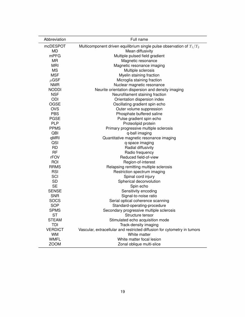
Abbreviation Full name

mcDESPOT Multicomponent driven equilibrium single pulse observation of T1/T2

MD Mean diffusivitymPFG Multiple pulsed field gradient

MR Magnetic resonanceMRI Magnetic resonance imagingMS Multiple sclerosis

MSF Myelin staining fractionµGSF Microglia staining fractionNMR Nuclear magnetic resonance

NODDI Neurite orientation dispersion and density imagingNSF Neurofilament staining fractionODI Orientation dispersion index

OGSE Oscillating gradient spin echoOVS Outer volume suppressionPBS Phosphate buffered saline

PGSE Pulse gradient spin echoPLP Proteolipid protein

PPMS Primary progressive multiple sclerosisQBI q-ball imaging

qMRI Quantitative magnetic resonance imagingQSI q-space imagingRD Radial diffusivityRF Radio frequency

rFOV Reduced field-of-viewROI Region-of-interest

RRMS Relapsing remitting multiple sclerosisRSI Restriction spectrum imagingSCI Spinal cord injurySD Spherical deconvolutionSE Spin echo

SENSE Sensitivity encodingSNR Signal-to-noise ratio

SOCS Serial optical coherence scanningSOP Standard-operating-procedure

SPMS Secondary progressive multiple sclerosisST Structure tensor

STEAM Stimulated echo acquisition modeTDI Track-density imaging

VERDICT Vascular, extracellular and restricted diffusion for cytometry in tumorsWM White matter

WMFL White matter focal lesionZOOM Zonal oblique multi-slice

19

List of Frequent Symbols

Symbol Meaning

α Structure tensor anisotropy indexb Diffusion weighting strength (b-value)B Magnetic fieldB0 Static magnetic field (polarisation)B1 RF magnetic field (excitation)

∆Bz Longitudinal magnetic field inhomogeneityβ0, β1, ... Coefficients of linear regression models

D Diffusion tensorD Diffusivityd‖ NODDI neural tissue diffusivitydiso NODDI isotropic compartment diffusivityδ Magnetic field gradient duration (PGSE sequence)∆ Pulse separation (PGSE sequence)f0 Larmor frequencyG Magnetic field gradientg Magnetic field gradient directionG Magnetic field gradient strengthγ Gyromagnetic ratioθ Structure tensor orientationθf Flip angleI0 Modified Bessel function of the first kind and order zeroJ Structure tensork Spatial frequency vectorκ Concentration parameter of directional distributions

logL Logarithm of the likelihood (log-likelihood)λ1, λ2, ... Eigenvalues of structure/diffusion tensors

M Magnetisation vectorM⊥, M⊥ Transverse component of the magnetisation

m Symbol used to indicate one among a list of metricsµ, µ Mean orientation of directional distributionsµ Magnetic moment (in chapter 3)ν Spread parameter of a Rician distributionp Set of parameters of a modelq q-vectorr Spatial position vectorR2 Coefficient of determination

20

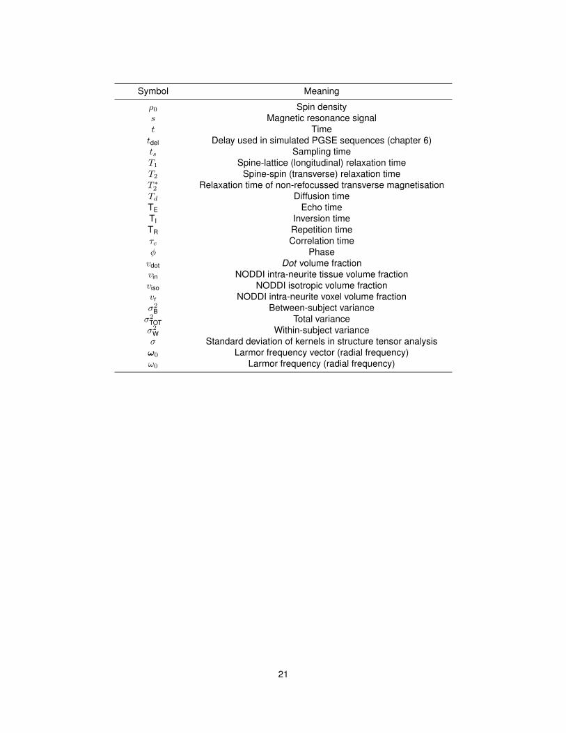
Symbol Meaning

ρ0 Spin densitys Magnetic resonance signalt Timetdel Delay used in simulated PGSE sequences (chapter 6)ts Sampling timeT1 Spine-lattice (longitudinal) relaxation timeT2 Spine-spin (transverse) relaxation timeT ∗2 Relaxation time of non-refocussed transverse magnetisationTd Diffusion timeTE Echo timeTI Inversion timeTR Repetition timeτc Correlation timeφ Phasevdot Dot volume fractionvin NODDI intra-neurite tissue volume fractionviso NODDI isotropic volume fractionvr NODDI intra-neurite voxel volume fractionσ2

B Between-subject varianceσ2

TOT Total varianceσ2

W Within-subject varianceσ Standard deviation of kernels in structure tensor analysisω0 Larmor frequency vector (radial frequency)ω0 Larmor frequency (radial frequency)

21

Chapter 1

Introduction

1.1 Background

Magnetic resonance imaging (MRI) is an important diagnostic tool employed routinely in clinicalpractice. MRI is key in monitoring disorders affecting the spinal cord, such as multiple sclerosis(MS), a disabling disease of the central nervous system. Current clinical MRI protocols for imagingthe spinal cord in MS rely on conventional techniques that detect the number and volume of focallesions and spinal cord atrophy. These are useful outcome measures, but alone do not capture thecomplexity of the disease. They underestimate the overall, widespread effects that MS has on thespinal cord [96], and provide only a partial explanation for the progression of the disability.

1.2 Problem statement

Novel MRI biomarkers are urgently needed to measure specific features of tissue pathology in neu-rological disorders. The intrinsic limitations of conventional MRI techniques, which detect macro-scopic aspects of disease processes and are not sensitive to early microscopic tissue damage,demand efforts by the MRI research community to develop new quantitative imaging methods.

Innovative MRI metrics are required in neurological conditions such as MS, in order to disen-tangle the pathophysiological components of the disease in a non-invasive fashion. This couldpotentially lead to earlier diagnosis and more accurate prognosis. Moreover, such new MRI mea-sures could also offer more effective ways of monitoring treatment efficacy than current techniques,with the benefit of reducing sample sizes in clinical trials of emerging neuroprotective treatments.

1.3 Aims

New quantitative MRI techniques are currently being developed to study tissue pathology in neuro-logical conditions in vivo. One such technique, neurite orientation dispersion and density imaging(NODDI) [215], is a model-based diffusion-weighted (DW) MRI method that provides estimates of

22

density and orientation dispersion of neuronal fibres. NODDI has previously been applied in studiesof the brain in neurological disorders, and we hypothesise that it could provide useful biomarkersfor microstructural changes occurring in the spinal cord.

In this PhD thesis, we aim to evaluate the potential of NODDI metrics as new biomarkers inspinal cord disorders, with a particular focus on MS. Innovative clinically feasible acquisition strate-gies and MRI signal analysis methods are tested on the spinal cords of healthy volunteers in vivo.Additionally, the specificity of the indices obtained with NODDI is examined in specimens of postmortem human spinal cord via systematic comparison to measures obtained from histology.

Our objectives are:

1. to demonstrate that innovative acquisition methods such as NODDI, which could potentiallyprovide new quantitative biomarkers of pathology, are feasible in the human spinal cord invivo and in a clinical setting (i.e. in about 20 minutes);

2. to relate NODDI-derived indices to results from a routine DW MRI method employed in clinicalstudies of the spinal cord, known as diffusion tensor imaging (DTI) [12];

3. to study the possibility of applying NODDI analysis to standard DW data;

4. to investigate the influence of specific microstructural features of the spinal cord on NODDImetrics;

5. to test the specificity of NODDI indices and the validity of the model assumptions in the pres-ence of MS pathology via comparison to quantitative histological features.

1.4 Scientific relevance of the work

This thesis provides a number of innovative contributions to MRI research, which led to a publishedpeer-reviewed journal article and to several abstracts accepted for presentation at internationalscientific meetings. Three further manuscripts are also currently in preparation to be submitted forpublication in peer-reviewed journals.

Specific contributions to the research field are listed below.

1. NODDI was demonstrated for the first time in the human spinal cord in vivo. This study isshown in chapter 4. Preliminary results were presented at international meetings as:

• “In vivo estimation of neuronal orientation dispersion and density of the human spinalcord”. Grussu F. et al, International Society for Magnetic Resonance in Medicine (ISMRM)workshop “Multiple sclerosis as a whole-brain disease” (2013), oral presentation.

• “Neurite orientation dispersion and density imaging of the cervical cord in vivo”. GrussuF. et al, ISMRM annual meeting (2014), p.1720, traditional poster.

The full study was later published in a peer-reviewed scientific journal as:

23

• “Neurite orientation dispersion and density imaging of the healthy cervical spinal cord invivo”, Grussu F. et al, NeuroImage (2015), vol. 111, p.590-601 (reference [67]).

2. The limitations of NODDI analysis of standard DW data of the spinal cord were identified.These are reported in chapter 5, and the work was presented to the scientific community as:

• “Single-shell diffusion MRI NODDI with in vivo cervical cord data”. Grussu F. et al,ISMRM annual meeting (2014), p.1716, traditional poster.

• “Characterisation of single-shell NODDI fitting in spinal cord grey and white matter”.Grussu F. et al, British Chapter of ISMRM annual meeting (2014), traditional poster.

3. The influence of spinal cord axon diameter distribution on NODDI metrics was evaluated viacomputer simulations and in vivo. This work is described in chapter 6. A scientific abstract de-scribing the study has also been submitted for consideration to the 2016 ISMRM annual meet-ing. Additionally, a manuscript is currently in preparation for submission to a peer-reviewedscientific journal. The ISMRM abstract submission was:

• “Axon diameter distribution influences diffusion-derived axonal density estimation in thehuman spinal cord: in silico and in vivo evidence”. Grussu F. et al, ISMRM annualmeeting (2016), p.2009, poster presentation.

4. A high-field, high-resolution diffusion MRI protocol for fixed ex vivo spinal cord specimenswas implemented, as well as a procedure for NODDI analysis of the acquired data. Theseimplementations are described in chapter 7.

5. A strategy to identify the radiographic position of histological material derived from spinal cordspecimens was designed, and is discussed in chapter 7.

6. A framework based on structure tensor (ST) analysis [16] for the estimation of neurite orien-tations from optical images of spinal cord tissue was developed. The framework is describedin chapter 8, and a manuscript is currently in preparation.

7. The associations between NODDI indices and quantitative histological features were identi-fied in a study involving MRI and histological analysis of non-pathological and MS spinal cordtissue. The study is discussed in chapter 9 and relies on the technical achievements listedin previous points 4, 5 and 6. We plan to publish it in a peer-reviewed scientific journal. Re-sults of preliminary analyses were submitted in abstract form to two scientific meetings, andpresented as:

• “Histological metrics confirm microstructural characteristics of NODDI indices in multiplesclerosis spinal cord”. Grussu F. et al, ISMRM annual meeting (2015), p.0909, oralpresentation.

• “Quantitative histological correlates of NODDI orientation dispersion estimates in thehuman spinal cord”. Grussu F. et al, ISMRM annual meeting (2015), p.0154, oral pre-sentation.

24

• “Quantitative histological validation of NODDI MRI indices of neurite morphology in mul-tiple sclerosis spinal cord”. Grussu F. et al, 31st congress of the European Committee forthe Research and Treatment in Multiple Sclerosis (ECTRIMS 2015), p.0469, traditionalposter presentation.

1.5 Structure of the thesis

This thesis is structured as follows. In chapter 2, an overview of the anatomy of the spinal cord andof its involvement in MS is presented. In chapter 3, background MRI theory and literature on whichthe methods of this thesis rely is summarised. In chapters 4, 5 and 6, experiments performed toinvestigate the potential of NODDI for applications in the human spinal cord in vivo are discussed.Ex vivo investigations are described in chapters 7, 8 and 9. The ultimate objective of that part of thethesis is the direct comparison of NODDI indices to quantitative histological features, to test theirspecificity in the non-pathological and MS spinal cord. Lastly, in chapter 10, a general discussionof the findings and the conclusions of the entire work are reported, as well as potential futuredirections.

25

Chapter 2

Neuroanatomy and multiplesclerosis: an overview

2.1 Neurons and neural tissue

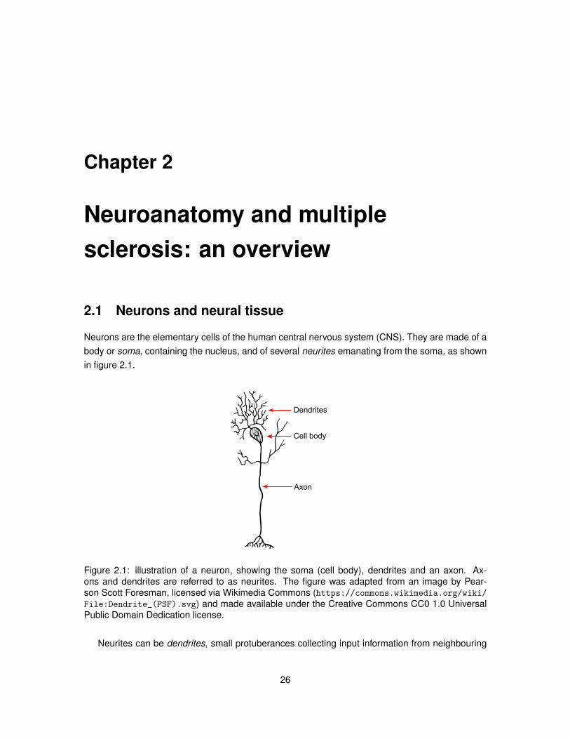
Neurons are the elementary cells of the human central nervous system (CNS). They are made of abody or soma, containing the nucleus, and of several neurites emanating from the soma, as shownin figure 2.1.

Dendrites

Cell body

Axon

Figure 2.1: illustration of a neuron, showing the soma (cell body), dendrites and an axon. Ax-ons and dendrites are referred to as neurites. The figure was adapted from an image by Pear-son Scott Foresman, licensed via Wikimedia Commons (https://commons.wikimedia.org/wiki/File:Dendrite_(PSF).svg) and made available under the Creative Commons CC0 1.0 UniversalPublic Domain Dedication license.

Neurites can be dendrites, small protuberances collecting input information from neighbouring

26

https://commons.wikimedia.org/wiki/File:Dendrite_(PSF).svg

https://commons.wikimedia.org/wiki/File:Dendrite_(PSF).svg

neurons, or axons, generally long projections transmitting information via action potentials. In thehuman CNS most axons are protected by a sheath that improves the conduction speed and whosethickness is about 40% of the radius of the bare axon. This sheath is made of myelin, a substanceproduced by specialised cells. Myelin is made by a mixture of lipids and proteins and is affected inseveral neurological conditions, such as MS.

Neurons are not the only elements of the neural tissue, which in fact contains also blood vesselsand several types of glial cells. Glial cells provide important support functions to neurons, such asproduction of myelin and immune response. Neural tissue can be distinguished into grey and whitematter (GM/WM). GM is made of neuronal cell bodies, dendritic arborisations as well as afferentand efferent myelinated and unmyelinated axons, glial cells and capillaries. WM represents thecabling connecting GM regions to other GM areas and to the periphery, and is made of myelinatedaxons and glial cells.

2.2 The human spinal cord

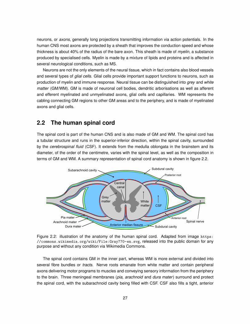
The spinal cord is part of the human CNS and is also made of GM and WM. The spinal cord hasa tubular structure and runs in the superior-inferior direction, within the spinal cavity, surroundedby the cerebrospinal fluid (CSF). It extends from the medulla oblongata in the brainstem and itsdiameter, of the order of the centimetre, varies with the spinal level, as well as the composition interms of GM and WM. A summary representation of spinal cord anatomy is shown in figure 2.2.

Centralcanal

Subdural cavity

Subdural cavityDura materArachnoid mater

Pia mater

Subarachnoid cavity

Spinal nerve

Posterior root

Anterior root

Grey matter White

matter

Anterior median fissure

CSF

Figure 2.2: illustration of the anatomy of the human spinal cord. Adapted from image https:

//commons.wikimedia.org/wiki/File:Gray770-en.svg, released into the public domain for anypurpose and without any condition via Wikimedia Commons.

The spinal cord contains GM in the inner part, whereas WM is more external and divided intoseveral fibre bundles or tracts. Nerve roots emanate from white matter and contain peripheralaxons delivering motor programs to muscles and conveying sensory information from the peripheryto the brain. Three meningeal membranes (pia, arachnoid and dura mater ) surround and protectthe spinal cord, with the subarachnoid cavity being filled with CSF. CSF also fills a tight, anterior

27

https://commons.wikimedia.org/wiki/File:Gray770-en.svg

https://commons.wikimedia.org/wiki/File:Gray770-en.svg

invagination known as anterior median fissure, and the central canal running longitudinally from theventricular system of the brain to the lumbar level.

In spite of its small size, the spinal cord has essential functions, and spinal cord pathologycan have severe consequences on the vital functions. As an example, traumatic spinal cord injury(SCI) is a complex phenomenon involving a cascade of noxious events that follow the primaryinjury [121, 179], and is often associated to major clinical disability. Several other diseases canalso affect the the spinal cord, such as MS, a neurodegenerative condition that often leads to animportant accrual of disability [112].

2.3 Multiple sclerosis

MS is an inflammatory and demyelinating disease affecting brain, spinal cord and optic nerves.In MS, several pathological features can coexist [31, 115], and some of them are thought to begenetically driven [188].

In around 85% of the patients, the disease starts with an acute neurological episode, generallyfollowed by other acute relapses, which alternate with periods of high level of functional recov-ery [47]. This form of the disease, called relapsing remitting MS (RRMS), is characterised by acuteinflammation, disruption of the blood-brain-barrier [141] and demyelination. RRMS is usually fol-lowed after 15-20 years from the symptom onset by a progressive stage, or secondary progressiveMS (SPMS), whose main feature is the irreversible accrual of disability. However, in 10-15% of MScases, the disease starts as a progressive neurological condition from the beginning, and it is calledprimary progressive MS (PPMS).

MS leads to neurodegeneration, which is believed to be triggered by the inflammatory demyeli-nating disease process of the early stages [115]. Phenomena such as microglia activation [39],oxidative stress [72] due to the release of iron in the extra-cellular space and toxic intra-axonalsodium accumulation due to the redistribution of sodium channels after demyelination [149] arethought to be involved in neurodegeneration.

Spinal cord involvement in MS is very common, and MRI of the spinal cord in clinical practice isrecommended [96]. Although spinal cord involvement in MS is expected to affect the clinical statusof patients, the correlation between clinical disability and MRI-derived spinal lesion number is mod-erate [96]. Conventional MRI, despite being able to detect focal MS pathology, lacks in sensitivityand specificity, and underestimates the real overall effect of the disease. Recent advances in MRItechnology and efforts in developing quantitative approaches may help to overcome this intrinsiclimitation, providing novel, specific metrics able to better characterise non-focal abnormalities andto detect intrinsic cord damage [63]. These new metrics may lead to more accurate prediction ofprognosis, to the improvement of our understanding of the disease and to better treatment moni-toring, with consequent reduction of sample sizes in clinical trials.

Several, innovative quantitative MRI techniques have shown promise in the MS brain and spinalcord. Among them: quantitative magnetization transfer imaging, providing indices of macromolec-ular proton fraction [164]; myelin water imaging, estimating myelin water fraction [107]; DTI [12],

28

sensitive to demyelination and diffuse changes in normal-appearing spinal cord [99]; diffusion ba-sis spectrum imaging (DBSI), modelling the effect of axonal injury, demyelination and inflammation[195]; g-ratio mapping, a potential tool to reveal between-lesion heterogeneity [173]; NODDI [215],capturing the density and the spread of neurite orientations, shown to be affected by MS [156];quantitative susceptibility mapping, sensitive to iron deposition in lesions [210]; sodium MRI, de-tecting pathological sodium accumulation [144].

29

Chapter 3

Background

3.1 Introduction to magnetic resonance imaging

MRI refers to a family of non-invasive medical imaging methods that produce images of the humanbody with magnetic fields. These images reflect how differently tissues immersed in a strong, staticmagnetic field react to externally applied radio frequency (RF) pulses, leading to between andwithin-tissue contrasts. MRI is based on the nuclear magnetic resonance (NMR) effect, which isthe interaction between nuclei magnetic moments and a static magnetic field. Also, MRI exploitsspatially variant magnetics fields (magnetic field gradients) to encode the position of the measuredsignals.

To date, MRI is an important diagnostic tool in several clinical disciplines and an active fieldof research. The success of MRI is related to the lack of employment of ionising radiation andto its versatility. Several different sources of contrast among tissues of similar densities can beexploited when producing an MRI image, provided that an adequate sequence (i.e. an ordered andtimed application of magnetic field pulses and gradients) is designed and employed. Therefore,the same physical machine can produce different types of images, conveying different pieces ofinformation about the imaged tissues. A careful design of the MRI experiment can produce imagesoptimised to emphasise the signals of specific areas or to suppress contributions from unwantedtissues. Moreover, specific biophysical properties such as cell density, myelin amount or blood flow,can be related to the measured MRI signals via mathematical models. This allows the inferenceof such properties when multiple images are acquired varying the sequence parameters. Thesequantitative approaches are often referred to as quantitative MRI (qMRI). qMRI has the potential ofproviding novel, sensitive and specific biomarkers capable of improving diagnosis and prognosis ina number of conditions, although the specificity and the validity of such new indices in pathologyalways needs to be confirmed and verified.

This thesis deals with qMRI of the human spinal cord for MS applications, and focusses onDW MRI. In this chapter, the theoretical background on which the MRI methods of this work relyis described. Elementary magnetic properties of the nuclei will be firstly introduced. Then, phe-

30

nomenological equations describing the behaviour of a macroscopic ensemble of nuclei, the Blochequations, will be presented. Afterwards, key concepts regarding the image formation process andmodern solutions to accelerate the acquisition are described. These are followed by a whole sec-tion on DW MRI and by one on qMRI of the human spinal cord. Lastly, a final part introducing recentapproaches commonly employed for the validation of qMRI is included. Extensive consultation ofreferences [36,69,92,180] has been essential for writing this chapter.

3.2 Spins and magnetic moments

Nuclei are characterised by certain physical properties such as an intrinsic angular momentum L, orspin, which arises from the contribution of its protons and neutrons. Nuclei that do not have an evennumber of both protons and neutrons are characterised by a non-vanishing angular momentum,and possess a net magnetic moment µ related to L via

µ = γ L, (3.1)

where γ is the gyromagnetic ratio, whose value depends on the nucleus in question.Nuclei would align their elementary magnetic moments in parallel and anti-parallel directions

with respect to a static magnetic field in which they were to be immersed. A small excess of nucleiin one of the two configurations gives rise to a net magnetisation of the ensemble, which can beimaged. Several nuclei, such as 1H, 23Na, 31P and others can potentially be object of an NMRexperiment. In practice, the relative amplitude of the detectable signals is limited by the physicalabundance of the nucleus in the imaged tissue. In the human body, due to the abundance ofwater, the nucleus that is more easily employed to give rise to a net magnetisation and to produceNMR signals is 1H.1H-MRI has improved dramatically since the first steps in the years forties of thetwentieth century, and various imaging modalities based on signals from 1H are nowadays available.

This thesis deals with 1H-MRI, and focuses on the signal arising from water protons and onthe effect that diffusion has on it. As common in current 1H-MRI literature, the term spin will beemployed from now onwards as a synonymous of water proton.

3.2.1 Dynamics of a spin from classical mechanics

The rigorous description of the interaction between a spin magnetic moment and an external mag-netic field relies on quantum mechanics. Nevertheless, an effective formalism based on a classicaldescription also allows the understanding of the main phenomena occurring during an MRI experi-ment.

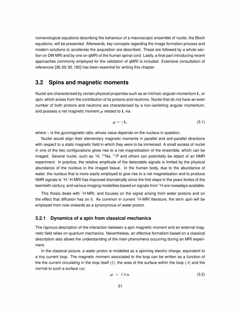
In the classical picture, a water proton is modelled as a spinning electric charge, equivalent toa tiny current loop. The magnetic moment associated to the loop can be written as a function ofthe the current circulating in the loop itself (I), the area of the surface within the loop (A) and thenormal to such a surface (u):

µ = IAu. (3.2)

31

For the same simple system, the gyromagnetic ratio can be calculated from the properties of thespinning charge (i.e. its mass m and charge q) as γ = q

2m . Plugging the mass and charge of theproton would provide the gyromagnetic ratio of an isolated proton. In practice, the real value of γfor water protons has been derived experimentally and it is equal to 2.675 · 108 s−1 T−1.

If the current loop is immersed in a magnetic field B, a net torque τ depending on the propertiesof the loop and on the field itself will act upon it. This torque can be calculated as the cross product

τ = µ×B. (3.3)

The temporal evolution of the loop angular momentum can be obtained from Newton’s second lawof motion in angular terms (conservation of angular momentum), which in this case is written asddtL(t) = τ (t). Recalling from equation 3.1 that L(t) = 1

γ µ(t) and substituting the expression ofτ (t) from equation 3.3, the vectorial partial differential equation describing the dynamics of the spinunder the external field B in classical terms is readily obtained as

dµ(t)

dt= γ µ(t)×B(t). (3.4)

Equation 3.4 states that under a generic field B(t), the magnetic moment µ(t) rotates with aninstantaneous angular velocity ω(t) = − γB(t) proportional to the field B(t) at any given time t.

3.2.2 Larmor precession of a spin

The solution of equation 3.4 under a static field B(t) = B0 =[0 0 B0

]Tand for an initial condition

µ(0) =[µx(0) µy(0) µz(0)

]Tdescribes the free precession of the spin magnetic moment about

the direction z of the static field. Describing the component of µ(t) orthogonal to B0 with a complex-valued notation, i.e. defining µ⊥(t) = µx(t) + j µy(t), the free precession solution of equation 3.4is written as

µ⊥(t) = e−j ω0tµ⊥(0), (3.5)

while µz(t) = µz(0) ∀ t ≥ 0. This is equivalent to state that the component of µ(t) orthogonal tothe main field rotates clockwise about +z.

As illustrated by figure 3.1, the magnetic moment µ(t) precesses with angular frequency ω0 =

γB0 about the direction of the field B0 from the initial condition µ(0). Such phenomenon is referredto as Larmor precession and the frequency ω0 is called Larmor frequency or resonance frequency.The precession is associated to the component of µ(t) orthogonal to B0, while the component µz(t)parallel to B0 is constant and equal to the initial value.

The phase accrual during the free precession is the quantity φ(t) = ∠µ⊥(t) − ∠µ⊥(0), which,in the general case of spatially and time variant polarising fields aligned with the z direction, can becalculated as

φ(r, t) = − γ∫ t

0

Bz(r, t′) dt

′. (3.6)

32

Spinning

proton

B0

Current

loop

B0 µµ

b)a)

Figure 3.1: illustration showing how a spinning proton, pictured in a), is described in terms of acurrent loop, pictured in b), according to the classical formalism.

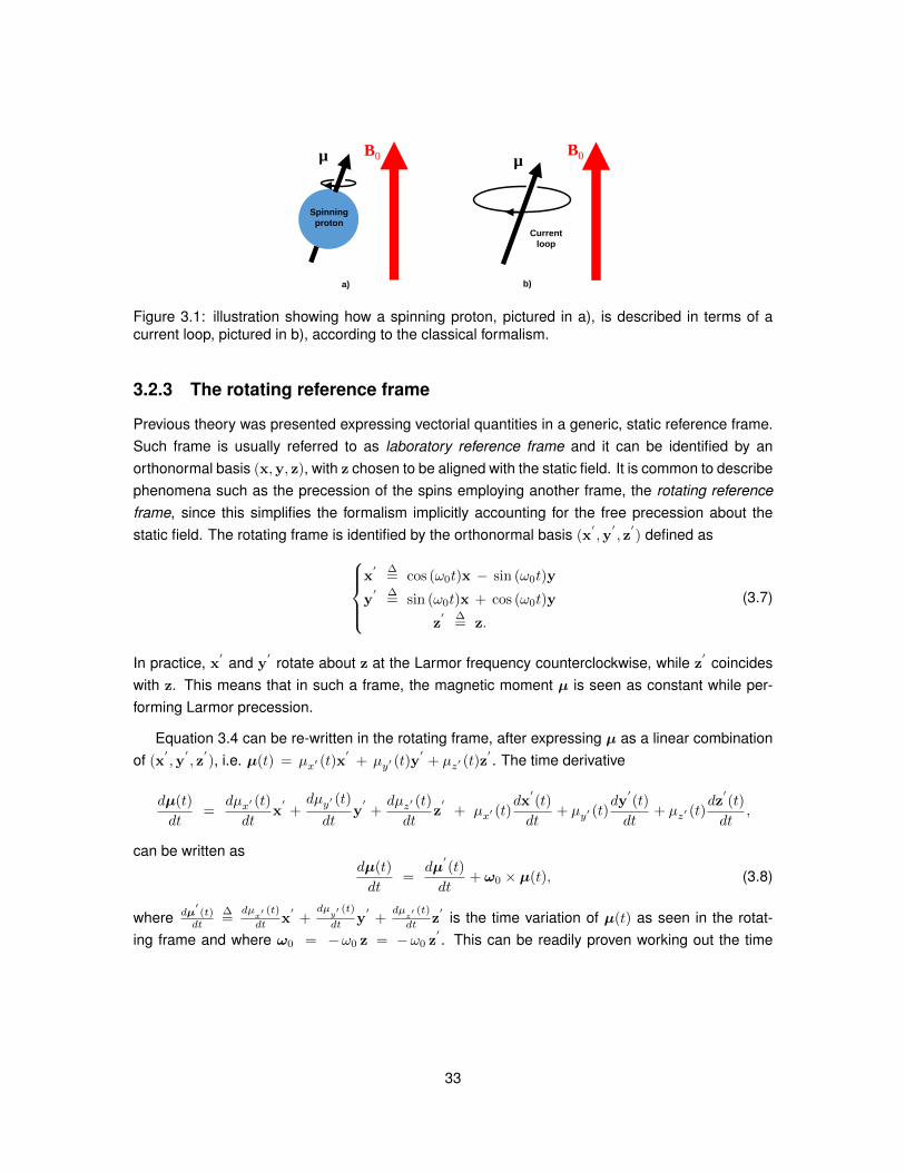
3.2.3 The rotating reference frame

Previous theory was presented expressing vectorial quantities in a generic, static reference frame.Such frame is usually referred to as laboratory reference frame and it can be identified by anorthonormal basis (x,y, z), with z chosen to be aligned with the static field. It is common to describephenomena such as the precession of the spins employing another frame, the rotating referenceframe, since this simplifies the formalism implicitly accounting for the free precession about thestatic field. The rotating frame is identified by the orthonormal basis (x

′,y′, z′) defined as

x′ ∆

= cos (ω0t)x − sin (ω0t)y

y′ ∆

= sin (ω0t)x + cos (ω0t)y

z′ ∆

= z.

(3.7)

In practice, x′

and y′

rotate about z at the Larmor frequency counterclockwise, while z′

coincideswith z. This means that in such a frame, the magnetic moment µ is seen as constant while per-forming Larmor precession.

Equation 3.4 can be re-written in the rotating frame, after expressing µ as a linear combinationof (x

′,y′, z′), i.e. µ(t) = µx′ (t)x

′+ µy′ (t)y

′+ µz′ (t)z

′. The time derivative

dµ(t)

dt=

dµx′ (t)

dtx′+dµy′ (t)

dty′+dµz′ (t)

dtz′

+ µx′ (t)dx′(t)

dt+ µy′ (t)

dy′(t)

dt+ µz′ (t)

dz′(t)

dt,

can be written asdµ(t)

dt=

dµ′(t)

dt+ ω0 × µ(t), (3.8)

where dµ′(t)

dt

∆=

dµx′ (t)

dt x′

+dµy′ (t)

dt y′

+dµz′ (t)

dt z′

is the time variation of µ(t) as seen in the rotat-ing frame and where ω0 = −ω0 z = −ω0 z

′. This can be readily proven working out the time

33

derivatives of the expressions in equation 3.7, which lead todx′

dt = −ω0 (sin (ω0t)x + cos (ω0t)y) = −ω0 y′

= ω0 × x′

dy′

dt = ω0 (cos (ω0t)x − sin (ω0t)y) = ω0 x′

= ω0 × y′

dz′

dt = 0 = ω0 × z′.

The right side of equation 3.8 must equal that of equation 3.4, i.e. it must hold that

γ µ(t)×B(t) ≡ dµ′(t)

dt+ ω0 × µ(t).

Writing the term γ µ(t)×B(t) as

γ µ(t)×B(t) = γ µ(t)×B0 + γ µ(t)×Bext(t) = ω0 × µ(t) + γ µ(t)×Bext(t)

allows the expression of the temporal variation of the magnetic moment in the rotating frame as afunction of the magnetic field from which the static, polarising component has been removed. Thedynamics of the magnetic moment in the rotating frame becomes

dµ(t)

dt= γ µ(t)×Bext(t). (3.9)

3.3 Bloch equations and relaxation

In the previous section, the elementary magnetic moment µ of a spin was introduced. When anensemble of spins contained in a volume V is considered, it is useful to define the net magnetisationM of the spin ensemble, which is the total magnetic moment per unit of volume:

M =1

V

∑n

µn. (3.10)

The net magnetisation, at equilibrium, is aligned with the static field B0, so that M = M0 =[0 0 M0

]T. M0 is proportional to the field strength, the spin density and inversely proportional to

the temperature. Quantum physics principle lead to the following expression of M0:

M0 =14γ22

KTB0 ρ0, (3.11)

where K is the Boltzmann constant, is the reduced Planck’s constant, T is the temperature andρ0 is the spin density.

The magnetisation M can be perturbed from the equilibrium condition by the exposure to ra-diation, in the form of time variant magnetic fields orthogonal to the main static field. In the nextsections, details about the response of M to perturbations from the equilibrium are presented.

34

3.3.1 The Bloch equations

The behaviour of the net magnetisation M under the application of external magnetic fields canbe described rigorously in terms of quantum mechanics. Nevertheless, it is common to employmacroscopic ordinary differential equations to predict the time evolution of M, i.e. the so calledBloch equations [18]. The Bloch equations model the Larmor precession of M about a staticfield, its response to any applied time variant field and describe the return of M to its equilib-rium value, i.e. its relaxation. In the laboratory reference frame introduced in section 3.2, where

the static field B0 =[0 0 B0

]Tis directed along the z-axis, the Bloch equations can be sum-

marised in the following vectorial ordinary differential equation describing the time evolution of

M(t) =[Mx(t) My(t) Mz(t)

]T:

dM(t)

dt= γM(t)×B(t) − R (M(t)−M0). (3.12)

In equation 3.12, × is the cross product, M0 is the equilibrium magnetisation; B(t) = B0 + Bext(t)

is the total magnetic field; B0 is the static field; R = diag(T−12 , T−1

2 , T−11 ) is the relaxation matrix,

with T1 being the spin-lattice relaxation time and T2 the spin-spin relaxation time.The first term to the right hand side of equation 3.12 describes the instantaneous precession of

M(t) about the total field B(t) with angular frequency ω(t) = −γB(t), whereas the second termdescribes the tendency of M(t) to return to the equilibrium condition M(t) = M0. Integration ofequation 3.12 provides the behaviour of M(t) for a given field B(t), of which two examples arereported in sections 3.3.3 and 3.3.4.

3.3.2 Relaxation time constants

The spin-lattice and spin-spin relaxation times T1 and T2 respectively describe the rate at which thelongitudinal component Mz(t) of M(t) approaches the equilibrium value M0, and the rate at whichany component of M(t) orthogonal to the main static field decays. At 3 T, typical values of T1 andT2 are on the order of 1300 ms and 830 ms (T1) and of 100 ms and 80 ms (T2) for brain grey andwhite matter [197].

The molecular basis from which T1 and T2 originate have been extensively studied at the dawnof the NMR field, and a theory by Bloembergen, Purcell and Pound (BPP theory), which relates thevalues of T1 and T2 to the tumbling motion of the molecules, has been proposed [19].

In the BPP formalisms, T1 and T2 are related to the line widths of the curves describing theabsorption of energy by a material immersed in a static magnetic field and exposed to radiation [19].They can be expressed as a function of τc, the correlation time determining the time scale of theinteractions among molecules due to vibrational, rotational and translational motion. Specifically,T1 is the time constant characterising the transfer of energy from the irradiated spin system tothe heat reservoir comprising all remaining degrees of freedom of the substance in question. Onthe other hand, T2 is related to the interactions among the magnetic nuclei themselves. Theseoccur due to the fact that each spin experiences the local fluctuating magnetic field produced by

35

neighbouring spins, which causes the spin ensemble to dephase. Local inhomogeneities of themain static field can also affect the field experienced by each spin, and a time constant T ∗2 smallerthan the theoretical T2 may need to be introduced. In [19], expressions of T1 and T2 as a functionof τc are provided.

As far as water is concerned, the authors in [19] claim that for T1, τc is driven by the interactionsof each proton with its proton partner in a water molecule. τc is in practice approximated as thetime during which the orientation of a molecule persists, and in its calculation vibrational, and, to aless extent, rotational and translational components of the thermal motion of water molecules canbe neglected [19]. For a given field strength B0 and a resonance angular frequency ω0 = γ B0, thereciprocal of T1 is found to be

1

T1= C1

(τc

1 + (ω0 τc)2+

2τc1 + (2ω0 τc)2

), (3.13)

with C1 being a constant depending on factors such as the interproton distance, assumed to be1.5 · 10−10 m.

With regard to T2, the authors of [19] provide the expression

1

T2=

√2π

1

T′2

+1

2T1, (3.14)

which is a function of T1 and of T′

2, with the latter being the solution of the transcendental equation(1

T′2

)2

=3πC1 atan

(2 τcT′2

). (3.15)

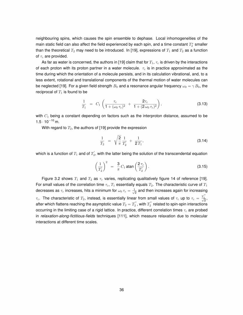
Figure 3.2 shows T1 and T2 as τc varies, replicating qualitatively figure 14 of reference [19].For small values of the correlation time τc, T1 essentially equals T2. The characteristic curve of T1

decreases as τc increases, hits a minimum for ω0 τc = 1√2

and then increases again for increasing

τc. The characteristic of T2, instead, is essentially linear from small values of τc up to τc =T′′2√2,

after which flattens reaching the asymptotic value T2 = T′′

2 , with T′′

2 related to spin-spin interactionsoccurring in the limiting case of a rigid lattice. In practice, different correlation times τc are probedin relaxation-along-fictitious-fields techniques [111], which measure relaxation due to molecularinteractions at different time scales.

36

τc [s]

T1andT2

[s]

T2T1

τc = 1/√2ω0 →

τc = T′′

2 /√2 →

10−15 10−310−11 10−7

10−1

10−5

103

Figure 3.2: illustration replicating qualitatively figure 14 of reference [19]. The plot describes thedependence of relaxation times T1 and T2 on the correlation time τc for water.

The BPP theory was also applied to materials other than water, such as various liquids char-acterised by different viscosities. In those cases, experimental results confirmed the theoreticalfinding that the correlation time τc can be considered proportional to the ratio η/T , with η and T

indicating the viscosity and the temperature of the liquid [19].

Lastly, it is reported that the relaxation properties depend on the field strength. In a clinicalsystem with a field strength of the order of the Tesla, T1 of water protons is longer than T2. Theformer increases for increasing field strength, whereas the latter decreases. This fact is exploited infield cycling MRI as a source of contrast among tissues, since in field cycling methods the strengthof the static field is varied during the experiment [152].

3.3.3 Evolution of the magnetisation under a static field

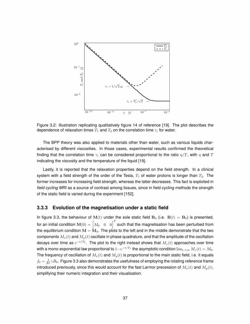
In figure 3.3, the behaviour of M(t) under the sole static field B0 (i.e. B(t) = B0) is presented,

for an initial condition M(0) =[M0 0 0

]Tsuch that the magnetisation has been perturbed from

the equilibrium condition M = M0. The plots to the left and in the middle demonstrate that the twocomponentsMx(t) andMy(t) oscillate in phase quadrature, and that the amplitude of the oscillationdecays over time as e−t/T2 . The plot to the right instead shows that Mz(t) approaches over timewith a mono-exponential law proportional to 1−e−t/T1 the asymptotic condition limt→∞Mz(t) = M0.The frequency of oscillation of Mx(t) and My(t) is proportional to the main static field, i.e. it equalsf0 = 1

2πγB0. Figure 3.3 also demonstrates the usefulness of employing the rotating reference frameintroduced previously, since this would account for the fast Larmor precession of Mx(t) and My(t),simplifying their numeric integration and their visualisation.

37

0 0.2 0.4−1

−0.5

0

0.5

1

time [s]

Mx(t)/M

0

0 0.2 0.4−1

−0.5

0

0.5

1

time [s]

My(t)/M

0

0 2 40

0.5

1

time [s]

Mz(t)/M

0

Figure 3.3: behaviour of the magnetisation under a static field B(t) = B0 and for an initial conditionM(0) = [M0 0 0 ]

T, in the laboratory frame. The plot to the left describes the time evolution ofMx(t); the central plot of My(t); the plot to the right of Mz(t). Values of 830 ms and of 70 ms wereemployed respectively for T1 and T2. For illustrative purposes, in practice a static field strength ofB0 = 1µT, corresponding to a Larmor frequency f0 = 1

2πγB0 = 42.58 Hz, was employed. Typicalfield strengths of modern MRI machines (on the order of the Tesla) would have provided oscillationsat much higher frequencies, on the order of the hundreds of MHz. Oscillations at that frequencyare difficult to visualise in a time interval of duration appropriate to demonstrate relaxation effects.

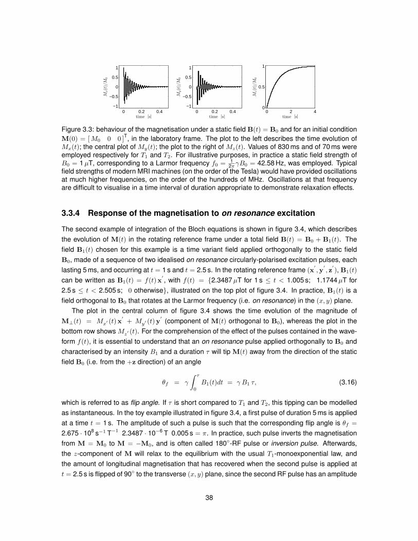
3.3.4 Response of the magnetisation to on resonance excitation

The second example of integration of the Bloch equations is shown in figure 3.4, which describesthe evolution of M(t) in the rotating reference frame under a total field B(t) = B0 + B1(t). Thefield B1(t) chosen for this example is a time variant field applied orthogonally to the static fieldB0, made of a sequence of two idealised on resonance circularly-polarised excitation pulses, eachlasting 5 ms, and occurring at t = 1 s and t = 2.5 s. In the rotating reference frame (x

′,y′, z′), B1(t)

can be written as B1(t) = f(t)x′, with f(t) = 2.3487µT for 1 s ≤ t < 1.005 s; 1.1744µT for

2.5 s ≤ t < 2.505 s; 0 otherwise, illustrated on the top plot of figure 3.4. In practice, B1(t) is afield orthogonal to B0 that rotates at the Larmor frequency (i.e. on resonance) in the (x, y) plane.

The plot in the central column of figure 3.4 shows the time evolution of the magnitude ofM⊥(t) = Mx′ (t)x

′+ My′ (t)y

′(component of M(t) orthogonal to B0), whereas the plot in the

bottom row shows Mz′ (t). For the comprehension of the effect of the pulses contained in the wave-form f(t), it is essential to understand that an on resonance pulse applied orthogonally to B0 andcharacterised by an intensity B1 and a duration τ will tip M(t) away from the direction of the staticfield B0 (i.e. from the +z direction) of an angle

θf = γ

∫ τ

0

B1(t)dt = γ B1 τ, (3.16)

which is referred to as flip angle. If τ is short compared to T1 and T2, this tipping can be modelledas instantaneous. In the toy example illustrated in figure 3.4, a first pulse of duration 5 ms is appliedat a time t = 1 s. The amplitude of such a pulse is such that the corresponding flip angle is θf =

2.675 · 108 s−1 T−1 2.3487 · 10−6 T 0.005 s = π. In practice, such pulse inverts the magnetisationfrom M = M0 to M = −M0, and is often called 180-RF pulse or inversion pulse. Afterwards,the z-component of M will relax to the equilibrium with the usual T1-monoexponential law, andthe amount of longitudinal magnetisation that has recovered when the second pulse is applied att = 2.5 s is flipped of 90 to the transverse (x, y) plane, since the second RF pulse has an amplitude

38

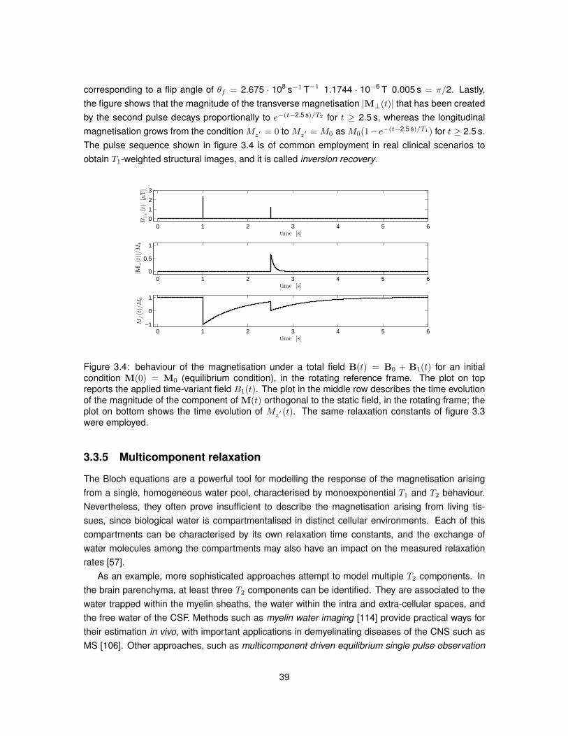
corresponding to a flip angle of θf = 2.675 · 108 s−1 T−1 1.1744 · 10−6 T 0.005 s = π/2. Lastly,the figure shows that the magnitude of the transverse magnetisation |M⊥(t)| that has been createdby the second pulse decays proportionally to e−(t−2.5 s)/T2 for t ≥ 2.5 s, whereas the longitudinalmagnetisation grows from the condition Mz′ = 0 to Mz′ = M0 as M0(1−e−(t−2.5 s)/T1) for t ≥ 2.5 s.The pulse sequence shown in figure 3.4 is of common employment in real clinical scenarios toobtain T1-weighted structural images, and it is called inversion recovery.

0 1 2 3 4 5 60

1

2

3

time [s]

B1x′(t)

[µT]

0 1 2 3 4 5 60

0.5

1

time [s]

|M⊥(t)|/M

0

0 1 2 3 4 5 6−1

0

1

time [s]

Mz′(t)/M

0

Figure 3.4: behaviour of the magnetisation under a total field B(t) = B0 + B1(t) for an initialcondition M(0) = M0 (equilibrium condition), in the rotating reference frame. The plot on topreports the applied time-variant field B1(t). The plot in the middle row describes the time evolutionof the magnitude of the component of M(t) orthogonal to the static field, in the rotating frame; theplot on bottom shows the time evolution of Mz′ (t). The same relaxation constants of figure 3.3were employed.

3.3.5 Multicomponent relaxation

The Bloch equations are a powerful tool for modelling the response of the magnetisation arisingfrom a single, homogeneous water pool, characterised by monoexponential T1 and T2 behaviour.Nevertheless, they often prove insufficient to describe the magnetisation arising from living tis-sues, since biological water is compartmentalised in distinct cellular environments. Each of thiscompartments can be characterised by its own relaxation time constants, and the exchange ofwater molecules among the compartments may also have an impact on the measured relaxationrates [57].

As an example, more sophisticated approaches attempt to model multiple T2 components. Inthe brain parenchyma, at least three T2 components can be identified. They are associated to thewater trapped within the myelin sheaths, the water within the intra and extra-cellular spaces, andthe free water of the CSF. Methods such as myelin water imaging [114] provide practical ways fortheir estimation in vivo, with important applications in demyelinating diseases of the CNS such asMS [106]. Other approaches, such as multicomponent driven equilibrium single pulse observation

39

of T1/T2 (mcDESPOT) [42], try to model in a single experimental framework multicomponent trans-verse and longitudinal relaxation, while accounting for the residence time of the water molecules inthe different physical compartments.

3.3.6 Bloch-Torrey equations

Section 3.3 is concluded with an extension of the Bloch equations that allows to model the effectof diffusion. Water molecules in tissues are not still but diffuse randomly due to their thermalagitation [50]. Hence, spins that diffuse in the presence of a spatially variant magnetic field probedifferent local fields as they vary their position in space. The ensemble average of the magneticmoments of the diffusing water molecules provides the total magnetisation M(r, t), whose evolutionis described by the Bloch-Torrey equations [181]. They are usually written as a vectorial partialdifferential equation in the following form:

∂M(r, t)

∂t= γM(r, t)×B(r, t) − R (M(r, t)−M0) − ∇T D(r)∇(M(r, t)−M0). (3.17)

Equation 3.17 is similar to equation 3.12, with the only differences that now M(r, t) and B(r, t)

are modelled as function of both time and spatial position r =[x y z

]Tand that and additional

decay term proportional to the spatial gradient of the magnetisation has been added. Such a termis related to the diffusion tensor D(r), a rank-2 tensor represented in the form of a positive semi-definite, symmetric 3× 3 matrix, which describes how far along any possible spatial direction watermolecules diffuse.

Analytical or numerical integration of equation 3.17 for different boundary conditions describingthe domains within which water molecules diffuse and for a generic magnetic field

B(r, t) = B0 + B1(t) + G(t)Tr (3.18)

can provide useful descriptions of the MRI signal arising from porous media [130]. In equation 3.18,B0 and B1(t) are the static polarising field and a time variant RF excitation field, whereas G(t) is atime variant magnetic field gradient that makes the signal sensitive to diffusion.

3.4 Signal detection and imaging equation

Previous sections have described how the NMR effect and relaxation create potential sources ofcontrast among tissues. In this section, we aim to review how this potential is in practice exploitedto measure signals that reflect the properties of tissues, leading ultimately to images.

3.4.1 From the magnetisation to a measurable signal

Faraday’s law of induction is the principle upon which the detection of the NMR signal relies. Thetime variant component of the magnetisation generates a time variant magnetic field in the proximity

40

of a coil. Hence, an electromotive force is induced in the coil due to temporal variations of the fieldflux. Its measure ultimately allows inference about the tissues magnetisation.

The magnetic flux induced on the coil by the magnetisation can be written according to Fara-day’s law as E(t) = − d

dt

∫ABM(r, t)Tn d2A, where BM(r, t) is the magnetic field due to the tissue

magnetisation, A is the surface of the coil with n being the normal to the surface, d2A is the surfaceelement. The field BM(r, t) can be expressed directly as a function of the magnetisation M(r, t).Also, employing the reciprocity principle, the expression of the flux of the magnetisation through thecoil can be written as a function of the field that the coil would produce per unit of current in pointswhere the magnetisation does not vanish. If the latter is indicated as βr(r), E(t) can be rewritten as

E(t) = −∫V∂M(r,t)∂t

Tβr(r) d3V , having indicated with V the volume from which the magnetisation

M(r, t) arises and with d3V the volume element [69].

After excitation, ∂M(r,t)∂t is described by the Bloch equations. The transverse component M⊥(r, t)

of M(r, t) decays while rotating at the Larmor frequency ω0, whereas the longitudinal componentMz(r, t) relaxes depending on the local value of T1. It follows that the magnitude of the timevariation of M⊥(r, t) and Mz(r, t) are respectively proportional to ω0 and T−1

1 . For modern fieldstrengths of the order of the Tesla, ω0 T−1

1 , and therefore the contribution of ∂Mz(r,t)∂t can be

neglected as compared to ∂M⊥(r,t)∂t . Hence, adopting the complex-valued notation M⊥(r, t) =

Mx(r, t) + j My(r, t) and indicating with βr⊥(r) = βr,x(r) + j βr,y(r), the signal in the receiver coilcan be written as

s(t) = ζ ω0

∫V

M⊥(r, t)βr⊥(r) d3V (3.19)

with ζ accounting for gains from the electronics and with s(t) being in general complex. In practice,a real and an imaginary channel are obtained from the induced electromotive force E(t) via cosineand sine demodulation, i.e. multiplying E(t) with two oscillatory signals in phase quadrature whileremoving oscillations at the Larmor frequency.

By virtue of equation 3.11 it is possible to express M⊥(r, t) in equation 3.19 as

M⊥(r, t) =1

4

γ2

KTω0 w (T1(r), T2(r), T ∗2 (r), t) ρ0(r),

where ρ0(r) is the spin density, , K and T have been already introduced, w (T1(r), T2(r), T ∗2 (r), t)

is a relaxation-weighting factor depending on the adopted sequence of RF pulses. Ultimately, thesignal measured by the receiver becomes

s(t) =1

4ζγ2

KTω2

0

∫V

w (T1(r), T2(r), T ∗2 (r), t) ρ0(r)βr⊥(r) d3V. (3.20)

3.4.2 The imaging problem

Previous discussion has related the signal as measured by the receiver coil to the spin density.Equation 3.20 can rather be written in terms of an effective spin density ρ such that

ρ e jψ =1

4ζγ2

KTω2

0 w (T1(r), T2(r), T ∗2 (r), t) ρ0(r)βr⊥(r).

41

ρ depends on factors such as field strength, temperature, receiver coil geometry, electronic gains,relaxation rates, actual spin density and ψ is the phase accumulated by spins in the transverse planeafter signal demodulation. Equation 3.20 can the be generically reformulated as s =

∫Vρ(r) e jψ d3V

having omitted the dependence of ρ(r) on factors other than the position. Above, ψ is ψ = φ+γB0t,with φ from equation 3.6.

If a magnetic field gradient G(t)∆= ∇Bz(t) is switched on when the magnetisation has a trans-

verse component, ψ can be expressed as ψ = − γ(∫ t

0G(t

′) dt

′)T

r = −kTr, leading to

s(k) =

∫V

ρ(r) e−j kTr d3V. (3.21)

Equation 3.21 is the fundamental upon which imaging relies, since it states that the measuredsignal, expressed as a function of the variable

k(t)∆= γ

∫ t

0

G(t′) dt

′(3.22)

encoding the history of the magnetic field gradient, is the Fourier transform of the effective spindensity in the spatial domain. Hence, knowledge of s(k) from a set of measurements obtainedwhile gradients are turned on (i.e. sampling of the k-space) can lead to the estimation of ρ(r)

via inverse Fourier transformation. Equation 3.22 implies that three independent coils capable ofgenerating three mutually orthogonal gradient components are necessary for imaging.

3.5 Common MRI signal weightings

In the previous section, the fundamental principles concerning the detection of NMR signals fromthe body by a coil element have been described. In particular, it has been reported that the mea-sured signals are proportional to the component of magnetisation M⊥ = Mx + j My orthogonal tothe static polarising field. Differences in terms of properties such as relaxation times and protondensity cause M⊥ to differ among tissues, leading eventually to image contrast.

Generally, an MRI experiment can be thought as composed of two stages. In the first stage, orpreparation stage, RF pulses in combination with magnetic field gradients are employed in orderto obtain the desired type of weighting of the signal, determining the driving source of contrastamong tissues. For instance, for T1-weighted imaging, the preparation stage will be such that themeasured signals will be strongly dependent on the T1 of tissues, rather than T2. In the second oracquisition stage, the signal induced in the coil is sampled. Magnetic field gradients are employedduring this stage in order to encode the spatial position from which the signals originate.

In this section, a summary review of preparation sequences of RF pulses and their correspond-ing signal weighting are presented. The review aims to demonstrate to the reader how relativelysimple manipulations of the magnetisation can lead to a variety of contrasts.

The notation x-pulse will be employed to indicate an RF pulse whose flip angle equals x (for

42

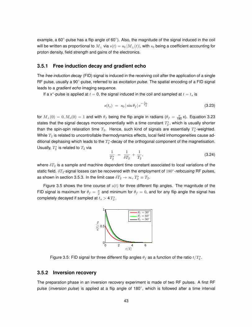
example, a 60-pulse has a flip angle of 60). Also, the magnitude of the signal induced in the coilwill be written as proportional to M⊥ via s(t) = s0 |M⊥(t)|, with s0 being a coefficient accounting forproton density, field strength and gains of the electronics.

3.5.1 Free induction decay and gradient echo

The free induction decay (FID) signal is induced in the receiving coil after the application of a singleRF pulse, usually a 90-pulse, referred to as excitation pulse. The spatial encoding of a FID signalleads to a gradient echo imaging sequence.

If a x-pulse is applied at t = 0, the signal induced in the coil and sampled at t = ts is

s(ts) = s0 | sin θf | e− tsT∗2 (3.23)

for M⊥(0) = 0,Mz(0) = 1 and with θf being the flip angle in radians (θf = π180 x). Equation 3.23

states that the signal decays monoexponentially with a time constant T ∗2 , which is usually shorterthan the spin-spin relaxation time T2. Hence, such kind of signals are essentially T ∗2 -weighted.While T2 is related to uncontrollable thermodynamics effects, local field inhomogeneities cause ad-ditional dephasing which leads to the T ∗2 -decay of the orthogonal component of the magnetisation.Usually, T ∗2 is related to T2 via

1

T ∗2=

1

δT2+

1

T2, (3.24)

where δT2 is a sample and machine dependent time constant associated to local variations of thestatic field. δT2-signal losses can be recovered with the employment of 180-refocusing RF pulses,as shown in section 3.5.3. In the limit case δT2 →∞, T ∗2 ≡ T2.

Figure 3.5 shows the time course of s(t) for three different flip angles. The magnitude of theFID signal is maximum for θf = π

2 and minimum for θf = 0, and for any flip angle the signal hascompletely decayed if sampled at ts > 4T ∗2 .

0 2 4 60

0.5

1

t/T ∗

2

s(t)/s 0

θf = 30

θf = 60

θf = 90

Figure 3.5: FID signal for three different flip angles θf as a function of the ratio t/T ∗2 .

3.5.2 Inversion recovery

The preparation phase in an inversion recovery experiment is made of two RF pulses. A first RFpulse (inversion pulse) is applied at a flip angle of 180, which is followed after a time interval

43

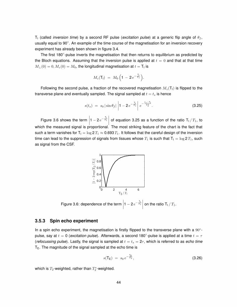
TI (called inversion time) by a second RF pulse (excitation pulse) at a generic flip angle of θf ,usually equal to 90. An example of the time course of the magnetisation for an inversion recoveryexperiment has already been shown in figure 3.4.

The first 180-pulse inverts the magnetisation that then returns to equilibrium as predicted bythe Bloch equations. Assuming that the inversion pulse is applied at t = 0 and that at that timeM⊥(0) = 0,Mz(0) = M0, the longitudinal magnetisation at t = TI is

Mz(TI) = M0

(1 − 2 e−

TIT1

).

Following the second pulse, a fraction of the recovered magnetisation Mz(TI) is flipped to thetransverse plane and eventually sampled. The signal sampled at t = ts is hence

s(ts) = s0 | sin θf |∣∣∣∣1− 2 e−

TIT1

∣∣∣∣ e− ts−TIT∗2 . (3.25)

Figure 3.6 shows the term∣∣∣∣1− 2 e−

TIT1

∣∣∣∣ of equation 3.25 as a function of the ratio TI / T1, to

which the measured signal is proportional. The most striking feature of the chart is the fact thatsuch a term vanishes for TI = log 2T1 ≈ 0.693T1. It follows that the careful design of the inversiontime can lead to the suppression of signals from tissues whose T1 is such that TI = log 2T1, suchas signal from the CSF.

0 2 4 60

0.2

0.4

0.6

0.8

1

TI / T1

∣ ∣

1−2exp(T

I/T1)∣ ∣

Figure 3.6: dependence of the term∣∣∣∣1− 2 e−

TIT1

∣∣∣∣ on the ratio TI / T1.

3.5.3 Spin echo experiment

In a spin echo experiment, the magnetisation is firstly flipped to the transverse plane with a 90-pulse, say at t = 0 (excitation pulse). Afterwards, a second 180-pulse is applied at a time t = τ

(refocussing pulse). Lastly, the signal is sampled at t = ts = 2τ , which is referred to as echo timeTE. The magnitude of the signal sampled at the echo time is

s(TE) = s0 e− TET2 , (3.26)

which is T2-weighted, rather than T ∗2 -weighted.

44

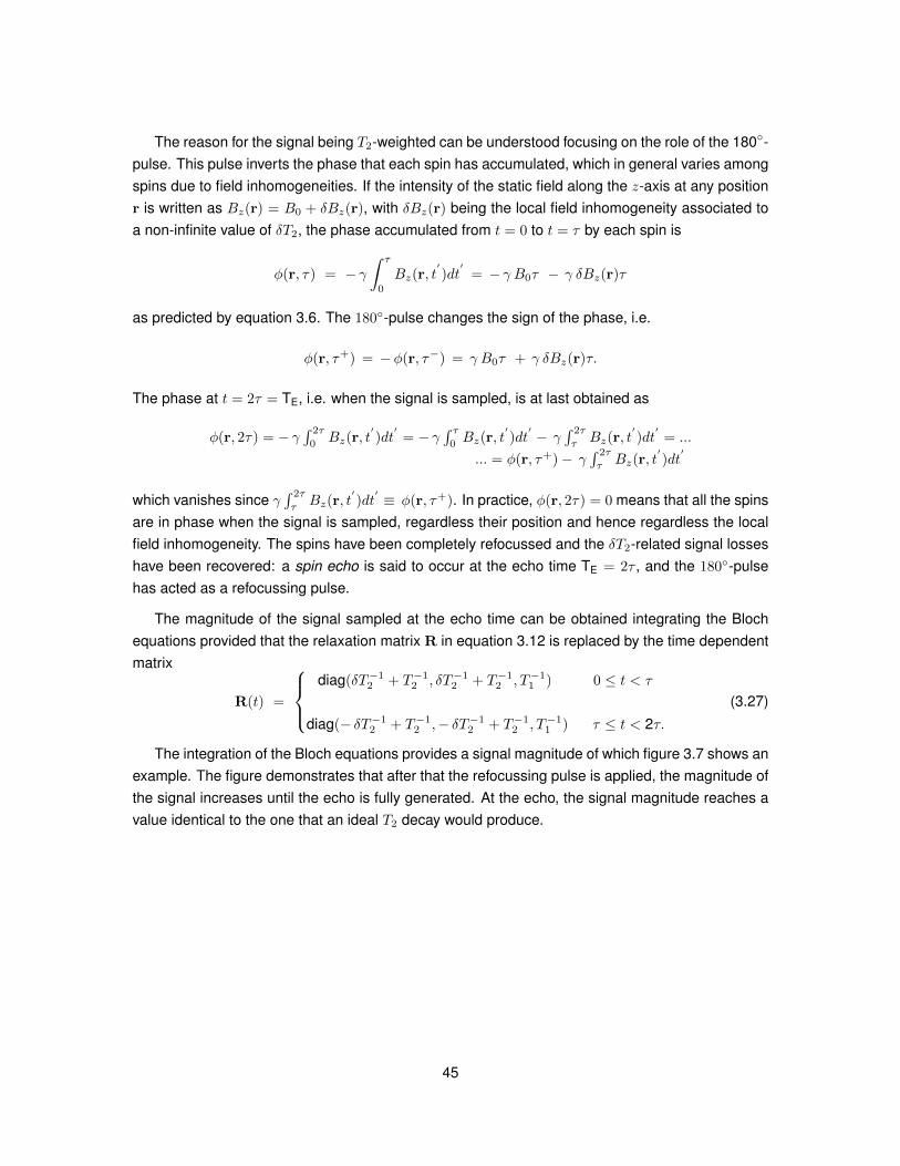
The reason for the signal being T2-weighted can be understood focusing on the role of the 180-pulse. This pulse inverts the phase that each spin has accumulated, which in general varies amongspins due to field inhomogeneities. If the intensity of the static field along the z-axis at any positionr is written as Bz(r) = B0 + δBz(r), with δBz(r) being the local field inhomogeneity associated toa non-infinite value of δT2, the phase accumulated from t = 0 to t = τ by each spin is

φ(r, τ) = − γ∫ τ

0

Bz(r, t′)dt′

= − γ B0τ − γ δBz(r)τ

as predicted by equation 3.6. The 180-pulse changes the sign of the phase, i.e.

φ(r, τ+) = −φ(r, τ−) = γ B0τ + γ δBz(r)τ.

The phase at t = 2τ = TE, i.e. when the signal is sampled, is at last obtained as

φ(r, 2τ) = − γ∫ 2τ

0Bz(r, t

′)dt′

= − γ∫ τ

0Bz(r, t

′)dt′ − γ

∫ 2τ

τBz(r, t

′)dt′

= ...

... = φ(r, τ+)− γ∫ 2τ

τBz(r, t

′)dt′

which vanishes since γ∫ 2τ

τBz(r, t

′)dt′ ≡ φ(r, τ+). In practice, φ(r, 2τ) = 0 means that all the spins

are in phase when the signal is sampled, regardless their position and hence regardless the localfield inhomogeneity. The spins have been completely refocussed and the δT2-related signal losseshave been recovered: a spin echo is said to occur at the echo time TE = 2τ , and the 180-pulsehas acted as a refocussing pulse.

The magnitude of the signal sampled at the echo time can be obtained integrating the Blochequations provided that the relaxation matrix R in equation 3.12 is replaced by the time dependentmatrix

R(t) =

diag(δT−1

2 + T−12 , δT−1

2 + T−12 , T−1

1 ) 0 ≤ t < τ

diag(− δT−12 + T−1

2 ,− δT−12 + T−1

2 , T−11 ) τ ≤ t < 2τ.

(3.27)

The integration of the Bloch equations provides a signal magnitude of which figure 3.7 shows anexample. The figure demonstrates that after that the refocussing pulse is applied, the magnitude ofthe signal increases until the echo is fully generated. At the echo, the signal magnitude reaches avalue identical to the one that an ideal T2 decay would produce.

45

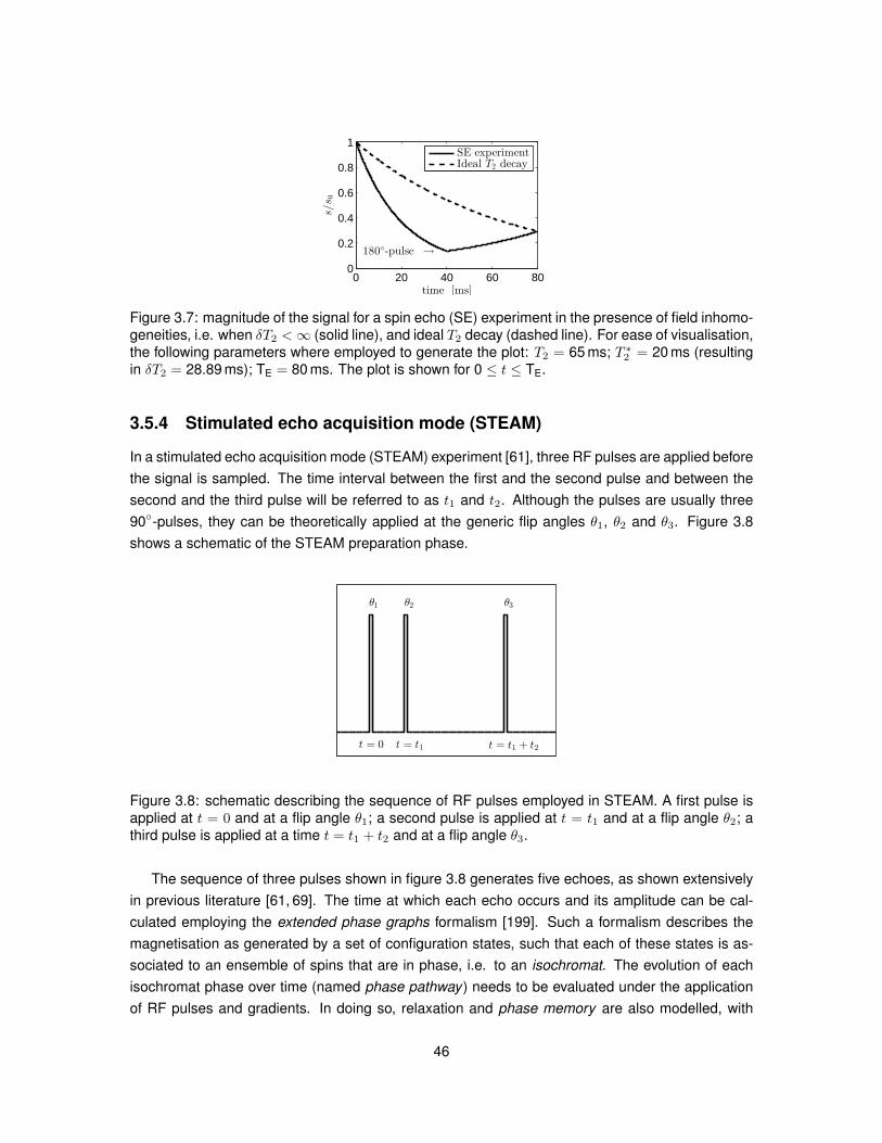
0 20 40 60 800

0.2

0.4

0.6

0.8

1

time [ms]

s/s 0

180-pulse →

SE experimentIdeal T2 decay

Figure 3.7: magnitude of the signal for a spin echo (SE) experiment in the presence of field inhomo-geneities, i.e. when δT2 <∞ (solid line), and ideal T2 decay (dashed line). For ease of visualisation,the following parameters where employed to generate the plot: T2 = 65 ms; T ∗2 = 20 ms (resultingin δT2 = 28.89 ms); TE = 80 ms. The plot is shown for 0 ≤ t ≤ TE.

3.5.4 Stimulated echo acquisition mode (STEAM)

In a stimulated echo acquisition mode (STEAM) experiment [61], three RF pulses are applied beforethe signal is sampled. The time interval between the first and the second pulse and between thesecond and the third pulse will be referred to as t1 and t2. Although the pulses are usually three90-pulses, they can be theoretically applied at the generic flip angles θ1, θ2 and θ3. Figure 3.8shows a schematic of the STEAM preparation phase.

θ1 θ2 θ3

t = 0 t = t1 t = t1 + t2

Figure 3.8: schematic describing the sequence of RF pulses employed in STEAM. A first pulse isapplied at t = 0 and at a flip angle θ1; a second pulse is applied at t = t1 and at a flip angle θ2; athird pulse is applied at a time t = t1 + t2 and at a flip angle θ3.

The sequence of three pulses shown in figure 3.8 generates five echoes, as shown extensivelyin previous literature [61, 69]. The time at which each echo occurs and its amplitude can be cal-culated employing the extended phase graphs formalism [199]. Such a formalism describes themagnetisation as generated by a set of configuration states, such that each of these states is as-sociated to an ensemble of spins that are in phase, i.e. to an isochromat. The evolution of eachisochromat phase over time (named phase pathway) needs to be evaluated under the applicationof RF pulses and gradients. In doing so, relaxation and phase memory are also modelled, with

46

the latter term referring to the phenomenon by which an isochromat in the longitudinal configura-tion (i.e. aligned to the polarising field) stores the phase previously accumulated in a transverseconfiguration, i.e. while being in the transverse plane.

In practice, the echo that is usually sampled and spatially encoded is the third echo, whichoccurs at a time t = 2t1 + t2 and is classified as a stimulated echo. The amplitude of such an echosampled at ts = 2t1 + t2 is [61]

s(ts) =12s0 | sin θ1| | sin θ2| | sin θ3| e−

t2T1 e−

2 t1T2 . (3.28)

In equation 3.28, t2 is usually referred to as mixing time TM whereas TE = 2 t1 is the echo time [151].

STEAM was developed as an alternative to spin echo experiments in order to i) deal with partialrefocussing due to imperfections of the 180-pulse; ii) limit the RF power deposition to the bodyreducing the number of required 180-pulses; iii) obtain T1-weighting in a non-time-consumingmanner, since during the time interval between the second and the third pulse the magnetisationis stored in the longitudinal direction. Nevertheless, it should be noted that even in the favourablecondition t2 T1, implying e−

t2T1 ≈ 1, STEAM can only provide half of the signal level of a spin

echo experiment with matching echo time, which is clear comparing equation 3.28 and 3.26.

3.5.5 Repeated sequences

Pulse sequences such as those described in the previous sections are often repeated in a cyclicmanner. This may be done to obtain several repetitions of a whole MRI image at each cycle foraveraging or because the spatial encoding leading to an image is distributed over different cycles.In general, the repetition time TR describes the period of these repeated cycles of acquisition, andthe overall duration of the MRI experiment is proportional to the value of TR. In spite of a reductionof the total acquisition time as TR shortens, it should be noted that often the amount of signalavailable for spatial encoding increases as TR increases, leading to better image quality.

Figure 3.9 shows and example of the impact of TR for a repeated single-pulse experiment (FIDexperiment introduced in section 3.5.1). Two scenarios are presented, illustrated respectively tothe right and to the left of the figure. For both cases, transverse relaxation was modelled viaT ∗2 monoexponential decay with T ∗2 = 45 ms, whereas T1 = 830 ms was used for longitudinalrelaxation. In the first case, a 60-pulse lasting 5 ms is repeated with TR = 100 ms, whereas in thesecond case a similar pulse is repeated with TR = 300 ms. Pulses are shown on top, whereas thecorresponding normalised signals to the bottom.

47

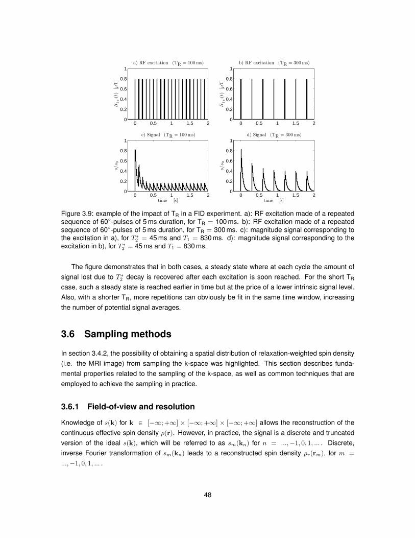
0 0.5 1 1.5 20

0.2

0.4

0.6

0.8

1

B1x′(t)

[µT]

a) RF excitation (TR = 100ms)

0 0.5 1 1.5 20

0.2

0.4

0.6

0.8

1

B1x′(t)

[µT]

b) RF excitation (TR = 300ms)

0 0.5 1 1.5 20

0.2

0.4

0.6

0.8

1

s/s 0

time [s]

c) Signal (TR = 100ms)

0 0.5 1 1.5 20

0.2

0.4

0.6

0.8

1

time [s]

s/s 0

d) Signal (TR = 300ms)

Figure 3.9: example of the impact of TR in a FID experiment. a): RF excitation made of a repeatedsequence of 60-pulses of 5 ms duration, for TR = 100 ms. b): RF excitation made of a repeatedsequence of 60-pulses of 5 ms duration, for TR = 300 ms. c): magnitude signal corresponding tothe excitation in a), for T ∗2 = 45 ms and T1 = 830 ms. d): magnitude signal corresponding to theexcitation in b), for T ∗2 = 45 ms and T1 = 830 ms.

The figure demonstrates that in both cases, a steady state where at each cycle the amount ofsignal lost due to T ∗2 decay is recovered after each excitation is soon reached. For the short TR

case, such a steady state is reached earlier in time but at the price of a lower intrinsic signal level.Also, with a shorter TR, more repetitions can obviously be fit in the same time window, increasingthe number of potential signal averages.

3.6 Sampling methods

In section 3.4.2, the possibility of obtaining a spatial distribution of relaxation-weighted spin density(i.e. the MRI image) from sampling the k-space was highlighted. This section describes funda-mental properties related to the sampling of the k-space, as well as common techniques that areemployed to achieve the sampling in practice.

3.6.1 Field-of-view and resolution

Knowledge of s(k) for k ∈ [−∞; +∞] × [−∞; +∞] × [−∞; +∞] allows the reconstruction of thecontinuous effective spin density ρ(r). However, in practice, the signal is a discrete and truncatedversion of the ideal s(k), which will be referred to as sm(kn) for n = ...,−1, 0, 1, ... . Discrete,inverse Fourier transformation of sm(kn) leads to a reconstructed spin density ρr(rm), for m =

...,−1, 0, 1, ... .

48

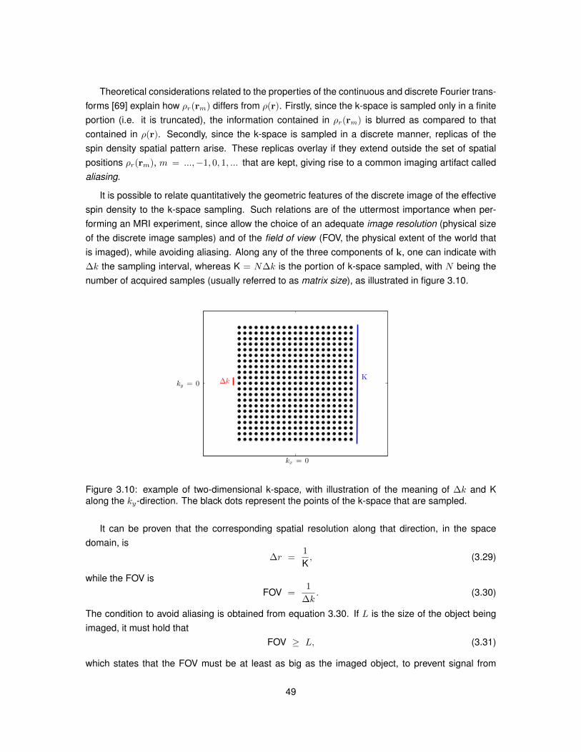
Theoretical considerations related to the properties of the continuous and discrete Fourier trans-forms [69] explain how ρr(rm) differs from ρ(r). Firstly, since the k-space is sampled only in a finiteportion (i.e. it is truncated), the information contained in ρr(rm) is blurred as compared to thatcontained in ρ(r). Secondly, since the k-space is sampled in a discrete manner, replicas of thespin density spatial pattern arise. These replicas overlay if they extend outside the set of spatialpositions ρr(rm), m = ...,−1, 0, 1, ... that are kept, giving rise to a common imaging artifact calledaliasing.

It is possible to relate quantitatively the geometric features of the discrete image of the effectivespin density to the k-space sampling. Such relations are of the uttermost importance when per-forming an MRI experiment, since allow the choice of an adequate image resolution (physical sizeof the discrete image samples) and of the field of view (FOV, the physical extent of the world thatis imaged), while avoiding aliasing. Along any of the three components of k, one can indicate with∆k the sampling interval, whereas K = N∆k is the portion of k-space sampled, with N being thenumber of acquired samples (usually referred to as matrix size), as illustrated in figure 3.10.

kx = 0

K∆kky = 0

Figure 3.10: example of two-dimensional k-space, with illustration of the meaning of ∆k and Kalong the ky-direction. The black dots represent the points of the k-space that are sampled.

It can be proven that the corresponding spatial resolution along that direction, in the spacedomain, is

∆r =1

K, (3.29)

while the FOV isFOV =

1

∆k. (3.30)

The condition to avoid aliasing is obtained from equation 3.30. If L is the size of the object beingimaged, it must hold that

FOV ≥ L, (3.31)

which states that the FOV must be at least as big as the imaged object, to prevent signal from

49

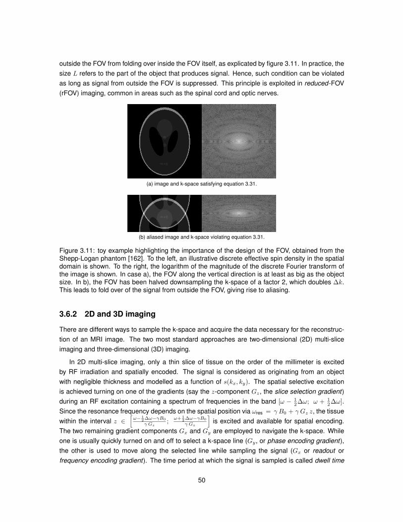
outside the FOV from folding over inside the FOV itself, as explicated by figure 3.11. In practice, thesize L refers to the part of the object that produces signal. Hence, such condition can be violatedas long as signal from outside the FOV is suppressed. This principle is exploited in reduced-FOV(rFOV) imaging, common in areas such as the spinal cord and optic nerves.

(a) image and k-space satisfying equation 3.31.

(b) aliased image and k-space violating equation 3.31.

Figure 3.11: toy example highlighting the importance of the design of the FOV, obtained from theShepp-Logan phantom [162]. To the left, an illustrative discrete effective spin density in the spatialdomain is shown. To the right, the logarithm of the magnitude of the discrete Fourier transform ofthe image is shown. In case a), the FOV along the vertical direction is at least as big as the objectsize. In b), the FOV has been halved downsampling the k-space of a factor 2, which doubles ∆k.This leads to fold over of the signal from outside the FOV, giving rise to aliasing.

3.6.2 2D and 3D imaging

There are different ways to sample the k-space and acquire the data necessary for the reconstruc-tion of an MRI image. The two most standard approaches are two-dimensional (2D) multi-sliceimaging and three-dimensional (3D) imaging.

In 2D multi-slice imaging, only a thin slice of tissue on the order of the millimeter is excitedby RF irradiation and spatially encoded. The signal is considered as originating from an objectwith negligible thickness and modelled as a function of s(kx, ky). The spatial selective excitationis achieved turning on one of the gradients (say the z-component Gz, the slice selection gradient)during an RF excitation containing a spectrum of frequencies in the band [ω − 1

2∆ω; ω + 12∆ω].

Since the resonance frequency depends on the spatial position via ωres = γ B0 + γ Gz z, the tissuewithin the interval z ∈

[ω− 1

2 ∆ω−γB0

γ Gz;

ω+ 12 ∆ω−γB0

γ Gz

]is excited and available for spatial encoding.

The two remaining gradient components Gx and Gy are employed to navigate the k-space. Whileone is usually quickly turned on and off to select a k-space line (Gy, or phase encoding gradient),the other is used to move along the selected line while sampling the signal (Gx or readout orfrequency encoding gradient). The time period at which the signal is sampled is called dwell time

50

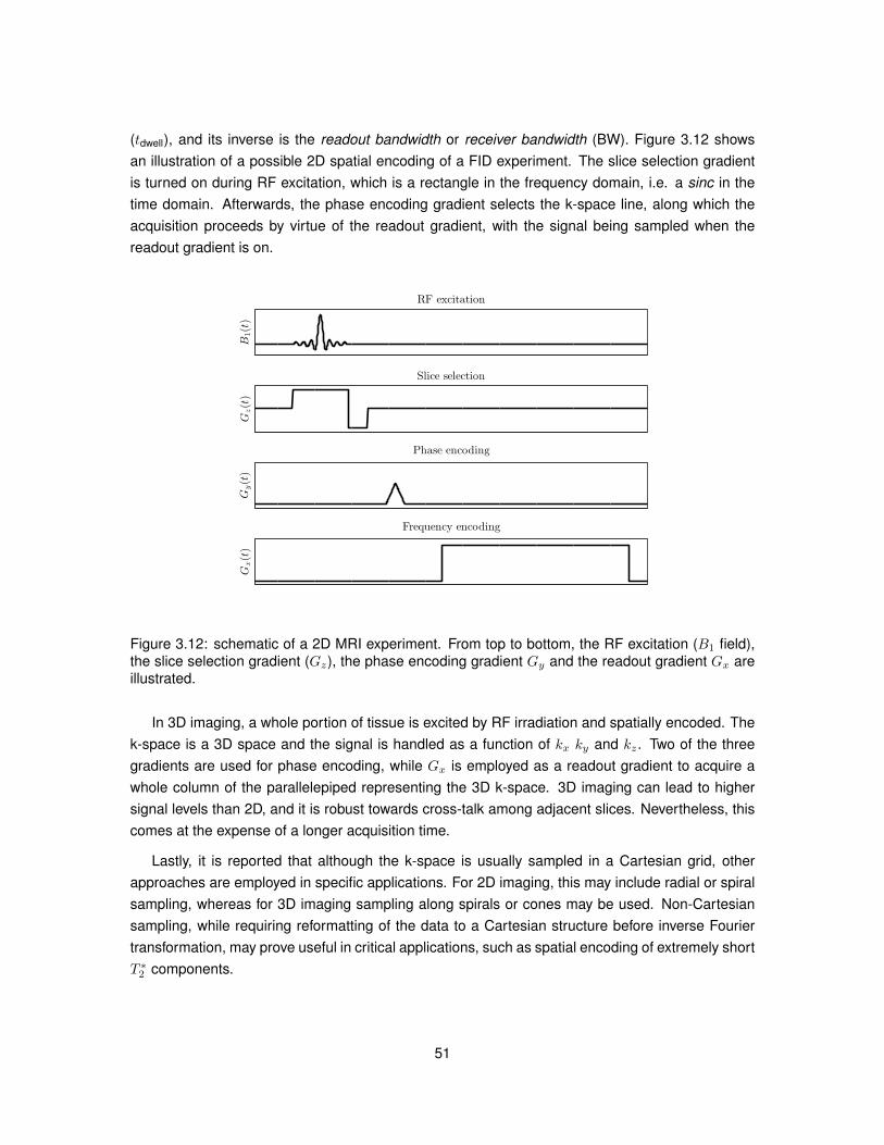
(tdwell), and its inverse is the readout bandwidth or receiver bandwidth (BW). Figure 3.12 showsan illustration of a possible 2D spatial encoding of a FID experiment. The slice selection gradientis turned on during RF excitation, which is a rectangle in the frequency domain, i.e. a sinc in thetime domain. Afterwards, the phase encoding gradient selects the k-space line, along which theacquisition proceeds by virtue of the readout gradient, with the signal being sampled when thereadout gradient is on.

B1(t)

RF excitation

Gz(t)

Slice selection

Gy(t)

Phase encoding

Gx(t)

Frequency encoding

Figure 3.12: schematic of a 2D MRI experiment. From top to bottom, the RF excitation (B1 field),the slice selection gradient (Gz), the phase encoding gradient Gy and the readout gradient Gx areillustrated.

In 3D imaging, a whole portion of tissue is excited by RF irradiation and spatially encoded. Thek-space is a 3D space and the signal is handled as a function of kx ky and kz. Two of the threegradients are used for phase encoding, while Gx is employed as a readout gradient to acquire awhole column of the parallelepiped representing the 3D k-space. 3D imaging can lead to highersignal levels than 2D, and it is robust towards cross-talk among adjacent slices. Nevertheless, thiscomes at the expense of a longer acquisition time.

Lastly, it is reported that although the k-space is usually sampled in a Cartesian grid, otherapproaches are employed in specific applications. For 2D imaging, this may include radial or spiralsampling, whereas for 3D imaging sampling along spirals or cones may be used. Non-Cartesiansampling, while requiring reformatting of the data to a Cartesian structure before inverse Fouriertransformation, may prove useful in critical applications, such as spatial encoding of extremely shortT ∗2 components.

51

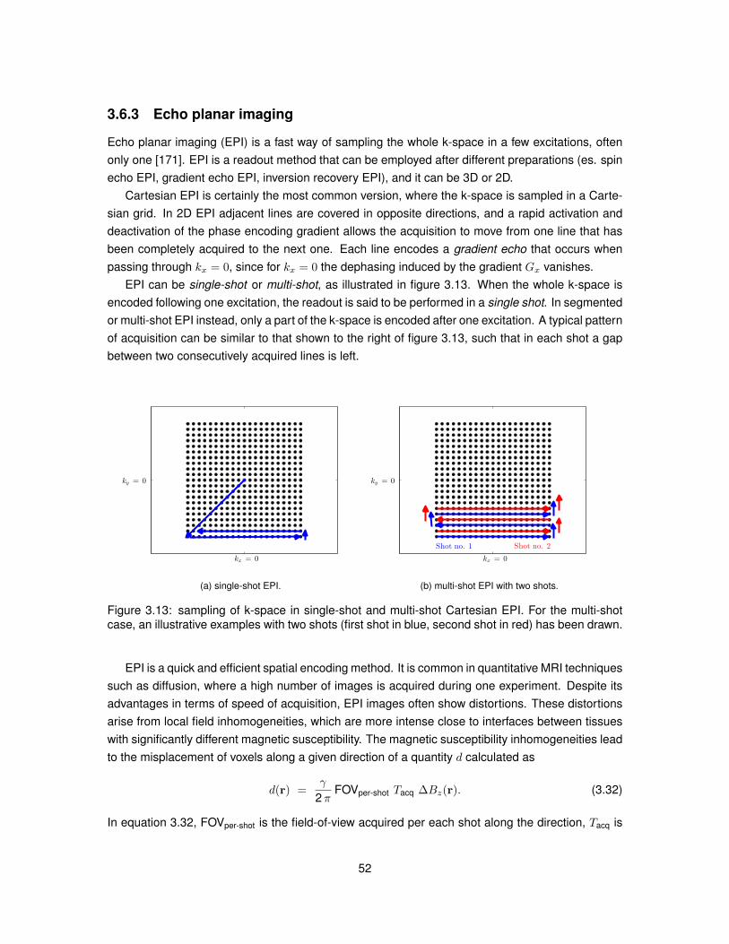
3.6.3 Echo planar imaging

Echo planar imaging (EPI) is a fast way of sampling the whole k-space in a few excitations, oftenonly one [171]. EPI is a readout method that can be employed after different preparations (es. spinecho EPI, gradient echo EPI, inversion recovery EPI), and it can be 3D or 2D.

Cartesian EPI is certainly the most common version, where the k-space is sampled in a Carte-sian grid. In 2D EPI adjacent lines are covered in opposite directions, and a rapid activation anddeactivation of the phase encoding gradient allows the acquisition to move from one line that hasbeen completely acquired to the next one. Each line encodes a gradient echo that occurs whenpassing through kx = 0, since for kx = 0 the dephasing induced by the gradient Gx vanishes.

EPI can be single-shot or multi-shot, as illustrated in figure 3.13. When the whole k-space isencoded following one excitation, the readout is said to be performed in a single shot. In segmentedor multi-shot EPI instead, only a part of the k-space is encoded after one excitation. A typical patternof acquisition can be similar to that shown to the right of figure 3.13, such that in each shot a gapbetween two consecutively acquired lines is left.

kx = 0

ky = 0

(a) single-shot EPI.

kx = 0

ky = 0

Shot no. 1 Shot no. 2

(b) multi-shot EPI with two shots.

Figure 3.13: sampling of k-space in single-shot and multi-shot Cartesian EPI. For the multi-shotcase, an illustrative examples with two shots (first shot in blue, second shot in red) has been drawn.

EPI is a quick and efficient spatial encoding method. It is common in quantitative MRI techniquessuch as diffusion, where a high number of images is acquired during one experiment. Despite itsadvantages in terms of speed of acquisition, EPI images often show distortions. These distortionsarise from local field inhomogeneities, which are more intense close to interfaces between tissueswith significantly different magnetic susceptibility. The magnetic susceptibility inhomogeneities leadto the misplacement of voxels along a given direction of a quantity d calculated as

d(r) =γ

2πFOVper-shot Tacq ∆Bz(r). (3.32)

In equation 3.32, FOVper-shot is the field-of-view acquired per each shot along the direction, Tacq is

52

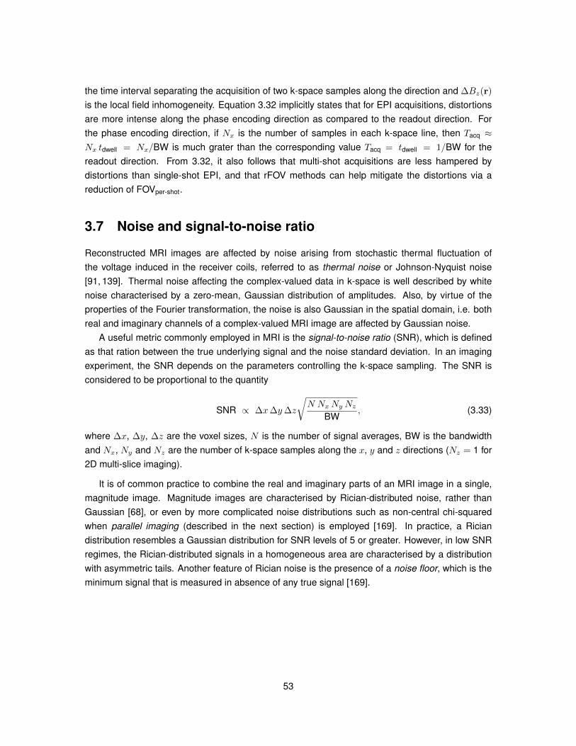
the time interval separating the acquisition of two k-space samples along the direction and ∆Bz(r)

is the local field inhomogeneity. Equation 3.32 implicitly states that for EPI acquisitions, distortionsare more intense along the phase encoding direction as compared to the readout direction. Forthe phase encoding direction, if Nx is the number of samples in each k-space line, then Tacq ≈Nx tdwell = Nx/BW is much grater than the corresponding value Tacq = tdwell = 1/BW for thereadout direction. From 3.32, it also follows that multi-shot acquisitions are less hampered bydistortions than single-shot EPI, and that rFOV methods can help mitigate the distortions via areduction of FOVper-shot.

3.7 Noise and signal-to-noise ratio

Reconstructed MRI images are affected by noise arising from stochastic thermal fluctuation ofthe voltage induced in the receiver coils, referred to as thermal noise or Johnson-Nyquist noise[91, 139]. Thermal noise affecting the complex-valued data in k-space is well described by whitenoise characterised by a zero-mean, Gaussian distribution of amplitudes. Also, by virtue of theproperties of the Fourier transformation, the noise is also Gaussian in the spatial domain, i.e. bothreal and imaginary channels of a complex-valued MRI image are affected by Gaussian noise.

A useful metric commonly employed in MRI is the signal-to-noise ratio (SNR), which is definedas that ration between the true underlying signal and the noise standard deviation. In an imagingexperiment, the SNR depends on the parameters controlling the k-space sampling. The SNR isconsidered to be proportional to the quantity

SNR ∝ ∆x∆y∆z

√N NxNy Nz

BW, (3.33)

where ∆x, ∆y, ∆z are the voxel sizes, N is the number of signal averages, BW is the bandwidthand Nx, Ny and Nz are the number of k-space samples along the x, y and z directions (Nz = 1 for2D multi-slice imaging).

It is of common practice to combine the real and imaginary parts of an MRI image in a single,magnitude image. Magnitude images are characterised by Rician-distributed noise, rather thanGaussian [68], or even by more complicated noise distributions such as non-central chi-squaredwhen parallel imaging (described in the next section) is employed [169]. In practice, a Riciandistribution resembles a Gaussian distribution for SNR levels of 5 or greater. However, in low SNRregimes, the Rician-distributed signals in a homogeneous area are characterised by a distributionwith asymmetric tails. Another feature of Rician noise is the presence of a noise floor, which is theminimum signal that is measured in absence of any true signal [169].

53

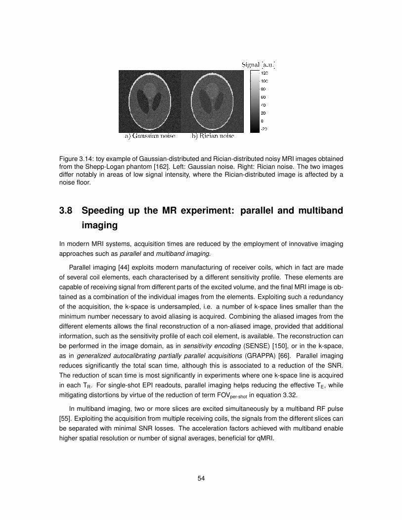
Figure 3.14: toy example of Gaussian-distributed and Rician-distributed noisy MRI images obtainedfrom the Shepp-Logan phantom [162]. Left: Gaussian noise. Right: Rician noise. The two imagesdiffer notably in areas of low signal intensity, where the Rician-distributed image is affected by anoise floor.

3.8 Speeding up the MR experiment: parallel and multibandimaging

In modern MRI systems, acquisition times are reduced by the employment of innovative imagingapproaches such as parallel and multiband imaging.

Parallel imaging [44] exploits modern manufacturing of receiver coils, which in fact are madeof several coil elements, each characterised by a different sensitivity profile. These elements arecapable of receiving signal from different parts of the excited volume, and the final MRI image is ob-tained as a combination of the individual images from the elements. Exploiting such a redundancyof the acquisition, the k-space is undersampled, i.e. a number of k-space lines smaller than theminimum number necessary to avoid aliasing is acquired. Combining the aliased images from thedifferent elements allows the final reconstruction of a non-aliased image, provided that additionalinformation, such as the sensitivity profile of each coil element, is available. The reconstruction canbe performed in the image domain, as in sensitivity encoding (SENSE) [150], or in the k-space,as in generalized autocalibrating partially parallel acquisitions (GRAPPA) [66]. Parallel imagingreduces significantly the total scan time, although this is associated to a reduction of the SNR.The reduction of scan time is most significantly in experiments where one k-space line is acquiredin each TR. For single-shot EPI readouts, parallel imaging helps reducing the effective TE, whilemitigating distortions by virtue of the reduction of term FOVper-shot in equation 3.32.

In multiband imaging, two or more slices are excited simultaneously by a multiband RF pulse[55]. Exploiting the acquisition from multiple receiving coils, the signals from the different slices canbe separated with minimal SNR losses. The acceleration factors achieved with multiband enablehigher spatial resolution or number of signal averages, beneficial for qMRI.

54

3.9 Diffusion MRI

DW MRI is a qMRI method that exploits the diffusion of water molecules as a source of contrastamong tissues [90, 92, 108, 124]. Water molecules diffuse by means of a ceaseless random walkknown as Brownian motion [50] due to thermal agitation. In absence of confinements, moleculesdiffuse isotropically with equal probability along any direction, and the average root mean squareddisplacement of this motion over a time interval Td is [50]

< r > =√

6DTd. (3.34)

However, water in human tissue is not free but it is compartmentalised within structures thatrestrict its diffusion, as demonstrated by the image of an axon and of its surrounding in figure 3.15.The patterns of diffusion in this restricted environment depart from the ideal case of equation 3.34[138]. For instance, diffusion within cerebral and spinal white matter is characterised by anisotropy,implying that along certain directions molecules diffuse more than along others (specifically, theydiffuse more along, rather than across, fibre bundles).

Figure 3.15: transmission electron micrograph of an axon and of its surrounding, showing threecompartments: intra-axonal space, myelin space and extra-axonal space. Image obtained fromhttps://upload.wikimedia.org/wikipedia/commons/c/c1/Myelinated_neuron.jpg, generatedand deposited into the public domain by the Electron Microscopy Facility at Trinity College (Road-nottaken) under the GNU Free Documentation License v.1.2 via Wikimedia Commons https:

//commons.wikimedia.org/wiki/File:Myelinated_neuron.jpg?uselang=it.

The MRI signal can be made sensitive to diffusion by virtue of the application of magnetic field

55

https://upload.wikimedia.org/wikipedia/commons/c/c1/Myelinated_neuron.jpg

https://commons.wikimedia.org/wiki/File:Myelinated_neuron.jpg?uselang=it

https://commons.wikimedia.org/wiki/File:Myelinated_neuron.jpg?uselang=it

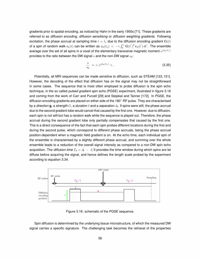
gradients prior to spatial encoding, as noticed by Hahn in the early 1950s [71]. These gradients arereferred to as diffusion encoding, diffusion sensitising or diffusion weighting gradients. Followingexcitation, the phase accrual at sampling time t = ts due to the diffusion encoding gradient G(t)

of a spin of random walk rk(t) can be written as φk(ts) = −γ∫ ts

0G(t

′)T rk(t

′) dt

′. The ensemble

average over the set of all spins in a voxel of the elementary transverse magnetic moment ejφk(ts)

provides to the ratio between the DW signal s and the non-DW signal s0:

s

s0= < ejφk(ts) > . (3.35)

Potentially, all MRI sequences can be made sensitive to diffusion, such as STEAM [123, 151].However, the decoding of the effect that diffusion has on the signal may not be straightforwardin some cases. The sequence that is most often employed to probe diffusion is the spin echotechnique, in the so called pulsed gradient spin echo (PGSE) experiment, illustrated in figure 3.16and coming from the work of Carr and Purcell [29] and Stejskal and Tanner [172]. In PGSE, thediffusion encoding gradients are placed on either side of the 180-RF pulse. They are characterisedby a direction g, a strength G, a duration δ and a separation ∆. If spins were still, the phase accrualdue to the second gradient lobe would cancel that caused by the first one. However, due to diffusion,each spin is not still but has a random walk while the sequence is played out. Therefore, the phaseaccrual during the second gradient lobe only partially compensates that caused by the first one.This is a direct consequence of the fact that each spin probes different locations during the first andduring the second pulse, which correspond to different phase accruals, being the phase accrualposition-dependent when a magnetic field gradient is on. At the echo time, each individual spin ofthe ensemble is characterised by a slightly different phase accrual, and summing over the wholeensemble leads to a reduction of the overall signal intensity as compared to a non-DW spin echoacquisition. The diffusion time Td = ∆ − δ/3 provides the time window during which spins are letdiffuse before acquiring the signal, and hence defines the length scale probed by the experimentaccording to equation 3.34.

δ

TE / 2 TE / 2

Sampling

Diffusion

encoding

gradient

RF pulses90-pulse

180-pulse

G

∆

Figure 3.16: schematic of the PGSE sequence.

Spin diffusion is determined by the underlying tissue microstructure, of which the measured DWsignal carries a specific signature. The challenging task becomes the retrieval of the properties

56

of the underlying microstructure from the observation of a set of DW signals. For this purpose,different approaches have been proposed in literature, of which a brief review follows below.

3.9.1 q-space imaging

In q-space imaging (QSI), the acquired signal is related to the Fourier transform of the probabilitydistribution of displacement of spins due to diffusion [28,43,126], named diffusion propagator, suchthat

s(q; ∆) =

∫R3

P (r; ∆) e−j2πqTr d3r. (3.36)

In equation 3.36, q = (2π)−1γ δ Gg is the q-vector (in m−3), s(q; ∆) is the acquired signal andP (r; ∆) is the diffusion propagator.

In some cases, such as in q-ball imaging (QBI) [186], only the angular information content ofP (r; ∆) is retained and is described in terms of a diffusion orientation distribution function (dODF)[2,184], expressed as

dODF(θ, φ; ∆) =

∫ ∞0

P (r(ρ, θ, φ); ∆) ρ2 dρ, (3.37)

where (ρ, θ, φ) are the spherical coordinates.The propagator in equation 3.36 describes the probability distribution of the random walks. The

equation holds true only in the narrow pulse limit [43], i.e. when δ ∆, so that diffusion during thepulse duration δ can be neglected. This is not often the case in clinical systems, and alternativeapproaches need to be adopted. For instance, the phase accrual during the finite pulse durationδ is modelled as a Gaussian distribution (Gaussian phase distribution approximation [46]). Also,reformulations of equation 3.36 in terms of a mean “centre-of-mass diffusion propagator” [125]have been proposed. In those cases, an apparent propagator depending on the centre of mass ofthe random walks occurring while the pulses are turned on is introduced.

A popular example of q-space imaging technique is diffusion spectrum imaging (DSI) [198]. QSImethods such as DSI do not make assumptions about the underlying microstructure. In spite of thisadvantage, their employment in clinical settings is limited by the long acquisition time necessary tosample the q-space. Moreover, they can only measure the effects of microstructure on the shape ofthe propagator, without providing estimates of the geometric features that determine such a shape.

3.9.2 Phenomenological models

Phenomenological models aim to capture the characteristics of the signal decay, but do not parametrisethe expression of the DW signal as a function of specific microstructural parameters.

Gaussian diffusion

In the simplest cases, it is hypothesised that the diffusion propagator is a Gaussian probabilitydensity function. This hypothesis supports signal models such as the apparent diffusion coefficient

57

(ADC) [172] model, such thats(b; ADC) = s0 e

−bADC. (3.38)

Above, the b-value b = (2π q)2(∆ − δ/3) measures the overall diffusion-weighting strength, withq being q = (2π)−1γ δ G. The ADC model can provide a reasonable description of the diffusionsignal attenuation in biological tissues if b is not too high. The ADC evaluated along a direction ofrestricted diffusion yields information about the local geometry, such as the surface-to-volume ratioof the structures within which spin diffuse [62]. This model can be generalised to account for spatialanisotropy of diffusion, which is a known feature of the central nervous system [108].

Diffusion anisotropy is taken into account in popular DTI [12]. In DTI, the signal attenuation in aPGSE experiment is written as

s(b,g; D) = s0 e−b gT D g. (3.39)

In equation 3.39, g is the gradient direction and D is the diffusion tensor, already introduced inequation 3.17. From the three eigenvalues of D λ1 ≥ λ2 ≥ λ3 ≥ 0, voxel-wise metrics summarisingthe diffusion profile are obtained [13], such as axial, radial and mean diffusivities (AD, RD andMD) and fractional anisotropy (FA). AD quantifies the amount of diffusion along the tensor principaldirection; RD orthogonal to it; MD quantifies the average amount of diffusion. FA summarises theanisotropy of the diffusion profile, minimum when it is equal to 0 (isotropic tensor) and maximumwhen it is 1. FA is often employed as a marker of neuronal integrity, while AD values measured inwell-aligned WM fibre bundles are taken as estimates of the neuronal diffusivity.

Non-Gaussian diffusion

Other phenomenological models extend equations 3.38 and 3.39 to relax the hypothesis of Gaus-sianity of diffusion [76], which does not describe the observed DW signals in neural tissue at highb-value [33]. This can be achieved introducing dependences on higher-order terms, proportional topowers of b, i.e. via cumulant expansion of the DW signal [59,137]. For example, diffusion kurtosisimaging (DKI) [84] is currently a standard method to quantify the amount of non-Gaussian diffusion.In one dimension, the DKI model can be written as

s(b;Dapp,K) = s0 e−bDapp+ 1

6 K (bDapp)2 , (3.40)

where Dapp is the apparent diffusivity and K is the kurtosis. Non-Gaussian behaviours are quan-tified directly by K. They are believed to arise from the presence of structures that impede andrestrict the diffusion of water molecules, such as axons in WM, whose density can be estimatedfrom the maximum kurtosis [59].

Other phenomenological models

Some categories of biophysical models are used to estimate complex distributions of fibre bun-dles within WM voxels [79], recovering quantities such as the fibre orientation distribution func-tion (fODF). As an example, spherical deconvolution (SD) [182] and its improved constrained ver-

58

sion [183] model the measured DW signals in WM as the contribution of several elementary fibrebundles weighted by their fODF. The elementary fibre bundles are usually modelled as identicalcompared to each other, but this assumption is relaxed in restriction spectrum imaging (RSI) [207],where a spectrum of diffusivities across the fibre bundles is allowed to account for different levelsof restriction.

Other phenomenological models have been introduced in literature. In spite of their capabilityof describing well the variability of the measured DW signals [136], their main limitation is that theyare unable to provide direct estimates of microstructural parameters, which is necessary to betterunderstand the pathophysiology of disease.

3.9.3 Multi-compartment models

In multi-compartment DW MRI methods, the signal is written as the contributions coming from N

tissue compartments, or pores, each occupying a relative voxel volume fraction vi for i = 1, ..., N

and representing water pools in different environments (such as intra and extra-axonal). When thesystem is observed at diffusion times much shorter than the time scale at which compartmentsexchange water, the signal can be written as

s(g,∆, δ, G; p) = s0

N∑i=1

vi si(g,∆, δ, G; pi), (3.41)

under the constraint∑Ni=1 vi = 1, with s0 being the non-DW signal. In equation 3.41, the charac-

teristic signal si(g,∆, δ, G; pi) of the i-th compartment depends in general on a set of parameterspi. The overall set of parameters p = s0,p1,p2, ...,pN , v1, v2, ..., vN−1 is estimated fitting theadopted model to a set of M measurements [87,135,170].

Practical representations of the tissue in the form of combinations of simple geometric do-mains are of common usage, such as cylinders or sticks modelling axons, hindered spaces forthe extracellular water or isotropic compartments (“balls”) modelling CSF [147]. Models such asCHARMED [8] (or composite hindered and restricted model of diffusion), ball-and-stick [15] andthe model proposed in [87] mainly aim to quantify neurite density; AxCaliber [7] and ActiveAx [4]mainly focus on axon diameter; ball-and-rackets [168] and NODDI [215] model neurite orientationdispersion; the spherical mean technique provides indices of per axon anisotropy [95]; DBSI [196]separates different rates of diffusion; intravoxel incoherent motion (IVIM) distinguishes diffusionfrom perfusion-related pseudo-diffusion [109]; vascular, extracellular and restricted diffusion for cy-tometry in tumors (VERDICT) MRI was designed for applications in cancer research [148].

3.9.4 Alternative diffusion encoding approaches

Diffusion encoding approaches different from PGSE have been explored in literature. A briefoverview of those is presented to the reader in this section.

Oscillating gradient spin echo (OGSE) sequences are similar to PGSE, but oscillating gradientwaveforms, rather than pulsed, are placed on other side of the refocusing pulse, as illustrated in

59

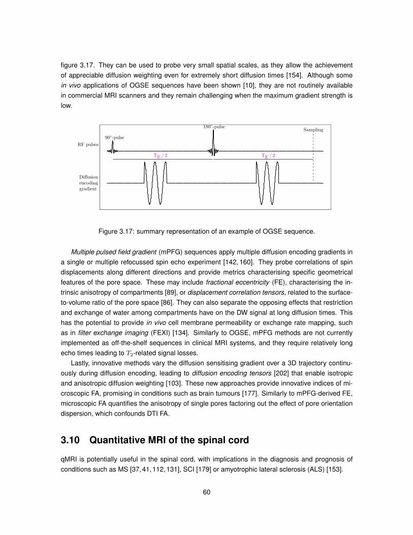
figure 3.17. They can be used to probe very small spatial scales, as they allow the achievementof appreciable diffusion weighting even for extremely short diffusion times [154]. Although somein vivo applications of OGSE sequences have been shown [10], they are not routinely availablein commercial MRI scanners and they remain challenging when the maximum gradient strength islow.

TE / 2 TE / 2

Sampling180-pulse

90-pulse

RF pulses

Diffusion

encoding

gradient

Figure 3.17: summary representation of an example of OGSE sequence.

Multiple pulsed field gradient (mPFG) sequences apply multiple diffusion encoding gradients ina single or multiple refocussed spin echo experiment [142, 160]. They probe correlations of spindisplacements along different directions and provide metrics characterising specific geometricalfeatures of the pore space. These may include fractional eccentricity (FE), characterising the in-trinsic anisotropy of compartments [89], or displacement correlation tensors, related to the surface-to-volume ratio of the pore space [86]. They can also separate the opposing effects that restrictionand exchange of water among compartments have on the DW signal at long diffusion times. Thishas the potential to provide in vivo cell membrane permeability or exchange rate mapping, suchas in filter exchange imaging (FEXI) [134]. Similarly to OGSE, mPFG methods are not currentlyimplemented as off-the-shelf sequences in clinical MRI systems, and they require relatively longecho times leading to T2-related signal losses.

Lastly, innovative methods vary the diffusion sensitising gradient over a 3D trajectory continu-ously during diffusion encoding, leading to diffusion encoding tensors [202] that enable isotropicand anisotropic diffusion weighting [103]. These new approaches provide innovative indices of mi-croscopic FA, promising in conditions such as brain tumours [177]. Similarly to mPFG-derived FE,microscopic FA quantifies the anisotropy of single pores factoring out the effect of pore orientationdispersion, which confounds DTI FA.

3.10 Quantitative MRI of the spinal cord

qMRI is potentially useful in the spinal cord, with implications in the diagnosis and prognosis ofconditions such as MS [37,41,112,131], SCI [179] or amyotrophic lateral sclerosis (ALS) [153].

60

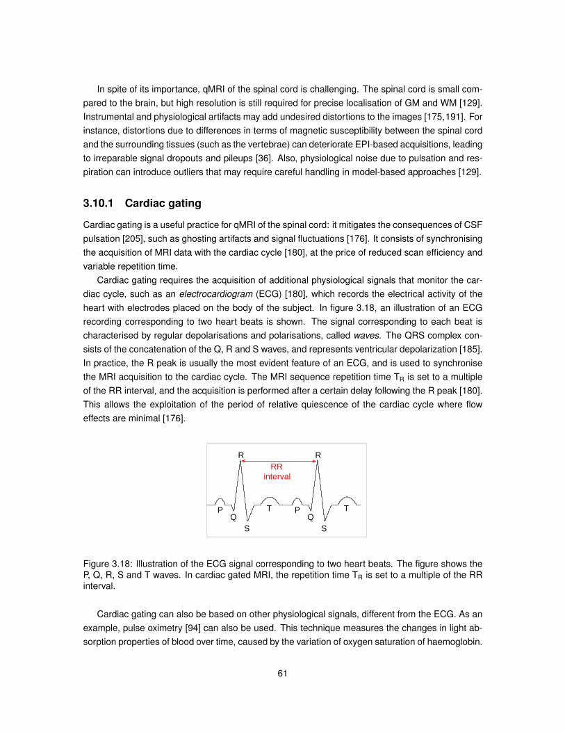
In spite of its importance, qMRI of the spinal cord is challenging. The spinal cord is small com-pared to the brain, but high resolution is still required for precise localisation of GM and WM [129].Instrumental and physiological artifacts may add undesired distortions to the images [175,191]. Forinstance, distortions due to differences in terms of magnetic susceptibility between the spinal cordand the surrounding tissues (such as the vertebrae) can deteriorate EPI-based acquisitions, leadingto irreparable signal dropouts and pileups [36]. Also, physiological noise due to pulsation and res-piration can introduce outliers that may require careful handling in model-based approaches [129].

3.10.1 Cardiac gating

Cardiac gating is a useful practice for qMRI of the spinal cord: it mitigates the consequences of CSFpulsation [205], such as ghosting artifacts and signal fluctuations [176]. It consists of synchronisingthe acquisition of MRI data with the cardiac cycle [180], at the price of reduced scan efficiency andvariable repetition time.

Cardiac gating requires the acquisition of additional physiological signals that monitor the car-diac cycle, such as an electrocardiogram (ECG) [180], which records the electrical activity of theheart with electrodes placed on the body of the subject. In figure 3.18, an illustration of an ECGrecording corresponding to two heart beats is shown. The signal corresponding to each beat ischaracterised by regular depolarisations and polarisations, called waves. The QRS complex con-sists of the concatenation of the Q, R and S waves, and represents ventricular depolarization [185].In practice, the R peak is usually the most evident feature of an ECG, and is used to synchronisethe MRI acquisition to the cardiac cycle. The MRI sequence repetition time TR is set to a multipleof the RR interval, and the acquisition is performed after a certain delay following the R peak [180].This allows the exploitation of the period of relative quiescence of the cardiac cycle where floweffects are minimal [176].

PQ

S

T PQ

S

T

RR RRinterval

Figure 3.18: Illustration of the ECG signal corresponding to two heart beats. The figure shows theP, Q, R, S and T waves. In cardiac gated MRI, the repetition time TR is set to a multiple of the RRinterval.

Cardiac gating can also be based on other physiological signals, different from the ECG. As anexample, pulse oximetry [94] can also be used. This technique measures the changes in light ab-sorption properties of blood over time, caused by the variation of oxygen saturation of haemoglobin.

61

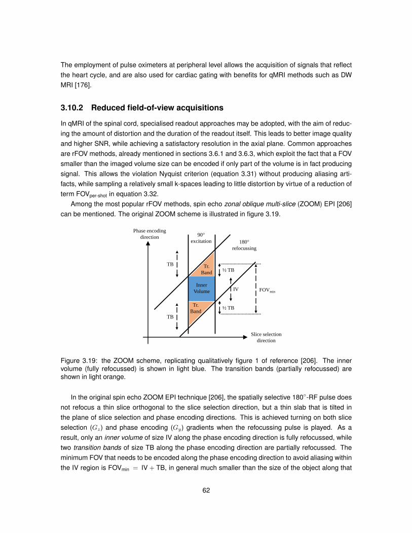
The employment of pulse oximeters at peripheral level allows the acquisition of signals that reflectthe heart cycle, and are also used for cardiac gating with benefits for qMRI methods such as DWMRI [176].

3.10.2 Reduced field-of-view acquisitions

In qMRI of the spinal cord, specialised readout approaches may be adopted, with the aim of reduc-ing the amount of distortion and the duration of the readout itself. This leads to better image qualityand higher SNR, while achieving a satisfactory resolution in the axial plane. Common approachesare rFOV methods, already mentioned in sections 3.6.1 and 3.6.3, which exploit the fact that a FOVsmaller than the imaged volume size can be encoded if only part of the volume is in fact producingsignal. This allows the violation Nyquist criterion (equation 3.31) without producing aliasing arti-facts, while sampling a relatively small k-spaces leading to little distortion by virtue of a reduction ofterm FOVper-shot in equation 3.32.

Among the most popular rFOV methods, spin echo zonal oblique multi-slice (ZOOM) EPI [206]can be mentioned. The original ZOOM scheme is illustrated in figure 3.19.

Phase encoding

direction

Slice selection

direction

Inner

Volume

Tr.

Band

Tr.

Band

180°

refocussing

90°

excitation

FOVminIV

½ TB

½ TBTB

TB

Figure 3.19: the ZOOM scheme, replicating qualitatively figure 1 of reference [206]. The innervolume (fully refocussed) is shown in light blue. The transition bands (partially refocussed) areshown in light orange.

In the original spin echo ZOOM EPI technique [206], the spatially selective 180-RF pulse doesnot refocus a thin slice orthogonal to the slice selection direction, but a thin slab that is tilted inthe plane of slice selection and phase encoding directions. This is achieved turning on both sliceselection (Gz) and phase encoding (Gy) gradients when the refocussing pulse is played. As aresult, only an inner volume of size IV along the phase encoding direction is fully refocussed, whiletwo transition bands of size TB along the phase encoding direction are partially refocussed. Theminimum FOV that needs to be encoded along the phase encoding direction to avoid aliasing withinthe IV region is FOVmin = IV + TB, in general much smaller than the size of the object along that

62

direction. This leads to a mitigation of EPI distortions due to a reduction of the k-space matrix size,while also allowing shorter echo times. However, for the implementation of multi-slice imaging, asuitable gap between slices acquired one after the other needs to be set, since the 180-RF pulseacting as a refocussing pulse for a certain slice inverts the magnetisation of adjacent slices.

rFOV methods are often preceded by preparation stages of outer volume suppression (OVS)[208], with the aim of saturating the magnetisation from outside the inner volume to further minimisethe risk of signal aliasing. This is for instance the strategy employed in clinical Philips MRI systems,where in fact the excitation pulse is tilted, rather than the refocussing one.

3.10.3 Diffusion: DTI studies

The majority of DW MRI studies in the spinal cord still rely on conventional DTI, due to severaltechnical challenges [174, 203]. DTI of the spinal cord has shown good reproducibility in normalsubjects [166], and improved DTI methods at 3T have been recently proposed [213].

Several studies have also proven the sensitivity of DTI metrics to pathology effects in the spinalcord. For instance, a study in ALS recently showed that DTI FA is a good predictor of disease sever-ity, and that changes in RD may reflect abnormalities in myelination [35]. DTI indices characteriseddiffuse cord pathology [3] and discriminated pathology levels in MS [140]. DTI-based tractographyprovided connectivity measurements that were reduced in patients with MS compared to controlsat cervical level [32].

Furthermore, DTI has also shown good sensitivity in acute spinal cord compression [52] andcervical compression myelopathy [116] and in SCI patients [34], although in the latter case itsindices were not specific to sensorimotors scores. Despite its good sensitivity towards changesin tissue microstructure, DTI indices are inherently non-specific [14], since they are influencedby several factors, only provide surrogate information and are hence prone to misinterpretations[203,204].

3.10.4 Diffusion: non-DTI studies

Advanced DW MRI techniques may help to provide more specific markers than DTI for spinal cordapplications. QSI was applied to the MS spinal cord in vivo [54], demonstrating that MS pathol-ogy does alter the diffusion profile of water molecules. DTI and QBI were successfully performedon SCI patients [34]. Both DTI FA and QBI-derived generalised FA (GFA) detected differencesbetween the normal-appearing WM of patients and controls’ WM, but the latter showed higher cor-relations with disability scores. More recently, very long diffusion times were probed in the healthyspinal cord in vivo with STEAM [151]; axon diameter was estimated in the cervical cord of healthyvolunteers [48] with a modified AxCaliber [7] method and cutting edge 300 mT m−1 gradients; track-density imaging (TDI) [27] was related to magnetic resonance spectroscopy in cervical spondyloticmyelopathy [51].

63

3.11 Validation of quantitative MRI

qMRI has the potential of providing novel and highly specific biomarkers. However, it is essentialthat these innovative methods undergo systematic validation in phantoms and, ideally, comparisonto histology. This can help to confirm the specificity of the indices and to exclude the influenceof other confounding factors, especially in the presence of pathology. To date, a huge effort in thisdirection was made by the research community, and this section of the thesis aims to report notableresults for the reader.

3.11.1 Phantom studies

Validation may include the development of controlled imaging phantoms. These are of particularinterest for DW MRI methods aiming to quantify geometric features such as size or diameter ofpores, and a few examples are listed below. A phantom of highly ordered glass has been built tovalidate a mPFG-based pore diameter estimation method [100], with promising results. Co-axialelectrospinning has been successfully employed to build a phantom mimicking WM [75], whereasco-axial electrospraying to build a phantom made of a collection of polymer spheres mimickingcancer tissue [122]. A phantom of yeast cells, ordered and disordered crystal was instead employedto validate the estimation of microscopic FA, quantifying the anisotropy of the single pore afterfactoring out dispersion of pore orientations [103].

3.11.2 Histological validation

In literature, qMRI techniques such as DW MRI have often been compared to indices from conven-tional 2D histology, as in the cases listed below. Manual delineation of neuronal processes in the ratbrain identified the histological correlates of DTI principal direction and FA [110]. The rat brain wasalso employed as a model for the comparison and validation of four different model-based PGSEapproaches in [85], with good agreement between neurite density and dendrite complexity indicesand optical intensity of myelin stained sections. DTI-derived information, such as local dominantdirection, was also found to agree well with estimates derived from 2D Fourier domain analysis ofowl monkey brain histology [30]. Extensive 2D structure tensor [16] analysis of the rat brain [22]and of the human cortex [159] showed good correspondence of local neurite orientation and DWMRI indices of dominant orientation. Recently, RSI was validated in the rat brain using myelin stain-ing [207]. In vivo DW microimaging of the mice brain was shown to provide constrained SD [182]and TDI maps that qualitatively confirmed histology [211]. Also, a method for in vivo myelin g-ratioquantification was designed with applications in MS after validation in the macaque brain [173].

Novel 3D histology overcomes the main limitation of 2D methods, which neglect through-sectionfibre information. Confocal microscopy has been used to reconstruct the 3D morphology of ferretindividual neurons [88] and to perform ST analysis of the Rhesus macaque hippocampus [98].Polarised light imaging (PLI) [9] provides detailed 3D information of neural fibre architecture, butits application in demyelinating diseases remains challenging since it relies on optical properties of

64

the myelin sheath. Recently, serial optical coherence scanning (SOCS) [192,193], which integratesoptical coherence tomography and serial cutting with a vibratome, has shown unique information inthe human medulla oblongata correlating with DTI indices.

Several studies have also investigated the histological correlates of qMRI in pathological tissue.For instance, MS effects have been extensively studied. DTI AD and RD have been proposed assurrogate markers of axonal loss and demyelination respectively, as suggested in animal models invivo [24] and ex vivo [78,167], in unfixed human brain [155] and unfixed [131] and fixed [99] humanspinal cord. Quantitative T1 and T2 estimation and magnetisation transfer ratio MRI were comparedto histopathology in the MS spinal cord [20]. Recently, positive magnetic susceptibility in MS lesionwas associated to iron deposition via histology [210].

DTI indices were compared to histology in several other models of diseases. For instance,stained sections demonstrating myelin, neurofilaments and immunoreactive material in experimen-tal autoimmune encephalomyelitis (EAE) mice were compared to DTI in [25], while in [23] theinvestigation focussed on 2D Fourier domain analysis of sections imaged with confocal laser mi-croscopy in a model of traumatic brain injury. To date, other DW MRI methods such as DKI [84] andDBSI [214] have also been proven useful to detect demyelination in a cuprizone mouse model [53]and to distinguish inflammation, demyelination and axonal injury in EAE mice [194] and MS [195].

Lastly, it is reported that DW MRI has been compared to histology also in cancer, as for examplein xenografts of mice tumours [148] or in human brain meningiomas and glioblastomas [177]. Theseresults show that DW MRI has a potential to characterise the microstructure of tumours in a clinicallyfeasible and non-invasive manner.

65

In vivo diffusion MRI of the humanspinal cord

66

Background and motivations

Previous background information has underlined the need of novel and more specific MRI biomark-ers for spinal cord diseases such as MS. The new MRI indices should better characterise diffusepathology and focal damage, as well as their association to clinical disability, leading ultimately toearlier diagnosis and more accurate prognosis.

This part of the thesis describes the investigation of a recent DW MRI method known as NODDIfor in vivo spinal cord applications. NODDI enables the characterisation of key features of neuronalmorphology in clinically feasible scans, and its employment in spinal cord conditions is appealingand potentially useful. The objectives of this first part of the dissertation are: i) to demonstrate thefeasibility of NODDI and characterise its metrics in the spinal cord; ii) to study its reproducibility andrelation with a routine diffusion method known as DTI; iii) to study the feasibility of its application tostandard DW data; iv) to assess how axon diameter distributions typical of the spinal cord influenceNODDI metrics.

Experiments

Three experimental chapters report our work carried out in vivo. In chapter 4, NODDI is demon-strated in the healthy cervical spinal cord, its reproducibility is assessed and its metrics are charac-terised and compared to DTI indices. In chapter 5, the application of NODDI to routine single-shellDW MRI data of the spinal cord is discussed. Lastly, as a conclusion for the in vivo part, theinfluence of axon diameter distribution on NODDI metrics is studied in chapter 6.

Conclusions

The chapters of this first in vivo part demonstrate that the recent NODDI technique is feasible in thespinal cord and in a clinical setting. NODDI can disentangle key factors contributing to the patternsof diffusion anisotropy as measured by DTI, namely the density and the orientation dispersion ofneurites. Nevertheless, its reproducibility is slightly lower than that of DTI indices, and its applicationto standard DW MRI data appears challenging. Lastly, our experiments suggest that typical featuresof spinal cord microstructure (i.e. presence of large axons) can have an impact on NODDI metrics.

67

Chapter 4

Demonstration of NODDI in thehealthy spinal cord

4.1 Introduction

This chapter shows the demonstration of NODDI in the healthy cervical spinal cord in vivo. NODDIhas already shown promise in brain applications [17, 101, 156, 200, 209], and it may prove usefulalso in the spinal cord. NODDI provides indices of neurite morphology, namely neurite densityand orientation dispersion, in a clinically feasible acquisition. The former index may be employed tocharacterise axonal loss and other pathological mechanisms underlying pathology in MS. The lattermetric may instead be of interest at the level of nerve roots or to assess the integrity of neuronalprocesses or the complexity of dendritic trees. Also, it is known that neurite orientation dispersionis a non-negligible feature at the MRI voxel scale even in coherent brain WM areas such as thecorpus callosum [21,58]. Therefore, we hypothesise that it may be an important feature also in thetightly packed WM of the spinal cord.

For this study, five healthy volunteers were scanned in London with the 3T Philips Achieva MRIsystem in Queen Square House, Queen Square MS Centre, UCL Institute of Neurology. The mainobjectives were i) to demonstrate the feasibility of NODDI in the spinal cord and to obtain trends ofits metrics; ii) to study its reproducibility and relation to routine DTI. Specifically, the following pointswere investigated in detail:

1. characterisation of NODDI metrics, in terms of GM and WM differences and contrast;

2. quantification of their reproducibility;

3. quantification of their relationship with DTI indices;

4. comparison of the quality of fit of NODDI and DTI models;

5. assessment of the impact of collateral WM fibres on NODDI indices.

68

4.2 Research dissemination

Some of the results described in this chapter have been presented in abstract form at internationalmeetings as:

• “In vivo estimation of neuronal orientation dispersion and density of the human spinal cord”.Grussu F. et al, ISMRM workshop “Multiple sclerosis as a whole-brain disease” (2013), oralpresentation.

• “Neurite orientation dispersion and density imaging of the cervical cord in vivo”. Grussu F. etal, ISMRM annual meeting (2014), p.1720, traditional poster.

Some of the findings were also published in a peer-reviewed journal as “Neurite orientation disper-sion and density imaging of the healthy cervical spinal cord in vivo”, Grussu F. et al, NeuroImage(2015), vol. 111, p.590-601 (reference [67]).

4.3 Theory: the NODDI model

NODDI considers water protons in each MRI voxel as belonging to three pools: i) isotropic water; ii)intra-neurite water; iii) extra-neurite water. The isotropic compartment is designed to capture CSFcontamination; the intra-neurite compartment models axons and dendrites, excluding myelin; theextra-neurite compartment describes the extra-cellular environment, glial cells and neuronal cellbodies. The DW signal for a PGSE experiment is written as

s(g, b) = s0

(viso siso(b) +

(1− viso

)(vin sin(g, b) +

(1− vin

)sen(g, b)

)). (4.1)

Above, s0 is the non-DW signal; viso is the voxel volume fraction of the the isotropic compartment;vin is the intra-neurite tissue volume fraction; siso, sin and sen are the characteristic signal decays forthe isotropic, intra and extra-neurite compartments respectively. The signal decays depend on thegradient direction g and on the b-value, as explained below.

siso models signal decay due to isotropic diffusion characterised by a diffusivity diso:

siso(b) = e−b diso . (4.2)

sin describes the signal attenuation due to restricted diffusion within Watson-distributed zero-radius cylinders, or sticks, characterised by intrinsic diffusivity d‖:

sin(g, b) =

∮‖n‖=1

f(n;κ,µ) e−b d‖(gT n)2 d2n. (4.3)

In equation 4.3, f(n;κ,µ) is the neurite orientation distribution, modelled as a Watson distributionwith concentration κ ∈ (0;∞) and mean orientation µ. In [215], the orientation dispersion index(ODI) was proposed as a more intuitive representation of κ. ODI is monotonically related to κ as

69

ODI = 2π arctan

(1κ

), and it ranges from 0 (neurites all aligned in a voxel) to 1 (neurites isotropically,

randomly oriented).Lastly, sen describes the attenuation due to anisotropic hindered diffusion in the extraneurite

space:

sen(g, b) = exp(− bgT

( ∮‖n‖=1

f(n;κ,µ) D(n; vin, d‖) d2n)

g), (4.4)

whereD(n; vin, d‖) = vin d‖ nnT + (1− vin) d‖ I (4.5)

is a cylindrically symmetric diffusion tensor with diffusivity d‖ parallel to the generic direction n anddiffusivity perpendicular to n constrained by a tortuosity model to (1− vin) d‖.

Multiple b-value DW data are required to fit the model parameters. The b-values and the totalnumber of measurements were optimised to be performed in a clinically feasible time [215], andconsist of two high angular resolution diffusion imaging (HARDI) [187] DW shells with b-values ofb = 711 s mm−2 (30 directions) and b = 2855 s mm−2 (60 directions).

4.4 Methods

4.4.1 Data acquisition

Five healthy volunteers (2 males, median age of 34 years, range 25-47) provided informed writtenconsent and were scanned on a 3T Philips Achieva scanner, in ethically approved experimentalsessions. The MRI scans were performed on the system in Queen Square House, Queen Square,Institute of Neurology (NMR Unit, Department of Neuroinflammation). Four volunteers (subjects1 to 4) were scanned twice, within eight months of the first scan. The protocol lasted about 25minutes and followed the optimised multi-shell diffusion encoding prescribed in [215] (30 directionsat b = 711 s mm−2 and 60 at b = 2855 s mm−2), plus 6 interleaved non-DW measurements. A rFOVPGSE ZOOM-EPI sequence [206] with OVS [208] and oxymeter-based peripheral cardiac gatingwas employed, as described in sections 3.10.1 and 3.10.2 of chapter 3.

Twelve axial slices were acquired with the following parameters: TR = 12 RR repeats (as ex-plained in figure 3.18), TE = 65.50 ms (minimum TE achievable at b = 2855 s mm−2), rFOV of64×48 mm2, SENSE factor of 1.5, resolution of 1×1×5 mm3, triggering delay of 150 ms. We variedthe gradient strength to achieve the two b-values, and employed ∆ = 32.20 ms and δ = 20.50 msfor both shells, resulting in a diffusion time of Td = 25.37 ms, constrained by the TE that was keptto minimum.

4.4.2 Motion correction

Motion was corrected realigning all acquired images to the first (non-DW) one, which was takenas registration reference. Currently, there are no well established motion correction pipelines forDW MRI of the spinal cord. However, it has been suggested that slice-wise linear registration is

70

the most effective strategy to correct the motion [129]. Therefore, we adopted such a strategy, andused FSL flirt [64,82,83] to implement the linear registration.

Let n = 1, ...,6 be the index of the n-th b = 0 volume and let x, y and z be the subjects’ right-left,posterior-anterior and inferior-superior directions, so that z = 1, ...,12 is the slice index. Motioncorrection was implemented as follows.

• Firstly, we estimated the transformations

Tn(z) =

[I pn(z)

0T 1

]

with FSL flirt (correlation ratio search cost) for n = 2, ...,6 and all z values. Tn(z) ∈ R4×4

is a rigid transformation warping slice z of the n-th b = 0 volume to the same slice of b = 0volume n = 1. Tn(z) accounts for in-plane translations pn(z) = [ δxn(z) δyn(z) 0 ]

T.

• Secondly, transformations Tn(z) were applied to the corresponding slices of the non-DWvolumes to correct the motion.

• Lastly, we also employed Tn(z) to warp slice z of all DW volumes acquired between the n-thand (n+ 1)-th b = 0 volumes.

Quality assessment of the motion correction stage was always performed by visual comparisonof the motion-corrected and motion-uncorrected data.

4.4.3 Segmentation

For each subject and scan, the spinal cord was segmented on the mean b = 0 image, calculatedafter motion correction. A semi-automatic active surface method [74] available in Jim (http://www.xinapse.com/home.php) was employed to create a binary mask (fitting cord mask ) of the spinalcord. The fitting cord mask was then eroded slice-by-slice to limit CSF contamination and croppedto the 6 central slices (whole-cord mask ).

Afterwards, manual grey matter (GM) outlining was carried out on the average DW volumeobtained according to the method described in [97], which is illustrated in figure 4.1. The methodaverages DW images obtained for gradient directions at an angle smaller than a threshold from thelongitudinal spinal cord axis, since they show good contrast between GM and WM. The thresholdwas set to 45, as some tests demonstrated that this value is a reasonable choice.

71

http://fsl.fmrib.ox.ac.uk/fsl/fslwiki/FLIRT

http://www.xinapse.com/home.php

http://www.xinapse.com/home.php

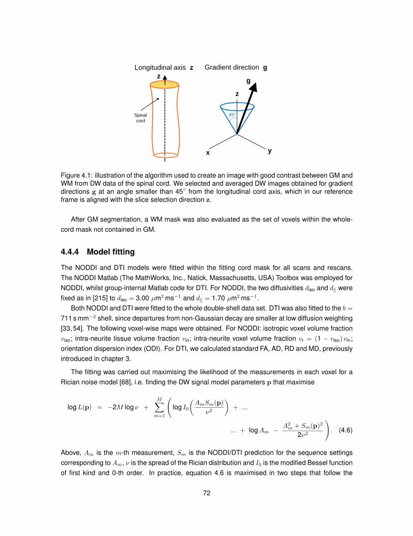
Longitudinal axis z

Spinal

cord

z

x y

45°

g

Gradient direction g

z

Figure 4.1: illustration of the algorithm used to create an image with good contrast between GM andWM from DW data of the spinal cord. We selected and averaged DW images obtained for gradientdirections g at an angle smaller than 45 from the longitudinal cord axis, which in our referenceframe is aligned with the slice selection direction z.

After GM segmentation, a WM mask was also evaluated as the set of voxels within the whole-cord mask not contained in GM.

4.4.4 Model fitting

The NODDI and DTI models were fitted within the fitting cord mask for all scans and rescans.The NODDI Matlab (The MathWorks, Inc., Natick, Massachusetts, USA) Toolbox was employed forNODDI, whilst group-internal Matlab code for DTI. For NODDI, the two diffusivities diso and d‖ werefixed as in [215] to diso = 3.00 µm2 ms−1 and d‖ = 1.70 µm2 ms−1.

Both NODDI and DTI were fitted to the whole double-shell data set. DTI was also fitted to the b =

711 s mm−2 shell, since departures from non-Gaussian decay are smaller at low diffusion weighting[33,54]. The following voxel-wise maps were obtained. For NODDI: isotropic voxel volume fractionviso; intra-neurite tissue volume fraction vin; intra-neurite voxel volume fraction vr = (1 − viso) vin;orientation dispersion index (ODI). For DTI, we calculated standard FA, AD, RD and MD, previouslyintroduced in chapter 3.

The fitting was carried out maximising the likelihood of the measurements in each voxel for aRician noise model [68], i.e. finding the DW signal model parameters p that maximise

logL(p) = −2M log ν +

M∑m=1

(log I0

(AmSm(p)

ν2

)+ ...

... + logAm −A2m + Sm(p)2

2ν2

). (4.6)

Above, Am is the m-th measurement, Sm is the NODDI/DTI prediction for the sequence settingscorresponding to Am, ν is the spread of the Rician distribution and I0 is the modified Bessel functionof first kind and 0-th order. In practice, equation 4.6 is maximised in two steps that follow the

72

http://nitrc.org/projects/noddi_toolbox

estimation of ν as the standard deviation of the non-DW measurements. A plausible set of modelparameters is found performing an initial grid search. These parameters are then used as a startingpoint for a gradient descent, where −logL(p) is minimised.

The fitting settings of the NODDI Toolbox were tested. We found that the default options arenot well suited for spinal cord MRI. By default, the Toolbox divides the estimate of the Rician noiselevel by 100, pulling the noise model to a Gaussian regime. While this has little impact on braindata where the SNR is on the order of 20, simulations proved that NODDI metrics are biased whenobtained from fitting with such an option enabled on data with low SNR. This option was thereforedisabled.

4.4.5 Analysis

Characterisation of the metrics

We visually inspected the fitted metrics and characterised GM/WM variation calculating the me-dians of each metric within each region-of-interest (ROI) (GM, WM and whole-cord), focusing onmetrics obtained from the b = 711 s mm−2 shell for DTI. We also calculated the contrast C andthe contrast-to-noise ratio (CNR) between GM and WM for all metrics from NODDI and DTI. C andCNR were calculated similarly to [65]:

C =|mGM −mWM|

12 (mGM +mWM)

(4.7)

andCNR =

|mGM −mWM|√s2

GM + s2WM

, (4.8)

where mGM, mWM are the sample means of the metric in GM and WM and where sGM and sWM arethe sample standard deviations of the metric in GM and WM.

Reproducibility

The reproducibility of NODDI metrics was investigated in Matlab for the GM, WM and whole-cordROIs separately, with the aim of quantifying: i) the total variability associated to each metric; ii) thewithin-subject and between-subject fractions of the total variability. The two fractions are represen-tative of the variation due to measurement errors (within-subject) and biological variation (between-subject) [11].

For this purpose, we calculated for each metric and ROI a percentage coefficient of variation(CoV) and the intraclass correlation coefficient (ICC). CoV, expressed in percentage points, mea-sures the total variability of a metric with respect to the average value of the same metric acrosssubjects and scans. Conversely, ICC was defined as the ratio between the variance associatedto biological variation and the total variance. If ICC > 0.5, the total variability is driven by biologi-cal differences in the cohort, whereas an ICC < 0.5 suggests that the total variability is driven bymeasurements errors.

73

Let mi,j be the median of a metric within a fixed ROI for subject i = 1, ...,4 and scan j = 1,2.We estimated the within-subject (σ2

W) and between-subject (σ2B) variances as

σ2W = 1

4

∑4i=1

(∑2j=1

(mi,j − mi

)2 ) and as σ2B = 1

3

∑4i=1

(mi − m

)2, with mi and m being

mi = 12

∑2j=1 mi,j and m = 1

4

∑4i=1 mi.

The total variance of the metric within the ROI was quantified as σ2TOT = σ2

B + σ2W, while the

percentage CoV and the ICC were ultimately calculated as

CoV = 100

√σ2

TOT

m(4.9)

and

ICC =σ2

Bσ2

TOT. (4.10)

For comparison, CoV and ICC were also calculated for DTI metrics obtained from the b =

711 s mm−2 shell.

Relationship NODDI-DTI

We investigated the experimental relationship between DTI metrics and NODDI vin and ODI scat-tering values of vin and ODI and colour-coding the points according to FA, AD, RD and MD. Weemployed DTI metrics obtained from the b = 711 s mm−2 shell and only studied voxels with lowisotropic volume fraction (viso < 0.05). In order to support the relationships observed in vivo, wealso evaluated via computer simulations the theoretical patterns of DTI indices as functions of vin

and ODI for a NODDI-like substrate at b = 711 s mm−2.The simulations were run as follows. The noise-free DW signal was synthesised according to

equation 4.1 with the NODDI Matlab Toolbox. We varied parameters vin and ODI in a grid of 64×64uniform values in [ 0.05; 0.95 ] × [ 0.005; 0.5 ], while fixing s0 = 1, viso = 0, d‖ = 1.70µm2 ms−1

and µ = [ 0 0 1 ]T. The signal was synthesised for the gradient directions of the b = 711 s mm−2

shell with b = 711 s mm−2. Subsequently, Rician noise was added to the synthesised signals (SNRof 10, comparable to the SNR of our data and of other in vivo studies [189]). Lastly, the DTI modelwas fitted to the noise-free and noisy synthetic data for all combinations of vin and ODI. DTI indicesFA, AD, RD and MD were then obtained and ultimately displayed as functions of vin and ODI.

Quality of fit

We investigated the quality of fit of NODDI and DTI models on the first scan of each of the five sub-jects, employing the whole double-shell set of measurements. The Bayesian Information Criterion(BIC) [158] was employed for this purpose, as in [147]. BIC is a useful statistics to compare modelsof different complexity, since lower BIC values imply better fit, while accounting for the number offree model parameters.

74

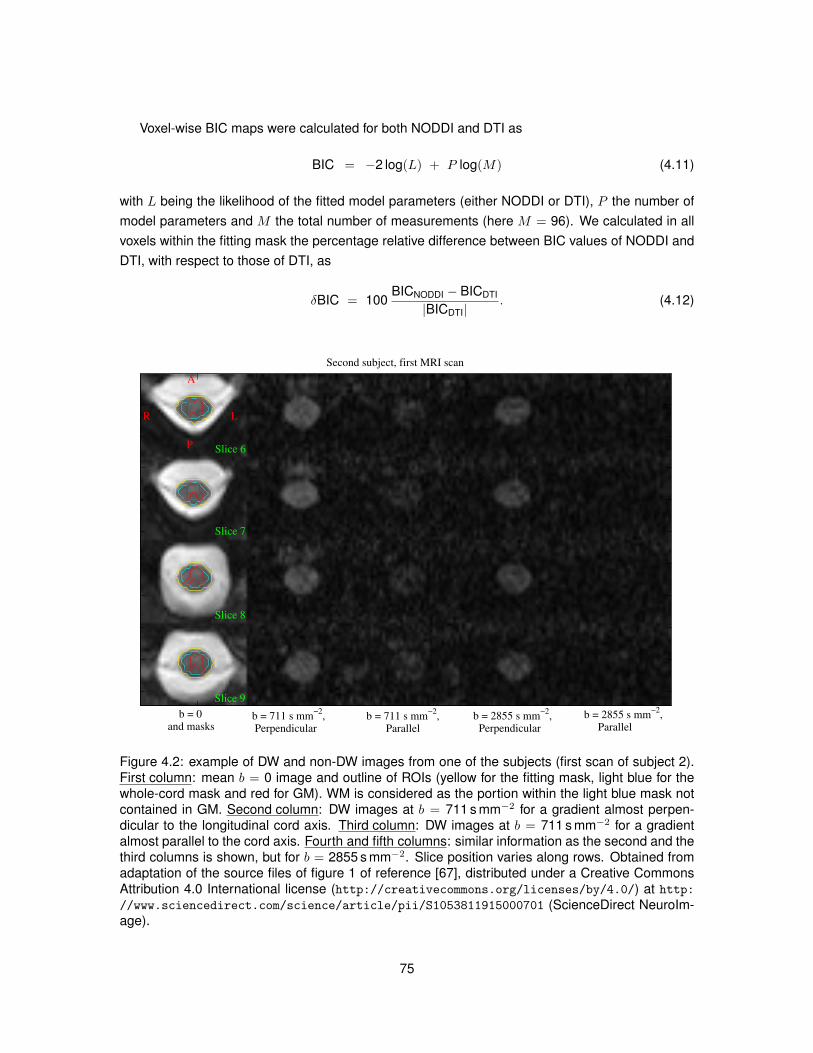
Voxel-wise BIC maps were calculated for both NODDI and DTI as

BIC = −2 log(L) + P log(M) (4.11)

with L being the likelihood of the fitted model parameters (either NODDI or DTI), P the number ofmodel parameters and M the total number of measurements (here M = 96). We calculated in allvoxels within the fitting mask the percentage relative difference between BIC values of NODDI andDTI, with respect to those of DTI, as

δBIC = 100BICNODDI − BICDTI

|BICDTI|. (4.12)

R

A

P

b = 0 and masks

b = 711 s mm−2

, Perpendicular

b = 2855 s mm−2

, Perpendicular

b = 2855 s mm−2

, Parallel

b = 711 s mm−2

, Parallel

Second subject, first MRI scan

L

Slice 6

Slice 7

Slice 8

Slice 9

Figure 4.2: example of DW and non-DW images from one of the subjects (first scan of subject 2).First column: mean b = 0 image and outline of ROIs (yellow for the fitting mask, light blue for thewhole-cord mask and red for GM). WM is considered as the portion within the light blue mask notcontained in GM. Second column: DW images at b = 711 s mm−2 for a gradient almost perpen-dicular to the longitudinal cord axis. Third column: DW images at b = 711 s mm−2 for a gradientalmost parallel to the cord axis. Fourth and fifth columns: similar information as the second and thethird columns is shown, but for b = 2855 s mm−2. Slice position varies along rows. Obtained fromadaptation of the source files of figure 1 of reference [67], distributed under a Creative CommonsAttribution 4.0 International license (http://creativecommons.org/licenses/by/4.0/) at http://www.sciencedirect.com/science/article/pii/S1053811915000701 (ScienceDirect NeuroIm-age).

75

http://creativecommons.org/licenses/by/4.0/

http://www.sciencedirect.com/science/article/pii/S1053811915000701


Effect of crossing fibres

WM fibres in the spinal cord are mainly directed along the superior-inferior direction. However,several collateral axons orthogonal to this dominant direction project into GM [113]. The areaswhere these axons branch are therefore characterised by crossing fibres. NODDI does not accountdirectly for multiple fibre populations, and in this piece of analysis we investigated the effect ofcrossing fibres on its metrics. We proceeded in two steps: i) firstly, WM voxels likely to containcrossing fibres were detected; ii) secondly, a permutation test was performed to compare WMareas likely and unlikely to contain crossing fibres.

Detection of crossing fibres: voxels likely to contain collateral fibres were selected from the WMmask thresholding the mode of the diffusion tensor obtained from the b = 711 s mm−2 shell, asproposed in [113]. The method hypothesises that voxels with significant crossing fibres have aplanar diffusion tensor, and proposes to threshold the tensor mode as a way to distinguish betweentrue and noise-induced planarity. In [113], the optimal threshold is provided as a function of the SNRvia simulations. We estimated that in the WM of our subjects the SNR was roughly 13, implyinga threshold of 0.88. Lastly, the number of false positives was reduced by eliminating voxels thatintersect the dilated GM mask.

Permutation test : for each subject i = 1, ...,5 the medians of all NODDI metrics were calculatedfor WM voxels likely and unlikely to contain crossing fibres (indicated as mxing

i and mnon-xingi ), and

their difference (di = mxingi −mnon-xing

i ) was calculated. The calculation was repeated 1000 timespermuting over the labels of groups “xing” and “non-xing” in order to obtain a distribution of dif-ferences di and of the mean difference d = 1

5

∑5i=1 di. A two-tailed test with significance level of

p = 0.05 was performed comparing the measured differences di and d with their distributions overthe permutations (significance guaranteed by a measured difference either bigger than the 97.5percentile or smaller than the 2.5 percentile of the distribution).

4.5 Results

4.5.1 Data acquisition and tissue segmentation

Figure 4.2 shows DW and non-DW images and ROIs from the first scan of the second subject.The figure shows that stronger signal decay occurs for gradients along the cord axis, and that atb = 2855 s mm−2 the signal is almost completely attenuated for encoding along that direction.

Figure 4.3 shows an example of the images that were used for tissue segmentation. The figuredemonstrates that in the mean b = 0 image GM and WM can not be told apart. However, contrastbetween the two tissue types is visible in the average DW image obtained as described in section4.4.3. In that image, the MRI signal in GM is more intense than in WM, due to the less strong signaldecay. This fact enables the possibility of outlining manually GM. Lastly, the figure demonstratesthat the erosion of the fitting cord mask reduces the possibility of inclusion of voxels contaminatedby CSF.

76

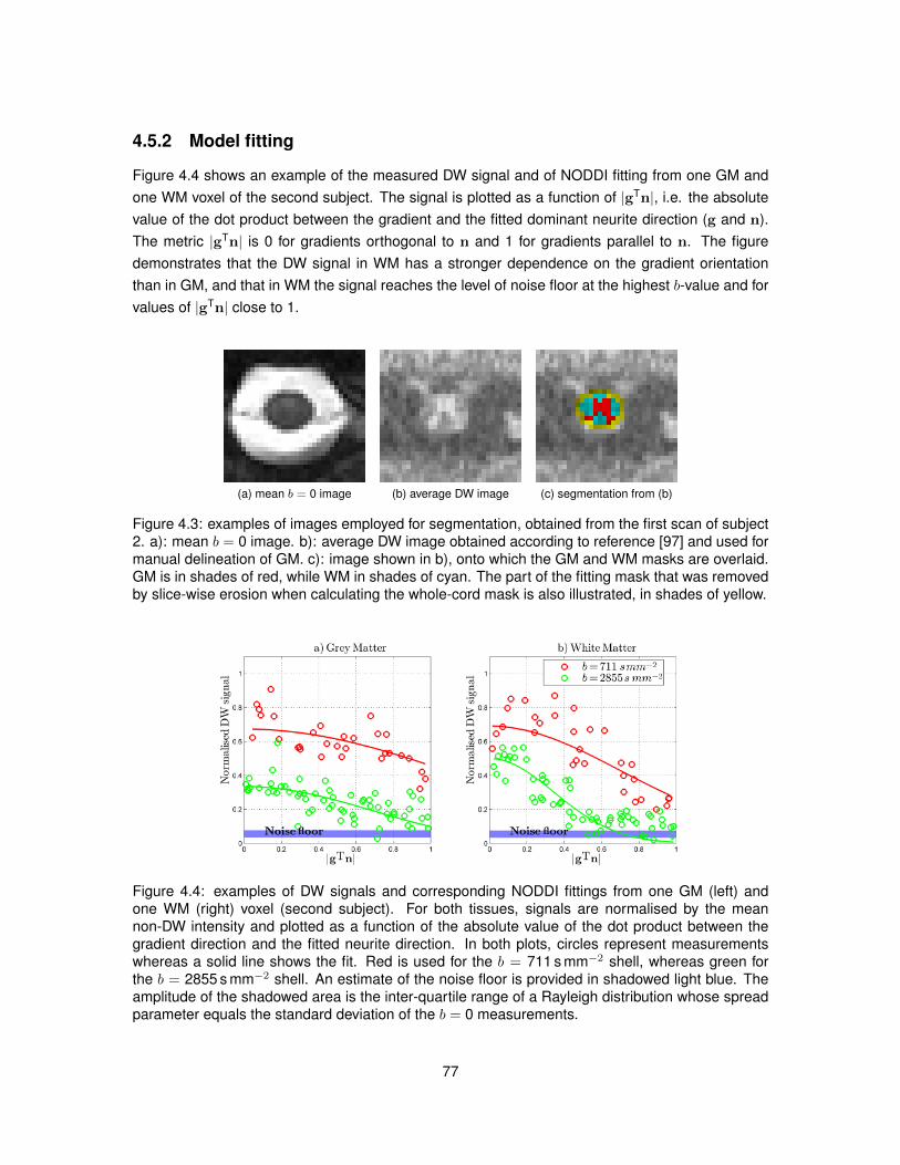
4.5.2 Model fitting

Figure 4.4 shows an example of the measured DW signal and of NODDI fitting from one GM andone WM voxel of the second subject. The signal is plotted as a function of |gTn|, i.e. the absolutevalue of the dot product between the gradient and the fitted dominant neurite direction (g and n).The metric |gTn| is 0 for gradients orthogonal to n and 1 for gradients parallel to n. The figuredemonstrates that the DW signal in WM has a stronger dependence on the gradient orientationthan in GM, and that in WM the signal reaches the level of noise floor at the highest b-value and forvalues of |gTn| close to 1.

(a) mean b = 0 image (b) average DW image (c) segmentation from (b)

Figure 4.3: examples of images employed for segmentation, obtained from the first scan of subject2. a): mean b = 0 image. b): average DW image obtained according to reference [97] and used formanual delineation of GM. c): image shown in b), onto which the GM and WM masks are overlaid.GM is in shades of red, while WM in shades of cyan. The part of the fitting mask that was removedby slice-wise erosion when calculating the whole-cord mask is also illustrated, in shades of yellow.

Figure 4.4: examples of DW signals and corresponding NODDI fittings from one GM (left) andone WM (right) voxel (second subject). For both tissues, signals are normalised by the meannon-DW intensity and plotted as a function of the absolute value of the dot product between thegradient direction and the fitted neurite direction. In both plots, circles represent measurementswhereas a solid line shows the fit. Red is used for the b = 711 s mm−2 shell, whereas green forthe b = 2855 s mm−2 shell. An estimate of the noise floor is provided in shadowed light blue. Theamplitude of the shadowed area is the inter-quartile range of a Rayleigh distribution whose spreadparameter equals the standard deviation of the b = 0 measurements.

77

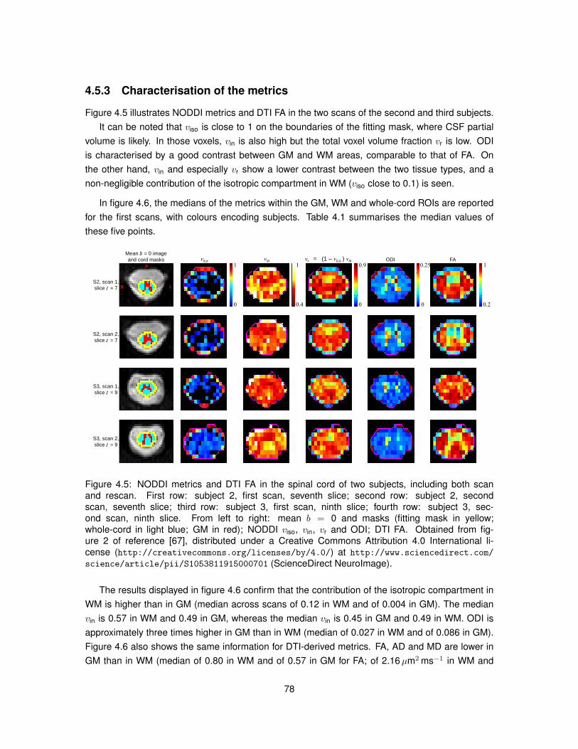
4.5.3 Characterisation of the metrics

Figure 4.5 illustrates NODDI metrics and DTI FA in the two scans of the second and third subjects.It can be noted that viso is close to 1 on the boundaries of the fitting mask, where CSF partial

volume is likely. In those voxels, vin is also high but the total voxel volume fraction vr is low. ODIis characterised by a good contrast between GM and WM areas, comparable to that of FA. Onthe other hand, vin and especially vr show a lower contrast between the two tissue types, and anon-negligible contribution of the isotropic compartment in WM (viso close to 0.1) is seen.

In figure 4.6, the medians of the metrics within the GM, WM and whole-cord ROIs are reportedfor the first scans, with colours encoding subjects. Table 4.1 summarises the median values ofthese five points.

viso vin vr = (1 – viso ) vin ODI FA

A

P

R L

Mean b = 0 image

and cord masks

S2, scan 1,

slice z = 7

S2, scan 2,

slice z = 7

S3, scan 1,

slice z = 9

S3, scan 2,

slice z = 9

1

0

1

0.4

0.9

0

0.25

0

1

0.2

Figure 4.5: NODDI metrics and DTI FA in the spinal cord of two subjects, including both scanand rescan. First row: subject 2, first scan, seventh slice; second row: subject 2, secondscan, seventh slice; third row: subject 3, first scan, ninth slice; fourth row: subject 3, sec-ond scan, ninth slice. From left to right: mean b = 0 and masks (fitting mask in yellow;whole-cord in light blue; GM in red); NODDI viso, vin, vr and ODI; DTI FA. Obtained from fig-ure 2 of reference [67], distributed under a Creative Commons Attribution 4.0 International li-cense (http://creativecommons.org/licenses/by/4.0/) at http://www.sciencedirect.com/

science/article/pii/S1053811915000701 (ScienceDirect NeuroImage).

The results displayed in figure 4.6 confirm that the contribution of the isotropic compartment inWM is higher than in GM (median across scans of 0.12 in WM and of 0.004 in GM). The medianvin is 0.57 in WM and 0.49 in GM, whereas the median vin is 0.45 in GM and 0.49 in WM. ODI isapproximately three times higher in GM than in WM (median of 0.027 in WM and of 0.086 in GM).Figure 4.6 also shows the same information for DTI-derived metrics. FA, AD and MD are lower inGM than in WM (median of 0.80 in WM and of 0.57 in GM for FA; of 2.16µm2 ms−1 in WM and

78




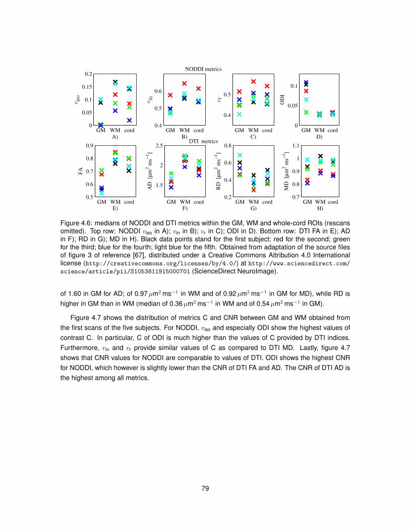
GM WM cord0

0.05

0.1

0.15

0.2viso

A)

GM WM cord0.4

0.5

0.6

vin

B)

GM WM cord

0.4

0.5

vr

C)

GM WM cord0

0.05

0.1

OD

I

D)

GM WM cord0.5

0.6

0.7

0.8

0.9

FA

E)

GM WM cord

1.5

2

2.5A

D [µ

m2 m

s−1]

F)

GM WM cord0.2

0.4

0.6

0.8

RD

[µ

m2 m

s−1]

G)

GM WM cord0.7

0.8

0.9

1

1.1

MD

[µ

m2 m

s−1]

H)

NODDI metrics

DTI metrics

Figure 4.6: medians of NODDI and DTI metrics within the GM, WM and whole-cord ROIs (rescansomitted). Top row: NODDI viso in A); vin in B); vr in C); ODI in D). Bottom row: DTI FA in E); ADin F); RD in G); MD in H). Black data points stand for the first subject; red for the second; greenfor the third; blue for the fourth; light blue for the fifth. Obtained from adaptation of the source filesof figure 3 of reference [67], distributed under a Creative Commons Attribution 4.0 Internationallicense (http://creativecommons.org/licenses/by/4.0/) at http://www.sciencedirect.com/science/article/pii/S1053811915000701 (ScienceDirect NeuroImage).

of 1.60 in GM for AD; of 0.97µm2 ms−1 in WM and of 0.92µm2 ms−1 in GM for MD), while RD ishigher in GM than in WM (median of 0.36µm2 ms−1 in WM and of 0.54µm2 ms−1 in GM).

Figure 4.7 shows the distribution of metrics C and CNR between GM and WM obtained fromthe first scans of the five subjects. For NODDI, viso and especially ODI show the highest values ofcontrast C. In particular, C of ODI is much higher than the values of C provided by DTI indices.Furthermore, vin and vr provide similar values of C as compared to DTI MD. Lastly, figure 4.7shows that CNR values for NODDI are comparable to values of DTI. ODI shows the highest CNRfor NODDI, which however is slightly lower than the CNR of DTI FA and AD. The CNR of DTI AD isthe highest among all metrics.

79




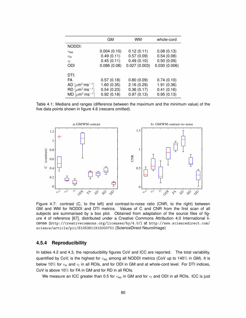
GM WM whole-cord

NODDI:viso 0.004 (0.10) 0.12 (0.11) 0.08 (0.13)vin 0.49 (0.11) 0.57 (0.09) 0.54 (0.08)vr 0.45 (0.11) 0.49 (0.10) 0.50 (0.09)ODI 0.086 (0.08) 0.027 (0.003) 0.030 (0.006)

DTI:FA 0.57 (0.18) 0.80 (0.09) 0.74 (0.10)AD [µm2 ms−1] 1.60 (0.35) 2.16 (0.29) 1.91 (0.36)RD [µm2 ms−1] 0.54 (0.23) 0.36 (0.17) 0.41 (0.16)MD [µm2 ms−1] 0.92 (0.18) 0.97 (0.13) 0.95 (0.13)

Table 4.1: Medians and ranges (difference between the maximum and the minimum value) of thefive data points shown in figure 4.6 (rescans omitted).

0

0.2

0.4

0.6

0.8

1

1.2

C

(co

nst

rast

)

a) GM/WM contrast

v iso

v in v r

ODI

FA

AD

RD

MD

0

0.5

1

1.5C

NR

b) GM/WM contrast−to−noise

v iso

v in v r

ODI

FA

AD

RD

MD

Figure 4.7: contrast (C, to the left) and contrast-to-noise ratio (CNR, to the right) betweenGM and WM for NODDI and DTI metrics. Values of C and CNR from the first scan of allsubjects are summarised by a box plot. Obtained from adaptation of the source files of fig-ure 4 of reference [67], distributed under a Creative Commons Attribution 4.0 International li-cense (http://creativecommons.org/licenses/by/4.0/) at http://www.sciencedirect.com/

science/article/pii/S1053811915000701 (ScienceDirect NeuroImage)

4.5.4 Reproducibility

In tables 4.2 and 4.3, the reproducibility figures CoV and ICC are reported. The total variability,quantified by CoV, is the highest for viso among all NODDI metrics (CoV up to 140% in GM). It isbelow 10% for vin and vr in all ROIs, and for ODI in GM and at whole-cord level. For DTI indices,CoV is above 10% for FA in GM and for RD in all ROIs.

We measure an ICC greater than 0.5 for viso in GM and for vr and ODI in all ROIs. ICC is just

80




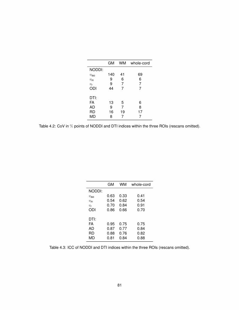
GM WM whole-cord

NODDI:viso 140 41 69vin 9 6 6vr 9 7 7ODI 44 7 7

DTI:FA 13 5 6AD 9 7 8RD 16 19 17MD 8 7 7

Table 4.2: CoV in % points of NODDI and DTI indices within the three ROIs (rescans omitted).

GM WM whole-cord

NODDI:viso 0.63 0.33 0.41vin 0.54 0.62 0.54vr 0.70 0.84 0.91ODI 0.86 0.66 0.70

DTI:FA 0.95 0.75 0.75AD 0.87 0.77 0.84RD 0.88 0.76 0.82MD 0.81 0.84 0.88

Table 4.3: ICC of NODDI and DTI indices within the three ROIs (rescans omitted).

81

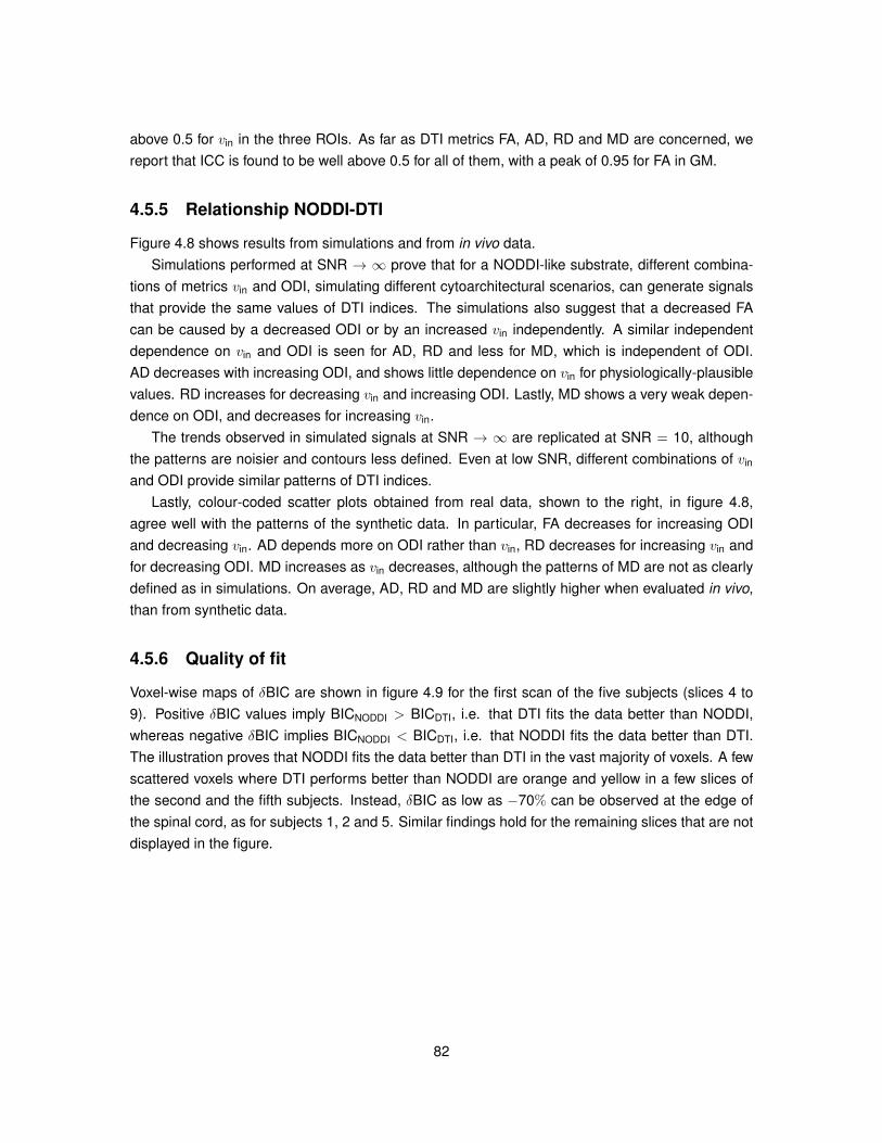
above 0.5 for vin in the three ROIs. As far as DTI metrics FA, AD, RD and MD are concerned, wereport that ICC is found to be well above 0.5 for all of them, with a peak of 0.95 for FA in GM.

4.5.5 Relationship NODDI-DTI

Figure 4.8 shows results from simulations and from in vivo data.Simulations performed at SNR → ∞ prove that for a NODDI-like substrate, different combina-

tions of metrics vin and ODI, simulating different cytoarchitectural scenarios, can generate signalsthat provide the same values of DTI indices. The simulations also suggest that a decreased FAcan be caused by a decreased ODI or by an increased vin independently. A similar independentdependence on vin and ODI is seen for AD, RD and less for MD, which is independent of ODI.AD decreases with increasing ODI, and shows little dependence on vin for physiologically-plausiblevalues. RD increases for decreasing vin and increasing ODI. Lastly, MD shows a very weak depen-dence on ODI, and decreases for increasing vin.

The trends observed in simulated signals at SNR → ∞ are replicated at SNR = 10, althoughthe patterns are noisier and contours less defined. Even at low SNR, different combinations of vin

and ODI provide similar patterns of DTI indices.Lastly, colour-coded scatter plots obtained from real data, shown to the right, in figure 4.8,

agree well with the patterns of the synthetic data. In particular, FA decreases for increasing ODIand decreasing vin. AD depends more on ODI rather than vin, RD decreases for increasing vin andfor decreasing ODI. MD increases as vin decreases, although the patterns of MD are not as clearlydefined as in simulations. On average, AD, RD and MD are slightly higher when evaluated in vivo,than from synthetic data.

4.5.6 Quality of fit

Voxel-wise maps of δBIC are shown in figure 4.9 for the first scan of the five subjects (slices 4 to9). Positive δBIC values imply BICNODDI > BICDTI, i.e. that DTI fits the data better than NODDI,whereas negative δBIC implies BICNODDI < BICDTI, i.e. that NODDI fits the data better than DTI.The illustration proves that NODDI fits the data better than DTI in the vast majority of voxels. A fewscattered voxels where DTI performs better than NODDI are orange and yellow in a few slices ofthe second and the fifth subjects. Instead, δBIC as low as −70% can be observed at the edge ofthe spinal cord, as for subjects 1, 2 and 5. Similar findings hold for the remaining slices that are notdisplayed in the figure.

82

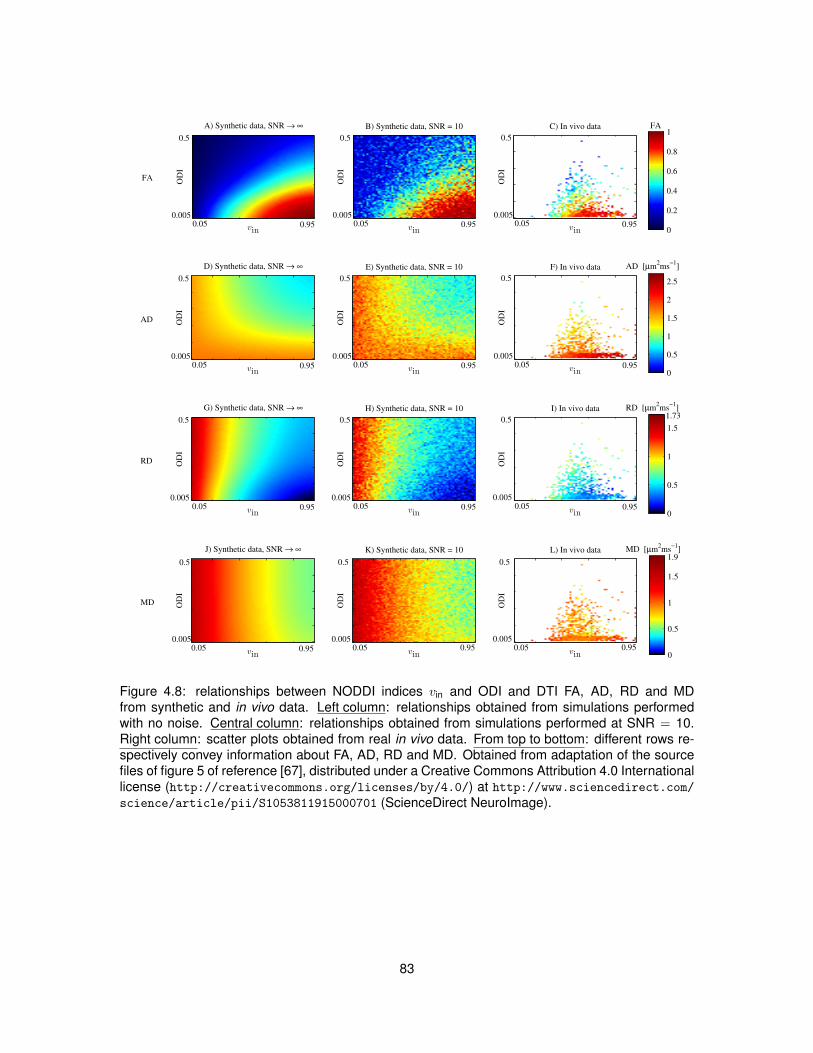
vin

OD

I

A) Synthetic data, SNR → ∞

vin

OD

I

B) Synthetic data, SNR = 10

vin

OD

I

C) In vivo data

0

0.2

0.4

0.6

0.8

1

0.005 0.005

0.5 0.5 0.5

0.95 0.95 0.950.050.05

FA

FA

0.050.005

vin

OD

I

D) Synthetic data, SNR → ∞

vin

OD

I

E) Synthetic data, SNR = 10

vin

OD

I

F) In vivo data

0

0.5

1

1.5

2

2.50.5 0.5 0.5

0.005 0.0050.95 0.95 0.95

0.0050.050.050.05

AD

AD [µm2ms

−1]

vin

OD

I

G) Synthetic data, SNR → ∞

vin

OD

I

H) Synthetic data, SNR = 10

vin

OD

I

I) In vivo data

0

0.5

1

1.50.5 0.5 0.5

0.0050.005 0.0050.050.050.05 0.95 0.95 0.95

RD

RD [µm2ms

−1]

1.73

vin

OD

I

J) Synthetic data, SNR → ∞

vin

OD

I

K) Synthetic data, SNR = 10

vin

OD

I

L) In vivo data

0

0.5

1

1.5

0.5 0.5 0.5

0.0050.0050.95 0.95

0.0050.05 0.05 0.05

MD

1.9MD [µm

2ms

−1]

0.95

Figure 4.8: relationships between NODDI indices vin and ODI and DTI FA, AD, RD and MDfrom synthetic and in vivo data. Left column: relationships obtained from simulations performedwith no noise. Central column: relationships obtained from simulations performed at SNR = 10.Right column: scatter plots obtained from real in vivo data. From top to bottom: different rows re-spectively convey information about FA, AD, RD and MD. Obtained from adaptation of the sourcefiles of figure 5 of reference [67], distributed under a Creative Commons Attribution 4.0 Internationallicense (http://creativecommons.org/licenses/by/4.0/) at http://www.sciencedirect.com/science/article/pii/S1053811915000701 (ScienceDirect NeuroImage).

83




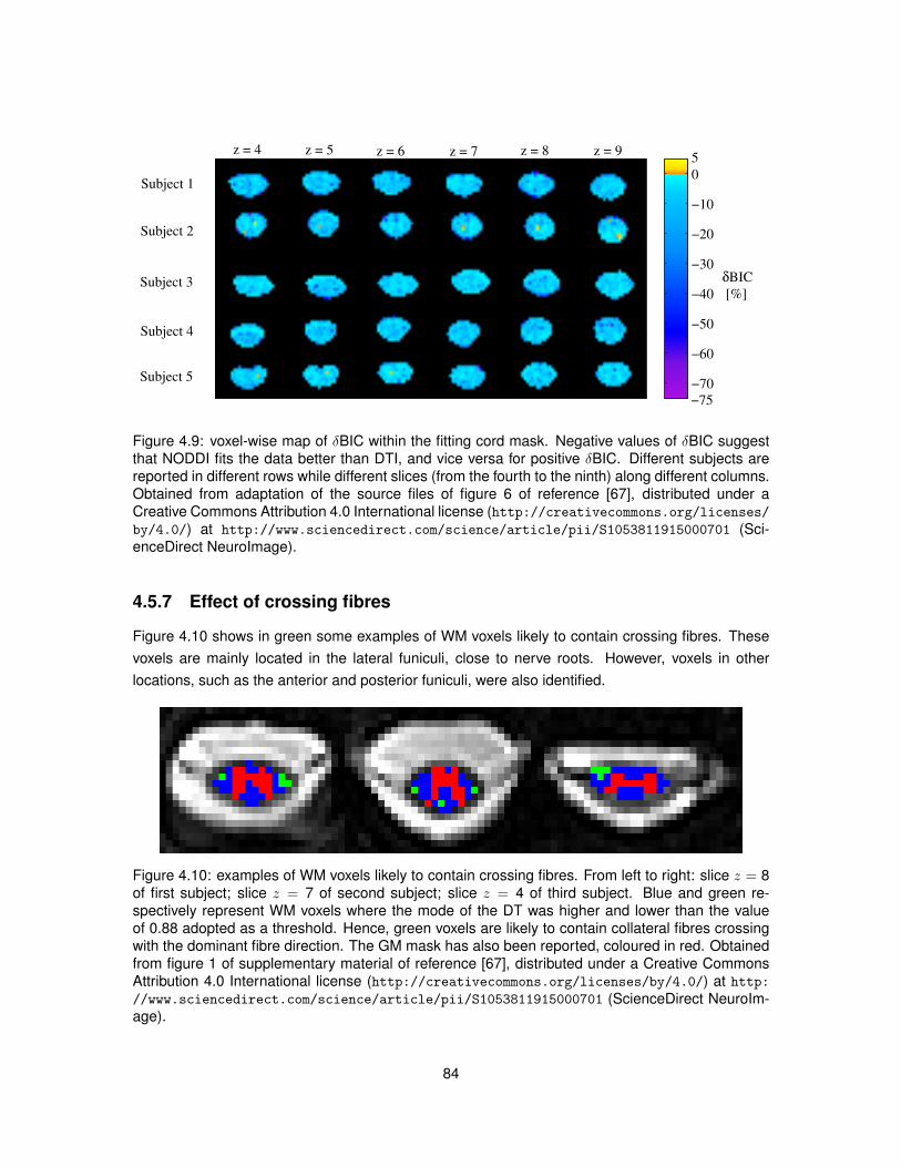
−70

−60

−50

−40

−30

−20

−10

0

−75

5

δBIC

[%]

z = 4 z = 5 z = 6 z = 7 z = 8 z = 9

Subject 1

Subject 2

Subject 3

Subject 4

Subject 5

Figure 4.9: voxel-wise map of δBIC within the fitting cord mask. Negative values of δBIC suggestthat NODDI fits the data better than DTI, and vice versa for positive δBIC. Different subjects arereported in different rows while different slices (from the fourth to the ninth) along different columns.Obtained from adaptation of the source files of figure 6 of reference [67], distributed under aCreative Commons Attribution 4.0 International license (http://creativecommons.org/licenses/by/4.0/) at http://www.sciencedirect.com/science/article/pii/S1053811915000701 (Sci-enceDirect NeuroImage).

4.5.7 Effect of crossing fibres

Figure 4.10 shows in green some examples of WM voxels likely to contain crossing fibres. Thesevoxels are mainly located in the lateral funiculi, close to nerve roots. However, voxels in otherlocations, such as the anterior and posterior funiculi, were also identified.

Figure 4.10: examples of WM voxels likely to contain crossing fibres. From left to right: slice z = 8of first subject; slice z = 7 of second subject; slice z = 4 of third subject. Blue and green re-spectively represent WM voxels where the mode of the DT was higher and lower than the valueof 0.88 adopted as a threshold. Hence, green voxels are likely to contain collateral fibres crossingwith the dominant fibre direction. The GM mask has also been reported, coloured in red. Obtainedfrom figure 1 of supplementary material of reference [67], distributed under a Creative CommonsAttribution 4.0 International license (http://creativecommons.org/licenses/by/4.0/) at http://www.sciencedirect.com/science/article/pii/S1053811915000701 (ScienceDirect NeuroIm-age).

84







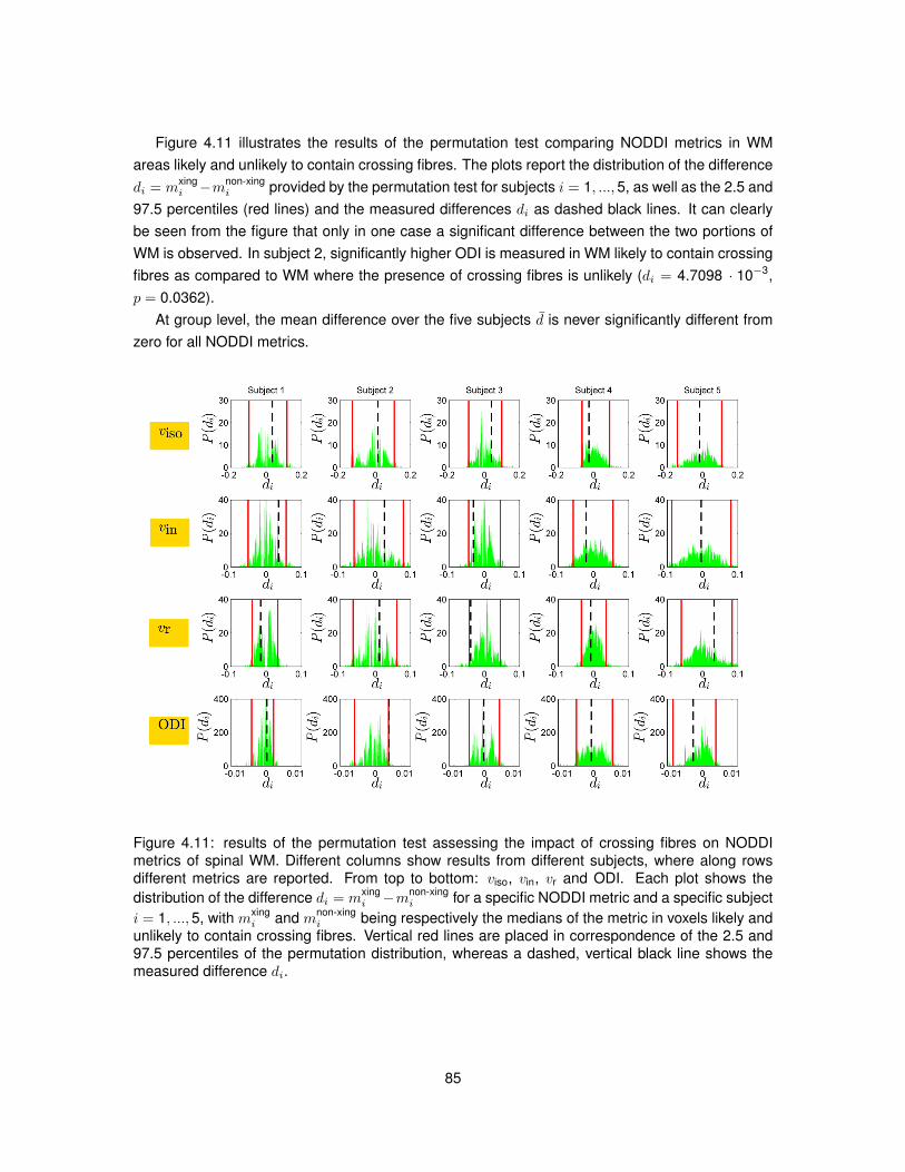
Figure 4.11 illustrates the results of the permutation test comparing NODDI metrics in WMareas likely and unlikely to contain crossing fibres. The plots report the distribution of the differencedi = m

xingi −mnon-xing

i provided by the permutation test for subjects i = 1, ...,5, as well as the 2.5 and97.5 percentiles (red lines) and the measured differences di as dashed black lines. It can clearlybe seen from the figure that only in one case a significant difference between the two portions ofWM is observed. In subject 2, significantly higher ODI is measured in WM likely to contain crossingfibres as compared to WM where the presence of crossing fibres is unlikely (di = 4.7098 · 10−3,p = 0.0362).

At group level, the mean difference over the five subjects d is never significantly different fromzero for all NODDI metrics.

Figure 4.11: results of the permutation test assessing the impact of crossing fibres on NODDImetrics of spinal WM. Different columns show results from different subjects, where along rowsdifferent metrics are reported. From top to bottom: viso, vin, vr and ODI. Each plot shows thedistribution of the difference di = m

xingi −mnon-xing

i for a specific NODDI metric and a specific subjecti = 1, ...,5, with mxing

i and mnon-xingi being respectively the medians of the metric in voxels likely and

unlikely to contain crossing fibres. Vertical red lines are placed in correspondence of the 2.5 and97.5 percentiles of the permutation distribution, whereas a dashed, vertical black line shows themeasured difference di.

85

4.6 Discussion

The work presented in this chapter demonstrates the feasibility of applying NODDI to the healthyspinal cord in vivo. Five healthy volunteers were scanned at 3T following a multi-shell diffusionencoding protocol to obtain for the first time NODDI metrics of the spinal cord. These metrics mapspecific features of neurite morphology and may be relevant biomarkers for spinal cord conditions.Trends of NODDI indices seen in the brain were replicated, although some differences were seen.For comparison, conventional DTI metrics were also evaluated, and they were found to agree withprevious literature [189,205,213].

Characterisation of the metricsOur analysis suggests that viso captures CSF contamination, being close to 1 in the edge of the

fitting cord mask, where CSF partial volume may occur. In those voxels, vin is also high. This islikely due to the inherent difficulty of determining properties of the restricted compartment whenhigh CSF contamination occurs, which causes a poorly defined vin. Our work reveals that viso isnot negligible within the spinal cord, especially in WM (median across the five subjects of 0.12,against 0.004 in GM). A number of reasons may explain this fact. Firstly, we speculate that CSFcontamination in the anterior median fissure and the central canal may contribute to a high viso.Secondly, it may be that the isotropic compartment captures contributions from the water pool thatcan not be characterised directly by restricted diffusion. Although a high viso may be a simple effectof noise, it was initially speculated that the isotropic compartment may capture contributions fromthe biggest axons, whose diameter in the spinal cord can be as high as 15µm [56, 70, 117, 201].In this study, a diffusion time of Td = 25.37 ms was employed, corresponding to a mean squaredisplacement of Ld =

√2Dfree Td = 10.5µm, if one adopts the observed median AD in WM as an

estimate of the free diffusivity (Dfree). Therefore, diffusion within the biggest axons may not havereached the long diffusion time limit, and may appear as relatively free. Further investigation wascarried out to study in detail this possibility. Results presented in chapter 6 suggest that althoughNODDI parameter estimation is influenced by the choice of the diffusion time when large axons arepresent, viso values as high as roughly 0.10 are simply attributable to noise.

The ROI analysis proved that ODI reflects differences in terms of neurite morphology betweenGM and WM. This is in line with previous qualitative findings in the brain [215]. On the one hand,ODI shows the highest contrast C between GM and WM among all metrics. On the other hand, itsCNR is just below 1 and is surpassed by FA and AD. This shows the potential of NODDI for char-acterising differences in terms of microstructure between spinal GM and WM, but also suggeststhat future optimisation may help reduce the variability of the metrics. This would potentially lead tohigher CNR values for ODI and help improve the reproducibility, as discussed below. Furthermore,volume fractions vin and vr show a reduced contrast between GM and WM, if compared to ODI,similar to DTI MD. Although GM-WM partial volume effects due to the coarse in-plane resolutionmay have contributed, this may indicate that vin and vr are more homogeneous between GM andWM compared to the brain. For instance, it was originally speculated that the presence in GM ofaxons that originates from spinal nerve roots and WM funiculi, or the presence in WM (especially

86

at cervical level) of the formatio reticularis, made of GM strands separated by interwoven fibres,may have contributed to a reduced heterogeneity in terms of neurite density between GM and WM.However, recent work carried out subsequently and described in chapter 6 points to incompleterestriction of diffusion within the biggest axons as another factor contributing to the relatively low vin

and vr in WM. This could potentially cause the measured values of vin and viso to be underestimatedand hence similar to those of GM.

ReproducibilityThe aim of the reproducibility analysis was the quantification of the total variability of NODDI

metrics, and the estimation of the fractions of variability due to biological differences in the cohortand to measurement errors. The analysis shows that the total variability of NODDI vin, vr and ODI iscomparable to that of DTI FA, AD, RD and MD, whilst the variability of viso is considerably greater,causing CoV to be as high as 140% in GM. This last fact is not surprising, since viso is found tobe negligible on average within the GM mask (median across subjects of 0.004), and hence poorlydefined. Also, our work highlights that the total variability is driven by biological differences in thecohort for vr and ODI, by measurement errors for viso, whilst the two sources contribute equally tothe variability of vin (ICC close to 0.5 in all ROIs). On the other hand, DTI indices are less variablethan NODDI ones, and biological variation drives the total variability. As compared to DTI, the worsereproducibility scores of NODDI may be due to the higher susceptibility of its non-linear model tothermal and physiological noise, imperfect B0 field shimming and different alignment of the spinalcord with the main field between scans and rescans. Nevertheless, our analysis suggests thatNODDI in the current form can be applied in spinal cord studies. However, the technique could befurther optimised for spinal cord anatomy and potentially improved.

Relationship NODDI-DTIWe performed computer simulations to visualise the theoretical dependence of DTI metrics on

NODDI vin and ODI, and compared these theoretical patterns to colour-coded scatter plots obtainedfrom in vivo data. Both synthetic and in vivo data show an important fact: a similar value of all DTImetrics can be produced by combinations of vin and ODI sensibly different from each other, repre-senting different cytoarchitectures. For instance, the dependence of FA on vin and ODI observedon the in vivo data resembles pattern previously reported in [215]. It reveals that a decrease ofFA can be caused independently by an increase of ODI or by a decrease of vin. The two effectshave clearly different biological meaning, but they cannot be distinguished only looking at FA, aconventional marker of neuronal integrity. Therefore, NODDI appears to provide indices that disen-tangle two of the main microarchitectural sources contributing to DTI metrics: the density and theorientation complexity of neuronal processes.

Quality of fitThe last focus of our analysis was the study of the performance of NODDI and DTI in terms

of goodness of fit. We derived the BIC for the two models on the full double-shell data set andcalculated their percentage relative difference δBIC, positive when DTI fits better than NODDI, neg-

87

ative when the opposite holds. The inspection of voxel-wise δBIC maps clearly demonstrates thatNODDI outperforms DTI in terms of quality of fit. Only a few scattered voxels are characterised byδBIC > 0. Negative δBIC values, as low as −70%, are seen in the boundary of the fitting mask.This demonstrates how multi-compartment models such as NODDI are more flexible than mono-compartment DTI and can fit the data better in presence of partial volume.

Effect of crossing fibresA published method based on the thresholding of the diffusion tensor mode was employed to

detect areas in WM likely to contain collateral fibres crossing with the main fibre population di-rected along the superior-inferior direction. Values of all NODDI metrics were then compared with apermutation tests between WM voxels likely and unlikely to contain such crossing fibres. The inves-tigation suggests that the presence of crossing fibres may affect NODDI metrics. In most of cases,no significant differences between the two portions of WM are observed. However, in one case, asignificantly higher ODI is measured in WM voxels likely to contain crossing fibres, as comparedto voxels where their presence is unlikely. Despite the preliminary nature of this analysis and thesmall size of the sample, results point towards a potential weak but measurable impact on NODDImetrics of crossing fibres in spinal cord WM at the present MRI voxel resolution. In particular, themajor sign of presence of crossing fibres seems to be an increase in ODI. Therefore, ODI appearsas an intriguing index for the characterisation of neurite organisation complexity in the spinal cordand of its changes due to pathology. Nonetheless, future analysis with a higher number of subjectswould be needed to further confirm this finding.

LimitationsThis work demonstrates that NODDI can be applied to the human spinal cord in vivo. However, a

number of limitations of our approach need to be acknowledged. The main limitation is probably thefact that the diffusion encoding protocol was not optimised explicitly for the spinal cord. Therefore,the b-values adopted in this study may not be optimal, since they were designed for priors on d‖

and diso typically employed for the brain in vivo. For instance, a slightly higher prior on d‖, similarto the AD measured here in WM, would have resulted in a slightly lower maximum b-value, andhence in a better SNR of the experiment due to the lower TE that could have been used. Also, thechoice of diso = 3.00µm2 ms−1 may not be able to account for pseudo-diffusion effects due to flowand pulsation, such as in voxels characterised by partial volume with the branches of the anteriorspinal artery and vein, which pass into the anterior median fissure. As far as the diffusion-weightingprotocol is concerned, we also speculate that the directional sampling scheme, here isotropic asin [215], may have been optimised according to single fibre approaches similar to those followedin [157], in order to reduce the total acquisition time.

Another limitation of our work is that the reproducibility scores of DTI may have been under-estimated for two reasons. Firstly, a different number of measurements compared to NODDI wereemployed. Secondly, the TE employed to acquire the b = 711 s mm−2 shell was not the minimumachievable at that b-value. We acquired both b-shells with the same TE to achieve the same T2-weighting. However, this caused the SNR of the b = 711 s mm−2 shell on its own to be suboptimal.

88

The choices of the free water and neural tissue diffusivities, i.e. diso = 3.00µm2 ms−1 andd‖ = 1.70µm2 ms−1), may not be optimal in the presence of pathology. In our approach, thediffusion coefficients were fixed rather than fitted as in [215]. However, the adopted values may notbe the best ones in presence of phenomena such as oedema or inflammation, leading to biases inthe other fitted metrics. In those cases, data-driven priors for diso and d‖ may be evaluated, whilesensitivity analysis would help assess the impact of fixing such diffusivites on other NODDI indices.

Lastly, the motion correction strategy may also have represented a limiting factor of our pipeline.We exploited the interleaved position of the non-DW images and estimated motion only on thoseimages, given the challenge of co-registering DW and non-DW images of the spinal cord reliably.Although in other studies DW images were registered to non-DW ones [34, 129, 213], it should benoticed that in those works weaker diffusion weighting was employed.

4.7 Conclusion

In this chapter, we demonstrated the feasibility of applying the published NODDI technique to thehealthy cervical cord in vivo and in a clinical setting. NODDI provides metrics that have the potentialto be valid biomarkers for spinal cord conditions describing specific features of pathology at sub-voxel scale.

NODDI fits the acquired data better than DTI, and provides contrast between GM and WM interms of neurite orientation dispersion, a key source of diffusion anisotropy. This is in line withrecent findings, which showed that orientation dispersion at the MRI voxel scale is an importantcharacteristic even in organised areas such as the corpus callosum [21], improving the performanceof diffusion models [58] when accounted for. The measured reproducibility of NODDI metrics,despite being slightly lower than that of DTI, would allow its application in studies involving largergroups of subjects.

In conclusion, at present NODDI is a valid and feasible alternative to DTI for spinal cord appli-cations. Future optimisation may help further reduce the variability of the metrics with benefits interms of contrast and reproducibility.

89

Chapter 5

NODDI analysis of single-shell data:a feasibility study

5.1 Introduction

NODDI provides indices of neurite density and orientation dispersion in clinically feasible acquisi-tions, with potential applications in several neurological conditions, such as MS [112], SCI [179]and ALS [153]. The published NODDI technique relies on the acquisition of two HARDI shells withdifferent b-values. Although a standard single-shell acquisition allows the quantification of the orien-tation dispersion, the estimation of neurite and isotropic compartment volume fractions requires atleast two shells [215]. However, in [215], it was not tested whether the neurite compartment volumefraction could be estimated from single-shell data, when the isotropic compartment is not included.

The objective of this chapter is to study whether a reduced NODDI model without isotropic com-partment could be fitted to standard single-shell DW data. We focussed on the impact that theb-value and the number of diffusion encoding directions have on single-shell estimates of NODDImetrics, as compared to two-shell gold standard. For our study, we employed the same data em-ployed in the previous chapter (five healthy volunteers scanned at 3T with a rFOV DW ZOOM-EPIsequence).

Our analysis is informative for those interested in applying retrospective NODDI analysis onroutine DW scans of the spinal cord, which are common, especially a low b-value [34, 129, 213].Single-shell analysis, if proven to be feasible, would enable the investigation of new research ques-tions without requiring the acquisition of new data and would facilitate the design of new studies.


Some of the results described in this chapter have been presented in abstract form at internationalmeetings as:

90

• “Single-shell diffusion MRI NODDI with in vivo cervical cord data”. Grussu F. et al, ISMRMannual meeting (2014), p.1716, traditional poster.

• “Characterisation of single-shell NODDI fitting in spinal cord grey and white matter”. GrussuF. et al, British Chapter of ISMRM annual meeting (2014), traditional poster.

5.3 Methods


Data from the the same healthy volunteers of chapter 4 were studied, omitting rescans. Briefly,our data set consisted of five rFOV PGSE ZOOM-EPI [206] scans with OVS [208] obtained fromfive different healthy volunteers. Salient parameters were: TR = 12 RR repeats (oxymeter-basedperipheral cardiac gating, triggering delay of 150 ms), TE = 65.50 ms, rFOV of 64×48 mm2, SENSEfactor of 1.5, resolution of 1×1×5 mm3, 6 non-DW images, 30 diffusion directions at b = 711 s mm−2

and 60 at b = 2855 s mm−2 (∆ = 32.20 ms, δ = 20.50 ms for both shells).

5.3.2 Motion correction

Motion was corrected as described in chapter 4, section 4.4.2. The correction relied on slice-wiselinear registration accounting for in-plane translations, with registration transformations estimatedamong b = 0 images exploiting their interleaved acquisition throughout the MRI scan.

5.3.3 Segmentation

The same segmentation methods followed for the study in chapter 4 were employed, after perform-ing motion correction. Segmentation allowed the identification of a whole-cord, a GM and a WMmask for each subject.

The spinal cord was segmented on the mean b = 0 image with an active surface method [74].On the other hand, GM was segmented manually on an image obtained averaging DW images withgood contrast between GM and WM, as firstly shown in [97] and previously discussed in section4.4.3 of chapter 4. Finally, WM voxels were defined as voxels within the eroded spinal cord masknot containing voxels from the GM mask.

5.3.4 Model fitting

The full NODDI model and a reduced version without the isotropic compartment were fitted todifferent subsets of data with the NODDI Matlab toolbox. The original model was introduced byequation 4.1, whilst the reduced model is written as

s(g, b) = s0

(vr sin(g, b) +

(1− vr

)sen(g, b)

), (5.1)

91

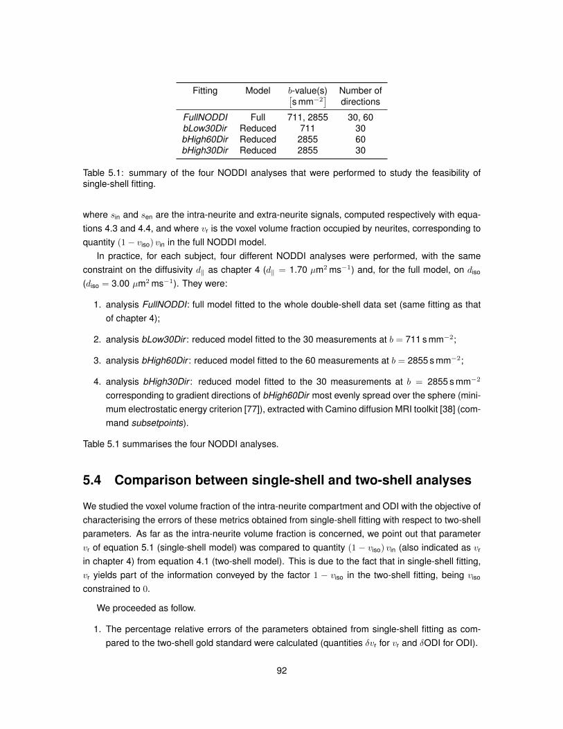
Fitting Model b-value(s) Number of[s mm−2

]directions

FullNODDI Full 711, 2855 30, 60bLow30Dir Reduced 711 30bHigh60Dir Reduced 2855 60bHigh30Dir Reduced 2855 30

Table 5.1: summary of the four NODDI analyses that were performed to study the feasibility ofsingle-shell fitting.

where sin and sen are the intra-neurite and extra-neurite signals, computed respectively with equa-tions 4.3 and 4.4, and where vr is the voxel volume fraction occupied by neurites, corresponding toquantity (1− viso) vin in the full NODDI model.

In practice, for each subject, four different NODDI analyses were performed, with the sameconstraint on the diffusivity d‖ as chapter 4 (d‖ = 1.70 µm2 ms−1) and, for the full model, on diso

(diso = 3.00 µm2 ms−1). They were:

1. analysis FullNODDI: full model fitted to the whole double-shell data set (same fitting as thatof chapter 4);

2. analysis bLow30Dir : reduced model fitted to the 30 measurements at b = 711 s mm−2;

3. analysis bHigh60Dir : reduced model fitted to the 60 measurements at b = 2855 s mm−2;

4. analysis bHigh30Dir : reduced model fitted to the 30 measurements at b = 2855 s mm−2

corresponding to gradient directions of bHigh60Dir most evenly spread over the sphere (mini-mum electrostatic energy criterion [77]), extracted with Camino diffusion MRI toolkit [38] (com-mand subsetpoints).

Table 5.1 summarises the four NODDI analyses.

5.4 Comparison between single-shell and two-shell analyses

We studied the voxel volume fraction of the intra-neurite compartment and ODI with the objective ofcharacterising the errors of these metrics obtained from single-shell fitting with respect to two-shellparameters. As far as the intra-neurite volume fraction is concerned, we point out that parametervr of equation 5.1 (single-shell model) was compared to quantity (1 − viso) vin (also indicated as vr

in chapter 4) from equation 4.1 (two-shell model). This is due to the fact that in single-shell fitting,vr yields part of the information conveyed by the factor 1 − viso in the two-shell fitting, being viso

constrained to 0.

We proceeded as follow.

1. The percentage relative errors of the parameters obtained from single-shell fitting as com-pared to the two-shell gold standard were calculated (quantities δvr for vr and δODI for ODI).

92

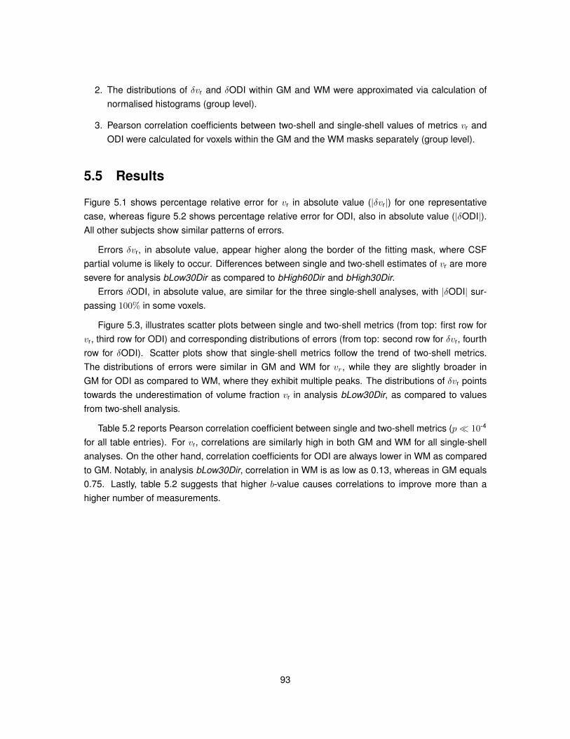
http://cmic.cs.ucl.ac.uk/camino//index.php?n=Man.Subsetpoints

2. The distributions of δvr and δODI within GM and WM were approximated via calculation ofnormalised histograms (group level).

3. Pearson correlation coefficients between two-shell and single-shell values of metrics vr andODI were calculated for voxels within the GM and the WM masks separately (group level).

5.5 Results

Figure 5.1 shows percentage relative error for vr in absolute value (|δvr|) for one representativecase, whereas figure 5.2 shows percentage relative error for ODI, also in absolute value (|δODI|).All other subjects show similar patterns of errors.

Errors δvr, in absolute value, appear higher along the border of the fitting mask, where CSFpartial volume is likely to occur. Differences between single and two-shell estimates of vr are moresevere for analysis bLow30Dir as compared to bHigh60Dir and bHigh30Dir.

Errors δODI, in absolute value, are similar for the three single-shell analyses, with |δODI| sur-passing 100% in some voxels.

Figure 5.3, illustrates scatter plots between single and two-shell metrics (from top: first row forvr, third row for ODI) and corresponding distributions of errors (from top: second row for δvr, fourthrow for δODI). Scatter plots show that single-shell metrics follow the trend of two-shell metrics.The distributions of errors were similar in GM and WM for vr, while they are slightly broader inGM for ODI as compared to WM, where they exhibit multiple peaks. The distributions of δvr pointstowards the underestimation of volume fraction vr in analysis bLow30Dir, as compared to valuesfrom two-shell analysis.

Table 5.2 reports Pearson correlation coefficient between single and two-shell metrics (p 10-4

for all table entries). For vr, correlations are similarly high in both GM and WM for all single-shellanalyses. On the other hand, correlation coefficients for ODI are always lower in WM as comparedto GM. Notably, in analysis bLow30Dir, correlation in WM is as low as 0.13, whereas in GM equals0.75. Lastly, table 5.2 suggests that higher b-value causes correlations to improve more than ahigher number of measurements.

93

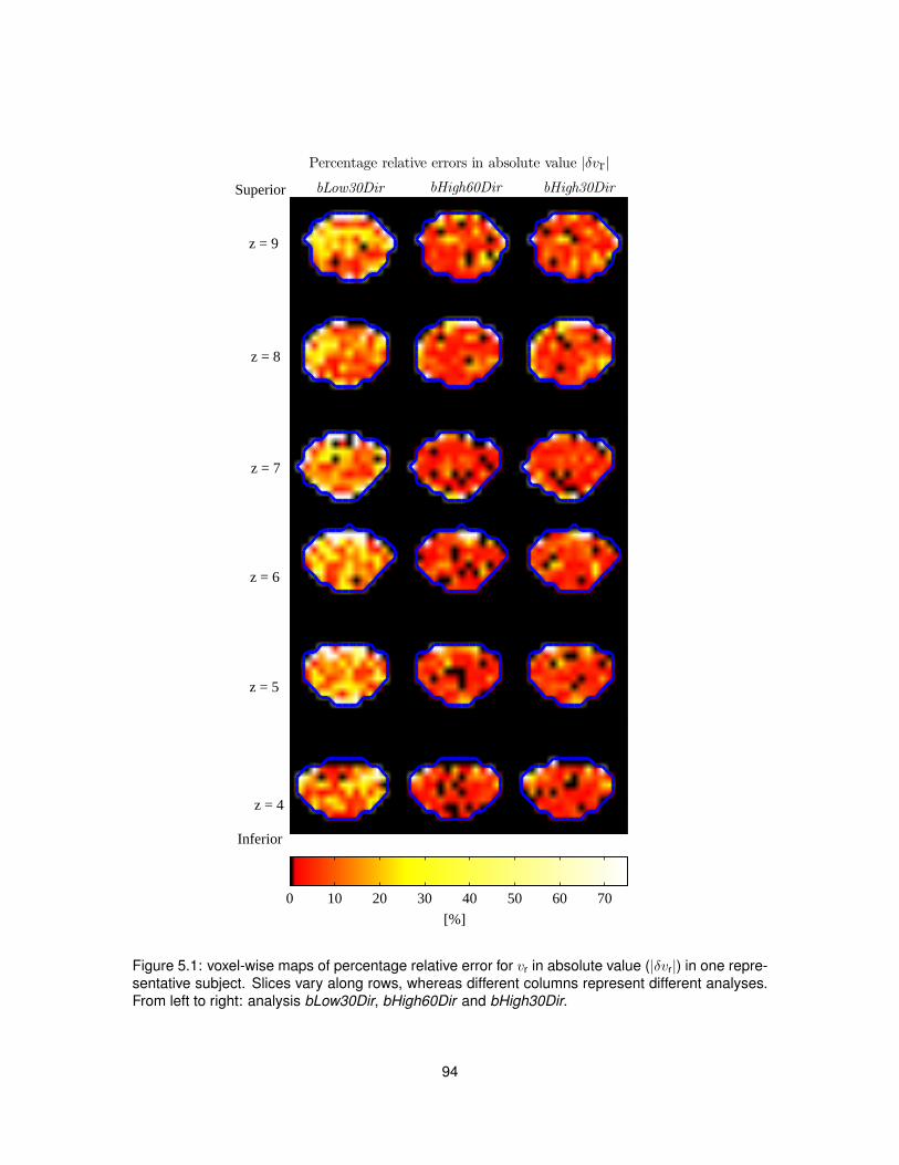
0 10 20 30 40 50 60 70

[%]

Inferior

z = 5

z = 6

z = 7

z = 8

z = 9

bLow30Dir bHigh60Dir bHigh30Dir

z = 4

Superior

Percentage relative errors in absolute value |δvr|

Figure 5.1: voxel-wise maps of percentage relative error for vr in absolute value (|δvr|) in one repre-sentative subject. Slices vary along rows, whereas different columns represent different analyses.From left to right: analysis bLow30Dir, bHigh60Dir and bHigh30Dir.

94

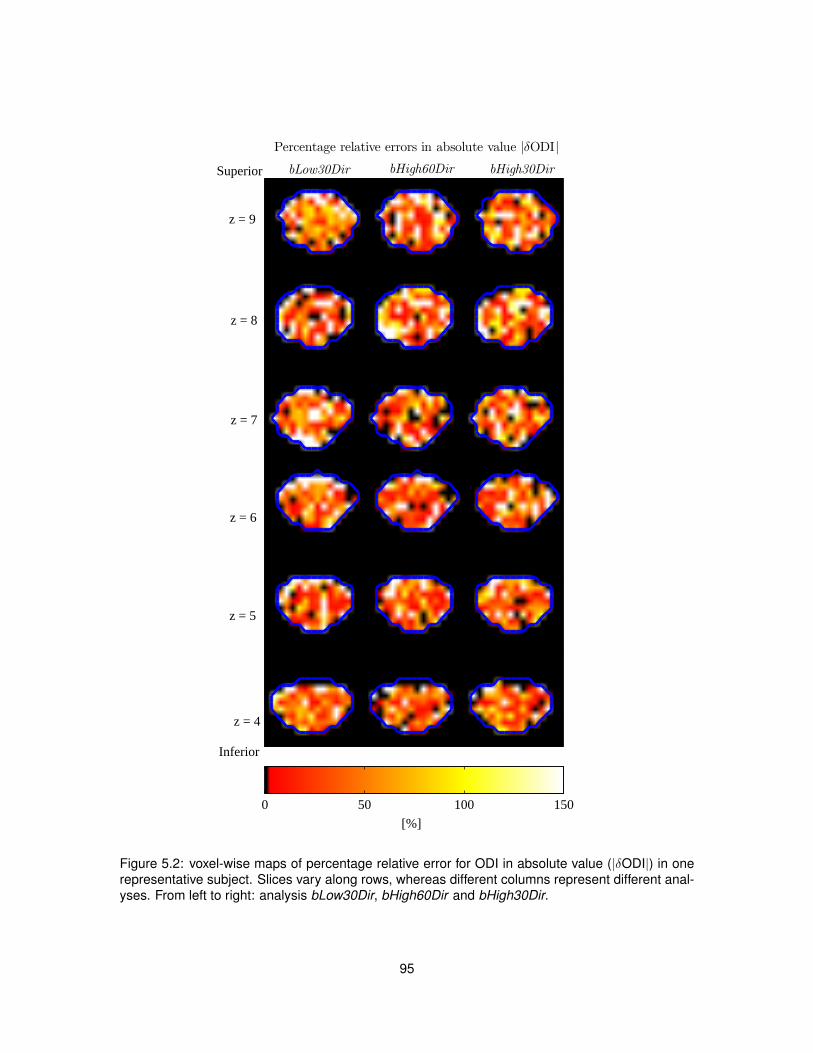
0 50 100 150

[%]

bLow30Dir bHigh60Dir bHigh30DirSuperior

z = 9

z = 8

z = 7

z = 6

z = 5

z = 4

Inferior

Percentage relative errors in absolute value |δODI|

Figure 5.2: voxel-wise maps of percentage relative error for ODI in absolute value (|δODI|) in onerepresentative subject. Slices vary along rows, whereas different columns represent different anal-yses. From left to right: analysis bLow30Dir, bHigh60Dir and bHigh30Dir.

95

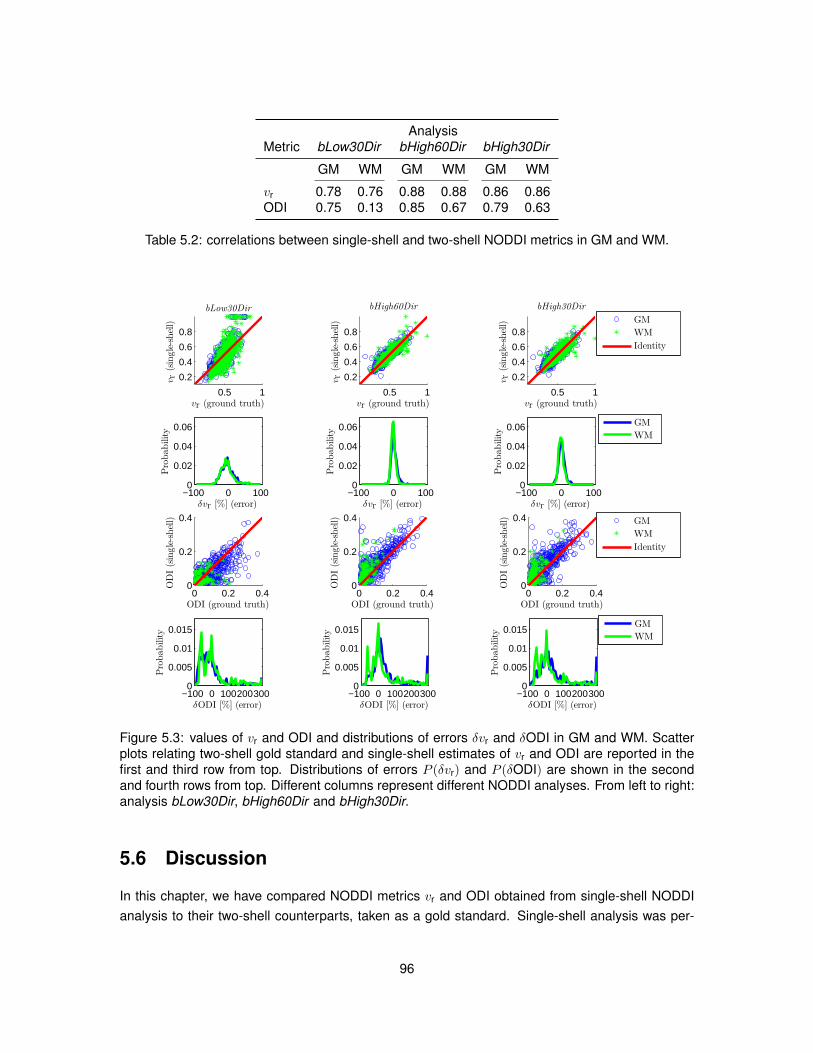
AnalysisMetric bLow30Dir bHigh60Dir bHigh30Dir

GM WM GM WM GM WM

vr 0.78 0.76 0.88 0.88 0.86 0.86ODI 0.75 0.13 0.85 0.67 0.79 0.63

Table 5.2: correlations between single-shell and two-shell NODDI metrics in GM and WM.

0.5 1

0.2

0.4

0.6

0.8

vr (ground truth)

vr(single-shell)

bLow30Dir

0.5 1

0.2

0.4

0.6

0.8

vr (ground truth)

vr(single-shell)

bHigh60Dir

0.5 1

0.2

0.4

0.6

0.8

vr (ground truth)

vr(single-shell)

bHigh30Dir

GM

WM

Identity

−100 0 1000

0.02

0.04

0.06

δvr [%] (error)

Probability

−100 0 1000

0.02

0.04

0.06

δvr [%] (error)

Probability

−100 0 1000

0.02

0.04

0.06

δvr [%] (error)Probability

GM

WM

0 0.2 0.40

0.2

0.4

ODI (ground truth)

ODI(single-shell)

0 0.2 0.40

0.2

0.4

ODI (ground truth)

ODI(single-shell)

0 0.2 0.40

0.2

0.4

ODI (ground truth)

ODI(single-shell)

GM

WM

Identity

−100 0 1002003000

0.005

0.01

0.015

δODI [%] (error)

Probability

−100 0 1002003000

0.005

0.01

0.015

δODI [%] (error)

Probability

−100 0 1002003000

0.005

0.01

0.015

δODI [%] (error)

Probability

GM

WM

Figure 5.3: values of vr and ODI and distributions of errors δvr and δODI in GM and WM. Scatterplots relating two-shell gold standard and single-shell estimates of vr and ODI are reported in thefirst and third row from top. Distributions of errors P (δvr) and P (δODI) are shown in the secondand fourth rows from top. Different columns represent different NODDI analyses. From left to right:analysis bLow30Dir, bHigh60Dir and bHigh30Dir.

5.6 Discussion

In this chapter, we have compared NODDI metrics vr and ODI obtained from single-shell NODDIanalysis to their two-shell counterparts, taken as a gold standard. Single-shell analysis was per-

96

formed employing a reduced NODDI model without isotropic compartment. Three different single-shell analyses were compared to two-shell gold standard: one performed on a DW data set withlow b-value and 30 gradient directions; one on a DW data set with high b-value and 60 gradientdirections; one on a DW data set with high b-value and 30 gradient directions. Errors of single-shellanalysis with respect to the gold standard were calculated in GM and WM, as well as their distri-butions. Moreover, correlations between single and double-shell metrics were evaluated within GMand WM separately.

Voxel-wise percentage relative errorsThe calculation of errors demonstrates that stronger differences between single and two-shell

analysis may be observed where CSF partial volume occurs, due to the lack of the isotropic com-partment in the model employed for single-shell fitting. At a glance, voxel-wise maps of errorsalso highlight that differences between single and two-shell values of vr are stronger at low b-value,whereas for ODI errors appear more homogeneous across single-shell analyses, as high as 150%

in certain voxels.

Tissue-specific distributions of errorsDistributions show that errors in estimating vr are similar between GM and WM for all single-

shell analyses. The distributions show a single peak, and, at low b-value, demonstrate that vr isbiased and in general underestimated. As far as ODI is concerned, the error distributions havemore complex shapes than those of vr, with multiple peaks in WM. They suggest that relative errorsin estimating ODI can be higher than for vr.

Correlation coefficientsLastly, association between single-shell estimates of vr and ODI and their two-shell counter-

parts was assessed calculating a Pearson correlation coefficient in GM and WM. Fitting to dataacquired with higher diffusion weighting provides in general higher correlations, possibly becauseas b increases, subtler differences in terms of neurite morphology can be captured, due to a sharperdiffusion signal profile [93]. Correlations are similar between GM and WM for vr, whereas they arealways lower for WM as compared to GM for ODI (as low as 0.13 at low b-value). The lower corre-lation in WM may be due to the difficulty of resolving subtle variations in terms of neurite orientationdispersion in a well organised structure such as the spinal cord, when a simple, single-shell diffu-sion encoding protocol is employed. Lastly, the analysis reveals that a higher number of directionsis beneficial (i.e. compare analysis bHigh60Dir with bHigh30Dir ), but not as much as increases interms of b-value.

LimitationsThis work presents a number of limitations. Two of them are the same of those discussed in

chapter 4, i.e. the choice of the intrinsic diffusivities and the motion correction strategy.Here, d‖ = 1.70µm2 ms−1 was fixed for both single and two-shell analyses, whereas diso =

3.00µm2 ms−1 was employed for the two-shell case. These values are usually employed in diffusion

97

MRI of the brain, and slightly different values may provide minor improvements when performingNODDI in the spinal cord.

As far as the motion correction is concerned, we recall that motion was estimated studyingthe b = 0 images only. Minor improvements to NODDI analysis of spinal cord data may come, ingeneral, from a more precise motion correction approach.

A specific limitation of this chapter is related to the small number of b-values that were sampled.The same data employed for chapter 4 was analysed, due to time constraints. A more precisequantification of the effect of the choice of the b-value could be evaluated by sampling more b-shells. For instance, this would enable the investigation of whether a breakdown between poor andacceptable single-shell analysis as a function of b exists.

5.7 Conclusion

In this chapter we have investigated the feasibility of performing single-shell NODDI analysis inthe healthy spinal cord in vivo, with the aim of informing those interested in retrospective NODDIanalysis of standard DW data.

Our results suggest that single-shell NODDI metrics obtained with a simplified NODDI modelagree reasonably well with two-shell counterparts in certain conditions, whereas they differ in oth-ers. In particular, the volume fraction of the intra-neurite compartment (vr) is underestimated at lowb-value, whereas the orientation dispersion index ODI is less dependent on b but exhibits notabledifferences between GM and WM.

In conclusion, single-shell NODDI analysis of DW spinal cord data appears more suitable forGM rather than WM. It should be performed at high b-value to reduce biases, bearing in mind thatfree diffusion cannot be modelled [215], limiting the analysis to areas without CSF partial volumeeffects or other sources of isotropic diffusion.

98

Chapter 6

Influence of axon diameterdistribution on NODDI metrics

6.1 Introduction

NODDI models axons and dendrites as “sticks” (zero-radius cylinders), neglecting heterogeneitiesin terms of neurite diameters. This simplification is reasonable in the long diffusion time limit, acondition practically achievable in most brain WM, as for example the genu of the corpus callosumwhere the diameter of myelinated axons does not exceed 2µm [1].

However, in other WM regions, diffusion times of 20-30 ms conventionally employed in DWPGSE may not be sufficiently long to support the stick model. For example, in spinal cord WM,the tails of the axon diameter distribution may extend up to 15µm and beyond [56, 70, 117, 201].Water molecules diffusing within large axons may not fully experience the effect of boundaries forconventional diffusion times. This can potentially lead to underestimation of neurite density due toconsiderable departures from the stick signal model.

Underestimation of neurite density due to the employment of short diffusion times should beaccounted for in multi-modal approaches such as g-ratio mapping [173], where neurite densityindices from diffusion MRI are combined to myelin maps to provide new biomarkers. Also, sincebiological variability in terms of axon diameter distribution is expected, the level of underestimationmay differ from subject to subject. This could potentially lead to an increase of the between-subjectvariability of neurite density maps, and ultimately to the requirement of bigger sample sizes inclinical studies to detect significant differences.

In this chapter, we explore whether in clinical settings the employment of certain diffusion timesin presence of axons characterised by large diameters can influence neurite density estimation, aswell as of other NODDI microstructural indices, in the spinal cord. For this purpose, diffusion-timedependency of NODDI metrics was studied in silico and in vivo.

Monte Carlo computer simulation of the diffusion process were run to obtain idealised DW sig-nals for different diffusion times and microstructural geometries, studying clinically realistic PGSE

99

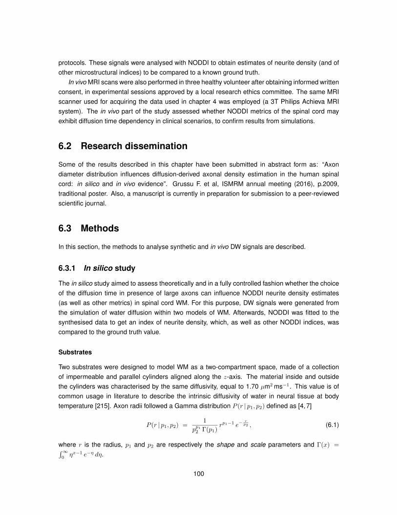
protocols. These signals were analysed with NODDI to obtain estimates of neurite density (and ofother microstructural indices) to be compared to a known ground truth.

In vivo MRI scans were also performed in three healthy volunteer after obtaining informed writtenconsent, in experimental sessions approved by a local research ethics committee. The same MRIscanner used for acquiring the data used in chapter 4 was employed (a 3T Philips Achieva MRIsystem). The in vivo part of the study assessed whether NODDI metrics of the spinal cord mayexhibit diffusion time dependency in clinical scenarios, to confirm results from simulations.


Some of the results described in this chapter have been submitted in abstract form as: “Axondiameter distribution influences diffusion-derived axonal density estimation in the human spinalcord: in silico and in vivo evidence”. Grussu F. et al, ISMRM annual meeting (2016), p.2009,traditional poster. Also, a manuscript is currently in preparation for submission to a peer-reviewedscientific journal.

6.3 Methods

In this section, the methods to analyse synthetic and in vivo DW signals are described.

6.3.1 In silico study

The in silico study aimed to assess theoretically and in a fully controlled fashion whether the choiceof the diffusion time in presence of large axons can influence NODDI neurite density estimates(as well as other metrics) in spinal cord WM. For this purpose, DW signals were generated fromthe simulation of water diffusion within two models of WM. Afterwards, NODDI was fitted to thesynthesised data to get an index of neurite density, which, as well as other NODDI indices, wascompared to the ground truth value.

Substrates

Two substrates were designed to model WM as a two-compartment space, made of a collectionof impermeable and parallel cylinders aligned along the z-axis. The material inside and outsidethe cylinders was characterised by the same diffusivity, equal to 1.70 µm2 ms−1. This value is ofcommon usage in literature to describe the intrinsic diffusivity of water in neural tissue at bodytemperature [215]. Axon radii followed a Gamma distribution P (r | p1, p2) defined as [4,7]

P (r | p1, p2) =1

pp12 Γ(p1)rp1−1 e−

rp2 , (6.1)

where r is the radius, p1 and p2 are respectively the shape and scale parameters and Γ(x) =∫∞0ηx−1 e−η dη.

100

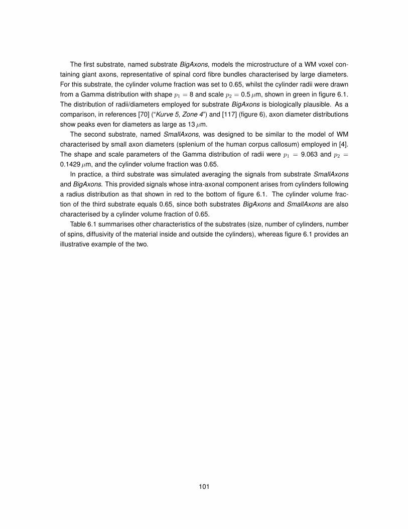
The first substrate, named substrate BigAxons, models the microstructure of a WM voxel con-taining giant axons, representative of spinal cord fibre bundles characterised by large diameters.For this substrate, the cylinder volume fraction was set to 0.65, whilst the cylinder radii were drawnfrom a Gamma distribution with shape p1 = 8 and scale p2 = 0.5µm, shown in green in figure 6.1.The distribution of radii/diameters employed for substrate BigAxons is biologically plausible. As acomparison, in references [70] (“Kurve 5, Zone 4”) and [117] (figure 6), axon diameter distributionsshow peaks even for diameters as large as 13µm.

The second substrate, named SmallAxons, was designed to be similar to the model of WMcharacterised by small axon diameters (splenium of the human corpus callosum) employed in [4].The shape and scale parameters of the Gamma distribution of radii were p1 = 9.063 and p2 =

0.1429µm, and the cylinder volume fraction was 0.65.In practice, a third substrate was simulated averaging the signals from substrate SmallAxons

and BigAxons. This provided signals whose intra-axonal component arises from cylinders followinga radius distribution as that shown in red to the bottom of figure 6.1. The cylinder volume frac-tion of the third substrate equals 0.65, since both substrates BigAxons and SmallAxons are alsocharacterised by a cylinder volume fraction of 0.65.

Table 6.1 summarises other characteristics of the substrates (size, number of cylinders, numberof spins, diffusivity of the material inside and outside the cylinders), whereas figure 6.1 provides anillustrative example of the two.

101

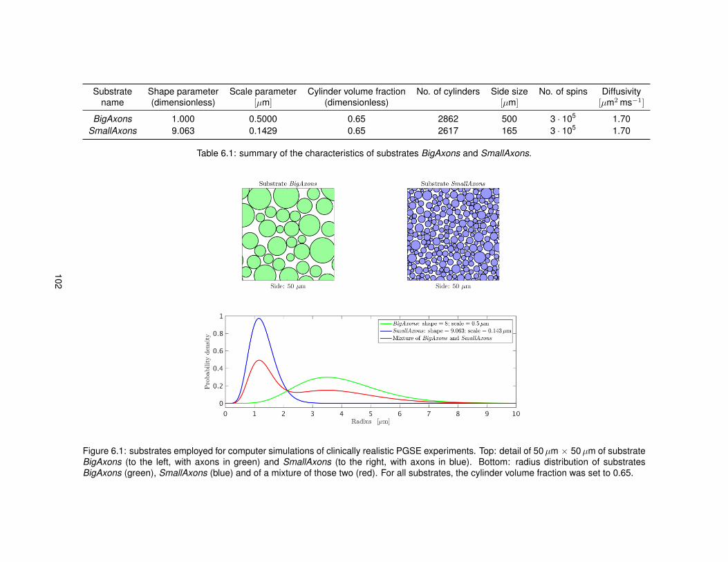
Substrate Shape parameter Scale parameter Cylinder volume fraction No. of cylinders Side size No. of spins Diffusivityname (dimensionless) [µm] (dimensionless) [µm] [µm2 ms−1]

BigAxons 1.000 0.5000 0.65 2862 500 3 · 105 1.70SmallAxons 9.063 0.1429 0.65 2617 165 3 · 105 1.70

Table 6.1: summary of the characteristics of substrates BigAxons and SmallAxons.

Figure 6.1: substrates employed for computer simulations of clinically realistic PGSE experiments. Top: detail of 50µm × 50µm of substrateBigAxons (to the left, with axons in green) and SmallAxons (to the right, with axons in blue). Bottom: radius distribution of substratesBigAxons (green), SmallAxons (blue) and of a mixture of those two (red). For all substrates, the cylinder volume fraction was set to 0.65.

102

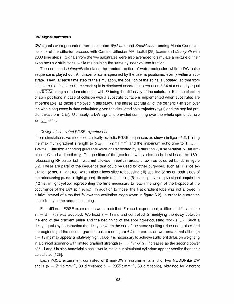
DW signal synthesis

DW signals were generated from substrates BigAxons and SmallAxons running Monte Carlo sim-ulations of the diffusion process with Camino diffusion MRI toolkit [38] (command datasynth with2000 time steps). Signals from the two substrates were also averaged to simulate a mixture of theiraxon radius distributions, while maintaining the same cylinder volume fraction.

The command datasynth simulates the random motion of water molecules while a DW pulsesequence is played out. A number of spins specified by the user is positioned evenly within a sub-strate. Then, at each time step of the simulation, the position of the spins is updated, so that fromtime step t to time step t+ ∆t each spin is displaced according to equation 3.34 of a quantity equalto√

6D∆t along a random direction, with D being the diffusivity of the substrate. Elastic reflectionof spin positions in case of collision with a substrate surface is implemented when substrates areimpermeable, as those employed in this study. The phase accrual φk of the generic k-th spin overthe whole sequence is then calculated given the simulated spin trajectory rk(t) and the applied gra-dient waveform G(t). Ultimately, a DW signal is provided summing over the whole spin ensembleas |

∑k e

jφk |.

Design of simulated PGSE experimentsIn our simulations, we modelled clinically realistic PGSE sequences as shown in figure 6.2, limitingthe maximum gradient strength to Gmax = 72 mT m−1 and the maximum echo time to TE max =

124 ms. Diffusion encoding gradients were characterised by a duration δ, a separation ∆, an am-plitude G and a direction g. The position of the gradients was varied on both sides of the 180-refocussing RF pulse, but it was not allowed in certain areas, shown as coloured bands in figure6.2. These are parts of the sequence that could be used for other purposes, such as: i) slice ex-citation (8 ms, in light red, which also allows slice refocussing); ii) spoiling (2 ms on both sides ofthe refocussing pulse, in light green); iii) spin refocussing (8 ms, in light violet); iv) signal acquisition(12 ms, in light yellow, representing the time necessary to reach the origin of the k-space at theoccurrence of the DW spin echo). In addition to those, the first gradient lobe was not allowed ina brief interval of 4 ms that follows the excitation stage (cyan in figure 6.2), in order to guaranteeconsistency of the sequence timing.

Four different PGSE experiments were modelled. For each experiment, a different diffusion timeTd = ∆ − δ/3 was adopted. We fixed δ = 18 ms and controlled ∆ modifying the delay betweenthe end of the gradient pulse and the beginning of the spoiling-refocussing block (tdel). Such adelay equals by construction the delay between the end of the same spoiling-refocussing block andthe beginning of the second gradient pulse (see figure 6.2). In particular, we remark that althoughδ = 18 ms may appear a relatively high value, it is necessary to achieve sufficient diffusion weightingin a clinical scenario with limited gradient strength (b = γ2 δ2G2 Td increases as the second powerof δ). Long δ is also beneficial since it would make our simulated cylinders appear smaller than theiractual size [125].

Each PGSE experiment consisted of 9 non-DW measurements and of two NODDI-like DWshells (b = 711 s mm−2, 30 directions; b = 2855 s mm−2, 60 directions), obtained for different

103

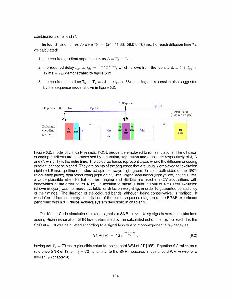
http://cmic.cs.ucl.ac.uk/camino/index.php?n=Man.Datasynth

combinations of ∆ and G.

The four diffusion times Td were Td = 24, 41.33, 58.67, 76ms. For each diffusion time Td,we calculated:

1. the required gradient separation ∆ as ∆ = Td + δ/3;

2. the required delay tdel as tdel = ∆− δ− 12 ms2 , which follows from the identity ∆ ≡ δ + tdel +

12 ms + tdel demonstrated by figure 6.2;

3. the required echo time TE as TE = 2 δ + 2 tdel + 36 ms, using an expression also suggestedby the sequence model shown in figure 6.2.

δ

G

TE / 2TE / 2

δ

RF pulses

(k-space origin)Spin echo

90-pulse

180-pulse

Diffusionencodinggradient

∆

msmsmsms

42 2

8ms

ms

128 tdel tdel

Figure 6.2: model of clinically realistic PGSE sequence employed to run simulations. The diffusionencoding gradients are characterised by a duration, separation and amplitude respectively of δ, ∆andG, whilst TE is the echo time. The coloured bands represent areas where the diffusion encodinggradient cannot be placed. They are points of the sequence that are usually employed for excitation(light red, 8 ms), spoiling of undesired spin pathways (light green, 2 ms on both sides of the 180-refocussing pulse), spin refocussing (light violet, 8 ms), signal acquisition (light yellow, lasting 12 ms,a value plausible when Partial Fourier imaging and SENSE are used in rFOV acquisitions withbandwidths of the order of 150 KHz). In addition to those, a brief interval of 4 ms after excitation(shown in cyan) was not made available for diffusion weighting, in order to guarantee consistencyof the timings. The duration of the coloured bands, although being conservative, is realistic. Itwas inferred from summary consultation of the pulse sequence diagram of the PGSE experimentperformed with a 3T Philips Achieva system described in chapter 4.

Our Monte Carlo simulations provide signals at SNR → ∞. Noisy signals were also obtainedadding Rician noise at an SNR level determined by the calculated echo time TE. For each TE, theSNR at b = 0 was calculated according to a signal loss due to mono-exponential T2-decay as

SNR(TE) = 13 e72 ms − TE

T2 , (6.2)

having set T2 = 73 ms, a plausible value for spinal cord WM at 3T [165]. Equation 6.2 relies on areference SNR of 13 for TE = 72 ms, similar to the SNR measured in spinal cord WM in vivo for asimilar TE (chapter 4).

104

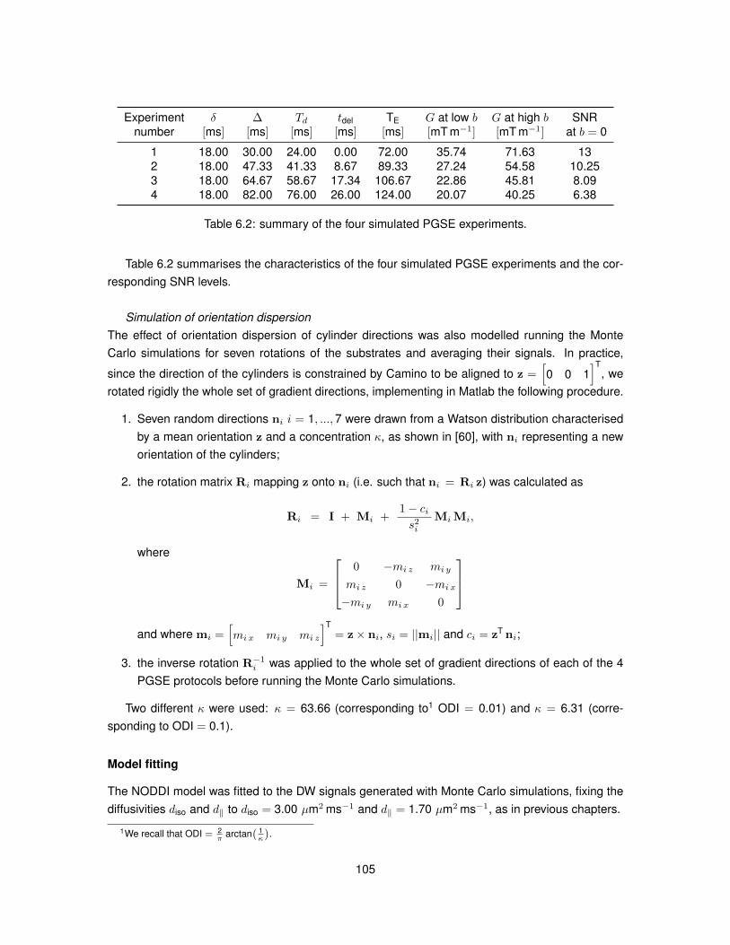
Experiment δ ∆ Td tdel TE G at low b G at high b SNRnumber [ms] [ms] [ms] [ms] [ms] [mT m−1] [mT m−1] at b = 0

1 18.00 30.00 24.00 0.00 72.00 35.74 71.63 132 18.00 47.33 41.33 8.67 89.33 27.24 54.58 10.253 18.00 64.67 58.67 17.34 106.67 22.86 45.81 8.094 18.00 82.00 76.00 26.00 124.00 20.07 40.25 6.38

Table 6.2: summary of the four simulated PGSE experiments.

Table 6.2 summarises the characteristics of the four simulated PGSE experiments and the cor-responding SNR levels.

Simulation of orientation dispersionThe effect of orientation dispersion of cylinder directions was also modelled running the MonteCarlo simulations for seven rotations of the substrates and averaging their signals. In practice,

since the direction of the cylinders is constrained by Camino to be aligned to z =[0 0 1

]T, we

rotated rigidly the whole set of gradient directions, implementing in Matlab the following procedure.

1. Seven random directions ni i = 1, ...,7 were drawn from a Watson distribution characterisedby a mean orientation z and a concentration κ, as shown in [60], with ni representing a neworientation of the cylinders;

2. the rotation matrix Ri mapping z onto ni (i.e. such that ni = Ri z) was calculated as

Ri = I + Mi +1− cis2i

MiMi,

where

Mi =

0 −mi z mi y

mi z 0 −mi x

−mi y mi x 0

and where mi =

[mi x mi y mi z

]T= z× ni, si = ||mi|| and ci = zT ni;

3. the inverse rotation R−1i was applied to the whole set of gradient directions of each of the 4

PGSE protocols before running the Monte Carlo simulations.

Two different κ were used: κ = 63.66 (corresponding to1 ODI = 0.01) and κ = 6.31 (corre-sponding to ODI = 0.1).

Model fitting

The NODDI model was fitted to the DW signals generated with Monte Carlo simulations, fixing thediffusivities diso and d‖ to diso = 3.00 µm2 ms−1 and d‖ = 1.70 µm2 ms−1, as in previous chapters.

1We recall that ODI = 2π

arctan( 1κ

).

105

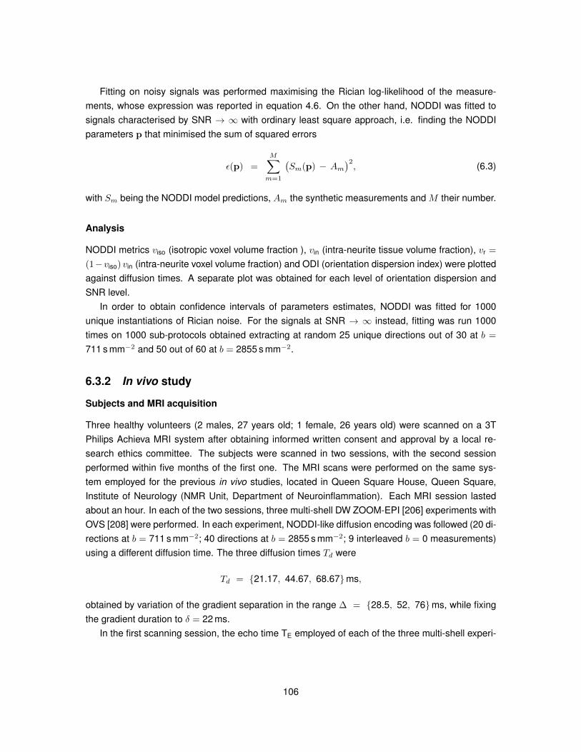
Fitting on noisy signals was performed maximising the Rician log-likelihood of the measure-ments, whose expression was reported in equation 4.6. On the other hand, NODDI was fitted tosignals characterised by SNR → ∞ with ordinary least square approach, i.e. finding the NODDIparameters p that minimised the sum of squared errors

ε(p) =

M∑m=1

(Sm(p) − Am

)2, (6.3)

with Sm being the NODDI model predictions, Am the synthetic measurements and M their number.

Analysis

NODDI metrics viso (isotropic voxel volume fraction ), vin (intra-neurite tissue volume fraction), vr =

(1−viso) vin (intra-neurite voxel volume fraction) and ODI (orientation dispersion index) were plottedagainst diffusion times. A separate plot was obtained for each level of orientation dispersion andSNR level.

In order to obtain confidence intervals of parameters estimates, NODDI was fitted for 1000unique instantiations of Rician noise. For the signals at SNR → ∞ instead, fitting was run 1000times on 1000 sub-protocols obtained extracting at random 25 unique directions out of 30 at b =

711 s mm−2 and 50 out of 60 at b = 2855 s mm−2.

6.3.2 In vivo study

Subjects and MRI acquisition

Three healthy volunteers (2 males, 27 years old; 1 female, 26 years old) were scanned on a 3TPhilips Achieva MRI system after obtaining informed written consent and approval by a local re-search ethics committee. The subjects were scanned in two sessions, with the second sessionperformed within five months of the first one. The MRI scans were performed on the same sys-tem employed for the previous in vivo studies, located in Queen Square House, Queen Square,Institute of Neurology (NMR Unit, Department of Neuroinflammation). Each MRI session lastedabout an hour. In each of the two sessions, three multi-shell DW ZOOM-EPI [206] experiments withOVS [208] were performed. In each experiment, NODDI-like diffusion encoding was followed (20 di-rections at b = 711 s mm−2; 40 directions at b = 2855 s mm−2; 9 interleaved b = 0 measurements)using a different diffusion time. The three diffusion times Td were

Td = 21.17, 44.67, 68.67ms,

obtained by variation of the gradient separation in the range ∆ = 28.5, 52, 76ms, while fixingthe gradient duration to δ = 22 ms.

In the first scanning session, the echo time TE employed of each of the three multi-shell experi-

106

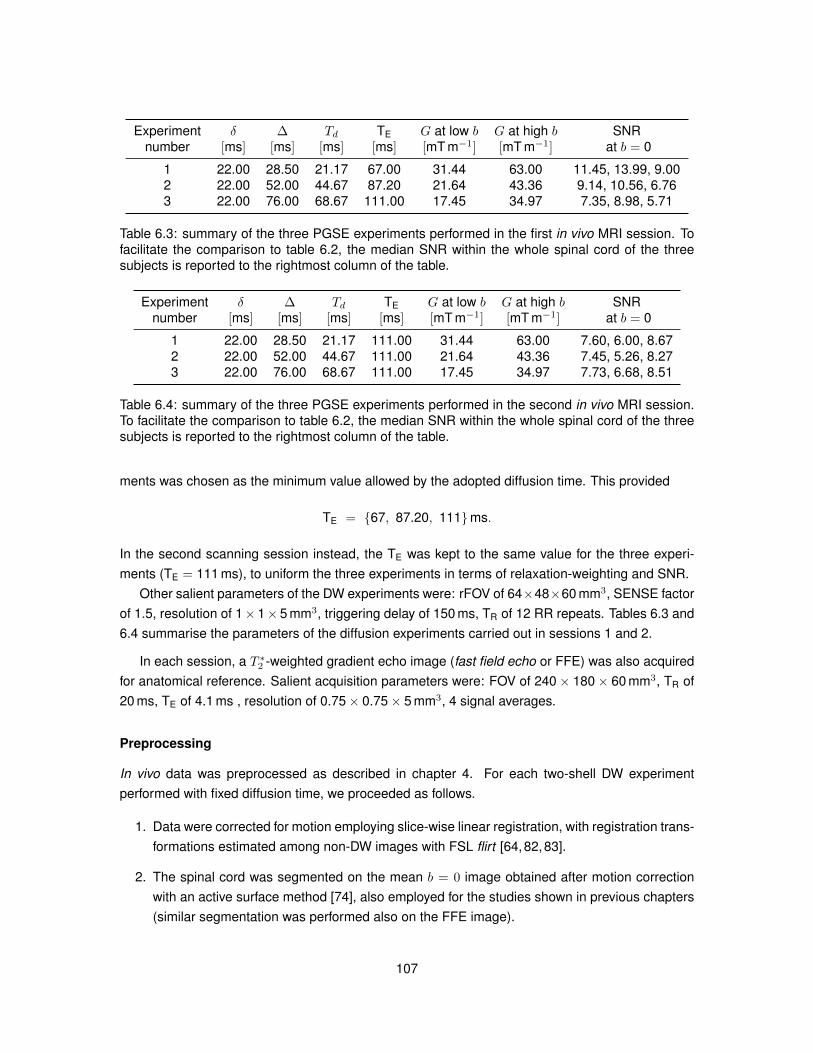
Experiment δ ∆ Td TE G at low b G at high b SNRnumber [ms] [ms] [ms] [ms] [mT m−1] [mT m−1] at b = 0

1 22.00 28.50 21.17 67.00 31.44 63.00 11.45, 13.99, 9.002 22.00 52.00 44.67 87.20 21.64 43.36 9.14, 10.56, 6.763 22.00 76.00 68.67 111.00 17.45 34.97 7.35, 8.98, 5.71

Table 6.3: summary of the three PGSE experiments performed in the first in vivo MRI session. Tofacilitate the comparison to table 6.2, the median SNR within the whole spinal cord of the threesubjects is reported to the rightmost column of the table.

Experiment δ ∆ Td TE G at low b G at high b SNRnumber [ms] [ms] [ms] [ms] [mT m−1] [mT m−1] at b = 0

1 22.00 28.50 21.17 111.00 31.44 63.00 7.60, 6.00, 8.672 22.00 52.00 44.67 111.00 21.64 43.36 7.45, 5.26, 8.273 22.00 76.00 68.67 111.00 17.45 34.97 7.73, 6.68, 8.51

Table 6.4: summary of the three PGSE experiments performed in the second in vivo MRI session.To facilitate the comparison to table 6.2, the median SNR within the whole spinal cord of the threesubjects is reported to the rightmost column of the table.

ments was chosen as the minimum value allowed by the adopted diffusion time. This provided

TE = 67, 87.20, 111ms.

In the second scanning session instead, the TE was kept to the same value for the three experi-ments (TE = 111 ms), to uniform the three experiments in terms of relaxation-weighting and SNR.

Other salient parameters of the DW experiments were: rFOV of 64×48×60 mm3, SENSE factorof 1.5, resolution of 1× 1× 5 mm3, triggering delay of 150 ms, TR of 12 RR repeats. Tables 6.3 and6.4 summarise the parameters of the diffusion experiments carried out in sessions 1 and 2.

In each session, a T ∗2 -weighted gradient echo image (fast field echo or FFE) was also acquiredfor anatomical reference. Salient acquisition parameters were: FOV of 240× 180× 60 mm3, TR of20 ms, TE of 4.1 ms , resolution of 0.75× 0.75× 5 mm3, 4 signal averages.

Preprocessing

In vivo data was preprocessed as described in chapter 4. For each two-shell DW experimentperformed with fixed diffusion time, we proceeded as follows.

1. Data were corrected for motion employing slice-wise linear registration, with registration trans-formations estimated among non-DW images with FSL flirt [64,82,83].

2. The spinal cord was segmented on the mean b = 0 image obtained after motion correctionwith an active surface method [74], also employed for the studies shown in previous chapters(similar segmentation was performed also on the FFE image).

107

3. GM was segmented manually after motion correction on an image obtained averaging DWimages with good contrast between GM and WM, as firstly shown in [97] and previouslydiscussed in section 4.4.3 of chapter 4.

4. WM voxels were defined as voxels within the eroded spinal cord mask that did not belong tothe GM mask.

Model fitting

NODDI was fitted to the in vivo data with the NODDI Matlab toolbox, maximising the likelihood ofthe data for a Rician noise model. In practice, the opposite of the log-likelihood was minimised intwo steps. An initial grid search was used to find a plausible set of NODDI model parameters, whichwere then used as a starting point for a gradient descent minimisation. In our fitting, the diffusivitiesdiso and d‖ on which the NODDI model depends were fixed as by default to diso = 3.00 µm2 ms−1

and d‖ = 1.70 µm2 ms−1,Due to the low SNR levels, especially at the highest echo time, multi-start fitting was performed

to reduce the risk of routines finding suboptimal solutions in local minima of the fitting objectivefunction. The gradient descent was performed 100 times per voxel, perturbing the starting point ofthe descent from the grid search and returning the best fit out of 100 iterations.

Analysis

For each subject, each scanning session and each diffusion time, we evaluated the distribution ofall NODDI metrics (viso, vin, vr = (1− viso) vin and ODI) within the GM and WM masks.

For the visualisation of voxel-wise maps, the mean b = 0 image from each experiment withfixed diffusion time was registered to an image obtained averaging all the b = 0 images after slice-wise realignment. The estimated transformations, accounting for in-plane translations only andcalculated with FSL flirt slice-by-slice, were also applied to the fitted NODDI metrics.

Originally, it was planned to exploit the anatomical FFE image for the segmentation of WM andGM. Descriptive statistics from the two tissue types could have then been extracted after warpingNODDI metrics to the FFE image space, or vice versa.

We planned to estimate the warping transformations between the mean b = 0 image of eachmulti-shell experiment and the anatomical FFE image. A preliminary co-registration pipeline be-tween diffusion and FFE spaces was implemented with a combination of the tools offered by thesoftware packages NiftyReg [127,128] and FSL. It consisted of the following steps:

1. straightening of the spinal cord in both FFE and mean b = 0 images, obtained moving thecentre of mass of the spinal cord mask slice-by-slice to the centre of the image;

2. re-sampling of the FFE to the resolution of the diffusion images;

3. estimation of a 3D affine transformation or a slice-wise affine transformation to warp the meanb = 0 image to the FFE, with the transformation obtained considering only voxels within thespinal cord mask dilated of a controlled amount.

108

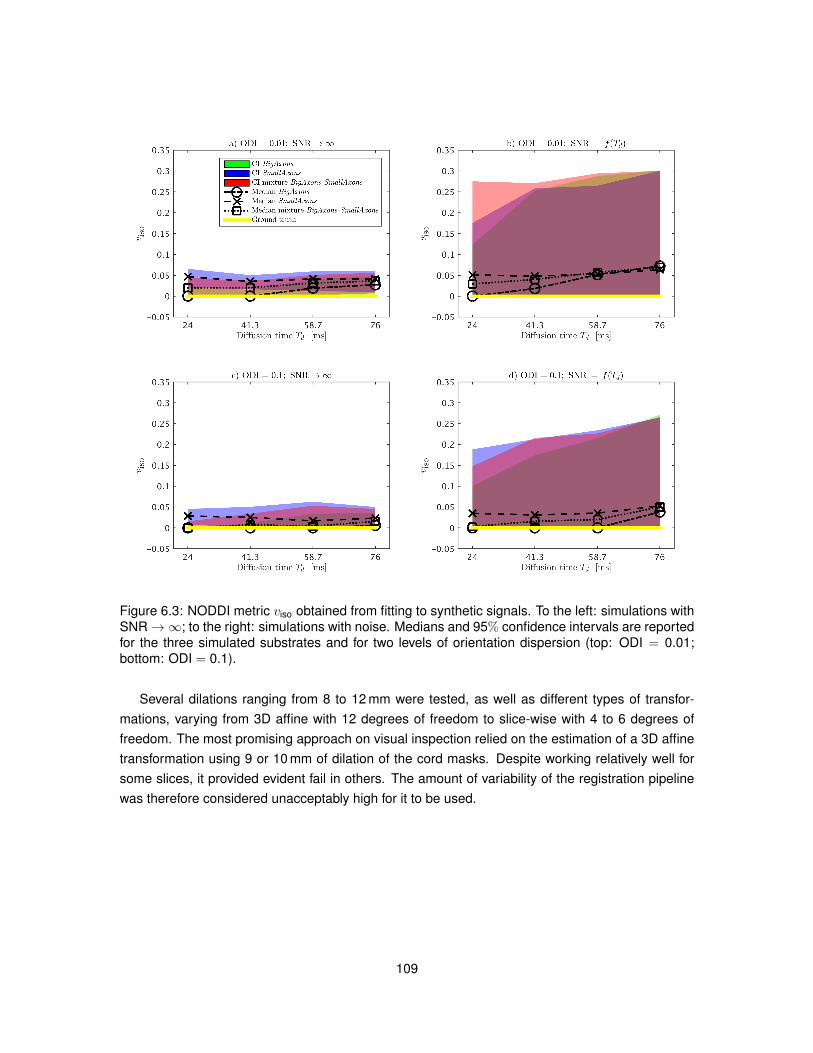
Figure 6.3: NODDI metric viso obtained from fitting to synthetic signals. To the left: simulations withSNR→∞; to the right: simulations with noise. Medians and 95% confidence intervals are reportedfor the three simulated substrates and for two levels of orientation dispersion (top: ODI = 0.01;bottom: ODI = 0.1).

Several dilations ranging from 8 to 12 mm were tested, as well as different types of transfor-mations, varying from 3D affine with 12 degrees of freedom to slice-wise with 4 to 6 degrees offreedom. The most promising approach on visual inspection relied on the estimation of a 3D affinetransformation using 9 or 10 mm of dilation of the cord masks. Despite working relatively well forsome slices, it provided evident fail in others. The amount of variability of the registration pipelinewas therefore considered unacceptably high for it to be used.

109

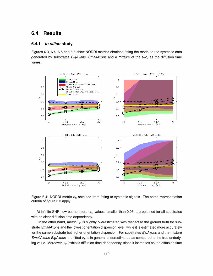
6.4 Results

6.4.1 In silico study

Figures 6.3, 6.4, 6.5 and 6.6 show NODDI metrics obtained fitting the model to the synthetic datagenerated by substrates BigAxons, SmallAxons and a mixture of the two, as the diffusion timevaries.

Figure 6.4: NODDI metric vin obtained from fitting to synthetic signals. The same representationcriteria of figure 6.3 apply.

At infinite SNR, low but non-zero viso values, smaller than 0.05, are obtained for all substrateswith no clear diffusion time dependency.

On the other hand, metric vin is slightly overestimated with respect to the ground truth for sub-strate SmallAxons and the lowest orientation dispersion level, while it is estimated more accuratelyfor the same substrate but higher orientation dispersion. For substrates BigAxons and the mixtureSmallAxons-BigAxons, the fitted vin is in general underestimated as compared to the true underly-ing value. Moreover, vin exhibits diffusion-time dependency, since it increases as the diffusion time

110

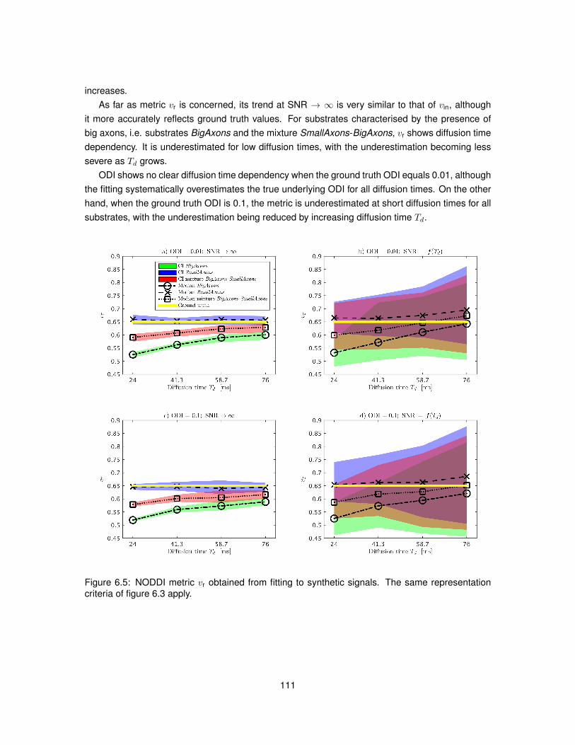
increases.As far as metric vr is concerned, its trend at SNR → ∞ is very similar to that of vin, although

it more accurately reflects ground truth values. For substrates characterised by the presence ofbig axons, i.e. substrates BigAxons and the mixture SmallAxons-BigAxons, vr shows diffusion timedependency. It is underestimated for low diffusion times, with the underestimation becoming lesssevere as Td grows.

ODI shows no clear diffusion time dependency when the ground truth ODI equals 0.01, althoughthe fitting systematically overestimates the true underlying ODI for all diffusion times. On the otherhand, when the ground truth ODI is 0.1, the metric is underestimated at short diffusion times for allsubstrates, with the underestimation being reduced by increasing diffusion time Td.

Figure 6.5: NODDI metric vr obtained from fitting to synthetic signals. The same representationcriteria of figure 6.3 apply.

111

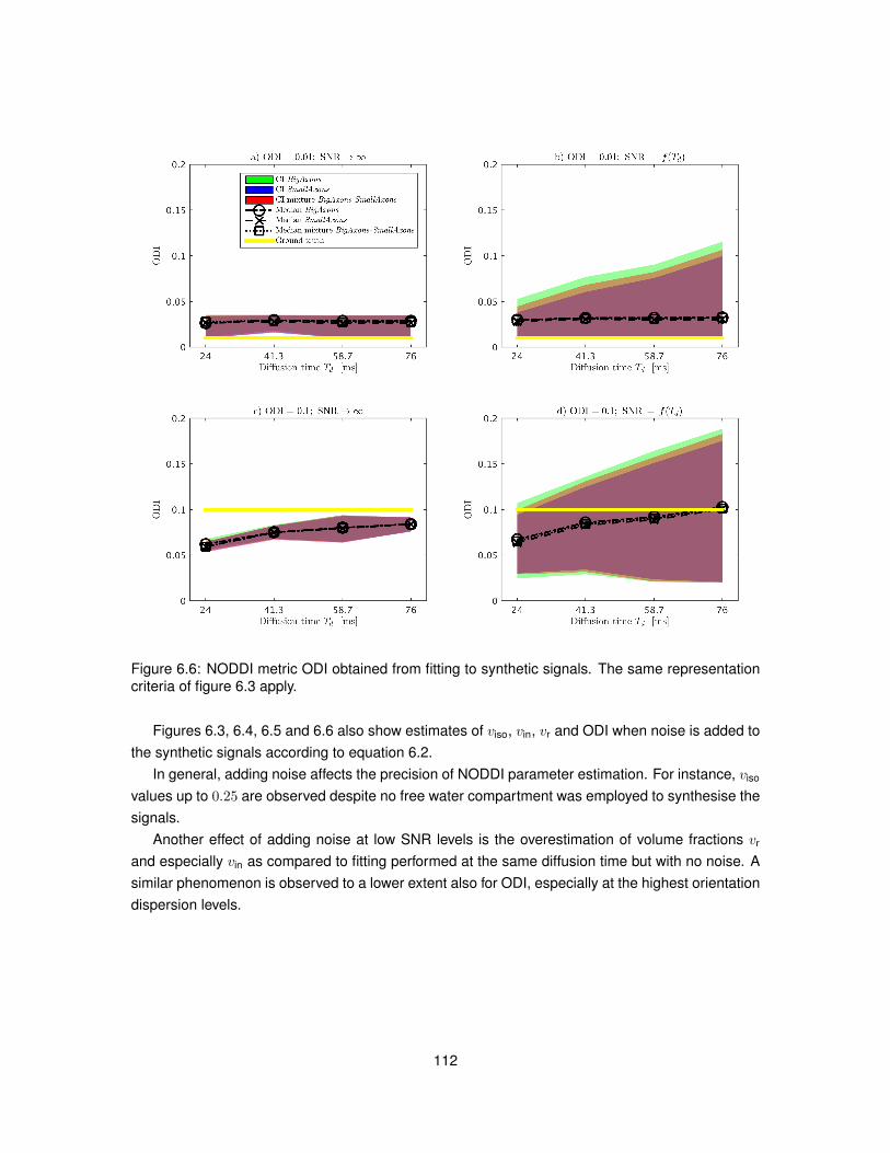
Figure 6.6: NODDI metric ODI obtained from fitting to synthetic signals. The same representationcriteria of figure 6.3 apply.

Figures 6.3, 6.4, 6.5 and 6.6 also show estimates of viso, vin, vr and ODI when noise is added tothe synthetic signals according to equation 6.2.

In general, adding noise affects the precision of NODDI parameter estimation. For instance, viso

values up to 0.25 are observed despite no free water compartment was employed to synthesise thesignals.

Another effect of adding noise at low SNR levels is the overestimation of volume fractions vr

and especially vin as compared to fitting performed at the same diffusion time but with no noise. Asimilar phenomenon is observed to a lower extent also for ODI, especially at the highest orientationdispersion levels.

112

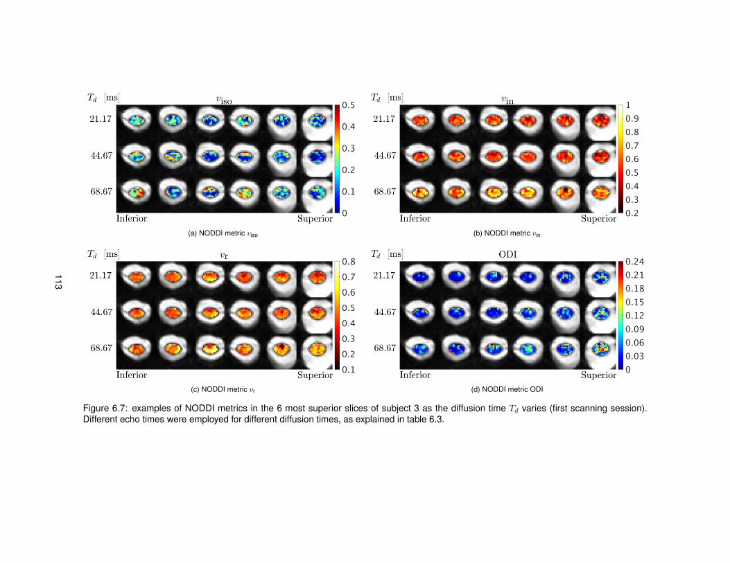
(a) NODDI metric viso (b) NODDI metric vin

(c) NODDI metric vr (d) NODDI metric ODI

Figure 6.7: examples of NODDI metrics in the 6 most superior slices of subject 3 as the diffusion time Td varies (first scanning session).Different echo times were employed for different diffusion times, as explained in table 6.3.

113

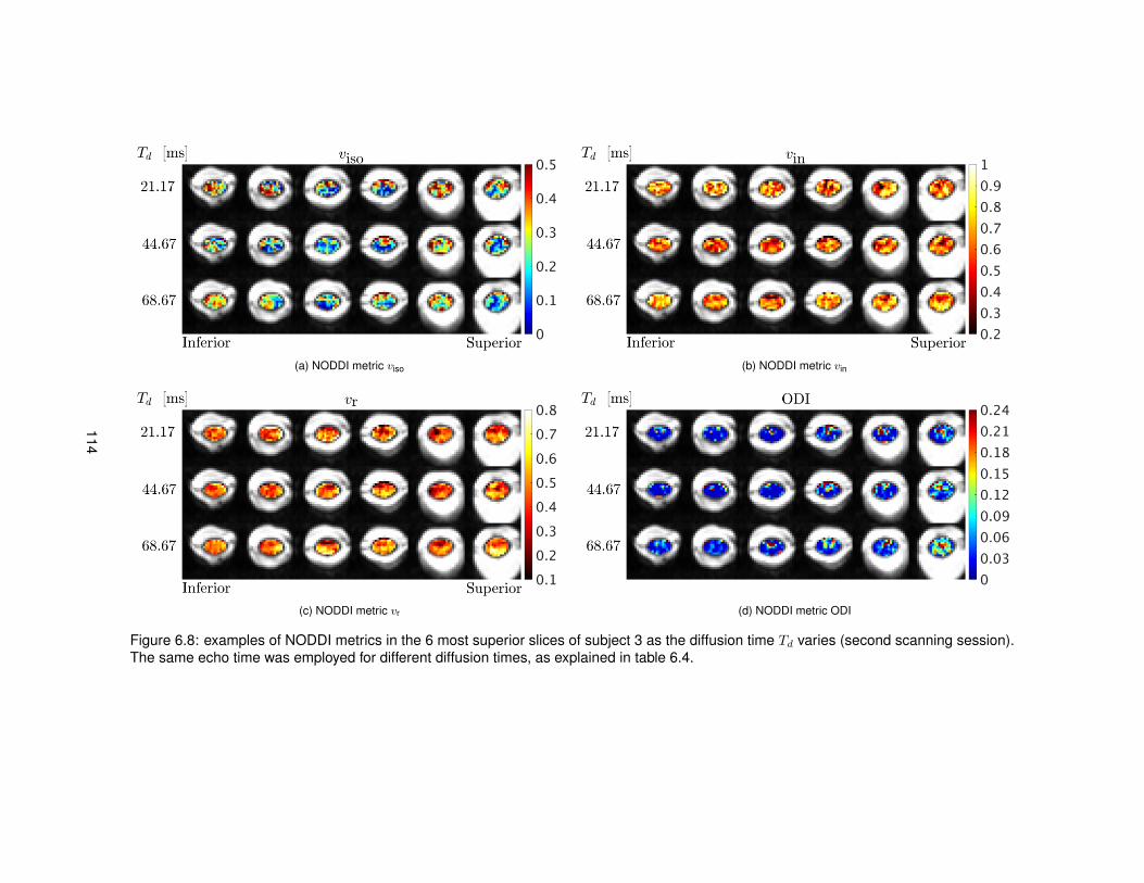
(a) NODDI metric viso (b) NODDI metric vin

(c) NODDI metric vr (d) NODDI metric ODI

Figure 6.8: examples of NODDI metrics in the 6 most superior slices of subject 3 as the diffusion time Td varies (second scanning session).The same echo time was employed for different diffusion times, as explained in table 6.4.

114

6.4.2 In vivo study

Figures 6.7 and 6.8 report NODDI metrics obtained from the second volunteer in 6 illustrative slicesas the diffusion time Td varies. The trend illustrated is representative of what, to a similar extent, isobserved in the other two subjects.

Metrics from the first scanning session (minimum echo time TE for each diffusion time, as re-ported in table 6.3) are shown in figure 6.7.

Qualitative visual inspection reveals that viso increases as Td increases, as apparent in the firstand fourth slices from the most inferior to the most superior position. Also, the metric is relativelynoisy at all diffusion times. Metrics vin and vr increase as Td increases (see first, third, fourth andsixth slices from the most inferior to the most superior), with the former looking noisier as comparedto the latter. Lastly, the figure demonstrates that ODI does not exhibit a clear trend, although in themost superior slice higher ODI is seen as Td grows from 21.17 to 68.67 ms.

Figure 6.8 shows similar information as 6.7 but with metrics obtained from the second scanningsession, i.e. when TE = 111 ms was employed for all Td values. All metrics are less smooth thentheir counterparts from the first session shown in figure 6.7, especially as far as viso is concerned.The increase of metrics vin and vr is less apparent, although still noticeable in some slices, as forexample in the most superior slice.

In figures 6.9 and 6.10, the distributions of NODDI metrics in WM and GM obtained from thefirst scanning session are illustrated for the three diffusion times. No clear trends can be observedfor viso and ODI in GM and WM with increasing Td, whereas the distributions of vr and especially vin

appear shifted to higher values as Td increases in WM. The shift is less evident in GM, especiallyfor subject 2. Figures 6.11 and 6.12 report similar information as figures 6.9 and 6.10, but for thesecond scanning session. As compared to the first scanning session, distributions are in generalless smooth, especially at shorter diffusion times. Nonetheless, the shift of the distributions of vr inWM towards higher vr values as Td increased is still noticeable.

115

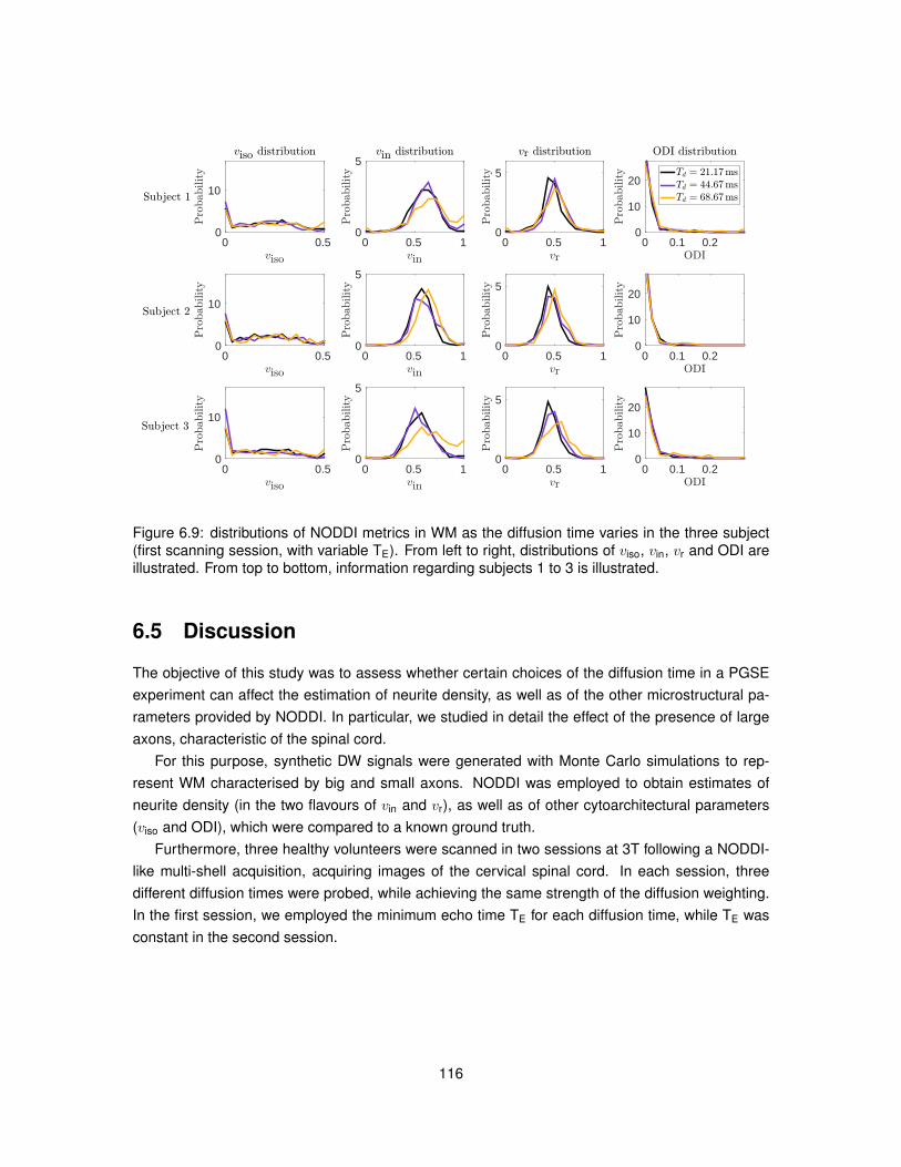
viso

0 0.5

Pro

bability

0

10

viso distribution

vin

0 0.5 1

Pro

bability

0

5vin distribution

vr

0 0.5 1

Pro

bability

0

5

vr distribution

ODI0 0.1 0.2

Pro

bability

0

10

20

ODI distribution

Td = 21:17msTd = 44:67msTd = 68:67ms

viso

0 0.5

Pro

bability

0

10

vin

0 0.5 1Pro

bability

0

5

vr

0 0.5 1

Pro

bability

0

5

ODI0 0.1 0.2

Pro

bability

0

10

20

viso

0 0.5

Pro

bability

0

10

vin

0 0.5 1

Pro

bability

0

5

vr

0 0.5 1

Pro

bability

0

5

ODI0 0.1 0.2

Pro

bability

0

10

20

Subject 1

Subject 2

Subject 3

Figure 6.9: distributions of NODDI metrics in WM as the diffusion time varies in the three subject(first scanning session, with variable TE). From left to right, distributions of viso, vin, vr and ODI areillustrated. From top to bottom, information regarding subjects 1 to 3 is illustrated.

6.5 Discussion

The objective of this study was to assess whether certain choices of the diffusion time in a PGSEexperiment can affect the estimation of neurite density, as well as of the other microstructural pa-rameters provided by NODDI. In particular, we studied in detail the effect of the presence of largeaxons, characteristic of the spinal cord.

For this purpose, synthetic DW signals were generated with Monte Carlo simulations to rep-resent WM characterised by big and small axons. NODDI was employed to obtain estimates ofneurite density (in the two flavours of vin and vr), as well as of other cytoarchitectural parameters(viso and ODI), which were compared to a known ground truth.

Furthermore, three healthy volunteers were scanned in two sessions at 3T following a NODDI-like multi-shell acquisition, acquiring images of the cervical spinal cord. In each session, threedifferent diffusion times were probed, while achieving the same strength of the diffusion weighting.In the first session, we employed the minimum echo time TE for each diffusion time, while TE wasconstant in the second session.

116

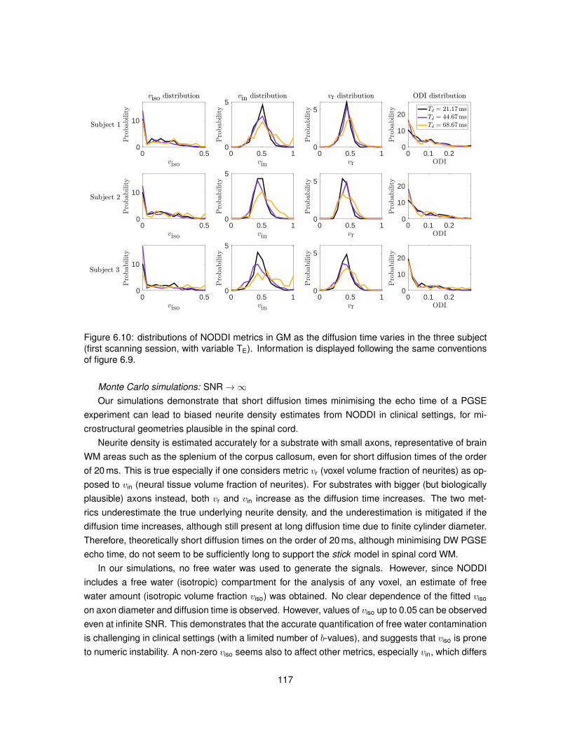
viso

0 0.5

Pro

bability

0

10

viso distribution

vin

0 0.5 1

Pro

bability

0

5vin distribution

vr

0 0.5 1

Pro

bability

0

5

vr distribution

ODI0 0.1 0.2

Pro

bability

0

10

20

ODI distribution

Td = 21:17msTd = 44:67msTd = 68:67ms

viso

0 0.5

Pro

bability

0

10

vin

0 0.5 1Pro

bability

0

5

vr

0 0.5 1

Pro

bability

0

5

ODI0 0.1 0.2

Pro

bability

0

10

20

viso

0 0.5

Pro

bability

0

10

vin

0 0.5 1

Pro

bability

0

5

vr

0 0.5 1

Pro

bability

0

5

ODI0 0.1 0.2

Pro

bability

0

10

20

Subject 1

Subject 2

Subject 3

Figure 6.10: distributions of NODDI metrics in GM as the diffusion time varies in the three subject(first scanning session, with variable TE). Information is displayed following the same conventionsof figure 6.9.

Monte Carlo simulations: SNR→∞Our simulations demonstrate that short diffusion times minimising the echo time of a PGSE

experiment can lead to biased neurite density estimates from NODDI in clinical settings, for mi-crostructural geometries plausible in the spinal cord.

Neurite density is estimated accurately for a substrate with small axons, representative of brainWM areas such as the splenium of the corpus callosum, even for short diffusion times of the orderof 20 ms. This is true especially if one considers metric vr (voxel volume fraction of neurites) as op-posed to vin (neural tissue volume fraction of neurites). For substrates with bigger (but biologicallyplausible) axons instead, both vr and vin increase as the diffusion time increases. The two met-rics underestimate the true underlying neurite density, and the underestimation is mitigated if thediffusion time increases, although still present at long diffusion time due to finite cylinder diameter.Therefore, theoretically short diffusion times on the order of 20 ms, although minimising DW PGSEecho time, do not seem to be sufficiently long to support the stick model in spinal cord WM.

In our simulations, no free water was used to generate the signals. However, since NODDIincludes a free water (isotropic) compartment for the analysis of any voxel, an estimate of freewater amount (isotropic volume fraction viso) was obtained. No clear dependence of the fitted viso

on axon diameter and diffusion time is observed. However, values of viso up to 0.05 can be observedeven at infinite SNR. This demonstrates that the accurate quantification of free water contaminationis challenging in clinical settings (with a limited number of b-values), and suggests that viso is proneto numeric instability. A non-zero viso seems also to affect other metrics, especially vin, which differs

117

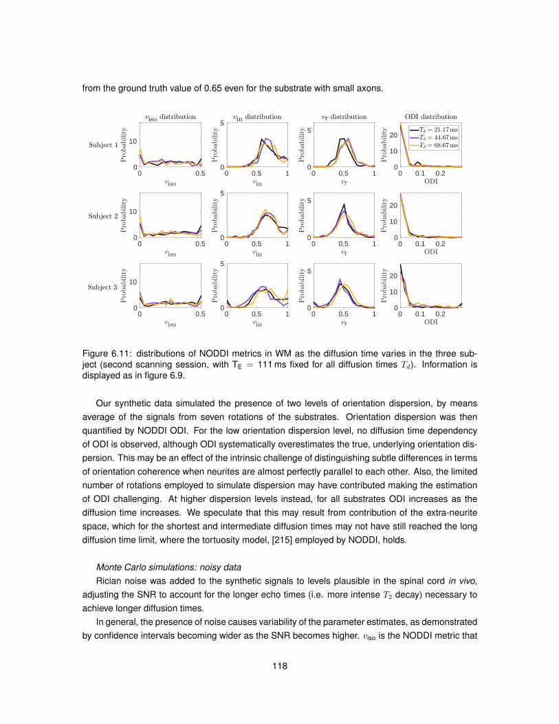
from the ground truth value of 0.65 even for the substrate with small axons.

viso

0 0.5

Pro

bability

0

10

viso distribution

vin

0 0.5 1

Pro

bability

0

5vin distribution

vr

0 0.5 1

Pro

bability

0

5

vr distribution

ODI0 0.1 0.2

Pro

bability

0

10

20

ODI distribution

Td = 21:17msTd = 44:67msTd = 68:67ms

viso

0 0.5

Pro

bability

0

10

vin

0 0.5 1

Pro

bability

0

5

vr

0 0.5 1

Pro

bability

0

5

ODI0 0.1 0.2

Pro

bability

0

10

20

viso

0 0.5

Pro

bability

0

10

vin

0 0.5 1

Pro

bability

0

5

vr

0 0.5 1

Pro

bability

0

5

ODI0 0.1 0.2

Pro

bability

0

10

20

Subject 1

Subject 2

Subject 3

Figure 6.11: distributions of NODDI metrics in WM as the diffusion time varies in the three sub-ject (second scanning session, with TE = 111 ms fixed for all diffusion times Td). Information isdisplayed as in figure 6.9.

Our synthetic data simulated the presence of two levels of orientation dispersion, by meansaverage of the signals from seven rotations of the substrates. Orientation dispersion was thenquantified by NODDI ODI. For the low orientation dispersion level, no diffusion time dependencyof ODI is observed, although ODI systematically overestimates the true, underlying orientation dis-persion. This may be an effect of the intrinsic challenge of distinguishing subtle differences in termsof orientation coherence when neurites are almost perfectly parallel to each other. Also, the limitednumber of rotations employed to simulate dispersion may have contributed making the estimationof ODI challenging. At higher dispersion levels instead, for all substrates ODI increases as thediffusion time increases. We speculate that this may result from contribution of the extra-neuritespace, which for the shortest and intermediate diffusion times may not have still reached the longdiffusion time limit, where the tortuosity model, [215] employed by NODDI, holds.

Monte Carlo simulations: noisy dataRician noise was added to the synthetic signals to levels plausible in the spinal cord in vivo,

adjusting the SNR to account for the longer echo times (i.e. more intense T2 decay) necessary toachieve longer diffusion times.

In general, the presence of noise causes variability of the parameter estimates, as demonstratedby confidence intervals becoming wider as the SNR becomes higher. viso is the NODDI metric that

118

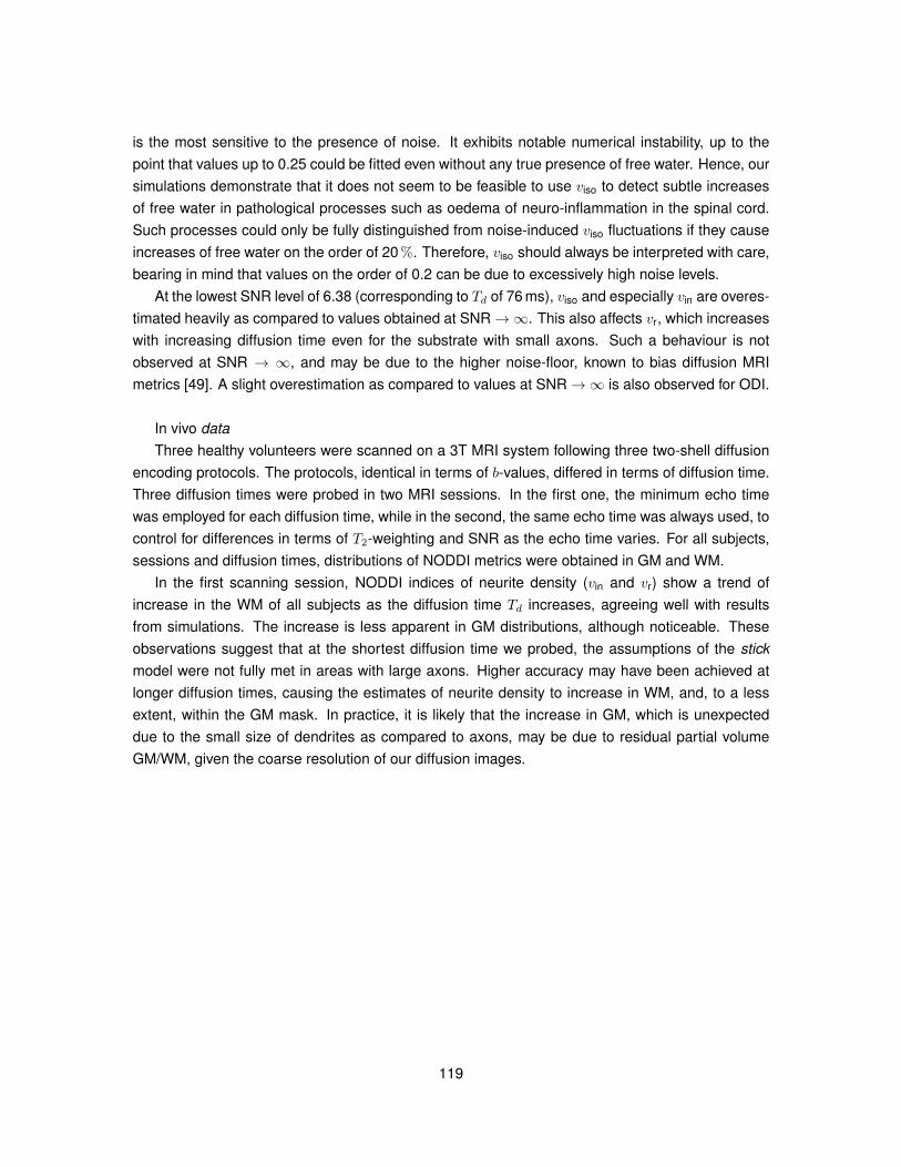
is the most sensitive to the presence of noise. It exhibits notable numerical instability, up to thepoint that values up to 0.25 could be fitted even without any true presence of free water. Hence, oursimulations demonstrate that it does not seem to be feasible to use viso to detect subtle increasesof free water in pathological processes such as oedema of neuro-inflammation in the spinal cord.Such processes could only be fully distinguished from noise-induced viso fluctuations if they causeincreases of free water on the order of 20 %. Therefore, viso should always be interpreted with care,bearing in mind that values on the order of 0.2 can be due to excessively high noise levels.

At the lowest SNR level of 6.38 (corresponding to Td of 76 ms), viso and especially vin are overes-timated heavily as compared to values obtained at SNR→∞. This also affects vr, which increaseswith increasing diffusion time even for the substrate with small axons. Such a behaviour is notobserved at SNR → ∞, and may be due to the higher noise-floor, known to bias diffusion MRImetrics [49]. A slight overestimation as compared to values at SNR→∞ is also observed for ODI.

In vivo dataThree healthy volunteers were scanned on a 3T MRI system following three two-shell diffusion

encoding protocols. The protocols, identical in terms of b-values, differed in terms of diffusion time.Three diffusion times were probed in two MRI sessions. In the first one, the minimum echo timewas employed for each diffusion time, while in the second, the same echo time was always used, tocontrol for differences in terms of T2-weighting and SNR as the echo time varies. For all subjects,sessions and diffusion times, distributions of NODDI metrics were obtained in GM and WM.

In the first scanning session, NODDI indices of neurite density (vin and vr) show a trend ofincrease in the WM of all subjects as the diffusion time Td increases, agreeing well with resultsfrom simulations. The increase is less apparent in GM distributions, although noticeable. Theseobservations suggest that at the shortest diffusion time we probed, the assumptions of the stickmodel were not fully met in areas with large axons. Higher accuracy may have been achieved atlonger diffusion times, causing the estimates of neurite density to increase in WM, and, to a lessextent, within the GM mask. In practice, it is likely that the increase in GM, which is unexpecteddue to the small size of dendrites as compared to axons, may be due to residual partial volumeGM/WM, given the coarse resolution of our diffusion images.

119

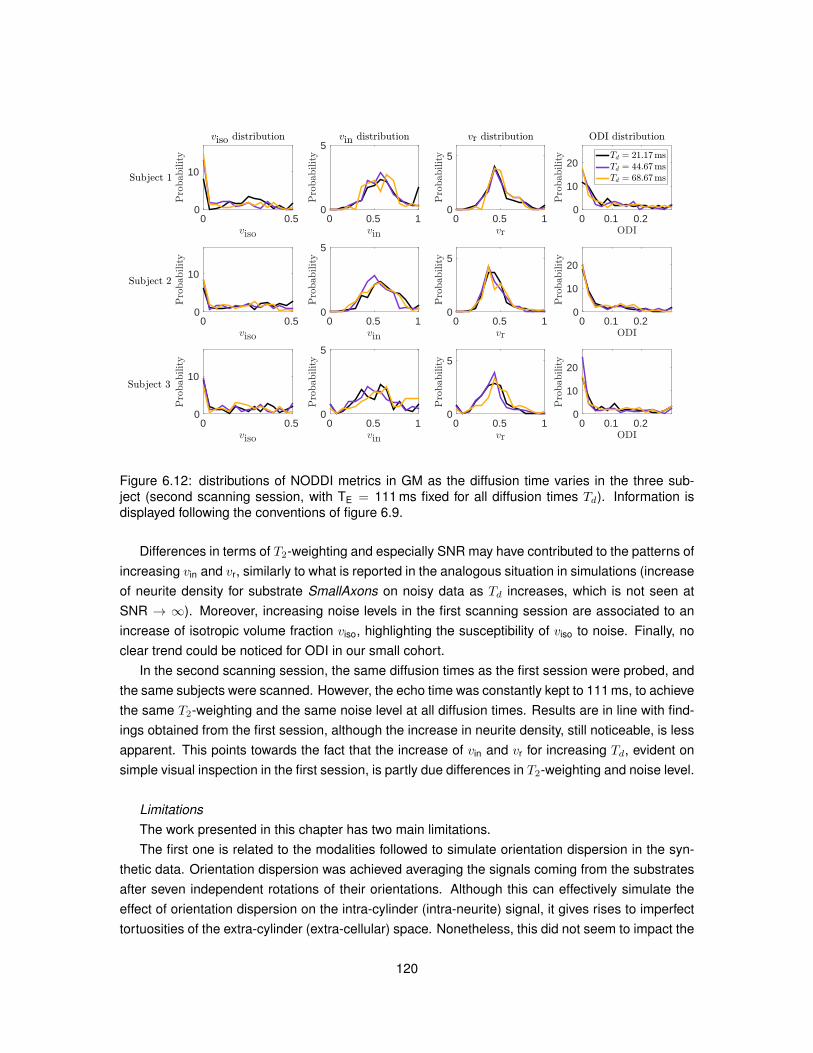
viso

0 0.5

Pro

bability

0

10

viso distribution

vin

0 0.5 1

Pro

bability

0

5vin distribution

vr

0 0.5 1

Pro

bability

0

5

vr distribution

ODI0 0.1 0.2

Pro

bability

0

10

20

ODI distribution

Td = 21:17msTd = 44:67msTd = 68:67ms

viso

0 0.5

Pro

bability

0

10

vin

0 0.5 1Pro

bability

0

5

vr

0 0.5 1

Pro

bability

0

5

ODI0 0.1 0.2

Pro

bability

0

10

20

viso

0 0.5

Pro

bability

0

10

vin

0 0.5 1

Pro

bability

0

5

vr

0 0.5 1

Pro

bability

0

5

ODI0 0.1 0.2

Pro

bability

0

10

20

Subject 1

Subject 2

Subject 3

Figure 6.12: distributions of NODDI metrics in GM as the diffusion time varies in the three sub-ject (second scanning session, with TE = 111 ms fixed for all diffusion times Td). Information isdisplayed following the conventions of figure 6.9.

Differences in terms of T2-weighting and especially SNR may have contributed to the patterns ofincreasing vin and vr, similarly to what is reported in the analogous situation in simulations (increaseof neurite density for substrate SmallAxons on noisy data as Td increases, which is not seen atSNR → ∞). Moreover, increasing noise levels in the first scanning session are associated to anincrease of isotropic volume fraction viso, highlighting the susceptibility of viso to noise. Finally, noclear trend could be noticed for ODI in our small cohort.

In the second scanning session, the same diffusion times as the first session were probed, andthe same subjects were scanned. However, the echo time was constantly kept to 111 ms, to achievethe same T2-weighting and the same noise level at all diffusion times. Results are in line with find-ings obtained from the first session, although the increase in neurite density, still noticeable, is lessapparent. This points towards the fact that the increase of vin and vr for increasing Td, evident onsimple visual inspection in the first session, is partly due differences in T2-weighting and noise level.

LimitationsThe work presented in this chapter has two main limitations.The first one is related to the modalities followed to simulate orientation dispersion in the syn-

thetic data. Orientation dispersion was achieved averaging the signals coming from the substratesafter seven independent rotations of their orientations. Although this can effectively simulate theeffect of orientation dispersion on the intra-cylinder (intra-neurite) signal, it gives rises to imperfecttortuosities of the extra-cylinder (extra-cellular) space. Nonetheless, this did not seem to impact the

120

estimation of neurite density, since very similar trends were exhibited by metrics vin and vr for bothsimulated orientation dispersion levels.

The second is related to the small size of our cohort recruited for the in vivo part of the inves-tigation. Although its size was sufficient to capture trends confirming results from simulations, ahigher number of subjects would allow a better characterisation of the between-subject variabilityinduced by the employment of short diffusion time.

6.6 Conclusion

In this work, we investigated whether certain choices of the diffusion time, in presence of largeaxons characteristic of the spinal cord, can affect neurite density indices from NODDI, as well asother microstructural indices.

Monte Carlo simulations of the diffusion process demonstrated that neurite density, and to aminor extent neurite orientation dispersion, can be underestimated in microstructural geometriesplausible in the spinal cord if short diffusion times are employed. Longer diffusion times reduce theunderestimation, which is still seen at Td = 76 ms due to finite cylinder diameter.

In vivo data showed a trend of increasing neurite density as the diffusion time increased, alsowhen controlling for the effects of varying TE. This fact could be explained by the fact that at shortestdiffusion time we probed, the assumptions of the stick model were not fully met in areas with largeaxons.

We conclude that long diffusion times can improve the accuracy of neurite density estimationfrom NODDI in the spinal cord, as well as of other microstructural indices characteristic of neuritemorphology. Nevertheless, longer diffusion time imply longer echo times, which ultimately reducethe precision of the estimation due to lower SNR. Therefore, a trade-off between accuracy andprecision has to be evaluated for each specific application.

STEAM acquisitions may help achieve better signal-to-noise levels than spin echo experimentsfor very long diffusion times. The feasibility of performing DW ZOOM-STEAM EPI will be evaluated,and the potential confounding effect of exchange will also be accounted for. This may be necessaryshould diffusion times exceed 100 ms, as suggested by recent work of other groups [133].

121

Ex vivo diffusion MRI of the humanspinal cord

122

Background and motivations

In the first part of this thesis, in vivo data were studied. Results demonstrated that NODDI, a novelmodel-based DW MRI method, can be applied in the spinal cord in vivo, enabling the quantificationof neuronal morphology in clinical scenarios.

The new metrics provided by NODDI are designed to be specific to characteristics of neuronaltissue microstructure such as density and orientation dispersion of axons and dendrites. However,NODDI relies on some assumptions that aim to capture the complexity of the microstructure un-derlying the DW signal in such a way that it can be handled in practice. The implications of theseassumptions need to be assessed via comparison to ground truth histological indices, quantifyingthe actual features of the tissue that NODDI aims to measure. In this way, the specificity of NODDImetrics could be ultimately validated. This is of great importance in presence of pathology, whichalters the structure of the normal, healthy neuronal tissue upon which NODDI hypotheses rely.

In this second ex vivo part of the PhD thesis, our objective is to confirm the specificity and thevalidity of NODDI metrics in the non-pathological and MS spinal cord via comparison to histology.

Experiments

Three experimental chapters are included in this second part of the thesis. The experiments weremade possible by the collaboration between UCL (Institute of Neurology, Departments of Neuroin-flammation, Brain Repair and Rehabilitation and NeuroResource; Department of Computer Sci-ence and Centre for Medical Image Computing) and the University of Oxford (Nuffield Departmentof Clinical Neurosciences).

In chapter 7, the work carried out to design a multi-shell DW experiment at high field is pre-sented. Moreover, the chapter also illustrates the strategy that was designed to adapt NODDI anal-ysis from in vivo to ex vivo data, as well as the approach followed to determine the radiographicposition of histological material derived from the scanned samples.

In chapter 8, digital images from histological sections of fixed human spinal cord were anal-ysed. The objective of the analysis was to derive a histological counterpart of NODDI ODI, whichquantifies the variability of neurite orientations in each voxel.

Lastly, in chapter 9, the systematic comparison between NODDI metrics and histological fea-tures derived from four spinal cord specimens (two healthy, two MS) is described. This piece ofwork relies on the technical achievements reported in chapters 7 and 8.

Tissue specimens were provided by the UCL NeuroResource tissue bank and by the Oxfordbrain bank. MRI was performed in London, at UCL, whilst histological procedures were carried outat the University of Oxford.

123

Conclusions

In the second part of this thesis, technical work was carried out to implement the histological val-idation of NODDI metrics in the healthy and MS spinal cord. A procedure for the acquisition andthe analysis of high-field DW images of ex vivo human spinal cord tissue was designed, as wellas a strategy to find the radiographic position of histological material derived from the same tissue.Moreover, a procedure based on ST calculation was designed and optimised in order to estimateneurite orientation dispersion from histological images, i.e. a ground truth measure for NODDI ODI.These technical achievements enabled the comparison of NODDI metrics to quantitative histolog-ical features in four ex vivo spinal cord samples. This last piece of analysis proves that NODDI ismore specific to histology than conventional DTI. NODDI ODI is specific to the underlying orienta-tion dispersion of neuronal fibres in both healthy and MS tissue, and could be a useful biomarker ofmicrostructural complexity. Furthermore, NODDI-derived neurite density estimates capture spatialvariations of the density of axons and dendrites, but are also influenced by other factors, such asmyelin density. Finally, the investigation did not allow the identification of clear associations be-tween NODDI isotropic (free water) volume fraction and histological features, although this metricis able to demonstrate areas of focal damage.

124

Chapter 7

A pipeline for the histologicalvalidation of NODDI in the spinalcord

7.1 Introduction

DW MRI methods such as NODDI have the potential of probing tissue microstructure in a non-invasive fashion, thus providing novel, quantitative indices that could be highly specific biomarkersin a number of neurological conditions. Nevertheless, these innovative DW methods rely on anumber of assumptions. Histological validation is therefore of the highest importance, since thevalidity of these assumptions and the claimed specificity of the novel indices need to be confirmed.

In previous chapters we have shown that NODDI indices may become valuable biomarkers inspinal cord applications. In this chapter, we describe our technical effort to implement a pipelinefor the histological validation of NODDI indices in the non-pathological and MS spinal cord. Thepipeline has been used to investigate the histological correlates of NODDI metrics, in order toconfirm their specificity.

We studied fixed specimens of human spinal cord tissue (controls and MS) with the objective ofimplementing a reliable MRI-histology pipeline. The pipeline consists of a DW MRI protocol at 9.4T,of a procedure for NODDI analysis of ex vivo data and of a strategy to determine the radiographicposition of histological material in the acquired MRI images.

In particular, as far as the MRI acquisition is concerned, we explored a number of protocolscharacterised by different image resolution, repetition time TR and number of diffusion encodingdirections. Also, we studied how to adapt the model fitting as proposed for NODDI analysis of invivo data for the analysis of the acquired ex vivo DW images.

125


The main result of this chapter is the implementation of a procedure based on high-field DW MRI forthe comparison of NODDI metrics to quantitative histology in post mortem human spinal cord tissue.The technical achievements of this chapter are the fundamentals upon which the comparison shownin chapter 9 relies. Results from chapter 9 have been disseminated in preliminary form as explainedin section 9.2 of that chapter.

7.3 Methods

Six post mortem specimens of formalin-fixed non-MS and MS spinal cord from five different humansubjects were employed. Our objectives were:

• to set up a rich, high-resolution DW MRI protocol at 9.4T;

• to adapt NODDI analysis as proposed for in vivo data for the analysis of the acquired ex vivoDW images;

• to design a strategy to determine the radiographic position of histological material derivedfrom the imaged samples.

The tissue was provided by the Oxford brain bank and by the UCL NeuroResource tissue bank,following approval by a local research ethics committee and appropriate consent as per HumanTissue Authority guidelines. All experimental procedures were in compliance with the UK Parlia-ment Human Tissue Act.

7.3.1 Samples and MRI sessions

Samples, stored in 10% formalin, were washed for 24 hours in 10 mM phosphate buffered saline(PBS) solution before undergoing MRI. PBS was replaced with freshly prepared solution every 12hours. MRI was performed with the samples immersed in PBS, which was eventually replacedby formalin at the end of the MRI session. MRI scans were performed with the 9.4T Agilent MRIsystem in the basement of Queen Square House, Queen Square, Department of Brain Repair andRehabilitation, UCL Institute of Neurology. The agreed duration of the MRI sessions between theUCL Department of Neuroinflammation and of Brain Repair and Rehabilitation was of an overnight.

The six specimens from the five subjects were scanned in five MRI sessions. A 9.4T horizontalbore scanner (Agilent Technologies, Santa Clara, CA, USA) equipped with a 60 mm inner diametergradient coil (maximum gradient amplitude of 1 T m−1 and maximum slew rate of 6.7 KT m−1 s−1).A 33 mm diameter volume coil (Rapid Biomedical GmbH, Rimpar, Germany) was instead used forMRI signal reception.

126

Subject Sex Specimen Age at decease Cause of decease Decease-to-fixation MRI session(s) Cord level Lengthno. [years] [hours] [cm]

1, control F 1 68 Colo-rectal 23 1,2,3 Thoracic 4.0metastatic tumour

2, MS F 2 67 Pneumonia, 23 1,2,3 Upper lumbar 2.1secondary to MS

3 4 Upper lumbar 2.4

3, control M 4 66 Cardiac arrest < 48 4 Upper thoracic 3.1

4, MS M 5 75 Asphyxiation, < 48 5 Upper thoracic 3.3secondary to MS

5, control F 6 67 Infective < 48 5 Upper lumbar 2.1exacerbation of

severe end-stage COPD

Table 7.1: information regarding the six specimens of fixed spinal cord tissues that were used to implement a procedure for the histologicalvalidation of NODDI metrics. COPD stands for chronic obstructive pulmonary disease.

127

The first three MRI sessions were initial attempts, whilst sessions four and five led to the ac-quisition of useful DW MRI data that were employed for the direct comparison of NODDI metricsto histology, shown in chapter 9. During each MRI session, temperature was measured and keptstable at 35 C using a temperature probe and an MR compatible air heater connected to a smallanimal monitoring system (Small Animals Instruments, Inc., Stony Brook, NY, USA).

Table 7.1 provides information about the tissue specimens.

Diffusion encoding

Table 7.2 summarises the characteristics of the DW MRI protocols. All protocols were characterisedby the acquisition of six DW shells (b = 520, 2080, 4680, 8320, 13000, 18720 s mm−2, δ, ∆ andTE fixed to δ = 12 ms, ∆ = 18 ms and TE = 39.5 ms for all shells). In MRI sessions 1, 2 and 3, 56non-collinear gradient directions were acquired for each shell. In MRI sessions 4 and 5, instead,a fewer directions were acquired, with increasing angular resolution as b increased (respectively6, 15, 24, 33, 42, 51 directions for b = 520, 2080, 4680, 8320, 13000, 18720 s mm−2). In allprotocols, 25 b = 0 images were also acquired, interleaved with DW measurements. MRI sliceswere not taken axially, but coronally (initially) and sagittally (final protocol). This choice was madesince we did not plan to obtain histological sections axially. Axial sectioning is best suited forquantifying axonal density or axon diameter, but it does not allow the visualisation of the directionsalong which neuronal fibres run, preventing the calculation of any histology-derived index of neuriteorientation dispersion, sought in this project.

For our diffusion acquisitions, a conventional DW PGSE sequence with single k-space line read-out per TR was employed. In sessions 1 and 2, the different shells were acquired one after the other,with b-value increasing over time. In sessions 3, 4 and 5 instead, the shells were acquired in a ran-domized order to get a better performance out of the gradients system by reducing the duty cycleand avoiding its overheating.

Moreover, in the first three MRI sessions, a relatively short TR (1300 ms) was adopted to keepthe acquisition time of each individual DW image short. In sessions 4 and 5 instead, a slightlylonger TR (2200 ms) was chosen. Although this implied a reduction of the total number of DW im-ages that could be acquired in the allocated scanning slot, it improved the quality of each individualDW measurement. This comes from the fact that a longer TR increases the amount of longitudi-nal magnetisation available for diffusion encoding, practically increasing the intrinsic SNR of eachindividual DW measurement.

SNR was estimated from the b = 0 images in each session as voxel-wise ratio between themean and the standard deviation of the signal over the 25 repetitions of the b = 0 acquisitions, forqualitative comparison among diffusion protocols.

Axial views

In all sessions, structural images were also acquired using a multi-slice spin echo sequence. Thestructural scan consisted of 24 axial slices, characterised by the following salient acquisition param-

128

Session TR TE Resolution FOV Slices No. of DW[ms] [ms] [µm× µm× µm] [mm×mm×mm] images

1 1300 39.5 200×200×800 24×51.2×21.6 Coronal 3362 1300 39.5 200×200×800 24×51.2×21.6 Coronal 3363 1300 39.5 150×200×500 19.2×51.2×10 Coronal 3364 2200 39.5 164×200×800 21×51.2×16 Sagittal 1715 2200 39.5 164×200×800 21×51.2×16 Sagittal 171

Table 7.2: details of the DW protocols implemented in the five MRI sessions. In each session, δand ∆ were fixed to δ = 12 ms and ∆ = 18 ms. The diffusion encoding consisted of 6-DW shells(b = 520, 2080, 4680, 8320, 13000, 18720 s mm−2), with increasing angular resolution. 25 b = 0images were also acquired in all MRI sessions.

eters: FOV of 25.68 × 25.68 mm2, slice thickness of 2 mm, matrix size of 256 × 128, TE = 20 ms,TR = 614 ms.

Effectiveness of fixative washing

Quantitative T2 mapping was performed in one session (session 5) to check the effect of our 24hours fixative wash out. T2 of neural tissue is known to increase dramatically when aldehyde-fixedspecimens are washed and scanned in PBS, up to the point that T2, reduced by the fixation process,returns to levels comparable to values obtained from post mortem unfixed tissue [161]. Therefore,one would expect T2 to change during a long MRI experiment involving formalin-fixed specimensimmersed in PBS, if the samples were not washed from the fixative adequately. This would becaused by diffusion effects that would lead to further dilution of the fixative with the PBS, effectivelyreducing the concentration of the fixative within the tissue specimens.

T2 maps were obtained from three multi-echo spin echo scans, performed before the start, in themiddle and at the end of the diffusion experiment. The same image resolution, FOV and TR of theDW MRI data were employed. Four echoes were sampled following the 90-excitation (samplingtimes ts = 13,26,39,52ms), and T2 was fitted to the acquired data voxel-by-voxel maximisingtheir likelihood for a Rician noise model and mono-exponential T2 decay.

7.3.2 Adaptation of NODDI analysis for ex vivo DW data

We investigated how to perform NODDI analysis of our ex vivo data. NODDI is a model developedfor in vivo applications, and it may require certain adjustments for ex vivo studies.

For instance, a fourth tissue compartment may be required to model stationary water. Previousstudies have demonstrated that it is often necessary to account for non-diffusing water to analyseDW data obtained from fixed tissue [4, 146, 170]. Although the exact origin of this non-diffusingcomponent is unclear, it has been suggested that it could correspond to water trapped within glialcells, which lose any active function after decease [4].

In this chapter, we studied whether a compartment of stationary water (the “dot” compartment

129

of isotropic restriction, as proposed in [147]) is necessary to describe the DW signal measured fromour samples and to improve the quality of DW MRI model fit. We also sought an optimal value ofthe intrinsic diffusivity of the neural tissue (parameter d‖), which is usually not fitted in NODDI. Thevalue employed in vivo, d‖ = 1.70 µm2 ms−1, may not be best suited to model our data, and herewe studied the impact of changing the value of d‖ from that value in terms of quality of fit.

The analysis was performed on the data acquired with the final diffusion encoding protocol, i.e.using data from MRI sessions 4 and 5. We studied one MRI slice of specimens 3, 4, 5 and 6 (seetable 7.1), considering different tissue types: WM and GM for the control cases; non-focal WM andGM and WM focal lesion (WMFL) for the MS cases.

Model fitting

NODDI was fitted to the whole six-shell data set with and without the dot compartment of isotropicrestriction (respectively called NODDI-Dot and NODDI models). The NODDI model without dotcompartment has been previously introduced in equation 4.1. When such a compartment is ac-counted for, the model becomes

swith-dot = vdot s0 + (1− vdot) swithout-dot, (7.1)

having indicated with s0 the non-DW signal, with vdot the volume fraction of the dot, with swithout-dot

the signal when no dot compartment is included (i.e. the expression to the right side of equation4.1) and with swith-dot the signal when the dot is accounted for. Notably, since the dot describes thecontribution of a stationary (non-diffusing) water pool, its signal component is not attenuated by dif-fusion weighting and is constant for any applied diffusion encoding gradient [147]. The introductionof the dot allows the explanation of residual signal well above the noise floor measured even forvery intense b-values and for gradients parallel to WM fibres.

Both NODDI and NODDI-Dot models were fitted voxel-by-voxel with the NODDI Matlab toolbox,maximising the likelihood of the measurements given a Rician noise model. The diffusivity of theisotropic compartment diso was fixed to the ADC of the PBS, since the isotropic compartment isdesigned to capture partial volume with surrounding liquid (ADC was estimated using the b =

520 s mm−2 shell with Camino [38], command adcfit). On the other hand, the intrinsic diffusivity ofthe neural tissue d‖ was varied. Both NODDI and NODDI-Dot models were fitted fixing d‖ to eachof the following 12 evenly-spaced values: 0.10, 0.38, 0.66, 0.95, 1.23, 1.51, 1.79, 2.07, 2.35, 2.63,2.92, 3.20 µm2 ms−1.

For comparison, the DTI model was also fitted in the same voxels, with and without the dotcompartment (models DTI and DTI-Dot). In-house Matlab code implementing the same algorithmemployed to fit NODDI in the NODDI Matlab toolbox was used. In practice, the DTI-Dot model waswritten using a notation equivalent to the one used in equation 7.1, but plugging into the signalswith-dot the DTI model as expressed to the right side of equation 3.39.

All models were fitted after correcting diffusion weighting gradients to account for extra diffusion-sensitisation due to imaging/spoiling gradients fully refocused at the occurrence of the spin echo.

130

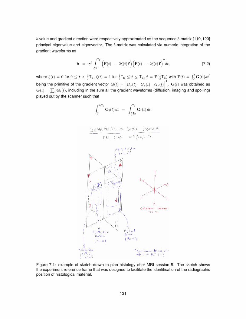
http://cmic.cs.ucl.ac.uk/camino/index.php?n=Man.Adcfit

b-value and gradient direction were respectively approximated as the sequence b-matrix [119,120]principal eigenvalue and eigenvector. The b-matrix was calculated via numeric integration of thegradient waveforms as

b = γ2

∫ TE

0

(F(t) − 2ξ(t) f

)(F(t) − 2ξ(t) f

)Tdt, (7.2)

where ξ(t) = 0 for 0 ≤ t < 12TE, ξ(t) = 1 for 1

2TE ≤ t ≤ TE, f = F( 12TE) with F(t) =

∫ t0G(t

′)dt′

being the primitive of the gradient vector G(t) =[Gx(t) Gy(t) Gz(t)

]T. G(t) was obtained as

G(t) =∑iGi(t), including in the sum all the gradient waveforms (diffusion, imaging and spoiling)

played out by the scanner such that

∫ 12 TE

0

Gi(t) dt =

∫ TE

12 TE

Gi(t) dt.

5CHE f1 AT\c oF SnmPle slr cnn Ge

flR\ svrN o+tl. lo, lrn

il

\

: c".J HirL,-(us-H)'

€xERlHe^rT REFERFNCe

FRAM E

H*ttLl C"*J

Hi3\^?n-

(nt-u1

H5 G^dlLO W ur-

( ns-L)

He"ff^r Ct-A

Lo *tn-*

H rll^,^ f u*,^ leN*.J w,thr*,>'go-.t' + TOP (a)

( uc-L)

$

tI-/

*---'I

t"| --'/l.---)'

I

6I

I

I

I

I

T

I

I

lq\

Figure 7.1: example of sketch drawn to plan histology after MRI session 5. The sketch showsthe experiment reference frame that was designed to facilitate the identification of the radiographicposition of histological material.

131

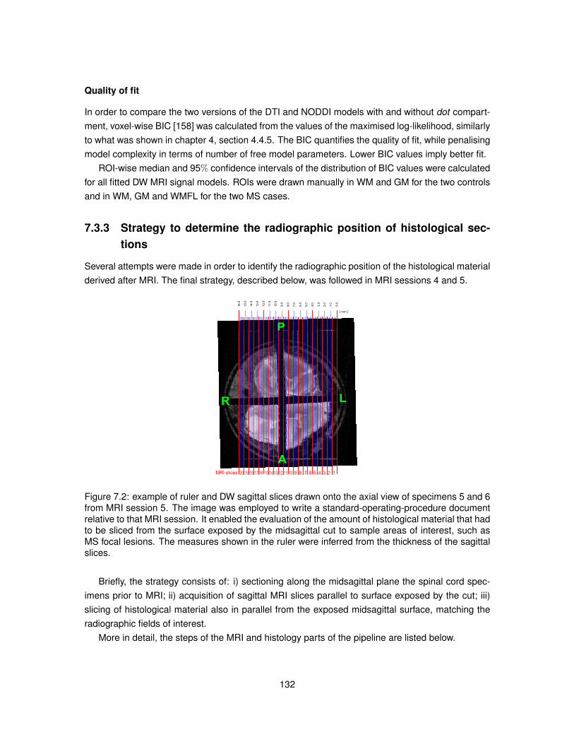
Quality of fit

In order to compare the two versions of the DTI and NODDI models with and without dot compart-ment, voxel-wise BIC [158] was calculated from the values of the maximised log-likelihood, similarlyto what was shown in chapter 4, section 4.4.5. The BIC quantifies the quality of fit, while penalisingmodel complexity in terms of number of free model parameters. Lower BIC values imply better fit.

ROI-wise median and 95% confidence intervals of the distribution of BIC values were calculatedfor all fitted DW MRI signal models. ROIs were drawn manually in WM and GM for the two controlsand in WM, GM and WMFL for the two MS cases.

7.3.3 Strategy to determine the radiographic position of histological sec-tions

Several attempts were made in order to identify the radiographic position of the histological materialderived after MRI. The final strategy, described below, was followed in MRI sessions 4 and 5.

MRI slices

LR

1234567891011121314151617181920

P

A

0.0

[ mm ]

1.0

2.0

3.0

4.0

5.0

6.0

7.0

8.0

9.0

10.0

11.0

12.0

13.0

14.0

15.0

16.0

Figure 7.2: example of ruler and DW sagittal slices drawn onto the axial view of specimens 5 and 6from MRI session 5. The image was employed to write a standard-operating-procedure documentrelative to that MRI session. It enabled the evaluation of the amount of histological material that hadto be sliced from the surface exposed by the midsagittal cut to sample areas of interest, such asMS focal lesions. The measures shown in the ruler were inferred from the thickness of the sagittalslices.

Briefly, the strategy consists of: i) sectioning along the midsagittal plane the spinal cord spec-imens prior to MRI; ii) acquisition of sagittal MRI slices parallel to surface exposed by the cut; iii)slicing of histological material also in parallel from the exposed midsagittal surface, matching theradiographic fields of interest.

More in detail, the steps of the MRI and histology parts of the pipeline are listed below.

132

MRI acquisitionOur procedure allows the acquisition of MR images from two specimens per session.

1. Prior to MRI, each of the two spinal cord specimens is sectioned midline for the whole sagittallength in approximately two halves with a surgical blade;

2. the four tissue chunks are positioned in the four slots of a syringe plunger and tied withVELCRO R©, while using medical bandage for padding;

3. an experiment reference frame is defined, identifying anterior, posterior, top and bottom partsof the plunger (letters A, P, T and B to be written with a non-erasable highlighter in the plunger);

4. holes made with fine point scissors in the plunger are exploited for radiographic reference(one hole made to the top, anterior part of the plunger; two holes made to the bottom, left partof the plunger).

5. the plunger is fitted into a FALCON R© tube, which is finally filled with freshly prepared 10 mMPBS solution for MRI acquisition (the PBS will in fact also fill the holes in the plunger, whichmay then be visible).

Histological procedures

1. After MRI, standard histological processing steps are carried out (dehydration, paraffin-embedding);

2. specimen sizes are measured before and after paraffin-embedding, to estimate the tissueshrinkage caused by the process;

3. histological sections are sliced sagittally from the surface exposed by the midsagittal cut,consistently with the experiment reference frame introduced prior to MRI;

4. the MRI slice from which each sagittal section is taken is inferred recording the amount ofmaterial removed from the exposed surface while looking at an axial MRI view, onto which thesagittal slices have been overlaid (in doing so, the MRI slice thickness is scaled to account fortissue shrinkage, using the shrinkage factor estimated as per point 2).

Figure 7.1 shows a manual sketch illustrating the experimental reference frame that was createdfor MRI session number 5. The drawing was included in the standard-operating-procedure (SOP)document provided to the Oxford team, which was useful to plan histology. As a further example,the entire SOP document written after MRI session 4 is also provided in appendix A.

Figure 7.2 shows instead the axial view with sagittal slices overlaid onto it, from the same MRIsession. A ruler was also added (measures inferred from sagittal slice thickness; measures showndo not account yet for tissue shrinkage).

133

7.4 Results

7.4.1 Samples and MRI sessions

The first three MRI sessions were preliminary acquisitions exploring the feasibility of the designeddiffusion encoding protocol, as well as FOV and resolution.

In the first session, data were lost since the scanner did not save any image due to an unex-pected conflict of the acquisition software. In the second session, data were acquired but had alsoto be discarded due to an unexpected drift of the signal throughout the acquisition, made evident bya drop of more than 50% of the signal intensity when the last and first b = 0 images were comparedto each other. In the third session, DW images were acquired and saved. However, they werenot used for the comparison NODDI-histology for two main reasons: i) the image SNR was disap-pointing; ii) the Oxford team did not consider reliable to match the position of MRI and histology ifsections were to be obtained from a surface exposed by a cut performed after the MRI scan.

Figure 7.3 shows the SNR map estimated from the b = 0 images in MRI sessions 3 and 4. TheSNR in session 3 is on the order of 10-15 in WM, while in session 4 is about 20-25. The SNR insession 4 is higher than in session 3, since the SNR of session 3 was considered unsatisfactory.The higher SNR level was achieved increasing the TR from 1300 ms (session 3) to 2200 ms (ses-sions 4 and 5), while also increasing the slice thickness from 500 to 800µm. As a consequence ofthis, the number of DW images had to be reduced, since the allocated scan time did not change.The number of DW directions was then reduced from 336 (session 3) to 171 (sessions 4 and 5).Moreover, it was decided to adopt increasing angular resolution of the gradients as the b-valueincreased, rather than constant. This choice is in line with the published in vivo NODDI protocol,where the angular resolution of the b-shells also increases as b increases [215].

The final DW protocol consisted of 171 directions split onto 6 b-shells of increasing angularresolution (b = 520, 2080, 4680, 8320, 13000, 18720 s mm−2, with respectively 6, 15, 24, 33,42 and 51 diffusion sensitising gradient directions).

Figure 7.4 shows the quantitative T2 map obtained from the multi-echo spin echo acquisitionsperformed before the start, in the middle and at the end of the DW protocol in MRI session number5. The maps demonstrate that T2 was stable throughout the diffusion MRI experiment.

7.4.2 Adaptation of NODDI analysis for ex vivo DW data

This section presents the results of the investigation aimed to adapt NODDI analysis, as developedfor in vivo data, for the acquired ex vivo DW images.

Figures 7.5 and 7.6 show the quality of fit of NODDI, with and without dot compartment, incontrol and MS specimens from MRI sessions 4 and 5. For control specimen 3 (upper thoracic),the characteristic BIC = f(d‖) is U-shaped as a function of d‖. The median BIC without the dotis always similar to the case with dot, but in the latter case the confidence intervals are narrower.For control specimen 6 (upper lumbar), instead, the shape of the curve BIC = f(d‖) resembles a Uonly when the dot is included. When a dot-like DW signal is not accounted for by the model in WM,

134

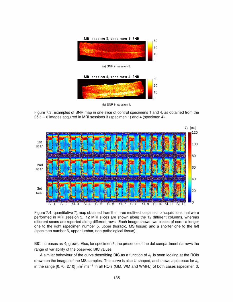
(a) SNR in session 3.

(b) SNR in session 4.

Figure 7.3: examples of SNR map in one slice of control specimens 1 and 4, as obtained from the25 b = 0 images acquired in MRI sessions 3 (specimen 1) and 4 (specimen 4).

0

20

40

60

80

100

120

2ndscan

3rdscan

1stscan

Sl. 10

T2 [ms]

Sl. 12Sl. 11 Sl. 7 Sl. 2 Sl. 1 Sl. 3 Sl. 4 Sl. 5 Sl. 6 Sl. 8 Sl. 9

Figure 7.4: quantitative T2 map obtained from the three multi-echo spin echo acquisitions that wereperformed in MRI session 5. 12 MRI slices are shown along the 12 different columns, whereasdifferent scans are reported along different rows. Each image shows two pieces of cord: a longerone to the right (specimen number 5, upper thoracic, MS tissue) and a shorter one to the left(specimen number 6, upper lumbar, non-pathological tissue).

BIC increases as d‖ grows. Also, for specimen 6, the presence of the dot compartment narrows therange of variability of the observed BIC values.

A similar behaviour of the curve describing BIC as a function of d‖ is seen looking at the ROIsdrawn on the images of the MS samples. The curve is also U-shaped, and shows a plateaux for d‖in the range [0.70; 2.10] µm2 ms−1 in all ROIs (GM, WM and WMFL) of both cases (specimen 3,

135

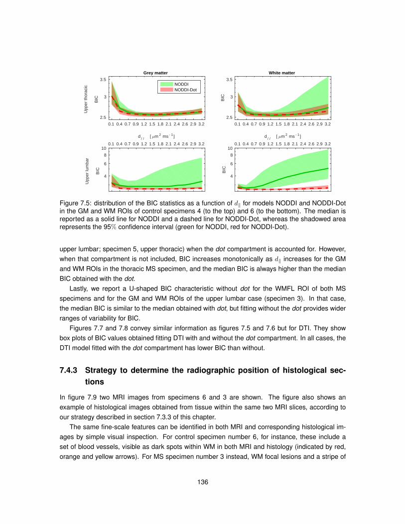
0.1 0.4 0.7 0.9 1.2 1.5 1.8 2.1 2.4 2.6 2.9 3.2

Upp

er th

orac

ic

B

IC

2.5

3

3.5

Grey matter

NODDINODDI-Dot

0.1 0.4 0.7 0.9 1.2 1.5 1.8 2.1 2.4 2.6 2.9 3.2

BIC

2.5

3

3.5

White matter

d/ /

[ 7m 2 ms - 1 ]

0.1 0.4 0.7 0.9 1.2 1.5 1.8 2.1 2.4 2.6 2.9 3.2

Upp

er lu

mba

r

BIC

4

6

8

10

d/ /

[ 7m 2 ms - 1 ]

0.1 0.4 0.7 0.9 1.2 1.5 1.8 2.1 2.4 2.6 2.9 3.2

BIC

4

6

8

10

Figure 7.5: distribution of the BIC statistics as a function of d‖ for models NODDI and NODDI-Dotin the GM and WM ROIs of control specimens 4 (to the top) and 6 (to the bottom). The median isreported as a solid line for NODDI and a dashed line for NODDI-Dot, whereas the shadowed arearepresents the 95% confidence interval (green for NODDI, red for NODDI-Dot).

upper lumbar; specimen 5, upper thoracic) when the dot compartment is accounted for. However,when that compartment is not included, BIC increases monotonically as d‖ increases for the GMand WM ROIs in the thoracic MS specimen, and the median BIC is always higher than the medianBIC obtained with the dot.

Lastly, we report a U-shaped BIC characteristic without dot for the WMFL ROI of both MSspecimens and for the GM and WM ROIs of the upper lumbar case (specimen 3). In that case,the median BIC is similar to the median obtained with dot, but fitting without the dot provides widerranges of variability for BIC.

Figures 7.7 and 7.8 convey similar information as figures 7.5 and 7.6 but for DTI. They showbox plots of BIC values obtained fitting DTI with and without the dot compartment. In all cases, theDTI model fitted with the dot compartment has lower BIC than without.

7.4.3 Strategy to determine the radiographic position of histological sec-tions

In figure 7.9 two MRI images from specimens 6 and 3 are shown. The figure also shows anexample of histological images obtained from tissue within the same two MRI slices, according toour strategy described in section 7.3.3 of this chapter.

The same fine-scale features can be identified in both MRI and corresponding histological im-ages by simple visual inspection. For control specimen number 6, for instance, these include aset of blood vessels, visible as dark spots within WM in both MRI and histology (indicated by red,orange and yellow arrows). For MS specimen number 3 instead, WM focal lesions and a stripe of

136

demyelination in GM can be seen in both MRI (signal hyperintensities) and histological image (lackof stain). These are pointed out by green and violet arrows (WM focal lesions) and by a cyan arrow(stripe of demyelination in GM).

7.5 Discussion

In this chapter, the work carried out to implement a pipeline for the histological validation of NODDImetrics was described. We set up a rich, high-resolution DW MRI protocol at 9.4T, and adaptedNODDI analysis as proposed for in vivo data to fit our ex vivo images. Moreover, we developed astrategy to identify radiographically the position of histological material.

MRI protocolA high-field DW MRI protocol rich in terms of b-values and gradient directions was set up in order

to probe the microstructure of fixed spinal cord tissue. High-field MRI enables the possibility ofacquiring images with high resolution, revealing fine-scale anatomical detail. This ultimately leadsto accurate and precise delineation of the microstructural properties of relatively small portions oftissue such as focal MS lesions.

The final diffusion encoding protocol consisted of 171 DW measurements spread over 6 b-shellswith increasing angular resolution. The protocol also includes the acquisition of 25 non-DW images.The total number of images of the diffusion protocol was a trade-off between the total amount ofDW data that could be acquired in the available MRI slot and the quality of each individual DWmeasure. This quality is controlled mainly by TR, to which the total scan duration is proportional.

Also, T2 was monitored throughout the last MRI session to verify the effectiveness of the fixativewashing. T2 was stable during the whole diffusion protocol, demonstrating that 24 hours of bath inPBS were sufficient to effectively wash out the fixative, given the relatively small dimensions of thespecimens (section of roughly 0.5 cm2, length of 2 to 4 cm).

Model fitting of ex vivo dataA procedure for NODDI analysis of ex vivo data was implemented. NODDI is a model devel-

oped for applications in vivo, and its employment for the analysis of data acquired from fixed postmortem tissue may require some adaptations. We investigated whether a compartment of isotropicrestriction (stationary water or “dot” [147]) was needed to account for some effects that fixationhas on the tissue, as shown in other studies [4, 146, 170]. Moreover, we assessed the impact ofthe choice of the intrinsic diffusivity of the neural tissue d‖ on the quality of fit, since the valuescommonly employed in vivo may not be best suited to describe our data.

To study the role of the dot compartment and of the choice of d‖, we fitted NODDI with andwithout dot for 12 values of d‖ in [0.10; 3.20] µm2 ms−1, while fixing the isotropic diffusivity diso tothe ADC of the PBS. We then derived the BIC statistics, an index of quality of fit, within differenttissue types (pathological and non-pathological). A similar comparison was also performed forconventional DTI, which was fitted with and without the inclusion of the dot compartment.

137

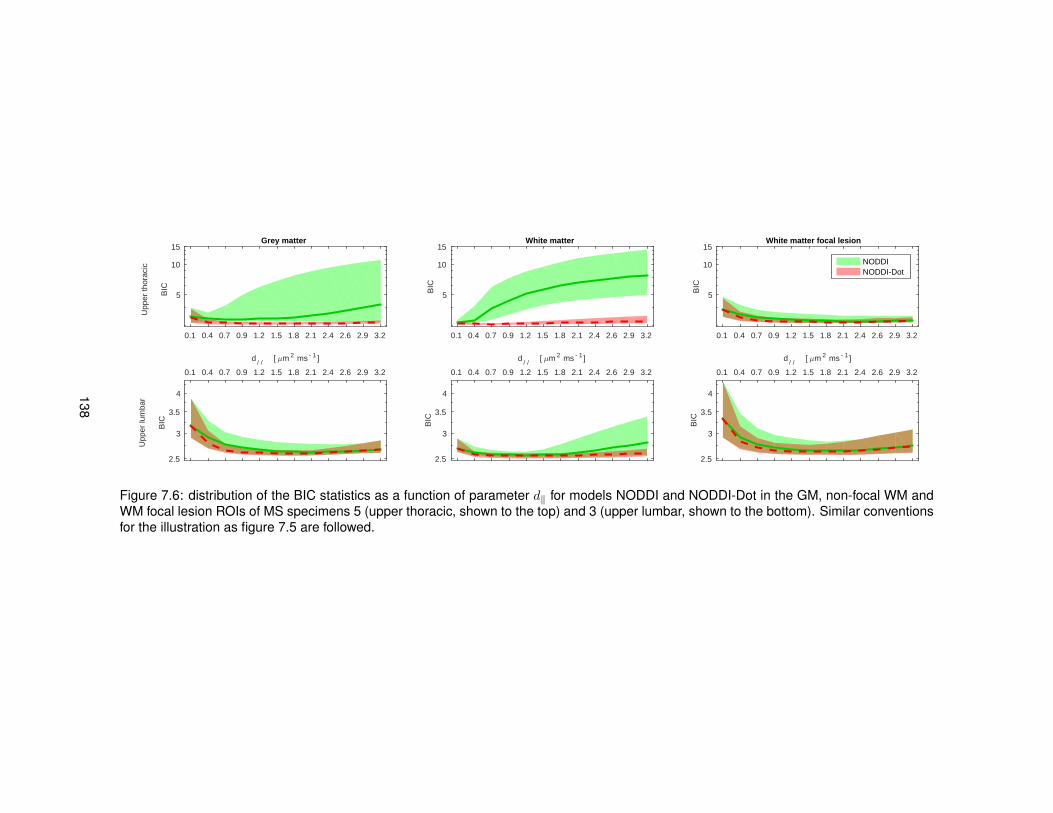
0.1 0.4 0.7 0.9 1.2 1.5 1.8 2.1 2.4 2.6 2.9 3.2

Upp

er th

orac

ic

B

IC

5

10

15Grey matter

0.1 0.4 0.7 0.9 1.2 1.5 1.8 2.1 2.4 2.6 2.9 3.2

BIC

5

10

15White matter

0.1 0.4 0.7 0.9 1.2 1.5 1.8 2.1 2.4 2.6 2.9 3.2

BIC

5

10

15White matter focal lesion

NODDINODDI-Dot

d/ /

[ 7m 2 ms - 1 ]

0.1 0.4 0.7 0.9 1.2 1.5 1.8 2.1 2.4 2.6 2.9 3.2

Upp

er lu

mba

r

BIC

2.5

3

3.5

4

d/ /

[ 7m 2 ms - 1 ]

0.1 0.4 0.7 0.9 1.2 1.5 1.8 2.1 2.4 2.6 2.9 3.2

BIC

2.5

3

3.5

4

d/ /

[ 7m 2 ms - 1 ]

0.1 0.4 0.7 0.9 1.2 1.5 1.8 2.1 2.4 2.6 2.9 3.2

BIC

2.5

3

3.5

4

Figure 7.6: distribution of the BIC statistics as a function of parameter d‖ for models NODDI and NODDI-Dot in the GM, non-focal WM andWM focal lesion ROIs of MS specimens 5 (upper thoracic, shown to the top) and 3 (upper lumbar, shown to the bottom). Similar conventionsfor the illustration as figure 7.5 are followed.

138

As far as NODDI is concerned, our results show that in some cases (specimen 4, control, upperthoracic; specimen 3, MS, upper lumbar), the dot stabilises the fit, since the confidence intervalsof the BIC characteristic of the NODDI-Dot model are narrower than those of NODDI without dot,although the two have similar median BIC. However, in other cases (specimen 6, control, upperlumbar; specimen 5, MS, upper thoracic), the dot compartment plays even a more important role.In those cases, in all ROIs the quality of fit of NODDI-Dot is always better than NODDI, giventhe lower median BIC values. The quality of fit of NODDI without dot worsens as d‖ increases,especially in WM (monotonically increasing BIC). This finding suggests the presence of a waterpool characterised by extremely low apparent diffusivity, which is well described by a compartmentof isotropic restriction such as the dot, even in the WMFL ROI, where the dot compartment improvesthe quality of fit.

Our study has also highlighted the importance of choosing an appropriate value to which theintrinsic diffusivity of the neural tissue should be constrained. For NODDI, when diso is fixed tothe ADC of the PBS and the dot compartment is included, certain choices of d‖ provide better fitthan others, as demonstrated by the characteristic curve describing BIC as a function of d‖. Thequality of fit improves as d‖ increases from 0.10 µm2 ms−1 to 0.70 µm2 ms−1, reaches a plateauxfor intermediate values of d‖ in the range [0.70; 2.10] µm2 ms−1, and then worsens as d‖ increasesapproaching values similar to the diffusivity of free water. This trend is consistently observed in allsamples and tissue types, pathological and non-pathological.

For comparison, we assessed the impact of the inclusion of the dot compartment also for DTI.The higher BIC of the DTI model, with respect to the DTI-Dot one, suggests that the inclusion ofthe dot compartment is beneficial to improve the quality of fit of DTI in all tissue types.

Strategy to determine the radiographic position of histological materialLastly, a strategy to determine the position in the acquired MRI images of tissue material sec-

tioned for histological processing was developed. The strategy relies on:

• sectioning the spinal cord specimens along the midsagittal plane prior to MRI;

• acquisition of the diffusion MRI protocol sagittally, with slices taken parallel to surface exposedby the midline cut;

• acquisition of axial MRI slices for anatomical reference;

• sectioning of histological material also sagittally, from the surface exposed by the midsagittalcut.

139

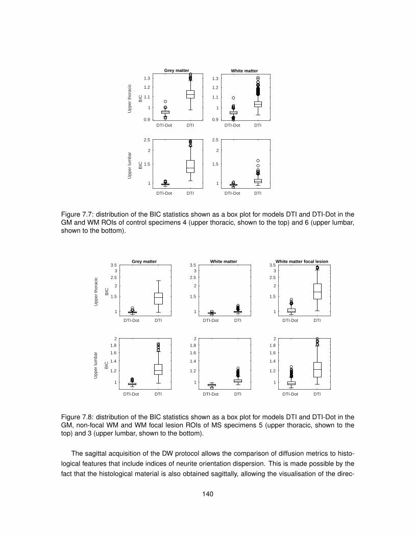
DTI-Dot DTIU

pper

thor

acic

BIC

0.9

1

1.1

1.2

1.3

Grey matter

DTI-Dot DTI0.9

1

1.1

1.2

1.3

White matter

DTI-Dot DTI

Upp

er lu

mba

r

BIC

1

1.5

2

2.5

DTI-Dot DTI

1

1.5

2

2.5

Figure 7.7: distribution of the BIC statistics shown as a box plot for models DTI and DTI-Dot in theGM and WM ROIs of control specimens 4 (upper thoracic, shown to the top) and 6 (upper lumbar,shown to the bottom).

DTI-Dot DTI

Upp

er th

orac

ic

B

IC

1

1.5

2

2.5

33.5

Grey matter

DTI-Dot DTI

1

1.5

2

2.5

33.5

White matter

DTI-Dot DTI

1

1.5

2

2.5

33.5

White matter focal lesion

DTI-Dot DTI

Upp

er lu

mba

r

BIC

1

1.2

1.4

1.6

1.8

2

DTI-Dot DTI

1

1.2

1.4

1.6

1.8

2

DTI-Dot DTI

1

1.2

1.4

1.6

1.8

2

Figure 7.8: distribution of the BIC statistics shown as a box plot for models DTI and DTI-Dot in theGM, non-focal WM and WM focal lesion ROIs of MS specimens 5 (upper thoracic, shown to thetop) and 3 (upper lumbar, shown to the bottom).

The sagittal acquisition of the DW protocol allows the comparison of diffusion metrics to histo-logical features that include indices of neurite orientation dispersion. This is made possible by thefact that the histological material is also obtained sagittally, allowing the visualisation of the direc-

140

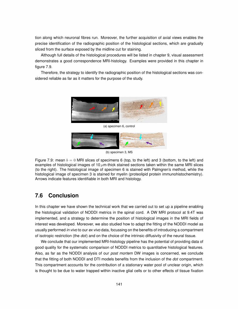
tion along which neuronal fibres run. Moreover, the further acquisition of axial views enables theprecise identification of the radiographic position of the histological sections, which are graduallysliced from the surface exposed by the midline cut for staining.

Although full details of the histological procedures will be listed in chapter 9, visual assessmentdemonstrates a good correspondence MRI-histology. Examples were provided in this chapter infigure 7.9.

Therefore, the strategy to identify the radiographic position of the histological sections was con-sidered reliable as far as it matters for the purpose of the study.

(a) specimen 6, control

(b) specimen 3, MS

Figure 7.9: mean b = 0 MRI slices of specimens 6 (top, to the left) and 3 (bottom, to the left) andexamples of histological images of 10µm-thick stained sections taken within the same MRI slices(to the right). The histological image of specimen 6 is stained with Palmgren’s method, while thehistological image of specimen 3 is stained for myelin (proteolipid protein immunohistochemistry).Arrows indicate features identifiable in both MRI and histology.

7.6 Conclusion

In this chapter we have shown the technical work that we carried out to set up a pipeline enablingthe histological validation of NODDI metrics in the spinal cord. A DW MRI protocol at 9.4T wasimplemented, and a strategy to determine the position of histological images in the MRI fields ofinterest was developed. Moreover, we also studied how to adapt the fitting of the NODDI model asusually performed in vivo to our ex vivo data, focussing on the benefits of introducing a compartmentof isotropic restriction (the dot) and on the choice of the intrinsic diffusivity of the neural tissue.

We conclude that our implemented MRI-histology pipeline has the potential of providing data ofgood quality for the systematic comparison of NODDI metrics to quantitative histological features.Also, as far as the NODDI analysis of our post mortem DW images is concerned, we concludethat the fitting of both NODDI and DTI models benefits from the inclusion of the dot compartment.This compartment accounts for the contribution of a stationary water pool of unclear origin, whichis thought to be due to water trapped within inactive glial cells or to other effects of tissue fixation

141

[4]. Furthermore, values of d‖ in the range [0.70; 2.10] µm2 ms−1 seem suitable to maximise thequality of the fit of NODDI to our data. Therefore, we decided to employ an intermediate value ofd‖ = 1.50 µm2 ms−1 for the study that will be shown in chapter 9, where we report the histologicalvalidation of NODDI metrics obtained from MRI sessions 4 and 5.

142

Chapter 8

Estimation of neurite orientationdispersion from histological images

8.1 Introduction

In previous chapters, the potential of NODDI for spinal cord imaging as a feasible and more specificalternative to DTI was highlighted. NODDI provides indices of neurite morphology, namely den-sity and orientation dispersion of neurites. Such features are potential biomarkers in neurologicalconditions, and may provide useful insights about tissue pathology.

Nonetheless, histological validation is essential to confirm the specificity of the indices and thevalidity of the model in presence of pathology. Suitable counterparts of NODDI metrics need to beidentified in histological images, in order to obtain ground truth measures to which NODDI indicescan be compared to. Counterparts of NODDI neurite density come naturally from histological stainsand immunostains demonstrating neuronal elements. However, finding a specific counterpart ofNODDI orientation dispersion index ODI is less straightforward.

In this chapter, we present the work carried out to identify a suitable histological equivalentof NODDI ODI, an index of directional coherence of axons and dendrites. In line with publishedexamples in recent literature [21,98,159], we propose to compare ODI to histological measures ofdirectional spread of neurite orientations derived from structure tensor (ST) [16] analysis.

ST analysis was developed in the context of computer vision as a technique to detect the localorientation of an image. The method has recently shown great potential as an automatic tool forthe characterisation of neuronal fibres in histological images, as in studies of rat [22] and humanbrain [21] microstructure.

In the spinal cord, axial sectioning has shown great value for the quantification of spinal cordproperties [40, 41, 99]. However, the method is best suited for quantifying axonal density or axondiameter, and it does not allow the visualisation of the directions along which fibres run. Conversely,stained sections taken in the sagittal plane could be used to demonstrate the directions of neuronalprocesses, with little amount of through-plane fibres, especially in WM. ST analysis could then be

143

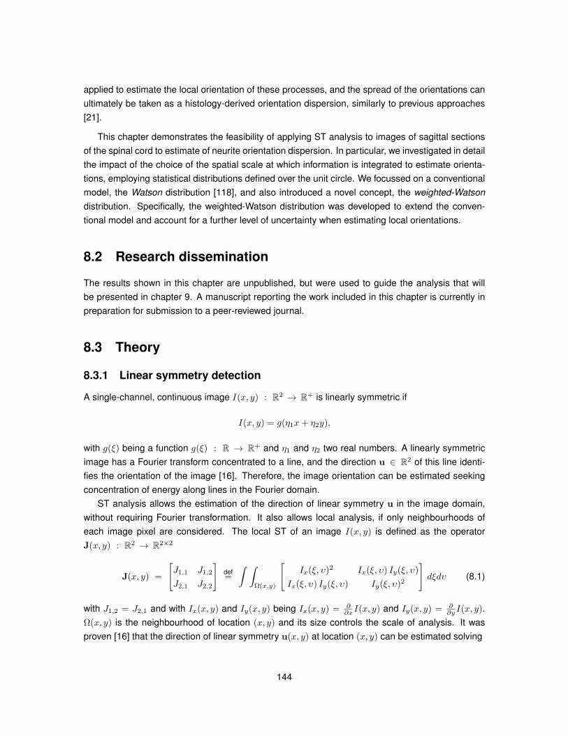
applied to estimate the local orientation of these processes, and the spread of the orientations canultimately be taken as a histology-derived orientation dispersion, similarly to previous approaches[21].

This chapter demonstrates the feasibility of applying ST analysis to images of sagittal sectionsof the spinal cord to estimate of neurite orientation dispersion. In particular, we investigated in detailthe impact of the choice of the spatial scale at which information is integrated to estimate orienta-tions, employing statistical distributions defined over the unit circle. We focussed on a conventionalmodel, the Watson distribution [118], and also introduced a novel concept, the weighted-Watsondistribution. Specifically, the weighted-Watson distribution was developed to extend the conven-tional model and account for a further level of uncertainty when estimating local orientations.


The results shown in this chapter are unpublished, but were used to guide the analysis that willbe presented in chapter 9. A manuscript reporting the work included in this chapter is currently inpreparation for submission to a peer-reviewed journal.

8.3 Theory

8.3.1 Linear symmetry detection

A single-channel, continuous image I(x, y) : R2 → R+ is linearly symmetric if

I(x, y) = g(η1x+ η2y),

with g(ξ) being a function g(ξ) : R → R+ and η1 and η2 two real numbers. A linearly symmetricimage has a Fourier transform concentrated to a line, and the direction u ∈ R2 of this line identi-fies the orientation of the image [16]. Therefore, the image orientation can be estimated seekingconcentration of energy along lines in the Fourier domain.

ST analysis allows the estimation of the direction of linear symmetry u in the image domain,without requiring Fourier transformation. It also allows local analysis, if only neighbourhoods ofeach image pixel are considered. The local ST of an image I(x, y) is defined as the operatorJ(x, y) : R2 → R2×2

J(x, y) =

[J1,1 J1,2

J2,1 J2,2

]def=

∫ ∫Ω(x,y)

[Ix(ξ, υ)2 Ix(ξ, υ) Iy(ξ, υ)

Ix(ξ, υ) Iy(ξ, υ) Iy(ξ, υ)2

]dξdυ (8.1)

with J1,2 = J2,1 and with Ix(x, y) and Iy(x, y) being Ix(x, y) = ∂∂xI(x, y) and Iy(x, y) = ∂

∂y I(x, y).Ω(x, y) is the neighbourhood of location (x, y) and its size controls the scale of analysis. It wasproven [16] that the direction of linear symmetry u(x, y) at location (x, y) can be estimated solving

144

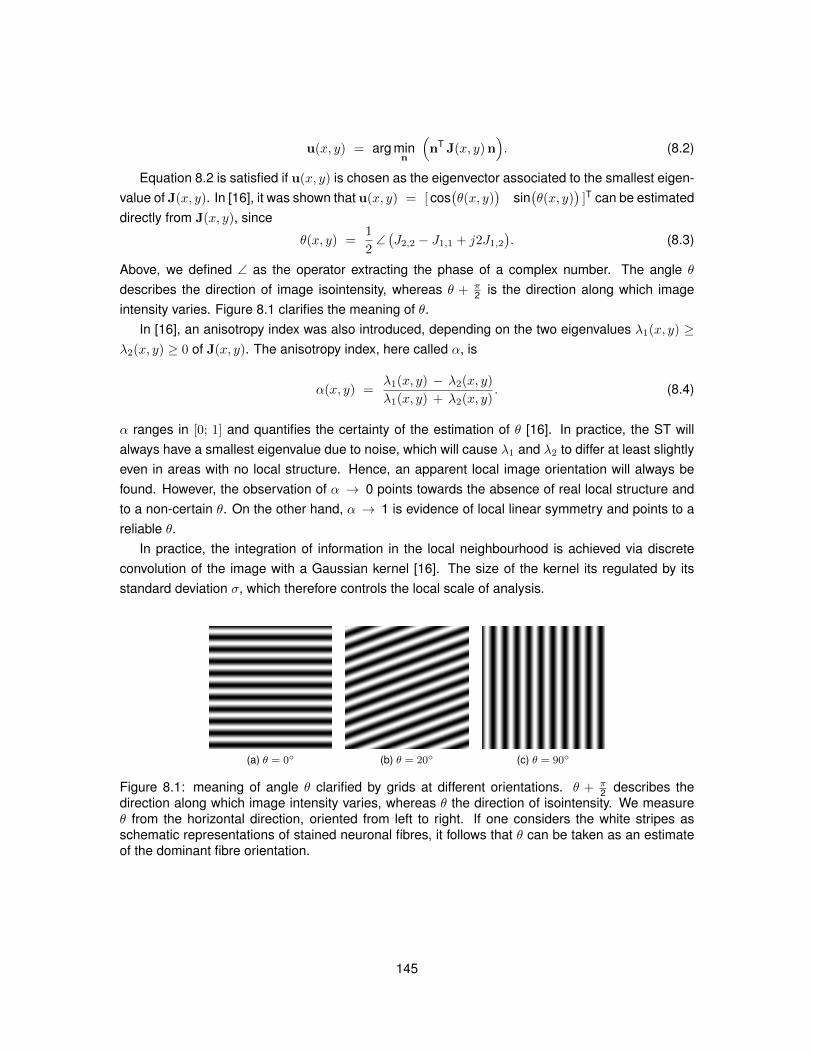
u(x, y) = arg minn

(nT J(x, y)n

). (8.2)

Equation 8.2 is satisfied if u(x, y) is chosen as the eigenvector associated to the smallest eigen-value of J(x, y). In [16], it was shown that u(x, y) = [ cos

(θ(x, y)

)sin(θ(x, y)

)]T can be estimated

directly from J(x, y), since

θ(x, y) =1

2∠(J2,2 − J1,1 + j2J1,2

). (8.3)

Above, we defined ∠ as the operator extracting the phase of a complex number. The angle θ

describes the direction of image isointensity, whereas θ + π2 is the direction along which image

intensity varies. Figure 8.1 clarifies the meaning of θ.In [16], an anisotropy index was also introduced, depending on the two eigenvalues λ1(x, y) ≥

λ2(x, y) ≥ 0 of J(x, y). The anisotropy index, here called α, is

α(x, y) =λ1(x, y) − λ2(x, y)

λ1(x, y) + λ2(x, y). (8.4)

α ranges in [0; 1] and quantifies the certainty of the estimation of θ [16]. In practice, the ST willalways have a smallest eigenvalue due to noise, which will cause λ1 and λ2 to differ at least slightlyeven in areas with no local structure. Hence, an apparent local image orientation will always befound. However, the observation of α → 0 points towards the absence of real local structure andto a non-certain θ. On the other hand, α → 1 is evidence of local linear symmetry and points to areliable θ.

In practice, the integration of information in the local neighbourhood is achieved via discreteconvolution of the image with a Gaussian kernel [16]. The size of the kernel its regulated by itsstandard deviation σ, which therefore controls the local scale of analysis.

(a) θ = 0 (b) θ = 20 (c) θ = 90

Figure 8.1: meaning of angle θ clarified by grids at different orientations. θ + π2 describes the

direction along which image intensity varies, whereas θ the direction of isointensity. We measureθ from the horizontal direction, oriented from left to right. If one considers the white stripes asschematic representations of stained neuronal fibres, it follows that θ can be taken as an estimateof the dominant fibre orientation.

145

8.3.2 Patch-wise statistics of ST orientation

When ST-derived orientation from histological images is compared to DW MRI indices, the analysisis usually performed at a scale comparable to the MRI voxel size. For instance, in [22] the STorientation maps were split into patches and for each patch an histogram of the orientations wascalculated and fitted to a von Mises distribution defined over the unit circle.

In this work, we propose to follow a similar approach, e.g. to divide the orientation map θ(x, y)

of spinal cord histological images into patches of size comparable to the resolution of an MRI voxel.Then, directional statistics [118] can be employed to model the distribution of orientations withineach patch. This allows the evaluation of indices of spread, which can be considered as estimatesof neurite orientation dispersion and hence counterparts of NODDI ODI.

In particular, we focus on the Watson distribution defined over the unit circle, being bimodal in[0; 2π] (i.e. its value is the same for orientations +n and−n [118]). This is a conventional model thatdescribes the bimodal distribution of orientations about a mean orientation, equivalent to NODDIneurite orientation distribution, with the difference that for NODDI the distribution is defined over theunit sphere, rather than over the unit circle.

We also introduce a new bivariate probability density function, which we call weighted-Watsondistribution. This distribution considers both ST orientation θ and anisotropy index α as two distinctrandom variables, and attempts to model them jointly, in order to account not only for the spreadabout a mean orientation, but also for the uncertainty of the individual orientation from each singlepixel.

In conventional approaches, the only ST metric considered for analysis is the local dominantorientation θ. Analysis usually provides statistics of mean and spread of θ, given a sample Γ =

θ1, ..., θN coming from several pixels of a histological image. The indices of spread, particularly,can be seen as the overall measures of uncertainty with respect to a mean orientation within thewhole set Γ.

With our novel weighted-Watson distribution, a further level of uncertainty is modelled. Similarlyto conventional approaches, the weighted-Watson distribution provides an index of spread abouta mean orientation, given the sample Γ of orientations from several pixels. However, due to thedependency on the anisotropy index α, the weighted-Watson distribution also captures uncertaintyat the level of the individual pixel, i.e. at the individual element θi, i = 1, ..., N of Γ, whose reliabilityis described by the value of the corresponding anisotropy index αi. Therefore, in our weighted-Watson model, reliable orientations contribute more than unreliable ones to the estimation of thedescriptive statistics of mean and spread.

The two probability density functions are described in the next two sections, and both rely onthe hypothesis that there is only one dominant orientation within a patch.

146

Conventional model: the Watson distribution

Let θ be an angular random variable defined in [0; 2π]. The Watson distribution of parameters κ andµ is defined as

PΘ(θ;κ, µ) = c e k cos2(θ−µ) (8.5)

with κ ∈ (0;∞) being the concentration of the distribution and µ describing its mean orientation. cis a normalising constant that can be worked out writing

∫ 2π0 PΘ(θ;κ, µ) dθ = 1, which provides

c(κ) =1

2π e 12κ I0

( 12κ)

with I0(ξ) = 12π

∫ 2π0 e ξcos(x) dx being the modified Bessel function of the first kind and 0-th order.

The parameters κ and µ can be estimated given a sample of N observations Γ = θn | n =

1, ..., N via maximisation of the likelihood of the sample. Under the hypothesis of independenceof the observations, it is possible to show that the maximum likelihood estimates κ and µ of theparameters κ and µ are

κ = 2A−1(1− CV)

(8.6)

and

µ =12∠

(1N

N∑n=1

e j 2θn

), (8.7)

where the operator ∠ extracts the phase of a complex number. In equation 8.6 above, we definedA(ξ) as A(ξ)

def=

ddξ I0(ξ)

I0(ξ) , and indicated with CV the circular variance of Γ [118], i.e.

CV = 1−

∣∣∣∣∣ 1N

N∑n=1

e j 2θn

∣∣∣∣∣. (8.8)

CV is a measure of spread of the orientation and ranges in [0; 1], with CV = 0 if all orientations arethe same (θi = θj ∀ i 6= j) and CV = 1 indicating maximum spread.

Lastly, the value of the log-likelihood at maximum is

logLmax =12N κ (1− CV) + N log

(1

2π I0( 1

2 κ)). (8.9)

Figure 8.2 shows the Watson distribution for different values of κ and for a fixed µ. The distribu-tion is bimodal and has little dependence on θ for very low κ, whereas it has a peak centred on themean orientation for higher values of κ, which gets sharper as κ increases.

147

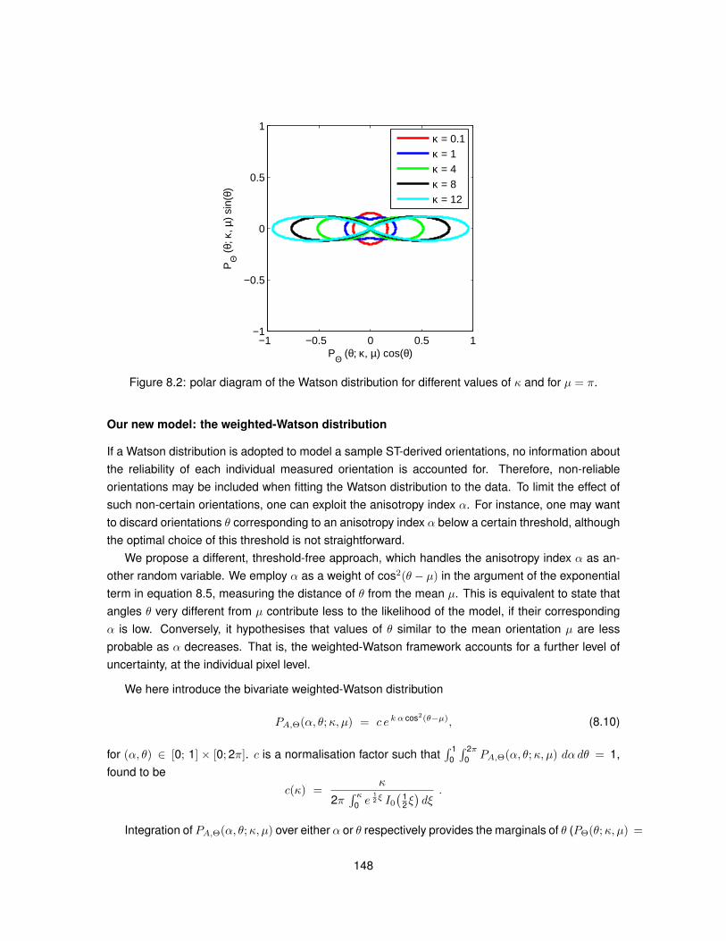
−1 −0.5 0 0.5 1−1

−0.5

0

0.5

1

PΘ (θ; κ, µ) cos(θ)

PΘ

(θ;

κ, µ

) si

n(θ)

κ = 0.1κ = 1κ = 4κ = 8κ = 12

Figure 8.2: polar diagram of the Watson distribution for different values of κ and for µ = π.

Our new model: the weighted-Watson distribution

If a Watson distribution is adopted to model a sample ST-derived orientations, no information aboutthe reliability of each individual measured orientation is accounted for. Therefore, non-reliableorientations may be included when fitting the Watson distribution to the data. To limit the effect ofsuch non-certain orientations, one can exploit the anisotropy index α. For instance, one may wantto discard orientations θ corresponding to an anisotropy index α below a certain threshold, althoughthe optimal choice of this threshold is not straightforward.

We propose a different, threshold-free approach, which handles the anisotropy index α as an-other random variable. We employ α as a weight of cos2(θ − µ) in the argument of the exponentialterm in equation 8.5, measuring the distance of θ from the mean µ. This is equivalent to state thatangles θ very different from µ contribute less to the likelihood of the model, if their correspondingα is low. Conversely, it hypothesises that values of θ similar to the mean orientation µ are lessprobable as α decreases. That is, the weighted-Watson framework accounts for a further level ofuncertainty, at the individual pixel level.

We here introduce the bivariate weighted-Watson distribution

PA,Θ(α, θ;κ, µ) = c e k α cos2(θ−µ), (8.10)

for (α, θ) ∈ [0; 1] × [0; 2π]. c is a normalisation factor such that∫ 1

0

∫ 2π0 PA,Θ(α, θ;κ, µ) dα dθ = 1,

found to bec(κ) =

κ

2π∫ κ

0 e12 ξ I0

( 12ξ)dξ

.

Integration of PA,Θ(α, θ;κ, µ) over either α or θ respectively provides the marginals of θ (PΘ(θ;κ, µ) =

148

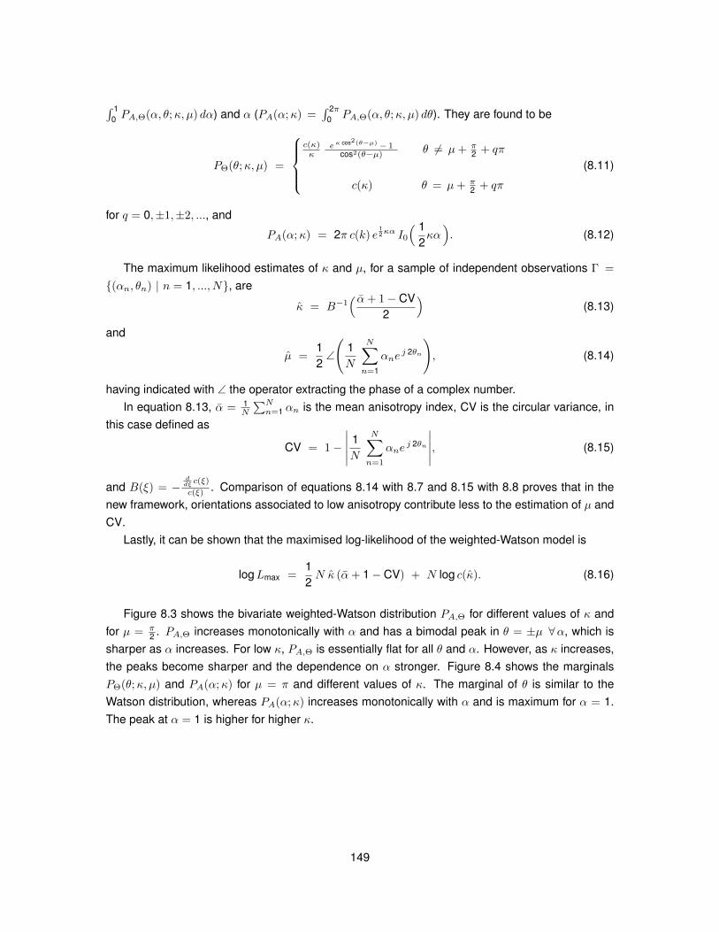
∫ 10 PA,Θ(α, θ;κ, µ) dα) and α (PA(α;κ) =

∫ 2π0 PA,Θ(α, θ;κ, µ) dθ). They are found to be

PΘ(θ;κ, µ) =

c(κ)κ

eκ cos2(θ−µ)− 1cos2(θ−µ) θ 6= µ+ π

2 + qπ

c(κ) θ = µ+ π2 + qπ

(8.11)

for q = 0,±1,±2, ..., and

PA(α;κ) = 2π c(k) e12κα I0

( 12κα). (8.12)

The maximum likelihood estimates of κ and µ, for a sample of independent observations Γ =

(αn, θn) | n = 1, ..., N, are

κ = B−1( α+ 1− CV

2

)(8.13)

and

µ =12∠

(1N

N∑n=1

αnej 2θn

), (8.14)

having indicated with ∠ the operator extracting the phase of a complex number.In equation 8.13, α = 1

N

∑Nn=1 αn is the mean anisotropy index, CV is the circular variance, in

this case defined as

CV = 1−

∣∣∣∣∣ 1N

N∑n=1

αnej 2θn

∣∣∣∣∣, (8.15)

and B(ξ) = −ddξ c(ξ)

c(ξ) . Comparison of equations 8.14 with 8.7 and 8.15 with 8.8 proves that in thenew framework, orientations associated to low anisotropy contribute less to the estimation of µ andCV.

Lastly, it can be shown that the maximised log-likelihood of the weighted-Watson model is

logLmax =12N κ (α+ 1− CV) + N log c(κ). (8.16)

Figure 8.3 shows the bivariate weighted-Watson distribution PA,Θ for different values of κ andfor µ = π

2 . PA,Θ increases monotonically with α and has a bimodal peak in θ = ±µ ∀α, which issharper as α increases. For low κ, PA,Θ is essentially flat for all θ and α. However, as κ increases,the peaks become sharper and the dependence on α stronger. Figure 8.4 shows the marginalsPΘ(θ;κ, µ) and PA(α;κ) for µ = π and different values of κ. The marginal of θ is similar to theWatson distribution, whereas PA(α;κ) increases monotonically with α and is maximum for α = 1.The peak at α = 1 is higher for higher κ.

149

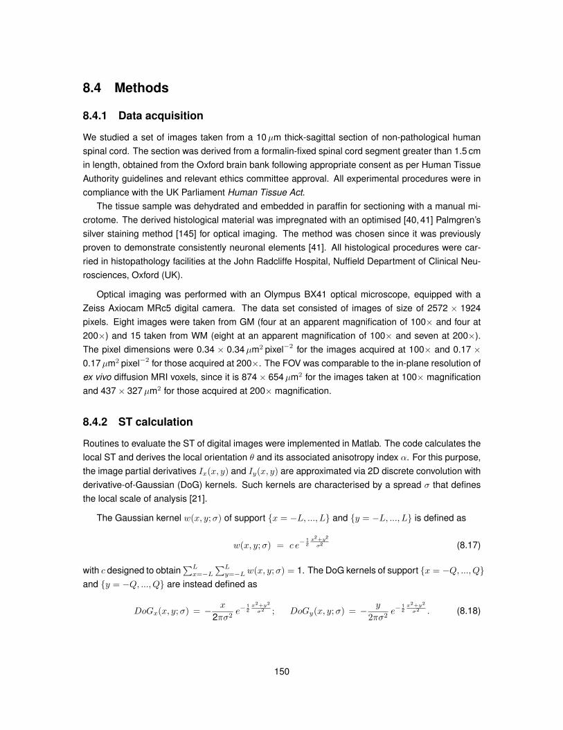
8.4 Methods


We studied a set of images taken from a 10µm thick-sagittal section of non-pathological humanspinal cord. The section was derived from a formalin-fixed spinal cord segment greater than 1.5 cmin length, obtained from the Oxford brain bank following appropriate consent as per Human TissueAuthority guidelines and relevant ethics committee approval. All experimental procedures were incompliance with the UK Parliament Human Tissue Act.

The tissue sample was dehydrated and embedded in paraffin for sectioning with a manual mi-crotome. The derived histological material was impregnated with an optimised [40, 41] Palmgren’ssilver staining method [145] for optical imaging. The method was chosen since it was previouslyproven to demonstrate consistently neuronal elements [41]. All histological procedures were car-ried in histopathology facilities at the John Radcliffe Hospital, Nuffield Department of Clinical Neu-rosciences, Oxford (UK).

Optical imaging was performed with an Olympus BX41 optical microscope, equipped with aZeiss Axiocam MRc5 digital camera. The data set consisted of images of size of 2572 × 1924pixels. Eight images were taken from GM (four at an apparent magnification of 100× and four at200×) and 15 taken from WM (eight at an apparent magnification of 100× and seven at 200×).The pixel dimensions were 0.34 × 0.34µm2 pixel−2 for the images acquired at 100× and 0.17 ×0.17µm2 pixel−2 for those acquired at 200×. The FOV was comparable to the in-plane resolution ofex vivo diffusion MRI voxels, since it is 874 × 654µm2 for the images taken at 100× magnificationand 437× 327µm2 for those acquired at 200× magnification.

8.4.2 ST calculation

Routines to evaluate the ST of digital images were implemented in Matlab. The code calculates thelocal ST and derives the local orientation θ and its associated anisotropy index α. For this purpose,the image partial derivatives Ix(x, y) and Iy(x, y) are approximated via 2D discrete convolution withderivative-of-Gaussian (DoG) kernels. Such kernels are characterised by a spread σ that definesthe local scale of analysis [21].

The Gaussian kernel w(x, y;σ) of support x = −L, ..., L and y = −L, ..., L is defined as

w(x, y;σ) = c e−12x2+y2

σ2 (8.17)

with c designed to obtain∑Lx=−L

∑Ly=−L w(x, y;σ) = 1. The DoG kernels of support x = −Q, ..., Q

and y = −Q, ..., Q are instead defined as

DoGx(x, y;σ) = − x

2πσ2e−

12x2+y2

σ2 ; DoGy(x, y;σ) = − y

2πσ2e−

12x2+y2

σ2 . (8.18)

150

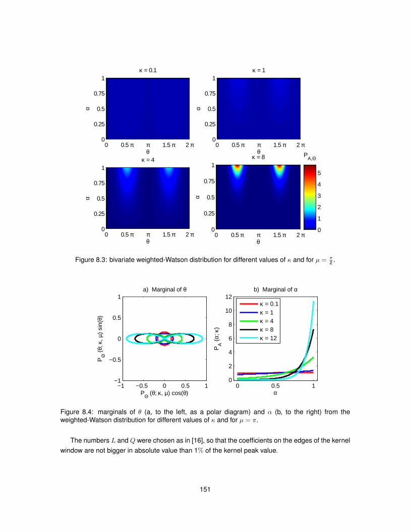
θ

α

κ = 0.1

0 0.5 π π 1.5 π 2 π

1

0.75

0.5

0.25

0

θ

α

κ = 1

0 0.5 π π 1.5 π 2 π

1

0.75

0.5

0.25

0

θ

α

κ = 4

0 0.5 π π 1.5 π 2 π

1

0.75

0.5

0.25

0

θ

α

κ = 8

0 0.5 π π 1.5 π 2 π

1

0.75

0.5

0.25

0

PA,Θ

0

1

2

3

4

5

Figure 8.3: bivariate weighted-Watson distribution for different values of κ and for µ = π2 .

−1 −0.5 0 0.5 1−1

−0.5

0

0.5

1

PΘ (θ; κ, µ) cos(θ)

PΘ

(θ;

κ, µ

) si

n(θ)

a) Marginal of θ

0 0.5 10

2

4

6

8

10

12

α

PA (

α; κ

)

b) Marginal of α

κ = 0.1κ = 1κ = 4κ = 8κ = 12

Figure 8.4: marginals of θ (a, to the left, as a polar diagram) and α (b, to the right) from theweighted-Watson distribution for different values of κ and for µ = π.

The numbers L and Q were chosen as in [16], so that the coefficients on the edges of the kernelwindow are not bigger in absolute value than 1% of the kernel peak value.

151

The ST J(x, y;σ) at pixel (x, y) is calculated as

J(x, y;σ) = w(x, y;σ) ∗

[Ix(x, y;σ)2 Ix(x, y;σ) Iy(x, y;σ)

Ix(x, y;σ) Iy(x, y;σ) Iy(x, y;σ)2

]

with Ix(x, y) and Iy(x, y) estimated as in [21]:

Ix(x, y;σ) = DoGx(x, y;σ) ∗ I(x, y), (8.19)

Iy(x, y;σ) = DoGy(x, y;σ) ∗ I(x, y). (8.20)

Above, ∗ indicates the discrete 2D convolution. All images were zero-padded before convolutionwith kernels w(x, y;σ), DoGx(x, y;σ) and DoGy(x, y;σ), of an amount equal to max(L,Q).

The local dominant orientation θ(x, y;σ) ∈ [0; π] is calculated according to equation 8.3, whereasthe anisotropy index α(x, y;σ) is calculated as specified in equation 8.4.

The implementation was tested and validated on grids of orientation spanning the interval [0; π],as those shown in figure 8.1. The implementation supports optional parallel computing, which splitsthe task of calculating pixel-wise θ(x, y;σ) and α(x, y;σ) into threads run in parallel by differentprocessors.

8.4.3 ST implementation efficiency

To test the efficiency of the parallel implementation, a test was performed to estimate the compu-tational time required to calculate the ST on a image of variable size. The image had the samenumber of pixels along the horizontal and vertical directions, and it was a grid similar to thosedepicted in figure 8.1.

We fixed σ = 0.5 pixel and run the test on a 8-core Dell Precision T1650 machine (3.5 GHzprocessor speed, 16 GB memory). The ST calculation was run without parallel computing (allpixels analysed one after the other) and also splitting the ST calculation into 4 parallel threads(each analysing serially a separate subset of pixels). The calculation of the ST was run 10 timesper image width, and median and range of the computational time over the 10 runs were measured.

8.4.4 Variation of the local scale

We calculated the ST of all images in our data set varying σ in a set of 80 evenly spaced valuesranging from 0.1 to 100 pixels. For each image and each σ, the local orientation θ(x, y;σ) and theanisotropy index α(x, y;σ) were derived, and their distributions were approximated by normalisedhistograms. The maximum-likelihood estimates of the parameters of the Watson and weighted-Watson models and the corresponding maximised log-likelihoods were also calculated. In doingso, an adequate portion of each image close to the edges was removed, being influenced by thezero-padding of the filtering routines.

152

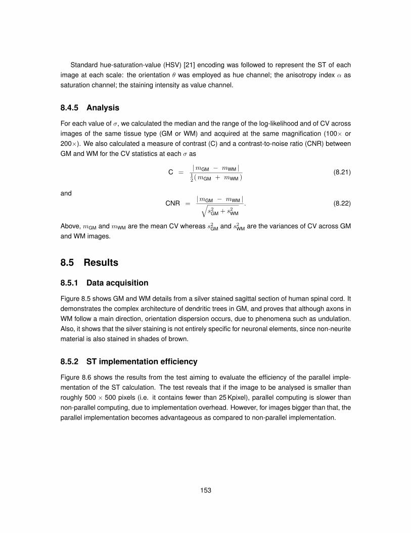
Standard hue-saturation-value (HSV) [21] encoding was followed to represent the ST of eachimage at each scale: the orientation θ was employed as hue channel; the anisotropy index α assaturation channel; the staining intensity as value channel.

8.4.5 Analysis

For each value of σ, we calculated the median and the range of the log-likelihood and of CV acrossimages of the same tissue type (GM or WM) and acquired at the same magnification (100× or200×). We also calculated a measure of contrast (C) and a contrast-to-noise ratio (CNR) betweenGM and WM for the CV statistics at each σ as

C =|mGM − mWM |

12 (mGM + mWM )

(8.21)

andCNR =

|mGM − mWM |√s2

GM + s2WM

. (8.22)

Above, mGM and mWM are the mean CV whereas s2GM and s2

WM are the variances of CV across GMand WM images.

8.5 Results


Figure 8.5 shows GM and WM details from a silver stained sagittal section of human spinal cord. Itdemonstrates the complex architecture of dendritic trees in GM, and proves that although axons inWM follow a main direction, orientation dispersion occurs, due to phenomena such as undulation.Also, it shows that the silver staining is not entirely specific for neuronal elements, since non-neuritematerial is also stained in shades of brown.

8.5.2 ST implementation efficiency

Figure 8.6 shows the results from the test aiming to evaluate the efficiency of the parallel imple-mentation of the ST calculation. The test reveals that if the image to be analysed is smaller thanroughly 500 × 500 pixels (i.e. it contains fewer than 25 Kpixel), parallel computing is slower thannon-parallel computing, due to implementation overhead. However, for images bigger than that, theparallel implementation becomes advantageous as compared to non-parallel implementation.

153

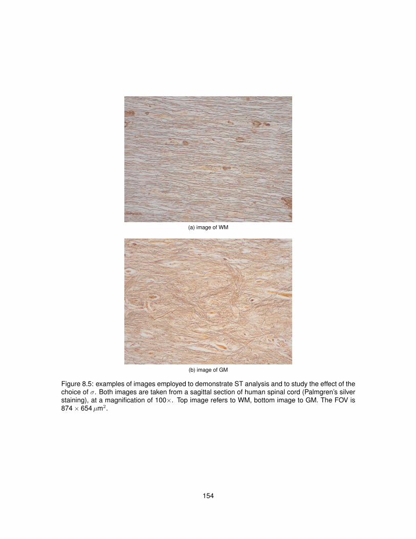
(a) image of WM

(b) image of GM

Figure 8.5: examples of images employed to demonstrate ST analysis and to study the effect of thechoice of σ. Both images are taken from a sagittal section of human spinal cord (Palmgren’s silverstaining), at a magnification of 100×. Top image refers to WM, bottom image to GM. The FOV is874× 654µm2.

154

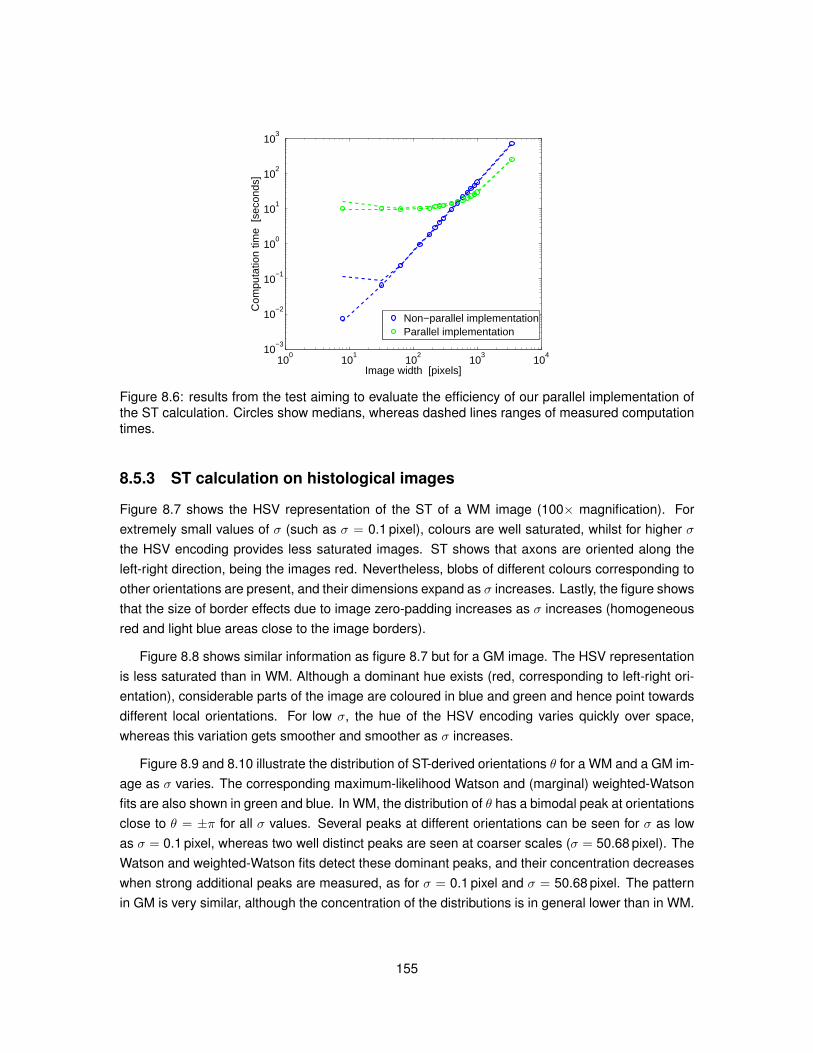
100

101

102

103

104

10−3

10−2

10−1

100

101

102

103

Image width [pixels]

Com

puta

tion

time

[sec

onds

]

Non−parallel implementationParallel implementation

Figure 8.6: results from the test aiming to evaluate the efficiency of our parallel implementation ofthe ST calculation. Circles show medians, whereas dashed lines ranges of measured computationtimes.

8.5.3 ST calculation on histological images

Figure 8.7 shows the HSV representation of the ST of a WM image (100× magnification). Forextremely small values of σ (such as σ = 0.1 pixel), colours are well saturated, whilst for higher σthe HSV encoding provides less saturated images. ST shows that axons are oriented along theleft-right direction, being the images red. Nevertheless, blobs of different colours corresponding toother orientations are present, and their dimensions expand as σ increases. Lastly, the figure showsthat the size of border effects due to image zero-padding increases as σ increases (homogeneousred and light blue areas close to the image borders).

Figure 8.8 shows similar information as figure 8.7 but for a GM image. The HSV representationis less saturated than in WM. Although a dominant hue exists (red, corresponding to left-right ori-entation), considerable parts of the image are coloured in blue and green and hence point towardsdifferent local orientations. For low σ, the hue of the HSV encoding varies quickly over space,whereas this variation gets smoother and smoother as σ increases.

Figure 8.9 and 8.10 illustrate the distribution of ST-derived orientations θ for a WM and a GM im-age as σ varies. The corresponding maximum-likelihood Watson and (marginal) weighted-Watsonfits are also shown in green and blue. In WM, the distribution of θ has a bimodal peak at orientationsclose to θ = ±π for all σ values. Several peaks at different orientations can be seen for σ as lowas σ = 0.1 pixel, whereas two well distinct peaks are seen at coarser scales (σ = 50.68 pixel). TheWatson and weighted-Watson fits detect these dominant peaks, and their concentration decreaseswhen strong additional peaks are measured, as for σ = 0.1 pixel and σ = 50.68 pixel. The patternin GM is very similar, although the concentration of the distributions is in general lower than in WM.

155

(a) σ = 0.1 pixel (b) σ = 2.63 pixel

(c) σ = 6.42 pixel (d) σ = 20.33 pixel

(e) σ = 50.68 pixel

Figure 8.7: HSV representation of the ST of the same WM image shown in figure 8.5. Resultscorresponding to various choices of σ are presented. The colour-wheel describes how orientationis mapped onto the hue channel.

156

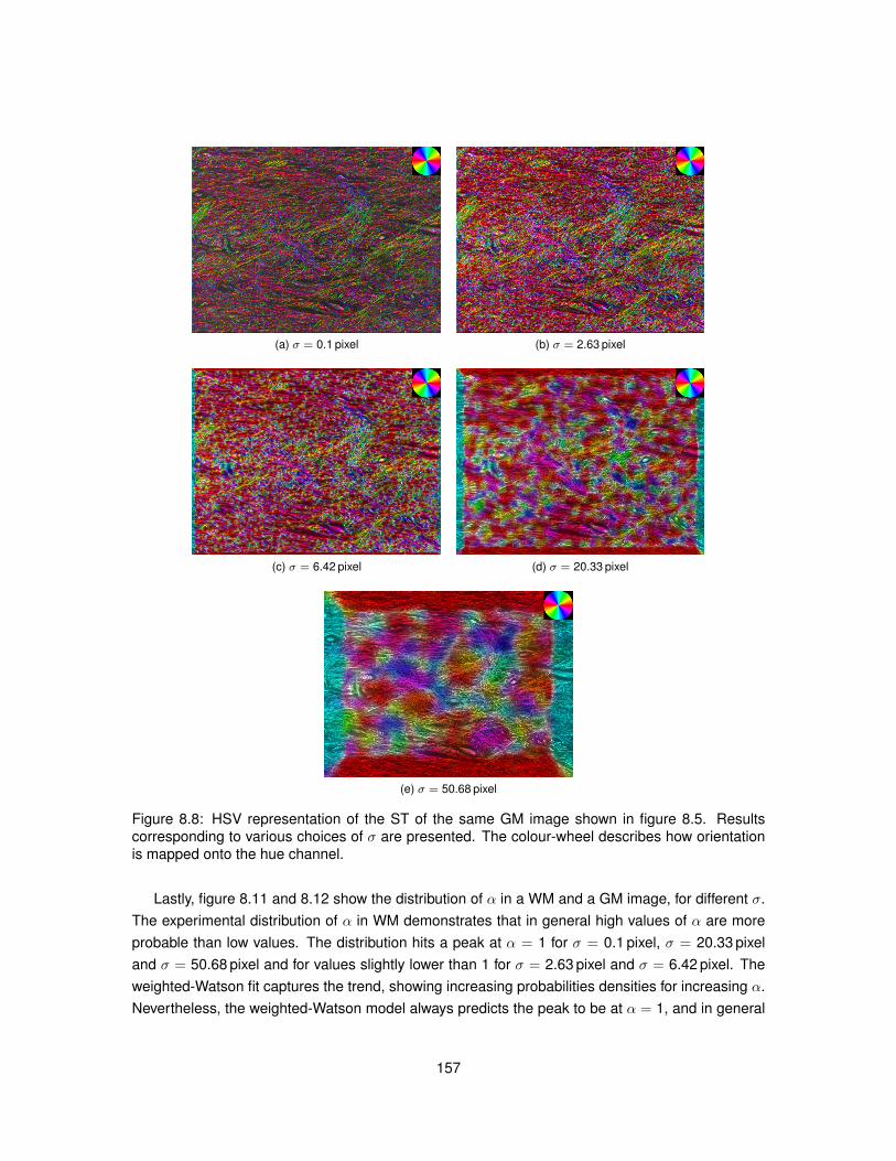
(a) σ = 0.1 pixel (b) σ = 2.63 pixel

(c) σ = 6.42 pixel (d) σ = 20.33 pixel

(e) σ = 50.68 pixel

Figure 8.8: HSV representation of the ST of the same GM image shown in figure 8.5. Resultscorresponding to various choices of σ are presented. The colour-wheel describes how orientationis mapped onto the hue channel.

Lastly, figure 8.11 and 8.12 show the distribution of α in a WM and a GM image, for different σ.The experimental distribution of α in WM demonstrates that in general high values of α are moreprobable than low values. The distribution hits a peak at α = 1 for σ = 0.1 pixel, σ = 20.33 pixeland σ = 50.68 pixel and for values slightly lower than 1 for σ = 2.63 pixel and σ = 6.42 pixel. Theweighted-Watson fit captures the trend, showing increasing probabilities densities for increasing α.Nevertheless, the weighted-Watson model always predicts the peak to be at α = 1, and in general

157

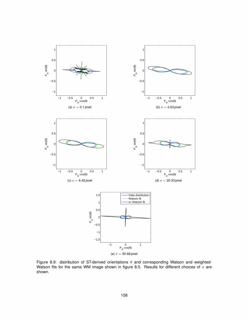
−1 −0.5 0 0.5 1

−1

−0.5

0

0.5

1

PΘ cos(θ)

PΘ

sin

(θ)

(a) σ = 0.1 pixel

−1 −0.5 0 0.5 1

−1

−0.5

0

0.5

1

PΘ cos(θ)

PΘ

sin

(θ)

(b) σ = 2.63 pixel

−1 −0.5 0 0.5 1

−1

−0.5

0

0.5

1

PΘ cos(θ)

PΘ

sin

(θ)

(c) σ = 6.42 pixel

−1 −0.5 0 0.5 1

−1

−0.5

0

0.5

1

PΘ cos(θ)

PΘ

sin

(θ)

(d) σ = 20.33 pixel

−1 0 1

−1.5

−1

−0.5

0

0.5

1

1.5

PΘ cos(θ)

PΘ

sin

(θ)

Data distributionWatson fitw−Watson fit

(e) σ = 50.68 pixel

Figure 8.9: distribution of ST-derived orientations θ and corresponding Watson and weighted-Watson fits for the same WM image shown in figure 8.5. Results for different choices of σ areshown.

158

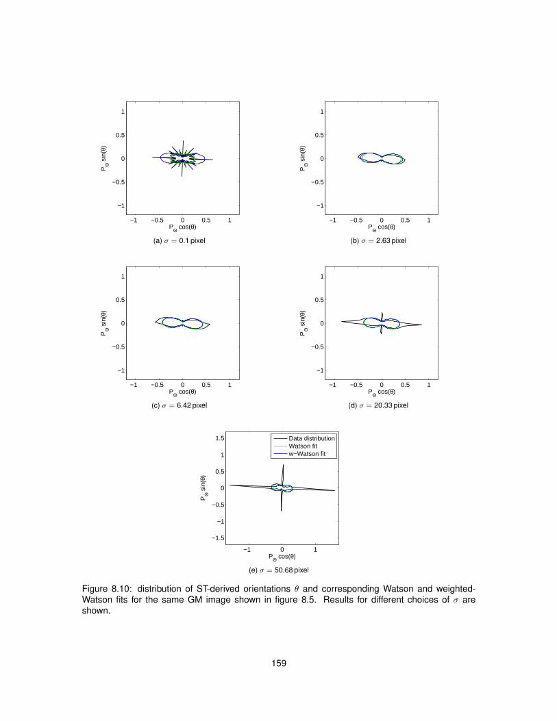
−1 −0.5 0 0.5 1

−1

−0.5

0

0.5

1

PΘ cos(θ)

PΘ

sin

(θ)

(a) σ = 0.1 pixel

−1 −0.5 0 0.5 1

−1

−0.5

0

0.5

1

PΘ cos(θ)

PΘ

sin

(θ)

(b) σ = 2.63 pixel

−1 −0.5 0 0.5 1

−1

−0.5

0

0.5

1

PΘ cos(θ)

PΘ

sin

(θ)

(c) σ = 6.42 pixel

−1 −0.5 0 0.5 1

−1

−0.5

0

0.5

1

PΘ cos(θ)

PΘ

sin

(θ)

(d) σ = 20.33 pixel

−1 0 1

−1.5

−1

−0.5

0

0.5

1

1.5

PΘ cos(θ)

PΘ

sin

(θ)

Data distributionWatson fitw−Watson fit

(e) σ = 50.68 pixel

Figure 8.10: distribution of ST-derived orientations θ and corresponding Watson and weighted-Watson fits for the same GM image shown in figure 8.5. Results for different choices of σ areshown.

159

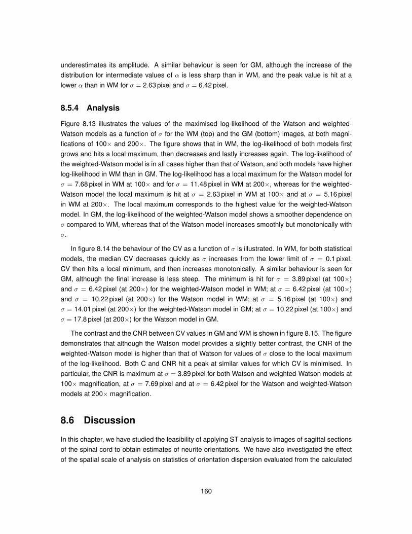
underestimates its amplitude. A similar behaviour is seen for GM, although the increase of thedistribution for intermediate values of α is less sharp than in WM, and the peak value is hit at alower α than in WM for σ = 2.63 pixel and σ = 6.42 pixel.

8.5.4 Analysis

Figure 8.13 illustrates the values of the maximised log-likelihood of the Watson and weighted-Watson models as a function of σ for the WM (top) and the GM (bottom) images, at both magni-fications of 100× and 200×. The figure shows that in WM, the log-likelihood of both models firstgrows and hits a local maximum, then decreases and lastly increases again. The log-likelihood ofthe weighted-Watson model is in all cases higher than that of Watson, and both models have higherlog-likelihood in WM than in GM. The log-likelihood has a local maximum for the Watson model forσ = 7.68 pixel in WM at 100× and for σ = 11.48 pixel in WM at 200×, whereas for the weighted-Watson model the local maximum is hit at σ = 2.63 pixel in WM at 100× and at σ = 5.16 pixelin WM at 200×. The local maximum corresponds to the highest value for the weighted-Watsonmodel. In GM, the log-likelihood of the weighted-Watson model shows a smoother dependence onσ compared to WM, whereas that of the Watson model increases smoothly but monotonically withσ.

In figure 8.14 the behaviour of the CV as a function of σ is illustrated. In WM, for both statisticalmodels, the median CV decreases quickly as σ increases from the lower limit of σ = 0.1 pixel.CV then hits a local minimum, and then increases monotonically. A similar behaviour is seen forGM, although the final increase is less steep. The minimum is hit for σ = 3.89 pixel (at 100×)and σ = 6.42 pixel (at 200×) for the weighted-Watson model in WM; at σ = 6.42 pixel (at 100×)and σ = 10.22 pixel (at 200×) for the Watson model in WM; at σ = 5.16 pixel (at 100×) andσ = 14.01 pixel (at 200×) for the weighted-Watson model in GM; at σ = 10.22 pixel (at 100×) andσ = 17.8 pixel (at 200×) for the Watson model in GM.

The contrast and the CNR between CV values in GM and WM is shown in figure 8.15. The figuredemonstrates that although the Watson model provides a slightly better contrast, the CNR of theweighted-Watson model is higher than that of Watson for values of σ close to the local maximumof the log-likelihood. Both C and CNR hit a peak at similar values for which CV is minimised. Inparticular, the CNR is maximum at σ = 3.89 pixel for both Watson and weighted-Watson models at100× magnification, at σ = 7.69 pixel and at σ = 6.42 pixel for the Watson and weighted-Watsonmodels at 200× magnification.

8.6 Discussion

In this chapter, we have studied the feasibility of applying ST analysis to images of sagittal sectionsof the spinal cord to obtain estimates of neurite orientations. We have also investigated the effectof the spatial scale of analysis on statistics of orientation dispersion evaluated from the calculated

160

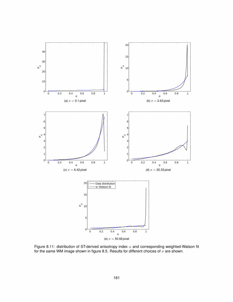
0 0.2 0.4 0.6 0.8 10

10

20

30

40

α

PA

(a) σ = 0.1 pixel

0 0.2 0.4 0.6 0.8 10

5

10

15

20

α

PA

(b) σ = 2.63 pixel

0 0.2 0.4 0.6 0.8 10

1

2

3

4

5

6

7

α

PA

(c) σ = 6.42 pixel

0 0.2 0.4 0.6 0.8 10

1

2

3

4

5

6

7

α

PA

(d) σ = 20.33 pixel

0 0.2 0.4 0.6 0.8 10

5

10

15

20

α

PA

Data distributionw−Watson fit

(e) σ = 50.68 pixel

Figure 8.11: distribution of ST-derived anisotropy index α and corresponding weighted-Watson fitfor the same WM image shown in figure 8.5. Results for different choices of σ are shown.

161

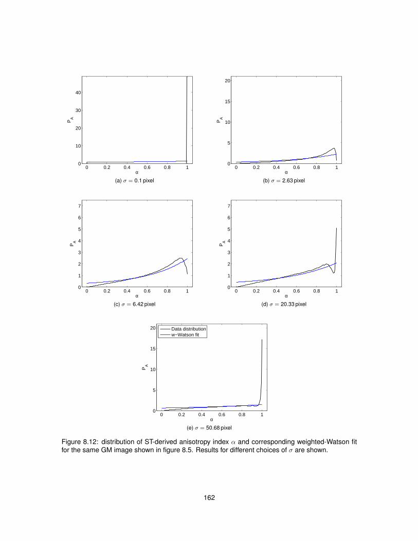
0 0.2 0.4 0.6 0.8 10

10

20

30

40

α

PA

(a) σ = 0.1 pixel

0 0.2 0.4 0.6 0.8 10

5

10

15

20

α

PA

(b) σ = 2.63 pixel

0 0.2 0.4 0.6 0.8 10

1

2

3

4

5

6

7

α

PA

(c) σ = 6.42 pixel

0 0.2 0.4 0.6 0.8 10

1

2

3

4

5

6

7

α

PA

(d) σ = 20.33 pixel

0 0.2 0.4 0.6 0.8 10

5

10

15

20

α

PA

Data distributionw−Watson fit

(e) σ = 50.68 pixel

Figure 8.12: distribution of ST-derived anisotropy index α and corresponding weighted-Watson fitfor the same GM image shown in figure 8.5. Results for different choices of σ are shown.

162

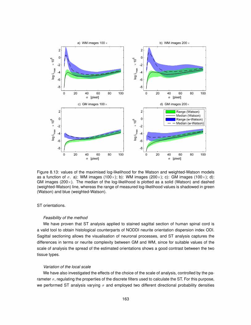
Figure 8.13: values of the maximised log-likelihood for the Watson and weighted-Watson modelsas a function of σ. a): WM images (100×); b): WM images (200×); c): GM images (100×); d):GM images (200×). The median of the log-likelihood is plotted as a solid (Watson) and dashed(weighted-Watson) line, whereas the range of measured log-likelihood values is shadowed in green(Watson) and blue (weighted-Watson).

ST orientations.

Feasibility of the methodWe have proven that ST analysis applied to stained sagittal section of human spinal cord is

a valid tool to obtain histological counterparts of NODDI neurite orientation dispersion index ODI.Sagittal sectioning allows the visualisation of neuronal processes, and ST analysis captures thedifferences in terms or neurite complexity between GM and WM, since for suitable values of thescale of analysis the spread of the estimated orientations shows a good contrast between the twotissue types.

Variation of the local scaleWe have also investigated the effects of the choice of the scale of analysis, controlled by the pa-

rameter σ, regulating the properties of the discrete filters used to calculate the ST. For this purpose,we performed ST analysis varying σ and employed two different directional probability densities

163

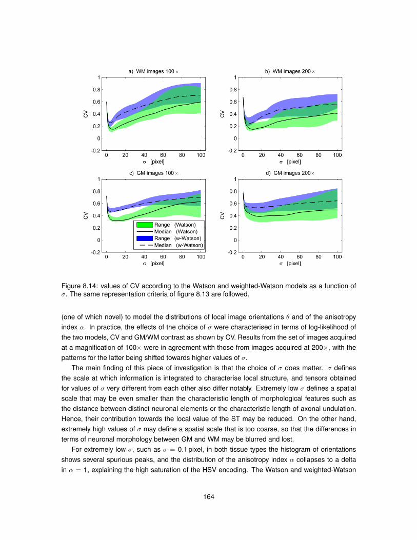
Figure 8.14: values of CV according to the Watson and weighted-Watson models as a function ofσ. The same representation criteria of figure 8.13 are followed.

(one of which novel) to model the distributions of local image orientations θ and of the anisotropyindex α. In practice, the effects of the choice of σ were characterised in terms of log-likelihood ofthe two models, CV and GM/WM contrast as shown by CV. Results from the set of images acquiredat a magnification of 100× were in agreement with those from images acquired at 200×, with thepatterns for the latter being shifted towards higher values of σ.

The main finding of this piece of investigation is that the choice of σ does matter. σ definesthe scale at which information is integrated to characterise local structure, and tensors obtainedfor values of σ very different from each other also differ notably. Extremely low σ defines a spatialscale that may be even smaller than the characteristic length of morphological features such asthe distance between distinct neuronal elements or the characteristic length of axonal undulation.Hence, their contribution towards the local value of the ST may be reduced. On the other hand,extremely high values of σ may define a spatial scale that is too coarse, so that the differences interms of neuronal morphology between GM and WM may be blurred and lost.

For extremely low σ, such as σ = 0.1 pixel, in both tissue types the histogram of orientationsshows several spurious peaks, and the distribution of the anisotropy index α collapses to a deltain α = 1, explaining the high saturation of the HSV encoding. The Watson and weighted-Watson

164

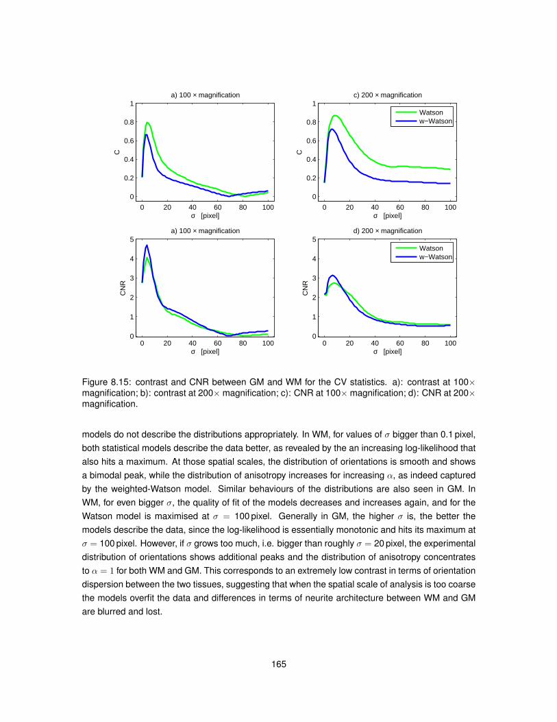
0 20 40 60 80 100

0

0.2

0.4

0.6

0.8

1

σ [pixel]

C

a) 100 × magnification

0 20 40 60 80 100

0

0.2

0.4

0.6

0.8

1

σ [pixel]

C

c) 200 × magnification

Watsonw−Watson

0 20 40 60 80 1000

1

2

3

4

5

σ [pixel]

CN

R

a) 100 × magnification

0 20 40 60 80 1000

1

2

3

4

5

σ [pixel]

CN

R

d) 200 × magnification

Watsonw−Watson

Figure 8.15: contrast and CNR between GM and WM for the CV statistics. a): contrast at 100×magnification; b): contrast at 200×magnification; c): CNR at 100×magnification; d): CNR at 200×magnification.

models do not describe the distributions appropriately. In WM, for values of σ bigger than 0.1 pixel,both statistical models describe the data better, as revealed by the an increasing log-likelihood thatalso hits a maximum. At those spatial scales, the distribution of orientations is smooth and showsa bimodal peak, while the distribution of anisotropy increases for increasing α, as indeed capturedby the weighted-Watson model. Similar behaviours of the distributions are also seen in GM. InWM, for even bigger σ, the quality of fit of the models decreases and increases again, and for theWatson model is maximised at σ = 100 pixel. Generally in GM, the higher σ is, the better themodels describe the data, since the log-likelihood is essentially monotonic and hits its maximum atσ = 100 pixel. However, if σ grows too much, i.e. bigger than roughly σ = 20 pixel, the experimentaldistribution of orientations shows additional peaks and the distribution of anisotropy concentratesto α = 1 for both WM and GM. This corresponds to an extremely low contrast in terms of orientationdispersion between the two tissues, suggesting that when the spatial scale of analysis is too coarsethe models overfit the data and differences in terms of neurite architecture between WM and GMare blurred and lost.

165

Performance of patch-wise statistical models in WM and GMST analysis appears more suitable for WM, rather than GM, since for the former a clear peak of

the log-likelihood is seen and since in WM the actual values of log-likelihood are higher than in GM.This may be a consequence of the potentially higher amount of through-plane fibres in GM, whichour 2D analysis cannot account for, as well as the higher amount of unspecific staining.

Comparison between Watson and weighted-Watson modelsIn this chapter we have introduced a novel model to describe the spread of ST-derived ori-

entations of histological images of the spinal cord, the weighted-Watson distribution. We havealso studied a conventional model, the Watson distribution, which is related to the NODDI neuriteorientation distribution function. Our analysis reveals that the weighted-Watson model providesperformance comparable, if not superior, to the standard Watson model. The log-likelihood of theweighted-Watson distribution surpasses that of Watson in WM. Unlike the Watson framework, whichcompletely disregards the anisotropy index α, the weighted-Watson model captures the trend of themarginal distribution of α. It accounts for the uncertainty of orientations at the individual pixel level,without requiring any thresholding. Moreover, it also shows better CNR than the Watson distribu-tion, although its contrast C is slightly lower.

LimitationsThis work has two main limitations. The first, and possibly main one, is that we limited ourselves

to 2D analysis, relying on the hypothesis that sagittal sectioning is adequate to capture neuriteorientation dispersion equally well in both WM and GM. This is equivalent to state that there is novariation in terms of fibre orientation along the direction orthogonal to the sectioning plane, andthat the amount of through-plane neurites is negligible. Although this appears as a reasonablehypothesis in WM, especially far from areas containing collateral fibres, it may not hold true for theintricate dendritic trees in GM or at the interface between WM and GM, where WM axons branchand project into GM. Nevertheless, the variation in terms of neurite orientation in our GM imageswas sufficient to produce an appreciable contrast between the two tissue types.

Another limitation is related to the staining method. Here, we employed Palmgren’s silver stain-ing, which has been proven to optimally demonstrate axons [41]. Nevertheless, it is non-specific,since it also impregnates cell bodies and other elements, especially in GM. Therefore, a smallamount of non-neurite material can contribute to the estimation of the local orientation θ and of itsdispersion. Nevertheless, undesired stained areas could always be masked out before running STanalysis.

8.7 Conclusion

In this chapter we studied optimal strategies of obtaining a histological-derived orientation disper-sion index for the human spinal cord, for the prospective validation of NODDI ODI.

We demonstrated a ST analysis framework for sagittal histological images of the human spinal

166

cord, which provides contrast in terms of orientation dispersion between WM and GM.We have also introduced a new directional statistical model, the weighted-Watson distribution,

and proved that it could be a valid alternative to standard directional statistics models to describeorientations as estimated from ST analysis.

Finally, we have investigated the effect of the choice of the ST scale of analysis, which wascrucial for the precise characterisation of neurite orientations. Given the resolution of our histo-logical images, values of σ of the order of 1µm, comparable to the characteristic length of axonaland dendritic features, seem recommendable. For our own purposes, we will use σ = 0.89µm forST-derived estimation of neurite orientation dispersion in the next chapter.

In conclusion, ST analysis of high-resolution sagittal images is a valid tool for the histologicalvalidation of DW MRI-derived orientation dispersion metrics, such as NODDI ODI, in the spinalcord. We adopt the method for our MRI-histology comparison shown in the next chapter, and pointout that careful design of the scale at which information is integrated to calculate the ST is of highimportance.

167

Chapter 9

Histological correlates of NODDImetrics

9.1 Introduction

DW MRI methods have the potential of providing indices specific to tissue microstructure, whichcould become novel, useful biomarkers in a number of conditions. Such novel approaches rely oncertain hypotheses that are necessary for their practical application in clinical scenarios. Thesehypotheses aim to capture salient features of the tissue, and are often formulated with healthystructures in mind. Comparison of the new MRI-derived metrics to ground truth histology is essen-tial to confirm the validity of the model assumptions and to confirm the specificity of the innovativeindices, while excluding the confounding effect of other factors.

We have previously shown the potential of applying NODDI to the spinal cord in vivo and inclinical scenarios. NODDI is designed to provide salient descriptors of neuronal morphology, no-tably the density and the orientation dispersion of neurites, which could be useful biomarkers inconditions such as MS.

The objective of this chapter is to validate NODDI in the non-pathological and MS spinal cord.We compared NODDI metrics obtained from fixed specimens of human spinal cord to quantita-tive histological measures from the same samples. We performed a similar analysis also forDTI indices, since DTI is still the most common DW MRI method in spinal cord applications.The histological features were calculated from tissue sections impregnated with Palmgren’s sil-ver method [145] to delineate neuronal processes, and from sections immunostained with primaryantibodies to demonstrate myelin (proteolipid protein, PLP), inflammation (microglia, labelled withionized calcium-binding adapter molecule 1, Iba1), astrocytes (glial fibrillary acidic protein, GFAP)and neurons/axons (phos. and non-phos. neurofilaments).

For this work, we exploited the technical achievements discussed in chapters 7 and 8, namely:i) the implementation of a rich high-resolution DW MRI protocol at high-field; ii) the adaptation ofNODDI analysis from in vivo for post mortem fixed spinal cord tissue; iii) a strategy to identify the

168

location of histological material in the MRI images, enabling the correspondence between MRI andhistology; iv) the estimation of neurite orientation dispersion from sagittal histological images.


Some of the results discussed in this chapter have been presented in preliminary, abstract form attwo international scientific meetings, as listed below.

• “Histological metrics confirm microstructural characteristics of NODDI indices in multiple scle-rosis spinal cord”. Grussu F. et al, ISMRM annual meeting (2015), p.0909, oral presentation.

• “Quantitative histological correlates of NODDI orientation dispersion estimates in the humanspinal cord”. Grussu F. et al, ISMRM annual meeting (2015), p.0154, oral presentation.

• “Quantitative histological validation of NODDI MRI indices of neurite morphology in multiplesclerosis spinal cord”. Grussu F. et al, 31st ECTRIMS congress (2015), p.0469, traditionalposter presentation.

A manuscript is currently in preparation for submission to a peer-reviewed scientific journal.

9.3 Methods

We compared NODDI metrics derived from high-field DW data of formalin-fixed spinal cord tissue(two controls cases and two MS cases) to histological features obtained from the same specimens,following the pipeline presented in chapter 7. In the next sections, we summarise the steps that ledto the comparison of NODDI metrics to histology.

9.3.1 Samples

Four samples were used for the comparison NODDI-histology. These were specimens 3, 4, 5 and 6in chapter 7 (table 7.1, section 7.4). The non-MS specimens were obtained from subjects deceaseddue to non-neurological problems, while the MS specimens were obtained from progressive cases(one PPMS, one SPMS) whose decease was attributed as secondary to MS. For both controls andMS cases, one specimen was obtained from the upper thoracic spinal cord, while the other from theupper lumbar spinal cord. Details regarding the MS cases, including the disability level evaluatedwith the expanded disability status scale (EDSS) [102], are reported in table 9.1.

All samples were immersion-fixed in formalin within 48 hours from decease, and stored in 10%

formalin. Tissue was obtained for employment in experimental sessions following appropriate con-sent and research ethics committee approval. All experimental procedures were in compliance withHuman Tissue Authority guidelines and the 2004 UK Parliament Human Tissue Act.

169

9.3.2 High-field DW MRI

On the day preceding MRI, samples were removed from the fixative and washed in a bath of 10 mMPBS for 24 hours, with the liquid being replaced by freshly prepared solution every 12 hours. MRIwas performed with the samples immersed in PBS, following the procedure described previously insection 7.3.3 of chapter 7, and summarised for completeness again below.

A 9.4T horizontal bore scanner (Agilent Technologies, Santa Clara, CA, USA) was used forimaging. The scanner is located in Queen Square House, Queen Square, Institute of Neurology(Department of Brain Repair and Rehabilitation). The MRI machine was equipped with a 60 mminner diameter gradient coil, capable of delivering a maximum gradient strength of 1 T m−1 with amaximum slew rate of 6.7 KT m−1 s−1. For signal reception, a 33 mm diameter volume coil (RapidBiomedical GmbH, Rimpar, Germany) was used.

The MRI protocol consisted of sagittal DW images for quantitative analysis as well as axialimages acquired for anatomical reference. The protocol was already discussed in chapter 7 (MRIsessions 4 and 5, also listed in table 7.2), and is summarised below.

Preparation of a custom-made holder for imaging

Prior to MRI, samples were sectioned in two halves by a midsagittal cut, to allow the correspon-dence of MRI and histology. Samples were scanned in two sessions: specimens 3 and 4 in onesession, and specimens 5 and 6 in the other session, as previously reported in tables 7.1 and 7.2.

In each session, a custom-made holder was obtained placing the four chunks of tissue resultingfrom the cut of two samples in the four slots of a syringe plunger. The tissue was firmly tied withVELCRO R© and medical bandage, and the plunger was fit inside a syringe. This was filled withfreshly prepared 10 mM PBS solution, and sealed. For imaging, the holder was placed within thereceiver coil, and temperature was measured and kept stable at 35 C with a temperature probeand an MRI compatible air heater, connected to an external monitoring system (Small AnimalsInstruments, Inc., Stony Brook, NY, USA).

Quantitative MRI: DW protocol

DW images were acquired sagittally, in parallel to the surface exposed by the midline cut. Thediffusion encoding protocol consisted of 25 non-DW images and of 6 b-shells of increasing angularresolution (b = 520, 2080, 4680, 8320, 13000, 18720 s mm−2, with respectively 6, 15, 24, 33,42 and 51 gradient directions; δ = 12 ms and ∆ = 18 ms for all shells). Other parameters were:TE = 39.5 ms; TR = 2200 ms, resolution of 164×200×800 µm3, FOV of 21×51.2×16 mm3.

Anatomical reference: axial views

A multi-slice spin echo sequence was used to acquire axial images, which were used to plan thehistological procedures. The axial scans consisted of 24 slices, with FOV of 25.68 × 25.68 mm2,slice thickness of 2 mm, matrix size of 256× 128, TE = 20 ms, TR = 614 ms.

170

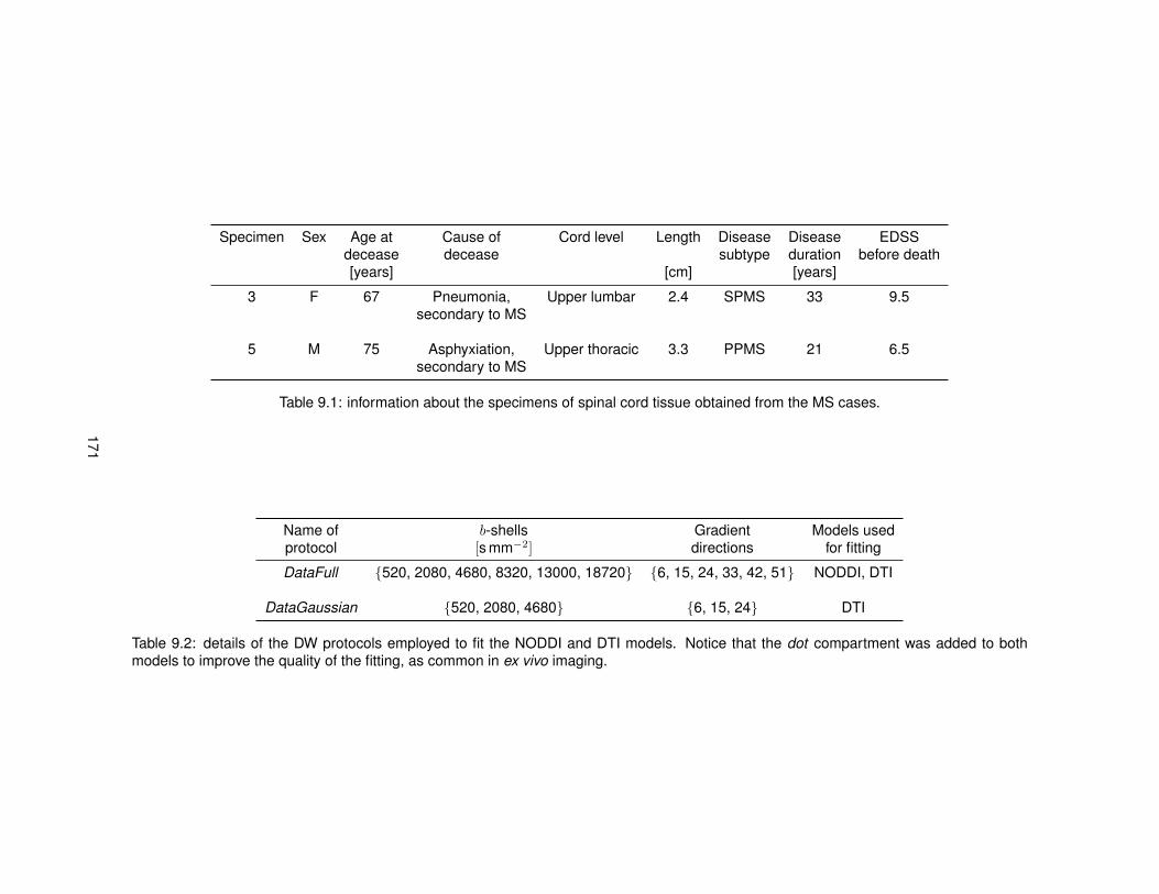
Specimen Sex Age at Cause of Cord level Length Disease Disease EDSSdecease decease subtype duration before death[years] [cm] [years]

3 F 67 Pneumonia, Upper lumbar 2.4 SPMS 33 9.5secondary to MS

5 M 75 Asphyxiation, Upper thoracic 3.3 PPMS 21 6.5secondary to MS

Table 9.1: information about the specimens of spinal cord tissue obtained from the MS cases.

Name of b-shells Gradient Models usedprotocol [s mm−2] directions for fitting

DataFull 520, 2080, 4680, 8320, 13000, 18720 6, 15, 24, 33, 42, 51 NODDI, DTI

DataGaussian 520, 2080, 4680 6, 15, 24 DTI

Table 9.2: details of the DW protocols employed to fit the NODDI and DTI models. Notice that the dot compartment was added to bothmodels to improve the quality of the fitting, as common in ex vivo imaging.

171

9.3.3 DW MRI signal model fitting

The NODDI model was fitted to the acquired data using the NODDI Matlab toolbox. We also fitteda second model of the DW signal, DTI, since DTI is still a routine method in clinical studies of thespinal cord [203] and is known to be sensitive to diffuse MS pathology [25, 99]. In-house Matlabcode implementing the same fitting algorithm as the NODDI Matlab Toolbox was used to fit theparameters of the DTI model.

Voxel-wise metrics

Model fitting was carried out after correcting b-values and gradient directions to account for addi-tional diffusion-weighting due to imaging and spoiling gradients, as previously described in detailin section 7.3.2 of chapter 7. Both NODDI and DTI models were fitted including an additional dotcompartment, since this improved the quality of fit, as previously discussed in chapter 7. The dotdescribes the contribution of a stationary water pool, and accounts for residual signal well abovethe noise floor that is measured even for very intense diffusion weighting and for gradient directionsparallel to WM fibres.

For NODDI, we fixed the intrinsic diffusivity of the isotropic compartment diso to the mean ADCwithin an ROI drawn manually in PBS voxels. Also, we fixed the intrinsic diffusivity of the neuraltissue d‖ to d‖ = 1.50 µm2 ms−1, as chapter 7 has shown that this value is a reasonable choice,providing good quality of fit.

The following voxel-wise metrics were obtained, whose meaning has been discussed in theprevious chapters of this thesis. For NODDI: isotropic (free water) volume fraction (viso); intra-neurite tissue volume fraction (vin); orientation dispersion index (ODI). For DTI: fractional anisotropy(FA); axial diffusivity (AD); radial diffusivity (RD); mean diffusivity (MD). Furthermore, the volumefraction of the dot compartment included for the fitting of both diffusion models was also obtained(DVFNODDI for NODDI and DVFDTI for DTI).

Data sets

The two diffusion models (NODDI and DTI, with the inclusion of the dot compartment) were fittedto the whole six-shell DW set of measurements (data set DataFull). Moreover, we fitted DTI to areduced data set, containing only the b = 520,2080,4680 s mm−2 shells (data set DataGaus-sian). This was done to limit the contribution of non-Gaussian diffusion, which is more evident asthe b-value increases [33], since DTI is a model that relies on the hypothesis of Gaussianity of thediffusion process.

Table 9.2 summarises the data sets employed in this chapter.

9.3.4 Histological procedures

Within one month of the MRI sessions, samples were taken to the Nuffield Department of ClinicalNeurosciences of the University of Oxford for histological processing.

172

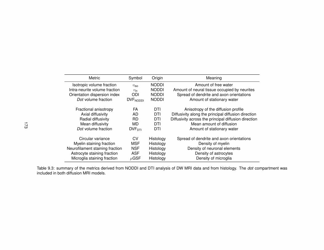
Metric Symbol Origin Meaning

Isotropic volume fraction viso NODDI Amount of free waterIntra-neurite volume fraction vin NODDI Amount of neural tissue occupied by neuritesOrientation dispersion index ODI NODDI Spread of dendrite and axon orientations

Dot volume fraction DVFNODDI NODDI Amount of stationary water

Fractional anisotropy FA DTI Anisotropy of the diffusion profileAxial diffusivity AD DTI Diffusivity along the principal diffusion direction

Radial diffusivity RD DTI Diffusivity across the principal diffusion directionMean diffusivity MD DTI Mean amount of diffusion

Dot volume fraction DVFDTI DTI Amount of stationary water

Circular variance CV Histology Spread of dendrite and axon orientationsMyelin staining fraction MSF Histology Density of myelin

Neurofilament staining fraction NSF Histology Density of neuronal elementsAstrocyte staining fraction ASF Histology Density of astrocytesMicroglia staining fraction µGSF Histology Density of microglia

Table 9.3: summary of the metrics derived from NODDI and DTI analysis of DW MRI data and from histology. The dot compartment wasincluded in both diffusion MRI models.

173

Strategy to determine the radiographic position of histological sections

Samples were dehydrated and embedded in paraffin, following standard histological procedures.Subsequently, 10µm-thick sections were sliced manually from the formalin-fixed paraffin-embeddedsamples using a microtome, for subsequent staining and optical imaging. The histological materialwas sectioned following the strategy previously described in chapter 7, section 7.3.3. Briefly, thematerial was sliced sagittaly, from the surface exposed by the midline cut performed with a surgicalblade prior to MRI. Consultation of the axial MRI views, onto which the sagittal slices acquired forDW imaging were overlaid, allowed the identification of the radiographic position of the histologicalsections. Shrinkage of the samples due to the dehydration necessary for paraffin embedding wasaccounted for, via measurement of the dimensions of the samples before and after the embeddingprocess.

Staining and optical imaging

For each spinal cord sample, four sections were obtained from two separate MRI slices (two sec-tions per MRI slice, 200µm apart from each other) and immunostained with primary antibodiesto demonstrate myelin (proteolipid protein, PLP), inflammation (microglia labelled with Iba1), andastrocytes (glial fibrillary acidic protein, GFAP), while neurons/axons were detected by both im-munohistochemistry (phosphorylated and non-phosphorylated neurofilaments) and impregnationwith an optimised [40,41] Palmgren’s silver procedure [145].

Afterwards, high resolution optical images of the stained sections were acquired in digital formatwith an Aperio slide scanner (ScanScope AT Turbo) at a magnification of 400×, and downsampledfor a final pixel resolution of 1.008× 1.008µm2 pixel−2.

9.3.5 Histological feature calculation

The histological images were analysed with in-house Matlab code in order to extract quantitativefeatures to which NODDI and DTI metrics could be related. We estimated neurite orientation dis-persion and the fraction of material stained by the neurofilamants, PLP, Iba1 and GFAP immunos-tains. Histological features were evaluated patch-by-patch, after dividing the histological imagesinto patches of size of 164×200 µm2, matching the within-slice MRI resolution. All histologicalfeatures are defined in the range [0; 1].

Neurite orientation dispersion

Neurite orientation dispersion was estimated from the sections impregnated with the Palmgren’ssilver method. They were preferred to the neurofilaments images since Palmgren’s silver impreg-nation [145] more consistently demonstrates axons as compared to neurofilaments [41], at the priceof a lower specificity.

The local image orientation was evaluated for all Palmgren’s silver images with ST analysis. Weused the same routines employed for the study described in the previous chapter, choosing σ =

174

0.89µm to control the spatial scale of analysis (detailed description of the Matlab implementationavailable in section 8.4.2 of chapter 8).

We calculated patch-wise circular variance (CV) of ST-derived orientation according to equa-tion 8.8 to obtain an index of neurite orientation dispersion, after manual removal of gross cellbodies and blood vessels. CV ranges in [0; 1], with increasing CV implying increasing orientationdispersion. CV was obtained according to a conventional Watson model, which was preferred toour weighted-Watson approach. Preliminary exploratory tests demonstrated that the values of CVobtained with the conventional Watson model (equation 8.8) and with the novel weighted-Watsonmodel (equation 8.15) are highly correlated, and follow similar trends. For this reason, a conven-tional model was employed as a first exploratory step, appearing suitable for the purposes of thestudy.

Fractions of stained material

We evaluated the fractions of material labelled by the immunohistochemistry within the samepatches of size 164×200 µm2 employed for the calculation of the CV. As a preprocessing step,spatial linear trends of the staining intensity were removed.

For each image, a well established clustering algorithm (k-means with k-means++ initialisation[6]) was run in Matlab to segment the stained material. We chose to segment three clusters,representing the space of the cover slip outside the specimen, the specimen background and theactual stained material. We considered as stained material pixels belonging to the darkest cluster.

Finally, we evaluated patch-wise fraction of stained material as the ratio between the number ofpixels that were segmented in each patch and the total number of pixels in the same patch.

The following nomenclature will be employed for the indices of staining fraction, which all rangein [0; 1]: myelin staining fraction (MSF) for the PLP immunostaining; neurofilament staining frac-tion (NSF) for the neurofilament immunostaining; astrocyte staining fraction (ASF), for the GFAPimmunostaining; microglia staining fraction (µGSF) for the Iba1 immunostaining.

Table 9.3 recapitulates the metrics the were object of analysis in this chapter.

9.3.6 MRI-histology registration

Histological images were registered to the corresponding MRI slices from which the histologicalmaterial was obtained. The registration transformation were then applied to the quantitative histo-logical maps, which were evaluated in native histology space.

We implemented a landmark-guided non-linear registration similar to other approaches previ-ously reported in literature [99], basing our algorithm on Matlab routines (Image Processing Tool-box, function fitgeotrans). For each histological image, we proceeded as follows.

1. The histological image was downsampled to the resolution of the patch-wise maps and of thewithin-MRI-slice resolution (164×200 µm2);

2. we visually identified and manually marked matching control points in the downsampled his-tological image and in the corresponding mean b = 0 image from MRI;

175

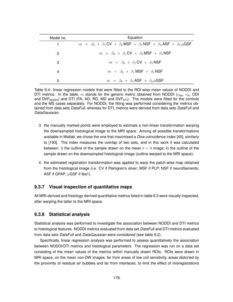
http://uk.mathworks.com/help/images/ref/fitgeotrans.html

Model no. Equation

1 m = β0 + β1 CV + β2 MSF + β3 NSF + β4 ASF + β5 µGSF

2 m = β0 + β1 CV + β2 MSF + β3 NSF

3 m = β0 + β1 CV + β2 NSF

4 m = β0 + β1 MSF + β2 NSF

5 m = β0 + β1 ASF + β2 µGSF

Table 9.4: linear regression models that were fitted to the ROI-wise mean values of NODDI andDTI metrics. In the table, m stands for the generic metric obtained from NODDI (viso, vin, ODIand DVFNODDI) and DTI (FA, AD, RD, MD and DVFDTI). The models were fitted for the controlsand the MS cases separately. For NODDI, the fitting was performed considering the metrics ob-tained from data sets DataFull, whereas for DTI, metrics were derived from data sets DataFull andDataGaussian.

3. the manually marked points were employed to estimate a non-linear transformation warpingthe downsampled histological image to the MRI space. Among all possible transformationsavailable in Matlab, we chose the one that maximised a Dice coincidence index [45], similarlyto [193]. The index measures the overlap of two sets, and in this work it was calculatedbetween: i) the outline of the sample drawn on the mean b = 0 image; ii) the outline of thesample drawn on the downsampled histological image (outline warped to the MRI space);

4. the estimated registration transformation was applied to warp the patch-wise map obtainedfrom the histological image (i.e. CV if Palmgren’s silver; MSF if PLP; NSF if neurofilaments;ASF if GFAP; µGSF if Iba1).

9.3.7 Visual inspection of quantitative maps

All MRI-derived and histology-derived quantitative metrics listed in table 9.3 were visually inspected,after warping the latter to the MRI space.

9.3.8 Statistical analysis

Statistical analysis was performed to investigate the association between NODDI and DTI metricsto histological features. NODDI metrics evaluated from data set DataFull and DTI metrics evaluatedfrom data sets DataFull and DataGaussian were considered (see table 9.2).

Specifically, linear regression analysis was performed to assess quantitatively the associationbetween NODDI/DTI metrics and histological parameters. The regression was run on a data setconsisting of the mean values of the metrics within manually drawn ROIs. ROIs were drawn inMRI space, on the mean non-DW images, far from areas of low coil sensitivity, areas distorted bythe proximity of residual air bubbles and far from interfaces, to limit the effect of misregistrations

176

histology-MRI. In practice, the ROIs were drawn within non-focal WM and GM and within focal WMand GM lesions for the MS cases. On the other hand, for the control cases, ROIs were outlined inWM and GM.

Before running the regressions, values from the two different histological sections taken fromeach MRI slice were averaged.

Choice of outcome measures and predictors

The set of ROI-wise values of MRI and histological indices was used to regress each MRI metric m(outcome measure) as a linear combination of histological indices CV, MSF, NSF, ASF and µGSF(predictors). We chose MRI indices as outcome measures since in practice one would use MRI asa non-invasive probe of the underlying, unknown histological features. With an analogy borrowedfrom engineering, MRI indices would practically be used as “sensors” of the underlying histologicalcharacteristics. The scenario is similar, for instance, to that of certain chemosensors based onISFET technology [143], used to measure concentrations of ions in solutions. Such sensors in factprovide as output a voltage or electric current, which is the true outcome of any experiment andfrom which the underlying ion concentration needs to be inferred. The voltage/current is practicallyhandled as a dependent variable, and used as a probe of the ion concentration. In our view, thesame holds here, since NODDI/DTI metrics are the outcome of the MRI experiment, and act asprobes of the underlying microstructural properties, from which they depend.

Our analysis allows the evaluation of the sensitivity of each MRI metric m with respect to thehistological parameters (i.e. quantities ∂m

∂CV , ∂m∂MSF , ∂m

∂NSF , ∂m∂ASF and ∂m

∂µGSF ), while controlling forspecificity, since the effect of all histological features can be modelled jointly.

Linear regression models

In this work, we fitted five different univariable linear regression models, independently for the con-trol cases and the MS cases, using the R software (http://www.r-project.org, function lm).The five models are listed in table 9.4, and focus on the relation between NODDI/DTI metrics withdifferent aspects of the neural tissue cellular environment.

The first model employs all histological features as joint predictors of MRI. In addition, wegrouped histological metrics into features directly related to neurons/neurites (CV, MSF and NSF, inmodel number 2) and features of extra-neurite space (glial fractions ASF and µGSF, in model num-ber 5). This allows the investigation of whether NODDI/DTI metrics are more strongly associated toone group of features, rather than the other, which follows from fitting separately models 2 and 5.

Moreover, we derived two additional models from the features mapping properties of neu-rons/axons (CV, MSF and NSF). Model number 3 focusses on the joint dependence of MRI metricson the orientation dispersion and on the density of neuronal processes. These two features arebelieved to be key factors contributing to the diffusion signal profile in neural tissue [88, 215], andmodel number 3 enables the investigation of their joint contribution to the outcome MRI metrics.On the other hand, model number 4 was formulated to study specifically demyelination and ax-

177

http://www.r-project.org

https://stat.ethz.ch/R-manual/R-devel/library/stats/html/lm.html

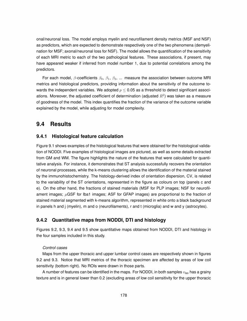
onal/neuronal loss. The model employs myelin and neurofilament density metrics (MSF and NSF)as predictors, which are expected to demonstrate respectively one of the two phenomena (demyeli-nation for MSF; axonal/neuronal loss for NSF). The model allows the quantification of the sensitivityof each MRI metric to each of the two pathological features. These associations, if present, mayhave appeared weaker if inferred from model number 1, due to potential correlations among thepredictors.

For each model, β-coefficients β0, β1, β2, ... measure the association between outcome MRImetrics and histological predictors, providing information about the sensitivity of the outcome to-wards the independent variables. We adopted p ≤ 0.05 as a threshold to detect significant associ-ations. Moreover, the adjusted coefficient of determination (adjusted R2) was taken as a measureof goodness of the model. This index quantifies the fraction of the variance of the outcome variableexplained by the model, while adjusting for model complexity.

9.4 Results

9.4.1 Histological feature calculation

Figure 9.1 shows examples of the histological features that were obtained for the histological valida-tion of NODDI. Five examples of histological images are pictured, as well as some details extractedfrom GM and WM. The figure highlights the nature of the features that were calculated for quanti-tative analysis. For instance, it demonstrates that ST analysis successfully recovers the orientationof neuronal processes, while the k-means clustering allows the identification of the material stainedby the immunohistochemistry. The histology-derived index of orientation dispersion, CV, is relatedto the variability of the ST orientations, represented in the figure as colours on top (panels c ande). On the other hand, the fractions of stained materials (MSF for PLP images; NSF for neurofil-ament images; µGSF for Iba1 images; ASF for GFAP images) are proportional to the fraction ofstained material segmented with k-means algorithm, represented in white onto a black backgroundin panels h and j (myelin), m and o (neurofilaments), r and t (microglia) and w and y (astrocytes).

9.4.2 Quantitative maps from NODDI, DTI and histology

Figures 9.2, 9.3, 9.4 and 9.5 show quantitative maps obtained from NODDI, DTI and histology inthe four samples included in this study.

Control casesMaps from the upper thoracic and upper lumbar control cases are respectively shown in figures

9.2 and 9.3. Notice that MRI metrics of the thoracic specimen are affected by areas of low coilsensitivity (bottom right). No ROIs were drawn in those parts.

A number of features can be identified in the maps. For NODDI, in both samples viso has a grainytexture and is in general lower than 0.2 (excluding areas of low coil sensitivity for the upper thoracic

178

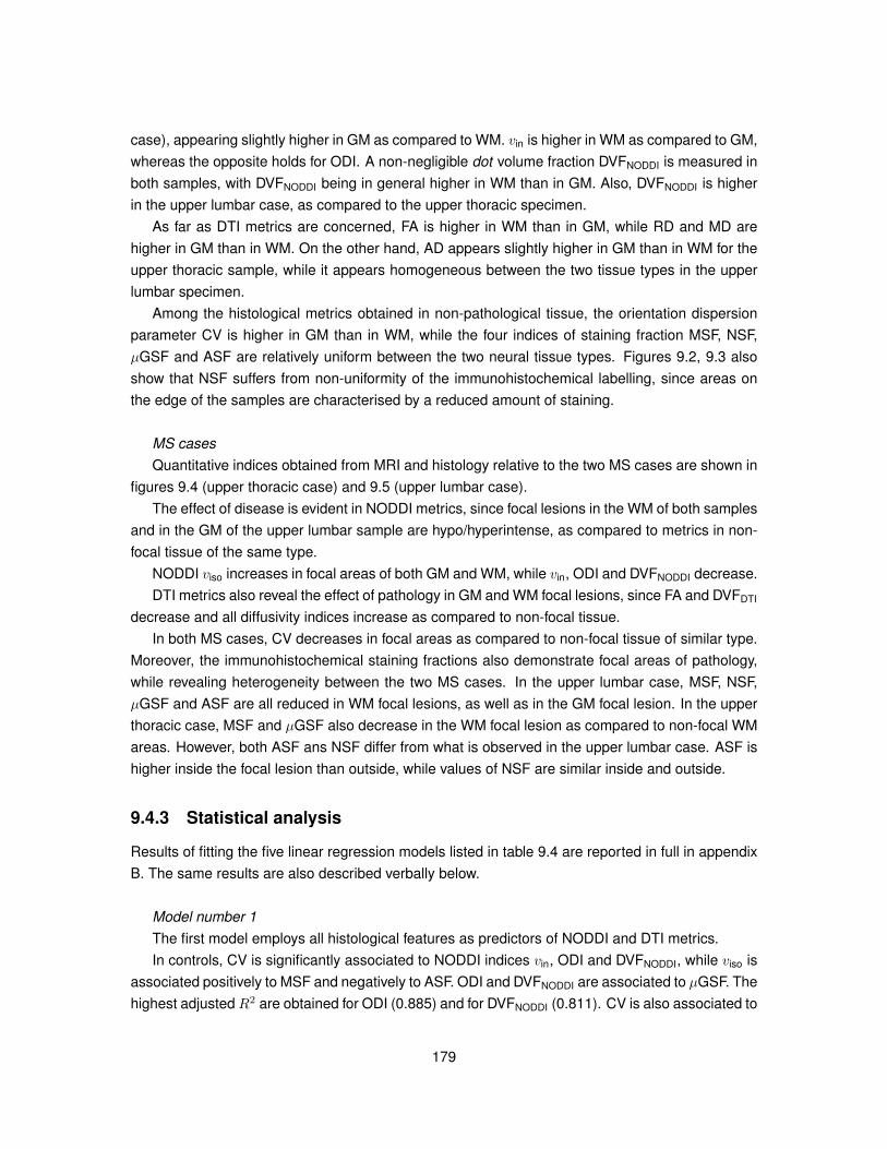
case), appearing slightly higher in GM as compared to WM. vin is higher in WM as compared to GM,whereas the opposite holds for ODI. A non-negligible dot volume fraction DVFNODDI is measured inboth samples, with DVFNODDI being in general higher in WM than in GM. Also, DVFNODDI is higherin the upper lumbar case, as compared to the upper thoracic specimen.

As far as DTI metrics are concerned, FA is higher in WM than in GM, while RD and MD arehigher in GM than in WM. On the other hand, AD appears slightly higher in GM than in WM for theupper thoracic sample, while it appears homogeneous between the two tissue types in the upperlumbar specimen.

Among the histological metrics obtained in non-pathological tissue, the orientation dispersionparameter CV is higher in GM than in WM, while the four indices of staining fraction MSF, NSF,µGSF and ASF are relatively uniform between the two neural tissue types. Figures 9.2, 9.3 alsoshow that NSF suffers from non-uniformity of the immunohistochemical labelling, since areas onthe edge of the samples are characterised by a reduced amount of staining.

MS casesQuantitative indices obtained from MRI and histology relative to the two MS cases are shown in

figures 9.4 (upper thoracic case) and 9.5 (upper lumbar case).The effect of disease is evident in NODDI metrics, since focal lesions in the WM of both samples

and in the GM of the upper lumbar sample are hypo/hyperintense, as compared to metrics in non-focal tissue of the same type.

NODDI viso increases in focal areas of both GM and WM, while vin, ODI and DVFNODDI decrease.DTI metrics also reveal the effect of pathology in GM and WM focal lesions, since FA and DVFDTI

decrease and all diffusivity indices increase as compared to non-focal tissue.In both MS cases, CV decreases in focal areas as compared to non-focal tissue of similar type.

Moreover, the immunohistochemical staining fractions also demonstrate focal areas of pathology,while revealing heterogeneity between the two MS cases. In the upper lumbar case, MSF, NSF,µGSF and ASF are all reduced in WM focal lesions, as well as in the GM focal lesion. In the upperthoracic case, MSF and µGSF also decrease in the WM focal lesion as compared to non-focal WMareas. However, both ASF ans NSF differ from what is observed in the upper lumbar case. ASF ishigher inside the focal lesion than outside, while values of NSF are similar inside and outside.

9.4.3 Statistical analysis

Results of fitting the five linear regression models listed in table 9.4 are reported in full in appendixB. The same results are also described verbally below.

Model number 1The first model employs all histological features as predictors of NODDI and DTI metrics.In controls, CV is significantly associated to NODDI indices vin, ODI and DVFNODDI, while viso is

associated positively to MSF and negatively to ASF. ODI and DVFNODDI are associated to µGSF. Thehighest adjustedR2 are obtained for ODI (0.885) and for DVFNODDI (0.811). CV is also associated to

179

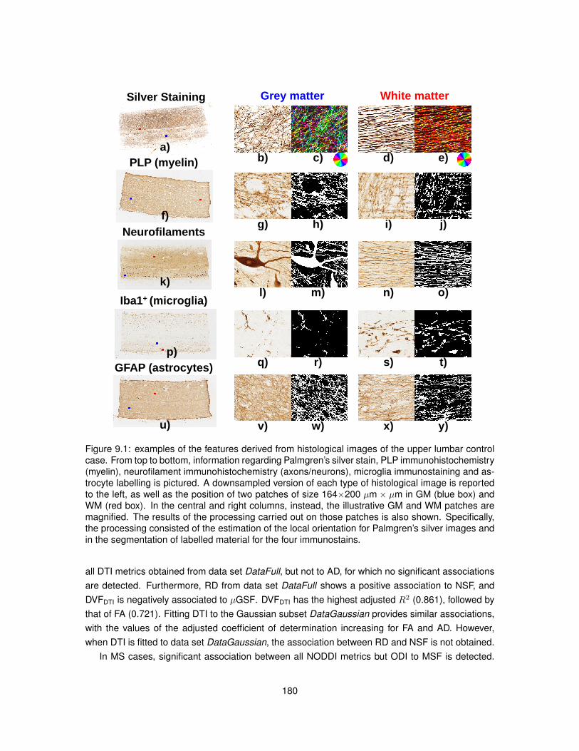
a)

PLP (myelin)

Neurofilaments

Iba1+ (microglia)

GFAP (astrocytes)

Grey matter White matterSilver Staining

f)

b) c) d) e)

g) h) i) j)

k)l) m) n) o)

p)q) r) s) t)

v) w) x) y)u)

Figure 9.1: examples of the features derived from histological images of the upper lumbar controlcase. From top to bottom, information regarding Palmgren’s silver stain, PLP immunohistochemistry(myelin), neurofilament immunohistochemistry (axons/neurons), microglia immunostaining and as-trocyte labelling is pictured. A downsampled version of each type of histological image is reportedto the left, as well as the position of two patches of size 164×200 µm × µm in GM (blue box) andWM (red box). In the central and right columns, instead, the illustrative GM and WM patches aremagnified. The results of the processing carried out on those patches is also shown. Specifically,the processing consisted of the estimation of the local orientation for Palmgren’s silver images andin the segmentation of labelled material for the four immunostains.

all DTI metrics obtained from data set DataFull, but not to AD, for which no significant associationsare detected. Furthermore, RD from data set DataFull shows a positive association to NSF, andDVFDTI is negatively associated to µGSF. DVFDTI has the highest adjusted R2 (0.861), followed bythat of FA (0.721). Fitting DTI to the Gaussian subset DataGaussian provides similar associations,with the values of the adjusted coefficient of determination increasing for FA and AD. However,when DTI is fitted to data set DataGaussian, the association between RD and NSF is not obtained.

In MS cases, significant association between all NODDI metrics but ODI to MSF is detected.

180

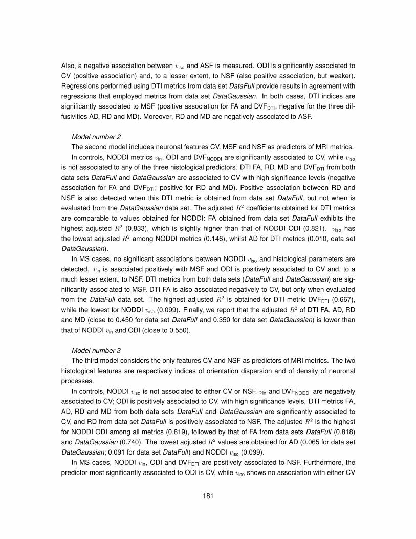
Also, a negative association between viso and ASF is measured. ODI is significantly associated toCV (positive association) and, to a lesser extent, to NSF (also positive association, but weaker).Regressions performed using DTI metrics from data set DataFull provide results in agreement withregressions that employed metrics from data set DataGaussian. In both cases, DTI indices aresignificantly associated to MSF (positive association for FA and DVFDTI, negative for the three dif-fusivities AD, RD and MD). Moreover, RD and MD are negatively associated to ASF.

Model number 2The second model includes neuronal features CV, MSF and NSF as predictors of MRI metrics.In controls, NODDI metrics vin, ODI and DVFNODDI are significantly associated to CV, while viso

is not associated to any of the three histological predictors. DTI FA, RD, MD and DVFDTI from bothdata sets DataFull and DataGaussian are associated to CV with high significance levels (negativeassociation for FA and DVFDTI; positive for RD and MD). Positive association between RD andNSF is also detected when this DTI metric is obtained from data set DataFull, but not when isevaluated from the DataGaussian data set. The adjusted R2 coefficients obtained for DTI metricsare comparable to values obtained for NODDI: FA obtained from data set DataFull exhibits thehighest adjusted R2 (0.833), which is slightly higher than that of NODDI ODI (0.821). viso hasthe lowest adjusted R2 among NODDI metrics (0.146), whilst AD for DTI metrics (0.010, data setDataGaussian).

In MS cases, no significant associations between NODDI viso and histological parameters aredetected. vin is associated positively with MSF and ODI is positively associated to CV and, to amuch lesser extent, to NSF. DTI metrics from both data sets (DataFull and DataGaussian) are sig-nificantly associated to MSF. DTI FA is also associated negatively to CV, but only when evaluatedfrom the DataFull data set. The highest adjusted R2 is obtained for DTI metric DVFDTI (0.667),while the lowest for NODDI viso (0.099). Finally, we report that the adjusted R2 of DTI FA, AD, RDand MD (close to 0.450 for data set DataFull and 0.350 for data set DataGaussian) is lower thanthat of NODDI vin and ODI (close to 0.550).

Model number 3The third model considers the only features CV and NSF as predictors of MRI metrics. The two

histological features are respectively indices of orientation dispersion and of density of neuronalprocesses.

In controls, NODDI viso is not associated to either CV or NSF. vin and DVFNODDI are negativelyassociated to CV; ODI is positively associated to CV, with high significance levels. DTI metrics FA,AD, RD and MD from both data sets DataFull and DataGaussian are significantly associated toCV, and RD from data set DataFull is positively associated to NSF. The adjusted R2 is the highestfor NODDI ODI among all metrics (0.819), followed by that of FA from data sets DataFull (0.818)and DataGaussian (0.740). The lowest adjusted R2 values are obtained for AD (0.065 for data setDataGaussian; 0.091 for data set DataFull) and NODDI viso (0.099).

In MS cases, NODDI vin, ODI and DVFDTI are positively associated to NSF. Furthermore, thepredictor most significantly associated to ODI is CV, while viso shows no association with either CV

181

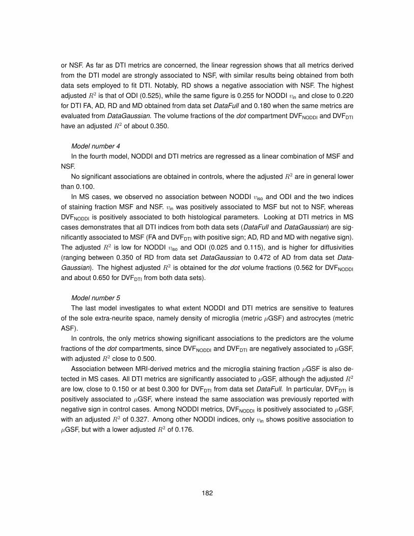
or NSF. As far as DTI metrics are concerned, the linear regression shows that all metrics derivedfrom the DTI model are strongly associated to NSF, with similar results being obtained from bothdata sets employed to fit DTI. Notably, RD shows a negative association with NSF. The highestadjusted R2 is that of ODI (0.525), while the same figure is 0.255 for NODDI vin and close to 0.220for DTI FA, AD, RD and MD obtained from data set DataFull and 0.180 when the same metrics areevaluated from DataGaussian. The volume fractions of the dot compartment DVFNODDI and DVFDTI

have an adjusted R2 of about 0.350.

Model number 4In the fourth model, NODDI and DTI metrics are regressed as a linear combination of MSF and

NSF.No significant associations are obtained in controls, where the adjusted R2 are in general lower

than 0.100.In MS cases, we observed no association between NODDI viso and ODI and the two indices

of staining fraction MSF and NSF. vin was positively associated to MSF but not to NSF, whereasDVFNODDI is positively associated to both histological parameters. Looking at DTI metrics in MScases demonstrates that all DTI indices from both data sets (DataFull and DataGaussian) are sig-nificantly associated to MSF (FA and DVFDTI with positive sign; AD, RD and MD with negative sign).The adjusted R2 is low for NODDI viso and ODI (0.025 and 0.115), and is higher for diffusivities(ranging between 0.350 of RD from data set DataGaussian to 0.472 of AD from data set Data-Gaussian). The highest adjusted R2 is obtained for the dot volume fractions (0.562 for DVFNODDI

and about 0.650 for DVFDTI from both data sets).

Model number 5The last model investigates to what extent NODDI and DTI metrics are sensitive to features

of the sole extra-neurite space, namely density of microglia (metric µGSF) and astrocytes (metricASF).

In controls, the only metrics showing significant associations to the predictors are the volumefractions of the dot compartments, since DVFNODDI and DVFDTI are negatively associated to µGSF,with adjusted R2 close to 0.500.

Association between MRI-derived metrics and the microglia staining fraction µGSF is also de-tected in MS cases. All DTI metrics are significantly associated to µGSF, although the adjusted R2

are low, close to 0.150 or at best 0.300 for DVFDTI from data set DataFull. In particular, DVFDTI ispositively associated to µGSF, where instead the same association was previously reported withnegative sign in control cases. Among NODDI metrics, DVFNODDI is positively associated to µGSF,with an adjusted R2 of 0.327. Among other NODDI indices, only vin shows positive association toµGSF, but with a lower adjusted R2 of 0.176.

182

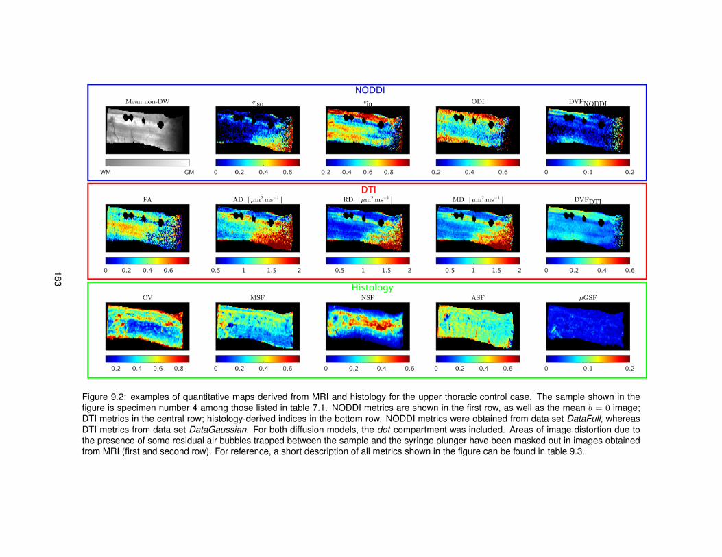
Figure 9.2: examples of quantitative maps derived from MRI and histology for the upper thoracic control case. The sample shown in thefigure is specimen number 4 among those listed in table 7.1. NODDI metrics are shown in the first row, as well as the mean b = 0 image;DTI metrics in the central row; histology-derived indices in the bottom row. NODDI metrics were obtained from data set DataFull, whereasDTI metrics from data set DataGaussian. For both diffusion models, the dot compartment was included. Areas of image distortion due tothe presence of some residual air bubbles trapped between the sample and the syringe plunger have been masked out in images obtainedfrom MRI (first and second row). For reference, a short description of all metrics shown in the figure can be found in table 9.3.

183

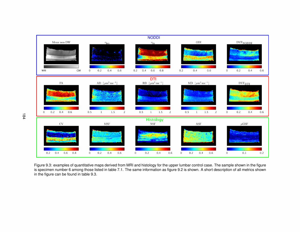
Figure 9.3: examples of quantitative maps derived from MRI and histology for the upper lumbar control case. The sample shown in the figureis specimen number 6 among those listed in table 7.1. The same information as figure 9.2 is shown. A short description of all metrics shownin the figure can be found in table 9.3.

184

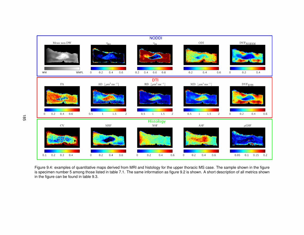
Figure 9.4: examples of quantitative maps derived from MRI and histology for the upper thoracic MS case. The sample shown in the figureis specimen number 5 among those listed in table 7.1. The same information as figure 9.2 is shown. A short description of all metrics shownin the figure can be found in table 9.3.

185

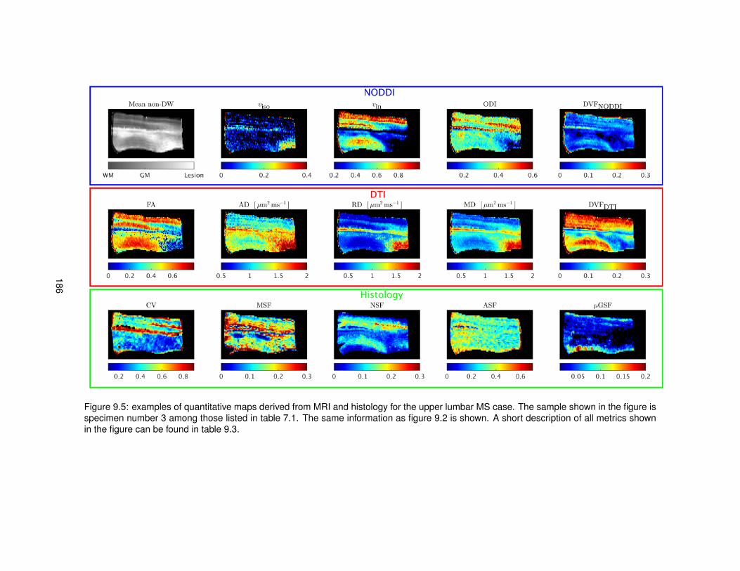
Figure 9.5: examples of quantitative maps derived from MRI and histology for the upper lumbar MS case. The sample shown in the figure isspecimen number 3 among those listed in table 7.1. The same information as figure 9.2 is shown. A short description of all metrics shownin the figure can be found in table 9.3.

186

9.5 Discussion

In this chapter we studied the histological correlates of NODDI metrics in the spinal cord. Weperformed MRI scans at high field on four specimens of post mortem human spinal cord (twonon-pathological cases and two progressive cases of MS), and derived NODDI and DTI metrics.For NODDI, we obtained voxel-wise estimates of isotropic (free water) volume fraction (viso), intra-neurite tissue volume fraction (vin), orientation dispersion index (ODI) and stationary water (dot)volume fraction (DVFNODDI). For DTI, we instead calculated fractional anisotropy (FA), axial, radialand mean diffusivities (AD/RD/MD), as well as stationary water (dot) volume fraction (DVFDTI).

Moreover, histological sections were also obtained at known radiographic position, and stainedto label neurons/axons, myelin, astrocytes and microglia. Optical imaging provided high resolutionimages of the stained sections, which were processed with well established digital image process-ing methods. This provided features quantifying neurite orientation dispersion (circular varianceCV) and density of myelin (MSF), neurofilaments (NSF), astrocytes (ASF) and microglia (µGSF).The histological features were finally warped to the MRI space via manual registration.

All quantitative maps were visually inspected. Furthermore, five univariable linear regressionmodels were fitted to evaluate the sensitivity of each MRI metric to the histological features. Ourregressions also controlled for specificity, since the dependence of each individual MRI metric onmultiple histological features was modelled jointly.

Trends on visual inspection: NODDI metricsVisual inspection proved that NODDI metrics obtained in control cases follow patterns that agree

well with trends previously shown in vivo in chapter 4. For instance, the neurite density index vin issmaller in GM than in WM, while the opposite holds for the index of neurite orientation dispersionODI.

NODDI metrics are also sensitive to MS pathology, since in the MS specimens areas of focaldamage are evident in all metrics. In lesions, we observe an increase of isotropic volume fraction(viso), as well as a reduction of both neurite density vin and ODI. The reduction of vin is plausiblesince axonal loss is a known feature of MS [41], whereas the reduction of ODI in lesions, clearfor instance in figure 9.4, is probably less intuitive. This latter finding suggests that neuronal fibresare more parallel in focal lesions than they are in non-focal areas. This may be indicative of areduction of the complexity of the tissue. The reduction in complexity may affect the amount ofinformation that can be conveyed, with consequent impairment of sensorimotor functions. Also, itis known that small fibres are more likely to be lost in the MS spinal cord, as compared to largeones [41]. Therefore, we speculate that the big axons that survive in MS lesions may be the leastundulated, since we expect that the characteristic undulation length increases as the calibre of theaxon increases. This may also lead to a reduction of orientation dispersion at the MRI voxel scale,as each MRI voxel would essentially contain axons characterised by less undulation.

Finally, the dot volume fraction DVFNODDI shows a contrast among tissues that reflects that ofvin, although the range of values varies notably from specimen to specimen.

187

Trends on visual inspection: DTI metricsDTI metrics FA, RD and MD in controls are consistent with what we showed in chapter 4 in vivo.

FA is higher in WM than in GM, RD is higher in GM than in WM and MD is rather homogeneousbetween the two tissue types. However, in our data AD is higher in GM than in WM, unlike whatwe showed in vivo in the previous chapters. We suspect that this could be an effect of the fixationprocess, which seems to have increased the restriction parallel to WM fibres, as also flagged bythe relatively high values of dot volume fractions DVFNODDI and DVFDTI measured in WM. Thepresence of a highly restricted, almost stationary water pool in fixed neural tissue has been reportedbefore [4, 146, 170], and has been attributed to water trapped in small structures such as glialcells [4].

DTI metrics detect areas of focal lesion, which are characterised by a reduction of FA and anincrease of AD, RD and MD. These trends are consistent with previous literature [99]. Interestingly,despite the reduction of neurite orientation dispersion ODI in focal lesions, which we expect to beconcomitant to an increase of FA (panel A of figure 4.8), we observed an overall reduction of FA.FA is influenced by both density and orientation dispersion of neuronal processes, of which NODDIODI and vin provide estimates. In focal lesions, both ODI and vin are reduced. The former is ex-pected to contribute to an increase of FA, whilst the second to a decrease. Overall, we observe areduction of FA, implying that the reduction of neurite density has a stronger effect on FA than thereduction of ODI. This latter effect seems to be more subtle, and it can not be detected by lookingat FA.

Trends on visual inspection: histological metricsQuantitative histological maps were also obtained for the four samples, and warped to the MRI

space. In controls, the staining fractions MSF (myelin), NSF (neurofilaments), ASF (astrocytes)and µGSF (microglia) are relatively homogeneous between GM and WM, whereas the orientationdispersion index CV shows a clear contrast between GM and WM. CV is higher in GM than in WM,demonstrating the higher complexity in terms or neurite orientations of the former compared to thelatter. CV confirms the trend showed by NODDI ODI, which is its direct MRI counterpart.

Histological maps demonstrate MS pathology, revealing the same areas of focal lesion that arevisible in MRI images. In both MS cases, for instance, CV is reduced in focal lesions. This is animportant result per se, since to our knowledge the effect of MS pathology on neurite complexity hasnever been studied on histological material derived from human tissue before. Our results supportthe hypothesis of MS as a disease reducing the complexity of neural tissue, in line with recentfindings in a cohort of MS patients at cortical level [132]. Moreover, CV confirms the trends shownby NODDI ODI, which also detects a reduction of neurite orientation dispersion in MS lesions.

The staining fractions MSF, NSF, ASF and µGSF also demonstrate focal lesions, but with certaindifferences between the two MS cases. In both specimens, MSF and µGSF decrease in areas offocal pathology, highlighting demyelination and suggesting the presence of little activated microglia(i.e. little inflammation). The absence of inflammation is expected, since the two MS specimenswere obtained from two chronic patients who were affected by MS for more than 20 years. However,while in the upper lumbar case also NSF and ASF decrease in focal areas, in the upper thoracic

188

case ASF and NSF do not do so. In the upper thoracic case, ASF is higher within the focal WMas compared to non-focal WM, while values of NSF are relatively similar in both. The MS lesion ofthis sample, well evident in figure 9.4, is therefore characterised by little amount of axonal loss, andappears as a dense astrocytic scar, a known feature of chronic MS [73]. The differences betweenthe two MS cases are plausible and are not surprising, given the known heterogeneity of tissueinjury mechanism among MS patients [105].

Interestingly, in the upper lumbar MS case, MSF and NSF decrease in focal lesions, indicatingdemyelination and axonal loss. On the other hand, in the upper thoracic MS case, only MSF de-creases in the focal area, pointing towards demyelination but negligible axonal loss. However, theNODDI-derived index of neurite density vin decreases dramatically in the MS focal lesions of bothcases. Therefore, the two phenomena (demyelination and axonal loss) seem to be both factorsthat can be associated to vin. Although the decrease of vin in lesions could be a consequence ofthe altered permeability of the axon [104, 163], variations of myelin density may affect vin directly.This fact could be explained considering the multicomponent origin of spin-spin relaxation in neuraltissue. Myelin water has a very short T2, on the order of 10 ms in vivo [212]. Therefore, at the echotimes usually employed in DW experiments, myelin signal decays and does not contribute to themeasurements. However, in demyelinated areas, myelin is replaced by material that may have alonger T2, effectively increasing the amount of MRI visible water. Therefore, this suffices per se tocause a reduction of the neurite density, even without occurrence of axonal loss. Ultimately, thefraction of water within neurites with respect to the total amount of visible water may decrease dueto the increase of the amount of visible water, rather than due to the decrease of the amount ofintra-neurite water.

Statistical analysis: design of modelsWe compared NODDI and DTI metrics obtained from the whole set of DW measurements and

DTI metrics obtained from a Gaussian subset of measurements to histology. We fitted five linearregression models to quantify the strength of the association between histological features and MRImetrics. The models allow the evaluation of the sensitivity of each DW MRI metric with respect toindividual histological features, while controlling for specificity.

The first model considers all histological metrics as predictors of MRI indices. The other models,instead, employ only subsets of the histological features as independent variables. They focus onspecific aspects of neuronal tissue microstructure, which may not be fully characterised by modelnumber 1, due to potential correlations among predictors (five in that model). The second modelconsiders only neuronal features (myelin and neuronal element density; orientation dispersion),whereas features of the extra-neurite space (astrocyte and microglia density) are considered inmodel number 5. From model number 2, other two models are also obtained. The third modelaccounts for density and orientation dispersion of neuronal elements, to investigate how the two,believed to be key factors of the diffusion MRI signal profile, jointly contribute to NODDI and DTImetrics. The fourth model instead accounts for myelin and neuronal element densities, enablingthe study of how demyelination and axonal/neuronal loss affect MRI indices.

189

Statistical analysis: association NODDI-histologyOverall, our statistical analysis proves that ODI is the DW MRI metric most specific to histology,

among those considered in this study. Moreover, NODDI metrics are specific to neuronal elementsand do not show any clear association to features of the extra-neurite space, namely density ofastrocytes and microglia. This is demonstrated, for instance, by the higher adjusted R2 of model 2as compared to model 5.

The statistical analysis shows different associations between NODDI metrics and histologicalfeatures in control cases and in MS cases.

In controls, the measure of orientation dispersion derived from histology, CV, is the main factorexplaining the variation of all NODDI metrics. This appears as an effect of its high contrast, sincethe remaining metrics of staining fraction show little difference between GM and WM. Therefore,the only metric capable of explaining the between-tissue contrast of NODDI maps is CV.

On the other hand, in MS cases, the feature that drives the variability of almost all NODDImetrics is MSF, an index of myelin density. This is again quite possibly a result of the high between-region contrast of MSF. As an exception, NODDI ODI is the only MRI-derived metric that even in MScases exhibits consistently sensitivity to CV. ODI shows no association to MSF, even when CV is notincluded as a predictor variable (model number 4), and has a weak, positive association to NSF.The association to NSF may be a consequence of the highest chance of observing orientationdispersion of neuronal elements when these are in a greater number (i.e. when NSF is higher).Moreover, ODI shows the highest values of the adjusted R2 coefficient, demonstrating that most ofthe variability of ODI can be explained by the variability of histological features via linear regression.ODI faithfully replicates the patterns of histology-derived orientation dispersion, and allows thesystematic detection of variations of neural tissue complexity in focal lesions, surpassing even theperformance of well established DTI FA.

Our analysis demonstrates that NODDI vin, a descriptor of axon and dendrite density, is poten-tially sensitive to axonal loss in MS, as demonstrated by the positive association with NSF in MScases for model number 3. However, demyelination seems to be a phenomenon that can explainthe observed trends of vin, even more than axonal loss. This is demonstrated by the fact that NSFis not the strongest correlate of vin in controls, and when the sensitivities of vin to MSF and NSFare compared (model number 4), the former is stronger than the latter. Although the associationbetween decrease of vin and demyelination could be a consequence of the increases permeabilityof demyelinated axons [104, 163], variations of myelin density may affect vin directly. The appar-ent reduction of neurite density in demyelinated areas could be a consequence of the increasedamount of visible water, discussed above, even when neurites are not reduced in number. In de-myelinated areas, myelin, which is MRI-invisible, may be replaced by MRI-visible water. Hence, vin,which is proportional to the ratio between the intra-neurite water and the total amount of MRI-visiblewater, may decrease due to the increased amount of MRI visible water. Overall, vin appears as asurrogate index of focal damage, potentially able to convey information about both axonal loss anddemyelination. vin on its own does not appear to suffice to distinguish between the demyelinationof axonal elements and axonal loss. Nonetheless, its combination with myelin density indices frommyelin water imaging [107] or quantitative magnetisation transfer [164] may help overcome this

190

issue, as recently demonstrated in g-ratio mapping [173].Lastly, our result do not allow the identification of strong associations between NODDI viso and

the histological features object of this study. NODDI viso is designed to capture the amount of freewater in a voxel, as in areas of partial volume with the liquid surrounding the brain parenchyma. Inthis chapter, we demonstrated that viso is consistently hyperintense in focal WM lesions, agreeingwith preliminary findings in vivo [156]. However, the metric did not show any clear association withhistological metrics other than a negative association with the density of astrocytes (ASF), but onlywhen all histological indices were considered as predictors. viso is designed to capture the amountof free water in each MRI voxel. In our study, no histology-derived metrics quantifying this featurecould be obtained, also because specimens underwent dehydration as part of the histological pro-cessing. In conclusion, the lack of association between viso and our five histological features doesnot appear surprising.

Statistical analysis: association DTI-histologyAs far as DTI metrics are concerned, our results were in line with previously published find-

ings [99]. Similarly to NODDI, the main correlates of DTI metrics are CV in controls and MSF inMSF, possibly due to the high between-tissue-type contrast of CV in controls and MSF in MS cases.Moreover, DTI metrics do not show notable association to features of the extra-neurite space (den-sity of astrocytes and microglia).

DTI metrics are sensitive to demyelination and axonal loss, but can not detect other effects ofMS pathology, perhaps less evident, such as the decrease in neurite orientation dispersion. DTI FAis vaguely sensitive to CV in MS, but the sensitivity is lost in favour of a much stronger dependencyon NSF when the only features included as predictors in the linear regression models are CV andNSF. This holds true even when the whole six-shell data set is used to evaluate DTI metrics, whichin general provides similar results as the Gaussian data set.

Moreover, our statistical analysis provides a disappointing and weak association between ADand histological features in MS cases. In WM, AD quantifies the amount of diffusion along neuronalfibres, which, in vivo, is relatively free. The diffusion regime is known to be altered by fixation, sincediffusion restriction has been reported even parallel to WM fibres [146,170]. We speculate that theincreased restriction parallel to WM fibres, suggested by the higher AD in GM than in WM, may bethe main cause of the lack of association between histology and AD. Lack of association betweenAD obtained from fixed MS spinal cord and metrics quantifying axonal density have been previouslyreported in literature [99].

Statistical analysis: the dot compartmentIn this work, we employed a compartment of isotropic restriction, the dot, to model stationary wa-

ter and account for the high level of signal measured parallel to WM fibres even for strong diffusionweighting. This signal component has been described before, and has an unclear origin [146,170].We included a dot compartment to fit both NODDI and DTI, obtaining similar trends in terms of dotcompartment volume fraction.

It was speculated that a dot-like diffusion component may arise from phenomena such as protein

191

cross-linking and from water trapped within glial cells, which lose their active function after death [4].In this work, we quantified the association between the dot volume fraction from NODDI and DTIand the local density of glial cells, measured by metrics ASF and µGSF. We detect significant as-sociations of dot volume fractions with all histological metrics, but the direction of the associations(positive/negative) are not always consistent. For instance, the dot volume fraction is associated toµGSF positively in controls and negatively in MS cases. In view of these observations, we concludethat the dot volume fraction reflects an overall alteration of the diffusion properties following fixation.Moreover, our data do not allow us to conclude whether the alteration is characteristic of the intraor of the extra-neurite space, but it appears more as a global effect.

LimitationsA number of interesting findings have been reported and discussed in this chapter, but some

limitations of our methods also need to be acknowledged.The biggest limitation is the fact that we evaluated NODDI metrics from ex vivo fixed spinal cord

tissue and with a non-clinical MRI protocol. It is well known that fixation alters the characteristic ofbiological tissues, causing phenomena such as cross-linking of proteins [161]. Therefore, NODDImetrics shown in this chapter may not be fully representative of their in vivo counterparts. Never-theless, trends obtained in our controls and MS cases are in line with preliminary findings reportedin vivo [156], suggesting by extrapolation that the conclusions of this ex vivo study are likely to holdalso in vivo. Nonetheless, the comparison to histology of NODDI metrics obtained from unfixedpost mortem tissue may help to further confirm this statement.

A number of limitation are associated to our histological procedures. Most importantly, histologi-cal indices and MRI metrics were obtained from slivers of tissue whose thickness was considerablydifferent compared to each other. Our MRI protocol consisted of 800µm-thick slices, whereas thehistological staining was performed on 10µm-thick sections. As a consequence of this, portionsof tissue that did contribute to the MRI signal were not included in the evaluation of histologicalfeatures, leading to a potential underestimation of the association between MRI and histology. Tolimit this effect, we derived two different histological sections per MRI slice, sampling the tissue attwo different locations, 200µm apart.

The inherent 2D nature of our histological images may have affected the estimation of neuriteorientation dispersion via calculation of the index CV from ST analysis. The contribution of through-plane neurites was ignored by our 2D method, leading to a potential underestimation of orientationdispersion in areas such as GM. However, this did not seem to affect the possibility of discriminatingbetween-tissue differences in terms of orientation dispersion, since CV exhibited clear betwee-tissue contrast in both controls and MS cases. Recent published work has shown that 3D STanalysis of confocal microscopy data can provide invaluable information for the validation of DWMRI [98]. Nevertheless, these 3D approaches are limited to small portions of tissue due to theirrequirements in terms of computational power. Therefore, for our purposes, 2D analysis sufficedfor the characterisation of the wide range of tissue types that were included in the study, even atthe price of reduced accuracy.

Another limitation of our work is related to unspecific staining affecting the Palmgren’s silver

192

images. In Palmgren’s silver impregnation, blood vessels, neuronal and non-neuronal cell bodiesas well as neuropil are labelled. Although most of these structures were manually removed, someof them may have remained and contributed to the estimation of neurite orientation dispersion.Tests demonstrated that the inclusion of such unwanted material did not bias the calculation of CV.CV maps qualitatively similar to those shown in this chapter were obtained when the spread ofST orientations was calculated only considering pixels within neurites, which were detected with acrude thresholding of the image intensity.

The labelling of neuronal cell bodies also influenced the NSF map, which describes the patch-wise density of phosphorylated and non-phosphorylated neurofilaments. In our images, neurofil-ament immunohistochemistry labelled not only axons and dendrites, but also the cell bodies ofneurons. Therefore, although NSF is the closest counterpart of NODDI vin, it is rather an index ofneuronal density rather than neurite density. Therefore, we speculate that a more specific histology-derived marker of neurite density may exhibit higher association with vin than what NSF does.

Another limitation of our histological procedures is to do with staining non-uniformity. Within-image and between-image non-uniformities were clearly appreciable in a number of our histologicalimages. A considerable amount of code was implemented to correct these issues via removal oflinear trends of image intensities and via segmentation of the stained material. In spite of thiseffort, minor residual non-uniformities still affect metrics such as NSF, potentially leading to anunderestimation of the real association between MRI metrics and histological indices.

9.6 Conclusion

In this chapter we compared NODDI metrics to histology, with the aim of validating their specificityin non-pathological and MS spinal cord. NODDI metrics were obtained from fixed spinal cord tissueand related to five different measures provided by histology. A similar analysis was also performedfor DTI, since DTI is still a common method in clinical studies of spinal cord conditions.

NODDI accurately captures the dispersion of axon and dendrite orientations, and improves thespecificity of routine methods such as DTI. NODDI ODI faithfully replicates its histology-derivedcounterpart CV, and is the only metric among those considered capable of detecting in a consistentmanner alterations of orientation dispersion associated with MS pathology. NODDI also offers sen-sitivity to the density of axons and dendrites, although it provides indices of neurite density that arealso influenced by demyelination. This could be a direct consequence of the increased amount ofvisibile water that follows demyelination, although the altered permeability of demyelinated neuritesmay also play a role.

In conclusion, NODDI offers a unique opportunity to study changes of neural tissue microstruc-ture. With NODDI it becomes feasible to detect subtle effects of neurodegnerative diseases onneuronal tissue complexity, which can not be measured with standard DW MRI methods. However,NODDI on its own can not distinguish between demyelination and axonal loss. Therefore, we alsoconclude that NODDI would benefit from complementary MRI contrasts that are also commonlyapplied in MS, such as myelin water imaging or quantitative magnetisation transfer.

193

Chapter 10

Conclusions

This PhD thesis shows the work carried out to advance the state-of-the-art of spinal cord MRI inMS, a demyelinating, inflammatory and neurodegenerative disease of the central nervous system.

10.1 Key findings

We studied in detail the potential of NODDI, a novel DW MRI technique that tries to overcomethe limitations of conventional methods, which are sensitive to macroscopic aspects of diseasesand do not detect early microscopic tissue damage. NODDI belongs to an emerging family ofmicrostructural imaging methods, and provides metrics that could be new useful biomarkers in MS.Our key findings are that:

1. NODDI, originally proposed for in vivo brain imaging, can also be performed in the spinal cordin clinically feasible scans;

2. NODDI can detect reliably variations of axon and dendrite orientation dispersion due to pathol-ogy, unlike conventional DTI;

3. NODDI metrics offer new opportunities to study how neurodegenerative diseases such as MSalter neural tissue complexity.

10.2 Summary

Conventional MRI is commonly employed in the MS spinal cord for the detection of focal lesion num-ber and volume as well as for measuring atrophy. These are certainly useful outcome measures,but alone provide a partial explanation for the progression of the disability and do not characterisediffuse abnormality. Conversely, a number of emerging MRI methods are currently under investi-gation in MS. These new techniques measure quantitatively biophysical properties of tissues, andunlike conventional methods have the potential of better characterising widespread tissue damage.

194

They could provide new insights about MS pathology in vivo, as well as more accurate diagnosis,prognosis and treatment monitoring in clinical trials.

Among the new quantitative methods, DW MRI exploits the random motion of water moleculesas a non-invasive probe of neural tissue microstructure. NODDI is a model-based DW MRI tech-nique that provides estimates of the density and of the orientation dispersion of neuronal processes.These biophysically relevant metrics may be useful biomarkers also in the spinal cord, where theycould prove useful to disentangle different pathophysiological features of MS.

NODDI was developed to improve the specificity of DW MRI in clinically feasible acquisitions,and in this PhD thesis we explore its potential for the spinal cord, with a focus on MS. For thispurpose, in vivo and post mortem MRI data were acquired and analysed. Specifically, our researchobjectives were:

1. to demonstrate that NODDI is feasible in the human spinal cord in vivo and in clinical times(i.e. in approximately 20 minutes);

2. to relate NODDI indices to metrics obtained from DTI, another DW MRI method that is rou-tinely employed in MRI-based research of the spinal cord;

3. to investigate whether NODDI analysis could be performed on standard (single-shell) DWdata;

4. to assess how certain microstructural features typical of the spinal cord influence NODDImetrics;

5. to validate the specificity of NODDI indices in the non-pathological and MS spinal cord viacomparison to quantitative histology.

10.3 General conclusions

In view of the data in our possession, we conclude that NODDI provides new opportunities to studyneurodegenerative diseases such as MS in the spinal cord. NODDI offers the invaluable advantageof measuring accurately neurite orientation dispersion, thus enabling the detection of subtle effectsthat MS pathology has on tissue complexity. NODDI also offers sensitivity to axon and dendritedensity, but on its own can not fully resolve demyelination from axonal loss.

Clinical studies where DW MRI data of the spinal cord are acquired would benefit from NODDIanalysis, as compared to DTI. New and more specific research questions could be investigated, atthe price of the acquisition of more DW images and of the recruitment of more subjects, due to thelower reproducibility scores of NODDI metrics, as opposed to those of DTI.

We also conclude that NODDI, and more generally DW MRI on its own, is not sufficient toobtain a complete picture describing the effects that complex diseases such as MS have on thespinal cord. NODDI could be a key element of a more general multi-modal MRI approach, whereother techniques such as myelin water imaging or quantitative magnetisation transfer would providecomplementary information.

195

10.4 Specific conclusions from in vivo studies

In the first part of this thesis, in vivo DW MRI images were acquired on healthy volunteers andanalysed with NODDI and DTI. Moreover, in silico and in vivo data were studied to characterisehow axon diameter distributions typical of the spinal cord influence the patterns of NODDI metrics.Our work led to a publication in a peer-reviewed scientific journal and to the presentation of inter-mediate results to several international meetings. Another manuscript is currently in preparation forsubmission to a peer-reviewed journal.

Following careful analysis and interpretation of our in vivo data, we conclude what follows.

1. NODDI is feasible in the human spinal cord and in clinical settings (i.e. in about 20 minutes).

2. NODDI describes the acquired data better than more naıve techniques such as DTI.

3. However, NODDI is slightly less reproducible than DTI, and therefore would benefit from re-cent advances in MRI technology that increase the number of images acquired per unit oftime.

4. NODDI can separate the two main sources of diffusion anisotropy in neural tissue, i.e. thedensity and the orientation dispersion of neuronal processes.

5. NODDI estimates of orientation dispersion show high contrast between GM and WM, and inthe latter type of tissue may also be able to demonstrate crossing fibres.

6. NODDI isotropic volume fraction is highly sensitive to noise. Therefore, its employment forthe measurement of subtle increases of free water in pathology is difficult, at least for currentSNR levels of in vivo DW MRI of the spinal cord.

7. NODDI analysis of standard (single b-value) DW data is challenging: high b-values are ingeneral required, and the analysis is not well suited for WM.

8. The employment of short diffusion times can reduce the accuracy of NODDI metrics in ge-ometries plausible in the spinal cord, characterised by the presence of large axons.

9. Long diffusion times can improve the accuracy of NODDI neurite density estimation, but re-duce the precision due to the longer echo times required, which cause more intense T2 decay.Hence, a trade-off accuracy-precision needs to be evaluated for each specific application.

Dissemination of results is essential to scientific knowledge, and the conclusions of our in vivowork listed above were presented at international meetings and in a scientific journal.

Conclusions from 1 to 6 were included in a peer-reviewed journal publication:

• “Neurite orientation dispersion and density imaging of the healthy cervical spinal cord in vivo”,Grussu F. et al, NeuroImage (2015), vol. 111, p.590-601 (reference [67]).

Previously, preliminary findings were also presented at scientific meetings as:

196

• “In vivo estimation of neuronal orientation dispersion and density of the human spinal cord”.Grussu F. et al, International Society for Magnetic Resonance in Medicine (ISMRM) workshop“Multiple sclerosis as a whole-brain disease” (2013), oral presentation.

• “Neurite orientation dispersion and density imaging of the cervical cord in vivo”. Grussu F. etal, ISMRM annual meeting (2014), p.1720, traditional poster.

Conclusion number 7 is the main message of these two works:

• “Single-shell diffusion MRI NODDI with in vivo cervical cord data”. Grussu F. et al, ISMRMannual meeting (2014), p.1716, traditional poster.

• “Characterisation of single-shell NODDI fitting in spinal cord grey and white matter”. GrussuF. et al, British Chapter of ISMRM annual meeting (2014), traditional poster.

Conclusions number 8 and 9 were recently included in an abstract, submitted for considerationto the 2016 ISMRM annual meeting:

• “Axon diameter distribution influences diffusion-derived axonal density estimation in the hu-man spinal cord: in silico and in vivo evidence”. Grussu F. et al, ISMRM annual meeting(2016), p.2009, traditional poster.

10.5 Specific conclusions from ex vivo studies

The second part of the thesis presented our work ex vivo. We compared NODDI metrics to quanti-tative histological features to confirm their specificity in non-pathological and MS spinal cord tissue.A considerable amount of preliminary technical work was required to enable the comparison. Weimplemented a high-field DW MRI protocol and developed a strategy to obtain histological materialfrom the spinal cord specimens at known radiographic position. Moreover, we implemented and op-timised a ST analysis framework for the estimation of neurite orientation dispersion from histologicalimages. We studied sections impregnated with Palmgren’s silver method, and developed a novelprobability density function, the weighted-Watson distribution, that may provide useful descriptivestatistics of orientation dispersion.

In view of the data that we collected ex vivo, we conclude what follows.

1. Our MRI-histology pipeline allows the acquisition of data of good quality, suitable for the sys-tematic comparison of MRI-derived metrics with quantitative histological features.

2. ST analysis of sagittal histological images of the human spinal cord is a valuable method forthe estimation of neurite orientation dispersion.

3. However, careful design of the spatial scale at which information is integrated to calculate theST is necessary.

4. Our weighted-Watson distribution could be a valid alternative to standard directional statisticsmodels.

197

5. NODDI orientation dispersion index is confirmed by histology. NODDI accurately capturesthe dispersion of axon and dendrite orientations, improving the specificity of naıve DW MRImethods.

6. NODDI enables the detection of subtle variations of tissue complexity in terms of neuriteorientation dispersion in MS pathology, which can not be captured with simpler methods suchas DTI.

7. NODDI is sensitive to axon and dendrite density, but can not distinguish between demyelina-tion and axonal loss.

8. NODDI isotropic volume fraction is a potential biomarker in diseases such as MS, since itdemonstrates focal tissue damage. However, its employment in vivo is limited by its highsensitivity to noise.

Our ex vivo work led to a total of three abstracts that were accepted at two different inter-national conferences. Moreover, two manuscripts are currently in preparation for submission topeer-reviewed journals. The abstract submissions accepted at scientific meetings focussed on thefindings listed above in conclusions 5 to 8. They were:

• “Histological metrics confirm microstructural characteristics of NODDI indices in multiple scle-rosis spinal cord”. Grussu F. et al, ISMRM annual meeting (2015), p.0909, oral presentation.

• “Quantitative histological correlates of NODDI orientation dispersion estimates in the humanspinal cord”. Grussu F. et al, ISMRM annual meeting (2015), p.0154, oral presentation.

• “Quantitative histological validation of NODDI MRI indices of neurite morphology in multiplesclerosis spinal cord”. Grussu F. et al, 31st congress of the European Committee for theResearch and Treatment in Multiple Sclerosis (ECTRIMS 2015), p.0469, traditional posterpresentation.

10.6 Future directions

Each research study naturally leads to new questions and prompts further investigation, and in thissection we discuss a number of future directions that emerge from this thesis.

Our work has demonstrated that more specific information about spinal cord pathology can beobtained from quantitative MRI, exploiting models of the underlying biology. We employed NODDIto model how tissue microstructure influences diffusion MRI signals. Our work proved that NODDIoffers new opportunities to study MS pathology in the spinal cord.

However, as any model, NODDI is not perfect. It relies on some assumptions that seem towork well for healthy tissue, but may not always hold true in pathology. A limitation of NODDI isthat the intrinsic diffusivities of the tissue compartments are usually fixed to some a priori valuesand are not estimated from the data. Although this alleviates the ill-posedness that characterisesthe inversion of the NODDI model, it could potentially bias the fitting of the other parameters when

198

wrong priors are adopted [80, 81]. Another limitation comes from the fact that NODDI employs asimple model for the extra-neurite space, which does not account for phenomena such as diffusiontime dependency of the extra-neurite signal [26].

In future, improvements to the technique may come from the optimisation of parameters ofthe diffusion encoding protocol that go beyond the simple b-value. For instance, diffusion timessuch that the assumptions of the extra-neurite signal model are better verified could be probed.Furthermore, other cutting-edge diffusion MRI models that relax the hypotheses of the NODDItechnique could be tested, and their performance could be compared to NODDI. For instance,these may include the recently published spherical mean technique [95], or approaches that avoidnon-linear fitting and infer microstructural parameters from the cumulant expansion of the DW MRIsignal [59,137].

Our investigation has also shown that advanced techniques such as NODDI are sensitive tonoise and imperfections of the input data, which impair their reproducibility. Therefore, future workis required to improve the quality of the DW data themselves. This may include: i) improved noisecharacterisation [190]; ii) denoising and reduction of the noise floor [49]; iii) better motion correction;iv) increase of the number of images acquired per unit of time with multiband imaging [55]; v) single-fibre direction optimisation of the diffusion encoding [157].

One of the findings of our research was that the accuracy of neurite density estimation in thespinal cord can benefit from long diffusion times. However, longer diffusion times require longerecho times, which would reduce the precision of the estimation due to the more intense T2 decay(i.e. lower SNR). A comparison between the accuracy and the precision of neurite density estima-tion as derived from STEAM and from spin echo is therefore of interest. STEAM can provide atbest half of the signal level of a spin echo experiment, but allows the employment of long diffusiontimes without penalisation in terms of T2 decay.

Furthermore, we also demonstrated that NODDI analysis of single-shell DW data of the spinalcord is challenging. This hampers the possibility of analysing retrospectively with NODDI routinesingle b-value acquisitions, which seem to support only simple models. However, recent innovativemethods could be used to enable NODDI analysis even on such data. The methods transfer theinformation contained in high quality data sets to enhance data from standard acquisitions or toalleviate the ill-posedness of certain analyses. In our context, multi-shell DW acquisitions of thespinal cord could be practically used to train algorithms capable of predicting NODDI metrics fromsingle b-value data sets. As an example, maximum a posteriori fitting with population-based priorscould be used [178]. Equivalently, image quality transfer, a supervised algorithm based on randomforest linear regression [5], could also be tested.

Other future work could lead to the integration of NODDI, or of other DW MRI methods, in amulti-modal MRI framework. For instance, techniques such as myelin water imaging or quantitativemagnetisation transfer in conjunction with NODDI could lead to the differentiation of axonal loss,demyelination and perhaps remyelination in MS. New experiments in this direction should be de-signed and performed. They could include not only in vivo and ex vivo imaging, but also supportfrom computer simulations.

We conclude remarking that all that is developed should always have patients in mind, who

199

represent the real demand behind our effort to improve quantitative imaging in clinically feasiblescan times.

200

Appendices

201

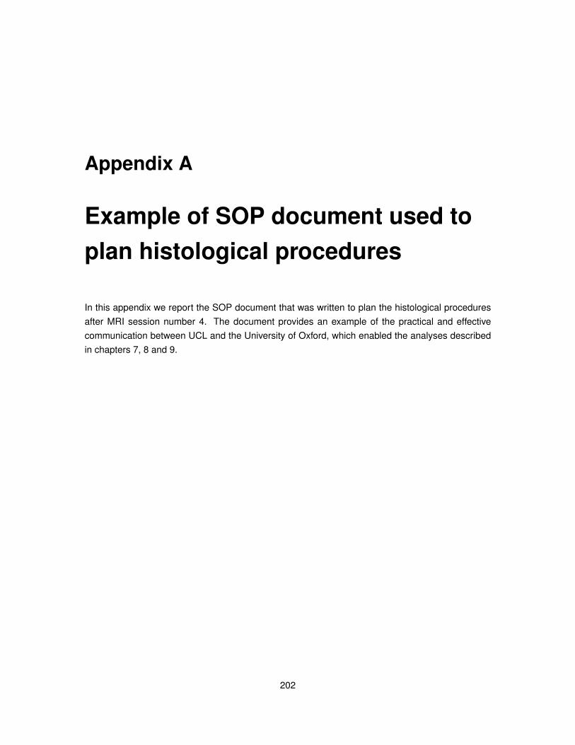
Appendix A

Example of SOP document used toplan histological procedures

In this appendix we report the SOP document that was written to plan the histological proceduresafter MRI session number 4. The document provides an example of the practical and effectivecommunication between UCL and the University of Oxford, which enabled the analyses describedin chapters 7, 8 and 9.

202

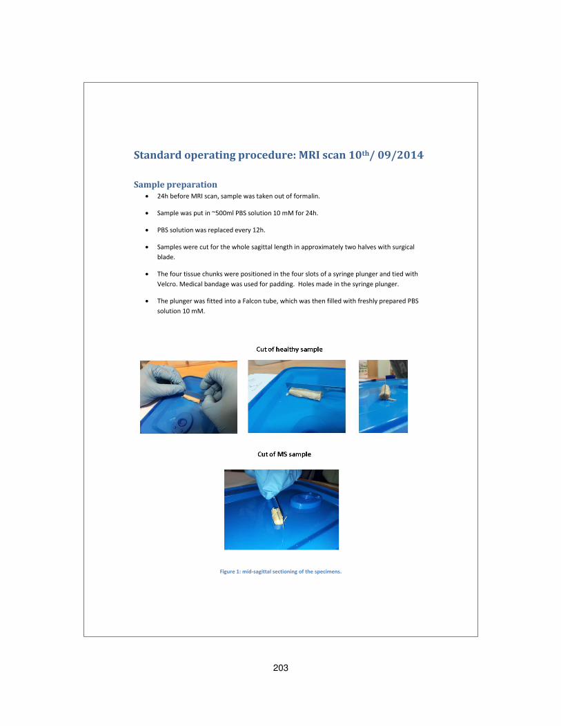
Standard operating procedure: MRI scan 10th/ 09/2014

Sample preparation 24h before MRI scan, sample was taken out of formalin.

Sample was put in ~500ml PBS solution 10 mM for 24h.

PBS solution was replaced every 12h.

Samples were cut for the whole sagittal length in approximately two halves with surgical

blade.

The four tissue chunks were positioned in the four slots of a syringe plunger and tied with

Velcro. Medical bandage was used for padding. Holes made in the syringe plunger.

The plunger was fitted into a Falcon tube, which was then filled with freshly prepared PBS

solution 10 mM.

Figure 1: mid-sagittal sectioning of the specimens.

203

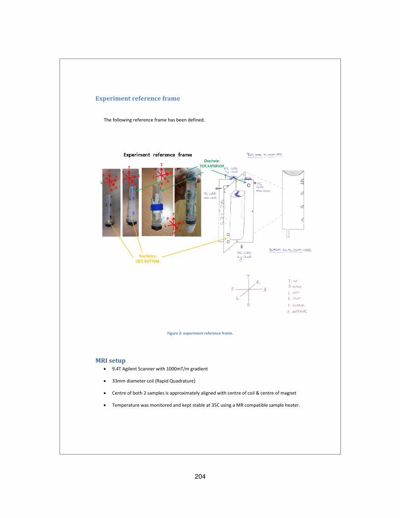
Experiment reference frame

The following reference frame has been defined.

Figure 2: experiment reference frame.

MRI setup 9.4T Agilent Scanner with 1000mT/m gradient

33mm diameter coil (Rapid Quadrature)

Centre of both 2 samples is approximately aligned with centre of coil & centre of magnet

Temperature was monitored and kept stable at 35C using a MR compatible sample heater.

204

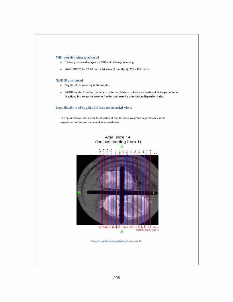
MRI positioning protocol T2-weighted axial images for MRI and histology planning

Axial: FOV 25.6 x 25.68 mm2 / 24 slices (2 mm thick); 256 x 128 matrix.

NODDI protocol Sagittal slices covering both samples.

NODDI model fitted to the data in order to obtain voxel-wise estimates of isotropic volume

fraction, intra-neurite volume fraction and neurite orientation dispersion index.

Localisation of sagittal slices onto axial view

The figure below clarifies the localisation of the diffusion-weighted sagittal slices in the

experiment reference frame and in an axial view.

Figure 3: sagittal slices overlaid onto axial slice 14.

205

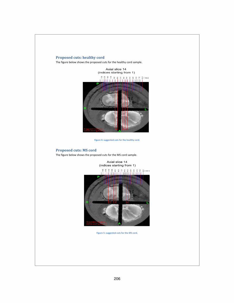
Proposed cuts: healthy cord The figure below shows the proposed cuts for the healthy cord sample.

Figure 4: suggested cuts for the healthy cord.

Proposed cuts: MS cord The figure below shows the proposed cuts for the MS cord sample.

Figure 5: suggested cuts for the MS cord.

206

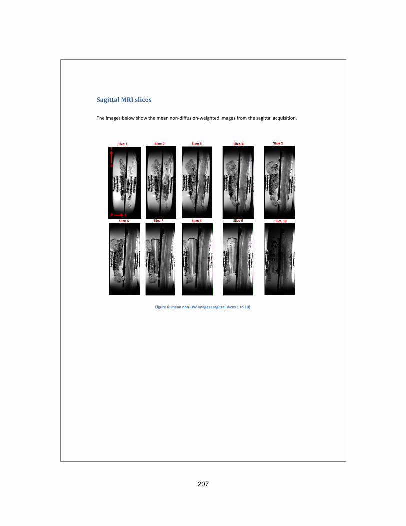
Sagittal MRI slices

The images below show the mean non-diffusion-weighted images from the sagittal acquisition.

Figure 6: mean non-DW images (sagittal slices 1 to 10).

207

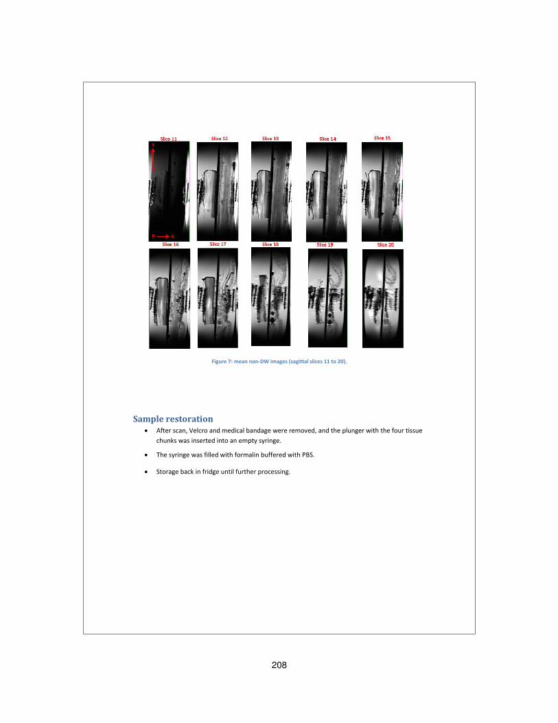
Figure 7: mean non-DW images (sagittal slices 11 to 20).

Sample restoration After scan, Velcro and medical bandage were removed, and the plunger with the four tissue

chunks was inserted into an empty syringe.

The syringe was filled with formalin buffered with PBS.

Storage back in fridge until further processing.

208

Appendix B

Fitting of linear regression models:relationship MRI-histology

In this appendix we report in full the results of fitting the five linear regression models listed in table9.4. We use a light shade of grey to flag associations between histological features and MRI-derivedmetrics characterised by a p-value p ≤ 0.05.

The results reported in this appendix are introduced and discussed in sections 9.4.3 and 9.5of chapter 9. A description of the metrics used as predictors (histology-derived) and as outcomemeasures (MRI-derived) in the linear regression models can be found in table 9.3.

209

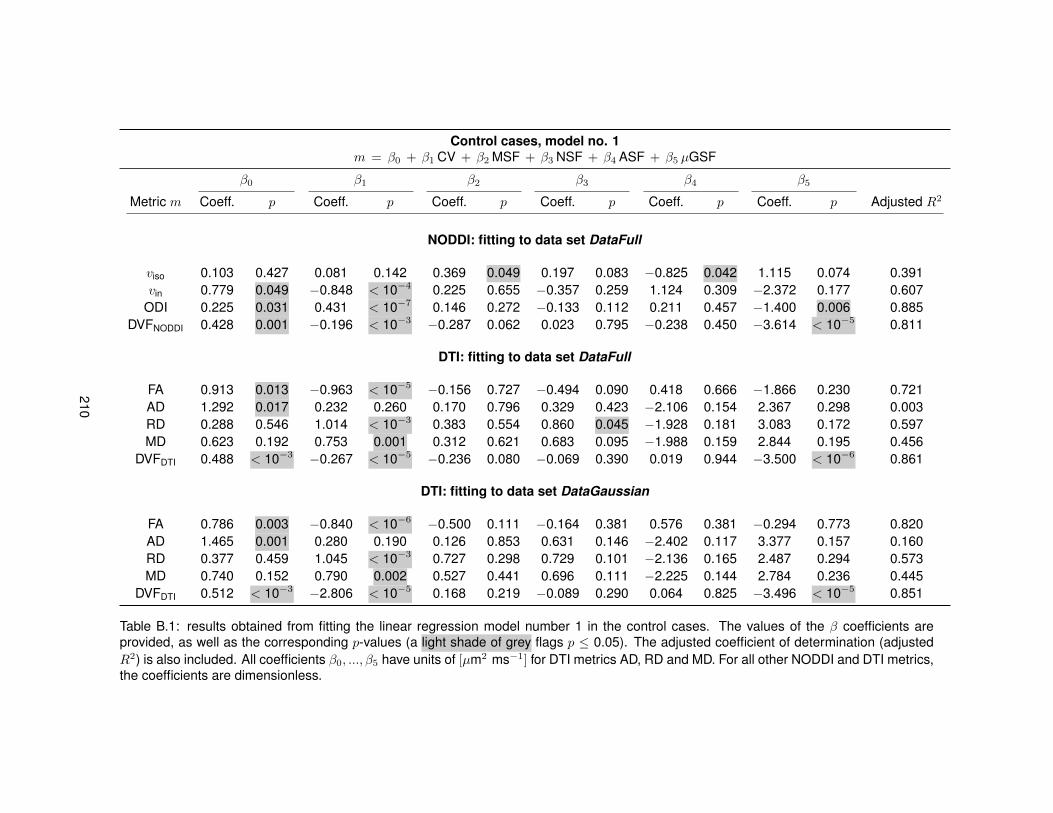
Control cases, model no. 1m = β0 + β1 CV + β2 MSF + β3 NSF + β4 ASF + β5 µGSF

β0 β1 β2 β3 β4 β5

Metric m Coeff. p Coeff. p Coeff. p Coeff. p Coeff. p Coeff. p Adjusted R2

NODDI: fitting to data set DataFull

viso 0.103 0.427 0.081 0.142 0.369 0.049 0.197 0.083 −0.825 0.042 1.115 0.074 0.391vin 0.779 0.049 −0.848 < 10−4 0.225 0.655 −0.357 0.259 1.124 0.309 −2.372 0.177 0.607

ODI 0.225 0.031 0.431 < 10−7 0.146 0.272 −0.133 0.112 0.211 0.457 −1.400 0.006 0.885DVFNODDI 0.428 0.001 −0.196 < 10−3 −0.287 0.062 0.023 0.795 −0.238 0.450 −3.614 < 10−5 0.811

DTI: fitting to data set DataFull

FA 0.913 0.013 −0.963 < 10−5 −0.156 0.727 −0.494 0.090 0.418 0.666 −1.866 0.230 0.721AD 1.292 0.017 0.232 0.260 0.170 0.796 0.329 0.423 −2.106 0.154 2.367 0.298 0.003RD 0.288 0.546 1.014 < 10−3 0.383 0.554 0.860 0.045 −1.928 0.181 3.083 0.172 0.597MD 0.623 0.192 0.753 0.001 0.312 0.621 0.683 0.095 −1.988 0.159 2.844 0.195 0.456

DVFDTI 0.488 < 10−3 −0.267 < 10−5 −0.236 0.080 −0.069 0.390 0.019 0.944 −3.500 < 10−6 0.861

DTI: fitting to data set DataGaussian

FA 0.786 0.003 −0.840 < 10−6 −0.500 0.111 −0.164 0.381 0.576 0.381 −0.294 0.773 0.820AD 1.465 0.001 0.280 0.190 0.126 0.853 0.631 0.146 −2.402 0.117 3.377 0.157 0.160RD 0.377 0.459 1.045 < 10−3 0.727 0.298 0.729 0.101 −2.136 0.165 2.487 0.294 0.573MD 0.740 0.152 0.790 0.002 0.527 0.441 0.696 0.111 −2.225 0.144 2.784 0.236 0.445

DVFDTI 0.512 < 10−3 −2.806 < 10−5 0.168 0.219 −0.089 0.290 0.064 0.825 −3.496 < 10−5 0.851

Table B.1: results obtained from fitting the linear regression model number 1 in the control cases. The values of the β coefficients areprovided, as well as the corresponding p-values (a light shade of grey flags p ≤ 0.05). The adjusted coefficient of determination (adjustedR2) is also included. All coefficients β0, ..., β5 have units of [µm2 ms−1] for DTI metrics AD, RD and MD. For all other NODDI and DTI metrics,the coefficients are dimensionless.

210

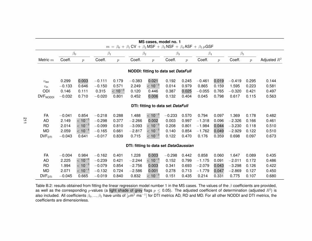
MS cases, model no. 1m = β0 + β1 CV + β2 MSF + β3 NSF + β4 ASF + β5 µGSF

β0 β1 β2 β3 β4 β5

Metric m Coeff. p Coeff. p Coeff. p Coeff. p Coeff. p Coeff. p Adjusted R2


viso 0.299 0.003 −0.111 0.179 −0.383 0.021 0.192 0.245 −0.461 0.019 −0.419 0.295 0.144vin −0.133 0.646 −0.150 0.571 2.249 < 10−3 0.014 0.979 0.865 0.159 1.595 0.223 0.581

ODI 0.146 0.111 0.315 < 10−3 0.120 0.446 0.387 0.025 −0.055 0.765 −0.320 0.421 0.497DVFNODDI −0.032 0.710 −0.020 0.801 0.452 0.006 0.132 0.404 0.045 0.798 0.617 0.115 0.563


FA −0.041 0.854 −0.218 0.288 1.488 < 10−3 −0.233 0.570 0.794 0.097 1.369 0.178 0.482AD 2.149 < 10−5 −0.298 0.377 −2.266 0.002 0.003 0.997 −1.318 0.096 −2.326 0.166 0.461RD 2.014 < 10−3 −0.099 0.810 −3.093 < 10−3 0.208 0.801 −1.984 0.044 −3.230 0.118 0.510MD 2.059 < 10−4 −0.165 0.661 −2.817 < 10−3 0.140 0.854 −1.762 0.049 −2.929 0.122 0.510

DVFDTI −0.043 0.641 −0.017 0.839 0.715 < 10−3 0.122 0.470 0.176 0.359 0.698 0.097 0.673


FA −0.004 0.984 −0.162 0.401 1.228 0.003 −0.298 0.442 0.858 0.060 1.647 0.089 0.435AD 2.225 < 10−6 −0.239 0.421 −2.244 < 10−3 0.152 0.799 −1.175 0.091 −2.011 0.172 0.486RD 1.994 < 10−3 −0.079 0.854 −2.756 0.003 0.341 0.693 −2.079 0.043 −3.298 0.126 0.422MD 2.071 < 10−4 −0.132 0.724 −2.586 0.001 0.278 0.713 −1.779 0.047 −2.869 0.127 0.450

DVFDTI −0.045 0.665 −0.019 0.840 0.832 < 10−3 0.151 0.435 0.214 0.331 0.775 0.107 0.680

Table B.2: results obtained from fitting the linear regression model number 1 in the MS cases. The values of the β coefficients are provided,as well as the corresponding p-values (a light shade of grey flags p ≤ 0.05). The adjusted coefficient of determination (adjusted R2) isalso included. All coefficients β0, ..., β5 have units of [µm2 ms−1] for DTI metrics AD, RD and MD. For all other NODDI and DTI metrics, thecoefficients are dimensionless.

211

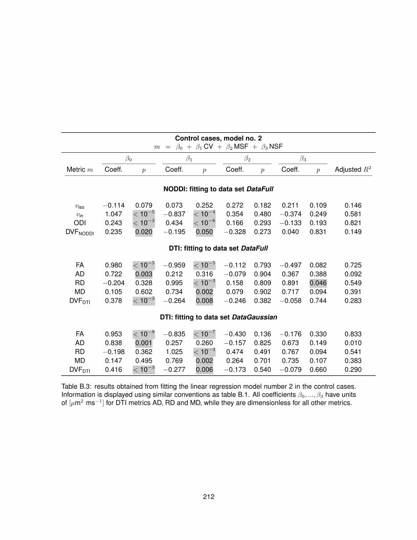
Control cases, model no. 2m = β0 + β1 CV + β2 MSF + β3 NSF

β0 β1 β2 β3

Metric m Coeff. p Coeff. p Coeff. p Coeff. p Adjusted R2


viso −0.114 0.079 0.073 0.252 0.272 0.182 0.211 0.109 0.146vin 1.047 < 10−5 −0.837 < 10−4 0.354 0.480 −0.374 0.249 0.581

ODI 0.243 < 10−3 0.434 < 10−6 0.166 0.293 −0.133 0.193 0.821DVFNODDI 0.235 0.020 −0.195 0.050 −0.328 0.273 0.040 0.831 0.149


FA 0.980 < 10−5 −0.959 < 10−5 −0.112 0.793 −0.497 0.082 0.725AD 0.722 0.003 0.212 0.316 −0.079 0.904 0.367 0.388 0.092RD −0.204 0.328 0.995 < 10−3 0.158 0.809 0.891 0.046 0.549MD 0.105 0.602 0.734 0.002 0.079 0.902 0.717 0.094 0.391

DVFDTI 0.378 < 10−3 −0.264 0.008 −0.246 0.382 −0.058 0.744 0.283


FA 0.953 < 10−8 −0.835 < 10−7 −0.430 0.136 −0.176 0.330 0.833AD 0.838 0.001 0.257 0.260 −0.157 0.825 0.673 0.149 0.010RD −0.198 0.362 1.025 < 10−3 0.474 0.491 0.767 0.094 0.541MD 0.147 0.495 0.769 0.002 0.264 0.701 0.735 0.107 0.383

DVFDTI 0.416 < 10−3 −0.277 0.006 −0.173 0.540 −0.079 0.660 0.290

Table B.3: results obtained from fitting the linear regression model number 2 in the control cases.Information is displayed using similar conventions as table B.1. All coefficients β0, ..., β3 have unitsof [µm2 ms−1] for DTI metrics AD, RD and MD, while they are dimensionless for all other metrics.

212

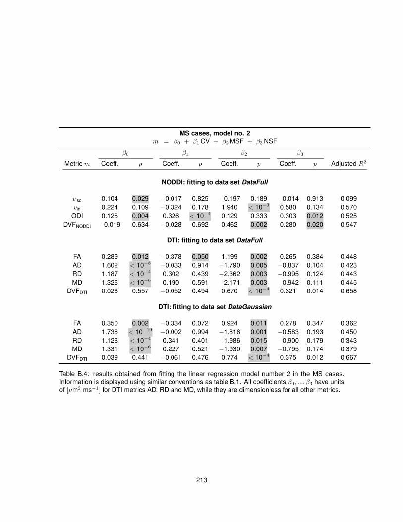
MS cases, model no. 2m = β0 + β1 CV + β2 MSF + β3 NSF

β0 β1 β2 β3

Metric m Coeff. p Coeff. p Coeff. p Coeff. p Adjusted R2


viso 0.104 0.029 −0.017 0.825 −0.197 0.189 −0.014 0.913 0.099vin 0.224 0.109 −0.324 0.178 1.940 < 10−3 0.580 0.134 0.570

ODI 0.126 0.004 0.326 < 10−4 0.129 0.333 0.303 0.012 0.525DVFNODDI −0.019 0.634 −0.028 0.692 0.462 0.002 0.280 0.020 0.547


FA 0.289 0.012 −0.378 0.050 1.199 0.002 0.265 0.384 0.448AD 1.602 < 10−8 −0.033 0.914 −1.790 0.005 −0.837 0.104 0.423RD 1.187 < 10−4 0.302 0.439 −2.362 0.003 −0.995 0.124 0.443MD 1.326 < 10−6 0.190 0.591 −2.171 0.003 −0.942 0.111 0.445

DVFDTI 0.026 0.557 −0.052 0.494 0.670 < 10−4 0.321 0.014 0.658


FA 0.350 0.002 −0.334 0.072 0.924 0.011 0.278 0.347 0.362AD 1.736 < 10−10 −0.002 0.994 −1.816 0.001 −0.583 0.193 0.450RD 1.128 < 10−4 0.341 0.401 −1.986 0.015 −0.900 0.179 0.343MD 1.331 < 10−6 0.227 0.521 −1.930 0.007 −0.795 0.174 0.379

DVFDTI 0.039 0.441 −0.061 0.476 0.774 < 10−4 0.375 0.012 0.667

Table B.4: results obtained from fitting the linear regression model number 2 in the MS cases.Information is displayed using similar conventions as table B.1. All coefficients β0, ..., β3 have unitsof [µm2 ms−1] for DTI metrics AD, RD and MD, while they are dimensionless for all other metrics.

213

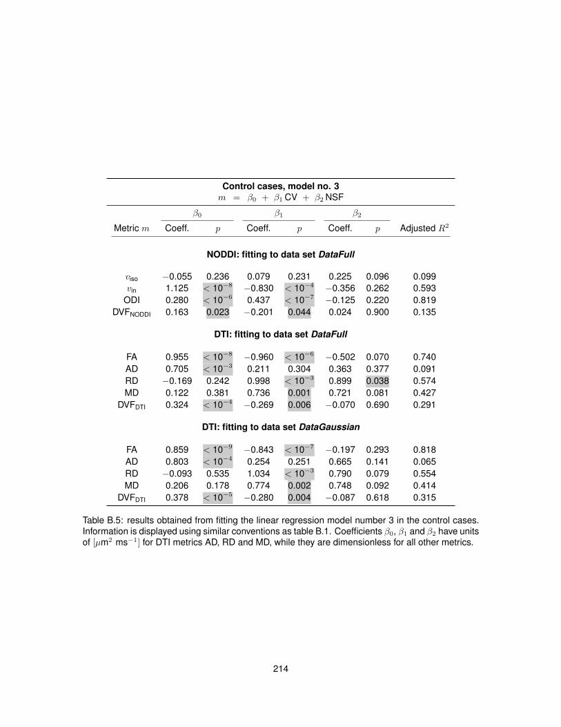
Control cases, model no. 3m = β0 + β1 CV + β2 NSF

β0 β1 β2

Metric m Coeff. p Coeff. p Coeff. p Adjusted R2


viso −0.055 0.236 0.079 0.231 0.225 0.096 0.099vin 1.125 < 10−8 −0.830 < 10−4 −0.356 0.262 0.593

ODI 0.280 < 10−6 0.437 < 10−7 −0.125 0.220 0.819DVFNODDI 0.163 0.023 −0.201 0.044 0.024 0.900 0.135


FA 0.955 < 10−8 −0.960 < 10−6 −0.502 0.070 0.740AD 0.705 < 10−3 0.211 0.304 0.363 0.377 0.091RD −0.169 0.242 0.998 < 10−3 0.899 0.038 0.574MD 0.122 0.381 0.736 0.001 0.721 0.081 0.427

DVFDTI 0.324 < 10−4 −0.269 0.006 −0.070 0.690 0.291


FA 0.859 < 10−9 −0.843 < 10−7 −0.197 0.293 0.818AD 0.803 < 10−4 0.254 0.251 0.665 0.141 0.065RD −0.093 0.535 1.034 < 10−3 0.790 0.079 0.554MD 0.206 0.178 0.774 0.002 0.748 0.092 0.414

DVFDTI 0.378 < 10−5 −0.280 0.004 −0.087 0.618 0.315

Table B.5: results obtained from fitting the linear regression model number 3 in the control cases.Information is displayed using similar conventions as table B.1. Coefficients β0, β1 and β2 have unitsof [µm2 ms−1] for DTI metrics AD, RD and MD, while they are dimensionless for all other metrics.

214

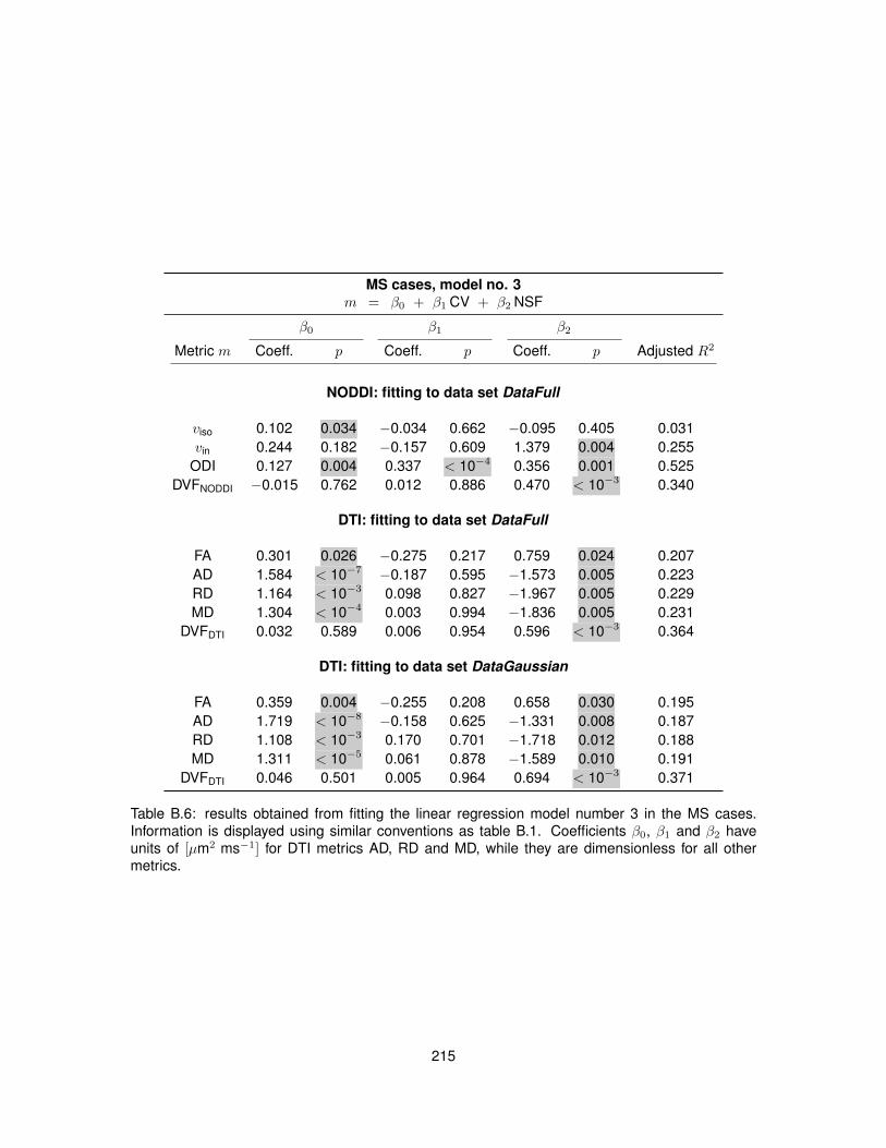
MS cases, model no. 3m = β0 + β1 CV + β2 NSF

β0 β1 β2



viso 0.102 0.034 −0.034 0.662 −0.095 0.405 0.031vin 0.244 0.182 −0.157 0.609 1.379 0.004 0.255

ODI 0.127 0.004 0.337 < 10−4 0.356 0.001 0.525DVFNODDI −0.015 0.762 0.012 0.886 0.470 < 10−3 0.340


FA 0.301 0.026 −0.275 0.217 0.759 0.024 0.207AD 1.584 < 10−7 −0.187 0.595 −1.573 0.005 0.223RD 1.164 < 10−3 0.098 0.827 −1.967 0.005 0.229MD 1.304 < 10−4 0.003 0.994 −1.836 0.005 0.231

DVFDTI 0.032 0.589 0.006 0.954 0.596 < 10−3 0.364


FA 0.359 0.004 −0.255 0.208 0.658 0.030 0.195AD 1.719 < 10−8 −0.158 0.625 −1.331 0.008 0.187RD 1.108 < 10−3 0.170 0.701 −1.718 0.012 0.188MD 1.311 < 10−5 0.061 0.878 −1.589 0.010 0.191

DVFDTI 0.046 0.501 0.005 0.964 0.694 < 10−3 0.371

Table B.6: results obtained from fitting the linear regression model number 3 in the MS cases.Information is displayed using similar conventions as table B.1. Coefficients β0, β1 and β2 haveunits of [µm2 ms−1] for DTI metrics AD, RD and MD, while they are dimensionless for all othermetrics.

215

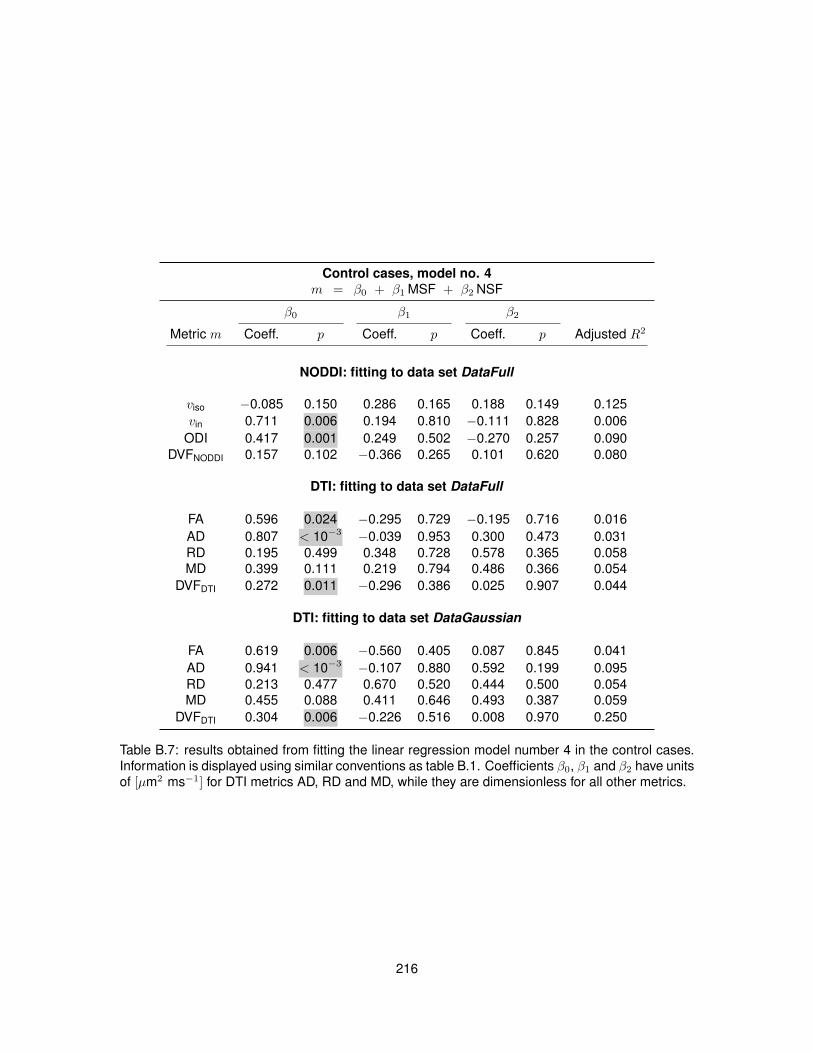
Control cases, model no. 4m = β0 + β1 MSF + β2 NSF

β0 β1 β2



viso −0.085 0.150 0.286 0.165 0.188 0.149 0.125vin 0.711 0.006 0.194 0.810 −0.111 0.828 0.006

ODI 0.417 0.001 0.249 0.502 −0.270 0.257 0.090DVFNODDI 0.157 0.102 −0.366 0.265 0.101 0.620 0.080


FA 0.596 0.024 −0.295 0.729 −0.195 0.716 0.016AD 0.807 < 10−3 −0.039 0.953 0.300 0.473 0.031RD 0.195 0.499 0.348 0.728 0.578 0.365 0.058MD 0.399 0.111 0.219 0.794 0.486 0.366 0.054

DVFDTI 0.272 0.011 −0.296 0.386 0.025 0.907 0.044


FA 0.619 0.006 −0.560 0.405 0.087 0.845 0.041AD 0.941 < 10−3 −0.107 0.880 0.592 0.199 0.095RD 0.213 0.477 0.670 0.520 0.444 0.500 0.054MD 0.455 0.088 0.411 0.646 0.493 0.387 0.059

DVFDTI 0.304 0.006 −0.226 0.516 0.008 0.970 0.250


216

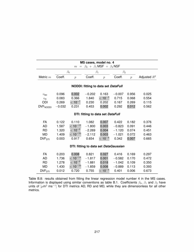
MS cases, model no. 4m = β0 + β1 MSF + β2 NSF

β0 β1 β2



viso 0.096 0.002 −0.202 0.163 −0.007 0.956 0.025vin 0.083 0.366 1.840 < 10−3 0.715 0.068 0.554

ODI 0.269 < 10−7 0.230 0.202 0.167 0.269 0.115DVFNODDI −0.032 0.231 0.453 0.002 0.292 0.012 0.562


FA 0.122 0.110 1.082 0.007 0.422 0.182 0.376AD 1.587 < 10−12 −1.800 0.003 −0.823 0.091 0.446RD 1.320 < 10−8 −2.269 0.004 −1.120 0.074 0.451MD 1.409 < 10−10 −2.112 0.003 −1.021 0.072 0.463

DVFDTI 0.003 0.917 0.654 < 10−4 0.342 0.007 0.665


FA 0.203 0.008 0.821 0.027 0.416 0.169 0.297AD 1.736 < 10−14 −1.817 0.001 −0.582 0.170 0.472RD 1.278 < 10−8 −1.881 0.018 −1.042 0.109 0.350MD 1.430 < 10−10 −1.859 0.008 −0.889 0.113 0.393

DVFDTI 0.012 0.720 0.755 < 10−4 0.401 0.006 0.673


217

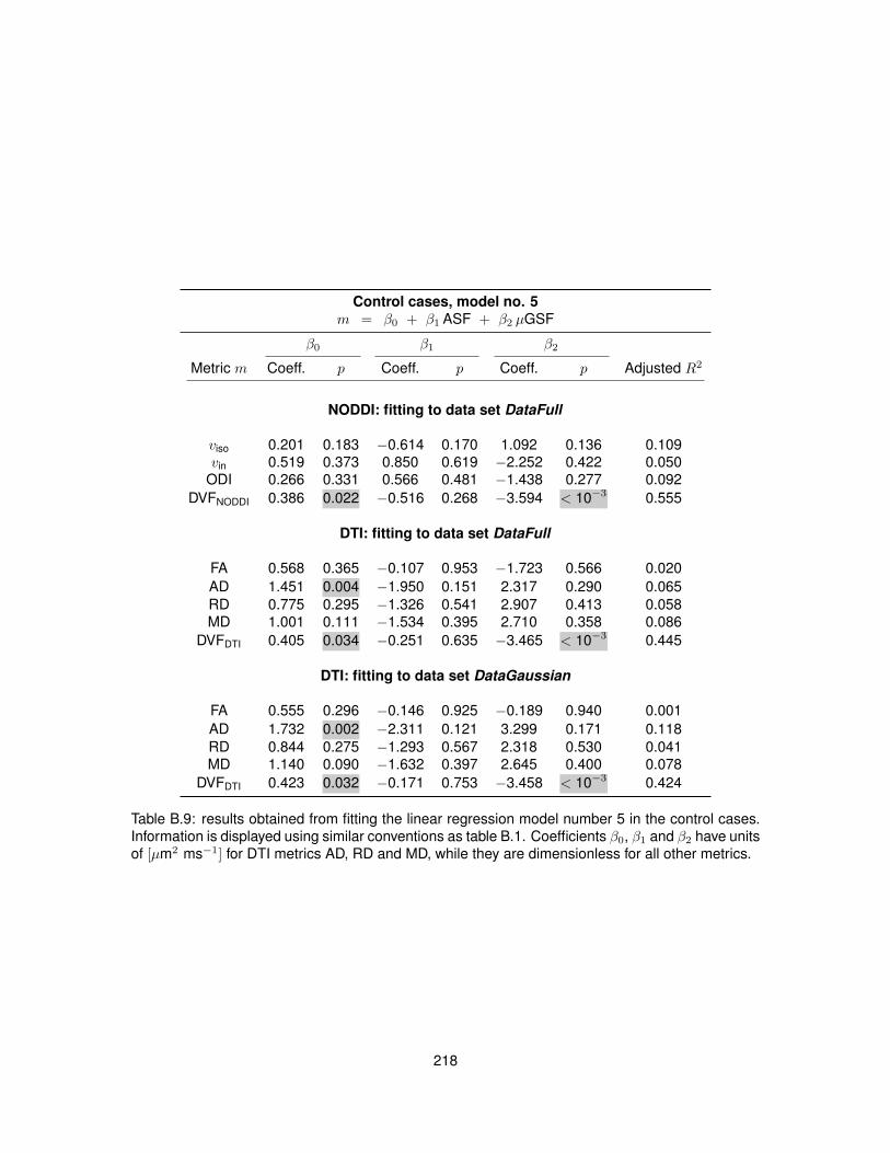
Control cases, model no. 5m = β0 + β1 ASF + β2 µGSF

β0 β1 β2



viso 0.201 0.183 −0.614 0.170 1.092 0.136 0.109vin 0.519 0.373 0.850 0.619 −2.252 0.422 0.050

ODI 0.266 0.331 0.566 0.481 −1.438 0.277 0.092DVFNODDI 0.386 0.022 −0.516 0.268 −3.594 < 10−3 0.555


FA 0.568 0.365 −0.107 0.953 −1.723 0.566 0.020AD 1.451 0.004 −1.950 0.151 2.317 0.290 0.065RD 0.775 0.295 −1.326 0.541 2.907 0.413 0.058MD 1.001 0.111 −1.534 0.395 2.710 0.358 0.086

DVFDTI 0.405 0.034 −0.251 0.635 −3.465 < 10−3 0.445


FA 0.555 0.296 −0.146 0.925 −0.189 0.940 0.001AD 1.732 0.002 −2.311 0.121 3.299 0.171 0.118RD 0.844 0.275 −1.293 0.567 2.318 0.530 0.041MD 1.140 0.090 −1.632 0.397 2.645 0.400 0.078

DVFDTI 0.423 0.032 −0.171 0.753 −3.458 < 10−3 0.424


218

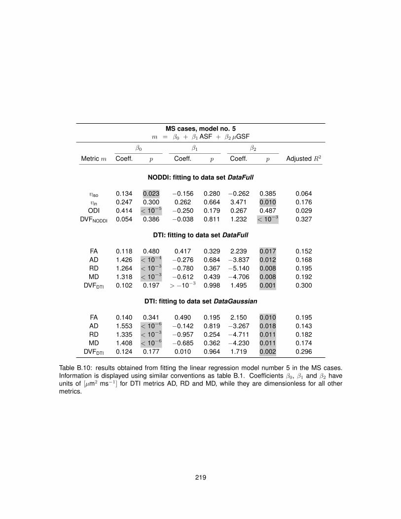
MS cases, model no. 5m = β0 + β1 ASF + β2 µGSF

β0 β1 β2



viso 0.134 0.023 −0.156 0.280 −0.262 0.385 0.064vin 0.247 0.300 0.262 0.664 3.471 0.010 0.176

ODI 0.414 < 10−5 −0.250 0.179 0.267 0.487 0.029DVFNODDI 0.054 0.386 −0.038 0.811 1.232 < 10−3 0.327


FA 0.118 0.480 0.417 0.329 2.239 0.017 0.152AD 1.426 < 10−4 −0.276 0.684 −3.837 0.012 0.168RD 1.264 < 10−3 −0.780 0.367 −5.140 0.008 0.195MD 1.318 < 10−3 −0.612 0.439 −4.706 0.008 0.192

DVFDTI 0.102 0.197 > −10−3 0.998 1.495 0.001 0.300


FA 0.140 0.341 0.490 0.195 2.150 0.010 0.195AD 1.553 < 10−6 −0.142 0.819 −3.267 0.018 0.143RD 1.335 < 10−3 −0.957 0.254 −4.711 0.011 0.182MD 1.408 < 10−6 −0.685 0.362 −4.230 0.011 0.174

DVFDTI 0.124 0.177 0.010 0.964 1.719 0.002 0.296


219

Bibliography

[1] F Aboitiz, AB Scheibel, RS Fisher, and E Zaidel. Fiber composition of the human corpuscallosum. Brain research, 598(1):143–153, 1992.

[2] I Aganj, C Lenglet, G Sapiro, E Yacoub, K Ugurbil, and N Harel. Reconstruction of the ori-entation distribution function in single-and multiple-shell q-ball imaging within constant solidangle. Magnetic Resonance in Medicine, 64(2):554–566, 2010.

[3] F Agosta, B Benedetti, MA Rocca, P Valsasina, M Rovaris, G Comi, and M Filippi. Quan-tification of cervical cord pathology in primary progressive MS using diffusion tensor MRI.Neurology, 64(4):631–635, 2005.

[4] DC Alexander, PL Hubbard, MG Hall, EA Moore, M Ptito, GJM Parker, and TB Dyrby. Ori-entationally invariant indices of axon diameter and density from diffusion MRI. NeuroImage,52(4):1374–1389, 2010.

[5] DC Alexander, D Zikic, J Zhang, H Zhang, and A Criminisi. Image quality transfer via randomforest regression: applications in diffusion MRI. In proceedings of Medical Image Computingand Computer-Assisted Intervention (MICCAI) meeting, pages 225–232, 2014.

[6] D Arthur and S Vassilvitskii. k-means++: the advantages of careful seeding. In proceedingsof the eighteenth annual ACM-SIAM symposium on discrete algorithms, Society for Industrialand Applied Mathematics, pages 1027–1035, 2007.

[7] Y Assaf, T Blumenfeld-Katzir, Y Yovel, and PJ Basser. AxCaliber: a method for measuringaxon diameter distribution from diffusion MRI. Magnetic Resonance in Medicine, 59(6):1347–1354, 2008.

[8] Y Assaf, RZ Freidlin, GK Rohde, and PJ Basser. New modeling and experimental frame-work to characterize hindered and restricted water diffusion in brain white matter. MagneticResonance in Medicine, 52(5):965–978, 2004.

[9] M Axer, K Amunts, D Grassel, C Palm, J Dammers, H Axer, U Pietrzyk, and K Zilles. A novelapproach to the human connectome: ultra-high resolution mapping of fiber tracts in the brain.NeuroImage, 54(2):1091–1101, 2011.

220

[10] CA Baron and C Beaulieu. Oscillating gradient spin-echo (OGSE) diffusion tensor imagingof the human brain. Magnetic Resonance in Medicine, 72(3):726–736, 2014.

[11] JW Bartlett and C Frost. Reliability, repeatability and reproducibility: analysis of measurementerrors in continuous variables. Ultrasound in Obstetrics and Gynecology, 31(4):466–475,2008.

[12] PJ Basser, J Mattiello, and D LeBihan. MR diffusion tensor spectroscopy and imaging. Bio-physical Journal, 66(1):259–267, 1994.

[13] PJ Basser and C Pierpaoli. Microstructural and physiological features of tissues elucidatedby quantitative-diffusion-tensor MRI. Journal of Magnetic Resonance, 213(2):560–570, 2011.

[14] C Beaulieu. The basis of anisotropic water diffusion in the nervous system – a technicalreview. NMR in Biomedicine, 15(7-8):435–455, 2002.

[15] TEJ Behrens, MW Woolrich, M Jenkinson, H Johansen-Berg, RG Nunes, S Clare,PM Matthews, JM Brady, and SM Smith. Characterization and propagation of uncertainty indiffusion-weighted MR imaging. Magnetic Resonance in Medicine, 50(5):1077–1088, 2003.

[16] J Bigun and GH Granlund. Optimal orientation detection of linear symmetry. In proceedingsof the IEEE first international conference on computer vision, pages 433–438, 1987.

[17] T Billiet, B Madler, F D’Arco, R Peeters, S Deprez, E Plasschaert, A Leemans, H Zhang,BV den Bergh, M Vandenbulcke, E Legius, S Sunaert, and L Emsell. Characterizing themicrostructural basis of “unidentified bright objects” in neurofibromatosis type 1: a combinedin vivo multicomponent T2 relaxation and multi-shell diffusion MRI analysis. NeuroImage:Clinical, 4:649–658, 2014.

[18] F Bloch. Nuclear induction. Physical review, 70(7-8):460, 1946.

[19] N Bloembergen, EM Purcell, and RV Pound. Relaxation effects in nuclear magnetic reso-nance absorption. Physical Review, 73(7):679, 1948.

[20] JCJ Bot, ELA Blezer, W Kamphorst, GJ Lycklama a Nijeholt, HJ Ader, JA Castelijns, E Berg-ers, R Ravid, C Polman, and F Barkhof. The spinal cord in multiple sclerosis: relationship ofhigh-spatial-resolution quantitative MR imaging findings to histopathologic results. Radiology,233(2):531–540, 2004.

[21] MD Budde and J Annese. Quantification of anisotropy and fiber orientation in human brainhistological sections. Frontiers in Integrative Neuroscience, 7, 2013.

[22] MD Budde and JA Frank. Examining brain microstructure using structure tensor analysis ofhistological sections. NeuroImage, 63(1):1–10, 2012.

[23] MD Budde, L Janes, E Gold, LC Turtzo, and JA Frank. The contribution of gliosis to diffusiontensor anisotropy and tractography following traumatic brain injury: validation in the rat usingFourier analysis of stained tissue sections. Brain, 134(8):2248–2260, 2011.

221

[24] MD Budde, JH Kim, HF Liang, JH Russell, AH Cross, and SK Song. Axonal injury detectedby in vivo diffusion tensor imaging correlates with neurological disability in a mouse model ofmultiple sclerosis. NMR in Biomedicine, 21(6):589–597, 2008.

[25] MD Budde, M Xie, AH Cross, and SK Song. Axial diffusivity is the primary correlate of axonalinjury in the EAE spinal cord: a quantitative pixelwise analysis. The Journal of Neuroscience,29(9):2805–2813, 2009.

[26] LM Burcaw, E Fieremans, and DS Novikov. Mesoscopic structure of neuronal tracts fromtime-dependent diffusion. NeuroImage, 114:18–37, 2015.

[27] F Calamante, JD Tournier, GD Jackson, and A Connelly. Track-density imaging (TDI):super-resolution white matter imaging using whole-brain track-density mapping. NeuroIm-age, 53(4):1233–1243, 2010.

[28] PT Callaghan, A Coy, D MacGowan, KJ Packer, and FO Zelaya. Diffraction-like effects inNMR diffusion studies of fluids in porous solids. Nature, 351:467–469, 1991.

[29] HY Carr and EM Purcell. Effects of diffusion on free precession in nuclear magnetic reso-nance experiments. Physical Review, 94(3):630, 1954.

[30] AS Choe, I Stepniewska, DC Colvin, Z Ding, and AW Anderson. Validation of diffusion tensorMRI in the central nervous system using light microscopy: quantitative comparison of fiberproperties. NMR in Biomedicine, 25(7):900–908, 2012.

[31] O Ciccarelli, F Barkhof, B Bodini, N De Stefano, X Golay, K Nicolay, D Pelletier, PJW Pouwels,SA Smith, CAM Wheeler-Kingshott, B Stankoff, T Yousry, and DH Miller. Pathogenesis ofmultiple sclerosis: insights from molecular and metabolic imaging. The Lancet Neurology,13(8):807–822, 2014.

[32] O Ciccarelli, CA Wheeler-Kingshott, MA McLean, M Cercignani, K Wimpey, DH Miller, andAJ Thompson. Spinal cord spectroscopy and diffusion-based tractography to assess acutedisability in multiple sclerosis. Brain, 130(8):2220–2231, 2007.

[33] CA Clark and D Le Bihan. Water diffusion compartmentation and anisotropy at high b valuesin the human brain. Magnetic Resonance in Medicine, 44(6):852–859, 2000.

[34] J Cohen-Adad, MM El Mendili, S Lehericy, PF Pradat, S Blancho, S Rossignol, and H Benali.Demyelination and degeneration in the injured human spinal cord detected with diffusion andmagnetization transfer MRI. NeuroImage, 55(3):1024–1033, 2011.

[35] J Cohen-Adad, MME Mendili, R Morizot-Koutlidis, S Lehericy, V Meininger, S Blancho,S Rossignol, H Benali, and PF Pradat. Involvement of spinal sensory pathway in ALS andspecificity of cord atrophy to lower motor neuron degeneration. Amyotrophic Lateral Sclerosisand Frontotemporal Degeneration, 14(1):30–38, 2013.

222

[36] J Cohen-Adad and CAM Wheeler-Kingshott. Quantitative MRI of the spinal cord. AcademicPress, 2014.

[37] A Compston and A Coles. Multiple sclerosis. The Lancet, 372:1502–1517, 2008.

[38] PA Cook, Y Bai, S Nedjati-Gilani, KK Seunarine, MG Hall, GJ Parker, and DC Alexander.Camino: open-source diffusion-MRI reconstruction and processing. In proceedings of the14th meeting of the International Society for Magnetic Resonance in Medicine (ISMRM),page 2759, 2006.

[39] J Correale. The role of microglial activation in disease progression. Multiple Sclerosis Jour-nal, 20(10):1288–1295, 2014.

[40] GC DeLuca, R Alterman, JL Martin, A Mittal, S Blundell, S Bird, H Beale, L San Hong, andMM Esiri. Casting light on multiple sclerosis heterogeneity: the role of HLA-DRB1 on spinalcord pathology. Brain, 134(4):1025–1034, 2013.

[41] GC DeLuca, GC Ebers, and MM Esiri. Axonal loss in multiple sclerosis: a pathological surveyof the corticospinal and sensory tracts. Brain, 127(5):1009–1018, 2004.

[42] SCL Deoni, BK Rutt, T Arun, C Pierpaoli, and DK Jones. Gleaning multicomponent T1 and T2information from steady-state imaging data. Magnetic Resonance in Medicine, 60(6):1372–1387, 2008.

[43] M Descoteaux, R Deriche, D Le Bihan, JF Mangin, and C Poupon. Multiple q-shell diffusionpropagator imaging. Medical Image Analysis, 15(4):603–621, 2011.

[44] A Deshmane, V Gulani, MA Griswold, and N Seiberlich. Parallel MR imaging. Journal ofMagnetic Resonance Imaging, 36(1):55–72, 2012.

[45] LR Dice. Measures of the amount of ecologic association between species. Ecology,26(3):297–302, 1945.

[46] DC Douglass and DW McCall. Diffusion in paraffin hydrocarbons. The Journal of PhysicalChemistry, 62(9):1102–1107, 1958.

[47] R Dutta and BD Trapp. Relapsing and progressive forms of multiple sclerosis: insights frompathology. Current opinion in Neurology, 27(3):271–278, 2014.

[48] T Duval, JA McNab, K Setsompop, T Witzel, T Schneider, SY Huang, B Keil, EC Klaw-iter, LL Wald, and J Cohen-Adad. In vivo mapping of human spinal cord microstructure at300mT/m. NeuroImage, 118:494–507, 2015.

[49] C Eichner, SF Cauley, J Cohen-Adad, HE Moller, R Turner, K Setsompop, and LL Wald.Real diffusion-weighted MRI enabling true signal averaging and increased diffusion contrast.NeuroImage, 122:373–384, 2015.

223

[50] A Einstein. On the movement of small particles suspended in stationary liquids required bythe molecular-kinetic theory of heat. Annalen der Physik (in German), 322(8):549–560, 1905.

[51] BM Ellingson, N Salamon, AJ Hardy, and LT Holly. Prediction of neurological impairment incervical spondylotic myelopathy using a combination of diffusion MRI and proton MR spec-troscopy. PloS one, 10(10):e0139451, 2015.

[52] D Facon, A Ozanne, P Fillard, JF Lepeintre, C Tournoux-Facon, and D Ducreux. MR dif-fusion tensor imaging and fiber tracking in spinal cord compression. American Journal ofNeuroradiology, 26(6):1587–1594, 2005.

[53] MF Falangola, DN Guilfoyle, A Tabesh, ES Hui, X Nie, JH Jensen, SV Gerum, C Hu,J LaFrancois, HR Collins, and JA Helpern. Histological correlation of diffusional kurtosis andwhite matter modeling metrics in cuprizone-induced corpus callosum demyelination. NMR inBiomedicine, 27(8):948–957, 2014.

[54] JAD Farrell, SA Smith, EM Gordon-Lipkin, DS Reich, PA Calabresi, and P van Zijl. Highb-value q-space diffusion-weighted MRI of the human cervical spinal cord in vivo: feasibilityand application to multiple sclerosis. Magnetic Resonance in Medicine, 59(5):1079–1089,2008.

[55] DA Feinberg and K Setsompop. Ultra-fast MRI of the human brain with simultaneous multi-slice imaging. Journal of magnetic resonance, 229:90–100, 2013.

[56] HKP Feirabend, H Choufoer, S Ploeger, J Holsheimer, and JD Van Gool. Morphometry of hu-man superficial dorsal and dorsolateral column fibres: significance to spinal cord stimulation.Brain, 125(5):1137–1149, 2002.

[57] FRE Fenrich, C Beaulieu, and PS Allen. Relaxation times and microstructures. NMR inBiomedicine, 14(2):133–139, 2001.

[58] U Ferizi, T Schneider, M Tariq, CAM Wheeler-Kingshott, H Zhang, and DC Alexander. Theimportance of being dispersed: a ranking of diffusion MRI models for fibre dispersion using invivo human brain data. In proceedings of Medical Image Computing and Computer-AssistedIntervention (MICCAI) meeting, pages 74–81, 2013.

[59] E Fieremans, JH Jensen, and JA Helpern. White matter characterization with diffusionalkurtosis imaging. NeuroImage, 58(1):177–188, 2011.

[60] NI Fisher, T Lewis, and BJJ Embleton. Statistical analysis of spherical data. Cambridgeuniversity press, 1987.

[61] J Frahm, KD Merboldt, W Hanicke, and A Haase. Stimulated echo imaging. Journal ofMagnetic Resonance (1969), 64(1):81–93, 1985.

[62] AF Frøhlich, SN Jespersen, L Østergaard, and VG Kiselev. The effect of impermeable bound-aries of arbitrary geometry on the apparent diffusion coefficient. Journal of Magnetic Reso-nance, 194(1):128–135, 2008.

224

[63] A Gass, MA Rocca, F Agosta, O Ciccarelli, D Chard, P Valsasina, JCW Brooks, A Bischof,P Eisele, L Kappos, F Barkhof, M Filippi, and for the MAGNIMS Study Group. MRI monitoringof pathological changes in the spinal cord in patients with multiple sclerosis. The LancetNeurology, 14(4):443–454, 2015.

[64] DN Greve and B Fischl. Accurate and robust brain image alignment using boundary-basedregistration. NeuroImage, 48(1):63–72, 2009.

[65] T Gringel, W Schulz-Schaeffer, E Elolf, A Frolich, P Dechent, and G Helms. Optimizedhigh-resolution mapping of magnetization transfer (MT) at 3 Tesla for direct visualization ofsubstructures of the human thalamus in clinically feasible measurement time. Journal ofMagnetic Resonance Imaging, 29(6):1285–1292, 2009.

[66] MA Griswold, PM Jakob, RM Heidemann, M Nittka, V Jellus, J Wang, B Kiefer, and A Haase.Generalized autocalibrating partially parallel acquisitions (GRAPPA). Magnetic resonance inmedicine, 47(6):1202–1210, 2002.

[67] F Grussu, T Schneider, H Zhang, DC Alexander, and CAM Wheeler-Kingshott. Neurite orien-tation dispersion and density imaging of the healthy cervical spinal cord in vivo. NeuroImage,111:590–601, 2015.

[68] H Gudbjartsson and S Patz. The Rician distribution of noisy MRI data. Magnetic Resonancein Medicine, 34(6):910–914, 1995.

[69] EM Haacke, RW Brown, MR Thompson, and R Venkatesan. Magnetic resonance imaging:physical principles and sequence design. John Wiley & Sons, 1999.

[70] G Haggqvist. Analyse der faserverteilung in einem ruckenmarkquerschnitt (th 3). Z MikroskAnat Forsch, 39:1–34, 1936.

[71] EL Hahn. Spin echoes. Physical Review, 80(4):580, 1950.

[72] L Haider. Inflammation, iron, energy failure, and oxidative stress in the pathogenesis ofmultiple sclerosis. Oxidative Medicine and Cellular Longevity, 2015, 2015.

[73] JE Holley, D Gveric, J Newcombe, ML Cuzner, and NJ Gutowski. Astrocyte characterizationin the multiple sclerosis glial scar. Neuropathology and Applied Neurobiology, 29(5):434–444,2003.

[74] MA Horsfield, S Sala, M Neema, M Absinta, A Bakshi, MP Sormani, MA Rocca, R Bakshi,and M Filippi. Rapid semi-automatic segmentation of the spinal cord from magnetic reso-nance images: application in multiple sclerosis. NeuroImage, 50(2):446–455, 2010.

[75] PL Hubbard, FL Zhou, SJ Eichhorn, and GJM Parker. Biomimetic phantom for the validationof diffusion magnetic resonance imaging. Magnetic Resonance in Medicine, 73(1):299–305,2015.

225

[76] C Ingo, RL Magin, L Colon-Perez, W Triplett, and TH Mareci. On random walks and en-tropy in diffusion-weighted magnetic resonance imaging studies of neural tissue. MagneticResonance in Medicine, 71(2):617–627, 2014.

[77] KM Jansons and DC Alexander. Persistent angular structure: new insights from diffusionmagnetic resonance imaging data. Inverse problems, 19(5):1031, 2003.

[78] VA Janve, Z Zu, SY Yao, K Li, FL Zhang, KJ Wilson, X Ou, MD Does, S Subramaniam, andDF Gochberg. The radial diffusivity and magnetization transfer pool size ratio are sensitivemarkers for demyelination in a rat model of type III multiple sclerosis (MS) lesions. NeuroIm-age, 74:298–305, 2013.

[79] S Jbabdi and H Johansen-Berg. Tractography: where do we go from here? Brain Connec-tivity, 1(3):169–183, 2011.

[80] IO Jelescu, J Veraart, V Adisetiyo, SS Milla, DS Novikov, and E Fieremans. One diffusionacquisition and different white matter models: how does microstructure change in humanearly development based on WMTI and NODDI? NeuroImage, 107:242–256, 2015.

[81] IO Jelescu, J Veraart, E Fieremans, and DS Novikov. Degeneracy in model parameter esti-mation for multi-compartmental diffusion in neuronal tissue. NMR in Biomedicine, 29(1):33–47, 2016.

[82] M Jenkinson, P Bannister, M Brady, and S Smith. Improved optimization for the robust andaccurate linear registration and motion correction of brain images. NeuroImage, 17(2):825–841, 2002.

[83] M Jenkinson and S Smith. A global optimisation method for robust affine registration of brainimages. Medical Image Analysis, 5(2):143–156, 2001.

[84] JH Jensen, JA Helpern, A Ramani, H Lu, and K Kaczynski. Diffusional kurtosis imaging:the quantification of non-gaussian water diffusion by means of magnetic resonance imaging.Magnetic Resonance in Medicine, 53(6):1432–1440, 2005.

[85] SN Jespersen, CR Bjarkam, JR Nyengaard, MM Chakravarty, B Hansen, T Vosegaard,L Østergaard, D Yablonskiy, NC Nielsen, and P Vestergaard-Poulsen. Neurite density frommagnetic resonance diffusion measurements at ultrahigh field: comparison with light mi-croscopy and electron microscopy. NeuroImage, 49(1):205–216, 2010.

[86] SN Jespersen and N Buhl. The displacement correlation tensor: microstructure, ensembleanisotropy and curving fibers. Journal of Magnetic Resonance, 208(1):34–43, 2011.

[87] SN Jespersen, CD Kroenke, L Østergaard, JJH Ackerman, and DA Yablonskiy. Modeling den-drite density from magnetic resonance diffusion measurements. NeuroImage, 34(4):1473–1486, 2007.

226

[88] SN Jespersen, LA Leigland, A Cornea, and CD Kroenke. Determination of axonal and den-dritic orientation distributions within the developing cerebral cortex by diffusion tensor imag-ing. IEEE Transactions on Medical Imaging, 31(1):16–32, 2012.

[89] SN Jespersen, H Lundell, CK Sønderby, and TB Dyrby. Orientationally invariant metrics ofapparent compartment eccentricity from double pulsed field gradient diffusion experiments.NMR in Biomedicine, 26(12):1647–1662, 2013.

[90] H Johansen-Berg and TEJ Behrens. Diffusion MRI: from quantitative measurement to in-vivoneuroanatomy. Academic Press, 2009.

[91] JB Johnson. Thermal agitation of electricity in conductors. Physical review, 32(1):97, 1928.

[92] DK Jones. Diffusion MRI: theory, methods and applications. Oxford University Press, 2010.

[93] DK Jones and PJ Basser. “Squashing peanuts and smashing pumpkins”: how noise distortsdiffusion-weighted MR data. Magnetic Resonance in Medicine, 52(5):979–993, 2004.

[94] A Jubran. Pulse oximetry. Critical Care, 19(1):1–7, 2015.

[95] E Kaden, F Kruggel, and DC Alexander. Quantitative mapping of the per-axon diffusioncoefficients in brain white matter. Magnetic Resonance in Medicine, 75(4):1752–1763, 2016.

[96] H Kearney, DH Miller, and O Ciccarelli. Spinal cord MRI in multiple sclerosis – diagnostic,prognostic and clinical value. Nature Reviews Neurology, 11:327–338, 2015.

[97] H Kearney, T Schneider, MC Yiannakas, DR Altmann, CAM Wheeler-Kingshott, O Ciccarelli,and DH Miller. Spinal cord grey matter abnormalities are associated with secondary pro-gression and physical disability in multiple sclerosis. Journal of Neurology, Neurosurgery andPsychiatry, 86(6):608–614, 2015.

[98] AR Khan, A Cornea, LA Leigland, SG Kohama, SN Jespersen, and CD Kroenke. 3D structuretensor analysis of light microscopy data for validating diffusion MRI. NeuroImage, 111:192–203, 2015.

[99] EC Klawiter, RE Schmidt, K Trinkaus, HF Liang, MD Budde, RT Naismith, SK Song,AH Cross, and TL Benzinger. Radial diffusivity predicts demyelination in ex vivo multiplesclerosis spinal cords. NeuroImage, 55(4):1454–1460, 2011.

[100] ME Komlosh, E Ozarslan, MJ Lizak, F Horkay, V Schram, N Shemesh, Y Cohen, andPJ Basser. Pore diameter mapping using double pulsed-field gradient MRI and its validationusing a novel glass capillary array phantom. Journal of Magnetic Resonance, 208(1):128–135, 2011.

[101] N Kunz, H Zhang, L Vasung, KR O’Brien, Y Assaf, F Lazeyras, DC Alexander, and PS Huppi.Assessing white matter microstructure of the newborn with multi-shell diffusion MRI and bio-physical compartment models. NeuroImage, 96:288–299, 2014.

227

[102] JF Kurtzke. Rating neurologic impairment in multiple sclerosis – an expanded disability statusscale (EDSS). Neurology, 33(11):1444–1452, 1983.

[103] S Lasic, F Szczepankiewicz, S Eriksson, M Nilsson, and D Topgaard. Microanisotropy imag-ing: quantification of microscopic diffusion anisotropy and orientational order parameter bydiffusion MRI with magic-angle spinning of the q-vector. Frontiers in Physics, 2:11, 2014.

[104] H Lassmann. Axonal injury in multiple sclerosis. Journal of Neurology, Neurosurgery &Psychiatry, 74(6):695–697, 2003.

[105] H Lassmann, W Bruck, and CF Lucchinetti. The immunopathology of multiple sclerosis: anoverview. Brain Pathology, 17(2):210–218, 2007.

[106] C Laule, P Kozlowski, E Leung, DKB Li, AL MacKay, and GRW Moore. Myelin water imagingof multiple sclerosis at 7 T: correlations with histopathology. NeuroImage, 40(4):1575–1580,2008.

[107] C Laule, IM Vavasour, Y Zhao, AL Traboulsee, J Oger, JD Vavasour, AL Mackay, and DKBLi. Two-year study of cervical cord volume and myelin water in primary progressive multiplesclerosis. Multiple Sclerosis, 16(6):670–677, 2010.

[108] D Le Bihan. Looking into the functional architecture of the brain with diffusion MRI. NatureReviews Neuroscience, 4(6):469–480, 2003.

[109] D Le Bihan, E Breton, D Lallemand, ML Aubin, J Vignaud, and M Laval-Jeantet. Separation ofdiffusion and perfusion in intravoxel incoherent motion MR imaging. Radiology, 168(2):497–505, 1988.

[110] TB Leergaard, NS White, A De Crespigny, I Bolstad, H D’Arceuil, JG Bjaalie, and AM Dale.Quantitative histological validation of diffusion MRI fiber orientation distributions in the ratbrain. PloS one, 5(1):e8595, 2010.

[111] T Liimatainen, DJ Sorce, R O’Connell, M Garwood, and S Michaeli. MRI contrast fromrelaxation along a fictitious field (RAFF). Magnetic Resonance in Medicine, 64(4):983–994,2010.

[112] C Lukas, MH Sombekke, B Bellenberg, HK Hahn, V Popescu, K Bendfeldt, EW Radue,A Gass, SJ Borgwardt, L Kappos, Y Naegelin, DL Knol, CH Polman, JJG Geurts, F Barkhof,and H Vrenken. Relevance of spinal cord abnormalities to clinical disability in multiple scle-rosis: MR imaging findings in a large cohort of patients. Radiology, 269(2):542–52, 2013.

[113] H Lundell, JB Nielsen, M Ptito, and TB Dyrby. Distribution of collateral fibers in the monkeycervical spinal cord detected with diffusion-weighted magnetic resonance imaging. Neuroim-age, 56(3):923–929, 2011.

[114] AL Mackay, K Whittall, J Adler, D Li, D Paty, and D Graeb. In vivo visualization of myelin waterin brain by magnetic resonance. Magnetic Resonance in Medicine, 31(6):673–677, 1994.

228

[115] DH Mahad, BD Trapp, and H Lassmann. Pathological mechanisms in progressive multiplesclerosis. The Lancet Neurology, 14(2):183–193, 2015.

[116] S Maki, M Koda, M Ota, Y Oikawa, K Kamiya, T Inada, T Furuya, K Takahashi, Y Masuda,K Matsumoto, M Kojima, T Obata, and M Yamazaki. Reduced field-of-view diffusion tensorimaging of the spinal cord shows motor dysfunction of the lower extremities in patients withcervical compression myelopathy. Spine (early view), 2015.

[117] M Makino, K Mimatsu, H Saito, N Konishi, and Y Hashizume. Morphometric study of myeli-nated fibers in human cervical spinal cord white matter. Spine, 21(9):1010–1016, 1996.

[118] KV Mardia and PE Jupp. Directional statistics, volume 494. John Wiley & Sons, 2009.

[119] J Mattiello, PJ Basser, and D Le Bihan. The b matrix in diffusion tensor echo-planar imaging.Magnetic Resonance in Medicine, 37(2):292–300, 1997.

[120] J Mattiello, PJ Basser, and D LeBihan. Analytical expressions for the b matrix in NMR diffu-sion imaging and spectroscopy. Journal of magnetic resonance, Series A, 108(2):131–141,1994.

[121] JW McDonald and C Sadowsky. Spinal-cord injury. The Lancet, 359(9304):417–425, 2002.

[122] DJ McHugh, F Zhou, PL Cristinacce Hubbard, JH Naish, and GJM Parker. Ground truthfor diffusion MRI in cancer: a model-based investigation of a novel tissue-mimetic material.In proceedings of Medical Image Computing and Computer-Assisted Intervention (MICCAI)meeting, pages 179–190, 2015.

[123] KD Merboldt, W Hanicke, and J Frahm. Self-diffusion NMR imaging using stimulated echoes.Journal of Magnetic Resonance, 64(3):479–486, 1985.

[124] L Minati and WP Weglarz. Physical foundations, models, and methods of diffusion mag-netic resonance imaging of the brain: a review. Concepts in Magnetic Resonance Part A,30(5):278–307, 2007.

[125] PP Mitra and BI Halperin. Effects of finite gradient-pulse widths in pulsed-field-gradient diffu-sion measurements. Journal of Magnetic Resonance, Series A, 113(1):94–101, 1995.

[126] PP Mitra, PN Sen, LM Schwartz, and P Le Doussal. Diffusion propagator as a probe of thestructure of porous media. Physical Review Letters, 68(24):3555, 1992.

[127] M Modat, MJ Cardoso, P Daga, D Cash, NC Fox, and S Ourselin. Inverse-consistent sym-metric free form deformation. In Biomedical Image Registration, pages 79–88. Springer,2012.

[128] M Modat, GR Ridgway, ZA Taylor, M Lehmann, J Barnes, DJ Hawkes, NC Fox, andS Ourselin. Fast free-form deformation using graphics processing units. Computer meth-ods and programs in biomedicine, 98(3):278–284, 2010.

229

[129] S Mohammadi, P Freund, T Feiweier, A Curt, and N Weiskopf. The impact of post-processingon spinal cord diffusion tensor imaging. NeuroImage, 70:377–385, 2013.

[130] BF Moroney, T Stait-Gardner, B Ghadirian, NN Yadav, and WS Price. Numerical analysis ofNMR diffusion measurements in the short gradient pulse limit. Journal of Magnetic Reso-nance, 234:165–175, 2013.

[131] JP Mottershead, K Schmierer, M Clemence, JS Thornton, F Scaravilli, GJ Barker, PS Tofts,J Newcombe, ML Cuzner, RJ Ordidge, WI McDonald, and DH Miller. High field MRI cor-relates of myelin content and axonal density in multiple sclerosis. Journal of Neurology,250(11):1293–1301, 2003.

[132] N Muhlert, V Sethi, T Schneider, P Daga, L Cipolotti, HA Haroon, GJM Parker, S Ourselin,CAM Wheeler-Kingshott, DH Miller, MA Ron, and DC Chard. Diffusion MRI-based corticalcomplexity alterations associated with executive function in multiple sclerosis. Journal ofMagnetic Resonance Imaging, 38(1):54–63, 2013.

[133] M Nilsson, J Latt, E Nordh, R Wirestam, F Stahlberg, and S Brockstedt. On the effects of avaried diffusion time in vivo: is the diffusion in white matter restricted? Magnetic resonanceimaging, 27(2):176–187, 2009.

[134] M Nilsson, J Latt, D van Westen, S Brockstedt, S Lasic, F Stahlberg, and D Topgaard. Non-invasive mapping of water diffusional exchange in the human brain using filter-exchangeimaging. Magnetic Resonance in Medicine, 69(6):1572–1580, 2013.

[135] M Nilsson, D van Westen, F Stahlberg, PC Sundgren, and J Latt. The role of tissue mi-crostructure and water exchange in biophysical modelling of diffusion in white matter. Mag-netic Resonance Materials in Physics, Biology and Medicine, 26(4):345–370, 2013.

[136] L Ning, F Laun, Y Gur, EVR DiBella, S Deslauriers-Gauthier, T Megherbi, A Ghosh, M Zuc-chelli, G Menegaz, R Fick, S St-Jean, M Paquette, R Aranda, M Descoteaux, R Deriche,L O’Donnell, and Y Rathi. Sparse reconstruction challenge for diffusion MRI: validation ona physical phantom to determine which acquisition scheme and analysis method to use?Medical Image Analysis, 26(1):316–331, 2015.

[137] DS Novikov, IO Jelescu, and E Fieremans. From diffusion signal moments to neurite dif-fusivities, volume fraction and orientation distribution: an exact solution. In proceedings ofthe 23rd meeting of the International Society for Magnetic Resonance in Medicine (ISMRM),page 0469, 2015.

[138] DS Novikov, JH Jensen, JA Helpern, and E Fieremans. Revealing mesoscopic structuraluniversality with diffusion. Proceedings of the National Academy of Sciences, 111(14):5088–5093, 2014.

[139] H Nyquist. Thermal agitation of electric charge in conductors. Physical review, 32(1):110,1928.

230

[140] J Oh, S Saidha, M Chen, SA Smith, J Prince, C Jones, M Diener-West, PCM van Zijl, DS Re-ich, and PA Calabresi. Spinal cord quantitative MRI discriminates between disability levels inmultiple sclerosis. Neurology, 80(6):540–547, 2013.

[141] GG Ortiz, FP Pacheco-Moises, MA Macıas-Islas, LJ Flores-Alvarado, MA Mireles-Ramırez,ED Gonzalez-Renovato, VE Hernandez-Navarro, AL Sanchez-Lopez, and MA Alatorre-Jimenez. Role of the blood–brain barrier in multiple sclerosis. Archives of medical research,45(8):687–697, 2014.

[142] E Ozarslan and PJ Basser. MR diffusion – “diffraction” phenomenon in multi-pulse-field-gradient experiments. Journal of Magnetic Resonance, 188(2):285–294, 2007.

[143] B Palan, FV Santos, JM Karam, B Courtois, and M Husak. New ISFET sensor interfacecircuit for biomedical applications. Sensors and Actuators B: Chemical, 57(1):63–68, 1999.

[144] D Paling, BS Solanky, F Riemer, DJ Tozer, CAM Wheeler-Kingshott, R Kapoor, X Golay, andDH Miller. Sodium accumulation is associated with disability and a progressive course inmultiple sclerosis. Brain, 136(7):2305–2317, 2013.

[145] A Palmgren. Specific silver staining of nerve fibres - 1. Technique for vertebrates. ActaZoologica, 41(3):239–265, 1960.

[146] E Panagiotaki, H Fonteijn, B Siow, MG Hall, A Price, MF Lythgoe, and DC Alexander. Two-compartment models of the diffusion MR signal in brain white matter. In proceedings ofMedical Image Computing and Computer-Assisted Intervention (MICCAI) meeting, pages329–336, 2009.

[147] E Panagiotaki, T Schneider, B Siow, MG Hall, MF Lythgoe, and DC Alexander. Compart-ment models of the diffusion MR signal in brain white matter: a taxonomy and comparison.NeuroImage, 59(3):2241–2254, 2012.

[148] E Panagiotaki, S Walker-Samuel, B Siow, SP Johnson, V Rajkumar, RB Pedley, MF Lythgoe,and DC Alexander. Noninvasive quantification of solid tumor microstructure using VERDICTMRI. Cancer Research, 74(7):1902–1912, 2014.

[149] M Petracca, L Fleysher, N Oesingmann, and M Inglese. Sodium MRI of multiple sclerosis.NMR in Biomedicine (ahead of print), 2015.

[150] KP Pruessmann, M Weiger, MB Scheidegger, and P Boesiger. SENSE: sensitivity encodingfor fast MRI. Magnetic resonance in medicine, 42(5):952–962, 1999.

[151] NA Rangwala, DB Hackney, W Dai, and DC Alsop. Diffusion restriction in the human spinalcord characterized in vivo with high b-value STEAM diffusion imaging. NeuroImage, 82:416–425, 2013.

[152] PJ Ross, LM Broche, and DJ Lurie. Rapid field-cycling MRI using fast spin-echo. MagneticResonance in Medicine, 73(3):1120–1124, 2015.

231

[153] S Sasaki, Y Tsutsumi, K Yamane, H Sakuma, and S Maruyama. Sporadic amyotrophic lateralsclerosis with extensive neurological involvement. Acta Neuropathologica, 84(2):211–215,1992.

[154] M Schachter, MD Does, AW Anderson, and JC Gore. Measurements of restricted diffu-sion using an oscillating gradient spin-echo sequence. Journal of Magnetic Resonance,147(2):232–237, 2000.

[155] K Schmierer, CAM Wheeler-Kingshott, PA Boulby, F Scaravilli, DR Altmann, GJ Barker,PS Tofts, and DH Miller. Diffusion tensor imaging of post mortem multiple sclerosis brain.NeuroImage, 35(2):467–477, 2007.

[156] T Schneider, W Brownlee, H Zhang, O Ciccarelli, DH Miller, and CAM Wheeler-Kingshott.Application of multi-shell NODDI in multiple sclerosis. In proceedings of the 22nd meeting ofthe International Society for Magnetic Resonance in Medicine (ISMRM), page 0019, 2014.

[157] T Schneider, CAM Wheeler-Kingshott, and DC Alexander. In-vivo estimates of axonal char-acteristics using optimized diffusion MRI protocols for single fibre orientation. In proceedingsof Medical Image Computing and Computer-Assisted Intervention (MICCAI) meeting, pages623–630, 2010.

[158] G Schwarz. Estimating the dimension of a model. The Annals of Statistics, 6(2):461–464,1978.

[159] A Seehaus, A Roebroeck, M Bastiani, L Fonseca, H Bratzke, N Lori, A Vilanova, R Goebel,and R Galuske. Histological validation of high-resolution DTI in human post mortem tissue.Frontiers in Neuroanatomy, 9, 2015.

[160] N Shemesh, D Barazany, O Sadan, L Bar, Y Zur, Y Barhum, N Sochen, D Offen, Y Assaf,and Y Cohen. Mapping apparent eccentricity and residual ensemble anisotropy in the graymatter using angular double-pulsed-field-gradient MRI. Magnetic Resonance in Medicine,68(3):794–806, 2012.

[161] TM Shepherd, PE Thelwall, GJ Stanisz, and SJ Blackband. Aldehyde fixative solutions al-ter the water relaxation and diffusion properties of nervous tissue. Magnetic Resonance inMedicine, 62(1):26–34, 2009.

[162] LA Shepp and BF Logan. The Fourier reconstruction of a head section. IEEE Transactionson nuclear science, 21(3):21–43, 1974.

[163] M Shintaku, A Hirano, and JF Llena. Increased diameter of demyelinated axons in chronicmultiple sclerosis of the spinal cord. Neuropathology and applied neurobiology, 14(6):505–510, 1988.

[164] AK Smith, RD Dortch, LM Dethrage, and SA Smith. Rapid, high-resolution quantitative mag-netization transfer MRI of the human spinal cord. NeuroImage, 95:106–116, 2014.

232

[165] SA Smith, RAE Edden, JAD Farrell, PB Barker, and P Van Zijl. Measurement of T1 and T2 inthe cervical spinal cord at 3 Tesla. Magnetic Resonance in Medicine, 60(1):213–219, 2008.

[166] SA Smith, CK Jones, A Gifford, V Belegu, BA Chodkowski, JAD Farrell, BA Landman, DS Re-ich, PA Calabresi, JW McDonald, and PC van Zijl. Reproducibility of tract-specific magne-tization transfer and diffusion tensor imaging in the cervical spinal cord at 3 Tesla. NMR inBiomedicine, 23(2):207–217, 2010.

[167] SK Song, J Yoshino, TQ Le, SJ Lin, SW Sun, AH Cross, and RC Armstrong. Demyelinationincreases radial diffusivity in corpus callosum of mouse brain. NeuroImage, 26(1):132–140,2005.

[168] SN Sotiropoulos, TEJ Behrens, and S Jbabdi. Ball and rackets: inferring fiber fanning fromdiffusion-weighted MRI. NeuroImage, 60(2):1412–1425, 2012.

[169] SN Sotiropoulos, S Moeller, S Jbabdi, J Xu, JL Andersson, EJ Auerbach, E Yacoub, D Fein-berg, K Setsompop, LL Wald, TEJ Behrens, K Ugurbil, and C Lenglet. Effects of imagereconstruction on fiber orientation mapping from multichannel diffusion MRI: reducing thenoise floor using SENSE. Magnetic Resonance in Medicine, 70(6):1682–1689, 2013.

[170] GJ Stanisz, GA Wright, RM Henkelman, and A Szafer. An analytical model of restricteddiffusion in bovine optic nerve. Magnetic Resonance in Medicine, 37(1):103–111, 1997.

[171] MK Stehling, R Turner, and P Mansfield. Echo-planar imaging: magnetic resonance imagingin a fraction of a second. Science, 254(5028):43–50, 1991.

[172] EO Stejskal and JE Tanner. Spin diffusion measurements: spin echoes in the presence of atime-dependent field gradient. The Journal of Chemical Physics, 42(1):288–292, 1965.

[173] N Stikov, JSW Campbell, T Stroh, M Lavelee, S Frey, J Novek, S Nuara, MK Ho, BJ Bedell,RF Dougherty, IR Leppert, M Boudreau, S Narayanan, T Duval, J Cohen-Adad, PA Picard,A Gasecka, D Cote, and GB Pike. In vivo histology of the myelin g-ratio with magneticresonance imaging. NeuroImage, 118:397–405, 2015.

[174] PW Stroman, C Wheeler-Kingshott, M Bacon, JM Schwab, R Bosma, J Brooks, D Cadotte,T Carlstedt, O Ciccarelli, J Cohen-Adad, A Curt, N Evangelou, MG Fehlings, M Filippi, BJ Kel-ley, S Kollias, A Mackay, CA Porro, S Smith, SM Strittmatter, P Summers, and I Tracey. Thecurrent state-of-the-art of spinal cord imaging: methods. NeuroImage, 84:1070–1081, 2014.

[175] P Summers, A Bauleo, S Favilla, F Cretti, F Lui, and C Porro. Gross structure of magneticfield inhomogeneity in the human cervical spinal cord. In proceedings of the 22nd meeting ofthe International Society for Magnetic Resonance in Medicine (ISMRM), page 1721, 2014.

[176] P Summers, P Staempfli, T Jaermann, S Kwiecinski, and S Kollias. A preliminary study ofthe effects of trigger timing on diffusion tensor imaging of the human spinal cord. AmericanJournal of Neuroradiology, 27(9):1952–1961, 2006.

233

[177] F Szczepankiewicz, S Lasic, D van Westen, PC Sundgren, E Englund, CF Westin,F Stahlberg, J Latt, D Topgaard, and M Nilsson. Quantification of microscopic diffusionanisotropy disentangles effects of orientation dispersion from microstructure: applications inhealthy volunteers and in brain tumors. NeuroImage, 104:241–252, 2015.

[178] M Taquet, B Scherrer, N Boumal, JM Peters, B Macq, and SK Warfield. Improved fidelityof brain microstructure mapping from single-shell diffusion MRI. Medical Image Analysis,26(1):268–286, 2015.

[179] CH Tator and MG Fehlings. Review of the secondary injury theory of acute spinal cord traumawith emphasis on vascular mechanisms. Journal of Neurosurgery, 75(1):15–26, 1991.

[180] P Tofts. Quantitative MRI of the brain: measuring changes caused by disease. John Wiley &Sons, 2005.

[181] HC Torrey. Bloch equations with diffusion terms. Physical Review, 104(3):563, 1956.

[182] J Tournier, F Calamante, DG Gadian, and A Connelly. Direct estimation of the fiber ori-entation density function from diffusion-weighted MRI data using spherical deconvolution.NeuroImage, 23(3):1176–1185, 2004.

[183] J Tournier, Chun-Hung Yeh, Fernando Calamante, Kuan-Hung Cho, Alan Connelly, andCP Lin. Resolving crossing fibres using constrained spherical deconvolution: validation usingdiffusion-weighted imaging phantom data. NeuroImage, 42(2):617–625, 2008.

[184] A Tristan-Vega, CF Westin, and S Aja-Fernandez. Estimation of fiber orientation probabilitydensity functions in high angular resolution diffusion imaging. NeuroImage, 47(2):638–650,2009.

[185] C Tso, GM Currie, D Gilmore, and H Kiat. Electrocardiography: a technologist’s guide tointerpretation. Journal of Nuclear Medicine Technology, 43(4):247–252, 2015.

[186] DS Tuch. Q-ball imaging. Magnetic Resonance in Medicine, 52(6):1358–1372, 2004.

[187] DS Tuch, TG Reese, MR Wiegell, N Makris, JW Belliveau, and VJ Wedeen. High angularresolution diffusion imaging reveals intravoxel white matter fiber heterogeneity. MagneticResonance in Medicine, 48(4):577–582, 2002.

[188] C Tur, S Ramagopalan, DR Altmann, B Bodini, M Cercignani, Z Khaleeli, DH Miller,AJ Thompson, and O Ciccarelli. HLA-DRB1*15 influences the development of brain tissuedamage in early PPMS. Neurology, 83(19):1712–1718, 2014.

[189] A Vedantam, MB Jirjis, BD Schmit, MC Wang, JL Ulmer, and SN Kurpad. Characterizationand limitations of diffusion tensor imaging metrics in the cervical spinal cord in neurologicallyintact subjects. Journal of Magnetic Resonance Imaging, 38(4):861–867, 2013.

[190] J Veraart, E Fieremans, and DS Novikov. Diffusion MRI noise mapping using random matrixtheory. Magnetic Resonance in Medicine (early view), 2015.

234

[191] T Verma and J Cohen-Adad. Effect of respiration on the B0 field in the human spinal cord at3T. Magnetic Resonance in Medicine, 72(6):1629–1636, 2014.

[192] H Wang, J Zhu, and T Akkin. Serial optical coherence scanner for large-scale brain imagingat microscopic resolution. NeuroImage, 84:1007–1017, 2014.

[193] H Wang, J Zhu, M Reuter, LN Vinke, A Yendiki, DA Boas, B Fischl, and T Akkin. Cross-validation of serial optical coherence scanning and diffusion tensor imaging: a study on neuralfiber maps in human medulla oblongata. NeuroImage, 100:395–404, 2014.

[194] X Wang, MF Cusick, Y Wang, P Sun, JE Libbey, K Trinkaus, RS Fujinami, and SK Song. Dif-fusion basis spectrum imaging detects and distinguishes coexisting subclinical inflammation,demyelination and axonal injury in experimental autoimmune encephalomyelitis mice. NMRin Biomedicine, 27(7):843–852, 2014.

[195] Y Wang, P Sun, Q Wang, K Trinkaus, RE Schmidt, RT Naismith, AH Cross, and SK Song.Differentiation and quantification of inflammation, demyelination and axon injury or loss inmultiple sclerosis. Brain, 138(5):1223–1238, 2015.

[196] Y Wang, Q Wang, JP Haldar, FC Yeh, M Xie, P Sun, TW Tu, K Trinkaus, RS Klein, AH Cross,and SK Song. Quantification of increased cellularity during inflammatory demyelination.Brain, 134(12):3590–3601, 2011.

[197] JP Wansapura, SK Holland, RS Dunn, and WS Ball. NMR relaxation times in the humanbrain at 3.0 Tesla. Journal of magnetic resonance imaging, 9(4):531–538, 1999.

[198] VJ Wedeen, P Hagmann, WYI Tseng, TG Reese, and RM Weisskoff. Mapping complex tis-sue architecture with diffusion spectrum magnetic resonance imaging. Magnetic Resonancein Medicine, 54(6):1377–1386, 2005.

[199] M Weigel. Extended phase graphs: dephasing, RF pulses, and echoes – pure and simple.Journal of Magnetic Resonance Imaging, 41(2):266–295, 2015.

[200] Q Wen, DAC Kelley, S Banerjee, JM Lupo, SM Chang, D Xu, CP Hess, and SJ Nelson.Clinically feasible NODDI characterization of glioma using multiband EPI at 7 T. NeuroImage:Clinical, 9:291–299, 2015.

[201] WA Wesselink, J Holsheimer, B Nuttin, HBK Boom, GW King, JM Gybels, and P de Sutter.Estimation of fiber diameters in the spinal dorsal columns from clinical data. IEEE Transac-tions on Biomedical Engineering, 45(11):1355–1362, 1998.

[202] CF Westin, F Szczepankiewicz, O Pasternak, E Ozarslan, D Topgaard, H Knutsson, andM Nilsson. Measurement tensors in diffusion MRI: generalizing the concept of diffusion en-coding. In proceedings of Medical Image Computing and Computer-Assisted Intervention(MICCAI) meeting, pages 209–216, 2014.

235

[203] CA Wheeler-Kingshott, PW Stroman, JM Schwab, M Bacon, R Bosma, J Brooks,DW Cadotte, T Carlstedt, O Ciccarelli, J Cohen-Adad, A Curt, N Evangelou, MG Fehlings,M Filippi, BJ Kelley, S Kollias, A Mackay, C Porro, S Smith, SM Strittmatter, P Summers,and I Tracey. The current state-of-the-art of spinal cord imaging: applications. NeuroImage,84:1082–1093, 2014.

[204] CAM Wheeler-Kingshott and M Cercignani. About “axial” and “radial” diffusivities. MagneticResonance in Medicine, 61(5):1255–1260, 2009.

[205] CAM Wheeler-Kingshott, SJ Hickman, GJM Parker, O Ciccarelli, MR Symms, DH Miller, andGJ Barker. Investigating cervical spinal cord structure using axial diffusion tensor imaging.NeuroImage, 16(1):93–102, 2002.

[206] CAM Wheeler-Kingshott, GJM Parker, MR Symms, SJ Hickman, PS Tofts, DH Miller, andGJ Barker. ADC mapping of the human optic nerve: increased resolution, coverage, andreliability with CSF-suppressed ZOOM-EPI. Magnetic Resonance in Medicine, 47(1):24–31,2002.

[207] NS White, TB Leergaard, H D’Arceuil, JG Bjaalie, and AM Dale. Probing tissue microstruc-ture with restriction spectrum imaging: histological and theoretical validation. Human BrainMapping, 34(2):327–346, 2013.

[208] BJ Wilm, J Svensson, A Henning, KP Pruessmann, P Boesiger, and SS Kollias. Reducedfield-of-view MRI using outer volume suppression for spinal cord diffusion imaging. MagneticResonance in Medicine, 57(3):625–630, 2007.

[209] GP Winston, C Micallef, MR Symms, DC Alexander, JS Duncan, and H Zhang. Advanceddiffusion imaging sequences could aid assessing patients with focal cortical dysplasia andepilepsy. Epilepsy Research, 108(2):336–339, 2014.

[210] C Wisnieff, S Ramanan, J Olesik, S Gauthier, Y Wang, and D Pitt. Quantitative susceptibilitymapping (QSM) of white matter multiple sclerosis lesions: interpreting positive susceptibilityand the presence of iron. Magnetic Resonance in Medicine, 74(2):564–570, 2005.

[211] D Wu, D Reisinger, J Xu, SA Fatemi, P van Zijl, S Mori, and J Zhang. Localized diffusionmagnetic resonance micro-imaging of the live mouse brain. NeuroImage, 91:12–20, 2014.

[212] Y Wu, AL Alexander, JO Fleming, ID Duncan, and AS Field. Myelin water fraction in humancervical spinal cord in vivo. Journal of computer assisted tomography, 30(2):304–306, 2006.

[213] J Xu, JS Shimony, EC Klawiter, AZ Snyder, K Trinkaus, RT Naismith, TLS Benzinger,AH Cross, and SK Song. Improved in vivo diffusion tensor imaging of human cervical spinalcord. NeuroImage, 67:64–76, 2013.

[214] DA Yablonskiy, GL Bretthorst, and JJH Ackerman. Statistical model for diffusion attenuatedMR signal. Magnetic Resonance in Medicine, 50(4):664–669, 2003.

236

[215] H Zhang, T Schneider, CA Wheeler-Kingshott, and DC Alexander. NODDI: practical invivo neurite orientation dispersion and density imaging of the human brain. NeuroImage,61(4):1000–1016, 2012.

237

Microstructural imaging of the human spinal cord with ... - CORE

Documents

Transcript of Microstructural imaging of the human spinal cord with ... - CORE