Overboard Expansion Board for actuation on Wireless Sensor ...
Upload
independentCategory
view
1download
0
Journal of Micromechatronics Vol 3 No 1 pp 51ndash73 (2005) VSP 2005Also available online - wwwvsppubcom
Micro-motion selective-actuation XYZ flexure parallelmechanism design and modeling
HUY-HOANG PHAM 1lowast I-MING CHEN 2 and HSIEN-CHI YEH 1
1 Robotics Research Center School of Mechanical and Production Engineering NanyangTechnological University N3-01A 50 Nanyang Avenue Singapore 639798 Republic of Singapore
2 Singapore-MIT-Alliance and School of Mechanical and Production Engineering NanyangTechnological University 50 Nanyang Avenue Singapore 639798 Republic of Singapore
AbstractmdashThis paper presents the design of a selective-actuation flexure parallel mechanism thatcan provide three de-coupled micro-motions along the X- Y - and Z-axes This mechanism can beused as an ultra-precision positioning system The modeling of this flexure parallel mechanism isthen established based on a pseudo-rigid-body model with consideration of deformation of the flexuremember The factor of deformation allows us to formulate the accurate kinematics analysis of theflexure mechanism Via this modeling dimension and free shape of the mechanism are determinedbased on the criteria of isotropic resolution transmission scale An experiment was set up to verifythe modeling and the design The experiment shows the advantage of the proposed model versus themodel currently used The similarity of the resolutions obtained from the experiment and predictedby the optimal design shows the validity of the resolution evaluation and the optimal design
Keywords Flexure micro-motion selective actuation pseudo-rigid body
1 INTRODUCTION
A flexure mechanism which has a moving platform connected to the base by atleast two kinematic chains with flexure joints is called a flexure parallel mechanism(FPM) The degree-of-freedom (DOF) of the flexure joint is obtained from thedeflection of flexure members and not from the sliding or rolling contacts as theDOF of traditional joint is Therefore a FPM possesses high stiffness high naturalfrequencies and there is no error accumulation no backlash no friction vacuumcompatibility and no need of lubrication FPM provides high accurate motions
lowastTo whom correspondence should be addressed Tel (65) 6790-6317 Fax (65) 6793-5921E-mail pbz0254391ntuedusg
52 H-H Pham et al
within small range and can be used as an ultra-precision manipulation system infields like optics precision machine tools and micro-component fabrication
Recently several FPM-based precision positioning stages have been developed[1ndash13] Beside the topology synthesis of compliant mechanisms [12 13] most ofthe flexure mechanisms are not designed based on the precision criterion but on thecriteria of large range [1ndash4 8 12] and compliancestiffness [5ndash8] Only whenthe mechanism control is implemented the precision of the flexure mechanismis taken into consideration Some measures are proposed to manage the errordistribution [1] to predict the error and modify the control [2 3] or to use theprecise measurement instruments to aid the control system [6 7] These post-designmeasures are not sufficient for obtaining a system with high accuracy There isa need for pre-design measures which can guarantee the desired resolution rightat the design stage Another problem is how to model the flexure mechanismRecent studies [1ndash4 6ndash8] simplify the modeling of a flexure mechanism by usinga pseudo-rigid-body (PRB) model as proposed by Howell [14] This method doesnot lead to accurate modeling because the deformation of the flexure members isnot studied when establishing the model Recently to obtain a more precise PRBmodel Yi et al proposed a base-fixed flexure hinge as a two-link chain consistingof a revolving joint with torsion spring and a prismatic joint [5] However theelongation and the bending of the flexure hinge are actually tied together Thereforethe replacement of a flexure hinge by a revolving joint and a prismatic jointis not sufficient and makes the modeling more complicated for a spatial flexuremechanism with more joints and links Another disadvantage is that the deflectionof passive flexure joints is still not considered An additional problem that needs tobe considered is the selective actuation (SA) of the mechanism Usually the costof a precise actuator is very high All the DOF motions of the mechanism are notalways used for a positioning task Therefore the mechanism needs to be designedso that the actuators can be moved to obtain the desired number of DOF withoutaffecting on the precision of the mechanism An additional benefit of SA is that theactuators can be used for multiple tasks As a precision positioning system cannot bere-configured often selective actuation can be considered as the re-configurabilityin a precision mechanism In addition the motion of the end-effector relies on theactuation of all actuators Usually the motions are de-coupled by using a controlalgorithm Selective actuation rejects fully or eliminates partially the dependenceof the end-effector motion on all the actuation of actuators and therefore aids thedecoupling control This allows the users to make adjustments to accurately achieveone desired position
This paper is organized as follows First the paper presents the design of a micro-motion selective-actuation XYZ flexure parallel mechanism (SA XYZ FPM) thatcan perform three decoupled translation motions Secondly a more accurate modelhas been realized by taking the effects of flexure deformations into account Theerror of PRB model caused by deformation of flexure members are estimatedand compensated The paper continues with the formulation of the resolution
Micro-motion selective-actuation XYZ flexure parallel mechanism 53
transmission scale that represents the effect of the mechanism configuration on theresolution amplification That scale is used to compute the average resolution of theend-effector The global value and the uniformity of the defined scale are employedas the criterion and the constraint in an optimal computation of the dimension andfree shape of the FPM Finally experiments are set up to verify the advantage of thestated modeling versus the PRB model and the selective-actuation characteristicAn experiment is also carried out to determine the resolution of the designed FPMequipped a feedback control system
2 CONCEPTUAL DESIGN OF A SA XYZ FPM
Several multi-axis-positioning devices are developed based on FPM [1 2 4ndash16]However the coupling of motions and parasitic motions limit the accuracy of thedevices It is stated in the Introduction that a SA mechanism overcomes the abovedisadvantages
A SA mechanism is defined as a mechanism whose number of DOF is equalto the number of actuators The actuators can be removed so as to inhibitcorresponding DOF whereas other DOF motions are not affected Each actuatorprovides independent DOF motion without parasitic motions
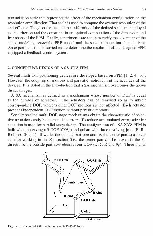
Serially stacked multi-DOF stage mechanisms obtain the characteristic of selec-tive actuation easily but accumulate errors To reduce accumulated error selectiveactuation is used for parallel stage design The configuration of a SA XYZ FPM isbuilt when observing a 3-DOF XYθZ mechanism with three revolving joint (RndashRndashR) limbs (Fig 1) If we let the outside part free and fix the center part to a linearactuator working in the Z-direction (ie the center part can be moved in the Z-direction) the outside part now obtains four DOF (X Y Z and θZ) Three planar
Figure 1 Planar 3-DOF mechanism with RndashRndashR limbs
54 H-H Pham et al
Figure 2 Passive 3D frame and three prismatic joints
3-DOF mechanisms are fixed together in one frame at the outside parts so that thethree mechanism planes are perpendicular to each other (see Fig 2) If we let eachcenter part of the frame move along the corresponding direction perpendicular tothe side containing the center part each outside part individually can perform fourDOF motions Correspondingly the DOF motions of the X-side Y -side and Z-sideare (Y Z θX X) (Z X θY Y ) and (X Y θZ Z) Actually the outside part of theframe possesses only three translation DOF that is the intersection of three aboveDOF set
(Y Z θX X) cap (Z X θY Y ) cap (X Y θZ Z) = (X Y Z)
The designed micro-motion SA XYZ FPM consists of a passive 3-dimensional (3D)flexure frame fixed to three flexure prismatic joints compounded by a double-flexurelinear slide (Figs 2 and 3) The dimensions of the double linear spring are deter-mined to guarantee very high torsion and bending stiffness and to allow the linearmotion The passive 3D flexure frame has three mutually perpendicular sides Eachside is a 3-flexure-limb group that consists of a center part connected to the edge ofthe passive 3D frame by three symmetrically located limbs The limb has a V-shapewith three hinges to create an RndashRndashR kinematics chain Each flexure prismaticjoint is actuated by a linear actuator Three linear actuators provide the platformthree decoupled translation motions following the X- Y - and Z-axis respectivelyThe number of DOF can be from 1 to 3 depending on the number of linear actuatorsmounted on the mechanism The passive 3D frame is fabricated in one piece (mono-lithic structure) in order to avoid the error of perpendicular caused by the assemblingwork In practice there are very small deformations in the non-working axes of the
Micro-motion selective-actuation XYZ flexure parallel mechanism 55
Figure 3 Selective-actuation XYZ flexure parallel mechanism
flexure element These deformations can cause error of straightness To overcomethis problem each side (3-flexure-limb group) of the 3D frame is designed as asymmetric group of three legs The dimensions of the flexure elements are also de-termined so that the stiffness in the non-working axis is maximized Those designpoints guarantee the very small and acceptable error of straightness in the expectedworking range The mechanism can perform 1ndash3 positioning tasks and possessesadvantages such as high stiffness high natural frequencies selective actuation noparasitic motion simple design and minimal number of components
3 MODELING
Recently the PRB model has been used as an analytical model to investigate flexuremechanisms Because some flexure characteristics are not taken into considerationthe PRB model is suitable only for force analysis This section presents a PRBmodel with consideration of deformation of flexure members (PRB-D model) thatcan be used to express precisely the motion of flexure mechanisms
31 PRB-D model
Suppose the desired position of the end-effector and the computed active joint vari-ables (actuated joint variables) are specified by vector X and vector x respectivelyForward kinematics based on the PRB model leads to X as a function of x as givenbelow
X = H (x) (1)
56 H-H Pham et al
However actual motion of the end-effector is assumed to be the combined effect ofthe deformation Et and PRB modeling given as below
X = H (x) + Et (2)
Assuming that the flexure mechanism complies with the linear deformation andsuperposition principles the combined effect of deformation Et is the accumulateddeflection of all flexure members so
Et =nsum
i=1
Ei (3)
where n is the number of flexure members existing in the mechanism and Ei is theindividual deformation of flexure member i that can be determined as
Ei = Giεi (4)
where εi is the deflection of flexure member i and Gi is the transformation matrixof the deformation from the flexure member i to the end-effector
The deflection of flexure member i is caused by reaction forces or moments Fi
applied to that member given as below
εi = Kminus1i Gf iFi (5)
where Ki is the stiffness matrix of that flexure member and matrix Gf i is used totransform the force Fi from the base frame to the local frame of the flexure memberThe reaction Fi is determined in the force analysis of the flexure mechanism basedon the PRB model
The total effect of deformation of flexure members on the end-effector can beexpressed as
Et =nsum
i=1
GiKminus1i Gf iFi (6)
Substituting equation (6) into equation (2) we have the PRB-D model of the flexuremechanism given as
X = H (x) +nsum
i=1
GiKminus1i Gf iFi (7)
The PRB-D model of a flexure mechanism can be summarized in a scheme as shownin Fig 4 The PRB-D model needs extensive computations because it concerns allthe flexure members Fortunately the flexure mechanism used for ultra-precisionmanipulation must have a simple structure with few flexure members
Micro-motion selective-actuation XYZ flexure parallel mechanism 57
Figure 4 Schema of pseudo-rigid-body model
32 Application to the designed XYZ FPM
321 PRB model The PRB model of the FPM is obtained by replacing theflexure hinges of the passive 3D frame by the revolving joints and the doublelinear slides by the prismatic joints (see Fig 5a) Each 3-flexure-limb groupof the PRB model is illustrated in Fig 5b as a 3-DOF planar parallel mecha-nism
Denote X = (X Y Z) and x = (x y z) as the displacement vector of end-effector and the vector of the active joint variable we have
(XY Z)T = J(xyz)T (8)
where the Jacobian matrix J is a unity matrix To determine all joint variables(passive and active) we use the notation ηij which indicates the quantity η of limbj of the 3-flexure limb group i for example θ120 represents the initial angle betweenthe X-axis and link A12B12 of limb 2 of 3-flexure limb group 1 and
i = 1 u v and w represent x y and zi = 2 u v and w represent y z and x and
i = 3 u v and w represent z x and y respetively
Consider limb j of the 3-flexure limb group i of the PRB model (Fig 6) thevector loop equation of the limb is
rarrOiCij = rarr
OiAij + rarrAijBij + rarr
BijCij
58 H-H Pham et al
(a)
(b)
Figure 5 Pseudo-rigid-body model (a) Mechanism (b) one 3-flexure limb group
Denote Bij0 and Cij0 as the initial positions of joints Bij and Cij on limb j of sidei the equation can be changed to
rarrAijBij0 + rarr
Bij0Cij0 + rarru + rarr
v = rarrAijBij + rarr
BijCij
Micro-motion selective-actuation XYZ flexure parallel mechanism 59
Figure 6 Vector close loop of limb j on 3-flexure limb group i
With projection of the vector equation on the two axes u and v we have
a cos θij0 + b cos ψij0 + u = a cos θij + b cos ψij
a sin θij0 + b sin ψij0 + v = a sin θij + b sin ψij (9)
where a b are the lengths of links AijBij BijCij and θij0 ψij0 θij ψij are theinitial and current position angles of links AijBij BijCij
Define two intermediate variables c and d as
c = a cos θij0 + b cos ψij0 + u and d = a sin θij0 + b sin ψij0 + v (10)
Solving equation (9) we obtain passive joint variables as follows
θij = γ + cosminus1
(c2 + d2 + a2 minus b2
2aradic
c2 + d2
) (11)
ψij = 2π + γ minus cosminus1
(c2 + d2 + b2 minus a2
2bradic
c2 + d2
)
where γ is defined by
cos γ = cradicc2 + d2
and sin γ = dradicc2 + d2
Differentiating equation (9) and solving the equation we have the passive jointdisplacement rates as follows
θij = cos ψij
a sin(ψij minus θij )u + sin ψij
a sin(ψij minus θij )v and
ψij = minus cos θij
b sin(ψij minus θij )u + minus sin θij
b sin(ψij minus θij )v (12)
60 H-H Pham et al
322 PRB-D model The PRB-D model of the designed FPM is
(X Y Z)T = (x y z)T +nsum
i=1
GiKminus1i Gf iFi (13)
The terms of equation (13) are determined as followsThe stiffness matrix Ki of a flexure hinge i is given by
Ki =
KxminusFx 0 0 0 0 00 KyminusFy 0 0 0 KαzminusFy
0 0 KzminusFz 0 KαyminusFz 00 0 0 KαxminusMx 0 00 0 KzminusMy 0 KαyminusMy 00 KyminusMz 0 0 0 KαzminusMz
(14)
where the terms of the stiffness matrix are cited from Ref [17] and can be seen inthe Appendix
Consider limb j of three 3-flexure limb group i of the frame (Fig 7) the effectEijw of deformation of flexure hinges of the limb on the end-effector motion in the
Figure 7 Configuration of one limb
Figure 8 Force transformation
Micro-motion selective-actuation XYZ flexure parallel mechanism 61
w-direction (w follows the notation as given in the previous section) is
Eijw = a cos(ψij minusθij )εαyAij+a sin(ψij minusθij )εαxAij
+εzAij+εzBij
+bεαyBij+εzCij
(15)where εzAij εzBij and εzCij are respectively the linear deformation of hingesAij Bij and Cij along the z-direction of the local frame fixed to the correspondingflexure hinges (see Figs 7 and 8) εαxAij and εαyAij are respectively the rotationdeformation of hinges Aij around the x- and y-axis of the local frame and εαyBij isthe rotation deformation of hinges Bij around the y-axis of the local frame
Matrix Gi expressing the flexurendashhinge deformation contributed to the overalleffect on the end-effector motion can be obtained based on equation (15) as follows
Flexure hinge Aij on limb j of 3-flexure limb group i
GA1j=
0 0 0 0 0 0
0 0 0 0 0 0
0 01
3
a cos(ψ1j minus θ1j )
3
a sin(ψ1j minus θ1j )
30
GA2j=
0 0
1
3
a cos(ψ2j minus θ2j )
3
a sin(ψ2j minus θ2j )
30
0 0 0 0 0 0
0 0 0 0 0 0
(16)
GA3j=
0 0 0 0 0 0
0 01
3
a cos(ψ3j minus θ3j )
3
a sin(ψ3j minus θ3j )
30
0 0 0 0 0 0
Flexure hinge Bij on limb j of 3-flexure limb group i
GB1j=
0 0 0 0 0 0
0 0 0 0 0 0
0 01
30
b
30
GB2j=
0 0
1
30
b
30
0 0 0 0 0 0
0 0 0 0 0 0
GB3j=
0 0 0 0 0 0
0 01
30
b
30
0 0 0 0 0 0
(17)
Flexure hinge Cij on limb j of 3-flexure limb group i
GC1j=
0 0 0 0 0 0
0 0 0 0 0 0
0 01
30 0 0
GC2j=
0 0
1
30 0 0
0 0 0 0 0 0
0 0 0 0 0 0
62 H-H Pham et al
GC3j=
0 0 0 0 0 0
0 01
30 0 0
0 0 0 0 0 0
(18)
Matrices Gf i transforming the reaction forces from the base frame to the flexurendashhinge frame (local frame fixed to flexure hinge) are determined based on Fig 8relying only on the 3-flexure limb group and expressed as below
3-flexure limb group 1
Gf 1j =
cos ψ1j sin ψ1j 0 0 0 0
minus sin ψ1j cos ψ1j 0 0 0 00 0 1 0 0 0
0 0 0 cos ψ1j sin ψ1j 0
0 0 0 minus sin ψ1j cos ψ1j 0
0 0 0 0 0 1
3-flexure limb group 2
Gf 2j =
cos ψ2j 0 sin ψ2j 0 0 0
0 1 0 0 0 0
minus sin ψ2j 0 cos ψ2j 0 0 0
0 0 0 cos ψ2j 0 sin ψ2j
0 0 0 0 1 0
0 0 0 minus sin ψ2j 0 cos ψ2j
(19)
3-flexure limb group 3
Gf 3j =
1 0 0 0 0 0
0 cos ψ3j sin ψ3j 0 0 0
0 minus sin ψ3j cos ψ3j 0 0 0
0 0 0 1 0 0
0 0 0 0 cos ψ3j sin ψ3j
0 0 0 0 minus sin ψ3j cos ψ3j
To determine the reaction forces Fi first the actuation forces Fx Fy and Fz aredetermined by using the virtual work method as follows
δW = F Tdx + P TdX + δV = 0 (20)
where δW is the virtual work F = (Fx Fy Fz)T is actuation force P =
(PX PY PZ) is the load actuating at end-effector and δV is the differentiation ofthe potential energy accumulated at the flexure joints
Micro-motion selective-actuation XYZ flexure parallel mechanism 63
Figure 9 Simplified model for reaction computation
The potential energy is computed as
V = 1
2
3sum
i=1
3sum
j=1
[KAij(θij minus θij0)
2 + KCij(ψij minus ψij0)
2 + KBij(ψij minus θij minus ψij0
+ θij0)2] + KSi
(w minus w0)2
(21)
where KAij KBij KCij are respectively the torsional stiffness KαzminusMz of theflexure hinges Aij Bij Cij and KSi(i = 1 2 and 3) is the linear stiffness of theflexure prismatic joints of sides 1 2 and 3 (see Appendix)
Solving equation (21) we obtain the actuation forces and reduce the number ofvariables in the computation of reactions We assume that the center and the outsideparts of the 3-flexure-limb groups of the passive 3D frame are absolutely rigid andthe loads are distributed symmetrically on the limbs The model of force analysiscan be simplified to the 3-limb model as shown in Fig 9
Denote the 54 reactions at the flexure joints as
Joint Ai RxAi
Ry
Ai Rz
Ai Mx
Ai M
y
Ai Mz
Ai(i = 1 2 3)
Joint Bi RxBi
Ry
Bi Rz
Bi Mx
Bi M
y
Bi Mz
Bi(i = 1 2 3)
Joint Ci RxCi
Ry
Ci Rz
Ci Mx
Ci M
y
Ci Mz
Ci(i = 1 2 3)
where the reaction moments in the plane of limbs are determined as follows
MzA1
= KA11(θ11 minus θ110)MzC1
= KC11(ψ11 minus ψ110)
MzB1
= KB11(ψ11 minus θ11 minus ψ110 + θ110)
64 H-H Pham et al
MxA2
= KA21(θ21 minus θ210)MxC2
= KC21(ψ21 minus ψ210) (22)
MxB2
= KB21(ψ21 minus θ21 minus ψ210 + θ210)
My
A3= KA31(θ31 minus θ310)M
y
C3= KC31(ψ31 minus ψ310)
My
B3= KB31(ψ31 minus θ31 minus ψ310 + θ310)
and the reactions at the input joints Ai are as follows
RzA1
= FzRxA2
= FxRy
A3= Fy (23)
Therefore the remaining number of variables is 42 The reaction can be obtained byestablishing and solving the NewtonndashEuler equations for 7 links with 42 equations
4 RESOLUTION TRANSMISSION SCALE AND OPTIMAL DESIGN
41 Resolution transmission scale
Consider a non-redundant FPM with n degree-of-freedoms and denote dq =(dq1 dq2 dqn) as the vector of the infinitesimal displacements of n actuatorsand dX = (dX1 dX2 dXn) as the vector of the infinitesimal motions(displacements andor orientations) of the end-effector Let J (n times n matrix) bethe coefficient matrix of resolution transmission from actuators to the end-effector(Jacobian matrix) The amplification effect of infinitesimal actuator displacementson the infinitesimal motion of the end-effector can be described by
dX = Jdq (24)
To examine the resolution of the FPM we observe the available motions of the end-effector when one of the actuators carries out the smallest controllable motion thatequal to the resolution δ of the actuator
dq2 = dqTdq = dq21 + dq2
2 + middot middot middot + dq2n = δ2 (25)
Assuming that the FPM operates in free singular workspace equation (24) andequation (25) lead to
dXT(JJT)minus1dX = δ2 (26)
Thus
dXT(JJT)minus1dX = dX21σ
21 + dX2
2σ22 + middot middot middot + dX2
nσ2n = δ2 (27)
where σ1 σ2 σn are the singular values of Jacobian J [18] and
JJT = diag(σ 21 σ 2
2 σ 2n ) (28)
Equation (27) shows that the smallest motions (resolution) that the end-effector canperform along the principal axes are σ1δ σ2δ σnδ and the singular values σiare the coefficients of the resolution transmission from actuator to the end-effector
Micro-motion selective-actuation XYZ flexure parallel mechanism 65
The resolution of end-effector varies following the motion direction Thereforewe use a concept called lsquoresolution transmission scalersquo to represent the averageresolution of the end-effector at one particular point
411 Resolution transmission scale The resolution transmission (RT) scale isdefined as the geometric mean of the resolution scale along all directions σi
R = nradic
σ1σ2σn (29)
Equations (28) and (29) show that the resolution transmission scale is computed asfollows
R = 2n
radicdet(JJT) (30)
Since J is configuration dependent the RT scale is a local performance measurethat will be valid at a certain pose only We use the average RT scale over theworkspace
Rglobal =int
W
R dwint
W
dw (31)
where W is the workspace and dw is an infinitesimal area in which the RT scale isconsidered to be constant
The resolution of an ultra-precision manipulation system must be uniform overthe entire workspace Therefore to have a full assessment of resolution we utilizean additional indicator the uniformity U as parameter for variety evaluation givenas below
U = RminRmax (32)
where Rmin and Rmax are the minimum and the maximum of the RT scale over theentire workspace W
Both indices the global RT scale R and the uniformity U require integration overthe entire workspace W that is bounded by three workspaces
W = W1 cap W2 cap W3 (33)
where W1 is the workspace determined by the architecture reachability
W1 = P(x y z)| det(J) = 0 (34)
W2 is the workspace determined by the actuator range
W2 = P(x y z)|foralli = 1 2 n qi S (35)
here the actuated joint variables qi result from the inverse kinematics and S isthe actuator range and W3 is the workspace based on the limited motion of flexuremembers
W3 = P(x y z)|Smax lt Sy (36)
66 H-H Pham et al
Figure 10 Global indices sampling algorithm
here Smax and Sy are the maximum stress in the flexure members and the yield stressof the material of the FPM respectively
The maximal stress does not exist at the same position within the structure of theFPM when the end-effector moves within the workspace Therefore it is difficultto describe the closed-form boundary equation of workspace W3 Consequently theintegration over the workspace based on closed-form description of the boundarycannot be guaranteed Therefore a numerical approach is proposed here todetermine the workspace and the global indices (Fig 10) The features of themethod are the partition of a covering volume A into small sampling pieces vi
Micro-motion selective-actuation XYZ flexure parallel mechanism 67
Table 1Results of optimization
Inputs Aluminum alloy with yield stress Sy = 500 MPa and Youngrsquos modulusE = 71 GPaa = 35 mm h = 60 mmKθ = Kψ = 1240 Nmiddotmmrad (7 Nmiddotmm) KS = 025 NmmUmin = 06
Outputs Dimension kab = ba = 114Free shapeinitial posture θij0 = 80 ψij0 = 165Global RT scale Rglobal = 61 and uniformity U = 061
and the piece-by-piece test in order to know whether the piece vi belongs to theworkspace The dimension of the samples is determined based on the requiredaccuracy The samples that belong to the workspace are added to workspace variableW of the algorithm and the local RT scales at those samples are added to thesumming variable SumR Samples are compared to identify the maximal and theminimal values of RT scale After all of the sampling pieces are examined theworkspace is obtained and stored in variable W The summing variable SumR isdivided by the number of samples identified within the workspace in order to obtainthe global RT scale Rglobal The uniformity U is determined based on the minimaland the maximal values of the local RT scales
42 Optimal design
In general the global scale of RT needs to be minimized to obtain the highestresolution However the Jacobian J is a coefficient matrix of the force transmissionfrom actuators to the end-effector The decrease of the RT scale leads to the increaseof the actuation load requirement and causes difficulty in the actuator selectionbecause the precise actuator usually possesses small load capability To satisfy bothrequirements ie high resolution and small actuation load the global RT scaleRglobal needs to be as close to 1 as possible Moreover to limit the variety of the RTscale in the workspace the uniformity must be kept as close to unity as possibleThe optimal design of the FPM can be formulated as
Minimize |Mglobal minus 1| (37)
Subject to U Umin (38)
where Umin is the allowed lower limit of uniformityOptimization variables The dimension of the PRB and PRB-D models and the
initial posturefree shape of the FPMThe conjugate direction method is used to reduce computation resource and to
speed up the searching process The result of the optimization is shown in Table 1
68 H-H Pham et al
5 EXPERIMENTS
Theoretically the workspace of the XYZ stage is determined by equation (33) andyield stress Sy = 500 MPa Practically the picomotors with the actuation forcelimit of 22 N are used to actuate the stage Therefore only 20 of the max strain(maximum strain caused when Sy is used as the limit of strain in equation (36)) isaccepted and the developed XYZ stage has workspace of 800 microm times 800 microm times800 microm An experiment is set up to verify the selective-actuation characteristic andthe PRB-D model (see Fig 11) The motion of the end-effector is measured by aprobe with a resolution of 01 microm an increase of measuring force of 004 Nmmand measurement range from minus037 mm to +16 mm The stiffness of measuringaction is very small (004 Nmm) the deformation of probersquos stand is negligibleand the measuring result can be considered the motion of end-effector When theactuator in the X-direction is working the unexpected motions dZ and dY of theend-effector along the Z- and Y -axis is measured The unexpected motions are lessthan 7 (see Fig 12) To verify the advantage of the PRB-D model versus the PRBmodel the solutions of the kinematics based on the PRB-D and PRB models areapplied to control the FPM The PRB modelrsquos error increases very early even whenthe end-effector displacement is under 5 microm whereas the errors of PRB-D modelcan be negligible The error produced by the PRB-D model is only 13 of that bythe PRB model (Fig 12) It is possible to study the tendency of the error of PRB-Dmodel in Fig 13 and provide compensation for the control of the system
Figure 11 Selective-actuation XYZ flexure parallel mechanism and experimental setup
Micro-motion selective-actuation XYZ flexure parallel mechanism 69
Figure 12 Unexpected motion dZ versus the actuated motion X
Figure 13 Comparison between pseudo-rigid-body model and pseudo rigid-body model withconsideration of deformation
A feedback system is established to control the developed FPM (see Fig 14)The motion of the end-effector of FPM is measured by the optical sensors (LC-2430 Keyence) with a resolution of 002 microm and measurement range of 1 mm
70 H-H Pham et al
Figure 14 Flexure parallel mechanism with close-loop control system
Figure 15 Response of end-effector position
and the data obtained are fed back to the controlling program We let the FPMprovide a series of small motions The range of the motions is gradually reducedand the response of end-effector position is recorded to determine the smallestcontrollable motion of the FPM The responses of the end-effector position to the
Micro-motion selective-actuation XYZ flexure parallel mechanism 71
position commands with ranges of 300 20 02 and 01 microm are illustrated in Fig 15Resolution of the developed FPM equipped with a feedback system is determinedexperimentally as 02 microm whereas the resolution as predicted by the design isδRglobal asymp 018 microm (resolution of the used actuator δ asymp 003microm and global RTscale Rglobal asymp 61)
6 CONCLUSIONS
The design of a translational FPM with three de-coupled motions is presentedThe selective-actuation configuration allows the designed mechanism to be usedin a multi-positioning task with different requirements for the number of DOFMoreover the expensive precision actuator can be removed and reused for anothertask The selective-actuation configuration is also useful for control aspect Itallows the user to adjust the mechanism easily and rapidly to obtain the precisedesired position A design of the micro-motion mechanism is needed to considerthe factors of resolution Therefore the resolution transmission scale is defined toevaluate the resolution criteria of the mechanism The defined scale is utilized asthe criteria of the optimal design for dimension and free shape of the flexure parallelmechanism The PRB-D model based on the PRB model currently used and theaddition of the deformation of flexure members is specified to obtain the preciseanalytical model for the position control and the formulation of the optimal designThe experiment confirmed the selective-actuation characteristic of the developedFPM and the validity of the PRB-D model in precision positioning Also theexperimental result proves that the desired resolution of the FPM can be achievedby the optimization based on the global value and the uniformity of the resolutiontransmission scale
Acknowledgements
This project is financially sponsored by Ministry of Education Singapore underARP RG 0602 and Innovation in Manufacturing Science and Technology (IMST)program of Singapore-MIT Alliance We would like to thank Prof David Butler forhis highly valuable comments and suggestions
REFERENCES
1 S Chang C Tseng and H Chien An ultra-precision XYθZ piezo-micropositioner mdash Part IDesign and analysis IEEE Transactions on Ultrasonics Ferrorelectrics and Frequency Control46 (4) 897ndash905 (1999)
2 J Ryu D G Gweon and K Moon Optimal design of a flexure hinge based XYθ wafer stagePrecision Engineering 2 (1) 18ndash28 (1997)
3 J Ryu S Lee D Gweon and K Moon Inverse kinematic modeling of a coupled flexure hingemechanism Mechatronics 9 658ndash674 (1999)
72 H-H Pham et al
4 Y Koseki T Tanikawa N Koyachi and T Arai Kinematic analysis of translational 3-dofmicro parallel mechanism using matrix method in Proceedings of the IEEERSJ InternationalConference on Intelligent Robots and Systems Takamatsu pp 786ndash792 (2000)
5 B J Yi H Y Na G B Chung W K Kim and I H Suh Design and experiment of a3DOF parallel micro-mechanism utilizing flexure hinges in IEEE International Conferenceon Robotics and Automation Washington DC pp 604ndash612 (2002)
6 J Shim S Song D Kwion and H Cho Kinematic feature analysis of a 6-degree-of-freedomin-parallel manipulator for micro-positioning in Proceedings of the IEEERSJ InternationalConference on Intelligent Robots and Systems Volume 3 Grenoble pp 1617ndash1623 (1997)
7 P Gao and S-M Swei A six-degree-of-freedom micro-manipulator based on piezoelectrictranslators Nanotechnology 10 447ndash452 (1999)
8 C Han J Hudgens D Tesar and A Traver Modeling synthesis analysis and design of highresolution micro-manipulator to enhance robot accuracy in IEEERSJ International Workshopon Intelligent Robots and Systems IROS rsquo91 Osaka pp 1157ndash1162 (1991)
9 S L Canfield and J Beard Development of a spatial compliant manipulator InternationalJournal of Robotics and Automation 17 (1) 63ndash71 (2002)
10 T Oiwa and M Hirano Six degree-of-freedom fine motion mechanism using parallel mecha-nism Journal of Japan Society of Precision Engineering 65 (10) 1425ndash1429 (1999)
11 M L Culpepper and G Anderson Design of a low-cost nano-manipulator which utilizes amonolithic spatial compliant mechanism Precision Engineering 28 469ndash482 (2004)
12 Y M Moon and S Kota Design of compliant parallel kinematic machines in Proceedings ofthe 27th Biannual Mechanisms and Robotics Conference DETC2002MECH-34204 Montrealpp 1ndash7 (2002)
13 G K Ananthasuresh and S Kota Designing Compliant Mechanisms Mechanical Engineering117 (11) 93ndash96 (1995)
14 L Howell Compliant Mechanism Wiley New York NY (2001)15 Davis A Philips and Melles Griot Limited Positioning mechanism US Patent Application
702353 (2000)16 Laboratoire de Systemes Robotiques EPFL-LSRO website httplsroepflch17 J M Paros and L Weisbord How to design flexure hinges Machine Design 37 151ndash156 (1965)18 D H Griffel Linear Algebra and Its Applications Vol 2 Ellis Horwood Chichester (1989)19 N Lobontiu Compliant Mechanisms Design of Flexure Hinges CRC Press Boca Raton FL
(2003)
APPENDIX
The inverse of stiffness of flexure hinges
1
KxminusFx
= π(rt)12 minus 257
Ee
1
KyminusFy
= 9πr52
2Eet52+ π(rt)12 minus 257
Ge
1
KzminusFz
= 12πr2
Ee3[(rt)12 minus 14] + π(rt)12 minus 257
Ge
1
KαxminusMx
= 9πr12
8Get52
1
KαyminusMy
= 12
Ee3[π(rt)12 minus 257] (A1)
1
KαzminusMz
= 9πr12
2Eet52
1
KyminusMz
= 1
KαzminusFy
= 9πr32
2Eet52
Micro-motion selective-actuation XYZ flexure parallel mechanism 73
Figure 16 Flexure hinge dimension
1
KzminusMy
= 1
KαyminusFz
= 12r
Ee3[π(rt)12 minus 257]
where e t and r are respectively the thickness of the link the thickness and theradius of the hinge described in Fig 16 E and G are the Youngrsquos modulus and theshear modulus of the used material
Stiffness of a flexure prismatic joint double
KSi= 8KαzminusMz
L2 (A2)
where L is the length of the links in the double linear spring used as a flexureprismatic joint
52 H-H Pham et al
within small range and can be used as an ultra-precision manipulation system infields like optics precision machine tools and micro-component fabrication
Recently several FPM-based precision positioning stages have been developed[1ndash13] Beside the topology synthesis of compliant mechanisms [12 13] most ofthe flexure mechanisms are not designed based on the precision criterion but on thecriteria of large range [1ndash4 8 12] and compliancestiffness [5ndash8] Only whenthe mechanism control is implemented the precision of the flexure mechanismis taken into consideration Some measures are proposed to manage the errordistribution [1] to predict the error and modify the control [2 3] or to use theprecise measurement instruments to aid the control system [6 7] These post-designmeasures are not sufficient for obtaining a system with high accuracy There isa need for pre-design measures which can guarantee the desired resolution rightat the design stage Another problem is how to model the flexure mechanismRecent studies [1ndash4 6ndash8] simplify the modeling of a flexure mechanism by usinga pseudo-rigid-body (PRB) model as proposed by Howell [14] This method doesnot lead to accurate modeling because the deformation of the flexure members isnot studied when establishing the model Recently to obtain a more precise PRBmodel Yi et al proposed a base-fixed flexure hinge as a two-link chain consistingof a revolving joint with torsion spring and a prismatic joint [5] However theelongation and the bending of the flexure hinge are actually tied together Thereforethe replacement of a flexure hinge by a revolving joint and a prismatic jointis not sufficient and makes the modeling more complicated for a spatial flexuremechanism with more joints and links Another disadvantage is that the deflectionof passive flexure joints is still not considered An additional problem that needs tobe considered is the selective actuation (SA) of the mechanism Usually the costof a precise actuator is very high All the DOF motions of the mechanism are notalways used for a positioning task Therefore the mechanism needs to be designedso that the actuators can be moved to obtain the desired number of DOF withoutaffecting on the precision of the mechanism An additional benefit of SA is that theactuators can be used for multiple tasks As a precision positioning system cannot bere-configured often selective actuation can be considered as the re-configurabilityin a precision mechanism In addition the motion of the end-effector relies on theactuation of all actuators Usually the motions are de-coupled by using a controlalgorithm Selective actuation rejects fully or eliminates partially the dependenceof the end-effector motion on all the actuation of actuators and therefore aids thedecoupling control This allows the users to make adjustments to accurately achieveone desired position
This paper is organized as follows First the paper presents the design of a micro-motion selective-actuation XYZ flexure parallel mechanism (SA XYZ FPM) thatcan perform three decoupled translation motions Secondly a more accurate modelhas been realized by taking the effects of flexure deformations into account Theerror of PRB model caused by deformation of flexure members are estimatedand compensated The paper continues with the formulation of the resolution
Micro-motion selective-actuation XYZ flexure parallel mechanism 53
transmission scale that represents the effect of the mechanism configuration on theresolution amplification That scale is used to compute the average resolution of theend-effector The global value and the uniformity of the defined scale are employedas the criterion and the constraint in an optimal computation of the dimension andfree shape of the FPM Finally experiments are set up to verify the advantage of thestated modeling versus the PRB model and the selective-actuation characteristicAn experiment is also carried out to determine the resolution of the designed FPMequipped a feedback control system
2 CONCEPTUAL DESIGN OF A SA XYZ FPM
Several multi-axis-positioning devices are developed based on FPM [1 2 4ndash16]However the coupling of motions and parasitic motions limit the accuracy of thedevices It is stated in the Introduction that a SA mechanism overcomes the abovedisadvantages
A SA mechanism is defined as a mechanism whose number of DOF is equalto the number of actuators The actuators can be removed so as to inhibitcorresponding DOF whereas other DOF motions are not affected Each actuatorprovides independent DOF motion without parasitic motions
Serially stacked multi-DOF stage mechanisms obtain the characteristic of selec-tive actuation easily but accumulate errors To reduce accumulated error selectiveactuation is used for parallel stage design The configuration of a SA XYZ FPM isbuilt when observing a 3-DOF XYθZ mechanism with three revolving joint (RndashRndashR) limbs (Fig 1) If we let the outside part free and fix the center part to a linearactuator working in the Z-direction (ie the center part can be moved in the Z-direction) the outside part now obtains four DOF (X Y Z and θZ) Three planar
Figure 1 Planar 3-DOF mechanism with RndashRndashR limbs
54 H-H Pham et al
Figure 2 Passive 3D frame and three prismatic joints
3-DOF mechanisms are fixed together in one frame at the outside parts so that thethree mechanism planes are perpendicular to each other (see Fig 2) If we let eachcenter part of the frame move along the corresponding direction perpendicular tothe side containing the center part each outside part individually can perform fourDOF motions Correspondingly the DOF motions of the X-side Y -side and Z-sideare (Y Z θX X) (Z X θY Y ) and (X Y θZ Z) Actually the outside part of theframe possesses only three translation DOF that is the intersection of three aboveDOF set
(Y Z θX X) cap (Z X θY Y ) cap (X Y θZ Z) = (X Y Z)
The designed micro-motion SA XYZ FPM consists of a passive 3-dimensional (3D)flexure frame fixed to three flexure prismatic joints compounded by a double-flexurelinear slide (Figs 2 and 3) The dimensions of the double linear spring are deter-mined to guarantee very high torsion and bending stiffness and to allow the linearmotion The passive 3D flexure frame has three mutually perpendicular sides Eachside is a 3-flexure-limb group that consists of a center part connected to the edge ofthe passive 3D frame by three symmetrically located limbs The limb has a V-shapewith three hinges to create an RndashRndashR kinematics chain Each flexure prismaticjoint is actuated by a linear actuator Three linear actuators provide the platformthree decoupled translation motions following the X- Y - and Z-axis respectivelyThe number of DOF can be from 1 to 3 depending on the number of linear actuatorsmounted on the mechanism The passive 3D frame is fabricated in one piece (mono-lithic structure) in order to avoid the error of perpendicular caused by the assemblingwork In practice there are very small deformations in the non-working axes of the
Micro-motion selective-actuation XYZ flexure parallel mechanism 55
Figure 3 Selective-actuation XYZ flexure parallel mechanism
flexure element These deformations can cause error of straightness To overcomethis problem each side (3-flexure-limb group) of the 3D frame is designed as asymmetric group of three legs The dimensions of the flexure elements are also de-termined so that the stiffness in the non-working axis is maximized Those designpoints guarantee the very small and acceptable error of straightness in the expectedworking range The mechanism can perform 1ndash3 positioning tasks and possessesadvantages such as high stiffness high natural frequencies selective actuation noparasitic motion simple design and minimal number of components
3 MODELING
Recently the PRB model has been used as an analytical model to investigate flexuremechanisms Because some flexure characteristics are not taken into considerationthe PRB model is suitable only for force analysis This section presents a PRBmodel with consideration of deformation of flexure members (PRB-D model) thatcan be used to express precisely the motion of flexure mechanisms
31 PRB-D model
Suppose the desired position of the end-effector and the computed active joint vari-ables (actuated joint variables) are specified by vector X and vector x respectivelyForward kinematics based on the PRB model leads to X as a function of x as givenbelow
X = H (x) (1)
56 H-H Pham et al
However actual motion of the end-effector is assumed to be the combined effect ofthe deformation Et and PRB modeling given as below
X = H (x) + Et (2)
Assuming that the flexure mechanism complies with the linear deformation andsuperposition principles the combined effect of deformation Et is the accumulateddeflection of all flexure members so
Et =nsum
i=1
Ei (3)
where n is the number of flexure members existing in the mechanism and Ei is theindividual deformation of flexure member i that can be determined as
Ei = Giεi (4)
where εi is the deflection of flexure member i and Gi is the transformation matrixof the deformation from the flexure member i to the end-effector
The deflection of flexure member i is caused by reaction forces or moments Fi
applied to that member given as below
εi = Kminus1i Gf iFi (5)
where Ki is the stiffness matrix of that flexure member and matrix Gf i is used totransform the force Fi from the base frame to the local frame of the flexure memberThe reaction Fi is determined in the force analysis of the flexure mechanism basedon the PRB model
The total effect of deformation of flexure members on the end-effector can beexpressed as
Et =nsum
i=1
GiKminus1i Gf iFi (6)
Substituting equation (6) into equation (2) we have the PRB-D model of the flexuremechanism given as
X = H (x) +nsum
i=1
GiKminus1i Gf iFi (7)
The PRB-D model of a flexure mechanism can be summarized in a scheme as shownin Fig 4 The PRB-D model needs extensive computations because it concerns allthe flexure members Fortunately the flexure mechanism used for ultra-precisionmanipulation must have a simple structure with few flexure members
Micro-motion selective-actuation XYZ flexure parallel mechanism 57
Figure 4 Schema of pseudo-rigid-body model
32 Application to the designed XYZ FPM
321 PRB model The PRB model of the FPM is obtained by replacing theflexure hinges of the passive 3D frame by the revolving joints and the doublelinear slides by the prismatic joints (see Fig 5a) Each 3-flexure-limb groupof the PRB model is illustrated in Fig 5b as a 3-DOF planar parallel mecha-nism
Denote X = (X Y Z) and x = (x y z) as the displacement vector of end-effector and the vector of the active joint variable we have
(XY Z)T = J(xyz)T (8)
where the Jacobian matrix J is a unity matrix To determine all joint variables(passive and active) we use the notation ηij which indicates the quantity η of limbj of the 3-flexure limb group i for example θ120 represents the initial angle betweenthe X-axis and link A12B12 of limb 2 of 3-flexure limb group 1 and
i = 1 u v and w represent x y and zi = 2 u v and w represent y z and x and
i = 3 u v and w represent z x and y respetively
Consider limb j of the 3-flexure limb group i of the PRB model (Fig 6) thevector loop equation of the limb is
rarrOiCij = rarr
OiAij + rarrAijBij + rarr
BijCij
58 H-H Pham et al
(a)
(b)
Figure 5 Pseudo-rigid-body model (a) Mechanism (b) one 3-flexure limb group
Denote Bij0 and Cij0 as the initial positions of joints Bij and Cij on limb j of sidei the equation can be changed to
rarrAijBij0 + rarr
Bij0Cij0 + rarru + rarr
v = rarrAijBij + rarr
BijCij
Micro-motion selective-actuation XYZ flexure parallel mechanism 59
Figure 6 Vector close loop of limb j on 3-flexure limb group i
With projection of the vector equation on the two axes u and v we have
a cos θij0 + b cos ψij0 + u = a cos θij + b cos ψij
a sin θij0 + b sin ψij0 + v = a sin θij + b sin ψij (9)
where a b are the lengths of links AijBij BijCij and θij0 ψij0 θij ψij are theinitial and current position angles of links AijBij BijCij
Define two intermediate variables c and d as
c = a cos θij0 + b cos ψij0 + u and d = a sin θij0 + b sin ψij0 + v (10)
Solving equation (9) we obtain passive joint variables as follows
θij = γ + cosminus1
(c2 + d2 + a2 minus b2
2aradic
c2 + d2
) (11)
ψij = 2π + γ minus cosminus1
(c2 + d2 + b2 minus a2
2bradic
c2 + d2
)
where γ is defined by
cos γ = cradicc2 + d2
and sin γ = dradicc2 + d2
Differentiating equation (9) and solving the equation we have the passive jointdisplacement rates as follows
θij = cos ψij
a sin(ψij minus θij )u + sin ψij
a sin(ψij minus θij )v and
ψij = minus cos θij
b sin(ψij minus θij )u + minus sin θij
b sin(ψij minus θij )v (12)
60 H-H Pham et al
322 PRB-D model The PRB-D model of the designed FPM is
(X Y Z)T = (x y z)T +nsum
i=1
GiKminus1i Gf iFi (13)
The terms of equation (13) are determined as followsThe stiffness matrix Ki of a flexure hinge i is given by
Ki =
KxminusFx 0 0 0 0 00 KyminusFy 0 0 0 KαzminusFy
0 0 KzminusFz 0 KαyminusFz 00 0 0 KαxminusMx 0 00 0 KzminusMy 0 KαyminusMy 00 KyminusMz 0 0 0 KαzminusMz
(14)
where the terms of the stiffness matrix are cited from Ref [17] and can be seen inthe Appendix
Consider limb j of three 3-flexure limb group i of the frame (Fig 7) the effectEijw of deformation of flexure hinges of the limb on the end-effector motion in the
Figure 7 Configuration of one limb
Figure 8 Force transformation
Micro-motion selective-actuation XYZ flexure parallel mechanism 61
w-direction (w follows the notation as given in the previous section) is
Eijw = a cos(ψij minusθij )εαyAij+a sin(ψij minusθij )εαxAij
+εzAij+εzBij
+bεαyBij+εzCij
(15)where εzAij εzBij and εzCij are respectively the linear deformation of hingesAij Bij and Cij along the z-direction of the local frame fixed to the correspondingflexure hinges (see Figs 7 and 8) εαxAij and εαyAij are respectively the rotationdeformation of hinges Aij around the x- and y-axis of the local frame and εαyBij isthe rotation deformation of hinges Bij around the y-axis of the local frame
Matrix Gi expressing the flexurendashhinge deformation contributed to the overalleffect on the end-effector motion can be obtained based on equation (15) as follows
Flexure hinge Aij on limb j of 3-flexure limb group i
GA1j=
0 0 0 0 0 0
0 0 0 0 0 0
0 01
3
a cos(ψ1j minus θ1j )
3
a sin(ψ1j minus θ1j )
30
GA2j=
0 0
1
3
a cos(ψ2j minus θ2j )
3
a sin(ψ2j minus θ2j )
30
0 0 0 0 0 0
0 0 0 0 0 0
(16)
GA3j=
0 0 0 0 0 0
0 01
3
a cos(ψ3j minus θ3j )
3
a sin(ψ3j minus θ3j )
30
0 0 0 0 0 0
Flexure hinge Bij on limb j of 3-flexure limb group i
GB1j=
0 0 0 0 0 0
0 0 0 0 0 0
0 01
30
b
30
GB2j=
0 0
1
30
b
30
0 0 0 0 0 0
0 0 0 0 0 0
GB3j=
0 0 0 0 0 0
0 01
30
b
30
0 0 0 0 0 0
(17)
Flexure hinge Cij on limb j of 3-flexure limb group i
GC1j=
0 0 0 0 0 0
0 0 0 0 0 0
0 01
30 0 0
GC2j=
0 0
1
30 0 0
0 0 0 0 0 0
0 0 0 0 0 0
62 H-H Pham et al
GC3j=
0 0 0 0 0 0
0 01
30 0 0
0 0 0 0 0 0
(18)
Matrices Gf i transforming the reaction forces from the base frame to the flexurendashhinge frame (local frame fixed to flexure hinge) are determined based on Fig 8relying only on the 3-flexure limb group and expressed as below
3-flexure limb group 1
Gf 1j =
cos ψ1j sin ψ1j 0 0 0 0
minus sin ψ1j cos ψ1j 0 0 0 00 0 1 0 0 0
0 0 0 cos ψ1j sin ψ1j 0
0 0 0 minus sin ψ1j cos ψ1j 0
0 0 0 0 0 1
3-flexure limb group 2
Gf 2j =
cos ψ2j 0 sin ψ2j 0 0 0
0 1 0 0 0 0
minus sin ψ2j 0 cos ψ2j 0 0 0
0 0 0 cos ψ2j 0 sin ψ2j
0 0 0 0 1 0
0 0 0 minus sin ψ2j 0 cos ψ2j
(19)
3-flexure limb group 3
Gf 3j =
1 0 0 0 0 0
0 cos ψ3j sin ψ3j 0 0 0
0 minus sin ψ3j cos ψ3j 0 0 0
0 0 0 1 0 0
0 0 0 0 cos ψ3j sin ψ3j
0 0 0 0 minus sin ψ3j cos ψ3j
To determine the reaction forces Fi first the actuation forces Fx Fy and Fz aredetermined by using the virtual work method as follows
δW = F Tdx + P TdX + δV = 0 (20)
where δW is the virtual work F = (Fx Fy Fz)T is actuation force P =
(PX PY PZ) is the load actuating at end-effector and δV is the differentiation ofthe potential energy accumulated at the flexure joints
Micro-motion selective-actuation XYZ flexure parallel mechanism 63
Figure 9 Simplified model for reaction computation
The potential energy is computed as
V = 1
2
3sum
i=1
3sum
j=1
[KAij(θij minus θij0)
2 + KCij(ψij minus ψij0)
2 + KBij(ψij minus θij minus ψij0
+ θij0)2] + KSi
(w minus w0)2
(21)
where KAij KBij KCij are respectively the torsional stiffness KαzminusMz of theflexure hinges Aij Bij Cij and KSi(i = 1 2 and 3) is the linear stiffness of theflexure prismatic joints of sides 1 2 and 3 (see Appendix)
Solving equation (21) we obtain the actuation forces and reduce the number ofvariables in the computation of reactions We assume that the center and the outsideparts of the 3-flexure-limb groups of the passive 3D frame are absolutely rigid andthe loads are distributed symmetrically on the limbs The model of force analysiscan be simplified to the 3-limb model as shown in Fig 9
Denote the 54 reactions at the flexure joints as
Joint Ai RxAi
Ry
Ai Rz
Ai Mx
Ai M
y
Ai Mz
Ai(i = 1 2 3)
Joint Bi RxBi
Ry
Bi Rz
Bi Mx
Bi M
y
Bi Mz
Bi(i = 1 2 3)
Joint Ci RxCi
Ry
Ci Rz
Ci Mx
Ci M
y
Ci Mz
Ci(i = 1 2 3)
where the reaction moments in the plane of limbs are determined as follows
MzA1
= KA11(θ11 minus θ110)MzC1
= KC11(ψ11 minus ψ110)
MzB1
= KB11(ψ11 minus θ11 minus ψ110 + θ110)
64 H-H Pham et al
MxA2
= KA21(θ21 minus θ210)MxC2
= KC21(ψ21 minus ψ210) (22)
MxB2
= KB21(ψ21 minus θ21 minus ψ210 + θ210)
My
A3= KA31(θ31 minus θ310)M
y
C3= KC31(ψ31 minus ψ310)
My
B3= KB31(ψ31 minus θ31 minus ψ310 + θ310)
and the reactions at the input joints Ai are as follows
RzA1
= FzRxA2
= FxRy
A3= Fy (23)
Therefore the remaining number of variables is 42 The reaction can be obtained byestablishing and solving the NewtonndashEuler equations for 7 links with 42 equations
4 RESOLUTION TRANSMISSION SCALE AND OPTIMAL DESIGN
41 Resolution transmission scale
Consider a non-redundant FPM with n degree-of-freedoms and denote dq =(dq1 dq2 dqn) as the vector of the infinitesimal displacements of n actuatorsand dX = (dX1 dX2 dXn) as the vector of the infinitesimal motions(displacements andor orientations) of the end-effector Let J (n times n matrix) bethe coefficient matrix of resolution transmission from actuators to the end-effector(Jacobian matrix) The amplification effect of infinitesimal actuator displacementson the infinitesimal motion of the end-effector can be described by
dX = Jdq (24)
To examine the resolution of the FPM we observe the available motions of the end-effector when one of the actuators carries out the smallest controllable motion thatequal to the resolution δ of the actuator
dq2 = dqTdq = dq21 + dq2
2 + middot middot middot + dq2n = δ2 (25)
Assuming that the FPM operates in free singular workspace equation (24) andequation (25) lead to
dXT(JJT)minus1dX = δ2 (26)
Thus
dXT(JJT)minus1dX = dX21σ
21 + dX2
2σ22 + middot middot middot + dX2
nσ2n = δ2 (27)
where σ1 σ2 σn are the singular values of Jacobian J [18] and
JJT = diag(σ 21 σ 2
2 σ 2n ) (28)
Equation (27) shows that the smallest motions (resolution) that the end-effector canperform along the principal axes are σ1δ σ2δ σnδ and the singular values σiare the coefficients of the resolution transmission from actuator to the end-effector
Micro-motion selective-actuation XYZ flexure parallel mechanism 65
The resolution of end-effector varies following the motion direction Thereforewe use a concept called lsquoresolution transmission scalersquo to represent the averageresolution of the end-effector at one particular point
411 Resolution transmission scale The resolution transmission (RT) scale isdefined as the geometric mean of the resolution scale along all directions σi
R = nradic
σ1σ2σn (29)
Equations (28) and (29) show that the resolution transmission scale is computed asfollows
R = 2n
radicdet(JJT) (30)
Since J is configuration dependent the RT scale is a local performance measurethat will be valid at a certain pose only We use the average RT scale over theworkspace
Rglobal =int
W
R dwint
W
dw (31)
where W is the workspace and dw is an infinitesimal area in which the RT scale isconsidered to be constant
The resolution of an ultra-precision manipulation system must be uniform overthe entire workspace Therefore to have a full assessment of resolution we utilizean additional indicator the uniformity U as parameter for variety evaluation givenas below
U = RminRmax (32)
where Rmin and Rmax are the minimum and the maximum of the RT scale over theentire workspace W
Both indices the global RT scale R and the uniformity U require integration overthe entire workspace W that is bounded by three workspaces
W = W1 cap W2 cap W3 (33)
where W1 is the workspace determined by the architecture reachability
W1 = P(x y z)| det(J) = 0 (34)
W2 is the workspace determined by the actuator range
W2 = P(x y z)|foralli = 1 2 n qi S (35)
here the actuated joint variables qi result from the inverse kinematics and S isthe actuator range and W3 is the workspace based on the limited motion of flexuremembers
W3 = P(x y z)|Smax lt Sy (36)
66 H-H Pham et al
Figure 10 Global indices sampling algorithm
here Smax and Sy are the maximum stress in the flexure members and the yield stressof the material of the FPM respectively
The maximal stress does not exist at the same position within the structure of theFPM when the end-effector moves within the workspace Therefore it is difficultto describe the closed-form boundary equation of workspace W3 Consequently theintegration over the workspace based on closed-form description of the boundarycannot be guaranteed Therefore a numerical approach is proposed here todetermine the workspace and the global indices (Fig 10) The features of themethod are the partition of a covering volume A into small sampling pieces vi
Micro-motion selective-actuation XYZ flexure parallel mechanism 67
Table 1Results of optimization
Inputs Aluminum alloy with yield stress Sy = 500 MPa and Youngrsquos modulusE = 71 GPaa = 35 mm h = 60 mmKθ = Kψ = 1240 Nmiddotmmrad (7 Nmiddotmm) KS = 025 NmmUmin = 06
Outputs Dimension kab = ba = 114Free shapeinitial posture θij0 = 80 ψij0 = 165Global RT scale Rglobal = 61 and uniformity U = 061
and the piece-by-piece test in order to know whether the piece vi belongs to theworkspace The dimension of the samples is determined based on the requiredaccuracy The samples that belong to the workspace are added to workspace variableW of the algorithm and the local RT scales at those samples are added to thesumming variable SumR Samples are compared to identify the maximal and theminimal values of RT scale After all of the sampling pieces are examined theworkspace is obtained and stored in variable W The summing variable SumR isdivided by the number of samples identified within the workspace in order to obtainthe global RT scale Rglobal The uniformity U is determined based on the minimaland the maximal values of the local RT scales
42 Optimal design
In general the global scale of RT needs to be minimized to obtain the highestresolution However the Jacobian J is a coefficient matrix of the force transmissionfrom actuators to the end-effector The decrease of the RT scale leads to the increaseof the actuation load requirement and causes difficulty in the actuator selectionbecause the precise actuator usually possesses small load capability To satisfy bothrequirements ie high resolution and small actuation load the global RT scaleRglobal needs to be as close to 1 as possible Moreover to limit the variety of the RTscale in the workspace the uniformity must be kept as close to unity as possibleThe optimal design of the FPM can be formulated as
Minimize |Mglobal minus 1| (37)
Subject to U Umin (38)
where Umin is the allowed lower limit of uniformityOptimization variables The dimension of the PRB and PRB-D models and the
initial posturefree shape of the FPMThe conjugate direction method is used to reduce computation resource and to
speed up the searching process The result of the optimization is shown in Table 1
68 H-H Pham et al
5 EXPERIMENTS
Theoretically the workspace of the XYZ stage is determined by equation (33) andyield stress Sy = 500 MPa Practically the picomotors with the actuation forcelimit of 22 N are used to actuate the stage Therefore only 20 of the max strain(maximum strain caused when Sy is used as the limit of strain in equation (36)) isaccepted and the developed XYZ stage has workspace of 800 microm times 800 microm times800 microm An experiment is set up to verify the selective-actuation characteristic andthe PRB-D model (see Fig 11) The motion of the end-effector is measured by aprobe with a resolution of 01 microm an increase of measuring force of 004 Nmmand measurement range from minus037 mm to +16 mm The stiffness of measuringaction is very small (004 Nmm) the deformation of probersquos stand is negligibleand the measuring result can be considered the motion of end-effector When theactuator in the X-direction is working the unexpected motions dZ and dY of theend-effector along the Z- and Y -axis is measured The unexpected motions are lessthan 7 (see Fig 12) To verify the advantage of the PRB-D model versus the PRBmodel the solutions of the kinematics based on the PRB-D and PRB models areapplied to control the FPM The PRB modelrsquos error increases very early even whenthe end-effector displacement is under 5 microm whereas the errors of PRB-D modelcan be negligible The error produced by the PRB-D model is only 13 of that bythe PRB model (Fig 12) It is possible to study the tendency of the error of PRB-Dmodel in Fig 13 and provide compensation for the control of the system
Figure 11 Selective-actuation XYZ flexure parallel mechanism and experimental setup
Micro-motion selective-actuation XYZ flexure parallel mechanism 69
Figure 12 Unexpected motion dZ versus the actuated motion X
Figure 13 Comparison between pseudo-rigid-body model and pseudo rigid-body model withconsideration of deformation
A feedback system is established to control the developed FPM (see Fig 14)The motion of the end-effector of FPM is measured by the optical sensors (LC-2430 Keyence) with a resolution of 002 microm and measurement range of 1 mm
70 H-H Pham et al
Figure 14 Flexure parallel mechanism with close-loop control system
Figure 15 Response of end-effector position
and the data obtained are fed back to the controlling program We let the FPMprovide a series of small motions The range of the motions is gradually reducedand the response of end-effector position is recorded to determine the smallestcontrollable motion of the FPM The responses of the end-effector position to the
Micro-motion selective-actuation XYZ flexure parallel mechanism 71
position commands with ranges of 300 20 02 and 01 microm are illustrated in Fig 15Resolution of the developed FPM equipped with a feedback system is determinedexperimentally as 02 microm whereas the resolution as predicted by the design isδRglobal asymp 018 microm (resolution of the used actuator δ asymp 003microm and global RTscale Rglobal asymp 61)
6 CONCLUSIONS
The design of a translational FPM with three de-coupled motions is presentedThe selective-actuation configuration allows the designed mechanism to be usedin a multi-positioning task with different requirements for the number of DOFMoreover the expensive precision actuator can be removed and reused for anothertask The selective-actuation configuration is also useful for control aspect Itallows the user to adjust the mechanism easily and rapidly to obtain the precisedesired position A design of the micro-motion mechanism is needed to considerthe factors of resolution Therefore the resolution transmission scale is defined toevaluate the resolution criteria of the mechanism The defined scale is utilized asthe criteria of the optimal design for dimension and free shape of the flexure parallelmechanism The PRB-D model based on the PRB model currently used and theaddition of the deformation of flexure members is specified to obtain the preciseanalytical model for the position control and the formulation of the optimal designThe experiment confirmed the selective-actuation characteristic of the developedFPM and the validity of the PRB-D model in precision positioning Also theexperimental result proves that the desired resolution of the FPM can be achievedby the optimization based on the global value and the uniformity of the resolutiontransmission scale
Acknowledgements
This project is financially sponsored by Ministry of Education Singapore underARP RG 0602 and Innovation in Manufacturing Science and Technology (IMST)program of Singapore-MIT Alliance We would like to thank Prof David Butler forhis highly valuable comments and suggestions
REFERENCES
1 S Chang C Tseng and H Chien An ultra-precision XYθZ piezo-micropositioner mdash Part IDesign and analysis IEEE Transactions on Ultrasonics Ferrorelectrics and Frequency Control46 (4) 897ndash905 (1999)
2 J Ryu D G Gweon and K Moon Optimal design of a flexure hinge based XYθ wafer stagePrecision Engineering 2 (1) 18ndash28 (1997)
3 J Ryu S Lee D Gweon and K Moon Inverse kinematic modeling of a coupled flexure hingemechanism Mechatronics 9 658ndash674 (1999)
72 H-H Pham et al
4 Y Koseki T Tanikawa N Koyachi and T Arai Kinematic analysis of translational 3-dofmicro parallel mechanism using matrix method in Proceedings of the IEEERSJ InternationalConference on Intelligent Robots and Systems Takamatsu pp 786ndash792 (2000)
5 B J Yi H Y Na G B Chung W K Kim and I H Suh Design and experiment of a3DOF parallel micro-mechanism utilizing flexure hinges in IEEE International Conferenceon Robotics and Automation Washington DC pp 604ndash612 (2002)
6 J Shim S Song D Kwion and H Cho Kinematic feature analysis of a 6-degree-of-freedomin-parallel manipulator for micro-positioning in Proceedings of the IEEERSJ InternationalConference on Intelligent Robots and Systems Volume 3 Grenoble pp 1617ndash1623 (1997)
7 P Gao and S-M Swei A six-degree-of-freedom micro-manipulator based on piezoelectrictranslators Nanotechnology 10 447ndash452 (1999)
8 C Han J Hudgens D Tesar and A Traver Modeling synthesis analysis and design of highresolution micro-manipulator to enhance robot accuracy in IEEERSJ International Workshopon Intelligent Robots and Systems IROS rsquo91 Osaka pp 1157ndash1162 (1991)
9 S L Canfield and J Beard Development of a spatial compliant manipulator InternationalJournal of Robotics and Automation 17 (1) 63ndash71 (2002)
10 T Oiwa and M Hirano Six degree-of-freedom fine motion mechanism using parallel mecha-nism Journal of Japan Society of Precision Engineering 65 (10) 1425ndash1429 (1999)
11 M L Culpepper and G Anderson Design of a low-cost nano-manipulator which utilizes amonolithic spatial compliant mechanism Precision Engineering 28 469ndash482 (2004)
12 Y M Moon and S Kota Design of compliant parallel kinematic machines in Proceedings ofthe 27th Biannual Mechanisms and Robotics Conference DETC2002MECH-34204 Montrealpp 1ndash7 (2002)
13 G K Ananthasuresh and S Kota Designing Compliant Mechanisms Mechanical Engineering117 (11) 93ndash96 (1995)
14 L Howell Compliant Mechanism Wiley New York NY (2001)15 Davis A Philips and Melles Griot Limited Positioning mechanism US Patent Application
702353 (2000)16 Laboratoire de Systemes Robotiques EPFL-LSRO website httplsroepflch17 J M Paros and L Weisbord How to design flexure hinges Machine Design 37 151ndash156 (1965)18 D H Griffel Linear Algebra and Its Applications Vol 2 Ellis Horwood Chichester (1989)19 N Lobontiu Compliant Mechanisms Design of Flexure Hinges CRC Press Boca Raton FL
(2003)
APPENDIX
The inverse of stiffness of flexure hinges
1
KxminusFx
= π(rt)12 minus 257
Ee
1
KyminusFy
= 9πr52
2Eet52+ π(rt)12 minus 257
Ge
1
KzminusFz
= 12πr2
Ee3[(rt)12 minus 14] + π(rt)12 minus 257
Ge
1
KαxminusMx
= 9πr12
8Get52
1
KαyminusMy
= 12
Ee3[π(rt)12 minus 257] (A1)
1
KαzminusMz
= 9πr12
2Eet52
1
KyminusMz
= 1
KαzminusFy
= 9πr32
2Eet52
Micro-motion selective-actuation XYZ flexure parallel mechanism 73
Figure 16 Flexure hinge dimension
1
KzminusMy
= 1
KαyminusFz
= 12r
Ee3[π(rt)12 minus 257]
where e t and r are respectively the thickness of the link the thickness and theradius of the hinge described in Fig 16 E and G are the Youngrsquos modulus and theshear modulus of the used material
Stiffness of a flexure prismatic joint double
KSi= 8KαzminusMz
L2 (A2)
where L is the length of the links in the double linear spring used as a flexureprismatic joint
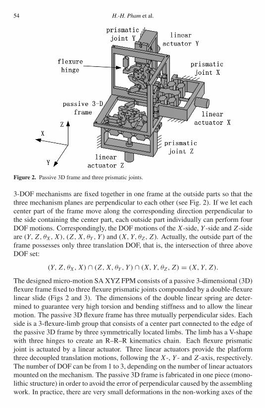
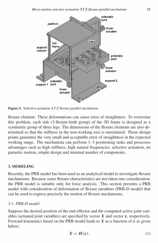
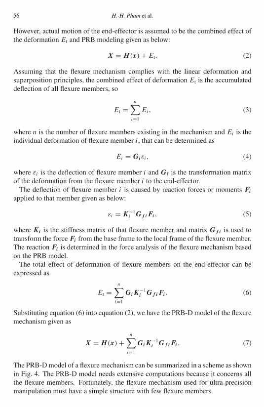
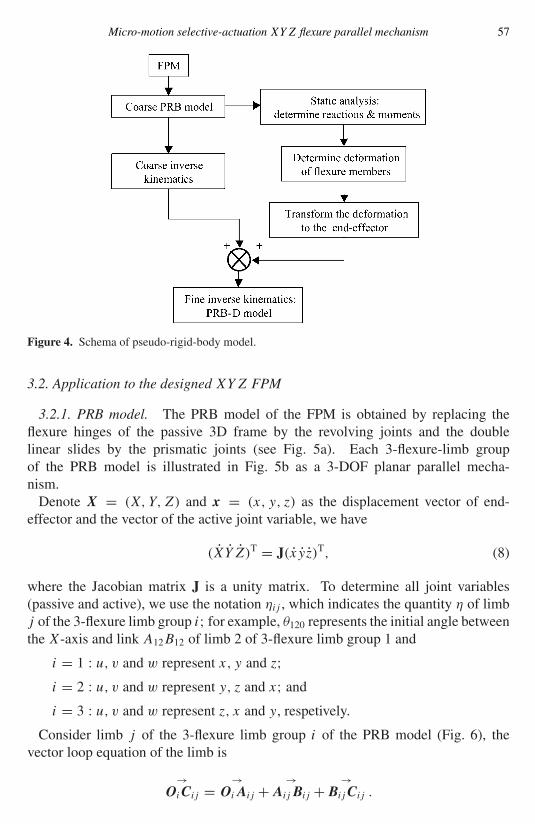
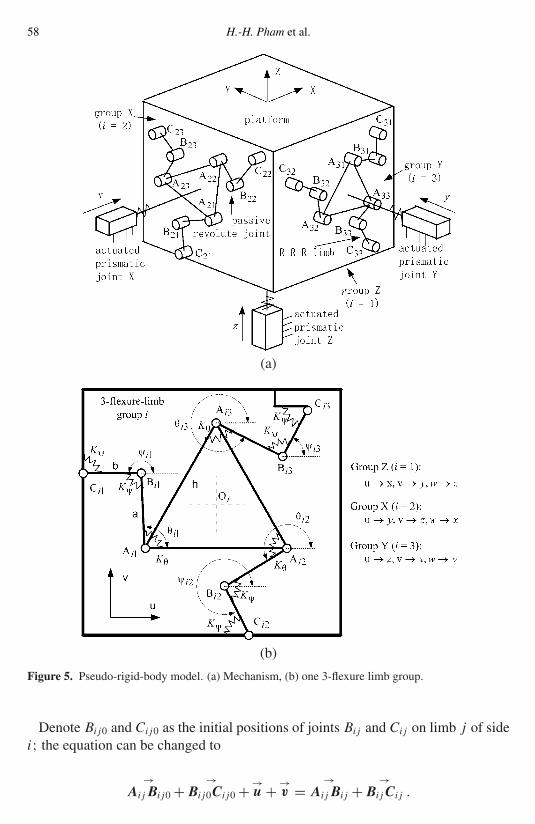
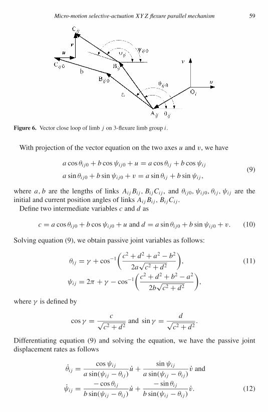
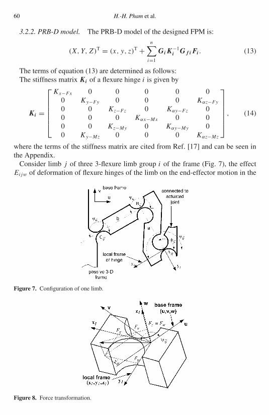
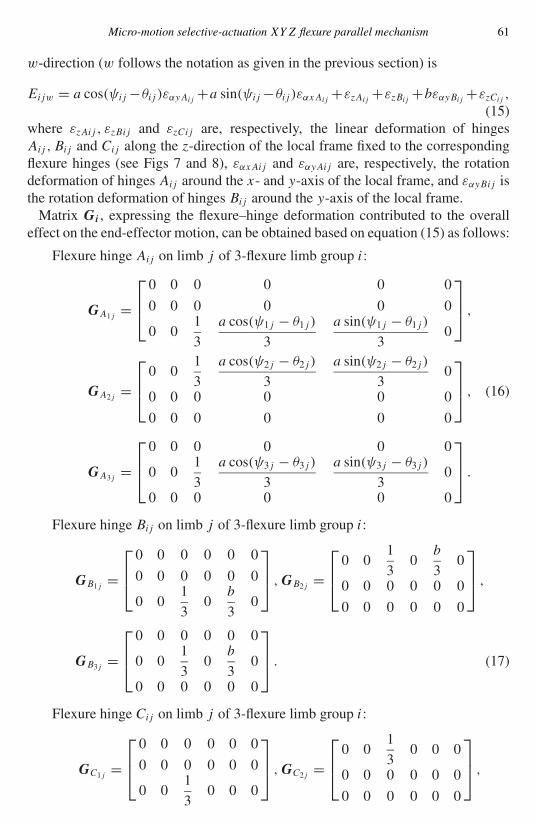
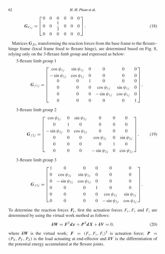
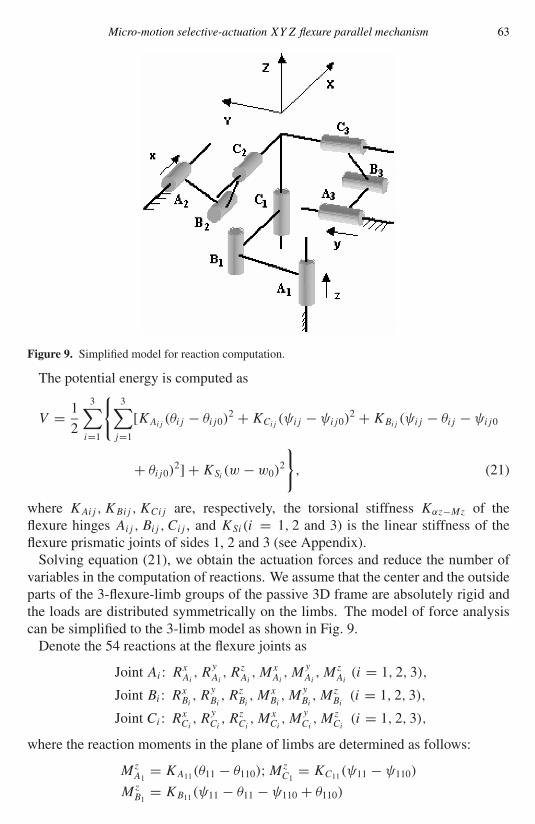
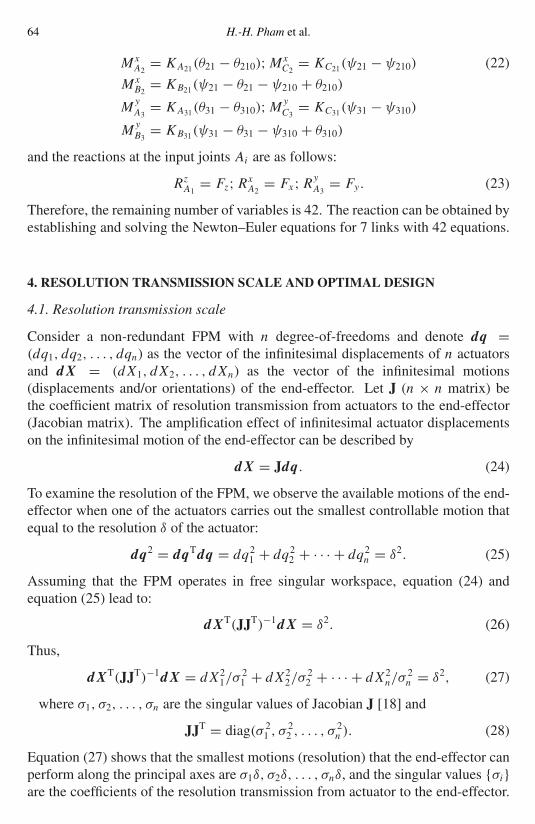
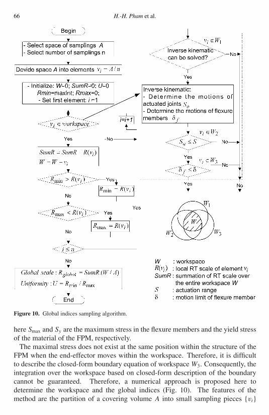
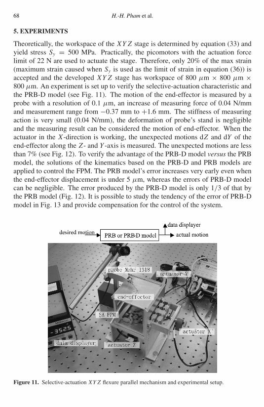
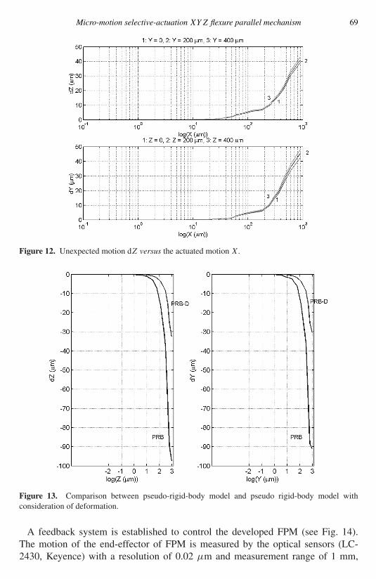
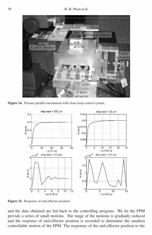
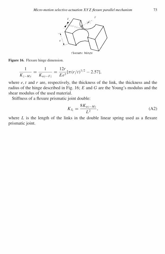
Copyright © 2022 FDOKUMEN