New Jersey Institute of Technology New Jersey Institute of Technology

Digital Commons @ NJIT Digital Commons @ NJIT

Dissertations Electronic Theses and Dissertations

5-31-2021

Selective neural stimulation by leveraging electrophysiological Selective neural stimulation by leveraging electrophysiological

diversity and using alternative stimulus waveforms diversity and using alternative stimulus waveforms

Bemin Ghobreal New Jersey Institute of Technology

Follow this and additional works at: https://digitalcommons.njit.edu/dissertations

Part of the Electrical and Electronics Commons, Neuroscience and Neurobiology Commons, and the

Social and Behavioral Sciences Commons

Recommended Citation Recommended Citation Ghobreal, Bemin, "Selective neural stimulation by leveraging electrophysiological diversity and using alternative stimulus waveforms" (2021). Dissertations. 1515. https://digitalcommons.njit.edu/dissertations/1515

This Dissertation is brought to you for free and open access by the Electronic Theses and Dissertations at Digital Commons @ NJIT. It has been accepted for inclusion in Dissertations by an authorized administrator of Digital Commons @ NJIT. For more information, please contact digitalcommons@njit.edu.

Copyright Warning & Restrictions

The copyright law of the United States (Title 17, United States Code) governs the making of photocopies or other

reproductions of copyrighted material.

Under certain conditions specified in the law, libraries and archives are authorized to furnish a photocopy or other

reproduction. One of these specified conditions is that the photocopy or reproduction is not to be “used for any

purpose other than private study, scholarship, or research.” If a, user makes a request for, or later uses, a photocopy or reproduction for purposes in excess of “fair use” that user

may be liable for copyright infringement,

This institution reserves the right to refuse to accept a copying order if, in its judgment, fulfillment of the order

would involve violation of copyright law.

Please Note: The author retains the copyright while the New Jersey Institute of Technology reserves the right to

distribute this thesis or dissertation

Printing note: If you do not wish to print this page, then select “Pages from: first page # to: last page #” on the print dialog screen

The Van Houten library has removed some of the personal information and all signatures from the approval page and biographical sketches of theses and dissertations in order to protect the identity of NJIT graduates and faculty.

ABSTRACT

SELECTIVE NEURAL STIMULATION BY LEVERAGING ELECTROPHYSIOLOGICAL DIVERSITY AND USING ALTERNATIVE

STIMULUS WAVEFORMS

by Bemin Ghobreal

Efforts on finding the principle mechanism for selective neural stimulation have

concentrated on segregating the neurons based on their size and other geometric

factors. However, neuronal subtypes found in different parts of the nervous system

also differ in their electrophysiological properties. The primary objective of this

study is to investigate the feasibility of selective activation of neurons by leveraging

the diversity seen in passive and active membrane properties.

Using both a local membrane model and an axon model based on the

CRRSS, the diversity of electrophysiological properties is simulated by varying four

model parameters (membrane leakage-Gleak and capacitance-Cm, temperature

coefficient-Ktemp, and maximum sodium conductance-GNamax) by ±25% around

their default value. Temperature coefficient is used as a means to alter the opening

rate of the sodium channel. Three different stimulus waveforms are implemented

to test the effects of hyperpolarizing pre-pulsing (HPP) and depolarizing pre-

pulsing (DPP) on selectivity in comparison to monophasic (Mono) waveform.

The default value of Cm is found to play a critical role in amplifying or

attenuating the sensitivity of the chronaxie time (Chr) and rheobase (Rhe) to

variations in all the membrane parameters. The HPP waveform is able to

selectively activate neurons diversified in Gleak only. Maximum selectivity indices

are obtained when passive parameters (Cm & Gleak) are allowed to vary. The

impact of dynamic parameter (Ktemp and GNamax) diversity increased slightly for the

smallest value of Cm. In all cases, the HPP waveforms (with zero inter-phase gap)

produce higher selectivity than the other two stimulus waveforms.

These results reveal a novel mechanism of selectivity based on

electrophysiological diversity, and it is particularly pronounced with the

hyperpolarizing pre-pulsing stimulation waveform. The proposed method of

selectivity may lead to a paradigm-shifting approach if the electrophysiological

diversity can also segregate neurons into functional subtypes, as evidence

suggests in reports from numerous sites in the central nervous systems. This basic

concept of selectivity should generalize to more complex neural models, though

probably to different extents, that include a voltage-gated fast sodium channel and

a leakage current, as in the CRRSS model.

Furthermore, this study expanded the investigation of neural selectivity to

include stimulus waveform. Historically, rectangular stimulus pulse has been used

in various neural stimulation application, however several limitations reside when

using the tradition rectangular pulse to achieve selectivity. Hence, the study

investigated using seven different non-rectangular waveforms as the stimulus

pulse proceeded with hyperpolarizing pre-pulsing stimulus as a method to improve

selectivity. The seven non-rectangular pulses are Charge-discharge curve (Chr-

Dis), increasing and decreasing exponential (ExpInc and ExpDec) respectively,

Gaussian (Gauss), KT2, Linear (Lin), and sinewave (Sine). Results revealed that

𝐾𝑡2 maximized selectivity, followed by Gauss, ExpInc, and ExpDec stimulus, when

proceeded by hyperpolarizing pre-puls. Furthermore, results showed with higher

diversity in neural cells, specifically in GLeak & Ktemp or GLeak & GNamax using

𝐾𝑡2 allows higher stimulation selectivity between neural cells.

Additionally, to get more realistic results that represents the behavior of

neural cell in the human body we expanded the investigation to include a

compartmental axon mode. We used a 10 µm myelinated axon that incorporated

the CRRSS local model at the nodes of Ranvier that had widths of 1 µm and an

inter-nodal distance of 1 mm. A monopolar point electrode was placed 1 mm away

from the axon and aligned with its central node. Using all eight stimulus waveforms

the SD curves and SIs were found with the same passive and active parameter

ranges tested in the local membrane model.

The Axon model further confirmed the results obtained from the local model

revealing that diversification in the membrane parameters leads to selective neural

stimulation. Both model results indicate that the most selective stimulus waveform

changes depending on the membrane parameter combination that is allowed to

vary, and no single stimulus waveform is the best for all combinations. These

simulation results warrant further investigation of the concept of “selectivity based

on electrophysiological diversity” using experimental data from real neurons.

SELECTIVE NEURAL STIMULATION BY LEVERAGING ELECTROPHYSIOLOGICAL DIVERSITY AND USING ALTERNATIVE

STIMULUS WAVEFORMS

by Bemin Ghobreal

A Dissertation Submitted to the Faculty of

New Jersey Institute of Technology and Rutgers University Biomedical and Health Sciences – Newark

in Partial Fulfillment of the Requirements for the Degree of Doctor of Philosophy in Biomedical Engineering

Department of Biomedical Engineering

May 2021

Copyright © 2021 by BEMIN GHOBREAL

ALL RIGHTS RESERVED

.

APPROVAL PAGE

SELECTIVE NEURAL STIMULATION BY LEVERAGING ELECTROPHYSIOLOGICAL DIVERSITY AND USING ALTERNATIVE

STIMULUS WAVEFORMS

Bemin Ghobreal

Dr. Mesut Sahin, Dissertation Advisor Date Professor of Biomedical Engineering, NJIT

Dr. Farzan Nadim, Dissertation Co-Advisor Date Professor of Biological Sciences, NJIT

Dr. Bryan Pfister, Committee Member Date Professor of Biomedical Engineering, NJIT

Dr. Sergei Adamovich, Committee Member Date Professor of Biomedical Engineering, NJIT

Dr. Viji Santhakumar, Committee Member Date Associate Professor of Pharmacology, Physiology, and Neuroscience, Rutgers

iv

BIOGRAPHICAL SKETCH

Author: Bemin Ghobreal

Degree: Doctor of Philosophy

Date: May 2021

Undergraduate and Graduate Education:

• Doctor of Philosophy in Biomedical Engineering, New Jersey Institute of Technology, Newark, NJ, 2021

• Bachelor of Science in Biomedical Engineering, New Jersey Institute of Technology, Newark, NJ, 2012

• Bachelor of Science in Electrical Engineering, New Jersey Institute of Technology, Newark, NJ, 2012 Major: Biomedical Engineering & Electrical Engineering Presentations and Publications: Serrador, Jorge & Blatt, M. & Acosta, A. & Ghobreal, Bemin & Falvo, Michael.

(2013). Blast exposure is associated with impaired cerebral blood flow regulation in US veterans. Cerebrovascular Diseases. 35. 36-36.

Serrador, Jorge & Blatt, M. & Acosta, A. & Ghobreal, Bemin & Falvo, Michael.

(2013). Differences in Cerebral Autoregulation between Arterial Beds is Not Reflected in CO2 Reactivity. Cerebrovascular Diseases. 35. 34-35.

Serrador, Jorge & Castro, Pedro & Rocha, Isabel & Blatt, M. & Ghobreal, Bemin

& Sorond, Farzaneh & Azevedo, Elsa. (2013). Cerebral blood flow is reduced in the vascular territory of ischemic stroke in the first 24 hours. Cerebrovascular Diseases. 35. 36-36..

Castro, Pedro & Serrador, Jorge & Azevedo, Elsa & Rocha, Isabel & Blatt, M. &

Ghobreal, Bemin & Sorond, Farzaneh. (2013). Ischemic stroke is associated with transiently impaired autoregulation. Cerebrovascular Diseases. 35. 25-25.

v

B. Ghobreal, E. H. Kim, P. R. Moinot and T. L. Alvarez, "Custom software for NJIT flexible visual stimulator," 2012 38th Annual Northeast Bioengineering Conference (NEBEC), 2012, pp. 49-50, doi: 10.1109/NEBC.2012.6206956.

B. Ghobreal, A. Giokas, F. Dort, A. Gandhi and R. Foulds, "Telemanipulation

using Exact Dynamics iARM," 2012 38th Annual Northeast Bioengineering Conference (NEBEC), 2012, pp. 123-124, doi: 10.1109/NEBC.2012.6206993.

vi

Praise the Lord, Praise the name of the lord.

Search me, O God and know my heart: try me, and know my thoughts.

See if there is any wicked way in me and lead me in the way everlasting.

To my beloved Parents, for their encouragement throughout my life,

Nabil Basta Ghobreal & Nadia Sabet Narouz.

vii

ACKNOWLEDGMENT

First and foremost, I would like to sincerely thank my advisor, Dr. Mesut Sahin, on

his continuous support, guidance, and encouragement. This work would not have

been possible without his knowledge and mentorship. His expertise was invaluable

in formulating the research topic and generating high-quality results. His insightful

feedback pushed me to sharpen my thinking and brought my work to the highest

quality level. His great commitment to the project inspired me to become the best

version of myself.

Additionally, I would like to thank my Co-Advisor Dr. Farzan Nadim, who put

a lot with my questions and offer a great insight and collaboration to guide me

through that long path.

I would also like to thank Dr. Sergei Adamovich, Dr. Brian Pfister and

Dr. Viji Santhkumar for serving on my dissertation committee and their valuable

contributions to my research.

I would like to thank the NSF and NRC bridge to doctorate program for the

partial financial support they provided me and special thanks to the Ronald E.

McNair program director Dr. Angelo Perna and assistant director Zara Williams.

Above all, I am forever indebted to my parents, my uncle, my sister and my

brother for praying and believing in me, encouraging and supporting me.

Always thankful for my soul mate, my love and future wife who always has

been with me through the tough times.

viii

TABLE OF CONTENTS

Chapter Page

1 INTRODUCTION …………………………………………………………. 1

1.1 Selectivity …………………………………………………………… 2

1.2 Selectivity Via Current-Diameter Relationship ………………….. 3

1.3 Stimulus Waveform ………………………………………………… 6

1.4 Selectivity Via Current-Distance Relationship …………………... 8

1.5 Neural Model ……………………………………………………….. 11

1.5.1 Hodgkin-Huxley Model (H-H) …………………………….. 11

1.5.2 CRRSS Model ……………………………………………… 12

1.5.3 Inferior Olive Model ………………………………………... 13

1.6 Dynamic Membrane Parameters …………………………………. 15

1.7 Passive Membrane Parameters ………………………………….. 18

1.8 CRRSS Action Potential …………………………………………... 19

1.9 Strength-Duration Curve …………………………………………... 21

2 SELECTIVE NEURAL STIMULATION BASED ON ELECTROPHYSIOLOGICAL DIVERSITY ……………………………

22

2.1 Background & Significance …………………………...………….. 22

2.2 Methods……………………….....……………….......................... 25

2.2.1 Neural Model ……………………………………………… 25

2.2.2 Sensitivity Analysis ………………………………………. 26

2.2.3 Rectangular Stimulus Waveforms …………………… 27

2.2.4 Strength-Duration Curve …………………………………. 27

ix

2.2.5 Selectivity Index (SI) …………………………………….... 28

2.3 Results………...……………………...……………………………... 32

2.3.1 Sensitivity to Individual Membrane Parameters ……… 32

2.3.2 Selectivity with Single Parameter Variation …………….. 39

2.3.3 Selectivity with Dual Parameter Variation ………………. 39

2.4 Discussion …………………………………...……………………… 41

2.4.1 Sensitivity to Individual Membrane Parameters ………... 41

2.4.2 Mechanisms of Selectivity ………………………………… 42

3 DIVERSITY-BASED NEURAL SELECTIVITY USING ALTERATIVE STIMULUS WAVEFORMS ………………………………………………

50

3.1 Background & Significance ……………………………………….. 50

3.2 Methods ……………………………………………………………... 52

3.2.1 Neuron Model ……………………………………………… 52

3.2.2 Sensitivity Analysis ………………………………………… 53

3.2.3 Stimulus Waveforms ………………………………………. 53

3.2.4 Strength-Duration Curve (SD) ……………………………. 55

3.2.5 Selectivity Index (SI) ……………………………………..... 55

3.3 Results ………………………………………………………………. 58

3.3.1 Sensitivity to Individual Membrane Parameters ………... 58

3.3.2 Selectivity with Single Parameter Variation …………….. 58

3.3.3 Selectivity with Dual Parameter Variation……………….. 60

3.4 Discussion…………………………………………………………… 69

4 Compartmental Axon Model …………………………………………….. 71

x

TABLE OF CONTENTS (Continued)

Chapter Page

4.1 Background & Significance ………………………………………. 71

4.2 Methods …………………………………………………………… 73

4.2.1 Axon Model………………………………………………… 73

4.2.2 Stimulus Waveform ……………………………………….. 74

4.2.3 Strength Duration Curve …………………………………. 75

4.2.1 Selectivity Index …………………………………………… 75

4.3 Results……………………………………………………………… 76

4.3.1 Selectivity with Rectangular Waveform ……………….. 76

4.3.2 Selectivity with Non-Rectangular Waveform …………… 81

4.4 Discussion …………………………………………………………... 86

5 CONCLOSUIOSN AND FUTURE WORK ……………………..……... 88

6 APPENDIX A………………………………………………………………. 89

7 APPENDIX B ……………………………………………………………… 96

8 APPENDIX C ……………………………………………………………... 103

9 REFERENCES …………………………………………………………… 122

xi

LIST OF TABLES

Table Page

2.1 Three Different Values Used for Each Membrane Parameter to Represent Diversity ……………………………………………………

31

3.1 Eight Monophasic Stimulus Waveforms.…………………………….

50

3.2 Percent of Change in Chronaxie and Rheobase Slopes for all HPP Stimulus Waveforms ……………………………………………………

55

xii

LIST OF FIGURES

Figure Page

1.1 Threshold current as a function of fiber diameter …………….......... 5

1.2 The inversion of the current distance relationship using a pre-pulsed stimulus waveform …………………………………………….

9

1.3 Pulse waveform configuration; Conf1: single pulse. Conf2 and Conf 3 : 4 pre-pulses pp1 to pp4.

10

1.4 Mean selectivity index for each configuration and various target size SI …………………………………………………………………..

10

1.5 Electrical circuit representing H-H model membrane parameters which are GNa, Gl, Gk , and Cm ……………………………………..

14

1.6 The CRRSS Local model is represented as an electrical circuit. The circuit showing both Leakage channel (gL) and sodium channel (gNa) ………………………………………………………….

14 1.7 Voltage gated sodium channel at rest………………………………... 16

1.8 CRRSS Action Potential is generated when a rectangular pulse stimulates the nerve cell ……………………………………………...

20

1.8 The strength–duration activation curves are plotted for four different neurons. Crossing found between B25 &B19, B4&B2 ……

21

2.1 Stimulus waveforms: Mono-phasic (Mono), Mono with hyperpolarizing pre-pulse (HPP), and Mono with depolarizing pre-pulse (DPP).…………………………………………………………….

27

2.2 Definition of Selectivity Index based on crossing of strength-duration curves.………………………………………………………..

28

2.3 Sensitivity analysis of chronaxie time and rheobase repeated for all three different stimulus waveforms ………………………………

29

2.4 Sensitivity of chronaxie time and rheobase normalized to the default value, to the membrane parameters (Gleak, Gnamax, Ktemp, and Cm) as they are altered by ±25% from the default value and evaluated at intermediate values ……………………………………

32

2.5 The effects of the four model parameters on the strength-duration curve as they are altered individually by ±25% ……………………..

33

xiii

LIST OF FIGURES (Continued)

Figure Page

2.6 Varying Gleak and using hyperpolarization pulse (HPP) causes crossing between SD Curves …………………………………………

33

2.7 Two of the four membrane parameters are altered simultaneously in each case by the same amount…………………………………….

34

2.8A Comparison of SI values with Mono (Blue), HPP (Green), and DPP (Red) stimulus waveforms and for each parameter combination. Default Cm=2µF∕𝑐𝑚2 . Each dot in the plot represents an SD crossing …………………………………………………………

35

2.8B Te crossing PW at the maximum selectivity index ratio for each parameter marked with “*” . Crossing PW is the point where both SD curves cross together …………………………………………….

36

2.9 Comparison between three CRRSS model variations produced by

setting the default value of Cm to 0.5µF∕𝒄𝒎𝟐, 2 µF∕𝒄𝒎𝟐, and 4

µF∕𝒄𝒎𝟐, represented in different shades of green. HPP is the

stimulus waveform …………………………………………………….

47

3.1A Sensitivity analysis showing the Rheobase data, each line represents the behavior of stimulus waveform. Eight stimulus waveforms are used with a hyperpolarization pulse (HPP) included…………………………………………………………………

54

3.1B Sensitivity analysis showing the Chronaxie data, each line represents the behavior of stimulus waveform. Eight stimulus waveforms are used with a hyperpolarization pulse (HPP) include…………………………………………………………………...

55

3.2 Percentage of all possible Selectivity Index ratio (%SI) is plotted in the y-axis in relation to the PW(ms) in x-axis ………………………..

61

3.3 The Selectivity Index ratio is plotted in percentage (%SI). The graph is color coded to differentiate between different parameters companions. Bars are grouped by stimulus Type. A) For stimulus with hyperpolarization pre-pulse. B) For Using Monophasic stimulus pulse…………………………………………………………..

62

3.4 The Selectivity Index ratio is plotted in percentage (%SI). The graph is color coded to differentiate between different parameters companions. …………………………………………………………

63

xiv

LIST OF FIGURES (Continued)

Figure Page

3.5 Selectivity Index ratio is plotted in percentage (%SI). The graph is color coded to differentiate between different parameters companions as shown in the top left of the figure. Bars are grouped by stimulus Type……………………………………………………..

64

3.6 Pulse width (mSec) where the crossing occurred is plotted. The graph is color coded to differentiate between different combinations as shown in the top right of the figure. …………….

66

4.1 Anatomy of the neuron, the yellow parts is called Myelin (internodal). Node o Ranvier falls between two intermodals.

69

4.2 Placement of the electrode on the center node of the axon model.

71

4.3 Percent selectivity index generated from crossing SD curves in the compartmental axon model …………………………………………...

75

4.4 PWs at which the SDs cross are shown (“+”) for the compartmental axon model. Parameter diversity is ±25% and the waveform is HPP ……………………………………………………………………..

75

4.5 Selectivity Index plotted against the varied membrane parameters in pairs …………………………………………………………………..

76

4.6 SI values for all waveforms, in the Compartmental Axon Model are represented with a “+” sign. The graph is color coded for each combination and the bars are grouped based on the waveform …...

78

4.7 Crossing Locations (PW) in the Axon Model, are represented with a “+” sign. The graph is color coded for each combination and the bars are grouped based on the waveform …………………………..

79

4.8 Percent of Number of crossing (NOC), in the axon model is plotted to compare between different waveforms. The graph is color coded for each combination bars are grouped based on the waveform.

79

A.1 Selectivity Index reaches 85% of its max at 1ms and plateaus at 2ms for increasing durations of depolarizing phase in the DPP waveform……………………………………………………………

83

xv

LIST OF FIGURES (Continued)

Figure Page

A.2 Sensitivity of rheobase to the membrane parameters (GLeak, Gnamax, Temp.

Coef-KTemp, and Cm) as they are altered by ±25% from the nominal value

and evaluated at many intermediate values………………………………

84

A.3 Only Gleak variations, shown on top right panel, produce a few crossings

(red dash lines) between the SD curves when using HPP stimulus

waveform………………………………………………………………

85

A.4 The effects of the four model parameters (GLeak, Gnamax, Temp. Coef-Ktemp, and Cm) on the strength-duration curve when DPP stimulus waveform is used. No SD crossings occur…………

86

A.5 Adding a 200 µs gap in the HPP waveform on the SD curve. It reverses the HPP effects for all parameter variations. Only the Gleak results are shown here. The SD crossings seen for Gleak

diversity in Supplemental Figure A.4 are eliminated………………

87

A.6 The magnitude of the second spatial difference of the extracellular voltage due a monopolar electrode is plotted as a function of electrode-fiber distance for a 10µm myelinated axon assuming that intermodal distance is 100 times the fiber diameter ………………

88

A.6 The magnitude of the second spatial difference of the extracellular voltage at 1mm from a monopolar electrode as a function of axon diameter ………………………………………………………………

89

B.1 Sensitivity analysis for monophasic waveforms. Both rheobase and chronaxie

time slope differed small percentage from rectangular waveform slope………..

90

B.2 GNAMAX & GLEAK are altered simultaneously in each case by the

same amount, using eight different waveform. Different colors legend

indicates different values for Cm parameter shown on top right of the

figure. Second parameter is not color coded for clarity………………….

91

B.3 KTEMP & GLEAK are altered simultaneously in each case by the same

amount, using eight different waveform. ……………………………………….

92

B.4 GLEAK & CM are altered simultaneously in each case by the same

amount, using eight different waveform ………………………………...

93

1

CHAPTER 1

INTRODUCTION

Neural diseases are one of the leading causes of disabilities in the world.

According to the United Nation World Health Organization’s (WHO) report, about

1 billion people, nearly one in sixth of the world’s population, suffer from

neurological disorders like Alzheimer’s disease (AD), Parkinson’s disease, stroke,

multiple sclerosis and epilepsy [4], causing roughly 6.8 million people to die every

year [4]. In 2006, the U.S. National Institute for Neurological Disorders and Stroke

(NINDS) estimated about 50,000 new cases of Parkinson’s disease are diagnosed

in the U.S. every year [5]. Therefore, finding a treatment for neural disorders has

been the research focus for decades.

Electrical neural stimulation techniques have been used for decades

showing a great impact on patients’ health. It remains one of the most critical brain

disorder treatments known to be effective at low cost [6, 7]. Various clinical

approaches, as oral medication and surgical procedure, may accomplish similar

therapeutic results, nevertheless neural electrical stimulation has higher

spatiotemporal precision compared to oral medication combined with low cost and

reversibility that is not present in surgical procedures [7]. Currently, it is a widely

used treatment for several brain diseases and has proved to be an effective tool

for patients who suffer from neurological and neuropsychiatric disorders [8].

Yet, neural electrical stimulation has several limitations and challenges that

needed to be addressed. One of the most critical challenges, which we are

addressing in this study, is neural stimulation selectivity [6, 7, 9]. Several

2

applications require the ability to selectively activate or inhibit a targeted population

or neurons without activating neighboring neurons. Neural stimulation selectivity is

a measure of the efficiency of the stimulus. Current electrical stimulation

techniques stimulate a large area of the tissue, causing a nonlinear response [10],

high rate of damaged tissue close to the stimulation electrode, loss of power and

decrease in the stimulation efficiency [6, 7]. High power consumption increases

the number of replacement surgeries for implanted pulse generators, since it

reduces the battery lifetime [7, 10]. It is also important to acknowledge that, as a

result the mechanism of action for neural electrical stimulation is still not well

comprehended in addition to how neural network dynamics relate to single-cell

dynamics remains poorly understood [7, 10]. Therefore, there is a high demand to

develop more precise neural stimulation technique with the ability to target a

specific group of neurons.

1.1 Selectivity

Neural electrical stimulation is an effective therapy for the majority of neural

dysfunctions, however, there remains a clear clinical need to improve the

technology [7, 8] to increase stimulation selectivity. Selectivity of a stimulus is the

ability to stimulate a specific group of neurons without targeting other neurons

within the same range. Improving neural stimulation selectivity increases the

efficiency of the therapeutic effect and reduces the magnitude of the side effects

[10]. Selectivity could be determined based on several neural cell properties,

geometry properties, and stimulation properties, however, the two most studied

3

types of selectivity are diameter selectivity and spatial selectivity. Diameter

selectivity indicates the capability to stimulate a specific population of neurons that

have a common diameter, while simultaneously not including other neighboring

populations [1, 10]. Spatial selectivity is the ability to excite or inhibit a specific

group of neurons located from a specific distance from the stimulation electrode.

For instance targeting neurons farther away from the stimulation electrode without

targeting the neuron close to the electrode [1].

1.2 Selectivity Via Current-Diameter Relationship

Several studies showed the possibility of selectively stimulating a group of neurons

or nerve fibers that have the same diameter size. In 1991 Fang and Mortimer

conducted a study to investigate the possibility of targeting fibers based on their

diameter, using quasitrapezoidal current pulses [11]. The study demonstrated that

at lower current levels, the larger alpha motor axons could be blocked more than

smaller alpha motor axons [11].

In another study, DONALD R. MCNEAL plotted the relationship between

Activation threshold current and fiber diameter as shown Figure 1.1. [12]. The

study concluded that between (2<d< 25 μm) the activation threshold current

increases as fiber diameter decreased, at larger diameters (d> 15 μm) the

threshold inversely proportional to the square root of the fiber diameter, and at

smaller diameters (d<2 μum) the activation threshold has an inverse square

relationship with fiber diameter [12].

4

Moreover, Mortimer and Creasey were able to influence the action potential,

on small diameter motor fibers serving the bladder, without affecting larger

diameter motor fibers [1]. In another application, Kristen E I. and Deurloo, Jan

investigated the influence of subthreshold of depolarizing prepulses on threshold-

diameter relationship, concluding that smaller fibers have a lower threshold current

than the larger fibers up to a certain distance from stimulation electrode [13].

In 2014, Kurt Qing and Mathew P. Ward proposed a novel technique to

change the current diameter recruitment order. Using a Brust Modulated

rectangular waveform they showed selective activation between A (larger

diameter) and C (small diameter) fibers. They compared between the traditional

rectangular pulse and the burst modulated pulse. The burst modulated waveform

is created by replacing each pulse with a burst of narrow pulses “pulsons”. Each

pulson burst has a defined pulse width (pWx), amplitude (ampx), interpulson

interval (IpIx) and number of pulses (Nop) [14]. The results suggested that

waveform with short PW or pWx more likely to be more selective to larger diameters

than shorter fibers [14].

Figure 1.1 Threshold current as a function of fiber diameter. Current-Diameter

relationship.

5

1.3 Stimulation Waveform

Published data has shown that stimulation parameters play a critical role in

increasing stimulation selectivity. Several parameters were investigated, including

but are not limited to, stimulation waveform [15], electrode polarity [16, 17],

electrode distance from the target (electrode location), and waveform pulse width

[18]. A study lead by Sahin, Mesut, investigated the effect of various non-

rectangular waveforms on the stimulation efficiency, demonstrating that optimum

pulse width changes as a function of the stimulus waveform, the study also showed

that linearly and exponentntially decreasing and Gaussian waveforms are the most

efficient pulse shapes, because the chronaxie time was longer compared to

traditional rectangular pulse. The study showed that non-rectangular pulse shapes

can move the chronaxie time to longer pulse duration.

Lately, non-rectangular waveforms have been gaining more interest as a

unique stimulus pulse that could perform better than the traditional rectangle pulse

and improve neural stimulation. Previous research demonstrated the benefits of

non-rectangular waveform as a mean to decrease energy consumption. For

instance, the exponentially rising waveform was shown to be the optimal stimulus

to decrease energy consumptions [19, 20]. Moreover, Exponentially increasing,

Gaussian and Sinusoidal stimulus pulses reduced energy requirements depending

on the stimulation pulse width (PW) [15]. Additionally, in 2010 a study by Grill using

a genetic algorithm concluded that a waveform similar to Gaussian was optimal for

peripheral nerve stimulation [21].

6

The type of stimulus waveform has been always tied to stimulation

selectively, several studies tried to improve selectivity by manipulating the stimulus

pulse parameters. As we discussed previously, in majority of cases the biphasic

pulse is used to reach higher selectivity by introducing the cathodic pulse first then

followed by the anodic pulse. Other studies investigated adding a small

intermediate gap between the two phases. A study was done in 2014, concluded

that using the anodic pulse immediately after the short cathodic phase immediately

may abolish the activation of targeted fibers [22]. Moreover, they recommended

adding a 100 µsec gap between the two phases to decrease the charge required

for activating nerve fibers [22, 23]. However, they reported that adding the 100usec

gap reduced the selectivity index (SI). Likewise, in a previous paper of this series,

we demonstrated that add a 200 µsec [22] gap between the two stimulus phases

negates the effect using HPP – no inter-gap on selectivity Index.

Although, all previous studies revealed that the advantage of the non-

rectangular pulse out weights the advantages of the rectangular pulse, yet more

studies are required to better understand the specific details for the optimal

stimulus pulse. Hence, we are extending the previous work and focusing on using

non-rectangular waveform as a mean to improve electrical stimulation selectivity.

7

1.4 Selectivity Via Current-Distance Relationship

Spatial selectivity requires that the stimulation electrode sets in a close distance to

the targeted population of neurons [1, 24]. However, Deurloo, Jan. performed a

modeling study presenting that in order to stimulate distant fibers without

stimulating close fibers, one should use subthreshold depolarizing repulses [13],

which is confirmed by Grill and Mortimer Figure 1.2. [3]. A recent study conducted

by Lehto, L.J. and his team investigated the effect of implanted electrode

orientation on the neural stimulation selectivity. The results showed that maximum

selectivity achieved when axons are parallel to the electric field orientation [8].

Additionally, type of electrode influence the recruitment characteristics of the

stimulus, data showed that monopolar electrodes have higher selectivity compared

to ring electrodes [25].

Several other studies tried improving spatial selectivity by manipulating

multipolar electrode configuration, and some other tried to reverse the recruitment

order using prepulsed stimulus. Yet, a study by Melissa Dali and Olivier Rossel

[26], combined both methods together to guarantee both spatial selectivity while

reversing the diameter recruitment order using the CRRSS model. Using three

different multipolar configurations in addition to pre-pulses stimulus they achieved

both spatial selectivity while reversing the diameter current relation [26]. The first

configuration was a single 300 µsec pulse duration with TT electrode configuration

(TT: One cathode at 90° and two anodes at 0° and 180°). The second configuration

was Four pre-pulses with TT electrode configuration, finally the third configuration

(Conf 3) used four pre-pulses in addition to the activation pulse with LTR electrode

8

configuration (LTR: cathodes at 0°, 90°, 180°, 270°) Figure 1.3 [26]. The previous

three configurations were used on four different fiber diameters 5µm, 10µm, 15µm,

20µm. The pre-pulse parameters were set to reduce the activation of both 15µm

and 20µm diameter fibers. From the study results, the first configuration activated

the closer and larger diameter fibers first, the 2nd configuration reversed the current

distance relationship yet, still recruited the larger diameter before the smaller ones.

Finally, the third configuration which was designed to inactivate 15µm and 20µm

fibers over the whole nerve, activated the 10µm diameter fiber in addition to

reversing the current distance relationship, Figure 1.4 [26].

Figure 1.2 The inversion of the current distance relationship, using a pre-

pulsed stimulus waveform. Smaller activation threshold at distant fibers. [3]

9

Figure 1.3 Pulse Waveform. Conf 1: single pulse. Conf 2 and 3: 4 pre-

pulses, pp1 to pp4 followed by the activation pulse.

Figure 1.4 Mean selectivity index for each configuration and various

target size SI is the optimal fibers with 10µm diameter.

10

1.5 Neural Model

1.5.1 Hodgkin-Huxley Model (H-H)

One of the early developed neural models is the Hodgkin-Huxley (H-H) model

which is based on experimental data collected with squid giant axon. H-H model

successfully explain the behavior of the dynamic membrane parameters via

serious of mathematical equations [27]. They also developed an electrical circuit

model that mimics the behavior of the neural cell as seen in Figure 1.5. If the ion

concentration and temperature is known then the total membrane current I as a

function of time and voltage can be calculated using the following equation [27]:

𝐼 = 𝐶𝑚

𝑑𝑉

𝑑𝑡+ �̅�𝑘𝑛4(𝑉 − 𝐸𝑘) + �̅�𝑁𝑎𝑚3ℎ (𝑉 − 𝑉𝑁𝑎) + �̅�𝑙(𝑉 − 𝑉𝑙)

(1.1)

𝛼𝑛 = 0.01 (𝑉 + 10)

𝑒𝑥𝑝𝑉+10

10 − 1

(1.2)

𝛽𝑛 = 0.125 𝑒𝑥𝑝𝑉

80 (1.3)

𝛼𝑚 = 0.1 (𝑉 + 25)

𝑒𝑥𝑝𝑉+25

25 − 1

(1.4)

𝛽𝑚 = 4 𝑒𝑥𝑝𝑉

18 (1.5)

𝛼ℎ = 0.07 𝑒𝑥𝑝𝑉

20 (1.6)

𝛽ℎ = 1

𝑒𝑥𝑝𝑉+30

10 + 1

(1.7)

11

1.5.2 CRRSS Model

In 1987. Sweeney et al. published the first model based on one of the mammalian

nerves, which uses data of Chiu et al. [15, 28, 29]. The model based of a voltage

-clamp study was carried out on a single rabbit myelinated nerve fibers and it was

fitted to the Hodgkin-Huxley (H-H) model. Data then altered to set the model

temperature to 37° [29] [15] and the leakage conductance was adjusted to give

action potential conduction velocity of 57 m/s (ref). The Chiu-Ritchie-Rogart-Stagg-

Sweeney (CRRSS) model has only voltage-gated sodium channel and a leakage

current, and no potassium current, which fits well with the purpose of this study

since there are almost no potassium currents in mammalian nodes of Ranvier.

Hence, the CRRSS model was used in the simulation for both the local and the

axon models. The Electrical circuit of the model shown in Figure 1.6 and the

following mathematical equation are the representation of the model and they were

used in the simulation [15, 29]. The change in Membrane potential is given by

𝑑𝑉

𝑑𝑡=

𝑖𝑠𝑡 − 𝑖𝑁𝑎 − 𝑖𝐿

𝐶𝑚

(1.8)

𝑖𝑠𝑡 → 𝑖𝑠 𝑡ℎ𝑒 𝑠𝑡𝑖𝑚𝑢𝑙𝑎𝑡𝑖𝑜𝑛 𝑐𝑢𝑟𝑟𝑒𝑛𝑡

𝑖𝑁𝑎 → 𝑖𝑠 𝑡ℎ𝑒 𝑐𝑢𝑟𝑟𝑒𝑛𝑡 𝑑𝑒𝑛𝑠𝑖𝑡𝑖𝑦 𝑜𝑓 𝑠𝑜𝑑𝑖𝑢𝑚 𝑐𝑎𝑛𝑛𝑒𝑙 (µ𝐴 𝐶𝑚−2)

𝑖𝐿 → 𝑖𝑠 𝑡ℎ𝑒 𝑐𝑢𝑟𝑟𝑒𝑛𝑡 𝑑𝑒𝑛𝑠𝑖𝑡𝑖𝑦 𝑜𝑓 𝐿𝑒𝑎𝑘𝑎𝑔𝑒 𝑐𝑎𝑛𝑛𝑒𝑙 (µ𝐴 𝐶𝑚−2)

𝑖𝑁𝑎 = �̅�𝑁𝑎𝑚2ℎ(𝑉 − 𝐸𝑁𝑎) (1.9)

𝑖𝐿 = �̅�𝐿(𝑉 − 𝐸𝐿) (1.10)

Where m is the gating variable, which are gives as

12

𝑚(𝑡) = 𝑚0 − [(𝑚0 − 𝑚∞)(1 − 𝑒−𝑡Ʈ𝑚 )

(1.11)

𝑚∞ = 𝛼𝑚

𝛼𝑚 + 𝛽𝑚 (1.12)

𝛼𝑚 = 𝑘 126 + 0.363 𝑉

1 + 𝑒−𝑉+49

5.3

(1.13)

𝛽𝑚 = 𝑘𝛼𝑚

𝑒𝑉+56.2

4.17

(1.14)

Ƭ𝑚 = 1

𝛼𝑚 + 𝛽𝑚

(1.15)

Then the equations for h, 𝛼ℎ and 𝛽ℎ are

ℎ(𝑡) = ℎ0 − [(ℎ0 − ℎ∞)(1 − 𝑒−𝑡Ƭℎ )

(1.16)

ℎ∞ = 𝛼ℎ

𝛼ℎ + 𝛽ℎ (1.17)

𝛽ℎ = 𝑘 15.6

1 + 𝑒− 𝑉+56

10

(1.18)

𝛼ℎ = 𝑘𝛽ℎ

𝑒𝑉+74.5

5

(1.19)

Ƭℎ = 1

𝛼ℎ + 𝛽ℎ

(1.20)

1.5.3 Inferior Olive Model

Another well-known neural model is the inferior olive model which was developed

by Torben-Nielsen, B., I. Segev, and Y. Yarom. Inferior Olive (IO) Is the major

source input to the cerebellum, and it is a part of the medulla oblongata. It is formed

from a gray folded layer opened in the middle by a hilum, where the olivocerebellar

13

fibers pass through. It is the only source of the climbing fibers to the Purkinje cells

in the cerebellum and it projects to both the cortex and the deeper nuclei of the

cerebellum [30]. Its function is not well known, however it is thought that it is

responsible for learning and timing of movements, for example it transmits error

signals during eye-blink conditioning or adaptation of the vestibulo-ocular reflex.

Additionally, it carries motor command signals beating on the rhythm of the

oscillating and synchronous firing of ensembles of olivary neurons [30, 31]. The

used IO model contains only a leak current and a low threshold (T-Type) Ca2+

current and there is no Sodium channel like the CRRSS model. The dynamics of

the model are described by :

𝑑𝑉

𝑑𝑡= −1

1

𝐶𝑚 (𝐼𝐿 + 𝐼𝐶𝑎) (1.21)

𝐼𝐿 = 𝑔𝐿 (𝑉 − 𝐸1) (1.22)

𝐼𝐶𝑎 = 𝑔̅𝐶𝑎

𝑚∞3 ℎ (𝑉 − 𝐸𝐶𝑎) (1.23)

𝑚∞3 = [1 + 𝑒𝑥𝑝(

−61−𝑉4.2 ) ]

−3

(1.24)

𝑑ℎ

𝑑𝑡=

ℎ∞(𝑉) − ℎ

𝑡ℎ(𝑉) (1.25)

ℎ∞ = [1 + 𝑒𝑥𝑝(𝑉+85.5

8.6 ) ]−1

(1.26)

𝑡ℎ(𝑉) = 40 + 30 [𝑒𝑥𝑝(𝑉+84

8.3 )]−1

𝑒𝑥𝑝(𝑉+160

30 ) (1.27)

In which the dynamic membrane parameters in this model are, the maximum

conductance of calcium channels (𝑔𝐶𝑎), the maximum conductance of leakage

channel (𝑔𝐿), and the gating coefficients are (m & h).

14

Figure. 1.5 Electrical circuit representing H-H model membrane

parameters which are GNa, Gl, Gk, and Cm.

Figure. 1.6 The CRRSS Local model is represented as an electrical circuit.

The circuit showing both Leakage channel (gL) and sodium channel (gNa).

15

1.6 Dynamic Membrane Parameters

Although there have been several studies focused on improving electrical

stimulation selectivity, however, there is little attention paid to membrane

parameters as a method to increase stimulation selectivity, even though it plays a

critical role in determining cell activation threshold and in generating membrane

action potential. Dynamic membrane properties were first explained in 1952 by

Hodgkin and Huxley (H-H) [27] when they successfully modeled the giant axon of

the squid. They revealed that both sodium conductance (Gna) and potassium

conductance (Gk) are functions of time and membrane potential, while the rest of

parameters are constant [32].

The original H-H model had three types of channels, sodium gated channel,

leakage channels and potassium channels [27, 32]; in the purpose of this study,

we will focus on the first two channels type Sodium channel and leak channel.

Sodium channels are permeable to Na+ and the conductance depends on the

voltage across the membrane [27] and it plays a vital role in generating action

potential. The maximum conductance of the sodium channels (GNamax) is a function

in the variable m & h gates, where m is the activation gating variable and h is the

inactivation gating variable. In the H-H model, the assumption was, that the model

contains three m gates and one H gate, therefore Gna = m3*h* GNamax [27];

however, in the Chiu-Ritchie-Rogart-Stagg-Sweeney (CRRSS) model, sodium

channels have two m gates, therefore the conductance is modeled as, Gna =

Gnamax* m2 * h, since it is a mammalian nerve fiber, as shown in Figure 1.7. [1, 2].

The values of m and h range from 0 to 1, causing the Gna to vary between 0 and

16

Gnamax [1]. Hence, changes in the value of Gnamax change the range for the sodium

gate conductance causing a change in cell activation threshold.

Another two parameters of interest are α & β, which are the opening and

closing rates for sodium channel gates. Alpha (α) is the number of time per second

the gate will open, while beta (β) is the number of time per second that a gate will

close [27, 32]. An increase in alpha increases the rate of opening for the gates

causing higher probabilities to ions to flow in, conversely increasing beta will cause

a higher closing rate lowering the probabilities for ions to flow through, causing a

change in activation threshold. Therefore, we expect that membrane properties

affect the activation threshold, and influence stimulation selectivity. Both Alpha and

Beta can be altered simultaneously by changing the temperature coefficient of the

model (Ktemp) Equation 0.1.

𝛼 = Ktemp 126 + 0.363 ∗ 𝑉

1 + 𝑒−(𝑉+49

5.3 )

(1.28)

β = Ktemp

𝛼

𝑒(𝑉+56.2

4.17 ) (1.29)

17

Figure 1.7 Voltage gated sodium channel at rest. A) sodium channel pore

opening is modeled by the activation variable m, while the inactivation gate is

modeled by the inactivation variable, h. The conductance of the channel

depends on the value of both gating variables. (B) the steady-state values of

m and has a function of transmembrane voltage. (C) The steady state values

of the time constant of the activation variables, 𝞃m, and the inactivation

variable, 𝞃h, as a function of membrane voltage [1, 2].

18

1.7 Passive Membrane Parameters

The Passive membrane parameters are leak conductance (Gleak) and membrane

capacitance (Cm). Leakage channels has a low conductance Gleak and it is mainly

responsible for resting membrane potential (33). Leak current is calculate based

on the value of Gleak.

𝐼𝐿 = 𝑮𝑳 ̅̅ ̅̅ ( 𝑽 − 𝑬𝑳)

Membrane capacitance is a fundamental parameter in modelling the

electrophysiological properties of neurons [33, 34] . The specific membrane

capacitance is determined by the thickness of the membrane, its lipid constituents

of the cell and influenced by its protein content [33]. Cm is a crucial functional role

in signal propagation, it is directly related to the membrane time constant

𝑇𝑚 = 𝑅𝑚 ∗ 𝐶𝑚

where Rm is membrane resistance and Cm is membrane Capacitance. The direct

relation between CM and tm plays an important role on influencing the chronaxie

time of the Strength Duration curves.

19

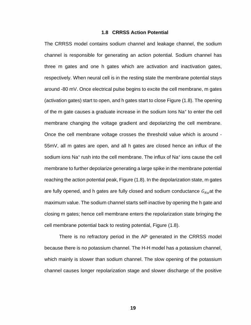
1.8 CRRSS Action Potential

The CRRSS model contains sodium channel and leakage channel, the sodium

channel is responsible for generating an action potential. Sodium channel has

three m gates and one h gates which are activation and inactivation gates,

respectively. When neural cell is in the resting state the membrane potential stays

around -80 mV. Once electrical pulse begins to excite the cell membrane, m gates

(activation gates) start to open, and h gates start to close Figure (1.8). The opening

of the m gate causes a graduate increase in the sodium Ions Na+ to enter the cell

membrane changing the voltage gradient and depolarizing the cell membrane.

Once the cell membrane voltage crosses the threshold value which is around -

55mV, all m gates are open, and all h gates are closed hence an influx of the

sodium ions Na+ rush into the cell membrane. The influx of Na+ ions cause the cell

membrane to further depolarize generating a large spike in the membrane potential

reaching the action potential peak, Figure (1.8). In the depolarization state, m gates

are fully opened, and h gates are fully closed and sodium conductance 𝐺𝑁𝑎at the

maximum value. The sodium channel starts self-inactive by opening the h gate and

closing m gates; hence cell membrane enters the repolarization state bringing the

cell membrane potential back to resting potential, Figure (1.8).

There is no refractory period in the AP generated in the CRRSS model

because there is no potassium channel. The H-H model has a potassium channel,

which mainly is slower than sodium channel. The slow opening of the potassium

channel causes longer repolarization stage and slower discharge of the positive

20

ions. Additionally, it drives the cell to hyperpolarization state before going back to

resting membrane potential.

Figure 1.8 CRRSS Action Potential is generated when a rectangular pulse

stimulates the nerve cell. Sodium conductance follows the action potential

curve shape. Both m and h gate are showing, m gate is open during the

peak of AP and h gate is close.

21

1.9 Strength-Duration Curve

Is a well-defined method that is used to quantify stimulation selectivity. Strength-

duration (SD) curve has been used in several studies as a measure to stimulation

selectivity [1, 35]. The two-dimensional curve, plots the stimulus strength as a

function of pulse width (PW), as shown in Figure 1.8 [35]. Selectivity of stimulation

is represented with a crossing between two curves on the SD curve. For instance

on Figure 1.8. [35], shows an intersection between neuron B4 & B21, and a

stimulus strength of 15 μA at PW 250 μs can activate B4 without activating B21,

also a stimulus with amplitude of 5 uA at Pw = 2000 μs can activate B21 without

activating B4 or any of the other neurons. The same measures can be used with

neurons B25& B19. Accordingly, we can design a custom stimulus waveform that

can be selective to neuron B4, but not to B21, B19 or B25.

Figure 1.9 The strength–duration activation curves are plotted for four

different neurons. Crossing found between B25 &B19, B4&B21.

22

CHAPTER 2

SELECTIVE NEURAL STIMULATION BASED ON ELECTROPHYSIOLOGICAL DIVERSITY

2.1 Objective / Background and Significance

Stimulation of neurons by way of delivering small electric currents has led to

treatment of numerous neurological disorders and injuries in the central and

peripheral nervous system. One of the primary limitations of electrical nerve

stimulation is the lack of specificity [6, 7]. In general, larger axons and somas have

lower activation thresholds and are activated before the smaller ones, the opposite

of the natural order of recruitment for motor neurons by volition. Also, due to fast

decline of the electric field strength by distance from the stimulating electrode, the

nearby neurons or axons are activated before the distant ones (current-distance

relation). Both of these phenomena often emerge as major limitations in selectively

activating neuronal subtypes defined by their electrophysiological properties or

function rather than their size or distance from the electrode.

Earlier efforts considered placing a depolarizing pre-pulse before the

stimulating phase (pre-pulsing) [3, 13], in order to reduce the excitability of the

nearby and large axons to reverse the recruitment order defined by either the size

principle or current-distance relation. Introducing a short time gap between the two

phases of the charge-balanced biphasic waveform removes the effect of the first

phase on the excitation threshold [36]. Shorter pulse widths [37], biphasic

waveforms as opposed to monophasic ones [37], and hyperpolarizing pre-pulses

[38]; none of these reverses the recruitment order, but they allow a better control

of muscle force by increasing the margin between the stimulus thresholds dictated

23

by fiber size or distance. Overall, the techniques proposed for selective activation

usually make the assumption that the neurons share the same electrophysiological

properties but only differ in their size and morphology [39], and sometimes the

types of ionic channels and their density in different neuronal compartments.

No study so far has tried to leverage the intrinsic variations in membrane

properties that occur naturally between different neural subtypes as a means to

achieve selective activation. Diversity in passive and dynamic membrane

properties of neurons clearly exists as evidenced in many parts of the central

nervous system (CNS). For instance, four different pyramidal neuron subtypes

were found in layer V of the rat medial prefrontal cortex [40], classified based on

their morphology and membrane resistance. Different neurons had significantly

different membrane time constants and rheobase currents. It is difficult to study

the threshold currents and chronaxie times independent of the cell size. However,

the range of distribution in the action potential rise times and the sub-threshold

time constants between the pyramidal cells of different layers as well as within

layer V clearly indicates a great deal of diversity in electrophysiological properties

[40, 41].

Another well-known case of diversity is found in the motoneuron (MN) pools

of the spinal cord. The MNs in the ventral horn present electrophysiological

diversity in the cellular subtypes where each MN pool reflects the characteristics

of the muscle fiber types that it controls [42, 43]. A MN pool is defined as a compact

anatomical group of MNs sharing similar intrinsic characteristics and connecting to

24

a single type of extrafusal fibers in the skeletal muscle; mainly slow-twitch fatigue-

resistant, fast-twitch fatigue-resistant, or fast-twitch fatigable types [44].

A third example can be found in Purkinje Cells (PCs) of the cerebellar cortex

that have been studied extensively for their membrane dynamics. De Schutter and

Bower developed a comprehensive model of the cerebellar PCs based on ten

different types of voltage-gated membrane channels and matched the Hodgkin-

Huxley type model parameters to the voltage clamp data [45-47]. The diversity in

the Na+ channel parameters was documented as the source of differentiation in

the PC spiking patterns.

Diversification of intrinsic membrane parameters is not random, but it is

systematic and linked to function as seen in these examples. With more attention

to intrinsic diversity, future studies will probably find more evidence associating the

electrophysiological diversity to some form of functional specialization in other

parts of the CNS as well. Such reports of experimental data are scarce perhaps

due to methodological difficulties.

“Selectivity based on diversity” of electrophysiological membrane properties

can lead to functionally selective stimulation, and thus improve therapeutic effects

and reduce the magnitude of side effects [10]. The list of applications includes

many forms of deep brain stimulation, applications dealing with spinal cord

stimulation, and various forms of sensory prostheses. The degree of selectivity will

depend on how well the cells can be segregated into functionally distinct units as

defined by their membrane properties.

25

In this chapter, we examined vertical and horizontal translations, introduced

by variations in each membrane parameter, of the strength-duration curves using

a local membrane model. The sensitivity of chronaxie time and rheobase to each

of the membrane parameters was investigated individually and in pairs. We

demonstrated that significant levels of selectivity can be achieved as the strength-

duration curves begin to cross as a result of these translations. Rectangular

stimulation waveforms with hyperpolarizing and depolarizing pre-pulses were

tested to investigate if the design of the stimulus waveform can further improve this

form of selectivity.

2.2 Methods

2.2.1 Neuron Model

In order to avoid geometry specific effects and maximize the potential for the

results to generalize to many neuronal types in the CNS, a basic local membrane

model with only one voltage-gated fast sodium channel was used in this study. The

Chiu-Ritchie-Rogart-Stagg-Sweeney (CRRSS) model [2, 29, 48], based on

myelinated rabbit nerve node data, was utilized as the local membrane model. The

CRRSS model is built on gating mechanism similar to the Hodgkin-Huxley (H-H)

model [27] and it was altered using a Q10 value to bring the model to 37°C and the

leakage conductance (Gleak) was adjusted to give the action potential conduction

velocity of 57 m/s by Sweeney et al. [29]. The original H-H model has two voltage-

gated currents, sodium and potassium, and a leakage current [27, 32]. The

CRRSS model contains only the voltage-gated sodium and the leakage current,

26

since there are almost no potassium currents in mammalian nodes of Ranvier [2,

48, 49].

2.2.2 Sensitivity Analysis

For sensitivity analysis, we varied both the passive and active membrane

parameters by ±25% around their default value, first individually and then in pairs.

The ±25% change in membrane parameters is representative of the natural

diversity, for instance, observed in the reported values of the cell input resistance

and the action potential rise times from the cortical pyramidal neurons [40, 41, 50].

These variations in input resistance and action potential rise time were simulated

by changing the membrane leakage conductance (Gleak) and the temperature

coefficient of the model (Ktemp), respectively. The other two parameters were the

membrane capacitance (Cm) and the maximum sodium conductance (GNamax). We

hypothesized that if the passive membrane properties impose a much shorter time

constant than the active sodium kinetics, the dynamic parameters that control the latter

(Ktemp and GNamax) would start making a stronger influence on the chronaxie time. To test

this hypothesis, we set the default value of Cm (Cm-def) to three different numbers, 0.5, 2,

and 4 μF/cm2 to adjust the passive time constant.

2.2.3 Rectangular Stimulus Waveforms

Three different variations of the rectangular waveform were defined for the

(intracellular) stimulation current; a monophasic-anodic pulse (Mono), a biphasic

waveform where the (cathodic) hyperpolarizing pre-pulse (HPP) precedes the

anodic phase, and an anodic pulse with (anodic) depolarizing pre-pulse (DPP),

27

(Figure 2.1). The hyperpolarizing pre-pulse was identical to the anodic phase in

amplitude and duration to make the waveform charge-balanced. The DPP pre-

pulse amplitude was set to 95% of the excitation threshold [38] at each pulse width

independently. In order to determine the shortest duration for the depolarizing

pulse, we investigated the effect of DPP duration on the selectivity index (SI)

(Supplemental Figure A.1) and observed that selectivity index increased with DPP

duration and reached 85% of its maximum effect at DPP duration of 1ms when two

membrane parameters are varied simultaneously. So, we decided to use 1ms of

fixed DPP duration in selectivity analysis. We also investigated the effect of adding

a 200 µs gap between the two phases in the HPP waveform, as it is commonly

used in neural stimulation applications [38].

2.2.4 Strength-Duration Curve

The pulse-width (PW) of the primary stimulating (anodic) phase was varied from

0.01 to 1 ms, in order to compute the strength-duration (SD) curve for each neuron

designed with a unique set of membrane parameters. The strength-duration (SD)

curve is defined by threshold level PW and pulse amplitude pairs that result in an

action potential. The action potential threshold for each stimulation was determined

by a quick search algorithm until the step size was smaller than 0.01 µA/cm2. An

action potential was decided to occur if the m-gate variable exceeded the 0.98

threshold. The rheobase (Rhe) and chronaxie time (Chr) were determined by fitting

the Lapicque equation [51] to the simulated SD curve.

28

2.2.5 Selectivity Index (SI)

Selectivity here is defined as the ability to stimulate a neuron in exclusion of others

that differ in their membrane properties under the exact same stimulus waveform.

Different neurons can be activated selectively by carefully choosing the stimulus

parameters only if the strength-duration (SD) curves of those neurons cross. The

neuron with the red strength-duration (SD) curve in Figure 2.2, for instance, can

be activated selectively before the black one with appropriate selection of stimulus

parameters on the right side of the crossing point. For selective stimulation of the

neuron with black SD curve, another intensity-PW pair has to be chosen on the left

side of the crossing point between the two SD curves. Thus, maximization of the

separation between the SD curves implies maximization of the intensity range on

both sides of the SD curve that can be utilized for selectivity.

The passive (Cm and Gleak) and active (GNamax and Ktemp) membrane

parameters were varied individually by ± 25% (Table 2.1), and produced three

different neurons with the minimum, maximum and default value of each

parameter. All possible parameter combinations were tested in pairs to produce

nine different neurons and strength-duration (SD) curves were plotted for each.

The MATLAB (MathWorks) algorithm found the crossing points between each SD

curve pair and calculated a selectivity index (SI). The selectivity index was

calculated at the PW where the ratio of the amplitude difference between the SD

curves divided by the amplitude of the higher SD curve is maximum. The maximum

SI was found on each side of the crossing point (𝑆𝐼1 = 𝐴1/(𝐴1 + 𝐵1) and 𝑆𝐼2 =

𝐴2/(𝐴2 + 𝐵2) as shown in Figure 2.2 ) and the smaller of the two was taken as a

29

conservative value for the final SI for that particular neuron pair. Note that the SI

measure here will be somewhat dependent on the minimum and maximum PWs

tested because in most cases the largest SI value occurs at the extreme ends of

the PW range. Other measures, such as the SD crossing angle, were considered

but the ratiometric measure defined here was chosen as the best representative

metric for selectivity.

Figure 2.1 Stimulus waveforms: Mono-phasic (Mono), Mono with

hyperpolarizing pre-pulse (HPP), and Mono with depolarizing pre-pulse

(DPP). Waveforms are shifted to show overlapping parts clearly.

30

Figure 2.2 Definition of Selectivity Index based on crossing of strength-

duration curves.

31

(a)

(b)

Figure 2.3 Sensitivity analysis of (a) chronaxie time (b) rheobase, repeated

for three different stimulus waveforms shown in Figure 2.1 Mono in blue, DPP

in Red, and HPP in Green, in addition to HPP with 200 μsec inter-phase gap

in Purple. Default value of Cm is 2 µF/cm2. (a) Chronaxie time increases with

Cm while Gleak and Ktemp have opposite effects for all three stimulation

waveforms. (b) Rheobase increases with Gleak, Ktemp, and Cm (except for

HPP), and decreases with GNamax.

32

2.3 Results

2.3.1 Sensitivity to Individual Membrane Parameters

strength-duration (SD) curves will cross if one moves with respect to the other as

the membrane parameters are varied. The horizontal and vertical translations of

the SD curve can be captured by examining the chronaxie time (Chr) and the

rheobase (Rhe). Any membrane parameter (by itself or in combination with others)

that alters these two characteristics in such a way that the SD curve moves along

the left-tilted diagonal (\), as opposed to moving along the other diagonal (/), can

potentially make the SD curve cross with others and lead to selectivity. Thus, we

first performed a sensitivity analysis for Chr and Rhe to the four membrane

parameters individually (Figure 2.3 (a) & (b)). Interestingly, increases in both GLeak

and Ktemp decreased Chr and increased Rhe, thus shifted the SD curve to the left

and up on the chart. Cm primarily increased Chr and had small effect on Rhe.

Increasing GNamax caused a significant reduction in Rhe with virtually no change in

Chr. This analysis suggested that Gleak and Ktemp are most likely to produce a

crossing in the SD curves, followed by Cm and GNamax combination if they are varied

together.

In order to further expand the sensitivity analysis, we set the default value

of Cm (Cm-def) to two other values, 0.5 and 4 µF/cm2, besides the original value of

2 µF/cm2 (Figure 2.4). The rationale was to investigate the effects of the other

membrane parameters on the strength-duration (SD) curve when the passive time

constant of the membrane was substantially lower or higher than those dictated by

sodium dynamics. The rise time of the action potential (from 10% to 90% of the

33

peak) with a very small Cm-def in the model (0.1 µF/cm2) was measured as 12.8 µs.

The passive time constant for the same Cm, measured with a small amplitude long

hyperpolarization pulse, was less than a microsecond, suggesting that the

measured action potential rise time was primarily determined by the sodium

channel kinetics for this small value of Cm-def. The passive time constant for Cm= 2

µF/cm2 was around 16 µs, which was comparable to the rise time dictated by the

sodium kinetics, and ~32 µs for Cm= 4 µF/cm2.

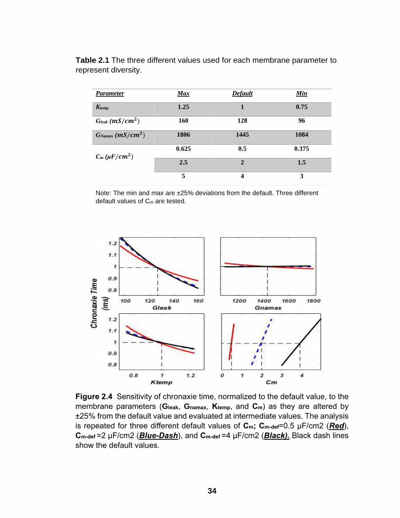
Changing Cm-def, first and foremost, altered the sensitivity of Chr to

perturbations of Cm around Cm-def (Figure 2.4 bottom right). Reducing Cm-def to 0.5

µF∕𝑐𝑚2decreased the slope of the Chr vs. Gleak plot and increased the slopes of

Chr vs. Ktemp and GNamax plots. In summary, reducing Cm-def reduced the effect of

Gleak and increased the effects of Cm, Ktemp, and GNamax on Chr. On the other hand,

Increasing the Cm-def to 4 µF∕𝑐𝑚2 had an opposite effect on the slopes of these

plots, but to a much lesser extent (black lines). Moreover, varying Cm-def had no

significant effect on the slopes of the plots for Rhe vs. other membrane parameters

(Supplemental Figure A.2). This is understandable because Rhe is calculated for

a long PW where Cm is completely charged, and the capacitive current is zero

before the end of the stimulus.

34

Parameter Max Default Min

Ktemp 1.25 1 0.75

Gleak (𝒎𝑺/𝒄𝒎𝟐) 160 128 96

GNamax (𝒎𝑺/𝒄𝒎𝟐) 1806 1445 1084

Cm (μF/𝒄𝒎𝟐)

0.625 0.5 0.375

2.5 2 1.5

5 4 3

Figure 2.4 Sensitivity of chronaxie time, normalized to the default value, to the

membrane parameters (Gleak, Gnamax, Ktemp, and Cm) as they are altered by

±25% from the default value and evaluated at intermediate values. The analysis

is repeated for three different default values of Cm; Cm-def=0.5 µF/cm2 (Red),

Cm-def =2 µF/cm2 (Blue-Dash), and Cm-def =4 µF/cm2 (Black). Black dash lines

show the default values.

Table 2.1 The three different values used for each membrane parameter to

represent diversity.

Note: The min and max are ±25% deviations from the default. Three different

default values of Cm are tested.

35

Figure 2.5 The effects of the four model parameters on the strength-duration

curve as they are altered individually by ±25%. None of the perturbations

produces SD curve crossings. Mono stimulus waveform is used. . Cm-def = 2

µF∕𝑐𝑚2 .

Figure 2.6 Varying Gleak and using hyperpolarization pulse (HPP)

causes crossing between SD Curves.

36

Figure 2.7 Two of the four membrane parameters are altered

simultaneously in each case by the same amount as in Fig.4, using HPP

waveform. Different colors in each subplot indicate different values for the

first parameter shown on top. Second parameter is not color coded for

clarity. Red dash lines mark the points of SD crossings, some of which fall

outside the figure window.

37

Figure 2.8A Comparison of SI values with Mono (Blue), HPP (Green), and

DPP (Red) stimulus waveforms and for each parameter combination. Default

Cm=2µF∕𝑐𝑚2 . Each dot in the plot represents an SD crossing. Cm & Gleak

combination produces the largest SI values with Mono and HPP stimulus

waveforms. The plot highlights the mean value at the cross mark, the median at

the line mark which divides the box into the 2nd and 3rd Quartiles and the max

& min value at the top and bottom whiskers, respectively.

38

Figure 2.8B Shows the crossing PW at the maximum selectivity index ratio

for each parameter marked with “*” . Crossing PW is the point where both SD

curves cross together. Diamond shape points “♦” are marking the PW where SI

ration is maxima. Rectangular “▲” and “Χ” markers representing the two SI

ratio at the left and right of the crossing point receptively, showing only for

maximum SI. Dots ‘•’ marks all other crossing PW points. Mono in

blue, HPP in Green DPP in Red

39

2.3.2 Selectivity with Single Parameter Variation

The strength-duration (SD) curves are shown in Figure 2.5 as the four membrane

parameters are altered individually by ±25% and using the traditional monophasic

rectangular current pulse (Mono) for stimulation. Each parameter was tested for

two extreme and the default values (Table 2.1). As mentioned, the Gleak and Ktemp

shifted the SD curves most, although not enough to make them cross. When we

added a hyperpolarizing pre-pulse (HPP) to the stimulus waveform, more radical

shifts in the SD curve were observed leading to crossing for Gleak variations (Figure

2.6 & Supplemental Figure A.3), as predicted by the sensitivity analysis in Figure

2.3. However, the SD crossings were at the lower end of the PW range and the

crossing angles were small.

Next, we included a depolarizing pre-pulse (DPP) to the Mono waveform

(Figure 2.1). The SD curves with DPP and single parameter diversity did not yield

to SD crossings (Supplemental Data, Figure A.4).

Finally, a short time interval of 200 µs between the two phases of the HPP

waveform was inserted, giving a waveform commonly used in neural stimulation

applications [38]. The effect of having a gap in the HPP waveform on the SD curve

was to negate the effects produced by single parameter alterations in all cases

(Supplemental Figure A.5).

2.3.3 Selectivity with Dual Parameter Variation

In order to maximize selectivity index (SI), two of the membrane parameters were

altered in pairs for all three-stimulus waveform tested. Since each parameter was

set to three different values; min, max, and default, the combinations produced

40

nine different SD curves and a maximum of 36 possible crossings between them.

This time, multiple strength-duration (SD) curves crossed for different parameter

combinations (Figure 2.7). Although most of the crossings occurred at the extreme

pulse widths, there were many crossings in the middle of the PW range as well.

The selectivity index (SI), as defined in Methods, was computed for each

one of these SD curve crossings to quantify and compare the selectivity obtained

for each stimulus waveform (Figure 2.8A). As expected, HPP (with no gap)

stimulus had much higher selectivity values across all combinations compared to

Mono and DPP waveforms. The largest selectivity index (SI) values were produced

by diversifying GLeak & Cm combination followed by GLeak & GNamax , Ktemp & Cm

and Ktemp & GLeak, respectively. Contrarily, the DPP waveform produced smaller

SI values especially when GLeak is one of the parameters varied. Interestingly, DPP

did better than other waveforms only with the Ktemp & GNamax combination, the

dynamic membrane parameters. Ktemp & Cm combination stood out among those

SI where DPP is the stimulus waveform.

For the SI values reported in Figure 2.8A, the PWs at which SD crossings

occur and where the SIs are measured are depicted in Figure 2.8B. The crossing

PWs are pushed to longer PWs by inclusion of the hyperpolarizing pre-pulse (HPP

vs. Mono and DPP) for almost all membrane parameter combinations. The PWs

where the maximum SI values occur are usually at the ends of the PW range tested

(0.01ms and 1ms). Nonetheless, one can use PWs longer than 0.01ms by

sacrificing some selectivity. The longer PWs are preferable for the design of

41

implantable stimulators where the current intensities are lower and electronic

efficiencies are higher.

Then, the selectivity analysis was repeated for three different default values

of Cm (Cm-def = 0.5, 2, and 4 µF∕𝑐𝑚2 ), and for each default value, all membrane

parameters, including Cm, were perturbed ±25% from their default value. As

anticipated from sensitivity analysis (Figure 2.4), for Cm-def = 0.5 µF/cm2, the effect

of Gleak was reduced. Thus, the SI for all parameter combinations that included

Gleak was significantly lower (Figure 2.9), compared to the cases for Cm-def = 2

µF/cm2. Although increasing Cm-def from 2 to 4 µF/cm2 did not produce appreciable

changes in Chr (Figure 2.4), it produced significant differences in selectivity (Figure

2.9). The dynamic membrane parameter combination, Ktemp & GNamax, generated

the smallest selectivity for Cm-def = 4 µF/cm2.

2.4 Discussion

2.4.1 Sensitivity to Individual Membrane Parameters

In this study, we investigated a potential mechanism of selective neural stimulation

that leverages diversity in passive and active membrane parameters, which we

refer to as diversity-based selectivity. The motivation for the current study comes

from the correlation reported in literature that links the intrinsic variations in the

passive and active membrane parameters to neuronal subtypes that serve

different functions in the CNS, as mentioned in the Introduction. This correlation

suggests that diversity-based selectivity may lead to functional selectivity, the

ultimate objective in all previous efforts on selective neural stimulation.

42

The spatial selectivity in real neural tissue depends on many geometric

factors, including the size and shape of the cell soma, the axon, and other neuronal

compartments, and their orientation in the electric field. A 3D model would provide

more realistic results, but a local membrane model was selected here to avoid

geometry specific effects and maximize the potential for the results to generalize

to many neuron types in the CNS. Nonetheless, maximizing the stimulation

selectivity based on diversity of membrane parameters can also provide spatial

and size selectivity if neurons with distinct membrane parameters also differ in size

and localization, which are often linked to function. This step would require 3D

neuron models to study if the predicted selectivity values can reverse the current-

distance relation and/or the large-to-small recruitment order. The ultimate levels of

selectivity will be proportional to the degree by which the neurons can be separated

by their membrane properties. Such a separation will have to be verified with

electrophysiological experiments in neural tissue, and the selectivity figures would

most likely be different in different parts of the CNS.

2.4.2 Mechanisms of Selectivity

2.4.2.1 Temperature Coefficient Effect

Altering the temperature coefficient of the model is equivalent to scaling both α and

β coefficients that determine the opening and closing rates of the membrane

channels in the model [2, 27, 52]. This scalar, expressed as a function of Q10

coefficient, is typically used to set the temperature of the model to values other

than the temperature at which the experimental data were collected. Increasing

temperature makes the model faster and shifts the SD curve to the left, (in the -X

43

direction), resulting in smaller chronaxie times (Figure 2.3-a) [53, 54].

Furthermore, the initial values of the rate coefficients also affect the stimulus

threshold. Particularly increasing α, the channel opening rate, makes the neuronal

membrane more permeable to Na+ ions, which in turn increases the activation

threshold (Supplemental Figure A.5) and moves the SD curve upward (in the +Y

direction); Ktemp in Figure 2.3 (b) & Figure 2.5). Note that this result is in contrast

with the temperature effect seen in another report with Frankenhaeuser-Huxley

model [55], where, unlike the CRRSS model, a potassium current that has a

negative Nernst potential below the resting membrane voltage, is included. Thus,

the net effect of the temperature increase on rheobase could be in opposite

directions in these two models. However, the effect on chronaxie, which is due

sodium kinetics, should be same.

2.4.2.2 Effect of Gleak

Conductivity of the leakage channel is relatively low compared to the maximum

conductivity of the sodium channel (GNamax), but it significantly influences two

other parameters, the cell input resistance (Ri) and the resting membrane voltage.

Because Gleak is a parallel current pathway, it directly contributes to the input

conductance, the inverse of input resistance, and determines the passive time

constant of the membrane together with Cm. Thus, an increase in Gleak reduces

the differential depolarization in the transmembrane voltage as a response to the

same stimulus current pulse. This increases the stimulus thresholds and moves

the strength-duration (SD) curve in the (+Y) direction (Figure 2.3-b and Figure 2.5

bottom left). On the other hand, the passive time constant of the cell also

44

determines how fast the transmembrane potential will move towards the activation

threshold at sub-threshold voltages before the voltage-gated currents become

significant. A larger Gleak results in a shorter time constant, and thus a shorter

chronaxie time (Figure 2.3 (a)). Similar trends in Gleak effects on the strength-

duration SD curve were observed by Bostock based on myelinated axon model

by Goldman and Albus [56]. In sum, a reduction in the input resistance due to a

Gleak increase moves the strength-duration SD curve up (+Y) and to the left (-X),

hence potentially making the SD curves cross even without needing any other

parameter to be modified (Supplemental Figure A.2 - Top right).

2.4.2.3 Effect of Capacitance

Cm determines the passive time constant of the cell and directly affects the

chronaxie time, but does not influence the rheobase or the resting cell potential,

as also confirmed by the Bostock study [57] . We repeated the analysis for three

different default values of Cm (Cm-def) in order to see how the sensitivites to other

membrane parameters change for different values of the passive membrane time

constant. No significant change was observed in the rheobase plots for ±25%

variation of Cm around any of the Cm-def values. However, switching Cm-def to lower

and higher values (0.5 and 4 µF/cm2) influenced the sensitivity of Chr to all the

other membrane parameters as well as to Cm itself. Decreasing Cm-def reduced the

effect of GLeak, but amplified the effects of Ktemp, Cm, and GNamax on Chr. This

confirms our hypothesis that a smaller passive time constant allows the temporal

dynamics, imposed by sodium channels, to dominate the activation time.

Consequently, it reduces the effect of Gleak, the other passive membrane

45

parameter. Conversely, it increases the effects of the dynamic parameters, Ktemp

and GNamax.The sensitivity of Chr to Cm itself seems to become larger for the

smaller value of Cm-def because of the increase in slope (Figure 2.4), but in fact the

total change in Chr is less for the smaller Cm-def (0.5 µF/cm2). The opposite trends

should occur with the larger value of Cm-def (4 µF/cm2 ). Indeed, they do but only to

a lesser extent because at 2 µF/cm2 the passive time constant (16 µs) is already

quite dominant and increaseing it further provides only marginal effects. However,

those small changes in Chr and Rhe result in substantial improvements in the SI

values in the final plots when GLeak is one of the parameters allowed to vary

(compare plots for Cm-def = 2 and 4 µF/cm2 in GLeak & GNamax and Ktemp & GLeak in

Figure 1.8).

2.4.2.4 Effect of GNamax

GNamax defines the maximum conductance of the sodium channel [58, 59]. While

at first sight, this may not seem directly related to the activation threshold, the small

percent of change that GNamax introduces to the sodium current at the onset of

sodium channel activation seems to be significant enough to make the SD curve

move downward (in the -Y direction), by decreasing Rhe (Figure 2.3 (b)). Similarly,

the Bostock study reported a 10% decrease in rheobase when GNamax was doubled

and 10% increase when GNamax was reduced by 50% [57]. Nonetheless, GNamax

effect on Chr was insignificant for Cm-def=2 µF/cm2 (Figure 2.3(a)) and very small

for Cm-def=0.5 µF/cm2 (Figure 2.4). This is comparable to results of the Bostock

study where doubling the GNamax reduced the chronaxie time only by 3% [57].

46

2.4.2.5 Dual Parameter Effects

When two membrane parameters are allowed to vary, the individual effects begin

to add and make the SD curves move by larger amounts, thereby leading to higher

selectivity. For instance, GLeak & Cm combination produces the largest number of

crossings at mid-values of the PW with large angles, yielding the highest selectivity

index (SI) values. Supporting evidence exists in literature that these variations in

individual membrane parameters occur in the CNS neurons [44, 60-62]. However,

it is not clear if we can realistically assume that two or more parameters can

simultaneously differ by significant amounts in groups of CNS neurons that sub-

serve different functions. Literature reporting on such comprehensive set of

measurements on neuronal properties is scarce.

2.4.2.6 Rectangular Stimulus Waveform

A study by Grill et al. [38] investigated the effect of depolarizing pre-pulsing (DPP)

on the current-distance relationship and showed that it increases the activation

threshold of fibers close to the electrode more than the fibers further away,

whereas the HPP produces the opposite effect. In this study, HPP moves Rhe in

(-Y) direction causing more strength-duration (SD) crossings and increases the SI,

whereas DPP moves it in the (+Y) direction sending the SD curve away from the

crossing region and reduces selectivity, as shown with larger Rhe in Figure 2.3 (b).

This is interesting to note since DPP was proposed to reverse the current-distance

relation by activating the distant (and smaller) fibers before the closer (and larger)

ones [3], and HPP did not provide any selectivity. Contrarily, our results show that

47

HPP waveform in fact provides larger selectivity values than DPP. This suggests

that the selectivity mechanism reported here is only possible if diversity of

electrophysiological parameters is introduced to the model. In addition, our results

showed that adding a 200 µsec gap between the phases in the HPP waveform

eliminated the effect of hyperpolarizing pre-pulse, which confirms the earlier

reports on the effects of pre-pulsing [36, 38].

2.4.2.7 Reversing the size or distance rule

We can find out how much spatial or fiber size selectivity the computed diversity-

based SI values correspond to using some simple calculations. Let us assume that

the proposed electrophysiological diversity exists among the axonal fibers of the

same caliber at a few nodes of Ranvier nearest to the stimulation electrode. An

activation function was formulated by Rattay [25, 63] for a myelinated fiber in an

infinite homogeneous medium at a certain distance from a monopolar electrode.

After all terms that do not depend on the fiber diameter, including the nodal lengths,

are eliminated in the function, it can be shown that the second difference of the

voltage along the axon is what determines if the stimulus current can generate an

action potential:

𝑉𝑒,𝑛−1 − 2𝑉𝑒,𝑛+𝑉𝑒,𝑛+1 (2.1)

where n is the index for the node of Ranvier. Thus, the activation function is

different for different fiber sizes only because the inter-nodal distance increases

48

almost proportionally with the fiber dimeter. As the activation function is evaluated

for a 10 µm fiber located at 1.0 mm and 1.25 mm from the stimulation electrode,

we find a 40% difference in the threshold (Supplement Figure A.6). This implies

that the SI values reported in this paper (Figure 2.8 (A)) can reverse the stimulation

order for these two fibers in favor of the distant one. The 0.25 mm separation

between these two fibers is a practically useful level of spatial selectivity for many

neural stimulation applications. Note that the threshold difference would be larger

for fiber pairs closer to the electrode with the same inter-fiber separation.

A similar analysis can be conducted for fibers of different caliber but at the

same distance from the electrode (Supplemental Figure A.7). As we compare a 10

µm and 20 µm axons both at 1 mm from the electrode, we find that the threshold

difference is 47%, which is also comparable to the best SI values reported here.

This implies that the fiber size order can be reversed in favor of the smaller fiber

by the selectivity gained by electrophysiological diversity together with the HPP

waveform.

49

Figure 2.9 Comparison between three CRRSS model variations produced by

setting the default value of Cm to 0.5µF∕𝒄𝒎𝟐, 2 µF∕𝒄𝒎𝟐, and 4 µF∕𝒄𝒎𝟐,

represented in different shades of green. HPP is the stimulus waveform. The

smaller value of Cm provides superior SI values only with Temp & GNamax

combination, both of which are dynamic membrane parameters. With all other

parameter pairs where at least one of the parameters is a passive membrane

parameter, the larger Cm values (2 and 4 µf/cm2) produce higher SI values.

50

CHAPTER 3

DIVERSITY-BASED NEURAL SELECTIVITY USING ALTERATIVE STIMULUS WAVEFORMS

3.1 Background and Significance

Stimulation of neurons by way of delivering small electric currents has led to

treatment of numerous neurological disorders and injuries in the central and

peripheral nervous system. One of the primary limitations of electrical nerve

stimulation is the lack of specificity [6, 7]. The techniques proposed for selective

activation make the assumption that the neurons or axons share the same

membrane properties but only differ in their size, morphology [39], or location in

the electric field.

No study so far has tried to select an optimal stimulus waveform that would

match the neuronal membrane properties of neuronal subtypes as a means to

achieve selective activation. Diversity in passive and dynamic membrane

properties of neurons clearly exists as evidenced in many parts of the central

nervous system (CNS). For instance, four different pyramidal neuron subtypes

were found in layer V of the rat medial prefrontal cortex [40], classified based on

their morphology and membrane resistance. Different neurons had significantly

different membrane time constants and rheobase currents. The range of

distribution in the action potential rise times and the sub-threshold time constants

between the pyramidal cells of different layers as well as within layer V clearly

indicates a great deal of diversity in electrophysiological properties [40, 41].

51

Diversification of intrinsic membrane parameters is not random, but it is

systematic and linked to function. With more attention to intrinsic diversity, future

studies will probably find more evidence associating the electrophysiological

diversity to some form of functional specialization in other parts of the CNS as well.

Such reports of experimental data are scarce perhaps due to methodological

difficulties.

Selective activation of neurons by levering their differences in the

electrophysiological membrane properties can lead to functional selective

stimulation, and thus improve therapeutic effects and reduce the magnitude of side

effects [10].

Historically, rectangular waveform has been widely used for neural

stimulation in most therapeutic applications. Offiner (1964) determined that an

exponentially increasing stimulus can minimize the power required for stimulation,

hence it reduces the neural damage caused by the generated heat [64]. In our lab,

we investigated seven different non-rectangular waveforms for minimization of the

stimulus energy, and showed that a linear ramp, exponential decrease (ExpDec),

and Gaussian (Gauss) waveforms were most efficient [15]. They required the

smallest electrode surface area to generate the strongest stimulation effect.

Inspired by this original finding, several other reports looked at efficiency of non-

rectangular waveforms. Kajimoto et al (2004), Fishler (2000), and Jezernike &

Morarii (2005) all agreed that an exponentially increasing (ExpInc) waveform is the

most energy optimal waveform for current stimulation [20, 65, 66].

52

A study by Grill et al investigated the effect of stimulus waveform on

stimulus selectivity. The study compared between the traditional rectangular pulse

and the depolarization pre-pulses (DPP), the study showed that DPP inverses the

slope of the current-distance relationship allowing the stimulation on fibers further

away from the electrode at lower current than for closer ones[38].

In the first chapter, we showed that selectivity could be achieved using the

rectangular stimulus waveform preceded by a hyperpolarizing pulse (HPP) in a

population of neurons with varying passive and active membrane parameters. In

this chapter, we further investigate this topic by introducing non-rectangular

waveforms for the main stimulation phase of the stimulus. The results suggest that

non-rectangular waveform can significantly increase the level of selectivity when

combined with hyperpolarization pre pulse (HPP).

3.2 Methods

3.2.1 Neuron Model

The methodology used is similar to the method use in the first chapter . Briefly, the

Chiu-Ritchie-Rogart-Stagg-Sweeney (CRRSS) model [2, 29, 48], based on

myelinated rabbit nerve node experimental data and modified for body

temperature, is utilized as a local membrane model in this study. The CRRSS

model contains only the voltage-gated sodium and the leakage current, since there

are almost no potassium currents in mammalian nodes of Ranvier [2, 48, 49]. The

data produced using a basic model, like the CRRSS, may generalize across many

53

neuronal subtypes since most excitable neurons have voltage-gated sodium

channels and leakage.

3.2.2 Sensitivity Analysis:

As in chapter one, we varied all the membrane parameters by ±25% around their

default value, first individually and then in pairs, to simulate the diversity and its

effect on strength duration (SD) curve. The ±25% change in membrane

parameters is taken as a representative value for the natural diversity reported for

some of these parameters, such as the cell input resistance and the action

potential rise times [40, 41, 50]. Unfortunately, there are no reported studies that

looked into the diversity of all or most electrophysiological parameters in a specific

neuronal subtype for us to adopt here. In the previous chapter, depolarizing and

hyperpolarizing pre-pulsing options with rectangular stimulus waveform were

tested for selectivity. In this chapter, we introduced eight different stimulus

waveforms [15, 19], with and without the hyperpolarization pre-pulse (HPP) [38],

which was critical to maximize the selectivity. We hypothesized that using non-

rectangular stimulus waveforms may shift the SD curves in a way to achieve higher

levels of selectivity than the classical rectangular waveform in the presence of

electrophysiological diversity.

3.2.3 Stimulus Waveforms

Eight stimulus waveforms tested were (Table 1); Charge-discharge curve (Chr-

Dis), increasing and decreasing exponential (ExpInc and ExpDec) respectively,

Gaussian (Gauss), KT2, Linear (Lin), sinewave (Sine), and rectangular (Rect) as

54

defined and tested previously for minimization of stimulation energy [15]. All

stimulus waveforms were applied either as a monophasic-anodic pulse (Mono) or

a biphasic waveform where a rectangular hyperpolarizing pre-pulse (HPP),

cathodic, preceded the anodic phase (Table 3.1). The hyperpolarizing pre-pulse

had the same duration as the stimulus pulse and identical area to the anodic

phase to make the waveform charge-balanced.

Table 3.1 Eight monophasic stimulus waveforms tested.

1

Chr-Dis

𝐾 [1 − 𝑒−10𝑡

𝜏 1 − 𝑒−10(𝜏−𝑡)

𝜏 ]

2

ExpDec )(

)(5

t

eK

−−

3

ExpInc )(

5

t

eK−

4

Gauss

2

52

2

2)5/(

−

−

t

eK

5

Kt2

𝐾𝑡2

6

Lin

Kt

7

Sine

)sin(

tK

8

Rect

)]()([ −− tutuK

-0.05 0 0.05 0.1 0.15 0.2 0.25 0.3 0 0.2 0.4 0.6 0.8 1

-0.1 0 0.1 0.2 0.3 0 0.2 0.4 0.6 0.8 1

-0.05 0 0.05 0.1 0.15 0.2 0.25 0.3 0 0.2 0.4 0.6 0.8 1

-0.05 0 0.05 0.1 0.15 0.2 0.25 0.3 0 0.2 0.4 0.6 0.8 1

-0.05 0 0.05 0.1 0.15 0.2 0.25 0.3 0 0.2 0.4 0.6 0.8 1

-0.05 0 0.05 0.1 0.15 0.2 0.25 0.3 0 0.1 0.2 0.3 0.4 0.5 0.6 0.7 0.8 0.9 1

55

3.2.4 Strength-Duration Curve (SD)

The SD curve shows the threshold values for the pulse width (PW) and pulse

amplitude that result in an action potential. The PW of the primary stimulating

(anodic) phase was varied from 0.01 to 5 ms in order to compute the strength-

duration (SD) curve for each neuron designed with a unique set of membrane

parameters. The threshold amplitude at each PW was determined by an adaptive

search algorithm that finds the smallest step size that allows cell activation. An

action potential was decided to occur if the m-gate variable exceeded the 0.98

threshold. The rheobase current (Rhe) and chronaxie time (Chr) were determined

by following the general accepted definitions from SD curve, i.e. the Chr is the

pulse width at which the threshold is twice the Rhe. The idea of fitting the Lapicque-

Weiss [51] or Lapicque-Blair [67, 68] equations to the simulated SD curve for

estimation of Rhe and Chr was abandoned because of poor curve fittings for the

non-rectangular waveforms.

3.2.5 Selectivity Index (SI)

Selectivity here is defined as the ability to stimulate a group of neurons in exclusion

of others that differ in their membrane properties under the same stimulus

waveform. The passive (Cm and Gleak) and active (GNamax and Ktemp) membrane

parameters were varied individually by ± 25%, and produced three different

neurons with the minimum, maximum and default value of each parameter. Then,

parameters were varied in pairs to produce nine different neurons (3x3). Crossing

between SD curves implied selectivity. The MATLAB (MathWorks Inc., MA)

algorithm found the crossing points between SD curve pairs and calculated a

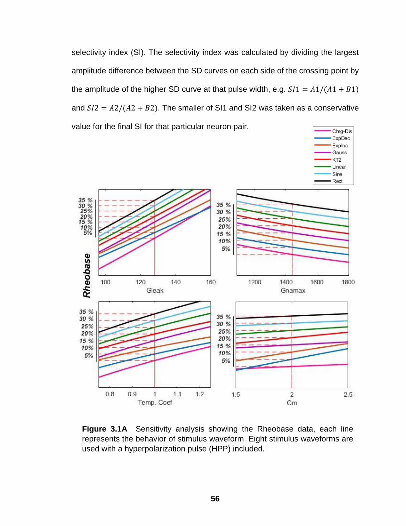
56

selectivity index (SI). The selectivity index was calculated by dividing the largest

amplitude difference between the SD curves on each side of the crossing point by

the amplitude of the higher SD curve at that pulse width, e.g. 𝑆𝐼1 = 𝐴1/(𝐴1 + 𝐵1)

and 𝑆𝐼2 = 𝐴2/(𝐴2 + 𝐵2). The smaller of SI1 and SI2 was taken as a conservative

value for the final SI for that particular neuron pair.

Figure 3.1A Sensitivity analysis showing the Rheobase data, each line

represents the behavior of stimulus waveform. Eight stimulus waveforms are

used with a hyperpolarization pulse (HPP) included.

57

Figure 3.1B Sensitivity analysis showing the Chronaxie data, each line

represents the behavior of stimulus waveform. Eight stimulus waveforms are

used with a hyperpolarization pulse (HPP) included.

58

3.3 Results

3.3.1 Sensitivity to Individual Membrane Parameters

SD curve’s horizontal and vertical translations as the membrane parameters are

varied can be captured by examining the Chr and the Rhe. Any stimulus waveform

that alters these two characteristics in such a way to make the SD curves cross

can lead to selectivity. Thus, we first performed a sensitivity analysis for Chr and

Rhe to the four membrane parameters individually while each one of the eight

different stimulus waveforms is being used for stimulation (Figure 3.1).

Interestingly, the choice of the stimulus waveform played a critical role in

augmenting the diversity effects of membrane parameters on the SD curve.

However, this was true only when the HPP was included in the waveform. Without

the HPP (i.e., Mono), the SD sensitivity plots for various membrane parameters

did not deviate more than a few percent from that of the Rect (Supplementary

Figure B.1). When HPP included, the parameter diversity introduced larger percent

changes in Rhe with the non-rectangular waveforms than with the Rect (smaller

slopes in Figure 3.1 A ). The most prominent baseline translations were observed

with ExpDec and ExpInc. Moreover, ExpDec, ExpInc, and Kt2 had smaller slopes

in the Chr plots (Figure 3.1 B), i.e. stronger dependence on the membrane

parameter compared to that of Rect. An increase in the Chr slope tends to spread

the SD crossing points towards the center of the PW range. The Chr slope for Sine

and Gauss were almost identical, small percent of change, to that of the Rect for

all four parameters (Table 3.2). Consistently, rheobase analysis revealed that

59

ExpDec, ExpInc, and Kt2 slope had a decrease, shown by (-) sign, in the slope

when varying GLeak and Ktemp. When Varying Cm all eight waveform had equal or

greater slope, specially ExpDec and ExpInc have a high percent change compared

to Rect, specially for Rhe. Additionally, for all four parameters the Chr and Rhe

slope for Sine was almost identical to that of Rect. The effects of all eight stimulus

waveforms were negligible on both Chr and Rhe when GNamax was diversified.

Table 3.2. Percent of change in Chronaxie and Rheobase slopes for HPP stimulus waveforms compared to Rect waveform

GLeak GNamax Ktemp Cm

Percent Change in Chr %

Chrg-Dis -1.43 0.00 -3.60 1.09

ExpDec -47.14 0.00 -61.60 -45.10

ExpInc -40.00 0.00 -33.03 -37.31

Gauss -4.29 0.00 -7.58 -3.69

𝑲𝒕𝟐 -20.00 0.00 -5.24 -18.72

Linear -8.57 0.00 11.54 -7.26

Sine -1.43 0.00 -3.53 -1.32

Rect 0.00 0.00 0.00 0.00

Percent Change in Rheobase %

Chrg-Dis 0.00 0.00 -8.94 -1.82

ExpDec -20.65 0.00 -25.51 357.75

ExpInc -14.13 0.00 -32.09 267.78

Gauss -2.17 0.00 -9.52 26.44

𝑲𝒕𝟐 -6.52 0.00 -19.33 132.83

Linear -2.17 0.00 -9.44 54.71

Sine -1.09 0.00 -7.72 5.47

Rect 0.00 0.00 0.00 0.00

Note: Change in slope were calculated using the following equation 100*(Sw-SRect)/SRect). Sw is the slope for non-rectangular waveform, and SRect is the slope for rectangular waveform.

60

ExpInc and ExpDec waveforms stand out for having a higher change in

slope than others in terms of sensitivity of both Chr and Rhe to changes in GLeak

and Cm. Chr and Rhe sensitivities to Ktemp diversity are the highest with ExpDec

waveform only (Chr and Rhe slopes are -0.12 and 0.38, respectively, compared to

that of Rect: -0.31 and 0.508) with a 61.6 % change in Chr and 25.5 % change in

Rhe. Furthermore, for Gnamax diversity, Rhe had a slope of 0.0002 for ExpDec while

Chr slope was near zero for all other waveforms (Supplement Table B.2).

Although, Rhe slopes with KT2 were in the same range as with other waveforms,

KT2 imporved the effect of the parameters to make the SD curves cross and lead

to selectivity more so than other stimulus waveforms.

3.3.2 Selectivity with Single Parameter Variation

Varying a single parameter did not results in SD curve crossings except in the case

of GLeak. In the first chapter we showed that using hyperpolarization pre-pulse with

the Rect stimulus waveform in combination with GLeak diversity led to selectivity. In

this paper, we investigated the effect of non-rectangular stimulus waveform. The

results are similar for all non-rectangular stimulus waveforms with HPP and all

introduced crossings when GLeak is varied. Only ExpInc produced crossings when

Ktemp is varied as well (Supplementary. Figure B.5).

3.3.3 Selectivity with Dual Parameter Variation

The selectivity index (SI) was calculated as defined earlier at the PW where the

ratio of the amplitude difference between the SD curves divided by the amplitude

of the higher SD curve is maximum. The maximum SI was found on each side of

61

the crossing point (𝑆I1=𝐴1/(𝐴1+𝐵1) and 𝑆I2=𝐴2/(𝐴2+𝐵2 in and the smaller of the

two was taken as the conservative value for the final SI for that particular neuron

pair. In order to maximize the SI two of the membrane parameters were altered in

pairs. Since each parameter in the pair was set to three different values; min, max,

and default, the combinations produced 9 different SD curves (i.e. neurons) and a

maximum of 36 possible crossings between the SD curves. This time, multiple SD

curves crossed for all parameter combinations (Supplementary. Figures. B.2, B.3,

and B.4). Each stimulus pulse was tested as a monophasic waveform (Mono, not

shown) and with hyperpolarization pre-pulse (HPP) added. All crossings occurred

at PWs shorter than the chronaxie times of the SD pairs.

To take a closer look at how the calculated SI value was dependent on the

PW at which it is calculated, the SI was plotted as a function of PW for three of the

six parameter pairs and for two of the waveforms (Lin and Rect) as examples in

Figure 3.2. The SI values are zero at the points of SD crossings. Most SDs cross

only once but others cross at two different PWs. The SI takes its maximum values

mostly at the extreme ends of the PW range. However, there are cases where the

maximum occurs in the mid-PW values especially when there are two crossings in

the SD pair (see top right panel in Figure 3.2). In those case, three SI values; one

to the left of the first crossing, one between the two crossings, and a third one to

the right of the second crossing were calculated at the PWs that maximized the SI

value, and that the second from the largest value was taken as the final SI

measurement. The PWs where the final SI values are taken are shown in Figure

3.4 for all membrane parameter pairs and different stimulus waveforms (with HPP).

62

The PWs for SI measurements distributed across the entire range for most

waveforms, except for DecExp and IncExp where they were taken either at the

smallest (10µs) or largest PW (5ms) in most cases. These plots show that for these

two stimulus waveforms, the SI value was monotonously increasing as the PW

moved from that of the crossing point. For all other waveforms, the SI had local

peaks.

The max SIs computed from multiple SDs obtained by diversifying each

membrane parameter pair are plotted in Figure 3.5 for all stimulus waveforms.

When GLeak is one of the diversified parameters (GLeak & Cm, GLeak & GNamax, and

GLeak & Ktemp) the biphasic waveforms (with HPP) produced much higher selectivity

values compared to that of Mono with all stimulus waveforms. (compare blue,

purple and green bars in Figure. 3.5A and 5B). For all remaining three pairs (Ktemp

& GNamax, Cm & GNamax, and Ktemp & Cm), the difference was less and not necessary

in favor of the biphasic waveform. Diversifying GLeak & GNamax, and GLeak & Ktemp

introduced a large increase in the SI for all non-rectangular stimulus waveforms

compared to that of Rect but only when HPP included (purple and green bars in

Figure 3.5 B). In fact, GLeak & Ktemp diversity did not even result in any SD crossings

(zero selectivity) with Mono (purple bars in Figure 3.5 A). Furthermore, Kt2 stood

out as the most selective waveform followed by ExpInc, Lin and Gauss (Figure 3.5

B). Interestingly, in case of Mono, the SI was the largest with all waveforms when

Cm was one of the parameters (blue, black, and red bars in Figure 3.7A). Thus,

GLeak & Cm combination was the best both for Mono and biphasic waveforms (blue

bars in Figures 3.7 A and 3.7 B).

63

Figure 3.2 Percentage of all possible Selectivity Index ratio (%SI) is plotted

in the y-axis in relation to the PW(ms) in x-axis. The top three plots are for the

linear stimulus waveform and the bottom three plots when using a rectangular

waveform. Only three combinations are shown, KTEMP & CM, KTEMP &

GLEAK and KTEMP & GNAMAX.

64

Figure 3.3 The Selectivity Index ratio is plotted in percentage (%SI). The

graph is color coded to differentiate between different parameters

companions. Bars are grouped by stimulus Type. A) For stimulus with

hyperpolarization pre-pulse. B) For Using Monophasic stimulus pulse.

65

Figure 3.4 Pulse width (mSec) where the SI was selected is plotted. The

graph is color coded to differentiate between different combinations as

shown in the top right of the figure.

66

Figure 3.5A the Selectivity Index ratio is plotted in percentage (%SI). The

graph is color coded to differentiate between different parameters companions

as shown in the top left of the figure. Bars are grouped by stimulus Type. A)

For stimulus with hyperpolarization pre-pulse.

67

Figure 3.5B the Selectivity Index ratio is plotted in percentage (%SI). The

graph is color coded to differentiate between different parameters companions

as shown in the top left of the figure. Bars are grouped by stimulus Type. B)

For Using Monophasic stimulus pulse.

68

Figure 3.6 Pulse width (mSec) where the crossing occurred is plotted. The

graph is color coded to differentiate between different combinations as

shown in the top right of the figure.

69

3.4 Discussion

In the first chapter sensitivity analysis reported the effect of each parameter on the

chronaxie time (Chr) and the rheobase (Rhe). We showed that variance in two or

more parameters have a large effect causing higher selectivity Index (SI).

Additionally, we compared between different combinations and different variation

of the rectangular stimulus pulse, showing the great impact that Hyperpolarization

rectangular pulse on selectivity index especially if GLeak is different between two

different neural cells.

This chapter further investigates the effect of non-rectangular waveform on

neural selectivity by studying seven different non-rectangular waveforms. We

started by running sensitivity analysis for each waveform to quantify the effect of

stimulus waveform on chronaxie time (Chr) and rheobsae (Rhe). Sensitivity

analysis revealed that some of the nonrect angular waveforms have higher Chr

slope compared to rectangular waveform, and a lower Rhe slope specifically

ExpInc, ExpDec and KT2. The change in the sensitivity slope influence the SD

curves movements introducing higher probability to cross. The nonrectangular

waveform causes the SD curves to shift diagonally in the Chr and Rhe direction

increasing the number of crossing between SD curves. The movements in the SD

curves generated by ExpInc, ExpDec and KT2 stimulus waveform is large enough

to allow more crossing between SD curves compared to rectangular waveform and

other nonrectangular waveforms, hence it gives higher SI% values.

Non-rectangular waveforms do not lead to selective activation of neurons

per se unless the membrane parameters are allowed to vary from cell to cell. That

70

is, the SD curve moves in the same direction in different neurons when the

electrophysiological parameters change together and do not cause the SD curves

cross. Once we assume diversity of membrane parameters, however, the non-

rectangular waveforms tested here seem to produce higher levels of selectivity

compared to the traditional rectangular current waveforms.

Moreover, results revealed that crossing points occur at different PWs for

different waveforms because the chronaxie time is different for each waveform fig

(7). Therefore, designing an ideal stimulus needs to take in consideration both

stimulus waveform and the neural properties of neural cells. To illustrate the

importance of matching the stimulus with neural properties, one can investigate

figure (7A) where rectangular stimulus waveform scored the lowest SI value

percent for neural properties combination of GLeak & Ktemp (purple) and GLeak &

Gnamax (green). Moreover, KT2 scored the highest SI index percentage followed

by Linear, Gaussain ExpInc and ExpDec. With the assumption that two groups or

neural cells diverse in GLeak & Ktemp or GLeak & Gnamax we suggest using a Kt2

stimulus to achieve higher selectivity between neural cells.

71

CHAPTER 4

COMPARTMENTAL AXON MODEL

4.1 Background and Significance

Nerve cell Is a major role player in transferring signal and information from the

brain to all parts of the human body. It forms the electrical path that the brain uses

to send signals efficiently to other locations in the human body. Nerve cells are

categorized based on functionality three different groups: motor neurons, sensory

neurons, and interneurons. Motor neurons are neuronal cells located in the central

nervous system (CNS), they connect the brain or spinal cord to muscles and

glands. MNs are categorized to two groups: Cranial and spinal subsets. they carry

signal from the brain and the sensory system to control voluntary and involuntary

movements. spinal MNs (SPMNs) form an irreplaceable component of the

neuronal circuity they convey the commands from the CNS to the effector muscles

and their axons extending through several meters in mammals. Sensory neurons

are part of the nervous system and they are activated by sensory inputs from the

surrounding environment. Touch, smell, and taste all are managed by different

sensory neurons. Some sensory neurons can response to external stimuli and

activate motor neurons to achieve involuntary movements, for instance involuntary

motor reflex and involuntary pain avoidance. Finally, the interneurons which are

divided into two subgroups, local and relay. Local interneurons have short axons

and connects with nearby neurons to form a local circuitry. Relay interneurons

have long axons and form neuro circuitry between different brain regions.

72

Axons usually are wrapped with insulating layers called myelin. Myelin

forming neurons are specialized cells transmits information between nerve cells,

muscles, and gland cells. The basic structure of neuron is like other cells, it has a

cell body which is called soma and it is where the nucleus of the neuron is found.

Extended from the cell body short branching processes called dendrites and longer

ones which is called axon, Figure 4.1. The dendrites are where the incoming

excitatory or inhibitory signals gets received and processed. The sum of all signals

collected at the dendrites influence the excitation of the neurons. Then, when a

neuron fires it sends an action potential along the axon to the receiving end. Axon

travels for long distance allowing an efficient propagation of the action potential.

Axons arise from the cell body at the hillock and they travel for longer

distance with the same diameter for most of the length. They are enclosed inside

an insulating material called myelin. Between each two-myelin located node of

Node of Ranvier

Internodal Nucleus

Figure 4.1 Anatomy of the neuron, the yellow parts is called Myelin

(internodal). Node o Ranvier falls between two intermodals.

73

Ranvier, where action potential jumps from node to the next across the axon.

Axons usually have multi-node of Ranvier depending on the axon length and node

size, Figure 4.1.

Node of Ranvier contains a neural cell that allows the propagation of the

action potential along the axon length. One of the well know neural cell model is

H-H which we discussed in section 1.5. The H-H model is based on experimental

data that was collected on a squid giant axon[27] and represented by mathematical

equations to mimic the behavior of the neural cells in. Additionally, it was modeled

as an electrical circuit that gives and approximation of an action potential voltage

traveling along the axon, Figure 1.3. However, to confirm our findings from the

previous chapters we modeled node of Ranvier as a CRRSS model, same model

used in the previous two chapters.

4.2 Methods

4.2.1 Axon Model

To confirm our findings from the previous chapters we investigated selectivity in a

compartmental axon model. A 10 µm myelinated axon was simulated by

incorporating the CRRSS local model [2, 29, 48], at the nodes of Ranvier that had

widths of 1 µm and an inter-nodal distance of 1 mm. Since, there are almost no

potassium currents in mammalian nodes of Ranvier [2, 48, 49], the CRRSS model

is a good fit for the purpose of this study, it contains only the voltage-gated sodium

and the leakage current. A monopolar electrode was placed 1 mm away from the

74

axon and aligned with its central node in a homogeneous volume conductor with

a specific conductivity of 1.8 S/cm Figure 4.2.

Axon with 25 nodes were found sufficiently long for accurate predictions of

the stimulation thresholds since the extracellular voltage at the ends were less than

4% of the maximum voltage in the center. The extracellular voltages generated by

the monopolar current source at the nodes of Ranvier were computed and the SD

curves and SIs were found with the same passive and active parameter ranges

tested in the local membrane model. We selected 7 data points within the same

range tested previously, that yields to 49 neurons and 1176 crossing possibility.

The selected data points are ±5%, ± 15%, ±25%, that range gave us the ability to

investigate the effect of the range on Selectivity.

1 mm 1 mm

Center Node

Figure 4.2 Placement of the electrode on the center node of the

axon model.

75

4.2.2 Stimulus Waveform

The same eight stimulus waveforms used (Table 1); Charge-discharge curve (Chr-

Dis), increasing and decreasing exponential (ExpInc and ExpDec) respectively,

Gaussian (Gauss), KT2, Linear (Lin), sinewave (Sine), and rectangular (Rect) as

defined and tested previously for minimization of stimulation energy [15]. Results

from previous simulation showed that HPP performed the best hence, all stimulus

waveforms were applied as a biphasic waveform where a rectangular

hyperpolarizing pre-pulse (HPP), cathodic, preceded the anodic phase (Table 3.1).

The hyperpolarizing pre-pulse had the same duration as the stimulus pulse and

identical area to the anodic phase to make the waveform charge-balanced.

4.2.3 Strength Duration Curve

As discussed previously the strength duration curve was calculated by sweeping

over the whole range of the PW (0.01 to 5 msec) to find the stimulation threshold

at each pulse width. The threshold was determined using an adaptive search

algorithm to find the smallest current to activate the neural cell. An action potential

was decided to occur if the m-gate variable exceeded the 0.98 threshold. Both

Lapicque-Weiss [51] or Lapicque-Blair [67, 68] equations showed a poor fitting

profile to the non-rectangular stimulus SD curve hence, the chronaxie time (Chr)

and rheobase (Rhe) were computed using the traditional definitions. The Chr is the

pulse width at which the threshold is twice the Rhe and the Rhe is the lowest

intensity required to stimulate neuron within indefinite period.

76

4.2.4 Selectivity Index

Several selectivity measurements were proposed i.e angle measurements

between Crossed SD curves and percent of number of crossings (NOC) however,

the ratiometric selectivity index (rSI) used in the previous chapters showed the best

representation for selectivity. All four membrane parameters, the passive (Cm and

Gleak) and the active (GNamax and Ktemp) parameters were varied in pairs by ± 25%.

Seven data points were taking in between the maximum and minimum values, as

±5%, ±15% and ±25%, the three proposed ranges were used later for investigating

the effect of range on selectivity index (SI). The variation produced 49 different

neurons (7X7) with 1176 possibilities of crossing. Selectivity Index ration was

computed in the same way discussed in section 2.2.5.

4.3 Results

4.3.1 Selectivity - Rectangular Waveform

The feasibility of selectivity by diversity of electrophysiological parameters was

confirmed in a compartmental axon model that incorporated the CRRSS local

model for the nodes of Ranvier. With seven different values that each parameter

was set to within the ±25% range, the combinations produced 49 different neurons

with different SD curves and a maximum of 1176 possible crossings. Once more

Cm & Gleak combination outperformed the rest with a maximum SI value of 19.2%,

followed by Ktemp & Cm, Ktemp & GNamax, and Gleak & Ktemp at 18.2%, 16.11%,

77

15.24%, respectively (Figure 4.3). The Cm & GNamax combination performed the

least with 9.3 % selectivity.

One unique characteristic that the compartmental axon model revealed was

that most of the crossing points occurred between 0.2 and 0.4 msec (Figure 4.4)

compared to ~0.01 and ~0.1 ms in the local model (Figure 2.7 B). The PWs where

the SIs were maximum also spread across the entire PW range compared to PWs

less than 1ms in Figure 2.7 B.

Finally, we examined how the SI values changed as the range within which

the membrane parameters were allowed to vary. This analysis showed that the

selectivity increased with increasing range of diversity (Figure 4.5). The SI

increased as the range of each parameter was increased individually for Gleak &

Cm, Cm & GNamax and Gleak & GNamax combinations (Figure 4.5 - Top). However,

Ktemp dominated the SI effect regardless of the other parameter that it is paired

with (Figure 4.5, bottom row). In all three combinations with Ktemp, the maximum

SI depended on Ktemp only, suggesting the importance of diversity in sodium

kinetics to achieve selectivity.

78

Figure 4.3 Percent selectivity index generated from crossing SD curves in

the compartmental axon model. Diversity range is ±25% and the waveform

is HPP. Each bar represents the combination of parameters that were

diversified.

79

Figure 4.4 PWs at which the SDs cross are shown (“+”) for the

compartmental axon model. Parameter diversity is ±25% and the waveform

is HPP.

80

Figure 4.5 Selectivity Index plotted against the varied membrane

parameters in pairs. In the top three figures, maximum SI achieved when

both parameters are varied maximally (±25%). Selectivity is determined

primarily by Ktemp only when it is one of the parameters tested (bottom

plots).

81

4.3.2 Selectivity with Non-Rectangular Waveform

To be able to draw a conclusion from the results obtained from the local model, we

ran a similar simulation in the compartmental axon model. Using eight stimulus

waveforms, while membrane parameters were altered in pairs. Although, the

results were similar yet there were few divergences. The axon model yet confirmed

that KT2 is the most selective waveform followed by Lin, Gauss when HPP is

included Figure 4.6. Conversely, the axon model showed that the sine waveform

more selective compared to ExpInc Figure 4.6. This could be due to the increasing

contributions made to the activation threshold from the neighboring nodes in the

axonal model as the PW is increasing [69]. This difference between the local and

compartmental model would certainly affect the SD curve and thereby the SI

values.

The axon model revealed that combinations where Cm is one of the varying

parameters generated higher selectivity Index value, this is true for Cm & GNamax

(black), Cm & Ktemp (red) and Cm & Gleak (blue) Figure 4.6. In the controversy

parameters when Gleak is varying, then selectivity index values were reduced Gleak

& GNamax (green) and Gleak & Ktemp (purple) Figure 4.6. Nevertheless, we still can

draw the same conclusion from both simulation models which is, in most cases the

hyperpolarization non-rectangular pulse is more selective than the rectangular one

regardless to which parameters are varying.

Interestingly, when we run the simulation on the compartmental axon model,

we observed that crossing PWs (the PW where crossing occurred) were more

scattered over the whole range of the stimulus period (0.01 top 5 mses) except for

82

ExpInc Figure 4.7. which contributes to the small SI value. Comparing between the

crossing PWs, we can observe that in the axon model, ExpInc has less crossing

scattered compared to Sinewave Figure 4.7. Additionally, percentage of number

of crossing in the Sine Waveform is higher than ExpInc supplementary Figure 4.8.

Thus, translates to a higher SI values in Sinewave compared to ExpInc pulse. The

contrary happened in the local axon model.

83

Figure 4.6 SI values for all waveforms, in the Compartmental Axon

Model are represented with a “+” sign. The graph is color coded for each

combination and the bars are grouped based on the waveform.

84

Figure 4.7 Crossing Locations (PW) in the Axon Model, are represented

with a “+” sign. The graph is color coded for each combination and the bars

are grouped based on the waveform.

85

Figure 4.8 Percent of Number of crossing (NOC), in the axon model is plotted

to compare between different waveforms. The graph is color coded for each

combination bars are grouped based on the waveform.

86

4.4 Discussion

Comparing between the axon model and the local model results while using the

rectangular stimulus pulse, one can notice similarity in the SI values. Gleak & Ktemp

combination produces SI values near 20% and the Cm & GNamax combination

around 10% in both models (Figure 2.7A vs. Figure 4.3). Nevertheless, the

maximum SI of ~45% achieved with Cm & Gleak combination in the local model was

limited to 19.2% in the axon model. This could be due to the increasing

contributions made to the activation threshold from the neighboring nodes in the

axonal model as the PW is increasing [69]. This difference between the local and

compartmental model would certainly affect the SD curve and thereby the SI

values.

It was crucial to run the simulation for a compartmental axon model to

confirm that the same phenomena happen when introducing the nodes of Ranvier,

while using non-rectangular stimulus pulse. Although, adding 25 nodes shifted the

selectivity away from ExpInc and more towards Sinewave, yet it confirmed the

main vital finding which is Rec is the least selective stimulus pulse. Also, it

confirmed that KT2 is the most selective waveform followed by Lin, Gauss when

HPP is included Figure 4.6. Adding 25 nodes of Ranvier add a more realistic

simulation to the model taking in consideration the contribution made from each

node to the activation threshold which certainly affect the SD curve and thereby

the SI values.

87

The compartmental axon model simulation results showed that no one

stimulus waveform generated the absolute highest selectivity index value for all

combinations, hence combinations complement stimulus waveform. In other

words, we can select the stimulus waveform based on neurons properties and the

variation found in a specific cluster of neurons. For instance, If one group of

neurons are different in GLeak & Ktemp then using Sinewave or Gauss as the

stimulus pulse achieves higher selectivity index. On the contrary, if the cluster of

neurons are different in Ktemp & GNamax then Linear or Gauss stimulus pulse

should be used to achieve better Selectivity. Furthermore, if the neurons are

varied in Cm & GLeak then using KT2 stimulus pulse allows higher selectivity

between the neurons. Yet, more work is essential to further investigate the

phenomena using experimental data in addition to quantifying neurons based on

their functionality and properties. Then the proposed technique can be used to

select a stimulus pulse that best fit the targeted group of neurons to achieve neural

selectivity.

88

CHAPTER 5

CONCLUSION AND FUTURE WORK

Both the local and the axon model results of this study suggest that intrinsic

variations that naturally occur in the passive and dynamic membrane properties of

neurons can lead to substantial levels of stimulation selectivity when the biphasic

waveform is used for stimulation where the hyperpolarizing pulse precedes the

depolarizing pulse. The passive membrane parameters (GLeak and Cm) seem to be

more influential on producing a diverse set of SD curves that can be leveraged for

selectivity. The impact of diversity in dynamic parameters (Ktemp and GNamax)

increase but not supersede the effect of passive parameters for smaller values of

the membrane time constant. Results produced from the axon model further

confirmed our main hypothesis, that the intersect variation in neuron properties

combined with the non-rectangular waveform leads to high level of selectivity. The

predicted levels of selectivity may lead to substantial improvemens and a paradigm

shifting approach in functional neural stimulation provided that assumed

electrophysiological diversity can be demonstrated between neuronal subtypes

serving different functions in the CNS. We expect these results to generalize to

other neuron models that include a fast voltage-gated sodium channel, which is

the only kinematic variable in the basic model used in this study. It should be noted

however that the diversity in other ionic channel kinematics that are not included

in this study (e.g. slow sodium and potassium channels) may influence the

rheobase and thereby the levels of selectivity that can be achieved.

89

APPEDNIX A

ELECTROPHYSIOLOGICAL DIVERSITY- SUPPLEMENTARY FIGURES

0

1

2

3

4

5

6

7

8

0 0.5 1 1.5 2 2.5 3 3.5 4 4.5 5

Sele

ctiv

ity

Ind

ex

(%)

DPP PW (ms)

Figure A.1 Selectivity Index reaches 85% of its max at 1ms and plateaus at

2ms for increasing durations of depolarizing phase in the DPP waveform.

90

Figure A.2 Sensitivity of rheobase to the membrane parameters (GLeak, Gnamax, Temp.

Coef-KTemp, and Cm) as they are altered by ±25% from the nominal value and evaluated

at many intermediate values. The analysis is repeated for three different default values

of Cm; Cm-def=0.5 µF/cm2 (Red), Cm-def=2 µF/cm2 (Blue), and Cm-def=4 µF/cm2 (Black)

. Dash lines show the nominal values.

91

Figure A.3 Only Gleak variations, shown on top right panel, produce a few

crossings (red dash lines) between the SD curves when using HPP stimulus

waveform.

92

Figure A.4 The effects of the four model parameters (GLeak, Gnamax, Temp.

Coef-Ktemp, and Cm) on the strength-duration curve when DPP stimulus

waveform is used. No SD crossings occur.

93

Figure A.5 Adding a 200 µs gap in the HPP waveform on the SD curve. It

reverses the HPP effects for all parameter variations. Only the Gleak results

are shown here. The SD crossings seen for Gleak diversity in Supplemental

Figure A.4 are eliminated.

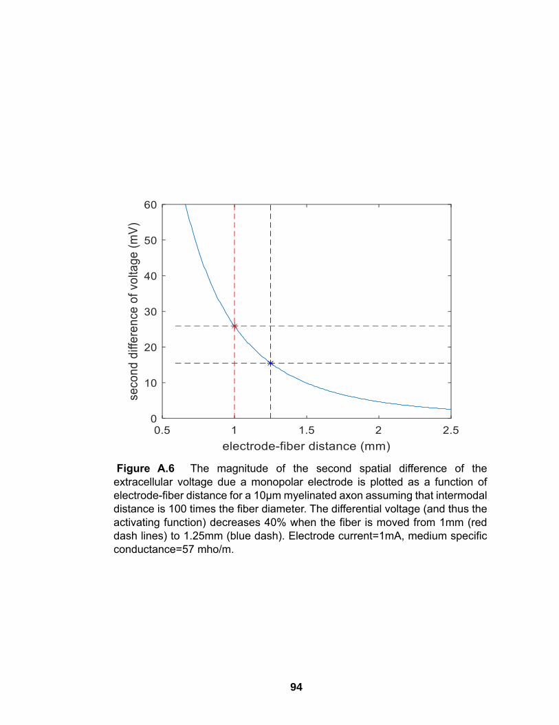
94

Figure A.6 The magnitude of the second spatial difference of the

extracellular voltage due a monopolar electrode is plotted as a function of

electrode-fiber distance for a 10µm myelinated axon assuming that intermodal

distance is 100 times the fiber diameter. The differential voltage (and thus the

activating function) decreases 40% when the fiber is moved from 1mm (red

dash lines) to 1.25mm (blue dash). Electrode current=1mA, medium specific

conductance=57 mho/m.

95

Figure A.7The magnitude of the second spatial difference of the extracellular

voltage at 1mm from a monopolar electrode as a function of axon diameter.

The differential voltage (and thus the activating function) decreases 47% when

a 20µm fiber (blue dash lines) is replaced by a 10µm axon (red dash). Other

parameters are same as in Supplemental Figure 6.

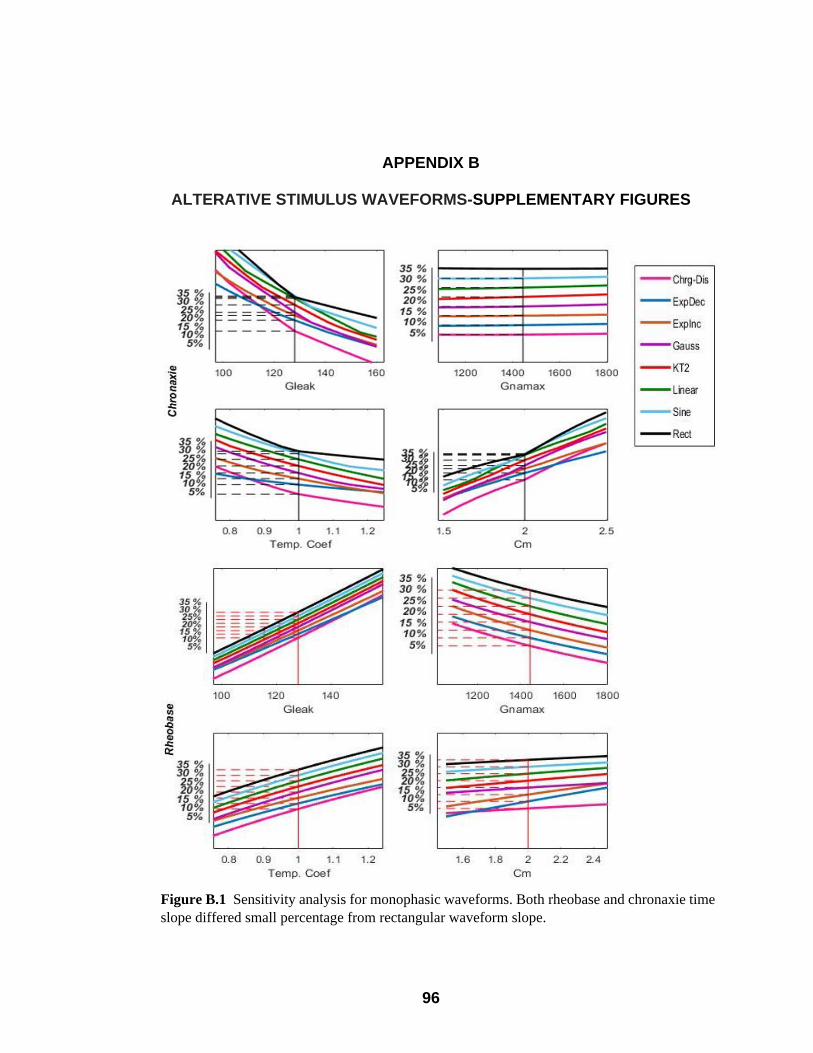
96

APPENDIX B

ALTERATIVE STIMULUS WAVEFORMS-SUPPLEMENTARY FIGURES

Figure B.1 Sensitivity analysis for monophasic waveforms. Both rheobase and chronaxie time

slope differed small percentage from rectangular waveform slope.

97

Figure B.2 GNAMAX & GLEAK are altered simultaneously in each case by the same

amount, using eight different waveform. Different colors legend indicates different

values for Cm parameter shown on top right of the figure. Second parameter is not color

coded for clarity. The SD curves cross multiple times usually at extreme pulse widths

(PW), but in mid-PWs as well in some cases. X-scale is divided for clarity, from 0 to

0.2/0.3 then from 1 to 5 mSec. The area between (0.2/0.3 to 1) ms is not shown.

98

Figure B.3 KTEMP & GLEAK are altered simultaneously in each case by the same

amount, using eight different waveform. Different colors legend indicates different values

for Ktemp parameter shown on top right of the figure. Second parameter is not color coded

for clarity. The SD curves cross multiple times usually at extreme pulse widths (PW), but in

mid-PWs as well in some cases. X-scale is divided for clarity, from 0 to 0.2 then from 1 to

5 mSec. The area between (0.2 to 1) ms is not shown.

99

Figure B.4 GLEAK & CM are altered simultaneously in each case by the same amount,

using eight different waveform. Different colors in each subplot indicate different

values for Cm parameter shown on top right. Second parameter is not color coded for

clarity. The SD curves cross multiple times usually at extreme pulse widths (PW), but

in mid-PWs as well in some cases. X-scale is divided for clarity, from 0 to 0.2 then

from 1 to 5 mSec. The area between (0.2 to 1) ms is not shown.

100

Table B.1. Percent of change in Chronaxie and Rheobase slopes for mono stimulus waveforms compared to Rect waveform.

GLeak GNamax Ktemp Cm

Percent Change in Chr %

Chrg-Dis 4.761905 0 -0.539 9.777424

ExpDec -30.1587 0 -54.8827 -26.974

ExpInc -19.0476 0 -13.6652 -14.8119

Gauss 4.761905 0 6.341154 6.783254

𝑲𝒕𝟐 0 0 10.68484 1.139375

Linear 4.761905 0 11.44578 3.471118

Sine 1.587302 0 12.77743 6.465289

Rect 0 0 0 0

Percent Change in Rheobase %

Chrg-Dis 0 0 0.134078 10.23891

ExpDec -13.0435 0 -12.8492 261.0922

ExpInc -7.6087 0 -14.4134 185.6655

Gauss -1.08696 0 0.692737 21.843

𝑲𝒕𝟐 -2.17391 0 -2.86034 74.06143

Linear -1.08696 0 0.916201 55.9727

Sine 0 0 0.558659 15.69966

Rect 0 0 0 0

Note: . Change in slope were calculated using the following equation 100*(Sw-

SRect)/SRect). Sw is the slope for non-rectangular waveform , and SRect is the slope for

rectangular waveform.

101

Table B.2. Chronaxie and Rheobase slopes for HPP stimulus waveforms.

Waveform/Parameter Gleak Gnamax ktemp CM

Chronaxie time

Chrg-Dis -0.0069 0.0000 -0.3000 0.4357

ExpDec -0.0037 0.0000 -0.1195 0.2366

ExpInc -0.0042 0.0000 -0.2084 0.2702

Gauss -0.0067 0.0000 -0.2876 0.4151

KT -0.0056 0.0000 -0.2949 0.3503

Linear -0.0064 0.0000 -0.3471 0.3997

Sine -0.0069 0.0000 -0.3002 0.4253

Rect -0.0070 0.0000 -0.3112 0.4310

Rheobase

Chrg-Dis 0.0092 -0.0002 0.4622 0.0323

ExpDec 0.0073 -0.0002 0.3781 0.1506

ExpInc 0.0079 -0.0002 0.3447 0.1210

Gauss 0.0090 -0.0002 0.4593 0.0416

KT 0.0086 -0.0002 0.4095 0.0766

Linear 0.0090 -0.0002 0.4597 0.0509

Sine 0.0091 -0.0002 0.4684 0.0347

Rect 0.0092 -0.0002 0.5076 0.0329

102

Table B.3. Chronaxie and Rheobase slopes for Mono stimulus waveforms.

Waveform/Parameter Gleak Gnamax ktemp CM

Chronaxie time

Chrg-Dis -0.0066 0.0000 -0.3137 0.4143

ExpDec -0.0044 0.0000 -0.1423 0.2756

ExpInc -0.0051 0.0000 -0.2723 0.3215

Gauss -0.0066 0.0000 -0.3354 0.4030

KT -0.0063 0.0000 -0.3491 0.3817

Linear -0.0066 0.0000 -0.3515 0.3905

Sine -0.0064 0.0000 -0.3557 0.4018

Rect -0.0063 0.0000 -0.3154 0.3774

Rheobase

Chrg-Dis 0.009185 -0.000171 0.448081 0.032345

ExpDec 0.007979 -0.000164 0.390040 0.105780

ExpInc 0.008473 -0.000179 0.382965 0.083724

Gauss 0.009138 -0.000172 0.450570 0.035748

KT 0.009029 -0.000184 0.434742 0.050986

Linear 0.009103 -0.000182 0.451593 0.045664

Sine 0.009158 -0.000171 0.450015 0.033944

Rect 0.009214 -0.000170 0.447520 0.029269

103

APPENDIX C

MATLAB CODE AND FUNCTIONS FOR THE MODEL

%Update bY: B.Ghobreal Date: 09/25/2018

% Version 12 is the last stable version release on 10/17/2017.

% Version 012 in this version

% it is going back to the original and repeating everything and replotting

% changing the K value for both of them or indvidually

%PLOTS THE Action potential

% Problem that mentioned by Dr. Sahin is fix , where the plotting was not

% correct and I fixed the plotting and the threshold porblem

% we plot the SUB threshold Vs THe PW

% I discovered an issue on the 11/11/2019 that cm is define as parm_array

% and it should of been difeind as parm_array2..

% I fixed the issue and it didn't effect the results because CM was always

% pram1 11/29/2019

close all;

clear all

current_directry = pwd;

v0=-80;%mv Resting memebrane voltage

duration=5;%ms

KQM_alpha = 1;

KQM_Beta=1;

KQH_alpha = 1;

KQH_Beta = 1;

Temp_Cofe = 1;

Next =0 ;

signal_used = 0;

%PW=[0.02,0.04,0.06,0.08,0.1,0.2,0.3,0.5]; % Creathinga Pulsh Width Array to cycle

throught and find the best K

% PW = 0.01:.01:duration;

% PW =[ 0.01:.01:1 1.1:0.1:5 ] ;

% PW =[ 0.01:.01:1 1.1:0.5: 5 ] ;

PW =[ 0.01:.01:0.25 0.3:0.05:0.95 1:1: 5 ] ;

%PW_half=PW/2; % I divided the PW to two halfs, each ahlf willhave part of the signal.

for example if PW =.2 --> PW1 =.1 for the cathodic part andPW2 = .1 for the Anodic part

of the signal

Q=length(PW); % length of Puls Width array

dt=10^(-3); %10^(-3);%ms Delta t

M=duration/dt; % length of time change array to

IS=zeros(1,M); % the simulation current, unit: microAmpere, 0.1 msec duration.

Paramter_chng = [];

output1=zeros(1,Q);

output11=zeros(1,Q);

output12=zeros(1,Q);

output2=zeros(1,Q);

output21=zeros(1,Q);

output22=zeros(1,Q);

output3=zeros(1,Q);

output31=zeros(1,Q);

output32=zeros(1,Q);

output4=zeros(1,Q);

output41=zeros(1,Q);

output42=zeros(1,Q);

output5=zeros(1,Q);

output51=zeros(1,Q);

output52=zeros(1,Q);

output6=zeros(1,Q);

output61=zeros(1,Q);

output62=zeros(1,Q);

104

output7=zeros(1,Q);

output71=zeros(1,Q);

output72=zeros(1,Q);

output8=zeros(1,Q);

output81=zeros(1,Q);

output82=zeros(1,Q);

gnamax=1445; % mmho/(cm*cm) [K/ ( Ohm* CM*CM)2.5

gleak=128; % mmho/(cm*cm)

%Ek=-84;%mV ?????

Ena= 35.64; %mV

Eleak=-80.01;%mV

Cm=2;%uF/(cm*cm)

% Cm=0.25

i=1;

m=1;

n=1;

k=0;

k1=0;

AM=zeros(1,M);

BM=zeros(1,M);

AH=zeros(1,M);

BH=zeros(1,M);

HINF=zeros(1,M);

MGATE=zeros(1,M);

HGATE=zeros(1,M);

GNA=zeros(1,M);

INA=zeros(1,M);

ILEAK=zeros(1,M);

Signal_names = {' INcreasing Expotential' , ' Rectangular Waveform' ' Linear Waveform'

'KT^2 Waveform' ' Decaying Expotential' ' Charge Dis-Charge waveform ' ' Gaussian

Waveform' ' Sine Waveform',...

' Cathodic Puls and INcreasing Expotential' , ' Cathodic Puls and

Rectangular Waveform' ' Cathodic Puls and Linear Waveform' 'Cathodic Puls and KT^2

Waveform' ' ' ' Cathodic Puls and Decaying Expotential' ' Cathodic Puls and Charge

Dis-Charge waveform ' ' Cathodic Puls and Gaussian Waveform' ' Cathodic Puls and Sine

Waveform' '' '' ' Cathodic + 200uS gap + Rectangular'};

% Prectage_bar = waitbar(0, 'Precentage completead ....');

%% Choosing variable you wanna change

NumOFParameters=0;

NumOFParameters = str2num( questdlg ('How many Parameters Of Interest for this Cell ?',

'Number of Parameters Of Interest' ,'1', '2' ,'3' ));% uiwait(NumOFParameters_MSGBOX) ;

% num_of_parm = str2num(NumOFParameters);

%% Choosing variable you wanna change

Exit = 0;

Min=0;

Max=0;

step=0;

Max_P2 =0;

Min_P2=0;

step_P2=0;

Skip =5;

sensitivity=0;

DefinedPrecentage = 0;

Paramter_chng=0;

Paramter2_chng=0;

Paramter_VAl=1;

Paramter_VAl2=1;

Paramters_Of_Interest = {'Gnamax','Gleak','Alpha','Beta','Temp. Coef', 'Cm'};

switch NumOFParameters

case 1

while Exit <1

105

figure(1)

clf

% scrsz = get(0,'ScreenSize');

position_default = [650 250 600 300];

set(gcf,'position',position_default)

set(gcf,'ToolBar','none')

set(gcf,'MenuBar','none')

popup = uicontrol(gcf,'Style', 'popup','String',

{'gnamax','gleak','KQM_alpha','KQM_Beta','Tempreature Coef' ,

'Cm'},'Value',Paramter_VAl,'units','normalized','Position',[.125 .8 .35

.1],'Callback','if popup.Value == 1;Paramter_chng = gnamax ; elseif popup.Value == 2;

Paramter_chng = gleak;elseif popup.Value ==3; Paramter_chng = KQM_alpha ;elseif

popup.Value ==4;Paramter_chng = KQM_Beta; elseif popup.Value ==5;Paramter_chng =

Temp_Cofe;elseif popup.Value ==6;Paramter_chng = Cm;else; end; uiresume;');

pbStr =

uicontrol(gcf,'Style','edit','String',Paramter_chng,'units','normalized','Position',[.60

.8 .25 .1],'Callback',' uiresume;');

pbStr =

uicontrol(gcf,'Style','text','String','Current','units','normalized','Position',[.60 .90

.25 .05],'Callback','uiresume;');

pbStrMIN =

uicontrol(gcf,'Style','edit','Value',Min,'units','normalized','Position',[.10 .40 .25

.15],'Callback', 'Min = str2num(pbStrMIN.String);');

pbStr =

uicontrol(gcf,'Style','text','String','Min','units','normalized','Position',[.10 .60 .25

.05],'Callback',' ');

pbStrMax =

uicontrol(gcf,'Style','edit','Value',Max,'units','normalized','Position',[.40 .40 .25

.15],'Callback',' Max = str2num(pbStrMax.String) ;');

pbStr =

uicontrol(gcf,'Style','text','String','MAx','units','normalized','Position',[.40 .60 .25

.05],'Callback',' uiresume;');

pbStrStep =

uicontrol(gcf,'Style','edit','Value',step,'units','normalized','Position',[.70 .40 .25

.15],'Callback',' step = str2num(pbStrStep.String);');

pbStr =

uicontrol(gcf,'Style','text','String','Step','units','normalized','Position',[.70 .60 .25

.05],'Callback','uiresume;');

pbexit =

uicontrol(gcf,'Style','pushbutton','String','Skip','units','normalized','Position',[.65

.10 .15 .15],'Callback','Skip=0;Exit = 5; uiresume;');

pbexit =

uicontrol(gcf,'Style','pushbutton','String','Sensitivity','units','normalized','Position'

,[.45 .10 .15 .15],'Callback','sensitivity = 5; Exit = 5; uiresume;');

pbexit =

uicontrol(gcf,'Style','pushbutton','String','Next','units','normalized','Position',[.25

.10 .15 .15],'Callback','Exit = 5; uiresume;');

uiwait(gcf)

Paramter_VAl = popup.Value;

end

if Skip >0

if (sensitivity >0)

switch(Paramter_VAl)

case 1

Pram_Array = 1084:2*36.1:1806;

case 2

Pram_Array = 96:2*3.2:160;

case 5

Pram_Array = 0.75:2*0.025:1.25;

case 6

Pram_Array = 1.5:2*0.05:2.5;

end

else

Pram_Array=Min:step:Max;

106

end

else

Pram_Array =0;

end

LBL = popup.String(Paramter_VAl);

Pram_Array2 = [ 1445]; % Array for the second paramter (gnamax now)

Paramter_VAl2 = 1 ;

case 2

while Exit <1

figure(1)

clf

% scrsz = get(0,'ScreenSize');

position_default = [650 250 600 300];

set(gcf,'position',position_default)

set(gcf,'ToolBar','none')

set(gcf,'MenuBar','none')

% first paramter contorl panel

Frame =

uicontrol(gcf,'Style','frame','String','','units','normalized','Position',[.65 .1 .32

.72],'Callback',' uiresume;');

Fram_text = uicontrol(gcf,'Style','text','String','Parameter #

1','FontSize',11.0,'units','normalized','Position',[.65 .85 .25

.05],'Callback','uiresume;');

popup = uicontrol(gcf,'Style', 'popup','String',

{'gnamax','gleak','KQM_alpha','KQM_Beta','Tempreature

Coef','Cm'},'Value',Paramter_VAl,'units','normalized','Position',[.7 .7 .25

.1],'Callback','if popup.Value == 1;Paramter_chng = gnamax; elseif popup.Value == 2;

Paramter_chng = gleak;elseif popup.Value ==3; Paramter_chng = KQM_alpha ;elseif

popup.Value ==4;Paramter_chng = KQM_Beta ; elseif popup.Value ==5;Paramter_chng =

Temp_Cofe ;elseif popup.Value ==6; Paramter_chng = Cm;else; end; uiresume;');

pbStr =

uicontrol(gcf,'Style','edit','String',Paramter_chng,'units','normalized','Position',[.80

.6 .1 .1],'Callback',' uiresume;');

pbStr =

uicontrol(gcf,'Style','text','String','Current','units','normalized','Position',[.70 .6

.1 .05],'Callback','uiresume;');

pbStrMax =

uicontrol(gcf,'Style','edit','Value',Max,'units','normalized','Position',[.80 .45 .1

.1],'Callback',' Max = str2num(pbStrMax.String) ;');

pbStr =

uicontrol(gcf,'Style','text','String','MAx','units','normalized','Position',[.70 .45 .1

.05],'Callback',' uiresume;')

pbStrMIN =

uicontrol(gcf,'Style','edit','Value',Min,'units','normalized','Position',[.80 .3 .1

.1],'Callback', 'Min = str2num(pbStrMIN.String);');

pbStr =

uicontrol(gcf,'Style','text','String','Min','units','normalized','Position',[.70 .3 .1

.05],'Callback',' ');

pbStrStep =

uicontrol(gcf,'Style','edit','Value',step,'units','normalized','Position',[.80 .15 .1

.1],'Callback',' step = str2num(pbStrStep.String);');

pbStr =

uicontrol(gcf,'Style','text','String','Step','units','normalized','Position',[.70 .15 .1

.05],'Callback','uiresume;');

% second Parameter control panel

Frame =

uicontrol(gcf,'Style','frame','String','','units','normalized','Position',[.05 .1 .32

.72],'Callback',' uiresume;');

Fram_text = uicontrol(gcf,'Style','text','String','Parameter #

2','FontSize',11.0,'units','normalized','Position',[.05 .85 .25

.05],'Callback','uiresume;');

popup_Par2 = uicontrol(gcf,'Style', 'popup','String',

{'gnamax','gleak','KQM_alpha','KQM_Beta','Tempreature

Coef','Cm'},'Value',Paramter_VAl2,'units','normalized','Position',[.1 .7 .25

107

.1],'Callback','if popup_Par2.Value == 1;Paramter2_chng = gnamax; elseif popup_Par2.Value

== 2; Paramter2_chng = gleak;elseif popup_Par2.Value ==3; Paramter2_chng = KQM_alpha

;elseif popup_Par2.Value ==4;Paramter2_chng = KQM_Beta; elseif popup_Par2.Value

==5;Paramter2_chng = Temp_Cofe;elseif popup_Par2.Value ==6; Paramter2_chng = Cm ;else;

end; uiresume;');

pbStr_Par2 =

uicontrol(gcf,'Style','edit','String',Paramter2_chng,'units','normalized','Position',[.2

.6 .1 .1],'Callback',' uiresume;');

pbStr_Par2 =

uicontrol(gcf,'Style','text','String','Current','units','normalized','Position',[.1 .6 .1

.05],'Callback','uiresume;');

pbStrMax_Par2 =

uicontrol(gcf,'Style','edit','Value',Max_P2,'units','normalized','Position',[.2 .45 .1

.1],'Callback',' Max_P2 = str2num(pbStrMax_Par2.String) ;');

pbStr_Par2 =

uicontrol(gcf,'Style','text','String','MAx','units','normalized','Position',[.1 .45 .1

.05],'Callback',' uiresume;');

pbStrMIN_Par2 =

uicontrol(gcf,'Style','edit','Value',Min_P2,'units','normalized','Position',[.2 .3 .1

.1],'Callback', 'Min_P2 = str2num(pbStrMIN_Par2.String);');

pbStr_par2 =

uicontrol(gcf,'Style','text','String','Min','units','normalized','Position',[.1 .3 .1

.05],'Callback',' ');

pbStrStep_par2 =

uicontrol(gcf,'Style','edit','Value',step_P2,'units','normalized','Position',[.2 .15 .1

.1],'Callback',' step_P2 = str2num(pbStrStep_par2.String);');

pbStr_par2 =

uicontrol(gcf,'Style','text','String','Step','units','normalized','Position',[.1 .15 .1

.05],'Callback','uiresume;');

pbexit =

uicontrol(gcf,'Style','pushbutton','String','Skip','units','normalized','Position',[.425

.2 .15 .15],'Callback','Skip=0;Exit = 5; uiresume;');

pbexit =

uicontrol(gcf,'Style','pushbutton','String','Next','units','normalized','Position',[.425

.6 .15 .15],'Callback','Exit = 5; uiresume;');

pbexit = uicontrol(gcf,'Style','pushbutton','String','Use defined Percentage

" +-25 %" ','units','normalized','Position',[.330 .84 .35

.15],'Callback','DefinedPrecentage=5;Exit = 5; uiresume;');

uiwait(gcf)

Paramter_VAl = popup.Value;

Paramter_VAl2= popup_Par2.Value;

end

if Skip >0

if DefinedPrecentage > 0

if Paramter_VAl2 == 1 %gnamax

Pram_Array2 = round(([-.25 -.15 -.05 0 0.05 0.15 0.25 ]

*1445+1445));% 1084:120.33333:1806;% 1084:180.5:1806 ; %1011.5:144.5:1878.5; %

1084:144.5:1878.5; %1084:361:1806

elseif Paramter_VAl2 == 2 %gleak

Pram_Array2= round(([-.25 -.15 -.05 0 0.05 0.15 0.25 ] *128+128))

;%96:10.666666:160; %96:16:160;% 89.6:12.8:166.4; %96:32:160;

elseif Paramter_VAl2 ==3

Pram_Array2 = KQM_alpha *Pram_Array2;

elseif Paramter_VAl2 ==4

Pram_Array2 = KQM_Beta * Pram_Array2;

elseif Paramter_VAl2 ==5 % Change in Tempreature chznges both K for alpha

and Beta H and M gates

Pram_Array2=([-.25 -.15 -.05 0 0.05 0.15 0.25 ] *1+1); %

0.75:0.08333:1.25; % 0.75:0.125:1.25 ;% 0.7:0.1:1.3;% 0.75:0.25:1.25;

elseif Paramter_VAl2 ==6 % Change in Cm

Pram_Array2 =([-.25 -.15 -.05 0 0.05 0.15 0.25 ] *2+2); %

1.5:0.16666:2.5 ;%1.5:0.25:2.5;% 1.4:0.2:2.6;%1.5:0.5:2.5;

end

108

if Paramter_VAl == 1 %gnamax

Pram_Array = round(([-.25 -.15 -.05 0 0.05 0.15 0.25 ] *1445+1445));%

1084:120.33333:1806; % 1084:180.5:1806 ;% 1084:180.5:1806 ;% 1084:120.33333:1806

;%1011.5:144.5:1878.5; % 1084:361:1806; 1084:361:1806 ;%

elseif Paramter_VAl == 2

Pram_Array= round(([-.25 -.15 -.05 0 0.05 0.15 0.25 ] *128+128)) ;

%96:10.666666:160; %89.6:12.8:166.4; % 96:32:160;

elseif Paramter_VAl ==3

Pram_Array = KQM_alpha * Pram_Array;

elseif Paramter_VAl ==4

Pram_Array = KQM_Beta * Pram_Array;

elseif Paramter_VAl ==5 % Change in Tempreature chznges both K for alpha

and Beta H and M gates

Pram_Array= ([-.25 -.15 -.05 0 0.05 0.15 0.25 ] *1+1);

%0.75:0.08333:1.25; %0.7:0.1:1.3;% 0.75:0.25:1.25;

elseif Paramter_VAl ==6 % Change in Cm

Pram_Array =([-.25 -.15 -.05 0 0.05 0.15 0.25 ] *2+2) ;%

1.5:0.16666:2.5 ;%1.4:0.2:2.6;% 1.5:0.5:2.5;

end

else

Pram_Array=Min:step:Max;

Pram_Array2=Min_P2:step_P2:Max_P2;

end

else

Pram_Array2 = 0;

Pram_Array = 0;

end

LBL = popup.String(Paramter_VAl);

LBL_2 = popup_Par2.String(Paramter_VAl2);

end

%%

K_DPP=0;

Answer = questdlg ('What type of stimulation ?','Stimulation Type!','DPP', 'Gap',

'Non','Skip' );% uiwait(NumOFParameters_MSGBOX) ;

if (strcmp(Answer,'DPP'))

DPP_PW=1;

M=M+DPP_PW/dt;

PW =(PW(1)+DPP_PW):.01:(duration+DPP_PW);

elseif (strcmp(Answer,'Gap'))

PW_Gap=200/1000;

end

%%

Exit = 0;

while Exit <1

while Next < 1

cd (current_directry);

figure(2)

clf

scrsz = get(0,'ScreenSize');

position_default = [0.01*scrsz(3) 0.07*scrsz(4) 0.98*scrsz(3) 0.85*scrsz(4)];

set(gcf,'position',position_default)

Frame =

uicontrol(gcf,'Style','frame','String','','units','normalized','Position',[.922 .14 .057

.77],'Callback',' uiresume;');

Fram_text = uicontrol(gcf,'Style','text','String','Anodic

Signal','FontSize',11.0,'units','normalized','Position',[.9255 .85 .05

.1],'Callback','uiresume;');

pbexit = uicontrol(gcf,'Style','pushbutton','String','Increasing

EXP','units','normalized','Position',[.925 .85 .05 .05],'Callback','signal_used = 1;

uiresume;');

pbexit = uicontrol(gcf,'Style','pushbutton','String','rectangular

waveform','units','normalized','Position',[.925 .75 .05 .05],'Callback','signal_used = 2;

uiresume;');

109

pbexit = uicontrol(gcf,'Style','pushbutton','String','linear

waveform','units','normalized','Position',[.925 .65 .05 .05],'Callback','signal_used = 3;

uiresume;');

pbexit = uicontrol(gcf,'Style','pushbutton','String','KT^2 wave

form','units','normalized','Position',[.925 .55 .05 .05],'Callback','signal_used = 4;

uiresume;');

pbexit = uicontrol(gcf,'Style','pushbutton','String',' Decaying

exponential','units','normalized','Position',[.925 .45 .05 .05],'Callback','signal_used =

5; uiresume;');

pbexit = uicontrol(gcf,'Style','pushbutton','String','Charge-Discharge

Curve','units','normalized','Position',[.925 .35 .05 .05],'Callback','signal_used = 6;

uiresume;');

pbexit = uicontrol(gcf,'Style','pushbutton','String','Gaussian

Stimulus','units','normalized','Position',[.925 .25 .05 .05],'Callback','signal_used = 7;

uiresume;');

pbexit = uicontrol(gcf,'Style','pushbutton','String','Sinusoidal

Stimulus','units','normalized','Position',[.925 .15 .05 .05],'Callback','signal_used = 8;

uiresume;');

% pbexit = uicontrol(gcf,'Style','pushbutton','String','ALL Signals

','units','normalized','Position',[.925 .95 .05 .05],'Callback','All_Signals = 1;

uiresume;');

Frame =

uicontrol(gcf,'Style','frame','String','','units','normalized','Position',[.122 .14 .057

.77],'Callback',' uiresume;');

Fram_text = uicontrol(gcf,'Style','text','String','Cathodic + Anodic

Signal','FontSize',11.0,'units','normalized','Position',[.1255 .85 .05

.1],'Callback','uiresume;');

pbexit = uicontrol(gcf,'Style','pushbutton','String','Increasing

EXP','units','normalized','Position',[.125 .85 .05 .05],'Callback','signal_used = 9;

uiresume;');

pbexit = uicontrol(gcf,'Style','pushbutton','String','rectangular

waveform','units','normalized','Position',[.125 .75 .05 .05],'Callback','signal_used =

10; uiresume;');

pbexit = uicontrol(gcf,'Style','pushbutton','String','linear

waveform','units','normalized','Position',[.125 .65 .05 .05],'Callback','signal_used =

11; uiresume;');

pbexit = uicontrol(gcf,'Style','pushbutton','String','KT^2 wave

form','units','normalized','Position',[.125 .55 .05 .05],'Callback','signal_used = 12;

uiresume;');

pbexit = uicontrol(gcf,'Style','pushbutton','String',' Decaying

exponential','units','normalized','Position',[.125 .45 .05 .05],'Callback','signal_used =

14; uiresume;');

pbexit = uicontrol(gcf,'Style','pushbutton','String','Charge-Discharge

Curve','units','normalized','Position',[.125 .35 .05 .05],'Callback','signal_used = 15;

uiresume;');

pbexit = uicontrol(gcf,'Style','pushbutton','String','Gaussian

Stimulus','units','normalized','Position',[.125 .25 .05 .05],'Callback','signal_used =

16; uiresume;');

pbexit = uicontrol(gcf,'Style','pushbutton','String','Sinusoidal

Stimulus','units','normalized','Position',[.125 .15 .05 .05],'Callback','signal_used =

17; uiresume;');

% adding the Gap between the cathodic and anodic

pbexit = uicontrol(gcf,'Style','pushbutton','String','200uS +

Rec','units','normalized','Position',[.180 .75 .06 .05],'Callback','signal_used = 20;

uiresume;');

pbexit =

uicontrol(gcf,'Style','pushbutton','String','Next','units','normalized','Position',[.925

.05 .05 .05],'Callback','Next = 5; uiresume;');

uiwait(gcf)

end

110

%%

for Pram2 = 1:length(Pram_Array2)

if Paramter_VAl2 == 1

gnamax=Pram_Array2(Pram2);

elseif Paramter_VAl2 == 2

gleak=Pram_Array2(Pram2);

elseif Paramter_VAl2 ==3

KQM_alpha = Pram_Array2(Pram2);

KQH_alpha = Pram_Array2(Pram2);

elseif Paramter_VAl2 ==4

KQM_Beta = Pram_Array2(Pram2);

KQH_Beta = Pram_Array2(Pram2);

elseif Paramter_VAl2 ==5 % Change in Tempreature chznges both K for alpha and Beta

H and M gates

KQM_alpha = Pram_Array2(Pram2);

KQH_alpha = Pram_Array2(Pram2);

KQM_Beta = Pram_Array2(Pram2);

KQH_Beta = Pram_Array2(Pram2);

elseif Paramter_VAl2 ==6 % Change in Cm

Cm = Pram_Array2(Pram2);

end

for P=1:length(Pram_Array)

clear HGATE_Array_at_eah_K GNA_array_at_each_K Minfinite_array_at_each_K

Tm_array_at_each_K Hinfinite_array_at_each_K Th_array_at_each_K AM_array_At_each_K

BM_Array_At_each_K AH_array_At_each_K BH_Array_At_each_K V_Action_potential

MGATE_Array_at_each_K

clear K mgate V2 MGATE MGATE_AP HGATE HGATE_AP GNA GNA_AP

Minfinite Minfinite_AP Tm Tm_AP Hinfinite Hinfinite_AP Th Th_AP AM AM_AP BM

BM_AP AH AH_AP BH BH_AP Is1_AP

clear am bm bh ah m0 h0 minfinite tm hinfinite th mgate hgate gna Slope

deltav V V_plotting V2 T_plotting Current deltav_array slope_Array

clear AM BM AH BH HINF Hinfinite Th Minfinite tm MGATE HGATE GNA INA ILEAK

if Paramter_VAl == 1

gnamax=Pram_Array(P);

elseif Paramter_VAl == 2

gleak=Pram_Array(P);

elseif Paramter_VAl ==3

KQM_alpha = Pram_Array(P);

KQH_alpha = Pram_Array(P);

elseif Paramter_VAl ==4

KQM_Beta = Pram_Array(P);

KQH_Beta = Pram_Array(P);

elseif Paramter_VAl ==5 % Change in Tempreature chznges both K for alpha and

Beta H and M gates

KQM_alpha = Pram_Array(P);

KQH_alpha = Pram_Array(P);

KQM_Beta = Pram_Array(P);

KQH_Beta = Pram_Array(P);

elseif Paramter_VAl ==6 % Change in Cm

Cm = Pram_Array(P);

end

% increasing exponential waveform

IS=zeros(1,M);

T_plotting=zeros(1,M);

i=1;

m=1;

n=1;

klow = 0;

khigh = 8.8897e+007;%uA/cm^2

Kstart=khigh;

K_AP = 0;

AP = 1;

111

for n=1:Q, % changing the PW for The current it is clear when changing T and

calculaes a new Is (stimulation current) every cycle based on PW

if (PW(n) ==5 && P == 2 && Pram2==3)

Pram_Array2(3)

Pram_Array(P)

PW(n)

end

n;

T1=dt:dt:PW(n);

klow = 0;

khigh = 8.8897e+007;

K_AP = 0;

V_AP=0;

if strcmp(Answer,'Non')

[ K_AP V_AP] =

FIndIdealThreshold(v0,M,T1,PW,n,dt,signal_used,KQM_alpha,KQM_Beta,KQH_Beta,KQH_alpha,gnam

ax,gleak,Ena,Eleak,Cm);

elseif (strcmp(Answer,'DPP'))

[ K_AP V_AP] =

FIndIdealThreshold(v0,M,T1,DPP_PW,1,dt,signal_used,KQM_alpha,KQM_Beta,KQH_Beta,KQH_alpha,

gnamax,gleak,Ena,Eleak,Cm);

K_DPP = 0.95* K_AP ;

% construct the DPP Waveform

[ K_AP V_AP] =

FIndIdealThreshold(v0,M,T1,PW,n,dt,signal_used,KQM_alpha,KQM_Beta,KQH_Beta,KQH_alpha,gnam

ax,gleak,Ena,Eleak,Cm,Answer,DPP_PW,K_DPP);

elseif (strcmp(Answer,'Gap'))

[ K_AP V_AP] =

FIndIdealThreshold(v0,M,T1,PW,n,dt,signal_used,KQM_alpha,KQM_Beta,KQH_Beta,KQH_alpha,gnam

ax,gleak,Ena,Eleak,Cm,Answer,PW_Gap);

end

%%%%%%%%%%%%%%%%%%%%%%%%%%%%%%%%%%%%%%%%%%%%%%%%%%%%%%%%%%%%%%%%%%%%%%%

if (length(V_AP)> 1)

V2=0;

K=0;

k=K_AP ;

V2= V_AP ;

% elseif(~exist('V_AP'))

% break;

% end

% klow = 0;

% khigh = 2*k;

a(n)=k;

% figure(900);plot(V_AP,'r');

%%%% this loop is to generrate the full action potential at the selected

K ,

%%%% IT usese the selected K values and

%%%% recalcualte the current at this value and

%%%% recalcualte the Full cycle of the AP and all

%%%% other variables

%%% in order to replot V as a full scale we have to

%%% recalcualte all Other varaibles, this will

%%% save the variables at the selected K only

if (strcmp(Answer,'Non'))

IS(1:round(PW(n)/dt))=SimulationCurrent( k,T1,PW , n , dt , signal_used

); % Current at selected k

elseif (strcmp(Answer,'DPP'))

IS(1:round(PW(n)/dt))=ReconstructDPP( k,T1,PW , n , dt ,

signal_used,K_DPP,DPP_PW );

elseif (strcmp(Answer,'Gap'))

% IS(1:round(PW(n)/dt)+2000)=SimulationCurrent( k,T1,PW , n , dt ,

signal_used ); % Current at selected k

IS(1:round(PW(n)/dt) + round(PW_Gap/dt))=SimulationCurrent( k,T1,PW , n

, dt , signal_used ,Answer, K_DPP,PW_Gap);

if length(IS)>M

IS(M+1:end)=[];

112

end

end

V=-80;

am= KQM_alpha * ((126+0.363*V)/(1+exp(-(49+V)/53)));

bm= KQM_Beta * (am/(exp((V+56.2)/4.17)));

bh= KQH_Beta * (15.6/(1+exp(-(V+56)/10)));

ah=KQH_alpha * (bh/(exp((V+74.5)/5)));

%

mgate=am/(am+bm);

hgate=ah/(ah+bh);

Current=[];

deltav_array=[];

slope_Array=[];

V2=[];

T_plotting =[];

V2(1) = v0;

for i=1:M

i;

am= KQM_alpha * ((126+0.363*V)/(1+exp(-(49+V)/53)));

bm= KQM_Beta * (am/(exp((V+56.2)/4.17)));

bh= KQH_Beta *(15.6/(1+exp(-(V+56)/10)));

ah= KQH_alpha * (bh/(exp((V+74.5)/5)));

m0=mgate;

h0=hgate;

minfinite=am/(am+bm);

tm=1/(am+bm);

hinfinite=ah/(ah+bh);

th=1/(ah+bh);

mgate=m0-(m0-minfinite)*(1-exp(-dt/tm)) ;

hgate=h0-(h0-hinfinite)*(1-exp(-dt/th)) ;

gna=gnamax*(mgate^2)*hgate;

slope=(IS(i)-gna*(V-Ena)-gleak*(V-Eleak))/Cm;

deltav=slope*dt;

V=deltav+V;

V_plotting(i) = V;

V2(i)=V;

T_plotting(i)= i*dt; %(ms) (Micro Seconds )

Current(i) = IS(i);

deltav_array (i) = deltav;

slope_Array (i) =slope;

AM(i)=am;

BM(i)=bm;

AH(i)=ah;

BH(i)=bh;

HINF(i)=hinfinite;

Hinfinite (i) = hinfinite;

Th(i) =th;

Minfinite(i) = minfinite;

Tm(i) = tm;

MGATE(i)=mgate;

HGATE(i)=hgate;

GNA(i)=gna;

INA(i)=gna*(V-Ena);

ILEAK(i)=gleak*(V-Eleak);

end

%%%%%%%%%%%%%%%%%%%%%%%%%%%%%%%%%%%%%%%%%%%%%%%%%%%%%%%%%

% IS(1:round(PW(n)/dt))=[ -k*100*ones(1,round(PW_half(n)/dt))

k*(exp(5*T1/PW_half(n))-1)]; % the simulation current array in time

% IS(1:round(PW(n)/dt))=k*(exp(5*T1/PW(n))-1);

% WE only save data at the fitted/ selected K value

% at each Is(n) which is generated at PW(n)

% K is printed on the screen as well. All the

113

% following array represents what happens at PW(n)

% all is saved in terms of (n) so if size of PW is

% 50 then all the below array should be size of 50

% as well,

% output1=zeros(1,Q);

if (signal_used ==1)

output1(n)=k*(exp(5)-1);

elseif (signal_used == 2)

output1(n)=k;

elseif (signal_used == 3 )

output1(n)= k*PW(n);

elseif (signal_used==4)

output1(n)=k*PW(n)^2;

elseif (signal_used==5)

output1(n)=k;

elseif (signal_used==6)

A=5;

output1(n)=k*(1-exp(-A));

elseif (signal_used== 7)

A=5;

output1(n)=k*normpdf(PW(n)/2,PW(n)/2,PW(n)/A);

elseif (signal_used== 8)

output1(n)=k;

elseif (signal_used== 9 )

output1(n)=k*(exp(5)-1);

elseif (signal_used == 10)

output1(n)=k;

elseif (signal_used == 11 )

output1(n)= k*PW(n);

elseif (signal_used== 12 )

output1(n)=k*PW(n)^2;

elseif(signal_used== 13 )

elseif (signal_used== 14)

output1(n)=k;

elseif (signal_used==15)

A=5;

output1(n)=k*(1-exp(-A));

elseif (signal_used== 16)

A=5;

output1(n)=k*normpdf(PW(n)/2,PW(n)/2,PW(n)/A);

elseif (signal_used== 17)

output1(n)=k;

elseif (signal_used== 20)

output1(n)=k;

end

V_Action_potential(n) = {V2};

PW_Action_potential(n) = PW(n) ; % the same as PW

K_Action_potentail(n) = k; % actuaal K values the same as K_Array_INCEXP

when K = output 1

114

c(n) = output1(n);% the plotted k values K_Array_INCEXP

V_Action_potential_plotting{n} ={V_plotting};

MGATE_Array_at_each_K(n) = {MGATE};

HGATE_Array_at_eah_K(n) = {HGATE};

GNA_array_at_each_K (n) = {GNA};

Minfinite_array_at_each_K(n) = { Minfinite};

Tm_array_at_each_K(n)= {Tm };

Hinfinite_array_at_each_K(n)= {Hinfinite};

Th_array_at_each_K(n)= {Th};

AM_array_At_each_K(n)= {AM};

BM_Array_At_each_K(n)= {BM};

AH_array_At_each_K(n)= {AH};

BH_Array_At_each_K(n)= {BH};

k

for m=1:M,

output11(n)=output11(n)+IS(m)^2*dt;

output12(n)=output12(n)+IS(m)*dt;

end

figure(121)

clf

scrsz = get(0,'ScreenSize');

position_default = [0.01*scrsz(3) 0.07*scrsz(4) 0.98*scrsz(3)

0.85*scrsz(4)];

set(gcf,'position',position_default)

subplot(331)

plot(T_plotting , V2)

xlabel ('Time (ms) ')

title('Action Potential ')

subplot(332)

plot(T_plotting,MGATE)

xlabel ('Time (ms) ')

title('Mgate')

subplot(333)

plot(T_plotting,HGATE)

xlabel ('Time (ms) ')

title('Hgate')

subplot(334)

plot(T_plotting,GNA)

xlabel ('Time (ms) ')

title('GNA')

subplot(335)

% plot(Tm,Minfinite)

plot(T_plotting,Minfinite)

xlabel ('Time (ms) ')

ylabel ('Minfinitea (am/(am+bm)) ');

% xlabel ('Tm (1/am+bm)')

subplot(336)

% plot(Th,Hinfinite)

plot(T_plotting,Hinfinite)

xlabel ('Time (ms) ')

ylabel('Hinifinite (ah/(ah+bh))')

% xlabel ('Th (1/ah+bh)')

subplot(337)

plot(T_plotting,AM)

hold on

plot(T_plotting,BM,'r')

xlabel('AM && BM')

legend ('AM','BM')

subplot(338)

plot(T_plotting,AH)

hold on

plot(T_plotting,BH,'r')

xlabel('AH && BH')

legend ('AH','BH')

subplot(339)

plot(T_plotting,IS)

% hold on

115

% plot(T_plotting,Current,'r')

xlabel ('Time (ms) ')

pause(0)

annotation('textbox',[ 0.4 0.9 0.50 .10 ],'LineStyle','none','String',['PW

= ' num2str(PW(n)) Paramters_Of_Interest{Paramter_VAl} ' = ' num2str(Pram_Array(P)) ' &

' Paramters_Of_Interest{Paramter_VAl2} ' = '

num2str(Pram_Array2(Pram2))],'FitBoxToText','on','FontSize',12,'FontWeight','bold','FontN

ame','Times New Roman','FontAngle','italic','Color','r');

% elseif(~exist('V_AP'))

% break;

% end

PW(n)

else

% The reason I added the nan is that sometimes at a specific PW we can't

generate an AP

% So I but a nan instead as a markler that at this pulse wedith no action

potential was generate

output11(n) = NaN;

output1(n) = NaN;

end

end

[Val,Index] = min(output11);

figure(2)

subplot(221)

plot(PW,output1);

hold on ;

plot(PW(Index),output1(Index),'r*');hold off;

title('Exponential');

set(gcf,'color',[1,1,1]);

subplot(222)

plot(PW,output11,'r')

hold on;

plot(PW(Index),output11(Index),'k*');hold off;

title('Energy: red-exponential - Outpit 1')

subplot(223)

plot(PW,output12,'r')

hold on

plot(PW(Index),output12(Index),'r*');hold off;

title('Charge: red-exponential - output 2')

subplot(224)

plot(IS)

title('Simulation signal')

% if(exist('V_AP'))

% Saving Data

IdeaL_K_Array_INCEXP(Pram2,P) = output1(Index); % THis is the mimum K at each

gnamax or gleak.Minmum K represnts the best values to consume power

IdeaL_Energey_Array_INCEXP(Pram2,P) = output11(Index); % Energy value at the

K_min for each gnamax or gleak

IdeaL_Charge_Array_INCEXP (Pram2,P)= output12(Index); % Charge required at

k_min for each gnamax or gleak

Ideal_PW_Array_INCEXP(Pram2,P) = PW(Index); %% the Pw at K_min

% Energy_array_INCEXP(P,1:length(PW))= output11;

% Energy_array_INCEXP(P,1:length(PW))= output11;

Energy_array_INCEXP(Pram2,P)= {output11};

% K_Array_INCEXP(P,1:length(PW)) = output1;

% K_Array_INCEXP(Pram2,P,1:length(PW)) = output1;

K_Array_INCEXP(Pram2,P) = {output1};

% Stimulation_Amplitude_INCEXP(P,1:length(IS)) = IS;

% Stimulation_Amplitude_INCEXP(Pram2,P,1:length(IS)) = IS;

Stimulation_Current(Pram2,P) = {IS};

Ideal_V_Action_potential(Pram2,P) = V_Action_potential(Index);

Ideal_MGATE_Array(Pram2,P) = MGATE_Array_at_each_K(Index);

Ideal_HGATE_Array(Pram2,P) = HGATE_Array_at_eah_K(Index);

116

Ideal_GNA_array (Pram2,P) = GNA_array_at_each_K(Index);

Ideal_Minfinite_array(Pram2,P) = Minfinite_array_at_each_K(Index);

Ideal_Tm_array (Pram2,P) = Tm_array_at_each_K(Index);

Ideal_Hinfinite(Pram2,P) =Hinfinite_array_at_each_K(Index);

Ideal_Th_array (Pram2,P) = Th_array_at_each_K(Index);

Ideal_AM_array (Pram2,P) = AM_array_At_each_K(Index);

Ideal_BM_Array(Pram2,P) = BM_Array_At_each_K(Index);

Ideal_AH_array(Pram2,P) = AH_array_At_each_K(Index);

Ideal_BH_Array(Pram2,P) = BH_Array_At_each_K(Index);

All__V_Action_potential{Pram2,P} = V_Action_potential;

% end

P

pause(.001);

end

end

%% plotting when more than variable is changing

gcf1 = figure(8);

fig_num = 1;

Prameter1_array_L = length(Pram_Array) ;

Prameter2_array_L = length(Pram_Array2) ;

for Parm2 = 1 :length(Pram_Array2)

if length(Pram_Array2)>1

subplot(round(Prameter2_array_L/2),2,Parm2)

end

for P = 1 : length(Pram_Array)

plot(PW, K_Array_INCEXP {Parm2,P})

hold on

xlabel ('PW')

ylabel (' K-Array' )

if length(Pram_Array2)>1

legendinfo{P} = [ num2str(Paramters_Of_Interest{Paramter_VAl2}) '= '

num2str(Pram_Array2(Parm2)) ' ' num2str(Paramters_Of_Interest{Paramter_VAl}) '= '

num2str(Pram_Array(P))];

title(['Waveform is ' cell2mat(Signal_names(signal_used)) ':'

num2str(Paramters_Of_Interest{Paramter_VAl2}) ' = ' num2str(Pram_Array2(Parm2)) ]);

else

legendinfo{P} = [ num2str(Paramters_Of_Interest{Paramter_VAl}) '= '

num2str(Pram_Array(P))];

title(['Waveform is ' cell2mat(Signal_names(signal_used)) ':'

num2str(Paramters_Of_Interest{Paramter_VAl})])

end

%legendinfo{P} = [ 'gnamax = ' num2str(Pram_Array(P))];

end

legend(legendinfo)

end

%%

for Pram2 = 1:length(Pram_Array2)

for P = 1:length(Pram_Array)

if length(Pram_Array2)>1

title_fig = (['Waveform is ' cell2mat(Signal_names(signal_used)) ': @ PW = '

num2str(PW(1)) ' ' num2str(Paramters_Of_Interest{Paramter_VAl2}) ' ='

num2str(Pram_Array2(Pram2)) num2str(Paramters_Of_Interest{Paramter_VAl}) ' = '

num2str(Pram_Array(P)) '( a-> alpha & b-> beta)']) ;

117

else

title_fig = (['Waveform is ' cell2mat(Signal_names(signal_used)) ':'

num2str(Paramters_Of_Interest{Paramter_VAl}) ' = ' num2str(Pram_Array(P)) '( a-> alpha

& B-> beta)']) ;

end

figure(fig_num+ 100)

suptitle(title_fig)

subplot(331)

plot(T_plotting,Ideal_V_Action_potential{Pram2,P})

ylabel('Action Potential ')

subplot(332)

plot( T_plotting,Ideal_MGATE_Array{Pram2,P})

ylabel('Mgate')

subplot(333)

plot( T_plotting,Ideal_HGATE_Array{Pram2,P})

ylabel('Hgate')

subplot(334)

plot( T_plotting, Ideal_GNA_array {Pram2,P})

ylabel('GNA')

subplot(335)

% plot(Ideal_Tm_array {Pram2,P},

Ideal_Minfinite_array{Pram2,P})

plot(T_plotting,Ideal_Minfinite_array{Pram2,P})

ylabel ('Minfinitea (am/(am+bm)) ');

% xlabel ('Tm (1/am+bm)')

subplot(336)

%plot(Ideal_Th_array {Pram2,P}, Ideal_Hinfinite{Pram2,P})

plot(T_plotting, Ideal_Hinfinite{Pram2,P})

ylabel('Hinifinite (ah/(ah+bh))')

%xlabel ('Th (1/ah+bh)')

subplot(337)

plot(T_plotting, Ideal_AM_array {Pram2,P})

hold on

plot(T_plotting,Ideal_BM_Array{Pram2,P})

ylabel('Alpha M & Beta M')

subplot(338)

%plot(T_plotting,Ideal_Tm_array{Pram2,P})

plot(T_plotting,Stimulation_Current{Pram2,P})

ylabel('Stimulation Current')

ylim([0 nanmax(Stimulation_Current{Pram2,P})])

subplot(339)

plot(T_plotting,Ideal_AH_array{Pram2,P})

hold on

plot(T_plotting,Ideal_BH_Array{Pram2,P},'r')

ylabel('Alpha H && Beta H')

legend ('AH','BH')

pause(0)

POI_Value_plotted (Pram2,P ) = fig_num ;

fig_num = fig_num+1;

end

end

%% Automatically Count number of corssing Between ALl neurons update 9/25/2018

{Selectivity Index based on angle between STD curves)

%%This is the most updated way to calculate number fo crossing, it doesn't allow

%%curve to be crossed with its self, and it doesn't allow duplicated crossing

% AUtomatically find number of crossings usign the interscection function

% When adding the Catrhodic part I noticed that all the signals crossed @

% specific PW and a specific Threshold seems like they all starting from

% the same point so to count the correct number of crossing I search for

% the crossing after that point

figure(18);

% subplot(224)

118

LG=1;

Start =1;

for Parm2 = 1 :length(Pram_Array2)

if length(Pram_Array2)>1

% subplot(round(Prameter2_array_L/2),2,Parm2)

end

for P = 1 : length(Pram_Array)

Neuron_SD_curve =K_Array_INCEXP {Parm2,P} ;

plot(PW(Start:end), Neuron_SD_curve(Start:end))

hold on

xlabel ('PW')

ylabel (' K-Array' )

if length(Pram_Array2)>1

ALLlegendinfo{LG} = [ num2str(Paramters_Of_Interest{Paramter_VAl2}) '= '

num2str(Pram_Array2(Parm2)) ' ' num2str(Paramters_Of_Interest{Paramter_VAl}) '= '

num2str(Pram_Array(P))];

title(['Waveform is ' cell2mat(Signal_names(signal_used)) ':'

num2str(Paramters_Of_Interest{Paramter_VAl2}) ' = ' num2str(Pram_Array2(1)) ':'

num2str(Pram_Array2(end)) ]);

else

ALLlegendinfo{LG} = [ num2str(Paramters_Of_Interest{Paramter_VAl}) '= '

num2str(Pram_Array(P))];

title(['Waveform is ' cell2mat(Signal_names(signal_used)) ':'

num2str(Paramters_Of_Interest{Paramter_VAl})])

end

LG=LG+1;

end

legend(ALLlegendinfo)

end

% AUtomatically find number of crossings usign the interscection function

NOC = 0;

count=1;

c=1;

UC=1;

used_crossing=zeros(0,1);

N2_Ind_array=zeros(0,1);

for I = 1 :Parm2

for L= 1 :P

SD_Curve_Neuron1 = K_Array_INCEXP {I,L};

for ISearch = 1:Parm2

for LSearch =L :P

SD_Curve_Neuron2 = K_Array_INCEXP{ISearch,LSearch} ;

% to make usre crossing counts only once number of

% crossing = n!/r!-(n-r)! --r=2 (pairs)

N1_IND = I*10+L;

N2_Ind = ISearch*10+LSearch;

comb1 =N1_IND*100+N2_Ind;

Comb2 = N2_Ind*100+N1_IND;

if(SD_Curve_Neuron1~=SD_Curve_Neuron2)

if (isempty(find (ismember(used_crossing,comb1 )==1) ) && isempty(find

(ismember(used_crossing,Comb2 )==1) ))

crossing{c} = [ I L ; ISearch LSearch];

c=c+1;

used_crossing (UC) = comb1;

used_crossing(UC+1) = Comb2;

UC=UC+2;

if ~isempty(

intersections(PW(Start:end),SD_Curve_Neuron1(Start:end),PW(Start:end),SD_Curve_Neuron2(St

art:end),0))

[x0,y0,iout,jout] =

intersections(PW(Start:end),SD_Curve_Neuron1(Start:end),PW(Start:end),SD_Curve_Neuron2(St

art:end),0);

if(~isempty(x0) && (~isempty(y0)))

NOC = NOC+1;

119

figure(18);

hold on;

for NumX =1:length(x0)

x =x0(NumX);y=y0(NumX);

plot([0 x],[y y],'r--')

plot([x x],[0 y],'r--')

end

%%%%%%%%%%%%%%%%%%%%%%%%%%%%%%%%%%%%%%%%%%%%%%%%%%%

% Angle ANalysis

[Great_array_rows Great_array]= find(PW> x); P1 =

(Great_array(1));

[Less_array_rows Less_array] = find(PW< x); P2=Less_array(end);

Slope_Neuron1 = (SD_Curve_Neuron1(P2)-

SD_Curve_Neuron1(P1))/((PW(P2)-PW(P1)));

Slope_Neuron2 = (SD_Curve_Neuron2(P2)-

SD_Curve_Neuron2(P1))/((PW(P2)-PW(P1)));

Inclination_angle_neuron1 = atand(Slope_Neuron1);

Inclination_angle_neuron2 = atand(Slope_Neuron2);

Inclination_angle_Difference = abs( Inclination_angle_neuron2 -

Inclination_angle_neuron1);

% %%%%%%%%%%%%%%%%%%%%%%%%%%%%%%%%%%%%%%%%%%%%%%%%%

% ratiometric Analysis

A1 = abs( SD_Curve_Neuron2-SD_Curve_Neuron1);

if ( nanmean(SD_Curve_Neuron2(1:P2))

<nanmean(SD_Curve_Neuron1(1:P2)))

B1 = SD_Curve_Neuron2(1:P2);

elseif ( nanmean(SD_Curve_Neuron1(1:P2))

<nanmean(SD_Curve_Neuron2(1:P2)))

B1 = SD_Curve_Neuron1(1:P2);

end

if ( nanmean(SD_Curve_Neuron2(P1:end))

<nanmean(SD_Curve_Neuron1(P1:end)))

B2 = SD_Curve_Neuron2(P1:end);

elseif ( nanmean(SD_Curve_Neuron1(P1:end))

<nanmean(SD_Curve_Neuron2(P1:end)))

B2 = SD_Curve_Neuron1(P1:end);

end

Ratio1 = A1(1:length(B1))./(A1(1:length(B1))+B1);

Ratio2 = (A1(end-length(B2)+1:end))./(A1(end-

length(B2)+1:end)+B2);

[Value1 Indx1 ] = max(Ratio1);

[Value2 Indx2 ] = max(Ratio2);

Actual_Indx2 = Indx2 + length(B1);

PW_max_ratio1 = PW(Indx1);

PW_max_ratio_2 = PW(Actual_Indx2);

plot(PW(Indx1),SD_Curve_Neuron1(Indx1),'rh')

plot(PW(Indx1),SD_Curve_Neuron2(Indx1),'rh')

plot(PW(Actual_Indx2),SD_Curve_Neuron1(Actual_Indx2),'rh')

plot(PW(Actual_Indx2),SD_Curve_Neuron2(Actual_Indx2),'rh')

%%%%%%%%%%%%%%%%%%%%%%%%%%%%%%%%%%%%%%%%%%%%%%%

Slope_Neuron1_array(count) = Slope_Neuron1 ;

Slope_Neuron2_array (count) = Slope_Neuron2 ;

Inclination_angle_neuron1_array (count)

=Inclination_angle_neuron1;

Inclination_angle_neuron2_array (count) =

Inclination_angle_neuron2;

Inclination_angle_Difference_array(count)

=Inclination_angle_Difference;

Ratio_array(count)= min(Value1 ,Value2);

120

count =count +1;

end

end

end

end

end

end

end

end

Total_Number_of_Crossing = NOC

if(NOC~=0)

Avrage_Angle = nanmean(Inclination_angle_Difference_array)

Avrage_Std = nanstd(Inclination_angle_Difference_array)

Total_Number_of_Neurons = length(Pram_Array) *length(Pram_Array2)

Avrage_Ratio = nanmean(Ratio_array)

STD_Ratio = nanstd(Ratio_array)

Total_Number_of_possibilities = factorial(Total_Number_of_Neurons) /(factorial(2)*

factorial(Total_Number_of_Neurons-2))

Crossing_Percentage= ((Total_Number_of_Crossing*100)/Total_Number_of_possibilities) %

Precentage Analysis

if length(Pram_Array2)>1

title(['Waveform is ' cell2mat(Signal_names(signal_used)) '; POI :- '

num2str(Paramters_Of_Interest{Paramter_VAl}) ' & '

num2str(Paramters_Of_Interest{Paramter_VAl2}) ' ; Avrage Angle = ' num2str(

nanmean(Inclination_angle_Difference_array)) ' ^o ; STD Angle = '

num2str(nanstd(Inclination_angle_Difference_array)) ' ; NOC = ' num2str(NOC) ' ;

%Crossing = ' num2str((Total_Number_of_Crossing*100)/Total_Number_of_possibilities) '%'

, ' ; Avrage Ratio = ' num2str(Avrage_Ratio ) ' ; STD_Ratio = ' num2str(STD_Ratio)]);

else

title(['Waveform is ' cell2mat(Signal_names(signal_used)) ':'

num2str(Paramters_Of_Interest{Paramter_VAl}) ' ; Avrage Angle = ' num2str(

mean(Inclination_angle_Difference_array)) ' ^o ; STD Angle = '

num2str(std(Inclination_angle_Difference_array)) ' ; Crossing % = '

num2str((Total_Number_of_Crossing*100)/Total_Number_of_possibilities) '%',' ; Avrage

Ratio = ' num2str(Avrage_Ratio ) ' ; STD Ratio = ' num2str(STD_Ratio)]);

end

end

%%

if length(Pram_Array2)>1

folder_name = ['Waveform' cell2mat( Signal_names(signal_used)) ' POI '

Paramters_Of_Interest{Paramter_VAl2} ' && ' Paramters_Of_Interest{Paramter_VAl}];

else

folder_name = ['Waveform' cell2mat( Signal_names(signal_used)) ' POI '

Paramters_Of_Interest{Paramter_VAl}];

end

New_folder = [current_directry '\' folder_name];

mkdir(New_folder)

cd (New_folder );

%%

n =Min:step:Max ;

FigArray= 101:1:100+fig_num;

for FigIdx = 1:fig_num-1

[ Rparm2 , CP] = find(POI_Value_plotted == FigIdx);

if length(Pram_Array2)>1

Figname =[ 'Parameters plotted when ' Paramters_Of_Interest{Paramter_VAl} '='

num2str(Pram_Array(CP)) ' & ' Paramters_Of_Interest{Paramter_VAl2} '='

num2str(Pram_Array2(Rparm2)) '.fig'] ;

else

Figname =[ 'Parameters plotted when ' Paramters_Of_Interest{Paramter_VAl} '='

num2str(Pram_Array(CP)) '.fig'] ;

end

saveas(figure(FigArray(FigIdx)),Figname)

121

end

%%

if length(Pram_Array2)>1

Figname = ['SD_Curve ' 'POI_' Paramters_Of_Interest{Paramter_VAl2} '_'

Paramters_Of_Interest{Paramter_VAl} ' Wavefrom_' cell2mat(Signal_names(signal_used)) '

Min_' num2str(Min) '_MAX_' num2str(Max) '_Step=' num2str(step)];

Crossing_Figname = ['Crossing_for_SD_Curve ' 'POI_'

Paramters_Of_Interest{Paramter_VAl2} '_' Paramters_Of_Interest{Paramter_VAl} ' Wavefrom_'

cell2mat(Signal_names(signal_used)) ' Min_' num2str(Min) '_MAX_' num2str(Max) '_Step='

num2str(step)];

else

Figname = ['SD_Curve ' 'POI_' '_' Paramters_Of_Interest{Paramter_VAl} ' Wavefrom_'

cell2mat(Signal_names(signal_used)) ' Min_' num2str(Min) '_MAX_' num2str(Max) '_Step='

num2str(step)];

Crossing_Figname = ['Crossing_For_SD_Curve ' 'POI_' '_'

Paramters_Of_Interest{Paramter_VAl} ' Wavefrom_' cell2mat(Signal_names(signal_used)) '

Min_' num2str(Min) '_MAX_' num2str(Max) '_Step=' num2str(step)];

end

saveas(figure(8),[Figname '.fig'])

saveas(figure(18),[Crossing_Figname '.fig'])

Mfilename = [Figname '.mat' ];

save(Mfilename);

SAvingMSGBOX = msgbox ('please select a nother waveform or exit ?', 'End Of Saving' );

uiwait(SAvingMSGBOX) ;

%MSfilename = cell2mat(Signal_names(signal_used)) ;

%save(MSfilename,'K_Array_INCEXP','PW','Pram2','Pram_Array2','Pram_Array');

gcf = figure(2);

pbexit =

uicontrol(gcf,'Style','pushbutton','String','Exit','units','normalized','Position',[.225

.05 .05 .05],'Callback','Exit = 5; uiresume;');

uiwait(gcf)

end

%% End OF MAIN CODE

122

REFERENCES

1. Warren, M.G., J. Thomas Mortimer, <Stimulus waveforms for selective neural stimulation>. IEEE Engineering in Medicine and biology 1995. 0739-5175/96.

2. Chiu, S.Y., et al., A quantitative description of membrane currents in rabbit myelinated nerve. J Physiol, 1979. 292: p. 149-66.

3. Grill, W.M. and J.T. Mortimer, Inversion of the current-distance relationship by transient depolarization. IEEE Trans Biomed Eng, 1997. 44(1): p. 1-9.

4. Nearly 1 in 6 of world's population suffer from neurological disorders – UN report, in UN News Center. 2007, United Nations: Online p. 1.

5. Brain Disorders: By the Numbers. 2014, Brain Research at MIT

McGovern Institute for Brain Research at MIT. p. 1. 6. Espay, A.J., et al., Technology in Parkinson's disease: Challenges and opportunities. Mov

Disord, 2016. 31(9): p. 1272-82. 7. Johnson, M.D., et al., Neuromodulation for brain disorders: challenges and

opportunities. IEEE Trans Biomed Eng, 2013. 60(3): p. 610-24. 8. Lehto, L.J., et al., Orientation selective deep brain stimulation. J Neural Eng, 2017. 14(1):

p. 016016. 9. Rush, A.J., et al., Vagus nerve stimulation (VNS) for treatment-resistant depressions: a

multicenter study. Biol Psychiatry, 2000. 47(4): p. 276-86. 10. Grill, W.M., Model-based analysis and design of waveforms for efficient neural

stimulation. Prog Brain Res, 2015. 222: p. 147-62. 11. Fang, Z.P. and J.T. Mortimer, Selective activation of small motor axons by quasi-

trapezoidal current pulses. IEEE Trans Biomed Eng, 1991. 38(2): p. 168-74. 12. McNeal, D.R., Analysis of a model for excitation of myelinated nerve. IEEE Trans Biomed

Eng, 1976. 23(4): p. 329-37. 13. Deurloo, K.E., J. Holsheimer, and P. Bergveld, The effect of subthreshold prepulses on the

recruitment order in a nerve trunk analyzed in a simple and a realistic volume conductor model. Biol Cybern, 2001. 85(4): p. 281-91.

14. Qing, K.Y., M.P. Ward, and P.P. Irazoqui, Burst-Modulated Waveforms Optimize Electrical Stimuli for Charge Efficiency and Fiber Selectivity. IEEE Trans Neural Syst Rehabil Eng, 2015. 23(6): p. 936-45.

15. Sahin, M. and Y. Tie, Non-rectangular waveforms for neural stimulation with practical electrodes. J Neural Eng, 2007. 4(3): p. 227-33.

16. Rijkhoff, N.J., et al., Modelling selective activation of small myelinated nerve fibres using a monopolar point electrode. Med Biol Eng Comput, 1995. 33(6): p. 762-8.

17. Stieglitz, T., Diameter-dependent excitation of peripheral nerve fibers by multipolar electrodes during electrical stimulation. Expert Rev Med Devices, 2005. 2(2): p. 149-52.

18. Grill, W.M., Jr. and J.T. Mortimer, The effect of stimulus pulse duration on selectivity of neural stimulation. IEEE Trans Biomed Eng, 1996. 43(2): p. 161-6.

19. Foutz, T.J. and C.C. McIntyre, Evaluation of novel stimulus waveforms for deep brain stimulation. J Neural Eng, 2010. 7(6): p. 066008.

20. Jezernik, S. and M. Morari, Energy-optimal electrical excitation of nerve fibers. (0018-9294 (Print)).

123

21. Wongsarnpigoon, A. and W. Grill, Energy-efficient waveform shapes for neural stimulation revealed with genetic algorithm. Journal of neural engineering, 2010. 7: p. 046009.

22. Maciejasz, P., et al., Delaying discharge after the stimulus significantly decreases muscle activation thresholds with small impact on the selectivity: an in vivo study using TIME. Medical &amp; biological engineering &amp; computing, 2015. 53(4): p. 371-379.

23. van den Honert, C. and J.T. Mortimer, The response of the myelinated nerve fiber to short duration biphasic stimulating currents. Ann Biomed Eng, 1979. 7(2): p. 117-25.

24. Kilgore, K.L., et al., Electrode characterization for functional application to upper extremity FNS. IEEE Trans Biomed Eng, 1990. 37(1): p. 12-21.

25. Rattay, F., Analysis of models for extracellular fiber stimulation. IEEE Trans Biomed Eng, 1989. 36(7): p. 676-82.

26. Dali, M., O. Rossel, and D. Guiraud, Numerical simulation of multipolar configuration and prepulse technique to obtain spatially reverse recruitment order. Annu Int Conf IEEE Eng Med Biol Soc, 2016. 2016: p. 5461-5464.

27. Hodgkin, A.L. and A.F. Huxley, A quantitative description of membrane current and its application to conduction and excitation in nerve. J Physiol, 1952. 117(4): p. 500-44.

28. Rattay, F. and M. Aberham, Modeling axon membranes for functional electrical stimulation. IEEE Transactions on Biomedical Engineering, 1993. 40(12): p. 1201-1209.

29. Sweeney, J.D., J.T. Mortimer, and D. Durand. Modeling of mammalian myelinated nerve for functional neuromuscular stimulation 1987. IEEE.

30. De Zeeuw, C.I., et al., Microcircuitry and function of the inferior olive. Trends Neurosci, 1998. 21(9): p. 391-400.

31. Torben-Nielsen, B., I. Segev, and Y. Yarom, The generation of phase differences and frequency changes in a network model of inferior olive subthreshold oscillations. PLoS Comput Biol, 2012. 8(7): p. e1002580.

32. Zhang, Y., et al., Effects of maximal sodium and potassium conductance on the stability of Hodgkin-Huxley model. Comput Math Methods Med, 2014. 2014: p. 761907.

33. Gentet, L.J., G.J. Stuart, and J.D. Clements, Direct measurement of specific membrane capacitance in neurons. Biophys J, 2000. 79(1): p. 314-20.

34. Rall, W., Theory of physiological properties of dendrites. Ann N Y Acad Sci, 1962. 96: p. 1071-92.

35. Kuykendal, M., et al., Targeted Stimulation Using Differences in Activation Probability across the Strength–Duration Space. Processes, 2017. 5(2): p. 14.

36. McKay, C.M. and H.J. McDermott, Loudness perception with pulsatile electrical stimulation: the effect of interpulse intervals. J Acoust Soc Am, 1998. 104(2 Pt 1): p. 1061-74.

37. Gorman, P.H. and J.T. Mortimer, The effect of stimulus parameters on the recruitment characteristics of direct nerve stimulation. IEEE Trans Biomed Eng, 1983. 30(7): p. 407-14.

38. Grill, W.M. and J.T. Mortimer, Stimulus waveforms for selective neural stimulation. IEEE Engineering in Medicine and Biology Magazine, 1995. 14(4): p. 375-385.

39. McIntyre, C.C. and W.M. Grill, Selective microstimulation of central nervous system neurons. Ann Biomed Eng, 2000. 28(3): p. 219-33.

40. van Aerde, K.I. and D. Feldmeyer, Morphological and physiological characterization of pyramidal neuron subtypes in rat medial prefrontal cortex. Cereb Cortex, 2015. 25(3): p. 788-805.

124

41. Cho, R.H., et al., Intracellularly labeled pyramidal neurons in the cortical areas projecting to the spinal cord. I. Electrophysiological properties of pyramidal neurons. Neurosci Res, 2004. 50(4): p. 381-94.

42. Dasen, J.S., et al., A Hox regulatory network establishes motor neuron pool identity and target-muscle connectivity. Cell, 2005. 123(3): p. 477-91.

43. Gao, B.X. and L. Ziskind-Conhaim, Development of ionic currents underlying changes in action potential waveforms in rat spinal motoneurons. J Neurophysiol, 1998. 80(6): p. 3047-61.

44. Stifani, N., Motor neurons and the generation of spinal motor neuron diversity. Front Cell Neurosci, 2014. 8: p. 293.

45. De Schutter, E. and J.M. Bower, An active membrane model of the cerebellar Purkinje cell II. Simulation of synaptic responses. J Neurophysiol, 1994. 71(1): p. 401-19.

46. De Schutter, E. and J.M. Bower, An active membrane model of the cerebellar Purkinje cell. I. Simulation of current clamps in slice. J Neurophysiol, 1994. 71(1): p. 375-400.

47. Jaeger, D. and J.M. Bower, Synaptic control of spiking in cerebellar Purkinje cells: dynamic current clamp based on model conductances. J Neurosci, 1999. 19(14): p. 6090-101.

48. Schwarz, J.R. and G. Eikhof, Na currents and action potentials in rat myelinated nerve fibres at 20 and 37 degrees C. Pflugers Arch, 1987. 409(6): p. 569-77.

49. Schwarz, J.R., G. Reid, and H. Bostock, Action potentials and membrane currents in the human node of Ranvier. Pflugers Arch, 1995. 430(2): p. 283-92.

50. Cho, R.H., et al., Intracellularly labeled pyramidal neurons in the cortical areas projecting to the spinal cord. II. Intra- and juxta-columnar projection of pyramidal neurons to corticospinal neurons. Neurosci Res, 2004. 50(4): p. 395-410.

51. Lapicque , L., Recherches Quantitatives sur l'Excitation Electrique des Nerfs Traitée comme une Polarization. Journal de Physiologie et Pathologie General, 1907. 9: p. 620--635.

52. Rattay, F., Modelling of the excitation and the propagation of nerve impulses by natural and artificial stimulations. Mathematics and Computers in Simulation, 1995. 39(5): p. 589-595.

53. Kiernan, M.C., K. Cikurel, and H. Bostock, Effects of temperature on the excitability properties of human motor axons. Brain, 2001. 124(Pt 4): p. 816-25.

54. Smit, J.E., T. Hanekom, and J.J. Hanekom, Modelled temperature-dependent excitability behaviour of a generalised human peripheral sensory nerve fibre. Biol Cybern, 2009. 101(2): p. 115-30.

55. Motz, H. and F. Rattay, A study of the application of the Hodgkin-Huxley and the Frankenhaeuser-Huxley model for electrostimulation of the acoustic nerve. Neuroscience, 1986. 18(3): p. 699-712.

56. Goldman, L. and J.S. Albus, Computation of impulse conduction in myelinated fibers; theoretical basis of the velocity-diameter relation. Biophysical journal, 1968. 8(5): p. 596-607.

57. Bostock, H., The strength-duration relationship for excitation of myelinated nerve: computed dependence on membrane parameters. J Physiol, 1983. 341: p. 59-74.

58. Cohen, I., D. Attwell, and G. Strichartz, The dependence of the maximum rate of rise of the action potential upstroke on membrane properties. Proc R Soc Lond B Biol Sci, 1981. 214(1194): p. 85-98.

59. Walton, M. and H.A. Fozzard, The relation of Vmax to INa, GNa, and h infinity in a model of the cardiac Purkinje fiber. Biophys J, 1979. 25(3): p. 407-20.

125

60. Carp, J.S., Physiological properties of primate lumbar motoneurons. J Neurophysiol, 1992. 68(4): p. 1121-32.

61. Mitra, P. and R.M. Brownstone, An in vitro spinal cord slice preparation for recording from lumbar motoneurons of the adult mouse. J Neurophysiol, 2012. 107(2): p. 728-41.

62. Eccles, J.C., R.M. Eccles, and A. Lundberg, The action potentials of the alpha motoneurones supplying fast and slow muscles. J Physiol, 1958. 142(2): p. 275-91.

63. Rattay, F., Analysis of models for external stimulation of axons. IEEE Trans Biomed Eng, 1986. 33(10): p. 974-7.

64. Offner, F., Stimulation with minimum power. (0022-3077 (Print)). 65. Kajimoto, H., N. Kawakami, and S. Tachi, Optimal design method for selective nerve

stimulation. Electronics and Communications in Japan (Part III: Fundamental Electronic Science), 2004. 87(9): p. 62-72.

66. Fishler, M.G., Theoretical predictions of the optimal monophasic and biphasic defibrillation waveshapes. (0018-9294 (Print)).

67. Blair, H.A., On the Intensity-Time Relations for Stimulation by Electric Currents. Ii. J Gen Physiol, 1932. 15(6): p. 731-55.

68. Blair, H.A., On the Intensity-Time Relations for Stimulation by Electric Currents. I. J Gen Physiol, 1932. 15(6): p. 709-29.

69. Warman, E.N., W.M. Grill, and D. Durand, Modeling the effects of electric fields on nerve fibers: Determination of excitation thresholds. IEEE Transactions on Biomedical Engineering, 1992. 39(12): p. 1244-1254.