Selective Learning for Recommender Systems
201
-
Upload
khangminh22 -
Category
Documents
-
view
2 -
download
0
Transcript of Selective Learning for Recommender Systems


S E L E C T I V E L E A R N I N G F O R R E C O M M E N D E R S Y S T E M S
pawel matuszyk
D I S S E RTAT I O N Z U R E R L A N G U N G D E S A K A D E M I S C H E N G R A D E SD O K T O R I N G E N I E U R ( D R . - I N G . )
First Supervisor: Prof. Myra Spiliopoulou
Second Supervisor: Prof. Alípio Mário Guedes Jorge
Third Supervisor: Prof. Ernesto William De Luca
Knowledge Management and DiscoveryFaculty of Computer ScienceOtto von Guericke University
September 13, 2017

Pawel Matuszyk: Selective Learning for Recommender Systems, Dissertation zur Er-langung des akademischen Grades Doktoringenieur (Dr.-Ing.), © September 13,2017

A B S T R A C T
Recommender systems learn models of users’ preferences towardsitems and use those models to predict future items of interest. Theyaim to solve the problem of information overload that users are con-fronted with. In the age of digital information users are especiallyoften overwhelmed by the number of available products (e.g. books,websites, music, medications) from which only a few are relevant forthem. The task of recommender systems is to find and recommendthe relevant items to users in a personalized way.
To learn models of preferences recommender systems use users’feedback. Since the feedback is, typically, extremely sparse, learningalgorithms use all available data for learning. However, we argue thatit is beneficial to be selective about what information is used for learn-ing of preference models. Thus, we introduce the term of selectivelearning for recommender systems. We propose three types of selectivelearning approaches for both: stream-based and batch-based learning.
In this work we focus on the stream-based learning, since it hasseveral advantages over the conventional, batch-based learning. Oneof the advantage is the ability to immediately incorporate new infor-mation into a preference model without relearning the entire model.This is an essential feature for real-life recommender systems, as theirapplication scenarios are highly dynamic. Therefore, new informationtypically appears at a high rate.
Our first type are forgetting methods for stream-based recommendersystems. Selecting what information to forget is equivalent to selectingwhich information to learn from. We propose eleven different forget-ting strategies that select the obsolete information to be forgotten andthree different algorithms that enforce forgetting on a stream of rat-ings. We stress that obsolete information is not necessarily old. Nextto incorporating new information into a preference model, our forget-ting techniques are the second way of adapting to concept drift orshift.
In our second type of selective learning we introduce selective neigh-bourhood for collaborative filtering methods. It encompasses a novelselection criterion based on the Hoeffding Bound for removing unre-liable users from a neighbourhood. Our criterion considers both, thenumber of common ratings between users and the value of their simi-larity.
Our last selective approach is based on semi-supervised learning(SSL) for stream-based recommender systems. In this approach a rec-ommender system exploits the abundant unlabelled information (user-
5

item-pairs without ratings), which, typically, reaches 99% of all infor-mation. To exploit this information for training of preference modelswe propose the first stream-based semi-supervised recommendationframework. In semi-supervised learning, predictions are used as la-bels. However, not all predictions are equally reliable. We proposecomponents that selectively and incrementally estimate reliability ofpredictions and filter out the unreliable ones. Only highly reliablepredictions are used for training in one of two SSL approaches: co-training and self-learning.
Our evaluation on real-world datasets shows that selective learningyields a substantial improvement in quality of recommendations ascompared to recommender systems without selective learning.
In the process of evaluation, many recommender systems, includ-ing our methods, require setting of hyperparameters. To make reliableconclusions about the performance of the algorithms, it is necessaryto optimize their hyperparameters and compare their optima. How-ever, hyperparameter optimization is not a trivial task and it has notbeen researched thoroughly in recommender systems. Therefore, asour last contribution, we conduct the first comparative study on hy-perparameter optimization for recommender systems. Furthermore,we propose a distributed experimentation framework using ApacheHadoop.
6

Z U S A M M E N FA S S U N G
Empfehlungsmaschinen (recommender systems) lernen Modelle derNutzerpräferenzen und verwenden sie, um zukünftigt relevante Pro-dukte vorherzusagen. Das Ziel der Empfehlungsmaschinen ist es, dasProblem der Informationsüberladung zu lösen. Im Zeitalter der dig-italen Information sind zahlreiche Nutzer mit diesem Problem kon-frontiert. Dieses Problem entsteht bei einer großen Zahl von Produk-ten (z.B. bei Büchern, Filmen, Musik, oder Medikamenten), von denennur Wenige relevant sind. Die Aufgabe der Empfehlungsmaschinenbesteht darin, die relevanten Produkte zu finden und sie den Nutzernauf eine personalisierte Art und Weise zu empfehlen.
Um Präferenzmodelle zu lernen, nutzen EmpfehlungsmaschinenDaten zum Nutzefeedback aus der Vergangenheit. Da dieses Feed-back typischerweise extrem rar ist, werden alle verfügbaren Datenverwendet. In dieser Dissertationsschrift argumentieren wir jedoch,dass es vorteilhaft ist, bei der Wahl der Trainingsdaten selektiv zusein. Deswegen führen wir den Begriff vom selektiven Lernen für Emp-fehlungsmaschinen ein. Wir entwickeln drei Typen von Ansätzen zumselektiven Lernen, sowohl für strombasierte, als auch für batch-basierteAlgorithmen.
Der Fokus dieser Arbeit liegt bei den strombasierten Algorithmen,da sie gegenüber den batch-basierten Methoden zahlreiche Vorteileaufweisen. Einer der wichtigsten Vorteile ist die Fähigkeit, neue Infor-mation sofort in ein Präferenzmodell zu integrieren, ohne das Modellneu lernen zu müssen. Da die Anwendungsszenarien von Empfehlungs-maschinen typischerweise dynamisch und volatil sind, ist dies eineessenzielle Eigenschaft.
Unser erste Ansatz zum selektiven Lernen sind Vergessensmetho-den für strombasierte Empfehlungsmaschinen. Die Selektion von Daten,die vergessen werden sollten, ist äquivalent zur Selektion von Train-ingsdaten. Wir schlagen elf unterschiedliche Vergessensstrategien vor,die entscheiden, welche Daten obsolet sind und vergessen werden soll-ten. Weiterhin entwickeln wir drei Algorithmen, die das Vergessen derselektierten Daten auf einem Strom von Nutzerfeedback umsetzen.Wir betonen hierbei, dass obsolete Daten nicht notwendigerweise alteDaten sind. Unsere Vergessensmethoden stellen, neben der Berück-sichtigung neuer Information, eine weitere Möglichkeit dar, wie Mod-elle inkrementell an Veränderungen über die Zeit angepasst werdenkönnen.
In unserem zweiten Ansatz zum selektiven Lernen führen wir einneuartiges Kriterium zum selektiven Entfernen von Nutzern aus einerNachbarschaft in nachbarschaftsbasiertem Collaborative Filtering ein.
7

Dieses Kriterium basiert auf der Hoeffding-Ungleichung und berück-sichtigt sowohl die Anzahl der gemeinsamen Ratings, als auch denWert der Ähnlichkeit zwischen Nutzern.
Unser letzter selektiver Ansatz basiert auf teilüberwachten Tech-niken (SSL). In diesem Ansatz nutzt eine Empfehlungsmaschine dieungelabelte, im großen Umfang vorhandene Information. Die Mengeder ungelabelten Information erreicht oft 99% aller Information undist extrem groß im Vergleich zur gelabelten Information. Um das Poten-zial dieser ungelabelten Information auszunutzen, schlagen wir daserste strombasierte Framework für teilüberwachtes Lernen für Emp-fehlungsmaschinen vor. In diesem Framework werden Vorhersagenfür die ungelabelte Information zum Lernen verwendet. Nicht alleVorhersagen sind jedoch im gleichen Maß vertrauenswürdig. Deswe-gen führen wir Komponenten ein, welche die Zuverlässigkeit der Vorher-sagen inkrementell schätzen und nur die zuverlässigsten Vorhersagenselektieren. Nur diese Vorhersagen werden in einem von zwei SSL-Ansätzen (Co-Training und Self-Learning) zum Lernen verwendet.
Unsere Evaluierung auf reellen Daten zeigt, dass selektives Lerneneine wesentliche Verbesserung der Qualität der Empfehlungen im Ver-gleich zu Systemen ohne selektives Lernen mit sich bringt.
Viele Empfehlungsalgorithmen, einschließlich unserer Methoden,sind parametrisch. Um zwei parametrische Algorithmen zuverlässigvergleichen zu können, ist es erforderlich, ihre Hyperparameter zuoptimieren. Nach der Optimierungsphase können dann die Optimader Algorithmen verglichen werden. Die Optimierung der Hyperpa-rameter ist allerdings eine komplexe Aufgabe, die im Kontext vonEmpfehlungsmaschinen nicht ausführlich erforscht wurde. Deswegenist unser letzter Beitrag in dieser Dissertationsschrift eine vergleichendeStudie zu Hyperparameteroptimierung im Kontext von Empfehlungs-maschinen. Darüber hinaus schlagen wir ein experimentelles Frame-work zur verteilten Berechnung von Experimenten im Prozess der Hy-perparameteroptimierung unter Nutzung von Apache Hadoop vor.
8

A C K N O W L E D G M E N T S
Throughout my work on this thesis I received support from manypeople, to all of whom I am deeply thankful.
First of all, I would like to thank my mentor and first supervisor,Prof. Myra Spiliopoulou, for the opportunity to work under her super-vision. During this time I have learned a lot from her and greatly im-proved my professional skills. Many fruitful discussions and valuablefeedback helped me progress with my research and with the work onthis thesis.
My cordial thanks also go to my second supervisor, Prof. AlípioMário Guedes Jorge. Discussions with him, his feedback and insight-ful questions helped me to critically assess my research and to see itfrom a different perspective.
I would also like to express my gratitude to Prof. Ernesto WilliamDe Luca, who agreed to review my thesis and gave me many valuableadvices regarding writing of the thesis.
During my time at the KMD lab I had the opportunity to work withremarkable colleagues. I am very grateful too all of them for providinga great working atmosphere. In particular, I thank Dr. Georg Krempland Daniel Kottke for many enriching discussions that inspired someof our research.
Furthermore, I am very grateful to my co-authors for their contri-butions to our research, as well as for inviting me to contribute totheir research. In particular, I am very happy to have collaboratedwith Dr. João Vinagre, who shares my enthusiasm for recommendersystems. We exchanged many ideas that helped me immensely withmy research and resulted in common publications.
Finally, I give my greatest thanks to my beloved wife, who encour-aged and supported me unconditionally throughout the entire thesisand my research work.
Thank you all!
9


C O N T E N T S
i introduction and preliminaries 21
1 introduction 23
1.1 Motivation for Selective Learning . . . . . . . . . . . . . . 24
1.1.1 Selective Forgetting . . . . . . . . . . . . . . . . . . 24
1.1.2 Selective Neighbourhood . . . . . . . . . . . . . . 28
1.1.3 Stream-based Semi-supervised Learning . . . . . 31
1.2 Research Questions . . . . . . . . . . . . . . . . . . . . . . 32
1.3 Summary of Scientific Contributions . . . . . . . . . . . . 34
1.4 Outline of the Thesis . . . . . . . . . . . . . . . . . . . . . 35
2 preliminaries on recommender systems 37
2.1 Overview on Types of Recommendation Algorithms . . 37
2.2 Collaborative Filtering . . . . . . . . . . . . . . . . . . . . 37
2.2.1 Neighbourhood-based Methods . . . . . . . . . . 39
2.2.2 Matrix Factorization . . . . . . . . . . . . . . . . . 42
2.2.3 Tensor Factorization . . . . . . . . . . . . . . . . . 45
2.3 Content-based Methods . . . . . . . . . . . . . . . . . . . 46
2.4 Hybrid Methods . . . . . . . . . . . . . . . . . . . . . . . . 47
ii selective learning methods 49
3 formal definition of selective learning 51
3.1 General Algorithm for Selective Learning . . . . . . . . . 51
3.2 Selective Learning as an Optimization Problem . . . . . 53
3.2.1 Optimization Problem in Non-selective Learning 54
3.2.2 Optimization Problem in Selective Learning . . . 55
3.2.3 Answering the Core Research Question . . . . . . 56
4 forgetting methods 57
4.1 Related Work on Forgetting Methods . . . . . . . . . . . 57
4.2 Forgetting Strategies . . . . . . . . . . . . . . . . . . . . . 59
4.2.1 Rating-based Forgetting . . . . . . . . . . . . . . . 60
4.2.2 Latent Factor Forgetting . . . . . . . . . . . . . . . 63
4.3 Enforcing Forgetting on a Stream of Ratings . . . . . . . 66
4.3.1 Baseline Algorithm . . . . . . . . . . . . . . . . . . 66
4.3.2 Matrix factorization for Rating-based Forgetting . 69
4.3.3 Matrix factorization for Latent Factor Forgetting . 70
4.3.4 Approximation of Rating-based Forgetting . . . . 70
4.4 Evaluation Settings . . . . . . . . . . . . . . . . . . . . . . 71
4.4.1 Dataset Splitting . . . . . . . . . . . . . . . . . . . 72
4.4.2 Evaluation Measure . . . . . . . . . . . . . . . . . 73
4.4.3 Parameter Selection . . . . . . . . . . . . . . . . . 73
4.4.4 Significance Testing . . . . . . . . . . . . . . . . . . 74
11

12 contents
4.5 Experiments . . . . . . . . . . . . . . . . . . . . . . . . . . 75
4.5.1 Impact of Forgetting Strategies . . . . . . . . . . . 76
4.5.2 Impact of the Approximative Implementation . . 82
4.6 Conclusions from Forgetting Methods . . . . . . . . . . . 82
5 selective neighbourhood 89
5.1 Related Work on Reliable Neighbourhood . . . . . . . . . 89
5.2 Reliable Neighbourhood . . . . . . . . . . . . . . . . . . . 90
5.2.1 Baseline Users . . . . . . . . . . . . . . . . . . . . . 91
5.2.2 Reliable Similarity between Users . . . . . . . . . 91
5.2.3 Algorithms . . . . . . . . . . . . . . . . . . . . . . 95
5.3 Experiments . . . . . . . . . . . . . . . . . . . . . . . . . . 95
5.3.1 Evaluation Settings . . . . . . . . . . . . . . . . . . 97
5.3.2 Results . . . . . . . . . . . . . . . . . . . . . . . . . 98
5.3.3 Summary of Findings . . . . . . . . . . . . . . . . 101
5.4 Conclusions from Selective Neighbourhood . . . . . . . . 102
6 semi-supervised learning 105
6.1 Related Work on SSL in Recommender Systems . . . . . 105
6.2 Semi-supervised Framework for Stream Recommenders 106
6.2.1 Incremental Recommendation Algorithm . . . . . 107
6.2.2 Stream Co-training Approach . . . . . . . . . . . . 108
6.2.3 Stream-based Self-learning . . . . . . . . . . . . . 112
6.3 Instantiation of Framework Components . . . . . . . . . 113
6.3.1 Incremental Recommendation Algorithm - extBRISMF113
6.3.2 Training Set Splitter . . . . . . . . . . . . . . . . . 114
6.3.3 Prediction Assembler . . . . . . . . . . . . . . . . 116
6.3.4 Selector of Unlabelled Instances . . . . . . . . . . 117
6.3.5 Reliability Measure . . . . . . . . . . . . . . . . . . 118
6.4 Evaluation Protocol . . . . . . . . . . . . . . . . . . . . . . 120
6.4.1 Parameter Optimization . . . . . . . . . . . . . . . 120
6.4.2 Dataset Splitting . . . . . . . . . . . . . . . . . . . 121
6.4.3 Significance Testing . . . . . . . . . . . . . . . . . . 122
6.5 Experiments . . . . . . . . . . . . . . . . . . . . . . . . . . 124
6.5.1 Datasets . . . . . . . . . . . . . . . . . . . . . . . . 124
6.5.2 Performance of SSL . . . . . . . . . . . . . . . . . . 125
6.5.3 Analysing the Impact of Component Implemen-tations . . . . . . . . . . . . . . . . . . . . . . . . . 128
6.6 Conclusions from Semi-supervised Learning . . . . . . . 131
7 experimental framework 135
7.1 Comparative Study on Hyperparameter Optimization . 135
7.1.1 Motivation for Hyperparameter Optimization . . 135
7.1.2 Related Work on Hyperparameter Optimization . 136
7.1.3 Hyperparameter Optimization Algorithms . . . . 137
7.1.4 Full Enumeration . . . . . . . . . . . . . . . . . . . 138
7.1.5 Random Search . . . . . . . . . . . . . . . . . . . . 138
7.1.6 Random Walk . . . . . . . . . . . . . . . . . . . . . 139

contents 13
7.1.7 Genetic Algorithm . . . . . . . . . . . . . . . . . . 139
7.1.8 Sequential Model-based Algorithm Configuration 142
7.1.9 Greedy Search . . . . . . . . . . . . . . . . . . . . . 143
7.1.10 Simulated Annealing . . . . . . . . . . . . . . . . . 144
7.1.11 Nelder-Mead . . . . . . . . . . . . . . . . . . . . . 145
7.1.12 Particle Swarm Optimization . . . . . . . . . . . . 147
7.1.13 Evaluation Settings . . . . . . . . . . . . . . . . . . 147
7.1.14 Experiments . . . . . . . . . . . . . . . . . . . . . . 151
7.1.15 Conclusions on Hyperparameter Optimization . 154
7.2 Distribution of Experiments . . . . . . . . . . . . . . . . . 156
iii conclusions and future work 161
8 conclusions 163
8.1 Selective Forgetting . . . . . . . . . . . . . . . . . . . . . . 163
8.2 Selective Neighbourhood . . . . . . . . . . . . . . . . . . 164
8.3 Semi-supervised Learning . . . . . . . . . . . . . . . . . . 164
8.4 Core Research Question . . . . . . . . . . . . . . . . . . . 165
8.5 Limitations . . . . . . . . . . . . . . . . . . . . . . . . . . . 166
8.6 Future Work . . . . . . . . . . . . . . . . . . . . . . . . . . 167
iv appendix 169
a correcting the usage of the hoeffding bound 171
a.1 Related Work on Hoeffding Bound . . . . . . . . . . . . . 171
a.2 Hoeffding Bound - Prerequisites and Pitfalls . . . . . . . 172
a.2.1 Violation of Prerequisites . . . . . . . . . . . . . . 172
a.2.2 Insufficient Separation between Attributes . . . . 173
a.3 New Method for Correct Usage of the Hoeffding Bound 173
a.3.1 Specifying a Correct Decision Bound . . . . . . . 174
a.3.2 Specifying a HB-compatible Split Function . . . . 175
a.4 Validation . . . . . . . . . . . . . . . . . . . . . . . . . . . 176
a.4.1 Satisfying the Assumptions of the Hoeffding Bound176
a.4.2 Is a Correction for Multiple Testing Necessary? . 176
a.5 Experiments . . . . . . . . . . . . . . . . . . . . . . . . . . 178
a.5.1 Experimenting under Controlled Conditions . . . 179
a.5.2 Experiments on a Real Dataset . . . . . . . . . . . 181
a.6 Conclusions on the Usage of the Hoeffding Bound . . . 182
bibliography 185

L I S T O F F I G U R E S
Figure 1 A simplified classification of recommendationalgorithms . . . . . . . . . . . . . . . . . . . . . . 38
Figure 2 Overview of the selective forgetting framework 60
Figure 3 Split of the dataset between the initializationand online phase . . . . . . . . . . . . . . . . . . 72
Figure 4 Results of our forgetting strategies vs. "No For-getting Strategy" with positive-only feedback . . 78
Figure 5 Results of our forgetting strategies vs. "No For-getting Strategy" with explicit feedback . . . . . 81
Figure 6 Incremental recall of approximative rating-basedforgetting . . . . . . . . . . . . . . . . . . . . . . . 86
Figure 7 Observed vs. true similarity values (correct con-clusion) . . . . . . . . . . . . . . . . . . . . . . . . 94
Figure 8 Observed vs. true similarity values (incorrectconclusion) . . . . . . . . . . . . . . . . . . . . . . 94
Figure 9 Results of our selective CF algorithm vs. com-parison baselines . . . . . . . . . . . . . . . . . . 102
Figure 10 A simplified overview of the framework com-ponents . . . . . . . . . . . . . . . . . . . . . . . . 107
Figure 11 Division of a dataset into batch and stream modein SSL . . . . . . . . . . . . . . . . . . . . . . . . . 109
Figure 12 Function of a training set splitter . . . . . . . . . 109
Figure 13 Stream mode in SSL and prediction assembler . 110
Figure 14 Unsupervised learning with a unlabelled instanceselector and a reliability measure . . . . . . . . . 111
Figure 15 Unsupervised learning in the self-learning ap-proach . . . . . . . . . . . . . . . . . . . . . . . . 113
Figure 16 Splitting of the dataset between the batch andstreaming mode for evaluation in SSL . . . . . . 122
Figure 17 SSL vs. noSSL: incremental recall on the Movie-lens 1M dataset . . . . . . . . . . . . . . . . . . . 125
Figure 18 SSL vs. noSSL: incremental recall on the Movie-lens 100k dataset . . . . . . . . . . . . . . . . . . 126
Figure 19 SSL vs. noSSL: incremental recall on the Flixsterdataset . . . . . . . . . . . . . . . . . . . . . . . . 126
Figure 20 SSL vs. noSSL: incremental recall on the Epin-ions dataset . . . . . . . . . . . . . . . . . . . . . . 126
Figure 21 SSL vs. noSSL: incremental recall on the Netflixdataset . . . . . . . . . . . . . . . . . . . . . . . . 126
Figure 22 Analysis of the impact of SSL components . . . 130
14

List of Figures 15
Figure 23 Explanation of learning curves in hyperparam-eter optimization . . . . . . . . . . . . . . . . . . 150
Figure 24 Median learning curves of hyperparameter op-timization algorithms on the Netflix dataset . . . 153
Figure 25 Median learning curves of hyperparameter op-timization algorithms on the ML1M dataset . . . 154
Figure 26 Median learning curves of hyperparameter op-timization algorithms on the Flixster dataset . . 155
Figure 27 Median learning curves of hyperparameter op-timization algorithms on the ML100k dataset . . 156
Figure 28 Observed vs. real averages of two random vari-ables . . . . . . . . . . . . . . . . . . . . . . . . . . 174
Figure 29 Separable means of random variables . . . . . . 177
Figure 30 Likelihood of all possible outcomes of two Ho-effding Bounds . . . . . . . . . . . . . . . . . . . 178

L I S T O F TA B L E S
Table 1 Example of an unreliable similarity (few co-ratings) 29
Table 2 Example of an unreliable similarity (many co-ratings) . . . . . . . . . . . . . . . . . . . . . . . . 30
Table 3 Exemplary matrix in collaborative filtering withexplicit rating feedback . . . . . . . . . . . . . . . 38
Table 4 Description of datasets used in experiments onforgetting . . . . . . . . . . . . . . . . . . . . . . . 76
Table 5 Results of the Friedman rank sum test on for-getting strategies . . . . . . . . . . . . . . . . . . 77
Table 6 Forgetting results on datasets with positive onlyfeedback (Lastfm 600k and ML1M GTE5) . . . . 79
Table 7 Forgetting results on datasets with positive onlyfeedback (Music-Listen and Music-Playlist) . . . 80
Table 8 Forgetting results on datasets with explicit rat-ing feedback (Epinions and ML100k) . . . . . . . 83
Table 9 Forgetting results on datasets with explicit rat-ing feedback (ML1M and Netflix) . . . . . . . . . 84
Table 10 Runtime of the approximative and rating-basedimplementation of forgetting . . . . . . . . . . . 85
Table 11 Samples of users used in experiments on Hoeffding-CF . . . . . . . . . . . . . . . . . . . . . . . . . . . 97
Table 12 Results of Hoeffding-CF on Ml100k and Flixterdatasets . . . . . . . . . . . . . . . . . . . . . . . . 99
Table 13 Results of Hoeffding-CF on Netflix and Epin-ions datasets . . . . . . . . . . . . . . . . . . . . . 100
Table 14 Summary of notation and abbreviations usedin this chapter . . . . . . . . . . . . . . . . . . . . 108
Table 15 An exemplary input to the McNemar’s test . . . 123
Table 16 Datasets used in SSL experiments . . . . . . . . . 125
Table 17 Results of SSL vs. noSSL . . . . . . . . . . . . . . 129
Table 18 P-values from the McNemar’s test on SSL results131
Table 19 Summary of datasets and samples used in hy-perparameter optimization experiments . . . . . 151
Table 20 Parameters of the hyperparameter optimizationmethods . . . . . . . . . . . . . . . . . . . . . . . 152
Table 21 Number of parallel experiments by different op-timization algorithms . . . . . . . . . . . . . . . . 158
Table 22 Joint probability distribution of the syntheticdataset . . . . . . . . . . . . . . . . . . . . . . . . 179
16

List of Tables 17
Table 23 Results of 100 000 repetitions of decision pro-cess on a split attribute at a node in a decisiontree . . . . . . . . . . . . . . . . . . . . . . . . . . 180
Table 24 Results of 100 000 repetitions of decision pro-cess on a split attribute at a node in a decisiontree (confidence = 0.99) . . . . . . . . . . . . . . . 181
Table 25 Performance of VFDT and correctedVFDT . . . 181

L I S T O F A L G O R I T H M S
Algorithm 1 Incremental Selective Training . . . . . . . . . . . 52
Algorithm 2 Selective Prediction . . . . . . . . . . . . . . . . . 53
Algorithm 3 Incremental Learning - Baseline without forget-ting . . . . . . . . . . . . . . . . . . . . . . . . . . 67
Algorithm 4 Extend and initialize new dimensions . . . . . . 68
Algorithm 5 Incremental Learning with Rating-based For-getting . . . . . . . . . . . . . . . . . . . . . . . . 69
Algorithm 6 Incremental Learning with Latent Factor For-getting . . . . . . . . . . . . . . . . . . . . . . . . 70
Algorithm 7 Incremental Learning with Approximative Rating-based Forgetting . . . . . . . . . . . . . . . . . . . 71
Algorithm 8 Reliable CF . . . . . . . . . . . . . . . . . . . . . . 96
Algorithm 9 isReliable(ua, uB, ux, δ, θ) . . . . . . . . . . . . . . . 96
Algorithm 10 extBRISMF - trainIncrementally(ru,i) . . . . . . . 114
Algorithm 11 Random Walk Algorithm . . . . . . . . . . . . . . 140
Algorithm 12 Genetic Algorithm . . . . . . . . . . . . . . . . . . 141
Algorithm 13 Get Next Population . . . . . . . . . . . . . . . . 141
Algorithm 14 Sequential Model Based Algorithm . . . . . . . . 143
Algorithm 15 Greedy search algorithm . . . . . . . . . . . . . . 144
Algorithm 16 Simulated annealing algorithm . . . . . . . . . . 145
Algorithm 17 Nelder-Mead algorithm . . . . . . . . . . . . . . 146
Algorithm 18 Particle Swarm Optimization . . . . . . . . . . . 148
Algorithm 19 Evaluation Framework . . . . . . . . . . . . . . . 149
Algorithm 20 Map (hyperparameter optimization) . . . . . . . 157
Algorithm 21 Reduce (hyperparameter optimization) . . . . . 157
18

A C R O N Y M S
CF Collaborative Filtering
MF Matrix Factorization
RS Recommender System
HB Hoeffding Bound
SSL Semi-supervised Learning
SL Self-learning
USL Unsupervised Learning
NN Nearest Neighbours
SGD Stochastic Gradient Descent
ALS Alternating Least Squares
BRISMF Biased Regularized Incremental Simultaneous MatrixFactorization
RMSE Root Mean Square Error
SVD Singular Value Decomposition
RQ Research Question
HPO Hyperparameter Optimization
RW Random Walk
GA Genetic Algorithm
SMAC Sequential Model-based Algorithm Configuration
SMBO Sequential Model-Based Optimization
SA Simulated Annealing
PSO Particle Swarm Optimization
19

S Y M B O L S
A learning algorithm . . . . . . . . . . . . . . . . . . . . . . . . . . . . . . 47
I set of items . . . . . . . . . . . . . . . . . . . . . . . . . . . . . . 25, 34, 64
Mt model at the time point t . . . . . . . . . . . . . . . . . . . . . . . 49
P latent user matrix . . . . . . . . . . . . . . . . . . . . . . . . . . . . . . . 38
Q latent item matrix. . . . . . . . . . . . . . . . . . . . . . . . . . . . . . . 38
S u a stream of ratings S u = (rt1u,i1 , rt2
u,i2 , . . . , rtnu,i3) . . . . . . 22
Te test data set . . . . . . . . . . . . . . . . . . . . . . . . . . . . . . . . 50, 153
Tr training data set . . . . . . . . . . . . . . . . . . . . . . . . 47–49, 153
Trt training data set at the time point t . . . . . . . . . . 47, 48
U set of users . . . . . . . . . . . . . . . . . . . . . . . . . . . 25, 34, 36, 64
η learning rate in SGD . . . . . . . 39, 62, 70, 123, 133, 147
λ regularization parameter in matrix factorization 39,62, 70, 116, 123, 133, 147
τ similarity threshold defining neighbourhood of anactive user . . . . . . . . . . . . . . . . . . . . . . . . . . . . . . . . . . . . . . 36
ε deviation of an observed mean from the true meanaccording to the Hoeffding Bound. . . . . . . . . . . 88–90
ru,i prediction for a rating ru,i . . . . . . . . . . . . . . . . . . . . . . . 39
k number of latent dimensions in matrix factorization38, 39, 62, 70, 123, 133, 146, 147
pu latent user vector. . . . . . . . . . . . . 38, 57, 59, 63, 65, 114
qi latent item vector . . . . . . . . . . . . . . . . . . . . . . . . . . . 38, 59
ru,i rating by the user u towards the item i . . . 25, 34, 35,49, 50, 57, 63
rtu,i rating by the user u to the item i at the time point t
22
ua active user . . . . . . . . . . . . . . . . . . . . . . . . 36, 87, 88, 90, 91
20

Part I
I N T R O D U C T I O N A N D P R E L I M I N A R I E S


1I N T R O D U C T I O N
Recommender systems alleviate the problem of information overloadthat occurs in presence of abundant choices, from which only a feware relevant. This problem is characteristic, but not limited to, digitalinformation. Considering the continuous growth of digital informa-tion, it can be expected that the information overload problem willbe aggravated even further in the future. Therefore, it is essential toaddress this problem in research.
A challenge in finding the relevant information lies in its relativenature. Relevance depends, among others, on such factors as the pref-erences of the person in need of information, context in wide sense(social, temporal, geo-spacial, etc.), historical interests and many more.Therefore, recommender systems (RS) aim to find the relevant informa-tion in a personalized way, i.e. in a way that is tailored to its recipientand often to her/his context.
Possible application scenarios for recommender systems are man-ifold. They encompass e-commerce [Lin14; SKR99; PNH15], recom-mending friends in social networks [NGL11; Che+09; Hsu+06], rec-ommending medication for patients [WP14; Che+12], tags in informa-tion systems [SVR09], educational materials [Man+11; WLZ15], newsarticles [LW15; Plu+11] and many more. Recommender systems haveshown to be indispensable in many applications. They benefit not onlytheir users, who search for relevant information, but also informationproviders, as recent studies suggest [GH16; Dia+08; LH14].
Recommender systems operate with high-dimensional data. Typicaldimensions reach many millions of users and items. Since human per-ception is limited, each user can perceive only a few items, from whichonly a subset is relevant. Possibly, for each of the users it is a differentsubset of items. Considering the large dimensions typical to the RS
domain, it is clear that recommendations cannot be created manuallyby human experts. This signifies the necessity for automated recom-mender systems. To provide accurate recommendations those systemsbuild models of users’ preferences based on past data. Those modelsare then used to predict future items of interest to selected users.
Since data in the recommender systems domain is typically sparse,state-of-the-art algorithms use all available data for building models.We argue that this is not beneficial and propose selective learning forrecommender systems. In the next section we further motivate theneed for selective learning.
23

24 introduction
1.1 motivation for selective learning
Learning users’ preferences poses numerous challenges to learningalgorithms. Those challenges encompass high volatility of preferences,concept drift or shift, sparse data, outliers, etc. We address them byproposing three types of selective learning methods:
• stream-based learning with selective forgetting
• selective neighbourhood
• stream-based semi-supervised learning
All these methods focus on selecting different aspects of data ormodels. In the first type of methods we select the information to learnfrom, instead of using all available information. This is equivalent toforgetting of selected information. Therefore, this type is called selec-tive forgetting.
In the selective neighbourhood we focus on neighbourhood-based colla-borative filtering methods. Usually, those methods rely on a definitionof a neighbourhood based merely on a similarity threshold. We pro-pose a more selective criterion for deciding, whether a neighbour be-longs to a neighbourhood.
The last type of selective learning algorithms are semi-supervised al-gorithms. In those algorithms several learners provide predictions toeach other. Those predictions are then used for training preferencemodels. Since not all predictions can be trusted, we propose methodsfor selecting only the reliable ones for the purpose of learning.
The motivation behind each of the selective learning methods isexplained below in more detail.
1.1.1 Selective Forgetting
Users’ preferences are volatile - they are subject to change over time.Ideally, a recommender system should adapt to those changes. Theadaptation can be implemented in three ways:
• by relearning an entire model from the scratch
• by incorporating new information into a model
• by forgetting obsolete information
The first way of adapting to changes is often implemented in so-called batch learning. In this scenario an algorithm considers all datato be available at once, i.e. all data is provided to the algorithm in formof a batch. The learning is carried out only on the provided batch ofdata. New data that accumulates after the last time point of learning

1.1 motivation for selective learning 25
is temporarily disregarded. To incorporate the new data into a model,a new batch containing the new data is provided to the algorithmand the learning procedure is repeated from the beginning. The oldmodel is completely discarded and substituted by a new model fromthe updated batch.
Clearly, this type of adapting to changes carries several disadvan-tages with it. It is computationally expensive to relearn the entiremodel periodically. Considering that, typically, only a part of the modelneeds to be updated when new data is collected, discarding the entiremodel is not efficient. Furthermore, in real-world applications newdata constantly comes in after a model has been retrained. Conse-quently, the model becomes gradually out of date with respect to thenew data, until the next retraining time point. In dynamic domains,such as recommending news articles, the period between retrainingtime points must be short to adapt to new events and changing users’interests. With a growing database of news articles and users the re-learning time might become longer than the period, in which a modelis considered up to date. In this case, the algorithm in the batch learn-ing mode becomes infeasible. Also storing all data in the main mem-ory of a computer might become infeasible when the numbers of usersand items continuously grow.
To alleviate those problems researchers proposed stream-based learn-ing algorithms. Unlike in the batch mode, here, algorithms only re-quire a sequential, often one-pass access to the data. Changes areincorporated into models by performing incremental updates usingonly the new data. Consequently, the old model is not entirely dis-carded, but only adjusted to be up-to-date with respect to the newdata.
Stream-based learning algorithms use the second way of adaptationto changes, i.e. incorporating new data into a model. If the newly ac-quired data contains a change of the learned concept, then throughthe incremental update this change will be incorporated into a model.A side effect of incorporating new data is that the importance of theold data will decrease over time, as the total amount of data increases.This way of adaptation has been investigated thoroughly in the re-cent research on stream-based recommender systems [Cha+11; LW15;Cha+17].
However, we argue that incorporating new information is not suffi-cient as an adaptation mechanism. Even, if the importance of the olddata diminishes over time, its impact onto a model always remains tosome extent in the the model. Its impact tends to go to zero as timegoes to infinity. However, in real-life applications this consideration isnot applicable.
Therefore, to remove the impact of the obsolete data from a modelwe propose selective forgetting methods. Selective forgetting is equiva-

26 introduction
lent to selective learning, since by selecting what to forget, we selectwhat to learn from. The obsolete data is candidate to be forgotten byour selective learning algorithms.
The data used for model learning in the past can become obsoletefor several reasons1. In data stream mining, common terms used todescribe this phenomenon are concept drift or shift, i.e. a gradualor sudden change in concept (user’s preferences in our case). Furtherreasons that are typical to recommender systems are purchasing itemsfor other people, multiple persons sharing one account, noise, etc.
Motivating example 1 presents a hypothetical user u, who is subjectto a concept drift.
Motivating Example 1 (Concept Drift). — Let u be a user, who pro-vides a stream of ratings S u = (rt1
u,i1 , rt2u,i2 , . . . , rtn
u,i3). Where rtu,i is a rat-
ing that the user u gave to the item i at the time point t. If the timeinterval between t1 and tn spans several years, then it is likely that atthe time point tn the rating rt1
u,i1 is obsolete, since it does not reflectthe current preferences any more. Possibly, considering this ratingin the model is even counterproductive, as in the course of years theuser u gradually changed preferences. In a hypothetical scenario ofrecommending movies, this happens e.g. when a user stops watch-ing animated movies and starts watching thriller movies as she/hegrows up.
In the medical scenario, of e.g. recommending medication to pa-tients [Che+12], concept drift can occur as the condition of a patientworsens and new symptoms start occurring.
The change in users’ preferences does not have to be gradual. Oftenexternal events trigger a sudden change of preferences that make con-siderable parts of a model obsolete. Motivating example 2 illustratessuch an event.
Motivating Example 2 (Concept Shift). — Consider the user u with astream of ratings S u from the previous example. An external eventat a time point ti, 0 < i < n, where i is typically unknown to thesystem, might change the preferences of the user u drastically. Sucha change makes large parts of a preference model obsolete, since thepreferences they reflect are not valid any more. Consequently, theinformation obtained before the time point ti, i.e. S ′u = (rt1
u,i1 , . . . , rtiu,ix
)
,should be forgotten by the system.Such an external event might be, for example, birth of a child,
which results in a sudden change in the type of relevant products.A new parent, probably, focusses mostly on baby products, whileprevious interests become secondary.
1 note that obsolete does not necessarily mean old

1.1 motivation for selective learning 27
The examples 1 and 2 motivate that past preferences are often sub-ject to change and the data that becomes obsolete due to this changeshould be removed from a preference model. However, forgetting ap-plies not only to old or outdated data. Often a newly obtained piece ofinformation (e.g. in form of a rating rt
u,i) is obsolete as well. Example3 motivates a possible scenario of this type.
Motivating Example 3 (Outliers). — Similarly to the example 2 at thetime point ti a user might provide a rating that is not consistent withthe past behaviour of this user. In the e-commerce scenario this hap-pens frequently, when a user buys an item as a present for someoneelse. Also, users often share their account with other people, wherenext to the main user there are further, non-identified users - e.g. ina household, where a whole family shares an account. Such a rat-ing rti
u,i is an outlier to the main user’s profile and should, therefore,not be considered for learning this user’s preferences. Note that inthe previous example all ratings before ti would be forgotten. Here,only the rating rti
u,i is affected. Ratings of this type can occur severaltimes for each user. Despite the name "outlier" this phenomenonis not uncommon in the recommender system domain. Repeatedoccurrence of such outliers results in a selective, non-consecutiveforgetting, where the forgotten data instances do not need to beclose to each other with respect to the time dimension.
Examples 1 - 3 focus on the motivation from the machine learn-ing perspective. They depict a situation, where it is beneficial for thequality of a model to forget certain data. Apart from this type of mo-tivation, there is also a motivation from the user’s perspective.
Recommender systems build user profiles, which often contain sen-sitive data. A well-designed system should consider privacy concernsof its users. One way of giving the users more control over theirprivacy is implementing their right to forget selected information.Note that forgetting is more than just deleting an information froma database. While deleting information might prevent unwanted ac-cess, it does not remove the impact of this information from a prefer-ence model (e.g. latent matrices). Consequently, a model would stillcontain the removed information implicitly and it would continue togive recommendations to a user based on the removed information.Example 4 illustrates such a scenario.
Motivating Example 4 (Privacy). — Consider an example of an onlinepharmacy, where users buy medications and receive recommenda-tions based on their historical purchases. A user who does not needa certain medication any more might be interested in removing itfrom the recommendation model. Some users might be afraid of anaccidental disclosure of their preferences (drugs used in the past)by receiving unwanted recommendations in a non-private context

28 introduction
(e.g. at work). Implementing forgetting mechanisms that removethe selected information not only from a database but also from apreference model provides a solution to this problem.
In the example 4 a user decides which information should be for-gotten. In all other cases, it is a challenge to correctly identify suchinformation. Typically, there is no ground truth that defines, which in-formation should be forgotten. Therefore, no supervised methods areapplicable here. Thus, we propose 11 unsupervised forgetting strate-gies that determine obsolete information. We then evaluate experimen-tal results of a recommender system with forgetting strategies and ofa system without forgetting. From our results we conclude that selec-tive forgetting significantly improves the predictive power of a recom-mender system (cf. Section 4.5.1 for more results). Furthermore, weaddress more research questions regarding forgetting methods, suchas, how to identify obsolete information (cf. Sec. 1.2).
1.1.2 Selective Neighbourhood
Our second type of selective methods is selective neighbourhood. Thistype of selective learning focuses on the neighbourhood-based colla-borative filtering (CF). Those methods use a similarity measure to finda neighbourhood for the active user (i.e. the user, for whom recom-mendations are to be made). To define which users belong to theneighbourhood of the active user, a threshold value for the similaritycan be defined. All users, who are above this threshold are consideredneighbours to the active user.
Alternatively, a fixed number n of users is defined. All users arethen sorted with respect to the similarity to the active user and thetop n most similar users are considered neighbours (cf. Sec. 2.2.1 formore details on those methods).
However, in any of those methods considering the similarity valuealone is often problematic, since the calculation of similarity is oftenbased on a few common ratings (the so-called "co-ratings"). Motivat-ing example 5 illustrates this problem using cosine similarity.
Note that there is more than one way of calculating the cosine sim-ilarity between users. The main difference between them is the waythey define user vectors. In our examples we use the cosine similaritythat operates on vectors with co-ratings only (cf. Eq. 2.5 in [Agg16],Eq. 24.6 in [AMK11] and Fig. 2 (for item-based CF) in [Sar+01]). Nev-ertheless, the problem illustrated in this example is not specific to thisway of calculating cosine similarity only. Pearson correlation coeffi-cient, adjusted cosine similarity, Spearman Rank Correlation, etc. arealso affected by this problem.

1.1 motivation for selective learning 29
Motivating Example 5 (Unreliable Similarity). — Consider the fol-lowing (simplified) user-item-rating matrix. The set of users is de-noted as U = {u1, u2, u3} and the set of items as I = {i1, i2, i3, i4}. En-tries in the matrix are ratings from the range [1, 5], where 5 meansa high preference and 1 a low preference. Hereafter, we use the no-tation ru,i for the rating of the user u towards the item i. The lastcolumn represents the cosine similarity to the user u1.
Users \ Items i1 i2 i3 i4cosine sim.
to u1
u1 4 5 5 5 –
u2 4 1
u3 4 5 5 4 0.9956
Table 1.: Example of an unreliable similarity between users u1 and u2 due toa small number of co-ratings.
The similarity measures in the last column of the figure are basedon co-ratings only. The only co-rating those users share is the onefor the item i1. Therefore, the similarity between the users u1 and u2is equal to 1.
The similarity between the users u1 and u3 is lower than 1, becausethey diverge in their ratings of the item i4. Consequently, the useru2 is considered more similar to u1 than u3 is. This is a non-reliableconclusion, since similarity(u1, u2) could be this high only due to achance. Because similarity(u1, u3) is based on more observations, itshould be considered more reliable.
Adjusting the similarity threshold does not solve the problem, as ahigher threshold would still favour unreliable but high similarities (i.e.the similarity of u1 to u2 rather than to u3 in the motivating example 5).To solve the problem of unreliable similarities in RS, researchers pro-posed several extensions to CF, including e.g. shrinkage [BKV07] andsignificance weighting [Her+99]. Those methods assign lower weightsto similarities that are based on few observations only.
However, we argue that those extension are not sufficient to solvethe reliability problem in collaborative filtering. In example 6 we presenta scenario, where similarity between users is unreliable even thoughthey have many co-ratings.
Motivating Example 6 (Unreliable Similarity despite Many Obser-vations). — Consider an extension of the matrix from example 5.We assume that items i1 − i4 are highly popular, i.e. they are ratedby nearly all users highly (marked in red). In contrast, items i5 − i7

30 introduction
are known only to few users, whose opinions on these items differ(marked in blue).
Users \ Items i1 i2 i3 i4 i5 i6 i7cosine sim.
to u1
u1 4 5 5 5 2 4 5 –
u2 4 1
u3 4 5 5 4 0.9956
u4 2 3 5 0.9915
Table 2.: Example of an unreliable similarity between users u1 and u3 despitemany co-ratings.
As in the previous example the similarity(u1, u2) is considered un-reliable due to the low number of co-ratings. This can be achievedby applying e.g. the shrinkage method [BKV07] or significance weight-ing [Her+99]. Using those extensions, the similarity(u1, u3) would beconsidered the most reliable. However, we claim that similar ratingsupon items that are uncommon and controversial are more infor-mative for a recommender system than ratings upon items liked byeveryone. Therefore, a reliable similarity measure should not onlyconsider the number of observations, but also the characteristics ofitems those observations relate to.
To solve the problem shown in example 6 we propose a method fora reliable selection of neighbours based on the Hoeffding Bound [Hoe63]and the notion of a baseline user. Informally, a baseline user is, forinstance, an average user (cf. Sec. 5.2 for a formal definition). By thisdefinition a baseline user rates popular items highly. Using the Hoeffd-ing Bound (HB) we test if a potential neighbour is significantly moresimilar to the active user than the baseline user (e.g. an average user)is. By doing so we consider the additional information about popularitems and typical user behaviour and penalize the neighbours, whohave a high similarity just due to the typical behaviour. If the testusing the HB is positive, then a user is included into the neighbour-hood of the active user. Therefore, our method selectively learns theneighbourhood of an active user.
We again show that selective usage of information, also in neigh-bourhood based CF methods, improves the quality of recommenda-tions.

1.1 motivation for selective learning 31
1.1.3 Stream-based Semi-supervised Learning
The last of our selective learning methods is semi-supervised learn-ing (SSL). With this method we address the problem of data spar-sity. Sparsity in recommender systems often reaches an extreme valueof 99%, i.e. there is only 1% of labelled data. We consider a triplet(u, i, ru,i) as labelled information, where ru,i is considered a label (inanalogy to data mining and machine learning literature). Unlabelledinformation is then a triplet (u, i, NULL), where the corresponding rat-ing is not known.
Sparsity is inherent to recommender systems due to large dimen-sions in typical application scenarios. Motivating example 7 illustratessuch a scenario.
Motivating Example 7 (SSL). — Consider an e-commerce applicationof an online shop that has 10,000 items in its assortment and 1 mil-lion users. Typically, a user can provide ratings to only few items.Assuming that an average user buys 20 items, but rates only 10 ofthem, then we obtain a sparsity rate of 99.9%.
An additional challenge in this scenario lies in the non-uniformdistribution of the rated items. While some items are popular andfrequently rated, the majority of items receive ratings only sporadi-cally. Next to sparsity, this also leads to the problem of recommend-ing items from the co-called "long tail" of the distribution (cf. e.g.[Yin+12] for more information on the long tail problem).
As shown in the example 7, recommender systems face the problemof inferring users’ preferences about all items given only few labelsthat are non-uniformly distributed in the item space. To alleviate thisproblem we propose two stream-based SSL methods: co-training andself-learning. Both of those methods utilize the abundant unlabelledinformation.
In the co-training approach there are multiple learners that run inparallel and learn not only using the provided ratings (labelled infor-mation), but also they train each other using their predictions (unla-belled information). The predictions of one learner are provided toanother as labels.
In the self-learning approach a learner provides labels to itself bymaking predictions about the unlabelled information, i.e. by predict-ing the value of ru,i in the (u, i, NULL) triplet.
Since the number of possible unlabelled triplets in recommendersystems is large, it is essential to perform a well-informed selectionof predictions ru,i that can be used as label information. Therefore, inboth approaches we propose unsupervised methods to select reliablepredictions that can be used as labels.
Since SSL in recommender systems is a new field, we propose anovel stream-based framework with several components and we test

32 introduction
their influence onto the quality of recommendations. An importantaspect of our framework is being able to work on streams of ratings,which yields several advantages. One of them is incorporating theunlabelled information incrementally without relearning the entiremodel. Consequently, the trained models can benefit from the unla-belled information nearly immediately. Furthermore, a method thatincorporates new information as the stream goes on can adapt to po-tential changes without the need of periodical retraining.
Finally, also in this aspect of selective learning, we show that se-lective usage of unlabelled information in recommender systems signifi-cantly improves their predictive power.
1.2 research questions
The motivation described in this chapter leads us to the followingresearch questions, including the core research question (RQ).
Core research question:Does selective learning improve the quality of predictions in recom-mender systems?
This question is central for the thesis, as it focusses on selectivelearning. It can be answered positively, if any of the following threeresearch questions (RQ 1 - RQ 3) is answered positively.
RQ 1 Does forgetting improve the quality of recommendations?
Our first type of selective learning is based on forgetting in-formation selectively. To answer this question we comparerecommender systems that apply our forgetting mechanismsto ones without forgetting. If the performance in terms ofrecommendation quality of the former is significantly higherthan the performance of the latter, then the answer is positive.However, to answer this question, we first need to address thefollowing subquestions:
RQ 1.1 How to select information to be forgotten?
RQ 1.2 How can forgetting be implemented in a state-of-the-art recommendation algorithm?
RQ 2 Does selective removal of users from a neighbourhood im-prove the quality of neighbourhood-based CF?
To answer this question we measure the predictive perfor-mance of a CF algorithm with and without our method forselective removal of users from a neighbourhood. The resultof this comparison determines the answer to this researchquestion. To make the comparison possible we, first, answerthe following subquestion:

1.2 research questions 33
RQ 2.1 How to select users to be removed from a neighbour-hood?
RQ 3 Does selective learning from predictions (semi-supervisedlearning) improve the quality of recommendations?
The answer to this question depends on the result of the com-parison between our SSL method and a conventional methodwithout SSL. If the SSL method performs significantly better interms of recommendation quality, then the answer is positive.However, to be able to use SSL methods for recommendersystems in a stream setting, we, first, answer the followingsubquestions:
RQ 3.1 How to select unlabelled instances for SSL?
In the SSL setting recommender systems learn from un-labelled instances (user-item-pairs without ratings). Asdiscussed in the motivation, the number of unlabelledinstances is typically large. Therefore, only a subset ofthem can be used for training. To answer this questionwe propose methods for defining this subset.
RQ 3.2 How to select reliable predictions to learn from?
Ratings of unlabelled instances, which are selected asspecified in the previous answer, are predicted usingmodels trained on a stream of ratings. Those predictedrating values can be used for training in SSL. However,not all of the predictions are reliable. To answer thisquestion we propose measures that determine if a pre-diction can be considered reliable.
RQ 3.3 How to assemble predictions from an SSL system usingco-training into a single prediction?
In the co-training approach there are multiple learnersthat run in parallel on a stream. Assuming that we usen learners, for each unlabelled instance we obtain n pre-dictions. For this prediction to be used in real-world ap-plication, i.e. to rank items with respect to user’s prefer-ences, these n predictions have to be aggregated into asingle value. To answer this question we propose severalaggregation mechanisms for rating predictions.
RQ 3.4 How to divide labelled instances among multiple learn-ers in an SSL system?
In the co-training approach the labelled information isused to train multiple learners. However, to gain an ad-vantage from such a system, the learners have to differfrom each other. Otherwise, they would provide same

34 introduction
or similar (for non-deterministic algorithms) predictionsgiven the same input. Difference in the learners is ben-eficial, since it allows for specialization of learners ondifferent aspects of a dataset. To achieve this specializa-tion of learners, they receive different views onto thelabelled instances that they learn from. To answer thisquestion we propose several mechanisms that divide thelabelled information among the learners, i.e. create dif-ferent views for the learners.
1.3 summary of scientific contributions
Our contributions span three different types of selective learning, asdiscussed in Sec. 1.1, a formal definition that unites them and aux-iliary contributions, such as hyperparameter optimization for recom-mender systems, which helped achieving reliable results in the re-maining fields discussed in this thesis.
To summarize, in this thesis, we make the following contributions:
• We propose methods for selective forgetting on streams of rat-ings that encompass:
– eleven forgetting strategies of two types
– three alternative algorithms enforcing forgetting, i.e. remov-ing impact of selected data from a preference model
– an evaluation protocol including significance testing andincremental recall
• We provide insights on forgetting with positive-only feedbackand with rating feedback.
• We propose a method for selective removal of users from aneighbourhood in CF that includes the following sub-contributions:
– We introduce the notion of baseline users.
– We define a reliable similarity measure for CF based on theHoeffding Bound.
– We point out problems in the usage of the Hoeffding Boundin data stream mining and propose a correction.
• We design semi-supervised learning methods for stream-basedrecommender systems. To achieve that we provide the followingsub-contributions:
– We propose a novel framework for stream-based recom-mender systems with two approaches:
* co-training

1.4 outline of the thesis 35
* self-learning
– We propose several components in the framework, such as:
* reliability measures
* aggregation mechanisms for multiple predictions in co-training
* methods for creating views onto ratings for co-trainers
* methods for selecting unlabelled instances as predic-tion candidates
– We introduce a new evaluation protocol with significancetesting for stream-based recommender systems.
• We provide a unified definition of selective learning for recom-mender systems.
• We implement an experimental framework including parallelprocessing with Apache Hadoop and hyperparameter optimiza-tion.
• We conduct the first comparative survey on hyperparameter op-timization for Recommender System (RS) (as a part of our exper-imental framework) that includes comparison of nine optimiza-tion algorithms on four real-world, public, benchmark datasets.
1.4 outline of the thesis
This thesis is divided into three parts and an appendix. The first partconsists of the introduction, including a summary of our scientificcontributions and research questions, and of preliminaries on recom-mender systems in Ch. 2. In the preliminaries we shortly introducethe topic of recommender systems and provide knowledge and liter-ature necessary to obtain a basic understanding of the research field.In this chapter we also position this thesis in the broader context ofrelated work. The related work on each aspect of selective learning,however, is discussed in the corresponding chapters separately.
The second part of the thesis describes our main contributions. Inthis part we describe our three types of selective learning. We startin Ch. 3 with a formal definition of selective learning. In this chapter,we also provide a theoretical framework for evaluation of our coreresearch question.
In Chapt. 4 we propose our first type of selective learning - forget-ting methods. This chapter contains parts of our papers [Mat+17]2
and [MS14b; Mat+15]. The reused parts in this thesis are always indi-cated at the beginning of the corresponding chapter with a reference
2 This paper is currently under review. The submitted version (draft) can be foundunder: http://pawelmatuszyk.com/download/Forgetting-techniques-for-RS.pdf

36 introduction
to the used source. Their reuse in this dissertation is in accordancewith guidelines regarding "Self-plagiarism and good scientific prac-tice" by Prof. Christoph Meinel (ombudsman of University Regens-burg) [Mei13].
The second type of selective learning, selective neighbourhood, isdescribed in Ch. 5. This chapter is based on our publications [MS14a;MKS13]. Semi-supervised learning, as the last type of selective learn-ing methods, is addressed in Ch. 6, where we present results pub-lished in the following papers [MS17; MS15].
Our last contribution encompasses the experimental framework thatinvolves distributed computing of experiments using Apache Hadoopand a study on hyperparameter optimization for recommender sys-tems [Mat+16].
The third part of the thesis concludes our work with a summary ofresults and answers to our research questions. We also discuss possi-ble limitations of our methods and potential future work.
In the appendix we discuss our work related to the Hoeffding Bound.We used the results of this work in Ch. 5, where we present our se-lective neighbourhood method that is also based on the HoeffdingBound. The appending is followed by a bibliography.

2P R E L I M I N A R I E S O N R E C O M M E N D E R S Y S T E M S
In this section we discuss preliminary knowledge necessary to under-stand our contributions in the further sections. Furthermore, we posi-tion our research in the broader context of existing work. The relatedwork to topics of selective learning will be discussed in more detail inthe respective sections (cf. Sections 4.1, 5.1, 6.1, 7.1.2).
2.1 overview on types of recommendation algorithms
One of the first recommender systems was Tapestry, a system forpersonalized filtering of electronic documents [Gol+92]. Already in1992 the authors recognized that the amount of documents (includingemails) often overwhelms users. Therefore, they proposed a systemfor automatic filtering of relevant information. The relevance of infor-mation in Tapestry is determined using content-based features andannotations from users. Thus, this systems also has a collaborativefiltering component, because users collaborate indirectly to help fil-tering relevant documents for other users by providing annotation toitems they know.
Since then, a plethora of different methods for personalized infor-mation filtering has been created and it is still an active and devel-oping research area. Those methods encompass several types of algo-rithms. In Fig. 1 we provide a simplified overview over those types.The sub-disciplines that we focus on in this thesis are marked in red.This overview is not exhaustive, as it only serves the purpose of po-sitioning our research in the broader context and giving introductoryknowledge necessary to understand the following sections.
In the following subsections we provide a detailed description ofeach type of RS algorithms, focussing on the CF algorithms.
2.2 collaborative filtering
Collaborative filtering algorithms use user feedback to make predic-tions about future items of interest without the need of analysing thecontent of items. They use structured feedback that can be representedas a matrix. The example in Tab. 3 illustrates such a matrix.
37

38 preliminaries on recommender systems
Recommender SystemsAlgorithms
Content-basedMethods
CollaborativeFiltering
Neighbourhood-basedMethods
MatrixFactorization
TensorFactorization
HybridMethods
Figure 1.: A simplified classification of main types of recommendation algo-rithms. In this thesis we focus on the algorithm types marked inred.
Users \ Items i1 i2 i3 i4 i5
u1 4 5 5 3
u2 4 2 1
u3 4 2 1 2
Table 3.: Exemplary matrix in collaborative filtering with explicit rating feed-back
In the matrix, we denote users from a set U as ui with i ∈ {1, ..., |U |}
and items from an item set I as i j with j ∈ {1, ..., |I|}. The cells in thematrix stand for the relevance feedback of user ui to the item i j, whichis denoted as ru,i. The user feedback can be of different types. Depend-ing on the way the feedback was acquired we distinguish between:
• explicit feedback
• implicit feedback
The explicit feedback is acquired from users, who specify directlyhow relevant an item is to them, e.g. by answering a questionnaire orrating an item on a ordinal scale. The implicit feedback is acquired in-directly by analysing users’ behaviour and inferring a relevance scorefrom it, e.g. a value of 1, if a user purchased an item and 0 otherwise.
With respect to the range of values the relevance feedback can as-sume, we distinguish between:
• rating feedback
• binary feedback
• positive-only (unary) feedback

2.2 collaborative filtering 39
Rating feedback involves a discrete multi-level or a real-numberedordinal scale, over which a total order can be defined. The ordinalscale expresses the level of preference. Typically, the higher the valueof ru,i, the more relevant is the item i to user u. The example in Tab.3 uses such rating feedback with the range {1, ..., 5}, where 5 means ahigh preference and 1 means a low preference.
The rating feedback can be of both types: explicit or implicit. Forthe explicit type users are often asked to rate an item with a scorecorresponding to their level of preference (e.g. 5 stars). The ratingfeedback can also be inferred from the user behaviour by mapping itto a real-valued number (e.g. a high percentage of a watched videoimplies a high relevance).
The binary feedback allows users to rate items with only two values(e.g preference vs. no preference), whereas the positive-only feedbackallows only for one value (i.e. expressing preference only). Those twotypes of relevance feedback can also be implicit or explicit.
In this thesis we conduct experiments with rating and positive-onlyfeedback of both explicit and implicit types.
All collaborative filtering algorithms share this type of data. How-ever, they differ in the way they predict the ratings ru,i, where thoseratings are missing in the user-item-rating matrix. In the followingsubsections, we describe main types of CF algorithms, starting withneighbourhood-based methods.
2.2.1 Neighbourhood-based Methods
Neighbourhood-based CF methods can be divided into user-based anditem-based variants. We focus on the explanation of the user-basedvariant, as they are more intuitive and, otherwise, nearly equivalentto the item-based CF.
According to Sarwar et al. the work of neighbourhood-based algo-rithms can divided into two phases [Sar+01]:
• prediction phase
• recommendation phase
In the prediction phase the missing rating values of the active user(i.e. the user, for whom the recommendations are made) are predicted.Once this phase is completed, then the predicted values are rankedwith most relevant items first. From this ranking, top n items are rec-ommended to the active user, where n is specified either by an expertor it is derived from domain-specific constraints (e.g. screen real es-tate). These tasks belong to the recommendation phase.
While the recommendation phase is straightforward and can befound in the same form in many recommendation algorithms, the pre-

40 preliminaries on recommender systems
diction phase is what defines a recommendation algorithm and posesmore challenges.
To predict missing ratings of an active user (the user for whomrecommendations are made), the user-based method works with theassumption that similar users have similar preferences. Therefore, thefirst step of this method is to determine a neighbourhood of the activeuser, i.e. a set of similar users with respect to their rating behaviour.For this purpose users are modelled as rows in the matrix (cf. thematrix in Tab.3). Consequently, each user ui ∈ U is a rating vector.To determine the neighbourhood of the active user, denoted hereafteras ua, a similarity measure to all remaining users is calculated. Thisresults in the following set of |U |− 1 user similarities:
{∀u ∈ U ∧ u 6= ua : sim(ua, ui)} (1)
This set is then sorted in descending order and only top k users withhighest similarity form a neighbourhood. Alternatively, instead of theparameter k, a threshold value τ for the similarity measure can beused. In this case, all users with sim(ua, ui) > τ form a neighbourhood,i.e. the following user set (NN for nearest neighbours):
NN(ua) = {u ∈ U | sim(ua, u) > τ∧ u 6= ua} (2)
In both cases the parameters k or τ are set by a domain expert. How-ever, even for domain experts, it is a difficult task to set them well,which motivates our research on hyperparameter optimization (cf. Sec.7.1).
In the literature there are several similarity measures sim(ua, ub) thatcan be used in neighbourhood-based CF. Widely used measures in-clude e.g. the cosine similarity [Agg16] (notation adjusted):
cos(u, v) =
∑i∈Iuv
ru,i · rv,i√∑i∈Iuv
r2u,i ·√∑
i∈Iuv
r2v,i
(3)
and the Pearson-correlation coefficient [DK11]:
PCC(u, v) =
∑i∈Iuv
(ru,i − ru)(rv,i − rv)√∑i∈Iuv
(ru,i − ru)2∑
i∈Iuv
(rv,i − rv)2(4)
with u, v ∈ U and Iuv ⊆ I containing items rated both by u and v, i.e.a set of their co-ratings. ru denotes an average rating by user u and Iu
a set of items rated by the user u [DK11].Once a neighbourhood of the active user is defined using a simi-
larity measure, the ratings for items not rated by ua are predicted by

2.2 collaborative filtering 41
aggregating ratings of neighbours. A commonly used way of aggrega-tion is a weighted average of neighbours’ ratings using their similar-ities as weights. Accordingly, a rating prediction is calculated usingthe following formula [DK11]:
rui =
∑v∈NN(ua)
wuv · rv,i∑v∈NN(ua)
|wuv|(5)
Different extensions and variations to this formula are possible, ase.g. in case of significance weighting [Her+99] and shrinkage [BKV07](cf. Sec.5.1 for more details) or in case of different normalization schemas[DK11].
Once the predictions for all missing ratings of user ua have beencalculated, we obtain the following rating set:
{∀i ∈ I : rua,i | i /∈ Iua} (6)
At this stage, the prediction phase of the algorithm is completed. It isfollowed by the recommendation phase, in which the items with high-est predicted preference score are recommended. Usually, the numberof recommendations is restricted by the application domain to onlytop-n recommendations.
2.2.1.1 Stream-based Neighbourhood methods
So far, we have discussed only batch-based algorithms that suffer fromseveral disadvantages, as mentioned in the introduction. The mostimportant ones are problems with scalability, missing adaptivity andneed for regular relearning of the entire model. Also batch-based CF
suffers from these problems.To alleviate them, Papagelis et al. proposed a method called "in-
cremental collaborative filtering" (ICF) [Pap+05]. According to theirmethod, there is no need for recalculating the entire user similaritymatrix, when new ratings occur in the system. Their method performsincremental updates of similarity measures between users. They pro-vide incremental update operations for the Pearson correlation coef-ficient in user-based CF. Those update operations replace vector op-erations with a scalar operation, which are more efficient in terms ofcomputation time.
Miranda and Jorge proposed an incremental algorithm for CF withbinary feedback [MJ08] [MJ09]. To update the similarity matrix inan incremental manner they maintain an auxiliary matrix containingcounts of item pairs that have been rated within the same user session.Updating the auxiliary matrix can be performed with little computa-tional effort. Miranda and Jorge show that the similarity matrix canbe derived directly from the auxiliary matrix for the cosine similarity

42 preliminaries on recommender systems
[MJ09]. Compared to the approach by Papagelis et al., here, there isno need for rescanning the rating database, which further saves com-putation time.
2.2.2 Matrix Factorization
Despite simplicity and a good predictive performance of neighbourhood-based methods, a different type of collaborative filtering algorithmsestablished their position as state-of-the-art. They are based on matrixfactorization (MF). Similarly to neighbourhood-based methods the in-put to MF is a rating matrix, as e.g. shown in Example 3. However,the process of predicting missing ratings for an active user is differentfrom the neighbourhood-based methods and will be explained in thissection.
MF works by decomposing the original rating matrix, denoted here-after as R, into a product of, typically two, other matrices. This can beexpressed by the following formula:
Rm×n ≈ Pm×k · Qk×n (7)
The original rating matrix R has dimensions m = |U | and n = |I|.Rows of this matrix are user vectors u ∈ {F ∪ NULL}n and items arecolumn vectors i ∈ {F ∪ NULL}m. F stands for the range of possiblevalues of the rating feedback. Often the feedback is real-valued, thenF = R, or it is a finite subset of natural numbers, e.g. F = {1, 2, ..., 5}.NULL represents a missing value.
P and Q denote a matrix with latent user features and a matrixwith latent items features respectively. The matrix P contains m latentuser vectors pu∈ P. The vectors pu lie in a real-valued, latent space ofdimensionality k, i.e. pu ∈ Rk. Similarly, the item matrix Q containsn latent, real-valued item vectors also of the same dimensionality asthe user vectors qi ∈ Rk. The dimensionality of the latent space k is anexogenous parameter defined by a domain expert.
As indicated by the dimensionality k, the latent user and item vec-tors share the same latent space. The dimensions of the latent vectorsare latent features of, usually, unknown meaning. In case of latentitem vectors, a value in a cell of a vector, denoted hereafter as qi f withf ∈ {1, ...,k}, expresses to what degree the item i has the feature f .Analogously, the values in the cells of the user vectors, denoted as pu f ,express to what degree a feature is relevant to a user.
As shown in Eq. 7, the decomposition is approximative. It is ob-tained by solving a minimization problem. To define this problem for-mally, we first introduce a formula used for rating prediction [Tak+09]:
ru,i ≈ pu · qᵀi =
k∑f=1
pu, f · qi, f (8)

2.2 collaborative filtering 43
A prediction of a rating by the user u towards item i, denoted here-after as ru,i, is a product of the corresponding latent vectors, i.e. the la-tent user vector pu and the latent item vector qi. This rating predictionformula, when carried out for all cells in the matrix R, is equivalent tothe multiplication of the latent matrices as in Eq. 7.
Using this formula the minimization problem can be defined in thefollowing way [Tak+09]:
(P∗, Q∗) = arg min(P,Q)
∑(u,i)∈T
(ru,i − ru,i)2 (9)
P∗ and Q∗ denote the optimal user and item matrices and T standsfor a test set, which is a subset of all available ratings. Therefore, thegoal of this optimization problem is to find matrices P∗ and Q∗ thatminimize the squared rating prediction error.
By using the Eq. 8 we obtain the following formula, as proposed byTakács et al. [Tak+09]:
(P∗, Q∗) = arg min(P,Q)
∑(u,i)∈T
(ru,i −
k∑f=1
pu, f · qi, f )2 (10)
This problem can be solved using different optimization methods.In the literature on recommender systems two methods are preva-lent in this context: stochastic gradient descent (SGD) (used e.g. in[Tak+09]) and alternating least squares (ALS) (used e.g. in [HKV08]).In SGD, which is the most frequently used method, the latent matricesare initialized randomly and they are improved incrementally usingthe iterative gradient formulas. For the derivation of these formulaswe refer to [Tak+09]. Usage of SGD introduces the parameter η into thesystem, which controls the learning rate of SGD. Same as other param-eters, such as k and λ (defined below), η also needs to be optimized,which further motivates our research in Sec. 7.1.
This basic prediction model from Eq. 8 suffers from a few problems.One of them is overfitting. Without countermeasures the aforemen-tioned minimization problem result in unnecessarily long latent vec-tors that do not generalize well. To alleviate this problem, several MF
methods incorporate regularization.Takács et al. proposed the following implementation of regulariza-
tion (notation was adapted) [Tak+09]:
(P∗, Q∗) = arg min(P,Q)
∑(u,i)∈T
(ru,i −
k∑f=1
pu, f ·qi, f )2+λ · pu · pᵀu +λ ·qi ·qᵀi (11)
Adding the scalar products of the latent vectors to the minimizationformula automatically penalizes solutions with high values in the vec-tors. Additionally, to control the impact of this penalty, Takács et al.introduced a control parameter λ.

44 preliminaries on recommender systems
Koren implemented regularization in a similar way. However, in-stead of adding scalar products of latent vectors, the Frobenius normof these vectors [Kor09] is used. This translates to the following mini-mization problem:
(P∗, Q∗) = arg min(P,Q)
∑(u,i)∈T
(ru,i −
k∑f=1
pu, f · qi, f )2+ λ(||pu||
2+ ||qi||2) (12)
To further improve the predictive performance of matrix factoriza-tion models, they can be extended by user biases. Koren proposed toextend the rating prediction formula in the following way [Kor09]:
ru,i ≈ µ+ bu + bi + pu · qᵀi (13)
The added components stand for biases at different levels. µ standsfor a global bias, i.e. an average tendency of all users towards a givenvalue, bu is a user-specific bias, and bi is specific for an item. Consid-ering those biases allows matrix factorization models to focus on thepart of users’ preferences that cannot be explained by the differentlevel of neutral ratings.
Takács et al. also implemented user and item biases in the BRISMF
algorithm (biased regularized incremental simultaneous matrix factor-ization), however, they did so in a different way [Tak+09]. In BRISMF,the baselines are implemented by fixating one latent dimension in thematrices P and Q (a different one in each matrix). This means thatthose latent dimensions are kept at a constant value of 1 and are notupdated in the training phase of the SGD algorithm. This results inthe corresponding dimension of the remaining matrix assuming thevalues of the baselines. For instance, if the latent dimension f1 (thefirst column) in the user feature matrix, P, is kept equal to an identityvector, then the corresponding latent dimension f1 (the first row) inthe item feature matrix, Q, will assume values of the user biases. Thesame applies for item biases, but with a different latent dimension.Therefore, BRISMF implements user and item biases without the needof explicitly modelling them in the optimization formula (cf. Eq. 12).
In this thesis, we use the BRISMF algorithm frequently, as it serves asa representative of the class of matrix factorization algorithms. Whilethere is a plethora of different extensions to MF algorithms, in theircore many of them work in the same way as the BRISMF algorithm does.Therefore, to maximize the generalization potential of our methodsand transferability of our results, we apply them to extend the BRISMF
algorithm. This shows that our methods do not depend on a specificextension to MF, but can be applied to any algorithm that works in asimilar way to BRISMF.
A further extension to the basic matrix factorization model hasbeen proposed by Koren in his algorithm timeSVD++ [Kor09]. Ko-ren declared model variables as functions of time. Those variables

2.2 collaborative filtering 45
include user and item biases and the latent user vectors. To modelchanges over time Koren used different method for different aspectsof a model. Those methods encompass linear regression, splines andof parameter estimation for discretized time intervals. Despite consid-ering the time dimension, timeSVD++ is not a stream-based methodand it is not adaptive. For more methods that exploit the time infor-mation we refer to recent studies by Vinagre et al. [VJG15a] and byCampos et al. [CDC14].
2.2.2.1 Stream-based Matrix Factorization
The MF algorithms discussed so far are batch-based, i.e. they haveaccess to any rating information also from the past and they assumethat the concept they model (i.e. users’ preferences) is stationary. Sincethose algorithms do not adapt and do not incorporate new informa-tion, as it appears in an online system, they need regular retraining.That leads to problems with scalability, because retraining an entiremodel from scratch is computationally expensive. Therefore, in thiswork we focus on stream-based methods that incorporate new infor-mation incrementally without the expensive retraining.
Incremental matrix factorization was first used in recommender sys-tems in [Sar+00], where the fold-in method for Singular Value De-composition (SVD) [BDO95] was used. However, due to the reasonsof computational efficiency and due to a high degree of missing data,state-of-the-art methods mostly use SGD [Pat07]. Incremental matrixfactorization for positive-only feedback was investigated by Vinagreet al. in [VJG14]. Here however, we focus more on the ratings feedback.Therefore, we use an incremental MF algorithm proposed by Takács etal. [Tak+09]. Next to a batch-based version, Takács et al. also proposedan incremental version of BRISMF (cf. Algorithm 2 in [Tak+09]).
The incremental BRISMF algorithm preforms iterations of gradientdescent using new rating information and, therefore, updating the af-fected latent user vectors in the matrix P. However, the incrementalBRISMF algorithm does not update the latent item features in the ma-trix Q. Thus, it requires a sporadic retraining to update latent itemfeatures. We lift this limitation in our extension described in Chap-ter 6.
2.2.3 Tensor Factorization
In matrix factorization algorithms, users and items are considered di-mensions in the preference learning problem. However, in real-worldscenarios these are not the only dimensions that affect recommenda-tions. Tensor factorization algorithms offer an additional flexibility inmodelling those dimensions. Additionally to the user and item di-mensions, tensors allow to add an arbitrary number of further dimen-

46 preliminaries on recommender systems
sions such as users’ context [HT12; Kar+10], time dimensions [Xio+10],topics of items [Zhe+16], or tags in social tagging systems [SNM08;SNM10].
However, typically tensors of third order (i.e. with three dimensions)are used, as higher orders aggravate the problem of data sparsity andthe factorization algorithms often suffer from scalability problems.
Often tensor factorization is considered a generalization of the ma-trix factorization task. A matrix can be considered a tensor of sec-ond order. Both matrix and tensor factorization share a common goal,which is predicting missing values in a matrix or in a tensor respec-tively. Also a commonly used method in tensor factorization, HOSVD(Higher Order SVD), is a generalization of the SVD method (SingularValue Decomposition) [LMV00].
As tensor factorization is not essential to this thesis, we refer torecent surveys for more details on HOSVD and other tensor factoriza-tion algorithms [FO16; RGS14].
2.3 content-based methods
The focus of this thesis is not on content-based methods. However,to make the fundamental differences between content-based and CF
methods clear, we also describe them shortly in this section.Unlike collaborative filtering algorithms, which only analyse users’
feedback, content-based methods also analyse content of items. Thecontent can be of manifold types, typically represented by unstruc-tured or semi-structured data. Depending on the application domainthe content can have form of music, videos, text, etc. Therefore, oneof the challenges in content-based recommenders is transforming thedata into a structured form.
Lops et al. propose an abstract framework shared by all content-based recommender systems [LGS11]. One of the components, thecontent analyser, is responsible for transforming unstructured datainto a structured representation. For textual data a common modelused in this transformation is the word-vector-model. Some of thetransformation also include e.g. semantic information [Gem+15]. Thistransformation is domain-specific and needs to be designed differ-ently for different types of data (e.g. music and videos). Therefore,we do not cover this topic in detail here.
Once the data in a structured form is available, a further componentfrom the framework by Lops et al. [LGS11], the profile learner, takesthem as an input. The task of profile learner is often a classificationor a regression task. To train a model, the profile learner relates thecontent-related features of items to a relevance class or score providedby a given user in the past.

2.4 hybrid methods 47
In case of a classification task, the profile learner trains the followingfunction:
f (Θ) : F→ C (14)
where F = { f1× f2× ...× fn} is an n-dimensional item feature space cre-ated by the content analyser, C = {c1, ..., cm} is a set of relevance classes(e.g. {relevant, irrelevant}) and Θ denotes parameters of the classifier.
In case of a regression task this function changes as follows:
f (Θ) : F→ S (15)
where the set S determines the range of relevance scores. Typically, itis a subset of real numbers S ⊆ R.
For training the function f (Θ), next to the features from the fea-ture space F, the profile learner additionally uses users’ feedback thatplays the role of a target variable. A profile trained this way is a user-specific predictive model trained on users’ preferences.
Typically, conventional data and stream mining algorithms are ap-plied as a profile learners. Pazzani et al. applied decision trees, nearestneighbours classifier, Rocchio’s algorithm, Naive Bayes, etc. as a learn-ing component [PB07].
Once each user has a personal profile, this profile can be employedby a filtering component to predict the relevance of an item unknownto the user. Finally, users’ feedback is collected and used for furthertraining.
2.4 hybrid methods
The last type of methods from Fig. 1 are hybrid methods. While wedo not focus on them in this thesis, we still explain the basic conceptbehind them to clarify the differences to the methods within the scopeof the thesis.
Hybrid recommender systems combine two or more methods topotentially achieve a better quality of recommendations than any ofthese methods alone. Since all methods have specific weaknesses, itis possible to compensate them by using a hybrid RS in combinationwith a method that does not share this weakness.
Ghazanfar et al., for instance, proposed a cascading hybrid RS thatcombines rating, feature, and demographic information and showedthat it outperforms other state-of-the-art algorithms [GP10].
Furthermore, using hybrid recommender systems allows for em-ploying different sources of information in one system. A hybrid sys-tem encompassing e.g. a matrix factorization algorithm and a content-based algorithm can use both rating feedback and textual features ofitems. While a matrix factorization algorithm struggles with the new-item-problem, content-based algorithms easily provide a solution in

48 preliminaries on recommender systems
such a case, thus, improving the overall quality of recommendationsby the system [Bur07].
Also in case, when one of the methods cannot provide a recom-mendation to a given user e.g. due to missing data in one of theinformation sources, a hybrid system that uses different sources ofinformation can potentially still make a recommendation. Therefore,it can outperform a single method in terms of user space coverage[GP10].
Combining multiple algorithms into one hybrid system is a non-trivial task. Robin Burke, in his studies, defined and compared sevenways of hybridizing recommendation algorithms [Bur02; Bur07]. Heconcluded that cascading algorithms are very effective, particularlywhen combining algorithms with different strengths [Bur07].
In this chapter on preliminaries of recommender systems, we de-scribed main classes of recommendation algorithms. While there arefurther types, e.g. demographic or knowledge-based recommendersystems, they are not directly relevant to this thesis. Therefore, forfurther information on those algorithms we refer to recent studies[Par+12; Lü+12; Bob+13; Bee+16].

Part II
S E L E C T I V E L E A R N I N G M E T H O D S


3F O R M A L D E F I N I T I O N O F S E L E C T I V E L E A R N I N G
In this chapter, we define selective learning for recommender systemsand provide a formal framework for evaluating our core researchquestion.
Definition: Selective learning in recommender systems en-compasses methods for learning and predicting users’ pref-erences not by using all available data and models, but byselecting data and aspects of models that maximise thequality of recommendations.
In the next section we define a general algorithm common for allof these methods. Afterwards, we define selective learning as an opti-mization problem and, finally, we use those definitions to formulate alogical criterion for evaluating our core research question.
3.1 general algorithm for selective learning
We focus on selective learning for stream-based methods. Therefore,in Alg. 1 we present a generalized algorithm for incremental selectivetraining. As inputs it takes a training set Trt at time point t, a storageof training instances Tr, a learning algorithm A, a model Mt−1 from theprevious time point and a selection strategy S t−1, also from the pre-vious time point, as some selections strategies are adaptive and learnover time. A selection strategy can be one of the three types mentioned inthe introduction.
Note that this is an incremental algorithm that is called at everytime point t of a stream, beginning from t = 0. Since it is a trainingalgorithm, its sole purpose is to train the model (i.e. adjust their in-ternal parameters and store them for the next iteration) and not tooutput predictions.
Trt contains only ratings that arrive in a stream of ratings at the timepoint t and it is not a cumulative training set. Usually, this set containsonly the newest rating that needs to be incorporated into a preferencemodel. Lines 1-4 initialize the necessary variables at the beginning ofa stream. Tr stores training instances over a longer period of time,as opposed to Trt. The algorithm A is responsible for initializationof a model if the previous model Mt−1 is not known. A can be anyincremental collaborative filtering algorithm (including incrementalmatrix factorization).
51

52 formal definition of selective learning
Algorithm 1 Incremental Selective Training
Input: Trt, Tr, Mt−1, A, S t−1
1: if t = 0 then2: Tr = ∅3: Mt−1 = A.initializeModel()4: end if5: Trselection := S t−1.S electTrainingInstances(Tr, Mt−1)
6: TrtoForget = Tr \ Trselection
7: TrtoAdd = S t−1.S electTrainingInstances(Trt, Mt−1)
8: Mt := A. f orget(Mt−1, TrtoForget)
9: Mt := A.updateModel(TrtoAdd, Mt, S t−1)
10: S t = S t−1.adapt(TrtoAdd, Mt)
11: Tr := Trselection ∪ Trt
Output: Mt, S t, Tr
In line 5 the selection strategy S decides which ratings should beused for learning by removing unwanted ratings from the set Tr. Todecide upon this selection, the strategy also considers the currentlyavailable preference model Mt−1. Considering the model in this pro-cess is essential as it allows to decide upon a rating e.g. based on itsutility to the model.
Different selection strategies employ different mechanisms to carryout this selection. Those strategies will be defined in more detail in thechapters on forgetting methods (cf. Ch. 4) and SSL (cf. Ch. 6). Despitethe diametric differences in the selection strategies between forgettingmethods and semi-supervised learning, Algorithm 1 unifies them intoone common framework.
Formally, the function S electTrainingInstances of a selection strategyS , which is used in lines 5 and 7, maps a training set of ratings intoanother set of ratings
f : Tr → Trselection (16)
such that Trselection ⊆ Tr.After the selection is completed, in line 6 the set of ratings to be
forgotten, TrtoForget, is determined. In line 7 the selection is also car-ried out for the set Trt. If the set contains only one new rating, theselection is equivalent to deciding, if the preference model should beupdated using this rating or not. In case of SSL this set contains severalcandidate ratings that are filtered e.g. based on their reliability (cf. Ch.6).
In lines 8 and 9 the preference model M is incrementally updated.Line 9 carries out an iterative update of the model using the set TrtoAdd,determined before. This update operation is typical to stream-basedalgorithms. Additionally, this function takes a selection strategy as an

3.2 selective learning as an optimization problem 53
argument, because the strategy can also modify the model selectivelyby e.g. giving more importance to selected parts of the model.
Line 8 implements the forgetting of ratings from the set TrtoForget.Forgetting a ratings is equivalent to reversing its impact that it hadon the preference model in the learning process. We describe possibleimplementations in Chapt. 4.
In line 10 the selection strategy is adapted using the new data fromthe stream TrtoAdd and the adjusted preference model Mt. Finally, inline 11 the training set Tr is adapted so that it contains the ratingscurrently reflected by the preference model.
In Algorithm 1 the selective strategies affect the way an algorithmtrains its preference model. However, our selective strategies also changethe way an algorithm calculates predictions by using an existing pref-erence model M partially in a selective way. This is shown abstractlyin Algorithm 2.
Algorithm 2 Selective Prediction
Input: ru,i, M, A, S1: ru,i = A.selectivePredicting(ru,i, M, S )2: return ru,i
While conventional algorithms calculate their predictions for a rat-ing ru,i considering only a given preference model M, our methodsadditionally consider the selection strategy S , which, in this case,controls which parts of the model are used for calculating this pre-diction. This type of selection strategies are particularly useful inneighbourhood-based models, where a part of a model, e.g. a neigh-bourhood of a user, can be selectively modified, e.g. by removing unre-liable users from the neighbourhood. The selective prediction shownin Algorithm 2 can also be used in static algorithms (not only instream-based ones) as we present it in Chapt. 5. There, we also pro-pose a possible definition and implementation of such strategy.
3.2 selective learning as an optimization problem
Learning preference models in recommender systems can be under-stood as an optimization problem. In this section we formally definethe problems that our methods aim to solve. First, to show the differ-ence between the conventional, non-selective learning and our meth-ods, we define the optimization problems for the non-selective meth-ods.

54 formal definition of selective learning
3.2.1 Optimization Problem in Non-selective Learning
Let Q be a quality measure that needs to be maximized. In the conven-tional batch learning we define the quality measure as the followingfunction:
Q : (Te, M)→ R (17)
The quality function takes a test data set Te and a predictive model Mas arguments. Then, this function internally uses the model M to cal-culate predictions for all ratings ru,i ∈ Te. Based on those predictionsa quality value for each rating is calculated and aggregated into one,real-valued quality measure.
For the non-selective, stream-based methods the quality measure iscalculated for each time point. Therefore, we denote it as follows:
Qt : (Tet, Mt)→ R (18)
with Tet begin a test set used at the time point t and Mt the currentmodel at the time point t.
Accordingly, the goal of non-selective batch-based methods is tofind an optimal model:
M∗ = arg maxM
Q(Te, M) (19)
For the definition of the optimization problem for stream-basedmethods we, first, introduce the term of a model series M:
M = (M0, ..., Mt) (20)
The model series is composed of different versions of a model M fordifferent time points. Since models in stream-based methods adaptover time, there is no single model M for all time points, but there isa series of models with one model for each time point, i.e. Mt.
Considering this definition, the goal of stream-based recommendersystems is to find an optimal series of models M∗:
M∗ = arg maxM
∑t
Qt(Tet, Mt) (21)
with Mt ∈M.According to this definition, the optimal series of models is one that
has the maximal sum of quality measures over time. Ideally, but notnecessarily, it is a model series that dominates all other model seriesat all time points with respect to their quality.

3.2 selective learning as an optimization problem 55
3.2.2 Optimization Problem in Selective Learning
In selective learning we introduce the selection strategies both: instream-based and batch-based learning. This additional component af-fects also the optimization problems our methods aim to solve. There-fore, in this section we introduce definitions and a specification of theoptimization problem for selective learning.
To measure the quality of batch-based selective methods, we definea quality measure as follows:
QS : (Te, M, S )→ R (22)
This quality measures additionally considers a selection strategy S ,when calculating the quality value. To visually differentiate it fromthe non-selective counterpart, this quality measure is denoted with Sin index.
Analogously, we also define a quality measure for stream-based se-lective methods:
QS ,t : (Tet, Mt, S t)→ R (23)
Additionally to its non-selective counterpart, this measure also consid-ers the selection strategy S t at the time point t. Since some selectionstrategies are adaptive and change over time, there is no single strat-egy S for all time points, but they are specific for each time point. Alsohere, we denote the selective variant with S in the index to ease thedifferentiation.
Since a selection strategy is time-point-specific, we introduce thedefinition of series of selection strategies:
S = (S 0, ..., S t) (24)
Given those definitions, we define the goal of selective batch-basedmethods as finding the optimal pair (M, S )∗:
(M, S )∗ = arg max(M,S )
QS (Te, M, S ) (25)
Accordingly, stream-based methods optimise the following pair ofseries of models and selection strategies:
(M, S)∗ = arg max(M,S)
∑t
QS ,t(Tet, Mt, S t) (26)
with S t ∈ S and Mt ∈ M. The optimal pair of (M, S) has the maximalsum of prediction quality over all time points.

56 formal definition of selective learning
3.2.3 Answering the Core Research Question
The definitions given in the proceeding sections allow us to answerour core research question from Sec. 1.2 by evaluating the followinglogical expression:
[∃(M, S) :∑
t
QS ,t(Tet, Mt, S t) >∑
t
Qt(Tet, M∗t )]∨
[∃(M, S ) : QS (Te, M, S ) > Q(Te, M∗)] (27)
where Mt ∈ M, S t ∈ S, M∗t ∈ M∗, M∗ is the optimal solution fromEq. 21 and M∗ is a solution from Eq. 19.
If the expression in Eq. 27 is true, then we answer the core researchquestion positively, i.e. we conclude that selective learning improvesthe quality of predictions in recommender systems.
The first part of Eq. 27 (before ∨) is true if there exists a series ofmodels and selections strategies used by our method that outperformthe optimal series of models M∗ of a corresponding non-selective method.The second part of the equation is true if our batch-based selectivemethod outperforms the corresponding, optimal, non-selective batch-based method. Since those two parts are connected with a logical OR,the expression is true, if any of the parts is true.
In the following chapters we provide answers necessary to evaluatethis logical expression.

4F O R G E T T I N G M E T H O D S
The first type of our selective learning techniques for recommendersystems is selective forgetting, as motivated in Sec. 1.1.1. In this chapterwe address the following research questions:
RQ 1: Does forgetting improve the quality of recommenda-tions?
RQ 1.1: How to select information to be forgotten?
RQ 1.2: How can forgetting be implemented in a state-of-the-art recommendation algorithm?
We begin with work related to forgetting techniques. In Sec. 4.2 wepresent our forgetting techniques, i.e. how to select information whichshould be forgotten. In the following section we show how the forget-ting of selected information can be enforced on a stream of ratings. InSec. 4.4 we present our evaluation settings and in Sec. 4.5 our exper-imental results. Finally, in Sec. 4.6 we conclude this chapter and giveanswers to the aforementioned research questions. The sections 4.1 -4.6 come (with modifications) from our previous publications on thistopic [Mat+17; MS14b; Mat+15].
4.1 related work on forgetting methods
In real world systems, data used by recommender systems has allcharacteristics of a data stream. Data streams arrive on-line, at unpre-dictable order and rate, and they are potentially unbounded [Bab+02].Once a data element is processed it must be discarded or archived,and subsequent access to past data gets increasingly expensive. Algo-rithms that learn from data streams should process data in one pass, atleast as fast as data elements arrive, and memory consumption shouldto be independent from the number of data points [DH01].
Forgetting past data is a model maintenance strategy frequentlyused in data stream mining. The underlying assumption is that somedata points are more representative than others of the concept(s) cap-tured by the algorithm. Common forgetting strategies in stream min-ing encompass a sliding window and weighting with an exponentialdecay function [Gam+14] [Gam12].
Although recommendation is seldom approached as a data streammining problem, the following contributions must be pointed out.Two of them apply generic data stream mining algorithms in recom-mender systems. In [LBD07], Li et al. propose an approach to drifting
57

58 forgetting methods
preferences of individual users using the CVFDT algorithm [HSD01b].This is a popular classification algorithm for high speed data streams.The CVFDT algorithm is used to build a decision tree for each item inthe dataset, given the ratings of other highly correlated items. The rat-ings given by users to these correlated items are used to predict the rat-ings for the target item. The mechanics of CVFDT provides automaticadjustment to drifts in user interests, avoiding accuracy degradation.In [Nas+07] Nasraoui et al. use the TECHNO-STREAMS stream clus-tering algorithm [Nas+03], using a sliding window through user ses-sions to compute a clustering-based recommendation model. How-ever, those two approaches do not use dedicated recommendation al-gorithms, but rather rely on conventional stream-mining techniques.
In recommender systems, forgetting was introduced by Koychevin a content-based algorithm [Koy00]. The technique assigns higherweights to recent observations, forgetting past data gradually. Thisway, the algorithm is able to recover faster from changes in the data,such as user preference drift. A similar approach is used with neigh-bourhood-based collaborative filtering by Ding and Li in [DL06]: therating prediction for an item is calculated using a time decay functionover the ratings given to similar items. In practice, recently rated itemshave a higher weight than those rated longer ago. In [Liu+10], Liu etal. use the same strategy, additionally introducing another time decayfunction in the similarity computation, causing items rated closely intime to be more similar than those rated far apart in time.
Another contribution is made by Vinagre and Jorge in [VJ12]. Theauthors use two different forgetting strategies with neighbourhood-based algorithms for positive-only data. Forgetting is achieved eitherabruptly, using a fixed-size sliding window over data and repeatedlytraining the algorithm with data in the window, or gradually, usinga decay function in the similarity calculation causing older items tobe less relevant. However, these techniques are only effective in thepresence of sudden changes with a high magnitude global impact, i.e.for all users, and do not account for more subtle and gradual changesthat occur on the individual users’ level. In our experiments we alsocompare to those strategies.
In [Kor09] Koren modelled users in a dynamic way, i.e. he tried tocapture changes in latent user vectors by using linear regression andsplines. However, his method was not able to recognize and forget ob-solete information. Additionally, unlike our method, Koren’s methodis not able to work on streams of ratings. In 2014 Sun et al. introducedcollaborative Kalman filtering [SPV14]. This method also attempts tomodel changes in users’ preferences, but similarly to Koren’s method,it is not designed for streams of data and it does not forget any in-formation. Chua et al. modelled temporal adoptions using dynamicmatrix factorization [COL13]. Their approach is not stream-based, but

4.2 forgetting strategies 59
works on chunks of data and combines models of single chunks us-ing a linear dynamic system. Similarly to Sun et al., in [COL13] theauthors also used Kalman filters.
The focus of this chapter is on stream-based recommender systemsdue to their relevance to real-world applications. As a representativeof stream-based recommender systems we use an incremental matrixfactorization algorithm BRISMF [Tak+09] explained in Chap. 2.
Forgetting for this type of algorithms had not been studied be-fore the work in [MS14b] and [Mat+15]. Since matrix factorizationin recommender systems is an active research field, there are numer-ous recommendation algorithms based on it. Those algorithms en-compass several extensions, e.g. for implicit feedback [HKV08], timeaspects (different than forgetting) [KBV09; Kor09], semi-supervisedlearning [MS15], active learning [Kar+11], etc. Despite different exten-sions, many of those algorithms work in the core in the same or similarway to BRISMF. Therefore, we show the effectiveness of our forgettingmethods using this typical representative of MF algorithms.
4.2 forgetting strategies
In this section we discuss how to select information that should be for-gotten. We introduce the term of forgetting strategies as methods for se-lecting this obsolete information. They work in an unsupervised way,since there is no ground truth determining when a rating becomesobsolete.
While detailed explanation on how those forgetting strategies areused is provided in Sec. 4.3, in Fig. 2 we give a simplified overviewover the function and components of our framework with selectiveforgetting. Fig. 2 illustrates how selecting forgetting is embedded intothe learning process on a stream of ratings. The process in Fig. 2 isrepeated for every rating in a stream. Forgetting strategies play anessential role in this framework.
In total we present 11 forgetting strategies. We divide them into twocategories based on their output. The first category is rating-based for-getting (cf. Sec. 4.2.1). As the name suggests, all strategies of this typetake a user-specific list of ratings as input and decide which ratingsshould be forgotten. Data returned by those strategies is a filtered listof ratings of a user.
Forgetting strategies of the second type are based on latent factorsfrom the matrix factorization model. The latent-factor-based strategies(cf. Sec. 4.2.2) modify a latent factor of a user or of an item in a waythat lowers the impact of past ratings.

60 forgetting methods
Rating from a Stream
Rating Prediction
Forgetting Strategy
Updating Model
tru1,i1 r
u7,i2ru3,i5
ru4,i9
Stream of Ratings
Modelt
Modelt -1
Evaluation Measure
t -1
Evaluation Measure
t
Substitutes at the next time point
Substitutes at the next time point
Figure 2.: Overview of the selective forgetting framework. The process pre-sented here is repeated for every rating in the stream.
4.2.1 Rating-based Forgetting
This category of forgetting strategies operates on sets of users’ ratings.We define R(u) as a set of ratings provided by the user u. Formally, arating-based forgetting strategy is a function f (R(u)):
f : R(u)→ R(u) ′ (28)
where R(u) ′ ⊆ R(u). Furthermore, for each user we define a thresholdof n ratings a user must have, before forgetting is applied. This thresh-old ensures that no new users are affected by forgetting and that nousers or items are forgotten completely. Therefore, it is not possiblethat a badly chosen forgetting strategy forgets everything and is un-able to make recommendations. In our experiments we use n = 5.
In the context of our formal definition from Chapt. 3, those for-getting strategies are used in line 5 in Alg. 1, when the functionS electTrainingInstances(Tr, Mt−1) is called.

4.2 forgetting strategies 61
4.2.1.1 Sensitivity-based Forgetting
As the name suggests this strategy is based on sensitivity analysis.We analyse how much a latent user vector pu changes after includinga new rating of this user ru,i into a model. A latent user vector shouldalways reflect user’s preferences. With a new rating ru,i we gain moreinformation about a user and we can adjust the model of his/herpreferences (the latent vector pu) accordingly. If the new rating is con-sistent with the preferences that we know so far of this particular user,the change of the latent vector should be minimal. However, if weobserve that the latent vector of this user changed dramatically aftertraining on the new rating, then this indicates that the new rating isnot consistent with the past preferences of this user. Thus, we forgetthis rating, i.e. we do not update the user’s latent vector using thisrating, since it does not fit to the rest of user’s preferences.
In real life recommenders this occurs frequently, e.g. when usersbuy items for other people as presents, or when multiple personsshare one account. Those items are outliers with respect to preferencesobserved so far. Learning model based on those outliers distorts theimage of user’s preferences.
In order to identify those outlier ratings, we first store the latentuser vector at time point t, denoted hereafter as pt
u. Then, we simulateour incremental training on the new rating ru,i without making thechanges permanent. We obtain an updated latent user vector pt+1
u . Ournext step is then calculating a squared difference between those twolatent vectors using the following formula:
∆pu =
k∑i=0
(pt+1u,i − pt
u,i)2 (29)
Furthermore, for each user we store and update incrementally ateach time point the standard deviation of the squared difference. Thenotation x stands for a mean value of vector x and S D(x) is standarddeviation of this vector. If the following inequality is true, then it indi-cates that the new rating ru,i is an outlier:
∆pu > ∆pu + α · S D(∆pu) (30)
Where α is a parameter that controls the sensitivity of the forgettingstrategy. It is specific for every dataset and has to be determined ex-perimentally.
4.2.1.2 Global Sensitivity-based Forgetting
Similarly to the previous strategy, Global Sensitivity-based Forgettingis also based on sensitivity analysis. However, in contrast to Sensitivity-based Forgetting, this strategy does not store the standard deviation

62 forgetting methods
of squared differences of latent vectors separately for each user butrather globally. Formally, it means that the inequality (30) needs to bechanged into:
∆pu > ∆+ α · S D(∆) (31)
Where ∆ is a squared difference of latent user vectors before and afterincluding a new rating for all users.
4.2.1.3 Last N Retention
To the category of rating-based forgetting we also count the Last N Re-tention strategy. This forgetting strategy uses sliding window, whichoften finds an application in stream mining and adaptive algorithms.Here however, a sliding window is defined for each user separately.LastNRetention means that the last N ratings in a stream of a user areretained and all remaining ratings are forgotten. If a user has fewerratings than N, then forgetting will not be applied onto this user.
4.2.1.4 Recent N Retention
This forgetting strategy is also based on a user-specific sliding window[MS14b]. However, here the size of a window is not defined in termsof ratings, but in terms of time. Therefore, unlike last N retention itconsiders the time that has passed between providing ratings. If N =
3days, then only ratings from the last three days are retained and allthe remaining ones will be forgotten. This strategy can be also set upto use only ratings from e.g. the last session. In contrast to the Last NRetention, this strategy allows to define a lifetime of a rating, whichis especially beneficial in highly dynamic environments, such as newsrecommendations.
4.2.1.5 Recall-based Change Detection
In many applications a change of preferences takes place gradually.However, there are applications where a change can happen abruptlyand without prior indication. For instance, a person who becomes aparent is likely to start preferring items suitable for children. A recom-mender system that adapts gradually is not able to capture this abruptchange. Consequently, the importance of these new preferences willbe underestimated for a long period of time. Therefore, we propose aforgetting strategy that detects a change in preferences and forgets allratings from before the change. This is equivalent to resetting a singleprofile of the affected user without discarding the entire model.
In recall-based change detection, incremental recall (or a differentincremental quality measure) for each user is monitored. A high dropin the quality measure indicates a change of preferences.

4.2 forgetting strategies 63
In more quantitative terms, let incremental recall for user u at time-point t be denoted as incrRecalltu. A change is detected, if the followinginequality is true:
incrRecalltu < incrRecallu − α · S D(incrRecallu) (32)
i.e. when the current recall of a user is lower than this user’s meanrecall by at least α · S D(incrRecallu). The parameter α controls the sen-sitivity of the detector.
4.2.1.6 Sensitivity-based Change Detection
Similarly to the previous forgetting strategy, this one is also a changedetector. We assume that, if incorporating a new rating from the streamprovided by a user changes the underlying user’s model dramatically,then this new rating does not fit into the old model. Consequently, weconclude that the user’s preferences have changed.
To express the relative change of a user’s model over time we usethe notion of local model sensitivity and the formula 29. Let ∆t
pube the
change of user’s model after incorporating a new rating at timepointt. A change is detected, if the following inequality holds:
∆tpu> ∆pu + α · S D(∆pu) (33)
i.e. when the change to the current model is higher than the stan-dard deviation of all changes of this user multiplied with a controlparameter α.
This strategy is similar to Sensitivity-based Forgetting, because it alsouses the idea of an outlier-rating that does not fit into the learnt model.However, the key difference is that, here, we conclude that it is themodel learnt so far that should be forgotten due to a concept shiftand not the single outlier-rating.
4.2.2 Latent Factor Forgetting
Latent factor forgetting is the second type of our forgetting strategies.Unlike rating-based forgetting, this type of strategies operates directlyon preference models and not on the ratings. Therefore, in the con-text of our formal definition in Alg. 1, the usage of these strategies isequivalent to function updateModel(TrtoAdd, Mt, S t−1) (cf. line 9 in Alg.1). In this function the model Mt is adjusted in a way controlled by theforgetting strategy.
In matrix factorization, preference models have form of latent uservectors, denoted as pu, or latent item vectors, denoted as qi. This typeof forgetting is triggered when a new rating of the corresponding useru towards item i has been observed in a stream.

64 forgetting methods
Formally, a latent factor forgetting strategy is a linear transforma-tion of a latent user vector (cf. Eq. 34) or of a latent item vector (cf. Eq.35):
→pt+1
u = γ ·→pt
u + β (34)
→qt+1
i = γ ·→qt
i + β (35)
The parameters γ and β are dictated by the strategies described inthe following subsections. Since those strategies transform latent vec-tors, it is also not possible that users or items are forgotten completely.This could happen only if γ and β are equal to 0, which we do notallow in the following strategies.
4.2.2.1 Forgetting Unpopular Items
In this forgetting strategy unpopular items are penalized. Latent itemvectors are multiplied with a value that is lower for unpopular itemsto decrease their importance in the prediction of interesting items. For-mally, this strategy is expressed by the following formula:
→qt+1
i = (−α−|R(i)| + 1) ·→qt
i (36)
R(i) is the set of ratings for item i. α is a parameter that controls,how much the latent item vector is penalized. (−α−|R(i)| + 1) is anexponential function that takes low values for items with few ratings(for α values > 1). Additionally, this function has an advantage ofbeing limited to value range of [0, 1), for α > 1.
4.2.2.2 User Factor Fading
User Factor Fading is similar to using fading factors in stream mining.In this strategy latent user factors are multiplied by a constant α ∈(0, 1]
→pt+1
u = α ·→pt
u (37)
The lower is this constant, the higher is the effect of forgetting andthe less important are the past user’s preferences.
4.2.2.3 SD-based User Factor Fading
As in user factor fading, this strategy alters latent user vectors. Hov-erer, the multiplier here is not a constant but it depends on the volatil-ity of user’s factors. The assumption behind this strategy is that highly

4.2 forgetting strategies 65
volatile latent vectors (the ones that change a lot), are unstable. There-fore, forgetting should be increased until the latent vectors stabilize.
Similarly to sensitivity-based forgetting, in this strategy we measurehow much the latent user factor changed compared to the previoustime point. We calculate again the squared difference between pt+1
uand pt
u and denote it as ∆pu (cf. Equation 29). Subsequently, we use thestandard deviation of ∆pu in an exponential function:
→pt+1
u = α−S D(∆pu) ·→pt
u (38)
For high standard deviation of ∆pu the exponential function takeslow values, penalizing unstable user vectors. The parameter α controlsthe extent of the penalty. For α > 1 this function always takes valuesin the range [0, 1).
4.2.2.4 Recall-based User Factor Fading
As in the previous strategy, users’ latent vectors are also multipliedwith a weight, which, here is based on user-specific recall. The idea isas follows: if a prediction model performs poorly for a user in terms ofincremental recall, this forgetting strategy assumes that preferences ofthis user are changing. Therefore, forgetting should be amplified. Incontrast, if the performance of the model is high, then forgetting issuppressed, so that a stable and well functioning model is not alteredby the forgetting. To model this strategy we use the following formula:
→pt+1
u = (−α−incrRecalltu + 1) ·→pt
u (39)
The exponential term −α−incrRecalltu + 1 takes high values for highrecall values (for α > 1). Therefore, if a model performs well, thisterm is close to 1, which makes the effect of the forgetting strategylow. Otherwise, a lower value of the exponential function increasesthe forgetting rate.
4.2.2.5 Forgetting Popular Items
This strategy is opposite to the one presented in Section 4.2.2.1. Here,popular items are penalized, so that their impact on the model is re-duced. Forgetting popular items can be used to decrease the impactof mainstream products onto a preference model.
To achieve that, an exponential function is used that decreases themultiplier of the latent item vector (for α > 1), when an item was ratedby many users.
→qt+1
i = α−|R(i)| ·→qt
i (40)

66 forgetting methods
4.3 enforcing forgetting on a stream of ratings
Thus far, we have described how to select information that shouldbe forgotten. In this section we discuss how the forgetting is imple-mented, i.e. how an impact of selected information can be removedfrom a model. We propose three alternative implementations. Firsthowever, we describe our baseline algorithm that does not use forget-ting techniques. We use this algorithm in all our implementations andalso in experiments as a comparison baseline.
4.3.1 Baseline Algorithm
We extend a state-of-the-art matrix factorization algorithm BRISMF byTakács et al. [Tak+09]. BRISMF is a batch method, however, Tákacs etal. also proposed an algorithm for retraining latent users features (cf.Algorithm 2. in [Tak+09]) that can be used as a stream-based algo-rithm. Latent user features are updated as new observations arrivein a stream, ideally in real time. Since item features are not updatedonline (as dictated by Tákacs et al. [Tak+09]), the method requires aninitial phase, in which the latent item features are trained. We adoptedthis procedure also in our extension of this algorithm.
4.3.1.1 Initial Phase
Similarly to [Tak+09], in this phase we use stochastic gradient descent(SGD) to decompose the user-item-rating matrix R into two matrices oflatent factors R ≈ P ·Q, where P is the latent user matrix and Q the la-tent item matrix with elements pu, f and qi, f respectively. f is an indexof the corresponding latent factor. In every iteration of SGD we use thefollowing formulas to update latent factors [Tak+09] (notation adjusted):
pu, f ← pu, f + η · (predictionError · qi, f − λ · pu, f ) (41)
qi, f ← qi, f + η · (predictionError · pu, f − λ · qi, f ) (42)
Where η is a learning rate of the SGD and λ is a regularization pa-rameter that prevents SGD from overfitting and f ∈ {1, 2, ..., k} with kequal to the number of latent dimensions.
4.3.1.2 Online Phase
Once the initial phase is finished the online phase starts. Here, eval-uation and prediction tasks run in parallel (cf. Section 4.4 for moreinformation on the evaluation setting). With every new rating arriv-ing in a data stream the corresponding latent user factor is updated.

4.3 enforcing forgetting on a stream of ratings 67
The pseudo code showing our extended incremental training ap-proach is presented in Algorithm 3. The algorithm takes as input theoriginal rating matrix R, two factor matrices P and Q learnt in the ini-tial phase and the aforementioned parameters required by the SGD.ru,i is most recent rating in a data stream that the algorithm uses toupdate the preference model, i.e. the latent user vector pu. The up-date is carried out by performing further iterations of SGD using thenew rating. optimalNumberO f Epochs is determined during the initialphase. The complexity of updating a model with one rating is O(E),where E = optimalNumberO f Epochs.
Algorithm 3 Incremental Learning - Baseline
Input: ru,i, R, P, Q, η, k, λ, optimalNumberO f Epochs1: pu ← getLatentUserVector(P, u)2: qi ← getLatentItemVector(Q, i)3: Extend and initialize new dimensions(pu, qi, P, Q, R)4: ru,i = pu · qi //predict a rating for ru,i
5: evaluatePrequentially(ru,i, ru,i) //update evaluation measures6: R.storeRating(ru,i)7: epoch = 0
8: while epoch < optimalNumberO f Epochs do9: epoch++
10: predictionError = ru,i − pu · qi
11: for all latent dimensions f 6= 1 in pu do12: pu, f ← pu, f + η · (predictionError · qi, f − λ · pu, f )
13: end for14: end while
In the pseudo code two of our extensions to the BRISMF algorithmare visible (cf. line 3 in Algorithm 3 and Algorithm 4):
• extending dimensions of the matrix
• different initialization of new dimensions
Extending dimensions of the matrix is an essential feature for stream-based algorithms. In a stream new users and items are introduced intothe system frequently. Those users and items do not appear in theuser/item matrix from the training phase of the algorithm. In orderto make predictions for those users we extend the original matrix bynew rows or columns. In experiments with offline datasets this exten-sion allows to reduce the number of missing predictions considerably.
Our second extension regards initialization of new dimensions inthe matrix. According to Takács et al. [Tak+09] latent matrices areinitialized with small random values centered around zero. In batchalgorithms this type of initialization is not problematic, since after the

68 forgetting methods
initialization those values are overridden in multiple iterations of gra-dient descent that scans several times over a training set. In a datastream, however, scanning a training set multiple times is not pos-sible. Ideally, stream-based algorithms are one-pass algorithms thatscan all data only once. Therefore, we adjust the initialization of newdimensions in the matrix to be more meaningful from the start. Weinitialize new latent dimensions with average values over all latentusers/items. After the initial phase of the algorithm, the latent matri-ces already contain meaningful values, therefore, their averages aredifferent from just random values. Additionally, we add a uniformlydistributed random component Z as in [Tak+09] from a small rangeof (−0.02, 0.02). Thus, a new user vector pnew_user and new item vectorqnew_item are initialized as follows:
pnew_user, f =1
|U |·|U|∑i=1
pi, f + Z ∼ U(−0.02, 0.02) (43)
qnew_item, f =1
|I|·
|I|∑i=1
qi, f + Z ∼ U(−0.02, 0.02) (44)
Where f is the index of a latent dimension, U is a set of all usersand I a set of all items. Accordingly, new user and items are treated asaverage users/items until there is enough learning examples to makethem more specialized. The pseudo code presenting the initializationof new dimensions is shown in Algorithm 4.
Algorithm 4 Extend and initialize new dimensions
Input: pu, qi, P, Q, R1: if pu == null then {if u is a new user}2: R.addNewUserDimension(u)
3: ∀ f : pu, f =1|U|·|U|∑i=1
pi, f + Z ∼ U(−0.02, 0.02)
4: P.addLatentUserVector(pu)5: end if6: if qi == null then {if i is a new item}7: R.addNewItemDimension(i)
8: ∀ f : qi, f =1|I| ·
|I|∑i=1
qi, f + Z ∼ U(−0.02, 0.02)
9: Q.addLatentItemVector(qi)10: end if
Those two extensions are necessary adaptations of the BRISMF algo-rithm to the streaming scenario. However, our central contributionsare the extensions to follow in the next subsections together with theforgetting strategies discussed before. Our goal is to investigate theirimpact.

4.3 enforcing forgetting on a stream of ratings 69
Algorithm 5 Incremental Learning with Rating-based Forgetting
Input: ru,i, R, P, Q, η, k, λ1: pu ← getLatentUserVector(P, u)2: qi ← getLatentItemVector(Q, i)3: Extend and initialize new dimensions(pu, qi, P, Q, R)4: ru,i = pu · qi //predict a rating for ru,i
5: evaluatePrequentially(ru,i, ru,i) //update evaluation measures6:→ru∗ ← getUserRatings(R, u)7: (→ru∗).addRating(ru,i)8: rating-basedForgetting(→ru∗) //obsolete ratings removed9: epoch = 0
10: while epoch < optimalNumberO f Epochs do11: epoch++12: for all ru,i in→ru∗ do13: pu ← getLatentUserVector(P, u)14: qi ← getLatentItemVector(Q, i)15: predictionError = ru,i − pu · qi
16: for all latent dimensions f 6= 1 in pu do17: pu, f ← pu, f + η · (predictionError · qi, f − λ · pu, f )
18: end for19: end for20: end while
4.3.2 Matrix factorization for Rating-based Forgetting
In this subsection we present incremental matrix factorization withrating-based forgetting in the online phase. This implementation ex-tends the baseline algorithm from the previous subsection. Therefore,all differences in the performance between this algorithm and the base-line are due to our forgetting techniques. Those forgetting strategiescan be also applied to different incremental matrix factorization meth-ods analogously.
Algorithm 5 shows pseudo code of our rating-based forgetting. First,we introduce a new notation, where→ru∗ is a vector of all ratings of useru. In line 6 such a user vector is retrieved from the matrix and in line8 a rating-based forgetting strategy is called. Consequently, all ratingfrom the user’s vector that have been deemed obsolete by the forget-ting strategy are removed. Subsequently, the user’s latent vector pu isretrained using all remaining ratings from the→ru∗ rating vector.
This procedure introduces a further loop into the algorithm, due towhich its complexity of a model update rises to O(E · ||→ru∗||).

70 forgetting methods
4.3.3 Matrix factorization for Latent Factor Forgetting
In Algorithm 6 we present an implementation that uses latent factorforgetting strategies. In lines 6 and 7 a forgetting strategy is invokedto modify the corresponding latent user or item vectors.
Algorithm 6 Incremental Learning with Latent Factor Forgetting
Input: ru,i, R, P, Q, η, k, λ1: pu ← getLatentUserVector(P, u)2: qi ← getLatentItemVector(Q, i)3: Extend and initialize new dimensions(pu, qi, P, Q, R)4: ru,i = pu · qi //predict a rating for ru,i
5: evaluatePrequentially(ru,i, ru,i) //update evaluation measures6: pu ← latentForgetting(pu)7: qi ← latentForgetting(qi)8: epoch = 0
9: while epoch < optimalNumberO f Epochs do10: epoch++11: predictionError = ru,i − ru,i
12: for all latent dimensions f 6= 1 in pu do13: pu, f ← pu, f + η · (predictionError · qi, f − λ · pu, f )
14: end for15: end while
Other than that, no further changes compared to the baseline algo-rithm are necessary. Latent factor forgetting does not require retrain-ing on past ratings, therefore the complexity is here again at O(E).
4.3.4 Approximation of Rating-based Forgetting
Since rating-based forgetting increased the complexity of updating apreference model to O(E · ||→ru∗||), we propose a faster approximativemethod of implementing this type of forgetting.
The implementation in Algorithm 7 eliminates the need for the ad-ditional loop for retraining of the user latent vector on past ratings.Instead of this loop, impact of learning upon a rating is stored in adeltaS torage (cf. line 25). The impact in form of δpu results from sub-traction of a latent user vector before and after learning. If at a latertime point this rating has to be forgotten, the impact of this rating isretrieved from the deltaS torage (cf. line 12) and subtracted from thecorresponding latent user vector (cf. line 13).
Update of the preference model upon a new rating is done in thesame way as in the baseline algorithm. The complexity of an updateis again O(E). However, the procedure requires a higher memory con-sumption due to the deltaS torage.

4.4 evaluation settings 71
Algorithm 7 Incremental Learning with Approximative Rating-basedForgetting
Input: ru,i, R, P, Q, η, k, λ1: pu ← getLatentUserVector(P, u)2: qi ← getLatentItemVector(Q, i)3: Extend and initialize new dimensions(pu, qi, P, Q, R)4: ru,i = pu · qi //predict a rating for ru,i
5: evaluatePrequentially(ru,i, ru,i) //update evaluation measures6:→ru∗ ← getUserRatings(R, u)7: (→ru∗).addRating(ru,i)8: remainingRatings = ratingBasedForgetting(→ru∗)
9: ratingsToBeForgotten =→ru∗ − remainingRatings10: for all ratingu,i in ratingsToBeForgotten do11: pu ← getLatentUserVector(P, u)12: δpu = deltaS torage.getUserVectorImpact(ratingu,i)13: pu ← pu − δpu
14: end for15: epoch = 0
16: pbe f oreU pdateu = pu
17: while epoch < optimalNumberO f Epochs do18: epoch++19: predictionError = ru,i −
→pu · qi
20: for all latent dimensions f 6= 1 in pu do21: pu, f ← pu, f + η · (predictionError · qi, f − λ · pu, f )
22: end for23: end while24: δpu = pbe f oreU pdate
u − pu
25: deltaS torage.storeImpactOnUser(δpu)
4.4 evaluation settings
In this section we describe how we evaluate our methods. Our evalu-ation protocol encompasses
• a method for splitting datasets for incremental matrix factoriza-tion
• incremental recall measure by Cremonesi et al. [CKT10]
• parameter optimization
• significance testing
We applied this evaluation protocol to all 8 datasets used in ourexperiments (cf. Sec. 4.5).

72 forgetting methods
4.4.1 Dataset Splitting
Our method operates on a stream of ratings. However, matrix factor-ization requires an initialization phase. According to the descriptionof the BRISMF algorithms, which we adopted here with modifications(cf. baseline algorithm in Sec. 4.3.1), latent item features are trainedonly in the initial phase. Therefore, this phase is of even higher impor-tance to the BRISMF algorithm.
Because our methods operate in two phases, we use the evaluationprotocol from [Mat+15; MS15], briefly explained hereafter. Figure 3
represents an entire dataset with with three parts. Part 1) is used forinitial training in the batch mode. To evaluate training of latent factorson part 1), we use the part 2) of the dataset ("batch testing"). Afterthe initial training is finished, our method changes into the streamingmode, which is its main mode.
In this mode we use prequential evaluation, as proposed by Vinagreet al. [VJG15b] for recommender systems and by Gama et al. for gen-eral data stream mining [GSR09]. As Vinagre et al. described in theirpaper, the prequential evaluation offers several advantages comparedto the conventional offline evaluation. Those advantages include con-tinuous monitoring of selected metrics over time, usage of the real-time metrics in the logic of the algorithms, respecting the time dimen-sion (unlike e.g. cross validation, which shuffles the data instances),etc. Due to those benefits of the prequential evaluation we use it inour streaming mode.
The main idea behind it is as follows. For each new rating, first, aprediction is made and evaluated. Only after that, the new rating isused for updating the corresponding preference model. Due to thistemporal separation of prediction and update procedures, separationof the training and test datasets is guaranteed. In our experiments weuse the following split ratios for the datasets: 20% for batch training,30 % for batch testing and 50 % for the stream mode.
Figure 3.: Split of the dataset between the initialization and online phase(figure from [MS15]).
Since part 1) and 3) are used for training, part 2) of the datasetwould represent a temporal gap in the training data. For stream-based

4.4 evaluation settings 73
methods that rely heavily on time aspects it is highly beneficial tomaintain time continuity in the model. Therefore, we also use part 2)of the dataset for stream training. However, since it was used for batchtesting, we don’t use it as test set for the streaming mode.
4.4.2 Evaluation Measure
As quality measure we use incremental recall, as proposed by Cre-monesi et al. [CKT10]. It measures how often a recommender systemcan find a relevant item among random items in a stream. This mea-sure should not be confused with the conventional recall. Also, whileconventional precision and recall are complementary to each otherand should always be considered together, it is not the case with theincremental recall and incremental precision. If the incremental recallwas measured, then incremental precision can be derived from it and,therefore, it is redundant. For readers unfamiliar with this measure werefer to [CKT10] and summarise the process of measuring it briefly.
First, in the process of measuring incremental recall, a relevancethreshold is defined, above which items are considered relevant e.g.more than 4 out of 5 stars. If a relevant item is encountered in a stream,1000 further items are chosen randomly. Those additional 1000 itemsare assumed to be irrelevant. All those 1000 random items and therelevant item are put into one set without indication of relevance. Sub-sequently, a recommender systems ranks all 1001 items from this set.If the relevant item has been ranked as one of top N items, then ahit is counted. The final value of incremental recall for a given N iscalculated using the following formula:
incrementallRecall@N =#hits
|Testset|(45)
In our experiments we use incrementalRecall@10. In experimentswith explicit rating feedback, the ranking made by the recommendersystems is sorted with respect to the relevance score (highest first).In experiments with positive-only feedback, the value of 1 indicatesthe existence of feedback. Therefore, the ranking in this case is sortedwith respect to the proximity of a predicted rating to 1.
4.4.3 Parameter Selection
Each of our forgetting strategies uses an additional parameter thatneeds to be set in advance (e.g. the size of a sliding window). To findthe optimal values of the parameters we used a grid search algorithmthat optimizes the average incremental recall for each dataset sepa-rately.

74 forgetting methods
To avoid overfitting, the grid search was performed on a small sam-ple from our datasets, called optimization set. The size of the opti-mization sets, expressed as a percentage of all users, ranged between0.01 and 0.1 depending on the dataset size (cf. Table 4, column "Ratioof Users for Parameter Optimization"). Using the optimization set, wedetermined an approximately optimal parameter value. This valuewas then applied onto the holdout dataset, which is the remaining,bigger part of a dataset. The results reported in the next section areresults on the holdout sets.
The remaining parameters used by matrix factorization and SGD
were set to the following, approximately optimal values: number ofdimensions k = 40, learning rate η = 0.003 and regularization parame-ter λ = 0.01.
4.4.4 Significance Testing
To study the effect of our forgetting strategies we use significance test-ing. However, in the streaming scenario following all requirements ofstatistical tests is not a trivial task. One of the prerequisites of statisti-cal tests is independence of observations of a random variable.
In our case the random variable is the average incremental recall.However, considering two measurements of incremental recall at time-point t and t + 1 as independent would be wrong, since incrementalrecall is a cumulative measure. Therefore, quality at timepoint t af-fects the measurement of quality at timepoint t + 1. Consequently, theprerequisite of independent observations is violated.
As a solution to this problem we propose an alternative understand-ing of an observation. We partition every dataset into n disjoint, con-secutive parts along the time dimension (imagine Fig. 3 n times alongthe time axis). Each of the parts is a sample of the entire dataset i.e. asample from the same population. Since the samples are disjoint, theyare also independent. As one observation we define the average incre-mental recall on one such sample. Consequently, on each dataset weobserve n realisations of the random variable for each forgetting strat-egy. In our experiments we use n = 10, except for the ML100k dataset,where n = 5 due to its small size (cf. Table 4, column "Observationsfor Significance Testing").
Having n observations for each forgetting strategy and for our base-line, the "No Forgetting Strategy", we first test, if there is a signifi-cant difference among the strategies. Since we have several forgettingstrategies and each one has n observations, we use the Friedman testfor this purpose . It is more appropriate here than e.g. ANOVA, sinceit does not assume the normal distribution of the random variableand it is not parametric. If the null hypothesis is rejected, then it can

4.5 experiments 75
be assumed that there is a significant difference among the forgettingstrategies.
If this is the case, we perform post-hoc tests to find out, which for-getting strategies are significantly better than our baseline, the "NoForgetting Strategy". Therefore, we use the Wilcoxon signed rank test(paired measurements with no assumption of normal distribution)with the following null hypothesis:
incr.RecallS trategyX = incr.RecallNoForgettingS trategy (46)
and alternative hypothesis:
incr.RecallS trategyX > incr.RecallNoForgettingS trategy (47)
where x denotes the median of the vector x.If the null hypothesis is rejected, then the forgetting strategy X is sig-
nificantly better than no forgetting. Since we test multiple hypothesis,we apply a correction for multiple testing according to the Hommel’smethod [Sha95] to avoid the alpha error accumulation. In the next sec-tion we report the corresponding adjusted p-values and a summaryof significant improvements.
4.5 experiments
In this section we present results of our experiments on eight real-world datasets. We divide the results into ones showing the effects ofthe forgetting strategies (cf. Sec. 4.5.1) and ones showing the effects ofour approximation of the rating-based implementation of forgetting(cf. Sec. 4.5.2). In total we conducted more than 1040 experiments ona cluster running a (Neuro)Debian operating system [HH12]. In thoseexperiments we used datasets from Table 4.
The first type of datasets encompasses data with explicit rating feed-back: MovieLens 1M and 100k1 [HK16], a sample of 10 000 users fromthe extended Epinions [MA06] dataset and a sample of the same sizefrom the Netfilx dataset. In this type of datasets our selection is lim-ited, because many forgetting strategies require timestamp informa-tion.
The second type of datasets is based on positive-only feedback.Those datasets contain chronologically ordered user-item pairs in theform (u, i). Music-listen consists of music listening events, where eachpair corresponds to a music track being played by a user. Music-playlist consists of a timestamped log of music track additions to per-sonal playlists. Contrary to Music-listen, Music-playlist contains onlyunique (u, i) pairs – users are not allowed to add a music track twice tothe same playlist. Both Music-listen and Music-playlist are extracted
1 http://www.movielens.org/

76 forgetting methods
Dataset Ratings Users Items Sparsity
Ratio ofUsers forParameterOptimiza-
tion
Observa-tions forSignifi-cance
Testing
Music-listen 335,731 4,768 15,323 99.54% 0.1 10
Music-playlist 111,942 10,392 26,117 99.96% 0.1 10
LastFM-600k 493,063 164 65,013 95.38% 0.1 10
ML1M GTE5 226,310 6,014 3,232 98.84% 0.1 10
ML100k 100,000 943 1,682 93.7% 0.1 5
Netflix(10k users) 2,146,187 10,000 17,307 98.76% 0.01 10
Epinions (10kusers)
1,016,915 10,000 365,248 99.97% 0.03 10
ML1M 1,000,209 6,040 3,706 95.53% 0.05 10
Table 4.: Description of datasets used in experiments. The column "Ratio ofUsers for Parameter Optimization" indicates what ratio of users wasused to create an optimization dataset for the grid search. "Observa-tions for Significance Testing" indicates the number of partitions ofa dataset used as observations for significance testing. Table from[Mat+17]
from Palco Principal2, an online community of portuguese-speakingmusicians and fans. Furthermore, we also use a subset of the LasfFM3
dataset [Cel10] – LastFM-600k – and a binarized version of Movie-Lens 1M dataset that we call ML1M-GTE5 hereafter. In ML1M-GTE5
we assume that a rating value of 5 indicates a positive feedback. Allremaining ratings have been removed and considered negative.
4.5.1 Impact of Forgetting Strategies
To show the impact of our forgetting strategies we compare them withthe baseline algorithm from Sec. 4.3.1. This baseline employs no forget-ting strategy. Therefore, we call it "No Forgetting Strategy" hereafter.In this subsection no approximation from Alg. 7 was used (for resultsusing the approximation, see the next subsection).
First, we tested if the application of forgetting strategies has a sig-nificant impact on the quality of recommendations measured in incre-mental recall. For this purpose we used the Friedman rank sum testfor each dataset separately as an omnibus test. The null hypothesis ofthis test states that all recall values are equal, no matter what forget-ting strategy or no forgetting strategy was used (cf. Sec. 4.4.4 for moredetails on the test and motivation behind it).
In Table 5 we present results of the test on each dataset. The null hy-pothesis was clearly rejected on all datasets, which is indicated by low
2 http://www.palcoprincipal.com
3 http://last.fm

4.5 experiments 77
p-values. Consequently, we conclude that forgetting strategies make asignificant difference in incremental recall values. Further in this sec-tion, we use post-hoc tests to find out which forgetting strategies aresignificantly better than no forgetting.
Datasetp-value
(Friedman ranksum test)
Epinions Extended (10k users sample) 4.381e-16
Lastfm 600k 1.852e-04
ML1M GTE5 1.911e-09
ML1M 4.565e-11
ML100k 3.389e-09
Netflix (10k users sample) 1.735e-09
Music-listen 2.773e-05
Music-Playlist 7.246e-15
Table 5.: Results of the Friedman rank sum test as an omnibus test for eachdataset. Very low p-values indicate that forgetting makes a signif-icance difference in the quality of recommendations (table from[Mat+17]).
In Figure 4 we visualize the results of forgetting strategies on datasetswith positive-only feedback. This figure contains box plots of incre-mental recall (higher values are better). Incremental precision in thestreaming setting can be derived from the recall measure and is, there-fore, redundant (cf. [CKT10]). Thus, we do not present the incrementalprecision.
Horizontal bars in each box in Fig. 4 represent medians of incremen-tal recall from multiple partitions of a dataset (cf. Sec. 4.4). The hingesof each box represent the first and the third quartile of the distribution.Dots stand for outliers.
In the figure we, again, see that forgetting strategies have a great im-pact on the quality of recommendations as compared to the "No For-getting Strategy" (leftmost in the plots). The latent factor forgettingstrategies are particularly successful. On three out of four positive-only datasets the "SD-based User Factor Fading" was the best strategy.The "Forget Unpopular" strategy (also a latent factor forgetting strat-egy) performed the best on the MLGTE5 dataset only.
From this group of forgetting strategies the "Forget Popular" strat-egy is not recommendable. It performed better than the baseline onthe Lastfm dataset only and otherwise considerably worse. The per-formance of rating-based strategies was generally worse than the oneof the latent factor forgetting, often marginally different from the base-line.

78 forgetting methods
●●
●
●
●●
●●
●
●
●
●
●
●
●
●
●
●
●●
●●
●
●
●
●●●
●● ●● ●●
●
●
●
●
●
Lastfm 600k ML1M GTE5
Music−listen Music−Playlist
0.025
0.050
0.075
0.100
0.02
0.03
0.04
0.05
0.05
0.10
0.15
0.02
0.03
0.04
0.05
0.06
0.07
Forgetting Strategy
Incr
emen
tal R
ecal
l
Forgetting Strategy
No Forgetting Strategy
Recall−based User Factor Fading
SD−based User Factor Fading
User Factor Fading
Forget Unpopular
Forget Popular
Last N Retention
Recent N Retention
Global Sensitivity−based Forgetting
Sensitivity−based Change Detection
Sensitivity−based Forgetting
Recall−based Change Detection
Figure 4.: Results of our forgetting strategies vs. "No Forgetting Strategy"(leftmost in the plots) on datasets with positive-only feedback(higher values are better). Latent factor based strategies are par-ticularly successful (figure from [Mat+17]).
In Tabs. 6 and 7 we present the corresponding results of experi-ments with positive only feedback. The column "Param." describesthe parameter setting for each forgetting strategy. The meaning of theparameter depends on the strategy itself (cf. Sec. 4.2). The parameterwas determined by a grid search on a separate dataset not used forthe final evaluation.
The column with mean incremental recall uses the following no-tation: mean±std. deviation. The values of mean and standard deviationare based on multiple runs on different, consecutive parts of eachdataset (cf. Sec. 4.4.4). The number of runs is indicated in Tab. 4 bycolumn "Observations for Significance Testing". The forgetting strat-egy with the best value of mean incremental recall is marked in red.
P-values in the table refer to the Wilcoxon signed rank test, whichwe used as a post-hoc test (cf. Sec. 4.4.4). They are adjusted usingHommel’s method to account for multiple testing. Values in bold fontand a single asterisk indicate that the given strategy is better than the"No Forgetting Strategy" with significance level of 0.1. Values markedby two asterisks are significant at level of 0.05 and by three asterisks atlevel of 0.01. The column "Runtime" follows the same notation as themean incremental recall. Values in each cell of this column representa mean runtime in seconds on one partition of each dataset.
Tabs. 6 and 7 show that on all datasets with positive only feedbackthere is at least one forgetting strategy that is significantly better thanno forgetting at the significance level better than 0.054. On three out of

4.5 experiments 79
Forgetting Strategy Param.Mean Incr.Recall
AdjustedP-value
Runtime(ms)
Lastfm 600kNo Forgetting Strategy 0 0.01583±0.00361 - 65.84±5.23
Recall-based User FactorFading
1012 0.0525±0.00909 0.00684*** 74.11±7.78
SD-based User FactorFading
1.2 0.06953±0.00768 0.00684*** 64.21±4.91
User Factor Fading 0.5 0.05541±0.00889 0.00684*** 64.31±3.2
Forget Unpopular 2 0.02458±0.00465 0.00684*** 66.41±4.87
Forget Popular 1.005 0.04436±0.02379 0.00684*** 66.24±5.11
Last N Retention 10 0.01496±0.00241 0.88379 88.7±9.4
Recent N Retention 1h 0.01519±0.00183 0.88379 86.04±7.31
Global Sensitivity-basedForgetting
0.1 0.01718±0.00424 0.32032 55.99±5.77
Sensitivity-based ChangeDetection
0.5 0.01716±0.00426 0.32032 58.29±3.48
Sensitivity-based Forgetting 10 0.01716±0.00426 0.32032 58.14±5.61
Recall-based ChangeDetection
0.05 0.01478±0.00225 0.88379
1284.42±196.36
ML1M GTE5No Forgetting Strategy 0 0.04005±0.00501 - 9.04±1.36
Recall-based User FactorFading
1012
0.02787±0.00621 0.99903 9.38±1.28
SD-based User FactorFading
1.08 0.04075±0.00795 0.99903 9.78±2.46
User Factor Fading 0.99 0.04627±0.00545 0.00977*** 8.94±1.38
Forget Unpopular 1.2 0.05094±0.00452 0.00977*** 8.9±0.69
Forget Popular 1.00001 0.03706±0.00403 0.99903 9.74±2.41
Last N Retention 5 0.03692±0.00517 0.99903 13.67±2.06
Recent N Retention 1h 0.03803±0.00342 0.99903 43.77±13.41
Global Sensitivity-basedForgetting
0.1 0.03792±0.00405 0.99903 11.3±1.92
Sensitivity-based ChangeDetection
0.5 0.03789±0.00408 0.99903 10.59±1.61
Sensitivity-based Forgetting 10 0.03795±0.00407 0.99903 10.81±1.53
Recall-based ChangeDetection
0.05 0.03808±0.00335 0.99903 45.06±10.74
Table 6.: Results on datasets with positive only feedback (Lastfm 600k andML1M GTE5). Best value of incremental recall is marked in red.Asterisks indicate that a given strategy is significantly better thanthe no forgetting strategy (* at 0.1; ** at 0.05; *** at 0.01). Table from[Mat+17]

80 forgetting methods
Forgetting Strategy Param.Mean Incr.Recall
AdjustedP-value
Runtime(ms)
Music-ListenNo Forgetting Strategy 0 0.07083±0.02328 - 68.42±4.09
Recall-based User FactorFading
1012
0.09178±0.02308 0.58887 61.36±5.35
SD-based User FactorFading
1.2 0.12713±0.02976 0.01075** 61.19±5.7
User Factor Fading 0.5 0.1033±0.02649 0.18555 67.83±8.67
Forget Unpopular 2 0.06078±0.02505 1 66.58±9.02
Forget Popular 1.005 0.02227±0.00241 1 73.01±9.58
Last N Retention 40 0.05588±0.01745 1 101.73±14.09
Recent N Retention 1 week 0.05527±0.01885 1 224.31±108.35
Global Sensitivity-basedForgetting
0.1 0.07082±0.02473 1 34.99±1.88
Sensitivity-based ChangeDetection
0.5 0.07082±0.02476 1 36.8±4.57
Sensitivity-based Forgetting 10 0.0709±0.02473 1 35.97±4.59
Recall-based ChangeDetection
0.05 0.05477±0.01661 1 249.34±93.92
Music-PlaylistNo Forgetting Strategy 0 0.03712±0.00946 - 4.12±0.9
Recall-based User FactorFading
1012
0.0366±0.01358 0.99805 4.16±0.75
SD-based User FactorFading
1.2 0.04708±0.01214 0.05372* 4.2±0.49
User Factor Fading 0.99 0.04058±0.01232 0.99805 3.85±0.63
Forget Unpopular 1.5 0.02972±0.0109 0.99805 4.09±0.91
Forget Popular 1.00001 0.03679±0.00986 0.99805 4.1±0.67
Last N Retention 40 0.03393±0.01201 0.99805 10.94±1.5
Recent N Retention 1 year 0.03333±0.01231 0.99805 39.64±48.78
Global Sensitivity-basedForgetting
0.1 0.03609±0.01171 0.99805 4.2±0.66
Sensitivity-based ChangeDetection
0.5 0.03604±0.01171 0.99805 4.06±0.75
Sensitivity-based Forgetting 10 0.03616±0.0116 0.99805 4±0.56
Recall-based ChangeDetection
0.05 0.03333±0.01231 0.99805 38.75±48.41
Table 7.: Results on datasets with positive only feedback (Music-Listen andMusic-Playlist). Best value of incremental recall is marked in red.Asterisks indicate that a given strategy is significantly better thanthe no forgetting strategy (* at 0.1; ** at 0.05; *** at 0.01). Table from[Mat+17]

4.5 experiments 81
four datasets the best strategy was the SD-based User Factor Fading,on the remaining dataset it was the Forget Unpopular strategy.
Forgetting strategies brought on this type of datasets an improve-ment in the incremental recall of 118.18 % on average (as a result ofcomparison of the best strategy with the "No Forgetting Strategy"). Es-pecially on the Lastfm 600k dataset recall improved from 0.01583 to0.06953 . The median of improvement is 53,34%.
Not only did quality improve, the computation time decreased forthe best strategy by 3,21 % on average. However, considering thehigh variance of runtime, this decrease is not substantial. Some strate-gies, e.g. "Recall-based Change Detection" showed higher computa-tion time.
In Fig. 5 and in Tabs. 8 and 9 we present analogous results of experi-ments with datasets with explicit rating feedback. Also here, the latentfactor based strategies perform the best except for the "Forget Popu-lar" strategy. In Tabs. 8 and 9 we show improvements in quality of rec-ommendations over the baseline. The significance level on three out offour of the datasets is better than 0.01. Only on the ML100k dataset nosignificant improvement could be shown. ML100k is a small datasetwith only five observations, therefore, it is difficult to show signifi-cance on this dataset.
●
●
●
●
●
●
● ●● ● ● ● ● ●●
● ●
●
●
●
Epinions Extended (10k users sample) ML100k
ML1M Netflix (10k users sample)
0.000
0.003
0.006
0.009
0.012
0.05
0.06
0.07
0.08
0.09
0.10
0.11
0.06
0.08
0.10
0.12
0.14
0.16
0.10
0.15
0.20
Forgetting Strategy
Incr
emen
tal R
ecal
l
Forgetting Strategy
No Forgetting Strategy
Recall−based User Factor Fading
SD−based User Factor Fading
User Factor Fading
Forget Unpopular
Forget Popular
Last N Retention
Recent N Retention
Global Sensitivity−based Forgetting
Sensitivity−based Change Detection
Sensitivity−based Forgetting
Recall−based Change Detection
Figure 5.: Results of our forgetting strategies vs. "No Forgetting Strategy"(leftmost in the plots) on datasets with explicit rating feedback(higher values are better). Latent factor based strategies are partic-ularly successful (figure from [Mat+17]).
The improvement of quality due to forgetting reached 147,83 % onaverage (best strategy vs. no forgetting). The percentage is so highbecause of the extreme improvement on the Epinions dataset. Themedian of the improvement amounts to 19,67%. The runtime, when
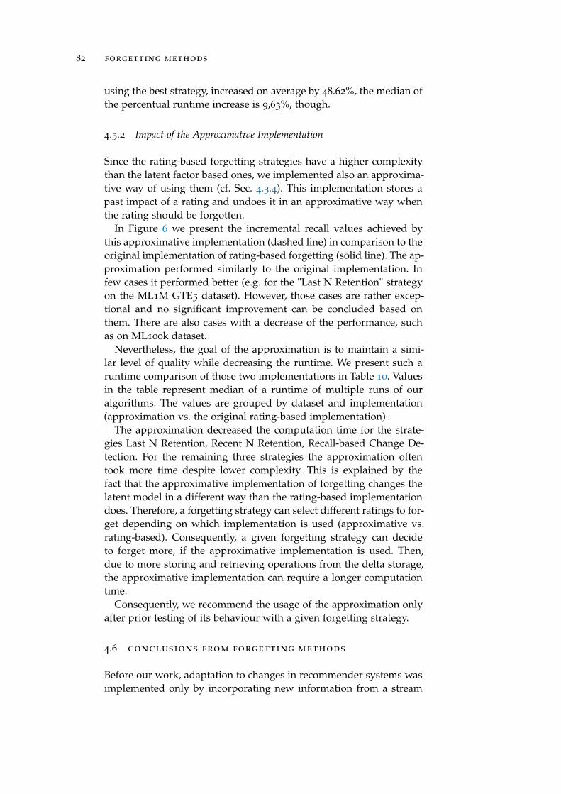
82 forgetting methods
using the best strategy, increased on average by 48.62%, the median ofthe percentual runtime increase is 9,63%, though.
4.5.2 Impact of the Approximative Implementation
Since the rating-based forgetting strategies have a higher complexitythan the latent factor based ones, we implemented also an approxima-tive way of using them (cf. Sec. 4.3.4). This implementation stores apast impact of a rating and undoes it in an approximative way whenthe rating should be forgotten.
In Figure 6 we present the incremental recall values achieved bythis approximative implementation (dashed line) in comparison to theoriginal implementation of rating-based forgetting (solid line). The ap-proximation performed similarly to the original implementation. Infew cases it performed better (e.g. for the "Last N Retention" strategyon the ML1M GTE5 dataset). However, those cases are rather excep-tional and no significant improvement can be concluded based onthem. There are also cases with a decrease of the performance, suchas on ML100k dataset.
Nevertheless, the goal of the approximation is to maintain a simi-lar level of quality while decreasing the runtime. We present such aruntime comparison of those two implementations in Table 10. Valuesin the table represent median of a runtime of multiple runs of ouralgorithms. The values are grouped by dataset and implementation(approximation vs. the original rating-based implementation).
The approximation decreased the computation time for the strate-gies Last N Retention, Recent N Retention, Recall-based Change De-tection. For the remaining three strategies the approximation oftentook more time despite lower complexity. This is explained by thefact that the approximative implementation of forgetting changes thelatent model in a different way than the rating-based implementationdoes. Therefore, a forgetting strategy can select different ratings to for-get depending on which implementation is used (approximative vs.rating-based). Consequently, a given forgetting strategy can decideto forget more, if the approximative implementation is used. Then,due to more storing and retrieving operations from the delta storage,the approximative implementation can require a longer computationtime.
Consequently, we recommend the usage of the approximation onlyafter prior testing of its behaviour with a given forgetting strategy.
4.6 conclusions from forgetting methods
Before our work, adaptation to changes in recommender systems wasimplemented only by incorporating new information from a stream

4.6 conclusions from forgetting methods 83
Forgetting Strategy Param.Mean Incr.Recall
AdjustedP-value
Runtime(ms)
Epinions Extended (10k users sample)No Forgetting Strategy 0 0.0005±0.00084 - 160.03±16.1
Recall-based User FactorFading
1010 0.00307±0.00357 0.00879*** 451.89±38.52
SD-based User FactorFading
1.08 0.00219±0.00163 0.00879*** 154.45±11.68
User Factor Fading 0.5 0.00274±0.00297 0.00879*** 152.92±14.87
Forget Unpopular 2 0.00035±0.00057 1 156.5±15.81
Forget Popular 1.00001 0.0005±0.00084 1 161.76±18.74
Last N Retention 10 0.0005±0.00084 1 192.48±24.29
Recent N Retention 4 weeks 0.0005±0.00084 1 2923±601.75
Global Sensitivity-basedForgetting
0.1 0.00052±0.00087 1 148.81±16.9
Sensitivity-based ChangeDetection
0.5 0.00052±0.00087 1 143.67±10.98
Sensitivity-based Forgetting 10 0.00052±0.00087 1 144.04±13.9
Recall-based ChangeDetection
0.05 0.00051±0.00085 1
5857.13±4815.21
ML100kNo Forgetting Strategy 0 0.07336±0.0093 - 3.22±0.39
Recall-based User FactorFading
1010
0.07201±0.0155 1 3.24±0.19
SD-based User FactorFading
1.04 0.08708±0.01319 0.1875 1.72±0.12
User Factor Fading0.99999999
0.07336±0.0093 1 1.63±0.09
Forget Unpopular 1.5 0.08307±0.01151 0.1875 1.8±0.11
Forget Popular 1.00001 0.07039±0.01093 1 1.96±0.28
Last N Retention 10 0.08112±0.00476 0.1875 9.42±0.83
Recent N Retention 1h 0.08186±0.01331 0.1875 70.55±7.59
Global Sensitivity-basedForgetting
0.1 0.07462±0.00901 0.375 3.47±0.39
Sensitivity-based ChangeDetection
0.5 0.07462±0.00901 0.375 3.5±0.3
Sensitivity-based Forgetting 10 0.07462±0.00901 0.375 3.51±0.34
Recall-based ChangeDetection
0.05 0.08185±0.01331 0.1875 72.89±7.98
Table 8.: Results on datasets with explicit rating feedback (Epinions andML100k). Best value of incremental recall is marked in red. Aster-isks indicate that a given strategy is significantly better than theno forgetting strategy (* at 0.1; ** at 0.05; *** at 0.01). Table from[Mat+17]

84 forgetting methods
Forgetting Strategy Param.Mean Incr.Recall
AdjustedP-value
Runtime(ms)
ML1MNo Forgetting Strategy 0 0.10211±0.01104 - 32.41±7.35
Recall-based User FactorFading
1012
0.11249±0.01479 0.10547 63.63±16.63
SD-based User FactorFading
1.1 0.1244±0.01697 0.02051** 33.65±7.07
User Factor Fading 0.99 0.11327±0.01237 0.00586*** 33.41±7.33
Forget Unpopular 1.2 0.14088±0.01014 0.00586*** 37.44±9.3
Forget Popular 1.00001 0.06073±0.01053 1 37.52±8.69
Last N Retention 10 0.10679±0.01115 0.00586*** 64.18±3.56
Recent N Retention 1 week 0.10585±0.01056 0.00782*** 939.05±103.08
Global Sensitivity-basedForgetting
0.1 0.1041±0.01153 0.01172** 25.88±2.03
Sensitivity-based ChangeDetection
0.5 0.10412±0.01154 0.01172** 25.95±2.19
Sensitivity-based Forgetting 10 0.10408±0.01151 0.01172** 25.81±2.07
Recall-based ChangeDetection
0.05 0.10585±0.01056 0.00782*** 951.31±107.55
Netflix (10k users sample)No Forgetting Strategy 0 0.15455±0.0165 - 38.24±9.32
Recall-based User FactorFading
1010
0.16687±0.02184 0.64063 73.58±13.47
SD-based User FactorFading
1.02 0.18644±0.01707 0.00977*** 39.67±9.25
User Factor Fading 0.99 0.17442±0.0163 0.00977*** 38.16±7.61
Forget Unpopular 1.1 0.18341±0.01988 0.06153* 47.64±7.61
Forget Popular 1.00001 0.08305±0.0129 1 47.2±7.93
Last N Retention 5 0.1454±0.01463 1 78.61±12.89
Recent N Retention 1 year 0.14521±0.0125 1 1446.4±342.16
Global Sensitivity-basedForgetting
0.5 0.14935±0.01454 1 61.86±13.76
Sensitivity-based ChangeDetection
0.5 0.14933±0.01465 1 58.37±10.4
Sensitivity-based Forgetting 3 0.14942±0.01439 1 59.43±11.4
Recall-based ChangeDetection
0.05 0.14521±0.01251 1
1508.71±333.19
Table 9.: Results on datasets with explicit rating feedback (ML1M and Net-flix). Best value of incremental recall is marked in red. Asterisksindicate that a given strategy is significantly better than the no for-getting strategy (* at 0.1; ** at 0.05; *** at 0.01). Table from [Mat+17]

4.6 conclusions from forgetting methods 85
Forgetting Strategy Approx. Rating-based
Approx. Rating-based
Epinions (10k users) Lastfm 600k
Last N Retention 106.22 185.60 74.74 91.48
Recent N Retention 235.61 3068.94 91.59 86.51
Global Sensitivity-basedForgetting
381.59 142.08 198.23 56.16
Sensitivity-basedChange Detection
439.96 142.07 211.40 59.68
Sensitivity-basedForgetting
387.46 143.43 208.36 58.69
Recall-based ChangeDetection
375.18 3352.39 128.50 1255.23
ML100k ML1M
Last N Retention 2.27 23 621.00 16.99 65.18
Recent N Retention 2.52 69.52 35.37 948.10
Global Sensitivity-basedForgetting
4.16 16 497.00 64.84 26.33
Sensitivity-basedChange Detection
3.87 16 862.00 60.44 26.73
Sensitivity-basedForgetting
3.63 23 802.00 55.35 26.52
Recall-based ChangeDetection
4.30 72.60 46.72 955.87
ML1M GTE5 Music-listen
Last N Retention 9.41 42 627.00 49.13 100.29
Recent N Retention 9.22 45.27 51.63 187.98
Global Sensitivity-basedForgetting
9.66 33 909.00 47.86 35.11
Sensitivity-basedChange Detection
10.22 42 411.00 55.00 36.17
Sensitivity-basedForgetting
9.58 34 608.00 55.75 35.06
Recall-based ChangeDetection
8.85 47.31 51.55 225.22
Music-Playlist Netflix (10k users)
Last N Retention 3.61 43 405.00 63.72 77.04
Recent N Retention 3.82 42 571.00 81.58 1299.18
Global Sensitivity-basedForgetting
4.84 44 287.00 156.48 62.35
Sensitivity-basedChange Detection
4.57 30 376.00 161.85 59.99
Sensitivity-basedForgetting
3.79 42 404.00 158.41 61.00
Recall-based ChangeDetection
3.40 19.22 153.33 1327.40
Table 10.: Median runtime (in seconds) of the approximative and rating-based implementation of forgetting (table from [Mat+17]).

86 forgetting methods
● ●●
● ● ● ● ● ● ● ● ● ●●
●
●
●
● ● ● ●
●
●
● ●● ● ● ●
Epinions Extended (10k users sample)
ML100k
ML1M GTE5
Music−Playlist
0.00000.00050.00100.00150.0020
0.06
0.07
0.08
0.09
0.10
0.03
0.04
0.05
0.020.030.040.050.06
●
●
●
●
●
●
●
● ● ● ●● ● ●● ● ●● ●
Lastfm 600k
ML1M
Music−listen
Netflix (10k users sample)
0.010
0.015
0.020
0.025
0.080.090.100.110.12
0.050
0.075
0.100
0.12
0.14
0.16
0.18
Forgetting Strategy
Incr
emen
tal R
ecal
l
ImplementationApproximationRating−based Forgetting
Forgetting StrategyLast N RetentionRecent N RetentionGlobal Sensitivity−based ForgettingSensitivity−based Change DetectionSensitivity−based ForgettingRecall−based Change Detection
Figure 6.: Incremental recall of approximative rating-based forgetting is sim-ilar to the non-approximative variant (figure from [Mat+17]).
into a preference model. While this is a valid method of adaptation, itis not sufficient. In this chapter, we have shown that forgetting obso-lete information (additionally to incorporating new one) significantlyimproves predictive power of recommender systems. Therefore we an-swer our research question RQ 1 positively, as we have shown that thefollowing expression from Ch. 3 is true:
∃(M, S) :∑
t
QS ,t(Tet, Mt, S t) >∑
t
Qt(Tet, M∗t ) (48)
for Q being incremental recall. In our statistical tests we comparedaverage incremental recall with forgetting (left side of the inequality)and without forgetting (right side of the inequality). As the time a rec-ommender system observes is discrete, the average incremental recallover time is proportionate to its sum.

4.6 conclusions from forgetting methods 87
To answer the RQ 1.1, we proposed eleven unsupervised strategiesto select the obsolete information and three algorithms to enforceforgetting. In our experiments we used a state-of-the-art incremen-tal matrix factorization algorithm, BRISMF [Tak+09], and extended itby the ability to forget information and to add new dimensions tothe matrix. Our forgetting strategies can be applied to any matrixfactorization algorithm. Rating-based strategies are also applicable toneighbourhood-based methods.
Further, we proposed a new evaluation approach that includes sig-nificance testing. We conducted more than 1040 experiments on eightreal world datasets with explicit rating feedback and positive onlyfeedback. On seven out of eight of those datasets we observed a sig-nificantly better performance when using forgetting. On five of them theimprovement was significant at level better than 0.01.
From all our forgetting strategies, the latent factor based ones wereparticularly successful in terms of quality of recommendations and interms of computation time. On five out of eight datasets the SD-basedUser Factor Fading strategy achieved the best result, followed by theForget Unpopular strategy with best result on two out of eight datasets.Therefore, we answer the RQ 1.1 about how to select information tobe forgotten with those two forgetting strategies.
Rating-based forgetting strategies also showed significant improve-ments over the "No Forgetting" strategy, however, their improvementwas not as high, as in the case of latent-based strategies. We remarkthat not all of the forgetting strategies achieved a significant improve-ment. The strategy that achieved highly significant improvement onthe most datasets (6 out of 8) is the SD-based user factor fading strategy.
Rating-based forgetting strategies have higher complexity and, there-fore, a higher runtime than latent factor based strategies. Therefore,we proposed an approximative implementation that maintains a sim-ilar level of incremental recall as the original, rating-based implemen-tation. For half of the strategies it reduced the computation time con-siderably. For the other half the computation often took longer. There-fore, we recommend to use this approximation only in time-criticalapplications and after prior testing.
Our recommendation to practitioners is to, first, use the latent factorbased forgetting strategies (e.g. the SD-based user factor fading strategy)due to their outstanding performance in terms of incremental recalland only slightly increased computation time. This also answers ourresearch question RQ 1.2 about how to implement forgetting in rec-ommender systems (cf. Alg. 6). The rating-based implementation for-getting is the next best alternative.
In the next chapter we address our research questions related toanother form of selective learning - selective neighbourhood.


5S E L E C T I V E N E I G H B O U R H O O D
In this chapter we demonstrate that selective learning methods arealso applicable in neighbourhood-based collaborative filtering and weanswer the following two research questions:
RQ 2: Does selective removal of users from a neighbourhoodimprove the quality of neighbourhood-based CF?
RQ 2.1: How to select users to be removed from a neighbour-hood?
As motivated in Sec. 1.1.2, we propose a method for selecting re-liable users in a neighbourhood of an active user and evaluate itseffect onto the quality of recommendations. In Sec. 5.1 we discuss re-lated work on selective neighbourhood. In Sec. 5.2 we introduce ourmethod, which is evaluated in Sec. A.5. We conclude the chapter onselctive neighbourhood in Sec. 5.4, where we also give answers to theabove research questions. Sections 5.1 - 5.4 come (with modifications)from our publication on this topic [MS14a].
5.1 related work on reliable neighbourhood
Neighbourhood-based collaborative filtering has been studied thor-oughly in numerous publications (cf. studies on the most importantaspects of them [DK11; Lü+12; Bob+13; Bee+16] and Ch. 2 for moredetails). In the existing work much emphasis is put on the predictivequality of a recommender’s output. However, only little work focuseson selecting reliable neighbours. Reliability of neighbours should notbe confused with the reliability of conclusions made about recom-mender systems, in the process of evaluation using hypothesis testing,as described in [SG11]. In contrast to statistical testing in the evalua-tion that aims to measure the significance of results, we investigatethe significance of users’ neighbourhood.
Herlocker et al. noticed that user similarity based on few co-ratingsis unreliable [Her+99] (cf. example 5 in Ch. 1). Researchers have al-ready proposed solutions to this problem, such as thresholds on thenumber of ratings two users should share to be considered similar, orassigning lower weights to users that have too few ratings in common[Her+99; BKV07; MKL07].
Herlocker et al. introduced the term of significance weighting [Her+99].They recognized that similarity based on only few co-ratings is notrepresentative and the amount of trust in this value should be lim-
89

90 selective neighbourhood
ited. To limit the influence of those unreliable similarity values theyweight them with a term min(n,γ)
γ , where n is the number of co-ratingsand γ a control parameter that is fit to data (usually around 50). If nis greater than γ, then the weight is set to 1. Otherwise, the weightis always lower than 1, which gives lower importance to users withfewer co-ratings than γ.
Ma et al. use a similar but adjusted weighting schema [MKL07]. Bellet al. also define a different weighting schema, which they call "shrink-age" [BKV07]. They shrink the similarities towards zero to an extentthat is inversely proportional to the number of co-ratings. The fewerco-ratings between users exist, the less influence does the particularsimilarity value have on the predicted rating value. Formally, they alsouse an additional weighting that is derived using the following term
nn+β . n is again the number of co-ratings and β is a control parameter,which is also fit to the data.
However, none of these methods answers the question "how manyco-ratings are enough?", nor addresses the more important underly-ing question "whose co-ratings are useful enough?". They are basedonly on the number of co-ratings. We formalize the latter questionand proposed a criterion for selecting neighbours. Instead of usingweights, we can decide whether a similarity between two users can berelied upon. We stress that our method is not a solution to the coldstart problem, where no enough information about users is known.Our goal is to quantify the reliability of the known information.
In our approach, we first formalize the concept of baseline user – in-formally, an average user for the population under observation. Then,we introduce the concept of reliable similarity: we use the HoeffdingBound (HB), derived from Hoeffding’s Inequality [Hoe63] to testwhether a given user is more similar to the active user than the base-line user is. We then consider neighbours to the active user only thoseusers whose similarity to the active user satisfies the bound. Hence,the recommender system decides on statistical grounds whether itcan make a recommendation on neighbourhood-based similarity, nomatter how small this neighbourhood is.
5.2 reliable neighbourhood
Our approach consists of a formal model on reliable similarity of a user,an adjusted CF-based recommendation method and a mechanism thatbuilds a user’s neighbourhood by only considering users that are trulysimilar to the active user and ignoring all other users. We concentrateon user-user collaborative filtering, but our approach can be used foritem-item CF analogously.

5.2 reliable neighbourhood 91
5.2.1 Baseline Users
To compute the neighborhood of the active user ua, for whom recom-mendations must be formulated, we first introduce the notion of a"baseline user" uB – a default, fictive user. Informally, a user x is re-liably similar to ua, if ua is more similar to x than to uB; then, theneighbourhood of ua consists of the users who are reliably similar toher. Formally, uB is a vector:
uB = [ir1, ir2, ..., irn−1, irn] (49)
where ir j is a rating of the item j and n is the total number of items.We consider three types of baseline users: the average user, the randomGaussian user and the random uniform user. For the computation of thebaseline users, we use an initial sample of ratings Rtrain for training.
average user : This baseline is computed by defining ir j for anitem j as the average rating of j in Rtrain:
ir j =1
|U( j)|
∑x∈U( j)
rx, j (50)
where rx, j ∈ Rtrain is the rating of user x for item j and U( j) = {x|rx, j ∈Rtrain} is the set of users who rated j.
random gaussian user : Each item j in this baseline is assumedto follow the normal distribution with parameters µ and σ approxi-mated on Rtrain. The value of ir j for any j is drawn from this distribu-tion:
ir j ∼ N(µ,σ2) (51)
random uniform user : Each item j in this baseline follows thediscrete uniform distribution with rmin and rmax being the extreme rat-ing values. Hence:
ir j ∼ U{rmin, ..., rmax} (52)
For example, if a rating can assume values between one and five stars,then rmin = 1 and rmax = 5.
We use the term of a baseline user to define the concept of reliablesimilarity, which is based on the Hoeffding Bound (HB).
5.2.2 Reliable Similarity between Users
To define reliable similarity, we begin with an arbitrary similarity func-tion sim(). We will specify sim() explicitly later.

92 selective neighbourhood
Definition 1 (Reliable similarity). Let sim() be a similarity function, andlet uB be the baseline user learned on Rtrain. We define the "reliable similarity"simrel between a user ua , for whom recommendations must be formulated,and an arbitrary other user ux as
simrel(ua, uB, ux) =
sim(ua, ux) , if sim(ua, ux)� sim(ua, uB)
0 , otherwise(53)
where we use the symbol� for "significantly greater than". User ux is "reli-ably similar" to ua if simrel(ua, uB, ux) > 0.
5.2.2.1 Testing significance.
We implement the "significantly greater than"-test of Def. 1 with helpof the Hoeffding Inequality [Hoe63]:
Pr(X − X > ε) 6 exp(−2nε2
R2) (54)
The Hoeffding Inequality quantifies the probability that the devia-tion of an observed average X from the real average X of a randomvariable X is greater than or equal to ε. It takes the range R of therandom variable and the number of observed instances n as inputs.The Hoeffding Inequality is independent of any probability distribu-tion, however, it is thereby more conservative than other distribution-specific bounds [DH00]. The inequality can be transformed into theHoeffding Bound that specifies the maximal allowed deviation ε givena confidence level of 1− δ:
X − X < ε , where ε =
√R2 · ln(1/δ)
2n(55)
We apply the Hoeffding Bound to ensure that the true similarity be-tween two users is inside the ε-vicinity of the observed similarity. Inparticular, let u1, u2 be two users. Then, X stands for the observed dif-ference in similarity between them and X stands for the difference oftheir true similarities, thereby demanding that the similarity functionis an average, as dictated in [Hoe63].
Definition 2 (Similarity Function for Significance Testing). Let u1, u2be two users and let Ico-rated(u1, u2) be the set of items that both have rated.Then, the similarity between u1, u2 is the following average (for a rating scalebetween 0 and 1, otherwise normalization is required):
sim(u1, u2) = 1−
∑j∈Ico-rated(u1,u2)
|ru1 j − ru2 j|
|Ico-rated(u1, u2)|(56)
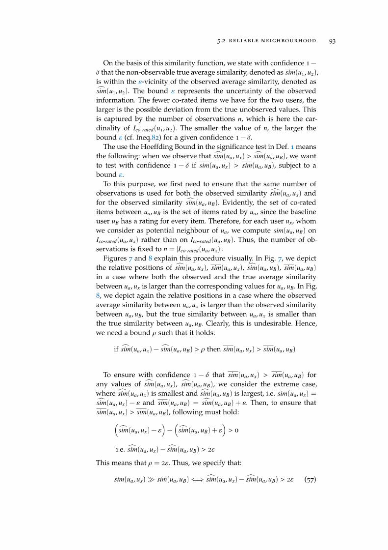
5.2 reliable neighbourhood 93
On the basis of this similarity function, we state with confidence 1−δ that the non-observable true average similarity, denoted as sim(u1, u2),is within the ε-vicinity of the observed average similarity, denoted assim(u1, u2). The bound ε represents the uncertainty of the observedinformation. The fewer co-rated items we have for the two users, thelarger is the possible deviation from the true unobserved values. Thisis captured by the number of observations n, which is here the car-dinality of Ico-rated(u1, u2). The smaller the value of n, the larger thebound ε (cf. Ineq.82) for a given confidence 1− δ.
The use the Hoeffding Bound in the significance test in Def. 1 meansthe following: when we observe that sim(ua, ux) > sim(ua, uB), we wantto test with confidence 1 − δ if sim(ua, ux) > sim(ua, uB), subject to abound ε.
To this purpose, we first need to ensure that the same number ofobservations is used for both the observed similarity sim(ua, ux) andfor the observed similarity sim(ua, uB). Evidently, the set of co-rateditems between ua, uB is the set of items rated by ua, since the baselineuser uB has a rating for every item. Therefore, for each user ux, whomwe consider as potential neighbour of ua, we compute sim(ua, uB) onIco-rated(ua, ux) rather than on Ico-rated(ua, uB). Thus, the number of ob-servations is fixed to n = |Ico-rated(ua, ux)|.
Figures 7 and 8 explain this procedure visually. In Fig. 7, we depictthe relative positions of sim(ua, ux), sim(ua, ux), sim(ua, uB), sim(ua, uB)
in a case where both the observed and the true average similaritybetween ua, ux is larger than the corresponding values for ua, uB. In Fig.8, we depict again the relative positions in a case where the observedaverage similarity between ua, ux is larger than the observed similaritybetween ua, uB, but the true similarity between ua, ux is smaller thanthe true similarity between ua, uB. Clearly, this is undesirable. Hence,we need a bound ρ such that it holds:
if sim(ua, ux) − sim(ua, uB) > ρ then sim(ua, ux) > sim(ua, uB)
To ensure with confidence 1 − δ that sim(ua, ux) > sim(ua, uB) forany values of sim(ua, ux), sim(ua, uB), we consider the extreme case,where sim(ua, ux) is smallest and sim(ua, uB) is largest, i.e. sim(ua, ux) =
sim(ua, ux) − ε and sim(ua, uB) = sim(ua, uB) + ε. Then, to ensure thatsim(ua, ux) > sim(ua, uB), following must hold:(
sim(ua, ux) − ε)−(
sim(ua, uB) + ε)> 0
i.e. sim(ua, ux) − sim(ua, uB) > 2ε
This means that ρ = 2ε. Thus, we specify that:
sim(ua, ux)� sim(ua, uB)⇐⇒ sim(ua, ux) − sim(ua, uB) > 2ε (57)

94 selective neighbourhood
sim(uA ,uB) sim(uA , uB)
sim (uA , )sim(uA ,ux) ux
ε ε
ε ε
Figure 7.: Relative positions of the observed similarity between ua, ux andbetween ua, uB and true similarity within the ε-vicinity of the cor-responding observed similarity; the observed similarities allow theconclusion that the true similarity between ua, ux is larger than thetrue similarity between ua, uB (figure from [MS14a]).
sim(uA ,uB) sim(uA ,uB)
sim (uA ,ux)sim(uA ,ux)
ε ε
ε ε
Figure 8.: Unlike in Fig. 7, the observed similarities, here, would lead to anerroneous conclusion, since their ε-regions overlap (figure from[MS14a]).
Due to our application of the Hoeffding Bound in recommendersystems, which was inspired by numerous algorithms from the streammining domain, we noticed that many algorithms in this domain usea border of only one ε for deciding between two means. Furthermore,more prerequisites for the application of the Hoeffding Bound areoften not fulfilled. We investigated this problem and its effects in ourwork [MKS13]. We describe it in more detail in the Appendix A.
Definition 3 (Reliable Neighbourhood). Let ua be an active user. Subjectto Def. 1, the similarity function of Eq. 56 and the two invocations of theHoeffding Bound, we define her reliable neighbourhood as:
relNeighbourhood(ua, θ) = {ux ∈ U |simrel(ua, uB, ux) > θ} (58)
where U is a set of users and the similarity threshold θ is applied on reli-able neighbours only. All unreliable neighbours are excluded, even if theirsimilarity to ua is larger than θ.

5.3 experiments 95
5.2.3 Algorithms
Algorithms 8 and 9 show a pseudocode of our extensions to collabora-tive filtering. Algorithm 8 computes a neighbourhood of an activeuser ua using our method of checking the reliability of neighboursisReliableNeighbour, presented in Algorithm 9.
These algorithms require two hyperparameters: θ is a similaritythreshold, also used in conventional CF, and δ that controls the confi-dence of the Hoeffding Bound used for checking the reliability. Sincethe criterion of the reliable similarity is much stricter than the conven-tional similarity, it can happen that no neighbours for an active usercan be found at all. For this case we also adjusted the conventionalCF algorithm. Our method can either abstain from recommendingany items until more information about the given user is collected,or it provides non-personal recommendations e.g. the most popularitems from the trainings dataset. We state that it is beneficial to makefewer, but reliable recommendations, than to recommend items thatwill cause a negative attitude or a distrust of users towards the recom-mender system.
5.3 experiments
We evaluate our method on the datasets MovieLens (100k), Flixter,Netflix and Epinions [MA06], comparing it to: a conventional user-based collaborative filtering recommender with cosine similarity, de-noted as CF, to the method by Bell et al. called shrinkage[BKV07] andto significance weighting by Herlocker et al.[Her+99]. Since our goal isto compare different ways of building a neighbourhood, we imple-mented only the weighting schemas from the methods described in[BKV07] and [Her+99] and coupled them with the conventional CFalgorithm. To ensure a fair comparison, all methods use the same coreCF algorithm with no further extensions, so that only the way theybuild and weight their neighbourhoods differs.
We name our method Hoeffding-CF, abbreviated hereafter as H-CF.We consider one variant of our method per type of baseline user, de-noted as H-CF_Gauss (Gaussian user), H-CF_Uniform (uniform user)and H-CF_Avg (average user). To optimise the parameters of the meth-ods we run multiple experiments using a grid search over the pa-rameter space. Since the number of experiments in the grid search ishigh, we chose a sample of users per dataset, taking over all their rat-ings. The evaluation settings are detailed below. Further informationregarding datasets and our samples is summarized in Table 11.

96 selective neighbourhood
Algorithm 8 Reliable CF
Input: θ similarity thresholdδ confidence in the Hoeffding Boundua the active userU set of usersRtrain training set
reliableNeighbourhood(ua)← {}
uB ← initializeBaseline(Rtrain, baseline_type)for all {ux ∈ U |ux 6= ua} do
ux reliable← isReliable(ua, uB, ux, δ, θ)if ux reliable then
reliableNeighbourhood(ua).add(ux)end if
end forif reliableNeighbourhood(uA) == ∅ then
abstain or recommend most popular itemselse
for all item i ∈ missingValues(ua) dorua,i =weightedAverage(reliableNeighbourhood(ua))ranking.add(rua,i)
end forranking.sort()return top ranked items
end if
Algorithm 9 isReliable(ua, uB, ux, δ, θ)
Input: ua active useruB baseline userua any other userδ confidence in the Hoeffding Boundθ similarity threshold
ux_reliable← trueif sim(ua, ux) 6 θ then
ux_reliable← falseend ifε← computeHoeffdingBound(δ, Range, numberCoRatings(ua, ux))(cf. Ineq. 82 and Eq. 58)if sim(ua, ux) − sim(ua, uB) 6 2ε then
ux_reliable← falseend ifreturn ux_reliable

5.3 experiments 97
Dataset total Ratings sampled ratings
Flixter 572531 59560
MovieLens 100k 100k 100k (no sampling)
Netflix 100 M 216329
Epinions 550823 165578
Table 11.: Samples of users on four datasets used in experiments (table from[MS14a]).
5.3.1 Evaluation Settings
As basis for our evaluation we use (a) the Root Mean Square Er-ror (RMSE) of the predictions made by each method, and (b) the num-ber of cases where the method encounters an empty neighbourhoodand cannot make a neighbourhood-based prediction; this is denotedas Missing Predictions. However, a prediction is still provided usinga fallback-strategy explained later. We further compute the AverageNeighbourhood Size, the average size of non-empty neighbourhoodsbuilt by each method.
It is evident that the RMSE values for the three variants of our methodare not directly comparable, because the value of Missing Predictionsvaries among the methods. Hence, we refine RMSE into following mea-sures:
• Neighbourhood-based RMSE: the RMSE of the predictions made us-ing the neighbourhoods of the users; limited to users with non-empty neighbourhoods (abbreviated hereafter as CF-RMSE)
• Fallback-strategy RMSE: the RMSE of the predictions made usingthe fallback strategy; limited to users with empty neighbour-hoods
• Global RMSE: total RMSE by both Neighbourhood-based RMSE andFallback-strategy RMSE
As fallback strategy we use the recommendation of the most popu-lar items not rated by the active user. The impact of this strategy isencapsulated in Fallback-strategy RMSE.
For the variants of our method, we vary δ: the lower the value, themore restrictive is the confidence level of the Hoeffding Inequality andthe less users are considered reliably similar to a given user. Hence, weexpect that a decrease of δ will negatively affect the Average Neighbour-hood Size and the Missing Predictions. For shrinkage and significanceweighting we also optimize β and γ.

98 selective neighbourhood
We further consider different similarity threshold values. Setting thethreshold to a high value is not adequate for prohibiting recommen-dations on the basis of unreliable neighbourhoods. It must be notedthat the CF may also fail to build neighbourhoods for some users,if the threshold is set very restrictively. In total, we performed morethan 250 experiments, all of which were evaluated using 5-fold crossvalidation.
5.3.2 Results
In Tables 12 and 13, we present our results on each of the four datasets.For each of the methods we present only the best value found by thegrid search in course of the optimization. The symbol "— " indicatesthat there are no applicable values for this position (e.g. δ is not appli-cable for the CF). The sizes of the neighbourhood in Tables 12 and 13
is seemingly high, however, these are the values found as approxima-tively optimal by the grid search.
The best result on on the Movie Lens 100k dataset was achieved byour method (1st row in the Table) with a setting of δ = 0.999, a uniformbaseline user, and distance threshold of 0.25. The best value of globalRMSE was 0.9864. The best result achieved by the conventional CF was1.0207 (5th row in the table). This is a stable improvement verifiedusing the 5-fold cross validation. Shrinkage and significance weight-ing yielded a result close to the conventional CF. When we compareour method with e.g. shrinkage with respect to the average neighbour-hood size (row 1 and 3), then we notice an essential reduction fromca. 898 to 447 users. This means that our method reduced the neigh-bourhoods by 451 users on average and still performed better thanthe conventional CF. Regarding the baseline users on the Movie Lensdataset, the best results were achieved by the uniform random base-line. The average user baseline led to small neighbourhoods. This canbe explained by the fact that many users in the MovieLens datasetare similar to the average user. Using this baseline makes the differ-ences between user vectors insignificant and, consequently, many ofthe users are not considered as reliable neighbours to the active user.
If no reliable neighbours of an active user can be found, then is notpossible to estimate the rating. We counted the occurrences of thiscase in our method (column "missing predictions"). In this situationa fallback-strategy (e.g. popular items) takes over the task of provid-ing a recommendation (prediction error is included in global RMSE).We observed that those cases become more frequent when δ is low.This causes a more extensive pruning behaviour of our method, be-cause more neighbourhoods are considered unreliable. If we allow ourmethod to abstain from recommendation instead of using the fallback-strategy the improvement of RMSE is even higher (0.9683; row 1, col-

5.3 experiments 99
Row
Met
hod
Dis
tanc
eT
hres
hold
Sett
ing
Mis
sing
Pred
icti
ons
avgN
eigh
-bo
rhoo
dSiz
egl
obal
RM
SEC
F-R
MSE
fallb
ack-
RM
SE
Mov
ieLe
ns10
0k
1H
-CF_
Uni
form
0.2
5δ=0.999
2905
447
0.9
864
0.9
683
1.4
929
2H
-CF_
Gau
ss0.2
5δ=0.95
3229
259.5
50.9
875
0.9
684
1.4
693
3Sh
rink
age
0.2
β=500
215
898.0
81.0
192
1.0
192
—
4Si
g.W
eigh
ting
0.2
γ=200
215
898.0
81.0
192
1.0
192
—
5C
F0.2
—215
898.0
81.0
207
1.0
207
—
6H
-CF_
Avg
0.4
δ=0.999
13079
132.3
81.0
321
1.0
390
0.9
839
Flix
ter
(sam
ple
of1000
user
s)
7H
-CF_
Gau
ss0.8
δ=0.95
7047
78.1
41.0
149
1.0
133
1.0
381
8H
-CF_
Avg
0.8
δ=0.95
49918
5.8
41.0
221
1.1
355
0.9
969
9H
-CF_
Uni
form
0.4
δ=0.95
4357
241.3
580
1.0
549
1.0
532
1.1
576
10
CF
0.7
—3998
442.7
564
1.0
856
1.0
856
—
11
Shri
nkag
e0.7
β=50
3998
442.7
564
1.0
872
1.0
872
—
12
Sig.
Wei
ghti
ng0.7
γ=50
3998
442.7
564
1.0
889
1.0
889
—
Tabl
e1
2.:
Res
ults
onM
l100k
and
Flix
ter
data
sets
sort
edw
ith
resp
ect
togl
obal
RM
SE(l
ower
valu
esar
ebe
tter
),gr
oupe
dby
the
data
set
(tab
lefr
om[M
S14a]
).

100 selective neighbourhood
Row
Method
Distance
ThresholdSetting
Missing
PredictionsavgN
eigh-borhoodSize
globalR
MSE
CF-
RM
SEfallback-R
MSE
Netflix
(sample
of1000
users)
13
H-C
F_Gauss
0.2
δ=0.9
513601
199.
66
0.9619
0.9511
1.1551
14
H-C
F_Uniform
0.2
δ=0.9
511171
382.
74
0.9622
0.9529
1.1849
15
H-C
F_Avg
0.2
δ=0.9
99
60394
96.
94
1.0075
1.0225
0.9669
16
Shrinkage0.
2β=200
4023
916.
2519
1.0210
1.0210
—
17
Sig.Weighting
0.2
γ=100
4023
916.
2519
1.0214
1.0214
—
18
CF
0.2
—4023
916.
2519
1.0233
1.0233
—
Epinions(sam
pleof
10
000
users)
19
H-C
F_Avg
0.3
δ=0.5
165578
01.
0074
—1.
0074
20
H-C
F_Gauss
0.8
δ=0.5
164948
0.2770
1.01100
1.3964
1.0106
21
H-C
F_Uniform
0.4
δ=0.5
159842
1.5113
1.0279
1.3215
1.0109
22
CF
0.7
—113117
461.
39
1.2843
1.2843
—
23
Shrinkage0.
7β=50
113117
461.
39
1.2894
1.2894
—
24
Sig.Weighting
0.7
γ=100
113117
461.
39
1.2907
1.2907
—
Table1
3.:Results
onN
etflixand
Epinionsdatasets
sortedw
ithrespectto
globalR
MSE
(lower
valuesare
better),groupedby
thedataset
(tablefrom
[MS
14a]).

5.3 experiments 101
umn CF-RMSE). Also the conventional CF, shrinkage and significanceweighting exhibit some missing predictions. They are caused by eithernew users or new items that are not known from the training dataset.
We performed similar experiments on a random sample of 1000
users on the Flixter dataset. Also on this dataset our method achievedthe best globalRMSE value of 1.0149 this time using a Gaussian base-line. The conventional CF (row 10) yielded a value of 1.0856 usingneighbourhoods bigger by 365 users on average. Shrinkage and signif-icance weighting were not able to outperform CF.
Also on a random sample of 1000 users from the Netflix datasetour method outperformed other approaches with respect to globalRMSE, reaching the level of 0.9619 using the Gaussian user baseline.When abstention was allowed, the improvement was even more sub-stantial and reached the level of 0.9511, compared to e.g. shrinkagewith 1.0210 (row 16). Again here, we observed an essential reduc-tion of the neighbourhood cardinality from ca. 916 by the shrinkagemethod down to ca. 200 by our approach. This proves that our ap-proach selects the reliable neighbours, who are more informative forthe preferences of an active user than the competitive methods.
The last dataset we performed our experiments on is the (small)Epinions dataset (cf. Table 13). Here our method clearly dominated theconventional CF. Hoeffding-CF achieved an RMSE of 1.0074 comparedto 1.2843 by the conventional CF. Significance weighting and shrink-age performed worse than CF. Our approach recognized unreliableneighbourhoods and switched from the neighbourhood-based recom-mendation to the fallback-strategy that performs better on this dataset(cf. the columns CF-RMSE and fallback-RMSE). The average numberof neighbours in the first row shows that the neighbourhood was lim-ited to the minimum and this yielded the best result. Differently thanon the other datasets, here the average user baseline performed thebest. The statement about its strictness in the significance testing stillholds. This very strictness was beneficial on this dataset. In row 19
we see that the neighbourhood was reduced to 0 i.e. there was noneighbourhood-based recommendations. All recommendations wereprovided by the fallback-strategy that, in this case, performed better.
5.3.3 Summary of Findings
Our experiments show that Hoeffding-CF is capable of recognizingunreliable neighbourhoods and selecting neighbours that are informa-tive for the preferences of an active user. It outperformed the conven-tional collaborative filtering, shrinkage and significance weighting onall datasets. When abstention from providing recommendations wasallowed, the improvement in terms of RMSE was often even more sub-stantial. All of the best results were achieved using a smaller neigh-

102 selective neighbourhood
0.9
1.0
1.1
1.2
1.3
Epinions Flixter ML100k NetflixDataset
glob
al R
MS
EMethod
Hoeffding−CFShrinkageSignificance WeightingCF
Figure 9.: Best results achieved by each method. Lower values of globalRMSE are better. Our method, Hoeffding-CF, achieves best resultson each dataset (figure from [MS14a]).
bourhood than in case of conventional CF and remaining approaches.A summary of the best results by each method is presented in Fig. 9.
We also observed that the parameter δ plays an important role infinding the optimal results. The lower its value, the stricter is thetesting of the neighbourhood and the smaller is the average neigh-bourhood. Consequently, the number of predictions provided by thebaseline method rises. The optimal value of δ varies across differentdataset around 0.95. Cross-validation can be used for tuning on eachdataset.
The choice of the baseline user has also an effect on the performance.We observed that the random-based user (Gaussian and uniform base-line) perform better than the average user baseline on most datasets.The reason for that is that many users are similar to the average user,so it is difficult to identify a user that is significantly more similar to agiven user than the average. Hence, when the average user is the base-line, each user has only a few significant neighbours. On the Epinionsdataset, however, this led to an improvement of accuracy.
5.4 conclusions from selective neighbourhood
We investigated the problem of neighbourhood-based recommenda-tions when the similarity between users cannot be fully trusted. Thisproblem does not emanate solely from data sparsity: even users withmany ratings may be uninformative. We introduced the concepts ofbaseline user and of reliable similarity, and we use the Hoeffding Boundto select, for a given active user, those users who are informative, ig-noring users that do not contribute more information than the base-line user.

5.4 conclusions from selective neighbourhood 103
Experiments on real datasets show that the use of reliable similar-ity improves recommendation quality. Our method outperforms theconventional CF, shrinkage and significance weighting on all datasets.However, the superior performance on the forth dataset is mainlyowed to a good performance of the fallback-strategy rather than toneighbourhood-based recommendations. Our method outperforms otherapproaches despite using smaller neighbourhoods. This means thatthe reliability, rather than the size of a neighbourhood is decisive forgood predictions.
By proposing our selective criterion for excluding of neighboursfrom a neighbourhood we answer the RQ 2.1. Our experimental re-sults show that removing selected neighbours from a neighbourhoodimproves the predictive performance of CF algorithms. Therefore, weanswer the RQ 2 positively.


6S E M I - S U P E RV I S E D L E A R N I N G
In this chapter we address the third type of selective learning for rec-ommender systems - semi-supervised learning. Our SSL frameworklearns from selected unlabelled data instances as motivated in Sec.1.1.3. Furthermore, we answer the following research questions:
RQ 3: Does selective learning from predictions (semi-supervisedlearning) improve the quality of recommendations?
RQ 3.1: How to select unlabelled instances for SSL?
RQ 3.2: How to select reliable predictions to learn from?
RQ 3.3: How to assemble predictions from an SSL system usingco-training into a single prediction?
RQ 3.4: How to divide labelled instances among multiple learn-ers in an SSL system?
First however, we discuss related work and the differences betweenour approach and existing work. In the following section we presentan overview and components of our framework. Section 6.4 discussesthe evaluation settings used in our experiments. In Sec. 6.5 we presentour experimental results and we conclude this chapter in Sec. 6.6. Sec-tions 6.1 - 6.6 come (with modifications) from our previous publica-tions on this topic [MS17; MS15].
6.1 related work on ssl in recommender systems
SSL has been investigated thoroughly in conventional data miningand machine learning [ZZQ07], also in the stream setting [DCP14;Sou+15]. A comprehensive survey of those techniques can be foundin [Zhu05]. Those techniques encompass both co-training [SNB05]and self-learning techniques [RHS05]. Semi-supervised approachesfor regression problems also have been proposed [ZL07]. However,the problem in recommender systems is inherently different from theconventional classification or regression. In recommender systems anentire matrix of real, binary or positive-only values is predicted. Thismatrix is extremely sparse (typically, around 99% of missing values)and there are no further features for a conventional regressor to trainupon. Therefore, the methods from the conventional SSL are not appli-cable to recommender systems.
Dedicated SSL methods for recommender systems have been re-searched far less. Christakou et al. proposed in 2005 a model-based
105

106 semi-supervised learning
recommender system using the k-means algorithm with SSL [Chr+05].Nevertheless, this is not a dedicated recommender systems method,but clustering applied to the recommendation problem.
To decide which predictions can be used as labels, semi-supervisedmethods use reliability measures. A prediction with high estimated re-liability can be then used for training. Hernando et al. proposed sucha reliability measure, however, they did not use it in semi-supervisedlearning, but presented it to users to indicate certainty of the recom-mendation algorithm [Her+13]. Rodrigues et al. [RGB08] and Bosnicet al. [Bos+14] also proposed reliability measures, however, not for rec-ommender systems, but for classification problems on streams. Never-theless, we adopted their idea of reliability based on local sensitivityand adapted it to recommender systems (cf. Sec. 6.3.5).
Zhang et al. proposed a SSL method for batch-based recommendersystems. In their approach they assess the reliability of a rating pre-diction based on frequency of occurrence of items and users [Zha+14].They assume that popular items and active users are easier to predict,since there is more data about them. We implemented this reliabilitymeasure, that we call hereafter "popularity-based reliability measure",and we compare it to results of other measures. The method by Zhanget al. is batch-based. Once the model is trained, it cannot be changedincrementally. As a consequence, it is also not adaptive to changesand not responsive to new users and items. With our stream-basedframework we lift those limitations.
Preisach et al. proposed a graph-based tag recommender systemthat employs untagged items [PMS10]. In this method the authorsused a semi-supervised relational classification to find relevant tags.Therefore, this method is also not applicable to the typical rating pre-diction task in recommender systems.
Zhu et al. proposed a recommender system for web pages that usesconventional classification with self-learning on natural language data[Zhu+10]. Also this method is not applicable to the general collabora-tive filtering scenario in recommender systems.
6.2 semi-supervised framework for stream recommenders
In this section we present our semi-supervised framework togetherwith its components. We start with an incremental recommendationalgorithm in Sec. 6.2.1 and then explain how it is applied in two alter-native approaches: co-training (cf. Sec. 6.2.2) and self-learning (SL) (cf.Sec. 6.2.3). In Tab. 14 we present a summary of notation and abbrevi-ations used in this work. Fig. 10 gives a simplified overview over theframework components and their interaction.

6.2 semi-supervised framework for stream recommenders 107
Dataset Training Set Splitter
Batch Mode Initial Training
Co-Tr1
Co-Trn
Streaming Mode
Training Stream
Test Stream
Supervised Learning
Unsupervised Learning
Incremental Update of Co-
Trainers
Predictions by all Co-Trainers
PredictionAssembler
Aggregated Prediction Evaluation
...
Unlabelled InstanceSelector
Predictions by Co-
Trainers
Reliability Measure
Reliable Co-Trainers Provide
Labels to Unreliable Ones
Incremental Update
view 1
viewn
UnlabelledInstances
Figure 10.: A simplified overview of the framework visualizing the keycomponents of the framework (in red) and their interplay (from[MS17] with modifications).
6.2.1 Incremental Recommendation Algorithm
The core of our framework is a recommendation system algorithm.Fig. 11 depicts two modes of a stream-based recommendation algo-rithm. The entire rectangle in the figure represents a dataset consistingof ratings. The dataset is split between a batch mode (blue part) and astream mode (yellow part). The stream mode is the main mode of analgorithm, where information about new ratings is incorporated incre-mentally into the model, so that it can be used immediately in the nextprediction. Semi-supervised learning takes place in this phase (greenbars stand for Unsupervised Learning (USL)).
Before the stream mode can start, the algorithm performs an initialtraining in the batch mode. The batch mode data is, therefore, splitagain into training and test set. On the training dataset latent factorsare initialized and trained. The corresponding prediction error is thencalculated on the test dataset (second blue rectangle) and the latentfactors are readjusted iteratively. Once the initial training is finished,the algorithm switches into the streaming mode, where learning andpredicting take place simultaneously. Any incremental MF algorithmis applicable. We use our extended version of the BRISMF algorithm,etxBRISMF, as described in Section 6.3.1.

108 semi-supervised learning
Notation Meaning
SSL3 Semi-supervised Learning with co-training using 3
parallel learners
USL Unsupervised Learning
noSSL Algorithm without SSL (i.e. supervised learning only);it is used as a comparison baseline
SL Self-Learning
IR@10 Incremental Recall at 10 (cf. [CKT10])
CoTrn The n-th Co-Trainer; one of incremental MF algo-rithms running in parallel
C A set of all Co-Trainers
rx True value of rating x (ground truth)
rx A prediction of value of rating x
rx CoTrn A prediction of value of rating x made by the Co-Trainer n
rx Agg An aggregate of all predictions of rating x made by allCo-Trainers from C
rel(ri CoTra) Reliability of prediction ri by CoTra
Table 14.: Summary of notation and abbreviations used in this chapter (tablepartially from [MS17]).
6.2.2 Stream Co-training Approach
In semi-supervised learning we use two approaches: self-learning andco-training. The latter was proposed by Zhang et al. for batch recom-mender systems [Zha+14]. In this section we focus on the co-trainingapproach. According to this approach we run in parallel multiplestream-based recommendation algorithms that are specialized on dif-ferent aspects of a dataset and can teach each other. Due to this spe-cialization an ensemble of co-trainers can outperform a single modelthat uses all available information.
6.2.2.1 Initial Training.
The specialization of the models takes place already in the initial train-ing. In Figure 12 we present the batch mode from Figure 11. Here,the initial training set is divided between N co-trainers from the setC = {CoTr1, ..., CoTrN}, where N > 2.
The component that decides, how the initial training set is dividedbetween the co-trainers is called training set splitter (marked in redin Fig. 12; cf. Sec. 6.3.2 for instances of this component). Formally, a

6.2 semi-supervised framework for stream recommenders 109
Figure 11.: Division of a dataset (entire rectangle) into batch (blue part) andstream mode (yellow part). The stream mode is the main part ofan algorithm with incremental learning. Batch mode is used forinitial training (figure from [MS15; MS17]).
Figure 12.: Different co-trainers are trained on different parts of the initialtraining set. The component responsible for splitting the trainingset is training set splitter (figure from [MS15; MS17]).
training set splitter is a function that relates all co-trainers to subsetsof all ratings in the initial training set RinitialTrain:
f : C → P(RinitialTrain) (59)
such that f (CoTr) = RCoTrinitialTrain and P(X) is a power set of X. Therefore,
RCoTrninitialTrain ⊆ RinitialTrain. This function is not a partitioning function,
since overlapping between different RCoTrninitialTrain is allowed and often
beneficial. Implementations of this component are provided in Sec.6.3.2.
6.2.2.2 Streaming Mode - Supervised and Unsupervised Learning.
After the initial training is finished, all co-trainers switch into thestreaming mode. In this mode a stream of ratings rt is processed in-crementally. Figure 13 is a close-up of the stream mode from Figure

110 semi-supervised learning
11. It represents a stream of ratings r1, r2, ... 1. The yellow part of thefigure depicts the supervised learning, whereas the green part standsfor the unsupervised learning (cf. next section).
In the supervised learning we distinguish between training and test-ing i.e. making recommendations. In the training all co-trainers calcu-late predictions for each rating rx in the stream:
∀n : CoTrn(rx) = rx CoTrn (60)
Please, note that co-trainers are instances of the extBRISMF algo-rithm (cf. Sec. 6.3.1). Consequently, all extBRISMF instances calculatepredictions for the rating in the stream. Once the predictions are made,all co-trainers receive the true value of the predicted rating. This valueis then used to update the models of the co-trainers incrementally (cf.Algorithm 10).
Figure 13.: A close-up of the stream mode from Figure 11. The yellow partrepresents the supervised learning and the green one unsuper-vised learning. Predictions made by co-trainers are aggregatedby a prediction assembler (figure from [MS15; MS17]).
For the evaluation and for making recommendations, one morestep is necessary. Since the co-trainers provide multiple predictions,they need to be aggregated into one common prediction of the entiresystem. Because the co-trainers had a different view of the trainingdata in the batch mode, they can provide different predictions. In thestream mode all co-trainers receive the same ground truth.
In order to aggregate all predictions made by co-trainers into oneprediction rxAgg we use a component called prediction assembler. Themost simple implementation is arithmetical average (further imple-mentations in Section 6.3.3). The function of prediction assembler isas follows:
predictionAssembler(rx, C) = rx Agg (61)
In Fig. 13 this process is visualized only for the rating r1 due tospace constraints, however in a real application, it is repeated for all
1 Note that we diverge from the standard notation of ru,i for clarity. A rating rx is stilla triplet of user, item and a rating value, just the user u and item i are not relevant inthis context. Different index x signifies different ratings.

6.2 semi-supervised framework for stream recommenders 111
ratings in the stream with known ground truth (supervised learning).For instances with no ground truth the procedure is different.
6.2.2.3 Unsupervised Learning.
Unsupervised Learning (USL) takes place periodically in the stream.After every m-th rating (m can be set to 1) our framework executes thefollowing procedure. First, a component called unlabelled instance selec-tor selects z unlabelled instances (cf. Fig. 14). Unlabelled instances inrecommender systems are user-item-pairs that have no ratings. We in-dicate those instances with the purple colour in the following figures.The unlabelled instance selector is important, because the number ofunsupervised instances is much larger then the number of supervisedones. Processing all unsupervised instances is not possible, therefore,with this component we propose several strategies of instance selec-tion (cf. Sec. 6.3.4).
Figure 14.: The procedure of unsupervised learning. User-item-pair withoutratings are selected using an unlabelled instance selector. Predic-tions and their reliability values are estimated. The most reliablepredictions are used as labels for the least reliable co-trainers (fig-ure from [MS15; MS17]).
Once the unlabelled instances r1, ..., rz are selected, co-trainers areused again to make predictions:
∀n, i : CoTrn(ri) = ri CoTrn (62)
where i = 1, ..., z and n = 1, ..., N. After this step we use a reliabilitymeasure (cf. Sec. 6.3.5 for instantiation) to assess in an unsupervisedway, how reliable is a prediction made by each co-trainer. Formally, areliability measure is the following function:
reliability : (CoTrn, ri CoTrn)→ [0, 1] (63)

112 semi-supervised learning
This function takes a co-trainer and its prediction as arguments andmaps them into a value range between 0 and 1, where 1 means themaximal and 0 the minimal reliability. Subsequently, we calculate pair-wise differences of all reliability values of the predictions for ri :
∆ = |rel(ri CoTra) − rel(ri CoTrb)| (64)
for all a, b = 1, ..., N and a 6= b. All values of ∆ are stored temporarilyin a list, which is then sorted. From this list we extract the top-q high-est differences of reliability i.e. cases, where one co-trainer was veryreliable and the second one very unreliable. In such cases the reliableco-trainer provides a label to the unreliable co-trainer, who then trainsincrementally using the provided label.
6.2.3 Stream-based Self-learning
Our second approach to semi-supervised learning on streams is self-learning (SL). According to this approach, a single learner is responsi-ble for generating labels. Those labels are then scored with respect totheir reliability values. The most reliable labels are used to train thelearner. Our co-training framework described in the previous sectionis flexible, therefore it can be used for self-learning as well. In the fol-lowing we describe the few changes that are necessary to adapt it toself-learning.
The first of those changes is in the initial training. While the co-training approach uses several learners and splits the initial trainingset among them, there is only one learner in the self-learning ap-proach. Therefore, the entire initial training dataset is used by thislearner. Consequently, there is no need for a co-training splitter.
Since there is only one learner, there is also no need for a predictionassembler that, otherwise, is responsible for aggregating predictionsfrom several learners.
As a consequence of those changes the procedure shown in Fig.14 changes as shown in Fig. 15. Unlabelled instances (user-item-pairswithout a rating) are selected by the component called "unlabelled in-stance selector". Subsequently, the self-learner makes predictions foreach of the selected instances r1, r2, ..., rz. The reliability of this predic-tions is assessed using a reliability measure (cf. Sec. 6.3.5). Differentlythan in co-training, here the difference in reliability of learners, ∆ fromEquation 64, cannot be calculated. Therefore, the best label candidatesare the predictions with highest reliability.
A further change affects the unlabelled instance selector. Its func-tion remains the same, however, the possible implementations of thiscomponent are restricted to the ones working with a single learner.That criterion excludes, for example, implementations based on dis-agreement among multiple trainers (cf. Section 6.3.4 for details).

6.3 instantiation of framework components 113
Figure 15.: Adjusted procedure of unsupervised learning from Fig. 14 for theself-learning approach. In this approach there is only one learner,whose predictions are assessed using a reliability measure (figurepartially from [MS15; MS17]).
6.3 instantiation of framework components
In the previous section we provided definitions of the componentsof our framework and explained their interplay. In this section wepresent several instances for each of the components. The reliabilitymeasure, for example, has many possible implementations (cf. Sec6.3.5).
6.3.1 Incremental Recommendation Algorithm - extBRISMF
The core of our framework is a matrix factorization algorithm. Weextended the BRISMF algorithm by Takács et al. [Tak+09] by the abil-ity to deal with changing dimensions of the matrix over time. Wenamed this new variant of the algorithm extBRISMF for dimensional-ity extending BRISMF. The original BRISMF keeps the dimensions ofthe matrix fixed and does not update latent item factors. In our algo-rithm we lift those limitations. This ability is important in SSL, becausethe algorithms often encounter items and users not seen before.
In Alg. 10 we present our extBRISMF. Apart from expanding dimen-sions of latent matrices, we also introduced a different type of initial-ization for new user/item vectors. Next to the initialization of the firstcolumn of P and second row of Q with a fixed constant value, whichis typical for BRISMF, we initialize the vectors as an average vector ofthe corresponding matrix plus a small random component instead ofjust a random vector.

114 semi-supervised learning
Algorithm 10 extBRISMF - trainIncrementally(ru,i)
Input: ru,i, P, Q, η, k, λ1: pu ← getLatentUserVector(P, u)2: qi ← getLatentItemVector(Q, i)3: if pu = null then4: pu ← getAverageVector(P) + randomVector5: pu1 ← 1
6: P← P.append(pu)
7: end if8: if qi = null then9: qi ← getAverageVector(Q) + randomVector
10: qi2 ← 1
11: Q← Q.append(qi)
12: end if13: ru,i = pu · qi //predict a rating for ru,i
14: evaluatePrequentially(ru,i, ru,i) //update evaluation measures15: epoch = 0
16: for all epoch ∈ {1, ..., optimalNumberO f Epochs} do17: pu ← getLatentUserVector(P, u)18: qi ← getLatentItemVector(Q, i)19: predictionError = ru,i − pu · qi
20: for all latent dimensions k do21: if k 6= 1: pu,k ← pu,k + η · (predictionError · qi,k − λ · pu,k)
22: if k 6= 2: qi,k ← qi,k + η · (predictionError · pu,k − λ · qi,k)
23: end for24: end for
6.3.2 Training Set Splitter
Training set splitters are used in the co-training approach to dividethe initial training set among co-trainers. In the following we proposeseveral types of training set splitters (cf. Fig. 11). All of them haveone parameter p that controls the degree of overlapping between theco-trainers.
6.3.2.1 User Size Splitter
This splitter discriminates between users of different sizes. Size of auser is defined as the number of rating she/he has provided. Usersare divided into segments based on their sizes and assigned to co-trainers. In case of only two co-trainers, for instance, one of themwill be trained on so called "power users" and the other one on smallusers. This method is based on a histogram of user sizes. It createsN segments (N = number of co-trainers) using equal density binning

6.3 instantiation of framework components 115
(each segment has the same number of users). Analogously, we alsoexperiment with an item size splitter.
6.3.2.2 Random Splitter
Ratings are divided between co-trainers randomly. This method servesas a baseline for comparisons.
6.3.2.3 Dimension Preserving Random Splitter
This splitter also assigns ratings randomly to co-trainers, however, incontrast to the previous method, it guarantees that all co-trainers havea matrix with same dimensions. This means that all co-trainers haveat least one rating from each user and item that appeared in the initialtraining set. This might be beneficial for methods not able to extendthe dimensions of their matrices over time.
6.3.2.4 User Variance Splitter
As the name suggests, this splitter assigns users to different co-trainersbased on their rating variance. For each users her/his rating varianceis calculated. Using the histogram method and equal density binning,as in the user size splitter, different types of users are divided amongco-trainers.
The rationale behind this splitter is that users with high variancetend to give differentiated ratings i.e. they rate both items they likeand the ones they do not like. Users with low rating variance tend togive a standard rating to all items. This splitter utilizes this differencein users’ behaviour and allows different co-trainers to specialize onseparate groups of users.
6.3.2.5 Item Variance Splitter
Similarly to the user variance splitter, this splitter is also based on rat-ing variance. However, here the variance is calculated for single items(within item). Based on this variance, ratings of items are dividedamong co-trainers.
The rationale behind this splitter is different than in the previousone. Items with a small rating variance are the ones that users agreeupon. i.e. all users rate those items with approximately same value(e.g. 5 stars). Items with a high rating variance are not agreed uponby users. It means that there is a group of users rating a given itemhighly and a different group having an opposite opinion of it.
6.3.2.6 Average Rating Splitter
The division of ratings is performed by this splitter with respect toaverage rating of a user. Users with a high average rating are assigned

116 semi-supervised learning
to a different co-trainer than the ones with a low average rating. Thissplitter can be used analogously for items.
6.3.3 Prediction Assembler
Prediction assembler aggregates rating predictions from all co-trainersinto a single value. We propose several ways of calculating this aggre-gation that have the form of the following formula, but with differentweights w(ru,i, CoTr j):
ru,iAgg =
∑Nj=0 w(ru,i, CoTr j) · ru,iCoTr j∑N
j=0 w(ru,i, CoTr j)(65)
Each of the following components defines the weight w(ru,i, CoTr j)
in a different way.
6.3.3.1 Recall-based Prediction Assembler
Recall-based prediction assembler aggregates predictions of N co-trainersusing a weighted average with weights depending on their past recallvalues. Accordingly:
w(ru,i, CoTr j) = recall(CoTr j) (66)
In the above formula recall is measured globally for each co-trainer.Alternatively, recall can be measured also on user or item level. In thiscase recall(CoTr j) can be substituted with recall(CoTr j, u) or recall(CoTr j, i).
6.3.3.2 RMSE-based Prediction Assembler
Similarly to the previous method, this prediction assembler uses aweighted average, however, here the RMSE measures (root mean squareerror) serve as weights. Also here, measuring RMSE on user and itemlevels are possible.
w(ru,i, CoTr j) = RMS E(CoTr j) (67)
6.3.3.3 Reliability-weighted Prediction Assembler.
This prediction assembler uses a reliability measure to give moreweight to more reliable co-trainers.
w(ru,i, CoTr j) = relru,iCoTr j
(68)

6.3 instantiation of framework components 117
6.3.3.4 Maximum Reliability Prediction Assembler
Differently than in the previous prediction assembler, here only theprediction of the most reliable co-trainer is used. The aggregation is,therefore, performed using the following formula:
w(ru,i, CoTr j) =
1, if relru,i
CoTr j= max
k=1,...,Nrelru,i
CoTrk
0, otherwise(69)
6.3.4 Selector of Unlabelled Instances
This component is used in unsupervised learning to select unlabelledinstances as candidates for training. Due to a large number of unla-belled instances a method for selecting them is needed. We proposesuch methods that as parameter take the number of instances to beselected.
6.3.4.1 Random Selector
Random combinations of known users and items are generated by se-lecting random users and random items independently. This methodis used as a baseline for comparisons.
6.3.4.2 Latent Disagreement Selector
For each user each co-trainer stores a latent vector. We denote thisvector as pCoTrn
u . In this method we search for those users, whose dis-agreement of the latent user vectors among the co-trainers is the high-est. For each user u and a pair of co-trainers CoTra and CoTrb, wedefine the disagreement as follows:
disagreement(CoTra, CoTrb, u) = |pCoTrau − pCoTrb
u | (70)
This measure can be computed for all known users and all co-trainerpairs. Users with highest disagreement are then selected as candidatestogether with a random selection of items. The motivation behind thismethod is that the instances with highest disagreement can contributethe most to the learners. This method can be applied analogously ontolatent item vectors.
6.3.4.3 User-specific Incremental-recall-based Selector
This selector chooses users with best incremental recall achieved bythe framework. For those users it selects random items to generate un-labelled instances (user-item pairs without a rating). The rationale be-hind this selector is that users, for whom the past predictions were ac-curate, are good candidates for semi-supervised learning. Predictions

118 semi-supervised learning
for those users should be reliable, assuming that the performance onthe selected instances is consistent with the performance observed sofar.
To avoid selecting instances from the user with highest incrementalrecall only, we create a list of best user candidates. From this list, theuser on the first position is used for creating twice as many unlabelledinstances as the second user, etc. This procedure is repeated, until thespecified number of unlabelled instances is created.
Analogously to this selector, we experiment also with the Item-specificIncremental-recall-based Selector. The incremental measure of recall canbe substituted by, e.g. the RMSE measure, creating User-specific and Item-specific RMSE-based Selector.
6.3.5 Reliability Measure
Reliability measures are used in our framework to assess the reliabilityof a rating prediction in an unsupervised way. Based on predictionreliability, decisions on which co-trainer teaches which one are made.
6.3.5.1 Sensitivity-based Reliability Measure
This is a novel measure of reliability for recommender systems that isbased on local sensitivity of a matrix factorization model. As a usermodel in matrix factorization we understand a latent user vector pu.This vector changes over time as new rating information from thestream is incorporated incrementally into the model. The changes ofthis vector can be captured using the following formula:
∆pu =
k∑i=0
(pt+1u,i − pt
u,i)2 (71)
where pt+1u,i and pt
u,i are latent feature values in the i-th position in theuser vector pu at different time points. If ∆pu is high, then it meansthat the user model is not stable and it changes considerably overtime. Therefore, predictions made by this model can be trusted less.Similarly to the user sensitivity we can also measure a global sensitiv-ity of the entire model as a different variant of this measure. Since ∆pu
has a value range [0,∞) a normalization is needed (cf. Par. 6.3.5.5).
6.3.5.2 Popularity-based Reliability Measure
Zhang et al. proposed in [Zha+14] a reliability measure based on pop-ularity. This measure uses the idea that the quality of recommenda-tions increases as the recommender system accumulates more ratings.They used the absolute popularity of users and items normalized bya fixed term. We implemented this reliability measure in our frame-work for comparison, however, with a different normalization method.

6.3 instantiation of framework components 119
Normalisation on streams is different and more challenging (cf. Par.6.3.5.5).
6.3.5.3 Random Reliability Measure
A random number from the range [0, 1] is generated and used as areliability value. This measure is used as a baseline.
6.3.5.4 RMSE-based Reliability Measure
Another approach to assess the reliability of a prediction is to assumethat the current performance of a prediction model will be consistentwith its past performance. For instance, if a co-trainer performed bet-ter than others in the past, the reliability of the current prediction bythis co-trainer can also be assumed higher then the reliability of theremaining co-trainers.
The reliability measure presented here uses the RMSE measure toevaluate the past performance of co-trainers. Other quality or errormeasures are also applicable. We also experiment with the incremental-recall-based reliability measure.
Furthermore, the performance of co-trainers can be measured ona finer level. For instance, on the level of single users or items. Itcould be that the past performance of a co-trainer is better for a spe-cific user, even though on a global level, it performs worse than otherco-trainers. In our experiments we use the reliability measures withdifferent abstraction levels, e.g. the RMSE-based reliability measureon a user level is called "user-RMSE-based reliability measure". In ourresults we followed this naming convention.
6.3.5.5 Normalization of Reliability Measures
As defined in Section 6.2.2, a reliability measure is a function withvalue range of [0, 1]. With many aforementioned reliability measuresthis is not the case, therefore, a normalization is necessary. Normaliza-tion on a stream, however, is not trivial. Division by a maximal valueis not sufficient, since this value can be exceeded in a stream and aretrospective re-normalization is not possible. Let rel be a reliabilityvalue returned by one of our reliability measures. In our frameworkwe use the following sigmoid function for normalization:
f (rel) =1
1+ eα·(rel−µ) (72)
where α controls the slope of the function and µ is the mean of the dis-tribution. The parameters can be set either manually, or automaticallyand adaptively in a self-tuning approach. While the adaptive calcula-tion of µ in a stream is trivial, the calculation of α requires more effort.

120 semi-supervised learning
For that purpose we store 1000 most recent arguments of this func-tion and determine their fifth percentile. We define that the value ofthe sigmoid function for this percentile should be equal to 0.9. Fromthat, the optimal value of α can be derived. Note that α also controlsif the function is monotonically increasing or decreasing. Reliabilitymeasures using this adaptive normalization can be recognized in ournotation by the prefix "ST" (for self-tuning).
6.4 evaluation protocol
We propose a novel evaluation protocol for stream-based recommendersystems that encompasses the following components:
• parameter optimization on a separate dataset
• a method for dataset splitting that allows for hypothesis testing
• an incremental recall measure by Cremonesi et al. [CKT10]
• significance testing
The incremental recall measure was explained in Sec. 4.4.2 in detail.In the following subsections we describe each of the remaining com-ponents.
6.4.1 Parameter Optimization
Our semi-supervised method consists of multiple components, eachof which has several possible instantiations (e.g. a reliability measurecan be instantiated as sensitivity-based, or popularity-based reliabilitymeasure, etc.). Additionally, matrix factorization itself requires settingof parameters, such as number of latent dimensions and the regular-ization constant λ. To find the optimal setting for the parameters andcomponents, we perform an initial optimization step.
For that we hold out a small subset of an original dataset and run agrid search in the parameter space on it. The approximately optimalparameter settings from the grid search are then used in the finalevaluation (cf. Ch. 7).
To create the holdout subsets we sample randomly a small percent-age of users from the original dataset. Those percentages are listedin Tab. 16 for all datasets. Sampling users instead of ratings has theadvantage of not artificially increasing the sparsity of the data.
Optimization of the parameters on a separate subset prevents fa-vorizing methods with more parameters. Otherwise, such methodscould be tuned more than methods with fewer parameters to performbest on the test dataset. This procedure ensures that all methods, nomatter how many parameters they have, are run only once on the finalevaluation set.

6.4 evaluation protocol 121
6.4.2 Dataset Splitting
Splitting the data set into training and testing in our evaluation isinspired by the prequential evaluation proposed by Vinagre et al. forrecommender systems [VJG15b] and by Gama et al. for data streammining [GSR09]. We described this evaluation protocol in detail in Sec.4.4.1.
However, the prequential evaluation has a major disadvantage. Eval-uation measures calculated on a stream at time point t and t + 1 arestatistically not independent from each other, even if the evaluationmeasure is not cumulative. This is due to the fact that the learner atthe time point t + 1 already trained on an instance from time point t.
In consequence, due to the lack of statistical independence, runningof hypothesis tests is not possible on an instance level. For instance, letQt be a quality measure at time point t. We consider Qt, Qt+1, ..., Qt+n
observations for a hypothesis test. The most basic prerequisite for ahypothesis test is the independence of those observations. In the pre-quential evaluation this prerequisite is violated and, therefore, hypoth-esis testing is not permitted.
To solve this problem, we propose to use two disjoint streams ofratings (one stream for training and one for evaluation). Because ofthis separation the observations Qt, Qt+1, ..., Qt+n for a hypothesis testare independent for non-cumulative quality measures. In section 6.4.3we describe how to use a state-of-the-art evaluation measure in thissetting.
A stream-based matrix factorization, the state-of-the-art in recom-mender systems, usually starts with a batch-based initialization phase.Before the algorithm switches into the streaming-mode, a short batch-training is performed, where the initial latent matrices are trained ina supervised way. While it is not strictly necessary to perform this ini-tial phase, it is realistic to assume that in nearly all applications thereis some historical data that can be used for this purpose. By using it, abad initial performance at the beginning of the stream can be avoided.
Therefore, this initial phase also has to be considered, when split-ting a dataset. Therefore, our method for splitting datasets incorpo-rates all the following aspects:
• initial training and testing in batch mode
• a training stream for incremental updates of a model
• a disjoint test stream for evaluation and significance testing
A schematic representation of dataset splitting is in Fig. 16. Part1) in the figure is used for batch training in the initialization phase.Since this is a supervised method, it also needs a test set in the batch

122 semi-supervised learning
Figure 16.: Splitting of the dataset between the batch and streaming mode.Separation of training and test datasets in each of the modes (fig-ure from [MS17]).
mode (part 2 in the figure). After the initialization phase the algo-rithm switches to the streaming mode, which is the main mode ofthis method.
In the streaming mode (part 3 of the dataset) there are two disjointstreams, one stream for training and one for testing. The results wepresent in the next section are calculated on the test stream.
If we consider the parts of the dataset used for training, so far itwas part 1) and a subset of part 3). Part 2) would represent a temporalgap in the training data. Since many of methods in recommender sys-tems rely heavily on the time aspect present in the data, such a gapwould be problematic. Therefore, we include part 2) of the datasetinto the training stream (represented by the colour gradient in the fig-ure). Since this part was used once for batch testing already, we donot include it into the test stream.
The split ratios between the subsets of the dataset can be adjustedto the need of an application scenario. For our experiments we use thefollowing ratios: 30% of a dataset are used for the batch training, 20%for batch testing. Those 20% are also included into the training stream.The remaining part of the dataset is used in the streaming mode, 30%of which is used as the test stream.
6.4.3 Significance Testing
To show that the improvement due to the application of semi-super-vised learning is statistically significant, we incorporate hypothesistests into our evaluation protocol. Hypothesis testing on instance levelis possible, since we use two separate streams (one for evaluation andone for testing), which guarantees the independence of observationsfor non-cumulative quality measures.
As a quality measure for the hypothesis testing we use a binary hitcount from the incremental recall@10. An example for observations ofthis quality measure is represented in Tab. 15.

6.4 evaluation protocol 123
Timepoint (rating)
Algorithm t0 (rua,iw) t1 (rub,ix) t2 (ruc,iy) t3 (rud ,iz) ...
Alg1 1 0 1 1 ...
Alg2 1 0 0 1 ...
Table 15.: An exemplary input to the McNemar’s test. Rows indicate perfor-mance of algorithms over time. 1 means a hit in the sense of incre-mental recall. Therefore, an algorithm with significantly more hitsis considered better (table from [MS17]).
The columns of the table indicate a time point in the stream withthe corresponding rating (in the parenthesis). Rows represent the per-formance of algorithms over time. The performance is the binary rep-resentation of a hit. For instance, at the time point t0 the rating rua,iwoccurred in the stream. The Alg1 was able to rank the item iw in top10 (we measure the incremental recall at 10) among 1000 additionalrandom items. Therefore, for this rating the Alg1 scores a hit (1 inbinary notation). At time point t1 none of the algorithm was able torank the relevant item in top 10, therefore they both score zero in thetable.
In this exemplary table we see that the Alg1 scored more hits thanthe Alg2. However, the evidence in this example is not sufficient toconsider any of them superior. To test if the improvement of the Alg1
is statistically significant, we use the McNemar’s test [McN47]. Thistest is used for paired, nominal, dichotomous data, same as presentedhere.
For this test, our exemplary input from Table 15 is transformedinto a contingency table and odds ratio (OR) is calculated. The nullhypothesis of the test is: H0 : OR = 1 and the alternative hypothesisis H1 : OR > 1. If the null hypothesis is rejected, we can say that Alg1
is significantly better than Alg2. All p-values reported in Section 6.5result from this test (lower p-values are better).
In [GSR09] Gama et al. suggested to apply a sliding window orforgetting factors onto the test statistic in the McNemar test. By doingso, information about the dynamics of the learning process can beobtained. In this case, the test statistic reflects mostly the recent timeinterval and, therefore, allows to test hypotheses specific to a selectedtime period.
In this work, however, we are interested in the global effect of SSL,i.e., we test if there is a significant improvement due to SSL withoutrestricting the time interval. Therefore, we do not apply sliding win-dows or forgetting factors and use the entire test stream for out signif-icance testing.

124 semi-supervised learning
Since we perform tests several times (e.g. SSL vs. noSSL and self-learning vs. noSSL, etc.), there is a risk of alpha error inflation. Toaccount for this fact we correct the reported p-values for multipletesting. For this purpose we use the Hommel’s method [Sha95]. Allp-values in Section 6.5 have been corrected using this method.
6.5 experiments
In this section we report the results of empirical evaluation on fivereal world datasets (cf. next subsection). To show the improvementsby our method we compare the semi-supervised framework to a sin-gle learner without semi-supervised learning (noSSL). In both casesthe algorithm used is the extBRISMF (cf. Sec. 6.3.1), so that the onlydifference between the compared algorithms is the application of SSL.
Within the SSL framework we distinguish between three cases:
• self-learning (SL)
• co-training with two learners (SSL2)
• co-training with three learners (SSL3)
• comparison baseline without SSL (noSSL)
Our framework is also capable of using more that 3 co-trainers inan analogous way. However, the computation time rises with everyadditional co-trainer.
Results reported in this section are all calculated using the approxi-mately optimal parameter and component settings from the grid searchperformed on hold-out datasets (cf. Sec. 6.4). Therefore, for each of themethods we have only one setting used in the final evaluation.
The grid search was performed on a cluster running the (Neuro)Debianoperating system [HH12]. In total we conducted more than 700 exper-iments. In Section 6.5.3 we analyse the impact of different instances offramework components (e.g. which reliability measure performs thebest).
6.5.1 Datasets
In Table 16 we present summary statistics of five real-world datasetthat we used in our evaluation. Those datasets are: MovieLens 1Mand 100k2 [HK16], a sample of 5000 users from the extended Epinions[MA06] dataset, a sample of 10 000 users from the Netflix dataset3 anda sample of the same size from the Flixster dataset4. From some of the
2 http://www.movielens.org
3 https://www.netflix.com
4 https://www.flixster.com

6.5 experiments 125
Dataset Ratings Users Items SparsityRatio of Users for
Parameter Optimization
ML1M 1,000,209 6,040 3,706 95.53% 0.05
ML100k 100,000 943 1,682 93.7% 0.1
Flixster (10k users) 569,623 10,000 18,108 99.69% 0.01
Epinions (5k users) 496,222 5000 250,488 99.96% 0.03
Netflix(10k users) 2,143,622 10,000 17,249 98.76% 0.01
Table 16.: Dataset statistics; "Ratio of Users for Parameter Optimization" in-dicates what percentage of users was used for parameter optimiza-tion using a grid search. Extreme sparsity values show the abun-dance of unlabelled information (table from [MS17]).
big dataset we took a sample of users because of a huge number ofexperiments we run in our grid search.
The last column in the table shows what percentage of users hasbeen held out for parameter optimization. The sparsity values in thefifth column are extremely high. They show that more than 90% ofthe user/item combinations are unknown.Our semi-supervised frame-work exploits this abundantly available information.
6.5.2 Performance of SSL
In Figs. 17 - 21 we present the IncrementalReall@10 for each of thedatasets. In Tab. 18 we report the significance of the differences inperformance among the algorithms per dataset. and in Tab. 17 wesummarize the results.
Figure 17.: Incremental Recall@10 over time on the Movielens 1M datasetachieved by different SSL methods as compared to noSSL (highervalues are better). The box plot on the right visualizes an aggre-gated distribution of incremental recall. Figure from [MS17].
In Fig. 17 we present a comparison of those methods on the ML1Mdataset. The figure presents incremental recall@10 over time (higherresults are better). The right part of the figure shows a box plot witha simplified distribution of incremental recall. The middle bars of theboxes represent the median of recall values and the hinges stand forthe first and third quartile of the distribution.

126 semi-supervised learning
Figure 18.: Incremental Recall@10 over time on the Movielens 100k datasetachieved by different SSL methods as compared to noSSL (highervalues are better). Figure from [MS17]
Figure 19.: Incremental Recall@10 over time on the Flixster (10k users) datasetachieved by different SSL methods as compared to noSSL (highervalues are better). Figure from [MS17]
Figure 20.: Incremental Recall@10 over time on the Epinions (5k users) datasetachieved by different SSL methods as compared to noSSL (highervalues are better). Figure from [MS17]
Figure 21.: Incremental Recall@10 over time on the Netflix (10k users) datasetachieved by different SSL methods as compared to noSSL (highervalues are better). Figure from [MS17]

6.5 experiments 127
Fig. 17 shows that SSL3, i.e. co-training with three learners, per-formed the best on the Movielens 1M dataset, followed by the SSL2
method. Self-learning performed worse than noSSL and convergedtowards the noSSL-level towards the end of the dataset.
Tab. 17 shows the corresponding numerical values together withthe parameter and component settings used in this experiment. Thistable is grouped with respect to datasets and methods. For instance,for the ML1M dataset and the SSL3 method the optimal number ofdimensions k was 30, the regularization λ was 0.03 and the best reli-ability estimator was the global sensitivity estimator. In the table wedo not present the learning rate parameter η, since its optimal valuewas 0.003 for all methods on all datasets. Also the periodicity of unsu-pervised learning (USL) m was set to 50 (USL every 50 rating), wherez = 100 unlabelled instances were selected. SSL3 improved the incre-mental recall by ca. 8 % compared to noSSL on this dataset. However,the computation time was longer by ca. 18 milliseconds on average foreach data instance.
To show that this improvement is statistically significant and notdue to a chance, we performed the McNemar’s test, as described inSec. 6.4.3. In Table 18 we show the resulting p-values corrected formultiple testing using the Hommel’s method. The columns in the ta-ble represent different hypothesis. The second column, for instance,indicates the p-values from the comparison of SSL3 to noSSL. For theML1M dataset this value is extremely low indicating that the improve-ment due to SSL3 is highly significant (low p-values are better). AlsoSSL2 achieves a significant improvement compared to noSSL. Self-learning was not significantly better on the ML1M dataset.
While the improvement on ML1M dataset was 8%, on the ML100kdataset it reached a substantial improvement from 0.0872 (noSSL) to0.2718 (SSL3). The comparison for this dataset is presented in Fig. 18.Similarly to ML1M, SSL3 is the best performing method, followedby SSL2. SL achieved no substantial improvement. Also here, the im-provement is at cost of computation time that increased by 11.5% forSSL3 (cf. Tab. 17). Statistical significance was achieved by both SSL3
and SSL2 (cf. Tab. 18).On the Flixster dataset (random sample of 10 000 users) the self-
learning method showed the best performance (cf. Fig. 19). SSL3 im-proved the results towards the end of the dataset and SSL2 preformedlower than noSSL. Consequently, only SL and SSL3 achieved statisticalsignificance in the McNemar’s test.
On the Epinions dataset (random sample of 5 000 users), whichshows the highest sparsity of all tested datasets, SSL2 performed thebest. SSL3 achieved a similar performance at the end of the datastream, but it was dominated by the noSSL baseline on parts of thedata stream. SL preformed well initially, but did not achieve a sig-

128 semi-supervised learning
nificant improvement over noSSL (cf. Tab. 18). Both SSL2 and SSL3
yielded a significant improvement over noSSL. However, the compu-tation time for a data instance rose from 18.3 ms with noSSL to 311.7ms with SSL3.
On the Netflix dataset (random sample of 10 000 users) improve-ments of recommendation quality are clear for all SSL methods. Thisis also reflected by p-values in Table 18.
To summarise, our SSL framework achieved significant improve-ments in the recommendations quality on all datasets. However, thecomputation time rose, especially when SSL3 was used. Nevertheless,the average processing time of a single data instance remained in therange of milliseconds, ensuring that our approach can be used in realtime.
6.5.3 Analysing the Impact of Component Implementations
In our framework we propose multiple components and several possi-ble implementations for each of them. To find the best implementationfor each of the components, in this section we present an analysis ofimpact of the implementations onto the quality of recommendations(IncrementalRecall@10).
In Fig. 22 we present the results of this analysis. Each sub-plot repre-sents the impact analysis of one component. To quantify the impact animplementation has, we performed a series of experiments with theapproximately optimal parameter setting from the grid search. Onlythe implementation of the analysed component varied between sin-gle experiments. Those experiments were run on all datasets. In thestacked bar plot in Fig. 22 we observe the cumulative performance ofeach implementation on all datasets.
Since not all datasets are equally difficult (e.g. incremental recallof 0.009 on Epinions dataset is a high result, while on other datasetsit would be considered low), we normalized the bar height for eachdataset separately. This gives the same importance to each dataset inthe cumulative sum. The labels within the bars, however, indicate theincremental recall before normalization. This is the reason why in thefirst column, for instance, the bar with IncrementalRecall@10 of 0.006
on the Epinions dataset is higher that 0.058 on the ML1M dataset.In the upper left subplot of Fig. 22 we see several instances of the
reliability estimator component together with their cumulative perfor-mance on all datasets (cf. colour legend). The best cumulative perfor-mance was reached by the "STUser Popularity" reliability estimatorwith the stream-based normalization (ST for self-tuning). It is followedby the "Item Recall-based" estimator, "User Popularity" estimator and"User Recall-based" estimator with similar results. Those implementa-

6.5 experiments 129
Method k λReliability
Estim.PredictionAssembler
UnlabelledInstanceSelector
Training SetSplitter
Avg.IR@10
t(ms)
ML1MnoSSL 30 0.03 - - - - 0.1103 0.2
SL 30 0.03 RandomReliability-weighted
Item-RMSE-based
- 0.1082 1.2
SSL3 30 0.03
GlobalSensitivity
Reliability-weighted
User-Recall-based
Dim.-preservingRandom
0.1190 18.1
SSL2 30 0.03
GlobalSensitivity
Global-Recall-based
Latent UserDisagreement
Dim.-preservingRandom
0.1160 9.1
ML100knoSSL 50 0.03 - - - - 0.0872 0.2
SL 50 0.03
ST-UserPopularity
Max.Reliability
Item-RMSE-based
- 0.0884 0.5
SSL3 30 0.01
ST-UserPopularity
Max.Reliability
RandomDim.-preserving
Random0.2718 2.3
SSL2 30 0.01
ST-UserPopularity
Max.Reliability
Item-Recall-based
User Size Splitter 0.2016 2.6
Flixter 10k usersnoSSL 50 0.03 - - - - 0.2147 0.3
SL 30 0.03
GlobalSensitivity
Global-Recall-based
Random - 0.2205 1.1
SSL3 30 0.03
GlobalSensitivity
Global-Recall-based
Item-Recall-based
Dim.-preservingRandom
0.2144 30.9
SSL2 30 0.03
GlobalSensitivity
Global-Recall-based
Item-Recall-based
Item Size Splitter 0.2085 16.2
Epinions 5k usersnoSSL 50 0.01 - - - - 0.0018 18.3
SL 30 0.03
GlobalSensitivity
Global-Recall-based
Item-Recall-based
- 0.0024 41.9
SSL3 30 0.01
GlobalSensitivity
Global-Recall-based
Item-Recall-based
User Size Splitter 0.0020 311.7
SSL2 30 0.01
GlobalSensitivity
Global-Recall-based
Item-Recall-based
User VarianceSplitter
0.0031 165.8
Netflix 10k usersnoSSL 50 0.01 - - - - 0.2337 0.4
SL 50 0.01
GlobalSensitivity
Global-Recall-based
Item-Recall-based
- 0.2412 3.1
SSL3 30 0.01
GlobalSensitivity
Global-Recall-based
Item-Recall-based
Dim.-preservingRandom
0.2409 57.8
SSL2 50 0.01
GlobalSensitivity
Global-Recall-based
Item-Recall-based
Item AverageSplitter
0.2388 34.2
Table 17.: Results of our SSL framework in comparison to the noSSL methodon five datasets together with the corresponding parameter set-tings. Values of average incremental recall (Avg. IR@10) better thanin noSSL are marked in bold. On all datasets our SSL frameworkachieved an improvement, however, at cost of average computationtime for a data instance t. (table from [MS17])

130 semi-supervised learning
STUser Popularity
Item Recall-based
User Popularity
User Recall-based
Item Popularity
Item RMSE-based
Global Sensitivity
STGlobal Sensitivity
STItem Popularity
Random
STUser Sensitivity
User Sensitivity
User RMSE-based
Imple
menta
tion
Avg. Incremental Recall
0.2
72
0.0
87
0.0
86
0.0
86
0.0
87
0.0
87
0.0
86
0.0
86
0.0
87
0.0
85
0.0
85
0.0
85
0.0
85
0.0
06
0.0
07
0.0
07
0.0
07
0.0
02
0.0
02
0.0
02
0.0
02
0.0
01
0.0
01
0.0
00
0.0
00
0.0
00
0.0
58
0.1
17
0.1
18
0.1
17
0.1
17
0.1
18
0.1
19
0.1
20
0.1
25
0.1
21
0.1
19
0.1
18
0.1
18
0.2
14
0.2
14
0.2
14
0.2
14
0.2
14
0.2
14
0.2
14
0.2
14
0.2
15
0.2
14
0.2
15
0.2
14
0.2
14
0.2
40
0.2
41
0.2
41
0.2
41
0.2
41
0.2
40
0.2
41
0.2
41
0.2
41
0.2
41
0.2
41
0.2
41
0.2
40
Relia
bility
Estim
ato
r
Latent Item Disagreement
User-Recall-based
Random
User-RMSE-based
Latent User Disagreement
Item-Recall-based
Item-RMSE-based
Imple
menta
tion
Avg. Incremental Recall
0.2
68
0.2
62
0.2
72
0.2
65
0.2
60
0.2
66
0.2
67
0.0
09
0.0
07
0.0
06
0.0
06
0.0
06
0.0
02
0.0
00
0.1
05
0.1
19
0.1
18
0.1
17
0.1
17
0.1
12
0.1
13
0.2
07
0.2
13
0.2
15
0.2
14
0.2
11
0.2
14
0.2
14
0.2
26
0.2
41
0.2
42
0.2
41
0.2
42
0.2
41
0.2
41
Unla
belle
d In
stance
s Sele
ctor
Max. Reliability
Item-Recall-based
User-Recall-based
User-RMSE-based
Global-RMSE-based
Reliability-weighted
Item-RMSE-based
Global-Recall-based
Imple
menta
tion
Avg. Incremental Recall
0.2
72
0.0
86
0.0
86
0.0
86
0.0
86
0.0
08
0.0
86
0.0
86
0.0
08
0.0
08
0.0
05
0.0
05
0.0
04
0.0
05
0.0
02
0.0
02
0.1
19
0.1
19
0.1
19
0.1
19
0.1
19
0.1
19
0.1
19
0.1
19
0.2
14
0.2
14
0.2
14
0.2
14
0.2
14
0.2
14
0.2
15
0.2
14
0.2
38
0.2
41
0.2
41
0.2
41
0.2
41
0.2
41
0.2
41
0.2
41
Pre
dictio
n A
ssem
ble
r
Item Average Splitter
Dim.-preserving Random
User Average Splitter
Random
User Size Splitter
User Variance Splitter
Imple
menta
tion
Avg. Incremental Recall
0.2
72
0.2
72
0.2
71
0.2
60
0.2
67
0.2
60
0.0
02
0.0
02
0.0
02
0.0
02
0.0
02
0.0
02
0.1
23
0.1
19
0.1
16
0.1
15
0.1
10
0.1
24
0.2
08
0.2
14
0.2
06
0.2
06
0.2
01
0.2
05
0.2
32
0.2
41
0.2
31
0.2
31
0.2
34
0.2
31
Tra
inin
g S
et S
plitte
r
Data
set
ML1
00k
Epin
ions 5
kM
L1M
Flixte
r 10k
Netflix
10k
Figure2
2.:Analysis
ofim
pactof
component
instancesonto
thequality
ofrecom
mendations
(avg.incremental
recall).We
conductedexperim
entsw
iththe
optimalparam
etersetting,w
hereonly
onecom
ponentvaried
(e.g.reliabilityestim
atorin
theupper
leftsubplot).C
omponent
instancesw
iththe
highestcum
ulativesum
ofperform
anceon
alldatasetare
thebest
(leftmost
inallsubplots).Figure
from[M
S1
7]

6.6 conclusions from semi-supervised learning 131
P-values
Dataset SSL3 vs. noSSL SSL2 vs. noSSL SL vs. noSSL
ML1M 4.400e-16 4.400e-16 0.6058
ML100k 4.400e-16 4.400e-16 0.5722
Flixster (10k users) 0.006648 0.992 4.431e-10
Epinions (5k users) 1.9592e-08 6.6e-16 1
Netflix(10k users) 4.400e-16 2.612e-15 4.400e-16
Table 18.: P-values from the McNemar’s test, corrected for multiple testingaccording to the Hommel’s method (cf. Sec. 6.4.3). P-values lowerthan 0.05 are marked in red. They indicate a statistically significantimprovement over the noSSL algorithm (lower values are better).Table from [MS17]
tions of the reliability estimator answer our research question abouthow to select reliable predictions to learn from (RQ 3.2).
The upper right subplot presents the same analysis for the unla-belled instance selector component. Here, the "Latent Item Disagree-ment" reached the best performance. However, the random selectorachieved a similar result while being computationally less expensive.Therefore, in time-critical application scenarios we recommend the us-age of the random unlabelled instance selector. This is also our answerto RQ 3.1 about how to select unlabelled instances as candidates forsemi-supervised learning.
The best implementation of the prediction assembler component isbased on "Max.l Reliability", i.e. the prediction with maximal relia-bility serves as the final prediction of all co-trainers. This predictionassembler answer our question about how to aggregate multiple pre-dictions of a co-training approach into one prediction of the entiresystem (RQ 3.3). Using reliability estimates as weights performed rel-atively poor (sixth place in the figure).
As a method of splitting the training dataset among co-trainers the"Item Average Splitter" works the best. It assigns items with differ-ent average ratings to different co-trainers (e.g. good items to one co-trainer, bad items to the other one), so that they can specialize on eachsubgroup. This implementation answers our research question regard-ing the division of labelled instances among different co-trainers in asemi-supervised setting (RQ 3.4).
6.6 conclusions from semi-supervised learning
Recommender systems suffer from extreme data sparsity. Only fewitems are labelled by users. Therefore, the number of unlabelled itemsis unproportionally higher than the number of labelled ones. We pro-

132 semi-supervised learning
pose a novel framework for stream-based semi-supervised learningfor recommender systems that selectively exploits this abundant unla-belled information and alleviates the sparsity problem.
We proposed the first such framework for stream-based recommendersystems. We implemented two semi-supervised learning approaches:self-learning and co-training and evaluated them in a streaming set-ting on five real-world datasets. We have shown that our SSL frame-work achieves statistically significant improvements in the quality ofrecommendations. The best performing approach is co-training withthree learners (SSL3). This approach achieved significant improvementscompared to noSSL on all datasets. Co-Training with two learners(SSL2) was significantly better than noSSL on four out of five datasets.The improvements achieved by the self-learning method were not con-sistent on all datasets. Therefore, we recommend this technique onlyafter prior testing.
The improvements due to the co-training approach show that se-lective learning from unlabelled information improves the quality ofrecommendations. Therefore, we answer the RQ 3 positively.
Even though the computation time increased, especially with theSSL3 method, the resulting computation time for each data instanceremained in the range of milliseconds (maximally 311.7 ms on theEpinions dataset). This proves the applicability of our framework toreal-time applications.
In our experiments we used the BRISMF algorithm by Takács etal. [Tak+09], a state-of-the-art matrix factorization algorithm. We ex-tended the it by the ability to add dimensions to a rating matrix dur-ing runtime, as new users and items appear in the stream. This is animportant feature, especially for volatile applications.
We also introduced a new evaluation protocol for stream-based rec-ommender systems that incorporates statistical testing, a correctionfor multiple tests and a sophisticated method of splitting datasets foran unbiased stream-based evaluation.
A limitation of our method is the computation time, which forcedus to limit the number of co-trainers. While three co-trainers stillshowed to be applicable in real-time, their number cannot be muchhigher at the current state-of-the-art. This problem could be alleviatedby parallelization and distributed computing.
Also, in our current framework, co-trainers use different views ofthe training data during the batch training phase. In the streamingmode, all co-trainers receive the same training instances. While it isnot a problem for short streams, in potentially infinite streams the co-trainers can approximate each other (i.e. they can converge to predictthe same values). In this case the advantage of SSL would slowly de-grade and the performance of the algorithm would converge towardsthe performance of a noSSL algorithm. Once this happens, a retrain-

6.6 conclusions from semi-supervised learning 133
ing of the models with new data is needed. In our future work, weplan to extend our framework so that views are also applied onlineonto the stream instances. Thus, the potential retraining of modelswould not be necessary.


7E X P E R I M E N TA L F R A M E W O R K
To answer our research questions we have developed an experimen-tal framework that made extensive experimentation possible. In thischapter, we describe two essential aspects of our framework:
• a component for automatic hyper-parameter optimization
• a mechanism for distributed computation of experiments
In Sec. 7.1 we explain the motivation behind hyperparameter op-timization and describe our comparative study of different optimiza-tion algorithms in the context of recommendation algorithms.
To answer our research questions in a reliable way a large numberof experiments is necessary. To conduct such a large number of ex-periments our framework includes a mechanism for distributing thecomputation. In Sec. 7.2 we explain this mechanism and describe howthe numerous experiments can be distributed across multiple comput-ers using Apache™ Hadoop ® 1. Sec. 7.1 comes (with modifications)from our paper on hyperparameter optimization [Mat+16].
7.1 comparative study on hyperparameter optimization
in recommender systems
In this section, we discuss hyperparameter optimization (HPO) in rec-ommender systems. First, in Sec. 7.1.1, we motivate the need for HPO.Sec. 7.1.2 describes the related work on HPO techniques. In Sec. 7.1.3,we describe the implemented algorithms. In Sec. 7.1.13 we explainour evaluation protocol. Experiments and results are presented in Sec.7.1.14. In Sec. 7.1.15 we draw conclusion from this study.
7.1.1 Motivation for Hyperparameter Optimization
Hyperparameter optimization is an indispensable tool for researchersand practitioners working with machine learning and data mining al-gorithms. Many of those algorithms are highly sensitive to parametersetting, which is considered a task of a human expert. An example isthe k-means algorithm that requires setting of the parameter k, i.e. thenumber of centroids. Setting a non-optimal number results in cluster-ing of a bad quality. Often human experts have no means to know inadvance what a good hyperparameter setting is. Therefore, they try
1 http://hadoop.apache.org/
135

136 experimental framework
several settings blindly until an acceptable setting is found. Hyperpa-rameter optimization algorithms offer a solution to this problem.
For researchers hyperparameter optimization is essential, for in-stance, when comparing two algorithms. Let A and B be two algo-rithms with different hyperparameters that need to be tuned. Afterexperimental evaluation we obtain the error measure H of the twoalgorithms: HA and HB. Let HA < HB. When the tuning is done man-ually by a human, it is unknown if the difference in the measurederror is due to the algorithm A being better than B, or it is because thehuman expert tuned A better than B. A reliable conclusion is not pos-sible. To marginalize the influence of the human expert, an objectiveand fair tuning component is required. Hyperparameter optimizationmethods play the role of the objective component.
Formally, we define the hyperparameter optimization task as fol-lows. Let A be the target algorithm with n number of parameters tobe tuned. Each parameter θi can be a value taken from an interval[ai, bi] in parameter configuration space Θ = [a1, b1]× . . .× [an, bn]. Letthe vector
→θ = [θ1, θ2, . . . , θn] represent a parameter configuration and
H : Θ → R be an error measure that maps→θ to a numeric score com-
puted over a set of instances. Therefore, the optimization problemaims to find
→θ ∈ Θ that minimizes H(
→θ). In our problem definition we
partially adopted the notation proposed by Lindawati et al. [LLL11].As many other algorithms, RS are also sensitive to setting param-
eters correctly. We first investigate which hyperparameter optimiza-tion method is the most appropriate for them compare nine optimiza-tion algorithms on four real-world, public, benchmark datasets. As resultof our research, we give clear recommendations to practitioners andresearchers in the RS domain (cf. Sec. 7.1.15).
7.1.2 Related Work on Hyperparameter Optimization
Two main classes of algorithms in the hyper-parameter optimizationare model based (MB) and derivative-free (DF) approaches. MB ap-proaches approximate the response surface with another function bysampling points using the current model. DF approaches make use ofheuristics in order to achieve the best parameter combination.
Recently, MB approaches are gaining popularity over DF approachesdue to the fact that evaluating a surrogate model instead of the re-sponse surface is computationally cheaper. Jones et al. proposed theEfficient Global Optimization algorithm (EGO), which computes theexpected improvement using a combination of a linear regressionmodel and a noise-free stochastic Gaussian process model (also knownas DACE model)[JSW98]. Many Sequential Model Based Optimiza-tion algorithms (SMBO) are based on EGO [Ber+11],[SLA12], amongothers also the SMAC algorithm [HHL11] (cf. Sec. 7.1.8). The main

7.1 comparative study on hyperparameter optimization 137
competitor of SMAC is a meta-heuristic called genetic algorithm GGA[AST09], which combines the power of heuristics and model-based ap-proaches. A recent direct search approach is CALIBRA. It uses a sim-ple local search algorithm combined with fractional factorial design[AL09]. Frank Hutter et al. (the authors of SMAC, which we used inour experiments, cf. Sec. 7.1.8) implemented another prominent localsearch algorithm called PARAMILS[Hut+14], and proved its superior-ity over CALIBRA.
There is also a wide range of stochastic optimization algorithms.However, most of them depend on the availability of a gradient (e.g.stochastic gradient descent, alternating least squares, etc.), makingthem inapplicable to our problem. The gradient can be, however, finelyapproximated by heuristic algorithms or DF approaches. Commonlyused heuristics encompass genetic algorithms (Sec. 7.1.7), simulatedannealing and particle swarm optimization.
To our knowledge, this is the first such comparative study for rec-ommender systems. While hyperparameter optimization has been in-vestigated for classification or regression problems, recommender sys-tems pose additional challenges that do not occur in conventional re-gression or classification problems. In contrast to regression problems,the challenge in RS is often to predict a real-valued sparse matrix ofratings that express the degree of preference of users towards items.This results in a different response surface in the optimization prob-lem than in the case of regression or classification. Consequently, opti-mization methods known to perform well for the conventional regres-sion or classification do not necessarily perform well in recommendersystems.
We focus on matrix factorization as recommendation algorithms. MF
algorithms are one of the most successful types of algorithms in rec-ommender systems. In the current research they are considered state-of-the-art, since they have shown their superiority in terms of pre-dictive performance and runtime in numerous publications [Tak+09][KBV09]. Hence, in this work we use a generic representative of thosealgorithms, the BRISMF algorithm by Takács. et al. [Tak+09], which re-quires optimization of three parameters: learn rate η, regularizationλ and the number of latent dimensions k. While there are numerousMF methods, most of them are based on the same principle that theBRISMF algorithm also uses. Since it is not possible to experiment withcountless variants of MF algorithms, we focus on BRISMF, which is rep-resentative to most of them and, therefore, allows for generalization.
7.1.3 Hyperparameter Optimization Algorithms
In this section, we provide descriptions of the implemented hyperpa-rameter optimization algorithms. In the following, we assume without

138 experimental framework
loss of generality that the goal of the algorithms is minimization of anerror function (and not maximization of a quality function). For all ofthe described algorithms we use an the same stopping criterion, i.e. apredefined budget of E experiments. 2
7.1.4 Full Enumeration
Full enumeration (also known as grid search) attempts to calculate allpossible parameter settings. It works only with discrete parameters,since the number of possible combinations with continuous parame-ters is infinite. Therefore, it often requires a discretization of parame-ters. Even then, it is highly inefficient, because the number of possiblecombinations grows combinatorially with the number of parameters.
This method iterates over the whole multi-dimensional grid start-ing from a randomly selected dimension. The dimensions of the gridare the hyperparameters. A grid point is, therefore, a point in thishyperparameter space and is equivalent to a hyperparameter setting.For the sake of feasibility and of a fair comparison to other methods,we cap this process after 50 experiments (cf. Sec. 7.1.13). This cappingis performed equally with all tested methods.
This method serves to us as a comparison baseline that simulatesbehaviour of a user, who starts an optimization, intending to test allcombinations, but interrupts the process due to the excessive compu-tation time and uses the best result found so far.
7.1.5 Random Search
We use two versions of random search. Random search with discretizedparameters is equivalent to the random grid search. In our experimentwe call it “Random discrete”. The second version works in the con-tinuous search space and is, therefore, called “Random continuous”hereafter.
Despite its simplicity the random method has several advantages. Itis highly parallelizable, in contrast to sequential methods, such as Se-quential Model-based Algorithm Configuration (SMAC). This featureof random search is particularly useful when a computational clusteror multi-core processors are available.
Furthermore, it is possible to specify theoretical guarantees on thegoodness of the found optimum, as Bergstra and Bengio did [BB12].They define a hyper-cube around the optimal point in the search space.Let v be volume of the hypercube and V volume of the search space.
2 All algorithms presented in this section (except for SMAC) have been implementedwithin our framework. In this context we thank our students: Renê Tatua Castillo,Ananth Murthy, Elson Serrao, Ajay Jason Andrade and Prashanth Siddagangaiah fortheir help with the implementation.

7.1 comparative study on hyperparameter optimization 139
Then the likelihood of finding a point in this hypercube after T trialsis equal to:
1− (1−vV)T (73)
If we define vV as 5%, then the likelihood of finding a setting within
this hypercube after 50 trials amounts to 0.9231.
7.1.6 Random Walk
In random walk (RW), the entire search space can be seen as a (high-dimensional) grid, where each point represents a specific hyperpa-rameter setting
→θ ∈ Θ. The RW algorithm is an iterative method. First,
it selects a random point on the grid and considers it a central gridpoint
→θt
c. Then, it computes the performance of each neighbour sur-rounding that specific grid point. Using a selection mechanism whichis described later, we select one of the neighbours and make a steptowards this neighbour. This neighbour then becomes the new cen-tral grid point
→θt+1
c . The whole process is repeated until a stoppingcriterion is satisfied which is either a maximum number of steps t(iterations) or a maximum number of experiments.
In each iteration of RW a selection of a neighbour is made. We ap-ply a roulette selection algorithm. According to this algorithm, neigh-bours with high fitness values have a higher chance to be selected. Thefitness value is computed as follows. We have K neighbours
→θ1, . . . ,
→θK
and their error measures H(→θ1), . . . , H(
→θK). We sort them and obtain a
ranking H1, . . . , HK , so that H1 6 . . . 6 Hi 6 . . . 6 HK . Then, the fitnessvalue fi, assigned for the neighbour at the position i in the ranking isfi = 1
i·Hi.
The error measure Hi is multiplied with its ranking i to give morepriority to higher ranked settings. Otherwise, the roulette selectionwould be nearly equivalent to a random selection, since H1, ..., Hn arevery similar to each other. Consequently, the probability pi, for select-ing a neighbour at the position i is:
pi =fi∑n
i=1 fi(74)
The pseudo-code for RW is shown in Alg. 11. In our algorithms weused the naming convention proposed by Hutter et al. [HHL11].
7.1.7 Genetic Algorithm
Genetic algorithms are widely used for solving optimization prob-lems by exploiting the process of natural selection present in evolu-tion. Over the last decades, many GA have been proposed by the re-search community. One of the best known ones is the Simple Genetic

140 experimental framework
Algorithm 11 Random Walk AlgorithmInput: R storage of all runs and their performances;
N the current neighbours;Θ the configuration space for target algorithm A;S the max. number of steps;E the max. number of experiments
Output: Optimized parameter configuration→θinc
1: [→θinc, R]= Initialization(Θ)
2: while S and E are not exhausted do3: [N]=GetCurrentNeighbors(
→θinc,Θ)
4: for i := 1, ...., length(N) do5: [R]=RunExperiment(N(i), R)6: end for7: [→θinc]= GetCurrentGridPointbyRoulette(
→θinc, R)
8: end while
Algorithm (SGA) by Holland [Hol93], which lays the foundations ofgenetic algorithm (GA). GA aims to optimize a function by evolving apopulation of candidate solutions (called phenotypes). The informa-tion of each candidate solution is encoded into an array (called chro-mosomes) which can be mutated and altered. The symbols that formthe array are called genes.
The GA evolution process is iterative. Usually the first populationis generated randomly, and at each generation the fitness of eachmember of the population is evaluated. Only those individuals withhigh fitness are likely to transfer their information to the next gener-ation. The process continues until it reaches a stopping mechanism.For instance, when a maximum number of generations is reached orby obtaining a target value within a given threshold. More detailsabout how GA works can be found in [Hol93]. In Alg. 12 we show thepseudo-code for the GA.
A selection mechanism is required to evaluate who are the fittestmembers in the population. Since the differences in the fitness valuesare not high we use selection by ordering. It sorts the candidate so-lutions in decreasing order of fitness value. The population is thentrimmed to the original population size. Therefore, only the best can-didate solutions (those with high fitness value) are kept and passedto the next generation. In our experiments we used the populationsize of 4. The pseudo-code for this process is shown in Alg. 13. Thisversion of genetic we call "GA-ordering" in our experiments. Addi-tionally, we use another version "GA-roulette", where the selection isperformed by a roulette algorithm.
The recombination (also known as chromosomal crossover) is a con-vergence operation that is intended to pull the population towards a

7.1 comparative study on hyperparameter optimization 141
Algorithm 12 Genetic AlgorithmInput: R storage of all runs and their performances;
P the current population;si the original population size;parameter configuration space Θ;
G maximum number of generations;E maximum number of experiments (budget)
Output: Optimized parameter configuration→θinc
1: [P, R]= Initialization(Θ)2: while G and E are not exhausted do3: for i := 1, ...., length(P) do4: [R]=RunExperiment(P(i), R)5: end for6: SortPopulation(P)7: TrimPopulation(si)8: [→θinc]=P(0)
9: [P]= GetNextPopulation(P)10: end while
Algorithm 13 Get Next PopulationInput: P a population;
C a chromosomeOutput: New population Pnew
1: for i := 1, ...., length(P) do2: Pnewadd(P(i))3: end for4: for i := 1, ...., length(P) do5: C = GetChromosomebyIndex(i)6: Cmutated = MutateChromosome(C)
7: Crandom = GetRandomChromosome(P)8: [Ccross1, Ccross2] = Crossover(C, Crandom)
9: Pnewadd(Cmutated)
10: Pnewadd(Ccross1)
11: Pnewadd(Ccross2)
12: end for13: return Pnew

142 experimental framework
local minimum/maximum by combining genes. On the other hand,mutation is a divergence operation that acts as a source of diversity.The GA requires a trade-off between exploitation and exploration sim-ilarly to other optimization algorithms.
In our application, a chromosome is the parameter vector→θ (cf. the
definition in Sec. 7.1.1). Mutation in the chromosome→θ is equivalent to
changing a parameter value at a random position m from this vectorinto a random value θrandom
m from the predefined interval [am, bm]. Theresulting, mutated chromosome is
→θ = [θ1, . . . , θrandom
m , . . . , θn] (75)
Crossover is a binary operation that swaps parts of two chromo-somes with each other. Let
→θy and
→θz be chromosomes of length n. A
result of crossover on→θy and
→θz looks as follows:
→θy = [θy1 , . . . , θym , θzm+1 , . . . , θzn ] (76)
and
→θz = [θz1 , . . . , θzm , θym+1 , . . . , θyn ] (77)
where m is a random number from [0, . . . , n].
7.1.8 Sequential Model-based Algorithm Configuration
Sequential Model-based Algorithm Configuration (SMAC) [HHL11] isa state-of-the-art, model-based algorithm using Sequential Model-BasedOptimization (SMBO). SMBO tackles optimization problems by usingfour components: an initialization mechanism, a surrogate model, aselection mechanism, and an intensification phase. As described in[HHL11], the first step in SMBO algorithm is the “initialization mech-anism” which aims to find the best initial configuration
→θinc. Random
or default selection is commonly used in this step. In the next step amodel M is fitted in order to characterize the response surface H (thesurface defined by the error measure). M uses all target algorithmruns performed so far as training data . In other words, a training setof K instances can be seen as
{(→θ1, H(→θ1)), . . . , (
→θK , H(
→θK))} (78)
where a parameter configuration is→θi and H(
→θi) is the corresponding
target algorithm’s observed performance. The selection mechanism’smain goal is to select the most promising parameter configurationsbased on M and the configuration’s expected improvement EI. EI(
→θ)
tells us how promising a configuration→θ could be by giving a trade-off

7.1 comparative study on hyperparameter optimization 143
between exploration and exploitation. More details about the calcula-tion of expected improvement can be found in [JSW98]. Finally, the in-tensification mechanism compares a list of promising configurationsP against the current incumbent
→θinc in order to select the new incum-
bent for the next iteration. The SMBO algorithm is shown in Alg. 14.This pseudo-code comes from [HHL11] and was minimally adjustedto our problem definition.
Algorithm 14 Sequential Model Based Algorithm [HHL11]Input: R storage of all runs and their performances;
M a model;P list of promising configurations;t f it the run times required to fit the;E the maximum number of experiments (budget) modeltselect the run times required to select configurations;
c the cost metric.Output: Optimized parameter configuration
→θinc
1: [→θinc, R]= Initialize(Θ)
2: while total time for configuration or budget not exhausted do3: [M, t f it]= FitModel(R)4: [P, tselect]= S electCon f igurations(M,
→θinc,Θ)
5: [R,→θinc]=Intensi f y(P,
→θinc, M, R, t f it, tselect, c)
6: reduce available time and budget7: end while8: return(
→θinc)
Internally, SMAC models are based on random forests [Bre01], a ma-chine learning technique for classification and regression tasks. Ran-dom forest models are, in this case, an ensemble of regression trees.SMAC uses random forest models to compute EI and implements itsown simple multi-start local search for finding configuration
→θ with
large EI(→θ). In [HHL11], SMAC is explained in more detail. In our ex-
periments we used the SMAC software developed by Hutter et al.3.While SMAC can use two types of stopping criteria: a time budget or
a maximal number of experiments, we use only the latter for the sakeof comparison with other algorithms.
7.1.9 Greedy Search
Greedy search optimizes only one dimension/parameter at a time,while keeping other dimensions fixed. To optimize one dimension, itsets the value of the corresponding parameter to a random value. For
3 http://www.cs.ubc.ca/labs/beta/Projects/SMAC/

144 experimental framework
Algorithm 15 Greedy search algorithmInput: R storage of all runs and their performances;
E the maximum number of experiments (budget)Output: Optimized parameter configuration
→θinc
1: [→θinc, R]= RandomInitialization(Θ)
2: while E is not exhausted do3: for ∀θi ∈
→θinc do
4: for i := 1, ....,√
E|→θinc|
do
5: θnewi = random ∼ U{ai, bi}
6:→θinc = [θ1, ..., θnew
i , ..., θn]
7: [R]=RunExperiment(→θinc, R)
8: end for9: θi = R.getBest
→θ.get(θi)
10: end for11: end while
each parameter it selects m random samples. m is determined accord-ing to a heuristic rule m =
√E/n, where E is the maximal number
of experiments (so called budget) and n is the dimensionality of thesearch space. Then, the value of the parameter is fixated to the bestsetting from the random samples and the procedure is repeated withall remaining parameters. A pseudo-code explaining this procedurein detail in shown in Alg. 15.
7.1.10 Simulated Annealing
Simulated Annealing (SA) is a method motivated by the cooling pro-cesses observed in metals. SA uses temperature as a control variablethat determines the probability of acceptance of worse solutions thanthe current one. As temperature goes down, the probability of accept-ing worse solutions also decreases.
SA systematically compares the current incumbent (parameter set-ting) with random configurations (so called neighbours). Then, a dif-ference ∆ in the error measure between the incumbent and each neigh-bour is computed. The probability of accepting a neighbour as newincumbent depends on the current temperature and ∆. It is calculated
using the formula e−(∆
Temp). Finally, the temperature is updated using acooling schedule (e.g. linear or geometric). The algorithm stops whenit reaches a maximum number of experiments or when a temperaturethreshold is reached. The pseudo-code in Alg. 16 describes SA.
In our experiments we use two versions of SA with a different defini-tion of a neighbourhood. The first version "SA-discrete" uses a discretegrid and considers adjacent nodes in the grid neighbours. The second

7.1 comparative study on hyperparameter optimization 145
version "SA-Gaussian" uses a Gaussian distribution with mean equalto current parameter value and standard deviation adjusted so that98% of points lay in the range of parameter values. According to thisvariant of SA, a neighbouring value is a sample from this distribution.For more details and the initial publication on SA we refer to [KJV83].
Algorithm 16 Simulated annealing algorithmInput: R storage of all runs and their performances;
E the maximum number of experiments;Tini the initial temperature;Tmin the minimal temperature;N current neighbours;Trate temperature cooling rate.
Output: Optimized parameter configuration→θinc
1: [→θinc, R]= RandomInitialization(Θ)
2: Temp = Tini
3: while E is not exhausted and Temp > Tmin do4: [N]=GetCurrentNeighbors(Θ)5: for i := 1, ...., lenght(N) do6: [R]=RunExperiment(N(i))7: ∆ = RN(i) − R→
θinc
8: P = e−(∆
Temp)
9: if P > random ∼ U{ai, bi} then10:
→θinc = N(i)
11: end if12: end for13: Temp = Temp ∗ Trate
14: return(→θinc)
15: end while
7.1.11 Nelder-Mead
This algorithm, also called downhill simplex method, minimizes afunction by spanning a simplex in the parameter space. This simplexhas k + 1 vertices, where k is the number of dimensions of the param-eter space. In two dimensional space, for instance, the simplex is atriangle.
The position of the vertices of the first simplex is determined ran-domly. After that, the simplex is transformed iteratively by using aset of operations: reflection, contraction and expansion described in[NM65]. For every new vertex determined by those operations thefunction value is calculated. Based on its value, further transforma-

146 experimental framework
Algorithm 17 Nelder-Mead algorithm [NM65]Input: E the maximum number of experiments;
α reflection coefficient;γ expansion coefficient;ρ contraction coefficient;σ shrink coefficient;n number of parameters to be tuned.
Output: Optimized parameter configuration→θ0
1: initialize n + 1 points randomly→→θ0,→θ1, ...,→θn
2: while E is not exhausted do3: sort the points
→θ0,→θ1, ...,→θn (best first)
4: calculate a centroid→θm of→θ0, ...,→θn−1(without the worst point)
5: calculate the reflection→θr of the worst point
→θn using the centroid
→θr = (1+ α)
→θm − α ·→θn
6: if H(→θ0) 6 H(
→θr) < H(
→θn−1) then
7:→θn :=→θr
8: GoTo line 2
9: end if10: if H(
→θr) < H(
→θ0) then
11: calculate the expanded point→θe =→θm + γ · (→θr −
→θm)
12:→θn := arg min
x∈{→θe,→θr}
H(x)
13: GoTo line 2
14: end if15: if H(
→θr) > H(
→θn−1) then
16:→θc :=→θm + ρ(
→θn −→θm)
17: if H(→θc) < H(
→θn) then
18:→θn :=→θc
19: GoTo line 2
20: end if21: end if22: for i ∈ {1, ..., n} do23:
→θi =→θ0 +σ(
→θi −→θ0)
24: end for25: GoTo line 2
26: end while27: Return
→θ0

7.1 comparative study on hyperparameter optimization 147
tions are carried out iteratively to minimize the values associated withvertices.
An important feature of the Nelder-Mead algorithm is that is doesnot require the function to be differentiable, in contrast to e.g. gra-dient descent. Its transformations are based solely on the functionvalues evaluated at the vertices of the simplex. This advantage is es-sential when optimizing e.g. RMSE as a function of hyperparameters inrecommender systems. In Alg. 17 we present the pseudo-code of thisalgorithm. For details on the transformations, we refer to the work byNelder and Mead [NM65].
7.1.12 Particle Swarm Optimization
Particle Swarm Optimization (PSO) is an optimization method pro-posed originally by Eberhart and Kennedy [EK95]. It is inspired bythe behaviour of swarms in nature. Accordingly, this optimizationmethods maintains a population of particles (parameter settings inour case) called "swarm".
First, the positions of the particles in the swarm are initialized ran-domly (cf. pseudo-code in Alg. 18). Each particle maintains addition-ally its velocity vector and its best position. The entire swarm alsostores its best position. Subsequently, guided by the optimum of theswarm and their local optima, each particle in the swarm adjusts itsposition using the previous position and its velocity. The velocity is de-rived from the distance of a particle from its own optimum and fromthe swarm’s optimum. Additionally, updating the velocity contains arandom component.
7.1.13 Evaluation Settings
Our evaluation framework provides a fair and realistic comparisonof different hyperparameter optimization methods for recommendersystems. In particular:
• The hyperparameter optimizer cannot access information froma hold-out evaluation set (it provides a parameter configurationusing only the given training data),
• We repeat the experiments several times to exclude random ef-fects,
• In every repetition each algorithm uses the same permutation ofdata.
This evaluation framework is given in Alg. 19. As input, it uses alist of different hyperparameter optimization algorithms to be evalu-ated, a dataset, a recommender system algorithm, and the number ofrepetitions of experiments.

148 experimental framework
Algorithm 18 Particle Swarm OptimizationInput: E the maximum number of experiments;
S number of particles;n number of parameters to optimize;ω parameter controlling the impact of past particle speed;ϕp parameter controlling the impact of the distance from the
particle optimum;ϕg parameter controlling the impact of the distance from the
swarm optimum.Output: Optimized parameter configuration
→θ∗G
1: for s ∈ {1, ..., S } do2: the position of the particle
→θs ∈ Rn is initialized randomly
3: the velocity of the particle→vs ∈ Rn is initialized randomly4: particle’s best position is initialized
→θ∗s :=→θs
5: end for6: swarm’s best position is initialized
→θ∗G := arg min
x∈{→θ1,...,→θS }
H(x)
7: while E is not exhausted do8: for s ∈ {1, ..., S } do9: random numbers a and b are generated
10: particle’s→θs velocity is updated→vs := ω ·→vs + ϕp · a · (
→θ∗s −→θs) +
ϕg · b · (→θ∗G −→θs)
11:→θs :=→θs +→vs
12: if H(→θs) < H(
→θ∗s ) then
13:→θ∗s :=→θs
14: end if15: if H(
→θs) < H(
→θ∗G) then
16:→θ∗G :=
→θs
17: end if18: end for19: end while20: Return
→θ∗G

7.1 comparative study on hyperparameter optimization 149
Algorithm 19 Evaluation FrameworkInput: HO (list of hyperparameter optimizers)
X (dataset)RS (recommender system)M (number of repetitions, e.g., 100)N (number of experiments, e.g., 50)
1: for i ∈ {1, . . . , M} do2: res∗ ← { }
3: for j ∈ {1, . . . , N} do4: (XRS Tr, XRS Te, Xeval)← randSplit(X)5: for HO ∈ HO do6: Training phase7: θ← nextParam(HO, resHO)
8: rstr ← trainRS(RS , θ, XRS Tr)
9: per ftr ← evalPerf(rstr, XRS Te)
10: resHO ← resHO ∪ {(θ, per ftr)}
11: Evaluation phase12: θ∗ ← getBestParam(resHO)
13: rsev ← trainRS(RS , θ∗, XRS Tr ∪ XRS Te)
14: per f (i,HO, j)ev ← evalPerf(rsev, Xeval)
15: end for16: end for17: end for
The outer loop repeats the whole experiment a given number oftimes (in this work: M = 100). To decide on the best parameter setting,each optimizer has to store all tested parameter configurations and thecorresponding performances. This is done in res∗ which is initializedwith an empty set (∗ indicates that all cells are initialized accordingly).The optimizer is allowed to conduct a given number of experiments(in this work: N = 50) with different parameters.
In each experiment, we split the dataset into three non-overlappingsubsets (40%, 27%, 33%). The first two of them (XRS Tr, XRS Te) are train-ing sets for the hyperparameter optimizer. More specific, the first oneis used to train a recommender system with a chosen parameter set-ting and the second one to test the recommender. The evaluation setis not accessible to the optimizer to ensure unbiased results.
After splitting the dataset, each hyperparameter optimizer HO se-lects its next parameter setting θ. The recommender RS is trained onthe training set XRS Tr with the chosen parameters, which are thenevaluated on XRS Te to obtain a performance score. Each parameter-performance-tuple (θ, per ftr) is added to the optimizer’s result setresHO.

150 experimental framework
In the evaluation phase, we determine the best parameter settingbased on the calculated parameter-performance-tuples, i.e. the onewith the best training performance. Using this parameters θ∗, we traina recommender on all available training data (XRS Tr ∪ XRS Te), and eval-uate it on Xeval to obtain the evaluation performance. To evaluate thequality of a recommender system, we use the RMSE measure.
Since every optimization method can request RMSE values for a se-quence of 50 parameter settings, the result is a learning curve thatshows how this method reduces the RMSE with every further experi-ment performed. Example of such learning curves are shown in Fig.23 (any blue curve). This figure shows the evaluation RMSE score ofeach repetition (blue) of the greedy algorithm w.r.t. the experimentnumber on the Netflix dataset. Since comparing 100 learning curvesof one method to sets of curves of a different method would be im-possible, we aggregate all those 100 curves into one median curve andplot its 25th and 75th percentiles using the shaded area. This meansthat half of all curves lies in the shaded area (cf. the red curve inFig. 23). This enables a simple comparison of many methods. Conse-quently, all curves in the next section are the median curves.
0 10 20 30 40Experiment Number
0.91
0.92
0.93
0.94
0.95
0.96
0.97
0.98
0.99
1.00
RM
SE
Netflix
Figure 23.: An example of learning curves of the greedy algorithm on theNetflix dataset. To prevent random effects, every algorithm wasrun 100 times (blue curves). For comparison, we aggregate theminto a median learning curve (in red) and indicate the 25th and75th percentile by red shaded area (figure from [Mat+16]).

7.1 comparative study on hyperparameter optimization 151
7.1.14 Experiments
To evaluate different hyperparameter optimization methods, we usefour real-world datasets from the RS domain. The datasets are Movie-Lens 1M and 100k4 [HK16], a sample of 2000 users from the Netflixdataset5 and 2000 random users from the Flixster dataset6. A descrip-tion of these datasets is given in Table 19. Since we performed morethan 160,000 experiments in our evaluation, we took a random sampleof 2000 users from the big datasets (i.e. Netflix and Flixter). Withoutsampling a comparative study of this size would be not feasible dueto a long computation time. For our computations, we used a clusterrunning the (Neuro)Debian operating system [HH12].
Dataset Ratings Users Items Sparsity
ML1M 1,000,209 6,040 3,706 95.53%
ML100k 100,000 943 1,682 93.7%
Flixster (2k) 101,106 2,000 8,419 99.4%
Netflix (2k) 427,223 2,000 13,588 98.43%
Table 19.: Summary of datasets and samples used in hyperparameter opti-mization experiments (table from [Mat+16]).
For our experiments, we define a search space with three dimen-sions. The first dimension is k from the matrix factorization algorithm.k is the number of latent dimensions and it is an integer number in therange [10, 200]. The second parameter is η, which is a learn rate usedby the stochastic gradient descent in the process of factorizing a ratingmatrix. For η we define a range of [0.001, 0.1]. The last parameter is λ.It is a regularization parameter used also by the gradient descent toprevent overly high latent factors in the matrix factorization. Its rangeis also set to [0.001, 0.1].
Some of the hyperparameter optimization algorithms require dis-crete parameters. One of them is e.g. the full enumeration (cf. Sec.7.1.4). Using this method in a continuous search space is not possiblebecause of the infinite number of parameter values. Therefore, we dis-cretize the parameters for those methods by determining 20 different,equidistant values in the aforementioned range. For λ this results inthe following set of possible values: λ ∈ {0.0010, 0.0062, ..., 0.1}.
The same discretization procedure is also applied to the remainingparameters. According to this discrete definition of parameters, the
4 http://www.movielens.org
5 https://www.netflix.com
6 https://www.flixster.com

152 experimental framework
entire search space encompasses 8000 possible parameter combina-tions. Every optimization method used in our experiments is allowedto request computation of maximally 50 parameter combinations.
Since some hyperparameter optimization methods are also paramet-ric, we specify the parameters that were set manually for this applica-tion in Tab. 20. Ideally, they should also be optimized, however, it isnot feasible to also optimize the parameters of the optimizers.
Method Parameters
GA pop. size = 4; mutation perc. = 0.5
PSO swarm size = 5; influence by local opt. = 1; influenceby global opt. = 3;
Nelder-Mead reflection coeff.=1; expansion coeff.=2; contractioncoeff.=0.5; shrinking coeff.=0.5
SA cooling schedule=geometric; cooling rate=0.8; iter.for equilibrium=10; init. temp.=100
Table 20.: Parameters of the hyperparameter optimization methods (tablefrom [Mat+16]).
In Fig. 24, we present the median learning curves (cf. Sec. 7.1.13) ona sample of 2000 random users from the Netflix dataset. Every learn-ing curve represents a median of cumulative minimum achieved overK experiments, where K is on the horizontal axis. The curves visual-ize the results of all methods described in Sec. 7.1.3 except for the fullenumeration. The results of this method are considerably worse thanthe rest (full enumeration was capped after 50 experiments, same asall other methods). Therefore, plotting its curve would make the plotunreadable.
On the Netflix dataset only the random walk algorithm and the fullenumeration worked considerably worse than other methods (lowervalues are better). Other optimization methods converged to a similarlevel as random methods. The Nelder-Mead algorithm performed thebest most of the time, but only with slightly better results than randommethods or simulated annealing. A high degree of overlapping in theshaded areas suggests that the differences between the algorithms arenot substantial.
Fig. 25 shows the learning curves on the ML1M dataset. The ran-dom walk and the full enumeration (not plotted due to high error)were outperformed by the random methods. Also on this datasetthe Nelder-Mead algorithm dominated other algorithms with only amarginal improvement as compared to random sampling. At the end

7.1 comparative study on hyperparameter optimization 153
0 10 20 30 40Experiment Number
0.88
0.90
0.92
0.94
0.96
0.98
1.00
RM
SE
Ne tflix
Random Walk GA-Roule tte SA-discre teGA-Ordering PSO SA-gauss ian
SMAC Random (disc.)Greedy Random (cont.) Ne lder-Mead
Figure 24.: Median learning curves on a random sample of 2000 usersfrom the Netflix dataset (lower results are better). Figure from[Mat+16]
of the optimization, simulated annealing with Gaussian neighbour-hood reached nearly the same result as the Nelder-Mead algorithm.
We observe similar results on a sample from the Flixster dataset (cf.Fig. 26). Here, also the Nelder-Mead algorithm achieves the best resultby converging to a similar level as the random algorithms.
Results on the ML100k dataset in Fig. 27 are consistent with previ-ous observations. The Nelder-Mead algorithm performs the best. Ran-dom walk and the greedy algorithm are considerably worse.

154 experimental framework
0 10 20 30 40Experiment Number
0.84
0.86
0.88
0.90
0.92
0.94
0.96
RM
SE
ML1M
Random Walk GA-Roule tte SA-discre teGA-Ordering PSO SA-gauss ian
SMAC Random (disc.)Greedy Random (cont.) Ne lder-Mead
Figure 25.: Median learning curves on ML1M (figure from [Mat+16]).
7.1.15 Conclusions on Hyperparameter Optimization
In this study we compared nine hyperparameter optimization algo-rithms. To our knowledge, this is the first such study in the domain ofrecommender systems. We performed more than 160,000 experimentson four real-world datasets.
From our experiments, we conclude that random walk, greedy algo-rithm and full enumeration (also known as grid search) are certainlynot recommendable. Those algorithms were outperformed by the ran-dom search on all datasets or, in the best case, converged to the levelof random search.
SMAC, PSO and genetic algorithms performed similarly to the ran-dom search. The best results were achieved by the Nelder-Mead algo-

7.1 comparative study on hyperparameter optimization 155
0 10 20 30 40Experiment Number
0.96
0.98
1.00
1.02
1.04
1.06
1.08
RM
SE
Flixs te r
Random Walk GA-Roule tte SA-discre teGA-Ordering PSO SA-gauss ian
SMAC Random (disc.)Greedy Random (cont.) Ne lder-Mead
Figure 26.: Median learning curves on a random sample of 2000 users fromthe Flixster dataset (figure from [Mat+16]).
rithm on all datasets, followed by simulated annealing. Their improve-ment compared to the random search was, however, only marginal.
Considering the advantages of random search, such as full paral-lelization, simplicity, constant and nearly negligible computation time,we clearly recommend the random search for optimizing hyperparam-eters in the domain of recommender systems. Only in application sce-narios, where marginal improvements play an important role, the pa-rameters are numerical and paralleization is not necessary, we recom-mend the application of the Nelder-Mead algorithm or of simulatedannealing.

156 experimental framework
0 10 20 30 40Experiment Number
0.90
0.92
0.94
0.96
0.98
1.00
1.02
RM
SE
ML100k
Random Walk GA-Roule tte SA-discre teGA-Ordering PSO SA-gauss ian
SMAC Random (disc.)Greedy Random (cont.) Ne lder-Mead
Figure 27.: Median learning curves on the ML100k dataset (figure from[Mat+16]).
7.2 distribution of experiments
To conduct a large number of experiments, e.g. in the process of hy-perparameter optimization, we extend our framework by the abilityto run several experiments in parallel using the Apache™ Hadoop ®
framework. In HPO we understand as experiment the computationof a single parameter setting, i.e. computation of a function f thattransforms a parameter setting
→θ into a real-valued quality or error
measure:
f :→θ→ R (79)
HPO is ideal for distributed computing, for the following reasons:

7.2 distribution of experiments 157
• experiments in the optimization process are independent fromeach other
• after distribution of the computation, only little communicationbetween nodes is required
• networking overhead is minimal, since the transferred informa-tion contains only parameter settings and results (assuming ex-istence of a distributed storage system for datasets)
• the ratio of networking time to computation time is low
To exploit this potential for parallelization, we express the executionof HPO in terms of map-reduce functions that the Hadoop ® frameworkcan parallelize easily. Algs. 20 and 21 show these functions 7.
Algorithm 20 Map
Input:→θi a candidate configuration
A a learning algorithmTr training set (from a distributed file system)Te test set (from a distributed file system)
1: A.setParameters(→θi)
2: M = A.trainModel(Tr)3: RMS Ei = M.testModel(Te)
Output: a tuple <→θi, RMS Ei >
Algorithm 21 Reduce
Input: list L of <→θi, RMS Ei > pairs, |L| = n
1: RMS E∗ = ∞2: for i := 1, ...., n do3: if RMS Ei < RMS E∗ then4:
→θ∗ =→θi
5: RMS E∗ = RMS Ei
6: end if7: end for
Output: the optimal tuple <→θ∗, RMS E∗ >
The process of hyperparameter optimization starts with an opti-mization algorithm that defines which parameter combinations arecalculated. This algorithm, e.g. one of the algorithms discussed in the
7 These functions are based on results of a team projects by our students: Renê TatuaCastillo and Tugce Habip.

158 experimental framework
previous section, creates a list of n parameter configurations→θ1, ...,→θn.
This list of configurations serves as input to a splitter in the Hadoopframework. The splitter divides the configurations among several map-pers. A mapper takes a configuration
→θi as input and invokes the map
function described in Alg. 20.In the map function the main part of the computation takes place.
The mapper runs an experiment with the given configuration→θi. The
result of this computation is a quality or an error measure. Once thecomputation of the given experiment is completed, the mapper issuesa <key,value> pair. In this case it is a <
→θi, RMS Ei > pair. This process
is repeated by several mappers until the results of all n configurationsare known. This results in a set of <
→θi, RMS Ei > pairs for all n configu-
rations. They are input to a reducer that calls the function described inAlg. 21. The goal of the reducer is to aggregate all given <key,value>pairs into one final result. In our case the reducer returns the opti-mal parameter setting together with the corresponding RMSE value:<→θ∗, RMS E∗ >. Generally, the Hadoop framework supports usage of
several reducers, however, in our application scenario it is sufficientto use only one of them. Once the reducer returns the optimal config-uration
→θ∗ the distributed hyperparameter optimization is completed.
For the distribution of the optimization process the choice of theoptimization algorithm is essential. This algorithm creates the list of ncandidate configurations. However, the number n is different for eachalgorithm. Genetic algorithms, for instance, can create only n equal tothe size of a population. If the desired total number of experiments,the so-called budget, is higher than this n, then several iterations ofthe algorithm are necessary.
Algorithm Number of parallel experiments
Genetic algorithm Size of a population
SMAC 1 (fully sequential)
PSO Number of particles
Random Walk Number of neighbours
Nelder-Mead 1 (fully sequential)
Sim. Annealing Number of exp. for the equilibrium state
Random Size of a budget (fully parallel)
Table 21.: Number of parallel experiments by different optimization algo-rithms
In Tab. 21, we present the maximal number n for different optimiza-tion algorithms. Algorithms, such as SMAC or Nelder-Mead are fully

7.2 distribution of experiments 159
sequential, i.e. for them n = 1. Only after calculation of this singleexperiment, the optimization algorithm can determine the next candi-date configuration.
Random algorithms, on the other hand, are fully parallelizable. Forthose algorithms n = E (budget). They can create an arbitrary numberof candidate configurations in a single iteration. Combined with a lowcomputational effort and a good performance in finding the optimalconfiguration, it makes the random algorithms the preferred choicefor the HPO in recommender systems.


Part III
C O N C L U S I O N S A N D F U T U R E W O R K


8C O N C L U S I O N S
In this thesis we proposed selective learning for recommender sys-tems. Since recommender systems suffer from the data sparsity prob-lem, it is commonly believed that all available data should be usedto train preference models. We, however, argue that it is beneficial toselect the data used for training. We proposed three types of selec-tive learning and formulated corresponding research questions thatwe address in the subsections below.
Furthermore, in this chapter we answer our core research questionusing the formalism proposed in Ch. 3 and draw final conclusionsfrom the combined contributions of this thesis. Finally, we discusslimitations of the proposed approaches and directions for future re-search.
8.1 selective forgetting
First of our selective learning approaches is selective forgetting. Select-ing what to forget is complementary to selecting what to learn from.Our first research question is related to this approach:
RQ 1: Does forgetting improve the quality of recommenda-tions?
To answer this one and further questions we proposed 11 forgettingstrategies and three algorithms that enforce forgetting in matrix factor-ization. We also proposed a new evaluation protocol for stream-basedevaluation that includes significance testing.
In our evaluation we used a state-of-the-art matrix factorization al-gorithm, BRISMF, and compared its performance with and withoutforgetting strategies. Our experimental results on eight real-worlddatasets with positive-only and rating feedback show that the samealgorithm with forgetting methods performs significantly better thanthe same algorithm without forgetting.
This enables us to validate the following inequality (cf. Ch. 3 fornotation and details):
∃(M, S) :∑
t
QS ,t(Tet, Mt, S t) >∑
t
Qt(Tet, M∗t ) (80)
Our results show that this inequality is true, as there is a pair ofmodel series and selection strategy series (M, S) that, in sum, out-performs the optimal model without a selection strategy over time.Therefore we answer the RQ 1 affirmatively.
163

164 conclusions
This answer has consequences for practitioners and researchers inthe recommender systems domain. Improvement of prediction qual-ity due to forgetting proves the existence of concept drift in typicalRS applications. Forgetting techniques, for instance, provide a furtherway of adaptation to such changes over time. With those techniques itis also possible to the providers of recommendations to support users’privacy. Recommendation providers can give their users a possibilityto decide what should be forgotten.
8.2 selective neighbourhood
Our second approach to selective learning is selective neighbourhoodcomputation. We proposed a method that builds a reliable neighbour-hood, i.e. it selectively excludes non-reliable neighbours from a neigh-bourhood of the active user. We introduced the notion of a baselineuser and a selection criterion based on the Hoeffding Bound, in orderto answer the following research question:
RQ 2: Does selective removal of users from a neighbourhoodimprove the quality of neighbourhood-based CF?
To address RQ 2, we have studied CF methods and have enhancedthem with our new selective approach. We then compared them withtwo other variants of CF algorithms, shrinkage and significance weightingthat also attempt to decrease the impact of unreliable users in theneighbourhood.
Our results on four datasets show that our method with selectivelearning outperforms the remaining ones with respect to the qualityof recommendations. Therefore, we have shown that the followinginequality from Ch. 3 is true:
∃(M, S ) : QS (Te, M, S ) > Q(Te, M∗) (81)
as there is a pair of a model and of a selection strategy, which out-performs the best model that can be built without selection of neigh-bours. Therefore, we answer the RQ 2 positively.
By answering this question we have shown that selective learningimproves the predictive power not only in the streaming setting, butalso in frequently used and simple algorithms, such as neighbourhood-based CF.
8.3 semi-supervised learning
Our last type of selective learning is SSL. We proposed a stream-basedframework for SSL in recommender systems. In this type of selectivelearning a recommender system exploits some of the abundantly avail-able unlabelled information (user-item-pairs without ratings). A semi-

8.4 core research question 165
supervised system makes predictions for those unrated pairs in a se-lective way and uses those predictions for training.
We proposed two approaches to stream-based SSL in recommendersystems:
• co-training
• self-learning
In the co-training approach there are several different learners thatteach each other by providing their predictions as labels. Not all pre-dictions are used for training.We proposed criteria for the selection ofthe pairs and of the predicted ratings.
In the self-learning approach a learner provides labels to itself. Alsoin this case the labels are selected using our criteria.
We conducted a thorough evaluation to answer the following re-search question:
RQ 3: Does selective learning from predictions (semi-supervisedlearning) improve the quality of recommendations?
We compared the results of a representative of MF algorithms, theBRISMF algorithm, with our selective SSL techniques and without them.Our results show that the co-training approach significantly outper-forms the method without SSL in terms of quality of recommendations.From our two approaches, the co-training approach showed better re-sults. Results of the self-training method were not consistent acrossdatasets.
Those results allow us to validate the Ineq. 80 in the SSL setting. Asthere is a series of models and selection strategies that outperform thebest model without any selection, the inequality is true. Therefore, weanswer the RQ 3 affirmatively.
This answer has impact on numerous applications of recommendersystems that suffer from an extreme data sparsity. Our research showsthat it is possible to selectively exploit the abundant unlabelled infor-mation to improve the quality of recommendations, however, at costof computation time.
8.4 core research question
Our core research question, as defined in Sec. 1.2, is:
Does selective learning improve the quality of predictions in recom-mender systems?
In Ch. 3 we described a formalism to determine the answer to thisquestion. According to this formalism, which combines Ineq. 80 andIneq. 81, the answer is positive if any of selective learning types out-performs the optimal non-selective model (cf. Ineq. 27). Given that this

166 conclusions
is the case and all aforementioned research questions were answeredpositively, we conclude that selective learning does improve the qualityof predictions in recommender systems. This answer applies, obviously, tocarefully designed and tuned selection strategies, as described in thisthesis and to any thinkable selective learning.
This conclusion has many consequences for numerous applicationscenarios. We show that selective learning can be combined with manydifferent methods, which makes it relevant to practitioners and re-searchers. For practitioners it is not strictly necessary to implementnew recommendation methods. It is possible to combine selectivelearning of various types with existing methods to potentially benefitfrom them.
The fact that selective learning improves predictive performance ofrecommender systems, shows the challenges of real world data. Thisdata is often affected by concept drift or shift. User behaviour is oftenunpredictable, e.g. when account is shared with other parties, or itemsare purchased for other people. This causes even new data instances tobe obsolete. Therefore, instances used for training should be selectedcarefully. Also when learning from other algorithms, as in the SSL
setting, not all of the available training instances are trustworthy oruseful. In this thesis we investigated those challenges and proposedselective learning methods that tackle them.
Lastly, next to answering the aforementioned research questions weconducted the first comparative study on hyperparameter optimiza-tion for recommender system. To further aid researchers and practi-tioners we additionally proposed a distributed HPO framework usingApache Hadoop.
8.5 limitations
In our experiments with matrix factorization algorithms we used arepresentative of this class of algorithms, the BRISMF algorithm byTakács et al. [Tak+09]. As recommender systems are an active researchfield, there are numerous extensions of matrix factorization and sev-eral different versions of it. The number of different algorithms is sohigh that it is not feasible to use all of them in experiments. Therefore,we decided to use an algorithm that is representative for all of them.Despite the abundance of different MF algorithms, most of them inter-nally work in the same way as BRISMF. To ensure generalizability andtransferability of results it is meaningful to use this basic version ofMF without any extensions.
Similarly to a high number of algorithms, there is also a high num-ber of possible application domains in recommender systems. Alsoin this case it is not feasible to test all of them. Therefore, we focuson domains with available benchmark datasets. Those include movie

8.6 future work 167
recommendation (Movielens, Flixster and Netflix datasets), music rec-ommendation (Lastfm, Palco Principal) and general product opinions(Epinions dataset). Those datasets include positive-only and ratingfeedback. While it is not clear how our results and findings wouldtransfer to other domains, the diversity and number of the datasetsused in our evaluation together with strict evaluation protocols implythat our results are general.
Even though selection strategies can be combined with differenttypes of methods, they cannot be understood as a preprocessing step.For a successful application of these strategies, it is necessary to em-bed them into a learning algorithm. Many of them cannot be de-coupled from the learning algorithm, as e.g. forgetting strategy thatis based on local sensitivity of latent features, excluding neighboursfrom a neighbourhood or measuring a reliability of an SSL predictionbased on past error measured on a stream.
Selective learning from predictions, i.e. SSL, also has a drawbackof highly increased computation time. This issue, however, will beaddressed in our future work (cf. Sec. 8.6).
8.6 future work
During our work on selective learning in recommender systems werecognized further domains where selective learning can be applied.Our techniques can be transferred to e.g. conventional regression prob-lems and other data mining and machine learning algorithms. Whilethere are approaches in data mining that use sliding window for adap-tation, it can be investigated if the selective forgetting of parts of amodel leads to improved predictive power.
Another problem, which has been addressed in the conventionaldata mining already, but needs more investigation in RS, is changedetection. In recommender systems this problem is particularly chal-lenging, as a sudden change in user’s preferences is difficult to pre-dict or detect. Unlike in conventional data mining, in recommendersystems the change manifests itself in form of only few data instances.A successful change detector could be coupled with our forgettingstrategies, so that information from before the change is forgotten.
Our definition of selective learning could be also extended to cap-ture active learning methods. These methods let the learner selectwhat labels / ratings it would like to use for training. Those selectedlabels are then requested from users. Active learning for recommendersystems is already an active research field with work e.g. by Karimi etal. [Kar+12; Kar+15], Eliahi et al. [ERR16], etc.
Our selective forgetting enables providers of recommender systemsto let their users decide what should be forgotten. The applicationof forgetting methods as means of privacy preservation should be

168 conclusions
researched more in the future work. A relevant topic in this context is,for instance, the possibility to allow users to select parts / aspects ofa model to be forgotten instead of single items only.
A further topic worth investigating is combining different selectivelearning methods e.g. forgetting strategies with SSL, different forget-ting strategies with each other or active learning with one of our se-lective learning methods. The interplay and synergies in such combi-nations are not clear and require more research.
In this work we have shown that not all data instances should beused for learning. This can have many possible reasons, such as con-cept drift and shift, or several persons sharing one account. Especiallythe latter is an unresolved challenge in recommender systems. In sucha case, a user profile is a compound of preferences of several persons.Ideally, a recommender system should recognize this phenomenonand create sub-profiles. The learning should then take place selectivelywith ratings corresponding to a sub-profile. As the detection of suchsub-profiles is challenging and, probably, not possible in a clear way,probabilistic or fuzzy methods are promising in this setting.
Also within our selective learning methods there is potential forfuture work. Our framework is designed in a modular way, so that ex-tending it by implementing more components is easily possible. Oneof the components worth extending in the future are dataset splittersin the SSL framework. The extension could encompass the capabilityto apply views onto the stream instances adaptively, so that no retrain-ing is necessary. Especially for our SSL methods, reducing the compu-tation time also remains a challenge. One of possible solutions canexploit distributed computing of models in the co-training approach.

Part IV
A P P E N D I X


AC O R R E C T I N G T H E U S A G E O F T H E H O E F F D I N GB O U N D
Our work on selective neighbourhood (cf. Ch. 5) relies on the appli-cation of the Hoeffding Bound. To build selective neighbourhoods inCh. 5 we use findings presented in this appendix. For instance, the testfor significance of two users’ similarities and the width of the appliedbound (cf. Sec. 5.2.2.1) is based on results presented here.
The Hoeffding Inequality is often used to derive theoretical bounds.In particular, we have observed that the assumptions, on which theHoeffding Inequality builds, are often not satisfied in stream mining.This leads to invalid bounds. In this chapter we investigate the impactof the problem and propose a correction. The following sections ofthe appendix come (with modifications) from our paper on this topic[MKS13].
a.1 related work on hoeffding bound
After the seminal work of Domingos and Hulten on a Very Fast Deci-sion Tree for stream classification [DH00], several decision tree streamclassifiers have been proposed, including CVFDT [HSD01a], Hoeffd-ing Option Tree [PHK07], CFDTu [Xu+11], etc. All of them apply theHoeffding Bound [Hoe63] to decide whether a tree node should besplit and how. We show that the bounds derived from the HoeffdingInequality do not hold due to not fulfilled prerequisites.
Concerns on the reliability of stream classifiers using the HoeffdingBound have been raised in [PHK07]: Pfahringer et al. point out that"Despite this guarantee, decisions are still subject to limited looka-head and stability issues." In Section A.5, we show that the instabilitydetected in [PHK07] is quantifiable.
Rutkowski et al. [Rut+12] state that the Hoeffding Inequality [Hoe63]is too restrictive, since it only operates on numerical variables andsince it demands an input that can be expressed as a sum of the inde-pendent variables, which is not the case for Information Gain and GiniIndex. They recommend McDiarmid’s Inequality instead, and designa McDiarmid’s Bound for Information Gain and Gini Index [Rut+12].However, as we explain in Section A.2, the violation of the HoeffdingInequality in stream classification concerns the independence of obser-vations. This violation of the Inequality’s assumptions is not peculiarto the Hoeffding Inequality. It would apply even if the McDiarmid’sBound would be used in this setting without further changes. Hence,
171

172 correcting the usage of the hoeffding bound
we rather replace the split criterion with one that satisfies the prereq-uisites.
We propose correctedVFDT, which uses the Hoeffding Bound witha new split criterion that satisfies the prerequisites. Thus, correctedVFDTprovides the expected performance guarantees. We stress that our aimis not to propose a more accurate method, but one, whose theoreticalbounds are reliable and can be interpreted.
a.2 hoeffding bound - prerequisites and pitfalls
The Hoeffding Inequality proposed by Wassily Hoeffding [Hoe63]states that for a random variable Z with range R, the true averageof Z, Z, deviates from the observed average Z not more than ε, subjectto an error-likelihood δ:
|Z − Z| < ε , where ε =
√R2 · ln(1/δ)
2n(82)
where n is the number of instances. Inequality 82 has the followingPrerequisites:
1. The random variables must be identically distributed and al-most surely bounded; the variable ranges are used when com-puting the bound.
2. Random observations of the variables must be independent ofeach other.
In many stream classification algorithms, Z is the value returned bythe function computing the ’goodness’ of a split attribute. Given a sig-nificance level δ, the Hoeffding Inequality states whether the instancesn seen thus far are enough for choosing the best split attribute. Thisis essential, since wrong splits (especially for nodes close to the root)affect the performance of the classifier negatively. In the presence ofdrift, this may also lead to uninformed decisions about discarding orreplacing a subtree. We show that stream classification methods vi-olate the prerequisites of the Hoeffding Inequality (subsection A.2.1)and that the decision bound is wrongly set (A.2.2).
a.2.1 Violation of Prerequisites
Domingos and Hulten [DH00] proposed Information Gain (IG) andGini Index (GI) as exemplary split functions appropriate for the Ho-effding Bound: at each time point, the data instances in the tree nodeto be split are considered as the observations input to the Hoeffd-ing Inequality, and the values computed upon them by IG/GI areassumed to be averages.

A.3 new method for correct usage of the hoeffding bound 173
violation 1 : The Hoeffding Inequality applies to arithmetical av-erages only [Hoe63]. IG and GI are clearly not arithmetical averages.
violation 2 : The variables, i.e. the observations used for the com-putation of the split criterion must be independent (Prereq. 2). How-ever, consider a sliding window of length 4 and assume the windowcontents w1 = [x1, x2, x3, x4] and then w2 = [x3, x4, x5, x6], after the win-dow has moved by two positions. Obviously, the window contentsoverlap. When a function like IG computes a value over the contentsof each window, it considers some instances more than once. Thus,the computed values are not independent.
a.2.2 Insufficient Separation between Attributes
Domingos and Hulten specify that the Hoeffding Bound should beapplied as follows. Xa is the best attribute and Xb be the second-bestattribute with respect to a split function G after seeing n examples.∆G = G(Xa) − G(Xb) > 0 is the difference between their observedheuristic values. The Hoeffding Bound guarantees with probability1− δ that Xa is indeed the best attribute if ∆G > ε. 1 [DH00]
Claim 1. The Hoeffding Bound does not provide the guarantee expected in[DH00].
Proof. Assume that the split candidates are X, Y with IG values GX andGY , observed averages GX , GY and real averages GX , GY (cf. Figure 28).Considering n observations in range R (of the split test), the probabil-ity that the real average Z deviates from the observed one Z by morethan ε is bounded by Ineq. 82 [Hoe63]:
Pr(Z − Z > ε) 6 exp(−2nε2
R2) (83)
In Figure 28, we see that GY is greater then GX by more than ε, butthis does not hold for the real averages GY and GX . Hence, a span ofone ε is not sufficient to guarantee separation of the gain values.
This claim holds also when we consider GX −GY as a single randomvariable ∆G (as done in [DH00]): the range of ∆G is the sum of rangesof GX and GY , again requiring a change of the decision bound. Wegive the correct bound in A.3.1.
a.3 new method for correct usage of the hoeffding bound
Our new core correctedVFDT encompasses a correction on the deci-sion bound, and a new split function that satisfies the prerequisites of[Hoe63] (cf. section A.2).
1 Note: we use ε instead of ε, Z for the true average and Z for the observed one.

174 correcting the usage of the hoeffding bound
G X G X
GYGY
ε ε
ε ε
Figure 28.: Observed vs. real averages of two random variables: the observedaverages differ by more than ε, but the Hoeffding Bound does notguarantee that GY is superior (figure from [MKS13]).
a.3.1 Specifying a Correct Decision Bound
Domingos and Hulten define ∆G = GY − GX as a random variablewith range R = log(c) (for Information Gain IG, c is the number ofclasses) and check whether ∆G − ∆G exceeds ε [DH00], where ε isa positive number. However, this definition of ∆G assumes that it isalready non-negative, i.e. there exists some non-negative constant k,so that |GY −GX | > k holds.
Assume that there exists a k > 0 so that E(|GY −GX |) > k, where wedenote the true average of Z as E(Z) instead of Z for better readability.The absolute value is a convex function and |GY −GX | does not followa degenerate distribution, so Jensen’s inequality [JZ00] holds in itsstrict form, i.e.:
E(|GY −GX |) > |E(GY −GX)| ≡ |E(GY) − E(GX)| (84)
So, we cannot conclude that |GY − GX | > k, i.e. even if the true aver-age of |GY −GX | exceeds some positive value, we cannot say that Y issuperior to X.
We must thus perform two tests with the Hoeffding Inequality, (1)for ∆G1 := GY − GX under the assumption that ∆G1 > 0, and (2) for−∆G1 := GX − GY , assuming that ∆G1 < 0. Equivalently, we can per-form a single modified test on a variable ∆G := GY − GX that rangesover [− log c;+ log c], i.e. it may take negative values. Consequently,the new range of the variable ∆G that we denote as R ′ is twice as highas the original range R. To apply the Hoeffding Inequality on such avariable, we must reset the decision bound to:
ε ′ =
√R ′2 · ln(1/δ)
2n=
√4
R2 · ln(1/δ)2n
= 2 ·√
R2 · ln(1/δ)2n
(85)
i.e. to twice the bound dictated by Ineq. 82. Then, the correctness ofthe split decision is guaranteed given δ. Alternatively, we can keep the

A.3 new method for correct usage of the hoeffding bound 175
original decision bound and adjust the error-likelihood to δ4. Further,a larger number of instances is required to take a split decision. Westudy both effects in Section A.5.
a.3.2 Specifying a HB-compatible Split Function
Functions such as information gain cannot be used in combinationwith the Hoeffding Inequality, because they are not arithmetic aver-ages [Rut+12]. We propose a split function that is an arithmetic av-erage and satisfies the two prerequisites of the Hoeffding Bound (cf.Section A.2). We call it HB-compatible.
In the new split function we perform the computation of the ex-pected quality of a node split on each element of the node indepen-dently. We propose Quality Gain, which we define as the improvementon predicting the target variable at a given node v in comparison toits parent Parent(v), i.e.
QGain(v) = Q(v) − Q(Parent(v)) (86)
where the quality function Q() is the normalized sum:
Q(v) =1
|v|
∑o∈v
oq(o) (87)
and oq() is a function that can be computed for each instance o in v.Two possible implementations of oq() are: isCorrect() (Eq. 88), whereasQ() corresponds to the conventional accuracy, and lossReduction() (Eq.89) that can capture the cost of misclassification in skewed distribu-tions:
isCorrect(o) =
1, if o is classified correctly
0, is misclassified(88)
lossReduction(o) = 1− misclassificationCost(o) (89)
We use isCorrect() to implement oq() hereafter, and term the so im-plemented QGain() function as AccuracyGain. However, the validationin the next Section holds for all implementations of oq(). In the re-search regarding split measures the misclassification error has beenindicated as a weaker metric than e.g. information gain [Has+09]. Ourgoal is, however, not to propose a metric that yields higher accuracy ofa model, but one that can be used together with the Hoeffding Boundwithout violating its prerequisites and thus allowing for interpreta-tion of the performance guarantees given by this bound. In SectionA.5.2 we show that this metric is competitive to information gain interms of accuracy and it reveals further positive features importantfor a streaming scenario.

176 correcting the usage of the hoeffding bound
a.4 validation
We first show that our new split function satisfies the prerequisites ofthe Hoeffding Inequality. Next, we show that no correction for multi-ple testing is needed.
a.4.1 Satisfying the Assumptions of the Hoeffding Bound
Quality Gain, as defined in Eq. 86 using a quality function as in Eq.87, satisfies the Prerequisites of the Hoeffding Inequality. Prereq 1
(cf. Section A.2) says that the random variable has to be almost surelybounded. The implementations of oq() in Eq. 88, range in [0, 1] and thesame holds for the quality function Q() in Eq. 87 by definition. HencePrereq 1 is satisfied.
Prereq 2 (cf. Section A.2) demands independent observations. Instream mining, the arriving data instances are always assumed to beindependent observations of an unknown distribution. However, aswe have shown in subsection A.2.1, when Information Gain is com-puted over a sliding window, the content overlap and the combina-tion of the instances for the computation of entropy lead to a vio-lation of Prereq 2. In contrast, our Quality Gain considers only oneinstance at each time point for the computation of Q() and buildsthe arithmetical average incrementally, without considering past in-stances. This ensures that the instances are statistically independentfrom each other. The Quality Gain metric uses those independent in-stances to compute the goodness of a split. The result of this computa-tion depends, however, on the performance of the classifier. Since, weconsider a single node in a decision tree, the classifier and the entirepath to the given node remains constant during the computation ofthe Hoeffding Bound. Consequently, all instances that fall into thatnode are conditionally independent given the classifier. This condi-tional independence of instances given the classifier allows us to usethe Hoeffding Bound upon our split function.
a.4.2 Is a Correction for Multiple Testing Necessary?
As explained in subsection A.3.1, the split decision of correctedVFDTrequires two tests on the same data sample: we compute ε for thebest and second-best attributes. Since the likelihood of witnessing arare event increases as the number of tests increases, it is possible thatthe α-errors (errors of first type) accumulate. To verify whether a cor-rection for multiple tests (e.g. Bonferroni correction) is necessary, weconsider the different possible areas of value combinations separately.The areas, enumerated as I-IV, are depicted in Figure 29.

A.4 validation 177
Figure 29.: When stating that Y is superior to X with confidence 1− δ, theerror likelihood is δ; error and non-error areas are represented bynumbers I - IV (figure from [MKS13]).
Figure 29 depicts a situation where the Hoeffding Bounds of at-tributes X and Y are separable, and allow us to state with confidence1− δ that Y is superior to X. There is a chance of δ that this statementis wrong. We distinguish three cases for variable X (and equivalentlyfor Y):
case (1): the true average X is indeed in the ε-vicinity of X: X − ε 6X 6 X + ε (area represented by II in Figure 29)
case (2): X is left to the ε-vicinity of X: X < X − ε (area I)
case (3): X is right to the ε-vicinity of X: X > X + ε (areas III and IV)
According to the Hoeffding Inequality, the likelihood of the Case(1) is 1− δ; we denote this case as normal or (n). We assume that thelikelihood of error δ is distributed symmetrically around the ε-vicinityof X, hence the likelihood of Case (2) and of Case (3) is equal to δ/2.In Case (2), the real average X is at the left of the ε-vicinity, hence thesplit decision would be the same as in Case (1). Therefore, we markCase (2) as not_harmful (nh). In contrast, Case (3) for variable X maylead to a different split decision, because we would incorrectly assumethat X is higher than it truly is. This is represented by areas III and IVin Figure 29. We mark Case (3) as harmful (h).
In Figure 30 we show all possible combinations of cases and theirlikelihoods. This tree depicts the likelihood of the outcome of eachcombination; the middle level corresponds to the first test, the leaf-level contains the outcomes after the first and the second test. Forinstance, the left node on the middle level denotes the not_harmful
(nh) error of the first test. At its right we see the normal case (n) withlikelihood 1− δ. The leaf nodes of the tree represent the likelihood ofoutcomes after performing two tests: green nodes correspond to thenot_harmful outcomes (n), (nh); red ones are potentially harmful (h);the blue ones contain both harmful and not_harmful outcomes.
Even if we consider all blue solid nodes as harmful, the sum ofthe likelihoods of harmful outcomes (cf. Eq. 90) is still smaller than δ,

178 correcting the usage of the hoeffding bound
1
δ/2
δ2/4
nh
δ2 (1− δ)
n
δ2/4
h
nh
1− δ
δ2 (1− δ)
nh
(1− δ)2
n
δ2 (1− δ)
h
n
δ/2
δ2/4
nh
δ2 (1− δ)
n
δ2/4
h
h
Figure 30.: Likelihood of all possible test outcomes. The middle level of thetree stands for outcomes of the first test. The leafs correspond tolikelihood of outcomes after performing two tests. Green dashedleafs stand for no error (n) or not_harmful error (nh). Red dot-ted ones denote harmful error (h). Blue solid leafs combineharmful and not_harmful errors, so they have no label (figurefrom [MKS13]).
hence a correction for multiple tests (e.g. Bonferroni correction) is notnecessary.
δ2
4+δ
2(1− δ) +
δ2
4+δ
2(1− δ) +
δ2
4= δ−
δ2
4(90)
a.5 experiments
We evaluate our correctedVFDT with oq() implemented as isCorrect()(Eq. 88), i.e. with AccuracyGain as our split function (cf. end of Section5.2). We measure the impact of the modifications to VFDT [DH00] onclassifier performance.
To quantify the impact of the incorrect use of the Hoeffdingin In-equality we use two indicators: the number of Incorrect Decisions andthe average number of instances (Average n) considered before taking asplit decision. For this experiment, a dataset with known ground truthis necessary. The artificial dataset and the experiment are described inA.5.1.
When experimenting on real data, we quantify the performance ofthe stream classifier as Avg. Accuracy and the tree size as Avg. # Nodes.For this experiment, presented in subsection A.5.2, we use the Adultdataset from the UCI repository[FA10].

A.5 experiments 179
a.5.1 Experimenting under Controlled Conditions
For the experiment under controlled conditions, we generate a datasetwith a discrete multivariate distribution, as described in Table 22. Thedataset has two attributes: A1 with three discrete values in {A, B, C},and A2 with two discrete values in {D, E}. The target variable takesvalues from {c1, c2}.
A2 D E
A1
A c1 : 0.0675 c2 : 0.1575 c1 : 0.0675 c2 : 0.1575
B c1 : 0.1350 c2 : 0.0900 c1 : 0.1575 c2 : 0.0675
C c1 : 0.0450 c2 : 0.0050 c1 : 0.0450 c2 : 0.0050
Table 22.: Joint probability distribution of the synthetic dataset (table from[MKS13]).
In this experiment, we simulate a decision tree node and observewhat split decision is taken in it. Since the distribution of the datasetis known , the attribute that each split function should choose at eachmoment is known. As we show in Table 23, we consider VFDT withIG - denoted as ’InfoGain’ (cf. first two rows of Table 23 below thelegend) for a decision bound of 1ε and 2ε, and we compare withour correctedVFDT with Accuracy Gain - denoted as ’AccuracyGain’(cf. last two rows of Table 23), again for 1ε and 2ε. This means thatwe consider both the erroneous decision bound 1ε and the correctedinvocation of the Inequality with 2ε (cf. A.3.1) for both VFDT andcorrectedVFDT.
In Table 23 we show the results, aggregated over 100,000 runs. Inthe second column, we count the ’Incorrect Decisions’ over a total of100,000 decisions. The third column ’Average n’ counts the number ofinstances seen before deciding to split a node. The confidence level ofthe Hoeffding Inequality was set to 1− δ = 0.95, hence only 5,000 (5%)incorrect split decisions are theoretically permitted. We run a binomialtest to check whether the difference between the observed error andthe expected one is significant (column before last) and return thecomputed p-value (last column of Table 23).
The original VFDT (1st row below legend in Table 23) exceeds thetheoretical threshold of 5000 Incorrect Decisions by far. The correctedinvocation of the Hoeffding Inequality (subsection A.3.1) reduces thenumber of incorrect decisions by 92.497% (cf. 2
nd row in Table 23), butat the cost of increasing the number of instances required to make asplit from 117.31 to 1671.53. This means that the learner would waitapproximatively 10 times longer to take a split decision and would

180 correcting the usage of the hoeffding bound
Setup IncorrectDecisions
Average n Alternative Hypothesis p-value
InfoGain, 1ε 25738 117.31 P(incorrect decision) > 0.05 < 2.2e − 16
InfoGain, 2ε 1931 1671.53 P(incorrect decision) < 0.05 < 2.2e − 16
AccuracyGain, 1ε 3612 17.68 P(incorrect decision) < 0.05 < 2.2e − 16
AccuracyGain, 2ε 22 37.45 P(incorrect decision) < 0.05 < 2.2e − 16
Table 23.: Results of 100 000 repetitions of decision process on a split at-tribute at a node in a decision tree. We compare VFDT with ’In-foGain’ to correctedVFDT with ’AccuracyGain’ for the incorrectinvocation of the Hoeffding Inequality (decision bound 1ε) and forthe correct invocation (decision bound 2ε). For the performanceindicators ’Incorrect Decisions’ and ’Average n’ lower values arebetter. The last column shows the results of the significance test onthe deviation of the measured error from the theoretically permit-ted one, depicted in the ’Alternative Hypothesis’ column, wherethe error-likelihood δ of the Hoeffding Bound is set to 0.05 (tablefrom [MKS13]).
abstain from possibly good split decisions. In contrast, correctedVFDTmakes less incorrect decisions and decides sooner, as seen in the lasttwo rows of Table 23. The 3
rd row shows that even with the incorrectdecision bound, correctedVFDT makes less incorrect decisions thanthe theoretic threshold. Best results are achieved for the correct deci-sion bound of course (4th row): only 22 of the total 100,000 decisionsare wrong, corresponding to an improvement of 99.915 %. At the sametime, our method for 2ε needs only 2.24% of the instances needed byVFDT, i.e. correctedVFDT converges much sooner than VFDT.
To ensure that these results are statistically significant we presentthe results of the binomial tests. The alternative hypothesis in the 4
th
column in Table 23 differs from row to row. In the first row, the alter-native hypothesis says that the number of incorrect decisions will behigher than the theoretic bound (by the Hoeffding Inequality); the p-value in the last column states that the alternative hypothesis shouldbe accepted already at a confidence level lower then 2.2e − 16. Hence,the theoretical bound is clearly violated by the original VFDT. The al-ternative hypothesis in the other three rows states that the number ofincorrect decisions will stay within bound; this hypothesis is accepted.
In Table 24, we compare VFDT to correctedVFDT at a confidencelevel 1 − δ =99%. The results are similar to Table 23, except for thecorrectedVFDT with incorrect decision bound: the theoretic bound isviolated (significantly, see last column), i.e. even a good method willultimatively fail if the Hoeffding Inequality is used erroneously: boththe corrected decision bound and a HB-compatible split function arenecessary for good performance (see last row).

A.5 experiments 181
Setup IncorrectDecisions
Average n Alternative Hypothesis p-value
InfoGain, 1ε 14034 347.55 P(incorrect decision) > 0.01 < 2.2e − 16
InfoGain, 2ε 339 2872.24 P(incorrect decision) < 0.01 < 2.2e − 16
AccuracyGain, 1ε 1062 22.42
P(incorrect decision) < 0.01 0.9757
P(incorrect decision) > 0.01 0.02617
AccuracyGain, 2ε 2 49.7 P(incorrect decision) < 0.01 < 2.2e − 16
Table 24.: Results analogous to those in Table 23, but with a confidence levelof 0.99 (table from [MKS13]).
a.5.2 Experiments on a Real Dataset
We have shown that the correctedVFDT with Accuracy Gain and cor-rect decision bound (2ε) leads to an essential reduction of incorrectsplit decisions and that the decisions are taken much sooner. We nowinvestigate how these new components influence the classification per-formance and size of created models on a real dataset. We use thedataset "Adults" from the UCI repository [FA10].
Stream mining algorithms are sensitive to the order of data instancesand to concept drift. To minimize the effect of concept drift in thedataset, we created 10 permutations of it and repeated our tests oneach permutation, setting the grace period of each run to 1. Therefore,the results presented in this section are averages over ten runs. Thisalso increases the stability of the measures and lowers the effect ofrandom anomalies.
For the two algorithms, we used the parameter settings that leadto best performance. For VFDT, these were 1− δ = 0.97 and decisionbound ε = 0.05, i.e. the use of the Hoeffding Inequality is incorrect.According to subsection A.3.1, the true confidence is therefore muchlower. For correctedVFDT, the correct decision bound 2ε was used, theconfidence level was set to 1− δ = 0.6. The second column of Table 25
shows the average accuracy over the 10 runs, the third columns showsthe average number of nodes of the models built in all runs.
Algorithm Avg. Accuracy Avg. # Nodes
VFDT 81,992 863.7
correctedVFDT 80,784 547.2
Table 25.: Performance of VFDT and correctedVFDT of it on the "Adultdataset". The columns "Avg. Accuracy" and "Avg. # Nodes" de-note the accuracy and the number of nodes of the decision trees,as averaged over ten runs (table from [MKS13]).

182 correcting the usage of the hoeffding bound
According to the results in Table 25, VFDT reached a high accuracy,but it also created very large models with 863.7 nodes on average. Thathigh amount of nodes not only consumes a lot of memory, but it alsorequires much computation time to create such models. Furthermore,such extensive models often tend to overfit the data distribution. Inthe second row of the table we see that correctedVFDT maintainedalmost the same accuracy, but needed only 63.36% of the nodes thatwere created by VFDT.
Our correctedVFDT does not only have the advantage of lower com-putation costs regarding time and memory usage, but also a split con-fidence that is interpretable. As we have shown in the previous sub-section, the Hoeffding Bound of the VFDT cannot be trusted, for itdoes not bound the error the way it is expected. Consequently, settingthe split confidence to 0.97 does not mean that the split decisions arecorrect with this level of confidence. In contrast to that, our methoddoes not violate the requirements for using the Hoeffding Bound andthus, we can rely on the split decisions with the confidence that wehave set.
For this particular amount of data and concept contained in thisdataset (approximatively) optimal results have been achieved usingthe confidence of 0.6. This is much lower than 0.97 used with theVFDT, but this is only an illusory disproportion. In fact, the confidenceguaranteed by the VFDT was much lower due to the violations of therequirements of the Hoeffding bound and it is probably not possibleto estimate it. Usage of our method allows to interpret the results. Wecan see that it is necessary to give up the high confidence to achievethe best result on a so small dataset.
a.6 conclusions on the usage of the hoeffding bound
We have shown that the prerequisites for the use of the HoeffdingInequality in stream classification are not satisfied by the VFDT algo-rithm [DH00] and its successors. In a controlled experiment, we havedemonstrated that the prerequisite violations do have an impact inclassifier performance.
To alleviate this problem, we have first shown that the HoeffdingInequality must be applied differently, to cater for an input that maytake negative values. We have adjusted the decision bound accord-ingly. We have further specified a family of split functions that sat-isfies the Inequality’s prerequisites and incorporated them into ourcorrectedVFDT.
Our experiments on synthetic data show that correctedVFDT achievessignificantly more correct split decisions and needs less instances tomake a decision than the original VFDT. Our experiments on realdata show that correctedVFDT produces smaller models, converges

A.6 conclusions on the usage of the hoeffding bound 183
faster and maintains a similar level of accuracy. More importantly, thesplit decision of correctedVFDT are reliable given the predefined con-fidence level, while those of the original VFDT are not guaranteed bythe Hoeffding Inequality.
Those findings allowed us to design our selective neighbourhoodmethod in Ch. 5 in a way that satisfies the prerequisites of the Hoeffd-ing Bound. The design decisions influenced by these findings encom-pass specifying a sufficient ε-distance between two mean similaritiesand applying a HB-compatible similarity measure that can be rep-resented as a mean difference in independent observations (ratings).This allowed us to design a theoretically correct method for selectingneighbours (cf. Ch. 5) with a reliable confidence setting in the Hoeffd-ing Bound.


B I B L I O G R A P H Y
[AL09] Belarmino Adenso-Díaz and Manuel Laguna. “Fine-Tuningof Algorithms Using Fractional Experimental Designs andLocal Search.” In: OR (Sept. 7, 2009).
[AMK11] Gediminas Adomavicius, Nikos Manouselis, and Youn-gOk Kwon. “Multi-Criteria Recommender Systems.” In:Recommender Systems Handbook. Ed. by Francesco Ricci,Lior Rokach, Bracha Shapira, and Paul B. Kantor. Springer,2011, pp. 769–803. isbn: 978-0-387-85819-7.
[Agg16] Charu C. Aggarwal. Recommender Systems - The Textbook.Springer, 2016. Chap. 2, pp. 1–498. isbn: 978-3-319-29659-3.
[AST09] Carlos Ansótegui, Meinolf Sellmann, and Kevin Tierney.“A Gender-Based Genetic Algorithm for the AutomaticConfiguration of Algorithms.” In: LNCS. Oct. 1, 2009.
[Bab+02] Brian Babcock, Shivnath Babu, Mayur Datar, Rajeev Mot-wani, and Jennifer Widom. “Models and Issues in DataStream Systems.” In: PODS. Ed. by Lucian Popa, SergeAbiteboul, and Phokion G. Kolaitis. ACM, 2002, pp. 1–16.isbn: 1-58113-507-6.
[Bee+16] Jöran Beel, Bela Gipp, Stefan Langer, and Corinna Bre-itinger. “Research-paper recommender systems: a litera-ture survey.” In: Int. J. on Digital Libraries 17.4 (2016), pp. 305–338.
[BKV07] Robert Bell, Yehuda Koren, and Chris Volinsky. “Model-ing relationships at multiple scales to improve accuracyof large recommender systems.” In: Proceedings of the 13thACM SIGKDD international conference on Knowledge discov-ery and data mining. 2007.
[Ber+11] James Bergstra, Rémi Bardenet, Yoshua Bengio, and BalázsKégl. “Algorithms for Hyper-Parameter Optimization.” In:NIPS. 2011.
[BB12] James Bergstra and Yoshua Bengio. “Random Search forHyper-Parameter Optimization.” In: JMLR (2012).
[BDO95] M.W. Berry, S.T. Dumais, and G.W. O’Brien. “Using linearalgebra for intelligent information retrieval.” In: SIAM re-view (1995), pp. 573–595.
185

186 Bibliography
[Bob+13] Jesús Bobadilla, Fernando Ortega, Antonio Hernando, andAbraham Gutiérrez. “Recommender systems survey.” In:Knowl.-Based Syst. 46 (2013), pp. 109–132.
[Bos+14] Zoran Bosnic, Jaka Demšar, Grega Kešpret, Pedro PereiraRodrigues, João Gama, and Igor Kononenko. “Enhancingdata stream predictions with reliability estimators and ex-planation.” In: Engineering Applications of Artificial Intelli-gence 34 (2014), pp. 178–192. issn: 0952-1976.
[Bre01] Leo Breiman. “Random Forests.” In: Machine Learning 45
(2001), pp. 5–32.
[Bur02] Robin Burke. “Hybrid Recommender Systems: Survey andExperiments.” In: User Modeling and User-Adapted Interac-tion 12.4 (2002), pp. 331–370.
[Bur07] Robin Burke. “Hybrid Web Recommender Systems.” In:The Adaptive Web. Ed. by Peter Brusilovsky, Alfred Kobsa,and Wolfgang Nejdl. Vol. 4321. Lecture Notes in Com-puter Science. Springer, 2007. isbn: 978-3-540-72078-2.
[CDC14] Pedro G. Campos, Fernando Díez, and Iván Cantador.“Time-aware recommender systems: a comprehensive sur-vey and analysis of existing evaluation protocols.” In: UserModeling and User-Adapted Interaction 24.1 (2014), pp. 67–119. issn: 1573-1391.
[Cel10] O. Celma. Music Recommendation and Discovery in the LongTail. Springer, 2010.
[Cha+11] Badrish Chandramouli, Justin J. Levandoski, Ahmed El-dawy, and Mohamed F. Mokbel. “StreamRec: a real-timerecommender system.” In: SIGMOD Conference. Ed. byTimos K. Sellis, Renée J. Miller, Anastasios Kementsiet-sidis, and Yannis Velegrakis. ACM, 2011, pp. 1243–1246.isbn: 978-1-4503-0661-4.
[Cha+17] Shiyu Chang, Yang Zhang, Jiliang Tang, Dawei Yin, YiChang, Mark A. Hasegawa-Johnson, and Thomas S. Huang.“Streaming Recommender Systems.” In: ACM InternationalWorld Wide Web Conference. WWW. 2017.
[Che+09] Jilin Chen, Werner Geyer, Casey Dugan, Michael Muller,and Ido Guy. “Make new friends, but keep the old: rec-ommending people on social networking sites.” In: Pro-ceedings of the 27th international conference on Human factorsin computing systems. CHI ’09. Boston, MA, USA: ACM,2009, pp. 201–210. isbn: 978-1-60558-246-7. doi: 10.1145/1518701.1518735.

Bibliography 187
[Che+12] Rung-Ching Chen, Yun-Hou Huang, Cho-Tsan Bau, andShyi-Ming Chen. “A recommendation system based ondomain ontology and SWRL for anti-diabetic drugs se-lection.” In: Expert Systems with Applications 39.4 (2012),pp. 3995–4006. issn: 0957-4174. doi: 10 . 1016 / j . eswa .
2011.09.061.
[Chr+05] C. Christakou, L. Lefakis, S. Vrettos, and A. Stafylopatis.“A Movie Recommender System Based on Semi-supervisedClustering.” In: Computational Intelligence for Modelling, Con-trol and Automation, 2005 and International Conference on In-telligent Agents, Web Technologies and Internet Commerce, In-ternational Conference on. Vol. 2. Nov. 2005, pp. 897–903.
[COL13] Freddy Chong Tat Chua, Richard Jayadi Oentaryo, andEe-Peng Lim. “Modeling Temporal Adoptions Using Dy-namic Matrix Factorization.” In: ICDM. Ed. by Hui Xiong,George Karypis, Bhavani M. Thuraisingham, Diane J. Cook,and Xindong Wu. IEEE Computer Society, 2013, pp. 91–100. isbn: 978-0-7695-5108-1.
[CKT10] Paolo Cremonesi, Yehuda Koren, and Roberto Turrin. “Per-formance of Recommender Algorithms on Top-n Recom-mendation Tasks.” In: Proceedings of ACM RecSys. RecSys’10. ACM, 2010, pp. 39–46. isbn: 978-1-60558-906-0. doi:10.1145/1864708.1864721.
[DK11] Christian Desrosiers and George Karypis. “A Compre-hensive Survey of Neighborhood-based RecommendationMethods.” In: Recommender Systems Handbook. Ed. by FrancescoRicci, Lior Rokach, Bracha Shapira, and Paul B. Kantor.Springer US, 2011, pp. 107–144. isbn: 978-0-387-85819-7.
[Dia+08] M. Benjamin Dias, Dominique Locher, Ming Li, Wael El-Deredy, and Paulo J. G. Lisboa. “The value of person-alised recommender systems to e-business: a case study.”In: RecSys. Ed. by Pearl Pu, Derek G. Bridge, BamshadMobasher, and Francesco Ricci. ACM, Oct. 27, 2008, pp. 291–294. isbn: 978-1-60558-093-7.
[DL06] Yi Ding and Xue Li. “Time weight collaborative filtering.”In: CIKM. Ed. by Otthein Herzog, Hans-Jörg Schek, Nor-bert Fuhr, Abdur Chowdhury, and Wilfried Teiken. ACM,Feb. 10, 2006, pp. 485–492. isbn: 1-59593-140-6.
[DH00] P. Domingos and G. Hulten. “Mining High Speed DataStreams.” In: ACM SIGKDD Conference on Knowledge Dis-covery and Data Mining. 2000.

188 Bibliography
[DH01] Pedro Domingos and Geoff Hulten. “Catching up withthe Data: Research Issues in Mining Data Streams.” In:DMKD. 2001.
[DCP14] Karl B. Dyer, Robert Capo, and Robi Polikar. “COMPOSE:A Semisupervised Learning Framework for Initially La-beled Nonstationary Streaming Data.” In: IEEE Trans. Neu-ral Netw. Learning Syst. 25.1 (2014), pp. 12–26.
[EK95] R C Eberhart and J Kennedy. “A new optimizer using par-ticle swarm theory.” In: International Symposium on MicroMachine and Human Science (1995).
[ERR16] Mehdi Elahi, Francesco Ricci, and Neil Rubens. “A surveyof active learning in collaborative filtering recommendersystems.” In: Computer Science Review 20 (2016), pp. 29–50.
[FA10] A. Frank and A. Asuncion. UCI Machine Learning Reposi-tory. 2010.
[FO16] Evgeny Frolov and Ivan Oseledets. “Tensor Methods andRecommender Systems.” In: CoRR abs/1603.06038 (2016).
[Gam12] João Gama. “A Survey on Learning from Data Streams:Current and Future Trends.” In: Progress in Artificial Intel-ligence 1.1 (2012), pp. 45–55. issn: 2192-6352. doi: 10.1007/s13748-011-0002-6.
[GSR09] João Gama, Raquel Sebastião, and Pedro Pereira Rodrigues.“Issues in evaluation of stream learning algorithms.” In:KDD. 2009.
[Gam+14] João Gama, Indre Zliobaite, Albert Bifet, Mykola Pech-enizkiy, and Abdelhamid Bouchachia. “A survey on con-cept drift adaptation.” In: ACM Comput. Surv. 46.4 (2014),44:1–44:37.
[Gem+15] Marco de Gemmis, Pasquale Lops, Cataldo Musto, Fedelu-cio Narducci, and Giovanni Semeraro. “Semantics-AwareContent-Based Recommender Systems.” In: RecommenderSystems Handbook. Ed. by Francesco Ricci, Lior Rokach,and Bracha Shapira. Boston, MA: Springer US, 2015, pp. 119–159. isbn: 978-1-4899-7637-6. doi: 10.1007/978-1-4899-7637-6_4.
[GP10] Mustansar Ali Ghazanfar and Adam Prügel-Bennett. “AScalable, Accurate Hybrid Recommender System.” In: WKDD.IEEE Computer Society, 2010, pp. 94–98. isbn: 978-0-7695-3923-2.
[Gol+92] David Goldberg, David Nichols, Brian M. Oki, and Dou-glas Terry. “Using Collaborative Filtering to Weave an In-formation Tapestry.” In: Commun. ACM (1992).

Bibliography 189
[GH16] Carlos A. Gomez-Uribe and Neil Hunt. “The Netflix Rec-ommender System: Algorithms, Business Value, and In-novation.” In: ACM Trans. Management Inf. Syst. 6.4 (2016),p. 13.
[HH12] Yaroslav O. Halchenko and Michael Hanke. “Open is NotEnough. Let’s Take the Next Step: An Integrated, Community-Driven Computing Platform for Neuroscience.” In: Front.Neuroinform. (2012).
[HK16] F. Maxwell Harper and Joseph A. Konstan. “The Movie-Lens Datasets: History and Context.” In: TiiS 5.4 (2016),p. 19.
[Has+09] Trevor Hastie, Robert Tibshirani, Jerome Friedman, andEbooks Corporation. The Elements of Statistical Learning.Dordrecht: Springer, 2009. Chap. 9.2.3, pp. 324–329. isbn:9780387848587 0387848584.
[Her+99] Jonathan L. Herlocker, Joseph A. Konstan, Al Borchers,and John Riedl. “An algorithmic framework for perform-ing collaborative filtering.” In: Proceedings of the 22nd An-nual International ACM SIGIR Conference on Research andDevelopment in Information Retrieval. New York, NY, USA:ACM, 1999, pp. 230–237.
[Her+13] Antonio Hernando, Jesús Bobadilla, Fernando Ortega, andJorge Tejedor. “Incorporating reliability measurements intothe predictions of a recommender system.” In: InformationSciences 218 (2013), pp. 1–16. issn: 0020-0255.
[HT12] Balázs Hidasi and Domonkos Tikk. “Fast ALS-based ten-sor factorization for context-aware recommendation fromimplicit feedback.” In: CoRR abs/1204.1259 (2012).
[Hoe63] Wassily Hoeffding. “Probability inequalities for sums ofbounded random variables.” In: J. Amer. Statist. Assoc. 58
(1963), pp. 13–30. issn: 0162-1459.
[Hol93] J. H. Holland. Adaptation in Natural and Artificial Systems.MIT Press, 1993.
[Hsu+06] William H. Hsu, Andrew L. King, Martin S. R. Paradesi,Tejaswi Pydimarri, and Tim Weninger. “Collaborative andStructural Recommendation of Friends using Weblog-basedSocial Network Analysis.” In: Computational Approaches toAnalyzing Weblogs - Papers from the 2006 Spring Symposium(2006). AAAI Press Technical Report SS-06-03. Stanford,USA, March 2006., pp. 24–31.

190 Bibliography
[HKV08] Yifan Hu, Yehuda Koren, and Chris Volinsky. “Collabora-tive Filtering for Implicit Feedback Datasets.” In: Proceed-ings of the 8th IEEE International Conference on Data Min-ing (ICDM 2008), December 15-19, 2008, Pisa, Italy. 2008,pp. 263–272. doi: 10.1109/ICDM.2008.22.
[HSD01a] G. Hulten, L. Spencer, and P. Domingos. “Mining Time-Changing Data Streams.” In: ACM SIGKDD (2001).
[HSD01b] Geoff Hulten, Laurie Spencer, and Pedro Domingos. “Min-ing time-changing data streams.” In: KDD. Ed. by DoheonLee, Mario Schkolnick, Foster J. Provost, and Ramakrish-nan Srikant. ACM, 2001, pp. 97–106. isbn: 1-58113-391-X.
[HHL11] Frank Hutter, H. H. Hoos, and K. Leyton-Brown. “Sequen-tial Model-Based Optimization for General Algorithm Con-figuration.” In: LION. LNCS. 2011.
[Hut+14] Frank Hutter, Thomas Stützle, Kevin Leyton-Brown, andHolger H. Hoos. “ParamILS: An Automatic AlgorithmConfiguration Framework.” In: CoRR (2014).
[JSW98] Donald R. Jones, Matthias Schonlau, and William J. Welch.“Efficient Global Optimization of Expensive Black-Box Func-tions.” In: J. Global Optimization (1998).
[Kar+10] Alexandros Karatzoglou, Xavier Amatriain, Linas Baltrunas,and Nuria Oliver. “Multiverse Recommendation: N-dimensionalTensor Factorization for Context-aware Collaborative Fil-tering.” In: Proceedings of the Fourth ACM Conference onRecommender Systems. RecSys ’10. Barcelona, Spain: ACM,2010, pp. 79–86. isbn: 978-1-60558-906-0.
[Kar+11] Rasoul Karimi, Christoph Freudenthaler, Alexandros Nanopou-los, and Lars Schmidt-Thieme. “Towards Optimal ActiveLearning for Matrix Factorization in Recommender Sys-tems.” In: ICTAI. IEEE, 2011, pp. 1069–1076. isbn: 978-1-4577-2068-0.
[Kar+12] Rasoul Karimi, Christoph Freudenthaler, Alexandros Nanopou-los, and Lars Schmidt-Thieme. “Exploiting the character-istics of matrix factorization for active learning in recom-mender systems.” In: RecSys. Ed. by Padraig Cunning-ham, Neil J. Hurley, Ido Guy, and Sarabjot Singh Anand.ACM, 2012, pp. 317–320. isbn: 978-1-4503-1270-7.
[Kar+15] Rasoul Karimi, Christoph Freudenthaler, Alexandros Nanopou-los, and Lars Schmidt-Thieme. “Comparing Prediction Mod-els for Active Learning in Recommender Systems.” In:LWA. Ed. by Ralph Bergmann, Sebastian Görg, and GilbertMüller. Vol. 1458. CEUR Workshop Proceedings. CEUR-WS.org, 2015, pp. 171–180.

Bibliography 191
[KJV83] S. Kirkpatrick, C. D. Gelatt Jr., and M. P. Vecchi. “Opti-mization by Simulated Annealing.” In: Science (1983).
[KBV09] Y. Koren, R. Bell, and C. Volinsky. “Matrix FactorizationTechniques for Recommender Systems.” In: Computer 42.8(Aug. 2009), pp. 30–37. issn: 0018-9162. doi: 10.1109/MC.2009.263.
[Kor09] Yehuda Koren. “Collaborative filtering with temporal dy-namics.” In: KDD. Paris, France, 2009. isbn: 978-1-60558-495-9. doi: 10.1145/1557019.1557072.
[Koy00] I. Koychev. “Gradual Forgetting for Adaptation to Con-cept Drift.” In: ECAI 2000 Workshop on Current Issues inSpatio-Temporal Reasoning, Berlin, Germany. 2000, pp. 101–106.
[LMV00] Lieven De Lathauwer, Bart De Moor, and Joos Vandewalle.“A Multilinear Singular Value Decomposition.” In: SIAMJ. Matrix Anal. Appl. 21.4 (2000), pp. 1253–1278. issn: 0895-4798. doi: 10.1137/S0895479896305696.
[LH14] Dokyun Lee and Kartik Hosanagar. “Impact of Recom-mender Systems on Sales Volume and Diversity.” In: ICIS.Ed. by Michael D. Myers and Detmar W. Straub. Associa-tion for Information Systems, 2014. isbn: 978-0-615-15788-7.
[LBD07] Xue Li, Jorge M. Barajas, and Yi Ding. “Collaborative fil-tering on streaming data with interest-drifting.” In: Intell.Data Anal. 11.1 (2007), pp. 75–87.
[Lin14] Zhijie Lin. “An empirical investigation of user and sys-tem recommendations in e-commerce.” In: Decision Sup-port Systems 68 (2014), pp. 111–124.
[LLL11] Lindawati, Hoong Chuin Lau, and David Lo. “Instance-Based Parameter Tuning via Search Trajectory SimilarityClustering.” In: LION. 2011.
[Liu+10] Nathan Nan Liu, Min Zhao, Evan Wei Xiang, and QiangYang. “Online evolutionary collaborative filtering.” In: Proc.of the ACM RecSys. 2010.
[LW15] Andreas Lommatzsch and Sebastian Werner. “Optimiz-ing and Evaluating Stream-Based News RecommendationAlgorithms.” In: CLEF. Ed. by Josiane Mothe, Jacques Savoy,Jaap Kamps, Karen Pinel-Sauvagnat, Gareth J. F. Jones,Eric SanJuan, Linda Cappellato, and Nicola Ferro. Vol. 9283.Lecture Notes in Computer Science. Springer, 2015, pp. 376–388. isbn: 978-3-319-24026-8.

192 Bibliography
[LGS11] Pasquale Lops, Marco de Gemmis, and Giovanni Semer-aro. “Content-based Recommender Systems: State of theArt and Trends.” In: Recommender Systems Handbook. Ed.by Francesco Ricci, Lior Rokach, Bracha Shapira, and PaulB. Kantor. Springer, 2011, pp. 73–105. isbn: 978-0-387-85819-7.
[Lü+12] Linyuan Lü, Matus Medo, Chi Ho Yeung, Yi-Cheng Zhang,Zi-Ke Zhang, and Tao Zhou. “Recommender Systems.” In:CoRR abs/1202.1112 (2012).
[MKL07] Hao Ma, Irwin King, and Michael R. Lyu. “Effective miss-ing data prediction for collaborative filtering.” In: Proceed-ings of the 30th annual international ACM SIGIR conferenceon Research and development in information retrieval. SIGIR’07. 2007. doi: 10.1145/1277741.1277751.
[Man+11] Nikos Manouselis, Hendrik Drachsler, Riina Vuorikari, HansHummel, and Rob Koper. “Recommender Systems in Tech-nology Enhanced Learning.” In: Recommender Systems Hand-book. Ed. by Francesco Ricci, Lior Rokach, Bracha Shapira,and Paul B. Kantor. Boston, MA: Springer US, 2011, pp. 387–415. isbn: 978-0-387-85820-3. doi: 10.1007/978-0-387-85820-3_12.
[MA06] Paolo Massa and Paolo Avesani. “Trust-aware bootstrap-ping of recommender systems.” In: ECAI Workshop on Rec-ommender Systems. Citeseer. 2006, pp. 29–33.
[Mat+16] Pawel Matuszyk, Rene Tatua Castillo, Daniel Kottke, andMyra Spiliopoulou. “A Comparative Study on Hyperpa-rameter Optimization for Recommender Systems.” In: Work-shop on Recommender Systems and Big Data Analytics (RS-BDA’16) @ iKNOW 2016. Ed. by Elisabeth Lex, RomanKern, Alexander Felfernig, Kris Jack, Dominik Kowald,and Emanuel Lacic. 2016.
[MKS13] Pawel Matuszyk, Georg Krempl, and Myra Spiliopoulou.“Correcting the Usage of the Hoeffding Inequality in StreamMining.” In: IDA. Ed. by Allan Tucker, Frank Höppner,Arno Siebes, and Stephen Swift. Vol. 8207. Lecture Notesin Computer Science. Springer, 2013, pp. 298–309. isbn:978-3-642-41397-1.
[MS14a] Pawel Matuszyk and Myra Spiliopoulou. “Hoeffding-CF:Neighbourhood-Based Recommendations on Reliably Sim-ilar Users.” English. In: User Modeling, Adaptation, and Per-sonalization. Ed. by Vania Dimitrova, Tsvi Kuflik, DavidChin, Francesco Ricci, Peter Dolog, and Geert-Jan Houben.Vol. 8538. Lecture Notes in Computer Science. Springer

Bibliography 193
International Publishing, 2014, pp. 146–157. isbn: 978-3-319-08785-6. doi: 10.1007/978-3-319-08786-3_13.
[MS14b] Pawel Matuszyk and Myra Spiliopoulou. “Selective For-getting for Incremental Matrix Factorization in Recom-mender Systems.” In: Discovery Science. Vol. 8777. LNCS.Springer International Publishing, 2014, pp. 204–215.
[MS15] Pawel Matuszyk and Myra Spiliopoulou. “Semi-supervisedLearning for Stream Recommender Systems.” In: Discov-ery Science. Ed. by Nathalie Japkowicz and Stan Matwin.Vol. 9356. LNCS. Springer International Publishing, 2015,pp. 131–145. isbn: 978-3-319-24281-1.
[MS17] Pawel Matuszyk and Myra Spiliopoulou. “Stream-basedsemi-supervised learning for recommender systems.” In:Machine Learning (2017), pp. 1–28. issn: 1573-0565.
[Mat+15] Pawel Matuszyk, João Vinagre, Myra Spiliopoulou, Alí-pio Mário Jorge, and João Gama. “Forgetting Methods forIncremental Matrix Factorization in Recommender Sys-tems.” In: Proceedings of the ACM SAC. SAC ’15. Salamanca,Spain: ACM, 2015, pp. 947–953.
[Mat+17] Pawel Matuszyk, João Vinagre, Myra Spiliopoulou, Alí-pio Mário Jorge, and João Gama. “Forgetting Methods forIncremental Matrix Factorization in Recommender Sys-tems.” In: (under review). 2017.
[McN47] Quinn McNemar. “Note on the Sampling Error of the Dif-ference between Correlated Proportions or Percentages.”In: Psychometrika 12.2 (1947), pp. 153–157.
[Mei13] Christoph Meinel. ‚Selbstplagiat’ und gute wissenschaftlichePraxis. 2013. url: http : / / www . uni - regensburg . de /
universitaet/ombudspersonen/medien/selbstplagiat-
memo.pdf (visited on 12/22/2016).
[MJ08] C. Miranda and A.M. Jorge. “Incremental CollaborativeFiltering for Binary Ratings.” In: Web Intelligence and Intel-ligent Agent Technology, 2008. WI-IAT ’08. IEEE/WIC/ACMInternational Conference on. Vol. 1. Dec. 2008, pp. 389–392.doi: 10.1109/WIIAT.2008.263.
[MJ09] Catarina Miranda and AlípioMário Jorge. “Item-Based andUser-Based Incremental Collaborative Filtering for WebRecommendations.” In: Progress in Artificial Intelligence. Ed.by Luís Seabra Lopes, Nuno Lau, Pedro Mariano, andLuísM. Rocha. Vol. 5816. Lecture Notes in Computer Sci-ence. Springer Berlin Heidelberg, 2009, pp. 673–684. isbn:978-3-642-04685-8.

194 Bibliography
[NGL11] Jeffrey Naruchitparames, Mehmet Hadi Gunes, and SushilJ. Louis. “Friend recommendations in social networks us-ing genetic algorithms and network topology.” In: IEEECongress on Evolutionary Computation. IEEE, 2011, pp. 2207–2214. isbn: 978-1-4244-7834-7.
[Nas+07] Olfa Nasraoui, Jeff Cerwinske, Carlos Rojas, and FabioA. González. “Performance of Recommendation Systemsin Dynamic Streaming Environments.” In: SDM. SIAM,Sept. 6, 2007.
[Nas+03] Olfa Nasraoui, Cesar Cardona Uribe, Carlos Rojas Coro-nel, and Fabio A. González. “TECNO-STREAMS: Track-ing Evolving Clusters in Noisy Data Streams with a Scal-able Immune System Learning Model.” In: Proceedings ofthe IEEE ICDM 2003. 2003, pp. 235–242.
[NM65] J. A. Nelder and R. Mead. “A simplex method for functionminimization.” In: Computer Journal 7 (1965).
[Pap+05] Manos Papagelis, Ioannis Rousidis, Dimitris Plexousakis,and Elias Theoharopoulos. “Incremental Collaborative Fil-tering for Highly-Scalable Recommendation Algorithms.”In: Proceedings of the 15th International Symposium on Method-ologies of Intelligent Systems (ISMIS’05. 2005.
[PNH15] D. Paraschakis, B. J. Nilsson, and J. Holländer. “Compara-tive Evaluation of Top-N Recommenders in e-Commerce:An Industrial Perspective.” In: 2015 IEEE 14th InternationalConference on Machine Learning and Applications (ICMLA).Dec. 2015, pp. 1024–1031. doi: 10.1109/ICMLA.2015.183.
[Par+12] Deuk Hee Park, Hyea Kyeong Kim, Il Young Choi, andJae Kyeong Kim. “A literature review and classificationof recommender systems research.” In: Expert Syst. Appl.39.11 (2012), pp. 10059–10072.
[Pat07] Arkadiusz Paterek. “Improving regularized singular valuedecomposition for collaborative filtering.” In: Proc. KDDCup Workshop at SIGKDD’07. 2007.
[PB07] Michael J. Pazzani and Daniel Billsus. “Content-Based Rec-ommendation Systems.” In: The Adaptive Web. Ed. by Pe-ter Brusilovsky, Alfred Kobsa, and Wolfgang Nejdl. Vol. 4321.Lecture Notes in Computer Science. Berlin / Heidelberg:Springer, 2007, pp. 325–341.
[PHK07] Bernhard Pfahringer, Geoffrey Holmes, and Richard Kirkby.“New Options for Hoeffding Trees.” In: Australian Confer-ence on Artificial Intelligence. 2007, pp. 90–99.

Bibliography 195
[Plu+11] Till Plumbaum, Andreas Lommatzsch, Ernesto WilliamDe Luca, and Sahin Albayrak. “SERUM: Collecting Se-mantic User Behavior for Improved News Recommenda-tions.” In: UMAP Workshops. Ed. by Liliana Ardissono andTsvi Kuflik. Vol. 7138. Lecture Notes in Computer Science.Springer, 2011, pp. 402–405. isbn: 978-3-642-28508-0.
[PMS10] Christine Preisach, Leandro Balby Marinho, and Lars Schmidt-Thieme. “Semi-supervised Tag Recommendation - UsingUntagged Resources to Mitigate Cold-Start Problems.” In:Advances in Knowledge Discovery and Data Mining. 14th Pacific-Asia Conference, PAKDD 2010, Hyderabad, India, June 21-24,2010. Proceedings. Part I. Ed. by Mohammed Javeed Zaki,Jeffrey Xu Yu, B. Ravindran, and Vikram Pudi. Vol. 6118.Lecture Notes in Computer Science. Springer, 2010, pp. 348–357. isbn: 978-3-642-13656-6. doi: 10.1007/978-3-642-13657-3_38.
[RGS14] Giuseppe Ricci, Marco de Gemmis, and Giovanni Semer-aro. “Mathematical Methods of Tensor Factorization Ap-plied to Recommender Systems.” In: New Trends in Databasesand Information Systems: 17th East European Conference onAdvances in Databases and Information Systems. Ed. by Bar-bara Catania, Tania Cerquitelli, Silvia Chiusano, GiovannaGuerrini, Mirko Kämpf, Alfons Kemper, Boris Novikov,Themis Palpanas, Jaroslav Pokorný, and Athena Vakali.Cham: Springer International Publishing, 2014, pp. 383–388. isbn: 978-3-319-01863-8. doi: 10.1007/978-3-319-01863-8_40.
[RGB08] Pedro Pereira Rodrigues, João Gama, and Zoran Bosnic.“Online Reliability Estimates for Individual Predictions inData Streams.” In: ICDM Workshops. IEEE Computer Soci-ety, 2008, pp. 36–45.
[RHS05] Chuck Rosenberg, Martial Hebert, and Henry Schneider-man. “Semi-Supervised Self-Training of Object DetectionModels.” In: WACV/MOTION. IEEE Computer Society, Feb. 9,2005, pp. 29–36. isbn: 0-7695-2271-8.
[Rut+12] Leszek Rutkowski, Lena Pietruczuk, Piotr Duda, and Ma-ciej Jaworski. “Decision Trees for Mining Data StreamsBased on the McDiarmid’s Bound.” In: IEEE Trans. onKnowledge and Data Engineering (2012). accepted in 2012.
[Sar+00] Badrul M. Sarwar, George Karypis, Joseph A. Konstan,and John T. Riedl. “Application of Dimensionality Reduc-tion in Recommender System - A Case Study.” In: In ACMWEBKDD Workshop. 2000.

196 Bibliography
[Sar+01] Badrul Sarwar, George Karypis, Joseph Konstan, and JohnRiedl. “Item-based collaborative filtering recommendationalgorithms.” In: WWW ’01. Hong Kong, Hong Kong, 2001.isbn: 1-58113-348-0. doi: 10.1145/371920.372071.
[SKR99] J. Schafer, J. Konstan, and J. Reidl. “Recommender Sys-tems in E-Commerce.” In: Proceedings of ACM Conferenceon Electronic Commerce. Denver, Colorado, USA, Nov. 1999.
[SVR09] Shilad Sen, Jesse Vig, and John Riedl. “Tagommenders:connecting users to items through tags.” In: WWW. Ed.by Juan Quemada, Gonzalo León, Yoëlle S. Maarek, andWolfgang Nejdl. ACM, 2009, pp. 671–680. isbn: 978-1-60558-487-4.
[Sha95] J P Shaffer. “Multiple Hypothesis Testing.” In: Annual Re-view of Psychology 46.1 (1995), pp. 561–584.
[SG11] Guy Shani and Asela Gunawardana. “Evaluating Recom-mendation Systems.” In: Recommender Systems Handbook.Ed. by Francesco Ricci, Lior Rokach, Bracha Shapira, andPaul B. Kantor. 2011.
[SNB05] V. Sindhwani, P. Niyogi, and M. Belkin. “A Co–RegularizedApproach to Semi–supervised Learning with Multiple Views.”In: Proceedings of the ICML Workshop on Learning with Mul-tiple Views. 2005.
[SLA12] Jasper Snoek, Hugo Larochelle, and Ryan P. Adams. “Prac-tical Bayesian Optimization of Machine Learning Algo-rithms.” In: NIPS. 2012.
[Sou+15] Vinícius M. A. de Souza, Diego Furtado Silva, João Gama,and Gustavo E. A. P. A. Batista. “Data Stream Classifi-cation Guided by Clustering on Nonstationary Environ-ments and Extreme Verification Latency.” In: SDM. Ed. bySuresh Venkatasubramanian and Jieping Ye. SIAM, 2015,pp. 873–881. isbn: 978-1-61197-401-0.
[SPV14] John Z. Sun, Dhruv Parthasarathy, and Kush R. Varshney.“Collaborative Kalman Filtering for Dynamic Matrix Fac-torization.” In: IEEE Trans. Signal Processing 62.14 (2014),pp. 3499–3509.
[SNM10] P. Symeonidis, A. Nanopoulos, and Y. Manolopoulos. “AUnified Framework for Providing Recommendations inSocial Tagging Systems Based on Ternary Semantic Anal-ysis.” In: IEEE Transactions on Knowledge and Data Engineer-ing 22.2 (Feb. 2010), pp. 179–192. issn: 1041-4347.

Bibliography 197
[SNM08] Panagiotis Symeonidis, Alexandros Nanopoulos, and Yan-nis Manolopoulos. “Tag recommendations based on ten-sor dimensionality reduction.” In: RecSys ’08: Proceedingsof the 2008 ACM conference on Recommender systems. Lau-sanne, Switzerland: ACM, 2008, pp. 43–50. isbn: 978-1-60558-093-7. doi: 10.1145/1454008.1454017.
[JZ00] “Fourier, Laplace, and Mellin Transforms.” In: Table of In-tegrals, Series, and Products (Sixth Edition). Ed. by Alan Jef-frey and Daniel Zwillinger. Sixth Edition. San Diego: Aca-demic Press, 2000, pp. 1099–1125. isbn: 978-0-12-294757-5.doi: 10.1016/B978-012294757-5/50021-0.
[Tak+09] Gábor Takács, István Pilászy, Bottyán Németh, and DomonkosTikk. “Scalable Collaborative Filtering Approaches for LargeRecommender Systems.” In: J. Mach. Learn. Res. 10 (2009).issn: 1532-4435.
[VJ12] João Vinagre and Alípio Mário Jorge. “Forgetting mecha-nisms for scalable collaborative filtering.” In: Journal of theBrazilian Computer Society 18.4 (2012), pp. 271–282. issn:0104-6500.
[VJG14] João Vinagre, Alípio Mário Jorge, and João Gama. “FastIncremental Matrix Factorization for Recommendation withPositive-Only Feedback.” In: UMAP. 2014, pp. 459–470.
[VJG15a] João Vinagre, Alípio Mário Jorge, and João Gama. “Anoverview on the exploitation of time in collaborative filter-ing.” In: Wiley Interdisciplinary Reviews: Data Mining andKnowledge Discovery 5.5 (2015), pp. 195–215. issn: 1942-4795.
[VJG15b] João Vinagre, Alípio Mário Jorge, and João Gama. “Evalu-ation of recommender systems in streaming environments.”In: CoRR abs/1504.08175 (2015).
[WP14] Wiesner Martin and Pfeifer Daniel. “Health RecommenderSystems: Concepts, Requirements, Technical Basics andChallenges.” In: International Journal of Environmental Re-search and Public Health 11.3 (Feb. 2014), pp. 2580–2607.issn: 1661-7827 1660-4601.
[WLZ15] Dianshuang Wu, Jie Lu, and Guangquan Zhang. “A fuzzytree matching-based personalized e-learning recommendersystem.” In: IEEE Transactions on Fuzzy Systems 23.6 (2015),pp. 2412–2426.
[Xio+10] Liang Xiong, Xi Chen, Tzu-Kuo Huang, Jeff Schneider,and Jaime G Carbonell. “Temporal collaborative filteringwith bayesian probabilistic tensor factorization.” In: Pro-

198 Bibliography
ceedings of the 2010 SIAM International Conference on DataMining. SIAM. 2010, pp. 211–222.
[Xu+11] Wenhua Xu, Zheng Qin, Hao Hu, and Nan Zhao. “Min-ing Uncertain Data Streams Using Clustering Feature De-cision Trees.” In: ADMA (2). Ed. by Jie Tang, Irwin King,Ling Chen, and Jianyong Wang. Vol. 7121. Lecture Notesin Computer Science. Springer, 2011, pp. 195–208. isbn:978-3-642-25855-8.
[Yin+12] Hongzhi Yin, Bin Cui, Jing Li, Junjie Yao, and Chen Chen.“Challenging the Long Tail Recommendation.” In: PVLDB5.9 (2012), pp. 896–907.
[Zha+14] Mi Zhang, Jie Tang, Xuchen Zhang, and Xiangyang Xue.“Addressing cold start in recommender systems: a semi-supervised co-training algorithm.” In: SIGIR. ACM, 2014.
[Zhe+16] Xiaolin Zheng, Weifeng Ding, Zhen Lin, and ChaochaoChen. “Topic tensor factorization for recommender sys-tem.” In: Inf. Sci. 372 (2016), pp. 276–293.
[ZL07] Zhi-Hua Zhou and Ming Li. “Semisupervised Regressionwith Cotraining-Style Algorithms.” In: IEEE Transactionson Knowledge and Data Engineering 19.11 (2007). issn: 1041-4347.
[ZZQ07] Zhi-Hua Zhou, De-Chuan Zhan, and Yang Qiang. “Semi-Supervised Learning with Very Few Labeled Training Ex-amples.” In: AAAI. AAAI Press, 2007, pp. 675–680. isbn:978-1-57735-323-2.
[Zhu+10] T. Zhu, B. Hu, J. Yan, and X. Li. “Semi-Supervised Learn-ing for Personalized Web Recommender System.” In: Com-puting and Informatics 29.4 (2010), pp. 617–627.
[Zhu05] Xiaojin Zhu. Semi-supervised learning literature survey. Tech.rep. 1530. Computer Sciences, University of Wisconsin-Madison, 2005.

colophon
This document was typeset using the typographical look-and-feel classicthesisdeveloped by André Miede. The style was inspired by Robert Bringhurst’sseminal book on typography “The Elements of Typographic Style”. classicthesisis available for both LATEX and LYX:
http://code.google.com/p/classicthesis/
Final Version as of September 14, 2017 (classicthesis version 4.1).


E H R E N E R K L Ä R U N G
Ich versichere hiermit, dass ich die vorliegende Arbeit ohne unzuläs-sige Hilfe Dritter und ohne Benutzung anderer als der angegebenenHilfsmittel angefertigt habe; verwendete fremde und eigene Quellensind als solche kenntlich gemacht. Insbesondere habe ich nicht dieHilfe eines kommerziellen Promotionsberaters in Anspruch genom-men. Dritte haben von mir weder unmittelbar noch mittelbar geld-werte Leistungen für Arbeiten erhalten, die im Zusammenhang mitdem Inhalt der vorgelegten Dissertation stehen.Ich habe insbesondere nicht wissentlich:
• Ergebnisse erfunden oder widersprüchliche Ergebnisse verschwie-gen,
• statistische Verfahren absichtlich missbraucht, um Daten in un-gerechtfertigter Weise zu interpretieren,
• fremde Ergebnisse oder Veröffentlichungen plagiiert,
• fremde Forschungsergebnisse verzerrt wiedergegeben.
Mir ist bekannt, dass Verstöße gegen das Urheberrecht Unterla-ssungs- und Schadensersatzansprüche des Urhebers sowie eine straf-rechtliche Ahndung durch die Strafverfolgungsbehörden begründenkann. Die Arbeit wurde bisher weder im Inland noch im Ausland ingleicher oder ähnlicher Form als Dissertation eingereicht und ist alsGanzes auch noch nicht veröffentlicht.
Magdeburg, 13.09.2017
Pawel Matuszyk
201