HAL Id: tel-00768731https://tel.archives-ouvertes.fr/tel-00768731v1

Submitted on 23 Dec 2012 (v1), last revised 3 Oct 2014 (v2)

HAL is a multi-disciplinary open accessarchive for the deposit and dissemination of sci-entific research documents, whether they are pub-lished or not. The documents may come fromteaching and research institutions in France orabroad, or from public or private research centers.

L’archive ouverte pluridisciplinaire HAL, estdestinée au dépôt et à la diffusion de documentsscientifiques de niveau recherche, publiés ou non,émanant des établissements d’enseignement et derecherche français ou étrangers, des laboratoirespublics ou privés.

Methods for identification of biochemical networkmodels

Sara Berthoumieux

To cite this version:Sara Berthoumieux. Methods for identification of biochemical network models. Quantitative Methods[q-bio.QM]. Université Claude Bernard - Lyon I, 2012. English. �tel-00768731v1�

THESE

Pour obtenir le grade de

DOCTEUR DE L’UNIVERSITE CLAUDE BERNARD LYON 1Specialite : Biologie des systemes et microbiologie

Arrete ministeriel : 7 aout 2006

Presentee par

Sara BERTHOUMIEUX

These dirigee par Hidde DE JONG et Daniel KAHN

preparee au sein de l’equipe-projet IBIS, INRIA Grenoble - Rhone - Alpes

et de l’Ecole Doctorale E2M2

Methodes pour l’identification des modelesde reseaux biochimiques

These soutenue publiquement le 13/06/2012,

devant le jury compose de :

Dr. Joseph J. HEIJNENProfesseur, Universite Technique de Delft, Rapporteur

Dr. Beatrice LAROCHEDirectrice de recherche, INRA Jouy, Rapporteur

Dr. Johannes GEISELMANNProfesseur, Universite Joseph Fourier de Grenoble, Examinateur

Dr. Sandrine CHARLESMaıtre de conference universitaire, Universite Claude Bernard Lyon 1, Examinatrice

Dr. Madalena CHAVESChargee de recherche, INRIA Sophia-Antipolis, Examinatrice

Dr. Hidde DE JONGDirecteur de recherche, INRIA Grenoble-Rhone-Alpes, Directeur de these

Dr. Daniel KAHNDirecteur de recherche, INRA, Universite Claude Bernard Lyon 1, Directeur de these

ACKNOLEDGEMENTS

First of all, I present my deepest acknowledgements to Hidde DE JONG, my PhD advisor.

Without his involvment in my PhD, his availability at any moment of the day (and night)

to discuss anything and his constant trust and support, the work presented here would have

never been possible.

I would also like to thank Daniel KAHN, my other PhD advisor, for his involvement in

my work despite the distance between our two laboratories and for showing understanding

during the difficult times of this PhD.

My deepest thanks go to Eugenio CINQUEMANI, with whom I had a great time working

and whose arrival in the team had a key impact on my work.

I would like to thank Delphine ROPERS for all the many useful discussions and advices

and for being present and understanding when necessary.

I present my acknowledgements to Hans GEISELMANN, Guillaume BAPTIST, Mat-

teo BRILLI, Corinne PINEL, Caroline RANQUET, Jerome IZARD, Alain VIARI, Francois

RECHENMANN and Francoise DE CONINCK for always being available to answer my nu-

merous questions and for doing it with so much kindness and clarity.

I also thank all the students and trainees of the IBIS team during the 4 years of my PhD

as well as the engineers of GENOSTAR for the friendly work atmosphere and the breaks,

also numerous.

Last but not least, I thank all my friends that endured my constant complaining during

these last 4 years and specially Anna, Aurore and Magali for their determining support during

the writing of this manuscript.

2

RESUME en francais

Les bacteries ajustent constamment leur composition moleculaire pour repondre a des

changements environnementaux. Nous nous interessons aux systemes de regulation metabolique

et genique permettant une telle adaptation, notamment dans le contexte de la diauxie chez

Escherichia coli lors de la transition de croissance sur une source de carbone riche, le glu-

cose, a une source plus pauvre, l’acetate. Afin de modeliser de tels reseaux metaboliques,

nous utilisons un formalisme cinetique approche appele linlog et abordons les problemes ren-

contres lors de l’estimation de parametres. Ainsi, nous proposons une methode d’estimation

de parametres a partir de jeux de donnees incomplets basee sur l’algorithme EM (“Expec-

tation Maximization”) et l’appliquons au modele linlog du metabolisme central du carbone.

Nous proposons egalement une methode d’analyse d’identifiabilite et de reduction de modeles

non identifiables que nous appliquons ensuite sur des jeux de donnees simules ou obtenus

experimentalement. Par ailleurs, nous mesurons des profils temporels d’expression de genes

impliques dans le controle de la diauxie et mettons en evidence, a l’aide de modeles cinetiques

developpes dans ces travaux, l’importance de la contribution de l’etat physiologique de la cel-

lule dans la regulation genique. En se confrontant aux defis methodologiques rencontres lors

du developpement de modeles de reseaux metabolique et genique, cette these contribue aux

efforts futurs portant sur l’integration de ces deux types de reseaux dans des modeles quan-

titatifs.

TITRE en anglais

METHODS FOR IDENTIFICATION OF BIOCHEMICAL NETWORK

MODELS

RESUME en anglais

Bacteria manage to constantly adapt their molecular composition to respond to environ-

mental changes. We focus on systems of both metabolic and gene regulation that enable

such type of adaptation, notably in the context of diauxic growth of Escherichia coli, when it

shifts from glucose to acetate as a carbon source. To model a metabolic network, we use an

approximate kinetic formalism called linlog and address methodological issues encountered

when performing parameter estimation. We propose a maximum-likelihood method based

on Expectation Maximization for parameter estimation from incomplete datasets. We then

3

apply it to the linlog model of central carbon metabolism. We also propose a method for

identifiability analysis and reduction of nonidentifiable models that we then apply to both

simulated and experimental datasets. Moreover, we monitored gene expression patterns for a

gene network involved in the control of diauxie and highlight, by means of kinetic models de-

veloped in this study, the role of the global physiological state of the cell in regulation of gene

expression. By addressing methodological challenges encountered with models of metabolic

and gene networks, this thesis contributes to future efforts integrating both types of networks

into quantitative models.

DISCIPLINE

Biologie des systemes et microbiologie

MOTS CLES

Estimation de parametres, identifiabilite, metabolisme, reseau genique, modelisation quan-

titative, microbiologie, regulation

INTITULE ET ADRESSE DU LABORATOIRE

Equipe IBIS, INRIA Grenoble-Rhone-Alpes

655 avenue de l’Europe

38330 Montbonnot-Saint-Martin

4

RESUME SUBSTANTIEL EN FRANCAIS

Les bacteries maintiennent en permanence une coordination cellulaire complexe qui leur

permet de croıtre et de se diviser, ceci meme au sein d’environnements en constante evolution.

Une telle adaptation aux aleas exterieurs implique des changements rapides et globaux dans

la composition moleculaire des cellules, comme les pools metaboliques ou la machinerie

d’expression genique, ainsi que des changements plus specifiques dans les profils d’expression

genique. Nous nous interessons aux comportements dynamiques de tels systemes, et plus

precisement aux reseaux de regulation metabolique et genique dans le contexte de la diauxie

chez Escherichia coli, c’est-a-dire lors de la transition de croissance sur une source de carbone

riche (glucose) a une source pauvre (acetate). Un grand nombre de donnees moleculaires sur

ce type de reseaux a ete accumule ces dernieres annees grace au developpement de tech-

niques experimentales adaptees. La presence de telles donnees permet l’etude dynamique

des reseaux de regulation et pour cela, nous developpons des modeles quantitatifs de deux

sous-reseaux d’interet: le reseau metabolique qui englobe le metabolisme central du carbone,

presente Fig. 1, et un reseau genique implique dans le controle de la diauxie, presente Fig. 2.

Figure 1: Reseau du metabolisme central du carbone chez E. coli

5

Pour le modele du reseau metabolique, nous utilisons un formalisme cinetique approche

et nous focalisons sur certaines complications rencontrees en pratique lors de l’estimation de

parametres de ces modeles, appeles linlogs. Premierement, a cause de limitations experimentales

ou de defaillances instrumentales, les jeux de donnees disponibles contiennent une quantite

importante de valeurs manquantes. Face a de telles donnees, les methodes d’estimation

lineaires standards sont peu efficaces. Nous proposons une methode de maximisation de la

vraisemblance basee sur l’algorithme EM (“Expectation Maximization”) pour l’estimation

de parametres a partir de jeux de donnees incomplets. Nous montrons a l’aide d’experiences

simulees que notre approche donne de meilleurs resultats que la regression lineaire et que

l’imputation multiple, une methode standard en cas de donnees manquantes. Nous l’appliquons

ensuite a un modele linlog du metabolisme central chez E. coli, ce qui nous permet d’obtenir

des estimations raisonnables pour la plupart des parametres identifiables du modele, meme

lorsque la regression ne peut donner de resultats.

Deuxiemement, selon le jeu de donnees disponible pour l’estimation de parametres, un

modele peut s’averer non identifiable, c’est-a-dire que les valeurs de parametres ne peuvent

etre reconstituees de maniere unique a partir des donnees. Nous traitons cette problematique

en discutant de maniere theorique l’identifiabilite de modeles cinetiques approches du metabolisme.

Nous proposons des definitions rigoureuses de l’identifiabilite structurelle et l’identifiabilite

pratique de ces modeles, ainsi qu’un cadre theorique reliant ces deux notions. Par ailleurs,

nous decrivons une methode de reduction de modeles, lorsque ceux-ci sont detectes comme non

identifiables, basee sur la decomposition en valeurs singulieres. Nous discutons l’adaptation

de cette methode dans les cas ou les effets du bruit, du biais d’echantillonnage et des donnees

manquantes sont explicitement pris en compte et l’appliquons ensuite a des jeux de donnees

simules ou obtenus experimentalement.

���

�������

�����������

��

�����������

ABCD

DEF�������A��

�����

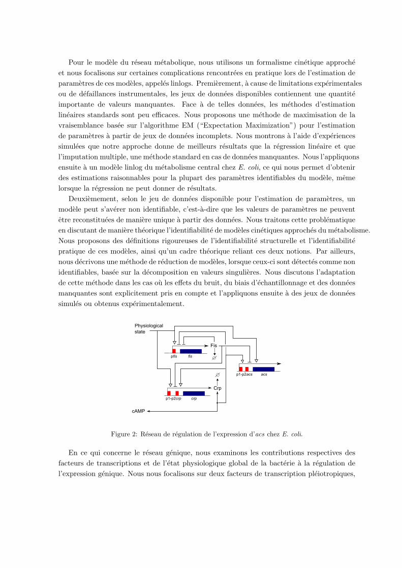
Figure 2: Reseau de regulation de l’expression d’acs chez E. coli.

En ce qui concerne le reseau genique, nous examinons les contributions respectives des

facteurs de transcriptions et de l’etat physiologique global de la bacterie a la regulation de

l’expression genique. Nous nous focalisons sur deux facteurs de transcription pleiotropiques,

Fis et Crp, ainsi que sur le gene acs qui code pour l’enzyme cle de l’assimilation d’acetate.

Nous enregistrons in vivo, sous differentes conditions physiologiques et pour differents con-

textes genetiques, les profils temporels d’expression de ces genes a l’aide de plasmides rap-

porteurs . Nous deduisons des donnees ainsi obtenues que les changements dans l’expression

de fis et crp au cours de la transition de croissance sont principalement expliques par des

changements de l’etat physiologique global de la bacterie alors que l’induction d’acs est prin-

cipalement controlee par Crp et le metabolite cAMP. Nous approfondissons l’etude de la dis-

tribution des roles dans la regulation genique avec un modele d’equations differentielles ordi-

naires (EDO). La regulation par les facteurs de transcription est modelisee par des cinetiques

de Hill alors que l’activite de l’etat physiologique global de la bacterie est representee par

une fonction phenomenologique. Les parametres sont estimes a l’aide d’un sous-ensemble des

donnees enregistrees et le modele est valide sur le reste du jeu de donnees.

En se confrontant aux defis methodologiques rencontres lors du developpement de modeles

de reseaux metaboliques et geniques, cette these contribue aux efforts futurs portant sur

l’integration de ces deux types de reseaux au sein de modeles quantitatifs.

7

Contents

1 Introduction 11

1.1 Context . . . . . . . . . . . . . . . . . . . . . . . . . . . . . . . . . . . . . . . 11

1.2 Problem statement . . . . . . . . . . . . . . . . . . . . . . . . . . . . . . . . . 18

1.3 Questions and approaches . . . . . . . . . . . . . . . . . . . . . . . . . . . . . 20

1.3.1 Development of a simplified kinetic model for central carbon metabolism

of E. coli . . . . . . . . . . . . . . . . . . . . . . . . . . . . . . . . . . 20

1.3.2 Interplay between specific regulators and global cell physiology in the

dynamic adaptation of gene expression in bacteria . . . . . . . . . . . 22

1.4 Thesis overview . . . . . . . . . . . . . . . . . . . . . . . . . . . . . . . . . . . 24

2 State of the art 25

2.1 Kinetic modeling of biochemical reaction systems . . . . . . . . . . . . . . . . 25

2.1.1 Metabolic reactions . . . . . . . . . . . . . . . . . . . . . . . . . . . . 27

2.1.2 Gene expression . . . . . . . . . . . . . . . . . . . . . . . . . . . . . . 29

2.1.3 Protein-metabolite complexes . . . . . . . . . . . . . . . . . . . . . . . 30

2.2 Approximate kinetic models and model reduction . . . . . . . . . . . . . . . . 31

2.2.1 Reduction based on time-scale discrepancies . . . . . . . . . . . . . . . 31

2.2.2 Approximate kinetic models . . . . . . . . . . . . . . . . . . . . . . . . 33

2.3 Measurements of gene expression and metabolism . . . . . . . . . . . . . . . . 34

2.4 Parameter estimation of kinetic models . . . . . . . . . . . . . . . . . . . . . . 37

2.4.1 Defining the objective function . . . . . . . . . . . . . . . . . . . . . . 38

2.4.2 Minimizing the objective function . . . . . . . . . . . . . . . . . . . . 39

2.5 Quantitative modeling of growth transitions in E. coli . . . . . . . . . . . . . 42

3 Parameter estimation of linlog metabolic models 44

3.1 Parameter estimation in linlog models . . . . . . . . . . . . . . . . . . . . . . 44

3.2 Likelihood-based identification of linlog models from missing data . . . . . . . 47

3.3 Validation on simulated data . . . . . . . . . . . . . . . . . . . . . . . . . . . 50

3.4 Application to central metabolism in E. coli . . . . . . . . . . . . . . . . . . . 54

3.5 Discussion . . . . . . . . . . . . . . . . . . . . . . . . . . . . . . . . . . . . . . 60

8

4 Identifiability of linlog metabolic models 63

4.1 Parameter estimation in linlog and other approximate kinetic modeling for-

malisms . . . . . . . . . . . . . . . . . . . . . . . . . . . . . . . . . . . . . . . 64

4.2 Identifiability of linlog and related models . . . . . . . . . . . . . . . . . . . . 68

4.2.1 Identifiability from a theoretical perspective . . . . . . . . . . . . . . . 69

4.2.2 Identifiability from a practical perspective . . . . . . . . . . . . . . . . 72

4.3 Reduction to identifiable models . . . . . . . . . . . . . . . . . . . . . . . . . 77

4.3.1 Model reduction by PCA . . . . . . . . . . . . . . . . . . . . . . . . . 78

4.3.2 Model reduction put in practice . . . . . . . . . . . . . . . . . . . . . . 79

4.3.3 The overall model reduction procedure . . . . . . . . . . . . . . . . . . 82

4.4 Applications of the model identifiability and reduction approach . . . . . . . 84

4.4.1 Application to a network with simulated data . . . . . . . . . . . . . . 84

4.4.2 Application to central carbon metabolism of E. coli . . . . . . . . . . 88

4.5 Discussion . . . . . . . . . . . . . . . . . . . . . . . . . . . . . . . . . . . . . . 92

5 Shared control of gene expression in bacteria by transcriptional regulators

and global physiological state 97

5.1 Materials and methods . . . . . . . . . . . . . . . . . . . . . . . . . . . . . . . 99

5.1.1 Strains and growth conditions . . . . . . . . . . . . . . . . . . . . . . . 99

5.1.2 Real-time monitoring of gene expression . . . . . . . . . . . . . . . . . 101

5.1.3 Measurement of cAMP concentrations . . . . . . . . . . . . . . . . . . 101

5.2 Results . . . . . . . . . . . . . . . . . . . . . . . . . . . . . . . . . . . . . . . . 101

5.2.1 Monitoring the dynamic response of the acs network . . . . . . . . . . 101

5.2.2 Dissecting the local and global control of gene expression . . . . . . . 104

5.2.3 Distributed local and global control of gene expression in acs network

during growth transition . . . . . . . . . . . . . . . . . . . . . . . . . . 107

5.2.4 Local and global gene expression control in different physiological con-

ditions and genetic backgrounds . . . . . . . . . . . . . . . . . . . . . 109

5.3 Dynamical model of both global and transcriptional regulation of the acs network114

5.4 Discussion . . . . . . . . . . . . . . . . . . . . . . . . . . . . . . . . . . . . . . 119

6 Conclusion 122

Appendices 123

A Additional information on parameter estimation of linlog metabolic models125

A.1 Likelihood-based identification of linlog models . . . . . . . . . . . . . . . . . 125

A.2 Validation of parameter estimation of linlog models on simulated data . . . . 128

9

B Additional information on identifiability of linlog metabolic models 133

B.1 Proofs of theorems and propositions concerning identifiability of linlog models 133

B.2 Reduction to identifiable models in case of sampling bias . . . . . . . . . . . . 135

C Additional information on analysis of gene expression regulation of E. coli141

C.1 Analysis of reporter gene data . . . . . . . . . . . . . . . . . . . . . . . . . . . 141

C.2 Analysis of cAMP measurements . . . . . . . . . . . . . . . . . . . . . . . . . 147

C.3 Measurement of time-varying plasmid copy number . . . . . . . . . . . . . . . 151

C.4 Additional gene expression profiles and analysis results during glucose/acetate

diauxie for different conditions . . . . . . . . . . . . . . . . . . . . . . . . . . 151

C.5 Additional information on parameter estimation of the ODE model of the acs

network . . . . . . . . . . . . . . . . . . . . . . . . . . . . . . . . . . . . . . . 157

C.5.1 Making the model consistent with available experimental data . . . . 157

C.5.2 Divide estimation problem into subproblems . . . . . . . . . . . . . . 159

10

Chapter 1

Introduction

1.1 Context

Microbes, organisms not visible with the human eye, are very ancient and the first living

cells on Earth. They are essential for human life, e.g., as part of the microbial flora or as the

main source of nitrogen for plants. Microbes grow everywhere even in extreme environments

with extreme temperatures, pH, hydrostatic or osmotic pressures, where humans would not

be able to survive. In one sentence, “Where there is life, there are microbes” [Schaechter

et al., 2006].

An important property of microbes is that they can grow when subject to continuous

environmental changes in nutrient availability, temperature, pH or pressure, alteration of the

physical properties of the niche, or exposition to various radiation or toxic factors. As an

example of the sudden changes microbes have to cope with, imagine a gut bacterium expelled

from animal intestine [Schaechter et al., 2006]. Despite all these stresses and changes, micro-

bial organisms manage to maintain the complex coordination of the cell enabling cell growth

and division. How does a living organism first sense and then adapt to such environmental

alterations ? Which dynamical changes appear in the internal behavior of the cell during this

adaptation to the environment ?

We will explore these questions by means of the example of the enterobacterium Es-

cherichia coli during its adaptation to the exhaustion of one nutrient and the consequent

transition to the uptake and assimilation of another nutrient. The switch of one growth

substrate to another by a bacterial population is called a diauxie. Consider the example of a

glucose/acetate diauxie shown Fig. 1.1. In a glucose-rich environment, the bacterial popula-

tion grows exponentially, and the cells produce and excrete acetate into the growth medium.

When the glucose level drops, the excreted acetate can be utilized as a carbon source, leading

to a much lower growth rate [Wolfe, 2005]. Growth in the presence of acetate is interesting

for biotechnology as a high concentration of acetate in the medium has a negative effect on

bacterial growth [Luli and Strohl, 1990].

11

Figure 1.1: Transcription (or, equivalently, promoter activity) of acs (solid line) during growth on

glucose and glucose/acetate diauxie taken from [Wolfe, 2005]. Bacteria grow in a minimal medium

supplemented with glucose. The population growth is represented by the optical density (OD) curve

(semi-dotted line). The extracellular concentrations of glucose (glc) and acetate (ace) are shown in

dotted lines. The relative change of the intracellular concentrations of proteins Fis and IHF over the

bacterial growth phase is represented below the figure.

As a consequence of the diauxie, morphological changes are observed concerning among

other things the cell membrane and cell volume. Moreover, the molecular composition of the

cell changes: DNA concentration, ribosome concentration, RNA polymerase concentration,

enzyme and transcription factor concentrations, metabolic fluxes and metabolic pools [Bremer

and Dennis, 1996]. Below, we briefly discuss the extent of these changes.

The contents of the cellular machinery, including DNA, RNA and protein, depends on

the growth rate of the bacterial population [Schaechter et al., 2006, §4] [Bremer and Dennis,

1996]. Indeed, these macromolecular quantities decrease in the cell when the growth rate

decreases during diauxie [Neidhardt and Fraenkel, 1961]. Moreover, not only the quantities

in the cell vary with the growth rate but also the relative proportions compared to cell mass:

the ratio of the amounts of DNA and protein per cell mass increases, while the ratio of RNA

per cell mass decreases.

The central carbon metabolism of E. coli degrades, via a network of metabolic reactions,

the external carbon source to several intermediate metabolites to produce the energy (ATP)

and to synthesize the precursors of macromolecules (amino acids) necessary for the develop-

ment and growth of the cell. Fig. 1.2 shows the network of central carbon metabolism of

E. coli. When growing on glucose, the substrate is imported into the cell by the phospho-

transferase system (PTS) and converted it to glucose-6-phosphate (G6P) [Gorke and Stulke,

2008, Saier Jr et al., 1996]. G6P is then metabolized through glycolysis to phosphoenolpyru-

vate (PEP). Mostly, PEP is used to produce energy and precursors. At high carbon fluxes,

acetate is produced and excreted from the cell. Once glucose is exhausted and no other car-

bon source is present in the medium, acetate is imported back into the cell and converted to

12

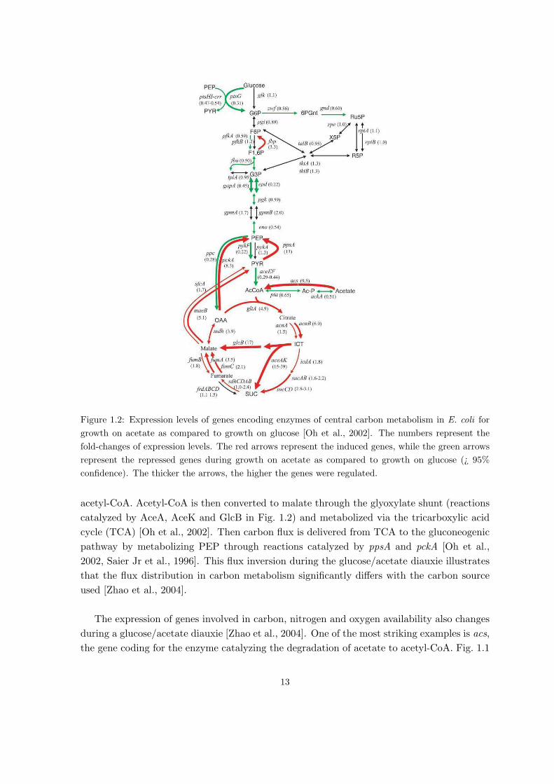
Figure 1.2: Expression levels of genes encoding enzymes of central carbon metabolism in E. coli for

growth on acetate as compared to growth on glucose [Oh et al., 2002]. The numbers represent the

fold-changes of expression levels. The red arrows represent the induced genes, while the green arrows

represent the repressed genes during growth on acetate as compared to growth on glucose (¿ 95%

confidence). The thicker the arrows, the higher the genes were regulated.

acetyl-CoA. Acetyl-CoA is then converted to malate through the glyoxylate shunt (reactions

catalyzed by AceA, AceK and GlcB in Fig. 1.2) and metabolized via the tricarboxylic acid

cycle (TCA) [Oh et al., 2002]. Then carbon flux is delivered from TCA to the gluconeogenic

pathway by metabolizing PEP through reactions catalyzed by ppsA and pckA [Oh et al.,

2002, Saier Jr et al., 1996]. This flux inversion during the glucose/acetate diauxie illustrates

that the flux distribution in carbon metabolism significantly differs with the carbon source

used [Zhao et al., 2004].

The expression of genes involved in carbon, nitrogen and oxygen availability also changes

during a glucose/acetate diauxie [Zhao et al., 2004]. One of the most striking examples is acs,

the gene coding for the enzyme catalyzing the degradation of acetate to acetyl-CoA. Fig. 1.1

13

Figure 1.3: Different levels of regulation involved in the molecular adaptation of E. coli during the

glucose/acetate diauxie [Kotte et al., 2010]. The scheme is centered around the gene-metabolite

interactions and establishes a feedback loop from the metabolic layer through the transcriptional

regulation layer and the gene expression layer back to the metabolic layer.

shows the gene expression pattern of acs during subsequent growth on glucose and acetate.

As we can see, there is a significant increase in acs expression when glucose is exhausted. In

addition, the relative amounts of the proteins Fis and IHF differ with the carbon source used

for cell metabolism.

How are the gene expression changes coordinated and controlled to allow a coherent func-

tioning of the bacterial cell ? Fig. 1.3 shows a scheme of the different regulation levels of the

cell involved in the glucose/acetate diauxie [Kotte et al., 2010]. Let us explore the internal

regulatory behavior of the bacterium following this scheme.

Responding to environmental changes necessitates a sensory mechanism to monitor the

state of the environment. In the case of growth on glucose, the flux through the PTS system

is sensed by the cell. The import and degradation of glucose leads to catabolite repression,

i.e., the prevention of the import of other carbon sources [Kremling et al., 2009, Betten-

brock et al., 2006, Gorke and Stulke, 2008]. Catabolite repression operates when glucose is

14

in the medium and inactivates adenylate cyclase, thus preventing the formation of the small

metabolite cyclic AMP (cAMP). When glucose is exhausted, catabolite repression is lifted,

leading to activation of adenylate cyclase which causes accumulation of cAMP, derepression

of other import pathways and consumption of acetate.

In microbes, an important control process of the metabolic flux distribution, though not

the only one, is the regulation of the concentrations of enzymes catalyzing metabolic reactions

[Schaechter et al., 2006, §12]. Indeed, Fig. 1.2, taken from Oh et al. [2002], shows the difference

in gene expression for enzymes catalyzing reactions of central carbon metabolism in E. coli in

conditions of growth on glucose and growth on acetate. As an example, consider the reversible

metabolic reaction converting PEP to oxaloacetate (OAA). Each direction is catalyzed by a

different enzyme. During growth on glucose, Ppc is more expressed than growth on acetate,

which favors the conversion of PEP to OAA. On the contrary, when acetate is the carbon

source, PckA is more highly expressed than growth on glucose and leads to flux inversion,

thus favoring the conversion of OAA to PEP.

Metabolic fluxes are indirectly regulated via the control of the expression of enzymes.

Gene expression is mainly controlled by regulatory proteins, called transcription factors,

that bind to the promoter region of a gene and activate or repress transcription. We can

distinguish between transcription factors that are specific to a given promoter, and thus only

impact the transcription of genes inside one operon, and transcription factors that have a

more global regulatory role in that they can bind to a larger number of promoters and thus

impact the transcription of an entire group of genes. Regulatory proteins falling in this

latter category, called global regulators, are key components of the cell regulation process,

notably when adaptation to environmental changes imposes a major re-organization of the

protein composition of the cell. For example, the catabolite repression system is driven

by the complex Crp.cAMP which regulates many genes related to substrate utilization by

the cell [Schaechter et al., 2006, §12]. Fig. 1.4 shows the global transcriptional regulatory

network of E. coli. Seven proteins (ArcA, FNR, Fis, Crp, IHF, Lrp and Hns) have been

detected as global regulators, as they directly regulate expression of more than half of the

genes in E. coli [Martinez-Antonio and Collado-Vides, 2003]. Some of them are of major

importance during the glucose/acetate diauxie. For instance, Crp, when bound to the small

metabolite cAMP, regulates catabolite repression. Moreover, Fis, IHF and Hns bind to DNA

and regulate gene transcription by altering DNA topology according to the energy levels in

the cell [Martinez-Antonio and Collado-Vides, 2003].

Global regulators involved in environmental adaptation need to get information about

external changes from molecules involved in signaling pathways. Indeed, half of the known

transcription factors have known binding sites for small metabolites, so they can achieve

activation or repression according to metabolic changes [Martinez-Antonio and Collado-

Vides, 2003]. Four transcription factors have been identified as playing a key role in the

glucose/acetate diauxie and being active regulators when bound to intermediates of cen-

15

Figure 1.4: Overview of the transcriptional regulatory network in E. coli [Martinez-Antonio and

Collado-Vides, 2003]. Regulated genes are shown as yellow ovals, transcription factors are shown as

green ovals and global regulators are shown as blue ovals. The green lines indicate activation, red

lines indicate repression, and dark blue lines indicate dual regulation (activation and repression).

16

tral metabolism (Crp.cAMP, Cra.FBP, IclR-GLX, IclR-PYR and PdhR-PYR) [Kotte et al.,

2010]. Cra, when forming a complex with fructose-biphosphate (FBP), also regulates catabo-

lite repression. IclR, when bound to glyoxylate or pyruvate, regulates the enzymes catalyzing

glyoxylate shunt [Lorca et al., 2007] and PdhR regulates aceEF [Quail and Guest, 1995].

In summary, the metabolic flux distribution is controlled by the activities of metabolic

enzymes and the environment. Those activities depend on enzyme concentrations, while

the expression levels of enzyme-coding genes is regulated by transcription factors, so indi-

rectly, metabolism is regulated by transcriptional regulation. Moreover, some transcription

factors are only active when forming a complex with a metabolite (Cra, Crp, IclR, PdhR

[Kotte et al., 2010]). Thus gene regulation is controlled by metabolism. Metabolic and gene

regulations are connected to form a complex and heterogeneous regulatory network (Fig. 1.3).

Finally, the adaptation of the cell to external changes also involves regulation by the gene

expression machinery, which includes all molecules necessary for gene expression, notably as

transcription and translation (ribosomes, amino acids, RNA polymerase). Changes in the

growth rate impact the synthesis rate of all cellular proteins (translation and transcription

mechanisms) via the resulting change in concentration and activity of ribosomes and RNA

polymerase [Bremer and Dennis, 1996, Tadmor and Tlusty, 2008]. Thus the cell has one

more level of regulation: global regulation of gene expression by the growth rate [Scott et al.,

2010]. This impacts the overall functioning of the cell, including gene regulation (proteins

binding to gene promoters) and metabolic regulation (enzyme activities and concentrations).

In summary, E. coli reacts to environmental changes with a coordinated response between

different levels of molecular processes and it is necessary to consider a global system involving

all these regulation levels.

Recent developments of high-throughput techniques for obtaining experimental data of

internal molecules of E. coli have led to massive accumulation of information on such mech-

anisms [Oh et al., 2002, Kao et al., 2004, Ishii et al., 2007]. Since the integrated system we

are interested in involves complex feedback loops between its molecular elements, it is very

difficult to have an intuitive understanding of its dynamical behavior. Mathematical models

are useful tools to deduce dynamical information from mechanistic biological knowledge and

the available experimental data. Indeed, the modeler translates his knowledge of regulatory

mechanisms into an unambiguous system structure, chooses mathematical formalisms to de-

scribe the molecular kinetics involved and uses simulation methods and computer tools to

make predictions of the dynamical behavior of the system.

In the past decades, mathematical formalisms for modeling the kinetics of metabolic re-

actions [Heijnen, 2005, Chen et al., 2010, Heinrich and Schuster, 1996] and gene regulatory

networks [de Jong, 2002] have been developed. Models focusing on the dynamical behavior

of metabolic or gene regulatory networks intervening in diauxic behavior in E. coli have been

17

developed ([Ropers et al., 2006, Bettenbrock et al., 2006], see [Kremling et al., 2009] for a

review, [Hardiman et al., 2009, Chassagnole et al., 2002]). However, models of networks in-

tegrating both regulation levels have been little studied so far [Kotte et al., 2010, Baldazzi

et al., 2010, Tenazinha and Vinga, 2011]. One of the reason is that integrated networks

are large and heterogeneous, so they imply the development of complex models with many

parameters, which raises a number of methodological challenges. Another reason is that the

amount of data necessary for model development is huge.

In order to understand the dynamics of such complicated networks, quantitative modeling

and data are necessary. Indeed, quantitative measurements of the outputs of the model un-

der various conditions are required for the calibration of the model on the wild-type dataset

and the validation of the model predictions in the other conditions by means of other datasets.

In all the steps for system modeling enumerated above, the current bottleneck is the cali-

bration of the model [Ashyraliyev et al., 2009]. In quantitative modeling, it boils down to the

estimation of the kinetic parameters of the system. These parameters need to be estimated

as the majority of them can not be measured experimentally. Moreover, some of them may

not have a physical interpretation, in case of phenomenological models. “The parameter

estimation problem can be formulated from the mathematical viewpoint as a constrained

optimization problem where the goal is to minimize the objective function, defined as the

error between model predictions and real data.” [Marucci et al., 2011] Parameter estimation

is a difficult task as models contain a large number of variables, whose dynamics evolve on

different time-scales and are described by complex, nonlinear rate equations. Thus, these

models also contain a large number of parameters and their nonlinearity implies complex ob-

jective functions for parameter estimation. Moreover, identification requires a large quantity

of experimental data of good quality. These data, in practice, are noisy, partial and they are

obtained with heterogeneous techniques and experimental conditions.

1.2 Problem statement

How can we build a quantitative model of complex biological systems, and particularly net-

works involving regulation on multiple levels? As we investigate dynamical molecular pro-

cesses of integrated networks, mathematical models may grow very quickly in terms of num-

ber of parameters and variables involved and the complexity of the nonlinear rate equations.

Such models usually generate analytical and numerical problems. Moreover, the fact that the

model has many parameters, given an available dataset whose size and accuracy are limited

by experimental considerations in many cases, renders the model nonidentifiable. This means

that it is not possible to distinguish between different sets of parameters, as they all lead

to the same dynamical behavior of the model. Model identifiability has been well-studied in

control theory and applied mathematics [Walter and Pronzato, 1997] and nonidentifiability

is a problem commonly encountered in the field of systems biology [Ashyraliyev et al., 2009,

18

Gutenkunst et al., 2007]. In the case where, given the available information on a biological

system, it is not possible to distinguish between different kinetic models having the same

outputs, the model with the simplest formalism and the lowest number of variables should be

considered. A standard strategy to tackle this difficulty when working with complex systems

of all kinds (may they be electronic, physical or social) is to reduce the model. There are

several methods available for reducing the complexity and the size of a model, depending on

the systemic properties of interest and of the initial model complexity. Below, we highlight

some of the most commonly-used methods.

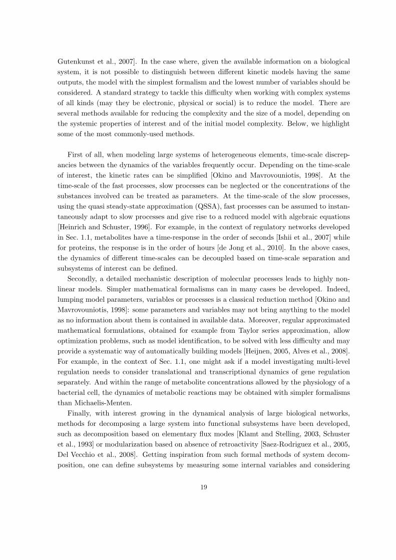
First of all, when modeling large systems of heterogeneous elements, time-scale discrep-

ancies between the dynamics of the variables frequently occur. Depending on the time-scale

of interest, the kinetic rates can be simplified [Okino and Mavrovouniotis, 1998]. At the

time-scale of the fast processes, slow processes can be neglected or the concentrations of the

substances involved can be treated as parameters. At the time-scale of the slow processes,

using the quasi steady-state approximation (QSSA), fast processes can be assumed to instan-

taneously adapt to slow processes and give rise to a reduced model with algebraic equations

[Heinrich and Schuster, 1996]. For example, in the context of regulatory networks developed

in Sec. 1.1, metabolites have a time-response in the order of seconds [Ishii et al., 2007] while

for proteins, the response is in the order of hours [de Jong et al., 2010]. In the above cases,

the dynamics of different time-scales can be decoupled based on time-scale separation and

subsystems of interest can be defined.

Secondly, a detailed mechanistic description of molecular processes leads to highly non-

linear models. Simpler mathematical formalisms can in many cases be developed. Indeed,

lumping model parameters, variables or processes is a classical reduction method [Okino and

Mavrovouniotis, 1998]: some parameters and variables may not bring anything to the model

as no information about them is contained in available data. Moreover, regular approximated

mathematical formulations, obtained for example from Taylor series approximation, allow

optimization problems, such as model identification, to be solved with less difficulty and may

provide a systematic way of automatically building models [Heijnen, 2005, Alves et al., 2008].

For example, in the context of Sec. 1.1, one might ask if a model investigating multi-level

regulation needs to consider translational and transcriptional dynamics of gene regulation

separately. And within the range of metabolite concentrations allowed by the physiology of a

bacterial cell, the dynamics of metabolic reactions may be obtained with simpler formalisms

than Michaelis-Menten.

Finally, with interest growing in the dynamical analysis of large biological networks,

methods for decomposing a large system into functional subsystems have been developed,

such as decomposition based on elementary flux modes [Klamt and Stelling, 2003, Schuster

et al., 1993] or modularization based on absence of retroactivity [Saez-Rodriguez et al., 2005,

Del Vecchio et al., 2008]. Getting inspiration from such formal methods of system decom-

position, one can define subsystems by measuring some internal variables and considering

19

them as entries of smaller systems. Thus, models for such subsystems are not required to

predict the dynamics of the measured variables and subsystems can be detached from the

global network and analyzed separately without losing information or introducing bias.

Back to our original problematic, the aim of my thesis is to develop a quantitative model

investigating the dynamics of interconnection of metabolic, gene and cellular machinery reg-

ulations during the glucose/acetate diauxie of E. coli. As the dynamics of the large and

embedded system of interest cannot be analyzed simultaneously, we will decompose the sys-

tem and its dynamics inspired by the reduction methods described above. For each of the

subsystems obtained in this way, a model will be developed using approximate kinetic equa-

tions and calibrated using parameter estimation approaches and appropriate experimental

datasets. Most of the work consists of computational and mathematical issues, but there is

also some effort spent on obtaining experimental data for parameter estimation.

1.3 Questions and approaches

We are interested in the dynamical behavior of the system integrating regulation by metabo-

lites, transcription factors and the gene expression machinery during the glucose/acetate

diauxie in E. coli. The network involved is extremely large and complex. Thus, to efficiently

address the question, we need to decompose the original system and isolate subsystems of

interest based on biological considerations taking inspiration from the reduction methods

described in Sec. 1.2.

As mentioned in the previous section, several orders of magnitude separate the time-scales

of metabolic and gene expression processes. So we can separate the variables of the global

system into slow variables (mRNA and protein concentrations) and fast variables (metabo-

lite concentrations) [Baldazzi et al., 2010]. Then, depending on the time scale of interest,

dynamical processes can be simplified. In this chapter, we carry out these simplifications

for the development of reduced models of the two following subsystems: the central carbon

metabolism and a gene regulatory network involved in the glucose/acetate diauxie of E. coli.

1.3.1 Development of a simplified kinetic model for central carbon metabolism

of E. coli

The network of central carbon metabolism, introduced in the previous sections, can be de-

composed into 5 subnetworks: glycolysis/gluconeogenesis, pentose-phosphate pathway, Krebs

cycle, EDD pathway and glyoxylate shunt, as shown Fig. 1.5.

As mentioned previously during a glucose/acetate diauxie, metabolic fluxes in central

carbon metabolism are reorganized [Zhao et al., 2004]. But before even adapting to a new

20

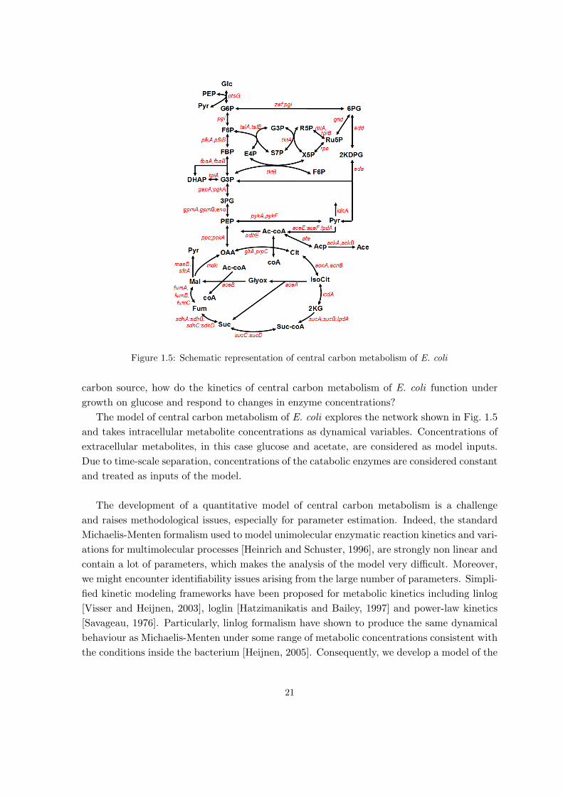
Figure 1.5: Schematic representation of central carbon metabolism of E. coli

carbon source, how do the kinetics of central carbon metabolism of E. coli function under

growth on glucose and respond to changes in enzyme concentrations?

The model of central carbon metabolism of E. coli explores the network shown in Fig. 1.5

and takes intracellular metabolite concentrations as dynamical variables. Concentrations of

extracellular metabolites, in this case glucose and acetate, are considered as model inputs.

Due to time-scale separation, concentrations of the catabolic enzymes are considered constant

and treated as inputs of the model.

The development of a quantitative model of central carbon metabolism is a challenge

and raises methodological issues, especially for parameter estimation. Indeed, the standard

Michaelis-Menten formalism used to model unimolecular enzymatic reaction kinetics and vari-

ations for multimolecular processes [Heinrich and Schuster, 1996], are strongly non linear and

contain a lot of parameters, which makes the analysis of the model very difficult. Moreover,

we might encounter identifiability issues arising from the large number of parameters. Simpli-

fied kinetic modeling frameworks have been proposed for metabolic kinetics including linlog

[Visser and Heijnen, 2003], loglin [Hatzimanikatis and Bailey, 1997] and power-law kinetics

[Savageau, 1976]. Particularly, linlog formalism have shown to produce the same dynamical

behaviour as Michaelis-Menten under some range of metabolic concentrations consistent with

the conditions inside the bacterium [Heijnen, 2005]. Consequently, we develop a model of the

21

catabolic network of E. coli using linlog kinetics.

As mentioned before, the most sensitive step of modeling is parameter estimation. Ex-

perimental data for inputs and outputs of the model are needed. Large-scale and high-

throughput techniques for measuring metabolite concentration [Vemuri and Aristidou, 2005]

and gene expression data [Dharmadi and Gonzalez, 2004], respectively, have been devel-

oped and large-scale datasets comprising simultaneous measurements of metabolism (fluxes,

metabolite concentrations) and gene expression (protein and mRNA concentrations) have be-

come available. Notwithstanding these experimental advances, parameter estimation remains

a particularly challenging problem, among other things due to noisy and partial observations

and heterogeneous experimental methods and conditions. We focus on two principal compli-

cations encountered in practice when performing model calibration.

First of all, the large-scale datasets contain a substantial amount of missing values, due to

experimental limitations or instrument failures. Standard linear estimation methods perform

poorly in that case. We develop an estimation method adapted to incomplete datasets. We

then apply this method for calibrating the model of central carbon metabolism of E. coli

using the largest dataset available in the literature [Ishii et al., 2007].

Secondly, given an experimental dataset, a model may be nonidentifiable, i.e., the param-

eter values cannot be uniquely reconstructed from the data. We address this issue by defining

a theoretical background for both structural and practical identifiability and by describing a

model reduction method to resolve identifiability issues. We then discuss the practical ap-

plication of this reduction method depending on the properties of the experimental dataset

available for parameter estimation.

1.3.2 Interplay between specific regulators and global cell physiology in

the dynamic adaptation of gene expression in bacteria

Gene expression is regulated by transcription factors via gene regulatory networks that have

been widely studied. However during growth transitions, such as the glucose/acetate diauxie,

major changes in the physiological state of the cell occur, which also affect gene expression, as

described in Sec. 1.1. Which part of the dynamics of gene expression is due to gene regulation

and which part to changes in the macromolecular composition of the cell? We tackle this

problem by producing time-series data of the expression of transcription factors during the

exhaustion of glucose and by developing a quantitative model describing the dynamics of the

network of transcription factors.

In order to study the impact of gene regulation and the global physiological state on gene

expression during the glucose/acetate diauxie in E. coli, we focus on the network shown in

22

���

�������

�����������

��

�����������

ABCD

DEF�������A��

�����

Figure 1.6: Reciprocal regulation of global regulators Crp and Fis and regulation of acs.

Fig. 1.6. The network includes two global regulators, Crp and Fis, which regulate each other

[Martinez-Antonio and Collado-Vides, 2003]. The network of interest also embraces the most

characteristic expression pattern of diauxic change, acs, the gene coding for the enzyme cat-

alyzing the degradation of acetate into acetyl-CoA, which is regulated by Crp, when forming

a complex with the small metabolite cAMP, and Fis [Wolfe, 2005].

We monitored in real time and in vivo, by means of GFP reporters, the expression of

the genes in the network in response to glucose depletion. In parallel, we also measured the

time-varying concentration of extracellular cAMP and computed from these data intracellu-

lar cAMP dynamic behaviors. GFP reporter driven by a non-regulated, constitutive phage

promoter was used to assay the time-varying physiological state. The above experiments were

repeated when the network was submitted to various physiological and genetic perturbations,

such as shifting the cell to a low-glucose medium or deleting the genes fis and crp.

We first use a simple, parameterless mathematical model that can be used to analyze

the roles of global physiological control and transcription regulation in the variation of the

promoter activity of the genes of the network in Fig. 1.6. Additionally, we investigate the roles

of the different regulatory mechanisms by developing and analyzing a quantitative ODEmodel

of the network. The model takes the protein concentrations of Crp and Fis as dynamical

variables and returns the promoter activity of acs. At the time-scale of gene regulation,

the metabolite concentration can be considered as adapting instantaneously to changes in

gene expression using the quasi-steady-state approximation [Heinrich and Schuster, 1996].

Thus, the dynamical evolution of intracellular cAMP concentration is considered as a model

input. Gene regulation kinetics are modeled by Hill formalisms and the translational and

transcriptional dynamics are merged. The parameters are estimated using heuristic methods

and the gene expression data. The predictions of the model are compared to experimental

data on fis and crp mutant strains.

23

1.4 Thesis overview

This thesis is organized as follows:

Chapter 2 introduces fundamental notions of ODE models of metabolism and gene expres-

sion as well as the estimation of model parameters and reduction methods based on time-scale

discrepancies and approximate kinetic formalisms. The chapter also lists the experimental

techniques and datasets that can be used for the investigation of cellular adaptation processes

during growth transitions. Finally, quantitative models of metabolism and gene regulation

of E. coli during growth transitions are reviewed.

Chapter 3 describes a method for estimating parameters of linlog models from high-throughput

incomplete datasets. The method is applied to experimental data to identify the linlog model

of central carbon metabolism of E. coli and returns reasonable estimates for most of the iden-

tifiable model parameters. The results of this chapter were presented in the ISMB/ECCB

conference in 2011 and published in Bioinformatics [Berthoumieux et al., 2011].

Chapter 4 investigates the identifiability of metabolic network models by presenting precise

definitions of structural and practical identifiability and clarifying the fundamental relations

between these concepts. This work will be presented at the SYSID conference in 2012 and

published in the proceedings of the conference [Berthoumieux et al., 2012b].

Moreover, the chapter describes a method based on Singular Value Decomposition (SVD)

to detect identifiability problems and to reduce the model to an identifiable approximation.

Moreover, it discusses the application of this method to scarce, incomplete and noisy data.

The identifiability analysis of the linlog model of central carbon metabolism of E. coli revealed

that very few parameters are identifiable from currently available, state-of-the-art datasets.

These results were submitted for publication [Berthoumieux et al., 2012a].

Chapter 5 presents results of the investigation of the relative contributions of transcription

factors and the global physiological state of the cell to the regulation of gene expression.

By means of gene expression measurements and development of kinetic models, this chapter

highlights the importance of the global physiological state of the cell in gene expression

regulation during the glucose/acetate diauxie. This work forms the basis for a paper currently

in preparation.

24

Chapter 2

State of the art

In this chapter, we develop the different steps encountered when quantitatively modeling a

biological regulatory system. First, a mathematical formulation has to be defined and in

Sec. 2.1, we present some standard kinetic models in the formalism of ordinary differential

equations for regulatory networks. It is also important to investigate the possibility to reduce

the complexity and dimension of a model by looking at mathematical and biological properties

of the system. In Sec. 2.2, we briefly describe reduction approaches for biological network

models. Once the equations of the model are defined, the calibration of the model, i.e.,

the estimation of its parameters, requires experimental data on the outputs of the system.

In Sec. 2.3 we introduce common experimental techniques that allow measurement of high-

throughput datasets for different biochemical species. In Sec. 2.4, we address the challenge of

defining the parameter estimation problem and solving it using the best adapted algorithm.

Finally, we present in Sec. 2.5 the state of the art of quantitative modeling of regulatory

networks in E. coli during growth transitions.

2.1 Kinetic modeling of biochemical reaction systems

Being the most widespread formalism to model dynamical systems in science and engineering,

ordinary differential equations (ODEs) have been widely used to analyze biochemical reaction

networks. The ODE formalism models the concentrations of proteins, metabolites and other

molecules by time-dependent variables which are real and positive. Biochemical reactions

take the form of functional and differential relations between the concentration species.

More specifically, biochemical reactions are modeled by the following mathematical equa-

tion

dx

dt= N · v(x, p, u) (2.1)

with x ∈ Rn+ the vector of concentration variables of the system, N ∈ Z

n×m a stoichiometry

matrix describing the network structure, v ∈ Rm rate functions, p ∈ R

np the vector of model

25

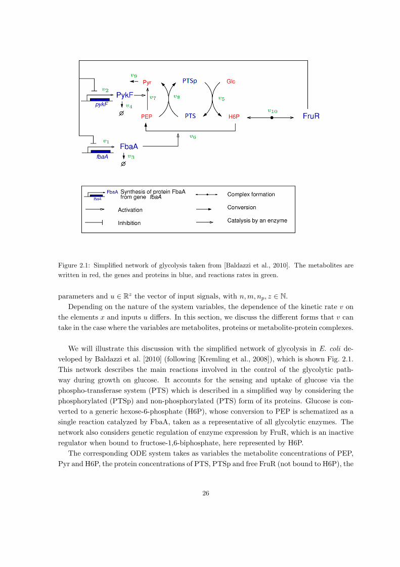
Figure 2.1: Simplified network of glycolysis taken from [Baldazzi et al., 2010]. The metabolites are

written in red, the genes and proteins in blue, and reactions rates in green.

parameters and u ∈ Rz the vector of input signals, with n,m, np, z ∈ N.

Depending on the nature of the system variables, the dependence of the kinetic rate v on

the elements x and inputs u differs. In this section, we discuss the different forms that v can

take in the case where the variables are metabolites, proteins or metabolite-protein complexes.

We will illustrate this discussion with the simplified network of glycolysis in E. coli de-

veloped by Baldazzi et al. [2010] (following [Kremling et al., 2008]), which is shown Fig. 2.1.

This network describes the main reactions involved in the control of the glycolytic path-

way during growth on glucose. It accounts for the sensing and uptake of glucose via the

phospho-transferase system (PTS) which is described in a simplified way by considering the

phosphorylated (PTSp) and non-phosphorylated (PTS) form of its proteins. Glucose is con-

verted to a generic hexose-6-phosphate (H6P), whose conversion to PEP is schematized as a

single reaction catalyzed by FbaA, taken as a representative of all glycolytic enzymes. The

network also considers genetic regulation of enzyme expression by FruR, which is an inactive

regulator when bound to fructose-1,6-biphosphate, here represented by H6P.

The corresponding ODE system takes as variables the metabolite concentrations of PEP,

Pyr and H6P, the protein concentrations of PTS, PTSp and free FruR (not bound to H6P), the

26

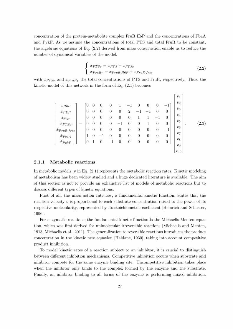
concentration of the protein-metabolite complex FruR·H6P and the concentrations of FbaA

and PykF. As we assume the concentrations of total PTS and total FruR to be constant,

the algebraic equations of Eq. (2.2) derived from mass conservation enable us to reduce the

number of dynamical variables of the model.

{xPTST

= xPTS + xPTSp

xFruRT= xFruR·H6P + xFruR·free

(2.2)

with xPTSTand xFruRT

the total concentrations of PTS and FruR, respectively. Thus, the

kinetic model of this network in the form of Eq. (2.1) becomes

xH6P

xPEP

xPyr

xPTSp

xFruR·free

xFbaA

xPykF

=

0 0 0 0 1 −1 0 0 0 −1

0 0 0 0 0 2 −1 −1 0 0

0 0 0 0 0 0 1 1 −1 0

0 0 0 0 −1 0 0 1 0 0

0 0 0 0 0 0 0 0 0 −1

1 0 −1 0 0 0 0 0 0 0

0 1 0 −1 0 0 0 0 0 0

v1

v2

v3

v4

v5

v6

v7

v8

v9

v10

. (2.3)

2.1.1 Metabolic reactions

In metabolic models, v in Eq. (2.1) represents the metabolic reaction rates. Kinetic modeling

of metabolism has been widely studied and a huge dedicated literature is available. The aim

of this section is not to provide an exhaustive list of models of metabolic reactions but to

discuss different types of kinetic equations.

First of all, the mass action rate law, a fundamental kinetic function, states that the

reaction velocity v is proportional to each substrate concentration raised to the power of its

respective molecularity, represented by its stoichiometric coefficient [Heinrich and Schuster,

1996].

For enzymatic reactions, the fundamental kinetic function is the Michaelis-Menten equa-

tion, which was first derived for unimolecular irreversible reactions [Michaelis and Menten,

1913, Michaelis et al., 2011]. The generalization to reversible reactions introduces the product

concentration in the kinetic rate equation [Haldane, 1930], taking into account competitive

product inhibition.

To model kinetic rates of a reaction subject to an inhibitor, it is crucial to distinguish

between different inhibition mechanisms. Competitive inhibition occurs when substrate and

inhibitor compete for the same enzyme binding site. Uncompetitive inhibition takes place

when the inhibitor only binds to the complex formed by the enzyme and the substrate.

Finally, an inhibitor binding to all forms of the enzyme is performing mixed inhibition.

27

Each of these inhibition mechanisms are modeled using different kinetic expressions [Cornish-

Bowden, 1995].

The models listed above, however, are not able to reproduce the sigmoidal shape of the de-

pendence of enzymatic activity on substrate concentrations that has sometimes been observed

experimentally [Heinrich and Schuster, 1996]. Models accounting for enzyme cooperativity

and allosteric interactions have been developed. Commonly encountered models are the phe-

nomenological Hill function [Hill, 1910], the Monod-Wyman-Changeux rate law [Monod et al.,

1965] and the sequential model of Koshland, Nemethy and Filmer [Koshland et al., 1966].

In the case of multimolecular reactions, kinetic modeling gets more difficult and kinetic

rate laws quickly become complex non linear equations with a lot of parameters [Cornish-

Bowden, 1995, Liebermeister and Klipp, 2006].

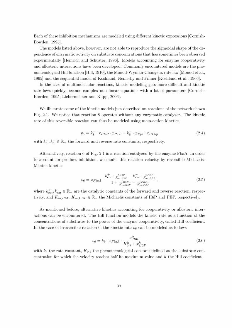
We illustrate some of the kinetic models just described on reactions of the network shown

Fig. 2.1. We notice that reaction 8 operates without any enzymatic catalyzer. The kinetic

rate of this reversible reaction can thus be modeled using mass-action kinetics,

v8 = k+8 · xPEP · xPTS − k−8 · xPyr · xPTSp (2.4)

with k+8 , k−8 ∈ R+ the forward and reverse rate constants, respectively.

Alternatively, reaction 6 of Fig. 2.1 is a reaction catalyzed by the enzyme FbaA. In order

to account for product inhibition, we model this reaction velocity by reversible Michaelis-

Menten kinetics

v6 = xFbaA ·k+cat · xH6P

Km,H6P− k−cat · xPEP

Km,PEP

1 + xH6P

Km,H6P+ xPEP

Km,PEP

, (2.5)

where k+cat, k−cat ∈ R+ are the catalytic constants of the forward and reverse reaction, respec-

tively, and Km,H6P ,Km,PEP ∈ R+ the Michaelis constants of H6P and PEP, respectively.

As mentioned before, alternative kinetics accounting for cooperativity or allosteric inter-

actions can be encountered. The Hill function models the kinetic rate as a function of the

concentrations of substrates to the power of the enzyme cooperativity, called Hill coefficient.

In the case of irreversible reaction 6, the kinetic rate v6 can be modeled as follows

v6 = k6 · xFbaA · xhH6P

Kh0.5 + xhH6P

(2.6)

with k6 the rate constant, K0.5 the phenomenological constant defined as the substrate con-

centration for which the velocity reaches half its maximum value and h the Hill coefficient.

28

2.1.2 Gene expression

In gene expression models, v can represent either the synthesis rate of a protein or its degra-

dation rate. Gene expression is a very complex process that can be regulated at several

stages of mRNA and protein synthesis [Schaechter et al., 2006]. Although it is possible to

develop mechanistic models of gene expression taking all steps into account ([Kremling, 2007]

and references therein), in practice, the lack of quantitative biological knowledge about these

processes and the complexity of the mathematical equations obtained render those models

very difficult to properly develop and analyze. Usually, phenomenological functions are used

to describe gene expression kinetics. Gene regulation modeling has been widely studied and

a variety of different modeling formalisms have been developed (see [de Jong, 2002] for a

review).

In the context of continuous ODE models, a common formalism uses Hill functions to de-

scribe gene expression rate laws. The activation of gene expression by a transcription factor

is modeled by a Hill function whereas inhibition is modeled by an inverse Hill function. When

several transcription factors act on the same promoter, the Hill functions can form complex

expressions, whose structures are inspired from Boolean networks [de Jong, 2002].

In the simplified glycolytic network shown Fig. 2.1, the enzyme FbaA is negatively regu-

lated by the transcription factor FruR, when the latter is not bound to H6P. We can therefore

model the synthesis rate of FbaA using the Hill formalism, which gives

v1 = κb + κr ·(1−

xhFruR·free

θh + xhFruR·free

)= κb + κr ·

θh

θh + xhFruR·free

(2.7)

with κb ∈ R+ the basal synthesis rate of FbaA, κr ∈ R+ the regulated synthesis rate of FbaA

and h, θ ∈ R+ the Hill coefficient and threshold for regulation of FbaA by FruR, respectively.

As for the degradation rate of FbaA, which is not regulated according to Fig. 2.1, we can

model its rate by a first-order rate law. v3 is then defined by

v3 = γFbaA · xFbaA (2.8)

with γFbaA ∈ R+ the protein degradation constant.

Usually the degradation rate is extended in order to account for the dilution of protein

concentration due to bacterial growth as well. The degradation rate still depends linearly on

the protein concentration, but the proportionality coefficient changes. This gives rise to

v3 = (γFbaA + µ) · xFbaA (2.9)

with µ ∈ R+ the bacterial growth rate.

29

Figure 2.2: Network of FbaA synthesis when transcription and translation processes are considered

separately.

A more detailed representation of gene expression kinetics is obtained by considering

protein synthesis as a two-step process, transcription leading to mRNA and translation to

protein. In that case, mRNA concentration can be treated as another system variable. In

the example of FbaA synthesis, as shown Fig. 2.2, reaction 1 now produces mRNA and the

new reaction 11 produces the protein. A reaction for mRNA degradation should also be

considered (v12).

When the transcription process is considered explicitly, reaction 1 becomes the synthesis

of fbaA mRNA and the protein synthesis reaction is no longer directly regulated by FruR. Its

kinetic rate can be modeled using first-order rate laws giving rise to the following model for

the reactions of Fig. 2.2

v1 = κb + κr · θh

θh+xhFruR·free

v3 = (γFbaA + µ) · xFbaA

v11 = κp ·mFbaA

v12 = (γfbaA + µ) ·mFbaA

(2.10)

with κb, κr the basal and regulated synthesis constant of fbaA mRNA, mFbaA ∈ R+ the

concentration of fbaA mRNA, κp ∈ R+ the synthesis constant of FbaA and γfbaA ∈ R+ the

degradation constant of fbaA mRNA.

2.1.3 Protein-metabolite complexes

We can see that a complex formed of the metabolite H6P and the protein FruR is involved

in the network of Fig. 2.1. The reaction of complex formation, shown in Eq. (2.11), is not

catalyzed and can be modeled using mass-action kinetics.

FruR + H6P ⇋ FruR· H6P (2.11)

The dynamics of the complex concentration can be written in the following way:

30

xFruR·H6P = kon · xFruR·free · xH6P − koff · xFruR·H6P (2.12)

with kon and koff the rate constants for complex association and dissociation, respectively.

With mass conservation Eq. (2.2), we can reformulate Eq. (2.12) in terms of the concen-

trations of total FruR and FruR·H6P.

xFruR·H6P = kon · (xFruR − xFruR·H6P ) · xH6P − koff · xFruR·H6P (2.13)

2.2 Approximate kinetic models and model reduction

As mentioned in Sec. 1.2, quantitative models of biochemical kinetics can be difficult to

handle and model simplifications appear to be helpful, if not necessary. In this chapter,

we briefly present some approaches for reducing a model based on time-scale discrepancies

(quasi-steady-state approximation) or based on linearization of local behaviours (approxi-

mated kinetic formats).

2.2.1 Reduction based on time-scale discrepancies

To a first approximation, three different classes of biological processes in a network can be

distinguished based on their time scale. The main class is the class of processes which oper-

ate on the time-scale of interest. The second and third classes comprise processes that move

much slower and much faster than the time-scale of interest, respectively.

When the time scale of interest is the time scale of a metabolic reaction, typical slow

processes are, for example, changes in enzyme concentrations due to gene regulation and, in

the case of excess substrate levels, changes in external metabolite concentrations. Examples

of fast processes would be the association and dissociation of protein-metabolite complexes,

either composed of a substrate and the enzyme catalyzing its consumption or complexes such

as FruR·H6P in Fig. 2.1. When the time-scale of interest is the time-scale of gene expression,

the third class of fast reactions comprises for example metabolic reactions or metabolite-

protein complex formation.

The processes of the second class of slow reactions can be neglected or the concentrations

of the substances involved can be treated as parameters of the model. As for the processes

of the third class, their time-scale is so fast that after a rapid transient phase, they reach a

quasi-stationary state in which their concentrations follow changes in the slow processes. This

is the rationale behind the quasi-steady-state approximation, abbreviated to QSSA [Heinrich

and Schuster, 1996], which states that the fast processes can be assumed to be at quasi-steady

state, instantly adapting to the dynamics of variables of the main class. This approximation

only applies if some conditions on system stability and steady-state uniqueness are satisfied.

31

These conditions are given by the Tikhonov theorem, which imposes exponential stability of

the processes in the third class [Heinrich and Schuster, 1996].

A tremendous literature is dedicated to the mathematical analysis of the QSSA and its

application to the modeling of biological systems. It has notably been applied to the dy-

namics of enzyme-substrate complexes to derive the Michaelis-Menten kinetics presented in

Sec. 2.1. It can also be applied to reduce a model integrating both metabolic and gene regu-

lation [Baldazzi et al., 2010, Roussel and Fraser, 2001].

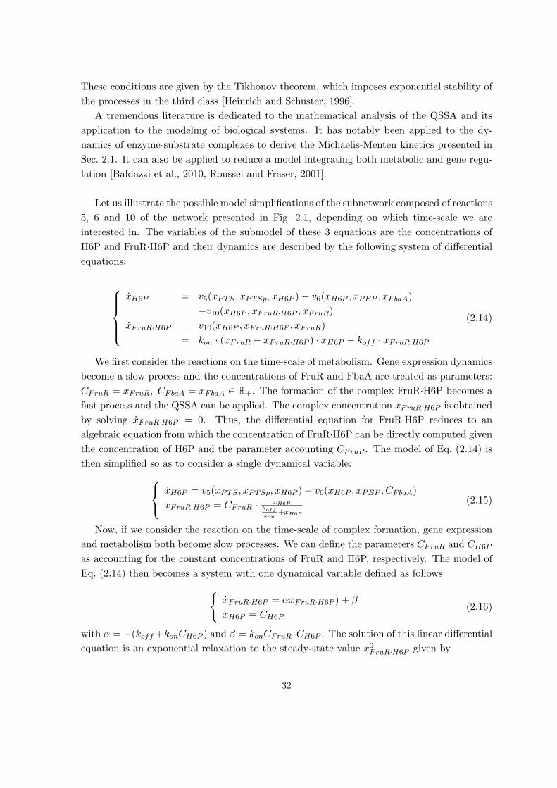
Let us illustrate the possible model simplifications of the subnetwork composed of reactions

5, 6 and 10 of the network presented in Fig. 2.1, depending on which time-scale we are

interested in. The variables of the submodel of these 3 equations are the concentrations of

H6P and FruR·H6P and their dynamics are described by the following system of differential

equations:

xH6P = v5(xPTS , xPTSp, xH6P )− v6(xH6P , xPEP , xFbaA)

−v10(xH6P , xFruR·H6P , xFruR)

xFruR·H6P = v10(xH6P , xFruR·H6P , xFruR)

= kon · (xFruR − xFruR·H6P ) · xH6P − koff · xFruR·H6P

(2.14)

We first consider the reactions on the time-scale of metabolism. Gene expression dynamics

become a slow process and the concentrations of FruR and FbaA are treated as parameters:

CFruR = xFruR, CFbaA = xFbaA ∈ R+. The formation of the complex FruR·H6P becomes a

fast process and the QSSA can be applied. The complex concentration xFruR·H6P is obtained

by solving xFruR·H6P = 0. Thus, the differential equation for FruR·H6P reduces to an

algebraic equation from which the concentration of FruR·H6P can be directly computed given

the concentration of H6P and the parameter accounting CFruR. The model of Eq. (2.14) is

then simplified so as to consider a single dynamical variable:

xH6P = v5(xPTS , xPTSp, xH6P )− v6(xH6P , xPEP , CFbaA)

xFruR·H6P = CFruR · xH6Pkoff

kon+xH6P

(2.15)

Now, if we consider the reaction on the time-scale of complex formation, gene expression

and metabolism both become slow processes. We can define the parameters CFruR and CH6P

as accounting for the constant concentrations of FruR and H6P, respectively. The model of

Eq. (2.14) then becomes a system with one dynamical variable defined as follows

{xFruR·H6P = αxFruR·H6P ) + β

xH6P = CH6P(2.16)

with α = −(koff+konCH6P ) and β = konCFruR ·CH6P . The solution of this linear differential

equation is an exponential relaxation to the steady-state value x0FruR·H6P given by

32

x0FruR·H6P = −β

α= CFruR · CH6P

koff

kon+ CH6P

(2.17)

Notice that this value is the same as Eq. (2.15). Therefore, the definition of the time-scale

of interest, and the resulting simplifications, do not alter the reduced model of the system in

this case.

2.2.2 Approximate kinetic models

The reaction rates v are nonlinear and generally complex functions of x, u, and e, with many

kinetic parameters that are difficult to reliably estimate from the data. This has motivated

the use of approximate rate functions, which can be obtained from mathematical approxima-

tion techniques, such as the Taylor series expansion [Alves et al., 2008]. We will present two

approximated representations of metabolic kinetics obtained in this way.

The first approximated model for v is the power-law formalism [Savageau, 1976]. This

formalism is a consequence of approximating the rate equation in logarithmic space using a

first-order Taylor series and then returning to Cartesian coordinates. For a metabolic reaction

of the form

X1 + · · ·+XsE−→ Xs+1 + · · ·+Xs+p , (2.18)

the power-law model of the kinetic rate boils down to

v = k · e ·s∏

i=1

xb0ii (2.19)

with k a rate constant, e the concentration of enzyme E, xi the concentration of substrate

Xi with i = 1, · · · , s, and b0i the local sensitivity of v to changes in Xi at a given operating

point (x0i , v0), defined by

b0i =

(∂v

∂xi

)

0

· x0i

v0(2.20)

In case that reaction (2.18) is reversible, the same approximation can be applied to the

reverse reaction and the rate v has the following form

v = k+ · e ·s∏

i=1

xb0ii − k− · e ·

s+p∏

j=s+1

xc0jj (2.21)

with k+, k− rate constants of the forward and reverse reactions, xj the concentration of prod-

uct Xj with j = s+1, · · · , s+ p and c0j the local sensitivity of the reverse rate v− to changes

in Xj at a given operating point (x0j , v0−).

33

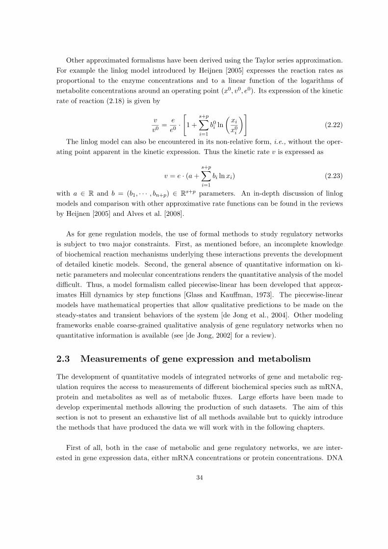
Other approximated formalisms have been derived using the Taylor series approximation.

For example the linlog model introduced by Heijnen [2005] expresses the reaction rates as

proportional to the enzyme concentrations and to a linear function of the logarithms of

metabolite concentrations around an operating point (x0, v0, e0). Its expression of the kinetic

rate of reaction (2.18) is given by

v

v0=

e

e0·[1 +

s+p∑

i=1

b0i ln

(xix0i

)](2.22)

The linlog model can also be encountered in its non-relative form, i.e., without the oper-

ating point apparent in the kinetic expression. Thus the kinetic rate v is expressed as

v = e · (a+

s+p∑

i=1

bi lnxi) (2.23)

with a ∈ R and b = (b1, · · · , bn+p) ∈ Rs+p parameters. An in-depth discussion of linlog

models and comparison with other approximative rate functions can be found in the reviews

by Heijnen [2005] and Alves et al. [2008].

As for gene regulation models, the use of formal methods to study regulatory networks

is subject to two major constraints. First, as mentioned before, an incomplete knowledge

of biochemical reaction mechanisms underlying these interactions prevents the development

of detailed kinetic models. Second, the general absence of quantitative information on ki-

netic parameters and molecular concentrations renders the quantitative analysis of the model

difficult. Thus, a model formalism called piecewise-linear has been developed that approx-

imates Hill dynamics by step functions [Glass and Kauffman, 1973]. The piecewise-linear

models have mathematical properties that allow qualitative predictions to be made on the

steady-states and transient behaviors of the system [de Jong et al., 2004]. Other modeling

frameworks enable coarse-grained qualitative analysis of gene regulatory networks when no

quantitative information is available (see [de Jong, 2002] for a review).

2.3 Measurements of gene expression and metabolism

The development of quantitative models of integrated networks of gene and metabolic reg-

ulation requires the access to measurements of different biochemical species such as mRNA,

protein and metabolites as well as of metabolic fluxes. Large efforts have been made to

develop experimental methods allowing the production of such datasets. The aim of this

section is not to present an exhaustive list of all methods available but to quickly introduce

the methods that have produced the data we will work with in the following chapters.

First of all, both in the case of metabolic and gene regulatory networks, we are inter-

ested in gene expression data, either mRNA concentrations or protein concentrations. DNA

34

microarrays are the most widely adopted technology for high-throughput measurements of

gene expression. The underlying principle of DNA microarrays is the complementary binding

property of mRNA. In a microarray, single-stranded DNA, acting as probes, are arrayed on

a solid substrate. RNA is extracted from a sample, fluorescently labeled, reverse-transcribed

and hybridized on the microarray, where the probes will capture their complementary la-

beled cDNAs. Thereby, the probes act as molecular sensors for quantitative measurements

and the intensity of fluorescence is a measure of the expression level of its targeted gene

[Dharmadi and Gonzalez, 2004, Crampin, 2006]. Many choices of DNA microarray platforms

and physical formats are available, such as cDNA microarrays or oligonucleotide microarrays

[Schena et al., 1995, Lockhart et al., 1996]. This approach enables the characterization of

gene expression at a genomic scale.

Microarrays have been extensively used to produce high-throughput datasets for the study

of bacterial systems, including E. coli. Notably, they have been used to report gene expres-

sion changes in response to specific stimuli from the environment, to provide insights into

specific transcriptional events and for genetic and metabolic engineering (see [Dharmadi and

Gonzalez, 2004] for a review). Oh et al. [2002] characterized the transcript profile of E. coli

in acetate cultures using DNA microarray on glass slides. As for using microarrays to look for

transcriptional regulation, reviews of microarray datasets for E. coli can be found in [Faith

et al., 2007, Park et al., 2005].

However DNA microarrays only return relative RNA concentration values computed from

a comparison with a control experiment. Other techniques have been developed to measure

absolute mRNA concentrations, such as quantitative PCR, but they do not generally allow

high-throughput measurements [Crampin, 2006] (see [White et al., 2011] for an exception).

Moreover, even if DNA microarray is the most used technology for gene expression measure-

ments (see [Meloni et al., 2004] and references therein), heterogeneity of experimental designs,

target preparation protocols and data analysis methods prevents a reliable comparison be-

tween available microarray data. [Dharmadi and Gonzalez, 2004]. Moreover, as microarray

technology necessitates to extract mRNA from a bacterial sample, measurements cannot be

made in vivo or used to assess individual cells.

The use of reporter genes for the measurement of gene expression allows the measurement

of promoter activity in vivo at high-temporal resolution. The technology is based on the

fusion of the promoter region of a gene of interest to a fluorescent or luminescent reporter

gene. The expression of the reporter gene generates a visible fluorescent or luminescent signal

that is easy to capture and reflects the expression of the gene of interest. These constructions

enable single-cell measurements, which helps probing key biological phenomena in individual

living cells [Longo and Hasty, 2006]. Moreover, the GFP protein has been modified to produce

blue, cyan, yellow and red fluorescent proteins, making it possible to study the expression of

multiple genes in the same cell.

Data analysis requires precise information on half life of signal proteins, be it fluorescent

35

or luminescent, and plasmids used [de Jong et al., 2010]. The reporter gene can be expressed

from a (low-copy) plasmid or integrated into the chromosome. Using a plasmid enables an

easier construction and emphasizes the signal intensity, which can be very close to back-

ground when reporter genes are placed on the chromosome. However, reporter plasmids can

introduce bias in the signal as their copy number in the cell can vary depending on experi-

mental conditions [Lin-Chao and Bremer, 1986]. This bias can be quantitatively monitored

by measuring the copy number of reporter plasmids using qRT-PCR technology [Lee et al.,

2004, Chen et al., 2005].

Several examples of the real-time quantification of gene expression in E. coli using re-

porter genes have been reported in the literature. For example, Ronen et al. [2002] and Dyk

et al. [2001] used fluorescent and luminescent reporter genes to investigate the DNA damage

response. Kalir et al. [2005] analyzed the feed-forward loop motif of flagella gene-regulation

network, the system that allows the bacteria to swim. And recently, a high-throughput li-

brary of fluorescent reporter genes has been constructed for E. coli and enabled the discovery

of new transcription units [Zaslaver et al., 2006].

Although transcription profiling by microarrays or reporter genes delivers valuable mRNA

concentration patterns, a systematic post-genomic approach which describes the overall state

of a biological system is an important supplement to transcriptome analysis. Methods for

high-throughput measurement of protein abundance such as liquid chromatography tandem

mass spectrometry (LC-MS/MS) and 2D fluorescence difference gel electrophoresis have been

developed [Gstaiger and Aebersold, 2009, Marouga et al., 2005]. These methods have been

widely applied to study the proteome of E. coli. For example, combined analyses of tran-

scriptome and proteome were performed to investigate the effects of recombinant protein

production on metabolic enzymes [Durrschmid et al., 2008] and to understand metabolic and

physiological changes during high cell-density cultivation [Yoon et al., 2003].

The measurement of changes in intracellular metabolite concentrations reveals an aspect of

regulation that cannot be studied by measuring changes in mRNA or protein concentrations

only [Vemuri and Aristidou, 2005]. Metabolomics draws on a range of analytical platforms

including mass spectrometry (MS) and chromatography- and electrophoresis-based separation

methods. The popular technologies for the identification and quantification of metabolites are

a combination of gas (or liquid) chromatography and mass spectrometry called GC-MS (or

LC-MS) or capillary electrophoresis and mass spectrometry called CE-MS (see [Villas-Boas

et al., 2005, Monton and Soga, 2007] for reviews).

It is not currently possible to quantify all intracellular metabolites in a cell due to the lack

of a robust, automated and reproducible analytical technique. Thus, metabolomics, in the

strictest sense, is practically impossible, and the term is used broadly to cover approaches

concerned with investigating subsets of the metabolome.

These methods have been applied to the metabolome analysis of E. coli. Examples include

36

the profiling of bacterial metabolites [Jia et al., 2005], the quantification of changes in central

carbon metabolism under different growth conditions and for different mutant strains [Ishii

et al., 2007] or the effect of the lpdA gene knockout on metabolism [Li et al., 2006]. More

recently, the LC-MS/MS method was used to compute absolute metabolite concentrations

during growth on glucose [Bennett et al., 2009] and a combination of transcriptomic and

metabolomic data was analyzed to investigate gene and metabolic regulatory interactions

during stress response [Jozefczuk et al., 2010].

When it comes to the study of dynamics of a complex network, genomic or proteomic data

are not sufficient as they do not contain full information on the functional behaviour of the

network. The network response is also characterized by changing metabolic fluxes through

the network, which can be computed with 13C-based flux analysis. 13C-labeled substrates are

introduced into the growing medium and metabolized by the cell population until the isotope

label is distributed throughout the network. Then mass spectrometry detects the isotopic

carbon in amino acids and from those data and a stoichiometric model of metabolic network,

the flux distribution is computed [Sauer, 2006].13C-labeled flux analysis has been intensively applied to microbes, and to E. coli in par-

ticular, to determine the phenotypic effects of structural changes in the metabolic network,

providing direct evidence for the nature and extent of the mechanisms that compensate the

effects of perturbations. For example, Nicolas et al. [2007] studied the redistribution of cen-

tral metabolic fluxes when the zwf gene, which codes the enzyme catalyzing the production

of 6PG from G6P, was deleted. To study the consequences of lpdA gene knockout on the

metabolism, Li et al. [2006] used both metabolite concentration measurements and flux anal-

ysis. More recently, van Rijsewijk et al. [2011] provided insights in the transcriptional control

of carbon metabolism when bacteria grow on glucose and on galactose using GC-MS-detected

mass isotope partitioning.

2.4 Parameter estimation of kinetic models

Parameter estimation is an important step in the process of developing data-driven models

for biological systems with a predicted value. To compare a model with experimental data,

the mathematical model has to be simulated. Then, model parameters can be estimated from

measured observations [Ashyraliyev et al., 2009]. Typically, parameter estimation starts with

a guess about parameter values and then changes them to minimize an objective function,

defined by the modeler. A usual objective function is the discrepancy between model and

data using a particular metric. To estimate these parameters, optimization methods have

been developed, depending on the nature of the estimation problem.

Here, we focus on parameter estimation in the case of dynamical ODE models of biochem-

ical species discussed in Sec. 2.1. Recall that these models have the following form:

37

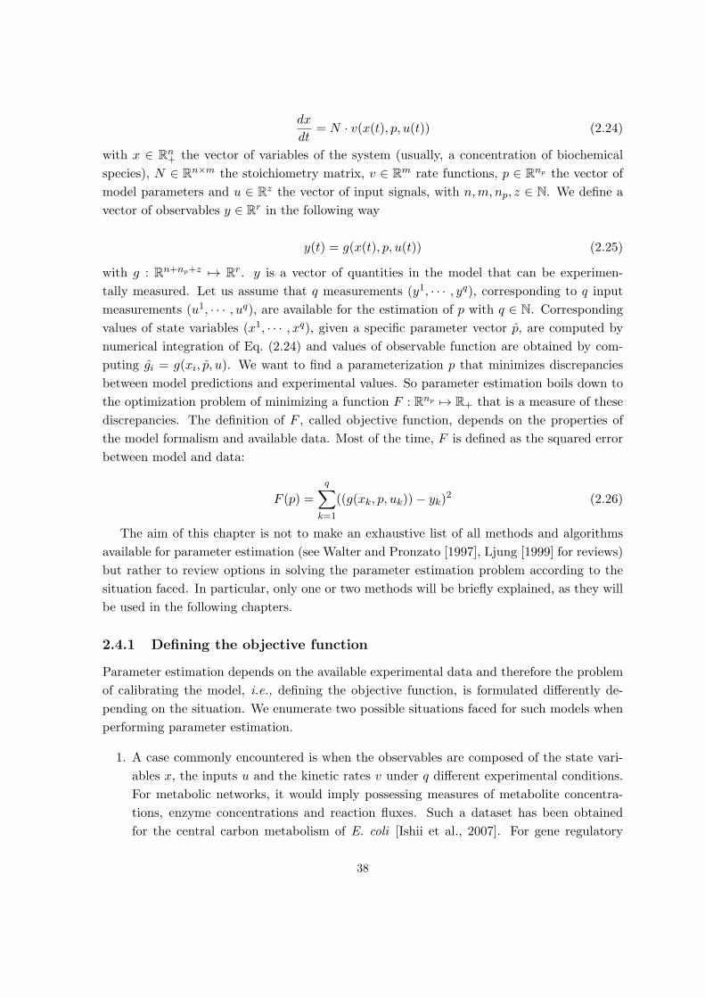
dx

dt= N · v(x(t), p, u(t)) (2.24)

with x ∈ Rn+ the vector of variables of the system (usually, a concentration of biochemical

species), N ∈ Rn×m the stoichiometry matrix, v ∈ R

m rate functions, p ∈ Rnp the vector of

model parameters and u ∈ Rz the vector of input signals, with n,m, np, z ∈ N. We define a

vector of observables y ∈ Rr in the following way

y(t) = g(x(t), p, u(t)) (2.25)

with g : Rn+np+z 7→ Rr. y is a vector of quantities in the model that can be experimen-

tally measured. Let us assume that q measurements (y1, · · · , yq), corresponding to q input

measurements (u1, · · · , uq), are available for the estimation of p with q ∈ N. Corresponding

values of state variables (x1, · · · , xq), given a specific parameter vector p, are computed by

numerical integration of Eq. (2.24) and values of observable function are obtained by com-

puting gi = g(xi, p, u). We want to find a parameterization p that minimizes discrepancies

between model predictions and experimental values. So parameter estimation boils down to

the optimization problem of minimizing a function F : Rnp 7→ R+ that is a measure of these

discrepancies. The definition of F , called objective function, depends on the properties of

the model formalism and available data. Most of the time, F is defined as the squared error

between model and data:

F (p) =

q∑

k=1

((g(xk, p, uk))− yk)2 (2.26)

The aim of this chapter is not to make an exhaustive list of all methods and algorithms

available for parameter estimation (see Walter and Pronzato [1997], Ljung [1999] for reviews)

but rather to review options in solving the parameter estimation problem according to the

situation faced. In particular, only one or two methods will be briefly explained, as they will

be used in the following chapters.

2.4.1 Defining the objective function

Parameter estimation depends on the available experimental data and therefore the problem

of calibrating the model, i.e., defining the objective function, is formulated differently de-

pending on the situation. We enumerate two possible situations faced for such models when

performing parameter estimation.

1. A case commonly encountered is when the observables are composed of the state vari-

ables x, the inputs u and the kinetic rates v under q different experimental conditions.

For metabolic networks, it would imply possessing measures of metabolite concentra-

tions, enzyme concentrations and reaction fluxes. Such a dataset has been obtained

for the central carbon metabolism of E. coli [Ishii et al., 2007]. For gene regulatory

38

networks, measurements of growth rate, protein concentrations and promoter activities

would be available, for instance as time series of fluorescent signal. With an appropri-

ate data analysis, data about protein concentrations and promoter activities (synthesis

rates of mRNA) can be computed [de Jong et al., 2010].

Let us call xk ∈ Rn+, u

k ∈ Rz+ and vk ∈ R

m, with k = 1, · · · , q, the measurements

of variables, inputs and kinetic rates. The experimental conditions for the production

of the q datapoints may vary. Datasets may be composed of steady-state or time-

series measurements. In the first case, each datapoint k is obtained for different genetic

backgrounds or under different environmental conditions. In the second case, each

measurement k is associated to tk, the timepoint at which the measurement was taken.

Regardless of the experimental conditions, the parameter estimation problem is for-

mulated as finding a solution in p for an algebraic system composed of the following

equations

vk = v(xk, uk, p) (2.27)

with k = 1, · · · , q. Thus, by defining the observables of the system as the kinetic rates

(y = g(x, p, u) = v(x, p, u)), the objective function of this parameter estimation problem

becomes

F (p) =

q∑

k=1

(vk − v(xk, p, uk))2. (2.28)

2. We also face situations where only data about the variables of the system and the

inputs are available. In that case, we can define the vector of observables as the vector

of variables, y = x and the objective function becomes

F (p) =

q∑

k=1

(xk − x(uk, p))2. (2.29)

The computation of F for a given parameter vector p requires the integration of the

ODE system (2.24) in order to calculate x given p and the input uk.

2.4.2 Minimizing the objective function

The optimization problem of minimizing F depends on the form of the observable function

g(x, p, u). In case that g is linear in the parameters, one can use linear regression to find the

optimal p. Indeed, the observable g(x, p, u) can be reformulated as

g(x, p, u) = a(x, u) + b1(x, u) · p1 + · · ·+ bnp(x, u) · pnp

(2.30)

39

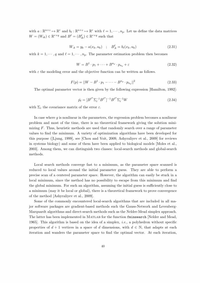
with a : Rn+z 7→ Rr and bℓ : R

n+z 7→ Rr with ℓ = 1, · · · , np. Let us define the data matrices

W = (Wik) ∈ Rr×q and Bℓ = (Bℓ

ik) ∈ Rr×q such that

W.k = yk − a(xk, uk) ; Bℓ.k = bℓ(xk, uk) (2.31)

with k = 1, · · · , q and ℓ = 1, · · · , np. The parameter estimation problem then becomes

W = B1 · p1 + · · ·+Bnp · pnp+ ε (2.32)

with ε the modeling error and the objective function can be written as follows.

F (p) = ||W −B1 · p1 − · · · −Bnp · pnp||2 (2.33)

The optimal parameter vector is then given by the following expression [Hamilton, 1992]:

pℓ = [BℓTΣ−1ε BℓT ]−1BℓTΣ−1ε W (2.34)

with Σε the covariance matrix of the error ε.

In case where g is nonlinear in the parameters, the regression problem becomes a nonlinear

problem and most of the time, there is no theoretical framework giving the solution mini-

mizing F . Thus, heuristic methods are used that randomly search over a range of parameter

values to find the minimum. A variety of optimization algorithms have been developed for

this purpose ([Ljung, 1999], see [Chou and Voit, 2009, Ashyraliyev et al., 2009] for reviews

in systems biology) and some of them have been applied to biological models [Moles et al.,

2003]. Among them, we can distinguish two classes: local-search methods and global-search

methods.

Local search methods converge fast to a minimum, as the parameter space scanned is

reduced to local values around the initial parameter guess. They are able to perform a

precise scan of a centered parameter space. However, the algorithm can easily be stuck in a

local minimum, since the method has no possibility to escape from this minimum and find

the global minimum. For such an algorithm, assuming the initial guess is sufficiently close to

a minimum (may it be local or global), there is a theoretical framework to prove convergence

of the method [Ashyraliyev et al., 2009].

Some of the commonly encountered local-search algorithms that are included in all ma-

jor software packages are gradient-based methods such the Gauss-Network and Levenberg-

Marquardt algorithms and direct-search methods such as the Nelder-Mead simplex approach.

The latter has been implemented in Matlab for the function fminsearch [Nelder and Mead,

1965]. This algorithm is based on the idea of a simplex, i.e., a polyhedron without specific

properties of d + 1 vertices in a space of d dimensions, with d ∈ N, that adapts at each

iteration and wanders the parameter space to find the optimal vector. At each iteration,

40

the objective function is evaluated at each vertex and the one giving the highest objective

function, i.e., the worst one, is deleted. Its replacement is searched on the line formed by

this former vertex and the center of the remaining vertices.

To avoid the problem of being stuck in a local minimum, global-search methods that

search over the entire parameter space to find increasingly smaller values for F have been

developed. In general, there is no proof of convergence for these methods [Ashyraliyev et al.,

2009]. Several search strategies have been developed, taking inspiration from other scientific

domains.

For example, simulated annealing is inspired by the physical process of heating up a

solid until it melts and slowly cooling it down until the molecules are aligned in a crystalline

structure corresponding to the minimum energy state [Kirkpatrick et al., 1983]. Evolutionary

algorithms, such as genetic algorithms or evolutionary strategies, are inspired by concepts of

biological evolution such as reproduction, mutation and selection, to produce an optimized

parameter vector [Beyer and Schwefel, 2002]. First, an initial population of possible parameter

vectors, whose size is specified by the modeler, is defined. Part of the population is selected to

form the parents of a new generation. A population of children, whose values are computed

from recombination of values of random parents, is created. Each child can be mutated, i.e.,

its values can be altered based on mutation strategies. Finally, the parameter vectors that

return the lowest objective function values are selected among the old and new generations to

create the next generation. This process is iterated until some convergence criterion, defined

by the modeler and usually based on the change of objective function between estimates, is

reached.

One major drawback of global-search algorithms is their convergence speed, which is in

general much lower than for local-search methods. Usually, users define a time limit when they

run these algorithms. Another strategy is to combine both types of optimization algorithms

and use hybrid methods. Indeed, first a global-search algorithm can be used to scan efficiently

the range of possible parameter values to find the area with the global minimum. Then, a

local-search algorithm can be applied with the parameter vector obtained by the global-search

method as initial vector to perform a more precise scan of the promising area. These hybrid

methods have shown better results than global- or local-search methods alone and faster

computation [Rodriguez-Fernandez et al., 2006].

In the case where the computation of F requires integration of the ODE system, the opti-

mization procedure of minimizing Eq. (2.29) is very demanding on the computational level,

as at each iteration of the optimization algorithm, an ODE system has to be solved. One may

thus encounter extreme computational lengths or numerical issues that practically prevent

the parameter estimation to be performed.

Another situation not yet mentioned is the case where not all observables have been

measured for all experimental conditions. Due to this lack of data, parameter estimation

41

problem gets trickier as the objective function defined as in Eq. (2.28) or Eq. (2.29) cannot

be computed. One way to overcome this difficulty is to estimate the missing values of the

dataset. Some methods for missing data imputation have been developed [Oba et al., 2003,

Scholz et al., 2005, Rubin, 1976], enabling the computation of the objective function as defined

in the previous section and the use of optimization algorithms just described. Alternatively,

Expectation-Maximization is an iterative method that minimizes the least-square error by

maximizing an intermediary function which is recomputed at each iteration [Dempster et al.,

1977]. This method does not require values for missing data. We will present it in detail in

Chap. 3.

2.5 Quantitative modeling of growth transitions in E. coli

In this section, we list quantitative models of growth transitions in E. coli published in

the literature. We will mainly talk about continuous models, but other types of modeling

frameworks such as logic-based or flux balance analysis are reviewed in [Tenazinha and Vinga,

2011, Bulik et al., 2011].

Central carbon metabolism of E. coli has been extensively studied. More particularly,

several quantitative models of this network using kinetic formalisms such as those described

in Sec. 2.1 have been developed. Chassagnole et al. [2002] have first developed a quanti-

tative dynamical model of glycolysis and the pentose-phosphate pathway. They validated

this model with metabolite concentrations that they measured at transient conditions and

showed, using metabolic control analysis, that the flux control during glucose uptake was

shared by the PTS system and enzymes degrading PTS inhibitors. Bettenbrock et al. [2006]

investigated this question and modeled dynamically the uptake of glucose, lactose, glycerol,

sucrose and galactose. They quantitatively predicted the behaviour of catabolite repression,

i.e, the system that prevents uptake of other carbon sources when glucose is available, and

validated it on metabolite and enzyme concentrations that they measured in different growth

situations. Moreover, Kremling et al. [2007] highlighted, by means of a quantitative model of

the PTS, the relationship between the bacterial growth rate and the phosphorylation state of

an element of the PTS. Both in the last two examples, the authors estimated the parameters

and discussed the choices of kinetic formalisms. The systems of carbohydrate uptake involve

signalling metabolites as well as enzymes and regulation by transcription factors, such as

Crp. Thus, the models of this system, which are reviewed in [Kremling et al., 2009] combine

metabolic and gene regulations.

More recently, Kotte et al. [2010] have considered a simplified network of glycolysis and

the Krebs cycle and extended it to take gene regulation of metabolic enzymes into account.

They developed a quantitative model with Monod-Wyman-Changeux, Hill and Michaelis-

Menten kinetics and estimated the parameters from published steady-state data. With their

model, they were able to reproduce the flux inversion between glycolysis and gluconeogenesis

42

that occurs during the glucose/acetate diauxie. Usuda et al. [2010] also looked at an inte-

grated network by considering glycolysis, the pentose-phosphate pathway, the Krebs cycle,

the glyoxylate shunt and anaplerotic pathways as well as transcription factors involved in the

regulation of catabolic enzymes. Their model used Michaelis-Menten kinetics, was calibrated

with parameter estimation and was validated on metabolite concentrations that they mea-

sured on wild-type and glutamate-producing strains. Note that in these last two examples,

gene regulation kinetics were described as being dependent to the bacterial growth rate.

There exists also quantitative models of such networks that were developed using the

approximate kinetic formalisms introduced in Sec. 2.2.2. For the linlog formalism, simulation

studies on the level of both individual enzymatic reactions [Heijnen, 2005] and metabolic

networks [Hadlich et al., 2009] have shown that they provide reasonable approximations

of classical enzymatic rate laws. Moreover, Visser et al. [2004] developed a linlog model

of glycolysis and validated the dynamical predictions by comparing them to a complete

mechanistic model. With the help of a recent genome-scale linlog model of yeast metabolism,

parametrized using previously-published kinetic models, it has been possible to identify key

steps in the network, that is, reactions exerting most control over glucose transport and

biomass production [Smallbone et al., 2010]. Moreover, Hardiman et al. [2009] have presented

a model of a network combining metabolism and gene regulation with linlog kinetics. As for

other approximate formalisms, models of metabolic networks using power-law kinetics mixed

with Petri Nets have also been developed [Wu and Voit, 2009].

It is also possible to mix different kinetic formalisms in quantitative modeling. Costa

et al. [2010] studied the predictive performances of a model of the central carbon metabolism

using a mix of Michaelis-Menten and approximate kinetics. They found out that the linlog

model, combined with Michaelis-Menten, was the most efficient. A review of models with

hybrid kinetics of regulatory networks from other organisms than E. coli can be found in

[Bulik et al., 2009].

Finally, we mention the existence of qualitative studies of the dynamics of the metabolic

and gene regulation networks during growth transitions. Ropers et al. [2006] developed

a piecewise-linear model to investigate the dynamics of the network formed by the global

regulators of E. coli during glucose exhaustion. Baldazzi et al. [2012] extended the network

of global regulators so as to consider the glycolytic pathway as well. They show, by the

comparison of predictions of different piecewise-linear models to steady-state data of enzyme

and metabolite concentrations under growth on glucose and acetate, that interactions between

metabolism and gene regulation are essential to describe the adaptation of gene expression

during diauxie. Other examples of gene regulatory models can be found in the review by

Karlebach and Shamir [2008].

43

Chapter 3

Parameter estimation of linlog

metabolic models

We focus in this chapter on the modeling of central carbon metabolism of E. coli shown

in Fig. 1.5 and described in Sec. 1.3.1. This network has been studied for a long time

from different perspectives. A rather precise idea of the structure of the network exists and

several kinetic models of the network dynamics are available ([Bettenbrock et al., 2006, Kotte

et al., 2010] and references therein). Moreover, a high-throughput dataset gathering required

information for parameter estimation has recently been published [Ishii et al., 2007].

The usefulness of approximate kinetic laws for the mathematical formalism of the metabolic

model has been presented before in Chaps. 1 and 2. Linlog models are a particularly inter-

esting choice for modeling metabolism [Heijnen, 2005, Visser and Heijnen, 2003]. A major

advantage of linlog models is that, when measurements of fluxes, enzyme concentrations, and

metabolite concentrations are available, the parameter estimation problem reduces to multiple

linear regression [Nikerel et al., 2006]. Power-law models, up to a logarithmic transformation,

and loglin models also have this convenient property. However, in all of the above formalisms,

the performance of regression approaches quickly degrades in the presence of missing data, as

is often the case in high-throughput datasets due to experimental limitations or instrument

failures.

In order to deal with this problem, we propose in this chapter a maximum-likelihood

method for the identification of linlog models of metabolism from incomplete datasets.

3.1 Parameter estimation in linlog models

We recall that the dynamics of metabolic networks are described by kinetic models having

the form of systems of ordinary differential equations (ODEs) [Heinrich and Schuster, 1996]:

x = N · v(x, u, e) (3.1)

44

where x ∈ Rnx

+ denotes the vector of (nonnegative) internal metabolite concentrations,

u ∈ Rnu

+ the vector of external metabolite concentrations, e ∈ Rm+ the vector of enzyme

concentrations, and v : Rnx+nu+m+ → R

m the vector of reaction rate functions. N ∈ Znx×m

is a stoichiometry matrix. As mentioned in Sec. 2.2.2, the complexity and non-linearity of

v stimulate the use of approximate kinetic laws. The linlog approximation leads to the rate

equation

v(x, u, e) = diag(e) ·(a+Bx · lnx+Bu · lnu

)(3.2)

where diag(e) is the square diagonal matrix with the elements of e on the diagonal, and the

logarithm of a vector means the vector of logarithms of its elements. For conciseness, in the

sequel we shall drop the dependence of v on (x, u, e) from the notation.

The identification of metabolic networks in the linlog formalism amounts to estimating

the (generally unknown) parameters a ∈ Rm, Bx ∈ R

m×nx and Bu ∈ Rm×nu from q ex-

perimental datapoints (vk, xk, uk, ek), k = 1, . . . , q. That is, the data used for parameter

estimation are parallel measurements of enzyme and metabolite levels as well as metabolic

fluxes. The datapoints (vk, xk, uk, ek) are obtained under different experimental conditions,

for instance different dilution rates in continuous cultures or different mutant strains. Notice

that in practice reaction rates are most of the time measured at (quasi-)steady state (see also

Sec. 3.5). That is, on the time-scale of interest the derivatives of metabolite concentrations

vanish and Eq. (3.1) can be rewritten as N · v = 0.

For the purpose of parameter estimation, it is convenient to rewrite (3.2) in the form of a

regression model:

(ve

)T= [1 lnxT lnuT ] ·

aT

(Bx)T

(Bu)T

(3.3)

where the ratio of two vectors (here v/e) denotes element-wise division. Let us use an

upperbar to denote the mean of a quantity over its q experimental observations, for instance:

v/e = (1/q)∑q

k=1 vk/ek. By the linearity of (3.3), it holds that

(ve

)= [1 lnx

Tlnu

T] ·

aT

(Bx)T

(Bu)T

. (3.4)

This allows (3.3) to be reformulated as a mean-removed model

(v

e−(ve

))T

=

[lnx− lnx

lnu− lnu

]T·[(Bx)T

(Bu)T

](3.5)

and we obtain the following parameter estimation problem:

45

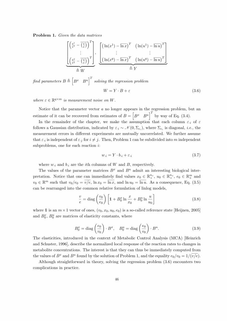
Problem 1. Given the data matrices

(v1

e1 −(ve

))T

...(vq

eq −(ve

))T

︸ ︷︷ ︸, W

,

(ln(x1)− lnx

)T (ln(u1)− lnu

)T...

...(ln(xq)− lnx

)T (ln(uq)− lnu

)T

︸ ︷︷ ︸, Y

find parameters B ,

[Bx Bu

]Tsolving the regression problem

W = Y ·B + ε (3.6)

where ε ∈ Rq×m is measurement noise on W .

Notice that the parameter vector a no longer appears in the regression problem, but an

estimate of it can be recovered from estimates of B =[Bx Bu

]Tby way of Eq. (3.4).

In the remainder of the chapter, we make the assumption that each column ε·i of ε

follows a Gaussian distribution, indicated by ε·i ∼ N (0,Σεi), where Σεi is diagonal, i.e., the

measurement errors in different experiments are mutually uncorrelated. We further assume

that ε·i is independent of ε·j for i 6= j. Then, Problem 1 can be subdivided intom independent

subproblems, one for each reaction i:

w·i = Y · b·i + ε·i (3.7)

where w·i and b·i are the ith columns of W and B, respectively.

The values of the parameter matrices Bx and Bu admit an interesting biological inter-

pretation. Notice that one can immediately find values x0 ∈ Rnx

+ , u0 ∈ Rnu

+ , e0 ∈ Rm+ and

v0 ∈ Rm such that v0/e0 = v/e, lnx0 = lnx, and lnu0 = lnu. As a consequence, Eq. (3.5)

can be rearranged into the common relative formulation of linlog models,

v

e= diag

(v0e0

)[1+Bx

0 lnx

x0+Bu

0 lnu

u0

](3.8)

where 1 is an m×1 vector of ones, (v0, x0, u0, e0) is a so-called reference state [Heijnen, 2005]

and Bx0 , B

u0 are matrices of elasticity constants, where

Bx0 = diag

(e0v0

)·Bx, Bu

0 = diag

(e0v0

)·Bu. (3.9)

The elasticities, introduced in the context of Metabolic Control Analysis (MCA) [Heinrich

and Schuster, 1996], describe the normalized local response of the reaction rates to changes in

metabolite concentrations. The interest is that they can thus be immediately computed from

the values of Bx and Bu found by the solution of Problem 1, and the equality e0/v0 = 1/(v/e).

Although straightforward in theory, solving the regression problem (3.6) encounters two

complications in practice.

46

1. Since the measurements are carried out at (quasi-)steady state, we haveN ·v(x, u, e) = 0.

This introduces dependencies among the data and thus reduces the information content

of the data matrix Y , in the sense that Y becomes rank deficient. Like in earlier

work [Nikerel et al., 2009], we use standard approaches to solve this problem. We

notably rely on Principal Component Analysis (PCA) [Jolliffe, 1986, Nikerel et al., 2009]

applied to the data matrix Y to reduce the model order, i.e., the number of independent

parameters, and ensure well-posedness of the regression problem. Identifiability analysis

will be discussed in detail in Chap. 4.

Briefly, we use Singular Value Decomposition (SVD), a technique decomposing the data

matrix into dominant and marginal components according to a variance criterion. For

the purpose of linear regression, this corresponds to decomposing the parameter vector

into a reduced number of components that can be determined with certainty based on

the data, while the remaining components are poorly determined, i.e., they are ‘non-

identifiable’, and are discarded with negligible effect on the fit. We note in passing that

the columns of W and Y are zero-mean, an important requirement for the correctness

of the outlined analysis.

2. The high-throughput datasets contain a substantial amount of missing values, due to

experimental limitations or instrument failures. If, for any given reaction, we only used

the datapoints in which all relevant metabolite concentrations, enzyme concentrations,

and metabolic fluxes playing a role in that reaction are available, then a large amount

of data would have to be thrown away. In practice, we would run the risk that the

parameters cannot be reliably identified. The development of a method that is capable

of maximally exploiting the information contained in incomplete datasets for solving

Problem 1 is the main subject of this chapter and will be fully developed in the later

sections.

3.2 Likelihood-based identification of linlog models from miss-

ing data

For every reaction i, we are concerned with the problem of estimating the unknown param-

eters b·i of the model given in (3.7) in the case where some entries of Y are unknown. We

address the estimation problem by a likelihood-maximization approach, which is known to

yield optimal (unbiased and minimum variance) estimates for our problem setting in the case

where Y is fully known. As the problem is identical for all reactions i, in the remainder of

the section we will drop for simplicity index ·i from the notation.

Let I be the set of indices (row, column) corresponding to the known entries of Y , i.e.,

(j, k) ∈ I if and only if Yj,k is available. It is convenient to introduce the decomposition

47

Y = Y + Y , where

Yj,k =

Yj,k, if (j, k) ∈ I ,

0, otherwise;Yj,k =

0, if (j, k) ∈ I ,

Yj,k, otherwise.

Matrix Y is fully determined: Once measurements y of Y are collected, we treat Y = y as fixed

parameters of the regression problem. Matrix Y collects the unknown entries of Y . We model

these missing data as unobserved independent random variables, whose prior distributions

encode our generic knowledge about them. Assuming that the a-priori distributions are

not known (worst case), we define a Gaussian prior for each quantity that is missing in an

experiment based on the measurements of the same quantity available from other experiments.

For every (j, k) 6∈ I and Yj,k = {Yj′,k : (j′, k) ∈ I } (assumed nonempty), we let

Yj,k ∼ N (µj,k, σ2j,k),

µj,k = mean(Yj,k),

σj,k = std(Yj,k).

(3.10)

We can now formulate the estimation problem.

Problem 2. Given measurements W = w and Y = y, compute the estimate b = argmaxb logL (b),

with L (b) = fW |y,b(w), where, for any b, fW |y,b(·) is the probability density function of W

given Y = y corresponding to model (3.7)–(3.10).

Note that L (b) is a likelihood function for a linear model with missing data, in the

sense that it is defined with respect to available data Y only. One can express L (b) by

marginalization,

logL (b) = log

∫fW |y,y,b(w)fY |y,b(y)dy (3.11)

where fW |y,y,b(·) is the standard likelihood function for model (3.7) given Y = y and y, with

y varying over all possible values of Y , and fY |y,b is determined by the prior (3.10). The

explicit solution to the integral and the technical details of its computation are reported in

Appendix A.1. A direct approach to solving Problem 2 is to maximize (3.11) by numerical

optimization. However, the function is not convex in b, whence its direct optimization is

prone to end up in local minima and the use of global optimization strategies is required.

Alternatively, we propose to tackle Problem 2 by an Expectation-Maximization (EM) al-

gorithm [Dempster et al., 1977]. EM provides a general methodology for the optimization of

a likelihood function with missing information. It is based on an iterative two-step procedure

that, for the problem at hand, we implement as follows. Let us define the random variable

Z = Y ·b, so that model (3.7) becomes W = Y ·b+Z+ε. Note that Z ∼ N (µy,b,Σy,b), where

for any given b, mean and variance can be derived from (3.10). Let b0 be an initial guess of

b. At every iteration ℓ = 1, 2, 3, . . ., compute an updated estimate bℓ from the estimate bℓ−1

at the previous iteration by performing the following EM steps:

48

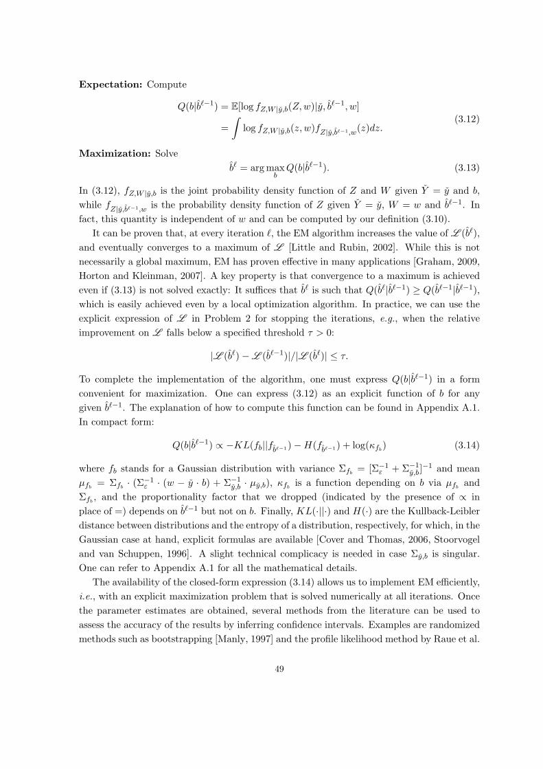
Expectation: Compute

Q(b|bℓ−1) = E[log fZ,W |y,b(Z,w)|y, bℓ−1, w]

=

∫log fZ,W |y,b(z, w)fZ|y,bℓ−1,w(z)dz.

(3.12)

Maximization: Solve

bℓ = argmaxb

Q(b|bℓ−1). (3.13)

In (3.12), fZ,W |y,b is the joint probability density function of Z and W given Y = y and b,

while fZ|y,bℓ−1,w is the probability density function of Z given Y = y, W = w and bℓ−1. In

fact, this quantity is independent of w and can be computed by our definition (3.10).

It can be proven that, at every iteration ℓ, the EM algorithm increases the value of L (bℓ),

and eventually converges to a maximum of L [Little and Rubin, 2002]. While this is not

necessarily a global maximum, EM has proven effective in many applications [Graham, 2009,

Horton and Kleinman, 2007]. A key property is that convergence to a maximum is achieved

even if (3.13) is not solved exactly: It suffices that bℓ is such that Q(bℓ|bℓ−1) ≥ Q(bℓ−1|bℓ−1),which is easily achieved even by a local optimization algorithm. In practice, we can use the

explicit expression of L in Problem 2 for stopping the iterations, e.g., when the relative

improvement on L falls below a specified threshold τ > 0:

|L (bℓ)− L (bℓ−1)|/|L (bℓ)| ≤ τ.

To complete the implementation of the algorithm, one must express Q(b|bℓ−1) in a form

convenient for maximization. One can express (3.12) as an explicit function of b for any

given bℓ−1. The explanation of how to compute this function can be found in Appendix A.1.

In compact form:

Q(b|bℓ−1) ∝ −KL(fb||fbℓ−1)−H(fbℓ−1) + log(κfb) (3.14)

where fb stands for a Gaussian distribution with variance Σfb = [Σ−1ε + Σ−1y,b]−1 and mean

µfb = Σfb · (Σ−1ε · (w − y · b) + Σ−1y,b · µy,b), κfb is a function depending on b via µfb and

Σfb , and the proportionality factor that we dropped (indicated by the presence of ∝ in

place of =) depends on bℓ−1 but not on b. Finally, KL(·||·) and H(·) are the Kullback-Leibler

distance between distributions and the entropy of a distribution, respectively, for which, in the

Gaussian case at hand, explicit formulas are available [Cover and Thomas, 2006, Stoorvogel

and van Schuppen, 1996]. A slight technical complicacy is needed in case Σy,b is singular.

One can refer to Appendix A.1 for all the mathematical details.

The availability of the closed-form expression (3.14) allows us to implement EM efficiently,

i.e., with an explicit maximization problem that is solved numerically at all iterations. Once

the parameter estimates are obtained, several methods from the literature can be used to

assess the accuracy of the results by inferring confidence intervals. Examples are randomized

methods such as bootstrapping [Manly, 1997] and the profile likelihood method by Raue et al.

49

[2009]. This method derives confidence intervals using a threshold on a function called the

profile likelihood. In our application, this is obtained separately for each parameter bj by re-

maximization of (3.11) with respect to all parameters bk 6=j , for all values bj in a neighborhood

of bj .

3.3 Validation on simulated data

Before applying the EM algorithm to actual biological identification problems, we test the

performance of the method on simulated data. For this purpose, a synthetic model has been

developed, a simplified variant of the linlog model of E. coli central metabolism studied in

Sec. 3.4 below. The model, in the form (3.2), contains 17 variables, representing internal

and external metabolites involved in 25 reactions, and 78 parameters. The model equations

are presented in Appendix A.2. We generate data matrices Y from this model by means

of simulation, for different percentages of missing data and experimental noise. Using the

model structure and the simulated data, we solve Problem 1 for each reaction independently,

as described in Sec. 3.2.

In order to assess the added value of our specific implementation of likelihood optimization,

we first compare the performance of the EM algorithm of Sec. 3.2 with the direct maximization

of the loglikelihood (3.11) implemented with a general-purposeMatlab optimization routine.

This method will be referred to as MaxLL in the sequel.

Second, we compare the likelihood-based identification approaches with standard methods,

notably linear regression (referred to as Rg) and the commonly-used multiple imputation (MI)

method [Rubin, 1976, 1996]. Regression is performed based on full datasets only, i.e., it does

not consider an experimentally-determined datapoint (vk, xk, uk, ek) when at least one of the

measurements is missing. MI is based on imputation of missing data by random draws of

the missing values, i.e., non-zero elements of Y , from the a-priori distribution defined in

(3.10). Both methods thus exploit only part of the information contained in an incomplete

dataset and provide a lower limit for quantifying the performance of the methods proposed

in Sec. 3.2.

Third, we compare the results of EM with the least-squares identification of the model on

complete datasets (a method referred to as RgF, where F stands for Full datasets). Though

inapplicable to real data with missing measurements, the method is statistically optimal.

Hence, it provides us an upper performance bound that can be used to assess the role of

missing data in performance degradation, separately from the role of noise.

Most of the high-throughput datasets available in the literature have been obtained when

metabolism is at (quasi-)steady-state (Sec. 3.1). In order to mimic available experimen-

tal data as closely as possible, simulated data obtained from the synthetic model should

therefore be steady-state data. We generated steady states of (3.1)-(3.2), and recorded the

corresponding metabolite concentrations and metabolic flux values for 30 different conditions,

50

each consisting of a random change in the enzyme concentration with respect to a reference

value.

We compared performance of the five methods described above (EM, MaxLL, MI, Rg,

RgF) on datasets with different amounts of missing data (40% and 75%) for the metabolite

concentrations and noise levels (10% and 20%) for w. The only difference with the dataset

used for the reference method RgF is that the latter has no missing data. A noise level

of 10% means that the distribution used to generate the noise has a standard deviation

equal to 10% of the values in w. The percentages of missing data in the simulation study

are comparable to those observed in practice (Sec. 3.4 and [Ishii et al., 2007]). For every

different combination of missing data percentage and noise level, a dataset was generated by

homogeneously distributing missing data among columns of Y , the indices for each column

being chosen at random. For every simulated scenario, randomly generated noise was added

to w in the dataset.

For all of the above scenarios, identification of each reaction was addressed separately, in

accordance with the discussion of Sec. 3.1. For every reaction, we first tested the identifiability

of the synthetic linlog model by PCA of the full data matrix Y. In our simulation, 9 reactions

out of the 25 composing the model were detected as having nonidentifiable parameters. For

those reactions, identification of a reduced-order model

w = Y · b+ ε (3.15)

was performed in place of the identification of the original model. Y ∈ Rq×r, with r ≤ nx+nu,

is a reduced-order data matrix obtained by linear transformation of Y , and b ∈ Rr is a

parameter vector, smaller than b, that is ‘identifiable’, in the sense that it is well determined

by the data (see Appendix A.2).

We implemented the different parameter estimation algorithms in Matlab, using the

lscov function for the regression-based methods and fminsearch for global optimization in

MaxLL and the maximization step in EM. Both EM and MaxLL require an initial guess

of the parameters to be specified. We proposed 10 different initial parameter vectors, in-

cluding the estimation obtained with the baseline method Rg where available. In order to

draw statistics for the estimation performance, each of the five algorithms was applied on 100

Monte-Carlo repetitions of the identification problem. The complete performance test over

all methods, conditions and 100 repetitions took about 7 h 40 min in Matlab 7.4.0 on a

Linux PC workstation (1862 MhZ, 2 Gb RAM).

The most informative results from all identification methods are summarized by boxplots

of the ratio of the estimated parameter values b over the reference parameter values bref used

to simulate the data. The closer the ratio to 1, the better the estimates. Ensemble statistics

are drawn for all parameters corresponding to the same reaction. Fig. 3.1 is dedicated to

the scenario with 40% missing data and 10% noise, whereas Fig. 3.2 reports on 75% missing

data and 20% noise. Complete results for all reactions under all conditions are reported in

51

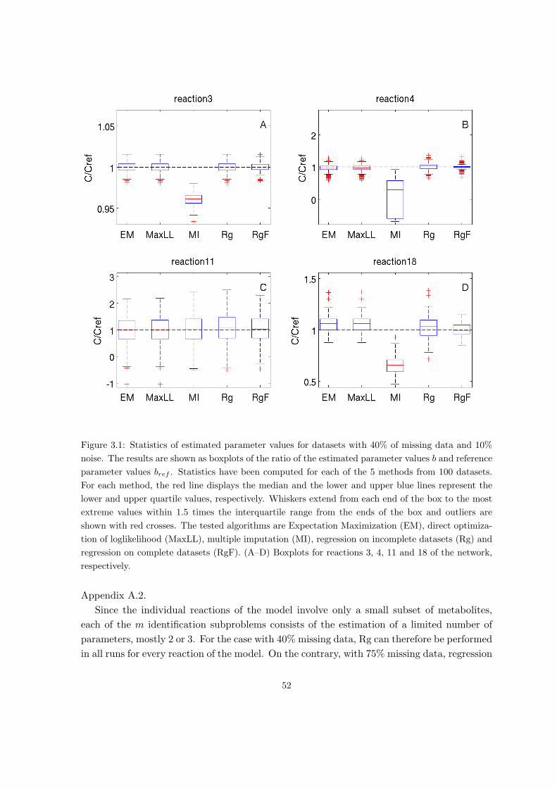
Figure 3.1: Statistics of estimated parameter values for datasets with 40% of missing data and 10%

noise. The results are shown as boxplots of the ratio of the estimated parameter values b and reference

parameter values bref . Statistics have been computed for each of the 5 methods from 100 datasets.

For each method, the red line displays the median and the lower and upper blue lines represent the

lower and upper quartile values, respectively. Whiskers extend from each end of the box to the most

extreme values within 1.5 times the interquartile range from the ends of the box and outliers are

shown with red crosses. The tested algorithms are Expectation Maximization (EM), direct optimiza-

tion of loglikelihood (MaxLL), multiple imputation (MI), regression on incomplete datasets (Rg) and

regression on complete datasets (RgF). (A–D) Boxplots for reactions 3, 4, 11 and 18 of the network,

respectively.

Appendix A.2.

Since the individual reactions of the model involve only a small subset of metabolites,

each of the m identification subproblems consists of the estimation of a limited number of

parameters, mostly 2 or 3. For the case with 40% missing data, Rg can therefore be performed

in all runs for every reaction of the model. On the contrary, with 75% missing data, regression

52

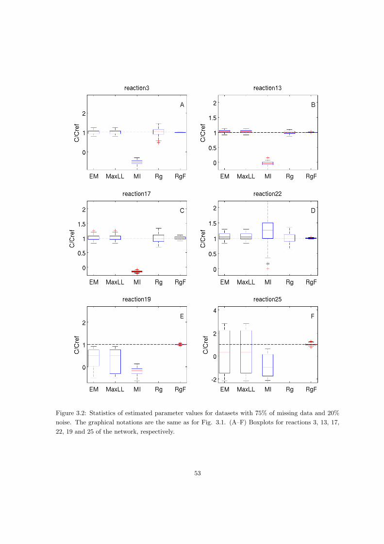
Figure 3.2: Statistics of estimated parameter values for datasets with 75% of missing data and 20%

noise. The graphical notations are the same as for Fig. 3.1. (A–F) Boxplots for reactions 3, 13, 17,

22, 19 and 25 of the network, respectively.

53

cannot be applied to 6 reactions which is apparent from the absence of the Rg statistics for

2 reactions in Fig. 3.2.

In comparison with the other methods, multiple imputation (MI) gives the worst results

(largest bias) in 3 out of the 4 reactions shown in Fig. 3.1, and in 5 out of 6 reactions in Fig.

3.2. In reactions 11 of Fig. 3.1 and 22 of Fig. 3.2, the relatively small biases are accompanied

by an estimation uncertainty wider than for EM and MaxLL. This could be explained by a

restricted use of information contained in the distribution of missing data. Indeed, MI only

considers random draws from the distribution while EM and MaxLL are based on all possible

values taken by missing data through integration of the distribution.

Analysis of Fig. 3.1 reveals that, for 40% missing data and 10% noise, the performance

of EM and MaxLL is almost identical and similar to that of regression (Rg and RgF), with

limited improvements on Rg, i.e., slightly smaller variability. In some cases, such as for re-

actions 11 and 18, their performance approaches the optimal, unattainable bound provided

by RgF, i.e., they have similar bias and variability.

Performance improvements of likelihood-based methods over Rg become more significant

when identification is performed on the dataset with higher percentage of missing data and

larger noise. Fig. 3.2A-D show results for reactions where Rg was applicable. Both EM and

MaxLL substantially reduce estimation variability in reactions 3, 17 and 22. At the same

time, due to the larger amount of missing data, performance loss with respect to RgF is more

significant. Turned another way, this shows the accuracy that could be recovered were all

datasets complete.

Fig. 3.2E-F show the results when Rg fails to produce estimates and cannot be used to

initialize EM and MaxLL optimization. Still, EM provides estimates of the right order of

magnitude and, for the case of Fig. 3.2E, of the right sign in at least 75% of the runs (box

entirely above 0), while the median has the right sign and is reasonably close to 1. The

estimation of the sign provided by MaxLL is less reliable (box crossing 0).

Overall, we conclude that the EM-based approach provides the most accurate estimates

under all simulated conditions. We will therefore apply this method to the identification of

the linlog model of an actual metabolic network from a published high-throughput dataset.

3.4 Application to central metabolism in E. coli

The network we consider here gathers enzymes, metabolites and reactions that make up

the bulk of E. coli central carbon metabolism, including glycolysis, the pentose-phosphate

pathway, the tricarboxylic acid cycle and anaplerotic reactions such as glyoxylate shunt and

PEP-carboxylase (Fig. 3.3).

The dataset used for identification of this network was obtained by experiments with 24

single-gene mutants that were grown at a fixed dilution rate of 0.2 h−1 in a glucose-limited

chemostat, and with wild-type cells at 5 different dilution rates [Ishii et al., 2007]. The

54

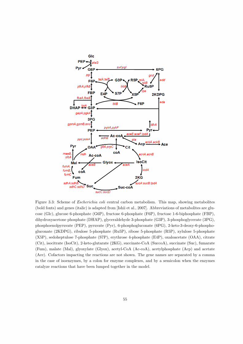
Figure 3.3: Scheme of Escherichia coli central carbon metabolism. This map, showing metabolites

(bold fonts) and genes (italic) is adapted from [Ishii et al., 2007]. Abbreviations of metabolites are glu-

cose (Glc), glucose 6-phosphate (G6P), fructose 6-phosphate (F6P), fructose 1-6-biphosphate (FBP),

dihydroxyacetone phosphate (DHAP), glyceraldehyde 3-phosphate (G3P), 3-phosphoglycerate (3PG),

phosphoenolpyruvate (PEP), pyruvate (Pyr), 6-phosphogluconate (6PG), 2-keto-3-deoxy-6-phospho-

gluconate (2KDPG), ribulose 5-phosphate (Ru5P), ribose 5-phosphate (R5P), xylulose 5-phosphate

(X5P), sedoheptulose 7-phosphate (S7P), erythrose 4-phosphate (E4P), oxaloacetate (OAA), citrate

(Cit), isocitrate (IsoCit), 2-keto-glutarate (2KG), succinate-CoA (SuccoA), succinate (Suc), fumarate

(Fum), malate (Mal), glyoxylate (Glyox), acetyl-CoA (Ac-coA), acetylphosphate (Acp) and acetate

(Ace). Cofactors impacting the reactions are not shown. The gene names are separated by a comma

in the case of isoenzymes, by a colon for enzyme complexes, and by a semicolon when the enzymes

catalyze reactions that have been lumped together in the model.

55

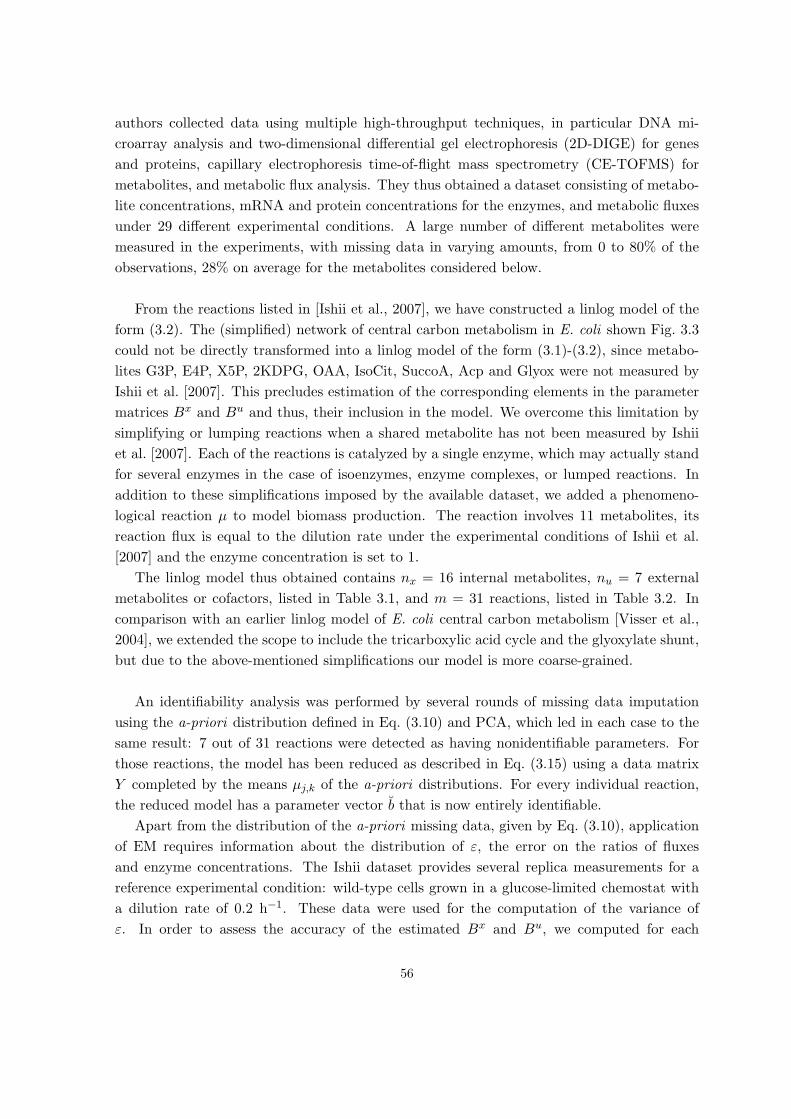
authors collected data using multiple high-throughput techniques, in particular DNA mi-

croarray analysis and two-dimensional differential gel electrophoresis (2D-DIGE) for genes

and proteins, capillary electrophoresis time-of-flight mass spectrometry (CE-TOFMS) for

metabolites, and metabolic flux analysis. They thus obtained a dataset consisting of metabo-

lite concentrations, mRNA and protein concentrations for the enzymes, and metabolic fluxes

under 29 different experimental conditions. A large number of different metabolites were

measured in the experiments, with missing data in varying amounts, from 0 to 80% of the

observations, 28% on average for the metabolites considered below.

From the reactions listed in [Ishii et al., 2007], we have constructed a linlog model of the

form (3.2). The (simplified) network of central carbon metabolism in E. coli shown Fig. 3.3

could not be directly transformed into a linlog model of the form (3.1)-(3.2), since metabo-

lites G3P, E4P, X5P, 2KDPG, OAA, IsoCit, SuccoA, Acp and Glyox were not measured by

Ishii et al. [2007]. This precludes estimation of the corresponding elements in the parameter

matrices Bx and Bu and thus, their inclusion in the model. We overcome this limitation by

simplifying or lumping reactions when a shared metabolite has not been measured by Ishii

et al. [2007]. Each of the reactions is catalyzed by a single enzyme, which may actually stand

for several enzymes in the case of isoenzymes, enzyme complexes, or lumped reactions. In

addition to these simplifications imposed by the available dataset, we added a phenomeno-

logical reaction µ to model biomass production. The reaction involves 11 metabolites, its

reaction flux is equal to the dilution rate under the experimental conditions of Ishii et al.

[2007] and the enzyme concentration is set to 1.

The linlog model thus obtained contains nx = 16 internal metabolites, nu = 7 external

metabolites or cofactors, listed in Table 3.1, and m = 31 reactions, listed in Table 3.2. In

comparison with an earlier linlog model of E. coli central carbon metabolism [Visser et al.,

2004], we extended the scope to include the tricarboxylic acid cycle and the glyoxylate shunt,

but due to the above-mentioned simplifications our model is more coarse-grained.

An identifiability analysis was performed by several rounds of missing data imputation

using the a-priori distribution defined in Eq. (3.10) and PCA, which led in each case to the

same result: 7 out of 31 reactions were detected as having nonidentifiable parameters. For

those reactions, the model has been reduced as described in Eq. (3.15) using a data matrix

Y completed by the means µj,k of the a-priori distributions. For every individual reaction,

the reduced model has a parameter vector b that is now entirely identifiable.

Apart from the distribution of the a-priori missing data, given by Eq. (3.10), application

of EM requires information about the distribution of ε, the error on the ratios of fluxes

and enzyme concentrations. The Ishii dataset provides several replica measurements for a

reference experimental condition: wild-type cells grown in a glucose-limited chemostat with

a dilution rate of 0.2 h−1. These data were used for the computation of the variance of

ε. In order to assess the accuracy of the estimated Bx and Bu, we computed for each

56

Internal metabolites

Index Symbol Index Symbol

1 PEP 9 Ru5P

2 G6P 10 R5P

3 Pyr 11 S7P

4 F6P 12 2KG

5 FBP 13 Suc

6 DHAP 14 Fum

7 3PG 15 Mal

8 6PG 16 Cit

IndexExternal metabolites

or cofactors

17 Glc

18 Ac-coA/coA

19 ATP/ADP

20 NADPH/NADP

21 NADH/NAD

22 FAD

23 Ace

Table 3.1: Internal and external metabolites and cofactors of the linlog model of carbon metabolism

in E. coli. Some of the cofactors are modeled as ratios of metabolite concentrations, e.g., ATP/ADP.

parameter a 95% confidence interval, by means of the profile likelihood method outlined in

Sec. 3.2. Running the EM method on the model and the data took about 220 s using the

implementation of Sec. 3.3. The computation of the confidence intervals for all parameters

required about 23 min.

Contrary to the simulation studies reported in Sec. 3.3, a reference or ‘real’ model for the

evaluation of the results does not exist in this case. However, a-priori biochemical knowl-

edge on the signs of the elasticities is available, i.e., elasticities are positive for substrates

and negative for products. This information can be compared with the estimated signs of

the elasticities, and their confidence intervals, computed from the parameter matrices using

the relations in Eq. (3.9). The results are shown in Table 3.3. Similar unshown results are

obtained by means of the MaxLL method.

We observe that the EM method obtains estimates for all reactions, including the 7 cases

where the insufficient amount of data made regression not applicable. However, 26 of the 100

non-zero elasticities of the model are not identifiable from this dataset. Moreover, out of the

remaining 74 elasticity estimates, more than half of them have signs that are not statistically

significant, in the sense that the 95% confidence interval straddles 0. This is most likely due

to the fact that the magnitude of noise in metabolite concentrations is comparable to the

magnitude of relevant information. For example, for PEP the standard deviation over all

experimental conditions equals the standard deviation of the replicates in a single condition

(0.06 mM vs 0.05 mM). This precludes the estimation of an unambiguous sign.

Of the elasticities with statistically significant signs, 20 out of 34 are correct, in the sense

that they have the expected positive or negative sign. The remaining elasticities, distributed

over 9 reactions, are incorrectly estimated. Let us now discuss what we believe are potential

sources of these errors, giving information that could be used to single out erroneous estimates

57

Index Reaction

1 Glc + PEPptsG←−−→ Pyr+G6P

2 G6Ppgi←−→ F6P

3 F6P + ATP/ADPpfkA,pfkB←−−−−−−−→ FBP [PEP]in

4 FBPfbaA,fbaB←−−−−−−→ DHAP

5 DHAPtpiA←−−→ 3PG

6 FBP + ATP/ADPgapA;pgk←−−−−−→ 3PG + NADH/NAD

7 3PGgpmA,gpmB;eno←−−−−−−−−−−→ PEP

8 PEP + ATP/ADPpykA,pykF←−−−−−−→ Pyr [FBP]act

9 PyraceE:aceF :lpdA←−−−−−−−−−−→ Ac-coA/coA + NADH/NAD

10 G6Pzwf ;pgl←−−−−→ 6PG + NADPH/NADP

11 6PGgnd←−→ Ru5P + NADPH/NADP

12 Ru5Prpe←−→ S7P

13 Ru5PrpiA,rpiB←−−−−−−→ R5P [G6P]in

14 R5PtktA←−−→ S7P

15 S7PtalA,talB←−−−−−→ F6P

16 Ru5PtktB←−−→ F6P

17 Ac-coA/coAgltA,prpC←−−−−−−→ Cit [2KG]in [NADH/NAD]act

18 CitacnA,acnB←−−−−−−−→ 2KG

19 Ac-coA/coAicdA←−−→ 2KG + NADPH/NADP

20 2KGsucA:sucB:lpdA;sucC:sucD←−−−−−−−−−−−−−−−−−−→ Suc + NADH/NAD

21 Suc + FADsdhA:sdhB:sdhC:sdhD←−−−−−−−−−−−−−−−→ Fum

22 FumfumA,fumB,fumC←−−−−−−−−−−−−−→ Mal

23 Mal + PEPmdh←−−→ Cit +NADH/NAD

24 PEPppc;pckA←−−−−−→ Mal + Cit + ATP/ADP [FBP]act

25 MalmaeB,sfcA←−−−−−−−→ Pyr + NADPH/NADP [Ac-coA/coA]in [NADH/NAD]act

26 Ac-coA/coAaceA;aceB←−−−−−−→ Suc + Mal

27PEP+G6P+Pyr+F6P+3PG+Ac-coA/coA+R5P+2KG+ATP/ADPµ−→NADPH/NADP+NADH/NAD

28 6PGedd;eda←−−−−→ Pyr

29Ac-coA/coA

pta;ackA,ackB←−−−−−−−−−→ Ace+ATP/ADP

[Pyr]act [NADPH/NADP]in [NADH/NAD]in

30 Pyr + NADH/NADldhA−−−→

31 Ac-coA/coAadhE−−−−→

Table 3.2: Reactions of the linlog model of carbon metabolism in E. coli. Activators and inhibitors of

the reaction are shown with [·]act and [·]in, respectively. Reaction 27, labeled µ, is a phenomenological

reaction for biomass production. The enzyme names are separated by a comma in the case of isoen-

zymes, by a colon for enzyme complexes, and by a semicolon when the enzymes catalyze reactions

that have been lumped together in the model. Reactions 20, 26, 28 and 29 result from the merging

of reactions due to the absence of measurements of SuccoA, Glyox, 2KDPG and Acp, respectively, in

the dataset of Ishii et al. [2007].

58

Table 3.3: Elasticity matrix [Bx0 Bu

0 ] estimated by EM from the data of [Ishii et al., 2007] for the linlog model of E. coli central carbon

metabolism (the columns of the matrix have been permuted for readability). Unidentifiable elasticities are shown in gray, uncertain elasticities

(i.e., having a sign that is not significant with 95% confidence) in yellow, and correctly/incorrectly identified elasticities (i.e., having a sign that

is significant with 95% confidence) in green/red. Abbreviations are as in Fig. 3.3. Some of the cofactors are modeled as ratios of metabolite

concentrations, e.g. ATP/ADP. Reaction 27, labeled µ, is a phenomenological reaction for biomass production. The last row indicates the

percentage of missing data per metabolite and the right-most column displays the amount of complete datapoints available for each reaction.

For reactions labeled with ∗, regression was not able to produce any result.

Enzyme

MetaboliteGlc PEP G6P Pyr F6P FBP DHAP 3PG Ac-coA

coA

6PG Ru5P R5P S7P 2KG Suc Fum Mal ATP

ADP

Cit NADPH

NADP

NADH

NAD

FAD Ace # complete

datapoints

1 PtsG 0.29 -0.89 0.79 1.87 0 0 0 0 0 0 0 0 0 0 0 0 0 0 0 0 0 0 0 14

2 Pgi 0 0 -0.33 0 0.23 0 0 0 0 0 0 0 0 0 0 0 0 0 0 0 0 0 0 27

3 PfkA,PfkB 0 -0.16 0 0 0.04 -0.28 0 0 0 0 0 0 0 0 0 0 0 0.09 0 0 0 0 0 18

4 FbaA,FbaB 0 0 0 0 0 -0.3 0.06 0 0 0 0 0 0 0 0 0 0 0 0 0 0 0 0 8

5 TpiA 0 0 0 0 0 0 -0.07 0.22 0 0 0 0 0 0 0 0 0 0 0 0 0 0 0 12

6 GapA;Pgk 0 0 0 0 0 -0.18 0 -0.05 0 0 0 0 0 0 0 0 0 0.32 0 0 -0.17 0 0 5

7 GpmA,GpmB;Eno 0 0.26 0 0 0 0 0 -0.12 0 0 0 0 0 0 0 0 0 0 0 0 0 0 0 24

8 PykA,PykF 0 0.12 0 0.49 0 -0.19 0 0 0 0 0 0 0 0 0 0 0 0.16 0 0 0 0 0 11

9 AceE:AceF:LpdA 0 0 0 0.64 0 0 0 0 0.05 0 0 0 0 0 0 0 0 0 0 0 -0.21 0 0 6

10 Zwf;Pgl 0 0 -0.22 0 0 0 0 0 0 -0.24 0 0 0 0 0 0 0 0 0 -0.01 0 0 0 2

11 Gnd 0 0 0 0 0 0 0 0 0 0.48 -0.09 0 0 0 0 0 0 0 0 -0.01 0 0 0 2∗

12 Rpe 0 0 0 0 0 0 0 0 0 0 0.46 0 -0.39 0 0 0 0 0 0 0 0 0 0 28

13 RpiA,RpiB 0 0 -0.74 0 0 0 0 0 0 0 0.3 -0.16 0 0 0 0 0 0 0 0 0 0 0 18

14 TktA 0 0 0 0 0 0 0 0 0 0 0 0.01 -0.1 0 0 0 0 0 0 0 0 0 0 18

15 TalA,TalB 0 0 0 0 -0.32 0 0 0 0 0 0 0 0.51 0 0 0 0 0 0 0 0 0 0 27

16 TktB 0 0 0 0 -0.58 0 0 0 0 0 0.35 0 0 0 0 0 0 0 0 0 0 0 0 27

17 GltA,PrpC 0 0 0 0 0 0 0 0 0.22 0 0 0 0 -0.001 0 0 0 0 0.49 0 -0.01 0 0 1∗

18 AcnA,AcnB 0 0 0 0 0 0 0 0 0 0 0 0 0 0.99 0 0 0 0 0.55 0 0 0 0 5

19 IcdA 0 0 0 0 0 0 0 0 0.08 0 0 0 0 -0.09 0 0 0 0 0 -0.59 0 0 0 4

20 SucA:SucB:LpdA;SucC:SucD 0 0 0 0 0 0 0 0 0 0 0 0 0 1.26 0.3 0 0 0 0 0 -0.48 0 0 2∗

21 SdhA:SdhB:SdhC:SdhD 0 0 0 0 0 0 0 0 0 0 0 0 0 0 1.08 -0.44 0 0 0 0 0 0.4 0 21

22 FumA,FumB,FumC 0 0 0 0 0 0 0 0 0 0 0 0 0 0 0 0.46 0.1 0 0 0 0 0 0 25

23 Mdh 0 0.15 0 0 0 0 0 0 0 0 0 0 0 0 0 0 -0.01 0 0.31 0 -0.12 0 0 3∗

24 Ppc;PckA 0 0.29 0 0 0 -0.13 0 0 0 0 0 0 0 0 0 0 0.1 -1.15 0.21 0 0 0 0 9

25 MaeB,SfcA 0 0 0 -0.31 0 0 0 0 -0.21 0 0 0 0 0 0 0 0.38 0 0 0.36 -0.05 0 0 2∗

26 AceA;AceB 0 0 0 0 0 0 0 0 -0.11 0 0 0 0 0 0.26 0 -0.18 0 0 0 0 0 0 25

27 µ 0 0.1 -0.09 0.04 -0.06 0 0 0.17 0.1 0 0 0.09 0 -0.01 0 0 0 -0.46 0 -0.003 0.01 0 0 0∗

28 Edd;Eda 0 0 0 -0.03 0 0 0 0 0 -0.93 0 0 0 0 0 0 0 0 0 0 0 0 0 5

29 Pta;AckA,AckB 0 0 0 -0.06 0 0 0 0 -0.01 0 0 0 0 0 0 0 0 0.21 0 -0.25 -2.03 0 2.19 2∗

30 LdhA 0 0 0 2.67 0 0 0 0 0 0 0 0 0 0 0 0 0 0 0 0 -0.11 0 0 6

31 AdhE 0 0 0 0 0 0 0 0 0.91 0 0 0 0 0 0 0 0 0 0 0 0 0 0 28

% Missing Data 3 17 0 48 7 34 59 10 3 72 3 38 3 59 3 14 14 0 62 79 79 17 17

59

a-priori.

We first note that for 3 of these 9 reactions (GapA;Pgk, Mdh and Edd;Eda, see Table 3.3),

only very few complete datapoints are available (between 3 and 5) and regression mostly fails

in these cases. In addition, all of these reactions involve at least one metabolite missing in

more than 70% of the experimental conditions. The combination of very few complete dat-

apoints and a high percentage of missing metabolite measurements obviously makes model

identification extremely difficult and it is fair to say that here we reach the limit of the ap-

plicability of our method, or of any method for that matter, due to the lack of data.

Second, 4 reactions are known to operate close to equilibrium: Pgi, FbaA,FbaB, TpiA

and GpmA,GpmB;Eno [Visser et al., 2004]. Theoretically, these reactions are not identifiable,

as their elasticities are not independent [Visser et al., 2004], but PCA did not detect this.

Most likely, this is due to the above-mentioned noise in metabolite concentrations, which

decreases their correlations. A cautious, preemptive strategy would be to reduce the model

for any reaction known to be close to equilibrium and eliminate the corresponding dependent

variables.

The errors in the signs of some elasticities in the remaining 2 reactions (PtsG and PykA,PykF)

are less straightforward to explain. It is unlikely that they can be attributed to the EM

method, given that regression is applicable here with a relatively large number of complete

datapoints available (14 and 11, respectively) and gives the same results. Alternatively, they

may be explained by a modeling error or a hidden variable, for instance an unknown cofac-

tor, biasing the estimation results. It is also possible that the approximations of the linlog

model are not suitable for these reactions, for instance because there are large variations

in metabolite concentrations between conditions, driving the system far from the reference

state.

In summary, EM gives reasonable results for a fairly complicated model on a challenging

dataset. Even though some puzzling issues remain, we believe that these can be safely

attributed to the inherent difficulty of the identification problem.

3.5 Discussion

In this chapter we have addressed the problem of estimating parameters of approximate

models of metabolic networks from incomplete datasets. Even with the largest datasets

available at present, such as those reported in [Ishii et al., 2007], the absence or corruption

of a large number of measurements may reduce the effective number of datapoints to a

handful of experimental conditions, thus making simple regression techniques ineffective or

even inapplicable. Making full use of all the available data is therefore essential to render

identification well-posed and improve the quality of the estimated models.

To this aim, we have proposed a maximum-likelihood method for the identification of

linlog metabolic network models that compensates for the missing data by the use of statis-

60

tical priors. We developed an algorithm that attains maximization of the likelihood based

on Expectation Maximization, a well accepted paradigm for the numerical optimization of

likelihood functions in the presence of unobserved variables. A simpler implementation based

on direct likelihood maximization via general-purpose numerical optimization algorithms was

also considered and found slightly less powerful. The performance of EM was compared to

that of an existing method of reference, namely multiple imputation, and to worst-case and

best-case scenarios given by least-squares regression on the sole complete datapoints and on

complete datasets, respectively. We showed that EM outperforms multiple imputation by a

wide margin. In comparison with worst-case regression, it reduces the estimation variabil-

ity and is able to produce reasonable estimation results even when regression on incomplete

datasets is inapplicable. It also approaches the ideal performance of regression on complete

datasets for low rates of missing data, regardless of noise.

Based on these findings, we applied EM to the identification of a linlog model for the cen-

tral carbon metabolism in E. coli from the experimental data presented by Ishii et al. [2007].

Even with the large amount of incomplete datapoints, due to the difficulty of experimentally

measuring metabolite concentrations, EM was able to estimate many of the model parameters

(elasticities) in agreement with the current understanding of the system. This is even true for

reactions where the reduced number of complete datapoints impairs the applicability of least

squares regression. On the other hand, the challenging quality of the data sheds light on the

performance limits of the method, which tends to fail when large measurement noise makes

the estimation of small parameters statistically unreliable, when the same variable cannot be

measured in most conditions, or when reactions operate near equilibrium.

Overall, results from the simulations and the application on real data showed that our

EM approach is able to make the most of incomplete, noisy high-throughput datasets for

the estimation of parameters in approximate kinetic models. In the future, we expect to

improve performance by developing a number of technical points, including approximate an-

alytical/dedicated numerical solutions for the EM maximization steps and a more detailed

modeling of measurement noise. It is worth noting that, while the method has been developed

for linlog models, it is more generally applicable to any other metabolic network model that

can be put in a form linear in the parameters by straightforward manipulations, such as gen-

eralized mass action models that provide advantages when some metabolite concentrations

approach 0 [Savageau, 1976, del Rosario et al., 2008]. In addition, estimated parameters of

approximate metabolic models, such as elasticities of linlog models, provide useful hints for

the identification of more detailed nonlinear kinetic models.

From a broader perspective, the application of the EM method to the unique multi-omics

dataset for E. coli carbon metabolism allowed us to isolate issues that are critical for the

appropriate exploitation of the data for parameter estimation. These issues may need to

be taken into account during the design of the experiments. One such issue is that a high

61

percentage of missing data for some of the individual variables, even at a relatively low average

percentage over the entire dataset, was found to be much detrimental to the identification

results. This may influence sampling strategies, especially for metabolites that are difficult

to measure.

Another issue is the identifiability problems caused by steady-state measurements, which

cannot always be resolved by genetic mutation or by varying physiological conditions. From

this perspective time-resolved observations of the network dynamics, although much more

demanding experimentally, carry great promise [Hardiman et al., 2007]. We discuss these

identifiability issues in detail in the next chapter.

62

Chapter 4

Identifiability of linlog metabolic

models

A major and often overlooked problem in parameter estimation is the identifiability of the

model, that is, the problem of unambiguously reconstructing the unknown parameter values

from the observed network behavior. In the context of approximate kinetic models, we address

the key problem of the identifiability of biochemical networks in a principled and scalable

way. We focus on the case where the structure of the model is fixed by a-priori knowledge on

the network (i.e., the chemical species considered, the reactions among them and the eventual

regulatory interactions), and discuss the identifiability of the model parameters. That is, we

are interested in the problem of unambiguously reconstructing the unknown parameter values

from the observed network behavior.

A distinction is usually made between structural (or a-priori) and practical (or a-posteriori)

identifiability [Ljung, 1999, Walter and Pronzato, 1997]. Structural identifiability is an intrin-

sic property of the model family, guaranteeing that unique parameter reconstruction would be

possible from perfect observations of the system response to an arbitrarily rich set of inputs.

Practical identifiability refers to the ability of estimating unknown parameter values from

the available experimental data within a prespecified degree of accuracy. In classical control

theory, this concept is essentially related to the notion of persistence of excitation [Ljung,

1999]. Unfortunately, limitations in the variety and quality of the observed inputs and out-

puts that can be obtained make this notion inapplicable to biological applications. In recent

years, the topic of identifiability has gained considerable interest in the field of systems biol-

ogy [Ashyraliyev et al., 2009, Nikerel et al., 2009, Chis et al., 2011b, Chen et al., 2010, Raue

et al., 2009, 2011, Srinath and Gunawan, 2010, Jaqaman and Danuser, 2006, Gutenkunst

et al., 2007, Nemcova, 2010, Voit et al., 2006a] and several specialized software packages have

been developed to support the modeler [Chis et al., 2011a, Maiwald and Timmer, 2008]. De-

spite these efforts, however, no common agreement on definitions and links between structural

and practical identifiability exist to date.

63

The aim of this chapter is to develop methods for the analysis of the (parameter) iden-

tifiability of kinetic models of metabolism, and for the reduction of non-identifiable models

to identifiable approximations. These methods should have a solid mathematical foundation,

but at the same time be applicable to practical problems and currently available data sets,

such as those obtained by means of recent high-throughput methods in biology [Ishii et al.,

2007]. While many of our definitions are of general applicability, identifiability results will

be developed primarily for linlog models, whose pseudo-linear form enables us to apply tools

from linear algebra and estimation theory in a straightforward manner. Similar results can

be derived easily for many other approximate kinetic modeling formalisms in pseudo-linear

form, such as the linear, loglin and generalized mass-action kinetic formats [Delgado and

Liao, 1992, Hatzimanikatis and Bailey, 1997, Savageau, 1976].

The main contributions of the chapter are threefold. First, we precisely define the notions

of structural and practical identifiability of approximate kinetic models, drawing upon the

systems identification literature. This conceptual clarification allows us to develop the rela-

tions between structural and practical identifiability in a fundamental way. Second, we show

how model reduction using singular value decomposition (SVD) [Jolliffe, 1986] provides a

suitable theoretical framework for addressing identifiability problems. We discuss several dif-

ferent criteria for model reduction, based on the singular values returned by the SVD analysis,

and we show to which extent these criteria are appropriate for dealing with actual biological

data sets, which are typically scarce, noisy and incomplete. Third, we apply the methods

for identifiability analysis and model reduction to both simulated data and the dataset of

Ishii et al. [2007] concerning central metabolism in E. coli. These examples show that the

mathematical tools developed in this chapter are of practical utility for the estimation of

parameters in models of metabolic networks and beyond, from current high-throughput data

sets. In order to simplify the reading of the main text, the proofs of all theoretical results

are reported in Appendix B.1.

4.1 Parameter estimation in linlog and other approximate ki-

netic modeling formalisms

We recall the general ODE form of kinetic models of biochemical networks and the linlog

formulation for metabolic models:

x = N · v(x, u, e), (4.1)

v(x, u, e) = diag(e) ·(a+Bx · lnx+Bu · lnu

)(4.2)

where x ∈ X ⊆ Rnx

>0 denotes the vector of (nonnegative) internal metabolite concentrations,

u ∈ U ⊆ Rnu

>0 the vector of external metabolite concentrations, e ∈ E ⊆ Rm>0 the vector of

enzyme concentrations, and v : Rnx+nu+m>0 → V , with V ⊆ R

m, the vector of reaction rate

64

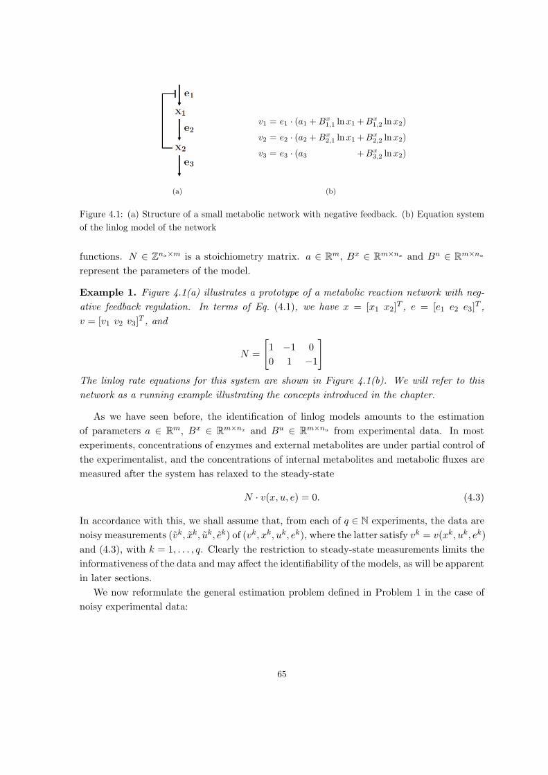
(a)

v1 = e1 · (a1 +Bx1,1 lnx1 +Bx

1,2 lnx2)

v2 = e2 · (a2 +Bx2,1 lnx1 +Bx

2,2 lnx2)

v3 = e3 · (a3 +Bx3,2 lnx2)

(b)

Figure 4.1: (a) Structure of a small metabolic network with negative feedback. (b) Equation system

of the linlog model of the network

functions. N ∈ Znx×m is a stoichiometry matrix. a ∈ R

m, Bx ∈ Rm×nx and Bu ∈ R

m×nu

represent the parameters of the model.

Example 1. Figure 4.1(a) illustrates a prototype of a metabolic reaction network with neg-

ative feedback regulation. In terms of Eq. (4.1), we have x = [x1 x2]T , e = [e1 e2 e3]

T ,

v = [v1 v2 v3]T , and

N =

[1 −1 0

0 1 −1

]

The linlog rate equations for this system are shown in Figure 4.1(b). We will refer to this

network as a running example illustrating the concepts introduced in the chapter.

As we have seen before, the identification of linlog models amounts to the estimation

of parameters a ∈ Rm, Bx ∈ R

m×nx and Bu ∈ Rm×nu from experimental data. In most

experiments, concentrations of enzymes and external metabolites are under partial control of

the experimentalist, and the concentrations of internal metabolites and metabolic fluxes are

measured after the system has relaxed to the steady-state

N · v(x, u, e) = 0. (4.3)

In accordance with this, we shall assume that, from each of q ∈ N experiments, the data are

noisy measurements (vk, xk, uk, ek) of (vk, xk, uk, ek), where the latter satisfy vk = v(xk, uk, ek)

and (4.3), with k = 1, . . . , q. Clearly the restriction to steady-state measurements limits the

informativeness of the data and may affect the identifiability of the models, as will be apparent

in later sections.

We now reformulate the general estimation problem defined in Problem 1 in the case of

noisy experimental data:

65

Problem 3. Given the data matrices

(v1

e1 −(ve

))T

...(vq

eq −(ve

))T

︸ ︷︷ ︸, W

,

(ln x1 − ln x

)T (ln u1 − ln u

)T...

...(ln xq − ln x

)T (ln uq − ln u

)T

︸ ︷︷ ︸, Y

find parameters B ,

[Bx Bu

]Tminimizing |||W − Y · B|||, where ||| · ||| is a convenient

matrix norm on Rq×m.

To this avail we consider the probabilistic measurement error model:

W = W + ε ε =[ε1, . . . , εm

]εi ∼ N (0,Σεi) (4.4)

with Σεi = σ2i I > 0 and εi mutually independent for all i = 1, . . . ,m.

Notice that, as in Sec. 3.1, the parameter vector a can be estimated from experimental

data and estimates of B =[Bx Bu

]T. Assuming that the measurement noise is indepen-

dent across different reactions, it makes sense to separate the problem into the independent

estimation of the parameter vector Bi of each reaction i, with i = 1, . . . ,m.

Example 2. Let W and Y denote the noiseless versions of W and Y , respectively. Consider

the case where W = W + ε = Y · B + ε, i.e., the measurement error for the metabolite

concentrations is negligible. This corresponds to the case described in Sec. 3.1. Maximum

likelihood estimation of B amounts to minimizing the negative logarithm of the likelihood of

W given Y . After simple computations and thanks to the independence assumptions on ε,

one finds that the maximum likelihood estimate of B is any solution of

minB

1

2

m∑

i=1

(Wi − Y Bi)TΣ−1εi (Wi − Y Bi),

which can be solved separately for every column of B by solving, for i = 1, . . . ,m,

minBi

(Wi − Y Bi)TΣ−1εi (Wi − Y Bi) = ||Wi − Y Bi||2Σ−1

εi

.

Thus, defining || · ||i = || · ||Σ−1εi

and

||| · ||| : Rq×m → R+ : M 7→

√√√√√√√

M1

...

Mm

T Σ−1ε1

. . .

Σ−1εm

M1

...

Mm

,

we see that Problem 3 is equivalent to the maximum likelihood estimation of B, which is

in turn equivalent to separate maximum likelihood estimation of the parameters Bi of each

reaction i.

66

Similar to, but in more generality than Example 2, from now on we consider the proba-

bilistic measurement error model

W = W + ε, ε =[ε1, . . . , εm

], εi ∼ N (0,Σεi), (4.5)

Y = Y + η, η =[η1, . . . , ηm

], ηi ∼ N (0,Σηi

), (4.6)

with Σεi = σ2I > 0, Σηi= ν2I ≥ 0, and εi, ηi′ mutually independent for all i = 1, . . . ,m and

i′ = 1, . . . ,m.

We can now fully detail Problem 3 and express it as a series of estimation problems on

individual reactions. In doing so we note that each reaction i depends only on a (known)

subset of metabolites C(i) ⊆ {1, . . . , nx + nu}. Therefore, the entries of Bi corresponding

to metabolites that do not participate in reaction i can be set to zero, and the least-squares

problem can be reduced accordingly. We will address two cases, formalized by two alternative

problem statements. The first we consider is a standard regression problem [Nikerel et al.,

2009, Sands and Voit, 1996]. In analogy with Sec. 3.1 and Example 2, it amounts to assuming

negligible metabolite measurement noise.

Problem 4. Given Y and W as in (4.5),

minBC(i),i

||Wi − YC(i) ·BC(i),i||i, i = 1, . . . ,m. (4.7)

The second case is more challenging and less commonly addressed in the literature. It

corresponds to an errors-in-variables regression model [van Huffel and Vandewalle, 1991] and

accounts explicitly for noise on the relative fluxes as well as on metabolite concentrations.

Problem 5. Given Y as in (4.6) and W as in (4.5), solve

minBC(i),i

||Wi − YC(i) ·BC(i),i||i, i = 1, . . . ,m. (4.8)

From now on we will drop subscript i from || · ||i, the meaning being clear from the

argument of the norm.

Remark 1. A similar parameter estimation problem can be formulated for other pseudo-

linear modeling formalisms. Models linear in metabolite concentrations [Delgado and Liao,

1992], loglin models [Hatzimanikatis and Bailey, 1997], and generalized mass-action models

[Savageau, 1976] can be defined analogously to Eq. (3.3). This gives rise to, respectively,

67

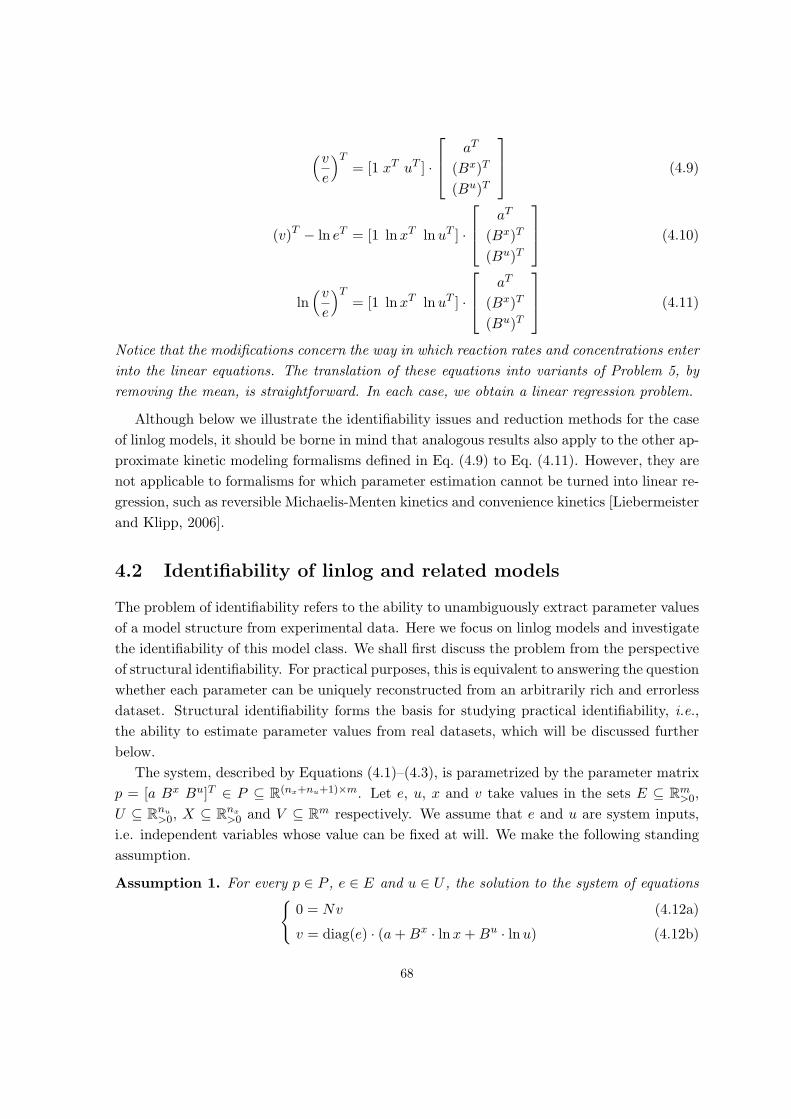
(ve

)T= [1 xT uT ] ·

aT

(Bx)T

(Bu)T

(4.9)

(v)T − ln eT = [1 lnxT lnuT ] ·

aT

(Bx)T

(Bu)T

(4.10)

ln(ve

)T= [1 lnxT lnuT ] ·

aT

(Bx)T

(Bu)T

(4.11)

Notice that the modifications concern the way in which reaction rates and concentrations enter

into the linear equations. The translation of these equations into variants of Problem 5, by

removing the mean, is straightforward. In each case, we obtain a linear regression problem.

Although below we illustrate the identifiability issues and reduction methods for the case

of linlog models, it should be borne in mind that analogous results also apply to the other ap-

proximate kinetic modeling formalisms defined in Eq. (4.9) to Eq. (4.11). However, they are

not applicable to formalisms for which parameter estimation cannot be turned into linear re-

gression, such as reversible Michaelis-Menten kinetics and convenience kinetics [Liebermeister

and Klipp, 2006].

4.2 Identifiability of linlog and related models

The problem of identifiability refers to the ability to unambiguously extract parameter values

of a model structure from experimental data. Here we focus on linlog models and investigate

the identifiability of this model class. We shall first discuss the problem from the perspective

of structural identifiability. For practical purposes, this is equivalent to answering the question

whether each parameter can be uniquely reconstructed from an arbitrarily rich and errorless

dataset. Structural identifiability forms the basis for studying practical identifiability, i.e.,

the ability to estimate parameter values from real datasets, which will be discussed further

below.

The system, described by Equations (4.1)–(4.3), is parametrized by the parameter matrix

p = [a Bx Bu]T ∈ P ⊆ R(nx+nu+1)×m. Let e, u, x and v take values in the sets E ⊆ R

m>0,

U ⊆ Rnu

>0, X ⊆ Rnx

>0 and V ⊆ Rm respectively. We assume that e and u are system inputs,

i.e. independent variables whose value can be fixed at will. We make the following standing

assumption.

Assumption 1. For every p ∈ P , e ∈ E and u ∈ U , the solution to the system of equations{

0 = Nv (4.12a)

v = diag(e) · (a+Bx · lnx+Bu · lnu) (4.12b)

68

is unique in x ∈ X and v ∈ V .

This guarantees that, for every admissible parametrization and system input, a steady-

state exists and is unique. In order for this steady-state to be observable experimentally, we

also make the assumption that it is locally asymptotically stable. In accordance with the

metabolic control theory literature [Heinrich and Schuster, 1996], fluxes v at steady-state are

denoted by J . We write Jp(e, u) to emphasize dependence on inputs and model parameters.

For varying values of p, Assumption 1 enables us to express the linlog model with param-

eters p as a map

Mp : E × U → V ×X : (e, u) 7→(Jp(e, u), xp(e, u)

). (4.13)

Assumption 1 is met, in particular, when matrix N diag(e)Bx is invertible. In this case, one

may write the output (Jp, xp) = Mp(e, u) as an explicit function of the input (e, u),{

Jp(e, u) = diag(e) · (a+Bx · lnxp(e, u) +Bu · lnu), (4.14a)

lnxp(e, u) = −(N diag(e)Bx)−1 ·N diag(e) · (a+Bu · lnu). (4.14b)

As can be easily verified, this requires that the stoichiometry matrix N is full row rank,

which is the case for systems with no mass conservation constraints [Heinrich and Schuster,

1996].

In agreement with Sec. 4.1, where the identification problem is split into the identification

of each reaction separately, we look at the identifiability of the parameters of the generic ith

reaction, and say that a model is identifiable if all its reactions are.

4.2.1 Identifiability from a theoretical perspective

We adapt the definition from Ljung [1999] to our context as follows. Recall that pi is the ith

column of p, i.e., the parameter vector for reaction i.

Definition 1. A reaction i of model Mp is identifiable at p∗ if there exists D ⊆ E × U such

that, for all p ∈ P , ((Jp)i, xp

)|D =

((Jp∗)i, xp∗

)|D ⇒ pi = p∗i . (4.15)

Here (Jp, xp) is seen as a function from E × U to X × V , and “|D” is its restriction to

a specific input set. In words, a reaction i is considered identifiable for a particular model

parametrization p∗ if no p ∈ P with pi 6= p∗i exists such that the predictions of Mp and

Mp∗ are identical over all possible input sets D. Note that this definition is applicable to

any metabolic reaction model, provided suitable definition of the parameters of the model

class. In particular, it applies to the linlog form of the reaction rates as well as to any other

pseudo-linear form reviewed in Sec. 4.1.

How can we apply Def. 1 to the analysis of identifiability of linlog models? The following

proposition establishes the link between this definition and the uniqueness of the solution

69

to Problems 4–1. Given the input set D = {(e1, u1) , · · · , (eq, uq)} and a “true” parameter

vector p∗, let Jk∗ and xk∗ denote the outputs Jp∗(ek, uk) and xp∗(ek, uk), respectively, with

k = 1, . . . , q.

Proposition 1. A reaction i of Mp is structurally identifiable at p∗ if and only if there exists

D = {(e1, u1) , · · · , (eq, uq)} ⊆ E × U such that the solution of the equation W ∗i = Y ∗B∗i ,

with

W ∗i =[(

J1∗

e1 −(J∗

e

))i

· · ·(Jq∗

eq −(J∗

e

))i

]T,

Y ∗ =

[lnx1∗ − lnx∗ · · · lnxq∗ − lnx∗

lnu1 − lnu · · · lnuq − lnu

]T,

is unique in the parameters B∗i =([Bx∗ Bu∗]T

)i.

Corollary 1. A reaction i of Mp is structurally identifiable at p∗ if and only if there exists

D = {(e1, u1) , · · · , (eq, uq)} ⊆ E × U such that Y ∗C(i) is full column-rank.

It is clear that the rank condition of Corollary 1 can be fulfilled only for a number of

experiments q = |D| greater than or equal to the number of unknown parameters nb = |C(i)|of reaction i. The possibility to find q ≥ |C(i)| experiments making Y ∗C(i) full column rank

depends on the network model and parameters themselves. Indeed, in our framework, the

experimentalist can impose different enzyme concentrations e and inputs u, but the resulting

metabolite concentrations are determined by the network. In other words, there is no full

control of the regression matrix Y , which impairs the design of optimal experiments for

parameter regression. Let us show this by a simple example.

Example 3. Consider the negative feedback network structure shown in Figure 4.1. Let us

define the network parameter values

a =

a1

0.0297

0.0296

, Bx = BT =

−0.0938 B2,1

0.0286 −0.0073

0 0.0287

,

where different values of a1 ∈ R and B2,1 ∈ R<0 (the coefficient that determines the strength

of the feedback regulation) will be considered. For all values of the enzyme concentrations

ei > 0, with i = 1, 2, 3, and all a1, B2,1, the equation Nv(x, e) = N diag(e)(a + Bx lnx) = 0

yields a unique solution lnx = −(N diag(e)Bx)−1N diag(e)a. This defines the unique steady-

state of the system. Provided it is asymptotically stable, this gives us a steady state of the

system that can be observed experimentally. One first consideration is that different values of

a1 and B2,1 may lead to very different properties of the matrix Y ∗ even when this remains full

rank, i.e. the system is structurally identifiable. For a1 = 0.0297 and values of B2,1 equal to

0.0073 (weaker feedback action) and −7.2961 (stronger feedback action), respectively, scatter

plots of the steady state solutions lnx from 1000 randomly generated samples of e are reported

70

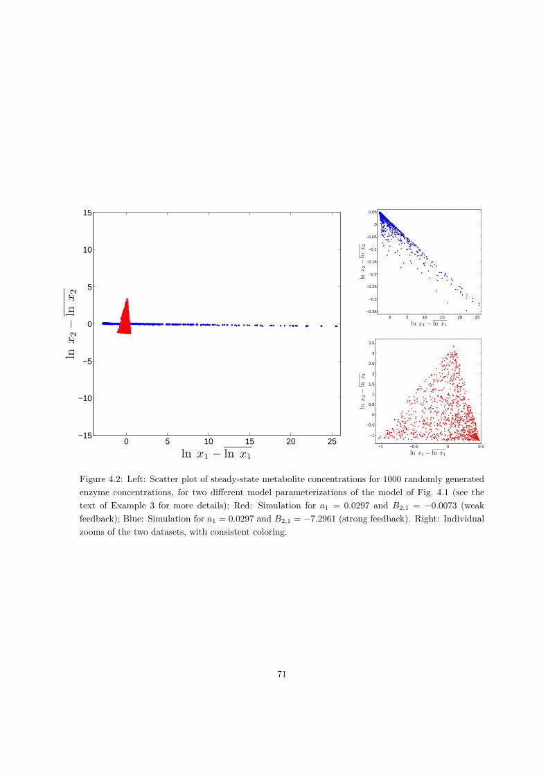
0 5 10 15 20 25−15

−10

−5

0

5

10

15

ln x1 − ln x1

lnx

2−

lnx

2

0 5 10 15 20 25−0.35

−0.3

−0.25

−0.2

−0.15

−0.1

−0.05

0

0.05

ln x1 − ln x1

lnx

2−

lnx

2

−1 −0.5 0 0.5

−1

−0.5

0

0.5

1

1.5

2

2.5

3

3.5

ln x1 − ln x1

lnx

2−

lnx

2

Figure 4.2: Left: Scatter plot of steady-state metabolite concentrations for 1000 randomly generated

enzyme concentrations, for two different model parameterizations of the model of Fig. 4.1 (see the

text of Example 3 for more details); Red: Simulation for a1 = 0.0297 and B2,1 = −0.0073 (weak

feedback); Blue: Simulation for a1 = 0.0297 and B2,1 = −7.2961 (strong feedback). Right: Individual

zooms of the two datasets, with consistent coloring.

71

in Figure 4.2. Steady-state metabolite concentrations in the case of weak feedback are spread

similarly in all directions, while with stronger feedback they are essentially aligned along a

one-dimensional line.Here the strong feedback exerted by metabolite X2 on the production of

X1 induces a negative correlation between their concentrations, which may result in an ill-

conditioned estimation problem. In addition this strong feedback results in a near homeostasis

of X2 that may also impede identification. These points will be further developed in the

next example. Second, some pathological parameterizations may give rise to a nonidentifiable

model. Indeed, if a is in the span of Bx, then the unique solution of N diag(e)(a+Bx lnx) = 0

always corresponds to the value of lnx satisfying Bx lnx = −a, independently of the value of

e. Thus, no matter the number of experiments q, the rank of Y ∗ is at most 1 and the model

is not identifiable. In our example, this is the case for a1 = −7.5491 and B2,1 = −7.2961.

From the example above it is clear that a reaction may be nonidentifiable for specific

values of the parameters even if it is identifiable for other parameterizations. In the light

of this, a generalization of Def. 1 from reaction identifiability at a parameter p∗ to reaction

identifiability tout court can be obtained following Walter and Pronzato [1997]. Namely, we

stipulate that a model in Mp is identifiable if it is identifiable at almost every p∗ ∈ P or almost

everywhere in P , where ‘almost every’ and ‘almost everywhere’ are interpreted in terms of a

suitable (e.g., the Lebesgue) measure on P . Hence, the negative feedback network structure

of Example 3 is identifiable in the sense of Walter and Pronzato. The identifiability criterion

of Def. 1 holds except for the “rare” parameter combinations p∗ such that a ∈ span(Bx).

A second observation, following from the example above, is that the mathematical condi-

tions that the system must fulfill to be declared nonidentifiable are too strong to be useful in

practice. If we look at Figure 4.2, we see that strong collinearities exist between the metabo-

lite concentrations x1 and x2. As a result, an unreasonably large number of experiments

would be needed to resolve the effects of the two. Moreover, the definition of identifiability

assumes that the measurements are not corrupted by noise, which is even less realistic. We

therefore need to weaken our definition of identifiability in order to make it more suitable for

applications to actual data on metabolism. While taking into account realistic assumptions

on the experimental datasets, i.e., measurements available in a limited amount and affected

by experimental error, this notion of identifiability should draw upon the theoretical notion

of model identifiability discussed above.

4.2.2 Identifiability from a practical perspective

Let D be a fixed set of q inputs (external metabolites and enzyme concentrations), and let

O be the set of the corresponding system outputs (fluxes and steady-state concentrations of

internal metabolites determined by Mp∗). Consider the problem of estimating the parameters

Bi of reaction i given observations of D and O affected by measurement error. An estimator

Bi of Bi is a function of the observations of D and O, well-defined for every possible (a-

priori unknown) value of p∗ ∈ Rnb (compare [Ljung, 1999, §7.4]). Since, due to noise, the

72

observations are stochastic variables, Bi is itself a stochastic variable. Therefore, one cannot

hope to estimate Bi exactly, but only within a certain degree of approximation. In this

spirit, we define identifiability in terms of the existence of an estimator satisfying prespecified

statistical requirements. In doing this, we restrict attention to the nonzero entries of Bi, i.e.,

BC(i)i. Let Bi ⊂ Rnb be a bounded neighbourhood of the origin, and let α ∈ (0, 1).

Definition 2. For a given D ⊆ E×U , reaction i of Mp is identifiable at p∗ with uncertainty

region Bi and confidence level 1− α if there exists an estimator BC(i),i such that

Pp∗ [BC(i),i −BC(i),i ∈ Bi] ≥ 1− α, (4.16)

where Pp∗ is the probability measure induced by Mp∗. 1

Note that this definition is conceptually different from the one suggested by Raue et al.

[2009], where the definition of practical identifiability requires that the uncertainty on the

parameter estimates (as defined via the profile likelihood) is bounded, but, contrary to our

definition, can be arbitrarily large. In addition, the definition in [Raue et al., 2009] is given

in terms of a specific, not necessarily optimal choice of the estimator.

The point of view expressed by Def. 2 is that the experimentalist, or the modeler, sets

the requirements (estimation accuracy and confidence level) that the estimates must fulfill

in order to be useful, via the a-priori specification of Bi and α. Then, the possibility of

fulfilling (4.16), i.e. the practical identifiability of the model, depends on the system itself and

on the richness of the input set D. In general, the larger the D, the tighter the requirements

that one can fulfill (i.e., the smaller the values of Bi and α for which practical identifiability

in the sense of Def. 2 holds).

From an alternative viewpoint, one may start from a given input set D, and look for the

choices of α and Bi that ensure satisfaction of Eq. (4.16). Here in turn, one may fix α and

look for the Bi that makes Eq. (4.16) achievable, or fix the acceptable estimation uncertainty

Bi and establish at what confidence level α this performance can be attained.

In all of the above cases, the natural questions that arise are how Def. 2 can be verified

in practice, how this notion of identifiability depends on the structural system identifiability

discussed in the previous section, and what Bi may look like. To answer these questions, the

relation between observations and observed quantities must be specified further. We refer to

the measurement model introduced in Sec. 4.1. For the sake of simplicity, we assume for this

section that ν = 0, i.e., we address Problem 4. Problem 1 can be addressed with the same

tools, but at the price of technical complications.

For the case into question, the following proposition answers the questions above.

1Strictly speaking, a better version of Def. 2 would require that condition (4.16) holds for all p∗ within a sufficiently

large subset of P . This would automatically rule out trivial definitions of BC(i),i such as BC(i),i , BC(i),i (which makes

the reaction identifiable for any α and Bi but cannot be built without the knowledge of BC(i),i itself). Unfortunately,

this is not a good choice in general, in that the uncertainty set Bi may severely depend on p∗, as we shall see later on

in Example 4. Hence we stick to Def. 2 with the understanding that any such triviality is avoided.

73

Proposition 2. If a reaction i of Mp is structurally identifiable at p∗ in the sense of

Def. 1 then, for every α ∈ (0, 1), it is practically identifiable in the sense of Def. 2 with

confidence level at least 1 − α for any uncertainty set Bi ⊇ EΣ(α), where EΣ(α) denotes

the (1 − α)-confidence ellipsoid of a zero-mean Gaussian distribution with variance Σ =

(Y TC(i)Σ

−1εi YC(i))

−1.

The proof relies on the use of minimum variance estimators, as dictated by standard

results in linear estimation theory ([Ljung, 1999, Appendix II], see also Appendix B.1). From

now on, estimation will be performed based on this type of estimator.

Observe that EΣ(α), and hence the shape and size of the uncertainty regions Bi for which

the model is practically identifiable, depends on the choice of inputs D. In particular, the

noise on Wi affects the covariance matrix Σ by its statistics Σεi , while the contribution of the

data YC(i) is apparent. The number of data points q enters the picture in terms of the size

of the matrix Σεi and the number of rows of YC(i). Typically, the larger q, the smaller Bi

for a fixed α. We argue that similar identifiability results can be derived even in cases where

the noise is not Gaussian and metabolite measurements are affected by stochastic error,

at the price of a much more complicated characterization of Bi. Finally, one may speak

about identifiability of the whole model, e.g., by requiring that each reaction i is individually

identifiable with a given confidence level α and uncertainty set Bi ∈ Rnb . Alternatively, one

may require that all reactions be simultaneously identifiable with confidence level 1− α and

a suitably defined joint uncertainty set.

A discussion of practical identifiability in terms of covariance matrix of a (linearized)

parameter estimation problem also appears in [Srinath and Gunawan, 2010], in the context

of power-law models. However, the discussion in Srinath and Gunawan [2010] is essentially

limited to one particular choice of the admissible estimation uncertainty Bi, namely the one

ensuring that the sign of the parameter values is estimated correctly with probability 1− α.

A useful tool for better understanding Proposition 2 and the links between the data and

practical identifiability is the Singular Value Decomposition (SVD) of a matrix [Jolliffe, 1986].

The SVD of YC(i) is given by

YC(i) = USV T , S = diag(s1, s2, ..., snb), (4.17)

with U ∈ Rq×nb and V ∈ R

nb×nb orthonormal matrices and s1 ≥ · · · ≥ snb≥ 0 the singular

values of YC(i). In the presence of dependencies between the columns, there exists an index r

with 1 ≤ r < nb such that sr+1 = . . . = snb= 0, and YC(i) is of rank r. Based on this, the co-

variance matrix of Proposition 2 can be written as (Y TC(i)Σ

−1εi YC(i))

−1 = V S−1UTΣεiUS−1V T .

Because of the independence assumption for εi, Σεi = σ2i I and the previous formula simplifies

to

(Y TC(i)Σ

−1εi YC(i))

−1 = V σ2i S−2V T , (4.18)

which is (up to resorting of the entries) the SVD of the covariance matrix with singular values

given by σ2i s−21 , . . . , σ2

i s−2nb

. Multiplied by a factor λ(α) fixed by α, these values define the

74

length of the axes of the confidence ellipsoid of Proposition 2. Now suppose that we seek

parameter estimates that, with confidence 1 − α, fall within a ball Bδ = {p : |p| < δ}, forsome δ > 0. That is, all the entries of the parameter vector must be estimated with accuracy

at least δ. From Proposition 2 and Def. 2, reaction i is practically identifiable if it is struc-

turally identifiable and the ellipsoid associated with (4.18) fits into Bδ, i.e. if λ(α)σi/sℓ < δ

for ℓ = 1, . . . , nb. Since s1 ≥ . . . ≥ snb, this holds whenever λ(α)σi/snb

≤ δ, i.e., the smallest

singular value of YC(i) dictates the overall estimation performance.

If YC(i) is ill-conditioned, i.e., some data vectors are nearly collinear, large discrepancies

exist between its largest and its smallest singular values. Then, the condition s1 ≫ snb

implies that, for practical identifiability, it must hold that λ(α)σi/s1 ≪ δ, which sets the

accuracy in the estimation of the components of p along direction V1. Achieving the required

accuracy λ(α)σi/snb≤ δ along direction Vnb

would generally require an unreasonable amount

of experimental effort in terms of experimental replicas and/or measurement accuracy (see

also Gutenkunst et al. [2007]). Note, however, that such high accuracy is solely needed to

ensure that the less accurate estimates of the components of p in direction Vnbbe acceptably

good. In a sense, this hard requirement is an artifact of the problem statement: If we accept

that certain components are just not relevant, the remaining part of the model is identifiable

in practice with good accuracy and much less experimental effort. To quantify our discussion,

let us look at a numerical example.

Example 4. To illustrate the implications for parameter identifiability of a poorly condi-

tioned data matrix, consider the estimation results from noisy and finite datasets for the two

different identifiable parameterizations of the model of Example 3. As in the latter example,

data-points were simulated from random values of enzyme concentrations. Noise was added

to W by drawing values from normal distributions with standard deviations proportional to

the corresponding elements of W . Two different dataset sizes (q = 20 and q = 100) and two

different noise levels (20% and 50%) were tested, resulting in a total of 4 experimental sce-

narios for each model parameterization. For each scenario, 100 datasets were simulated and

the corresponding estimates for reaction 2 are reported in the scatter plots of Figure 4.3(a)

(a1 = 0.0297 and B2,1 = −0.0073) and 4.3(b) (a1 = 0.0297 and B2,1 = −7.2961).

An immediate observation is that the shape of the 95%-confidence ellipse of the parameter

estimates is different for the two model parameterizations. While estimation accuracy for

B1,1 and B2,1 is comparable in the case of weaker feedback (B2,1 = −0.0073), the shape of the

uncertainty ellipse becomes very skewed in the case of stronger feedback (B2,1 = −7.2961).

In particular, in the latter case estimation accuracy is much higher for B1,1 than for B2,1

regardless of the features of the dataset because of the strong homeostasis on x2 (note the

change in scale of the vertical axes of the plots in Figure 4.3(a) and Figure 4.3(b)). The

plots also show that larger and/or less noisy datasets improve estimation performance, as

expected. However, in the case of B2,1 in Figure 4.3(b), this improvement is seen to require

75

−0.1 −0.098 −0.096 −0.094 −0.092 −0.09 −0.088

−12

−10

−8

−6

−4

−2

x 10−3

B1,1

B2,1

20% error,20 datapoints

50% error,20 datapoints

−0.1 −0.098 −0.096 −0.094 −0.092 −0.09 −0.088

−12

−10

−8

−6

−4

−2

x 10−3

B1,1

B2,1

20% error,100 datapoints

50% error,100 datapoints

(a)

−0.3 −0.2 −0.1 0 0.1

−7.5

−7.45

−7.4

−7.35

−7.3

−7.25

−7.2

−7.15

−7.1

−7.05

B1,1

B2,1

20% error,20 datapoints

50% error,20 datapoints

−0.3 −0.2 −0.1 0 0.1

−7.5

−7.45

−7.4

−7.35

−7.3

−7.25

−7.2

−7.15

−7.1

−7.05

B1,1

B2,1

20% error,100 datapoints

50% error,100 datapoints

(b)

Figure 4.3: Estimates of parameters B1,1, B2,1 (first row of Bx) from metabolite concentration, enzyme

concentration and flux measurements in steady state, for a linlog model of the negative feedback

network in Figure 4.1. These coefficients mediate the effect of the metabolite log-concentrations lnx1

and lnx2 in reaction 2. In each panel, scatter plots are reported for four different experimental

scenarios: 20% noise and q = 20 datapoints (blue); 20% noise and q = 100 datapoints (green); 50%

noise and q = 20 datapoints (red); 50% noise level and q = 100 datapoints (magenta). 95%-confidence

ellipses are drawn for each scenario (solid lines). Reference parameter values are indicated by the

intersection of horizontal and vertical dotted lines. Refer to the text of Example 4 for additional

details. True parameter values are given in Example 3. (a) Case a1 = 0.0297 and B2,1 = −0.0073.

(b) Case a1 = 0.0297 and B2,1 = −7.2961.

76

extremely large and high-quality datasets. In other words, accurately estimating all parameters

of the model demands a significant increase in experimental effort, even when most individual

parameters are easy to estimate.

It is apparent that the skewed estimation uncertainty in Fig. 4.3(b) is related to the poor

conditioning of the data matrix Y in the case of stronger feedback (the shape of the ellipsoid

is determined by the ratio of the singular values of Y ). In terms of practical identifiability,

assuming a modeler has set a maximum allowable uncertainty B1 for some confidence level

α, it is clear that in this case the system will not be practically identifiable (even if the model

is structurally identifiable at the given p∗), unless B1 is large enough, i.e., rather sloppy

estimates are deemed acceptable.

To summarize the main points of the section, we have discussed practical identifiability

as a relative concept that depends on the parameter estimation uncertainty that is deemed

acceptable. If this is compatible with the quality of the data (dataset size, amount of noise)

and the dataset is sufficiently diverse (more independent components than unknown parame-

ters), then practical identifiability follows from structural identifiability. On the other hand,

if the experiments are not informative enough or the network itself implies heavy correla-

tions among the data, we detect lack of practical identifiability from the existence of nearly

zero singular values in the decomposition of the regression matrix. For metabolic systems

this will occur when feedback regulation results in strong homeostasis or when metabolite

concentrations are correlated, which could be due in general to steady-state constraints. A

particularly relevant situation concerns reactions that operate close to equilibrium. Indeed,

in this situation, mass-action law relates metabolite concentrations as follows:

∑

j

Nji lnxj ≈ lnKi (4.19)

whereKi is the equilibrium constant of reaction i. This results in a quasi-dependency between

lnxj that makes the reaction nonidentifiable in practice.

In addition to providing little information for the estimation of the model parameters, the

smallest components of YC(i) have negligible effect on the solution of the steady-state equation

(4.3), i.e., in the determination of the system steady-state. In the next section, we will build

upon this analysis to define a criterion for eliminating the components of YC(i) associated

to the smallest singular values and reduce the network model accordingly. This will make

parameter estimation (regression) a well-conditioned problem for every single reaction while

minimally affecting the quality of the model.

4.3 Reduction to identifiable models

It was shown in Example 4 that attempting to identify the parameters of a reaction that is not

practically identifiable leads to an ill-posed estimation problem. That is, certain parameter

77

combinations are practically indistinguishable from the data. Eliminating redundant compo-

nents of the model parameters by Principal Component Analysis (PCA, see Jolliffe [1986])

is a way to ensure well-posedness of parameter estimation (i.e., practical identifiability) by a

“minimal” approximation of the model.

The method applies as usual reaction by reaction. For any given reaction i, with i =

1, . . . ,m, we compute and manipulate the SVD of the matrix YC(i), so as to get transformed

data and a corresponding model with a reduced number of parameters that can be estimated

reliably.

4.3.1 Model reduction by PCA

We start by considering the case where the regression matrix is noiseless, i.e., YC(i) = Y ∗C(i),

and rank(Y ∗C(i)) = r, with r < nb. Notice that the latter is always the case for structurally

nonidentifiable models. The extension of the method to practical identifiability (where YC(i)

is full column rank but ill-conditioned) and to noisy and incomplete data Y will be discussed

in the next sections.

Consider again the SVD YC(i) = U · diag(s1, s2, ..., snb) ·V T , with s1 ≥ s2 ≥ . . . ≥ snb

≥ 0.

Since r < nb, it holds that s1 ≥ . . . ≥ sr > 0 and sr+1 = . . . = snb= 0. Then, YC(i) has

an (nb − r)-dimensional kernel KY , given by KY = range(Vr+1:nb). For any BC(i) and any

kY ∈ KY , it holds that YC(i) ·BC(i),i = YC(i) · (BC(i),i+kY ). For the purpose of identification,

this means that BC(i),i cannot be uniquely reconstructed from the data. On the other hand,

span(YC(i)) = span(YC(i)V1:r), where YC(i)V1:r is full column rank. Then, for every BC(i),i

there exists a unique Bi ∈ Rr×1 such that YC(i) · BC(i),i = YC(i)V1:r · Bi. This suggests to

modify the regression problem Wi = YC(i) ·BC(i),i + εi into

{Wi = Yi · Bi + εi

Yi = YC(i)V1:r(4.20)

which has a unique solution in Bi, i.e. Bi is identifiable. We call (4.20) the reduced model

and Bi the reduced parameter vector.

For a fixed outcome of the noise εi, from the unique solution B in the reduced parameter

space one can infer a whole subspace of equivalent solutions in the original parameter space as

{BC(i),i = V1:r ·Bi+kY , kY ∈ KY }. Thus, in general, a fixed solution B does not determine

uniquely any of the parameters Bji (j being an element of C(i)). However, depending on

the structure of V , we may be able to isolate some parameters Bji that can be reconstructed

without ambiguity.

Proposition 3. Suppose that, for an index j with 1 ≤ j ≤ nb, the entries of Vj,r+1:nbare all

zero. If Bi is the (unique) solution to Eq. (4.20), then Bji = Vj,1:rBi is uniquely determined.

A similar, but less general approach to separate identifiable from nonidentifiable parame-

ters has been considered by [Nikerel et al., 2009].

78

4.3.2 Model reduction put in practice

In a real setting, as shown in Example 4, small nonzero values of sr+1, . . . , snbcan also

make the problem of estimating BC(i) ill-conditioned, thus preventing practical identifiability.

In addition, measurement error can make certain components of the data indistinguishable

from noise. The idea here is to remove the components of the parameters that are poorly

determined from the data, thus ensuring smaller estimation uncertainty and hence practical

identifiability in a reduced parameter space. In order to develop and explain the rationale of

our method, we will first reconsider model reduction in the setting of Problem 4, where the

metabolite data are assumed noiseless, and then move on to the more realistic scenario of

Problem 1, where metabolite data are noisy. In the remarks concluding the section, we will

briefly discuss the application of the method to datasets with missing or corrupted entries

(e.g., outliers) and its biological interpretation. We will then summarize the model reduction

procedure in Sec. 4.3.3.

The scenario of Problem 4. Here YC(i) = Y ∗C(i). One may consider the rank-r approxima-

tion of the data matrix

Y ∗C(i) = U · diag(s1, s2, ..., snb) · V T ≃ U · diag(s1, s2, ..., sr, 0, . . . , 0︸ ︷︷ ︸

nb−r

) · V T = Yi.

Following the previous section, for Yi = YiV1:r, consider the reduced model{

Wi = Yi · Bi + εi

Yi = YiV1:r. (4.21)

with unique least-squares solution for the reduced parameter Bi. With the same arguments

as in Sec. 4.2.2, for Σεi = σ2i I, one observes that the confidence ellipsoid associated with

the estimate of Bi is determined by the matrix σ2i

(Y Ti Yi

)−1. In particular, the largest axis

length, corresponding to the largest parameter estimation uncertainty, is proportional to

σi/sr, i.e. it has been reduced by a factor sr/snbwith respect to the original estimation

problem. This analysis suggests a criterion for the choice of r based on our definition of

practical identifiability. Suppose that, with a given confidence 100 · (1−α)%, the admissible

uncertainty Bi is a ball of radius δ. Since the radii of the estimation error confidence ellipsoid

are given by λ(α)σi/sr ≥ . . . ,≥ λ(α)σi/s1 it suffices to choose r as the minimum value for

which λ(α)σi/sr ≤ δ for the reduced model to be practically identifiable. If this holds for

r = nb, the full model is practically identifiable and needs no reduction.

The scenario of Problem 1. Here the noisy versions Y of Y are the available data. The idea

is to remove from the problem not only the components that make estimation ill-conditioned,

but also those components that are detrimental in that they are dominated by noise. To

do this, let us look at the empirical covariance matrix of the data Y TC(i)YC(i)/q. From the

79

approximation2

Y TC(i)YC(i) = Y T

C(i)YC(i) + ηTC(i)ηC(i) + Y TC(i)ηC(i) + ηTC(i)YC(i) ≃ Y T

C(i)YC(i) + qΣηC(i),

where ΣηC(i)= ν2I, it follows that

Y TC(i)YC(i)/q ≃

(U diag(s1, . . . , snb

)V T)T (

U diag(s1, . . . , snb)V T

)/q + ν2I

= V(diag(s21, . . . , s

2nb)/q + ν2I

)V T ,

where the right-hand side is the SVD of Y TC(i)YC(i)/q, with singular values s2ℓ = s2ℓ/q + ν2,

ℓ = 1, . . . , nb composed of the signal contribution s2ℓ/q and the noise contribution ν2. In the

light of this, to remove the components of the data dominated by noise, we compute the

(noisy) singular values s21 ≥ s22 ≥ . . . ≥ s2nb≥ 0 from the SVD of Y T

C(i)YC(i)/q, draw estimates

s2ℓ of the true (noiseless) singular values s2ℓ by posing s2ℓ = max(0, s2ℓ − ν2) for ℓ = 1, . . . , nb,

and define what we call the “effective rank” of the data matrix as follows.

Definition 3. The effective rank of the data matrix is

r = max{ℓ : s2ℓ ≥ ν2, ℓ = 1, . . . , nb} (4.22)

According to this definition, the effective rank indicates the number of independent com-

ponents that can be safely distinguished in the data in that not blurred by noise. Notice that

noise, by its very nature, tends to decorrelate all matrix entries. Following on the discussion

for the scenario of Problem 4, this criterion may also be seen as implementing model reduc-

tion for practical identifiability, with a choice of the uncertainty region Bi depending on ν,

i.e., adapted to the presence of noise on metabolite data.

An alternative approach to determine the effective rank of a data matrix, useful when ν is

assumed small but is not known with certainty, is to remove the components associated with

the smallest singular values by setting r so that a suitable proportion θ ∈ (0, 1) of the total

variance∑nb

ℓ=1 s2ℓ of the data is retained, as used in Chap. 3. This gives rise to the following

definition of effective rank.

Definition 4. The 100 · θ%-variance effective rank of the data matrix is

r = min

{r′ :

r′∑

ℓ=1

s2ℓ ≥ θ ·nb∑

ℓ=1

s2ℓ , r′ = 1, . . . , nb

}. (4.23)

Different from the previous definition, effective rank is intended here simply as the number

of components needed to express most of the data information content. When applied to data

with small noise, data components dominated by noise are also small and are hence excluded

from the count. For large noise levels, this reasoning no longer applies. Note that precise

2This holds as an equality in the sense of expectation, and can also be motivated by asymptotic arguments as

q → +∞.

80

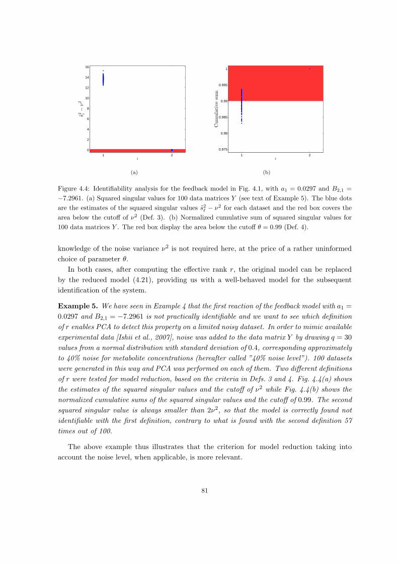
1 2

0

2

4

6

8

10

12

14

16

i

s2 i−

ν2

(a)

1 2

0.975

0.98

0.985

0.99

0.995

1

i

Cum

ula

tiv

esum

(b)

Figure 4.4: Identifiability analysis for the feedback model in Fig. 4.1, with a1 = 0.0297 and B2,1 =

−7.2961. (a) Squared singular values for 100 data matrices Y (see text of Example 5). The blue dots

are the estimates of the squared singular values s2ℓ − ν2 for each dataset and the red box covers the

area below the cutoff of ν2 (Def. 3). (b) Normalized cumulative sum of squared singular values for

100 data matrices Y . The red box display the area below the cutoff θ = 0.99 (Def. 4).

knowledge of the noise variance ν2 is not required here, at the price of a rather uninformed

choice of parameter θ.

In both cases, after computing the effective rank r, the original model can be replaced

by the reduced model (4.21), providing us with a well-behaved model for the subsequent

identification of the system.

Example 5. We have seen in Example 4 that the first reaction of the feedback model with a1 =

0.0297 and B2,1 = −7.2961 is not practically identifiable and we want to see which definition

of r enables PCA to detect this property on a limited noisy dataset. In order to mimic available

experimental data [Ishii et al., 2007], noise was added to the data matrix Y by drawing q = 30

values from a normal distribution with standard deviation of 0.4, corresponding approximately

to 40% noise for metabolite concentrations (hereafter called ”40% noise level”). 100 datasets

were generated in this way and PCA was performed on each of them. Two different definitions

of r were tested for model reduction, based on the criteria in Defs. 3 and 4. Fig. 4.4(a) shows

the estimates of the squared singular values and the cutoff of ν2 while Fig. 4.4(b) shows the

normalized cumulative sums of the squared singular values and the cutoff of 0.99. The second

squared singular value is always smaller than 2ν2, so that the model is correctly found not

identifiable with the first definition, contrary to what is found with the second definition 57

times out of 100.

The above example thus illustrates that the criterion for model reduction taking into

account the noise level, when applicable, is more relevant.

81

Remark 2. The data matrix YC(i) may suffer from the lack of certain data entries, typically

due to the removal of outliers or faults of the experimental machinery. A simple but wasteful

option to recover a full data matrix for later use in a well-defined model reduction/parameter

estimation problem is to discard those data points YjC(i), and the corresponding flux informa-

tion Wji, suffering from the absence of some entry. In Chap. 3, in the context of parameter

estimation, we have proposed methods compensating for the missing entries by the use of

statistical priors inferred from the available data. For the sake of model reduction, which

requires in our approach the SVD of the data matrix, completion of the data matrix by a

suitable imputation method was suggested. Several imputation methods can be considered,

still relying on statistics from the available data, such as multiple imputation, completion by

the mean of the available metabolite data, and so on (see Chap. 3 and references therein).

As an appealing alternative we cite minimal rank SVD, which has been developed and applied

in Brand [2002] for reduced-order modelling in computer vision.

Remark 3. The reduction of the model to Eq. (4.21) introduces new parameters that are

linear combinations of the original parameters. As a consequence, the results of the identi-

fication may be difficult to interpret from a biological point of view. Proposition 3 suggests

a way to isolate identifiable parameters in nonidentifiable reactions, and thus extract partial,

but unambiguous information from the dataset. Unfortunately, the condition of the propo-

sition is not usually verified in practice, since due to noise the entries of the kernel of Y ,

given by the vectors Vj,r+1:nb, j = 1, · · · , nb, will never be exactly 0. In order to ease the

interpretation of the results, one may relax this condition as follows. Bearing in mind that

Vj,r+1:nbis composed of unit-L 2-norm vectors, we consider negligible all entries of Vj,r+1:nb

whose square is below a threshold ρ2 significantly smaller than 1. Further study of the kernel-

generating matrix Vr+1:nbwould yield a theoretically more sophisticated criterion, but we will

not pursue this discussion here.

Remark 4. In general, data from repeated experiments may happen to be more densely con-

centrated in some regions than in others. In the extreme case, homeostatic control of metabo-

lite concentrations may cluster most datapoints around a single value. Thus, the variance

will be dominated by the variance of experimental error, strongly distorting the analysis of

practical identifiability as outlined above. To compensate for this bias, we modify the estima-

tion problem by introducing a weighting scheme to rebalance the importance of the datapoints,

that we develop in Appendix B.2. However, application of this data weighting to Example 3

with a weak feedback showed no significant improvement of the model reduction method (see

Appendix B.2).

4.3.3 The overall model reduction procedure

Based on the discussion of the previous sections, here we summarize the procedure for obtain-

ing a practically identifiable approximate kinetic model from noisy and incomplete datasets.

The procedure is also summarized in Figure 4.5.

82

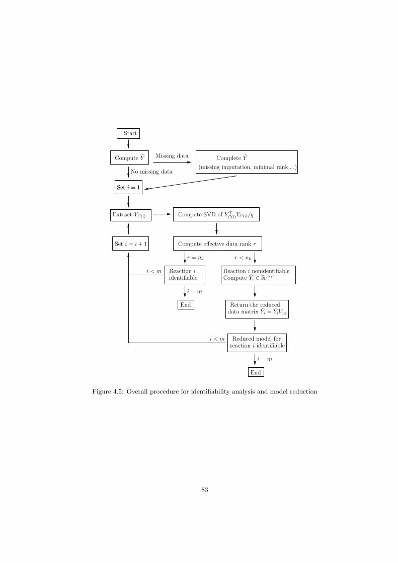
Start

(missing imputation, minimal rank,...)

Complete YCompute Y

Set i = 1Set i = 1

Compute effective data rank r

Compute SVD of Y TC(i)YC(i)/q

Compute Yi ∈ Rq×r

Reaction i nonidentifiable

data matrix Yi = YiV1:r

Return the reduced

End

i = m

Reduced model forreaction i identifiable

End

i = m

Missing data

No missing data

Set i = i+ 1

Extract YC(i)

identifiableReaction i

r = nb r < nb

i < m

i < m

Figure 4.5: Overall procedure for identifiability analysis and model reduction

83

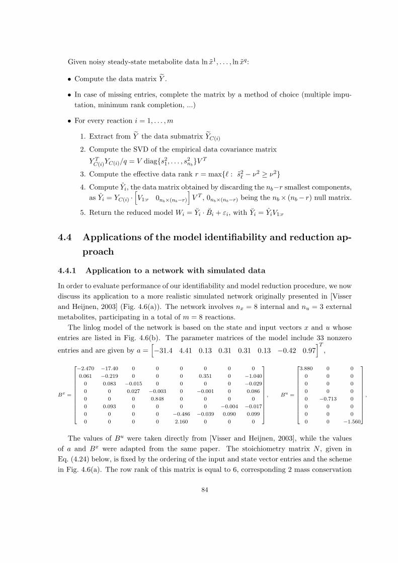
Given noisy steady-state metabolite data ln x1, . . . , ln xq:

• Compute the data matrix Y .

• In case of missing entries, complete the matrix by a method of choice (multiple impu-

tation, minimum rank completion, ...)

• For every reaction i = 1, . . . ,m

1. Extract from Y the data submatrix YC(i)

2. Compute the SVD of the empirical data covariance matrix

Y TC(i)YC(i)/q = V diag{s21, . . . , s2nb

}V T

3. Compute the effective data rank r = max{ℓ : s2ℓ − ν2 ≥ ν2}4. Compute Yi, the data matrix obtained by discarding the nb−r smallest components,

as Yi = YC(i) ·[V1:r 0nb×(nb−r)

]V T , 0nb×(nb−r) being the nb× (nb− r) null matrix.

5. Return the reduced model Wi = Yi · Bi + εi, with Yi = YiV1:r

4.4 Applications of the model identifiability and reduction ap-

proach

4.4.1 Application to a network with simulated data

In order to evaluate performance of our identifiability and model reduction procedure, we now

discuss its application to a more realistic simulated network originally presented in [Visser

and Heijnen, 2003] (Fig. 4.6(a)). The network involves nx = 8 internal and nu = 3 external

metabolites, participating in a total of m = 8 reactions.

The linlog model of the network is based on the state and input vectors x and u whose

entries are listed in Fig. 4.6(b). The parameter matrices of the model include 33 nonzero

entries and are given by a =[−31.4 4.41 0.13 0.31 0.31 0.13 −0.42 0.97

]T,

Bx =

−2.470 −17.40 0 0 0 0 0 0

0.061 −0.219 0 0 0 0.351 0 −1.040

0 0.083 −0.015 0 0 0 0 −0.029

0 0 0.027 −0.003 0 −0.001 0 0.086

0 0 0 0.848 0 0 0 0

0 0.093 0 0 0 0 −0.004 −0.017

0 0 0 0 −0.486 −0.039 0.090 0.099

0 0 0 0 2.160 0 0 0

, Bu =

3.880 0 0

0 0 0

0 0 0

0 0 0

0 −0.713 0

0 0 0

0 0 0

0 0 −1.560

,

The values of Bu were taken directly from [Visser and Heijnen, 2003], while the values

of a and Bx were adapted from the same paper. The stoichiometry matrix N , given in

Eq. (4.24) below, is fixed by the ordering of the input and state vector entries and the scheme

in Fig. 4.6(a). The row rank of this matrix is equal to 6, corresponding 2 mass conservation

84

(a)

Internal metabolites External metabolites

Variable Metabolite Input Metabolite

x1 M1 u1 S

x2 M2 u2 P1

x3 M3 u3 P2

x4 M4

x5 M6

x6 A

x7 M5

x8 AH

(b)

Figure 4.6: (a) A branched metabolic pathway with feedback from [Visser and Heijnen, 2003]. All

reactions are chemically reversible, the arrows represent the positive flux directions. Dashed lines

represent allosteric interactions. (b) Model variables and external metabolites

constraints given in Eq. (4.25). Following the analysis of Reder [1988], it is possible to

factor the matrix into a link matrix L expressing dependencies between concentrations and

a reduced-order full-row rank matrix N corresponding to stoichiometries of independent

metabolites. Factorization is non-unique. In our case, one such factorization gives

N =

1 −1 0 0 0 0 0 0

0 1 −1 0 0 −1 0 0

0 0 1 −1 0 0 0 0

0 0 0 1 −1 0 0 0

0 0 0 0 0 0 1 −1

0 −1 0 1 0 0 1 0

0 0 0 0 0 1 −1 0

0 1 0 −1 0 0 −1 0

=

1 0 0 0 0 0

0 1 0 0 0 0

0 0 1 0 0 0

0 0 0 1 0 0

0 0 0 0 1 0

0 0 0 0 0 1

0 −1 −1 0 0 −1

0 0 0 0 0 −1

·

1 −1 0 0 0 0 0 0

0 1 −1 0 0 −1 0 0

0 0 1 −1 0 0 0 0

0 0 0 1 −1 0 0 0

0 0 0 0 0 0 1 −1

0 −1 0 1 0 0 1 0

(4.24)

= L · N.

With this factorization, the entries of x1:6 (M1, M2, M3, M4, M6 and A) are treated as

independent quantities, and determine the values of x7 (M5) and x8 (AH) via conservation

of mass. That is, for some fixed constants T1, T2 ∈ R>0,

x1:6 = N diag e(a+Bx · lnx+Bu · lnu)T1 = x2 + x3 + x6 + x7

T2 = x6 + x8

(4.25)

In addition to analysis purposes, this reformulation allows one to compute the steady-

85

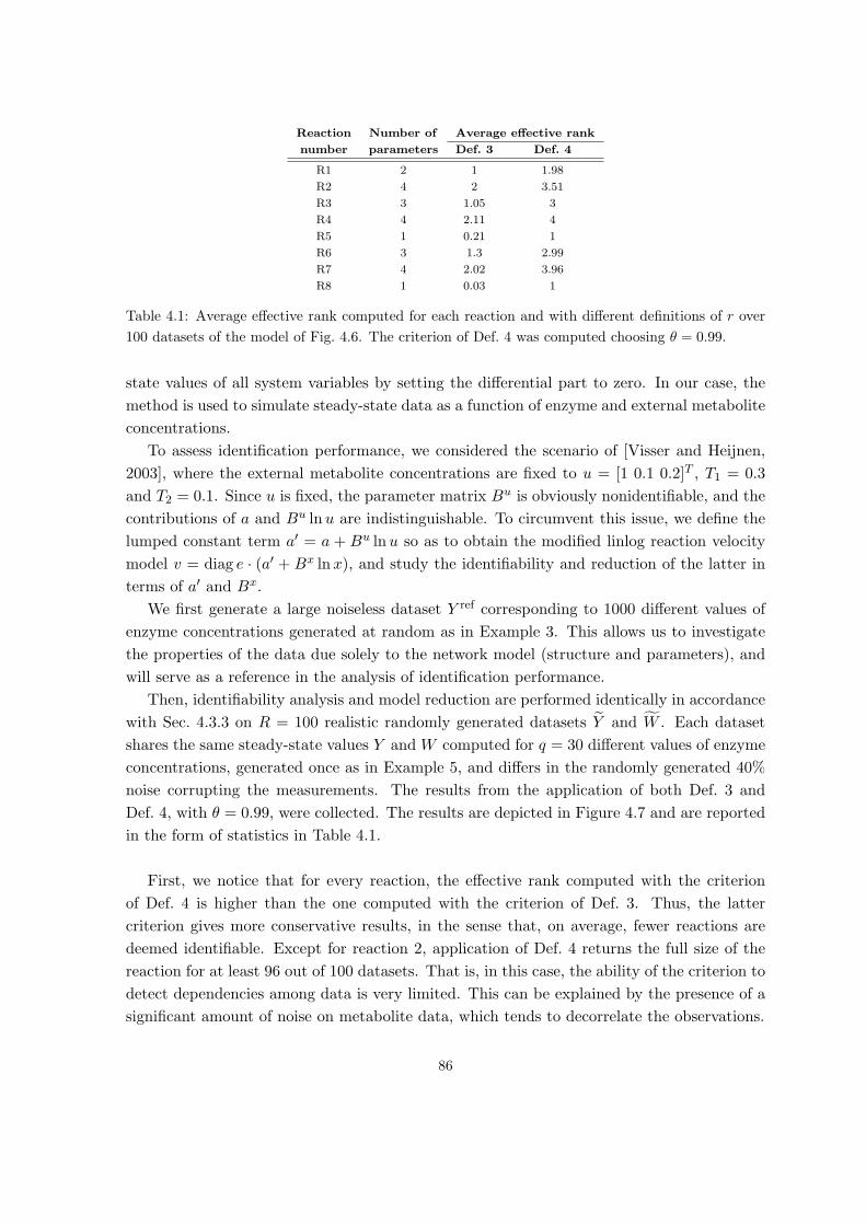
Reaction Number of Average effective rank

number parameters Def. 3 Def. 4

R1 2 1 1.98

R2 4 2 3.51

R3 3 1.05 3

R4 4 2.11 4

R5 1 0.21 1

R6 3 1.3 2.99

R7 4 2.02 3.96

R8 1 0.03 1

Table 4.1: Average effective rank computed for each reaction and with different definitions of r over

100 datasets of the model of Fig. 4.6. The criterion of Def. 4 was computed choosing θ = 0.99.

state values of all system variables by setting the differential part to zero. In our case, the

method is used to simulate steady-state data as a function of enzyme and external metabolite

concentrations.

To assess identification performance, we considered the scenario of [Visser and Heijnen,

2003], where the external metabolite concentrations are fixed to u = [1 0.1 0.2]T , T1 = 0.3

and T2 = 0.1. Since u is fixed, the parameter matrix Bu is obviously nonidentifiable, and the

contributions of a and Bu lnu are indistinguishable. To circumvent this issue, we define the

lumped constant term a′ = a + Bu lnu so as to obtain the modified linlog reaction velocity

model v = diag e · (a′ + Bx lnx), and study the identifiability and reduction of the latter in

terms of a′ and Bx.

We first generate a large noiseless dataset Y ref corresponding to 1000 different values of

enzyme concentrations generated at random as in Example 3. This allows us to investigate

the properties of the data due solely to the network model (structure and parameters), and

will serve as a reference in the analysis of identification performance.

Then, identifiability analysis and model reduction are performed identically in accordance

with Sec. 4.3.3 on R = 100 realistic randomly generated datasets Y and W . Each dataset

shares the same steady-state values Y and W computed for q = 30 different values of enzyme

concentrations, generated once as in Example 5, and differs in the randomly generated 40%

noise corrupting the measurements. The results from the application of both Def. 3 and

Def. 4, with θ = 0.99, were collected. The results are depicted in Figure 4.7 and are reported

in the form of statistics in Table 4.1.

First, we notice that for every reaction, the effective rank computed with the criterion

of Def. 4 is higher than the one computed with the criterion of Def. 3. Thus, the latter

criterion gives more conservative results, in the sense that, on average, fewer reactions are

deemed identifiable. Except for reaction 2, application of Def. 4 returns the full size of the

reaction for at least 96 out of 100 datasets. That is, in this case, the ability of the criterion to

detect dependencies among data is very limited. This can be explained by the presence of a

significant amount of noise on metabolite data, which tends to decorrelate the observations.

86

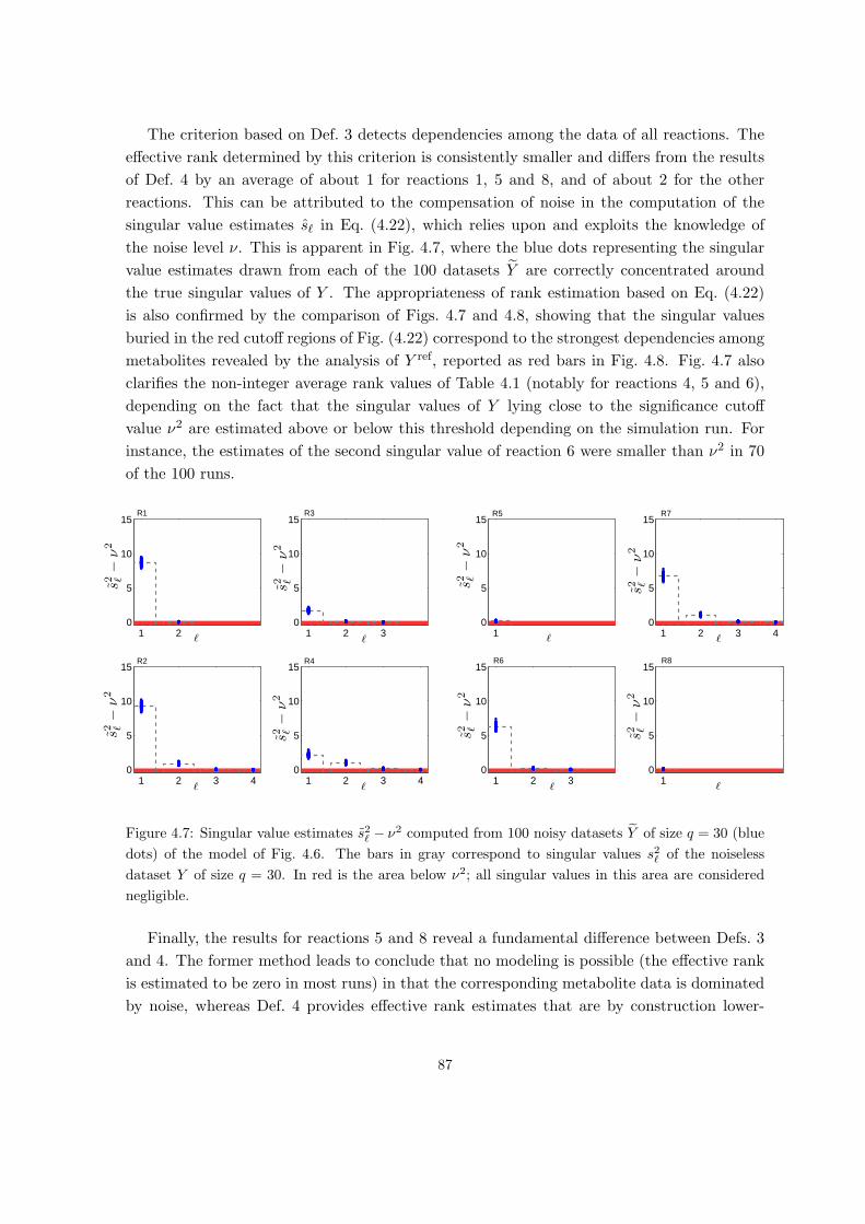
The criterion based on Def. 3 detects dependencies among the data of all reactions. The

effective rank determined by this criterion is consistently smaller and differs from the results

of Def. 4 by an average of about 1 for reactions 1, 5 and 8, and of about 2 for the other

reactions. This can be attributed to the compensation of noise in the computation of the

singular value estimates sℓ in Eq. (4.22), which relies upon and exploits the knowledge of

the noise level ν. This is apparent in Fig. 4.7, where the blue dots representing the singular

value estimates drawn from each of the 100 datasets Y are correctly concentrated around

the true singular values of Y . The appropriateness of rank estimation based on Eq. (4.22)

is also confirmed by the comparison of Figs. 4.7 and 4.8, showing that the singular values

buried in the red cutoff regions of Fig. (4.22) correspond to the strongest dependencies among

metabolites revealed by the analysis of Y ref, reported as red bars in Fig. 4.8. Fig. 4.7 also

clarifies the non-integer average rank values of Table 4.1 (notably for reactions 4, 5 and 6),

depending on the fact that the singular values of Y lying close to the significance cutoff

value ν2 are estimated above or below this threshold depending on the simulation run. For

instance, the estimates of the second singular value of reaction 6 were smaller than ν2 in 70

of the 100 runs.

1 20

5

10

15

ℓ

R1

s2 ℓ−

ν2

1 2 3 40

5

10

15

ℓ

R2

s2 ℓ−

ν2

1 2 30

5

10

15

ℓ

R3

s2 ℓ−

ν2

1 2 3 40

5

10

15

ℓ

R4

s2 ℓ−

ν2

10

5

10

15

ℓ

R5

s2 ℓ−

ν2

1 2 30

5

10

15

ℓ

R6

s2 ℓ−

ν2

10

5

10

15

ℓ

R8

s2 ℓ−

ν2

1 2 3 40

5

10

15

ℓ

R7

s2 ℓ−

ν2

Figure 4.7: Singular value estimates s2ℓ − ν2 computed from 100 noisy datasets Y of size q = 30 (blue

dots) of the model of Fig. 4.6. The bars in gray correspond to singular values s2ℓ of the noiseless

dataset Y of size q = 30. In red is the area below ν2; all singular values in this area are considered

negligible.

Finally, the results for reactions 5 and 8 reveal a fundamental difference between Defs. 3

and 4. The former method leads to conclude that no modeling is possible (the effective rank

is estimated to be zero in most runs) in that the corresponding metabolite data is dominated

by noise, whereas Def. 4 provides effective rank estimates that are by construction lower-

87

bounded by one.

We would like to compare the results from the model reduction criterion of Def. 3 with

the reference dataset Y ref . Apart from an arbitrary threshold on the norm, we do not have

an objective quantitative criterion to determine rank deficiency on submatrices of noiseless

Y ref . For each reaction, the SVD of the corresponding submatrix of Y ref was computed

and singular values are shown in Fig. 4.8. In this figure are highlighted in red the reference

singular values that would be considered negligible with the rank reductions of last column

of Table 4.1. We observe that all singular values that intuitively matter are captured. Thus

the method of Def. 3 gives consistent results with the ’ideal’ dataset Y ref .

1 20

5

10

15

ℓ

s2 ℓ

R1

1 2 3 40

5

10

15

ℓ

s2 ℓ

R2

1 2 30

5

10

15

ℓ

s2 ℓ

R3

1 2 3 40

5

10

15

ℓ

s2 ℓ

R4

10

5

10

15

ℓ

s2 ℓ

R5

1 2 30

5

10

15

ℓ

s2 ℓ

R6

1 2 3 40

5

10

15

ℓ

s2 ℓ

R7

10

5

10

15

ℓs2 ℓ

R8

Figure 4.8: Squared singular values of the noiseless dataset Y ref of the model of Fig. 4.6 (q = 1000).

The bars in red correspond to singular values that are detected as negligible in at least 70% of the

cases by Def. 3 on 100 noisy datasets.

From the results of this section, it is clear that identifiability analysis and model reduction

in the presence of noise should be performed on the basis of the effective rank of Def. 3, which

outperforms Def. 4 to all practical effects and returns consistent results (Table 4.1; compare

Fig. 4.7 and 4.8). This makes us select Def. 3 as the basis for identifiability analysis and model

reduction of real data. The actual application of the method to a real dataset is discussed in

the next section.

A discussion about the application of the model reduction methods discussed in Sec. 4.3.2

in case of a biased dataset can be found in Appendix B.2.

4.4.2 Application to central carbon metabolism of E. coli

As a second example, we illustrate the application of our method to a complex network of

biochemical reactions involved in carbon assimilation in the enterobacterium Escherichia coli.

88

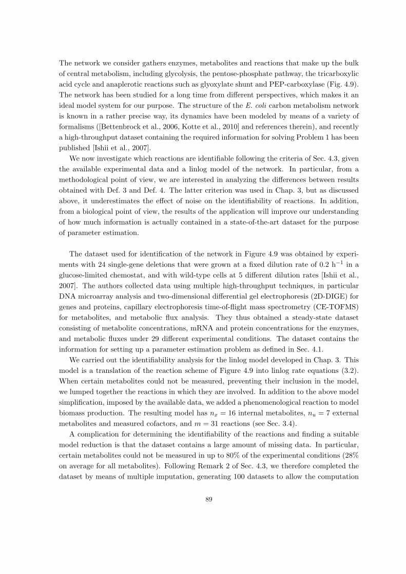
The network we consider gathers enzymes, metabolites and reactions that make up the bulk

of central metabolism, including glycolysis, the pentose-phosphate pathway, the tricarboxylic

acid cycle and anaplerotic reactions such as glyoxylate shunt and PEP-carboxylase (Fig. 4.9).

The network has been studied for a long time from different perspectives, which makes it an

ideal model system for our purpose. The structure of the E. coli carbon metabolism network

is known in a rather precise way, its dynamics have been modeled by means of a variety of

formalisms ([Bettenbrock et al., 2006, Kotte et al., 2010] and references therein), and recently

a high-throughput dataset containing the required information for solving Problem 1 has been

published [Ishii et al., 2007].

We now investigate which reactions are identifiable following the criteria of Sec. 4.3, given

the available experimental data and a linlog model of the network. In particular, from a

methodological point of view, we are interested in analyzing the differences between results

obtained with Def. 3 and Def. 4. The latter criterion was used in Chap. 3, but as discussed

above, it underestimates the effect of noise on the identifiability of reactions. In addition,

from a biological point of view, the results of the application will improve our understanding

of how much information is actually contained in a state-of-the-art dataset for the purpose

of parameter estimation.

The dataset used for identification of the network in Figure 4.9 was obtained by experi-

ments with 24 single-gene deletions that were grown at a fixed dilution rate of 0.2 h−1 in a

glucose-limited chemostat, and with wild-type cells at 5 different dilution rates [Ishii et al.,

2007]. The authors collected data using multiple high-throughput techniques, in particular

DNA microarray analysis and two-dimensional differential gel electrophoresis (2D-DIGE) for

genes and proteins, capillary electrophoresis time-of-flight mass spectrometry (CE-TOFMS)

for metabolites, and metabolic flux analysis. They thus obtained a steady-state dataset

consisting of metabolite concentrations, mRNA and protein concentrations for the enzymes,

and metabolic fluxes under 29 different experimental conditions. The dataset contains the

information for setting up a parameter estimation problem as defined in Sec. 4.1.

We carried out the identifiability analysis for the linlog model developed in Chap. 3. This

model is a translation of the reaction scheme of Figure 4.9 into linlog rate equations (3.2).

When certain metabolites could not be measured, preventing their inclusion in the model,

we lumped together the reactions in which they are involved. In addition to the above model

simplification, imposed by the available data, we added a phenomenological reaction to model

biomass production. The resulting model has nx = 16 internal metabolites, nu = 7 external

metabolites and measured cofactors, and m = 31 reactions (see Sec. 3.4).

A complication for determining the identifiability of the reactions and finding a suitable

model reduction is that the dataset contains a large amount of missing data. In particular,

certain metabolites could not be measured in up to 80% of the experimental conditions (28%

on average for all metabolites). Following Remark 2 of Sec. 4.3, we therefore completed the

dataset by means of multiple imputation, generating 100 datasets to allow the computation

89

Figure 4.9: Scheme of Escherichia coli central carbon metabolism. The map shows metabolites (bold

fonts) and genes (italic). Abbreviations of metabolites are glucose (Glc), glucose 6-phosphate (G6P),

fructose 6-phosphate (F6P), fructose 1-6-biphosphate (FBP), dihydroxyacetone phosphate (DHAP),

glyceraldehyde 3-phosphate (G3P), 3-phosphoglycerate (3PG), phosphoenolpyruvate (PEP), pyru-

vate (Pyr), 6-phosphogluconate (6PG), 2-keto-3-deoxy-6-phospho-gluconate (2KDPG), ribulose 5-

phosphate (Ru5P), ribose 5-phosphate (R5P), xylulose 5-phosphate (X5P), sedoheptulose 7-phosphate

(S7P), erythrose 4-phosphate (E4P), oxaloacetate (OAA), citrate (Cit), isocitrate (IsoCit), 2-keto-

glutarate (2KG), succinate-CoA (Suc-coA), succinate (Suc), fumarate (Fum), malate (Mal), glyoxy-

late (Glyox), acetyl-CoA (Ac-coA), acetylphosphate (Acp) and acetate (Ace). Cofactors impacting the

reactions are not shown: adenosine triphosphate (ATP), adenosine diphosphate (ADP), nicotinamide

adenine dinucleotide phosphate (NADP) and its reduced form (NADPH), nicotinamide adenine din-

ucleotide (NAD) and its reduced form (NADH) and flavin adenine dinucleotide (FAD). The gene

names are separated by a comma in the case of isoenzymes, by a colon for enzyme complexes, and by

a semicolon when the enzymes catalyze reactions that have been lumped together in the model.

90

of statistics and test the robustness of the results.

Table 4.2 summarizes the results of applying the reduction method of Sec. 4.3.3 to the

model and the data. For each of the reactions in the model, we computed the average of the

effective rank of the 100 datasets. The effective rank for the individual datasets was usually

found to be the same (in at least 82 of the 100 datasets), which explains that the computed

average values are close to integers. Remarkably, out of the 31 reactions in the model, only

4 were found to be identifiable: reactions 4, 5, 14, and 31. The first three reactions involve

two metabolites: fructose 1-6-biphosphate (FBP) and dihydroxyacetone phosphate (DHAP)

(reaction 4), dihydroxyacetone phosphate (DHAP) and 3-phosphoglycerate (3PG) (reaction

5) and ribose 5-phosphate (R5P) and sedoheptulose 7-phosphate (S7P) (reaction 14). The

identifiability of these reactions means that the method did not detect any dependencies

between these pairs of metabolite concentrations. Reaction 31 involves a single metabolic

variable acetyl-CoA (Ac-coA). In the remaining 27 nonidentifiable reactions, the effective

rank is reduced by 1 (in the case of 18 reactions), 2 (6 reactions), 3 (2 reactions), and 6

(1 reaction). The latter case concerns the growth-rate reaction, which has 11 variables. A

striking observation on Tables 4.2 and 4.3 is therefore the large number of nonidentifiable

reactions and parameters.

Average Full Average Full

Reaction Enzyme effective rank dimension Reaction Enzyme effective rank dimension

1 PtsG 3 4 17 GltA,PrpC 2.97 4

2 Pgi 1 2 18 AcnA,AcnB 1 2

3 PfkA,PfkB 2.85 4 19 IcdA 1 3

4 FbaA,FbaB 2 2 20 SucA:SucB:LpdA;SucC:SucD 1 3

5 TpiA 2 2 21 SdhA:SdhB:SdhC:SdhD 1 3

6 GapA;Pgk 2.99 4 22 FumA,FumB,FumC 1 2

7 GpmA,GpmB;Eno 1 2 23 Mdh 2.97 4

8 PykA,PykF 2 4 24 Ppc;PckA 3 5

9 AceE:AceF:LpdA 1.99 3 25 MaeB,SfcA 2 5

10 Zwf;Pgl 1.98 3 26 AceA;AceB 1 3

11 Gnd 2 3 27 µ 4.94 11

12 Rpe 1 2 28 Edd;Eda 1 2

13 RpiA,RpiB 1.99 3 29 Pta;AckA,AckB 3 6

14 TktA 1.82 2 30 LdhA 1 2

15 TalA,TalB 1 2 31 AdhE 1 1

16 TktB 1.01 2

Table 4.2: Average effective rank computed for the reactions in the linlog model of E. coli central

carbon metabolism, using the data of Ishii et al. [2007]. SVD has been applied on YC(i) for each

reaction and singular values were discarded based on Def. 3. Identifiable reactions are shown in green.

Reaction 27, labeled µ, is a phenomenological reaction for biomass production.

In order to isolate identifiable parameters in nonidentifiable reactions, Prop. 3 proposes a

criterion that has been relaxed in Remark 3 so as to make it applicable to noisy data. The

approach is based on the choice of a threshold ρ2 for neglecting components of the kernel

matrix of Y . In what follows, to set a ground for discussion, we set ρ equal to 0.15. We

91

verified that changes of this threshold within the range ρ ∈ [0.1, 0.2] do not significantly alter

the results as reported in Table 4.3. In this table, parameters that were diagnosed as being

identifiable in more than 50% of the completed datasets are highlighted in green. From the

27 nonidentifiable reactions, no individual parameter could be unambiguously extracted in

8 cases (reactions 2, 7, 8, 12, 15, 16, 22 and 24). Of the 94 parameters in the remaining

19 reactions, 30 are identifiable in more than half of the datasets. In particular, we observe

that all parameters associated to glucose (Glc), DHAP, acetyl-CoA/CoA (Ac-coA/coA), 6-

phosphogluconate (6PG), ribose 5-phosphate (R5P), FAD and acetate (Ace) are identifiable,

in the sense that no significant dependencies with other metabolites could be detected in the

experimental conditions of Ishii et al. [2007].

The results shown in Table 4.3 are different from those obtained in Sec. 3.4, where we

used a method based on Def. 4 with θ = 0.99 instead of Def. 3. Indeed, we previously found

many more reactions to be identifiable (24 out of 31) although, for most cases, parameter

estimates were unreliable because of large confidence intervals. We believe that the results

shown in Tables 4.2 and 4.3 more faithfully reflect the noisy character of the data, which

is not explicitly taken into account by the criterion of Def. 4. Therefore, the results of the

identifiability analysis in Sec. 3.4 appear to be overly optimistic, i.e., overestimating the

number of identifiable reactions and parameters because measurement noise on metabolite

concentrations are not taken into account. Notwithstanding, the results of both analyses are

consistent in the sense that all 7 reactions detected as nonidentifiable by means of Def. 4

remain nonidentifiable according to Def. 3 (reactions 10, 11, 17, 25, 27, 28 and 29).

We verified that taking into account the bias in the data sampling did not significantly

change the identifiability analysis of the model (see Appendix B.2 for further details).

4.5 Discussion

A major, but often overlooked problem in the identification of metabolic network models is

the identifiability of the parameters, and hence of the model. Informally speaking, the iden-

tifiability of a model (parameter) consists in the possibility to unambiguously reconstruct

the model (parameter) from the observed behavior of the network. Identifiability problems

may reside in the very structure of the model, notably the occurrence of (implicit) depen-

dencies between parameters. These dependencies might be due to an inappropriate model

formulation, constraints on the kind of experimental perturbations that can be realized, and

unobserved variables. In addition, practical identifiability problems may arise from limita-

tions on the quality and quantity of available data, in particular the fact that experimental

data in biology are usually noisy, biased, sparse and incomplete.

We have studied identifiability issues in the context of approximate kinetic modeling for-

malisms, notably linear-logarithmic (linlog) models. On the theoretical side, following the

classical systems identification literature [Ljung, 1999, Walter and Pronzato, 1997], we have

92

Table 4.3: Parameter matrix [Bx Bu] and results of identifiability analysis and model reduction on the data by [Ishii et al., 2007] for the linlog

model of E. coli central carbon metabolism (the columns of the matrix have been permuted for readability). SVD has been applied on YC(i)i

for each reaction and singular values were discarded based on Def. 3. Nonidentifiable parameters are shown in gray and identifiable ones,

as well as identifiable reactions, in green. The percentages of cases for which the parameters were found identifiable out of the 100 imputed

datasets are mentioned. Abbreviations are as in Fig. 4.9. To avoid complications deriving from the presence of conserved moieties, some of

the metabolites are modeled as ratios of metabolite concentrations, e.g. ATP/ADP. Reaction 27, labeled µ, is a phenomenological reaction for

biomass production. The last row indicates the percentage of missing data per metabolite.

Enzyme

MetaboliteGlc PEP G6P Pyr F6P FBP DHAP 3PG Ac-coA

coA

6PG Ru5P R5P S7P 2KG Suc Fum Mal ATP

ADP

Cit NADPH

NADP

NADH

NAD

FAD Ace

1 PtsG 100% 100% 31% 0 %

2 Pgi 0 % 0 %

3 PfkA,PfkB 70% 2% 63% 8%

4 FbaA,FbaB 100% 100%

5 TpiA 100% 100%

6 GapA;Pgk 84% 6% 0% 51%

7 GpmA,GpmB;Eno 0% 0%

8 PykA,PykF 5% 0% 22% 0%

9 AceE:AceF:LpdA 1% 99% 94%

10 Zwf;Pgl 70% 100% 2%

11 Gnd 100% 100% 0%

12 Rpe 0% 0%

13 RpiA,RpiB 0% 0% 66%

14 TktA 82% 82%

15 TalA,TalB 0% 0%

16 TktB 1% 1%

17 GltA,PrpC 97% 2% 98% 97%

18 AcnA,AcnB 0% 100%

19 IcdA 100% 0% 0%

20 SucA:SucB:LpdA;SucC:SucD 0% 0% 90%

21 SdhA:SdhB:SdhC:SdhD 0% 0% 62%

22 FumA,FumB,FumC 0% 0%

23 Mdh 87% 0% 75% 35%

24 Ppc;PckA 19% 5% 0% 0% 32%

25 MaeB,SfcA 0% 99% 0% 0% 30%

26 AceA;AceB 100% 0% 0%

27 µ 0% 0% 0% 0% 0% 68% 81% 0% 0% 0% 27%

28 Edd;Eda 0% 100%

29 Pta;AckA,AckB 0% 70% 0% 0% 37% 100%

30 LdhA 0% 95%

31 AdhE 100%

% Missing data 3 17 0 48 7 34 59 10 3 72 3 38 3 59 3 14 14 0 62 79 79 17 17

93

first precisely defined the notions of structural (a-priori) identifiability (Def. 1) and practical

(a-posteriori) identifiability (Def. 2). The latter notion is obviously related to the former,

in the sense that structural nonidentifiability entails practical nonidentifiability. However,

Proposition 2 goes beyond this evidence by saying that identifiability in the theoretical sense

may also imply identifiability in the practical sense, provided that the uncertainty on the pa-

rameters, as determined by the available dataset, remains within the desired accuracy bounds.

Notice that practical identifiability is thus not an absolute notion, but rather conditional on

the data properties and the required model precision.

A second methodological contribution of this chapter is the development of theoretically

sound and practically applicable methods for the detection of identifiability problems and

the transformation of a nonidentifiable model to a reduced identifiable model. In particular,

we have formulated criteria based on the singular value decomposition (SVD) of the matrix

of log-transformed and centered measurements of metabolite concentrations. These criteria

define the effective rank of the data matrix, corresponding to the number of parameters that

can be safely distinguished from the output. The criterion privileged in this chapter (Def. 3),

contrary to a criterion that we proposed in the previous chapter (Def. 4), takes into account

the estimated variance of the noise. The flow chart in Fig. 4.5 gives a step-by-step procedure

for identifiability analysis and model reduction.

The identifiability of models of biological systems is a topic that has been much studied in

mathematical biology, and that has received renewed attention in the context of systems biol-

ogy in recent years (see Chappell et al. [1990], Chis et al. [2011b], Cobelli and di Stefano 3rd

[1980], Raue et al. [2011] for reviews). Systems of biochemical reactions, which have the

general form of Eq. (4.3) at steady-state, have a number of peculiarities for identifiability

analysis. When reaction rates, enzyme concentrations and metabolite concentrations are

measured, the identification problem can be decomposed into subproblems for each of the

individual reactions. Determining the identifiability of a model then reduces to checking the

identifiability of the reactions. If in addition the reaction rates are expressed in terms of lin-

log or other pseudo-linear equations, identification becomes a linear or orthogonal regression

problem, depending on whether noise on the metabolite concentrations is taken into account

or not (Problem 4 and Problem 5, respectively). Identifiability analysis then amounts to

checking for linear dependencies in the transformed data matrix, which can be easily done

using standard techniques from linear algebra and statistics. Related ideas starting from this

general approach can be found in other recent work [Srinath and Gunawan, 2010, Nikerel

et al., 2009]. However, as discussed in more detail in previous sections, the development of

this approach in this chapter is different in fundamental ways, such as the very definition

of structural and practical identifiability, and the application of SVD to detect and resolve

identifiability problems.

Although linlog models have been central in this chapter, the results directly carry over

to the other approximate formalisms mentioned in Sec. 4.1. In addition, they also bear on

94

more general classes of nonlinear models of metabolic networks.Indeed the parameters in the

mean-removed linlog model of Eq. (3.5) are proportional to elasticity coefficients that de-

scribe the sensitivities of reaction rates to changes in metabolite concentrations. If a reaction

in a linlog model is nonidentifiable, this means that elasticity coefficients are not identifiable,

therefore any other class of kinetic models is liable to encounter similar identifiability issues.

The approach for determining the identifiability of linlog models proposed in this chap-

ter has been tested on a network with simulated data (Sec. 4.4.1) and applied to a high-

throughput dataset for central carbon metabolism in E. coli (Sec. 4.4.2). The use of sim-

ulated data has made it possible to demonstrate that, for typical sizes of the dataset and

realistic noise levels, our approach is able to correctly identify the principal components of

the parameter vector (Fig. 4.7 and Fig. 4.8). Surprisingly, the determination of the effective

rank of the datasets for the different reactions in the E. coli metabolic network shows that

only a small fraction of the reactions (4 out of 31) is fully identifiable from the data of Ishii

et al. [2007]. In addition, only 37 out of a total of 100 model parameters are individually

identifiable. We note that these results are different from those reported in Sec. 3.4, due to

the fact that here we take into account the measurement noise of metabolite concentrations

to decide whether a parameter associated with a principal component is negligible. The low

numbers of identifiable reactions and parameters agree with those obtained with power-law

models on other state-of-the-art datasets Srinath and Gunawan [2010]. This further demon-

strates the importance of a preliminary identifiability analysis when estimating parameters

in metabolic network models.

The rank analysis carried out to determine the identifiability of a reaction also shows

how the model can be reduced if the data does not allow the parameters of the model to

be unambiguously determined. This reduction step yields minimal models in the form of

Eq. (4.21), that have the advantage of being adapted to the informativeness of the dataset.

A disadvantage of this approach, however, is that the parameters of the reduced model may

be difficult to interpret from a biological point of view, as they do not generally determine

the original parameters in a unique way, but rather define a linear subspace of the parameter

space. Nevertheless, in some cases it may still be possible to identify some parameters of

the original model (Proposition 3 and Remark 3). This criterion was shown to be useful in

practice, as it allowed to uniquely identify 30 out of 93 parameters in the nonidentifiable

reactions of the E.coli metabolic network model (Table 4.3).

If the parameters of the original, non-reduced model cannot be uniquely determined from

the data, then additional experiments are necessary. Generally speaking, experimental con-

ditions that explore the range of possible behaviors of the network as much as possible

improve identifiability. Given that experiments are usually carried out at steady-state, es-

pecially for metabolic flux measurements, the available datasets have a sampling bias that

may complicate parameter estimation. In particular, metabolic systems almost invariably

contain highly evolved regulatory loops that may homeostatically buffer the concentrations

95

of some metabolic pools [Bennett et al., 2009, Ishii et al., 2007]. As a consequence, a range

of different growth conditions and genetic backgrounds may lead to little variation in steady-

state metabolite concentrations. The growing availability of time-series data (e.g., Voit et al.

[2006b], Hardiman et al. [2007]), although more demanding from an experimental point of

view, promises to relieve this problem.

96

Chapter 5

Shared control of gene expression

in bacteria by transcriptional

regulators and global physiological

state

Bacterial cells continuously adjust gene expression in response to challenges from their envi-

ronment. These adjustments involve transcription factors that sense metabolic signals and

specifically activate or inhibit target genes. Several hundreds of transcription factors have

been identified in E. coli [Martinez-Antonio and Collado-Vides, 2003]: while some respond to

a particular stress and have only a few targets, others coordinate the expression of hundreds

of genes across a variety of cellular functions. Well-known examples of the latter are global

regulators of transcription such as Crp, Fis, and RpoS (σS) [Hengge-Aronis, 2002, Gosset

et al., 2004, Bradley et al., 2007, Cho et al., 2008].

In addition to local regulation by DNA-binding transcription factors, the adjustments of

gene expression involve global, regulatory mechanisms responding to the overall physiolog-

ical state of the cell. More specifically, changes in the environment lead to the adaptation

of metabolic pools and the macromolecular composition of the cell, which in turn affect the

rate of transcription and translation. In balanced exponential growth, changes in the physi-

ological state are reflected in the growth rate supported by the medium. Classical studies in

bacterial physiology, reviewed in [Bremer and Dennis, 1996, Neidhardt et al., 1990, Maaloe

and Kjeldgaard, 1966], have demonstrated the variation with the growth rate of a variety

of physiological parameters, such as the concentrations of free RNA polymerase, ribosome

abundance, gene copy number, and the size of amino acid and nucleotide pools. The depen-

dencies between these parameters and the steady-state growth rate of the cells have been

expressed in the form of phenomenological growth laws [Scott et al., 2010].

97

The joint control of gene expression by both local effects of transcription factors and global

effects of the physiological state has received relatively little attention thus far. Among the

exceptions, we cite the work of Klumpp et al. [2009], who have shown by a combination

of models and experiments that the steady-state concentration of proteins in simple net-

work architectures depends on the combined action of transcription factors and the growth

rate. Dennis et al. review the huge amount of data on the control of rRNA synthesis in

E. coli accumulated over several decades [Dennis et al., 2004]. They propose a model that

integrates both growth-rate dependent effects on the activity of rrn promoters and specific

regulatory control exerted by Fis. Notwithstanding the insights gained from these and other

studies, they are limited in two respects. First, they consider the control of gene expression at

steady-state, not during transitions between physiological states. Second, there is currently

no dataset available that allows the contributions of local and global effects to be studied

on the level of an entire regulatory network, consisting of several genes and their interactions.

Here we address the above questions in the case of a central regulatory circuit in Es-

cherichia coli (Fig. 5.1). The network consists of the two most pleiotropic transcription

factors of the cell, Fis and Crp, as well as the gene acs, encoding the enzyme acetyl-CoA

synthetase (Acs). This enzyme converts acetate to acetyl-CoA, a critical step in acetate

metabolism [Wolfe, 2005]. We are notably interested in the question how Fis and Crp share

control over acs expression with the physiological state of the cell when glucose is used as the

sole carbon source. Acetate is excreted during growth on glucose and, after exhaustion of the

latter, utilized by the cells to continue growth at a lower rate. Glucose depletion triggers the

accumulation of the signaling metabolite cyclic AMP (cAMP), which activates Crp and thus

enables it to stimulate the expression of acs, an effect counteracted by Fis. At the same time,

the redistribution of metabolic fluxes upon glucose depletion affects the series of metabolic

pools and other global physiological parameters, thus indirectly affecting the expression of

acs and other genes.

What are the relative contributions of transcription factors and global physiological pa-

rameters to changes in gene expression? In order to answer this question in a quantitative

way, we monitored in real time and in vivo, by means of GFP reporters, the expression of

the genes in the acs network in response to glucose depletion. In parallel, a GFP reporter

driven by a non-regulated phage promoter was used to assay the time-varying physiological

state. We show that a simple, parameterless mathematical model can be used to separate the

variation of the promoter activity of the genes into a part due to global physiological control

and a part due to local transcription regulation. In order to verify if the latter part can be

accounted for by known regulators, in particular Crp, we extended the model and measured

the time-varying concentration of cAMP. The above experiments were repeated when the

network was submitted to various physiological and genetic perturbations, such as shifting

the cell to a low-glucose medium or deleting the genes fis and crp.

98

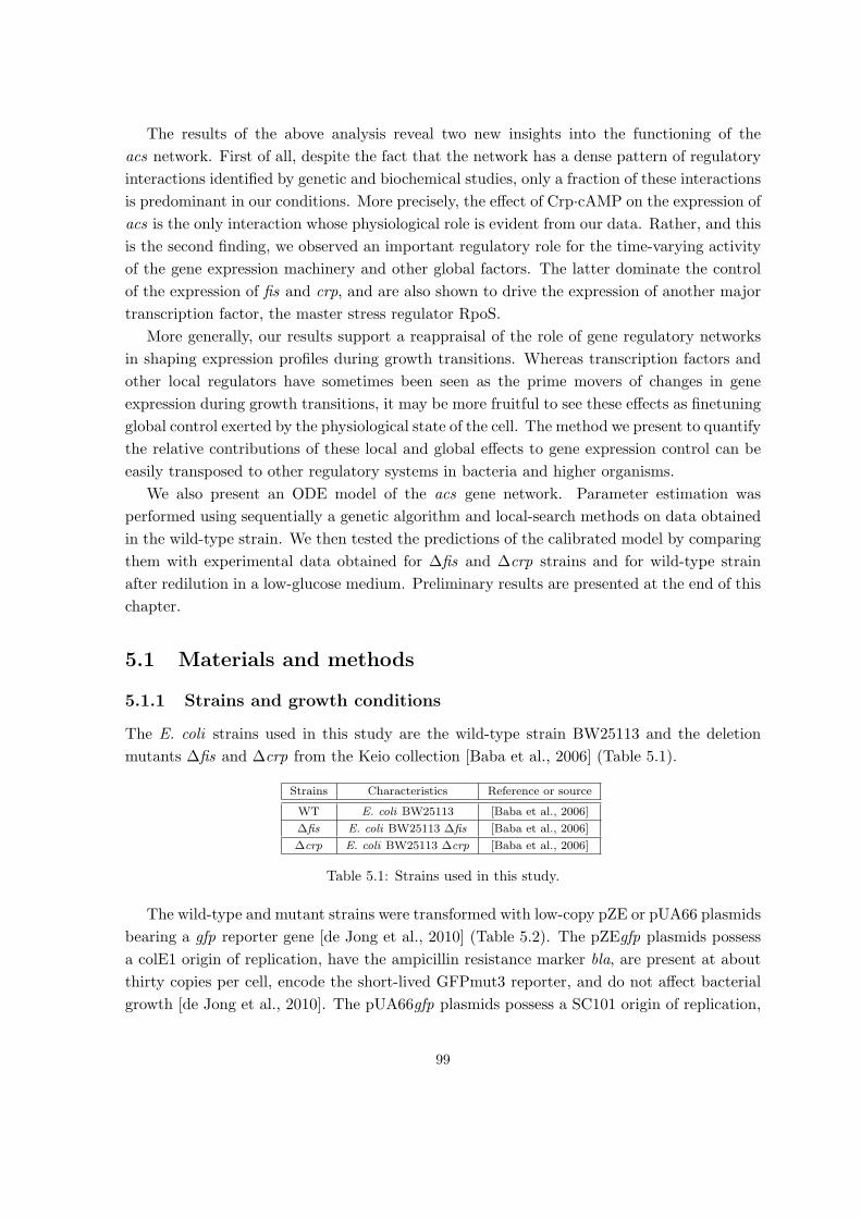
The results of the above analysis reveal two new insights into the functioning of the

acs network. First of all, despite the fact that the network has a dense pattern of regulatory

interactions identified by genetic and biochemical studies, only a fraction of these interactions

is predominant in our conditions. More precisely, the effect of Crp·cAMP on the expression of

acs is the only interaction whose physiological role is evident from our data. Rather, and this

is the second finding, we observed an important regulatory role for the time-varying activity

of the gene expression machinery and other global factors. The latter dominate the control

of the expression of fis and crp, and are also shown to drive the expression of another major

transcription factor, the master stress regulator RpoS.

More generally, our results support a reappraisal of the role of gene regulatory networks

in shaping expression profiles during growth transitions. Whereas transcription factors and

other local regulators have sometimes been seen as the prime movers of changes in gene

expression during growth transitions, it may be more fruitful to see these effects as finetuning

global control exerted by the physiological state of the cell. The method we present to quantify

the relative contributions of these local and global effects to gene expression control can be

easily transposed to other regulatory systems in bacteria and higher organisms.

We also present an ODE model of the acs gene network. Parameter estimation was

performed using sequentially a genetic algorithm and local-search methods on data obtained

in the wild-type strain. We then tested the predictions of the calibrated model by comparing

them with experimental data obtained for ∆fis and ∆crp strains and for wild-type strain

after redilution in a low-glucose medium. Preliminary results are presented at the end of this

chapter.

5.1 Materials and methods

5.1.1 Strains and growth conditions

The E. coli strains used in this study are the wild-type strain BW25113 and the deletion

mutants ∆fis and ∆crp from the Keio collection [Baba et al., 2006] (Table 5.1).

Strains Characteristics Reference or source

WT E. coli BW25113 [Baba et al., 2006]

∆fis E. coli BW25113 ∆fis [Baba et al., 2006]

∆crp E. coli BW25113 ∆crp [Baba et al., 2006]

Table 5.1: Strains used in this study.

The wild-type and mutant strains were transformed with low-copy pZE or pUA66 plasmids

bearing a gfp reporter gene [de Jong et al., 2010] (Table 5.2). The pZEgfp plasmids possess

a colE1 origin of replication, have the ampicillin resistance marker bla, are present at about

thirty copies per cell, encode the short-lived GFPmut3 reporter, and do not affect bacterial

growth [de Jong et al., 2010]. The pUA66gfp plasmids possess a SC101 origin of replication,

99

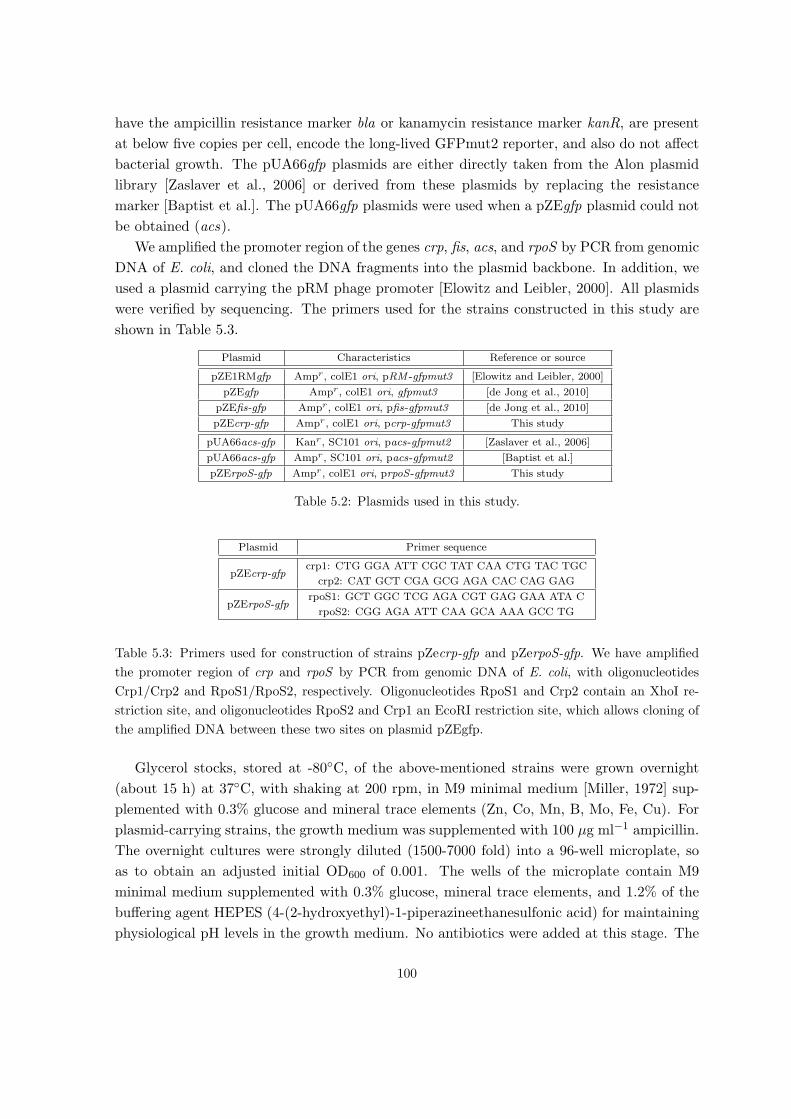
have the ampicillin resistance marker bla or kanamycin resistance marker kanR, are present

at below five copies per cell, encode the long-lived GFPmut2 reporter, and also do not affect

bacterial growth. The pUA66gfp plasmids are either directly taken from the Alon plasmid

library [Zaslaver et al., 2006] or derived from these plasmids by replacing the resistance

marker [Baptist et al.]. The pUA66gfp plasmids were used when a pZEgfp plasmid could not

be obtained (acs).

We amplified the promoter region of the genes crp, fis, acs, and rpoS by PCR from genomic

DNA of E. coli, and cloned the DNA fragments into the plasmid backbone. In addition, we

used a plasmid carrying the pRM phage promoter [Elowitz and Leibler, 2000]. All plasmids

were verified by sequencing. The primers used for the strains constructed in this study are

shown in Table 5.3.

Plasmid Characteristics Reference or source

pZE1RMgfp Ampr, colE1 ori, pRM -gfpmut3 [Elowitz and Leibler, 2000]

pZEgfp Ampr, colE1 ori, gfpmut3 [de Jong et al., 2010]

pZEfis-gfp Ampr, colE1 ori, pfis-gfpmut3 [de Jong et al., 2010]

pZEcrp-gfp Ampr, colE1 ori, pcrp-gfpmut3 This study

pUA66acs-gfp Kanr, SC101 ori, pacs-gfpmut2 [Zaslaver et al., 2006]

pUA66acs-gfp Ampr, SC101 ori, pacs-gfpmut2 [Baptist et al.]

pZErpoS-gfp Ampr, colE1 ori, prpoS -gfpmut3 This study

Table 5.2: Plasmids used in this study.

Plasmid Primer sequence

pZEcrp-gfpcrp1: CTG GGA ATT CGC TAT CAA CTG TAC TGC

crp2: CAT GCT CGA GCG AGA CAC CAG GAG

pZErpoS-gfprpoS1: GCT GGC TCG AGA CGT GAG GAA ATA C

rpoS2: CGG AGA ATT CAA GCA AAA GCC TG

Table 5.3: Primers used for construction of strains pZecrp-gfp and pZerpoS-gfp. We have amplified

the promoter region of crp and rpoS by PCR from genomic DNA of E. coli, with oligonucleotides

Crp1/Crp2 and RpoS1/RpoS2, respectively. Oligonucleotides RpoS1 and Crp2 contain an XhoI re-

striction site, and oligonucleotides RpoS2 and Crp1 an EcoRI restriction site, which allows cloning of

the amplified DNA between these two sites on plasmid pZEgfp.

Glycerol stocks, stored at -80◦C, of the above-mentioned strains were grown overnight

(about 15 h) at 37◦C, with shaking at 200 rpm, in M9 minimal medium [Miller, 1972] sup-

plemented with 0.3% glucose and mineral trace elements (Zn, Co, Mn, B, Mo, Fe, Cu). For

plasmid-carrying strains, the growth medium was supplemented with 100 µg ml−1 ampicillin.

The overnight cultures were strongly diluted (1500-7000 fold) into a 96-well microplate, so

as to obtain an adjusted initial OD600 of 0.001. The wells of the microplate contain M9

minimal medium supplemented with 0.3% glucose, mineral trace elements, and 1.2% of the

buffering agent HEPES (4-(2-hydroxyethyl)-1-piperazineethanesulfonic acid) for maintaining

physiological pH levels in the growth medium. No antibiotics were added at this stage. The

100

wells were covered with 60 µl of mineral oil to avoid evaporation. The microplate cultures

were then grown for about 24 h at 37◦C, with agitation at regular intervals, in the Fusion

microplate reader (Perkin Elmer).

5.1.2 Real-time monitoring of gene expression

The strains growing in the wells of the microplate express a fluorescent reporter of the genes

crp, fis, acs, and rpoS in a particular genetic background (wild type, ∆fis, and ∆crp). During

a typical acquisition period of about 10 h, we obtain about 120 readings each of absorbance

and fluorescence. Fluorescence excitation was at 485 nm and emission was monitored at 520

nm. Absorbance measurements used a 600 nm filter. In order to correct the primary data for

background levels of absorbance and fluorescence, we used wells containing growth medium

only and wells with strain carrying a promoterless gfp plasmid, respectively. We obtained the

promoter activity of the genes from these data using methods and computer tools developed

previously ([de Jong et al., 2010, Boyer et al., 2010, Ronen et al., 2002], see Appendix C.1

for details). The growth rate µ(t) was also computed from the absorbance data.

We determined 95%-confidence intervals for the promoter activities and growth rate by

computing standard errors from experimental replicas. In order to correct for any bias intro-

duced by small inoculation differences, the growth curves have been synchronized with respect

to the maximum of the absorbance derivative ([Isalan et al., 2008] and Appendix C.1).

5.1.3 Measurement of cAMP concentrations

In order to measure concentrations of cAMP (adenosine 3’,5’-cyclic monophosphate), we used

a commercially-available immunoassay kit (Upstate). The assay is a competitive ELISA in

which cAMP quantification occurs by means of a chemiluminescence signal. We took 100

µL samples at regular intervals from cultures in a microplate, under the growth conditions

described above (12 time-points, 3 replicates). Following the manufacturer’s instructions, the

cAMP concentration at the different time-points was determined from luminescence measure-

ments in the Fusion microplate reader (Perkin Elmer) and a calibration standard relating lu-

minescence intensity to cAMP concentration. From these measurements of the time-varying

concentration of extracellular cAMP, exported from the cells into the growth medium, we

compute the intracellular cAMP concentration by means of a kinetic model developed for

this purpose (see Appendix C.2 for details).

5.2 Results

5.2.1 Monitoring the dynamic response of the acs network

In order to experimentally characterize the dynamic response of the network in Fig. 5.1 to

glucose depletion, we systematically measured input signals connecting the network to the

101

���

�������

�����������

��

�����������

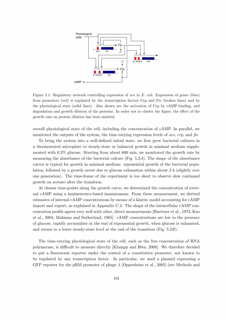
ABCD

DEF�������A��

�����

Figure 5.1: Regulatory network controlling expression of acs in E. coli. Expression of genes (blue)

from promoters (red) is regulated by the transcription factors Crp and Fis (broken lines) and by

the physiological state (solid lines). Also shown are the activation of Crp by cAMP-binding, and

degradation and growth dilution of the proteins. In order not to clutter the figure, the effect of the

growth rate on protein dilution has been omitted.

overall physiological state of the cell, including the concentration of cAMP. In parallel, we

monitored the outputs of the system, the time-varying expression levels of acs, crp, and fis.

To bring the system into a well-defined initial state, we first grew bacterial cultures in

a thermostated microplate to steady-state or balanced growth in minimal medium supple-

mented with 0.3% glucose. Starting from about 600 min, we monitored the growth rate by

measuring the absorbance of the bacterial culture (Fig. 5.2A). The shape of the absorbance

curves is typical for growth in minimal medium: exponential growth of the bacterial popu-

lation, followed by a growth arrest due to glucose exhaustion within about 2 h (slightly over

one generation). The time-frame of the experiment is too short to observe slow continued

growth on acetate after the transition.

At chosen time-points along the growth curve, we determined the concentration of exter-

nal cAMP using a luminescence-based immunoassay. From these measurement, we derived

estimates of internal cAMP concentrations by means of a kinetic model accounting for cAMP

import and export, as explained in Appendix C.2. The shape of the intracellular cAMP con-

centration profile agrees very well with other, direct measurements [Buettner et al., 1973, Kao

et al., 2004, Makman and Sutherland, 1965]. cAMP concentrations are low in the presence

of glucose, rapidly accumulate at the end of exponential growth, when glucose is exhausted,

and return to a lower steady-state level at the end of the transition (Fig. 5.2B).

The time-varying physiological state of the cell, such as the free concentration of RNA

polymerase, is difficult to measure directly [Klumpp and Hwa, 2008]. We therefore decided

to put a fluorescent reporter under the control of a constitutive promoter, not known to

be regulated by any transcription factor. In particular, we used a plasmid expressing a

GFP reporter for the pRM promoter of phage λ [Oppenheim et al., 2005] (see Methods and

102

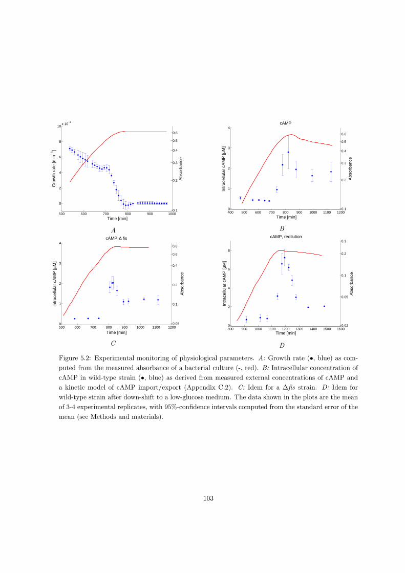
500 600 700 800 900 1000

0

2

4

6

8

10x 10

−3

Gro

wth

rat

e [m

in−

1 ]

0.1

0.2

0.3

0.4

0.5

0.6

Abs

orba

nce

Time [min]

A

400 500 600 700 800 900 1000 1100 12000

1

2

3

4

Intr

acel

lula

r cA

MP

[µM

]

cAMP

0.1

0.2

0.3

0.4

0.5

0.6

Abs

orba

nce

Time [min]

B

500 600 700 800 900 1000 1100 12000

1

2

3

4

Intr

acel

lula

r cA

MP

[µM

]

cAMP, ∆ fis

0.05

0.1

0.2

0.4

0.6

0.8

Abs

orba

nce

Time [min]

C

800 900 1000 1100 1200 1300 1400 1500 16000

2

4

6

8

Intr

acel

lula

r cA

MP

[µM

]

cAMP, redilution

0.02

0.05

0.1

0.2

0.3

Abs

orba

nce

Time [min]

D

Figure 5.2: Experimental monitoring of physiological parameters. A: Growth rate (•, blue) as com-

puted from the measured absorbance of a bacterial culture (-, red). B: Intracellular concentration of

cAMP in wild-type strain (•, blue) as derived from measured external concentrations of cAMP and

a kinetic model of cAMP import/export (Appendix C.2). C: Idem for a ∆fis strain. D: Idem for

wild-type strain after down-shift to a low-glucose medium. The data shown in the plots are the mean

of 3-4 experimental replicates, with 95%-confidence intervals computed from the standard error of the

mean (see Methods and materials).

103

Materials). The variations in the activity of the constitutive promoter reflect changes in the

overall physiological state of the cell, including the gene expression machinery and amino acid

and nucleotide metabolism. This approach allows the global state of the cell to be monitored

in real-time and in vivo during the growth transition. The promoter activity computed from

the fluorescence signal is shown in Fig. 5.3D. The activity of the pRM promoter is seen to be

approximately stationary in exponential phase, but then decreases to a lower value, slightly

preceding the drop of the growth rate.

In parallel, we monitored the promoter activities of the genes in the network using GFP

reporter plasmids for the fis, crp, and acs promoters. The results are shown in Fig. 5.3. The

promoter activities of fis and crp gradually decrease at the end of exponential phase, and

then remain at a basal level after exhaustion of glucose, with a slight recovery towards the

end of the experiment, possibly as a consequence of acetate consumption by the cells. The

expression pattern of acs in exponential phase seems to be similar, but as the fluorescence

signal is close to the background level, the confidence intervals are wide and do not allow an

unambiguous conclusion to be drawn. However, contrary to what was observed for fis and

crp, the expression of acs is strongly induced when glucose is exhausted at about 700 min.

This latter observation is consistent with other reports in the literature [Baptist et al., Wolfe,

2005].

de Jong et al. [2010] have shown that the promoter activities derived from the absorbance

and fluorescence data are in good agreement with Northern blot quantifications of mRNA.

Here we additionally measured the variation of the plasmid copy number (number of plasmids

per chromosomal equivalent of DNA) using qPCR. The number is known to change with the

growth rate [Lin-Chao and Bremer, 1986] and may bias the profiles shown in Fig. 5.3. We

found that the plasmid copy number increases by a factor of 2 during the growth transition

following glucose exhaustion (see Appendix C.3). This does not invalidate the qualitative

shape of the profiles, especially the fall in the activity of the constitutive promoter (which is

actually underestimated). However, it means that a quantitative bias exists and it requires

the development of analysis methods that corrects for this bias.

5.2.2 Dissecting the local and global control of gene expression

In order to analyze the relative contributions of local and global factors to the response of the

acs network, we developed a simple mathematical model of the measured promoter activity

of the genes. Let p(t) denote the promoter activity as a function of time t [min]. We write

p(t) = k p1(t) p2(t) (5.1)

with k the maximum promoter activity and p1(t) and p2(t) the time-varying contributions of

the global and local factors to p(t), respectively. For simplicity, without loss of generality, we

assume that p1(t) and p2(t) vary between 0 and 1. The term p1(t) quantifies the influence of

the global physiological state on the promoter activity, for instance through the availability of

104

500 600 700 800 900 10000

5000

10000

15000

Pro

mot

er a

ctiv

ity [R

FU

min

−1 ]

crp

0.1

0.2

0.3

0.4

0.5

0.6

Abs

orba

nce

Time [min]

A

500 600 700 800 900 10000

20

40

60

80

Pro

mot

er a

ctiv

ity [R

FU

min

−1 ]

acs

0.1

0.2

0.3

0.4

0.5

0.6

Abs

orba

nce

Time [min]

B

500 600 700 800 900 10000

200

400

600

800

Pro

mot

er a

ctiv

ity [R

FU

min

−1 ]

fis

0.1

0.2

0.3

0.4

0.5

0.6

Abs

orba

nce

Time [min]

C

500 600 700 800 900 10000

500

1000

1500

2000

Pro

mot

er a

ctiv

ity [R

FU

min

−1 ]

pRM

0.1

0.2

0.3

0.4

0.5

0.6

Abs

orba

nce

Time [min]

D

Figure 5.3: Experimental monitoring of gene expression. A: Time-varying promoter activity of crp

(•, blue), derived from GFP data with 95%-confidence interval obtained from experimental replicas,

and absorbance (solid line, red). Details on the strains and data analysis procedures can be found in

Methods and Materials and Appendix C.1. B-D: Idem for promoter activities of fis and acs, as well

as the activity of the pRM promoter of phage λ. The latter promoter is constitutive in our conditions

and reflects the global physiological state of the cell. The primary fluorescence data for these curves

are shown in Appendix C.1.

105

free RNA polymerase and ribosome. The term p2(t) accounts for the effect of transcription

factors and other local regulators, and may take the form of regulation functions usually

found in gene network modeling [Bintu et al., 2005, de Jong, 2002, Bolouri, 2008].

In order to eliminate the usually unknown constant k, we normalize Eq. (5.1) with respect

to a reference state at time t0. At t0 we have p(t0) = k p1(t0) p2(t

0). Writing p0 = p(t0),

p01 = p1(t0), and p02 = p2(t

0), we divide Eq. (5.1) by the reference promoter activity and after

a logarithmic transformation find

logp(t)

p0= log

p1(t)

p01+ log

p2(t)

p02. (5.2)

Two special cases of this model will be examined in more detail below.

(i) When the global physiological effect is dominant, that is, when the effect of the local

regulators is negligible, we have p2(t) ≈ p02 and the second terms in Eq. (5.2) approximates

0. Bearing in mind that the global effect is measured by the activity of the constitutive pRM

promoter, we can rewrite the model as

logp(t)

p0= log

pRM (t)

p0RM

, (5.3)

with pRM (t) and p0RM the time-varying activity of the pRM promoter and its reference value,

respectively.

(ii) Figs. 5.2-5.3 show that the expression peak of acs at glucose exhaustion seems to

correlate with cAMP kinetics. This motivates a model in which the variation of the pro-

moter activity of acs, and potentially other Crp·cAMP-regulated genes, is dominated, after

subtraction of control by the global physiological state, by the concentration of cAMP. That

is, we have

logp(t)

p0− log

pRM (t)

p0RM

= logc(t)

c0, (5.4)

where c(t) is the time-varying intracellular concentration of cAMP and c0 its value in the

reference state.

The above models allow us to address a number of questions. To which extent can the

observed variation in the promoter activity of the genes be accounted for by the effect of

the global physiological state only? And if gene expression control is shared with other,

local regulators, how much of the remaining variation is explained by cAMP? Notice that

the models of Eqs. (5.3)-(5.4) have a number of advantages for this purpose. First, they

are parameterless and therefore do not require preliminary model calibration. Second, the

growth-phase-dependent variation of the plasmid copy number equally affects the terms p(t)

and pRM (t), and therefore cancels out in the equations.

In order to see this, we make an explicit distinction between p(t), the activity of a promoter

on the chromosome, and p(t), the activity of the same promoter on a reporter plasmid. Let

106

r(t) denote the (time-varying) relative plasmid copy number and k the plasmid copy number

at t0 (Appendix C.3). Then we have

p(t) = k r(t) p(t). (5.5)

In our reporter gene experiments we do not directly measure p(t), but rather p(t). As a

consequence, Eqs. (5.3)-(5.4) are redefined as

logp(t)

p0= log

pRM (t)

p0RM

, (5.6)

logp(t)

p0− log

pRM (t)

p0RM

= logc(t)

c0. (5.7)

Substituting the expressions for p(t) and p(t) into these equations yields

logr(t)

r0p(t)

p0= log

r(t)

r0pRM (t)

p0RM

,

logr(t)

r0p(t)

p0− log

r(t)

r0pRM (t)

p0RM

= logc(t)

c0,

where r0 = r(t0). It is easy to see that by eliminating the terms r(t)/r0 the original Eqs. (5.3)-

(5.4) are obtained. That is, the variation of the plasmid copy number equally affects the terms

p(t) and pRM (t), and therefore cancels out.

Third, the hypotheses contained in the model can be immediately tested by means of the

experimental data, by inserting for p(t) the measured promoter activities of fis, crp, and acs

(denoted below by pfis(t), pcrp(t), and pacs(t), respectively).

5.2.3 Distributed local and global control of gene expression in acs network

during growth transition

We first test the hypothesis that the adaptation of gene expression to glucose exhaustion

is mainly controlled by the physiological state of the cell, measured by the activity of the

pRM promoter. The reference state is chosen to be the state where the growth rate vanishes,

that is, after exhaustion of glucose. In this case, Eq. (5.3) predicts a linear relation between

log(p(t)/p0) and log(pRM (t)/p0RM ), the diagonal in the scatter plots of Fig. 5.4A-C. If the

global effects are dominant, then one would expect the data points to be spread out along

the diagonal. This is indeed seen to be the case for fis and crp. In order to quantify the

proportion of the variance explained by the model, we compute the coefficient of determina-

tion (R2), the square of the correlation coefficient [Hamilton, 1992]. For fis and crp, we have

high R2 values (0.71 and 0.83). However, for acs the R2 value is found to be much lower (0.54).

107

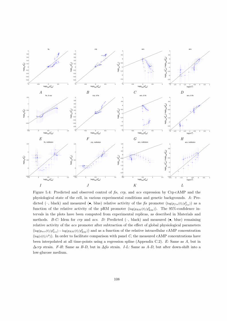
−1 −0.5 0 0.5 1−1

−0.8

−0.6

−0.4

−0.2

0

0.2

0.4

0.6

0.8

1 fis

log(pRM

/p0RM

)

log(

p fis/p

0 fis)

A

−1 −0.5 0 0.5 1−1

−0.8

−0.6

−0.4

−0.2

0

0.2

0.4

0.6

0.8

1 crp

log(pRM

/p0RM

)

log(

p crp/p

0 crp)

B

−1 −0.5 0 0.5 1−3

−2.5

−2

−1.5

−1

−0.5

0

0.5

1 acs

log(pRM

/p0RM

)

log(

p acs/p

0 acs)

C

−3 −2.5 −2 −1.5 −1 −0.5 0 0.5 1−3

−2.5

−2

−1.5

−1

−0.5

0

0.5

1 acs

log(c/c0)

log(

p acs/p

0 acs)−

log(

p RM

/p0 R

M)

D

−0.5 0 0.5 1 1.5−1

−0.5

0

0.5

1

1.5 fis, ∆ crp

log(pRM

/p0RM

)

log(

p fis/p

0 fis)

E

−1 −0.5 0 0.5 1−1

−0.8

−0.6

−0.4

−0.2

0

0.2

0.4

0.6

0.8

1 crp, ∆ fis

log(pRM

/p0RM

)

log(

p crp/p

0 crp)

F

−1 −0.5 0 0.5 1−3

−2.5

−2

−1.5

−1

−0.5

0

0.5

1 acs, ∆ fis

log(pRM

/p0RM

)

log(

p acs/p

0 acs)

G

−3 −2.5 −2 −1.5 −1 −0.5 0 0.5 1−3

−2.5

−2

−1.5

−1

−0.5

0

0.5

1 acs, ∆ fis

log(c/c0)

log(

p acs/p

0 acs)−

log(

p RM

/p0 R

M)

H

−0.5 0 0.5 1 1.5−0.5

0

0.5

1

1.5 fis, redilution

log(pRM

/p0RM

)

log(

p fis/p

0 fis)

I

−0.5 0 0.5 1 1.5−0.5

0

0.5

1

1.5 crp, redilution

log(pRM

/p0RM

)

log(

p crp/p

0 crp)

J

−0.5 0 0.5 1 1.5−3

−2.5

−2

−1.5

−1

−0.5

0

0.5

1

1.5 acs, redilution

log(pRM

/p0RM

)

log(

p acs/p

0 acs)

K

−2.5 −2 −1.5 −1 −0.5 0 0.5 1−2.5

−2

−1.5

−1

−0.5

0

0.5

1 acs, redilution

log(c/c0)

log(

p acs/p

0 acs)−

log(

p RM

/p0 R

M)

L

Figure 5.4: Predicted and observed control of fis, crp, and acs expression by Crp·cAMP and the

physiological state of the cell, in various experimental conditions and genetic backgrounds. A: Pre-

dicted (–, black) and measured (•, blue) relative activity of the fis promoter (log(pfis(t)/p0fis)) as a

function of the relative activity of the pRM promoter (log(pRM (t)/p0RM )). The 95%-confidence in-

tervals in the plots have been computed from experimental replicas, as described in Materials and

methods. B-C: Idem for crp and acs. D: Predicted (–, black) and measured (•, blue) remaining

relative activity of the acs promoter after subtraction of the effect of global physiological parameters

(log(pacs(t)/p0acs)− log(pRM (t)/p0RM )) and as a function of the relative intracellular cAMP concentration

(log(c(t)/c0)). In order to facilitate comparison with panel C, the measured cAMP concentrations have

been interpolated at all time-points using a regression spline (Appendix C.2). E: Same as A, but in

∆crp strain. F-H: Same as B-D, but in ∆fis strain. I-L: Same as A-D, but after down-shift into a

low-glucose medium.

108

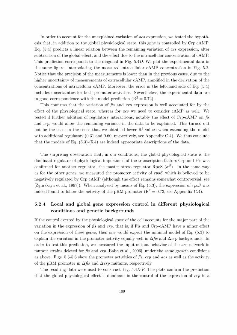
In order to account for the unexplained variation of acs expression, we tested the hypoth-

esis that, in addition to the global physiological state, this gene is controlled by Crp·cAMP.

Eq. (5.4) predicts a linear relation between the remaining variation of acs expression, after

subtraction of the global effect, and the effect due to the intracellular concentration of cAMP.

This prediction corresponds to the diagonal in Fig. 5.4D. We plot the experimental data in

the same figure, interpolating the measured intracellular cAMP concentration in Fig. 5.2.

Notice that the precision of the measurements is lower than in the previous cases, due to the

higher uncertainty of measurements of extracellular cAMP, amplified in the derivation of the

concentrations of intracellular cAMP. Moreover, the error in the left-hand side of Eq. (5.4)

includes uncertainties for both promoter activities. Nevertheless, the experimental data are

in good correspondence with the model prediction (R2 = 0.72).

This confirms that the variation of fis and crp expression is well accounted for by the

effect of the physiological state, whereas for acs we need to consider cAMP as well. We

tested if further addition of regulatory interactions, notably the effect of Crp·cAMP on fis

and crp, would allow the remaining variance in the data to be explained. This turned out

not be the case, in the sense that we obtained lower R2-values when extending the model

with additional regulators (0.31 and 0.60, respectively, see Appendix C.4). We thus conclude

that the models of Eq. (5.3)-(5.4) are indeed appropriate descriptions of the data.

The surprising observation that, in our conditions, the global physiological state is the

dominant regulator of physiological importance of the transcription factors Crp and Fis was

confirmed for another regulator, the master stress regulator RpoS (σS). In the same way

as for the other genes, we measured the promoter activity of rpoS, which is believed to be

negatively regulated by Crp·cAMP (although the effect remains somewhat controversial, see

[Zgurskaya et al., 1997]). When analyzed by means of Eq. (5.3), the expression of rpoS was

indeed found to follow the activity of the pRM promoter (R2 = 0.73, see Appendix C.4).

5.2.4 Local and global gene expression control in different physiological

conditions and genetic backgrounds

If the control exerted by the physiological state of the cell accounts for the major part of the

variation in the expression of fis and crp, that is, if Fis and Crp·cAMP have a minor effect

on the expression of these genes, then one would expect the minimal model of Eq. (5.3) to

explain the variation in the promoter activity equally well in ∆fis and ∆crp backgrounds. In

order to test this prediction, we measured the input-output behavior of the acs network in

mutant strains deleted for fis and crp [Baba et al., 2006], under the same growth conditions

as above. Figs. 5.5-5.6 show the promoter activities of fis, crp and acs as well as the activity

of the pRM promoter in ∆fis and ∆crp mutants, respectively.

The resulting data were used to construct Fig. 5.4E-F. The plots confirm the prediction

that the global physiological effect is dominant in the control of the expression of crp in a

109

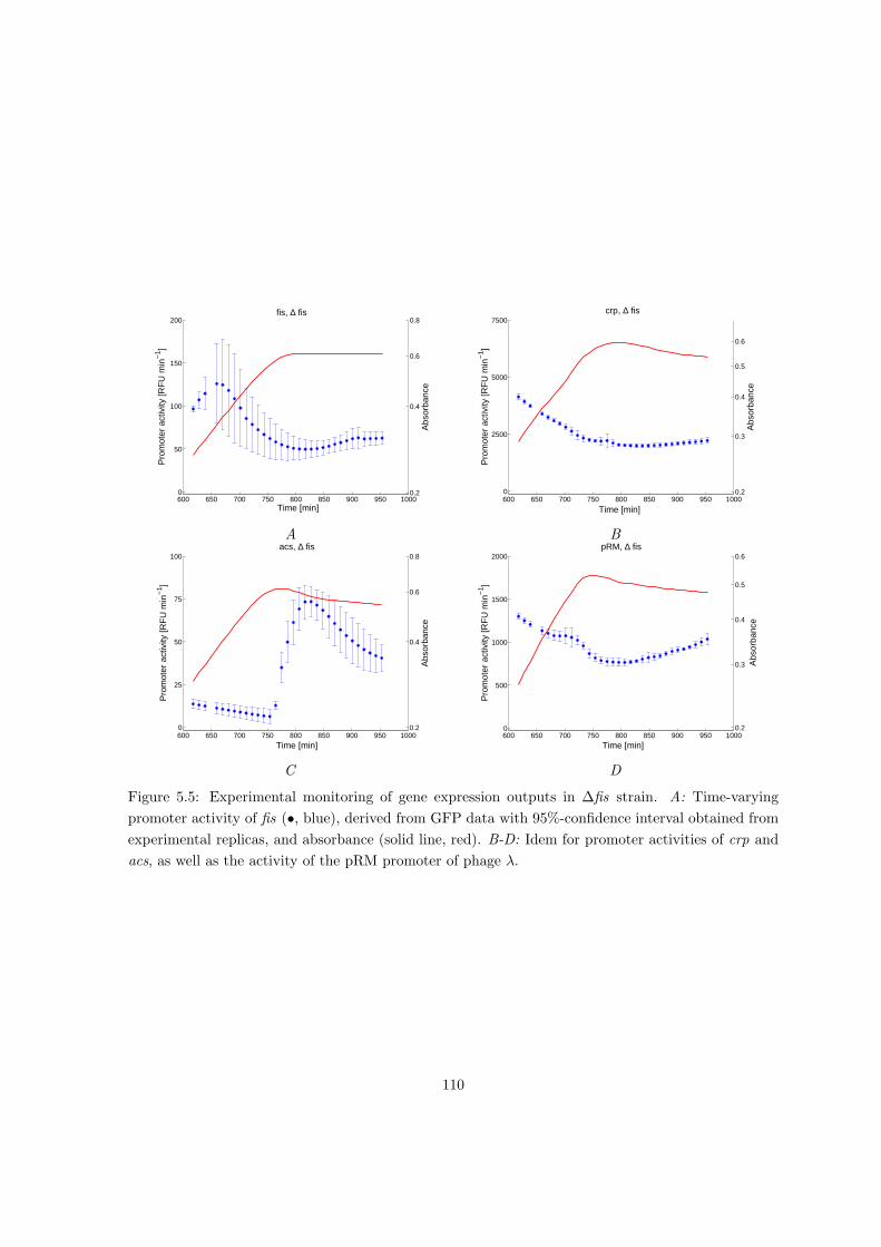
600 650 700 750 800 850 900 950 10000

50

100

150

200

Pro

mot

er a

ctiv

ity [R

FU

min

−1 ]

fis, ∆ fis

0.2

0.4

0.6

0.8

Abs

orba

nce

Time [min]

A

600 650 700 750 800 850 900 950 10000

2500

5000

7500

Pro

mot

er a

ctiv

ity [R

FU

min

−1 ]

crp, ∆ fis

0.2

0.3

0.4

0.5

0.6

Abs

orba

nce

Time [min]

B

600 650 700 750 800 850 900 950 10000

25

50

75

100

Pro

mot

er a

ctiv

ity [R

FU

min

−1 ]

acs, ∆ fis

0.2

0.4

0.6

0.8

Abs

orba

nce

Time [min]

C

600 650 700 750 800 850 900 950 10000

500

1000

1500

2000

Pro

mot

er a

ctiv

ity [R

FU

min

−1 ]

pRM, ∆ fis

0.2

0.3

0.4

0.5

0.6

Abs

orba

nce

Time [min]

D

Figure 5.5: Experimental monitoring of gene expression outputs in ∆fis strain. A: Time-varying

promoter activity of fis (•, blue), derived from GFP data with 95%-confidence interval obtained from

experimental replicas, and absorbance (solid line, red). B-D: Idem for promoter activities of crp and

acs, as well as the activity of the pRM promoter of phage λ.

110

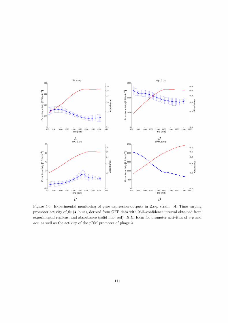
900 950 1000 1050 1100 1150 1200 1250 1300 13500

200

400

600

800

Pro

mot

er a

ctiv

ity [R

FU

min

−1 ]

fis, ∆ crp

0.1

0.2

0.3

0.4

0.5

0.6

Abs

orba

nce

Time [min]

A

900 950 1000 1050 1100 1150 1200 1250 1300 13500

2500

5000

7500

Pro

mot

er a

ctiv

ity [R

FU

min

−1 ]

crp, ∆ crp

0.1

0.2

0.3

0.4

0.5

0.6

Abs

orba

nce

Time [min]

B

900 950 1000 1050 1100 1150 1200 1250 1300 1350−20

0

20

40

60

80

Pro

mot

er a

ctiv

ity [R

FU

min

−1 ]

acs, ∆ crp

0.1

0.2

0.3

0.4

0.5

0.6

Abs

orba

nce

Time [min]

C

900 950 1000 1050 1100 1150 1200 1250 1300 13500

500

1000

1500

2000

2500

Pro

mot

er a

ctiv

ity [R

FU

min

−1 ]

pRM, ∆ crp

0.1

0.2

0.3

0.4

0.5

0.6

Abs

orba

nce

Time [min]

D

Figure 5.6: Experimental monitoring of gene expression outputs in ∆crp strain. A: Time-varying

promoter activity of fis (•, blue), derived from GFP data with 95%-confidence interval obtained from

experimental replicas, and absorbance (solid line, red). B-D: Idem for promoter activities of crp and

acs, as well as the activity of the pRM promoter of phage λ.

111

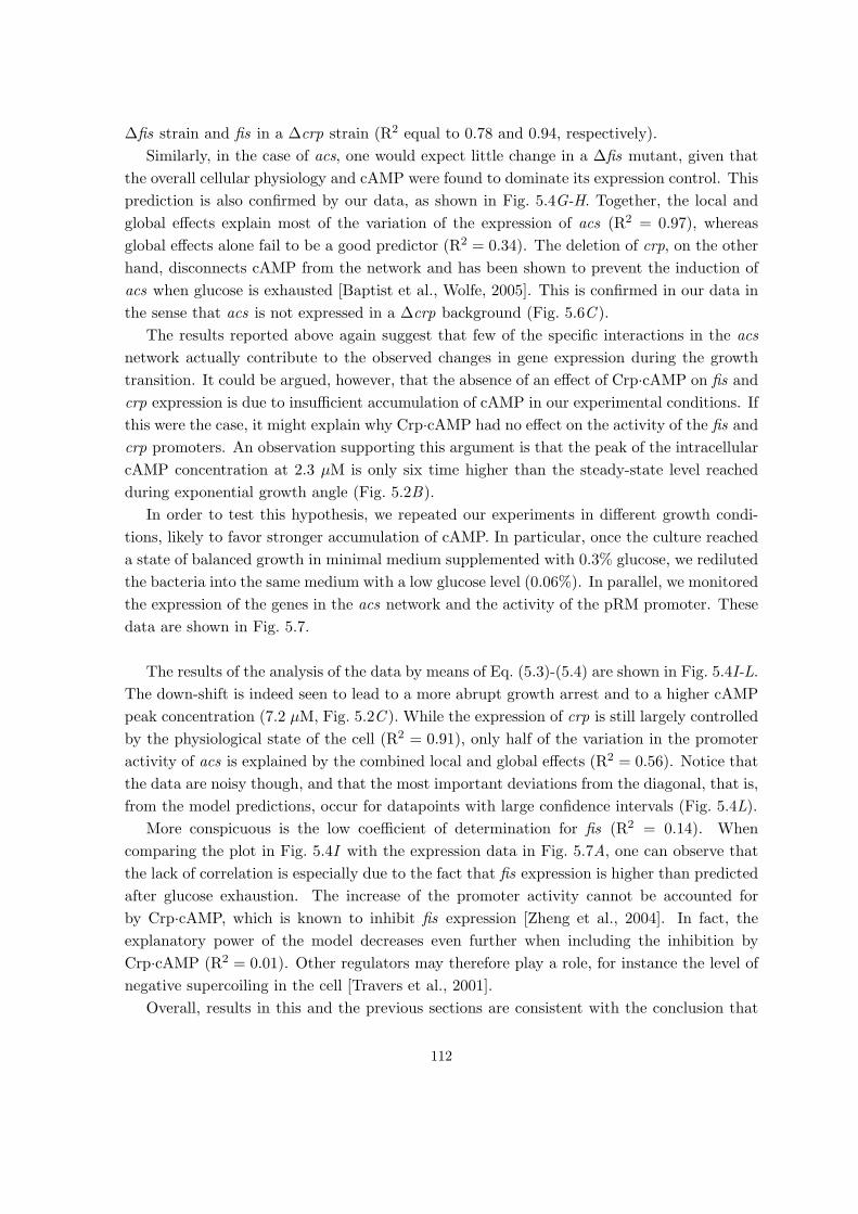
∆fis strain and fis in a ∆crp strain (R2 equal to 0.78 and 0.94, respectively).

Similarly, in the case of acs, one would expect little change in a ∆fis mutant, given that

the overall cellular physiology and cAMP were found to dominate its expression control. This

prediction is also confirmed by our data, as shown in Fig. 5.4G-H. Together, the local and

global effects explain most of the variation of the expression of acs (R2 = 0.97), whereas

global effects alone fail to be a good predictor (R2 = 0.34). The deletion of crp, on the other

hand, disconnects cAMP from the network and has been shown to prevent the induction of

acs when glucose is exhausted [Baptist et al., Wolfe, 2005]. This is confirmed in our data in

the sense that acs is not expressed in a ∆crp background (Fig. 5.6C ).

The results reported above again suggest that few of the specific interactions in the acs

network actually contribute to the observed changes in gene expression during the growth

transition. It could be argued, however, that the absence of an effect of Crp·cAMP on fis and

crp expression is due to insufficient accumulation of cAMP in our experimental conditions. If

this were the case, it might explain why Crp·cAMP had no effect on the activity of the fis and

crp promoters. An observation supporting this argument is that the peak of the intracellular

cAMP concentration at 2.3 µM is only six time higher than the steady-state level reached

during exponential growth angle (Fig. 5.2B).

In order to test this hypothesis, we repeated our experiments in different growth condi-

tions, likely to favor stronger accumulation of cAMP. In particular, once the culture reached

a state of balanced growth in minimal medium supplemented with 0.3% glucose, we rediluted

the bacteria into the same medium with a low glucose level (0.06%). In parallel, we monitored

the expression of the genes in the acs network and the activity of the pRM promoter. These

data are shown in Fig. 5.7.

The results of the analysis of the data by means of Eq. (5.3)-(5.4) are shown in Fig. 5.4I-L.

The down-shift is indeed seen to lead to a more abrupt growth arrest and to a higher cAMP

peak concentration (7.2 µM, Fig. 5.2C ). While the expression of crp is still largely controlled

by the physiological state of the cell (R2 = 0.91), only half of the variation in the promoter

activity of acs is explained by the combined local and global effects (R2 = 0.56). Notice that

the data are noisy though, and that the most important deviations from the diagonal, that is,

from the model predictions, occur for datapoints with large confidence intervals (Fig. 5.4L).

More conspicuous is the low coefficient of determination for fis (R2 = 0.14). When

comparing the plot in Fig. 5.4I with the expression data in Fig. 5.7A, one can observe that

the lack of correlation is especially due to the fact that fis expression is higher than predicted

after glucose exhaustion. The increase of the promoter activity cannot be accounted for

by Crp·cAMP, which is known to inhibit fis expression [Zheng et al., 2004]. In fact, the

explanatory power of the model decreases even further when including the inhibition by

Crp·cAMP (R2 = 0.01). Other regulators may therefore play a role, for instance the level of

negative supercoiling in the cell [Travers et al., 2001].

Overall, results in this and the previous sections are consistent with the conclusion that

112

950 1000 1050 1100 1150 1200 1250 1300 13500

250

500

750

1000

1250

Pro

mot

er a

ctiv

ity [R

FU

min

−1 ]

fis, redilution

0.05

0.1

0.2

0.3

0.4

0.5

0.6

Abs

orba

nce

Time [min]

A

950 1000 1050 1100 1150 1200 1250 1300 13500

1

2

3x 10

4

Pro

mot

er a

ctiv

ity [R

FU

min

−1 ]

crp, redilution

0.05

0.1

0.2

0.3

0.4

0.5

0.6

Abs

orba

nce

Time [min]

B

950 1000 1050 1100 1150 1200 1250 1300 13500

50

100

150

Pro

mot

er a

ctiv

ity [R

FU

min

−1 ]

acs, redilution

0.05

0.1

0.2

0.3

0.4

0.5

0.6

Abs

orba

nce

Time [min]

C

950 1000 1050 1100 1150 1200 1250 1300 13500

1000

2000

3000

Pro

mot

er a

ctiv

ity [R

FU

min

−1 ]

pRM, redilution

0.05

0.1

0.2

0.3

0.4

0.5

0.6

Abs

orba

nce

Time [min]

D

Figure 5.7: Experimental monitoring of gene expression outputs in wild-type strain after redilution

into low-glucose medium. A: Time-varying promoter activity of fis (•, blue), derived from GFP data

with 95%-confidence interval obtained from experimental replicas, and absorbance (solid line, red).

B-D: Idem for promoter activities of crp and acs, as well as the activity of the pRM promoter of

phage λ.

113

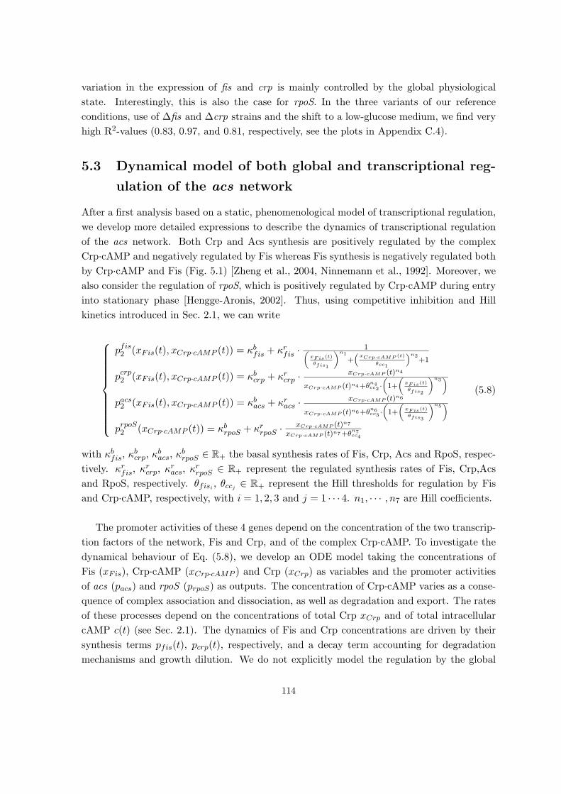
variation in the expression of fis and crp is mainly controlled by the global physiological

state. Interestingly, this is also the case for rpoS. In the three variants of our reference

conditions, use of ∆fis and ∆crp strains and the shift to a low-glucose medium, we find very

high R2-values (0.83, 0.97, and 0.81, respectively, see the plots in Appendix C.4).

5.3 Dynamical model of both global and transcriptional reg-

ulation of the acs network

After a first analysis based on a static, phenomenological model of transcriptional regulation,

we develop more detailed expressions to describe the dynamics of transcriptional regulation

of the acs network. Both Crp and Acs synthesis are positively regulated by the complex

Crp·cAMP and negatively regulated by Fis whereas Fis synthesis is negatively regulated both

by Crp·cAMP and Fis (Fig. 5.1) [Zheng et al., 2004, Ninnemann et al., 1992]. Moreover, we

also consider the regulation of rpoS, which is positively regulated by Crp·cAMP during entry

into stationary phase [Hengge-Aronis, 2002]. Thus, using competitive inhibition and Hill

kinetics introduced in Sec. 2.1, we can write

pfis2 (xFis(t), xCrp·cAMP (t)) = κbfis + κrfis · 1(xFis(t)

θfis1

)n1

+(

xCrp·cAMP (t)

θcc1

)n2+1

pcrp2 (xFis(t), xCrp·cAMP (t)) = κbcrp + κrcrp · xCrp·cAMP (t)n4

xCrp·cAMP (t)n4+θn4cc2 ·

(1+

(xFis(t)

θfis2

)n3)

pacs2 (xFis(t), xCrp·cAMP (t)) = κbacs + κracs · xCrp·cAMP (t)n6

xCrp·cAMP (t)n6+θn6cc3 ·

(1+

(xFis(t)

θfis3

)n5)

prpoS2 (xCrp·cAMP (t)) = κbrpoS + κrrpoS · xCrp·cAMP (t)n7

xCrp·cAMP (t)n7+θn7cc4

(5.8)

with κbfis, κbcrp, κ

bacs, κ

brpoS ∈ R+ the basal synthesis rates of Fis, Crp, Acs and RpoS, respec-

tively. κrfis, κrcrp, κ

racs, κ

rrpoS ∈ R+ represent the regulated synthesis rates of Fis, Crp,Acs

and RpoS, respectively. θfisi , θccj ∈ R+ represent the Hill thresholds for regulation by Fis

and Crp·cAMP, respectively, with i = 1, 2, 3 and j = 1 · · · 4. n1, · · · , n7 are Hill coefficients.

The promoter activities of these 4 genes depend on the concentration of the two transcrip-

tion factors of the network, Fis and Crp, and of the complex Crp·cAMP. To investigate the

dynamical behaviour of Eq. (5.8), we develop an ODE model taking the concentrations of

Fis (xFis), Crp·cAMP (xCrp·cAMP ) and Crp (xCrp) as variables and the promoter activities

of acs (pacs) and rpoS (prpoS) as outputs. The concentration of Crp·cAMP varies as a conse-

quence of complex association and dissociation, as well as degradation and export. The rates

of these processes depend on the concentrations of total Crp xCrp and of total intracellular

cAMP c(t) (see Sec. 2.1). The dynamics of Fis and Crp concentrations are driven by their

synthesis terms pfis(t), pcrp(t), respectively, and a decay term accounting for degradation

mechanisms and growth dilution. We do not explicitly model the regulation by the global

114

physiological state of the cell. Instead, we treat this term as an input and measure it by

setting k · p1(t) = pRM (t), with k ∈ R+. We define γFis and γCrp the degradation rates of

Fis and Crp, respectively, and µ the growth rate of the bacterial population. We have

xFis(t) = pRM (t) · pfis2 (xFis(t), xCrp·cAMP (t))− (µ(t) + γFis) · xFis(t)

xCrp(t) = pRM (t) · pcrp2 (xFis(t), xCrp·cAMP (t))− (µ(t) + γCrp) · xCrp(t)

xCrp·cAMP (t) = roncc (t)− roffcc (t)− (µ(t) + γCrp) · xCrp·cAMP (t)

pacs(t) = pRM (t) · pacs2 (xFis(t), xCrp·cAMP (t))

prpoS(t) = pRM (t) · prpoS2 (xCrp·cAMP (t))

(5.9)

with roncc and roffcc the association and dissociation rates of the Crp·cAMP complex. As

extracellular cAMP is not degraded [Epstein et al., 1975], the degradation rate of Crp·cAMP

is equal to γCrp.

As we have seen in Sec. 2.1, roncc and roffcc can be modeled by the following first-order rate

laws {roncc (t) = kon · (xCrp − xCrp·cAMP ) · c(t)roffcc (t) = koff · xCrp·cAMP

(5.10)

with koncc and koffcc the association and dissociation constants of the Crp·cAMP complex,

respectively.

Using QSSA, introduced in Sec. 2.2.1, we set xCrp·cAMP = 0 and determine xCrp·cAMP as

xCrp·cAMP (t) =xCrp(t)

1 + γCrp+µ(t)+koffcc

koncc ·(c(t)−xcc(t))

(5.11)

The dissociation of a complex is much faster than the degradation of a protein or dilution,

so that we can assume that (γCrp + µ(t)) << koffcc .

The resulting ODE model is composed of 2 variables (x(t) = [xFis(t) xCrp(t)]), takes as

inputs the concentration of intracellular cAMP c(t), the growth rate µ(t) and the promoter

activity of pRM pRM (t), returns the promoter activities of acs and rpoS and follows

xFis(t) = pRM (t) · pfis2 (xFis(t), xCrp·cAMP (t))− (µ(t) + γFis) · xFis(t)

xCrp(t) = pRM (t) · pcrp2 (xFis(t), xCrp·cAMP (t))− (µ(t) + γCrp) · xCrp(t)

xCrp·cAMP (t) =xCrp(t)

1+Kcc/c(t)

pacs(t) = pRM (t) · pacs2 (xFis(t), xCrp·cAMP (t))

prpoS(t) = pRM (t) · prpoS2 (xCrp·cAMP (t))

(5.12)

with Kcc = koffcc /koncc .

This model contains 21 parameters, listed in Table 5.4. To estimate them, we confronted

the model to the data of promoter activities presented in Fig. 5.3 (and Fig. A7A of Ap-

pendix C.4 for rpoS promoter activity). The model was rescaled in order to be consistent

with these experimental data (see Appendix C.5 for details).

115

As mentioned in Sec. 2.4.1, parameter estimation of an ODE model when the vector of

observables only contains the outputs of the model has an important computational cost and

is performing poorly. Consequently, we divided the parameter estimation procedure in two

steps:

Parameters Description Units

Kcc equilibrium constant for Crp·cAMP formation reaction mM

fis expression

κbfis basal protein synthesis rate mM·min−1

κrfis maximal protein synthesis rate mM·min−1

θfis1 , θcc1 affinity constants mM

n1, n2 Hill coefficients adimensional

γFis protein degradation constant min−1

crp expression

κbcrp basal protein synthesis rate mM·min−1

κrcrp maximal protein synthesis rate mM·min−1

θfis2 , θcc2 affinity constants mM

n3, n4 Hill coefficients adimensional

γCrp protein degradation constant min−1

acs expression

κbacs basal protein synthesis rate mM·min−1

κracs maximal protein synthesis rate mM·min−1

θfis3 , θcc3 affinity constants mM

n5, n6 Hill coefficients adimensional

rpoS expression

κbrpoS basal protein synthesis rate mM·min−1

κrrpoS maximal protein synthesis rate mM·min−1

θcc4 affinity constant mM

n7 Hill number adimensional

Table 5.4: Parameters of the ODE model of global and transcriptional regulation of the acs network

shown in Fig. 5.1 (+ rpoS ). The model is detailed in Eq. (5.12)

1. We decomposed the ODE model into four different kinetic models of promoter activities

using measurements of GFP concentrations as representative of Fis and Crp concen-

trations (Eq. (5.9)). This way, we face the case where the observable vector of the

model contains the variables, which corresponds to the first situation enumerated in

Sec. 2.4.1. The parameter estimation problem becomes a set of 4 independent prob-

lems of estimating between 5 and 7 parameters with an algebraic objective function (see

Appendix C.5).

2. Using the estimates obtained from decomposed estimation problems to form the initial

116

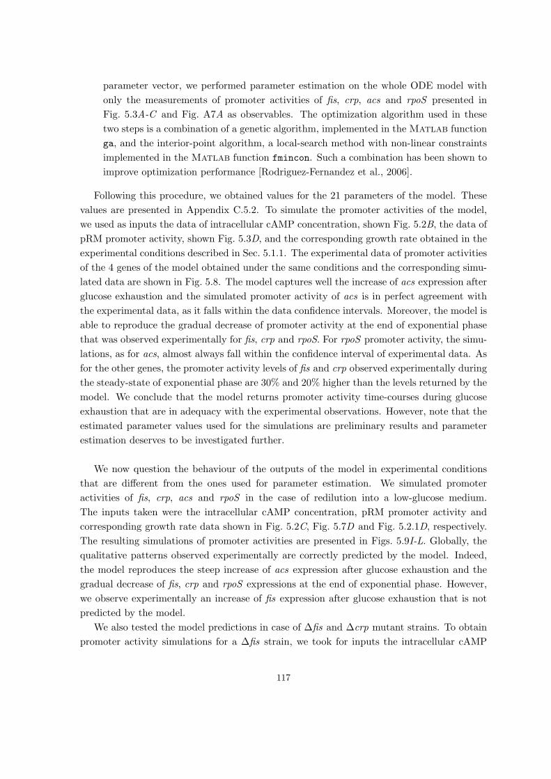
parameter vector, we performed parameter estimation on the whole ODE model with

only the measurements of promoter activities of fis, crp, acs and rpoS presented in

Fig. 5.3A-C and Fig. A7A as observables. The optimization algorithm used in these

two steps is a combination of a genetic algorithm, implemented in the Matlab function

ga, and the interior-point algorithm, a local-search method with non-linear constraints

implemented in the Matlab function fmincon. Such a combination has been shown to

improve optimization performance [Rodriguez-Fernandez et al., 2006].

Following this procedure, we obtained values for the 21 parameters of the model. These

values are presented in Appendix C.5.2. To simulate the promoter activities of the model,

we used as inputs the data of intracellular cAMP concentration, shown Fig. 5.2B, the data of

pRM promoter activity, shown Fig. 5.3D, and the corresponding growth rate obtained in the

experimental conditions described in Sec. 5.1.1. The experimental data of promoter activities

of the 4 genes of the model obtained under the same conditions and the corresponding simu-

lated data are shown in Fig. 5.8. The model captures well the increase of acs expression after

glucose exhaustion and the simulated promoter activity of acs is in perfect agreement with

the experimental data, as it falls within the data confidence intervals. Moreover, the model is

able to reproduce the gradual decrease of promoter activity at the end of exponential phase

that was observed experimentally for fis, crp and rpoS. For rpoS promoter activity, the simu-

lations, as for acs, almost always fall within the confidence interval of experimental data. As

for the other genes, the promoter activity levels of fis and crp observed experimentally during

the steady-state of exponential phase are 30% and 20% higher than the levels returned by the

model. We conclude that the model returns promoter activity time-courses during glucose

exhaustion that are in adequacy with the experimental observations. However, note that the

estimated parameter values used for the simulations are preliminary results and parameter

estimation deserves to be investigated further.

We now question the behaviour of the outputs of the model in experimental conditions

that are different from the ones used for parameter estimation. We simulated promoter

activities of fis, crp, acs and rpoS in the case of redilution into a low-glucose medium.

The inputs taken were the intracellular cAMP concentration, pRM promoter activity and

corresponding growth rate data shown in Fig. 5.2C, Fig. 5.7D and Fig. 5.2.1D, respectively.

The resulting simulations of promoter activities are presented in Figs. 5.9I-L. Globally, the

qualitative patterns observed experimentally are correctly predicted by the model. Indeed,

the model reproduces the steep increase of acs expression after glucose exhaustion and the

gradual decrease of fis, crp and rpoS expressions at the end of exponential phase. However,

we observe experimentally an increase of fis expression after glucose exhaustion that is not

predicted by the model.

We also tested the model predictions in case of ∆fis and ∆crp mutant strains. To obtain

promoter activity simulations for a ∆fis strain, we took for inputs the intracellular cAMP

117

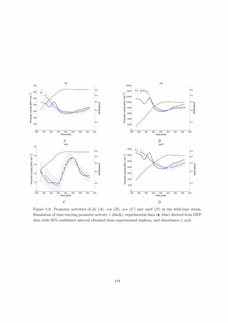
200 250 300 350 400 450 500 550 6000

100

200

300

400

500

600

700

Pro

mot

er a

ctiv

ity [R

FU

min

−1 ]

fis

0.2

0.3

0.4

0.5

0.6

Abs

orba

nce

Time [min]

A

200 250 300 350 400 450 500 550 6000

2000

4000

6000

8000

10000

12000

14000

16000

Pro

mot

er a

ctiv

ity [R

FU

min

−1 ]

crp

0.2

0.3

0.4

0.5

0.6

Abs

orba

nce

Time [min]

B

200 250 300 350 400 450 500 550 6000

10

20

30

40

50

Pro

mot

er a

ctiv

ity [R

FU

min

−1 ]

acs

0.2

0.3

0.4

0.5

0.6

Abs

orba

nce

Time [min]

C

200 250 300 350 400 450 500 550 6000

500

1000

1500

2000

2500

3000

3500

Pro

mot

er a

ctiv

ity [R

FU

min

−1 ]

rpoS

0.2

0.3

0.4

0.5

0.6

Abs

orba

nce

Time [min]

D

Figure 5.8: Promoter activities of fis (A), crp (B), acs (C ) and rpoS (D) in the wild-type strain.

Simulation of time-varying promoter activity (-,black), experimental data (•, blue) derived from GFP

data with 95%-confidence interval obtained from experimental replicas, and absorbance (-,red).

118

concentration, pRM promoter activity and growth rate data measured in a ∆fis strain and

shown in Fig. 5.2B, Fig. 5.5D and Fig. 5.2.1B, respectively. We fixed xFis(t) = 0 for all t

and computed the promoter activities of the 4 genes. The results are shown in Figs. 5.9A-D.

Although the model captures again the decrease of fis, crp and rpoS promoter activities at the

end of exponential phase, the simulated data are systematically higher than the experimental

data, with a 3-fold and 2-fold difference for fis and crp, respectively. Moreover, the model

predicts a significant increase after glucose exhaustion that we do not observe experimentally

in fis and crp data. More importantly, the increase of acs promoter activity observed in

the data is not captured by the model. We also computed predictions for a ∆crp strain

by fixing xCrp·cAMP (t) = xCrp(t) = 0 and taking the corresponding inputs. The resulting

simulations are presented in Figs. 5.9E-H. Although the qualitative patterns of expression are

correctly predicted by the model, quantitatively, the differences in promoter activity levels

at steady-state of exponential phase are higher than 2-fold for fis and crp.

The significant differences observed between model simulations and experimental data in

the mutant strains suggest that the model can not yet be considered as a predictive tool of the

dynamical behaviour of the acs network. A possible explanation may come from the change

of plasmid copy number in the cell that we observed experimentally (see Appendix C.3).

Thus, the model needs to incorporate this bias in order to be compared with experimental

data obtained from reporter plasmids. In addition, further investigation into parameter

estimation of the model could help improving the predictive performances of this model.

5.4 Discussion

The variation of gene expression across growth phases is controlled both by transcriptional

regulators and the global physiological state of the cell. We have presented a method to

distinguish between these two effects, based on a simple mathematical model of promoter

activity. The approach has several advantages making it easy to put it to work for bacteria

but also in higher organisms. The models do not have free parameters that need to be

calibrated, hypotheses on the effect of regulators can be readily tested by monitoring the

expression of target genes and a constitutive control, and the use of plasmid-borne reporter

systems does not bias the analysis. This allows the relative contributions of transcriptional

regulators and the global state of the cell to be monitored on the level of a regulatory network

and over time.

When applied to the network controlling the expression of the gene acs, we obtained a

number of surprising results. First, even though the interactions involving the two major

pleiotropic transcription factors Fis and Crp have been amply documented in the literature,

and are held responsible for the coordination of gene expression changes between growth

phases [Bradley et al., 2007, Gosset et al., 2004], we found that they do not play a critical

physiological role in our conditions. One explanation for this apparent discrepancy might be

that we only considered a single growth condition, minimal medium with glucose as the carbon

119

250 300 350 400 450 500 550 600 6500

50

100

150

200

250

300

350

Pro

mot

er a

ctiv

ity [R

FU

min

−1 ]

fis, ∆ fis

0.3

0.4

0.5

0.6

0.7

0.8

Abs

orba

nce

Time [min]

A

500 600 700 800 900 10000

100

200

300

400

500

600

700

Pro

mot

er a

ctiv

ity [R

FU

min

−1 ]

fis, ∆ crp

0.2

0.3

0.4

0.5

0.6

0.7

Abs

orba

nce

Time [min]

E

200 250 300 350 400 450 500 550 6000

200

400

600

800

1000

1200

1400

Pro

mot

er a

ctiv

ity [R

FU

min

−1 ]

fis, redilution

0.05

0.1

0.15

0.2

0.3

Abs

orba

nce

Time [min]

I

250 300 350 400 450 500 550 600 6500

1000

2000

3000

4000

5000

6000

7000

8000

Pro

mot

er a

ctiv

ity [R

FU

min

−1 ]

crp, ∆ fis

0.3

0.4

0.5

0.6

0.7

0.8

Abs

orba

nce

Time [min]

B

500 600 700 800 900 10000

3000

6000

9000

12000

Pro

mot

er a

ctiv

ity [R

FU

min

−1 ]

crp, ∆ crp

0.2

0.3

0.4

0.5

0.6

0.7

Abs

orba

nce

Time [min]

F

200 250 300 350 400 450 500 550 6000

0.5

1

1.5

2

2.5

x 104

Pro

mot

er a

ctiv

ity [R

FU

min

−1 ]

crp, redilution

0.05

0.1

0.15

0.2

0.3

Abs

orba

nce

Time [min]

J

250 300 350 400 450 500 550 600 6500

10

20

30

40

50

60

70

80

90

Pro

mot

er a

ctiv

ity [R

FU

min

−1 ]

acs, ∆ fis

0.3

0.4

0.5

0.6

0.7

0.8

Abs

orba

nce

Time [min]

C

500 600 700 800 900 1000

0

20

40

60

80

Pro

mot

er a

ctiv

ity [R

FU

min

−1 ]

acs, ∆ crp

0.2

0.3

0.4

0.5

0.6

0.7

Abs

orba

nce

Time [min]

G

200 250 300 350 400 450 500 550 6000

50

100

Pro

mot

er a

ctiv

ity [R

FU

min

−1 ]

acs, redilution

0.05

0.1

0.15

0.2

0.3

Abs

orba

nce

Time [min]

K

250 300 350 400 450 500 550 600 6500

500

1000

1500

2000

2500

Pro

mot

er a

ctiv

ity [R

FU

min

−1 ]

rpoS, ∆ fis

0.3

0.4

0.5

0.6

0.7

0.8

Abs

orba

nce

Time [min]

D

500 600 700 800 900 10000

1000

2000

3000

4000

Pro

mot

er a

ctiv

ity [R

FU

min

−1 ]

rpoS, ∆ crp

500 600 700 800 900 1000

0.2

0.3

0.4

0.5

0.6

0.7

Abs

orba

nce

Time [min]

H

200 250 300 350 400 450 500 550 6000

2000

4000

6000

Pro

mot

er a

ctiv

ity [R

FU

min

−1 ]

rpoS, redilution

0.05

0.1

0.15

0.2

0.3

Abs

orba

nce

Time [min]

L

Figure 5.9: Promoter activities obtained by experimental measure and by model simulations for

different genes under different conditions. Simulation of time-varying promoter activity (-,black),

experimental data (•, blue) derived from GFP data with 95%-confidence interval obtained from ex-

perimental replicas, and absorbance (-,red). A: Promoter activity of fis in a ∆fis strain. B: Promoter

activity of fis in a crp strain. C: Promoter activity of fis in a wild-type strain after redilution to a

low-glucose medium. D-F: Idem but for promoter activity of crp. G-I: Idem but for promoter activity

of acs. J-L: Idem but for promoter activity of rpoS.

120

source. After all, the interactions that were not found to be important in our experiments

may play a role in other physiological conditions. The absence of an effect of Fis and Crp

remains puzzling though, as these regulators are believed to be important in glucose-limited

growth [Gutierrez-Rıos et al., 2007]. An alternative explanation for the discrepancy might

be that many studies do not control for global physiological effects [Dennis et al., 2004].

This brings us to the second surprising finding of this study, namely the dominant role

of global physiological control in the case of the expression of the genes encoding the tran-

scription regulators fis, crp, and rpoS. The molecular bases of this global effect are diverse

and complex, involving among other things guanosine 3’,5’-bispyrophosphate or (p)ppGpp

[Potrykus and Cashel, 2008, Traxler et al., 2006], which exerts control on the abundance and

activity of the components of the transcription and translation machinery. For the purpose

of this study, we have encapsulated these mechanisms into an easy-to-measure variable, the

expression of a constitutive gene.

We also developed an ODE model of the network of Fig. 5.1 accounting for regulation both

by transcriptional factors and by the global physiological state of the cell. After calibration

of the model using a combination of global-search and local-search optimization methods and

experimental data presented in this chapter, we computed simulations for all the genes of the

network in different experimental conditions. In its current version, the model is not able to

correctly predict quantitatively the behaviour of gene expression during glucose exhaustion

in the case of ∆fis and ∆crp strains. In the future, we expect the predictive power of the

model to be improved by further investigation of parameter estimation or by correction of

the model for the change of plasmid copy number in the cell observed experimentally during

glucose exhaustion.

Another interesting extension of the work presented here would be to analyze the global

control of the promoter activities in more detail, distinguishing between the contributions

from individual physiological parameters, such as ppGpp-dependent reprogramming of RNA

polymerase, the variation in gene copy number, and the size of nucleotide pools.

Our results question the dominant role often attributed to gene regulatory networks in

controlling genome-wide expression changes during physiological transitions [Regenberg et al.,

2006]. The picture that emerges is closer to that advocated in classical studies of bacterial

physiology, which focused on global changes in the macromolecular composition of the cell,

including the transcription and translation machinery, in response to changes in the growth-

supporting ability of the environment [Neidhardt et al., 1990, Maaloe and Kjeldgaard, 1966].

It could indeed be most fruitful to see local regulators as finetuning the global control exerted

by the physiological state of the cell.

121

Chapter 6

Conclusion

We focused on the regulation mechanisms responsible for metabolic and gene expression

changes during growth transition in E. coli. The analysis of dynamics of such large and em-

bedded systems required the development of quantitative models. This chapter summarizes

the contributions of this thesis on two topics: parameter estimation of metabolic network

models and regulation undergone by gene expression during growth transition.

We developed a method for estimating parameters of approximated kinetic models called

linlog from high-throughput incomplete datasets. We have seen on simulated data that our

method outperforms both regression and multiple imputation, a standard method in case

of missing data. Moreover, when applied on the largest dataset available, the method was

able to estimate many parameters of a linlog model of central carbon metabolism of E. coli.

Although it has been developed for linlog models, the method is applicable to approximate

kinetic models that allow a mathematical formalism linear in the parameters and provides

information on network elasticities, which is useful for identification of detailed kinetic models.

It is also important to notice that, even with a simplified formalism, the largest dataset

available and a method specifically developed for the case of missing data, the parameter

values obtained were not, for most of them, significantly different from 0. We were able, from

these results, to highlight critical issues for data exploitation in order to estimate parameters.

Indeed, high percentages of missing data for some metabolites tend to critically impact the

identification results and the use of steady-state data can prevent the estimation of some

parameters, due to identifiability issues.

We investigated this question further and defined a theoretical background for identifi-

ability analysis of linlog models, given steady-state data. We presented precise definitions

of structural and practical identifiability and clarified the link between those concepts. We

also developed a method to detect nonidentifiability and to reduce the model to an identifi-

able approximation. Adaptations of the method in case of noisy or incomplete datasets were

122

discussed and their application on simulated data showed improvements on identifiability

analysis. Again, the definitions and methods presented are not only applicable to linlog mod-

els, but to all kinetic formalisms that allow a linear formulation of the parameter estimation

problem.

Moreover, application of our method, taking noise on metabolite measurements into ac-

count for identifiability analysis, on experimental data showed that most of the parameters of

the linlog model of central carbon metabolism of E. coli were actually not identifiable. These

results enforce the diagnosis that identification remains very sensitive to noise and missing

data, even with the largest high-throughput and steady-state datasets available.

Another important contribution of this thesis is the analysis of regulation of gene expres-

sion during growth rate and more specifically, the distribution between the role of the global

physiological state of the cell and the role of transcriptional regulation. We developed a

method to distinguish between those two effects, based on a simple parameterless model of

promoter activity. We applied our method to time-series gene expression data of the network

controlling the expression of acs, that we measured in vivo using reporter plasmids. Sur-

prisingly, we found that the global physiological state of the cell has a dominant regulatory

role on gene expression of the transcription factors involved in this network. More generally,

our results question the role attributed to gene regulatory networks in the control of gene

expression changes during growth transitions, which could be seen as a complement to a

global control by the physiological state of the cell.

To explore this role distribution further, we developed a quantitative ODE model of this

network that takes the macromolecular composition of the cell into account. After estimating

the model parameters on a subset of our experimental data, we tested the model predictions

by comparing them to the rest of the dataset. Although the model simulations showed in this

thesis are preliminary results, we are confident that, by means of model improvement such as

correction for plasmid copy number, we will be able to correctly reproduce gene expression

patterns observed for different genetic backgrounds or growth conditions.

123

Appendices

124

Appendix A

Additional information on

parameter estimation of linlog

metabolic models

A.1 Likelihood-based identification of linlog models

We rely on the notation of Sec. 3.2 of the main section, i.e., we focus on a single reaction

and drop index i from the notation. The loglikelihood of the model is:

logL (b) = log

∫fW |y,y,b(w)fY |y,b(y)dy. (A1)

For convenience, we rewrite (A1) in terms of the random variable Z = Y · b introduced in

Sec. 3.2 so that it becomes:

logL (b) = log

∫fW |y,z,b(w)fZ|y,b(z)dz. (A2)

Here fW |y,z,b(·) is the Gaussian likelihood function of model (3.7), equivalently rewritten

as W = Y · b + Z + ε, given Y = y and Z = z, with z varying over all possible values of Z,

and fZ|y,b is the Gaussian prior of Z = Y · b following from (3.10). The expressions of fW |y,z,band fZ|y,b are thus

fW |y,z,b(w) =1√

det(2πΣε)exp(−1

2 [w − Y · b− z]TΣ−1ε [w − Y · b− z]),

fZ|y,b(z) =1√

det(2πΣy,b)exp(−1

2 [z − µy,b]TΣ−1y,b[z − µy,b]),

(A3)

with µy,b = M · b, where the entry Mj,k of matrix M is the mean µj,k of the distribution

of Yj,k, and Σy,b is the variance matrix of the random variable Z. By the independence

assumptions on Y , it turns out that

125

Σy,b = diag

(nb∑

k=1

b2k · [σ21,k · · ·σ2

q,k]T

)(A4)

where σj,k is defined in (3.10).

Assume for the moment that Σy,b is invertible. Defining

fpb(z) = fW |y,z,b(w) · fZ|y,b(z), (A5)

after simple but tedious calculations, we obtain

fpb(z) = κfb · fb(z) (A6)

with fb the density function of a Gaussian distribution N (µfb ,Σfb) and

Σfb = [Σ−1ε +Σ−1y,b]−1,

µfb = Σfb · [Σ−1ε · (w − Y · b) + Σ−1y,b · µy,b],

κfb =exp(− 1

2[w−Y ·b−µy,b]T ·[Σε+Σy,b]−1·[w−Y ·b−µy,b])√

det(2π[Σε+Σy,b]).

(A7)

The proportionality factor κfb does not depend on the integration variable z, so it can be

taken out of the integral and (A2) can be rewritten as follows:

logL (b) = log(κfb) + log

(∫fb(z)dz

). (A8)

The integral of a normalized Gaussian density function being 1, we finally have an ana-

lytical expression for the loglikelihood: logL (b) = log(κfb).

The above results are used in the expectation step of the EM algorithm. Recall the

definition

Q(b|bℓ−1) =∫

log(fZ,W |y,b(z, w))fZ|y,bℓ−1,w(z)dz. (A9)

The Bayes theorem allows us to rewrite (A9) as follows:

Q(b|bℓ−1) =∫

log(fW |y,z,b(w)fZ|y,b(z))fW |y,z,bℓ−1(w)fZ|y,bℓ−1(z)

fW |y,bℓ−1(w)dz. (A10)

Function fW |y,bℓ−1(w) does not depend on z so it can be taken out of the integral. More-

over, this function does not depend on b so it will have no impact on the maximization step

of EM. Thus, we can ignore this function from the computation of the expectation function

above.

Using definitions (A5) and (A6), we can rewrite (A10) in the following way:

Q(b|bℓ−1) ∝∫

κfbℓ−1fbℓ−1(z) log(κfbfb(z))dz

∝∫

fbℓ−1(z) log(κfbfb(z))dz.

(A11)

126

We have dropped the constant factor κfbℓ−1 as it does not depend on b and thus does not

influence the maximization step of EM. By replacing log(κfbfb(z)) by log(κfbfb(z)fbℓ−1(z)/

fbℓ−1(z)) and separating the integrand in a sum of terms, we can rewrite (A11) as

−Q(b|bℓ−1) ∝∫

fbℓ−1(z) log

(fbℓ−1(z)

fb(z)

)dz −

∫fbℓ−1(z) log(fbℓ−1(z))dz − log(κfb). (A12)

We recognize in the first term the definition of the Kullback-Leibler divergence KL(fb||fbℓ−1) between the two probability distributions fb and fbℓ−1 and in the second term the

entropy H(fbℓ−1) of fbℓ−1 [Cover and Thomas, 2006, Stoorvogel and van Schuppen, 1996]. For

Gaussian distributions, these can be written explicitly as

KL(fb||fbℓ−1) =1

2(log

(det(Σfb)

det(Σfbℓ−1 )

)+ Tr(Σ−1fb

Σfbℓ−1 )

+ [µfb − µfbℓ−1 ]TΣ−1fb

[µfb − µfbℓ−1 ]), (A13)

where Tr(. . .) stands for trace and

H(fbℓ−1) = log(√

det(2πeΣfbℓ−1 )). (A14)

To summarize, together with (A7), this gives us the explicit formula

Q(b|bℓ−1) ∝ −KL(fb||fbℓ−1)−H(fbℓ−1) + log(κfb), (A15)

which we employ in our implementation of EM.

In more generality, for some values of b, Σy,b may be singular or poorly conditioned. To

avoid this circumstance, we can adapt our procedure as follows. We consider a decomposition

W = Y · b+ Z + (ε′ + ε′′) = Y · b+ (Z + ε′) + ε′′ (A16)

where ε′ and ε′′ are independent zero-mean Gaussian random vectors such that Σε′ ,

V ar(ε′) = αΣε and Σε′′ , V ar(ε′′) = (1 − α)Σε, with α ∈ (0, 1) a tunable parameter.

Since Σε > 0 by assumption, it follows that Σε′ > 0 and Σε′′ > 0. Moreover, Σε = Σε′ +Σε′′ ,

i.e., the statistics of ε and of ε′ + ε′′ are identical. Since V ar(Z + ε′) = Σy,b +Σε′ > 0, if we

interpret Z + ε′ as the unknown observations (in place of Z) and ε′′ as the model noise (in

place of ε), we ensure that the variance of the ‘missing data’ is invertible. Thus, in practice,

we apply all formulas developed above with Σy,b+Σε′ in place of Σy,b and Σε′′ in place of Σε.

The effect of the specific choice of α is under investigation. In this work, we took α = 0.2,

a value that leads to good results in practice.

127

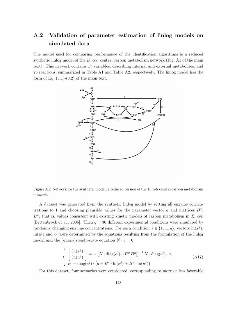
A.2 Validation of parameter estimation of linlog models on

simulated data

The model used for comparing performance of the identification algorithms is a reduced

synthetic linlog model of the E. coli central carbon metabolism network (Fig. A1 of the main

text). This network contains 17 variables, describing internal and external metabolites, and

25 reactions, summarized in Table A1 and Table A2, respectively. The linlog model has the

form of Eq. (3.1)-(3.2) of the main text.

Figure A1: Network for the synthetic model, a reduced version of the E. coli central carbon metabolism

network.

A dataset was generated from the synthetic linlog model by setting all enzyme concen-

trations to 1 and choosing plausible values for the parameter vector a and matrices Bx,

Bu, that is, values consistent with existing kinetic models of carbon metabolism in E. coli

[Bettenbrock et al., 2006]. Then q = 30 different experimental conditions were simulated by

randomly changing enzyme concentrations. For each condition j ∈ {1, ..., q}, vectors ln(xj),ln(uj) and vj were determined by the equations resulting from the formulation of the linlog

model and the (quasi-)steady-state equation N · v = 0:

[ln(xj)

ln(uj)

]= −

[N · diag(e)) · [BxBu]

]−1N · diag(ej) · a,

vj = diag(ej) ·(a+Bx · ln(xj) +Bu · ln(uj)

).

(A17)

For this dataset, four scenarios were considered, corresponding to more or less favorable

128

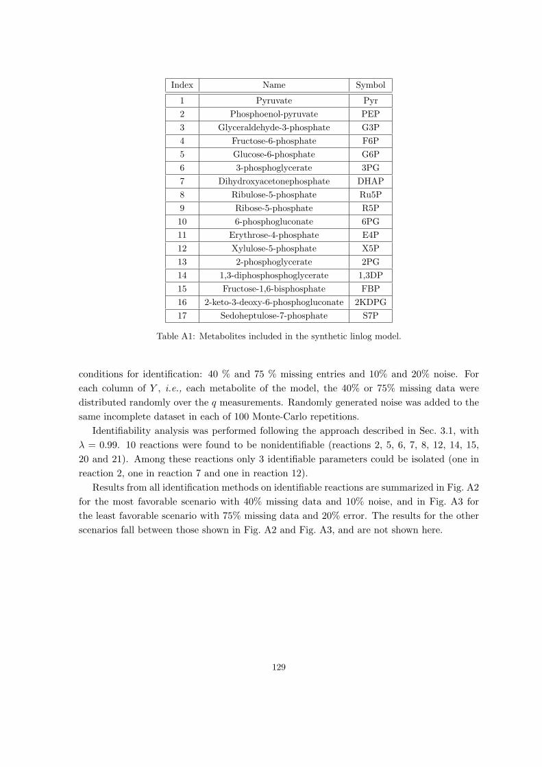
Index Name Symbol

1 Pyruvate Pyr

2 Phosphoenol-pyruvate PEP

3 Glyceraldehyde-3-phosphate G3P

4 Fructose-6-phosphate F6P

5 Glucose-6-phosphate G6P

6 3-phosphoglycerate 3PG

7 Dihydroxyacetonephosphate DHAP

8 Ribulose-5-phosphate Ru5P

9 Ribose-5-phosphate R5P

10 6-phosphogluconate 6PG

11 Erythrose-4-phosphate E4P

12 Xylulose-5-phosphate X5P

13 2-phosphoglycerate 2PG

14 1,3-diphosphosphoglycerate 1,3DP

15 Fructose-1,6-bisphosphate FBP

16 2-keto-3-deoxy-6-phosphogluconate 2KDPG

17 Sedoheptulose-7-phosphate S7P

Table A1: Metabolites included in the synthetic linlog model.

conditions for identification: 40 % and 75 % missing entries and 10% and 20% noise. For

each column of Y , i.e., each metabolite of the model, the 40% or 75% missing data were

distributed randomly over the q measurements. Randomly generated noise was added to the

same incomplete dataset in each of 100 Monte-Carlo repetitions.

Identifiability analysis was performed following the approach described in Sec. 3.1, with

λ = 0.99. 10 reactions were found to be nonidentifiable (reactions 2, 5, 6, 7, 8, 12, 14, 15,

20 and 21). Among these reactions only 3 identifiable parameters could be isolated (one in

reaction 2, one in reaction 7 and one in reaction 12).

Results from all identification methods on identifiable reactions are summarized in Fig. A2

for the most favorable scenario with 40% missing data and 10% noise, and in Fig. A3 for

the least favorable scenario with 75% missing data and 20% error. The results for the other

scenarios fall between those shown in Fig. A2 and Fig. A3, and are not shown here.

129

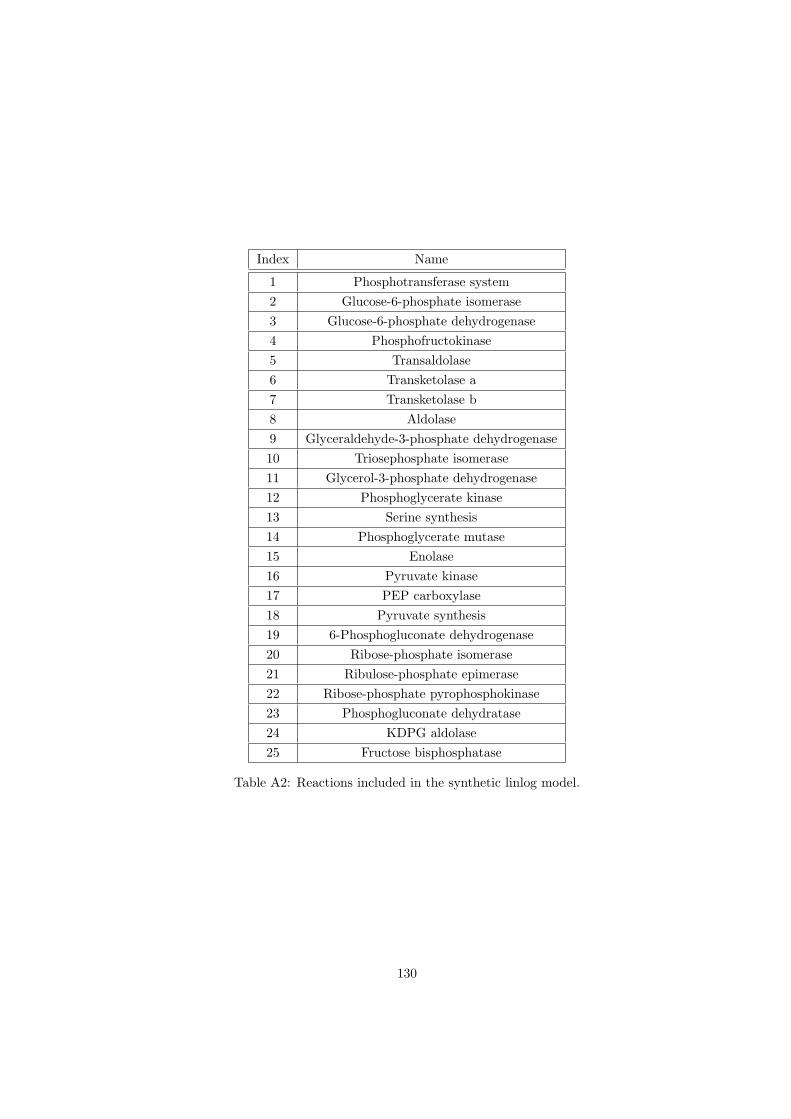
Index Name

1 Phosphotransferase system

2 Glucose-6-phosphate isomerase

3 Glucose-6-phosphate dehydrogenase

4 Phosphofructokinase

5 Transaldolase

6 Transketolase a

7 Transketolase b

8 Aldolase

9 Glyceraldehyde-3-phosphate dehydrogenase

10 Triosephosphate isomerase

11 Glycerol-3-phosphate dehydrogenase

12 Phosphoglycerate kinase

13 Serine synthesis

14 Phosphoglycerate mutase

15 Enolase

16 Pyruvate kinase

17 PEP carboxylase

18 Pyruvate synthesis

19 6-Phosphogluconate dehydrogenase

20 Ribose-phosphate isomerase

21 Ribulose-phosphate epimerase

22 Ribose-phosphate pyrophosphokinase

23 Phosphogluconate dehydratase

24 KDPG aldolase

25 Fructose bisphosphatase

Table A2: Reactions included in the synthetic linlog model.

130

Figure A2: Statistics of estimated parameter values in identifiable reactions for datasets with 40% of

missing data and 10% noise. The graphical notations are the same as for Fig. 3.1.

131

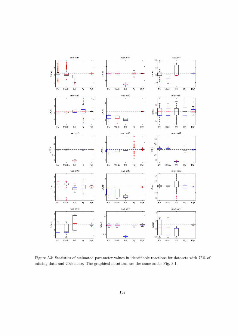
Figure A3: Statistics of estimated parameter values in identifiable reactions for datasets with 75% of

missing data and 20% noise. The graphical notations are the same as for Fig. 3.1.

132

Appendix B

Additional information on

identifiability of linlog metabolic

models

B.1 Proofs of theorems and propositions concerning identifi-

ability of linlog models

Proposition 1. A reaction i of Mp is structurally identifiable at p∗ if and only if there exists

D ⊆ E × U such that the solution of the equation W ∗i = Y ∗B∗i , with

W ∗i =[(

J1∗

e1 −(J∗

e

))i

· · ·(Jq∗

eq −(J∗

e

))i

]T,

Y ∗ =

[lnx1∗ − lnx∗ · · · lnxq∗ − lnx∗

lnu1 − lnu · · · lnuq − lnu

]T,

is unique in the parameters Bi =([Bx∗ Bu∗]T

)i.

Proof. (If) Assume that, for a given D ⊆ E × U , the solution of W ∗i = Y ∗B∗i is unique. We

need to prove that((Jp)i, xp

)|D =

((Jp∗)i, xp∗

)|D implies pi = p∗i . For simplicity, here we

drop index i from subscripts.

Given any two parameters p∗ =[a∗ B∗T

]Tand p =

[a BT

]T, for which Mp : (e, u) 7→

(Jp, xp) and Mp∗ : (e, u) 7→ (Jp∗ , xp∗), it holds by construction that W = Y B and W ∗ =

Y ∗B∗. If (Jp, xp)|D = (Jp∗ , xp∗)|D, then it also holds that Y = Y ∗ and W = W ∗, therefore

we can write W ∗ = Y ∗B. Because the solution in B of the latter is unique and one solution

is B∗, it follows that B = B∗. To conclude that p = p∗, we are left with showing that a = a∗.

This follows from

a∗ =

(J∗e

)−[lnx∗

lnu

]T·B∗ =

(J

e

)−[lnx

lnu

]T·B = a.

133

(Only if) Here the hypothesis is that, for a given D ⊆ E × U ,((Jp)i, xp

)|D =

((Jp∗)i, xp∗

)|D

implies pi = p∗i , and we need to show that the solution in Bi of W∗i = Y ∗Bi is unique. For

simplicity, we will again drop i from the subscripts.

For the sake of contradiction, assume that W ∗ = Y ∗B admits distinct solutions. Since B∗ is

a solution, all solutions are of the form B = B∗ + z, with z in the nontrivial kernel of Y ∗.

For any such z we can write Y ∗B∗ = Y ∗(B∗ + z), i.e.,[(lnx∗ − lnx∗)

T (lnu∗ − lnu∗)T]B∗ =

[(lnx∗ − lnx∗)

T (lnu∗ − lnu∗)T](B∗ + z). (A1)

Let p∗ =[a∗ B∗T

]T. For any (e, u) ∈ D, J∗ = Jp∗(e, u) and x∗ = xp∗(e, u) are given by the

solution of{

0 = N · Jp∗ , (A2a)

Jp∗ = diag(e) · (a∗ +[lnxT∗ lnuT∗

]B∗) (A2b)

(which is unique by virtue of Assumption 1). Using Eq. (A1), the term[lnxT∗ lnuT∗

]B∗

can be rewritten as[lnxT∗ lnuT∗

](B∗ + z)−

[lnxT∗ lnuT∗

]z. Replacing this into Eq. (A2)

yields

0 = N · J∗, (A3a)

J∗ = diag(e) ·((a∗ −

[lnxT∗ lnuT∗

]z)

︸ ︷︷ ︸,a

+[lnxT∗ lnuT∗

](B∗ + z)︸ ︷︷ ︸

=B

), (A3b)

for all (e, u) ∈ D.

From this we see that p = [a BT ]T , with a defined as above, is different from p∗ but is

such that(Jp(e, u), xp(e, u)

)=(Jp∗(e, u), xp∗(e, u)

)for all (e, u) ∈ D, which contradicts the

hypothesis.

Corollary 1. A reaction i of Mp is structurally identifiable at p∗i if and only if Y ∗ is full

column-rank.

Proof. From Proposition 1, we know that identifiability is equivalent to the uniqueness of the

solution in Bi of W∗i = Y ∗Bi. Uniqueness holds if and only if ker(Y ∗) = {0}, i.e., Y ∗ is full

column-rank or equivalently rank(Y ∗) = nb.

Proposition 2. If a reaction i of Mp is structurally identifiable at p∗ in the sense of

Def. 1 then, for every α ∈ (0, 1), it is practically identifiable in the sense of Def. 2 with

confidence level at least 1 − α for any uncertainty set Bi ⊇ EΣ(α), where EΣ(α) denotes

the (1 − α)-confidence ellipsoid of a zero-mean Gaussian distribution with variance Σ =

(Y TC(i)Σ

−1εi YC(i))

−1.

Proof. The definition of Mp ensures that W ∗i = Y ∗B∗i . Hence, given a noisy dataset Wi =

W ∗i + εi and the errorless dataset Y ∗, the regression problem becomes

134

Wi = Y ∗ ·B∗i + εi. (A4)

From Sec. 4.2.1, identifiability of Mp at p∗i is equivalent to Y ∗ being full column rank.

Thus, if Mp is identifiable at p∗i , Y is full column rank, and the weighted pseudoinverse of Y ,

Y † ,(Y TΣ−1εi Y

)−1Y TΣ−1εi , is well-defined. This enables us to define the minimum variance

estimator of B∗i , Bi = Y †W . From the linearity of the estimator in the Gaussian noise εi,

after simple calculations of first and second-order moments, one gets Bi ∼ N

(B∗i , Σ

)(also

compare [Ljung, 1999, Appendix II]). Thus, from the definition of Bi, Pp∗

i[Bi − B∗i ∈ Bi] ≥

Pp∗

i[Bi −B∗i ∈ EΣ(α)] = 1− α.

B.2 Reduction to identifiable models in case of sampling bias

In general, data from repeated experiments may happen to be more densely concentrated

in some regions than in others. This is particularly true in our case, where the metabolite

log-concentrations play the role of regression data but are not controlled directly by the

experimenter. In the extreme case, homeostatic control of metabolite concentrations may

cluster most datapoints around a single value. Thus, the variance will be dominated by the

variance of experimental error, strongly distorting the analysis of practical identifiability as

outlined above. To compensate for this bias, we modify the estimation problem by introducing

a weighting scheme to rebalance the importance of the datapoints. Following Sander and

Schneider [1991], we seek positive coefficients α =[α1 · · · αq

]T, with L1-norm ||α||1 =

∑qk=1 αk = 1, such that αk weights the importance of experiment k based on the mean

distance of the corresponding datapoint from all other datapoints, where the mean shall be

weighted accordingly. Mathematically, consider YC(i), where each row Yk,C(i) corresponds to

a different experiment k = 1, . . . , q, and define the Euclidean distance between datapoints k

and k′ as Dk,k′ = ||Yk,C(i) − Yk′,C(i)||. Then we want that

αk = λ ·q∑

k′=1

Dk,k′αk′ , k = 1, . . . , q,

for some λ > 0 independent of k. Let D ∈ Rq×q+ be the matrix with entries Dk,k′ , k, k′ =

1, . . . , q. The above set of q equations is then written compactly as α = λ ·Dα, i.e., α must

be an eigenvector of D. From the properties of D (nonnegativity and irreducibility, assuming

there are no identical datapoints), it can be shown that this set of equations implies that λ

is the unique largest real eigenvalue of D and α is the unique eigenvector associated with λ

satisfying ||α||1 = 1. In practice, α can be computed by efficient numerical algorithms such

as the Matlab routine eig or by fast iterative schemes. Once this weighting is found, in

view of model reduction, the SVD analysis of Sec. 4.3.2 is performed on reweighted data as

follows. Data are centered with respect to their weighted mean and rescaled according to the

importance weights√α, thus obtaining a new matrix YC(i) where Yk,C(i) =

√αk

(Yk,C(i) −

135

αT YC(i)

), with k = 1, . . . , q. We can apply the SVD analysis of Sec. 4.3.2 to the reweighted

empirical covariance matrix of the data,

Y TC(i)YC(i) = V diag{s21, . . . , s2nb

}V T

and choose the effective rank of the data r with the criterion (4.22) applied to s21, . . . , s2nb

instead of s21, . . . , s2nb.

In practice, since Yk,C(i) is noisy and the largest components are amplified, the reweighting

procedure has the effect to systematically amplify the noise. To correct for this, (4.22) is

modified so as to compensate for an amplification factor β > 1, i.e.,

r = max{ℓ : s2ℓ − βν2 ≥ βν2}. (A5)

While an appropriate value of β is difficult to compute analytically, suitable values of β for

different datasets noise levels can be determined via simulation.

Example 6. To illustrate the effect of biased datasets on identifiability analysis and the model

reduction technique to overcome it, we consider the model of Example 4 with a1 = 0.0297 and

B2,1 = −0.0073 which has been shown to be practically identifiable on noiseless datasets. We

want to see which model reduction method diagnoses well this identifiability property on a

limited, noisy and biased dataset. A dataset of q = 30 datapoints was simulated and sampling

bias was introduced by limiting the range of the log-uniform distribution of enzyme values

to [− ln 1.05 ln 1.05] for 26 conditions and extending it to [− ln 7 ln 7] for the remaining

4 conditions. Noise following a normal distribution with a standard deviation of 0.4 was

added to the data matrix Y . We tested two model reduction approaches: the method defined

in Sec. 4.3.2 using criteria of Eq. (4.22) and the method correcting for sampling bias using

criteria of Eq. (A5) with β = 1.2. Figs. B.1(a)-B.1(b) show results of both methods on 100

datasets, respectively. Out of 100 datasets, the model reaction was diagnosed identifiable

49 and 55 times with the first and second methods, respectively. Thus, the correction for

sampling bias using the weighting scheme defined above produces slightly more relevant results

for identifiability analysis and model reduction.

We apply the model reduction method using Eq. (A5) on the linlog model of the network

shown in Fig. 4.6(a). We consider the case when data available are sampled with bias. We

computed noisy metabolite concentrations and metabolic flux values from Eq. (4.12) for 30

different conditions with sampling bias, as in Example 6. The metabolite concentrations were

computed with 40% noise level and 100 datasets were generated in this way. The same criteria

as in Table 4.1 were applied on the 100 data matrices Y and on the corresponding corrected

matrices Y . Average effective ranks computed from those different criteria are reported in

Table A1.

First of all, we notice that, compared to Table 4.1, model reduction of Def. 4 with θ =

0.99 on a biased dataset give the same results as on the dataset of Sec. 4.4.1. Indeed, no

136

1 20

0.2

0.4

0.6

0.8

1

1.2

1.4

1.6

i

s2 i−

ν2

(a)

1 20

0.2

0.4

0.6

0.8

1

1.2

1.4

1.6

i

s2 i−

ν2

(b)

Figure A1: Squared singular values for 100 data matrices Y . The data matrices, biased and noisy

(40% noise level) were computed from model of Example 3 with a1 = 0.0297 and B2,1 = −0.0073. (a)

Singular values and cutoff computed like described in Sec. 4.3.2 with Eq. (4.22). The blue dots are

the estimates of the squared singular values s2ℓ − ν2 and the red box covers the area below the cutoff

of ν2. (b) Singular values and cutoff computed on data matrices Y corrected for sampling bias with

Eq. (A5) and β = 1.2. The blue dots are the estimates of the squared singular values s2ℓ − βν2 and

the red box covers the area below the cutoff of βν2.

137

Average effective rank

Reaction Number of Def. 4 Def. 3

number parameters No correction Correction No correction Correction

R1 2 2 2 1 1

R2 4 3.99 3.88 1.3 1.3

R3 3 3 3 0.7 0.74

R4 4 4 4 1.15 1.2

R5 1 1 1 0.01 0.05

R6 3 3 3 0.84 0.88

R7 4 4 3.98 1.21 1.24

R8 1 1 1 0 0.01

Table A1: Average effective rank computed for each reaction and with different definitions of r over

100 noisy and biased datasets (40% noise, 86% sampling bias) of the model of Fig. 4.6(a). The criteria

of Def. 4 was computed with θ = 0.99. Method 2 corresponds to model reduction using r as defined

in Eq. (4.22). Model reduction was applied both on Y and Y , the data matrix corrected for sampling

bias, and the results are shown in the columns titled “No correction” and “Correction”, respectively.

dependencies have been detected for any reaction of the network. However, the results of

model reduction of Def. 3 on the biased dataset give lower average effective ranks than Def. 3

applied in Table 4.1 for all reactions but the first. Moreover, the average effective rank is

reduced by more than 0.7 for reactions 2, 4 and 7. Thus, sampling bias in the data favours

the detection of more collinearities in the data when model reduction of Def. 3 is used.

Secondly, the results of Table A1 show that the correction for sampling bias does not sig-

nificantly affect the results of model reduction. Indeed, the biggest changes in the results for

model reduction with and without correction for sampling bias are 0.11 and 0.05 for model

reduction methods of Def. 4 with θ = 0.99 and Def. 3, respectively. Finally, the correction

for sampling bias does not change the results of identifiability analysis.

We then apply the model reduction method accounting for sampling bias in the data on

the linlog model of central carbon metabolism shown Fig. 4.9 to verify that we do not find

different results than the ones obtained using Def. 3, presented in Sec. 4.4.2. The results

are reported in Table A2. Globally, the identifiability analysis, whether using correction for

sampling bias or not, returns similar results. The only exception is reaction 1, for which 1

or 2 singular values were found negligible depending on the method in Tables 4.2 and A2,

respectively.

The same method as in Sec. 4.4.2 has been applied to the dataset to detect identifiable

parameters. The results are shown in Table A3.

138

Average Full Average Full

Reaction Enzyme effective rank dimension Reaction Enzyme effective rank dimension

1 PtsG 2.01 4 17 GltA,PrpC 2.95 4

2 Pgi 1 2 18 AcnA,AcnB 1 2

3 PfkA,PfkB 2.82 4 19 IcdA 1 3

4 FbaA,FbaB 2 2 20 SucA:SucB:LpdA;SucC:SucD 1 3

5 TpiA 2 2 21 SdhA:SdhB:SdhC:SdhD 1 3

6 GapA;Pgk 2.97 4 22 FumA,FumB,FumC 1 2

7 GpmA,GpmB;Eno 1 2 23 Mdh 2.92 4

8 PykA,PykF 2 4 24 Ppc;PckA 3 5

9 AceE:AceF:LpdA 1.99 3 25 MaeB,SfcA 2 5

10 Zwf;Pgl 1.55 3 26 AceA;AceB 1 3

11 Gnd 2 3 27 µ 4.76 11

12 Rpe 1.04 2 28 Edd;Eda 1 2

13 RpiA,RpiB 1.99 3 29 Pta;AckA,AckB 2.97 6

14 TktA 1.89 2 30 LdhA 1 2

15 TalA,TalB 1 2 31 AdhE 1 1

16 TktB 1.01 2

Table A2: Average effective rank computed for the reactions in the linlog model of E. coli central

carbon metabolism, using the data of Ishii et al. [2007]. SVD has been applied on YC(i) for each

reaction and singular values were discarded based on Eq. (A5). Identifiable reactions are shown in

green. Reaction 27, labeled µ, is a phenomenological reaction for biomass production.

139

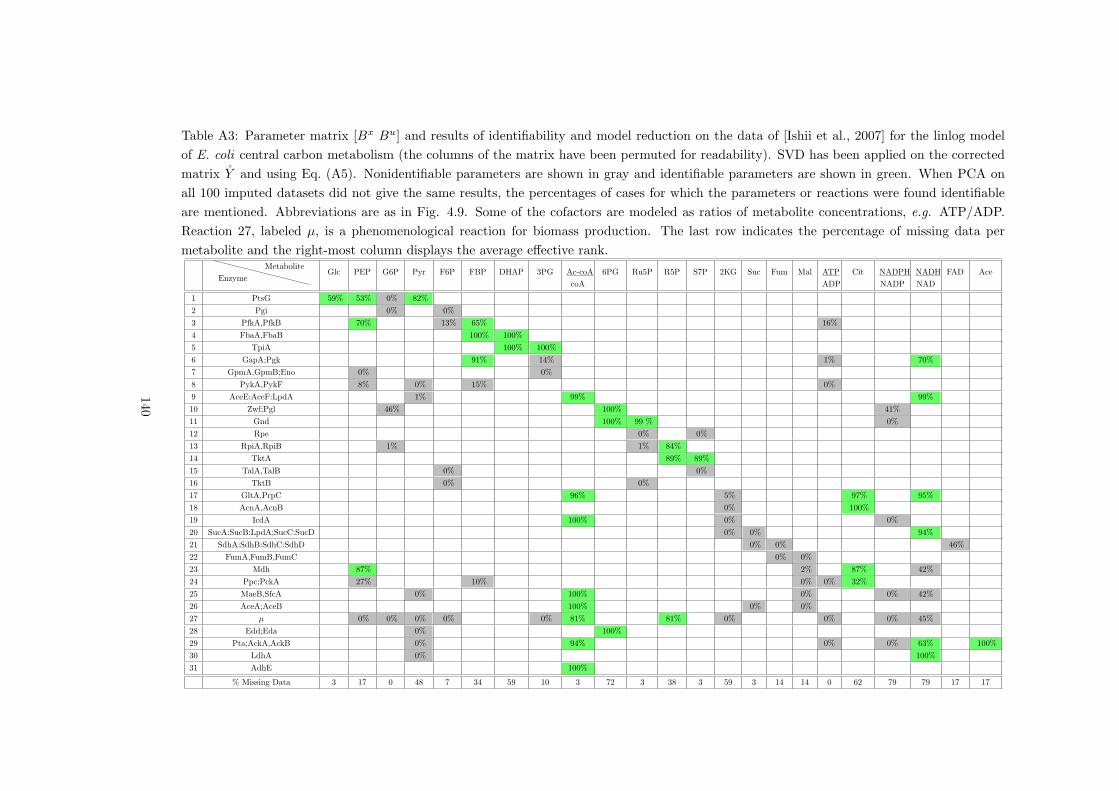
Table A3: Parameter matrix [Bx Bu] and results of identifiability and model reduction on the data of [Ishii et al., 2007] for the linlog model

of E. coli central carbon metabolism (the columns of the matrix have been permuted for readability). SVD has been applied on the corrected

matrix Y and using Eq. (A5). Nonidentifiable parameters are shown in gray and identifiable parameters are shown in green. When PCA on

all 100 imputed datasets did not give the same results, the percentages of cases for which the parameters or reactions were found identifiable

are mentioned. Abbreviations are as in Fig. 4.9. Some of the cofactors are modeled as ratios of metabolite concentrations, e.g. ATP/ADP.

Reaction 27, labeled µ, is a phenomenological reaction for biomass production. The last row indicates the percentage of missing data per

metabolite and the right-most column displays the average effective rank.

Enzyme

MetaboliteGlc PEP G6P Pyr F6P FBP DHAP 3PG Ac-coA

coA

6PG Ru5P R5P S7P 2KG Suc Fum Mal ATP

ADP

Cit NADPH

NADP

NADH

NAD

FAD Ace

1 PtsG 59% 53% 0% 82%

2 Pgi 0% 0%

3 PfkA,PfkB 70% 13% 65% 16%

4 FbaA,FbaB 100% 100%

5 TpiA 100% 100%

6 GapA;Pgk 91% 14% 1% 70%

7 GpmA,GpmB;Eno 0% 0%

8 PykA,PykF 8% 0% 15% 0%

9 AceE:AceF:LpdA 1% 99% 99%

10 Zwf;Pgl 46% 100% 41%

11 Gnd 100% 99 % 0%

12 Rpe 0% 0%

13 RpiA,RpiB 1% 1% 84%

14 TktA 89% 89%

15 TalA,TalB 0% 0%

16 TktB 0% 0%

17 GltA,PrpC 96% 5% 97% 95%

18 AcnA,AcnB 0% 100%

19 IcdA 100% 0% 0%

20 SucA:SucB:LpdA;SucC:SucD 0% 0% 94%

21 SdhA:SdhB:SdhC:SdhD 0% 0% 46%

22 FumA,FumB,FumC 0% 0%

23 Mdh 87% 2% 87% 42%

24 Ppc;PckA 27% 10% 0% 0% 32%

25 MaeB,SfcA 0% 100% 0% 0% 42%

26 AceA;AceB 100% 0% 0%

27 µ 0% 0% 0% 0% 0% 81% 81% 0% 0% 0% 45%

28 Edd;Eda 0% 100%

29 Pta;AckA,AckB 0% 94% 0% 0% 63% 100%

30 LdhA 0% 100%

31 AdhE 100%

% Missing Data 3 17 0 48 7 34 59 10 3 72 3 38 3 59 3 14 14 0 62 79 79 17 17

140

Appendix C

Additional information on analysis

of gene expression regulation of E.

coli

C.1 Analysis of reporter gene data

In order to monitor gene expression in vivo and in real time, we used fluorescent reporter

genes in combination with automated microplate readers. The reporter gene experiments

result in up to 120 measurements of absorbance and fluorescence during a typical acquisition

period (about 10 h). The absorbance or optical density is a measure of the biomass of a

bacterial population. It can be used to estimate the total volume of bacterial cells in a well

over a large range of growth rates [Volkmer and Heinemann, 2011]. The fluorescence emitted

is proportional to the quantity of GFP in the cell population. The absorbance is expressed

in dimensionless units, whereas fluorescence intensities are reported in relative fluorescence

units (RFU).

The primary data are corrected for background levels of absorbance and fluorescence. For

the absorbance background, we use wells in the microplate containing growth medium only,

that is, without bacterial cells. Denoting by au(t) the uncorrected absorbance at time t and

by ab(t) the background absorbance, the corrected absorbance a(t) is given by

a(t) = au(t)− ab(t) (A1)

The fluorescence background is usually determined by performing measurements on a

strain carrying the promoterless vector pZEgfp, that is, a strain with a nonfunctional re-

porter system. Contrary to the absorbance, the fluorescence background is not constant, but

varies with the population size due to the autofluorescence of cells. Since the growth curves of

the reporter strain and the strain with the nonfunctional reporter system are not necessarily

identical, we cannot straightforwardly subtract the background readings at each time-point.

141

Instead, we develop a calibration curve relating absorbance readings to background fluores-

cence levels.

Let au(t) and fu(t) denote the uncorrected absorbance and fluorescence at time t, respec-

tively, for bacteria carrying the functional reporter plasmid. Similarly, let bu(t) and gu(t)

denote the uncorrected absorbance and fluorescence, respectively, for bacteria carrying the

promoterless plasmid pZEgfp. We call β the empirical function relating bu(t) to gu(t), that

is, gu = β(bu(t)). The function β is obtained in our case by non-parametric regression using

smoothing splines (Matlab) [de Jong et al., 2010]. By means of this calibration curve, the

corrected absorbance is defined as

f(t) = fu(t)− β(a(t)) (A2)

Fig. A1A-D shows an example of background correction, applied to fluorescence data ac-

quired for the gene fis in a wild-type strain. The corrected data are included in Fig. 3 of the

main text. The fluorescence background correction procedure described above was slightly

modified from the one described in [de Jong et al., 2010, Boyer et al., 2010]. The modifi-

cations notably take into account that part of the fluorescence background is contributed

by the growth medium, that is, the fluorescence background does not approach 0 for small

absorbance values.

In the remainder of this section, we explain how the absorbance and fluorescence mea-

surements can be related to biologically relevant quantities, notably promoter activities. Fol-

lowing [de Jong et al., 2010, Boyer et al., 2010], we develop a simple kinetic model describing

the expression of the reporter gene. Let xg(t) [µM] denote the time-varying concentration

of GFP in the cells in the population. The dynamics of xg(t) is defined by the differential

equation

dxg(t)

dt= p(t)− (µ(t) + γg)xg(t) (A3)

where p(t) [µM min−1] represents the synthesis rate of the reporter protein, γg [min−1] its

degradation constant, and µ(t) [min−1] the growth rate. In the absence of post-transcriptional

regulation, p(t) varies with the rate of transcription of the reporter gene, and is therefore

often called promoter activity [Ronen et al., 2002]. In the case of transcriptional fusions,

the promoter activity of the reporter is a good indicator of the promoter activity of the host

gene. We recall that ln 2/γg equals the half-life of the reporter protein.

Given that the fluorescence is a measure of the quantity of GFP and the absorbance a

measure of the total cell volume, we infer that

xg(t) = δf(t)

a(t)(A4)

for some positive constant δ [µM RFU−1]. The growth rate is conveniently defined in terms

of the absorbance, that is,

142

550 600 650 700 750 800 850 900 9500

0.2

0.4

0.6

Time [min]

Abs

orba

nce

A

0 0.1 0.2 0.3 0.4 0.5 0.6 0.70

2000

4000

6000

8000

10000

12000

Absorbance

Flu

ores

cenc

e [R

FU

]B

550 600 650 700 750 800 850 900 9500

5000

10000

15000

20000

Time [min]

Flu

ores

cenc

e [R

FU

]

C

500 600 700 800 900 10000

200

400

600

800P

rom

oter

act

ivity

[RF

U m

in−

1 ] fis

0.1

0.2

0.3

0.4

0.5

0.6

Abs

orba

nce

Time [min]

D

Figure A1: Example of the analysis of fluorescence reporter gene data. A: Primary (uncorrected)

absorbance (•, green), background absorbance (•, black), and the corrected absorbance (•, blue)

following Eq. (A1). The plot also shows the spline fits of the data (-,blue). B: Calibration curve

for background correction obtained by means of the strain carrying the promoterless vector pZEgfp,

plotting primary fluorescence data against primary absorbance data. The curve is obtained by inter-

polation of the data points. C: Primary fluorescence (•, green) data for the pZEfis-gfp strain. The

plot also shows the background fluorescence (•, black), and the corrected fluorescence (•,blue) ob-

tained after subtracting the two (Eq. (A2)). D: Promoter activity of fis and 95%-confidence intervals

computed from the corrected absorbance and fluorescence data of 4 replicates by means of Eq. (A6).

This plot is the same as Fig. 3C of the main text.

143

µ(t) =da(t)

dt

1

a(t)=

d ln(a(t))

dt(A5)

This allows Eq. (A3) to be recast, after some basic calculus, into a expression defining the

promoter activity in terms of the measured fluorescence and absorbance intensities

p(t) = δ

(df(t)

dt

1

a(t)+ γg

f(t)

a(t)

)(A6)

Notice that for µ(t) ≫ γy, the second term in the right-hand side of Eq. (A6) can be neglected,

and we obtain the expression for the promoter activity usually found in the literature (e.g.,

[Ronen et al., 2002]).

In the absence of knowledge of the value of δ, we arbitrarily set this parameter to 1,

and thus express the promoter activity and reporter protein concentration in RFU and RFU

min−1, respectively. This leads to a relative instead of absolute measure of gene expres-

sion, which is usual for this kind of experiments and sufficient for the purpose of Chap. 5.

Recent developments in single-molecule measurements of gene expression will make abso-

lute measurements of gene expression feasible in the future [Cai et al., 2006, Itzkovitz and

van Oudenaarden, 2011].

In order to actually compute p(t), the corrected absorbance and fluorescence data are

fitted using regression splines [de Jong et al., 2010]. For the GFP reporter used in this study,

γ = 0.012± 0.001 min−1, which corresponds to a half-life of about 1 h [de Jong et al., 2010].

We also take into account the maturation time of GFP (25 min for our reporter).

Confidence intervals for p(t) are computed from technical replicas in the same experiment

(see [de Jong et al., 2010] for an alternative approach, based on a residual resampling boot-

strap). In order to correct for small inoculation differences, the replicates are synchronized

with respect to the absorbance curves. In particular, based on the observation in [Isalan

et al., 2008] that the absorbance derivative profile provides a reproductive signature of bac-

terial growth, we synchronize the promoter activities with respect to the time-points t∗ at

which da(t∗)/dt = 0. Fig. A1D shows the fis promoter activity, as well as the 95%-confidence

intervals computed from 4 replicates. Fig. A2 shows the time-varying growth rates com-

puted by means of Eq. (A5) from the absorbance data, for the four experimental conditions

considered in Chap. 5.

Fig. A3 shows the primary fluorescence and absorbance data from which the promoter

activities of fis, crp and acs as well as the activity of the pRM promoter of phage λ in the

reference conditions have been derived (Fig. 3 in main text), following the method outlined

in Sec. C.1. The plots in Fig. A3 show the data for a single replicate.

144

500 600 700 800 900 1000

0

2

4

6

8

10x 10

−3

Gro

wth

rat

e [m

in−

1 ]

0.1

0.2

0.3

0.4

0.5

0.6

Abs

orba

nce

Time [min]

A

600 650 700 750 800 850 900 950 1000

0

2

4

6

8

10x 10

−3

Gro

wth

rat

e [m

in−

1 ]

∆ fis

0.2

0.4

0.6

0.8

Abs

orba

nce

Time [min]

B

900 950 1000 1050 1100 1150 1200 1250 1300 1350

0

2

4

6

8

10x 10

−3

Gro

wth

rat

e [m

in−

1 ]

∆ crp

0.1

0.2

0.3

0.4

0.5

0.6

Abs

orba

nce

Time [min]

C

950 1000 1050 1100 1150 1200 1250 1300 1350

0

2

4

6

8

10

12x 10

−3

Gro

wth

rat

e [m

in−

1 ]

0.05

0.1

0.2

0.3

0.4

0.5

0.6

Abs

orba

nce

Time [min]

redilution

D

Figure A2: Growth rate computed from the corrected absorbance data by means of Eq. (A5). The

growth-rate values are the mean of 4 replicates, synchronized with respect to their the absorbance

curves as described in the text. The 95%-confidence intervals are computed from the standard error

of the mean. A: Wild-type strain. B: ∆fis deletion strain. C: ∆crp deletion strain. D: Wild-type

strain after redilution into low-glucose medium.

145

0

5000

10000

15000

20000

Flu

ores

cenc

e [R

FU

]

fis

500 600 700 800 900 10000.1

0.3

0.5

0.7

Abs

orba

nce

Time [min]

A

500 600 700 800 900 10000

1

2

3x 10

5

Flu

ores

cenc

e [R

FU

]

crp

0.1

0.2

0.3

0.4

0.5

Abs

orba

nce

Time [min]

B

500 600 700 800 900 10000

2000

4000

6000

8000

Flu

ores

cenc

e [R

FU

]

acs

0.1

0.3

0.5

0.7

Abs

orba

nce

Time [min]

C

500 600 700 800 900 10000

1

2

3

4

5x 10

4

Flu

ores

cenc

e [R

FU

]

pRM

0.1

0.2

0.3

0.4

0.5

Abs

orba

nce

Time [min]

D

Figure A3: Primary data for computation of promoter activities. A: Primary (uncorrected) absorbance

(+, red) and fluorescence (o, blue) data for the pZEfis-gfp strain. B-D: Idem for data from pZEcrp-

gfp, pUA66acs-gfp, and pZE1RMgfp. The primary data in this figure have been used to derive the

promoter activities shown in Fig. 3 of the main text.

146

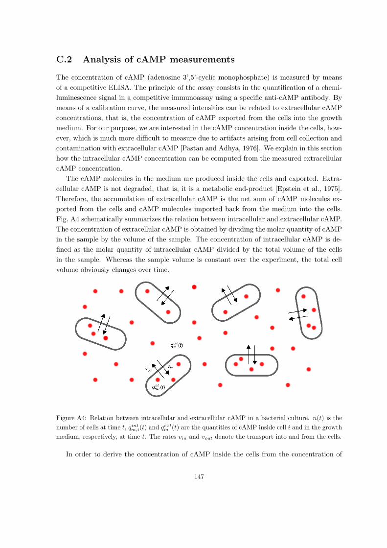
C.2 Analysis of cAMP measurements

The concentration of cAMP (adenosine 3’,5’-cyclic monophosphate) is measured by means

of a competitive ELISA. The principle of the assay consists in the quantification of a chemi-

luminescence signal in a competitive immunoassay using a specific anti-cAMP antibody. By

means of a calibration curve, the measured intensities can be related to extracellular cAMP

concentrations, that is, the concentration of cAMP exported from the cells into the growth

medium. For our purpose, we are interested in the cAMP concentration inside the cells, how-

ever, which is much more difficult to measure due to artifacts arising from cell collection and

contamination with extracellular cAMP [Pastan and Adhya, 1976]. We explain in this section

how the intracellular cAMP concentration can be computed from the measured extracellular

cAMP concentration.

The cAMP molecules in the medium are produced inside the cells and exported. Extra-

cellular cAMP is not degraded, that is, it is a metabolic end-product [Epstein et al., 1975].

Therefore, the accumulation of extracellular cAMP is the net sum of cAMP molecules ex-

ported from the cells and cAMP molecules imported back from the medium into the cells.

Fig. A4 schematically summarizes the relation between intracellular and extracellular cAMP.

The concentration of extracellular cAMP is obtained by dividing the molar quantity of cAMP

in the sample by the volume of the sample. The concentration of intracellular cAMP is de-

fined as the molar quantity of intracellular cAMP divided by the total volume of the cells

in the sample. Whereas the sample volume is constant over the experiment, the total cell

volume obviously changes over time.

Figure A4: Relation between intracellular and extracellular cAMP in a bacterial culture. n(t) is the

number of cells at time t, qintm,i(t) and qextm (t) are the quantities of cAMP inside cell i and in the growth

medium, respectively, at time t. The rates vin and vout denote the transport into and from the cells.

In order to derive the concentration of cAMP inside the cells from the concentration of

147

cAMP in the medium, we develop a simple kinetic model. We denote by qintm,i(t) and qextm (t)

the quantities of cAMP inside cell i and in the growth medium [mol], respectively, at time

t [min]. At t there are n(t) ≥ 1 cells in the sample, so i ∈ {1, . . . , n(t)}. This gives the

following balance equation for the quantity of external cAMP

dqextm (t)

dt=

∑

i∈{1,...,n(t)}

vout(qintm,i(t))− n(t) vin(q

extm (t)) (A7)

The first term in the right-hand side of Eq. (A7) denotes the rate of export of cAMP from the

cells into the growth medium, while the second term concerns the rate of import of cAMP

from the medium into the cells.

The export and import rates follow simple first-order kinetics [Epstein et al., 1975], so

that vout is a linear function of the internal cAMP concentrations with rate constant kout

[min−1] and vin a linear function of the external cAMP concentration with rate constant kin

[min−1]. This results in

vout(qintm,i(t)) = kout q

intm,i(t) , vin(q

extm (t)) = n(t) kin q

extm (t) (A8)

Defining

qintm (t) =∑

i∈{1,...,n(t)}

qintm,i(t) (A9)

we rewrite Eq. (A7) as

dqextm (t)

dt= kout q

intm (t)− n(t) kin q

extm (t) (A10)

In order to obtain concentration variables, we now introduce volume parameters Vtot and

Vcell(t), representing the sample volume and the volume of individual cells, respectively [L].

Notice that the cell volume is a function of time, since the growth rate changes over time

and the cell volume varies with the growth rate [Bremer and Dennis, 1996, Volkmer and

Heinemann, 2011]. In order to obtain concentrations, the quantity of internal cAMP needs

to be weighted by the total cellular volume, given by n(t)Vcell(t), and the quantity of external

cAMP by Vtot − n(t)Vcell(t). Given that the cells occupy only a tiny fraction of the sample

volume, the latter term is approximated by Vtot.

We multiply the left-hand and right-hand side of the equation with volume terms

dqextm (t)

dt

1

Vtot= kout q

intm (t)

1

Vtot

n(t)Vcell(t)

n(t)Vcell(t)− n(t) kin

1

Vtotqextm (t)

which results induextm (t)

dt= n(t)Vcell(t)

koutVtot

uintm (t)− n(t) kin uextm (t) (A11)

uintm (t) and uextm (t) are the concentrations of intracellular and extracellular cAMP [M], respec-

tively. From Eq. (A11) we obtain the following expression for the concentration of intracellular

cAMP

148

uintm (t) =1

n(t)Vcell(t)

Vtot

kout

duextm (t)

dt+

kinkout

Vtot

Vcell(t)uextm (t) (A12)

The interest of this equation lies in that it allows uintm (t) to be computed from the measured

concentration of extracellular cAMP. For this we need to know the constant kout, the constant

Vtot, the constant kin and the total cellular volume n(t)Vcell(t). kout has been measured as

2.1 min−1 [Epstein et al., 1975], while the sample volume Vtot equals 100 µL. Interestingly,

Volkmer and Heinemann [2011] have shown that the ratio n(t)Vcell(t)/a(t) is constant, where

a(t) is the measured absorbance of the culture volume in the microplate at time t. The value

of this ratio, which we call α, can be computed for our conditions by means of a calibration

curve previously published [de Jong et al., 2010], given that E. coli cells growing on glucose

have a cell volume of about 3 ·10−9 µL. We find α = 0.3 µL and replace n(t)Vcell(t) by αa(t).

When equating the cell volume in the import term to 3 · 10−9 µL, we obtain the expression

used in Chap. 5

uintm (t) =1

1.5 · 10−3 a(t) koutduextm (t)

dt+

kin3 · 10−11 kout

uextm (t) (A13)

The concentrations of extracellular cAMP and the absorbance are measured at different

time-points. In particular, we took samples from a growing bacterial culture at 12 time-points

(3 replicates). In order to obtain a(t), we fit a regression spline to the data (as described

above). As for obtaining uextm (t), we fitted a cubic spline to the data and took the derivative of

the uextm -spline to obtain duextm (t)/dt. The value of kin can then be estimated from Eq. (A13)

by using the measured steady-state concentration for intracellular cAMP during exponential

growth on glucose, namely 0.4 µM [Epstein et al., 1975, Pastan and Adhya, 1976], as well as

the absorbance and the (time-derivative of the) extracellular cAMP concentration measured

in our experiments. We thus find a value kin = 12 · 10−10 min−1.

With all parameter values known, Eq. (A13) allows the reconstruction of the temporal

profile of the concentration of intracellular cAMP from a(t), uextm (t), and duextm (t)/dt. The

values for uintm (t) reported in Chap. 5 are the mean of three replicates. 95%-confidence

intervals are computed from the standard error of the mean after synchronization of the

absorbance curves, as described in Sec. C.1. One of the advantages of the use of splines

is that the intracellular cAMP concentration can easily be calculated at all time-points by

spline interpolation.

Fig. A5 shows plots of the measured extracellular and derived intracellular cAMP con-

centrations over the duration of the experiment. The shape of the intracellular cAMP con-

centration profile agrees very well with other, direct measurements [Buettner et al., 1973,

Kao et al., 2004, Makman and Sutherland, 1965]. cAMP rapidly accumulates at the end of

exponential growth, when glucose is exhausted, and returns to a lower level after the growth

transition.

149

400 500 600 700 800 900 1000 1100 12000

0.2

0.4

0.6

0.8

1E

xtra

cellu

lar

cAM

P [µ

M]

cAMP

0.1

0.2

0.3

0.4

0.5

0.6

Abs

orba

nce

Time [min]

A

400 500 600 700 800 900 1000 1100 12000

1

2

3

4

Intr

acel

lula

r cA

MP

[µM

]

cAMP

0.1

0.2

0.3

0.4

0.5

0.6

Abs

orba

nce

Time [min]

B

500 600 700 800 900 1000 1100 12000

0.2

0.4

0.6

0.8

1

Ext

race

llula

r cA

MP

[µM

]

cAMP, ∆ fis

500 600 700 800 900 1000 1100 12000.05

0.1

0.2

0.4

0.6

0.8

Abs

orba

nce

Time [min]

C

500 600 700 800 900 1000 1100 12000

1

2

3

4

Intr

acel

lula

r cA

MP

[µM

]

cAMP, ∆ fis

0.05

0.1

0.2

0.4

0.6

0.8

Abs

orba

nce

Time [min]

D

800 900 1000 1100 1200 1300 1400 1500 16000

0.2

0.4

0.6

0.8

1

Ext

race

llula

r cA

MP

[µM

]

cAMP, redilution

800 900 1000 1100 1200 1300 1400 1500 16000.02

0.05

0.1

0.2

0.3

Abs

orba

nce

Time [min]

E

800 900 1000 1100 1200 1300 1400 1500 16000

2

4

6

8

Intr

acel

lula

r cA

MP

[µM

]

cAMP, redilution

0.02

0.05

0.1

0.2

0.3

Abs

orba

nce

Time [min]

F

Figure A5: Measurements of cAMP concentration in samples taken from a bacterial culture growing

in a microplate. A Absorbance and measured concentration of extracellular cAMP, with spline fit

to cAMP data. B Absorbance and derived concentration of intracellular cAMP. The cAMP concen-

trations are the mean of 3 replicates, synchronized with respect to their the absorbance curves as

described in Sec. C.1. The 95%-confidence intervals are computed from the standard error of the

mean. This plot corresponds to Fig. 2B of the main text. C-D: Idem in ∆fis strain. E-F: Idem in

wild-type strain after glucose down-shift.

150

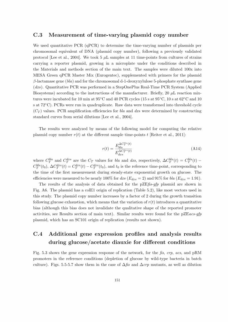
C.3 Measurement of time-varying plasmid copy number

We used quantitative PCR (qPCR) to determine the time-varying number of plasmids per

chromosomal equivalent of DNA (plasmid copy number), following a previously validated

protocol [Lee et al., 2004]. We took 5 µL samples at 11 time-points from cultures of strains

carrying a reporter plasmid, growing in a microplate under the conditions described in

the Materials and methods section of the main text. The samples were diluted 100x into

MESA Green qPCR Master Mix (Eurogentec), supplemented with primers for the plasmid

β-lactamase gene (bla) and for the chromosomal d-1-deoxyxylulose 5-phosphate synthase gene

(dxs). Quantitative PCR was performed in a StepOnePlus Real-Time PCR System (Applied

Biosystems) according to the instructions of the manufacturer. Briefly, 20 µL reaction mix-

tures were incubated for 10 min at 95◦C and 40 PCR cycles (15 s at 95◦C, 10 s at 62◦C and 10

s at 72◦C). PCRs were run in quadruplicate. Raw data were transformed into threshold cycle

(CT ) values. PCR amplification efficiencies for bla and dxs were determined by constructing

standard curves from serial dilutions [Lee et al., 2004].

The results were analyzed by means of the following model for computing the relative

plasmid copy number r(t) at the different sample time-points t [Reiter et al., 2011]:

r(t) =E

∆CblaT (t)

bla

E∆Cdxs

T (t)dxs

(A14)

where CblaT and Cdxs

T are the CT values for bla and dxs, respectively, ∆CblaT (t) = Cbla

T (t) −CblaT (t0), ∆Cdxs

T (t) = CdxsT (t)−Cdxs

T (t0), and t0 is the reference time-point, corresponding to

the time of the first measurement during steady-state exponential growth on glucose. The

efficiencies were measured to be nearly 100% for dxs (Edxs = 2) and 91% for bla (Edxs = 1.91).

The results of the analysis of data obtained for the pZEfis-gfp plasmid are shown in

Fig. A6. The plasmid has a colE1 origin of replication (Table 5.2), like most vectors used in

this study. The plasmid copy number increases by a factor of 2 during the growth transition

following glucose exhaustion, which means that the variation of r(t) introduces a quantitative

bias (although this bias does not invalidate the qualitative shape of the reported promoter

activities, see Results section of main text). Similar results were found for the pZEacs-gfp

plasmid, which has an SC101 origin of replication (results not shown).

C.4 Additional gene expression profiles and analysis results

during glucose/acetate diauxie for different conditions

Fig. 5.3 shows the gene expression response of the network, for the fis, crp, acs, and pRM

promoters in the reference conditions (depletion of glucose by wild-type bacteria in batch

culture). Figs. 5.5-5.7 show them in the case of ∆fis and ∆crp mutants, as well as dilution

151

Figure A6: Variation in number of plasmids per chromosomal equivalent of DNA (plasmid copy

number) measured by means of qPCR. The quantities have been normalized with respect to the

observed plasmid copy number in steady-state exponential growth on glucose, corresponding to the

first time-point. The 95%-confidence intervals were computed from the standard error of the mean of

4 replicates, after synchronization of the absorbance curves (Sec. C.1).

152

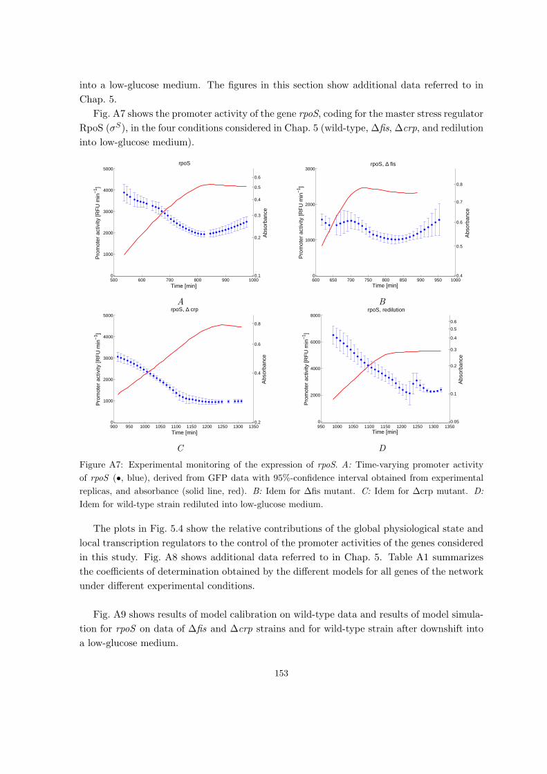
into a low-glucose medium. The figures in this section show additional data referred to in

Chap. 5.

Fig. A7 shows the promoter activity of the gene rpoS, coding for the master stress regulator

RpoS (σS), in the four conditions considered in Chap. 5 (wild-type, ∆fis, ∆crp, and redilution

into low-glucose medium).

500 600 700 800 900 10000

1000

2000

3000

4000

5000

Pro

mot

er a

ctiv

ity [R

FU

min

−1 ]

rpoS

0.1

0.2

0.3

0.4

0.5

0.6

Abs

orba

nce

Time [min]

A

600 650 700 750 800 850 900 950 10000

1000

2000

3000

Pro

mot

er a

ctiv

ity [R

FU

min

−1 ]

rpoS, ∆ fis

0.4

0.5

0.6

0.7

0.8

Abs

orba

nce

Time [min]

B

900 950 1000 1050 1100 1150 1200 1250 1300 13500

1000

2000

3000

4000

5000

Pro

mot

er a

ctiv

ity [R

FU

min

−1 ]

rpoS, ∆ crp

0.2

0.4

0.6

0.8

Abs

orba

nce

Time [min]

C

950 1000 1050 1100 1150 1200 1250 1300 13500

2000

4000

6000

8000

Pro

mot

er a

ctiv

ity [R

FU

min

−1 ]

rpoS, redilution

0.05

0.1

0.2

0.3

0.4

0.5

0.6

Abs

orba

nce

Time [min]

D

Figure A7: Experimental monitoring of the expression of rpoS. A: Time-varying promoter activity

of rpoS (•, blue), derived from GFP data with 95%-confidence interval obtained from experimental

replicas, and absorbance (solid line, red). B: Idem for ∆fis mutant. C: Idem for ∆crp mutant. D:

Idem for wild-type strain rediluted into low-glucose medium.

The plots in Fig. 5.4 show the relative contributions of the global physiological state and

local transcription regulators to the control of the promoter activities of the genes considered

in this study. Fig. A8 shows additional data referred to in Chap. 5. Table A1 summarizes

the coefficients of determination obtained by the different models for all genes of the network

under different experimental conditions.

Fig. A9 shows results of model calibration on wild-type data and results of model simula-

tion for rpoS on data of ∆fis and ∆crp strains and for wild-type strain after downshift into

a low-glucose medium.

153

−1 −0.5 0 0.5 1−1

−0.8

−0.6

−0.4

−0.2

0

0.2

0.4

0.6

0.8

1 rpoS

log(pRM

/p0RM

)

log(

p rpoS

/p0 rp

oS)

A

−0.5 0 0.5 1 1.5−0.5

0

0.5

1

1.5 rpoS, redilution

log(pRM

/p0RM

)

log(

p rpoS

/p0 rp

oS)

D

−1 −0.5 0 0.5 1−1

−0.8

−0.6

−0.4

−0.2

0

0.2

0.4

0.6

0.8

1 rpoS, ∆ fis

log(pRM

/p0RM

)

log(

p rpoS

/p0 rp

oS)

B

−1 −0.5 0 0.5 1−1

−0.8

−0.6

−0.4

−0.2

0

0.2

0.4

0.6

0.8

1 fis, ∆ fis

log(pRM

/p0RM

)

log(

p fis/p

0 fis)

E

−0.5 0 0.5 1 1.5−0.5

0

0.5

1

1.5 rpoS, ∆ crp

log(pRM

/p0RM

)

log(

p rpoS

/p0 rp

oS)

C

−0.5 0 0.5 1 1.5−0.5

0

0.5

1

1.5 crp, ∆ crp

log(pRM

/p0RM

)

log(

p crp/p

0 crp)

F

Figure A8: Predicted and observed control of rpoS, fis, and crp expression by the GEM and Crp·cAMP,

in various experimental conditions and genetic backgrounds. A: Predicted (-, black) and measured

(•, blue) relative activity of the rpoS promoter (log(prpoS(t)/p0rpoS)) as a function of the relative

activity of the pRM promoter (log(pRM (t)/p0RM )). The 95%-confidence intervals in the plots have

been computed from experimental replicas, as described in Sec. C.1. B-C: Idem for rpoS in ∆fis and

∆crp strains. D: Idem for rpoS in a wild-type strain after a down-shift into a low-glucose medium.

E: Idem for fis in a ∆fis strain. F: Idem for crp in a ∆crp strain.

154

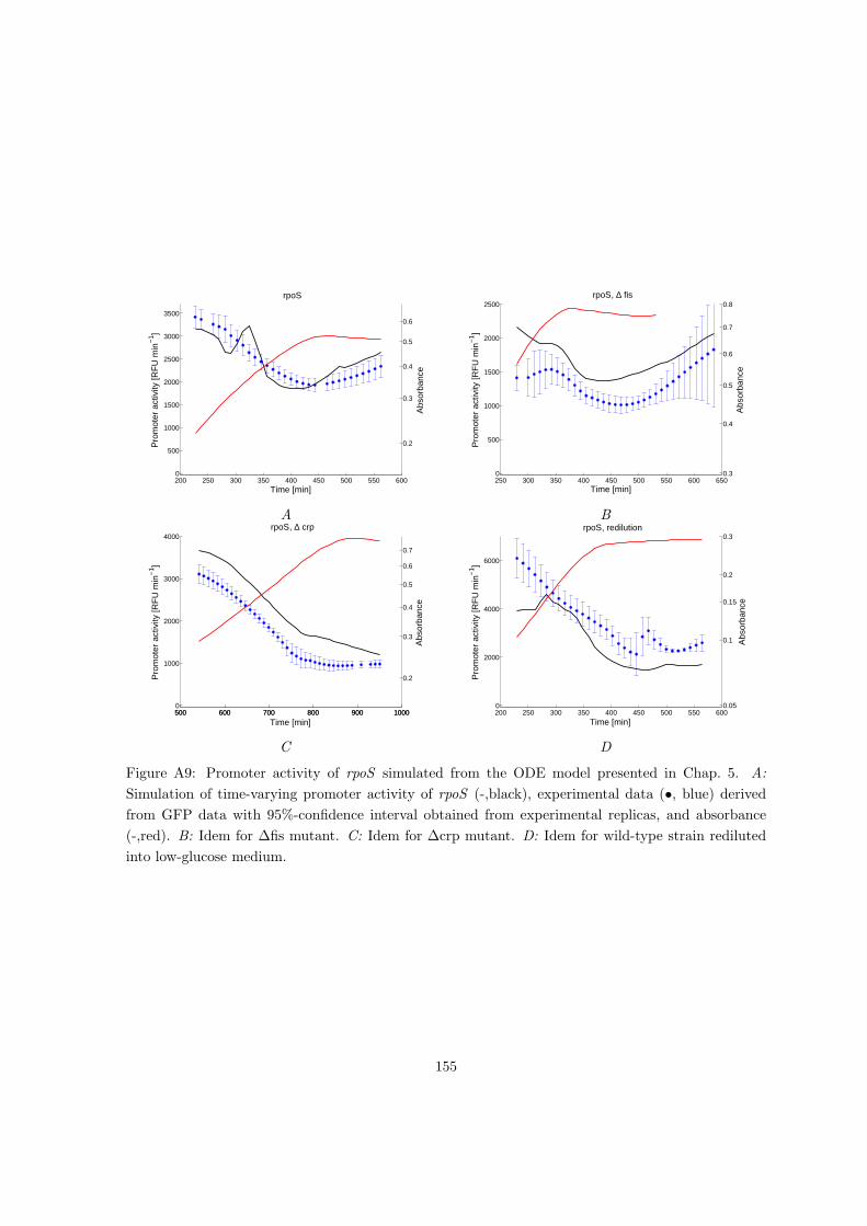
200 250 300 350 400 450 500 550 6000

500

1000

1500

2000

2500

3000

3500

Pro

mot

er a

ctiv

ity [R

FU

min

−1 ]

rpoS

0.2

0.3

0.4

0.5

0.6

Abs

orba

nce

Time [min]

A

250 300 350 400 450 500 550 600 6500

500

1000

1500

2000

2500

Pro

mot

er a

ctiv

ity [R

FU

min

−1 ]

rpoS, ∆ fis

0.3

0.4

0.5

0.6

0.7

0.8

Abs

orba

nce

Time [min]

B

500 600 700 800 900 10000

1000

2000

3000

4000

Pro

mot

er a

ctiv

ity [R

FU

min

−1 ]

rpoS, ∆ crp

500 600 700 800 900 1000

0.2

0.3

0.4

0.5

0.6

0.7

Abs

orba

nce

Time [min]

C

200 250 300 350 400 450 500 550 6000

2000

4000

6000

Pro

mot

er a

ctiv

ity [R

FU

min

−1 ]

rpoS, redilution

0.05

0.1

0.15

0.2

0.3

Abs

orba

nce

Time [min]

D

Figure A9: Promoter activity of rpoS simulated from the ODE model presented in Chap. 5. A:

Simulation of time-varying promoter activity of rpoS (-,black), experimental data (•, blue) derived

from GFP data with 95%-confidence interval obtained from experimental replicas, and absorbance

(-,red). B: Idem for ∆fis mutant. C: Idem for ∆crp mutant. D: Idem for wild-type strain rediluted

into low-glucose medium.

155

Experimental condition Model R2

WT

pfis vs pRM 0.71

pcrp vs pRM 0.83

pacs vs pRM 0.54

prpoS vs pRM 0.73

pfis − pRM vs c 0.31

pcrp − pRM vs c 0.6

pacs − pRM vs c 0.72

∆fis

pfis vs pRM 0.70

pcrp vs pRM 0.78

pacs vs pRM 0.34

prpoS vs pRM 0.83

pfis − pRM vs c 0.83

pcrp − pRM vs c 0.33

pacs − pRM vs c 0.97

prpoS − pRM vs c 0.04

∆crppfis vs pRM 0.94

pcrp vs pRM 0.97

prpoS vs pRM 0.97

WT+Redilution

pfis vs pRM 0.14

pcrp vs pRM 0.91

pacs vs pRM 0.20

prpoS vs pRM 0.81

pfis − pRM vs c 0.01

pcrp − pRM vs c 0.03

pacs − pRM vs c 0.56

prpoS − pRM vs c 0.17

Table A1: Summary of the coefficient of determinations found for the model on different experimen-

tal conditions. “pfis vs pRM” corresponds to the coefficient of correlation between log(pfis(t)/p0fis)

and log(pRM (t)/p0RM ) while “pfis − pRM vs c” corresponds to the coefficient of correlation between

log(pfis(t)/p0fis)− log(pRM (t)/p0RM ) and log(c(t)/c0). Idem for crp, acs and rpoS.

156

C.5 Additional information on parameter estimation of the

ODE model of the acs network

In Sec. 5.3, we present an ODE model of the dynamics of the acs regulatory network presented

in Fig. 5.1 and extended to also consider rpoS regulation by the complex Crp·cAMP. The

model, presented in Eq. (5.8) and Eq. (5.12), contains 21 parameters that need to be estimated

in order to obtain quantitative simulations of the behaviours of the promoter activities of these

genes during glucose/acetate diauxie. Below we detail the parameter estimation procedure

we followed.

C.5.1 Making the model consistent with available experimental data

In order to estimate the model parameters, we compared simulations of promoter activities

with promoter activities measured for fis, crp, acs and rpoS in the conditions described in

the Methods and Materials section in Chap 5. These experimental data, which are shown

in Fig. 5.3A-C and Fig. A7A, are measured in fluorescence units per minute (RFU·min−1).

However, the model of Eq. (5.12) returns promoter activities in units of mRNA concentra-

tion per minute (mM·min−1). In order to confront model simulations with available data, we

rescale the model in order to obtain variables and outputs expressed in the same unit as the

data.

Let us define xFis′ and xCrp′ the rescaled concentrations of Fis and Crp expressed in

fluorescence units (RFU) as well as pfis′ , pcrp′ , pacs′ and prpoS′ the rescaled promoter activities

of fis, crp, acs and rpoS expressed in RFU·min−1, respectively. We have

xFis′ =xFis

αfis, xCrp′ =

xCrp

αfis(A15)

pfis′ =pfisαfis

, pcrp′ =pcrpαfis

, pacs′ =pacsαacs

, prpoS′ =prpoSαrpoS

with αfis, αcrp, αacs and αrpoS the scaling factors for fis, crp, acs and rpoS, respectively. We

can reformulate the model of Eq. (5.12) with xFis′ and xCrp′ as variables and pacs′ and prpoS′

as outputs. This gives

xFis′(t) = pfis′(xFis′(t), xCrp·cAMP ′(t))− (µ(t) + γFis)× xFis′(t)

xCrp′(t) = pcrp′(xFis′(t), xCrp·cAMP ′(t))− (µ(t) + γCrp)× xCrp′(t)

xCrp·cAMP ′(t) =xCrp′ (t)

1+Kccc(t)

pacs′(t) = pacs′(xFis′(t), xCrp·cAMP ′(t))

prpoS′(t) = prpoS′(xCrp·cAMP ′(t))

(A16)

with xCrp·cAMP ′ = xCrp·cAMP /αcrp. This reformulation requires the definition of the following

157

rescaled parameters:

κbfis′ =

κbfis

αfis

, κbcrp′ =

κbcrp

αcrp

, κbacs′ =

κbacs

αacs

, κbrpoS′ =

κbrpoS

αrpoS

(A17)

κrfis′ =

κrfis

αfis

, κrcrp′ =

κrcrp

αcrp

, κracs′ =

κracs

αacs

, κrrpoS′ =

κrrpoS

αrpoS

θfis′i=

θfisiαfis

∀i = 1, · · · , 3 , θcc′j=

θcc′j

αcrp

∀j = 1, · · · , 4

The kinetic expressions for promoter activities of the 4 genes become

pfis′(xFis′(t), xCrp·cAMP ′(t)) = pRM (t) ·

κbfis′ + κrfis′ · 1(

xFis′

(t)

θfis′

1

)n1

+

(xrCrp·cAMP

(t)

θcc′

1

)n2

+1

pcrp′(xFis′(t), xCrp·cAMP ′(t)) = pRM (t) ·

κbcrp′ + κrcrp′ · xCrp·cAMP ′ (t)n4

xCrp·cAMP ′ (t)n4+θn4cc′

2·

(

1+

(xFis′

(t)

θfis′

2

)n3)

pacs(xFis′(t), xCrp·cAMP ′(t)) = pRM (t) ·

κbacs′ + κracs′ ·

xCrp·cAMP ′ (t)n6

xCrp·cAMP ′ (t)n6+θn6cc′

3·

(

1+

(xFis′

(t)

θfis′

3

)n5)

prpoS(xCrp·cAMP ′(t)) = pRM (t) ·(κbrpoS′ + κrrpoS′ · xCrp·cAMP ′ (t)n7

xCrp·cAMP ′ (t)n7+θn7cc′

4

)

(A18)

and the parameters of the rescaled model are listed in Table A2.

In order to obtain simulations of the promoter activities of the genes of the acs network and

rpoS, we need to specify the inputs of the model, i.e., the time-course data of intracellular

cAMP concentration c(t), bacterial growth rate µ(t) and pRM promoter activity pRM (t)

during glucose/acetate diauxie. Contrary to the promoter activity data, we were able to

compute, from measurements of extracellular cAMP, the intracellular cAMP concentration

in units of micromolar (see Appendix C.2). As Kcc, the equilibrium constant for Crp·cAMP

formation is also in the unit of micromolar (mM), no rescaling is required. As for the growth

rate input, we computed it, following the procedure described in Appendix C.1, from the

corrected absorbance data measured in the experiment recording pRM promoter activity

in the conditions described in Sec. 5.1.1. Finally, the promoter activity of pRM has been

measured in the units of RFU·min−1, which is in agreement with Eqs. (A16)-(A18). The

time-course data of promoter activities of fis, crp, acs and rpoS have been synchronized to

the pRM promoter activity data with respect to the maximum of absorbance (see [Isalan

et al., 2008] and Appendix C.1).

Eventually, the rescaled model is in agreement with inputs and promoter activity data.

Thus, we can confront it with outputs of the system so as to perform parameter estimation.

158

Parameters Description Units

Kcc equilibrium constant for Crp·cAMP formation reaction mM

fis expression

κbfis′ basal protein synthesis rate RFU·min−1

κrfis′ maximal protein synthesis rate RFU·min−1

θfis′1 , θcc′1 affinity constants RFU

n1, n2 Hill numbers adimensional

γFis protein degradation constant min−1

crp expression

κbcrp′ basal protein synthesis rate RFU·min−1

κrcrp′ maximal protein synthesis rate RFU·min−1

θfis′2 , θcc′2 affinity constants RFU

n3, n4 Hill numbers adimensional

γCrp protein degradation constant min−1

acs expression

κbacs′ basal protein synthesis rate RFU·min−1

κracs′ maximal protein synthesis rate RFU·min−1

θfis′3 , θcc′3 affinity constant RFU

n5, n6 Hill number adimensional

rpoS expression

κbrpoS′ basal protein synthesis rate RFU·min−1

κrrpoS′ maximal protein synthesis rate RFU·min−1

θcc′4 affinity constant RFU

n7 Hill number adimensional

Table A2: List of parameters of the rescaled model of Eqs. A16-A18. Units of the parameters are

specified.

C.5.2 Divide estimation problem into subproblems

To perform parameter estimation, we minimize the difference between the promoter activities

of fis, crp, acs and rpoS simulated by the model and measured experimentally. We define ρ

the vector of all 21 parameters, t1, · · · , tT the measurement time-points, with T ∈ N and pfis,

pcrp, pacs and prpoS the simulated promoter activities of fis, crp, acs and rpoS, respectively.

Thus, the objective function can be defined as

F (ρ) =

T∑

i=1

(pfis(ti, ρ)− pfis(i))2

pfis(i)2+

T∑

i=1

(pcrp(ti, ρ)− pcrp(i))2

pcrp(i)2

+

T∑

i=1

(pacs(ti, ρ)− pacs(i))2

pacs(i)2+

T∑

i=1

(prpoS(ti, ρ)− prpoS(i))2

prpoS(i)2

(A19)

The estimation problem is nonlinear in the parameters and the computation of F (ρ)

159

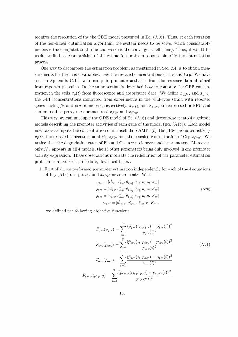
requires the resolution of the the ODE model presented in Eq. (A16). Thus, at each iteration

of the non-linear optimization algorithm, the system needs to be solve, which considerably

increases the computational time and worsens the convergence efficiency. Thus, it would be

useful to find a decomposition of the estimation problem so as to simplify the optimization

process.

One way to decompose the estimation problem, as mentioned in Sec. 2.4, is to obtain mea-

surements for the model variables, here the rescaled concentrations of Fis and Crp. We have

seen in Appendix C.1 how to compute promoter activities from fluorescence data obtained

from reporter plasmids. In the same section is described how to compute the GFP concen-

tration in the cells xg(t) from fluorescence and absorbance data. We define xg,fis and xg,crp

the GFP concentrations computed from experiments in the wild-type strain with reporter

genes having fis and crp promoters, respectively. xg,fis and xg,crp are expressed in RFU and

can be used as proxy measurements of xFis′ and xCrp′ .

This way, we can uncouple the ODE model of Eq. (A16) and decompose it into 4 algebraic

models describing the promoter activities of each gene of the model (Eq. (A18)). Each model

now takes as inputs the concentration of intracellular cAMP c(t), the pRM promoter activity

pRM , the rescaled concentration of Fis xFis′ and the rescaled concentration of Crp xCrp′ . We

notice that the degradation rates of Fis and Crp are no longer model parameters. Moreover,

only Kcc appears in all 4 models, the 18 other parameters being only involved in one promoter

activity expression. These observations motivate the redefinition of the parameter estimation

problem as a two-step procedure, described below.

1. First of all, we performed parameter estimation independently for each of the 4 equationsof Eq. (A18) using xFis′ and xCrp′ measurements. With

ρfis = [κbfis′ κ

rfis′ θfis′1 θcc′1 n1 n2 Kcc]

ρcrp = [κbcrp′ κ

rcrp′ θfis′2 θcc′2 n3 n4 Kcc] (A20)

ρacs = [κbacs′ κ

racs′ θfis′3 θcc′3 n5 n6 Kcc]

ρrpoS = [κbrpoS′ κ

rrpoS′ θcc′4 n7 Kcc],

we defined the following objective functions

Ffis(ρfis) =

T∑

i=1

(pfis(ti, ρfis)− pfis(i))2

pfis(i)2

Fcrp(ρcrp) =

T∑

i=1

(pcrp(ti, ρcrp)− pcrp(i))2

pcrp(i)2(A21)

Facs(ρacs) =

T∑

i=1

(pacs(ti, ρacs)− pfis(i))2

pacs(i)2

FrpoS(ρrpoS) =

T∑

i=1

(prpoS(ti, ρrpoS)− prpoS(i))2

prpoS(i)2.

160

Each of these 4 objective functions was minimized using a combination of global-search

and local-search methods. The global-search method used is the genetic algorithm im-

plemented in the Matlab function ga, parameterized with 5000 generations. The local-

search method used is the sequential quadratic programming algorithm implemented in

the Matlab function fmincon. For each parameter estimation problem, the optimiza-

tion algorithms were launched with 100 different initial parameter vectors, randomly

obtained within a specified range, and the parameter vector giving the lowest objective

function was chosen. As the parameter Kcc appears in all 4 estimation problems, we

limited the range of parameter search in order to obtain consistent estimated values.

2. Using the estimated values obtained in the previous step to define the initial vector,

we launched optimization algorithms to minimize the objective function of the whole

model, defined in Eq. (A19). For Kcc, we took the value estimated when minimizing

Facs(ρacs). For γFis and γCrp, that were not estimated in the previous step, we defined a

range of parameter search and randomly set initial values. The optimization algorithm

used is a combination of the genetic algorithm implemented in the Matlab function ga,

parameterized with 5000 generations, and the interior-point algorithm, a local-search

method with non-linear constraints implemented in the Matlab function fmincon.

In the preliminary results we present in this section and in Sec. 5.3, γFis and γCrp were

not estimated but fixed to values taken from the literature [de Jong et al., 2010]. More-

over, the affinity constants for regulation by Crp·cAMP and the equilibrium constant

of Crp·cAMP formation reaction were the only parameters estimated again in this step.

All other parameters were fixed to their values estimated in the previous step.

The parameter values obtained in this way are presented in Table A3.

161

Parameters Description Estimated value

Kcc equilibrium constant for Crp·cAMP formation reaction 5.57

fis expression

κbfis′ basal protein synthesis rate 2.48 · 10−1

κrfis′ maximal protein synthesis rate 6.60 · 10−2

θfis′1 affinity constant for regulation by Fis 5.23 · 103θcc′1 affinity constant for regulation by Crp·cAMP 1.04 · 102n1 Hill number for regulation by Fis 2.8

n2 Hill number for regulation by Crp·cAMP 3

γFis protein degradation constant 6.50 · 10−3

crp expression

κbcrp′ basal protein synthesis rate 6.39

κrcrp′ maximal protein synthesis rate 2.82 · 10−2

θfis′2 affinity constant for regulation by Fis 3.04 · 103θcc′2 affinity constant for regulation by Crp·cAMP 1.31 · 104n3 Hill number for regulation by Fis 1

n4 Hill number for regulation by Crp·cAMP 2.85

γCrp protein degradation constant 6.50 · 10−3

acs expression

κbacs′ basal protein synthesis rate 5 · 10−3

κracs′ maximal protein synthesis rate 1.14

θfis′3 affinity constant for regulation by Fis 1.61 · 103θcc′3 affinity constant for regulation by Crp·cAMP 1.34 · 103n5 Hill number for regulation by Fis 3

n6 Hill number for regulation by Crp·cAMP 3

rpoS expression

κbrpoS′ basal protein synthesis rate 1.79

κrrpoS′ maximal protein synthesis rate 1.40 · 10−3

θcc′4 affinity constant for regulation by Crp·cAMP 8.76 · 102n7 Hill number for regulation by Crp·cAMP 1

Table A3: Estimated values of parameters of the model of Eq. (A16).

162

Bibliography

R. Alves, E. Vilaprinyo, B. Hernandez-Bermejo, and A. Sorribas. Mathematical formalisms based on approximated

kinetic representations for modeling genetic and metabolic pathways. Biotechnol. Genet. Eng. Rev., 25:1–40, 2008.

M. Ashyraliyev, Y. Fomekong-Nanfack, J.A. Kaandorp, and J.G. Blom. Systems biology: Parameter estimation for

biochemical models. FEBS J., 276(4):886–902, 2009.

T. Baba, T. Ara, M. Hasegawa, Y. Takai, Y. Okumura, M. Baba, K.A. Datsenko, M. Tomita, B.L. Wanner, and H. Mori.

Construction of Escherichia coli K-12 in-frame, single-gene knockout mutants: the Keio collection. Mol. Syst. Biol.,

2:2006.0008, 2006.

V. Baldazzi, D. Ropers, Y. Markowicz, D. Kahn, J. Geiselmann, and H. de Jong. The carbon assimilation network in

Escherichia coli is densely connected and largely sign-determined by directions of metabolic fluxes. PLoS Comput.

Biol., 6(6):e1000812, 2010.

V. Baldazzi, D. Ropers, J. Geiselmann, D. Kahn, and H. de Jong. Importance of metabolic coupling for the dynamics

of gene expression following a diauxic shift in Escherichia coli. J. Theor. Biol., 296:100–15, 2012.

B.D. Bennett, E.H. Kimball, M. Gao, R. Osterhout, S.J. Van Dien, and J.D. Rabinowitz. Absolute metabolite concen-

trations and implied enzyme active site occupancy in Escherichia coli. Nat. Chem. Biol., 5(8):593–9, 2009.

S. Berthoumieux, M. Brilli, H. de Jong, D. Kahn, and E. Cinquemani. Identification of linlog models of metabolic

networks from incomplete high-throughput datasets. Bioinformatics, 27(13):i186–i195, 2011.

S. Berthoumieux, M. Brilli, D. Kahn, H. de Jong, and E. Cinquemani. Identifiability analysis of metabolic network

models. 2012a. Submitted.

S. Berthoumieux, D. Kahn, H. de Jong, and E. Cinquemani. Structural and practical identifiability of approximate

metabolic network models. Proc. 16th IFAC Symp. System Identif. (SYSID 2012), 2012b. To appear.

K. Bettenbrock, S. Fischer, K. Jahreis, T. Sauter, and E.D. Gilles. A quantitative approach to catabolite repression in

Escherichia coli. J. Biol. Chem., 281(5):2578–84, 2006.

H.G. Beyer and H.P. Schwefel. Evolution strategies, a comprehensive introduction. Natural Computing, 1:3–52, 2002.

L. Bintu, N.E. Buchler, H.G. Garcia, U. Gerland, T. Hwa, J. Kondev, T. Kuhlman, and R. Phillips. Transcriptional

regulation by the numbers: applications. Curr. Opin. Genet. Dev., 15(2):125–35, 2005.

H. Bolouri. Computational modeling of gene regulatory networks-a primer. Imperial College Press, 2008.

F. Boyer, B. Besson, G. Baptist, J. Izard, C. Pinel, D. Ropers, J. Geiselmann, and H. de Jong. WellReader: a MATLAB

program for the analysis of fluorescence and luminescence reporter gene data. Bioinformatics, 26(9):1262–63, 2010.

M.D. Bradley, M.B. Beach, A.P.J. de Koning, T.S. Pratt, and R. Osuna. Effects of Fis on Escherichia coli gene

expression during different growth stages. Microbiology, 153:2922–40, 2007.

M. Brand. Incremental singular value decomposition of uncertain data with missing values. In A. Heyden, G. Sparr,

M. Nielsen, and P. Johansen, editors, Proc. 7th Eur. Conf. Comput. Vision (ECCV 2002), volume 2350 of LNCS,

pages 707–20. Springer Verlag, 2002.

163

H. Bremer and P.P. Dennis. Modulation of chemical composition and other parameters of the cell by growth rate.

In F.C. Neidhardt, R. Curtiss III, J. Ingraham, E.C.C. Lin, K.B. Low, B. Magasanik, W. Reznikoff, M. Riley,

M. Schaechter, and H.E. Umbarger, editors, Escherichia coli and Salmonella: Cellular and molecular biology, 2nd

Ed., pages 1553–69. ASM Press, 1996.

M.J. Buettner, E. Spitz, and H.V. Rickenberg. Cyclic adenosine 3’,5’-monophosphate in Escherichia coli. J. Bacteriol.,

14(3):1068–73, 1973.

S. Bulik, S. Grimbs, C. Huthmacher, J. Selbig, and H.G. Holzhutter. Kinetic hybrid models composed of mechanistic

and simplified enzymatic rate laws a promising method for speeding up the kinetic modelling of complex metabolic

networks. FEBS J., 276(2):410–24, 2009.

S. Bulik, S. Grimbs, C. Huthmacher, J. Selbig, and H.G. Holzhutter. Integration of metabolic reactions and gene

regulation. Mol. Biotechnol., 47(1):70–82, 2011.

L. Cai, N. Friedman, and X.S. Xie. Stochastic protein expression in individual cells at the single molecule level. Nature,

440(7082):358–62, 2006.

M.J. Chappell, K.R. Godfrey, and S. Vajda. Global identifiability of the parameters of nonlinear systems with specified

inputs: A comparison of methods. Math. Biosci., 102(1):41–73, 1990.

C. Chassagnole, N. Noisommit-Rizzi, J.W. Schmid, K. Mauch, and M. Reuss. Dynamic modeling of the central carbon

metabolism of Escherichia coli. Biotechnol. Bioeng., 79(1):53–73, 2002.

C. Chen, D.A. Ridzon, A.J. Broomer, Z. Zhou, D.H. Lee, J.T. Nguyen, M. Barbisin, N.L. Xu, V.R. Mahuvakar, M.R.

Andersen, K.Q. Lao, K.J. Livak, and K.J. Guegler. Real-time quantification of microRNAs by stem-loop RT-PCR.

Nucleid Acids Res., 33(20):e179, 2005.

W.W. Chen, M. Nieper, and P.K. Sorger. Classic and contemporary approaches to modeling biochemical reactions.

Genes Dev., 24:1861–75, 2010.

O.T. Chis, J.R. Banga, and E. Balsa-Canto. GenSSI: a software toolbox for structural identifiability analysis of biological

models. Bioinformatics, 27(18):2610–1, 2011a.

O.T. Chis, J.R. Banga, and E. Balsa-Canto. Structural identifiability of systems biology models: a critical comparison

of methods. PLoS One, 6(11):e27755, 2011b.

B.-K. Cho, E.M. Knight, C.L. Barrett, and B.O. Palsson. Genome-wide analysis of Fis binding in Escherichia coli

indicates a causative role for A-/AT-tracts. Genome Res., 18(6):900–10, 2008.

I.C. Chou and E.O. Voit. Recent developments in parameter estimation and structure identification of biochemical and

genomic systems. Math. Biosci., 219(2):57–83, 2009.

C. Cobelli and J.J. di Stefano 3rd. Parameter and structural identifiability concepts and ambiguities: A critical review

and analysis. Am. J. Physiol., 239(1):R7–24, 1980.

A. Cornish-Bowden. Fundamentals of enzyme kinetics. Portland Press, 1995.

R.S. Costa, D. Machado, I. Rocha, and E.C. Ferreira. Hybrid dynamic modeling of Escherichia coli central metabolic

network combining Michaelis-Menten and approximate kinetic equations. Biosystems, 100(2):150–8, 2010.

T.M. Cover and J.A. Thomas. Elements of Information Theory, 2nd edition. Wiley, 2006.

E.J. Crampin. System identification challenges from systems biology. In Proc. 14th IFAC Symp. Syst. Identif. (SYSID

2006), pages 81–93, Newcastle, Australia, 2006.

H. de Jong. Modeling and simulation of genetic regulatory systems: A literature review. J. Comput. Biol., 9(1):67–103,

2002.

H. de Jong, J-L. Gouze, C. Hernandez, M. Page, T. Sari, and J. Geiselmann. Qualitative simulation of genetic regulatory

networks using piecewise-linear models. Bull. Math. Biol., 66:301–40, 2004.

164

H. de Jong, C. Ranquet, D. Ropers, C. Pinel, and J. Geiselmann. Experimental and computational validation of models

of fluorescent and luminescent reporter genes in bacteria. BMC Syst. Biol., 4:55, 2010.

R.C.H. del Rosario, E. Mendoza, and E.O. Voit. Challenges in lin-log modelling of glycolysis in Lactococcus lactis. IET

Syst. Biol., 2(3):136–49, 2008.

X. Delgado and J.C. Liao. Metabolic control analysis using transient metabolite concentrations. Biochem. J., 285:

965–72, 1992.

A.P. Dempster, N.M. Laird, and D.B. Rubin. Maximum likelihood from incomplete data via the EM algorithm. J. Roy.

Stat. Soc. Ser. B, 39(1):1–38, 1977.

P.P. Dennis, M. Ehrenberg, and H. Bremer. Control of rRNA synthesis in Escherichia coli : a systems biology approach.

Microbiol. Mol. Biol. Rev., 68(4):639–68, 2004.

Y. Dharmadi and R. Gonzalez. DNA microarrays: Experimental issues, data analysis, and application to bacterial

systems. Biotechnology Progress, 20(5):1309–24, 2004.

K. Durrschmid, H. Reischer, W. Schmidt-Heck, T. Hrebicek, R. Guthke, A. Rizzi, and K. Bayer. Monitoring of

transcriptome and proteome profiles to investigate the cellular response of E. coli towards recombinant protein

expression under defined chemostat conditions. J. Biotechnol., 135:34–44, 2008.

T.K. Van Dyk, E.J. Derose, and G.E. Gonye. LuxArray, a high-density, genomewide transcription analysis of Escherichia

coli using bioluminescent reporter strains. J. Bacteriol., 183(19):5496–505, 2001.

M.B. Elowitz and S. Leibler. A synthetic oscillatory network of transcriptional regulators. Nature, 403(6767):335–8,

2000.

W. Epstein, L.B. Rothman-Denes, and J. Hesse. Adenosine 3’:5’-cyclic monophosphate as mediator of catabolite

repression in Escherichia coli. Proc. Nat. Acad. Sci. USA, 72(6):2300–4, 1975.

J.J. Faith, B. Hayete, J.T. Thaden, I. Mogno, J. Wierzbowski, G. Cottarel, S. Kasif, J.J. Collins, and T.S. Gardner.

Large-scale mapping and validation of Escherichia coli transcriptional regulation from a compendium of expression

profiles. PLoS Biol., 5(1):e8, 2007.

L. Glass and S.A. Kauffman. The logical analysis of continuous non-linear biochemical control networks. J. Theor.

Biol., 39:103–29, 1973.

B. Gorke and J. Stulke. Carbon catabolite repression in bacteria: many ways to make the most out of nutrients. Nat.

Rev. Microbiol., 6(8):613–24, 2008.

G. Gosset, Z. Zhang, S. Nayyar, W. Cuevas, and M. Saier Jr. Transcriptome analysis of CRP-dependent catabolite

control of gene expression in Escherichia coli. J. Bacteriol., 186(11):3516–24, 2004.

J.W. Graham. Missing data analysis: Making it work in the real world. Annu. Rev. Psychol., 60:549–76, 2009.

M. Gstaiger and R. Aebersold. Applying mass spectrometry-based proteomics to genetics, genomics and network biology.

Nat. Rev. Genet., 10(9):617–27, 2009.

R.N. Gutenkunst, J.J. Waterfall, F.P. Casey, K.S. Brown, C.R. Myers, and J.P. Sethna. Universally sloppy parameter

sensitivities in systems biology models. PLoS Comput. Biol., 3(10):1871–78, 2007.

R.M. Gutierrez-Rıos, J.A. Freyre-Gonzalez, O. Resendis, J. Collado-Vides, M. Saier, and G. Gosset. Identification of

regulatory network topological units coordinating the genome-wide transcriptional response to glucose in Escherichia

coli. BMC Microbiol., 7:53, 2007.

F. Hadlich, S. Noack, and W. Wiechert. Translating biochemical network models between different kinetic formats.

Metab. Eng., 11(2):87–100, 2009.

J.B.S. Haldane. Enzymes. Monographs on biochemistry. Longmans, Green and Co, 1930.

165

L.C. Hamilton. Regression with graphics: a second course in applied statistics. Brooks/Cole Pub. Co., 1992.

T. Hardiman, K. Lemuth, M.A. Kellerand, M. Reuss, and M. Siemann-Herzberg. Topology of the global regulatory

network of carbon limitation in Escherichia coli. J. Biotechnol., 132(4):359–74, 2007.

T. Hardiman, K. Lemuth, M. Siemann-Herzberg, and M. Reuss. Dynamic modeling of the central metabolism of E. coli

linking metabolite and regulatory networks. In S.Y. Lee, editor, Systems Biology and Biotechnology of Escherichia

coli, pages 209–235. Springer Netherlands, 2009.

V. Hatzimanikatis and J.E. Bailey. Effects of spatiotemporal variations on metabolic control: approximate analysis

using (log)linear kinetic models. Biotechnol. Bioeng., 54(2):91–104, 1997.

J.J. Heijnen. Approximative kinetic formats used in metabolic network modeling. Biotechnol. Bioeng., 91(5):534–45,

2005.

R. Heinrich and S. Schuster. The regulation of cellular systems. ITP, 1996.

R. Hengge-Aronis. Signal transduction and regulatory mechanisms involved in control of the σS (RpoS) subunit of

RNA polymerase. Microbiol. and Mol. Biol. Rev., 66(3):373–95, 2002.

A.V. Hill. The possible effects of the aggregation of the molecules of hemoglobin on its dissociation curves. J. Physiol.,

40:iv–vii, 1910.

N.J. Horton and K.P. Kleinman. Much ado about nothing: A comparison of missing data methods and software to fit

incomplete data regression models. Am. Stat., 61(1):79–90, 2007.

M. Isalan, C. Lemerle, K. Michalodimitrakis, C. Horn, P. Beltrao, E. Raineri, M. Garriga-Canut, and L. Serrano.

Evolvability and hierarchy in rewired bacterial gene networks. Nature, 452(7189):840–5, 2008.

N. Ishii, K. Nakahigashi, T. Baba, M. Robert, T. Soga, A. Kanai, T. Hirasawa, M. Naba, K. Hirai, A. Hoque, P.Y.

Ho, Y. Kakazu, K. Sugawara, S. Igarashi, S. Harada, T. Masuda, N. Sugiyama, T. Togashi, M. Hasegawa, Y. Takai,

K. Yugi, K. Arakawa, N. Iwata, Y. Toya, Y. Nakayama, T. Nishioka, K. Shimizu, H. Mori, and M. Tomita. Multiple

high-throughput analyses monitor the response of E. coli to perturbations. Science, 316(5824):593–7, 2007.

S. Itzkovitz and A. van Oudenaarden. Validating transcripts with probes and imaging technology. Nat. Methods, 8(4

Supp):S12–9, 2011.

K. Jaqaman and G. Danuser. Linking data to models: data regression. Nat. Rev. Mol. Cell. Biol., 7(11):813–9, 2006.

L. Jia, N. Tanaka, and S. Terabe. Two-dimensional separation system of coupling capillary liquid chromatography to

capillary electrophoresis for analysis of Escherichia coli metabolites. Electrophoresis, 26(18):3468–78, 2005.

I.T. Jolliffe. Principal Component Analysis. Springer-Verlag, 1986.

S. Jozefczuk, S. Klie, G. Catchpole, J. Szymanski, A. Cuadros-Inostroza, D. Steinhauser, J. Selbig, and L. Willmitzer.

Metabolomic and transcriptomic stress response of Escherichia coli. Mol. Syst. biol., 6:364, 2010.

S. Kalir, S. Mangan, and U. Alon. A coherent feed-forward loop with a sum input function prolongs flagella expression

in Escherichia coli. Mol. Syst. biol., 1:2005.0006, 2005.

K.C. Kao, Y.-L. Yang, R. Boscolo, C. Sabatti, V. Roychowdhury, and J.C. Liao. Transcriptome-based determination

of multiple transcription regulator activities in Escherichia coli by using network component analysis. Proc. Natl.

Acad. Sci.USA, 101(2):641–6, 2004.

G. Karlebach and R. Shamir. Modelling and analysis of gene regulatory networks. Nat. Rev. Mol. Cell Biol., 9(10):

770–80, 2008.

S. Kirkpatrick, C.D. Gelatt, and M.P. Vecchi. Optimization by simulated annealing. Science, 220:671–80, 1983.

S. Klamt and J. Stelling. Two approaches for metabolic pathway analysis? Trends Biotechnol., 21(2):64–9, 2003.

166

S. Klumpp and T. Hwa. Growth-rate-dependent partitioning of RNA polymerases in bacteria. Proc. Nat. Acad. Sci.

USA, 105(51):20245–50, 2008.

S. Klumpp, Z. Zhang, and T. Hwa. Growth rate-dependent global effects on gene expression in bacteria. Cell, 139(7):

1366–75, 2009.

D.E. Koshland, G. Nemethy, and D. Filmer. Comparison of experimental binding data and theoretical models in proteins

containing subunits. Biochemistry, 5:365–85, 1966.

O. Kotte, J.B. Zaugg, and M. Heinemann. Bacterial adaptation through distributed sensing of metabolic fluxes. Mol.

Syst. Biol., 6:355, 2010.

A. Kremling. Comment on mathematical models which describe transcription and calculate the relationship between

mRNA and protein expression ratio. Biotechnol. Bioeng., 96(4):815–9, 2007.

A. Kremling, K. Bettenbrock, and E.D. Gilles. Analysis of global control of escherichia coli carbohydrate uptake. BMC.

Syst. Biol., 1:1–42, 2007.

A. Kremling, K. Bettenbrock, and E.D. Gilles. A feed-forward loop guarantees robust behavior in Escherichia coli

carbohydrate uptake. Bioinformatics, 24(5):704–10, 2008.

A. Kremling, S. Kremling, and K. Bettenbrock. Catabolite repression in Escherichia coli - a comparison of modeling

approaches. FEBS J., 276:594–602, 2009.

C. Lee, J. Kim, S.G. Shin, and S. Hwang. Absolute and relative QPCR quantification of plasmid copy number in

Escherichia coli. J. Biotechnol., 123(3):27380, 2004.

M. Li, P.Y. Ho, S. Yao, and K. Shimizu. Effect of lpdA gene knockout on the metabolism in Escherichia coli based on

enzyme activities, intracellular metabolite concentrations and metabolic flux analysis by 13C-labeling experiments.

Mass Spectrom. Rev., 122:254–66, 2006.

W. Liebermeister and E. Klipp. Bringing metabolic networks to life: Convenience rate law and thermodynamic con-

straints. Theor. Biol. Med. Model., 3:41, 2006.

S. Lin-Chao and H. Bremer. Effect of the bacterial growth rate on replication control of plasmid pBR322 in Escherichia

coli. Mol. Gen. Genet., 203(1):143–9, 1986.

R.J.A Little and D.B. Rubin. Statistical Analysis with Missing Data. Wiley, 2002.

L. Ljung. System identification, theory for the user. Prentice Hall PTR, 1999.

D.J. Lockhart, H. Dong, M.C. Byrne, M.T. Follettie, M.V. Gallo, M.S. Chee, M. Mittmann, C. Wang, M. Kobayashi,

H. Norton, and E.L. Brown. Expression monitoring by hybridization to high-density oligonucleotide arrays. Nat.

Biotechnol., 14(13):1675–80, 1996.

D. Longo and J. Hasty. Dynamics of single-cell gene expression. Mol. Syst. Biol., 2:64, 2006.

G.L. Lorca, A. Ezersky, V.V. Lunin, J.R. Walker, S. Altamentova, E. Evdokimova, M. Vedadi, A. Bochkarev, and

A. Savchenko. Glyoxylate and pyruvate are antagonistic effectors of the Escherichia coli IclR transcriptional regulator.

J. Biol. Chem., 282(22):16476–91, 2007.

G.W. Luli and W.R. Strohl. Comparison of growth, acetate production, and acetate inhibition of Escherichia coli

strains in batch and fed-batch fermentations. Appl. Environ. Microbiol., 56(4):1004–11, 1990.

O. Maaloe and N.O. Kjeldgaard. Control of macromolecular synthesis. W.A. Benjamin, 1966.

T. Maiwald and J. Timmer. Dynamical modeling and multi-experiment fitting with PottersWheel. Bioinformatics, 24

(18):2037–43, 2008.

R.S. Makman and E.W. Sutherland. Adenosine 3’,5’-phosphate in Escherichia coli. J. Biol. Chem., 240(3):1309–14,

1965.

167

B.F.J. Manly. Randomization, Bootstrap and Monte-Carlo Methods in Biology. Chapman and Hall, 1997.

R. Marouga, S. David, and E. Hawkins. The development of the DIGE system: 2D fluorescence difference gel analysis

technology. Anal. Bioanal. Chem., 382:669–78, 2005.

A. Martinez-Antonio and J. Collado-Vides. Identifying global regulators in transcriptional regulatory networks in

bacteria. Curr. Opin. Microbiol., 6:482–9, 2003.

L. Marucci, S. Santini, M. di Bernardo, and D. di Bernardo. Derivation, identification and validation of a computational

model of a novel synthetic regulatory network in yeast. J. Math. Biol., 62(5):685–706, 2011.

G. Baptist et al. A genome-wide screen for identifying all regulators of a target gene. Under revision.

D. Del Vecchio, A.J. Ninfa, and E.D. Sontag. Modular cell biology: retroactivity and insulation. Mol. Syst. Biol., 4:

161, 2008.

M.H. Saier Jr, T.M. Ramseier, and J. Reizer. Regulation of carbon utilization. In F.C. Neidhardt, R. Curtiss III,

J. Ingraham, E.C.C. Lin, K.B. Low, B. Magasanik, W. Reznikoff, M. Riley, M. Schaechter, and H.E. Umbarger,

editors, Escherichia coli and Salmonella: Cellular and molecular biology, 2nd Ed., pages 1325–43. ASM Press, 1996.

R. Meloni, O. Khalfallah, and N.F. Biguet. DNA microarrays and pharmacogenomics. Pharmacol. Res., 49(4):303–8,

2004.

L. Michaelis and M.L. Menten. Die Kinetik der Invertinwirkung. Biochem. Z., 49:333–69, 1913.

L. Michaelis, M.L. Menten, K.A. Johnson, and R.S. Goody. The original Michaelis constant: translation of the 1913

Michaelis-Menten paper. Biochemistry, 50(39):8264–9, 2011.

J.H. Miller. Experiments in molecular genetics. CSHL, 1972.

C.G. Moles, P. Mendes, and J.R. Banga. Parameter estimation in biochemical pathways: A comparison of global

optimization methods. Genome Res., 13:2467–74, 2003.

J. Monod, J. Wyman, and J.P. Changeux. On the nature of allosteric transitions: A plausible model. J. Mol. Biol., 12:

88–118, 1965.

M.R.N. Monton and T. Soga. Metabolome analysis by capillary electrophoresismass spectrometry. J. Chromatogr. A.,

1168:237–248, 2007.

F.C. Neidhardt and D.G. Fraenkel. Metabolic regulation of RNA synthesis in bacteria. Cold Spring Harb. Symp. Quant.

Biol., 26:63–74, 1961.

F.C. Neidhardt, J.L. Ingraham, and M. Schaechter. Physiology of the bacterial cell, a molecular approach. Sinauer

Associates, Inc. Sunderland, Mass, 1990.

J.A. Nelder and R. Mead. A simplex method for function minimization. Computer J., 7(4):308–13, 1965.

J. Nemcova. Structural identifiability of polynomial and rational systems. Math. Biosci., 223(2):83–96, 2010.

C. Nicolas, P. Kiefer, F. Letisse, J. Krmer, S. Massou, P. Soucaille, C. Wittmann, N.D. Lindley, and J-C. Portais.

Response of the central metabolism of Escherichia coli to modified expression of the gene encoding the glucose-6-

phosphate dehydrogenase. FEBS Lett., 581(20):3771–6, 2007.

I.E. Nikerel, W.A. van Winden, W.M. van Gulik, and J.J. Heijnen. A method for estimation of elasticities in metabolic

networks using steady state and dynamic metabolomics data and linlog kinetics. BMC Bioinform., 7:540, 2006.

I.E. Nikerel, W.A. van Winden, P.J.T. Verheijen, and J.J. Heijnen. Model reduction and a priori kinetic parameter

identifiability analysis using metabolome time series for metabolic reaction networks with linlog kinetics. Metab.

Eng., 11(1):20–30, 2009.

168

O. Ninnemann, C. Koch, and R. Kahmann. The E.coli fis promoter is subject to stringent control and autoregulation.

EMBO J., 11(3):1075–83, 1992.

S. Oba, M.A. Sato, I. Takemasa, M. Monden, K. Matsubara, and S. Ishii. A Bayesian missing value estimation method

for gene expression profile data. Bioinformatics, 19(16):2088–96, 2003.

M.K. Oh, L. Rohlin, K.C. Kao, and J.C. Liao. Global expression profiling of acetate-grown Escherichia coli. J. Biol.

Chem., 277(15):13175–83, 2002.

M.S. Okino and M.L. Mavrovouniotis. Simplification of mathematical models of chemical reaction systems. Chem. Rev.,

98(391-408):685–706, 1998.

A.B. Oppenheim, O. Kobiler, J. Stavans, D.L. Court, and S. Adhya. Switches in bacteriophage lambda development.

Annu. Rev. Genet., 39:409–29, 2005.

S.J. Park, S.Y. Lee, J. Cho, T.Y. Kim, J.W. Lee, J.H. Park, and M.J. Han. Global physiological understanding and

metabolic engineering of microorganisms based on omics studies. Appl. Microbiol. Biotechnol., 68:567–79, 2005.

I. Pastan and S. Adhya. Cyclic adenosine 5’-monophosphate in Escherichia coli. Bacteriol. Rev., 40(3):527–51, 1976.

K. Potrykus and M. Cashel. (p)ppGpp: Still magical? Ann. Rev. Microbiol., 62:35–51, 2008.

M.A. Quail and J.R. Guest. Purification, characterization and mode of action of PdhR, the transcriptional repressor of

the pdhR-aceEF-lpd operon of Escherichia coli. Mol. Microbiol., 15(3):519–29, 1995.

A. Raue, C. Kreutz, T. Maiwald, J. Bachmann, M. Schilling, U. Klingmuller, and J. Timmer. Structural and practical

identifiability analysis of partially observed dynamical models by exploiting the profile likelihood. Bioinformatics,

25(15):1923–29, 2009.

A. Raue, C. Kreutz, T. Maiwald, U. Klingmuller, and J. Timmer. Addressing parameter identifiability by model-based

experimentation. IET Syst. Biol., 5(2):120–30, 2011.

C. Reder. Metabolic control theory: a structural approach. J. Theor. Biol., 135(2):175–201, 1988.

B. Regenberg, T. Grotkjaer, O. Winther, A. Fausbøll, M. Akesson, C. Bro, L.K. Hansen, S. Brunak, and J. Nielsen.

Growth-rate regulated genes have profound impact on interpretation of transcriptome profiling in Saccharomyces

cerevisiae. Genome Biol., 7(11):R107, 2006.

M. Reiter, B. Kirchner, H. Muller, C. Holzhauer, W. Mann, and M.W. Pfaffl. Quantification noise in single cell

experiments. Nucleids Acids Res., 38(18):e124, 2011.

M. Rodriguez-Fernandez, P. Mendes, and J.R. Banga. A hybrid approach for efficient and robust parameter estimation

in biochemical pathways. BioSystems, 83:248–65, 2006.

M. Ronen, R. Rosenberg, B.I. Shraiman, and U. Alon. Assigning numbers to the arrows: Parameterizing a gene

regulation network by using accurate expression kinetics. Proc. Natl. Acad. Sci. USA, 99(16):10555–60, 2002.

D. Ropers, H. de Jong, M. Page, D. Schneider, and J. Geiselmann. Qualitative simulation of the carbon starvation

response in Escherichia coli. Biosystems, 84:124–52, 2006.

M.R. Roussel and S.J. Fraser. Invariant manifold methods for metabolic model reduction. Chaos, 11(1):196–206, 2001.

D.B. Rubin. Inference and missing data. Biometrika, 63:581–90, 1976.

D.B. Rubin. Multiple imputation after 18+ years. J. Am. Stat. A., 81:473–89, 1996.

J. Saez-Rodriguez, A. Kremling, and E.D. Gilles. Dissecting the puzzle of life: modularization of signal transduction

networks. Comput. Chem. Eng., 29:619–29, 2005.

C. Sander and R. Schneider. Database of homology-derived protein structures and the structural meaning of sequence

alignment. Proteins, 9:56–68, 1991.

169

P.J. Sands and E.O. Voit. Flux-based estimation of parameters in S-systems. Ecological Modelling, 93(1-3):75–88, 1996.

U. Sauer. Metabolic networks in motion: 13C-based flux analysis. Mol. Syst. biol., 2:62, 2006.

M.A. Savageau. Biochemical Systems Analysis: A Study of Function and Design in Molecular Biology. Addison-Wesley,

1976.

M. Schaechter, J.L. Ingraham, and F.C. Neidhardt. Microbe. ASM Press, 2006.

M. Schena, D. Shalon, R.W. Davis, and P.O. Brown. Quantitative monitoring of gene expression patterns with a

complementary DNA microarray. Science, 270(5235):467–70, 1995.

M. Scholz, F. Kaplan, C.L. Guy, J. Kopka, and J. Selbig. Non-linear PCA: A missing data approach. Bioinformatics,

21(20):3887–95, 2005.

S. Schuster, D. Kahn, and H.V. Westerhoff. Modular analysis of the control of complex metabolic pathways. Biophys.

Chem., 48(1):1–17, 1993.

M. Scott, C.W. Gunderson, E.M. Mateescu, Z. Zhang, and T. Hwa. Interdependence of cell growth and gene expression:

origins and consequences. Science, 330:1099–102, 2010.

K. Smallbone, E. Simeonidis, N. Swainston, and P. Mendes. Towards a genome-scale kinetic model of cellular

metabolism. BMC Syst. Biol., 4:6, 2010.

S. Srinath and R. Gunawan. Parameter identifiability of power-law biochemical system models. J. Biotechnol., 149(3):

132–40, 2010.

A. Stoorvogel and J.H. van Schuppen. System identification with information theoretic criteria. In S. Bittanti and

G. Picci, editors, Identification, Adaptation, Learning, volume 153 of NATO ASI, pages 289–338. Springer Verlag,

1996.

A.D. Tadmor and T. Tlusty. A coarse-grained biophysical model of E. coli and its application to perturbation of the

rRNA operon copy number. PLoS Comput. Biol., 4(5):e1000038, 2008.

N. Tenazinha and S. Vinga. A survey on methods for modeling and analyzing integrated biological networks. IEEE/ACM

Trans. Comput. Biol. Bioinform., 8(4):943–58, 2011.

A. Travers, R. Schneider, and G. Muskhelishvili. DNA supercoiling and transcription in Escherichia coli : The FIS

connection. Biochimie, 83(2):213–7, 2001.

M.F. Traxler, D.-E. Chang, and T. Conway. Guanosine 3’,5’-bispyrophosphate coordinates global gene expression during

glucose-lactose diauxie in Escherichia coli. Proc. Nat. Acad. Sci. USA, 103(7):2374–9, 2006.

Y. Usuda, Y. Nishio, S. Iwatani, S.J. Van Dien, A. Imaizumi, K. Shimbo, N. Kageyama, D. Iwahata, H. Miyano, and

K. Matsui. Dynamic modeling of Escherichia coli metabolic and regulatory systems for amino-acid production. J.

Biotechnol., 147(1):17–30, 2010.

S. van Huffel and J. Vandewalle. The Total Least Squares problems: Computational aspects and analysis. SIAM,

Philadelphia, PA, 1991.

B.R.B. Haverkorn van Rijsewijk, A. Nanchen, S. Nallet, R.J. Kleijn, and U. Sauer. Large-scale 13C-flux analysis reveals

distinct transcriptional control of respiratory and fermentative metabolism in Escherichia coli. Mol. Syst. biol., 7:

477, 2011.

G.N. Vemuri and A.A. Aristidou. Metabolic engineering in the -omics era: Elucidating and modulating regulatory

networks. Microbiol. Mol. Biol. Rev., 69(2):197–216, 2005.

S.G. Villas-Boas, S. Mas, M. Akesson, J. Smedsgaard, and J. Nielsen. Mass spectrometry in metabolome analysis. Mass

Spectrom. Rev., 24(5):613–46, 2005.

170

D. Visser and J.J. Heijnen. Dynamic simulation and metabolic re-design of a branched pathway using linlog kinetics.

Metab. Eng., 5:164–76, 2003.

D. Visser, J.W. Schmid, K. Mauch, M. Reuss, and J.J. Heijnen. Optimal re-design of primary metabolism in Escherichia

coli using linlog kinetics. Metab. Eng., 6(4):378–90, 2004.

E.O. Voit, J. Almeida, S. Marino, R. Lall, G. Goel, A.R. Neves, and H. Santos. Regulation of glycolysis in Lactococcus

lactis: an unfinished systems biological case study. Syst. Biol. (Stevenage), 153(4):286–98, 2006a.

E.O. Voit, A.R. Neves, and H. Santos. The intricate side of systems biology. Proc. Natl. Acad. Sci. USA, 103(25):

9452–7, 2006b.

B. Volkmer and M. Heinemann. Condition-dependent cell volume and concentration of Escherichia coli to facilitate

data conversion for systems biology modeling. PLoS One, 6(7):e23126, 2011.

E. Walter and L. Pronzato. Identification of parametric models. Springer, 1997.

A.K. White, M. VanInsberghe, O.I. Petriv, M. Hamidi, D. Sikorski, M.A. Marra, J. Piret, S. Aparicio, and C.L. Hansen.

High-throughput microfluidic single-cell RT-qPCR. Appl. Microbiol. Biotechnol., 108(34):13999–4004, 2011.

A.J. Wolfe. The acetate switch. Microbiol. Mol. Biol. Rev., 69(1):12–50, 2005.

J. Wu and E. Voit. Hybrid modeling in biochemical systems theory by means of functional petri nets. J. Bioinform.

Comput. Biol., 7(1):107–34, 2009.

S.H. Yoon, M.J. Han, S.Y. Lee, K.J. Jeong, and J.S. Yoo. Combined transcriptome and proteome analysis of Escherichia

coli during high cell density culture. Biotechnol. Bioeng., 81:753–67, 2003.

A. Zaslaver, A. Bren, M. Ronen, S. Itzkovitz, I. Kikoin, S. Shavit, W. Liebermeister, M.G. Surette, and U. Alon. A

comprehensive library of fluorescent transcriptional reporters for Escherichia coli. Nat. Methods, 3(8):623–8, 2006.

H.I. Zgurskaya, M. Keyhan, and A. Matin. The σs level in starving Escherichia coli cells increases solely as a result of

its increased stability, despite decreased synthesis. Mol. Microbiol., 24(3):643–51, 1997.

J. Zhao, T. Baba, H. Mori, and K. Shimizu. Effect of zwf gene knockout on the metabolism of Escherichia coli grown

on glucose or acetate. Metab. Eng., 6:164–74, 2004.

D. Zheng, C. Constantinidou, J.L. Hobman, and S.D. Minchin. Identification of the CRP regulon using in vitro and in

vivo transcriptional profiling. Nucleid Acids Res., 32(19):5874–93, 2004.

171

Notation and terminology

R, R+, R>0, Z and N denote the set of real, nonnegative real and strictly positive real, integer

and positive natural numbers, respectively.

For an index n ∈ N, Rn, Rn+ and R

n>0 denote the n dimensional versions of R, R+ and

R>0, respectively.

I denotes an identity matrix of dimension fixed by the context.

For a square matrix Σ, Σ > 0 (resp. Σ ≥ 0) means that Σ is positive definite (resp.

semidefinite).

For a vector µ of suitable dimension, ε ∼ N (µ,Σ) means that ε is a Gaussian random

vector with mean µ and covariance matrix Σ.

Let M be any matrix. For two indices i and j and a vector of indices C compatible with

the dimensions of M :

Mi denotes the i− th column of M .

MC denotes the submatrix of M formed by the columns of M with indices C.

Mj,i denotes the element of M in row j and column i.

Mj,C denotes the row vector formed by the elements of M in row j and columns indexed

by C.

[Σ]C,C denotes the diagonal minor formed by the rows and columns indexed by C.

When convenient, notationMi:i′ with i′ ≥ i is used instead ofMC with C =[i, i+ 1, . . . , i′

].

For vectors, a subscript i means the i-th element of the vector.

For two vectors v and e of equal size, both v/e and ve indicate the vector of equal size

obtained by element-wise division.

Given a vector sequence v1, . . . , vq, v is the mean (1/q)∑q

k=1 vk.

For sets, | · | denotes cardinality.

172