United StatesEnvironmental ProtectionAgency

Research and Development

Office of Health andEcological EffectsWashington DC 20460

EPA-600/5-79-001aFebruary 1979

Methods Developmentfor Assessing AirPollution ControlBenefits

Volume I,Experiments in theEconomics of AirPollution Epidemiology

EPA-600/5-79-001aFebruary 1979

METHODS DEVELOPMENT FOR ASSESSINGAIR POLLUTION CONTROL BENEFITS

Volume I

Experiments in the Economics of Air Pollution Epidemiology

by

Thomas D. Crocker and William SchulzeUniversity of Wyoming

Laramie, Wyoming 82071

Shaul Ben-DavidUniversity of New Mexico

Albuquerque, New Mexico 87131

Allen V. KneeseResources for the Future

1755 Massachusetts Avenue, N.W.Washington, D.C. 20036

USEPA Grant #R805059010

Project OfficerDr. Alan Carlin

Office of Health and Ecological EffectsOffice of Research and Development

U.S. Environmental Protection AgencyWashington, D.C. 20460

OFFICE OF HEALTH AND ECOLOGICAL EFFECTSOFFICE OF RESEARCH AND DEVELOPMENTU.S. ENVIRONMENTAL PROTECTION AGENCY

WASHINGTON, D.C. 20460

DISCLAIMER

This report has been reviewed by the Office of Health and EcologicalEffects, Office of Research and Development, U.S. Environmental ProtectionAgency, and approved for publication. Approval does not signify that thecontents necessarily reflect the views and policies of the U.S. EnvironmentalProtection Agency, nor does mention of trade names or commercial productsconstitute endorsement or recommendation for use.

ii

PREFACE

The motivation for this volume originated in the authors' mutual andreinforcing convictions that economic analysis and its techniques of empir-ical application could contribute to the resolution of certain puzzles instudies of the incidence and severity of diseases in human populations,particulary the epidemiology of air pollution. The prior works of LesterLave, Eugene Seskin, and V. Kerry Smith have provided an excellent base fromwhich to initiate our efforts. These researchers, in addition to DennisAigner, Shelby Gerking, Leon Hurwitz, and Roland Phillips have also providedmany worthwhile comments and criticisms. None of these individuals areresponsible, however, for the results we have obtained.

iii

ABSTRACT

This study employs the analytical and empirical methods of economicsto develop hypotheses on disease etiologies and to value labor productivityand consumer losses due to air pollution-induced mortality and morbidity.Since the major focus is on methodological development and experimentation,all the reported empirical results are to be regarded as tentative and on-going rather than definitive and final.

Two experiements have been conducted. First, using aggregate data fromsixty U.S. cities, 1970 city-wide mortality rates for major disease cate-gories have been statistically associated with aggregate population charac-teristics such as physicians per capita, per capita cigarette consumption,dietary habits, air pollution and other factors. Dietary variables, smoking,and physicians per capita are highly significant statistically. However, theestimated contribution the latter variable makes to reducing mortality ratesbecomes evident only after we recognize that human beings attempt to adjustto disease by seeking out more medical care. The estimated effect of airpollution on mortality rates is about an order of magnitude lower than someother estimates. Nevertheless, rather small but important associations arefound between pneumonia and bronchitis and particulates in air and betweenearly infant disease and sulfur dioxide air pollution.

The second experiment, which focused on morbidity, employed data on thegeneralized health states and the time and budget allocations of a nationwidesample of individual heads of household. For the bulk of the dose-responseexpressions estimated, air pollution appears to be significantly associatedwith increased time being spent acutely or chronically ill. Air pollution,in addition, appears to influence labor productivity, where the reductionin productivity is measured by the earnings lost due to reductions in work-time. The reduction in productivity and to air pollution-induced chronicillness seems to be much larger than any reductions due to air pollution-induced acute illness.

iv

CONTENTS

Page

Chapter I: Introduction to Volume I . . . . . . . . . . . . . . . . 1

Chapter II: Some Issues ...................... 3 2.1 Epidemiology and Economics ............... 3 2.2 When Microeconomics Doesn't Matter ........... 5 2.3 When Microeconomics Does Matter ............. 9 2.4 The Costs of Pollution-Induced Disease ......... 12

Chapter III: Sources of Error .................... 15 3.1 Problems in Statistical Analysis ............ 15 3.2 Heteroskedasticity ................... 15 3.3 Multicollinearity ................... 16

3.4 Causality and Hypothesis Testing ............ 17 3.5 Aggregation ...................... 19

Chapter IV: 4.1 4.2 4.3

4.4

4.5 4.6

Chapter V: 5.1 5.2 5.3

5.4

5.5

5.6

5.7

The Sixty-City Experiment . . . . . . . . . . . . . . . 24 Objectives of the Experiment . l . s . . . . . s . s . l 24 Value of Life Vs. Value of Safety . . . . l s . . . . . 27 A Methodological Basis: Does Economics

Matter? . . . . . . . . . . . . . . . . . . . . . . 32 The Sixty-City Data Set: Selection of

Variables . . . . . . . . . . . . . . . . . . . . . . 35 Empirical Analysis . . . . . . . . . . . . . . . . . . . 53 A Tentative Estimate of the Value of

Safety from Air Pollution Control . . . . . . - - * . 70

....... 72

....... 72

....... 72

. . . . . . * 96

The Michigan Survey Experiment . . a l l l Objectives of the Experiment . . l . . . . The Sample and the Variables . . . . . . . Estimates of Dose-Response Rates for Acute

and Chronic Illness . . . . . . . . . . Recursive Estimates of the Effect of Air

Pollution Upon Health, Labor Earnings, and Hours of Work . . . . . . . . . . .

A Model of the Effect of Air Pollution on the Demand for Health . . . . . . . .

Some Empirical Results: The Demand for Freedom from Air Pollution-Induced Acute and Chronic Illness . - . . l .** l

Overview of Empirical Results . . . . . .

. . . . . . 119

. . . . . . 137

...... 142

...... 148

v

CONTENTS (continued)

Page

Chapter VI: An Estimate of National Losses in Labor Productivity Due to Air Pollution- Induced Morbidity . . . . . . . . . . . . . . . . . 153

6.1 Introduction . . . . . . . . . . . . . . . . . . . . . 153 6.2 The Assumptions . . . . . . . . . . . . . . . . . . . 154

vi

FIGURES

Number Page

2.1 Alternative Measures of Disease Incidence . . . . . . . . . . 7

3.1 Marginal Purchase Price and Marginal Willingness-to-Pay . . . 22

4.1 Hypothetical Human Dose-Response Function . . . . . . . . . . 26

6.1 A Representation of the Effect of Air Pollution Upon Labor Productivity . . . . . . . . . . . . . . . . . . . . . . . . 153

vii

TABLES

Number

4.1

4.2

4.3

4.4

4.5

4.6

4.7

4.8

4.9

4.10

4.11

4.12

4.13

4.14

4.15

Objectives and limitations ..................

Mortality Variables .....................

Dietary Variables ......................

Social, Economic, Geographic, and Smoking Variables .....

Air Pollution Variables ...................

Sources of Data .......................

Simple Correlation Matrix for 1965 Diet Variables ......

Simple Correlation Matrix for Air Quality Variables .....

Simple Correlation Matrix for Included Variables .......

Complete Listing of Data Used ................

Summary of Two-Stage Linear Estimates of Factors in Human Mortality Hypotheses not Rejected at the 97.5% Confidence Level (One-tailed t-test, t 2 2.0) ................

Reduced Form Equation ....................

Total Mortality ......................

Vascular Disease ......................

Heart Disease ........................

4.16 Pneumonia and Influenze . . . . . . . . . . . . . . . . . . .

4.17 Emphysema and Bronchitis . . . . . . . . . . . . . . . . . . .

4.18 Cirrhoris . . . . . . . . . . . . . . . . . . . . . . . . . .

4.19 Kidney Disease . . . . : . . . . . . . . . . . . . . . . . . .

4.20 Congenital Birth Defects . . . . . . . . . . . . . . . . . . .

viii

Page

28

36

37

38

39

41

43

45

46

47

54

56

57

58

59

60

61

62

63

64

TABLES (continued)

Number

4.21

4.22

4.23

4.24

5.1

5.2a

5.2b

5.3

5.4 93

5.5

5.6a

5.6b

5.7a

5.7b

5.8

5.9

Early Infant Diseases . . . . . . . . . . . . . . . . . . . .

Cancer . . . . . . . . . . . . . . . . . . . . . . . . . . .

Methodology for Health Benefits Assessment . . . . . . . . .

Urban Benefits from Reduced Mortality: Value of Safety for 60% Air Pollution Control . . . . . . . . . . . . . . . . .

Complete Variable Definitions . . . . . . . . . . . . . . . .

Representative Means and Standard Deviations of Health and Air Pollution Variables for Samples Involving Family Heads Currently Employed or Actively Looking for Work* . . . . .

Representative Means and Standard Deviations of All Other Variablesa . . . . . . . . . . . . . . . . . . . . . . .

Expected Signs for Explanatory Variables in Estimated Dose- Response Functions . . . . . . . . . . . . . . . . . . . . .

Proportions of 'Entire Survey Research Center Sample Processing a Particular Characteristic During 1971 . . . . .

Matrix of Simple Correlation Coefficients for a 1971 Representative Dose-Response Function Sample . . . . . . T .

Dose-Response Rates for ACUT: Unpartitioned Samples . . . .

Dose-Response Rates for ACUT: Partitioned Samples . . . . .

Dose-Response Rates for LDSA: Unpartitioned Samples . . . .

Dose-Response Rates for LDSA: Partitioned Samples . . . . :

Lagged Effects of Total Suspended Particulates Upon Duration of Chronic Illnesses (LDSA) of Respondents Who, as of 1975, Had Always Lived in the Same State . . . . . . . . . . . . .

Simple Correlation Coefficients Between Labor Supply and Certain Other Variables for a 1970 Sample . . . . . . . . .

5.10a Empirical Results for a 1971 Sample Recursive Labor Supply

5.10b Empirical Results for a 1970 Sample Recursive Labor Supply .

5.10c Empirical Results for a 1971 Sample Recursive Labor Supply .

ix

Page

65

66

69

71

74

78

79

88

99

100

104

105

109

117

120

124

126

127

TABLES (continued)

Number Page

5.10d Empirical Results for a 1969 Sample Recursive Labor Supply . 128

5.11a Labor Supply Effects of Air Pollution-Induced Chronic and/or Acute Illnesses . . . . . . . . . . . . . . . . . . . . . . . 129

5.11b Value of Labor Supply Effects of Air Pollution-Induced Chronic and/or Acute Illnesses for Pollution Concentrations Two Standard Deviations Removed from the Mean Concentration . 131

5.12 Willingness to Pay to Avoid Acute Illness . . . . . . . . . . 145

5.13a Two-Stage Least Squares Estimates of WAGE Expressions for Chronic Illness . . . . . . . . . . . . . . . . . . . . . . 146

5.13b Two-Stage Least Squares Estimates of Chronic Illness Expressions (LDSA) . . . . . . . . . . :. . . . , . . . . . 147

6.1 Major Assumptions Limiting Generality of Results . . . . . . . 155

6.2 Distinguishing Features that Enhance the Generality of Results 157

6.3 Estimated Expressions to be Used to Calculate the Effect of Air Pollution-Induced Illness on Labor Productivity . . . . 158

6.4 Estimated Per Capita Aggregate Gains in 1970 U.S. Labor Productivity Due to a 60 Percent Reduction in Air Pollution . 161

x

CHAPTER I

INTRODUCTION TO VOLUME I

Volume I focuses on developing methodology for valuing the benefitsto human health associated with air pollution control. Air pollution mayaffect human health in three ways: (1) by increasing mortality rates,(2) by increasing the incidence and the severity of chronic illness(morbidity), and (3) by increasing the incidence and the severity ofacute illness (morbidity).

A number of approaches for determining health effects and valuingthem in economic terms are developed within the study. First, if a dose-response relationship is known between mortality rates and air pollutionor between days lost from work due to illness (productivity loss) and airpollution, economic losses can be approximated. In the former case, onemust know how consumers value increased safety. Thus, if air pollutioncontrol reduces risk of death from air pollution related disease, studiesof the value consumers place on safety in other situations -- on the job,in transportation, etc. -- can be applied to measuring, the benefits ofpollution control programs. Note, however, that valuing safety for smallchanges in risk is very different from the alternative of valuing humanlife through lost earnings -- an approach rejected here. Rather, thefocus is on examining the value of safety to individuals; that is, how muchconsumers are willing to pay for safety obtained through pollution control.For morbidity losses, lost time from work and lost productivity duringhours of work can be relatively easily valued using observed wage rates.

A second approach for valuing the effects of air pollution on humanhealth is to attempt to observe the effect of air pollution directly oneconomic factors, thus avoiding the necessity of developing dose-responserelationships. If one can develop relationships employing data on wages,wealth, socioeconomic and health status characteristics as well as airpollution concentrations, consumer willingness to pay to avoid illness canbe derived. We term this second methodology the willingness to pay approach.It is based on traditional microeconomic theory.

Volume I contains two experiments. First, a data set on sixty U.S.cities is explored to determine if some of the problems of aggregateepidemiology -- epidemiology using aggregate data on groups of individualsas opposed to data on individuals -- can be overcome. The study attempts toestimate a human dose-response function wherein city-wide mortality rates formajor disease categories in 1970 are statistically related to populationcharacteristics such as doctors per capita, cigarettes per capita,

1

information on dietary patterns, race, age and air pollution.unusual in two respects.

The study isFirst, it is the first such aggregate epidemiological

study of the effect of air pollution on mortality to include dietary variables,which, along with smoking and medical care , prove to be highly significant.Second, it may be the first study using aggregate data to account for thefact that human beings will attempt to adjust to disease by seeking outmore medical care. Thus, cities with high mortality rates are likely tohave more doctors per capita. This adjustment process has in the pastprevented an estimate of the direct effect of doctors on the prevention ofdisease. An estimation technique for handling this bias problem is employed,which identifies the contribution medical care makes in reducing mortalityrates. The impact of including these new variables in the analysis is sub-stantial.

The second experiment focuses on morbidity rather than mortality. Itemploys data on the health and the time and budget allocations of a randomsampling of the civilian population nationwide. The sample, which wascollected by the Survey Research Center of the University of Michigan,consisted of approximately 5,000 heads of households for nine years from1967 through 1975. Generalized measures of acute illness, stated interms of annual work-days ill, and of chronic illness, stated in termsof years ill, are available.

The procedures used to estimate dose-response expressions have twosomewhat unusual features: (1) care has been taken to employ as explana-tory variables only those factors not influenced by the individual's currentdecisions or health status; and (2) by randomly drawing different samplesof individuals, substantial effort was devoted to replicating results.

This volume begins in Chapter II by discussing the role of economicanalysis in epidemiology. We then introduce in Chapter III the formidablelist of statistical problems faced by epidemiological analysis of airpollution. Finally, Chapters IV and V present the Sixty-City and MichiganSurvey Experiments, respectively. Chapter VI presents additional economicresults on the valuation of air pollution-induced morbidity.

2

Chapter II

SOME ISSUES

2.1 Epidemiology and Economics

The motivation for this volume originated in the authors' mutualand reinforcing convictions that economic analysis and its techniques ofempirical application could contribute to the resolution of certain puzzlesin studies of the incidence and severity of diseases in human populations,particularly the epidemiology of air pollution. The results of our initialefforts to provide empirical support for this perspective are presentedin succeeding chapters. Before proceeding to these chapters, however,it is necessary, in order to display the basic rationale for our empiricalefforts, to explain our position that economics has some worthwhile thingsto offer epidemiology.

Many reviews of the epidemiological literature dealing with pollutionhave remarked upon the relative lack of consistent findings across studiesfor the effects thought to be caused by any one pollutant. Various reasonsare typically advanced for these inconsistencies: inadequate characteriza-tion of the pollutants; the use of noncomparable, and sometimes questionable,estimating techniques; failure to account for other environmental influencesand self-induced health stresses such as ambient temperature and cigarettesmoking; failure to distinguish between pollution levels at work and athome; insufficient attention to differences in genetic endowments, andother factors. The list is sufficiently long and repetitive to be re-miniscent of the beat of a somber military cortege. This march has twoelements: measurement error and specification error.

The first error element refers to the fact that some variables includedin epidemiological studies are inaccurately measured. Sources of error ofthis sort, however, are hardly unique to epidemiology. They are at leastequally common in empirical applications of economic analysis and willtherefore be accorded our scrutiny when we discuss our empirical efforts.For the moment, we wish to consider those possible sources of specificationerror in epidemiological studies that have a basis in the microeconomictheory of the behavior of the individual human being. Our fundamental pointis that human beings, the objects of epidemiological attention, makepurposive choices with respect to health states and phenomena that influencehealth states. To the extent that health states are a result of theindividual's purposive acts, one must explain these acts in order tocomprehend the determinants of the health state. Microeconomics providesa means for grasping the determinants of the individuals's purposive acts.

3

Acceptance of this perspective adds another dimension (in addition to thesocial provision of preventive and ameliorative medical inputs) by whichsocial policy can influence the health states of the population, i.e., thosefactors that influence choices of acts affecting health states can serve aspolicy instruments.

Specification error occurs in epidemiology (and in economics) whensome varibles relevant to the explanation of variations in the healthstate of interest are improperly introduced or are altogether excluded fromthe analysis. The biased and incosistent estimates that are the resultof excluding nomorthogonal explanatory variables from an expression to beestimated are well-known and intuitively obvious in any case. One canhardly, for example, expect to obtain an accurate estimate of the impact ofcigarette smoking on circulatory diseases if the ages of the sampleindividuals are not controlled. Less obvious, however, are the reasonswhy common economic variables such as prices often are relevant toepidemiological analyses and why certain variables, both biologic and economic,are sometimes improperly introduced to these analyses.

Some of the most widely known findings in the epidemiology literatureconcern the respiratory effects (cancer, acute bronchitis, emphysema, thecommon cold, and pneumonia) of air pollution. View the absence of theserespiratory effects as an output that can be reduced by various combinationsof clean air and ameliorative medical care, where the latter are consideredto be inputs. The literature suggests that there are significant differencesin the input-input ratios and in the input-output ratios among variouslocales, where these locales frequently differ in population size. Supposeit has been observed that:

1. Per capita absence of respiratory diseases is inversely associatedwith city size.

2. Per capita availability of ameliorative medical care is directlyassociated with city size.

3. Per capita absence of respiratory disease is directly associatedwith per capita availability of clean air and ameliorative medicalcare.

4. Per capita clean air is inversely associated with city size.

5. Respiratory disease absence per unit of clean air and ameliorativemedical care is directly associated with city size.

Do the five observations have sufficient informational content to justify ajudgment that the dirty air often found in large population concentrationsis associated with greater incidence of respiratory diseases and is thereforea plausible cause of these diseases? It would not be surprising if differentepidemiological investigators drew a variety of largely contradictory conclus-ions about the relationships between respiratory diseases, clean air, andameliorative medical care from these five observations. Contradictions areperhaps inevitable because the ratios expressed in the observations willoften be inappropriate means by which to attempt to make judgments about

4

the relative susceptibilities of human beings to respiratory diseases.

An intuitive notion of the incidence of a disease refers to the fre-quency of occurrence, given particular levels of instigating factors. In-tuition is sometimes misleading. Observation (1) suggests that small citieshave less incidence because they have less respiratory disease. Observation(5) leads to the opposite conclusion since large cities have fewer respiratorydiseases relative to their clean air. But observation (4) makes small citieslook favorable because of their greater provision of clean air. Or do largecities subject their populations to greater incidence of respiratory effectsby having fewer units of ameliorative medical care available? Observation(3) again favors small cities because of the greater per capita availabilityof ameliorative medical care.

One might suspect from (5), (4), and (2) that larger cities have moreameliorative medical care relative to clean air than do smaller cities. Theformer have dirtier air and thus try to compensate by providing additionalameliorative medical care. It is thus not surprising that the ratio ofof absence of disease per unit of available medical care favors the largercities. An alternative interpretation of (3) is that disease frequencyincreases with city size not only because of dirtier air but also becausethe price to the consumer of medical care is greater than in smaller cities.Greater prices of these services for the consumer can imply greater returnsfor the profession that provides these services. Greater returns attractthese professionals, resulting in greater availability of their services.However, these same higher prices also mean that sufferers from a respiratorydisease of given severity will seek out less ameliorative medical care.Are then these prices, the dirty air, or the consumption of medical care thecauses of the incidence of the respiratory disease? Recognition that theyare intertwined is a significant but insufficient step. The nature of theintertwining remains to be explained.

2.2 When Microeconomics Doesn't Matter

Microeconomic analysis specifies the conditions under which decision-makers (human beings) are expected to have identical ratios of inputs andoutputs. Basically, these identical ratios would occur if: (1) alldecisionmakers had identical biological endowments and transformed inputsinto health states in precisely the same fashion; (2) all decisionmakersfaced the same prices in (implicit and explicit) input and health statemarkets; (3) all decisionmakers had the same real income; and (4) alldecisionmakers had identical preference orderings. If all these conditionswere fulfilled with respect to a particular pollutant, only one point couldbe observed on the epidemiologist's dose-response curve: there would be novariation whatsoever in the observable behavior of individuals.

We nevertheless observe decisionmakers in the real world with similarstates-of-health who have different biological endowments and varying waysof transforming inputs into these health states. One can, of course, passmuster in explaining the real world by assuming that decisionmakers (?) behaverandomly or that all health states, whether present or future, are determinedby physical or biological factors beyond the decisionmaker's present control.

5

This is no different than assuming that the decisionmaker is abysmallyignorant of cause-and-effect with respect to health states or that he justdoes not care about his health state. If any of the conditions in thisparagraph are in fact true, then current epidemiological precedures, whichtend to give short shift to economic variables and which implicitly treatthe individual as being completely unable to exercise influence over eventsthat affect his choices, are entirely satisfactory. This abrupt statementrequires clarification.

Panels I through VI of Figure 2.1 represent two unit isoquants (loci ofpoints showing all combination of two inputs that will yield equal healthstates) for inputs medical care and clean air), with thecurrent positions R (a rural person) and C (a city person)indicated. Each isoquant represents the same state-of-health as the otherisoquant. Note that the effectiveness of each input in providing the unithealth state for each individual is assumed to decline progressively as moreof one input is substituted for the other. Thus additional medical carebecomes progressively less effective as the air becomes dirtier. Similarly,cleaner air becomes an increasingly poor substitute for medical care asless and less medical care becomes available.

All panels are drawn so that on the basis of his state-of-health perunit of clean air, decisionmaker C is in better shape than decisionmaker R.Conversely, decisionmaker R does better than C in terms of his health stateper unit of medical care. In each panel, therefore, C uses relatively lessclean air and R uses relatively less medical care to attain the unit healthstate. This situation is consistent with the previous five observations onthe associations between city size, clean air, and ameliorative medical care.

Panels I and II refer to the case where the question of whethereconomic variables should be included in dose-response function analysis,and, if included, how to include them, need never arise. The clean airand medical care each individual requires to attain the unit health stateare determined by physical and biological (technical) considerations alone.Purely economic considerations play no part. Nevertheless, the two panelsdo provide insights about cautions to exercise when attempting to establishdose-response functions by studying several individuals at one instant incalendar time. In Panel I, in the absence of knowledge about the isoquantsof R and C, any attempt to establish the population dose-response functionby averaging over the current positions of R and C is doomed to be amisrepresentation. The unit isoquants of Panel I belong to dose-responsefunctions that differ not only by a constant term but which also embodyentirely different responses of health states to particular cominations ofmedical care and clean air. The "average" or population dose-responsefunction or isoquant established by pooling a single medical care-clean aircombination from each isoquant will differ according to where each individualhappens to be on his isoquant when he is observed. For example, the averageof R and C' differs substantially from the average of R' and C. If and onlyif several medical care-clean air combinations for each individual wereobserved could a representative dose-response function be obtained. Thiswould generally require that several observations over time be made of eachindividual.

6

Figure 2.1

Alternative Measures of Disease Incidence

7

In Panel II, several observations of each individual over time are notrequired because the isoquants belong to dose-response functions differingonly by a constant term. This term could represent differences in biologicalendowments, childhood environment, previous lifestyles, and other factors withwhich epidemiologists traditionally deal. These same factors, however,could also explain the nonconstant difference between the isoquants of PanelI. Clearly, the current situation favors individual C in Panels I and IIsince he is able to attain the unit health state with smaller quantitiesof both medical care and clean air.

Panel III introduces the economic information of relative prices andthe income that each individual has already decided to devote to healthmaintenance. Assume, for the moment, that each individual has decided todevote the same income and faces exactly the same prices for medical careand clean air. The result is that individual R is unable to attain or main-tain the unit health state, although individual C, given his income and therelative prices, is fully able to do so. Individual R, due to his economiccircumstances and his dose-response function, must settle for something lessthan the unit health state. Both biological and economic factors inhibit himfrom reaching the unit health state. Insofar as health states do not affectincomes and relative prices, this panel would appear to justify the commonepidemiological practice of introducing incomes into a dose-response expres-sion that is to be estimated. Panel IV, which has the incomes of the twoindividuals differing but presumes they continue to face identical relativeprices, also seems to justify this practice. The justification is a mirage.

If the objective of epidemiological investigation is to ascertainthe extent to which various physical and biological factors contribute todifferences in the R and C-isoquants, then the introduction of income intoa dose-response expression must reduce the estimated impact of inputs suchas the medical care and clean air of Panel IV. The introduction of incomeis redundant. Income, along with relative prices and the form of the isoquants,determines the quantities of medical care and clean air each individualconsumes. As the panels indicate, for given relative prices, the greaterthe individuals's income, the more health care and clean air he will consume,assuming he has not yet reached the unit health state. The quantities ofmedical care and clean air that enter the dose-response function estimateare thus partially determined by each individual's income. Thus the latteris a measure of the former and must capture part of the influence thatwould and should otherwise be attributed to clean air and medical care.Bluntly, epidemiological studies that include income reduce the odds thatclean air will be seen as contributing to good health. The degree to whichthis reduction in odds is worthy of concern is dependent upon the extentto which income determines the consumption of clean air. The little evidencethat is available indicates that at least within individual cities theassociation between income levels and cleaner air tends to be quite high.

Panel V depicts a situation where individuals R and C have nothing incommon: they have different unit health isoquants, devote different incomelevels to health maintenance, and face different relative prices for medicalcare and clean air. Both individuals consume similar quantities of medicalcare but radically different quantities of clean air. Again, however, the

8

epidemiologist interested solely in dose-response functions can safely neglectgiving any attention to incomes and relative prices, for these serve only todetermine the quantities of medical care and clean air consumed that directlydetermine health states. Nevertheless, this conclusion does not justifyappealing to observations similar to those mentioned in the previous sectionas grounds for judging that clean air improves health states.

There are several alternative explanations for the ratios expressed inthese observations. Different individuals may have different dose-responsefunctions. Sometimes these differences may be captured by a constant term;at other times, the slopes of the functions may be dissimilar, invalidatingattempts to ascertain population dose-response functions solely by observingeach sample individual only once. Moreover, variations in individual incomesand in the relative prices of health inputs may be the cause of the observedratios. This implies that the policymaker can influence the quantities ofthese health inputs consumed by doing nothing more than manipulating a limitedset of purely economic variables. Under the conditions specified in thissection, however, these variables have no bearing on estimating, via standardepidemiological procedures, the responses of the human organism to variationsin the quantity of clean air.

2.3 When Microeconomics Does Matter

The preceding section employed stated, but not very visible, assumptionsto arrive at the conclusion that epidemiological studies err when they devoteattention to economic variables in attempting to establish dose-responsefunctions. In particular, it was assumed that the individual had alreadydecided the resources he would dedicate to health maintenance and that thisdecision did not influence any other decisions he might make. If either orboth of these assumptions are inaccurate descriptions of reality, thenmicroeconomics does matter in the determination of dose-response functions.The assumptions had the effect of removing the purposive nature of thehuman being from consideration: all the individual's choices were presumedto have already been made.

In implicit form, a good approximation of the expressions that epidemio-logists frequently use to estimate the response of a particular mortality ormorbidity effect to a particular environmental exposure is:

(2.1)

where r. is the probability of the ith individual dying or becoming ill fromthe exposure; X is a vector of available ameliorative medical care inputs;Y is a vector indicating the individuals's socioeconomic class, medical history,ethnic group, etc.; Z is a vector of the individual's activities representinglifestyle habits such as diet and exercise regimens; E is a vector of en-vironmental exposures that, a priori, are thought to be physical or biologicalinstigators of the health effect; and E is a stochastic error.

The form of fi(.) is typically unknown and must therefore be approximated,perhaps by a linear expression. The coefficient attached to the exposureof interest would, given an acceptable level of statistical significance, then

9

be interpreted as the increase in the health effect incidence caused by aone-unit change in the exposure. Would it then be reasonable to infer adose-response association from the coefficient of the exposure variable?

The aforementioned inference would be correct if and only if it ispossible to alter the environmental exposure without altering the value ofany other explanatory variables in the expression. It is easy to show thatthis cannot be done when the structure is presumed to consist of no morethan one relationship. The reason is that (2.1) contains at least twovariables, the current and future levels of which are subject to at leastsome control by the individual; that is, during the period in which it isthought the health effect can occur, the individual can influence by hisvoluntary choices the magnitude of explanatory variables supposed todetermine the health effect. For example, the probability of the individualsuffering the health effect, IT, is dependent upon the extent to which hechooses to use the available medical care and the mix and magnitude ofactivities he chooses to undertake. In order to explain the health effectoutcome, one must also explain the structure underlying these choices. Thefollowing simple example shows one way in which IT and Y, interpreted asincome, might be jointly determined.

If both the n and Y functions can be linearly approximated, they canbe written as:

(2.2)

(2.3)

Expression (2.2) states that the question of whether or not the individualis suffering from chronic bronchitis is related respectively to the non-cig-arette bronchitis-causing agents (e.g., air pollution) to which he is exposed,the ameliorative medical care he consumes, his income, and the number ofcigarettes he smokes. In turn, (2.3) states that the individual's incomeis determined respectively by whether or not he has bronchitis, his absenteeismrate, his schooling, and the length of time he has been on the job.

Solving (2.2) and (2.3) for 'rri alone, we have:

(2.4)

Consider the coefficient attached to E in (2.4). If E is air pollution,(2.4) shows that an estimate of (2.2) will not yield the response of bron-chitis incidence to dosages of air pollution , even though, in the languageof epidemiologists, the dose-response is "adjusted" for medical care, life-style, and socioeconomic class. Instead, the coefficient for E in (2.2)will be a mix of effects due to air pollution, income, and the effect of

10

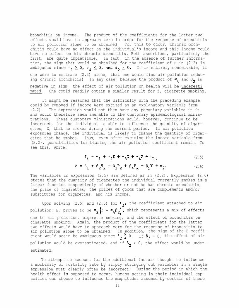
bronchitis on income. The product of the coefficients for the latter twoeffects would have to approach zero in order for the response of bronchitisto air pollution alone to be obtained. For this to occur, chronic bron-chitis could have no effect on the individual's income and this income couldhave no effect on his chronic bronchitis. Both assertions, particularly thefirst, are quite implausible. In fact, in the absence of further informa-tion, the sign that would be obtained for the coefficient of E in (2.2) isambiguous since It is entirely conceivable, if

one were to estimate (2.2) alone, that one would find air pollution reduc-ing chronic bronchitis! In any case, because the product of ~4 and 6, is

negative in sign, the effect of air pollution on health will be underesti-mated. One could readily obtain a similar result for Z, cigarette smoking.

It might be reasoned that the difficulty with the preceding examplecould be removed if income were excised as an explanatory variable from(2.2). The expression would not then have any pecuniary variables in itand would therefore seem amenable to the customary epidemiological minis-trations. These customary ministrations would, however, continue to beincorrect, for the individual is able to influence the quantity of cigar-ettes, Z, that he smokes during the current period. If air pollutionexposures change, the individual is likely to change the quantity of cigar-ettes that he smokes. Thus, even after excising the income variable from(2.2), possibilities for biasing the air pollution coefficient remain. Tosee this, write:

(2.5)

(2.6)

The variables in expression (2.5) are defined as in (2.2). Expression (2.6)states that the quantity of cigarettes the individual currently smokes is alinear function respectively of whether or not he has chronic bronchitis,the price of cigarettes, the prices of goods that are complements and/orsubstitutes for cigarettes, and his income.

Upon solving (2.5) and (2.6) for (Ii, the coefficient attached to air

pollution, E, proves to be which represents a mix of effects

due to air pollution, cigarette smoking, and the effect of bronchitis oncigarette smoking. Again, the product of the coefficients for the lattertwo effects would have to approach zero for the response of bronchitis toair pollution alone to be obtained. In addition, the sign of the E-coeffi-cient would again be ambiguous since B2 $ 0. If B2 > 0, the effect of air

pollution would be overestimated, and if 62 < 0, the effect would be under-

estimated.

To attempt to account for the additional factors thought to influencea morbidity or mortality rate by simply stringing out variables in a singleexpression must clearly often be incorrect. During the period in which thehealth effect is supposed to occur, humans acting in their individual cap-acities can choose to influence the magnitudes assumed by certain of these

11

variables. Each variable susceptible to this influence must be explained byan expression of its own. Economic analysis is necessary to impart aninterpretable form to these expressions. Physical and biological constructswill therefore often be insufficient tools with which to provide epidemio-logical explanations of disease incidences.

The previous two examples are about problems of joint determinationwhich involve economic variables. Nevertheless, the problem of jointdetermination does not require the presence of economic variables. Forexample, epidemiological studies frequently group disease incidences byindividual city and employ measures of central tendency of incidence andother variables as single units of observation. Thus one might try toexplain the frequency of deaths from cancer in a sample of U.S. cities byrelating it to the dietary habits, air pollution exposures, and median ageof the population in each city. Among the dietary variables, one mightinclude saturated fats and cholesterol, dietary components frequently saidto be positively related to cardiovascular disease. Inclusion of these twovariables in an expression intended to estimate the factors that contributeto cancer incidence would probably result in negative signs being attachedto their coefficients, implying that saturated fats and cholesterol preventcancer. This may, in fact, be true, but only indirectly. Specifically,median age in each city will tend to vary inversely with the incidence ofcardiovascular mortality; in other words, earlier death reduces median age.Thus, since cancer incidence is positively influenced by median age, onemight expect cancer to exhibit negative associations with saturated fatsand cholesterol even if they have no direct causal relationship with cancerincidence. The apparent effects of these two dietary variables upon cancerincidence would actually represent a confounding of: (1) the effect of thetwo variables upon cardiovascular disease; (2) the relation between cardio-vascular disease and median age; and (3) finally, but only via (1) and (2),the effect of the two variables upon cancer incidence. In short, at leastone other expression explaining median age is required.

2.4 The Costs of Pollution-Induced Disease

The preceding sections have discussed the circumstances under whichmicroeconomics and its methods of empirical application can contribute tothe epidemiology of pollution. It was observed that in trying to establishdose-response functions for particular pollutants, it is necessary to beextremely sensitive to the presence of jointly determined variables.Failure to account properly for these variables in the structure to beestimated can result in badly distorted depictions of the effect of ahealth input such as pollution upon the output, the state-of-health or theincidence of a particular disease. One could, of course, consider allvariables to be endogenously determined in some ultimate sense. The keyto stopping short of including the entire universe in the structure to beestimated is the formation of intelligent judgments about those variablesimportant to the question of interest over which the individual or system(e.g., urban areas) can immediately exercise no more than trivial control.The number of expressions must equal the number of variables it is positedthat the individual or system can control if a determinant solution is toemerge. Most importantly for our purposes, since many of the jointlydetermined variables in a dose-response structure will be economic requiring

12

the application of microeconomic analysis in order to specify how they areto be introduced to the structure, the actual design of epidemiologicalstudies must often include microeconomic considerations.

The potential application of microeconomic analysis to epidemiologicalconcerns extends beyond the estimation of dose-response functions. Theanalysis can be used to establish pecuniary values for pollution-inducedhealth effects. These values, which are consistent with the axiomaticstructure of benefit-cost analysis, can contribute to evaluations of theeconomic efficacy of existing and proposed pollution control programs.Attempts to establish these values can adopt two polar views of theindividual's degree of comprehension of the relation between pollution andhis state-of-health.

The first of these views presumes that the individual fails to com-prehend any connection between pollution and his health state, even thoughpollution does influence this state. To obtain the total loss due to apollution-induced health effect, this view justifies the estimation of adose-response function and the multiplication of the loss in healthattributed to pollution by a pecuniary value for the health loss. Theinformation and criteria used to set the pecuniary value, and thus thetotal pecuniary loss, come from outside the system being studied. Thebasic presumption is that the individual is unaware of the health effectsof pollution and therefore does not make any voluntary adjustments inresponse to its presence.

In addition to being a relatively easy and therefore desirable way toestablish pecuniary values for health losses, this first view has thefurther advantage of reducing the force of the joint determination problem.It thus removes problems similar to the cigarette example of the previoussection, where, in response to the presence of increased air pollution,the individual chose to reduce his cigarette consumption. However, theview would affect neither the income nor the dietary examples, for theill-health caused by pollution can affect the individual's earnings cap-acity and his dietary habits. These earnings and habits would thereforechange as pollution changes, even though the individual is utterly unawareof the cause and, consequently, fails to make any behavioral adjustmentsin response to pollution.

The polar opposite of the above view is that the individual is fullycognizant of the health effects of pollution and continually adjusts hisvoluntary behavior accordingly; that is, given the opportunities he hasavailable and the relative prices he faces, he alters his behavior so asto minimize the value of the pollution-induced health losses he suffers.These voluntary adjustments will involve shifts in his time and budgetallocations such as reductions in the time and intensity of outdooractivities, pursuit of a less toxic diet, and more visits to the familyphysician. A view of the individual that presumes he is unaware of thehealth effects of pollution does not account for these adjustments. Ineffect, it assumes that, whatever the variations in pollution, the indivi-dual's time and budget allocations have always accorded with the allocationsoccurring at the time of observation. Since, according to the second viewof the individual's response to pollution variations, these observed

13

allocations are the result of attempts to mitigate the health effects ofpollution, the first view of the individual results in underestimates ofpollution health effects. Furthermore, if individuals do reallocate theirtime and their budgets in response to pollution variations, then measurescan be obtained of the income the individual would have to receive or wouldbe willing to pay to leave himself as well off as he was before a change inpollution. These measures correspond to the ideal measures of economicloss established in the microeconomic theory of consumer behavior.

14

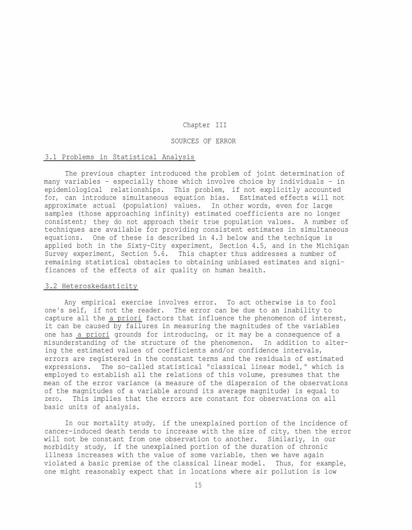
Chapter III

SOURCES OF ERROR

3.1 Problems in Statistical Analysis

The previous chapter introduced the problem of joint determination ofmany variables - especially those which involve choice by individuals - inepidemiological relationships. This problem, if not explicitly accountedfor, can introduce simultaneous equation bias. Estimated effects will notapproximate actual (population) values. In other words, even for largesamples (those approaching infinity) estimated coefficients are no longerconsistent; they do not approach their true population values. A number oftechniques are available for providing consistent estimates in simultaneousequations. One of these is described in 4.3 below and the technique isapplied both in the Sixty-City experiment, Section 4.5, and in the MichiganSurvey experiment, Section 5.6. This chapter thus addresses a number ofremaining statistical obstacles to obtaining unbiased estimates and signi-ficances of the effects of air quality on human health.

3.2 Heteroskedasticity

Any empirical exercise involves error. To act otherwise is to foolone's self, if not the reader. The error can be due to an inability tocapture all the a priori factors that influence the phenomenon of interest,it can be caused by failures in measuring the magnitudes of the variablesone has a priori grounds for introducing, or it may be a consequence of amisunderstanding of the structure of the phenomenon. In addition to alter-ing the estimated values of coefficients and/or confidence intervals,errors are registered in the constant terms and the residuals of estimatedexpressions. The so-called statistical "classical linear model," which isemployed to establish all the relations of this volume, presumes that themean of the error variance (a measure of the dispersion of the observationsof the magnitudes of a variable around its average magnitude) is equal tozero. This implies that the errors are constant for observations on allbasic units of analysis.

In our mortality study, if the unexplained portion of the incidence ofcancer-induced death tends to increase with the size of city, then the errorwill not be constant from one observation to another. Similarly, in ourmorbidity study, if the unexplained portion of the duration of chronicillness increases with the value of some variable, then we have againviolated a basic premise of the classical linear model. Thus, for example,one might reasonably expect that in locations where air pollution is low

15

and that the variation around this average level would not be very great.Low concentrations of air pollution are unlikely to generate severe chronicillnesses of long duration. However, where air pollution concentrationsare high, both the average level of air pollution-induced chronic illnessand the variations around this average are likely to be substantial. Inlow pollution locations, even those with a biological propensity to beharmed from pollution do not suffer any ill effects. However, those withthis propensity might be struck down if they are moved to a high pollutionlocation, whereas those who have great resistance will suffer little, ifat all. The variation in the duration of chronic illness is therefore muchhigher where pollution is suffocating because the magnitude of the greatestsuffering has greatly expanded, while the magnitude of the least sufferingcontinues to be zero.

Nonconstantcy of the variances of the errors (residuals) in an estimatedexpression is termed "heteroskedasticity," a term the linguistic roots ofwhich we don't know. Because it means that variation in the errors of anexpression varies systematically over observations, it implies that theconfidence intervals for estimated coefficients will also vary systematically.The result is that the same basis will not be used to calculate the confi-dence intervals among observations. Thus, although the estimatedcoefficients are not affected, the standard errors of these coefficients willbe biased. As a consequence, the customary tests of significance have nomeaning. Nevertheless, if one knows the direction of the bias, one cansometimes ascertain whether these customary tests of significance accordexcessive or too little precision to the estimated coefficients. Forexample, Kmenta (1971, p. 256) provides a formula that under limited cir-cumstances, permits the calculation of this magnitude and the sign of thisbias in standard errors. He also outlines ways in which the raw data canbe corrected to negate heteroskedasticity.

3.3 Multicollinearity

Multicollinearity occurs when two or more explanatory variables are sohighly correlated among themselves that it becomes difficult to separate ordetermine the independent effect of each variable. In the extreme casewhere two variables are perfectly collinear, they are effectively identical.However, if a priori information exists on the effect of the collinearvariables, then that information can be used. For example, if in attemptingto explain stomach cancer mortality rates using cross-sectional data, twoexplanatory variables, sulfur oxides in air and per capita consumption ofPolish sausage, are perfectly collinear, one might employ data from animalexperiments or epidemiological studies on select human populations (e.g.,Polish populations and industrial workers exposed to SO2 in high concen-trations) to determine the relative incidence of stomach cancer from eachfactor. By including only one of the variables in the regression, the totaleffect of both explanatory variables will be captured by the estimatedcoefficient on that one variable. Thus, if consumption of Polish sausageand sulfur oxide exposures are perfectly collinear and only consumption ofPolish sausage is included in the estimated equation, the estimated coef-ficient on consumption of Polish sausage will capture the effect of bothvariables. How that effect is to be allocated between the two variablesdepends on the availability of external information. For example, if animal

16

experiments do not show a link between sulfur oxide exposures and stomachcancer, but do show a link between consumption of cured meats (includingPolish sausage) and cancer, one might allocate the entire coefficient toconsumption of Polish sausage. Of course, if this were the case, and theinvestigator did not know that consumption of Polish sausage and sulfuroxide exposures was perfectly collinear and no dietary data was availablefor inclusion, then a false link between sulfur oxides and stomach cancermight be shown using the cross-sectional data alone.

The same arguments apply to cases of near perfect multicollinearitywherein explanatory variables are highly, as opposed to perfectly, corre-lated. This is, of course, the most likely case. However, the outcome ofincluding two or more collinear explanatory variables is an increase inthe standard error of the estimated coefficients for the collinear variables.The standard error is, of course, a measure of the accuracy with which acoefficient is estimated -- large standard errors imply that the actualcoefficient could be much larger or smaller than the estimated coefficient.Thus, when collinear variables are included, the inability to separateinfluences is reflected in the measure of uncertainty over the magnitude ofthe estimated coefficients on those variables.

The approach taken here to deal with multicollinearity -- and the 60-city experiment described below has a severe problem among the dietaryvariables -- is to a priori exclude variables which are highly collinearwith respect to a representative included variable. An alternative approachto multicollinearity is the use of a technique known as ridge regression[see Schwing, et. al. (1974)] which, however, makes interpretation of theresultant estimated coefficients unclear.

While multicollinearity within an available data set makes estimationand interpretation more difficult, at least the problem can sometimes berecognized and false conclusions thereby avoided. However, where unknowncollinearity occurs, for example when an included explanatory variable ishighly collinear with a variable which is not available to the investigator,the false conclusion can be reached that the included variable is solelyresponsible for the estimated effect. The investigator may not recognizethat the estimated effect includes the effect of one or several otherexcluded but collinear variables. We discuss this possibility below.

3.4 Causality and Hypothesis Testing

Aside from the problem of multicollinearity, the traditional problemsof causality underlying epidemiological studies still apply. For example,if heart attacks are actually related to cigarette consumption, but smokingis correlated with coffee consumption for behavioral reasons, a spuriouspositive correlation might be shown between heart attacks and coffee con-sumption, especially if cigarette consumption is excluded from an estimatedstatistical relationship. In other words, correlation does not provecausation, and statistical hypothesis testing can never confirm, but onlyreject, a maintained hypothesis. Turning to another example, if mostnitrite (used to cure meats) ingestion is through consumption of porkproducts (70 % of pork is cured), one might suspect, given the hypothesis

17

of in vivo nitrosamine (a carcinogen) formation from nitrite, that cancermortality and pork consumption would be correlated. If such a correlationcan be shown (as it has been; see Kneese and Schulze (1977) and NAS 1978)then the only valid conclusion is that we do not reject the hypothesis thatpork consumption (and perhaps, in turn, nitrite ingestion) is related tohuman cancer. If, alternatively, one accepts the maintained hypothesis ona priori grounds, and no bias exists in the estimation procedure, regressionanalysis can give a best linear estimate of the actual relationship in thesample population between, for example; cancer mortality and a dietaryfactor such as nitrite ingestion. However, regression analysis cannotprove causality; causality must be assumed in this procedure. This is whyit is so important to have hypotheses concerning causality before a regres-sion equation is specified.

A set of hypotheses concerning human health, including the effect ofair pollution, forms a model of human health. The concept of a completemodel of human health as the basis for hypothesis testing is an importantone for several reasons. First, a modeling framework immediately suggeststhat behavioral elements such as voluntary medical care may be importantand as pointed out above, a simultaneous equation structure may be necessaryto test hypotheses properly. Second, the modeling framework focusesattention on a complete specification of the determinants of human health.A "better" model will exclude fewer relevant variables and be both a moreaccurate predictor of human health and more accurately identify the effectof each explanatory variable. The modeling approach then helps avoid theproblem of unknown collinearity by focusing on a specification which pro-vides imformation about the effects of all relevant variables.

An alternative viewpoint has been expressed by Lave and Seskin (1977).Their argument rests on the assumption that excluded variables (medicalcare, diet, and smoking are excluded from their study of air pollution andhuman health) will not bias estimated effects of included variables if theexcluded variables are orthogonal (perfectly non-collinear) with respectto the included variables. Thus, if one assumes orthogonality with respectto excluded variables, following Lave and Seskin (1977), one can justifyestimation of incompletely specified equations. We take a differentapproach principally because we reject orthogonality as a reasonableassumption. If, as ecologists are fond of saying, "everything depends oneverything else," then simultaneity and collinearity are likely to bepervasive in the "real world." In fact, we argue below based on our ownepidemiological and economic data that this is just the case.

Finally, to test specific hypotheses, we will use the standard sig-nificance test; we will test the hypothesis that each explanatory variablehas no effect (has a coefficient of zero) by using the appropriate t-statistic which, in this case, is approximately equal to the estimatedcoefficient divided by its own standard error. For example, for largesamples, if for a specific coefficient t ~2.0 (if the coefficient isgreater than or equal to twice its own standard error), then, where thehypothesis tested includes an assumed sign for the coefficient, a 97.5%level of significance is achieved. This implies that, in random samplingof a population, one would draw a sample which accidentally confirmed the

18

hypothesis (effect non-zero) only 2.5% of the time.

It is important to note, that as the significance level is implicitlylowered from t = 2.0 toward t = 1.0, even in large samples, spurious rela-tionships begin not to be rejected. Practical experience and econometrictradition suggest that a 95% to 97.5% significance level is appropriate.The desired confidence level should be chosen a priori to avoid the temp-tation to "prove" desired relationships by ex post lowering of the level ofsignificance for rejecting or failing to reject hypotheses. Similarly,statements that an explanatory variable is "nearly significant" should beinterpreted with great caution. Where costly environmental programs are tobe justified by epidemiological analysis, rigorous tests of significanceshould be employed.

3.5 Aggregation

In one or another of his many books, Herbert Simon has used the term"bounded rationality" with reference to limited human abilities to arrange,comprehend, and manipulate large volumes of information. More succinctly,Simon is referring to the need to simplify in order to understand. Even thepure theorist, in both his analysis and exposition, must partition theuniverse into two parts: that with which he will and won't deal. Moreover,he must employ a limited and often quite small number of concepts to dealwith the part he has chosen. He who would measure as well as theorize mustsimplify beyond this, for he must be economic with his data manipulations.Both isomorphism with his theoretical variables and his less than fullyrobust empirical tools require this. Simplification is synonymous withthrowing away information, but that which is thrown away is often beyond ourpowers of use. As Stigler (1967) has remarked, ". . . information costs arethe costs of transportation from ignorance to omniscience and seldom can atrader afford to take the entire trip."

In the material to follow, we have played the role of the aforementionedtrader in two ways. First, in the mortality study, we have employed groupeddata for estimation; that is, we have employed a single measure of centraltendency (usually the arithmetic mean) of the distribution of some attributeacross a group of people or locations (a city) as the sole representation ofthe group's diversity. We have melted entire cities into one pot. Here wewish to discuss the issues this poses for estimation.

A second aggregation thing we have done is to embrace the notoriousrepresentative individual when discussing the pecuniary benefits or costs ofa given health effect. Too fond an embrace of this representative can leadto gross errors if his responses are incautiously applied to flesh and bloodindividuals. We wish to explain why. Initially, however, we will discussthe estimation issue.

In the mortality study, the unit of analysis is a city or some largerjurisdictional unit and the values attached to a particular variable repre-sent the per capita magnitudes of the variable in the cities. To form theseper capita magnitudes, someone had to collect observations on the values ofthe variables for the distinct individuals in each city. By using the percapita rather than variation of the individual observations within each city

19

and thereby reducing the efficiency of our estimators. Simultaneously, weare lessening the degrees of freedom and, thus, the variety of statisticaltests we can potentially employ. Our real gain from this is a drasticshrinking of the size of the data base we must manage. A vacuous gain alsoexists.

By using the per capita magnitudes for the values of our variables, wehave not changed the underlying sample of individual observations, but havereduced the variability of the sample we are using for estimation. We havestripped the outlying individual observations of influence. The result isthat the per capita magnitudes will be less dispersed around any expressionwe estimate, allowing us to appear to explain a larger proportion of thevariation in the sample; that is, the magnitude of the coefficient of deter-mination (R2) is enhanced. This enhancement, however, is misleading sinceit is entirely due to our prior exercise of collapsing all the variations ofindividuals' observations in a city to a single scaler measure. Similarly,nonvacuously, and therefore much more importantly, by reducing the variationin the sample, we are reducing the standard errors of each estimated (andstill unbiased) explanatory variable coefficient. As a consequence, we maybe overstating the level of significance to be attached to these coefficients.

Yet another nonvacuous and altogether serious way exists for theestimates obtained from per capita data to be seriously misleading. Themeasurement unit one is using for any particular variable may differ fromcity to city. Thus, for example, one might be measuring cigarette con-sumption per capita in the equivalent of packs in one city and pounds inanother. Consider the following simple algebraic argument.

Assume that a disaggregated dose-response expression for respiratorydisease is to be estimated. Let this expression be given by:

(3.1)

where i refers to a particular pollutant, j to a particular individual, aand b are coefficients to be estimated, and E is an error term having thecustomary properties. Per capita responses and doses are clearly:

(3.2)

With aggregation, the intercept and error terms are:

The aggregate relation is therefore:

(3.3)

(3.4)

(3.5)

(3.6)

20

where b, the coefficient of is apparently

(3.7)

In other words, the per capita response depends on the exposures suffered bythe n individuals. This perhaps seems reasonable, since (3.6) continues tobe linear and includes an error term the expected value of which is zero forall

Disregarding a and note, however, that both b and Pj are aggregated.

Thus:

(3.8)

and therefore(3.9)

Nothing goes awry if the dose-response functions are identical among sufferers.However, if they do differ, it is apparent from (3.8) that the value of thepollution exposure parameter, b, will be a weighted mean of the same parameterfor the individual suffers. In particular, those sufferers having highresponses will have a disproportionately strong influence upon a group's(e.g., a city) contribution to the value of the exposure parameter in (3.8).Similarly, those groups having low responses will have a disproportionately.weak influence. The conclusion is the rather dismaying one that the measureof responses, employing some group or aggregation of individuals as thefundamental unit of observation, can differ from one group to another. Therecould conceivably be as many unique measures employed as there are groups.

The preceding remarks refer to the prior aggregation of individualobservations and the subsequent use of the aggregates for estimation purposes.Suppose we employ individual observations for estimation purposes, establishresponses for the representative individual among these observations, andthen use the presumedly representative responses of this representativeindividual to obtain an aggregate measure of total response; that is, weaggregate after rather than before estimation. The study of the morbidityeffects of air pollution that follows readily lends itself to this treatment.Because it does so, we feel it worthwhile to caution the reader about thedangers this form of aggregation poses. We state the discussion in terms ofdemand functions although dose-response functions would serve equally well.Only because it is perhaps the most widely cited study to aggregate indivi-dual observations of air pollution damages, we employ Waddell (1974) as abasis for discussion.

Waddell (1974) first reviewed a collection of studies that had estimatedmarginal purchase price functions with respect to sulfur oxides and/orsuspended particulates for eight different cities. Interpreting the valuesof the air quality parameters in these several studies as measures for theaverage household in each study of equilibrium marginal willingness to payat given air quality states and with given demand functions for air quality,he selected a value within the range of these estimated values. By selectingthis value within the range of values, he assumed that what was interpreted

21

as the equilibrium marginal willingness to pay was the same for all householdin all cities.

Then, using the further assumption that this assumed equilibrium marginalwillingness to pay was in fact the actual marginal willingness to pay for allair quality states, he multiplied the constant marginal willingness to pay bythe number of households and the number of air quality states to obtain anestimate of aggregate national air pollution damages. That is, if b is themarginal willingness to pay and Q is an air quality state, Waddell (1974)calculated aggregate national air pollution damages, D, as

(3.10)

where the i's index households.

In effect, Waddell (1974) assumed that the decision problem of each andevery household in each urban area of the country could be represented asdepicted in Figure 3.1. In Figure 3.1, aP/aQ is the marginal purchase pricefunction and aD/aQ is the function representing marginal willingness to pay

for improvements in air quality. Since b is invariant with respect to

changes in air quality, calculation of that willingness to pay for thehousehold of Figure 3.1 involves only the multiplication of b by whateverchange in air quality is postulated. Thus, the value to the depicted house-hold of an improvement in air quality (Q** - Q*) is simply b(Q** - Q*).Given then that b is the same and invariant for all households, the soledistinction one need make among households in order to calculate aggregatenational damages is to account for the location of each household on the Qaxis.

Figure 3.1

Marginal Purchase Price andMarginal Willingness-to-Pay

22

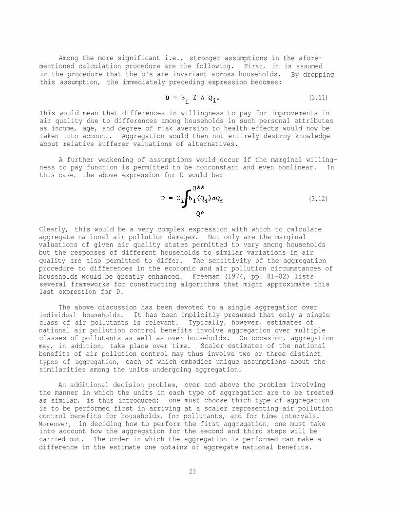
Among the more significant i.e., stronger assumptions in the afore-mentioned calculation procedure are the following. First, it is assumedin the procedure that the b's are invariant across households. By droppingthis assumption, the immediately preceding expression becomes:

(3.11)

This would mean that differences in willingness to pay for improvements inair quality due to differences among households in such personal attributesas income, age, and degree of risk aversion to health effects would now betaken into account. Aggregation would then not entirely destroy knowledgeabout relative sufferer valuations of alternatives.

A further weakening of assumptions would occur if the marginal willing-ness to pay function is permitted to be nonconstant and even nonlinear. Inthis case, the above expression for D would be:

(3.12)

Clearly, this would be a very complex expression with which to calculateaggregate national air pollution damages. Not only are the marginalvaluations of given air quality states permitted to vary among householdsbut the responses of different households to similar variations in airquality are also permitted to differ. The sensitivity of the aggregationprocedure to differences in the economic and air pollution circumstances ofhouseholds would be greatly enhanced. Freeman (1974, pp. 81-82) listsseveral frameworks for constructing algorithms that might approximate thislast expression for D.

The above discussion has been devoted to a single aggregation overindividual households. It has been implicitly presumed that only a singleclass of air pollutants is relevant. Typically, however, estimates ofnational air pollution control benefits involve aggregation over multipleclasses of pollutants as well as over households. On occasion, aggregationmay, in addition, take place over time. Scaler estimates of the nationalbenefits of air pollution control may thus involve two or three distincttypes of aggregation, each of which embodies unique assumptions about thesimilarities among the units undergoing aggregation.

An additional decision problem, over and above the problem involvingthe manner in which the units in each type of aggregation are to be treatedas similar, is thus introduced: one must choose thich type of aggregationis to be performed first in arriving at a scaler representing air pollutioncontrol benefits for households, for pollutants, and for time intervals.Moreover, in deciding how to perform the first aggregation, one must takeinto account how the aggregation for the second and third steps will becarried out. The order in which the aggregation is performed can make adifference in the estimate one obtains of aggregate national benefits.

23

Chapter IV

THE SIXTY-CITY EXPERIMENT

4.1 Objectives of the Experiment

Identification of substances in the environment which effect humanhealth and accurate quantifications of their effects, is extremely dif-ficult. Often there are multiple substances involved, there may be longlatency periods before effects are seen, and the amount and time of expo-sureis often unknown. There are three general approaches to identifyingsuch substances and quantifying their impact -- all more-or-less imperfect.In the first, laboratory animals are exposed to large doses of the suspectsubstance and, if effects appear, an effort is made to extrapolate them tothe human population. The correct manner in which to execute the secondstep is not well extablished. The second approach is to develop aggregatecross-sectional data, usually for cities or standard metropolitan areas,on a number of variables which might be associated with mortality rates orillness rates and then to use regression analysis in order to discoverstatistically significant associations. A third approach is to gather verydetailed data on individuals and to again use statistical analysis to de-termine the effect of various factors including environmental exposures onindividualized measures of health status.

The purpose of the research reported in this chapter is to exploreboth the possibilities and limitations of the second approach mentionedabove --aggregate epidemiology -- in the estimation of human dose-responsefunctions which include exposure to air pollution. The principal advantageof the use of aggregated data on cities or metropolitan areas is quitesimply the widespread availability and low cost of such data as opposed todata generated from animal experiments or collected on individual humanbeings through specialized surveys. However, the use of aggregated datacreates a number of special problems.

First, one ideally wishes to estimate a dose-response relationship orfunction as shown in Figure 4.1. Based on a priori considerations onewould suppose that for human populations, risk of death for an individualwould be a function of medical care, age of the individual, the geneticendowment of the individual, the behavior of the individual--does he orshe exercise, smoke, etc.--the diet of the individual, and exposures topossibly harmful substances or circumstances. However, aggregate epidemi-ology provides no data on individual risks or characteristics but only datafor population characteristics as a whole. Thus, aggregate mortality ratesin, for example a city are used as a proxy for risk of death in the

24

estimation of an individual dose-response function where it is implicitlyassumed that individuals can be represented by the average individual ineach city. Thus, in using the data set developed below for sixty U.S.cities to estimate a dose-response function of the form shown in Figure4.1, it is implicitly assumed that each city represents one average individ-ual. However, the list of assumptions required to allow such aggregation(all relationships must be perfectly linear, etc.) are not likely to be metin practice. Thus, one must recognize that estimated results are biasedto an unknown extent by the very use of aggregated data.

A second problem arises from the fact that aggregate epidemiologymust rely on secondary data. Since the investigator must depend on dataalready collected, he cannot add a question to a survey nor can he varythe design of an animal experiment to test the importance of a new variable.In the past this problem has led to the exclusion of data on importantvariables such as smoking,studies [see, for example,

diet and exercise from aggregate epidemiologicalLave and Seskin (1977) and Schwing, et. al.

(1974)] We have been able to gather some data -- not necessarily gooddata -- on both smoking and diet and as we show below, these are importantomissions from previous studies. The current study still excludes anymeasure of exercise.

Finally, aggregate epidemiological studies are likely to suffer froma number of simultaneous equation biases. One of the most obvious con-cerns the effect of medical care. The existing epidemiological literaturehas failed to show any significant effect of medical care on human mortalityrates. This counterintuitive result is easily explained. For example, inour sixty city sample, no effect of per capita doctors in each city can beshown on aggregate mortality rates for each city when simple regressiontechniques such as ordinary least squares are used. The explanation isthat, although doctors most likely do reduce mortality rates (as shownbelow), people in cities with higher mortality rates have in turn more ill-ness per capita and seek out more medical care, increasing the observednumber of doctors in such communities. In other words, higher mortalityrates create a greater demand for doctors. Thus, we have two offsettingeffects--doctors reduce mortality, while mortality increases the demand fordoctors--and simple regression analyses cannot untangle them. Severalstatistical techniques are available for coping with simultaneous equationproblems.We use a very simple approach, two-stage least squares, a tech-nique described in a little detail below.

A second simultaneous equation problem may arise because of multiplecauses of death. Cities with high coronary death rates may likely havelower cancer death rates because people die of heart attacks before theyhave a chance to die of cancer. In this situation, factors which, forexample, show up positively correlated with coronary disease may show upwith a spurious negative correlation with cancer rates. This simultaneousequation problem is likely to work "through" the age variable in thatmedian age is determined in part by mortality rates of individual diseases,while, in turn, age is used to explain mortality rates. We therefore havealso employed two-stage least squares on the age variable, but with noimpact on the estimated equations so these results are not reported here.

25

26

Figure 4.1

Hypothetical Human Dose-Response Function

An alternative approach to the problem which we do not employ, is use of age-specific mortality rates.

A third possible source of simultaneous equation bias occurs becausepeople make voluntary choices over location. Migration in and out of oursixty city sample is effectively disregarded. People may, for example,contract an air pollution related disease and, on a physician's advice,move from a highly polluted area to an unpolluted area, only then to die.A false negative association between air pollution and pollution-relatedmortality might then be shown. Although in the past we have included anet migration variable [see Kneese and Schulze (1977)] which was statis-tically significant, we have excluded such a variable in this analysisbecause it defies interpretation in a dose-response function context.

Table 4.1 summarizes the objectives and limitations of the currentstudy and to some extent those of aggregate epidemiology in general. Wenow turn to development of methodology for estimating the value of reducinghealth risks and for the effect of medical care on human health. Thislatter section focuses on the role of exonomics in aggregate epidemiology.

4.2 Value of Life Vs. Value of Safety

The direct costing approach employed by economists for evaluating themortality costs of diseases which result from environmental exposures isstraightforward but difficult to quantify fully [see, for example, Kneeseand Schulze, 1977]. First, the population at risk must be known. Second,the increased risk of mortality associated with environmental exposuresmust be quantified either through epidemiology or through extrapolationfrom animal experiments. Third, the amount of money or the value thatindividuals place on safety (avoiding risk of death) must be known. Multi-plying these three values together then gives an approximation of the incre-mental benefits of reducing such exposures. This cost or benefit is not inany way related to a "value of life" which is most likely unmeasureable,but rather focuses on a concept of the value of safety (alternatively "costof risk") to individuals where risks are statistically small.

27

Table 4.1

Objectives and limitations

Purposes of Study Are:

(1) To explore methodology for isolating an aggregate human dose-response function.

(2) to add medical inputs.

(3) to add diet.

(4) to add smoking.

(5) to account for simultaneous equation bias where possibleincluding:

(a) demand for doctors.

(b) multiple possible causes of death.

The Study Fails to Account for:

(1) simultaneous equation problems caused by migration.

(2) exercise.

(3) radiation.

(4) Biases introduced by estimating an aggregate as opposed toindividual dose-response function.

28

Economists in the past have attempted to value human life as the sumof the present value of future earnings over an individual's lifetime [seeLave and Seskin, 1970 and 1977]. This approach, however, is no longerviewed as acceptable. In the first place, it assumes that the value oflife can, in fact, be measured -- a point certainly open to debate. Sec-ond, it implies that the lives of children, housewives, retired and otherunemployed individuals are worth less than the lives of employed heads ofhouseholds.

Two measures can be used to value safety or risk to life which arebased on the economic concepts of equivalent variation (EV) and compensatingvariation (CV). An EV measure of the value of life is the amount of moneyan individual would pay to escape from or prevent certain death; in theory,a rational individual would part with all his available wealth to save hislife. CV, in contrast, measures the compensation required to induce anindividual to accept voluntarily a situation where the probability ofdeath is increased. As the probability of death approaches unity, the CVmeasure can be taken as an estimate of the value the individual places onhis life. Logically, though, the value of life measured this way must beinfinite, because as the probability of death approaches certainty, theprobability of enjoying any compensation offered (and thus the value of thecompensation) approaches zero. Thus, neither EV (which requires coercion)nor CV (which makes the value of life immeasurable) provides a whollysatisfactory way of extimating the dollar costs of mortality in realyworld situations that involve risk. An eleboration of the CV concept,however, can provide a useful measure of the compensation necessary toinduce an individual to accept a slight increase in the probability ofdeath.

Mishan (1971) was the first to distinguish between the concept of costof risk, which is ethically appealing, and earlier efforts to value humanlife based on lost earnings, which as a methodology, has strange and intu-itively objectionable features. The latter measure of the "value" of humanlife has now been rejected by economists both on theoretical and, to someextent, on ethical grounds. Thaler and Rosen (1975), using wage differ-entials between jobs varying in the level of job-associated risk of death,were the first to estimate explicitly the value of safety. In other words,workers in high risk jobs receive higher wages and a value of safety canbe inputed by examining risk-related wage differentials. Unfortunately,however, their study dealt with a high risk class of individuals. TheThaler and Rosen (1975) estimate suggests that in current dollars a smallreduction in risk over a large number of individuals which saves one lifeis worth about $340,000. Another study [Blumquist (1977)], which examinesseat belt use, suggests that the figure might be $260,000. This studyfirst estimates how people value their own time and then imputes a valueof safety from the amount of time a sample of individuals spent in bucklingup seat belts. These results may be biased downward because individualsseem to perceive risks differently when an element of personal controlsuch as driving an automobile is involved. Finally, Smith (1975) in a studysimilar to Thaler and Rosen (1975) has suggested that, for a more typicalpopulation and for job-related risks, the figure may exceed $1,000,000.Clearly, the cost of risk is not precisely known, and perhaps will neverbe, since attitudes -- risk preferences -- presumably can change over time,between groups, and can even vary in different situations. But, we at

29

least have a range of values with which to make order-of magnitude estimatesof the costs of environmental risks. This range of values does not, however,overlap the value-of-life estimates based on lost earnings. For example,Lave and Seskin (1977) use a value in the thirty to forty thousand dollarrange for a life lost. The Thaler and Rosen (1977) value of safety is,for example, about an order of magnitude larger than the Lave and Seskin(1977) lost earnings number.

The theoretical basis of a value of safety or cost of risk concept canbe shown briefly as follows: Assume that an individual has a utilityfunction, U(W), where utility is an increasing function of wealth, W. Ifrisk or death is JI, expected utility is (1-n)U(W). If we hold expectedutility constant, we have (l-fl)U(W) = constant, and the total differentialof this equation is:

(4.1)

where the prime denotes differentiation. Holding utility constant thenimplies that the increase in wealth (or income) necessary to offset anincrease in risk is:

(4.2)

This is the compensating variation measure of the cose to an individualattributable to an increased risk of death. Analysis of the last expres-sion can be simplified if we assume a constant elasticity of utility with

respect to wealth, n, such that U(W) = n and consequently n = $$z. Then(4.2) can be rewritten as:

(4.3)

The right hand side of (4.3) suggests several interesting points about thevalue of safety or cost of risk. First, if we assume that the elasticityof utility is less than one, people are risk averse. This in turn impliesthat since the risk of death is positive (PO) that (dW/dlI)>W. In otherwords, if an individual is risk averse, his life, in terms of the riskpremium necessary to get him to accept risk, is worth more to him than hiswealth. Second, from (4.3), as wealth increases, the risk premium requiredto accept an increase in risk voluntarily, dW/dll must increase with age,ceteris paribus. Thus, one would expect older people to act in a more riskaverse manner than younger individuals (require greater compensation tovoluntarily take a risky action), both because of increased income andbecause of increased initial age-related risk of death.

This model contrasts for a number of reasons with the value of lostearnings approach previously used in economic analysis. First, if lostincome itself is the measure, the "value of life" measured through lostearnings obviously cannot exceed wealth [see Conley, 1977]. Second, in-creased wealth will increase the lost earnings measure as well as the costof risk measure. However, the cost of risk measure may not increase pro-portionately if a different utility function is used. Third, the lostearnings measure must decrease with age at some point as individuals get

30

older because the expected remaining earnings must decrease, while the costof risk, as we argued above, will likely increase. Finally, it is clearfrom (4.3) that as II approaches unity, dW/dlI approaches infinity. In otherwords, the compensation required to induce an individual to accept a cer-tainty of death voluntarily is infinite. The lost income measure has nosimiliar property. Nevertheless, the implication is that small increasesin risk may be valued in terms of compensation required to induce individ-uals to accept such risks voluntarily. Individuals, of course, rationallyaccept small risks on a daily basis; presumably on the basis of somemonetary or psychic return.

Given the analysis above, the current methodology of multiplying valueof safety numbers times experimentally or epidemiologically determinedenviromental risks can then be justified as follows: assuming a utilityfunction U(W) where W is wealth, if risk of death is II, the marginal costof risk, as derived earlier, is (dW/dJI)n = U/U'(l-IT), where fi is a constantutility level. If risk, II, is a function of pollution, X, where utilityfunctions are identical for N individuals, one would wish to maximizeexpected utility,

subject to a constraint on total wealth, !?, or income of society

(4.4)

(4.5)

which is allocated to individual wealth, assumed identical for purposes ofexposition, (NW), and costs of controlling environmental pollution from theinitial level X0, [C(XO-X)]. Noting that IIorder conditions are (where X is the multipH

> 0, and C' > 0, the firstier on (4.5) and L denotes the

Lagrangian):

These imply:

(4.6)

or that the number of individuals, N, times the marginal cost of risk,ru/u'(l-w I, times the marginal effect of pollution on risk, lTx, equals themarginal cost of control, C'. Clearly, this model abstracts from manywelfare threoretic problems but it does imply that estimation of the lefthand side of (4.6) as suggested at the beginning of this section is alegitimate approximation of the incremental benefits of environmental con-trol.

In summary, the direct costing of mortality has the advantage offocusing attention on one positive output of environmental agencies whichhas clear economic value -- safety. It is important, however, to distin-guish between the value of safety to consumers which does have measurableeconomic value -- environmental agencies may be viewed as selling safety

31

to the public -- as opposed to techniques which claim to measure the valueof human life. Benefit-cost arguments for environmental programs shouldand can rest on demonstrable increases in public safety delivered atcosts comparable to what the public is willing to pay for safety, not onclaims as to the value of human life. However, the assessment of the riskof mortality associated with environmental exposures such as air pollution--whether based on animal experiments or epidemiological studies -- remainsdifficult and uncertain and is central to the direct costing methodology.Surprisingly, perhaps, the authors feel there is likely to be less profes-sional debate as to the economic measure of the dollar value of safety thanas to the quantification of environmental health effects. We now turn tothe possible role of economic analysis in the epidemiology of air pollution.

4.3 A Methodological Basis: Does Economics Matter?

The question posed above could be rephrased "does rational humanbehavior matter in the estimation of dose-response functions?" Economistswould certainly answer in the affirmative; individuals are likely to re-spond to illness with numerous ameliorative measures. Clearly, such mea-sures must be accounted its a properly specified dose-response functionis to be estimated. What follows is a simplified economic model of humanbehavior in response to health risks which in turn allows specification ofappropriate statistical techniques for estimating a human dose-responserelationship.

Let i'I denote risk of death for an individual where that risk can bereduced by medical care which we denote D, synonymous with our empiricalmeasure, doctors per capita. Thus, risk can be written as a function, II(D),where dll/dD = UI' < 0. If the price of medical care is p and income isdenoted Y, then utility, U, can be written U(Y - pD), a function of incomenet of expenditures on medical care, pD. In an uncertain world, economicanalysis assumes that an individual will choose to maximize expected util-ity -- the odds of remaining alive (1-X) times the utility level U -- or

(4.7)

so the first order condition for the quantity of medical care chosen whenrearranged is:

(4.8)

The term on the left-hand side of (4.8) is easily recongizable from section4.2 above as the marginal value of safety (or compensation required tovoluntarily accept a small increase in risk), while the term on the rightis the marginal cost of increased safety through medical care. Thus, thismodel of human behavior implies that an individual will choose a level ofmedical care which equates his or her marginal value of safety to themarginal cost of reducing risk through medical care. Of course, an individ-ual's perception of risk and of the ability of medical care to reduce riskof death may be imperfect. However, from (4.8) it is easy to show thatindividuals who are more risk averse, i.e., those with a large marginal

32

value of safety, will seek more medical care than those who are less riskaverse.

An explicit set of functional forms will simplify interpretation. Letus again (as in Section 4.2) constant elasticity of utility withrespect to income, n, so U = Also assume a linear (approximate)dose-response relationship, II = II + B'D, where II' < 0 is now a fixedcoefficient and l70

is a positive Oconstant. Equation (4.8) can then bewritten as:

(4.9)

which is a demand equation for medical care. If we take the supply priceof medical care to be fixed P =P* (infinitely elastic supply of medicalcare), the individual demand for medical care, doctors per capita forexample, is then a linear increasing function of total risk II, since

(j+ ' 0, and of income Y, since L- 0.P* Of course, we wish, as our prin-

cipal objective for policy purposes, to estimate the dose-response function:

(4.10)

in particular, we wish to obtain an unbiased estimate of II', the effect ofmedical care on mortality and of the effect of other variables such as airpollution. However, any attempt to directly estimate (4.10) is doomed tofailure. This occurs because the equation specified for statisticalestimation (equivalent to 4.10 where cx and cx

1are parameters for esti-

mation) 0

(4.11)

has a disturbance term uB which is not independent of D. In other words,

5sis correlated with D. This is easy to show if we specify the demand

equation for doctors (equivalent to 4.9 above with parameters f30’ B1 and

B )2

as stochastic:

(4.12)

as well, with a disturbance term pD. Now suppose some factor (random)

embodied in plI causes II to rise in (4.11). But if II rises, by (4.12), D

must increase since, from (4.9), 9 > 0 and D, through $, depends on II.

Thus, D depends on un: through (4.12) and D and uB are correlated. Now, if

in estimating (4.11) this correlation is not accounted for, not only willestimates of Cal and u. be biased, but if we had included other factors which

affect morality such as diet or pollution in (/..ll), coefficients on thesevariables would be biased as well. It is also true that if simultaneousequation biased is

33

present and not accounted for, it becomes possible that the estimatedeffect of medical care, a1' will appear not significantly different from

zero or even of the wrong sign (note we assume that that doctors

reduce mortality).

We can break the dependence of D on ulI by first substituting (4.10)

into (4.9), or (4.11) into (4.12), to obtain a reduced form equation formedical care,

(4.13)

where u is the disturbance term in the reduced form.r This equation can be

legitimately estimated since the income variable is exogenous, determinedoutside the relevant system of equations, and the endogenous variables Dand II, those determined within the system, do not appear on the right-handside of (4.13). Now, if we estimate (4.13) and obtain unbiased estimates

of the two coefficients y, = (* IT- 7) and y

12TI 1

= (9) we can use these

along with data on income, Y, to generate a new variable, estimated medicalcare, D, where

(4.14)

Note that this new variable, D, generated from data on Y does not dependon 1-1 II and can be used instead of actual data on D to estimate a dose-

response function:

(4.15)

This estimated equation gives a consistent estimate of al or il'. In fact,

if the hypothesis that doctors are both important and effective in reducingmortality rates is correct, a1 should show up negative and significantly

different from zero as estimated in (4.15). Note, however, that if indi-viduals perceive that doctors are effective, they will have a strongincentive to seek medical help when ill, thus making a direct least squaresestimate of the effect of medical care as specified in (4.11) impossible.

The procedure we have outlined above, two-stage least squares, has beenused successfully in many instances to resolve simultaneous equation pro-blems and has the advantage of requiring minimal additional data. In gen-eral, if an unbiased estimate of a structural equation (one equation is asimultaneous system) is desired, one need only use ordinary least squaresto estimate each of the endogenous variables as a function of all of theexogenous variables in the model (estimate a set of reduced form equations).Then, using the data on the exogenous variables, an estimated data set foreach of the endogenous variables is created. Consistent structural equa-tions can then be obtained by replacing each endogenous variable

34

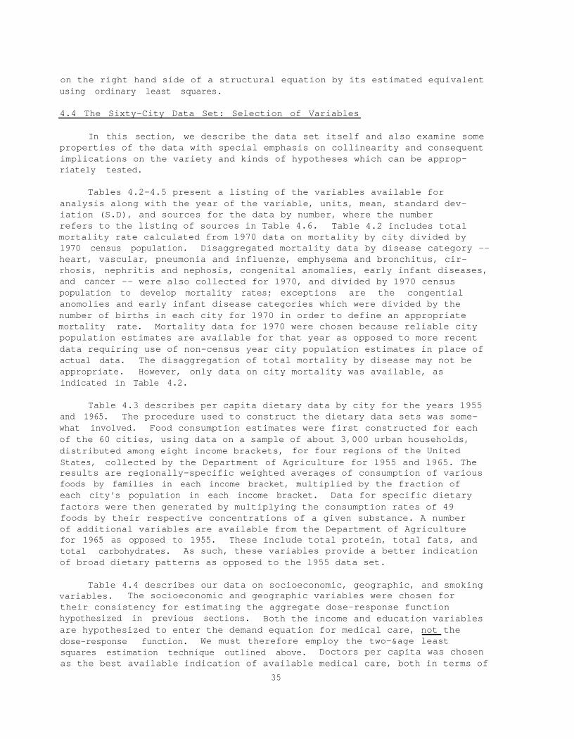
on the right hand side of a structural equation by its estimated equivalentusing ordinary least squares.

4.4 The Sixty-City Data Set: Selection of Variables

In this section, we describe the data set itself and also examine someproperties of the data with special emphasis on collinearity and consequentimplications on the variety and kinds of hypotheses which can be approp-riately tested.

Tables 4.2-4.5 present a listing of the variables available foranalysis along with the year of the variable, units, mean, standard dev-iation (S.D), and sources for the data by number, where the numberrefers to the listing of sources in Table 4.6. Table 4.2 includes totalmortality rate calculated from 1970 data on mortality by city divided by1970 census population. Disaggregated mortality data by disease category --heart, vascular, pneumonia and influenze, emphysema and bronchitus, cir-rhosis, nephritis and nephosis, congenital anomalies, early infant diseases,and cancer -- were also collected for 1970, and divided by 1970 censuspopulation to develop mortality rates; exceptions are the congentialanomolies and early infant disease categories which were divided by thenumber of births in each city for 1970 in order to define an appropriatemortality rate. Mortality data for 1970 were chosen because reliable citypopulation estimates are available for that year as opposed to more recentdata requiring use of non-census year city population estimates in place ofactual data. The disaggregation of total mortality by disease may not beappropriate. However, only data on city mortality was available, asindicated in Table 4.2.

Table 4.3 describes per capita dietary data by city for the years 1955and 1965. The procedure used to construct the dietary data sets was some-what involved. Food consumption estimates were first constructed for eachof the 60 cities, using data on a sample of about 3,000 urban households,distributed among eight income brackets, for four regions of the UnitedStates, collected by the Department of Agriculture for 1955 and 1965. Theresults are regionally-specific weighted averages of consumption of variousfoods by families in each income bracket, multiplied by the fraction ofeach city's population in each income bracket. Data for specific dietaryfactors were then generated by multiplying the consumption rates of 49foods by their respective concentrations of a given substance. A numberof additional variables are available from the Department of Agriculturefor 1965 as opposed to 1955. These include total protein, total fats, andtotal carbohydrates. As such, these variables provide a better indicationof broad dietary patterns as opposed to the 1955 data set.

Table 4.4 describes our data on socioeconomic, geographic, and smokingvariables. The socioeconomic and geographic variables were chosen fortheir consistency for estimating the aggregate dose-response functionhypothesized in previous sections. Both the income and education variablesare hypothesized to enter the demand equation for medical care, not thedose-response function. We must therefore employ the two-&age leastsquares estimation technique outlined above. Doctors per capita was chosenas the best available indication of available medical care, both in terms of

35

36

Table 4.2

Mortality Variables

Variable Year Units Mean S.D. Sources

Mortality Variables

M070HA70VA70PN70EM70CI70NE70C/B%I/B%CA70

Total Mortality 1970Heart Disease 1970Vascular Disease 1970Pneumonia & Influenza 1970Emphysema & Bronchitis 1970Cirrhosis 1970Nephritis & Nephrosis 1970Congenital Anom/Births 1970Early Infancy/Births 1970Cancer Mortality 1970

deaths/1000 pop. 11.283 2.161 (18) (6)4.216 1.078 (18) (6)1.566 0.395 (18) (6)0.375 0.114 (18) (6)0.178 0.059 (18) (6)0.238 0.106 (18) (6)0.058 0.027 (18) (6)

% 0.473 0.105 (18) (6)% 1.294 0.333 (18) (6)

deaths/1000 pop. 1.958 0.402 (18) (6)

Table 4.3

Dietary Variables

Variable Year Units Mean S.D. Source

Dietary Variables

NTRI

NTRA

SFAT

PROT

CHOL

CVIT

CALO

COFF

ALCO

XPRO

XFAT

XCAR

XASA

6NTI

6NTA

6SFT

6PRO

6CHL

6CAL

6CVT

6COF

6ALC

Nitrites in Food

Nitrates in Food

Saturated Fatty Acids*

Protein*

Cholesterol*

Vitamin C**

Calories

Coffee

Alcohol (S value)

Total Protein

Total Fats

Carbohydrates

Ascorbic Acid

Nitrites in Food

Nitrates in Food

Saturated Fatty Acids*

Protein*

Cholesterol*

Calories

Vitamin C**

Coffee

Alcohol ($ value)

1955 g/yr/cap 1.27 0.14

1955 g/yr/cap 69.86 9.05

1955 g/yr/cap 16220.00 874.65

1955 g/yr/cap 26557.00 1314.00

1955 g/yr/cap 234.81 6.98

1955 g/yr/cap 16.96 1.46

1955 kcal/yr/cap 1149.7 56.27

1955 kg/yr/cap 5.83 .70

1955 $/yr/cap 17.30 6.06

1965 g/yr/cap 39845. 706.46

1965 g/yr/cap 57512. 1795.7

1965 g/yr/cap 123490. 3623.0

1965 mg/yr/cap 42281. 2364.2

1965 g/yr/cap 1.14 .16

1965 g/yr/cap 52.87 2.47

1965 g/yr/cap 16315. 976.3

1965 g/yr/cap 28128. 1603.4

1965 g/yr/cap 219.9 5.80

1965 kcal/yr/cap 1171.1 27.63

1965 g/yr/cap 18.65 1.3

1965 kg/yr/cap 5.40 .18

1965 $/yr/cap 25.97 6.45

(2) (4) (27)

(2) (4) (27)

(2) (3) (4)

(2) (3) (4)

(2) (3) (4)

(2) (3) (4)

(2) (3) (4)

(2) (3) (4)

(2) (3) (4)

(28)

(28)

(28)

(28)

(4) (28) (27)

(4) (28) (27)

(3) (4) (28)

(3) (4) (28)

(3) (4) (28)

(3) (4) (28)

(3) (4) (28)

(3) (4) (28)

* Includes only animal products.

** Includes only vitamin C content for fruits and vegetables eaten fresh.

37

38

Table 4.4

Social, Economic, Geographic, and Smoking Variables

Variable Year Units Mean S.D. Sources

Social, Economic, Geographic

MDOC Medical Doctors 1970 M.D.'s/100,000 162.8 54.2 (19)

IN69 Median Income 1969 $/yr/Household 10763. 1060. (6)

EDUC Education 1969 %>25 w/H.S.yrs 55.3 7.4 (6)diploma

DENS Crowding In Homes 1969 %>1.5 persons/ 0.022 0.013 (8)room

COLD Cold Temperatures 1972 #days temp < 0 86.9 47.7 (9)0°C.

NONW Nonwhite Population 1969 Fraction 0.226 0.154 (6)

MAGE Median Age of Popu- 1969 Years 28.82 2.74 (6)lation

Smoking Variables

C156

Cigarettes

Cigarettes

C168

1956

1968

183.52

165.80

26.66

23.25

(22) (4)

(7) (1)

Data for states, 1960 census population used.

Data for states, 1970 census population used.

Table 4.5

Units Mean

Air Pollution Variables

Variable

Air Pollution

Year SourcesS.D.

SU66 Sulfate 1966 i-s/m3 10.67 5.44 (20)

AM66 Ammonium 1966 e/m3 1.15 1.42 (20)

NI66 Nitrates 1966 k&m3 1.96 0.68 (20)

PA66 Suspended Particulates 1966 w/m3 114.83 33.97 (20)

NO69 Nitrogen Dioxide 1969 wm 0.076 0.034 (11)

PA70 Suspended Particulates 1970 w.z/m3 102.30 30.11 (13)

SO70 Sulfur Dioxide 1970 tdm3 26.92 22.20 (13)

NI70 Nitrate, annual mean 1971-73 ug/m3 3.13 0.92 (14)

NI90 Nitrate, 90th %-tile con. 1971-73 ug/m3 5.21 1.80 (14)

SU70 Sulfate, annual mean 1971-73 ug/m3 10.65 4.01 (14)

SU90 Sulfate, 90th %-tile con. 1971-73 pg/m3 17.69 7.62 (14)

LEAD Lead 1970 w/m3 1.33 0.54 (16)

CO74 Carbon Monoxide 1974 mg/m3 11.86 3.50 (15)

BETA Beta Radioactivity 1966 PCi/m3 0.261 0.091 (20)

39

preventative and ameliorative care. Alternative variables such as hospitalbeds per capita were judged inferior, in that underutilization of hospitalfacilities is a common problem and adjustments for utilization factorswould prove troublesome. Also, if one assumes a less than perfectly elasticsupply of medical care, the doctors per capita variable is an appropriatesupply side variable in that it reflects patient loads for doctors in aparticular city. The possible importance of age and cold temperatures in adose-response relationship are clear. However, the nonwhite and crowdingvariables may be more difficult to interpret. The nonwhite variable wouldideally control to some extent for genetic variations in the population.Obviously, however, this variable may well proxy for education, poverty,habits, etc. Similarly, crowding would ideally be an indication of pos-sible contagion but may really proxy for poverty, old age, or even race.Thus, the role of these variables should be interpreted with great care.

Cigarette consumption was estimated from cigarette tax revenues foreach state in which a sample city was located; the result is thus a state-wide average that includes rural populations. Per capita cigarette consump-tion was estimated using the total state population over 16 years of ageboth for 1956 and 1968. It should be noted that both our dietary and oursmoking variables are quite crude, reflecting problems in utilizing second-ary data. However, the possible importance of their effects on human healthmay justify use of even these measures. We also attempted to develop ameasure of total exposure to radiation, collecting data on beta radioactiv-ity in air, terrestrial gamma radiation, and cosmic ray exposures, but haveto this point been able to account for only about half of the average indi-vidual annual dose associated with medical exposures. As a result, nosuitable total exposure variable is available at this time.

Table 4.5 presents the air pollution variables available for testing.All data are annual geometric means for each city unless otherwise specified.Unfortunately, hydrocarbon data was only available for about ten of oursample cities and are excluded for this reason. Finally, as noted above,Table 4.6 presents our data sources.

In summary, data available for testing include: (1) 1970 mortalityrates for total mortality and for major disease categories; (2) data ondietary patterns for 1955 and 1965; (3) data on medical doctors and socio-economic factors for 1970 or a nearby year; (4) data on smoking patterns for1956 and 1968; and (5) data on air quality for each city for 1970 or anearby year.

Since only 60 observations are available, we must obviously select asubsample of the available explanatory variables for hypothesis testing.To allow straightforward statistical tests of the significance of estimatedcoefficients, it is necessary to make the selection of included variablesa priori rather than testing each of the variables in various combinationsfor significance and excluding some on the basis of relative significances.Techniques do exist for testing significance where pre-testing has beenemployed but the standard t-statistic is no longer applicable.

The first problem in specifying the final data set is a decision onincluding lagged variables. Given a highly mobile U.S. population, the

40

Table 4.6

Sources of Data

(1) Advisory Commission on Intergovernmental Relations, State and LocalSignificant Features and Suggested Legislation, 1972, Table120, 1970.

(2) U.S. Department of Agriculture, Household Food Consumption Survey, 1955,Reports No. 2-5.

(3) , Composition of Foods: Raw, Processed and Prepared, Watt,Bernice K., and Merrill, Annabell L., Agricultural Handbook No. 8, 1968.

(4) U.S. Department of Commerce, Bureau of the Census, U.S. Census of thePopulation: 1960.

(5) , Cross Migration by County: 1965-1970, Current PopulationReports Series P-25, No. 701, issued May 1977.

(6) , U.S. Census of Population: 1970, Vol. 1-50.

(7) , State Tax Collections: 1968, Series GF 68 No. 1, Tables 7, 9.

(8) , 1970 Census of Housing by State.

(9) , National Oceanic and Atmospheric Administration, EnvironmentalData Service, Climatological Data, National Summary: Annual 1972, Vol.23, No. 13, Asheville, North Carolina.

(10) U.S. Environmental Protection Agency, Natural Radiation Exposure in theUnited States: 1972, Report No. ORP/SID 72-1, Table A-1, 1974 Reprint.

(11) , Air Quality Criteria for Nitrogen Dioxide, No. AP-84, Tables6-10, January 1971.

(12) , Chemical Analysis of Interstate Carrier Water Supply System,PB-257600/7BE April, 1975.

(13) , Air Quality Data - 1970 Annual Statistics, EPA-450/2-76-019,October 1976.

(14) , Air Quality for Nonmetallic Inorganic Ions, 1971 through 1974:From the National Air Surveillance Networks, EPA-600/4-77-003, January,1977.

(15) , Air Quality Data - 1974 Annual Statistics, EPA 450/2-76-011,August, 1976.

(16) U.S. Environmental Protection Agency, Air Quality Data for Metals 1970through 1974: From the National Air Surveillance Networks, EPA-600/4-76-041.

41

Table 4.6

(continued)

(17) Department of Health, Education and Welfare, Public Health Service,National Center for Health Statistics, Vital Statistics of the UnitedStates: 1960.

(18) , Vital Statistics of the United States: 1970.

(19) , Health Manpower -- A County and Metropolitan Area Data Book.

(20) , National Air Pollution Control Administration, Air QualityData from the National Surveillance Network and Contributing State andLocal Networks, 1966 Edition.

(21) , Vital Statistics of the United States: 1972.

(22) Tobacco Tax Council, Cigarette Taxes in the United States, 1956,Table 15.

(23) Directory of Medical Specialists, 1960-71, Marquis - Who's Who, Inc.,Chicago, Illinois.

(24) Adams, John A., et. al., eds., The Natural Radiation Environment II,Proceedings of the Second International Symposium on the NaturalRadiation Environment, Houston, Texas, August 7-11, 1972.

(25) Hickey, John, et. al., The Development of an Engineering ControlResearch and Development Plan for Carcinogenic Materials, U.S. Govern-ment Printing Office, Washington, D.C. (1977 in press).

(26) Pazand, Reza, Environmental Carcinogenesis - An Economic Analysis ofRisk, PhD. Dissertation, The University of New Mexico, July 1976.

(27) White, Jonathan W., Jr., "Relative Significance of Dietary Sources ofNitrate and Nitrite," Journal of Agricultural and Food Chemistry,Vol. 23, No. 5 (1975), Table VI, p. 890.

(28) U.S. Department of Agriculture, Household Food Consumption Survey, 1965-66, Reports No. 7-10 and Reports No. 13-16.

42

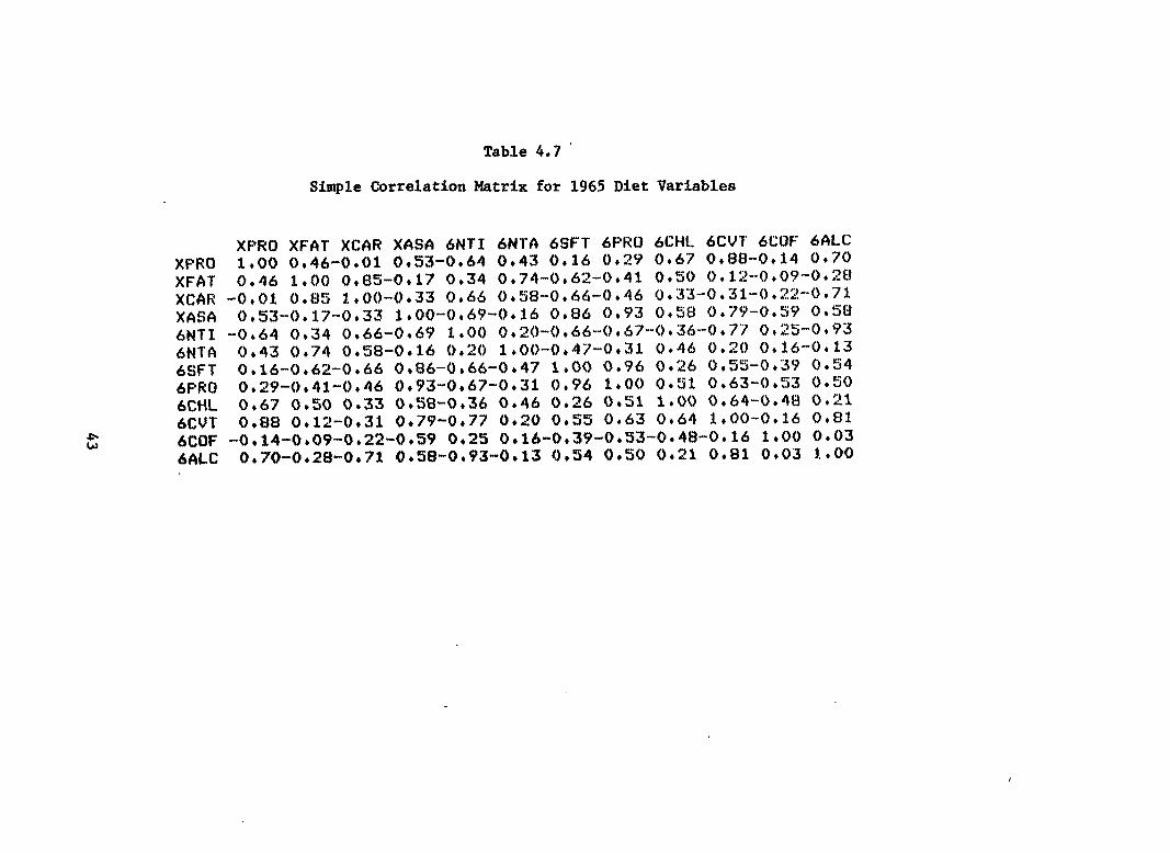
43

Table 4.7

Xlw?o XFAT XcAll XA!M 6NTI 6NTA 6SFT 6F’RO 6CW. 6CVT 6COF 6flLc

Simple Correlation Matrix for 1965 Diet Variables

XF’RO XFAT XCAR XASA 6NTI 6NTA 6SFT 6F’RO 6CHL 6CUT 6COF 6ALC 1,00 0,46-0,01 0,S3-0,64 0,43 0,16 0,29 ()+67 0,88-0,14 0470 0,46 1,00 0+83-0017 0+34 0+74-0062-0+41 OtSO 0*12--0*09-0+28

-0,01 0,83 1,00-0+33 (),66 0t3E1-0,66-()+46 0,33-0,3k-()+:?2-<)t71 0,!53-(),17-0,33 1,00-(),69--0+16 0,t16 (),93 0+S8 0,79-0039 0,38

-O*64 0,34 0.66-0+69 1*OO 0+20-0+66-()+67-()+36--0+77 0+25-0+93 0,43 0,74 0,38-0,16 0+:?0 1,00-0.47-0,31 0+46 0,20 (),16-0,13 0,i6-0,62-0t66 (),86-0,66-0*47 1,00 0+96 0+26 0t5Si-0+39 0+!34 0,29-(),41-0,46 0,93-0+67-0+31 0,96 1,00 O*31 0+63-0,53 O*5O 0,67 (),5() 0,33 0+58-0,36 0,46 0,26 0+51 3.+00 0+64-0,48 0+21 0,88 0+12-0+31 0,79-0,77 0,20 0,!35 0,63 0,64 1,00-0,16 0,81

-0,14-0,09-0,22-()+S9 0,25 0,16-0,39-0,33-0.48-0,16 1*OO 0,03 0+70-0,28-0,71 0058-0,93-0,13 (),54 0,S0 0+21 0,81 0,03 1.,00

question becomes, "do people now living in a city represent the same sampleas individuals who lived in cities 14-15 years before (the lags on smokingand diet, respectively)?" If the answer is no, and if people carry theirdietary and smoking characteristics with them as they move, the most recentavailable data is likely to better represent long-term dietary and smokingpatterns of individuals in a particular city. For these reasons, in thisstudy, we use the available data closest to 1970 throughout. However, itmay well be, for diseases with long lags such as cancer, that lagged vari-ables are superior in any case. The real answer is, of course, to accountproperly for mobility -- a near impossibility when using aggregate data.

The second consideration in specifying variables for inclusion is multi-collinearity, Typicall, multicollinearity problems can be avoided if thesimple correlations between explanatory variables are less than 0.4 to 0.6.Tables 4.7 and 4.8 present simple correlation matrices for 1965 diet and airquality variables, respectively.

Table 4.7 shows that a very high level of collinearity is probablypresent among dietary variables. It appears so high, in fact, that theproblem becomes one of finding a set of dietary variables which is suf-ficiently non-collinear to allow reasonable estimation of individual coef-ficients. Perhaps the broadest indicators of dietary patterns are thetotal protein (XPRO), total fat (XFAT) and total carbohydrate (XCAR)variables. Protein and fat will tend to indicate high consumption of meat.and nuts, while high carbohydrate consumption will indicate consumption ofgrains, fruits, vegetables, and refined sugars. However, total carbohydrateand total fat have a correlation coefficient of 0.85, too high to allowinclusion of both variables in an estimated equation. However, if wereplace total fats (XFAT) with animal fat (6SFT), a good proxy for con-sumption of saturated fats, the correlation between fat (now animal fat)and carbohydrates drops to 0.66, which although still high, will likelycause less difficulty. Thus, we include these three diet variables asbroad indicators of dietary patterns where, however, it must be clearlyrecognized that the estimated coefficients on these variables may wellinclude the effect partially or totally of a number of other highly col-linear dietary variables. For example, total protein (XPRO) has a cor-relation with cirrhosis, one might justifiably doubt that a causal relation-ship exists between protein and cirrhosis as opposed to one between slcoholand cirrhosis.

Table 4.8 suggests that multicollinearity may well be a problem withinthe air quality data set as well. Given previous research (see, for example,Lave and Seskin, 1977), the air quality measures of most concern are thosefor NO:!, S02, sulfate, and particulates, so we focus on these variableshere. However,mortality data,

our measures of S02and sulfate for 1970, the year of theare highly collinear -- S070 and SU70 have a simple correl-

ation of 0.74 -- so any separation of their relative importance is likelyimpossible. As a result, we use SO2 (S070) as a proxy variable for bothpollutants. Note also that among the included air pollution variables,NO (N060), particulates (PA70), and SO2 (S070), collinearity problems may

with respect to ammonium, carbon monoxide and lead (some correlationsgreater than or equal to 0.4). Since we exclude these variables here (as

44

45

Table 4.8

Simple Correlation Matrix for Air Quality Variables

I

AM(S6 )41($6 SU66 N().S9 F’A6/) F’r470 S070 t4X’70 N190 1..EI4II [;07’4 SU70 SIJYO AM(36 1*0()--O,I6 0+7$1 0.:!8 0.31 ()*:32 ()+v2.”’. ‘ 0+:13-.()+()[4 0,04 o+j.4 ()+~~ ()+~~~ N:16L?) ““0+1.6 1,00 0+07 ()+3A ()+24 0.0$3 ()+04 0.4$1 O*44 0,!21. 0+:1.Y ()+()7-0+01 sLJ66 O*7H 0+07 3,+00 ()+34 0+/)8 0+4;$ 0,7:? ()+()8 ()+:1.t 0.07 0+2[{ 0+86 0+73 N(J69 0+:?[1 0+36 0+34 I.*OO ()+30 0+09 o*3:!i 0+31. 0.33 0+40 0+21 0,37 O*2I PAA6 0+:;1 0+24 0+68 0+;30 :1.*OO O*69 0+30 0+1:1. 0+1,2 0+1.Y 0,36 0?53 0+53 F’A70 0+32 0,08 0043 0+09 ()+69 I.*()() 0,2!2 0,:1.7 0+1.:1.-.0,00 0+36 0+37 0,3:1. $[JYO 0+!5:! 0+04 0+”72 0+3!!; O*5O 0+2!3 I .00 0+2?0 0,2[1 0. :1.0 0+!30 ()+74 0+::;6 N17’O -“0,1:; 0,48 0+08 0+31. 0+11 0+1.7 0+20 1+00 0.’):? O*lH O*24 0,.19 O*O4 N:t90 -0,08 0,44 (),1. 1’0,3:? 0+120+11 0,28 0+Y2 1..00 0,:!0 0,24 0.22 ()+1,4 L.EAII 0+04 (),!51. 0+07’ 0+40 0+19--0+00 0,1,0 0+1.8 0+20 1.,00 0,20 0+00--0,08 C(IY4 O*I.4 0,+19 0+28 O*2I 0.36 0.:34 0*!50 0+24 .0+24 0,20 1.,00 ()+34 0.2:; $; {J “~ () (1+6(S 0,07 0,86 0+32’ 0+5:3 0+37 0074 0,1.9 0.;”22 0+00 0,;34 1.,00 0+$3!3 SU{?O ()+/)4--()+()1 ()+73 ()+J21. ()+tjj;$ ()+i31. 00Yi6 ()+()4 ()+jl.4-.O+()tl ()+J23; ()+[13 1+()()

46

Table 4.9

Simple Correlation Matrix for Included Variables

NONW MfiGE IN(59 EDl)C DENS COLIJ C16tl XPR(I XCAR 6!3F”I” NO(?)Y S070 F’A70 NoNw 1.00 0402”-0.:!6-0022 0*40-”0*04 O*O2 0+02! 0+23 O*O:! 0+22 0+:!9 0+03 MAGE 0,02 1,0() 0,00--0,14--0+30 0+01.-0+05 002!:!--0+24 0+32! 0,21 0025 0+13 IN(SY -0+26 O*O8 1+00 ()*49-()*32! O*O2 o+o:~ 0*20--O+23--O:;:; O* I:!-”0*12-”O*2!5 EIILJC -()+22-0+14 0+49 1+00--O+22 0+04-0+2G 00;!4-00~4Yi-.()+ l;5-.lt) t()t343()+2!42!4 [tENs o,40-(),3()--()+32--O,:!2! j.,00--O,3H-(),OH (),(.)3 (),39--0,26 ()+OG--O,O3--O,O7 COLE -O*O4 0+01. (),0:? 0+04-0.38 1*OO 0433-0+60-0+;3H ()+34-’0.03 0,35 0.34 c14a 0*02--O*O5 0.03-0+;!s--0+08 0.33 1+00-”0.24-0,01, (),09 0+17 (),23-().08 XFRCI O*O2 0,22 0+20 O*26 ()+03-0,60-0+::4 j.,oo-o,ol O*I6 0,11-()+0[1-0,31 X(;AR ()*21$-”()+f~4--O*Z!3-O+33 0*;59-().38--O*()I””0.():I j. *()()--() *4~6-0+ j.El-()*3;3--() *O3 6SF”T 0,0;! 0+;{2?--(),():j-0,j .:3.-(),26 ()+34 O+()(Y 0+16--O,66 1+()() 0+16 0+5Y (),12! No(5s’ ()*2:! 0+:!:1. 0+12--0+16 ()+08-0+03 O*I7 0+5.!.-’0+1.[3 0+16 1.+00 (),35 0.09 S070 0,2?9 ()+J?Vi.-()+l l?-O034-O*03 0+35 0+1!13--() +()8-0+3;5 0+59 ().35 1+00 O+i!5 F’&170 O*O3 ()* j.3”-() *:!:3-”o *24-”()*()”7 ()+:44--(} +()$]-0 *31”-()+():$ 0+1:! 0+09 0,:.!:; 1*OO

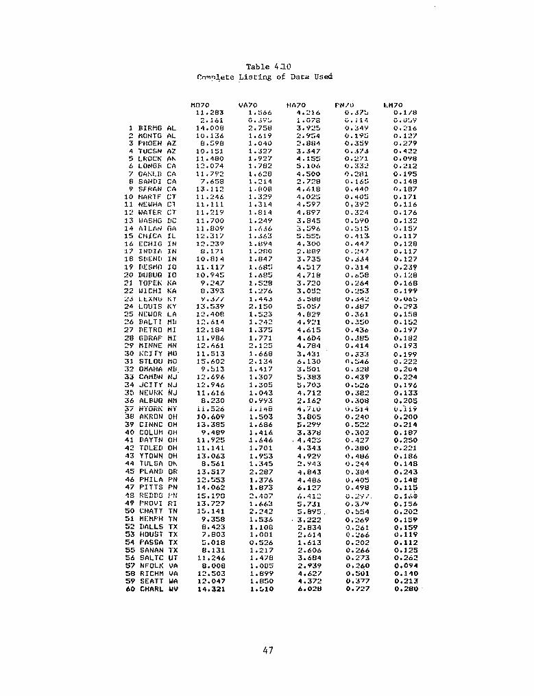
Table 4.10 Complete Listing of Data Used

3 BIRMG AL 2 HONTG AL 3 FHl-tEN AZ 4 TUCSN AZ 5 LROCK AK 6 LONGR CA 7 OkSLD CA 8 SAND1 CA 9 SFKkN CA

10 HAR-fF CT 11 NEWHA C7 12 WATER CT 13 WASHG DC 14 AlLAt GA 15 ctrrcn IL 16 ECHIG IN 17 INDIA IN 18 SBENO IN 19 KIESMO IO 20 DllBUn IO 21 TOPEK KA 22 WICHI KA 23 LEXNG KY 24 LOUIS KY 25 NtIWOR LA 26 BALTI MLI 27 IKTRO HI 28 GirFiAF HI 39 HINNE MN 30 KCITY MO 31 STLOU MO :32 OMAHA NB. 33 CAMEIN NJ 34 JCITY NJ 35 NEtiRK tiJ 36 ALEdtQ NM F7 NYOUK NY 38 AKUON OH 39 CINNC OH 40 COLUM OH 41 DAYTN OH 42 TOLED OH 43 YTOWN OH 44 TULSA Oh 45 PLAND OR 46 F’HILA PN 47 F'ITTS PN 48 REDDG FN 49 FROVI RI SO CHATT TN 51 MEMFH TN 52 IIALLS TX 53 HOUST TX 54 PASSA TX 55 SANAN TX 56 SALTC UT 57 NFOLK VA 58 R1CHt-l VA 59 SEATT WA 60 CHARL UV

HO70 VA70 HA70 F-N/O 11.283 1.566 4.216 0.57:)

2.161 O..4Yb 1.078 O.ll4 14.008 2.758 3.925 0.34Y 10.136 1.61Y 2.Y54 0.195

8.598 1.040 ".I384 0.35Y 10.151 1 . 3 2 7 3.347 0.373 11.480 1.Y27 4.155 0.271 12.074 3.782 s * 106 0 l 332

11.7Y2 1.6263 4.500 0.281

7.658 1.214 2.72tl (i.165 13.112 1.808 4.61El 0.440 11.246 1.32Y 4.025 0.40'5 11.111 1.314 4.597 0,392 11.21Y l.Hl4 4.EJY7 0 3-'4 . - 11.700 1.24Y 3.845 0.5YO 11.809 1.636 3 5?6 . 0.515 12.317 1.363 5.555 0.413. 12.239 l.UY4 4.300 0.447 S.171 1.280 2.&W O.247

10.814 l.U47 3.735 0.534 11.117 1.68:; 4.517 0.314 to.945 1.685 4.718 O.tl58

9.247 1.528 3.720 0.264 El.393 1.276 3.052 0 . 253 9.377 1.443 3.580 0.342

13.539 2.150 5.057 O.JU7 12,408 1.523 4.829 0.361 12.614 1 . 242 4.921 0.350 12.184 1.375 4.615 0.436 11.V86 1.771 4.604 0.385 12.661 2.125 4.784 0.414 11.513 1.668 3.431 0.333 15.602 2.134 6.130 0.546

9.513 1.417 3.501 0.328 12.696 1.307 5.383 0.439 12.946 1.305 5.703 0.526 11.616 1.043 4.712 0.382

8.230 0. YY3 2.162 0.308 11.526 1.1.48 4,710 O.Sl4 10,609 1.503 3.805 0.240 13.385 1.686 fii.2YY 0.522

9.489 1.416 3.37tl 0.302 11,925 .1.646 4 l 42’5 0 . 4 2 7 11.141 1.701 4.343 0.380 13.063 1.953 4.92Y (1.486

8.561 1.345 2.Y43 0.244 13.517 2.287 4.843 0.384 12.553 1.376 4.485 0.405 14.062 1.873 6.127 O.4V8 15.198 2.407 6.412 0.2Y7. 13.727 1.663 5.731 0.3/y 19.141 2.242 5.8Y'J 0.554

9.358 1.536 . 3,222 0.269 8.423 1.1on 2.834 0.. 261 7.803 1.001 2.614 0 .L'a6 5.018 c3,5”6 1.613 0.202 8.131 1.217 2.606 0.266

11,246 1.47S 3.684 0.273 8.000 1.005 2.939 0.26.0

12.503 1.89V 4.627 0.501 12.047 1.850 4.372 0.377 14.321 1.510 6.020 0.727

Lti70 0.1/R O.ObY 0 . T! 14 0.1'7 d. 0.279 0.422 O.OY8 0.212 0.195 0.148 0.187 0.171 0.116 0.176 0.132 0.157 0.117 0.128 0.117 0.127 0.239 0. 1'.'8 O&3 O.lV9 0.065 0.293 0.158 0.152 0.197 0.182 0.193 0.199 0 .32 0.204 0.224 O.lV6 0.133 0.205 O.il9 0.200 0.214 0.107 0.250 0. 221 0.186 0.148 0.243 0.148 0.115 0.16i) 0.156 0,202 O.lS9 0.159 0IllY 0.112 0.1as 0.262 0.094 0.140 0.213 0.280

47

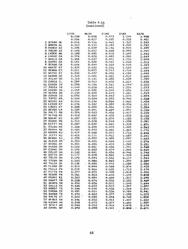
1 HIRMG AL 2 MONTG AL 3 PHOEN AZ 4 TUCSN AZ 5 LROCK AK 6 LUNGB CA 7 OAKL1.1 CA 8 SANUI CA 9 SFFiAN CA

10 HARTF Cl 11 NEWHA CT, 12 WRTEFi CT 13 WASHG DC 14 ATLAN GA 15 CHICA IL 16 ECHIG IN 17 INIlIR IN 18 SBEND IN , 19 DESMO IO 20 IIurwQ IO 21 TCtF’t:K KA, 22 WICHI KA :?3 L.EXNG KY 24 LOUIS KY 25 NEWOR LA 26 HALT1 MLI 27 DETf<O MI 20 GWiAP HI 29 HINNE MN 30 hCITY MO 31 STLOU MO 32 ONAHA Nlr 33 CAtiDN NJ. 34 JCITY NJ 35 NEWfiK NJ l 36 ALBUG NM 37 NYCIFX NY Xl AkRUN OH 39 CINNC OH 40 COLUH OH 41 IlAYTN OH 42 TOLED OH 43 YTCIWN OH 44 TULSA OK 45 PLAND OR 46 PHILA PN 47 PITTS PEI 4El F(‘EDllG PN 49 PfiOUI RF 50 CHATT TN 51 HEMF’H TN 5.2 DALLS TX 53 HOUST T)( 54 F’ASSR TX 55 SANAN TX 56 SALTC U-t 57 NFOLK VA 58 RICHfi VA >Y SEA11 WA 60 CHARL uv

Cl70 NFL70 C\HcX 0.23B o.osE( 0.473 0.106 0 . 0 2 7 ') . 1ci:; 0.116 0.116 L).r)oL, 0.112 0.112 0 . ‘2 4 3 0.20s 0.02Y O.L!46 6. LYEI 0.027 0.6HH 0.188 0.045 0.418 0.2YO 0.028 0.482 (! .35G 0.047 0.401 O.lYl 0.030 0.467 0.646 0.04Y 0*36t.3 0.329 0.632 0.506 0.211 0.022 0.513 0.333 0.037 0.3Y6 0.48Y 0.081 0.401 0.713 6 . 131 0.355 0.2H9 0,. Oh2 0.430 0.29S 0,106 0.561 0.140 0.098 0.441 0.159 0.080 O.S4Y 0.130 0.020 0.6lY. O.OY6 0.064 0.413 0.104 0.024 0.3Y2 0.116 0.036 Oi506 0.176 0.037 0.359 0.2ElEl 0.055 0.436 0.109 O.OYl 0.6OY 0.394 0.063 0.456 0.413’ 0.067 0.470 0.187 0.03’3 0.579 0.214 0.028 0.544 0.187 0.049 0.38*? 0.268 0.090 0.475 O.lEl4 0.043 0.4Sb 0.419 0.068 0.3l.Y 0.426 0.111 0.412 6 . 290 ,O+OY2 0.4flY 0.254 0.025 O.Slti 0.352 0.055 0.424 0.160 0,051 0.430 0.190 0.053 0.474 0.143 0.041 0.456 0.177 0.070 0.506 0.190 0.044 0.506 0.243 O.Of36 0.865 0.130 : 0.036 0.4Yl 0.314 0.044 0. :iEIR 0.219 0.066 0.535 0.377 0.071 0.4YO 0.251 0.023 0.676 0.262 O.OR4 0.600 0.218 0.076 0.556 0.154 0.056 0.572 0.165 0.034 0.512 0.166 0.03Y 0.436 0.101 0.011 0.526 0.194 0.064 0.377 0.222 o.oElo 0.296 0.146 0.052 0.411 0.248 0.072 0.377 0.266 0.053 0.416 0.392 0.098 0.421

Table 4.10 (continued)

I\tx% 1*2Y4 0.333 1. .J”7 1.335 0.975

.o. 9% 1.29Y $1.045 1.250 1 . o:;tt 0.934 1.51Y 1.758 1.18Y 1.937 1*53Y 1.613 1.794' 1.254 1.450 1.381 1.570 0.940 1.465 0.934 1.237 1.4Y/ 1.417 1.320 1.183 1.258 1.318 1.449 1.362 1.716 1.687 1.997 1.132 1.245 1.2Yl 1.040 0.046 1*224 0.127 1.259 1.188 0.874 1.713 1.5z.o 1.14Y 1 * 327 2.105 1.143 1.297 1.264 0.78Y 1.182 0.765 1.447 1.6Et4 1.075 0.843

c/\70 1.958 0.402 2.343 1.732 1.499 .1.719 1.942 2.049 2.090 1.316 2.493 1.987 2.004 P. 999 2.000 1.789 2.038 2.022 1.573 2.142 1.919 1.'894 1.568 1.454 1.517 2.304 2.158 2.220 2.126 2.155 2.281 1.871 2.562 1.776 2.048 2.241 1.663 1.276 2.151 1.968 2.510 1.740 2.048 1.964 2.389 1.586 2.425 2.170 2.426 2.818 2.690 2.469 1.644 1.397 1.311 0.941 1.373 1.558 1.322 1.959 2.174 2.671

48

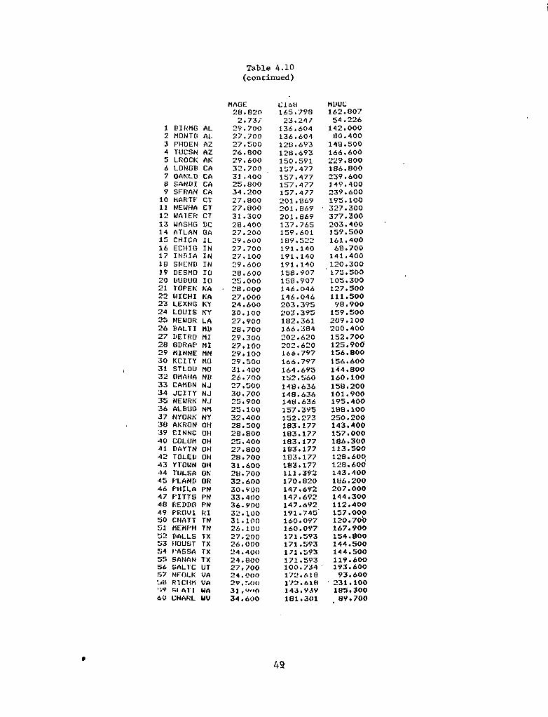
Table 4.10 (continued)

1 EtIliMG AL 2 HONTG AL 3 FHoEN Az 4 TUCSN AZ 5 LICOCK AK 6 LONG8 CA 7 OAKLI:I CA 8 SAND1 CA Y SFRAN CA

10 HAFlU-- CT 11 NEWHA CT 12 WAlER CT 13 WASHG DC 14 ATLAN GA 15 CHICA IL 16 ECHIG IN 17 INDIA IN 18 SlcLND IN 19 DESHD IO 20 L!\JBUQ ICI 21 TOFEK KA 22 WICHI tiA 23 LEXNG ICY 24 LOUIS KY 25 NEWOK LA 26 BALTI MLt 27 DETRO MI 28 GUt?AP MI 29 MINNE MN 30 KCITY MO

/ 31 STLOU MO 32 OMAHA NB 33 CAMDN NJ 34 JCITY NJ 35 NEWRK NJ 36 ALHUO NM 37 NYORK NY 38 AKRCIN OH :5Y CINNC Clti 40 COLUM OH 41 DAYTN OH 42 TOLED OH 43 YTOWN OH 44 TULSA OH 45 F’LAND OR 46 FHILA f:‘N 47 F'ITTS FN 48 REDDG FN 49 F'ROVI RI 50 CHATT TN 51 flEHPH TN 52 DALLS TX 53 )IOUST TX 54 I’ASSA TX S5 SANAN TX 56 SALTC UT 57 NFT1t.K VA :A1 RICHPI vn 'iv Fif nl' 1 tdn 60 CHAfIL WV

MAGE 28.820

2.73; 'Y.700 27.700 27,:;OO 26 l 000

29.600

32.700 31.400 25.800 34.200 27.800 27,000 31.300 28.400 27.200 2Y.600 27.700 27.100 29.600 28.600 25.000 28,000 27.000 24.600 30.100 27,YOO 28.700 29.300 27.100 29.100 29.500 31.400 26.700 27.500 30.700 25.900 25.100 32.400 2a. 500 28.800 25.400 27.800 28.700 31.600 28.700 32.600 30.5'00 33.400 36.YOO 32 . 100 31.100 26.100 27.200 26 IO00 24r400 24.800 27,700 24.000 29. :,oo 31 .ww 34.600

Clt.AJ

171.593

165.798 23 , 24 7

100*7;J4-

136.604 136.604

17".61U

128.6Y3 128.693

172.hlH

150.591 157.477 157.477

143.Y.sY

157.477 157.477

181.301

201.869 201.U69 203.869 137.765 159.601 109.522 lY1.140 191.140 191.140 158.907 l'i8.907 146.046 146.046 203.395 203.3Y5 182.361 166.384 202.620 202.620 116.797 166.797 164.695 152.560 14t3.636 148.636 148.636 157.395 152.273 183.177 183.177 183.177 183.177 183.177 183.177 111.3Y2 170.820 147.692 147.693 147.692 lY1.74S' 160.097 lbO.OY7 171.593 171.593 171r:iY3

MllUC 162.aO7

119.600

54,226 142.000

193.600

fJo.400 148.500

93.600

166.600

'

229.800 186.800

231.104

239,600 14Y.400

1HS.300

239.600 195.100

8Y.700

327.300

,

377.300 203.400 15Y.500 161.400

68.700 l41.400 120.300 175.500 105.300 127.900 111.500

98.900 159.500 2OY.100 200.400 152.700 125.906 156.800 156.600 144.800 1601100 158.200 101.900 195.400 188.100 250.200 143.400 157.000 186.300 113.500 128.60(! 128.600 143.400 ltl6.200 207.000 144.300 112.400 157.000 120.70b 167.900 154.000 144.500 144.500

49

Table 4.10 (continued)

1 HIRiiG AL 2 MONTG aL 3 PHOEN AZ 4 TUCSN hi! 5 LROCK AK 6 LONGB CA 7 OhtiLD cn 8 SAND1 CA 9 SFRAN CA

10 HARTF CT 11 NEWHA CT 12 UCIlER CT 13 UtiSIiG DC 14 ATLAN GA 1S CHICA IL 16 ECHIG IN 17 INDIA IN 18 SREND IN 19 DESMO IO 20 DU1wl IO 21 TOPEK KA 22 UICHI KA 23 LEXNG KY 24 LOUIS tiY 25 NEWOR LA 26 HALT1 UD 27 DETRO tt1 28 GDRAP HI 2Y HINNE MN 30 KCITY HO 31 STLOU HO 32 OHAHA ND 33 ChHDN NJ 34 JCITY NJ 3S NfWRK NJ 36 ALDUO NM 37 NYORti’ NY 38 AKRON OH 39 CINNC OH 40 COLUM OH 41 DAYTN OH 42 TOLED OH 43 YTOWN OH 44 TULSA OK 45 PLAND OR 46 PHILA PN 47 PITTS PN 48 REDDG YN 49 PKOVI RI 50 CHATT TN 51 MEflPH TN 52 DALLS TX 53 HOIJST TX 54 PASSA TX 55 SfiNRN TX "Jb SALTC UT 57 NFOLK WA Ml kIcHtl VA $9 SFA’IT WA 60 CHRRL uv

Dt NE; 0.022 0.013 0.037 0.037 0.027 0.032 0.017 0.013 0.023 0.019 0.027 0.029 0.015 0.015 0.048 0.034 0.026 0.047 0.017 0.010 0.010 0.018 0.011' 0.013 0.026 0.019 0.055 0.017 0.016 0.007 0.010 0.017 0.044 0.013

,0.018 0.024 0.640 0.022 0. C!Y 0.007 0.028 0.010 0.015 0.001 0.011 0.010 0.000 0.013 0.013 0.006 0.010 0.026 0.049 0.028 0.032 0.018 0.062 0.015 01021 0.018 O.OlO* 0.012

NONW 0.226 0.154 0 . 433 LW 0.336 0.067 0.052 0.251 0.082 0.407 0.111 0.286 0.292 0.274 0.105 0.723 0.516 0.344 0.2$4 0.104 0.147 0.062 0.003 0.096 0.107 0.174 0.241 0.045 0.470 0.44s

Oo%i 0:22&t 0.413 0.106 0.402 0.222 0.560 0.043 0.234 0.178 0.281 0.190 0.309 0.143 0.258 0.134 0.078 0,344 0.207 0.068 0.100 0.360 0.392 0.258 0.266 0.005 0.086 0.032 0.302 0.424 0.126 0.108

lN6-f ELIUC COLD 10762.895 55.298 86.900

lOW.562 7.45Y 47.654 86Y2.000 4s.400 48.000 Y933.000 51.600 29.000

1132Y.000 60.100 13.000 9922.000 43.100 22.000

10438.000 56.500 51 .ooo 11804.000 62.000 1.000 11279.000 66.100 7.000 11664.000 65.300 0.0 12507r000 66.100 11.00~0 10011.000 59.100 147.000 10444.000 56.OOO 102.000 11500.000 49.900 102.000 lL!lS;l).OOO 68.500 114*000 1065h.000 53.400 45.000 13'-.'7.000 .BL. 53.900 132*000 10068.000 53.60Q 132.000 12260.000 56.000 122.000 ll431.000 54.200 131*000

11350.000 68.000 151.000 11274.000. 54.600 152.000

10830.000 64.800 122.000 10940.000 63.200 122.000 10033.000 60.100 94.000

9980.000 46.900 91 .ooo

10246r000 45.ttoo 13*000 10035.000 44.600 90.000

110t5.000 52*100- 126.000

11242.000 54.000 157.000

11127.000 66.100 167.000

11306,000 60.100 106rOOO

9268.000 48.000 118.000 11605.000 .62.700 144.000

8627.000 50.600 09.000 10285.000 36.300 79.000

8637.000 55.100 84.000 10926.000 66.200 122.000 11632.898 51.800 79.000 11152.000 55 6 600 133.000 10435.000 48.400 100.000 10848.000 60.700 1141000 1032Y.000 56.200 125.000 11590.000 51,700 157.000

9928.000 52.100 150.000 11642.000 58.200 82.000 11377.000 6?.YOO 42.000 10431.000 so. 600 89.000 10536.000 53.400 124.000

YLY5.000 43.300 89.000 10208.000 4'5.900 128.000

8336.000 47.600 70.000 10104.000 49.200 61.000 12474.000 54.800 34.000 11737.000 51.700 21.000 11822.000 51.700 21.000

9027.000 46.800 23.000 10812.000 68.500 110*000

9236.000 48.300 31.000 10620.000 47.100 68 l 000

12557.000 67. BOO 32.000 10865.000 52. two 95.000

50

Table 4.10 (continued)

1 BIRHG 2 UONTG 3 FHOEN 4’ TIJCSN 5 LROCK k LONGB 7 OAKLD 8 SAND1 9 SFRAN

10 HARTF 11 NEWHA 12 UATER 13 WASHG 14 ATLAN 15 CHICA

6SFT 16314.0:#1

Y75.‘/4J AL 15079.503 AL 15030.398 AZ 16116.699 AZ 16054.102 AK 15186.500 CA 16079.102 CA 16030.898 CA 16090.398 CA 16030.898 CT 18240.500 CT 18118.801 CT 18255.801 DC 16219.500 GA 15737.398 IL 16404.699

16 ECHIG IN 16295.000 17 INDIA IN 16261.102 18 SBEND IN 16198.398 19 DEStlO 10 16244.699 20 DUDUQ IO 16153.102 21 TOPEK KA 16070.801 22 WICHI KA 16040.102 23 LEXNG KY 15555.602 24 LOUIS KY 15563.398 25 NEWOR LA 15119.199 26 DALTI HD 15724.500 27 DETRO tl1 16419.898 28 GDRAP HI 16266,801 29 MINNE HN 16431.801 30 KCITY WO 16217.199 31 STLOU MO 16175.398 32 GtfAfiA ND 16177.398 33 CAtlDN NJ 17976.199 34 JCITY NJ 18157.500 35 NEURK NJ 18148.801 36 ALDUG Ntl 16052.102 37 NYORK NY 18028.102 38 AKRON OH 16307.500 39 40 41 42 43 44 45 46 47 48

2: 51

CINNC OH 16160.301 COLUH OH 16194.898 DAYTN OH 16349.199 TOLED Off 16273.801 YTOWN OH 16232.602 TULSA OK 15467.898 PLAND OR 16006.199 PHILA PN 18187.398 PITTS PN 18287.898 REDDG PN 18399.699 PROVX RI 18237.699 CHATT TN 15181.398 KEtfPH TN lSl29.301

52 DALLS TX 15717.000 53 HOUST TX 15626.500 54 QASSA TX 15947.398 55 SANAN TX 15080.699 56 SAL’IC UT 16013.500 57 NFDLK VA 15177.000 :.8 RlCHfl VA 1564o.i,~*' GV SEATT UA 1604O.IYY 60 CHARL UV 15233.301

XCAR 123491.313

J618.011 129119.000 128765.000 120959.000 120957.000 129263.000 120519.000 120345.000 120865.000 120345.000 121166.000 120707.000 120882; 000 126710,000 128113.000 121525.000 121512rooa 121447.000 121453.000 121511,000 121495.000 121291.000 12106O.OoO 128726,000 128982.000 128678.000 128374.000 121501.000 121560.000 121751.000 121345.000 121333.000 121345.000 119345.000 120490.000 121000.000 120684.000 120486.000 121535.000 121335.000 121321.000 121493*000 121546.000 121441.000 129016.000 1211i5.000 120737.000 120748.000 121050.000 l20540.000 129289.000 128846.000 128359.000 128489.000 128755.000 129045.000 121539.000 128Y66.000 128727.000 120738.000 129243.000

AFRO 3PG44.547

/06.747 39517.699 39264.801 40696.199 40395.500 39630.301 41050,398 41306.898 40788.001 41306.898 40740*000 40348.500 40413r301 40232.000 40143.199 39337.301 39144 .doo 39100.199 39ov5.500 39096.000 38978.102 38877.500 38827.102 39981.301 40212.000 39532.602 40248.398 39346.500 39095.500 39322.000 39047.199 39030.199 38997.801 39194.500 39916.699. 40602.398 40456.801 40287.301 39152.102 39006.602 39035.602 39215.699 39135.398 39032.500 39958.602 40881.301 40271.699 39978.602 40029.699 39969.000 39708.500 39551.301 40155.199 40134.500 40795.199 - 39443.699 40791.102 3V734.602 40304.699 41333.699 39718.398

51

1 BIRtlG AL 2 HONTG AL 3 FHOEN AZ 4 TUCSN AZ 5 LROCK AK 6 LONGR CA 7 OAKLII CA 8 SAND1 CA 9 SFfiAN CA

10 HARTF CT 11 NEWHA CT 12 WATER CT 13 WASHG DC 34 ATLAN GA 15 CHICA IL 16 ECHIG IN 17 INDIA IN 18 SBEND IN 19 r~ESM0 IO 20 DUbLfR 10 21 TOFEK KA 22 WICtiI KA 23 LEXNG KY 24 LOUIS KY 25 NEWOR LA 26 BALTI flD 27 DETRO tl1 28 GDFiAP HI 29 tlINNE HN 30 KCITY HO 31 STLOU NO 32 OMAHA N8 33 CANON NJ 34 JCITY NJ 35 NEWHK NJ 36 ALRUO NM 37 NYORti NY 38 AKRON OH 39 CINNC OH 40 COLUM OH 41 DAYTN OH 42 TOLED OH 43 YTOWN OH 44 TULSA OK 45 PLAND OR 46 PHILA PN 47 FITTS FN 48 REDDG PN 4Y FROUI RI 50 CHATT TN 51 tlEtiPH TN 52 DALLS TX 93 HOUST TX 54 PASSA TX 5S SANAN TX 56 SALTC UT 57 NFOLK VA sn RICtvl Uh 59 SEATT WA 60 CHARL WV

Table 4.10 (continued)

NULY Pf$70 so70 0.076 102.300 26.917 0. 0’14 30.107 12.197 0.093 13tl.000 10.000 0.016 Y1.000 7.000 0.089 117.000 9.000 0.018 104.000 7.000 0.012 71.000 8.000 0.182 102.000 35.000 0.053 69.000 10.000 0.106 88.000 10.000 0.095 52.000 9.000 0.077 67.000 57.000 0.072 100.000 40.000 0.037 95.000 17.000 0.069 YY. 000 28.000 0.096 88.000 20.000 0.160 so. 000 73.000 0.086 189.000 07.000 0.079 Y6.000 Sl . 000 0.031 99.000 10.000 0.033 134.000 ll*OOO 0.072 194‘000 16.000 0.023 .97.000 8.000 0.064 95.000 6.000 0.062 71.000 12.000 0.096 117.000 .23.000 0.061 79.000 7.000 0.099 136.000 54.000 0.116 128.000 38.000 0.090 77.000 13.000 0.076 88.000 38.000 0.045 84.000 6.000 0.135 120.000 s2.000 0.075 132.000 '12.000 0,128 114.000 69.000 0,065 108.000 75.000 0.092 111.000 37.000 0.048 102.000 6.000 0.142 109.000 45.000 0.030 68.1000 70.000 0.099 95.000 18.000 0.087 97.000 22.000 0,057 102.000 25.000 0.096 111.000 13.000. 0.083 134.000 30.000 0.033 110.000 8.000 0.058 60.000 14.000 0.024 144.000 70.000 0.113 137.000 57.000 0,081 121.000 30.000

'0.087 93.000 67.000 0.042 127.000 18.000 0.078 86.000 17.000 0.074 105.000 7.000 0.105 YO.OVO lO.OdO 0.050 GO. 000 9.000 0*065 58.000 8.000 0.060 88.000 9.000 0.077 83.000 26.000 o.oss tlY.000 24.000 0.095 58.000 22.000 0.092 183.000 27.000

52

have most previous investigators) some unknown contribution from these pol-lutants may be included in estimated coefficients on N02, S02, and partic-ulates.

A complete correlation matrix for our choice of included variables ispresented in Table 4.9 with the exception of the doctors per capita variablefor which we use two-stage least squares. Several interesting collinearityissues are apparent here as well, not necessarily as a multicollinearityproblem since the highest simple correlation is 0.66 within the data set,but rather as an indication of problems of exclusion of variables in previousstudies. For example, SO (S070) shows a correlation of 0.59 with animalfat consumption (6SFT) an3 a correlation of 0.23 with cigarette consumption.In other words, air pollution as measured by SO2 might not be orthogonalwith respect to diet and smoking. The implication is that diet and smokingprobably must be included to obtain unbiased estimates of the effect of SO2on human health.

The final data set used in the analysis is presented is its entirely inTable 4.10. [Qualified investigators wishing to know about the additionaldata collected may obtain a complete listing by contacting the authors].

4.5 Empirical Analysis

The first step in estimating the model of human health we have specifiedis to attempt to account for human adjustments to disease in the form ofmedical care (doctors per capita). Thus, we first estimate a reduced formequation which has as the dependent variable doctors per capita and asindependent, exogenous explanatory variables: median age, % non-white,density, cold, per capita consumption of cigarettes, protein, carbohydrates,and animal fat (all exogenous variables from the dose response function);as well as per capita income and education level (exogenous variables inthe determination of the demand for doctors). This estimated equation isshown in Table 4.12 below.

Note that we have chosen linear specifications throughout the analysis.The linear form has several advantages. First, the entire modeling frame-work can be interpreted as providing a set of first-order approximationsof the slopes (the effects) of the variables in the model. As a linearapproximate system, the estimated effects, if unbiased, only hold true forthe neighborhood of the estimate -- that is for values of the variablesnear the means of our sample. Since we do not know the precise form (pre-sumably nonlinear) which our functions take, we are at least not implyingmore about our knowledge of effects than the data can support. However, ifsignificant nonlinearities do exist over the range of the data in our sample(and some of the estimated effects seem to imply this), then we have intro-duced a specification error by choosing linear estimates.

The second step in our analysis, then, is to generate, from the estimatedreduced form equation and from data on exogenous variables in the model,an estimated doctors per capita variable (DOCH) to replace actual data ondoctors per capita(MDOC) in the estimation of specific dose-responsefunctions. Table 4.11 summarizes our results, while Tables 4.13-4.22 give

53

54

Table 4.11

Summary of Two-Stage Linear Estimates of Factors in Human MortalityHypotheses not Rejected at the 97.5% Confidence Level

(One-tailed t-test, t~2.0)

Variable Total Pneumonia Emphysema Congenital EarlySign of Hypothetical Mortality Vascular Heart and and Kidney Birth Infant

Effect) Rate Disease Disease Influenza Bronchitis Cirrhosis Disease Defects Diseases Cancer

Doctors/Capita* (-)

Median Age (+)

% Nonwhite (+)

Cigarettes (+)

Room Density (+)

Cold (+)

Animal Fat (+)

Protein (+)

Carbohydrates (?)

NO2 (+)

SO2(+)

Particulate (+)

R2 .82 .60 .77 .54 .39 .64 .54 .22 .55 .86

* Two-stage estimator employed.

individual linear estimated dose-response functions where the first equationreported excludes the air quality variables and the second (for comparison)includes these variables. Note that the basic model actually excludes airquality. This reflects the approach taken; to first develop a model ofhuman health based on variables which are hypothesized to have large effects-- age, medical care, smoking, diet, etc. Once a basic model of satisfac-tory explanatory power is specified, it then may be appropriate to testfor variables such as air pollution which are hypothesized to have smalleffects.

We choose a 97.5% confidence level (t > 2.0) for the entire analysis.It should be noted that if actual doctors 2per capita are employed, thevariable is highly nonsignificant both when used in total mortality orwhen used in any of the component diseases. However, as indicated in oursummary of results shown in Table 4.11 the estimated two-stage doctors percapita variable is highly significant and has a uniform negative effect onmortality rates in total mortality, vascular disease, heart disease,emphysema and bronchitis, kidney disease, and cancer. We conclude, then,from a properly structured hypothesis test, that we cannot reject thehypothesis that medical care has a.highly important effect on human mortal-ity.

Both the median age and % nonwhite variables are widely significantacross the estimated equations and show up with uniformly positive effectson mortality rates.

Cigarette consumption shows significant positive partial correlationswith total mortality, vascular disease, heart disease and cancer, whileroom density and cold both show significant positive partial correlationswith total mortality and pneumonia and influenza. Room density also showssignificant positive correlations for cirrhosis and kidney disease.

The dietary variables show significance in total mortality, heartdisease, and cancer -- correlations between heart disease and saturated fatsand between cancer and meat consumption (note the positive association forprotein) have long been recognized -- as well as in emphysema and bron-chitis.

Again, however, it must be stressed, especially for the dietary variables,that collinearity abounds and the estimated effect may really not be re-lated to the specified variable but to a highly collinear one. Similarly,an estimated effect may include the sum of the effects of several collinearvariables. In other words, causality is not established by correlation.However, we cannot reject the hypotheses that doctors, cigarettes, and dietare all highly important in determining human mortality rates. Unfor-tunately, these variables have typically been excluded from previous aggre-gate epidemiological studies [Schwing,a smoking variable].

(1974) do, however, include

Turning to the air quality variables, only two significant partial cor-relations appear -- between particulates and the pneumonia and influenzavariable, and between SO2 and the early infant disease variable. The lat-ter of these effects is consistent with the work of Lave and Seskin (1977).

55

Table 4.12

Reduced Form Equation

MDOC 55 -- 10 11 13 14 21 24 54 25 27 41

WAR B

X10-NONW X11-MAGE X13-IN69 X14-EDUC X21-DENS X24-COLD X54-C168 X25-XFRO X27-XCAR X41-6SFT CONSTANT

50,447 1.1020 1.3513 0*50439

0.61649D-02 0.86708 1*9399 1.3418 161.53 Oe26107

-0.12806 -0.53850 0.45771 1.4919 0.22302D-01 1.4136 0.22804W02 0.72804 #+24002D-01 1.9402 -1691,3 -2.7124

R-SQUARE= Oe3877 SSR= 0+1062IPt06 DF= 49

T

56

Table 4.13

Total Mortality

MO70 3. --- 61 lo il 21 24 54 25 27 41

UAH B 7

X61-BOCH -0,53031D-01 -4,750l X10-NONW 5+60?2 5+0448 X11-MAGE Oe66172 12.360 X21-DENS 31+9lO 2.4494 X24-COLD 0 + 1437OD”“01 3+1093 X54-C168 0 + 21896D-01 3+0758 X25-XPRO 0 + 19325D-02 3e7525 X27-XCAR -0+82907D-04 -1.5347 X41-6SFT 0 + 36251 D-03 1+5938 CONSTANT -78.675 -3.7169

R-SQUARE= 0+8195 SSR= 49+74 IIF= 50

MO70 1 -- 61 10 11 21 24 54 25 27 41 31 57 60

UAR I( 7

X61-DOCH X10-NONW X11-MAGE X21-DENS x24-corn X54-C168 X25-XPRO X27-XCAR X41-6SFT X31+069 X57-SO70 X60-PA70 CONSTANT

-o.s2797r+-01 -4.3493 5+6276 4+5620

0+65893 11,540 32,772 2.3469

o+14436rl-o1 2+9089 0,21968D-01 ii?+8120 o,l9196D-02 3 ” + 5522

-0,7943m-04 -1e3612 0.39783D-03 Il.+4508

1 l 6457 0.35799 -o+31302rko2 to.34850

o+io744rko2 0 + 20059 -79,296 -3.5115

H-SRUAWE= 0.8205 SSR= 49+48 riF= 47

57

Table 4.14

Vascular Disease

WA70 2--611011212454252741

WAR E T

X6 1 -DOCH X10-NONW X11-MAGE X21-DENS X24-COLD X54-C168 x25-XPWO X27-XCAR X41-6SFT CONSTANT

-0,70223D-02 0.37954 0+10936

1+7016 0 + 1769511-02 0*30001&-02 0 + 1854211-03

-0 c 1346Oi+O4 -0.84316W04

-5+5672

R-SQUARE= 0‘5657 SSR= 3.998 DF= 50

-2,2186 1.2040 7+2050

Oe46071 1*3504 le4865 1.2699

-0+87885 -1c3075

-0.92769

VA70 2 -- 61 10 11 21 24 54 25 27 41 31 57 60

UAF? B T

X61-DOCH X10-NONW X11-MAGE X21-DENS X24-COLD X54-CI68 X25-XPHO X27-XCAR X41-6SFT X31+069 x57-5070 X60-PA70 CONSTANT

-0.88088X+02 -2.6671 0,63816 1.9014 0,11671 7.5127

2 l 7540 0.74768 0.20961&-02 1.5524 0,42167D-02 le9838 0,23976D-03 1.6306

-O.l7117D-04 -1.0781 -O.l8874D-04 -0125297 -0.86198 -0.68915 -0.3891lD-02 -1e5922 -0.63071D-03 -0.43278

-8.3456 -1.3583

R-SflUARE= Oe6022 SSR= 3.663 DF= 47

58

Table 4.15

Heart Disease

HA70 3 -- 61 10 11 21 24 54 25 27 41

VAR B T

X61-DOCH X10-NONW X11-MAGE X21-DENS X24-COLD X54-C168 X25-XF RO X27-XCAR X41-6SFT CONSTANT

-0.2234011-01 -3+4204 1.7509 2~6917

0.29627 9.4592 9e3338 1.2247

0.43566D-02 1.6113 0+13129D-01 3.1525 0.66878D-03 2.2197

-0e17969W04 -0.56857 0,4238OD-03 3.1849 -35.183 -2.8412

R-SQUARE= 0.7517 SSR= 17.03 DF= 50

HA70 3 -- 61 10 11 21 24 54 25 27 41 31 57 60

VAR B T

X61-DOCH X10-NONW X11-MAGE X21-DENS X24-COLD X54-C168 X25-XFRO X27-XCAR X41-6SFT X31-NO69 x57-so70 X60+%70 CONSTANT

-0.19800P01 -ii9132 1.3603 1 l 9694

0.28122 8.7965 7+4177 0.87861

0,43300D-02 l+SS83 0*10868D-01 2.4847 0.57165P03 1.8893

-0,22071&-05 -0+6755lD-01 0.39645W03 2.5822

4.8498 1.8842 0.82843D-03 0.16473 0+14052D-02 0.46855 -32.823 -2.5960

R-SQUARE= 0+7737 SSR= 15.51 DF= 47

59

Table 4.16

Pneumonia and Influenza

PN70 4 -- 61 10 11 21 24 54 25 27 41

UCSR E T

X61-BOCH -0,12925B-02 -1.2098 xlo-~oNw 0.18381 1.7274 X11-MAGE 0+19920D-01 3 l 8880 X21-DENS 2+9692 2.3816 X24-COLD O.l3030D-02 2.9460 X54-CI68 0+61524B-03 0*90310 X25-XPRO 0,70654D-04 1.4336 X27-XCAR -0+11329D-05 -0.21914 X41-6SFT 0+38010D-05 0.17462 CONSTANT -3.0478 -1.5046

R-SCWARE= 0.4108 SSR= 0+4556 DF= 50

PN70 4 -- 61 10 11 21 24 54 25 27 41 3i- 57 60

UAR E T

X61-DOCH -0.38115W03 X10-NONW 0.13820 X11-MAGE 0+16194D-01 X21-DENS 2.6677 X24-COLD 0.10428W02 X54-C168 0.61816W03 X25-XPRO 0,46048D-04 X27-XCAR -0,10027D-05 X41-6SFT -0.4926111-05 X31-+069 0.55215

-x57-so70 -0+47719B-03 X60-PA70 0+14272D-02 CONSTANT -2.1183

R-SQUARE= 0,5409 SSR= 0.3550 DF= 47

-0.37068 1,3226 3.3484 2 c 3264 2+4807

0.93415 1.0060

-0,20286 -0.21208

1.4180 -0.62722

3.1456 -1+1075

60

61

Table 4.17

Emphysema and Bronchitis

EM70 5 -- 61 10 11 21 24 54 25 27 41

UAR El 1

X61 -DOCH X10-NONW X11-MAGE X21 -DENS X24-COLD X54-CI68 X25-XPRO X27-XCAR X41-6SFT ,CONSTANT

-0,138510-02 0,22533D-01 Q.4Y451D-02 0.92106D-01 0,18996D-03 )' 0*5341YD-04 odxmm-04

-0,95199D-OS -0.i770m-04 -0+90721

-2.3989 ,0+39184

1.78SP 0.13670 0179468 0,145OY

2+4502 -3.4072 -1+5046

-0e82870

R-SRUARE= 0,3559 SSR= 0*1331

EM70 5 -- 61 10 11 21 24 54 25 27 41 31 57 60

WAR I.3 T

X61-DOCH -0+13761D-02 X10-NONW 0+46333D-01 X11-EIAGE Q+S1065D-02 X21-QENS 0.17013 X24-COLD 0*14392D-03 X54-C168 0*24382D-03 X25-XFRO 0 + 66687D-04 X27-XCAR -Q.l0427D-04 X41-6SFT -0. $3868D-04 X31+069 -0.11515 x57-5070 -0,47320Ib-03 X60-PA70 0.2~1m~13 CONSTANT -0,96354

-2~2419 0.74278

147687 Oe24853 0.57352 0.61719

2+4404 -3.5335 , -1,OOOl

-0*49533 -1.0419

1,0750 -0+84382

R-SQUARE= 0+3876 SSR= Oc1265 DF= 47

Table 4.18

Cirrhosis

CI70 6 -- 61 10 11 21 24 54 22; 27 41

UAR E T

X61-DOCH X10-NONW X11-HAGE X21-DENS X24-COLD X54-C168 X25 -XPRO X27-XCAFir X41-6SFT CONSTANT

0 + 51?23D-04 0.65875D-01 0.22721 2+8943 0 + 17323D-01 4+5831

2+1612 2.3497 0 +5243&b-03 1.6070 0.6178413-03 1+2293 0.7398211-04 2+0347

-0 + 77437D-05 --a.0303 -0*11197D-04 .0.69726

-2.3252 -1.5559

R-SQUARE= 0.6258 SSR= 012479 JjF= 50

CI70 6 -- 61 10 11 21 24 54 25 27 41 31 57 60

UAR B T

X61-IIOCH X10-NONW X11-MAGE X21-DENS X24-COLD X54-C168 X25-XPRO X27-XCAH X41-6SFT X31-+069 X57-so70 X60-PA70 CONSTANT

0+31818D-03 0.37741 0+18469 2.1558 0 + 16077B-0 1 4+0543

1.9819 2+1080 0*4934OD-03 1‘4315 0+39600D-03 0.72987 0.65122D-04 le7351

-0,67906D-05 -1.6755 -0.19734r.l-04 -1.0362

0+24209 0,75825 0 + 51883&-03 0.83173 0.6931 lD-04 0118632 -1.9446 -1.2399

R-SQUARE= 0+6399 SSR= 012387 DF= 47

62

Table 4.19

Kidney Disease

NE70 7 -- 61 IO 11 21 24 54 25 27 41

VAR I.1

X61-DclCCi x10--NONW X11-MAGE X21 -DENS X24-COLD X54-Cl.68 x25-XPRO X27-XCAR X41-6SFT CCINSTANI

-0 + 67302P03 0+9066lD-01 0+34110D-02 0.75879 0+73289D-04 0,101321r-03 0 + 15723i-04 0 l 4734911-07 0 + 6372411-05

-0+72766

T

-2+9834 490353 3*1531 2+8&325

0178479 0+70439

1 +5110 0 + 43376B-01

1.3866 -1*7013

R-SQUARE= 0+5419 SSR= 0,2031n-01 DF= 50

NE70 7--611011212454252741315760

UAR E T

x41 -nocr-r X10-NONW X11-PIAGE X21 -DENS x24-COLIS X54-CI68 x25-xF’tx) X27-XCAFil X41-6SFT X3X-NO69 X57-5070 X60-PA70 CONSTANT

-O+ 55265D-03 -2.3310 0 + 79829Kk01 3.3134 0 + 3085lD-02 2.7665 Oc71889 2+7189 0*29075rb-04 0*29997 0+80286JPO4 0+52619 0+12995D-04 1.2312

-0.2072lD-06 -0.18181 0*12112D-05 0 .22615

-0+66609D-01 -0+7418% 0,269561+03 1 .5366 0+97647D-04 0+93342

-0 .51502 -1.1677

R-SQUARE= 0,5743 ZjS~~~ 0+1887D-01 IsF= 47

63

Table 4.20

Congenital Birth Defects

C\B% 8 -- 61 10 11 21 24 54 25 27 41

unl? I3 T

X61-DQCH X10--NONW X11-tlGWE X21-DENS X24-COLD X54-C168 x25-xmo X27-XCAR X41-6SFT CONSTANT

-0*11009n-02 -0,10484

0,90212D-02 0 ‘51667 0,41358D-03 0*11415D-02 0,32274D-04

-0+150161~-06 0*154051k"04 -I+3390

-0*95740 -0+91545

1.6360 0+38505 Oe86881

1+5569 0‘60844

-0+26987D-01 Oc65758

-0e61416

R-SQUARE= O.i.867 SSR= 0.5277 DF= 50

C\B% 8 -- 61 10 11 21 24 54 25 27 41 31 57 60

VAR I3 T

X61-DOCH X10-NONW XXl-MAGE X21-DENS X24-COLD X54-C168 X25-XPRO X27-XCAR X41-6SFT X31+069 X57-SO70 X60-PA70 CONSTANT

-0.20806D-02 -0+62417D-01

0+96362D-02 0168174 0+29908D-03 0,15099D-02 0+36136D-04

-0.25284D-05 0.168331+04

-0e47663 -0+44966D-03

#.46820D-03 -1.3072

-0+88051 -0*50047

1+6693 0+49810 0*59609

1.9116 0.66141

-0+42856 0+60717 -1*0255

-0.49518 0+86461

-0157256

R-SQUARE= 0+2205 SSR= 0.5058 DF= 47

64

Table 4.21

Early Infant Diseases

I\BX 9 -- 61 10 11 21 24 54 25 27 41

WAR B r

X61-DOCti 0 + 3Y 159lJ-03 0113339 X10-NONW 0+89283 3.0537 X11-MAGE -0 + 44748IP02 -0131786 X21-rlENS 5+8110 . 1+6964 X24-COLD 0 + 357581:1-03 0‘2Y424 X54-C168 -0 l 13312n”“02 -0.71117 X2E.i”“XPRO -o+lo427rb-03 -0.76995 X27-XCAR o+l7641D-o4 I+2419 X41-6SFT o~5367rk-03 3 .c. + 5695 CONSTANT 0.68864 0 l 12373

R-SQUARE= 0+4741 SSRL!z 3,439 13F= 50

I\Ea 9 -- 61 10 11 21 24 54 25 27 41 31 57 60

UAR B T

X61-DOCH x10-NE)NW X11-MAGE X21-DENS X24-COLD X54-CI68 X25-XPRO X27-XCAR X41-6SFT X31+069 X57-so70 X60-PA70 CONSTANT

0+21825D-02 0173588 0.77575 2+5739

-0,79126D-02 -0+56722 5.4464 1+6467

-0.4737ln-03 -0+35’069 -0+12146D-02 ', -0163634 -0+i3747r+03 -1+0412

0+98932D-05 0+693YQ 0+67486D-04 1.0073 -2,045s -1.8215 0*43841D-02 1,997s o+i773irk02 1+3549

4+1x4 0.74792

R-SQUARE= 0+5484 SSR= 2+954 rlF= 47

65

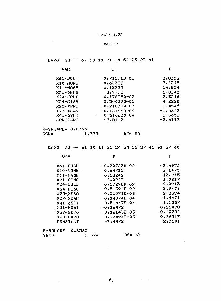
Table 4.22

Cancer

CA70 53 -- 61 10 11 21 24 54 25 27 41

VAR B.

X61-CIQCH X10-NONW X11-MAGE X21-DENS X24-COLD X54-C168 X25-XFRO X27-XCAR X41-6SFT CONSTANT

-0+7127lD-02 -3.8356 0.63382 3,4249 0*13235 14,854

3*9772 1.8342 0+17859D-02 2+3216 0.50032Ib02 4+2228 0.21038IPO3 2.4545

-0+13166D-04 -1.4643 0,51683D-04 1.3652 -9*5112 -2e6997

R-SQUARE= Oe8556 SSR= 1.378 BF= 50

T

CA70 53 -- 61 10 11 21 24 54 25 27 41 31 57 60

UAR B T

X61-ImCH X10-NONW X11-MAGE X21-DENS X24-COLD X54-CT68 X25-,XPRO X27-XCAR X41-6SFT

,X31-NO69 X57-SO70 X60-PA70 CONSTANT

-0+70763D-02 -3.4976 0.64712 3+1475 Oel3242 13.915

4,0247 lr7837 0,17298D-02 2.0913 Oc51394D-02 3.9471 0+21071D-03 2+3394

-0,14074D-04 -1.4471 0 .51447II-04 1+1257

-0.16472 -0.21498 -0,16143D-03 -0.10784.

0.23494W03 0.26317 -9+4472 -2.5101

R-SQUARE= 0+8560 SSR= 1,374 DF= 47

66

However, differences between our estimated air pollution effects as opposedto the Lave and Seskin (1977) work are profound. Lave and Seskin (1977)did not find a significant association between particulates and pneumonia.More importantly, Lave and Seskin (1977) found positive associationsbetween air quality (specifically sulfate) and a cardiovascular diseasemortality variable and between air quality and cancer mortality. Whetherwe use SO

2or the highly collinear sulfate measure, we cannot accept the

hypotheses that air pollution has any association with heart and vasculardisease or with cancer mortality. Further, our estimated total effects ofair pollution on human mortality are about one order of magnitude smallerthan those shown by Lave and Seskin (1977).

We can summarize the results of our analysis as follows. When weincrease each of the. following significant variables by one percent overtheir mean values in our sample, from the estimated total mortality equationthe following percentage change in mean total mortality rate results: (1)for doctors per capita a 0.76 percent decline in mortality rate; (2) forper capita cigarette consumption a 0.32 percent increase in mortality rate;and (3) for per capita protein consumption a 6.7 percent increase in mor-tality rate. These results suggest several observations. First, medicalcare, smoking, and diet appear to be enormously important factors in humanhealth. Second, if one looks to a 100% decrease from mean levels for thesevariables, i.e., the impact on average total mortality of setting thesevariables to zero, one obtains a 76% increase in mortality for a zero levelof doctors per capita, a 3.2% decrease in mortality for no smoking and a670% decrease in mortality for no protein in diet. Obviously, the last ofthese effects is impossible and suggests that we may only have linearapproximations of highly non-linear effects. Further, some protein isrequired to sustain life. Thus, the estimates of mortality effects arelikely to be valid only for relatively small changes in explanatory variables.Finally, the air pollution variables are insignificant in the total mor-tality equation -- as one might suspect if air pollution has only a smalleffect. on mortality rates. This is verified by the fact that the signi-ficant estimated effects of particulates on pneumonia and influenze, and ofSO2 on infant diseases are very small in terms of total mortality as com-pared to the effects of doctors, smoking, and diet.

Given these results, it is important to test the sensitivity of themodel to changes in specification of included variables and structure. Twoalternative formulations have been specified and tested. First, a versionof the model which: (1) uses lagged diet (1955 dietary variable) as op-posed to 1965 diet); (2) employs a two-stage doctors per capita variablewhich includes air pollution in the reduced form equation; and (3) addslead and sulfate to the air pollution variables, produces essentially iden-tical results both for the impact of medical care and, air pollution onmortality. Sulfate air pollution is statistically insignificant across alldiseases. The second alternative formulation is identical to the onepresented in detail above but the air pollution variables are again includedin the reduced form equation for doctors per capita. The results are con-sistent for the effect of medical care and for the positive associationsbetween sulfur oxides and infant diseases and for particulates and pneumonia.More interesting, however, is a significant negative association which

67

appears between doctors per capita and air pollution in the reduced formequation. It appears that doctors may choose not to live in pollutedcities (perhaps for aesthetic reasons). If this is the case, one can easilyexplain false positive associations between air pollution and mortalitywhere medical care is excluded as an explanatory variable. If doctorsavoid polluted cities, and if doctors do reduce mortality rates, thenpollution could well be associated with higher mortality rates; but notbecause of any direct health effect of air pollution on mortality. Rather,failure to account for the locational decisions of doctors (supply and de-mand for medical care) may well bias estimated epidemiological relationships.In fact, the negative association between doctors per-capita and pollutionis so strong, that when pollution is included in the reduced form equationfor doctors, the estimated doctors variable used in the two-stage procedurebecomes collinear with the pollution variables. This collinearity in somecases produced negative coefficients on the pollution variables in estimateddose-response relationships for some disease categories where pollution isused in the reduced form equation for docotrs per capita. Thus, it isimportant that, in spite of this collinearity, stable positive associationsare retained between pneumonia and influenza and particulates and betweeninfant diseases and sulfur oxides. The inclusion or exclusion of air qualityfrom the reduced form equation has little impact on the conclusions of thisstudy. In part, this occurs because air pollution is collinear with diet.In fact, saturated fats and sulfur oxides are reasonable proxy variables foreach other. It has been shown by McCarthy (1971) that the exogenousvariables which are collinear with included exogenous variables may beexcluded from estimated reduced forms with little loss in consistency in atwo-stage least squares procedure.

Another important question for analysis is the possibility that hetero-skedasticity is present. At this point, we have only examined one diseasecategory -- cancer mortality -- for this problem. An examination of theresiduals plotted against several important explanatory variables (age, forexample) showed no evidence of heteroskedasticity.

Finally, in interpreting the results, it should be observed that theassociations we have found between mortality and air pollution are princi-pally for diesases of the very young and very old -- particularly susceptiblegroups within the population. Further, these effects are those which onewould perhaps associate with short-term as opposed to long-term air pol-lution exposures. It may well be that aggregate epidemiology may be in-capable of revealing the long-term consequences of air pollution exposures.Two problems are particularly significant here. First, lagged data ordata on air pollution histories is not available for such studies. Second,it is nearly impossible to control for population mobility in such studies.Thus, even if one accepts the hypothesis that air pollution levels showenough persistence over time to reveal long-term effects, population mobil-ity will still distort and confound attempts at estimating such effects.A partial remedy for these problems is, of course, to use data on individ-uals as opposed to aggregate data. The next chapter provides a preliminaryexploration of just such a data set.

We now turn to an economic evaluation of the value of air pollutioncontrol in reducing mortality based on the value of safety approach described

68

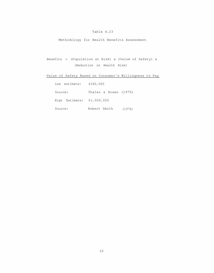
Table 4.23

Methodology for Health Benefits Assessment

Benefits = (Population at Risk) x (Value of Safety) x

(Reduction in Health Risk)

Value of Safety Based on Consumer's Willingness to Pay

Low estimate: $340,000

Source: Thaler & Rosen (1975)

High Estimate: $1,000,000

Source: Robert Smith (1974)

69

above.

4.6 A Tentative Estimate of The Value of Safety from Air Pollution Control

Given all of the caveats discussed above concerning the validity ofthe estimated effects of air pollution on mortality, it is possible to con-struct benefit measures using the methodology outlined in Section 4.2above. The methodology is briefly summarized in Table 4.23.

First, to obtain national estimates, we must know the population atrisk. Since our sixty-city sample is entirely urban, and since air pol-lution is principally an urban problem we will use a population risk for1970 of 150 million urban dwellers. As a range for the value of safety,we will employ Thaler and Rosen's (1975) estimate of $340,000 (in 1978dollars) as a lower bound and Smith's (1974) estimate of $1,000,000 (in1978 dollars) as an upper bound. Finally, to provide an estimate of re-duced risk from air pollution control, we will assume an average 60% reduc-tion in ambient urban concentrations both for SO2 and particulates. Then,using the mean concentration of these pollutants in our sixty-city sampleas a basis for calculation, we can derive the average reduction in risk ofpneumonia mortality for a 60% reduction in particulates and the averagereduction in risk of infant diseases for a 60% reduction in SO from ourestimated dose response functions for these diseases.

2

Multiplying the population at risk by the assumed value of safety, andthen by the average reduction in risk, gives a crude approximation of thebenefits for a 60% reduction in national urban ambient concentrations ofparticulates and SO2, respectively. National urban totals and the value ofthe average individual risk reduction are shown in Table 4.24.

The value estimates as shown in Table 4.24 agree surprisingly well withthose developed by Lave and Seskin (1977) for national air pollution damages.However, the dollar value is similar only because we use a range for thevalue of safety (derived from observed market behavior of consumers) whichis about an order of magnitude larger than the “value of life" figure basedon lost earnings which is employed by Lave and Seskin (1977). We, of course,reject the value of life notion, instead focusing on the measurable conceptof value of safety. Since there is no evidence to suggest that societyputs less value on safety for children, the aged or women than on employedheads of households, we feel that the best measures available now for thevalue of safety should be employed for all individuals. Eventually, morerefined measures of the value that different individuals place on safetymay become available. However, for the time being, these are the bestvaluations of the social worth of safety we can employ.

70

Table 4.24

Urban Benefits from Reduced Mortality: Valueof Safety for 60% Air Pollution Control

Average Individual NationalSafety Benefit Urban Benefits

Disease Pollutant (1978 Dollars/Year) (1978 Billion Dollars/Year)

Pneumonia Particulates 29 - 92 4.4 - 13.7

Early InfantDisease SO

25 - 14 .7 - 2.2

Total 34 - 106 5.1 - 15.9

71

CHARTER V

THE MICHIGAN SURVEY EXPERIMENT

5.1 Objectives of the Experiment

The data set employed in this chapter refers to the health status andthe time and budget allocations of each of several thousand household headsover a nine-year period. Its highly disaggregated form therefore avoidsmany of the estimation problems associated with the aggregate data used inChapter IV. This avoidance is not our only purpose, however. The richnessof detail in the data set allows us to extend the range of phenomena thatwe study. Most important, we are able to investigate the morbidity effectsof air pollution, considering acute effects and chronic effects separately.The detail of the data set allows us to identify much more readily thosevariables that are not current determinants of health status, thus providinga means of avoiding the simultaneity problems that plagued the aggregatedose-response functions of the previous chapter. It is important to notethat the results reported here reflect a preliminary attempt to evaluate theusefulness of Michigan Survey Data in estimating morbidity (sickness) effectsof air pollution and consequent economic losses. As a result of thepreliminary nature of the research, many highly desirable transformations ofthe variables as defined in the Michigan Survey Data set have not yet beenmade. However, in spite of the preliminary nature of the results theydo represent the first attempt to qualify the economic losses due to morbidityas opposed to mortality resulting from air pollution.

With the richness of the data available to us, we need not terminateour efforts after having estimated a set of dose-response expressions forthe morbidity effects of air pollution. We are able to ascertain the laborproductivity effects and the impact on willingness to pay to avoid chronicand/or acute illness as well. Both of these additional efforts are under-taken in this chapter.

5.2 The Sample and the Variables

Our analysis is based on yearly interviews conducted by the Universityof Michigan's Survey Research Center with a nationwide random sample of4,802 to 5,862 families from 1968 through 1976. No families with livingmembers were ever intentionally deleted from the sample, and, as familiesbroke apart, the adult components were added to the sample as distinctfamilies. The cumulative interview response rate over the nine-year perioddeclined from 76 percent in the 1968 and first interview year to 55 percent

72

in the 1976 interview year, implying an average yearly reinterview responserate of nearly 95 percent. From 1970 through 1976, this yearly responserate averaged 97 percent. Of special interest to us is that, in additionto substantial detail on household head time and budget allocations, thesample contains generalized measures of the head's health states as wellas information on lifestyle and biological and social endowment variablesthat might plausibly contribute to the health states.

Information from the interview has been combined with data on a limitedset of environmental variables, particularly information on air pollutionconcentrations, to establish imperfect measures of the environment in whicheach family head has lived during the nine-year period. To the best of ourknowledge, the Survey Research Center data set is the only one currentlyavailable that combines, for the same set of individuals over a substantialnumber of years, information on places of residence, states-of-health, andtime and budget allocations. The sample thus raises the prospect of ourbeing able to value, through empirical applications of the economic theoryof consumer behavior, the contributions of environmental pollution exposuresto states-of-health.

The major characteristics of our sample and the variables we employ inour empirical efforts are presented in Tables 5.1 and 5.2. All variablesrefer to household heads. Table 5.1 gives complete definitions of variables,their scalings, and their assigned acronyms; Table 5.2 provides representa-tive arithmetic means and standard deviations of variables used. Becausewe employ various partitions of the sample throughout the chapter, we do notuse the Survey Research Center sample weights. Cur samples are thereforenot entirely representative of the national population.

In Table 5.2a, so as not to make worse the already considerable andcumbersome length of the listing, only the two health variables, LDSA andACUT are listed as dependent variables. The geometric means of the airpollution variables have their means and standard deviations entered forthe various sample partitionings indicated at the bottom of the table.The means and standard deviations for the other variables are listed inTable 5.2b. This latter table refers only to the samples used for thechronic illness expressions, while the former refers to the acute illnessexpressions. Whether reference is to the partitioned or unpartitionedsamples, the means and standard deviations represent only those samplesused to estimate dose-response functions involving geometric mean measuresof the air pollution variables. All estimates employing different combina-tions of variables, whatever the combination might be, were establishedusing a random drawing from the entire Survey Research Center populationsample for a particular year. Therefore, the means and standard deviationslisted in Table 5.2, although extremely representative, are not the exactvalues for each of the samples used in the estimation effort.

The definition and measurement of most of the variables listed inTables 5.1 and 5.2 is standard, and we shall comment here only on those thatpose definitional and measurement problems for the major focus of thisreport. This criterion immediately directs attention to the air pollutionvariables.

73

Table 5.1

Complete Variable Definitions

Health State Variables

Acute illness (ACUT) -- workdays ill times 16 for the first 8 weeksand times 12 thereafter. Only individuals who are currentlyemployed or unemployed and looking for work could have positivevalues for this variable.

Degree of disability (DSAB) -- complete limitation on work = 1;severe limitation on work = 2; some limitation on work = 3;otherwise = 0.

Length of disability (LDSA) -- 2 years = 1; 2 - 4 years = 2;5 - 7 years = 3; 8 years = 4; otherwise = 0. This is afollow-up question to inquiries about whether the respondenthas any physical or nervous condition that limits the amountor kind of work or housework he can do.

Biological and Social Endowment Variables

Age of family head in years (AGEH)Grew up in city (CITY) = 1; otherwise = 0. This variable, as

transformed, is binary.Education attainment (EDUC) -- 6 - 8 grades = 2; 9 - 11 grades = 3;

12 grades = 4; 12 grades plus non-academic training = 5; college,no degree = 6; college degree = 7; advanced or professionaldegree = 8; otherwise = 1.

Father's educational attainment (FEDU) -- same scaling as for EDUC.Family size in number of persons in housing unit (FMSZ).Length of present employment (LOCC) -- ~1 year = 1; 12 - 19 months

= 2; 1-1/2 - 3-1/2 years = 3; 3-1/2 - 9-1/2 years = 4;9-1/2 - 19-1/2 years = 5; 19-1/2 years = 6; otherwise = 0.

Marital status (MARR) -- married = 1; otherwise = 0. This variable, astransformed, is binary.

Income level of parents (POOR) -- poor = 1; otherwise = 0. Thisquestion asked whether the respondent's parents were " . . . poorwhen you were growing up, pretty well off, or what?" Thevariable, as transformed, is binary.

Race of family head (RACE) -- white = 1; otherwise = 0. This variable,as transformed, is binary.

Sex of family head (SEXH) -- male = 1; otherwise = 0. This variable,as transformed, is binary.

Member of a labor union (UION) -- Yes = 1; otherwise = 0. Thisvariable, as transformed, is binary.

Life Style Variables

Practices absenteeism from work (ABSN) -- absent once or more a weekfrom work = 1; otherwise = 0. This refers to a question in whichthe respondent is asked if there are times when he doesn't goto work at all, even if he isn't sick. The variable, astransformed, is binary.

74

Table 5.1(continued)

Frequency of church attendance (CHCH) -- once a week or more = 1;otherwise = 0. This variable, as transformed, is binary.

Annual family expenditures on cigarettes in dollars (CIGE) -- thisvariable is not indexed for differences in prices among locales.

Participates in energetic activities (EXER) -- first mention = 1;otherwise = 0. This question asks the family head what heusually does in his spare time. Energetic activities includefishing, bowling, tennis, camping, travel, hunting, dancing,motorcycling, etc.

Family food consumption relative to food needs standard in percent(FOOD) -- family food consumption refers to food expenditures indollars and includes amounts spent in the home, school, work,and restaurants, as well as the amount saved in dollars byeating at work or school, raising, canning or freezing food,using food stamps, and receiving free food. The food needsstandard is in dollars and is based on USDA Low Cost Planestimates of weekly food costs as published in the March 1967issue of the Family Economics Review. The standard itself iscalculated by multiplying the aforementioned weekly food needsby 52 and making a series of adjustments according to the sizeof the family.

Is often late to work (LTWK) -- late once or more a week to work = 1;otherwise = 0. This question asks the respondent if. there aretimes when he is late getting to work. The variable, astransformed, is binary.

Daily number of cigarettes smoked per adult family member (NCIG) --53 =1; 3- 17 = 2; 18 - 22 = 3; 23 - 35 = 4; 2 - 3 packs = 5;24 packs = 6; otherwise = 0.

Fundamentalist religious preference (RELG) -- Mormon, United Churchof Christ, Disciples of Christ, Quaker, etc. = 1; otherwise = 0.This variable, as transformed, is binary.

Degree of risk aversion (RISK) -- a weighted index devised by thesurvey team in which the individual's degree of risk aversionincreases if he drives the newest car in good condition, doesnot own a car, has all cars insured, uses seat belts, hasmedical insurance, smokes less than a pack a day, has some liquidsavings, and has more than two month's income saved. Nine is thegreatest degree of risk aversion that can be exhibited.

Head's annual hours working for money (WORK).

Precuniary Variables

Cost-of-living in 1970 country of residence (BDALO) -- an index ofcomparative costs for a four-person family living in variousareas as published by the U.S. Bureau of Labor Statistics in theSpring 1967 issue of Three Standards of Living for an UrbanFamily of Four Persons. The lowest living standard was employed.This index is published for the thirty-nine largest SMSA's and byregion for the nonmetropolitan areas. For the remaining SMSA's,the regional average of the metropolitan indices was used.

75

Table 5.1(continued)

Has hospital or medical insurance (INSR) -- Yes = 1; otherwise = 0.This variable, as transformed, is binary.

Family income in dollars not due to current work effort (ICTR) -- thisvariable includes assorted welfare payments, pensions, andannuities, as well as earnings from assets.

Family net real income in dollars (RINC) -- this variable is the sum ofmoney income plus value of goods and services received at lessthan market prices less the cost of earning income.

Savings in dollars equal or greater than two month's income (SVGS) --Yes = 1; otherwise = 0.

Head's marginal hourly earnings rate in cents (WAGE) -- in circumstanceswhere the head neither has a second job nor commands overtime pay,this variable is simply total annual earnings from labor dividedby annual hours worked for money. Where he has two or more jobs,it is his hourly earnings in the last job he names. If he hasonly one job, can and does work overtime if he wishes, andreceives overtime pay, the variable is his average overtimehourly earnings.

Environmental Variables

Works in chemicals or metals manufacturing industries (CHEM) -- Yes =1; otherwise = 0. The chemicals industry includes chemicalsand allied products, petroleum and coal products, and rubber andmiscellaneous plastic products. The metals industry includessteel, aluminum, foundaries, etc.

Number of days in 1972 when temperatures were below freezing at sometime during the day (COLD). This data was obtained from USNOAA,Climatological Data, National Summary 1972.

Number of persons per room in family dwelling (DENS).Distance from nearest city of 50,000 or more people (MILE) -- 5 miles

or outside continental United States = 1; 5 - 15 miles = 2;15 - 30 miles = 3; 30 - 50 miles = 4; 50 miles = 5.

Nitrogen dioxide: annual 24-hour geometric mean (M), ninetiethpercentile (N), and 30th percentile (T) in micrograms percubic meter as measured by the Gas Bubbler TGS Method-Fritbefore 1974 and the Saltzman method for 1974 and after (NOX).This data was obtained from the annual USEPA publication,Air Quality Data -- Annual Statistics.

Sulfur dioxide: annual 24-hour geometric mean (M), 90th percentile(N), and 30th percentile (T) in micrograms per cubic meter asmeasured by the Gas Bubbler Pararosaniline-Sulfanic Acid Method(SUL). This data was obtained from the annual USEPA publication,Air Quality Data - Annual Statistics.

Total suspended particulates: annual 24-hour geometric mean (M),90th percentile (N), and 30th. percentile (T), in micrograms percubic meter as measured by the Hi-Vol Gravimetric method (TSP).This data was obtained from the annual USEPA publication,Air Quality Data -- Annual Statistics.

76

Table 5.1(continued)

Ultraviolet radiation in microwatts per square centimeter (ULTV).This data was taken from Pazand, R., Environmental Carcinogenesis-- An Economic Analysis of Risk, unpublished Ph.D. dissertation.University of New Mexico (June 1976).

Explanation of Table

Unless otherwise stated, all data is taken from tapes described inSurvey Research Center, A Panel Study of Income Dynamics, Ann Arbor:Institute for Social Research, University of Michigan (1972, 1973, 19741975, 1976).

All variables referring to an individual person refer only to thefamily head.

On occasion, definitions for the same phenomenon will differ fromyear to year. If this occurs, a single integer indicating the year towhich reference is made is attached to the end of the variable acronym.Thus 1967 = 7; 1968 = 8; . . .; 1976 = 6.

77

78

Table 5.2a

Representative Means and Standard Deviations of Health and Air PollutionVariables for Samples Involving Family Heads Currently Employed or

Actively Looking for Work*

YearVariableAcronym 1967 1968 1969 1970 1971 1972 1973 1974b

Health States

ACUT 100.414 120.486 133.657 113.750 113.323 149.845 112.530(183.594) (214.759) (332.171) (277.022) (266.274) (427.983) (259.120)

aLDSA

0.953 0.645 0.337 0.363 0.268 0.290 0.260 0.348(1.720) (1.326) (0.979) (0.971) (0.888) (0.921) (0.874) (0.952)

Environmental

NOXM 157.043 118.045(51.070) (72.230)

SULM 24.475 25.113 27.220 16.286 17.657 2.051 7.435(19.098) (18.714) (25.013) (12.150) ( 9.449) (4.188) (11.728)

TSPM 100.403 99.917 98.713 95.534 87.213 99.157 35.310 71.1.08(35.469) (30.628) (29.609) (18.943) (27.920) (30.941) (42.183) (36.085)

a Except for 1970, all samples refer to family heads who have never lived in more thanthan one state. In 1971, the reference is to family heads who currently live withinwalking distance of relatives.

b Includes housewives, retirees, and students.

*Standard deviations are enclosed in parentheses.

79

Table 5.2b

Representative Means and Standard Deviations of All Other Variablesa

VariableAcronym 1967 1968 1969 1970 1971 1972 1973 1974 1975

Health State

DSAB 0.493(1.291)

Biological and Social Endowment

AGEH 43.558(12.337)

CITY 0.646(0.481)

EDUC 3.680(1.696)

FEDU 2.391(2.254)

FMSZ 3.812(2.401)

LOCC 2.257(2.234)

MARR 0.617(0.489)

POOR 0.578(0.496)

0.111(0.315)

40.323(11.841)

0.451(0.498)

3.683(1.747)

2.300(2.036)

4.586(2.542)

3.271(1.869)

0.617(0.487)

0.543(0.499)

0.426(1.634)

43.745(13.451)

0.678(0.468)

3.878(1.862)

2.313(1.442)

3.993(2.376)

0.488(1.011)

44.218(13.649)

0.678(0.468)

3.923(1.866)

2.360(1.473)

3.930(2.412)

0.5200.500

0.470(0.949)

44.305(15.276)

0.632(0.459)

7.705(1.851)

2.458(1.609)

3.508(2.202)

2.283(2.168)

0.490(0.501)

0.304(0.754)

45.155(16.158)

0.655(0.476)

3.720(1.844)

2.395(1.451)

3.233(2.126)

2.168(2.188)

0.525(0.500)

0.520(0.500)

0.800(2.159)

37.322(15.421)

3.912(1.672)

0.468(0.500)

0.551(0.499)

(continued)

0.624(1.854)

37.92514.749

3.659(1.685)

0.540(0.500)

0.615(0.488)

80

Table 5.2b(continued)

VariableAcronym 1967 1968 1969 1970 1971 1972 1973 1974 1975

RACE 0.469(0.501).

0.917(0.276)

0.410(0.099)

0.635(0.482)

0.233(0.423)

0.225(0.418)

822.500

0.500(.0.501)

0.443(0.497)

0.475(0.500)

0.346(0.477)

0.631(0.417)

1145.150(707.099)

0.640(0.382)

1030.976(574.163)

SEXH 0.629(0.468)

0.677(0.496)

0.635(0.482)

0.573(0.495)

0.603(0.490)

UION 0.354(0.479)

0.198(0.399)

0.198(0.399)

Lifestyle

ABSN 0.108(0.310)

CHCH

CIGE

EXER

FOOD

0.440(0.448)

93.146(124.022)

0.144(0.352)

0.189(0.392)

0.198(0.399)

505.830 757.669 840.990(380.977) (372.594) (716.450) (716.100)

LTWK 0.070 0.209(0.255) (0.407)

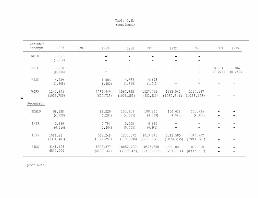
81

Table 5.2b(continued)

VariableAcronym 1967 1968 1969 1970 1971 1972 1973 1974 1975

NCIG 1.851(1.912)

RELG 0.018(0.136)

0.054 0.062(0.226) (0.242)

RISK 4.489(1.605)

4.503(1.452)

4.658(1.545)

4.673(1.540)

WORK 1245.875(1059.780)

Pecuniary

1989.649(674.723)

1560.895(1001.253)

1527.732 1333.540 1354.137(982.381) (1030.346) (1056.153)

BDALO 99.638(4.720)

99.220(4.297)

100.413(4,625)

100.266 100.618 100.736(4.788) (4.925) (4.819)

INSR 0.889(0.316)

0.794(0.404)

0.708(0.455)

0.695(0.461)

ICTR 1096.22 508.249 1238.392 1013.846 1342.585 1366.702(1314.401) (1124.259) (1198.698) (1721.377) (1874.235) (1993.720)

RINC 9148.605 8902.377 10852.230 10875.650 9556.803 11077.9506511.900 (6100.167) (7833.473) (7439.632) (7274.871) (8337.711)

(continued)

82

Table 5.2b(continued)

VariableAcronym 1967 1968 1969 1970 1971 1972 1973 1974 1975

0.371(0.484)

358.258(331.738)

61.768(38.495)

SVGS 0.342(0.475)

0.289(0.454)

0.333(0.472)

322.500(316.450)

0.008(0.086)

74.66366.016

336.525(337.425)

298.230(319.890)

WAGE 292.119(405.985)

314.440(221.346)

Environmental

CHEM 0.022(0.147)

0.003 0.049(0.050) (0.216)

0.045(0.206)

COLD 81.502(52.684)

DENS 3.420(1.797)

0.870(1.198)

0.725(0.414)

NOXN 246.57379.826

104.860 97.429(75.994) (44.564)

90.717(22.716)

NOXT 132.045(37.087)

31.536 32.931(23.964) (31.761)

48.597(13.911)

SULN 107.687(134.484)

42.625 34.566(31.115) (42.841)

25.650(41.603)

(continued)

83

Table 5.2b(continued)

VariableAcronym 1967 1968 1969 1970 1971 1972 1973 1974 1975

SULT 26.041 10.798 11.190 9.551 5.006 7.836(37.369) (10.663) (5.875) (9.305) (9.955) 8.233

TSPN 176.986 248.965 156.185 170.768 147.960 126.702 120.580(78.097) (339.668) (63.787) (58.121) (39.684) (43.086) (56.438)

TSPT 77.605 74.837 74.088 82.995 56.232 67.122 62.779(23.661) (43.932) (20.772) (26.627) (9.650) (22.200) (27.046)

ULTV 1494.75(634.638)

a All samples include housewives, retirees, and students.

*Standard deviations are in parentheses.

If one has detailed and real-time information on changes in healthstates, ideally one would like to have real-time records of all airpollution exposures. The coarse yearly indicators of acute and chronicillness in the Survey Research Center (SRC henceforth) data could notsupport such detail. We therefore chose to collect outdoor air pollutiondata averaged over a time period corresponding to the time intervalemployed in the SRC data. In addition, we wished to ascertain whetherrepresentations of moments of the outdoor air pollution frequencydistribution other than measures of central tendency might contribute toill-health. The result of these deliberations was a decision to acquiredata on the geometric mean (because outdoor air pollution tends to belog-normally distributed over time), 30th percentile, and 90th percentileof the annual concentrations of five pollutants: nitrogen dioxide; ozone;total oxidants; total suspended particulates; and sulfur dioxide.Although the ozone and total oxidant data has been combined with the SRCdata, the number of monitoring locations and the monitoring time intervalswere inadequate to allow other than minor variations in the exposures ofthe sample individuals. Thus the empirical results to be reportedneglect these two possibly important pollutants.

Matching the thousands of outdoor air pollution monitoring stationsin the United States to the hundreds of counties where the SRC samplefamilies resided could be a complex combinatorial problem. The matchingwas achieved for each of the nine years at the cost of not having outdoorair pollution information for some SRC sample families during some yearsand of assigning somewhat inappropriate air pollution exposures to somesample individuals. The full extent of this information loss is presentlyunknown.

The matching process started by listing all the counties in theUnited States where one or more SRC sample families had resided during thenine year interval. Separately for each of the five previously mentionedair pollutants, a yearly listing of the counties having outdoor airpollution data for one or more of the three frequency distributionmeasures being considered was constructed. Of the 301 counties in 50states where sample families resided during the nine year interval,outdoor air pollution monitoring data for one or more of the measures ofone or more of the five air pollutants existed at least for one year in118 of the counties in 50 states. No attempts were made to extrapolate airpollution data from one county to another, nor were any switches betweenmonitoring stations in a single county ever made. In counties wheremultiple outdoor monitoring stations were present, the data from the singlestation that had operated for the greatest portion of the nine years wasused. If two or more stations in a county had operated for equalportions of the nine years, the station having the most complete (interms of numbers of pollutants and pollutant measures) was employed.When air pollution data were available in a family's residence county fora particular year, these criteria served to assign outdoor air pollutionexposures to all sample families. For most years, somewhat more than3,000 families had some sort of outdoor air pollution data assigned them.Because of our reluctance to adopt a new monitoring station location in acounty whenever the activities of a station we had previously used wereterminated, we undoubtedly missed a few opportunities to assign air

84

pollution data to a few sample families. This issue pales, however,beside the issue of the extent to which the assigned data representactual outdoor air pollution exposures.

The SRC family data sample provides only the family's county andstate of residence: it does not give the home town or city. Thus, forlarge urban counties such as Cook County, Illinois, or Los Angeles County,California, or occasional rural counties such as San Bernardino County,California, where there exist major locational differences in potentialair pollution exposures within the county, substantial error could existin the air pollution assignations. This important source of measurementerror could perhaps be substantially reduced if all counties having thisproperty were identified and if all families residing in the identifiedcounties were

f7cised from the sample. We have made no attempt to perform

this excision.-

This criteria employed to select pollution monitoring stations probablyresult in the assignment of downtown urban locations, where pollutionconcentrations have historically tended to be greatest and where the mostextensive monitoring has been done. Since relatively few of the SRCsample families actually live in downtown areas, the constructed dataset generally exaggerates family outdoor air pollution exposures, implyingthat the health effects, if any, of air pollution will tend to be under-estimated. 2/

Outdoor air pollution at the place of residence is not the onlyplausible environmental source of deleterious health effects. Indoorair pollution at home and in the work place, outdoor air pollution atother locations, contaminants in diet, and water pollution are additionalwidely acknowledged possible sources. We introduce measures (albeitimperfect) of some of these plausible alternative sources in our empiricalefforts and fail to give any attention to others such as water pollution.If these excluded types of pollution have health effects of their own, andif their extent tends to be positively correlated with the extent ofoutdoor air pollution, then the included air pollution variables willcapture some of their contributions to ill-health, causing the measuredcontribution of the outdoor air pollution variables to be exaggerated.The extent of this upward bias will vary directly with the degree ofcorrelation between the included and the excluded variables and the extentto which the excluded variable actually contributes to the effect ofinterest. For this study, of the previously mentioned alternativeenvironmental pollution sources of health effects, the utter exclusion ofany measures of water pollution is perhaps the most serious, At variouspoints in the empirical effort, rather crude measures of indoor home airpollution (family smoking habits), diet (a dietary adequacy index), andindoor air pollution at the work place (employment in the chemicals or

3/metals manufacturing sector) are included.

The issue of excluding possibly relevant variables from the analysisincluded outdoor air pollution as well. Oxidants and ozone, Because ofinsufficient variation in apparent exposures among sample families, havebeen disregarded, even though exposure values are present in theconstructed data set. Other important air pollutants, for which data were

85

available such as carbon monoxide, were not even considered because of thelarge variations in their instantaneous concentrations within a fewhundreds of feet. Some pollutants that have attracted recent regulatoryand public concern, such as acid sulfates, had no data readily available.Finally, of the pollutants that were included in the constructed dataset and exploited in the empirical effort, the time series for all excepttotal suspended particulates were incomplete. Thus, for example, noinformation was available on sulfur dioxide concentrations in 1972.

Measurement error is not only an issue in the outdoor air pollutionvariables. What some might choose to interpret as measurement error is aprime feature of the two dependent variables, number of days annually

4/ill and length of time disabled. Although we have no basis other thanseemingly sensible intuitive interpretations of the form of the questionsasked the respondents (see the explanations for ACUT and LDSA in Table 5.1),we choose to interpret the former as acute illness and the latter aschronic illness. Definitional problems of the distinction between acuteand chronic illness aside, it must be remembered that what is an illnessto one individual is not an illness to another individual. Even the sameindividual may differ over time in what he considers to be a state ofillness. Illness is, in part, an idiosyncratic and subjective phenomenononly partly susceptible to consensus standards of definition. Therefore, ifone prefers a reductionist perspective and wishes to have all phenomenacollapse to, say, a chemical measurement, then the values of the variableswe are trying to explain in this study indeed leave a great deal to bedesired.?' Economic analysis, however, presumes that illness and itscosts lie in the eye of the beholder. No laws whatsoever governing choicesare innate in the material objects of ordinary cognition. As has beenemphasized in the introduction to this section of the report, the degreeof illness that afflicts an individual is, in part, often a matter ofpurposive choice. Economic principles relate to the subjective desiresmotivating individuals to become aware of and perhaps to alter theirenvironments. Thus no object or status becomes relevant in economicanalysis until humans perceive it can be used for or defeats somesubjective purpose. Illness that is defined in clinical terms but which isnever subjectively realized by the individual who is said to be clinicallyill is of little interest except to clinicians. It is certainly arguablewhether their standards of what constitutes illness should prevail over thoseof the individual who professes illness. For this study, we are forced bycircumstances to adopt the latter's perspective. Fortunately, it fitsreadily into economic analysis.

In spite of the preceding argument a type of measurement error doespersist in the two dependent health variables. This type of error isinherent in the use of any fairly encompassing measure of health status.Kinds of debilitating acute illness for an individual may range, for example,from headaches to heel blisters. Chronic illnesses may show similarvariations over body sites and implied debilitating effects for the sameindividuals. In effect, therefore, an individual's response to a questionabout the number of days he has been ill or the length of time he has beendisabled involves an aggregation of several attributes perhaps sampled fromsome larger population of attributes. The weights the respondent employsto combine these attributes to obtain the encompassing health measures

86

may differ among individuals. Furthermore, they may not be those weightsthat correspond to the contribution of the attribute to some otherparameter of interest, such as hours of work or money wages. Recognitionof the possibility that individuals may employ different weights toaggregate to the encompassing health measure serves perhaps to deepenthe reader's perception of the subjectivity of our measures of ill-health.It says only that there may be as many unique measures of ill-healthemployed as there are respondents in the sample. The import for ourempirical efforts of discrepancies between the contributions of attributesto ill-health and to other parameters of interest is greater, since weshall try to ascertain the impact of air pollution-induced ill-health uponlabor supply and productivity. In particular, the use of the encompassingmeasures of ill-health rather than the specific attributes may attenuatecur estimate of the effect of air pollution-induced health effects uponlabor supply and productivity.

As Table 5.1 indicates, all SRC sample individuals not currentlyemployed or seriously looking for current employment had no informationrecorded about the number of days they professed to be acutely ill.Furthermore, those individuals for whom information on ACUT was recordedwere never sick on weekends: their accute illneses occurred, according tothe data, only on workdays. The ACUT variable may thus be confounded by thewish of some respondents to legitimatize for the sake of social appearanceor internal self-respect their failure to go to work. In the empiricalefforts regarding ACUT therefore, an actual choice of leisure over laborcould thus be falsely attributed to ill health. Marquis (1978), howeverhas been unable to discover any basis for this source of bias.

The rather long list of other variables considered can be divided,somewhat imperfectly, into health state, biological and social endowment,lifestyle, pecuniary, and environmental variables. For the moment, we willlimit our discussion of the variables not already discussed to the partsthey are expected to play in dose-response functions, reserving thediscussion of labor supply and productivity impacts to a later section.Only those variables actually used in the estimated dose-response functionsare therefore discussed in this section. A summary table of expectedsigns is presented in Table 5.3.

DSAB, the degree of disability is the only included health statevariable not employed as a dependent variable. Since it is ordinallyscaled, its meaning when used as a dependent variable is arbitary. Anyfour or five monotonically increasing numbers would have no more and noless meaning. When entered as an explanatory variable in the chronicillness production function, its expected sign is unclear. If the individualcontinues to live in spite of having a chronic disability, one would expectthe period of recovery, if any, to be lengthier the more severe thedisability. However, in the general population, severe disabilitiesperhaps are more likely to lead to earlier death. Thus, those sampleindividuals who are severely disabled might be expected to have beendisabled only for a relatively short time span. This would lead one toexpect a negative association between DSAB and LDSA. Which effect woulddominate in any particular sample must be conjectural. In contrast, sincedisabilities, both in terms of length and severity, probably cause the

87

Table 5.3

Health StatesDSABLDSA

Expected Signs for Explanatory Variablesin Estimated Dose-Response Functions

Acute Illness Chronic Illness

Biological and Social EndowmentsAGEHCITYEDUCFEDUFMSZMARRPOORRACESEXH

LifestylesCHCHEXERFOODNCIGRELGRISK

PrecuniaryINSR

EnvironmentalCHEMCOLDDENSAll NOXAll SULAll TSPULTV

? unknownX irrelevant

88

individual to be more susceptible to common temporary illness, we expectLDSA and DSAB to contribute positively to ACUT. However, because thevalues for DSAB are not monotonically ordered, the magnitudes of thecoefficients for DSAB in both the LDSA or the ACUT expressions should bedisregarded.

No one holds that health states improve with adult age. The adulthuman organism suffers natural decay, making the investment necessary tomaintain a given health state progressively more costly. The inclusion oftwo additional irrevocable biological attributes, race and sex, can bejustified on at least two grounds. First, susceptibilities to somediseases differ by race or sex. Men, for example, don't have breastsurgery and whites don't contact sickle cell anemia. The implications ofthis for the signs of RACE and SEXH are unclear, however. Second, andprobably most important with respect to race, minorities have frequentlyhad less preventive and ameliorative medical care available to them and haveperhaps had less opportunity to learn how to use what is available wisely.The RACE variable might therefore capture some fair portion of past andpresent differences in the availability of medical services to individuals.If this speculation is correct, RACE, which has a value of 1 if the individ-ual is white and 0 otherwise, should have a negative sign attached forboth illness types.

CITY, FEDU, and POOR are intended to represent differences amongindividuals in their childhood environments. If one grew up in a city,he probably had better access to medical care. On the other hand, he wasprobably exposed to more toxics in his everyday environment. The sign tobe expected for CITY is therefore ambiguous. In contrast, the propersigns to expect for FEDU and POOR are relatively unambiguous. Educatedparents, in addition to their other knowledge about worldly affairs, willperhaps be more sensitive to the implications of childhood healthpractices for future adult health status of the child. In addition, theymight tend to be better at interpreting signals of health distress andchoosing the medically most effective course of action. If adult healthstates are positively influenced by childhood health practices, then thesign attached to the FEDU coefficients in either acute or chronic illnessdose-response functions should be negative. For similar reasons, thePOOR coefficients are expected to have positive signs.

With one ambiguous exception, EDUC, FMSZ, and MARR contribute to goodhealth. Many recent studies indicate that among socioeconomic variables,years of formal schooling completed is frequently the most importantpredictor of good health. Grossman (1975) has found empirical evidence ofa causal relationship running from past schooling to current health. Theindividual who is married has his wife's time available, as well as his own,for the protection of his health. At least for acute illness, increasingfamily size also implies that certain individuals within the family canspecialize in the production and the protection of other family members'health. This implies that over some interval there exist increasing returnsto health production specialization within the family, a proposition thataccords neatly with casual observation but for which no strong empiricalevidence appears to exist.

89

The expected sign for FMSZ in a chronic illness dose-response functionis ambiguous because the number of children a family has is, in part, aninvestment decision.6/ Older children provide more opportunities forfamily members to specialize in health production and protection; however,if a state of chronic disability was suffered by the family head before theaccumulation of a large family, it would seem that the investment processin children would be made more costly. The latter statement implies thatfewer children and chronic disability are positively associated, while theformer says that children, once they are able to assume some responsibilitiesfor family production, contribute to good health. Put in terms of ourconcerns in the introduction to this portion of the report, an observedassociation between an individual's state-of-health and his family sizecould reflect causality running both from family size to health and fromhealth to family size. This issue could, of course, be resolved bybuilding an analytical structure in which family size is made a decisionvariable. To do so would take us beyond the immediate scope of thisresearch effort. We have therefore employed family size as an explanatoryvariable in our estimated chronic illness dose-response functions withoutimposing any sign expectations upon it and recognizing that its presencecould bias the air pollution coefficients.

All of the lifestyle explanatory variables are standard entries inepidemiological studies of air pollution. There are, however some specialfeatures worthy of note for each variable. NCIG, for example, is not thenumber of cigarettes smoked by the individuals but rather the numbersmoked per adult family member. It is assumed this serves as a reasonableproxy for the smoking habits of the individual head. For the cigarettevariable therefore, its estimated coefficient is best considered as anindicator of the health effects of smoking or not smoking. Little, if any,credence should be assigned these coefficients as indicators, in theneighborhood of the average smoking habits of the respondent sample, ofthe incremental health effects of smoking an additional cigarette; that is,the sign of the coefficient rather than its magnitude is the result toinspect.

Biomedical wisdom says that continuing participation in energeticactivities and an adequate diet contribute to good health. Since the SRCdata set contained no information on the respondent's exercise habitsbefore he became disabled, we have not included EXER in the chronicillness dose-response function. Otherwise one must face the two-waycausality problem with inadequate data resources to handle it. Inneglecting this variable, however, which proves to be consistentlystatistically significant in the acute illness dose-response function,we raise the spectre of biasing the air pollution coefficients in theestimated chronic illness dose-response functions. Since, a priori,energetic activities are expected to reduce the incidence of chronicillness, the absolute magnitudes of the air pollution coefficients willbe biased downward, causing the effect of air pollution on chronic illnessto be underestimated. However, for those years in which EXER is availablein the SRC data set, the absolute value of the simple correlation betweenit and the air pollution variables is generally less than (0.15. The biasits exclusion introduces is probably therefore minor unless it intrinsicallyhas a very strong influence on the magnitude of the chronic illness

90

variable.

So as to enhance the creditability of the dietary habits variable, FOOD,we quote from Survey Research Center (1972a, p.75):

"Since expenditure on food is a relatively easy to measure proxyfor adequate nutrition and is one of the study's more importantvariables, much care has been taken to improve the technique of askingthese questions; several refinements, but no added objectives, haveresulted in a few changes to these questions over the five waves ofthe survey."

Accepting the assertion that the amount of food expenditures was one ofthe most carefully treated questions in the entire SRC survey effort, theissue remains as to whether these expenditures, even when stated relativeto food "needs," are capable of providing useful information on the etiologyof illness. Certainly they can provide no information on dietary contribu-tions to particular diseases unless expenditures on particular food groupsare known. But then we are dealing in any case only with generalizedmeasures of self-reported health status. As for the use of expenditures onfood rather than actual food consumption, one's comprehension of thismeasure is aided if it is viewed as a proxy for a stock variable relatingto the history of the individual's investments in diet. Real capital inthe hospital industry is not measured in terms of gadgets and buildings butrather as the discounted value of the accumulated investments. Similarly,dietary adequacy may be measured as the discounted value of the individual'saccumulated expenditures on food. FOOD, which is simply current expenditureson food relative to a "needs" standard, will generally tend to be positivelyrelated to this discounted value.

The intent of including the CHCH, RISK and RELG variables is to captureacquired behavioral traits consistent with an out-of-the-ordinaryaversion to health-endangering activities. We hope at least some of thoseforms of health-enhancing everyday behavior not otherwise available in thedata set collapse into these variables. Among these forms would beregulatory getting six to eight hours sleep, a tightly-knit and emotionallysupportive family life, a healthy mix of foods consumed, and the many otherlifestyle factors to which assorted medical commentators variouslyattribute the production and protection of good health.

INSR, a dummy variable referring to whether or not the individual iscovered by medical insurance, should be correlated with the individual'sconsumption of medical care. The variable should be negatively relatedto the price of medical care that the individual faces and thereforepositively related to the quality of medical care he has consumed. Ifmedical care improves health or maintains good health, then the medicalinsurance variable should have a negative coefficient in both the acuteand the chronic illness dose-response functions. Our use of this variablein a dose-response function might be criticized on grounds that it isserving as a proxy for the quantity of medical care consumed, where thisquantity and the proxy are the consequence of current period decisions. Weadmit the possible validity of this view but nevertheless chose to retainINSR as our only available proxy likely to be strongly associated with the

91

individual's adult history of medical service consumption. In short, weassume that the benefits to estimation from including a plausiblyrelevant variable (a history of the individual's adult consumption ofmedical services) outweigh the losses to estimation incurred by employinga current period decision variable as an explanatory variable in a singleequation structure.

Among the environmental variables, all the air pollution variables, aswell as DENS and CHEM, are expected to have positive signs for both acuteand chronic illnesses. People who live in crowded conditions are incloser contact with other individuals, making personal sanitation moredifficult, and increasing the probabilities of contracting whatevercommunicable illnesses plague others. The contacts of workers in thechemicals and metals manufacturing sectors are not so much with carriersof communicable illnesses, but rather with exposures to toxic substancesin the work place. These exposures are thought to exceed those of therest of the population.

Hippocrates, 460-337 B.C. (1939) and the writers of a large literaturedescending from those ancient times have asserted a sort of climatic

7/determinism with respect to health. We briefly acknowledge thisliterature by considering two climatic variables, COLD, to represent theextent of freezing weather, and ULTV, to indicate the amount of sunshine.Although the literature in this area says that climate has an influence onhealth, any advice it gives as to whether these climatic parameters areharmful or beneficial is unsettled. We therefore prefer not to makeassertions about the signs to be expected for the coefficients of thesevariables.

A great many more variables for each of our variable classes isavailable on the SRC survey tapes. In addition, since the county ofresidence is known for each individual respondent for each year of thesurvey, additional environmental and general area information could becombined with the SRC tapes. Many more variables could be constructed fromthe basic SRC information. We did initially consider some otherdefinitions and versions of the variables in Table 5.3, but this listshould provide a reaonable description of the data we had available.

Before proceeding to the presentation and discussion of the dose-response functions, there are several salient characteristics of theconstructed data set that do not necessarily have clear implications forthe results but which nevertheless provide form and a setting for them.Tables 5.2 and 5.4 are thus worthy of some attention. The reader isreminded, however, that these tables are incomplete: they are onlyrepresentative of the samples used to estimate the dose-response functions.

Note that three of the characteristics of Table 5.4 are consistent witha high proportion of the individuals in the sample having lived for longperiods in one locale. People who live within walking distance ofrelatives, have always lived in one state, and have never moved to takea job elsewhere have likely had a long history of exposures to the outsideair pollution of one municipality. In short, the SRC data allow one tocompensate somewhat for the lack of a long data series on the pollution

92

Table 5.4

Proportions of Entire Survey Research Center Sample Processinga Particular Characteristic During 1971

Characteristic

Asset income 2 $500Children 25 years in family unitHas relatives living within walking distanceEmployed headUnemployed headRetired headHousewife headStudent headWorking wifeDisabled person in family other than headNeighborhood of detached single-family homes or lesser densityRents dwelling unitAlways lived in one state (1970 data)*Never moved from a community for a job change (1970 data)*Disabled head

Percent

81.151.342.672.72.2

16.66.71.6

33.33.8

65.937.840.457.921.8

*These proportions are not indicated in the code book describing the1971 data. It is highly unlikely that they differ significantly from the1971 proportion.

93

exposures of sample individuals. If one is willing to assume thatrelative pollution concentrations among locations have been reasonablyconstant over time, then he can at least loosely grasp the effects ofcumulative exposures on differences in health states. These cumulativeexposures might not be terribly relevant with respect to acute illness,but they can be highly important with respect to chronic illness,Therefore in all our empirical efforts dealing with chronic illness, wedeal only with sample individuals who have always lived in one state orwho have never moved for a job change. Even though this partitioning byno means guarantees that we fully capture the cumulative air pollutionexposures of the sample individuals, we believe that it does so to asubstantially greater degree than do most air pollution epidemiology datasets.

The proportion of sample individuals who profess disabilitiesconsistently approximates one out of every five. Over the nine yearinterval of the data set, it ranges from a low 18.2 percent in 1974 to ahigh of 23.6 percent in 1969. In fact, only for the 1974 and 1975 entireSRC population samples was the proportion disabled below 20 percent (in1975, the proportion was 18.4 percent). These lower proportions for 1974and 1975 are probably due to the rather drastic drop in the mean age ofthe sample population occurring between 1973 and 1974, which is reflectedin the mean values for the AGEH variable in Table 5.2. The drop causesthe proportion of the SRC sample that reports being disabled to betterapproximate the proportion disabled in similar area probability samplesof the U.S. civilian non-institutionalized population. These othersamples generally tend to have ten to fifteen percent of their individualssuffering from self-reported disabilities.

A glance at Table 5.2 shows that the number of individuals employed inthe chemicals and metals manufacturing sector is usually too small, givensample sizes of about 400, to estimate reliably the extent to which theexposures associated with this employment generate illness. As earliernoted, the 1973 SRC data include information on three-digit occupationalcodes by three-digit industry for the sample individuals. If, afterhaving carefully perused the data to ascertain exactly which occupations inwhich industries involve substantial exposures to toxics, the entire SRCpopulation sample were to be used to estimate an acute or chronic illnessdose-response function, one might have sufficient degrees of freedomavailable to obtain reliable coefficients for these manufacturing sectors.At best, one or two of the samples we employ here have enough sampleindividuals employed in these sectors to be slightly suggestive about anassociation between exposures in them and acute or chronic illnesses.

Finally, when evaluating the empirical results reported in this study,one must face the question of the accuracy of respondent recall. Sincethere exists no data base referring to contemporaneously observed sampleindividual behavior and status, one's judgments about accuracy mustnecessarily be more-or-less personal and introspective. The following pairof facts can aid in the formation of this judgment. First, all respondentinterviews were conducted within 12 months of the year for which respondentbehavior and status was to be reported. Thus the longest interval thatcould pass between some respondent event and his reporting of that event

94

was 23 months. In all years, however, the great bulk of the interviewingwas completed by June of the year following the year that was to bereported. For these respondents, the greatest time lag that occurredbetween an event and its reporting was 17 months. The smallest lag thatcould occur, since interviewing started in early March of the year followingthe year to be reported, was two months. 8/

Perhaps more relevant to the recall issue than the question of lags isthe incentive respondents had to make mental or written note of theirbehavior and status to ensure accurate answers when the appointed time fortheir interviews arrived. Several points relevant to this incentiveissue can be made. First, as reinterviewing "waves" (this is the SRC'sterm) passed, those original respondents who were hostile to the interviewingprocess and purpose probably removed themselves from the sample. Wespeculate that those who voluntarily stayed in the sample possessed asubstantial incentive for accurate recall. This implies that data fromlater years is perhaps more reliable than data from earlier years. Second,those families that did remain in the sample became more familiar withwhat would be asked them with each reinterviewing wave and would thereforetake more care to make mental or written note of events so that they couldbe accurately reported. This too implies that data from later yearstends to be more reliable.($5.00 -

Third, the respondents were paid a small sum$7.00) for participating in the interview. Finally, after

having completed an interview, the respondent was left a postcard thathe was asked to send to the SRC in early January of the following year.This card informed the SRC of the respondent's current address. Those whodid and did not return the cards were sent a reminder and a postcard inJanuary, along with a summary explanation of empirical results from theinterviewing of the preceding year. All who returned the postcards,whether or not reminded, were rewarded with an additional payment of$5.0O. The SRC does not report the proportion of those who returnedpostcards, but, given the reinterview rate , one can reasonably conclude,that the return rate must have been fairly high. We judge from this thatrespondent interest in the survey must have been substantial, resultingin an incentive to keep rather careful track of behavior and status.

Aside from the detail of its information, the SRC sample and itscombination with the air pollution data contain little that is remarkablerelative to other data sets that have been used in air pollution epidemiology.Judging from the general sociodemographic attributes depicted in Tables5.2 and 5.4, the sample in spite of our disregard of the SRC sampleweights, appears to be close to a random sample of the U.S. civiliannon-institutionalized population. The high proportion of non-whitesdoes, however, raise some doubt about its exact representativeness. 9/The increasingly better control of sulfur dioxide emissions is clearlyregistered in Table 5.2, although control of particulates and nitrogendioxide appears not to have exhibited much improvement over the nine-yearinterval. Table 5.2, by its failure to show data for variables in someyears that appear in other years, exhibits both changes in the SRCinterview formats as well as our deletion of variables in expressionsestimated for some years when they were not statistically significantin expressions estimated for samples drawn from other years.

95

5.3 Estimates of Dose-Response Rates for Acute and Chronic Illness

To place any credence in the estimates presented in this section,one must believe that stochastic factors play a role in dose-responsefunctions. Stochastic disturbances may have a greater or a lesser part toplay than systematic biological, physical, economic, or social influences,but they nevertheless have a part. If all influences were entirelydeterministic, the statistical procedures employed here (as well as all ofepidemiology) would be unnecessary and redundant: all one would have todo to ascertain the values of the influences is go to the laboratoryand perform the relevant measures.phenomena of interest would suffice:

In fact, single observations on theif the observations conformed to

the proposition, one would accept the proposition for now. Otherwise,it would be rejected, Biomedical research employs both laboratory andhuman population studies (and several different variants within eachof these general classifications) to come to grips, most often with lessthen iron firmness, with dose-response functions. The use of theseapproaches and their variants is an admission that the functions involvesignificant stochastic elements.

Reference is made to rates rather than functions in the subtitle ofthis section because the empirical results reported apply only tochanges in measured illness for one-unit changes in the explanatoryvariables of interest at the mean values of these dependent and explanatoryvariables. These changes could properly describe an entire dose-responsefunction if and only if that function were linear in the originalvariables. Throughout the estimation procedure, we have employed linearfunctions for an assortment of reasons, not the least of which is thatthere appears to be no strong analytical or empirical precedence fordoing otherwise with the generalized measures of ill-health we are using.We don't know whether the air pollution dose-health response function issupposed to be increasing at an increasing or a decreasing rate over agiven interval. A linear function is the best available compromise betweenthese two possibilities. The linear form is easily interpreted at aglance and, furthermore, relative to other readily estimated forms suchas the multiplicative, it does not attenuate the potential influence ofobservations having extreme values. In the absence of knowledge about thefunctional form of the relationship one is estimating, the use of multiplica-tive and similar forms effectively reduces the variation of the sampleand thus will often allow one to explain a larger proportion of thevariation in the (rescaled sample. For purposes of the present study,since we lack prior knowledge of the form of the dose-response functions,we wish to provide the extremes of good and ill health, and pristine andfilthy air, full rein. This reluctance to reduce the influence ofoutliers, when combined with our use of data on individual human beingrather than group averages, means that we reduce, if not completelydeny, our chances of explaining large proportions of the variationamong our basic observational units in acute and chronic illness.

Tables 5.6a and 5.6b present estimates for household heads of dose-response relations for acute illness and Tables 5.7a and 5.7b do the samefor chronic illness. So as to reduce the extent to which cumulativeexposures to outdoor air pollutants are unaccounted for, all the estimated

96

chronic illness expressions employ as basic units of observation onlyhousehold heads who have always resided in one state. This restriction isimposed for all chronic illness estimates throughout the chapter.

Substantial care has been taken to assure that all explanatoryvariables have either always been outside the household head's domainof control or have been established by his actions prior to the periodbeing considered. Thus, variables such as the head's age, where hegrew up, his father's education, and past financial status, his sex andrace, and the cold, air pollution, and the ultraviolet radiation to whichhe is exposed at a particular location are matters over which he neverhas and never will exercise anything but the most trivial influence. Theyare inalterable. Other variables such as the severity of any disabilitieshe has, and his education, marital status, and family size were certainlyinfluenced by his decisions. However, the impact of past decisions onthe current values of these variables will, for nearly all adults,overwhelm any potential impact of decisions made within any current 12month period. The economic sector within which one is employed and therooms per family members in one's housing are perhaps subject to moreimmediate control but, for the great bulk of people, are not very quicklyor readily adjusted. Assertions of predetermination are clearly in-accurate for most of the life-style variables. One's current cigaretteconsumption, exercise, and dietary habits, etc., are quickly adapted tochanging circumstances. Yet one might also reasonably argue that eventhese current adaptations are isomorphic to acquired habits, and canthus be employed as proxies for these predilections. In fact, foritems such as medical insurance, food and cigarettes, there is abundantevidence in the empirical consumer demand literature that the quantitiesindividuals consume are quite insensitive to price changes, at leastfor the range of price changes likely to occur in a year. Similarly,these habits tend to persist for some time in the face of substantialyearly income changes. Finally, introspection says that one's religiousand risk aversion attitudes are the result of the accumulated experiencesand learning of a lifetime rather than a momentary diversion that willserve only until a new fad comes to one's attention.

A rather large data set like the SRC survey, when joined with aquite sparse set of a priori propositions with which to restrict theexpressions to be estimated, leads one into temptation. In particular,using an unchanging set of sample observations, one is tempted toadd and delete variables and try assorted functional forms until a resultis obtained that, on statistical grounds alone, looks good; that is, thecoefficients attached to the explanatory variables all have common senseor a priori acceptable signs and are generally statistically significantat high levels. Moreover, summary statistics such as the coefficientof determination are high and standard errors of estimate are low.Quite frequently, the results of this "data-grubbing" are reported withoutany description of the manipulations lying behind them. As is well-known, this practice can introduce substantial biases into estimatedcoefficients. In the words of Selvin and Stuart (1966, p. 21):

" . . . any preliminary search of data for a model, even when thealternatives are predesigned, affects the probability levels of

97

all subsequent tests based on that model on the same data, andin no very simple way, and also affects the characteristics ofsubsequent estimation procedures. The only valid course is touse different data for testing the model dredged from the firstset of data."

We have not conformed absolutely to this dictum, but have neverthelessfollowed it rather closely.l(?/

In Tables 5.6a, 5.6b, 5.7b, each estimated expression is numbered,with each number in each table corresponding to an entirely new sampledrawn at random from the entire SRC population sample or that portion of theSRC sample meeting certain imposed conditions. Thus, for example, inTable 5.6a expressions (1A), (1B), and (1C), are estimated from the sameset of observations but the expressions (1) and the expressions (2)are estimated from entirely different samples. Since the availabilityof variables in the SRC data set can differ greatly from year-to-year,and the definitions of variables can differ slightly, it is not possible toexploit formal statistical tests for replication. Nevertheless, if thedifferent samples do yield similar results for a particular set ofvariables, a dimension is added to the estimation procedure that undeniablyadds information and confidence in the results.

Even though a modicum of something resembling data-grubbing ispresent in the estimation of expressions like (1A), (1B), and (1C) inTable 5.6a, it does not involve anything more than using the same dataset to reestimate expressions in which nothing other than the airpollution variables has been changed. Thus, though (1) in Table 5.6ainvolves three expressions, only three "runs," with one run for eachcombination of air pollution variables, was performed.

Table 5.5 is a table of simple correlation coefficients for arepresentative sample. These coefficients, of course, differed from onesample to another, but the table provides a good idea of the generalpatterns of intercorrelation among the variables that were estimatedby the various samples. As a glance at the table shows, there is verylittle linear association between the air pollution variables and anysingle other variable used to explain acute and chronic illness. Noone of these other explanatory variables linearly accounts for more than23 percent of the variance of an air pollution variable, and, in mostcases, the variance accounted for is considerably below ten percent.Similarly, the intercorrelation among variables other than the airpollution variables tends to be very low. This, of course, does notmean that strong nonlinear associations between single variables areabsent. Neither does it mean that close associations between the airpollution variables and linear or nonlinear combinations of otherexplanatory variables are not present. Although there exist somestatistics that purport to test for these latter two possibilities,we have not employed them in this report. We thus proceed as if thefact that linear associations between single explanatory variables aretypically low implies that multicollinearities among all explanatoryvariables (except for the air pollution variables) are unlikely toinflate the standard errors of coefficients, thereby causing certain

98

Table 5.5

Matrix of Simple Correlation Coefficients for a 1971 Representative Dose-Response Function Sample

LIM LDIJC

I.""" -0.139

l.ooo

CICP:

-0.112

0.001

KXKR mou

-0.075 -0.202

0.230 0.442

0.006 0.077

0.054

KISK

-0.132

0.454

-0.268

0.134

0.454

wI!N USAl)

0.201 0.700

-0.155 -0.153

-0.091 -0.067

-0.106 -0.059

0.157 -0.172

-0.021 -0.200

0.231

E-l52

O.U3?

-0.191

0.126

n.038

-0.369

0.173

-0.081

-0.035

SEXN

-0.117

0.217

0.303

0.167

0.311

0.627

0.038

-0.184

0.081

INSR

-0.301

0.4Ul

0.186

0.151

0.414

0.678

0.001

-0.325

-0.206

0.217

WCS

-0.175

0.354

0.018

-0.150

0.501

0.043

0.284

-0.16)

-0.186 '

0.215

0.418

CNEH

0.02V

0.201

-0.037

-0.024

0.059

-0.032

0.076

-0.024

-0.006

0.033

0.033

0.065

CIIV

-0.008

0.057

0.303

-0.025

0.012

0.068

-0.094

-0.048

0.047

0.088

-0.027

-0.058

0.035

0.076

0.100

-0.017

-0.055

0.042

0.074

0.056

0.072

0.068

0.071

r

I.

0.115 0.137 0.156 -0.137 -0.124 0.024 -0.239 -0.133

-0.164 0.188 0.137 0.169 0.501 0.214

-0.160 0.419 0.306 0.170 0.732 0.447

0.006 -0.013 0.023 -0.080 0.289 -0.053

0.096 -0.012 -0.036 -0.084 0.044 0.042

0.153 -0.058 0.079 -0.196 O.OM 0.136

0.124 -0.024 0.079 -0.119 0.016 0.066

-0.002 0.053 0.057 -0.126 0.018 0.069

-0.006 0.113 0.037 -0.129 0.072 0.136

0.002 -0: 021 0.045 -0.142 -0.009 0.058

XACE

-0.130

0.326

0.108 0.030 -0.060 -0.165 -0.052

-0.182 0.147 0.277 0.119 -0.012

-0.235 0.353 0.413 0.414 0.050

-0.059 -0.071 0.046 -0.024 -0.018

0.036 0.110 0.066 0.155 0.091

0.055 0.091 LO89 0. L31 U.lL'O

0.040 0.133 0.067 0.172 0.083

0.021 0.155 -0.056 0.108 0.015

0.025 0.097 0.042 0.217 0.073

0.013 0.169 -0.031 0.119 0.031

F- > i

-0.176 -0.135

0.150 -0.136

0.026 0.155

-0.085 -0.043

-0.097 0.080

-0.0116 0.150

-0.031 0.066

-0.085 0.043

-0.044 0.045

m

-0.285

Acln ISPI

-0.094 0.054

0.030 0.094

-0.071

0.155

TSPN

O.Ob7

0.039

0.008

0.074

0.922

TSPN SUIT

0.056 0.004

0.075 0.039

0.056 -0.012

0.096 0.119

0.970 0.441

0.976 0.652

0.622

SULN

0.038

0.052

-0.082

0.122

0.742

0.857

0.861

0. St.8

SUUI

0.005

0.065

-0.100

0.122

‘0.658

0.821

0.800

0.945

0. ¶39

mos

m

K6cK

ACUT

TSP.2

nm

TSM

SULT

SULN

99

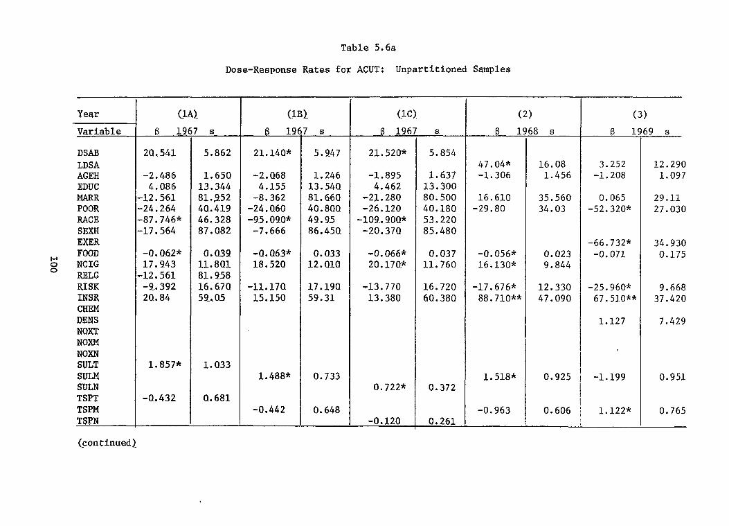
100

Year

Variable

DSAB LDSA AGEH EDUC MARR POOR RACE SEXH EXER FOOD NCIG RELG RISK INSR CHEM DENS NQXT N(XM NOXN SULT SULM SULN TSPT TSPM TSPN

(continued)

Table 5.6a

Dose-Response Rates for ACUT: Unpartitioned Samples

(LA).

B 1!2

20.541

-2.486 4.086

-12.561 -24.264 -87.746* -17.564

-0.O.62* 17.943

-12.561 -9..392 20..84

1.857*

-W432

r s

5.862

1.650 13.344 81..952 40..419 46.328 87.082

0.039 11.801 81..958 16.670 59..05

1.033

0..681

(lIQ

@ 19

21.14Q*

-2. Q68 4.155

-8.362 -24.0.60 -95.090*

-7.666

-Q. Q63* 18.520

-11.170 15,150

1.488*

-0.442

f s

5.247

1.246 13.54Q 81.660 40.80Q 49.95 86.450.

0.033 12.Q1O

17.19Q 59.31

0.733

0.648

(lC). (2)

@ 19(

21. 520*

-1.895 4.462

-21.280 -26.120

-109..9OQ* -20. 37Q

-0.066* 20. 170*

-13.770 13.380

0.722*

-0.120

s

5.854

1.637 13.300 8Q. 500 40.180. 53,220 85.480

0.037 11.760

16.720 60.380

61

47.04* -1.306

16.610 -29.80

-O. 056* 16.130*

-17.676* 88.71O**

1.518* 0.372

-0.963 0.261

i8 s

16.08 1.456

35.560 34.03

0.023 9.844

12.330 47.090

0.925

0.606

(3)

B lf

3.252 -1.208

0.065 -52.320*

-66.732* -0.071

-25.960* 67.51O**

1.127

-1.199

1.122*

59 s

12.290 1.097

29.11 27.030

34.930 0.175

9.668 37.420

7.429

0.951

0.765

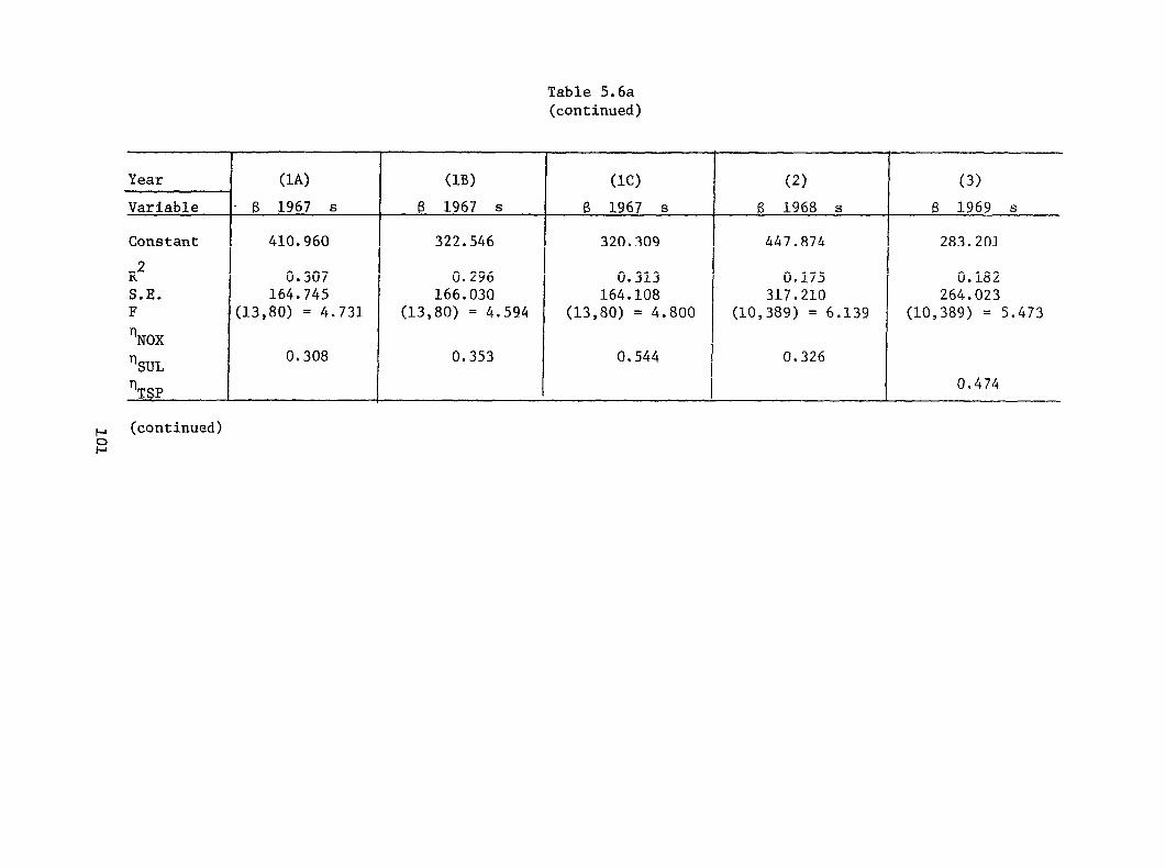
101

Table 5.6a (continued)

Year

Variable

Constant

R’ S.E. F

‘NOX

‘SUL

‘TSP

~ (continued)

(1A)

- f3 1967 S

410.960

0.307 164.745

(13,80) = 4.731

0.308

(113) (lC) (2)

6 1967 S (3 1967 S 6 1968 S

322.546 320.309 447.874

0.296 0.313 0.175 166.030 164.108 317.210

(13,80) = 4.594 (13,80) = 4.800 (10,389) = 6.139

0.353 0.544 0.326

(3)

f3 1969 S

283.201

0.182 264.023

(10,389) = 5.473

0.474

102

Table 5.6a (continued)

Year

Variable

DSAB LDSA AGEH EDUC POOR RACE SEXH CIGE EXER FOOD NCIG RELG RISK INSR CHEM DENS NOXT NOXM NOXN SULT sum SULN TSPT TSPM TSPN

(continued)

(4)

6 19

76.490 0.485

-63.200*

18.490

-48.620

-37.120* 9.885

-3.280

2.520*

)s

13.920 1.153

27.360

31.070

30.260

9.872 36.780 55.020

1.104

(5)

6 19

47.990* 2.542*

-15.800* -49.260*

-85.170*

-30.150 -0.030

-21.796* 7.439

2.257

1.453*

~ s

14.590 1.199 8.370

26.640

31.090

31.560 0.021

9.876 40.330

2.259

0.764

I (6)

B1

180.800*

1.411

128.1OO* 4.435

20.740

-99.730 3.529*

-0.972

1.782~

‘2 s

26.550

1.563

41.550 22.680 43.290

110.300 1.597

0.684

(7)

f31

19.340 0.355 2.550

-14.190 -36.450*

-123.600*

54.410 0.056

0. 223*

1 -0.361 I I

0.780 j -0.249

73 s

14.740 1.051 7.818

28.110 20.460 29.390

76.740 1.075

0.124

3.305

0.314

103

Table 5.6a (continued)

Year

Variable

Constant

R’ S.E. F

‘NOX

%’UL

‘TSP

(4)

$ 1970 s

305.260

0.123 262.333

(9,390) = 6.104

(5)

~ 1971 s

172.464

0.123 252.936

(11,388) = 4.926

0.361 0.518

I

*Significant at the 0.05 level of the one-tailed t-test.

**significant at the 0.05 level of the two-tailed t--test.

t

(6) (7)

B 1972 S (3 1973 s

-78.317 175.040

0.169 0.095 394.533 254.413

(9,390) =8.836 (11,388) = 4.435 0.618

0.497

104

Year

Variabl

DSAR LDSA AGEH EDUC MARR POOR RACE SEXN FOOD NCIG , RISK INSR SULM TSPM t EXER DENS

Constant R’ S.E. F NSUL NTSP

Table 5.6b Dose-Response Rates for ACUT: Partitioned Samples

(1) 1967

Jways lived in 1 stat, B

42. 056*

0.384* 2.716

-17.037 31.832

-60.5.49 13.327 -0.061 5.643

-4.047 -75.286 -0.992

J

. 1.765*

s

6.538

0.187 2.3o2

85.185 46.81’ 53.583 9.005 0.057 3.239*

17.600 70.361 7.631 0.865

121.290 0.152

352.420 (14,306) - 6.621

0.952

(2) 1969

RINC = S $7,500 8

111.200* 2 l 889

117.800 -116.400

-1. 648* 36.94o* 32.950 80.820 5.135*

-4.031

I

s

37.590 3.488

75.310 78.780

0.559 22.710 27.840 86.440 3.020 3.020

566.723 “ 0.186 443.738

(10,150) - 3.431 0.565

*si~if$cant at the 0.05 level of ‘the one-tailed ~-ees~. **sipificant ae the 0.05 level of the two-tailed t-teSt.

1?

17.960 -2.383

35.290 5.323

-0.084 34. 030* -4.700 -71.390*

0.007 -0.594

s

13.810 1.435

38.710 31.210

0.218 18.620 12.380 42.490 0.831 0.480

165.600 0.076

243.090 (10,268) = 2.191

(4) 1970

15 VSAB53 8

-94.990* 1.215

56.630 -66.900

-0.168

1.938 -54.560

0.114 1.215

200.600* -31.710

s

34.430

99.450 86.310

0.519

35.750 117.000

2.93o 2.210

125.600 21.700 ,

482.897 0.122

449.633 (10,114) =1.585

105

Year ..— — Variable

DSAB AGEH CITY EDUC FEDU MARR POOR RAcs SE.XH FOOD NCIG RISK INSR CHEM NOXT NOXM NOXN SULM SULN TSPM TSPN

Constant 1? S.E. F $00

‘lTSP

(1) 8 1967 s ——

0.003

0.079

0.204 0.188 0.344 0.410-4

-o. 7X1O 0.023

-0.009 -0.152

0.0036

0.0021

0.007

0.054

0.284 0’.157 0.200 0.297-3

0. 26x1O 0.047 0.006 0.245

0.0025

0.0037

-0.636 0.094 0.835

(12,134) = 2.158

Table 5.7a

Dose-Response Rates for LDSA: Unpartitioned Samplesa

.— (2)

B 1968 s — — 3.286*

-0.002

0.170

0.135

0.002* -0.089*

-0.336*

0.0067*

-0,0036

0,227 0.007

0.416

0.163

0.001 0.041

0.218

0.0035

0.0024

0.631 0.371 0.736

(9,390) =25,580

(3a] B 1970 s

o. 554** ().005

0.013 -0.044

-0.069 0.072 0.139

-0.902

-0.454* -1.645**

0.0028*

0.035 0.004

0.029 0.037

0.103 0.488 0.114 0.975

0.129 0.575

0.0011

2.980 0.525 0.964

(11,388) = 38.920

0.278

(-W) % 1970 s

o. 550** 0.005

0.001 0,043

0.065 0.088 0.132 .0.924

.O.459* -0.097

0.0018*

0.035 0.004

0.029 0.037

0.103 0,487 0.113 0.973

0.129 0.575

0. 66X1O -3

2.924 0.526 0.963

(11,388) = 39.170

0.341

,,- %. . . (5A)

e 1971 s

0.808** 0. 007*

-0.057 -0.044

0,086 -0.057 0.233**

-O.13X1O-3

-0.496* -0.002

0.0019

0.049 u. 004

0.030 0.035

0.096 0.119 0. lo9_4

O.81X1O

0.125 “:0.916

0.0017

0.265 0.530 0.904

(11,388) = 39.800

0.268

~continued]

106

Year

Variable

DSAB AGEH CITY EDUC FEDU

POOR RACE SEXH FOOD NCIG RISK INSR CHEM NOXT NOXM NOXN SULM SULN TSPM TSPN

Constant

R* S.E. F

‘NOX ‘kUL ~TSP

(5B )

6 1971 s

O. 809** 0.007*

-0.058 -0.043

0.088 -0.054

0. 240.** -Q.13X1O-3

-0.499* -0.016

0. 59x1Q -3

—

0.049 0.004

0.030 0.035

0. Q9.7 0.119 0. 109=4

0. 81x1O

0.125 0..917

0. 73X1O -3

0.181

0.529 0.905

(11,388) = 3!?.680

Table 5.7a (continued)

(6A)

6 1972 s

Q.023* -Q.057 -0.081

0.007

Q.1Q4 -Q.272 -0.156

-Q,QOQ7

O. QO.28

o l 005 0.Q50 0.0.45 Q. 050

Q.147 0.160 Q. 141

Q.0Q17

0.0Q27

Q. 701

0.119 1.347

(9.,390) = 5.879

0.376

(6B)

@ 1972 s

Q.020* -Q.085 -0.125**

0.048

0.116 -o. 22a -0.182

O.14X1O -3

0.0030*

0.005 0.045 0.043 0.055

0.145 0.154 0.142

O.’89X1O -3

0.0013

1.054

0.134 1.315

(9,390) = 6.706

0.630

107

Table 5.7a

Year

Variable

DSAB AGEH CITY EDUC FEDU

POOR RACE SEXH FOOD NCIG RELG

~ INSR u CHEM

NOXT NOXM NOXN SULM SULN TSPM TSPN

Constant

R2 S.E. F

‘lNOX %UL ‘TSP

(7A)

B 1973 s

0.017* 0.155

-Q. 122* 0.059

0.050 -C!. 208 -Cl. 207

0.0033

0.0017

0.044 0.140 0.043 0.052

0.143 0.154 a..l4l

0.0037

0.0015

0.309

0.106 1.303

(9,390) = 5.785

(continued)

(7B)

B 1973 s

0.017* 0.180

-0.128* 0.057

0.029 -Q. 202 -Q. 209

0. QC!3

0.0004

Q. 004 0.140 0.043 0.053

0.142 0.155 Q.141

0..002

0.0017

0..505

Q.109 1.303

(9,3!?0) = 5.290

(8A)

B 1974 s

0.017*

-(2.118**

-0.291 0.3Gil*

-0.001 -Q.(I6O

-0.459

-0,161

0.0023

-C.0047

0.0008

0.005

0.049

0.221 0.151

0.230 0.066

0.284

0.327

0.0017

0.0062

0.0028

-0.687

0.118 0.966

(11,214) = 4.591 0.363

(8B)

6 1974 s

0.017*

-0*111**

-0.287 0.305*

-o. aol -0.067

-0.457

-0.131

0. 0046*

0.(!002

-0.0007

0.005

0.049

0.221 0.151

0.230 0.067

0.284

0.325

0.0025

0.0022

0.0019

-0.828

0.112 0.964

(11,214) = 4.693 1.143

108

Table 5.7a(continued)

*Significant at the 0.05 level of the one-tailed t-test.

**Significant at the 0.05 level of the two-tailed t-test.

aAll observations in this table are limited to individuals who have always lived in one state.

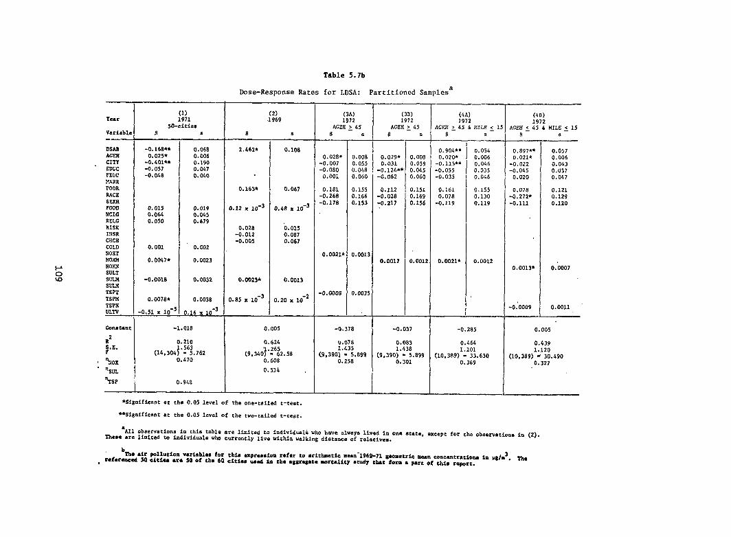
109

Table 5.7b

Dose-Response Rates for LDSA: Partitioned Samplesa

(2) .3969

(3B) 1972

ACEK~ 45

(4A) 1972

AGEK ~ 45 & MILE >1

(1) 1971

W-cities

(3A) 1972

(6B) 1972

AGEH ~ 45 6 llILE ~ 15 Year

Variable

DSAS ACSN CITY EDGC FEW MARR POOR NAcE Ssxsi FOCID NCIC RELC RISK INSR Ciicn COLD XOXT Nom NOXN SULT SUH SLIV TSPT TSPM TSPN ULTV

constant

R2 5A. F

, ~Jox

- %L

%P

6

2. St62h

.

0.163*

0.12 x 10-3

0.028 -0.012 -0.005

0. 0025*

0.s5 x 10-3

s

O.1O8

0.067

0.48 X 10-3

0,02s 0.087 0.067

0.0013

-2 0.20 x 10

E

-o. 165** 0.025*

-o. &ol** -0.057 -0.048

0.015 0.064 0.050

0.001

0.0047*

-o. 001s

0.0078*

-0.51 x 10-:

s

0.068 0.006 0.190 0.047 0.040

0.019 0.045 0.679

0.002

0.0023

0.0032

0.0038

0.16 X 10-3

s

0.02S* -0.007 -0.0s0

0.001

0. 1s1 -O. 26S -0.178

0.0021*

-o. 000s

s

0.008 0.055 0.048 0.060

0.155 0.166 0.153

0.001:

0.003!

$ s s s

0.054 0.006 0,046 0.035 0.046

0.155 0,130 0.119

0.0012

R —-

0.897** o.021*

-0.022 -0.045

0.020

0.07s -0.272* -0.111

0.0013*

-0:0009

s

o.90&** Q.020*

-0.115** -0.055 -0.035

0.161 0.078

-0.119

o.oo21*

0.057 0.006 0.043 0.037 0.047

0.121 0.129 0.120

0.0007

0.0011

0.029* 0.031

-0.124*9 -0.062

0.112 -0.028 -0.217

0.0017

0.00s 0.059 0.045 0.060

0.151 0.169 0.156

0.001:

I 0.005 -1.01s 0.005 -0.37s -0.037

0. 0s3 1.438

[9,390) - 5.s99 0,301

-0.2S5

0.464 1.101

(10,389) = 33.630 0.369

0.210 1.563

(14,304) - 5.762

0.624

(9,3407 ”:6i2.SS 0.608

U.0711 1.435

C9,390) - 5.s99 O. 25S

0.439 1.120

(10,3s9) * 30.490 0.327 0.470

0.514

*Significant at the 0.05 level of the one-tailed t-test.

**Significant at the 0.05 level of the two-tailed t-teat.

‘All observatimrs in this table are limited to indivfduali who have always lived in one State, except for the ~baervatioa~ in (2). These are limited to individuals who currently live within walking distance of relatives.

b Tbe air pr.llutioa variables for this expreseioa rafar to aritbsatic mMn-1969-71 gaometric -a cemc.ntratienm ~ pg/=3. ~

rtfermed SO cttfee *TS SO of the 6Q citla uaod in ;fm qgregam morrdity study the fors a pare of this re~rt.

coefficients to appear statistically non-significant when they areproperly viewed as significant.

There are, however, two very important exceptions to the supposedabsence of a multicollinearity problem: the types of air pollution tendto be very highly correlated and different moments of the same pollutantalso are closely associated. As Table 5.5 shows, total suspended par-ticulates and sulfur dioxide appear to have a very high linear associationas do all the moments of a particular air pollutant. If one were tointroduce nitrogen dioxide in Table 5.5, the linear association betweenthis pollutant and total suspended particulates and/or sulfur dioxidewould also be large, though somewhat smaller than that between thelatter two pollutants. For example, in 1975, the simple correlationcoefficient between various measures of total suspended particulates andnitrogen dioxide is never less than 0.50 and sometimes reaches intro the0.70 or greater range. Given these close linear associations among thetypes of air pollution, we are reluctant to assign a health effect to aparticular pollutant. Instead, it seems preferable to make the assignmentto the outdoor air pollution phenomenon. In addition, when one or moreair pollutants appear as explanatory variables in an estimated dose-response expression, the standard errors of each will tend to be somewhatinflated. Thus, a few of the air pollution coefficients to which we donot attach significance sometimes would be significant if one or more ofthe other air pollution variables were removed. Similarly, some ofthose air pollution coefficients that are significant would be moresignificant with the removal of a companion variable from the expression.

The above discussion does not deal with a dilemma posed by the issuesof bias and multicollinearity. If the different types or moments of airpollution have separable impacts on health, then one biases the coefficientsof the remaining explanatory variables by deleting one or more of the airpollution variables. Nevertheless, if one includes the highly collinearair pollution variables, he reduces the apparent statistical significanceof any one of them. In this study, we do not directly attack thedilemma by constructing and then applying rigorous criteria for choice.We choose an easier and less rigorous course by estimating some expressions,each from a different sample, that include all the types of air pollution,while including only one type of air pollution in other expressions.To a very substantial extent, this course was forced upon us by circum-stances: for some years over the nine-year SRC survey interval, therewas no available information on particular types and moments of theair pollution variables.

Table 5.5 exhibits one other intercorrelation that is a cause forconcern, namely a simple correlation coefficient of 0.70 between LDSA andDSAB, i.e., between the duration of a chronic illness and its self-reported severity. Relative to most other samples of the study, thisintercorrelation is a bit low. For most samples, it is closer to or inexcess of 0.80. Certainly, the length of a disease and its severity are notidentical. In fact, one might expect those who are severely disabled tohave relatively short disease durations: they are more likely to die.We may thus have increased the intercorrelation between these two variablesby not making DSAB be monotonically increasing. The high intercorrelation

110

arouses suspicions about whether the two variables might be measuring thesame thing, a clearly ridiculous state, if one is trying to explain thecovariation between the two variables. Furthermore, if air pollution isexpected to lengthen the duration of an illness, there is obvious reasonto think that it will also make an illness more severe. More accuratelyperhaps, air pollution causes illness and increases the severity ofpreexisting illness, thus in a recursive fashion lengthening, for those whosurvive, illness duration. This implies that the estimated expressionswhich include DSAB as an explanatory variable are actually reduced formexpressions, where DSAB is determined within the structural system.As a result, the single equation estimates with DSAB as an explanatoryvariable are not asymptotically efficient although they are consistentsince DSAB is the only explanatory variable that would be determined withinthe structure of a recursive system. If instead of DSAB being a determin-ant of LDSA, it is actually another measure of the same thing in respondents'views, then DSAB must be dropped from the estimated expression. For theexpressions estimated from some samples we include DSAB; for othersamples, we delete it, using whichever of the preceding rationalesconforms to the estimated expression. As we will see, inclusion orexclusion doesn't really make much difference to the signs and magnitudesof the coefficients for the major variables of interest, the air pollutionvariables.a/

In estimating dose-response expressions for chronic illness, we haveused LDSA rather than (or in addition to) DSAB because only the formeris stated in cardinal terms. LDSA, however, retains one disadvantage ofDSAB; as presented on the SRC tapes, it takes on only five values.Although the first four of these values apply to approximate two-yearintervals, the last value might better be termed "a long time," since itis meant to apply to disabilities lasting eight or more years. If oneinterprets, as we shall do in this chapter, this last value to beequal to exactly ten years, then the dependent variable for chronicillness has a measurement error that biases it downward, causing theeffects of the explanatory variables to be underestimated. This could bea serious source of error since about 40 percent of those who aredisabled in any given SRC survey year, or seven to eight percent of thetotal SRC respondent population, profess to have been disabled for eightor more years. Given this problem, which we disregard until a succeedingsection, it is perhaps preferable to interpret the coefficients attachedto the explanatory variables in the estimated chronic illness dose-response expressions as the proportion of one of the discrete valuescomprising LDSA associated with a one unit change in the relevantexplanatory variable.

Yet another estimation issue is caused by the five discrete valuesassumed by LDSA, This small number of discrete values means thatheteroskedasticity could be present in those expressions estimated byordinary-least-squares techniques. Ideally, multinomial logit estimationwould be employed; but because the number of parameters with multinomiallogit estimation increases so dramatically when the dependent variableassumes more than two values, there is an explicit tradeoff between themisspecification possibly introduced by the use of ordinary-least-squaresand the vastly increased cost and complexity of multinomial logit estima-

111

tion. We have opted here for simplicity and lesser cost while not dis-missing the heteroskedadicity issue: we estimate the chronic illnessdose-response functions by ordinary-least-squares hut peruse the estima-ted results. by simple graphic techniques to check for the presence ofheteroskedasticity. Even if this undesirable property is present,it does not follow that our estimates will be biased and inconsistent.They will not be efficient (they will not have the smallest variance in aclass of unbiased estimators), but they will be unbiased and consistent.The problem with heteroskedasdicity is thus not with the estimated co-efficients themselves but rather with the calculated standard errors.These standard errors are biased, thus invalidating the tests of signific-ance for the estimated coefficients.

There are a number of results for acute illness in Tables 5.6a and5.6b worthy of explicit note:

1) Of the seven different unpartitioned samples used to estimateacute illness dose-response expressions, statistically significant airpollution coefficients occur in all of them. Thus, an additional unit ofair pollution, as defined by any of the variety of measures employed here,was associated with an increase of from one to four hours in average annualhours of acute illness. Except for 1973, magnitudes of the air pollutioncoefficients are quite stable from one sample to another, even thoughthe specifications for the expressions often differ substantially. Notests have been performed to establish whether there are statisticallysignificant differences in the air pollution coefficients across samples.

2) For the unpartitioned samples, the elasticity, n, of acuteillness with respect to any of the air pollution variables (a unitlessmeasure of the response of acute illness to variations in air pollution)is substantially less than unity. This implies that in the immediateneighborhoods of the sample values of these variables, average annualhours of acute illness is increasing at a decreasing rate with respect toincreases in air pollution.

3) Two of the four partitioned samples in Table 5.6b do not havestatistically significant air pollution coefficients. If air pollutionhas any impact upon the frequency of acute illnesses among individualswho are chronically disabled and who live in families where a packor more of cigarettes is smoked, the estimataion techniques and samplesizes employed here are incapable of capturing it.

4) When measures of total suspended particulates and sulfurdioxide are included as explanatory variables in the same expression, thecoefficient for them usually assumes a negative sign. Generally, totalsuspended particulates will take on the negative sign. Similarly, whensulfur dioxide and nitrogen dioxide are included as explanatoryvariables in the same expression, nitrogen dioxide often assumes anegative sign. For estimated expressions in which total suspendedparticulates and/or nitrogen dioxide are used as explanatory variables,but which do not include sulfur dioxide, both of the former sirpollutants have positive signs. These sign switches could be dueto the high linear associations among the pollution variables.

112

5) With some exceptions, an increase of one discrete value ineither of the measures of chronic illness tends to increase theaverage annual hours of acute illness by from 20 to 40 hours.

6) With the sole exception of the variables for a poor child-hood and race, the variables representing biological and social endow-ments fail to play a statistically significant and consistent role in theacute illness dose-response expressions. It is possible, of course,and perhaps even likely, that the race and childhood background variablesare capturing many of the effects of low education, etc.

7) The life-style variables in the acute illness dose-responseexpressions consistently have the expected signs and are often statisticallysignificant. This is particularly true for the exercise and nutritionaladequacy variables: they reduce average annual hours of acute illness.

8) Contrary to expectations, the explanatory variable foravailability of medical care, INSR, usually has a positive sign, implyingthat people with better access to medical care have more acute illness.We have no explanation for this other than a pure speculation thatpeople with better access to medical care are more likely torecognize the symptoms of acute illness, perhaps because physiciciansprovide them with the information to recognize these symptoms. Onthe other hand, INSR might simply be a poor measure of the respondents'access to medical care.

9) Other than air pollution, only two alternative measuresof the respondents' environments were employed as explanatory variables.These variables were used in only a limited number of samples. DENS,the number of persons per room in the respondents' residence, increas-ed average annual hours of illness by more than three in the single samplewhere it was statistically significant. The variable for employmentin the chemicals and metals manufacturing sectors had too small anumber of individuals in each sample to yield statisticallymeaningful results.

Visual inspection of the residuals for expression (1A) of10)Table 5.6a and expression (1) of Table 5.6b did not reveal anyserious heteroskedasticity problems.

113

We tentatively conclude from the preceding findings that the life-styleand environmental variables, including air pollution, we have used probablyplay a significant role in acute illness. The evidence for the biologicaland social background and the access to medical care variables is substan-tially less clear both because of measurement problems and because racialdifferences in educational and childhood environment may be reflected insimple binary variables for race and a poor childhood. Finally, it shouldbe noted that none of our expressions "explains" a very large portion of thevariation in acute illness. The coefficients of determination never exceed0.31 and are often about 0.10. Moreover, the constant term in each expres-sion nearly always exceeds the sum of the coefficients of the explanatoryvariables. This is, of course , partly due to the scaling of the variables,but, given the number of binary variables (MARR, POOR, RACE SEXH, RELG,INSR), one might reasonably have not expected quite such a difference. Therelatively unimportant role that many of the most statistically significantvariables play in total variation in annual hours of acute illness is evidentin the following partial coefficients of determination for variables ap-pearing in various expressions of Table 5.6a: for expression (7), NOXM =0.004, SEXH = 0.044, and and LDSA = 0.004; for expression (1B), SULM = 0.021,FOOD = 0.002, RACE = 0.043, NCIG = 0.029, and DSAB = 0.136; and for expres-sion (5), TSPM = 0.013, POOR = 0.024, DSAB = 0.124. With no more than one ortwo exceptions, the two variables for chronic illness, LDSA and DSAB, madethe largest contributions to explaining variations in annual hours of acuteillness.

Tables 5.7a and 5.7b give the estimated dose-response expressions forchronic illness. The following features stand out in these expressions.

1. Of the twelve different partitioned and unpartitioned samplespresent in Tables 5.7a and 5.7b, air pollution coefficients are statisticallysignificant in nine of them. Not all air pollution coefficients are statis-tically significant in the samples where more than a single air pollutionvariable appears, nor are the signs always positive for those air pollutioncoefficients that are statistically nonsignificant. No pattern similar tothe negative signs that are attached to sulfur dioxide or other pollutantswhen sulfur dioxide is used as an explanatory variable in the acute illnessdose-response expressions appears here, however. Of the samples having noair pollution coefficients statistically significant at the 0.05 level orbetter of the one-tailed t-test [expressions (1), (5), and (7) in Table5.7a], all had air pollution coefficients with positive signs and t-valuesin excess of 1.0. Two of these samples [expressions (1) and (7)] had airpollution coefficients statistically significant at the 0.10 level of theone-tailed t-test. The magnitude (and signs) of the air pollution coef-ficients for expressions (1), (5), and (7) were similar to the magnitudesand signs of the air pollution coefficients for the other samples. Theyranged between slightly less than 0.0020 and slightly more than 0.0045,with the bulk being between 0.0020 and 0.0030. This means that a changebetween 0.2 and 0.4 or 0.5 percent in one of the discrete values comprisingLDSA is caused by a one-unit change in air pollution. In elasticity terms,these discrete values (index) of LDSA appear to be relatively unresponsiveto changes in air pollution. Nearly all the elasticities of the discretechronic illness index with respect to air pollution are in the 0.2 to 0.5

114

range, implying that a one percent change in air pollution generally causesa change in the index of substantially less than one-half of one percent.As was true for the acute illness dose-response expressions, this means that,in the immediate neighborhoods of the chronic illness index values and theair pollution values present in these samples, chronic illness duration in-creases at a decreasing rate with respect to increasing air pollution.

2. As earlier noted, translating the coefficients for the explanatoryvariables in the chronic illness dose-response expressions is invalidbecause the highest value in the index could, in real-time terms, be any-thing equal to or in excess of eight years. Nevertheless, if one assumesthat the real-time involved in this last index value is equivalent to thatin all the lower values, than the translation can be performed. With thisassumption, the air pollution coefficients imply that an additional unitof air pollution is, on average, associated with an increase of from oneand one-half to three and one-half days in the duration of chronic illness.As before, even with the aforementioned assumption, this rate is applicableonly in the immediate neighborhoods of the chronic illness index values andthe air pollution values present in the samples.

3. In those unpartitioned expressions where it is employed as anexplanatory variable, the severity of the respondent's disabilities hasa highly significant, positive, and strong effect on the duration of thesedisabilities. The partial coefficient of determination of DSAB with respectto LDSA was consistently about 0.40. The inclusion of DSAB in expressionsdid not appear to have an effect on either the magnitudes or the signifi-cances of the air pollution coefficients. Similarly, its presence or absencedid not seem to make much difference to coefficients for the other explan-atory variables.

4. Results for the biological and social endowment variables aremixed. Only respondent age is consistently significant with the expectedsign. Generally, as expected, the level of the respondent's education isassociated with lesser durations of chronic illness, but it is only occasion-ally significant. Poor parents tend to be consistently associated withincreased chronic illness durations, but POOR is statistically significantin only one sample. Otherwise, variables such as CITY, FEDU, MARR, RACE,and SEXH contributed very little to the expressions. Rarely were theysignificant statistically. More importantly, their magnitudes and theirsigns proved to be expremely sensitive to whatever specification wasadopted.

5. Because it is not clear that the magnitudes of lifestyle variablesare independent of the duration of chronic illness, fewer of them were used,and those that were used were used less frequently, than in the acuteillness dose-response expressions. EXER is an obvious case and it has notentered the chronic illness expressions. In fact, except for RELG, foodadequacy is the only explanatory variable that enters the expressionsestimated for more than one sample. It always has the expected sign but isnever quite statistically significant at the 0.05 level selected for thisstudy. On the rare occasions when they appear, both cigarette consumptionand fundamentalist religious affiliations have the expected signs. RELG inexpressions (7A) and (7B) just barely misses being crowned with statistical

115

respectability. Since religious affiliations seem likely to remain un-changed whether or not one is disabled, this variable probably shouldhave been included for the expressions estimated from each sample.

6. The variable representing the availability of medical care,INSR, performed well for those four samples where it was used. Its signwas consistent with an interpretation that medical care availabilityreduces the duration of chronic illness. Unfortunately, its sign is alsoconsistent with another interpretation: those who are chronically ill havedifficulty procuring medical insurance. This latter interpretation meansthat INSR could be a function of LDSA. Given these conflicting interpre-tations, and having no information on which interpretation is likely todominate, we have compromised and included INSR in some expressions whileneglecting it in others. Its inclusion or exclusion does not appear to haveany discernable effects on the coefficients for the air pollution variables.

7. Of the environmental variables, only CHEM seems worthy of comment.In the one expression where they appear, neither COLD nor ULTV were statis-tically signficant although COLD did have a positive sign. The statisticalsignificance of CHEM in expression (3) of Table 5.7a should be disregarded.Expression (3) was estimated from a sample having only three people employedin the chemicals and metals manufacturing sector. None of these threepeople had a chronic disability.

8. With the exception of DSAB, none of the included explanatory vari-ables explain substantial proportions of the variation in the index for dur-ation of chronic illness. The air pollution variables, taken together,explain no more than two percent of the variation in LDSA; AGEH sometimesexplains as much as five percent and EDUC usually explains around three per-cent of this variation. As with the acute illness dose-response functions,we have not been able to account for very much of the sources of variationin chronic illness.

9. Table 5.7b exhibits the estimated expressions for samples that wererestricted to the values of the variables indicated at the top of each col-umn. Contrary to similar restrictions placed on the samples for the acuteillness expressions, these restrictions did not alter the explanatory vari-able coefficients in any noticeable fashion.

10. The patterns of the residuals for several of the expressions inTable 5.7a have been visually inspected for evidence of heteroskedasticity.When this Problem is present, it appears that the residuals tend to increasewith increasing values of the dependent variable. Because the highest dis-crete value of LDSA has no upper bound, it is likely that the true varianceof the sample tends to increase with increasing values of LDSA. As Kmenta(1971, p. 256) shows for expressions with a single explanatory variable, ifthe residuals and the sample variance are positively associated, the stand-ard errors of the coefficients for the explanatory variable will be biaseddownward, causing the t-value to be too great. This need not be true, how-ever, for expressions with multiple explanatory variables. The extent towhich this has resulted in exaggeration or underestimates of the levels ofsignificance for the chronic illness dose-response expressions is presently

116

Table 5.8

Lagged Effects of Total Suspended Particulates upon Durationof Chronic Illnesses (LDSA) of Respondents Who,

as of 1975, Had Always Livedin the Same State

AGEHEDUCMARRPOORSEXHFOODRELGCHEMTSPM5TSPM4TSPM3TSPM2TSPM1TSPM0TSPM9

Constant

R2S.E.F

(1)

Unweighted

B

0.012* 0.004 0.017* 0.005-0.009 0.040 -0.103* 0.050-0.331* 0.160 -0.237 0.2320.150* 0.110 0.327* 0.153

-0.012 0.023 0.046 0.235-0.035* 0.021 -0.076 0.074-0.003 0.030 -0.501* 0.2860.249 -4 0.247 -0.147 0.332

0.4 x 10 0.061 0.002 0.0030.001 0.033 0.001 0.0050.001 0.003 -0.001 0.0040.003 0.016 -0.003 0.0040.008* 0.004 -0.003 0.0050.007 0.011 0.004 0.0050.006 0.006 0.002 0.005

s

0.444 -0.690

0.184 0.1291.032 0.969

(12,347) = 6.481 (15,210) = 4.082

Weighted

B

(2)

s

*Statistically significant at the 0.05 level of the one-tailed t-test.

117

unknown. The heteroskedasticity appears to be by far the most prominentfor those estimated expressions having coefficients of determination lessthan 0.10.

It is widely thought that pollution-induced chronic illness is usuallythe result of cumulative, rather than instantaneous, exposures. Previouslywe have taken the position that, if only non-movers are represented in thesample, air pollution exposures during the year for which the respondentreports his behavior and status serve as adequate proxies for differencesamong respondents in cumulative exposures. If this position is at alltenuous, we have available the data to remedy it at least partially; thatis, we have available information on respondent residential locations andair pollution exposures for a number of years. Table 8 presents some pre-liminary results involving an attempt to estimate the lagged effects oftotal suspended particulates upon the duration of chronic illness for 1975respondents who have always lived in the same state. Since it is unclearexactly what a lagged effect of pollution upon the duration of an illnessmeans, we exploit the high intercorrelation between LDSA and DSAB and inter-pret the expressions in terms of the lagged effects of air pollution uponthe severity of chronic illness. As in earlier tables, the integers attachedto the acronym for mean total suspended particulates refer to the year. Thus,for example, TSPMO refers to particulate concentrations in 1970.

The expressions presented in Table 8 have involved no tinkering: theseare the first expressions having LDSA as a dependent variable that haveused either of these samples. Expression (1) is an unweighted lag in whichearlier air pollution concentrations are simply entered as additional explan-atory variables. In spite of the very high simple correlation coefficients(Z 0.80) among the air pollution values of the various years, at least oneyear (1971) is statistically significant. Moreover, the magnitude of thecoefficient increases from 1975 to 1971, and then starts to decline. Wehave no explanation for this rather neat pattern and tend to suspect thatits very neatness in an anamoly that would fail to emerge in expressionsestimated from other samples. These other samples have not yet been ex-ploited.

The air pollution series in expression (2) has more structure imposedon it. In particular, the series is assumed to follow a geometric lagdistribution where the coefficients decline in fixed proportions, causingthe impact of more distant air pollution concentrations to become pro-gressively smaller. Clearly, expression (2) does not accord any importanceto total suspended particulates. However, this does not mean that allweighted lag structures will give similar results. Estimation techniquesare available that allow one to fit polynomial structures of any degree.These techniques have not been applied here.

In concluding these remarks about dose-response functions, we mustmake explicit a feature of the SRC data set that could readily cause themorbidity effects of air pollution and other negative health influencesto be biased downward. This possible bias is due to the retrospectivefeature of the SRC data: living individuals are questioned about theirbehavior and status during the preceding year. The problem arises because

118

some potential respondents who were alive during the preceding year aredead by the time the interview occurs. Presumedly, those who died wouldtend to be those who were most seriously ill. If air pollution and othernegative health influences contribute to this seriousness, or if thosewho are most seriously ill are most sensitive to air pollution, then thehealth impact of air pollution will be understated. Thus, the dose-responsefunctions presented here are relevant only for those individuals who man-aged to survive over the time interval which the interviews described and thecalendar date at which the interviews occurred. This qualification appliesto all sections of this report where the SRC data is exploited. It is nota minor qualification since approximately five percent of the respondentsdied between interview years.

5.4 Recursive Estimates of the Effect of Air Pollution Upon Health, LaborEarnings, and Hours of Work

In the past decade, a number of empirical studies have appeared thatdescribe the effect of health status upon labor productivity, where pro-ductivity effects are measured in lost earnings and work-time.12/ At thesame time, numerous epidemiological studies that attempt to associate healthstatus with air pollution have been published.13/ Thus far, no one has triedto combine the two study objectives in order to grasp the effect of air pol-lution upon either of the aforementioned measures of labor productivity.This section is a first attempt to do so. Labor productivity effects havenever been explicitly included in quantifications of the benefits of nationalair pollution control efforts. Our results suggest that these productivityeffects could constitute a significant portion of these benefits and arecertainly worthy of further study.

In spite of a number of limitations which will later be exposed, thesection has at least three unusual, if not utterly novel, features. First,although it treats health status as an exogenous rather than endogenousvariable, a structural equation for health status is specified. Thiscontrasts with nearly all epdemiological studies, where the analysis isconfined to reduced-form health status, making any direct assignment ofhealth effects to air pollution an extremely tenuous operation. Second, thehealth parameters in this section are estimated in the context of structuralexpressions for hourly earnings and annual hours of work. Finally, possibledifferences in effects of air pollution upon crude measures of acute andchronic generalized health status are recognized. The null hypothesis isthat air pollution, by enhancing initial susceptibility and by making re-covery more difficult, causes acute and/or chronic health problems. This,of course, was the theme of the previous section. In this section, wewish to ascertain the impact, if any, of these air pollution-induced healthadversities upon earnings rates and hours worked. Thus through the inter-mediary of any health problems it induces, air pollution can be said toindluence labor productivity.

Even though health is treated as being exogenously determined, the Gross-man (1972) model of health production can serve as the analytical foundationof the expressions to be estimated.14/ This model views the individual asthe producer, via his selections of mixes of market-purchased goods and hisown time, of health status. Within the context of this approach, earnings

119

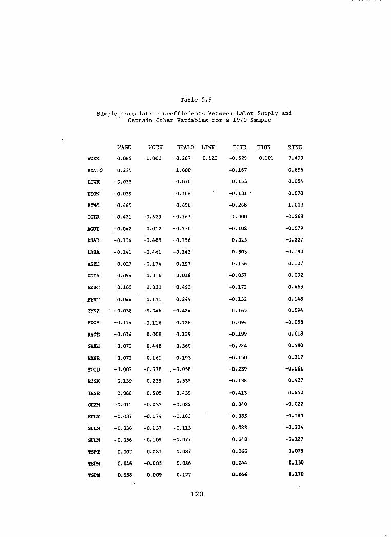
Table 5.9

Simple Correlation Coefficients Between Labor Supply and Certain Other Variables for a 1970 Sample

UORK

SiXLO

LTWK

UION

RING

ICTR

ACUT

DSAB

LDSA

AGRB

CITY

EDUC

. PEW

Fusz

POOR

RACE

SXH

EXRR

FOOD

BIBK

IlSR

CRRM

SULT

SULH

SULN

TSPT

TSPM

TSPII

FAGE

0.085

0.235

-0.038

-0.039

0.465

-0.421

$042

-0.134

-0.141

0.017

0.094

0.165

0.044

-0.038

-0.114

-0.014

0.072

0.072

-0.007

0.139

0.088

-a. 012

-0.037

-0.038

-0.056

0.002

0.046

0.058

NORK

1.000

-0.629

0.012

1-0.468

-0.441

-0.174

0.016

0.323

0.131

-0.046

-0.k

0.008

0.440

0.161

-0.078

0.235

0.505

-0.033

-0.174

-0.137

-0.109

0.081

-0.005

a. 009

BDALO LT& ICTR UION RING

0.2S7 0.123 -0.629 0.101 0.479

1.000 -0.167 0.656

0.070 0.155 0.054

0.108 -0.131 . 0.070

0.656 -0.268 1.000

-0~167 1.000 -0.268

-0.170 -0.102 -0.079

-0.156 0.325 -0.227

-0.143 0.303 -0.190

0.197 0.156 0.107

0.018 -0.057 0. a92

0.493 -0.172 0.465

0.244 -0.132 0.148

-0.424 0.165 0.094

-0.126 0.094 -0.058

0.139 -0.199 0.018

0.360 -0.284 0.480

0.193 -0.150 0.217

-0.058 -0.239 -0.061

0.538 -0.138 0.427

0.439 -0.413 0.440

-0.082 0.040 -0.022

-0.163 - 0.085 -0.183

-0.113 0.083 -0.134

-0.077 0.048 -0.127

0.087 0.066 0.075

0.086 0.044 0.130

0.122 0.046 0.170

120

r :

i

rates depend on various forms of investment in human "capital" (e.g., edu-.cation, prior lifestyles, and medical inputs) and labor market conditions;

and the time supplied to the labor market depends on the individual's hourlyearnings and the quantities of goods and time desired for household pro-duction and consumption. Health states depend on the prior resources theindividual has devoted to their production.

Except for certain of the environmental variables, the data used? toestimate the model consist of four distinct samples drawn from the 1969,1970 and 1971 SRC interview data. Several variables, defined in Table 5.1,are used in this section that were not used in the preceding section. Forone of the samples, Table 5.9 provides the simple correlation coefficientsbetween these additional variables and some of the other previously usedvariables. Representative means and standard deviations for the additionalvariables are available in Table 5.2.

Table 5.9 gives little attention to LTWK and UION because our majorinterest in them is their association with WORK, WAGE, and RINC. Absenteeismwas checked in this sample but apparently none of the respondents wouldadmit to being absent from work for reasons other than sickness. As wasnoted in Table 5.4, where 81.1 percent of the respondents had annual assetincomes of no more than $500, most of the respondents' annual incomes notearned during the current year appear to be governmental transfer payments.This accounts for the negative and high correlations between ICTR and RINCand WAGE. Note also in Table 5.9 that the simple correlations between thetwo chronic illness measures, DSAB and LDSA, and WORK and RINC are quitehigh.

The household head's annual number of work hours, WORK, and his hourlyearnings, WAGE, are used as the empirical representations of the endogenousvariables in the model. Remember from the definitions of Table 5.1 thatWAGE is an approximation of the marginal, rather than the average, wagerate. Annual number of work hours is used as the sole measure of laborsupply because the sample contains no information on the seasonal distri-bution of hours when working. Neither vacation time nor sick time is in-cluded in annual hours worked, even if the individual was paid during thesetimes.

The system to be estimated for each sample consists of four expressions:a chronic illness expression; an acute illness expression; a wage expression;and a labor supply expression. A representation, in implicit form, of thisstructural system is as follows:

1. LDSA = f(Biologica1 and social endowments, Lifestyles, Medicalcare, Environmental). (5.1)

2. ACUT = g(LDSA, Biological and social endowments, Lifestyles,Medical care, Environmental). (5.2)

3. WAGE = h(LDSA, ACUT, Cost-of Living, Experience, Biological andsocial endowments). (5.3)

121

4. WORK = k(WAGE, LDSA, ACUT, Transfer income, Wealth). (5.4)

As structured, this system is obviously recursive.

A great deal of research is available [e.g., Lazear (1976)] showingthat earnings are positively related to formal and informal schooling.Good health is here viewed as having effects on earnings analogous to theeffects of increased schooling; that is, good health increases the individ-ual's marginal value productivity and therefore raises his marginal earnings.In addition, previous good health may have had an indirect effect on earn-ings by easing the task of achieving schooling success and thereby ultimatelyimproving the individual's productivity and associated earnings. The EDUCand LOCC variables in (5.3) are intended to capture the effects of trainingupon earnings. They may also reflect, in part, the influence of past healthstatus. The health status variables, ACUT, DSAB, and LDSA, in (5.3) regis-ter the effect of current health status, via the effect on productivity,upon earnings. Since chronic illnesses reflect long duration, as opposedto temporary, reductions in productivity, we expect wages to exhibit greaterresponsiveness to the chronic illness variables than to the acute illnessvariable.

In addition to the aforementioned variables, the marginal earningsexpression includes variables representing the 1970 cost-of living in thecounty of residence as well as variables representing the individual's raceand sex. If, as is frequently asserted, being non-white or female negativelyinfluences marginal earnings, either labor market discrimination or lessmarket productivity in the current period could account for the influence.15/The structural system we employ is incapable of distinguishing between thetwo possible influences.

Cost-of-living, BDAL, in the county of residence is accounted for in(5.3) because it is real marginal earnings, rather than money earnings,that limit the extent to which the individual is able to satisfy hiscravings and yearnings.

As Mincer (1970) and others have shown, earnings expressions similarto (5.3) should be semi-logarithmic, where the dependent variable is thelogarithm of the earnings term. In this paper, we presume the earningsexpression to be linear in the original variables. This presumption wasadopted in order to obtain a sample of individuals possessing reasonablevariability in the values of the health variables, earnings, and hoursworked. If, in order to avoid having to assign positive earnings to indi-viduals who really had zero earnings, only individuals who actually hadpositive earnings were included in the sample, the variability of thechronic disability measures would have been substantially reduced, thusrequiring that inferences about the influence of air pollution on health,earnings, and hours worked be drawn from the relatively few remaining indi-viduals whose health status and work patterns differed substantially fromthe mean. Moreover, dropping individuals with zero earnings from thesample would have meant that those individuals with long-standing and/orsevere chronic health problems would be excluded.

122

Expression (5.4) the annual hours worked or labor supply expression,is consistent with the treatments of health capital in Grossman (1972).Improvements in health states increase the total time available for workand for consumption. With real earnings and consumption opportunitiesheld constant, the consumer would be inefficient, assuming he was initiallyin equilibrium, if he allocated all this additional time solely to consump-tion. This is because the ratio of consumption time to work would rise,causing the marginal value of consumption time to become less than themarginal earnings that could be obtained. To recover equilibrium the indi-vidual would have to devote the additional time to both work and consump-tion. We therefore expect the amount of work time to increase with improve-ments in health status.

In addition, since health status is assumed to be exogenous, animprovement in health would increase the wage rate as well as the pecuniaryequivalent of time spent in consumption. In terms of the household produc-tion approach to consumer theory, "full income" would be increased. Thehealth improvement therefore would constitute a pure income effect, causingthe individual to increase the value he attaches to any unit of consumptiontime. This increase in the value of consumption time would cause the indiv-idual to increase his demand for those marketed goods permitting him to usethis more highly valued consumption time with greater effectiveness. Thepurchase of these marketed goods requires that he obtain more income, andtherefore that he increase his work time.

An increase in income not earned in the current period, ICTR, wouldalso result in a pure income effect. However, because the additional incomeis not a consequence of improvements in work productivity, the value of worktime relative to consumption time decreases, assuming the wage rate andhealth status to be invariant. The result is that with an increase inincome not earned in the current period, the individual must reduce worktime in order to restore equilibrium.

The preceding remarks indicate why the sign of the marginal hourlyearnings variable, WAGE, in (5.4) is ambiguous. An increase in marginalhourly earnings would increase the value of work time relative to thevalue of consumption time , causing the former type of time to be substi-tuted for the latter. However, the increase in marginal hourly earnings hassimultaneously increased the individual's "full income," causing the valuehe attaches to any given unit of consumption time to increase. Whether theincrease in the value of consumption time exceeds the increase in the valueof work time is an empirical question.

Since the immediately preceding remarks refer only to real marginalhourly earnings, (5.4) includes BDALO, the cost-of living index, in orderto control differences in real earnings among counties of residence.

The four-equation system, in which acute and chronic illnesses areexogenously determined, represents a strictly recursive system. First,health status is determined independently of hourly earnings and hoursworked, and then health status is used to determine hourly earnings andhours worked. Similarly, hourly earnings are determined independently of

123

Table 5.10a

Empirical Results for a 1971 Sample a,b Recursive Labor Supply

1.

2.

3.

4.

LDSA = -1.018 + O.O6(NCIG) - O.l7(DSAB)* + O.O5(RELG) - 0.4O(CITY)* (0.04) (0.07) (0.68) (0.19)

- O.O5(FEDU) + O.OG(EDUC) + O.l5(FOOD) + O.O25(AGEH)* (0.04) (0.05) (0.19) (0.006)

+ O.OOl(COLD) + O.OOl(ULTV) - O.O02(SUlX) + O.O05(NOXM)* (0.002) (0.002) (0.003) (0.002)

+ O.O08(TSPM)* (0.004)

R2 = 0.21; F(13, 305) = 5.76; S.E. = 1.56

ACUT = 35.397 + 0.25(NCIG) - 0.38(DSA.B) - 4.98(LDSA) - 47.39(EXER) (6.20) (9.40) (7.59) (35.76)

+ 5.14(EDUC) - 0.36(AGEH) + O.O6(COLD) - O.Ol(uLTV) - 0.38(SULM) (4.85) (0.87) (0.27) (0.02) (0.44)

+ O.O6(NOXM) + 0.49(TSPM) (0.31) (0.52)

R2 = 0.15; F(ll, 307) = 0.43; S.E. = 215.15

WAGE = -5.619 + O.O8(BDALO) + O.OZ(ACUT) - 156.70(SEXH)* + 33.46(LOCC)* (0.06) (0.10) (44.41) (10.81)

- 3.00(DSAB) - 41.73(LDSA)* + 20.31(EDUC)* + 50.80(RACE) (14.35) (15.72) (10.20) (32.08)

lx2 = 0.20; F(8, 310) = 9.72; S.E. = 367.66

WORK = 2011.671 - O.lZ(BDALO) - O.Ol(ACUT) - O.O5(ICTR)* + 123.40(SVGS)* (0.15) (0.23) (0.01) (26.35)

- 10.55(DSAB) - 212.00(LDSA)* + 0.50(WAGE)* (34.26) (36.52) (0.13)

R2 = O.i5; F(7, 311) = 23.68; S.E. = 865.51

(continued)

124

Table 5.10a(continued)

aStandard errors are in parentheses.

bThe sample includes only respondents who resided in 50 large U.S. cities.

*Significant at the 0.05 level of the one-tailed t-test.

125

1.

2.

3.

4.

Table 5.10b

Empirical Results for a 1970 Samplea Recursive Labor Supply

LDSA = 2.980 +'0.554(DSAB) ** + o.o05(AC~H) + 0.013(~~uc) - 0.044(~~~U) (0.035) 0.004 0.029 _ 0.037

- O.O6g(POOR) + O.O72(RAcE) + 0.139(SEX.H) - 0.902(FCOD) - 0.454(lNSR)* 0.103 (0.488) (0.114) (0.975) (0.129)

- 1.645(CHEM)" + O.O028(TSPM)* (0.575) (0.0011)

R2 = 0.525; F(11,388) = 38.920; S.E. = 0.964

ACDT = 165.208 + 39.52(LDSA)* - 1.421(AGEH) - 16.92(SEXR) - 0.086(CIGE)b (13.34) (1.312) (39.16) (0.118)

- 78.40(EXER)* - O.l05(FOOD)* - 38.84(RISX) + (40.11) (0.033) (13.26)

R2 = 0.195; F(10,389) = 6.139; S.E. = 204.462

~~~.o(INsR)** + 0.623(TSPM)* (47.47) (0.317)

WAGE = -132.318 - 25.930(LDSA)* + 24.070(EDUC)* + 15.370(DSAB) (14.440) (8.5780) (18.260)

+ 26,88O(FMSZ)* + 42,38O(BDALO)* + 52.95O(LOCC)* - 7.163(LTWE) (6.079) (6.138) (22.130) (33.88)

+ 66.09O(UION)* + 47.60(RACE) (34.580) (34.22)

R2 = 0.408; F(11, 388) = 24.28; S.E. = 258.908

WORK = 1266.680 - 163.900(LDSA)* + 0.354(WAGE)* + 44.260(FMSZ)* (27.220) (0.130)

+ 519.800(SEXR)* - 0.272(ICTR)* + 23.060(BDALO) - O.O74(ACUT)* (80.27) (0.022) (15.200) (0.031)

R2 = 0.551; F(6, 393) = 80.41; S.E. = 663.196

aStandard errors are in parentheses

b Annual family expenditures on cigarettes in dollars

*Significant at the 0.05 level of the one-tailed t-test.

**S&nificant at the 0.05 level of the two-tailed t-test.

126

127

Table 5.10c

Empirical Results for a 1971 Samplea Recursive Labor Supply

1. LDSA = 0.265 + 0.808(DSAB)** + O.O07(AGEH)>$ - O.O57(EDUC)* - O.O44(FEDU) (0.049) (0.004) (0.030) (0.035)

+ O.O86(POOR) - (0.096)

0.057(RACE) + 0.233(SEXH)** - 0.138x10-;&FOOD)* (0.119) (0.109) (0.81x 10 >

- 0.496(INSR)* - o.o02(C~~~) + o.o019(~~P~) (0.125) (0.916) (0.0017)

TT2 = 3.539; F(11,388) = 39.800; S.E. = 3.?Q4

2. ACUT = 99.839 + 0.985(AGEH) + 55.55(INSR)* - 67.50(EXER)* - O.O52(FOOD)* (1.038) (27.69) (33.34)

- 10.59(RISK) f 21.784(LDSA) + l.l77(TSPM)* (11.29) (12.637) (0.676)

R2 = 0.091; F(lO, 389) = 4.095; S.E. = 236.224

3. Acute illness, ACUT, is assumed not to effect marginal hourly earnings. Marginal hourly earnings expressions that include ACUT as an explanatory variable have been estimated from three different samples. In each case, ACUT has proven to be statistically nonsignificant. See, for example, expression (3) of Table 5.10~.

4. WORK = 682.263 - O.O78(ACUT)* - 50.119(LDSA) - 154.20(DSAB)* 0.032 (34.073) (46.490)

+ 30.46O(FMSZ)* + 515.000(SEXH)* - 0.2771(ICTR)* + ;.%;(BDALO) (14.02) 76.190 (0.022) .

R2 = 0.562; F(7, 392) = 72.34; S.E. = 654.473

a Standard errors are in parentheses.

*Significant at the 0.05 level of the one-tailed t-test.

**Significant at the 0.05 level of the two-tailed t-test.

Table 5.10d

Empirical Results for a 1969 Sample= Recursive Labor Supply

1. LDSA = -0.223 + O.O41(NCIG)* - O.O90(INSR) + 1.964(DSAB)* (0.019) (0.104) (0.109)

+ O.l212(POOR) - (0.078)

O.O98(EDUC) + 0.10 x lOIf;(FOOD) + O.O03(AGEH) (0.199) (0.52 x 10 ) (0.003)

+ O.O013(TSPM) + O.O018(SULM) (0.0011) (0.0021)

R2 = 0.478; F(9,390) = 39.69; S.E. = 0.736

2. ACUT = 447.874 + 16.61(MARR) + 16.13(NCIG)* - 88.71(INSR)* (35.56) (9.844) (47.09)

+ 47.04(LDSA)* - 29.80(POOR) - 0.564(FOOD)* - 7.676(RISK) (16.08) (34.03) (0.231) (12.33)

- 1.306(~G~~) - 0.963(TSPM) + 1.518(SULM)* (1.456) (0.706) (0.925)

R2 = 0.095; F(10,389) = 3.139; S.E. = 317.201

3. WAGE = 49.305 + 1.275(PMSZ) + 28.2O(LOCC)* - 12.07(LDSA)* (2.369) (4.312) (7.203)

+ 34.98(UION)* - 24.16(EDUC) + 136.6(RACE)* + 116.9(SEXH)* (15.73) (38.13) (16.95) (17.75)

R2 = 0.411; F(7,392) = 39.03; S.E. = 143.265

4. WORK = 1779.540 - 0.623(ACUT)* + 25.87(FMSZ)* - O.O77(ICTR)* . (0.082) (10.15) (0.026)

+ 143.8(SVGS)* - 15.02(LDSA) - 0.277(WAGE)* + 394.8(SEXH)* (59.63) (25.90) (0.165) (66.31)

R2 = 0.253; F(7,392) = 18.95; S.E. = 514.153

a Standard errors are in parentheses.

*Significant at the 0.05 level of the one-tailed t-test.

128

Table 5.11a

Labor Supply Effects of Air Pollution-InducedChronic and/or Acute Illnesses

From Table 10a: Air Pollution Induced Chronic Illness Only

Effect of a One Unit Increase inAir Pollution Upon Labor Supply

NOXM TSPM

Direct Effect -1.0600 hours -1.6960 hoursIndirect (via WAGE) Effect -0.1044 hours -0.1669 hours

Total Effect -1.1644 hours -1.8629 hours

Sum of total effects from Table 10a expressions = -1.1644 - 1.8629 = -3.0273hours.

From Table 10b: Air Pollution Induced Chronic and Acute Illnesses

Effect of a One Unit Increase in Air PollutionUpon Labor Supply via Direct Impact

of Chronic Illness

TSPM

Direct Effect -0.458 hoursIndirect (via WAGE) Effect -0.026 hours

Total Effect -0.484 hours

Effect of a One Unit Increase in Air PollutionUpon Labor Supply via Impact of Chronic

Illness on Acute Illness

Direct EffectIndirect (via WAGE) Effect

Total Effect

(continued)

TSPM

-0.017 hoursZero, by assumption

-0.017 hours

129

130

Table 5.11a(continued)

Effect of a One Unit Increase in Air PollutionUpon Labor Supply via Direct Impact

of Acute Illness

TSPM

Direct EffectIndirect (via WAGE) Effect

Total Effect

-0.046 hoursZero, by assumption

-0.046 hours

Sum of total effects from Table 10b expressions = -0.484 - 0.017 - 0.046 = 0.547hours.

From Table 10C: Air Pollution Induced Acute Illness Only

Effect of a One Unit Increase in Air PollutionUpon Labor Supply via Direct Impact

of Acute Illness

TSPM

Direct EffectIndirect (via WAGE) Effect

Total Effect

-0.092 hoursZero, by assumption

-0.092 hours

From Table 10d: Air Pollution Induced Acute Illness Only

Effect of a One Unit Increase in Air PollutionUpon Labor Supply via Direct Impact

of Acute Illness

Direct EffectIndirect (via WAGE) Effect

TSPM

-0.9457 hoursZero, by assumption

Total Effect -0.9457 hours

Table 5.11b

Value of Labor Supply Effects of Air Pollution-InducedChronic and/or Acute Illnesses for Pollution

Concentrations Two Standard DeviationsRemoved from the Mean Concentration

From Tables 10a and 11a

Mean air pollution ± two standard deviations

NOXM = 95.320 ± 82.470TSPM = 115.818 ± 65.756

Labor supply effects

NOXM = (-1.164 hours) (± 82.470) Z 95.9951 hoursTSPM = (-1.8629 hours) (± 65.756) E 122.4975 hours

Total Effects 218.4926 hours

Value of labor supply effects: ($2.92)(215) = $638.00

From Tables 10b and 11a

Mean air pollution ± two standard deviations

TSPM = 74.837 ± 87.864

Labor supply effects

TSPM = (-0.547 hours) (± 87.864) = 48.062 hours

Value of labor supply effects: ($3.23)(48) = $155.00

From Tables 10C and 11a

Mean air pollution ± two standard deviations

TSPM = 89.210 ± 55.938

Labor supply effects

TSPM = (-0.092 hours) (55.938) = 5.146 hours

Value of labor supply effects: ($3.59)(5.146) = $18.47

(continued)

131

132

Table 5.11b

Value of Labor Supply Effects of Air Pollution-InducedChronic and/or Acute Illnesses for Pollution

Concentrations Two Standard DeviationsRemoved from the Mean Concentration

From Tables 10d and 11a

Mean air pollution ± two standard deviations

SULM = 24.583 ± 46.690

Labor supply effects

SULM = (-0.9457 hours) (46.690) = 44.155 hours

Value of labor supply effects: ($3.32) (44.155) = $146.59

hours worked. Similarly, hourly earnings are determined independently ofhours worked and then hours worked are determined from hourly earnings. AsKmenta (1971, p. 585) shows, estimation of a recursive system by ordinaryleast squares is equivalent to estimation by full information, maximumlikelihood.

At this juncture, we wish to emphasize that the use of a single airpollution health effect, or effect of health on wages and/or hours worked,may be somewhat misleading. These effects may differ, for example, withage and numerous other variables. As one gets older, it may be that airpollution-induced health effects become progressively more severe, implying,for given levels of training and work experience, that the absolute effectof air pollution upon hourly earnings and hours worked increases with age.Ideally, this possibility makes it worthwhile to estimate separate expres-sions for different age groups. Otherwise, one obtains, as we do, a coef-ficient representing effects for neither old nor young people but simplya weighted average of the two from which it is impossible to disentanglethe separate contributions of each group effect. In essence, in additionto all the other caveats that must be applied to the empirical results setforth here, one cannot blindly transfer these estimated air pollution-induced health, hourly earnings, and hours worked effects to other samplesof individuals unless their age distribution is similar to the age distri-bution in these samples. If air pollution-induced effects also differ byother demographic attributes such as race and sex, a similar caution applies.

Tables 5.10a, 5.10b, 5.10c, and 5.10d present estimates of the chronicillness dose-response expressions, the acute illness dose-response expres-sions, the marginal earnings expressions, and the labor supply expressions.The samples of individuals used to estimate these expressions include house-wives, retirees, and students, all of whom were assigned zero hours of acuteillness by the Survey Research Center. These individuals constitute abouttwenty percent of the sample, thus imparting what is probably a substantialdownward bias for these labor supply calculations in the estimated effectsof air pollution upon acute illness. Failure to include these groups wouldhave resulted, however, in the removal from the sample of a disproportion-ately high number of individuals with chronic illnesses.

Table 5.11a provides estimates of the direct and indirect effects uponlabor supply, as measured by annual hours worked, of air pollution-inducedacute and/or chronic illnesses. Assuming that the marginal hourly wage isan accurate representation of the market value of the worker's marginalproductivity, these reduced work hours are valued in Table 5.11b at themarginal wage applying before the reduction in work hours. Apart from anyissues dealing with the estimation procedures used to obtain each expression,the reader should be sensitive to the fact that assumptions stating thatillness is unaffected by work-hours and/or wages underlie the calculationsin these two sets of tables.

Detailed description of the calculation procedures in Tables 5.11a and5.11b is both tedious and repetitious. In order to inform the reader of theprocedure, we describe that applied to the material in Table 5.10a, leavingthe reader the responsibiliy to invent for himself the procedures we have

133

applied to Tables 5.10b, 5.10c, and 5.10d, which have resulted in the laborsupply effect estimates set forth in Tables 5.11a and 5.11b.

Of the three air pollution variables in the chronic illness dose-response expression of Table 5.10a, two

167NOXM and TSPM, have a positive

sign and are statistically significant.- Making the already acknowledgeddangerous assumption that each discrete interval of LDSA is slightly morethan two years, or 830 days, the coefficient attached to NOXM implies that,on average, each unit increase in annual geometric mean concentrations ofambient nitrogen dioxide increases the length of chronic illness by 4.15days.X/ Similarly, on average, each unit increase in annual geometric meanconcentrations of ambient total suspended particulates increases the lengthof chronic illness by 6.64 days. Calculated at the arithmetic means, theelasticity of LDSA with respect to NOXM is 0.47, while the elasticity forTSPM is 0.95.

The signs of the coefficients for the non-health variables in the hourlyearnings expression, (3), in Table 5.10a are in accord with a priori expec-tations. Except for BDALO and RACE, all are statistically significant atgenerally accepted levels. As for the health-related variables, neitheracute illness nor the severity of disability appears to have an effect uponhourly earnings. However, the length of time over which the individual hasbeen disabled has a substantial and statistically meaningful effect. Anincrease of two years in the length of time the individual suffers from achronic illness reduces hourly earnings, on average, by 41.73 cents. Whencalculated at the means, the elasticity of WAGE with respect to LDSA is-0.17, implying that within the ranges of chronic illness time length andhourly earnings considered here, the response of hourly earnings to chronicillness is rather sluggish.

Using the above results for the effect of LDSA on WAGE, and the earlierresults for the effect of NOXM and TSPM on LDSA, one can calculate theaverage effect of each of the two air pollutants upon hourly earnings. The4.15 day effect of an additional unit of NOXM on LDSA is 0.50 percent of the830 days said to constitute one unit of LDSA. Since a one unit increase inLDSA reduces hourly earnings by 41.73 cents, the average effect of anadditional unit of NOXM on hourly earnings is (0.005)(-41.73) = -0.2087cents. Performing the same calculations for TSPM, the average effect ofan additional unit of total suspended particulates on hourly earnings is(0.008) (-41.73) = -0.3338 cents.

Among the non-health variables in the labor supply expression, (4) ofTable 5.10a, only BDALO fails to be statistically significant. The coeffic-ient for WAGE has a t-value slightly less than four, and it implies anelasticity of WORK with respect to WAGE of 0.12. This means that the sub-stitution effect of a change in real earnings exceeds the income effect.The highly significant and negative coefficient attached to 1971 incomesecured by means other than 1971 labor, ICTR, is consistent with a sub-stantial income effect that causes the individual to substitute consumptionhours for work hours. The elasticity of WORK with respect to ICTR, whenevaluated at the means of the variables, is -0.18.

134

The positive and statistically significant coefficient attached toWAGE implies that the length of time the individual has been chronicallyill, LDSA, has an indirect as well as a direct effect upon the annual hoursof work the individual supplies. This occurs because, as was observed in thereferences to (3) of Table 5.10a, LDSA lowers hourly earnings as well ashaving a powerful direct effect, according to (4), upon labor supply. Table5.11a exhibits the direct, indirect, and total effects of NOXM and TSPM uponlabor supply, as measured by annual hours worked. The total effect is anestimate of the coefficient for LDSA in a reduced form expression.

Assuming the average work day to be eight hours long, a one unit in-crease in LDSA directly brings about a 212 hour or 26.50 day reduction inannual working time. As earlier noted, 0.5 percent of a one unit change inLDSA is attributable to NOXM, while 0.8 percent of a similar change is dueto TSPM. The direct effect of an additional unit of NOXM upon annual hoursworked is therefore (0.5 x 10W2)(-212) = -1.06 hours, while the directeffect of TSPM is (0.8 x 10W2)(-212) = -1.6960 hours.

The indirect effect of air pollution upon labor supply is obtained byfirst recognizing that in (4) of Table 5.10a, each one cent change in hourlyearnings generates an average change of the same sign of 0.50 in annualwork hours. As was noted in the discussion of the empirical results for(3), an additional unit of TSPM reduces hourly earnings by 0.3338 cents.The indirect effect of an additional unit of TSPM upon annual work hours isthen (-0.3338)(0.50) = -0.1669 hours; the indirect effect of an additionalunit of NOXM on annual work hours is then (-0.2087)(0.50) = -0.1044.

On average, the total reduction in labor supply caused by a one unitincrease in TSPM is 1.8629 hours, while the reduction for a one unit increasein NOXM is 1.1644 hours. Assuming the health of the representative individ-ual in this sample to be exogenously determined, and that no potentialinterviewee died between the year for which behavior and status is recordedand the time of the interview, the total reduction in his annual hoursworked caused by simultaneous one unit increases in NOXM and TSPM is then3.0273 hours, i.e., approximately three hours. This last figure assumesthat the effects of NOXM and TSPM are additive. Making the exceedinglystrong assumptions that the effects of these two air pollutants upon hourlyearnings and annual hours worked are constant over all ranges being consid-ered and that the effect of hourly earnings upon annual hours worked is also.constant, those individuals living in cities having air pollution concen-trations two standard deviations removed from the mean concentration of thecities considered in this paper will have changes in annual hours workedof 95.9951 hours due to NOXM, and 122.4975 hours due to TSPM; that is, anindividual who works and resides in an extremely clean city might work 218hours more a year than the individual who works and resides in a city withaverage air pollution concentrations. Valuing these 218 hours at the marginalwage applying before the reduction in work hours, we have a loss in averagetotal earnings of (218) ($2.92) or $638 per individual, a figure which, inspite of the grossness of our assumptions, is not in great discord withintuitive possibilities. Given our linearity assumption about the responseof labor supply to air pollution, this results in $1,276 in lost wages foran individual living in an extremely dirty location as compared to that sameindividual living in an extremely clean location.

135

In the preceding paragraphs, we have calculated:

As an alternative, we could readily have calculated:

This latter calculation procedure would yield results comparable to thoseobtained from the first calculation procedure. For example, the calculationfor the expressions in Table 5.10a would have yielded ($1,276)[-0.2087 +(-0.3338)] = $692.

The lost wages occurring in the remaining three samples are consider-ably less. In the example from Table 5.10b, the difference between anextremely dirty location amounts to $310, mainly because the total effectof air pollution upon chronic illness is much less in this sample (a coef-ficient of approximately 0.003 as opposed to a sum of coefficients of approx-imately 0.13) than in the sample of Table 5.10a. The lesser impact in thesample of Table 5.10b exists even though this sample includes a statis-tically significant acute illness effect of air pollution whereas the sampleof Table 5.10a does not.

On the basis of the limited experience of these four samples, air pol-lution-induced acute illness appears to have a much smaller effect uponlabor supply and productivity than does air pollution-induced chronic ill-ness. This is reflected in the example from Table 5.10c as well as thatfrom Table 5.10b. In the latter, although air pollution does significantlyaffect acute illness, its effect, via acute illness, upon labor supply isoverwhelmed by the effect of air pollution-induced chronic illness. Thesample of Table 5.10c must depend for its labor supply effects upon acuteillness alone. Its magnitude is trivial relative to the air pollutioninduced chronic effects of Tables 5.10a and 5.10b. Note, however, that themoney value of the labor supply effects of the air pollution-induced acuteillness in Table 5.10d are nearly one-quarter of the total effects of theair pollution induced illnesses in Table 5.10a.

The empirical results set forth in this section suggest that air pol-lution, mainly via its influence on chronic illness, affects labor produc-tivity, that at least the order of magnitude of the effect can be estimatedwithin the immediate neighborhood of existing air pollution concentrationsand health states, and that the estimates can be given meaning within arigorous analytical framework. Nevertheless, the estimates we have obtainedare basically reduced form estimates: the causally subsequent expressionsrelating to chronic and acute illnesses and marginal hourly earnings aresimply substituted into the labor supply expression to obtain the total ofthe direct and indirect effects of air pollution induced health effects uponlabor supply. This may be too extreme. We allow the individual's state-of-health to influence his earnings and his annual hours of work, but we donot permit these hours of work or earnings to influence his state-of-health.

136

Yet some empirical evidence exists that long hours of strenuous physicalwork may generate fatigue and thereby initiate or accentuate air pollutioninduced health effects.-18/ Moreover, presumedly in order to try to capturesocioeconomic and background influences for which they have no overtmeasures available, epidemiologists have often included earnings as anexplanatory variable in dose-response functions. Even economists [e.g.,Grossman (1972) and Cropper (1977)] have included wages or earnings inanalytical statements of health production functions.

In a succeeding section, we attempt to establish empirically whetherreciprocal relations exist between health states, work hours, and wages fora sample of respondents in the SRC data. Before doing so, however, wepresent an analytical model of consumer behavior which enables us to providesome a priori structure for these reciprocal relations. In particular, withthis model we are able to interpret the estimated relations as demand func-tions for avoiding acute or chronic illnesses and predict the behavior ofseveral of the function parameters. To the best of our knowledge, the modelset forth in the next section is the first to conform to the common sensenotion that health status is a direct source of utility as well as a factorthat influences the efficiency of production and consumption activities.

5.5 A Model of the Effect of Air Pollution on the Demand for Health19/

Let an individual obtain utility from two commodities: H, the dis-counted flow of health services in each period i, h.; and Z, the presentvalue of the stream of services per period of a comsosite commodity, zi.Thus:

(5.5)

where

and is the individual's discount factor for the ith period.

Presume that the individual has an initial health endowment, HO , thatwas provided instantaneously in period 0. However, due to natural agingthis initial health stock depreciates exogenously over time as given by(5.6), where Bi is the proportion of Ho remaining in the ith period.

(5.6)

The hi and zi are produced by linear homogeneous production functionsf.(j = H,Z) whose inputs are goods, X.., and time in each period i. AirpJllution and other environmental goo& are included among the Ingeneral when i is pollution.

137

(5.7)

(5.8)

where Thi is the time allocated specifically to health Care, and Tzi isleisure time In the Xhi, no distinction is made between ameliorative andpreventive medical care, since, if the ameliorative care returns the indiv-idual to his former health status, he is dropped back into the same riskpool he was in before receiving the ameliorative care.

We make a distinction between the time-based wage rate and an incentivepayment based on the flow of productive services the individual provides.The latter is viewed as a supplement to the time-based salary. It is areward varying directly with the effort the individual expends over andabove that minimum expenditure necessary for him to keep his job. Thisdistinction between time-based salary and incentive payments for non-pre-scribed effort expenditures allows us to discriminate between acute andchronic health effects insofar as they influence the efficiency of productionand consumption activities. Acute health effects do not alter total earningsexcept when they reduce time on the job, whereas chronic effects alter bothtime on the job and total earnings for any given amount of time on the job.

Total incentive payments, Mi, are given by (5.9), where g(*) is atwice-differentiable, decreasing returns-to-scale production function, Pis the incentive payment, and E and e are respectively stock and flow non-health environmental variables (e.g., schooling, services of a mate, airpollution that directly affects productivity, rather than via health, coffee,air conditioning, etc.) that may influence the ability

9to put forth effort.

The c's are their respective unit prices. Note that * varies directly withthe amount of output the individual's efforts produce, rather than theamount of effort he expends.

(5.9)

In (5.9) TDi represents time expended on other work activities in the theperiod, including household production. These activities are presumed todissipate energies that could otherwise be devoted to work. Alternatively,one could include TWi, work time, rather than TDi in (5.9) on the presumptionthat, beyond some time expenditure, additional work time causesfatigue and/or ennui. 20/

The individual's ith period time constraint is given by (5.10) where 8iis Becker's (1967) "full-time," and TWi is work time.

(5.10)

If Ph, Pz, are the price indices of the goods used in the production ofh and z, and if xh, xz are the average (= marginal) composite purchased goodcoefficients of hi and zi then the individual's budget constraint over hisplanning horizon can be represented as:

(5.11)

138

where Y. is the ith period flow of non-earnings income, and W is the time-based w&ge rate.

Upon combining (5.10) and (5.11), assuming W represents the shadow-price of time, one obtains the "full" intertemporal wealth constraint, (5.12):

(5.12)

The optimal levels of H and Z, the optimal uses of stock and flow non-health environmental variables, and the utility-maximizing time allocationsin each period are obtained by maximizing (5.5) subject to (5.12) with non-negativity constraints on Ho, Z, E, e, and TD. There are thus 3I + 2 first-order conditions including the full-wealth constraint.

(5.13)

(5.14)

(5.15)

(5.16)

(5.17)

Assuming internal solutions, expression (5.13) can be rewritten to form(5.18):

(5.18)

which says that the optimal state-of-health occurs where the present valueof health is less than the capitalized cost by the value of the marginalutility of the health stock. Thus, the net price of health as an unput intothe work process is the horizon period consumption price,less the pecuniary equivalent of marginal utility.

Upon combining (5.13) and (5.14), one obtains:

139

(5.19)

which states that the marginal value product of health in work offsets thepredetermined consumption price component. Thus, one consequence of thedual role of health is that, even though the time-based wage rate is fixedand the household production functions are linear homogeneous, the fullshadow price of health in production or consumption is endogenous, dependenton the state-of-health demanded since the marginal product of better health,

and the marginal utility of better health, U,/X, will decline as

increases.

To ascertain the response of health states demanded to changes in theparameters specified in the model and to formulate a demand function forhealth states, the first-order conditions (5.13) - (5.17) must be totallydifferentiated and the relevant partials for H calculated.

o

The response of health demand to own predetermined price,

VT ) can be decomposed into compensated substitution and (full) incomeef!!ects:

(5.20)

Since the first term on the right-hand side of (5.20) corresponds to acompensated price effect, the second-order conditions require it to benegative. It is unclear what the sign of h(8h) should be.

Under the assumption that the individual's price of time is equal to thetime-based wage rate, the uncompensated substitution elasticity of healthwith respect to the time-based wage rate is:

(5.21)

where ~$2~ is the own compensated price elasticity of health; ~~ is the

(full) income elasticity of health stock, H; and the consumption pricetime intensities are defined as:

(5.22)

140

(5.23)

In (5.21) a compensated increase in the time-based wage rate reducesthe demand for the absence of acute health effects (causing the value offreedom from air pollution exposures to be reduced) if the individual'sproduction of freedom from acute health effects is more time-intensive thanis his production of other goods from which he obtains utility. This isbecause the second-order conditions require that < 0. Although we

can only speculate, activities such as daily exercise programs and the care-ful preparation of healthy menus do seem more time-intensive than reading anovel or eating at the local fast-food emporium. Even if the consumptionprice time intensities are equal, i.e., y = y , an increase in W mightstill reduce the demand for freedom from %uteZhealth effects, since, from(5.22) and (5.23),

The second-order conditions imply that there will exist a discrepancybetween the observed income elasticity of health status and the "true"income elasticity. In fact, the former is likely to be less than the latterbecause the data used to calculate the observed elasticity will frequentlybe unable to distinguish between the time-based and the incentive paymentcomponents of the total wage. These two components imply that the individ-ual's budget constraint will be nonlinear since chronic health status in-fluences the ability of the individual to provide those productive servicesrewarded by incentive payments. This downward bias further implies thatestimates of the demand for the absence of air pollution induced chronichealth effects will also be biased downward whenever the data do not allow adistinction between the two earnings components. If an exogenous reductionin air pollution increases the optimal degree of absence of chronic illness,the marginal productivity portion of the full shadow price of health dimin-ishes, assuming that the supply of effort is negligibly reduced by the ad-ditional earnings. The shadow price of the health stock therefore, rises.

A second general consequence of the contribution of freedom from chronicillness to incentive payments is that changes in education and similarfactors related to the provision of productive services will influence theshadow price of health by altering horizon period productivity. In turn,these factors will affect the value the individual attaches to the absenceof air pollution-induced chronic illness. In short, the individual's demandfor freedom from air pollution exposures will be related to his education,job experience, and other influences on his productivity.

The uncompensated elasticity of freedom from chronic health effectswith respect to the price, c., of any of the aforementioned factors relatedto the provision of productiae services is ambiguous, however. Thiselasticity is given by (5.24), where q. refers to one of these productiveservices. j

141

(5.24)

The sign of this expression depends on whether the factor in question is asubstitute for (+ > 0, as with education), or a complement of (9 4 0 asperhaps with comfortable job surroundings) freedom from chronic illness.For example, assuming non-inferiority (E ' 0), if freedom from chronicillness and the services of a mate are (&perfect) substitutes in the pro-vision of productive services, then a compensated increase in c. wouldraise the demand for health; the sign of the uncompensated effest, however,would depend on the magnitude of E and the share of the costs of theservices of a mate in full income. s

The effect of a change in the price, P, of the output of productiveservices is also ambiguous. Expressed in elasticity terms, this effect is:

While an increase in P raises the marginal value product of good health,thus lowering c ,

P-and increases incentive-based income, the value of the

output contribu Ions of the other input factors in g(*) also rises. Thesign of the compensated substitution effect will thus depend on the com-plementarity-substitution relations between freedom from chronic healtheffects and other inputs.

Accounting for the preceding development, we can express the demand forfreedom from chronic and acute illnesses in terms of two functions dif-fering according to whether we are considering acute or chronic illness.Both of these functions will involve arguments, however, relating to pre-determined variables that influence the pride of time, in addition tovariables that relate to production and consumption activities. Thus, forthe willingness to accept chronic illness, we can write the demand functionas:

(Time-based wage, Incentive payment, Non-earningsincome, Environmental variables, Cost-of-living,Endowment variables).

In the case of the demand for acute illness,for similar to HLDSA above,

the demand function, 112(a),except that the term for incentive

is deleted.

5.6 Some Empirical Results: The Demand for Freedom from Air Pollution-Induced Acute and Chronic Illness

The model of the preceding section implies that changes in the willing-ness to accept acute illness will result in changes in work time alone,although the extent of the change will depend on other parameters such asthe time-based wage rate, transfer income, and assorted background variables.

142

In contrast, the wage rate is endogenous in the demand for freedom fromchronic illness, since the extent of chronic illness determines, in part,the wage rate. Thus, although the wage rate is determined outside thesystem in the demand for freedom from acute illness, it is determined withinthe system in the demand for freedom from chronic illness. This impliesthat we can treat the demand to avoid acute illness as a single expression,but must account for the simultaneity between the wage rage an

7chronic

illness when estimating the demand to avoid chronic illness.2 In thelatter case, we must resort to simultaneous equation estimation procedures.Here we adopt two-stage least squares.g/

The appropriate expressions to calculate the pecuniary amounts theindividual would have to receive to be willing to pay to avoid an increasein acute or chronic illness are, respectively, (5.21) and (5.24) of theprevious section. Calculation of these expressions is clearly rather com-plex. As an alternative, we have calculated this willingness to accept as:

Upon reflection, this proposed method of calculation seems no differentthan the procedure employed to calculate the pecuniary equivalent of therecursive effects of air pollution upon labor supply. A somewhat subtledifference does nonetheless exist. In particular, a difference exists inthe definition of illness time and its response to pollution variation:The recursive estimates dealt only with the physical effects of air pol-lution, while illness time in the above expression represents the individ-ual's utility-maximizing illness time. When estimating dose-responseexpressions, we included as explanatory variables only predetermined vari-ables either that described the individual's current health status or werea priori physical determinants of changes in this status. In contrast, whenestimating the individual's demand expression for willingness to pay toavoid illness, we include variables such as the time-based wage rate,transfer payments, incentive payments, etc., that influence the sacrificesthe individual is willing to make in order to avoid illness time. Forconsistency, and only when we have no alternative, we even sometimes re-interpret the meanings of identical explanatory variables that appear inboth the dose-response expressions and the demand expressions. Thus, INSR,which was conveniently interpreted as a proxy for the availability of medicalcare in the dose-response expressions, will be interpreted in the demandexpressions as a proxy for the price that the individual faces for a givenquantity of medical care.

In the analytical model of the preceding section, increased air pol-lution reduces the flow of health services, and, as a consequence, reducesutility and usually increases the marginal product of particular healthinvestments. These effects are opposing, causing the sign to be expectedfor the coefficients attached to the pollution variables to be ambiguous.However , pollution also causes the cost of supplying a given health statusto increase. The result is that the income the individual is willing toforego to avoid pollution-induced illness is positive. We therefore expectthe signs attached to the pollution coefficients in the demand expressionsto be unambiguously positive.

143

Table 5.12 below presents three estimated demand expressions relating toacute illness for two different samples drawn from the 1971 SRC data. Thesesamples include housewives, retirees and students, all of whom were assignedzero hours of acute illness by the SRC. The expressions are linear in theoriginal variables. Expressions (1) and (3) were estimated from the sameexample. Only in the first two expressions is at least one of the air pol-lution variables statistically significant. The individual's time-basedwage, which was measured as his hourly earnings on his regular job, appearsto have no influence on his demand for avoiding increased hours of acuteillness. Neither does annual work hours nor cigarette expenditures. Aspreviously noted, substantial measurement error is involved in CIGE. Peoplewho participate in energetic activities and have adequate diets tend to havegreater demands for the avoidance of acute illness, as do those who are riskaverse. Older people and those who face lower prices for medical care seemless willing to pay to avoid additional acute illness. As in the dose-response expressions for acute illness, the sign attached to INSR is puzzling.Additional income, the acquisition of which does not involve any currenttime, increases the demand for acute illness avoidance.

In expressions (1) and (2), each additional unit of TSPM results, respec-ively, in an additional 1.212 and 0.796 additional optimal acute annual hoursof illness. In expression (1) of Table 5.12, the arithmetic mean of WAGE is$3.62, meaning that the representative individual would, on average, bewilling to pay an additional $4.39 annually to avoid one additional unit ofTSPM. The arithmetic mean of WAGE for expression (2) in Table 5.12 is $3.58.Thus, the representative individual in this sample would be indifferentbetween paying $2.85 and an additional unit of TSPM. In expression (2), thearithmetic mean TSPM is 87.315 and 54.749 units of TSPM is two standarddeviations removed from this mean. Assuming a linear extrapolation of thepreceding marginal (= average) willingness to pay of $2.85 for avoiding anadditional unit of TSPM to be valid, the representative individual inexpression (2) would be willing to pay $312 annually to avoid the additionalhours of acute illness associated with living in a location where TSPM isextremely high as opposed to being extremely low. A similar calculation forthe representative individual in expression (1) indicates that he would bewilling to pay $457.97 in 1971 dollars annually in order to avoid a similarfate.

The basic calculations from the willingness to pay to avoid chronicillness expressions in Tables 5.13a and 5.13b are identical to the pro-cedures used for the willingness to pay to avoid acute illness expressionsof Table 5.12. The sole difference is the use of the arithmetic mean value

rather than WAGE. Table 5.13a holds no special surprises except for thesign attached to the statistically significant coefficients of DSAB. None-the less the sign is consistent with a finding of Hamushek and Quigley (1978)that disabliities appear to affect negatively the earnings of the blue-collar workers but have little, if any, effect on the earnings of (presumedly)higher paid white-collar workers.

The estimates in Table 5.13b indicate a reduced quantity demanded ofchronic illness avoidance with an increase in age, and an increased quantitydemanded with reduced prices for medical care. The significance of the

144

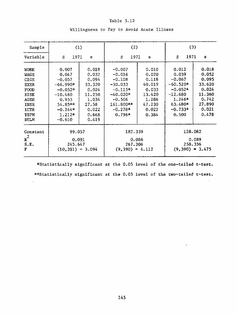
Sample

Variable

(1)

8 1971 s

WORK 0.007 0.018 WAGE 0.047 0.032 CIGE -0.057 0.094 EXER -66.990* 33.320 FOOD -0.052* 0.024 RISK -10.460 11.250 AGEH 0.955 1.034 INSR 54.85*-k 27.58 ICTR -0.244s: 0.022 TSPM 1.212* 0.668 SULM -0.610 0.419

Constant

R2 S.E. F

99.057

0.091 245.647

(10,391) = 3.094

Table 5.12

Willingness to Pay to Avoid Acute Illness

(2) (3)

8 1971 s B 1971 s

-0.007 -0.016 -0.108

-30.033 -0.115*

-40.020* -0.506

161.800** -0.278*

0.796*

0.010 0.012 0.020 0.039 0.118 -0.067

40.019 -60.520* 0.033 -0.052*

13.420 -12.680 1.286 1.246*

47.230 63.480* 0.022 -0.233* 0.384 0.500

0.018 0.052 0.095

33.620 0.024

11.360 0.742

27.890 0.021 0.478

182.339 128.082

0.086 0.089 267.306 258.336

(9,390) = 4.112 (9,390) = 3.475

*Statistically significant at the 0.05 level of the one-tailed t-test.

**Statistically significant at the 0.05 level of the two-tailed t-test.

145

Sample

Variable

(1)

6 1970 S

(2)

6 1971 S

EDUC WORK DSAB FMSZ BDALO J3MPNb. LTWK ABSN a UION RACE LDSA

31.730* 0.016

179.200** 33.610* 40.470*

0.554** -17.430

-5.401 87.320* 41.310

-255.600*

8.735 0.021

50.230 6.293 6.075 0.218

33.520 44.010 34.620 33.780 58.880

23.740" 5.307 0.0017* 0.0011

35.670** 17.220 63.790* 37.980 14.610* 3.447

0.642 0.927 -35.160 32.070

29.880 19.920 68.430 81.210

-69.940* 30.530

Constant -59.852 -28.345 S.E. 255.199 159.234 F (11,388) = 26.020 (10,389) = 13.685

Table 5.13a

Two-Stage Least Squares Estimates of WAGE Expressions for Chronic Illness

*Statistically significant at the 0.05 level of the one-tailed t-test.

**Statistically significant at the 0.05 level of the two-tailed t-test.

aABSN refers to the frequency with which the individual missed work for reasons other than illness.

b HME'N refers to annual hours of home production, e.g., car repairs, house additions and repairs, etc.

146

Table 5.13b

Two-Stage Least Squares Estimates of Chronic Illness Expressions

(LDSA)

.Sample

Variable

(1)

B 1970 S

(2)

B 1971 S

RISK AGEH INSR CHEM CITY POOR FEDU ICTR TSPN

-0.030 0.052 0.029* 0.006

-1.4756: 0.257 -6.804* 2.479

0.052 0.129 0.500* 0.150

-0.036-3 -0.17x10 *

o.044-3 0.05x10

0.0021 ' 0.0020 -0.001 0.004

0.005* 0.002

-0.016 0.048 0.031* 0.005

-o-553* 0.170 0.268 0.703 0.050 0.134 0.3456: 0.135

-0.028-4 -0.80~10 *

0.046-4 0.16x10

0.0039* 0.0010 -0.0007 O.OC14

0.005* 0.001

Constant I 0.521 I 0.033 S.E. 1.168 1.193 F (11,388) = 9.733 (11,388) = 13.250

*Statistically significant at the 0.05 level of the one-tailed t-test.

**Statistically significant at the 0.05 level of the two-tailed t-test.

147

coefficient for CHEM in expression (1) is undoubtedly an anamoly since onlyone person worked in the chemicals and metals manufacturing sector. Thoserespondents who were poor when growing up demand less chronic illness avoid-ance, perhaps because their health status is initially less and they there-fore must invest more to reach a given health status level. WAGE, and there-

fore WAGE, is defined here as the individual's marginal hourly earnings.This need not be his hourly earnings without overtime on his primary job.

In Table 5.13b, only expression (2) possesses a statistically signifi-cant air pollution coefficient. Assuming as in previous sections that eachunit of LDSA is slightly more than two years, or 830 days, in length, thateach of these days is a potential workday, and that the average workday iseight hours long, then an additional unit of TSPN in expression (2) of 5.13acauses the individual's utility-maximizing number of days of chronic illnessto increase by 3.25 days over his lifetime. We have no idea, however, howthese additional days will be distributed over his lifetime, nor can wetreat 3.25 additional days for someone who is already chronically ill assimilar to 3.25 additional days for someone who is not now chronically ill.Assume our representative individual currently has no chronic illness, andfurther assume that perpetual exposure to an additional unit of TSPN willcause him to acquire immediately a "chronic" illness. The arithmetic mean

for WAGE in 1971 is $3.72 per hour. Since our representative individualworks eight hours per day, and since he will now find that 3.25 days of hisworktime will at some time no longer be available, he would be willing topay an undiscounted amount of $96.72 in a single lump sum. The arithmeticmean of TSPN in sample (2) is 156.185, and 127.574 units of TSPN is twostandard deviations removed from this mean. Assuming the validity of alinear exprapolation of the preceding marginal (= average) willingness topay to avoid the chronic illness induced by perpetual exposure to an addi-tional unit of TSPN, we find that the representative respondent would bewilling to pay an undiscounted lump sum of approximately $25,000 ($24,678)to avoid the chronic illnesses associated with spending the rest of his lifein an extremely high TSPN location as opposed to an extremely low TSPNlocation.

5.7 Overview of Empirical Results

We view the empirical results of this chapter as tentative and ongoingrather than as definitive and final. The SRC interview data that we employis a random sampling of the civilian, noninstitutionalized population of theUnited States. Extrapolations of results to the entire population are there-fore fairly reasonable, even though we have not employed the SRC samplingweights. However, caution must be exercised in doing so: our measures ofillness are substantially less than ideal. In particular, the measure ofchronic illness is rather discrete and its uppermost value is unbounded.Moreover, individuals who died between the reference year of the interviewand the time of interview are not included. Both factors probably cause thehealth impact of air pollution to be underestimated. Nevertheless, we feelthat we have provided an example of some of the things that can be done withmicroepidemiological data on health status, endowments, and time and budgetallocations. In the bulk of the dose-response expressions we have estimated,most of which were estimated from distinct random samples, air pollution isassociated with increased time spent being acutely and/or chronically ill.

148

Air pollution, in addition, appears to influence labor productivity, wherethe reduction in productivity is measured in the earnings lost due to reduc-tions in salable skills and in work-time. The reduction in productivity dueto air pollution-induced chronic illness seems to overwhelm any reductionsdue to air pollution-induced acute illness.

The following examples involve linear extrapolations of estimated laborproductivity effects and willingnesses-to-pay at arithmetic mean air pol-lution concentrations. The linear exprapolations extend two standard devi-ations from the means of the frequency distributions of these concentrations.Geographical locations residing in the upper tails of these distributionsmight reasonably be regarded as extremely dirty while those along the ex-tended portion of the lower tails are bathed in extremely clean air. Therepresentative individual who is instantaneously and painlessly removedfrom an extremely dirty location to an extremely clean one might expect toacquire about $20 (in 1970-71 dollars) in additional annual earnings fromreductions in air pollution-induced acute illnesses. This same individualwould annually acquire several hundred 1970-71 dollars (approximately $100to $600 in our empirical tests) by the reduction in chronic illness he wouldobtain from a similar removal. Both these results assume that wage ratesare not adjusted in response to a cleaner environment.

The willingness of the representative individual to pay for the annualhours of acute illnesses he could avoid by being in a clean rather than adirty environment is, for the two samples for which we obtained estimates,between $300 and $500 annually in 1970-71 dollars. For chronic illnessavoidance, we calculated, under some extremely crude assumptions and on thebasis of only a single sample, that representative individual would bewilling to pay an undiscounted lump sum of $25,000 to be in the clean ratherthan the dirty environment.

149

FOOTNOTES

L'The Survey Research Center possesses the exact addresses of the samplefamilies, but does not include them in its data tapes.

?/This "errors in variables" problem is usually handled by using instru-mental variables which are highly correlated with the variable measured witherror but are uncorrelated with the error. We were unable to think of avariable having these properties.

?'SRC interviews for 1973 behavior and status include a three-digitoccupational code corresponding to the coding used in U.S. Bureau of theCensus, 1970 Census of Population Alphabetical Index of Industries and Oc-cupations, Washington, D.C.: USGPO (1971). This means that information isavailable in the SRC data set on nearly the exact kind of job held by thefamily head and/or his wife. This rather magnificent store of informationobviously has many research possibilities which remain completely unexploitedin this study.

k/0ther measures of ill-health are available in the SRC data set,particularly the severity of the disability, if any, and the number of weeksmissed from work due to sickness. Because of its qualitative nature, thedecision was made to use the first of these entirely as an explanatory ratherthan as a dependent variable.

S'Expressions of discomfort with the reductionist perspective are nowfairly common in the biomedical literature. See, for example, Syme and Berk-man (1970) and Engel (1977). More importantly, there is empirical evidencethat variations in self-reported health status reflect correct variationsin clinically objective measures of health. See Grossman (1975, p. 168) fora review of this literature as well as some additional empirical evidence.

&/The literature which views children as an investment is surveyed inseveral papers in a supplement to the March/April 1973 issue of the Journalof Political Economy.

7'The 18th century French jurist and philosopher, Montesquieu (1947,p. 245), succinctly stated the central theme of much of this literature:"The nations of hot countries are timorous like old men, the nations incolder regions are daring like youngsters." Recent efforts have been con-siderably less elitist and self-congratulatory.

s'A fair amount of work appears to have been done to ascertain the dis-crepancies, if any, between self-reported and clinically evaluated healthstatus. Survey Research Center (1977, pp. 7-10) states that the bulk ofstudies conclude: (1) as the time between an interview and an event lenghtens,there is increased underreporting about the magintude of the event; (2)important events are less likely to be incompletely and inaccurately reported;and (3) self-reported events are likely to be biased in what the respondentconsiders to be a socially acceptable direction. Marquis (1978), however,disputes these conclusions because all studies either check self-reportedhealth status against clinical records or check clinical records againststatus. He shows that a statistically correct test of bias requires both

150

checks. When he performed this check with a sample of individuals fromDayton, Ohio, he found that "...there is little or no average reporting biasin hospital admission/discharge data obtained by household interviews." (p.42).

?/This high proportion of non-whites is probably caused by the factthat 40 percent of the original 1967 sample was composed of families pre-viously interviewed by the U.S. Bureau of the Census for the 1966 Surveyof Economic Opportunity.

=/Wallace (1977) has surveyed a number of recently evolved testsenabling the investigator to ascertain the extent to which Selvin's andStuart's (1966) data-dredging alter the trustworthiness of later estimates.We have disregarded the Wallace (1977) tests in this study in favor ofdrawing entirely new samples each time a new expression is estimated.

11'There is another alternative: each of the following structuralexpressions could be estimated:

a) DSAB = f (Air pollution, lifestyle, . . ., etc.)

b) LDSA =

where the in expression (b) is the estimated value of DSAB. However,since DSAB is measured in ordinal and discrete terms, either a multinomiallogit or a basic logit specification using maximum likelihood estimationmethods would have to be employed. In the latter case, four differentversions of (a) would have to be estimated since DSAB involves four dis-crete ordinal measures.

z'See, for example, Grossman and Benham (1973), Thaler and Rosen (1975),and Parsons (1977).

=A review of recent work is available in Lave and Seskin (1977).

14'In Grossman's (1972) notation, the sick time production function is:

where TL represents chronic or acute sick time, H is the stock of healthcapital, It is current health investments, and 6is the rate at which thehealth stock decays. The term in parentheses is the stock of health capitalwritten in terms of the past stock of health capital and current investmentin health. Thus, for example, we treat such variables as POOR, DSAB, andFEDU as determinants of and FOOD, NCIG, TSPM, etc., as components of

It and 8. Grossman (1972) chosses a multiplicative form for this expression,

whereas we adopt a linear form. Most inportantly, Grossman (1972) makes boththe wage rate and the health state endogenous by making the former a functionof the latter and the latter a function of the former. We treat the healthstate as exogenously determined while retaining the dependence of the wageupon the health state.

151

15/This currently lesser productivity could readily be due to pastdiscrimination in the labor market and/or education as well as fewer pastopportunities for investment in physical health.

16/In this casestandard

it is unlikely that multicollinearity has seriouslyinflated the errors of the air pollution variables. The highestsimple correlation coefficient between an air pollution variable and anotherexplanatory variable was rTSP ' SULM = 0.65. All other simple correlation

coefficients were less than 0.20.

=/The 830-day interval is a weighted arithmetic mean established bytaking the midpoint of each of the time equivalents of the SRC indexmeasures for LDSA and weighting by the proportion of the entire SRC samplein 1971 having a particular LDSA index value. Ten years was treated as themidpoint for the uppermost LDSA index.

18'See Crocker and Horst (1977).

19'Ideal generalization of this model would have: (1) the flow of healthservices rather than the stock of health entering the individual's utilityfunction; and (2) the opportunity cost of time not be assumed equal to thewage rate but rather derived from the model to be equal to the wage rateweighted by the shadow price for expenditures on inputs into the productionof health and the composite commodity.

20'The time expenditure at which fatugue and/or boredom sets in on aparticular job and the rate at which it changes is itself likely to be afunction of the individual's state-of-health and education. We have nottried to capture this either in this model or in the subsequent empiricaleffort that accords with it. One might argue that various attitudinalmeasures such as job satisfaction, aspiration and ambition, and othersreadily available in the SRC data would serve as adequate proxies forfatugue and boredom.

1'Simultaneity is implied by the model in the demand for acute illness.In particular, although we considered it only in passing, the time expendedin other work activities is an endogenous variable, which, in turn, impliesthat work time is endogenous. We have, infact, tested this sumultaneityby treating work as endogenous and estimating the systme by two-stage leastsquares. The results, which we do not bother to report here, differed onlytrivially from the ordinary least squares estimates that we do report.

22/The reader should be aware that by adopting a TSLS estimation pro-cedure, we are giving up some efficiency in estimation in order to enhancethe consistency of our estimation. The cruelty of this tradeoff is due tothe quite low coefficients of determination involved in OLS estimates of thefreedom from chronic illness demand function.

152

Chapter VI

AN ESTIMATE OF NATIONAL LOSSES IN LABOR PRODUCTIVITYDUE TO AIR POLLUTION-INDUCED MORBIDITY

6.1 Introduction

In this brief chapter, we use what we consider to be the most repre-sentative of the recursive labor supply estimates in Table 5.10 to speculatewhat the aggregate gains in U.S. labor productivity could be from a reductionin air pollution-induced acute and chronic morbidity. Due to the preliminaryand exploratory nature of our work, we are most anxious that the readerwishing to employ or to communicate these calculations be careful always tomake highly visible the set of assumptions in which the calculations areembedded. Otherwise, he will be unable to make an informed judgment aboutthe extent to which the world represented in the text corresponds to reality.

Figure 6.1 is a hueristic representation of the structure forming thebasis of our estimate. Air pollution is viewed as increasing directly bothchronic and acute illness. In addition, it causes an indirect increase inacute illness via its positive effect on chronic illness. Acute illnessreduces hours worked, but, because of its passing nature, it has no impactupon the worker's long-term productivity that determines the level of hiswages. However, chronic illness, which does reduce long-term productivity,exerts a direct negative influence on both wages and hours worked. It alsoinfluences hours worked in an indirect manner through its effect upon wages.

Figure 6.1

A Representation of the Effect of Air PollutionUpon Labor Productivity

153

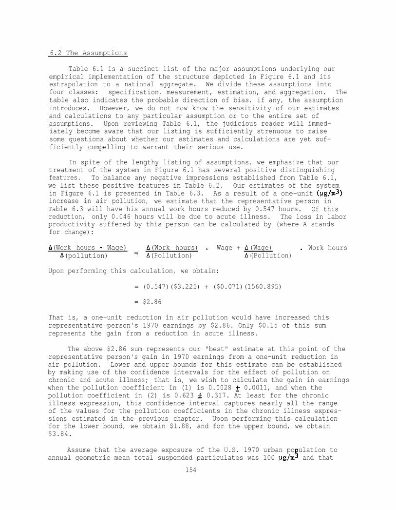
6.2 The Assumptions

Table 6.1 is a succinct list of the major assumptions underlying ourempirical implementation of the structure depicted in Figure 6.1 and itsextrapolation to a national aggregate. We divide these assumptions intofour classes: specification, measurement, estimation, and aggregation. Thetable also indicates the probable direction of bias, if any, the assumptionintroduces. However, we do not now know the sensitivity of our estimatesand calculations to any particular assumption or to the entire set ofassumptions. Upon reviewing Table 6.1, the judicious reader will immed-iately become aware that our listing is sufficiently strenuous to raisesome questions about whether our estimates and calculations are yet suf-ficiently compelling to warrant their serious use.

In spite of the lengthy listing of assumptions, we emphasize that ourtreatment of the system in Figure 6.1 has several positive distinguishingfeatures. To balance any negative impressions established from Table 6.1,we list these positive features in Table 6.2. Our estimates of the systemin Figure 6.1 is presented in Table 6.3. As a result of a one-unit (pg/m3>increase in air pollution, we estimate that the representative person inTable 6.3 will have his annual work hours reduced by 0.547 hours. Of thisreduction, only 0.046 hours will be due to acute illness. The loss in laborproductivity suffered by this person can be calculated by (where A standsfor change):

(Work hours Wage) = (Work hours) Wage + (Wage) Work hours(pollution) (Pollution) (Pollution)

Upon performing this calculation, we obtain:

= (0.547)($3.225) + ($0.071)(1560.895)

= $2.86

That is, a one-unit reduction in air pollution would have increased thisrepresentative person's 1970 earnings by $2.86. Only $0.15 of this sumrepresents the gain from a reduction in acute illness.

The above $2.86 sum represents our "best" estimate at this point of therepresentative person's gain in 1970 earnings from a one-unit reduction inair pollution. Lower and upper bounds for this estimate can be establishedby making use of the confidence intervals for the effect of pollution onchronic and acute illness; that is, we wish to calculate the gain in earningswhen the pollution coefficient in (1) is 0.0028 f 0.0011, and when thepollution coefficient in (2) is 0.623 f 0.317. At least for the chronicillness expression, this confidence interval captures nearly all the rangeof the values for the pollution coefficients in the chronic illness expres-sions estimated in the previous chapter. Upon performing this calculationfor the lower bound, we obtain $1.88, and for the upper bound, we obtain$3.84.

Assume that the average exposure of the U.S. 1970 urban population to5annual geometric mean total suspended particulates was 100 ug/m and that

154

Table 6.1

Major Assumptions Limiting Generality of Results

Specification

1) Air pollution affects only the duration of chronic illness. Ourinattention to the severity of chronic illness tends to reduce the estimatedimpact of air pollution on labor productivity.

2) Occupational exposures to hazards and environmental pollutants otherthan air pollution do not influence either acute or chronic illness. If airpollution is moderately and positively associated with these hazards andpollutants, this assuption tends to increase the estimated impact of airpollution on labor productivity.

3) Annual geometric mean ambient concentrations of total suspendedparticulates serve as an adequate proxy for all forms of air pollution.The effect of this assumption upon the estimated effect of air pollutionon labor productivity is unknown.

4) All relationships depicted in Figure 6.1 are linear. It is unknownwhat effect this assumption has on the estimated effect of air pollution onlabor productivity.

5) Air pollution-induced health effects do not cause the voluntarysubstitution of leisure for work. This assumption tends to reduce theestimated impact of air pollution on labor productivity.

Measurement

6) Air pollution exposures for each individual in the sample areadequately represented by a single annual average of ambient concentrationsobtained at a single monitoring station within the individual's county ofresidence. Since pollution monitoring stations in the early part of the1970's were predominantly in downtown urban locations, individuals' airpollution exposures probably tend to be exaggerated. This will reduce theestimated health effects of air pollution.

7) The duration of any air pollution-induced chronic illness cannotexceed ten years. This will reduce the estimated effect of air pollutionupon the duration of chronic illness.

8) Housewives, retirees, and students, who together constitute abouttwenty percent of our samples, do not contract air pollution-induced acuteillnesses. This assumption will tend to reduce the estimated impact of airpollution upon labor productivity.

9) Air pollution-induced chronic and acute illnesses are a constantproportion of all illnesses. The effect of this assumption is unknown.

(continued)

155

Table 6.1

(continued)

10) The quantity of preventive and ameliorative medical care anindividual consumes is adequately measured by whether or not he has medicalinsurance. This assumption has an unknown effect upon our estimates.

11) Relative air pollution concentrations across the U.S. have beenfairly constant. This assumption has an unknown effect upon our estimatesof air pollution-induced chronic illness.

12) When interviewed, the individuals in the sample had no incentiveto bias their answers nor did they have difficulty accurately recallingtheir personal medical histories of the previous twelve to sixteen months.The effect of this assumption upon our estimates is unknown.

13) No individual who would otherwise have been included in the sampledied between the time for which information was to be gathered and the timeof the interview. In fact, about five percent of the potential respondentsdied each year. The effect of this assumption is to reduce the effects ofair pollution upon labor productivity.

Estimation

14) With the available data, classical linear regression proceduresprovide consistent and unbiased estimates of the structure depicted inFigure 6.1. The effect of this assumption upon our estimates is unknown.

Aggregation

15) The response of the health state of each individual in the U.S. toany given change in ambient air pollution is a constant. The effect of thisassumption upon the calculation for the aggregate effect of air pollutionupon labor productivity is unknown.

16) The response of the health state of every individual in the U.S.to ambient air pollution changes is identical. The effect of this assump-tion upon the calculation for the aggregate effect of air pollution uponlabor productivity is unknown.

156

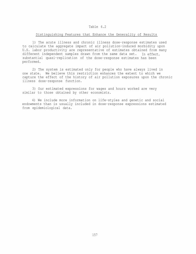
Table 6.2

Distinguishing Features that Enhance the Generality of Results

1) The acute illness and chronic illness dose-response estimates usedto calculate the aggregate impact of air pollution-induced morbidity uponU.S. labor productivity are representative of estimates obtained from manydifferent independent samples drawn from the same data set. In effect,substantial quasi-replication of the dose-response estimates has beenperformed.

2) The system is estimated only for people who have always lived inone state. We believe this restriction enhances the extent to which wecapture the effect of the history of air pollution exposures upon the chronicillness dose-response function.

3) Our estimated expressions for wages and hours worked are verysimilar to those obtained by other economists.

4) We include more information on life-styles and genetic and socialendowments than is usually included in dose-response expressions estimatedfrom epidemiological data.

157

Table 6.3

Estimated Expressions to be Used to Calculate the Effect ofAir Pollution-Induced Illness on Labor Productivitya

(1) 830 day years chronically ill = 2.980 + 0.554 (illness severity)** +(0.035)

0.005(age in years) + 0.013(years of school) - 0.044(father's years of(0.004) (0.029) (0.037)school) - 0.069(poor when growing up) + 0.072(Caucasoid) + 0.139(male)

(0.103) (0.488) (0.114)- 0.902(diet adequacy) - 0.454(has medical insurance)* - 1.645(works(0.975) (0.129) (0.575)

in chemicals/metals industries) b + 0.0028(mean total suspended(0.0011)

particulates)*

R2 = 0.525; S.E. = 0.964; F(11,388) = 38.920.

(2) Annual hours acutely ill = 165,208 + 39.52(years chronically ill)*(13.34)

-1.421(age in years) - 16.92(male) - 0.086(cigarette expenditures) -(1.312) (39.16) (0.118)78.47(gets strenuous exercise)* - 0.105(diet adequacy)* - 38.44(degree(40.11) (0.033) (13.26)of risk aversion)* + 187.70(has medical insurance)** - 85.56(works in

(47.47) (191.20)chemicals/metals industries) + 0.623(mean total suspended particulates)*

(0.317)

R2 = 0.195; S.E. = 204.462; F(10,389) = 5.721.

(3) Wage in cents = -132.318 - 25.930(years chronically ill)* + 24.070(years(14.440) (8.578)

of school)* + 15.370(illness severity) + 26.880(family size)* + 42.380(18.260) (6.079) (6.138)

(cost-of-living)* = 52.950(years on current job)* - 7.163(often late(22.130) (33.88)

for work) + 66.090(union member)* + 47.60(Caucasiod)(34.580) (34.22)

R2 = 0.408; S.E. = 258.908; F(11,388) = 24.28.

(continued)

158

Table 6.3

(continued)

(4) Annual hours worked = 1266.68 - 163.90(years chronically ill)* + 0.354(27.22) (0.130)

(wage in cents) * + 44.26(family size)* + 519.80(male)* - 0.272(dollars(16.68) (80.27) (0.022)

Of transfer income)* + 23.06(cost-of-living) - 0.074(annual hours(15.20) (0.031)

acutely ill)*

R2 = 0.551; S.E. = 663.196; F(6,393) = 80.41.

aExact variable definitions are available in Table 5.1.

bThe number of people in these industries was too small for this coefficientto be meaningful

*Statistically significant at the 0.05 level of the one-tailed t-test.

**Statistically significant at the 0.05 level of the two-tailed t-test.

159

the standard deviation of these exposures was 30 pg/m3. Throughout thisstudy, total suspended particulate measures have been highly correlatedwith other air pollutants so that total suspended particulates probablyserve as an adequate proxy for all air pollution. Further assume that thenational urban population is approximately 150 ~010~ people, each of whomis or will be a family head. After age 20, each of these family heads hasa life-span of 50 years and any air pollution-induced chronic illnesses hecontracts are distributed rectangularly over the 50 years. The earnings heloses due to the presence of an acute or chronic illness do not vary overthe years. Given these and earlier assumptions, a 60 percent reduction inair pollution would, in June 1978 dollars, increase the value of 1970U.S. labor productivity by the amounts shown in Table 6.4. Most of thegain would accrue due to reductions in air pollution-induced chronic illness.

It must be strongly emphasized that the magnitudes exhibited in Table6.4 are extremely sensitive to the assumptions we have made. Nevertheless,given any reasonable set of assumptions about air pollution exposures, sizeof the population exposed, etc., the estimates of labor productivity gainsin Table 6.4 are much larger than previous estimates of all types of annualgains from air pollution control in the United States. No gains in laborproductivity, via reductions in air pollution-induced health effects, havepreviously been developed. It thus appears that the economic gains fromthe morbidity effects of air pollution control have been greatly under-valued, perhaps because most prior research efforts have concentrated uponmortality rather than morbidity.

A more conservative but equally tenuous way of calculating the effectsin Table 6.4 might proceed as follows. Assume that the 75 percent, or 112x lo6 million people of the 150 x 106 urban population are 16 years orolder. At age 16, each of these adults has a lifespan of 56 years and anyair pollution-induced chronic illnesses he contracts are distributed rectan-gularly over the 56 years. The annual earnings he loses due to the presenceof an acute or chronic illness do not vary over the 56 years. If the medianhousehold size is 2.0, there are then 56.25 x 106 urban household heads.There is thus a $160.88 x lo6 = ($2.86) (56.25 x 106) gain in the laborproductivity for household heads from a one unit reduction in air pollution.

If two-thirds of the household heads are married, if 35 percent ofthese households have working wives, and if working wives earn 60 percent asmuch as their male counterparts, there would then be a $22.58 x 106 =($2.86) (0.6) (13.13 x 106) gain in the labor productivity of working wives.

If the value of household services provided by all household membersin each urban household is 40 percent of the household head, there wouldthen be a $64.35 x lo6 = ($2.86)(0.4) (56.25 x 106) gain in the householdlabor productivity of all urban households. Adding the results for house-hold heads, working wives, and household labor, we obtain a $247.81 x lo6gain in labor productivity for a one unit reduction in air pollution. A 60percent reduction in 1970 air pollution would then, in August 1978 dollars,increase the value of 1970 urban labor productivity by $25 x log dollars.This is a "best" estimate.$34 x log and $16 x 109.

Its upper and lower bounds are, respectively,If one performs these identical calculations in

precisely the same fashion for a 1977 U.S. total population of 216.1 x 106,one obtains a "best" estimate of $36 x 109.

160

Table 6.4

Estimated Per Capita Aggregate Gains in 1970 U.S. Labor Productivity Due toa 60 Percent Reduction in Air Pollution

(June 1978 Dollars)

Lower Bound

PerCapita

$189.50

"Best" Estimate $288.29

Upper Bound $387.07

Aggregate

28,426 x lo6

43,243 x lo6

58,061 x lo6

161

REFERENCES

Becker, G.S., "A Theory of the Allocation of Time," Economic Journal 75(September 1965), 493-517.

Blumquist, G., "Value of Life: Implications of Automobile Seat Belt Use,"Unpublished, March 1977.

Conley, B., "The Value of Human Life in the Demand for Human Safety,"American Economic Review 66, (March 1976), 45-57.

Crocker, T.D. and Horst, R.L, Jr., Oxidant Air Pollution and Work Performanceof Citrus Harvest Labor, Research Triangle Park, N.C.: USEPAPublication, 600/5-77-013 (September 1977).

Cropper, M.L., "Health, Investment in Health, and Occupational Choice,"Journal of Political Economy 85 (December 1977), 1273-1294.

Engel, G.L., "The Need for a New Medical Model: A Challenge for Biomedicine,"Science, (1977), 129-136.

Grossman, M., "On the Concept of Health Capital and the Demand for Health,"Journal of Political Economy 80 (March/April 1972), 223-255.

Grossman, M., and Benham, L., "Health, Hours, and Wages," in M. Perlman,(ed.), The Economics of Health and Medical Care, New York: HalsteadPress (1973), 205-233.

Grossman, M., "The Correlation between Health and Schooling," in N.E.Terleckyj (ed.), Household Production and Consumption, New York:Columbia University Press (1975), 147-211.

Hanushek, E.A., and Quigley, J.M., "Implicit Investment Profiles and Inter-temporal Adjustments of Relative Wages," American Economic Review 68(March 1978), 67-79.

Hippocrates, 460-377 B.C., "On Airs, Waters, and Places," in F. Adams, (ed.),The Genuine Works of Hippocrates, Baltimore (1939).

Kneese, A. V., and Schulze, W., "Environment, Health and Economics - TheCase of Cancer," American Economic Review 67, (February 1977), 26-32.

Kmenta, J., Elements of Econometrics, New York: Macmillan PublishingCompany (1971).

Lave, L. and Seskin, E., Air Pollution and Human Health, Baltimore: JohnsHopkins Press (1977)

Lazear, E., "Age, Experience, and Wage Growth," The American Economic Review66 (September 1976), 548-558.

162

Marquis, K. H., Record Check Validity of Survey Responses: A Reassessmentof Biases in Reports of Hospitalizations, Report R-2319-HEW, SantaMonica, California: The Rand Corp. (May 1978).

McCarthy, M.D., "Notes on the Selection of Instruments for Two Stage LeastSquares and K Class Type Estimators of Large Models," Southern EconomicJournal, (January 1971), 251-259.

Mincer, J., "The Distribution of Labor Incomes: A Survey with SpecialReference to the Human Capital Approach," Journal of Economic Liter-ature 8 (March 1970), 1-26.

Mishan, E.J., "Evaluation of Life and Limb: A Theoretical Approach,"Journal of Political Economy, Vol. 79, (December 1971).

National Academy of Science, Nitrates: An Environmental Assessment,Environmental Studies Board, NAS, Washington, D.C., 1978.

Schwing, R.C. and McDonald, G.C., "Measures of Association of Some AirPollutants, Natural Ionizing Radiation and Cigarette Smoking withMortality Rates," presented to the International Symposium on RecentAdvances in the Assessment of the Health Effects of EnvironmentalPollution, Paris, France (June 1974).

Schultz, T.P., The Estimation of Labor Supply Functions for SecondaryWorkers, Report R-1265-NIH/EDA, Santa Monica, California: The RandCorporation (February 1975).

Selvin, H.C. and A. Stuart, "Data-Dredging Procedures in Survey Analysis,"The American Statistician 20 (1966), 20-23.

Smith, R., "The Feasibility of an 'Injury Tax' Approach to OccupationalSafety," Law and Contemporary Problems, (Summer-Autumn, 1974).

Stigler, G.J., "Imperfections in the Capital Markets," Journal of PoliticalEconomy 75 (June 1967) 291.

Survey Research Center, University of Michigan, Experiments in InterviewingTechniques: Field Experiments in Health Reporting, 1971-1977,Washington, D.C." USDHEW Publication No. (HRA) 78-3204 (Nov. 1977).

Survey Research Center, A Panel Study of Income Dynamics: Study Design,Procedures, Available Data, Ann Arbor: Institute for Social Research,University of Michigan (1972a).

Syme, S.L. and Berkman; L.E., "Social Class, Susceptibility and Sickness,"American Journal of Epidemiology 104 (1976), 1-8.

Thaler, R. and Rosen, S., "The Value of Saving a Life: Evidence from theLabor Market," in N.E. Terleckyj, (ed.), Household Production andConsumption, New York: Columbia University Press (1975), 265-297.

163

Waddell, T.E., The Economic Damages, of Air Pollution, Washington, D.C.:Socioeconomic Environmental Studies Series, USEPA (1974).

Wallace, T.D., "Present Estimation in Regression: A Survey," AmericanJournal of Agricultural Economics 59 (August 1977), 431-443.

164