Bayesian uncertainty estimation methodology applied to air pollution modelling

ENVIRONMETRICSEnvironmetrics 1999^ 00]240!260

Received 0 October 0887Copyright ! 1999 John Wiley + Sons\ Ltd[ Accepted 6 November 0888

Bayesian uncertainty estimation methodology applied toair pollution modelling

Renata Romanowicz0"\ Helen Higson1 and Ian Teasdale2

0 IENS\ Lancaster University\ Lancaster LA0 3YQ\ U[K[1Cambridè Environmental Research Consultants\ 2 Kin`s Parade\ Cambridè CB1 0SJ\ U[K[

2Math Enìne plc\ Oxford Centre for Innovation\ Oxford OX1 9JX\ U[K[

SUMMARY

The aim of the study is an uncertainty analysis of an air dispersion model[ The model used is describedin NRPB!R80 "Clarke\ 0868#\ a model for short and medium range dispersion of radionuclides releasedinto the atmosphere[ Uncertainties in the model predictions arise both from the uncertainty of the inputvariables and the model simpli_cations\ resulting in parameter uncertainty[ The uncertainty of thepredictions is well described by the credibility intervals of the predictions "prediction limits#\ which inturn are derived from the distribution of the predictions[ The methodology for estimating this distributionconsists of running multiple simulations of the model for discrete values of input parameters followingsome assumed random distributions[ The value of the prediction limits lies in their objectivity[ However\they depend on the assumed input distributions and their ranges "as do the model results#[ Hence thechoice of distributions is very important for the reliability of the uncertainty analysis[ In this work\ thechoice of input distributions is analysed from the point of view of the reliability of the predictiveuncertainty of the model[ An analysis of the in~uence of di}erent assumptions regarding model inputparameters is performed[ Of the parameters investigated "i[e[ roughness length\ release height\ wind~uctuation coe.cient and wind speed#\ the model showed the greatest sensitivity to wind speed values[A major in~uence on the results of the stability condition speci_cation is also demonstrated[ Copyright! 1999 John Wiley + Sons\ Ltd[

KEY WORDS] Gaussian air dispersion model^ sensitivity analysis^ Bayesian uncertainty estimation^ like!lihood functions^ prior and posterior probability density functions^ prediction errors^prediction limits

0[ INTRODUCTION

This work addresses the problem of the uncertainty of predictions of an air pollution model andtheir dependence on the uncertainties of observations[ The uncertainty in atmospheric dispersionmodelling can be a result of both the uncertainty in modelled atmospheric processes and obser!vation errors\ and the structural and numerical errors of the mathematical model[ Structural

"Correspondence to] R[ Romanowicz\ IENS\ Lancaster University\ Lancaster LA0 3YQ\ U[K[ e!mail]R[Romanowicz"lancaster[ac[uk

R[ ROMANOWICZ\ H[ HIGSON AND I[ TEASDALE

Copyright ! 1999 John Wiley + Sons\ Ltd[ Environmetrics 1999^ 00]240!260

241

errors of the mathematical model originate from the simpli_cations involved in the descriptionof the atmospheric processes[ Also the scale represented by measured physical variables and thescale of their representation in the mathematical model di}er[ In the search for the physicalrepresentation of variables\ scientists often forget that the e}ective values of model parametersat a certain scale may not be truly represented by the quantities measured in the _eld[ This typeof uncertainty can be accounted for\ to a certain extent\ by the application of parametricuncertainty methodology and conditioning model results on observations[ However\ the degreeto which the uncertainties can be decreased depends on the amount of available information[Model structure limitations can substantially in~uence the predictions because the formulae usednecessarily include simplifying assumptions which di}er from reality and have been developedunder speci_c conditions[ Moreover\ the random nature of atmospheric processes does not allowthe model assumptions to be fully met[The proposed methodology is based on the concept of Bayesian Inference "e[g[ Box and Tiao\

0881^ Haylock and O|Hagan\ 0886#[ The method presented in this paper has been used inhydrology as the Generalised Uncertainty Estimation Technique "GLUE# "Beven and Binley\0881^ Romanowicz et al[\ 0883#\ and applies likelihood measures to estimating the predictiveuncertainty of the model[ Simulated model outputs are compared with available observations ofthe variables of interest and the distribution of the resulting errors of predictions is used to derivethe credibility intervals for the predictions[ The value of the credibility intervals "predictionlimits# lies in their objectivity[ However\ as the model results depend on the information includedin its input and output measurements\ prediction limits will depend on the assumed input andoutput distributions and their ranges[ Hence the choice of these distributions is very importantfor the reliability of the uncertainty analysis[ A sensitivity analysis of the model variables mayalso be important in gaining a better understanding of the model performance and its internalstructure[ However\ sensitivity analysis on its own is not su.cient to estimate the errors of modelpredictions and should be followed by uncertainty estimation techniques based on the comparisonof model predictions with observations[When applying the Gaussian plume model described in the next section to the prediction of

ground!level concentrations of a pollutant\ all input variables must be speci_ed\ based on theanalysis of the conditions in which the release takes place and\ in particular\ on the atmosphericconditions and geographical features of the terrain[ In the case of regulatory applications\ it iscrucial to know how reliable the model predictions are and how variability in the measurementsof the environmental variables will a}ect model performance[ The amount of information wepossess about these input variables will vary\ depending on the type of variable\ the accuracy ofthe measurements and on the role which the variable plays in the model[The resulting prediction limits rely strongly on assumptions regarding the distribution of input

variables and parameters[ As neither the model parameters nor the input distributions are knownexactly\ it is important to investigate the in~uence of di}erent assumptions regarding thesevariables and parameters on the predictive uncertainty of the model[ This analysis will also leadto recommendations about the degree of accuracy of the measurements[ The measurements ofthe variables which have the largest in~uence on model performance "e[g[ wind speed# will bemore important than themeasurements of global parameters\ which do not have a fully physically!based interpretation in the model "such as roughness length#[ Sensitivity analysis will be used toexamine the in~uence of the input variables and parameter variability on the model results\ whileuncertainty analysis will provide the analysis of in~uence of parameter and input distributionson prediction limits[

UNCERTAINTY ANALYSIS OF AN AIR DISPERSION MODEL


242

1[ PROBLEM DESCRIPTION

1[0[ Short description of the Gaussian plume model structure

The Gaussian plume model for a continuous source originates in the work of Sutton "0821#[Pasquill and Smith "0872# and Gi}ord "0850\ 0857#[ It is obtained as a solution to the Fickiandi}usion equation for constant di}usivity coe.cient and uniform wind speed[ The model isderived as a steady state solution of the basic transport model[ The assumption of constantdi}usivity is valid only if the size of the plume is greater than the size of the dominant turbulenteddies\ so that all turbulence implicit in this parameter is taking part in the di}usion[ In fact\di}usivity is seldom constant in time and space[ Also the assumption of constant wind speed isvery restrictive\ as wind speed varies with height throughout the atmospheric boundary layer[Assuming that the meteorological conditions are constant during the travel of the plume limitsthe application of the model to short time periods "04 minutes to 0 hour# and small distances"up to approximately 29 km#[ These limitations should be taken into account when applying themodel[ Even though these conditions are never met in practice\ the Gaussian plume model hasbeen widely adopted "see Hanna et al[\ 0871#[The mathematical description of the Gaussian model used in the present work is given in

NRPB!R80 "Clark\ 0868#\ and is hereafter referred to as the R80 model[ The basic equationusing a Gaussian plume model for an elevated release has the form "Clarke\ 0868#]

C"x\ y\ z# !Q

1pu09szsyexp$"9[4 0y

1

s1y

#"z"h#1

s1z 1% "0#

where C is air concentration "g m#2# or its time integral "g s m#2#^ Q is the release rate "g s#0# ortotal amount released "g#^ u09 is the wind speed at 09 m above the ground "m s#0#^ sz is thestandard deviation of the vertical Gaussian distribution "m#^ sy is the standard deviation of thehorizontal Gaussian distribution "m#^ x is the rectilinear co!ordinate along the wind direction"m#^ y is the rectilinear co!ordinate for cross!wind "m#^ z is the rectilinear co!ordinate above theground "m#^ and h is the e}ective release height "m#[ The origin of the co!ordinate system is atground level beneath the discharge point[The R80 model incorporates re~ection of the plume from the ground and the top of the

atmospheric boundary layer[ In this case the model solution has the form]

C"x\ y\ z# !Q

1pu09szsyexp $"y1

1s1y %F"h\ z\A# "1#

where

F"h\ z\A# ! exp$" "z"h#1

1s1z %#exp$" "z#h#1

1s1z %#exp $" "1A#z#h#1

1s1z %

#exp$" "1A#z"h#1

1s1z %#exp$" "1A"z#h#1

1s1z %#exp$" "1A"z"h#1

1s1z % "2#



243

Equation "1# should be used at distances where sz#A "where A denotes the depth of theboundary layer#[ When the value of the vertical dispersion coe.cient sz becomes much greaterthan the depth of the boundary layerA "sz!A#\ the vertical concentration distribution e}ectivelybecomes uniformly distributed throughout the mixing layer[ The concentration is then given by]

C"x\ y\ z# !Q

"1p#0:1u09Asy

exp$" y1

1s1y% "3#

Typical values of boundary layer depth are given in Table 1 of NRPB!R80 "Clarke\ 0868# forPasquill!Gi}ord stability categories A to G[The vertical standard deviation sz at a given distance from the source is modelled as being a

function of the atmospheric stability\ downwind distance and ground roughness[ Hosker "0863#derived analytical formulae used in the R80 methodology "NRPB!R80# for speci_c roughnesslengths and interpolation is used for intermediate values of roughness coe.cient[ This may besummarised as]

sz !F"x\z9# (G"x\CAT# "4#

where z9 denotes roughness length\ F"x\ z9# is an expression which varies continuously withdistance from the source and has a speci_c form for particular values of roughness length\ CATdenotes the stability condition and G"x\ CAT# is a function which has a slightly di}erent formfor each stability condition\ each of which is a continuous function of the distance downwindfrom the source[The horizontal dispersion of the plume\ characterised by the standard deviation sy\ is the result

of turbulence processes and ~uctuations in wind direction[ The formulation used in the R80model uses an expression for sy given originally by Pasquill for very short "2 minute# releases[This may be applied for releases much less than 29 minute duration[ For longer time releasessome account must be taken of ~uctuations in wind direction[ The _nal formula for sy is due toMoore "0865# and has the form]

s1y !s1

yt#s1yw "5#

where syt represents di}usion due to turbulence "2!minute term# and syw is the component dueto ~uctuations in wind direction[The values of syt are given in Figure 09 of NRPB!R80 "Clarke\ 0868#\ which shows separate

curves for each stability condition "CAT#\ each of which varies continuously with the distancex]

syt !P"CAT# ( x9[80 "6#

syw is evaluated using the following empirical formula "Jones\ 0872#]

syw ! 9[965$6Tu09%0:1

x "7#



244

where T denotes release duration "averaging period# in hours and the expression in brackets isnon!dimensional[These formulae for the horizontal distribution of a plume as represented by Equations "1# and

"3# can be used for any duration of release longer than about 29 minutes for which weathercategory and wind direction may be assumed constant[Explicit variables used in the R80 model are distance from the source\ wind speed at 09 m

height\ e}ective release height\ release rate\ roughness length and weather category[ All thosevariables must be speci_ed by the user[ Some of them can be treated as independent inputvariables and some act as parameters of the model[The standard deviations of the vertical and horizontal Gaussian distribution are implicit model

variables[ They are given in the form of empirical relations "4# and "5#\ "6# and "7#[ Theseformulae depend on the explicit parameters\ but also on some internal parameters based on _eldexperiments\ which are treated as _xed by the model[ These are\ for example\ the depth of theboundary layer\ which varies with the weather category\ and the wind direction coe.cient equalto 9[954 in Equation "7#[ Moreover\ di}erent relations apply depending on the weather category"i[e[ the dependence is not continuous#[In particular\ the vertical standard deviation "4# is a function of downwind distance\ with the

exact form of this function depending on the speci_ed roughness coe.cient and stabilitycondition[ Also the relationship describing the in~uence of wind direction deviations "7# in thede_nition of the horizontal plume dispersion "5# is very simplistic and may involve some error[The stability categories for the weather used in R80 are described in NRPB!R80 "Clarke\ 0868#

and have the form of seven discrete conditions with associated values of wind speed and boundarylayer height[ When analysing the R80 relations\ stability conditions a}ect the boundary layerheight\ horizontal dispersion and vertical dispersion[The uncertainty involved in the speci_cation of model variables in~uences the uncertainty of

the model predictions and hence is essential in this analysis[ In order to study this in~uence\variables are varied within speci_ed ranges\ according to the assumed random distribution asdescribed in Section 2 below[ In the case of the R80 model these will be] wind speed\ stabilitycondition\ roughness length\ release height\ turbulent wind ~uctuation coe.cient and inversionlayer height[Even though all these variables must be speci_ed to run the model in a particular application\

some are treated as input variables and others as model parameters[ When applying the modelto predict ground concentrations from a pollutant release\ some variables will be observed inputs"and therefore independent of the modeller# and some are treated as model parameters\ to becalibrated[ The distinction between input variables and model parameters is\ to some extent\subjective and depends on a knowledge of the physical process being modelled and a detailedanalysis of the model structure[ This distinction is important when the variable ranges anddistributions are estimated[ The variations introduced for independent "input# variables shouldre~ect the input observation errors and their ranges should not depend on themodel performance[Dependent parameter ranges should be chosen to give the best model performance based on thecomparison of model results with the available output observations[Among the explicit R80model variables\ roughness coe.cient should be treated as a dependent

model parameter[ It is de_ned as a value representing an integrated e}ect of the land surface onturbulent mixing^ hence it is not measurable[ The available point measurements of roughnesscoe.cient will not correspond to the e}ective roughness length required by the model\ as thesurrounding area is not homogenous[ All other variables can be treated as model inputs[



245

The next problem arises from the reliability of the measurements of the input variables[ Wecan assume that the wind speed measurements are accurate\ but wind speed is very variable\ andas in the case of the spatially variable roughness length\ some time averaged value of wind speedshould be used in the model[ The physical release height is a well de_ned parameter^ however\there are a number of e}ects which may in~uence the {e}ective| stack height\ namely the presenceof buildings and plume rise due to density:buoyancy driven e}ects[ Hence it was decided to varythe release height as well[ In addition to these explicit input variables\ there are other hiddenparameters in the model\ estimated from empirical relations derived from di}erent experiments[These are\ among others\ inversion layer height and wind direction ~uctuation coe.cient[ Inver!sion layer height is assumed constant for a particular weather category in the model and is givenby values in Table 1 of NRPB!R80 "Clarke\ 0868#[ The turbulent wind ~uctuation coe.cient$Equation "7#% is represented by the value 9[954\ which has been derived empirically from other_eld experiments^ this has been allowed to vary here\ to account for variations in horizontalplume spread[The stability condition is used by the model as a switch leading to di}erent model parameter!

isation[ Information about the stability condition is also uncertain and its uncertainty should beintroduced into the model[ One way of doing so would be by modifying the model structure toaccount for the lack of information about the stability conditions[ This can be equivalent tosetting the stability condition in the model to one category only and using such a model to derivethe predictions in di}erent atmospheric conditions[ Certain errors will be introduced in this way\which would re~ect the lack of information about the correct stability condition[ The othermethod may consist of changing the model structure such that the model chooses the stabilitycondition depending on the wind speed and also on some other parameters\ such as roughnesslength[The main factors in~uencing the di}usion process in the atmosphere are not easily measurable\

e[g[ the friction velocity in turbulent motion over heterogeneous surfaces or a measure of thebuoyancy generated by internal density or temperature di}erences[ The uncertainty involved inthe speci_cation of model variables in~uences the uncertainty of the model predictions and henceis essential from the point of view of this analysis[ The other essential source of errors come fromthe very limited range of data on the simulated variables\ which limits the calibration of themodel empirical parameters[ In this respect also the observations should be treated as samplesfrom a random process "Lee and Irwin\ 0884#[

1[1[ Description of the Copenha`en data set

The methodology was applied to the results of the Copenhagen experiment "Gryning\ 0870#[ TheCopenhagen data consist of 12 sets of cross!wind maximum concentration measurements from0!hour releases of SF5 tracer\ taken at di}erent times[ The experiment was performed in neutraland unstable conditions corresponding to Pasquill!Gi}ord stability categories C and D[ Thetracer SF5 was released without buoyancy from a tower at a height of 004 m[ The measurementswere obtained at 09 di}erent irregular distances from the source varying from 0[8 km to 5 km\from up to three cross!wind series of tracer sampling units[ The value of roughness coe.cientwas estimated as 9[5 m[ Meteorological measurements included vertical pro_les of wind speed at09 m and 099 m height[ The character of the data indicates that\ using the Pasquill!Gi}ordclassi_cation scheme\ only two stability conditions must be analysed[ This fact simpli_es con!siderably the R80 options that should be analysed using the Copenhagen experiment data[



246

Moreover\ in category C\ reliable observations are present only for four distances\ with at themost two samples at each distance[ For category D\ there are at most four samples at six di}erentdistances[ This scarity of observations does not enable any statistical analysis of the dependencebetween the observations to be performed[ Deposition processes are neglected in the analysis[Observations of cross!wind!integrated concentrations are also available in the Copenhagendataset[ However\ in practical applications\ the model is most commonly used to estimatemaximum concentrations at a speci_ed location\ or to estimate maximum ground level con!centrations[ Hence\ the analysis was limited only to the maximum cross!wind point concen!trations[

2[ SENSITIVITY ANALYSIS OF R80 MODEL

The sensitivity of the model predictions to the following _ve parameters will be sought] roughnesslength z9\ inversion layer height coe.cient b\ A?&A'b^ where A? denotes the inversion layerheight $Equation "1#% and b denotes the variation of inversion layer height around its referencelevel A^ turbulent wind ~uctuation coe.cient a\ such that 9[954 becomes "9[954'a# in equation"7#^ wind speed u and release height h[ The choice of parameters was based on the analysis of themodel equations and a preliminary sensitivity analysis of model responses[The sensitivity analysis was performed using a statistical analysis of output which utilises

Monte Carlo techniques "Helton\ 0882#[ It is based on multiple model evaluations\ with inputand parameter values of the model selected according to the chosen probabilistic sampling[ Theresults of the simulations are used to determine the uncertainties in model predictions and theirrelation to the uncertainty of input variables[ The sensitivity results are obtained without the useof an intermediate surrogate model by exploring the mapping from model input to modelpredictions[ Among the methods of analysis of the Monte Carlo generated random outputvariables are scatter plots\ sample mean\ variance\ output distribution function\ prediction limitsand Spearman!ranked correlation coe.cient[ Use of only two moments from the sample "meanand variance# to characterise the variability of the output is equivalent to assuming that thisvariable follows a Gaussian distribution[ Obviously\ large amounts of information can be neg!lected in such summary statistics[ Another way of summarising the variability in the modeloutput is by the estimation of a distribution function "e[g[ Helton\ 0882#[ The Spearman!rankedcorrelation coe.cient "Yong et al[\ 0882# uses the ranks of sample values rather than the samplevalues themselves[ Plots of standardised regression coe.cients or partial correlation coe.cientsas functions of time or location may also be used[The ranges and assumed distributions for all the varied parameters and input variables are

given in Table I[ All the parameter and input variable deviations were assumed to be uniform\

Table I[ Parameter ranges for sensitivity analysis used in multiple model simulations[

Parameter Symbol Distribution Lower limit Upper limit

Turbulent wind ~uct[ coe.c[ a $ % uniform #9[0 9[0Wind speed u $m s#0% uniform 9[0 7[9Inversion height coe}[ b $m% uniform #099 099Roughness length z9 $m% uniform 9[9990 3[9Stack height h $m% uniform 094 014



247

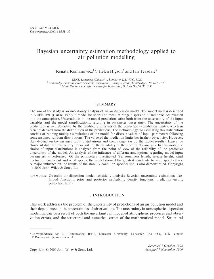
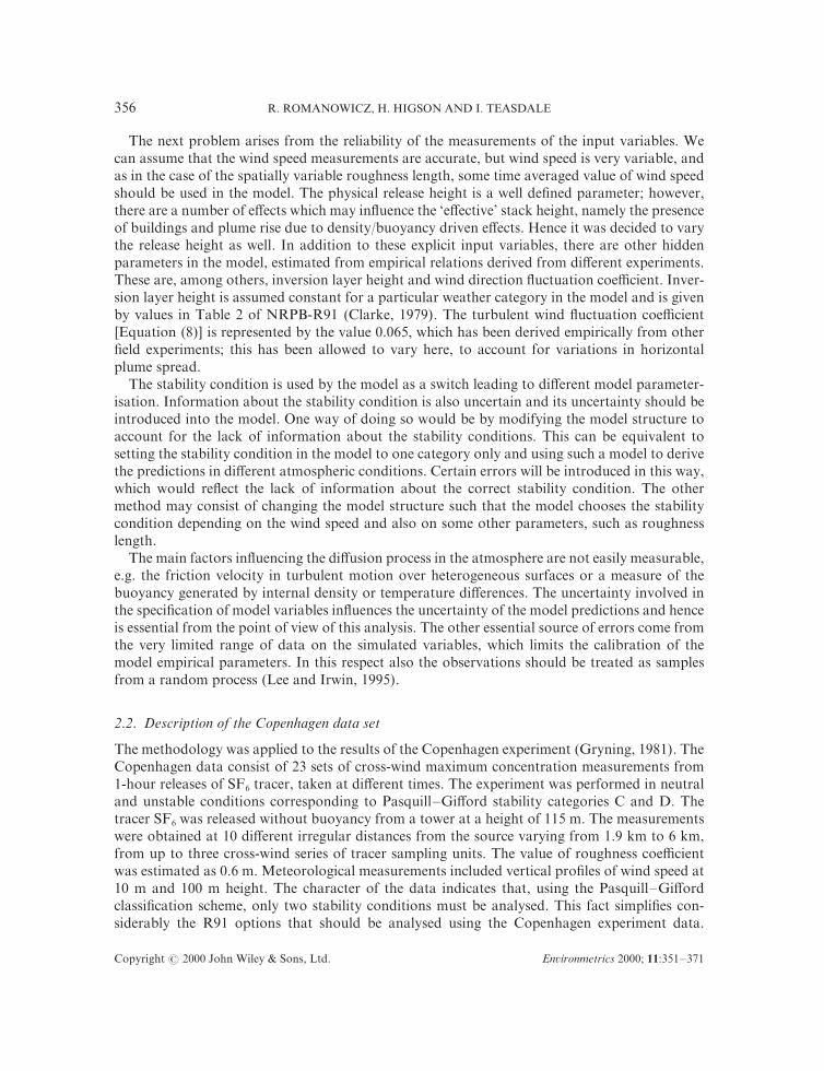
Figure 0[ Ninety!_ve per cent prediction limits for the predictions obtained from the sample outputdistribution without conditioning "$#^ 84 per cent prediction limits with the use of the input observations

"X#^ observations from the Copenhagen data set ""#[

to obtain a clear "not biased# image of the model sensitivity[ The stability category was set to D[From the scatterplots of model results against parameter values\ it is not evident which parametervalues give the best model performance[ The output results were used to evaluate the sampledistribution[ The 84 per cent prediction limits found using this distribution are shown in Figure0[ As the estimated prediction limits are very wide\ the prediction value of these results is ratherpoor[ These predictions would be equivalent to the case when the model is used in an accidentrisk assessment\ under partly unknown meteorological conditions[ Under a worst case scenario\it should be assumed that the polluting substance is released from the source at the maximumpossible rate in the speci_ed direction of human settlements[ The predictions should be performedfor all possible wind speed ranges\ corresponding to each stability category "A!G#[ The predictionlimits obtained with the use of input information "equivalent to sampling from the normal orlog!normal distribution with the mean value given by the observed values and spread estimatedfrom the possible variations# are also shown on Figure 0[ They are much narrower than in thecase of uniform input distributions[Spearman ranked correlation coe.cients for 09 distances from the source and _ve parameters

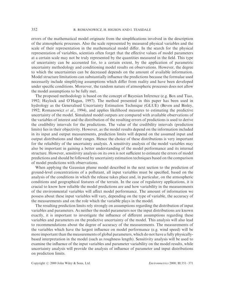
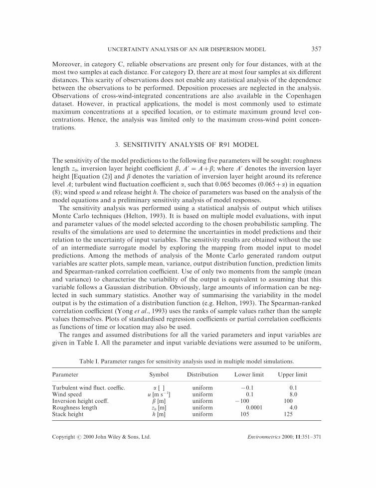
are shown on Figure 1[ The coe.cients for the wind speed and wind ~uctuation coe.cient havethe largest absolute values\ indicating that these variables have the greatest in~uence on theresults[ Next is roughness length for the _rst two distances from the source "0[8 and 1[0 km# andrelease height "for the same distances#[ This result is consistent with the physical features of thedispersion process under category D stability conditions[ For elevated releases\ both roughnesslength and the release height control the plume dispersion before it reaches the ground "i[e[ atsmall distances#[



248

Figure 1[ Spearman ranked correlation coe.cients versus distance from the source\ uniforminput distributions "Table III# " # wind speed^ "'# release height^ "(# inversion height^

"*# wind direction coe.cient^ "$# roughness length[

3[ APPLICATION OF THE BAYESIAN UNCERTAINTY ESTIMATION TECHNIQUETO THE R80 AIR DISPERSION MODEL

3[0[ Short description of the methodolo`y

Uncertainty analysis based on the statistical analysis of output alone does not give any infor!mation about the validity of the model predictions[ Uncertainty results are obtained by exploringthe mapping from model input to model predictions[ In that sense\ the predictive uncertainty ofthe model\ understood as the probable error of its predictions\ is still not known[ BayesianInference is a methodology which provides tools for the comparison of model results withobservations[In this study we follow the methodology developed in Romanowicz et al[ "0883# for the case

of hydrological rainfall!runo} modelling[ It is assumed that the errors between observed Zi andsimulated variables "maximum cross!wind concentrations at given distances# have the additiveform]

Zi ! `i"u##di i! 0\ [ [ [ \ n "8#

where `i"u# denotes simulated by the model maximum cross!wind concentrations being thefunction of u^ u denotes a vector of model parameters and input variables^ di denotes modelerrors and i denotes observation points at di}erent distances from the source\ n denotes a numberof measurement distances from the source[ Here\ d "dim d& n# is modelled by the Gaussianmodel with non!zero mean m\ and covariance matrix S[Due to the sparse amount of Copenhagen observation data\ for this univariate case\ a stationary

process was assumed for d\ with constant mean mI and S&s1I with no correlation between theerrors at the observation sites[ This assumption may be partly justi_ed by the fact that the



259

observations were obtained from independently performed series of 0!hour releases[ In general\the observations of ground concentration of the release along the distance from the source arecorrelated[ Themethodology presentedmay be applied to thismore general case using a correlatednoise process d[ Also the assumption about additive noise in Equation "8# should be re!examinedwhen more data are available[ A logarithmic form of this equation should be used when theerrors are assumed to have multiplicative form "see Romanowicz et al[\ 0883#[From the error model it is seen that the likelihood function of the predicted concentrations

can be expressed as the likelihood of the error variate with parameters "f\ u#&"m\ s\ u#\ dependingon the air dispersion model parameters and input variables u and noise parameters m\ s[

Under these assumptions the likelihood function is de_ned as "Romanowicz et al[\ 0883^Gri.th\ 0877#]

f "z=u\f# ! ti! 0\n

fdi"zi"`i"u# =f# "09#

where d is given by "8# and

fdi"d=f# !0

z1psexp0" 0

1s1"d"m#1

1

The above distribution "09# denotes the probability of the observations z given the input dataand model and error model parameters as a function of input variables and model parameters[It will be used to derive the predictive model uncertainty by applying Bayes theorem "Box andTiao\ 0881#]

f "u\f=z# !f "u\f# f "z=u\f#

f "z#"00#

where z is the vector of observations\ f "u\f=z# denotes the posterior distribution of input variablesand model parameters u given the output observations z\ f "u\ f# denotes the prior distributionof u and f[ f "z=u\ f# denotes the likelihood function "09#\ f "z# denotes the probability ofobservations and can be treated as a scaling factor[ Under the assumption of independencebetween modelling errors and parameters\ this joint distribution may be written as f "u# f "f#where f "u# denotes a prior distribution for the parameters:input variables "see the discussionabout its form in the next section#\ and f "f# denotes a prior distribution of parameters of theerror model "8# and is assumed uniform[Equation "00# can be applied sequentially as new data become available and the existing

posterior distribution\ based on "n#0# calibration sets\ is used as a prior distribution for the newdata in the nth calibration set[ This can be written in the form]

f "u\f=z0\ [ [ [ \ zn#% f "u\f=z0\ [ [ [ \ zn"0# f "zn =u\f# "01#

where f "zn=u\f# is the information about u and f from the nth calibration set[Di}erences between observations and simulated model output values\ together with the



250

assumed prior distributions of parameters\ are used to build the posterior distribution of par!ameters re~ecting the model performance[ In this way it is possible to incorporate the informationfrom observations from di}erent time periods and:or sites using the Bayesian updating describedby Equation "01#[The cumulative distribution of the error term at a location i\ given a particular set of statistical

model parameters f&"m\ s#\ is then given by]

P"di & d=m\s# !F 0d"m

s 1 i! 0\[ [ [\n "02#

where F is a standard normal distribution function N"9\ 0#[ In general\ it is a continuousdistribution\ which is discretised for computational convenience[The resulting predictive distribution of tracer concentrationsZ" conditioned on the calibration

data z is given by

P"Z$& z=z#!su

sf

F 0z"`"u#"m

s 1 f "u\f=z# "03#

From relation "03# one can evaluate the predictive limits for the concentrations at the observationsites[ The assumption that the errors are independent was introduced due to the limited numberof observations for the Copenhagen data set with individual observations made during di}erenttime periods and in di}erent stability conditions for the seven distances from the source[Wheneverpossible\ the correlation of the errors between di}erent observation sites should be checked andthe appropriate model should be chosen\ e[g[ as suggested in Romanowicz et al[ "0883#[Assumptions about the form of the error model and the prior distribution of parameters are

all rather subjective[ Due to the limited amount of input observations and their stochastic nature\assumptions regarding their distributions are also subjective[ In particular\ as a result of thestochastic nature of observations of concentrations on the ground\ the error model will be muchmore di.cult to justify than in the case of hydrological data[ However\ statistical analysis requirescertain assumptions about the nature of the processes to be made and one should be alwaysaware of the limitations of the method used[ Discussion on the choice of prior distributions isvery extensive in the statistical literature "e[g[ Box and Tiao\ 0881#[ From a practical point of view\the prior distribution of the calibrated parameters should be non!informative "seeWoodbury andUlrych\ 0882#[ The analysis of the in~uence of the form of prior distribution of model parameterson the predictions is one of the aims of this paper[ Also the analysis of in~uence of di}erentassumptions concerning the distribution of input covariates on the resulting model predictionswill be performed[ The distinction between the input covariates and parameters "i[e[ independentand dependent variables# is important only from the point of view of model calibration[ Fromthe point of view of uncertainty analysis\ it in~uences the statement of the problem only whenthe choice of priors is concerned[ The prior distribution of input variables will depend\ to agreater degree on measurements in the _eld than the priors for the parameters[ The techniqueoutlined will be applied to the evaluation of the uncertainty of the R80 model predictions[ Theuncertainty analysis is based on the Copenhagen data set\ outlined in Section 1[1 and describedin detail in Gryning "0870#[ The uncertainty analysis is applied only to model predictions of nearground!level concentrations[ It is assumed that there is no deposition to the ground[ Near _eld



251

data and far _eld data are treated separately\ which follows from a di}erent process descriptionat di}erent distances "see discussion by Lee and Irwin\ 0884#[ Near _eld data will be used for thederivation of predictive distributions of model response\ while the far _eld data will be used forthe validation of the predictions[

3[1[ The analysis of in~uence of observations of model variables

The analysis will include the in~uence of] "i# roughness length\ "ii# wind speed\ "iii# turbulentwind ~uctuation coe.cient and "iv# release height[ The choice of these variables was made usingthe results of the sensitivity analysis described in Section 2[ Marginal posterior distributions willbe de_ned from Equation "00# summed over the noise model parameters\ using the likelihoodfunctions based on the error between the simulated and observed values "Equation "8#%[ Followingthe analysis of model structure\ it was assumed that the roughness coe.cient can be treated as acalibration parameter\ while the rest of the variables form the set of independent\ input variables[This assumption was tested through the comparison of results obtained without the observations"uniform distribution for the input variables# and with the observations "normal! log!normaldistributions#[ Testing of di}erent standard deviations for the normal!type distribution "normalor log!normal# was also performed for some input variables in order to draw conclusionsregarding the in~uence of the variability of the measurements[

3[1[0[ In~uence of rou`hness len`th[ The analysis of the roughness coe.cient in~uence wasperformed in two stages] "i# uniform distribution in a wide range\ with parameter values givenin Table II^ "ii# log!normal distribution of roughness length with three values of standarddeviation "9[0\ 0 and 1 m#[ The analysis was done with all the remaining parameters varying\ soas to take into account the interactions between model parameters[The resulting posterior distributions for the four di}erent parameters as given in Table II "i#

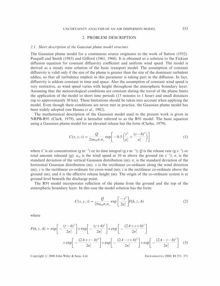
"roughness length\ release height\ wind direction ~uctuation coe.cient and wind speed# for near_eld "combined posterior distributions for distances up to 4 km from the source# are given inFigure 2[ Updating of the posterior distributions is performed using the Bayes formula "09#[Only posterior distributions for the near _eld distances were updated[ The posterior distributionsare shown as the projection of points resulting from Equation "09# onto one parameter space"release height\ roughness length\ wind speed or turbulent wind direction coe.cient#[ Only windspeed shows a pronounced in~uence on model predictions\ with the scatter plots for the otherparameters showing no speci_c regions of better model performance[ There is no evidence of a{best| region for roughness length\ within which the measure of model performance "posterior

Table II[ Parameter ranges for analysis of roughness coe.cient distribution !uniform case "i# and normal:log!normal case "ii#[

Parameter Distribution Lower Upper Distribution Mean SD"i# limit limit "ii#

z9 $m% uniform 9[9990 3 log!normal 9[5 9[0:0[9:1[9h $m% uniform 094 014 normal 004 09a $ % uniform #9[0 9[0 normal 9 9[0u $m s#0% uniform 9[0 00 log!normal 4 9[0:0[9:1[9



252

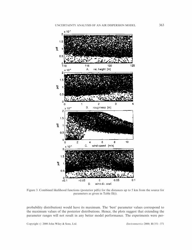
Figure 2[ Combined likelihood functions "posterior pdfs# for the distances up to 4 km from the source forparameters as given in Table II"i#[

probability distribution# would have its maximum[ The {best| parameter values correspond tothe maximum values of the posterior distributions[ Hence\ the plots suggest that extending theparameter ranges will not result in any better model performance[ The experiments were per!



253

formed with much larger parameter ranges than shown in the _gures and the results were notbetter[ When the parameter ranges assumed are too large\ there is a danger of missing someparticular features of model performance and that is why the parameter ranges are kept as smallas possible[One reason for the existence of the regions of {non!preference| for some parameters is over!

parameterisation of the model[ In other words\ there are many combinations of parametersgiving the same model performance measured with regard to the given set of output observations[From the behaviour of scatter plots alone\ it is not possible to say if certain model parametersdo or do not have in~uence on the model output[ However\ the results of the sensitivity analysis"Figure 1# may be helpful in this respect[ For example\ they indicated that the roughness lengthhas some in~uence on model predictions[ Going back to the formulae describing the model\ itcan be seen that roughness length in~uences the vertical dispersion of the plume $Equation "4#%[This means that observations of vertical dispersion of tracer concentrations "e[g[ from windtunnel experiments# might allow the roughness coe.cient to be calibrated[ However\ the obser!vations from the Copenhagen experiment are not su.cient for this task "see Figure 2#[The resulting 84 per cent prediction limits are shown in Figure 3[ The model predictions are

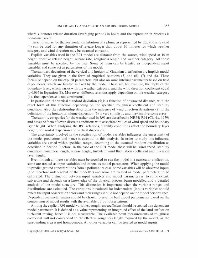
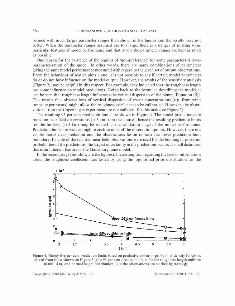
based on near!_eld observations "&4 km from the source#\ hence the resulting prediction limitsfor the far!_eld "'4 km# may be treated as the validation stage of the model performance[Prediction limits are wide enough to enclose most of the observation points[ However\ there is avisible model over!prediction and the observations lie on or near the lower prediction limitboundary[ In spite of the fact that near!_eld observations were used for the building of posteriorprobabilities of the predictions\ the largest uncertainty in the predictions occurs at small distances^this is an inherent feature of the Gaussian plume model[In the second stage "not shown in the _gures#\ the assumption regarding the lack of information

about the roughness coe.cient was tested by using the log!normal prior distribution for the

Figure 3[ Ninety!_ve per cent prediction limits based on predictive posterior probability density functionsderived from those shown on Figure 2 "$#^ 84 per cent prediction limits for the roughness length uniform

"9[990!3 m# and normal height distribution "'#^ the observations are marked by stars "P#[



254

roughness length\ with mean equal to that indicated by the Copenhagen experiment description"z9& 9[5 m#[ After conditioning on near!_eld observations\ the prediction limits for the log!normal roughness length were narrower than in the case of the uniform distribution for roughnesslength\ but the lower prediction limit was too high to enclose some of the observation points[This indicates that the recommended mean value is not adequate for the R80 model in thisapplication[ This might be interpreted as a con_rmation of our assumption of treating theroughness length as a parameter[

3[1[1[ In~uence of release hei`ht[ Release height has been treated as an input variable for aninter!comparison with the Copenhagen data\ as it should be generally well!de_ned in this case[However\ there are other cases in which the concept of e}ective stack height is used "e[g[ buoyantplume or to account for building e}ects#\ and\ consequently\ the release height used in the model"i[e[ e}ective stack height# di}ers from the measured physical stack height[ To represent thepossible prior information about release height\ we shall assume that it is normally distributedwith a mean value equal to the measured release height "004 m# and standard deviation equal to09[ The resulting posterior predictive limits\ with the remaining parameters as given in Table II"i#\ are shown on Figure 3[ The _gure illustrates that information about release height decreasesthe predictive limits considerably and the new predictions are more {central| with respect toobservations[ This means that the information about the release height is very important in thecase of the Copenhagen experiment[ The prediction limits obtained for release heights varied bya standard deviation of 0 m "not shown# were only very slightly narrower than those shown inFigure 3[ In conclusion\ conditioning on release height is important and improves the predictions\but only to a certain extent[

3[1[2[ In~uence of turbulent wind ~uctuation coef_cient[ The turbulent wind ~uctuation coe.cientis an internal model parameter derived empirically from earlier experiments not related to thegiven model application[ The prediction limits obtained from the simulations with uniformdistribution of this coe.cient were compared with the results obtained when the coe.cient wasvaried normally around its experimentally derived value[ The results in prediction limits did notshow any pronounced di}erences\ whichmeans that the observations are not giving any additionalinformation about the parameter value[ More detailed studies are necessary to determine whatdistribution this parameter should take[

3[1[3[ In~uence of wind speed[ The wind speed values are the basic R80 input variables[ In thissection\ the requirements regarding the accuracy of their measurements will be examined[ Windvariations will be altered\ with the rest of the parameters set to the values shown in Table III[The stability condition will be set as neutral "category D#[ It is assumed that the wind speed

Table III[ Parameter ranges for sensitivity analysis for wind speed distribution[

Parameter Distribution Lower limit Upper limit Mean SD "0# SD "1# SD "2# SD "3#

z9 $m% uniform 9[9990 3 ! ! ! ! !a $ % uniform #9[0 9[0 ! ! ! ! !u $m s#0% log!normal ! ! 4[9 9[0 9[4 0[9 1[9h $m% normal ! ! 004 09[9 09[9 09[9 09[9



255

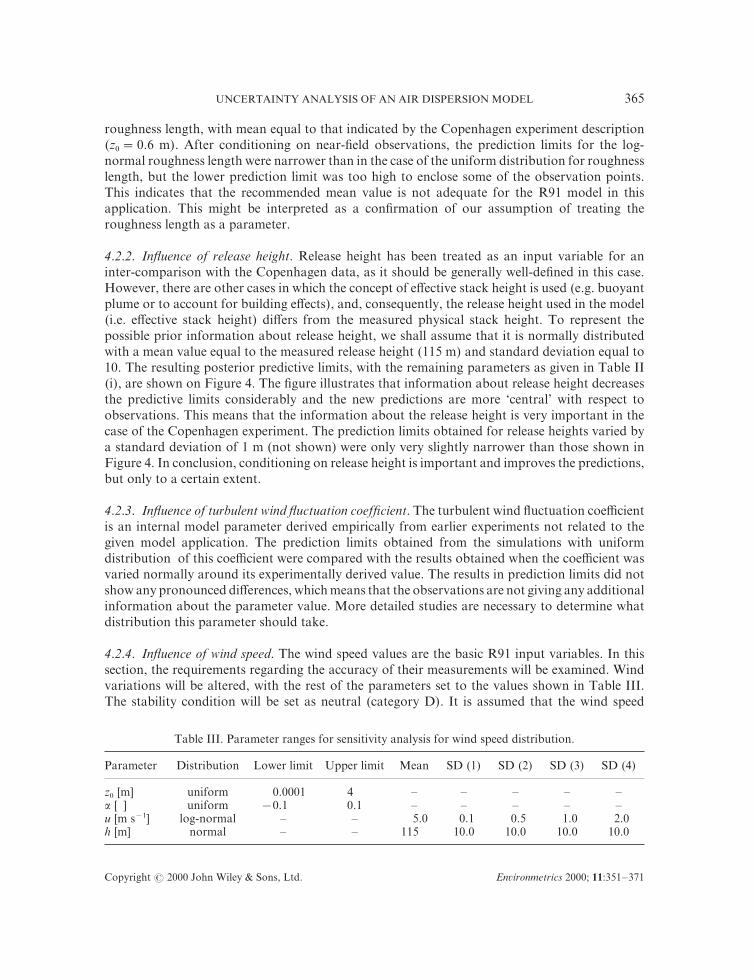
Figure 4[ Ninety!_ve per cent prediction limits for the predictions estimated using posteriorupdated predictive probabilities for log!normal wind speed distribution and parametersgiven in Table III with wind speed standard deviation equal to "## SD& 9[0 m s#0^ "(#

SD& 9[4 m s#0^ "$# SD& 0[9 m s#0^ "'# SD& 1[9 m s#0[

follows a log!normal distribution with mean value equal to 4 m s#0[ The e}ects of assumingdi}erent values of standard deviation were examined[Ninety!_ve per cent prediction limits obtained from the updated posterior predictive dis!

tribution for all four values of the variance are presented in Figure 4[ The results show that theprediction limits for the smallest standard deviation of wind speed "9[0 m s#0# are wider than theresults for the standard deviation equal to 0 m s#0[ The largest standard deviation "equal to 1 ms#0# shows wider prediction limits\ as expected[ Physically low wind speeds give unreliable andhighly variable results as the Gaussian model breaks down for low wind speeds[These results indicate that wind speed plays an important role in the predictions[ This clearly

illustrates one of the limitations of the Gaussian plume model\ which assumes that the windspeed is constant with height[ In reality the wind speed varies signi_cantly with height\ and modelpredictions will be highly dependent on the value of wind speed used and how much the actualwind speed varies with respect to this value[ The prediction limits obtained assuming a log!normal variation in wind speed are more central to the observations than the results obtainedbefore\ for uniform wind speed variations[The information about wind speed and weather category are not equivalent\ hence both should

be taken into account simultaneously\ when all the information about the experiment is to beused[

3[1[4[ In~uence of weather cate`ory[ Analysis of the in~uence of weather category informationon the predictions was performed by introducing uncertainty in the choice of weather category[The choice of Pasquill!Gi}ord stability category is always rather subjective and may vary fromperson to person[ To investigate the e}ect of this further\ the model was allowed to select theweather category based on some initial assumptions[ This is equivalent to introducing a di}erent



256

Table IV[ Parameter ranges for sensitivity analysis for wind speed distribution[

Parameter Distribution Lower limit Upper limit Mean SD

z9 $m% uniform 9[9990 3a $ % uniform #9[0 9[0 ! !u $m s#0% uniform 9[0 19h $m% normal 004 09

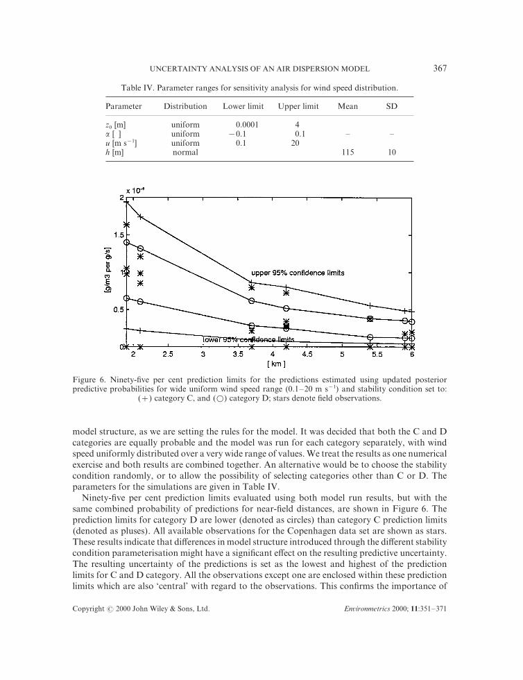
Figure 5[ Ninety!_ve per cent prediction limits for the predictions estimated using updated posteriorpredictive probabilities for wide uniform wind speed range "9[0!19 m s#0# and stability condition set to]

"'# category C\ and "$# category D^ stars denote _eld observations[

model structure\ as we are setting the rules for the model[ It was decided that both the C and Dcategories are equally probable and the model was run for each category separately\ with windspeed uniformly distributed over a very wide range of values[We treat the results as one numericalexercise and both results are combined together[ An alternative would be to choose the stabilitycondition randomly\ or to allow the possibility of selecting categories other than C or D[ Theparameters for the simulations are given in Table IV[Ninety!_ve per cent prediction limits evaluated using both model run results\ but with the

same combined probability of predictions for near!_eld distances\ are shown in Figure 5[ Theprediction limits for category D are lower "denoted as circles# than category C prediction limits"denoted as pluses#[ All available observations for the Copenhagen data set are shown as stars[These results indicate that di}erences in model structure introduced through the di}erent stabilitycondition parameterisation might have a signi_cant e}ect on the resulting predictive uncertainty[The resulting uncertainty of the predictions is set as the lowest and highest of the predictionlimits for C and D category[ All the observations except one are enclosed within these predictionlimits which are also {central| with regard to the observations[ This con_rms the importance of



257

Figure 6[ Ninety!_ve per cent prediction limits for the predictions estimated usingupdated posterior predictive probabilities with included errors for the observations

and parameters as in Figure 4^ SD& 1 m s#0 "Table IV#[

the uncertainty in the choice of weather condition category and indicates the necessity of furtherwork in this direction[

3[2[ In~uence of output observation errors

Application of the Bayesian Inference technique enables introduction of the observation errorsinto the likelihood function through the error model "8#[ It is equivalent to assuming that errorshave some additional spread and a mean value not equal to zero[ Also the correlation betweenthe observations at di}erent distances from the source may be introduced\ as described inRomanowicz et al[ "0883# for the correlation between neighbouring sites[ However\ in the caseof the Copenhagen data\ the correlation between neighbouring sites was neglected[ These two"or three\ when correlation is also taken into account# additional noise parameters are sampledwithin the assumed ranges\ thus giving the posterior distribution sampled on extended parameterspace[ In the analysis presented in Section 3[1\ the posterior distributions were derived in theform of marginal probabilities "summed over the noise f parameter space#\ i[e[ the probabilitydistributions "09# depended only on model parameters and input variables#[ These marginalprobabilities were similar to a least square estimation approach\ with the di}erence that we werenot aiming to _nd the best parameters but rather the best ranges for the parameter sets[ However\in order to take into account the observation errors\ the whole posterior distribution speci_edon bothmodel parameter and noise parameter space should be used in the derivation of predictionlimits[ The parameters for the simulations were set as in Table III\ with the exception of windspeed\ which was varied according to a log!normal distribution with mean equal to 3[8 m s#0

"observed in the _eld experiment# with the standard deviation equal to 1 m s#0 and stabilitycondition D[ The derived prediction limits are shown in Figure 6[ As expected\ the predictionlimits are wider and enclose all the observations "for both stability conditions D and C#[ The



258

information about the measurement errors would be useful in specifying of the lower boundariesof a combined error model variance "consisting of both structural and observation errors#[

4[ SUMMARY

The uncertainty analysis of an air dispersion model described in the paper consisted of anapplication of the Monte Carlo based sensitivity analysis and the Bayesian Inference techniquewhich was used to condition the model predictions on _eld observations[ Comparison of theresults of the modelling with di}erent amount of observation used "assuming di}erent priordistributions about input variables# was performed using a comparison of model prediction limitswith the observations of maximum near ground concentrations obtained from the Copenhagenexperiment "Gryning\ 0871#[ The prediction limits were derived for the output concentrationswithout conditioning on output observations and with conditioning on output observations usingthe Bayesian Inference technique[ Themajor cases analysedwere] "i# uniform parameter and inputvariable distributions^ "ii# input variable distributions normal:log!normal following informationfrom measurements^ "iii# uniform parameter distribution and normal:log!normal input dis!tributions^ "iv# uncertainty in the choice of stability conditions^ "v# in~uences of observationerrors[The results indicate that both sensitivity and predictive uncertainty analysis should be used

simultaneously and that additionally they should be combined with analysis of the model struc!ture[ The analysis also gave recommendations on the best possible use of the available informationabout the model variables[ It showed that] "i# assumed uniform priors give very wide predictionlimits^ "ii# assuming normal:log!normal priors gives more constrained prediction limits but doesnot enclose all the observations^ "iii# introducing Bayesian conditioning on output observationsnarrows the prediction limits but in the case of z9\ for example\ an assumed log!normal priordoes not appear to adequately re~ect the required e}ective values^ uniform prior does better inthis respect^ "iv# the use of output measurements for the conditioning of the predictions anduncertainty in the choice of weather category gives the prediction limits most central whencompared with observations which were not used for the model conditioning^ "v# taking intoaccount observation errors widens the prediction limits[The variables analysed were roughness length\ wind speed\ wind direction ~uctuation

coe.cient\ release height and stability condition[ Sensitivity analysis eliminated one parameter"variability in inversion height# from the chosen parameter set as not in~uencing model pre!dictions for the conditions corresponding to those under which the Copenhagen data wereobtained "i[e[ within 5 km of a 004 m stack in slightly unstable and neutral conditions#[ Moreover\it indicated that both wind speed and turbulent wind ~uctuation coe.cient have the greatestin~uence on the model results[The results of the uncertainty analysis using Bayesian Inference indicated that roughness length

should be treated as a model parameter and its distribution should follow a uniform distributionover a physically feasible range[ Conditioning the predictions on the release height observationssigni_cantly improves model predictions by decreasing the prediction limits[ The same is true ofwind speed measurements\ which are the most important model variable[ The in~uence of theturbulent wind ~uctuation coe.cient was not con_rmed by the Bayesian uncertainty analysis[More information is required to draw conclusions for this parameter[ The analysis of the in~uenceof the wind speed distribution spread indicated that the prediction limits decrease with decrease



269

of spread to a certain extent[ This is connected with the fact that model predictions will departfrom the observations if the spread of wind variations is too narrow[ An introduction of uncer!tainty in the choice of weather category gave the prediction limits\ which were the most centralwith respect to the observed concentration values[ This procedure required slight modi_cationof the model structure and more detailed studies are needed to recommend the best way ofrepresenting this type of uncertainty[Analysis of the distribution of model output without the use of available observations\ or some

independent expert judgement of the possible model results\ cannot increase the model reliability[Comparison of model results with observations can indicate how the model structure may bemodi_ed to give an improved model performance and provides an insight on the in~uence ofinput variables and their uncertainty on prediction errors[ More work should be done on weathercategory uncertainties\ vertical and horizontal dispersion representation and representation ofoutput observation errors in model predictive uncertainty[

ACKNOWLEDGEMENTS

This work was carried out at the Westlakes Research Institute\ Whitehaven\ Cumbria\ supported by BritishNuclear Fuels Ltd[ Jonathan Tawn and Keith Beven "Lancaster University# are thanked for their help[ Wewould also like to thank the anonymous reviewers for their valuable comments[

REFERENCES

Beven KJ\ Binley A[ 0881[ The future of distributed hydrological modelling[ Hydrolo`ical Processes 5]168!187[Box GEP\ Tiao GC[ 0881[ Bayesian Inference in Statistical Analysis[ Wiley] Chichester[Clark RH[ 0868[ A model for short and medium range dispersion of radionuclides released into the atmosphere[ NRPBreport R80[

Gi}ord Jr FA[ 0850[ Use of routine meteorological observations for estimating atmospheric dispersion[ Nuclear Safety1"3#]36!46[

Gi}ord Jr FA[ 0857[ An outline of theories of di}usion in the lower layers of the atmosphere[ InMeteorolo`y and AtomicEner`y % 0857\ Slade DH "ed[#[ USAEC Report TID!13089[ U[S[ Atomic Energy Commission\ NTIS^ 55!005[

Gri.th DA[ 0877[ Advanced Spatial Statistics[ Kluwer] Dordrecht^ 06!08[Gryning SE[ 0870[ Elevated source SF5!tracer dispersion experiments in the Copenhagen area[ Riso report R335\ Riso

National Laboratory[Hanna SR\ Briggs GA\ Hosker Jr RP[ 0871[ Handbook on Atmospheric Diffusion[ National Oceanic and AtmosphericAdministration] Oak Ridge\ TN\ DOE:TIC!00112[

Haylock R\ O|Hagan A[ 0886[ Bayesian uncertainty analysis and radiological protection[ In Statistics for the Environment2\ Barnett V\ Turkman F "eds#[ Wiley] New York[

Helton JC[ 0882[ Uncertainty and sensitivity analysis techniques for use in performance assessment for radioactive wastedisposal[ Reliability En`ineerin` and System Safety 31]216!256[

Hosker RP[ 0863[ Estimates of dry deposition and plume depletion over forests and grasslands[ In Proceedin`s of theSymposium on Physical Behaviour of Radioactive Contaminants in the Atmosphere\ Vienna\ November 0862[ IAEA]Vienna^ 180[

Jones JA[ 0872[Models to allow for the e}ects of coastal sites\ plume rise and buildings on the dispersion of radionuclides\and guidance on the deposition velocity and washout coe.cients[ NRPB report ! R046[

Lee RF\ Irwin JS[ 0884[ Methodology for a comparative evaluation of two air!quality models[ International Journal ofEnvironment and Pollution 4]612!622[

Moore DJ[ 0865[ Calculation of ground level concentration for di}erent sampling periods and source locations[ InAtmospheric Pollution\ Sturges WT "ed[#[ Elsevier] Amsterdam^ 4059[

Pasquill F\ Smith FB[ 0872[ Atmospheric Diffusion\ 2rd ed[ Ellis Horwood] Chichester[Priestly MB[ 0870[ Spectral Analysis and Time Series[ Academic Press] London[Romanowicz R\ Beven K\ Tawn J[ 0883[ Evaluation of predictive uncertainty in nonlinear hydrological models using a

https://www.researchgate.net/publication/222197462_Uncertainty_and_Sensitivity_Analysis_Techniques_for_Use_in_Performance_Assessment_for_Radioactive_Waste_Disposal?el=1_x_8&enrichId=rgreq-5fb2a79d28dd8eeeb991e64ab95d6f05-XXX&enrichSource=Y292ZXJQYWdlOzI0ODAxODM0MTtBUzoxNjcxMzIwNjcyNzg4NDhAMTQxNjg1ODc5ODM1MA==



https://www.researchgate.net/publication/292958870_Models_to_allow_for_the_effects_of_coastal_sites_plume_rise_and_buildings_on_dispersion_of_radionuclides_and_guidance_on_the_value_of_deposition_velocity_and_washout_coefficients?el=1_x_8&enrichId=rgreq-5fb2a79d28dd8eeeb991e64ab95d6f05-XXX&enrichSource=Y292ZXJQYWdlOzI0ODAxODM0MTtBUzoxNjcxMzIwNjcyNzg4NDhAMTQxNjg1ODc5ODM1MA==

https://www.researchgate.net/publication/292958870_Models_to_allow_for_the_effects_of_coastal_sites_plume_rise_and_buildings_on_dispersion_of_radionuclides_and_guidance_on_the_value_of_deposition_velocity_and_washout_coefficients?el=1_x_8&enrichId=rgreq-5fb2a79d28dd8eeeb991e64ab95d6f05-XXX&enrichSource=Y292ZXJQYWdlOzI0ODAxODM0MTtBUzoxNjcxMzIwNjcyNzg4NDhAMTQxNjg1ODc5ODM1MA==



260

Bayesian approach[ In Statistics for the Environment 1\Water Related Issues[ Barnett V\ Turkman F "eds#^ Wiley] NewYork\ 186!204[

Sutton OG[ 0821[ A theory of eddy di}usion in the atmosphere[ Proceedin`s Royal Society London A 024]032!054[Woodbury AD\ Ulrych TJ[ 0882[ Minimum relative entropy] forward probabilistic modelling[Water Resources Research

18]1736!1759[Yong NK\ Jong KK\ Tae WK[ 0882[ Risk assessment for shallow land burial of low level radioactive waste[ Waste

Mana`ement 02]478!487[

Bayesian uncertainty estimation methodology applied to air pollution modelling

Documents

Transcript of Bayesian uncertainty estimation methodology applied to air pollution modelling