Science of the Total Environment 454-455 (2013) 604–618

Contents lists available at SciVerse ScienceDirect

Science of the Total Environment

j ourna l homepage: www.e lsev ie r .com/ locate /sc i totenv

Methodology for the determination of normal background concentrations ofcontaminants in English soil

E. Louise Ander a,⁎, Christopher C. Johnson a, Mark R. Cave a, Barbara Palumbo-Roe a,C. Paul Nathanail b, R. Murray Lark a

a British Geological Survey, Environmental Science Centre, Keyworth, Nottingham NG12 5GG, UKb School of Geography, University of Nottingham, Nottingham NG7 2RD, UK

H I G H L I G H T S

• Contaminated land Statutory Guidance refers to normal levels of soil contaminants.• We represent normal levels by Normal Background Concentrations (NBCs).• We explore the most suitable systematically sampled soil data for English soils.• NBCs for soil contaminants presented not as a single national value but by domains.• We present a robust statistical methodology for determining domain NBCs.

⁎ Corresponding author.E-mail address: land@bgs.ac.uk (E.L. Ander).

0048-9697/$ – see front matter © 2013 Natural Environhttp://dx.doi.org/10.1016/j.scitotenv.2013.03.005

a b s t r a c t

a r t i c l e i n f o

Article history:Received 4 October 2012Received in revised form 24 January 2013Accepted 1 March 2013Available online 10 April 2013

Keywords:SoilContaminated landBackgroundContaminantNormal concentration

The revised Environmental Protection Act Part 2A contaminated land Statutory Guidance (England andWales) makes reference to ‘normal’ levels of contaminants in soil. The British Geological Survey has beencommissioned by the United Kingdom Department for Environment, Food and Rural Affairs (Defra) to esti-mate contaminant levels in soil and to define what is meant by ‘normal’ for English soil. The Guidance statesthat ‘normal’ levels of contaminants are typical and widespread and arise from a combination of both naturaland diffuse pollution contributions. Available systematically collected soil data sets for England are exploredfor inorganic contaminants (As, Cd, Cu, Hg, Ni and Pb) and benzo[a]pyrene (BaP). Spatial variability of con-taminants is studied in the context of the underlying parent material, metalliferous mineralisation and asso-ciated mining activities, and the built (urban) environment, the latter being indicative of human activitiessuch as industry and transportation. The most significant areas of elevated contaminant concentrations areidentified as contaminant domains. Therefore, rather than estimating a single national contaminant rangeof concentrations, we assign an upper threshold value to contaminant domains. Our representation of thisthreshold is a Normal Background Concentration (NBC) defined as the upper 95% confidence limit of the95th percentile for the soil results associated with a particular domain. Concentrations of a contaminantare considered to be typical and widespread for the identified contaminant domain up to (and including)the calculated NBC. A robust statistical methodology for determining NBCs is presented using inspection ofdata distribution plots and skewness testing, followed by an appropriate data transformation in order to re-duce the effects of point source contamination.

© 2013 Natural Environment Research Council. Published by Elsevier B.V. All rights reserved.

1. Introduction

The work described here is part of the process to simplify the con-taminated land regime for England and Wales (Defra, 2011). Part 2Aof the Environmental Protection Act 1990, as amended in 2012,defines contaminated land that poses a Significant Possibility ofSignificant Harm (SPOSH). The United Kingdom Secretary of Statefor the environment issues Statutory Guidance (SG) in accordance

ment Research Council. Published b

with section 78Y of the Environmental Protection Act 1990 to estab-lish a legal framework for dealing with contaminated land (DETR,2000). Revised SG was issued in April 2012 (Defra, 2012a). The intentof the SG is to explain how the contaminated land regime should beimplemented. However, the original SG and a previous update tothe SG (DETR, 2000; Defra, 2006), which were supposed to explainwhen land does (and does not) need to be remediated, did not re-solve significant uncertainties. Contaminated land was still, in part,defined on the basis of the toxicologically vague concept of ‘unaccept-able intake’. Therefore, following a year of consultation, the SG wasrevised to be more useable for those working with contaminated

y Elsevier B.V. All rights reserved.

605E.L. Ander et al. / Science of the Total Environment 454-455 (2013) 604–618

land and remediation. Land is placed into one of four new categoriesto help decide when land is (and is not) contaminated (Fig. 1).Category 1 describes land which is clearly posing SPOSH, for example,because similar sites are known to have caused a significant problemin the past. Category 4 describes land that is clearly not posing SPOSHand should not be determined as statutory contaminated land. Cate-gories 2 and 3 are land for which categorisation is less straightfor-ward. Category 2 land poses SPOSH and is defined by a combinationof expert opinion and scientific evidence that analogous conditionson other sites have or are highly likely to have caused significantharm. Category 3 land is that where the conditions for Category 2are not met and the land is not contaminated. There is a fifth categorynot shown in Fig. 1, informally termed Category 0, which is landwhere significant harm to human health has occurred as a direct re-sult of contamination, a category for which there is no example in En-gland, Scotland or Wales.

The revised SG (Defra, 2012a) introduced the concept of ‘normal’levels of contaminants in soil. Section 3 of the Guidance notes that‘normal’ presence/levels of contaminants:

• should not be considered to cause land to qualify as contaminatedland, unless there is a particular reason to consider otherwise(Section 3.22);

• may result from the natural presence of contaminants at levelsthat might be considered typical in a given area, and have notbeen shown to pose an unacceptable risk to health or the envi-ronment (Section 3.23(a)); and

• are caused by low level diffuse pollution, and common humanactivity other than specific industrial processes (Section 3.23(b)).

Fig. 1. The new four category system to help test when l

As part of its research programme to support Local Authorities im-plement the revised SG, a research project was instigated by Defra toinvestigate normal concentrations of contaminants in the soil ofEngland. The question of “what is normal?” should be a prerequisitein any investigation of potentially contaminated soil, and the resultsof our research are just one of the several tools to be provided byDefra to support the revised SG.

It is important to emphasise that this work to determine ‘normal’levels of contaminants in soil supports the English contaminated landregime rather than the planning regime. The contaminated land re-gime requires developers to show that land is safe, suitable for useand, after remediation, cannot be determined as statutory contami-nated land. The regimes differ in the level of risk at which remedia-tion is needed. In the case of planning, remediation is needed toensure a site is suitable for its future intended use. Under the contam-inated land regime, remediation is needed if the site, given its currentuse, is presenting such a high level of risk that if nothing is done, thereis a significant possibility of significant harm such as death, disease orserious injury.

The research comprised four work packages with the aim of defining‘normal’ level of contaminants in soil by determiningNormal BackgroundConcentrations (NBCs) for a selected number of contaminants:

a. Assessment of available soil contaminant data for English soil;b. Exploration of relevant soil data sets;c. Development of a robust statistical methodology for determining

NBCs; andd. Technical Guidance Sheets for the use of NBCs for selected

contaminants.

and is, and is not contaminated (from Defra, 2011).

606 E.L. Ander et al. / Science of the Total Environment 454-455 (2013) 604–618

This paper describes the first three of these work packages reportedin more detail in technical reports (Ander et al., 2011, 2012; Cave et al.,2012; Johnson et al., 2012).

2. Contaminants

A detailed review of how a contaminant is defined is beyond thescope of this work which focuses on contaminants as defined in Brit-ish legislation. A contaminant can be defined in many ways, here weuse the term as defined in the Part 2A contaminated land StatutoryGuidance (SG) (Defra, 2012a, page 4). In this the terms ‘contaminant’,‘pollutant’ and ‘substance’ are used with the same meaning, that is, “asubstance relevant to the Part 2A regime which is in, on or under the landand which has the potential to cause significant harm to a relevantreceptor, or to cause significant pollution of controlled waters”. Detailedclarification of what is meant as ‘significant harm’ and ‘relevant re-ceptor’ is also given in the SG. Receptors to be protected from harmfall into three categories: human, ecological systems and property(e.g., buildings, crops and livestock).

Literature covering aspects of contamination give less robustdefinitions of a contaminant. For example, BS EN ISO 19258:2011(BSI, 2011) defines a contaminant as “a substance or agent present inthe soil as a result of human activity”, and notes that there is no as-sumption in this definition that harm results from the presence ofthe contaminant. This definition does not include elements and sub-stances derived purely from geological sources that are defined ascontaminants but occur naturally in widespread and high concentra-tions (i.e. naturally occurring and contaminants). Cole and Jeffries(2009) in their report on using soil guideline values (SGVs) say“a contaminant is a substance that is in, on or under the land and hasthe potential to cause harm”.

There are thousands of potential contaminants which might bepresent on various sites around England (although a smaller sub-setprobably drives the risk on most sites) (Defra, 2008). The now with-drawn report on “Potential Contaminants for the Assessment of Land”(Defra and EA, 2002) identified the priority chemicals for the devel-opment of SGVs. This was based on the chemicals likely to be presentin sufficient concentrations on affected sites that were considered topose a risk. An updated priority chemical list is presented by Martinand Cowie (2008) (Table 1). This comprises fifty six chemicals, four-teen of which are chemical elements plus cyanides (an inorganicsubstance) and asbestos (mineralogically defined). The remainingcontaminants can be classified as organic substances, and these in

Table 1List of priority contaminants (from Martin and Cowie, 2008).

Inorganic Organic

Arsenic (As) Acetone FenitrothionBeryllium (Be) Aldrin Hexachlorobuta-1,3-dieneCadmium (Cd) Atrazine HexachlorocyclohexanesChromium (Cr) Azinphos-methyl MalathionCopper (Cu) Benzene NaphthaleneLead (Pb) Benzo(a)pyrene (BaP) Organolead compoundsMercury (Hg) Carbon disulphide Organotin compoundsMolybdenum (Mo) Carbon tetrachloride PentachlorophenolNickel (Ni) Chloroform PhenolSelenium (Se) Chlorobenzenes Polychlorinated biphenyls (PCB)Sulphur (S) Chlorophenols Polycyclic aromatic hydrocarbons

(PAH)Thallium (Tl) Chlorotoluenes TetrachloroethaneVanadium (V) 1,2-Dichloroethane TetrachloroetheneZinc (Zn) Dichlorvos TolueneCyanide DDT Total petroleum hydrocarbonsAsbestos Dieldrin 2,1,1,1-Trichloroethane

Dioxins and furans TrichloroetheneEndosulfan TrifluralinEthylbenzene Vinyl chlorideExplosives Xylenes

the soil environment will be overwhelmingly (though not exclusively)associated with anthropogenic activity (radioactive elements are out-side the remit of this investigation). Globally, there is generally goodagreement as to what are priority contaminants, though there arenational differences. In Finland, for example, the “Government Decreeon the Assessment of Soil Contamination and Remediation” (FinnishGovernment, 2007) lists eleven inorganic elements: antimony (Sb),arsenic (As), mercury (Hg), cadmium (Cd), cobalt (Co), chromium(Cr), copper (Cu), lead (Pb), nickel (Ni), vanadium (V) and zinc (Zn).Two of these elements, Sb and Co, are not present in Table 1.

In our data exploration and methodology development, eight con-taminants – As, Cd, Cu, Hg, Ni, Pb, benzo(a)pyrene (BaP) and asbestos– were selected to represent the range of data availability and con-tributing sources, though the exploration shows that asbestos is acontaminant for which a NBC cannot be determined. The remainingsubstances are discussed in subsequent sections.

3. Background concentrations

A number of terms are used to convey the expected concentra-tions of a contaminant in soil. These include: normal, typical, baseline,ambient, characteristic, natural, background and widespread. Thereare some subtle differences between these terms, they can mean dif-ferent things in different disciplines, and they can be confused withalternative uses. For example, a statistician would associate theword ‘normal’, in the context of defining the spread of a set of results,with the normal (or Gaussian) distribution. The terms normal, typical,characteristic and widespread are more or less synonymous. In thispaper, we use ‘normal’ in the sense of the SG (Defra, 2012a) as setout here in Section 1.

In our work, we represent what is normal by use of Normal Back-ground Concentrations (NBCs), so the term normal backgroundexcludes point contamination and encompasses typical variationaround a domain average (Fig. 2).

The term background has a more complex and varied usage thanthe term normal and is discussed in detail by Matschullat et al.(2000); Reimann and Garrett (2005); and Reimann et al. (2005). Itis used differently in different areas of science, for example:

• in exploration geochemistry the term background has been long-established and defines an area of normal element concentrations dis-tinguished from anomalously high concentrations (that may indicatethe presence of metalliferous mineralisation) by a threshold value;

• in environmental geochemistry background is a relative measure todistinguish between natural element or compound concentrationsand anthropogenically-influenced concentrations in real samplecollectives (Matschullat et al., 2000); and

• in the BSI (2011) guidance on soil background the content of a sub-stance in a soil results from both natural geological and pedologicalprocesses and includes diffuse source inputs.

In the work described here, where the definition of normal isgiven in statutory guidance, the use of the term normal backgroundis as defined by BS EN ISO 19258:2011 (BSI, 2011) and includesboth geogenic (i.e., of geological origin) and anthropogenic diffusepollution.

A further refinement in our use of NBCs is the realisation that, due tosignificant chemical variability in the underlying parent material onwhich soil is formed, different areas of the country will have differentranges of normal background concentrations. This will be particularlythe case in areas overlying mineralisation or those regions subjectedto a long history of anthropogenic activity, namely built-up or urbanareas. Rather than having single national NBCs, we have used our dataexploration of the different contaminants to identify areas, referred toas domains, which have characteristic NBCs.

The conceptualmodel thatwe follow for defining a contaminant con-centration is summarised in Fig. 2. The concentration of a contaminant in

Fig. 2. Conceptual model of contaminant concentration.

607E.L. Ander et al. / Science of the Total Environment 454-455 (2013) 604–618

soil varies about the domain mean due to geogenic and diffuse sourcesand, where present, point contamination. In the absence of point con-tamination, observed concentrations in soil within a domain representthe normal levels of concentration. Our aim is to identify contaminantdomains and, to characterise the statistical distribution of NBCs with astatistical methodology that is robust to the effects of any point sourcecontamination.

Methodologies for determining background concentrations are asnumerous as there are definitions for background. There are impor-tant strategic, economic and legislative drivers for understandingand quantifying soil element/contaminant concentrations. From aneconomic and strategic point of view, the exploration and develop-ment of economic metalliferous mineral deposits by geochemical ex-ploration have meant that much work has been done into developingmethods to determine background levels. For more than sixty years,statistical methods have been used to distinguish between anomalousand background concentrations of the chemical elements in soil inorder to locate buried mineralisation (e.g., Lovering et al., 1950;Hawkes and Bloom, 1955; Tennant and White, 1959; Lepeltier,1969; Tidball et al., 1974; Sinclair, 1976, 1983, 1986). Some of thesetechniques are described in detail by Matschullat et al. (2000) withapplication examples and include: the Lepeltier method; relativecumulative frequency curves; normality of sample ranges; regressiontechniques; mode analysis; 4-σ outlier test; interactive 2-σ tech-nique; and calculated distribution function.

Grunsky (2010), in a more recent review of interpreting geochem-ical survey data, discusses graphical methods for differentiating geo-chemical background from anomalies.

Legislation concerned with healthy and sustainable environmentsis also now a significant driver for information on background con-taminant concentrations. For this purpose, documents such as BritishStandards Institution guidance on the determination of backgroundvalues have been published. BS EN ISO 19258:2011 (BSI, 2011) coversthe prerequisites of sampling, analysis and data handling and outlinessome essentials of statistical evaluation of data.

Matschullat et al. (2000), Grunsky (2010) and BS EN ISO 19258:2011illustrate the fact that the determination of background requires goodquality concentration data and a statistical methodology to deliver esti-mates for background concentrations. The availability and robustness ofavailable data sets for contaminant concentrations in English soil werethe starting point for our work and are described in detail in Ander etal. (2011) and summarised here in Sections 4 and 5.

The majority of research to date has focused on methods for pro-viding typical background concentrations of Potentially Harmful Ele-ments (PHEs) in soil (e.g., Appleton, 1995; Appleton et al., 2008).Geochemists express the geochemical baseline (a spatially fluctuatingchemical environment at a given point in time) in terms of the naturalbaseline. This is stable over a long period of time, provided that thereare no sudden catastrophic events (such as flooding and marinetransgression), and will be associated with an overprint of the anthro-pogenic baseline (with many contributing sources) that changes overa relatively short period of time (Johnson and Ander, 2008). An un-derstanding of what constitutes the natural baseline enables the con-tribution of the anthropogenic component to be estimated. Theseapproaches to determining ‘backgrounds’ are largely based on soilsampling and analyses over different parent material groups, whichhave been shown to exert a dominant control on topsoil chemistryin England (Rawlins et al., 2003).

Alternative approaches have been investigated, based on associa-tions with particle size fractions across England and Wales (Zhao etal., 2007) or globally based on statistical relationships with total soiliron or manganese (Hamon et al., 2004). The approach proposed byAppleton et al. (2008) is to estimate typical background concentra-tions from a statistical measure (e.g., the geometric mean) based onexisting soil analyses within soil parent material polygons. The back-ground concentrations for a particular PHE are mapped using delinea-tions of the parent material polygons. Oliver et al. (2002) present avery thorough statistical analysis of the National Soil Inventory(NSI) results for England and Wales, and such work gives an appreci-ation of the concentration ranges for complete data sets.

In the United Kingdom, there are examples of previous work to de-fine ‘average’ trace element concentrations in soil. Archer and Hodgson(1987) report normal ranges — values between twice the log-derivedstandard deviation above and below the mean (i.e., approximately95% of the data) for soil in England andWales. Paterson et al. (2003) de-scribe background levels of contaminants in Scottish soil, citing mini-mum and maximum trace element ranges with the median and lowerand upper quartiles. The fundamental weakness of all these previousstudies is that the results cover mainly agricultural or rural soil, andhave no results for soil from urban areas. These use a simple statisticalapproach, essentially to define data ranges.

A review of worldwide national approaches to determining back-ground concentrations was outside the scope of this work, but it isworth noting some examples here from Italy and Finland. In Italy,APAT-ISS (2006) gives government guidance for the determinationof background values of metals and metalloids in Italian soil. This na-tional guidance uses the BSI (2011) definition of natural backgroundconcentration. The stepwise approach for deriving background valuesinvolves the collection of data, the statistical analysis of the data andthe determination of the background value. The selection of the sam-pling sites follows the typological approach (based on parent materi-al, soil type and land use), choosing sites within homogeneous areas.The statistical analysis is carried out on data sets, each representativeof homogenous typologies. The descriptive statistics for data distribu-tion include the minimum, maximum, median, percentile, standarddeviation, skewness, kurtosis and graphic representations, such asboxplots, histograms and percentage cumulative frequency plots.The guideline describes in detail a series of statistical tests to identifyoutliers and to define the distribution type of the data (normal,lognormal, gamma, non-parametric distribution). The backgroundvalue is defined as the 95th percentile of the population. In Finland,a Government Decree on the Assessment of Soil Contamination andRemediation Needs (214/2007) (Finnish Government Decree, 2007)became legislation on 1 June 2007 (Tarvainen and Jarva, 2011). Thedecree defines a geochemical baseline as being the natural geochem-ical background concentration and superimposed diffuse anthropo-genic input of elements in the topsoil. Backgrounds are assessed ona local investigation of the geochemical baseline rather than on na-tional values, and the upper limit of geochemical baseline variationfor element X (BLX) is estimated as follows:

BLX ¼ P75 þ 1:5 P75−P25ð Þ

where P75 is the 75th percentile of element X concentrations and P25is the 25th percentile of element X concentrations.

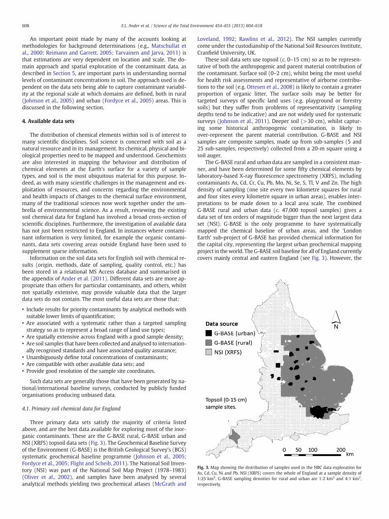
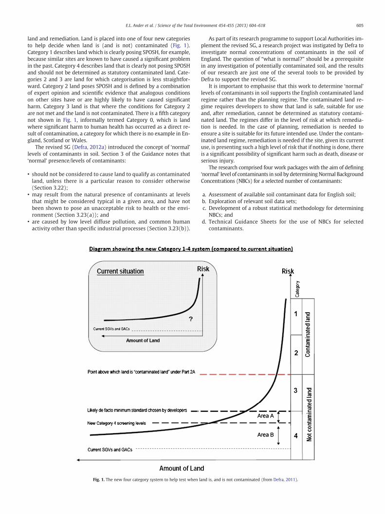
Fig. 3. Map showing the distribution of samples used in the NBC data exploration forAs, Cd, Cu, Ni and Pb. NSI (XRFS) covers the whole of England at a sample density of1:25 km2. G-BASE sampling densities for rural and urban are 1:2 km2 and 4:1 km2,respectively.

608 E.L. Ander et al. / Science of the Total Environment 454-455 (2013) 604–618

An important point made by many of the accounts looking atmethodologies for background determinations (e.g., Matschullat etal., 2000; Reimann and Garrett, 2005; Tarvainen and Jarva, 2011) isthat estimations are very dependent on location and scale. The do-main approach and spatial exploration of the contaminant data, asdescribed in Section 5, are important parts in understanding normallevels of contaminant concentrations in soil. The approach used is de-pendent on the data sets being able to capture contaminant variabil-ity at the regional scale at which domains are defined, both in rural(Johnson et al., 2005) and urban (Fordyce et al., 2005) areas. This isdiscussed in the following section.

4. Available data sets

The distribution of chemical elements within soil is of interest tomany scientific disciplines. Soil science is concerned with soil as anatural resource and in its management. Its chemical, physical and bi-ological properties need to be mapped and understood. Geochemistsare also interested in mapping the behaviour and distribution ofchemical elements at the Earth's surface for a variety of sampletypes, and soil is the most ubiquitous material for this purpose. In-deed, as with many scientific challenges in the management and ex-ploitation of resources, and concerns regarding the environmentaland health impacts of changes to the chemical surface environment,many of the traditional sciences now work together under the um-brella of environmental science. As a result, reviewing the existingsoil chemical data for England has involved a broad cross-section ofscientific disciplines. Furthermore, the investigation of available datahas not just been restricted to England. In instances where contami-nant information is very limited, for example the organic contami-nants, data sets covering areas outside England have been used tosupplement sparse information.

Information on the soil data sets for English soil with chemical re-sults (origin, methods, date of sampling, quality control, etc.) hasbeen stored in a relational MS Access database and summarised inthe appendix of Ander et al. (2011). Different data sets are more ap-propriate than others for particular contaminants, and others, whilstnot spatially extensive, may provide valuable data that the largerdata sets do not contain. The most useful data sets are those that:

• Include results for priority contaminants by analytical methods withsuitable lower limits of quantification;

• Are associated with a systematic rather than a targeted samplingstrategy so as to represent a broad range of land use types;

• Are spatially extensive across England with a good sample density;• Are soil samples that have been collected and analysed to internation-ally recognised standards and have associated quality assurance;

• Unambiguously define total concentrations of contaminants;• Are compatible with other available data sets; and• Provide good resolution of the sample site coordinates.

Such data sets are generally those that have been generated by na-tional/international baseline surveys, conducted by publicly fundedorganisations producing unbiased data.

4.1. Primary soil chemical data for England

Three primary data sets satisfy the majority of criteria listedabove, and are the best data available for exploring most of the inor-ganic contaminants. These are the G-BASE rural, G-BASE urban andNSI (XRFS) topsoil data sets (Fig. 3). The Geochemical Baseline Surveyof the Environment (G-BASE) is the British Geological Survey's (BGS)systematic geochemical baseline programme (Johnson et al., 2005;Fordyce et al., 2005; Flight and Scheib, 2011). The National Soil Inven-tory (NSI) was part of the National Soil Map Project (1978–1983)(Oliver et al., 2002), and samples have been analysed by severalanalytical methods yielding two geochemical atlases (McGrath and

Loveland, 1992; Rawlins et al., 2012). The NSI samples currentlycome under the custodianship of the National Soil Resources Institute,Cranfield University, UK.

These soil data sets use topsoil (c. 0–15 cm) so as to be represen-tative of both the anthropogenic and parent material contribution ofthe contaminant. Surface soil (0–2 cm), whilst being the most usefulfor health risk assessments and representative of airborne contribu-tions to the soil (e.g. Ottesen et al., 2008) is likely to contain a greaterproportion of organic litter. The surface soils may be better fortargeted surveys of specific land uses (e.g. playground or forestrysoils) but they suffer from problems of representativity (samplingdepths tend to be indicative) and are not widely used for systematicsurveys (Johnson et al., 2011). Deeper soil (>30 cm), whilst captur-ing some historical anthropogenic contamination, is likely toover-represent the parent material contribution. G-BASE and NSIsamples are composite samples, made up from sub-samples (5 and25 sub-samples, respectively) collected from a 20-m square using asoil auger.

The G-BASE rural and urban data are sampled in a consistent man-ner, and have been determined for some fifty chemical elements bylaboratory-based X-ray fluorescence spectrometry (XRFS), includingcontaminants As, Cd, Cr, Cu, Pb, Mo, Ni, Se, S, Tl, V and Zn. The highdensity of sampling (one site every two kilometre squares for ruraland four sites every kilometre square in urban areas), enables inter-pretations to be made down to a local area scale. The combinedG-BASE rural and urban data (c. 47,000 topsoil samples) gives adata set of ten orders of magnitude bigger than the next largest dataset (NSI). G-BASE is the only programme to have systematicallymapped the chemical baseline of urban areas, and the ‘LondonEarth’ sub-project of G-BASE has provided chemical information forthe capital city, representing the largest urban geochemical mappingproject in theworld. The G-BASE soil baseline for all of England currentlycovers mainly central and eastern England (see Fig. 3). However, the

609E.L. Ander et al. / Science of the Total Environment 454-455 (2013) 604–618

areas not yet sampled by G-BASE can be supplemented by the NSI(XRFS) data set for which topsoil samples, collected and prepared in asimilar way to the G-BASE project, have been reanalysed at the BGSXRFS laboratories to give total element concentrations. The earlier NSIdata only contained a limited number of element results, following de-termination by ICP-AES using an aqua regia extraction. The NSI datahas a sampling density that approximates to 1 sample per 25 km2.

4.2. Supplementary soil chemical data for England

There are other important data sets that usefully augment theG-BASE and NSI data, although collected at much lower samplingdensities. The EuroGeoSurveys' Geochemical Mapping of AgriculturalSoil (GEMAS — Reimann et al., 2012) and European geochemical atlas(FOREGS (Forum of European Geological Surveys) — Salminen et al.,2005; De Vos and Tarvainen, 2006), the Environment Agency's UK Soiland Herbage Survey (UKSHS — Barraclough, 2007), and the Centre forEcology & Hydrology (CEH) Countryside Survey (CS — Emmett et al.,2010) provide additional contaminant data for Hg and organic sub-stances. However, there are issues regarding the use of these data sets.For example, some only determine elements following an aqua regiaextraction and so do not unambiguously represent total contaminantconcentrations. Additionally, they also tend to have a much reducedsampling density and thus will fail to capture local, and some regional,variability. The use of the UKSHS and Countryside Survey 2000 datafor this purpose is also impeded by the fact that site coordinates are de-graded to the nearest 10 km in order to satisfy land access agreements.

Some other significant data sets are inappropriate to use as theytarget a specific land use or land group and would, therefore, biasany NBCs towards that particular land use. The largest of these isthe BGS Mineral Reconnaissance Programme (MRP) soil analyses.As these samples were collected in predominantly metalliferousmineralised areas, often associated with a long legacy of mining, sam-pling strategies were geared towards finding high results for metals.The MRP is also an example of a programme for which there wasgreat variability in the sampling and analytical methodology used,so the data set cannot be interpreted as a single entity. Site investiga-tions targeting contaminated land will similarly produce data thatcannot be used to establish normal backgrounds. Results will pre-dominantly be for contaminated soil, which is what is requiredwhen investigating such a site, but is not good for establishing localor regional backgrounds. Projects, specific to a particular land use,and targeting the humus layer rather than mineral soil, are also oflimited value to the project. A big Europe-wide project – LUCAS(Land Use Coverage and Area frame Survey) (Joint Research Centre(JRC) laboratory of the European Commission) – is currently in prog-ress (Montanarella et al., 2011) with some 1373 sample sites in theUK. Heavy metal analysis of top soil is proposed, but not yet complet-ed. Land access agreements may also prevent site coordinates beingreadily available when this project delivers some data.

Finally, an important source of soil results, particularly for Hgand organic contaminants is contained in peer-reviewed publications,e.g., Tipping et al. (2011), Cousins et al. (1997), and Jones et al.(1989). Jones et al. is an example of a paper containing originaldata, with site coordinates, but for Wales rather than England, datawhich can be extrapolated to supplement sparse BaP informationfor English soil. However, many publications contain just summarytables without site locations, and care has to be taken to note howmuch of the data is original or compiled from other publications.

Although the estimation of NBCs is concerned with soil, othersample media are used to define the surface chemical environmentand so can be used, particularly wherever there is no soil data, todefine areas where contaminant concentrations are particularly high.The use of fine stream sediment, collected from small (low order)streams, is the media of preference for defining the regional geochemi-cal baseline by geochemists (Johnson et al., 2008). Appleton et al.

(2008) have used the soil-stream sediment relationship to estimatenational-scale potentially harmful element ambient background con-centrations. For England, there is good high density stream sedimentdata available from the BGS G-BASE project and theWolfson Geochem-ical Atlas (Appleton et al., 2008).

5. Data exploration and definition of domains

Prior to developing a methodology for determining NBCs, the spa-tial distribution of the selected contaminants was explored in order tounderstand the spatial variability and the most important domains(Ander et al., 2011, 2012). Of the initial eight contaminants selectedfor study, the absence of any systematic information on the back-ground distribution of asbestos in soil meant that no data explorationwas possible for this contaminant, and this is an example of a contam-inant for which a NBC could not be determined. This is a reflection ofthe difficulty in applying a commonmethodology to the abundance ofminerals in soils and the concentration of chemical substances. Thedata exploration contained two components, firstly exploration ofthe spatial distribution of contaminants in topsoil across Englandand, secondly, exploring various landscape data sets with which todefine contaminant domains.

5.1. Spatial distribution

Where there is sufficient contaminant data, national maps can beplotted by interpolating between sample sites to give geochemicalimages, such as that shown in Fig. 4. These maps (for As, Cd, Cu, Niand Pb) are published in the contaminant NBC Technical GuidanceSheets, supplementary information (e.g., Defra, 2012b). Further map-ping, using other statistical techniques, such as k-means cluster anal-ysis (see Ander et al., 2011), in addition to these maps, gives anexcellent visualisation of a contaminant's variability in soils acrossEngland. The variability can be attributed to three main factors:

1. The single most important controlling factor is the underlyingparent material (geology), which provides the geogenic componentof natural background. England has a very varied geology, both inthe age of rocks and the rock types, and this contributes to a signifi-cant variability in elements that are defined as contaminants andoccur naturally.

2. A further geogenic component is when a contaminant is enrichedin soil, because of mineralisation in the underlying rocks. Thismay also be associated with an anthropogenic component causedby mining related activities.

3. England has a long history of urbanisation and industrialisationand, whilst there are now many environmental safeguards inplace, there is a legacy of pollution in our cities and towns. Thisis represented by both point source and diffuse anthropogenic in-puts to the natural background.

These form the basis for the landscape data used to define contam-inant domains. In a GIS environment (Arc GIS v9.2), this is integratedwith the spatial distribution maps so as to recognise domains associ-ated with elevated contaminant concentrations in soil. Domains aredefined as polygons and the contaminant data captured within thedomain polygons. For all the contaminants studied, there has beenat least one domain identified as having typically higher backgroundconcentrations. The area of England outside any defined domain istermed the Principal Domain. Therefore, there are always at leasttwo domains to which NBCs have been attributed. Domains identifiedfor the contaminants investigated are shown in Figs. 5 and 6. Thesedomains along with summary contaminant information are listed inTable 2. Our objective has been to identify the most significant do-mains on a national and regional scale. At a local scale, where higherdensity sampling provides more detailed information, further do-mains could undoubtedly be identified, say for example, within an

Fig. 4. Example of an interpolated geochemical image used to demonstrate contami-nant variability in topsoil across England. (Inverse distance squared weighting option,cell size 1000 m and search radius 5000 m. %iles = percentiles.)

610 E.L. Ander et al. / Science of the Total Environment 454-455 (2013) 604–618

urban domain residential and industrial areas could be attributedwith NBCs if the land use is significantly affected by widespread dif-fuse pollution.

Mercury and BaP have fewer data points to use in the data explo-ration, thus sites are widely spaced and so interpolated maps cannotbe validly made for these elements. Instead of interpolated images,classified point maps are plotted to illustrate the spatial variabilityin these contaminants (Defra, 2012c,d). Furthermore, for Hg andBaP, because far fewer data are available, data sets used lack themethodology consistency, and so there is greater uncertainty associ-ated with the data exploration (Ander et al., 2011, 2012). In orderto have sufficient data points for BaP it was necessary to include allBritish data, which maintained all other data selection criteriashown above (Section 4) and are still taken from within the UK(Ander et al., 2011). Sampling and analytical methods used for Hgand BaP are summarised in the supplementary technical guidancesheets written for these contaminants (Defra, 2012c,d).

5.2. Landscape data

5.2.1. Soil parent materialThe Soil-Parent Material Model (SPMM) for England, Wales and

Scotland (Lawley, 2011) has been developed by BGS, based on themapped boundaries of the national 1:50,000 superficial and bedrockgeological data. The results of this project were used to identify themost influential contributors to high contaminant concentrations.Soil parent material is the first recognisably geological materialfound beneath a soil profile, and is the lithology on which that soilhas developed. Soil thus inherits many properties, including chemicalcomposition, from this material. In the BGS SPMM the geological datahave been combined into one layer of information, which indicatesthe rock/sediment formation mapped as directly underlying soil.Where this is a superficial deposit (such as alluvium, glacial deposits,

peat) the data set also maintains the record of the solid geologicalformation first encountered beneath this surface sediment; such in-formation is useful where the underlying solid geology imparts chem-ical (or other) characteristics into the overlying superficial deposits,and thus into the soil. In the SPMM there is additional informationon texture, mineralogy and lithology not present in the geologicalmapping data, which is attributed in a hierarchical classificationsystem.

In the absence of a soil parent material map, a digital geology map(solid and drift editions) can be used to identify where elevated con-taminant concentrations in soil are related to the underlying geology.Soil maps are also a landscape resource that can be used in thiscontext, though these are often based on the underlying geology. Fur-thermore, for this work in England, geological and parent materialmaps are available at appropriate scales (i.e., 1:50,000) to do the re-quired interpretation.

5.2.2. Urban areasLand use is an important factor in controlling anthropogenic con-

taminant contributions to the soil. Certain activities, for example,metallurgical industries, areas of high traffic volume and coal burning,have been, and in some instances continue to be, responsible for rais-ing contaminant levels in the environment. At the scale of this work,we have not considered any one specific land use, but included indus-trial activities and the built environment under the general classifica-tion of urban. In order to delineate this, an index of urbanisation hasbeen defined (see Ander et al., 2011) using the Generalised LandUse Database 2005 statistics for England (Communities and LocalGovernment, 2007). Based on the index, a map of urban, semi-urban and rural areas has been generated (Fig. 7), and the delineatedurban areas were used to define an urban domain for many of thecontaminants. Those contaminants, where only the urban area isidentified as the important controlling factor on high contaminantconcentrations, will have just two domains associated with them —

the Urban Domain and the Principal Domain (i.e., non-urban areas).Other data sets are available in the UK for defining urban domains.

At a regional to national scale light pollution maps (e.g., CPRE, 2003)are a good way of defining the built environment. At a more localscale, detailed land use information is available from the OrdnanceSurvey Strategi® maps (Ordnance Survey, 2011).

5.2.3. Metalliferous mineralisation and miningA significant contributor to high levels of many inorganic contam-

inants in soil is non-ferrous mineralisation and associated miningactivities, referred to in this project as the mineralisation domain.Note that this domain does not include ferrous mineralisation orcoal mining, which are also noted to have significant controls on con-taminant levels in soil. Such mining is generally related to specificrock strata, rather than mineral veins that can cut across a variety ofrock types, and so are investigated in the context of underlying parentmaterial/geology. In the GIS environment, we have used the Britishnon-ferrous Metalliferous Mineralisation and Mining database, origi-nally produced in hard-copy by Ove Arup (1990) for DoE (Departmentof Environment), but which has been ‘cleaned’ and turned into a poly-gon layer by BGS.

5.3. Data distributions

The data distribution of concentrations of contaminants in soil,used for characterising domains, have been explored, as this is a fun-damental part of the methodology to determine NBCs (see next sec-tion). Cumulative distribution plots and boxplots are useful tools toexplore such distributions (Figs. 8 and 9). These plots are includedin the technical guidance sheets for each contaminant (e.g., Defra,2012b).

Fig. 5. Maps showing the contaminant domains for As, BaP, Cd and Cu.

611E.L. Ander et al. / Science of the Total Environment 454-455 (2013) 604–618

An important property of the distribution of data on a variable is itsdegree of symmetry, and this was also investigated in the data explora-tion. The Gaussian distribution is symmetrical, and is the distributionthatwewould expect for a variable that arises from the additive combi-nation of random effects (Allègre and Lewin, 1995). In geochemistry, itis common to find that concentrations have an asymmetric distribution,typicallywith a long upper tail of larger values (Reimann and Filzmoser,2000). This can arise from non-linear combination of random effects,

and such data can be transformed to a symmetrical distribution, forexample by calculating the logarithm of their values. The symmetryof the distribution of a variable can be measured by the skewnesscoefficient, SC:

SC ¼ ∑ni¼1 xi−mð Þ3�

ns3;

Fig. 6. Maps showing the contaminant domains for Hg, Ni and Pb.

612 E.L. Ander et al. / Science of the Total Environment 454-455 (2013) 604–618

where xi is the ith of n observations, m is the sample average and s isthe sample standard deviation. Data from a Gaussian distributionhave a skewness coefficient of zero, because it is symmetrical. It isa rule of thumb that we transform data if SC lies outside the interval[-1, 1] (Webster and Oliver, 2007).

If data from a domain can be regarded as variables with a Gaussiandistribution, perhaps after a transformation, then this distribution

allows us to characterise the NBCs of the domain, reflecting the mul-tiple processes that generate variation within a domain. However, thedistribution may be affected unduly by a relatively small number ofextreme observations resulting from point contamination. Plots mayhelp to identify when such processes are occurring. Such outlyingdata will also affect the value of SC. This means that a large positiveSC may be due to an underlying asymmetry in the distribution of

Table 2List of contaminant domains with summary statistical information for associated English topsoil (all concentrations in mg/kg).

Domain % area of England Samples Mean Minimum 25th percentile Median 75th percentile Maximum Skewness coefficient

As Principal 97 41,509 16 b0.5 10.6 14.1 18.6 1008 18Ironstone 1 437 73 4.1 27.8 45 83.4 555 3Mineralisation 2 187 181 6.9 27.8 45.6 105.5 15,110 13

BaP Principal 96 165 0.14 bDL 0.02 0.06 0.15 1.44 4Urban 4 13 0.67 0.07 0.30 0.52 1.00 1.56 1

Cd Principal 89 4418 0.5 0.3 0.3 0.3 0.5 20 17Urban 4 9308 0.9 b0.5 b0.5 b0.5 0.8 165 33Chalk South 5 265 1 0.3 0.5 0.9 1.4 5.6 2Min_Gp1 1 224 4.5 b0.5 2 3 5 48 4Min_Gp2 b1 95 0.9 0.3 0.3 0.5 0.9 13 6

Cu Principal 95 34,504 27 b1 14.3 19.8 27.7 5326 41Urban 4 7475 74 1.2 30.3 47.5 79.7 4577 14Mineralisation 1 153 92 3 30.4 47.4 77.6 2766 10

Hg Principal 96 1134 0.34 b0.07 0.07 0.12 0.23 31 15Urban 4 512 0.55 b0.07 0.18 0.33 0.65 9.6 5

Ni Principal 99 41,768 25.3 1 16.6 23.4 31.7 506 5Basic b1 23 60.9 20.5 33.4 62.5 80.9 107 0Ultrabasic b1 4 213 25.4 48.2 199 393 430 0Ironstone (Ni) b1 117 78.9 4.1 42.3 69.4 112 182 1Peak district b1 221 44.5 5.9 22.4 34.2 51.2 384 4

Pb Principal 94 34,257 72 3 31 41 66 10,000 22Urban 4 7529 276 2 89 166 322 10,000 8Mineralised 2 347 665 35 151 290 638 10,196 5

Using G-BASE and NSI topsoil results determined by laboratory based XRFS except BaP and Hg (see text). Cadmium data has variable detection limits between the Urban andMin_Gp1 domains (0.5 mg/kg) and other domains (0.25 mg/kg) as fully described in Ander et al. (2012).

613E.L. Ander et al. / Science of the Total Environment 454-455 (2013) 604–618

NBCs in the domain, the superimposed effects of point contamination,or both. A useful tool to discriminate between these circumstances isthe octile skewness coefficient, OC:

OC ¼ P87:5–P50ð Þ– P50–P12:5ð Þð Þ= P87:5–P12:5ð Þ;

where Py is the yth percentile of the data, here we consider the first andseventh octile and the median. The OC is zero for a symmetrical vari-able, but because it is based on order statistics it is not very sensitive

Fig. 7. A map showing urban, semi-urban and rural areas of England, defined using theGeneralised Land Use Database (GLUD — Communities and Local Government, 2007).The method for defining an urbanisation index is described in Ander et al. (2011).

to a few extreme observations. A comparable rule of thumb for the in-terpretation of OC is that the data require transformation if OC is outsidethe range [-0.2, 0.2] (Rawlins et al., 2005).

6. Methodology for determining normal backgroundconcentrations (NBCs)

The methodology is based on the assumption that the contami-nant data conform to a random variable:

Z ¼ fixed effectsþ continuous random variationþ point contamination:

The fixed effects are sources of variation in the observed concentra-tions that are attributable to geogenic sources or diffuse anthropogenicactivities that are represented by the domain mean. The continuousrandom variation (typically Gaussian (normal) or log-Gaussian) repre-sents the typical variation arising from geogenic or diffuse anthropo-genic sources within the defined domains. The point contamination isassumed to introduce outlying values into the data. The equationabove can be re-written informally as shown in Fig. 2. For any contam-inant, the first two terms (domain average + typical variations) giverise to the normal range of values or normal variation of the contami-nant. The objective of the procedure is to characterise this normal vari-ation in terms of a statistical distribution.

A robust statistical methodology was used for determining NBCsthat is based on exploration of data distributions (by testing the dis-tribution skewness) and applying data transformations (see Cave etal., 2012). The statistical analysis has been done using open source Rcode (R Development Core Team, 2011) employing ‘fBasics’, ‘Hmisc’,‘boot’ and ‘car’ packages.

Previous sections have described the gathering and division of soilcontaminant data into domains. The steps in this initial process aresummarised in Fig. 10. Having selected the contaminant for investiga-tion the first question to be asked is “can the contaminant be consideredfor a NBC?” Asbestos and manufactured organic contaminants with nonatural origin, for example, fail this question as there is a lack of dataon their natural distribution and concentration in soil. The contaminantdata set is then divided into domain data sets. A minimum of 30 resultsare considered necessary to determine a NBC (BSI, 2011). Once the data

100001000100101

99.9999

99.99

99

95

80

50

20

5

1

0.01

0.0001

Arsenic (mg/kg) by XRFS

Per

cen

t

IronstoneMineralisationPrincipal

Domain

Fig. 8. Example of a frequency distribution plot used in the data exploration — cumulative probability plot of topsoil As results categorised by domains.

614 E.L. Ander et al. / Science of the Total Environment 454-455 (2013) 604–618

has been allocated into domains, then exploratory statistics indicatingthe skewness coefficient and inspection of frequency distributionplots can be done to select the appropriate data transform and methodof calculating percentiles. The steps applied are:

i) If the data are symmetrically distributed, SC is b1 and the OS isb0.2, then the data are consistent with the assumption of aGaussian distribution, and the parametric percentiles are fitted,based on the mean and standard deviation of the data.

ii) If the data show a mostly symmetrical distribution with poten-tial outliers in the distribution tail, SC >1 but OS b0.2, then thedata are consistent with the assumption of a Gaussian distribu-tion, and the parametric percentiles are fitted using medianand the median absolute deviation (MAD), in place of themean and standard deviation, as these measures are robust tooutliers (Reimann and Filzmoser, 2000).

iii) If the data distribution is skewed, SC is >1 and the OS is >0.2,then the data are not suitable for fitting to a Gaussian model,and the data need to be transformed to using either a logarithmic

PrincipalMineralisationIronstone

250

200

150

100

50

0

Domain

Ars

enic

(m

g/k

g)

by

XR

FS

Fig. 9. Example of a boxplot used to display the range of domain concentrations for As.The box represents the interquartile range (Q1, Q3), with the median (Q2) as a linewithin the box. The point symbol shows the mean value. The upper whisker =Q3 + 1.5(Q3–Q1); lower whisker = Q1–1.5(Q3–Q1).

(loge) or the more general family of transformations known asthe Box–Cox transform (Box and Cox, 1964):

U∧λ−1� �

=λ:

Where U is vector of soil concentrations for a given contaminantand λ is the power coefficient which is optimised to give thetransformed data best fit to the normal distribution. This hasbeen shown to work well for geochemical applications (Reimannet al., 2008). After transform the distribution is re-examined andsteps i to iii are repeated. After calculation of the percentiles thedata are back transformed to their original units;

iv) Finally, if the data cannot bemade to be consistentwith aGaussiandistribution (even after transform) the empirical percentiles forthe data set are calculated.

In practice the empirical, parametric and robust percentiles havebeen reported for each domain to check for consistency betweenmethods (Ander et al., 2012; Cave et al., 2012). The methodologyassumes that data for a given domain come predominantly from asingle population, and that the data are either normally distributedor have a positive SC. For the contaminants and domains consideredthese assumptions hold true. Examples of distribution plots onuntransformed and transformed data, along with the skewness calcu-lations are displayed in Fig. 11. An example table (for As) of percen-tiles for different contaminant domains is shown in Table 3.

Having arrived at some robustly defined percentile values thathave been derived taking into account any skewness or outlyingdata in the data set, a decision has to be made as to what result touse to represent the upper limit of normal background concentra-tions. We define arbitrarily the upper limit of normal backgroundconcentrations as the 95th percentile. The percentile values are sub-ject to uncertainty based on the number of data points and theshape of the distribution. Where sample sizes are smaller, this resultsin wider confidence intervals for the domain percentiles (Ander et al.,2012; Cave et al., 2012). An assessment of the uncertainty on the 95thpercentile was estimated by empirical, parametric and robust para-metric methods, and has been included in the statistical estimations,using a bootstrap resampling routine implemented by employing the‘boot’ package within the R programming language. The bootstraproutine used 1000 resamples of the original or transformed data

Determine skewnesscoefficient (SC) and octileskew (OS) and plot of data

distribution

No NBC determined

Assemble and explore

contaminant data

Select contaminant

NO

NOYES

YES

Number of domain

samples ≥ 30?

Can the contaminant

be considered for NBC?

1

2Subset data into domains

based on major factors

controlling contaminant

variability

Fig. 10. Flow chart for the estimation of the NBC for a given contaminant — data gathering and exploration phase. For discussion of questions 1 & 2 see text.

615E.L. Ander et al. / Science of the Total Environment 454-455 (2013) 604–618

providing a 95% percentile confidence interval on the estimatedpercentile.

Estimation of the uncertainty using bootstrapping gives the upper95% confidence limit to the estimated 95th percentile. Comparison ofthe uncertainty on the estimations confirms that the parametric

Fig. 11. Example density distributions for the raw data and the loge transfo

uncertainties from the Gaussian fit are much less erratic than the em-pirical values, and thus the parametric limits have been chosen asbeing a better representation of the uncertainty on the percentiles.

This definition of a NBC considers what is typical and widespread(words used in the SG to describe ‘normal’ levels). The median (50th

rmed data for As in the Ironstone Domain (n = number of samples).

Table 3Empirical (Emp), Parametric Gaussian (P) and Robust Gaussian (R) percentile values for As in the ironstone domain (concentrations in mg/kg). L and H values represent low andhigh confidence intervals around the median. Shaded values indicate percentile method used to estimate NBC — this is determined by exploration of the data distribution.

Percentile Empirical Emp L Emp H Parametric (P) P L P H Robust (R) R L R H

50 45.0 41.7 49.4 50.0 46.2 53.7 45.0 41.3 49.455 49.7 45.3 55.8 55.5 51.1 59.7 49.8 45.5 55.160 56.0 50.2 60.0 61.7 56.7 66.6 55.2 49.8 61.665 60.9 56.7 69.6 68.8 63.2 74.5 61.4 54.8 68.770 71.4 61.7 81.0 77.3 70.6 84.1 68.6 60.7 77.575 82.7 72.6 97.7 87.5 79.6 95.9 77.4 67.7 88.780 104.8 86.4 116.6 100.6 91.1 111.0 88.5 76.4 102.085 122.7 108.9 147.1 118.3 106.4 131.7 103.5 88.1 120.790 165.6 140.7 179.3 145.1 129.1 163.5 126.1 105.2 149.395 221.7 179.7 291.4 196.2 171.6 223.9 168.8 136.6 205.4

Table 4Summary of domain normal background concentrations (NBCs) for the studied con-taminants. All concentrations in mg/kg. Number of samples used in each domain NBCestimation is shown in brackets. The Ni Basic and Ultrabasic Domains are shownhere, but as they are each defined by less than 30 samples, the NBCs are not estimated.Note that the number of samples in the Hg Principal Domain is eight fewer than cited inTable 2 because these eight samples had problems regarding the spatial resolution ofthe site locations.

AsMineralisation Ironstone

290 220(187) (437)

BaPDOMAIN (Great Britain)

Urban

3.6(32)

CdMin. Grp. 1 Min. Grp. 2 Urban Chalk (south)

17 2.9 2.1 2.5(224) (95) (9,308) (265)

CuMineralisation Urban

340 190(153) (7,475)

HgUrban

1.9

(512)

NiIronstone (Ni) Peak District Basic Ultrabasic

230 120 * *(117) (221) (23) (4)

PbMineralisation Urban

2,400 820

32

0.5

1.0

62

0.5

42

DOMAIN

Principal

(41,509)

Principal

(371)

DOMAIN

Principal

(4,418)

DOMAIN

Principal

(34,504)

DOMAIN

Principal

(1,126)

DOMAIN

Principal

(41,768)

DOMAIN

Principal

180(34,257) (347) (7,529)

616 E.L. Ander et al. / Science of the Total Environment 454-455 (2013) 604–618

percentile) is a measure of the central tendency, so half the observa-tions are expected to exceed it under normal background variation.The NBC should be represented by a larger percentile. Selecting the95th percentile is somewhat arbitrary, but will encompass a largeproportion of the normal background variation whilst excludingextremes. It has also been used in other approaches to define back-ground concentrations for environmental purposes (e.g., in Italy,APAT-ISS, 2006). As it has been argued that the NBC should representthe highest concentration of contaminant in this domain that is likelyto come from normal background, then the NBC should be the upperend of the confidence interval. The NBC is defined, therefore, as theupper 95% confidence limit of the 95th percentile (taking into accountdata transformations).

Any uncertainty in the 95th percentile value is fully captured bytaking the upper limit of the 95th percentile confidence interval. Inthe determination of geochemical background, of great economicvalue in the search for ore bodies, the mean (x) plus 2σ (σ = standarddeviation) is commonly used (Matschullat et al., 2000), which repre-sents c. 97% of the data for normalised distributions.

7. NBCs for As, BaP, Cd, Cu, Hg, Ni and Pb

A summary of domain NBCs for the investigated contaminants,using the methodology described above, is given in Table 4. Thosefor As, Cd, Cu, Ni and Pb are derived from a very large data set, thoughwhen subdivided into domains, some domain NBCs are only based ona small number of samples (e.g., Ni Basic and Ultrabasic Domainswhich have a very small spatial extent). Table 5 is an example ofthe summary information (in this case As) presented in the contam-inant technical guidance sheet.

8. Discussion and concluding remarks

1. There are large amounts of high quality and systematicallycollected soil data covering England containing inorganic ele-ment contaminant results that have enabled us to estimateNBCs for contaminant domains. Gaps in knowledge relate mainlyto organic contaminants, though the calculations of NBCs forthese can still be made for England by utilising results fromother parts of Great Britain, as has been done for BaP.

2. We use total element concentrations for inorganic contaminants(except Hg), determined by XRFS. The total amount of an elementpresent in a sample is the most fundamental (and reproducible)quantity in any sample, therefore, direct measurement techniques,e.g., XRFS or neutron activation analysis (NAA), or total extractionprocedures are desirable (Darnley et al., 1995). During the data ex-ploration, data sets for which determinands in soil had been deter-mined by XRFS and other methods (e.g., GEMAS (Reimann et al.,2012); TELLUS (Smyth, 2007); FOREGS (Salminen et al., 2005))have been compared, and for all the contaminants there was no

significant differences over normal ranges of concentrations for themethods concerned, which could be modelled by linear regression(e.g., see Defra, 2012b).

3. Once the contaminant data sets have been subdivided into domains,some areas are defined by a very small number of samples, particu-larly where only the lower density NSI soil results are available.Such domain NBCs could be improved by the collection of furthersamples. However, the more pressing need for further informationis likely to be driven by contaminants forwhich the geogenic and dif-fuse contributions are significant in terms of human health risks, andthese will primarily be in urban areas.

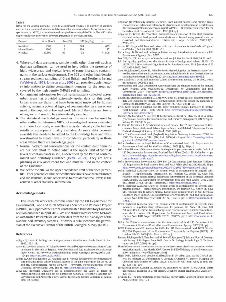
Table 5NBCs for the arsenic domains (cited to 2 significant figures, n is number of samplesused in the estimation). Arsenic is determined by laboratory-based X-ray fluorescencespectrometry (XRFS), i.e., total As in soil sampled from a depth 0–15 cm. The NBC is theupper confidence interval on the 95th percentile of the domain data.

Domain Area (km2) Area (%) NBC (mg/kg) n

Ironstone 1300 1 220 437Mineralisation 2300 2 290 187Principal 129,300 97 32 41,509

617E.L. Ander et al. / Science of the Total Environment 454-455 (2013) 604–618

4. Where soil data are sparse, sample media other than soil, such asdrainage sediments, can be used to help define the presence ofhigh, widespread and typical levels of some inorganic contami-nants in the surface environment. The BGS and other high densitystream sediment sampling of Great Britain and Northern Ireland(Webb et al., 1978; Johnson et al., 2005) can provide supplementa-ry information to define contaminant domains for the areas notcovered by the high density G-BASE soil sampling.

5. Contaminant information for soil systematically collected acrossurban areas has provided extremely useful data for this work.Urban areas are those that have been most impacted by humanactivity, leaving a potential legacy of contamination in areas wheremost of the population live and work. Many of the cities and townsof England still need to be systematically sampled.

6. The statistical methodology used in this work can be used byothers either to determine NBCs not investigated here or estimatedat a more local scale, where there is systematically collected soilresults of appropriate quality available. As more data becomesavailable this needs to be added to the knowledge base and NBCsre-estimated to greater levels of confidence, particularly in thoseareas where there are knowledge gaps.

7. Normal background concentrations for the contaminant domainsare our best effort to define what is the upper limit of ‘normal’levels of contaminants in soil, as described by the Part 2A contam-inated land Statutory Guidance (Defra, 2012a). They are not aplanning or risk assessment tool and must be used in the contextof the Guidance.

8. We define the NBC as the upper confidence limit of the 95th percen-tile. Other percentiles and their confidence limits have been estimatedand are available, should others wish to consider ‘normal’ levels in thecontext of other statistical information.

Acknowledgements

This research work was commissioned by the UK Department forEnvironment, Food and Rural Affairs as a Science and Research Project(SP1008) in support of the Part 2a contaminated land Statutory Guidancerevision published in April 2012. We also thank Professor Steve McGrathat Rothamsted Research for use of the data from the XRFS analyses of theNational Soil Inventory samples. This work is published with the permis-sion of the Executive Director of the British Geological Survey (NERC).

References

Allègre CJ, Lewin E. Scaling laws and geochemical distributions. Earth Planet Sci Lett1995;132:1-13.

Ander EL, Cave MR, Johnson CC, Palumbo-Roe B. Normal background concentrations of con-taminants in the soils of England. Available data and data explorationCommissionedreport CR/11/145. Keyworth, Nottinghamshire: British Geological Survey/Defra; 2011[124 pp. http://nora.nerc.ac.uk/19958].

Ander EL, Cave MR, Johnson CC, Palumbo-Roe B. Normal background concentrations ofcontaminants in the soils of England. Results of the data exploration for Cu, Ni, Cdand Hg. Commissioned report CR/12/041. Keyworth, Nottinghamshire: BritishGeological Survey/Defra; 2012 [88 pp. http://nora.nerc.ac.uk/19952/].

APAT-ISS. Protocollo Operativo per la determinazione dei valori di fondo dimetalli/metalloidi nei suoli dei siti d'interesse nazionale. Revisone 0. Agenzia perla Protezione dell'Ambiente e per i Servizi Tecnici and Istituto Superiore di Sanita;2006 [in Italian].

Appleton JD. Potentially harmful elements from natural sources and mining areas:characteristics, extent and relevance to planning and development in Great Britain.British Geological SurveyTechnical report WP/95/3. UK: Commission report for theDepartment of Environment (DoE); 1995 [63 pp.].

Appleton JD, Rawlins BG, Thornton I. National-scale estimation of potentially harmfulelement ambient background concentrations in topsoil using parent materialclassified soil:stream-sediment relationships. Appl Geochem 2008;23(9):2596–611.

Archer FC, Hodgson IH. Total and extractable trace element contents of soils in Englandand Wales. J Soil Sci 1987;38:421–31.

Barraclough D. UK soil and herbage pollutant survey. Introduction and summary. UK:Environment Agency (EA); 2007.

Box GEP, Cox DR. An analysis of transformations. J R Stat Soc Ser B 1964;26:211–46.BSI. Soil quality: guidance on the determination of background values. BS EN ISO

19258:2011. International Organisation for Standardisation; 2011 [revision of BSISO 19258:2005; 2011].

CaveMR, Johnson CC, Ander EL, Palumbo-Roe B. Methodology for the determination of nor-mal background contaminant concentrations in English soils. British Geological Surveycommissioned report, CR/12/003; 2012 [41 pp. http://nora.nerc.ac.uk/19959/].

Cole S, Jeffries J. Using soil guideline values. Environment agency, UK SC050021/SGVintroduction; 2009 [32 pp.].

Communities and Local Government. Generalised land use database statistics for England2005. Product Code 06CSRG04342. Department for Communities and LocalGovernment; 2007 [February; http://data.gov.uk/dataset/land_use_statistics_generalised_land_use_database].

Cousins IT, Kreibich H, Hudson LE, Lead WA, Jones KC. PAHs in soils: contemporary UKdata and evidence for potential contamination problems caused by exposure ofsamples to laboratory air. Sci Total Environ 1997;203(2):141–56.

CPRE. Night blight in England and UK. Light pollution images. Campaign to protectrural England (CPRE); 2003 [April; http://www.cpre.org.uk/resources/country-side/dark-skies/item/1977].

Darnley AG, Bjorklund A, Bolviken B, Gustavsson N, Koval PV, Plant JA, et al. A globalgeochemical database for environmental and resource management. UNESCO pub-lishing 19; 1995 [122 pp.].

De Vos W, Tarvainen T. Geochemical Atlas of Europe. Part 2. Interpretation of Geo-chemical Maps, Additional Tables, Figures, Maps, and Related Publications. Espoo,Finland: Geological Survey of Finland; 2006. [692 pp.].

Defra. The Contaminated Land (England) Regulation. Statutory instruments 2006 No.1380. The Stationery Office (UK) Ltd.; 2006 [4th August; http://www.legislation.gov.uk/uksi/2006/1380/contents/made].

Defra. Guidance on the Legal Definition of Contaminated Land. UK: Department forEnvironment Food and Rural Affairs (Defra); 2008 [July; 16 pp.].

Defra. Simplification of the contaminated land regime. Impact assessment (IA) NoDefra 113.UK: Department for Environment, Food and Rural Affairs (Defra); 2011 [October; 41 pp.http://archive.defra.gov.uk/environment/quality/land/contaminated/documents/contaminated-land-ia.pdf].

Defra. Environmental Protection Act 1990: Part 2A Contaminated Land Statutory Guidance.UK: Department for Environment, Food and Rural Affairs (Defra); 2012a [April; 69 pp.http://www.defra.gov.uk/publications/2012/04/10/pb13735contaminated-land/].

Defra. Technical Guidance Sheet on normal levels of contaminants in English soils:arsenic — supplementary information. In: Johnson CC, Ander EL, Cave MR,Palumbo-Roe B, editors. Normal background concentrations in Soil Technical Guidancesheet. London, UK: Department for Environment Food and Rural Affairs (Defra), SoilsR&D Project SP1008; 2012b. [TGS01s: pp21. http://nora.nerc.ac.uk/19964/].

Defra. Technical Guidance Sheet on normal levels of contaminants in English soils:benzo[a]pyrene — supplementary information. In: Johnson CC, Ander EL, CaveMR, Palumbo-Roe B, editors. Normal background concentrations in Soil TechnicalGuidance sheet. London, UK: Department for Environment Food and Rural Affairs(Defra), Soils R&D Project SP1008; 2012c. [TGS04s: pp16. http://nora.nerc.ac.uk/19966/].

Defra. Technical Guidance Sheet on normal levels of contaminants in English soils:mercury — supplementary information. In: Johnson CC, Ander EL, Cave MR,Palumbo-Roe B, editors. Normal background concentrations in Soil Technical Guid-ance sheet. London, UK: Department for Environment Food and Rural Affairs(Defra), Soils R&D Project SP1008; 2012d. [TGS07s: pp16. http://nora.nerc.ac.uk/19972/].

Defra, EA. Potential contaminants for the assessment of land. UK: Department forEnvironment, Food and Rural affairs and Environment Agency; 2002 [34 pp.].

DETR. Environmental Protection Act 1990: Part IIA Contaminated Land. DETR Circular02/2000, Department of the Environment, Transport & the Regions (DETR). UK.London: HMSO; 2000 [20th March; 162 pp.].

Emmett BA, Reynolds B, Chamberlain PM, Rowe E, SpurgeonDJ, Brittain SA, et al. Country-side Survey. Soils Report from 2007. Centre for Ecology & Hydrology CS Technicalreport no. 9/07; 2010 [194 pp.].

Finnish Government. Government decree on the assessment of soil contamination and re-mediation needs. . 1st March 2007. Decree 214/2007Ministry of the Environment;2007 [in Finnish — Unofficial translation].

Flight DMA, Scheib A. Soil geochemical baselines in UK urban centres: the G-BASE pro-ject. In: Johnson CC, Demetriades A, Locutura J, Ottesen RT, editors. Mapping theChemical Environment of Urban Areas. Chichester, UK: John Wiley & Sons Ltd;2011. p. 186–206.

Fordyce FM, Brown S, Ander EL, Rawlins BG, O'Donnell KE, Lister TR, et al. GSUE: urbangeochemical mapping in Great Britain. Geochem Explor Environ Anal 2005;5(4):325–36.

Grunsky EC. The interpretation of geochemical survey data. Geochem Explor EnvironAnal 2010;10(1):27–74.

618 E.L. Ander et al. / Science of the Total Environment 454-455 (2013) 604–618

Hamon RE,McLaughlinMJ, Gilkes RJ, Rate AW, Zarcinas B, Robertson A, et al. Geochemicalindices allow estimation of heavy metal background concentrations in soils. GlobalBiogeochem Cycles 2004;18:1–6.

Hawkes HE, Bloom H. Heavy metals in stream sediment used as exploration guides.Min Eng 1955;8:1121–6.

Johnson CC, Ander EL. Urban geochemical mapping studies: how and why we do them.Environ Geochem Health 2008;30:511–30.

Johnson CC, Breward N, Ander EL, Ault L. G-BASE: baseline geochemical mapping ofGreat Britain and Northern Ireland. Geochem Explor Environ Anal 2005;5(4):347–57.

Johnson CC, Flight DMA, Ander EL, Lister TR, Breward N, Fordyce FM, et al. The collec-tion of drainage samples for environmental analyses from active stream chan-nels. In: de Vivo B, Belkin HE, Lima A, editors. Environmental Geochemistry: sitecharacterisation, data analysis and case histories. Oxford: Elsevier; 2008.p. 59–92.

Johnson CC, Demetriades A, Locutura J, Ottesen RT. Mapping the chemical environmentof urban areas. Chichester, UK: John Wiley & Sons Ltd; 2011. [664 pp.].

Johnson CC, Ander EL, Cave MR, Palumbo-Roe B. Normal background concentrations(NBCs) of contaminants in English soils: final project report. British Geological sur-vey commissioned report, CR/12/035; 2012 [40 pp. http://nora.nerc.ac.uk/19946/].

Jones KC, Stratford JA, Waterhouse KS, Vogt NB. Organic contaminants in Welsh soils —polynuclear aromatic hydrocarbons. Environ Sci Technol 1989;23(5):540–50.

Lawley R. The soil-parent material database: a user guide. British Geological SurveyOpen Report, OR/08/034; 2011 [53 pp. http://nora.nerc.ac.uk/8048/].

Lepeltier C. A simplified statistical treatment of geochemical data by graphical repre-sentation. Econ Geol 1969;64(5):538–50.

Lovering TS, Huff LC, Almond H. Dispersion of copper from the San Manuel copper de-posit, Pinal County, Arizona. Econ Geol 1950;45:493–514.

Martin I, Cowie C. Compilation of data for priority organic pollutants for derivation ofsoil guideline values. UK: Environment Agency; 2008 [SC050021/SR7; 171 pp.].

Matschullat J, Ottenstein R, Reimann C. Geochemical background— can we calculate it?Environ Geol 2000;39:990-1000.

McGrath SP, Loveland PJ. The soil geochemical atlas of England and Wales. Glasgow:Blackie Academic and Professional; 1992.

Montanarella L, Tóth G, Jones DG. Soil component in the 2009 LUCAS survey. In: Tóth G,Németh T, editors. The international conference on ‘Land Quality and Land UseInformation in the European Union’ 26–27 May 2011 in Keszthely, Hungary.Keszthely, Hungary.: European Commission, Joint Research Centre, Institute forEnvironment and Sustainability; 2011. p. 209–18.

Oliver MA, Loveland PJ, Frogbrook ZL, Webster R, McGrath SP. Statistical andgeostatistical analysis of the National Soil Inventory of England and Wales. Defra(formerly MAFF) Soil Programme Technical Report Project SP0124; 2002.

Ordnance Survey. Strategi® user Guide and technical specification. Ordnance Survey; 2011[V8.3–12/2011; 102 pp. http://www.ordnancesurvey.co.uk/oswebsite/products/strategi/index.html].

Ottesen RT, Alexander J, Langedal M, Høygaard E. Soil pollution in day-care centres andplaygrounds in Norway: national action plan for mapping and remediation.Environ Geochem Health 2008;30:623–37.

Ove Arup. Mining instability in Britain. Department of Environment contract.Hard-copy maps digitised and adapted by the British Geological Survey; 1990[http://www.bgs.ac.uk/gbase/NBCDefraProject.html].

Paterson E, Towers W, Bacon JR, Jones M. Background levels of contaminants inScottish soils. Final contract report to SEPA. The Macaulay Institute; 2003 [60 pp.].

R Development Core Team. R: a language and environment for statistical computing.R Foundation for Statistical Computing; 2011 [http://www.r-project.org/].

Rawlins BG, Webster R, Lister TR. The influence of parent material on top soil geochem-istry in eastern England. Earth Surf Proc Land 2003;28:1389–409.

Rawlins BG, Lark RM, O'Donnell KE, Tye AM, Lister TR. The assessment of point and dif-fuse metal pollution of soils from an urban geochemical survey of Sheffield,England. Soil Use Manag 2005;21(4):353–62.

Rawlins BG, McGrath SP, Scheib AJ, Cave MR, Breward N, Lister TR, et al. The advancedsoil geochemical atlas of England and Wales. Keyworth, Nottingham: British Geo-logical Survey; 2012 [Published as an electronic book. http://www.bgs.ac.uk/gbase/advsoilatlasEW.html].

Reimann C, Filzmoser P. Normal and lognormal data distribution in geochemistry:death of a myth. Consequences for the statistical treatment of geochemical andenvironmental data. Environ Geol 2000;39(9):1001–14.

Reimann C, Garrett RG. Geochemical background— concept and reality. Sci Total Environ2005;350:12–27.

Reimann C, Garrett RG, Filzmoser P. Background and threshold— critical comparison ofmethods of determination. Sci Total Environ 2005;346:1-16.

Reimann C, Filzmoser P, Garrett RG, Dutter R. Statistical data analysis explained— appliedenvironmental statistics with R. John Wiley and Sons, Ltd.; 2008 [343 pp.].

Reimann C, de Caritat P, GEMAS Project Team, NGSA Project Team. New soil composi-tion data for Europe and Australia: demonstrating comparability, identifyingcontinental-scale processes and learning lessons for global geochemical mapping.Sci Total Environ 2012;416:239–52.

Salminen R, BatistaMJ, BidovecM, Demetriades A, de Vivo B, de VosW, et al. Geochemicalatlas of Europe. Part 1, background information, methodology and maps. Espoo,Finland: Geological Survey of Finland; 2005 [526 pp.].

Sinclair AJ. Applications of probability graphs. Nepean, Ontario: Association of ExplorationGeochemists; 1976 [95 pp.].

Sinclair AJ. Univaritate analysis. In: Govett GJS, editor. Handbook of exploration geo-chemistry. In: Howarth RJ, editor. Statistics and data analysis in geochemicalprospecting, Amsterdam: Elsevier; 1983. p. 59–81. (Chapter 3).

Sinclair AJ. Statistical interpretation of soil geochemical data. In: Fletcher WK, HoffmanSJ, Mehrtens MB, Sinclair AJ, Thompson I, editors. Exploration geochemistry:Design and interpretation of soil surveys. In: Robertson JM, editor. Reviews in Eco-nomic GeologyChelsea, MI, USA: Society of Economic Geologists; 1986. p. 97-115.

Smyth D. Methods used in the Tellus geochemical mapping of Northern Ireland. BritishGeological Survey open report OR/07/022; 2007 [http://nora.nerc.ac.uk/14008/].

Tarvainen T, Jarva J. Using geochemical baselines in the assessment of soil contamina-tion in Finland. In: Johnson CC, Demetriades A, Locutura J, Ottesen RT, editors.Mapping the Chemical Environment of Urban Areas. Chichester, UK: John Wiley& Sons Ltd; 2011. p. 223–31.

Tennant CB, White ML. Study of the distribution of some geochemical data. Econ Geol1959;54:1281–90.

Tidball RR, Erdman JA, Ebens RJ. Geochemical baselines for sagebrush and soil, PowderRiver Basin, Montama Wyoming. US Geological Survey open-file report, 74–250;19746-13.

Tipping E, Poskitt JM, Lawlor AJ, Wadsworth RA, Norris DA, Hall JR. Mercury in UnitedKingdom topsoils; concentrations, pools, and critical Limit exceedances. EnvironPollut 2011;159:3721–9.

Webb J, Thornton I, Thompson M, Howarth R, Lowenstein P. The Wolfson geochemicalatlas of England and Wales. Oxford: Clarendon Press; 1978.

Webster R, Oliver MA. Geostatistics for environmental scientists. 2nd ed. Chichester:John Wiley & Sons; 2007.

Zhao FJ, McGrath SP, Merrington G. Estimates of ambient background concentrations oftrace metals in soils for risk assessment. Environ Pollut 2007;148(1):221–9.