
Estimation of background levels of contaminants
28
Mathematical Geology, Vol. 26, No. 3, 1994 Estimation of Background Levels of Contaminants Anita Singh, 2 Ashok K. Singh, 3 and George Flatman 4 Samples from hazardous waste site investigations frequently come fram two or more statistical populations. Assessment of "background" levels of contaminants can be a significant problem. This problem is being investigated at the U.S. Environmental Protection Agency's Environmental Mon- itoring Systems Laboratory in Las Vegas. This paper describes a statistical approach fi~r assessing background levels from a dataset. The elevated values that may be associated with a plume or contaminated area of the site are separated from lower values that are assumed to represent background levels. It would be desirable to separate the two populations either spatially by Kriging the data or chronologically by a time series analysis, provided an adequate number of samples were properly collected in space and~or time. Unfortunately, quite often the data are too few in number or too improperly designed to support either spatial or time series analysis. Reg,dations typically call for nothing more than the mean and standard deviation of the background distribution. This paper provides a robust probabilistic approach for gaining this information from poorly col- lected data that are not suitable for above-mentioned alternative approaches. We assume that the site has some areas unaffected by the industrial activity, and that a subset of the given sample is from this clean part of the site. We can think of this multivariate data set as coming from two or more populations: the background population, and the contaminated populations (with varying degrees of contamination). Using robust M-estimators, we develop a procedure to classifi_'the sample into component populations. We derive robust simultaneous confidence ellipsoids to establish back- ground contamination levels. Some simulated as well as real examples from Superfund site inves- tigations are included to illustrate these procedures. The method presented here is quite general and is suitable for many geological and biological applications. KEY WORDS: robust M-estimators, influence function, background estimation, robust confidence limits, separation of mixed sample. ~TRODUCTION The United States Environmental Protection Agency (U.S. EPA) encounters the statistical problem of mixed samples from two or more populations in Resource Conservation and Reclamation Act (RCRA) and Superfund Amendment and Received 23 June 1993; accepted 5 November 1993. "Lockheed Environmental Systems and Technologies Company. 980 Kelly Johnson Drive, Las Vegas, Nevada 89119. aDepartment of Mathematics, University of Nevada. Las Vegas, Nevada 89154. a United States Environmental Protection Agency, Las Vegas, Nevada 89154. 361 0882-8121194/0400-0361 $07.00/I @ 1994lmcrnational Association fi~r Mathematical Geology
-
Upload
independent -
Category
Documents
-
view
1 -
download
0
Transcript of Estimation of background levels of contaminants

Mathematical Geology, Vol. 26, No. 3, 1994
Est imat ion of B a c k g r o u n d Leve l s o f C o n t a m i n a n t s
Anita Singh, 2 Ashok K. Singh, 3 and George Flatman 4
Samples from hazardous waste site investigations frequently come fram two or more statistical populations. Assessment of "background" levels of contaminants can be a significant problem. This problem is being investigated at the U.S. Environmental Protection Agency's Environmental Mon- itoring Systems Laboratory in Las Vegas. This paper describes a statistical approach fi~r assessing background levels from a dataset. The elevated values that may be associated with a plume or contaminated area of the site are separated from lower values that are assumed to represent background levels. It would be desirable to separate the two populations either spatially by Kriging the data or chronologically by a time series analysis, provided an adequate number of samples were properly collected in space and~or time. Unfortunately, quite often the data are too few in number or too improperly designed to support either spatial or time series analysis. Reg,dations typically call for nothing more than the mean and standard deviation of the background distribution. This paper provides a robust probabilistic approach for gaining this information from poorly col- lected data that are not suitable for above-mentioned alternative approaches. We assume that the site has some areas unaffected by the industrial activity, and that a subset of the given sample is from this clean part of the site. We can think of this multivariate data set as coming from two or more populations: the background population, and the contaminated populations (with varying degrees of contamination). Using robust M-estimators, we develop a procedure to classifi_' the sample into component populations. We derive robust simultaneous confidence ellipsoids to establish back- ground contamination levels. Some simulated as well as real examples from Superfund site inves- tigations are included to illustrate these procedures. The method presented here is quite general and is suitable for many geological and biological applications.
KEY WORDS: robust M-estimators, influence function, background estimation, robust confidence limits, separation of mixed sample.
~ T R O D U C T I O N
The United States Environmental Protection Agency (U.S. EPA) encounters the statistical problem of mixed samples from two or more populations in Resource Conservation and Reclamation Act (RCRA) and Superfund Amendment and
Received 23 June 1993; accepted 5 November 1993. "Lockheed Environmental Systems and Technologies Company. 980 Kelly Johnson Drive, Las
Vegas, Nevada 89119. aDepartment of Mathematics, University of Nevada. Las Vegas, Nevada 89154. a United States Environmental Protection Agency, Las Vegas, Nevada 89154.
361
0882-8121194/0400-0361 $07.00/I @ 1994 lmcrnational Association fi~r Mathematical Geology
362 Singh, Singh, and Flatman
Reauthorization Act (SARA) Evaluation and Remediation. This problem is being considered at U.S. EPA's Environmental Monitoring and Systems Laboratory at Las Vegas (EMSL-LV). This paper presents a solution from a probability distribution-based method. A sample of concentration values of contaminants from a Superfund site can be thought of as a mixed sample of background concentration values plus the concentration values from a plume or plumes. At first glance, a statistical analyst could think that the mixed sample from a Su- perfund site could be separated spatially by a Kriging analysis. However, these statistical techniques need data obtained using appropriate statistical designs. Unfortunately, regulatory life is not simple. Often only too few samples or improperly spaced data for spatial or time series analysis are available and the required regulatory information is only the mean and standard deviation of the distribution(s). This paper provides a robust probabilistic approach for gaining this information from data that are inadequate for above-mentioned alternative approaches.
The occurrence of mixture samples from two or more normal (lognormal) populations has been well recognized in several applied areas of interest such as biology, geology, medicine, reliability, and environmental science. Several classical partitioning methods are available in statistical literature. Sinclair (1976) used normal probability plots for graphical partitioning of mixture samples in mineral exploration studies. Holgersson and Jorner (1978) gave a good review of various methods including graphical, maximum likelihood (MLE), nonlinear least squares, and method of moments. Fowlkes (1979) performed extensive simulations to compare several graphical methods including the usual histogram method, the normal probability Q-Q plot, and the empirical cumulative distri- bution function. The ability of these classical and graphical methods to identify mixtures in samples is doubtful, especially if discordant observations are also present in these samples. Moreover, the detection of these mixtures becomes extremely difficult in the presence of overlap among the component populations. Campbell (1984) used robust methods to study the effect of anomalies on mixture models. Recently Fleischauer and Korte (1990) used the point of inflection of the normal probability plot to obtain an estimate of threshold background level contamination.
The graphical display, unarguably, is one of the most powerful diagnostic tools in the hands of a researcher. However, a subjective estimate of the point of inflection obtained by looking at these graphs is questionable, especially when more than two component populations are present. The overlap among the com- ponent populations generally masks the point of inflection. Moreover, the anom- alous observations (if any) and the presence of several (unknown) component populations can distort the Q-Q plot to such an extent that the resulting inflection point estimates may not be reliable. If one wants to use the Q-Q plots as a partitioning method, a stepwise procedure is desirable. The proposed stepwise

Background Levels of Contaminants 363
procedure requires construction of a Q-Q plot at each step. Populations with higher concentration levels will be identified first. Each step identifies a sample from a different population. In this article, we propose robust procedures to partition a given mixture sample into its component populations. Data-appraised robust confidence limits for the individual observations placed on the same Q-Q plot produce a more precise estimate of the cutoff point between two adjacent populations. This reduces the subjectivity involved in choosing the inflection point from the graph. Several simulated as well as real-life examples have been discussed to illustrate these procedures. The mathematical formulation is given in the second section, the third section has all the examples, and finally, there is a summary of our conclusions and recommendations.
M A T H E M A T I C A L F O R M U L A T I O N
The density function fM(x) of a mixture population with (g + 1) unknown component populations is given by
g
fM(X) = ~,, p i f ( x ; tzg; oi) (1) i = O
where g _> 1, a n d f ( x , ta i, ai) is the density function of the ith population H i, assumed to be normally (or lognormally) distributed with unknown mean and standard deviation (SD) /z i and ai respectively, and Pi is the unknown mixture proportion for IIi; i = 0, 1, 2 . . . . . g, with Epi = I. Throughout the rest of the article, it has been assumed that the researcher has performed a suitable data transformation to achieve normality or near-normality (e.g., log-transformation for positively skewed data) before proceeding with the following algorithm. Given a sample x t, x2 . . . . . x , of size n from this mixture model, the objective is to resolve it into its component populations, i.e., find ni >- 0 such that n i observations belong to H i with E~=0 ni + nE = n. Here n E _> 0 is the number of extreme unusual observations which stand alone and do not belong to any of the given (g + 1) populations. The subsample of size n i then can be used to estimate the parameters of population II~ and its proportion p~, i : = 0, 1 . . . . , g. The normal probability Q-Q plot is generally used to get an idea about g, the number of populations present. However, inevitable overlap among the component populations and/or the presence of anomalous observations generally distort the Q-Q plot significantly, resulting in masking of some of the component populations, especially those populations which have lower concentration levels. Traditionally, theoretical quantiles from a standard normal distribution are plot- ted along the x-axis in a typical Q-Q plot. However, in this article, we use the theoretical quanti lesfrom N(~ , s) for the classical Q-Q plot and the theoretical quantiles from N ( x * , s * ) for the robust Q-Q plot; here ~f is the sample mean,
364 Singh, Singh, and Flatman
s the sample standard deviation, and x*, s*, (defined later in this paper), rep- resent their robust versions, respectively.
The initial step in the process is to identify nE > 0 highly contaminated observations, which stand alone by themselves on a normal probability plot. These observations may require individual treatment and/or further investigation and should not be included in the subsequent partitioning of the underlying mixture sample. Due to masking effects, the exclusion of these observations from subsequent analysis may be required to identify intermediate populations. This does not mean at all that these observations have been thrown away. The new Q-Q plot will be drawn using the remaining n - nE observations. This Q-Q plot will reveal if any representative samples from populations with higher concentrations, namely I!~, 1-le_ etc. are present. Robust confidence limits for the individual observation x i drawn on these Q-Q plots provide an objective (rather than subjective) estimate of the cut-off point between two adjacent pop- ulations. The process is repeated until all of the observations have been classified into the various component populations. Each time a population is identified, a new Q-Q plot with the new robust limits is drawn using only the unclassified observations. This process provides a good estimate of the number of remaining populations that need to be identified. At each step, these robust limits corre- spond to the most dominant population present at that step. If there is such a population present, then this population may be identified first, using these robust limits as the estimates of its cutoff points from the adjacent populations. The separation between two populations is probably most difficult in the pres- ence of overlap. The overlapping populations (if any) should be identified in the very end. All these ideas have been explained by means of several examples presented in the following section.
Here, II 0 represents the background population and l-li; i = 1, 2 . . . . . g represents contaminated parts of the site with varying degrees of contamination levels in ascending order of magnitude, with II.e representing the population with highest contamination levels. A recently proposed redescending PROP (Singh, 1994) influence function used here to identify the discordant observations is given by
~b(d) = d i f d -< d o
= d o exp ( - ( d - do)) i f d > d o (2)
where d o is the (~) 100% critical value of the distribution of d~ = ( x i - y ,)2/
s 2 which is distributed as an (n - 1)2/3(1/2, (n - 2 ) / 2 ) / n , where n here rep- resents the number of observations used in the computation of ~ and s.
It should be noticed that the number of observations used will be updated each time the process is repeated. For the initial iteration all of the n observations will be used, next n - n~ will be used, and then the remaining n - n E of

Background Levels of Contaminants 365
observations classified into H e will be used, and so on. Each observation is assigned some weight according to its extremeness in either of the two tails of the distribution. These weights provide a very effective way of obtaining esti- mates of the degrees of freedom needed to compute the individual robust con- fidence limits at each step. The resulting M-estimators for a given sample are:
X* = ~ 1 ( d i ) x i / ~ l (di),
and
S'2 ---- ~602 (di) (x i _ ~)2/~, (3)
r (di) = ~ ( d i ) / d i , w2(di ) = [601 (di)] 2
= ~r - 1. The robustified distances d .2 = (x i - ~ ) 2 / s ' 2 follow a u 2 f l ( 1 / 2 , (~ - 1)/2)/0, + 1) distribution. The two-sided robust limits for the individual observation x i are given by the following probability statement:
P ( L T L <_ xi <__ U T L ) = 1 - e~, i = 1, 2 . . . . . n (4)
:r * whereLTL = x* - s d~ and U T L = x * + s * d * , x * a n d s * are given by (3), and d .2 is the (~) 100% critical value from the distribution of d .2. The one-sided (1 - c~) 100% robust limit for individual xi can be obtained similarly. The index i runs over the number of observations used in a typical step. Once the n e extreme observations have been identified and removed from the data set, new Q-Q plot using the rest of the n - n e observations is drawn. It should be emphasized that the limits used here are for the individual observations xi and not for the population mean /z, as is sometimes done in practice. For ex- ample, in the context of background level estimation, individual observations are being compared (and not the population mean/~) to these threshold limits. Therefore, these limits should be computed using the appropriate interval. A brief description of the various intervals and limits is given in Singh and No- cerino (1993).
The robust limits given by (4) when drawn on the same probability plot provide a good initial estimate of the cutoff point between the adjacent popu- lations. An estimate of the cutoff point c 8 between populations 178 and II e_ will be obtained first from this Q-Q plot. All of the unclassified observations x >- c 8 (not including the n e extreme observations) will be used to obtain the robust interval lg = ( L T L g , U T L ~ ) for the gth population He. All of the unclas- sified observations belonging to this interval will be declared as coming from II 8. Next, all the observations x > L T L g will be deleted from the subsequent partitioning and a new Q-Q plot with the new robust limits will be obtained using the remaining observations. An estimate of C 8 _ ~, the cutoff point between populations II 8_ 2 and Hg_ t, will be obtained from this plot. All unclassified observations x > cg_ ~ will be used to obtain the robust boundaries given by

366 Singh, Singh, and Flatman
l e - t = (LTLe- ~,UTLe- t) for the (g - 1)th population II~_ ~. All observations belonging to I e_ t will be declared as coming from IIe _ t. In case of any overlap between H e _ [ and II~,, i.e., when LTL e < UTL e _ ~, observations in the range (LTL~,UTLg_ i) can be assigned to either of the two populations H e or II e_ ~. However, the PROP influence function (2) used in the derivation of the robust limits given by (4) minimizes the overlap between the estimates for the two adjacent populations by down-weighing the extreme observations appropriately in either of the two tails of the distribution of the underlying populations. More- over, when the two adjacent populations have disjoint boundaries, the obser- vations (if any) belonging to this unclaimed region (LTLi,UTLg + j) should be assigned to their nearest neighbor.
This process will be repeated as many times as required until all of the observations have been classified into their respective populations. At the final step, the threshold values for the background population II o will be estimated. The remaining unclassified observations will be used to estimate UTLo, which is given by the one-sided probability statement:
P(x i < UTLo) = 1 -
where UTL o can be obtained using (4) by replacing c~ with 2 * t~. Observations smaller than UTLo will be declared as coming from II o. As
before, if there is overlap between lIo and II~, i.e., LTLI < UTLo, then obser- vations in the overlapping range (LTL~, UTLo) can be assigned to either of the two populations II o or II~. Once the boundaries for the various component populations have been established, the complete classification procedure can now be described in various steps as follows:
1. First of all, identify all of the extreme observations n E _ 0. These will not be used in any of the subsequent partitioning of the underlying sample.
2. Next define a i = no. of observations e the overlapping region (LTLi,UTLg_ ]) between populations IIg_ ~ and 1I i, with ai_ [,g - 0 of these EIIg_ ] and a~.i _> 0 of these eH~, i = 1, 2 . . . . . g, and bg = no. of observations e the unclaimed region (UTLg_ ~, LTLi) between populations IIg_ ~ and IIg, with bg.g >_ 0 of these dig and bg_ ~.g _> 0 of these eIIg_ ~, i = 1, 2 . . . . . g.
3. Identify all of the non-overlapping observations r i o . Then no = (no. of non-overlapping observations _< UTLo) + ao,~ + bo.~.
4. In general, the number of observations erI i is given by: ng -- (no. of non-overlapping observations clg) + ag.g + ag.g+t + b~.g + bg.i+t, where i = 1 , 2 . . . . . g - 1.
5. Identify all of the non-overlapping observations el-Ig. Then n e = (no. of non-overlapping observations >_ LTLg) + ae. e + be.g.
6. Once, the number (g + 1) of populations present, and the respective

Background Levels of Contaminants 367
subsample sizes n i, i -- 0, 1 . . . . . g have been estimated, the (g + l) population proportions are estimated using the following formula:
Pi = ni / (n -- hE), i = O, 1 . . . . . g
7. Finally, using these ni observations, the robust estimates of the param- eters of population II i, i = 0, 1 . . . . . g will be obtained using (3).
In order to illustrate the proposed statistical procedure, we now present some simulated as well as real examples.
E X A M P L E S AND DISCUSSION
The procedure described here has been applied to two simulated datasets as well as a real dataset from the Sacramento Army Depot Superfund Site from Region 9 EPA. There were six primary contaminants at the Sacramento Army Depot Superfund Site: Cadmium (Cd), Chromium (Cr), Copper (Cu), Lead (Pb), Nickel (Ni); and Zinc (Zn). A total of 45 samples were analyzed for the above contaminants, six from uncontaminated regions of the site; which will be referred to as the site-specific background sample; and 39 from contaminated regions of the site. Moreover, the procedure outlined here has been used on a simulated data set representing a sample from a mixture of two lognormal pop- ulations. Three simulated data sets and the Sacramento Army Depot Superfund Site data set are given in the Appendix. In the following, all letters with * as a superscript represent robust estimates, else, they are the classical maximum likelihood estimates (MLEs). All the computations have been done using the statistical software package SCOUT developed by the Lockheed Environmental Systems & Technologies Company (LESAT) for the U.S. EPA.
E x a m p l e I. A mixture sample of size 100 was generated from two rea- sonably separated normal populations with 90% (pt = 0.9) observations coming from a normal population IIo with mean 10 and SD 3 - N(10, 3) and 10% (P2 = 0.1) observations coming from l-I t - N(27, 8). Observations for the first sample ranged from 2.485 to 18.598, whereas observations for the second sam- ple ranged from 9.489 to 43.998, indicating some overlap between the two populations. This is the data set no. 1, given in the Appendix. The normal probability Q-Q plots for the whole data set with the classical and the robust limits placed on them are given in Figs. la and b, respectively. From both graphs, it is obvious that there are two populations present. The upper robust limit 15.99 for the dominating population II o provides an estimate of the cutoff point c~ between the two populations (Fig. lb). Next, using all observations _> c~, the 95% robust one-sided lower boundary for the population 1-I t with higher concentrations is given by L T L I = 17.5 (Fig. lc). Therefore, all of the obser- vations greater than LTLj are classified as coming from II~. Using the remaining

368 Singh, Singh, and Flatman
4
43.~02
) f ,~31
11.50"79
5 7621
43}J~g2
33 61'
1~ 2417
2 4 I ~
ffI b~mJm Lr~ - 31.16 Q
~ l i WlnV, nll UTL - ~"e "('el)
" ( ~ )
"(:IS)
& 4 ~&IAA ~ 4
9511, Wam~ I LTL - -2.$3
WII, Mmdmmm L'lflL. - -(L91
Z.$$21 12.0IS7 21.6212
Tl=m,k~ Q,,mdlm (l~md IXmlme~.)
Fig. la. Mixture of N(]0, 3) and N(28, 7)-classica) Q-Q plot
~ M
9915 I ~ i m u m ~ - [599
"(v~)
" (~)
9 ~ Wlu~lnl UTL - 14 5Q ~ ~ ^
�9 " ' ' " ~ ~11, Wlmdnll LTL 5.32 �9 99'1~ Maximum LTL - ).92
8 4
"(vS]
"(row)
31.1537
"f JO~}
3.9169 6.9~1 9.9553 12 9~45
Fig. lb. Mixture of N(10, 3) and N(27, 8)-robust Q-Q plot.
I�82 ~

Background Levels of Contaminants
c
)7 0254
16 106g
9~11 L T L * k 1 1 7 . 9 1
S i d m d I ~ , v , l o ~ tJ fl ~9'Et
369
10 3.5 6.0 $ 5 I t 0
C , m ~ o l l 3 ~ . t 0 l l d h . k l m l ~ )
Fig. lc. Mixtu~ of N(10, 3) and N(27, 8)-robust cha~-N(27, 8) contam, sample.
t6.1019'
12"/Q15
9 ~
2.48S2
d
9 9 s Mulm~ll UTL - 1~.97 L(I~)
*(?t)
9511 Wltmll~l IJ'rL - 14.~7
f g,
J ^
9'J1i, Wm'n~ml LTL - $ ]2
9911 Mu lmmm L l l . - ] 91
*tin)
6 928"2 9.9419 12 c ~ I~ 9~1
Theo~ica l (3umlilcs ~ nlstn'b~km)
Fig. ld. Mixture of NIl0, 3) and N(27, 8)-robust Q-Q plot unclassified sample

370 Singh, Singh, and Flatman
16. I~11
241152
~ ~ k 13.ram �9 �9 I['l~
-(,a)
"ml ,~r~
4
# l 8 I &
"(71)
(wZ)
^~lnqle b 9.N 19 �9
SwIIWil ~ Is 2 ~ "1';0)
4 i
1.0 23.2~I 45J 67 "/5 90.0
CJ tml ~ ~ ~ )
Fig. le. Mixture of N(10, 3) and Nf27, 8)-robust chart background N(10, 3) sample.
unclassified observations (smaller than 17.5), the Q-Q plot with the robust limits placed on it is shown in Fig. ld. From this figure, it is obvious that there is only one population left. The 95% one-sided robust upper boundary UTLo = 13.84 for II 0 is given in Fig. le. All observations less than 13.84 are classified as coming from IIo. Observations in the range (UTLo, LTLt) will be assigned to their nearest neighbor. Thus the observation 16. 107 (the only observation in this range with b~ = 1) will be assigned to 1-I t. Two observations from II 0, namely, 16.107 and 18.598 are misclassified into Hi, and one observation 9.489 of II~ has been misclassified into II~). All of the relevant estimates of the pop- ulation parameters after the final classification are summarized in Table I.
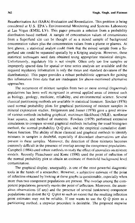
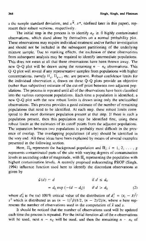
Example 2. In this simulated example, we consider a three population mixture model with ten observations from an N(20, 4) population, 100 from an N(0,1) population, and 30 from an N(5, 1). Moreover, in order to show the extent of distortion of the Q-Q plot by the presence of extreme observations, two extreme observations from an N(100,10) are also included in this mixed sample. This is data set no. 2 in the Appendix. The classical and the robust Q-Q plots using all of the 142 observations are given in Figs. 2a and b, re- spectively. Both graphs identify the two extreme observations. Moreover, both graphs give indications of the presence of a sample from a population with higher concentrations (observations no. 1-10). However, due to the large vari-

Background Levels of Contaminants 371
B4.22'r/
+(141) 4{142)
9915 M u i ~ U' t l . - 42.7"/
(t 1 5 ) ~ I I IN)
9 ~ W~r.ln E LTL - -/5.3
-342175 991, M ~ i m ~ t _ L T l . - -)4 )tl - -
-3~.414~ -I~ 619 419"7"/ 24 0144 4"~ 1111
" t ' T , ~ i c ~ Q m ~ i k ~ ~ Disui l~ lon)
Fig. 2a. Mixture of N(0, 1), N(5, 1), N(20.4) , N[100, 10)-classical Q-Q plot.
5
12].*~
92. I &'74
60.6121
~O"Jll~
91,I I ~ U'IIIL. - L~I
-I ~ -I.1~
�9 "($) �9 , '(T I
"1141) ~
1 " ~ -' " q u ~ m m m = n ~ l ~ p
Fig. 2b. Mixture of N(0, l), N(5, 1), N(20, 4), N(100, 10) robust Q-Q plot.
L O ~ I z 2 ~ 2 4 ~ 8
372 Singh, Singh, and Flatman
s
19.271
N
i 1.7422
+12.~16
~1~ Ni~tl~m I/'1~ - 17.]4 a+
951 Wn'~n I ~ rL - 13.gg
�9 �9 �9 + . 6 ~ a 6 ~
9SS Wmmi~ll LTL - 4.r~
991 k4huinmm I T L - +l~.~J
+12.6q11 -~ 1]~/2 2.3]~1G 10149) IT 76S Th,~o,r.~=l q, mmiles ~ O i ~ k m )
Fig. 2c. Mixture of N(0, 1), N(5, l), N(2O, 4)-classical Q-Q plot/two extremes removed.
d
29�84
21 715q
13 6)18
"~I0)
.,~r
"(s)
"(j)
'"" f 9911 M u l i m U11. - ~1.~
�9 2 ~52 -I.16 O.~d2 I 2239 24139
Fig. 2d . Mixture o f N(0 , 1), N(5 , 1), N(20, 4)-robust Q - Q plot / two extremes removed .
Background Levels of Contaminants 373
2 9 . ' ~
1~5 613,4
2192~
IT 1803
*Of
�9 O)
^(4)
A~m~ I~ 21.4484 5tlndl~d [~"vi$li~ II 4 1~74
*(2) l u )
13.11~3| 751 LTL I| 13 1~311_ I 0 ] 2~ 35 7 741 10 0
Comtim~ Clwl (Indlvidlml Obt.rvmio~s)
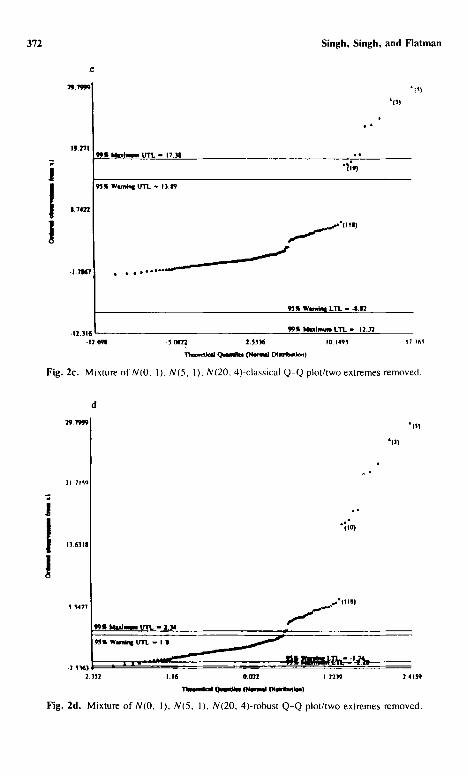
Fig. 2e. M ix tu re o f N(0 . ] ) , N (5 , 1). N(20, 4)-robust chart-contain, sample N(20, 4).
(111}
6 6rt6
H
i 2o6112
I �9 0 7141
.u I
/ t '
~ I M t ~ l ~ UTL - 2.34 ~ I F Z ]
Wm~dAII ~ - !.11
.*** ~ A* ~ W ~ L T L - -I.74
�9 * W S h l m t l m w m L'IIqL - - 2 .28
-I 141~ 11.0319 1 212 Qmmil~ ~ IXun~mtw)
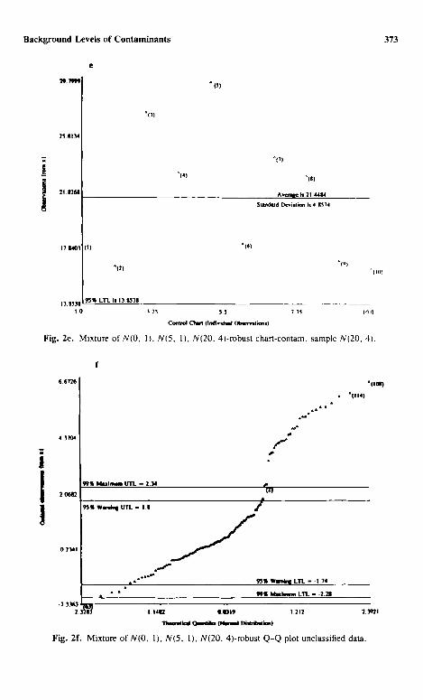
Fig. 2f. Mixture of N(0, ]), N(5, [), N(20, 4)-robust Q-Q plot unclassified data.
* l l l~ �9 *{ I14)
2.]921

374 Singh, Singh. and Flatman
g
6 6"T26 " (11 )
9~I$ IJTL Is 6.2561 *(*?)
* ( I t )
! �9 ~.vell l le ia 4.7'(~5 "112)
45265 S l ~ i ' d i ~ i ' t I~ Is 0 III I 4
4 ,
2 ] ~ *~zp(J) I 0 ( ) ~75 165 7425 170
Comical ~ (Indh'klul l Ob.serYI, i~'~l)
Fig. 2g. Mixture of N(0, l). N(5. 1), N(20, 4)-robust chart-intermed, sample N(5, 1).
241.41
t2291
-0.026
- I 2811
2 . ' ~ 3 1 . ~ i ~ �9 2 ~i049
h
W S Maal~ u'elL - ] . ) l , | i ) * (4 ) ) " ( m r
* * * * *
l J
f . J
..***'*
�9 �9 ~r~SsWlU~in| I T I : - I T?
. . ~ ; ( * ~ ) W ~ M u l m ~ , , tT t . - -2. )
( ~ m d k s ~ I~mrmmlm)
Fig. 2h. Mixture of N(0, 1), N(5, I), N(20, 4)-robust Q-Q plot unclassified data.
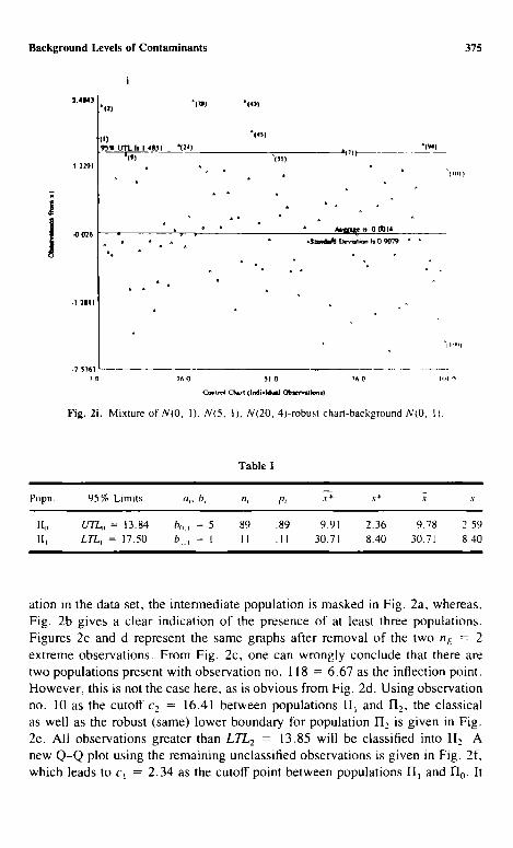
Background Levels of Contaminants 375
1.41143
I 2291
-0026
-I 2|11
-2 5163
" i l l " la l )
to) 9 'J l ~ l i 1,4851 " ( l i )
a l t I ^ ^
O i
"(1))
"(45)
"(~n) 117t)
, �9 ~ l l i l ~ t1.0 010l 4
~lllll )
*IiPIII
19 260 5! D ~60 Illl n
Civil'el ~ (Indivkl '~1 (Yolii'l'mulalll|
F ig . 2i . Mixture of N ( 0 , 1). N ( 5 . I), N(20 , 4)-robust char l -background N ( 0 , II .
Table 1
Popn, 95% Limits a,, b, n, p, x * s* ~ :,"
1I, UTL~) = 13.84 b i : 5 89 .89 9.91 2.36 9.78 2.59 1I I L T L I = 17.50 b t . I = l 11 .11 30.71 8.40 30.71 8,40
ation in the data set, the intermediate popula t ion is masked in Fig. 2a, whereas,
Fig. 2b gives a clear indicat ion of the presence of at least three populat ions.
Figures 2c and d represent the same graphs after removal of the two nF_ = 2
ext reme observat ions . F rom Fig. 2c, one can wrongly conclude that there are
two populat ions present with observat ion no. 118 = 6.67 as the inflection point.
However , this is not the case here, as is obvious f rom Fig. 2d. Using observat ion
no. 10 as the cutoff c 2 = 16.41 be tween populat ions FI~ and I] 2, the classical
as well as the robust (same) lower boundary for popula t ion H 2 is g iven in Fig.
2e. All observa t ions greater than LTL2_ = 13.85 will be classified into II 2. A new Q - Q plot using the remain ing unclassif ied observa t ions is g iven in Fig. 2f,
which leads to c~ = 2 .34 as the cutoff point be tween populat ions H~ and H o. It

376 Singh, Singh, and Flatrnan
should be noticed that the robust procedure used here has produced the same cutoff point of 2.34 between populations II o and I-I~, as can be seen from Fig. 2b, d, and f. Using all unclassified observations _>2.34, the two-sided 95% robust boundary for population 1-I I is (3.16, 6.26), as given in Fig. 2g. Next all observations less than 3.16 have been used to draw the robust Q - Q plot, given in Fig. 2h. From this graph it is obvious that there is only one population II o
left at this stage. Using these observations, the 95 % robust upper boundary for the background population is given by UTL 0 = 1.485. All observations less than this threshold will be classified into the background population IIo. Once
the boundaries have been set, observations in the overlapping and the unclaimed regions have been classified according to rules described above. All of the relevant statistics using the final classification are summarized in Table II.
E r a m p l e 3. In this example, we consider the data set from a Superfund Site with six samples known to come from the background population (obser- vations 33-38). As mentioned earlier, the site was sampled for six contaminants,
but the results for cadmium concentrations alone are included in this article. The data for the 45 collected samples (background samples included) is given in data set no. 3 in the Appendix.
The average site-specific background level of a contaminant plays an im- portant role in remediation decisions. As such, the estimation of the average site-specific background of a contaminant is an important problem. We now
show the results obtained by using the proposed procedure on Cadmium con- centrations. The classical as well as the robust Q - Q plots for cadmium are given in Figs. 3a and b, respectively. From these figures, it is obvious that observation nos. 15, 9, 22, and 21 represent extremely contaminated samples and should be treated individually. From Fig. 3b, there is a clear indication of the presence of at least three populations. Figure 3c represents the robust Q - Q plot after removal of these n~: = 4 extremes, which also indicates the presence of at least three populations. Using c 3 = 260.27 (observation no. 19 after the removal of extremes) as the cutoff point between populations II 2 and l-I 3, all observations
greater than c3 will be used to estimate the parameters of II 3, the population with high concentrations. Figure 3d indicates that these observations are from
Table II
II 95% Limits a,, b, n, p, .~ s* Y s
11~, UTI~, = 1.48 b,,t = 5 98 .7 -0.03 0.89 -0.07 0.97 III LTL I = 3.16 bi.L = 3 32 .23 4.71 0.81 4.59 1.06
UTL~ = 6.26 b~., = 1 112 LTL~ = 13.85 h2._, = 0 10 .07 21.45 4.86 21.45 4.86 n ~ - - - - 2 . . . . .

Background Levels of Contaminants 377
2_11~.9
1~13 3] ~ E411.thlmn UTL - 13117.42
I
9~ ! , Ww'~,~l I r l "L - 11)4.15
60071
-1~6 146 f~
.("a)
"(1~)
^ "(~,r)
.,'h%
~ J I W m i n I LTL - -97~ I ]
~ l M~lmmm LTL - - I ~ . ~
~ O m ~ l e l (Wlun~ [~ i f = ' l l ~ )
Fig. 3a. Cadmium concentration from a supeffund site-classical Q-Q plot.
2300.0
1~)6 27
1112 ~3
�9 "(TU I
qg*JI, M4uL|f~um UTL - ~ ~ " . ? ~ |
?'J~ Wea~lnll UTL - 176 7'? . - * ' * " ~
. . . . . . . . . . . . . . . . . . # 1 l e l i m ~ ] ~ - . - 4 } d ~ , - -74 939
-74 939 ~1 20(I"2 ~ 5 ~ J 117 2';
TI~'~ITI~IJ (~q~wl|i~l!1 (NOq~WII D i l l ~bu l l~ )
Fig. 3b. Cadmium concentration form a superfund site-robust Q-Q plot,
I]8"/42

378 Singh, Singh, and Flatman
i !
460 9"~4
ZI2 329
10'3 ?'~J]
.74 I~2 -7~1 M2
W S M a z l m ~ UT1. - 2~/")9.
"1+) "(~)
"O)
"117)
"06)
95S W ~ UTL - I ~ . i l �9 * i ( l l l )
t ~ ) j l i ' l
�9 . . , * *" i" j (41)
I~S ~ L1"1. - 4 1 , M
99S ~ i ~ LTL - - 7 4 , 1 ~
-4.1991 d~.4~42 I ]7 12|
Fig. 3c. Cd conc from a super'fund site-robust Q-Q plot/extremes removed
2~T7 ";91
"rEf.O2J
~7~404
423"7~5
27"2 I,
170 549
d
99S Muimmm UTL - "?27.02
95t i WDmJn| LITL - 6"/44
^(6) ^It0)
^(4)
^(2)
~(I)
^ (3)
9~S W ~ i n l [ L T L - 173 18
99~ Maximum LTL - 12~ '~"l
120 549 27"2 I f~ 42~ 7116 '575 404
Them'~k~ Qu~t l les (Nm'w~ I ~ r l l ~ l l ~ t
F i g . 3 d . C d ~ c o n c , f o r a s u p e ~ ' u n d s i t e - r o b u s t Q - Q p l o t - h i g h c o n e .
77 I IQ~

Background Levels of Con taminan t s 379
M I f ~
5Tt 72)
42~ 716
314 149
205 012 I
" f r l
- H i g h C o n c .
"11;)
(I)
"('Z)
"O}
~
"(4)
Av~aF It 4~.71M
DeTb~k~ b 1~9.)51
"(6)
~ 1 i LTL I120~,912
)2~ 3J " t ~
Cornel ~ flnd~Mml Obler , l~m)
Fig. 3e. Cd. conc for a superfund site-robust chart-high conc.
2OI 7211
132 ~d~
6.1 4023
-74924
f
991 Mludmom I.rrL - 2OI,TJ
"(~
"0))
9~S WIImin| UTL - 171.2] S(l~) ~(~)
9 ~ Wlm'llnl~ LTL - 44 4 )
9Qli MuImum LTL - .7492
"(]l) , i s , a ' ( I~ )
j ,
"(101
"110)
I0 0
~ h : : u J Qmmd b'= ~ Oi~rlb~iw)
Fig. 3f. Cd. conc. for a superfund site-robust Q-Q plot-high conc. removed.

380 Singh, Singh, and Flatman
II0.~
164 5?1
i i dl4S. iOl
121.6~
8
*t**}
"(2)
"O) "it)
'('7) S l i l ~ De~iifl~ Is 6 ) l II'7 '(6)
(I) 1~166 9515 LTLb IP. 166 *(I)
I :195 6.5 925 ~ Clml (llad~dml Olmms~m)
Fig. 3g. Cd. conc. for a superfund site-robust Q-Q chart-intermediate conc.
36 0742
!
l 21 o963
t 3 311~
- 1 0 4 6
~(tz)
120
h
"~,'9 9~s Waml~ ~ - 46 rI
4
^(I)
"(0)
�9 �9 *(11) i A &
~(t4)
95S W~ntre[ LTL - -3 92
9 9 S Maximum L '~ . - - I 0 r
-1046 5]Ir} ~1.0953 36 174) ~2 6571 ~ k : l J Qmmdk,- [I,~kmmI D4sU'Ibmk~)
Fig. 3h. Cd. conc. for a superfund site-robust Q-Q plot-highest 2 conc. removed.

"3uo3 punoa~12eq-ueq2 lsnqoa-~l!s punja~lns R Joj "3uo3 "PD ".fs "~!~I
(~utHIll",J-lsqo pmpqWll~l) IJlrlK) IOJl~.)
~ OL (t,i 0 s Ik't 0~9 1
00I
(01)
(~)~
(L)o IL911 0 Ilu~ p~z~uz'zS
1E~Q'II It alrl.",~; (I),
(~)~
(E) v
(Z)
f
s163
{l
s
6['[I
"3uo~ alP.!p~tuJalu!-ueq2 IsnqoJ-~l!s punJJ~lns R aoj "2uo2 "pD "!s "~!~1
I,t. t. s ~( 0 I
{~), 91~/J;'lZ q "LL1 II~
(I)
(z),
(r
(*).
(s
(d.
61C'l ) II -i.i.N lI~
9s I~
Lg~I "1~
6LI~
18s slueu!meluo 3 jo SpAO'] punoa~l;~B~]

382 Singh, Singh, and Flatman
a s ingle popula t ion . The o n e - s i d e d l o w e r 95% bounda ry for this popu la t ion is
LTL 3 = 205.91 as g iven in Fig . 3e.
A n e w robus t Q - Q plot us ing on ly the unc lass i f ied obse rva t i ons is g iven
in Fig . 3f. The re is a c l ea r ind ica t ion o f the p r e sence o f th ree more popu la t ions .
T h e robus t bounda r y (109 .166 , 131.623) g iven in Fig . 3g for the in t e rmed ia te
popu la t ion II 2 is ob ta ined us ing the top 12 obse rva t i ons o f Fig . 3f, wi th c~ =
1 1 1.60 as the cu to f f point . O b s e r v a t i o n nos . 2, 4, and 5 (wi th b 3 = 3) o f Fig.
3g be long to the unc l a imed region (UT/_~_, LTL3) and will be a s s igned to appro-
II.?d
9 1)5
i 671
4. |gqJ
160 I
k
1511 1/11. k I1.141~ "{I)
A~mm b ~ q m m ~ d D~mdm b L ~
(,) " ~
~
~1"1].~ )4;
C a e V a m t ~ J , k J l ~
4 75 6.0
Fig. 3k. Cd. conc. for a superfund site-robust chart-known background conc.
Table Il l
II 95% Limits a,, b, n, p, ~ s* ~: s
I1,, UTLv = 12.31 -- 9 .22 11.02 0.86 8.66 3.85 11, LTLI = 21.56 b]., = I 10 .24 31.45 5.55 32.78 7.39
UTL~ = 41.32 11~ LTL~. = 109.2 b2.~ = 2 11 .27 120.39 6.32 128.07 18.11
UTL~_ = 131.6 11~ LTL~ = 205.9 b~.~ = 1 l 1 .27 401.9 150.82 401.9 150.82 n.,. - - - - 4 . . . . . .

Background Levels of Contaminants 383
priate populations using the nearest neighbor technique (see Table III). Next, a new Robust Q-Q plot using only the remaining unclassified observations is given in Fig. 3h, giving a clear indication of the presence of two populations with the cutoff point ct = 22.05 (observation no. 12 in Fig. 3h). The 95% robust bound- ary = (21.576, 41.319) for population II , , using the top ten observations of Fig. 3h, is given in Fig. 3i, with one observation belonging to the unclaimed region (UTL~, LTL2), with b? = 1. Finally, using the last nine observations, the 95 % upper threshold value for the background level contamination is UTLo = 12.308 as can be seen in Fig. 3j. However, in this case, six samples from the background were also available. The robust 95 % upper boundary using these six background samples is given in Fig. 3k. The values in Figs. 3j and k are in close agreement, establishing the correctness and validity of the procedure de- scribed in this article. All relevant statistics after the final classification have been summarized in Table III.
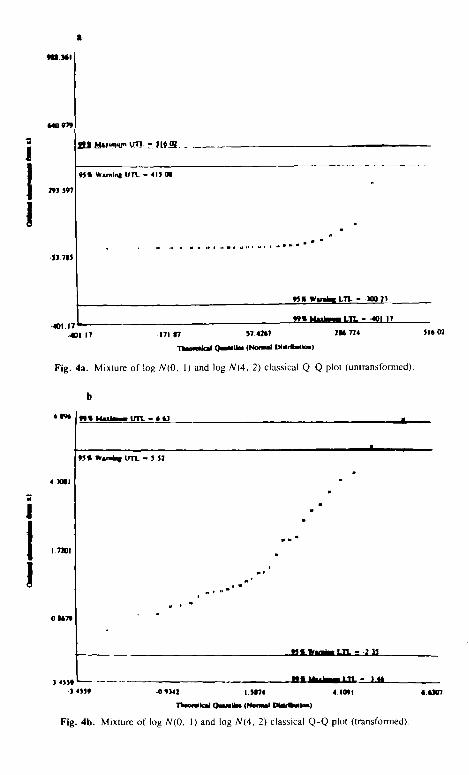
Example 4. In this example, we consider a simulated data set (given in the Appendix) which consists of a mixture sample from two lognormal popu- lations with some overlap. A sample of size 20 is obtained from a log N(0, 1) population and a sample of ten is generated from a log N(4, 2). We use this example to show the effectiveness of the proposed robust procedure in decom- posing the mixture into component populations. The classical Q-Q plots of the untransformed and the log-transformed data are given in Figs. 4a and b, re- spectively. From Fig. 4a, it can be concluded that the sample is from a single positively skewed population with observation no. 22 as an extreme observation. This may lead the user to take the log-transformation. From Fig. 4b, one can conclude that the mixture sample comes from a lognormal distribution with observation no. 22 to be slightly discordant. The corresponding robust Q-Q plot before and after the log-transformation are given by Figs. 4c and d, respectively. Figure 4c suggests that there are more than one population present. Figure 4d clearly separates the two underlying log-normal populations with cutoff point c, = 1.61. All of the relevant statistics are summarized as follows in Table IV.
C O N C L U S I O N S AND R E C O M M E N D A T I O N S
The proposed robust procedure works quite effectively in classifying a mixture sample into its component populations. In all of the examples discussed here, the procedure described here classified the observations correctly into their respective populations. When the data represent a mixture from lognormal pop- ulations, the procedure based upon the classical MLE estimates may identity some of these observations as anomalous. However, the robust procedure de- scribed here gives an indication that there is more than one population present (e.g., see Fig. 4c). This in turn, forces the user to verify the distributional assumptions. It is assumed that the user has some familiarity with symmetric
~.$61
14~J.9~ J N
i 293 597
I -53 "785
401. I1 - - ..401.1"/
21.3, L~r,~,u. , ~t~Tt). - . ~ l~,~. . _
9551, WsmJnil trl"t - 415 0 l
a m J l ~ ~ Q D ~ l i I m Q i ~ l g l W I J ~ m m i D ~ m
95'S W ~ L1'1- - ~00 'Z3
~ a , J4t, amm LI'L - - ' 91 17
- lT i 87 $?.4~7 ZlI6 T/4
Tbmmmkml QutmUm (f,kx~td DiHrlb,dlm)
Fig. 4a. Mixture of Io,~ N(0, 1) and log N(4, 2) classical Q-Q plot (tlnlransformed).
6f~
4 1081
i /TJOI
O M'/ql
b
19~,s M,,,dme. ~ r t - 6..~
H i Wsmiq UTL - 55~
o
m
J U 8
M I
N 0 el u 0 q
m J m
D
956 W~mba* L'FL - .2.)$
M 6 u~ .u , .m . L T t - 346 3 4550 . . . . . . . - - | 455g ~0 q~)4] 1.58"/4 4 1091
T l ~ l , c l l Qum,ulhe ( 1 4 o ~ O l i ~ l o u )
Fig. 4b. Mixture of log N(0, 1) and log N(4, 2) classical Q-Q plot (transformed).
51502
6.6,107

t i l l ~16l
741 179
493.997
|41 l l S
-0341
. a ,m
, m rata
~ s "" �9 u n . - 3 . * J - , ! . , : 7 - l , , _ . . . . . . ~ _ _ ~ _ _ s m �9 , J m l l ~ O
~ . ~ 1 W k r t ~ I u r n . - / ~ k ) ? ) I . N I ? 1 .2~1
Fig. 4c. Mixture of log N(O, 1) and log N(4, 2) robust Q-Q plot (untransformed).
) 1 ] 0 5
6.196
,t I~sOI
2 I Q 4 1
d
�9 m 9915 ~ I.rrlL 1.61
�9
9 5 S W a H ~ a t J ~ f ) 5
0 7 I S ! i ' '
, ,J
,i �9
~ S Wu~ml LTL - �9 7 . . . . . . . . . . . . . . . . 99% I,l~ummm LTL . -r ~r? . . . .
I 2 4 ~ . . . . . . . . . . . . . . . . . . . . . . . . . . . .
~J 9~9 ~321 0 32311 0 9613 [ 613~
~ ~ : l e s ( ~ Du~mnm)
Fig . 4(1. Mixture o f log N(0, l) and log N(4, 2) robust Q - Q plot (transformed).

386 Singh, Singh, and Flatman
Table IV
Popn. 95% Limits a,, b, n, p, ~ s* .~ s
II~ UTL~ = 1.143 -- 18 0.6 0.242 0.563 0.187 0.643 Ill LTL I = 1.419 -- 12 0.4 3.503 1.324 3.688 1.58
and skewed distributions. It is the user's responsibility to achieve near-normality (or at least symmetry) for each of the component populations before using the procedure described here. The robust procedure described here works quite effectively in decomposing a mixture sample into its component lognormal pop- ulations as well (see Fig. 4d). The stepwise procedure described here combines the natural separation between the component populations. The sample from the Sacramento Army Depot Superfund Site included a known site-specific back- ground sample. This, however, is not the case for many Superfund sites. The proposed statistical procedure will be a very useful tool for estimation of site- specific background for such Superfund sites.
A C K N O W L E D G M E N T S
The U.S. Environmental Protection Agency (EPA), through its Office of Research and Development (ORD), partially funded and collaborated in the research described here. It has been subjected to the Agency's peer review and has been approved as an EPA publication. The U.S. Government has a non- exclusive, royalty-free license in and to any copyright covering this article. The authors wish to thank Ken Brown of U.S. EPA\EMSL-Las Vegas for providing us the Superfund site data and for helpful suggestions during the preparation of this paper.
A P P E N D I X
Dataset 1:
Normal mixture generated from populations N(10, 3) and N(27, 8). 90 observations are from N(10, 3) and 10 are from N(27, 8). 2.49, 11.15 10.47, 10.62, 12.65, 13.52, 11.02, 13.40, 9.50, 6.93, 11.54, 6.83, 10.68, 10.38, 8.16, 10.57, 6.02, 6.49, 10.98, 6.25, 11.45, 12.31, 7.95, 13.89, 9.87, 10.10, 10.50, 11.95, 10.16, 11.09, 7.35, 11.01, 10.26, 12.06, 16.11, 12.03, 12.62, 10.29, 14.63, 11.65, 13.13, 7.93, 8.18, 11.11, 7.95, 8.15, 14.20, 7.99, 13.31, 9.63, 8.82, 8.42, 7.32, 18.59, 7.97, 6.43, 13.39, 3.59, 7.40, 12.73, 8.59, 13.34, 8.34, 5.71, 8.34, 8.29, 11.99, 11.23, 5.26, 9.04, 7.12, 14.85, 11.08,

Background Levels of Contaminants 387
10. I1, ll.01, 9.57, 11.01, 12.25, 7.93, 4.48, 9.13, 6.58, 13.89, 6.70, 12.04, 7.69, 10.84, 9.13, 6.84, 10.33, 33.38, 23.49, 30.01, 37.23, 37_66, 31.27, 34.94, 9.48, 31.08, 43.99.
Dataset 2:
Normal mixture with ten observations from N(20, 4), 100 from N(O, 1), 30 from a N(5, 1), and two extreme observations from N(100, 10). 18.12, 16.60, 27.60, 23.27, 29.80, 18.24, 24.40, 23.04, 16.98, 16.41, 1.77, 2.38, -0.22, -0.35, -0.40, 1.00, -0.01, -0.16, 1.44, -1.03, -1.84, 0.94, -0.31, -1.03, 1.19, -0.14, -1.42, -0.89, -0.23, 0.18, -0.96, -0.17, 0.06, 1.62, -0.03, -0.25, 0.30, 2.48, -0.02, 1.23, 0.10, 1.13, -0.69, 0.72, -0.86, 0.11, 1.16, 0.75, 0.27, -1.40, 0.29, -0.52, 2.47, 1.01, 1.89, -0.58, 0.20, -0.66, -1.05, -0.10, 1.44, 0.72, 0.33, 1.06, 0.48, -0_69, -0.48, -1.13, -0.67, 0.12, -0.15, -0.10, -2.54, 0.25, -2.04, 0.55, -1.32, -0.09, 0.51, 0.06, 1.54, 0.81, -1.65, -0.39, -0.01, 0.41, -0.51, -0.60, 1.24, -1.48, 0.51, 0.13, 0.93, -2.17, 0.63, -0.39, -1.37, 1.17, -1.29, -0.10, 0.30, 0.84, -0.11, 1.66, -0.66, -0.50, -0.87, -1.59, -0.69, -2.01,4.16, 3.97, 4.18, 3.71,4.55, 3.45, 5.62, 6.67, 4.25, 4.76, 5.24, 5.78, 5.23, 6.20, 1.18, 5.62, 4.51, 5.35, 4.34, 4.77, 6.07, 4.24, 4.26, 3.77, 5.16, 4.07, 5.46, 3.80, 5.50, 4.84, 123.76, 117.61.
Dataset 3:
Cadmium concentrations from the Sacramento Army Depot Super'fund Site: 26.20, 27.55, 445.01, 30.77, 486.31, 513.79, 112.81, 159.30, 1300, 6.68, 33.72, 35.01, 10.99, 22.05, 830.94, 125.07, 40.84, 345.52, 384.80, 183.04, 2300, 1500, 260.27, 32.09, 166.16, 31.68, 12.39, 614.53, 639.52, 116.24, 119.43, 111.60, 10.29, 1.68, 3.34, 10.47, 11.74, 10.32, 122.30, 283.03, 265.08, 125.49, 131.06, 47.90, 119.34.
Dataset 4:
Mixture of 20 observations from lognormal N(0, 1) and 10 from lognormal N(4, 2). 0.5300, 2.7538, 3.2237, 0.2871, 1.2915, 1.5795, 2.0817, 1.0633, 0.7486, 0.8284, 1.3252, 1.6477, 1.2311, 2.6518, 0.7258, 5.2913, 1.9187, 10.3898, 0.5373, 1.4311, 332.1949, 988.3606, 19.3491, 9.3424, 9.2353, 88.1362, 56.3981, 115.9378, 27.8464, 34.4647.
REFERENCES
Campbell, N. A., 1984, Mixture Models and Atypical Values: Math. Geol., v, 16, n~ 5. p. 465- 477.
Fleischhauer, H., and Korte, N., 1990, Formation of Cleanup Standards fi~r Trace Elements with

388 Singh, Singh, and Flatman
Probabili~' Plots, Environmental Management (Vol. 14; No. 1): Springer-Verlag, New York, p. 95-105.
Fowlkes, E. B., 1979, Some Methods for Studying the Mixture of two Normal (Lognormal) Dis- tributions: J. Am. Star. Assoc., v. 74, n. 367, p. 561-575.
Holgersson, M., and Joiner, U., 1978. Decomposition of a Mixture into Normal Components. A Review: J. Bio-Med. Comp., v. 9, p. 367-392.
Sinclair, A. J., 1976, Applications of Probability Graphs in Mineral Exploration, Assoc. of Explo- ration Geochemists: Rexdale, Ontario, p. 95.
Singh, A., 1994, Omnibus Robust Procedures for Assessment of Multivariate Normality and De- tection of Multivariate Outliers, in G. P. Patil and C, R. Rao, eds., Multivariate Environmental Statistics: North Holland, Elsevier Science Publishers, p. 445-488.
Singh, A., and Nocerino. J. 1994, Robust QA/QC for Environmental Applications, in The Pro- ceedings of the Ninth International Conference on Systems Engineering: University of Nevada, Las Vegas, p. 370-374.