metadat: Meta-Analysis Datasets - The Comprehensive R ...

Package ‘metadat’April 5, 2022

Version 1.2-0

Date 2022-04-05

Title Meta-Analysis Datasets

Depends R (>= 4.0.0)

Imports utils, tools, mathjaxr

Suggests metafor, numDeriv, BiasedUrn, dfoptim, igraph, ape, testthat, digest, lme4, clubSand-wich, meta, netmeta, mvtnorm, gridExtra, rms

Description A collection of meta-analysis datasets for teaching purposes, illustrating/testing meta-analytic methods, and validating published analyses.

License GPL (>=2)

ByteCompile TRUE

LazyData TRUE

Encoding UTF-8

RdMacros mathjaxr

URL https://github.com/wviechtb/metadat

BugReports https://github.com/wviechtb/metadat/issues

R topics documented:metadat-package . . . . . . . . . . . . . . . . . . . . . . . . . . . . . . . . . . . . . . 3dat.aloe2013 . . . . . . . . . . . . . . . . . . . . . . . . . . . . . . . . . . . . . . . . . 5dat.anand1999 . . . . . . . . . . . . . . . . . . . . . . . . . . . . . . . . . . . . . . . . 7dat.assink2016 . . . . . . . . . . . . . . . . . . . . . . . . . . . . . . . . . . . . . . . 9dat.axfors2021 . . . . . . . . . . . . . . . . . . . . . . . . . . . . . . . . . . . . . . . 11dat.bakdash2021 . . . . . . . . . . . . . . . . . . . . . . . . . . . . . . . . . . . . . . 12dat.baker2009 . . . . . . . . . . . . . . . . . . . . . . . . . . . . . . . . . . . . . . . . 18dat.bangertdrowns2004 . . . . . . . . . . . . . . . . . . . . . . . . . . . . . . . . . . . 20dat.baskerville2012 . . . . . . . . . . . . . . . . . . . . . . . . . . . . . . . . . . . . . 21dat.bcg . . . . . . . . . . . . . . . . . . . . . . . . . . . . . . . . . . . . . . . . . . . . 23dat.begg1989 . . . . . . . . . . . . . . . . . . . . . . . . . . . . . . . . . . . . . . . . 25dat.berkey1998 . . . . . . . . . . . . . . . . . . . . . . . . . . . . . . . . . . . . . . . 27

1

https://github.com/wviechtb/metadat

https://github.com/wviechtb/metadat/issues

2 R topics documented:

dat.besson2016 . . . . . . . . . . . . . . . . . . . . . . . . . . . . . . . . . . . . . . . 29dat.bonett2010 . . . . . . . . . . . . . . . . . . . . . . . . . . . . . . . . . . . . . . . 32dat.bornmann2007 . . . . . . . . . . . . . . . . . . . . . . . . . . . . . . . . . . . . . 34dat.bourassa1996 . . . . . . . . . . . . . . . . . . . . . . . . . . . . . . . . . . . . . . 35dat.cannon2006 . . . . . . . . . . . . . . . . . . . . . . . . . . . . . . . . . . . . . . . 37dat.cohen1981 . . . . . . . . . . . . . . . . . . . . . . . . . . . . . . . . . . . . . . . . 39dat.colditz1994 . . . . . . . . . . . . . . . . . . . . . . . . . . . . . . . . . . . . . . . 40dat.collins1985a . . . . . . . . . . . . . . . . . . . . . . . . . . . . . . . . . . . . . . . 42dat.collins1985b . . . . . . . . . . . . . . . . . . . . . . . . . . . . . . . . . . . . . . . 44dat.craft2003 . . . . . . . . . . . . . . . . . . . . . . . . . . . . . . . . . . . . . . . . 46dat.crede2010 . . . . . . . . . . . . . . . . . . . . . . . . . . . . . . . . . . . . . . . . 48dat.curtis1998 . . . . . . . . . . . . . . . . . . . . . . . . . . . . . . . . . . . . . . . . 50dat.dagostino1998 . . . . . . . . . . . . . . . . . . . . . . . . . . . . . . . . . . . . . . 52dat.damico2009 . . . . . . . . . . . . . . . . . . . . . . . . . . . . . . . . . . . . . . . 55dat.debruin2009 . . . . . . . . . . . . . . . . . . . . . . . . . . . . . . . . . . . . . . . 56dat.dogliotti2014 . . . . . . . . . . . . . . . . . . . . . . . . . . . . . . . . . . . . . . 58dat.dong2013 . . . . . . . . . . . . . . . . . . . . . . . . . . . . . . . . . . . . . . . . 60dat.dorn2007 . . . . . . . . . . . . . . . . . . . . . . . . . . . . . . . . . . . . . . . . 62dat.egger2001 . . . . . . . . . . . . . . . . . . . . . . . . . . . . . . . . . . . . . . . . 64dat.fine1993 . . . . . . . . . . . . . . . . . . . . . . . . . . . . . . . . . . . . . . . . . 66dat.franchini2012 . . . . . . . . . . . . . . . . . . . . . . . . . . . . . . . . . . . . . . 69dat.frank2008 . . . . . . . . . . . . . . . . . . . . . . . . . . . . . . . . . . . . . . . . 71dat.gibson2002 . . . . . . . . . . . . . . . . . . . . . . . . . . . . . . . . . . . . . . . 73dat.graves2010 . . . . . . . . . . . . . . . . . . . . . . . . . . . . . . . . . . . . . . . 77dat.gurusamy2011 . . . . . . . . . . . . . . . . . . . . . . . . . . . . . . . . . . . . . . 78dat.hackshaw1998 . . . . . . . . . . . . . . . . . . . . . . . . . . . . . . . . . . . . . . 80dat.hahn2001 . . . . . . . . . . . . . . . . . . . . . . . . . . . . . . . . . . . . . . . . 82dat.hannum2020 . . . . . . . . . . . . . . . . . . . . . . . . . . . . . . . . . . . . . . . 84dat.hart1999 . . . . . . . . . . . . . . . . . . . . . . . . . . . . . . . . . . . . . . . . . 85dat.hartmannboyce2018 . . . . . . . . . . . . . . . . . . . . . . . . . . . . . . . . . . . 87dat.hasselblad1998 . . . . . . . . . . . . . . . . . . . . . . . . . . . . . . . . . . . . . 89dat.hine1989 . . . . . . . . . . . . . . . . . . . . . . . . . . . . . . . . . . . . . . . . . 92dat.ishak2007 . . . . . . . . . . . . . . . . . . . . . . . . . . . . . . . . . . . . . . . . 93dat.kalaian1996 . . . . . . . . . . . . . . . . . . . . . . . . . . . . . . . . . . . . . . . 95dat.kearon1998 . . . . . . . . . . . . . . . . . . . . . . . . . . . . . . . . . . . . . . . 98dat.knapp2017 . . . . . . . . . . . . . . . . . . . . . . . . . . . . . . . . . . . . . . . . 100dat.konstantopoulos2011 . . . . . . . . . . . . . . . . . . . . . . . . . . . . . . . . . . 103dat.landenberger2005 . . . . . . . . . . . . . . . . . . . . . . . . . . . . . . . . . . . . 106dat.laopaiboon2015 . . . . . . . . . . . . . . . . . . . . . . . . . . . . . . . . . . . . . 108dat.lau1992 . . . . . . . . . . . . . . . . . . . . . . . . . . . . . . . . . . . . . . . . . 109dat.lee2004 . . . . . . . . . . . . . . . . . . . . . . . . . . . . . . . . . . . . . . . . . 111dat.lehmann2018 . . . . . . . . . . . . . . . . . . . . . . . . . . . . . . . . . . . . . . 112dat.li2007 . . . . . . . . . . . . . . . . . . . . . . . . . . . . . . . . . . . . . . . . . . 114dat.lim2014 . . . . . . . . . . . . . . . . . . . . . . . . . . . . . . . . . . . . . . . . . 116dat.linde2005 . . . . . . . . . . . . . . . . . . . . . . . . . . . . . . . . . . . . . . . . 118dat.linde2015 . . . . . . . . . . . . . . . . . . . . . . . . . . . . . . . . . . . . . . . . 120dat.linde2016 . . . . . . . . . . . . . . . . . . . . . . . . . . . . . . . . . . . . . . . . 123dat.lopez2019 . . . . . . . . . . . . . . . . . . . . . . . . . . . . . . . . . . . . . . . . 125

metadat-package 3

dat.maire2019 . . . . . . . . . . . . . . . . . . . . . . . . . . . . . . . . . . . . . . . . 128dat.mccurdy2020 . . . . . . . . . . . . . . . . . . . . . . . . . . . . . . . . . . . . . . 130dat.mcdaniel1994 . . . . . . . . . . . . . . . . . . . . . . . . . . . . . . . . . . . . . . 133dat.michael2013 . . . . . . . . . . . . . . . . . . . . . . . . . . . . . . . . . . . . . . . 135dat.molloy2014 . . . . . . . . . . . . . . . . . . . . . . . . . . . . . . . . . . . . . . . 137dat.moura2021 . . . . . . . . . . . . . . . . . . . . . . . . . . . . . . . . . . . . . . . 140dat.nakagawa2007 . . . . . . . . . . . . . . . . . . . . . . . . . . . . . . . . . . . . . . 142dat.nielweise2007 . . . . . . . . . . . . . . . . . . . . . . . . . . . . . . . . . . . . . . 144dat.nielweise2008 . . . . . . . . . . . . . . . . . . . . . . . . . . . . . . . . . . . . . . 145dat.normand1999 . . . . . . . . . . . . . . . . . . . . . . . . . . . . . . . . . . . . . . 147dat.obrien2003 . . . . . . . . . . . . . . . . . . . . . . . . . . . . . . . . . . . . . . . 149dat.pagliaro1992 . . . . . . . . . . . . . . . . . . . . . . . . . . . . . . . . . . . . . . 151dat.pignon2000 . . . . . . . . . . . . . . . . . . . . . . . . . . . . . . . . . . . . . . . 153dat.pritz1997 . . . . . . . . . . . . . . . . . . . . . . . . . . . . . . . . . . . . . . . . 155dat.raudenbush1985 . . . . . . . . . . . . . . . . . . . . . . . . . . . . . . . . . . . . . 157dat.riley2003 . . . . . . . . . . . . . . . . . . . . . . . . . . . . . . . . . . . . . . . . 159dat.senn2013 . . . . . . . . . . . . . . . . . . . . . . . . . . . . . . . . . . . . . . . . 161dat.stowe2010 . . . . . . . . . . . . . . . . . . . . . . . . . . . . . . . . . . . . . . . . 165dat.tannersmith2016 . . . . . . . . . . . . . . . . . . . . . . . . . . . . . . . . . . . . . 167dat.vanhowe1999 . . . . . . . . . . . . . . . . . . . . . . . . . . . . . . . . . . . . . . 170dat.viechtbauer2021 . . . . . . . . . . . . . . . . . . . . . . . . . . . . . . . . . . . . . 172dat.white2020 . . . . . . . . . . . . . . . . . . . . . . . . . . . . . . . . . . . . . . . . 177dat.woods2010 . . . . . . . . . . . . . . . . . . . . . . . . . . . . . . . . . . . . . . . 178dat.yusuf1985 . . . . . . . . . . . . . . . . . . . . . . . . . . . . . . . . . . . . . . . . 180datsearch . . . . . . . . . . . . . . . . . . . . . . . . . . . . . . . . . . . . . . . . . . 181

Index 184

metadat-package Meta-Analysis Datasets for R

Description

The metadat package contains a large collection of meta-analysis datasets. These datasets areuseful for teaching purposes, illustrating/testing meta-analytic methods, and validating publishedanalyses.

Browsing and Searching for Datasets

A listing of all datasets in the package can be obtained with help(package=metadat). Eachdatasets is also tagged with one or multiple concept terms. These concept terms refer to variousaspects of a dataset, such as the field/topic of research, the outcome measure used for the analysis,the model(s) used for analyzing the data, and the methods/concepts that can be illustrated with thedataset. The datsearch function can be used to search among the existing datasets in the packagebased on their concept terms or based on a full-text search of their corresponding help files.

You can also read the documentation online at https://wviechtb.github.io/metadat/ (wherethe output from the example analyses corresponding to each dataset is provided).

https://wviechtb.github.io/metadat/

4 metadat-package

Contributing New Datasets

We welcome contributions of new datasets to the package. For each dataset, there must be a citablereference, ideally in a peer-reviewed journal or publication. The general workflow for contributinga new dataset is as follows:

• Install the metadat package in R in the usual manner (i.e., install.packages("metadat")).

• If you are familiar with Git/GitHub and making pull requests, fork the package repository.Otherwise, download the source version of the package from GitHub and unzip the file tosome directory on your computer.

• Place the raw data (in a non-binary format) in the data-raw directory. The file should benamed dat.<author><year>.<ext>, where <author> is the last name of the first author ofthe publication from which the data come, <year> is the publication year, and <ext> is thefile extension (e.g., .txt, .csv).

• Place a corresponding R script in the data-raw directory named dat.<author><year>.r thatreads in the data, possibly does some data cleaning/processing, and then saves the dataset tothe data directory (using save), with name dat.<author><year>.rda.

• Start R, load the metadat package (i.e., library(metadat)), and then run the prep_datfunction (either set the working directory to the location of the source package beforehand oruse the pkgdir argument of the prep_dat function to specify the source package location).

• For a new dataset, this should create a boilerplate template for a corresponding help file inthe man directory, named dat.<author><year>.Rd. Edit the help file, adding the title and ashort description of the dataset in general, a description of each variable in the dataset, furtherdetails on the dataset (e.g., the field of research, how the data was collected, the purpose ofthe dataset / what it was used for, the effect size or outcome measure used in the analysis, thetypes of analyses/models that can be illustrated with the dataset), a reference for the source ofthe dataset, one or multiple concept terms, the name and email address of the contributor ofthe dataset, and (optionally) example code to illustrate the analysis of the dataset.

• Either make a pull request (if you are familiar with this workflow) or zip up the dat.<author><year>.<ext>,dat.<author><year>.r, dat.<author><year>.rda, and dat.<author><year>.Rd files andopen up a new issue at GitHub, attaching the zip file.

• If the above makes no sense to you, you can also email one of the package authors with acleaned, raw data file in .txt or .csv format, along with a meta-data file (format doesn’tmatter) that includes the information described above.

Citing the Package

If you use these data, please cite both the metadat package (see citation("metadat") for thereference) and the original source of the data as given under the help file of a dataset.

Bug/Error Reports

If you think you have found an error in an existing dataset or a bug in the package in general, pleasego to https://github.com/wviechtb/metadat/issues and open up a new issue.

https://github.com/wviechtb/metadat

https://github.com/wviechtb/metadat/archive/master.zip



dat.aloe2013 5

Author(s)

Thomas White, <[email protected]>Daniel Noble, <[email protected]>Alistair Senior, <[email protected]>W. Kyle Hamilton, <[email protected]>Wolfgang Viechtbauer, <[email protected]>

dat.aloe2013 Studies on the Association Between Supervision Quality and VariousOutcomes in Social, Mental Health, and Child Welfare Workers

Description

Results from 5 studies examining the association between various measures of supervision qualityand various work-related outcomes in social, mental health, and child welfare workers.

Usage

dat.aloe2013

Format

The data frame contains the following columns:

study character study author(s) and yearn integer sample sizetval numeric t-statistic for the test of the association/predictorpreds integer number of predictors included in the regression modelR2 numeric the coefficient of determination (i.e., R-squared value) of the regression model

Details

The dataset is based on studies that used regression models to examine the association between somemeasure of perceived supervision quality (e.g., the quality of the relationship with one’s supervisor)and some work-related outcome (e.g., job satisfaction) in social, mental health, and child welfareworkers. The dataset was extracted from Aloe and Thompson (2013), which in turn is a subset ofthe studies included in the meta-analysis by Mor Barak et al. (2009).

The dataset can be used to illustrate the meta-analysis of regression models, using measures suchas the (semi-)partial correlation coefficient. For this, the t-statistic from the regression model forthe association (i.e., predictor) of interest was extracted from each regression model (tval), as wellas the sample size (n), the number of predictors included in the regression model (preds), and thecoefficient of determination (i.e., R-squared value) of the regression model (R2). Based on thisinformation, the (semi-)partial correlation coefficient can be computed for each study, as well as itscorresponding sampling variance. These values can then be meta-analyzed using standard methods.

6 dat.aloe2013

Concepts

social work, (semi-)partial correlations, meta-regression

Author(s)

Wolfgang Viechtbauer, <[email protected]>, https://www.metafor-project.org

Source

Aloe, A. M., & Thompson, C. G. (2013). The synthesis of partial effect sizes. Journal of the Societyfor Social Work and Research, 4(4), 390–405. https://doi.org/10.5243/jsswr.2013.24

References

Mor Barak, M. E., Travis, D. J., Pyun, H., & Xie, B. (2009). The impact of supervision on workeroutcomes: A meta-analysis. Social Service Review, 83(1), 3–32. https://doi.org/10.1086/599028

Examples

### copy data into 'dat' and examine datadat <- dat.aloe2013dat

## Not run:

### load metafor packagesuppressPackageStartupMessages(library(metafor))

### compute the partial correlation coefficients and corresponding sampling variancesdat <- escalc(measure="PCOR", ti=tval, ni=n, mi=preds, data=dat)dat

### random-effects modelres <- rma(yi, vi, data=dat)res

### mixed-effects meta-regression model examining the relationship between the partial### correlation coefficients and the number of predictors included in the modelsres <- rma(yi, vi, mods = ~ preds, data=dat)res

### compute the r-to-z transformed partial correlation coefficients and their variancesdat <- escalc(measure="ZPCOR", ti=tval, ni=n, mi=preds, data=dat)dat


### back-transformation to the partial correlation scalepredict(res, transf=transf.ztor)

https://www.metafor-project.org

dat.anand1999 7

### compute the semi-partial correlation coefficients and their variancesdat <- escalc(measure="SPCOR", ti=tval, ni=n, mi=preds, r2i=R2, data=dat)dat


## End(Not run)

dat.anand1999 Studies on the Effectiveness of Oral Anticoagulants in Patients withCoronary Artery Disease

Description

Results from 34 trials examining the effectiveness of oral anticoagulants in patients with coronaryartery disease.

Usage

dat.anand1999

Format


study character author(s) or trial nameyear numeric publication yearintensity character intensity of anticoagulation (low, medium, or high)asp.t numeric concomitant use of aspirin in the treatment group (0 = no, 1 = yes)asp.c numeric concomitant use of aspirin in the control group (0 = no, 1 = yes)ai numeric number of deaths in the treatment groupn1i numeric number of patients in the treatment groupci numeric number of deaths in the control groupn2i numeric number of patients in the control group

Details

The dataset includes the results from 34 randomized clinical trials that examined the effectivenessof oral anticoagulants in patients with coronary artery disease. The results given here are focusedon the total mortality in the treatment versus control groups.

Concepts

medicine, cardiology, odds ratios, Mantel-Haenszel method

8 dat.anand1999

Note

Strictly speaking, there are only 31 trials, since Breddin et al. (1980) and ATACS (1990) are multi-arm trials.

According to a correction, dat.anand1999$ci[29] should be 1. But then dat.anand1999$ci[21]would also have to be 1 (if these data indeed refer to the same control group). This appears contra-dictory, so this correction was not made.

Author(s)


Source

Anand, S. S., & Yusuf, S. (1999). Oral anticoagulant therapy in patients with coronary arterydisease: A meta-analysis. Journal of the American Medical Association, 282(21), 2058–2067.https://doi.org/10.1001/jama.282.21.2058

Examples

### copy data into 'dat' and examine datadat <- dat.anand1999dat

## Not run:

### load metafor packagelibrary(metafor)

### High-Intensity OA vs Controlrma.mh(measure="OR", ai=ai, n1i=n1i, ci=ci, n2i=n2i, data=dat,

subset=(intensity=="high" & asp.t==0 & asp.c==0), digits=2)

### High- or Moderate-Intensity OA vs Aspirinrma.mh(measure="OR", ai=ai, n1i=n1i, ci=ci, n2i=n2i, data=dat,

subset=(intensity %in% c("high","moderate") & asp.t==0 & asp.c==1), digits=2)

### Moderate-Intensity OA vs Controlrma.mh(measure="OR", ai=ai, n1i=n1i, ci=ci, n2i=n2i, data=dat,

subset=(intensity=="moderate" & asp.t==0 & asp.c==0), digits=2)

### High- or Moderate-Intensity OA and Aspirin vs Aspirinrma.mh(measure="OR", ai=ai, n1i=n1i, ci=ci, n2i=n2i, data=dat,

subset=(intensity %in% c("high","moderate") & asp.t==1 & asp.c==1), digits=2)

### Low-Intensity OA and Aspirin vs Aspirinrma.mh(measure="OR", ai=ai, n1i=n1i, ci=ci, n2i=n2i, data=dat,

subset=(intensity=="low" & asp.t==1 & asp.c==1), digits=2)

## End(Not run)


dat.assink2016 9

dat.assink2016 Studies on the Association between Recidivism and Mental Health

Description

Results from 17 studies on the association between recidivism and mental health in delinquentjuveniles.

Usage

dat.assink2016

Format


study numeric study id numberesid numeric effect size within study id numberid numeric row id numberyi numeric standardized mean differencevi numeric corresponding sampling variancepubstatus numeric published study (0 = no; 1 = yes)year numeric publication year of the study (approximately mean centered)deltype character type of delinquent behavior in which juveniles could have recidivated (either general, overt, or covert)

Details

The studies included in this dataset (which is a subset of the data used in Assink et al., 2015) com-pared the difference in recidivism between delinquent juveniles with a mental health disorder and acomparison group of juveniles without a mental health disorder. Since studies differed in the wayrecidivism was defined and assessed, results are given in terms of standardized mean differences,with positive values indicating a higher prevalence of recidivism in the group of juveniles with amental health disorder.

Multiple effect size estimates could be extracted from most studies (e.g., for different delinquentbehaviors in which juveniles could have recidivated), necessitating the use of appropriate mod-els/methods for the analysis. Assink and Wibbelink (2016) illustrate the use of multilevel meta-analysis models for this purpose.

Concepts

psychology, criminology, standardized mean differences, multilevel models, cluster-robust infer-ence

Note

The year variable is not constant within study 3, as this study refers to two different publicationsusing the same data.

10 dat.assink2016

Author(s)


Source

Assink, M., & Wibbelink, C. J. M. (2016). Fitting three-level meta-analytic models in R: A step-by-step tutorial. The Quantitative Methods for Psychology, 12(3), 154–174. https://doi.org/10.20982/tqmp.12.3.p154

References

Assink, M., van der Put, C. E., Hoeve, M., de Vries, S. L. A., Stams, G. J. J. M., & Oort, F. J.(2015). Risk factors for persistent delinquent behavior among juveniles: A meta-analytic review.Clinical Psychology Review, 42, 47–61. https://doi.org/10.1016/j.cpr.2015.08.002

Examples

### copy data into 'dat' and examine datadat <- dat.assink2016head(dat, 9)

## Not run:


### fit multilevel modelres <- rma.mv(yi, vi, random = ~ 1 | study/esid, data=dat)res

### use cluster-robust inference methodsrobust(res, cluster=study)

### LRTs for the variance componentsres0 <- rma.mv(yi, vi, random = ~ 1 | study/esid, data=dat, sigma2=c(0,NA))anova(res0, res)res0 <- rma.mv(yi, vi, random = ~ 1 | study/esid, data=dat, sigma2=c(NA,0))anova(res0, res)

### examine some potential moderators via meta-regressionrma.mv(yi, vi, mods = ~ pubstatus, random = ~ 1 | study/esid, data=dat)rma.mv(yi, vi, mods = ~ year, random = ~ 1 | study/esid, data=dat)dat$deltype <- relevel(factor(dat$deltype), ref="general")rma.mv(yi, vi, mods = ~ deltype, random = ~ 1 | study/esid, data=dat)rma.mv(yi, vi, mods = ~ year + deltype, random = ~ 1 | study/esid, data=dat)

### assume that the effect sizes within studies are correlated with rho=0.6V <- vcalc(vi, cluster=study, obs=esid, data=dat, rho=0.6)round(V[dat$study %in% c(1,2), dat$study %in% c(1,2)], 4)

### fit multilevel model using this approximate V matrixres <- rma.mv(yi, V, random = ~ 1 | study/esid, data=dat)res


dat.axfors2021 11

### use cluster-robust inference methodsrobust(res, cluster=study)

## End(Not run)

dat.axfors2021 Mortality Outcomes with Hydroxychloroquine and Chloroquine inCOVID-19 from an International Collaborative Meta-Analysis of Ran-domized Trials

Description

Results from 33 trials examining the effectiveness of hydroxychloroquine or chloroquine in patientswith COVID-19.

Usage

dat.axfors2021

Format


id character registry numberacronym character shortened registry numberpatient_setting character patient settingblinding_exact character study blindinghigh_dose character high or low dose of medicationPublished character publication statushcq_cq character medication type (hcq = hydroxychloroquine or cq = chloroquine)hcq_arm_event numeric number of deaths in the treatment grouphcq_arm_total numeric number of patients in the treatment groupcontrol_arm_event numeric number of deaths in the control groupcontrol_arm_total numeric number of patients in the control groupControl character control group type (Standard of Care or Placebo)

Details

The dataset includes the results from 33 published and unpublished randomized clinical trials thatexamined the effectiveness of hydroxychloroquine or chloroquine in patients with COVID-19. Theresults given here are focused on the total mortality in the treatment versus control groups.

Concepts

medicine, covid-19, odds ratios

12 dat.bakdash2021

Author(s)

W. Kyle Hamilton <[email protected]> https://kylehamilton.com

Source

Axfors, C., Schmitt, A., Janiaud, P., van ’t Hooft, J., Moher, D., Goodman, S., . . . Hemkens, L. G.(2021, March 9). Hydroxychloroquine and chloroquine for survival in COVID-19: An internationalcollaborative meta-analysis of randomized trials. https://doi.org/10.17605/OSF.IO/QESV4

References

Axfors, C., Schmitt, A. M., Janiaud, P., van’t Hooft, J., Abd-Elsalam, S., Abdo, E. F., Abella,B. S., Akram, J., Amaravadi, R. K., Angus, D. C., Arabi, Y. M., Azhar, S., Baden, L. R., Baker,A. W., Belkhir, L., Benfield, T., Berrevoets, M. A. H., Chen, C.-P., Chen, T.-C., . . . Hemkens,L. G. (2021). Mortality outcomes with hydroxychloroquine and chloroquine in COVID-19 froman international collaborative meta-analysis of randomized trials. Nature Communications, 12(1),2349. https://doi.org/10.1038/s41467-021-22446-z

Examples

# copy data into 'dat' and examine datadat <- dat.axfors2021dat

## Not run:

# load metafor packagelibrary(metafor)

# calculate log odds ratios and corresponding sampling variancesdat <- escalc(measure="OR", ai=hcq_arm_event, n1i=hcq_arm_total,

ci=control_arm_event, n2i=control_arm_total, data=dat)

# meta-analysis Hydroxychloroquineres_hcq <- rma(yi, vi, subset=(hcq_cq=="hcq"), slab = id, data=dat)print(res_hcq, digits=2)

# meta-analysis Chloroquineres_cq <- rma(yi, vi, subset=(hcq_cq=="cq"), slab = id, data=dat)print(res_cq, digits=2)

## End(Not run)

dat.bakdash2021 Dataset on Situation Awareness and Task Performance Associations

https://kylehamilton.com

dat.bakdash2021 13

Description

Results from 77 papers with 678 effects evaluating associations among measures of situation aware-ness and task performance.

Usage

dat.bakdash2021

Format


Author character paper author(s)Year integer year of paper publicationTitle character title of paperDOI character digital object identifier (DOI)DTIC.link character permanent link for Defense Technical Information Collection (DITC) reports; see: https://www.dtic.milSA.measure.type character type of SA measureSample.size integer reported sample sizeSample.size.stats integer reported sample size based on reported statistics (this reflects excluded participants)es.z numeric z-transformed correlation coefficient; includes ghost results (disclosed and undisclosed non-significant effects not reported in detail) imputed using the draw method described in Bakdash et al. (2021a)vi.z numeric variance for z-transformed correlation (calculated using Sample.size.stats, not Sample.size)SampleID character unique identifier for each experiment/studyOutcome integer unique value for each effect size

Details

The dataset contains behavioral experiments from 77 papers/79 studies with a total of 678 effects,evaluating associations among measures of situation awareness (“knowing what is going on”) andtask performance. Examples of situation awareness include knowledge of current vehicle speedin a simulated driving task and location and heading of aircraft in a simulated air traffic controltask. Corresponding examples of task performance include “the number of collisions in a simulateddriving task” and “subject matter expert rating of conflict management in a simulated air controltask” (Bakdash et al. 2021a, p. 2). This dataset and the ‘Examples’ are a highly simplified versionof the data and code in Bakdash et al. (2021b; 2021c). The journal article by Bakdash et al. (2021a)describes the systematic review and meta-analysis in detail.

This dataset is used to illustrate multilevel multivariate meta-analytic models for the overall pooledeffect and pooled effects by situation awareness measure. We also adjust meta-analytic models us-ing cluster-robust variance estimation / cluster-robust inference with the robust function in metafor.Results are shown graphically in a customized forest plot with a prediction interval (estimated plau-sible range of individual effects). Last, we create a table summarizing the estimated meta-analyticheterogeneity parameters.

The meta-analytic results show most pooled effect sizes in the positive medium range or less. Therewas also substantial meta-analytic heterogeneity (estimated systematic variance in true effects),nearing the magnitude of the overall pooled effect. We interpret the meta-analytic results as situationawareness typically having limited validity for task performance (i.e., good situation awareness doesnot tend to have strong probabilistic links with good performance and vice-versa). More formally,measures of situation awareness do not generally and meaningfully capture cognitive processes and

14 dat.bakdash2021

other relevant factors underlying task performance.

Run-Time:The code run-time can be greatly sped-up using a linear algebra library with R that makes use ofmultiple CPU cores. See: https://www.metafor-project.org/doku.php/tips:speeding_up_model_fitting. To measure the run-time, uncomment these three lines: start.time <-Sys.time(),end.time <-Sys.time(), and end.time -start.time. Run-times on Windows 10 x64 with theIntel Math Kernel Library are:

CPU Run-Time (Minutes)i7-11850H 2.49i7-4770 5.38

Concepts

psychology, human factors, engineering, correlation coefficients, multilevel models, multivariatemodels, cluster-robust inference

Author(s)

Jonathan Bakdash, <[email protected]>, <[email protected]>Laura Marusich, <[email protected]>, <[email protected]>

Source

Bakdash, J. Z., Marusich, L. R., Cox, K. R., Geuss, M. N., Zaroukian, E. G., & Morris, K. M.(2021b). The validity of situation awareness for performance: A meta-analysis (Code Ocean Cap-sule). https://doi.org/10.24433/CO.1682542.v4

Bakdash, J. Z., Marusich, L. R., Cox, K. R., Geuss, M. N., Zaroukian, E. G., & Morris, K. M.(2021c). The validity of situation awareness for performance: A meta-analysis (Systematic Review,Data, and Code). https://doi.org/10.17605/OSF.IO/4K7ZV

References

Bakdash, J. Z., Marusich, L. R., Cox, K. R., Geuss, M. N., Zaroukian, E. G., & Morris, K. M.(2021a). The validity of situation awareness for performance: A meta-analysis. Theoretical Issuesin Ergonomics Science, 1–24. https://doi.org/10.1080/1463922X.2021.1921310

Supplemental materials: https://www.tandfonline.com/doi/suppl/10.1080/1463922X.2021.1921310/suppl_file/ttie_a_1921310_sm5524.docx

Examples

### copy data into 'dat' and examine datadat <- dat.bakdash2021head(dat[c(1,2,6,8:12)])

## Not run:#start.time <- Sys.time()

### load metafor

https://www.metafor-project.org/doku.php/tips:speeding_up_model_fitting

https://www.metafor-project.org/doku.php/tips:speeding_up_model_fitting

dat.bakdash2021 15

library(metafor)

### multilevel meta-analytic model to get the overall pooled effectres.overall <- rma.mv(es.z, vi.z, mods = ~ 1,

random = ~ 1 | SampleID / Outcome,data = dat,test = "t")

res.overall

### get prediction intervalpredict(res.overall)

### cluster-robust variance estimation (CRVE) / cluster-robust inferenceres.overall.crve <- robust(res.overall, cluster = SampleID)res.overall.crve

### get prediction intervalres.overall.crve.pred <- predict(res.overall.crve)res.overall.crve.pred

### multilevel meta-analytic model for SA measuresres.sa <- rma.mv(es.z, vi.z, mods = ~ SA.measure.type - 1,

random = ~ 1 | SampleID / Outcome,data = dat,test = "t")

res.sa

### cluster-robust variance estimation (CRVE) / cluster-robust inferenceres.sa.crve <- robust(res.sa, cluster = SampleID)res.sa.crve

### profile likelihood plotspar(mfrow=c(2,1))profile(res.sa.crve, progbar = FALSE)

### format and combine output of meta-analytic models for the forest plotall.z <- c(res.sa.crve$beta, # SA measures

res.overall.crve$beta, # pooled effect for confidence interval (CI)res.overall.crve$beta) # pooled effect for prediction interval (PI)

all.ci.lower <- c(res.sa.crve$ci.lb, # SA measuresres.overall.crve.pred$ci.lb, # pooled effect, lower CIres.overall.crve.pred$pi.lb) # pooled effect, lower PI

all.ci.upper <- c(res.sa.crve$ci.ub, # SA measuresres.overall.crve.pred$ci.ub, # pooled effect, upper CIres.overall.crve.pred$pi.ub) # pooled effect, upper PI

### note: there is no p-value for the PIall.pvals <- c(res.sa.crve$pval, res.overall.crve$pval)all.labels <- c(sort(unique(dat$SA.measure.type)), "Overall", "95% Prediction Interval")

### function to round p-values for the forest plot

16 dat.bakdash2021

pvals.round <- function(input) {input <- ifelse(input < 0.001, "< 0.001",

ifelse(input < 0.01, "< 0.01",ifelse(input < 0.05 & input >= 0.045, "< 0.05",ifelse(round(input, 2) == 1.00, "0.99",sprintf("%.2f", round(input, 2))))))}

all.pvals.rounded <- pvals.round(all.pvals)

### forest plotplot.vals <- data.frame(all.labels, all.z, all.ci.lower, all.ci.upper)

par(mfrow=c(1,1), cex = 1.05)forest(plot.vals$all.z,

ci.lb = plot.vals$all.ci.lower,ci.ub = plot.vals$all.ci.upper,slab = plot.vals$all.labels,psize = 1,efac = 0, xlim = c(-1.8, 2.5), clim = c(-1, 1),transf = transf.ztor, # transform z to rat = seq(-0.5, 1, by = 0.25),xlab = expression("Correlation Coefficient"~"("*italic('r')*")"),main = "\n\n\nSA Measures",ilab = c(all.pvals.rounded, ""), ilab.xpos = 2.45, ilab.pos = 2.5,digits = 2, refline = 0, annotate = FALSE)

### keep trailing zero using sprintfoutput <- cbind(sprintf("%.2f", round(transf.ztor(plot.vals$all.z), 2)),

sprintf("%.2f", round(transf.ztor(plot.vals$all.ci.lower), 2)),sprintf("%.2f", round(transf.ztor(plot.vals$all.ci.upper), 2)))

### alignment kludgeannotext <- apply(output, 1, function(x) {paste0(" ", x[1], " [", x[2],", ", x[3], "]")})text( 1.05, 12:1, annotext, pos = 4, cex = 1.05)text(-1.475, 14.00, "SA Measure", cex = 1.05)text( 2.30, 14.00, substitute(paste(italic('p-value'))), cex = 1.05)text( 1.55, 14.00, "Correlation [95% CI]", cex = 1.05)abline(h = 1.5)

### black polygon for overall mean CIsaddpoly(all.z[11], ci.lb = all.ci.lower[11], ci.ub = all.ci.upper[11],

rows = 2, annotate = FALSE, efac = 1.5, transf = transf.ztor)

### white polygon for PIaddpoly(all.z[12], ci.lb = all.ci.lower[12], ci.ub = all.ci.upper[12],

rows = 1, col = "white", border = "black",annotate = FALSE, efac = 1.5, transf = transf.ztor)

par(mfrow=c(1,1), cex = 1) # reset graph parameters to default

### confidence intervals for the variance componentsre.CI.variances <- confint(res.overall)re.CI.variances

dat.bakdash2021 17

sigma1.z <- data.frame(re.CI.variances[[1]]["random"])sigma2.z <- data.frame(re.CI.variances[[2]]["random"])

### fit model using alternative multivariate parameterizationres.overall.alt <- rma.mv(es.z, vi.z, mods = ~ 1,

random = ~ factor(Outcome) | factor(SampleID),data = dat,test = "t")

### confidence intervals for the total amount of heterogeneity variance componentres.overall.alt.tau <- confint(res.overall.alt, tau2=1)$random

### I^2: http://www.metafor-project.org/doku.php/tips:i2_multilevel_multivariateW <- diag(1/dat$vi.z)X <- model.matrix(res.overall)P <- W - W %*% X %*% solve(t(X) %*% W %*% X) %*% t(X) %*% W

### I^2 (variance due to heterogeneity): 61%I2 <- 100 * res.overall.alt$tau2 /

(res.overall.alt$tau2 + (res.overall$k-res.overall$p)/sum(diag(P)))I2

### 95% CI for I^2 using uncertainty around tau^2I2.CI.lb <- 100 * res.overall.alt.tau[1,2] /

(res.overall.alt.tau[1,2] + (res.overall$k-res.overall$p)/sum(diag(P)))I2.CI.lb

I2.CI.ub <- 100 * res.overall.alt.tau[1,3] /(res.overall.alt.tau[1,3] + (res.overall$k-res.overall$p)/sum(diag(P)))

I2.CI.ub

### total amount of heterogeneity (tau)sqrt(res.overall.alt$tau2)

### heterogeneity tabletable.heterogeneity <- data.frame(matrix(ncol = 3, nrow = 4))colnames(table.heterogeneity) <- c("Parameter Value",

"Lower 95% CI","Upper 95% CI")

rownames(table.heterogeneity) <- c("Tau (Total)","Tau1 (Between paper)","Tau2 (Within paper)","I2 (%)")

table.heterogeneity[1,] <- res.overall.alt.tau[2,]table.heterogeneity[2,] <- sigma1.z[2,]table.heterogeneity[3,] <- sigma2.z[2,]table.heterogeneity[4,] <- c(I2, I2.CI.lb, I2.CI.ub)

round(table.heterogeneity, 2)

#end.time <- Sys.time()

18 dat.baker2009

#end.time - start.time

## End(Not run)

dat.baker2009 Studies on Pharmacologic Treatments for Chronic Obstructive Pul-monary Disease

Description

Results from 39 trials examining pharmacologic treatments for chronic obstructive pulmonary dis-ease (COPD).

Usage

dat.baker2009

Format


study character study labelyear numeric year of publicationid numeric study IDtreatment character treatmentexac numeric number of individuals with one or more COPD exacerbationstotal numeric number of individuals

Details

This data set comes from a systematic review of randomized controlled trials on pharmacologictreatments for chronic obstructive pulmonary disease (COPD) (Baker et al., 2009).

The primary outcome, occurrence of one or more episodes of COPD exacerbation, is binary (yes/ no). For this outcome, five drug treatments (fluticasone, budesonide, salmeterol, formoterol,tiotropium) and two combinations (fluticasone + salmeterol, budesonide + formoterol) were com-pared to placebo. The authors considered the two combinations as separate treatments instead ofevaluating the individual components.

Concepts

medicine, odds ratios, network meta-analysis, component network meta-analysis

Author(s)

Guido Schwarzer, <[email protected]>, https://github.com/guido-s/

https://github.com/guido-s/

dat.baker2009 19

Source

Baker, W. L., Baker, E. L., & Coleman, C. I. (2009). Pharmacologic treatments for chronic ob-structive pulmonary disease: A mixed-treatment comparison meta-analysis. Pharmacotherapy: TheJournal of Human Pharmacology and Drug Therapy, 29(8), 891–905. https://doi.org/10.1592/phco.29.8.891

See Also

pairwise, metabin, netmeta, netcomb, netmetabin

Examples

### Show first 6 rows of the datasethead(dat.baker2009)

## Not run:

### Load netmeta packagesuppressPackageStartupMessages(library(netmeta))

### Print odds ratios and confidence limits with two digitssettings.meta(digits = 2)

### Transform data from long arm-based format to contrast-based### format. Argument 'sm' has to be used for odds ratio as summary### measure; by default the risk ratio is used in the metabin function### called internally.pw <- pairwise(treatment, exac, total, studlab = paste(study, year),

data = dat.baker2009, sm = "OR")

### Conduct random effects network meta-analysis (NMA)### with placebo as referencenet <- netmeta(pw, fixed = FALSE, ref = "plac")

### Show network graphnetgraph(net, seq = "optimal", start = "prcomp",

labels = gsub("+", " +\n", trts, fixed = TRUE),plastic = TRUE, thickness = "se.fixed", number = TRUE,points = TRUE, cex.points = 5, col.points = "red",offset = 0.025)

### Print and plot results for network meta-analysisnetforest(net)

### Conduct component network meta-analysis (CNMA)cnet <- netcomb(net)cnet

### Compare results of NMA and additive CNMAnb <- netbind(net, cnet, name = c("Standard NMA", "Additive CNMA"))forest(nb)

20 dat.bangertdrowns2004

## End(Not run)

dat.bangertdrowns2004 Studies on the Effectiveness of Writing-to-Learn Interventions

Description

Results from 48 studies on the effectiveness of school-based writing-to-learn interventions on aca-demic achievement.

Usage

dat.bangertdrowns2004

Format


id numeric study numberauthor character study author(s)year numeric publication yeargrade numeric grade level (1 = elementary; 2 = middle; 3 = high-school; 4 = college)length numeric treatment length (in weeks)minutes numeric minutes per assignmentwic numeric writing tasks were completed in class (0 = no; 1 = yes)feedback numeric feedback on writing was provided (0 = no; 1 = yes)info numeric writing contained informational components (0 = no; 1 = yes)pers numeric writing contained personal components (0 = no; 1 = yes)imag numeric writing contained imaginative components (0 = no; 1 = yes)meta numeric prompts for metacognitive reflection (0 = no; 1 = yes)subject character subject matterni numeric total sample size of the studyyi numeric standardized mean differencevi numeric corresponding sampling variance

Details

In each of the studies included in this meta-analysis, an experimental group (i.e., a group of studentsthat received instruction with increased emphasis on writing tasks) was compared against a controlgroup (i.e., a group of students that received conventional instruction) with respect to some content-related measure of academic achievement (e.g., final grade, an exam/quiz/test score). The outcomemeasure for this meta-analysis was the standardized mean difference (with positive values indicatinga higher mean level of academic achievement in the intervention group).

The standardized mean differences given here are bias-corrected and therefore differ slightly fromthe values reported in the article. Also, since only the total sample size is given in the article, thesampling variances were computed under the assumption that ni1 = ni2 = ni/2.

dat.baskerville2012 21

Concepts

education, standardized mean differences, meta-regression

Author(s)


Source

Bangert-Drowns, R. L., Hurley, M. M., & Wilkinson, B. (2004). The effects of school-basedwriting-to-learn interventions on academic achievement: A meta-analysis. Review of EducationalResearch, 74(1), 29–58. https://doi.org/10.3102/00346543074001029

Examples

### copy data into 'dat' and examine datadat <- dat.bangertdrowns2004dat[1:10,-13]

## Not run:


### fit random-effects modelres <- rma(yi, vi, data=dat)res

### some examples of mixed-effects meta-regression modelsres <- rma(yi, vi, mods = ~ factor(grade), data=dat)resres <- rma(yi, vi, mods = ~ length, data=dat)resres <- rma(yi, vi, mods = ~ info + pers + imag + meta, data=dat)res

## End(Not run)

dat.baskerville2012 Studies on the Effectiveness of Practice Facilitation Interventions

Description

Results from 23 studies on the effectiveness of practice facilitation interventions within the primarycare practice setting.

Usage

dat.baskerville2012


22 dat.baskerville2012

Format


author character study author(s)year numeric publication yearscore numeric quality score (0 to 12 scale)design character study design (cct = controlled clinical trial, rct = randomized clinical trial, crct = cluster randomized clinical trial)alloconc numeric allocation concealed (0 = no, 1 = yes)blind numeric single- or double-blind study (0 = no, 1 = yes)itt numeric intention to treat analysis (0 = no, 1 = yes)fumonths numeric follow-up monthsretention numeric retention (in percent)country character country where study was conductedoutcomes numeric number of outcomes assessedduration numeric duration of interventionpperf numeric practices per facilitatormeetings numeric (average) number of meetingshours numeric (average) hours per meetingtailor numeric intervention tailored to the context and needs of the practice (0 = no, 1 = yes)smd numeric standardized mean differencese numeric corresponding standard error

Details

Baskerville et al. (2012) describe outreach or practice facilitation as a "multifaceted approach thatinvolves skilled individuals who enable others, through a range of intervention components andapproaches, to address the challenges in implementing evidence-based care guidelines within theprimary care setting". The studies included in this dataset examined the effectiveness of practicefacilitation interventions for improving some relevant evidence-based practice behavior. The effectwas quantified in terms of a standardized mean difference, comparing the change (from pre- topost-intervention) in the intervention versus the comparison group (or the difference from baselinein prospective cohort studies).

Concepts

medicine, primary care, standardized mean differences, publication bias, meta-regression

Author(s)


Source

Baskerville, N. B., Liddy, C., & Hogg, W. (2012). Systematic review and meta-analysis of practicefacilitation within primary care settings. Annals of Family Medicine, 10(1), 63–74. https://doi.org/10.1370/afm.1312

Examples

### copy data into 'dat' and examine data


dat.bcg 23

dat <- dat.baskerville2012dat

## Not run:


### random-effects modelres <- rma(smd, sei=se, data=dat, method="DL")print(res, digits=2)

### funnel plotfunnel(res, xlab="Standardized Mean Difference", ylim=c(0,0.6))

### rank and regression tests for funnel plot asymmetryranktest(res)regtest(res)

### meta-regression analyses examining various potential moderatorsrma(smd, sei=se, mods = ~ score, data=dat, method="DL")rma(smd, sei=se, mods = ~ alloconc, data=dat, method="DL")rma(smd, sei=se, mods = ~ blind, data=dat, method="DL")rma(smd, sei=se, mods = ~ itt, data=dat, method="DL")rma(smd, sei=se, mods = ~ duration, data=dat, method="DL")rma(smd, sei=se, mods = ~ tailor, data=dat, method="DL")rma(smd, sei=se, mods = ~ pperf, data=dat, method="DL")rma(smd, sei=se, mods = ~ I(meetings * hours), data=dat, method="DL")

## End(Not run)

dat.bcg Studies on the Effectiveness of the BCG Vaccine Against Tuberculosis

Description

Results from 13 studies examining the effectiveness of the Bacillus Calmette-Guerin (BCG) vaccineagainst tuberculosis.

Usage

dat.bcg

Format


trial numeric trial numberauthor character author(s)

24 dat.bcg

year numeric publication yeartpos numeric number of TB positive cases in the treated (vaccinated) grouptneg numeric number of TB negative cases in the treated (vaccinated) groupcpos numeric number of TB positive cases in the control (non-vaccinated) groupcneg numeric number of TB negative cases in the control (non-vaccinated) groupablat numeric absolute latitude of the study location (in degrees)alloc character method of treatment allocation (random, alternate, or systematic assignment)

Details

The 13 studies provide data in terms of 2× 2 tables in the form:

TB positive TB negativevaccinated group tpos tnegcontrol group cpos cneg

The goal of the meta-analysis was to examine the overall effectiveness of the BCG vaccine forpreventing tuberculosis and to examine moderators that may potentially influence the size of theeffect.

The dataset has been used in several publications to illustrate meta-analytic methods (see ‘Refer-ences’).

Concepts

medicine, risk ratios, meta-regression

Author(s)


Source

Colditz, G. A., Brewer, T. F., Berkey, C. S., Wilson, M. E., Burdick, E., Fineberg, H. V., & Mosteller,F. (1994). Efficacy of BCG vaccine in the prevention of tuberculosis: Meta-analysis of the publishedliterature. Journal of the American Medical Association, 271(9), 698–702. https://doi.org/10.1001/jama.1994.03510330076038

References

Berkey, C. S., Hoaglin, D. C., Mosteller, F., & Colditz, G. A. (1995). A random-effects regressionmodel for meta-analysis. Statistics in Medicine, 14(4), 395–411. https://doi.org/10.1002/sim.4780140406

van Houwelingen, H. C., Arends, L. R., & Stijnen, T. (2002). Advanced methods in meta-analysis:Multivariate approach and meta-regression. Statistics in Medicine, 21(4), 589–624. https://doi.org/10.1002/sim.1040

Viechtbauer, W. (2010). Conducting meta-analyses in R with the metafor package. Journal ofStatistical Software, 36(3), 1–48. https://doi.org/10.18637/jss.v036.i03


dat.begg1989 25

Examples

### copy data into 'dat' and examine datadat <- dat.bcgdat

## Not run:


### calculate log risk ratios and corresponding sampling variancesdat <- escalc(measure="RR", ai=tpos, bi=tneg, ci=cpos, di=cneg, data=dat)dat


### average risk ratio with 95% CIpredict(res, transf=exp)

### mixed-effects model with absolute latitude and publication year as moderatorsres <- rma(yi, vi, mods = ~ ablat + year, data=dat)res

### predicted average risk ratios for 10-60 degrees absolute latitude### holding the publication year constant at 1970predict(res, newmods=cbind(seq(from=10, to=60, by=10), 1970), transf=exp)

### note: the interpretation of the results is difficult because absolute### latitude and publication year are strongly correlated (the more recent### studies were conducted closer to the equator)plot(ablat ~ year, data=dat, pch=19, xlab="Publication Year", ylab="Absolute Lattitude")cor(dat$ablat, dat$year)

## End(Not run)

dat.begg1989 Studies on Bone-Marrow Transplantation versus Chemotherapy forthe Treatment of Leukemia

Description

Results from controlled and uncontrolled studies on the effectiveness of allogeneic bone-marrowtransplantation (BMT) and conventional chemotherapy (CMO) in the treatment of acute nonlym-phocytic leukemia.

Usage

dat.begg1989

26 dat.begg1989

Format


study numeric study numbertrt character treatment (BMT or CMO)arms numeric number of arms in the study (1 = uncontrolled studies; 2 = controlled studies)yi numeric 2-year disease-free survival ratessei numeric corresponding standard errorsvi numeric corresponding sampling variances

Details

The dataset includes the results from controlled and uncontrolled studies on the 2-year disease-free survival rate in patients with acute nonlymphocytic leukemia receiving either allogeneic bone-marrow transplantation (BMT) or conventional chemotherapy (CMO). In the controlled (two-arm)studies (studies 1-4), a cohort of patients in complete remission and potentially eligible for BMTwas assembled, and those who consented and for whom a donor could be found received BMT,with the remaining patients used as controls (receiving CMO). In the uncontrolled (one-arm) studies(studies 5-16), only a single group was studied, receiving either BMT or CMO.

The data in this dataset were obtained from Table 1 in Begg and Pilote (1991, p. 902).

Concepts

medicine, oncology, single-arm studies, multilevel models

Author(s)


Source

Begg, C. B., & Pilote, L. (1991). A model for incorporating historical controls into a meta-analysis.Biometrics, 47(3), 899–906. https://doi.org/10.2307/2532647

References

Begg, C. B., Pilote, L., & McGlave, P. B. (1989). Bone marrow transplantation versus chemotherapyin acute non-lymphocytic leukemia: A meta-analytic review. European Journal of Cancer andClinical Oncology, 25(11), 1519–1523. https://doi.org/10.1016/0277-5379(89)90291-5

Examples

### copy data into 'dat' and examine datadat <- dat.begg1989dat

## Not run:



dat.berkey1998 27

### turn trt and arms into factors and set reference levelsdat$trt <- relevel(factor(dat$trt), ref="CMO")dat$arms <- relevel(factor(dat$arms), ref="2")

### create data frame with the treatment differences for the controlled studiesdat2 <- data.frame(yi = dat$yi[c(1,3,5,7)] - dat$yi[c(2,4,6,8)],

vi = dat$vi[c(1,3,5,7)] + dat$vi[c(2,4,6,8)])dat2

### DerSimonian and Laird method using the treatment differencesres <- rma(yi, vi, data=dat2, method="DL", digits=2)res

### Begg & Pilote (1991) model incorporating the uncontrolled studiesres <- rma.mv(yi, vi, mods = ~ trt, random = ~ 1 | study,

data=dat, method="ML", digits=2)res

### model involving bias terms for the uncontrolled studiesres <- rma.mv(yi, vi, mods = ~ trt + trt:arms, random = ~ 1 | study,

data=dat, method="ML", digits=2)res

### model with a random treatment effectres <- rma.mv(yi, vi, mods = ~ trt, random = list(~ 1 | study, ~ trt | study),

struct="UN", tau2=c(0,NA), rho=0, data=dat, method="ML", digits=2)res

### model with a random treatment effect, but with equal variances in both armsres <- rma.mv(yi, vi, mods = ~ trt, random = list(~ 1 | study, ~ trt | study),

struct="CS", rho=0, data=dat, method="ML", digits=2)res

## End(Not run)

dat.berkey1998 Studies on Treatments for Periodontal Disease

Description

Results from 5 trials comparing surgical and non-surgical treatments for medium-severity periodon-tal disease one year after treatment.

Usage

dat.berkey1998

28 dat.berkey1998

Format


trial numeric trial numberauthor character study author(s)year numeric publication yearni numeric number of patientsoutcome character outcome (PD = probing depth; AL = attachment level)yi numeric observed mean difference in outcome (surgical versus non-surgical)vi numeric corresponding sampling variancev1i numeric variances and covariances of the observed effectsv2i numeric variances and covariances of the observed effects

Details

The dataset includes the results from 5 trials that compared surgical and non-surgical methods forthe treatment of medium-severity periodontal disease. Reported outcomes include the change inprobing depth (PD) and attachment level (AL) one year after the treatment. The outcome measureused for this meta-analysis was the (raw) mean difference, calculated in such a way that positivevalues indicate that surgery was more effective than non-surgical treatment in decreasing the prob-ing depth and increasing the attachment level (so, the results from the various trials indicate thatsurgery is preferable for reducing the probing depth, while non-surgical treatment is preferable forincreasing the attachment level). Since each trial provides effect size estimates for both outcomes,the estimates are correlated. A multivariate model can be used to meta-analyze the two outcomessimultaneously.

The v1i and v2i values are the variances and covariances of the observed effects. In particular, foreach study, variables v1i and v2i form a 2× 2 variance-covariance matrix of the observed effects,with the diagonal elements corresponding to the sampling variances of the mean differences (thefirst for probing depth, the second for attachment level) and the off-diagonal value correspondingto the covariance of the two mean differences. Below, the full (block diagonal) variance-covariancefor all studies is constructed from these two variables.

Concepts

medicine, dentistry, raw mean differences, multivariate models

Author(s)


Source

Berkey, C. S., Antczak-Bouckoms, A., Hoaglin, D. C., Mosteller, F., & Pihlstrom, B. L. (1995).Multiple-outcomes meta-analysis of treatments for periodontal disease. Journal of Dental Research,74(4), 1030–1039. https://doi.org/10.1177/00220345950740040201

Berkey, C. S., Hoaglin, D. C., Antczak-Bouckoms, A., Mosteller, F., & Colditz, G. A. (1998). Meta-analysis of multiple outcomes by regression with random effects. Statistics in Medicine, 17(22),2537–2550. https://doi.org/10.1002/(sici)1097-0258(19981130)17:22<2537::aid-sim953>3.0.co;2-c


dat.besson2016 29

Examples

### copy data into 'dat' and examine datadat <- dat.berkey1998dat

## Not run:


### construct block diagonal var-cov matrix of the observed outcomes based on variables v1i and v2iV <- vcalc(vi=1, cluster=author, rvars=c(v1i, v2i), data=dat)

### fit multiple outcomes (meta-regression) model (with REML estimation)res <- rma.mv(yi, V, mods = ~ outcome - 1, random = ~ outcome | trial, struct="UN", data=dat)print(res, digits=3)

### test/estimate difference between the two outcomesanova(res, X=c(1,-1))

### fit model including publication year as moderator for both outcomes (with ML estimation)res <- rma.mv(yi, V, mods = ~ outcome + outcome:I(year - 1983) - 1,

random = ~ outcome | trial, struct="UN", data=dat, method="ML")print(res, digits=3)

## End(Not run)

dat.besson2016 Dataset on How Maternal Diet Impacts Copying Styles in Rodents

Description

Results from 46 studies synthesising maternal nutritional effects on coping styles in rodents.

Usage

dat.besson2016

Format


comp_ID character effect-size unique identifierstudy_ID character study unique identifierdam_ID character dam unique identifier (group of dams subjected to the same treatment)animal_ID character offspring unique identifier (group of offspring from the same dam group subjected to the same treatment)Reference character author’s names and datespecies character species [rats or mice]

30 dat.besson2016

strain character strainmanip_type character maternal nutritional manipulation type [protein or calorie]manip_direction character direction of maternal nutritional manipulation [- = restriction, + = overfeeding]nom_manip_val character degree of maternal nutritional manipulation as described in the original publications [% = percentage of caloric or protein restriction, # = increase in caloric intake]exp character percentage of caloric or protein maternal restriction or increase in caloric intake of the experimental groupcontrol character percentage of caloric or protein maternal restriction or increase in caloric intake for the control groupmanip_parameter character protein content, percentage fat or intakevitmin_eql character were vitamins equalized across maternal diets? [yes or no]adlib_con character were maternal control groups fed ad libitum? [yes or no]adlib_exp character were maternal experimental groups fed ad libitum? [yes or no]diet_con character name of maternal control diet?diet_exp character name of maternal experimental diet?dam_diet_start_dPC numeric start of the dam diet [in days post-conception]dam_diet_end_dPC numeric end of the dam diet [in days post-conception]diet_label character period of maternal diet manipulation [pregestation = pre-gestation, pre = pregnancy, lact = lactation, or pre+lact = pregnancy and lactation]age_mating numeric dam age at mating if knownn_con_dam integer sample size of the control dam groupsn_exp_dam integer sample size of the experimental dam groupsmulti_use_con character were control groups used multiple time? [yes or no]dam_housing character how were dams housed? [pair, group, or single]temperature numeric temperature during the experiment [°C]photoperiod integer photoperiod during the experiment [number of hours of light]litter_size integer size of the litter [number of pups per dam]litter_size_equalized character has litter size been equalized? [yes or no]crossfostered character have pups been cross-fostered? [yes or no]sex character sex of the offspring that were tested [m = male, f = female, both = mixed sex]housing character offspring housing during the test period [dam, pair, single, or group]bodymass_mean_contr numeric mean body mass of control offspring close to or during the testing period [g]bodymass_SE_contr numeric S.E. for body mass of control offspring close to or during the testing periodbodymass_mean_exp numeric mean body mass of experimental offspring close to or during the testing period [g]bodymass_SE_exp numeric S.E. for body mass of experimental offspring close to or during the testing periodbm_N_contr integer sample size for body mass of control offspring close to or during the testing periodbm_N_exp integer sample size for body mass of experimental offspring close to or during the testing periodbm_dPP integer age of offspring when body mass was measured [in days post-parturition]offspring_diet character offspring diet after weaning [type of control diet]offspring_con_adlib character were control offspring fed ad libitum after weaning? [yes or no]offspring_diet_level character name of offspring diet after weaningoffspring_diet_end_dPP integer end of the offspring diet [in days post-parturition]post_diet_adlib character were experimental offspring fed ad libitum after weaning? [yes or no]response_age_dPP numeric offspring age when behavioural testing started [in days post-parturition]authors_behaviour_classification character author’s classification of offspring behaviour [anxiety, exploration, or activity]our_behaviour_classification character our classification of offspring behaviour [anxiety, exploration, or activity]response_test character type of test used [elevated T-maze (ETM), open field, etc.] to measure offspring behaviourtime_trial integer duration of the testing [min]measure character measures taken during testing [total distance moved, time spent in open arm, etc.]unit character unit of the behavioural measure taken [min, s, m, number (#), etc.]high_better character for activity and exploration, a higher number is assumed to be better (i.e., animals were more active), but the opposite was assumed for anxiety (i.e., they were more anxious) [yes or no]night.day character time of day when behaviours were measured [night or day]

dat.besson2016 31

comparison character for a given control-treatment group comparison, animal group codes as used in the original article [e.g., LP, HP]. This field allows identification of exactly which data (i.e., comparison of which pairs of groups) were extracted from the original paper, and is not used in our analyses. For our analyses the groups were re-coded as control/experimental.exp_mean numeric mean of the offspring behaviour measured for the experimental groupexp_se numeric S.E. of the offspring behaviour measured for the experimental groupexp_n integer sample size for the offspring experimental groupcon_mean numeric mean of offspring behaviour measured for the control groupcon_se numeric S.E. of the offspring behaviour measured for the control groupcon_n integer sample size for the offspring control groupcon_ID character identifier for shared control groups within experimentpercentage character is the offspring behaviour measure a percentage? [yes or no]Data_source character figure or table number in the original paper from which the data were extractedmeasure_comments character any comments on the offspring behaviour measuresSE_imputed character was S.E. imputed for the offspring behaviour measure? [yes or no]Comments character any comments on the data

Details

Data from experiments where dams were subject to caloric or protein restriction or were overfedaround gestation were included. Offspring activity, exploration, or anxiety were measured outcomesvariables from maternal experimental treatments. Multilevel meta-analysis and meta-regressionmodels were used to analyze the meta-analytic data.

Concepts

ecology, evolution, standardized mean differences

Author(s)

Daniel Noble, <[email protected]>

Source

Besson, A. A., Lagisz, M., Senior, A. M., Hector, K. L., & Nakagawa, S. (2016). Effect of mater-nal diet on offspring coping styles in rodents: A systematic review and meta-analysis. BiologicalReviews, 91(4), 1065–1080. https://doi.org/10.1111/brv.12210

Examples

### copy data into 'dat' and examine datadat <- dat.besson2016head(dat)

## Not run:

### load metaforlibrary(metafor)

### compute SD from SEdat$sd_c <- with(dat, con_se * sqrt(con_n))dat$sd_e <- with(dat, exp_se * sqrt(exp_n))

32 dat.bonett2010

### compute standardized mean differences and corresponding sampling variancesdat <- escalc(measure="SMD", m1i=exp_mean, m2i=con_mean, sd1i=sd_e, sd2i=sd_c,

n1i=exp_n, n2i=con_n, data=dat, add.measure=TRUE)

### fit modelmod1 <- rma.mv(yi ~ 1, V = vi, random = list(~ 1 | study_ID, ~ 1 | comp_ID), data = dat)mod1

## End(Not run)

dat.bonett2010 Studies on the Reliability of the CES-D Scale

Description

Results from 9 studies on the reliability of the Center for Epidemiologic Studies Depression (CES-D) Scale administered to children providing care to an elderly parent.

Usage

dat.bonett2010

Format


study numeric study numbersource character source of datani numeric sample sizemi numeric number of items in the scaleai numeric observed value of Cronbach’s alphacaregivers character gender of the children in the sample

Details

The Center for Epidemiologic Studies Depression (CES-D) Scale is a 20-item questionnaire assess-ing various symptoms of depression, with each item scored on a 4-point scale. The scale has beenused in several studies to examine depressive symptoms in children providing care to an elderlyparent. The dataset includes information on the reliability of the scale as measured with Cronbach’salpha in 9 such studies. Also, the gender composition of the children in each sample is indicated.

Concepts

psychology, Cronbach’s alpha, reliability generalization, meta-regression

dat.bonett2010 33

Author(s)


Source

Bonett, D. G. (2010). Varying coefficient meta-analytic methods for alpha reliability. PsychologicalMethods, 15(4), 368–385. https://doi.org/10.1037/a0020142

References

Bonett, D. G. (2002). Sample size requirements for testing and estimating coefficient alpha. Journalof Educational and Behavioral Statistics, 27(4), 335–340. https://doi.org/10.3102/10769986027004335

Hakstian, A. R., & Whalen, T. E. (1976). A k-sample significance test for independent alpha coef-ficients. Psychometrika, 41(2), 219–231. https://doi.org/10.1007/BF02291840

Examples

### copy data into 'dat' and examine datadat <- dat.bonett2010dat

## Not run:


### meta-analysis using the raw alpha valuesres <- rma(measure="ARAW", ai=ai, mi=mi, ni=ni, data=dat)res

### meta-analysis using transformed alpha values (using the### transformation suggested by Hakstian & Whalen, 1976)res <- rma(measure="AHW", ai=ai, mi=mi, ni=ni, data=dat)respredict(res, transf=transf.iahw)

### meta-analysis using transformed alpha values (using the### transformation suggested by Bonett, 2002)res <- rma(measure="ABT", ai=ai, mi=mi, ni=ni, data=dat)respredict(res, transf=transf.iabt)

### forest plotforest(res, slab=source, header=TRUE, atransf=transf.iabt, refline=coef(res))

### examine whether female/mixed samples yield different alphas (with raw alphas)res <- rma(measure="ARAW", ai=ai, mi=mi, ni=ni, mods = ~ caregivers, data=dat)respredict(res, newmods=c(0,1), digits=2)


34 dat.bornmann2007

## End(Not run)

dat.bornmann2007 Studies on Gender Differences in Grant and Fellowship Awards

Description

Results from 21 studies on gender differences in grant and fellowship awards.

Usage

dat.bornmann2007

Format


study character study referenceobs numeric observation within studydoctype character document typegender character gender of the study authorsyear numeric (average) cohort yearorg character funding organization / programcountry character country of the funding organization / programtype character fellowship or grant applicationdiscipline character discipline / fieldwaward numeric number of women who received a grant/fellowship awardwtotal numeric number of women who applied for an awardmaward numeric number of men who received a grant/fellowship awardmtotal numeric number of men who applied for an award

Details

The studies in this dataset examine whether the chances of receiving a grant or fellowship awarddiffers for men and women. Note that many studies provide multiple comparisons (e.g., for differentyears / cohorts / disciplines). A multilevel meta-analysis model can be used to account for themultilevel structure in these data.

Concepts

sociology, odds ratios, multilevel models

Author(s)



dat.bourassa1996 35

Source

Bornmann, L., Mutz, R., & Daniel, H. (2007). Gender differences in grant peer review: A meta-analysis. Journal of Informetrics, 1(3), 226–238. https://doi.org/10.1016/j.joi.2007.03.001

References

Marsh, H. W., Bornmann, L., Mutz, R., Daniel, H.-D., & O’Mara, A. (2009). Gender effects in thepeer reviews of grant proposals: A comprehensive meta-analysis comparing traditional and multi-level approaches. Review of Educational Research, 79(3), 1290–1326. https://doi.org/10.3102/0034654309334143

Examples

### copy data into 'dat' and examine datadat <- dat.bornmann2007head(dat, 16)

## Not run:


### calculate log odds ratios and corresponding sampling variancesdat <- escalc(measure="OR", ai=waward, n1i=wtotal, ci=maward, n2i=mtotal, data=dat)

### fit multilevel meta-analysis modelres <- rma.mv(yi, vi, random = ~ 1 | study/obs, data=dat)res

### estimated average odds ratio (with 95% CI/PI)predict(res, transf=exp, digits=2)

### test for a difference between fellowship and grant applicationsres <- rma.mv(yi, vi, mods = ~ type, random = ~ 1 | study/obs, data=dat)respredict(res, newmods=0:1, transf=exp, digits=2)

## End(Not run)

dat.bourassa1996 Studies on the Association between Handedness and Eye-Dominance

Description

Results from 47 studies on the association between handedness and eye-dominance.

Usage

dat.bourassa1996

36 dat.bourassa1996

Format


study numeric study numbersample numeric sample numberauthor character (first) authoryear numeric publication yearselection character selection of subjects on the basis of eyedness or handednessinvestigator character investigator (psychologist, educationalist, or other)hand_assess character method to assess handedness (questionnaire or performance based)eye_assess character method to assess eyedness (see ‘Details’)mage numeric mean age of samplelh.le numeric number of left-handed left-eyed individualslh.re numeric number of left-handed right-eyed individualsrh.le numeric number of right-handed left-eyed individualsrh.re numeric number of right-handed right-eyed individualssex character sex of the sample (combined, male, or female)

Details

The 47 studies included in this meta-analysis examined the association between handedness andeye-dominance (ocular dominance or eyedness). Results are given in terms of 2 × 2 tables, in-dicating the number of left-handed left-eyed, left-handed right-eyed, right-handed left-eyed, andright-handed right-eyed individuals. Note that some studies included multiple (independent) sam-ples, so that the meta-analysis included 54 samples in total. Also, for some studies, the combineddata of the males and females are further broken down into the two subgroups.

In some studies, there was indication that the selection of subjects was not random with respect tohandedness and/or eyedness. While this should not influence the size of the association as measuredwith the odds ratio, this invalidates those studies for assessing the overall percentage of left-eyedand left-handed individuals.

Handedness was assessed in the individual studies either based on a questionnaire or inventoryor based on task performance. Eyedness was assessed based on various methods: E.1 methodsare based on task performance, while E.2.a denotes assessment based on a questionnaire. Theperformance based methods could be further broken down into: E.1.a.i (monocular procedurewith object/instrument held in one hand), E.1.a.ii (monocular procedure with object/instrumentheld in both hands), E.1.b (binocular procedure), E.1.c (a combination of the previous methods),and E.1.d (some other method).

Concepts

psychology, odds ratios

Author(s)



dat.cannon2006 37

Source

Bourassa, D. C., McManus, I. C., & Bryden, M. P. (1996). Handedness and eye-dominance: Ameta-analysis of their relationship. Laterality, 1(1), 5–34. https://doi.org/10.1080/713754206

Examples

### copy data into 'dat' and examine datadat <- dat.bourassa1996head(dat, 10)

## Not run:


### calculate log(OR) and corresponding sampling variance with 1/2 correctiondat <- escalc(measure="OR", ai=lh.le, bi=lh.re, ci=rh.le, di=rh.re, data=dat, add=1/2, to="all")head(dat, 10)

### overall association between handedness and eyednessres <- rma(yi, vi, data=dat, subset=sex=="combined")respredict(res, transf=exp, digits=2)

## End(Not run)

dat.cannon2006 Studies on the Effectiveness of Intensive Versus Moderate Statin Ther-apy for Preventing Coronary Death or Myocardial Infarction

Description

Results from 4 trials examining the effectiveness of intensive (high dose) versus moderate (standarddose) statin therapy for preventing coronary death or myocardial infarction.

Usage

dat.cannon2006

Format


trial character trial namepop character study population (post-ACS: post acute coronary syndrome; stable CAD: stable coronary artery disease)nt numeric number of patients in the high dose groupnc numeric number of patients in the standard dose groupep1t numeric number of events in the high dose group for end point 1: coronary death or non-fatal myocardial infarction

38 dat.cannon2006

ep1c numeric number of events in the standard dose group for end point 1: coronary death or non-fatal myocardial infarctionep2t numeric number of events in the high dose group for end point 2: coronary death or any cardiovascular event (MI, stroke, hospitalization for unstable angina, or revascularization)ep2c numeric number of events in the standard dose group for end point 2: coronary death or any cardiovascular event (MI, stroke, hospitalization for unstable angina, or revascularization)ep3t numeric number of events in the high dose group for end point 3: cardiovascular deathep3c numeric number of events in the standard dose group for end point 3: cardiovascular deathep4t numeric number of events in the high dose group for end point 4: non-cardiovascular deathep4c numeric number of events in the standard dose group for end point 4: non-cardiovascular deathep5t numeric number of events in the high dose group for end point 5: deaths (all-cause mortality)ep5c numeric number of events in the standard dose group for end point 5: deaths (all-cause mortality)ep6t numeric number of events in the high dose group for end point 6: strokeep6c numeric number of events in the standard dose group for end point 6: stroke

Details

The data were obtained from Figures 2, 3, 4, and 5 in Cannon et al. (2006). The authors used theMantel-Haenszel method for combining the results from the 4 trials. This approach is implementedin the rma.mh function.

Concepts

medicine, cardiology, odds ratios, Mantel-Haenszel method

Author(s)


Source

Cannon, C. P., Steinberg, B. A., Murphy, S. A., Mega, J. L., & Braunwald, E. (2006). Meta-analysisof cardiovascular outcomes trials comparing intensive versus moderate statin therapy. Journal ofthe American College of Cardiology, 48(3), 438–445. https://doi.org/10.1016/j.jacc.2006.04.070

Examples

### copy data into 'dat' and examine datadat <- dat.cannon2006dat

## Not run:


### meta-analysis of log odds ratios using the MH method for endpoint 1res <- rma.mh(measure="OR", ai=ep1t, n1i=nt, ci=ep1c, n2i=nc, data=dat, slab=trial)print(res, digits=2)

### forest plotforest(res, xlim=c(-.8,.8), atransf=exp, at=log(c(2/3, 1, 3/2)),

header=TRUE, top=2, cex=1.2, xlab="Odds Ratio")mtext("(high dose better)", side=1, line=par("mgp")[1]-0.5, at=log(2/3), cex=1.2, font=3)


dat.cohen1981 39

mtext("(standard dose better)", side=1, line=par("mgp")[1]-0.5, at=log(3/2), cex=1.2, font=3)

## End(Not run)

dat.cohen1981 Studies on the Relationship between Course Instructor Ratings andStudent Achievement

Description

Results from 20 studies on the correlation between course instructor ratings and student achieve-ment.

Usage

dat.cohen1981

Format


study character study author(s) and yearsample character course typecontrol character ability controlni numeric sample size of the study (number of sections)ri numeric observed correlation

Details

The studies included in this dataset examined to what extent students’ ratings of a course instruc-tor correlated with their achievement in the course. Instead of correlating individual ratings andachievement scores, the studies were carried out in multisection courses, in which the sectionshad different instructors but all sections used a common achievement measure (e.g., a final exam).The correlation coefficients reflect the correlation between the mean instructor rating and the meanachievement score of each section. Hence, the unit of analysis are the sections, not the individuals.

Note that this dataset (extracted from Table A.3 in Cooper & Hedges, 1994) only contains studieswith at least 10 sections.

Concepts

education, correlation coefficients

Author(s)



40 dat.colditz1994

Source

Cooper, H., & Hedges, L. V. (1994). Appendix A: Data Sets. In H. Cooper & L. V. Hedges (Eds.),The handbook of research synthesis (pp. 543-547). New York: Russell Sage Foundation.

References

Cohen, P. A. (1981). Student ratings of instruction and student achievement: A meta-analysis ofmultisection validity studies. Review of Educational Research, 51(3), 281–309. https://doi.org/10.3102/00346543051003281

Examples

### copy data into 'dat' and examine datadat <- dat.cohen1981dat[c(1,4,5)]

## Not run:


### calculate r-to-z transformed correlations and corresponding sampling variancesdat <- escalc(measure="ZCOR", ri=ri, ni=ni, data=dat[c(1,4,5)])dat

### meta-analysis of the transformed correlations using a random-effects modelres <- rma(yi, vi, data=dat, digits=2)res

### predicted average correlation with 95% CIpredict(res, transf=transf.ztor)

## End(Not run)

dat.colditz1994 Studies on the Effectiveness of the BCG Vaccine Against Tuberculosis

Description

Results from 13 studies examining the effectiveness of the Bacillus Calmette-Guerin (BCG) vaccineagainst tuberculosis.

Usage

dat.colditz1994

Format


dat.colditz1994 41

trial numeric trial numberauthor character author(s)year numeric publication yeartpos numeric number of TB positive cases in the treated (vaccinated) grouptneg numeric number of TB negative cases in the treated (vaccinated) groupcpos numeric number of TB positive cases in the control (non-vaccinated) groupcneg numeric number of TB negative cases in the control (non-vaccinated) groupablat numeric absolute latitude of the study location (in degrees)alloc character method of treatment allocation (random, alternate, or systematic assignment)

Details


TB positive TB negativevaccinated group tpos tnegcontrol group cpos cneg

The goal of the meta-analysis was to examine the overall effectiveness of the BCG vaccine forpreventing tuberculosis and to examine moderators that may potentially influence the size of theeffect.

The dataset has been used in several publications to illustrate meta-analytic methods (see ‘Refer-ences’).

Concepts

medicine, risk ratios, meta-regression

Author(s)


Source

Colditz, G. A., Brewer, T. F., Berkey, C. S., Wilson, M. E., Burdick, E., Fineberg, H. V., & Mosteller,F. (1994). Efficacy of BCG vaccine in the prevention of tuberculosis: Meta-analysis of the publishedliterature. Journal of the American Medical Association, 271(9), 698–702. https://doi.org/10.1001/jama.1994.03510330076038

References

Berkey, C. S., Hoaglin, D. C., Mosteller, F., & Colditz, G. A. (1995). A random-effects regressionmodel for meta-analysis. Statistics in Medicine, 14(4), 395–411. https://doi.org/10.1002/sim.4780140406

van Houwelingen, H. C., Arends, L. R., & Stijnen, T. (2002). Advanced methods in meta-analysis:Multivariate approach and meta-regression. Statistics in Medicine, 21(4), 589–624. https://doi.org/10.1002/sim.1040

Viechtbauer, W. (2010). Conducting meta-analyses in R with the metafor package. Journal ofStatistical Software, 36(3), 1–48. https://doi.org/10.18637/jss.v036.i03


42 dat.collins1985a

Examples

### copy data into 'dat' and examine datadat <- dat.colditz1994dat

## Not run:


### calculate log risk ratios and corresponding sampling variancesdat <- escalc(measure="RR", ai=tpos, bi=tneg, ci=cpos, di=cneg, data=dat)dat



### mixed-effects model with absolute latitude and publication year as moderatorsres <- rma(yi, vi, mods = ~ ablat + year, data=dat)res

### predicted average risk ratios for 10-60 degrees absolute latitude### holding the publication year constant at 1970predict(res, newmods=cbind(seq(from=10, to=60, by=10), 1970), transf=exp)

### note: the interpretation of the results is difficult because absolute### latitude and publication year are strongly correlated (the more recent### studies were conducted closer to the equator)plot(ablat ~ year, data=dat, pch=19, xlab="Publication Year", ylab="Absolute Lattitude")cor(dat$ablat, dat$year)

## End(Not run)

dat.collins1985a Studies on the Treatment of Upper Gastrointestinal Bleeding by a His-tamine H2 Antagonist

Description

Results from studies examining the effectiveness of histamine H2 antagonists (cimetidine or raniti-dine) in treating patients with acute upper gastrointestinal hemorrhage.

Usage

dat.collins1985a

dat.collins1985a 43

Format


id numeric study numbertrial character first author of trialyear numeric year of publicationref numeric reference numbertrt character C = cimetidine, R = ranitidinectrl character P = placebo, AA = antacids, UT = usual treatmentnti numeric number of patients in treatment groupb.xti numeric number of patients in treatment group with persistent or recurrent bleedingso.xti numeric number of patients in treatment group in need of operationd.xti numeric number of patients in treatment group that diednci numeric number of patients in control groupb.xci numeric number of patients in control group with persistent or recurrent bleedingso.xci numeric number of patients in control group in need of operationd.xci numeric number of patients in control group that died

Details

The data were obtained from Tables 1 and 2 in Collins and Langman (1985). The authors usedPeto’s (one-step) method for meta-analyzing the 27 trials. This approach is implemented in therma.peto function. Using the same dataset, van Houwelingen, Zwinderman, and Stijnen (1993)describe some alternative approaches for analyzing these data, including fixed- and random-effectsconditional logistic models. Those are implemented in the rma.glmm function.

Concepts

medicine, odds ratios, Peto’s method, generalized linear models

Author(s)


Source

Collins, R., & Langman, M. (1985). Treatment with histamine H2 antagonists in acute upper gas-trointestinal hemorrhage. New England Journal of Medicine, 313(11), 660–666. https://doi.org/10.1056/NEJM198509123131104

References

van Houwelingen, H. C., Zwinderman, K. H., & Stijnen, T. (1993). A bivariate approach to meta-analysis. Statistics in Medicine, 12(24), 2273–2284. https://doi.org/10.1002/sim.4780122405

Examples

### copy data into 'dat' and examine datadat <- dat.collins1985adat


44 dat.collins1985b

## Not run:


### meta-analysis of log ORs using Peto's method (outcome: persistent or recurrent bleedings)res <- rma.peto(ai=b.xti, n1i=nti, ci=b.xci, n2i=nci, data=dat)print(res, digits=2)

### meta-analysis of log ORs using a conditional logistic regression model (FE model)res <- rma.glmm(measure="OR", ai=b.xti, n1i=nti, ci=b.xci, n2i=nci, data=dat,

model="CM.EL", method="FE")summary(res)predict(res, transf=exp, digits=2)

### plot the likelihoods of the odds ratiosllplot(measure="OR", ai=b.xti, n1i=nti, ci=b.xci, n2i=nci, data=dat,

lwd=1, refline=NA, xlim=c(-4,4), drop00=FALSE)

### meta-analysis of log odds ratios using a conditional logistic regression model (RE model)res <- rma.glmm(measure="OR", ai=b.xti, n1i=nti, ci=b.xci, n2i=nci, data=dat,

model="CM.EL", method="ML")summary(res)predict(res, transf=exp, digits=2)

### meta-analysis of log ORs using Peto's method (outcome: need for surgery)res <- rma.peto(ai=o.xti, n1i=nti, ci=o.xci, n2i=nci, data=dat)print(res, digits=2)

### meta-analysis of log ORs using Peto's method (outcome: death)res <- rma.peto(ai=d.xti, n1i=nti, ci=d.xci, n2i=nci, data=dat)print(res, digits=2)

## End(Not run)

dat.collins1985b Studies on the Effects of Diuretics in Pregnancy

Description

Results from 9 studies examining the effects of diuretics in pregnancy on various outcomes.

Usage

dat.collins1985b

Format


dat.collins1985b 45

id numeric study numberauthor character study author(s)year numeric publication yearpre.nti numeric number of women in treatment group followed up for pre-eclampsia outcomepre.nci numeric number of women in control/placebo group followed up for pre-eclampsia outcomepre.xti numeric number of women in treatment group with any form of pre-eclampsiapre.xci numeric number of women in control/placebo group with any form of pre-eclampsiaoedema numeric dummy variable indicating whether oedema was a diagnostic criterionfup.nti numeric number of women in treatment group followed up for mortality outcomesfup.nci numeric number of women in control/placebo group followed up for mortality outcomesped.xti numeric number of perinatal deaths in treatment groupped.xci numeric number of perinatal deaths in control/placebo groupstb.xti numeric number of stillbirths in treatment groupstb.xci numeric number of stillbirths in control/placebo groupned.xti numeric number of neonatal deaths in treatment groupned.xci numeric number of neonatal deaths in control/placebo group

Details

The 9 studies in this dataset examined the effects of diuretics in pregnancy on various outcomes,including the presence of any form of pre-eclampsia, perinatal death, stillbirth, and neonatal death.

Concepts

medicine, obstetrics, odds ratios, Peto’s method

Author(s)


Source

Collins, R., Yusuf, S., & Peto, R. (1985). Overview of randomised trials of diuretics in pregnancy.British Medical Journal, 290(6461), 17–23. https://doi.org/10.1136/bmj.290.6461.17

Examples

### copy data into 'dat' and examine datadat <- dat.collins1985bdat

## Not run:


### calculate (log) odds ratio and sampling variancedat <- escalc(measure="OR", n1i=pre.nti, n2i=pre.nci, ai=pre.xti, ci=pre.xci, data=dat)summary(dat, digits=2, transf=exp)

### meta-analysis using Peto's method for any form of pre-eclampsia


46 dat.craft2003

rma.peto(n1i=pre.nti, n2i=pre.nci, ai=pre.xti, ci=pre.xci, data=dat, digits=2)

### meta-analysis including only studies where oedema was not a diagnostic criterionrma.peto(n1i=pre.nti, n2i=pre.nci, ai=pre.xti, ci=pre.xci, data=dat, digits=2, subset=(oedema==0))

### meta-analyses of mortality outcomes (perinatal deaths, stillbirths, and neonatal deaths)rma.peto(n1i=fup.nti, n2i=fup.nci, ai=ped.xti, ci=ped.xci, data=dat, digits=2)rma.peto(n1i=fup.nti, n2i=fup.nci, ai=stb.xti, ci=stb.xci, data=dat, digits=2)rma.peto(n1i=fup.nti, n2i=fup.nci, ai=ned.xti, ci=ned.xci, data=dat, digits=2)

## End(Not run)

dat.craft2003 Studies on the Relationship between the Competitive State AnxietyInventory-2 and Sport Performance

Description

Results from 10 studies on the relationship between the Competitive State Anxiety Inventory-2(CSAI-2) and sport performance.

Usage

dat.craft2003

Format


study numeric study numberni numeric sample sizesport character type of sport (T = team sport, I = individual sport)ri numeric correlation coefficientvar1 character variable 1 of the correlation coefficient (see ‘Details’)var2 character variable 2 of the correlation coefficient (see ‘Details’)

Details

The 10 studies included in this dataset are a subset of the studies included in the meta-analysis byCraft et al. (2003) on the relationship between the Competitive State Anxiety Inventory-2 (CSAI-2)and sport performance.

The CSAI-2 has three subscales: cognitive anxiety (acog), somatic anxiety (asom), and self-confidence(conf). The studies included in this dataset administered the CSAI-2 prior to some sport compe-tition and then measured sport performance based on the competition. Most studies provided all6 correlations (3 for the correlations among the 3 subscales and 3 for the correlations between thesubscales and sport performance), but 2 studies (with study numbers 6 and 17) only provided asubset.

dat.craft2003 47

Concepts

psychology, correlation coefficients, multivariate models

Author(s)


Source

Becker, B. J., & Aloe, A. M. (2019). Model-based meta-analysis and related approaches. In H.Cooper, L. V. Hedges, & J. C. Valentine (Eds.), The handbook of research synthesis and meta-analysis (3nd ed., pp. 339–363). New York: Russell Sage Foundation.

References

Craft, L. L., Magyar, T. M., Becker, B. J., & Feltz, D. L. (2003). The relationship between theCompetitive State Anxiety Inventory-2 and sport performance: A meta-analysis. Journal of Sportand Exercise Psychology, 25(1), 44–65. https://doi.org/10.1123/jsep.25.1.44

Examples

### copy data into 'dat' and examine datadat <- dat.craft2003head(dat, 18)

## Not run:


### construct dataset and var-cov matrix of the correlationstmp <- rcalc(ri ~ var1 + var2 | study, ni=ni, data=dat)V <- tmp$Vdat <- tmp$dat

### examine data for study 1dat[dat$study == 1,]V[dat$study == 1, dat$study == 1]



### multivariate random-effects modelres <- rma.mv(yi, V, mods = ~ var1.var2 - 1, random = ~ var1.var2 | study, struct="UN", data=dat)res


48 dat.crede2010

## End(Not run)

dat.crede2010 Studies on the Relationship between Class Attendance and Grades inCollege Students

Description

Results from 68 studies on the relationship between class attendence and class performance and/orgrade point average in college students.

Usage

dat.crede2010

Format


studyid numeric study numberyear numeric publication yearsource character study source (journal, dissertation, other)sampleid numeric sample within study numbercriterion character criterion variable (grade, gpa)class character class type (science, nonscience)ni numeric sample sizeri numeric observed correlation

Details

The 68 studies included in this dataset provide information about the relationship between classattendance of college students and their performance (i.e., grade) in the class and/or their overallgrade point average. Some studies included multiple samples and hence the dataset actually contains97 correlation coefficients.

The dataset was obtained via personal communication. Note that this dataset differs just slightlyfrom the one used by Credé et al. (2010).

Concepts

education, correlation coefficients, multilevel models

Author(s)



dat.crede2010 49

Source

Personal communication.

References

Credé, M., Roch, S. G., & Kieszczynka, U. M. (2010). Class attendance in college: A meta-analyticreview of the relationship of class attendance with grades and student characteristics. Review ofEducational Research, 80(2), 272–295. https://doi.org/10.3102/0034654310362998

Examples

### copy data into 'dat' and examine datadat <- dat.crede2010head(dat, 18)

## Not run:


### calculate r-to-z transformed correlations and corresponding sampling variancesdat <- escalc(measure="ZCOR", ri=ri, ni=ni, data=dat)

############################################################################

### meta-analysis for the relationship between attendance and gradesres <- rma(yi, vi, data=dat, subset=criterion=="grade")res

### estimated average correlation with 95% CI/PIpredict(res, transf=transf.ztor, digits=2)

### examine if relationship between attendance and grades differs for nonscience/science classesres <- rma(yi, vi, mods = ~ class, data=dat, subset=criterion=="grade")res

### estimated average correlations for nonscience and science classespredict(res, newmods=c(0,1), transf=transf.ztor, digits=2)

### examine if relationship between attendance and grades has changed over timeres <- rma(yi, vi, mods = ~ year, data=dat, subset=criterion=="grade")res

############################################################################

### meta-analysis for the relationship between attendance and GPAres <- rma(yi, vi, data=dat, subset=criterion=="gpa")res

### estimated average correlation with 95% CI/PIpredict(res, transf=transf.ztor, digits=2)

50 dat.curtis1998

### examine if relationship between attendance and GPA has changed over timeres <- rma(yi, vi, mods = ~ year, data=dat, subset=criterion=="gpa")res

############################################################################

### use a multilevel model to examine the relationship between attendance and gradesres <- rma.mv(yi, vi, random = ~ 1 | studyid/sampleid, data=dat, subset=criterion=="grade")respredict(res, transf=transf.ztor, digits=2)

### use a multilevel model to examine the relationship between attendance and gpares <- rma.mv(yi, vi, random = ~ 1 | studyid/sampleid, data=dat, subset=criterion=="gpa")respredict(res, transf=transf.ztor, digits=2)

## End(Not run)

dat.curtis1998 Studies on the Effects of Elevated CO2 Levels on Woody Plant Mass

Description

Results from studies examining the effects of elevated CO2 levels on woody plant mass.

Usage

dat.curtis1998

Format


id numeric observation numberpaper numeric paper numbergenus character genus namespecies character species namefungrp character plant functional groupco2.ambi numeric ambient CO2 level (control group)co2.elev numeric elevated CO2 level (treatment group)units character units for CO2 exposure levelstime numeric maximum length of time (days) of CO2 exposurepot character growing method (see ‘Details’)method character CO2 exposure facility (see ‘Details’)stock character planting stock codextrt character interacting treatment code (see ‘Details’)level character interacting treatment level codes (see ‘Details’)m1i numeric mean plant mass under elevated CO2 level (treatment group)

dat.curtis1998 51

sd1i numeric standard deviation of plant mass underelevated CO2 level (treatment group)n1i numeric number of observations under elevated CO2 level (treatment group)m2i numeric mean plant mass under ambient CO2 level (control group)sd2i numeric standard deviation of plant mass under ambient CO2 level (control group)n2i numeric number of observations under ambient CO2 level (control group)

Details

The studies included in this dataset compared the total above- plus below-ground biomass (in grams)for plants that were either exposed to ambient (around 35 Pa) and elevated CO2 levels (around twicethe ambient level). The co2.ambi and co2.elev variables indicate the CO2 levels in the control andtreatment groups, respectively (with the units variable specifying the units for the CO2 exposurelevels). Many of the studies also varied one or more additional environmental variables (defined bythe xtrt and level variables):

• NONE = no additional treatment factor

• FERT = soil fertility (either a CONTROL, HIGH, or LOW level)

• LIGHT = light treatment (always a LOW light level)

• FERT+L = soil fertility and light (a LOW light and soil fertility level)

• H2O = well watered vs drought (either a WW or DRT level)

• TEMP = temperature treatment (either a HIGH or LOW level)

• OZONE = ozone exposure (either a HIGH or LOW level)

• UVB = ultraviolet-B radiation exposure (either a HIGH or LOW level)

In addition, the studies differed with respect to various design variables, including CO2 exposureduration (time), growing method (pot: number = pot size in liters; GRND = plants rooted in ground;HYDRO = solution or aeroponic culture), CO2 exposure facility (method: GC = growth chamber; GH =greenhouse; OTC = field-based open-top chamber), and planting stock (stock: SEED = plants startedfrom seeds; SAP = plants started from cuttings). The goal of the meta-analysis was to examine theeffects of elevated CO2 levels on plant physiology and growth and the interacting effects of theenvironmental (and design) variables.

Concepts

ecology, ratios of means

Author(s)


Source

Hedges, L. V., Gurevitch, J., & Curtis, P. S. (1999). The meta-analysis of response ratios in experi-mental ecology. Ecology, 80(4), 1150–1156. https://doi.org/10.1890/0012-9658(1999)080[1150:TMAORR]2.0.CO;2(data obtained from Ecological Archives, E080-008-S1, at: https://esapubs.org/archive/ecol/E080/008/)


https://esapubs.org/archive/ecol/E080/008/

https://esapubs.org/archive/ecol/E080/008/

52 dat.dagostino1998

References

Curtis, P. S., & Wang, X. (1998). A meta-analysis of elevated CO2 effects on woody plant mass,form, and physiology. Oecologia, 113(3), 299–313. https://doi.org/10.1007/s004420050381

Examples

### copy data into 'dat' and examine datadat <- dat.curtis1998head(dat)

## Not run:


### calculate (log transformed) ratios of means and corresponding sampling variancesdat <- escalc(measure="ROM", m1i=m1i, sd1i=sd1i, n1i=n1i,

m2i=m2i, sd2i=sd2i, n2i=n2i, data=dat)head(dat)

### meta-analysis using a random-effects modelres <- rma(yi, vi, method="DL", data=dat)res

### average ratio of means with 95% CIpredict(res, transf=exp, digits=2)

### meta-analysis for plants grown under nutrient stressres <- rma(yi, vi, method="DL", data=dat, subset=(xtrt=="FERT" & level=="LOW"))predict(res, transf=exp, digits=2)

### meta-analysis for plants grown under low light conditionsres <- rma(yi, vi, method="DL", data=dat, subset=(xtrt=="LIGHT" & level=="LOW"))predict(res, transf=exp, digits=2)

## End(Not run)

dat.dagostino1998 Studies on the Effectiveness of Antihistamines in Reducing Symptomsof the Common Cold

Description

Results from 9 studies on the effectiveness of antihistamines in reducing the severity of runny noseand sneezing in the common cold.

Usage

dat.dagostino1998

dat.dagostino1998 53

Format


study numeric study idcold character natural or induced cold studyscale.rn character scale for measuring runny nose severityscale.sn character scale for measuring sneezing severitydrug character type of antihistamine studiedtnt numeric total sample size of the treatment grouptnc numeric total sample size of the control (placebo) groupoutcome character outcome variable (see ‘Details’)mt numeric mean in the treatment groupsdt numeric SD in the treatment groupmc numeric mean in the control groupsdc numeric SD in the control groupxt numeric number of patients reaching the therapy goal in the treatment groupxc numeric number of patients reaching the therapy goal in the control (placebo) groupnt numeric sample size of the treatment group for measuring the outcomenc numeric sample size of the control group for measuring the outcome

Details

The studies for this meta-analysis were assembled to examine the effectiveness of antihistamines inreducing the severity of runny nose and sneezing in the common cold. Effectiveness was measuredafter one and two days of treatment in terms of 4 different outcome variables:

1. rnic1 and rnic2 (continuous): incremental change (improvement) in runny nose severity atday 1 and day 2,

2. rngoal1 and rngoal2 (dichotomous): reaching the goal of therapy (of at least a 50% reductionin runny nose severity) at day 1 and day 2,

3. snic1 and snic2 (continuous): incremental change (improvement) in sneezing severity at day1 and day 2, and

4. rngoal1 and rngoal2 (dichotomous): reaching the goal of therapy (of at least a 50% reductionin sneezing severity) at day 1 and day 2.

For the continuous outcomes, standardized mean differences can be computed to quantify the dif-ference between the treatment and control groups. For the dichotomous outcomes, one can compute(log) odds ratios to quantify the difference between the treatment and control groups.

Concepts

medicine, standardized mean differences, odds ratios, multivariate models

Author(s)



54 dat.dagostino1998

Source

D’Agostino, R. B., Sr., Weintraub, M., Russell, H. K., Stepanians, M., D’Agostino, R. B., Jr., Can-tilena, L. R., Jr., Graumlich, J. F., Maldonado, S., Honig, P., & Anello, C. (1998). The effectivenessof antihistamines in reducing the severity of runny nose and sneezing: A meta-analysis. ClinicalPharmacology & Therapeutics, 64(6), 579–596. https://doi.org/10.1016/S0009-9236(98)90049-2

Examples

### copy data into 'dat' and examine datadat <- dat.dagostino1998head(dat, 16)

## Not run:


### compute standardized mean differences and corresponding sampling variancesdat <- escalc(measure="SMD", m1i=mt, m2i=mc, sd1i=sdt, sd2i=sdc, n1i=nt, n2i=nc, data=dat,

add.measure=TRUE)

### compute log odds ratios and corresponding sampling variancesdat <- escalc(measure="OR", ai=xt, ci=xc, n1i=nt, n2i=nc, data=dat,

replace=FALSE, add.measure=TRUE, add=1/2, to="all")

### inspect data for the first studyhead(dat, 8)

### fit a random-effects model for incremental change in runny nose severity at day 1res <- rma(yi, vi, data=dat, subset=outcome=="rnic1")res

### fit a random-effects model for reaching the goal of therapy for runny nose severity at day 1res <- rma(yi, vi, data=dat, subset=outcome=="rngoal1")respredict(res, transf=exp)

### construct approximate V matrix assuming a correlation of 0.7 for sampling errors within studiesdat$esid <- ave(dat$study, dat$study, FUN=seq)V <- vcalc(vi, cluster=study, obs=esid, rho=0.7, data=dat)

### fit a model for incremental change in runny nose severity at day 1 and at day 2, allowing for### correlated sampling errors (no random effects added, since there does not appear to be any### noteworthy heterogeneity in these data)res <- rma.mv(yi, V, mods = ~ outcome - 1, data=dat, subset=outcome %in% c("rnic1","rnic2"))res

### test if there is a difference in effects at day 1 and day 2anova(res, X=c(1,-1))

## End(Not run)

dat.damico2009 55

dat.damico2009 Studies on Topical plus Systemic Antibiotics to Prevent RespiratoryTract Infections

Description

Results from 16 studies examining the effectiveness of topical plus systemic antibiotics to preventrespiratory tract infections (RTIs).

Usage

dat.damico2009

Format


study character first authoryear numeric publication yearxt numeric number of RTIs in the treatment groupnt numeric number of patients in the treatment groupxc numeric number of RTIs in the control groupnc numeric number of patients in the control groupconceal numeric allocation concealment (0 = not adequate, 1 = adequate)blind numeric blinding (0 = open, 1 = double-blind)

Details

The dataset includes the results from 16 studies that examined the effectiveness of topical plussystemic antibiotics versus no prophylaxis to prevent respiratory tract infections (RTIs).

Concepts

medicine, odds ratios

Author(s)


Source

D’Amico, R., Pifferi, S., Torri, V., Brazzi, L., Parmelli, E., & Liberati, A. (2009). Antibiotic prophy-laxis to reduce respiratory tract infections and mortality in adults receiving intensive care. CochraneDatabase of Systematic Reviews, 4, CD000022. https://doi.org/10.1002/14651858.CD000022.pub3

Examples

### copy data into 'dat' and examine data


56 dat.debruin2009

dat <- dat.damico2009dat

## Not run:


### meta-analysis of the (log) odds ratios using the Mantel-Haenszel methodrma.mh(measure="OR", ai=xt, n1i=nt, ci=xc, n2i=nc, data=dat, digits=2)

### calculate log odds ratios and corresponding sampling variancesdat <- escalc(measure="OR", ai=xt, n1i=nt, ci=xc, n2i=nc, data=dat)

### meta-analysis using a random-effects modelres <- rma(yi, vi, data=dat, method="DL")respredict(res, transf=exp, digits=2)

## End(Not run)

dat.debruin2009 Studies on Standard Care Quality and HAART-Adherence

Description

Results from 13 trials providing information about standard care quality and HAART-adherence incontrol groups.

Usage

dat.debruin2009

Format


author character (first) author of studyyear numeric publication yearscq numeric standard care qualityni numeric number of patients in the standard care groupxi numeric number of patients with an undetectable viral load in standard care groupmi numeric number of patients with a detectable viral load in standard care groupethnicity character dominant ethnicity of the patients in the standard care grouppatients character inclusion of patients continuing or starting (a new) treatmentselect character baseline selection of patients with adherence problems or no selectionsens character sensitivity of viral load assessments (<400 vs. >=400 copies/ml)

dat.debruin2009 57

Details

Highly active antiretroviral therapy (HAART) refers to a combination of multiple antiretroviraldrugs that can effectively suppress the HIV virus. However, achieving viral suppression (to thepoint that the virus becomes essentially undetectable in a blood sample) requires high levels ofadherence to an often complicated medication regimen. A number of trials have examined variousinterventions that aim to increase adherence levels. In each trial, patients receiving the interventionare compared to patients in a control group receiving standard care (often referred to as ‘care asusual’). However, the quality of standard care can vary substantially between these studies. deBruin et al. (2009) assessed the quality of standard care provided (based on a quantification of thenumber of behavior change techniques applied) and examined to what extent the quality of standardcare was related to the proportion of patients achieving effective viral suppression in the controlgroups.

Concepts

psychology, medicine, proportions, single-arm studies, meta-regression

Author(s)


Source

de Bruin, M., Viechtbauer, W., Hospers, H. J., Schaalma, H. P., & Kok, G. (2009). Standard carequality determines treatment outcomes in control groups of HAART-adherence intervention stud-ies: Implications for the interpretation and comparison of intervention effects. Health Psychology,28(6), 668–674. https://doi.org/10.1037/a0015989

Examples

### copy data into 'dat' and examine datadat <- dat.debruin2009dat

## Not run:


### calculate proportions and corresponding sampling variancesdat <- escalc(measure="PR", xi=xi, ni=ni, data=dat)dat

### random-effects modelres <- rma(yi, vi, data=dat)print(res, digits=2)

### mixed-effects meta-regression model with all predictors/covariatesres <- rma(yi, vi, mods = ~ scq + ethnicity + patients + select + sens, data=dat)print(res, digits=3)


58 dat.dogliotti2014

### mixed-effects meta-regression model with scq and ethnicity as predictors/covariatesres <- rma(yi, vi, mods = ~ scq + ethnicity, data=dat)print(res, digits=3)

## End(Not run)

dat.dogliotti2014 Studies on Antithrombotic Treatments to Prevent Strokes

Description

Results from 20 trials examining the effectiveness of antithrombotic treatments to prevent strokesin patients with non-valvular atrial fibrillation.

Usage

dat.dogliotti2014

Format


study character study labelid numeric study IDtreatment character treatmentstroke numeric number of strokestotal numeric number of individuals

Details

This data set comes from a systematic review aiming to estimate the effects of eight antithrombotictreatments including placebo in reducing the incidence of major thrombotic events in patients withnon-valvular atrial fibrillation (Dogliotti et al., 2014).

The review included 20 studies with 79,808 participants, four studies are three-arm studies. Theprimary outcome is stroke reduction (yes / no).

Concepts

medicine, odds ratios, network meta-analysis, Mantel-Haenszel method

Author(s)



dat.dogliotti2014 59

Source

Dogliotti, A., Paolasso, E., & Giugliano, R. P. (2014). Current and new oral antithrombotics in non-valvular atrial fibrillation: A network meta-analysis of 79808 patients. Heart, 100(5), 396–405.https://doi.org/10.1136/heartjnl-2013-304347

See Also

pairwise, metabin, netmeta, netmetabin

Examples

### Show first 7 rows / 3 studies of the datasethead(dat.dogliotti2014, 7)

## Not run:



### Change appearance of confidence intervalscilayout("(", "-")

### Transform data from long arm-based format to contrast-based### format. Argument 'sm' has to be used for odds ratio as summary### measure; by default the risk ratio is used in the metabin function### called internally.pw <- pairwise(treat = treatment, n = total, event = stroke,

studlab = study, data = dat.dogliotti2014, sm = "OR")

### Print log odds ratios (TE) and standard errors (seTE)head(pw, 5)[, 1:5]

### Conduct network meta-analysis (NMA) with placebo as referencenet <- netmeta(pw, ref = "plac")

### Details on excluded studyselvars <- c("studlab", "event1", "n1", "event2", "n2")subset(pw, studlab == "WASPO, 2007")[, selvars]

### Show network graphnetgraph(net, seq = "optimal", number = TRUE)

### Conduct Mantel-Haenszel NMAnet.mh <- netmetabin(pw, ref = "plac")

### Compare results of inverse variance and Mantel-Haenszel NMAnb <- netbind(net, net.mh, random = FALSE,

name = c("Inverse variance", "Mantel-Haenszel"))forest(nb, xlim = c(0.15, 2), at = c(0.2, 0.5, 1, 2))

60 dat.dong2013

### Print and plot results for inverse variance NMAnetforest(net)

## End(Not run)

dat.dong2013 Studies on Safety of Inhaled Medications for Chronic Obstructive Pul-monary Disease

Description

Results from 41 trials examining the safety of inhaled medications in patients with chronic obstruc-tive pulmonary disease.

Usage

dat.dong2013

Format


id integer study IDtreatment character treatmentdeath integer mortalityrandomized integer number of individuals

Details

This network meta-analysis compared the safety of inhaled medications in patients with chronicobstructive pulmonary disease (Dong et al., 2013).

Mortality was reported in 41 randomized trials, with a total of 52 462 patients. Mortality waslow, with 2 408 deaths (4.6%) reported across all studies. There were nine studies that reportedzero events in at least one of the treatment arms and three additional studies had zero events in alltreatment arms.

This data set was used in Efthimiou et al. (2019) to illustrate the Mantel-Haenszel method fornetwork meta-analysis.

Concepts


Author(s)



dat.dong2013 61

Source

Dong, Y.-H., Lin, H.-H., Shau, W.-Y., Wu, Y.-C., Chang, C.-H., & Lai, M.-S. (2013). Comparativesafety of inhaled medications in patients with chronic obstructive pulmonary disease: Systematicreview and mixed treatment comparison meta-analysis of randomised controlled trials. Thorax,68(1), 48–56. https://doi.org/10.1136/thoraxjnl-2012-201926

References

Efthimiou, O., Rücker, G., Schwarzer, G., Higgins, J., Egger, M., & Salanti, G. (2019). A Mantel-Haenszel model for network meta-analysis of rare events. Statistics in Medicine, 38(16), 2992–3012. https://doi.org/10.1002/sim.8158

See Also

pairwise, metabin, netmetabin

Examples

### Show first 6 rows / 3 studies of the datasethead(dat.dong2013)

## Not run:




### Transform data from long arm-based format to contrast-based### format. Argument 'sm' has to be used for odds ratio as summary### measure; by default the risk ratio is used in the metabin function### called internally.pw <- pairwise(treatment, death, randomized, studlab = id,

data = dat.dong2013, sm = "OR")

### Calculated log odds ratios (TE) and standard errors (seTE)pw[1:3, 1:9]

### Conduct Mantel-Haenszel network meta-analysis (NMA)net <- netmetabin(pw, ref = "plac")

### Network graphnetgraph(net, seq = "optimal", col = "black", plastic = FALSE,

points = TRUE, pch = 21, cex.points = 3, col.points = "black",bg.points = "gray", thickness = "se.fixed",number.of.studies = TRUE)

62 dat.dorn2007

### Show results for Mantel-Haenszel NMAnetforest(net)

### League table with network estimates in lower triangle and direct### estimates in upper trianglenetleague(net)

### Assess inconsistencyprint(netsplit(net), show = "both", ci = TRUE, overall = FALSE,

nchar.trts = 6)

## End(Not run)

dat.dorn2007 Studies on Complementary and Alternative Medicine for IrritableBowel Syndrome

Description

Results from 19 trials examining complementary and alternative medicine (CAM) for irritablebowel syndrome (IBS).

Usage

dat.dorn2007

Format


id numeric trial id numberstudy character (first) authoryear numeric publication yearcountry character country where trial was conductedibs.crit character IBS diagnostic criteria (Manning, Rome I, Rome II, or Other)days numeric number of treatment daysvisits numeric number of practitioner visitsjada numeric Jadad scorex.a numeric number of responders in the active treatment groupn.a numeric number of participants in the active treatment groupx.p numeric number of responders in the placebo groupn.p numeric number of participants in the placebo group

dat.dorn2007 63

Details

The dataset includes the results from 19 randomized clinical trials that examined the effectivenessof complementary and alternative medicine (CAM) for irritable bowel syndrome (IBS).

Concepts

medicine, alternative medicine, risk ratios

Note

The data were extracted from Table I in Dorn et al. (2009). Comparing the funnel plot in Figure 1with the one obtained below indicates that the data for study 5 (Davis et al., 2006) in the table werenot the ones that were used in the actual analyses.

Author(s)


Source

Dorn, S. D., Kaptchuk, T. J., Park, J. B., Nguyen, L. T., Canenguez, K., Nam, B. H., Woods, K. B.,Conboy, L. A., Stason, W. B., & Lembo, A. J. (2007). A meta-analysis of the placebo response incomplementary and alternative medicine trials of irritable bowel syndrome. Neurogastroenterology& Motility, 19(8), 630–637. https://doi.org/10.1111/j.1365-2982.2007.00937.x

Examples

### copy data into 'dat' and examine datadat <- dat.dorn2007dat

## Not run:


### calculate log risk ratios and corresponding sampling variancesdat <- escalc(measure="RR", ai=x.a, n1i=n.a, ci=x.p, n2i=n.p, data=dat)

### random-effects modelres <- rma(yi, vi, data=dat, digits=2, method="DL")res

### estimated average risk ratiopredict(res, transf=exp)

### funnel plot with study 5 highlighted in redfunnel(res, atransf=exp, at=log(c(.1, .2, .5, 1, 2, 5, 10)),

ylim=c(0,1), steps=6, las=1, col=ifelse(id == 5, "red", "black"))

### change log risk ratio for study 5


64 dat.egger2001

dat$yi[5] <- -0.44

### results are now more in line with what is reported in the paper### (although the CI in the paper is not wide enough)res <- rma(yi, vi, data=dat, digits=2, method="DL")predict(res, transf=exp)

### funnel plot with study 5 highlighted in redfunnel(res, atransf=exp, at=log(c(.1, .2, .5, 1, 2, 5, 10)),

ylim=c(0,1), steps=6, las=1, col=ifelse(id == 5, "red", "black"))

## End(Not run)

dat.egger2001 Studies on the Effectiveness of Intravenous Magnesium in Acute My-ocardial Infarction

Description

Results from 16 trials examining the effectiveness of intravenous magnesium in the prevention ofdeath following acute myocardial infarction.

Usage

dat.egger2001

Format


id numeric trial id numberstudy character first author or trial nameyear numeric publication yearai numeric number of deaths in the magnesium groupn1i numeric number of patients in the magnesium groupci numeric number of deaths in the control groupn2i numeric number of patients in the control group

Details

The dataset includes the results from 16 randomized clinical trials that examined the effectivenessof intravenous magnesium in the prevention of death following acute myocardial infarction. Studies1-7 were included in the meta-analyses by Teo et al. (1991) and Horner (1992) and were combinedwith the results from the LIMIT-2 trial (Woods et al., 1992) in Yusuf et al. (1993), suggesting thatmagnesium is an effective treatment for reducing mortality. However, the results from the ISIS-4mega trial (ISIS-4 Collaborative Group, 1995) indicated no reduction in mortality with magnesiumtreatment. Publication bias has been suggested as one possible explanation for the conflicting find-

dat.egger2001 65

ings (Egger & Davey Smith, 1995).

The present dataset includes some additional trials and are based on Table 18.2 from Egger, DaveySmith, and Altman (2001).

Concepts

medicine, cardiology, Peto’s method, publication bias

Author(s)


Source

Egger, M., Davey Smith, G., & Altman, D. G. (Eds.) (2001). Systematic reviews in health care:Meta-analysis in context (2nd ed.). London: BMJ Books.

References

Egger, M., & Davey Smith, G. (1995). Misleading meta-analysis: Lessons from “an effective, safe,simple” intervention that wasn’t. British Medical Journal, 310(6982), 752–754. https://doi.org/10.1136/bmj.310.6982.752

Horner, S. M. (1992). Efficacy of intravenous magnesium in acute myocardial infarction in reducingarrhythmias and mortality: Meta-analysis of magnesium in acute myocardial infarction. Circula-tion, 86(3), 774–779. https://doi.org/10.1161/01.cir.86.3.774

ISIS-4 Collaborative Group (1995). ISIS-4: A randomised factorial trial assessing early oral capto-pril, oral mononitrate, and intravenous magnesium sulphate in 58,050 patients with suspected acutemyocardial infarction. Lancet, 345(8951), 669–685. https://doi.org/10.1016/S0140-6736(95)90865-X

Teo, K. K., Yusuf, S., Collins, R., Held, P. H., & Peto, R. (1991). Effects of intravenous magnesiumin suspected acute myocardial infarction: Overview of randomised trials. British Medical Journal,303(6816), 1499–1503. https://doi.org/10.1136/bmj.303.6816.1499

Woods, K. L., Fletcher, S., Roffe, C., & Haider, Y. (1992). Intravenous magnesium sulphatein suspected acute myocardial infarction: Results of the second Leicester Intravenous Magne-sium Intervention Trial (LIMIT-2). Lancet, 339(8809), 1553–1558. https://doi.org/10.1016/0140-6736(92)91828-v

Yusuf, S., Teo, K., & Woods, K. (1993). Intravenous magnesium in acute myocardial infarction: Aneffective, safe, simple, and inexpensive treatment. Circulation, 87(6), 2043–2046. https://doi.org/10.1161/01.cir.87.6.2043

See Also

dat.li2007

Examples

### copy data into 'dat' and examine datadat <- dat.egger2001dat


66 dat.fine1993

## Not run:


### meta-analysis of trials 1-7 using Peto's method (as in Teo et al., 1991)res <- rma.peto(ai=ai, n1i=n1i, ci=ci, n2i=n2i, data=dat, subset=1:7)print(res, digits=2)

### meta-analysis of trials 1-7 and LIMIT-2 (as in Yusuf et al., 1993)res <- rma.peto(ai=ai, n1i=n1i, ci=ci, n2i=n2i, data=dat, subset=c(1:7,14))print(res, digits=2)

### meta-analysis of all trials except ISIS-4res <- rma.peto(ai=ai, n1i=n1i, ci=ci, n2i=n2i, data=dat, subset=-16)print(res, digits=2)predict(res, transf=exp, digits=2)

### meta-analysis of all trials including ISIS-4res <- rma.peto(ai=ai, n1i=n1i, ci=ci, n2i=n2i, data=dat)print(res, digits=2)predict(res, transf=exp, digits=2)

### contour-enhanced funnel plot centered at 0funnel(res, refline=0, level=c(90, 95, 99), shade=c("white", "gray", "darkgray"))

## End(Not run)

dat.fine1993 Studies on Radiation Therapy with or without Adjuvant Chemotherapyin Patients with Malignant Gliomas

Description

Results from 17 trials comparing post-operative radiation therapy with and without adjuvant chemother-apy in patients with malignant gliomas.

Usage

dat.fine1993

Format


study numeric study numbernei numeric sample size in the experimental group receiving radiotherapy plus adjuvant chemotherapynci numeric sample size in the control group receiving radiotherapy alonee1i numeric number of survivors at 6 months in the experimental group

dat.fine1993 67

c1i numeric number of survivors at 6 months in the control groupe2i numeric number of survivors at 12 months in the experimental groupc2i numeric number of survivors at 12 months in the control groupe3i numeric number of survivors at 18 months in the experimental groupc3i numeric number of survivors at 18 months in the control groupe4i numeric number of survivors at 24 months in the experimental groupc4i numeric number of survivors at 24 months in the control group

Details

The 17 trials report the post-operative survival of patients with malignant gliomas receiving eitherradiation therapy with adjuvant chemotherapy or radiation therapy alone. Survival was assessed at6, 12, 18, and 24 months in all but one study (which assessed survival only at 12 and at 24 months).

The data were reconstructed by Trikalinos and Olkin (2012) based on Table 2 in Fine et al. (1993)and Table 3 in Dear (1994). The data can be used to illustrate how a meta-analysis can be conductedof effect sizes reported at multiple time points using a multivariate model.

Concepts

medicine, oncology, odds ratios, longitudinal models

Author(s)


Source

Dear, K. B. G. (1994). Iterative generalized least squares for meta-analysis of survival data atmultiple times. Biometrics, 50(4), 989–1002. https://doi.org/10.2307/2533438

Trikalinos, T. A., & Olkin, I. (2012). Meta-analysis of effect sizes reported at multiple time points:A multivariate approach. Clinical Trials, 9(5), 610–620. https://doi.org/10.1177/1740774512453218

References

Fine, H. A., Dear, K. B., Loeffler, J. S., Black, P. M., & Canellos, G. P. (1993). Meta-analysis ofradiation therapy with and without adjuvant chemotherapy for malignant gliomas in adults. Cancer,71(8), 2585–2597. https://doi.org/10.1002/1097-0142(19930415)71:8<2585::aid-cncr2820710825>3.0.co;2-s

Examples

### copy data into 'dat' and examine datadat <- dat.fine1993dat

## Not run:



68 dat.fine1993

### calculate log(ORs) and sampling variances for each time pointdat <- escalc(measure="OR", ai=e1i, n1i=nei, ci=c1i, n2i=nci, data=dat, var.names=c("y1i","v1i"))dat <- escalc(measure="OR", ai=e2i, n1i=nei, ci=c2i, n2i=nci, data=dat, var.names=c("y2i","v2i"))dat <- escalc(measure="OR", ai=e3i, n1i=nei, ci=c3i, n2i=nci, data=dat, var.names=c("y3i","v3i"))dat <- escalc(measure="OR", ai=e4i, n1i=nei, ci=c4i, n2i=nci, data=dat, var.names=c("y4i","v4i"))

### calculate the covariances (equations in Appendix of Trikalinos & Olkin, 2012)dat$v12i <- with(dat, nei / (e1i * (nei - e2i)) + nci / (c1i * (nci - c2i)))dat$v13i <- with(dat, nei / (e1i * (nei - e3i)) + nci / (c1i * (nci - c3i)))dat$v14i <- with(dat, nei / (e1i * (nei - e4i)) + nci / (c1i * (nci - c4i)))dat$v23i <- with(dat, nei / (e2i * (nei - e3i)) + nci / (c2i * (nci - c3i)))dat$v24i <- with(dat, nei / (e2i * (nei - e4i)) + nci / (c2i * (nci - c4i)))dat$v34i <- with(dat, nei / (e3i * (nei - e4i)) + nci / (c3i * (nci - c4i)))

### create dataset in long formatdat.long <- data.frame(study=rep(1:nrow(dat), each=4), time=1:4,

yi=c(t(dat[c("y1i","y2i","y3i","y4i")])),vi=c(t(dat[c("v1i","v2i","v3i","v4i")])))

### var-cov matrices of the sudiesV <- lapply(split(dat, dat$study),

function(x) matrix(c( x$v1i, x$v12i, x$v13i, x$v14i,x$v12i, x$v2i, x$v23i, x$v24i,x$v13i, x$v23i, x$v3i, x$v34i,

x$v14i, x$v24i, x$v34i, x$v4i), nrow=4, ncol=4, byrow=TRUE))

### remove rows for the missing time points in study 17dat.long <- na.omit(dat.long)

### remove corresponding rows/columns from var-cov matrixV[[17]] <- V[[17]][c(2,4),c(2,4)]

### make a copy of VVc <- V

### replace any (near) singular var-cov matrices with ridge corrected versionsrepl.Vi <- function(Vi) {

res <- eigen(Vi)if (any(res$values <= .08)) {

round(res$vectors %*% diag(res$values + .08) %*% t(res$vectors), 12)} else {

Vi}

}Vc <- lapply(Vc, repl.Vi)

### do not correct var-cov matrix of study 17Vc[[17]] <- V[[17]]

### construct block diagonal matrixVc <- bldiag(Vc)

### multivariate fixed-effects model

dat.franchini2012 69

res <- rma.mv(yi, Vc, mods = ~ factor(time) - 1, method="FE", data=dat.long)print(res, digits=3)

### multivariate random-effects model with heteroscedastic AR(1) structure for the true effectsres <- rma.mv(yi, Vc, mods = ~ factor(time) - 1, random = ~ time | study,

struct="HAR", data=dat.long, control=list(optimizer="hjk"))print(res, digits=3)

### profile the variance componentspar(mfrow=c(2,2))profile(res, tau2=1, xlim=c( 0,.2))profile(res, tau2=2, xlim=c( 0,.2))profile(res, tau2=3, xlim=c( 0,.2))profile(res, tau2=4, xlim=c(.1,.3))

### profile the autocorrelation coefficientpar(mfrow=c(1,1))profile(res, rho=1)

## End(Not run)

dat.franchini2012 Studies on Dopamine Agonists to Reduce “Off-Time” in Patients withAdvanced Parkinson Disease

Description

Results from 7 trials examining the effectiveness of four dopamine agonists and placebo to reduce“off-time” in patients with advanced Parkinson disease.

Usage

dat.franchini2012

Format


Study character study labelTreatment1 character treatment 1y1 numeric treatment effect arm 1sd1 numeric standard deviation arm 2n1 integer sample size arm 1Treatment2 character treatment 2y2 numeric treatment effect arm 2sd2 numeric standard deviation arm 2n2 integer sample size arm 1Treatment3 character treatment 3

70 dat.franchini2012

y3 numeric treatment effect arm 3sd3 numeric standard deviation arm 2n3 integer sample size arm 1

Details

This network meta-analysis compared the effectiveness of four active treatments and placebo inpatients with advanced Parkinson disease (Franchini et al., 2012). The outcome is mean lost work-time reduction in patients given dopamine agonists as adjunct therapy. The data are given as samplesize, mean, and standard deviation in each trial arm.

This data set was used as an example in the supplemental material of Dias et al. (2013) whereplacebo is coded as 1 and the four active drugs as 2 to 5.

Concepts

medicine, raw mean differences, network meta-analysis

Author(s)


Source

Dias, S., Sutton, A. J., Ades, A. E., & Welton, N. J. (2013). Evidence synthesis for decision making2: A generalized linear modeling framework for pairwise and network meta-analysis of randomizedcontrolled trials. Medical Decision Making, 33(5), 607–617. https://doi.org/10.1177/0272989X12458724

Franchini, A. J., Dias, S., Ades, A. E., Jansen, J. P., & Welton, N. J. (2012). Accounting forcorrelation in network meta-analysis with multi-arm trials. Research Synthesis Methods, 3(2), 142–160. https://doi.org/10.1002/jrsm.1049

Examples

### Show results from first three studies; third study is a three-arm### studyhead(dat.franchini2012, 3)

## Not run:


### Print mean differences with two digitssettings.meta(digits = 2)

### Transform data from wide arm-based format to contrast-based### format. Argument 'sm' must not be provided as the mean difference### is the default in R function metacont() called internally.pw <- pairwise(list(Treatment1, Treatment2, Treatment3),

n = list(n1, n2, n3),mean = list(y1, y2, y3),


dat.frank2008 71

sd = list(sd1, sd2, sd3),data = dat.franchini2012, studlab = Study, sm = "MD")

### Show calculated mean differences (TE) for first three studiespw[1:5, c(3:7, 10, 1)]

### Conduct network meta-analysisnet <- netmeta(pw)net

### Draw network graphnetgraph(net, points = TRUE, cex.points = 3, cex = 1.5,

plastic = TRUE, thickness = "se.fixed",iterate = TRUE, start = "eigen")

## End(Not run)

dat.frank2008 Studies on the Association Between the CASP8 -652 6N del PromoterPolymorphism and Breast Cancer Risk

Description

Results from 4 case-control studies examining the association between the CASP8 -652 6N delpromoter polymorphism and breast cancer risk.

Usage

dat.frank2008

Format


study character study identifierbc.ins.ins numeric number of cases who have a homozygous insertion polymorphismbc.ins.del numeric number of cases who have a heterozygous insertion/deletion polymorphismbc.del.del numeric number of cases who have a homozygous deletion polymorphismct.ins.ins numeric number of controls who have a homozygous insertion polymorphismct.ins.del numeric number of controls who are heterozygous insertion/deletion polymorphismct.del.del numeric number of controls who have a homozygous deletion polymorphism

Details

The 4 studies included in this dataset are case-control studies that have examined the associationbetween the CASP8 -652 6N del promoter polymorphism and breast cancer risk. Breast cancercases and controls were genotyped and either had a homozygous insertion, a heterozygous inser-tion/deletion, or a homozygous deletion polymorphism.

72 dat.frank2008

Ziegler et al. (2011) used the same dataset to illustrate the use of meta-analytic methods to examinedeviations from Hardy-Weinberg equilibrium across multiple studies. The relative excess heterozy-gosity (REH) is the proposed measure for such a meta-analysis, which can be computed by settingmeasure="REH".

Concepts

medicine, oncology, genetics, odds ratios

Author(s)


Source

Frank, B., Rigas, S. H., Bermejo, J. L., Wiestler, M., Wagner, K., Hemminki, K., Reed, M.W., Sutter, C., Wappenschmidt, B., Balasubramanian, S. P., Meindl, A., Kiechle, M., Bugert, P.,Schmutzler, R. K., Bartram, C. R., Justenhoven, C., Ko, Y.-D., Brüning, T., Brauch, H., Hamann,U., Pharoah, P. P. D., Dunning, A. M., Pooley, K. A., Easton, D. F., Cox, A. & Burwinkel, B.(2008). The CASP8 -652 6N del promoter polymorphism and breast cancer risk: A multicenterstudy. Breast Cancer Research and Treatment, 111(1), 139-144. https://doi.org/10.1007/s10549-007-9752-z

References

Ziegler, A., Steen, K. V. & Wellek, S. (2011). Investigating Hardy-Weinberg equilibrium in case-control or cohort studies or meta-analysis. Breast Cancer Research and Treatment, 128(1), 197–201. https://doi.org/10.1007/s10549-010-1295-z

Examples

### copy data into 'dat' and examine datadat <- dat.frank2008dat

## Not run:


### calculate log odds ratios comparing ins/del versus ins/insdat <- escalc(measure="OR", ai=bc.ins.del, bi=bc.ins.ins,

ci=ct.ins.del, di=ct.ins.ins, data=dat)

### fit random-effects model and get the pooled odds ratio (with 95% CI)res <- rma(yi, vi, data=dat)respredict(res, transf=exp, digits=2)

### calculate log odds ratios comparing del/del versus ins/insdat <- escalc(measure="OR", ai=bc.del.del, bi=bc.ins.ins,


dat.gibson2002 73

ci=ct.del.del, di=ct.ins.ins, data=dat)


### calculate log odds ratios comparing ins/del+del/del versus ins/insdat <- escalc(measure="OR", ai=bc.ins.del+bc.del.del, bi=bc.ins.ins,

ci=ct.ins.del+ct.del.del, di=ct.ins.ins, data=dat)


############################################################################

### compute the relative excess heterozygosity in the controlsdat <- escalc(measure="REH", ai=ct.ins.ins, bi=ct.ins.del, ci=ct.del.del,

slab=study, data=dat)

### fit random-effects model and get the pooled REH value (with 90% CI)res <- rma(yi, vi, data=dat, level=90)respredict(res, transf=exp, digits=2)

### draw forest plotforest(res, atransf=exp, header=TRUE, xlim=c(-1.5,1.5), at=log(c(0.5,5/7,1,7/5,2)))segments(log(5/7), -2, log(5/7), res$k+1, lty="dotted")segments(log(7/5), -2, log(7/5), res$k+1, lty="dotted")

## End(Not run)

dat.gibson2002 Studies on the Effectiveness of Self-Management Education and Reg-ular Medical Review for Adults with Asthma

Description

Results from 15 trials examining the effectiveness of self-management education and regular med-ical review for adults with asthma.

Usage

dat.gibson2002

74 dat.gibson2002

Format


dat.gibson2002 75

author character first author of studyyear numeric publication yearn1i numeric number of participants in the intervention groupm1i numeric mean number of days off work/school in the intervention groupsd1i numeric standard deviation of the number of days off work/school in the intervention groupn2i numeric number of participants in the control/comparison groupm2i numeric mean number of days off work/school in the control/comparison groupsd2i numeric standard deviation of the number of days off work/school in the control/comparison groupai numeric number of participants who had one or more days off work/school in the intervention groupbi numeric number of participants who no days off work/school in the intervention groupci numeric number of participants who had one or more days off work/school in the control/comparison groupdi numeric number of participants who no days off work/school in the control/comparison grouptype numeric numeric code for the intervention type (see ‘Details’)

Details

Asthma management guidelines typically recommend for patients to receive education and regularmedical review. While self-management programs have been shown to increase patient knowledge,it is less clear to what extent they actually impact health outcomes. The systematic review by Gibsonet al. (2002) examined the effectiveness of self-management education and regular medical reviewfor adults with asthma. In each study, participants receiving a certain management intervention werecompared against those in a control/comparison group with respect to a variety of health outcomes.One of the outcomes examined in a number of studies was the number of days off work/school.

The majority of studies reporting this outcome provided means and standard deviations allowinga meta-analysis of standardized mean differences. Seven studies also reported the number of par-ticipants who had one or more days off work/school in each group. These studies could be meta-analyzed using, for example, (log) risk ratios. Finally, one could also consider a combined analysisbased on standardized mean differences computed from the means and standard deviations whereavailable and using probit transformed risk differences (which also provide estimates of the stan-dardized mean difference) for the remaining studies.

Some degree of patient education was provided in all studies. In addition, the type variable indi-cates what additional intervention components were included in each study:

1. optimal self-management (writing action plan, self-monitoring, regular medical review),

2. self-monitoring and regular medical review,

3. self-monitoring only,

4. regular medical review only,

5. written action plan only.

Concepts

medicine, primary care, risk ratios, standardized mean differences

Author(s)



76 dat.gibson2002

Source

Gibson, P. G., Powell, H., Wilson, A., Abramson, M. J., Haywood, P., Bauman, A., Hensley,M. J., Walters, E. H., & Roberts, J. J. L. (2002). Self-management education and regular prac-titioner review for adults with asthma. Cochrane Database of Systematic Reviews, 3, CD001117.https://doi.org/10.1002/14651858.CD001117

Examples

### copy data into 'dat' and examine datadat <- dat.gibson2002dat

## Not run:


### compute standardized mean differences and corresponding sampling variancesdat <- escalc(measure="SMD", m1i=m1i, sd1i=sd1i, n1i=n1i, m2i=m2i, sd2i=sd2i, n2i=n2i, data=dat)dat

### fit an equal-effects model to the standardized mean differences (as in Gibson et al., 2002)res <- rma(yi, vi, data=dat, method="EE")print(res, digits=2)

### compute log risk ratios and corresponding sampling variancesdat <- escalc(measure="RR", ai=ai, bi=bi, ci=ci, di=di, data=dat)dat

### fit an equal-effects model to the log risk ratiosres <- rma(yi, vi, data=dat, method="EE")print(res, digits=2)predict(res, transf=exp, digits=2)

### note: Gibson et al. (2002) used the Mantel-Haenszel method for their analysisrma.mh(measure="RR", ai=ai, bi=bi, ci=ci, di=di, data=dat, digits=2)

### compute standardized mean differences where possible and otherwise probit transformed### risk differences (which also provide estimates of the standardized mean differences)dat <- escalc(measure="SMD", m1i=m1i, sd1i=sd1i, n1i=n1i,

m2i=m2i, sd2i=sd2i, n2i=n2i, data=dat, add.measure=TRUE)dat <- escalc(measure="PBIT", ai=ai, bi=bi, ci=ci, di=di, data=dat, replace=FALSE, add.measure=TRUE)dat

### fit a random-effects model to these estimatesres <- rma(yi, vi, data=dat)print(res, digits=2)

### meta-regression model examining if there are systematic differences based on the### type of measure used (there are only 2 studies where measure="PBIT", so this isn't### very conclusive here, but shown for illustration purposes)res <- rma(yi, vi, mods = ~ measure, data=dat)

dat.graves2010 77

print(res, digits=2)predict(res, newmods=1, digits=2)

## End(Not run)

dat.graves2010 Studies on the Effectiveness of Injected Cholera Vaccines

Description

Results from 17 studies on the effectiveness of injected vaccines against cholera.

Usage

dat.graves2010

Format


study character author/study name and publication yearai numeric number of cholera cases in the vaccinated groupn1i numeric number of individuals in the vaccinated groupci numeric number of cholera cases in the placebo groupn2i numeric number of individuals in the placebo group

Details

Cholera is an infection caused by certain strains of the bacterium Vibrio cholerae. When untreated,mortality rates can be as high as 50-60%. Proper sanitation practices are usually effective in pre-venting outbreaks, but a number of oral and injectable vaccines have also been developed. TheCochrane review by Graves et al. (2010) examined the effectiveness of injectable vaccines for pre-venting cholera cases and death. The present dataset includes results from 17 studies that reportedthe number of cholera cases in vaccinated and placebo/comparison groups up to 7 months after thetreatment.

Concepts

medicine, risk ratios, Mantel-Haenszel method

Author(s)


Source

Graves, P. M., Deeks, J. J., Demicheli, V., & Jefferson, T. (2010). Vaccines for preventing cholera:Killed whole cell or other subunit vaccines (injected). Cochrane Database of Systematic Reviews,


78 dat.gurusamy2011

8, CD000974. https://doi.org/10.1002/14651858.CD000974.pub2

Examples

### copy data into 'dat' and examine datadat <- dat.graves2010dat

## Not run:


### analysis using the Mantel-Haenszel methodrma.mh(measure="RR", ai=ai, n1i=n1i, ci=ci, n2i=n2i, data=dat, digits=2)

## End(Not run)

dat.gurusamy2011 Studies on Interventions to Reduce Mortality after Liver Transplanta-tion

Description

Results from 14 trials examining the mortality risk of interventions for decreasing blood loss andblood transfusion requirements during liver transplantation.

Usage

dat.gurusamy2011

Format


study character study informationtreatment character treatmentdeath integer mortality at 60 days post-transplantationn integer number of individuals

Details

This network meta-analysis compared the effectiveness of seven interventions for decreasing bloodloss and blood transfusion requirements during liver transplantation (Gurusamy et al., 2011).

Fourteen studies reported mortality at 60 days, in 1,002 patients. Forty-five deaths were reportedacross all studies (4.5%). Six studies observed deaths in all treatment arms while three studies didnot observe any deaths.

dat.gurusamy2011 79

This data set was used in Efthimiou et al. (2019) to introduce the Mantel-Haenszel method fornetwork meta-analysis.

One of the treatments (solvent detergent plasma) was only included in one study with zero eventsin both treatment arms; this study was excluded from all network meta-analyses. In addition, nodeath was observed in the antithrombin III arm of the only study evaluating this treatment whichwas excluded from the Mantel-Haenszel network meta-analysis.

Concepts


Author(s)


Source

Gurusamy, K. S., Pissanou, T., Pikhart, H., Vaughan, J., Burroughs, A. K., & Davidson, B. R.(2011). Methods to decrease blood loss and transfusion requirements for liver transplantation.Cochrane Database of Systematic Reviews, 12, CD009052. https://doi.org/10.1002/14651858.CD009052.pub2

References

Efthimiou, O., Rücker, G., Schwarzer, G., Higgins, J., Egger, M., & Salanti, G. (2019). A Mantel-Haenszel model for network meta-analysis of rare events. Statistics in Medicine, 38(16), 2992–3012. https://doi.org/10.1002/sim.8158

See Also

pairwise, metabin, netmetabin

Examples

### Show first 6 rows of the datasethead(dat.gurusamy2011)

### Only study evaluating solvent detergent plasmasubset(dat.gurusamy2011, study == "Williamson 1999")

### Only study evaluating antithrombin IIIsubset(dat.gurusamy2011, study == "Baudo 1992")

## Not run:



### Change appearance of confidence intervals


80 dat.hackshaw1998

cilayout("(", "-")

### Transform data from long arm-based format to contrast-based### format. Argument 'sm' has to be used for odds ratio as summary### measure; by default the risk ratio is used in the metabin function### called internally.pw <- pairwise(treatment, death, n, studlab = study,

data = dat.gurusamy2011, sm = "OR")

### Conduct Mantel-Haenszel network meta-analysis (NMA)net.MH <- netmetabin(pw, ref = "cont")

### Conduct inverse variance (IV) network meta-analysisnet.IV <- netmeta(pw, ref = "cont")

### Network graph (Mantel-Haenszel NMA)netgraph(net.MH, seq = "optimal", col = "black", plastic = FALSE,

points = TRUE, pch = 21, cex.points = 3, col.points = "black",bg.points = "gray", thickness = "se.fixed",number.of.studies = TRUE)

### Full network graph (based on inverse variance method, including### study comparing Antithrombin III with Control/Placebo)netgraph(net.IV,

seq = "optimal", col = "black", plastic = FALSE,points = TRUE, pch = 21, cex.points = 3, col.points = "black",bg.points = "gray", thickness = "se.fixed",number.of.studies = TRUE)

### Compare results for Mantel-Haenszel and IV NMAforest(netbind(net.MH, net.IV,

random = FALSE, name = c("MH NMA", "IV NMA")))

### Show results for Mantel-Haenszel NMAnet.MHforest(net.MH)

### League table with network estimates in lower triangle and direct### estimates in upper trianglenetleague(net.MH)

### Assess inconsistencyprint(netsplit(net.MH), show = "both", ci = TRUE, overall = FALSE,

nchar.trts = 6)

## End(Not run)

dat.hackshaw1998 Studies on the Risk of Lung Cancer in Women Exposed to Environmen-tal Tobacco Smoke

dat.hackshaw1998 81

Description

Results from 37 studies on the risk of lung cancer in women exposed to environmental tobaccosmoke (ETS) from their smoking spouse.

Usage

dat.hackshaw1998

Format


study numeric study numberauthor character first author of studyyear numeric publication yearcountry character country where study was conducteddesign character study design (either cohort or case-control)cases numeric number of lung cancer casesor numeric odds ratioor.lb numeric lower bound of 95% CI for the odds ratioor.ub numeric upper bound of 95% CI for the odds ratioyi numeric log odds ratiovi numeric corresponding sampling variance

Details

The dataset includes the results from 37 studies (4 cohort, 33 case-control) examining if women(who are lifelong nonsmokers) have an elevated risk for lung cancer due to exposure to environ-mental tobacco smoke (ETS) from their smoking spouse. Values of the log odds ratio greater than0 indicate an increased risk of cancer in exposed women compared to women not exposed to ETSfrom their spouse.

Note that the log odds ratios and corresponding sampling variances were back-calculated from thereported odds ratios and confidence interval (CI) bounds (see ‘Examples’). Since the reported valueswere rounded to some extent, this introduces some minor inaccuracies into the back-calculations.The overall estimate reported in Hackshaw et al. (1997) and Hackshaw (1998) can be fully repro-duced though.

Concepts

medicine, oncology, epidemiology, smoking, odds ratios

Author(s)


Source

Hackshaw, A. K., Law, M. R., & Wald, N. J. (1997). The accumulated evidence on lung cancer andenvironmental tobacco smoke. British Medical Journal, 315(7114), 980–988. https://doi.org/10.1136/bmj.315.7114.980


82 dat.hahn2001

Hackshaw, A. K. (1998). Lung cancer and passive smoking. Statistical Methods in Medical Re-search, 7(2), 119–136. https://doi.org/10.1177/096228029800700203

Examples

### copy data into 'dat' and examine datadat <- dat.hackshaw1998head(dat, 10)

## Not run:


### random-effects model using the log odds ratiosres <- rma(yi, vi, data=dat, method="DL")res

### estimated average odds ratio with CI (and prediction interval)predict(res, transf=exp, digits=2)

### illustrate how the log odds ratios and corresponding sampling variances### were back-calculated based on the reported odds ratios and CI boundsdat$yi <- log(dat$or)dat$vi <- ((log(dat$or.ub) - log(dat$or.lb)) / (2*qnorm(.975)))^2

## End(Not run)

dat.hahn2001 Studies on the Effectiveness of Different Rehydration Solutions for thePrevention of Unscheduled Intravenous Infusion in Children with Di-arrhoea

Description

Results from 12 trials examining the effectiveness of a reduced versus standard rehydration solutionfor the prevention of unscheduled intravenous infusion in children with diarrhoea.

Usage

dat.hahn2001

Format


study character trial name and yearai numeric number of children requiring unscheduled intravenous infusion in the reduced rehydration solution groupn1i numeric number of children in the reduced rehydration solution group

dat.hahn2001 83

ci numeric number of children requiring unscheduled intravenous infusion in the standard rehydration solution groupn2i numeric number of children in the standard rehydration solution group

Details

The dataset includes the results from 12 randomized clinical trials that examined the effective-ness of a reduced osmolarity oral rehydration solution (total osmolarity <250 mmol/l with reducedsodium) with a standard WHO oral rehydration solution (sodium 90 mmol/l, glucose 111mmol/l,total osmolarity 311 mmol/l) for the prevention of unscheduled intravenous infusion in childrenwith diarrhoea.

Concepts

medicine, odds ratios, Mantel-Haenszel method

Author(s)


Source

Hahn, S., Kim, Y., & Garner, P. (2001). Reduced osmolarity oral rehydration solution for treatingdehydration due to diarrhoea in children: Systematic review. British Medical Journal, 323(7304),81–85. https://doi.org/10.1136/bmj.323.7304.81

Examples

### copy data into 'dat' and examine datadat <- dat.hahn2001dat

## Not run:


### meta-analysis of (log) odds rations using the Mantel-Haenszel methodres <- rma.mh(measure="OR", ai=ai, n1i=n1i, ci=ci, n2i=n2i, data=dat, digits=2, slab=study)res

### forest plot (also show studies that were excluded from the analysis)options(na.action="na.pass")forest(res, atransf=exp, at=log(c(.01, .1, 1, 10, 100)), header=TRUE)options(na.action="na.omit")

## End(Not run)


84 dat.hannum2020

dat.hannum2020 Studies Comparing Objective and Subjective Olfactory Loss inCOVID-19 Patients

Description

Results from 35 studies measuring olfactory loss in COVID-19 patients using either objective orsubjective measures.

Usage

dat.hannum2020

Format


authorName character (first) author of studyDOI character article DOI numberni numeric number of Covid-19 positive patients in the studyxi numeric number of Covid-19 positive patients in the study with olfactory losspercentOlfactoryLoss numeric percent of the sample with olfactory lossobjectivity character objective or subjective measure usedmeasured character outcome measuretestType character type of test usedcountry character country where patients were treatedpatientType character type of patient information and location where being treated

Details

One of the symptoms of COVID-19 infection is olfactory loss (loss of smell) either recently acquiredanosmia (complete loss of smell) or hyposmia (partial loss of smell). One challenge to reaching thissymptom is the wide range of reported prevalence for this symptom ranging from 5 percent to 98percent. In this dataset studies were grouped into one of two groups based on the type of methodused to measure smell loss (either subjective measures, such as self-reported smell loss, or objectivemeasures using rated stimuli).

Concepts

medicine, covid-19, proportions

Author(s)

W. Kyle Hamilton <[email protected]> https://kylehamilton.com

https://kylehamilton.com

dat.hart1999 85

Source

Ramirez VA , Hannum ME, Lipson SJ, Herriman RD, Toskala AK, Lin C, Joseph PV, Reed DR.2020. COVID-19 Smell Loss Prevalence Tracker. Available from: https://vicente-ramirez.shinyapps.io/COVID19_Olfactory_Dashboard/and https://github.com/vramirez4/OlfactoryLoss (accessed August 11, 2021)

References

Hannum, M. E., Ramirez, V. A., Lipson, S. J., Herriman, R. D., Toskala, A. K., Lin, C., Joseph, P.V., & Reed, D. R. (2020). Objective sensory testing methods reveal a higher prevalence of olfactoryloss in COVID-19 positive patients compared to subjective methods: A systematic review and meta-analysis. Chemical Senses, 45(9), 865–874. https://doi.org/10.1093/chemse/bjaa064

Examples

# copy data into 'dat' and examine datadat <- dat.hannum2020dat

## Not run:

# load metafor packagelibrary(metafor)

# compute effect sizedat <- escalc(measure="PR", xi=xi, ni=ni, data=dat)

# split data into objective and subjective datasetsdat_split <- split(dat, dat$objectivity)dat_objective <- dat_split[["Objective"]]dat_subjective <- dat_split[["Subjective"]]

# random-effects model all studiesres_all <- rma(yi, vi, data=dat)print(res_all, digits=2)

# random-effects model objectiveres_objective <- rma(yi, vi, data=dat_objective)print(res_objective, digits=2)

# random-effects model subjectiveres_subjective <- rma(yi, vi, data=dat_subjective)print(res_subjective, digits=2)

## End(Not run)

dat.hart1999 Studies on the Effectiveness of Warfarin for Preventing Strokes

86 dat.hart1999

Description

Results from 6 clinical trials examining the effectiveness of adjusted-dose warfarin for preventingstrokes in patients with atrial fibrillation.

Usage

dat.hart1999

Format


trial numeric trial numberstudy character study name (abbreviated)year numeric publication yearx1i numeric number of strokes in the warfarin groupn1i numeric number of patients in the warfarin groupt1i numeric total person-time (in years) in the warfarin groupx2i numeric number of strokes in the placebo/control groupn2i numeric number of patients in the placebo/control groupt2i numeric total person-time (in years) in the placebo/control groupcompgrp character type of comparison group (placebo or control)prevtype character type of prevention (primary or secondary)trinr character target range for the international normalized ratio (INR)

Details

The 6 studies provide data with respect to the number of strokes in the warfarin and the comparison(placebo or control) group. In addition, the number of patients and the total person-time (in years)is provided for the two groups. The goal of the meta-analysis was to examine the effectiveness ofadjusted-dose warfarin for preventing strokes in patients with atrial fibrillation.

Concepts

medicine, cardiology, incidence rates

Author(s)


Source

Hart, R. G., Benavente, O., McBride, R., & Pearce, L. A. (1999). Antithrombotic therapy to preventstroke in patients with atrial fibrillation: A meta-analysis. Annals of Internal Medicine, 131(7),492–501. https://doi.org/10.7326/0003-4819-131-7-199910050-00003

Examples

### copy data into 'dat' and examine datadat <- dat.hart1999


dat.hartmannboyce2018 87

dat

## Not run:


### calculate log incidence rate ratios and corresponding sampling variancesdat <- escalc(measure="IRR", x1i=x1i, x2i=x2i, t1i=t1i, t2i=t2i, data=dat)dat

### meta-analysis of log incidence rate ratios using a random-effects modelres <- rma(yi, vi, data=dat)res

### average incidence rate ratio with 95% CIpredict(res, transf=exp)

### forest plot with extra annotationspar(mar=c(5,4,1,2))forest(res, xlim=c(-11, 5), at=log(c(.05, .25, 1, 4)), atransf=exp,

slab=paste0(study, " (", year, ")"),ilab=cbind(paste(x1i, "/", t1i, sep=" "),

paste(x2i, "/", t2i, sep=" ")),ilab.xpos=c(-6.5,-4), cex=.85, header="Study (Year)")

op <- par(cex=.85, font=2)text(c(-6.5,-4), 8.5, c("Warfarin", "Control"))text(c(-6.5,-4), 7.5, c("Strokes / PT", "Strokes / PT"))segments(x0=-8, y0=8, x1=-2.75, y1=8)par(op)

### meta-analysis of incidence rate differences using a random-effects modelres <- rma(measure="IRD", x1i=x1i, x2i=x2i, t1i=t1i, t2i=t2i, data=dat)res

## End(Not run)

dat.hartmannboyce2018 Studies on the Effectiveness of Nicotine Replacement Therapy forSmoking Cessation

Description

Results from 133 studies examining the effectiveness of nicotine replacement therapy (NRT) forsmoking cessation at 6+ months of follow-up.

Usage

dat.hartmannboyce2018

88 dat.hartmannboyce2018

Format


study numeric study identifierx.nrt numeric number of participants in the NRT group who were abstinent at the follow-upn.nrt numeric number of participants in the NRT groupx.ctrl numeric number of participants in the control group who were abstinent at the follow-upn.ctrl numeric number of participants in the control grouptreatment character type of NRT provided in the treatment group

Details

The dataset includes the results from 133 studies examining the effectiveness of nicotine replace-ment therapy (NRT) for smoking cessation. The results given in this dataset pertain to abstinence at6+ months of follow-up. NRT was provided to participants in the treatment groups in various formsas indicated by the treatment variable (e.g., gum, patch, inhalator). Note that the dataset includes136 rows, since a few studies included multiple treatments.

Concepts

medicine, smoking, risk ratios, Mantel-Haenszel method

Author(s)


Source

Hartmann-Boyce, J., Chepkin, S. C., Ye, W., Bullen, C. & Lancaster, T. (2018). Nicotine replace-ment therapy versus control for smoking cessation. Cochrane Database of Systematic Reviews, 5,CD000146. https://doi.org//10.1002/14651858.CD000146.pub5

Examples

### copy data into 'dat' and examine datadat <- dat.hartmannboyce2018head(dat, 10)

## Not run:


### turn treatment into a factor with the desired orderingdat$treatment <- factor(dat$treatment, levels=unique(dat$treatment))

### meta-analysis per treatment using the M-H methodlapply(split(dat, dat$treatment), function(x)

rma.mh(measure="RR", ai=x.nrt, n1i=n.nrt,ci=x.ctrl, n2i=n.ctrl, data=x, digits=2))


dat.hasselblad1998 89

### all combinedrma.mh(measure="RR", ai=x.nrt, n1i=n.nrt,

ci=x.ctrl, n2i=n.ctrl, data=dat, digits=2)

## End(Not run)

dat.hasselblad1998 Studies on the Effectiveness of Counseling for Smoking Cessation

Description

Results from 24 studies on the effectiveness of various counseling types for smoking cessation.

Usage

dat.hasselblad1998

Format


id numeric id number for each treatment armstudy numeric study id numberauthors character study author(s)year numeric publication yeartrt character intervention groupxi numeric number of individuals abstinentni numeric number of individuals in group

Details

The dataset includes the results from 24 studies on the effectiveness of various counseling types forsmoking cessation (i.e., self-help, individual counseling, group counseling, and no contact). Thedataset indicates the total number of individuals within each study arm and the number that wereabstinent from 6 to 12 months. The majority of the studies compared two interventions types againsteach other, while 2 studies compared three types against each other simultaneously.

The data can be used for a ‘network meta-analysis’ (also called a ‘mixed treatment comparison’).The code below shows how such an analysis can be conducted using an arm-based and a contrast-based model (see Salanti et al., 2008, for more details).

Concepts

medicine, psychology, smoking, odds ratios, network meta-analysis

90 dat.hasselblad1998

Author(s)


Source

Hasselblad, V. (1998). Meta-analysis of multitreatment studies. Medical Decision Making, 18(1),37–43. https://doi.org/10.1177/0272989X9801800110

References

Gleser, L. J., & Olkin, I. (2009). Stochastically dependent effect sizes. In H. Cooper, L. V. Hedges,& J. C. Valentine (Eds.), The handbook of research synthesis and meta-analysis (2nd ed., pp. 357–376). New York: Russell Sage Foundation.

Law, M., Jackson, D., Turner, R., Rhodes, K., & Viechtbauer, W. (2016). Two new methods tofit models for network meta-analysis with random inconsistency effects. BMC Medical ResearchMethodology, 16, 87. https://doi.org/10.1186/s12874-016-0184-5

Salanti, G., Higgins, J. P. T., Ades, A. E., & Ioannidis, J. P. A. (2008). Evaluation of networks of ran-domized trials. Statistical Methods in Medical Research, 17(3), 279–301. https://doi.org/10.1177/0962280207080643

Examples

### copy data into 'dat' and examine datadat <- dat.hasselblad1998dat

## Not run:


### create network graph ('igraph' package must be installed)library(igraph, warn.conflicts=FALSE)pairs <- data.frame(do.call(rbind,

sapply(split(dat$trt, dat$study), function(x) t(combn(x,2)))), stringsAsFactors=FALSE)lvls <- c("no_contact", "self_help", "ind_counseling", "grp_counseling")pairs$X1 <- factor(pairs$X1, levels=lvls)pairs$X2 <- factor(pairs$X2, levels=lvls)tab <- table(pairs[,1], pairs[,2])tab # adjacency matrixg <- graph_from_adjacency_matrix(tab, mode = "plus", weighted=TRUE, diag=FALSE)vertex_attr(g, "name") <- c("No Contact", "Self-Help",

"Individual\nCounseling", "Group\nCounseling")plot(g, edge.curved=FALSE, edge.width=E(g)$weight, layout=layout_on_grid,

vertex.size=45, vertex.color="lightgray", vertex.label.color="black", vertex.label.font=2)

### calculate log odds for each study armdat <- escalc(measure="PLO", xi=xi, ni=ni, add=1/2, to="all", data=dat)dat

### convert trt variable to factor with desired ordering of levels


dat.hasselblad1998 91

dat$trt <- factor(dat$trt, levels=c("no_contact", "self_help", "ind_counseling", "grp_counseling"))

### add a space before each level (this makes the output a bit more legible)levels(dat$trt) <- paste0(" ", levels(dat$trt))

### network meta-analysis using an arm-based model with fixed study effects### by setting rho=1/2, tau^2 reflects the amount of heterogeneity for all treatment comparisonsres <- rma.mv(yi, vi, mods = ~ factor(study) + trt - 1,

random = ~ trt | study, rho=1/2, data=dat, btt="trt")res

### all pairwise odds ratios of interventions versus no contactpredict(res, newmods=cbind(matrix(0, nrow=3, ncol=24), diag(3)),

intercept=FALSE, transf=exp, digits=2)

### all pairwise odds ratios comparing interventions (ic vs sh, gc vs sh, and gc vs ic)predict(res, newmods=cbind(matrix(0, nrow=3, ncol=24), rbind(c(-1,1,0), c(-1,0,1), c(0,-1,1))),

intercept=FALSE, transf=exp, digits=2)

### forest plot of ORs of interventions versus no contactdev.new(width=7, height=4)par(mar=c(5,4,1,2))forest(c(0,res$beta[25:27]), sei=c(0,res$se[25:27]), psize=1, xlim=c(-3,4), digits=c(2,1), efac=2,

slab=c("No Contact", "Self-Help", "Individual Counseling", "Group Counseling"),atransf=exp, at=log(c(.5, 1, 2, 4, 8)), xlab="Odds Ratio for Intervention vs. No Contact",

header=c("Intervention", "Odds Ratio [95% CI]"))

############################################################################

### restructure dataset to a contrast-based formatdat <- to.wide(dat.hasselblad1998, study="study", grp="trt", ref="no_contact", grpvars=6:7)

### calculate log odds ratios for each treatment comparisondat <- escalc(measure="OR", ai=xi.1, n1i=ni.1,

ci=xi.2, n2i=ni.2, add=1/2, to="all", data=dat)dat

### calculate the variance-covariance matrix of the log odds ratios for multitreatment studies### see Gleser & Olkin (2009), equation (19.11), for the covariance equationcalc.v <- function(x) {v <- matrix(1/(x$xi.2[1] + 1/2) + 1/(x$ni.2[1] - x$xi.2[1] + 1/2), nrow=nrow(x), ncol=nrow(x))diag(v) <- x$viv

}V <- bldiag(lapply(split(dat, dat$study), calc.v))

### add contrast matrix to datasetdat <- contrmat(dat, grp1="trt.1", grp2="trt.2")dat

### network meta-analysis using a contrast-based random-effects model### by setting rho=1/2, tau^2 reflects the amount of heterogeneity for all treatment comparisonsres <- rma.mv(yi, V, mods = ~ self_help + ind_counseling + grp_counseling - 1,

92 dat.hine1989

random = ~ comp | study, rho=1/2, data=dat)res

### predicted odds ratios of interventions versus no contactpredict(res, newmods=diag(3), transf=exp, digits=2)

### fit random inconsistency effects model (see Law et al., 2016)res <- rma.mv(yi, V, mods = ~ self_help + ind_counseling + grp_counseling - 1,

random = list(~ comp | study, ~ comp | design), rho=1/2, phi=1/2, data=dat)res

## End(Not run)

dat.hine1989 Studies on Prophylactic Use of Lidocaine After a Heart Attack

Description

Results from 6 studies evaluating mortality from prophylactic use of lidocaine in acute myocardialinfarction.

Usage

dat.hine1989

Format


study numeric study numbersource character source of datan1i numeric number of patients in lidocaine groupn2i numeric number of patients in control groupai numeric number of deaths in lidocaine groupci numeric number of deaths in control group

Details

Hine et al. (1989) conducted a meta-analysis of death rates in randomized controlled trials in whichprophylactic lidocaine was administered to patients with confirmed or suspected acute myocardialinfarction. The dataset describes the mortality at the end of the assigned treatment period for controland intravenous lidocaine treatment groups for six studies. The question of interest is whether thereis a detrimental effect of lidocaine. Because the studies were conducted to compare rates of ar-rhythmias following a heart attack, the studies, taken individually, are too small to detect importantdifferences in mortality rates.

The data in this dataset were obtained from Table I in Normand (1999, p. 322).

dat.ishak2007 93

Concepts

medicine, cardiology, risk differences

Author(s)


Source

Normand, S. T. (1999). Meta-analysis: Formulating, evaluating, combining, and reporting. Statis-tics in Medicine, 18(3), 321–359. https://doi.org/10.1002/(sici)1097-0258(19990215)18:3<321::aid-sim28>3.0.co;2-p

References

Hine, L. K., Laird, N., Hewitt, P., & Chalmers, T. C. (1989). Meta-analytic evidence against pro-phylactic use of lidocaine in acute myocardial infarction. Archives of Internal Medicine, 149(12),2694–2698. https://doi.org/10.1001/archinte.1989.00390120056011

Examples

### copy data into 'dat' and examine datadat <- dat.hine1989dat

## Not run:


### calculate risk differences and corresponding sampling variancesdat <- escalc(measure="RD", n1i=n1i, n2i=n2i, ai=ai, ci=ci, data=dat)dat

### meta-analysis of risk differences using a random-effects modelres <- rma(yi, vi, data=dat)res

## End(Not run)

dat.ishak2007 Studies on Deep-Brain Stimulation in Patients with Parkinson’s dis-ease

Description

Results from 46 studies examining the effects of deep-brain stimulation on motor skills of patientswith Parkinson’s disease.


94 dat.ishak2007

Usage

dat.ishak2007

Format


study character (first) author and yeary1i numeric observed mean difference at 3 monthsv1i numeric sampling variance of the mean difference at 3 monthsy2i numeric observed mean difference at 6 monthsv2i numeric sampling variance of the mean difference at 6 monthsy3i numeric observed mean difference at 12 monthsv3i numeric sampling variance of the mean difference at 12 monthsy4i numeric observed mean difference at the long-term follow-upv4i numeric sampling variance of the mean difference at the long-term follow-upmdur numeric mean disease duration (in years)mbase numeric mean baseline UPDRS score

Details

Deep-brain stimulation (DBS), which is delivered through thin surgically implanted wires in spe-cific areas of the brain and controlled by the patient, is meant to provide relief of the debilitatingsymptoms of Parkinson’s disease. The dataset includes the results from 46 studies examining theeffects of DBS of the subthalamic nucleus on motor functioning, measured with the Unified Parkin-son’s Disease Rating Scale (UPDRS). The effect size measure for this meta-analysis was the meandifference of the scores while the stimulator is active and the baseline scores (before implantationof the stimulator). Since lower scores on the UPDRS indicate better functioning, negative numbersindicate improvements in motor skills. Effects were generally measured at 3, 6, and 12 monthsafter implantation of the stimulator, with some studies also including a further long-term follow-up.However, the number of measurements differed between studies - hence the missing data on someof the measurement occasions.

Since the same patients were followed over time within a study, effect size estimates from multiplemeasurement occasions are likely to be correlated. A multivariate model accounting for the corre-lation in the effects can be used to meta-analyze these data. A difficulty with this approach is thelack of information about the correlation of the measurements over time in the individual studies.The approach taken by Ishak et al. (2007) was to assume an autoregressive (AR1) structure for theestimates within the individual studies. In addition, the correlation in the true effects was modeled,again using an autoregressive structure.

Concepts

medicine, raw mean differences, longitudinal models

Author(s)



dat.kalaian1996 95

Source

Ishak, K. J., Platt, R. W., Joseph, L., Hanley, J. A., & Caro, J. J. (2007). Meta-analysis of longitu-dinal studies. Clinical Trials, 4(5), 525–539. https://doi.org/10.1177/1740774507083567

Examples

### copy data into 'dat' and examine datadat <- dat.ishak2007head(dat, 5)

## Not run:


### create long format datasetdat <- reshape(dat, direction="long", idvar="study", v.names=c("yi","vi"),

varying=list(c(2,4,6,8), c(3,5,7,9)))dat <- dat[order(study, time),]

### remove missing measurement occasions from dat.longdat <- dat[!is.na(yi),]rownames(dat) <- NULLhead(dat, 8)

### construct the full (block diagonal) V matrix with an AR(1) structure### assuming an autocorrelation of 0.97 as estimated by Ishak et al. (2007)V <- vcalc(vi, cluster=study, time1=time, phi=0.97, data=dat)

### plot datawith(dat, interaction.plot(time, study, yi, type="b", pch=19, lty="solid", xaxt="n",

legend=FALSE, xlab="Time Point", ylab="Mean Difference", bty="l"))axis(side=1, at=1:4, lab=c("1 (3 months)", "2 (6 months)", "3 (12 months)", "4 (12+ months)"))

### multivariate model with heteroscedastic AR(1) structure for the true effectsres <- rma.mv(yi, V, mods = ~ factor(time) - 1, random = ~ time | study,

struct = "HAR", data = dat)print(res, digits=2)

## End(Not run)

dat.kalaian1996 Studies on the Effectiveness of Coaching for the SAT

Description

Results from studies examining the effectiveness of coaching on the performance on the ScholasticAptitude Test (SAT).

96 dat.kalaian1996

Usage

dat.kalaian1996

Format


id numeric row (effect) idstudy character study identifieryear numeric publication yearn1i numeric number of participants in the coached groupn2i numeric number of participants in the uncoached groupoutcome character subtest (verbal or math)yi numeric standardized mean differencevi numeric corresponding sampling variancehrs numeric hours of coachingets numeric study conducted by the Educational Testing Service (ETS) (0 = no, 1 = yes)homework numeric assignment of homework outside of the coaching course (0 = no, 1 = yes)type numeric study type (1 = randomized study, 2 = matched study, 3 = nonequivalent comparison study)

Details

The effectiveness of coaching for the Scholastic Aptitude Test (SAT) has been examined in numer-ous studies. This dataset contains standardized mean differences comparing the performance of acoached versus uncoached group on the verbal and/or math subtest of the SAT. Studies may reporta standardized mean difference for the verbal subtest, the math subtest, or both. In the latter case,the two standardized mean differences are not independent (since they were measured in the samegroup of subjects). The number of hours of coaching (variable hrs), whether the study was con-ducted by the Educational Testing Service (variable ets), whether homework was assigned outsideof the coaching course (variable homework), and the study type (variable type) may be potentialmoderators of the treatment effect.

Concepts

education, standardized mean differences, multivariate models, meta-regression

Note

The dataset was obtained from Table 1 in Kalaian and Raudenbush (1996). However, there appearto be some inconsistencies between the data in the table and those that were actually used for theanalyses (see ‘Examples’).

Author(s)


Source

Kalaian, H. A., & Raudenbush, S. W. (1996). A multivariate mixed linear model for meta-analysis.Psychological Methods, 1(3), 227–235. https://doi.org/10.1037/1082-989X.1.3.227


dat.kalaian1996 97

Examples

### copy data into 'dat' and examine datadat <- dat.kalaian1996head(dat, 12)

## Not run:


### check rangesrange(dat$yi[dat$outcome == "verbal"]) # -0.35 to 0.74 according to page 230range(dat$yi[dat$outcome == "math"]) # -0.53 to 0.60 according to page 231

### comparing this with Figure 1 in the paper reveals some discrepanciespar(mfrow=c(1,2), mar=c(5,4,1,1))plot(log(dat$hrs[dat$outcome == "verbal"]), dat$yi[dat$outcome == "verbal"],

pch=19, xlab="Log(Coaching Hours)", ylab="Effect Size (verbal)",xlim=c(1,6), ylim=c(-0.5,1), xaxs="i", yaxs="i")

abline(h=c(-0.5,0,0.5), lty="dotted")abline(v=log(c(5,18)), lty="dotted")plot(log(dat$hrs[dat$outcome == "math"]), dat$yi[dat$outcome == "math"],

pch=19, xlab="Log(Coaching Hours)", ylab="Effect Size (math)",xlim=c(1,6), ylim=c(-1.0,1), xaxs="i", yaxs="i")

abline(h=c(-0.5,0,0.5), lty="dotted")abline(v=log(c(5,18)), lty="dotted")

### construct variance-covariance matrix assuming rho = 0.66 for effect sizes### corresponding to the 'verbal' and 'math' outcome typesV <- vcalc(vi, cluster=study, type=outcome, data=dat, rho=0.66)

### fit multivariate random-effects modelres <- rma.mv(yi, V, mods = ~ outcome - 1,

random = ~ outcome | study, struct="UN",data=dat, digits=3)

res

### test whether the effect differs for the math and verbal subtestanova(res, X=c(1,-1))

### log-transform and mean center the hours of coaching variabledat$loghrs <- log(dat$hrs) - mean(log(dat$hrs), na.rm=TRUE)

### fit multivariate model with log(hrs) as moderatorres <- rma.mv(yi, V, mods = ~ outcome + outcome:loghrs - 1,

random = ~ outcome | study, struct="UN",data=dat, digits=3)

res

### fit model with tau2 = 0 for outcome verbal (which also constrains rho = 0)res <- rma.mv(yi, V, mods = ~ outcome + outcome:loghrs - 1,

random = ~ outcome | study, struct="UN", tau2=c(NA,0),

98 dat.kearon1998

data=dat, digits=3)res

## End(Not run)

dat.kearon1998 Studies on the Accuracy of Venous Ultrasonography for the Diagnosisof Deep Venous Thrombosis

Description

Results from diagnostic accuracy studies examining the accuracy of venous ultrasonography for thediagnosis of deep venous thrombosis.

Usage

dat.kearon1998

Format


id numeric study idauthor character study author(s)year numeric publication yearpatients character patient group (either symptomatic or asymptomatic patients)tp numeric number of true positivesnp numeric number of positive patients (cases)tn numeric number of true negativesnn numeric number of negative patients (non-cases)

Details

The studies included in the dataset examined the accuracy of venous ultrasonography for the di-agnossis of a first deep venous thrombosis in symptomatic and asymptomatic patients. Cases andnon-cases were determined based on contrast venography. Venous ultrasonography was then usedto make a diagnosis, leading to a given number of true positives and negatives.

A subset of this dataset (using only the studies with asymptomatic patients) was used by Deeks et al.(2005) to illustrate methods for detecting publication bias (or small-study effects) in meta-analysesof diagnostic accuracy studies.

Concepts

medicine, odds ratios, diagnostic accuracy studies, multivariate models, publication bias

dat.kearon1998 99

Author(s)


Source

Kearon, C., Julian, J. A., Math, M., Newman, T. E., & Ginsberg, J. S. (1998). Noninvasive diagnosisof deep venous thrombosis. Annals of Internal Medicine, 128(8), 663–677. https://doi.org/10.7326/0003-4819-128-8-199804150-00011

References

Deeks, J. J., Macaskill, P., & Irwig, L. (2005). The performance of tests of publication bias andother sample size effects in systematic reviews of diagnostic test accuracy was assessed. Journal ofClinical Epidemiology, 58(9), 882–893. https://doi.org/10.1016/j.jclinepi.2005.01.016

Examples

### copy data into 'dat' and examine datadat <- dat.kearon1998head(dat)

## Not run:


### calculate diagnostic log odds ratios and corresponding sampling variancesdat <- escalc(measure="OR", ai=tp, n1i=np, ci=nn-tn, n2i=nn, data=dat, add=1/2, to="all")head(dat)

### fit random-effects model for the symptomatic patientsres <- rma(yi, vi, data=dat, subset=patients=="symptomatic")res

### fit random-effects model for the asymptomatic patientsres <- rma(yi, vi, data=dat, subset=patients=="asymptomatic")res

### estimated average diagnostic odds ratio (with 95% CI)predict(res, transf=exp, digits=2)

### regression test for funnel plot asymmetry using SE as predictorreg <- regtest(res, model="lm")reg

### corresponding funnel plotfunnel(res, atransf=exp, xlim=c(0,7), at=log(c(1,10,100,1000)), ylim=c(0,1.5), steps=4)ys <- seq(0, 2, length=100)lines(coef(reg$fit)[1] + coef(reg$fit)[2]*ys, ys, lwd=2, lty=3)

### regression test for funnel plot asymmetry using total sample size as predictor


100 dat.knapp2017

reg <- regtest(res, model="lm", predictor="ni")reg

### corresponding funnel plotfunnel(res, yaxis="ni", atransf=exp, xlim=c(0,7), at=log(c(1,10,100,1000)), ylim=c(0,300), steps=4)ys <- seq(0, 300, length=100)lines(coef(reg$fit)[1] + coef(reg$fit)[2]*ys, ys, lwd=2, lty=3)

### regression test for funnel plot asymmetry using 1/sqrt(ESS) as predictor (Deeks et al., 2005)dat$invessi <- 1/(4*dat$np) + 1/(4*dat$nn)tmp <- rma(yi, invessi, data=dat, subset=patients=="asymptomatic")reg <- regtest(tmp, model="lm")reg

### corresponding funnel plotfunnel(tmp, atransf=exp, xlim=c(0,7), at=log(c(1,10,100,1000)), ylim=c(0,.15), steps=4,

refline=coef(res), level=0, ylab="1/root(ess)")ys <- seq(0, .20, length=100)lines(coef(reg$fit)[1] + coef(reg$fit)[2]*ys, ys, lwd=2, lty=3)

### convert data to long formatdat <- to.long(measure="OR", ai=tp, n1i=np, ci=tn, n2i=nn,

data=dat.kearon1998, subset=patients=="asymptomatic")dat <- dat[9:12]levels(dat$group) <- c("sensitivity", "specificity")dat

### calculate logit-transformed sensitivitiesdat <- escalc(measure="PLO", xi=out1, mi=out2, data=dat, add=1/2, to="all",

include=group=="sensitivity")dat

### calculate logit-transformed specificitiesdat <- escalc(measure="PLO", xi=out1, mi=out2, data=dat, add=1/2, to="all",

include=group=="specificity")dat

### bivariate random-effects model for logit sensitivity and specificityres <- rma.mv(yi, vi, mods = ~ group - 1, random = ~ group | study, struct="UN", data=dat)res

### estimated average sensitivity and specificity based on the modelpredict(res, newmods = rbind(c(1,0),c(0,1)), transf=transf.ilogit, tau2.levels=c(1,2), digits=2)

### estimated average diagnostic odds ratio based on the modelpredict(res, newmods = c(1,1), transf=exp, digits=2)

## End(Not run)

dat.knapp2017 101

dat.knapp2017 Studies on Differences in Planning Performance in Schizophrenia Pa-tients versus Healthy Controls

Description

Results from 31 studies examining differences in planning performance in schizophrenia patientsversus healthy controls.

Usage

dat.knapp2017

Format


author character study author(s)year numeric publication yearstudy numeric study id numbertask character type of taskdifficulty numeric task difficultygroup1 character identifier for patient group within studiesgroup2 character identifier for control group within studiescomp numeric identifier for comparisons within studiesyi numeric standardized mean difference for planning performancevi numeric corresponding sampling variancen_sz numeric number of schizophrenic patientsn_hc numeric number of healthy controlsyi numeric standardized mean difference for IQvi numeric corresponding sampling variance

Details

The studies included in this dataset examined differences between schizophrenia patients and healthycontrols with respect to their performance on the tower of London test (https://en.wikipedia.org/wiki/Tower_of_London_test) or a similar cognitive tasks measuring planning ability. Theoutcome measure for this meta-analysis was the standardized mean difference (with positive valuesindicating better performance in the healthy controls compared to the schizophrenia patients).

The dataset has a more complex structure for several reasons:

1. Studies 2, 3, 9, and 20 included more than one schizophrenia patient group and the standard-ized mean differences were computed by comparing these groups against a single healthycontrol group.

2. Studies 6, 12, 14, 15, 18, 19, 22, and 26 had the patients and controls complete different tasksof varying complexity (essentially the average number of moves required to complete a task).Study 6 also included two different task types.

3. Study 24 provides two standardized mean differences, one for men and the other for women.

https://en.wikipedia.org/wiki/Tower_of_London_test

https://en.wikipedia.org/wiki/Tower_of_London_test

102 dat.knapp2017

4. Study 29 provides three standardized mean differences, corresponding to the three differentCOMT Val158Met genotypes (val/val, val/met, and met/met).

All 4 issues described above lead to a multilevel structure in the dataset, with multiple standardizedmean differences nested within some of the studies. Issues 1. and 2. also lead to correlated samplingerrors.

Concepts

psychology, standardized mean differences, multilevel models, multivariate models, cluster-robustinference, meta-regression

Author(s)


Source

Knapp, F., Viechtbauer, W., Leonhart, R., Nitschke, K., & Kaller, C. P. (2017). Planning perfor-mance in schizophrenia patients: A meta-analysis of the influence of task difficulty and clinical andsociodemographic variables. Psychological Medicine, 47(11), 2002–2016. https://doi.org/10.1017/S0033291717000459

Examples

### copy data into 'dat' and examine datadat <- dat.knapp2017dat[-c(1:2)]

## Not run:


### fit a standard random-effects model ignoring the issues described aboveres <- rma(yi, vi, data=dat)res

### fit a multilevel model with random effects for studies and comparisons within studies### (but this ignored the correlation in the sampling errors)res <- rma.mv(yi, vi, random = ~ 1 | study/comp, data=dat)res

### create variable that indicates the task and difficulty combination as increasing integersdat$task.diff <- unlist(lapply(split(dat, dat$study), function(x) {

task.int <- as.integer(factor(x$task))diff.int <- as.integer(factor(x$difficulty))diff.int[is.na(diff.int)] <- 1paste0(task.int, ".", diff.int)}))

### construct correlation matrix for two tasks with four different difficulties where the### correlation is 0.4 for different difficulties of the same task, 0.7 for the same### difficulty of different tasks, and 0.28 for different difficulties of different tasks


dat.konstantopoulos2011 103

R <- matrix(0.4, nrow=8, ncol=8)R[5:8,1:4] <- R[1:4,5:8] <- 0.28diag(R[1:4,5:8]) <- 0.7diag(R[5:8,1:4]) <- 0.7diag(R) <- 1rownames(R) <- colnames(R) <- paste0(rep(1:2, each=4), ".", 1:4)R

### construct an approximate V matrix accounting for the use of shared groups and### for correlations among tasks/difficulties as specified in the R matrix aboveV <- vcalc(vi, cluster=study, grp1=group1, grp2=group2, w1=n_sz, w2=n_hc,

obs=task.diff, rho=R, data=dat)

### correlation matrix for study 3 with four patient groups and a single control groupround(cov2cor(V[dat$study == 3, dat$study == 3]), 2)

### correlation matrix for study 6 with two tasks with four difficultiescov2cor(V[dat$study == 6, dat$study == 6])

### correlation matrix for study 24 with two independent groupscov2cor(V[dat$study == 24, dat$study == 24])

### correlation matrix for study 29 with three independent groupscov2cor(V[dat$study == 29, dat$study == 29])

### fit multilevel model as above, but now use this V matrix in the modelres <- rma.mv(yi, V, random = ~ 1 | study/comp, data=dat)respredict(res, digits=2)

### use cluster-robust inference methods based on this modelrobust(res, cluster=study)

### use methods from clubSandwich packagerobust(res, cluster=study, clubSandwich=TRUE)

### examine if task difficulty is a potential moderator of the effectres <- rma.mv(yi, V, mods = ~ difficulty, random = ~ 1 | study/comp, data=dat)ressav <- robust(res, cluster=study)savsav <- robust(res, cluster=study, clubSandwich=TRUE)sav

### draw bubble plotregplot(sav, xlab="Task Difficulty", ylab="Standardized Mean Difference", las=1, digits=1, bty="l")

## End(Not run)

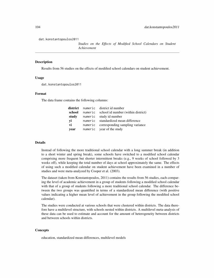
104 dat.konstantopoulos2011

dat.konstantopoulos2011

Studies on the Effects of Modified School Calendars on StudentAchievement

Description

Results from 56 studies on the effects of modified school calendars on student achievement.

Usage

dat.konstantopoulos2011

Format


district numeric district id numberschool numeric school id number (within district)study numeric study id numberyi numeric standardized mean differencevi numeric corresponding sampling varianceyear numeric year of the study

Details

Instead of following the more traditional school calendar with a long summer break (in additionto a short winter and spring break), some schools have switched to a modified school calendarcomprising more frequent but shorter intermittent breaks (e.g., 9 weeks of school followed by 3weeks off), while keeping the total number of days at school approximately the same. The effectsof using such a modified calendar on student achievement have been examined in a number ofstudies and were meta-analyzed by Cooper et al. (2003).

The dataset (taken from Konstantopoulos, 2011) contains the results from 56 studies, each compar-ing the level of academic achievement in a group of students following a modified school calendarwith that of a group of students following a more traditional school calendar. The difference be-tween the two groups was quantified in terms of a standardized mean difference (with positivevalues indicating a higher mean level of achievement in the group following the modified schoolcalendar).

The studies were conducted at various schools that were clustered within districts. The data there-fore have a multilevel structure, with schools nested within districts. A multilevel meta-analysis ofthese data can be used to estimate and account for the amount of heterogeneity between districtsand between schools within districts.

Concepts

education, standardized mean differences, multilevel models

dat.konstantopoulos2011 105

Author(s)


Source

Konstantopoulos, S. (2011). Fixed effects and variance components estimation in three-level meta-analysis. Research Synthesis Methods, 2(1), 61–76. https://doi.org/10.1002/jrsm.35

References

Cooper, H., Valentine, J. C., Charlton, K., & Melson, A. (2003). The effects of modified schoolcalendars on student achievement and on school and community attitudes. Review of EducationalResearch, 73(1), 1–52. https://doi.org/10.3102/00346543073001001

Examples

### copy data into 'dat' and examine datadat <- dat.konstantopoulos2011dat

## Not run:


### regular random-effects modelres <- rma(yi, vi, data=dat)print(res, digits=3)

### regular random-effects model using rma.mv()res <- rma.mv(yi, vi, random = ~ 1 | study, data=dat)print(res, digits=3)

### multilevel random-effects modelres.ml <- rma.mv(yi, vi, random = ~ 1 | district/school, data=dat)print(res.ml, digits=3)

### profile variance componentsprofile(res.ml, progbar=FALSE)

### multivariate parameterization of the modelres.mv <- rma.mv(yi, vi, random = ~ school | district, data=dat)print(res.mv, digits=3)

### tau^2 from multivariate model = sum of the two variance components from the multilevel modelround(sum(res.ml$sigma2), 3)

### rho from multivariate model = intraclass correlation coefficient based on the multilevel modelround(res.ml$sigma2[1] / sum(res.ml$sigma2), 3)

## End(Not run)


106 dat.landenberger2005

dat.landenberger2005 Studies on the Effectiveness of CBT for Reducing Recidivism

Description

Results from 58 studies on the effectiveness of cognitive-behavioral therapy (CBT) for reducingrecidivism in juvenile and adult offenders.

Usage

dat.landenberger2005

Format


study character (first) author and yearpubtype character publication type (book chapter, journal article, report, or thesis)country character country where study was carried out (Canada, New Zealand, UK, or USA)design character study design (matched groups, nonequivalent groups, or randomized trial)program character purpose of setting up the CBT program (for demonstration, practice, or research purposes)setting character treatment setting (community or prison)designprob character indication of study design problems (no, favors the control group, or favors the treatment group)n.ctrl.rec numeric number of recidivists in the control groupn.ctrl.non numeric number of non-recidivists in the control groupn.cbt.rec numeric number of recidivists in the CBT groupn.cbt.non numeric number of non-recidivists in the CBT groupinterval numeric recidivism interval (in months)group numeric study group (adults or juveniles)age numeric mean age of the study groupmale numeric percentage of males in the study groupminority numeric percentage of minorities in the study grouplength numeric treatment length (in weeks)sessions numeric number of CBT sessions per weekhrs_week numeric treatment hours per weekhrs_total numeric total hours of treatmentcbt.cogskills character CBT component: cognitive skills (yes, no)cbt.cogrestruct character CBT component: cognitive restructuring (yes, no)cbt.intpprbsolv character CBT component: interpersonal problem solving (yes, no)cbt.socskills character CBT component: social skills (yes, no)cbt.angerctrl character CBT component: anger control (yes, no)cbt.victimimpact character CBT component: victim impact (yes, no)cbt.subabuse character CBT component: substance abuse (yes, no)cbt.behavmod character CBT component: behavior modification (yes, no)cbt.relapseprev character CBT component: relapse prevention (yes, no)cbt.moralrsng character CBT component: moral reasoning (yes, no)cbt.roletaking character CBT component: role taking (yes, no)cbt.other character CBT component: other (yes, no)

dat.landenberger2005 107

Details

Landenberger and Lipsey (2005) conducted a meta-analysis of 58 experimental and quasi-experimentalstudies of the effects of cognitive-behavioral therapy (CBT) on the recidivism rates of adult and ju-venile offenders (see also Lipsey et al., 2007). The present dataset includes the results of thesestudies and a range of potential moderator variables to identify factors associated with variation intreatment effects.

Concepts

psychology, criminology, odds ratios, meta-regression

Author(s)


Source


References

Landenberger, N. A., & Lipsey, M. W. (2005). The positive effects of cognitive-behavioral pro-grams for offenders: A meta-analysis of factors associated with effective treatment. Journal ofExperimental Criminology, 1, 451–476. https://doi.org/10.1007/s11292-005-3541-7

Lipsey, M. W., Landenberger, N. A., & Wilson, S. J. (2007). Effects of cognitive-behavioral pro-grams for criminal offenders. Campbell Systematic Reviews, 3(1), 1–27. https://doi.org/10.4073/csr.2007.6

Examples

### copy data into 'dat' and examine datadat <- dat.landenberger2005head(dat)

## Not run:


### calculate log odds ratios (for non-recidivism in CBT vs. control groups) and sampling variancesdat <- escalc(measure="OR", ai=n.cbt.non, bi=n.cbt.rec, ci=n.ctrl.non, di=n.ctrl.rec, data=dat)

### fit random-effects modelres <- rma(yi, vi, data=dat)res

### estimated average OR and corresponding 95% CI/PIpredict(res, transf=exp, digits=2)

### examine if number of treatment sessions per week is a potential moderatorres <- rma(yi, vi, mods = ~ sessions, data=dat)


108 dat.laopaiboon2015

res

### predicted ORs for 1, 2, 5, or 10 sessions per weekpredict(res, newmods=c(1,2,5,10), transf=exp, digits=2)

## End(Not run)

dat.laopaiboon2015 Studies on the Effectiveness of Azithromycin for Treating Lower Res-piratory Tract Infections

Description

Results from 15 studies on the effectiveness of azithromycin versus amoxycillin or amoxycillin/clavulanicacid (amoxyclav) in the treatment of acute lower respiratory tract infections.

Usage

dat.laopaiboon2015

Format


author character author(s)year numeric publication yearai numeric number of clinical failures in the group treated with azithromycinn1i numeric number of patients in the group treated with azithromycinci numeric number of clinical failures in the group treated with amoxycillin or amoxyclavn2i numeric number of patients in the group treated with amoxycillin or amoxyclavage character whether the trial included adults or childrendiag.ab numeric trial included patients with a diagnosis of acute bacterial bronchitisdiag.cb numeric trial included patients with a diagnosis of chronic bronchitis with acute exacerbationdiag.pn numeric trial included patients with a diagnosis of pneumoniactrl character antibiotic in control group (amoxycillin or amoxyclav)

Details

Azithromycin is an antibiotic useful for the treatment of a number of bacterial infections. Laopai-boon et al. (2015) conducted a meta-analysis of trials comparing the effectiveness of azithromycinversus amoxycillin or amoxycillin/clavulanic acid (amoxyclav) in the treatment of acute lower res-piratory tract infections, including acute bacterial bronchitis, acute exacerbations of chronic bron-chitis, and pneumonia. The results from 15 trials are included in this dataset.

Concepts

medicine, risk ratios

dat.lau1992 109

Author(s)


Source

Laopaiboon, M., Panpanich, R., & Swa Mya, K. (2015). Azithromycin for acute lower respiratorytract infections. Cochrane Database of Systematic Reviews, 3, CD001954. https://doi.org/10.1002/14651858.CD001954.pub4

Examples

### copy data into 'dat' and examine datadat <- dat.laopaiboon2015dat

## Not run:


### analysis using the Mantel-Haenszel methodrma.mh(measure="RR", ai=ai, n1i=n1i, ci=ci, n2i=n2i, data=dat, digits=3)

### calculate log risk ratios and corresponding sampling variancesdat <- escalc(measure="RR", ai=ai, n1i=n1i, ci=ci, n2i=n2i, data=dat)



## End(Not run)

dat.lau1992 Studies on Intravenous Streptokinase for Acute Myocardial Infarction

Description

Results from 33 trials comparing intravenous streptokinase versus placebo or no therapy in patientswho had been hospitalized for acute myocardial infarction.

Usage

dat.lau1992

Format



110 dat.lau1992

trial character trial nameyear numeric publication yearai numeric number of deaths in the streptokinase groupn1i numeric number of patients in the streptokinase groupci numeric number of deaths in the control groupn2i numeric number of patients in the control group

Details

In the paper by Lau et al. (1992), the data are used to illustrate the idea of a cumulative meta-analysis, where the results are updated as each trial is added to the dataset. See ‘Examples’ for codethat replicates the results and shows corresponding forest plots.

Concepts

medicine, cardiology, odds ratios, cumulative meta-analysis

Author(s)


Source

Lau, J., Antman, E. M., Jimenez-Silva, J., Kupelnick, B., Mosteller, F., & Chalmers, T. C. (1992).Cumulative meta-analysis of therapeutic trials for myocardial infarction. New England Journal ofMedicine, 327(4), 248–254. https://doi.org/10.1056/NEJM199207233270406

Examples

### copy data into 'dat' and examine datadat <- dat.lau1992dat

## Not run:


### meta-analysis of log odds ratios using the MH methodres <- rma.mh(measure="OR", ai=ai, n1i=n1i, ci=ci, n2i=n2i, data=dat, slab=trial)print(res, digits=2)

### forest plotforest(res, xlim=c(-10,9), atransf=exp, at=log(c(.01, 0.1, 1, 10, 100)),

header=TRUE, top=2, ilab=dat$year, ilab.xpos=-6)text(-6, 35, "Year", font=2)

### cumulative meta-analysissav <- cumul(res)

### forest plot of the cumulative results


dat.lee2004 111

forest(sav, xlim=c(-5,4), atransf=exp, at=log(c(0.1, 0.5, 1, 2, 10)),header=TRUE, top=2, ilab=dat$year, ilab.xpos=-3)

text(-3, 35, "Year", font=2)id <- c(4, 8, 15, 33) # rows for which the z/p-values should be shown (as in Lau et al., 1992)text(1.1, (res$k:1)[id], paste0("z = ", formatC(sav$zval[id], format="f", digits=2),

", p = ", formatC(sav$pval[id], format="f", digits=4)))

## End(Not run)

dat.lee2004 Studies on Acupoint P6 Stimulation for Preventing Nausea

Description

Results from studies examining the effectiveness of wrist acupuncture point P6 stimulation forpreventing postoperative nausea.

Usage

dat.lee2004

Format


id numeric trial id numberstudy character first authoryear numeric study yearai numeric number of patients experiencing nausea in the treatment groupn1i numeric total number of patients in treatment groupci numeric number of patients experiencing nausea in the sham groupn2i numeric total number of patients in the sham group

Details

Postoperative nausea and vomiting are common complications following surgery and anaesthesia.As an alternative to drug therapy, acupuncture has been studied as a potential treatment in severaltrials. The dataset contains the results from 16 clinical trials examining the effectiveness of wristacupuncture point P6 stimulation for preventing postoperative nausea.

Concepts

medicine, alternative medicine, risk ratios

Author(s)



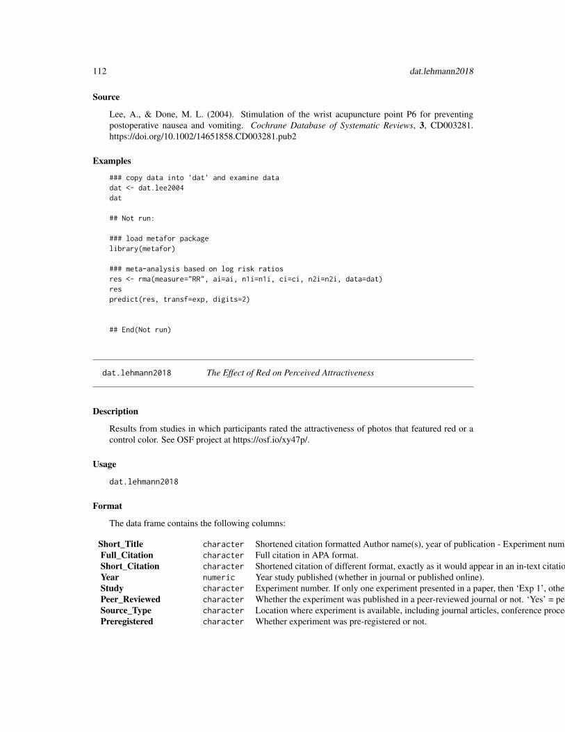
112 dat.lehmann2018

Source

Lee, A., & Done, M. L. (2004). Stimulation of the wrist acupuncture point P6 for preventingpostoperative nausea and vomiting. Cochrane Database of Systematic Reviews, 3, CD003281.https://doi.org/10.1002/14651858.CD003281.pub2

Examples

### copy data into 'dat' and examine datadat <- dat.lee2004dat

## Not run:


### meta-analysis based on log risk ratiosres <- rma(measure="RR", ai=ai, n1i=n1i, ci=ci, n2i=n2i, data=dat)respredict(res, transf=exp, digits=2)

## End(Not run)

dat.lehmann2018 The Effect of Red on Perceived Attractiveness

Description

Results from studies in which participants rated the attractiveness of photos that featured red or acontrol color. See OSF project at https://osf.io/xy47p/.

Usage

dat.lehmann2018

Format


Short_Title character Shortened citation formatted Author name(s), year of publication - Experiment number. All cells in the column are unique for use as labels in the meta-analysis.Full_Citation character Full citation in APA format.Short_Citation character Shortened citation of different format, exactly as it would appear in an in-text citation.Year numeric Year study published (whether in journal or published online).Study character Experiment number. If only one experiment presented in a paper, then ‘Exp 1’, otherwise numbered according to numbering within paper.Peer_Reviewed character Whether the experiment was published in a peer-reviewed journal or not. ‘Yes’ = peer-reviewed journal, ‘No’ can mean in press, online publication, or other. Column for moderator analysis.Source_Type character Location where experiment is available, including journal articles, conference proceedings, online-only, and other options. More specific than whether peer-reviewed or not.Preregistered character Whether experiment was pre-registered or not.

dat.lehmann2018 113

Moderator_Group character In some studies, a moderator was intentionally investigated that was meant to reduce the red-romance effect. Data for studies where the red-romance effect is expected to be moderated are marked ‘Yes’ in this column. All others are blank.Gender character Gender of rater (male or female). In all cases, gender of stimuli will be opposite.Color_Contrast character The color used as the contrast against red. In some cases, not every contrast color was listed. We chose to examine only contrasts that were present in the original studies, when possible. This column contains only the contrasts we examined in this meta-analysis.Color_Form character Location of color in photo. Background = background or border color manipulated; Face = facial redness manipulated; Shirt, Dress, Item = color of specified object manipulated; Dot = a dot of color on shirt manipulated.Photo_Type character Amount of body visible in photo. Head Shot = head only; Bust = head, shoulders, sometimes torso; Full Body = entire body visible.DV_Type character Scale used for DV. ‘Perceived attractiveness’ = the perceived attractiveness scale used in the original studies; alternate scales are differentiated.DV_Items numeric Number of items in DV scale.DV_Scale character Full length of DV scale, if clear.DV_ScaleBottom numeric Lower anchor of DV scale.DV_ScaleTop numeric Upper anchor of DV scale.Location character Country where study took place, if clear. ‘Worldwide’ in some cases of online participation without IP filtering of participants.Continent character Continent where study took place, for the sake of creating larger categories for analysis.Participants character Basic notes about participants. Students = high school, undergraduate, or graduate students; online = participants were gathered online; adult = no other common identifying factor given. Put into fewer categories for ease of analysis.Participant_Notes character A finer grained description of participant characteristics.Design character Whether study was a between- or within-subjects design.Eth_Majority character Basic notes about participant ethnicity for ease of analysis. This represents the ethnic majority within the sample.Eth_Majority_Detail character A finer grained description of participant characteristics, including in some cases participant counts when the ethnic majority was close to another category.Eth_Stim character Ethnicity of the people pictured in the stimulus materials.Eth_Match character Whether the ethnic majority of the participant pool matched the ethnicity of stimulus photos.Red_Age numeric Mean age of participants in red group. If not given for specific group, then mean age overall.Control_Age numeric Mean age of participants in control group. If not given for specific group, then mean age overall.Color_Red character Specific values of red color, if given. ‘No data’ if not given or unclear.Color_Control character Specific values of control color, if given. ‘No data’ if not given or unclear.Red_Original character Whether the red color used in the study is within 5 units of the LCh values for red used in the original study.Color_Match character Whether the control color used in the study is within 5 units of the red color on the L and C parameters. In cases where the control color used was white, it was not possible for the L and C parameters to match.Presentation_Control character Whether the color of the stimulus viewed by each participant was consistent, as in participants viewing everything on paper or the same computer, versus uncontrolled presentation of the stimulus, as in viewing stimulus on different computers.Stimuli_Presentation character Method for presenting stimuli. ‘Paper’ = stimuli printed on paper, shown in-person; ‘Screen’ = stimuli shown on-screen, not carefully controlled; ‘Screen Control’ = stimuli shown on-screen, but screen carefully color-matched.Red_N numeric Number of participants in red group.Red_M numeric Mean rating of DV in red group.Red_SD numeric Standard deviation of DV in red group.Control_N numeric Number of participants in control group.Control_M numeric Mean rating of DV in control group.Control_SD numeric Standard deviation of DV in control group.SD_diff numeric Calculated for within-subjects studies, standard deviation of difference scores.RM_r numeric Calculated for within-subjects studies, correlation between participant ratings of red and control attractiveness.Control_Attractiveness numeric Attractiveness of stimuli in control condition, calculated as (Control_M - DV_ScaleBottom) / DV_ScaleTop, in order to compare attractiveness ratings across different scales.Notes character Any additional notes on the study.Total.SampleSize numeric Total unique participants in the study.pooled numeric Pooled standard deviation for within-subjects studies.yi numeric Standardized mean difference.vi numeric Corresponding sampling variance.

Details

This is data from a meta-analysis of studies that test the red-romance hypothesis, which is that thecolor red enhances heterosexual attraction in romantic contexts. Analyzing male participants only,the meta-analysis should show a small, statistically significant effect (d = 0.26 [0.12, 0.40], p =.0004, N = 2,961). Analyzing female participants only should show a very small effect (d = 0.13

114 dat.li2007

[0.01, 0.25], p = .03, N = 2,739). The analyses in the published meta-analysis found clear evidenceof upward bias in the estimate for female participants and equivocal evidence for male participants.Moderator analyses suggest effect sizes may have declined over time (both genders), may be largestwhen an original shade of red is used (men only), and may be smaller in pre-registered studies(women only).

Concepts

psychology, attraction, standardized mean differences

Author(s)

Robert Calin-Jageman, <[email protected]>, https://calin-jageman.net

Source

Lehmann, G. K., Elliot, A. J., & Calin-Jageman, R. J. (2018). Meta-analysis of the effect of red onperceived attractiveness. Evolutionary Psychology, 16(4). https://doi.org/10.1177/1474704918802412https://osf.io/xy47p/

Examples

### copy data into 'dat' and examine datadat <- dat.lehmann2018head(dat)

## Not run:


### meta-analyses for male and female participantsred_romance_malep <- dat[dat$Gender == "Males", ]red_romance_femalep <- dat[dat$Gender == "Females", ]

res_malep <- rma(yi, vi, data=red_romance_malep, test="knha")res_malepres_femalep <- rma(yi, vi, data=red_romance_femalep, test="knha")res_femalep

## End(Not run)

dat.li2007 Studies on the Effectiveness of Intravenous Magnesium in Acute My-ocardial Infarction

https://calin-jageman.net

dat.li2007 115

Description

Results from 22 trials examining the effectiveness of intravenous magnesium in the prevention ofdeath following acute myocardial infarction.

Usage

dat.li2007

Format


id numeric trial id numberstudy character first author or trial nameyear numeric publication yearai numeric number of deaths in the magnesium groupn1i numeric number of patients in the magnesium groupci numeric number of deaths in the control groupn2i numeric number of patients in the control group

Details

The dataset includes the results from 22 randomized clinical trials that examined the effectivenessof intravenous magnesium in the prevention of death following acute myocardial infarction. It issimilar to the dataset dat.egger2001, with some slight differences in the included trials and dataused.

Concepts

medicine, cardiology, odds ratios, publication bias

Author(s)


Source

Li, J., Zhang, Q., Zhang, M., & Egger, M. (2007). Intravenous magnesium for acute myocardial in-farction. Cochrane Database of Systematic Reviews, 2, CD002755. https://doi.org/10.1002/14651858.CD002755.pub2

See Also

dat.egger2001

Examples

### copy data into 'dat' and examine datadat <- dat.li2007dat


116 dat.lim2014

## Not run:


### meta-analysis of all trials except ISIS-4res <- rma(measure="OR", ai=ai, n1i=n1i, ci=ci, n2i=n2i, data=dat, method="EE", subset=-14)print(res, digits=2)predict(res, transf=exp, digits=2)

### meta-analysis of all trials including ISIS-4res <- rma(measure="OR", ai=ai, n1i=n1i, ci=ci, n2i=n2i, data=dat, method="EE")print(res, digits=2)predict(res, transf=exp, digits=2)

### contour-enhanced funnel plot centered at 0funnel(res, refline=0, level=c(90, 95, 99), shade=c("white", "gray", "darkgray"))

## End(Not run)

dat.lim2014 Studies on the Association Between Maternal Size, Offspring Size, andNumber of Offsprings

Description

Results from studies examining the association between maternal size, offspring size, and numberof offsprings.

Usage

dat.lim2014

Format

The object is a list containing data frames m_o_size, m_o_fecundity, o_o_unadj, and o_o_adjthat contain the following columns and the corresponding phylogenetic trees called m_o_size_tree,m_o_fecundity_tree, o_o_unadj_tree, and o_o_adj_tree:

article numeric article idauthor character study author(s)year numeric publication yearspecies character speciesamniotes character whether the species was amnioticenvironment character whether the species were wild or captivereprounit character whether the data were based on lifetime reproductive output or a single reproductive event (only in m_o_size and m_o_fecundity)ri numeric correlation coefficientni numeric sample size

dat.lim2014 117

Details

The object dat.lim2014 includes 4 datasets:

m_o_size on the correlation between maternal size and offspring sizem_o_fecundity on the correlation between maternal size and number of offspringso_o_unadj on the correlation between offspring size and number of offspringso_o_adj on the correlation between offspring size and number of offsprings adjusted for maternal size

Objects m_o_size_tree, m_o_fecundity_tree, o_o_unadj_tree, and o_o_adj_tree are the cor-responding phylogenetic trees for the species included in each of these datasets.

Concepts

ecology, evolution, correlation coefficients, multilevel models, phylogeny

Author(s)


Source

Lim, J. N., Senior, A. M., & Nakagawa, S. (2014). Heterogeneity in individual quality and repro-ductive trade-offs within species. Evolution, 68(8), 2306–2318. https://doi.org/10.1111/evo.12446

References

Cinar, O., Nakagawa, S., & Viechtbauer, W. (in press). Phylogenetic multilevel meta-analysis: Asimulation study on the importance of modelling the phylogeny. Methods in Ecology and Evolution.https://doi.org/10.1111/2041-210X.13760

Hadfield, J. D., & Nakagawa, S. (2010). General quantitative genetic methods for comparative bi-ology: Phylogenies, taxonomies and multi-trait models for continuous and categorical characters.Journal of Evolutionary Biology, 23(3), 494–508. https://doi.org/10.1111/j.1420-9101.2009.01915.x

Nakagawa, S., & Santos, E. S. A. (2012). Methodological issues and advances in biological meta-analysis. Evolutionary Ecology, 26(5), 1253–1274. https://doi.org/10.1007/s10682-012-9555-5

Examples

### copy data into 'dat' and examine datadat <- dat.lim2014$o_o_unadjdat[1:14, -c(2:3)]

## Not run:


### load ape packagelibrary(ape, warn.conflicts=FALSE)


118 dat.linde2005


### copy tree to 'tree'tree <- dat.lim2014$o_o_unadj_tree

### compute branch lengthstree <- compute.brlen(tree)

### compute phylogenetic correlation matrixA <- vcv(tree, corr=TRUE)

### make copy of the species variabledat$species.phy <- dat$species

### create effect size id variabledat$esid <- 1:nrow(dat)

### fit multilevel phylogenetic meta-analytic modelres <- rma.mv(yi, vi,

random = list(~ 1 | article, ~ 1 | esid, ~ 1 | species, ~ 1 | species.phy),R=list(species.phy=A), data=dat)

res

## End(Not run)

dat.linde2005 Studies on the Effectiveness of St. John’s Wort for Treating Depression

Description

Results from 26 studies on the effectiveness of Hypericum perforatum extracts (St. John’s wort) fortreating depression.

Usage

dat.linde2005

Format


id numeric study numberstudy character study author(s)year numeric publication yearcountry character study locationni numeric total sample sizemajor numeric sample restricted to patients who met criteria for major depression

dat.linde2005 119

baseline numeric HRSD baseline scoreversion numeric HRSD version (17 or 21 items)duration numeric study duration (in weeks)prep character Hypericum extract preparationdosage numeric dosage (in mg)response numeric definition of response (see ‘Details’)ai numeric number of responses in treatment groupn1i numeric number of patients in treatment groupci numeric number of responses in placebo groupn2i numeric number of patients in placebo groupgroup numeric stratification variable used by the authors (see ‘Details’)

Details

The dataset includes the results from 26 double-blind placebo-controlled trials on the effectivenessof Hypericum perforatum extracts (St. John’s wort) for treating depression (note that 2 studies didnot provide sufficient response information).

Data were extracted from Table 1 and Figure 3 from Linde et al. (2005). For study duration,the assessment week (instead of the total study duration) was coded for Philipp et al. (1999) andMontgomery et al. (2000). For dosage, the midpoint was coded when a range of values was given.

The definition of what constitutes a response differed across studies and is coded as follows:

1. HRSD score reduction of at least 50% or HRSD score after therapy <10,

2. HRSD reduction of at least 50%,

3. based on HRSD scale but exact definition not reported,

4. global patient assessment of efficacy,

5. at least ‘much improved’ on the Clinical Global Impression sub-scale for global improvement.

The group variable corresponds to the variable used by Linde et al. (2005) to stratify their analysesand is coded as follows:

1. smaller trials restricted to major depression,

2. larger trials restricted to major depression,

3. smaller trials not restricted to major depression,

4. larger trials not restricted to major depression.

Concepts

medicine, psychiatry, risk ratios

Author(s)


Source

Linde, K., Berner, M., Egger, M., & Mulrow, C. (2005). St John’s wort for depression: Meta-analysis of randomised controlled trials. British Journal of Psychiatry, 186(2), 99–107. https://doi.org/10.1192/bjp.186.2.99


120 dat.linde2015

References

Viechtbauer, W. (2007). Accounting for heterogeneity via random-effects models and moderatoranalyses in meta-analysis. Zeitschrift für Psychologie / Journal of Psychology, 215(2), 104–121.https://doi.org/10.1027/0044-3409.215.2.104

Examples

### copy data into 'dat' and examine datadat <- dat.linde2005head(dat)

## Not run:


### remove studies with no response information and study with no responses in either groupdat <- dat[-c(5,6,26),]

### calculate log risk ratios and corresponding sampling variancesdat <- escalc(measure="RR", ai=ai, ci=ci, n1i=n1i, n2i=n2i, data=dat)head(dat)

### meta-analysis of the log risk ratios using a random-effects modelres <- rma(yi, vi, data=dat, method="DL")res

### mixed-effects meta-regression model with stratification variableres <- rma(yi, vi, mods = ~ factor(group) - 1, data=dat, method="DL")res

### predicted average risk ratio for each level of the stratification variablepredict(res, newmods=diag(4), transf=exp, digits=2)

## End(Not run)

dat.linde2015 Studies on Classes of Antidepressants for the Primary Care Setting

Description

Results from 66 trials examining eight classes of antidepressants and placebo for the primary caresetting.

Usage

dat.linde2015

dat.linde2015 121

Format


id integer study IDauthor character first authoryear integer year of publicationtreatment1 character treatment 1treatment2 character treatment 2treatment3 character treatment 3n1 integer number of patients (arm 1)resp1 integer number of early responder (arm 1)remi1 integer number of early remissions (arm 1)loss1 integer number of patients loss to follow-up (arm 1)loss.ae1 integer number of patients loss to follow-up due to adverse events (arm 1)ae1 integer number of patients with adverse events (arm 1)n2 integer number of patients (arm 2)resp2 integer number of early responder (arm 2)remi2 integer number of early remissions (arm 2)loss2 integer number of patients loss to follow-up (arm 2)loss.ae2 integer number of patients loss to follow-up due to adverse events (arm 2)ae2 integer number of patients with adverse events (arm 2)n3 integer number of patients (arm 3)resp3 integer number of early responder (arm 3)remi3 integer number of early remissions (arm 3)loss3 integer number of patients loss to follow-up (arm 3)loss.ae3 integer number of patients loss to follow-up due to adverse events (arm 3)ae3 integer number of patients with adverse events (arm 3)

Details

This data set comes from a systematic review of 8 pharmacological treatments of depression andplacebo in primary care with 66 studies (8 of which were 3-arm studies) including 14,785 patients.

The primary outcome is early response, defined as at least a 50% score reduction on a depressionscale after completion of treatment. Secondary outcomes (also measured as dichotomous) wereearly remission (defined as having a symptom score below a fixed threshold after completion oftreatment), lost to follow-up, lost to follow-up due to adverse events, and any adverse event. Theodds ratio was used as effect measure.

This data set was used as an example in Rücker and Schwarzer (2017) who introduced methods toresolve conflicting rankings of outcomes in network meta-analysis.

Concepts

medicine, psychiatry, odds ratios, network meta-analysis

Author(s)



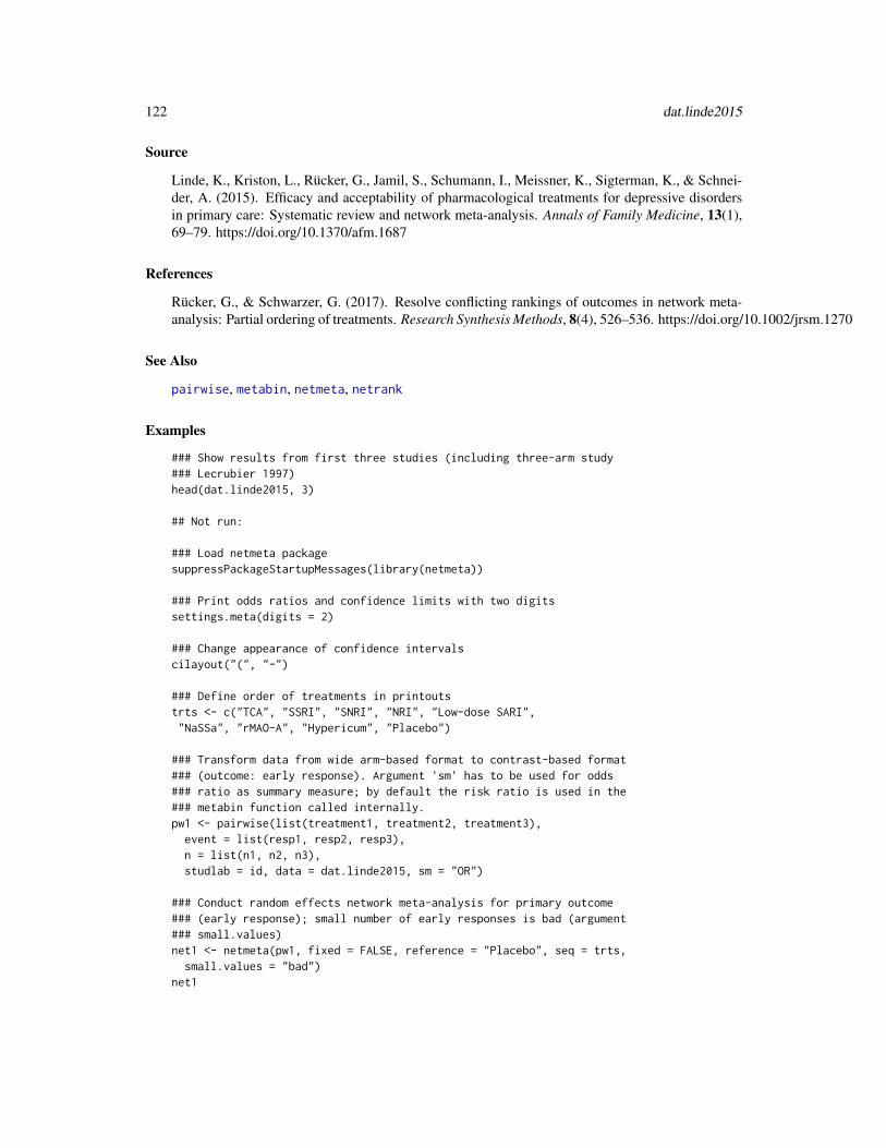
122 dat.linde2015

Source

Linde, K., Kriston, L., Rücker, G., Jamil, S., Schumann, I., Meissner, K., Sigterman, K., & Schnei-der, A. (2015). Efficacy and acceptability of pharmacological treatments for depressive disordersin primary care: Systematic review and network meta-analysis. Annals of Family Medicine, 13(1),69–79. https://doi.org/10.1370/afm.1687

References

Rücker, G., & Schwarzer, G. (2017). Resolve conflicting rankings of outcomes in network meta-analysis: Partial ordering of treatments. Research Synthesis Methods, 8(4), 526–536. https://doi.org/10.1002/jrsm.1270

See Also

pairwise, metabin, netmeta, netrank

Examples

### Show results from first three studies (including three-arm study### Lecrubier 1997)head(dat.linde2015, 3)

## Not run:




### Define order of treatments in printoutstrts <- c("TCA", "SSRI", "SNRI", "NRI", "Low-dose SARI","NaSSa", "rMAO-A", "Hypericum", "Placebo")

### Transform data from wide arm-based format to contrast-based format### (outcome: early response). Argument 'sm' has to be used for odds### ratio as summary measure; by default the risk ratio is used in the### metabin function called internally.pw1 <- pairwise(list(treatment1, treatment2, treatment3),

event = list(resp1, resp2, resp3),n = list(n1, n2, n3),studlab = id, data = dat.linde2015, sm = "OR")

### Conduct random effects network meta-analysis for primary outcome### (early response); small number of early responses is bad (argument### small.values)net1 <- netmeta(pw1, fixed = FALSE, reference = "Placebo", seq = trts,

small.values = "bad")net1

dat.linde2016 123

### Random effects NMA for early remissionpw2 <- pairwise(treat = list(treatment1, treatment2, treatment3),

event = list(remi1, remi2, remi3),n = list(n1, n2, n3),studlab = id, data = dat.linde2015, sm = "OR")

net2 <- netmeta(pw2, fixed = FALSE,seq = trts, ref = "Placebo", small.values = "bad")

net2

### Ranking of treatmentsnr1 <- netrank(net1)nr2 <- netrank(net2)nr1nr2

### Partial order of treatment rankings (two outcomes)outcomes <- c("Early response", "Early remission")po12 <- netposet(nr1, nr2, outcomes = outcomes)plot(po12)

## End(Not run)

dat.linde2016 Studies on Antidepressants for the Primary Care Setting

Description

Results from 93 trials examining 22 interventions (including placebo and usual care) for the primarycare of depression.

Usage

dat.linde2016

Format


id integer study IDlnOR numeric response after treatment (log odds ratio)selnOR numeric standard error of log odds ratiotreat1 character first treatmenttreat2 character second treatment

124 dat.linde2016

Details

This data set comes from a network meta-analysis of 22 treatments of depression in primary care(Linde et al., 2016), based on 93 trials (79 two-arm trials, 13 three-arm trials, and one four-armtrial). The primary outcome was response after treatment (yes/no), defined as a reduction frombaseline by at least 50% on a depression scale. The data set contains log odds ratios with standarderrors for all pairwise comparisons.

The interventions comprised both medical and psychological treatments, also in combination, in-cluding placebo and usual care (UC) (Linde et al., 2016). Pharmacological interventions were tri-cyclic antidepressants (TCA), selective serotonin reuptake inhibitors (SSRI), serotonin-noradrenalinereuptake inhibitors (SNRI), noradrenaline reuptake inhibitors (NRI), low- dose serotonin (5-HT2)antagonists and reuptake inhibitors (low-dose SARI), noradrenergic and specific serotonergic agents(NaSSa), reversible inhibitors of monoaminoxidase A (rMAO-A), hypericum extracts, and an indi-vidualized drug. Psychological interventions were cognitive behavioral therapy (CBT; four forms:face-to-face CBT, remote therapist-led CBT, guided self-help CBT, and no or minimal contactCBT), face-to-face problem-solving therapy (PST), face-to-face interpersonal psychotherapy, face-to-face psychodynamic therapy, and “other face-to-face therapy”. Combination therapies were face-to-face CBT + SSRI, face-to-face PST + SSRI, and face-to-face interpersonal psychotherapy +SSRI.

The data set was used as an example in Rücker et al. (2020) to illustrate component network meta-analysis using frequentist methods.

Concepts

medicine, psychiatry, odds ratios, network meta-analysis, component network meta-analysis

Author(s)


Source

Linde, K., Rücker, G., Schneider, A., & Kriston, L. (2016). Questionable assumptions hamperedinterpretation of a network meta-analysis of primary care depression treatments. Journal of ClinicalEpidemiology, 71, 86–96. https://doi.org/10.1016/j.jclinepi.2015.10.010

References

Rücker, G., Petropoulou, M., & Schwarzer, G. (2020). Network meta-analysis of multicomponentinterventions. Biometrical Journal, 62(3), 808–821. https://doi.org/10.1002/bimj.201800167

See Also

netmeta

Examples

### Show results of first three studies (first study has three treatment### arms)head(dat.linde2016, 5)


dat.lopez2019 125

## Not run:



### Define order of treatments in printouts and forest plotstrts <- c("SSRI",

"Face-to-face CBT", "Face-to-face interpsy", "Face-to-face PST","Face-to-face CBT + SSRI", "Face-to-face interpsy + SSRI","Face-to-face PST + SSRI","Face-to-face psychodyn", "Other face-to-face","TCA", "SNRI", "NRI", "Low-dose SARI", "NaSSa", "rMAO-A", "Ind drug","Hypericum","Remote CBT", "Self-help CBT", "No contact CBT","UC", "Placebo")

### Conduct random effects network meta-analysisnet <- netmeta(lnOR, selnOR, treat1, treat2, id,

data = dat.linde2016, reference.group = "placebo",seq = trts, sm = "OR", fixed = FALSE)

### Network graphnetgraph(net, seq = "o", number = TRUE)

### Show resultsnetforest(net, xlim = c(0.2, 50))

### Additive component network meta-analysis with placebo as inactive### treatmentnc <- netcomb(net, inactive = "placebo")ncforest(nc, xlim = c(0.2, 50))

## End(Not run)

dat.lopez2019 Studies on the Effectiveness of CBT for Depression

Description

Results from 76 studies examining the effectiveness of cognitive behavioral therapy (CBT) fordepression in adults.

126 dat.lopez2019

Usage

dat.lopez2019

Format


study character (first) author and year of studytreatment character treatment provided (see ‘Details’)scale character scale used to measure depression symptomsn numeric group sizediff numeric standardized mean changese numeric corresponding standard errorgroup numeric type of therapy (0 = individual, 1 = group therapy)tailored numeric whether the intervention was tailored to each patient (0 = no, 1 = yes)sessions numeric number of sessionslength numeric average session length (in minutes)intensity numeric product of sessions and lengthmulti numeric intervention included multimedia elements (0 = no, 1 = yes)cog numeric intervention included cognitive techniques (0 = no, 1 = yes)ba numeric intervention included behavioral activation (0 = no, 1 = yes)psed numeric intervention included psychoeducation (0 = no, 1 = yes)home numeric intervention included homework (0 = no, 1 = yes)prob numeric intervention included problem solving (0 = no, 1 = yes)soc numeric intervention included social skills training (0 = no, 1 = yes)relax numeric intervention included relaxation (0 = no, 1 = yes)goal numeric intervention included goal setting (0 = no, 1 = yes)final numeric intervention included a final session (0 = no, 1 = yes)mind numeric intervention included mindfulness (0 = no, 1 = yes)act numeric intervention included acceptance and commitment therapy (0 = no, 1 = yes)

Details

The dataset includes the results from 76 studies examining the effectiveness of cognitive behavioraltherapy (CBT) for treating depression in adults. Studies included two or more of the followingtreatments/conditions:

1. treatment as usual (TAU),

2. no treatment,

3. wait list,

4. psychological or attention placebo,

5. face-to-face CBT,

6. multimedia CBT,

7. hybrid CBT (i.e., multimedia CBT with one or more face-to-face sessions).

Multimedia CBT was defined as CBT delivered via self-help books, audio/video recordings, tele-phone, computer programs, apps, e-mail, or text messages.

dat.lopez2019 127

Variable diff is the standardized mean change within each group, with negative values indicatinga decrease in depression symptoms.

Concepts

psychiatry, standardized mean changes, network meta-analysis

Author(s)


Source


References

López-López, J. A., Davies, S. R., Caldwell, D. M., Churchill, R., Peters, T. J., Tallon, D., Dawson,S., Wu, Q., Li, J., Taylor, A., Lewis, G., Kessler, D. S., Wiles, N., & Welton, N. J. (2019). The pro-cess and delivery of CBT for depression in adults: A systematic review and network meta-analysis.Psychological Medicine, 49(12), 1937–1947. https://doi.org/10.1017/S003329171900120X

Examples

### copy data into 'dat' and examine datadat <- dat.lopez2019dat[1:10,1:6]

## Not run:


### create network graph ('igraph' package must be installed)library(igraph, warn.conflicts=FALSE)pairs <- data.frame(do.call(rbind,sapply(split(dat$treatment, dat$study), function(x) t(combn(x,2)))), stringsAsFactors=FALSE)

pairs$X1 <- factor(pairs$X1, levels=sort(unique(dat$treatment)))pairs$X2 <- factor(pairs$X2, levels=sort(unique(dat$treatment)))tab <- table(pairs[,1], pairs[,2])tab # adjacency matrixg <- graph_from_adjacency_matrix(tab, mode = "plus", weighted=TRUE, diag=FALSE)plot(g, edge.curved=FALSE, edge.width=E(g)$weight/2,

layout=layout_in_circle(g, order=c("Wait list", "No treatment", "TAU", "Multimedia CBT","Hybrid CBT", "F2F CBT", "Placebo")),


### restructure data into wide formatdat <- to.wide(dat, study="study", grp="treatment", ref="TAU",

grpvars=c("diff","se","n"), postfix=c("1","2"))

### compute contrasts between treatment pairs and corresponding sampling variances


128 dat.maire2019

dat$yi <- with(dat, diff1 - diff2)dat$vi <- with(dat, se1^2 + se2^2)

### calculate the variance-covariance matrix for multitreatment studiescalc.v <- function(x) {

v <- matrix(x$se2[1]^2, nrow=nrow(x), ncol=nrow(x))diag(v) <- x$viv


### add contrast matrix to the datasetdat <- contrmat(dat, grp1="treatment1", grp2="treatment2")

### network meta-analysis using a contrast-based random-effects model### by setting rho=1/2, tau^2 reflects the amount of heterogeneity for all treatment comparisons### the treatment left out (TAU) becomes the reference level for the treatment comparisonsres <- rma.mv(yi, V, data=dat,

mods = ~ No.treatment + Wait.list + Placebo + F2F.CBT + Hybrid.CBT + Multimedia.CBT - 1,random = ~ comp | study, rho=1/2)

res

### forest plot of the contrast estimates (treatments versus TAU)forest(coef(res), diag(vcov(res)), slab=sub(".", " ", names(coef(res)), fixed=TRUE),

xlim=c(-5,5), alim=c(-3,3), psize=1, header="Treatment",xlab="Difference in Standardized Mean Change (compared to TAU)")

### fit random inconsistency effects modelres <- rma.mv(yi, V, data=dat,

mods = ~ No.treatment + Wait.list + Placebo + F2F.CBT + Hybrid.CBT + Multimedia.CBT - 1,random = list(~ comp | study, ~ comp | design), rho=1/2, phi=1/2)

res

## End(Not run)

dat.maire2019 Studies on Temporal Trends in Fish Community Structures in FrenchRivers

Description

Results from studies examining changes in the abundance of fish species in French rivers.

Usage

dat.maire2019

dat.maire2019 129

Format

The object is a list containing a data frame called dat that contains the following columns anddistance matrix called dmat:

site character study sitestation character sampling station at sitesite_station character site and station combineds1 numeric Mann-Kendal trend statistic for relative abundance of non-local speciesvars1 numeric corresponding sampling variance (corrected for temporal autocorrelation)s2 numeric Mann-Kendal trend statistic for relative abundance of northern speciesvars2 numeric corresponding sampling variance (corrected for temporal autocorrelation)s3 numeric Mann-Kendal trend statistic for relative abundance of non-native speciesvars3 numeric corresponding sampling variance (corrected for temporal autocorrelation)const numeric constant value of 1

Details

The dataset includes the results from 35 sampling stations (at 11 sites along various French rivers)examining the abundance of various fish species over time (i.e., over 19-37 years, all until 2015).The temporal trend in these abundance data was quantified in terms of Mann-Kendal trend statis-tics, with positive values indicating monotonically increasing trends. The corresponding samplingvariances were corrected for the temporal autocorrelation in the data (Hamed & Rao, 1998).

The distance matrix dmat indicates the distance of the sampling stations (1-423 river-km). Forstations not connected through the river network, a high distance value of 10,000 river-km was set(effectively forcing the spatial correlation to be 0 for such stations).

The dataset can be used to illustrate a meta-analysis allowing for spatial correlation in the outcomes.

Concepts

ecology, climate change, spatial correlation

Author(s)


Source

Maire, A., Thierry, E., Viechtbauer, W., & Daufresne, M. (2019). Poleward shift in large-river fishcommunities detected with a novel meta-analysis framework. Freshwater Biology, 64(6), 1143–1156. https://doi.org/10.1111/fwb.13291

References

Hamed, K. H., & Rao, A. R. (1998). A modified Mann-Kendall trend test for autocorrelated data.Journal of Hydrology, 204(1-4), 182–196. https://doi.org/10.1016/S0022-1694(97)00125-X


130 dat.mccurdy2020

Examples

### copy data into 'dat' and examine datadat <- dat.maire2019$datdat[-10]

### copy distance matrix into 'dmat' and examine first 5 rows/columnsdmat <- dat.maire2019$dmatdmat[1:5,1:5]

## Not run:


### fit a standard random-effects model ignoring spatial correlationres1 <- rma.mv(s1, vars1, random = ~ 1 | site_station, data=dat)res1

### fit model allowing for spatial correlationres2 <- rma.mv(s1, vars1, random = ~ site_station | const, struct="SPGAU",

data=dat, dist=list(dmat), control=list(rho.init=10))res2

### add random effects for sites and stations within sitesres3 <- rma.mv(s1, vars1, random = list(~ 1 | site/station, ~ site_station | const), struct="SPGAU",

data=dat, dist=list(dmat), control=list(rho.init=10))res3

### likelihood ratio tests comparing the modelsanova(res1, res2)anova(res2, res3)

### profile likelihood plots for model res2profile(res2, cline=TRUE)

### effective range (river-km for which the spatial correlation is >= .05)sqrt(3) * res2$rho

### note: it was necessary to adjust the starting value for rho in models### res2 and res3 so that the optimizer does not get stuck in a local maximumprofile(res2, rho=1, xlim=c(0,200), steps=100)

## End(Not run)

dat.mccurdy2020 Studies on the Generation Effect

Description

Results from 126 articles that examined the so-called ‘generation effect’.

dat.mccurdy2020 131

Usage

dat.mccurdy2020

Format


article numeric article identifierexperiment character experiment (within article) identifiersample numeric sample (within experiment) identifierid numeric row identifierpairing numeric identifier to indicate paired conditions within experimentsyi numeric mean recall rate for the conditionvi numeric corresponding sampling varianceni numeric number of participants for the conditionstimuli numeric number of stimuli for the conditioncondition factor condition (‘read’ or ‘generate’)gen_difficulty factor generation difficulty (‘low’ or ‘high’)manip_type factor manipulation type of the generate versus read condition (using a ‘within’ or ‘between’ subjects design)present_style factor presentation style (‘mixed’ or ‘pure’ list presentation)word_status factor word status (‘words’, ‘non-words’, or ‘numbers’)memory_test factor memory test (‘recognition’, ‘cued recall’, or ‘free recall’)memory_type factor memory type (‘item’, ‘source’, ‘font color’, ‘font type’, ‘order’, ‘cue word’, ‘background color’, or ‘location’)gen_constraint factor generation constraint (‘low’, ‘medium’, or ‘high’)learning_type factor learning type (‘incidental’ or ‘intentional’)stimuli_relation factor stimuli relation (‘semantic’, ‘category’, ‘antonym’, ‘synonym’, ‘rhyme’, ‘compound words’, ‘definitions’, or ‘unrelated’)gen_mode factor generation mode (‘verbal/speaking’, ‘covert/thinking’, or ‘writing/typing’)gen_task factor generation task (‘anagram’, ‘letter transposition’, ‘word fragment’, ‘sentence completion’, ‘word stem’, ‘calculation’, or ‘cue only’)attention factor attention (‘divided’ or ‘full’)pacing factor pacing (‘self-paced’ or ‘timed’)filler_task factor filler task (‘yes’ or ‘no’)age_grp factor age group (‘younger’ or ‘older’ adults)retention_delay factor retention delay (‘immediate’, ‘short’, or ‘long’)

Details

The generation effect is the memory benefit for self-generated compared with read or experimenter-provided information (Jacoby, 1978; Slamecka & Graf, 1978). In a typical study, participants arepresented with a list of stimuli (usually words or word pairs). For half of the stimuli, participantsself-generate a target word (e.g., open–cl____), while for the other half, participants simply read anintact target word (e.g., above–below). On a later memory test for the target words, the commonfinding is that self-generated words are better remembered than read words (i.e., the generationeffect).

Although several theories have been proposed to explain the generation effect, there is still some de-bate on the underlying memory mechanism(s) contributing to this phenomenon. The meta-analysisby McCurdy et al. (2020) translated various theories on the generation effect into hypotheses thatcould then be tested in moderator analyses based on a dataset containing 126 articles, 310 experi-

132 dat.mccurdy2020

ments, and 1653 mean recall estimates collected under various conditions.

Detailed explanations of the various variables coded (and how these can be used to test varioushypotheses regarding the generation effect) can be found in the article. The most important variableis condition, which denotes whether a particular row of the dataset corresponds to the results of a‘read’ or a ‘generate’ condition.

The data structure is quite complex. Articles may have reported the findings from multiple ex-periments involving one or multiple samples that were examined under various conditions. Thepairing variable indicates which rows of the dataset represent a pairing of a read condition withone or multiple corresponding generate conditions within an experiment. A pairing may involvethe same sample of subjects (when using a within-subjects design for comparing the conditions) ordifferent samples (when using a between-subjects design).

Concepts

psychology, memory, proportions, raw means, multilevel models, cluster-robust inference

Author(s)


Source

McCurdy, M. P., Viechtbauer, W., Sklenar, A. M., Frankenstein, A. N., & Leshikar, E. D. (2020).Theories of the generation effect and the impact of generation constraint: A meta-analytic review.Psychonomic Bulletin & Review, 27(6), 1139–1165. https://doi.org/10.3758/s13423-020-01762-3

References

Slamecka, N. J., & Graf, P. (1978). The generation effect: Delineation of a phenomenon. Journal ofExperimental Psychology: Human Learning and Memory, 4(6), 592–604. https://doi.org/10.1037/0278-7393.4.6.592

Jacoby, L. L. (1978). On interpreting the effects of repetition: Solving a problem versus remember-ing a solution. Journal of Verbal Learning and Verbal Behavior, 17(6), 649–668. https://doi.org/10.1016/S0022-5371(78)90393-6

Examples

### copy data into 'dat' and examine datadat <- dat.mccurdy2020head(dat)

## Not run:


### fit multilevel mixed-effects meta-regression modelres <- rma.mv(yi, vi, mods = ~ condition,

random = list(~ 1 | article/experiment/sample/id, ~ 1 | pairing),data=dat, sparse=TRUE, digits=3)


dat.mcdaniel1994 133

res

### proportion of total amount of heterogeneity due to each componentdata.frame(source=res$s.names, sigma2=round(res$sigma2, 3),

prop=round(res$sigma2 / sum(res$sigma2), 2))

### apply cluster-robust inferencesav <- robust(res, cluster=article)sav

### estimated average recall rate in read and generate conditionspredict(sav, newmods = c(0,1), digits=3)

### use methods from clubSandwich packagesav <- robust(res, cluster=article, clubSandwich=TRUE)sav

## End(Not run)

dat.mcdaniel1994 Studies on the Validity of Employment Interviews

Description

Results from 160 studies on the correlation between employment interview assessments and jobperformance.

Usage

dat.mcdaniel1994

Format


study numeric study numberni numeric sample size of the studyri numeric observed correlationtype character interview type (j = job-related, s = situational, p = psychological)struct character interview structure (u = unstructured, s = structured)

Details

The 160 studies provide data in terms of the correlation between employment interview perfor-mance and actual job performance. In addition, the interview type and the interview structure areindicated.

McDaniel et al. (1994) describe the interview type and structure variables as follows. "Questionsin situational interviews [...] focus on the individual’s ability to project what his or her behavior

134 dat.mcdaniel1994

would be in a given situation. [...] Job-related interviews are those in which the interviewer is apersonnel officer or hiring authority and the questions attempt to assess past behaviors and job-related information, but most questions are not considered situational. Psychological interviewsare conducted by a psychologist, and the questions are intended to assess personal traits, such asdependability." In structured interviews, "the questions and acceptable responses were specified inadvance and the responses were rated for appropriateness of content. [...] Unstructured interviewsgather applicant information in a less systematic manner than do structured interviews. Althoughthe questions may be specified in advance, they usually are not, and there is seldom a formalizedscoring guide. Also, all persons being interviewed are not typically asked the same questions."

The goal of the meta-analysis was to examine the overall criterion-related validity of employmentinterviews and to examine whether the validity depends on the type and structure of the interview.

The data in this dataset were obtained from Table A.2 in Rothstein, Sutton, and Borenstein (2005,p. 325-329). Note that the type and struct variables contain some NAs.

Concepts

psychology, correlation coefficients, meta-regression

Author(s)


Source

Rothstein, H. R., Sutton, A. J., & Borenstein, M. (Eds.). (2005). Publication bias in meta-analysis:Prevention, assessment, and adjustments. Chichester, England: Wiley.

References

McDaniel, M. A., Whetzel, D. L., Schmidt, F. L., & Maurer, S. D. (1994). The validity of em-ployment interviews: A comprehensive review and meta-analysis. Journal of Applied Psychology,79(4), 599–616. https://doi.org/10.1037/0021-9010.79.4.599

Examples

### copy data into 'dat' and examine datadat <- dat.mcdaniel1994head(dat)

## Not run:


### calculate r-to-z transformed correlations and corresponding sampling variancesdat <- escalc(measure="ZCOR", ri=ri, ni=ni, data=dat)head(dat)

### meta-analysis of the transformed correlations using a random-effects modelres <- rma(yi, vi, data=dat)


dat.michael2013 135

res

### average correlation with 95% CIpredict(res, transf=transf.ztor)

### mixed-effects model with interview type as factor### note: job-related interviews is the reference levelrma(yi, vi, mods = ~ factor(type), data=dat)

### mixed-effects model with interview structure as factor### note: structured interviews is the reference levelrma(yi, vi, mods = ~ factor(struct), data=dat)

### note: the interpretation of the results is difficult since all### situational interviews were structured, almost all psychological### interviews were unstructured, and actually for the majority of### the psychological interviews it was unknown whether the interview### was structured or unstructuredtable(dat$type, dat$struct, useNA="always")

### meta-analysis of raw correlations using a random-effects modelres <- rma(measure="COR", ri=ri, ni=ni, data=dat.mcdaniel1994)res

## End(Not run)

dat.michael2013 The Non-Persuasive Power of a Brain Image

Description

Results from studies exploring how a superfluous fMRI brain image influences the persuasivenessof a scientific claim.

Usage

dat.michael2013

Format


Study character name of the study: Citation - Experiment - SubgroupNo_brain_n numeric sample size for no-brain-image conditionNo_brain_m numeric mean agreement rating for no-brain-image conditionNo_brain_s numeric standard deviation for no-brain-image conditionBrain_n numeric sample size for brain-image conditionBrain_m numeric mean agreement rating for brain-image condition

136 dat.michael2013

Brain_s numeric standard deviation for brain-image conditionIncluded_Critique character ‘Critique’ if article included critical commentary on conclusions, otherwise ‘No_critique’Medium character ‘Paper’ if conducted in person; ‘Online’ if conducted onlineCompensation character notes on compensation provided to participantsParticipant_Pool character notes on where participants were recruitedyi numeric raw mean difference, calculated as Brain_m - No_brain_mvi numeric corresponding sampling variance

Details

The dataset contains the data from the meta-analysis by Michael et al. (2013) of experiments on thepersuasive power of a brain image. The meta-analysis analyzed an original study by McCabe andCastel (2008) as well as 10 replication attempts conducted by the authors of the meta-analysis.

In each study, participants read an article about using brain imaging as a lie detector. The articleeither included a superfluous fMRI image of a brain (brain) or not (no_brain). After reading thearticle, all participants responded to the statement “Do you agree or disagree with the conclusionthat brain imaging can be used as a lie detector?” on a scale from 1 (strongly disagree) to 4 (stronglyagree).

The original study by McCabe and Castel (2008) reported a relatively large increase in agreementdue to the presence of brain images. Meta-analysis of the original study with the 10 replicationssuggests, however, a small, possibly null effect: an estimated average raw mean difference of 0.07points, 95% CI [-0.00, 0.14], under a random-effects model.

In some studies, the article included a passage critiquing the primary claims made in the article;this is coded in the Included_Critique column for analysis as a possible moderator. Note thatExperiment 3 by McCabe and Castel (2008) was a 2x2 between subjects design: brain image pres-ence was manipulated as well as the inclusion of a critique. The two different critique conditionsare recorded as separate rows in this dataset. Analysis of this dataset with metafor yields the sameresults (given rounding) reported in the manuscript.

Concepts

psychology, persuasion, raw mean differences

Author(s)

Robert Calin-Jageman, <[email protected]>, https://calin-jageman.net

Source

Michael, R. B., Newman, E. J., Vuorre, M., Cumming, G., & Garry, M. (2013). On the (non)persuasivepower of a brain image. Psychonomic Bulletin & Review, 20(4), 720—725. https://doi.org/10.3758/s13423-013-0391-6

References

McCabe, D. P., & Castel, A. D. (2008). Seeing is believing: The effect of brain images on judgmentsof scientific reasoning. Cognition, 107(1), 343–352. https://doi.org/10.1016/j.cognition.2007.07.017

https://calin-jageman.net

dat.molloy2014 137

Examples

### copy data into 'dat' and examine datadat <- dat.michael2013dat

## Not run:


### Data prep# yi and vi are already provided, but here's how you would use escalc() to obtain# a raw-mean difference and its variance.# Note the measure parameter is "MD" for 'raw mean difference'dat <- metafor::escalc(

measure = "MD",m1i = Brain_m,m2i = No_brain_m,sd1i = Brain_s,sd2i = No_brain_s,n1i = Brain_n,n2i = No_brain_n,data = dat

)

### meta-analysis using a random-effects model of the raw mean differencesres <- rma(yi, vi, data=dat)print(res, digits=2)

### examine if Included_Critique is a potential moderatorres <- rma(yi, vi, mods = ~ Included_Critique, data=dat)print(res, digits=2)

## End(Not run)

dat.molloy2014 Studies on the Relationship between Conscientiousness and Medica-tion Adherence

Description

Results from 16 studies on the correlation between conscientiousness and medication adherence.

Usage

dat.molloy2014

138 dat.molloy2014

Format


dat.molloy2014 139

authors character study authorsyear numeric publication yearni numeric sample size of the studyri numeric observed correlationcontrols character number of variables controlled fordesign character whether a cross-sectional or prospective design was useda_measure character type of adherence measure (self-report or other)c_measure character type of conscientiousness measure (NEO or other)meanage numeric mean age of the samplequality numeric methodological quality

Details

Conscientiousness, one of the big-5 personality traits, can be defined as “socially prescribed impulsecontrol that facilitates task- and goal-directed behaviour, such as thinking before acting, delayinggratification, following norms and rules and planning, organising and prioritising tasks” (John &Srivastava, 1999). Conscientiousness has been shown to be related to a number of health-relatedbehaviors (e.g., tobacco/alcohol/drug use, diet and activity patterns, risky behaviors). A recentmeta-analysis by Molloy et al. (2014) examined to what extent conscientiousness is related to med-ication adherence, that is, the extent to which (typically chronically ill) patients follow a prescribedmedication regimen (e.g., taking a daily dose of a cholesterol lowering drug in patients with highLDL serum cholesterol levels). The results from the 16 studies included in this meta-analysis areprovided in this dataset.

Variable a_measure indicates whether adherence was measured based on self-reports or a more‘objective’ measure (e.g., electronic monitoring of pill bottle openings, pill counts). Variablec_measure indicates whether conscientiousness was measured with some version of the NEO per-sonality inventory or some other scale. Methodological quality was scored by the authors on a 1to 4 scale with higher scores indicating higher quality (see article for details on how this score wasderived).

Concepts

psychology, medicine, correlation coefficients

Author(s)


Source

Molloy, G. J., O’Carroll, R. E., & Ferguson, E. (2014). Conscientiousness and medication adher-ence: A meta-analysis. Annals of Behavioral Medicine, 47(1), 92–101. https://doi.org/10.1007/s12160-013-9524-4

References

John, O. P., & Srivastava, S. (1999). The Big Five Trait taxonomy: History, measurement, andtheoretical perspectives. In L. A. Pervin & O. P. John (Eds.), Handbook of personality: Theory andresearch (2nd ed., pp. 102-138). New York: Guilford Press.


140 dat.moura2021

Examples

### copy data into 'dat' and examine datadat <- dat.molloy2014dat[-c(5:6)]

## Not run:


### calculate r-to-z transformed correlations and corresponding sampling variancesdat <- escalc(measure="ZCOR", ri=ri, ni=ni, data=dat, slab=paste(authors, year, sep=", "))dat[-c(5:6)]

### meta-analysis of the transformed correlations using a random-effects modelres <- rma(yi, vi, data=dat)res

### average correlation with 95% CIpredict(res, digits=3, transf=transf.ztor)

### forest plotforest(res, addpred=TRUE, xlim=c(-1.6,1.6), atransf=transf.ztor,

at=transf.rtoz(c(-.4,-.2,0,.2,.4,.6)), digits=c(2,1), cex=.8,header="Author(s), Year")

### funnel plotfunnel(res)

## End(Not run)

dat.moura2021 Studies on Assortative Mating

Description

Results from 457 studies on assortative mating in various species.

Usage

dat.moura2021

Format

The object is a list containing a data frame called dat that contains the following columns and aphylogenetic tree called tree:

study.id character study id

dat.moura2021 141

effect.size.id numeric effect size idspecies character speciesspecies.id character species id (as in the Open Tree of Life reference taxonomy)subphylum character the subphyla of the speciesphylum character the phyla of the speciesassortment.trait character the measure of body sizetrait.dimensions character dimensionality of the measurefield.collection character whether data were collected in the fieldpublication.year numeric publication year of the studypooled.data character whether data were pooled either spatially and/or temporallyspatially.pooled character whether data were pooled spatiallytemporally.pooled character whether data were pooled temporallyri numeric correlation coefficientni numeric sample size

Details

The 457 studies included in this dataset provide 1828 correlation coefficients describing the simi-larity in some measure of body size in mating couples in 341 different species.

Concepts

ecology, evolution, correlation coefficients, multivariate models, phylogeny, meta-regression

Author(s)


Source

Rios Moura, R., Oliveira Gonzaga, M., Silva Pinto, N., Vasconcellos-Neto, J., & Requena, G. S.(2021). Assortative mating in space and time: Patterns and biases. Ecology Letters, 24(5), 1089–1102. https://doi.org/10.1111/ele.13690

References

Cinar, O., Nakagawa, S., & Viechtbauer, W. (in press). Phylogenetic multilevel meta-analysis: Asimulation study on the importance of modelling the phylogeny. Methods in Ecology and Evolution.https://doi.org/10.1111/2041-210X.13760

Hadfield, J. D., & Nakagawa, S. (2010). General quantitative genetic methods for comparative bi-ology: Phylogenies, taxonomies and multi-trait models for continuous and categorical characters.Journal of Evolutionary Biology, 23(3), 494–508. https://doi.org/10.1111/j.1420-9101.2009.01915.x

Nakagawa, S., & Santos, E. S. A. (2012). Methodological issues and advances in biological meta-analysis. Evolutionary Ecology, 26(5), 1253–1274. https://doi.org/10.1007/s10682-012-9555-5

Examples

### copy data into 'dat' and examine datadat <- dat.moura2021$dat


142 dat.nakagawa2007

head(dat)

## Not run:


### load ape packagelibrary(ape, warn.conflicts=FALSE)


### copy tree to 'tree'tree <- dat.moura2021$tree

### turn tree into an ultrametric onetree <- compute.brlen(tree)

### compute phylogenetic correlation matrixA <- vcv(tree, corr=TRUE)

### make copy of the species.id variabledat$species.id.phy <- dat$species.id

### fit multilevel phylogenetic meta-analytic modelres <- rma.mv(yi, vi,random = list(~ 1 | study.id, ~ 1 | effect.size.id, ~ 1 | species.id, ~ 1 | species.id.phy),R=list(species.id.phy=A), data=dat)

res

### examine if spatial and/or temporal pooling of data tends to yield larger correlationsres <- rma.mv(yi, vi,

mods = ~ spatially.pooled * temporally.pooled,random = list(~ 1 | study.id, ~ 1 | effect.size.id, ~ 1 | species.id, ~ 1 | species.id.phy),R=list(species.id.phy=A), data=dat)

res

### estimated average correlation without pooling, when pooling spatially,### when pooling temporally, and when pooling spatially and temporallypredict(res, newmods = rbind(c(0,0,0),c(1,0,0),c(0,1,0),c(1,1,1)), transf=transf.ztor, digits=2)

## End(Not run)

dat.nakagawa2007 Assessing the Function of House Sparrows’ Bib Size Using a FlexibleMeta-Analysis Method

dat.nakagawa2007 143

Description

A meta-analysis on the association between the size of a male’s bib and their social status in housesparrows (Passer domesticus).

Usage

dat.nakagawa2007

Format


StudyID character identity of primary studyPlace character location of study populationCorrelation numeric correlation coefficientSampleSize integer sample size of population

Details

Each study measures the association between a sparrows bib size and its social status. Effects arequantified as correlation coefficients.

Concepts

ecology, correlation coefficients

Author(s)

Daniel Noble, <[email protected]>

Source

Nakagawa, S., Ockendon, N., Gillespie, D. O. S, Hatchwell, B. J., & Burke, T. (2007). Assessingthe function of house sparrows’ bib size using a flexible meta-analysis method. Behavioral Ecology,18(5), 831–840. https://doi.org/10.1093/beheco/arm050

Examples

### copy data into 'dat' and examine datadat <- dat.nakagawa2007dat

## Not run:


### calculate Zrdat <- escalc(measure="ZCOR", ri=Correlation, ni=SampleSize, data=dat)

144 dat.nielweise2007

### fit meta-analytic modelres <- rma.mv(yi, vi, random = list(~ 1 | StudyID), data=dat)res

## End(Not run)

dat.nielweise2007 Studies on Anti-Infective-Treated Central Venous Catheters for Pre-vention of Catheter-Related Bloodstream Infections

Description

Results from 18 studies comparing the risk of catheter-related bloodstream infection when usinganti-infective-treated versus standard catheters in the acute care setting.

Usage

dat.nielweise2007

Format


study numeric study numberauthor character (first) authoryear numeric publication yearai numeric number of CRBSIs in patients receiving an anti-infective cathetern1i numeric number of patients receiving an anti-infective catheterci numeric number of CRBSIs in patients receiving a standard cathetern2i numeric number of patients receiving a standard catheter

Details

The use of a central venous catheter may lead to a catheter-related bloodstream infection (CRBSI),which in turn increases the risk of morbidity and mortality. Anti-infective-treated catheters havebeen developed that are meant to reduce the risk of CRBSIs. Niel-Weise et al. (2007) conducted ameta-analysis of studies comparing infection risk when using anti-infective-treated versus standardcatheters in the acute care setting. The results from 18 such studies are included in this dataset.

The dataset was used in the article by Stijnen et al. (2010) to illustrate various generalized linearmixed-effects models for the meta-analysis of proportions and odds ratios (see ‘References’).

Concepts

medicine, odds ratios, generalized linear models

dat.nielweise2008 145

Author(s)


Source

Niel-Weise, B. S., Stijnen, T., & van den Broek, P. J. (2007). Anti-infective-treated central venouscatheters: A systematic review of randomized controlled trials. Intensive Care Medicine, 33(12),2058–2068. https://doi.org/10.1007/s00134-007-0897-3

References

Stijnen, T., Hamza, T. H., & Ozdemir, P. (2010). Random effects meta-analysis of event outcomein the framework of the generalized linear mixed model with applications in sparse data. Statisticsin Medicine, 29(29), 3046–3067. https://doi.org/10.1002/sim.4040

Examples

### copy data into 'dat' and examine datadat <- dat.nielweise2007dat

## Not run:


### standard (inverse-variance) random-effects modelres <- rma(measure="OR", ai=ai, n1i=n1i, ci=ci, n2i=n2i, data=dat, drop00=TRUE)print(res, digits=3)predict(res, transf=exp, digits=2)

### random-effects conditional logistic modelres <- rma.glmm(measure="OR", ai=ai, n1i=n1i, ci=ci, n2i=n2i, data=dat, model="CM.EL")print(res, digits=3)predict(res, transf=exp, digits=2)

## End(Not run)

dat.nielweise2008 Studies on Anti-Infective-Treated Central Venous Catheters for Pre-vention of Catheter-Related Bloodstream Infections

Description

Results from 18 studies comparing the risk of catheter-related bloodstream infection when usinganti-infective-treated versus standard catheters for total parenteral nutrition or chemotherapy.


146 dat.nielweise2008

Usage

dat.nielweise2008

Format


study numeric study numberauthors character study authorsyear numeric publication yearx1i numeric number of CRBSIs in patients receiving an anti-infective cathetert1i numeric total number of catheter days for patients receiving an anti-infective catheterx2i numeric number of CRBSIs in patients receiving a standard cathetert2i numeric total number of catheter days for patients receiving a standard catheter

Details

The use of a central venous catheter may lead to a catheter-related bloodstream infection (CRBSI),which in turn increases the risk of morbidity and mortality. Anti-infective-treated catheters havebeen developed that are meant to reduce the risk of CRBSIs. Niel-Weise et al. (2008) conducted ameta-analysis of studies comparing infection risk when using anti-infective-treated versus standardcatheters for total parenteral nutrition or chemotherapy. The results from 9 such studies are includedin this dataset.

The dataset was used in the article by Stijnen et al. (2010) to illustrate various generalized linearmixed-effects models for the meta-analysis of incidence rates and incidence rate ratios (see ‘Refer-ences’).

Concepts

medicine, incidence rates, generalized linear models

Author(s)


Source

Niel-Weise, B. S., Stijnen, T., & van den Broek, P. J. (2008). Anti-infective-treated central venouscatheters for total parenteral nutrition or chemotherapy: A systematic review. Journal of HospitalInfection, 69(2), 114–123. https://doi.org/10.1016/j.jhin.2008.02.020

References

Stijnen, T., Hamza, T. H., & Ozdemir, P. (2010). Random effects meta-analysis of event outcomein the framework of the generalized linear mixed model with applications in sparse data. Statisticsin Medicine, 29(29), 3046–3067. https://doi.org/10.1002/sim.4040


dat.normand1999 147

Examples

### copy data into 'dat' and examine datadat <- dat.nielweise2008dat

## Not run:


### standard (inverse-variance) random-effects modelres <- rma(measure="IRR", x1i=x1i, t1i=t1i, x2i=x2i, t2i=t2i, data=dat)print(res, digits=3)predict(res, transf=exp, digits=2)

### random-effects conditional Poisson modelres <- rma.glmm(measure="IRR", x1i=x1i, t1i=t1i, x2i=x2i, t2i=t2i, data=dat, model="CM.EL")print(res, digits=3)predict(res, transf=exp, digits=2)

## End(Not run)

dat.normand1999 Studies on the Length of Hospital Stay of Stroke Patients

Description

Results from 9 studies on the length of the hospital stay of stroke patients under specialized careand under conventional/routine (non-specialist) care.

Usage

dat.normand1999

Format


study numeric study numbersource character source of datan1i numeric number of patients under specialized carem1i numeric mean length of stay (in days) under specialized caresd1i numeric standard deviation of the length of stay under specialized caren2i numeric number of patients under routine carem2i numeric mean length of stay (in days) under routine caresd2i numeric standard deviation of the length of stay under routine care

148 dat.normand1999

Details

The 9 studies provide data in terms of the mean length of the hospital stay (in days) of strokepatients under specialized care and under conventional/routine (non-specialist) care. The goal ofthe meta-analysis was to examine the hypothesis whether specialist stroke unit care will result in ashorter length of hospitalization compared to routine management.

Concepts

medicine, raw mean differences, standardized mean differences

Author(s)


Source

Normand, S. T. (1999). Meta-analysis: Formulating, evaluating, combining, and reporting. Statis-tics in Medicine, 18(3), 321–359. https://doi.org/10.1002/(sici)1097-0258(19990215)18:3<321::aid-sim28>3.0.co;2-p

Examples

### copy data into 'dat' and examine datadat <- dat.normand1999dat

## Not run:


### calculate mean differences and corresponding sampling variancesdat <- escalc(measure="MD", m1i=m1i, sd1i=sd1i, n1i=n1i, m2i=m2i, sd2i=sd2i, n2i=n2i, data=dat)dat

### meta-analysis of mean differences using a random-effects modelres <- rma(yi, vi, data=dat)res

### meta-analysis of standardized mean differences using a random-effects modelres <- rma(measure="SMD", m1i=m1i, sd1i=sd1i, n1i=n1i, m2i=m2i, sd2i=sd2i, n2i=n2i,

data=dat, slab=source)res

### draw forest plotforest(res, xlim=c(-7,5), alim=c(-3,1), header="Study/Source")

### calculate (log transformed) ratios of means and corresponding sampling variancesdat <- escalc(measure="ROM", m1i=m1i, sd1i=sd1i, n1i=n1i, m2i=m2i, sd2i=sd2i, n2i=n2i, data=dat)dat


dat.obrien2003 149

### meta-analysis of the (log transformed) ratios of means using a random-effects modelres <- rma(yi, vi, data=dat)respredict(res, transf=exp, digits=2)

## End(Not run)

dat.obrien2003 Studies on the Relationship Between BMI and Risk of Preeclampsia

Description

Results from 13 studies on the relationship between maternal body mass index (BMI) and the riskof preeclampsia.

Usage

dat.obrien2003

Format


study numeric study idauthor character (first) author of the studyyear numeric publication yearref numeric reference numberch character exclusion due to chronic hypertension (yes/no)dm character exclusion due to diabetes mellitus (yes/no)mg character exclusion due to multiple gestation (yes/no)bmi.lb numeric lower bound of the BMI intervalbmi.ub numeric upper bound of the BMI intervalbmi numeric midpoint of the BMI intervalcases numeric number of preeclampsia cases in the BMI grouptotal numeric number of individuals in the BMI group

Details

The dataset includes the results from 13 studies examining the relationship between maternal bodymass index (BMI) and the risk of preeclampsia. For each study, results are given in terms of thenumber of preeclampsia cases within two or more groups defined by the lower and upper BMIbounds as shown in the dataset (NA means that the interval is either open to the left or right). Thebmi variable is the interval midpoint as defined by O’Brien et al. (2003).

Concepts

medicine, obstetrics, risk ratios, proportions, multilevel models, dose-response models

150 dat.obrien2003

Author(s)


Source

O’Brien, T. E., Ray, J. G., & Chan, W.-S. (2003). Maternal body mass index and the risk ofpreeclampsia: A systematic overview. Epidemiology, 14(3), 368–374. https://doi.org/10.1097/00001648-200305000-00020

Examples

### copy data into 'dat' and examine datadat <- dat.obrien2003dat

## Not run:


### restructure the data into a wide formatdat2 <- to.wide(dat, study="study", grp="grp", ref=1, grpvars=c("bmi","cases","total"),

addid=FALSE, adddesign=FALSE, postfix=c(1,2))dat2[1:10, -c(2:3)]

### calculate log risk ratios and corresponding sampling variancesdat2 <- escalc(measure="RR", ai=cases1, n1i=total1, ci=cases2, n2i=total2, data=dat2)dat2[1:10, -c(2:7)]

### forest plot of the risk ratiosdd <- c(0,diff(dat2$study))dd[dd > 0] <- 1rows <- (1:nrow(dat2)) + cumsum(dd)rows <- 1 + max(rows) - rowsslabs <- mapply(function(x,y,z) as.expression(bquote(.(x)^.(y)~.(z))),

dat2$author, dat2$ref, dat2$year)with(dat2, forest(yi, vi, header=TRUE, slab=slabs, xlim=c(-7,5.5), fonts="mono", cex=0.8,

psize=1, pch=19, efac=0, rows=rows, ylim=c(0,max(rows)+3), yaxs="i",atransf=exp, at=log(c(.05,0.1,0.2,0.5,1,2,5,10,20)), ilab=comp, ilab.xpos=-4, ilab.pos=4))

text(-4.4, max(rows)+2, "Comparison", font=2, cex=0.8, pos=4)

### within-study mean center the BMI variabledat$bmicent <- with(dat, bmi - ave(bmi, study))

### compute the proportion of preeclampsia cases and corresponding sampling variancesdat <- escalc(measure="PR", xi=cases, ni=total, data=dat)

### convert the proportions to percentages (and convert the variances accordingly)dat$yi <- dat$yi*100dat$vi <- dat$vi*100^2dat[1:10, -c(2:3)]


dat.pagliaro1992 151

### fit multilevel meta-regression model to examine the relationship between the### (centered) BMI variable and the risk of preeclampsiares <- rma.mv(yi, vi, mods = ~ bmicent, random = ~ 1 | study/grp, data=dat)res

### draw scatterplot with regression lineres$slab <- dat$refregplot(res, xlab=expression("Within-Study Mean Centered BMI"~(kg/m^2)),

ylab="Preeclampsia Prevalence (%)", las=1, bty="l",at=seq(0,18,by=2), olim=c(0,100), psize=2, bg="gray90",label=TRUE, offset=0, labsize=0.6)

### fit model using a random slope for bmicentres <- rma.mv(yi, vi, mods = ~ bmicent, random = ~ bmicent | study, struct="GEN", data=dat)res

### load rms packagelibrary(rms)

### fit restricted cubic spline modelres <- rma.mv(yi, vi, mods = ~ rcs(bmicent, 4), random = ~ 1 | study/grp, data=dat)res

### get knot positionsknots <- attr(rcs(model.matrix(res)[,2], 4), "parms")

### computed predicted values based on the modelxs <- seq(-10, 10, length=1000)sav <- predict(res, newmods=rcspline.eval(xs, knots, inclx=TRUE))

### draw scatterplot with regression line based on the modeltmp <- regplot(res, mod=2, pred=sav,

xvals=xs, xlab=expression("Within-Study Mean Centered BMI"~(kg/m^2)),ylab="Preeclampsia Prevalence (%)", las=1, bty="l",at=seq(0,18,by=2), olim=c(0,100), psize=2, bg="gray90",label=TRUE, offset=0, labsize=0.6)

abline(v=knots, lty="dotted")points(tmp)

## End(Not run)

dat.pagliaro1992 Studies on the Effectiveness of Nonsurgical Treatments in Cirrhosis

Description

Results from 26 trials examining the effectiveness of beta-blockers and sclerotherapy for the pre-vention of first bleeding in patients with cirrhosis

152 dat.pagliaro1992

Usage

dat.pagliaro1992

Format


study numeric study idtrt character either beta-blockers, sclerotherapy, or controlxi numeric number of patients with first bleedingni numeric number of patients treated

Details

The dataset includes the results from 26 randomized controlled trials examining the effectiveness ofnonsurgical treatments for the prevention of first bleeding in patients with cirrhosis. Patients wereeither treated with beta-blockers, endoscopic sclerotherapy, or with a nonactive treatment (control).Two trials included all three treatment conditions, 7 trials compared beta-blockers against control,and 17 trials compared sclerotherapy against control. The dataset has been used in various papersto illustrate methods for conducting a network meta-analysis / mixed treatment comparison.

Concepts

medicine, odds ratios, Mantel-Haenszel method, network meta-analysis

Author(s)


Source

Pagliaro, L., D’Amico, G., Sörensen, T. I. A., Lebrec, D., Burroughs, A. K., Morabito, A., Tiné, F.,Politi, F., & Traina, M. (1992). Prevention of first bleeding in cirrhosis: A meta-analysis of random-ized trials of nonsurgical treatment. Annals of Internal Medicine, 117(1), 59–70. https://doi.org/10.7326/0003-4819-117-1-59

Examples

### copy data into 'dat' and examine datadat <- dat.pagliaro1992dat

## Not run:


### restructure dataset to a contrast-based formatdat.c <- to.wide(dat, study="study", grp="trt", grpvars=3:4)dat.c


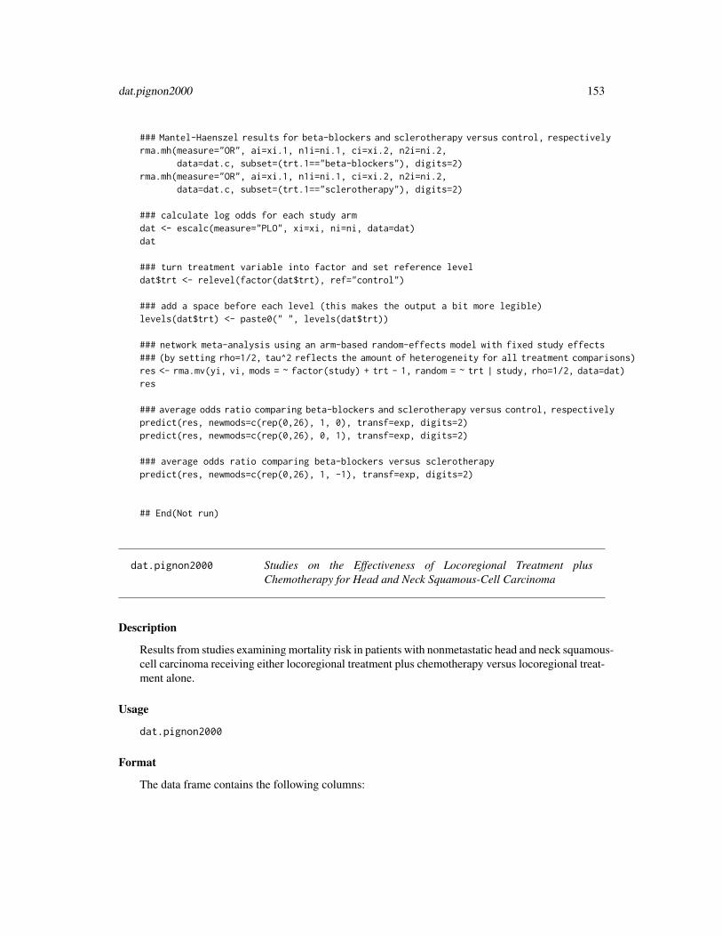
dat.pignon2000 153

### Mantel-Haenszel results for beta-blockers and sclerotherapy versus control, respectivelyrma.mh(measure="OR", ai=xi.1, n1i=ni.1, ci=xi.2, n2i=ni.2,

data=dat.c, subset=(trt.1=="beta-blockers"), digits=2)rma.mh(measure="OR", ai=xi.1, n1i=ni.1, ci=xi.2, n2i=ni.2,

data=dat.c, subset=(trt.1=="sclerotherapy"), digits=2)

### calculate log odds for each study armdat <- escalc(measure="PLO", xi=xi, ni=ni, data=dat)dat

### turn treatment variable into factor and set reference leveldat$trt <- relevel(factor(dat$trt), ref="control")

### add a space before each level (this makes the output a bit more legible)levels(dat$trt) <- paste0(" ", levels(dat$trt))

### network meta-analysis using an arm-based random-effects model with fixed study effects### (by setting rho=1/2, tau^2 reflects the amount of heterogeneity for all treatment comparisons)res <- rma.mv(yi, vi, mods = ~ factor(study) + trt - 1, random = ~ trt | study, rho=1/2, data=dat)res

### average odds ratio comparing beta-blockers and sclerotherapy versus control, respectivelypredict(res, newmods=c(rep(0,26), 1, 0), transf=exp, digits=2)predict(res, newmods=c(rep(0,26), 0, 1), transf=exp, digits=2)

### average odds ratio comparing beta-blockers versus sclerotherapypredict(res, newmods=c(rep(0,26), 1, -1), transf=exp, digits=2)

## End(Not run)

dat.pignon2000 Studies on the Effectiveness of Locoregional Treatment plusChemotherapy for Head and Neck Squamous-Cell Carcinoma

Description

Results from studies examining mortality risk in patients with nonmetastatic head and neck squamous-cell carcinoma receiving either locoregional treatment plus chemotherapy versus locoregional treat-ment alone.

Usage

dat.pignon2000

Format


154 dat.pignon2000

id numeric study id numbertrial character trial abbreviationOmE numeric observed minus expected number of deaths in the locoregional treatment plus chemotherapy groupV numeric corresponding variancegrp numeric timing of chemotherapy: 1 = adjuvant, 2 = neoadjuvant, 3 = concomitant

Details

The purpose of this meta-analysis was to examine the mortality risk in patients with nonmetastatichead and neck squamous-cell carcinoma receiving either locoregional treatment plus chemotherapyversus locoregional treatment alone. For 65 trials, the dataset provides the observed minus expectednumber of deaths and corresponding variances in the locoregional treatment plus chemotherapygroup. Based on these values, we can estimate the log hazard ratios with OmE/V and the correspond-ing sampling variance with 1/V.

The trials were also divided according to the timing of the chomotherapy: (1) adjuvant, after thelocoregional treatment, (2) neoadjuvant, before the locoregional treatment, and (3) concomitant,chemotherapy given concomitantly or alternating with radiotherapy.

Concepts

medicine, oncology, hazard ratios

Author(s)


Source

Pignon, J. P., Bourhis, J., Domenge, C., & Designe, L. (2000). Chemotherapy added to locoregionaltreatment for head and neck squamous-cell carcinoma: Three meta-analyses of updated individualdata. Lancet, 355(9208), 949–955. https://doi.org/10.1016/S0140-6736(00)90011-4

Examples

### copy data into 'dat' and examine datadat <- dat.pignon2000head(dat)

## Not run:


### calculate log hazard ratios and sampling variancesdat$yi <- with(dat, OmE/V)dat$vi <- with(dat, 1/V)head(dat)

### meta-analysis based on all 65 trialsres <- rma(yi, vi, data=dat, method="EE", digits=2)


dat.pritz1997 155

respredict(res, transf=exp)

### only adjuvant trialsres <- rma(yi, vi, data=dat, method="EE", subset=grp==1, digits=2)respredict(res, transf=exp)

### only neoadjuvant trialsres <- rma(yi, vi, data=dat, method="EE", subset=grp==2, digits=2)respredict(res, transf=exp)

### only concomitant trialsres <- rma(yi, vi, data=dat, method="EE", subset=grp==3, digits=2)respredict(res, transf=exp)

## End(Not run)

dat.pritz1997 Studies on the Effectiveness of Hyperdynamic Therapy for TreatingCerebral Vasospasm

Description

Results from 14 studies on the effectiveness of hyperdynamic therapy for treating cerebral va-sospasm.

Usage

dat.pritz1997

Format


study numeric study numberauthors character study authorsxi numeric number of patients that improved with hyperdynamic therapyni numeric total number of patients treated

Details

As described in Zhou et al. (1999), "hyperdynamic therapy refers to induced hypertension andhypervolaemia (volume expansion) to treat ischaemic symptoms due to vasospasm, and the successof this therapy is defined as clinical improvement in terms of neurologic deficits." For each studythat was included in the meta-analysis, the dataset includes information on the number of patients

156 dat.pritz1997

that improved under this form of therapy and the total number of patients that were treated. Thegoal of the meta-analysis is to estimate the true (average) success rate of hyperdynamic therapy.

Concepts

medicine, single-arm studies, proportions

Author(s)


Source

Zhou, X.-H., Brizendine, E. J., & Pritz, M. B. (1999). Methods for combining rates from severalstudies. Statistics in Medicine, 18(5), 557–566. https://doi.org/10.1002/(SICI)1097-0258(19990315)18:5<557::AID-SIM53>3.0.CO;2-F

References

Pritz M. B., Zhou, X.-H., & Brizendine, E. J. (1996). Hyperdynamic therapy for cerebral va-sospasm: A meta-analysis of 14 studies. Journal of Neurovascular Disease, 1, 6–8.

Pritz, M. B. (1997). Treatment of cerebral vasospasm due to aneurysmal subarachnoid hemorrhage:Past, present, and future of hyperdynamic therapy. Neurosurgery Quarterly, 7(4), 273–285.

Examples

### copy data into 'dat' and examine datadat <- dat.pritz1997dat

## Not run:


### computation of "weighted average" in Zhou et al. (1999), Table IVdat <- escalc(measure="PR", xi=xi, ni=ni, data=dat, add=0)theta.hat <- sum(dat$ni * dat$yi) / sum(dat$ni)se.theta.hat <- sqrt(sum(dat$ni^2 * dat$vi) / sum(dat$ni)^2)ci.lb <- theta.hat - 1.96 * se.theta.hatci.ub <- theta.hat + 1.96 * se.theta.hatround(c(estimate = theta.hat, se = se.theta.hat, ci.lb = ci.lb, ci.ub = ci.ub), 4)

### this is identical to an equal-effects model with sample size weightsrma(yi, vi, weights=ni, method="EE", data=dat)

### random-effects model with raw proportionsdat <- escalc(measure="PR", xi=xi, ni=ni, data=dat)res <- rma(yi, vi, data=dat)predict(res)


dat.raudenbush1985 157

### random-effects model with logit transformed proportionsdat <- escalc(measure="PLO", xi=xi, ni=ni, data=dat)res <- rma(yi, vi, data=dat)predict(res, transf=transf.ilogit)

### mixed-effects logistic regression modelres <- rma.glmm(measure="PLO", xi=xi, ni=ni, data=dat)predict(res, transf=transf.ilogit)

## End(Not run)

dat.raudenbush1985 Studies on Assessing the Effects of Teacher Expectations on Pupil IQ

Description

Results from 19 studies examining how teachers’ expectations about their pupils can influenceactual IQ levels.

Usage

dat.raudenbush1985

Format


study numeric study numberauthor character study author(s)year numeric publication yearweeks numeric weeks of contact prior to expectancy inductionsetting character whether tests were group or individually administeredtester character whether test administrator was aware or blindn1i numeric sample size of experimental groupn2i numeric sample size of control groupyi numeric standardized mean differencevi numeric corresponding sampling variance

Details

In the so-called ‘Pygmalion study’ (Rosenthal & Jacobson, 1968), “all of the predominantly poorchildren in the so-called Oak elementary school were administered a test pretentiously labeled the‘Harvard Test of Inflected Acquisition.’ After explaining that this newly designed instrument hadidentified those children most likely to show dramatic intellectual growth during the coming year,the experimenters gave the names of these ‘bloomers’ to the teachers. In truth, the test was atraditional IQ test and the ‘bloomers’ were a randomly selected 20% of the student population.After retesting the children 8 months later, the experimenters reported that those predicted to bloom

158 dat.raudenbush1985

had in fact gained significantly more in total IQ (nearly 4 points) and reasoning IQ (7 points) thanthe control group children. Further, at the end of the study, the teachers rated the experimentalchildren as intellectually more curious, happier, better adjusted, and less in need of approval thantheir control group peers” (Raudenbush, 1984).

In the following years, a series of studies were conducted attempting to replicate this rather contro-versial finding. However, the great majority of those studies were unable to demonstrate a statisti-cally significant difference between the two experimental groups in terms of IQ scores. Raudenbush(1984) conducted a meta-analysis based on 19 such studies to further examine the evidence for theexistence of the ‘Pygmalion effect’. The dataset includes the results from these studies.

The outcome measure used for the meta-analysis was the standardized mean difference (yi), withpositive values indicating that the supposed ‘bloomers’ had, on average, higher IQ scores than thosein the control group. The weeks variable indicates the number of weeks of prior contact betweenteachers and students before the expectancy induction. Testing was done either in a group settingor individually, which is indicated by the setting variable. Finally, the tester variable indicateswhether the test administrators were either aware or blind to the researcher-provided designationsof the children’s intellectual potential.

The data in this dataset were obtained from Raudenbush and Bryk (1985) with information on thesetting and tester variables extracted from Raudenbush (1984).

Concepts

education, standardized mean differences, meta-regression

Author(s)


Source

Raudenbush, S. W. (1984). Magnitude of teacher expectancy effects on pupil IQ as a function ofthe credibility of expectancy induction: A synthesis of findings from 18 experiments. Journal ofEducational Psychology, 76(1), 85–97. https://doi.org/10.1037/0022-0663.76.1.85

Raudenbush, S. W., & Bryk, A. S. (1985). Empirical Bayes meta-analysis. Journal of EducationalStatistics, 10(2), 75–98. https://doi.org/10.3102/10769986010002075

Examples

### copy data into 'dat' and examine datadat <- dat.raudenbush1985dat

## Not run:


### random-effects modelres <- rma(yi, vi, data = dat)res


dat.riley2003 159

### create weeks variable where values larger than 3 are set to 3dat$weeks.c <- ifelse(dat$weeks > 3, 3, dat$weeks)

### mixed-effects model with weeks.c variable as moderatorres <- rma(yi, vi, mods = ~ weeks.c, data = dat, digits = 3)res

## End(Not run)

dat.riley2003 Studies on MYC-N as a Prognostic Marker for Neuroblastoma

Description

Results from 81 studies examining overall and disease-free survival in neuroblastoma patients withamplified versus normal MYC-N protein levels.

Usage

dat.riley2003

Format


study numeric study numberyi numeric log hazard ratio of the outcome in those with amplified versus normal MYC-N protein levelsvi numeric sampling variance of the log hazard ratiosei numeric standard error of the log hazard ratiooutcome character outcome (OS = overall survival; DFS = disease-free survival)

Details

The meta-analysis by Riley et al. (2003) examined a variety of prognostic markers for overall anddisease-free survival in patients with neuroblastoma. One of the markers examined was amplifiedlevels of the MYC-N protein, with is associated with poorer outcomes.

The dataset given here was extracted from Riley (2011) and has been used in several other publica-tions (e.g., Riley et al., 2004, 2007). The dataset provides the (log) hazard ratios (and correspondingstandard errors) with respect to these two outcomes in 81 studies, with positive values indicating agreater risk of death (for OS) or disease recurrence/death (for DFS) for patients with high MYC-Nlevels compared to those with normal/low levels. Note that information on both outcomes couldonly be extracted from 17 studies (39 studies only provided sufficient information to extract the OSestimate, while 25 studies only allowed for extraction of the DFS estimate).

160 dat.riley2003

Concepts

medicine, oncology, hazard ratios

Author(s)


Source

Riley, R. D., Sutton, A. J., Abrams, K. R., & Lambert, P. C. (2004). Sensitivity analyses allowedmore appropriate and reliable meta-analysis conclusions for multiple outcomes when missing datawas present. Journal of Clinical Epidemiology, 57(9), 911–924. https://doi.org/10.1016/j.jclinepi.2004.01.018

Riley, R. D., Abrams, K. R., Lambert, P. C., Sutton, A. J., & Thompson, J. R. (2007). An evalu-ation of bivariate random-effects meta-analysis for the joint synthesis of two correlated outcomes.Statistics in Medicine, 26(1), 78–97. https://doi.org/10.1002/sim.2524

Riley, R. D. (2011). Erratum: An evaluation of bivariate random-effects meta-analysis for the jointsynthesis of two correlated outcomes. Statistics in Medicine, 30(4), 400. https://doi.org/10.1002/sim.4100

References

Riley, R. D., Burchill, S. A., Abrams, K. R., Heney, D., Lambert, P. C., Jones, D. R., Sutton, A. J.,Young, B., Wailoo, A. J., & Lewis, I. J. (2003). A systematic review and evaluation of the use oftumour markers in paediatric oncology: Ewing’s sarcoma and neuroblastoma. Health TechnologyAssessment, 7(5), 1–162. https://doi.org/10.3310/hta7050

Examples

### copy data into 'dat' and examine datadat <- dat.riley2003dat

## Not run:


### random-effects model analysis for outcome DFSres <- rma(yi, sei=sei, data=dat, subset=(outcome == "DFS"), method="DL")respredict(res, transf=exp, digits=2)

### random-effects model analysis for outcome OSres <- rma(yi, sei=sei, data=dat, subset=(outcome == "OS"), method="DL")respredict(res, transf=exp, digits=2)

## End(Not run)


dat.senn2013 161

dat.senn2013 Studies on the Effectiveness of Glucose-Lowering Agents

Description

Results from 26 trials examining the effectiveness of glucose-lowering agents in patients with type2 diabetes

Usage

dat.senn2013

Format


study character (first) author and year of studyni numeric sample size of the study armtreatment character treatment givencomment character whether figures given are based on raw values at outcome or on change from baselinemi numeric raw mean or mean changesdi numeric standard deviation

Details

The dataset includes the results from 26 randomized controlled trials examining the effectiveness ofadding various oral glucose-lowering agents to a baseline sulfonylurea therapy in patients with type2 diabetes. The outcome measured in the studies was either the mean HbA1c level at follow-up orthe mean change in HbA1c level from baseline to follow-up. A total of 10 different treatment typeswere examined in these studies: acarbose, benfluorex, metformin, miglitol, pioglitazone, placebo,rosiglitazone, sitagliptin, sulfonylurea alone, and vildagliptin. One study included three treatmentarms (Willms, 1999), while the rest of the studies included two treatment arms (hence, the datasetincludes the results from 53 treatment arms).

The data can be used for a network meta-analysis, either using an arm-based or a contrast-basedmodel. See ‘Examples’ below.

Concepts


Author(s)


Source

Senn, S., Gavini, F., Magrez, D., & Scheen, A. (2013). Issues in performing a network meta-analysis. Statistical Methods in Medical Research, 22(2), 169–189. https://doi.org/10.1177/0962280211432220


162 dat.senn2013

References

Law, M., Jackson, D., Turner, R., Rhodes, K., & Viechtbauer, W. (2016). Two new methods tofit models for network meta-analysis with random inconsistency effects. BMC Medical ResearchMethodology, 16, 87. https://doi.org/10.1186/s12874-016-0184-5

Rücker, G., & Schwarzer, G. (2015). Ranking treatments in frequentist network meta-analysisworks without resampling methods. BMC Medical Research Methodology, 15, 58. https://doi.org/10.1186/s12874-015-0060-8

Examples

### copy data into 'dat' and examine datadat <- dat.senn2013dat

## Not run:


### create network graph ('igraph' package must be installed)library(igraph, warn.conflicts=FALSE)pairs <- data.frame(do.call(rbind,sapply(split(dat$treatment, dat$study), function(x) t(combn(x,2)))), stringsAsFactors=FALSE)

pairs$X1 <- factor(pairs$X1, levels=sort(unique(dat$treatment)))pairs$X2 <- factor(pairs$X2, levels=sort(unique(dat$treatment)))tab <- table(pairs[,1], pairs[,2])tab # adjacency matrixg <- graph_from_adjacency_matrix(tab, mode = "plus", weighted=TRUE, diag=FALSE)plot(g, edge.curved=FALSE, edge.width=E(g)$weight, layout=layout_as_star(g, center="placebo"),


### table of studies versus treatments examinedprint(addmargins(table(dat$study, dat$treatment)), zero.print="")

### table of frequencies with which treatment pairs were studiedprint(as.table(crossprod(table(dat$study, dat$treatment))), zero.print="")

### add means and sampling variances of the means to the datasetdat <- escalc(measure="MN", mi=mi, sdi=sdi, ni=ni, data=dat)

### turn treatment variable into factor and set reference leveldat$treatment <- relevel(factor(dat$treatment), ref="placebo")

### add a space before each level (this makes the output a bit more legible)levels(dat$treatment) <- paste0(" ", levels(dat$treatment))

### network meta-analysis using an arm-based fixed-effects model with fixed study effectsres.fe <- rma.mv(yi, vi, mods = ~ study + treatment - 1, data=dat, slab=paste0(study, treatment))res.fe

### test if treatment factor as a whole is significant

dat.senn2013 163

anova(res.fe, btt="treatment")

### forest plot of the contrast estimates (treatments versus placebos)forest(tail(coef(res.fe), 9), tail(diag(vcov(res.fe)), 9), slab=levels(dat$treatment)[-1],

xlim=c(-2.5, 2.0), alim=c(-1.5, 0.5), psize=1, xlab="Estimate", header="Treatment")

### weight matrix for the estimation of the fixed effects (leaving out the study effects)w <- t(tail(vcov(res.fe) %*% t(model.matrix(res.fe)) %*% weights(res.fe, type="matrix"), 9))rownames(w) <- res.fe$slab

### create shade plot for the diabetes network with placebo as the reference treatment### negative values in blue shades, positive values in red shadescols <- colorRampPalette(c("blue", "gray95", "red"))(9)heatmap(w, Rowv=NA, Colv=NA, scale="none", margins=c(6,11), col=cols,

cexRow=.7, cexCol=1, labCol=levels(dat$treatment)[-1])

### network meta-analysis using an arm-based random-effects model with fixed study effects### by setting rho=1/2, tau^2 reflects the amount of heterogeneity for all treatment comparisonsres.re <- rma.mv(yi, vi, mods = ~ study + treatment - 1, random = ~ treatment | study, rho=1/2,

data=dat, slab=paste0(study, treatment))res.re

### test if treatment factor as a whole is significantanova(res.re, btt="treatment")

### forest plot of the contrast estimates (treatments versus placebos)forest(tail(coef(res.re), 9), tail(diag(vcov(res.re)), 9), slab=levels(dat$treatment)[-1],


### compute the contribution of each study to the overall Q-test valueqi <- sort(by((resid(res.fe) / sqrt(dat$vi))^2, dat$study, sum))

### check that the values add upsum(qi)res.fe$QE

### plot the valuess <- length(qi)par(mar=c(5,10,2,1))plot(qi, 1:s, pch=19, xaxt="n", yaxt="n", xlim=c(0,40), xlab="Chi-Square Contribution", ylab="")axis(side=1)axis(side=2, at=1:s, labels=names(qi), las=1, tcl=0)segments(rep(0,s), 1:s, qi, 1:s)

############################################################################

### restructure dataset to a contrast-based formatdat <- dat.senn2013[c(1,4:2,5:6)] # reorder variables firstdat <- to.wide(dat, study="study", grp="treatment", ref="placebo", grpvars=4:6)dat

### calculate mean difference and corresponding sampling variance for each treatment comparisondat <- escalc(measure="MD", m1i=mi.1, sd1i=sdi.1, n1i=ni.1,

164 dat.senn2013

m2i=mi.2, sd2i=sdi.2, n2i=ni.2, data=dat)dat

### calculate the variance-covariance matrix of the mean differences for the multitreatment studiescalc.v <- function(x) {

v <- matrix(x$sdi.2[1]^2 / x$ni.2[1], nrow=nrow(x), ncol=nrow(x))diag(v) <- x$viv


### add contrast matrix to datasetdat <- contrmat(dat, grp1="treatment.1", grp2="treatment.2")dat

### network meta-analysis using a contrast-based random-effects model### by setting rho=1/2, tau^2 reflects the amount of heterogeneity for all treatment comparisons### the treatment left out (placebo) becomes the reference level for the treatment comparisonsres <- rma.mv(yi, V, mods = ~ acarbose + benfluorex + metformin + miglitol + pioglitazone +

rosiglitazone + sitagliptin + sulfonylurea + vildagliptin - 1,random = ~ comp | study, rho=1/2, data=dat)

res

### forest plot of the contrast estimates (treatments versus placebos)forest(coef(res), diag(vcov(res)), slab=names(coef(res)), order="obs",


### estimate all pairwise differences between treatmentscontr <- data.frame(t(combn(names(coef(res)), 2)))contr <- contrmat(contr, "X1", "X2", last="vildagliptin")rownames(contr) <- paste(contr$X1, "-", contr$X2)contr <- as.matrix(contr[-c(1:2)])sav <- predict(res, newmods=contr)sav[["slab"]] <- rownames(contr)sav

### fit random inconsistency effects model (see Law et al., 2016)inc <- rma.mv(yi, V, mods = ~ acarbose + benfluorex + metformin + miglitol + pioglitazone +

rosiglitazone + sitagliptin + sulfonylurea + vildagliptin - 1,random = list(~ comp | study, ~ comp | design), rho=1/2, phi=1/2, data=dat)

inc

############################################################################

### compute P-scores (see Rücker & Schwarzer, 2015)contr <- data.frame(t(combn(c(names(coef(res)),"placebo"), 2))) # add 'placebo' to contrast matrixcontr <- contrmat(contr, "X1", "X2", last="placebo", append=FALSE)b <- c(coef(res),0) # add 0 for 'placebo' (the reference treatment)vb <- bldiag(vcov(res),0) # add 0 row/column for 'placebo' (the reference treatment)pvals <- apply(contr, 1, function(x) pnorm((x%*%b) / sqrt(t(x)%*%vb%*%x)))tab <- vec2mat(pvals, corr=FALSE)tab[upper.tri(tab)] <- t((1 - tab)[upper.tri(tab)])rownames(tab) <- colnames(tab) <- colnames(contr)

dat.stowe2010 165

round(tab, 2) # like Table 2 in the articlecbind(pscore=round(sort(apply(tab, 1, mean, na.rm=TRUE), decreasing=TRUE), 3))

# note: the values are slightly different from the ones given in Table 3 of Rücker and# Schwarzer (2015) since model 'res' above is fitted using REML estimation while the# results shown in the article are based on the 'netmeta' package, which uses a DL-type# estimator for the amount of heterogeneity by default

############################################################################

## End(Not run)

dat.stowe2010 Studies on Adjuvant Treatments to Levodopa Therapy for Parkinsondisease

Description

Results from 29 trials assessing efficacy of three drug classes as adjuvant treatment to levodopatherapy in patients with Parkinson disease and motor complications.

Usage

dat.stowe2010

Format


study character study labelid integer study idt1 character treatment 1y1 numeric treatment effect arm 1sd1 numeric standard deviation arm 1n1 integer sample size arm 1t2 character treatment 2y2 numeric treatment effect arm 2sd2 numeric standard deviation arm 2n2 integer sample size arm 2t3 character treatment 3y3 numeric treatment effect arm 3sd3 numeric standard deviation arm 3n3 integer sample size arm 3

166 dat.stowe2010

Details

This data set contains data from a Cochrane review assessing efficacy and safety of three drugclasses as adjuvant treatment to levodopa therapy in patients with Parkinson disease and motorcomplications (Stowe et al., 2010).

The authors conducted three pairwise meta-analyses comparing dopamine agonists, catechol-O-methyl transferase inhibitors (COMTI), and monoamine oxidase type B inhibitors (MAOBI) withplacebo. The primary outcome was the mean reduction of the time spent in a relatively immobile‘off’ phase (mean off-time), calculated in hours per day. Relative treatment effects were expressedas mean difference. Data on this outcome were available for 5,331 patients from 28 studies com-paring an active treatment with placebo and one three-arm study comparing two active treatmentswith placebo.

Concepts


Author(s)


Source

Stowe, R., Ives, N., Clarke, C. E., Deane, K., Hilten, V., Wheatley, K., Gray, R., Handley, K.,& Furmston, A. (2010). Evaluation of the efficacy and safety of adjuvant treatment to levodopatherapy in Parkinson’s disease patients with motor complications. Cochrane Database of SystematicReviews, 7, CD007166. https://doi.org/10.1002/14651858.CD007166.pub2

See Also

pairwise, metacont, netmeta, netrank, rankogram, netleague

Examples

### Show results from three studies (including three-arm study LARGO)dat.stowe2010[18:20, ]

## Not run:


### Print mean differences with two digits and standard errors with 3### digitssettings.meta(digits = 2, digits.se = 3)

### Transform data from wide arm-based format to contrast-based### format. Argument 'sm' must not be provided as the mean difference### is the default in R function metacont() called internally.pw <- pairwise(treat = list(t1, t2, t3), n = list(n1, n2, n3),

mean = list(y1, y2, y3), sd = list(sd1, sd2, sd3),


dat.tannersmith2016 167

studlab = study, data = dat.stowe2010, sm = "MD")

### Show calculated mean differences (TE) for three studiesselstudy <- c("COMTI(E) INT-OZ", "LARGO", "COMTI(E) Nomecomt")subset(pw, studlab %in% selstudy)[, c(3:7, 10, 1)]

### Conduct random effects network meta-analysis (NMA)### with placebo as referencenet <- netmeta(pw, fixed = FALSE, ref = "plac")

### Show network graphnetgraph(net, number = TRUE, multiarm = TRUE,

cex = 1.25, offset = 0.025,cex.number = 1, pos.number.of.studies = 0.3)

### Print NMA resultsnet

### Forest plot with NMA resultsforest(net)

### Forest plot showing all network estimates of active treatments### compared with other treatmentsforest(net, ref = c("C", "D", "M"), baseline = FALSE, drop = TRUE)

### Treatment ranking using P-scoresnetrank(net)

### Rankogram with all ranking probabilitiesset.seed(1909)ran <- rankogram(net)ranplot(ran)

### Treatment ranking using SUCRAsnetrank(ran)

### League table showing network and direct estimatesnetleague(net, seq = netrank(net), ci = FALSE)

## End(Not run)

dat.tannersmith2016 Studies on the Relationship between School Motivation and CriminalBehavior

Description

Results from 17 studies on the correlation between school motivation/attitudes and subsequentdelinquent/criminal behavior.

168 dat.tannersmith2016

Usage

dat.tannersmith2016

Format


studyid numeric study identifieryi numeric r-to-z transformed correlation coefficientvi numeric corresponding sampling variancesei numeric corresponding standard erroraget1 numeric age at which the school motivation/attitudes were assessedaget2 numeric age at which the delinquent/criminal behavior was assessedpropmale numeric proportion of male participants in the samplesexmix character whether the sample consisted only of males, only of females, or a mix

Details

The dataset includes 113 r-to-z transformed correlation coefficients from 17 prospective longitu-dinal studies that examined the relationship between school motivation/attitudes and subsequentdelinquent/criminal behavior.

Multiple coefficients could be extracted from the studies “given the numerous ways in which schoolmotivation/attitudes variables could be operationalized (e.g., academic aspirations, academic self-efficacy) as well as the numerous ways in which crime/delinquency could be operationalized (e.g.,property crime, violent crime)” (Tanner-Smith et al., 2016).

Since information to compute the covariance between multiple coefficients within studies is notavailable, Tanner-Smith et al. (2016) illustrate the use of cluster-robust inference methods for theanalysis of this dataset.

Note that this dataset is only meant to be used for pedagogical and demonstration purposes anddoes not constitute a proper review or synthesis of the complete and current research evidence onthe given topic.

Concepts

psychology, criminology, correlation coefficients, multilevel models, cluster-robust inference, meta-regression

Author(s)


Source

Tanner-Smith, E. E., Tipton, E. & Polanin, J. R. (2016). Handling complex meta-analytic datastructures using robust variance estimates: A tutorial in R. Journal of Developmental and Life-Course Criminology, 2(1), 85–112. https://doi.org/10.1007/s40865-016-0026-5


dat.tannersmith2016 169

Examples

### copy data into 'dat' and examine datadat <- dat.tannersmith2016head(dat)

## Not run:


### compute mean age variables within studiesdat$aget1 <- ave(dat$aget1, dat$studyid)dat$aget2 <- ave(dat$aget2, dat$studyid)

### construct an effect size identifier variabledat$esid <- 1:nrow(dat)

### construct an approximate var-cov matrix assuming a correlation of 0.8### for multiple coefficients arising from the same studyV <- vcalc(vi, cluster=studyid, obs=esid, rho=0.8, data=dat)

### fit a multivariate random-effects model using the approximate var-cov matrix Vres <- rma.mv(yi, V, random = ~ esid | studyid, data=dat)res

### use cluster-robust inference methodsrobust(res, cluster=studyid, clubSandwich=TRUE)

### note: the results obtained above and below are slightly different compared### to those given by Tanner-Smith et al. (2016) since the approach illustrated### here makes use a multivariate random-effects model for the 'working model'### before applying the cluster-robust inference methods, while the results given### in the paper are based on a somewhat simpler working model

### examine the main effects of the age variablesres <- rma.mv(yi, V, mods = ~ aget1 + aget2,

random = ~ 1 | studyid/esid, data=dat)robust(res, cluster=studyid, clubSandwich=TRUE)

### also examine their interactionres <- rma.mv(yi, V, mods = ~ aget1 * aget2,


### add the sexmix factor to the modelres <- rma.mv(yi, V, mods = ~ aget1 * aget2 + sexmix,


## End(Not run)

170 dat.vanhowe1999

dat.vanhowe1999 Studies on the Association between Circumcision and HIV Infection

Description

Results from 33 studies examining the association between male circumcision and HIV infection.

Usage

dat.vanhowe1999

Format


study character study authorcategory character study type (high-risk group, partner study, or population survey)non.pos numeric number of non-circumcised HIV positive casesnon.neg numeric number of non-circumcised HIV negative casescir.pos numeric number of circumcised HIV positive casescir.neg numeric number of circumcised HIV negative cases

Details


HIV positive HIV negativenon-circumcised non.pos non.negcircumcised cir.pos cir.neg

The goal of the meta-analysis was to examine if the risk of an HIV infection differs between non-circumcised versus circumcised men.

The dataset is interesting because it can be used to illustrate the difference between naively poolingresults by summing up the counts across studies and then computing the odds ratio based on theaggregated table (as was done by Van Howe, 1999) and conducting a proper meta-analysis (asillustrated by O’Farrell & Egger, 2000). In fact, a proper meta-analysis shows that the HIV infectionrisk is on average higher in non-circumcised men, which is the opposite of what the naive poolingapproach yields (which makes this an illustration of Simpson’s paradox).

Concepts

medicine, epidemiology, odds ratios

Author(s)



dat.vanhowe1999 171

Source

Van Howe, R. S. (1999). Circumcision and HIV infection: Review of the literature and meta-analysis. International Journal of STD & AIDS, 10(1), 8–16. https://doi.org/10.1258/0956462991913015

References

O’Farrell, N., & Egger, M. (2000). Circumcision in men and the prevention of HIV infection: A’meta-analysis’ revisited. International Journal of STD & AIDS, 11(3), 137–142. https://doi.org/10.1258/0956462001915480

Examples

### copy data into 'dat' and examine datadat <- dat.vanhowe1999dat

## Not run:


### naive pooling by summing up the counts within categories and then### computing the odds ratios and corresponding confidence intervalscat1 <- with(dat[dat$category=="high-risk group",],escalc(measure="OR", ai=sum(non.pos), bi=sum(non.neg), ci=sum(cir.pos), di=sum(cir.neg)))

cat2 <- with(dat[dat$category=="partner study",],escalc(measure="OR", ai=sum(non.pos), bi=sum(non.neg), ci=sum(cir.pos), di=sum(cir.neg)))

cat3 <- with(dat[dat$category=="population survey",],escalc(measure="OR", ai=sum(non.pos), bi=sum(non.neg), ci=sum(cir.pos), di=sum(cir.neg)))

summary(cat1, transf=exp, digits=2)summary(cat2, transf=exp, digits=2)summary(cat3, transf=exp, digits=2)

### naive pooling across all studiesall <- escalc(measure="OR", ai=sum(dat$non.pos), bi=sum(dat$non.neg),

ci=sum(dat$cir.pos), di=sum(dat$cir.neg))summary(all, transf=exp, digits=2)

### calculate log odds ratios and corresponding sampling variancesdat <- escalc(measure="OR", ai=non.pos, bi=non.neg, ci=cir.pos, di=cir.neg, data=dat)dat

### random-effects modelres <- rma(yi, vi, data=dat, method="DL")respredict(res, transf=exp, digits=2)

### random-effects model within subgroupsres <- rma(yi, vi, data=dat, method="DL", subset=category=="high-risk group")predict(res, transf=exp, digits=2)res <- rma(yi, vi, data=dat, method="DL", subset=category=="partner study")predict(res, transf=exp, digits=2)res <- rma(yi, vi, data=dat, method="DL", subset=category=="population survey")

172 dat.viechtbauer2021

predict(res, transf=exp, digits=2)

## End(Not run)

dat.viechtbauer2021 Studies to Illustrate Model Checking Methods

Description

Results from 20 hypothetical randomized clinical trials examining the effectiveness of a medicationfor treating some disease.

Usage

dat.viechtbauer2021

Format


trial numeric trial numbernTi numeric number of patients in the treatment groupnCi numeric number of patients in the control groupxTi numeric number of patients in the treatment group with remissionxCi numeric number of patients in the control group with remissiondose numeric dosage of the medication provided to patients in the treatment group (in milligrams per day)

Details

The dataset was constructed for the purposes of illustrating the model checking and diagnosticmethods described in Viechtbauer (2021). The code below provides the results for many of theanalyses and plots discussed in the book chapter.

Concepts

medicine, odds ratios, outliers, model checks

Author(s)


Source

Viechtbauer, W. (2021). Model checking in meta-analysis. In C. H. Schmid, T. Stijnen, & I. R.White (Eds.), Handbook of meta-analysis (pp. 219-254). Boca Raton, FL: CRC Press. https://doi.org/10.1201/9781315119403


dat.viechtbauer2021 173

Examples

### copy data into 'dat' and examine datadat <- dat.viechtbauer2021dat

## Not run:


### calculate log odds ratios and corresponding sampling variances

dat <- escalc(measure="OR", ai=xTi, n1i=nTi, ci=xCi, n2i=nCi, add=1/2, to="all", data=dat)dat

### number of studies

k <- nrow(dat)

### fit models

res.CE <- rma(yi, vi, data=dat, method="CE") # same as method="EE"res.CE

res.RE <- rma(yi, vi, data=dat, method="DL")res.RE

res.MR <- rma(yi, vi, mods = ~ dose, data=dat, method="FE")res.MR

res.ME <- rma(yi, vi, mods = ~ dose, data=dat, method="DL")res.ME

### forest and bubble plot

par(mar=c(5,4,1,2))

forest(dat$yi, dat$vi, psize=0.8, efac=0, xlim=c(-4,6), ylim=c(-3,23),cex=1, width=c(5,5,5), xlab="Log Odds Ratio (LnOR)")

addpoly(res.CE, row=-1.5, mlab="CE Model")addpoly(res.RE, row=-2.5, mlab="RE Model")text(-4, 22, "Trial", pos=4, font=2)text( 6, 22, "LnOR [95% CI]", pos=2, font=2)abline(h=0)

tmp <- regplot(res.ME, xlim=c(0,250), ylim=c(-1,1.5), predlim=c(0,250), shade=FALSE, digits=1,xlab="Dosage (mg per day)", psize="seinv", plim=c(NA,5), bty="l", las=1,lty=c("solid", "dashed"), label=TRUE, labsize=0.8, offset=c(1,0.7))

res.sub <- rma(yi, vi, mods = ~ dose, data=dat, method="DL", subset=-6)abline(res.sub, lty="dotted")points(tmp$xi, tmp$yi, pch=21, cex=tmp$psize, col="black", bg="darkgray")


par(mar=c(5,4,4,2))

### number of standardized deleted residuals larger than +-1.96 in each model

sum(abs(rstudent(res.CE)$z) >= qnorm(.975))sum(abs(rstudent(res.MR)$z) >= qnorm(.975))sum(abs(rstudent(res.RE)$z) >= qnorm(.975))sum(abs(rstudent(res.ME)$z) >= qnorm(.975))

### plot of the standardized deleted residuals for the RE and ME models

plot(NA, NA, xlim=c(1,20), ylim=c(-4,4), xlab="Study", ylab="Standardized (Deleted) Residual",xaxt="n", main="Random-Effects Model", las=1)

axis(side=1, at=1:20)abline(h=c(-1.96,1.96), lty="dotted")abline(h=0)points(1:20, rstandard(res.RE)$z, type="o", pch=19, col="gray70")points(1:20, rstudent(res.RE)$z, type="o", pch=19)legend("top", pch=19, col=c("gray70","black"), lty="solid",

legend=c("Standardized Residuals","Standardized Deleted Residuals"), bty="n")

plot(NA, NA, xlim=c(1,20), ylim=c(-4,4), xlab="Study", ylab="Standardized (Deleted) Residual",xaxt="n", main="Mixed-Effects Model", las=1)

axis(side=1, at=1:20)abline(h=c(-1.96,1.96), lty="dotted")abline(h=0)points(1:20, rstandard(res.ME)$z, type="o", pch=19, col="gray70")points(1:20, rstudent(res.ME)$z, type="o", pch=19)legend("top", pch=19, col=c("gray70","black"), lty="solid",

legend=c("Standardized Residuals","Standardized Deleted Residuals"), bty="n")

### Baujat plots

baujat(res.CE, main="Common-Effects Model", xlab="Squared Pearson Residual", ylim=c(0,5), las=1)baujat(res.ME, main="Mixed-Effects Model", ylim=c(0,2), las=1)

### GOSH plots (skipped because this takes quite some time to run)

if (FALSE) {

res.GOSH.CE <- gosh(res.CE, subsets=10^7)plot(res.GOSH.CE, cex=0.2, out=6, xlim=c(-0.25,1.25), breaks=c(200,100))

res.GOSH.ME <- gosh(res.ME, subsets=10^7)plot(res.GOSH.ME, het="tau2", out=6, breaks=50, adjust=0.6, las=1)

}

### plot of treatment dosage against the standardized residuals

plot(dat$dose, rstandard(res.ME)$z, pch=19, xlab="Dosage (mg per day)",ylab="Standardized Residual", xlim=c(0,250), ylim=c(-2.5,2.5), las=1)

abline(h=c(-1.96,1.96), lty="dotted", lwd=2)

dat.viechtbauer2021 175

abline(h=0)title("Standardized Residual Plot")text(dat$dose[6], rstandard(res.ME)$z[6], "6", pos=4, offset=0.4)

### quadratic polynomial model

rma(yi, vi, mods = ~ dose + I(dose^2), data=dat, method="DL")

### lack-of-fit model

resLOF <- rma(yi, vi, mods = ~ dose + factor(dose), data=dat, method="DL", btt=3:9)resLOF

### scatter plot to illustrate the lack-of-fit model

regplot(res.ME, xlim=c(0,250), ylim=c(-1.0,1.5), xlab="Dosage (mg per day)", ci=FALSE,predlim=c(0,250), psize=1, pch=19, col="gray60", digits=1, lwd=1, bty="l", las=1)

dosages <- sort(unique(dat$dose))lines(dosages, fitted(resLOF)[match(dosages, dat$dose)], type="o", pch=19, cex=2, lwd=2)points(dat$dose, dat$yi, pch=19, col="gray60")legend("bottomright", legend=c("Linear Model", "Lack-of-Fit Model"), pch=c(NA,19), col="black",

lty="solid", lwd=c(1,2), pt.cex=c(1,2), seg.len=4, bty="n")

### checking normality of the standardized deleted residuals

qqnorm(res.ME, type="rstudent", main="Standardized Deleted Residuals", pch=19, label="out",lwd=2, pos=24, ylim=c(-4,3), lty=c("solid", "dotted"), las=1)

### checking normality of the random effects

sav <- qqnorm(ranef(res.ME)$pred, main="BLUPs of the Random Effects", cex=1, pch=19,xlim=c(-2.2,2.2), ylim=c(-0.6,0.6), las=1)

abline(a=0, b=sd(ranef(res.ME)$pred), lwd=2)text(sav$x[6], sav$y[6], "6", pos=4, offset=0.4)

### hat values for the CE and RE models

plot(NA, NA, xlim=c(1,20), ylim=c(0,0.21), xaxt="n", las=1, xlab="Study", ylab="Hat Value")axis(1, 1:20, cex.axis=1)points(hatvalues(res.CE), type="o", pch=19, col="gray70")points(hatvalues(res.RE), type="o", pch=19)abline(h=1/20, lty="dotted", lwd=2)title("Hat Values for the CE/RE Models")legend("topright", pch=19, col=c("gray70","black"), lty="solid",

legend=c("Common-Effects Model", "Random-Effects Model"), bty="n")

### heatmap of the hat matrix for the ME model

cols <- colorRampPalette(c("blue", "white", "red"))(101)h <- hatvalues(res.ME, type="matrix")image(1:nrow(h), 1:ncol(h), t(h[nrow(h):1,]), axes=FALSE,

xlab="Influence of the Observed Effect of Study ...", ylab="On the Fitted Value of Study ...",col=cols, zlim=c(-max(abs(h)),max(abs(h))))


axis(1, 1:20, tick=FALSE)axis(2, 1:20, labels=20:1, las=1, tick=FALSE)abline(h=seq(0.5,20.5,by=1), col="white")abline(v=seq(0.5,20.5,by=1), col="white")points(1:20, 20:1, pch=19, cex=0.4)title("Heatmap for the Mixed-Effects Model")

### plot of leverages versus standardized residuals for the ME model

plot(hatvalues(res.ME), rstudent(res.ME)$z, pch=19, cex=0.2+3*sqrt(cooks.distance(res.ME)),las=1, xlab="Leverage (Hat Value)", ylab="Standardized Deleted Residual",xlim=c(0,0.35), ylim=c(-3.5,2.5))

abline(h=c(-1.96,1.96), lty="dotted", lwd=2)abline(h=0, lwd=2)ids <- c(3,6,9)text(hatvalues(res.ME)[ids] + c(0,0.013,0.010), rstudent(res.ME)$z[ids] - c(0.18,0,0), ids)title("Leverage vs. Standardized Deleted Residuals")

### plot of the Cook's distances for the ME model

plot(1:20, cooks.distance(res.ME), ylim=c(0,1.6), type="o", pch=19, las=1, xaxt="n", yaxt="n",xlab="Study", ylab="Cook's Distance")

axis(1, 1:20, cex.axis=1)axis(2, seq(0,1.6,by=0.4), las=1)title("Cook's Distances")

### plot of the leave-one-out estimates of tau^2 for the ME model

x <- influence(res.ME)

plot(1:20, x$inf$tau2.del, ylim=c(0,0.15), type="o", pch=19, las=1, xaxt="n", xlab="Study",ylab=expression(paste("Estimate of ", tau^2, " without the ", italic(i), "th study")))

abline(h=res.ME$tau2, lty="dashed")axis(1, 1:20)title("Residual Heterogeneity Estimates")

### plot of the covariance ratios for the ME model

plot(1:20, x$inf$cov.r, ylim=c(0,2.0), type="o", pch=19, las=1, xaxt="n",xlab="Study", ylab="Covariance Ratio")

abline(h=1, lty="dashed")axis(1, 1:20)title("Covariance Ratios")

### fit mixed-effects model without studies 3 and/or 6

rma(yi, vi, mods = ~ dose, data=dat, method="DL", subset=-3)rma(yi, vi, mods = ~ dose, data=dat, method="DL", subset=-6)rma(yi, vi, mods = ~ dose, data=dat, method="DL", subset=-c(3,6))

## End(Not run)

dat.white2020 177

dat.white2020 Studies on the Relationship between Sexual Signal Expression and In-dividual Quality

Description

Results from 41 studies examining the relationship between measures of individual quality and theexpression of structurally coloured sexual signals.

Usage

dat.white2020

Format

The object is a data frame which contains the following columns:

study_id character study-level IDobs character observation-level IDexp_obs character whether the study is observational or experimentalcontrol numeric whether the study did (1) or did not (0) include a non-sexual control traitclass character class of the study organismsgenus character class of the study organismsspecies character species of the study organismssex character sex of the study organismsiridescent numeric whether the colour signals were iridescent (1) or not (0)col_var character the colour variable quantifiedcol_component character whether the colour variable is chromatic or achromaticquality_measure character the measure of individual quality usedregion character the body region from which colour was sampledn numeric study sample sizer numeric Pearson’s correlation coefficient

Details

The 186 rows in this dataset come from 41 experimental and observational studies reporting onthe correlation between measures of individual quality (age, body condition, immune function,parasite resistance) and the expression of structurally coloured sexual signals across 28 species.The purpose of this meta-analysis was to test whether structural colour signals show heightenedcondition-dependent expression, as predicted by evolutionary models of ’honest’ signalling.

Concepts

ecology, evolution, correlation coefficients

178 dat.woods2010

Author(s)

Thomas E. White, <[email protected]>

Source

White, T. E. (2020). Structural colours reflect individual quality: A meta-analysis. Biology Letters,16(4), 20200001. https://doi.org/10.1098/rsbl.2020.0001

Examples

### copy data into 'dat' and examine datadat <- dat.white2020head(dat, 10)

## Not run:


### calculate r-to-z transformed correlations and corresponding sampling variancesdat <- escalc(measure="ZCOR", ri=r, ni=n, data=dat)

### fit multilevel meta-analytic modelres <- rma.mv(yi, vi, random = list(~ 1 | study_id, ~ 1 | obs), data=dat)res

## End(Not run)

dat.woods2010 Studies on Treatments for Chronic Obstructive Pulmonary Disease

Description

Results from 3 trials examining the mortality risk of three treatments and placebo in patients withchronic obstructive pulmonary disease.

Usage

dat.woods2010

Format


author character first author / study nametreatment character treatmentr integer number of deathsN integer number of patients

dat.woods2010 179

Details

Count mortality statistics in randomised controlled trials of treatments for chronic obstructive pul-monary disease (Woods et al., 2010, Table 1).

Concepts

medicine, odds ratios, network meta-analysis

Author(s)


Source

Woods, B. S., Hawkins, N., & Scott, D. A. (2010). Network meta-analysis on the log-hazardscale, combining count and hazard ratio statistics accounting for multi-arm trials: A tutorial. BMCMedical Research Methodology, 10, 54. https://doi.org/10.1186/1471-2288-10-54

Examples

### Show full data setdat.woods2010

## Not run:




### Transform data from long arm-based format to contrast-based### format. Argument 'sm' has to be used for odds ratio as summary### measure; by default the risk ratio is used in the metabin function### called internally.pw <- pairwise(treatment, event = r, n = N,

studlab = author, data = dat.woods2010, sm = "OR")pw

### Conduct network meta-analysisnet <- netmeta(pw)net

### Show forest plotforest(net, ref = "Placebo", drop = TRUE,

leftlabs = "Contrast to Placebo")

## End(Not run)


180 dat.yusuf1985

dat.yusuf1985 Studies of Beta Blockers During and After Myocardial Infarction

Description

Results from studies examining the effectiveness of beta blockers for reducing mortality and rein-farction.

Usage

dat.yusuf1985

Format


table character table numberid character trial id numbertrial character trial name or first authorai numeric number of deaths/reinfarctions in treatment groupn1i numeric number of patients in treatment groupci numeric number of deaths/reinfarctions in control groupn2i numeric number of patients in control group

Details

The dataset contains table 6 (total mortality from short-term trials of oral beta blockers), 9 (totalmortality at one week from trials with an initial IV dose of a beta blocker), 10 (total mortality fromlong-term trials with treatment starting late and mortality from day 8 onwards in long-term trialsthat began early and continued after discharge), 11 (nonfatal reinfarction from long-term trials ofbeta blockers), 12a (sudden death in long-term beta blocker trials), and 12b (nonsudden death inlong-term beta blocker trials) from the meta-analysis by Yusuf et al. (1985) on the effectiveness ofof beta blockers for reducing mortality and reinfarction.

The article also describes what is sometimes called Peto’s one-step method for meta-analyzing 2×2table data. This method is implemented in the rma.peto function.

Concepts

medicine, cardiology, odds ratios, Peto’s method

Author(s)


Source

Yusuf, S., Peto, R., Lewis, J., Collins, R., & Sleight, P. (1985). Beta blockade during and aftermyocardial infarction: An overview of the randomized trials. Progress in Cardiovascular Disease,


datsearch 181

27(5), 335–371. https://doi.org/10.1016/s0033-0620(85)80003-7

Examples

### copy data into 'dat'dat <- dat.yusuf1985dat[dat$table == 6,]

## Not run:


### to select a table for the analysistab <- "6" # either: 6, 9, 10, 11, 12a, 12b

### to double-check total counts as reported in articleapply(dat[dat$table==tab,4:7], 2, sum, na.rm=TRUE)

### meta-analysis using Peto's one-step methodres <- rma.peto(ai=ai, n1i=n1i, ci=ci, n2i=n2i, data=dat, subset=(table==tab))respredict(res, transf=exp, digits=2)

## End(Not run)

datsearch Search Function for the Datasets

Description

Function to search among the existing datasets.

Usage

datsearch(pattern, concept=TRUE, matchall=TRUE, fixed=TRUE, pkgdown=FALSE)

Arguments

pattern character string or vector of strings specifying the terms to search for within thedatasets. Can also be left unspecified to start the function in an interactive mode.

concept logical indicating whether the search should be confined to the concept terms(TRUE by default) or whether a full-text search should be conducted.

matchall logical indicating whether only the datasets matching all terms (if multiple arespecified) are returned (TRUE by default) or whether datasets matching any oneof the terms are returned.

182 datsearch

fixed logical indicating whether a term is a string to be matched as is (TRUE by default).If FALSE, a search term is a regular expression that grep will search for. Onlyrelevant when concept=FALSE (i.e., when doing a full-text search).

pkgdown logical indicating whether the standard help file or the pkgdown docs (at https://wviechtb.github.io/metadat/) should be shown for a chosen dataset (FALSEby default).

Details

The function can be used to search all existing datasets in the metadat package based on theirconcept terms (see below) or based on a full-text search of their corresponding help files.

When running datsearch() without the pattern argument specified, the function starts in aninteractive mode and prompts for one or multiple search terms.

Alternatively, one can specify a single search term via the pattern argument or multiple searchterms by using a string vector as the pattern or by separating multiple search terms in a singlestring with ‘,’, ‘;’, or ‘and’.

If matchall=TRUE (the default), only datasets matching all search terms (if multiple are specified)are returned. If matchall=FALSE, datasets matching any one of the search terms are returned.

If a single match is found, the corresponding help file is directly shown. If multiple matches arefound, the user is prompted to choose one of the matching datasets of interest.

Concept Terms

Each dataset is tagged with one or multiple concept terms that refer to various aspects of a dataset,such as the field/topic of research, the outcome measure used for the analysis, the model(s) used foranalyzing the data, and the methods/concepts that can be illustrated with the dataset.

• In terms of ‘fields/topics’, the following terms have been used at least once: alternativemedicine, attraction, cardiology, climate change, covid-19, criminology, dentistry, ecology,education, engineering, epidemiology, evolution, genetics, human factors, medicine, memory,obstetrics, oncology, persuasion, primary care, psychiatry, psychology, smoking, social work,sociology.

• In terms of ‘outcome measures’, the following terms have been used at least once: correla-tion coefficients, Cronbach’s alpha, hazard ratios, incidence rates, raw mean differences, oddsratios, proportions, ratios of means, raw means, risk differences, risk ratios, (semi-)partialcorrelations, standardized mean changes, standardized mean differences.

• In terms of ‘models/methods/concepts’, the following terms have been used at least once:cluster-robust inference, component network meta-analysis, cumulative meta-analysis, diag-nostic accuracy studies, dose response models, generalized linear models, longitudinal mod-els, Mantel-Haenszel method, meta-regression, model checks, multilevel models, multivariatemodels, network meta-analysis, outliers, Peto’s method, phylogeny, publication bias, reliabil-ity generalization, single-arm studies, spatial correlation.

Author(s)

Daniel Noble, <[email protected]>Wolfgang Viechtbauer, <[email protected]>



datsearch 183

Examples

# note: the examples below are not run since they require interactivity

if (FALSE) {

# start the function in the interactive modedatsearch()

# find all datasets tagged with the concept term 'standardized mean differences'datsearch("standardized mean differences")

# find all datasets tagged with the concept terms 'odds ratio' and 'multilevel'datsearch("odds ratio, multilevel")

# do a full-text search for the term 'infarct'datsearch("infarct", concept=FALSE)

# do a full-text search for 'rma.mv(' (essentially finds all datasets where# the rma.mv() function was used in the examples section of a help file)datsearch("rma.mv(", concept=FALSE)

}

Index

∗ (semi-)partial correlationsdat.aloe2013, 5

∗ Cronbach’s alphadat.bonett2010, 32

∗ Mantel-Haenszel methoddat.anand1999, 7dat.cannon2006, 37dat.dogliotti2014, 58dat.dong2013, 60dat.graves2010, 77dat.gurusamy2011, 78dat.hahn2001, 82dat.hartmannboyce2018, 87dat.pagliaro1992, 151

∗ Peto’s methoddat.collins1985a, 42dat.collins1985b, 44dat.egger2001, 64dat.yusuf1985, 180

∗ alternative medicinedat.dorn2007, 62dat.lee2004, 111

∗ attractiondat.lehmann2018, 112

∗ cardiologydat.anand1999, 7dat.cannon2006, 37dat.egger2001, 64dat.hart1999, 85dat.hine1989, 92dat.lau1992, 109dat.li2007, 114dat.yusuf1985, 180

∗ climate changedat.maire2019, 128

∗ cluster-robust inferencedat.assink2016, 9dat.bakdash2021, 12dat.knapp2017, 101

dat.mccurdy2020, 130dat.tannersmith2016, 167

∗ component network meta-analysisdat.baker2009, 18dat.linde2016, 123

∗ correlation coefficientsdat.bakdash2021, 12dat.cohen1981, 39dat.craft2003, 46dat.crede2010, 48dat.lim2014, 116dat.mcdaniel1994, 133dat.molloy2014, 137dat.moura2021, 140dat.nakagawa2007, 142dat.tannersmith2016, 167dat.white2020, 177

∗ covid-19dat.axfors2021, 11dat.hannum2020, 84

∗ criminologydat.assink2016, 9dat.landenberger2005, 106dat.tannersmith2016, 167

∗ cumulative meta-analysisdat.lau1992, 109

∗ datasetsdat.aloe2013, 5dat.anand1999, 7dat.assink2016, 9dat.axfors2021, 11dat.bakdash2021, 12dat.baker2009, 18dat.bangertdrowns2004, 20dat.baskerville2012, 21dat.bcg, 23dat.begg1989, 25dat.berkey1998, 27dat.besson2016, 29

184

INDEX 185

dat.bonett2010, 32dat.bornmann2007, 34dat.bourassa1996, 35dat.cannon2006, 37dat.cohen1981, 39dat.colditz1994, 40dat.collins1985a, 42dat.collins1985b, 44dat.craft2003, 46dat.crede2010, 48dat.curtis1998, 50dat.dagostino1998, 52dat.damico2009, 55dat.debruin2009, 56dat.dogliotti2014, 58dat.dong2013, 60dat.dorn2007, 62dat.egger2001, 64dat.fine1993, 66dat.franchini2012, 69dat.frank2008, 71dat.gibson2002, 73dat.graves2010, 77dat.gurusamy2011, 78dat.hackshaw1998, 80dat.hahn2001, 82dat.hannum2020, 84dat.hart1999, 85dat.hartmannboyce2018, 87dat.hasselblad1998, 89dat.hine1989, 92dat.ishak2007, 93dat.kalaian1996, 95dat.kearon1998, 98dat.knapp2017, 101dat.konstantopoulos2011, 104dat.landenberger2005, 106dat.laopaiboon2015, 108dat.lau1992, 109dat.lee2004, 111dat.lehmann2018, 112dat.li2007, 114dat.lim2014, 116dat.linde2005, 118dat.linde2015, 120dat.linde2016, 123dat.lopez2019, 125dat.maire2019, 128

dat.mccurdy2020, 130dat.mcdaniel1994, 133dat.michael2013, 135dat.molloy2014, 137dat.moura2021, 140dat.nakagawa2007, 142dat.nielweise2007, 144dat.nielweise2008, 145dat.normand1999, 147dat.obrien2003, 149dat.pagliaro1992, 151dat.pignon2000, 153dat.pritz1997, 155dat.raudenbush1985, 157dat.riley2003, 159dat.senn2013, 161dat.stowe2010, 165dat.tannersmith2016, 167dat.vanhowe1999, 170dat.viechtbauer2021, 172dat.white2020, 177dat.woods2010, 178dat.yusuf1985, 180

∗ dentistrydat.berkey1998, 27

∗ diagnostic accuracy studiesdat.kearon1998, 98

∗ dose-response modelsdat.obrien2003, 149

∗ ecologydat.besson2016, 29dat.curtis1998, 50dat.lim2014, 116dat.maire2019, 128dat.moura2021, 140dat.nakagawa2007, 142dat.white2020, 177

∗ educationdat.bangertdrowns2004, 20dat.cohen1981, 39dat.crede2010, 48dat.kalaian1996, 95dat.konstantopoulos2011, 104dat.raudenbush1985, 157

∗ engineeringdat.bakdash2021, 12

∗ epidemiologydat.hackshaw1998, 80

186 INDEX

dat.vanhowe1999, 170∗ evolution

dat.besson2016, 29dat.lim2014, 116dat.moura2021, 140dat.white2020, 177

∗ filedatsearch, 181

∗ generalized linear modelsdat.collins1985a, 42dat.nielweise2007, 144dat.nielweise2008, 145

∗ geneticsdat.frank2008, 71

∗ hazard ratiosdat.pignon2000, 153dat.riley2003, 159

∗ human factorsdat.bakdash2021, 12

∗ incidence ratesdat.hart1999, 85dat.nielweise2008, 145

∗ longitudinal modelsdat.fine1993, 66dat.ishak2007, 93

∗ medicinedat.anand1999, 7dat.axfors2021, 11dat.baker2009, 18dat.baskerville2012, 21dat.bcg, 23dat.begg1989, 25dat.berkey1998, 27dat.cannon2006, 37dat.colditz1994, 40dat.collins1985a, 42dat.collins1985b, 44dat.dagostino1998, 52dat.damico2009, 55dat.debruin2009, 56dat.dogliotti2014, 58dat.dong2013, 60dat.dorn2007, 62dat.egger2001, 64dat.fine1993, 66dat.franchini2012, 69dat.frank2008, 71dat.gibson2002, 73

dat.graves2010, 77dat.gurusamy2011, 78dat.hackshaw1998, 80dat.hahn2001, 82dat.hannum2020, 84dat.hart1999, 85dat.hartmannboyce2018, 87dat.hasselblad1998, 89dat.hine1989, 92dat.ishak2007, 93dat.kearon1998, 98dat.laopaiboon2015, 108dat.lau1992, 109dat.lee2004, 111dat.li2007, 114dat.linde2005, 118dat.linde2015, 120dat.linde2016, 123dat.molloy2014, 137dat.nielweise2007, 144dat.nielweise2008, 145dat.normand1999, 147dat.obrien2003, 149dat.pagliaro1992, 151dat.pignon2000, 153dat.pritz1997, 155dat.riley2003, 159dat.senn2013, 161dat.stowe2010, 165dat.vanhowe1999, 170dat.viechtbauer2021, 172dat.woods2010, 178dat.yusuf1985, 180

∗ memorydat.mccurdy2020, 130

∗ meta-regressiondat.aloe2013, 5dat.bangertdrowns2004, 20dat.baskerville2012, 21dat.bcg, 23dat.bonett2010, 32dat.colditz1994, 40dat.debruin2009, 56dat.kalaian1996, 95dat.knapp2017, 101dat.landenberger2005, 106dat.mcdaniel1994, 133dat.moura2021, 140

INDEX 187

dat.raudenbush1985, 157dat.tannersmith2016, 167

∗ model checksdat.viechtbauer2021, 172

∗ multilevel modelsdat.assink2016, 9dat.bakdash2021, 12dat.begg1989, 25dat.bornmann2007, 34dat.crede2010, 48dat.knapp2017, 101dat.konstantopoulos2011, 104dat.lim2014, 116dat.mccurdy2020, 130dat.obrien2003, 149dat.tannersmith2016, 167

∗ multivariate modelsdat.bakdash2021, 12dat.berkey1998, 27dat.craft2003, 46dat.dagostino1998, 52dat.kalaian1996, 95dat.kearon1998, 98dat.knapp2017, 101dat.moura2021, 140

∗ network meta-analysisdat.baker2009, 18dat.dogliotti2014, 58dat.dong2013, 60dat.franchini2012, 69dat.gurusamy2011, 78dat.hasselblad1998, 89dat.linde2015, 120dat.linde2016, 123dat.lopez2019, 125dat.pagliaro1992, 151dat.senn2013, 161dat.stowe2010, 165dat.woods2010, 178

∗ obstetricsdat.collins1985b, 44dat.obrien2003, 149

∗ odds ratiosdat.anand1999, 7dat.axfors2021, 11dat.baker2009, 18dat.bornmann2007, 34dat.bourassa1996, 35

dat.cannon2006, 37dat.collins1985a, 42dat.collins1985b, 44dat.dagostino1998, 52dat.damico2009, 55dat.dogliotti2014, 58dat.dong2013, 60dat.fine1993, 66dat.frank2008, 71dat.gurusamy2011, 78dat.hackshaw1998, 80dat.hahn2001, 82dat.hasselblad1998, 89dat.kearon1998, 98dat.landenberger2005, 106dat.lau1992, 109dat.li2007, 114dat.linde2015, 120dat.linde2016, 123dat.nielweise2007, 144dat.pagliaro1992, 151dat.vanhowe1999, 170dat.viechtbauer2021, 172dat.woods2010, 178dat.yusuf1985, 180

∗ oncologydat.begg1989, 25dat.fine1993, 66dat.frank2008, 71dat.hackshaw1998, 80dat.pignon2000, 153dat.riley2003, 159

∗ outliersdat.viechtbauer2021, 172

∗ packagemetadat-package, 3

∗ persuasiondat.michael2013, 135

∗ phylogenydat.lim2014, 116dat.moura2021, 140

∗ primary caredat.baskerville2012, 21dat.gibson2002, 73

∗ proportionsdat.debruin2009, 56dat.hannum2020, 84dat.mccurdy2020, 130

188 INDEX

dat.obrien2003, 149dat.pritz1997, 155

∗ psychiatrydat.linde2005, 118dat.linde2015, 120dat.linde2016, 123dat.lopez2019, 125

∗ psychologydat.assink2016, 9dat.bakdash2021, 12dat.bonett2010, 32dat.bourassa1996, 35dat.craft2003, 46dat.debruin2009, 56dat.hasselblad1998, 89dat.knapp2017, 101dat.landenberger2005, 106dat.lehmann2018, 112dat.mccurdy2020, 130dat.mcdaniel1994, 133dat.michael2013, 135dat.molloy2014, 137dat.tannersmith2016, 167

∗ publication biasdat.baskerville2012, 21dat.egger2001, 64dat.kearon1998, 98dat.li2007, 114

∗ ratios of meansdat.curtis1998, 50

∗ raw mean differencesdat.berkey1998, 27dat.franchini2012, 69dat.ishak2007, 93dat.michael2013, 135dat.normand1999, 147dat.senn2013, 161dat.stowe2010, 165

∗ raw meansdat.mccurdy2020, 130

∗ reliability generalizationdat.bonett2010, 32

∗ risk differencesdat.hine1989, 92

∗ risk ratiosdat.bcg, 23dat.colditz1994, 40dat.dorn2007, 62

dat.gibson2002, 73dat.graves2010, 77dat.hartmannboyce2018, 87dat.laopaiboon2015, 108dat.lee2004, 111dat.linde2005, 118dat.obrien2003, 149

∗ single-arm studiesdat.begg1989, 25dat.debruin2009, 56dat.pritz1997, 155

∗ smokingdat.hackshaw1998, 80dat.hartmannboyce2018, 87dat.hasselblad1998, 89

∗ social workdat.aloe2013, 5

∗ sociologydat.bornmann2007, 34

∗ spatial correlationdat.maire2019, 128

∗ standardized mean changesdat.lopez2019, 125

∗ standardized mean differencesdat.assink2016, 9dat.bangertdrowns2004, 20dat.baskerville2012, 21dat.besson2016, 29dat.dagostino1998, 52dat.gibson2002, 73dat.kalaian1996, 95dat.knapp2017, 101dat.konstantopoulos2011, 104dat.lehmann2018, 112dat.normand1999, 147dat.raudenbush1985, 157

dat.aloe2013, 5dat.anand1999, 7dat.assink2016, 9dat.axfors2021, 11dat.bakdash2021, 12dat.baker2009, 18dat.bangertdrowns2004, 20dat.baskerville2012, 21dat.bcg, 23dat.begg1989, 25dat.berkey1998, 27dat.besson2016, 29

INDEX 189

dat.bonett2010, 32dat.bornmann2007, 34dat.bourassa1996, 35dat.cannon2006, 37dat.cohen1981, 39dat.colditz1994, 40dat.collins1985a, 42dat.collins1985b, 44dat.craft2003, 46dat.crede2010, 48dat.curtis1998, 50dat.dagostino1998, 52dat.damico2009, 55dat.debruin2009, 56dat.dogliotti2014, 58dat.dong2013, 60dat.dorn2007, 62dat.egger2001, 64, 115dat.fine1993, 66dat.franchini2012, 69dat.frank2008, 71dat.gibson2002, 73dat.graves2010, 77dat.gurusamy2011, 78dat.hackshaw1998, 80dat.hahn2001, 82dat.hannum2020, 84dat.hart1999, 85dat.hartmannboyce2018, 87dat.hasselblad1998, 89dat.hine1989, 92dat.ishak2007, 93dat.kalaian1996, 95dat.kearon1998, 98dat.knapp2017, 100dat.konstantopoulos2011, 103dat.landenberger2005, 106dat.laopaiboon2015, 108dat.lau1992, 109dat.lee2004, 111dat.lehmann2018, 112dat.li2007, 65, 114dat.lim2014, 116dat.linde2005, 118dat.linde2015, 120dat.linde2016, 123dat.lopez2019, 125dat.maire2019, 128

dat.mccurdy2020, 130dat.mcdaniel1994, 133dat.michael2013, 135dat.molloy2014, 137dat.moura2021, 140dat.nakagawa2007, 142dat.nielweise2007, 144dat.nielweise2008, 145dat.normand1999, 147dat.obrien2003, 149dat.pagliaro1992, 151dat.pignon2000, 153dat.pritz1997, 155dat.raudenbush1985, 157dat.riley2003, 159dat.senn2013, 161dat.stowe2010, 165dat.tannersmith2016, 167dat.vanhowe1999, 170dat.viechtbauer2021, 172dat.white2020, 177dat.woods2010, 178dat.yusuf1985, 180datsearch, 3, 181

grep, 182

metabin, 19, 59, 61, 79, 122metacont, 166metadat (metadat-package), 3metadat-package, 3

netcomb, 19netleague, 166netmeta, 19, 59, 122, 124, 166netmetabin, 19, 59, 61, 79netrank, 122, 166

pairwise, 19, 59, 61, 79, 122, 166prep_dat, 4

rankogram, 166rma.glmm, 43rma.mh, 38rma.peto, 43, 180robust, 13

save, 4

metadat: Meta-Analysis Datasets - The Comprehensive R ...

Documents

Transcript of metadat: Meta-Analysis Datasets - The Comprehensive R ...