Available at: http://hdl.handle.net/2078.1/thesis:10695 [Downloaded 2022/02/02 at 07:33:09 ]

"Compressive clustering of high-dimensional datasets by 1-bit sketching"

Schellekens, Vincent

ABSTRACT

Machine learning algorithms, such as the k-means clustering problem, typically require several passes ona dataset of learning examples, which becomes prohibitive when the amount of examples becomes verylarge. Inspired by the field of Compressed Sensing, recent work has proposed a new technique to reducethe size of very large dataset by summarizing it into a single object called the sketch. To construct thissummary, the sketch passes random projections of the learning examples through a complex exponentialbefore a pooling step, i.e. a summation over the set of learning examples. The resulting sketch has asize that is independent of the size of the dataset and has been used successfully in Gaussian MixtureModel estimation and clustering problems. This work considers the possibility to define a new sketchingoperator that replaces the complex exponential with the universal quantization function. The idea of thismodification of the sketch is inspired by 1-bit embeddings of signals with the universal quantization, thatpreserve the local distances of high-dimensional vectors. This new sketch has the advantage of being astep closer to the hardware implementation of a sensor capturing the sketch of a dataset directly. Howeverthis modification of the sketch operator presents new challenges for the centroid retrieval algorithms dueto the discontinuous nature of the universal quantization operation, and raises questions regarding theselection of the parameters of this new sketch. New algorithms to find the centroids from the quantizedsketch are proposed. A theoretical ...

CITE THIS VERSION

Schellekens, Vincent. Compressive clustering of high-dimensional datasets by 1-bit sketching. Ecolepolytechnique de Louvain, Université catholique de Louvain, 2017. Prom. : Jacques, Laurent. http://hdl.handle.net/2078.1/thesis:10695

Le répertoire DIAL.mem est destiné à l'archivageet à la diffusion des mémoires rédigés par lesétudiants de l'UCLouvain. Toute utilisation de cedocument à des fins lucratives ou commercialesest strictement interdite. L'utilisateur s'engage àrespecter les droits d'auteur liés à ce document,notamment le droit à l'intégrité de l'oeuvre et ledroit à la paternité. La politique complète de droitd'auteur est disponible sur la page Copyrightpolicy

DIAL.mem is the institutional repository for theMaster theses of the UCLouvain. Usage of thisdocument for profit or commercial purposesis stricly prohibited. User agrees to respectcopyright, in particular text integrity and creditto the author. Full content of copyright policy isavailable at Copyright policy

Compressive Clusteringof High-Dimensional Datasets by 1-bit Sketching

Dissertation presented byVincent SCHELLEKENS

for obtaining the Master’s degree inElectrical Engineering

SupervisorLaurent JACQUES

ReadersDavid BOL, Christophe DE VLEESCHOUWER

Academic year 2016-2017

Abstract

Machine learning algorithms, such as the k-means clustering problem, typically require severalpasses on a dataset of learning examples, which becomes prohibitive when the amount of examplesbecomes very large. Inspired by the field of Compressed Sensing, recent work has proposed a newtechnique to reduce the size of very large dataset by summarizing it into a single object calledthe sketch. To construct this summary, the sketch passes random projections of the learningexamples through a complex exponential before a pooling step, i.e. a summation over the set oflearning examples. The resulting sketch has a size that is independent of the size of the datasetand has been used successfully in Gaussian Mixture Model estimation and clustering problems.This work considers the possibility to define a new sketching operator that replaces the complexexponential with the universal quantization function. The idea of this modification of the sketchis inspired by 1-bit embeddings of signals with the universal quantization, that preserve the localdistances of high-dimensional vectors. This new sketch has the advantage of being a step closer tothe hardware implementation of a sensor capturing the sketch of a dataset directly. However thismodification of the sketch operator presents new challenges for the centroid retrieval algorithmsdue to the discontinuous nature of the universal quantization operation, and raises questionsregarding the selection of the parameters of this new sketch.New algorithms to find the centroids from the quantized sketch are proposed. A theoreticalanalysis of generalized sketching operators that rely on any periodic function as signature functionallows to obtain new insights that highlight the consequences of changing the sketch signaturefunction. Eventually those new insights lead to empirical rules for tuning the parameters of thesketch relying on universal quantization.Experimental results show that the quantized sketch, combined with adapted algorithms andsketch parameters, allows for accurate clustering results. However, the required sketch size in thequantized case is at least 20 times larger than when the traditional sketch is used. The reasonfor this increase of the sketch dimension is discussed and potential solutions are proposed.

Contents

1 Introduction 1

2 State of the art 42.1 The task: the clustering problem . . . . . . . . . . . . . . . . . . . . . . . . . . . 4

2.1.1 Machine learning . . . . . . . . . . . . . . . . . . . . . . . . . . . . . . . . 42.1.2 Clustering . . . . . . . . . . . . . . . . . . . . . . . . . . . . . . . . . . . . 52.1.3 Clustering algorithms . . . . . . . . . . . . . . . . . . . . . . . . . . . . . 5

2.2 The tools: Compressed Sensing and embeddings . . . . . . . . . . . . . . . . . . 102.2.1 Compressed Sensing . . . . . . . . . . . . . . . . . . . . . . . . . . . . . . 102.2.2 Quantized embeddings . . . . . . . . . . . . . . . . . . . . . . . . . . . . . 13

2.3 The procedure: compressive clustering by sketching . . . . . . . . . . . . . . . . . 172.3.1 Working in the compressed domain and compressed learning . . . . . . . 182.3.2 Clustering by sketching: from sketching pdfs to a clustering algorithm . . 192.3.3 Additional interpretations and connexions to other work . . . . . . . . . . 28

3 Clustering with a 1-bit quantized sketch 353.1 Motivation and challenges . . . . . . . . . . . . . . . . . . . . . . . . . . . . . . . 35

3.1.1 Introducing the quantized sketch and motivations . . . . . . . . . . . . . . 353.1.2 Quantized sketching in practice with QCKM and its challenges . . . . . . . 38

3.2 Solutions to the challenges . . . . . . . . . . . . . . . . . . . . . . . . . . . . . . . 383.2.1 Parameters of the sketch . . . . . . . . . . . . . . . . . . . . . . . . . . . . 383.2.2 From CKM to QCKM: optimization of discontinuous objective functions . . . 40

4 Generalized sketches using any periodic signature function 424.1 Theoretical results for a general periodic signature function . . . . . . . . . . . . 42

4.1.1 Generalized sketching operator . . . . . . . . . . . . . . . . . . . . . . . . 424.1.2 Generalized objective function in the optimization problem . . . . . . . . 454.1.3 Kernel approximated by the general sketch . . . . . . . . . . . . . . . . . 484.1.4 New distribution of the frequencies . . . . . . . . . . . . . . . . . . . . . . 52

4.2 Particularisation to the universal quantization signature function . . . . . . . . . 544.2.1 Kernel approximated by the quantized sketch . . . . . . . . . . . . . . . . 544.2.2 Quantized frequency distribution . . . . . . . . . . . . . . . . . . . . . . . 56

4.3 Characterization of the different error terms . . . . . . . . . . . . . . . . . . . . . 57

5 Experimental results 595.1 Toy examples : mixture of Gaussians . . . . . . . . . . . . . . . . . . . . . . . . . 59

5.1.1 Experiment 1: from CKM to QCKM . . . . . . . . . . . . . . . . . . . . . . . 595.1.2 Experiment 2: comparing the different frequency drawing patterns . . . . 605.1.3 Experiment 3: phase transition diagrams . . . . . . . . . . . . . . . . . . 615.1.4 Experiment 4: the bottleneck of QCKM, aka execution time . . . . . . . . . 65

5.2 MNIST dataset . . . . . . . . . . . . . . . . . . . . . . . . . . . . . . . . . . . . . 66

6 Conclusion 696.1 Drawbacks and discussion . . . . . . . . . . . . . . . . . . . . . . . . . . . . . . . 696.2 Additional directions for future work . . . . . . . . . . . . . . . . . . . . . . . . . 70

A Newton and quasi-Newton methods for nonlinear optimization 75A.1 Line search methods . . . . . . . . . . . . . . . . . . . . . . . . . . . . . . . . . . 75A.2 The Newton method . . . . . . . . . . . . . . . . . . . . . . . . . . . . . . . . . . 75A.3 The quasi-Newton methods and (L-)BFGS . . . . . . . . . . . . . . . . . . . . . . 76

B Computing the gradients in CKM and QCKM 77B.1 Gradients for CKM . . . . . . . . . . . . . . . . . . . . . . . . . . . . . . . . . . . 77B.2 Gradients for the generalized sketch . . . . . . . . . . . . . . . . . . . . . . . . . 79B.3 Gradients for QCKM . . . . . . . . . . . . . . . . . . . . . . . . . . . . . . . . . . . 80

C Additionnal proofs 81C.1 Proof of Proposition 3 . . . . . . . . . . . . . . . . . . . . . . . . . . . . . . . . . 81C.2 Proof of Proposition 4 . . . . . . . . . . . . . . . . . . . . . . . . . . . . . . . . . 82

Chapter 1

Introduction

Throughout history, mankind has always been collecting information, written at first, and laterin the form of analog and digital signals generated by sensors that record physical quantitiesabout the surrounding world. In recent years, with an explosion in the number of sensors (e.g.for Internet of Things applications), and more generally of information producers and consumers,this amount of recorded information is reaching unprecedented peaks. The buzzword "big data"is a common name for datasets that are very large in size, and therefore costly to store, accessand process. Those enormous quantities of data play in favor of machine learning algorithmsthat exploit large datasets to learn useful information -a model- from them, and become thusmore accurate when more data -more learning examples- are available.

However, the training phase of machine learning, i.e. discovering a model from the data,asserting its performances on a test set and comparing it to other models, is well known to bevery demanding in terms of computational power. On very large datasets, machine learningalgorithms can keep running for days given the sheer amount of examples to process. Paradoxally,the output of those machine learning algorithms that treat tons of learning examples is usually avery "simple" model, in the sense that it can be expressed very compactly. Indeed, a machinelearning model is often represented in the form of a small amount of coefficients; e.g. in k-meansclustering, the problem we will focus on, those coefficient are the positions centroids defining theclusters, that are far less numerous than the amount of learning examples. It seems thus to be awaste to invest a lot of acquisition ressources to capture huge amounts of data to, at the end,produce "only" a simple model. Moreover, large datasets often are very redundant, first becausemany examples are very similar to each other, but also because the features of a single examplecan be themselves redundant, especially in high-dimensional dataset (for examples, neighbouringpixels in an image are -most of the time- very similar).

To account for this discrepancy in the size of the dataset and the true information contenthidden inside it (the model we want to learn), the redundancy inside datasets are often reducedwith one of the many existing dimensionality reduction tools. But since the number of trainingexamples is not reduced, this technique scales poorly with the size of very large datasets: theredundancy accross the different learning examples is still present. Recent work has proposedanother approach in dataset reduction consisting in mapping the dataset to a single object calledthe sketch, whose size is independent of the number of training examples [1],[2]. Given the sketchis computed beforehand, the resulting training algorithms possess an execution time that isindependent of the number of training examples, and are for this reason a promising alternativeto traditional learning techniques in the context of very large datasets. Those algorithms haveproven to compete favorably with state-of-the art traditional learning algorithms both in termsof learning speed and accuracy of the results.

1

However, in this compressive learning setting, the whole dataset still needs to be acquired atthe sensing stage. Similarities of sketched learning with the field of Compressed Sensing raisesthe question: why not acquiring, from the start, only the information needed for learning (i.e. thesketch)? In other words, is it possible to design sensors that record only the mimimum amountof information needed to train accurate machine learning models?

This work addresses this question in the context of the clustering problem. Clustering aimsat grouping training examples in an unsupervised way by producing centroids that are represen-tatives of the different classes in the data. The goal of this work will be to obtain the centroidsrepresenting a high-dimensional dataset from a compressed representation of this dataset in theform of a sketch. Unlike previous work, we focus on a sketch that is hardware-friendly, basedon the universal quantization operator, in the optic of designing sensors that would be ableto directly acquire the sketch of the learning examples. This would make way to designingacquisition devices to acquire the bare minimum information content for clustering applications,e.g. in low-power cameras or hyperspectral sensors.

Notations and conventions

In this work, lower case symbols (e.g. n,m...) usually denote scalar quantities, bold symbols(e.g. x,ω,α...) denote (column) vectors, and matrices are represented by upper case letters(e.g. A,Ω,Σ...). Oftentimes, we refer to a matrix and to the set whose elements are thecolumns of this matrix with the same symbol. By abuse of notation, we often write probabilitydistributions (e.g. P,Q,Λ, U (the uniform distribution),...) and their probability density function(pdf) with the same symbol. When a vector or matrix is passed as an argument to a scalarfunction (e.g. f(t), Q∆(t), et...), we mean by abuse of notation that this function is appliedcomponent-wise to each element of this vector/matrix. The Hadamard (or "component-wise")product on vectors/matrices is noted , the convolution between functions is noted ∗. Thecomplex number is noted i (i and j are summation indexes). The asymptotic notations Oand Ω mean that, respectively, f(n) = O(g(n)) ⇐⇒ ∃ N, c s.t. f(n) ≤ cg(n) ∀n ≥ N andf(n) = Ω(g(n)) ⇐⇒ ∃N, c s.t. f(n) ≥ cg(n) ∀n ≥ N .

Structure of the thesis

The rest of this master thesis is organized as follows:

• In Chapter 2, the preliminary concepts related to the field of machine learning (and inparticular, clustering) and Compressed Sensing are introduced. Then, the CompressiveK-Means (CKM) algorithm [1] for compressive clustering is presented in detail along withimportant interpretations of what it does exactly, and how it connects to other work.

• Starting from the CKM algorithm and inspired by quantized embeddings presented in Chapter2, Chapter 3 proposes Quantized Compressive K-Means (QCKM), a novel compressiveclustering algorithm based on 1-bit quantized measurements of the dataset. The advantagesand limitations of QCKM are discussed, and solutions to its main challenges are proposed,one of them being the main inspiration for the next chapter.

• Chapter 4 presents an unified framework for compressive clustering (or more generally,probability distribution matching) by sketching with general periodic signature functionsf . This framework allows to draw connexions between CKM and QCKM that can each beseen as particular cases of this generalized sketched learning procedure. After discussinghow the results and interpretations of CKM from Chapter 2 can be generalized, we thenparticularize those results to get new insights about QCKM proposed in Chapter 3, and

2

propose adapted choices of parameters that should enhance its performances. Based onthose insights, we conclude this chapter by a complete overview of the QCKM algorithm anddiscuss the different modelization and truncation errors that are present in the scheme.

• The QCKM algorithm from Chapter 3 (with parameters choices derived from Chapter 4) isinstantiated and experimental results asserting its performances are given in Chapter 5.In the light of empirical observations from this chapter, technical promises/requirements ofQCKM are discussed.

• Chapter 6 concludes this work by summarizing the main results and observations ofthe previous chapters, and discusses questions that remain open at this point along withdirections for future work.

3

Chapter 2

State of the art

This chapter presents the core concepts of this master thesis, and introduces the notations thatwill be used as consistently as possibly in the sections that follow. In a "top-down" style, wewill first present the fields that are related to this thesis (that is, in turn, machine learningand Compressed Sensing), and then focus our attention on the concepts that are relevant forthis work. Thus, the first section of this chapter will explain the clustering problem -a machinelearning problem- and present several state of the art algorithms to solve this problem such asthe popular k-means++. This clustering problem is the task that we want to solve in this work.In the second section, the Compressed Sensing (CS) framework will be presented. The field of CSwill provide us essential tools for this work, such as the Orthogonal Matching Pursuit algorithmand the notion of (1-bit universal quantization) embeddings. Finally, in the third section, thefields of machine learning and Compressed Sensing meet together in the form of "compressivelearning" (i.e. solving machine learning problems in the compressed domain, the procedureof solving machine learning tasks with tools from CS), and we present the CKM algorithm forcompressive clustering along with personal insights and interpretations.

2.1 The task: the clustering problem

2.1.1 Machine learning

Nowadays, machine learning is a very popular field in computer science and applied mathematics.As its name implies, the main idea of machine learning is to get computers (the "machine") toexecute a complicated task (such a pattern and face recognition in images, or spam classificationin a mailbox) by letting the computer discover by itself from a dataset of examples (the "learn-ing") how to do this task instead of programming the task explicitly. The dataset of examplesX is a set of N examples usually represented by vectors xi ∈ Rn living in a n-dimensionalspace : X = xi | i = 1, ... , N ⊂ Rn. Machine learning problems are called supervised if thetraining examples xi are associated with a (known) output value yi (that can be continuous fora regression problem or discrete for a classification problem, yi then being called the "label"),and the goal is then usually to predict this output value on new, unseen examples. On the otherside, unsupervised learning problems aim at extracting some form of knowledge from learningexamples that have no (or an unknown) output value.

The extracted knowledge in an unsupervised learning problem can take many forms, butusually the goal is to find some structure hidden in the unlabeled data. In our context, thelearning examples are assumed to be drawn independently from some distribution with associatedprobability density function P, in other words xi

iid∼ P1. This distribution P then completely1By abuse of notation, we will denote the probability distribution and the probability density function of a

random variable with the same symbol.

4

characterises the "structure" in the data.

2.1.2 Clustering

The most notable unsupervised machine learning problem is called the clustering problem. Inits general formulation clustering aims at finding, in the unlabeled dataset X = x1, ...,xN, Ksubsets of X (groups of examples) called clusters (or sometimes classes), such that data samplesin the same clusters are "similar" to each other, and "dissimilar" to the ones in different clusters.Usually, the number K of clusters is chosen beforehand; we will come back to this non-trivialchoice at the end of this section. The measure of similarity between points can equivalently beassociated with a measure of distance d(x,y), where the similarity between points decreaseswith the distance between those points. Different cluster definition exists but the most commonone is to represent Ck, the cluster k, by a single vector called the centroid ck. The cluster Ck isthen defined as the set of examples that are closer to the centroid ck than to any other centroid:

Ck = xi | ∀k′ 6= k, d(xi, ck) ≤ d(xi, ck′). (2.1)

The most popular choice for the distance d(x,y) is the Euclidean or `2-distance d(x,y) =‖x− y‖2 . We can then define the K-means clustering problem2, oftentimes refered to as "the"clustering problem: given a number of clusters K, the goal is to find the set of centroids C∗ thatare optimal in the sense that they minimize the Sum of Squared Errors (SSE), where the "errors"are the distances between the data samples and their respective (i.e. closest) centroid.

Definition 1. K-means clustering problem. Given X = x1, · · · ,xN ⊂ Rn a datasetand K a number of clusters, K-means clustering requires finding the optimal centroidsC∗ = c∗1, ..., c∗K ⊂ Rn satifying

C∗ = arg minC=c1,...,cK

N∑i=1

mink‖xi − ck‖22 = arg min

C

K∑k=1

∑xi∈Ck

‖xi − ck‖22. (2.2)

As expressed in last expression, minimizing the SSE objective function (also called the potential)is equivalent to choosing a partition of the data that minimizes the sum of variances of theclusters multiplied by the cluster cardinality. Making this interpretation requires the centroidsto be equal to the mean of their clusters, as it is always the case for an optimal solution of thecentroids, hence the name K-means clustering. A visual example of clustering is given Figure 2.1.

2.1.3 Clustering algorithms

Solving the K-means clustering problem as stated in the form (2.2) exactly has been proven to beNP-hard [3] and is thus intractable. However, there exist several heuristics that try to solve (2.2)approximatively, while other algorithms rely on other formulations of the clustering problem.We present here some of the most commonly used clustering algorithms, that are also relevant tothis work, with their advantages and drawbacks.

k-means and k-means++

The most popular clustering algorithm is the k-means algorithm, also named the Lloyd-Maxalgorithm after it was proposed by Lloyd [4]. The k-means algorithm, detailed as algorithm 1, is

2Although the particular clustering problem defined as (2.2) is called K-means clustering, it is important toavoid confusion with the k-means algorithm, one algorithm -amongst others- to solve the K-means clusteringproblem.

5

Figure 2.1: Example of clusters Ck of training examples (circles) defined by their centroids ck(squares) in two dimensions.

a local search algorithm: starting from an initial set of centroids C, it improves C iterativelyby alternatively i) assigning points to the clusters, then ii) moving the centroid to the mean ofits cluster. The algorithm iterates until no further improvements can be made; since k-meansdecreases the objective function at each iteration, it is guaranteed to converge to a (local)minimum. As most local search algorithms, k-means is sensible to initialization: the initial setof centroids that is fed to k-means is a critical parameter, bad initialization can result in a localminima with unsatisfying centroids (i.e. whose SSE is much higher than the one obtained withC∗, because some clusters are not "discovered" at all for example).

Algorithm 1: k-means algorithm with generic initialization method init.Input :A dataset X = x1, ...,xN ⊂ Rn, a number of centroids K, an initialization

strategy init (e.g. init = range or init = sample)Output :A set of centroids C that (locally) minimizes the SSE (the potential)

1 Initialization C = c1, ..., cK ← init ;2 while not stuck in local minima (stabilization) do3 for k = 1,...,K do4 Ck ← xi ∈ X | ∀k′ 6= k, ‖xi − ck‖2 ≤ ‖xi − ck′‖2 (group examples in clusters);5 end6 for k = 1,...,K do7 ck ← 1

|Ck|∑xi∈Ck xi (replace centroid by its cluster mean);

8 end9 end

Different initialization strategies init exist for k-means, the two simplest being:

• range: selects the initial centroids uniformly at random in a box ⊂ Rn bounded bythe minimum and maximum values taken by the training examples. In other words,ci

iid∼ U([l,u]) with the (tight) lower and upper bound vectors l ≤ xj ≤ u , ∀xj ∈ X. Notethat this strategy requires only access to the two n-dimensional vectors l and u.

• sample: sample elements of X uniformly at random3, i.e. choose ci = xj ∈ X with3To be completely rigorous, all initial centroids have to be different therefore sampling should be performed

6

probability pj = 1N . Note that this strategy requires access to the entire dataset X.

Although those initializations methods are fast, they lack guarantees on the accuracy of thepotential SSEkmeans obtained by k-means with respect to the optimal potential SSE∗ obtainedby exact solution of (2.2), in short, SSEkmeans

SSE∗ is unbounded. Therefore, the most widely usedinitialization strategy is the one used in k-means++ [5], a version of k-means with a specificinitialization, described as algorithm 2. In k-means++, the initial centroids are selected at randomfrom the dataset like in sample, but this time with a different probability for each sample. Thisprobability is increasing with the distance to the centroids already chosen (see the definition ofpi in algorithm 2). With this initialization scheme, the selected initial centroids are more oftenin different clusters, with as consequence an increased stability of the algorithm to initialization.Note that like sample, the k-means++ initialization strategy requires access to the whole datasetX.

Remark. In the litterature as well as in this work, "k-means++" does sometimes refer to algorithm2 (i.e. initialization and finding the centroids), and sometimes only to lines 1-6 (i.e. initializationphase only). On the other hand, oftentimes the name "k-means" is used instead of k-means++,implicitly assuming a particular initialization strategy. We will try to be as specific as possiblebut usually the meaning of those names should be either clear from the context or irrelevant.

Algorithm 2: k-means++: the k-means with a specific initialization init.Input :A dataset X = x1, ...,xN ⊂ Rn, a number of centroids KOutput :A set of centroids C that (locally) minimizes the SSE

1 Initialization C = ∅ ;2 c1 ← random sample from X (first centroid at random, such as in sample);3 for k = 2,...,K do4 D(xi)← minj∈1...k−1 ‖xi − cj‖ (Define the distance to closest exisiting centroid);5 ck ← xi with probability pi = D(xi)2∑

i′ D(xi′ )2 (Promote isolated new centroids);

6 end7 Run lines 2 to 9 of algorithm 1 (Run the usual k-means algorithm);

As hinted at before, the main advantage of k-means++ over k-means with simple initializationsis that we have a guarantee on the mean4 potential (SSE) obtained [5]:

E[SSEkmeans++] ≤ 8(lnK + 2)SSE∗, (2.3)

with SSE∗ the optimal value, at the cost of a slightly slower initialization of k-means (see thecomplexity analysis below). Due to its simplicity, k-means/k-means++ has also the advantage ofbeing easy to implement. It is worthwhile to mention that for its advantages, k-means++ is thedefault initialization strategy of Matlab’s kmeans() method.

The main disadvantage of k-means and (although to a lesser extent) k-means++ is theirinstability with respect to the initialization. Even with k-means++, the resulting clusters canbe very different accross multiple runs of the algorithms with different initial centroids. Also,the time complexity of k-means without taking into account the initialization is O(nNKI)where I is the number of iterations needed before convergence [6]. The number of iterations Iis highly dependent on the initialization, but as illustration, it has be shown that k-means issuperpolynomial in the worst case with Iworst = 2Ω(

√n) when range or sample are used [7]. For

k-means++, the runtime of initialization alone is O(nNK2).

without replacement.4The mean is taken over the initial centroids.

7

Remark. Usually, k-means is not considered to be particularly slow, since it is has a polynomial-and even linear- runtime in the sample size N , which is often considered acceptable. Howeverwe will later assume that N is very large (e.g. in the context of "big data"), making k-meanssruntime prohibitive given the multiple passes on the dataset it requires.Another problem, related to the complexity, arises when the dataset X is too large to store inmemory or, even worse, can be accessed only once. In the first case, chuncks of X will have to be-painfully slowly- loaded in memory one by one multiple times, and in the second case, k-meansis not even applicable. As we shall see at the end of this chapter, compressive clustering does notsuffer from those issues.

Spectral clustering

One of the disadvantages of k-means is that, since the cluster is represented by a single centroid,it does not account for the shape of the cluster and is therefore limited to simple cluster shapes.Another family of clustering methods that are more suitable to general cluster shapes are thespectral clustering algorithms that do not solve (2.2) but solve a different problem inspired bygraph theory. The idea behind spectral clustering is to account for the particular geometry ofthe dataset by creating a graph G = (V,E) in which a node i ∈ V is associated with a trainingsample xi ∈ X and an edge e = (i, j) ∈ E conveys information about the distance betweenxi and xj . Possibly, weigths wij are associated to the edges (i, j), and -weighted or not- theadjacency amtrix of the graph is W . There are several ways to built the graph depending on theway the edges represent d(xi,xj) the distance between their respective samples [8]:

• ε-neighborhood graph : there is an unweighted edge e = (i, j) if d(xi,xj) ≤ ε, where ε is ascale parameter that determines the distance between points in the same cluster and thusthe size of clusters.

• k-nearest neighbor graph : there is an unweighted edge e = (i, j) if xi is one of the knearest neighbors of xj and/or5 if xj is one of the k nearest neighbors of xi, where k is ascale parameter that determines the size of clusters.

• fully connected graph : there is an weighted edge e = (i, j) between each pair of nodes(i, j) with a weight wij ≥ 0 measuring the similarity between xi and xj . This similarityshould encode local neighbourhoods, an example being the Gaussian similarity functionwij = exp

(−‖xi−xj‖

2

2σ2

), where σ is a scale parameter that determines how quickly similarity

decays with distance and thus the size of the clusters.

Having defined the graph associated with the data, we need to define what clusters are in spectralclustering since we no longer rely on the definition based on centroids (2.1). As before, theclusters6 are subsets of the examples, or in graph-theoretic terms, subgraphs of G, such that thecut between each subgraph and its complement (i.e. sum of the weigth of the edges leaving thesubgraph) is as small as possible (this means that the sum of the weigths in the graph betweenthe clusters are as small as possible).

Definition 2. Spectral clustering problem [8]. Given G = (V,E) the graph associatedwith a dataset X = x1, · · · ,xN ⊂ Rn a dataset and K a number of clusters, spectral

5The nearest neighbor relation is not symetric, therefore choosing to add an edge if i and j are both one of thek nearest neighbors of the other (resulting in what is called the mutual k-nearest neighbor graph) is not the sameas choosing to add an edge if i or j are one of the k nearest neighbors of one another (resulting in what is calledsimply "the" k-nearest neighbor graph).

6The clusters defined in this context are also known as communities in the field of graph theory.

8

clustering requires finding the optimal clustering C∗1 , C∗2 , · · · , C∗K ⊂ V satifying

(C∗1 , C∗2 , · · · , C∗K) = arg min(C1,C2,··· ,CK)

K∑i=1

cut(Ci, V \ Ci)αi

(2.4)

where the cut is defined as the sum of weighted edges between two sets of nodes

cut(A,B) =∑i∈Aj∈B

wij , (2.5)

and αi is a measure of the size of Ci (to promote large clusters), for example αi = |Ci|.

As in K-means clustering, solving the spectral clustering problem (2.4) exactly is NP-hard[9], but the spectral clustering algorithm solves it approximatively by relaxing it. The spectralclustering algorithm is called spectral because it uses the eigenvectors of the Laplacian matrix L ofthe graph G (built in one of the three ways described just above). The property spectral clusteringis based upon is the fact that (assuming here an unweighted graph) given7 one eigenvector v ofL, the components vi and vj associated with the nodes i and j are equal iff i and j are in thesame connected component of G. Moreover, in the ideal case where there are no edges betweenthe desired clusters, finding clusters in X becomes equivalent to finding connected componentsin G. Based on this, if we build a feature vector associated to a data sample xi by taking thei-th elements of the k first eigenvectors of L and compare it to the vector constructed in thesame way for another point j, those feature vectors should be very similar when xi and xj are inthe same cluster. Then, it is possible to launch a traditional clustering such as k-means++ onthose feature vectors to retrieve the connected components hence the clusters.

Algorithm 3: The spectral clustering algorithm.Input :W the adjacency matrix of the graph associated with the dataset

X = x1, ...,xN ⊂ Rn, a number of centroids KOutput :A set of centroids C that locally minimizes the SSE

1 D ← diagonal matrix, Dii =∑jWij (Build the degree matrix D);

2 L = D −W (Build L, the graph Laplacian) ;3 v1, ...,vk = eigv(L) (Compute the k eigenvectors of L associated with smallest eigenvalues);4 ui = [(v1)i, (v2)i, ..., (vk)i]T ∈ Rk ;5 Run k-means++ on the dataset U = u1, ...,un ;

Note that with spectral clustering, it is still necessary to use an "external" clustering algorithm(usually k-means++): the "spectral" part of the algorithm can thus be seen as a pre-processingstep on the dataset X, converting it in a new dataset U . The advantage of this pre-processingare that the whole geometry (the connected components or communities in general) of thedataset is embedded in the eigenvectors. On top of that the "new dataset" originating from theeigenvectors is guaranteed to be easily solved by k-means++ since the shape of the clusters inthis new representation of the data are much more easy than in the original space.

The main advantage of spectral clustering is its ability to represent complex cluster shapes, ifthe parameters of the graph (see next paragraph) are well-chosen. However, this comes at thecost of computing W , the adjacency matrix of the graph, which is O(N2) given the number ofentries of W which becomes prohibitive for large N .

7And assuming that v is not the first eigenvector, that trivially is 1N .

9

Conclusion

The common feature of all clustering algorithm is that the user must define the scale of theclusters. This is done for the most part by choosing K, the number of clusters, and in the caseof spectral clustering, the parameters of the graph associated with the data (ε, the similarityfunction...). Indeed, the quality of the clusters cannot be compared for different values of K forexample, since the "best" clustering would be to pick K = N and we would obtain an optimalSSE of 0 since all the clusters contain only one single training example. This task is often nottrivial and require some insight about the clusters we would like to extract. As we will see, thisaspect of clustering also naturally applies to compressive clustering, where we have to choose thenumber of clusters K, but also to provide a frequency distribution Λ that implicitly defines theway distance between the training examples are evaluated; this will be developped in Chapter 4.

Our goal will thus be to solve the clustering problem in a compressive framework where wedo not have access to the whole dataset but a comrpessed representation of it. We first definethe Compressed Sensing tools that we will use to compress this dataset.

2.2 The tools: Compressed Sensing and embeddings

2.2.1 Compressed Sensing

Remark. In this section, the notations we use are usual notations in Compressed Sensing, withno particular link with the notations in the rest of this work. For example, here, f(t) does referto a generic signal acquired by a sensor, and not to the signature function used for sketchingdata, ψj does refer to a waveform or atom and not to the characterstic function of a pdf, and soon. In all the sections except this one, we will be as consistent as possible.

Compressed Sensing: why? The limits of "uncompressed sensing"

Nearly all sensors that aim at capturing a signal work in the following way : the continuoustarget signal f(t) is sampled, that is, aquired at different and equally spaced time instantsf [n] = f(t = n/fs). The rate of acquisition fs, called sampling frequency of the sensor, mustsatisfy the famous Shannon-Nyquist theorem: fs > 2fmax with fmax the maximal frequencypresent in the signal, in order to guarantee perfect reconstruction of the original signal from thesamples.

Although this sensing mechanism (we could call it "uncompressed sensing") has been extensen-sively used, it is not necessarily optimal, in the sense that it produces far more samples thannecessary. Why? As a first clue, it is good to keep in mind that the Shannon-Nyquist samplingtheorem is a sufficient condition for perfect recovery from the samples, but not a necessary one.The second observation, linked to the first, is that in the large majority of "useful signals" (signalsthat convey information), the "information rate" is much lower than the "signal rate", i.e. fmax.

Example 1. Consider a simple communication by Frequency-Shift Keying (FSK8): the transmittersends a bitstream of information bits bm by sending over a channel f(t) = cos((2πf0 + bm2π∆f)t)during the time interval t = [mT, (m+ 1)T ]. In realistic applications, the "information rate", 1/T ,is much smaller than the maximal frequency in the signal sent9 fmax ' f0 + ∆f . A traditionalsensor would need to acquire 2fmax >> 1/T samples per second to produce 1/T "information

8Actual FSK demodulation does not work in this way, but the point of the example is still valid.9To be perfectly rigourous, one should compute the power spectral density of f(t) since the bits can be

considered random, but we are making approximations for this example.

10

samples" per second.

Although we made observations for continuous-time signals, the same applies to finite-lengthdiscrete-time (or -space) signals such as images. Those signals are vectors x ∈ Rn, and sensorsmust acquire those full n samples, while in the end (after compression or other signal processingtasks) only a few information bits are kept. The theory of Compressed Sensing (CS) thus aimsat sensing signals with a number of samples that are directly related to the "information rate" inthe signal [10].

A few words about sparsity

Before diving into CS, it is necessary to formalize the "information rate" (or "information samples")through the notion of sparsity : indeed, the sparsity of a signal is a measure of the informationcontent in this signal, usually much lower than its length.

Definition 3. Sparsity.The signal α ∈ Rd is K-sparse ifa

‖α‖0 := |supp(α)| = |i | αi 6= 0| ≤ K, (2.6)

meaning that it has at most K non-zero entries.In a broader sense, for some basisb Ψ = [ψ1,ψ2, ...,ψd] ∈ Rn×d, a signal x = Ψα is alsocalled sparse in Ψ if α is (K-)sparse, i.e. the coefficients of x in the basis Ψ have fewnon-zero entries and x is thus described by the combination of only a few basis elements ψj.

aNote that ‖ · ‖0 not a true norm as its notation suggests.be.g. the Fourier basis, the wavelet basis, but also redundant dictionnaries and other transforms.

Sometimes, the signal x is not strictly sparse expressed in some basis Ψ but the associatedcoefficients α have only few entries that are significantly different from zero, and most coefficientscan be discarded without perceptual loss of information (when ordered, the magnitude of thecoeffients decay quicly, e.g. their decrease follows a power law). The signal x is then calledcompressible meaning that it is well approximated by the sparse signal xK = ΨαK where αKkeeps the K largest coefficients of α and sets the others to zero.

The core of CS : sparse signal reconstruction from few linear measurements

We now assume that we want to acquire a signal x = Ψα that is K-sparse in a basis Ψ. Inthe Compressed Sensing framework, x ∈ Rn is acquired through a few linear measurementsyi = 〈x,φi〉. Those m measurements are assembled in an observation vector

y = Φx = ΦΨα (2.7)

where Φ = [φ1,φ2, ...,φm]T ∈ Rm×n contains the waveforms ("sensing vectors") φi that arecorrelated with x at the sensing stage. The goal is then to reconstruct x from the m nmeasurements in y. Solving (2.7) for x directly is problematic since it is an undetermined linearsystem with infinitely many solutions. However, knowing that (by assumption!) x must besparse in Ψ, the Compressed Sensing reconstruction idea is then to select the sparsest vector xamongst this infinite set of solution x | y = Φx. More precisely, signal reconstruction fromcompressive measurements is achieved by solving

x∗ = Ψα∗ with α∗ = arg minα‖α‖0 s.t. y = ΦΨα. (2.8)

11

Constructing the sensing matrix and the RIP property

Before discussing how this optimization problem can be solved in practice, it is worth noting thatthe solution to (2.8) will yield a good reconstruction only if the sensing matrix Φ is well-chosen.First, let us define the Restricted Isometry Property (RIP) of a matrix A:

Definition 4. Restricted Isometry Property:The matrix A satisfies the RIP with isometry constand δK if

(1− δ)‖x‖22 ≤ ‖Ax‖22 ≤ (1 + δ)‖x‖22 ∀x ∈ ΣK := x| ‖x‖0 ≤ K (2.9)

where ΣK stands for the set of K-sparse signals. In words, if A satisfies the RIP with asmall constant δ, A approximatively preserves the Euclidian norm of sparse vectors.

The notion of sparsity enables to obtain guarantees on x∗ the reconstruction obtained through(2.8)10. In particular, we can obtain a guarantee on the reconstruction error with respect to xthe true original signal, well approximated by a K-sparse signal xK that keeps the K largestentries of x, in the form of the following theorem [11]:

Theorem 1. If Φ satisfies the RIP with δ2K < 1 and x is K-sparse, then x∗ the solution to(2.8) with Ψ = I is exact, i.e. x∗ = x.

Proof. First observe that x∗ must be K-sparse: if it has strictly more than K non-zero coefficients,it can’t be the optimal solution to (2.8) since there exists at least one strictly better solution,that is, x itself. Since x and x∗ are K-sparse, x− x∗ is at most 2K-sparse (if their supports aredisjoint). Then, because Φ satisfies the RIP for 2K-sparse vectors, we can apply the property tox− x∗ and write

(1− δ2K)‖x− x∗‖22 ≤ ‖Φ(x− x∗)‖22 ≤ (1 + δ2K)‖x− x∗‖22 (2.10)

and since y = Φx by definition of y and y = Φx∗ by contraints on x∗, this is equivalent to1

1 + δ2K‖y − y‖22︸ ︷︷ ︸

0

≤ ‖x− x∗‖22 ≤1

1− δ2K‖y − y‖22︸ ︷︷ ︸

0

, (2.11)

meaning that ‖x− x∗‖22 = 0, therefore x∗ = x.

It is thus possible to reconstruct sparse signals if the sensing matrix satisfies the RIP property.But how can we ensure in practice that the matrix Φ in the sensor we build satisfies the RIP,with the smallest amount of rows (the amount of measurements of the signal, m) possible? Itturns out that deterministic contructions of RIP matrices require large amouts of measurementsm [12], but surprisingly, random matrices allow to obtain RIP matrices with small amounts of m,with high probability. For example, if the elements of Φ are drawn from a Gaussian distributionΦi,j

iid∼ N (0, 1/m), it turns out that if the number of rows satisfies m ≥ cK log(n/K) for someconstant c, Φ satisfies the RIP with very high probability [12]. The key observation here is thatthe number of measurements m (the rate of the sensor) scales almost linearly (up to logarithmicfactors) with the sparsity of the measured signal K.

Before moving on to the reconstruction algorithms, we conclude this section about sensingwith the fact that there exist some practical sensor designs that capture signals through randommatrices, such as the single-pixel camera [13] or the CMOS compressed imager by randomconvolution [14]. Acquiring the compressed signals without ever recording the whole signal isthus practically feasible with known hardware components.

10For this result we focus wlog on signals that are sparse in the direct domain, i.e. we assume that Ψ = I.

12

OMP and OMPR algorithms

Sadly, once the compressed signal y has been acquired, solving (2.8) exactly turns out to beNP-hard, making it intractable in practice [15]. To make up for this problem, two general ap-proaches have been pursued: relaxation of the original problem, and iterative, greedy algorithmsthat solve it approximatively.

One relaxation approach is Basic Pursuit (BP, [16]), that replaces the number of nonzerocoefficients ‖α‖0 in (2.8) by the `1-norm ‖α‖1, which transforms it into a convex problemthat can be solved exaclty. The motivation for this approach lies in the fact that minima tothe `1-norm in this problem will almost always lie on the edges of the `1-sphere, thus indeedpromoting sparser solutions as was the objective. In fact for this relaxed problem we obtain anew guarantee that replaces Theorem 1: if ΦΨ satisfies the RIP with δ2K ≤

√2− 1, then x∗ the

solution to the relaxed version of (2.8) satisfies

‖x∗ − x‖2 ≤ C0‖x− xK‖1 /√K (2.12)

for some constant C0, and xK the best K-sparse approximation of x. In particular, if x is exactlyK-sparse, x∗ = x (the reconstruction of the relaxed problem is exact) [17].

Matching Pursuit (MP, [18]) and its variants Orthogonal Matching Pursuit (OMP, [19]) andOrthogonal Matching Pursuit with Replacement (OMPR, [20]) are iterative greedy algorithm toreconstruct x, based on a different formulation of the reconstruction problem. Indeed, they solveapproximatively11

x∗ = Ψα∗ with α∗ = arg minα

12‖y −Aα‖

22 s.t. ‖α‖0 ≤ K. (2.13)

where instead of minimizing the sparsity K in the reconstructed signal, the sparsity is imposed apriori as a constraint on the signal, and we thus search for the K-sparse signal that matches(hence the name) the observation vector y as best as possible. In other words, this formulationapproximates y as best as possible as a linear combination of K columns of A. The idea is tobuilt the support Γ of the reconstructed vector (i.e. the set of columns of A, also called atoms,that are taken in the K-term linear combination) iteratively by adding at each iteration the indexthat reduces the most the residual r and stops when the desired sparsity level K is atteined.The residual r measures the mismatch (distance) between the observation vector y and the onethat would be observed with the current best reconstruction given the currently chosen supportΓ. The OMPR algorithm is described as algorithm 4, in the same style as in [2].

Note that if the number of iterations of algorithm 4 is T = K, step 3 never occurs and algorithm4 reduces to the OMP algorithm. In OMPR, a typical choice of iterations is T = 2K. As mentionedabove, OMP(R) is a greedy algorithm: it does not "look back" (too much) on the greedy choices itmakes, the indexes of the support. It is therefore not guaranteed to find the optimal solution,although the replacement step in OMPR when t > K allows to eventually climb out of a localoptimum, but does still not guarantee that the optimal solution will be found. The OMPR algorithmwill be the inspiration of the main algorithm in compressive clustering, namely CLOMPR.

2.2.2 Quantized embeddings

In this subsection, 1-bit (universal) quantizion embeddings are reviewed, as they are the maininspiration for the modifications we propose on the existing CKM algorithm that we will discuss

11We introduce the notation A = ΦΨ.

13

Algorithm 4: OMPR algorithm for reconstruction of a sparse vector α′ from measurementsy = Aα by greedy construction of the support Γ (finds a local optimum for (2.13))Input :measurement matrix A = [a1, ...,ad] with normalized columns ai, an observation

vector y = Aα (α is unkown), a desired sparsity K, a number of iterationsT ≥ K.

Output :α′, a greedy (K-sparse) locally optimal solution to (2.13).1 Initialization r ← y, Γ← ∅ (Initialize the residual and the support set) ;2 for t = 1,...,T do3 Step 1 : find the column of A with highest correlation with residual:4 i∗ = arg maxi/∈Γ |〈ai, r〉|5 Step 2 : add it to the support:6 Γ = Γ ∪ i∗7 Step 3 : Reduce support by Hard Thresholding to keep sparsity ("Replacement" step):8 if |Γ| > K then9 β = arg minβ∈R|Γ| ‖y −AΓβ‖2 (AΓ are the columns of A indexed by Γ)

10 Γ← set of K indexes corresponding to K largest magnitude values of β11 end12 Step 4 : Find the optimal coefficients given the support (by projection):13 β = arg minβ∈R|Γ| ‖y −AΓβ‖214 r = y −AΓβ (Update residual, go back to step 1)15 end16 α′ = 0d17 α′Γ ← β (α′ is K-sparse with support Γ, and takes coefficent values β)

later. We begin by a general definition: an embedding is a mapping of signals from a high-dimensional space to a lower-dimensional one that preserves the distances. More formally, [21]defines an embedding as:

Definition 5. Embedding: The function f : S 7→ W is a (g, δ, ε) embedding of the signalset S into the set W if for all x,y ∈ S:

(1− δ)g (dS(x,y))− ε ≤ dW(f(x), f(y)) ≤ (1 + δ)g (dS(x,y)) + ε (2.14)

where g : R 7→ R is an invertible distance map.

Thus, a (g, δ, ε) embedding maps (or embeds) vectors of S to W (typically a space of lowerdimension than S) such that the distances of those vectors in W are equal to a mapping g oftheir distances in S, with a multiplicative error δ and an additive error ε.Example 2. If A ∈ Rm×n satisfies the RIP with constant δ, by definition f(x) = Ax is a (I, δ, 0)embedding (I is the identity function) of S = ΣK into W = Rm and with dS and dW being theEuclidean or `2-distance.

Although f(x) = Ax is an embedding that allows dimensionality reduction, to obtain a truecompression or rate reduction and to be stored on a digital system, the low-dimensional signalsmust be quantized, e.g. with a uniform quantizer. In this case, the quantization introduces anadditive error ε that depends on the number of bits assigned per dimension. The extreme case of1-bit CS, where only the sign of the random measurements are recorded f(x) = sign(Ax), thesignal amplitude is lost but the embedding preserves (with an additive error) the angle betweenvectors in the input space [22].

14

1-bit universal quantization embeddings

Besides the 1-bit quantization embedding that preserves angles, another 1-bit embedding has beenproposed, that preserves the distances up to a given radius [21], [23]. The difference here is thatthe random measurements Ax are quantized not with a uniform (scalar) quantizer q∆(t) = bt/∆cwith quantization step ∆ (Figure 2.2, left), but with a universal quantizer (Figure 2.2, right).The universal quantizer q∆(t) can be seen as the Least Significant Bit of the uniform quantizer,thus q∆(t) = q∆(t) mod 2.

t/∆-1 0 1 2 3

q ∆(t)

-2

-1

0

1

2

3

t/∆-1 0 1 2 3

q ∆(t)

-2

-1

0

1

2

3

Figure 2.2: Comparison of the usual uniform quantizer q∆(t) (left) and the universal quantizerq∆(t) (right) as a function of t/∆.

Remark. In order to simplify the mathematical expressions that we encounter later, we definethe centered universal quantization function Q∆(t) with quantization step ∆ that corresponds to

Q∆(t) = 2q∆(t)− 1 =−1 if t ∈ [2k∆, (2k + 1)∆[ for some k ∈ Z+1 otherwise.

, (2.15)

or more shortly, Q∆(t) maps to −1,+1 whereas q∆(t) maps to 0, 1. In the following sections,we will find it useful to re-formulate this function as an infinite linear combination of Heavisidestep functions u(t):

Q∆(t) = 2∑k∈Z

(−1)ku(t− k∆). (2.16)

Since later on we will almost exclusively work with Q∆(t) instead of q∆(t), we will usually referto the centered universal quantization simply as "the universal quantization" for convenience.

It turns out that combined with a random dithering ξ (a shift on the random projections),the quantized embedding using the universal quantizer preserves the local distances, as stated byTheorem 2 [23].

Theorem 2. Embedding by universal quantization.Let A be an Rm×n matrix whose entries are Aij

iid∼ N (0, σ2), ξ a random dither with uniformlydistributed entries ξj

iid∼ U([0,∆]). Then, f(x) = q∆(Ax+ ξ) is a (g, τ, 0) embedding of thespace Rn (with the Euclidian distance ‖x1 − x2‖2 as associated distance) into 0, 1m (withthe Hamming distance dH(y1,y2) as associated distance) with very high probability on thechoice of A and ξ. This means that

g(‖x1 − x2‖2)− τ ≤ dH(f(x1), f(x2)) ≤ g(‖x1 − x2‖2) + τ (2.17)

where we have τ ∝ 1/√m and the distance map g(d)

15

g(d) = 12 −

+∞∑i=0

e−(π(2i+1)σd√

2∆

)2

(π(i+ 1/2))2 (2.18)

which is represented graphically Figure 2.3.

Figure 2.3: The function g(d) (in blue), that represents the mapping of distances in Rn into0, 1m achieved by an embedding f(x) = q∆(Ax+ ξ), for ∆/σ = 2. On the left of the yellowseparation, d < D0 and the map is approximatively linear (it is a good representation of theoriginal distance d). On the right, d > D0 and all distances map to 0.5 and it becomes almostimpossible to inverse the relation accurately (to obtain a good estimation of d from the embeddeddistance g(d)).

The interesting property of the universal quantization embedding f(x) = q∆(Ax+ ξ) is thefact that it preserves the Euclidean distance of signals in the input space up to a critical distancethreshold D0. In this range d < D0, the distance map g(d) is almost linear (see Figure 2.3). Ifthe distance of the signals d is greater than D0, the map value is approximatively 1

2 wathever thevalue of d, and the embedded distance contains no information besides the fact that the originalsigals were separated by a distance greater than D0. The threshold distance D0 depends on theratio ∆

σ , since

D0 =√π

8∆σ. (2.19)

Increasing ∆σ will thus increase the "range of sight" of the embedding f . But because of the

additive error τ , at a fixed number of measurements m, the ambiguity on the reconstructeddistance increases with ∆

σ . More precisely, the ambiguity, i.e. the maximal difference between dSthe true distance in the input space S and dS the reconstructed distance using the compressivemeasurements, is bounded by

|dS − dS | ≤ cτ

g′(dS)' c

τ√2/π

∆σ

for d ≤ D0 (2.20)

for some constant c [23]. A trade-off for chosing the value ∆σ , illustrated Figure 2.4, thus appears:

∆σ should be large enough to represent correcltly the range of distances of interest, but as small

16

as possible to reduce the ambiguity.

Figure 2.4: Comparison of the distance map g(d) induced by a universal quantization embedding.The range of distances D0 captured increases with ∆/σ : we have D0 ' 1.25 for ∆/σ = 2 (left)but D0 ' 2.5 for ∆/σ = 4 (right). However, for a constant additive error τ (for this exampleτ = 0.1) the ambiguity |dS − dS | increases with ∆/σ : we have |dS − dS | ' 0.25 for ∆/σ = 2(left) but |dS − dS | ' 0.5 for ∆/σ = 4 (right).

The advantage of universal embeddings if that if ∆σ is chosen properly (assuming thus that in

the application of interest, it is only necessary to represent distances accurately up to a certainradius), they are efficient in the number of measurements m (here also equal to the number ofbits) required to represent the signals with a certain ambiguity since no bits are "wasted" toencode distance ranges that are not necessary given the target application. Intuitively, the wholebit budget is spent to represent only the distances of interest (up to D0) with the best accuracypossible.

Remark. In clustering applications, the information that we want to encode about pairs ofhigh-dimensional signals is "those signals belong to the same cluster since they are similar" or"those signals belong to different clusters since they are dissimilar". This can be translated, inthe view of 1-bit universal embeddings, as, "those signals are in the same cluster since theirdistance is less than D0" or "those signals are in different clusters since thetheir distance is largerthan D0". This suggests that it should be possible to build the high-dimensional clusters from1-bit universal quantization embeddings of signals. As we will see in the next section, this isnot exactly what we will do since we will consider an additional pooling of the data step in ourcompressive clustering framework (to obtain memory and storage requirements independent ofthe amount of learning examples for example) but this encouraging fact will nonethless be amotivation for the quantized sketch we propose in Chapter 3.

2.3 The procedure: compressive clustering by sketchingIn this section we present compressive clustering by sketching, a clustering strategy basedon Compressed Sensing ideas, the method at the very center of this thesis. Before divinginto compressive clustering, we present the general idea of compressive signal processing, i.e.,processing the compressed signals instead of the "full-length" signals.

17

2.3.1 Working in the compressed domain and compressed learning

As discussed above, the goal of Compressed Sensing is usually to reconstruct a sparse signalfrom a potentially very small set of linear -usually random- projections. However, in manyapplications the goal is not to extract the signal itself but some information about the signalby running some signal processing task on the signal. Typically, this information is the pres-ence/absence of a signal at all in a noisy environment (detection problem), a class label forthe signal (classification problem), or more generally some function of the signal (estimationproblem), and even filtering out some interfering signal (filtering problem). Thus, spending a lotof computational ressources to reconstruct the whole signal in order to extract a small amount ofinformation seems to be a waste. In fact, it is possible to design algorithm to solve those problems(detection, classification...) directly on the compressed signals, without ever reconstructingthe high-dimensional sparse signal [24]. Those signal processing methods are thus working inthe compressed domain without reconstructing the sparse signals; this idea is illustrated Figure 2.5.

Figure 2.5: Schematic view of signal processing steps when Compressed Sensing is used to samplesparse vectors. The upper branch represents the usual method, since traditional CS theoryfocuses only on reconstruction of signal regardless of their subsequent use in practical applications.The lower branch corresponds to processing directly in the compressed domain. This alternativeapproach ("compressive processing algorithm") can require far less samples m than what is neededfor an accurate reconstruction of the whole signal ("reconstruction algorithm").

More importantly, for the case of detection for example (but it is also true for the otherproblems we presented), the required number of samples to obtain a reliable detection (with asmall probability of error) is significantly smaller than what is needed for reconstructing the wholesignal accurately [25]. Intuitively, the fact that signal reconstruction produces a richer outputthan, e.g., signal detection (one single bit of information) explains why more measurements areneeded in the case of full reconstruction.

Since it is possible to perform signal processing tasks in the compressed domain for a singlesignal (i.e. compressed processing), it seems straighforward to extend this approach to performmachine learning in the compressed domain for a (data)set of signals (i.e. compressed or com-pressive learning).

There are two main ways to perform compressive learning on a dataset X, as summarizedFigure 2.6. The first one, on the top right in Figure 2.6 (an extension of Figure 2.5 to multiple

18

signals instead of a single one), is rather straightforward: the training data examples arecompressed one by one independently, forming a compressed dataset Y with as many elementsas in the original dataset, but with a smaller dimension. The other approach, bottom left inFigure 2.6, is to compress the whole dataset at once, into one single compressed object z (thatwill be called a sketch in the next section) representing the information associated with all theelements of the original dataset. As we will see in the next section, compressive clustering is acompressed learning algorithm that uses this second option.

Figure 2.6: The two ways compress a dataset for learning. In the top branch, the trainingexamples are compressed individually through random projections, and then fed to a compressivelearning algorithm. The bottom branch is the method we focus on, where the training examplesare projected randomly, then a pooling (sum of the elements) is applied to create a uniquevector, the sketch, to represent the whole dataset. Image inspired by [2], Figure 1.

2.3.2 Clustering by sketching: from sketching pdfs to a clustering algorithm

In this subsection, the core concepts of this thesis will be presented. We will start from theabstract definition of the sketch of a probability density function, and then see how we canparticularize this definition to the sketch of a dataset, and how it is used to solve compressivelearning problems such as compressive clustering in particular. Before presenting the theoreticalconcepts of CKM and discussing its different interpretations, we give in Figure 2.7 briefly anoverview of how the algorithm works in practice. A small subset of the dataset is used to designa sketching operator adapted to the dataset, then this operator is used to compute the sketch ofthe dataset. Clustering is achieved by accessing only this sketch.

Sketch of a probability density function and a few words on mixture models

The idea of sketching whole a dataset X, summarizing it into a single vector (the sketch) hasbeen proposed in [2] for compressive estimation of Gaussian Mixture Models (GMM), and hasbeen extended in [1] for performing Compressive K-Means clustering (a method called CKMand that is actually the main inspiration for this work). Although those two goals may seemdifferent, they can be interpreted as two particular cases of a more general problem where we aretrying to match two probability density functions (pdfs) P and Q in a compressive manner, using

19

Figure 2.7: The practical stages of centroid retrieval with the CKM algorithm. First, a smallsample of the dataset is acquired (dark grey portion) and is used to estimate the mean varianceσ2 in the clusters. This information is used to construct the frequency sampling pattern Λ(either (G), (Gr) or (Ar)) that defines the sketching operator. Once the sketch of the datasetis computed, the CKM algorithm is used to extract the centroids, without needing access to theoriginal dataset.

a particular choice of measure of distance between pdfs. Before explaining more precisely whatthis all means, and how the sketch of the sketch of a dataset is defined, we start with the generaldefinition of the sketch of a pdf P(x).

Definition 6. Sketch of a probability density function:The sketching operator A associated with m frequencies Ω = [ω1, ...,ωm] ∈ Rn×m in ndimensions is a linear compressive operator on the probability density function P(x) : Rn 7→R+ ∈ E (E is the set of continuous nonnegative measures with unit L1 norm, i.e., the set ofprobability density functions):

A : E 7→ Cm : P 7→ AP :=[Ex∼P

e−iωTj x]mj=1

= [ψP(ωj)]mj=1 , (2.21)

where the second equality is obtained by definition of ψP , the characteristic functiona of P

ψP(ω) = Ex∼P

e−iωTx =∫RnP(x)e−iωTxdx. (2.22)

aUsually in probability theory, the name "characteristic function" usually denotes φP(t) = Ex'P eitT x

instead of the function ψP(ω) defined here. However, those two definitions of "the" characteristic functionare linked by a simple change of variables : ψP(ω) = φP(t = −ω) so the difference has little importance.The definition here allows to interpret the characteristic function as the (direct) Fourier transform of theprobability desnity function P.

Thus, the j-th component of the sketch AP corresponds to a sample of the characteristic functionof P at ω = ωj , or said differently, to the projection of P(x) on the complex exponential e−iωTj x.The sketch AP is used as a compressed representation of the probability distribution P (aninfinite-dimensional vector). It is also possible to interpret the sketching operator as a vectorcomposed of generalized moments [26] of the probability distribution P:

A : P 7→ AP := 1√m

[∫RnM1dP, · · · ,

∫RnMmdP

]Twith Mj(x) =

√m e−iωTj x. (2.23)

As will become clear when we will define the problem of probability density function matchingfrom the sketch, this allows to interpret (2.28) as a particular case of the Generalized Method of

20

Moments (GeMM, [26]) where a parametric distribution is estimated by matching its generalizedmoments with empirical generalized moments of the data. We will come back later on thoseinterpretations and on the way the frequencies ωj are chosen.

The probability distibutions that we are interested in here are mixture models [27]: the setof distributions whose probability density function is a convex combination12 of L elementarydensities belonging to a parametric family of probability density functions G := Pθ |θ ∈ Θ ⊂ E.This means that P is of the form

P =L∑l=1

αlPθl ∈ GL with Pθl ∈ G, αl ≥ 0,∑l

αl = 1, (2.24)

and we call θ1, ...,θL the set of parameters of P. Before addressing how we can define thesketch of a dataset, we give simple examples to better understand the concept of mixture model.Example 3. As a first example, consider mixtures of L = 3 one-dimensional uniform probabilitydistributions G3, with the elementary distribution family G = U([a, b]) | (a, b) ∈ R2, a < b.One element of G3 is represented Figure 2.8 on the left, with the set of parameters (a, b)i =(−2, 2), (0, 1), (3, 4) and the weights αi = 0.2, 0.2, 0.6.As a second example, we consider the mixture of Gaussian distributions, thus here G =N (µ, σ2) | (µ, σ2) ∈ R2, σ2 > 0. One example of Gaussian mixture is shown Figure 2.8on the right, with the set of parameters (µ, σ2)i = (−3, 0.04), (3, 0.04), (−1, 4) and theweights αi = 1/6, 1/6, 4/6.

x

-5 -4 -3 -2 -1 0 1 2 3 4 5

P(x)

0

0.1

0.2

0.3

0.4

0.5

0.6

0.7

Pdf of a mixture of uniform distributions

x

-5 -4 -3 -2 -1 0 1 2 3 4 5

P(x)

0

0.05

0.1

0.15

0.2

0.25

0.3

0.35

0.4

0.45

Pdf of a mixture of Gaussian distributions

Figure 2.8: Examples of mixtures of uniform (left) and Gaussian (right) elementary distributions.

The reason why mixture models are so important for our work lies in the modelization choiceof the dataset. Signals that are aquired xi (elements of the dataset) are assumed to be realizationsof a random variable x. In this framework, the signals xi can belong to one of L different classesc(xi) ∈ 1, ..., L where c(xi) denotes the class index of xi. If Tx(x) denotes the probabilitydensity function of the random variable x, we can write using the total probability rule

P(x) := Tx(x) =L∑l=1

P [c(x) = l]︸ ︷︷ ︸αl

Tx|c(x)=l(x|c(x) = l)︸ ︷︷ ︸Pθl (x)

, (2.25)

which gives sense to the parameters of a mixture model in our setting of multiple classes: αl isthe prior probability of class l and Pθl(x) is the probability density function of x conditioned onthe fact that the signal x is of class l.

12A linear combination whose non-negative coeffients have a sum equal to 1.

21

Sketch of a dataset

To use the sketch of a probability distribution as we defined just above, one needs obviously toknow the probability density function of the random variable we are sensing. In practice however,when receiving a dataset X = [xi]Ni=1 of signals xi that are realisations of a random variable x,we do not have access to the true pdf P(x). However, we can construct an empirical probabilitydensity of the sketch, noted PX,1N/N (x) or sometimes P for conciseness, as

PX,1N/N (x) =N∑i=1

1Nδxi(x), (2.26)

where δxi(x) := δ(x − xi) is the Dirac delta function at xi. Note that (2.26) is a mixturedensity as in (2.24) with uniform weigths (the weights vector is 1N/N) and delta distributions aselementary distributions. We are now ready to introduce the sketch Sk (Y,β) of a dataset Y ofL points, where we allow non-uniform weigths βl on the points yl, associated with m frequenciesΩ = [ω1, ...,ωm]:

Sk (Y,β) := APY,β =[L∑l=1

βle−iωTj yl

]mj=1

= exp(−iΩTY )β ∈ Cm. (2.27)

The sketch Sk (Y,β) can be seen as a pooling over the dataset Y of the complex exponentialof the points of the dataset projected on the different frequencies ωj (with weights given byβ). The resulting vector is a summary of the dataset and can be used a posteriori to retrieveinformation about it, as we will now see.

How to use the sketch to match distributions, GMM estimation and CKM

Finally, the probability distribution reconstruction principle based on the sketch can be detailed,first in a general setting and then in the two particular cases of GMM estimation [2] andof Compressive K-Means [1]. In the general setting, one wishes to reconstruct the unknownprobability density function P characterizing the samples xi of a dataset X that is composed ofK classes, thus P ∈ GK (see (2.24)). The criterion for reconstruction is to select a reconstructionpdf Q such that the empirical sketch of the dataset z := APX,1N/N = Sk (X,1N/N) and thesketch of the reconstructed pdf AQ are close to each other. Thus, the reconstructed distributionQ∗ is selected by sketch matching with the empirical sketch of the data

Q∗ = arg minQ‖z −AQ‖22 s.t. Q ∈ GK , (2.28)

where the choice of the seach space GK ensures that Q is a mixture model of K classes. Thegeneral setup being defined, we will discuss the two particularizations of this setup that areinstantiated when the space of classes distributions is defined G := Pθ | θ ∈ Θ.

• Gaussian Mixture Estimation [2]: each class is assumed to be normally distributed13, whichmeans that G = Pθ(x) = N (x;µ,Σ) | θ = (µ,Σ), µ ∈ Rn, Σ = ΣT ∈ Rn×n 0. ThusQ will be of the form Q =

∑Kk=1 αk N (µk,Σk). In short, the reconstructed distribution is

a mixture of Gaussians with different weights, means and covariance matrices.

• Compressive K-Means [1]: each class is allowed to be at one single location c (the "centroid"),the density is thus a Dirac function: G = Pθ(x) = δc(x) |θ = c ∈ Rn. This means that Qwill be of the form Q =

∑Kk=1 αk δck . In short, the reconstructed distribution is a mixture

of Dirac deltas with different weights and locations.13In n dimensions, the normal distribution density is N (x;µ,Σ) = ((2π)n|Σ|)−1/2 exp

(− 1

2 (x− µ)TΣ−1(x− µ))

(remember that we are abusing notations a little bit, writing the distribution and its probability density functionwith the same symbol).

22

Usual CS Compressive mixture estimationSignal of interest Vectors α ∈ Rd Distributions P ∈ EK-Sparse model α ∈ ΣK = α′ =

∑Kk=1 α

′kelk P ∈ GK = P ′ =

∑Kk=1 αkPθk

Linear sensing object A ∈ Rm×n A : E 7→ CmMeasurement y = Ax ∈ Rm z = AP ∈ CmReconstruction procedure x∗ = arg minx′∈ΣK ‖y −Ax′‖22 Q∗ = arg minQ∈GK ‖z −AQ‖22

Table 2.1: Mapping of the "usual CS objects" to "pdf estimation through sketching objects",based on a table in [2]. The basis vector elk ∈ Rd is a vector with only zeroes as entries except a1 for the lk-th entry.

Having discussed the general framework, we focus mostly on CKM since we are interested,for this work, in the clustering problem. The probability density function matching problem(2.28) can in this case be re-written to obtain the compressed clustering problem, an optimizationproblem to solve to obtain the clusters centroids C = c1, · · · , cK and, as a by-product, therelative importance (or "class priors") of the clusters α = [α1, · · · , αK ]T .

Definition 7. Compressive K-Means clustering problem.The estimated cluster centroids C∗ = c∗1, · · · , c∗K and weights α∗ are solution to

(C∗,α∗) = arg minC,α‖Sk (X,1N/N)− Sk (C,α) ‖22 = arg min

C,α

∥∥∥∥z −A(

K∑k=1

αkδck

)∥∥∥∥2

2(2.29)

with a sketch operator (2.27) whose frequencies are drawn ωjiid∼ Λ for a distribution Λ to be

specified (see later).

Note that this problem (and more generally, the problem (2.28)) is a highly non-convexoptimization problem [2], an indication that solving it exactly will probably prove to be difficult.As we will soon see when discussing the CLOMPR algorithm and its variant CKM, an approximatesolution can be found using a greedy algorithm inspired by the OMPR algorithm (algorithm 4) fromthe field of Compressed Sensing. Before discussing how (2.29) can be approximatively solved, wediscuss the relation between probability density function matching through sketching and CS tounderstand why the OMPR is a good inspiration for solving the sketch matching problem.

Link with Compressed Sensing

Interestingly, the problem of sketch matching can be seen as a Compressed Sensing estimationproblem, where the sparse signal of interest is the infinite-dimensional propability density functionunderlying the acquired samples. The measured and reconstructed densities are "sparse" in thesense that they are expressed as a combination of a small number K of elementary densitiesPθk ∈ G (the "atoms"), just as a sparse vector is a combination of few basis vectors elk . Asin usual compressive sensing, the measurement operator (the sketch A) is made up of m lin-ear measurements, that is, correlation with well-chosen measurement vectors -or rather here,functions- e−iωTj x. The optimal reconstructed density is then the sparse density that matchesthe compressive measurements the best. More formally, the correspondance between usualCompressed Sensing of vectors and compressive density estimations is described table 2.1.

The sketch can thus be seen as an embedding of the set of probability distributions ("infinite-dimensional vectors") into the set of m-dimensional complex vectors. Just as in classical CSestimation where the measurement operator A is typically random (e.g. Ai,j

iid∼ N (0, 1/m)), the

23

sketching operator is also random since the sensing functions frequencies are random ωjiid∼ Λ.

In CS, the randomness is used to obtain the RIP on A with very high probability given mis high enough with respect to the sparsity of the signals, and the RIP in turn guaranteesbounds for the error of the reconstructed vector x∗. [2] generalizes the RIP and reconstructionerror guarantees of CS to sketching operators A, but those early results are pessimistic (the"compressive advantages" seem to be nullified). However, the authors believe those bounds canbe improved.

CLOMPR algorithm and CKM algorithm

We are now looking to solve (2.28) in practice. As we said before, this problem is highlynon-convex, and there are currently no (tractable) tools to solve it exactly. Given the strongrelationship between this problem and sparse reconstructions (see table 2.1, especially the lastline), the authors of [2] propose to adapt the OMPR algorithm (algorithm 4) for sparse recon-struction to the compressive mixture estimation framework, calling it Compressive LearningOrthogonal Matching Pursuit with Replacement (CLOMPR). The CLOMPR algorithm thus solves(2.28) approximatively by selecting, at each iteration, in a greedy manner the probability densityfunction Pθk to add to the support of Q that reduces the most the residual.

CLOMPR is an algorithm for generic mixture models. To stay to the point, we will notdescribe CLOMPR here extensively but we will instead present a particular case of CLOMPR: CKM forCompressive K-Means [1]. CKM, detailed as algorithm 5 is nothing but CLOMPR applied to the CKMsetting, where the elementary densities are Dirac deltas. Note that the algorithm only access thedataset X through its sketch z and the bounds l and u such that l ≤ xi ≤ u ∀ xi ∈ X.

The idea and structure of CKM are the same as OMPR (with T = 2K iterations), but there aresome significant differences that were introduced either by CLOMPR or by its particularization tomixtures of deltas, i.e. CKM:

• Non-negativity (added for CLOMPR): the weights α of the centroids (associated withthe prior probabilities of those clusters) must be positive, in constrast to the free coefficientsin OMPR. Therefore, in step 1 the amplitude of the correlation is replaced by its real part (ifthe correlation is negative, it means that only a negative weight can reduce the objectivefunction). Moreover in steps 3, 4 and 5 the weights are constrained to be positive.

• Continuous dictionary (added for CLOMPR): in OMPR, the support is a finite set ofindices ⊂ 1, · · · , d that can be exhaustively searched in step 1, but for CLOMPR thesupport is a set of centroids ⊂ Rn. Consequently, the maximization at steps 1 and 5 areapproximated by local optima searches with a quasi-Newton method (we explain this ingreater detail below). The main point is that step 1 and 5 are not solved exactly but localoptima are reached instead.

• Additional cost reduction (added for CLOMPR): there is an additional global minimiza-tion step where the centroids are allowed to move if the cost function is reduced. Rememberthat this minimization step is not a global minimization but a local minimization initializedwith the current centroids.

• Additional constraints (added for CKM): in steps 1 and 5, the centroids are constrainedto be in the box that bounds the whole dataset l ≤ xi ≤ u ∀ xi ∈ X.

The optimization problems to solve in step 1 and 5 are non-convex with respect to the positionof the centroids (c for step 1 and C = [c1, · · · , cmin(t,K)] for step 5). Thus, as mentioned, alocal optimum is computed using the L-BFGS method, a quasi-Newton minimization method fornon-linear problems. This method is presented in Appendix A but the property that is relevant

24

Algorithm 5: CKM : CLOMPR for K-means clustering.input :Empirical sketch z = Sk (X,1N/N), frequencies Ω, number of centroids K,

bounds l, uoutput :A set of centroids C and weights α that locally minimizes the sketch mismatch

‖z − Sk (C,α) ‖22 = ‖z −∑k αkAδck‖22

1 Initialization r ← z, C ← ∅ (Initialize the residual and the support (centroids)) ;2 for t = 1,...,2K do3 Step 1 : find the new centroid c with highest correlation with residual:4 c = arg maxc< < Aδc

‖Aδc‖ , r > s.t. l ≤ c ≤ u5 Step 2 : add it to the support:6 C = C ∪ c7 Step 3 : Reduce support by Hard Thresholding to keep sparsity ("Replacement" step):8 if |C| > K then

9 β = arg minβ∈R|C|+

∥∥∥∥z −∑|C|k=1 βkAδck‖Aδck‖

∥∥∥∥2

10 C ← set of K centroids ck corresponding to K largest magnitude values of β11 end12 Step 4 : Find the optimal coefficients given the support (by projection):

13 α = arg minα∈R|C|+

∥∥∥∥z −∑|C|k=1 αkAδck∥∥∥∥

214 Step 5 : Global gradient descent

15 (C,α)← arg minC,α∥∥∥∥z −∑|C|k=1 αkAδck

∥∥∥∥2

s.t. l ≤ c ≤ u

16 r = z −∑|C|k=1 αkAδck (Update residual, go back to step 1)

17 end

25

here is that it requires access to i) the function to minimize, ii) the gradient of this function withrespect to the decision variables and finally iii) an initial search point for the decision variables.

Appendix B.1 details how the first two requirements i) and ii) are computed to be fed toan external solver implementing L-BFGS. The key fact is that is that the gradients ii) requirecomputing the term ∇cAδc, and we will see in Chapter 3 that this term is problematic in thecontext of the QCKM method we propose. The initial point iii) is selected uniformly at random inthe box l ≤ c ≤ u (since once the sketch is computed we "forget" the dataset X, this is the onlyinformation we have about the location of the examples) for step 1 and at the current location ofthe centroids in step 5.

Selecting the frequency pattern Λ and the number of frequencies m

So far we have defined what the sketching operator is and described how to perform clusteringusing the sketch of a dataset in practice with the CKM algorithm. We still need to present howthe frequencies ωj of the sketch are chosen, and how many of those frequencies are required foraccuracte clustering.

The distribution Λ from which the frequencies are drawn ωjiid∼ Λ for Compressive K-Means

is, in fact, adapted to perform the Gaussian Mixture Model estimation (a different problem),but it has been shown that it performs well for CKM as well [1]. The design of the frequencydistribution is a based on a heuristic criterion for the synthetic case where the goal probabilitydensity function to estimate is a single known Gaussian (this is in practice not the case butwe will see how to use this criterion in real applications). Starting from this oracle density toestimate, three heuristic choices for Λ are presented: the Gaussian distribution (G), Gaussianradius distribution (Gr) and the adapted radius distribution (Ar).

Gaussian heuristic (G). Assumeing the Gaussian probability density function to estimate isknown

P(x) = N (x;µ,Σ) = 1√(2π)n|Σ|

e−12 (x−µ)TΣ−1(x−µ), (2.30)

we can then compute ψP(ω), the characteristic function associated with P, and its modulus|ψP(ω)|:

ψP(ω) = e−iωTµe−12ω

TΣω ⇒ |ψP(ω)| = e−12ω

TΣω ∝ N (ω; 0,Σ−1) (2.31)

it seems thus an inuitive choice to choose a Gaussian distribution ΛG(ω) = N (0,Σ−1). Sincethe sketch is a sampling of the characteristic function, choosing the frequencies ω ∼ ΛG(ω)corresponds to sampling frequencies of the characteristic function with probabilities proportionalto the amplitude of the characteristic function, hopefully producing more significant values forthe sketch.

Gaussian radius heuristic (Gr). Unfortunately, the -intuitively sound- choice ΛG(ω) doesnot account for the curse of dimensionality. Simply put, the curse of dimensionality is thefact that for increasing dimensions, the n-dimensional space becomes exponentially difficult tofill (for a simple example, an n-dimensional cube has 2n vertexes). In this context, the curseof dimensionality manifests in the fact that points drawn from high-dimensional Gaussiantsconcentrate on an ellipsoidal "shell", so ΛG(ω) will almost only sample high frequencies. Sadly,the sketch coefficients associated with high frequencies do bring little information about the pdf

26

we are sensing, and will almost always be close to zero.

To circumvent this problem and have precise control over the amplitude of the sketch,e−

12ω

TΣω, the Gaussian radius heuristic proposes not to sample ω directly but rather to samplethe radius of the high-dimensional Gaussian R =

√ωTΣω. More precisely, it chooses the

frequencies as14

ω = RΣ−1/2ϕ with ϕ ∼ U(Sn−1), R ∼ pR(R) (2.32)

where ϕ is a random direction sampled uniformly on the `2 unit sphere Sn−1, and R is a radiussampled from some radius distribution pR(R) to specify. Note that for this particular form ofω = RΣ−1/2ϕ, we have indeed that ωTΣω = R2 and the amplitude of the characteristic function(2.31) reduces to

ψP(RΣ−1/2ϕ) = e−iR

µ0︷ ︸︸ ︷ϕTΣ−1/2µ · e−

12R

2·

σ20︷︸︸︷1 = ψN (µ0,σ2

0)(R)

⇒ |ψP(RΣ−1/2ϕ)| = e−12R

2 ∝ N (R; 0, σ20 = 1)

(2.33)

and, unlike the n-dimensional intuitive Gaussian for ω we had in (2.31), we have a one-dimensionalintuitive Gaussian distribution for R, hence eliminating the curse of dimensionality that affectshigh-dimensional Gaussians. To summarize, the Gaussian radius heuristic ΛGr(ω) corresponds tosampling ω as (2.32) with

pR(R) = N (R; 0, 1). (2.34)

Adapted radius heuristic (Ar). In the two precedent heuristics, we sought to samplefrequencies that would produce a sketch with entries whose amplitude were significant. Actually,the relevance of this criterion to produce a "good" sketch is debatable: what a "good" sketchis should be determined by what the sketch is used for (i.e. discriminating probability densityfunctions). In fact, the Gaussian radius density has the highest sampling density at low radiusR, where all probability density functions are close to 1. The adapted radius heuristic aimstherefore at sampling the radius R where the one-dimensional characteristic function (2.33),noted ψN (µ0,σ2

0)(R), is sufficiently different from characteristic functions of other Gaussians, i.e.with other parameters µ and σ2. The (absolute) rate of change of

ψN (µ=µ0,σ2=σ20)(R) = e−iRµe−

12R

2σ2 (2.35)

with respect to the parameters (µ, σ2) is mathematically represented by the norm of the gradient

‖∇(µ,σ2)ψN (µ,σ2)(R)‖22 = ‖∇(µ,σ2)e−iRµe−

12R

2σ2‖22= |∇µψN (µ,σ2)(R)|2 + |∇σ2ψN (µ,σ2)(R)|2

=(R e−

12R

2σ2)2+(R2

2 e−12R

2σ2)2

=(R2 + R4

4

)e−R

2σ2.

(2.36)

We want to sample the radius R where the norm of the gradient is significant around theparameters (µ0 = ϕTΣ−1/2µ, σ2

0 = 1). The third heuristic ΛAr(ω) called adapted radius heuristicthus selects the frequencies ω as (2.32) with

14Σ−1/2 is the inverse of Σ1/2, the Cholesky factorization of Σ = Σ1/2(Σ1/2)T = (Σ1/2)TΣ1/2 (the secondequality coming from the fact that the covariance Σ must be symetric). The Cholesky factorization exists sincethe covariance Σ must be positive definite.

27

pR(R) ∝(R2 + R4

4

)1/2

e−12R

2. (2.37)

In practice in GMM, the probability distribution of interest is not a single Gaussian withknown parameters (µ,Σ) but a mixture of Gaussians whose true parameters (µk,Σk) are unknown.To be still able to use the three heuristics discussed above, the covariances of the Gaussianshave to be estimated. To do this, before sketching, a small subset of the dataset is acquiredto estimate15 σ2, the mean variance across all clusters and all dimensions, then the differentclusters are assumed to have a covariance σ2I. This procedure is inspired by Distilled Sensing(DS) [28], a sensing paradigm where some of the acquisition resources (measurement bits) arefirst spent to acquire very crude measurements to identify the support of a sparse signal, thenthe remaining of the resources are used to acquire this sparse signal with measurements that areadapted to this support.

Finally, as will be clear with the experimental results from Chapter 5, the number offrequencies m is a crucial parameter. Intuitively, larger values of m do contain more informationabout the characteristic function thus about the distribution of the dataset, but how manyfrequencies are "enough" for e.g. clustering applications? Empirical results from [1] show thatthere seems to be a rule that m should grow proportionally with the number of clusters and withthe dimension of the problem, i.e. m = O(Kn), in order to have clustering results that competewith state of the art clustering algorithms such as k-means++. For GMM estimation, under someassumtions this requirement m = O(Kn) is proven ([2], Corollary 3). The main advantage ofcompressive clustering is that the sketch dimension m is independent of the dataset cardinality(number of examples) N , just like the in CS the number of measurements is independent of thedimension of the input space.

2.3.3 Additional interpretations and connexions to other work

Although we now have completed our description of clustering by sketching, there are someinteresting interpretations of the sketch. Connexions can be made with Reproducing KernelHilbert Spaces (RKHS), where we will formalize the notion of distance between probabilitydensity functions captured by the sketch difference, and see that the selection of the frequencydistribution Λ is related to an implicit kernel design. There is also an interesting link betweenthe sketch and Random Fourier Features (RFF) for fast kernel approximations.

Reproducing Kernel Hilbert Spaces, embeddings of probability density functionsand implicit kernel design

What is a kernel and the kernel trick. Before diving into RKHS, we introduce what akernel is. In machine learning, the notion of kernel is mostly known for its applications in SupportVector Machines (SVM), a supervised binary classification problem. SVM classification relieson finding a separating hyperplane, where all the positive examples (training examples xi ∈ Xwith class yi = +1) are on one side of the hyperplane and all the negative examples (trainingexamlpes xi ∈ X with class yi = −1) are on the other side of the hyperplane. Because in mostdatasets X the examples are not linearly separable, nonlinear Support Vector Machines first mapthe dataset to a higher-dimensional space where they are (hopefully) linearly separable througha "feature map" ϕ : xi 7→ ϕ(xi) as represented Figure 2.9 (ϕ(xi) can be interpreted as "features"of the example xi).

15For conciseness, we do not detail this procedure here, it can be found in [2].

28

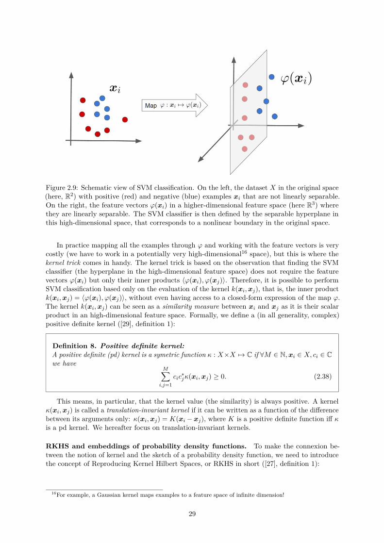
Figure 2.9: Schematic view of SVM classification. On the left, the dataset X in the original space(here, R2) with positive (red) and negative (blue) examples xi that are not linearly separable.On the right, the feature vectors ϕ(xi) in a higher-dimensional feature space (here R3) wherethey are linearly separable. The SVM classifier is then defined by the separable hyperplane inthis high-dimensional space, that corresponds to a nonlinear boundary in the original space.

In practice mapping all the examples through ϕ and working with the feature vectors is verycostly (we have to work in a potentially very high-dimensional16 space), but this is where thekernel trick comes in handy. The kernel trick is based on the observation that finding the SVMclassifier (the hyperplane in the high-dimensional feature space) does not require the featurevectors ϕ(xi) but only their inner products 〈ϕ(xi), ϕ(xj)〉. Therefore, it is possible to performSVM classification based only on the evaluation of the kernel k(xi,xj), that is, the inner productk(xi,xj) = 〈ϕ(xi), ϕ(xj)〉, without even having access to a closed-form expression of the map ϕ.The kernel k(xi,xj) can be seen as a similarity measure between xi and xj as it is their scalarproduct in an high-dimensional feature space. Formally, we define a (in all generality, complex)positive definite kernel ([29], definition 1):

Definition 8. Positive definite kernel:A positive definite (pd) kernel is a symetric function κ : X×X 7→ C if ∀M ∈ N,xi ∈ X, ci ∈ Cwe have

M∑i,j=1

cic∗jκ(xi,xj) ≥ 0. (2.38)

This means, in particular, that the kernel value (the similarity) is always positive. A kernelκ(xi,xj) is called a translation-invariant kernel if it can be written as a function of the differencebetween its arguments only: κ(xi,xj) = K(xi −xj), where K is a positive definite function iff κis a pd kernel. We hereafter focus on translation-invariant kernels.

RKHS and embeddings of probability density functions. To make the connexion be-tween the notion of kernel and the sketch of a probability density function, we need to introducethe concept of Reproducing Kernel Hilbert Spaces, or RKHS in short ([27], definition 1):

16For example, a Gaussian kernel maps examples to a feature space of infinite dimension!

29

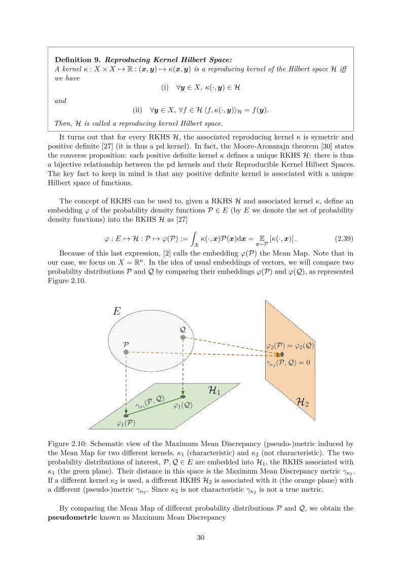
Definition 9. Reproducing Kernel Hilbert Space:A kernel κ : X ×X 7→ R : (x,y) 7→ κ(x,y) is a reproducing kernel of the Hilbert space H iffwe have

(i) ∀y ∈ X, κ(·,y) ∈ H

and(ii) ∀y ∈ X, ∀f ∈ H 〈f, κ(·,y)〉H = f(y).

Then, H is called a reproducing kernel Hilbert space.

It turns out that for every RKHS H, the associated reproducing kernel κ is symetric andpositive definite [27] (it is thus a pd kernel). In fact, the Moore-Aronszajn theorem [30] statesthe converse proposition: each positive definite kernel κ defines a unique RKHS H: there is thusa bijective relationship between the pd kernels and their Reproducible Kernel Hilbert Spaces.The key fact to keep in mind is that any positive definite kernel is associated with a uniqueHilbert space of functions.

The concept of RKHS can be used to, given a RKHS H and associated kernel κ, define anembedding ϕ of the probability density functions P ∈ E (by E we denote the set of probabilitydensity functions) into the RKHS H as [27]

ϕ : E 7→ H : P 7→ ϕ(P) :=∫Xκ(·,x)P(x)dx = E

x∼P[κ(·,x)] . (2.39)

Because of this last expression, [2] calls the embedding ϕ(P) the Mean Map. Note that inour case, we focus on X = Rn. In the idea of usual embeddings of vectors, we will compare twoprobability distributions P and Q by comparing their embeddings ϕ(P) and ϕ(Q), as representedFigure 2.10.

Figure 2.10: Schematic view of the Maximum Mean Discrepancy (pseudo-)metric induced bythe Mean Map for two different kernels, κ1 (characteristic) and κ2 (not characteristic). The twoprobability distributions of interest, P,Q ∈ E are embedded into H1, the RKHS associated withκ1 (the green plane). Their distance in this space is the Maximum Mean Discrepancy metric γκ1 .If a different kernel κ2 is used, a different RKHS H2 is associated with it (the orange plane) witha different (pseudo-)metric γκ2 . Since κ2 is not characteristic γκ2 is not a true metric.

By comparing the Mean Map of different probability distributions P and Q, we obtain thepseudometric known as Maximum Mean Discrepancy

30

γκ(P,Q) = ‖ϕ(P)− ϕ(Q)‖H (2.40)

and it is thus in general not a metric since the mean map is in general not injective, i.e., it ispossible to have P 6= Q but γκ(P,Q) = 0 (see for example the kernel κ2 in Figure 2.10: twodifferent pdfs or points in E could map to the same point in the space H2). A kernel κ inducingan injective Mean Map and hence for which γκ is a true metric, in other words a kernel for whichP = Q ⇔ γκ(P,Q) = 0, is called a characteristic kernel ([31], definition 6). In what follows,having a characteristic kernel will thus be a desirable property since we to obtain a true metricfor the probability density functions.

How the sketch approximates the MMD metric. We are not far from the link betweenthe MMD abd the sketch of a probability distribution, but we need one additional theorem ([32],Theorem 1.4.3):

Theorem 3. Bochner’s theorem: for a continuous function K(u)

K(u) : Rn 7→ C is a positive definite kernel ⇐⇒

K(u) =∫Rne−iωTuΛ(ω)dω for a finite nonnegative measure Λ

(2.41)

where the latter expression means that the translation-invariant kernel K(u) is the Fouriertransform of a finitea measure Λ on Rn.

aThis means that∫Rn dΛ(ω) <∞.

Thus, every positive definite kernel is the Fourier transform of a nonnegative measure Λ,that can in particular be normalized to a probability density function (this implies a kernelnormalization). A translation-invariant positive definite kernel is thus the Fourier transformof a probability density function Λ(ω) on the frequencies ω ∈ Rn. Moreover, a condition on Λguarantees that κ is characteristic17, thus defining a true metric γκ ([31], Theorem 9):

Theorem 4. Characterization of characteristic translation-invariant kernels:

A positive definite kernel κ(x,y) = K(x− y) is characteristic ⇐⇒supp(Λ) = Rn, i.e. ∀ω ∈ Rn, Λ(ω) > 0

(2.42)

with Λ defined in Theorem 3.

As last step before coming to the sketch, we need a corollary of Theorem 3 that re-writesthe γκ metric (that we will from now on also write, by abuse of notation, γΛ since there is abijective relation between κ and Λ) as a function of the frequency distribution Λ related to κ([31], Corollary 4):

γΛ(P,Q) := γκ(P,Q) =√∫

Rn|ψP(ω)− ψQ(ω)|2Λ(ω)dω, (2.43)

where ψP(ω) is the characteristic function of the pdf P. The interesting link between thesketch operator A and the frequencies ωj

iid∼ Λ is that the sketch distance ‖AP − AQ‖2 is anapproximation of the γκ metric [2]:

17In fact, Theorem 4 implies that the third frequency sampling heuristic ΛAr defines a kernel that is notcharacteristic since ΛAr(0) = 0⇒ supp(ΛAr) = Rn \ 0. However this frequency distribution produces good resultsin practice, this can be intuitively explained by the fact that for all characteristic functions, the value af ω = 0 is 1.

31

1m‖AP −AQ‖22 = 1

m

m∑j=1|ψP(ωj)− ψQ(ωj)|2 ' E

ω∼Λ|ψP(ω)− ψQ(ω)|2 = γ2

Λ(P,Q), (2.44)

where the approximation holds for, by law of large numbers, whenm is large enough (the empiricalmean concentrates around the true mean). This link betwen the sketch A and the RKHS Hwith kernel κ being the Fourier transform of the frequency sampling pattern of the sketch isrepresented Figure 2.11. The key fact is here that the sketch distance is an approximation ofthe MMD metric γΛ defined of the probability distributions that are sensed by the sketch. Thechoice of Λ determines the particular nature of the metric used to discriminate the pdfs and isthus a crucial parameter in the sketch design.

Figure 2.11: This figure represents how the sketch approximates the γκ metric. We want tocompare the two probability density functions P and Q ∈ E (top left). The way we acquire thosedistributions is by the sketh operator A, we thus only have access to the m-dimensional vectorsAP and AQ (on the right). However, for m large enough, the distance between those vectorsapproximates the γκ metric in the RKHS H (bottom left) defined by the frequency selectingpattern Λ (since κ is the Fourier transform of Λ).

Remark. As we will see, when designing the frequency distribution of a sketch, we are not reallyinterested in the high-frequency content and it is desirable to have Λ(ω)→ 0 as ‖ω‖ → ∞. Inthis optic, Theorem 4 is "bad news" since it forbids us to have, e.g., Λ(ω) = 0 for ‖ω‖ ≥ R0 forsome radius R0, which would be a nice property for the frequency sampling pattern.

Since in the sketching framework we are selecting Λ (that defines a kernel through Bochner’stheorem) based on a small subset of the dataset rather than -such as in traditional machinelearning approached- choosing the kernel κ based on a computationally-intensive cross-validationprocedure (basically, testing out a lot of different kernels and picking the best), the selectionof the frequency distribution can be seen as an "implicit kernel design", and it turn out to becompetitive with kernel design by cross validation in terms of performances while being muchmore faster [2]. In chapter 4, we come back to the kernel to make an interesting interpretation ofthe objective function of compressive clustering in regard of the kernel. We now start from therather abstract connexions between RKHS and the sketch to explain more intuitively what thismeans, in particular in the case of CKM where P and Q are mixtures of Dirac deltas.

32

The filter interpretation

At this point, the MMD metric might seem a little bit abstract. In addition to this, it mightseem surprising, in the CKM algorithm, to try to reconstruct (or approximate) the sketch of thedata distribution by a mixture of K Dirac delta functions although it is obvious that the trainingexamples can take more than K different values, so the mixture of K deltas is clearly "wrong"given the dataset. In this subsection we bring a new interpretation ("the filter interpretation") ofthe sketch that brings answers to those questions.

Figure 2.12: The interpretation of the Mean Map as a filtering of the empirical distribution of thedataset P and the distribution of weighted centroids Q (here there are three centroids, and wehave one-dimensional data). The Maximum Mean Discrepancy metric compares the low-frequencycontent of the probability density functions (or the convolution of those distributions with thekernel K(d)).

The filter interpretation is summarized Figure 2.12. In fact, the Mean Map ϕ(P) associatedwith a translation-invariant kernel κ(x,y) = K(x− y) corresponds to the convolution of P withthe kernel K (note that K is symetric):

ϕ(P)(x) =∫RnK(x− y)P(y)dy = K(x) ∗ P(x), (2.45)

meaning that, in other words, the mean map is a filtering of the input probability distribution Pwith a filter whose frequency response is given by Λ(ω). Given the shape of ω, we use low-passfilters to modify the probability distributions, then compare the filtered versions. For mixture ofdeltas in particular, we can hope that the filtered probability distributions are comparable eventhough the probability distributions are quite different (see Figure 2.12, bottom). With a goodfilter (i.e., a good choice of Λ) the filtered empirical probability distribution should approximatethe true probability distribution of the data, and the filtered mixture of clusters (deltas) shouldmodel this distribution approximatively.

33

Random Fourier Features

As seen above, the RKHS approch to matching probability distributions compares the probabilitydistrubtions through the MMD metric γκ for a kernel κ, and we have argued that the sketchdistance approximates this metric γκ. The nature of this approximation is best understood inthe light of Random Fourier Features, a method for approximating kernels.

Random Fourier Features [33] is method that maps input vectors x,y ∈ Rn to m-dimensionalvectors z(x), z(y) ∈ Rm for approximating translation-invariant kernels κ(x,y) = K(x − y).Building on Bochner’s theorem (Theorem 3), which can be re-written as

K(x− y) =∫Rn

Λ(ω)e−iωT (x−y))dω = Eω∼Λ

[e−iωTx

(e−iωT y

)∗](2.46)

and focusing on real kernels, the Random Fourier Feature vector z is defined as

z(x) =√

2m

[cos(ωT1 x+ ξ1), · · · , cos(ωTmx+ ξm)

]Twhere ωj

iid∼ Λ(ω), ξjiid∼ U([0, 2π]).

(2.47)The approximation of the kernel is achieved through the scalar product of the Fourier features

of the different input vectors

K(x− y) ' z(x)Tz(y) (2.48)

where z(x)Tz(y) can be seen as an unbiased estimator of the kernel K(x− y). The probabilityof committing a fixed error P

[|K(x− y)− z(x)Tz(y)| ≥ ε

]decreases exponentially with the

dimension of the features m , i.e., the estimator converges uniformly [33]. The Random FourierFeatures idea is to use the features z(x) instead of the much higher dimensional feature mapϕ(x), allowing to with feature vectors in a much lower dimension (as we saw, this was unnecessaryfor SVM learning for example since we then do not need the feature vectors).

The sketch of a dataset can be seen as the pooling (sum) of the Random Fourier Featuresof the whole dataset (except we are replacing the cosine function by the complex exponential).Another difference between sketching algorithms such as CKM and RFF it the fact that RFFare sampling the frequencies from the inverse Fourier transform of a data-independent kernelimposed a priori (that is the main drawback of RFF compared to other and better performingkernel approximation approaches such as the Nyström method [34]) while the sketch operatorchooses the frequency distrubtion conditionally on a small observation of the data. In Chapter 4,we come back to the connexions with RFF when we study the true objectife function of CKM andits variants.

34

Chapter 3

Clustering with a 1-bit quantizedsketch

In this chapter we present the main goal of this thesis: performing a version of compressiveclustering such as in [1] but using the universal quantization function (also called "a square wave")as non-linear periodic signature function for constructing the sketch, instead of the complexexponential. We present the QCKM algorithm that solves this problem, and technical questionsabout this algorithm motivates the study of generalized sketches in Chapter 4.

3.1 Motivation and challenges

3.1.1 Introducing the quantized sketch and motivations

Definition

Recall that the sketch Sk of a generic dataset Y = [y1, ...,yL] where each column correspondsto one example, is given by a pooling over the L examples of the complex exponential of theexamples at different frequencies given by Ω = [ω1, ...,ωm]:

Sk (Y,β) =[L∑l=1

βle−iωTj yl

]mj=1

= exp(−iΩTY )β ∈ Cm, (3.1)

with associated weigths β = [β1, ..., βL]T , βi ≥ 0 and∑i βi = 1. The objective of this thesis is to

replace the complex exponential e−it "signature function" by the universal quantization Q∆(t)defined as (2.15) with some quantization step ∆. We also introduce, inspired by [21] a randomdither ξ with components ξj ∼ U(0,∆). The quantized sketch SkQ then becomes

SkQ (Y,β) =[L∑l=1

βlQ∆(ωTj yl + ξj)]mj=1

= Q∆(ΩTY + ξ1TL)β ∈ [−1, 1]m, (3.2)

where we note that the sketch values are now real and in the interval [−1,+1]. The sketch is thus apooling -a sum- over the whole dataset of the 1-bit universal quantization of random projections ofthe high-dimensional signals (with an additional dithering). In contrast to Compressive K-Means(CKM) that uses the complex exponential, we name our new clustering approach QuantizedCompressive K-Means (QCKM). Defore diving into the implications of doing such a thing wewill first discuss why it could be a good idea.

Quantized sketch: why?

In the compressed k-means (CKM) approach [1], clustering can be performed in a time that isindependent of the size of the dataset (the amount of data), given that the sketch is already

35

known. Actually, for very large datasets, computing the sketch becomes the task that is themost computationally demanding, but with the advantage that computing the sketch is a heavilyparallelizable task. However, the current approach of CKM still assumes that the whole datasetis at one point acquired (although the sketch can be computed on-line, i.e. it is possible to aquireone example at a time and to forget it once its contribution to the sketch has been computed).Keeping the motivations that led to the theory of CS in mind, this seems to be a huge waste ofdata acquisition at the sensing step. We are thus investigation the feasability of a sensor (like[13] and [14]) that would, instead of acquiring the signals xi, compute their contribution to thesketch directly (in other words, we want to short-cut the "data acquisition" step).

Using the existing sketch, a sensor computing the usual sketch of a signal x should thus computee−iΩTx with Ω ∈ Rn×m, where the operation e−it is complicated to perform directly in hardware.On the other hand, computing Q∆(t) should be much easier to implement in an hardware sensor.Although this is beyond the scope of this work, ADC technologies such as pipelined (or "folding")ADCs [35], [36] and self-reset ADCs [37],[38] could here be an interesting starting point. We thusbelieve that computing Q∆(ΩTx+ ξ) instead of e−iΩTx is much easier to do in hardware, whichis the main motivation to introduce the new sketch SkQ. The actual design of such an efficientsensor is beyond the scope of this work but an important open question to keep in mind. Webelieve that changing the signature function e−it by another will not nullify the possibility touse the sketch to retrieve the centroids, as long as the signature function is periodic, such as Q∆(t).

Could it work?

At first, the (quantized) sketch of a dataset might seem rather strange, and the reader mightwonder how the sketch could convey the information needed to perform clustering. We givehere a reassuring geometric intuitive interpretation of the information captured by the sketch(quantized or not) by numerical illustrations on a toy example.

In Figure 3.1, the objective function to find the first centroid (step 1) of both the CKMalgorithm and the QCKM algorithms are compared for different sketch sizes m, for a Gaussianradius frequency sampling adapted to each case (we use the sampnling (Gr) and (Gr-h), seelater). The first row (m = 1) shows how we can interpret the contribution of one single coefficientj of the sketch to the objective: it attracts the centroid to positions (the blue region) wheremore data samples are located when projected on the waveform w(c) = (Aδc)j , and we obtainrespectively a sinusoidal and a squared wave-shaped objective function.

When adding coefficients to the sketch (the three following rows), different sketch coeffiencts,that is, correlations with different waveforms are combined to refine the objective function. Toobtain a "good" objective function fast enough (for m small enough), selecting the frequencies isin fact a crucial step of the sketching procedure. The frequencies must not be too small, nor toohigh, in order to locate the clusters accurately for acceptable values of m: the frequencies must,in fact, be adapted to the size of the clusters.

The reassuring observation is that the objective function of QCKM contains enough informationto find the good centroids (for m = 1000). From Figure 3.1 we can also already guess, as we willformally observe in Chapter 5, that the number of frequencies m to obtain a good estimationof the centroids is, at least for the current choices of freqeuncy distributions, higher for QCKMthan for CKM. Indeed for m = 100 the minima of CKMs objective function are very close to thetrue centroids, unlike QCKMs objective function. A final comment to be made is the fact that theobjective function of CKM is very smooth while the one of QCKM is a "stairsteps-shaped" objectivefunction.

36

Figure 3.1: Evolution of the objective function to find the first centroid on a 2-dimensional toyexample with CKM (left) and QCKM (right) and for different amounts of frequencies, from top tobottom: m = 1, 10, 100, 1000. The minima of the objective functions are the blue regions, andthe big red dots represents the dataset X.

37

3.1.2 Quantized sketching in practice with QCKM and its challenges

Although we have shown, at least intuitively for now, that provided its dimension m is highenough the quantized 1-bit sketch contains the information necessary to find centroids, we havenot yet addressed how the centroids can be found in practice. Adapting the CKM algorithm(algorithm 5) to our quantized sketch raises some technical questions:

• How should one choose the parameters of the sketch SkQ (Y,β) as defined (3.2)? Inparticular, what quantization step ∆ must be chosen? How should the random "frequencies"Ω be drawn? How many frequencies m shoud be used?

• How should one adapt the CKM algorithm to account for the discontinuous nature ofthe quantizer? As mentioned when we presented it in Chapter 2, CKM relies on solvingoptimization problems in a continuous space, that are solved with quasi-Newton methodsthat require the gradient of the objective function. Unfortunately in QCKM, the quantizedsketch version of CKM, the objective function becomes discontinuous with respect to thedecision variables, and the gradient of this function is therefore ill-defined.

Leaving aside those questions for the next section, the QCKM algorithm is presented below,indexed as algorithm 6. The differences with CKM are highlighted. Note in particular that thenorm of the quantized vector of a centroid c is always ‖SkQ (c, 1) ‖ =

√∑mj=1(±1)2 =

√m so we

drop it from the problem.

3.2 Solutions to the challenges

3.2.1 Parameters of the sketch

We answer here how the quantized sketch should be constructed, in particular, how to choosethe parameters ∆, Ω and m. The choice of the two latter parameters are in fact coming fromresults in Chapters 4 and 5, but for the sake of completeness of this section we already presentthe conclusions here.

Quantization stepsize ∆

How should the quantizer stepsize ∆ be chosen, given that the sketch entry j records the poolingof the values Q∆(ωTj xi + ξj)? Actually, it is interesting to note that, from the definition ofuniversal quantization, Q∆(t) = Q1( t∆), therefore for ∆ 6= ∆′,

Q∆(ωTj xi + ξj) = Q1

(ωTj xi

∆ + ξj∆

)= Q∆′

(∆′

∆ (ωTj xi) + ∆′

∆ ξj

)= Q∆′

(ω′Tj xi + ξ′j

)(3.3)

with ξj ∼ U([0,∆]), ξ′j ∼ U([0,∆′]) and ω′j = ∆′∆ ωj . What (3.3) means is that changing the

stepsize ∆ does not modify the sketch if the frequencies ωj are scaled proportionally. Thisis of course reminiscent of [23] where the embedding properties only depend on ∆

σ and noton ∆ alone. Note that it is also possible to obtain the same sketch for a different ∆′ byscaling the dataset x′i = ∆′

∆ xi instead of scaling the frequencies. In short, choosing ∆ arbi-trarily has no impact on future discussions as long as we keep in mind that we do possiblyneed to rescale the frequencies or the dataset, and the whole "decision" can be put in this rescaling.

Without loss of generality, we will therefore choose ∆ = π, resulting in a signature functionQ∆(t) that has the same period (T = 2π) as e−it, the signature function in CKM. This will alsosimplify notations in the Fourier series expressions in Chapter 4.

38

Algorithm 6: QCKM : CKM adapted to 1-bit sketches relying on universal quantization.input :Empirical quantized sketch z = SkQ (X,1N/N), frequencies Ω, number of

centroids K, bounds l, uoutput :A set of centroids C and weights α that locally minimizes the quantized sketch

mismatch ‖z − SkQ (C,α) ‖221 Initialization r ← z, C ← ∅ (Initialize the residual and the support (centroids)) ;2 for t = 1,...,2K do3 Step 1 : find the new centroid c with highest correlation with residual by solving

approximatively the discontinuous problem:4 c ' arg maxc < SkQ (c, 1) , r > s.t. l ≤ c ≤ u (The sketch is always real)5 Step 2 : add it to the support:6 C = C ∪ c7 Step 3 : Reduce support by Hard Thresholding to keep sparsity ("Replacement" step):8 if |C| > K then

9 β = arg minβ∈R|C|+

∥∥∥∥z −∑|C|k=1 βkSkQ (ck, 1)∥∥∥∥

210 C ← set of K centroids ck corresponding to K largest magnitude values of β11 end12 Step 4 : Find the optimal coefficients given the support (by projection):

13 α = arg minα∈R|C|+

∥∥∥∥z −∑|C|k=1 αkSkQ (ck, 1)∥∥∥∥

214 Step 5 : Global gradient descent by solving approximatively the discontinuous

problem:

15 (C,α) ' arg minC,α∥∥∥∥z −∑|C|k=1 αkSkQ (ck, 1)

∥∥∥∥2

s.t. l ≤ c ≤ u

16 r = z −∑|C|k=1 αkSkQ (ck, 1) (Update residual, go back to step 1)

17 end

Drawing the random projections vectors or "frequencies" Ω

With ∆ = π, the "sensing functions" used in CKM and QCKM are, for the same frequencies Ω, nottoo different (we replace the complex exponential by a real square wave, but the frequency ofthose sensing functions is the same). We show in Chapter 5 that re-using the frequencies Ω fromCKM in QCKM does indeed yield decent results, but is it possible to do better?

In CKM, the frequencies Ω = [ω1, · · · ,ωm] are drawn from a distribution ωjiid∼ Λ where Λ(ω)

is one of the three heuristic that matches, in "distilled sensing-like" approach, some small sampleof the dataset. Using the Fourier series decomposition of the sketch, we transpose in Chapter 4the heuristic choices of Λ(ω) in CKM to QCKM, obtain new frequency densities ΛQ(ω) adapted tothe universal quantization signature function. In Chapter 5 we show that the performances ofQCKM with ΛQ(ω) are improved compared to using Λ(ω).

Number of frequencies m

Empirically, it has been shown that CKM requires m = O(nK) frequencies to produce clusteringresults that compete with the state-of-the-art k-means++ algorithm [1]. In particular m isindependent of N , the number of training examples, which makes CKM a particularly appealingstrategy for very large datasets. In this work we show -empirically again- in Chapter 5 thatfor QCKM, the rule m = O(nK) still hold, but with a higher hidden constant: more precisely weobserve the rule mQCKM & 20...50mCKM in order to obtain similar clustering performances.

39

3.2.2 From CKM to QCKM: optimization of discontinuous objective functions

As illustrated Figure 3.1, in QCKM the objective functions of the optimization problems to solvebecome discontinuous and therefore non-differentiable and L-BFGS can’t be used as optimizationroutine. To circumvent this problem, we propose two strategies that approximate the objectivefunction by a differentiable approximation, hence allowing us to compute a gradient and to solvethis approximated problem with the L-BFGS method.

Strategy 1: Smoothing the universal quantization operator with a filter

The first strategy porposed consists in smoothing the discontinuous function. The only part ofthe gradients of CKM that we need to modify (those gradients are computed Appendix B.1) isthe Jacobian of the sketch of a single centroid c : we need ∇cSkQ (c, 1) = ∇cf(ΩTc+ ξ) withf(t) = Q∆(t). With the chain rule it comes

∇c (SkQ (c, 1))j = ∇cf(ωTj c+ξj) = ∂f(t)∂t

∣∣∣∣t=ωTj c+ξj

·∇c

(ωTj c+ ξj

)= ωj

∂f(t)∂t

∣∣∣∣t=ωTj c+ξj

(3.4)

where we have a problem since f(t) is discontinuous hence technically not differentiable. In fact,we can express ∂f(t)

∂t theoretically with Dirac delta functions using the expression of f(t) = Q∆(t)as a combination of step functions (2.16):

f(t) = 2∑k∈Z

(−1)ku(t− k∆)⇒ ∂f(t)∂t

= 2∑k∈Z

(−1)kδ(t− k∆) (3.5)

but this expression is of course not applicable in a practical algorithm on a computer. We proposethus to smoothen f(t) by convolution with a function g(t) to obtain f(t) = f(t) ∗ g(t), and wecan then replace

∂f(t)∂t

' ∂f(t)∂t

= ∂

∂t(f(t) ∗ g(t)) = ∂f(t)

∂t∗ g(t) = 2

∑k∈Z

(−1)kg(t− k∆). (3.6)

The function g(t) should satify∫R g(t)dt = 1 in order to leave the DC component of f(t)

untouched (if f(t) is a constant, f(t) should yield the same constant). We can also see thisstrategy as computing a moving average of f(t) before differentiation, with weights given by g(t).

For example, we can chose g(t) to be 0 everywhere except in t ∈ [−ε,+ε] where it is constant;this is equivalent to replace the disconinuity of by a linear slope of steepness ε. The parameter εcan in theory be chosen arbitrarily small but in practice, it should be chosen large enough inorder to avoid numerical instabilities.Remark. Since the second strategy that we present hereafter is more interesting to study from atheoretical point of view (see Chapter 4), we will focus on the second strategy in the followingchapters. However, this first strategy has also been implemented in Matlab and yields decentresults, so it is a viable strategy that could be considered in real applications, even though wewon’t come back to it in the rest of this work.

Strategy 2 : Approximating the universal quantization as a Fourier series

We present here another way to construct f(t), a smooth approximation of f(t) = Q∆(t) toreplace ∂f(t)

∂t by ∂f(t)∂t . Since f(t) is periodic with period T = 2∆, it can be written as a Fourier

series with coefficients given by Proposition 1.

40

Proposition 1. The Fourier series coefficients of the universal quantization func-tion. The universal quantization function f(t) = Q∆(t), of period T = 2∆ can be written ina Fourier series

f(t) =+∞∑

k=−∞Fke

i 2π2∆kt =

+∞∑k=−∞k odd

2ikπ

ei π∆kt (3.7)

where the Fourier series coefficients coefficients are independent of ∆ and given by

Fk =

0 if k is even,2ikπ if k is odd.

(3.8)

Proof. By definition, the Fourier coefficients are (with T = 2∆)

Fk = 1T

∫ T

0f(t)e−ik 2π

Ttdt = 1

T

∫ ∆

0(−1)e−ik 2π

Ttdt+ 1

T

∫ 2∆

∆(+1)e−ik 2π

Ttdt

= 1T

[+1

ik 2πT

e−ik 2π2∆ t

]∆

0+ 1T

[−1

ik 2πT

e−ik 2π2∆ t

]2∆

∆

= 1ik2π

(e−ikπ − 1

)− 1

ik2π(1− e−ikπ

)= ikπ

(1− (−1)k

)=

0 if k is even,2ikπ if k is odd.

(3.9)

We thus construct the approximation f(t) as a truncated Fourier series, where we truncatethe infinite summation on k to Kcoef coefficients:

f(t) =Kcoef∑

k=−Kcoef

Fkei 2π2∆kt (3.10)

with Fk the coefficients in Proposition 1. We leave an extensive discussion of this strategy forthe next chapter where we replace the signature function of the sketch by any periodic function,i.e. any function that can be represented as a Fourier series. Empirical results of strategy 2 arethen presented in Chapter 5.

41

Chapter 4

Generalized sketches using anyperiodic signature function

As seen in Chapter 2, it is possible with the CKM algorithm to obtain the centroids defining theclustering of a dataset from a nonlinear sketch of this dataset. This sketch is the result of poolingthe complex exponential of the examples xi (vectors in Rn) at m different frequencies ωj overthe whole dataset X containing N examples:

SkΩ (X,1N/N) =[

1N

N∑i=1

e−iωTj xi]mj=1

= 1Ne−iΩTX1N ∈ Cm (4.1)

where Ω = [ω1 · · ·ωm] ∈ Rn×m is the frequencies matrix and X = [x1 · · ·xN ] ∈ Rn×N is thedataset. Note that we added a subscript Ω to the sketch symbol to avoid confusion in the restof this chapter. In Chapter 3, we suggested to modify this sketch by replacing the signaturefunction of the data, the complex exponential e−it, by the universal quantization function Q∆(t),arguing that the key ingredient of a signature function is its periodicity.

In this context, we will in this chapter study what happens when the signature function isany periodic function f(t) of period T . Then, in the second section of this chapter, we will applythe results found in the general case to the universal quantization function to get new insightsabout the quantized sketch scenario. This will allow us in particular to propose new heuristicsto select the frequencies of the sketch, heuristics that are adapted to the modified signaturefunction. Finally, in the third section of this chapter, we will list and characterize the differenterror terms that appear in the whole compressed learning scheme.

4.1 Theoretical results for a general periodic signature function

4.1.1 Generalized sketching operator

Changing the sketching operator changes the way the information about the probability densityfunction of interest P is captured. In this section we show that the generalized sketch capturesmore high-frequency content information about P than the usual sketch, and that the sketchis not, as before, a sampling of the Fourier transform of P but a generalized transorm witharbitrary (periodic) basis functions.

Sketch from the data First, we are going to see what changes in the sketch that we computefrom the data. When we replace the complex exponential by a generic periodic functionf(t) : R→ C of period T , we obtain a new sketch:

42

SkΩ,ξ (X,1N/N) =[

1N

N∑i=1

f(ωTj xi + ξj)]mj=1

= 1Nf(ΩTX + ξ1TN )1N ∈ Cm (4.2)

where, by abuse of notation, f is applied component-wise in the outer right handside. In thiscase, we have added a random dither ξ with iid entries uniformly distributed between 0 and theperiod of f , i.e. ξj

iid∼ U([0, T ]), for reasons that will become clear later on.

Since f(t) is a periodic function, it can be expanded as a Fourier series with coefficientsFk ∈ C:

f(t) =∞∑

k=−∞Fke

ik 2πTt where Fk = 1

2π

∫ T

0f(t)e−ik 2π

Ttdt. (4.3)

Keeping this expansion in mind, the sketching operator using f(t) as signature function can bere-written (as a reminder, is the Hadamard product or "componenent-wise" product betweenvectors or matrices):

SkΩ,ξ (X,1N/N) =[

1N

N∑i=1

f(ωTj xi + ξj)]mj=1

=

1N

N∑i=1

+∞∑k=−∞

Fkeik 2π

T(ωTj xi+ξj)

mj=1

=+∞∑

k=−∞Fk

[1N

N∑i=1

eik 2πTωTj xieik 2π

Tξj

]mj=1

=+∞∑

k=−∞Fk

[1N

N∑i=1

eik 2πTωTj xi

]mj=1[eik 2π

Tξj]mj=1

=+∞∑

k=−∞Fk Sk−k 2π

TΩ (X,1N/N) eik 2π

Tξ

(4.4)

The last line relates the new sketch operator SkΩ,ξ (X,1N/N) that uses a general periodicfunction f to the usual sketch SkΩ (X,1N/N) that uses the complex exponential. This newsketch consists in a sum of the usual sketches over multiples of the frequency set Ω, weighted bythe Fourier coefficients Fk, and with an additional argument shift of k 2π

T ξj for each component j.

Sketching a probability distribution The previous paragraph shows how to compute thesketch of a set of points, but what really interests us for a theoretical analysis is the sketchingoperator AΩ defined on a probability distribution P (that is approximated by the sketch of thedataset of realisations of this distribution). As a reminder, the usual sketching operator AΩPlinear with respect to probability distributions P is a sampling of the characteristic functionψP(ω), so we have

AΩP =[Ex∼P

e−iωTj x]mj=1

=[∫

Rne−iωTj x P(x)dx

]mj=1

= [ψP(ωj)]mj=1 (4.5)

where the frequencies are drawn from some distribution ωjiid∼ Λ. In our generalization context,

we replace e−it by f(t), and add a dither term, so the new operator becomes

AΩ,ξP =[Ex∼P

f(ωTj x+ ξj)]mj=1

=[∫

Rnf(ωTj x+ ξj) P(x)dx

]mj=1

.

Similarly to what we did with the data sketch, we can re-write this sketch as a function of theusual sketching operator by writing f(t) in its Fourier series form:

43

AΩ,ξP =

Ex∼P

+∞∑k=−∞

Fkeik 2π

T(ωTj x+ξj)

mj=1

=

+∞∑k=−∞

Fkeik 2π

Tξj Ex∼P

eik 2πTωTj x

mj=1

=+∞∑

k=−∞Fk

[eik 2π

Tξj ψP

(−k2π

Tωj

)]mj=1

=+∞∑

k=−∞Fk[eik 2π

Tξj]mj=1 A−k 2π

TΩ.

In words, the generalized sketching operator AΩ,ξP is computing:

1. the usual sketches AΩP but where we changed the frequencies ωj ∈ Ω by all differentmultiples of −2π

T ωj ,

2. then each component of those sketches are affected by a (random) phase shift due to themultiplication by eik 2π

Tξj (different for each multiple k and component j),

3. finally, the phase-shifted sketches at all multiples of −2πT ωj are summed over all multiples

k with complex weights Fk, the Fourier coefficents of the signature function.

In short, we can interpret the new sketch as a weighted sum of the old sketches at differentfrequencies. This new sketch "captures" therefore the information about P at higher frequenciesthan the original sketch. Note that we still have a link between A and SkΩ,ξ (X,1N/N), sinceAP = SkΩ,ξ (X,1N/N) if P(x) = 1

N

∑xi∈X δ(x − xi) is the empirical probability distribution

function of the dataset X.

Coming back to the interpretation where the sketch of a probability density function Pcomputes generalized moments of P [26], based on given functions Mj defining the moments, wehad previously that

AΩ : P 7→ AΩP := 1√m

[∫RnM1dP, · · · ,

∫RnMmdP

]Twith Mj(x) =

√m e−iωTj x, (4.6)

we can also now interpret our new sketching operator as a computation of different momentsbased on new functions M j , that we will try to match as in GeMM:

AΩ,ξ : P 7→ AΩ,ξP := 1√m

[∫RnM1dP, · · · ,

∫RnMmdP

]Twith M j(x) =

√m f(ωTj x+ ξj).

(4.7)Before we chose particular moments that corresponded to a sampling of the characteristic functionof the random variable from which the learning example are realizations. Now we are replacingthe characteristic function by something else. For example, in the context of QCKM, instead ofcomputing samples of the Fourier transform of P, we could say that we are sampling anothertransform of P, a transform that uses square-shaped basis functions instead of sinusoidal ones;we will note this transform S (for Square).

44

4.1.2 Generalized objective function in the optimization problem

In the logical continuation of the description of AΩ,ξP , the new way we are sensing a probabilitydistribution P, we observe how this affects the general "sketch matching" optimization problemto solve

Q∗ = arg minQ‖AΩ,ξP −AΩ,ξQ‖22 s.t. Q ∈ GK . (4.8)

We first explain how the sketch distance in (4.8) captures the mismatch between a transformof the probability density functions that can be seen as a generalized characteristic function,then how the objective function is a weighted sum of the usual sketch distances. Finally weexplain how the γ-metric between probability distributions is changed. In a later section wecome back to the objective function applied to the particular case of clustering (where the pdfsare mixtures of deltas) in the light of the generalized sketch kernel.

Previously (in (2.44)), we have seen that the objective function, the `2-norm of the differencethe sketches of probability distributions P and Q, is (up to a factor m) the empirical meanamplitude squared of the difference of probability characteristic functions P and Q. This empiricalmean thus approximates, by law of large numbers, the true mean taken over the random variableω (that we called the γ distance):

1m‖AΩP −AΩQ‖22 = 1

m

m∑j=1|ψP(ωj)− ψQ(ωj)|2 ' Eω∼Λ

[|ψP(ω)− ψQ(ω)|2

](4.9)

with ψν is the characteristic function of the probability distribution function ν. In our case,we have (AΩ,ξP)j =

∑k Fke

ik 2πTξj ψP

(−k 2π

T ωj), thus, the distance between the sketches of

probability distrubtions P and Q gives (by comparing the empirical average with the trueexpectation)

1m‖AΩ,ξP−AΩ,ξQ‖22 = 1

m

m∑j=1

∣∣∣ψP(ωj ; ξj)− ψQ(ωj ; ξj)∣∣∣2 ' E

ω,ξ

[∣∣∣ψP(ω; ξ)− ψQ(ω; ξ)∣∣∣2] (4.10)

where we define the following ("generalized characteristic") function of ω with parameter ξ

ψP(ω; ξ) = Ex∼P

f(ωTx+ ξ) =∑k

Fkeik 2π

TξψP(−k2π

Tω). (4.11)

The main point here is that the sketch of the data defines the distance measure that we will use tocompare the probability distributions P and Q, so a new sketch means a different distance measure(we will come back to this when developping the generalized γ-distance). This shows clearly thatwe are generalizing the characteristic function ψP (i.e. the Fourier transform of P) by replacing itwith a more general function ψP that projects P(x) on generic periodic basis functions f(ωTx+ξ).

It is possible to show that the generalized sketch objective function is a weighted sum of theusual sketch objective function at different frequencies by developping (4.10) a little bit further.This will be useful to characterize the impact of truncating the Fourier series at the end of thischapter.

Proposition 2. The objective function of a generalized kernel. Using the generalized

45

sketching operator A with a signature f that has Fourier coefficients Fk

AΩ,ξP =[Ex∼P f(ωTj x+ ξj)

]mj=1

=[Ex∼P

∑k

Fk(eik 2π

T(ωTj x+ξj)

)]mj=1

(4.12)

we have‖AΩ,ξP −AΩ,ξQ‖22 '

∑k

|Fk|2‖Ak 2πT

ΩP −Ak 2πT

ΩQ‖22 (4.13)

with the original sketch with frequencies multiplied by α

AαΩP =[Ex∼P

(e−iαωTj x

)]mj=1

. (4.14)

More precisely, both expressions in (4.13) approximate the same expression

m∑k

|Fk|2 Eω∼Λ

∣∣∣∣ψP (k2πTω

)− ψQ

(k

2πTω

)∣∣∣∣2 (4.15)

with ψν the characteristic function of the distribution ν.

Proof. Similarly as what is written just before, the empirical mean approximates the true mean:

1m‖AΩ,ξP −AΩ,ξQ‖22 = 1

m

m∑j=1

∣∣∣∣∣∑k

Fk

(Ex∼P

(eik 2π

T(ωTj x+ξj)

)− Ex∼Q

(eik 2π

T(ωTj x+ξj)

))∣∣∣∣∣2

' Eω∼Λ

Eξ∼U(0,T )

∣∣∣∣∣∣∣∣∣∣∣∑k

Fk

(Ex∼P

(eik 2π

T(ωTx+ξ)

)− Ex∼Q

(eik 2π

T(ωTx+ξ)

))︸ ︷︷ ︸

akeik 2πTξ

∣∣∣∣∣∣∣∣∣∣∣

2

.

Now, we have the squared absolute value of the sum of complex numbers akeik 2πTξ with ak

independent on ξ. By developing the sum we have∣∣∣∣∣∑k

akeik 2π

Tξ

∣∣∣∣∣2

=(∑

k

akeik 2π

Tξ

)(∑k′

ak′eik′ 2π

Tξ

)∗=∑k

∑k′

aka∗k′e

i(k−k′) 2πTξ,

and going back to the original expression:

1m‖AΩ,ξP −AQΩ,ξ‖22 ' E

ω∼ΛE

ξ∼U(0,T )

∣∣∣∣∣∑k

akeik 2π

Tξ

∣∣∣∣∣2

= EωEξ

∑k

∑k′

aka∗k′e

i(k−k′) 2πTξ

= Eω

∑k

∑k′

aka∗k′ E

ξei(k−k′) 2π

Tξ

= Eω

∑k

∑k′

aka∗k′

1T

∫ T

0ei 2π

Tξ(k−k′)dξ︸ ︷︷ ︸

Tδ[k−k′]

= Eω

∑k

|ak|2 =∑k

|Fk|2 · Eω

∣∣∣∣ψP (k2πTω

)− ψQ

(k

2πTω

)∣∣∣∣2' 1m

∑k

|Fk|2‖Ak 2πT

ΩP −Ak 2πT

ΩQ‖22

where the last step comes from the fact that the initial sketch approximates the mean differencebetween the characteristic functions of the probability distributions P and Q, i.e. 1

m‖AαΩP −AαΩQ‖22 = 1

m

∑mj=1 |ψP(αωj)− ψQ(αωj)|2 ' Eω|ψP(αω)− ψQ(αω)|2.

46

Proposition 2 interprets the general sketch matching objective function as a sum -weighted bythe square amplitude of the Fourier coefficients- of the original sketch matching objective functionat different frequencies. Once again, it appears that in this generalization, we are "mixing up"information at higher frequencies to the original sketch. Note that the dithering allows to get ridof the "crossed products" at different frequencies in the objective function.

The generalized embedding of probability distributions

We now define rigorously the distance metric between probability distributions achieved by ageneral sketching operator. In chapter 2, we saw that (yet another) interpretation of the objectivefunction of general probability distribution matching approximates through an empirical meanthe Maximum Mean Discrepancy (MMD) metric γΛ on the set of probability distributions:

1m‖AΩP −AΩQ‖2 = 1

m

m∑j=1|ψP(ωj)− ψQ(ωj)|2 ' E

ω∼Λ|ψP(ω)− ψQ(ω)|2 = γ2

Λ(P,Q) (4.16)

meaning that minimizing the sketch distance between P and Q is equivalent to approximativelyminimizing the γΛ distance between P and Q, noted γΛ(P,Q). From a CS point of view, AΩP isan embedding of the probability distributions P that preserves the γΛ-distances. The generalizedsketch AΩ,ξP is in turn an embedding of the probability distributions P that preserves theγΛ-distances defined in the following proposition.

Proposition 3. The metric on probability distributions when sketching with ageneral signature function.The generalized sketch distance approximates a new MMD metric γΛ(P,Q):

1m‖AΩ,ξP −AΩ,ξQ‖2 ' γΛ

2(P,Q) (4.17)

with the new metric γΛ(P,Q) that can be written, when squared, as (equivalence 1)

γΛ2(P,Q) =

+∞∑k=−∞

|Fk|2γ2Λ(D2πk/TP, D2πk/TQ) (4.18)

where we define the n-dimensional dilation operator Dαg(·) := 1|α|n g(

·α). It can also be

written as (equivalence 2)

γΛ2(P,Q) = γ2

Λf (P,Q) (4.19)

with Λf =∑k |Fk|2D2πk/TΛ.

Proof. See Appendix C.1.

Proposition 3 formalizes our previous discussions: the new metric γΛ(P,Q) used to measurethe difference between the probability density functions can be seen either as a weighted sum ofthe usual γ-distances (defined by the same frequency distribution Λ) between contracted versionsof the probability density functions, or equivalently as using a new frequency distribution Λf todefine γ, that captures higher frequencies. It is important to stress the fact that here, Λ is stillthe actual frequency distribution used to draw the frequencies ωj

iid∼ Λ, and Λf is the equivalentfrequency distribution that determines which frequency content of the pdfs is compared (Figure4.2 can help visualize this fact, even though it illustrates primarily the equivalences for the dualnotion of Λ, that is, the kernel).

47

To conclude this section about the optimization problem solved with the general sketch, wenote that to solve this problem in practice with L-BFGS, we need the gradient of this objectivefunction, the details are given Appendix B.2.

4.1.3 Kernel approximated by the general sketch

The developpements of proposition 3 that led us to two interpretations for γΛ(P,Q) (measuringdistance between probability distributions), can in fact be transposed (since the kernel and thefrequency distribution function are related) to obtain two interpretations for κΛ(x1,x2) thekernel of the generalized signature function (measuring similarity between points).

As we said in Chapter 2, it is agrued in [2] that the design of the frequency sampling patternΛ is associated with an implicit kernel design. Indeed, the sketch of the learning examples areRandom Fourier Features whose scalar product approximates a translation-invariant kernel [33].This kernel κΛ is defined as

κΛ(x1,x2) = Eω∼Λ

[e−iωTx1

(e−iωTx2

)∗]= Eω∼Λ

[e−iωT (x1−x2)

]=: KΛ(x1 − x2) (4.20)

where we can write the kernel as KΛ(x1 − x2) since it is a translation-invariant kernel (i.e. itonly depends on the difference between x1 and x2 and not on their actual values). As a reminder,for the usual sketch, the translation-invariant kernel κΛ(x1,x2) = KΛ(x1 − x2) is related to thefrequency sampling distribution Λ through a Fourier transform (see Theorem 3 in chapter 2,Bochner’s theorem):

KΛ(u) =∫Rne−iωTuΛ(ω)dω, (4.21)

a visual representation of this relationship is given in Figure 4.1.

Figure 4.1: The relationship between the frequency sampling distribution Λ and the translation-invariant kernel K(u) (related to the objective function, that is, to the metric γκ) in the case ofusual sketching with complex exponentials: they are related by a Fourier transform F (Theorem3).

Let us generalize this result for the kernel to a complex nonlinear periodic signature functionf(t) with period T with Fourier series coefficients Fk as in (4.3) instead of e−it, and the additionof a dithering ξ. The kernel κΛ of this generalized case is

κΛ(x1,x2) = Eω,ξ

[f(ωTx1 + ξ)f∗(ωTx2 + ξ)

](4.22)

where ω ∼ Λ(ω) (we suppose the frequency sampling pattern is left unchanged) and ξ ∼ U([0, T ]).We make the claim that this kernel can be written in two ways, that each have an interestinginterpretation.

Proposition 4. The kernel when sketching with a general signature function. Thekernel as defined in (4.22) associated with a zero-mean function f that has Fk as Fourierseries coefficents is translation-invariant,

48

κΛ(x1,x2) = KΛ(x1 − x2) (4.23)

where KΛ can moreover be written as (equivalence 1)

KΛ(x1 − x2) =∞∑

k=−∞|Fk|2KΛ

(−k2π

T(x1 − x2)

)(4.24)

or can also equivalently be written as (equivalence 2)

KΛ(x1 − x2) = KΛf (x1 − x2) with Λf (ω) =∞∑

k=−∞|Fk|2D2πk/TΛ(ω) (4.25)

where we introduce the n-dimensional dilation operator Dαg(·) := 1|α|n g(

·α) that dilates a

function g by a factor α while preserving its L1-norm in Rn.

Proof. See Appendix C.2

We can see Propostion 4 as the generalization of the relationship between the frequency samplingdistribution Λ and the kernel κ depending on Λ. Previously, this relationship was directlyBochner’s theorem, that is, the one is the Fourier transform of the other, as represented Figure4.1. The main observation about propostion 4 is that the impact on the frequency distribution-kernel relationship of changing the signature function can be seen in two very different ways(illustrated Figure 4.2):

• Interpretation 1: the new kernel is a superposition (sum) of multiple copies of κΛ theoriginal kernel defined by Λ, shrinked and weighted by the squared amplitude of the Fouriercoefficients of f . This is represented by the top branch in Figure 4.2.

• Interpretation 2: the new kernel is a kernel that is defined through Bochner’s theoremby a new probability density function Λf . Λf is itself a superposition of multiple copies ofthe original density function Λ, shrinked and weighted by the squared amplitude of theFourier coefficients of f .

About the importance of dithering

The presence of a dither ξ is crucial in order to obtain Proposition 4. Supposing we don’t use adither vector, we will obtain, with very similar steps to the proof Appendix C.2, a kernel given by

κΛ(x1,x2) =∑k

∑l

FkF∗l KΛ

(−2πT

(kx1 − lx2)). (4.26)

The problem here is that this kernel without dithering is in general not translation invariantwhich is a desirable property for a kernel in clustering tasks (for example, taking the term ofthe sum coming from (k = 0, l = 1) are not translation invariant since they depend on x2alone). In fact, it follows from this result very clearly that the only periodic functions allowingto obtain a translation invariant kernel without dithering are the ones with only one nonzeroFourier coefficient (the complex exponential from the Compressive K-means!), or two complexconjugate coeffients (a sinusoidal signature function).

49

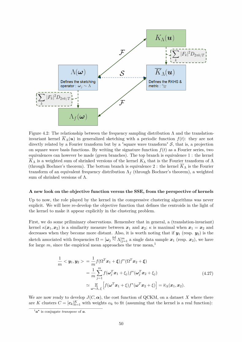
Figure 4.2: The relationship between the frequency sampling distribution Λ and the translation-invariant kernel KΛ(u) in generalized sketching with a periodic function f(t): they are notdirectly related by a Fourier transform but by a "square wave transform" S, that is, a projectionon square wave basis functions. By writing the signature function f(t) as a Fourier series, twoequivalences can however be made (green branches). The top branch is equivalence 1 : the kernelKΛ is a weighted sum of shrinked versions of the kernel KΛ that is the Fourier transform of Λ(through Bochner’s theorem). The bottom branch is equivalence 2 : the kernel KΛ is the Fouriertransform of an equivalent frequency distribution Λf (through Bochner’s theorem), a weightedsum of shrinked versions of Λ.

A new look on the objective function versus the SSE, from the perspective of kernels

Up to now, the role played by the kernel in the compressive clustering algorithms was neverexplicit. We will here re-develop the objective function that defines the centroids in the light ofthe kernel to make it appear explicitly in the clustering problem.

First, we do some priliminary observations. Remember that in general, a (translation-invariant)kernel κ(x1,x2) is a similarity measure between x1 and x2; κ is maximal when x1 = x2 anddecreases when they become more distant. Also, it is worth noting that if y1 (resp. y2) is thesketch associated with frequencies Ω = [ωj

iid∼ Λ]mj=1 a single data sample x1 (resp. x2), we havefor large m, since the empirical mean approaches the true mean,1

1m< y1,y2 > = 1

mf(ΩTx1 + ξ)f∗(ΩTx2 + ξ)

= 1m

m∑j=1

f(ωTj x1 + ξj)f∗(ωTj x2 + ξj)

' Eω∼Λ, ξ

[f(ωTx1 + ξ)f∗(ωTx2 + ξ)

]= κΛ(x1,x2).

(4.27)

We are now ready to develop J(C,α), the cost function of QCKM, on a dataset X where thereare K clusters C = [ck]Kk=1 with weights αk to fit (assuming that the kernel is a real function):

1a∗ is conjugate transpose of a.

50

J(C,α) = 1m‖SkΩ,ξ (X,1N/N)− SkΩ,ξ (C,α) ‖22

= 1m‖SkΩ,ξ (X,1N/N) ‖22 + 1

m‖SkΩ,ξ (C,α) ‖22 −

2m<(SkΩ,ξ (X,1N/N) SkΩ,ξ (C,α)∗

)= 1m

1N2

N∑i=1

N∑i′=1

f(ΩTxi + ξ)f∗(ΩTxi′ + ξ) + 1m

K∑k=1

K∑k′=1

αkαk′f(ΩTck + ξ)f∗(ΩTck′ + ξ)

− 2m<(

1N

N∑i=1

K∑k=1

αkf(ΩTxi + ξ)f∗(ΩTck + ξ))

' 1N2

N∑i=1

N∑i′=1

κΛ(xi,xi′)︸ ︷︷ ︸φX

+K∑k=1

K∑k′=1

αkαk′ κΛ(ck, ck′)︸ ︷︷ ︸φC

−2 1N

N∑i=1

K∑k=1

αkκΛ(xi, ck)︸ ︷︷ ︸φXC

.

(4.28)

We have thus shown that the approximated objective function of QCKM (this is also transposableto CKM) is made up of three contributions J(C,α) = φX + φC − 2φXC , that we can actuallyinterpret as follows:

• a cost φX , corresponding to the average similarity between all the pairs of learning examplesxi. Actually, this term depends solely on the dataset and not on the centroid positions orweights, so it is a constant for the optimization problem at hand and is irrelevant.

• a cost φC , corresponding to a weighted average of the similarity between all pairs ofcentroids. This term will promote centroids that are well separated. For centroids that areimportant (high weight αj), this penalty will increase, so important centroids do repell othercentroids stronger. Or equivalently, this term promotes smaller weights on the centroids ifthey are close to other centroids.

• a gain φXC , corresponding to the average similarity between the data samples and thecentroids. This is the most interesting term since it corresponds to the "clustering" partof the objective function2. This term promotes centroids that lie close to the data, butinstead of using the squared distance towards the centroids as objective function (as in"traditional clustering"), we use the kernel to evaluate the similarity between the examplesand the centroids. Note also that in this term it becomes clear that if a centroid is close toa lot of training examples, it should receive a higher weight. Or equivalently, if a centroidhas a small weight, it will be less attracted to the learning examples.

Given this interpretation, the objective function of QCKM makes a lot of sense intuitively, andthe role of the kernel appears explicitly. It is important to note that therefore, sketch-basedcompressive clustering algorithms (thus in particular, CKM and QCKM) do not aim at solving thek-means clustering problem (2.2) (although [1] presents CKM as a heuristic to solve (2.2)), but infact solve another clustering problem based on the cost J(C,α). Recall the general definitionof a clustering problem from Section 2.1.2: grouping data into clusters such that points withinclusters are "similar" and points in different clusters are "dissimilar": here similarity is measuredthrough a kernel. The differences between J(C,α) the (Q)CKM objective function and the SSEthe objective function of K-means clustering also appear more clearly.

• First, the SSE compares the examples and the centroids through the Euclidean distance,whereas J compares them through a similarity defined by a generic kernel.

2Thus, it is a good thing that it is weighted two times more than the other terms.

51

• Secondly, training examples only contribute to the SSE in pair with their closest centroid,while in J , the similarity of a training example with all the centroids does contribute(however, if the kernel is decaying fast enough with the distance, only the closest centroidswill really contribute to the objective).

• Third difference, the SSE does not take into account the relative distance between thecentroids. In J , one important (half as important as the "clustering" term) term is φC , thespacing of the centroids.

• Fourth difference (but this one was already clear), J has some additional variables comparedto K-means clustering, namely the weights (relative importance) of the different centroids.The objective J will promote well-spaced important centroids. Those additional values arevery helpful to detect "lost" centroids that are close to no cluster at all (a situation that canhappens in practice from time to time, when the algorithm is stuck in a local optimum).

4.1.4 New distribution of the frequencies

Previously, the frequencies ω were drawn iid from a distribution Λ, where Λ was choosen inorder to sample the characteristic function ψ of the data "well", i.e. choosing Λ such that |ψ(ω)|takes large values. Obviously, for our generalized case, this distribution Λ has to be changed toaccount for the fact that we are now evaluating the distance differently.

In (4.10) we saw that we are not evaluating the difference between the probability distributionsthrough the characteristic funcion ψP(ω) = Ex∼P e−iω

Tx anymore but through a new function

ψP(ω; ξ) = Ex∼P

f(ωTx+ ξ) =∑k

Fkeik 2π

TξψP

(−k2π

Tω

). (4.29)

with ξ uniformly distributed in [0, T ] with T is the period of f , and we now suppose withoutloss of generality that T = 2π.

Gaussian with adapted heuristic distribution (G-h). First, as is done in [2], we supposewe have a single known Gaussian, i.e. P is N (µ,Σ) with known parameters µ and Σ3. If wewant to proceed as before and choose the distribution Λ to sample |ψP | essentially where it takeslarge values, we could go for the intuitive choice Λ ∝ |ψP |. Although this approach has a goodintuitive motivation, problems could arise because this function |ψP | is unbounded when f is theuniversal quantization function:

|ψP(ω; ξ)| =

∣∣∣∣∣∣+∞∑

k=−∞FkψP(−kω)eikξ

∣∣∣∣∣∣ =

∣∣∣∣∣∣+∞∑

k=−∞Fke

ikωTµe−k22 ω

TΣωeikξ

∣∣∣∣∣∣≤

+∞∑k=−∞

|Fk| · 1 · |e−k22 ω

TΣω| · 1

=+∞∑

k=−∞k odd

2π|k|

e−k22 ω

TΣω =−1∑

k=−∞k odd

2π(−k)e

− k22 ω

TΣω ++∞∑k=+1k odd

2πke−

k22 ω

TΣω

= 2+∞∑k=1k odd

2πke−

k22 ω

TΣω = 4π

+∞∑k=1k odd

1ke−

k22 ω

TΣω

(4.30)

3Thus, we can write ψP(ω) = e−iωTµe−

12ω

T Σω.

52

thus in particular |ψP(0; ξ)| ≤ 4π

∑+∞k=1,k odd

1k which diverges: sampling the frequencies as

Λ ∝ |ψP | will potentially oversample the zero frequencies, exactly the point where the char-acteristic function does not contain any information since it is equal to 1 for all probabilitydistributions. Furthermore, even without this problem at the origin, it is in practice hard tosample ω ∼ Λ ∝ |ψP | because |ψP | is not easily converted into a probability distribution (tonormalize it we have to compute its integral over the whole domain Rm which is not trivial).

To circumvent those problem, we propose to select Λ ∝ Eξ |ψP(ω; ξ)|2. Intuitively it makessense: 1) we don’t want our frequency distribution to depend on a particular realisation of ξ(that will be different for each frequency we will have to draw, so we will have one differentfrequency distribution for each frequency we have to draw) but rather on the average behaviorof the function with ξ (and in this case, we have only one frequency distribution for all thefrequencies), and 2) if |ψP(ω; ξ)| is significant, |ψP(ω; ξ)|2 significant too4. In this case we have

Eξ|ψP(ω; ξ)|2 =

∑k

|Fk|2 |ψP(−kω)|2

=∑k

|Fk|2∣∣∣∣eikωTµe−

k22 ω

TΣω∣∣∣∣2

=∑k

|Fk|2e−2k22 ωTΣω =

∑k

|Fk|2e−12ω

T (2Σ/k2)ω

(4.31)

so it turns out that the intuitive choice is here to take Λ ∝∑k |Fk|2N (0, k2Σ−1/2). To do this

in practice, one idea is to select for each frequency that we have to draw a Fourier coefficientnumber r with probability P[r = k] = pk = |Fk|2/

∑l |Fl|2 and then to draw ω ∼ N (0, r2Σ−1/2).

Since this is the equivalent to the Gaussian frequency sampling (G) in [2], we will call thissampling of frequencies the Gaussian with adapted heuristic (G-h). Sadly, as was the case with(G), the (G-h) frequency sampling suffers from the curse of dimensionality and produces toomany frequencies concentrated on a sphere away from the origin, where the information contentof the sketch is small and the sketch takes small values.

Gaussian radius with adapted heuristic distribution (Gr-h). Similarly to the Gaussianradius (Gr) heuristic form [2], we therefore propose to select the frequencies as ω = RΣ−1/2ϕwith R a (random) radius whose distribution is to be determined later, and ϕ ∼ U(Sn−1) auniform direction vector of unit norm. In this case, the function we want to sample expresses as

Eξ|ψP(ω; ξ)|2 =

∑k

|Fk|2e−12ω

T (2Σ/k2)ω =∑k

|Fk|2e− 1

2R2k2/2 = ψP(R) (4.32)

which is a function of R only. The intuitive choice is here to pick R ∼ pR(R) with

pR(R) ∝ ψP(R) =∑k

|Fk|2N (0, k2/2) (4.33)

and we obtain thus a one-dimensional Gaussian distribution that no longer suffers from the curseof dimensionality. We denote this frequency sampling heuristic (Gr-h).

4Actually, empirical simulations have shown that taking the square root afterwards, i.e. choosing Λ ∝√Eξ |ψP(ω; ξ)|2 has no noticeable effect on the clustering performances.

53

Adapted radius with adapted heuristic distribution (Ar-h). Finally, similarly to theAdapted radius (Ar) density presented in [2] that samples the frequencies where they the bestat differentiating different data probability density functions, we propose its equivalent in thegeneralized sketch case, that we will call (Ar-h). We propose here to sample the frequencieswhere the average (with respect to ξ) norm of the gradient with respect to the parameters of theGaussian distribution is high. We have, given that ψN (µ,σ2)(R) =

∑k Fke

ikξeikRµe−k22 R

2σ2 andbuilding on developements from Chapter 2,

Eξ

∥∥∥∥∇(µ,σ2)ψN (µ,σ2)(R)∥∥∥∥2

2= E

ξ

∣∣∣∇µψN (µ,σ2)(R)∣∣∣2 + E

ξ

∣∣∣∇σ2ψN (µ,σ2)(R)∣∣∣2

=∑k

|Fk|2(k2R2 + k4R4

4

)e−k

2R2σ2(4.34)

and, when evaluating this gradient at the true parameters (µ = µ0, σ2 = σ2

0 = 1), we obtainfinally the distribution for the radius R:

pR(R) ∝∑k

|Fk|2(k2R2 + k4R4

4

)e−k

2R2 (4.35)

and the resulting frequency distribution is denoted as the (Ar-h) distribution.

4.2 Particularisation to the universal quantization signature func-tion

The previous section focused on general periodic functions f(t). In this section, we re-visit theresults of this section but in the particular case where the signature function is the universalquantization function Q∆(t). Recall from proposition 1 that f(t) = Q∆(t) can be written withFourier coefficients Fk = 2i

kπ for k odd (the coefficients are 0 whenever k is even). For thisparticular case, the gradients to solve the optimization problem can be more easily computedthan in the general case (see Appendix B.3). Interestingly, for the universal quantization sketch,the objective function of clustering can be linked to the distance map that characterizes theembedding induced by 1-but universal quantization of random projections of vectors [23].

4.2.1 Kernel approximated by the quantized sketch

From Proposition 4 and given the Fourier coefficients Fk and T = 2π for the universal quantization,we have that (equivalence 1)

KΛ(x1 − x2) =∞∑

k=−∞|Fk|2KΛ

(−k2π

T(x1 − x2)

)= 4π2

∞∑k=−∞k odd

1k2KΛ (−k(x1 − x2)) (4.36)

with Λ the frequency distribution of the frequencies. Let us first suppose that the frequencydrawing pattern we use is the Gaussian heuristic from CKM (G) with Σ = σ2I, where σ2 is thevariance of the dataset estimated from a small fraction of X. Thus, we have Λ(ω) = ΛG(ω) =N (ω; 0, σ−2I), and for the complex exponential sketch kernel, applying Bochner’s theorem yieldsa Gaussian kernel

KΛG(x1 − x2) = e− 1

2‖x1−x2‖

2

σ2 . (4.37)

54

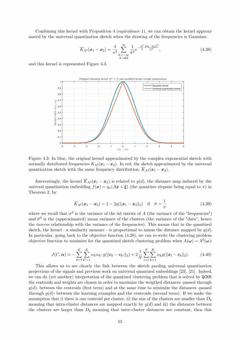
Combining this kernel with Proposition 4 (equivalence 1), we can obtain the kernel approxi-mated by the universal quantization sketch when the drawing of the frequencies is Gaussian:

KΛG(x1 − x2) = 4π2

∞∑k=−∞k odd

1k2 e

− k22‖x1−x2‖

2

σ2 , (4.38)

and this kernel is represented Figure 4.3.

‖x1 − x2‖-5 -4 -3 -2 -1 0 1 2 3 4 5

Kernel

valueκ(x

1,x2)

0

0.1

0.2

0.3

0.4

0.5

0.6

0.7

0.8

0.9

1

Original Gaussian kernel (σ2 = 1) and modified kernel trough quantization

Gaussian kernel

Universal quantization kernel

Figure 4.3: In blue, the original kernel approximated by the complex exponential sketch withnormally distributed frequencies KΛG(x1 −x2). In red, the sketch approximated by the universalquantization sketch with the same frequency distribution, KΛG(x1 − x2).

Interestingly, the kernel KΛG(x1 − x2) is related to g(d), the distance map induced by theuniveral quantization embedding f(x) = qπ(Ax+ ξ) (the quantizer stepsize being equal to π) inTheorem 2, by

KΛG(x1 − x2) = 1− 2g(‖x1 − x2‖2) if σ = 1σ

(4.39)

where we recall that σ2 is the variance of the iid entries of A (the variance of the "frequencies")and σ2 is the (approximated) mean variance of the clusters (the variance of the "data", hencethe inverse relationship with the variance of the frequencies). This means that in the quantizedsketch, the kernel - a similarity measure - is proportional to minus the distance mapped by g(d).In particular, going back to the objective function (4.28), we can re-write the clustering problemobjective function to minimiez for the quantized sketch clustering problem when Λ(ω) = ΛG(ω):

J(C,α) ' −K∑k=1

K∑k′=1

αkαk′ g(‖ck − ck′‖2) + 2 1N

N∑i=1

K∑k=1

αkg(‖xi − ck‖2). (4.40)

This allows us to see clearly the link between the sketch pooling universal quantizationprojections of the signals and previous work on universal quantized embeddings [23], [21]. Indeed,we can do (yet another) intepretation of the quantized clustering problem that is solved by QCKM:the centroids and weights are chosen in order to maximize the weigthed distances -passed throughg(d)- between the centroids (first term) and at the same time to minimize the distances -passedthrough g(d)- between the learning examples and the centroids (second term). If we make theassumption that i) there is one centroid per cluster, ii) the size of the clusters are smaller than D0meaning that intra-cluster distances are mapped exactly by g(d) and iii) the distances betweenthe clusters are larger than D0 meaning that inter-cluster distances are constant, then this

55

objective function becomes almost K-means’s objective function, without squaring the distancesand with weighted centroids:

J(C,α) ∝N∑i=1

minkαk‖xi − ck‖2. (4.41)

The connexions with [21] can be drawn even further by considering the general signaturefunction f(t) again, so we have a kernel

KΛG(x1 − x2) =∞∑

k=−∞|Fk|2KΛG

(−k2π

T(x1 − x2)

)(4.42)

for general Fourier coefficients Fk. Then, if we assume T = 1 (we do the same assumption as[21] in order to make the link more easily) the general kernel KΛG(x1 − x2) is related to thedistance map g(d) of the embedding defined by y = f(Ax+ ξ) for A an m-by-n matrix withAij

iid∼ N (0, σ2) and ξjiid∼ U([0, 1]) by

KΛG(x1 − x2) =∑k

|Fk|2 −12g(‖x1 − x2‖2) if σ = 1

σ(4.43)

since the distance map g(d) of y = f(Ax+ ξ) is given by ([21], Section 4.2.1)

g(d) = 2∑k

|Fk|2(1− e−2(πσdk)2). (4.44)

In particular, the CKM algorithm (where the signature function f(t) = e−it) with Λ = ΛG usesimplicitly a distance map that consists of a reversed Gaussian.

However, for the other frequency distribution heuristics, the kernel is not Gaussian anymore,and the distance map is different. In particular, when using the (G-h), (Gr-h) and (Ar-h)distributions, sampling heuristics that are adapted to the universal quantization sketch, since thefrequency distribution determines the kernel through proposition 4, the kernel approximated bythose new frequency sampling heuristics will also be changed.

4.2.2 Quantized frequency distribution

As we have sen with the equivalences, when we sample the quantized sketch at frequenices drawnfrom a frequency density Λ(ω), it is as we are sampling the original sketch with frequencies drawnfrom Λf (ω) =

∑∞k=−∞ |Fk|2D2πk/TΛ(ω). Λf (ω) can be interpreted as the equivalent frequency

content that is used to compare the frequency distributions. In the particular case of a Gaussiansampling of the frequencies (G), we provide bounds for Λf to show how the frequency content ischanged when the quantized sketch is used. We furthermore assume without loss of generalitythat Σ = I, thus Λ(ω) = ce−‖ω‖

2/2 for a normalization constant c. Then given the particularFourier series coefficients,

Λf (ω) ∝ c∑k odd

1|k|2· 1|k|n

e−‖ω‖2/2k2 = 2c

∑k oddk≥0

1kn+2 e

−‖ω‖2/2k2, (4.45)

and since all terms in the sum are strictly positive we can bound the sum below by keeping onlysome terms corresponding to k ≥ ‖ω‖, where we assume ‖ω‖ 1:

56

Λf (ω) = c1∑k oddk≥0

1kn+2 e

−‖ω‖2/2k2

≥ c1∑k oddk≥‖ω‖

1kn+2 e

−‖ω‖2/2k2

≥ c1∑k oddk≥‖ω‖

1kn+2 e

−‖ω‖2/2‖ω‖2︸ ︷︷ ︸e−1/2

= c2∑k oddk≥‖ω‖

1kn+2

≥ c21

‖ω‖n+2

(4.46)

where in the last step we only kept the smallest term in the sum. Thus, for large ‖ω‖, theequivalent frequency distribution Λf (ω) is Ω

(‖ω‖−n−2). We stated previously that the high

frequencies do not bring useful information to the sketch for clustering, and we have shownhere that naturally, the equivalent frequency distribution with the quantized sketch is samplinghigh frequency with a probability density that goes as Ω

(‖ω‖−n−2). In short, the equivalent

probability distribution oversamples high frequencies.

4.3 Characterization of the different error termsTo conclude the theoretic approach of this chapter, we summarize the different approximationsmade by QCKM (this discusion also applies to CKM), as represented Figure 4.4. The problem ontop is the k-means clustering problem, that is, the initial problem we want to solve. From there,there are two interpretations of the approximation made by replacing this problem by the sketchmatching problem.

• Approximation (1) is the replacement of the K-means clustering problem by anotherproblem, that minimizes the γκ-distance between two distributions P and Q. The distribu-tion P is the true distribution underlying the data, and the distribution Q is a mixtureof deltas that we are matching with the data (GK is the set of mixturs of K deltas).Characterizing this error term is not trivial due to the "heuristic nature" of approximation(1).

• Since in practice the true distribution P of the data is unknown, approximation (2)consists in replacing this distribution by the empirical distribution of the data, P. Thisapproximation induces an estimation error on the objective that is O(1/

√N) ([27], Theorem

3). In short, the quality of this approximation increases with N .

• In approximation (3), this problem is replaced by the sketch distance. This approximationrelies on the law of large numbers and is therefore valid for large m. Note that on average,the sketch distance is equal to the gamma distance (on average over the drawing of thefrequencies, approximation (3) induces no approximation error), and that increasing mdecreases the variance of this approximation error. Characterizing this error term requiresextensions of the "Information preserving guarantees" theorems from [2], theorems that arethemselves still to be improved in future work by the authors.

• As discussed in this chapter, we can also interpret the (Q)CKM problem as a differentclustering problem (instead of a pdf matching problem as done with approximation (1)).

57

Therefore, we can see approximation (4) as the replacement of the k-means clusterignproblem with a clustering problem that compares the similarity of training examplesthrough a translation-invariant kernel. Again, this new problem can be approximated bythe sketch distance, by law of large numbers (just as approximation (3)).

• Finally, the optimization problem based on the sketch distance is not solved exactly butthe centroids C∗ are a local optimum that is found by using the L-BFGS method and withapproximating the gradient as a truncated Fourier series, this is approximation (5). Notethat approximpation (5) is the combination of two approximations: replacing the exactsolution by a local minimum, and truncating the gradient in the local minimum searchmethod. The approximation error commited by (5) is still an open question and will requirean in-depth analysis of the properties of L-BFGS on our particular non-convex optimizationproblems.

Figure 4.4: Schematic view of the different approximations that are done in (Q)CKM, with twodifferent interpretations (left and right branches).

58

Chapter 5

Experimental results

Clustering with a general periodic signature function, and in particular the QCKM algorithm havebeen implemented in Matlab and tested on both synthetic Gaussian data and a real datasetoriginating from the MNIST handwritten digits image collection. This chapter presents anddiscusses the most significant experimental results obtained. The most important conclusion isthat QCKM can reach performances that compete with CKM and k-means++ as long as the sketchdimension m is high enough. Since we focused during our theoretical analysis on the Fourierseries approximation of the universal quantization function to obtain the gradient (strategy 2),we also focused on this approximation in the experimental results. However we also implementedstrategy 1 (smoothing the universal quantization function), even though we present no resultsfor this strategy for the sake of conciseness.

5.1 Toy examples : mixture of Gaussians

5.1.1 Experiment 1: from CKM to QCKM

As a starting point, we will see how the clustering performances are affected by the signaturefunction, and more particularly, when this signature function approaches the universal quantiza-tion. In this experiment, we run a variant of QCKM where the sketch (and the gradients) use assignature function f(t) a truncated Fourier series of the universal quantization function Q∆(t)

f(t) =+Kcoef∑

k=−Kcoef

Fkei 2πTkt, (5.1)

with Fk defined in Proposition 1. The dataset for this experiment is 7000 examples generatedfrom a mixture of 5 isotropic Gaussians in two dimensions, and we compare the following valuesof Kcoef = [1, 21, 41, 61, 81, 101]. The results are averaged over 60 repetitions of the experimentand are represented Figure 5.1.

We can see that for Kcoef = 1 the performances are similar to CKM, which is to be expectedsince the signature function is (almost) the same (the complex exmponential is replaced by a sinefunction). When the number of Fourier coefficients increase, the signature function ressembles lessand less to the complex exponential and becomes closer to the universal quantization function. Aswe can observe in Figure 5.1, this causes the clustering performances to degrade with the amountof Fourier coefficients. This shows that the clustering performances worsen when the complexexponential is replaced by the universal quantization. We also observe that the performances ofQCKM stabilize around Kcoef = 41..61. We will use this as an argument to choose the number ofFourier coefficients to keep in the following experiments.

59

Figure 5.1: Evolution of the average distance of the learning examples to the centroids with thenumber of Fourier coefficients used to approximate the universal quantization function.

5.1.2 Experiment 2: comparing the different frequency drawing patterns

We now keep a fixed number of Fourier coefficients in the approximation of the gradient,Kcoef = 51. In this second experiment, we compare the performances in terms of SSE ofthe CKM with the QCKM algorithm for different choices of a frequency density function Λ. Thelearning dataset is a set of N = 7500 points drawn from a mixture of 2 isotropic Gaussiansin dimension n = 10 with the same covariance Σ = 1

2√

10 ∗ I but with different means, respec-tively +110 and −110. We fit K = 10 centroids on this dataset using both CKM with the threeheuristics proposed by [2], and QCKM with the three same heuristics, as well as their variantsadapted to the quantized sketch. In this example, in order to reduce the variance of the results,we suppose that the covariance Σ of the data is known when drawing the frequencies, so wedon’t have to run an algorithm to estimate σ2 to approximate Σ as σ2I, but we must keepin mind that in practice Σ is unkown. Different values of m, the number of frequencies todraw, are tested, and for each value of m, we report the average performance over 10 repetitionsof the selection of the frequencies. The results are reported Figure 5.2 (for CKM) and 5.3 (for QCKM).

First, from Figure 5.2 we can conclude that the Gaussian heuristic performs very poorlyon the given dataset. Since we are in dimension n = 10, this was to be expected since the"curse of dimensionality" is of application and the Gaussian heuristic oversamples the highfrequencies (for the highest numbers of frequencies, the performances seem to improve, butonly slightly). The two other heuristics outperform k-means, although the adapted radius (Ar)heuristic requires at least m = 400 while the Gaussian radius (Gr) requires only m = 100.We thus observe, suprisingly, that at low frequencies (Gr) outperforms (Ar) even though [2]reports that (Ar) performs better (but note that (Ar) is still slightly better at high frequen-cies). We suggest that the better performances of (Ar) compared to (Gr) applies primarily toGMM estimation and not for compressive clustering. We justify this claim intuitively by notingthat the (Ar) heurisitics is built on a criterion that allows to discriminate Gaussian distribu-tions and in particular, allows discrimate different variances. In compressive clustering, we arenot interested in the information provided about the variance of the clusters, but only in theirmeans, so the intuitive gradient justification for (Ar) is less relevant than it is in GMM estimation.

We now turn to our new algorithm, QCKM, whose performances are represented Figure 5.3.

60

m

100 200 400 800 1600 3200 6400 12800

SS

E(C

KM

)/S

SE

(K-M

EA

NS

)

0.5

1

1.5

2

2.5

3

3.5Performances of CKM

G

Gr

Ar

Figure 5.2: Average Sum of Squared Errors of CKM relative to the SSE obtained by k-means++for 10 experiments as a function of m in a logarithmic scale. When the value is less than 1 (blackline), it means that CKM outperforms k-means++. The blue, orange and yellow line correspondto respectively the Gaussian heuristic (G), the Gaussian radius heuristic (Gr) and the adaptedradius heuristic (Ar).

First, we observe that, when using the same frequencies as the ones adapted to CKM (plainlines), the same relative performances between the three heuristics appear: (G) does not performwell even at high frequencies, and (Gr) and (Ar) outperform k-means++ given the number offrequencies is high enough, with again better performances for (Gr). However, the number offrequencies m to obtain accurate clustering results is much higher than needed by CKM. In generalfor all experiences (even the ones not presented in this report), we have observed that for QCKMthere seems to be a factor of 20...50 in the number of frequencies m needed in order to have good(i.e. same accuracy as k-means) clustering results compared to CKM . We will try to explain thisbehavior when discussing the next experience. If we look at the modified frequency densitiesadapted to QCKM that we proposed in Chapter 4 (the dashed lines in Figure 5.3), called (G-h),(Gr-h) and (Ar-h), we observe that each modified heuristic outperforms its counterpart that is notadapted to the quantization. The proposed heuristics are thus indeed improving the clusteringcapabilities of QCKM. When using the adapted heuristics less frequencies are needed, but at highfrequencies the performances are the same for all heuristics. Interestingly, the adapted Gaussianheuristic (G-h) outperforms the CKM performances of the Gaussian heuristic (G), Figure 5.2. Webelieve that this is due to the fact that the adapted heuristic has a tendency to sample more lowfrequencies. However, this advantage is not significant enough to make the Gaussian frequencydistribution a viable choice in pratice.

5.1.3 Experiment 3: phase transition diagrams

The last experience suggests that QCKM can obtain good clustering performances when the numberof frequencies m is increased. In this experiment we are going a little bit further by confirmingwhether or not the empirical rule m = O(nK) observed for CKM still holds for QCKM. In thisexperiment we use solely the Gaussian radius (Gr) frequency sampling distribution and its

61

m

100 200 400 800 1600 3200 6400 12800

SS

E(Q

CK

M)/

SS

E(K

-ME

AN

S)

0.5

1

1.5

2

2.5

3

3.5Performances of QCKM

G

Gr

Ar

G-h

GR-h

Ar-h

Figure 5.3: Average Sum of Squared Errors of QCKM relative to the SSE obtained by k-means++for 10 experiments as a function of m in a logarithmic scale. The blue, orange and yellow solidline correspond to respectively the Gaussian heuristic (G), the Gaussian radius heuristic (Gr)and the adapted radius heuristic (Ar) for CKM, while the dashed lines correspond to their variantsadapted to QCKM, respectively (G-h), (Gr-h) and (Ar-h).

adptation (Gr-h) since they yielded the best results in experiment 2.

Experiment 3a: the performances as a function of m and n, the problem dimension

We first let the dimension if the learning examples, n, vary. In this experience, the N = 10000learning examples are drawn from a mixture of two isotropic Gaussians with mean 1n and −1n.We chose a variance proportional to n in order to have a comparable distance between the clusterswhen n varies (because the distance between the two means of the Gaussians is 2

√n, therefore

the width σ of the clusters should be proportional to√n); more precisely we choose Σ = n

20I.On this data, we fit again K = 10 centroids. We let n vary from 5 to 30 dimensions by stepsof 5, and the number of frequencies we draw is m = cnK for various values of c, in particular,c = 0.2, 0.5, 1, 5, 10, 20 and 50. For each value of n and m, we are taking the average over 10repetitions of the experience for CKM and for QCKM with both the (Gr) and (Gr-h) frequencysampling patterns; the results are shown Figures 5.4 and 5.5.

The main observation from Figure 5.5 is the fact that the empirical rule m = O(n) stillholds for QCKM (except a deviation at small n that is also present in CKM, probably linked toa lesser impact of the curse of dimensionality). By comparing those graphs with Figure 5.4,as we already observed, we conclude that QCKM has good performances given the number offrequencies is approximatively 20 (for the (Gr-h) frequency distribution) to 40 (for the (Gr)frequency distribution) times higher than in CKM. Using our adapted frequency sampling heuristicgives a reduction of the number of frequency to use by almost a factor 2.

62

1.5

1.5

22

3

3

SSE(CKM)/SSE(kmeans), frequencies = Gaussian radius

m/nK

0.2 0.5 1 2 5 10 20 50

n

5

10

15

20

25

30

1.2

1.4

1.6

1.8

2

2.2

2.4

2.6

2.8

3

Figure 5.4: Phase transition diagram for the CKM perfomances : the color represents the averageSSE obtained for CKM relative to the one obtained with k-means++. In the yellow region, therelative SSE is higher than 3 while in the dark blue region it is lower than 1.5. In between, thereis a transition (we will call the isoline where the relative SSE = 2 the phase transition). Here thephase transition happens between m = 0.5nK and m = nK.

1.5

1.5

2

2

3

3

SSE(QCKM)/SSE(kmeans), frequencies = Gaussian radius

m/nK

0.2 0.5 1 2 5 10 20 50

n

5

10

15

20

25

30

1.2

1.4

1.6

1.8

2

2.2

2.4

2.6

2.8

3

(a) Sampling : (Gr)

1.5

1.5

22

3

3

SSE(QCKM)/SSE(kmeans), frequencies = Gaussian radius + heuristic

m/nK

0.2 0.5 1 2 5 10 20 50

n

5

10

15

20

25

30

1.2

1.4

1.6

1.8

2

2.2

2.4

2.6

2.8

3

(b) Sampling : (Gr-h)

Figure 5.5: Phase transition diagram for the QCKM perfomances with the (Gr) frequency sampling(left) and (Gr-h) frequency sampling (right) when the dimension n varies. The phase transitionhappens both between m = 10nK and m = 20nK for (Gr) and (Gr-h), and depends linearly onn.

Experiment 3b: the performances as a function of m and K, the number of clusters

We are now going to vary the number of clusters K in fixed dimension n = 5. Here the learningexamples are drawn from a mixture of K isotropic Gaussians with variance as described in exper-iment 3a (except we only have one value of n) and the K means of those Gaussian distributionsare K random draws from the set −1,+1n (we place clusters in K of the 25 = 32 hyperoctantsof R5). We use K centroids to cluster this dataset. This time, we only use the adapted Gaussian

63

radius heuristic (Gr-h) for drawing the frequencies for QCKM since it was the best performingheuristic in the previous experiments; the results are shown Figure 5.6.

1

1

1.5

1.5

2

2

3

3

SSE(CKM)/SSE(kmeans), frequencies = Gaussian radius

m/nK

2 5 10 20 50 100 200 500

K

5

10

15

20

1

1.5

2

2.5

3

(a) CKM with (Gr)

1

1

1.5

1.5

2

2

3

3

SSE(QCKM)/SSE(kmeans), frequencies = Gaussian radius + heuristic

m/nK

2 5 10 20 50 100 200 500

K

5

10

15

20

1

1.2

1.4

1.6

1.8

2

2.2

2.4

2.6

2.8

3

(b) CKM with (Gr-h)

Figure 5.6: Phase transition diagram for the CKM perfomances with the (Gr) frequency sampling(left) and the QCKM performances with (Gr-h) frequency sampling (right) when the number ofclusters and centroids K varies. For CKM, the phase transition happens for m ' 5nK, and forQCKM for m ' 100nK, and depends linearly on K.

From Figure 5.6 and experiment 3a we can conclude that CKM’s empirical rule m = O(nK)still holds for QCKM. As in the previous experiment, there is a factor of at least 20 between thenumber of frequencies necessary for CKM and QCKM.

We now give some hypotheses for the increase of m in the context of QCKM. There are twofactors that could play in this increase (the truth is most likely to be a combination of both ofthem). First, without considering the algorithm and the frequency distribution, the universalquantization might be less suited than the complex exponential to record information about theclusters in the form of a sketch. This would be due to an "inherent" difficulty of QCKM, intuitivelyjustified by the fact that the sketch contains "less" information1 than the complex exponential.Another way to see this is by remembering that the quantized sketch can be interpreted as asampling of a "square wave" transform of the probability density function underlying the datawhereas the usual sketch is its Fourier transform; this square wave transform is intuitively lesssuited to represent smooth probability density functions than the Fourier transform, i.e. it mightrequire more samples for an accuracte estimate of the centroids. If the increase of m is solelydue to this -potential- inherent inability of QCKM to perform clustering with as many frequenciesas CKM, this would be bad news since there is nothing we can do about it; however we believethere is cause for the increase in m.

The second -and more motivating- reason for the increasing m could lie in the actual imple-mentation of QCKM, more particularly in the way the sketch is designed (choice of Λ) and in theway the QCKM problem is solved. We have already seen that the choice of Λ is a crucial parameterregarding the sketch performances in terms of learning, and up to now we only have heuristics

1Since the quantized sketch can only take 2 values, it naturally contains less information than the complexexponential that can theoretically (i.e. not on an actual computer) take an infinite number of values. But as wediscuss in Chapter 6, we must be careful when defining a "fair" comparison between CKM and QCKM, since the latterrequires potentially less bits to store.

64

to select the frequency distributions. Empirical results -not reported here for conciseness- haveshown that downscaling the frequencies Ω by, for example, a factor 10 yield much better clusteringresults, suggesting that there is room for improvement in the choice of Λ. On the other hand, fora given frequency distribution, we also do not know how close the local optimum discovered byQCKM lies from the true optimum. It might very well be the case that the optimization steps inQCKM are more easily stuck in (bad) local optima than CKM, calling for an increased number offrequencies to reduce the amount of local optima. As we suggest in the next experiment, thepractical QCKM algorithm presented up to now might be improved by considering optimizationschemes specialized for discontinuous, or very flat, optimization landscapes.

5.1.4 Experiment 4: the bottleneck of QCKM, aka execution time

The QCKM algorithm produces clustering results that compete favorably with CKM and k-means++,but the main practical drawback -right now- is its execution time. The source of this slowerexecution time is double: first, more frequencies m are needed for QCKM (m = O(nK) is still validbut with a higher hidden constant in the big-O notation, see experience 2 and 3), but as we willsee now even for an equal number of frequencies m, the execution of QCKM is slower. If we lookat the complexity of QCKM, we obtain the same complexity as CKM, that is, O(K2mn) (this comesdirectly since the steps of both algorithms are the same, they are just executed differently). Weshow in this experiment that this rule indeed still holds (at least for the dependence in m) but-similarly to the rule for m- with a higher hidden constant. We have included the computation ofthe sketch in our measure of time even though it could be computed much faster using parallelcomputing, but we have empirically determined that the sketch computation time took up onlya small fraction (less than 5%) of the total computation time for the modest chosen value of N ,so the computation time computed can be interpreted as the time for running the algorithm andnot for computing the sketch.

m

100 200 400 800 1600 3200 6400 12800 25600

Avera

ge e

xecution tim

e [s]

100

101

102

103Execution time of CKM and QCKM

CKM

QCKM

Figure 5.7: Average execution time of CKM (blue) and QCKM (orange) algorithms in seconds as afunction of the number of frequencies m in a log-log scale for enhanced readability of the results.

65

In this experiment we consider the same dataset generation procedure as in experiment 2, andmeasure the average execution time of both algorithm over 10 realizations for different values ofm. Figure 5.7 represents the evolution of the mean execution time as a function of m. The firstobservation is that empirically, the linear dependence on m of the time complexity of those algo-rithms (O(K2mn), as reminder) is confirmed (the slope2 of both curves is approximatively 1, thiswas also confirmed by a -less elegant- plot without logarithmic axes). However, there is roughlyone order of magnitude between the execution time of CKM and QCKM (the latter being at least 10times slower). Although it is true that the current implementation of QCKM could probably befurther improved to run faster (the goal of our code is still to be a "proof of concept" rather thana competitive implementation), we strongly believe that the main reason for this slower executionresides in the solving time of the different optimization problems. More precisely, the optimizationproblems in QCKM are harder (hence more costly in time) to solve than for CKM. Indeed, the objec-tive function of QCKM, even when smoothed, is very flat compared to the one of CKM. As a result,the gradients of QCKM will most of the time be close to zero, and the L-BFGS optimization schemewill be forced to make a lot more, smaller, iterations than when solving the problems for CKM. Infuture work, more specialized optimization methods could be considered to counter this drawback.

5.2 MNIST datasetWe now consider a "real-life" dataset to assert the performances of QCKM on real data. We thusconsider the well-known MNIST dataset, a collection of N = 70000 28 × 28 pixel images ofhand-written digits. Our goal will be to detect, in an unsupervised manner (i.e., without usingthe labels of the images) the 10 clusters corresponding to the different numbers. Since theshape of the clusters in the original 28× 28-dimensional space are possibly very complex andnot representable by a single centroid, we will here use a spectral clustering algorithm, and useQCKM on the "new" dataset Y made of the eigenvectors, as illustrated Figure 5.8. To constructthe adjacency matrix of the graph associated with the dataset3, the SIFT descriptors of thedifferent images are computed, then, the a nearest-neighbor search is performed on those features,and edges are added between training examples if they share similar descriptors. The graphLaplacian of this graph is then computed and the 10 eigenvectors associated with the samllesteigenvalues are extracted, each of those vectors defning a feature in the new dataset Y . Finally,we compare the different clustering algorithms on this new dataset Y . We would like to stressthe fact that this experiment does not fit completely in a "compressive" framework since thereis a heavy pre-processign step prior to the compressive part, but the goal is to evaluate theclustering performances on real data that are not necessarily Gaussian.

Figure 5.8: Experimental setup on the MNIST dataset : the first two setps are spectral clustering"pre-processing", and it is only in the last step that the clustering is performed.

2If T represents the time and T = cmp for a constant c, we must have log T = p logm + log c, where in ourcase p = 1.

3Generously provided to us by the authors of [1].

66

We will use two metrics to evaluate the performances of the clustering algorithms. While thefirst one, the Sum of Squared Errors (or sum of distances to the closest centroids), is the most usedmetric for evaluating clustering performances, it is not necessarily the most meaningful for theapplication at hand. In our case for example, we would like to "discover" in an unsupervised man-ner (that is, without using the labels of the training examples) the clusters corresponding to theactual numbers: we somehow want to compare the clusters produced by our clustering algorithmwith the ground truth labels of the images. We therefore also use the Adjusted Rand Index (ARI)that measures the similarity between partitions of datasets by comparing the number of pairs ofexamples that are put in the same cluster for two different clusterigns. Without entering intothe details, the higher the ARI the better, with having ARI = 1 for two clusterings correspondsto having the exact same clusters, and ARI = 0 corresponds to assigning clusters at random.We compare the results obtained by k-means with range initialization4, CKM with m = 1000 and(Gr) frequency sampling, and QCKM with m = 20000 and (Gr-h) frequency sampling (since we ob-served on synthetic data that there was a factor of at least 20 in the number of frequencies needed).

K-Means CKM QCKM

SS

E/N

0.1

0.2

0.3

0.4

0.5

0.6

Mean SSE on MNIST for different clustering algorithms

Figure 5.9: Boxplot of the mean SSE obtained on the spectral MNIST dataset for differentclustering algorithms. The red line is the median of the performances, the blue box contains50% of the performances closest to the median, and the box with the whiskers contain all theperformances except eventual outliers represented by red crosses.

Figure 5.9 represents with a boxplot all the means SSE obtained by the three algorithms for10 experiments. We can see that both CKM and QCKM, for the selected numbers of frequencies,globally outperform k-means in terms of SSE, except for some outliers. Those algorithms arealso more stable to initialization as the variance of their performances is smaller, and comparedto CKM, the QCKM algorithm presents more variance in the results obtained, but with the positiveeffect of obtaining globally a better SSE (keeping in mind however that QCKM has here access toa sketch with 20 times more frequencies).

We now compare the clusters obtained with the ground truth labels through the ARI, as shownin Figure 5.10 (again for 10 experiments). Both compressive clustering algorithms producedclusters that are closer to the true labels (higher ARI) compared to k-means. Once again, CKM isvery stable except for some outliers. QCKM presents a higher variance than CKM but its median

4The initialization stage can thus be done in a compressive setting, where the dataset Y is forgotten but onlythe bounds are stored in memory.

67

K-Means CKM QCKM

Adju

ste

d R

and Index

0.6

0.65

0.7

0.75

0.8

0.85

0.9

0.95

1

ARI on MNIST for different clustering algorithms

Figure 5.10: Boxplot of the Adjusted Rand Index obtained on the spectral MNIST dataset fordifferent clustering algorithms (the closer to 1, the better). The red line is the median of theperformances, the blue box contains 50% of the performances closest to the median, and thebox with the whiskers contain all the performances except eventual outliers represented by redcrosses.

ARI is better for the selected number of frequencies: on this example, QCKM produces the bestdigit classification results but with a high variance on the drawing on the frequencies.

68

Chapter 6

Conclusion

After reviewing the existing CKM compressive clustering algorithm in Chapter 2, we have proposedthe new QCKM algorithm in Chapter 3 that should be easier to implement in hardware. However,this algorithm requires to solve optimization problems whose objective function is discontinuousin the decision variables. We thus have proposed two ways to smoothen this objective functionin order to solve the original discontinuous problem approximatively. To better understandthe implications of one of those approximations, i.e. approximating the discontinuous periodicsignature function by a (truncated) Fourier series, Chapter 4 presents some theoretical resultsfor general periodic signature functions and we particularized them to the universal quantizationfunction. We obtained new interpretations of the modified objective function of QCKM andindications about how the frequency distributions Λ should be adapted to the universal quantizedsketch. In Chapter 5 we have shown empirically that QCKM is feasible in practice at the cost of anincreased number of frequencies m and slower execution time, although the adapted frequencydistributions allow to reduce this increase in frequencies. The encouraging good news is thatwe have shown that, provided m is large enough, QCKM is competitive with the state of the artk-means++ and CKM methods, even on "real" data.

6.1 Drawbacks and discussionThe main bottleneck of the existing implementation of QCKM is its speed: since we observedempirically that QCKM requires at least 20 times more frequencies and is at least 10 times slower toconverge for a constant amount of frequencies, for a particular instance QCKM is at least 200 timesslower than CKM if we want to obtain similar clustering performances. Two ideas can be exploredto alleviate this computational cost: 1) to reduce m, refining the sketching operator (and inparticular, the frequency density Λ) in order to obtain a more "meaningful" sketch for clustering,and 2) to reduce the time spent optimizing, finding specialized optimization algorithmsthat are more suited to "stairsteps-like" objective functions.

The frequency selection heuristics, even when adapted to match the universal quantizationsignature function, are still originally selected to solve the Gaussian Mixture Estimation problem[2], and it has been shown empirically that they produce "good" results for CKM but are notnecessarily adapted to a clustering algorithm [1]. We believe that there is room for improvementin the choice of Λ by developing specialized heuristics to the clustering problem. This claim issupported by the fact that for GMM estimation, the Adapted radius heuristic (Ar) outperformsthe Gaussian radius heuristic (Gr) [2] while our empirical results from Chapter 5 suggest thatfor clustering problems the (Gr) heuristic yields better results. This suggests a fundamentaldifference in the optimal frequency distribution for those two problems. This fact is particularlynoticeable in the way that the Adapted radius frequency heuristic is defined: the goal is to be

69

able to differentiate Gaussian probability distributions.

Another line of though to improve the choice of frequency distribution lies in the way weadapted our heuristics to the general signature function in Chapter 4: we argued that we wantedto sample ψP "well enough" or based our choice on an intuitive gradient of this quantity. Wepropose another way to adapt the frequency distribution: since we observe that the frequencydistribution Λ of CKM produces a better objective function (see Figure 3.1 in Chapter 3), whynot choose the new frequency sampling Λ such that the objective function defined by QCKM is thesame as the one in CKM when Λ is used? Building on results from Chapter 4, this is possible ifwe are able to solve the following equation for Λ:∑

k

|Fk|2D2πk/TΛ = Λ, (6.1)

because we want to obtain the same kernel with QCKM and frequencies drawn from Λ as the kernelobtained with CKM and frequencies drawn from Λ. If the solution Λ exists and can be found, andassuming that the quality of the approximation of the γ-distance is the same for CKM and QCKMfor a given m, it would be theoretically possible to have mQCKM ' mCKM. Solving (6.1) is howevernot a trivial task and remains an open question.

Towards a fair comparison of CKM and QCKM

Besides being closer to hardware-like operations, quantized sketching could provide advantages inthe sketch storage requirements. The signature function of the quantized sketch maps to −1, 1or equivalently 0, 1 (represented by one single bit) and after pooling of N such signatures, we ob-tain an integer ∈ [0, N ] that can be stored on log2N+1 bits for each frequency. Thus QCKM’s sketchneedsm(log2N+1) bits. We are now going to see that this sketch size can be reduced even further

We assume that each contribution of an example i to the sketch entry j, q∆(ωTj xi + ξj), isan independent random variable Zij with P[Zij = 1] = P[Zij = 0] = 1/2. Therefore, the entrieszj =

∑i Zij of the universal quantization sketch can be modeled as Binomial distributed random

variables. The sketch coefficients therefore concentrate around N/2 with very high probability,and it should be possible to avoid encoding the whole range [0, N ] with no perceptual loss (forexample, this could allow to encode the sketch on only 0.5m log2N bits).

To compare CKM and QCKM on a fair basis, we should compare their performances with anequal bit budget. The bit budget needed to encode CKM’s sketch is 2Bm where B is the amount ofbits allocated to represent the real or the imaginary part of one sketch coefficient. In order toimplement a comparison of the performances with equal bit budget, we can act on two degreesof freedom. First, CKM’s sketch can be quantized (we reduce B) introducing a quantization error.As another option, the number of frequencies can be reduced (we reduce m) and the sketchcoefficients are encoded with full precision (where the precicison depends on the architecturerunning the algorithms, for example B = 32 bits). An in-depth comparison of CKM and QCKMat equal bit budget is left for future work. Our hope is that the conclusions of such an anlysiswould balance the drawback of QCKM, that needs a higher amount of measurements m.

6.2 Additional directions for future workAs suggested at the end of Chapter 4, there is still work to be done concerning the boundscharacterizing the quality of the solution achieved by the QCKM algorithm: so far, no guarantees

70

are known for the practical solution given by running QCKM relative to the actual optimal solutionto the sketch matching optimization problem. In turn, the quality of the approximation of thepdf matching problem by the sketch matching problem as a function of m still needs to bequantified precisely. The theorems of Section 7 in [2] are a start but i) the authours acknowledgethat they have to be improved, ii) they need to be particularized to the clustering problem andiii) adapted to the sketch by universal quantization.

In this work, we have focused on discovering the centroids in a dataset that is observedthrough a compressed version of it (a sketch). In practical applications, it would be interesting toactually use those centroids for classifying new learning examples (generalization). Future workshould also focus on this "second phase" of compressive clustering, that is, classifying previouslyunseen examples that are compressed at acquisition.

Towards using QCKM for real applications

To motivate further study of compressive clustering by 1-bit sketching, two conditions still needto be fulfilled. First, the practical feasability of hardware implementations of sensorsthat would acquire the sketch by universal quantization is still an open question. When weproposed QCKM, we assumed that the universal quantization was easy to implement in hardware,but this assumption needs to be backed up by practical design of sensors relying on this operationto compute the sketch.

The second requirement to motivate further work on QCKM is to find good applicativecontexts where clustering with QCKM provides substantial advantages over traditional clusteringalgorithms. For example, an imager that is able to detect certain events based on few compressivemeasurements could benefit from the datarate reduction achieved by QCKM. An other applicationcould be automated signature detection in hyperspectral images, where each hyperspectral pixelcan be seen as an "example" that can belong to different classes (spectral signatures). Acquiringthe whole hyperspectral volume would then not be needed, but only a sketch of it should suffice.However, since the hyperspectral pixels can be modeled by a Dirichelet distribution [39] and notas a simple clusters, the compressive clustering ideas would need to be modified before beingapplied to this setting.

Going even further

So far, compressive learning strategies that use the sketch of a dataset have been restrictedto GMM estimation and clustering. However, there are a lot of other machine learning tasksthat could benefit from a reduced size of the dataset. In the future, the entire machine learningfield could be revisited in the light of the possibility to sketch very large datasets without evenaquiring the whole dataset, with the possibility to reduce the heavy computational load of existingalgorithms. This work also raises an interesting question: besides the complex exponential andthe universal quantization, are there other interesting signature functions that can be usedto build a sketch? Maybe, there exists some "ideal" sketch signature function, that capturesexactly the information needed by given machine learning algorithms with a very small amountof measurements m?

In short, we only scratched the surface of the possibilities that could be explored by theconcept of the sketch of a dataset, both in the diversity of the applications that could benefit fromits datarate reduction capabilities and in its power to succintly represent "just the informationwe need" of very large datasets.

71

Bibliography

[1] N. Keriven, N. Tremblay, Y. Traonmilin, and R. Gribonval, “Compressive K-means,” inInternational Conference on Acoustics, Speech and Signal Processing (ICASSP), (NewOrleans, United States), Mar. 2017.

[2] N. Keriven, A. Bourrier, R. Gribonval, and P. Pérez, “Sketching for Large-Scale Learning ofMixture Models,” CoRR, vol. abs/1606.02838, 2016.

[3] D. Aloise, A. Deshpande, P. Hansen, and P. Popat, “NP-hardness of Euclidean sum-of-squaresclustering,” Machine Learning, vol. 75, no. 2, pp. 245–248, 2009.

[4] S. P. Lloyd, “Least squares quantization in PCM,” IEEE Transactions on InformationTheory, vol. 28, no. 2, pp. 129–137, 1982.

[5] D. Arthur and S. Vassilvitskii, “k-means++: The Advantages of Careful Seeding,” ACM-SIAM symposium on Discrete algorithms, pp. 1027–103, 2007.

[6] G. Hamerly and J. Drake, Accelerating Lloyd’s Algorithm for k-Means Clustering, pp. 41–78.Cham: Springer International Publishing, 2015.

[7] D. Arthur and S. Vassilvitskii, “On the Worst-Case Complexity of the k-means Method,”Technical Report, Stanford 698, 2005.

[8] U. von Luxburg, “A tutorial on spectral clustering,” Statistics and Computing, vol. 17, no. 4,pp. 395–416, 2007.

[9] D. Wagner and F. Wagner, “Between Min Cut and Graph Bisection,” in Proceedings of the18th International Symposium on Mathematical Foundations of Computer Science, MFCS’93, (London, UK, UK), pp. 744–750, Springer-Verlag, 1993.

[10] E. J. Candes and M. B. Wakin, “An Introduction To Compressive Sampling,” IEEE SignalProcessing Magazine, vol. 25, pp. 21–30, March 2008.

[11] E. J. Candès, J. K. Romberg, and T. Tao, “Stable signal recovery from incomplete andinaccurate measurements,” Communications on Pure and Applied Mathematics, vol. 59,no. 8, pp. 1207–1223, 2006.

[12] H. R. Simon Foucart, A Mathematical Introduction to Compressive Sensing. Applied andNumerical Harmonic Analysis, Birkhäuser Basel, 1 ed., 2013.

[13] M. F. Duarte, M. A. Davenport, D. Takhar, J. N. Laska, T. Sun, K. F. Kelly, andR. G. Baraniuk, “Single-pixel imaging via compressive sampling,” IEEE Signal ProcessingMagazine, vol. 25, pp. 83–91, March 2008.

[14] L. Jacques, P. Vandergheynst, A. Bibet, V. Majidzadeh, A. Schmid, and Y. Leblebici, “CMOScompressed imaging by Random Convolution,” in 2009 IEEE International Conference onAcoustics, Speech and Signal Processing, pp. 1113–1116, April 2009.

72

[15] B. K. Natarajan, “Sparse Approximate Solutions to Linear Systems,” SIAM Journal onComputing, vol. 24, no. 2, pp. 227–234, 1995.

[16] S. S. Chen, D. L. Donoho, and M. A. Saunders, “Atomic Decomposition by Basis Pursuit,”SIAM Journal on Scientific Computing, vol. 20, no. 1, pp. 33–61, 1998.

[17] E. J. Candès, “The restricted isometry property and its implications for compressed sensing,”Comptes Rendus Mathematique, vol. 346, no. 9, pp. 589 – 592, 2008.

[18] S. G. Mallat and Z. Zhang, “Matching pursuits with time-frequency dictionaries,” IEEETransactions on Signal Processing, vol. 41, pp. 3397–3415, Dec 1993.

[19] Y. C. Pati, R. Rezaiifar, Y. C. P. R. Rezaiifar, and P. S. Krishnaprasad, “OrthogonalMatching Pursuit: Recursive Function Approximation with Applications to Wavelet Decom-position,” in Proceedings of the 27 th Annual Asilomar Conference on Signals, Systems, andComputers, pp. 40–44, 1993.

[20] P. Jain, A. Tewari, and I. S. Dhillon, “Orthogonal Matching Pursuit with Replacement,”CoRR, vol. abs/1106.2774, 2011.

[21] P. T. Boufounos, S. Rane, and H. Mansour, “Representation and Coding of Signal Geometry,”CoRR, vol. abs/1512.07636, 2015.

[22] L. Jacques, J. N. Laska, P. Boufounos, and R. G. Baraniuk, “Robust 1-Bit CompressiveSensing via Binary Stable Embeddings of Sparse Vectors,” CoRR, vol. abs/1104.3160, 2011.

[23] P. T. Boufounos and S. Rane, “Efficient Coding of Signal Distances Using Universal QuantizedEmbeddings,” in 2013 Data Compression Conference, pp. 251–260, March 2013.

[24] M. A. Davenport, P. T. Boufounos, M. B. Wakin, and R. G. Baraniuk, “Signal ProcessingWith Compressive Measurements,” IEEE Journal of Selected Topics in Signal Processing,vol. 4, pp. 445–460, April 2010.

[25] M. F. Duarte, M. A. Davenport, M. B. Wakin, and R. G. Baraniuk, “Sparse Signal Detectionfrom Incoherent Projections,” in 2006 IEEE International Conference on Acoustics Speechand Signal Processing Proceedings, vol. 3, pp. III–III, May 2006.

[26] A. R. Hall, Generalized method of moments. Oxford University Press, 2005.

[27] B. K. Sriperumbudur, “Mixture density estimation via Hilbert space embedding of measures,”in 2011 IEEE International Symposium on Information Theory Proceedings, pp. 1027–1030,July 2011.

[28] J. Haupt, R. M. Castro, and R. Nowak, “Distilled Sensing: Adaptive Sampling for SparseDetection and Estimation,” IEEE Transactions on Information Theory, vol. 57, pp. 6222–6235, Sept 2011.

[29] B. Schölkopf, “The Kernel Trick for Distances,” in Proceedings of the 13th InternationalConference on Neural Information Processing Systems, NIPS’00, (Cambridge, MA, USA),pp. 283–289, MIT Press, 2000.

[30] N. Aronszajn, “Theory of reproducing kernels,” Transactions of the Amererican MathematicalSociecty, no. 68, pp. 337–404, 1950.

[31] B. K. Sriperumbudur, A. Gretton, K. Fukumizu, B. Schölkopf, and G. R. Lanckriet, “HilbertSpace Embeddings and Metrics on Probability Measures,” J. Mach. Learn. Res., vol. 11,pp. 1517–1561, Aug. 2010.

73

[32] W. Rudin, Fourier Analysis on Groups. Interscience Publishers, 1962.

[33] A. Rahimi and B. Recht, “Random Features for Large-Scale Kernel Machines,” in Advancesin Neural Information Processing Systems 20 (J. C. Platt, D. Koller, Y. Singer, and S. T.Roweis, eds.), pp. 1177–1184, Curran Associates, Inc., 2008.

[34] T. Yang, Y.-f. Li, M. Mahdavi, R. Jin, and Z.-H. Zhou, “Nyström Method vs Random FourierFeatures: A Theoretical and Empirical Comparison,” in Advances in Neural InformationProcessing Systems 25 (F. Pereira, C. J. C. Burges, L. Bottou, and K. Q. Weinberger, eds.),pp. 476–484, Curran Associates, Inc., 2012.

[35] B. Razavi, “A tale of Two ADCs: Pipelined Versus SAR,” IEEE Solid-State CircuitsMagazine, vol. 7, pp. 38–46, Summer 2015.

[36] W. Kester, “ADC Architectures VI: Folding ADCs,” Analog Devices Inc., Rev. A, vol. 10,no. 08.

[37] J. Rhee and Y. Joo, “Wide dynamic range CMOS image sensor with pixel level ADC,”Electronics Letters, vol. 39, pp. 360–361, Feb 2003.

[38] A. Spivak, A. Belenky, A. Fish, and O. Yadid-Pecht, “Wide-Dynamic-Range CMOS ImageSensors - Comparative Performance Analysis,” IEEE Transactions on Electron Devices,vol. 56, pp. 2446–2461, Nov 2009.

[39] S. Zou, H. Sun, and A. Zare, “Hyperspectral Unmixing with Endmember Variability usingSemi-supervised Partial Membership Latent Dirichlet Allocation,” Under Review.

74

Appendix A

Newton and quasi-Newton methodsfor nonlinear optimization

This section1 introduces the L-BFGS method that is used in this work to solve the many non-convex optimization problems that arise in the CKM algorithm and its variants. We gonsider thegeneral, unconstrained optimization problem with respect to decision variables x:

minxf(x), (A.1)

and we want to find a local optimum for f(x).

A.1 Line search methodsMost optimization schemes for nonlinear optimization are line search methods. A line searchmethod starts from an initial iterate x0 and updates the current iterate xk by moving it in thedirection pk with a step size αk:

xk+1 = xk + αkpk. (A.2)

Any line search method proceeds in two steps. First, the search direction pk is computed(the way this direction is chosen determines the particular optimization method). Then, the stepsize αk is chosen such that it minimizes

αk ' arg minαf(xk + αpk), (A.3)

eventually approximatively, with the use of some conditions such as Wolfe’s conditions. The mostpopular line search method is the gradient descent method, where pk = −∇f(xk). Althoughgradient descent has the advantage of converging globally (with assumptions on αk) it is howeverquite slow (compared to Newton and quasi-Newton) because it has a linear convergence speed(intuitively, the gradient "zigzags" towards an optimum).

A.2 The Newton methodThe gradient descent is a first-order method since it relies on the first-order Taylor expansion off(x) around xk. The Newton method is a second-order line search method since it relies on thesecond-order Taylor expansion approximation, that is,

1Inspired by the lectures of LINMA1702 - "Modèles et méthodes d’optimisation I" given at EPL by Prof. F.Glineur.

75

f(xk + p) ' f(xk) + ∇f(xk)Tp+ 12p

T∇2f(xk)p =: Tf,xk(p), (A.4)

and the Newton step pk is then the direction p that minimises this second-order approximation

pk = arg minpTf,xk(p) = −∇2f(xk)−1∇f(xk). (A.5)

The Newton steps have the advantage of having a quadratic convergence speed in the proximityof local optima. However, the Newton method requires to compute the (inverse of the) Hessianof f which is costly especially for high dimension n.

A.3 The quasi-Newton methods and (L-)BFGSTo combine the advantages of the Newton method (quadratic convergence speed) with thoseof gradient descent (only need to evaluate the gradient of f , and not the Hessian), quasi-Newton methods aim at approximating the Hessian at each iteration by Bk ' ∇2f(xk), and thequasi-Newton steps are then

pk = −B−1k ∇f(xk) (A.6)

where the particular choice of approximation Bk (usually updated from Bk−1) give rise to differentmethods. In particular, the Broyden-Fletcher-Goldfarb-Shanno (BFGS) approximation rule forthe Hessian approximates the Hessian by a matrix of rank 2 with the following update formula:

Bk+1 = Bk + ykyTk

yTk sk− Bksks

TkBk

sTkBkskwith sk = xk+1 − xk, yk = ∇f(xk+1)−∇f(xk) (A.7)

where we start from some initial approximation, for example B0 = I.

Under some mild assumptions on f , the BFGS method converges superlinearly (faster thanthe gradient descent method) while only requiring access to the evaluation of the function fand its gradient ∇f . The L-BFGS (Limited memory BFGS) is a BFGS variant that limits thememory consumption of the algorithm. Finally, the solver also imposes linear constraints on thedecision variables.

76

Appendix B

Computing the gradients in CKMand QCKM

This appendix gives more details about how CKM and QCKM can be implemented in practice bycomputing explicitly the cost functions and gradients that will have to be passed on to theLFGB-S optimization method.

B.1 Gradients for CKMWe detail here CKM (algorithm 5), step by step. As a preliminary result, note that the sketchfor a single centroid c is obviously Aδc = e−iΩT c. As we will see, the gradients of step 1 and 5require the Jacobian ∇cAδc, that will be ill-defined in the context of QCKM.

Step 1 : find a new centroid

Objective function

In this step we must find a new centroid c whose sketch matches the residual r the most(maximizes the real part of the correlation between them). More precisely, we must solve (sinceLFGB-S is a minimization algorithm, we turn the problem into a minimization by multiplyingthe objective by −1).

arg minc−<

(〈 Aδc‖Aδc‖2

, r〉2). (B.1)

First, it is interesting to note that the norm of the sketch for one centroid is

‖Aδc‖2 = ‖e−iΩT c‖2 =√

(e−iΩT c)T (e−iΩT c)∗ =

√√√√ m∑j=1

e−iωTj ce+iωTj c =√m

and thus doesn’t depend on c. We can simply drop it from the problem, and we re-write (B.1) as

arg mincf(c) = arg min

c−< (〈Aδc, r〉2) = −(<Aδc)T<r − (=Aδc)T=r (B.2)

where we used that for complex vectors a and b we have :

<〈a, b〉2 = <〈(<a+ i=a), (<b+ i=b)〉= <(<a+ i=a)T (<b− i=b)= <(<a)T<b+ (=a)T=b+ i(=a)T<b− (<a)T=b= (<a)T<b+ (=a)T=b.

(B.3)

77

Gradient

To optimize this function, we need to compute the gradient with respect to each coordinate ofthe centroid, noted ∇cf(c). Let us compute the l-th entry of this gradient : by linearity we havethat

(∇cf(c))l := ∂f(c)∂cl

= −(<∂Aδc∂cl

)T<r − (=∂Aδc∂cl

)T=r (B.4)

where ∂Aδc∂cl

is the result of applying the derivative with respect to cl component-wise to Aδc :we now need to explicit this term. We can write that for the k-th component we have(

∂Aδc∂cl

)k

= ∂ (Aδc)k∂cl

= ∂

∂cle−iωTk c = ∂

∂cle−i∑

j(ωk)jcj = −i(ωk)le−iωTk c. (B.5)

So putting everything together we write that ( denotes the Hadamard (or "element-wise")product)

∂Aδc∂cl

= −i(Ωl,:)T e−iΩT c = (Ωl,:)T sin(ΩTc)− i(Ωl,:)T cos(ΩTc) (B.6)

and this can be written in a compact form using the Jacobian matrix1:

∇cAδc = −i diag(e−iΩT c

)ΩT , (B.7)

we can then feed this term in (B.4) to obtain

(∇cf(c))l = −((Ωl,:)T sin(ΩTc))T<r − ((Ωl,:)T cos(ΩTc))T=r. (B.8)

Finally, this can be written for l = 1...n in a compact way as

∇cf(c) = −(ΩT sin(ΩTc)1Tn )T<r − (ΩT cos(ΩTc)1Tn )T=r= −(Ω 1n sin(cTΩ))<r − (Ω 1n cos(cTΩ))=r

(B.9)

giving us the gradient we were looking for. Or again alternatively using compact notations wefind

∇cf(c) = −(<∇cAδc)T<r − (=∇cAδc)T=r

= −Ω(diag

(sin(ΩT c)

)<r + diag

(cos(ΩT c)

)=r).

(B.10)

Step 3 and 4 : adjusting the weights

In this step we want to find the weights for the K centroids that minimize the l2 norm of theresidual2; we want to solve (we note AδC for [Aδc1 ...AδcK ])

αopt = arg min0≤α≤1

g(α) = arg min0≤α≤1

‖z −K∑k=1

αkAδck‖22

= arg min0≤α≤1

‖z −AδCα‖22

= arg min0≤α≤1

‖<z −AδCα‖22 + ‖=z −AδCα‖22

(B.11)

This is in fact a constrained least-squares problem. The gradient is1Here one column of the Jacobian matrix corresponds to the derivative with respect to one coordinate of c.2Actually we minimize the square of this quantity because it is easier and gives the same solution.

78

∇αg(α) = −2(<AδC)T (<z −AδCα)− 2(=AδC)T (=z −AδCα) (B.12)

which enables the use of LFGBS optimization. Note that although this is what is implementedin the SketchMLbox toolbox, it is also possible to solve the unconstrained least-squares problemand then to project the solution on the set of allowed values α|αi ≥ 0,

∑i αi = 1.

Step 5 : additional reduction of the cost function

Now we do a global gradient descent on the same objective function, initialized with the currentparameters. All the centroids and their weights are allowed to change. We want to solve

minα,c1,...,cK

g(α, c1, ..., cK) = minα,c1,...,cK

‖z −AδCα‖22 (B.13)

so we need the gradient with respect to all the variables : ∇αg, ∇c1g, ... , ∇cKg. We alreadycomputed the expression of ∇αg above, so it remains to compute ∇clg for l = 1...K.

We compute (first a general expression where ∇cAδc appears, then a more detailed expansion):

∇clg = ∇cl‖z −AδCα‖22 = 2(z −AδCα) · ∇cl (z −AδCα) = −2(z −AδCα) · αl∇clAδcl

= ∇cl‖<z −AδCα‖2 + ‖=z −AδCα‖2

= ∇cl‖<z −K∑k=1

αke−iΩT ck‖2 + ‖=z −

K∑k=1

αke−iΩT ck‖2

= ∇clm∑j=1

(<zj −

K∑k=1

αk<e−iωTj ck

)2

+m∑j=1

(=zj −

K∑k=1

αk=e−iωTj ck

)2

= 2m∑j=1

(<zj −

K∑k=1

αk<e−iωTj ck

)(+αl<e−iω

Tj cliωj

)+ same for =

(B.14)

and finally, we have the global gradient by putting all the gradients together.

B.2 Gradients for the generalized sketch

Note that we now have Aδc = f(ΩTc + ξ) =∑k Fke

ik 2πT

(ΩT c+ξ) and we must compute theJacobian ∇cAδc (it is the only term that changes in the previous expressions). We first computethe term associated with the j-th frequency using the chain rule

∇c

(Aδc

)j

= ∇cf(ωTj c+ ξj) = ∂f(t)∂t

∣∣∣∣t=ωTj c+ξj

·∇c

(ωTj c+ ξj

)= ωj

∂f(t)∂t

∣∣∣∣t=ωTj c+ξj

(B.15)

where we can express the derivative of the signature function using its Fourier series expression

∂f(t)∂t

= ∂

∂t

∑k

Fkeik 2π

Tt =

∑k

Fk∂

∂teik 2π

Tt =

∑k

Fkik2πTeik 2π

Tt. (B.16)

Putting the derivatives of all elements of the sketch together, the complete Jacobian can beexpressed compactly as

∇cAδc = i2πT

(∑k

(kFke

ik 2πT

(ΩT c+ξ))

1Tn

) ΩT . (B.17)

79

B.3 Gradients for QCKM

In the general case, we had

∇cAδc = i2πT

(∑k

(kFke

ik 2πT

(ΩT c+ξ))

1Tn

) ΩT (B.18)

but interestingly, this expression can be simplified when Fk = 2ikπ for k odd since the k factor in

the sum will simply:

∇cAδc = i2πT

( ∑k odd

(2iπeik 2π

T(ΩT c+ξ)

)1Tn

) ΩT = −4

T

∑k odd

(ei 2π

T(ΩT c+ξ)

)k︸ ︷︷ ︸

b

1Tn

ΩT (B.19)

which can be simplified since we obtain a geometric series for each component of b

bj =∑k odd

(ei 2π

T(ωTj c+ξj)

)k. (B.20)

If we suppose without loss of generality that we are truncating the Fourier series at an oddcoefficient index Kcoef = 2K ′coef + 1 we can re-write this sum by change of variables k = 2k′ + 1since we are only taking the sum on k odd

bj =(ei 2π

T(ωTj c+ξj)

) K′coef∑k′=−K′

coef+1

(ei 4π

T(ωTj c+ξj)

)k′, (B.21)

which can then easily be computed using the formula for a geometric series. In particular, thecomputation time to compute the gradient does not increase with Kcoef .

80

Appendix C

Additionnal proofs

C.1 Proof of Proposition 3We prove here Proposition 3, that is

1m‖AΩ,ξP −AΩ,ξQ‖2 ' γΛ

2(P,Q) (C.1)

with γΛ(P,Q) that can be written, when squared, as (equivalence 1)

γΛ2(P,Q) =

+∞∑k=−∞

|Fk|2γ2Λ(D2πk/TP, D2πk/TQ) (C.2)

where we define the n-dimensional dilation operator Dαg(·) := 1|α|n g( ·α). It can also be written

as (equivalence 2)

γΛ2(P,Q) = γ2

Λf (P,Q) (C.3)

with Λf =∑k |Fk|2D2πk/TΛ.

Proof. We first write, by assuming m is large and invoking the law of large numbers

1m‖AΩ,ξP−AΩ,ξQ‖2 = 1

m

m∑j=1|ψP(ωj ; ξj)−ψQ(ωj ; ξj)|2 ' E

ω∼Λ,ξ|ψP(ω; ξ)−ψQ(ω; ξ)|2 =: γΛ

2(P,Q)

(C.4)which defines γΛ(P,Q).

Equivalence 1:We develop the expectation (of course, ξ and ω are independent)

γΛ2(P,Q) = 1

T

∫Rn

∫ T

0|ψP(ω; ξ)− ψQ(ω; ξ)|2Λ(ω)dξdω

= 1T

∫Rn

∫ T

0

∣∣∣∣∣∑k

FkψP

(2πTkω

)eikξ −

∑k

FkψQ

(2πTkω

)eikξ

∣∣∣∣∣2

Λ(ω)dξdω

=∫Rn

∑k

|Fk|2∣∣∣∣ψP (2π

Tkω

)− ψQ

(2πTkω

)∣∣∣∣2 Λ(ω)dω

=∑k

|Fk|2∫Rn

∣∣∣∣ψP (2πTkω

)− ψQ

(2πTkω

)∣∣∣∣2 Λ(ω)dω

(C.5)

and note that by change of variables x′ = αx we have

81

ψP(αω) =∫RnP(x)e−iαωTxdx =

∫RnP(x

α

)e−iωTx′ 1

|α|ndx′ = ψDαP(ω) (C.6)

thus we can finally write

γΛ2(P,Q) =

∑k

|Fk|2∫Rn

∣∣∣∣ψP (2πTkω

)− ψQ

(2πTkω

)∣∣∣∣2 Λ(ω)dω

=∑k

|Fk|2∫Rn

∣∣∣ψD2πk/TP (ω)− ψD2πk/TQ (ω)∣∣∣2 Λ(ω)dω

=∑k

|Fk|2γ2Λ(D2πk/TP, D2πk/TQ)

(C.7)

where the last equality comes from (2.43).

Equivalence 2:By starting with the same steps as equivalence 1 and then by change of variables ω′ = 2π

T kω weobtain

γΛ2(P,Q) =

∑k

|Fk|2∫Rn

∣∣∣∣ψP (2πTkω

)− ψQ

(2πTkω

)∣∣∣∣2 Λ(ω)dω

=∫Rn

∣∣ψP (ω′)− ψQ (ω′)∣∣2∑k

|Fk|21

|2πk/T |nΛ(

ω′

2πk/T

)dω′

=∫Rn

∣∣ψP (ω′)− ψQ (ω′)∣∣2 Λf (ω′)dω′ = γ2Λf (P,Q).

(C.8)

C.2 Proof of Proposition 4We prove here Proposition 4, that is, the kernel as defined in (4.22) associated with a zero-meanfunction f that has Fk as Fourier series coefficents is translation-invariant,

κΛ(x1,x2) = KΛ(x1 − x2) (C.9)

where KΛ can moreover be written as (equivalence 1)

KΛ(x1 − x2) =∞∑

k=−∞|Fk|2KΛ

(−k2π

T(x1 − x2)

)(C.10)

or can also equivalently be written as (equivalence 2)

KΛ(x1 − x2) = KΛf (x1 − x2) with Λf (ω) =∞∑

k=−∞|Fk|2D2πk/TΛ(ω) (C.11)

where we introduce the n-dimensional dilation operator Dαg(·) := 1|α|n g( ·α) that dilates a function

g by a factor α while preserving its L1-norm in Rn.

82

Proof. Translation-invariance of κΛ and equivalence 1:We write, by definition of κΛ and developping f as a Fourier series,

κΛ(x1,x2) = Eω,ξ

[f(ωTx1 + ξ)f∗(ωTx2 + ξ)

]= E

ωEξ

∞∑k=−∞

∞∑l=−∞

FkF∗l e

ik 2πT

(ωTx1+ξ)e−il 2πT

(ωTx2+ξ)

= Eω

∞∑k=−∞

∞∑l=−∞

FkF∗l e

i 2πTωT (kx1−lx2) E

ξei 2π

T(k−l)ξ

︸ ︷︷ ︸δ[k−l]

= Eω

∞∑k=−∞

|Fk|2eik 2πTωT (x1−x2) =

∞∑k=−∞

|Fk|2 Eωeik 2πTωT (x1−x2)

=∞∑

k=−∞|Fk|2KΛ

(−k2π

T(x1 − x2)

).

(C.12)

where in the last step we used that KΛ(α(x1 − x2)) := Eω∼Λ[e−iαωT (x1−x2)

]to conclude the

proof of the first equivalence.

Equivalence 2:Starting from the second to last line of the proof of equivalence 1 we develop the expectation,then make a change of variables ω′ = 2π

T kω. We assumed that the mean of the signature functionis thus zero (which does not remove any information from the sketch) thus Fk = 0 so k = 0 doesnot pose a problem in the change of variables, and we have to keep in mind that for the termsk < 0 the integration limits are switched (hence the absolute value). We obtain

κΛ(x1,x2) =∞∑

k=−∞|Fk|2 E

ω∼Λeik 2π

TωT (x1−x2)

=∞∑

k=−∞|Fk|2

∫Rn

Λ(ω)eik 2πTωT (x1−x2)dω

=∞∑

k=−∞|Fk|2

∫Rn

Λ(T

2πkω′)eiω′T (x1−x2)

∣∣∣∣ T2πk∣∣∣∣n dω′

=∫Rn

∞∑k=−∞

|Fk|2∣∣∣∣ T2πk

∣∣∣∣n Λ(T

2πkω′)

︸ ︷︷ ︸D2πk/TΛ(ω′)

eiω′T (x1−x2)dω′

=∫Rn

Λf (ω′)eiω′T (x1−x2)dω′

= Eω′∼Λf

[e−iω′T (x1−x2)

]= KΛf (x1 − x2)

(C.13)

with Λf defined as in (C.11).

83

Rue Archimède, 1 bte L6.11.01, 1348 Louvain-la-Neuve www.uclouvain.be/epl