Efficient Annotation of SemanticSegmentation Datasets for SceneUnderstanding with Application to

Autonomous Driving

Alf-Rune Siqveland

Thesis submitted for the degree ofMaster in Electronics and Computer Technology

Cybernetics30 credits

Department of PhysicsFaculty of Mathematics and Natural Sciences

UNIVERSITY OF OSLO

Spring 2019

Efficient Annotation ofSemantic Segmentation

Datasets for SceneUnderstanding with Application

to Autonomous Driving

Alf-Rune Siqveland

© 2019 Alf-Rune Siqveland

Efficient Annotation of Semantic Segmentation Datasets for SceneUnderstanding with Application to Autonomous Driving

http://www.duo.uio.no/

Printed: Reprosentralen, University of Oslo

Abstract

An unmanned ground vehicle (UGV) that should operate autonomously onthe road as well as in the terrain, is equipped with sensors that perceivethe environment. The information from the sensors can be combined tocreate a high-level description of the scene. This thesis treats the computervision task of semantic segmentation using the camera. The objective withsemantic segmentation is to recognise objects and their spatial pixel-levelextent in an image. The semantic representation of the scene provides thelocal path planner system with knowledge of obstacles and possible driveablesurfaces.

Convolutional neural networks (CNNs) have recently shown prominent res-ults for a range of computer vision recognition tasks, including semanticsegmentation. The success of deep learning is mainly driven by the availabil-ity of large datasets and parallel computation in compact embedded formats.Several large-scale datasets exist for vehicle-based scene understanding, how-ever, they are limited to specific domains and typically only cover structuredurban scenes. Moreover, the process of creating datasets for semantic seg-mentation requires a considerable amount of human effort. This projectinvestigates techniques that try to reduce the work involved in annotatingsuch datasets. To this end, a novel active learning framework is proposedand tested on the Cityscapes benchmark dataset.

The proposed algorithm jointly train a convolutional neural network on theminority labelled training set, and regularly queries the human annotator tolabel a small sample of most informative images in the dataset. Moreover,a pseudo-labelling procedure is proposed to make the model utilise theunlabelled part of the dataset during training. The experiments suggestthat careful selection of informative images for annotation benefit modelperformance when the labelled images span a relatively small proportion ofthe dataset. In the closing, several enhancements and extensions to thisframework are proposed for future work.

i

ii

Preface

This thesis is submitted as part of the requirements for master’s degreein Electronics and Computer Science with specialisation in cybernetics.The work has been carried out in collaboration with the NorwegianDefence Research Establishment (Forsvarets Forskningsinstitutt, FFI) andDepartment of Techonlogy Systems at the University of Oslo. The thesiscontributes to the area of practical applications of deep learning on thecomputer vision problem of semantic segmentation, and the adaptation ofsuch techniques to label datasets for supervised learning.

I would like to thank my supervisor Idar Dyrdal for the support and guidancethroughout this project. I would also like to thank FFI for lending meequipment and office space for the occasion. A special thanks to my brotherOle Magnus Siqveland and Torbjørn Kringeland for fruitful discussions andconstructive feedback during the finalising work of this thesis. Finally, Iwould like to thank my family for support and encouragement throughoutmy years in Oslo.

iii

iv

Problem Formulation

An unmanned ground vehicle (UGV) that should be able to operateautonomously on the road as well as in the terrain, is equipped with sensorsto perceive the surrounding environment. The information from the sensorscan be combined to create a model of the scene, which supplies the local pathplanner with knowledge of where it is possible for the car to drive and avoidobstacles. The focus in this project is on using cameras to obtain high-levelscene understanding.

Deep convolutional neural networks (CNN) have been successfully appliedto several tasks related to scene understanding, semantic segmentation beingone of them. In semantic segmentation, the task is to divide an image intoregions of different semantic labels corresponding to what type of objectthe spatial pixel location is occupying in the image. While CNNs achievehigh performance on benchmark datasets, a significant problem still concernthe cost of manually creating labelled datasets for semantic segmentation.While large datasets exist for urban scenes, there are far fewer datasets thatconsider challenging environments such as adverse weather conditions andoff-road scenes. This project investigates deep learning applied to semanticsegmentation, and utilisation deep CNNs to mediate the work of creatinglarge labelled datasets.

The following should be considered:

1. Perform a literature review on convolutional neural networks applied tosemantic segmentation and techniques that utilise networks for annotatingdatasets.

2. Evaluate relevant network architectures and find a suitable architecture forthe project.

3. Implement the network architecture and validate implementation on astandardised benchmark dataset.

4. Implement a program that employs the network to mediate the annotationprocess.

5. Present results and discus challenges, limitations and further work.

Start date: 21.01.2019Duration: 18 weeks ordinary timeThesis performed at: Norwegian Defence Research Establishment, FFISupervisor: Idar Dyrdal, FFI

v

vi

Contents

Abstract i

Preface iii

Problem Formulation v

Table of Contents ix

List of Tables xi

List of Figures xiv

Abbreviations xv

Notation xvii

1 Introduction 11.1 Motivation . . . . . . . . . . . . . . . . . . . . . . . . . . . . . 11.2 Project Goals . . . . . . . . . . . . . . . . . . . . . . . . . . . 31.3 Contributions . . . . . . . . . . . . . . . . . . . . . . . . . . . 31.4 Outline . . . . . . . . . . . . . . . . . . . . . . . . . . . . . . 4

2 Background 52.1 Computer Vision . . . . . . . . . . . . . . . . . . . . . . . . . 5

2.1.1 Representation of a Digital Image . . . . . . . . . . . . 62.1.2 Digital Image Processing . . . . . . . . . . . . . . . . . 72.1.3 Computer Vision Recognition Tasks . . . . . . . . . . 11

2.2 Machine Learning . . . . . . . . . . . . . . . . . . . . . . . . . 122.2.1 Bayesian Classifiers . . . . . . . . . . . . . . . . . . . . 142.2.2 Estimating the Posterior . . . . . . . . . . . . . . . . . 172.2.3 Stochastic Gradient Descent . . . . . . . . . . . . . . . 202.2.4 Discriminant Functions . . . . . . . . . . . . . . . . . 212.2.5 Generalisation, Capacity and Dimensionality . . . . . 232.2.6 Sources of Error . . . . . . . . . . . . . . . . . . . . . 252.2.7 Towards Deep Learning . . . . . . . . . . . . . . . . . 26

2.3 Deep Learning . . . . . . . . . . . . . . . . . . . . . . . . . . 262.3.1 Computational Graphs . . . . . . . . . . . . . . . . . . 262.3.2 The Multilayer Perceptron . . . . . . . . . . . . . . . . 27

vii

2.3.3 Backward Propagation . . . . . . . . . . . . . . . . . . 302.3.4 Activation Functions . . . . . . . . . . . . . . . . . . . 322.3.5 Regularisation . . . . . . . . . . . . . . . . . . . . . . 342.3.6 Learning Dynamics . . . . . . . . . . . . . . . . . . . . 36

2.4 Convolutional Neural Networks . . . . . . . . . . . . . . . . . 402.4.1 The Convolutional Layer . . . . . . . . . . . . . . . . . 402.4.2 Composing Layers – Building a CNN Classifier . . . . 44

3 Related Work 473.1 Deep Semantic Segmentation . . . . . . . . . . . . . . . . . . 47

3.1.1 The Deep Segmentation Problem . . . . . . . . . . . . 473.1.2 Deep Segmentation Networks . . . . . . . . . . . . . . 48

3.2 Active Learning . . . . . . . . . . . . . . . . . . . . . . . . . . 523.2.1 The Active Learning Problem . . . . . . . . . . . . . . 523.2.2 Active Learning for CNNs . . . . . . . . . . . . . . . . 52

4 Method and Implementation Details 554.1 Segmentation Model . . . . . . . . . . . . . . . . . . . . . . . 55

4.1.1 Network Considerations . . . . . . . . . . . . . . . . . 554.1.2 ENet – Architecture Description . . . . . . . . . . . . 56

4.2 Active Learning with Self-Training . . . . . . . . . . . . . . . 594.3 Implementation Details . . . . . . . . . . . . . . . . . . . . . 63

4.3.1 Tensorflow . . . . . . . . . . . . . . . . . . . . . . . . . 634.3.2 Data Format . . . . . . . . . . . . . . . . . . . . . . . 654.3.3 Training Pipeline . . . . . . . . . . . . . . . . . . . . . 664.3.4 System Specifications . . . . . . . . . . . . . . . . . . 68

5 Experiments 715.1 Datasets . . . . . . . . . . . . . . . . . . . . . . . . . . . . . . 71

5.1.1 Cityscapes . . . . . . . . . . . . . . . . . . . . . . . . . 715.1.2 Auxiliary Dataset – Mapillary Vistas . . . . . . . . . . 73

5.2 Evaluation Metrics . . . . . . . . . . . . . . . . . . . . . . . . 755.2.1 Multi-class Metrics and the Confusion Matrix . . . . . 76

5.3 Experiments . . . . . . . . . . . . . . . . . . . . . . . . . . . . 775.3.1 Training ENet – Design Validation . . . . . . . . . . . 775.3.2 Active Learning . . . . . . . . . . . . . . . . . . . . . . 79

6 Results and Analysis 836.1 Training ENet . . . . . . . . . . . . . . . . . . . . . . . . . . . 83

6.1.1 Quantitative Results . . . . . . . . . . . . . . . . . . . 836.1.2 Qualitative Analysis . . . . . . . . . . . . . . . . . . . 88

6.2 Active learning . . . . . . . . . . . . . . . . . . . . . . . . . . 886.2.1 Random Initialisation . . . . . . . . . . . . . . . . . . 886.2.2 Pre-trained Initialisation . . . . . . . . . . . . . . . . . 93

7 Discussion and Further Work 977.1 Summary . . . . . . . . . . . . . . . . . . . . . . . . . . . . . 977.2 Discussion . . . . . . . . . . . . . . . . . . . . . . . . . . . . . 98

viii

7.3 Further Work . . . . . . . . . . . . . . . . . . . . . . . . . . . 997.3.1 Proposed Extensions . . . . . . . . . . . . . . . . . . . 100

8 Conclusion 105

A Pseudo-label Examples 115

B ENet Pre-training Results 117

ix

x

List of Tables

2.1 Convolutional layer hyperparameters. . . . . . . . . . . . . . . 42

4.1 ENet architecture specification. . . . . . . . . . . . . . . . . . 584.2 System specification . . . . . . . . . . . . . . . . . . . . . . . 69

5.1 Mapillary Vistas class associations . . . . . . . . . . . . . . . 745.2 Training hyperparameters. . . . . . . . . . . . . . . . . . . . . 785.3 Dataset partitioning for active learning. . . . . . . . . . . . . 805.4 Active learning hyperparameters. . . . . . . . . . . . . . . . . 81

6.1 Cityscapes test results. . . . . . . . . . . . . . . . . . . . . . . 86

xi

xii

List of Figures

2.1 Representation of an image. . . . . . . . . . . . . . . . . . . . 62.2 Pictorial illustration of convolution . . . . . . . . . . . . . . . 82.3 Filtering example . . . . . . . . . . . . . . . . . . . . . . . . . 92.4 Evolution of computer vision recognition tasks. . . . . . . . . 122.5 Example binary classification . . . . . . . . . . . . . . . . . . 162.6 Illustration of generalisation as function of model capacity. . . 242.7 Computational graph node examples. . . . . . . . . . . . . . . 262.8 Computational graph examples . . . . . . . . . . . . . . . . . 272.9 The multilayer perceptron . . . . . . . . . . . . . . . . . . . . 282.10 Activation functions . . . . . . . . . . . . . . . . . . . . . . . 322.11 Gradient descent momentum comparison. . . . . . . . . . . . 382.12 Convolutional layer illustration. . . . . . . . . . . . . . . . . . 412.13 Max-pooling example . . . . . . . . . . . . . . . . . . . . . . . 432.14 Dilated convolution example. . . . . . . . . . . . . . . . . . . 432.15 Resnet building block. . . . . . . . . . . . . . . . . . . . . . . 442.16 VGG-16 block diagram. . . . . . . . . . . . . . . . . . . . . . 45

3.1 Example segmentation architecture. . . . . . . . . . . . . . . . 483.2 Transposed convolution example. . . . . . . . . . . . . . . . . 493.3 Max-unpooling . . . . . . . . . . . . . . . . . . . . . . . . . . 503.4 SegNet architecture illustration. . . . . . . . . . . . . . . . . . 513.5 Active learning conceptual flow chart. . . . . . . . . . . . . . 52

4.1 Network performance comparison. . . . . . . . . . . . . . . . 564.2 ENet modules . . . . . . . . . . . . . . . . . . . . . . . . . . . 574.3 Algorithm flow chart. . . . . . . . . . . . . . . . . . . . . . . . 594.4 Pseudo labelling illustration . . . . . . . . . . . . . . . . . . . 624.5 Tensorflow Python example . . . . . . . . . . . . . . . . . . . 644.6 Tensorflow example graph . . . . . . . . . . . . . . . . . . . . 65

5.1 Cityscapes examples. . . . . . . . . . . . . . . . . . . . . . . . 725.2 Cityscapes class pixel-distribution. . . . . . . . . . . . . . . . 725.3 Cityscapes examples. . . . . . . . . . . . . . . . . . . . . . . . 735.4 Cityscapes class pixel-distribution. . . . . . . . . . . . . . . . 735.5 Binary metrics illustration. . . . . . . . . . . . . . . . . . . . 755.6 Confusion matrix illustration. . . . . . . . . . . . . . . . . . . 775.7 DEXTR failure example. . . . . . . . . . . . . . . . . . . . . . 82

xiii

6.1 Training results . . . . . . . . . . . . . . . . . . . . . . . . . . 846.2 Classwise intersection over union. . . . . . . . . . . . . . . . . 856.3 Confusion matrix on validation split . . . . . . . . . . . . . . 856.4 Example predictions, Cityscapes. . . . . . . . . . . . . . . . . 876.5 Validation (mIou) results for active learning from random

initialisation. . . . . . . . . . . . . . . . . . . . . . . . . . . . 896.6 Active learning test results (from random initialisation). . . . 916.7 Pseudo labelling comparison . . . . . . . . . . . . . . . . . . . 926.8 Validation (mIou) results for active learning from pre-trained

initialisation. . . . . . . . . . . . . . . . . . . . . . . . . . . . 936.9 Active learning test results (from random initialisation). . . . 956.10 Pseudo labelling comparison . . . . . . . . . . . . . . . . . . . 96

A.1 Sample pseudo-labels from first experiment. . . . . . . . . . . 115A.2 Sample pseudo-labels from pre-trained model. . . . . . . . . . 116

B.1 Training results. . . . . . . . . . . . . . . . . . . . . . . . . . 117B.2 Per-class intersection over union. . . . . . . . . . . . . . . . . 118B.3 Confusion matrix. . . . . . . . . . . . . . . . . . . . . . . . . . 118B.4 Example network prediction from Mapillary Vistas. . . . . . . 119

xiv

Abbreviations

ADDA Adversarial discriminative domain adaptationAPI Application programming interfaceCNN Convolutional neural networkCPU Central processing unitCRF Conditional random fieldCVAT Computer vision annotation toolDEXTR Deep Extreme Cut [53]FCN Fully convolutional networkFFI Forsvarets ForskningsinstituttFLOP Floating-point operationGAN Generative adversarial networkGPS Global positioning systemGPU Graphical processing uniti.i.d. Independently and identically distributedIoU Intersection over unionMAP Maximum aposteriori (estimation)ME Minimum error-ratemIoU Mean intersection over unionML Maximum likelihoodOLAV Off-road light autonomous vehicleRGB Red, green and blueRNN Recurrent neural networkSGD Stochastic gradient descentUGV Unmanned ground vehicle

xv

xvi

Notation

This section provides a concise reference describing the notation usedthroughout this thesis, describing notation and symbols with specialmeaning.

Numbers and arrays

a A scalar

a A vector

A A matrix or higher order tensor based on context

a A scalar random variable

a A vector-valued random variable

A A matrix-/tensor-valued random variable

ei The i-th unit vector

1 The vector of all ones

x,x,X arrays representing input feature vector

y,y,Y arrays representing true class

y, y, Y arrays representing output classification decissionof neural network (e.g. y = arg max y)

y, Y arrays representing output predicted (softmax)probability of a neural network

As capital letters are used for representing matrices and tensors, randomvariables use similar notation, however, in the standard non-italicized font.

xvii

Sets, datasets and indexing

A a set

A ∪ B set union, i.e. the set containing all elements of Aand B

A ∩ B set intersection, i.e. the set containing theelements that are member of both A and B

A \ B set difference, i.e. the set containing all elementsof A that are not in B

|A| set cardinality, i.e. the number of elements in A

R the set of real numbers

0, 1, ..., N the set of all integers between 0 and N

x(1), ...,x(N) a set containing N vectors

D a dataset of tuples (x(i),y(i))W the set of network parameters for a neural network

classifier

x(i) set indexing; the i-th element of a set

(x(i),y(i)) the i-th example feature-target vector pair of adataset for supervised learning

xi vector indexing; the i-th element of the vector x

Xi,j matrix indexing; elemnt (i,j) of matrix X

Xi,: , X:,j matrix slice indexing; the i-th row and j-th columnof matrix X respectively

Functions, statistics and classifiers

f : A 7→ B The function f with domain A and range B

f(x;θ) A function of x parametrized by θ

1(·) The indicator function, 1 if argument predicate istrue and 0 otherwise.

N (µ,Σ) the normal distribution with mean µ and covari-ance matrix Σ

pdata(D) the empirical data distribution∑|D|

i=1 = 1(x=xi)n

H(p) the entropy of distribution p. H(p) =∫p(x) log p(x)dx

H(p, q) the cross-entropy between distributions p and q.H(p, q) =

∫p(x) log q(x)dx

xviii

Other symbols

, Equality by definition.

∼ “has the distribution of” e.g. x ∼ N (µ, σ)

xix

xx

Chapter 1

Introduction

1.1 Motivation

Autonomous vehicles have received much attention in the last decades.The billion-dollar DARPA funded project: the “Autonomous Land Vehicle”(ALV) [77], showed already in the 1980s the possibility of making aself-driving car. The ALV successfully managed to drive a 2km presetroute on a paved road at speeds up to 10km/h. With big companieslike Google’s Waymo, Ford, Uber and Tesla investing large amounts ofresources developing and commercialising driverless cars, the interest aroundautonomous vehicles has never been so relevant as to this date. In fact,Ford claims that they will release fully autonomous vehicles that do notrequire human interaction by 2021 [48]. Due to commercial interests, mostof the research is done in structured environments such as urban streets andclosed facilities; manoeuvring off-road therefore remains a more significantchallenge. Achieving fully autonomous vehicles capable of manoeuvring inthe terrain enables a whole range of applications, from military tasks such asmine-sweeping, surveillance and search and rescue in addition to extendingthe commercial applications of personal transport.

For any vehicle to operate autonomously, whether on the road or in theterrain, the vehicle needs to be equipped with sensors that perceive theenvironment. These exteroceptive sensors are used in the scene modellingsubsystem of the vehicle that is responsible for creating a model of thesurrounding environment of the vehicle. This model is used by the local pathplanner subsystem that is responsible for navigating safely and efficientlytowards a higher level goal from the global path planner. Examples of sensorsused for scene modelling include active distance measuring sensors such assonar and laser range scanners (LIDAR) and the passive optical camera.Cameras are particularly attractive as the visual perception provides meansto recognise objects and textures in the scene, as well as geometric propertiesby combining images taken at different spatial locations observing the samepoints in the scene, for example using a stereo camera setup. Moreover,cameras are ubiquitous and inexpensive compared to other more dedicated

1

sensors such as LIDAR and sonar based range scanners. As the camera isa passive sensory device, it does not suffer from reflection artefacts of theactive LIDAR and sonar devices that can result in erroneous or missingmeasurements.

Creating a high-level representations of the scene using cameras asperception has developed into the research field called computer vision.Such models usually capture geometric information using structure-from-motion techniques to create a 3D-model of the environment, and semanticinformation by recognising objects and texture in the scene. Recently, anew machine learning paradigm called deep learning has emerged, settinga new level of performance on high-level tasks ranging from computervision to natural language processing tasks. Deep learning uses specificways of structuring large parameterised functions, called feedforward neuralnetworks, as a nested composition of simple parameterised functions calledlayers. The parameters of these networks are learned by observing labelleddata through a process commonly referred to as training. A specific topologyof feedforward neural networks, called Convolutional Neural Networks(CNNs), has become a de-facto standard for computer vision recognitionproblems. After the success on the most straightforward object recognitiontask, deep learning has been extended to more demanding computer visionapplications, including semantic segmentation, which will be the main topicof this project. The semantic segmentation problem is in loose termsdescribed as assigning a label, such as “road”, “sidewalk”, “building” and“human”, to each pixel in a given image.

The success of deep learning is mainly driven by the availability of largepublic collections of manually annotated datasets, in addition to the recenttrends of rapidly growing parallel computational power. A challenge withpractical applications of data-driven approaches such as deep learning is thefact that we have no explicit control of what the system learns over the courseof training. The resulting parameters are determined by the data itself,which leads to difficulty of determining the behaviour of such systems whenexposed to unseen data. A fundamental result in statistical learning theorystates that the expected performance increases linearly with exponentiallyincreasing size of the dataset. For image-based semantic segmentation ofdriving scenes, the data must contain sufficient examples to cover all possiblescenarios in terms of lighting conditions and adverse weather conditions.Moreover, the manual labour involved in creating large datasets for such acomplicated task becomes quite involved and time-consuming.

Different approaches have been proposed to mediate the annotation effort,either by exploiting different datasets or by training a machine learningmodel that suggest what data is most informative. In this project, wewill explore a machine learning task called active learning applied semanticsegmentation. Active learning methods utilise a machine learning modelinitialised by training on a relatively small set of labelled training data.Then, the model is trained iteratively whereby at each iteration it queriesthe user to annotate a subset of the data.

2

1.2 Project Goals

The Norwegian Defence Research Establishment (FFI) has collected severallong series of sensor data from an unmanned ground vehicle (UGV) calledOLAV (Offroad Light Autonomous Vehicle). The sensors on the vehicleincludes a colour camera, two greyscale cameras in stereo configuration, aLIDAR, inertial measurement unit and GPS. This thesis focus on utilisingthe video sequences from the colour camera on the vehicle, with theultimate goal of applying machine learning techniques to mediate the processof creating dense pixel-wise labels. A novel active learning algorithmis proposed and tested on a benchmark dataset for street-level semanticsegmentation, with the intent of being applied to the unlabelled OLAV-dataset.

1.3 Contributions

This thesis makes contributions to deep learning applied to the computervision scene understanding task of semantic segmentation. A novel activelearning algorithm targeted at semantic segmentation datasets is proposedand evaluated on Cityscapes benchmark dataset of urban driving scenes.

The repository containing the source code of implementations developedunder this project is made publicly available and found under the followingURL: https://github.com/alfrunesiq/SemanticSegmentationActiveLearning/

3

1.4 Outline

Chapter 1 Introduction

Chapter 2 Background – provides the theoretical background for the materialpresented in this thesis. The chapter includes background from thefields of computer vision and machine learning with special emphasison deep learning techniques.

Chapter 3 Related Work – serves as a presentation of the related backgroundand attributions to the work done in this project. The chapter coverssemantic segmentation and active learning applied to image-data.

Chapter 4 Method and Implementation – present the methods used and imple-mentations considerations.

Chapter 5 Experiments – provides a description of the experiments performed inthis project together with the included resources used and evaluationmetrics.

Chapter 6 Results and Analysis – presents the results obtained from theexperiments together with a description and analysis of the results.

Chapter 7 Discussion and Further Work – summarise and discuss the resultsobserved in this thesis and provides suggestions for further work andextensions to the proposed active learning algorithm.

Chapter 8 Conclusion

4

Chapter 2

Background

This chapter covers the theoretical background related to the work in thisthesis. The chapter begins with a brief overview of computer vision and coverthe fundamentals of image processing and recognition tasks. Then we moveon to the topic of machine learning – the primary tool used for solving theproblem in this thesis. We start by treating machine learning from a generalperspective, and later focus our discussion on specific topics of deep learning.We end our discussion on background theory by discussing convolutionalneural networks, a specific deep learning structure for processing image data.

Prerequisites

This chapter assumes the reader is familiar with multivariable calculusand linear algebra, as well as understanding of fundamental conceptsfrom multivariate statistics. This chapter attempts to cover the necessarybackground theory in topics of computer vision, image processing andmachine learning. The reader is not expected to require prior knowledgeabout these topics.

2.1 Computer Vision

Computer vision encompasses a vast field of research that in high-order termscan be described as making computer systems see and interpret the world.A more informative description can be found in [74, p. 3-9], using one ormore images to reconstruct descriptive properties of the world such as shape,illumination, colour distributions, recognise objects and so on. In this sectionwe are going through specific topics related to computer vision covering thenecessary background for our discussion on convolutional neural networksand dataset (pre-) processing. The material of this section is mainly coveredby the literature [27, 74].

5

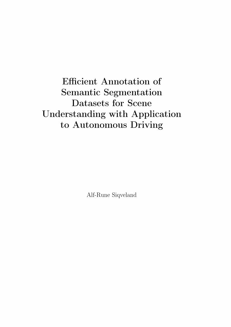
(a)

(b)

(c)

Figure 2.1: Representation of an image. (a) Representation of a greyscaleimage, the values represent the brightness of the corresponding pixel. (b)Representation of an RGB image as three individual component images(channels) stacked on top of each other. (c) The corresponding packedrepresentation of an RGB image. Image source (b,c): [70]

2.1.1 Representation of a Digital Image

In order to be able to process images, we need to understand how digitalimages are represented in a computing system. Though the perspectivecamera model is a quintessential part of computer vision involving geometricproperties and visual odometry (motion estimation), its not an integral partof recognition tasks. We will therefore skip the actual image formation modeland concentrate on the representation of a digital image in the discussionthat follows.

A digital image is an ordered array of numbers. Each element in the array,called a pixel, determines the brightness or intensity value at the spatiallocation in the image. The intensity values are restricted to the integerrange of the capturing device sampling bit depth. For example, most low-costcommercial cameras usually capture in 8-bit depth, restricting the intensityvalues to the integers in the range [0, 255] – on a computer, these imagesare treated as two-dimensional arrays of unsigned 8-bit integer data type.For greyscale images, an image is simply a two-dimensional matrix, and areusually referred to as single-channel images as each pixel holds a single scalarvalue.

For colour images, there are multiple ways of representing an imagedepending on what colour space we chose to represent the image. Here,we will only settle for images stored in RGB colour space. An RGB-imageis treated as a three-dimensional array, though the two spatial dimensionshave entirely different physical interpretation than the colour index. It istherefore useful to think of an RGB-image as a two-dimensional matrix of3-vector pixel values. On the other hand, an RGB-image has three channels,

6

determining the intensity value of the red, green and blue componentrespectively. We refer to the two types of representing an RGB imageas packed- and component order, respectively. Figure 2.1 summarises thediscussion on representing a digital image.

2.1.2 Digital Image Processing

Digital image processing is a sub-field of digital signal processing, the topicconcern methods that produce an altered or compressed representation of animage. Alternations typically include image pre-processing for creating anenhanced representation for a particular task, e.g. a higher level computervision task such as semantic segmentation. Some examples include blurring,contrast enhancement and JPEG compression. In the following, we willreview basic image processing techniques performed directly on the imageplane. We start with the simplest point operations before expanding thediscussion to neighbourhood operations. Then we move on to geometrictransformations that alter the spatial relations between pixels.

Point operations

Point operations, or intensity transformations, are the most straightforwardof all image processing transformations. The intensity value of a single pixelI(x, y) before and after applying a point operation is related by a functionthat takes the single pixel (point) as the argument. That is, the pointoperation is described by the relation

I ′(x, y) = T (I(x, y)) (2.1)

Example of two common point operations includes scaling by a (positive)factor and adding a bias. These two operations are more commonly referredto as contrast and brightness adjustment, respectively. Jointly applying thetwo transformations yields the following affine pixel-wise relation

I ′(x, y) = aI(x, y) + b (2.2)

Point operations are typically applied as a pre-processing step to normaliseintensity statistics or change the data type of an image. For example, whenwe later will discuss deep learning applied to computer vision, we usuallyconvert data type from integer to floating point and re-scaling the intensityrange to [0, 1] (a = 1/255, b = 0). For colour images, separate transformationsmay be applied to each channel, resulting in colour transformations.

Neighbourhood operations

Neighbourhood operations constitute a broader class of intensity transforma-tions. Let N(x,y) denote the set of coordinates contained in a neighbourhoodaround an arbitrary coordinate (x, y) in an image I. A neighbourhood op-eration creates a new intensity value at the corresponding coordinate as afunction of the pixels in N(x,y). The operator takes the neighbourhood in-tensity values as the argument, but may also include geometric relations as

7

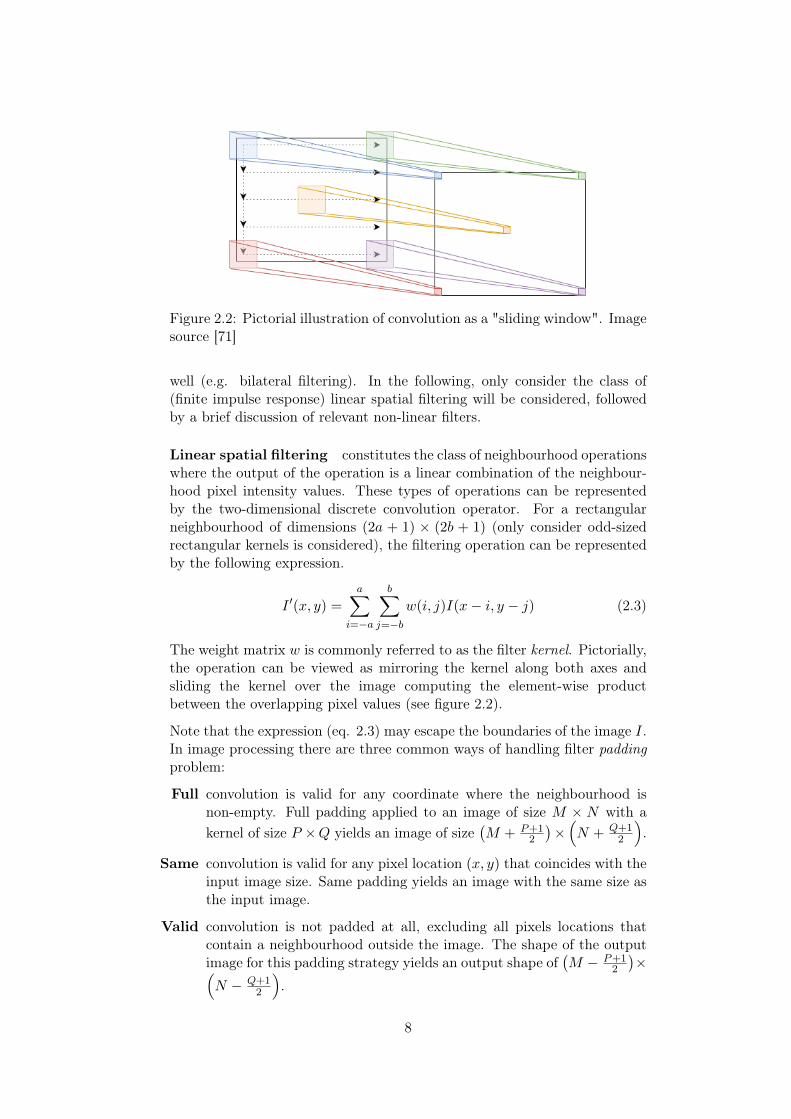
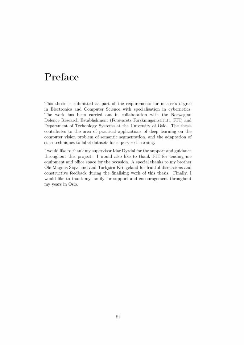
Figure 2.2: Pictorial illustration of convolution as a "sliding window". Imagesource [71]

well (e.g. bilateral filtering). In the following, only consider the class of(finite impulse response) linear spatial filtering will be considered, followedby a brief discussion of relevant non-linear filters.

Linear spatial filtering constitutes the class of neighbourhood operationswhere the output of the operation is a linear combination of the neighbour-hood pixel intensity values. These types of operations can be representedby the two-dimensional discrete convolution operator. For a rectangularneighbourhood of dimensions (2a + 1) × (2b + 1) (only consider odd-sizedrectangular kernels is considered), the filtering operation can be representedby the following expression.

I ′(x, y) =

a∑i=−a

b∑j=−b

w(i, j)I(x− i, y − j) (2.3)

The weight matrix w is commonly referred to as the filter kernel. Pictorially,the operation can be viewed as mirroring the kernel along both axes andsliding the kernel over the image computing the element-wise productbetween the overlapping pixel values (see figure 2.2).

Note that the expression (eq. 2.3) may escape the boundaries of the image I.In image processing there are three common ways of handling filter paddingproblem:

Full convolution is valid for any coordinate where the neighbourhood isnon-empty. Full padding applied to an image of size M × N with akernel of size P ×Q yields an image of size

(M + P+1

2

)×(N + Q+1

2

).

Same convolution is valid for any pixel location (x, y) that coincides with theinput image size. Same padding yields an image with the same size asthe input image.

Valid convolution is not padded at all, excluding all pixels locations thatcontain a neighbourhood outside the image. The shape of the outputimage for this padding strategy yields an output shape of

(M − P+1

2

)×(

N − Q+12

).

8

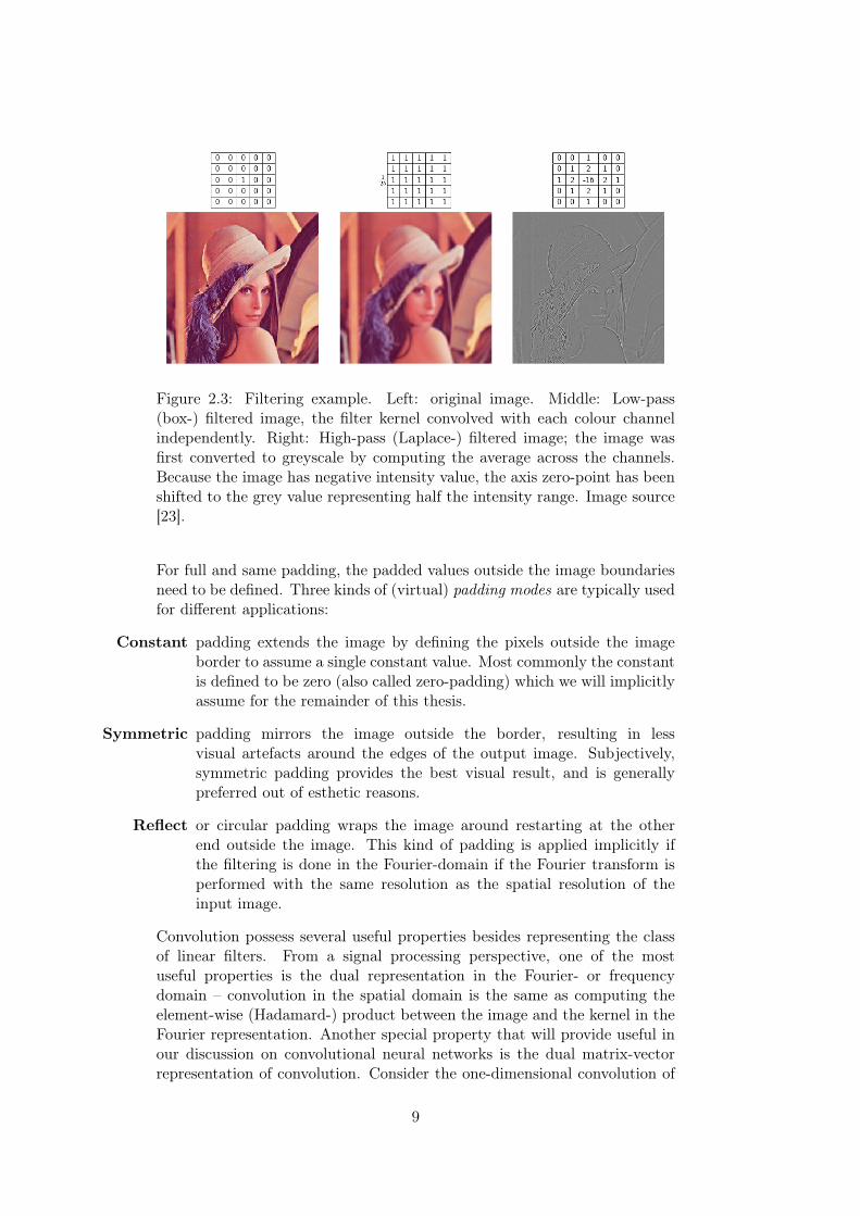
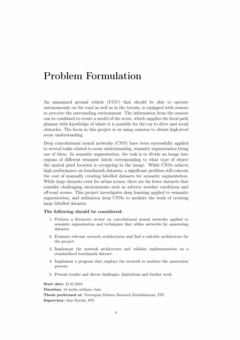
Figure 2.3: Filtering example. Left: original image. Middle: Low-pass(box-) filtered image, the filter kernel convolved with each colour channelindependently. Right: High-pass (Laplace-) filtered image; the image wasfirst converted to greyscale by computing the average across the channels.Because the image has negative intensity value, the axis zero-point has beenshifted to the grey value representing half the intensity range. Image source[23].

For full and same padding, the padded values outside the image boundariesneed to be defined. Three kinds of (virtual) padding modes are typically usedfor different applications:

Constant padding extends the image by defining the pixels outside the imageborder to assume a single constant value. Most commonly the constantis defined to be zero (also called zero-padding) which we will implicitlyassume for the remainder of this thesis.

Symmetric padding mirrors the image outside the border, resulting in lessvisual artefacts around the edges of the output image. Subjectively,symmetric padding provides the best visual result, and is generallypreferred out of esthetic reasons.

Reflect or circular padding wraps the image around restarting at the otherend outside the image. This kind of padding is applied implicitly ifthe filtering is done in the Fourier-domain if the Fourier transform isperformed with the same resolution as the spatial resolution of theinput image.

Convolution possess several useful properties besides representing the classof linear filters. From a signal processing perspective, one of the mostuseful properties is the dual representation in the Fourier- or frequencydomain – convolution in the spatial domain is the same as computing theelement-wise (Hadamard-) product between the image and the kernel in theFourier representation. Another special property that will provide useful inour discussion on convolutional neural networks is the dual matrix-vectorrepresentation of convolution. Consider the one-dimensional convolution of

9

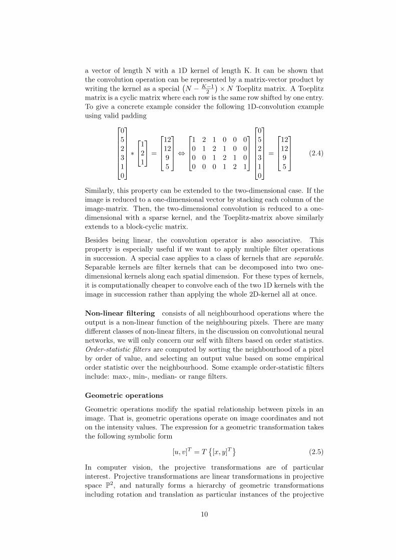
a vector of length N with a 1D kernel of length K. It can be shown thatthe convolution operation can be represented by a matrix-vector product bywriting the kernel as a special

(N − K−1

2

)×N Toeplitz matrix. A Toeplitz

matrix is a cyclic matrix where each row is the same row shifted by one entry.To give a concrete example consider the following 1D-convolution exampleusing valid padding

052310

∗1

21

=

121295

⇔

1 2 1 0 0 00 1 2 1 0 00 0 1 2 1 00 0 0 1 2 1

052310

=

121295

(2.4)

Similarly, this property can be extended to the two-dimensional case. If theimage is reduced to a one-dimensional vector by stacking each column of theimage-matrix. Then, the two-dimensional convolution is reduced to a one-dimensional with a sparse kernel, and the Toeplitz-matrix above similarlyextends to a block-cyclic matrix.

Besides being linear, the convolution operator is also associative. Thisproperty is especially useful if we want to apply multiple filter operationsin succession. A special case applies to a class of kernels that are separable.Separable kernels are filter kernels that can be decomposed into two one-dimensional kernels along each spatial dimension. For these types of kernels,it is computationally cheaper to convolve each of the two 1D kernels with theimage in succession rather than applying the whole 2D-kernel all at once.

Non-linear filtering consists of all neighbourhood operations where theoutput is a non-linear function of the neighbouring pixels. There are manydifferent classes of non-linear filters, in the discussion on convolutional neuralnetworks, we will only concern our self with filters based on order statistics.Order-statistic filters are computed by sorting the neighbourhood of a pixelby order of value, and selecting an output value based on some empiricalorder statistic over the neighbourhood. Some example order-statistic filtersinclude: max-, min-, median- or range filters.

Geometric operations

Geometric operations modify the spatial relationship between pixels in animage. That is, geometric operations operate on image coordinates and noton the intensity values. The expression for a geometric transformation takesthe following symbolic form

[u, v]T = T

[x, y]T

(2.5)

In computer vision, the projective transformations are of particularinterest. Projective transformations are linear transformations in projectivespace P2, and naturally forms a hierarchy of geometric transformationsincluding rotation and translation as particular instances of the projective

10

transform. As we will not introduce homogeneous coordinates, we rewritethe transformation in the form of equation 2.5 as

[u, v]T =

[xp11 + yp12 + p13xp31 + yp32 + p33

,xp21 + yp22 + p23xp31 + yp32 + p33

]T(2.6)

The class of affine transformations are obtained by setting p31 = p32 = 0 andp33 = 1. By further letting p13 = p23 = p21 = p12 = 0 amounts to scalingand stretching the image.

Applying the transformation in equation 2.5 directly to the pixels of an inputimage, generally results in an unevenly sampled output image, e.g. multiplepixels may be mapped to same output location, and some output pixels maynot have a defined value. In practice, the inverse transformation T−1(·) isapplied to a pre-defined output grid using interpolation to uniquely defineeach output intensity value. Interpolation provides a pseudo-continuousdescription of a digital image, thus providing a value for the reverse-transformed pixel locations that do not align perfectly with the image grid.Nearest neighbour interpolation rounds the pixel coordinates and assign thecorresponding value in the input image to the transformed output image.Bilinear interpolation computes a linear combination of the four nearestneighbours in the input image, weighted by components proportional to therelative coordinate distances.

2.1.3 Computer Vision Recognition Tasks

This thesis concerns semantic segmentation, which is a particular recognitiontask in computer vision. In this section, we will attempt to informallydescribe this type of recognition task, along with several related tasks. Inthe next chapter, semantic segmentation will be formulated as a particularmachine learning problem in order to apply deep learning.

Object classification is the most straightforward recognition problem. Asystem is to be constructed to assign a label to a given image out of a set ofpredefined labels. The images are assumed to each contain an object froma single label that occupies the majority of the camera field of view. Theapplication of such recognition tasks is hence limited to simple image queryproblems.

Object detection and localisation treat images with multiple objects,and the task consists of finding and assigning to each object in the image alabel from a predefined set of labels. Practically the task consists of drawingbounding boxes around objects and assign an object description to eachbounding box. Such detection algorithm provides a crude level of sceneunderstanding with limited applications within autonomous driving.

Semantic segmentation treats each pixel as possibly belonging to a class.The task consists of assigning a label to each pixel in the image to the correctclass. Semantic segmentation holds the promise of a fine-grained description

11

Figure 2.4: Evolution of recognition tasks in level of scene understanding:(a) object classification, (b) object detection and localisation, (c) semanticsegmentation and (d) instance segmentation. Image source: [25].

of the scene, being able not only to see what objects are contained in thescene but also at which areas in the image the objects occupy.

Instance segmentation is the hardest of all image-recognition tasks. Thetask consists of both detection and localisation, as well as segmenting theboundaries of each object to pixel-level accuracy. It can be viewed, andindeed some contributions treat the problem as the compound problemof first doing object detection and localisation, followed by semanticsegmentation of each proposed bounding box.

Figure 2.4 summarises the tasks discussed above. In the discussion thatfollows, to simplify the discussion, we will consider the object classification ina more general machine learning perspective, before we extend our discussionto semantic segmentation.

2.2 Machine Learning

A central topic of this thesis besides computer vision is machine learning.Machine learning is a broad field spanning a vast number of topics and isthe primary tool used in this project to generate semantic segmentation fromimages. In this section, a gentle introduction to machine learning is provided,covering only the topics needed as background for the more specialised field ofdeep learning. The material for this section is mostly based on the literature[18] and [28], with additional references provided wherever used.

12

Machine learning is the study of creating algorithms and statistical modelsthat can learn from data. For the sake of the discussion, Mitchell [56, p. 2]provides a succinct definition of learning.

Definition (Learning). A computer program is said to learn from experienceE with respect to some class of tasks T and performance measure P , if itsperformance at the task T , as measured by P , improves with experience E.

For example, a program that learns to classify products on a conveyorbelt based on input from a monitoring camera (task T ) might improve itsperformance (P ), e.g. measured by accuracy of correctly classified objects,through experience (E) by watching a set of hand-labelled objects.

The task is usually described in terms of how the machine learningalgorithm process an example, e.g. assigning a label to images of objectson a conveyor belt. Machine learning is interesting because it enables usto tackle problems that are too difficult to solve with a fixed algorithm. Inthis section, we will exclusively focus on the classification problem; we willstart by considering the general classification problem, and later see howwe can extend this problem to the task of semantic segmentation. Someother example types of problems machine learning have been successfullyapplied to include: regression, transcription, machine translation, anomalydetection, control applications, to name a few.

For the classification task, the machine learning algorithm is asked to specifywhat class, or category, the input feature vector x ∈ Rn belongs to out ofa fixed set of Nc categories. This problem is usually solved by making thelearning algorithm learn a function f : Rn 7→ 1, ..., Nc, mapping featurevectors to an index into the enumerated set of categories under consideration.Most classification approaches try to model the output as a probabilitydistribution over the set of categories, and along with a decision-rule assigna category y ∈ 1, ..., Nc to a given the feature vector x.

The experience comes in the form of a dataset. Depending on thenature of the task performed, the learning process can be performed withvarying degree of supervision. We generally distinguish between two classesof learning: supervised- and unsupervised learning.

In supervised learning, the dataset (experience) consists of a “hand-labelled”sample of manually annotated ground truth examples. We will denote sucha dataset D = (x(i),y(i)), where the feature vector x(i) takes values inthe source domain X , and the target label y(i) takes values from the setY. We will denote the discrete set of label values in symbolic terms asY , y1, y2, ..., yNc where Nc is the number of classes considered for thetask. The goal is to learn the function f : X 7→ Y that maps each featurevector x(i) to the correct target vector y(i). Each of the examples (x(i),y(i))in the dataset are assumed to be sample realisations drawn from an unknowndata-generating distribution pdata(D).

Unsupervised learning algorithms experience a dataset containing only

13

feature vectors D = x(i),x(2), .... The goal is then to learn usefulproperties of the structure of the dataset and the underlying data-generatingdistribution. In contrast to supervised learning, the dataset is generallyfar cheaper to produce when the labels are excluded, and can typically beautomated. Examples of unsupervised learning problems include: clustering,density estimation and dimensionality reduction.

The performance of a machine learning algorithm is evaluated in termsof a quantitative measure. This performance measure is usually dependenton the task carried out by the system. For tasks such as classification weoften measure the performance in terms of accuracy, i.e. the proportion ofcorrectly classified examples over the dataset, of the classifier. We will seelater that for segmentation, it is more informative to use other evaluationmetrics.

Usually, we are interested in how well the machine learning algorithm per-forms when the algorithm is deployed in the real world, i.e. we are moreinterested in the performance on data not seen while the algorithm is learn-ing. For several reasons we will come back to, depending on the trainingprocedure there will be a varying performance drop when evaluated on theexamples the learning algorithm has experienced and unseen examples. Thisperformance drop, called the generalisation error, is useful to quantify inorder to estimate how well the machine learning algorithm is expected per-formed when the system is deployed. Therefore, a proportion of the datasetis kept aside as a test set used for performance evaluation when the modelis finished training on the training set.

In summary, supervised learning involves observing several sample realisa-tions x of a random vector x and an associated target value (or vector) y andlearn to predict y from the observations of x by estimating P (y|x), calledthe class posterior distribution – or simply the posterior. On the other hand,unsupervised learning involves observing several examples of a random vec-tor x and attempt to learn the probability distribution p(x) or propertiesthereof. In the following, we are only going to deal with supervised learningapplied to the pattern classification problem. For this class of problems, thefeature-vector x is an N-dimensional vector, and the target y is a scalar in-teger indexing the enumerated set of classes. More specifically, we will firstconsider object classification, and later extend our discussion to semanticsegmentation when we have covered deep learning.

2.2.1 Bayesian Classifiers

In the discussion above, we briefly mentioned that the examples of adataset are drawn from a complicated and unknown distribution – the data-generating distribution pdata. In machine learning, the goal is to estimate thisdata-generating distribution, either explicitly or implicitly, in order to makedecisions that minimise a predefined cost. To this end, a set of simplifyingassumptions are made about the data-generating distributions commonly

14

known as the independent and identically distributed (i.i.d) assumptions. Insymbolic terms, this respectively means

pdata(D) =

|D|∏i=1

pdata(x(i), y(i)) (2.7)

pdata(x(i), y(i)) = pdata(x(j), y(j)), ∀i, j ∈ 1, 2, ..., |D| (2.8)

The first equation (2.7) states that all examples in the dataset aremutually independent. That is, any example in the dataset is conditionallyindependent on any subset of other examples from the dataset – by writingthe data distribution in terms of the chain-rule of conditional probability(p(x1, ..., xn) = p(x1)

∏nk=2 p(xk|x1, ..., xk−1)), we get the expression in 2.7.

The second equation (2.8) states the identically distributed part – all examplepairs are drawn from the same distribution.

The validity of these assumptions depends on the nature of the data andhow the dataset is collected. For image classification, the independenceassumption 2.7 breaks if the same object is imaged multiple times withoverlapping field of view (pixels in both images are correlated). The secondassumption of identical distributions 2.8 might be weakened if the datacollection process is not consistent. For example, if datasets acquiredby different set of equipment and policies are combined for a particularapplication.

By making the i.i.d. assumptions, and further assuming a candidate modeldistribution for the data-generating distribution which we will refer to asthe model- (or hypothesis-) distribution for the data pmodel(x, y); we canformulate the classification problem in probabilistic terms. Given the modeldistribution, we can use Bayes’ rule to get the expression for the posteriordistribution1

p(y|x) =p(x, y)∑|D|i=1 p(x, yi)

=p(x|y)P (y)∑|D|

i=1 p(x|yi)P (y = yi)(2.9)

Note that the denominator of the posterior (eq. 2.9) is independent ofthe value of y, this fact is usually taken into account. In fact, it is quitecommon to make model assumptions about the individual class-conditionaldistributions p(x|y = yi) by splitting the dataset into subsets of eachclass. This way, the (more tractable) class-conditional distributions can bemodelled in isolation, and then combined by asserting a prior probabilityP (y = yi) for each of the classes.

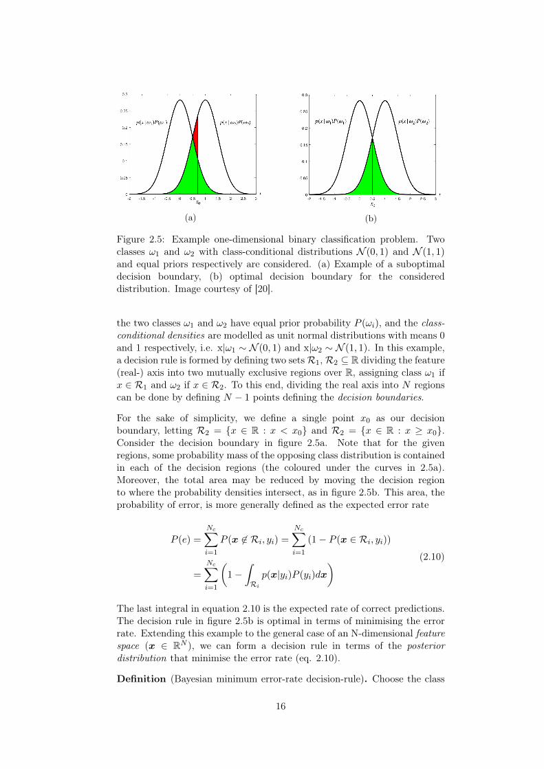
Given our model assumptions and the corresponding posterior distribution,how should we formulate our decision rule? To this end, we need to introduceone more concept: the (expected) probability of error. Consider the one-dimensional binary classification problem in figure 2.5. In this problem,

1For notational convenience, the subscript from the probability distributions will beomitted.

15

(a) (b)

Figure 2.5: Example one-dimensional binary classification problem. Twoclasses ω1 and ω2 with class-conditional distributions N (0, 1) and N (1, 1)and equal priors respectively are considered. (a) Example of a suboptimaldecision boundary, (b) optimal decision boundary for the considereddistribution. Image courtesy of [20].

the two classes ω1 and ω2 have equal prior probability P (ωi), and the class-conditional densities are modelled as unit normal distributions with means 0and 1 respectively, i.e. x|ω1 ∼ N (0, 1) and x|ω2 ∼ N (1, 1). In this example,a decision rule is formed by defining two setsR1, R2 ⊆ R dividing the feature(real-) axis into two mutually exclusive regions over R, assigning class ω1 ifx ∈ R1 and ω2 if x ∈ R2. To this end, dividing the real axis into N regionscan be done by defining N − 1 points defining the decision boundaries.

For the sake of simplicity, we define a single point x0 as our decisionboundary, letting R2 = x ∈ R : x < x0 and R2 = x ∈ R : x ≥ x0.Consider the decision boundary in figure 2.5a. Note that for the givenregions, some probability mass of the opposing class distribution is containedin each of the decision regions (the coloured under the curves in 2.5a).Moreover, the total area may be reduced by moving the decision regionto where the probability densities intersect, as in figure 2.5b. This area, theprobability of error, is more generally defined as the expected error rate

P (e) =

Nc∑i=1

P (x 6∈ Ri, yi) =

Nc∑i=1

(1− P (x ∈ Ri, yi))

=

Nc∑i=1

(1−

∫Ri

p(x|yi)P (yi)dx

) (2.10)

The last integral in equation 2.10 is the expected rate of correct predictions.The decision rule in figure 2.5b is optimal in terms of minimising the errorrate. Extending this example to the general case of an N-dimensional featurespace (x ∈ RN ), we can form a decision rule in terms of the posteriordistribution that minimise the error rate (eq. 2.10).

Definition (Bayesian minimum error-rate decision-rule). Choose the class

16

that maximises the posterior distribution given the observation x. That is

yME = arg maxyi

P (y = yi|x) (2.11)

This decision-rule is a particular case of Bayesian minimum risk classificationwith zero-one cost function [see 18, p. 24-27 for more details].

2.2.2 Estimating the Posterior

Instead of letting the model distribution be a fixed density, we willextend our model assumptions to a parameterised family of distributionspmodel(x, y;W). For example, consider using the normal family ofdistributions N (µ,Σ). Then, the set of parameters becomes W = µ,Σif the distribution is parameterised by the mean and covariance matrix.A parameter estimator w is a function of the dataset that either yield asingle (fixed) set of parameters W = g(D), or a probability-distribution overparameter-space W ∼ pW(w) that likely generated the observed sample.The two types of estimators are referred to as point estimators and Bayesianstatistics, respectively. In the following discussion, to simplify notation,the target labels of the dataset examples will be ignored, and the set ofparameters W are treated as a single vector w ∈ Rn.

Maximum likelihood point-estimation tries to estimate the constantparameter vector that best explains the data. Suppose that D contains Nexamples x(i), ...,x(N), all drawn i.i.d. from a data-generating distributionp(x;w) with the true parameter vector w. Then, because the examples areindependently generated from the same parametric distribution, we maywrite

p(D;w) =N∏i=1

p(x(i);w) (2.12)

The equation 2.12 is called the likelihood function when expressed as afunction of the parameter-vector w. For a given sample realisation D, thelikelihood function tells how well the parameterised distribution explainsthe data as function of w. The maximum likelihood estimate of theparameters w, is the value w that maximise the likelihood function, p(D; w),i.e. the parameters that best explain the data. Because the likelihoodfunction (2.12) quickly becomes vanishingly small for increasing sample size,finite-precision evaluation of the likelihood function becomes prohibitive fornumerical optimisation. Thus, it is far easier to work with the logarithm ofthe likelihood function, the log-likelihood function

l(w) = ln p(D;w) =N∑i=1

ln p(x(i);w) (2.13)

As the logarithm is a monotonic function, the extremal values w of p(D;w)does not change. For numerical considerations, it is useful to make the range

17

of the log-likelihood function independent of the sample size, N , by takingthe sample mean.

l(w) =1

N

N∑i=1

ln p(x(i);w) (2.14)

The mean log-likelihood function has an alternate interpretation that itis also the negative cross-entropy between the empirical data distribution(pdata(x) =

∑Ni=1

1(x=x(i))N ) and the parameterised model distribution, i.e.

l(w) = −H(pdata, p(·;w)) = Ex∼pdata [p(x;w)] (2.15)

In the deep learning literature, the term “cross-entropy loss” is used toidentify the negative mean log-likelihood of a Bernoulli or categorical(softmax-) distribution. The reader should keep in mind this identity –any negative log-likelihood is also the cross-entropy between the empiricaldistribution defined by the training set and the modelled probabilitydistribution.

From the discussion above, the expression for the maximum likelihoodestimate is

wML = arg maxw

p(D;w) = arg maxw

l(w) (2.16)

A necessary condition for a (local) extremal point can be obtained from theroots of the homogeneous equation

∇wl(w) = 0 (2.17)

The parameters satisfying equation (2.17) are either (local) maximum,(local) minimum or saddle points of the likelihood function. The modelswe will deal with later are of such complexity that finding the optimumanalytically by solving equation 2.17 becomes intractable. Thus, it isnecessary to resort to approximate numerical optimisation algorithms.

It is more common for deep learning models to parameterise the posteriordistribution (eq. 2.9) directly. The maximum likelihood estimator canbe readily generalised to the (discrete) posterior by following the samederivations as above. Under the i.i.d. assumptions, the log-likelihoodequation (2.13) becomes

wML = arg maxw

N∑i=0

lnP (y(i)|x(i);w) (2.18)

Under the assumption that the actual data-generating distribution iscontained in the parameterised family of distributions pdata(x) = p(x;w),then the maximum likelihood approaches the true data-generating inprobability as the sample size grows to infinity. This desirable property iscalled estimator consistency, which expressed symbolically as

limN→∞

P (|w − wML| > ε) = 0 (2.19)

Where N is the size of the sample (dataset) involved in the maximumlikelihood estimate wML and w is the parameter of the actual data-generating distribution.

18

Bayesian estimation in contrary to maximum likelihood yields anestimated density over the set of parameters. Up until now, we haveconsidered w to be a fixed value. With Bayesian estimation the parametersare considered to be random (w ∼ p(w)). The goal is then two-fold:estimating the parameter distribution given the observed data p(w|D) inorder to explain the model distribution given the observed data p(x|D).The equation relating the two distributions can be formulated by merelymarginalising the latter over the parameter vector, i.e.

p(x|D) =

∫p(x,w|D)dw =

∫p(x|w)p(w|D)dw (2.20)

The last equation holds under the assumption that the distribution of x giventhe parameter vector w is conditionally independent on the dataset D. Theparameter posterior distribution, p(w|D), is of interest in machine learningapplication as it expresses the uncertainty with respect to the parametersfor a particular set of parameters. Using Bayes’ rule, we have

p(w|D) =p(D|w)p(w)∫p(D|w)p(w)dw

(2.21)

where, by the independence assumption, we have

p(D|w) =

N∏i=1

p(x(i)|w) (2.22)

The complexity of computing the Bayesian estimate grows very quickly withthe dataset size and the model complexity. For complex model assumptions,like the ones we will see in the deep learning approach, the integrals inequations 2.20 and 2.21 are computationally intractable, and it is necessaryto resort to approximation techniques like Markov Chain Monte Carlo [28,ch. 17, sec 3] or variational approaches [61]. We will not elaborate anyfurther on Bayesian estimation here as the learning approaches conductedin this thesis are based on point-estimation, but include this section for thesake of completeness.

Maximum a posteriori (MAP) is another point estimation techniquethat may be thought of as a compromise between Bayesian- and maximumlikelihood estimation. However, the MAP-estimator is still a point estimator,and the similarity with the Bayesian estimate is merely expressed in termsof the parameter posterior. The MAP-estimate is expressed as

wMAP = arg maxw

p(w|x) = arg maxw

(ln p(w) +

N∑i=0

ln p(x(i)|w)

)(2.23)

Where we recognise the second term,∑

i ln p(x(i)|w), as the log-likelihoodterm of equation 2.13, whereas the second term incorporates the parameterprior distribution. Hence maximum a posteriori may be thought of as usingthe parameters that maximise equation 2.21.

19

2.2.3 Stochastic Gradient Descent

As the complexity and number of parameters for the model increases, solvingthe point estimation problems presented above quickly becomes analyticallyintractable, and it is necessary to resort to numerical techniques. This factis especially evident for the deep neural networks, and nearly all of deeplearning uses some form of stochastic gradient descent (SGD) algorithms asthe learning mechanism for training the model.

We saw how maximum likelihood estimation amounts to finding the globalmaximum of the log-likelihood function (eq. 2.13) by solving the equation2.16 and possibly comparing all solutions to find the maximum. It ismore common in the machine learning literature to express the optimisationproblem as finding the minimum of a cost function. In this regard, we definethe total cost – the negative log-likelihood – in terms of the mean per-exampleloss

C(W) =1

N

N∑i=1

L(x(i), y(i),W) = Ex,y∼pdataL(x, y,W) (2.24)

By comparing with equation 2.18, the per-example loss is defined asL(x, y,W) = − ln p(y|x;W).

The most straight forward approach to find the optimum numerically isthe gradient descent algorithm. The gradient evaluated at any point of ascalar field such as the cost, points in the direction of steepest ascent. Thustaking a step along the negative gradient, we would expect the value of thescalar field to decrease. Following this observation, the gradient descentalgorithm repeatedly takes a step along the negative gradient. The step sizeis controlled by scaling by a parameter η, thus we can formulate the gradientdescent algorithm as the recurrent relation

Wi+1 =Wi − η∇WC(Wi) (2.25)

The update (2.25) is applied until the gradient magnitude is sufficientlyclose to zero. The step size parameter η is what in machine learningis referred to as the learning rate hyperparameter. Hyperparameters areparameters that cannot be optimised using gradient based optimisation, andare usually manually tuned or searched for using algorithms that optimisenon-differentiable objective functions (e.g. genetic algorithms or particleswarm optimisation).

The computational cost of computing the gradient ∇wC(w) grows linearwith the size of the dataset (O(N)). For datasets containing millions or evenbillions of training examples, computing and accumulating a single gradientbecomes prohibitive. This observation leads us to the stochastic part ofSGD. Instead of evaluating the gradient over the whole dataset, using theinsight that the gradient of the cost function is an expectation over the per-example cost gradient, we can approximate this expectation by sampling amini-batch of examples from the empirical data distribution (uniformly overthe dataset examples). The stochastic gradient descent algorithm is shown in

20

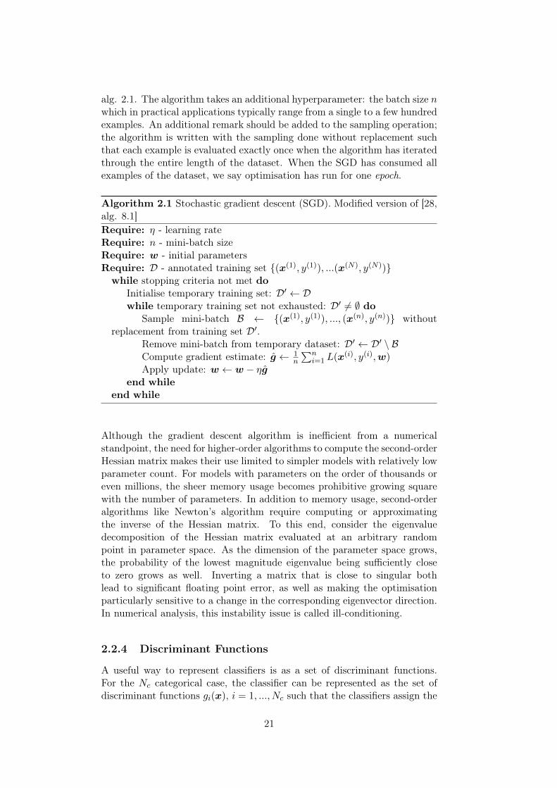
alg. 2.1. The algorithm takes an additional hyperparameter: the batch size nwhich in practical applications typically range from a single to a few hundredexamples. An additional remark should be added to the sampling operation;the algorithm is written with the sampling done without replacement suchthat each example is evaluated exactly once when the algorithm has iteratedthrough the entire length of the dataset. When the SGD has consumed allexamples of the dataset, we say optimisation has run for one epoch.

Algorithm 2.1 Stochastic gradient descent (SGD). Modified version of [28,alg. 8.1]Require: η - learning rateRequire: n - mini-batch sizeRequire: w - initial parametersRequire: D - annotated training set (x(1), y(1)), ...(x(N), y(N))while stopping criteria not met do

Initialise temporary training set: D′ ← Dwhile temporary training set not exhausted: D′ 6= ∅ do

Sample mini-batch B ← (x(1), y(1)), ..., (x(n), y(n)) withoutreplacement from training set D′.

Remove mini-batch from temporary dataset: D′ ← D′ \ BCompute gradient estimate: g ← 1

n

∑ni=1 L(x(i), y(i),w)

Apply update: w ← w − ηgend while

end while

Although the gradient descent algorithm is inefficient from a numericalstandpoint, the need for higher-order algorithms to compute the second-orderHessian matrix makes their use limited to simpler models with relatively lowparameter count. For models with parameters on the order of thousands oreven millions, the sheer memory usage becomes prohibitive growing squarewith the number of parameters. In addition to memory usage, second-orderalgorithms like Newton’s algorithm require computing or approximatingthe inverse of the Hessian matrix. To this end, consider the eigenvaluedecomposition of the Hessian matrix evaluated at an arbitrary randompoint in parameter space. As the dimension of the parameter space grows,the probability of the lowest magnitude eigenvalue being sufficiently closeto zero grows as well. Inverting a matrix that is close to singular bothlead to significant floating point error, as well as making the optimisationparticularly sensitive to a change in the corresponding eigenvector direction.In numerical analysis, this instability issue is called ill-conditioning.

2.2.4 Discriminant Functions

A useful way to represent classifiers is as a set of discriminant functions.For the Nc categorical case, the classifier can be represented as the set ofdiscriminant functions gi(x), i = 1, ..., Nc such that the classifiers assign the

21

feature vector x to the class yi if

gi(x) > gj(x), ∀j 6= i (2.26)

The discriminant function representation is by no means unique but allowsexpressing the decision rule in terms of more analytically tractable functionsthat may simplify computation for performing inference. Consider theminimum error-rate classifier of equation 2.11. Instead of using the completeexpression for the posterior as our decision premise, by noting that thedenominator in equation 2.9 is constant for all classes, we can use thefollowing truncated log-likelihood expression

gi(x) = ln p(x|yi) + lnP (y = yi) (2.27)

This expression is far more tractable than the full expression in equation 2.9,especially for a class-conditional distribution in the exponential family e.g.Gaussian- or Laplacian- distributions.

Linear discriminant functions

A particular class of discriminant functions are of particular interest; thelinear2 discriminant functions, also called linear perceptrons.

gi(x) = wTi x+ w0,i (2.28)

The linear discriminant function separates the feature space by a set ofplanar decision boundaries. To appreciate the importance of this class ofdiscriminant functions, consider the following example.

Example. Consider an N-dimensional binary classification problem. Thatis, the feature vectors are N-dimensional (x ∈ RN ) each belonging to oneout of two classes y1, y2. Further consider selecting a multivariate normalcandidate distribution as our model for the class-conditional distributions(x|yi ∼ N (µi,Σi)). The expression for the class posterior log-likelihoodthen becomes

lnP (yi|x) = ln p(x|yi) + lnP (y = yi)− ln p(x)

= −1

2(x− µi)TΣ−1i (x− µi) + lnP (y = yi)− ln p(x)

= −1

2xTΣ−1i x+ µTi Σ−1i x−

1

2µTi Σ−1i µi + lnP (y = yi)− ln p(x)

If we further assume that the covariance matrices are constant, equal anddiagonal (Σi = σ2I) and that the model is parameterised by the meanvectors, we further have

lnP (yi|x) =1

2σ2µTi (x− µi) + lnP (yi) + c(x)

2These functions are actually affine in the feature vector x; however since they aretypically written in homogeneous form (i.e. with an additional constant 1 as the lastentry of the feature vector) in the literature [18] they are usually referred to as lineardiscriminant functions.

22

By making the substitutions wi = 1σ2µi and w0,i = lnP (yi)− 1

2σ2µTi µi and

noting that the collective term c(x) does not depend on the model parameterswe finally get the desired discriminant function in equation 2.28.

2.2.5 Generalisation, Capacity and Dimensionality

In the discussion of evaluating the performance, it was mentioned that wewant our classifier to perform well on yet unseen data; that is, we want theclassifier to generalise from the training set to the test set. Consider thatwe initialise our model with a random set of weights. Then, the error onthe training set and test set should in expectation be the same. However,the parameters do not remain fixed but are estimated using numericaloptimisation like SGD to incrementally minimise the cost function (negativelog-likelihood) with respect to the training set. Under this process, the testset error must necessarily be greater or equal to the training set error as theestimation process only fits the parameters to the observed examples. Thisleads us to two central challenges in machine learning called underfitting andoverfitting. Underfitting occurs when the model performance on the trainingset ceases to improve too early. Overfitting occurs when the model achievesmuch higher performance on the training set over the test set.

To understand why a model starts to underfit or overfit, we need to introducethe abstract concept of model capacity. Informally, a model’s capacitymeasures the variety of functions the model is able to learn out of a selectedhypothesis-space. It is useful to think of the hypothesis space as the functionspace of the discriminant function. Underfitting occurs whenever the modeldoes not contain a solution in its hypothesis space that is close to theunderlying data-generating distribution. The problem of overfitting is alittle more complicated as there are three factors affecting a model’s abilityto overfit a particular problem: capacity, dimensionality and the number ofexamples in the training set. Roughly speaking, overfitting occurs wheneverthe model capacity exceeds the characteristic capacity of the problem. Figure2.6 shows a cartoon drawing of how the expected error typically varies as afunction of model capacity.

To be more specific about the notion of capacity, statistical learning theoryprovides a way of quantifying a model’s capacity. Statistical learning theoryis a theoretical branch of machine learning, attempting to prove from amathematical standpoint what properties of a learning algorithm to satisfyin order to be successful. The following discussion is based on the lectures[1–3], and results will be presented without further justification. For a gentleintroduction to statistical learning theory, the reader is referred to [49], whichtreats the subject in more general terms of risk.

The growth function, mH(N), gives a quantitative capacity measure of ahypothesis space H. It is defined as the maximum number of dichotomies abinary classifier over the given hypothesis space can produce for a set of Npoints. Formally the growth function is defined as [1, p. 8]

mH(N) = max∣∣∣(f(x(1)), ..., f(x(N))) | f ∈ H

∣∣∣ (2.29)

23

Figure 2.6: Hypothetical plot of training and test set error as a function ofmodel capacity. The optimal capacity is reached when the model performsbest on the test set, underfitting if the capacity is too low and overfitting iftoo high.

The maximal value of the growth function is at most 2N , which is the case ifthe binary classifier is able to classify the points in arbitrary configuration.The maximal number of points for which the growth function equals 2N iscalled the VC-dimension. The VC-dimension dV C , of a linear perceptron,is d + 1, with d the feature space dimension. It can be shown [2, 3] thatthe growth function is bounded above by the quantity that depends on theVC-dimension

mH(N) ≤dV C∑i=0

(N

i

)(2.30)

This expression (2.30) is a polynomial of a maximal degree of NdV C .Thus, the growth rate of the growth function mH is bounded by VC-dimension. An important result in statistical learning theory, called theVapnik-Chernovenkis inequality, is expressed as [2, p. 18]

P [|etrain − etest| > ε)] = 4mH(2N)e−18ε2N (2.31)

In light of equation 2.30, the equation (2.31) states that the generalisationerror is bounded by a quantity that grows with the capacity of the modeland feature space dimension, but shrinks with the size of the training dataN . To summarise, in order to reduce the generalisation error, more trainingdata needs to be collected or the model assumptions must be simplified toreduce the capacity. Later it will be shown how we can reduce a model’seffective capacity through regularisation.

Finally, notice how the VC dimension for the linear classifier and alsothe growth function depends on the feature space dimension. For thisparticular hypothesis, the growth rate upper bound grows exponentially with

24

the dimension of feature space. This phenomenon is commonly known inmachine learning as the curse of dimensionality.

Monitoring generalisation through validation

It is essential to keep track of how well a machine learning model is expectedto generalise to new examples. The process of estimating how much amodel is overfitting the training data is called validation. The most straightforward way of performing validation is by keeping aside a small proportion(10-20%) of the dataset as a validation set. Then throughout the learningphase, the model performance is evaluated regularly on the validation set.By comparing the model’s performance on the validation set to that of thetraining set performance, the amount at which the model is overfitting orunderfitting the data is estimated. More sophisticated validation algorithmsexist, most notably variations of the cross-validation algorithm; however,for models that are expensive to train these algorithms quickly becomesprohibitive.

2.2.6 Sources of Error

Up until now, we have encountered multiple forms of error for a machinelearning algorithm. To summarise, the following are the three differentcategories of errors encountered in any machine learning problem.

• Bayes error. Even though the true data-generating model was known,it is not necessarily the case that the features are perfectly separable.We saw in the simple binary example of figure 2.5 that even the optimaldecision boundary has non-zero expected probability of error (colouredarea under the curve). This indistinguishability error is an inherentproperty of the problem and cannot be eliminated.

• Model assumptions. If the model hypothesis does not contain thetrue data-generating distribution in the hypothesis space, a sub-optimalsolution is found. For example, if the true data-generating distributionis Laplacian, but we use a Gaussian hypothesis, or the data-set maynot satisfy the i.i.d. assumptions. Note that invalid model assumptionsimply that the model is underfitting the data.

• Estimation error. Stochastic gradient descent might not always leadto the optimal solution in a finite amount of time. It might be thecase that the solution converges to a local minimum, or get stuck in asaddle point of the cost function. Generalisation error also falls underthe category of estimation error. This type of error can be reduced bycollecting a larger dataset, or training ensembles of models initialisedwith different parameter configurations and using the mean ensembleprediction.

25

2.2.7 Towards Deep Learning

In the above discussion, a central machine learning topic, feature selectionand feature extraction, has been purposely avoided. We have simply assumedthat the feature vector x represent some data to be classified. The curse ofdimensionality states that careful choice of features is crucial for achievinggood performance for any machine learning algorithm. Good feature vectorscompress as much information as possible in a more compact representation.In the next section, we will discuss a particular approach that avoids themanual feature selection process alltogether.

Feedforward neural networks embed the feature extraction in the paramet-erised model itself. This way, the model operates on the data directly, andno search for manually constructed features through repeated validation ex-periments are necessary. The feedforward neural networks are composed of acascade of sub- structures called layers, that each computes a function thatit passes on to the input of the next layer. The term Deep Learning comesfrom the number of layers, also called the depth of the network.

2.3 Deep Learning

Deep learning is a specific approach to machine learning that utilisesdeep artificial neural networks with large representational capacity asthe machine learning model. Deep learning models typically containenough representational capacity to overfit the problem, but use extensiveregularisation techniques to restrict the effective capacity. In this section,feedforward neural networks will be discussed, and the backpropagationalgorithm will be introduced for the multilayer perceptron in order to performgradient descent. Different regularisation techniques will be presented,followed by a discussion of challenges with training deep networks as wellas some techniques that mitigates these challenges.

2.3.1 Computational Graphs

To aid our discussion on neural networks, we pause and review the languageof computational graphs. The way we define computational graphs here willalso be useful later in the implementation discussion. Computational graphsare unidirectional graphs describing a series of mathematical operations.There are many ways of formalising computational graphs, and this thesis

Figure 2.7: Computational graph node examples.

26

(a) (b) (c)

Figure 2.8: Computational graph examples. (a) A simple scalar addition z =x+ y. (b) The graph for linear discriminant function h(x;w, b) = wTx+ b.(c) The graph for a single-layer perceptron (see section 2.3.2) with a genericactivation function h(x;W,b) = f(W Tx+ b).

use the convention where each internal graph node is associated with anoperation. An operation is a simple function of one or more inputs, e.g.summation, matrix multiplication or any elementwise function. In additionto operations, all leaf nodes are special. A leaf node provides an input to thegraph and is either a constant or a variable. Figure 2.7 shows some examplenodes.

The edges in our graph language are naturally associated with the value ofthe preceding operations. Without loss of generality, every node has a singleoutput edge and can either be a scalar, vector, matrix or higher order tensorsdepending on the input dimensions and the operation. The number of inputsto an operation can be arbitrary but is usually defined in terms of the natureof the operator. Note especially the multiplication operation in figure 2.7,which we will use as generalised matrix multiplication, i.e. matrix-matrixor matrix-vector or scalar product depending on the input sizes. Figure 2.8shows some examples of some simple computational graphs.

2.3.2 The Multilayer Perceptron

The multilayer perceptrons (MLPs) are quintessential deep learning models.Almost all instances of deep learning models can be described as particularinstances or alternations of the multilayer perceptron. The MLP is also calledfeedforward neural networks as they are loosely inspired by neuroscience;however, modern neural network research is guided by mathematical andengineering disciplines rather than modelling the brain.

The MLP defines a parameterized function in terms of a specific acycliccomputational graph structure. The structure, as illustrated in figure

27

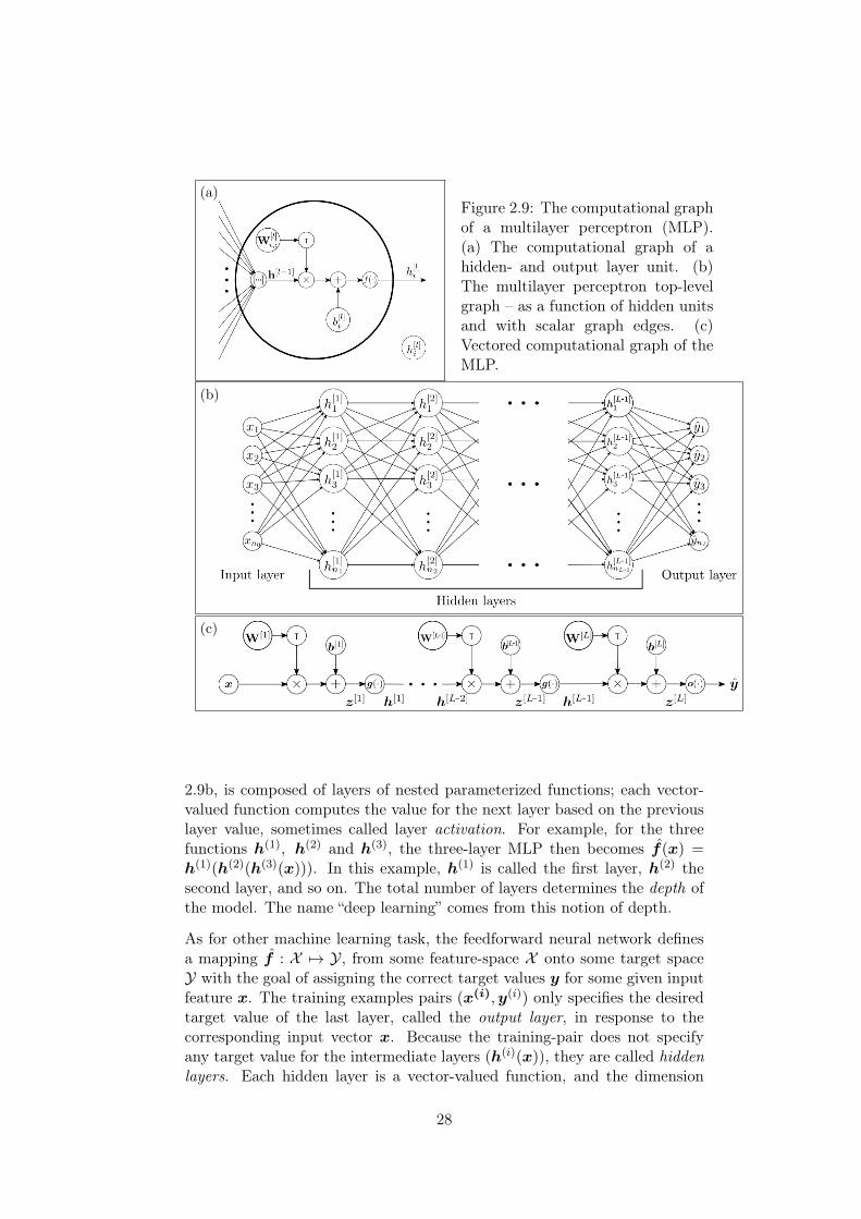
(a)Figure 2.9: The computational graphof a multilayer perceptron (MLP).(a) The computational graph of ahidden- and output layer unit. (b)The multilayer perceptron top-levelgraph – as a function of hidden unitsand with scalar graph edges. (c)Vectored computational graph of theMLP.

(b)

(c)

2.9b, is composed of layers of nested parameterized functions; each vector-valued function computes the value for the next layer based on the previouslayer value, sometimes called layer activation. For example, for the threefunctions h(1), h(2) and h(3), the three-layer MLP then becomes f(x) =h(1)(h(2)(h(3)(x))). In this example, h(1) is called the first layer, h(2) thesecond layer, and so on. The total number of layers determines the depth ofthe model. The name “deep learning” comes from this notion of depth.

As for other machine learning task, the feedforward neural network definesa mapping f : X 7→ Y, from some feature-space X onto some target spaceY with the goal of assigning the correct target values y for some given inputfeature x. The training examples pairs (x(i),y(i)) only specifies the desiredtarget value of the last layer, called the output layer, in response to thecorresponding input vector x. Because the training-pair does not specifyany target value for the intermediate layers (h(i)(x)), they are called hiddenlayers. Each hidden layer is a vector-valued function, and the dimension

28

associated with a hidden layer determines its width. An attractive motivationfor the MLP is evidenced by the universal function approximator theorem[16, 32]. The theorem states that an MLP with a single hidden layer canapproximate any smooth function over a closed interval to an arbitraryprecision by including a significant hidden layer width.

It is useful to think of the hidden layers as a cascade of learned featuretransformations, whereas the last layer is a simple (linear) classifier in thetransformed space. Rather than considering each layer as a single functionmapping from one vector space onto another, it is sometimes useful toconsider a hidden layer as many hidden units (see figure 2.9a) acting inparallel, each mapping the same vector input to a different scalar values.The structure of a unit in the computational graph consists of a single linearperceptron followed by non-linear function, called the activation function.With reference to figure 2.9, the k-th unit of layer l the unit computes

z[l]k =

(W

[l]:,k

)Th[l−1] + b

[l]k =

n[l−1]∑i=1

wi,kh[l−1]i + b

[l]k

h[l]k = g(z

[l]k )

(2.32)

Where g(·) is the activation function of the particular unit and W [l] andb the parameter weight matrix and bias vector, respectively. The completelayer output can be described using vector-notation with the single equation

z[l] =(W [l]

)Th[l−1] + b[l]

h[l] = g(z[l]) (2.33)

If we let h[0] = x, the equation 2.33 evaluated from l = 1 to the output layerdefines the forward propagation of evaluating the network.

The output layer and the loss function

Specific hidden layer activation functions will be deferred until thebackpropagation algorithm has been introduced. The activation functionfor the last layer, however, is especially tied to the particular choice of theloss function. Depending on whether the task is binary or multi-categoricalclassification, the two most common output functions are the sigmoid andsoftmax function, respectively. We will concern our self with the multi-categorical softmax function.

For multi-class classification, the target function f is the data posteriordistribution Pdata(y|x). The number of output units for the MLP functionapproximation f is therefore determined by the number of classes for thetask. Furthermore, the unnormalized probabilities, commonly called logits,is given by the output layer linear (affine) activations.

z[L] =(W [L]

)Th[L−1] + b[L] (2.34)

29

The activation function is typically chosen to satisfy a discrete categoricaldistribution, i.e. all output values need to assign a probability value in [0, 1]and sum to one. The most common choice of output function is the softmaxfunction given by the expression

yi = softmax(z)i =ezi∑Ncj=1 e

zj(2.35)

Comparing equation 2.35 with the Bayesian expression for the posterior (eq.2.9) reveals that under a non-informative prior assumption (P (y = yi) = 1

Nc),

the class-conditional distributions are exponentially distributed with respectto the logits. The softmax function preserves ordering of the unnormalizedmagnitudes, and for this reason, it is often dropped for performance reasonswhen the exact distribution is not needed; the decision rule (eq. 2.11) is onlyconcerned with the most probable class. Hence, when running inference, onlythe logits are required, that is

y = arg max y = arg max z[L] (2.36)

We will continue our notation using y to refer to the predicted posteriorprobabilities (yi = P (y = i|x;W)), and y to refer to the predicted class.

2.3.3 Backward Propagation

Besides knowing how to evaluate the network for a given set of parameters,it is equally important for gradient-based learning such as SGD to beable to compute the gradient of the loss function with respect to thenetwork parameters. The backward propagation algorithm, or simplybackpropagation, is a formulation of the chain rule of calculus. It allowsus to express the gradient in a similar recurrent relation as the forward-propagation equations (2.33) albeit in the reverse order – starting from theoutput layer and propagating backwards to the input. Backpropagationallows us to use the analytic derivative directly, eliminating the numericalerror arising from a non-zero step size finite difference approximations.Backward propagation is a particular formulation of a broader class of reversemode auto-differentiation algorithms [8].

In the following, we will consider the gradient of the loss for a single exampleto ease the notation. The gradient of a mini-batch simply amounts to takethe sample mean of the individual gradients computed by backpropagation.The strategy is to first compute the gradient of the loss with respect to theoutput layer predictions y, and then show how to compute the Jacobianof a hidden layer input with respect to its output. The multi-variablegeneralization of the chain rule of calculus then allow us to express thegradient of the loss with respect to an intermediate layer input as

∇h[l−1]L =

(∂h[l]

∂h[l−1]

)T∇h[l]L. (2.37)

30

Where the first term in equation 2.37 is the transposed Jacobian of hiddenlayer l. Finally, the expression for the network parameters will be expressedin terms of the individual hidden layer gradients. The following results maybe verified by considering a single element of the expressions.

Assuming a softmax output function (eq. 2.35) the single-example cross-entropy (log-likelihood) loss and the gradient of the loss with respect to thelogits becomes

L(z[L], y) = −Nc∑c=1

1(c = y) ln

ez[L]c∑Nc

j=1 ez[L]j

= ln

Nc∑j=1

ez[L]j − z[L]y

∇z[L]L = softmax(z[L])− ey = y − ey(2.38)

Where 1(·) is the indicator function and ey is unit vector along dimensiony. Continuing with the hidden layer Jacobians, with reference to equation2.33, we have

∂z[l]

∂h[l−1] =(W [l]

)T∂h[l]

∂h[l−1] =

(∂z[l]

∂h[l−1]

)T∂h[l]

∂z[l]= Wg′(z[l])

(2.39)

Where g′(·) is the Jacobian of the particular hidden layer activation function.Moreover, the gradient of the loss with respect to the perceptron output z[l]

of a layer becomes

∇z[l]L =

(∂h[l]

∂z[l]

)T∇h[l]L = g′(z[l])T∇h[l]L (2.40)

Lastly, to compute the gradient with respect to the parameters; for the biasparameters we have

∂z[l]

∂b[l]= I

∇b[l]L =

(∂z[l]

∂b[l]

)T∇z[l]L = ∇z[l]L

(2.41)

For the weight matrix, the Jacobian of the hidden layer perceptron (z[l])now becomes a 3-tensor with respect to the weight matrix. To omit thisnotation, we generalise from the derivative with respect to a single elementof the weight matrix. Considering the element (i, j) of the weight matrix inequation 2.33 we have

dL

dW[l]i,j

=dz

[l]j

dW[l]i,j

dL

dz[l]j

= h[l−1]i

dL

dz[l]j

∇W [l]L = h[l−1] (∇z[l]L)T

(2.42)

31

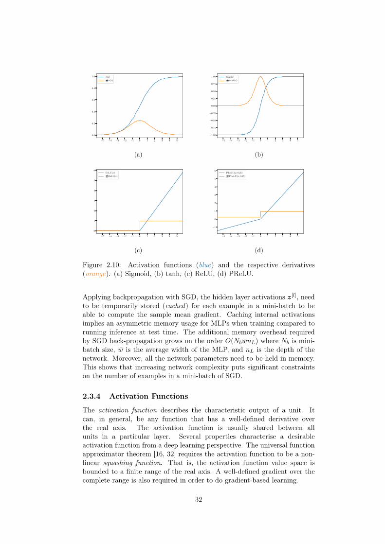
−5 −4 −3 −2 −1 0 1 2 3 4 5

0.0

0.2

0.4

0.6

0.8

1.0 σ(x)ddxσ(x)

(a)

−5 −4 −3 −2 −1 0 1 2 3 4 5

−1.00

−0.75

−0.50

−0.25

0.00

0.25

0.50

0.75

1.00 tanh(x)ddx tanh(x)

(b)

−5 −4 −3 −2 −1 0 1 2 3 4 5

0

1

2

3

4

5

6ReLU(x)ddxReLU(x)

(c)

−5 −4 −3 −2 −1 0 1 2 3 4 5

−1

0

1

2

3

4

5

6PReLU(x; 0.25)ddxPReLU(x; 0.25)

(d)

Figure 2.10: Activation functions (blue) and the respective derivatives(orange). (a) Sigmoid, (b) tanh, (c) ReLU, (d) PReLU.

Applying backpropagation with SGD, the hidden layer activations z[l], needto be temporarily stored (cached) for each example in a mini-batch to beable to compute the sample mean gradient. Caching internal activationsimplies an asymmetric memory usage for MLPs when training compared torunning inference at test time. The additional memory overhead requiredby SGD back-propagation grows on the order O(NbwnL) where Nb is mini-batch size, w is the average width of the MLP, and nL is the depth of thenetwork. Moreover, all the network parameters need to be held in memory.This shows that increasing network complexity puts significant constraintson the number of examples in a mini-batch of SGD.

2.3.4 Activation Functions

The activation function describes the characteristic output of a unit. Itcan, in general, be any function that has a well-defined derivative overthe real axis. The activation function is usually shared between allunits in a particular layer. Several properties characterise a desirableactivation function from a deep learning perspective. The universal functionapproximator theorem [16, 32] requires the activation function to be a non-linear squashing function. That is, the activation function value space isbounded to a finite range of the real axis. A well-defined gradient over thecomplete range is also required in order to do gradient-based learning.

32

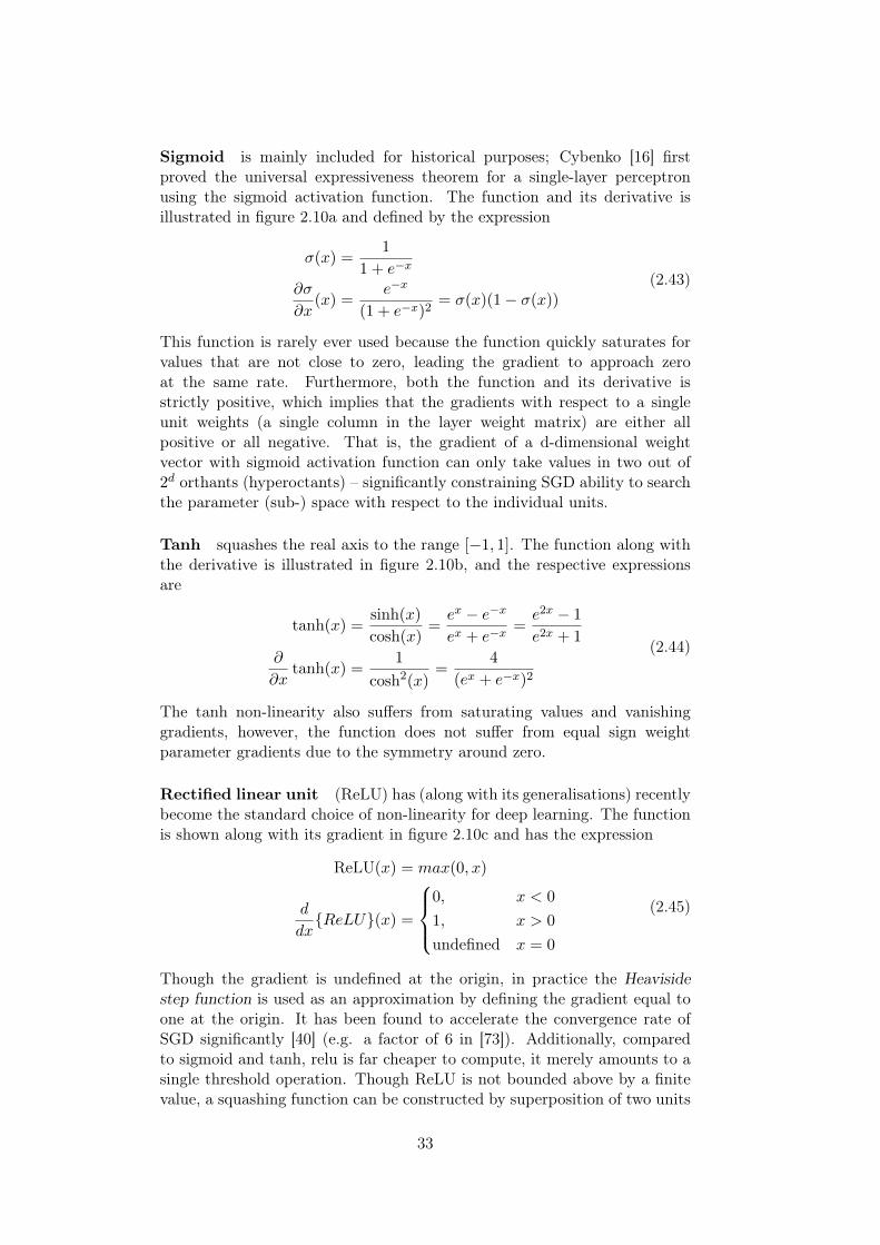
Sigmoid is mainly included for historical purposes; Cybenko [16] firstproved the universal expressiveness theorem for a single-layer perceptronusing the sigmoid activation function. The function and its derivative isillustrated in figure 2.10a and defined by the expression

σ(x) =1

1 + e−x

∂σ

∂x(x) =

e−x

(1 + e−x)2= σ(x)(1− σ(x))

(2.43)

This function is rarely ever used because the function quickly saturates forvalues that are not close to zero, leading the gradient to approach zeroat the same rate. Furthermore, both the function and its derivative isstrictly positive, which implies that the gradients with respect to a singleunit weights (a single column in the layer weight matrix) are either allpositive or all negative. That is, the gradient of a d-dimensional weightvector with sigmoid activation function can only take values in two out of2d orthants (hyperoctants) – significantly constraining SGD ability to searchthe parameter (sub-) space with respect to the individual units.

Tanh squashes the real axis to the range [−1, 1]. The function along withthe derivative is illustrated in figure 2.10b, and the respective expressionsare

tanh(x) =sinh(x)

cosh(x)=ex − e−xex + e−x

=e2x − 1

e2x + 1

∂

∂xtanh(x) =

1

cosh2(x)=

4

(ex + e−x)2

(2.44)

The tanh non-linearity also suffers from saturating values and vanishinggradients, however, the function does not suffer from equal sign weightparameter gradients due to the symmetry around zero.

Rectified linear unit (ReLU) has (along with its generalisations) recentlybecome the standard choice of non-linearity for deep learning. The functionis shown along with its gradient in figure 2.10c and has the expression

ReLU(x) = max(0, x)

d

dxReLU(x) =

0, x < 0

1, x > 0

undefined x = 0

(2.45)

Though the gradient is undefined at the origin, in practice the Heavisidestep function is used as an approximation by defining the gradient equal toone at the origin. It has been found to accelerate the convergence rate ofSGD significantly [40] (e.g. a factor of 6 in [73]). Additionally, comparedto sigmoid and tanh, relu is far cheaper to compute, it merely amounts to asingle threshold operation. Though ReLU is not bounded above by a finitevalue, a squashing function can be constructed by superposition of two units

33

using the ReLU function. The ReLU suffers from one significant problem: alarge gradient update might “push” the weights off the data manifold. Thatis, the ReLU output remains zero for every example in the training set,rendering the particular unit useless and redundant. This phenomenon iscommonly referred to as the dying relu problem and happens to a relativelysmall proportion of the units in a network during training.

Parameterised rectified linear unit (PReLU) [30] addresses the dyingrelu problem by making the slope of the inactive region be parameterizedby a trainable parameter. The PReLU function defines the negative part ofthe domain be a parameterised linear function (αx). The PReLU, alongwith its gradient, is shown in figure 2.10d for the parameter equal toα = 0.25. We will make frequent use of the PReLU activation functionin the implementation of this project.

2.3.5 Regularisation

In the context of deep learning, regularisation is a collective term oftechniques that reduces the effective representational capacity of a model.The success of deep learning relies on appropriate regularisation to keepthe model from overfitting the data. Here, we use the term capacity in aninformal manner of the capability of the network to fit a variety of functionsthat is proportional to the number of parameters and depth of a feedforwardnetwork.

Weight regularisation

Weight regularisation or parameter norm penalties, limits the networkcapacity by introducing an additional parameter norm term to the costfunction (eq. 2.24), such that the cost function becomes:

C(W) =1

N

N∑i=1

L(y(i), y(i);W) + λ∑w∈W

Ω(w) (2.46)

Where λ is the weight regularisation hyperparameter and Ω is either squareL2 norm or L1 norm. It can be shown (see for example [28, sec 7.1]) that theresulting cost function in equation 2.46 corresponds to the MAP estimate ofthe negative log-likelihood if the parameter prior is an isotropic Gaussian orLaplacian distribution for the two measures respectively.

Parameter tying and parameter sharing

Another somewhat related regularisation technique is to put direct con-straints on the parameter values. For example, making a subset of theparameters constant and equal to zero – tying the respective parametersto zero. In maximum a posteriori (MAP, see page 19), this corresponds tosetting infinite parameter-prior to the respective values. Similarly, one mayput infinite priors on the joint parameter distributions, and the parameter

34

difference – forcing parameter to share the same values. A particular to-pology that heavily uses these two regularisation techniques, which we willreturn to, is the convolutional neural networks.

Dropout

It is commonly known that ensemble methods, that is machine learningmodels that utilise the average prediction over multiple independentlytrained models, nearly always improves the results compared to a singlemodel. Motivated by ensemble learning, dropout [31, 72] is a regularisationtechnique that tries to approximate ensembles stochastically by samplingsub-models of an MLP during training. Dropout achieves this byfor each training example that is fed through the network, each layersamples a random vector from a Bernoulli distribution with a probabilityhyperparameter p and then use these vectors to mask the output of eachhidden layer. By using mini-batches of several examples, the sample meangradient amounts to averaging the gradient of an ensemble of models withshared parameters. During inference, the output of each hidden layer needsto be scaled by p so as to yield the same expected layer output magnitude.3

By doing this scaling, 2n networks with shared parameters are combined intoa single neural network during inference (test time) [72].

In the cited articles, they show that dropout yields a consistent andsignificant improvement on the test set when applied to MLP classifiers overdifferent datasets, despite a somewhat higher training set error. Dropout isalso very efficient to compute as it only amounts to sampling a binary vectorand a single element-wise product for each layer, with similar computationalcost as adding an additional unit at each layer.

Dataset augmentation

From our previous discussion, we argued how the expected generalisationerror through the Vapnik-Chernovenkis inequality (eq. 2.31) increases withmodel capacity, but on the other side decreases with training set size. Usingthis observation, we can artificially increase the dataset size by augmentingthe feature vectors as long as the augmentation does not obscure theassociated example label.

For convolutional neural networks that operate directly on images, bothgeometric and point operations are commonly applied augmentationmethods, as well as additive noise. Examples of dataset augmentationincludes random cropping the image (careful not to exclude the object label),random brightness, hue shift to name a few.

Early stopping

Training deep neural networks with sufficient representational capacity tooverfit the task, the validation error suddenly cease to decrease and even start

3Alternatively, scaling by 11−p

during training removes the overhead of scaling whenperforming inference.

35

to increase even though the training error continues to decrease. In [81] theoverfitting capability of feedforward networks was illustrated by achievingperfect training set accuracy when the labels were shuffled arbitrarily. Thisdemonstrates that models with sufficiently high capacity are capable ofmemorising the dataset if training is allowed to continue for long enough.

Early stopping suggests training until no improvement on the validation splitis observed, and then pick the set of parameters obtaining the best validationresults.

2.3.6 Learning Dynamics

Training deep models using stochastic gradient descent often poses severalchallenges that deep learning need to address. For example, flat regions andlocal minima of the cost function may cause the gradient descent to get stuckin a sub-optimal solution in parameter-space. On the other hand, regions ofthe parameter space for which the cost function is locally steep makes thegradient proportionally large, potentially undoing a large part of the trainingprogress.

The layer-wise structure of the multilayer perceptron also poses severalchallenges related to the feedforward and backward propagation propertiesof the network. Too large weight parameters may cause squashing activationfunctions such as sigmoid and tanh to saturate, or for ReLU activationthe activation grows in exponential order even causing the finite precisionarithmetic to yield “NaN” (Not a Number) results. Even worse, theexponential growing or decaying behaviour is an even more significantproblem for the backpropagation algorithm and is commonly known as theexploding or vanishing gradients problem. In addition to causing numericalproblems, exploding and vanishing gradients also cause the gradient updateto be layer-dependent, reducing the effective number of parameters that getadjusted.

Finally, a similar problem caused by the layer-wise structure comes from thefact that the distribution of the input values to a hidden layer changes duringtraining as the parameters of any of the preceding layers change. Such changeto the input distribution is called covariate shift [67]. In the following, wepresent advances in deep learning that addresses these challenges, making theneural networks significantly easier to train using gradient-based algorithms.

Initialisation schemes

Training a deep feedforward network is done using iterative gradient basedoptimisation. The time it takes for the optimisation procedure to convergeis highly dependent on the initial point in the objective landscape. Theinitial point can even determine whether the algorithm converges to a pointin parameter-space of high or low cost (local optima) or if it converges toany stable point at all.

Due to the high number of parameters for deep learning models, identifying

36

which initial parameters will lead to the best solutions is highly intractable.Initialisation schemes in the deep learning literature are usually based onheuristics and assumptions about the distribution of the individual hiddenlayer activations. Perhaps the only tractable property known with completecertainty is that the initial parameters need to break symmetry of theJacobian (eq. 2.39). If two hidden units in the same layer have the sameinitial parameter vectors (two different columns in the weight matrix W [l])then because the two units share the same input-output relationship theywill always receive the same gradient update. The bias parameters does notaffect this symmetry property and is typically initialised to the zero-vector.

Glorot and Bengio [26] considers the input of each layer to be zero-mean,unit-variance i.i.d. and propose a normalised initialisation scheme that inexpectation preserves these properties throughout the depth of the network.The initialisation scheme also considers the backwards pass for computingthe gradient, requiring a similar unit variance for the back-propagatedgradient. As a compromise between the statistics of the forward andbackward statistics, the initialisation scheme draws initial weights from azero-mean distribution with a standard deviation equal to the reciprocalaverage ( 2

nl−1+nl) of the fan-in (nl−1) and fan-out (nl) of the layer h[l].

This scheme tries to preserve an expected zero-mean unit-standarddeviationboth for the feedforward and backpropagation activations throughout thenetwork. The article propose two initialisation schemes for sampling initialweight matrices, based on sampling from a uniform or normal distribution.Sampling from a uniform distribution, the following distribution is used

W[l]i,j ∼ U

(−√

6

nl−1 + nl,

√6

nl−1 + nl

)(2.47)

Whereas initialising from a normal distribution takes the form

W[l]i,j ∼ N

(0,

√2

nl−1 + nl

)(2.48)

Batch normalisation

Though covariate shift can be mitigated by careful initialisation and reducingthe learning rate, this comes at the expense of increased training timeand initialisation sensitivity. Batch normalisation [36] is a techniqueintroduced to make the network significantly more robust to covariateshift. This technique further enables the advantage of using higher learningrates, making the training phase significantly faster and less sensitive toinitialisation schemes.

Batch normalisation is implemented as a sort of layer that, duringtraining, performs a normalising reparameterisation of the layer’s inputsby approximating the mean and variance by their corresponding sampleestimates over the mini-batch of examples. That is, if the layer input i-th example in a batch and the corresponding reparameterisation is denoted

37

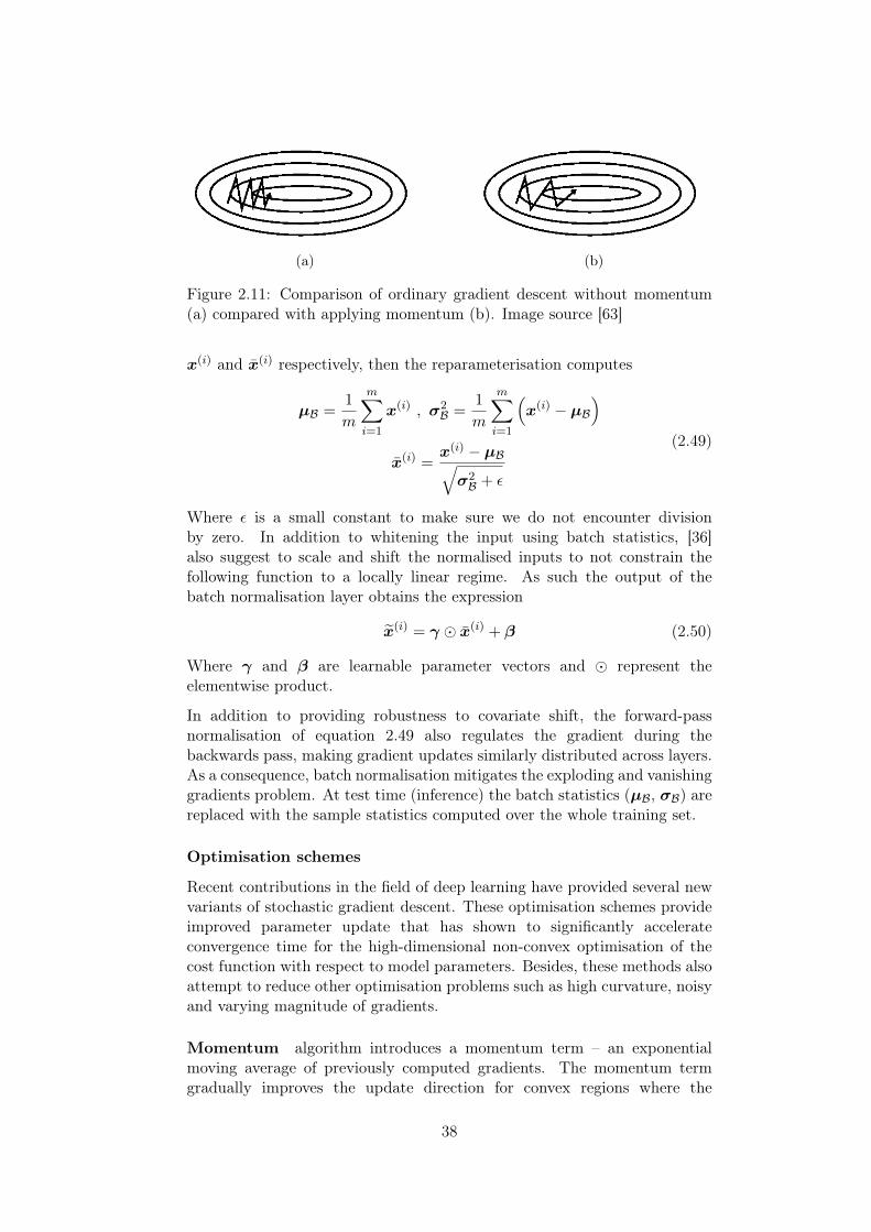
(a) (b)

Figure 2.11: Comparison of ordinary gradient descent without momentum(a) compared with applying momentum (b). Image source [63]

x(i) and x(i) respectively, then the reparameterisation computes

µB =1

m

m∑i=1

x(i) , σ2B =

1

m

m∑i=1

(x(i) − µB

)x(i) =

x(i) − µB√σ2B + ε

(2.49)

Where ε is a small constant to make sure we do not encounter divisionby zero. In addition to whitening the input using batch statistics, [36]also suggest to scale and shift the normalised inputs to not constrain thefollowing function to a locally linear regime. As such the output of thebatch normalisation layer obtains the expression

x(i) = γ x(i) + β (2.50)

Where γ and β are learnable parameter vectors and represent theelementwise product.

In addition to providing robustness to covariate shift, the forward-passnormalisation of equation 2.49 also regulates the gradient during thebackwards pass, making gradient updates similarly distributed across layers.As a consequence, batch normalisation mitigates the exploding and vanishinggradients problem. At test time (inference) the batch statistics (µB, σB) arereplaced with the sample statistics computed over the whole training set.

Optimisation schemes

Recent contributions in the field of deep learning have provided several newvariants of stochastic gradient descent. These optimisation schemes provideimproved parameter update that has shown to significantly accelerateconvergence time for the high-dimensional non-convex optimisation of thecost function with respect to model parameters. Besides, these methods alsoattempt to reduce other optimisation problems such as high curvature, noisyand varying magnitude of gradients.

Momentum algorithm introduces a momentum term – an exponentialmoving average of previously computed gradients. The momentum termgradually improves the update direction for convex regions where the

38

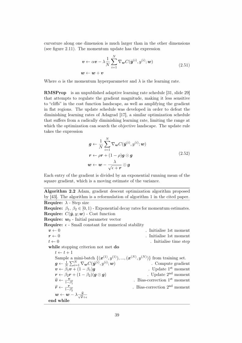
curvature along one dimension is much larger than in the other dimensions(see figure 2.11). The momentum update has the expression

v ← αv − λ 1

N

N∑i=1

∇wC(y(i), y(i);w)

w ← w + v

(2.51)

Where α is the momentum hyperparameter and λ is the learning rate.

RMSProp is an unpublished adaptive learning rate schedule [31, slide 29]that attempts to regulate the gradient magnitude, making it less sensitiveto “cliffs” in the cost function landscape, as well as amplifying the gradientin flat regions. The update schedule was developed in order to defeat thediminishing learning rates of Adagrad [17], a similar optimization schedulethat suffers from a radically diminishing learning rate, limiting the range atwhich the optimization can search the objective landscape. The update ruletakes the expression

g ← 1

N

N∑i=1

∇wC(y(i), y(i);w)

r ← ρr + (1− ρ)g g

w ← w − λ√ε+ r

g

(2.52)

Each entry of the gradient is divided by an exponential running mean of thesquare gradient, which is a moving estimate of the variance.

Algorithm 2.2 Adam, gradient descent optimization algorithm proposedby [43]. The algorithm is a reformulation of algorithm 1 in the cited paper.Require: λ - Step sizeRequire: β1, β2 ∈ [0, 1) - Exponential decay rates for momentum estimates.Require: C(y, y;w) - Cost functionRequire: w0 - Initial parameter vectorRequire: ε - Small constant for numerical stabilityv ← 0 . Initialise 1st momentr ← 0 . Initialise 1st momentt← 0 . Initialise time stepwhile stopping criterion not met do

t← t+ 1Sample a mini-batch (x(1), y(1)), ..., (x(N), y(N)) from training set.g ← 1

N

∑Ni=1∇wC(y(i), y(i);w) . Compute gradient

v ← β1v + (1− β1)g . Update 1st momentr ← β2r + (1− β2)(g g) . Update 2nd momentv ← v

1−βt1

. Bias-correction 1st moment

r ← r1−βt

2. Bias-correction 2nd moment

w ← w − λ v√r+ε

end while

39

Adam [43] is another adaptive learning rate schedule that incorporates theRMSProp squared gradient normalisation in a momentum update (eq. 2.51).It additionally performs an initial bias correction of the momentum updates;both for the first order momentum (mean estimate) in equation 2.51 and theRMSProp “second order” momentum (variance estimate) in equation 2.52.The complete algorithm is presented in algorithm 2.2.

Adam is generally considered robust to hyperparameter selection and is,therefore, a popular algorithm in the deep learning community. In this work,we have chosen Adam as the SGD method of choice for this reason.

2.4 Convolutional Neural Networks

The convolutional neural network (CNN) is specialised a topology offeedforward neural networks for processing features x that come in aregularly sampled data structure. For example, image data consists of aregularly sampled 2D-grid for which the feature vector consists of all pixelintensity values. With a new state-of-the-art set by the AlexNet [45] in the2012 ImageNet Large scale visual recognition and classification (ILSVRC-2012) [64], the scene for the latest “deep learning renaissance” was set. Thistopology has proven the method of choice for the computer vision taskspresented in section 2.1.3. The convolutional neural networks are simplyneural networks that use convolution in place of matrix multiplication withinthe layers.

Convolution leverages three essential aspects that utilise the data structureto reduce parameters and hence, the model growth function (capacity) (eq.2.29); these three aspects are [28, ch. 9.2]: sparse interactions, parametersharing and equivariant representations. Whereas (fully-connected) multi-layer perceptrons consist of layers of matrix multiplication, providing asingle parameter describing the interaction between each unit in consecutivelayers, convolutions provide a sparse set of weights, with kernels smaller thanthe input, that are reused over the spatial dimensions of the input. Theparameter sharing property is also evident through the equivalent matrix-representation, where the corresponding matrix has a constrained cyclicstructure (see page 10). The particular form of parameter sharing causeseach layer to have a property called equivariance to translation, meaningthat if the input experience a change in the form of a translation, the outputchanges in the same way. In the following discussion, we will formalisethe convolutional layer as a compound entity of possibly several operationson a spatially arranged feature-map. We will finally see an example of aCNN classifier network, deferring the more complicated task of semanticsegmentation to the next chapter.

2.4.1 The Convolutional Layer

As mentioned above, convolutional networks are simply feedforward neuralnetworks with one or more convolutional layers; which in turn is a hidden

40

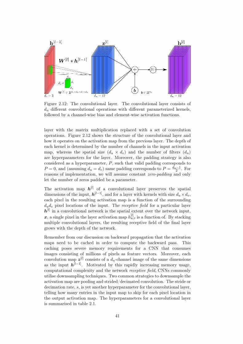
Figure 2.12: The convolutional layer. The convolutional layer consists ofdn different convolutional operations with different parameterized kernels,followed by a channel-wise bias and element-wise activation functions.

layer with the matrix multiplication replaced with a set of convolutionoperations. Figure 2.12 shows the structure of the convolutional layer andhow it operates on the activation map from the previous layer. The depth ofeach kernel is determined by the number of channels in the input activationmap, whereas the spatial size (du × dv) and the number of filters (dn)are hyperparameters for the layer. Moreover, the padding strategy is alsoconsidered as a hyperparameter, P , such that valid padding corresponds toP = 0, and (assuming du = dv) same padding corresponds to P = du−1

2 . Forreasons of implementation, we will assume constant zero-padding and onlylet the number of zeros padded be a parameter.

The activation map h[l] of a convolutional layer preserves the spatialdimensions of the input, h[l−1], and for a layer with kernels with size du×dv,each pixel in the resulting activation map is a function of the surroundingdudv pixel locations of the input. The receptive field for a particular layerh[l] in a convolutional network is the spatial extent over the network input,x, a single pixel in the layer activation map h[l]u,v is a function of. By stackingmultiple convolutional layers, the resulting receptive field of the final layergrows with the depth of the network.

Remember from our discussion on backward propagation that the activationmaps need to be cached in order to compute the backward pass. Thiscaching poses severe memory requirements for a CNN that consumesimages consisting of millions of pixels as feature vectors. Moreover, eachconvolution map z[l] consists of a dn-channel image of the same dimensionsas the input h[l−1]. Motivated by this rapidly increasing memory usage,computational complexity and the network receptive field, CNNs commonlyutilise downsampling techniques. Two common strategies to downsample theactivation map are pooling and strided/decimated convolution. The stride ordecimation rate, s, is yet another hyperparameter for the convolutional layer,telling how many entries in the input map to skip for each pixel location inthe output activation map. The hyperparameters for a convolutional layeris summarised in table 2.1.

41

Hyperparameter Description

du Kernel widthdu Kernel heightdn Number of kernelss Stride / decimation rateP Zero paddingg(·) Activation function, e.g. Tanh, ReLU, etc.

Table 2.1: Convolutional layer hyperparameters.

As we will see when constructing CNNs for segmentation, careful considera-tion of intermediate layer activation maps is required. Consider a layer withan input map with dimensions [Hi, Wi, Ci], we can compute the outputmap dimensions [Ho, Wo, Co] resulting from a convolutional layer for theset of parameters in table 2.1 (see [19] for derivations)

Ho =

⌊Hi + 2P − dv

s

⌋+ 1

Wo =

⌊Wi + 2P − du

s

⌋+ 1

Co = dn

Furthermore, the receptive field for layer k in a convolutional network canbe calculated by the recursive relation [38, p. 52]

R[k]u = R[k−1]

u +

[(d[k]u − 1)

k−1∏i=1

s[i]

]

R[k]v = R[k−1]

v +

[(d[k]v − 1)

k−1∏i=1

s[i]

] (2.53)

Where d[k]u , d

[k]v respectively denote the kernel size in the two spatial

dimensions and s[k] the convolutional stride.

Pooling

Pooling is a fixed parameter-less neighbourhood operation (see section 2.1.2)to provide invariance to small translations in the input. The poolingoperation is usually placed after the activation function of a convolutionallayer and is usually only added for a subset of the layers in a CNN. Thereare in general no restrictions on what kind of pooling function to use, butit is common to utilise the pooling operation as an additional non-linearityof the network. Some standard pooling functions include order statisticsfilters, fixed moving average filter and the L2 norm over a rectangularneighbourhood. Pooling is usually done along with decimation (stride) of theoutput; an example of a max-pooling operation using a 2×2 neighbourhoodand stride 2 is shown in figure 2.13.

42

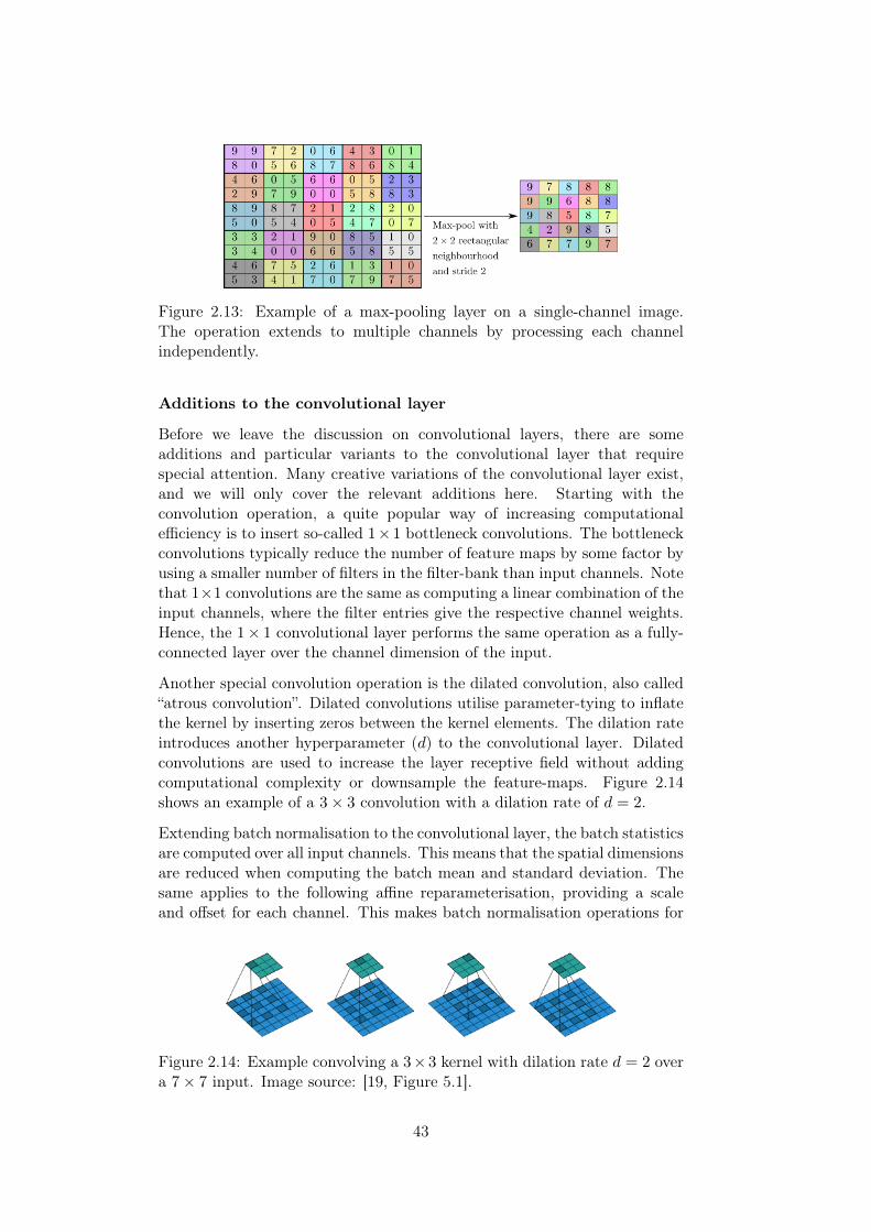
Figure 2.13: Example of a max-pooling layer on a single-channel image.The operation extends to multiple channels by processing each channelindependently.

Additions to the convolutional layer

Before we leave the discussion on convolutional layers, there are someadditions and particular variants to the convolutional layer that requirespecial attention. Many creative variations of the convolutional layer exist,and we will only cover the relevant additions here. Starting with theconvolution operation, a quite popular way of increasing computationalefficiency is to insert so-called 1×1 bottleneck convolutions. The bottleneckconvolutions typically reduce the number of feature maps by some factor byusing a smaller number of filters in the filter-bank than input channels. Notethat 1×1 convolutions are the same as computing a linear combination of theinput channels, where the filter entries give the respective channel weights.Hence, the 1× 1 convolutional layer performs the same operation as a fully-connected layer over the channel dimension of the input.

Another special convolution operation is the dilated convolution, also called“atrous convolution”. Dilated convolutions utilise parameter-tying to inflatethe kernel by inserting zeros between the kernel elements. The dilation rateintroduces another hyperparameter (d) to the convolutional layer. Dilatedconvolutions are used to increase the layer receptive field without addingcomputational complexity or downsample the feature-maps. Figure 2.14shows an example of a 3× 3 convolution with a dilation rate of d = 2.

Extending batch normalisation to the convolutional layer, the batch statisticsare computed over all input channels. This means that the spatial dimensionsare reduced when computing the batch mean and standard deviation. Thesame applies to the following affine reparameterisation, providing a scaleand offset for each channel. This makes batch normalisation operations for

Figure 2.14: Example convolving a 3×3 kernel with dilation rate d = 2 overa 7× 7 input. Image source: [19, Figure 5.1].

43

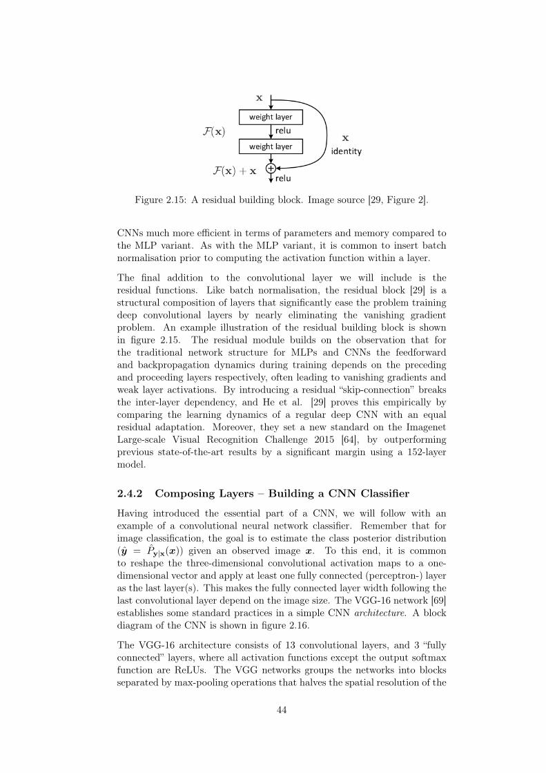
Figure 2.15: A residual building block. Image source [29, Figure 2].

CNNs much more efficient in terms of parameters and memory compared tothe MLP variant. As with the MLP variant, it is common to insert batchnormalisation prior to computing the activation function within a layer.

The final addition to the convolutional layer we will include is theresidual functions. Like batch normalisation, the residual block [29] is astructural composition of layers that significantly ease the problem trainingdeep convolutional layers by nearly eliminating the vanishing gradientproblem. An example illustration of the residual building block is shownin figure 2.15. The residual module builds on the observation that forthe traditional network structure for MLPs and CNNs the feedforwardand backpropagation dynamics during training depends on the precedingand proceeding layers respectively, often leading to vanishing gradients andweak layer activations. By introducing a residual “skip-connection” breaksthe inter-layer dependency, and He et al. [29] proves this empirically bycomparing the learning dynamics of a regular deep CNN with an equalresidual adaptation. Moreover, they set a new standard on the ImagenetLarge-scale Visual Recognition Challenge 2015 [64], by outperformingprevious state-of-the-art results by a significant margin using a 152-layermodel.

2.4.2 Composing Layers – Building a CNN Classifier

Having introduced the essential part of a CNN, we will follow with anexample of a convolutional neural network classifier. Remember that forimage classification, the goal is to estimate the class posterior distribution(y = Py|x(x)) given an observed image x. To this end, it is commonto reshape the three-dimensional convolutional activation maps to a one-dimensional vector and apply at least one fully connected (perceptron-) layeras the last layer(s). This makes the fully connected layer width following thelast convolutional layer depend on the image size. The VGG-16 network [69]establishes some standard practices in a simple CNN architecture. A blockdiagram of the CNN is shown in figure 2.16.

The VGG-16 architecture consists of 13 convolutional layers, and 3 “fullyconnected” layers, where all activation functions except the output softmaxfunction are ReLUs. The VGG networks groups the networks into blocksseparated by max-pooling operations that halves the spatial resolution of the

44

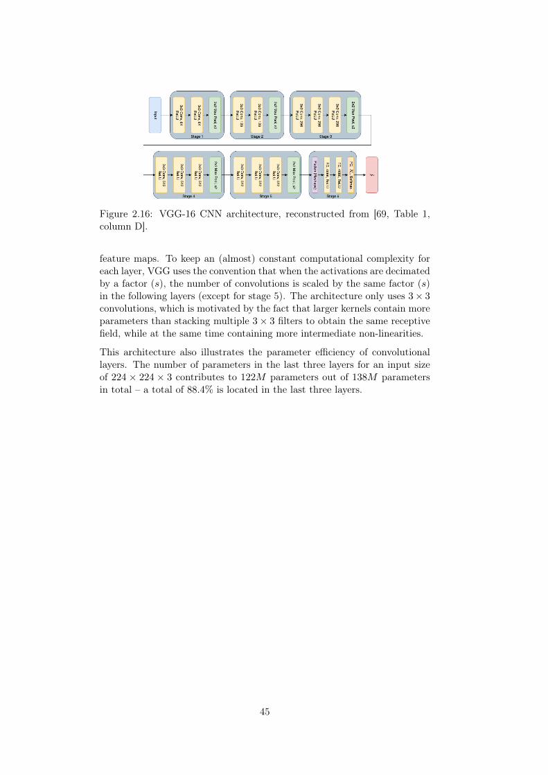
Figure 2.16: VGG-16 CNN architecture, reconstructed from [69, Table 1,column D].

feature maps. To keep an (almost) constant computational complexity foreach layer, VGG uses the convention that when the activations are decimatedby a factor (s), the number of convolutions is scaled by the same factor (s)in the following layers (except for stage 5). The architecture only uses 3× 3convolutions, which is motivated by the fact that larger kernels contain moreparameters than stacking multiple 3× 3 filters to obtain the same receptivefield, while at the same time containing more intermediate non-linearities.

This architecture also illustrates the parameter efficiency of convolutionallayers. The number of parameters in the last three layers for an input sizeof 224 × 224 × 3 contributes to 122M parameters out of 138M parametersin total – a total of 88.4% is located in the last three layers.

45

46

Chapter 3

Related Work

This chapter gives a brief overview of the more closely related fields to thework performed in this thesis. We will start with extending the machinelearning classification problem to that of semantic segmentation, followedby extending the CNN architecture to produce segmentation maps. In thesecond part we present the active learning paradigm for efficiently annotatinga database of examples as efficiently as possible, and presenting some of therelated work performed in the continuously developing field of research.

3.1 Deep Semantic Segmentation

Up until now, we have only considered the classification problem. In thissection, we will extend the classification problem to the task of semanticsegmentation. We will follow with a discussion of adapting CNNs for thistask, with emphasis on the features differentiating a segmentation networkfrom the more traditional classifiers presented above. Finally, we will presentan example architecture as an extension to the discussion of the VGG-16architecture above.

3.1.1 The Deep Segmentation Problem

Remember from the discussion in section 2.1.3 that the objective withsemantic segmentation consists of assigning a class to each pixel of the input.In practice, this means that we instead of mapping each H×W×C imageXto a single Nc-dimensional vector y, we now need to construct a three-tensorY of dimensions H ×W × Nc. The vector Yu,v,: determines the estimatedclass scores (posterior probability mass) over the set of Nc classes at thepixel location (u, v).

The way we are going to treat this problem is to assume that every pixellocation in the input image is an i.i.d. random variable over the set ofclasses. This allows us to express the cross-entropy (negative log-likelihood)loss function as a per-pixel loss. To perform a gradient step with respect toa mini-batch of images, we need to compute the mean loss both with respect

47

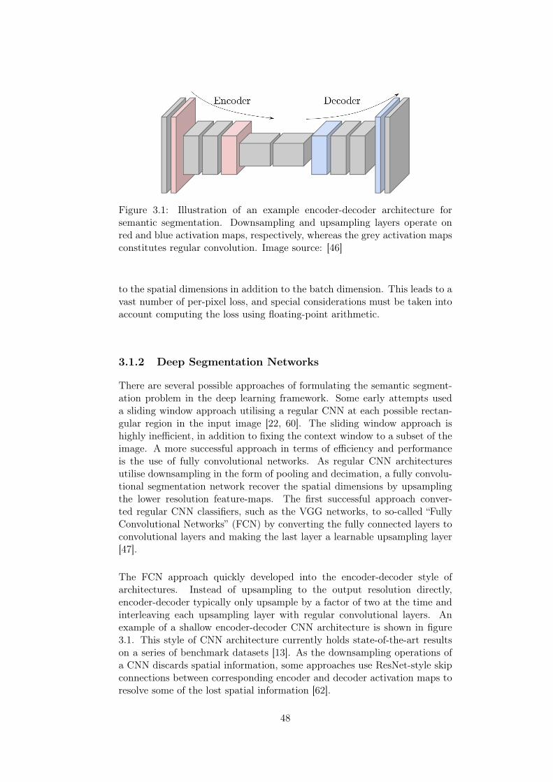
Figure 3.1: Illustration of an example encoder-decoder architecture forsemantic segmentation. Downsampling and upsampling layers operate onred and blue activation maps, respectively, whereas the grey activation mapsconstitutes regular convolution. Image source: [46]

to the spatial dimensions in addition to the batch dimension. This leads to avast number of per-pixel loss, and special considerations must be taken intoaccount computing the loss using floating-point arithmetic.

3.1.2 Deep Segmentation Networks

There are several possible approaches of formulating the semantic segment-ation problem in the deep learning framework. Some early attempts useda sliding window approach utilising a regular CNN at each possible rectan-gular region in the input image [22, 60]. The sliding window approach ishighly inefficient, in addition to fixing the context window to a subset of theimage. A more successful approach in terms of efficiency and performanceis the use of fully convolutional networks. As regular CNN architecturesutilise downsampling in the form of pooling and decimation, a fully convolu-tional segmentation network recover the spatial dimensions by upsamplingthe lower resolution feature-maps. The first successful approach conver-ted regular CNN classifiers, such as the VGG networks, to so-called “FullyConvolutional Networks” (FCN) by converting the fully connected layers toconvolutional layers and making the last layer a learnable upsampling layer[47].

The FCN approach quickly developed into the encoder-decoder style ofarchitectures. Instead of upsampling to the output resolution directly,encoder-decoder typically only upsample by a factor of two at the time andinterleaving each upsampling layer with regular convolutional layers. Anexample of a shallow encoder-decoder CNN architecture is shown in figure3.1. This style of CNN architecture currently holds state-of-the-art resultson a series of benchmark datasets [13]. As the downsampling operations ofa CNN discards spatial information, some approaches use ResNet-style skipconnections between corresponding encoder and decoder activation maps toresolve some of the lost spatial information [62].

48

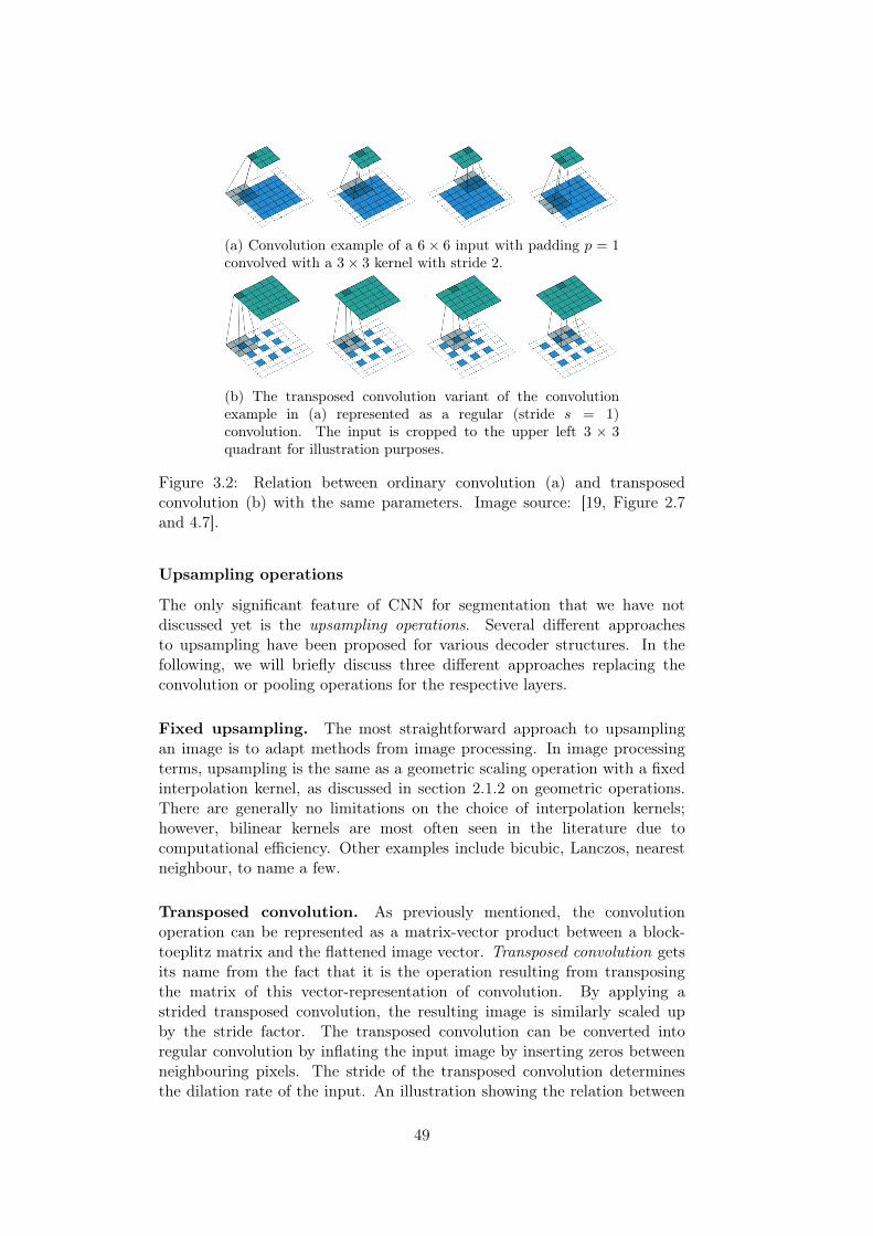
(a) Convolution example of a 6× 6 input with padding p = 1convolved with a 3× 3 kernel with stride 2.

(b) The transposed convolution variant of the convolutionexample in (a) represented as a regular (stride s = 1)convolution. The input is cropped to the upper left 3 × 3quadrant for illustration purposes.

Figure 3.2: Relation between ordinary convolution (a) and transposedconvolution (b) with the same parameters. Image source: [19, Figure 2.7and 4.7].

Upsampling operations

The only significant feature of CNN for segmentation that we have notdiscussed yet is the upsampling operations. Several different approachesto upsampling have been proposed for various decoder structures. In thefollowing, we will briefly discuss three different approaches replacing theconvolution or pooling operations for the respective layers.

Fixed upsampling. The most straightforward approach to upsamplingan image is to adapt methods from image processing. In image processingterms, upsampling is the same as a geometric scaling operation with a fixedinterpolation kernel, as discussed in section 2.1.2 on geometric operations.There are generally no limitations on the choice of interpolation kernels;however, bilinear kernels are most often seen in the literature due tocomputational efficiency. Other examples include bicubic, Lanczos, nearestneighbour, to name a few.

Transposed convolution. As previously mentioned, the convolutionoperation can be represented as a matrix-vector product between a block-toeplitz matrix and the flattened image vector. Transposed convolution getsits name from the fact that it is the operation resulting from transposingthe matrix of this vector-representation of convolution. By applying astrided transposed convolution, the resulting image is similarly scaled upby the stride factor. The transposed convolution can be converted intoregular convolution by inflating the input image by inserting zeros betweenneighbouring pixels. The stride of the transposed convolution determinesthe dilation rate of the input. An illustration showing the relation between

49

Figure 3.3: Illustration of the max-unpooling workings. The unpoolingoperation assigns the output to the value of the input corresponding to theselected max-pooling indexes in the encoder. Each unpooling layer in thedecoder needs to be matched with a corresponding max-pooling layer inthe encoder see figure 3.4 for an example architecture using max-unpooling.Image source: [80].

ordinary strided convolution and the transposed variant is shown in figure3.2.

A useful property of the transposed convolution is that it is able to representmost fixed upsampling interpolations as special parameterisations of thekernel. For example, a 3×3 stride s = 2 transposed convolution can representupsampling using bi-linear interpolation by using the following convolutionalkernel

W =

1/4 1/2 1/41/2 1 1/21/4 1/2 1/4

(3.1)

It is common to utilise equation 3.1 or other interpolation kernels, with somerandom noise to break symmetry, as an initialisation scheme for transposedconvolutional layers. As such, transposed convolution may be thought of asa learnable upsampling operation.

Unpooling. Another common upsampling technique found in the deeplearning literature is converting the downsampling pooling operationsto corresponding upsampling operations. The most common unpoolingoperation is the max-unpooling operation. A max-unpooling operation needsto be coupled with a corresponding max-pooling layer in the encoder of thenetwork, as illustrated in figure 3.3. Max-unpooling operates as a singlescatter operation, assigning the values in the output map according to theselected indexes corresponding max-pooling layer in the encoder.

Composing a CNN model for semantic segmentation

We end our discussion on CNNs for semantic segmentation with an examplearchitecture. Figure 3.4 shows an illustration of the SegNet [6, 7] modelby Badrinarayanan et al. The model is composed of a VGG-16 encoder,discarding the last three fully connected layers. The decoder is symmetricallyconstructed, utilising max-unpooling for upsampling. Discarding the fullyconnected layers results in the complete model having only 29.5M parameters

50

Figure 3.4: SegNet architecture illustration. Pooling and upsampling arematched max-pooling/unpooling pairs. All convolutions operations withblue activation map are 3×3, the softmax layer constitutes a 1×1 convolutionwith a softmax activation function. Image source [7].

compared to 138M parameters of the full VGG-16 model. The architecture isstrikingly similar to the Deconvnet proposed by Zeiler et al. [80] to visualiselearning for the task of classification. By utilising the VGG-16 architecture,the parameters from a pre-trained classification model can be reused forinitialising the encoder parameters.

51

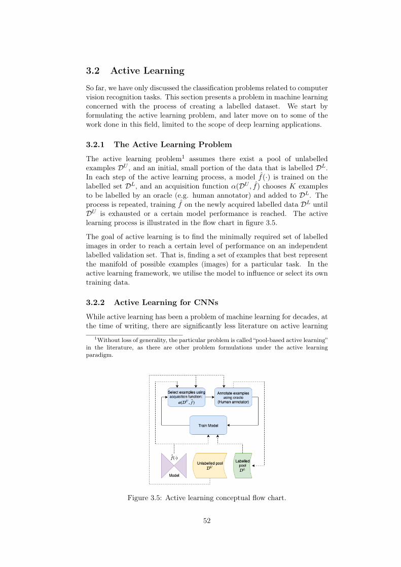
3.2 Active Learning

So far, we have only discussed the classification problems related to computervision recognition tasks. This section presents a problem in machine learningconcerned with the process of creating a labelled dataset. We start byformulating the active learning problem, and later move on to some of thework done in this field, limited to the scope of deep learning applications.

3.2.1 The Active Learning Problem

The active learning problem1 assumes there exist a pool of unlabelledexamples DU , and an initial, small portion of the data that is labelled DL.In each step of the active learning process, a model f(·) is trained on thelabelled set DL, and an acquisition function α(DU , f) chooses K examplesto be labelled by an oracle (e.g. human annotator) and added to DL. Theprocess is repeated, training f on the newly acquired labelled data DL untilDU is exhausted or a certain model performance is reached. The activelearning process is illustrated in the flow chart in figure 3.5.

The goal of active learning is to find the minimally required set of labelledimages in order to reach a certain level of performance on an independentlabelled validation set. That is, finding a set of examples that best representthe manifold of possible examples (images) for a particular task. In theactive learning framework, we utilise the model to influence or select its owntraining data.

3.2.2 Active Learning for CNNs

While active learning has been a problem of machine learning for decades, atthe time of writing, there are significantly less literature on active learning

1Without loss of generality, the particular problem is called “pool-based active learning”in the literature, as there are other problem formulations under the active learningparadigm.

Figure 3.5: Active learning conceptual flow chart.

52

that employ methods from deep learning. This section attempt to give anoutline of deep learning methods used for active learning; more specifically,we will focus on methods aimed at image recognition tasks. The majorityof the literature under this scope concerns the image classification task,with only a handful of methods proposed for the more complex semanticsegmentation task.

Working with this project, the author identified four general approachesto formulating the acquisition function. Wang et al. [78] use uncertaintymeasures with respect to the predicted posterior, such as the entropy frominformation theory, as a premise for the acquisition function. This particularapproach combines uncertainty based selection with the new self-pacedlearning paradigm, performing pseudo-labelling high-confidence examples.The second approach takes a geometric approach for the acquisition function,selecting the examples based on distance-metrics in feature space in order toachieve a best possible uniform sampling of the data manifold. Sener et al.[66] uses the model logits for creating lower dimensional feature embeddings,then computing geometric dissimilarity metrics on the lower-dimensionalfeatures. The particular article formulates the active learning problem asa core-set problem – selecting the points (examples) from the pool thatmaximise dissimilarity to the closest labelled example. The third approachtries to model the how an example is expected to affect or change the modelpredictions, with the hypothesis that informative examples will maximise theexpected change. Käding et al. [39] models the expected change for a set ofexamples (the query set) to a first order approximation of the L1-distance ofthe per-example change, resulting in the L1-norm of the matrix-product ofthe parameter Jacobian and the loss gradient for the particular unlabelledexample. Moreover, in order to evaluate the loss, they use the networkprediction as an approximation. The final method tries to employ Bayesianestimation by Monte Carlo approximations. Gal et al. [24] uses dropoutand Monte Carlo integration to approximate the Bayesian data posteriorp(y|x,DL) (see equation 2.20), then formulating the acquisition in terms ofvarious proposed statistical measures such as entropy and mean standarddeviation of the data posterior. [9] extends on this work by utilising modelensembles instead of dropout approximation and hold current state-of-the-art results on MNIST and CIFAR-10 benchmark datasets.

All the articles above mainly concern the task of image classification. Theliterature on active learning applied to the semantic segmentation task isscarce, and typically utilise one or more of the methods presented above.Yang et al. [79] applies active learning on segmentation data in two stagesusing an ensemble of models. First, a pool of uncertain examples is selectedby maximising the per-pixel prediction variance over the ensemble. Second,higher level feature maps are used for calculating dissimilarity by using thecosine-distance metric. Mackowiak et al. [50] similarly uses an ensemble ofmodels to measure per-example uncertainty comparing the vote-entropy andensemble average uncertainty measures. Besides, they train a separate modelthat do regression over the estimated number of polygon corners (number ofmouse-clicks), to create a map of the expected cost of annotation over the

53

image. The acquisition function uses a linear combination of the uncertaintymeasure and estimated annotation cost for querying image sub-regions forannotation. Mahapatra et al. [51] takes an entirely different approach, usingBayesian neural network [41] (BNN) to model the combined uncertaintyof network predictions and parameters. In practice, the BNN approachamounts to extending the model with a shallow network rooting from the(classifier-) network logits, trained with a loss to estimate prediction variance(actually log-variance), combined with Monte Carlo dropout. In additionto BNN uncertainty estimation, the approach uses conditional generativeadversarial networks [37] (cGAN) to virtually extend the labelled dataset.The cGAN is both conditioned on the dataset images along with the labelmasks.

54

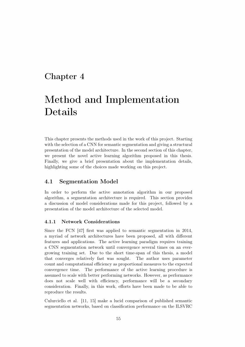
Chapter 4

Method and ImplementationDetails

This chapter presents the methods used in the work of this project. Startingwith the selection of a CNN for semantic segmentation and giving a structuralpresentation of the model architecture. In the second section of this chapter,we present the novel active learning algorithm proposed in this thesis.Finally, we give a brief presentation about the implementation details,highlighting some of the choices made working on this project.

4.1 Segmentation Model

In order to perform the active annotation algorithm in our proposedalgorithm, a segmentation architecture is required. This section providesa discussion of model considerations made for this project, followed by apresentation of the model architecture of the selected model.

4.1.1 Network Considerations

Since the FCN [47] first was applied to semantic segmentation in 2014,a myriad of network architectures have been proposed, all with differentfeatures and applications. The active learning paradigm requires traininga CNN segmentation network until convergence several times on an ever-growing training set. Due to the short time-span of this thesis, a modelthat converges relatively fast was sought. The author uses parametercount and computational efficiency as proportional measures to the expectedconvergence time. The performance of the active learning procedure isassumed to scale with better performing networks. However, as performancedoes not scale well with efficiency, performance will be a secondaryconsideration. Finally, in this work, efforts have been made to be able toreproduce the results.

Culurciello et al. [11, 15] make a lucid comparison of published semanticsegmentation networks, based on classification performance on the ILSVRC

55

(a) (b)

Figure 4.1: Network architecture comparison. (a) Top-1 classificationaccuracy vs the number of operations in a forward pass. The size of the blobsis proportional to the number of parameters. (b) Accuracy per parameterchart for the same variety of networks. Image source: [12]

[64] benchmark. The comparison is made in terms of accuracy and modelcomplexity in number of parameters. Figure 4.1 shows the most recentcomparison summary from this ongoing work. From these results, MobileNetv2 [65] from the MobileNet family of networks, and ENet [59] seems to betwo viable options in terms of efficiency and performance. The SqueezeNetand ShuffleNet show significantly less performance in figure 4.1a. Siam etal. [68] additionally compare a range of semantic segmentation networkspurposed for real-time applications. The comparison is made by decouplingthe encoder-decoder structure of segmentation networks, comparing differentpermutations of published network encoder and decoder structures. Thearticle finds that the combination of SkipNet-ShuffleNet encoder-decoderstructure yields comparable results as the ENet architecture despite havingapproximately 45% less estimated operations (in terms of floating-pointoperations, FLOPs).

We have let reproducibility be the decisive factor in this thesis, favouringENet [59] as our model of choice. The article provides a concise descriptionof the model, as well as reporting the hyperparameters used for obtaining thebenchmark results. This makes the effort of validating model implementationreasonably straight forward. MobileNet v2 [65], despite having superiorperformance in terms of classification accuracy and efficiency, the article doesnot report hyperparameters used obtaining the reported results. Besides, thereported model does not define a decoder that fully upsamples the predictionmap to the size of the input image.

4.1.2 ENet – Architecture Description

The core building block of ENet is the bottleneck module. Paszke et al.[59] define five different alternations of the ResNet bottleneck building block[29, Figure 5, Right]. The structure of the bottleneck modules consists ofthree convolutional layers, which we will refer to as projection, main andexpansion layer respectively, and a shortcut connection that bypasses the

56

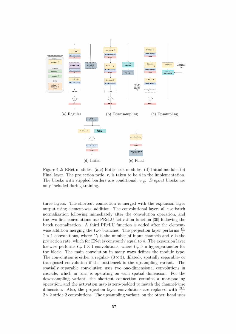
(a) Regular (b) Downsampling (c) Upsampling

(d) Initial (e) Final

Figure 4.2: ENet modules. (a-c) Bottleneck modules, (d) Initial module, (e)Final layer. The projection ratio, r, is taken to be 4 in the implementation.The blocks with stippled borders are conditional, e.g. Dropout blocks areonly included during training.

three layers. The shortcut connection is merged with the expansion layeroutput using element-wise addition. The convolutional layers all use batchnormalization following immediately after the convolution operation, andthe two first convolutions use PReLU activation function [30] following thebatch normalization. A third PReLU function is added after the element-wise addition merging the two branches. The projection layer performs Ci

r1 × 1 convolutions, where Ci is the number of input channels and r is theprojection rate, which for ENet is constantly equal to 4. The expansion layerlikewise performs Co 1 × 1 convolutions, where Co is a hyperparameter forthe block. The main convolution in many ways defines the module type.The convolution is either a regular- (3× 3), dilated-, spatially separable- ortransposed convolution if the bottleneck is the upsampling variant. Thespatially separable convolution uses two one-dimensional convolutions incascade, which in turn is operating on each spatial dimension. For thedownsampling variant, the shortcut connection contains a max-poolingoperation, and the activation map is zero-padded to match the channel-wisedimension. Also, the projection layer convolutions are replaced with 2Ci

r2×2 stride 2 convolutions. The upsampling variant, on the other, hand uses

57

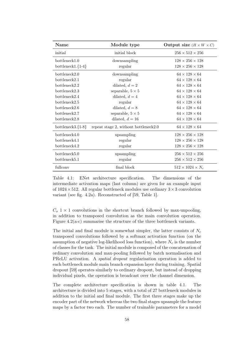
Name Module type Output size (H ×W × C)

initial initial block 256× 512× 256

bottleneck1.0 downsampling 128× 256× 128

bottleneck1.1-4 regular 128× 256× 128

bottleneck2.0 downsampling 64× 128× 64

bottleneck2.1 regular 64× 128× 64

bottleneck2.2 dilated, d = 2 64× 128× 64

bottleneck2.3 separable, 5× 5 64× 128× 64

bottleneck2.4 dilated, d = 4 64× 128× 64

bottleneck2.5 regular 64× 128× 64

bottleneck2.6 dilated, d = 8 64× 128× 64

bottleneck2.7 separable, 5× 5 64× 128× 64

bottleneck2.8 dilated, d = 16 64× 128× 64

bottleneck3.1-8 repeat stage 2, without bottleneck2.0 64× 128× 64

bottleneck4.0 upsampling 128× 256× 128

bottleneck4.1 regular 128× 256× 128

bottleneck4.2 regular 128× 256× 128

bottleneck5.0 upsampling 256× 512× 256

bottleneck5.1 regular 256× 512× 256

fullconv final block 512× 1024×Nc

Table 4.1: ENet architecture specification. The dimensions of theintermediate activation maps (last column) are given for an example inputof 1024×512. All regular bottleneck modules use ordinary 3×3 convolutionvariant (see fig. 4.2a). Reconstructed of [59, Table 1].

Co 1 × 1 convolutions in the shortcut branch followed by max-unpooling,in addition to transposed convolution as the main convolution operation.Figure 4.2(a-c) summarise the structure of the three bottleneck variants.

The initial and final module is somewhat simpler, the latter consists of Nc

transposed convolutions followed by a softmax activation function (on theassumption of negative log-likelihood loss function), where Nc is the numberof classes for the task. The initial module is composed of the concatenation ofordinary convolution and max-pooling followed by batch normalisation andPReLU activation. A spatial dropout regularisation operation is added toeach bottleneck module main branch expansion layer during training. Spatialdropout [59] operates similarly to ordinary dropout, but instead of droppingindividual pixels, the operation is broadcast over the channel dimension.

The complete architecture specification is shown in table 4.1. Thearchitecture is divided into 5 stages, with a total of 27 bottleneck modules inaddition to the initial and final module. The first three stages make up theencoder part of the network whereas the two final stages upsample the featuremaps by a factor two each. The number of trainable parameters for a model

58

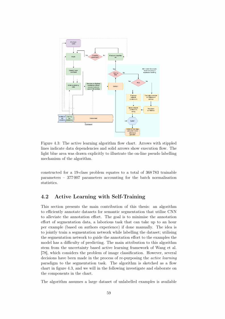
Figure 4.3: The active learning algorithm flow chart. Arrows with stippledlines indicate data dependencies and solid arrows show execution flow. Thelight blue area was drawn explicitly to illustrate the on-line pseudo labellingmechanism of the algorithm.

constructed for a 19-class problem equates to a total of 368 783 trainableparameters – 377 007 parameters accounting for the batch normalisationstatistics.

4.2 Active Learning with Self-Training

This section presents the main contribution of this thesis: an algorithmto efficiently annotate datasets for semantic segmentation that utilise CNNto alleviate the annotation effort. The goal is to minimise the annotationeffort of segmentation data, a laborious task that can take up to an hourper example (based on authors experience) if done manually. The idea isto jointly train a segmentation network while labelling the dataset; utilisingthe segmentation network to guide the annotation effort to the examples themodel has a difficulty of predicting. The main attribution to this algorithmstem from the uncertainty based active learning framework of Wang et al.[78], which considers the problem of image classification. However, severaldecisions have been made in the process of re-purposing the active learningparadigm to the segmentation task. The algorithm is sketched as a flowchart in figure 4.3, and we will in the following investigate and elaborate onthe components in the chart.

The algorithm assumes a large dataset of unlabelled examples is available

59

for which the goal is to annotate as efficiently as possible. To bootstrapthe annotation process, a small proportion needs to be annotated. Thislabelled subset is split into two separate splits, a training split and avalidation split that is set aside and used for validation throughout thealgorithm execution. The algorithm starts with using the labelled trainingsubset, which we will later refer to as the seed set, for pre-training of theconvolutional segmentation network. In practice, it would be wise to pre-train the CNN on a large dataset if available before running this algorithm,and then use the labelled subset for finetuning on the particular datasetunder consideration. However, in the context of this algorithm, this isreferred to as the “pre-training” phase. When the CNN inevitably convergeson the seed set, execution proceeds to the main loop of the algorithm.

The outer loop starts with ranking all unlabelled examples in the datasetaccording to a confidence measure. The confidence measure is a functionof the network’s softmax class probability output that should reflect howcertain the network is in making the classification decision of each pixelin the image. To derive our measure of the model’s confidence, we startwith the measures proposed in [78]. The most straightforward confidencemeasure ranks all examples according to the respective maximum predictedprobability of the classifier

d1(yu,v) = maxyiyu,v (4.1)

If the maximum probability (eq. 4.1) of the model is relatively low, the modelmakes a weak classification decision. By only considering the maximumprobability, we discard the rest of the output information of the network.More specifically, the output confidence is not measured relative to theother classes, which brings us to our second margin sampling [78] confidencemeasure.

d2(yu,v) = maxyiyu,v −max2

yiyu,v (4.2)

The confidence, according to equation 4.2, is reflected as the differencebetween the two max-scoring classes. As such confusion is typically madebetween visually similar object (e.g. car and lorry or road and sidewalk),this measure assign lower confidence to such difficult classes. Extending onthis discussion and taking the complete categorical distribution into accountleads us to our final confidence measure used in the proposed algorithm.

d3(yu,v) = 1−(−

NC∑i=1

yu,v,i logNCyu,v,i

)= 1−H(y(u,v)) (4.3)

The justification of equation 4.3 as a confidence measure is reflected byusing the entropy of the softmax-categorical distribution as a measure ofuncertainty. The entropy is defined as the expected self-information of arandom variable H(x) , Ex [logb x], where b is the logarithm base giving theunits of the self-information. Intuitively the entropy tells how “surprised”an observer is expected to be when sampling from the random variable.It can be shown that the entropy over a discrete random variable assumes

60

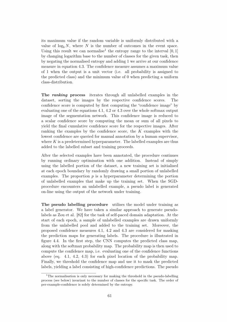
its maximum value if the random variable is uniformly distributed with avalue of logbN , where N is the number of outcomes in the event space.Using this result we can normalise1 the entropy range to the interval [0, 1]by changing logarithm base to the number of classes for the given task, thenby negating the normalised entropy and adding 1 we arrive at our confidencemeasure in equation 4.3. The confidence measure assumes a maximum valueof 1 when the output is a unit vector (i.e. all probability is assigned tothe predicted class) and the minimum value of 0 when predicting a uniformclass-distribution.

The ranking process iterates through all unlabelled examples in thedataset, sorting the images by the respective confidence scores. Theconfidence score is computed by first computing the “confidence image” byevaluating one of the equations 4.1, 4.2 or 4.3 over the whole softmax outputimage of the segmentation network. This confidence image is reduced toa scalar confidence score by computing the mean or sum of all pixels toyield the final cumulative confidence score for the respective images. Afterranking the examples by the confidence score, the K examples with thelowest confidence are queried for manual annotation by a human supervisor,whereK is a predetermined hyperparameter. The labelled examples are thusadded to the labelled subset and training proceeds.

After the selected examples have been annotated, the procedure continuesby running ordinary optimisation with one addition. Instead of simplyusing the labelled portion of the dataset, a new training set is initialisedat each epoch boundary by randomly drawing a small portion of unlabelledexamples. The proportion p is a hyperparameter determining the portionof unlabelled examples that make up the training set. When the SGD-procedure encounters an unlabelled example, a pseudo label is generatedon-line using the output of the network under training.

The pseudo labelling procedure utilises the model under training asa label generator. We have taken a similar approach to generate pseudo-labels as Zou et al. [82] for the task of self-paced domain adaptation. At thestart of each epoch, a sample of unlabelled examples are drawn uniformlyfrom the unlabelled pool and added to the training set. Moreover, theproposed confidence measures 4.1, 4.2 and 4.3 are considered for maskingthe prediction maps for generating labels. The procedure is illustrated infigure 4.4. In the first step, the CNN computes the predicted class map,along with the softmax probability map. The probability map is then used tocompute the confidence map, i.e. evaluating one of the confidence functionsabove (eq. 4.1, 4.2, 4.3) for each pixel location of the probability map.Finally, we threshold the confidence map and use it to mask the predictedlabels, yielding a label consisting of high-confidence predictions. The pseudo

1The normalisation is only necessary for making the threshold in the pseudo-labellingprocess (see below) invariant to the number of classes for the specific task. The order ofper-example-confidence is solely determined by the entropy.

61

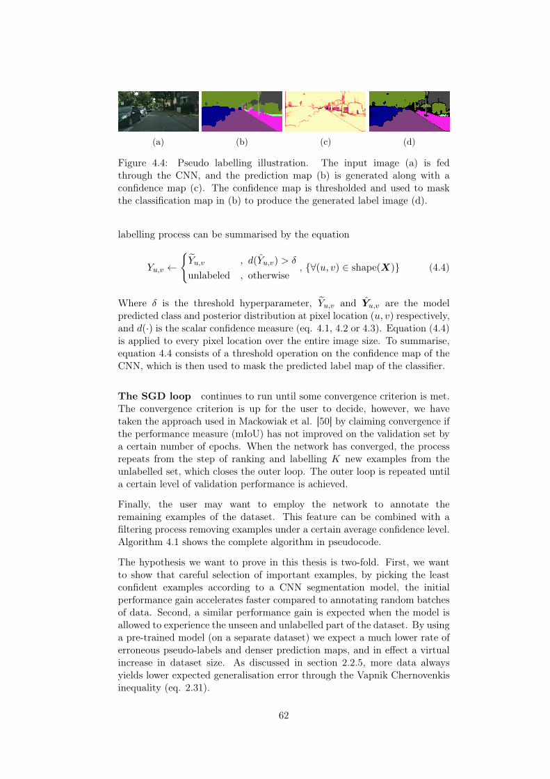
(a) (b) (c) (d)

Figure 4.4: Pseudo labelling illustration. The input image (a) is fedthrough the CNN, and the prediction map (b) is generated along with aconfidence map (c). The confidence map is thresholded and used to maskthe classification map in (b) to produce the generated label image (d).

labelling process can be summarised by the equation

Yu,v ←Yu,v , d(Yu,v) > δ

unlabeled , otherwise, ∀(u, v) ∈ shape(X) (4.4)

Where δ is the threshold hyperparameter, Yu,v and Yu,v are the modelpredicted class and posterior distribution at pixel location (u, v) respectively,and d(·) is the scalar confidence measure (eq. 4.1, 4.2 or 4.3). Equation (4.4)is applied to every pixel location over the entire image size. To summarise,equation 4.4 consists of a threshold operation on the confidence map of theCNN, which is then used to mask the predicted label map of the classifier.

The SGD loop continues to run until some convergence criterion is met.The convergence criterion is up for the user to decide, however, we havetaken the approach used in Mackowiak et al. [50] by claiming convergence ifthe performance measure (mIoU) has not improved on the validation set bya certain number of epochs. When the network has converged, the processrepeats from the step of ranking and labelling K new examples from theunlabelled set, which closes the outer loop. The outer loop is repeated untila certain level of validation performance is achieved.

Finally, the user may want to employ the network to annotate theremaining examples of the dataset. This feature can be combined with afiltering process removing examples under a certain average confidence level.Algorithm 4.1 shows the complete algorithm in pseudocode.

The hypothesis we want to prove in this thesis is two-fold. First, we wantto show that careful selection of important examples, by picking the leastconfident examples according to a CNN segmentation model, the initialperformance gain accelerates faster compared to annotating random batchesof data. Second, a similar performance gain is expected when the model isallowed to experience the unseen and unlabelled part of the dataset. By usinga pre-trained model (on a separate dataset) we expect a much lower rate oferroneous pseudo-labels and denser prediction maps, and in effect a virtualincrease in dataset size. As discussed in section 2.2.5, more data alwaysyields lower expected generalisation error through the Vapnik Chernovenkisinequality (eq. 2.31).

62

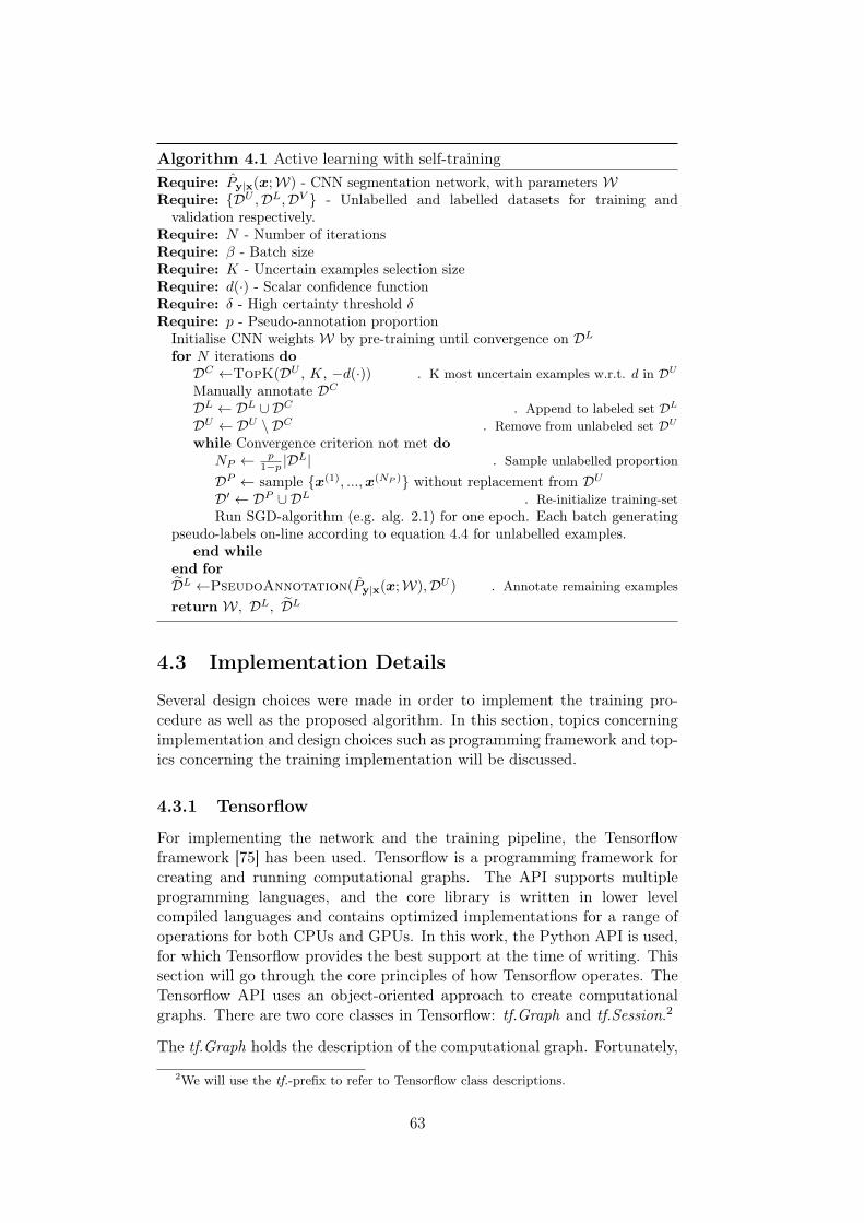
Algorithm 4.1 Active learning with self-trainingRequire: Py|x(x;W) - CNN segmentation network, with parameters WRequire: DU ,DL,DV - Unlabelled and labelled datasets for training andvalidation respectively.

Require: N - Number of iterationsRequire: β - Batch sizeRequire: K - Uncertain examples selection sizeRequire: d(·) - Scalar confidence functionRequire: δ - High certainty threshold δRequire: p - Pseudo-annotation proportionInitialise CNN weights W by pre-training until convergence on DL

for N iterations doDC ←TopK(DU , K, −d(·)) . K most uncertain examples w.r.t. d in DU

Manually annotate DC

DL ← DL ∪ DC . Append to labeled set DL

DU ← DU \ DC . Remove from unlabeled set DU

while Convergence criterion not met doNP ← p

1−p |DL| . Sample unlabelled proportion

DP ← sample x(1), ...,x(NP ) without replacement from DU

D′ ← DP ∪ DL . Re-initialize training-setRun SGD-algorithm (e.g. alg. 2.1) for one epoch. Each batch generating

pseudo-labels on-line according to equation 4.4 for unlabelled examples.end while

end forDL ←PseudoAnnotation(Py|x(x;W),DU ) . Annotate remaining examples

return W, DL, DL

4.3 Implementation Details

Several design choices were made in order to implement the training pro-cedure as well as the proposed algorithm. In this section, topics concerningimplementation and design choices such as programming framework and top-ics concerning the training implementation will be discussed.

4.3.1 Tensorflow

For implementing the network and the training pipeline, the Tensorflowframework [75] has been used. Tensorflow is a programming framework forcreating and running computational graphs. The API supports multipleprogramming languages, and the core library is written in lower levelcompiled languages and contains optimized implementations for a range ofoperations for both CPUs and GPUs. In this work, the Python API is used,for which Tensorflow provides the best support at the time of writing. Thissection will go through the core principles of how Tensorflow operates. TheTensorflow API uses an object-oriented approach to create computationalgraphs. There are two core classes in Tensorflow: tf.Graph and tf.Session.2

The tf.Graph holds the description of the computational graph. Fortunately,

2We will use the tf.-prefix to refer to Tensorflow class descriptions.

63

1 import t en so r f l ow as t f # import l i b r a r y2

3 # Def ine cons tant s and va r i ab l e input t en so r s4 A = t f . Var iab le ( [ [ 1 . 0 , 2 . 0 , 3 . 0 ] ,5 [ 4 . 0 , 5 . 0 , 6 . 0 ] ,6 [ 7 . 0 , 8 . 0 , 9 . 0 ] ] , name="A" )7 b = t f . constant ( [ [ 1 . 0 ] ,8 [ 2 . 0 ] ,9 [ 3 . 0 ] ] , name="b" )

10 c = t f . constant ( [ [ 4 . 0 ] ,11 [ 5 . 0 ] ,12 [ 6 . 0 ] ] , name="c" )13 # Create some s imple ope ra t i on s14 d = t f . matmul (A, b)15 f = t f . add (d , c )16 g = t f . subt rac t (d , c )17 # Create graph f o r computing g rad i en t s .18 opt = t f . t r a i n . GradientDescentOptimizer ( 1 . 0 )19 grad = opt . compute_gradients ( f , v a r_ l i s t =[A, b , c ] )20

21 # Create a s e s s i o n ob j e c t22 s e s s i o n = t f . S e s s i on ( )23 s e s s i o n . run (A. i n i t i a l i z e r ) # I n i t i a l i z e v a r i b l e24 # Run the matrix ope ra t i on s and pr in t r e s u l t25 pr in t ( "Ab+c=" ) ; p r i n t ( s e s s i o n . run ( f ) )26 g rad i en t s = s e s s i o n . run ( grad ) ; p r i n t ( "Gradients : " )27 f o r grad in g rad i en t s :28 pr in t ( grad [ 0 ] ) # grad = ( gradient , Var iab le )29 s e s s i o n . c l o s e ( ) # Destroy execut ion environment

Ab+c=[ [ 1 8 . ][ 3 7 . ][ 5 6 . ] ]

Gradients :[ [ 1 . 2 . 3 . ][ 1 . 2 . 3 . ][ 1 . 2 . 3 . ] ]

[ [ 1 2 . ][ 1 5 . ][ 1 8 . ] ]

[ [ 1 . ][ 1 . ][ 1 . ] ]

Figure 4.5: A simple Tensorflow example in Python, creating the graph in4.6, computing Ab+ c and the gradients using backprop. Right: the outputfrom the program.

Tensorflow uses the same convention of representing computational graphsas we defined in section 2.3.1, with operations (tf.Operation) as nodes,and tensors (tf.Tensor) as edges. The tf.Tensor holds a reference to thetf.Operation that produces the tensor as output, as well as various propertiessuch as data-type, shape and device placement. Note that the tf.Tensor isnot a specific value, nor does it contain the data of the operation; it is merelya reference describing the output of an operation. The tf.Operation holdsa reference to the operation definition as well as properties such as inputs,outputs (tf.Tensor), dependencies for execution and device placement.

tf.Session encapsulates the executable environment of a tf.Graph in whichthe tf.Operations and tf.Tensors are evaluated. A tf.Session object is usedto execute operations or to evaluate tensors in a graph; when a tensor isevaluated, the graph is traversed backwards from the tensor to the all sources(leaf nodes) providing input to the graph before executing the graph in asingle forward operation. Input sources are either variables, constants orspecial operations like placeholders, where data is specified at run-time.

Consider the code snippet in 4.5. First, we define a tf.Variable A containinga matrix, and two vector constants b and c with the specified initial values.

64

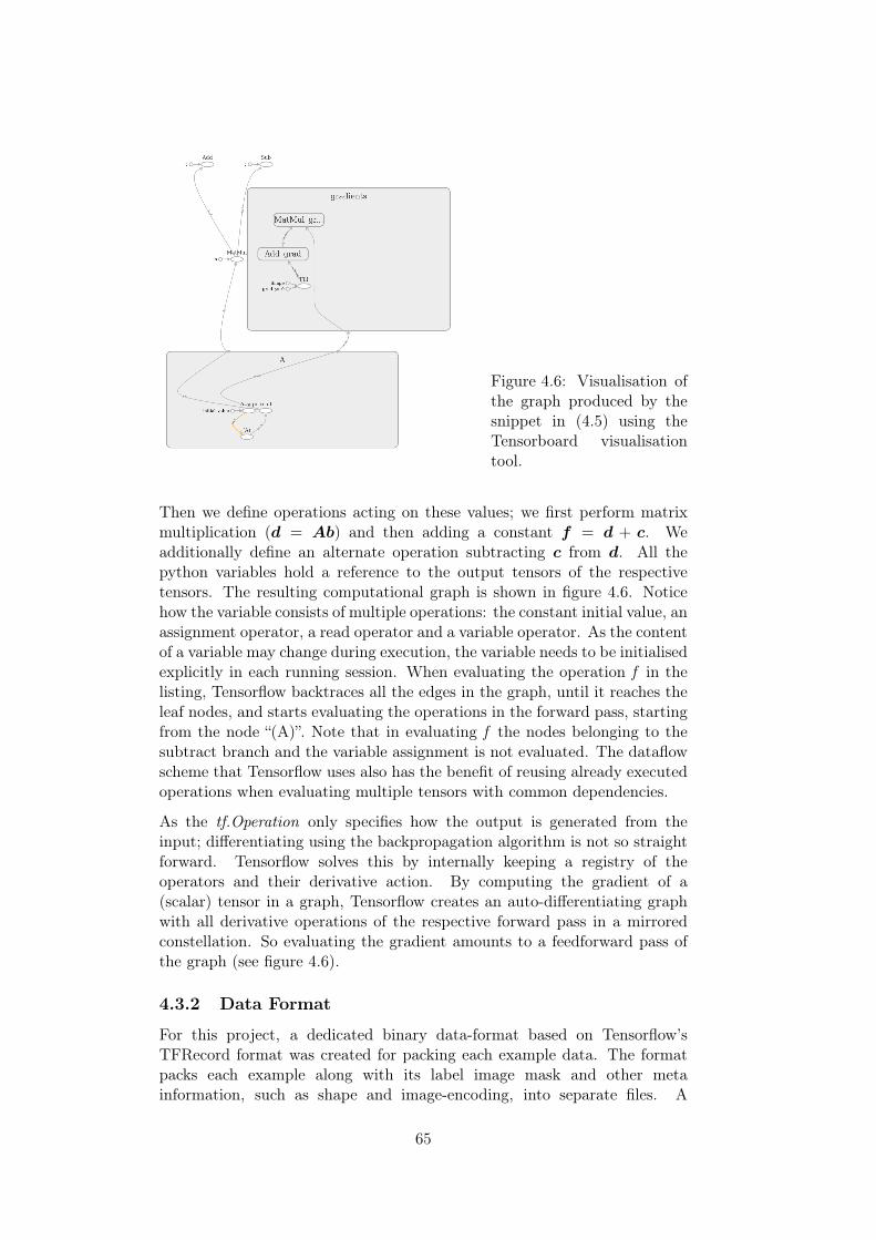
Figure 4.6: Visualisation ofthe graph produced by thesnippet in (4.5) using theTensorboard visualisationtool.

Then we define operations acting on these values; we first perform matrixmultiplication (d = Ab) and then adding a constant f = d + c. Weadditionally define an alternate operation subtracting c from d. All thepython variables hold a reference to the output tensors of the respectivetensors. The resulting computational graph is shown in figure 4.6. Noticehow the variable consists of multiple operations: the constant initial value, anassignment operator, a read operator and a variable operator. As the contentof a variable may change during execution, the variable needs to be initialisedexplicitly in each running session. When evaluating the operation f in thelisting, Tensorflow backtraces all the edges in the graph, until it reaches theleaf nodes, and starts evaluating the operations in the forward pass, startingfrom the node “(A)”. Note that in evaluating f the nodes belonging to thesubtract branch and the variable assignment is not evaluated. The dataflowscheme that Tensorflow uses also has the benefit of reusing already executedoperations when evaluating multiple tensors with common dependencies.

As the tf.Operation only specifies how the output is generated from theinput; differentiating using the backpropagation algorithm is not so straightforward. Tensorflow solves this by internally keeping a registry of theoperators and their derivative action. By computing the gradient of a(scalar) tensor in a graph, Tensorflow creates an auto-differentiating graphwith all derivative operations of the respective forward pass in a mirroredconstellation. So evaluating the gradient amounts to a feedforward pass ofthe graph (see figure 4.6).

4.3.2 Data Format

For this project, a dedicated binary data-format based on Tensorflow’sTFRecord format was created for packing each example data. The formatpacks each example along with its label image mask and other metainformation, such as shape and image-encoding, into separate files. A

65

dedicated dataset-packing script was developed to pack the datasets inthis format as well as providing a consistent directory structure separatingthe training, validation and test splits. Structuring the dataset in ageneric format avoids significant overhead in the main programs that wouldotherwise take into account the dataset-specific conventions. Besides,packing the examples together in such a format increases the on-disk locality,marginally increasing hard drive bandwidth as loading an example now takesa single read query of consecutive disk sectors.

4.3.3 Training Pipeline

Training the model is an essential part of the active learning algorithm. Inpractice, training in Tensorflow involves repeatedly executing a comprehens-ive computational graph that encapsulates the network, essentially applyinga single mini-batch optimisation step. We will refer to this computational(Tensorflow-) graph as the training pipeline. The training pipeline is alsoresponsible for computing and logging performance metrics in order to mon-itor training progress. An outline of the various components in the trainingpipeline will be discussed in the following.

Input pipeline

The input pipeline is responsible for feeding the training pipeline withdata. Loading, parsing and decoding examples as well as pre-processingand applying data-augmentation. The implemented pre-processing stepmerely changes the data type to (32-bit) floating point and re-scales therange to [0, 1]. Data-augmentation was carefully chosen not to potentiallyviolate the semantic label for any region in the image. Therefore we havelimited geometric transformations to only crop the image randomly if theimage is larger than the network input, omitting any re-scaling or projectivedistortions. In addition, a slight random scaling of the channels is applied,resulting in a slight shift in contrast and hue (colour). Tensorflow providesa dedicated tf.data API optimized for loading and processing examples inparallel, as well as prefetching the next mini-batch of examples in advance.

Model

The ENet segmentation model has been built from the ground up fromthe specification above using the Tensorflow low-level API. A hierarchicalapproach was taken during implementation, building the ENet modules(see figure 4.2) as custom layer modules. Then assembling the network bystacking the modules according to table 4.1. The layer modules and thefinalised model satisfy the standardised Keras API [42].

Multi-GPU implementation. To save computational time and utilisea system setup with two separate GPU hardware accelerators, performingtraining and evaluation on the validation split is done in parallel. Multi-GPUsupport is an inherent feature of Tensorflow as each node (tf.Opeartion)has an associated device property that is specified upon creation. To

66

achieve parallel execution, a separate validation pipeline is constructedon the secondary GPU, while keeping the training pipeline on theprimary GPU. When the tf.Session is invoked to execute the training andvalidation operations, Tensorflow utilise the resources where the respectivecomputational graphs are placed in parallel. At the start of each epoch, thevariables from the model under training on the primary GPU is copied tothe model under evaluation on the second GPU.

Loss

Each input image contains thousands or even millions of (highly correlated)examples, and some pixels do not have any corresponding (valid) label.Consider an image from the Cityscapes [14] dataset; say we were using thefull size of 2048 × 1024 and a mini-batch size of 4. This yields almost 8.4million single-example cross-entropy loss for a single mini-batch of 4 exampleimages. Computing the sample-mean over such a vast number of exampleswith finite precision floating-point [35] introduces a significant amount offloating-point error. This error can be alleviated by using double precisionfloating-point but at the cost of twice memory usage and worse than halfthe throughput compared to single precision (32-bit) floating point. Thuswe are faced with two problems: how to tackle unlabelled pixels and how topreserve precision upon evaluating the loss.

The datasets used in this thesis [14, 57] has a predefined subset of traininglabels, and typically some regions in an image may fall outside the discreteset of labels chosen for the given dataset. These pixels need to be excludedfrom the evaluation metrics and cross-entropy loss. To achieve this, all thevoid labels are mapped to a predefined value outside the range of legal labels.The label images are stored as a single-channel unsigned 8-bit image of theone-hot (unit vector) indices; thus, 255 makes a convenient choice. Then, asthe images are loaded, the label images are pre-processed by creating a maskwith the void pixels zero and valid labels ones, while simultaneously mappingthe void indexes into the legal label range before expanding the labels to one-hot elementary vectors. Upon evaluation of the pixel-wise softmax-loss, allpixels are evaluated. However, the output loss image is immediately maskedout before aggregating the mean cross-entropy loss. Which brings us to thesecond problem of numerical errors.

The approach used in this setup is to use single-precision (32-bit) floatingpoint in all operations, even computation of the cross-entropy loss for eachindividual pixel is computed using single precision. Then, computing thesample-mean is divided into two steps: First, the mean is aggregated in thebatch dimension using single precision, creating a single batch mean lossimage. Second, the loss image from step one is cast to double precisionbefore computing the mean over the spatial dimensions.

67

Custom loss function. Paszke et al. [59] report a custom class weightingscheme, which we adopt with a slight modification.

w =1

ln (c+ (e− c)yy)(4.5)

Where c is a hyperparameter, and e is Euler’s constant used to scale theminimum weight to 1. This weighting is applied to each pixel location of theprediction map and is multiplied with the per-pixel loss at the specific pixellocations. The weighting put additional cost on assigning a low class-score onthe correct class, which is usually the case for sparse classes occupying smallregions in the image. Putting an additional penalty on weak predictionsaids the training progress not to gravitate towards correctly classifying theclasses occupying large regions, neglecting sparse classes.

In addition to the custom weighting scheme, [59] pre-train the encoder parton downsampled examples. To this end, a temporary 1 × 1 convolutionallayer with softmax output activation function is placed on top of thebottleneck3.8 (see table 4.1) computing a lower resolution prediction map.The implementation extends on this and applies a prediction endpoint tothe three scales given by the output of bottleneck3.8, bottleneck4.2 andbottleneck5.1 in addition to the final layer (table 4.1). The additionalprediction end-points are discarded after model pre-training. The motivationfor this pre-training is that we want to use the capacity in the decoder partto solely “learn to up-sample” the prediction map. The idea was taken froma previous project based on the work of Mahjourian et al. [52], which uses asimilar type of encoder-decoder network to learn depth maps from geometricconstraints.

Regularisation

Several regularisation techniques were implemented including L2 and L1parameter penalty, label smoothing, early stopping, dropout and dataaugmentation, to keep ENet from overfitting the training set. However,in favour of reproducibility and lack of time for hyperparameter tuning, onlythe set of regularisation techniques reported in the ENet article [59] is used.

4.3.4 System Specifications

For the sake of reference and reproducibility, we report the systemspecifications used for generating the results in table 4.2.

68

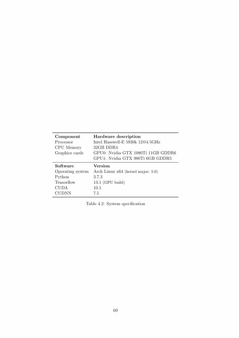
Component Hardware descriptionProcessor Intel Hasswell-E 5930k 12@4.5GHzCPU Memory 32GB DDR4Graphics cards GPU0: Nvidia GTX 1080Ti 11GB GDDR6

GPU1: Nvidia GTX 980Ti 6GB GDDR5

Software VersionOperating system Arch Linux x64 (kernel major: 5.0)Python 3.7.3Tensorflow 13.1 (GPU build)CUDA 10.1CUDNN 7.5

Table 4.2: System specification

69

70

Chapter 5

Experiments

This chapter provides details regarding the experiments conducted in thisthesis. The first section discusses the datasets used for training andevaluation of the network and the proposed algorithm, followed by adiscussion of evaluation metrics. The last section gives an outline of theexperiment setup and hyperparameters used while training and performingthe active learning procedure.

5.1 Datasets

For any supervised machine learning task, a dataset containing labelledexamples for the task at hand is required. A dataset is also needed inorder to assess the performance – both for training the CNN and for eachiteration of the active learning algorithm. In this thesis, our target isto annotate semantic segmentation datasets for unmanned ground vehicles(UGVs). Several datasets were considered for this task [5, 10, 14, 34, 57, 76].Cityscapes [14] and CamVid [10] were both used for reporting benchmarks onENet [59], enabling us to validate the results. We have selected Cityscapesas the benchmark dataset of this thesis out of superior size and quality ofimages and annotations. Mapillary Vistas [57] and Apolloscape [34] aretwo new additions to datasets for scene understanding. These datasets areenormous, making comprehensive testing on these datasets a challenge on thelimited time-span of this work. We selected Mapillary Vistas as an auxiliarydataset for pre-training the segmentation network in our final experiment.The Apolloscape dataset [34] is still under development at the time of writing,and is expected to have 200 000 annotated images on completion.

5.1.1 Cityscapes

Cityscapes [14] is a large-scale, high-quality dataset for semantic sceneunderstanding of complex urban street scenes. The dataset consists of atotal of 25 000 RGB-images of size 2048×1024 of urban street scenes spreadover 50 cities in Germany and neighbouring countries. Each example iscaptured using the same set of equipment, and the dataset also features

71

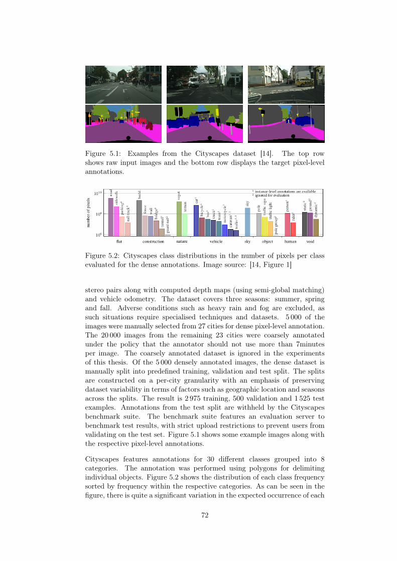
Figure 5.1: Examples from the Cityscapes dataset [14]. The top rowshows raw input images and the bottom row displays the target pixel-levelannotations.

Figure 5.2: Cityscapes class distributions in the number of pixels per classevaluated for the dense annotations. Image source: [14, Figure 1]

stereo pairs along with computed depth maps (using semi-global matching)and vehicle odometry. The dataset covers three seasons: summer, springand fall. Adverse conditions such as heavy rain and fog are excluded, assuch situations require specialised techniques and datasets. 5 000 of theimages were manually selected from 27 cities for dense pixel-level annotation.The 20 000 images from the remaining 23 cities were coarsely annotatedunder the policy that the annotator should not use more than 7minutesper image. The coarsely annotated dataset is ignored in the experimentsof this thesis. Of the 5 000 densely annotated images, the dense dataset ismanually split into predefined training, validation and test split. The splitsare constructed on a per-city granularity with an emphasis of preservingdataset variability in terms of factors such as geographic location and seasonsacross the splits. The result is 2 975 training, 500 validation and 1 525 testexamples. Annotations from the test split are withheld by the Cityscapesbenchmark suite. The benchmark suite features an evaluation server tobenchmark test results, with strict upload restrictions to prevent users fromvalidating on the test set. Figure 5.1 shows some example images along withthe respective pixel-level annotations.

Cityscapes features annotations for 30 different classes grouped into 8categories. The annotation was performed using polygons for delimitingindividual objects. Figure 5.2 shows the distribution of each class frequencysorted by frequency within the respective categories. As can be seen in thefigure, there is quite a significant variation in the expected occurrence of each

72

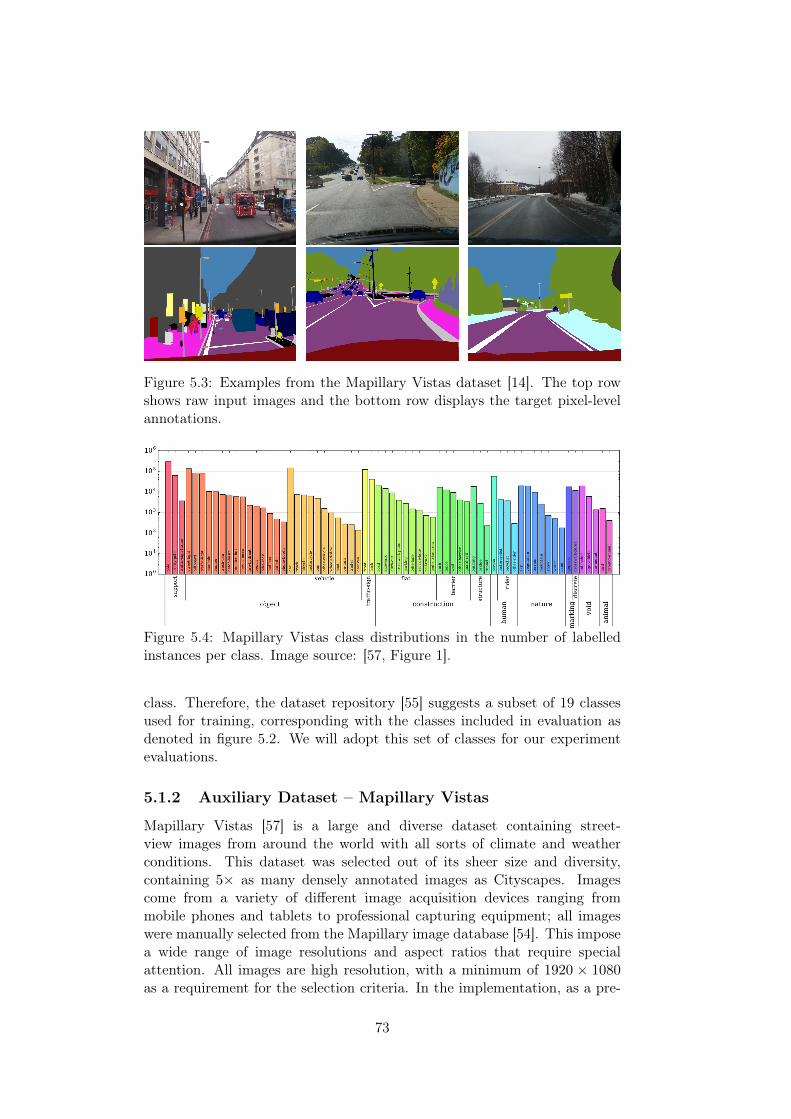
Figure 5.3: Examples from the Mapillary Vistas dataset [14]. The top rowshows raw input images and the bottom row displays the target pixel-levelannotations.

Figure 5.4: Mapillary Vistas class distributions in the number of labelledinstances per class. Image source: [57, Figure 1].

class. Therefore, the dataset repository [55] suggests a subset of 19 classesused for training, corresponding with the classes included in evaluation asdenoted in figure 5.2. We will adopt this set of classes for our experimentevaluations.

5.1.2 Auxiliary Dataset – Mapillary Vistas

Mapillary Vistas [57] is a large and diverse dataset containing street-view images from around the world with all sorts of climate and weatherconditions. This dataset was selected out of its sheer size and diversity,containing 5× as many densely annotated images as Cityscapes. Imagescome from a variety of different image acquisition devices ranging frommobile phones and tablets to professional capturing equipment; all imageswere manually selected from the Mapillary image database [54]. This imposea wide range of image resolutions and aspect ratios that require specialattention. All images are high resolution, with a minimum of 1920 × 1080as a requirement for the selection criteria. In the implementation, as a pre-

73

Cityscapes Mapillary Vistasroad road, lane marking – generalsidewalk curb, bike lane, curb cut, sidewalk, pedestrian areabuilding buildingwall wallfence fencepole pole, utility poletraffic light traffic lighttraffic sign traffic sign frontvegetation vegetationterrain terrainsky skyperson personrider bicyclist, motorcyclist, other ridercar cartruck truckbus bustrain on railsmotorcycle motorcyclebicycle bicycleunlabelled bird, ground animal, guard rail, barrier, crosswalk –

plain, parking, rail track, service lane, bridge, tunnel,lane marking – crosswalk, mountain, sand, snow, ter-rain, water, banner, bench, bike rack, billboard, catchbasin, cctv camera, fire hydrant, junction box, mailbox,manhole, phone booth, pothole, street light, traffic signframe, traffic sign back, trash can, boat, caravan, othervehicle, trailer, wheeled slow, car mount, ego vehicle, un-labelled.

Table 5.1: Class associations mapping Cityscapes training labels to MapillaryVistas labels used for the experiments.

processing step, all images were resized to a common width and images witha wider aspect ratio than 2:1 is crop to the centre – the aspect ratio ofCityscapes’ images. Under the assumption of (approximately) equal field ofview for the capturing devices, this resolves variations of object scale betweenthe images and datasets. As with Cityscapes, Mapillary Vistas provides fixeddataset splits of training, validation and test set, withholding the labels forthe test set. The training and validation data respectively comprise 18 000and 2 000 examples, and the remaining 5 000 forms the test set. Figure 5.3shows three example images along with the class labels.

The dataset includes 66 classes – more than twice that of Cityscapes, groupedin 7 root-level categories. Figure 5.4 shows the distribution of each classin terms of instances per class label. Instead of using all 66 classes, wehave manually created a mapping that maps a subset of the classes to thecorresponding 19 classes used for training in Cityscapes. Table 5.1 shows theclass associations used for training on the Mapillary Vistas. We will use this

74

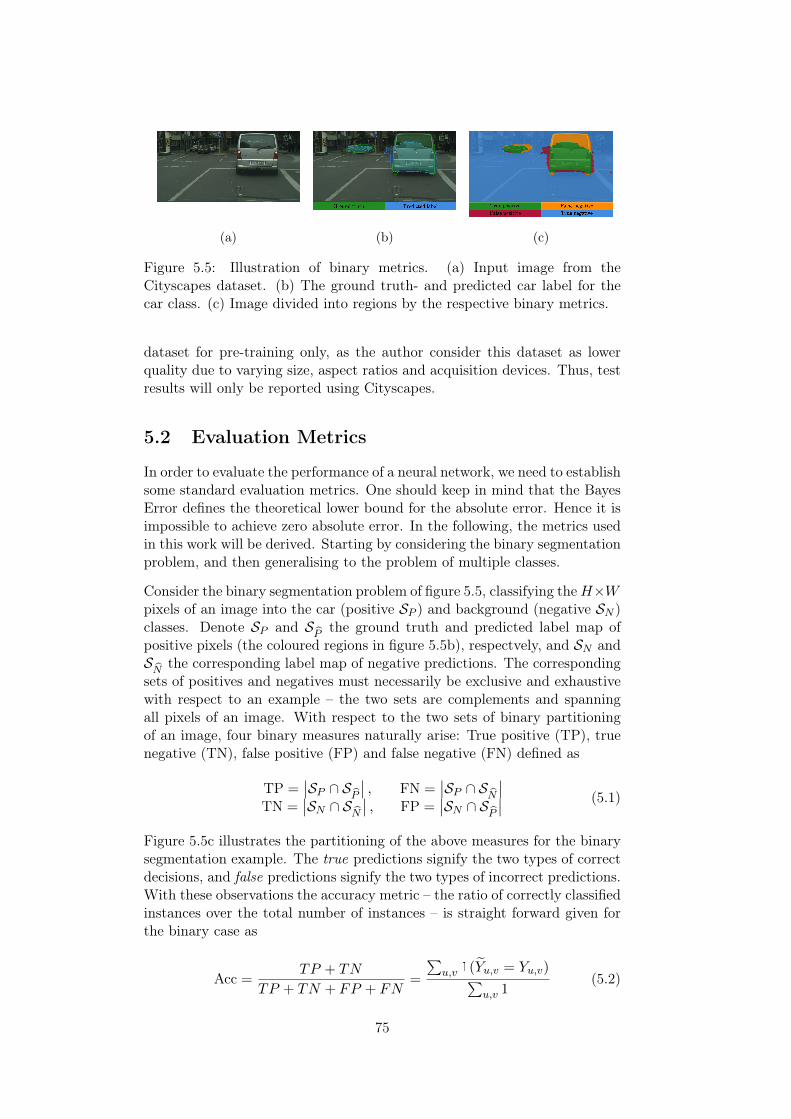
(a) (b) (c)

Figure 5.5: Illustration of binary metrics. (a) Input image from theCityscapes dataset. (b) The ground truth- and predicted car label for thecar class. (c) Image divided into regions by the respective binary metrics.

dataset for pre-training only, as the author consider this dataset as lowerquality due to varying size, aspect ratios and acquisition devices. Thus, testresults will only be reported using Cityscapes.

5.2 Evaluation Metrics

In order to evaluate the performance of a neural network, we need to establishsome standard evaluation metrics. One should keep in mind that the BayesError defines the theoretical lower bound for the absolute error. Hence it isimpossible to achieve zero absolute error. In the following, the metrics usedin this work will be derived. Starting by considering the binary segmentationproblem, and then generalising to the problem of multiple classes.

Consider the binary segmentation problem of figure 5.5, classifying theH×Wpixels of an image into the car (positive SP ) and background (negative SN )classes. Denote SP and S

Pthe ground truth and predicted label map of

positive pixels (the coloured regions in figure 5.5b), respectvely, and SN andSN

the corresponding label map of negative predictions. The correspondingsets of positives and negatives must necessarily be exclusive and exhaustivewith respect to an example – the two sets are complements and spanningall pixels of an image. With respect to the two sets of binary partitioningof an image, four binary measures naturally arise: True positive (TP), truenegative (TN), false positive (FP) and false negative (FN) defined as

TP =∣∣SP ∩ SP ∣∣ , FN =

∣∣SP ∩ SN ∣∣TN =

∣∣SN ∩ SN ∣∣ , FP =∣∣SN ∩ SP ∣∣ (5.1)

Figure 5.5c illustrates the partitioning of the above measures for the binarysegmentation example. The true predictions signify the two types of correctdecisions, and false predictions signify the two types of incorrect predictions.With these observations the accuracy metric – the ratio of correctly classifiedinstances over the total number of instances – is straight forward given forthe binary case as

Acc =TP + TN

TP + TN + FP + FN=

∑u,v 1(Yu,v = Yu,v)∑

u,v 1(5.2)

75

The last equation shows how the metric is expressed in numerical terms usingthe indicator function 1(·). The summation over u, v iterates over the widthand height dimensions respectively.

For the semantic segmentation task, there is an inherent problem of usingaccuracy as evaluation metric – the metric is biased towards classes that onaverage occupy substantial portions in the image. To see why this is, noticehow the true negative is by far the largest region in figure 5.5c. If we tookan even more sparse class (e.g. traffic sign), the classification network wouldobtain reasonable accuracy by always predicting negatives. If we eliminatethe true negatives (TN) from equation 5.2, we arrive at the Pascal VOCIntersection over Union [21], also called the Jaccard index, defined

IoU =TP

TP + FN + FP=

∣∣SP ∩ SP ∣∣∣∣SP ∪ SP ∣∣=

∑u,v 1(Yu,v = 1)1(Yu,v = 1)∑

u,v 1(Yu,v = 1)1(Yu,v = 0) + 1(Yu,v = 1)

(5.3)

We will refer to this metric as the intersection over union (IoU), as is evidentfrom the second equality in equation 5.3.

5.2.1 Multi-class Metrics and the Confusion Matrix

Generalising the above metrics to multiple classes is not as straight forward asin the binary case. The binary metrics in equation 5.1 needs to be consideredfor each class individually, but note that true negatives for one predicted classcan be a true positive, a false negative or a false positive for another class.The most straight forward multi-class metric is the extension of the accuracygiven by the expression1

Acc =1

Nc

Nc∑c=1

Accc =1

Nc

Nc∑c=1

TPcTPc + TNc + FPc + FNc

=

∑u,v 1(Yu,v = Yu,v)∑

u,v 1

(5.4)

For multi-class segmentation, the most common way to report theperformence of a model is by computing the class average intersection overunion, commonly referred to as the mean instersection over union, given by

mIoU =1

Nc

Nc∑c=1

IoUi =1

Nc

Nc∑c=1

TPcTPc + FPc + FNc

=1

Nc

Nc∑c=1

∑u,v 1(Yu,v = c)1(Yu,v = c)∑

u,v 1(Yu,v = c)1(Yu,v 6= c) + 1(Yu,v = c)

(5.5)

1Note that the true negatives (TN) are not included in the numerator of equation 5.4.If we reconsider the binary case, the true negatives (TN) in the expression 5.2 is the truepositives for the negative (background) class.

76

Figure 5.6: Illustration of the multi-class confusion matrix and thepartitioning of binary metrics for class k. The binary metrics are computedby summation over the respective entries of each region.

In the above discussion, we have only explained how to compute the metricsfor a single example. However, in order to assess the performance on adataset split (training, validation or test), the sample mean is used. Tocompute the metric in a clean and efficient manner, we aggregate theconfusion matrix over the dataset. The confusion matrix C is a Nc × Nc

frequency matrix resembling a two-dimensional histogram of class predictionsversus ground truth labels. That is, element (i, j) signifies the number oftimes a pixel having label i is predicted as class j. Figure 5.6 shows how thebinary metrics discussed above can be extracted from the confusion matrixfor class k. By aggregating the confusion matrix for all examples over anepoch, the sample-mean metrics can be computed as illustrated in figure 5.6.For instance, the pixel accuracy is computed as the ratio of sums of diagonalentries to all entries in the matrix. To summarise, the two metrics are givenby the expressions

Acc =

∑Nck=1Ckk∑Nc

i=1

∑Ncj=1Cij

, mIoU =

Nc∑k=1

Ckk∑Nci=1 (Cik) +

∑Ncj=1 (Ckj)− Ckk

5.3 Experiments

This section discusses the details regarding the experiments performed in thisthesis. Two experiments were performed during the work of this thesis. First,we train and validate our implementation of ENet against the publishedbenchmark. In the second part, we test and benchmark the proposed activelearning algorithm. Finally, we discuss the task that started as the primaryobjective for this thesis, but after planning and preparation we did not havetime to perform.

5.3.1 Training ENet – Design Validation

In order to verify the implementation against the published results, wehave tried to replicate the experiments performed by Paszke et al. [59] onCityscapes. The image size for the Cityscapes dataset is quite large (2048×1024) resulting in severe memory usage when performing backpropagationin addition to the added computational cost. To this end, we downsample

77

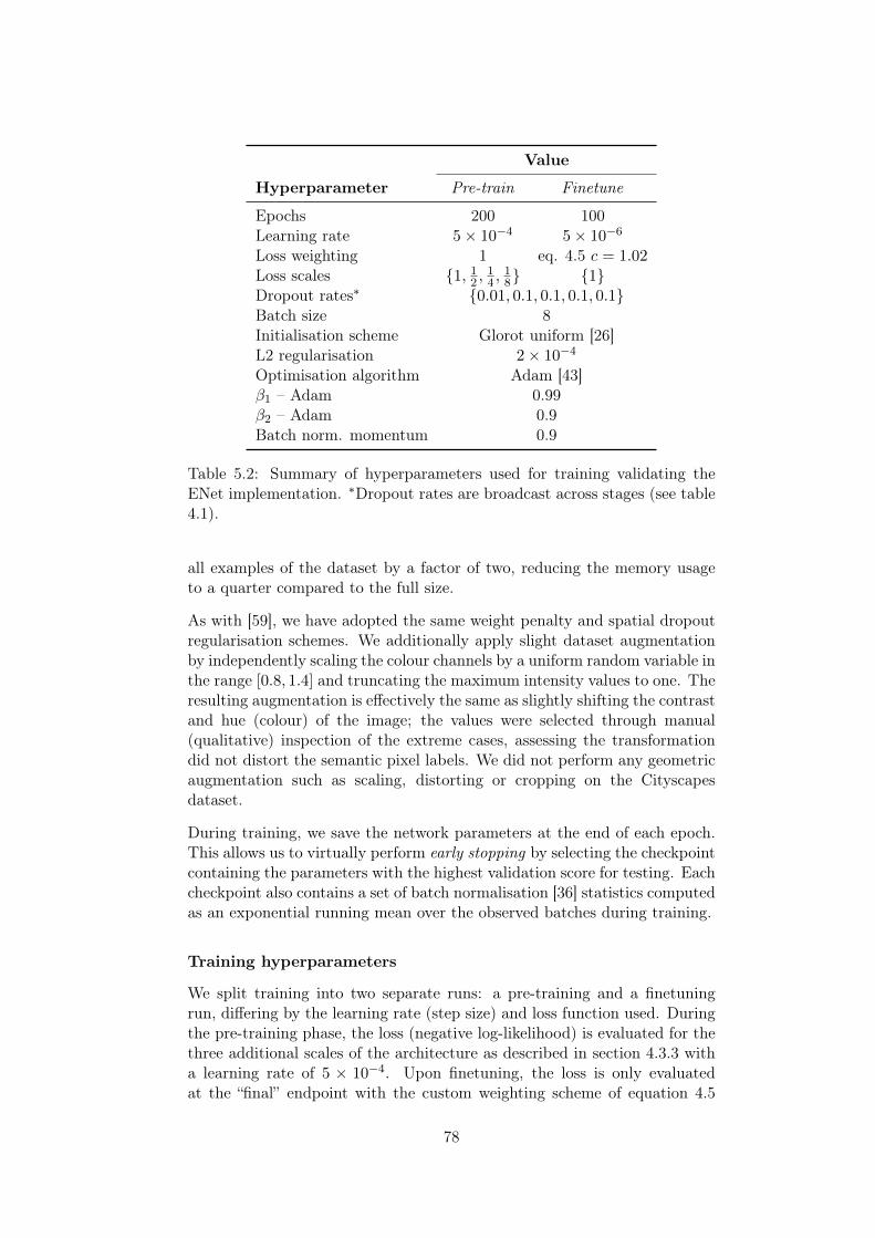
Value

Hyperparameter Pre-train Finetune

Epochs 200 100Learning rate 5× 10−4 5× 10−6

Loss weighting 1 eq. 4.5 c = 1.02Loss scales 1, 12 , 14 , 18 1Dropout rates∗ 0.01, 0.1, 0.1, 0.1, 0.1Batch size 8Initialisation scheme Glorot uniform [26]L2 regularisation 2× 10−4

Optimisation algorithm Adam [43]β1 – Adam 0.99β2 – Adam 0.9Batch norm. momentum 0.9

Table 5.2: Summary of hyperparameters used for training validating theENet implementation. ∗Dropout rates are broadcast across stages (see table4.1).

all examples of the dataset by a factor of two, reducing the memory usageto a quarter compared to the full size.

As with [59], we have adopted the same weight penalty and spatial dropoutregularisation schemes. We additionally apply slight dataset augmentationby independently scaling the colour channels by a uniform random variable inthe range [0.8, 1.4] and truncating the maximum intensity values to one. Theresulting augmentation is effectively the same as slightly shifting the contrastand hue (colour) of the image; the values were selected through manual(qualitative) inspection of the extreme cases, assessing the transformationdid not distort the semantic pixel labels. We did not perform any geometricaugmentation such as scaling, distorting or cropping on the Cityscapesdataset.

During training, we save the network parameters at the end of each epoch.This allows us to virtually perform early stopping by selecting the checkpointcontaining the parameters with the highest validation score for testing. Eachcheckpoint also contains a set of batch normalisation [36] statistics computedas an exponential running mean over the observed batches during training.

Training hyperparameters

We split training into two separate runs: a pre-training and a finetuningrun, differing by the learning rate (step size) and loss function used. Duringthe pre-training phase, the loss (negative log-likelihood) is evaluated for thethree additional scales of the architecture as described in section 4.3.3 witha learning rate of 5 × 10−4. Upon finetuning, the loss is only evaluatedat the “final” endpoint with the custom weighting scheme of equation 4.5

78

with the hyperparameter c = 1.02, along with a learning rate of 5 × 10−6.The finetuning learning rate was found through several runs performing alogarithmic grid-search over the range [5 × 10−4, 1 × 10−6]. Pre-training isrun for 200 epochs, then continuing from the parameters for the highestscoring validation results in terms of mIoU (eq. 5.5) finetuning is run for anadditional 100 epochs.

The regularisation parameters are shared between the two runs and we useL2 weight penalty constant of 2 × 10−4 along with spatial dropout rateof 0.1 except for first stage where the rate is reduced to 0.01. The dataaugmentation procedure remains as described above as well. Table 5.2summarise all the training hyperparameters.

Testing

After training for a total of 300 epochs, the checkpoint containing theparameters achieving best validation results in terms of mIoU are used forperforming inference (predictions) over the test images. The Cityscapesevaluation server requires prediction maps in the original image resolutionof 2048 × 1024. To this end, we upsample the model logits using a bilinearinterpolation kernel before computing the (arg max) predictions. The testingis done on the hidden ground truth labels by uploading the prediction mapsto the Cityscapes benchmark suite [14].

5.3.2 Active Learning

This section concerns the second central part of this thesis, evaluating theproposed active learning framework (algorithm 4.1). We report results fortwo constructed experiments each containing four different runs: a baselinethat annotates K examples randomly drawn each iteration, and threedifferent runs using 0%, 25% and 50% pseudo labels during training. Noticethat the baseline is better than annotating the dataset sequentially, andtherefore by no means the worst thinkable approach. The two experimentsstart from different network initialisation. The first is initialised by onlypre-training on the seed set, whereas the second experiment uses a networkpre-trained on Mapillary Vistas [57] (using the label mapping in table 5.1).In the following, we will present the details of the experiment executionstarting with dataset partitioning.

Dataset partitioning

At the end of each iteration of the outer loop in algorithm 4.1, when theCNN has converged on the validation set, the performance is evaluated on anindependent test set. In order to do testing, we can no longer use the officialCityscapes test set as the evaluation server has strict uploading constraints,allowing only two uploads in 48 hrs and six uploads in 30 days. To this end,we re-partition the Cityscapes training and validation set. Like [50], we usethe validation set as a test set. We also separate the two first cities, Aachenand Bochum, from the training set and use the 270 examples as a separate

79

Dataset Training Validation Testing

Cityscapes 2705 270 500Mapillary Vistas 18 000 2000 -

Table 5.3: The number of examples per split for the datasets used in theactive learning setup. Mapillary Vistas is only used for pre-training in thesecond part of this experiment.

validation set. The validation set is used exclusively for asserting whetherthe CNN has converged, such that the test evaluations remains unbiased.The remaining examples from the training set make up the training set. Thetraining set is used as the pool of “unlabelled examples” by withholding thelabels until queried for annotation. An overview of the number of examplesper split is shown in table 5.3.

Experimental setup

We provide results comparing two different experiments. First for runningsolely on the Cityscapes dataset, initialising the CNN by pre-training onthe initial seed set from a random weight initialisation. Second, we executethe same experiment but using the parameters from a pre-trained modelon Mapillary Vistas before further adjusting the parameters on the seed setbefore executing the main loop. The latter experiment represents a morerealistic use case of executing the algorithm.

For both experiments, we use the same experiment setup. We use aninitial seed set of 50 examples drawn randomly from the pool of unlabelledexamples. Each iteration we query 50 examples for annotation selectedfrom the unlabelled pool. For performing pseudo-labelling, we only use theentropy-based confidence measure in equation 4.3. We fix the threshold to0.9, a value found by manual qualitative inspection to yield a reasonabletrade-off between labelling density without too many erroneous annotations.For the convergence criterion, we claim convergence if the model performancehas not improved on the validation set for 20 epochs, and let the model runfor at least 50 epochs from the start of each iteration.

We report results for three different runs, comprising the proportions 50%,25% and 0% of pseudo-labelled examples in the training loop. Theseruns are compared with a baseline annotation procedure that picks 50examples randomly at each iteration. The parameters resulting from thepre-training phase are shared between the different runs in order to make afair comparison of the different configurations.

The training loop hyperparameters adopts the same parameters used for pre-training above (see table 5.2) with a slight modification. Though we use thesame pre-training parameters with the multi-scale loss for the initial pre-training phase, we only evaluate the loss at the final scale while performingactive learning. Table 5.4 summarises the hyperparameters associated with

80

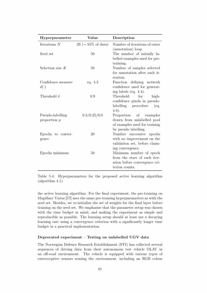
Hyperparameter Value Description

Iterations N 29 (∼ 55% of data) Number of iterations of outer(annotation) loop.

Seed set 50 The number of initially la-belled examples used for pre-training.

Selection size K 50 Number of samples selectedfor annotation after each it-eration.

Confidence measured(·)

eq. 4.3 Function defining networkconfidence used for generat-ing labels (eq. 4.4).

Threshold δ 0.9 Threshold for high-confidence pixels in pseudo-labelling procedure (eq.4.4).

Pseudo-labellingproportion p

0.5/0.25/0.0 Proportion of examplesdrawn from unlabelled poolof examples used for trainingby pseudo labelling.

Epochs to conver-gence

20 Number successive epochswith no improvement on thevalidation set, before claim-ing convergence.

Epochs minimum 50 Minimum number of epochfrom the start of each iter-ation before convergence cri-terion counts.

Table 5.4: Hyperparameters for the proposed active learning algorithm(algorithm 4.1).

the active learning algorithm. For the final experiment, the pre-training onMapillary Vistas [57] uses the same pre-training hyperparameters as with theseed set. Besides, we re-initialise the set of weights for the final layer beforetraining on the seed set. We emphasise that the parameter setup was chosenwith the time budget in mind, and making the experiment as simple andreproducible as possible. The learning setup should at least use a decayinglearning rate using a convergence criterion with a significantly longer timebudget in a practical implementation.

Deprecated experiment – Testing on unlabelled UGV data

The Norwegian Defence Research Establishment (FFI) has collected severalsequences of driving data from their autonomous test vehicle OLAV inan off-road environment. The vehicle is equipped with various types ofexteroceptive sensors sensing the environment, including an RGB colour

81

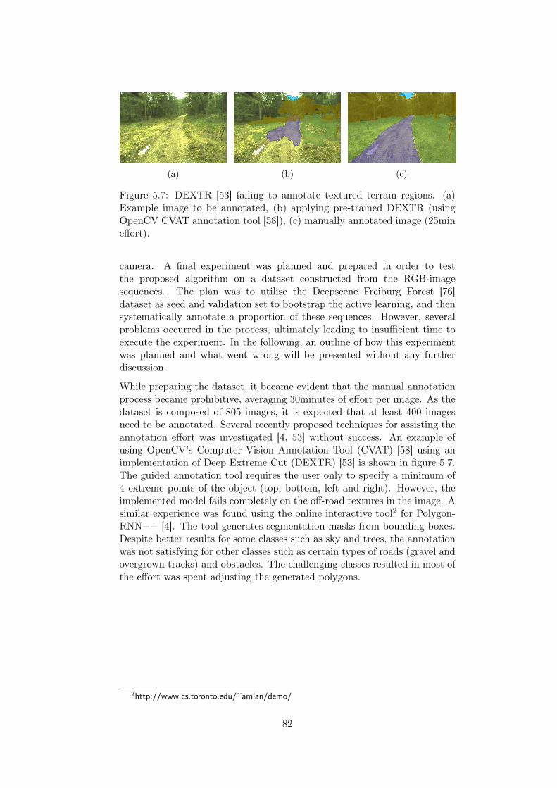
(a) (b) (c)

Figure 5.7: DEXTR [53] failing to annotate textured terrain regions. (a)Example image to be annotated, (b) applying pre-trained DEXTR (usingOpenCV CVAT annotation tool [58]), (c) manually annotated image (25mineffort).

camera. A final experiment was planned and prepared in order to testthe proposed algorithm on a dataset constructed from the RGB-imagesequences. The plan was to utilise the Deepscene Freiburg Forest [76]dataset as seed and validation set to bootstrap the active learning, and thensystematically annotate a proportion of these sequences. However, severalproblems occurred in the process, ultimately leading to insufficient time toexecute the experiment. In the following, an outline of how this experimentwas planned and what went wrong will be presented without any furtherdiscussion.

While preparing the dataset, it became evident that the manual annotationprocess became prohibitive, averaging 30minutes of effort per image. As thedataset is composed of 805 images, it is expected that at least 400 imagesneed to be annotated. Several recently proposed techniques for assisting theannotation effort was investigated [4, 53] without success. An example ofusing OpenCV’s Computer Vision Annotation Tool (CVAT) [58] using animplementation of Deep Extreme Cut (DEXTR) [53] is shown in figure 5.7.The guided annotation tool requires the user only to specify a minimum of4 extreme points of the object (top, bottom, left and right). However, theimplemented model fails completely on the off-road textures in the image. Asimilar experience was found using the online interactive tool2 for Polygon-RNN++ [4]. The tool generates segmentation masks from bounding boxes.Despite better results for some classes such as sky and trees, the annotationwas not satisfying for other classes such as certain types of roads (gravel andovergrown tracks) and obstacles. The challenging classes resulted in most ofthe effort was spent adjusting the generated polygons.

2http://www.cs.toronto.edu/~amlan/demo/

82

Chapter 6

Results and Analysis

This chapter presents the results of the experiments described in the previouschapter. We start with the results of training ENet on Cityscapes andcompare our results with the published results [59]. In the second part,we present the result of running the proposed active learning annotationscheme in algorithm 4.1. The results will be provided with a qualitativeanalysis of visual examples generated by the model.

6.1 Training ENet

This section presents the results of training ENet on Cityscapes [14]. We firstpresent the quantitative results in terms of mean intersection over union andaccuracy over the course of training and at test time. We also present theper-class intersection over union and the confusion matrix to inspect whichclasses are more challenging. Finally, we show some examples of predictionsproduced by the trained model for visual inspection.

6.1.1 Quantitative Results

Figure 6.1 shows the performance evaluated on the training and validationover the course of training. Mean intersection over union scores are shownin figure 6.1a, and the pixel accuracy is shown in figure 6.1b for reference.The metrics are computed as the sample mean over the respective datasetsplits. For the first 200 epochs, the pre-training hyperparameters are used,then training is continued from the epoch that resulted in the best validationmIoU (epoch 194) using the finetune parameters (see table 5.2), resulting inless noisy dynamics. Comparing the training and validation curves, we canconclude that the model has a reasonably low generalisation error, indicatingthat the model is appropriately regularised. The mean IoU seems to flattenout at 64% for the validation set, leaving only marginal gain from finetuning.As for the accuracy, the metric climbs to 90% during the first ten epochsand flattening around 92%. Figure 6.1c also show how the cross-entropy lossdevelops throughout the training. We can see the exponentially decayingshape of the loss along with logarithmic gain in performance, as expected.

83

0 50 100 150 200 250 3000

20

40

60

80

Epoch

mIoU

(%)

Training

Validation

(a) Mean intersection over union.

0 100 200 300

20

40

60

80

100

Epoch

Accuracy

(%)

Training

Validation

(b) Pixelwise accuracy.

0 0.5 1 ·1050

2

4

6

0.25 0.75

Step

Loss

(c) Cross entropy loss.

Figure 6.1: Training results: mIoU (a) and accuracy (b) evaluation resultsaveraged over all training (blue) and validation (orange) examples per epoch.(c) show the loss with respect to per batch of training examples. The pointin (a) annotates the highest validation score of 64.3% mIoU, the parametersfor this evaluation was used to generate the test results in table 6.1. Atthe 194th epoch, the model parameters was further optimised using thefinetuning hyperparameters (see table 5.2).

84

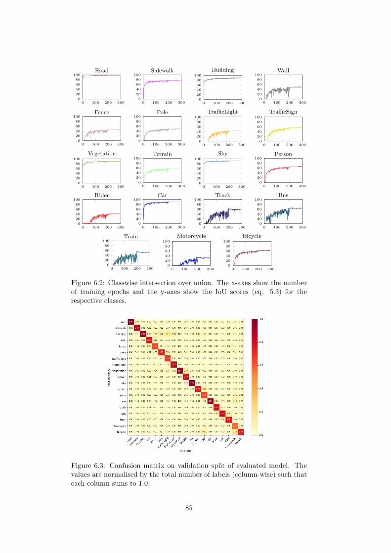
0 100 200 3000

20

40

60

80

100Road

0 100 200 3000

20

40

60

80

100Sidewalk

0 100 200 3000

20

40

60

80

100

Building

0 100 200 3000

20

40

60

80

100Wall

0 100 200 3000

20

40

60

80

100Fence

0 100 200 3000

20

40

60

80

100Pole

0 100 200 3000

20

40

60

80

100

TrafficLight

0 100 200 3000

20

40

60

80

100

TrafficSign

0 100 200 3000

20

40

60

80

100

Vegetation

0 100 200 3000

20

40

60

80

100Terrain

0 100 200 3000

20

40

60

80

100

Sky

0 100 200 3000

20

40

60

80

100Person

0 100 200 3000

20

40

60

80

100Rider

0 100 200 3000

20

40

60

80

100Car

0 100 200 3000

20

40

60

80

100Truck

0 100 200 3000

20

40

60

80

100Bus

0 100 200 3000

20

40

60

80

100Train

0 100 200 3000

20

40

60

80

100

Motorcycle

0 100 200 3000

20

40

60

80

100

Bicycle

Figure 6.2: Classwise intersection over union. The x-axes show the numberof training epochs and the y-axes show the IoU scores (eq. 5.3) for therespective classes.

Figure 6.3: Confusion matrix on validation split of evaluated model. Thevalues are normalised by the total number of labels (column-wise) such thateach column sums to 1.0.

85

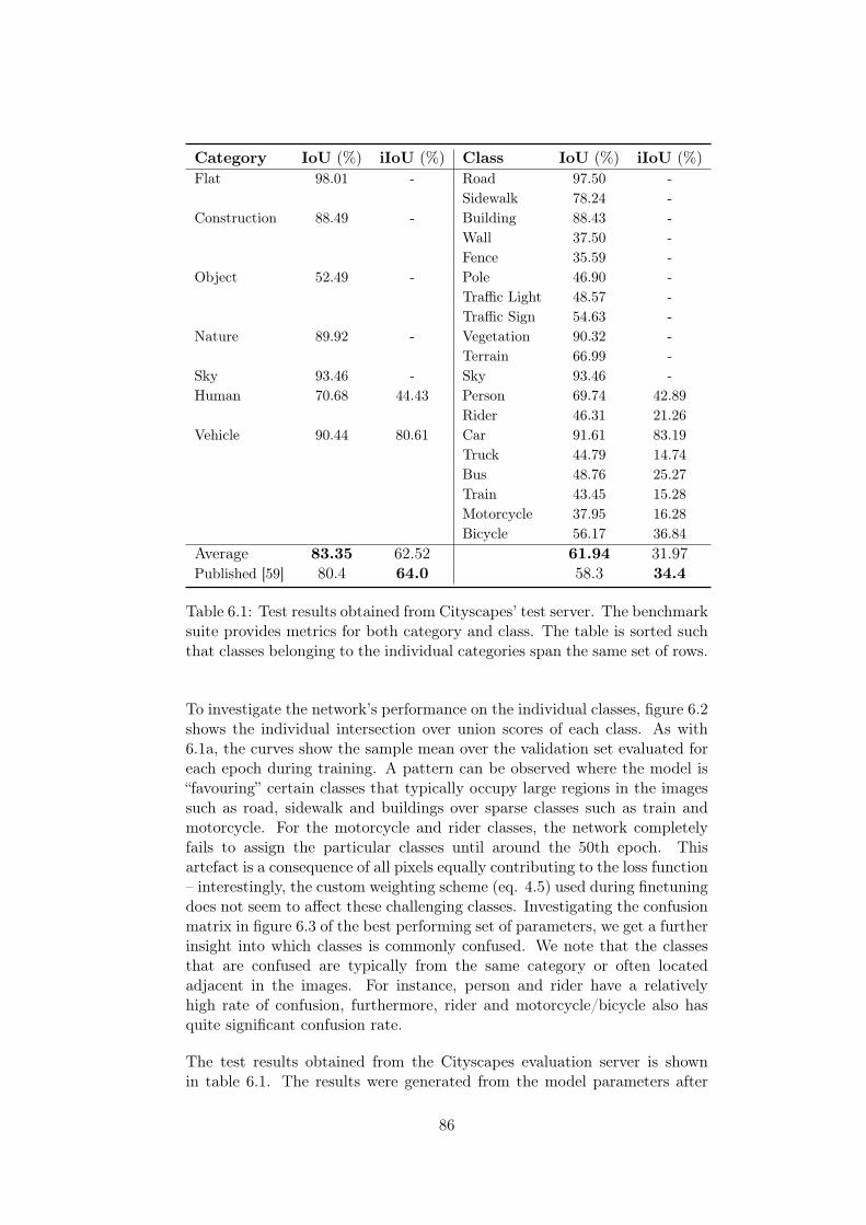
Category IoU (%) iIoU (%) Class IoU (%) iIoU (%)Flat 98.01 - Road 97.50 -

Sidewalk 78.24 -Construction 88.49 - Building 88.43 -

Wall 37.50 -Fence 35.59 -

Object 52.49 - Pole 46.90 -Traffic Light 48.57 -Traffic Sign 54.63 -

Nature 89.92 - Vegetation 90.32 -Terrain 66.99 -

Sky 93.46 - Sky 93.46 -Human 70.68 44.43 Person 69.74 42.89

Rider 46.31 21.26Vehicle 90.44 80.61 Car 91.61 83.19

Truck 44.79 14.74Bus 48.76 25.27Train 43.45 15.28Motorcycle 37.95 16.28Bicycle 56.17 36.84

Average 83.35 62.52 61.94 31.97Published [59] 80.4 64.0 58.3 34.4

Table 6.1: Test results obtained from Cityscapes’ test server. The benchmarksuite provides metrics for both category and class. The table is sorted suchthat classes belonging to the individual categories span the same set of rows.

To investigate the network’s performance on the individual classes, figure 6.2shows the individual intersection over union scores of each class. As with6.1a, the curves show the sample mean over the validation set evaluated foreach epoch during training. A pattern can be observed where the model is“favouring” certain classes that typically occupy large regions in the imagessuch as road, sidewalk and buildings over sparse classes such as train andmotorcycle. For the motorcycle and rider classes, the network completelyfails to assign the particular classes until around the 50th epoch. Thisartefact is a consequence of all pixels equally contributing to the loss function– interestingly, the custom weighting scheme (eq. 4.5) used during finetuningdoes not seem to affect these challenging classes. Investigating the confusionmatrix in figure 6.3 of the best performing set of parameters, we get a furtherinsight into which classes is commonly confused. We note that the classesthat are confused are typically from the same category or often locatedadjacent in the images. For instance, person and rider have a relativelyhigh rate of confusion, furthermore, rider and motorcycle/bicycle also hasquite significant confusion rate.

The test results obtained from the Cityscapes evaluation server is shownin table 6.1. The results were generated from the model parameters after

86

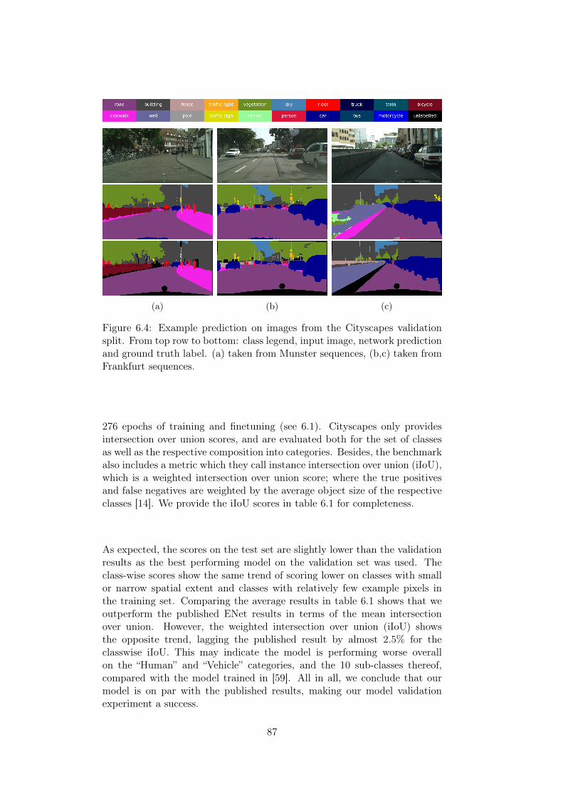
(a) (b) (c)

Figure 6.4: Example prediction on images from the Cityscapes validationsplit. From top row to bottom: class legend, input image, network predictionand ground truth label. (a) taken from Munster sequences, (b,c) taken fromFrankfurt sequences.

276 epochs of training and finetuning (see 6.1). Cityscapes only providesintersection over union scores, and are evaluated both for the set of classesas well as the respective composition into categories. Besides, the benchmarkalso includes a metric which they call instance intersection over union (iIoU),which is a weighted intersection over union score; where the true positivesand false negatives are weighted by the average object size of the respectiveclasses [14]. We provide the iIoU scores in table 6.1 for completeness.

As expected, the scores on the test set are slightly lower than the validationresults as the best performing model on the validation set was used. Theclass-wise scores show the same trend of scoring lower on classes with smallor narrow spatial extent and classes with relatively few example pixels inthe training set. Comparing the average results in table 6.1 shows that weoutperform the published ENet results in terms of the mean intersectionover union. However, the weighted intersection over union (iIoU) showsthe opposite trend, lagging the published result by almost 2.5% for theclasswise iIoU. This may indicate the model is performing worse overallon the “Human” and “Vehicle” categories, and the 10 sub-classes thereof,compared with the model trained in [59]. All in all, we conclude that ourmodel is on par with the published results, making our model validationexperiment a success.

87

6.1.2 Qualitative Analysis

Before closing our discussion on training and verifying the model imple-mentation, we provide a couple of visual examples for qualitative inspection.Figure 6.4 show some colour-coded prediction examples generated by thenetwork. The selected images are somewhat challenging in that they containa significant amount of smaller objects such as humans, poles and trafficsigns. For the first two examples (a-b), the network captures most of thesmaller objects in the scenes, only missing out on object far away from thecamera in the middle example (b). Some minor errors are present in regionsnear object boundaries as expected, making the objects look “smeared” outin the prediction map. In the first example (a), we see some class confu-sion between pedestrians and riders in the left half of the image, most likelydue to the presence of the adjacent bikes. The last image (c) is an examplefailure case, where the network misses out on the railing in the middle lefthalf which is camouflaged in the background and confuses the closest anddarkest part of the wall with terrain, vegetation and sidewalk. Also, thenetwork imposes a weak traffic sign assignment over the car to the right. Onthe hand, the sidewalk classification of the unlabelled region in the lower lefthalf seems to be a reasonable assignment from a semantic interpretation.

6.2 Active learning

In this section, we present the results obtained from running the two sets ofexperiments for testing the performance of the active learning algorithm, asdescribed in section 5.3.2. We split this section into two parts, presentingthe results of each of the two experiments in succession. Each partdiscusses the quantitative results followed by a qualitative discussion ofexamples generated by the pseudo-labelling process, as done in the lastsection. Hypothetically, the difference in performance with the baselineshould initially be more considerable, and as the proportion of examplesin the dataset gets labelled, the difference should eventually vanish. In thesecond experiment using the pre-trained model, we want to compare theresult to see if the better conditioned model is able to better utilise itsgenerated pseudo-labels.

The total execution time of each of the experiments took 25 and 35days, respectively. Where a single run took up to 8 days, this leftlittle room for experimenting with different hyperparameters. Thisthesis, therefore, focused on experimenting with different pseudo-labellingproportions, exploring what consequences are observed as more labels aregenerated by the model itself. This excludes the opportunity of gatheringsample statistics by repeating each run multiple times.

6.2.1 Random Initialisation

We start by presenting the results obtained from the first experiment wherethe model is initialised with a random set of parameters (under the Glorot

88

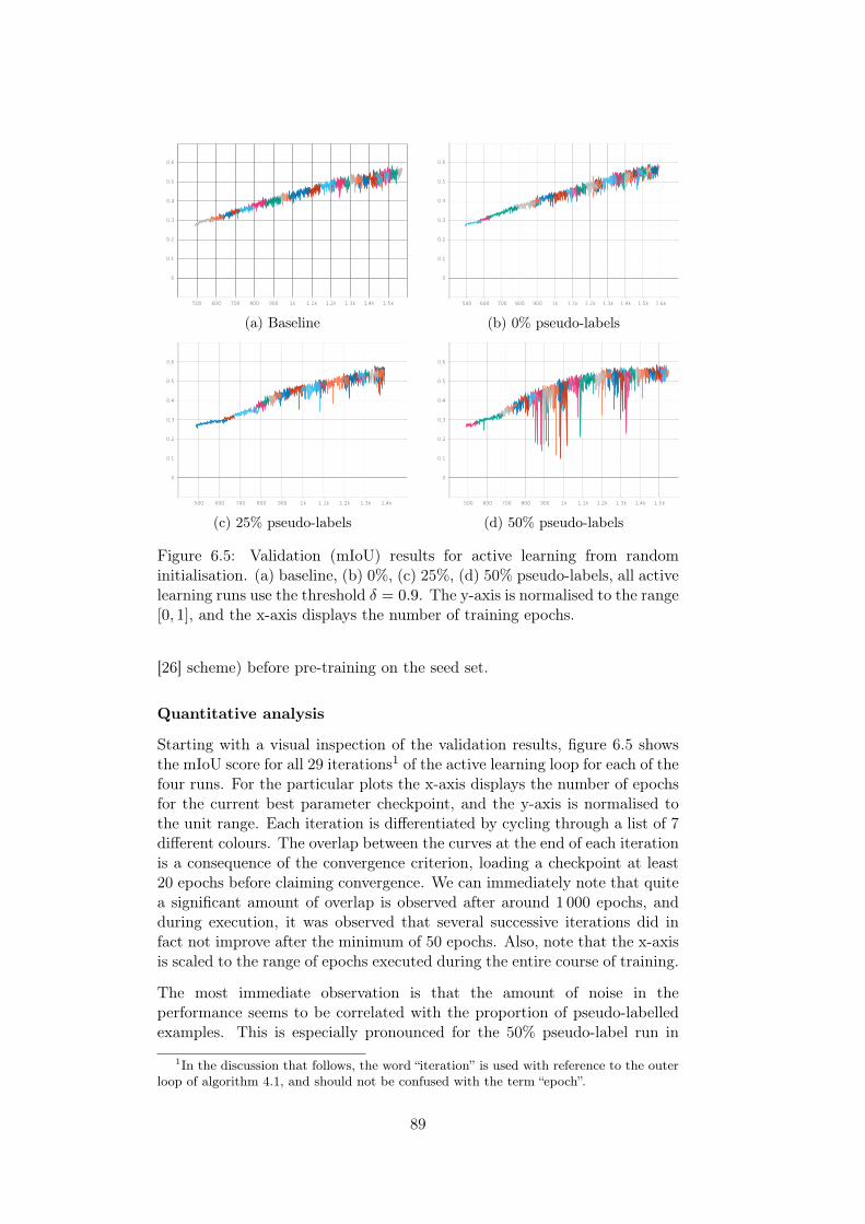
0

0.1

0.2

0.3

0.4

0.5

0.6

500 600 700 800 900 1k 1.1k 1.2k 1.3k 1.4k 1.5k

(a) Baseline

0

0.1

0.2

0.3

0.4

0.5

0.6

500 600 700 800 900 1k 1.1k 1.2k 1.3k 1.4k 1.5k 1.6k

(b) 0% pseudo-labels

0

0.1

0.2

0.3

0.4

0.5

0.6

500 600 700 800 900 1k 1.1k 1.2k 1.3k 1.4k

(c) 25% pseudo-labels

0

0.1

0.2

0.3

0.4

0.5

0.6

500 600 700 800 900 1k 1.1k 1.2k 1.3k 1.4k 1.5k

(d) 50% pseudo-labels

Figure 6.5: Validation (mIoU) results for active learning from randominitialisation. (a) baseline, (b) 0%, (c) 25%, (d) 50% pseudo-labels, all activelearning runs use the threshold δ = 0.9. The y-axis is normalised to the range[0, 1], and the x-axis displays the number of training epochs.

[26] scheme) before pre-training on the seed set.

Quantitative analysis

Starting with a visual inspection of the validation results, figure 6.5 showsthe mIoU score for all 29 iterations1 of the active learning loop for each of thefour runs. For the particular plots the x-axis displays the number of epochsfor the current best parameter checkpoint, and the y-axis is normalised tothe unit range. Each iteration is differentiated by cycling through a list of 7different colours. The overlap between the curves at the end of each iterationis a consequence of the convergence criterion, loading a checkpoint at least20 epochs before claiming convergence. We can immediately note that quitea significant amount of overlap is observed after around 1 000 epochs, andduring execution, it was observed that several successive iterations did infact not improve after the minimum of 50 epochs. Also, note that the x-axisis scaled to the range of epochs executed during the entire course of training.

The most immediate observation is that the amount of noise in theperformance seems to be correlated with the proportion of pseudo-labelledexamples. This is especially pronounced for the 50% pseudo-label run in

1In the discussion that follows, the word “iteration” is used with reference to the outerloop of algorithm 4.1, and should not be confused with the term “epoch”.

89

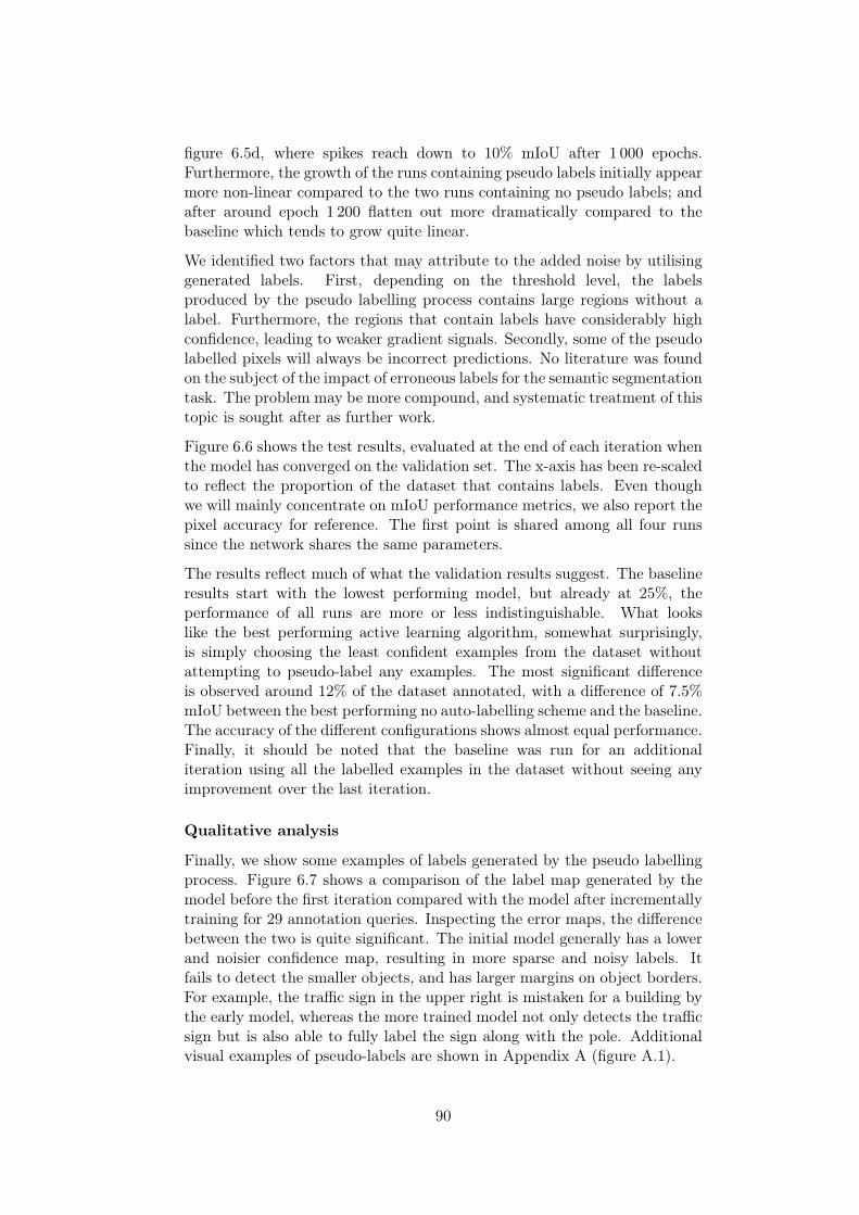
figure 6.5d, where spikes reach down to 10% mIoU after 1 000 epochs.Furthermore, the growth of the runs containing pseudo labels initially appearmore non-linear compared to the two runs containing no pseudo labels; andafter around epoch 1 200 flatten out more dramatically compared to thebaseline which tends to grow quite linear.

We identified two factors that may attribute to the added noise by utilisinggenerated labels. First, depending on the threshold level, the labelsproduced by the pseudo labelling process contains large regions without alabel. Furthermore, the regions that contain labels have considerably highconfidence, leading to weaker gradient signals. Secondly, some of the pseudolabelled pixels will always be incorrect predictions. No literature was foundon the subject of the impact of erroneous labels for the semantic segmentationtask. The problem may be more compound, and systematic treatment of thistopic is sought after as further work.

Figure 6.6 shows the test results, evaluated at the end of each iteration whenthe model has converged on the validation set. The x-axis has been re-scaledto reflect the proportion of the dataset that contains labels. Even thoughwe will mainly concentrate on mIoU performance metrics, we also report thepixel accuracy for reference. The first point is shared among all four runssince the network shares the same parameters.

The results reflect much of what the validation results suggest. The baselineresults start with the lowest performing model, but already at 25%, theperformance of all runs are more or less indistinguishable. What lookslike the best performing active learning algorithm, somewhat surprisingly,is simply choosing the least confident examples from the dataset withoutattempting to pseudo-label any examples. The most significant differenceis observed around 12% of the dataset annotated, with a difference of 7.5%mIoU between the best performing no auto-labelling scheme and the baseline.The accuracy of the different configurations shows almost equal performance.Finally, it should be noted that the baseline was run for an additionaliteration using all the labelled examples in the dataset without seeing anyimprovement over the last iteration.

Qualitative analysis

Finally, we show some examples of labels generated by the pseudo labellingprocess. Figure 6.7 shows a comparison of the label map generated by themodel before the first iteration compared with the model after incrementallytraining for 29 annotation queries. Inspecting the error maps, the differencebetween the two is quite significant. The initial model generally has a lowerand noisier confidence map, resulting in more sparse and noisy labels. Itfails to detect the smaller objects, and has larger margins on object borders.For example, the traffic sign in the upper right is mistaken for a building bythe early model, whereas the more trained model not only detects the trafficsign but is also able to fully label the sign along with the pole. Additionalvisual examples of pseudo-labels are shown in Appendix A (figure A.1).

90

0 5 10 15 20 25 30 35 40 45 50 55

30

40

50

60

% of dataset labelled

mIoU

(%)

Baseline

0%

25%

50%

(a) Mean intersection over union.

0 5 10 15 20 25 30 35 40 45 50 55

84

86

88

90

92

% of dataset labelled

Accuracy

(%)

Baseline

0%

25%

50%

(b) Mean accuracy.

Figure 6.6: Test results for the active learning algorithm evaluated periteration of the outer loop in algorithm 4.1. The figures respectively showthe mean intersection over union and pixel-wise accuracy as a function ofthe proportion of dataset containing labels. Three different pseudo labellingproportions: 50%, 25% and 0% along with a baseline, are shown.

91

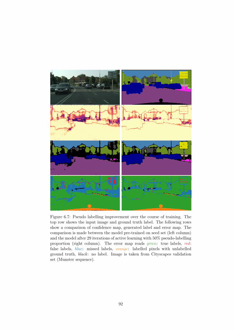
Figure 6.7: Pseudo labelling improvement over the course of training. Thetop row shows the input image and ground truth label. The following rowsshow a comparison of confidence map, generated label and error map. Thecomparison is made between the model pre-trained on seed set (left column)and the model after 29 iterations of active learning with 50% pseudo-labellingproportion (right column). The error map reads green: true labels, red :false labels, blue: missed labels, orange: labelled pixels with unlabelledground truth, black : no label. Image is taken from Cityscapes validationset (Munster sequence).

92

6.2.2 Pre-trained Initialisation

In this second part of this section, we present the results obtained usinga pre-trained model. The validation results from the 200 epochs of pre-training on Mapillary Vistas is given in Appendix B. In these experimentswe use the resulting parameters after 200 epochs of training. Before pre-training on the seed set, the parameters of the last layer of the network isreinitialised. We reinitialise the network because of the difference in labeldistribution and the fact that the model completely fails to learn the “train”class entirely (see figure B.2). The hope and intent of this experiment is tosee a more considerable benefit of using higher quality labels generated fromthe network predictions.

0

0.1

0.2

0.3

0.4

0.5

0.6

300 350 400 450 500 550 600 650 700

(a) Baseline

0

0.1

0.2

0.3

0.4

0.5

0.6

0.7

300 350 400 450 500 550 600 650 700 750 800 850

(b) 0% pseudo-labels

0

0.1

0.2

0.3

0.4

0.5

0.6

300 350 400 450 500 550 600 650 700 750

(c) 25% pseudo-labels, δ = 0.9

0

0.1

0.2

0.3

0.4

0.5

0.6

300 350 400 450 500 550 600

(d) 50% pseudo-labels, δ = 0.9

0

0.1

0.2

0.3

0.4

0.5

0.6

300 350 400 450 500 550 600 650 700 750 800

(e) 25% pseudo-labels, δ = 0.5

Figure 6.8: Validation (mIoU) results for active learning from pre-trainedinitialisation, with the given configurations. The y-axis is normalised to therange [0, 1], and the x-axis displays the number of training epochs.

93

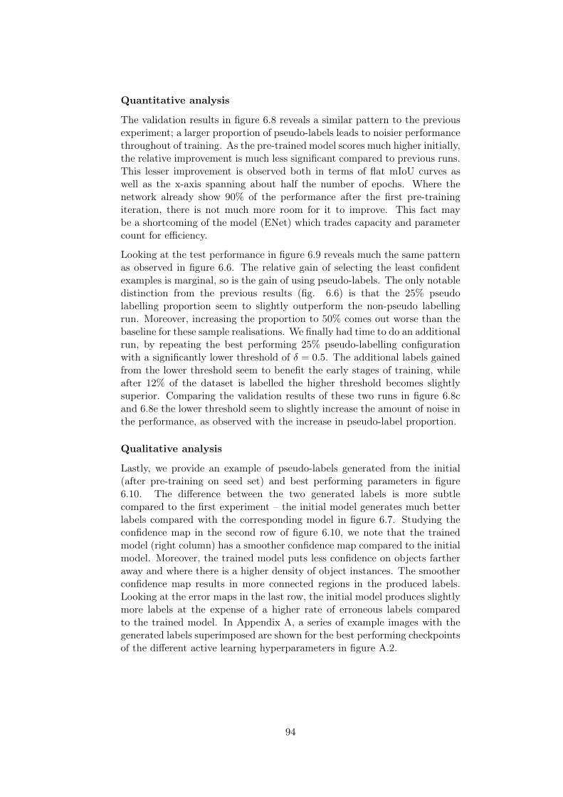
Quantitative analysis

The validation results in figure 6.8 reveals a similar pattern to the previousexperiment; a larger proportion of pseudo-labels leads to noisier performancethroughout of training. As the pre-trained model scores much higher initially,the relative improvement is much less significant compared to previous runs.This lesser improvement is observed both in terms of flat mIoU curves aswell as the x-axis spanning about half the number of epochs. Where thenetwork already show 90% of the performance after the first pre-trainingiteration, there is not much more room for it to improve. This fact maybe a shortcoming of the model (ENet) which trades capacity and parametercount for efficiency.

Looking at the test performance in figure 6.9 reveals much the same patternas observed in figure 6.6. The relative gain of selecting the least confidentexamples is marginal, so is the gain of using pseudo-labels. The only notabledistinction from the previous results (fig. 6.6) is that the 25% pseudolabelling proportion seem to slightly outperform the non-pseudo labellingrun. Moreover, increasing the proportion to 50% comes out worse than thebaseline for these sample realisations. We finally had time to do an additionalrun, by repeating the best performing 25% pseudo-labelling configurationwith a significantly lower threshold of δ = 0.5. The additional labels gainedfrom the lower threshold seem to benefit the early stages of training, whileafter 12% of the dataset is labelled the higher threshold becomes slightlysuperior. Comparing the validation results of these two runs in figure 6.8cand 6.8e the lower threshold seem to slightly increase the amount of noise inthe performance, as observed with the increase in pseudo-label proportion.

Qualitative analysis

Lastly, we provide an example of pseudo-labels generated from the initial(after pre-training on seed set) and best performing parameters in figure6.10. The difference between the two generated labels is more subtlecompared to the first experiment – the initial model generates much betterlabels compared with the corresponding model in figure 6.7. Studying theconfidence map in the second row of figure 6.10, we note that the trainedmodel (right column) has a smoother confidence map compared to the initialmodel. Moreover, the trained model puts less confidence on objects fartheraway and where there is a higher density of object instances. The smootherconfidence map results in more connected regions in the produced labels.Looking at the error maps in the last row, the initial model produces slightlymore labels at the expense of a higher rate of erroneous labels comparedto the trained model. In Appendix A, a series of example images with thegenerated labels superimposed are shown for the best performing checkpointsof the different active learning hyperparameters in figure A.2.

94

0 5 10 15 20 25 30 35 40 45 50 55

52

54

56

58

60

62

% of dataset labelled

mIoU

(%)

Baseline

p = 0%, δ = 0.9

p = 25%, δ = 0.9

p = 50%, δ = 0.9

p = 25%, δ = 0.5

(a) Mean intersection over union.

0 5 10 15 20 25 30 35 40 45 50 5592

92.5

93

93.5

94

% of dataset labelled

Accuracy

(%)

Baseline

p = 0%, δ = 0.9

p = 25%, δ = 0.9

p = 50%, δ = 0.9

p = 25%, δ = 0.5

(b) Pixel accuracy.

Figure 6.9: Test results for the active learning algorithm evaluated periteration of the outer loop in algorithm 4.1. The figures respectively showthe mean intersection over union and mean accuracy as a function of theproportion of dataset that is labelled.

95

Figure 6.10: Pseudo labelling improvement over the course of training. Thetop row shows the input image and ground truth label. The following rowsshow a comparison of confidence map, generated label and error map. Thecomparison is made between the model pre-trained on seed set (left column)and the model after 29 iterations of active learning with 25% pseudo-labellingproportion (right column). The colours of the error map read, green: truelabels, red : false labels, blue: missed labels, orange: labelled pixels withunlabelled ground truth, black : no label. Images in the first row is fromCityscapes validation set (Frankfurt sequence).

96

Chapter 7

Discussion and Further Work

The thesis is wrapped up with a summary of experiments performed, followedby a discussion on the obtained results and what could be done differently.Finally, a discussion of further work and extensions to the active learningframework are proposed.

7.1 Summary

In this thesis, the goal was to investigate the problem of improvingannotation efficiency for semantic segmentation utilising deep neuralnetworks. A novel uncertainty based active learning algorithm was proposed,utilising the network’s predictions and the unlabelled pool of the dataset tovirtually increase the number of labelled examples.

Motivated by efficiency in terms of parameters and computational complex-ity, we chose ENet [59] as the baseline architecture for the conducted exper-iments. As a first experiment, the model was trained using a replication ofthe experiment performed in [59] in order to validate the implementation.We report the performance of the network in terms of mean intersectionover union (mIoU) and also report the pixel accuracy performance on thevalidation set. All experiments performed in this thesis were evaluated onthe Cityscapes [14] urban scene understanding dataset.

In the second part of the experiments, we tested the proposed active learningalgorithm using the ENet model. As a first experiment, we benchmark thealgorithm solely on the Cityscapes dataset, initialising the model by trainingon a seed set of 50 examples. The algorithm was compared with a baselineconsisting of annotating examples randomly for each iteration. We furtherrepeated the same experiments initialised from the parameters obtained frompre-trained on a the Mapillary Vistas [57], a dataset composed of 18 000labelled training images.

A final experiment was prepared to utilise the proposed algorithm toannotate a dataset composed of off-road driving scenes. However,due to unforeseen problems and slow execution time of performing the

97

aforementioned experiments, time did not permit the experiment to beconducted as part of this thesis.

7.2 Discussion

The results observed from training ENet were comparable with the publishedresults [59], with slightly higher mIoU performance on the Cityscapesdataset. These results suggests that the model implementation is correct,concluding the first experiment a success. A slight decrease in performancewas observed for the weighted iIoU measure, possibly indicating that themodel perform worse on the sparse object categories. The custom weightingof the loss (eq. 4.5) used while finetuning the model did not improve theresults on these sparse classes. This may be a result of weak predictions alsooccurring along object boundaries of large objects as well as for the smallerobjects in the scene. As a consequence leading, this may defeat the initialhypothesis about this custom loss making smaller objects more significantfor the gradient updates.

Results obtained from active learning experiments performed in this thesissuggest that carefully selecting the examples of highest cumulative entropyaccording to the model predictions yield a slight performance increasecompared to randomly selecting examples. Except for the 50% pseudo-labelling proportion in the experiment using a pre-trained model, the activelearning algorithm consistently outperformed the baseline when utilisingless than 25% of the dataset labels. To make assertions about therelative discrepancies between the different pseudo-labelling proportions,it is required to gather a larger sample of simulation-data to measurethe relative variance and average performance of different hyperparameterconfigurations. We did, however, observe that higher pseudo labellingproportions resulted in more noise in the performance dynamics on thevalidation set over the course of training, and slightly different initial growthrate.

The small discrepancies between the baseline and the active learning resultsmay partially be explained by the fact that the Cityscapes dataset hasalready manually filtered the less informative examples from the dataset.It would be interesting to perform tests with the proposed algorithm onvideo sequences to see if the method is able to select informative exampleswith a non-overlapping field of view as part of the process.

Generating erroneous labels is inevitable when using the model predictions,and systematic analysis of the impact of erroneous labels is sought. Anotherproblem with the pseudo-labelling procedure is the fact that they aregenerated from high-confidence pixels of the model – the predicted classdistribution is close to the unit vector for the assigned label. To see how thisbecomes a problem, consider the single-example loss gradient in equation2.38, which approaches the zero vector as the output approaches the labelunit vector, making the upstream gradient small. This significantly increasesthe gradient signal to stochastic mini-batch noise, and furthermore lead to

98

variable (relative) regularisation rate of the fixed parameter penalty loss.To alleviate some of the problems with low gradient magnitude of pseudo-labelled examples, model ensembles can be utilised. We defer the ensembleextension of this active learning algorithm to the next section.

When planning the experiments, the comparison with the pre-trainedmethod was constructed with the expectation of demonstrating betterutilisation of higher quality pseudo-labels. The sample realisations of theexperiments obtained do not clearly demonstrate this expected outcome.Inspecting the performance curves for the pre-trained initialisation (fig.6.9), the performance saturates rather quickly, and the noise becomesa more substantial factor in the observed results. A natural questionto ask is whether our choice of a parameter-efficient model leads tounderfitting-problems. From the pre-trained configuration, we observe theperformance saturates for the same 62% mIoU score as obtained withthe same hyperparameters training on the complete dataset in the firstexperiment (getting 2.4% gain in performance by finetuning). We leave it asa task for further work to test the proposed algorithm with better performingmodels with higher capacity.

The execution time of the active learning part of the experiments tookunexpectedly long. In hindsight, further downscaling the input dimensionswould decrease the computational time in the order of the square of thedownscaling factor, in addition to a square decrease of memory usage forstoring the hidden layer activations for backpropagation. This would, in turn,allow gathering more extensive sample statistics of the performance resultsfor each hyperparameter configuration. Moreover, the reduced memoryrequirements would enable larger batch size and potentially a higher capacitymodel.

7.3 Further Work

The constrained time frame of this project affected several decisions made forthis project. In this section, we summarise some of the work that time did notpermit and directions to develop further this project based on observationsmade working with the project.

Training a deep feedforward network is subject to estimation error whichmanifests as stochastic noise (see section 2.2.6) over independent executions.In addition to estimation noise, the active learning algorithm is subject tofluctuations with respect to selecting the initial seed set. Moreover, theexperiments need to be executed independently and identically for severalrepetitions in order to gather sample statistics. By using the sample meanperformance, more rigid assertions about the performance can be madeprovided the standard error is relatively low.

99

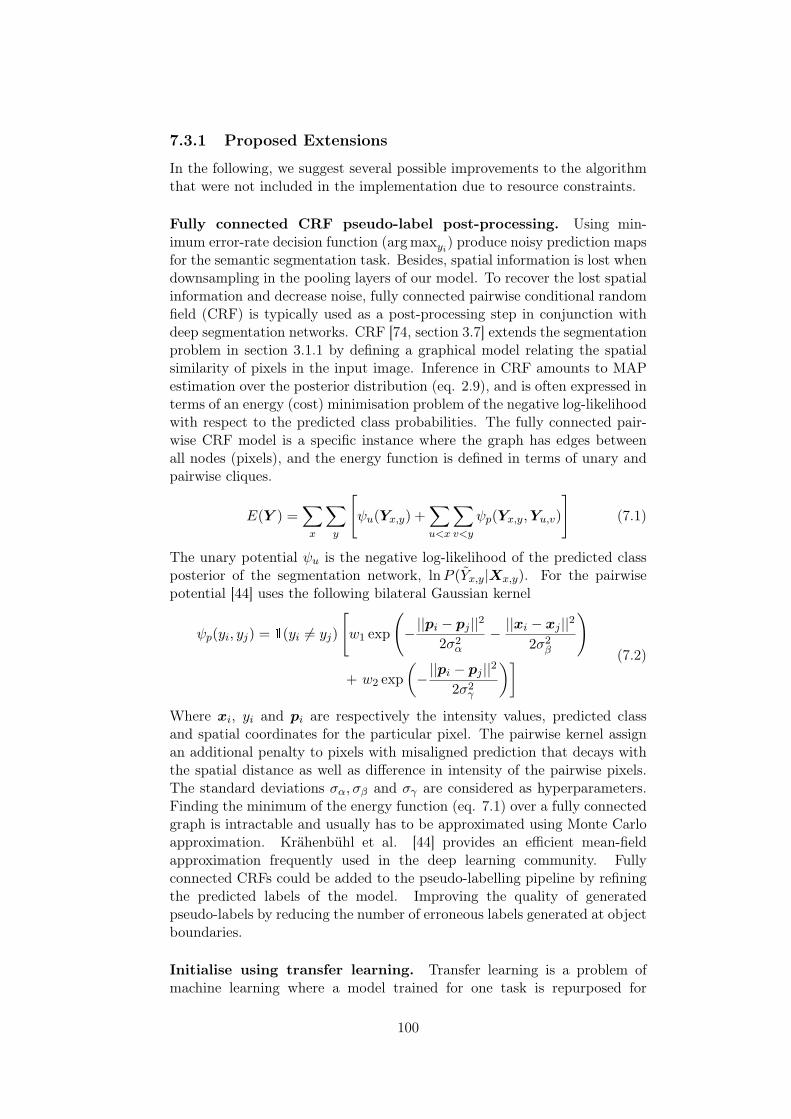
7.3.1 Proposed Extensions

In the following, we suggest several possible improvements to the algorithmthat were not included in the implementation due to resource constraints.

Fully connected CRF pseudo-label post-processing. Using min-imum error-rate decision function (arg maxyi) produce noisy prediction mapsfor the semantic segmentation task. Besides, spatial information is lost whendownsampling in the pooling layers of our model. To recover the lost spatialinformation and decrease noise, fully connected pairwise conditional randomfield (CRF) is typically used as a post-processing step in conjunction withdeep segmentation networks. CRF [74, section 3.7] extends the segmentationproblem in section 3.1.1 by defining a graphical model relating the spatialsimilarity of pixels in the input image. Inference in CRF amounts to MAPestimation over the posterior distribution (eq. 2.9), and is often expressed interms of an energy (cost) minimisation problem of the negative log-likelihoodwith respect to the predicted class probabilities. The fully connected pair-wise CRF model is a specific instance where the graph has edges betweenall nodes (pixels), and the energy function is defined in terms of unary andpairwise cliques.

E(Y ) =∑x

∑y

[ψu(Yx,y) +

∑u<x

∑v<y

ψp(Yx,y,Yu,v)

](7.1)

The unary potential ψu is the negative log-likelihood of the predicted classposterior of the segmentation network, lnP (Yx,y|Xx,y). For the pairwisepotential [44] uses the following bilateral Gaussian kernel

ψp(yi, yj) = 1(yi 6= yj)

[w1 exp

(−||pi − pj ||

2

2σ2α− ||xi − xj ||

2

2σ2β

)

+ w2 exp

(−||pi − pj ||

2

2σ2γ

)] (7.2)

Where xi, yi and pi are respectively the intensity values, predicted classand spatial coordinates for the particular pixel. The pairwise kernel assignan additional penalty to pixels with misaligned prediction that decays withthe spatial distance as well as difference in intensity of the pairwise pixels.The standard deviations σα, σβ and σγ are considered as hyperparameters.Finding the minimum of the energy function (eq. 7.1) over a fully connectedgraph is intractable and usually has to be approximated using Monte Carloapproximation. Krähenbühl et al. [44] provides an efficient mean-fieldapproximation frequently used in the deep learning community. Fullyconnected CRFs could be added to the pseudo-labelling pipeline by refiningthe predicted labels of the model. Improving the quality of generatedpseudo-labels by reducing the number of erroneous labels generated at objectboundaries.

Initialise using transfer learning. Transfer learning is a problem ofmachine learning where a model trained for one task is repurposed for

100

another (similar) task. We have already applied transfer learning in theform of model pre-training in the last experiment. There are other kindsof unsupervised transfer learning techniques that have empirically shownpromising results.

Domain adaptation is a specific transfer learning problem where a networktrained on a labelled dataset from a source domain in a supervised manner,and the goal is to use unlabelled data from a target domain to learn the sametask on a different set of data. This problem is inherently ill-posed, and thesuccess of this problem is primarily driven by assumptions regarding thesource and target domains. Adversarial Discriminative Domain Adaptation(ADDA) is a recent application to the domain transfer problem, whichtreats the problem using Generative Adversarial Networks (GANs). Theassumption used in ADDA is that abstract feature (activations) distributionsinside the networks are to some extent shared across the domains. Theclassifier model is treated as a generator network by implicitly modelling thedistributions of feature representations at different layers of the model. Thegoal is then to constrain the distributions of two networks for the source andtarget domain to be similar.

Huang et al. [33] propose a practical implementation of ADDA for semanticsegmentation. The method places discriminator networks, i.e. binaryclassifiers, that are trained to discriminate features from the source andtarget domain when fed through the two networks (using least squaresvariant of the GAN minimax loss). The generator (classifier/segmentationmodels) are trained by maximising the discriminator loss. For the activelearning pipeline, if the datasets collected come from different geographicallocations but with similar class distributions, this kind of unsuperviseddomain adaptation may be used as an intermediate step after pre-training onthe source domain dataset. Then, the adapted model can be used to selectthe initial seed set. The validation set should however remain uncorrelatedto the model and is drawn uniformly from the dataset.

Model ensemble. Ensemble methods, more specifically model averaging,consists of training a range of models independently (from differentinitialisation and perhaps network structure) and upon inference use theaverage class scores (logits) as means for the estimated class distribution.Model averaging is a robust method for reducing generalisation error.Furthermore, Beluch et al. [9] show that ensemble methods achieve state-of-the-art performance on several active learning benchmarks. Its usein this thesis was discouraged due to the overhead of training multiplemodels, ultimately leading to insufficient computational resources. Inthe following, an ensemble extension of the pseudo-labelling and exampleselection components are sketched, allowing the algorithm to be scaled toarbitrary computational resources.

Two methods are considered for combining the ensemble predictions inour active learning framework. The simplest and most straight forwardway is to directly use the ensemble average as the joint model prediction,

101

and use the uncertainty based scheme as done using a single model. Theincreased robustness in the model prediction may allow a lower pseudo-labelling threshold as a consequence of the better predictions. In the secondapproach, each model contributes to a committee, and the label predictionof each model is averaged upon computing the uncertainty. Active learningmethods that use ensemble committees is referred to as Query by Committee.Mackowiak et al. [50] uses the vote-entropy as an uncertainty measure

Vu,v , −Nc∑c=1

∑Nei=1 1(Y

iu,v = c)

Nelog

∑Nei=1 1(Y

iu,v = c)

Ne(7.3)

Where Vu,v is the vote-entropy at pixel location (u, v), Nc is the numberof classes, Ne the number of models and Y iu,v is the predicted (arg maxyi)class of the i-th model in the ensemble. The vote-entropy does not extendto produce smooth confidence maps for generating pseudo-labels. However,a query by committee extension with respect to the thresholded confidencemaps is suggested. If the majority of the ensemble has high confidence at agiven pixel location the class with the majority of votes is assigned the givenlabel, and leaving the pixel unlabelled if there are ties.

Using ensembles and on-line pseudo-labelling may lead to severe bottlenecksif a large ensemble is going to be trained independently (with independentsampled mini-batches of data). To favour efficiency, it is suggested that thepseudo-labelling is done offline on a common example pool at the start ofeach epoch. The networks continue by independently sample mini-batchesfrom the augmented pool of labelled and pseudo-labelled examples.

Regularisation and hyperparameters. In the experiments performedin this project, no regularisation directly affects the entropy of the predictedclass distribution. It was observed that the model predicted labels to a largeextent for unlabelled regions in the image, and made confident mistakes – anartefact of the softmax cross-entropy loss driving the logits to positive andnegative infinity. This problem can, to some extent, be alleviated by addingadditional activation regularisation directly on the output of the CNN. Zouet al. [82] uses an additional term proportional to the softmax probabilityof the predicted class. Label smoothing [28, p. 236] is another regularisationtechnique that keeps the model from making over-confident classificationdecisions without discouraging correct classification by distributing a smallproportion of the target probability to all other classes. Another, more directapproach to increase the entropy is to subtract a term proportional to thesample mean entropy of all pixel predictions.

C(W) = C ′(W)− κ

HWNB

NB∑i=1

H∑u=1

W∑v=1

H(Y (i)u,v ) (7.4)

Where C ′(·) is the cost function without activation regularisation, κ is theregularisation rate hyperparameter, and H, W and NB are height, widthand batch size respectively.

102

The experiments conducted only used a limited set of hyperparameters forthe active learning algorithm (see table 5.4). The parameters used in thisproject were merely selected out of intuition and observation of the pseudo-label quality for different thresholds. A more large-scale hyperparametersearch using genetic or swarm-based optimisation algorithms is sought.Moreover, in order to make the model converge properly on a subset ofthe dataset, a decaying learning rate scheme is necessary. Furthermore,the model used in this thesis is not an ideal choice for a practicalimplementation. Intuitively, it would seem that better performing modelswith higher representational capacity would reach higher performancewithout saturating. Better performance would in turn lead to higher qualityof pseudo-labels and possibly better utilisation of the unlabelled examples.

103

104

Chapter 8

Conclusion

This thesis investigated the problem of semantic segmentation and applyingconvolutional neural networks to mediate the process of making densepixelwise annotations. To guide the annotation process, an active learningframework was proposed for this task. The sample selection strategy selectsthe most informative sample as measured by the cumulative entropy of themodel predictions. Moreover, the framework utilises the model to generatelabels from the unlabelled pool of examples.

Two different experiments were performed in this thesis evaluated onthe Cityscapes dataset. In the first part of this thesis, the ENetimplementation was evaluated and resulted in comparable results with theoriginal publication [59]. For the second and central part of this thesis, weevaluated the active learning framework using the 19 class labels from theCityscapes dataset. Two sets of experiments were conducted, comparing theresults of a model initialised from a small seed set with a model pre-trainedon a large dataset of annotated street-view images. The results suggestthat careful selection of informative samples initially yields slightly higherrelative performance compared to a random selection baseline in either of theexperiments. It was also observed that large proportions of pseudo labelsresulted in noise in the validation performance throughout training. Thediscrepancies between the individual hyperparameter configurations werenot as substantial as initially expected, and extensive experimentation usingsample statistics is needed to quantify the differences.

Due to lack of time, the initial goal of annotating the images from the OLAVdataset became prohibitive, and leave this task for future work. A seriesof improvements, enhancing the pseudo-labelling pipeline and the selectionstrategy using ensembles, are proposed in the closing of this thesis.

105

106

Bibliography

[1] Yaser S. Abu-Mostafa. Learning From Data – Lecture 5: Trainingversus Testing. 17th Apr. 2012. url: http://work.caltech.edu/slides/slides05.pdf (visited on 23/04/2019).

[2] Yaser S. Abu-Mostafa. Learning From Data – Lecture 6: Theory ofGeneralization. 19th Apr. 2012. url: http://work.caltech.edu/slides/slides06.pdf (visited on 23/04/2019).

[3] Yaser S. Abu-Mostafa. Learning From Data – Lecture 7: The VC-Dimension. 24th Apr. 2012. url: http : / /work . caltech . edu / slides /slides07.pdf (visited on 23/04/2019).

[4] David Acuna et al. ‘Efficient Interactive Annotation of SegmentationDatasets with Polygon-RNN++’. In: (2018).

[5] Hassan Alhaija et al. ‘Augmented Reality Meets Computer Vision:Efficient Data Generation for Urban Driving Scenes’. In: InternationalJournal of Computer Vision (IJCV) (2018).

[6] Vijay Badrinarayanan, Ankur Handa and Roberto Cipolla. ‘SegNet:A Deep Convolutional Encoder-Decoder Architecture for RobustSemantic Pixel-Wise Labelling’. In: arXiv preprint arXiv:1505.07293(2015).

[7] Vijay Badrinarayanan, Alex Kendall and Roberto Cipolla. ‘SegNet:A Deep Convolutional Encoder-Decoder Architecture for ImageSegmentation’. In: IEEE Transactions on Pattern Analysis andMachine Intelligence (2017).

[8] Atilim Gunes Baydin et al. ‘Automatic Differentiation in MachineLearning: a Survey’. In: Journal of Machine Learning Research 18.153(2018), pp. 1–43. url: http://jmlr.org/papers/v18/17-468.html.

[9] William H. Beluch et al. ‘The Power of Ensembles for Active Learningin Image Classification’. In: 2018 IEEE/CVF Conference on ComputerVision and Pattern Recognition. IEEE, June 2018, pp. 9368–9377.isbn: 978-1-5386-6420-9. doi: 10.1109/CVPR.2018.00976. url: https://ieeexplore.ieee.org/document/8579074/ (visited on 30/05/2019).

[10] Gabriel J. Brostow, Julien Fauqueur and Roberto Cipolla. ‘SemanticObject Classes in Video: A High-Definition Ground Truth Database’.In: Pattern Recognition Letters xx.x (2008), pp. xx–xx.

107

[11] Alfredo Canziani, Adam Paszke and Eugenio Culurciello. ‘An Analysisof Deep Neural Network Models for Practical Applications’. In:arXiv:1605.07678 [cs] (24th May 2016). arXiv: 1605.07678. url: http://arxiv.org/abs/1605.07678 (visited on 05/02/2019).

[12] Alfredo Canziani et al. Analysis of deep neural networks. 8th Sept.2018. url: https://medium.com/@culurciello/analysis-of-deep-neural-networks-dcf398e71aae (visited on 14/05/2019).

[13] Liang-Chieh Chen et al. ‘Encoder-Decoder with Atrous SeparableConvolution for Semantic Image Segmentation’. In: ECCV. 2018.

[14] Marius Cordts et al. ‘The Cityscapes Dataset for Semantic Urban SceneUnderstanding’. In: Proc. of the IEEE Conference on Computer Visionand Pattern Recognition (CVPR). 2016.

[15] Eugenio Culurciello. Neural Network Architectures. Towards DataScience. 23rd Mar. 2017. url: https://towardsdatascience.com/neural-network-architectures-156e5bad51ba (visited on 05/02/2019).

[16] George Cybenko. ‘Approximation by superpositions of a sigmoidalfunction’. In: Mathematics of control, signals and systems 2.4 (1989),pp. 303–314. url: https : / / link . springer . com / article / 10 . 1007 /BF02551274 (visited on 28/04/2019).

[17] John Duchi, Elad Hazan and Yoram Singer. ‘Adaptive subgradientmethods for online learning and stochastic optimization’. In: Journalof Machine Learning Research 12.Jul (2011), pp. 2121–2159.

[18] Richard O. Duda, Peter E. Hart and David G. Stork. PatternClassification. 2nd edition. Wiley-Interscience, 2000. 680 pp. isbn: 978-0-471-05669-0.

[19] Vincent Dumoulin and Francesco Visin. ‘A guide to convolutionarithmetic for deep learning’. In: arXiv preprint arXiv:1603.07285(2016). url: https://arxiv.org/abs/1603.07285 (visited on 28/04/2019).

[20] Idar Dyrdal. TEK5020/TEK9020 - Mønstergjenkjenning – Beslutning-steori. Aug. 2018. url: https://www.uio.no/studier/emner/matnat/its/TEK5020/h18/presentasjoner/p02.pdf (visited on 17/04/2019).

[21] M. Everingham et al. ‘The Pascal Visual Object Classes (VOC)Challenge’. In: International Journal of Computer Vision 88.2 (June2010), pp. 303–338.

[22] Clement Farabet et al. ‘Learning hierarchical features for scenelabeling’. In: IEEE transactions on pattern analysis and machineintelligence 35.8 (2012), pp. 1915–1929. url: http://yann.lecun.com/exdb/publis/pdf/farabet-pami-13.pdf (visited on 29/05/2019).

[23] File:Lenna (test image).png. Original full portrait: "Playmate of theMonth". Playboy Magazine. November 1972, photographed by DwightHooker. url: https://en.wikipedia.org/wiki/File:Lenna_(test_image).png (visited on 22/04/2019).

108

[24] Yarin Gal, Riashat Islam and Zoubin Ghahramani. ‘Deep BayesianActive Learning with Image Data’. In: arXiv:1703.02910 [cs, stat](Mar. 2017). url: http : / / arxiv . org / abs / 1703 . 02910 (visited on30/05/2019).

[25] Alberto Garcia-Garcia et al. ‘A Review on Deep Learning Tech-niques Applied to Semantic Segmentation’. In: arXiv:1704.06857 [cs](22nd Apr. 2017). arXiv: 1704.06857. url: http://arxiv.org/abs/1704.06857 (visited on 06/02/2019).

[26] Xavier Glorot and Yoshua Bengio. ‘Understanding the difficulty oftraining deep feedforward neural networks’. In: Proceedings of theThirteenth International Conference on Artificial Intelligence andStatistics. Ed. by Yee Whye Teh and Mike Titterington. Vol. 9.Proceedings of Machine Learning Research. Chia Laguna Resort,Sardinia, Italy: PMLR, May 2010, pp. 249–256. url: http : / /proceedings.mlr.press/v9/glorot10a.html.

[27] Rafael C. Gonzales and Richard E. Woods. Digital Image Processing.Third Edition (International). Pearson, 2010.

[28] Ian Goodfellow, Yoshua Bengio and Aaron Courville. Deep Learning.MIT Press, 2016.

[29] Kaiming He et al. ‘Deep Residual Learning for Image Recognition’.In: arXiv:1512.03385 [cs] (10th Dec. 2015). arXiv: 1512.03385. url:http://arxiv.org/abs/1512.03385 (visited on 16/01/2019).

[30] Kaiming He et al. ‘Delving Deep into Rectifiers: SurpassingHuman-Level Performance on ImageNet Classification’. In: CoRRabs/1502.01852 (2015). arXiv: 1502 . 01852. url: http : / / arxiv . org /abs/1502.01852 (visited on 02/05/2019).

[31] Geoffrey E. Hinton et al. ‘Improving neural networks by preventingco-adaptation of feature detectors’. In: arXiv:1207.0580 [cs] (3rd July2012). arXiv: 1207.0580. url: http://arxiv.org/abs/1207.0580 (visitedon 03/05/2019).

[32] Kurt Hornik, Maxwell Stinchcombe and Halbert White. ‘Multilayerfeedforward networks are universal approximators’. In: Neural Net-works 2.5 (1st Jan. 1989), pp. 359–366. issn: 0893-6080. doi: 10.1016/0893-6080(89)90020-8. url: http://www.sciencedirect.com/science/article/pii/0893608089900208 (visited on 22/04/2019).

[33] Haoshuo Huang, Qixing Huang and Philipp Krähenbühl. ‘DomainTransfer Through Deep Activation Matching’. en. In: Computer Vision– ECCV 2018. Ed. by Vittorio Ferrari et al. Vol. 11220. SpringerInternational Publishing, 2018, pp. 611–626. isbn: 978-3-030-01269-4 978-3-030-01270-0. doi: 10 . 1007 / 978 - 3 - 030 - 01270 - 0_36. url:http://link.springer.com/10.1007/978-3-030-01270-0_36 (visited on04/03/2019).

[34] Xinyu Huang et al. ‘The ApolloScape Dataset for AutonomousDriving’. In: arXiv: 1803.06184 (2018).

109

[35] ‘IEEE Standard for Binary Floating-Point Arithmetic’. In: AN-SI/IEEE Std 754-1985 (1985), 0_1–. doi: 10.1109/IEEESTD.1985.82928.

[36] Sergey Ioffe and Christian Szegedy. ‘Batch Normalization: AcceleratingDeep Network Training by Reducing Internal Covariate Shift’. In:arXiv:1502.03167 [cs] (10th Feb. 2015). arXiv: 1502.03167. url: http://arxiv.org/abs/1502.03167 (visited on 02/05/2019).

[37] Phillip Isola et al. ‘Image-to-Image Translation with ConditionalAdversarial Networks’. In: arXiv:1611.07004 [cs] (Nov. 2016). url:http://arxiv.org/abs/1611.07004 (visited on 31/05/2019).

[38] Tollef Jahren. INF5860 Machine learning for image classification –Lecture 6: Convolutional neural networks. Feb. 2017. url: https :/ / www . uio . no / studier / emner / matnat / ifi / INF5860 / v18 /undervisningsmateriale / lectures / inf5860 _ lecture6 _ convolutional _nerual_networks.pdf (visited on 08/05/2019).

[39] Christoph Käding et al. ‘Active and Continuous Exploration withDeep Neural Networks and Expected Model Output Changes’. In:arXiv:1612.06129 [cs] (Dec. 2016). url: http://arxiv.org/abs/1612.06129 (visited on 30/05/2019).

[40] Andrej Karpathy. CS231n Convolutional Neural Networks for VisualRecognition – Neural Networks 1. url: http://cs231n.github.io/neural-networks-1/ (visited on 02/05/2019).

[41] Alex Kendall and Yarin Gal. ‘What Uncertainties Do We Need inBayesian Deep Learning for Computer Vision?’ en. In: arXiv:1703.04977[cs] (Mar. 2017). url: http://arxiv.org/abs/1703.04977 (visited on31/05/2019).

[42] Keras: The Python Deep Learning library. url: https : / / keras . io/(visited on 16/05/2019).

[43] Diederik P. Kingma and Jimmy Ba. ‘Adam: A Method for StochasticOptimization’. In: CoRR abs/1412.6980 (2014). arXiv: 1412.6980. url:http://arxiv.org/abs/1412.6980.

[44] Philipp Krähenbühl and Vladlen Koltun. ‘Efficient Inference in FullyConnected CRFs with Gaussian Edge Potentials’. In: arXiv:1210.5644[cs] (Oct. 2012). url: http : //arxiv . org/abs/1210 . 5644 (visited on03/06/2019).

[45] Alex Krizhevsky, Ilya Sutskever and Geoffrey E Hinton. ‘ImageNetClassification with Deep Convolutional Neural Networks’. In: Advancesin Neural Information Processing Systems 25. Ed. by F. Pereira et al.Curran Associates, Inc., 2012, pp. 1097–1105. url: http://papers.nips.cc/paper/4824- imagenet-classification-with-deep-convolutional-neural-networks.pdf.

[46] Fei-Fei Li, Justin Johnson and Serena Yeung. Lecture 11: Detectionand Segmentation. 10th May 2017. url: http://cs231n.stanford.edu/slides/2017/cs231n_2017_lecture11.pdf (visited on 29/05/2019).

110

[47] Jonathan Long, Evan Shelhamer and Trevor Darrell. ‘Fully convolu-tional networks for semantic segmentation’. In: Proceedings of the IEEEconference on computer vision and pattern recognition. 2015, pp. 3431–3440. url: https://people.eecs.berkeley.edu/~jonlong/long_shelhamer_fcn.pdf (visited on 22/01/2019).

[48] Looking Further. Ford will have a fully autonomous vehicle in operationby 2021. Ford Corporate. url: http://corporate.ford.com/innovation/autonomous-2021.html (visited on 07/06/2019).

[49] Ulrike von Luxburg and Bernhard Schoelkopf. ‘Statistical LearningTheory: Models, Concepts, and Results’. In: (27th Oct. 2008). url:https://arxiv.org/abs/0810.4752v1 (visited on 27/04/2019).

[50] Radek Mackowiak et al. ‘CEREALS - Cost-Effective REgion-basedActive Learning for Semantic Segmentation’. In: (Oct. 2018). url:https://arxiv.org/abs/1810.09726v1 (visited on 20/03/2019).

[51] Dwarikanath Mahapatra et al. ‘Efficient Active Learning for ImageClassification and Segmentation using a Sample Selection and Con-ditional Generative Adversarial Network’. In: arXiv:1806.05473 [cs](June 2018). url: http : / / arxiv . org / abs / 1806 . 05473 (visited on20/03/2019).

[52] Reza Mahjourian, Martin Wicke and Anelia Angelova. ‘UnsupervisedLearning of Depth and Ego-Motion From Monocular Video Using 3DGeometric Constraints’. In: (2018), p. 9. url: https://arxiv.org/pdf/1802.05522.pdf (visited on 04/10/2018).

[53] K.-K. Maninis et al. ‘Deep Extreme Cut: From Extreme Points toObject Segmentation’. In: Computer Vision and Pattern Recognition(CVPR). 2018.

[54] Mapillary. url: https : / / www . mapillary . com / app/ (visited on19/05/2019).

[55] mcordts/cityscapesScripts – README and scripts for the CityscapesDataset. url: https://github.com/mcordts/cityscapesScripts (visited on28/01/2019).

[56] Tom M. Mitchell. Machine Learning. McGraw-Hill Education, 1997.isbn: 978-0070428072.

[57] Gerhard Neuhold et al. ‘The Mapillary Vistas Dataset for SemanticUnderstanding of Street Scenes’. In: 2017 IEEE International Confer-ence on Computer Vision (ICCV). 2017 IEEE International Confer-ence on Computer Vision (ICCV). Venice: IEEE, Oct. 2017, pp. 5000–5009. isbn: 978-1-5386-1032-9. doi: 10 . 1109 / ICCV . 2017 . 534. url:http://ieeexplore.ieee.org/document/8237796/ (visited on 07/02/2019).

[58] opencv/cvat – Powerful and efficient Computer Vision AnnotationTool (CVAT). url: https : / / github . com / opencv / cvat (visited on08/04/2019).

111

[59] Adam Paszke et al. ‘ENet: A Deep Neural Network Architecturefor Real-Time Semantic Segmentation’. In: arXiv:1606.02147 [cs](7th June 2016). arXiv: 1606.02147. url: http://arxiv.org/abs/1606.02147 (visited on 27/01/2019).

[60] Pedro HO Pinheiro and Ronan Collobert. Recurrent convolutionalneural networks for scene labeling. Tech. rep. 2014. url: http : / /proceedings.mlr.press/v32/pinheiro14.pdf (visited on 29/05/2019).

[61] Rajesh Ranganath, Sean Gerrish and David M Blei. ‘Black boxvariational inference’. In: arXiv preprint arXiv:1401.0118 (2013).

[62] Olaf Ronneberger, Philipp Fischer and Thomas Brox. ‘U-Net:Convolutional Networks for Biomedical Image Segmentation’. In:arXiv:1505.04597 [cs] (May 2015). url: http://arxiv.org/abs/1505.04597 (visited on 13/09/2018).

[63] Sebastian Ruder. An overview of gradient descent optimization al-gorithms. Jan. 2016. url: http://ruder.io/optimizing-gradient-descent/index.html (visited on 05/05/2019).

[64] Olga Russakovsky et al. ‘ImageNet Large Scale Visual RecognitionChallenge’. In: International Journal of Computer Vision (IJCV) 115.3(2015), pp. 211–252. doi: 10.1007/s11263-015-0816-y.

[65] Mark Sandler et al. ‘MobileNetV2: Inverted Residuals and LinearBottlenecks’. In: arXiv:1801.04381 [cs] (12th Jan. 2018). arXiv: 1801.04381. url: http://arxiv.org/abs/1801.04381 (visited on 04/03/2019).

[66] Ozan Sener and Silvio Savarese. ‘Active Learning for ConvolutionalNeural Networks: A Core-Set Approach’. In: arXiv:1708.00489 [cs,stat] (Aug. 2017). url: http : / / arxiv . org / abs / 1708 . 00489 (visitedon 30/05/2019).

[67] Hidetoshi Shimodaira. ‘Improving predictive inference under covariateshift by weighting the log-likelihood function’. In: Journal of statisticalplanning and inference 90.2 (2000), pp. 227–244.

[68] Mennatullah Siam et al. ‘RTSeg: Real-time Semantic SegmentationComparative Study’. In: arXiv:1803.02758 [cs] (7th Mar. 2018). arXiv:1803 . 02758. url: http : / / arxiv . org / abs / 1803 . 02758 (visited on22/01/2019).

[69] Karen Simonyan and Andrew Zisserman. ‘Very Deep ConvolutionalNetworks for Large-Scale Image Recognition’. In: arXiv:1409.1556 [cs](4th Sept. 2014). arXiv: 1409.1556. url: http://arxiv.org/abs/1409.1556 (visited on 13/05/2019).

[70] Ole-Johan Skrede. Color Images, Color Spaces and Color ImageProcessing. Mar. 2017. url: https : / /www . uio . no / studier / emner /matnat/ifi/INF2310/v17/undervisningsmateriale/slides_inf2310_s17_week08.pdf (visited on 09/05/2019).

[71] Ole-Johan Skrede. Image filtration I. Feb. 2017. url: https://www.uio.no/studier/emner/matnat/ifi/INF2310/v17/undervisningsmateriale/slides_inf2310_s17_week06.pdf (visited on 08/05/2019).

112

[72] Nitish Srivastava et al. ‘Dropout: A Simple Way to Prevent NeuralNetworks from Overfitting’. In: Journal of Machine Learning Research15 (2014), pp. 1929–1958. url: http : / / jmlr . org / papers / v15 /srivastava14a.html.

[73] Ilya Sutskever, Geoffrey E Hinton and A Krizhevsky. ‘Imagenetclassification with deep convolutional neural networks’. In: Advancesin neural information processing systems (2012), pp. 1097–1105. url:http://papers.nips.cc/paper/4824- imagenet- classification-with-deep-convolutional-neural-networks.pdf.

[74] Richard Szeliski. Computer Vision: Algorithms and Applications.Springer, 2010.

[75] Tensorflow – An open source machine learning library for research andproduction. url: http://tensorflow.org (visited on 16/05/2019).

[76] Abhinav Valada et al. ‘Deep Multispectral Semantic Scene Under-standing of Forested Environments using Multimodal Fusion’. In: In-ternational Symposium on Experimental Robotics (ISER). 2016.

[77] James W. Lowrie et al. ‘The Autonomous Land Vehicle (ALV)Preliminary Road-Following Demonstration’. In: vol. 579. Dec. 1985,pp. 336–350. doi: 10.1117/12.950819.

[78] Keze Wang et al. ‘Cost-Effective Active Learning for Deep ImageClassification’. In: IEEE Transactions on Circuits and Systems forVideo Technology 27.12 (Dec. 2017), pp. 2591–2600. issn: 1051-8215,1558-2205. doi: 10.1109/TCSVT.2016.2589879. url: http://arxiv.org/abs/1701.03551 (visited on 07/02/2019).

[79] Lin Yang et al. ‘Suggestive Annotation: A Deep Active LearningFramework for Biomedical Image Segmentation’. In: arXiv:1706.04737[cs] (June 2017). url: http://arxiv.org/abs/1706.04737 (visited on20/03/2019).

[80] Matthew D. Zeiler and Rob Fergus. ‘Visualizing and UnderstandingConvolutional Networks’. In: arXiv:1311.2901 [cs] (Nov. 2013). url:http://arxiv.org/abs/1311.2901 (visited on 10/04/2019).

[81] Chiyuan Zhang et al. ‘Understanding deep learning requires rethinkinggeneralization’. In: arXiv:1611.03530 [cs] (10th Nov. 2016). arXiv:1611 . 03530. url: http : / / arxiv . org / abs / 1611 . 03530 (visited on25/03/2019).

[82] Yang Zou et al. ‘Unsupervised Domain Adaptation for SemanticSegmentation via Class-Balanced Self-training’. In: Computer Vision– ECCV 2018. Ed. by Vittorio Ferrari et al. Vol. 11207. SpringerInternational Publishing, 2018, pp. 297–313. isbn: 978-3-030-01218-2 978-3-030-01219-9. doi: 10 . 1007 / 978 - 3 - 030 - 01219 - 9_18. url:http://link.springer.com/10.1007/978-3-030-01219-9_18 (visited on28/05/2019).

113

114

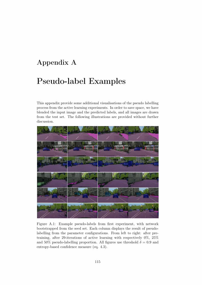
Appendix A

Pseudo-label Examples

This appendix provide some additional visualisations of the pseudo labellingprocess from the active learning experiments. In order to save space, we haveblended the input image and the predicted labels, and all images are drawnfrom the test set. The following illustrations are provided without furtherdiscussion.

Figure A.1: Example pseudo-labels from first experiment, with networkbootstrapped from the seed set. Each column displays the result of pseudo-labelling from the parameter configurations. From left to right: after pre-training, after 29-iterations of active learning with respectively 0%, 25%and 50% pseudo-labelling proportion. All figures use threshold δ = 0.9 andentropy-based confidence measure (eq. 4.3).

115

Figure A.2: Example pseudo-labels bootstrapped from pretraining onMapillary Vistas. Each column displays the result of pseudo-labelling usingENet with the following parameter configurations (left to right): after pre-training on seed set, after 29-iterations of active learning with respectively0%, 25% and 50% pseudo-labelling proportion. All images use thresholdδ = 0.9 and entropy-based confidence measure (eq. 4.3).

116

Appendix B

ENet Pre-training Results

This section provides validation results for the Mapillary Vistas [57] dataset,used for initializing the pre-trained network parameter configuration forthe experiment in section 5.3.2. The following figures correspond with thevalidation figures in section 6.1 and are provided for reference without anyfurther discussion.

0 20 40 60 80 100 120 140 160 180 2000

20

40

60

80

Epoch

mIoU

(%)

Training

Validation

(a) Mean intersection over union.

0 50 100 150 200

20

40

60

80

100

Epoch

Accuracy

(%)

Training

Validation

(b) Pixelwise accuracy.

0 2 4

·105

2

4

Step

Loss

(c) Cross entropy loss.

Figure B.1: Performance scores for training on mapillary vistas for 200epochs. (a,b) respectively show the mIoU and pixel accuracy scores for thetraining set (blue) and validation set (orange). (c) show the cross-entropyloss evaluated per batch of training examples.

117

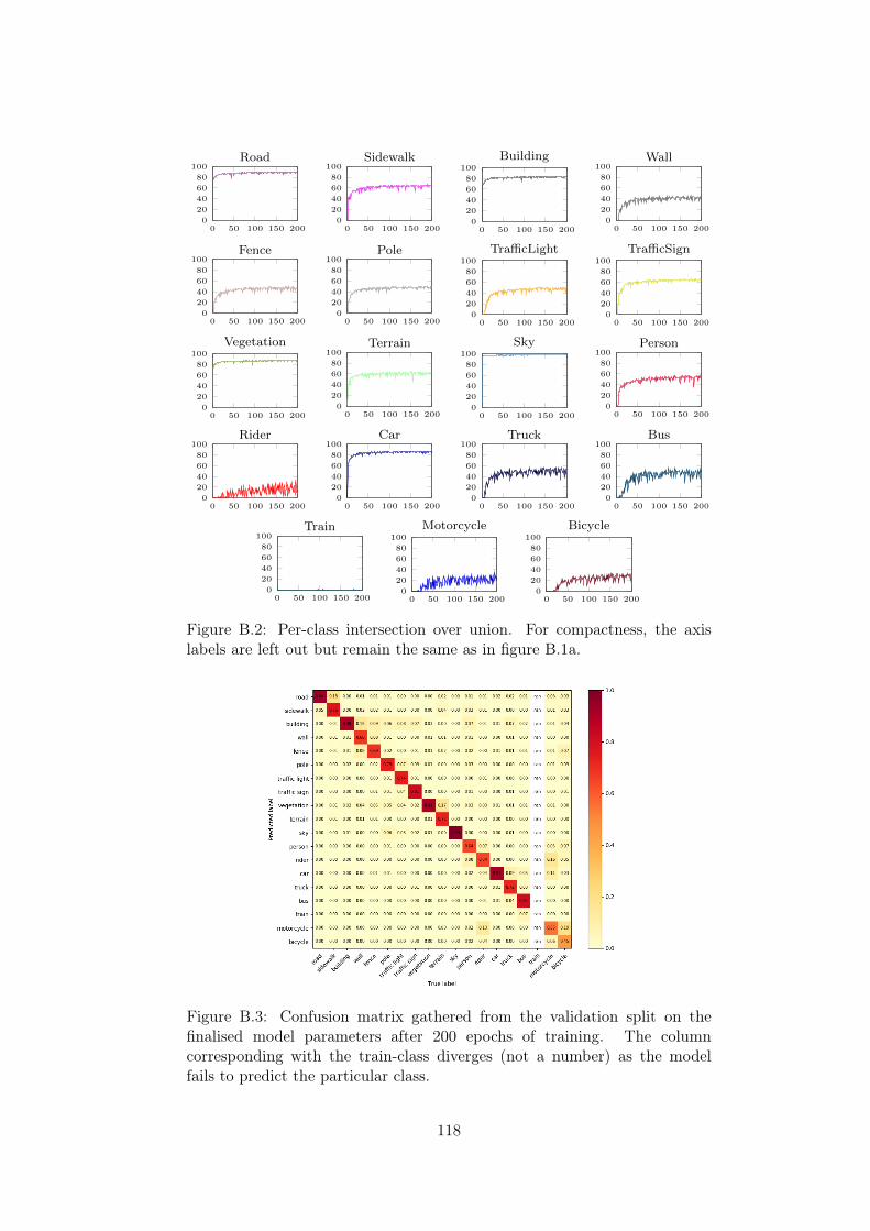
0 50 100 150 2000

20

40

60

80

100Road

0 50 100 150 2000

20

40

60

80

100Sidewalk

0 50 100 150 2000

20

40

60

80

100

Building

0 50 100 150 2000

20

40

60

80

100Wall

0 50 100 150 2000

20

40

60

80

100Fence

0 50 100 150 2000

20

40

60

80

100Pole

0 50 100 150 2000

20

40

60

80

100

TrafficLight

0 50 100 150 2000

20

40

60

80

100

TrafficSign

0 50 100 150 2000

20

40

60

80

100

Vegetation

0 50 100 150 2000

20

40

60

80

100Terrain

0 50 100 150 2000

20

40

60

80

100

Sky

0 50 100 150 2000

20

40

60

80

100Person

0 50 100 150 2000

20

40

60

80

100Rider

0 50 100 150 2000

20

40

60

80

100Car

0 50 100 150 2000

20

40

60

80

100Truck

0 50 100 150 2000

20

40

60

80

100Bus

0 50 100 150 2000

20

40

60

80

100Train

0 50 100 150 2000

20

40

60

80

100

Motorcycle

0 50 100 150 2000

20

40

60

80

100

Bicycle

Figure B.2: Per-class intersection over union. For compactness, the axislabels are left out but remain the same as in figure B.1a.

Figure B.3: Confusion matrix gathered from the validation split on thefinalised model parameters after 200 epochs of training. The columncorresponding with the train-class diverges (not a number) as the modelfails to predict the particular class.

118

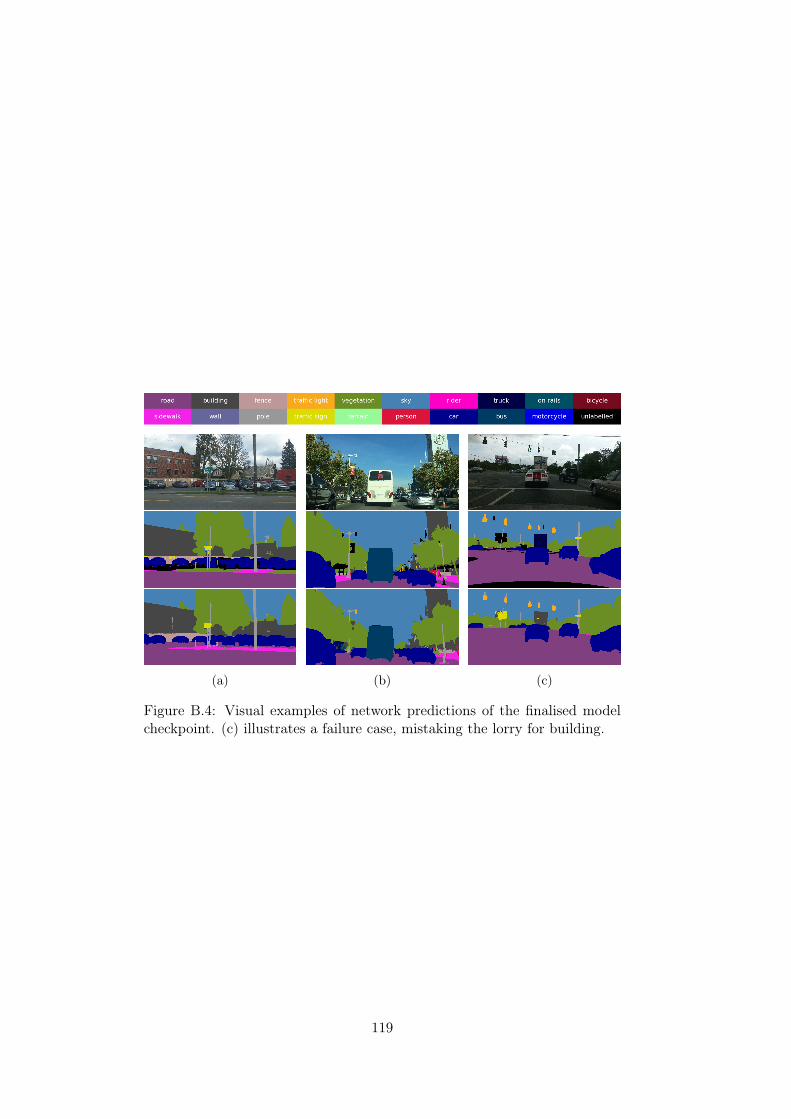
(a) (b) (c)

Figure B.4: Visual examples of network predictions of the finalised modelcheckpoint. (c) illustrates a failure case, mistaking the lorry for building.

119