Membraneless Electrolyzers for Solar Fuels Production

Jonathan T. Davis

Submitted in partial fulfillment of the

requirements for the degree of

Doctor of Philosophy

in the Graduate School of Arts and Sciences

Columbia University

2019

© 2019

Jonathan T. Davis

All rights reserved

ABSTRACT

Membraneless electrolyzers for solar fuels production

Jonathan “Jack” Davis

Solar energy has the potential to meet all of society’s energy demands, but challenges

remain in storing it for times when the sun is not shining. Electrolysis is a promising means of

energy storage which applies solar-derived electricity to drive the production of chemical fuels.

These so-called solar fuels, such as hydrogen gas produced from water electrolysis, can be fed

back to the grid for electricity generation or used directly as a fuel in the transportation sector.

Solar fuels can be generated by coupling a photovoltaic (PV) cell to an electrolyzer, or by directly

converting light to chemical energy using a photoelectrochemical cell (PEC). Presently, both PV-

electrolyzers and PECs have prohibitively high capital costs which prevent them from generating

hydrogen at competitive prices. This dissertation explores the design of membraneless

electrolyzers and PECs in order to simplify their design and decrease their overall capital costs.

A membraneless water electrolyzer can operate with as few as three components: A

cathode for the hydrogen evolution reaction, an anode for the oxygen evolution reaction, and a

chassis for managing the flows of a liquid electrolyte and the product gas streams. Absent from

this device is an ionically conducting membrane, a key component in a conventional polymer

electrolyte membrane (PEM) electrolyzer that typically serves as a physical barrier for separating

product gases generated at the anode and cathode. These membranes can allow for compact and

efficient electrolyzer designs, but are prone to degradation and failure if exposed to impurities in

the electrolyte. A membraneless electrolyzer has the opportunity to reduce capital costs and

operate in non-pristine environments, but little is known about the performance limitations and

design rules that govern operation of membraneless electrolyzers. These design rules require a

thorough understanding of the thermodynamics, kinetics, and transport processes in

electrochemical systems. In Chapter 2, these concepts are reviewed and a framework is provided

to guide the continuum scale modeling of the performance of membraneless electrochemical cells.

Afterwards, three different studies are presented which combine experiment and theory to

demonstrate the mechanisms of product transport and efficiency loss.

Chapter 3 investigates the dynamics of hydrogen bubbles during operation of a

membraneless electrolyzer, which can strongly affect the product purity of the collected hydrogen.

High-speed video imaging was implemented to quantify the size and position of hydrogen gas

bubbles as they detach from porous mesh electrodes. The total hydrogen detected was compared

to the theoretical value predicted by Faraday’s law. This analysis confirmed that not all

electrochemically generated hydrogen enters the gas phase at the cathode surface. In fact,

significant quantities of hydrogen remain dissolved in solution, and can result in lower product

collection efficiencies. Differences in bubble volume fraction evolved along the length of the

cathode reflect differences in the local current densities, and were found to be in agreement with

the primary current distribution. Overall, this study demonstrates the ability to use in-situ HSV to

quantitatively evaluate key performance metrics of membraneless electrolyzers in a non-invasive

manner. This technique can be of great value for future experiments, where statistical analysis of

bubble sizes and positions can provide information on how to collect hydrogen at maximum purity.

Chapter 4 presents an electrode design where selective placement of the electrocatalyst is

shown to enhance the purity of hydrogen collected. These “asymmetric electrodes” were prepared

by coating only one planar face of a porous titanium mesh electrode with platinum electrocatalyst.

For an opposing pair of electrodes, the platinum coated surface faces outwards such that the

electrochemically generated bubbles nucleate and grow on the outside while ions conduct through

the void spacing in the mesh and across the inter-electrode gap. A key metric used in evaluating

the performance of membraneless electrolyzers is the hydrogen cross-over percentage, which is

defined as the fraction of electrochemically generated hydrogen that is collected in the headspace

over the oxygen-evolving anode. When compared to the performance of symmetric electrodes –

electrodes coated on both faces with platinum – the asymmetric electrodes demonstrated

significantly lower rates of cross-over. With optimization, asymmetric electrodes were able to

achieve hydrogen cross-over values as low as 1%. These electrodes were then incorporated into a

floating photovoltaic electrolysis device for a direct demonstration of solar driven electrolysis.

The assembled “solar fuels rig” was allowed to float in a reservoir of 0.5 M sulfuric acid under a

light source calibrated to simulate sunlight, and a solar to hydrogen efficiency of 5.3% was

observed.

In Chapter 5, the design principles for membraneless electrolyzers were applied to a

photoelectrochemical (PEC) cell. Whereas an electrolyzer is externally powered by electricity, a

PEC cell can directly harvest light to drive an electrochemical reaction. The PEC reactor was based

on a parallel plate design, where the current was demonstrated to be limited by the intensity of

light and the concentration of the electrolyte. By increasing the average flow rate of the electrolyte,

mass transport limitations could be alleviated. The limiting current density was compared to

theoretical values based off of the solution to a convection-diffusion problem. This modeled

solution was used to predict the limitations to PEC performance in scaled up designs, where solar

concentration mirrors could increase the total current density. The mass transport limitations of a

PEC flow cell are also highly relevant to the study of CO2 reduction, where the solubility limit of

CO2 in aqueous electrolyte can also limit performance.

i

TABLE OF CONTENTS

List of Figures ............................................................................................................................... iv

List of Tables ............................................................................................................................... xii

Acknowledgements .................................................................................................................... xiii

Introduction................................................................................................................. 1

1.1 Electrochemically generated fuels for energy storage .................................................. 1

1.2 Water electrolysis.......................................................................................................... 2

1.3 Economic motivations .................................................................................................. 3

1.4 Reactor designs for electrolyzers .................................................................................. 5

1.5 Integrating membraneless electrolyzers with solar power .......................................... 11

1.6 Dissertation overview ................................................................................................. 12

1.7 References ................................................................................................................... 13

Design principles for membraneless electrolyzers ................................................. 17

2.1 Thermodynamics of the water electrolysis reaction ................................................... 17

2.2 Kinetics ....................................................................................................................... 20

2.3 Ohmic Resistance........................................................................................................ 24

2.4 Transport ..................................................................................................................... 28

2.5 Bubble dynamics in an electrochemical system ......................................................... 32

2.6 Approach to modeling the ionic current in an electrolyzer ......................................... 35

2.6.1 Modeling the electric field ............................................................................. 37

2.6.2 Modeling the concentration gradient ............................................................. 41

2.7 References ................................................................................................................... 43

High Speed Video Investigation of Bubble Dynamics and Current Density

Distributions in Membraneless Electrolyzers ........................................................ 47

3.1 Introduction ................................................................................................................. 48

3.2 Materials and Methods ................................................................................................ 52

3.3 Results and Discussion ............................................................................................... 57

3.3.1 Description of the electrolyzer and HSV setup ............................................. 57

3.3.2 Description of image analysis procedure ....................................................... 59

3.3.3 Determining gas evolution efficiency and bubble size distribution .............. 63

3.3.4 Comparing HSV-derived current transients to measured current transients . 72

ii

3.3.5 HSV-derived current distributions ................................................................. 74

3.4 Conclusions ................................................................................................................. 80

3.5 Appendix A ................................................................................................................. 81

3.5.1 Parameters used for Hough transform ........................................................... 81

3.5.2 Limiting current density and I-V curve of electrolyzer ................................. 82

3.5.3 Calculation of Wagner Number ..................................................................... 84

3.5.4 Description of algorithm for detecting unique bubbles ................................. 85

3.5.5 Relationship between time step and total volume of bubbles detected at 100

mA cm-2 ......................................................................................................... 87

3.5.6 Comparison of the primary and secondary current distributions ................... 87

3.6 Acknowledgements ..................................................................................................... 90

3.7 References ................................................................................................................... 90

Floating Membraneless PV-Electrolyzer Based on Buoyancy-Driven Product

Separation .................................................................................................................. 96

4.1 Introduction ................................................................................................................. 97

4.2 Experimental ............................................................................................................. 102

4.3 Results and discussion .............................................................................................. 104

4.3.1 Description and demonstration of a passive membraneless electrode assembly

..................................................................................................................... 104

4.3.2 Analyzing product gas cross-over ............................................................... 108

4.3.3 Measuring product collection efficiencies ................................................... 117

4.3.4 Demonstration of a floating PV-electrolysis module .................................. 120

4.3.5 Challenges for Seawater Electrolysis .......................................................... 123

4.4 Conclusions ............................................................................................................... 127

4.5 Appendix B ............................................................................................................... 128

4.5.1 iR-corrected IV characteristics of membraneless electrolyzers ................... 128

4.5.2 Calculating the percent cross-over of H2 ..................................................... 128

4.5.3 Lid used for volumetric collection efficiency experiments ......................... 130

4.5.4 Circuit diagram for the PV electrolysis device ............................................ 131

4.6 Acknowledgements ................................................................................................... 131

4.7 References ................................................................................................................. 132

iii

Limiting Photocurrent Analysis of a Wide Channel Photoelectrochemical Flow

Reactor ..................................................................................................................... 138

5.1 Introduction ............................................................................................................... 139

5.2 Experimental ............................................................................................................. 143

5.3 Results and discussion .............................................................................................. 145

5.3.1 Description of PEC flow cell and its operation ........................................... 145

5.3.2 Light limited photocurrent ........................................................................... 148

5.3.3 Mass transport-limited photocurrent ............................................................ 150

5.3.4 Predicting limiting photocurrent operating regimes .................................... 154

5.4 Conclusions ............................................................................................................... 161

5.5 Appendix C ............................................................................................................... 161

5.5.1 UV-Vis analysis of photoelectrode optical losses ....................................... 161

5.6 Acknowledgements ................................................................................................... 163

5.7 References ................................................................................................................. 163

Conclusions and future directions ......................................................................... 169

6.1 Modeling multiphase flows in membraneless electrochemical cells ........................ 171

6.2 Engineering the electrode surface tension ................................................................ 172

6.3 Improving downstream phase separation.................................................................. 173

6.4 Scale-up of membraneless electrolyzers ................................................................... 175

6.5 Membraneless electrolyzers for CO2 reduction ........................................................ 175

6.6 References ................................................................................................................. 176

iv

LIST OF FIGURES

Figure 1.1: Design schematics and transport processes for a a) PEM electrolyzer and an b) alkaline

electrolyzer. Each schematic shows a cathode and anode connected to an external

power supply to drive the water splitting reaction. ....................................................... 7

Figure 1.2: Reactor designs for membraneless electrochemical cells. a) A flow-by electrolyzer

design which uses solid electrodes mounted to the walls of a laminar flow channel b)

A flow-through electrolyzer where porous mesh electrodes extend into the center of a

flow channel. In these devices, electrolyte flows through the gap spacing in the mesh

and pushes the product bubbles downstream. ............................................................. 10

Figure 2.1: Simple force balance of a H2 bubble growing on an electrode surface. ..................... 33

Figure 2.2: Framework for the simulation of the current density in a membraneless electrochemical

cell. .............................................................................................................................. 36

Figure 3.1: a) Schematic top-view of membraneless electrolyzer based on two flow-through mesh

electrodes placed at an angle of 90⁰ with respect to the direction of fluid flow. The

close-up photo on the right shows a magnified view of the front of a woven mesh

electrode used in this study. b) Exploded diagram of the membraneless cell used in this

study. c) Schematic of the assembled flow cell. ......................................................... 52

Figure 3.2: Procedure used for processing HSV images recorded during electrolysis. a) Schematic

showing the region of the electrolyzer recorded with HSV. b.) Still frame from a HSV

showing H2 bubbles evolving from a mesh cathode operating with an average current

density of 50 mA cm-2 in 0.5 M H2SO4 c.) The still frame is cropped to limit analysis

to a narrow section of the channel located immediately downstream of the cathode. d.)

Conversion of the cropped still frame into a binary image to reduce background

interference. e.) The size and position of bubbles are determined using a circle detection

algorithm, with detected bubbles shown by red circles that are overlaid with the binary

image from (d). The local density of bubbles, used to estimate the local current density,

is determined by discretizing the analysis area into equal control volume................. 60

Figure 3.3: a) Terminal velocity of H2 bubbles rising off of the cathode as a function of bubble

radius. Individual bubble velocities were determined in an electrolyte of 0.5 M H2SO4

purged with Ar and pumped at an average velocity of 0.5 cm s-1. Bubbles were

generated at an operating current density of 20 mA cm-2. b) Total volume of gas

v

detected over the duration of a 10 s HSV as a function of time step between image

frames. Image analysis was conducted for the same experimental conditions as in (a).

Also marked on the plot is the maximum residence time for a bubble traveling across

the analysis area. The red star corresponds to a time step of 0.1 s, which was the time

step used for the remainder of the analyses in this paper. c) Cumulative volume of H2

bubbles detected during a 10 s long HSV. Image analysis was conducted for the same

experimental conditions as in (a). The upper trace corresponds to the total volume of

all bubbles detected in the image frame, whereas the lower trace uses an algorithm that

ensures that each individual bubble is only counted once. ......................................... 62

Figure 3.4: a) Total volume of H2 detected over the cathode during a 10 s long HSV. Each trace

corresponds to bubbles detected for a constant average applied current density of 20,

50, or 100 mA cm-2. In each trial, the electrolyte was pre-saturated with Ar. b) Gas

evolution efficiency of the cathode as a function of time. Each data point corresponds

to the average gas evolution efficiency over the course of a 10 s HSV. Experiments

were carried out for a cathode operating at 20 mA cm-2 in 0.5 M H2SO4, and the effect

of Ar and H2 saturation gases is compared. The total volumetric flow rate of electrolyte

through the cell was set to 1 mL s-1. ........................................................................... 65

Figure 3.5: Analysis of H2 bubble sizes determined from HSV recorded during a 10 s of electrolysis

in 0.5 M H2SO4 with electrolyte pumped through the electrolysis cell at a rate of 1 mL

s-1. a) Probability histogram of bubble diameters evolved from the cathode during

electrolysis at 20 mA cm-2 in Ar saturated electrolyte. HSV was recorded after 5

minutes of electrolysis. Number probabilities were calculated based on the number of

bubbles counted, while volumetric probabilities were calculated based on the total

volume of gas generated. b) Cumulative volume fraction as a function of bubble

diameter for H2 bubbles evolving from a cathode operating at 20 mA cm-2 in Ar

saturated electrolyte. Each trace corresponds to a different start time of HSV and

represents the same data set reported in Figure 3.4b. c) Cumulative volume fraction as

a function of bubble diameter for different operating current densities in Ar saturated

electrolyte. HSVs were recorded after 5 minutes of electrolysis. d) Comparison of

cumulative volume fraction as a function of bubble diameter for a cathode operating at

vi

50 mA cm-2 in different saturation gases. HSVs were recorded after 5 minutes of

electrolysis. ................................................................................................................. 70

Figure 3.6: Comparison of the total electrolysis current recorded by the potentiostat to the volume

of gas detected during a 10 s HSV. The HSV was recorded after five minutes of

electrolysis at a constant applied voltage of 2.7 V. Electrolysis was carried out in 0.5

M H2SO4 with electrolyte pumped through the cathode at a rate of 0.5 mL s-1. ........ 73

Figure 3.7: Comparison of the predicted current distribution to the local volume fraction along the

length of the electrode, 𝑥/𝐿𝑒. All experiments were carried out at an operating current

density of 50 mA cm-2. a) Simulated primary current distribution of the electrolysis cell

for different separator tab insertion lengths between electrodes. b) Relative gas volume

fraction along the length of the electrode for a cathode operating in Ar-saturated H2SO4

and tab insertion length of 2 mm. c) Relative gas volume for a cathode operating in Ar-

saturated H2SO4 and a tab insertion length of 10 mm. Error bars were determined by

calculating the 95 % confidence interval based on averaging the volume fraction over

100 frames of data. ...................................................................................................... 77

Figure 3.8: Current-voltage curve for an electrolyzer with a tab insertion length 𝐿𝑡𝑎𝑏 of 2 mm.

0.5 M H2SO4 was pumped to the cathode at a rate of 0.5 mL s-1. The LSV was measured

at a scan rate of 20 mV s-1. .......................................................................................... 84

Figure 3.9: Detection of unique bubbles in a single image analysis frame. Green arrows show the

path traveled by bubbles from the previous frame to the current frame. Red circles

correspond to a previous bubble position which was already in the window of analysis.

Black circles correspond to bubbles which were previously out of frame, and thus have

not yet been detected. .................................................................................................. 86

Figure 3.10: Total volume of gas detected over the duration of a 10 s HSV as a function of time

step between image frames. Experiment was carried out in 0.5 M H2SO4 purged with

Ar and pumped at an average velocity of 0.5 cm s-1. Bubbles were generated at a current

density of 100 mA cm-2............................................................................................... 87

Figure 3.11: Comparison of the primary and secondary current distributions of the cathode for a

tab insertion length of 𝐿𝑡𝑎𝑏 = 2 mm. ......................................................................... 89

Figure 4.1: a) Schematic of a deep sea “Solar Fuels Rig” based on a utility-scale, floating

photovoltaic (PV)-electrolysis platform which uses sunlight to generate the solar fuel,

vii

H2. On this rig, PV arrays mounted on a floating platform harvest sunlight and produce

electricity that is sent to durable membraneless electrolyzers that split water into O2

and H2. Hydrogen generated by the electrolyzers is collected and stored in tanks above

the surface where they wait to be shipped back to shore. b) Schematic of novel

membraneless electrode assemblies that are the basis of the current study and might

one day be key components of the solar fuels rig. Alternating sets of membraneless

electrolyzers wired in parallel use electricity supplied from the PV cells to split water

into H2 and O2. c) Close up schematic of a passive membraneless electrolyzer

employing buoyancy-based product separation. The mesh electrodes are oriented at an

angle 𝜃, resulting in an average separation distance 𝐿. The electrocatalyst is deposited

on the outward facing sides of the mesh in order to constrain product gas nucleation

and growth to this region only. When the gas bubbles become large enough to detach,

they float directly upward for collection or venting to the atmosphere. ..................... 99

Figure 4.2: a) Photo of the electrolysis cell with interior components shown through the viewing

window. b) Still frame image of bubble growth on an asymmetric electrode operating

at 150 mA cm-2 in 0.5 M H2SO4. c) Still frame image of bubble growth on a symmetric

electrode at the same conditions as in (b). The full videos can be found in the online

publication of Int. J. Hydrogen Energy, 43, 1224–1238 (2018). .............................. 105

Figure 4.3: LSV analysis for the passive membraneless electrolyzer for various electrode

configurations. Experiments were carried out for a two-electrode setup in 0.5 M

sulfuric acid and a scan rate of 100 mV s-1. a) IV curves for asymmetric and symmetric

electrodes held at θ=0⁰. Current density is normalized relative to the geometric area of

the mesh electrodes. b) Re-plotting the data in (a) correcting for IR losses and

accounting for the fact that the symmetric electrodes have twice as much

electrochemically active surface area. c) IV curves for asymmetric electrodes at varying

separation angles. The current density is normalized relative to the geometric area of

the mesh electrodes. d) Ohmic resistance measured across the cell for asymmetric

electrodes as a function of electrode angle. Values for the ohmic resistance were

determined using electrochemical impedance spectroscopy (EIS). .......................... 108

Figure 4.4: Percent H2 cross-over into the O2 collection chamber of the static electrolyzer measured

by gas chromatography. Experiments were carried out in 0.5 M sulfuric acid at a

viii

constant applied current. a) Comparing the percent H2 cross-over recorded for

symmetric and asymmetric electrodes at varying angles and operating at 20 mA cm-2,

where the current density is reported with respect to the geometric area of the

electrodes. b) Percent H2 cross-over measured for asymmetric electrodes at varying

electrode angles and current densities. ...................................................................... 110

Figure 4.5: Mechanisms of product gas cross-over in a static fluid electrolyzer. a) Direct bubble

cross-over: bubbles from one electrode detach and migrate to the opposite collection

chamber. b) Indirect bubble cross-over: bubbles from both electrodes accumulate on

the central baffle, forming a mixed gas bubble which can detach and travel into either

collection chamber. c) Dissolved gas cross-over: the electrolyte becomes saturated with

dissolved product gas which can diffuse over to the opposing electrode. The dissolved

gas can equilibrate with bubbles as they float upwards to the collection chamber. For

simplicity, dissolution and diffusion was only shown for dissolved H2. Still frame

images taken from high speed video measurements showing instances of d) direct

bubble cross-over recorded for parallel asymmetric electrodes and e) indirect bubble

cross-over recorded for asymmetric electrodes at a 30 degree angle and 100 mA cm-2.

................................................................................................................................... 112

Figure 4.6: Visualization of dissolved species cross-over during electrolysis in 0.5 M NaCl solution

with universal pH indicator. The indicator turns from red to dark purple in the presence

of the hydroxyls generated at the cathode. The experiment was carried out with

asymmetric electrodes operating at a current density of 40 mA cm-2. ...................... 114

Figure 4.7: a.) Schematic of a modified electrolysis cell involving a sensor electrode that is used

to measure current efficiency losses due to the HOR of H2 at the anode. b) Average

losses in current efficiency due to HOR during constant current electrolysis while

holding the applied potential of the sensing electrode at +0.8 V vs. Ag/AgCl. The

current efficiency loss was calculated by dividing the total integrated charge recorded

by the sensing electrode by the total charge passed between the anode and cathode

throughout the electrolysis experiment. Measurements were recorded for a 30°

electrode angle in 0.5 M H2SO4. ............................................................................... 116

Figure 4.8: a) Volume of product gas collected as a function of time. Data was recorded for a 30°

electrode separation angle and an operating current density of 40 mA cm-2. The error

ix

bars correspond to a 95% confidence interval for data averaged over three trials. The

solid lines represent the theoretical volumetric collection based on Faraday’s law and

the Ideal gas law. b) Mole balance on H2 generated during electrolysis with an electrode

angle of 30° and operating at 40 mA cm-2 for 3.9 minutes. ...................................... 118

Figure 4.9: a) Schematic side-view of the floating PV-electrolysis module, which is based on two

sets of asymmetric mesh electrodes that are wired in parallel to each other and to four

PV panels. The module floats in a reservoir of sulfuric acid. Hydrogen evolved at the

cathode is collected underneath the PV panels while the oxygen is allowed to vent to

the atmosphere. b) Photo of the PV-electrolyzer module floating in a sulfuric acid

reservoir. c) I-V curve matching for the electrolyzer and PV cells. The electrolyzer

curve is for 6 cm2 of asymmetric mesh electrodes submerged in 0.5 M sulfuric acid and

was recorded at a scan rate of 10 mV s-1. The PV curve is the combined I-V response

for four PVs wired in parallel under a lamp calibrated to the AM 1.5G intensity, and

was recorded at a scan rate of 100 mV s-1. The intersection of these curves predicts the

operating current of the device when the PV panels and electrolyzer are connected to

each other. d) Operating current of the floating PV-electrolysis unit as a function of

time during unassisted water electrolysis under the same illumination conditions as

described for the measurements in c.)....................................................................... 121

Figure 4.10: IV characteristics of parallel asymmetric electrodes in 0.5 M H2SO4 and 0.6 M NaCl

recorded at a scan rate of 100 mV s-1. ....................................................................... 125

Figure 4.11: iR-corrected IV curves measured for asymmetric Pt/Ti electrodes in 0.5 M H2SO4.

The curves presented are from the data set as shown in Figure 4.3c, which were shifted

to lower voltages by subtracting the iR voltage drop at each current density using the

series resistance values obtained from electrochemical impedance spectroscopy (EIS)

and provided in Figure 4.3d. IV curves were recorded at 100 mV s-1. ..................... 128

Figure 4.12: Sample chromatograph showing the H2 peak on both the cathode and anode side

collected for symmetric electrodes held at 30 degrees and an operating current density

of 20 mA cm-2 in 0.5 M H2SO4. ................................................................................ 129

Figure 4.13: Percent H2 crossover into the O2 collection chamber of the membraneless electrolyzer

measured by gas chromatography. Experiments were carried out in 0.5 M sulfuric acid

at a constant applied current and using symmetric Pt/Ti electrodes. ........................ 130

x

Figure 4.14: Lid used to record volumetric collection of product gasses. Front end contains epoxied

windows with graduated lines reading the level height in 2 mm increments. At the

beginning of the experiment, electrolyte is drawn up with a syringe to the top line. As

the electrolysis reaction proceeds, gas bubbles displace the electrolyte and the liquid

level drops. ................................................................................................................ 130

Figure 4.15: Schematic of an individual PV panel and its connection to the floating PV electrolysis

module. a) A photograph of an individual PV panel, which consists of 6 individual PV

cells that are wired in series. b) A total of four PV panels are wired together in parallel.

The cathode and anode terminals are connected to two parallel sets of angled

electrolyzers. An ammeter (A) measures the current between the positive terminals of

the PV panels and the electrolyzers during operation. A schematic of the PV

electrolysis device is shown in Figure 4.9a of the main text. ................................... 131

Figure 5.1: a.) Schematic side-view of a parallel plate PEC flow cell used to investigate the

influence of convective mass transport and light intensity on the limiting photocurrent.

b) Zoomed in side-view of fundamental processes occurring near the photoelectrode

surface and within the diffusion boundary layer of thickness δ. .............................. 141

Figure 5.2: a) Exploded view of 3D printed PEC flow cell assembly. b) Photograph of PEC flow

cell. c) Simplified flow diagram of experimental set-up. ......................................... 145

Figure 5.3: Standard LSV curves for the p-Si MIS photocathode under simulated AM 1.5G

illumination in 200 mM H2SO4 with 1 M Na2SO4. The potential is swept from positive

to negative at a scan rate of 20 mV s-1. At positive potentials, the photovoltage is

insufficient for HER to proceed, and no photocurrent is recorded (Region I). As the

potential is scanned more negative than the photocurrent onset potential (Vonset), the

current becomes strongly dependent on the reaction kinetics (Region II). Below -0.24

V vs. NHE, the photocurrent becomes independent of the applied potential and is

determined by the relative rates of light absorption and mass transfer (Region III). 147

Figure 5.4: Photo-limited PEC operation. a) Linear sweep voltammetry (LSV) curves recorded for

a p-Si MIS photocathode under varying solar concentrating factors. All scans were

swept from positive to negative potential at a rate of 10 mV s-1 in 200 mM H2SO4

flowing at an average velocity of 22 cm s-1. b) Limiting photocurrent densities recorded

xi

for a p-Si MIS photocathode under varied solar concentration factors in weakly and

strongly acidic electrolytes flowing at an average velocity of 22 cm s-1. ................. 150

Figure 5.5: Mass transport-limited PEC operation. a) Linear sweep voltammetry for varying fluid

velocities in 4 mM sulfuric acid. Scans are from positive to negative potential at a rate

of 10 mV s-1. b) Comparing the average limiting current density of an MIS

photoelectrode to a metallic electrode (p+Si). The limiting current was measured using

chronoamperometry. ................................................................................................. 152

Figure 5.6: Predicting the boundary between photo-limited and mass transport-limited PEC

operation. a) The limiting current of a photoelectrode operated in varying H2SO4

concentration under 1 sun illumination. At low fluid velocities the current is mass

transport-limited, but increasing the flow velocity allows the current to reach the 1 sun

photo-limited value, which is equal to the limiting current in 500 mM H2SO4 ([H+] =

1000 mM). b) Predicted boundary between photo-limited and mass transport-limited

current at 1 sun. Individual data points on the plot correspond to the same experimental

data points shown in a). The tie line was calculated using Equation 5.4, and 𝜓 is defined

in the text. c) Predicted boundary at higher levels of solar concentration for a reaction

with n= 1 mole of electrons transferred per mole reactant. d) Predicted boundary for

reactions involving n= 8 moles of electrons transferred per mole reactant. ............. 157

Figure 5.7: Percent transmittance for a glass slide deposited with a 10 nm Ti 3 nm Pt metal bi-

layer........................................................................................................................... 162

xii

LIST OF TABLES

Table 1.1 Performance characteristics for alkaline and PEM electrolyzers. .................................. 8

Table 2.1: Tafel kinetic parameters for HER and OER on Pt mesh flow through electrodes,

reproduced from O’Neil, et al. .................................................................................... 23

Table 3.1: Input parameters for Hough Transform algorithm used in this study ......................... 82

xiii

ACKNOWLEDGEMENTS

I would like to first thank my advisor, Dr. Daniel Esposito, for his guidance and support

over these past five years – without him this thesis would not be possible. The Solar Fuels lab has

grown tremendously since the Fall of 2014, when Dr. Natalie Labrador, Dr. Glen O’Neil and I

were working on borrowed bench space until we could have a permanent room to call our own.

Natalie and Glen – I can’t thank you enough for your wisdom and friendship over all these years!

I’d like to thank my thesis committee for their guidance during my PhD. In particular, I

thank Dr. Alan West for his vast knowledge of electrochemistry and willingness to take time out

of his schedule to answer my questions. I also thank Dr. Jingguang Chen and Dr. Chris Boyce for

the knowledge they’ve shared both inside and outside of the classroom. Lastly, I thank Dr. Albert

Harvey for his mentorship, which dates back to my internship at Shell Oil Co. in the summer of

2017.

I thank the Long Range Research Group at Shell for the financial support and research

guidance that they have provided during my PhD. In addition to Dr. Harvey, I’d like to thank my

collaborators Dr. Santhosh Shankar and Vijay Narasaiah for their insights and contributions to the

membraneless electrolyzer project. So much amazing work is coming out of this project and I look

forward to reading the many publications to come.

Next, I wish to thank my fellow lab mates in the Solar Fuels Lab for their friendship and

support throughout my PhD. I could not have made it through without you. In particular, I thank

Anna Dorfi for her friendship, which dates back to our college years at Ohio State. A very special

thank you to Marissa Beatty and Xueqi Pang, who are both very fast learners and are ready to take

on the PhD student leadership roles within the group. In addition to Pang, who will be taking

charge of the membraneless electrolyzer project, I am thankful for MS students Ji Qi, Xinran Fan,

xiv

and Wade Mao for their research contributions. I also thank the undergraduate researchers who

have made significant contributions over the years: David Brown, Kareem Stanley, Chinedu

Okorafor, Shin Cousens, Maya Bhat, and Julie Raiff. Of course, a very special thanks to

undergraduate Justin Bui, whose knowledge of 3D printing is rivaled by none. I also thank our

post doc Dr. Xiangye Liu, who has been very helpful in setting up the gas chromatograph in the

lab. Additionally, I thank Chen research group members Elaine Gomez and Zhenhua Xie for their

help with gas chromatography experiments.

I’d also like to thank my many friends in Houston, who were very accommodating during

my time there: Dr. Lizzy Mahoney, Dr. Zack Whiteman, Dr. Federico Barrai, Aaron Strickland

and Radhika Madhavan. I will also thank Stefan Heglas, who did not live in Houston at the time

but was around nonetheless.

A special thank you to the department office workers, who work tirelessly to keep the ship

afloat: Kathy Marte, Rezarta Binaj, Aurna Malakar, Ariel Sanchez, Emeley Aquino, and Irina

Katz. The department could not function without you. Thank you to the long line of ChEGO

presidents who I have had the pleasure to work with and serve under during my time at Columbia:

Kevin William Knehr, Christopher James Hawxhurst, Brian Michael Tackett, Andrew Matthew

Jimenez, and Ryan Gusley. Their shrewd leadership has brought upon us an era of great prosperity.

Of course, I thank the many graduate students with whom I’ve shared so many laughs and

fond memories with over the years. In particular, I want to thank Brian Tackett, Nick “The

Logician” Brady, and Dr. Christianna Lininger – I don’t know what I’d do without you fine

academics. I am also very thankful for the friendship of graduate students Andrew Jimenez, Jon

Vardner, Steven Denny, Sebastian Russell, Thi Vo, Gianna Credaroli, Dr. Ellie Buenning, and

Allison Fankhauser. I’d be remiss if I did not also thank their family members, who I’ve become

xv

very good friends with during my time at Columbia: Lauren Carlsen, Kevin Evans, Ronin Jones

Jr., Maggie Tomaszewski, Bambi Tomaszewski-Denny, and Jessica Small. And on the subject of

family, I’d also like to thank my old roommate Dr. Longxi Luo. I wish all the best to him, his wife

Lijun, and baby Henry. I also thank my college friends whose support and humor have kept me

positive the whole way through: Parker Hall, Alex Kuhn, Chris Zuccarelli, JP Sundej, Brandon

Scott, Luke Laws, Jenn Laws, Zac Baaske, and Massey Pierce.

I thank my brother Rawley, who along with Max Minillo, has served two tours of active

duty with me in the online tactical combat games Battlefield 1 and Battlefield V. Over five years

of research, I’ve learned that it is indeed healthy to carve out a time where I don’t think about

reactors. I thank you both for the consistent laughs. I also thank my sister Anna for her consistent

and unyielding support. Her intelligence and maturity is way under-appreciated, and I can’t wait

to be closer to her when I move out west. I thank my parents Carol and Bryan, who have always

believed in me and have been in my corner since day one. Lastly, I thank Christopher Lim and his

cat Goose for their love and support.

1

INTRODUCTION

1.1 Electrochemically generated fuels for energy storage

The sun is a highly abundant resource which has the potential to meet all of society’s energy

demands without emitting greenhouse gases. A pitfall of solar energy is that it is intermittent, and

must be stored for use during hours when the sun does not shine. An energy infrastructure which

is both renewable and robust will be able to store solar electricity by transferring it into chemical

energy. This can be achieved using an electrolyzer, an electrochemical reactor that uses an

electrical power source to drive a thermodynamically uphill reaction. One of the simplest of these

reactions is the electrolysis of water into hydrogen (H2) and oxygen (O2) gases. As an energy

carrier, H2 is storable and can be used as a fuel source for on demand electricity generation.

Additionally, H2 can be used as a fuel in the transportation sector. Although electric vehicles are

emerging in the market for light transportation, chemical fuels will likely continue to be the

dominant fuel source for commercial applications, especially in the airline and heavy freight

industries.1 In the chemical industry, H2 will continue to be necessary for the production of

ammonia for fertilizers, which is one of the leading applications for H2 use today.2 More broadly,

electrolyzers are also of interest for the renewable production of commodity chemicals, where

electrode materials have been demonstrated for the reduction of nitrogen3 and carbon dioxide.4,5

Although the design of membraneless electrolyzers is highly relevant to these processes, the focus

of this dissertation is the production of H2 from water electrolysis.

2

1.2 Water electrolysis

Hydrogen in today’s market is produced via the steam methane reforming (SMR) reaction,

a process which relies on fossil fuels and releases carbon dioxide (CO2). Water electrolysis is a

more sustainable means of H2 production, provided that there is a renewable source of electricity.

An electrolyzer operates by applying a voltage across two electrodes separated by an electrolyte.

In an acidic electrolyte, protons are reduced at the cathode to evolve H2. At the anode, water is

oxidized to evolve O2. These half reactions, known as the hydrogen evolution reaction (HER) and

the oxygen evolution reaction (OER) in an acidic electrolyte, are shown in Equations 1.1 and 1.2

respectively. The overall reaction, shown in Equation 1.3, is the splitting of water into H2 and O2

gases.

2𝐻+ + 2𝑒− → 𝐻2 𝑈𝐻2|𝐻+0 = 0.0 𝑉 𝑣𝑠 𝑁𝐻𝐸 1.1

𝐻2𝑂 →1

2𝑂2 + 2𝐻+ + 2𝑒− 𝑈𝐻2𝑂|𝑂2

0 = 1.23 𝑉 𝑣𝑠 𝑁𝐻𝐸 1.2

𝐻2𝑂 → 𝐻2 +1

2𝑂2 𝑈𝑐𝑒𝑙𝑙

0 = −1.23 𝑉 1.3

Also shown in Equations 1.1 and 1.2 is the standard reduction potential 𝑈0 of each half

reaction, which is reported relative to the normal hydrogen electrode (NHE). The standard cell

potential, 𝑈𝑐𝑒𝑙𝑙0 = 𝑈𝐻2|𝐻+

0 − 𝑈𝐻2𝑂|𝑂2

0 = -1.23 V, is the thermodynamic minimum voltage which

must be applied in order for the reaction to occur. Although Equations 1.1 and 1.2 are written

assuming an acidic electrolyte, an acid intermediate is not strictly necessary for the overall reaction

shown in Equation 1.3. The water electrolysis reaction can also be carried out in alkaline and pH-

neutral electrolytes. Provided that the pH of the electrolyte is the same at both electrodes, 𝑈𝑐𝑒𝑙𝑙

will be equal to -1.23 V across the entire pH scale. At non-standard conditions, the cell potential

𝑈𝑐𝑒𝑙𝑙 can deviate from -1.23 V, and Chapter 2 explores how to calculate these deviations using the

Nernst equation.

3

Regardless of the composition of the electrolyte, a larger voltage must be applied to

overcome barriers due to kinetics, mass transport, and ohmic resistance. These losses are shown

in Equation 1.4:

Δ𝑉 = |𝑈𝑐𝑒𝑙𝑙| + 𝜂𝐻𝐸𝑅 + 𝜂𝑂𝐸𝑅 + 𝜂𝑀𝑇 + 𝐼𝑅𝑠 1.4

where Δ𝑉 is the applied voltage to the electrolyzer electrodes, 𝜂𝐻𝐸𝑅 is the kinetic overpotential for

HER, 𝜂𝑂𝐸𝑅 is the kinetic overpotential for OER, 𝜂𝑀𝑇 is the mass transport overpotential, 𝐼 is the

total current passed through the electrolyzer, and 𝑅𝑠 is the ohmic resistance in the electrolyte. Each

of these loss mechanisms can significantly hamper the performance of an electrolyzer, and will be

explored in greater detail in Chapter 2. Minimizing these voltage penalties is necessary for

electrolysis to proceed efficiently. The overall efficiency of an electrolyzer 𝜂𝑒𝑙𝑒𝑐 is given by

Equation 1.5 below:

𝜂𝑒𝑙𝑒𝑐 =

|𝑈𝑐𝑒𝑙𝑙|

Δ𝑉𝜂𝐹𝐸 1.5

where 𝜂𝐹𝐸 is the Faradaic efficiency, or selectivity, of the electrochemical reaction. For water

electrolysis, it can be generally assumed that there are no major side reactions and that 𝜂𝐹𝐸 is

100%.

1.3 Economic motivations

The efficiency of an electrolyzer is an important metric for determining if it can be cost

competitive with SMR for H2 production. A technoeconomic analysis (TEA) by Shaner, et al.

estimated that for an operating efficiency of 61%, the breakeven price for electrochemically

generated H2 is approximately $6.10/kg.6 By comparison, the price of H2 from SMR is

approximately $1.59/kg.7 This disparity in price can be attributed to the costs of inputs for each

process. The required methane and heat input for SMR is inexpensive relative to the cost of

4

purified water and electricity for electrolysis. In fact, 66% of the cost of electrochemically

generated H2 can be attributed to the price of electricity consumed.8 By operating more efficiently,

less electricity is required per kg of H2, bringing down operating costs. However, even at 100%

efficiency, the price of electrochemically generated H2 would still not be cost competitive with

SMR at today’s electricity prices. A more fair comparison between the two technologies should

also account for externalities such as the consequences of emitting CO2 into the atmosphere. This

could be accounted for through a carbon tax or other environmental regulations which discourage

CO2 emissions. Although H2 from SMR can be produced at $1.59 today, an upper bound on this

price would also include the cost of carbon capture and storage.

Another important consideration for the cost of H2 from electrolysis is the capacity factor.

The break-even price in the Shaner TEA assumed that the electrolyzer had a capacity factor of

97%, meaning that it was operating 97% of the time.6 However, an electrolyzer used for energy

storage will operate at significantly lower capacity factors, particularly when coupled with solar

electricity. For example, a fixed angle photovoltaic (PV) panel in Phoenix, Arizona can use an

average of 6.5 hours of sunlight per day.9 If an electrolyzer was coupled with this PV system, its

capacity factor would therefore be 27%. For this PV-electrolyzer pair to produce the same amount

of H2 at the same efficiency as the electrolyzer with a 97% capacity factor, you would need to

increase the electrode area by a factor of four, and consequently the capital costs increase by a

factor of four. In summary, electricity consumption accounts for 66% of the price of H2 in the

hypothetical case where an electrolyzer operates at 97% capacity factor. When the electrolyzer is

used for energy storage, however, significantly higher capital investment is required to compensate

for a lower capacity factor, and therefore the capital costs are expected to dominate.

5

Thus, efficiency improvements alone cannot make water electrolysis economically viable.

There must also be reductions in the price of electricity and reductions in the capital cost of the

electrolyzer itself. Fortunately, innovations in PV generation have shown steady declines in the

price of renewable electricity in the past decade.10 There could also be opportunity for electrolyzers

to purchase electricity at significant discount if operation is limited to hours of excess electricity

generation. Decreasing the capital costs, however, requires reexamination of the reactor design of

the electrolyzer itself, and is the central focus of this dissertation. In the next section, we review

the current state of the art designs for water electrolyzers and the relationship between capital costs

and energy efficiency.

1.4 Reactor designs for electrolyzers

An electrolyzer should be designed to operate efficiently while also ensuring that the

generated gases can be collected with high purity. The efficiency of an electrolyzer is largely a

product of the construction materials, but can also depend on the electrode separation distance. In

general, an electrolyzer is most efficient when the electrodes are closest together. A smaller

electrode separation distance will cause a decrease in the ohmic resistance and therefore increase

the overall efficiency of the device. Placing electrodes too close, however, can cause the generated

H2 and O2 to mix, which will incur downstream separation costs and possibly create an explosive

mixture. An optimal electrolyzer design will balance this distance tradeoff between energy

efficiency and product purity, which will largely depend on the transport mechanism of the

reactants and products. Figure 1.1 shows a generalized schematic of the transport and separation

processes for two established electrolyzer technologies: The polymer electrolyte membrane (PEM)

electrolyzer and the alkaline electrolyzer.

6

A PEM electrolyzer, shown in Figure 1.1a, uses a proton exchange membrane such as

Nafion to facilitate ionic transport between the electrodes. This design is a conventional approach

for electrolysis, and is presently used in the chloralkali industry. Although ionically conductive,

the membrane is also electronically insulating, allowing for extremely close electrode separation

distances (<150 μm) without risk of electrical short circuiting. This narrow electrode separation

distance is desirable because it reduces the ohmic resistance of the electrolyzer, and is sometimes

referred to as a “zero gap resistance.” The membrane also serves as a rigid barrier to prevent gas

permeation, ensuring that the electrochemically generated H2 and O2 streams have high purities

that are outside the flammability range.

Figure 1.1b shows an alkaline electrolyzer, which is another conventional design for

electrolyzers. Gas separation in an alkaline electrolyzer is maintained by a porous diaphragm,

typically constructed out of asbestos. The ionic current between the electrodes is carried by an

alkaline electrolyte which hydrates the pores of the diaphragm. The diaphragm typically has a

higher ohmic resistance than the Nafion membranes in PEM electrolyzers, and thus must operate

at lower current densities to achieve the same efficiency. Although the diaphragm is mostly

capable of preventing product gases from crossing over and mixing, gas bubbles can enter the

pores and block pathways for ionic conduction, further increasing the ohmic resistance of the cell.

7

Figure 1.1: Design schematics and transport processes for a a) PEM electrolyzer and an b) alkaline

electrolyzer. Each schematic shows a cathode and anode connected to an external power supply to

drive the water splitting reaction.

In terms of energy efficiency and operating capacity, PEM electrolyzers are superior to

alkaline electrolyzers. A comparison of the typical performance values for PEM and alkaline

electrolyzers is given in Table 1.1. Despite the performance advantages of PEM electrolyzers,

there are many costs associated with the Nafion membrane which contribute to the overall capital

cost. First is the material cost of the membrane, which can account for 3% of the total cost of the

electrolyzer.11 However, there are additional capital costs associated with the membrane beyond

its material cost. In order to achieve the benefits of a zero-gap resistance, electrocatalysts must be

directly impregnated onto the membrane, known as a membrane electrode assembly (MEA). The

improved performance comes at the cost of durability, which is directly tied to the cost of

maintenance and the overall lifetime of the electrolyzer.12 If any one component of the MEA fails,

the entire MEA must be replaced. Studies have investigated the possibility of recycling the MEA,

but the process is highly destructive and can result in significant losses in material and

performance.13,14

8

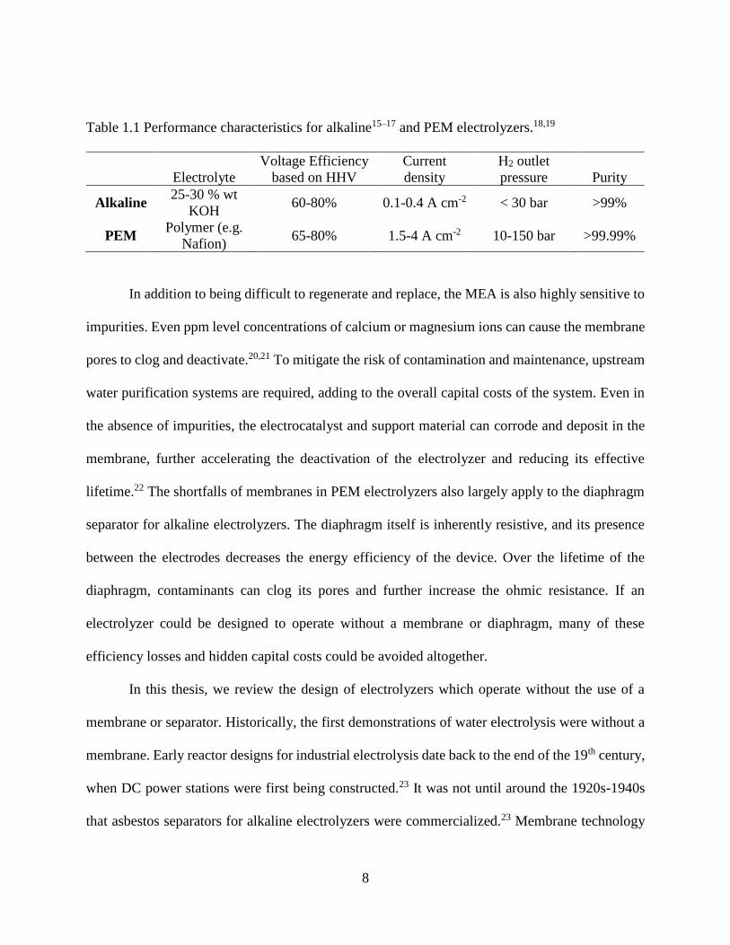
Table 1.1 Performance characteristics for alkaline15–17 and PEM electrolyzers.18,19

Electrolyte

Voltage Efficiency

based on HHV

Current

density

H2 outlet

pressure Purity

Alkaline 25-30 % wt

KOH 60-80% 0.1-0.4 A cm-2 < 30 bar >99%

PEM Polymer (e.g.

Nafion) 65-80% 1.5-4 A cm-2 10-150 bar >99.99%

In addition to being difficult to regenerate and replace, the MEA is also highly sensitive to

impurities. Even ppm level concentrations of calcium or magnesium ions can cause the membrane

pores to clog and deactivate.20,21 To mitigate the risk of contamination and maintenance, upstream

water purification systems are required, adding to the overall capital costs of the system. Even in

the absence of impurities, the electrocatalyst and support material can corrode and deposit in the

membrane, further accelerating the deactivation of the electrolyzer and reducing its effective

lifetime.22 The shortfalls of membranes in PEM electrolyzers also largely apply to the diaphragm

separator for alkaline electrolyzers. The diaphragm itself is inherently resistive, and its presence

between the electrodes decreases the energy efficiency of the device. Over the lifetime of the

diaphragm, contaminants can clog its pores and further increase the ohmic resistance. If an

electrolyzer could be designed to operate without a membrane or diaphragm, many of these

efficiency losses and hidden capital costs could be avoided altogether.

In this thesis, we review the design of electrolyzers which operate without the use of a

membrane or separator. Historically, the first demonstrations of water electrolysis were without a

membrane. Early reactor designs for industrial electrolysis date back to the end of the 19th century,

when DC power stations were first being constructed.23 It was not until around the 1920s-1940s

that asbestos separators for alkaline electrolyzers were commercialized.23 Membrane technology

9

continued to mature throughout the 20th century, but in the 2000s membraneless electrochemical

cell designs began to re-emerge in research for fuel cells24,25 and flow batteries.26,27 This research

was largely motivated by the capital cost and performance constraints imposed by membrane

separators. In the proposed membraneless electrolyzers, adequate separation of the fuel streams

was maintained by controlling the flow properties of the electrolyte.

Hashemi, et. al extended the concept of membraneless flow cells to electrolyzers for water

splitting.28 Whereas earlier demonstrations of membraneless flow cells were designed to prevent

mixing of the inlet fuel streams for fuel cell applications, flow electrolyzers are designed to prevent

mixing of the product gases. In the study by Hashemi, et. al, this was accomplished by using

parallel plate, flow-by electrodes in a microfluidic cell.28 Gillespie, et al. first reported on the use

of mesh, flow through electrodes, where product separation was achieved by pumping electrolyte

through the void spacing in the mesh.29

Schematics of example membraneless flow electrolyzers are shown in Figure 1.2. An

example of the flow-by design is shown in Figure 1.2a. The laminar flow profile between the

electrodes exerts a force on the H2 and O2 bubbles that causes them to remain near the walls as

they’re pushed downstream and into their respective collection channels. Figure 1.2b shows a

schematic of a flow-through electrolyzer reported by O’Neil, et al.30 In this design, H2 and O2

bubbles are generated on the metal surfaces of the mesh wires as aqueous electrolyte continuously

flows through the gap spacing, pushing the generated bubbles into their collection channels. The

flow of the electrolyte both ensures continuous replenishment of the reactants while also removing

product gas bubbles occupying reaction sites on the electrode surface.

10

Figure 1.2: Reactor designs for membraneless electrochemical cells. a) A flow-by electrolyzer

design which uses solid electrodes mounted to the walls of a laminar flow channel b) A flow-

through electrolyzer where porous mesh electrodes extend into the center of a flow channel. In

these devices, electrolyte flows through the gap spacing in the mesh and pushes the product

bubbles downstream.

A membraneless architecture can simplify the cost of assembly for an electrolyzer as well

as reduce the overall capital costs. The study by O’Neil, et al. demonstrated that a membraneless

flow through electrolyzer can be assembled out of as few as three parts: an anode, a cathode, and

a plastic chassis to facilitate fluid flow and product collection.30 The absence of a membrane in

these devices improves their overall durability and tolerance to impurities in the electrolyte, but

the same design tradeoffs exist between the ohmic resistance and the purity of the product gas

streams. Ideally, the electrodes should be placed as close together as possible to minimize ohmic

resistance losses, but doing so also increases the likelihood of cross-over – an event defined by an

electrochemically generated bubble crossing over the flow channel and entering the incorrect

collection chamber. The transport mechanisms for bubble cross-over can be complicated, and

involve an understanding of how bubbles detach from the electrode, how they transport in response

11

to electrolyte convection, and how they equilibrate with gas dissolved in solution. A better

understanding of these loss mechanisms would give insight into the true cost and performance

limitations of a membraneless electrolyzer. Furthermore, a key challenge for membraneless

electrolyzers is to demonstrate that they can generate H2 gas with purities similar to membrane and

diaphragm cells.

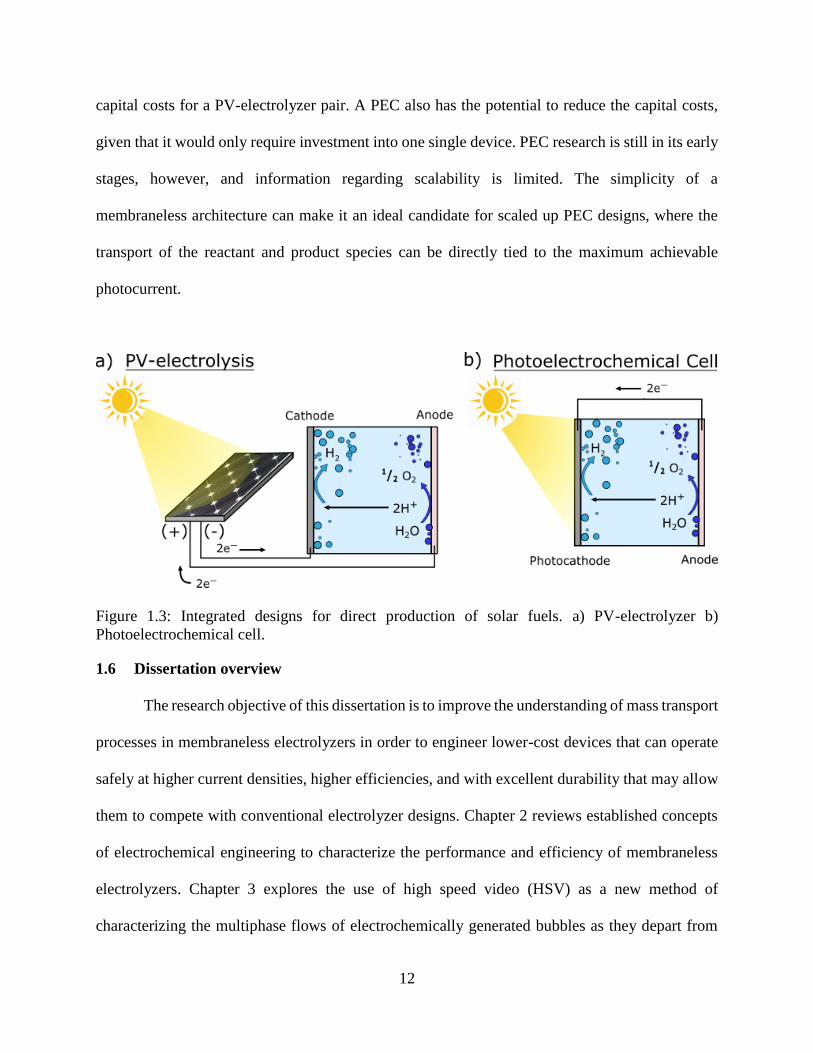
1.5 Integrating membraneless electrolyzers with solar power

Up until this point, the discussion has largely assumed that the proposed electrolyzers are

connected to a grid infrastructure which supplies clean energy. However, if membraneless

electrolyzers are to be used as a means for solar fuels production, it is important to understand how

they would be directly integrated with a solar powered system. One way is by directly coupling

the electrolyzer to a PV system, as shown in Figure 1.3a. Another way is by using a

photoelectrochemical (PEC) cell, shown in Figure 1.3b. A PEC is an all-in-one device which uses

semiconducting electrode to both extract energy from light and catalyze the electrochemical

reaction. Hydrogen can also be produced using photocatalytic suspension reactors,31 however this

area of research is largely outside the scope of this dissertation.

A key metric for comparing solar water splitting devices is the solar-to-hydrogen

efficiency, that is, the efficiency by which solar power is converted to storable chemical energy.

PV-electrolysis systems have the advantage of using two relatively mature technologies which can

be separately optimized. For a PV-electrolysis system, the record solar to hydrogen efficiency is

30%, which was achieved for a multi-junction PV cell connected to a PEM electrolyzer.32 For a

PEC, the record solar to hydrogen efficiency is 14%.33 Although PV-electrolyzers have so far been

demonstrated to be more efficient, they have the drawback of requiring capital investment into two

separate pieces of equipment. Using a membraneless electrolyzer design could help reduce the

12

capital costs for a PV-electrolyzer pair. A PEC also has the potential to reduce the capital costs,

given that it would only require investment into one single device. PEC research is still in its early

stages, however, and information regarding scalability is limited. The simplicity of a

membraneless architecture can make it an ideal candidate for scaled up PEC designs, where the

transport of the reactant and product species can be directly tied to the maximum achievable

photocurrent.

Figure 1.3: Integrated designs for direct production of solar fuels. a) PV-electrolyzer b)

Photoelectrochemical cell.

1.6 Dissertation overview

The research objective of this dissertation is to improve the understanding of mass transport

processes in membraneless electrolyzers in order to engineer lower-cost devices that can operate

safely at higher current densities, higher efficiencies, and with excellent durability that may allow

them to compete with conventional electrolyzer designs. Chapter 2 reviews established concepts

of electrochemical engineering to characterize the performance and efficiency of membraneless

electrolyzers. Chapter 3 explores the use of high speed video (HSV) as a new method of

characterizing the multiphase flows of electrochemically generated bubbles as they depart from

13

the electrodes. The findings in this chapter largely explain the physical processes taking place in a

membraneless electrolyzer.

After establishing an understanding of the modeling and transport processes in

membraneless electrolyzers, the second half of this thesis is devoted to improving their

performance and integrating them with solar powered systems. Chapter 4 explores how the

electrode design can be leveraged to optimize the efficiency of a mesh flow through electrode

while maximizing the reliability of product collection. A complete membraneless electrolyzer is

then integrated into an array of PV cells to directly generate H2 using light energy. Chapter 5

explores the application of membraneless electrolyzers to a photoelectrochemical (PEC) cell.

Concluding remarks and future directions for membraneless electrolyzers are presented in

Chapter 6.

1.7 References

1. Dominković, D. F., Bačeković, I., Pedersen, A. S. & Krajačić, G. The future of

transportation in sustainable energy systems: Opportunities and barriers in a clean energy

transition. Renew. Sustain. Energy Rev. 82, 1823–1838 (2018).

2. Joseck, F., Nguyen, T., Klahr, B. & Talapatra, A. DOE Hydrogen and Fuel Cells Program

Record #16015. (2016).

3. Zhou, F. et al. Electro-synthesis of ammonia from nitrogen at ambient temperature and

pressure in ionic liquids. Energy Environ. Sci. 10, 2516–2520 (2017).

4. Qiao, J., Liu, Y., Hong, F. & Zhang, J. A review of catalysts for the electroreduction of

carbon dioxide to produce low-carbon fuels. Chem. Soc. Rev. 43, 631–675 (2014).

5. Lu, Q. & Jiao, F. Electrochemical CO2 reduction: Electrocatalyst, reaction mechanism, and

14

process engineering. Nano Energy (2015). doi:10.1016/j.nanoen.2016.04.009

6. Shaner, M. R., Atwater, H. A., Lewis, N. S. & McFarland, E. W. A comparative

technoeconomic analysis of renewable hydrogen production using solar energy. Energy

Environ. Sci. 9, 2354–2371 (2016).

7. Dillich, S., Ramsden, T. & Melaina, M. Hydrogen Productio Cost Using Low-Cost Natural

Gas, DOE Hydrogen and Fuel Cells Program. (2012).

8. Colella, W. G., James, B. D., Moron, J. M., Saur, G. & Ramsden, T. Techno-economic

Analysis of PEM Electrolysis for Hydrogen Production. (2014).

9. Swift, K. D. A comparison of the cost and financial returns for solar photovoltaic systems

installed by businesses in different locations across the United States. Renew. Energy 57,

137–143 (2013).

10. International Energy Agency. Technology Roadmap: Solar Photovoltaic Energy. (2014).

11. Bertuccioll, L. et al. Study on development of water electrolysis in the EU. (2014).

12. Garzon, F. et al. Scientific Aspects of Polymer Electrolyte Fuel Cell Durability and

Degradation. Chem. Rev. 107, 3904–3951 (2007).

13. Oki, T., Katsumata, T., Hashimoto, K. & Kobayashi, M. Recovery of Platinum Catalyst and

Polymer Electrolyte from Used Small Fuel Cells by Particle Separation Technology. Mater.

Trans. 50, 1864–1870 (2009).

14. Laforest, V. et al. Environmental assessment of proton exchange membrane fuel cell

platinum catalyst recycling. J. Clean. Prod. 142, 2618–2628 (2016).

15. Zeng, K. & Zhang, D. Recent progress in alkaline water electrolysis for hydrogen

production and applications. Prog Energy Combust Sci 307–26 (2010).

16. Carmo, M., Fritz, D. L., Mergel, J. & Stolten, D. A comprehensive review on PEM water

15

electrolysis. Int. J. Hydrogen Energy 38, 4901–4934 (2013).

17. Xiang, C., Papadantonakis, K. M. & Lewis, N. S. Principles and implementations of

electrolysis systems for water splitting. Mater. Horiz. 3, 169–173 (2016).

18. Paidar, M., Fateev, V. & Bouzek, K. Membrane electrolysis - History, current status and

perspective. Electrochim. Acta 209, 737–756 (2016).

19. Ayers, K. E. et al. Research Advances towards Low Cost, High Efficiency PEM

Electrolysis. in ECS Transactions 33, 3–15 (2010).

20. Bergner, D. Membrane cells for chlor-alkali electrolysis. J. Appl. Electrochem. 12, 631–644

(1982).

21. Ping, Q., Cohen, B., Dosoretz, C. & He, Z. Long-term investigation of fouling of cation and

anion exchange membranes in microbial desalination cells. Desalination 325, 48–55

(2013).

22. Zhang, S. et al. A review of accelerated stress tests of MEA durability in PEM fuel cells.

Int. J. Hydrogen Energy 34, 388–404 (2009).

23. Santos, D. M. F., Sequeira, C. A. C. & Figueiredo, J. L. Hydrogen production by alkaline

water electrolysis. Quim. Nova 36, 1176–1193 (2013).

24. Choban, E., Markoski, L., Wieckowski, A. & Kenis, P. Microfluidic fuel cell based on

laminar flow. J. Power Sources 128, 54–60 (2004).

25. Kjeang, E., Michel, R., Harrington, D. a., Djilali, N. & Sinton, D. A microfluidic fuel cell

with flow-through porous electrodes. J. Am. Chem. Soc. 130, 4000–4006 (2008).

26. Braff, W. a, Bazant, M. Z. & Buie, C. R. Membrane-less hydrogen bromine flow battery.

Nat. Commun. 4, 2346 (2013).

27. Braff, W. a., Buie, C. R. & Bazant, M. Z. Boundary Layer Analysis of Membraneless

16

Electrochemical Cells. J. Electrochem. Soc. 160, A2056–A2063 (2013).

28. Hashemi, S. M. H., Modestino, M. A. & Psaltis, D. A membrane-less electrolyzer for

hydrogen production across the pH scale. Energy Environ. Sci. 8, 2003–2009 (2015).

29. Gillespie, M. I., van der Merwe, F. & Kriek, R. J. Performance evaluation of a

membraneless divergent electrode-flow-through (DEFT) alkaline electrolyser based on

optimisation of electrolytic flow and electrode gap. J. Power Sources 293, 228–235 (2015).

30. O’Neil, G. D., Christian, C. D., Brown, D. E. & Esposito, D. V. Hydrogen Production with

a Simple and Scalable Membraneless Electrolyzer. J. Electrochem. Soc. 163, F3012–F3019

(2016).

31. Mckone, J. R., Lewis, N. S. & Gray, H. B. Will Solar-Driven Water-Splitting Devices See

the Light of Day? Chem. Mater. 26, 407–414 (2014).

32. Jia, J. et al. Solar water splitting by photovoltaic-electrolysis with a solar-to-hydrogen

efficiency over 30%. Nat. Commun. 7, 13237 (2016).

33. May, M. M., Lewerenz, H., Lackner, D., Dimroth, F. & Hannappel, T. Efficient direct solar-

to-hydrogen conversion by in situ interface transformation of a tandem structure. Nat.

Commun. 6, 1–7 (2015).

17

DESIGN PRINCIPLES FOR MEMBRANELESS ELECTROLYZERS

Chapter 1 outlined three important metrics used for evaluating the performance of an

electrolysis system: efficiency, capital cost, and durability. Although a full technoeconomic

analysis of membraneless electrolyzers is outside the scope of this dissertation, one could imagine

that each of these metrics is governed by an optimizable objective function. The equations that

form the basis of this objective function are highly coupled, meaning that designing an electrolyzer

with the aim of improving one metric can easily cause another metric to become worse off. For

example, using a more efficient electrocatalyst material may cause the efficiency of the

electrolyzer to increase, but if the material is more expensive it will also increase the capital costs.

Behind the overall objective function is the governing physics of the electrochemical system.

Recognizing this, Chapter 2 provides an overview of the thermodynamics, kinetics, and transport

phenomena that governing the performance and design considerations for membraneless

electrolyzers. At the end of this chapter, these concepts are built into a framework for modeling

the performance of a membraneless electrochemical cell.

2.1 Thermodynamics of the water electrolysis reaction

The efficiency of an electrolyzer is calculated by comparing the actual power consumed to

the theoretical minimum power based on thermodynamics. For any electrical system, the power

consumed is the product of current and voltage. The current of an electrolyzer is directly

proportional to the rate of reaction, which can be calculated using Faraday’s law shown in

Equation 2.1. The voltage, on the other hand, describes the change in energy state of the reactants

18

and products. Equation 2.2 shows that the change in Gibbs free energy at standard state can be

used to calculate the cell potential 𝑈𝑐𝑒𝑙𝑙0 .

𝐼 = 𝑟 ∙ 𝑛 ∙ 𝐹 2.1

𝑈𝑐𝑒𝑙𝑙

0 = −Δ𝐺0

𝑛𝐹

2.2

Typically, in chemical engineering processes, quantities are expressed using moles. In Equation

2.1, the reaction rate 𝑟 is expressed in dimensions of moles per unit time. Similarly, the Gibbs free

energy of formation, 𝐺0, has dimensions of energy per mole. In electrochemistry, however, it is

typically more convenient to convert from units of moles to units of charge. This is achieved by

either multiplying or dividing by number of electrons participating in the overall reaction, 𝑛, and

the Faraday number, 𝐹. In this way, the reaction rate can be described using the current, 𝐼, which

has dimensions of charge per unit time. Equation 2.2 shows that the cell potential, 𝑈𝑐𝑒𝑙𝑙0 , is the

change in free energy per unit charge passed through the electrolyzer. In the previous chapter, we

established that for the water splitting reaction, 𝑈𝑐𝑒𝑙𝑙0 = −1.23 𝑉.

However, a water electrolysis system does not always operate at standard state. Under non-

standard conditions, the reduction potential at each electrode must be recalculated using the Nernst

Equation. Equations 2.3 and 2.4 show the non-standard reduction potentials for HER and OER,

respectively:1

𝑈𝐻2|𝐻+ = 𝑈𝐻2|𝐻+0 −

𝑅𝑇

2𝐹ln [

𝑃𝐻2

1 𝑏𝑎𝑟

(𝑐𝐻+

1 𝑀 )2 ] 2.3

𝑈𝐻2𝑂|𝑂2= 𝑈𝐻2𝑂|𝑂2

0 +𝑅𝑇

2𝐹ln [(

𝑐𝐻+

1 𝑀 )

2

√𝑃𝑂2

1 𝑏𝑎𝑟 ] 2.4

19

where 𝑈𝑗 is the reversible potential at non-standard conditions for each half reaction 𝑗, 𝑅 is the gas

constant, 𝑇 is the temperature, 𝑃𝐻2 is the partial pressure of H2, 𝑃𝑂2 is the partial pressure of O2,

and 𝑐𝐻+ is the concentration of protons in the electrolyte. The dependence on concentration and

partial pressure for each equation is based on the activity ratio of the respective half reaction. Each

species activity is raised to the power of its stoichiometric coefficient. The activity of the solvent

water is assumed to be 1. When the system is at standard state, 𝑐𝐻+ = 1 M and 𝑃𝐻2 = 𝑃𝑂2 = 1 bar,

and therefore 𝑈𝑗 = 𝑈𝑗0 for both half reactions.

Operating at elevated pressures will cause the value of 𝑈𝑐𝑒𝑙𝑙 = 𝑈𝐻2|𝐻+ − 𝑈𝐻2𝑂|𝑂2 to

increase. Likewise, allowing for a concentration gradient across the electrodes can also cause the

value of 𝑈𝑐𝑒𝑙𝑙 to increase. One should note that the value of 𝑐𝐻+ in Equations 2.3 and 2.4 should

be evaluated locally at each electrode. If 𝑐𝐻+, and consequently the pH, is the same at both

electrodes, then the Nernstian shift for 𝑈𝐻2|𝐻+ and 𝑈𝐻2𝑂|𝑂2 will cancel each other. However, over

long periods of operation, a concentration gradient can form if there is no significant mixing in the

electrolyte.

One motivation for operating an electrolyzer in strongly acidic or strongly alkaline

electrolytes is that the local change in pH across the cell will be negligible at practical current

densities. This prevents additional voltage penalties described by the Nernst equation. However,

when using an unbuffered pH-neutral electrolyte such as sodium sulfate, a concentration gradient

will form across the cell. In a flow-through membraneless electrolysis system reported by Talabi,

et al., this concentration gradient was deliberately formed as a means for simultaneous production

of acid and base.2 At the cathode, protons were locally consumed according to Equation 1.1,

causing the local pH to become more alkaline. At the anode, protons were locally generated

according to Equation 1.2, causing the local pH to become more acidic. Along with the

20

electrochemically generated H2 and O2, the resulting acid and base streams were collected.

Although the resultant concentration gradient caused the total voltage required for electrolysis to

increase, the extra voltage penalty can be justified if the acid and base streams are able to be

collected at quantities and concentrations that are practical for commercial use.

In summary, a thermodynamic analysis is necessary for determining the minimum

theoretical voltage required for water electrolysis. The Nernst equation can be used to determine

the value of the minimum cell voltage 𝑈𝑐𝑒𝑙𝑙 at non-standard conditions. In reality, an applied

voltage that exceeds 𝑈𝑐𝑒𝑙𝑙 is required to overcome losses due to kinetics, ionic conduction, and

mass transport. Being able to calculate 𝑈 for each electrode half reaction is also important for

understanding the relationship between the external voltage applied to the electrode and the kinetic

rate of reaction. In the next section, this relationship is discussed in greater detail in the context of

membraneless electrolyzer designs.

2.2 Kinetics

One reason that designing a membraneless electrolyzer is challenging is that it requires

careful consideration of phenomena that occur across a wide range of length scales. The

performance of an electrolyzer device, which typically occupies space on the cm to m length scale,

can be determined in part by the kinetics of the reaction, which are engineered at the Å to nm scale.

The kinetics of the surface reaction are often dictated by the properties of the electrode material

and the contents of the surrounding electrolyte. In an acidic electrolyte, the state-of-the-art

electrode materials are platinum (Pt) for HER and iridium (Ir) for OER. These materials are scarce

and expensive, and research in this area focuses on developing alternative electrode materials

which are low-cost, active, and stable over long periods of operation. Although improved

21

electrocatalyst materials have the potential to lower the overall capital costs and increase

efficiency, research in this area is largely outside the scope of this dissertation.

Nonetheless, understanding the kinetic processes at the electrode/electrolyte interface is

essential for designing an electrochemical cell. In order to better understand the relationship

between the electrode surface and its catalytic properties, we first draw attention to the

thermodynamic driving force of the electrode half reaction: the surface overpotential, 𝜂𝑠. In the

previous section, we detailed how to calculate the reversible potential 𝑈 of an electrode at

thermodynamic equilibrium. An overpotential at the electrode surface is the difference between

the externally applied potential of the electrode, 𝑉, and the reversible potential of the half reaction,

shown in Equation 2.5.

𝜂𝑠 = 𝑉 − 𝑈 2.5

It is important to note that 𝑉 in Equation 2.5 is not the overall voltage applied to the electrochemical

cell, but rather the local thermodynamic potential of the electrode in contact with the electrolyte.

When 𝑉 > 𝑈, 𝜂𝑠 is positive and the driving force for the reaction favors oxidation. When 𝑉 < 𝑈,

𝜂𝑠 is negative and the reaction equilibrium shifts towards reduction. Lastly, when 𝑉 = 𝑈, 𝜂𝑠 is

zero and no current passes through the electrode because it is at equilibrium.

The relationship between current density and surface overpotential is described by the

Butler Volmer equation, which is derived for a single electron transfer reaction (Equation 2.6):1

𝑖 = 𝑖0 [exp (

𝛼𝐴𝐹𝜂𝑠

𝑅𝑇) − exp (

−𝛼𝐶𝐹𝜂𝑠

𝑅𝑇)]

2.6

where 𝑖 is the current density of the electrode half reaction, 𝑖0 is the exchange current density, and

𝛼𝐴 and 𝛼𝐶 are the apparent transfer coefficients. By convention, positive values of 𝑖 refer to

oxidation currents whereas negative values refer to reduction currents. The exchange current

density 𝑖0 is a property of the electrode material, and is descriptive of the rate of the forward and

22

reverse reactions when they are at equilibrium with each other. The magnitude of 𝑖0 correlates

directly to the catalytic activity of the electrode material. When the overpotential is sufficiently

large, it can be shown that the Tafel equation applies, and is reported below in Equations 2.7 and

2.8. Equation 2.7 is the Tafel equation for anodic currents at positive overpotentials, and Equation

2.8 is the Tafel equation for cathodic currents at negative overpotentials.

𝑖 = 𝑖0 exp [

𝛼𝐴𝐹𝜂𝑠

𝑅𝑇]

2.7

𝑖 = −𝑖0 exp [−

𝛼𝐶𝐹𝜂𝑠

𝑅𝑇]

2.8

The Tafel equation is particularly useful for describing the kinetics of the half reactions in

electrolyzers, where high current densities and therefore large overpotentials are necessary to

produce practical quantities of H2. This relationship is also convenient because it is easy to extract

kinetic rate parameters from experimental data. Equation 2.9 shows the linear form of the Tafel

Equation, which is used for a so-called Tafel analysis.

𝜂𝑠 =

𝑅𝑇

𝛼𝐹ln(|𝑖|) −

𝑅𝑇

𝛼𝐹ln(𝑖0)

2.9

A linear plot of 𝜂𝑠 vs ln(|𝑖|) can be used to determine the values of 𝛼 and 𝑖0 for a given electrode

half reaction on a specific material. The quantity 𝑅𝑇

𝛼𝐹 is often referred to as the Tafel slope, and 𝑖0

can be calculated based on the intercept. O’Neil et. al performed a Tafel analysis on Pt-coated

titanium (Ti) mesh flow through electrodes which were used in a membraneless electrolyzer, the

results of which are reproduced in Table 2.1.3 These electrodes are similar to the electrodes used

in chapters 3 and 4 of this dissertation.

23

Table 2.1: Tafel kinetic parameters for HER and OER on Pt mesh flow through electrodes,

reproduced from O’Neil, et al.3

𝒊𝟎 / A cm-2 𝑹𝑻

𝜶𝑭 / mV

HER on Pt 6.6 E-04 38.8 ±- 2.2

OER on Pt 1.8 E-07 133.2± 9.0

The Tafel analysis for Table 2.1 was carried out in 0.5 M sulfuric acid. 𝑖0 for HER on Pt is

several orders of magnitude larger than 𝑖0 for OER. Although Pt is the state-of-the-art electrode

material for HER, it is not very efficient as an OER catalyst. In many cases, at least 500 mV of

overpotential at the anode are required before a sufficient onset of current density can be observed.

Thus, even though a minimum voltage of 1.23 V is thermodynamically predicted for electrolysis,

practical current densities for a pair of Pt electrodes in 0.5 M H2SO4 are not realized until a total

voltage of at least 1.8 V is applied.

An optimized combination of electrode materials can decrease the surface overpotential to

improve the efficiency of the electrolyzer. For the experiments presented in this dissertation, Ti

coated Pt electrodes were used because of their stability in 0.5 M sulfuric acid at both reducing

and oxidizing potentials. While the catalytic activity of Pt for HER in acid is excellent, its activity

for OER in acid is at least tolerable for the purposes of characterizing new electrolyzer designs. A

comprehensive study by McCrory et al benchmarks the catalytic activity of several electrode

materials in both acidic and alkaline electrolytes.4 Operating in alkaline conditions has the

advantage of offering a wider selection of catalyst materials. Nickel, for example, corrodes in acid

but in an alkaline electrolyte it is an active and stable anode material for OER. A drawback of

alkaline electrolytes, however, is their lower conductivity relative to acidic electrolytes. This lower

24

conductivity increases the ohmic resistance of the electrolyzer, potentially offsetting any

advantages from decreasing the activation overpotential.

Ohmic resistances can also have a strong impact on the overall efficiency of an electrolyzer.

Conceptually, it is useful to think of the relationship between current density and overpotential

using a charge transfer resistance, 𝑅𝐶𝑇. At large overpotentials, the charge transfer resistance can

be calculated by evaluating the derivative of ηs from the Tafel equation at the average current

density, shown in Equation 2.10.

𝑅𝐶𝑇 =

𝜕𝜂

𝜕𝑖|

𝑖=𝑖𝑎𝑣𝑔

=𝑅𝑇

𝛼𝐹|𝑖𝑎𝑣𝑔|

2.10

At large current densities, the charge transfer resistance becomes negligible, and the relationship

between current and voltage is no longer described by the Tafel equation. Rather, the performance

of the electrolyzer is limited by the conduction of ions in the electrolyte. Ionic conduction is

governed by Ohm’s law, which will be discussed in greater detail in the next section.

2.3 Ohmic Resistance

When an electric field is applied across an electrolyte, the ions will flow in response. This

flow of ions is necessary to complete the circuit of an electrochemical cell. The magnitude of ionic

flow, or current, depends on the strength of the electric field and the ohmic resistance of the

electrolyte. This relationship is widely known as Ohm’s law, and the differential form is shown in

Equation 2.11:

𝑖 = 𝜅∇𝜙 2.11

where 𝜙(𝑥, 𝑦, 𝑧) is the local potential of the electrolyte and 𝜅 is the conductivity. If the potential

field across an electrolyte domain is known, the integrated form of Ohm’s law can be solved for,

shown in Equation 2.12:1

25

Δ𝑉 = 𝐼𝑅Ω 2.12

where Δ𝑉 is the voltage drop between electrodes, 𝐼 is the total current, and 𝑅Ω is the overall ohmic

resistance of the electrolyte. The ohmic resistance is a function of the electrolyte conductivity 𝜅,

and the geometry of the electrodes. For a pair of planar electrodes enclosed by insulating walls,

𝑅Ω can be solved for directly using the electrode separation distance, 𝐿, and the nominal area of

the electrodes 𝐴𝑐. This relationship is shown in Equation 2.13.

𝑅Ω =

𝐿

𝐴𝑐𝜅

2.13

The cross-sectional area of the electrolyte channel is assumed to be equal to the area of the

electrodes. In some derivations of the overall ohmic resistance, numerator of Equation 2.13 may

also include a cell constant, 𝛽𝑟, to account for geometries where the electrodes are not parallel,

have non-planar shapes, or have unequal areas.5 In these cases, 𝛽𝑟 serves as a dimensionless shape

factor with a magnitude typically on the order of 1. For a pair of large, parallel electrodes, 𝛽𝑟 = 1.

When the electrodes are not parallel, the value of 𝛽𝑟 will depend on how 𝐿 is defined. If available,

an analytical solution can calculate an exact value of 𝛽𝑟, and is typically a dimensionless ratio of

important length scales in the reactor design. 𝛽𝑟 can also be obtained from simulations, which will

be explained in greater detail in section 2.5 of this chapter. Newman, for example, has shown both

analytically and using simulations that 𝛽𝑟 =𝜋

4 for the ohmic resistance between a rotating disc

electrode and a faraway reference electrode.6

Ohm’s law reveals the trade-off between productivity and efficiency for an electrolyzer.

For example, a water electrolyzer produces the most H2 when the current is maximized. However,

Ohm’s law clearly indicates that increasing the current will also increase the voltage penalty

26

required to conduct ions between the electrodes. Therefore, to minimize this efficiency loss, the

ohmic resistance should be as low as possible when designing an electrolyzer.

One way to decrease the ohmic resistance is to increase the conductivity, 𝜅, of the

electrolyte. Typically, 𝜅 can be calculated using Equation 2.14, and depends directly on the

concentration 𝑐𝑗, mobility 𝑢𝑗 , and valence charge 𝑧𝑗 of each ion 𝑗 present in the electrolyte.1 For

the majority of demonstrations of membraneless electrolyzers in this dissertation, 0.5 M H2SO4 is

used and has a conductivity of 0.226 S/cm.7 The conductivity of an electrolyte typically scales

linearly with its ion concentration, but the relationship becomes non-linear at high concentrations.

Using higher acid concentrations also introduces hazards due to the general corrosiveness of the

electrolyte. Concentrated acids can be dangerous to handle and may require additional safety

protocols if used on an industrial scale. They may also require the electrolyzer to be constructed

out of more expensive, corrosion resistant parts.

𝜅 = 𝐹2 ∑ 𝑧𝑗2𝑢𝑗𝑐𝑗

𝑗

2.14

Another way to minimize the ohmic resistance is to decrease the separation distance 𝐿

between the electrodes. This is largely the motivation for using an ion conducting solid electrolyte

such as a Nafion membrane. Nafion membranes used in PEM electrolyzers typically have

thicknesses between 100 and 200 μm.2 Demonstrations of microfluidic membraneless

electrolyzers have also achieved electrode separation distances as narrow as 150 μm, but the lack

of a physical barrier presents challenges with managing the product gas flows of H2 and O2.

Related to this complicated interplay of ionic transport and gas phase transport is the area of the

electrodes themselves. Increasing the electrode area can also decrease the ohmic resistance of the

electrolyzer, but this also raises questions on how to precisely control fluid flow and maintain

effective separation of anode and cathode products over larger length scales. For example, the

27

electrode area for a parallel plate design such as in Figure 1.2a can be increased simply by making

the electrodes longer. However, as bubbles detach and migrate away from the channel wall, their

probability of crossover will likely increase with longer travel distances and residence times spent

in the channel. A major focus of this dissertation is to better understand the physical mechanisms

of product gas transport in order to improve the product purity of collected gases and demonstrate

safe operation at close electrode separation distances.

The discussion in this section has focused mostly on the ohmic resistance as it relates to

the electrolyte of a membraneless electrolyzer. However, the contacts between the electrolyzer and

the external circuit can also contribute to the overall resistance. Maintaining high quality electrical

connections is important for ensuring efficient operation throughout the life of the electrolyzer.

Degradation and corrosion of the contacts over time can increase the overall ohmic resistance. In

a laboratory setting, if a higher than normal ohmic resistance is measured, a good first step is to

check that the external contacts are connected properly and free of corroded surfaces. Sometimes,

a source of ohmic resistance is the electrode material itself. Typically, this is not considered as

metallic electrodes have a conductivity that is several orders of magnitude higher than that of the

electrolyte. However, Equation 2.13 also applies to the calculation of electronic conduction in an

electrode material. At large electrode length scales, the ohmic drop within the electrode may be

relevant to the overall resistance.

Lastly, the ohmic resistance of a membraneless electrolyzer can also increase due to the

presence of the electrochemically generated gas bubbles. Gases behave as insulators, and when

they occupy area on an electrode surface, the effective cross-sectional area available for ionic

conduction decreases. In the bulk electrolyte, the presence of bubbles can be modeled using an

effective conductivity of the electrolyte. Equation 2.15 is known as the Bruggeman correlation,6,8

28

and is an empirical correlation between the effective conductivity of the electrolyte 𝜅𝑒𝑓𝑓 and the

void fraction of gas bubbles in the liquid electrolyte, 𝜖.

𝜅𝑒𝑓𝑓 = 𝜅(1 − 𝜖)1.5 2.15

As the void fraction of gas bubbles increases, the effective conductivity decreases to account for

the decrease in accessible volume for ions to conduct through. In a membraneless electrolyzer,

using flowing electrolyte can help remove gas bubbles and thereby decrease the bubble void

fraction, resulting in decreased overall ohmic resistance of the device. The next section reviews

transport processes which take place in electrochemical cells.

2.4 Transport

In the previous section, we addressed the efficiency losses due to the conduction of ions

between electrodes. Although ionic conduction is necessary for a complete circuit in an

electrochemical cell, it is not the only mode of transport in an electrolyte. Equation 2.16 shows the

Nernst-Planck Equation for the total molar flux of all species present in the electrolyte:1

𝑵𝒊 = −𝑧𝑖𝑢𝑖𝐹𝑐𝑖𝛻𝜙 − 𝐷𝛻𝑐𝑖 + 𝑐𝑖𝒗 2.16

For a given species 𝑖, 𝑧𝑖 is the valance charge, 𝑢𝑖 is the ionic mobility, 𝑐𝑖(𝑥, 𝑦, 𝑧) is the local

concentration, and 𝐷𝑖 is the diffusion coefficient. 𝜙(𝑥, 𝑦, 𝑧) is the local potential of the electrolyte

and 𝒗 is the velocity vector. The first term in Equation 2.16 is simply Ohm’s law, describing how

ions move in response to the local potential gradient, ∇𝜙. This term is often referred to as the

migration current. The second term refers to the diffusion of species throughout the electrolyte in

the presence of a concentration gradient. The last term on the right is the convection term. The

total ionic current can be calculated by summing up the fluxes of all species, as shown in Equation

2.17:

29

𝑖 = 𝐹 ∑ 𝑧𝑖𝑵𝒊

𝑖

2.17

An important constraint in electrochemical systems is the electroneutrality condition,

which states that the total sum of all charges at any location in the electrolyte must be zero

(Equation 2.18). When Equation 2.16 is summed up using Equation 2.17, it can be shown that the

convection term for ionic currents can be neglected due to electroneutrality. The resulting

combined equation for the ionic current is Equation 2.19.

∑ 𝑧𝑖𝑐𝑖

𝑖

= 0 2.18

𝑖 = −𝐹 ∑(𝑧𝑗2𝑢𝑗𝐹𝑐𝑗∇𝜙 + 𝑧𝑗𝐷𝑗∇𝑐𝑗)

𝑗

2.19

Concentration gradients typically form as the operating current of the electrolyzer

approaches the mass transfer limited current, 𝑖𝑙𝑖𝑚. An electrochemical device reaches 𝑖𝑙𝑖𝑚 when

the limiting process is no longer the reaction kinetics, but rather the mass transport in the

electrolyte. When a diffusing species carries an ionic charge, Equation 2.19 shows that it can be

affected by both the electric field and the concentration gradient. Being able to solve Equation 2.19

in its entirety can be complicated and difficult to achieve convergence. Good physical intuition of

the system can help guide decisions on how to simplify the model and obtain a solution.

For an initial guess of the mass transport limited current, the electric field can be

temporarily neglected in the case where there is excess supporting electrolyte. In such a case, one

must solve for the diffusive flux of the limiting reagent across a diffusion boundary layer. For

diffusion to a planar electrode across a boundary layer of thickness 𝛿, the concentration profile

across the boundary layer is linear and the limiting current can be obtained from Fick’s law

(Equation 2.20):

30

𝑖𝑙𝑖𝑚 = 𝑛𝐹𝐷𝑖

𝑐𝑖,𝑏𝑢𝑙𝑘

𝛿 2.20

where 𝑐𝑖,𝑏𝑢𝑙𝑘 is the bulk concentration of reagent 𝑖 and 𝑛 is the number of electrons participating

in the electrode half reaction. The best way to determine the thickness and profile of 𝛿 is by first

determining the dominant mode of transport in the electrolyte. This can be calculated using the

Péclet number (𝑃𝑒), defined in Equation 2.21. 𝑃𝑒 is the dimensionless ratio of the convective

transport rate to the diffusive transport rate, where 𝑈 is the characteristic velocity, 𝐿 is the

characteristic length, and 𝐷 is the diffusion coefficient of the limiting reagent.

𝑃𝑒 =

𝑈𝐿

𝐷

2.21

When the value of 𝑃𝑒 ≫ 1, convection is the dominant mode of transport. In such a case, the

diffusion boundary layer can be solved based on the developed flow profile near the electrode.

Several empirical correlations for 𝛿 exist in the literature, where 𝛿 is a function of the Reynolds

number 𝑅𝑒 and the Schmidt number 𝑆𝑐.1

As 𝑃𝑒 → 0, bulk diffusion becomes the dominant mode of transport. In such a case, a

diffusion cloud will grow at the electrode surface, and 𝛿 will increase as a function of time, such

as in the Cottrell equation.5 After long periods of operation, a steady state diffusion boundary layer

can also be achieved. However, a purely diffusion limited current is rarely expected to arise in a

membraneless electrolyzer, where the product gases are separated using bulk convection. Even in

cases when there is no pumped electrolyte, the free convection of the departing bubbles can be

expected to have a large impact on the diffusion boundary layer thickness. Free convection is

particularly relevant to the studies presented in Chapters 3 and 4.

Regardless of the thickness of the diffusion boundary layer, the bulk reactant concentration

in Equation 2.20 is also a driving force of the limiting current density. The relevant concentration

31

is determined by the limiting reagent of an electrode half reaction. A membraneless electrolyzer

operating in 0.5 M H2SO4 will be limited by the concentration of protons at the cathode and by the

concentration of the solvent water at the anode. In reality, these concentrations are quite large, and

therefore neither electrode half reaction is expected to be limited by mass transport of the reactant

species at practical current densities. However, for electrolysis reactions such as CO2 reduction in

an aqueous electrolyte, the bulk concentration of CO2 is limited by its solubility. In these cases,

understanding and modeling the diffusion boundary layer thickness may be more relevant to the

overall performance of the device. This topic of discussion is explored in greater detail in Chapter

5, where forced convection is used to enhance the rate of mass transport in a device with dilute

reactant concentrations.

It is important to note that although the convection term does not appear explicitly in

Equation 2.19, the bulk fluid velocity is an important component for calculating the diffusion

boundary layer. Equation 2.19 also assumes that the concentration of ions is dilute relative to the

concentration of the supporting electrolyte. Thus, the ionic current between the electrodes is not

expected to directly influence the macroscopic flow properties of the electrolyte, and in many

cases, the two can be modeled independently.

To model the transport of non-charged species, such as the solvent water or the

electrochemically generated gas bubbles, the Navier-Stokes equations are used. Modeling

multiphase flows can be particularly difficult, and the computational cost depends on the total

number of bubbles present, the size distribution of the bubbles, and the size of the bubbles relative

to the critical dimensions of the electrolyzer cell. Understanding these transport processes as they

relate to the collection of product gases in membraneless electrolyzers is a topic of ongoing

research. In Chapters 3 and 4, both quantitative and qualitative observations are made to

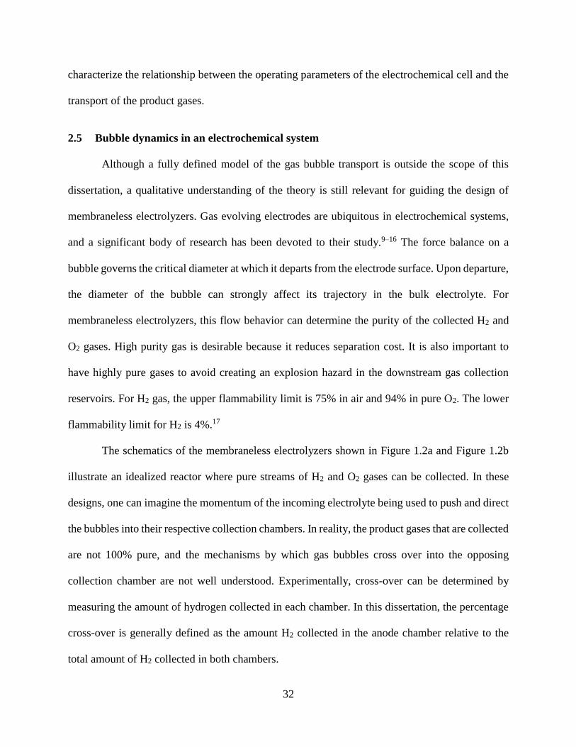
32

characterize the relationship between the operating parameters of the electrochemical cell and the

transport of the product gases.

2.5 Bubble dynamics in an electrochemical system

Although a fully defined model of the gas bubble transport is outside the scope of this

dissertation, a qualitative understanding of the theory is still relevant for guiding the design of

membraneless electrolyzers. Gas evolving electrodes are ubiquitous in electrochemical systems,

and a significant body of research has been devoted to their study.9–16 The force balance on a

bubble governs the critical diameter at which it departs from the electrode surface. Upon departure,

the diameter of the bubble can strongly affect its trajectory in the bulk electrolyte. For

membraneless electrolyzers, this flow behavior can determine the purity of the collected H2 and

O2 gases. High purity gas is desirable because it reduces separation cost. It is also important to

have highly pure gases to avoid creating an explosion hazard in the downstream gas collection

reservoirs. For H2 gas, the upper flammability limit is 75% in air and 94% in pure O2. The lower

flammability limit for H2 is 4%.17

The schematics of the membraneless electrolyzers shown in Figure 1.2a and Figure 1.2b

illustrate an idealized reactor where pure streams of H2 and O2 gases can be collected. In these

designs, one can imagine the momentum of the incoming electrolyte being used to push and direct

the bubbles into their respective collection chambers. In reality, the product gases that are collected

are not 100% pure, and the mechanisms by which gas bubbles cross over into the opposing

collection chamber are not well understood. Experimentally, cross-over can be determined by

measuring the amount of hydrogen collected in each chamber. In this dissertation, the percentage

cross-over is generally defined as the amount H2 collected in the anode chamber relative to the

total amount of H2 collected in both chambers.

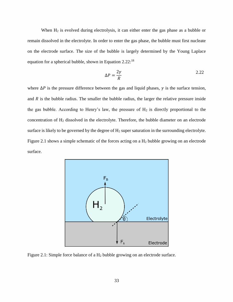
33

When H2 is evolved during electrolysis, it can either enter the gas phase as a bubble or

remain dissolved in the electrolyte. In order to enter the gas phase, the bubble must first nucleate

on the electrode surface. The size of the bubble is largely determined by the Young Laplace

equation for a spherical bubble, shown in Equation 2.22:18

Δ𝑃 =

2𝛾

𝑅

2.22

where Δ𝑃 is the pressure difference between the gas and liquid phases, 𝛾 is the surface tension,

and 𝑅 is the bubble radius. The smaller the bubble radius, the larger the relative pressure inside

the gas bubble. According to Henry’s law, the pressure of H2 is directly proportional to the

concentration of H2 dissolved in the electrolyte. Therefore, the bubble diameter on an electrode

surface is likely to be governed by the degree of H2 super saturation in the surrounding electrolyte.

Figure 2.1 shows a simple schematic of the forces acting on a H2 bubble growing on an electrode

surface.

Figure 2.1: Simple force balance of a H2 bubble growing on an electrode surface.

34

In this diagram, the buoyancy force 𝐹𝐵 lifts the bubble upwards while the surface tension

force 𝐹𝑆 pulls to keep the bubble attached to the electrode. Equation 2.23 shows the buoyancy force

is a function of the bubble radius:19

𝐹𝐵 =

4

3𝜋𝑅3𝛥𝜌𝑔

2.23

where 𝛥𝜌 is the difference in density between the gas and the electrolyte and 𝑔 is the gravitational

constant. As the bubble radius increases, the buoyancy force eventually exceeds the surface tension

force and the bubble departs from the electrode surface. Also shown in Figure 2.1 is the contact

angle between the bubble and the electrode surface, 𝜃. The contact angle can be used to calculate

the surface tension force, and is related to the hydrophilicity of the electrode surface. When 𝜃 <

90°, the electrode is hydrophilic and prefers contact with electrolyte. When 𝜃 > 90°, the surface

is hydrophobic and prefers contact with the gas bubble. The contact angle is a property of the

electrode material and the composition of the gas and surrounding electrolyte.

The force balance shown in Figure 2.1 is simplified, and there are in reality many other

forces which act on the bubble. In the presence of forced convection, the drag forces and lift forces

acting on the bubble can also affect the departure diameter. A more complete force balance

diagram on a bubble is offered by Taqieddin, et al.20 Although detailed models exist for a single

bubble force balance and departure diameter, gas evolving electrodes typically produce a wide

distribution of bubble sizes, many of which are significantly smaller than what would be predicted

based on the force balance. The departure of a neighboring bubble induces turbulence, causing the

surrounding bubbles to depart even if they have diameters smaller than the predicted departure

diameter.20 The surface tension forces surrounding a bubble are also not constant, and can change

as a function of the dissolved gas concentration.20

35

Once a bubble detaches from the electrode surface, it is exposed to lift and drag forces

which cause it to permeate throughout the electrolyte.21 Hashemi, et al. proposed that a balance

between lift forces and wall forces, known as the Segré-Silberberg effect, can be engineered to

predict and control where the bubbles migrate in a membraneless flow channel.22 In the context of

a membraneless electrolyzer, these forces are still not fully understood and it is challenging to

relate stochastic bubble phenomena with the overall performance of the device. As a part of the

work of this dissertation, observations of the bubble dynamics in a membraneless electrolyzer are

related to the predicted current distributions typically solved for in electrochemical systems. In the

next section, these current distributions and the governing equations behind them are explored in

greater detail.

2.6 Approach to modeling the ionic current in an electrolyzer

Having established the fundamentals of thermodynamics, kinetics, and mass transport for

electrochemical cells, this last section of the chapter outlines how to connect these concepts into a

computational model. The ultimate goal of this modeling framework is to be able to model or

predict the current distribution on electrodes (for cases where there is non-uniform current

distribution) and the overall current-voltage curve for an electrolysis device of known geometry.

Knowing the current-voltage curve for the electrolysis device, it is easy to compute the electrolyzer

efficiency by Equation 1.5. A visual framework for the approach taken in this dissertation is shown

in Figure 2.2, which is largely inspired by the approach given in Chapter 6 of Electrochemistry

and Electrochemical Engineering.5 The starting point for this analysis is the Nernst-Planck

Equation (Equation 2.16). As mentioned previously, solving Equation 2.16 without simplification

can be tedious, computationally expensive, and difficult to achieve convergence. Rather,

simplifying the governing physics and judiciously neglecting terms in Equation 2.16 can yield

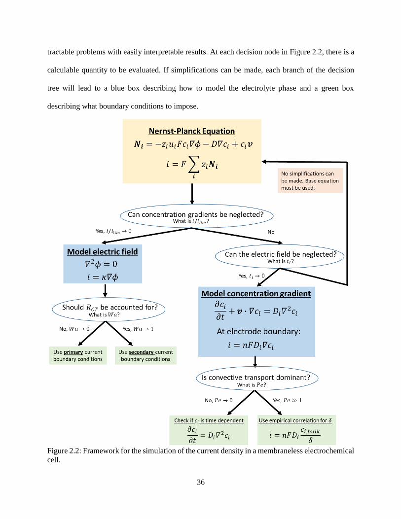
36

tractable problems with easily interpretable results. At each decision node in Figure 2.2, there is a

calculable quantity to be evaluated. If simplifications can be made, each branch of the decision

tree will lead to a blue box describing how to model the electrolyte phase and a green box

describing what boundary conditions to impose.

Figure 2.2: Framework for the simulation of the current density in a membraneless electrochemical

cell.

37

The first decision node in Figure 2.2 checks to see if concentration gradients can be

ignored. This is determined by calculating the dimensionless quantity 𝑖/𝑖𝑙𝑖𝑚, where 𝑖 is the

designed operating current density. This dimensionless grouping can be thought of as a Damkohler

number, which compares the kinetically limited rate of reaction to the mass transfer limited rate of

reaction. In the previous section, we reviewed a simplified approach for calculating 𝑖𝑙𝑖𝑚 assuming

that electrical migration can be neglected. For common acidic and alkaline electrolytes used for

water electrolysis, 𝑖𝑙𝑖𝑚 is often times expected to be very large therefore can be assumed that

𝑖/𝑖𝑙𝑖𝑚 → 0. A sample calculation of the limiting current density in an electrolyzer in 0.5 M H2SO4

is given in Chapter 3, Appendix A, section 3.5.2.

2.6.1 Modeling the electric field

As long as the operating current is significantly below the mass transfer limited current,

then the electrolyte can be assumed to be well mixed and we are able to neglect the effect of

concentration gradients. The Nernst-Planck equation then simplifies to differential form of Ohm’s

law (Equation 2.11). It can be shown that by applying a conservation of charge and

electroneutrality, the potential field must obey Laplace’s equation, Equation 2.24:1

∇2𝜙 = 0 2.24

By imposing Equation 2.24 for 𝜙 everywhere in the electrolyte domain, the potential field

(𝜙(𝑥, 𝑦, 𝑧)) may be solved. Software packages such as COMSOL can be useful for drawing out

the domain and boundaries for a model electrolyzer in a 2D or 3D simulation. Once the electrolyte

domain and conductivity are defined, regions along the boundary walls must be specified as either

an electrode surface or an insulating wall, and the appropriate boundary conditions must be

imposed. At an insulating wall, the potential gradient is set to zero, as shown in Equation 2.25. In

38

the context of Ohm’s law, Equation 2.25 specifies that there can be no ionic current flow into an

insulating surface. The vector 𝒏 refers to the normal direction of the insulating surface.

Insulating walls: 𝒏 ∙ ∇𝜙 = 0 2.25

The boundary conditions at the cathode and anode depend on the desired level of

complexity for the model. The simplest set of boundary conditions ignore the kinetic processes at

the electrodes and model only the ohmic resistance in the electrolyte. This model is often times

referred to as the primary current distribution. For the primary current distribution, the potential of

the electrolyte at the boundary is equal to the externally applied potential to the electrode, shown

in Equations 2.26 and 2.27:

Cathode boundary: 𝜙(𝑥𝑐𝑎𝑡ℎ, 𝑦𝑐𝑎𝑡ℎ, 𝑧𝑐𝑎𝑡ℎ) = 𝑉𝑐𝑎𝑡ℎ 2.26

Anode boundary: 𝜙(𝑥𝑎𝑛𝑜𝑑𝑒 , 𝑦𝑎𝑛𝑜𝑑𝑒 , 𝑧𝑎𝑛𝑜𝑑𝑒) = 𝑉𝑎𝑛𝑜𝑑𝑒 2.27

where 𝑥𝑐𝑎𝑡ℎ , 𝑦𝑐𝑎𝑡ℎ, and 𝑧𝑐𝑎𝑡ℎ are the coordinates of the cathode and 𝑥𝑎𝑛𝑜𝑑𝑒 , 𝑦𝑎𝑛𝑜𝑑𝑒 , and 𝑧𝑎𝑛𝑜𝑑𝑒 are

the coordinates of the anode. 𝑉𝑐𝑎𝑡ℎ and 𝑉𝑎𝑛𝑜𝑑𝑒 are the externally applied potentials of the cathode

and anode electrodes, respectively. Solving the primary current distribution is computationally

inexpensive for most geometries and is convenient for calculating the total ohmic resistance of an

electrolyzer. For a given electrolyte conductivity 𝜅 and total voltage Δ𝑉 = 𝑉𝑎𝑛𝑜𝑑𝑒 − 𝑉𝑐𝑎𝑡ℎ, a

simulation of the primary current distribution can calculate the total current expected to pass

through the cell and the ohmic resistance between the electrodes.

A simulation of the primary current also serves as a limiting case estimate for the maximum

degree of nonuniformity of the local current density across an electrode surface. It is well known

in electrical circuits that the current will follow the path of least resistance. This is also true for

ionic conduction in the electrolyte. Depending on the geometry of the electrode, non-uniform

current density profiles can arise if some regions of the electrode surface are more easily accessible

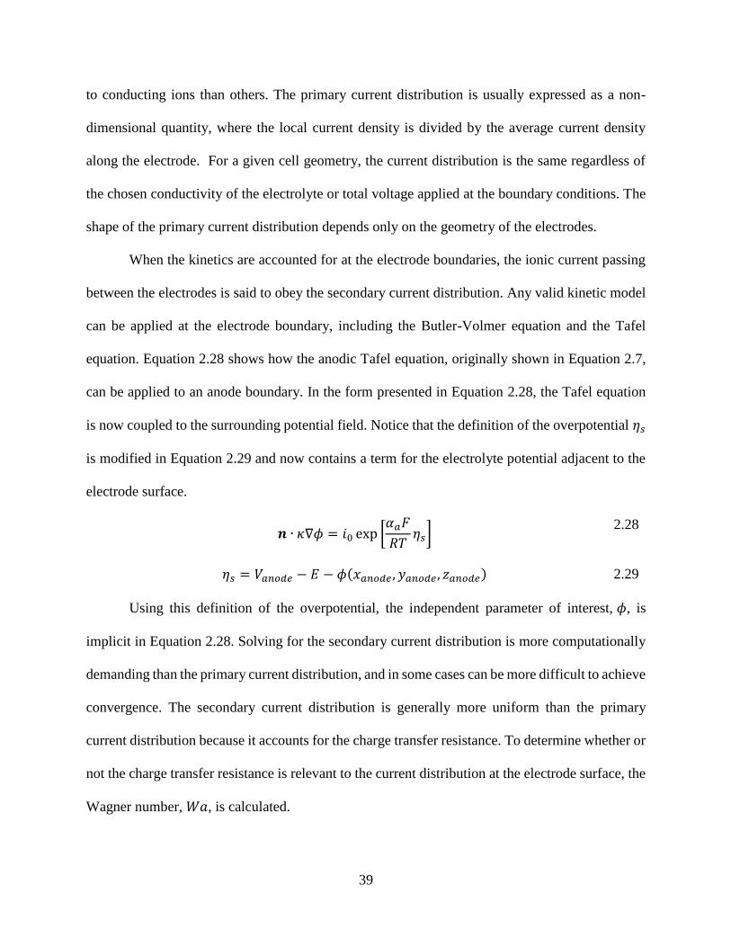
39

to conducting ions than others. The primary current distribution is usually expressed as a non-

dimensional quantity, where the local current density is divided by the average current density

along the electrode. For a given cell geometry, the current distribution is the same regardless of

the chosen conductivity of the electrolyte or total voltage applied at the boundary conditions. The

shape of the primary current distribution depends only on the geometry of the electrodes.

When the kinetics are accounted for at the electrode boundaries, the ionic current passing

between the electrodes is said to obey the secondary current distribution. Any valid kinetic model

can be applied at the electrode boundary, including the Butler-Volmer equation and the Tafel

equation. Equation 2.28 shows how the anodic Tafel equation, originally shown in Equation 2.7,

can be applied to an anode boundary. In the form presented in Equation 2.28, the Tafel equation

is now coupled to the surrounding potential field. Notice that the definition of the overpotential 𝜂𝑠

is modified in Equation 2.29 and now contains a term for the electrolyte potential adjacent to the

electrode surface.

𝒏 ∙ 𝜅∇𝜙 = 𝑖0 exp [

𝛼𝑎𝐹

𝑅𝑇𝜂𝑠]

2.28

𝜂𝑠 = 𝑉𝑎𝑛𝑜𝑑𝑒 − 𝐸 − 𝜙(𝑥𝑎𝑛𝑜𝑑𝑒 , 𝑦𝑎𝑛𝑜𝑑𝑒 , 𝑧𝑎𝑛𝑜𝑑𝑒) 2.29

Using this definition of the overpotential, the independent parameter of interest, 𝜙, is

implicit in Equation 2.28. Solving for the secondary current distribution is more computationally

demanding than the primary current distribution, and in some cases can be more difficult to achieve

convergence. The secondary current distribution is generally more uniform than the primary

current distribution because it accounts for the charge transfer resistance. To determine whether or

not the charge transfer resistance is relevant to the current distribution at the electrode surface, the

Wagner number, 𝑊𝑎, is calculated.

40

𝑊𝑎 is the ratio of the charge transfer resistance to the ohmic resistance in the vicinity of

the electrode. The charge transfer resistance is defined for a system with Tafel kinetics using

Equation 2.10. In the context of the Wagner number, the ohmic resistance is defined using

Equation 2.30:

𝑅Ω

′ =𝑙

𝜅

2.30

where 𝑙 is the characteristic length scale. Equation 2.30 is slightly different from the total ohmic

resistance given by Equation 2.13 in that the relevant length scale in the vicinity of the electrode

being modeled is often times not the electrode separation distance, 𝐿. Rather, it is more likely to

be related to the length of the electrode itself. Equation 2.30 does not include the electrode cross

sectional area in its calculation because it is built into the variable 𝑅Ω′ . Dimensionally, 𝑅Ω

′ defined

in Equation 2.30 is consistent with 𝑅𝐶𝑇 defined in Equation 2.10. Using these definitions, 𝑊𝑎 is

calculated using Equation 2.31 for an electrode using Tafel kinetics:

𝑊𝑎 =

𝑅𝐶𝑇

𝑅Ω′ =

𝑅𝑇𝜅

𝛼𝐹|𝑖𝑎𝑣𝑔|𝑙

2.31

As the value of 𝑊𝑎 approaches zero, the ohmic resistance dominates and the current distribution

on the electrode surface follows the primary current distribution. This is most likely to happen at

large average current densities and large electrode sizes. Thus, the primary current distribution is

typically the most relevant current distribution profile for a scaled up device. As the value of 𝑊𝑎

approaches 1, the current distribution obeys the secondary current distribution. Depending on the

choice of length scale, the current distribution may be nearly uniform as the value of 𝑊𝑎 reaches

or exceeds 1.

Although the primary current is more likely to describe the current distribution profile for

scaled up devices when 𝑊𝑎 ≪ 1, using the boundary conditions for the secondary current can still

41

calculate the same result. The reverse is not true, and the primary current does not apply as 𝑊𝑎 →

1. Additionally, the kinetic boundary conditions must be used in order to simulate IV performance

curves of the electrolyzer. As the voltage becomes sufficiently large, however, the mass transport

limiting current will be approached and the concentration gradient in the electrolyzer must be

modeled.

2.6.2 Modeling the concentration gradient

As 𝑖/𝑖𝑙𝑖𝑚 → 1, concentration gradients begin to form in the electrolyzer and the diffusion

(∇𝑐) term in the Nernst Planck equation can no longer be neglected. Instead, the Nernst Planck

equation can be simplified for conditions where the effects of the electric field on species transport

can be neglected. The electric field must be present in the electrolyte such that the ions can conduct

between the electrodes, but in many cases, this migration current is carried by spectator ions which

otherwise do not participate in the electrochemical reaction. In order to determine if the electric

field is relevant to the mass transport limited current, the transference number for the limiting

reagent, 𝑡𝑖, must be calculated as shown in Equation 2.32:

𝑡𝑖 =

𝑧𝑖2𝑢𝑖𝑐𝑖

∑ 𝑧𝑘2𝑢𝑘𝑐𝑘𝑘

2.32

Conceptually, the transference number refers to the fraction of the total ionic current which

is carried by a given species. It is related to the calculation of the conductivity of the electrolyte,

shown in Equation 2.14. All parameters in the numerator in Equation 2.32 refer to the limiting

reagent, designated as species 𝑖, whereas the denominator is a summation over all ionic species 𝑘.

Calculation of the transference number requires a knowledge of all the ionic species present in the

electrolyte, their bulk concentrations, and conductivities. As the value of 𝑡𝑖 → 0, a minimal

fraction of the ionic current between the electrodes is carried by the limiting reagent, and it can be

42

assumed that species transport of the limiting reagent by migration can be ignored. As the value

of 𝑡𝑖 → 1, the limiting reagent is significantly affected by the electric field, and the migration

current cannot be neglected. When the migration current is significant, further simplifications

cannot be applied to the Nernst-Planck equation, and both the concentration gradient and the

potential field must be modeled. For some special cases, such as for a binary electrolyte, it can be

shown that the electric field can also be ignored if corrective factors are applied to the diffusion

coefficient.1

If the electric field is neglected, it can be shown that the concentration gradient can be

solved for using the equation of convective diffusion, Equation 2.33.1 At the electrode boundary,

the current can be solved for based on the diffusive flux of the limiting reagent, shown in Equation

2.34.

𝜕𝑐𝑖

𝜕𝑡+ 𝒗 ∙ 𝛻𝑐𝑖 = 𝐷𝑖𝛻

2𝑐𝑖 2.33

𝑖 = 𝑛𝐹𝐷𝑖∇𝑐𝑖 2.34

In the previous section, the potential field was solved by applying the appropriate boundary

conditions at the cathode and anode. For solving concentration fields using the equation of

convective diffusion, however, the analysis and subsequent boundary conditions are typically only

applied in the region near the electrode surface. In the bulk electrolyte, 𝑐𝑖 is determined by its bulk

concentration, 𝑐𝑖,𝑏𝑢𝑙𝑘. At the limiting current density, the concentration 𝑐𝑖 at the electrode surface

is assumed to be zero. As previously discussed, the governing equations of the surrounding

concentration profile is largely determined by calculating 𝑃𝑒, which can help determine if the

transport is predominantly diffusion or convection. Once 𝑃𝑒 is known, the concentration field can

largely be solved for using the strategies given in section 2.4 of this chapter.

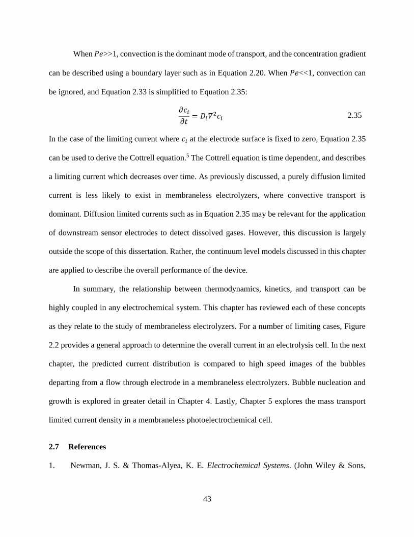
43

When 𝑃𝑒>>1, convection is the dominant mode of transport, and the concentration gradient

can be described using a boundary layer such as in Equation 2.20. When 𝑃𝑒<<1, convection can

be ignored, and Equation 2.33 is simplified to Equation 2.35:

𝜕𝑐𝑖

𝜕𝑡= 𝐷𝑖𝛻2𝑐𝑖 2.35

In the case of the limiting current where 𝑐𝑖 at the electrode surface is fixed to zero, Equation 2.35

can be used to derive the Cottrell equation.5 The Cottrell equation is time dependent, and describes

a limiting current which decreases over time. As previously discussed, a purely diffusion limited

current is less likely to exist in membraneless electrolyzers, where convective transport is

dominant. Diffusion limited currents such as in Equation 2.35 may be relevant for the application

of downstream sensor electrodes to detect dissolved gases. However, this discussion is largely

outside the scope of this dissertation. Rather, the continuum level models discussed in this chapter

are applied to describe the overall performance of the device.

In summary, the relationship between thermodynamics, kinetics, and transport can be

highly coupled in any electrochemical system. This chapter has reviewed each of these concepts

as they relate to the study of membraneless electrolyzers. For a number of limiting cases, Figure

2.2 provides a general approach to determine the overall current in an electrolysis cell. In the next

chapter, the predicted current distribution is compared to high speed images of the bubbles

departing from a flow through electrode in a membraneless electrolyzers. Bubble nucleation and

growth is explored in greater detail in Chapter 4. Lastly, Chapter 5 explores the mass transport

limited current density in a membraneless photoelectrochemical cell.

2.7 References

1. Newman, J. S. & Thomas-Alyea, K. E. Electrochemical Systems. (John Wiley & Sons,

44

2012).

2. Tsampas, M. N., Pikos, A., Brosda, S., Katsaounis, A. & Vayenas, C. G. The effect of

membrane thickness on the conductivity of Nafion. Electrochim. Acta 51, 2743–2755

(2006).

3. O’Neil, G. D., Christian, C. D., Brown, D. E. & Esposito, D. V. Hydrogen Production with

a Simple and Scalable Membraneless Electrolyzer. J. Electrochem. Soc. 163, F3012–F3019

(2016).

4. McCrory, C. C. L. et al. Benchmarking Hydrogen Evolving Reaction and Oxygen Evolving

Reaction Electrocatalysts for Solar Water Splitting Devices. J. Am. Chem. Soc. 137, 4347–

4357 (2015).

5. West, A. C. Electrochemistry and Electrochemical Engineering: An Introduction. (2012).

6. Newman, J. S. Resistance for Flow of Current to a Disk. J. Electrochem. Soc. 113, 501

(1966).

7. Darling, H. E. Conductivity of Sulfuric Acid Solutions. J. Chem. Eng. Data 9, 421–426

(1964).

8. Riegel, H., Mitrovic, J. & Stephan, K. Role of mass transfer on hydrogen evolution in

aqueous media. J. Appl. Electrochem. 28, 10–17 (1998).

9. Vogt, H. The rate of gas evolution of electrodes-I. An estimate of the efficiency of gas

evolution from the supersaturation of electrolyte adjacent to a gas-evolving electrode.

Electrochim. Acta 29, 167–173 (1984).

10. Vogt, H. The rate of gas evolution at electrodes-II. An estimate of the efficiency of gas

evolution on the basis of bubble growth data. Electrochim. Acta 29, 175–180 (1984).

11. Vogt, H. On the supersaturation of gas in the concentration boundary layer of gas evolving

45

electrodes. Electrochim. Acta 25, 527–531 (1980).

12. Vogt, H. The problem of the departure diameter of bubbles at gas-evolving electrodes.

Electrochim. Acta 34, 1429–1432 (1989).

13. Tobias, C. W. Effect of Gas Evolution on Current Distribution and Ohmic Resistance in

Electrolyzers. J. Electrochem. Soc. 106, 833 (1959).

14. Albuquerque, I. L. T., Cavalcanti, E. B. & Vilar, E. O. Mass transfer study of

electrochemical processes with gas production. Chem. Eng. Process. Process Intensif. 48,

1432–1436 (2009).

15. Sutija, Davor P. and Tobias, C. W. Mass-Transport Enhancement by Rising Bubble

Curtains. J. Electrochem. Soc. 141, 2599–2607 (1994).

16. Chandran, P., Bakshi, S. & Chatterjee, D. Study on the characteristics of hydrogen bubble

formation and its transport during electrolysis of water. Chem. Eng. Sci. 138, 99–109

(2015).

17. Kumar, R. K. Flammability Limits of Hydrogen-Oxygen-Diluent Mixtures. J. Fire Sci. 3,

245–262 (1985).

18. Fernández, D., Maurer, P., Martine, M., Coey, J. M. D. & Möbius, M. E. Bubble formation

at a gas-evolving microelectrode. Langmuir 30, 13065–13074 (2014).

19. Hong, G., Yan, X., Yang, Y. H., Xie, T. Z. & Xu, J. J. Bubble departure size in forced

convective subcooled boiling flow under static and heaving conditions. Nucl. Eng. Des. 247,

202–211 (2012).

20. Taqieddin, A., Nazari, R., Rajic, L. & Alshawabkeh, A. Review—Physicochemical

Hydrodynamics of Gas Bubbles in Two Phase Electrochemical Systems. J. Electrochem.

Soc. 164, E448–E459 (2017).

46

21. Aoyama, S., Hayashi, K., Hosokawa, S., Lucas, D. & Tomiyama, A. Lift force acting on

single bubbles in linear shear flows. Int. J. Multiph. Flow 96, 113–122 (2017).

22. Hashemi, S. M. H., Modestino, M. A. & Psaltis, D. A membrane-less electrolyzer for

hydrogen production across the pH scale. Energy Environ. Sci. 8, 2003–2009 (2015).

47

HIGH SPEED VIDEO INVESTIGATION OF BUBBLE DYNAMICS AND CURRENT

DENSITY DISTRIBUTIONS IN MEMBRANELESS ELECTROLYZERS

Gas evolving electrodes are found in many electrochemical systems, such as water

electrolysis, where the dynamics of multiphase flow at these electrodes can strongly impact cell

performance. This is especially true for membraneless water electrolyzers that have emerged in

recent years as a promising approach to low cost hydrogen production. However, experimental

and modeling efforts to characterize the multiphase dynamics in these systems can be non-trivial

due to the complexity of the coupled chemistry and physics that underlie their operation. In this

chapter, we utilize a high speed video (HSV) camera as a non-invasive analytical tool to better

understand bubble dynamics in membraneless electrolyzers and to better quantify the void fraction

of gas bubbles in the region directly downstream of the mesh flow-through electrodes. By detecting

and quantifying the void fraction of bubbles immediately downstream of an operating electrode,

the local current density distribution can be determined along the length of the electrode. This

HSV-measured void fraction distribution is in good agreement with the modeled primary current

distribution. This study also highlights the ability to utilize in situ HSV analysis to monitor gas

evolution efficiency yields and bubble size distributions under varying operating conditions.

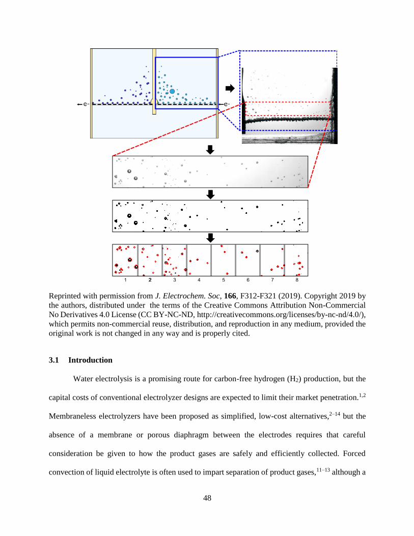
48

Reprinted with permission from J. Electrochem. Soc, 166, F312-F321 (2019). Copyright 2019 by

the authors, distributed under the terms of the Creative Commons Attribution Non-Commercial

No Derivatives 4.0 License (CC BY-NC-ND, http://creativecommons.org/licenses/by-nc-nd/4.0/),

which permits non-commercial reuse, distribution, and reproduction in any medium, provided the

original work is not changed in any way and is properly cited.

3.1 Introduction

Water electrolysis is a promising route for carbon-free hydrogen (H2) production, but the

capital costs of conventional electrolyzer designs are expected to limit their market penetration.1,2

Membraneless electrolyzers have been proposed as simplified, low-cost alternatives,2–14 but the

absence of a membrane or porous diaphragm between the electrodes requires that careful

consideration be given to how the product gases are safely and efficiently collected. Forced

convection of liquid electrolyte is often used to impart separation of product gases,11–13 although a

49

passive design based on buoyancy induced product separation has also been demonstrated.15

Questions still remain on the effectiveness of gas collection in these systems, especially as devices

are scaled up and a wider range of operating conditions are explored.

Gas evolving electrodes are ubiquitous in electrochemistry, with common examples

including PEM and alkaline electrolyzers, electrowinning cells, the chlor alkali process,

electrodialysis cells, photoelectrochemical cells, the Hall-Heroult process, and as side reactions in

many batteries.16 Being able to directly and continuously monitor gas evolution behavior during

operation through in situ imaging is of particular interest for the study of membraneless

electrolyzers, where insight into the downstream transport and collection of gas bubbles is of

particular interest. Membraneless electrolyzers are particularly amenable to such in situ studies

since their simple architecture and void space between electrodes allows for direct optical imaging

through windows placed on the side of modified electrolysis cells. Observations of bubble

dynamics in membraneless electrolyzers have been used in several previous studies to qualitatively

characterize device performance. In their demonstration of a microfluidic membraneless

electrolyzer, Hashemi et al. used in situ imaging to visualize gaseous product separation through

the Segre-Silberberg effect, whereby gas bubbles remain pinned close to the channel walls in the

presence of forced convection and laminar fluid flow.11,17 In a bench scale demonstration, O’Neil

et al. used in-situ imaging to observe non-uniform bubbling along the length of angled mesh

electrodes.13 Gillespie et al. visualized a phenomena they referred to as void fracture, whereby

evolved bubbles merge to form a gaseous void that bridges the inter-electrode gap and greatly

reduces electrolyzer performance.12 In all of these studies, in situ imaging of membraneless

electrolyzers has proven to be very useful for tracking cross-over events and observing bubble

dynamics in flowing electrolytes, but has been largely limited to qualitative analyses.

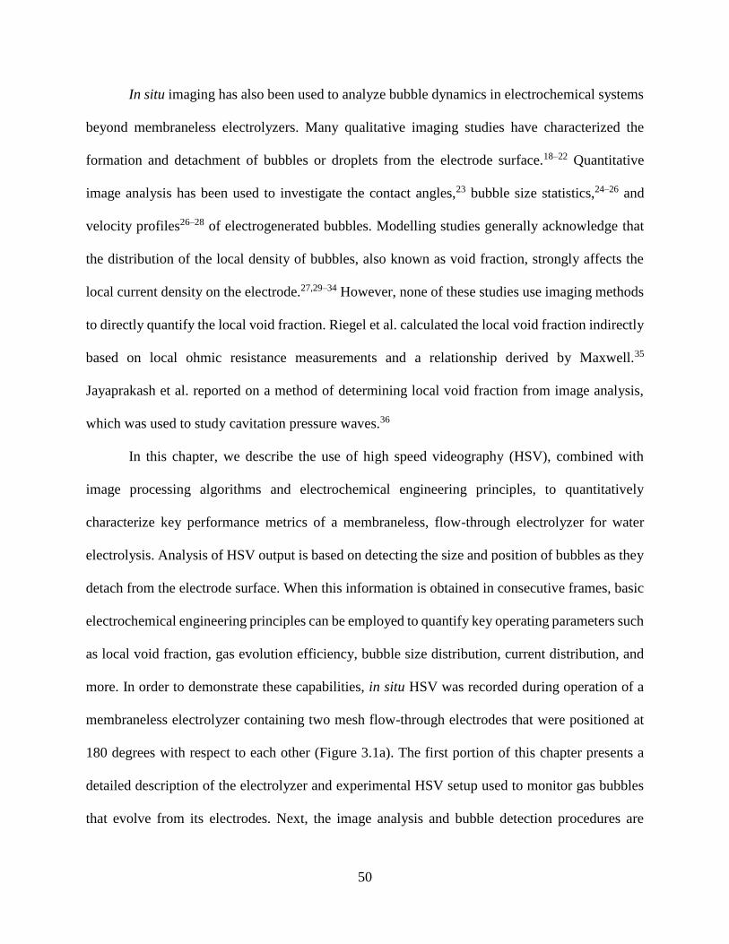
50

In situ imaging has also been used to analyze bubble dynamics in electrochemical systems

beyond membraneless electrolyzers. Many qualitative imaging studies have characterized the

formation and detachment of bubbles or droplets from the electrode surface.18–22 Quantitative

image analysis has been used to investigate the contact angles,23 bubble size statistics,24–26 and

velocity profiles26–28 of electrogenerated bubbles. Modelling studies generally acknowledge that

the distribution of the local density of bubbles, also known as void fraction, strongly affects the

local current density on the electrode.27,29–34 However, none of these studies use imaging methods

to directly quantify the local void fraction. Riegel et al. calculated the local void fraction indirectly

based on local ohmic resistance measurements and a relationship derived by Maxwell.35

Jayaprakash et al. reported on a method of determining local void fraction from image analysis,

which was used to study cavitation pressure waves.36

In this chapter, we describe the use of high speed videography (HSV), combined with

image processing algorithms and electrochemical engineering principles, to quantitatively

characterize key performance metrics of a membraneless, flow-through electrolyzer for water

electrolysis. Analysis of HSV output is based on detecting the size and position of bubbles as they

detach from the electrode surface. When this information is obtained in consecutive frames, basic

electrochemical engineering principles can be employed to quantify key operating parameters such

as local void fraction, gas evolution efficiency, bubble size distribution, current distribution, and

more. In order to demonstrate these capabilities, in situ HSV was recorded during operation of a

membraneless electrolyzer containing two mesh flow-through electrodes that were positioned at

180 degrees with respect to each other (Figure 3.1a). The first portion of this chapter presents a

detailed description of the electrolyzer and experimental HSV setup used to monitor gas bubbles

that evolve from its electrodes. Next, the image analysis and bubble detection procedures are

51

described and applied to experimental HSV data to generate bubble size distributions and

determine gas evolution efficiencies as a function of operating time, current density, and choice of

purge gas. The volume of gas detected using HSV is directly compared to the current output from

the potentiostat to demonstrate the influence of bubbles on the rate of reaction. Lastly, time-

averaged void fractions are calculated immediately downstream of the electrode, and the spatial

variation in void fraction is compared to the primary current distribution. We expect that the

experimental methods and image analysis procedures described herein will find broad utility in

helping to diagnose inefficiencies and guide the design of membraneless electrolyzers.

52

Figure 3.1: a) Schematic top-view of membraneless electrolyzer based on two flow-through mesh

electrodes placed at an angle of 90⁰ with respect to the direction of fluid flow. The close-up photo

on the right shows a magnified view of the front of a woven mesh electrode used in this study. b)

Exploded diagram of the membraneless cell used in this study. c) Schematic of the assembled flow

cell.

3.2 Materials and Methods

Chemicals – All solutions were prepared using 18.2 MΩ cm deionized water. Electrolyte solutions

were prepared using concentrated sulfuric acid (Certified ACS plus, Fischer Scientific).

Electrolytes were purged with either argon (Ar) (PurityPlus, 99.998% purity) or H2 (PurityPlus,

99.999% purity) gas.

53

Electrode fabrication – The electrodes were fabricated using Titanium (Ti) woven mesh sheets

(40 wires per inch; 0.007″ wire diameter, Unique Wire Weaving Co., Inc.). Based on the wire

diameter and number of wires per inch, 51% of the nominal area of the mesh was calculated to be

void space. The measured nominal thickness of the mesh was 0.014″, an equivalent of two wire

diameters. The wires were coated with 50 nm thick layers of platinum (Pt) by electron-beam

evaporation. The nominal dimensions of the electrodes were a width of 0.30 cm and a length of

2.0 cm, resulting in a geometric area of 0.6 cm2. The average current density of the electrode was

calculated by dividing the applied current by the geometric area.

Electrolyzer fabrication – The body of the electrolysis cell was printed using polylactic acid (PLA)

(Makergear LLC). Design files have been made available at http://echem.io. A 0.25” thick glass

sheet is clamped to the front of the device to allow for visual observation with a high speed camera.

A glass window is epoxied (J.B. Weld) to the backside of the device to allow for backlighting and

improved contrast for the HSV experiments. The electrolyzer has a channel height of 0.5 cm and

a full channel width of 4.5 cm. A 2 mm wide separator tab is inserted into the device to split the

channel into two equal streams with a width of 2.2 cm. The central 3D printed tabs are standalone

pieces allowing them to be easily interchanged to evaluate the effect of tab length (𝐿𝑡𝑎𝑏) on the

measured current density distribution. A Viton gasket is inserted above and below the tab to ensure

a mechanical seal when the device is clamped shut. 1 mm thick PLA baffles running parallel to

the fluid flow are positioned in the regions far downstream of the electrodes as well as upstream

of the electrodes to dampen any large convective cells which may form during electrolysis.

The electrodes are inserted into slots in the side of the electrolysis device and epoxied into

place. The ends of the electrodes (< 1 mm) are also coated with epoxy to eliminate any

54

electrochemical activity at the interface between the tip of the electrode and the location where

they rest on the central tab.

Device characterization and operation – The electrolyzer is oriented vertically such that the

buoyant force acting on the electrogenerated bubbles is normal to the electrode surface. Flexible

silicone tubing (Masterflex L/S 16, Cole Parmer) is fitted to the electrolyzer inlets and outlets to

allow for electrolyte circulation. The tubing is connected to a peristaltic pump (Cole Parmer) which

circulates the electrolyte at a total flow rate of 1 mL s-1. After splitting into two separate effluent

streams, the average flow velocity through each sub channel of the device is 0.5 cm s-1. A pulse

dampener (Cole Parmer) is connected between the pump and the flow cell to dampen oscillations

in flow rate that are inherent to the flow from the peristaltic pump. The ends of inlet and outlet

tubes are submerged in an electrolyte reservoir containing 0.5 M H2SO4, which was continuously

purged with either Ar or H2 gas. Experiments were carried out at room temperature and

atmospheric pressure.

All electrochemical measurements were carried out with a Biologic SP-300 bi-potentiostat.

High-speed videos of bubble evolution were recorded using an Edgertronic SC1 high-speed

camera operating at 500 frames per second (fps) and a resolution of 1280 x 1024 pixels. The

camera was fitted with a FotodioX 52 mm reverse mount macro adapter ring and a Nikon AF

Nikor 50 mm f/1.8D lens. Each video recording captured the flow of bubbles over 10 s of

operation.

HSV processing – Data files from HSV experiments were analyzed using MATLAB Image

Processing Toolbox (R2017b). Videos were cropped to an area of analysis spanning the width of

the channel (2 cm) and a vertical height of 150 px (3.2 mm). This area was located as close to the

electrode as possible to capture the bubbles as they detach. More precisely, the analysis area was

55

located ≈1 mm above the gas film on the electrode, such that the large stationary bubbles adhered

to the electrode did not overlap with the analysis area. The mean bubble diameter detected was

112 microns, meaning that ≈ 4% of the pixels in the analysis window were located within a distance

of one mean bubble radius from the edge. It is possible that bubbles detected within this region

could be detected with less accuracy since a portion of the bubble will be out of frame. However,

the Hough transform algorithm is able to resolve the presence of partially visible bubbles by

detecting the boundary between the bubble edge of the background. If the bubble center point is

calculated to be outside the region of interest, however, the bubble will not be detected in the

current frame. Another possible source of error results when the algorithm misinterprets a cluster

of bubbles as a single, larger bubble. This error overestimates the total volume of gas collected,

and is more likely to occur at higher applied current densities when larger quantities of bubbles

are generated.

Bubble detection was carried out over 100 frames of video, with each frame separated by

a time difference of 0.1 s. Each frame was converted to a binary image using an adaptive

thresholding algorithm developed by Bradley.37 In MATLAB this algorithm is included in the

‘imbinarize’ function, and a sensitivity parameter of 0.7 was specified. After binarizing the image,

a circular Hough transform algorithm was used to detect circles of varying radii and spatial

position.38 The Hough transform is included in the ‘imfindcircles’ function, which requires an

estimated size range of bubbles to detect. Table 3.1 in the Appendix A, Section 3.5.1, lists the size

range and sensitivity parameter inputs used for circle detection. The ‘imfindcircles’ command was

run five consecutive times to account for detection of bubbles in different size ranges. The

algorithm searches for the largest bubbles before searching for smaller bubbles. Within each step,

the Hough transform is capable of identifying multiple circles which partially overlap each other.

56

In some instances, if the bubbles are too close together, the algorithm may interpret them as 1

larger bubble. Once a bubble is detected, it is temporarily “deleted” from the image before

searching for more bubbles. Thus, if there is a smaller bubble present directly in the foreground of

a larger bubble, the smaller bubble will likely not be counted due to “shadowing” by the larger

bubble. The parameters in Table 3.1: Input parameters for Hough Transform algorithm used in this

study for bubble radius detection range and sensitivity were optimized to minimize these errors.

Finite element modeling – The potential field in the electrolyte was modeled using the COMSOL

Electrochemistry Multiphysics package. The current distribution along the electrode was

determined by numerically by solving Laplace’s equation, ∇2𝜙(𝑥, 𝑧) = 0, for a two dimensional

system where 𝜙 is the local potential as a function of position.39 This equation is valid only when

there are no concentration gradients present in the cell. In 0.5 M H2SO4, the operating current was

determined to be well below the maximum possible current for electrodes with mixing due to free

convection, and thus it is reasonable to assume that concentration gradients are negligible. For the

electrolyzer in this report, the limiting current was estimated to be ≈ 3.7 A cm-2, which was

determined by solving for the effective diffusion of protons across a boundary layer. A more

detailed overview of this calculation, which uses a mass transfer correlation for a system with free

convection, can be found in the Appendix A, Section 3.5.2. At an applied current density of 100

mA cm-2, the electrolyzer is operating at approximately 2.7% of the calculated limiting current

value.

The spatial coordinates of the electrodes and insulating walls were specified and the

appropriate boundary conditions were imposed. At an insulating boundary, the current normal to

the insulator was fixed to be zero. At the counter electrode, a constant potential boundary condition

was applied where 𝜙 = 0. A constant potential boundary condition was also applied to the working

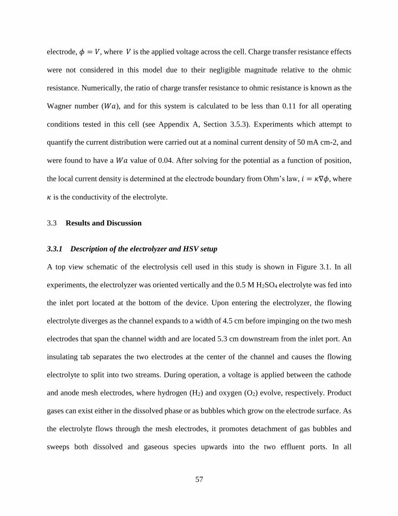
57

electrode, 𝜙 = 𝑉, where 𝑉 is the applied voltage across the cell. Charge transfer resistance effects

were not considered in this model due to their negligible magnitude relative to the ohmic

resistance. Numerically, the ratio of charge transfer resistance to ohmic resistance is known as the

Wagner number (𝑊𝑎), and for this system is calculated to be less than 0.11 for all operating

conditions tested in this cell (see Appendix A, Section 3.5.3). Experiments which attempt to

quantify the current distribution were carried out at a nominal current density of 50 mA cm-2, and

were found to have a 𝑊𝑎 value of 0.04. After solving for the potential as a function of position,

the local current density is determined at the electrode boundary from Ohm’s law, 𝑖 = 𝜅∇𝜙, where

𝜅 is the conductivity of the electrolyte.

3.3 Results and Discussion

3.3.1 Description of the electrolyzer and HSV setup

A top view schematic of the electrolysis cell used in this study is shown in Figure 3.1. In all

experiments, the electrolyzer was oriented vertically and the 0.5 M H2SO4 electrolyte was fed into

the inlet port located at the bottom of the device. Upon entering the electrolyzer, the flowing

electrolyte diverges as the channel expands to a width of 4.5 cm before impinging on the two mesh

electrodes that span the channel width and are located 5.3 cm downstream from the inlet port. An

insulating tab separates the two electrodes at the center of the channel and causes the flowing

electrolyte to split into two streams. During operation, a voltage is applied between the cathode

and anode mesh electrodes, where hydrogen (H2) and oxygen (O2) evolve, respectively. Product

gases can exist either in the dissolved phase or as bubbles which grow on the electrode surface. As

the electrolyte flows through the mesh electrodes, it promotes detachment of gas bubbles and

sweeps both dissolved and gaseous species upwards into the two effluent ports. In all

58

measurements carried out in this study, the electrolyte passes through the electrolyzer at an average

velocity of 0.5 cm s-1.

The woven pattern of the mesh electrodes is shown in the inset in Figure 3.1a. The void

spaces in the mesh enable the electrodes to span the width of the channel (𝐿𝑒) while also allowing

electrolyte to continuously flow through the electrodes. Ionic transport occurs in the region

upstream of the electrodes. For larger values of 𝐿𝑒, the ionic conduction path increases and a larger

overall ohmic resistance to the outer edges of the cell is expected. A tab of variable length 𝐿𝑡𝑎𝑏

extends into the upstream portion of the cell (the region below the electrodes in Figure 3.1a). A

tab of this nature can help prevent cross-over of product species between the anode and cathode,

but does so at the expense of increasing the average ionic conduction path between the two

electrodes. As a result, changes in the tab length are expected to both increase the ohmic resistance

of the cell and alter the current distribution.

The current distribution of the cell arrangement illustrated in Figure 3.1a is also strongly

dependent on the ohmic resistance of the electrolyte to ion transport (RΩ) and the charge transfer

resistance at the electrode surface due to reaction kinetics (RS). The ratio RS/RΩ is known as the

Wagner number (Wa), the magnitude of which can be used as a useful guide for modeling non-

uniform current distributions. For the length scale and current densities being passed through the

electrolysis cell in this study, 𝑊𝑎 ≪ 1 (see Appendix A, Section 3.5.3), meaning that the current

distribution along the length of the electrodes is expected to depend strongly on the ohmic

resistance and the geometric orientation of the electrodes relative to the insulating boundaries.

An exploded view of the electrolyzer is shown in Figure 3.1b. The front side window is

clamped to the body of the cell and allows for a clear viewing path for the high speed camera. A

permanent window is epoxied to the backside of the device to ensure adequate lighting. The

59

separator tab is printed as an insert-able piece, allowing for different tab lengths to be tested in one

cell. The mesh electrodes are inserted through slits in the sides of the cell and are epoxied into

place. Figure 3.1c shows the fully assembled device.

3.3.2 Description of image analysis procedure

Once the cell is assembled, sulfuric acid is pumped through the device and a current is applied to

drive the electrolysis reaction at a specified rate. Using HSV, the electrogenerated bubbles are

detected immediately downstream of the electrode. Figure 3.2a shows the region downstream of

the cathode which is recorded using HSV, while Figure 3.2b contains a representative still frame

image taken during electrolysis. During HSV post processing, individual frames are cropped down

to the region of interest, typically spanning the width of the cathode channel and a vertical height

of 3.2 mm, corresponding to 150 pixels (Figure 3.2c). Using the MATLAB Image Processing

Toolbox, the grayscale image is converted into a binary black and white image (Figure 3.2d). A

Hough transform algorithm is used to determine the size and positions of circles in the frame.38

The algorithm is carried out in five successive steps as described in the Appendix A, Section 3.5.1.

In order to verify the accuracy of the circle detection algorithm, the recorded bubble size and

coordinate data is used to digitally super-impose red circles on top of the binarized image. As

shown in Figure 3.2e, good agreement exists when the circles are able to outline all the bubbles in

the image. In order to determine the local void fraction of gas, the image can be further discretized

into finite volumes. Although 5,000 frames of images are recorded over 10 s, only 100 evenly

spaced frames were typically analyzed to reduce computational cost. A sample video showing 100

frames of analysis for a cathode operating at 50 mA cm-2 is available in the online publication of

J. Electrochem. Soc, 166, F312-F321 (2019).

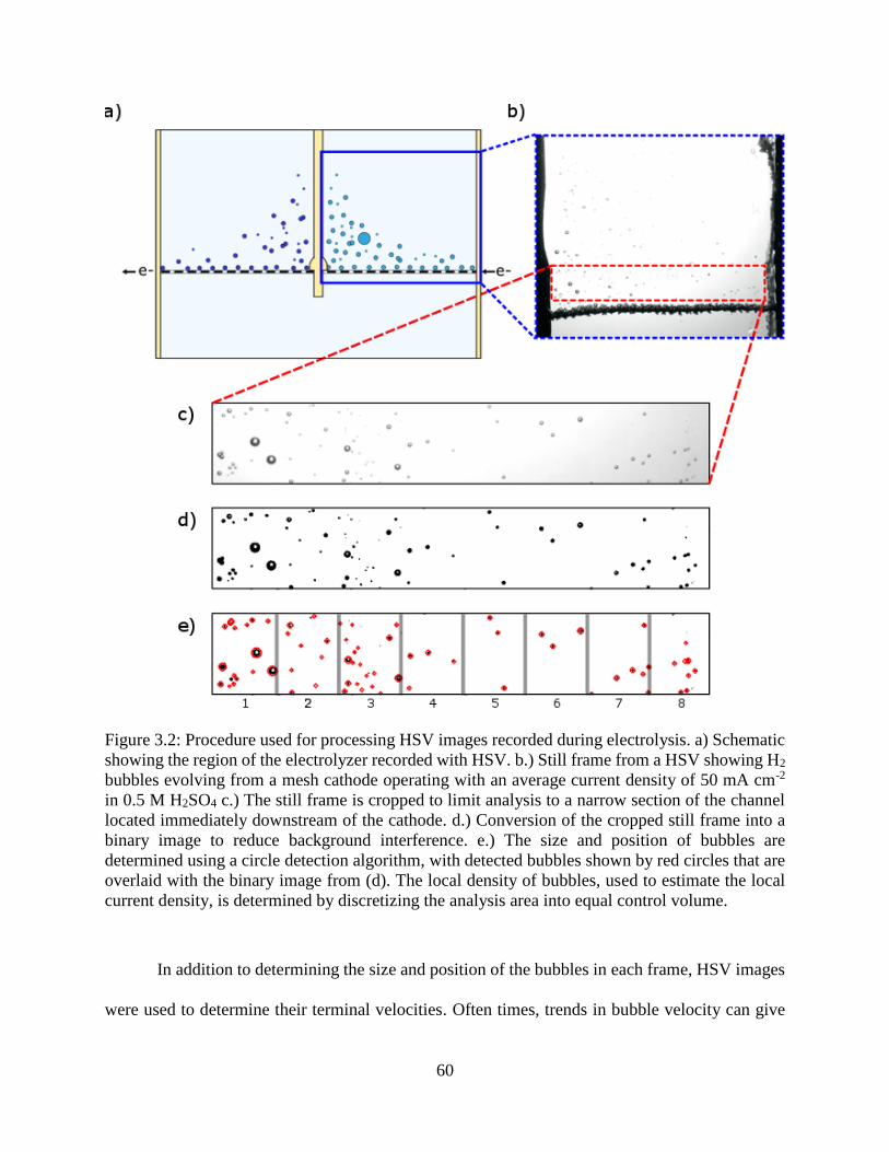
60

Figure 3.2: Procedure used for processing HSV images recorded during electrolysis. a) Schematic

showing the region of the electrolyzer recorded with HSV. b.) Still frame from a HSV showing H2

bubbles evolving from a mesh cathode operating with an average current density of 50 mA cm-2

in 0.5 M H2SO4 c.) The still frame is cropped to limit analysis to a narrow section of the channel

located immediately downstream of the cathode. d.) Conversion of the cropped still frame into a

binary image to reduce background interference. e.) The size and position of bubbles are

determined using a circle detection algorithm, with detected bubbles shown by red circles that are

overlaid with the binary image from (d). The local density of bubbles, used to estimate the local

current density, is determined by discretizing the analysis area into equal control volume.

In addition to determining the size and position of the bubbles in each frame, HSV images

were used to determine their terminal velocities. Often times, trends in bubble velocity can give

61

insights into the flow properties of a fluidic system. Because of the vertical orientation of the

electrolysis cell and the slow rate of electrolyte pumping, the bubble velocities depend

predominantly on buoyancy forces. In general, bubbles leaving the electrode surface were found

to rise vertically with minimal motion in the horizontal direction. During post processing of HSV

experiments, the terminal velocities of bubbles of varying size were determined by directly

measuring the time required to rise vertically across a set distance (6.4 mm). Figure 3.3a shows

the terminal velocities of several H2 bubbles as a function of bubble radius in an electrolyzer

operating at 20 mA cm-2. The linear trend in terminal velocity with the radius of the bubble

suggests that the velocity is governed by the buoyancy force, which scales with the volume of gas

contained.40 The Reynolds numbers of the bubbles in Figure 3.3a were found to be between 0.6

and 150 depending on the diameter of the bubble. Given the predictable relationship between

bubble radius and velocity, an empirical fit of the trend was incorporated in the analysis algorithm

to calculate bubble velocities without the need to track bubbles between frames. For example, if a

bubble is detected with a radius of 0.2 mm, then a vertical velocity vector of 5 cm s-1 can be

reasonably assumed based off of the fit in Figure 3.3a. A similar analysis comparing the total

bubble volume detected to the unique bubble volume detected as a function of the size of the time

step is shown in Figure 3.10 (see Appendix A, Section 3.5.5) for an operating current density of

100 mA cm-2.

62

Figure 3.3: a) Terminal velocity of H2 bubbles rising off of the cathode as a function of bubble

radius. Individual bubble velocities were determined in an electrolyte of 0.5 M H2SO4 purged with

Ar and pumped at an average velocity of 0.5 cm s-1. Bubbles were generated at an operating current

density of 20 mA cm-2. b) Total volume of gas detected over the duration of a 10 s HSV as a

function of time step between image frames. Image analysis was conducted for the same

63

experimental conditions as in (a). Also marked on the plot is the maximum residence time for a

bubble traveling across the analysis area. The red star corresponds to a time step of 0.1 s, which

was the time step used for the remainder of the analyses in this paper. c) Cumulative volume of

H2 bubbles detected during a 10 s long HSV. Image analysis was conducted for the same

experimental conditions as in (a). The upper trace corresponds to the total volume of all bubbles

detected in the image frame, whereas the lower trace uses an algorithm that ensures that each

individual bubble is only counted once.

3.3.3 Determining gas evolution efficiency and bubble size distribution

After determining the size, position, and velocity of all detected bubbles in each frame, the

total volume of gas detected can be calculated as a function of time. This is calculated by summing

up the total volume of bubbles detected in each frame. However, for a given size of the analysis

area and time step between video frames (Δ𝑡), individual bubbles can be counted multiple times

depending on their velocity and distance traveled between frames. An algorithm for avoiding

counting a bubble multiple times was implemented to ensure accurate measurements of the total

volume of gas detected. As shown in Figure 3.9 (See Appendix A, Section 3.5.4), the velocity

vector of each detected bubble can be used to infer where a bubble was located in a previous frame.

If the bubble is calculated to be out of frame in the previous time step, then it is counted as a

uniquely detected bubble. Figure 3.3b shows the total volume of gas bubbles summed across all

frames of a 10 s HSV as a function of Δ𝑡. This analysis was conducted for the same experimental

conditions as in Figure 3.3a. Decreasing Δ𝑡 increases the total number of frames, and thus total

number of bubbles detected over the duration of a 10 s video. The plot compares the sum of all

bubbles detected to the total sum when applying the unique bubble algorithm. At large Δ𝑡, the two

traces converge, suggesting that every bubble in the analysis area is being detected for the first

time. Δ𝑡 is considered large when it exceeds the maximum residence time of a bubble in the

analysis area (𝜏𝑚𝑎𝑥). This value is based on the time required for the smallest and therefore slowest

64

moving bubbles to cross the analysis area, and is calculated to be approximately 0.3 s.

When Δ𝑡 < 𝜏𝑚𝑎𝑥, the trace for uniquely detected bubbles begins to diverge and plateau as

duplicate bubbles are screened out from the total sum. In the interest of the computational time for

analysis, a time step of 0.1 s was chosen for this study, and is marked as a red star on Figure 3.3b.

Choosing an even smaller Δ𝑡 can potentially result in a greater volume of unique bubbles detected,

but this is dependent on the precision of the algorithm itself. Any errors in determining the size

and velocity of a bubble can increase the uncertainty of the unique detection algorithm, and thus

bubbles can still be counted multiple times. A more thorough error analysis can help better

determine the optimal choice of time step, but is beyond the scope of this report.

Having chosen a time step of 0.1 s, Figure 3.3c shows the cumulative sum of H2 bubble

volumes detected as a function of time for electrolysis at 20 mA cm-2. The linear trend in

cumulative volume suggests a constant rate of H2 production, which is expected due to the constant

applied current density. A fit of the slope can be taken to calculate the average volumetric flow

rate of H2 coming off of the electrode. The second trace in Figure 3.3c shows the total volume of

uniquely detected bubbles for the same HSV recording. By employing the algorithm for

determining uniquely detected bubbles, we avoid overestimating the volumetric flow rate of H2

evolved by a factor of two.

The volume detection analysis can be applied to higher current densities as well. As shown

in Figure 3.4a, the slope of the cumulative volume detected as a function of time increases in

proportion to the current density applied. This trend is unsurprising, as higher current densities

should correspond to higher rates of gas production according to Faraday’s law. However, the

relationship between current density and volumetric flow rate of gas is not necessarily perfect. The

empirically fitted volumetric flow rate based on uniquely detected bubbles can be compared to the

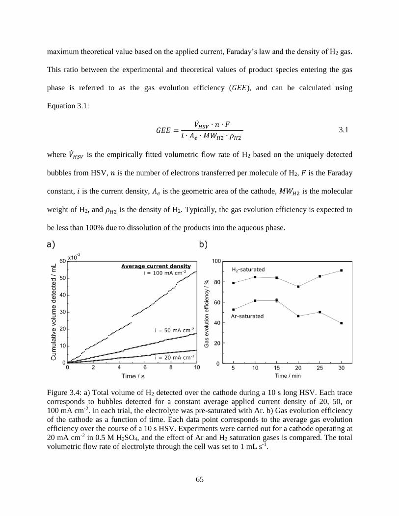
65

maximum theoretical value based on the applied current, Faraday’s law and the density of H2 gas.

This ratio between the experimental and theoretical values of product species entering the gas

phase is referred to as the gas evolution efficiency (𝐺𝐸𝐸), and can be calculated using

Equation 3.1:

𝐺𝐸𝐸 =𝐻𝑆𝑉 ∙ 𝑛 ∙ 𝐹

𝑖 ∙ 𝐴𝑒 ∙ 𝑀𝑊𝐻2 ∙ 𝜌𝐻2 3.1

where 𝐻𝑆𝑉 is the empirically fitted volumetric flow rate of H2 based on the uniquely detected

bubbles from HSV, 𝑛 is the number of electrons transferred per molecule of H2, 𝐹 is the Faraday

constant, 𝑖 is the current density, 𝐴𝑒 is the geometric area of the cathode, 𝑀𝑊𝐻2 is the molecular

weight of H2, and 𝜌𝐻2 is the density of H2. Typically, the gas evolution efficiency is expected to

be less than 100% due to dissolution of the products into the aqueous phase.

Figure 3.4: a) Total volume of H2 detected over the cathode during a 10 s long HSV. Each trace

corresponds to bubbles detected for a constant average applied current density of 20, 50, or

100 mA cm-2. In each trial, the electrolyte was pre-saturated with Ar. b) Gas evolution efficiency

of the cathode as a function of time. Each data point corresponds to the average gas evolution

efficiency over the course of a 10 s HSV. Experiments were carried out for a cathode operating at

20 mA cm-2 in 0.5 M H2SO4, and the effect of Ar and H2 saturation gases is compared. The total

volumetric flow rate of electrolyte through the cell was set to 1 mL s-1.

66

Using this methodology, Figure 3.4b shows the gas evolution efficiency of the cathode as

a function of time. For this experiment, a fixed current density of 20 mA cm-2 was applied for

30 minutes. Each data point corresponds to the average gas evolution efficiency calculated from

10 s long HSVs that were recorded every 5 minutes. The plot also compares the effect of saturating

the electrolyte feed with different dissolved gases. For both H2 and Ar, there was no clear time

dependence of gas evolution efficiency. In general, a lower gas evolution efficiency of 40-60% is

observed when the electrolyte feed is saturated with inert Ar. When the saturation gas is changed

to H2, the gas evolution efficiency increases to 80-90%. This trend is expected, as losses in gas

evolution efficiency are typically attributed to solvation of the product gas.41 By pre-saturating the

electrolyte feed with H2, its capacity to solvate electrogenerated H2 at the cathode is diminished.

Although the applied current density during these experiments is constant and continuous, the rate

of bubble detachment, particularly large bubbles, is not. The departure events of large bubbles can

be missed if they occur in the time between video recordings. For comparison, the electrolysis

experiment spanned 30 minutes, but the image analysis was only carried out for only 60 s of

recorded footage. Thus, in the 29 minutes of electrolysis between recorded HSVs, large bubble

detachment events can occur undetected.

Apparent losses in gas evolution efficiency can also be attributed to small bubbles that are

not detected by the camera. The minimum bubble diameter detected in this work was

approximately 85 μm (4 px). Bubbles smaller than this radius could go undetected and thus

unaccounted for in the volumetric measurements. The smallest bubble sizes for electrochemically

generated H2 have been proposed to be as small as nanometers in diameter.42 The stability of these

nanobubbles is debated in literature,43 but it is well known that the concentration of dissolved H2

in the vicinity of the electrodes is often at super saturation levels.44 In either case, the presence of

67

H2 in the electrolyte at concentrations exceeding the solubility limit would manifest itself in an

even lower gas evolution efficiency. Using higher optical magnification, beyond that which is

available in this study, is one approach to overcoming this limitation.

From a product collection perspective, achieving a 100% gas evolution efficiency is

desirable. Flowing the electrolyte can help separate the electrogenerated H2 and O2 bubbles, but

flowing too fast can cause dissolution losses and decrease the gas evolution efficiency. A drawback

of the present calculation procedure for gas evolution efficiency is that it assumes that the dominant

mode of bubble transport is buoyancy, and thus bubble velocity can be inferred from its size.

Knowing this velocity is a critical aspect of the unique bubble counting method that prevents

overestimation of the gas evolution efficiency. At higher flow rates, however, the velocity of the

bubbles is determined by the drag and slip relationship with the surrounding liquid velocity profile.

Because the bubbles are being detected in the immediate wake of the mesh flow through electrodes,

the liquid phase velocity profile is not readily known or easily solved for without using advance

computational fluid dynamics (CFD) tools. An alternative approach could be to use a method

which tracks bubbles between frames to directly calculate their velocities.

Ideally, the HSV analysis should be able to guide the design and choice of operating

conditions for membraneless electrolyzers such that the gas evolution efficiency and the collection

of the products is maximized. When considering the transport and collection of product gas

bubbles, it can be advantageous to know or be able to predict the sizes of bubbles produced by the

electrolyzer. Figure 3.5a shows the number and volumetric probability distributions of bubble

diameters generated by a cathode in H2 saturated electrolyte. For the number probability

distribution, each detected bubble is weighted equally and the height of each bar corresponds to

the number of bubbles detected in a bin range relative to the total number of bubbles detected

68

across all bins. Using this methodology, ~99% all the bubbles detected were less than 250 μm in

diameter. The volumetric probability distribution was generated by weighting each bubble by its

volume relative to the total volume of gas detected. Although only 1% of bubbles detected were

larger than 250 μm, these bubbles contained ~25% of the generated volume. It can be convenient

to re-plot the size distribution data as a cumulative volume distribution function (CVDF) as shown

in Figure 3.5b. For a given bubble diameter 𝑑𝑖, the cumulative volume fraction refers to the

summation of volumes detected for all bubbles with a diameter less than or equal to 𝑑𝑖. The volume

fraction is normalized to the total cumulative volume detected for all bubbles. The data in Figure

3.5b corresponds to the same experiments as reported in Figure 3.4b for an electrolyzer operating

at 20 mA cm-2 in Ar saturated electrolyte. In these experiments, the arithmetic mean bubble

diameter was found to be 112 ± 0.5 μm. When weighted by the gas of volume contained, the

average bubble diameter was found to be 177 ± 1.7 μm. The error bars associated with the mean

bubble diameter represent 95% confidence intervals based on analysis of 600 still frames of the

HSV recordings. Approximately 25% of the total detected gas volume comes from bubbles smaller

than 100 μm for all of the 10 s HSV clips analyzed, although the volume distribution of larger

bubbles can vary greatly between experiments. We attribute the large variation in the shape of the

cumulative volume fraction curves in Figure 3.5b at large bubble diameters to the fact that the

frequency of larger bubble detachment events is similar to the 10 s window of the HSV recording.

Not surprisingly, the reported gas evolution efficiency values in Figure 3.4b show some common

trends with the bubble size statistics reported in Figure 3.5b for the Ar-saturated electrolyte. In

particular, the trials in which larger bubbles are detected – such as the videos recorded at the 10

and 15 minute mark – tend to exhibit higher gas evolution efficiencies (~60%) in Figure 3.4b. HSV

recordings characterized by bubble distributions skewed to smaller sizes – such as at the 5, 20, and

69

30 minute marks – the gas evolution efficiency is found to be at or below 50%. Again, these trends

do not necessarily imply that larger bubbles cause an increase in the average gas evolution

efficiency. These quantities are nonetheless correlated in our experiments, and this is likely due to

the fact that large bubbles detach less frequently than smaller bubbles, on average. An exception

to this trend is the video at the 25 minute mark, for which a large bubble detachment event was

recorded but a relatively low gas evolution efficiency was still calculated. This suggests that the

variation in gas evolution efficiency with time cannot be entirely explained by infrequent large

bubble detachment events.

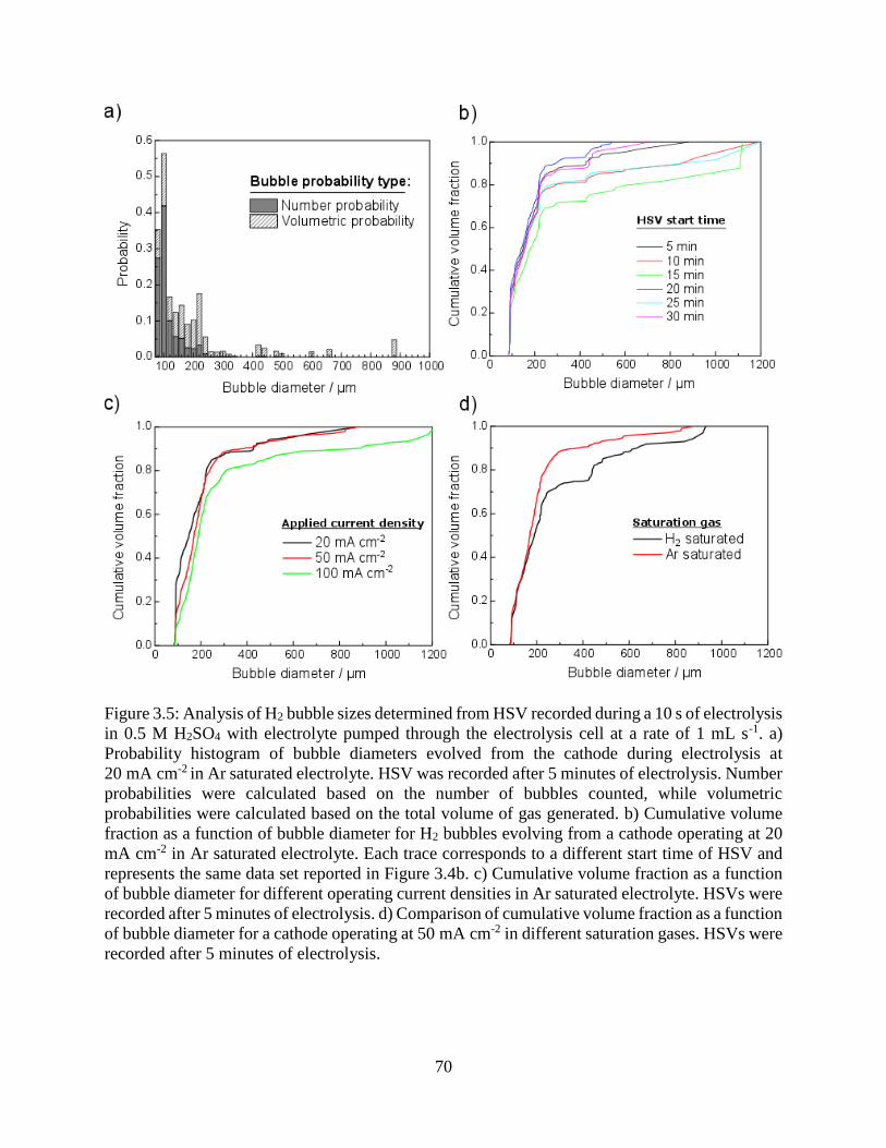
70

Figure 3.5: Analysis of H2 bubble sizes determined from HSV recorded during a 10 s of electrolysis

in 0.5 M H2SO4 with electrolyte pumped through the electrolysis cell at a rate of 1 mL s-1. a)

Probability histogram of bubble diameters evolved from the cathode during electrolysis at

20 mA cm-2 in Ar saturated electrolyte. HSV was recorded after 5 minutes of electrolysis. Number

probabilities were calculated based on the number of bubbles counted, while volumetric

probabilities were calculated based on the total volume of gas generated. b) Cumulative volume

fraction as a function of bubble diameter for H2 bubbles evolving from a cathode operating at 20

mA cm-2 in Ar saturated electrolyte. Each trace corresponds to a different start time of HSV and

represents the same data set reported in Figure 3.4b. c) Cumulative volume fraction as a function

of bubble diameter for different operating current densities in Ar saturated electrolyte. HSVs were

recorded after 5 minutes of electrolysis. d) Comparison of cumulative volume fraction as a function

of bubble diameter for a cathode operating at 50 mA cm-2 in different saturation gases. HSVs were

recorded after 5 minutes of electrolysis.

71

It should be noted that the presented analysis on bubble size distributions is not exhaustive,

and many factors can contribute to the observed profiles. Figure 3.5c shows the effect of current

density on the CVDF, and suggests that higher current densities promote the formation and

detachment of more large bubbles from the electrode. In reality, the frequency of detachment for

all bubbles increases with increasing current density. For large bubbles with long periods between

isolated detachment events, an increase in frequency means a higher likelihood of large bubbles

being detected by the camera during the 10 s window of recording. Figure 3.5d shows that

saturating the electrolyte with H2 gas results in larger bubbles being formed compared to saturating

the electrolyte with Ar gas, which may be attributed to the higher frequency of gas bubble

detachment from the electrodes due to the higher gas evolution efficiency in H2 saturated

electrolyte.

Despite the complexities of modelling and quantifying the distribution of bubble sizes, this

information is highly relevant for membraneless electrolyzers that rely on transport of multiphase

electrolyte fluid to separate the electrogenerated gases. One question is if there is an optimal bubble

size for maximum product collection efficiency. Intuitively, a multiphase mixture containing a

large volume fraction of small bubbles may not separate as readily as larger bubbles. The shape of

the electrodes can also affect the size and frequency of detaching bubbles. For example, on a large

planar electrode, bubbles adhere for longer before growing to a size in the millimeter scale when

they can detach. On the mesh electrodes, however, smaller bubbles readily form and detach. Given

that the mesh wire diameter in this study is approximately 180 μm, it is not surprising that the

majority of bubbles detected have a diameter of less than 200 μm. Many plots in Figure 3.5

commonly show an uptick in bubbles detected at d = 425 μm, which may be a result of the gap

spacing distance in between wires (approximately 460 μm) . Surface treatment of the electrodes

72

could also affect the bubble detachment size by altering the average contact angle of the bubbles

attached to the surface, and therefore the average force of adhesion.

3.3.4 Comparing HSV-derived current transients to measured current transients

Most of the discussion up until this point has focused on the response of bubble behavior to

changes in the electrochemical properties of the system. However, the presence of bubbles can

also affect the observed electrochemical properties. For example, the electrogenerated bubbles can

behave as resistors to ionic flow as well as block active sites on the electrode surface.45 The

relationship between the effective conductivity and the void fraction of bubbles in the electrolyte

has been widely observed, and can be described by the Bruggeman equation.35,46 An important

consideration for the electrolysis cell presented herein is that the detached bubbles in the electrolyte

exist downstream of the electrodes, whereas the ionic transport and potential field gradient exists

only upstream of the electrodes. Thus, any effect of the bubbles on the electrochemical properties

of this electrolyzer will result from bubbles that are attached to the electrode.

To view the impact of bubbles on the electrochemical performance of this electrolyzer,

HSV was recorded simultaneously with electrical current during a chronoamperometry experiment

where a constant 2.7 V was applied between the anode and the cathode. The relationship between

the volumes of bubbles detected and the current readout from the potentiostat is shown in Figure

3.6 over a 10 s period. The current measured by the potentiostat varies between 60-65 mA, with

the largest jumps in the current occurring at t = 0.8 and 3.8 s. These step changes in current

correspond precisely with the timing of large bubble departure events measured using HSV. The

increase in current at these points is likely due to improved ionic conductivity of the electrolyte

between the electrodes in the absence of the detached bubbles. A smaller step change in the current

density at t=6.5 s also coincides with a large bubble detachment event. However, some changes in

73

the current versus time plot have no direct correlation to large bubble departure events, such as at

t = 2.5 and 8.5 s. One explanation for these changes is that only the cathode was filmed for large

bubble departure events, but bubble departures at the anode can also decrease the ohmic resistance

of the ionic conduction path. Because the experiment was conducted without a reference electrode,

bubble departure events at the anode cannot be isolated from the current response.

Figure 3.6: Comparison of the total electrolysis current recorded by the potentiostat to the volume

of gas detected during a 10 s HSV. The HSV was recorded after five minutes of electrolysis at a

constant applied voltage of 2.7 V. Electrolysis was carried out in 0.5 M H2SO4 with electrolyte

pumped through the cathode at a rate of 0.5 mL s-1.

One might expect to see a direct correlation at a given time between the measured current

and the detected volume of H2. In reality, there are temporal differences between the rate of

reaction and the rate of hydrogen bubble accumulation, growth, and departure. As mentioned in

74

the discussion of Figure 3.4a and b, when the volume H2 detected is averaged over time, a direct

relationship to the applied current can be calculated using Faraday’s law. When comparing the

measured current to the volume of gas in an individual video frame, however, the relationship with

Faraday’s law is less straight forward. Large bubbles are the result of hydrogen accumulation over

the course of several seconds or even minutes. For an experiment with a constant applied potential,

the departure of a large hydrogen bubble causes an increase in current because it is no longer able

to insulate the electrode from ions conducting to it. However, it is not necessarily true that a sudden

increase in current causes a large bubble to detach.

3.3.5 HSV-derived current distributions

Because the rates of gas bubble generation are proportional to current density, as seen in Figure

3.4a, HSV recordings of gas-evolving electrodes can also be used to measure the current

distribution of an electrochemical cell. A non-uniform current distribution, or variation in local

reaction rate, can arise from differences in ohmic resistance, charge transfer resistance, or mass

transport resistance along the length of the electrode.47,48 In our system, mass transport effects can

be neglected because the typical operating current densities used in this study are well below the

mass transport-limited current for the water splitting half reactions in 0.5 M sulfuric acid. In

electrochemical systems without mass transport limitations, the governing physics of the current

distribution can be determined by calculating 𝑊𝑎 – the ratio of charge transfer resistance to ohmic

resistance.39 In most electrochemical systems, ohmic resistance is dominated by the ionic transport

in the electrolyte, and depends on the conductivity and path length for ion transport between

electrodes. The charge transfer resistance is determined by the kinetics of the electrode reaction.

Equation 3.2 shows the calculation for 𝑊𝑎 when the charge transfer resistance is modeled using

Tafel kinetics:39

75

𝑊𝑎 =𝑅 ∙ 𝑇 ∙ 𝜅

𝛼𝐶𝑇 ∙ 𝐹 ∙ |𝑖𝑎𝑣𝑔| ∙ 𝑙 3.2

where 𝑅 is the gas constant, 𝑇 is the temperature, 𝜅 is the conductivity of the electrolyte, 𝛼𝐶𝑇 is

the charge transfer coefficient, 𝐹 is the Faraday constant, 𝑖𝑎𝑣𝑔 is the average current density of the

electrode, and 𝑙 is a characteristic length, which in this study is taken to be the length of the

electrode. As 𝑊𝑎 approaches zero the current distribution is governed by the ohmic resistance and

the kinetics of reaction do not need to be modelled. Such systems are said to obey the primary

current distribution. For larger values of 𝑊𝑎, the reaction kinetics at the electrode surface also

become important to describing the variation in current along an electrode. A higher relative charge

transfer resistance generally causes the current distribution to be more uniform, resulting in what

is referred to as the secondary current distribution.

When the electrolyzer is operated at a nominal current density of 50 mA cm-2, the

calculated value of 𝑊𝑎 is 0.04, indicating that the current distribution can be modeled as a primary

current distribution. The current distribution can be determined after solving the potential field,

which is governed by Laplace’s equation, ∇2𝜙 = 0, where 𝜙 refers to the local potential of the

electrolyte. Non-uniformities in the primary current distribution arise due to the geometry of the

electrolyzer and the spatial position of the electrodes. In this work, the lowest ohmic resistances to

ion transport, and hence the highest local current densities, are expected in the center of the

electrolyzer where the shortest distance for ion transport between electrodes is possible. Moving

outward from the central baffle, longer ion transport distances are required, leading to higher ohmic

overpotentials and small local current densities that decrease to a minimum at the outer edges of

the channel walls. Figure 3.7a shows the simulated local current density of the cathode as a

function of position along the length of the electrode. Each trace corresponds to a different tab

length, 𝐿𝑡𝑎𝑏. When the insulating tab extends only 2 mm upstream of the electrodes, the current

76

distribution is very non-uniform, with the modeled local current density at the inner edge of the

electrode being 3 times the average current density (𝑖𝑎𝑣𝑔). The current density decreases along the

length of the electrode, with the local value tapering off to approximately half of 𝑖𝑎𝑣𝑔 at the outer

edge.

77

Figure 3.7: Comparison of the predicted current distribution to the local volume fraction along the

length of the electrode, 𝑥/𝐿𝑒. All experiments were carried out at an operating current density of

50 mA cm-2. a) Simulated primary current distribution of the electrolysis cell for different separator

tab insertion lengths between electrodes. b) Relative gas volume fraction along the length of the

electrode for a cathode operating in Ar-saturated H2SO4 and tab insertion length of 2 mm. c)

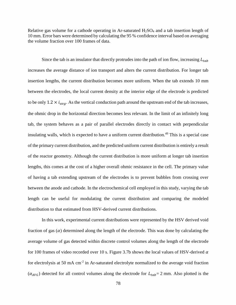
78

Relative gas volume for a cathode operating in Ar-saturated H2SO4 and a tab insertion length of

10 mm. Error bars were determined by calculating the 95 % confidence interval based on averaging

the volume fraction over 100 frames of data.

Since the tab is an insulator that directly protrudes into the path of ion flow, increasing 𝐿𝑡𝑎𝑏

increases the average distance of ion transport and alters the current distribution. For longer tab

insertion lengths, the current distribution becomes more uniform. When the tab extends 10 mm

between the electrodes, the local current density at the interior edge of the electrode is predicted

to be only 1.2 × 𝑖𝑎𝑣𝑔. As the vertical conduction path around the upstream end of the tab increases,

the ohmic drop in the horizontal direction becomes less relevant. In the limit of an infinitely long

tab, the system behaves as a pair of parallel electrodes directly in contact with perpendicular

insulating walls, which is expected to have a uniform current distribution.49 This is a special case

of the primary current distribution, and the predicted uniform current distribution is entirely a result

of the reactor geometry. Although the current distribution is more uniform at longer tab insertion

lengths, this comes at the cost of a higher overall ohmic resistance in the cell. The primary value

of having a tab extending upstream of the electrodes is to prevent bubbles from crossing over

between the anode and cathode. In the electrochemical cell employed in this study, varying the tab

length can be useful for modulating the current distribution and comparing the modeled

distribution to that estimated from HSV-derived current distributions.

In this work, experimental current distributions were represented by the HSV derived void

fraction of gas (𝛼) determined along the length of the electrode. This was done by calculating the

average volume of gas detected within discrete control volumes along the length of the electrode

for 100 frames of video recorded over 10 s. Figure 3.7b shows the local values of HSV-derived 𝛼

for electrolysis at 50 mA cm-2 in Ar-saturated electrolyte normalized to the average void fraction

(𝛼𝐴𝑉𝐺) detected for all control volumes along the electrode for 𝐿𝑡𝑎𝑏= 2 mm. Also plotted is the

79

simulated primary current distribution normalized to the average applied current density. The

experimental and modeled current distributions show reasonable agreement, with the local void

fraction being highest at the interior edge of the electrode. When 𝐿𝑡𝑎𝑏 is extended further upstream,

the void fraction profile responds accordingly. Figure 3.7c shows the void fraction profile during

electrolysis at 50 mA cm-2 in an Ar-saturated electrolyte with a 10 mm tab length bisecting the

anode and cathode. Under these conditions, the HSV-derived void fraction exhibits significantly

lower variation along the length of the electrode, consistent with the simulated primary current

distribution. A large bubble detachment event at 𝑥/𝐿𝑒 = 0.8 causes a large local spike in void

fraction which does not correspond with the predicted local current density. This suggests that

although small bubble departure events accurately reflect the local current density, larger bubbles

in the gas film may depend on other mechanisms for growth and detachment and lead to significant

error in measuring current distributions by our method. For example, a disturbance in the flow may

cause a large bubble to detach from a random position. The time period between large bubble

detachment events is also likely to occur at intervals longer than the video recording time of 10 s,

yielding uncertainty as to where on an electrode a large bubble will detach. In general, the

deviations between the simulated current distribution and the void fraction distribution are likely

due to the dynamics of bubble growth and detachment. It may be possible that the role of charge

transfer resistance may also help resolve these deviations, but a comparison of the primary and

secondary current distributions in Figure 3.11 (See Appendix A, Section 3.5.6) shows that adding

kinetic parameters to the boundary conditions modifies the local distribution by no more than 11%

at any point along the electrode.

In light of these uncertainties, more can be done to resolve differences between theory and

experimental data gathered from HSV. Deviations from the predicted current distribution also exist

80

in Figure 3.7b at the ends of the electrodes where they approach the inner insulating divider and

the outer channel wall. It is possible that both flow and electric field effects contribute to these

deviations at the boundaries. For example, fluid velocity gradients caused by the separator tab and

the exterior channel walls may affect bubble transport in ways that are not accounted for in our

analysis method. An algorithm which tracks bubbles in between frames could better determine the

velocity profile and in turn help incorporate a theoretical model which accounts for velocity field

effects.

3.4 Conclusions

This Chapter has described and demonstrated methods of using HSV to quantitatively characterize

the behavior of electrochemically-generated bubbles in a membraneless electrolyzer. A circle

detection algorithm was employed to determine the size and position of H2 bubbles as they

detached from a mesh flow-through cathode. By ensuring that bubbles were not counted multiple

times, average gas evolution efficiencies were calculated as a function of time and for different

electrolyte conditions. The gas evolution efficiency was found to be 40-60% in Ar saturated

electrolyte, but increased to almost 90% when the electrolyte was pre-saturated with H2. These

results suggest that dissolution of the electrogenerated H2 can be a major source of product loss in

this membraneless electrolysis system. Statistical analysis of the bubble size distribution indicates

that inaccuracies in gas evolution efficiency can be attributed to the infrequent detachment of larger

bubbles. Although only 1% of the bubbles detected were larger than 250 μm, they contained over

20% of the generated volume. During experiments for which a constant potential applied, large

bubble departure events were associated with a temporary increase in the current passed through

the cell. This study has also demonstrated that in situ HSV imaging can be used to determine the

local void fraction of bubbles immediately downstream of a flow-through electrode. When the

81

void fraction is plotted as a function of position along the length of the electrode, the profile was

found to correspond to the primary current distribution. Overall, we show that HSV can be a

versatile non-invasive imaging tool to quantitatively analyze bubble evolution dynamics and

electrochemical properties of membraneless electrolyzers.

3.5 Appendix A

3.5.1 Parameters used for Hough transform

The imfindcircles function in the MATLAB Image Processing Toolbox uses a Hough transform

algorithm that is able to analyze a still frame image and return the radius and (X,Y) center point

locations of all circular features present. Circles are determined by first identifying bubble edges,

which are defined by dark pixels that are directly adjacent to white background pixels. The center

point for each circle is determined statistically based on the coordinates of the detected edges and

the anticipated range of bubble radii. The function requires that the user specify the size range of

circles to be detected, as well as a sensitivity parameter which sets the minimum threshold

probability value for whether or not a grouping of boundary pixels constitute a circle with a

common center. The sensitivity parameter must be specified within the range of 0 to 1, with a

value of 1 corresponding to the highest sensitivity. Increasing the sensitivity allows for the

detection of overlapping or poorly defined circles, but setting it too high increases the likelihood

of false positive detection. Setting the sensitivity parameter too low can result in not detecting any

bubbles. In order to avoid false positive detection of smaller bubbles, it is also recommended that

the size range be specified such that the maximum anticipated radius size does not exceed three

times the magnitude of the minimum radius size to be detected. Because of the wide range of

possible bubble sizes present in the videos imaged in this study, the imfindcircles function was

used to analyze each image frame five different times, where successively smaller bubble size

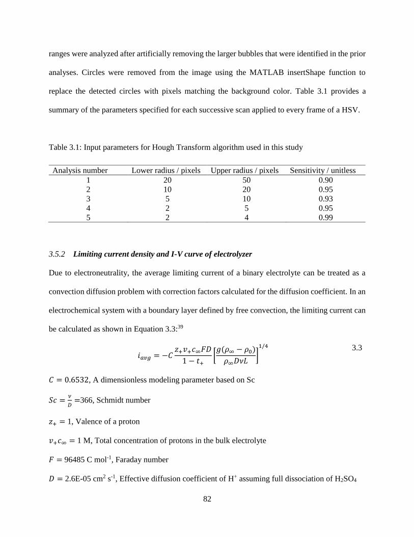
82

ranges were analyzed after artificially removing the larger bubbles that were identified in the prior

analyses. Circles were removed from the image using the MATLAB insertShape function to

replace the detected circles with pixels matching the background color. Table 3.1 provides a

summary of the parameters specified for each successive scan applied to every frame of a HSV.

Table 3.1: Input parameters for Hough Transform algorithm used in this study

Analysis number Lower radius / pixels Upper radius / pixels Sensitivity / unitless

1 20 50 0.90

2 10 20 0.95

3 5 10 0.93

4 2 5 0.95

5 2 4 0.99

3.5.2 Limiting current density and I-V curve of electrolyzer

Due to electroneutrality, the average limiting current of a binary electrolyte can be treated as a

convection diffusion problem with correction factors calculated for the diffusion coefficient. In an

electrochemical system with a boundary layer defined by free convection, the limiting current can

be calculated as shown in Equation 3.3:39

𝑖𝑎𝑣𝑔 = −𝐶

𝑧+𝑣+𝑐∞𝐹𝐷

1 − 𝑡+[𝑔(𝜌∞ − 𝜌0)

𝜌∞𝐷𝜈𝐿]

1/4

3.3

𝐶 = 0.6532, A dimensionless modeling parameter based on Sc

𝑆𝑐 =𝜈

𝐷=366, Schmidt number

𝑧+ = 1, Valence of a proton

𝑣+𝑐∞ = 1 M, Total concentration of protons in the bulk electrolyte

𝐹 = 96485 C mol-1, Faraday number

𝐷 = 2.6E-05 cm2 s-1, Effective diffusion coefficient of H+ assuming full dissociation of H2SO4

83

𝑡+ = 0.814, Transference number of protons assuming full dissociation of H2SO4

𝑔 = 980 cm s-2, gravitational constant

𝜌∞ = 1030 kg m-3, density of 0.5 M H2SO4

𝜌0 = 0.8 kg m-3, density of H2 at standard conditions

𝜈 =0.0095 cm2 s-1, kinematic viscosity of 0.5 M H2SO4

𝑆𝑐 =𝜈

𝐷=366, Schmidt number

𝐿 = 2 cm, Length of electrode

Using these parameters, the calculated limiting current density is 3.7 A cm-2. The largest

current density applied in our experiments was 100 mA cm-2, or 2.7% of the calculated limiting

current density. The limiting current density is likely higher since electrolyte is also being pumped

at a rate of 0.5 mL s-1 to the cathode, replenishing protons and decreasing the diffusion boundary

layer thickness. Figure 3.8 shows a current voltage (I-V) curve of the electrolyzer. No evidence of

mass transport limitations are observed up to the maximum recorded current density of 300 mA

cm-2. If concentration gradients were present, the slope of the IV curve would become shallower

until it eventually reached the mass transfer limiting current.

84

Figure 3.8: Current-voltage curve for an electrolyzer with a tab insertion length 𝐿𝑡𝑎𝑏 of 2 mm.

0.5 M H2SO4 was pumped to the cathode at a rate of 0.5 mL s-1. The LSV was measured at a scan

rate of 20 mV s-1.

3.5.3 Calculation of Wagner Number

The Wagner number is defined as the ratio of charge transfer resistance to ohmic resistance. At

large overpotentials, the charge transfer resistance can be described using Tafel kinetics, and the

Wagner number is defined using Equation 3.4:

𝑊𝑎 =𝑅𝑇𝜅

𝛼𝐶𝑇𝐹|𝑖𝑎𝑣𝑔|𝑙 3.4

85

where 𝑅 is the gas constant, 𝑇 is the temperature, 𝜅 is the conductivity of the electrolyte, 𝛼𝐶𝑇 is

the transfer coefficient, 𝐹 is Faraday’s constant, 𝑖𝑎𝑣𝑔 is the average current density of the electrode,

and 𝑙 is a characteristic length. For a 0.5 M H2SO4 electrolyte, the conductivity 𝜅 is 0.226 S/cm.50

The grouping 𝑅𝑇

𝛼𝐶𝑇𝐹 can be determined from the slope of a Tafel plot. In a previous study

for HER in 0.5 M H2SO4 on a Pt coated Ti mesh, the value of this grouping was determined to be

0.039 V.13 The characteristic length of the system was taken to be the length of the electrode, 2.0

cm. The value of 𝑖𝑎𝑣𝑔 used must be normalized to the active area of the electrode, and not the

geometric area. For example, a current density of 20 mA cm-2 in the main text was calculated by

dividing an applied current of 12 mA by the geometric area of the electrode, 0.3 cm × 2.0 cm =

0.6 cm2. Based off of the wire diameter and woven pattern of the mesh electrodes, however, 51%

of the electrode area is actually void area. Thus, the corrected value of 𝑖𝑎𝑣𝑔 relative to the active

surface area would be 40.8 mA cm-2, and the calculated value of 𝑊𝑎 for these conditions would

be 0.11. Figure 3.7 in the main text shows the current distributions for an electrolysis cell operating

at 50 mA cm-2 of geometric area, and the calculated value of 𝑊𝑎 is 0.04.

3.5.4 Description of algorithm for detecting unique bubbles

For a given image frame taken from a HSV for analysis, the size, position, and velocity of each

detected bubble was determined using the Hough transform algorithm (See Appendix A, Section

3.5.1) and the bubble size velocity correlation reported in Figure 3.3a. In order to determine if a

bubble appearing in a given frame was already detected in the prior frame, the position of the

bubble in the prior frame was first estimated by multiplying its velocity (determined from Figure

3.3a) by the time step between frames. Figure 3.9 shows a visualization of the logic arguments

used for the unique bubble detection algorithm. If the calculated bubble position in the prior frame

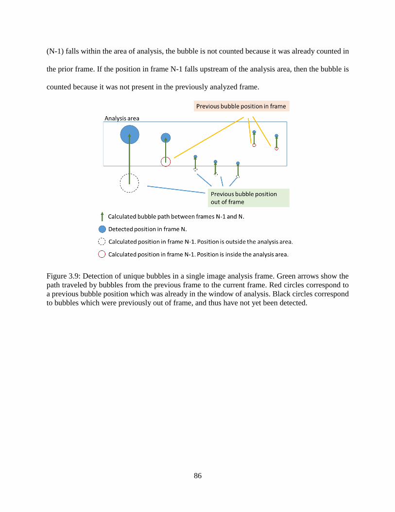
86

(N-1) falls within the area of analysis, the bubble is not counted because it was already counted in

the prior frame. If the position in frame N-1 falls upstream of the analysis area, then the bubble is

counted because it was not present in the previously analyzed frame.

Figure 3.9: Detection of unique bubbles in a single image analysis frame. Green arrows show the

path traveled by bubbles from the previous frame to the current frame. Red circles correspond to

a previous bubble position which was already in the window of analysis. Black circles correspond

to bubbles which were previously out of frame, and thus have not yet been detected.

87

3.5.5 Relationship between time step and total volume of bubbles detected at 100 mA cm-2

Figure 3.10: Total volume of gas detected over the duration of a 10 s HSV as a function of time

step between image frames. Experiment was carried out in 0.5 M H2SO4 purged with Ar and

pumped at an average velocity of 0.5 cm s-1. Bubbles were generated at a current density of

100 mA cm-2.

3.5.6 Comparison of the primary and secondary current distributions

The simulated current distribution shown in Figure 3.7 is based on the primary current distribution,

which only accounts for nonuniformity due to the ohmic resistance in the electrolyte. In Appendix

A, Section 3.5.3, the choice of solving the primary current distribution was justified by calculating

Wa, which was found to be 0.04. In this case, effects of charge transfer are thought to be negligible.

Figure 3.11 below compares the simulated primary current distribution to the secondary current

distribution, which includes the physics for charge transfer at the electrode surface.

88

The current distribution was modeled for an insulating tab insertion length of 2 mm. The

electrolyte was assumed to be 0.5 M H2SO4 with a conductivity 0.226 S cm-1. The average current

density at the cathode and anode boundaries was fixed to be 50 mA cm-2 on a geometric basis.

Similar to the primary current distribution simulation, the solution was determined by solving

Laplace’s equation for the potential field in the electrolyte, ∇2𝜙 = 0. While constant potential

boundary conditions were applied for the primary current distribution, Tafel kinetic boundary

conditions were applied for the secondary current distribution. Kinetic parameters were obtained

using Tafel analysis from a previous study.13 At the anode, the oxygen evolution reaction (OER)

on Pt was modeled: the equilibrium potential was specified to be 1.23 V, the exchange current

density 𝑖0,𝑂𝐸𝑅 = 1.87E-07 A m-2, and a Tafel slope 𝛽𝑂𝐸𝑅 = 133 mV/decade. At the cathode kinetic

parameters for the hydrogen evolution reaction (HER) were used: the equilibrium potential was

specified to be 0.0 V, the exchange current density 𝑖0,𝐻𝐸𝑅 = 6.6E-04 A m-2, and a Tafel slope

𝛽𝐻𝐸𝑅 = -39 mV/decade. At insulating boundaries the gradient in the potential field normal to the

surface was specified to be zero.

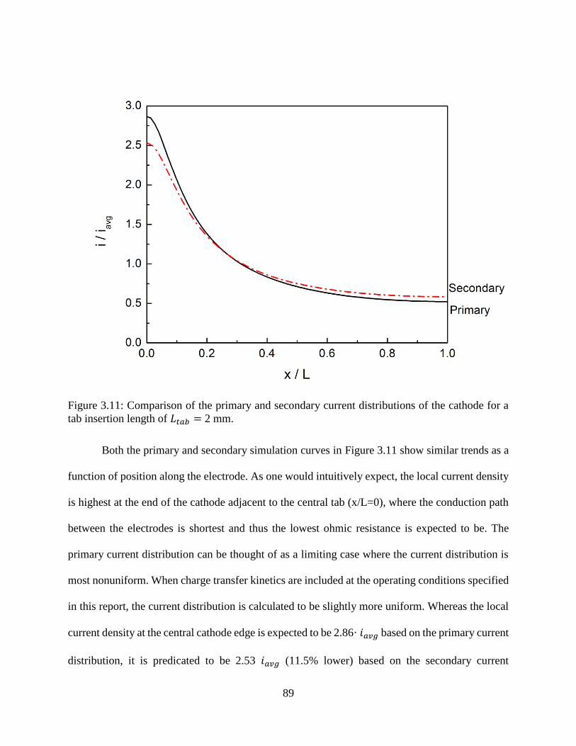
89

Figure 3.11: Comparison of the primary and secondary current distributions of the cathode for a

tab insertion length of 𝐿𝑡𝑎𝑏 = 2 mm.

Both the primary and secondary simulation curves in Figure 3.11 show similar trends as a

function of position along the electrode. As one would intuitively expect, the local current density

is highest at the end of the cathode adjacent to the central tab (x/L=0), where the conduction path

between the electrodes is shortest and thus the lowest ohmic resistance is expected to be. The

primary current distribution can be thought of as a limiting case where the current distribution is

most nonuniform. When charge transfer kinetics are included at the operating conditions specified

in this report, the current distribution is calculated to be slightly more uniform. Whereas the local

current density at the central cathode edge is expected to be 2.86· 𝑖𝑎𝑣𝑔 based on the primary current

distribution, it is predicated to be 2.53 𝑖𝑎𝑣𝑔 (11.5% lower) based on the secondary current

90

distribution At the outer edge of the electrode (x/L=1.0), the local current density tapers off to a

value of 0.52 𝑖𝑎𝑣𝑔 in the primary current distribution case, and 0.58 𝑖𝑎𝑣𝑔 for the secondary current

distribution. Overall, the current distribution is slightly more uniform for the secondary current

case, but the differences are small enough to warrant our choice of using the primary current

distribution for comparison to experimental measurements in this study.

3.6 Acknowledgements

The authors acknowledge funding from Shell International’s New Energies Research &

Technology program. The authors also thank Albert Harvey and Santhosh Shankar for their helpful

input and discussions.

3.7 References

1. Shaner, M. R., Atwater, H. A., Lewis, N. S. & McFarland, E. W. A comparative

technoeconomic analysis of renewable hydrogen production using solar energy. Energy

Environ. Sci. 9, 2354–2371 (2016).

2. Esposito, D. V. Membraneless Electrolyzers for Low-Cost Hydrogen Production in a

Renewable Energy Future. Joule 1, 651–658 (2017).

3. Xuan, J., Leung, D. Y. C., Leung, M. K. H., Wang, H. & Ni, M. Chaotic flow-based fuel

cell built on counter-flow microfluidic network: Predicting the over-limiting current

behavior. J. Power Sources 196, 9391–9397 (2011).

4. Ferrigno, R., Stroock, A. D., Clark, T. D., Mayer, M. & Whitesides, G. M. Membraneless

vanadium redox fuel cell using laminar flow. J. Am. Chem. Soc. 124, 12930–12931 (2002).

5. Choban, E., Markoski, L., Wieckowski, A. & Kenis, P. Microfluidic fuel cell based on

laminar flow. J. Power Sources 128, 54–60 (2004).

6. Braff, W. a, Bazant, M. Z. & Buie, C. R. Membrane-less hydrogen bromine flow battery.

91

Nat. Commun. 4, 2346 (2013).

7. Nasharudin, M. N., Kamarudin, S. K., Hasran, U. A. & Masdar, M. S. Mass transfer and

performance of membrane-less micro fuel cell: A review. Int. J. Hydrogen Energy 39,

1039–1055 (2014).

8. Talabi, O. O., Dorfi, A. E., O’Neil, G. D. & Esposito, D. V. Membraneless electrolyzers for

the simultaneous production of acid and base. Chem. Commun. 53, 8006–8009 (2017).

9. Modestino, M. A., Fernandez Rivas, D., Hashemi, S. M. H., Gardeniers, J. G. E. & Psaltis,

D. The potential for microfluidics in electrochemical energy systems. Energy Environ. Sci.

9, 3381–3391 (2016).

10. Hartvigsen, J., Smith, J. & Dogan, F. New Low to Medium Temperature Electrolyte

Separation Method and System for Alkaline Water Electrolysis. ECS Trans. 68, 133–137

(2015).

11. Hashemi, S. M. H., Modestino, M. A. & Psaltis, D. A membrane-less electrolyzer for

hydrogen production across the pH scale. Energy Environ. Sci. 8, 2003–2009 (2015).

12. Gillespie, M. I., van der Merwe, F. & Kriek, R. J. Performance evaluation of a

membraneless divergent electrode-flow-through (DEFT) alkaline electrolyser based on

optimisation of electrolytic flow and electrode gap. J. Power Sources 293, 228–235 (2015).

13. O’Neil, G. D., Christian, C. D., Brown, D. E. & Esposito, D. V. Hydrogen Production with

a Simple and Scalable Membraneless Electrolyzer. J. Electrochem. Soc. 163, F3012–F3019

(2016).

14. Mousavi Shaegh, S. A., Nguyen, N. T. & Chan, S. H. A review on membraneless laminar

flow-based fuel cells. Int. J. Hydrogen Energy 36, 5675–5694 (2011).

15. Davis, J. T., Qi, J., Fan, X., Bui, J. C. & Esposito, D. V. Floating membraneless PV-

92

electrolyzer based on buoyancy-driven product separation. Int. J. Hydrogen Energy 43,

1224–1238 (2018).

16. Sides, P. J. in Modern Aspects of Electrochemistry 303–354 (1986). doi:10.1007/978-1-

4613-1791-3_6

17. Hadikhani, P. et al. Inertial manipulation of bubbles in rectangular microfluidic channels.

Lab Chip 18, 1035–1046 (2018).

18. Matsushima, H. et al. Water electrolysis under microgravity. Electrochim. Acta 48, 4119–

4125 (2003).

19. Janssen, L. J. J. & Hoogland, J. G. The effect of electrolytically evolved gas bubbles on the

thickness of the diffusion layer. Electrochim. Acta 15, 1013–1023 (1970).

20. Sides, P. J. A Close View of Gas Evolution from the Back Side of a Transparent Electrode.

J. Electrochem. Soc. 132, 583 (1985).

21. Nagai, N., Takeuchi, M. & Nakao, M. Effects of Generated Bubbles Between Electrodes on

Efficiency of Alkaline Water Electrolysis. JSME Int. J. Ser. B 46, 549–556 (2003).

22. Yang, X. G., Zhang, F. Y., Lubawy, A. L. & Wang, C. Y. Visualization of Liquid Water

Transport in a PEFC. Electrochem. Solid-State Lett. 7, A408 (2004).

23. Fernández, D., Maurer, P., Martine, M., Coey, J. M. D. & Möbius, M. E. Bubble formation

at a gas-evolving microelectrode. Langmuir 30, 13065–13074 (2014).

24. Matsushima, H., Fukunaka, Y. & Kuribayashi, K. Water electrolysis under microgravity.

Part II. Description of gas bubble evolution phenomena. Electrochim. Acta 51, 4190–4198

(2006).

25. Chandran, P., Bakshi, S. & Chatterjee, D. Study on the characteristics of hydrogen bubble

formation and its transport during electrolysis of water. Chem. Eng. Sci. 138, 99–109

93

(2015).

26. Boissonneau, P. & Byrne, P. Experimental investigation of bubble-induced free convection

in a small electrochemical cell. J. Appl. Electrochem. 30, 767–775 (2000).

27. Liu, C., Sun, Z., Lu, G., Song, X. & Yu, J. Experimental and Numerical Investigation of

Two-Phase Flow Patterns in Magnesium Electrolysis Cell with Non-Uniform Current

Density Distribution. Can. J. Chem. Eng. 93, 565–579 (2015).

28. Baczyzmalski, D., Weier, T., Kähler, C. J. & Cierpka, C. Near-wall measurements of the

bubble- and Lorentz-force-driven convection at gas-evolving electrodes. Exp. Fluids 56, 1–

13 (2015).

29. Philippe, M., Jérôme, H., Sebastien, B. & Gérard, P. Modelling and calculation of the

current density distribution evolution at vertical gas-evolving electrodes. Electrochim. Acta

51, 1140–1156 (2005).

30. El-Askary, W. A., Sakr, I. M., Ibrahim, K. A. & Balabel, A. Hydrodynamics characteristics

of hydrogen evolution process through electrolysis: Numerical and experimental studies.

Energy 90, 722–737 (2015).

31. Aldas, K. Application of a two-phase flow model for hydrogen evolution in an

electrochemical cell. Appl. Math. Comput. 154, 507–519 (2004).

32. Jupudi, R. S., Zhang, H., Zappi, G. & Bourgeois, R. Modeling Bubble Flow and Current

Density Distribution in an Alkaline Electrolysis Cell. J. Comput. Multiph. Flows 1, 341–

347 (2009).

33. Mat, M. D., Aldas, K. & Ilegbusi, O. J. A two-phase flow model for hydrogen evolution in

an electrochemical cell. Int. J. Hydrogen Energy 29, 1015–1023 (2004).

34. Aldas, K., Pehlivanoglu, N. & Mat, M. D. Numerical and experimental investigation of two-

94

phase flow in an electrochemical cell. Int. J. Hydrogen Energy 33, 3668–3675 (2008).

35. Riegel, H., Mitrovic, J. & Stephan, K. Role of mass transfer on hydrogen evolution in

aqueous media. J. Appl. Electrochem. 28, 10–17 (1998).

36. Jayaprakash, A., Singh, S. & Chahine, G. Experimental and Numerical Investigation of

Single Bubble Dynamics in a Two-Phase Bubbly Medium. J. Fluids Eng. 133, 121305

(2011).

37. Bradley, D. & Roth, G. Adaptive Thresholding using the Integral Image. J. Graph. Tools

12, 13–21 (2007).

38. Atherton, T. J. & Kerbyson, D. J. Size invariant circle detection. Image Vis. Comput. 17,

795–803 (1999).

39. Newman, J. S. & Thomas-Alyea, K. E. Electrochemical Systems. (John Wiley & Sons,

2012).

40. Garner, F. H. & Hammerton, D. Circulation inside gas bubbles. Chem. Eng. Sci. 3, 1–11

(1954).

41. Vogt, H. The rate of gas evolution of electrodes-I. An estimate of the efficiency of gas

evolution from the supersaturation of electrolyte adjacent to a gas-evolving electrode.

Electrochim. Acta 29, 167–173 (1984).

42. Kikuchi, K., Nagata, S., Tanaka, Y., Saihara, Y. & Ogumi, Z. Characteristics of hydrogen

nanobubbles in solutions obtained with water electrolysis. J. Electroanal. Chem. 600, 303–

310 (2007).

43. Zhang, X. H., Khan, A. & Ducker, W. A. A Nanoscale Gas State. Phys. Rev. Lett. 98,

136101 (2007).

44. Vogt, H. On the supersaturation of gas in the concentration boundary layer of gas evolving

95

electrodes. Electrochim. Acta 25, 527–531 (1980).

45. Sides, P. J. Primary Potential and Current Distribution Around a Bubble on an Electrode. J.

Electrochem. Soc. 127, 288 (1980).

46. Hreiz, R., Abdelouahed, L., Fünfschilling, D. & Lapicque, F. Electrogenerated bubbles

induced convection in narrow vertical cells: A review. Chem. Eng. Res. Des. 100, 268–281

(2015).

47. West, A. C. & Newman, J. S. Current Distributions on Recessed Electrodes. J. Electrochem.

Soc. 138, 1620 (1991).

48. West, A. C. & Newman, J. S. Interpretation of Kinetic Rate Data Taken in a Channel Flow

Cell. J. Electrochem. Soc. 136, 3755 (1989).

49. De Maubeuge, H. L. Influence of geometric variables on the current distribution uniformity

at the edge of parallel plate electrodes. Electrochim. Acta 56, 10603–10611 (2011).

50. Darling, H. E. Conductivity of Sulfuric Acid Solutions. J. Chem. Eng. Data 9, 421–426

(1964).

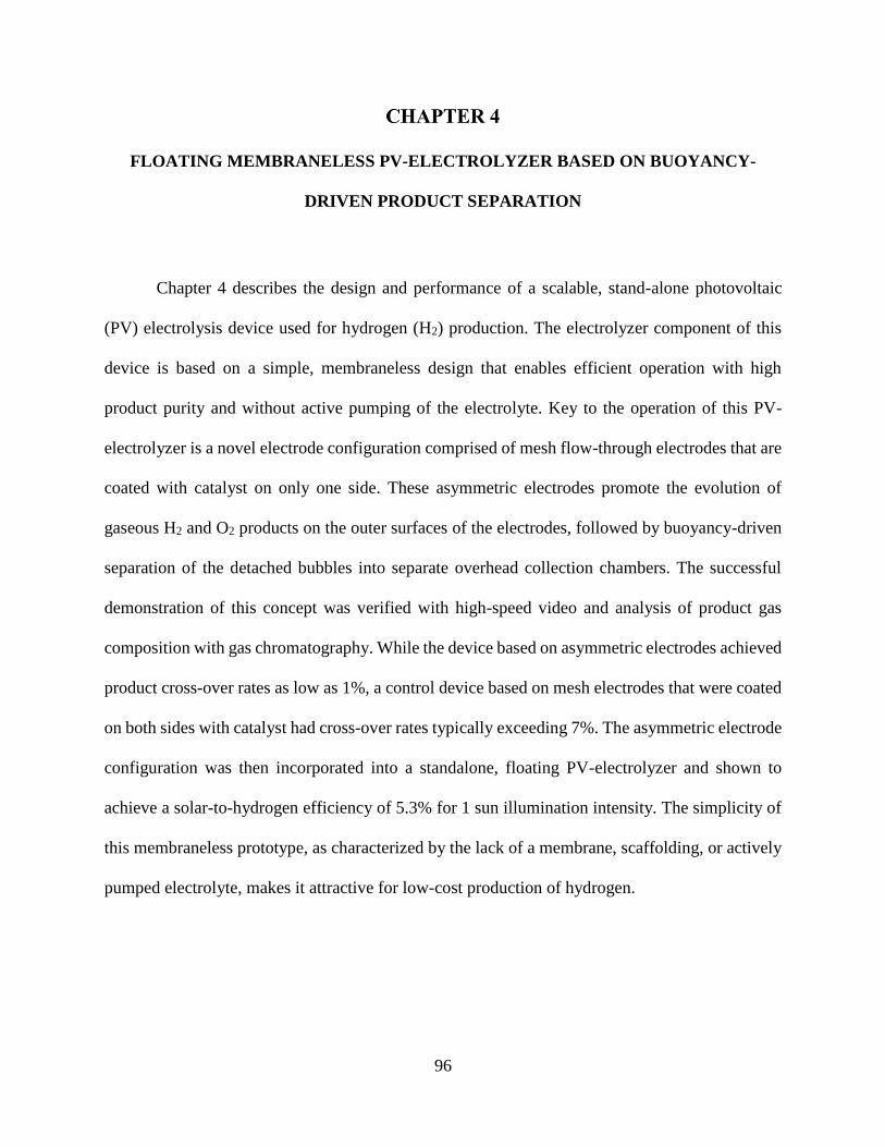
96

FLOATING MEMBRANELESS PV-ELECTROLYZER BASED ON BUOYANCY-

DRIVEN PRODUCT SEPARATION

Chapter 4 describes the design and performance of a scalable, stand-alone photovoltaic

(PV) electrolysis device used for hydrogen (H2) production. The electrolyzer component of this

device is based on a simple, membraneless design that enables efficient operation with high

product purity and without active pumping of the electrolyte. Key to the operation of this PV-

electrolyzer is a novel electrode configuration comprised of mesh flow-through electrodes that are

coated with catalyst on only one side. These asymmetric electrodes promote the evolution of

gaseous H2 and O2 products on the outer surfaces of the electrodes, followed by buoyancy-driven

separation of the detached bubbles into separate overhead collection chambers. The successful

demonstration of this concept was verified with high-speed video and analysis of product gas

composition with gas chromatography. While the device based on asymmetric electrodes achieved

product cross-over rates as low as 1%, a control device based on mesh electrodes that were coated

on both sides with catalyst had cross-over rates typically exceeding 7%. The asymmetric electrode

configuration was then incorporated into a standalone, floating PV-electrolyzer and shown to

achieve a solar-to-hydrogen efficiency of 5.3% for 1 sun illumination intensity. The simplicity of

this membraneless prototype, as characterized by the lack of a membrane, scaffolding, or actively

pumped electrolyte, makes it attractive for low-cost production of hydrogen.

97

Reprinted with permission from Int. J. Hydrogen Energy, 43, 1224–1238 (2018). Copyright 2017

Hydrogen Energy Publications LLC.

4.1 Introduction

Hydrogen is an attractive carbon-free energy carrier that can be sustainably produced by

water electrolysis if the electricity is provided by a renewable energy source. The commercial

market for electrolyzers that are used to drive water electrolysis are currently dominated by two

technologies: polymer electrolyte membrane (PEM) electrolyzers1 and alkaline electrolyzers.2 In

both technologies, a membrane or diaphragm is positioned between hydrogen (H2) and oxygen

(O2) evolving electrodes and serves a crucial role in device operation by separating product gases

while enabling efficient transport of ions between the electrodes. However, membranes can be

costly, prone to degradation and failure, and susceptible to cross-over issues.3 An electrolyzer

design that is able to operate with similar energy and collection efficiencies as the conventional

technology but without a membrane is highly attractive.4–7

While membrane-free electrolysis has the potential to reduce the capital costs of the

electrolyzer, its integration with a renewable energy source must be carefully considered in order

for carbon-free H2 generation from water electrolysis to become commercially viable. In the case

of photovoltaic (PV)-electrolysis, integration of PV-cells with the electrolysis cells in a single

98

device offers an opportunity to reduce the complexity and cost of the system.8–17 The current study

is motivated by the idea of incorporating PV-electrolysis reactors into a large-scale solar-hydrogen

plant that operates on open water where sunlight, water, and non-agricultural space are extremely

abundant. Such “solar fuels rigs” might be reminiscent, in some respects, to “deep sea rigs” used

to harvest fossil fuels today.18 Figure 4.1a shows an idealized rendering of a floating solar fuels

rig, where PV panels extending from the rig are integrated with low-cost membraneless

electrolysis cells, which utilize the solar-generated electricity to split water into oxygen and

hydrogen. Although seawater is cheap and abundant, there are substantial barriers to utilizing

commercially available, membrane-based electrolyzers for H2 production from seawater

electrolysis. Microorganisms in seawater can lead to biofouling,19 and trace amounts of

magnesium and calcium ions can form hydroxides that clog the pores of the membrane and

increase cell resistance.20 In contrast to conventional membrane-based electrolyzers, a

membraneless electrolyzer is expected to have less stringent requirements for electrolyte purity,

and thus may be uniquely suited for seawater electrolysis.

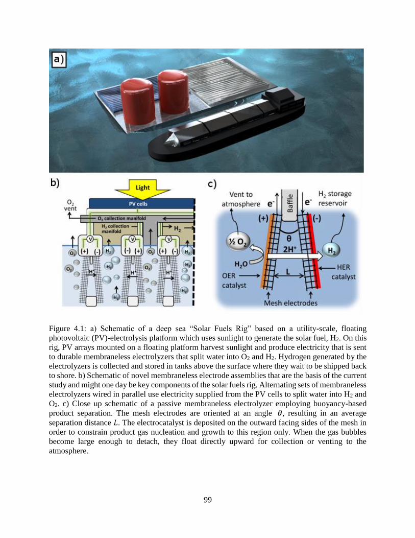
99

Figure 4.1: a) Schematic of a deep sea “Solar Fuels Rig” based on a utility-scale, floating

photovoltaic (PV)-electrolysis platform which uses sunlight to generate the solar fuel, H2. On this

rig, PV arrays mounted on a floating platform harvest sunlight and produce electricity that is sent

to durable membraneless electrolyzers that split water into O2 and H2. Hydrogen generated by the

electrolyzers is collected and stored in tanks above the surface where they wait to be shipped back

to shore. b) Schematic of novel membraneless electrode assemblies that are the basis of the current

study and might one day be key components of the solar fuels rig. Alternating sets of membraneless

electrolyzers wired in parallel use electricity supplied from the PV cells to split water into H2 and

O2. c) Close up schematic of a passive membraneless electrolyzer employing buoyancy-based

product separation. The mesh electrodes are oriented at an angle 𝜃, resulting in an average

separation distance 𝐿. The electrocatalyst is deposited on the outward facing sides of the mesh in

order to constrain product gas nucleation and growth to this region only. When the gas bubbles

become large enough to detach, they float directly upward for collection or venting to the

atmosphere.

100

In this chapter, we describe and demonstrate a prototype membraneless PV-electrolyzer

design (Figure 4.1b, c) that might one day be scaled up and incorporated into a large scale, floating

solar fuels rig such as that shown in Figure 4.1a. The primary novelty of this device is that efficient

separation and collection of the H2 and O2 product gases may be achieved without the use of a

membrane, diaphragm, or active pumping of the electrolyte. In previous studies, membraneless

separation of product species was demonstrated in electrochemical membraneless flow cells based

on flow-by electrodes,5,21–26 although these microfluidic devices possess significant challenges for

scale-up.27 More recently, membraneless electrolyzers based on mesh flow-through electrodes

have been demonstrated,6,28 including by our research group.4,29 In all of these previous studies on

membraneless electrolyzers, an essential feature was “flow-induced product separation”, whereby

convective forces associated with flowing electrolyte continuously remove product species before

they can cross-over to the opposing electrode. Thus, the reduced complexity that is achieved by

using a membraneless architecture is partially offset by the need to actively pump the electrolyte.

By contrast, we show that membraneless electrolyzers based on mesh flow through electrodes can

operate in a stagnant electrolyte in the absence of forced advection. Figure 4.1c shows a side-view

schematic of a single electrolysis cell consisting of angled mesh electrodes separated by a baffle.

Two key features of this device are i.) the slight angle between the electrodes, and ii.) the selective

placement of the active electrocatalysts only on the outer surfaces of the mesh electrodes. We

herein refer to these electrodes as “asymmetric electrodes”, as opposed to symmetric electrodes

with catalyst coated on both sides. Importantly, the product gas bubbles that form on an

asymmetric electrode predominately nucleate, grow, and detach from the outer (catalytic) side of

the mesh electrodes such that there is minimal cross-over of the product species between the two

electrodes. If the two mesh electrodes are oriented vertically and perfectly parallel to each other,

101

detached bubbles can still cross-over from one electrode to the other by colliding with objects

directly above them, such as other bubbles or mesh wires of the electrode itself. However, by

positioning the electrodes at a slight angle, separation is improved by facilitating bubbles to float

upwards unimpeded. Whereas previous membraneless electrolyzers employed “flow-induced

separation”, this study presents electrolyzers that utilize asymmetric mesh electrodes for

“buoyancy induced separation” in which growing gas bubbles passively detach from the active

electrode surfaces and float into separate collection manifolds or chambers.

The electrode configuration utilized in this study consists of titanium mesh electrodes

coated with platinum catalyst that was deposited by physical vapor deposition on the outer surfaces

of the mesh. These electrodes were integrated into a 3D-printed floating PV-electrolysis device

with onboard collection of the generated H2. The device was fabricated using 3D printing, or

additive manufacturing, which has numerous advantages over traditional manufacturing processes

and has found increasing use for (photo)electrochemical applications.4,30–37 Among these

advantages are rapid prototyping, efficient materials utilization, and fabrication capabilities that

are simply not possible with traditional tools. In this work, we have 3D-printed an electrochemical

device from PLA filament, which may be derived from renewable resources, and exhibits

reasonable chemical stability for the purpose of prototyping demonstrations in acidic and neutral

electrolytes.

In the remainder of this chapter, we present a detailed description of the novel electrode

configuration, followed by physical and electrochemical characterization of the electrodes in 2-

electrode measurements. For these proof of principle demonstrations, most characterization is

performed in 0.5 M H2SO4, a commonly employed laboratory electrolyte. Using a combination of

high speed video and gas chromatography measurements, product gas cross-over is characterized

102

under varied electrode angles and operating current densities. After demonstrating the efficacy of

passive membraneless electrolysis based on asymmetric flow-through electrodes, this concept is

applied to integrated, standalone PV-electrolysis cells. Finally, we discuss challenges and

opportunities for application of membraneless electrolyzers for H2 production from sea water

electrolysis.

4.2 Experimental

Chemicals – Solutions of sulfuric acid were prepared as described in Chapter 3. pH-neutral

electrolytes were prepared using sodium chloride (ACS Reagent grade, Sigma Aldrich), and

universal pH indicator (pH 4-10, Sigma Aldrich). Prior to experiments, electrolytes were de-

aerated by purging with nitrogen gas.

Electrode fabrication – Titanium (Ti) mesh sheets (40 wires per inch; 0.007” wire

diameter, Unique Wire Weaving Co., Inc.) were coated with 50 nm thick layers of platinum (Pt)

by electron-beam evaporation. Electrodes were designated as “asymmetric” if Pt was deposited on

only one side of the mesh sheet, and “symmetric” if Pt was deposited on both sides. The electrodes

were cut into rectangles with a width of 1.5 cm and a length of 6.0 cm. When incorporated into the

electrolyzer, only the bottom 2.0 cm of the mesh was submerged in electrolyte such that the

geometric area of the electrode involved in electrochemical reactions was 3.0 cm2.

Electrolyzer fabrication – The gas collection lid was printed out of Formlabs Grey

photopolymer resin, and was fitted with rubber septa for gas sampling. The electrodes were

mounted in the cell through slotted holes in the lid. For volumetric collection experiments, a

specialized lid was printed with a viewing window and graduated lines to read the height of the

electrolyte level. A specialized lid was also printed to measure the crossover of dissolved species

103

electrochemically. For these experiments, a separate electrode slot and guide rail was included to

allow for the insertion of an auxiliary sensor electrode.

The body of the floating PV-electrolysis module was assembled from several 3D-printed

components: the electrode scaffolding, a PV support raft, and a gas collection lid. The electrode

scaffolding was printed out of PLA and contained slits to incorporate two pairs of mesh electrodes.

Glass windows were epoxied to the walls of the scaffolding opposite of the electrodes to allow for

visual observation of accumulating H2 gas. The scaffolding also contained connection ports to

form a snap fit with the PV support raft. In addition to housing the PV panels, an important function

of the PV support raft is to provide floatation for the whole device. Thus, the PV support raft was

printed at low density, filling only 15% of the interior volume with PLA. The PV support raft

contained insets for four polycrystalline Si PV cells (Sundance Solar Products Inc.), each rated

with an open circuit voltage of 3.0 V and a short circuit current of 70 mA. Each panel comprised

of six smaller PV cells connected in series which together occupied an area of 14.4 cm2. The gas

collection lid was printed using Formlabs Tough photopolymer resin and included a port on which

a rubber septum was placed to withdraw the collected gas with a syringe.

Device characterization and performance – The electrolyzer and PV panels were

characterized using linear sweep voltammetry (LSV) and electrochemical impedance spectroscopy

(EIS). All current densities reported are normalized to the 2D rectangular area of the mesh

electrodes immersed in the electrolyte (3.0 cm2). For PV-electrolysis experiments, the illumination

source was a 500 W halogen work lamp (Utilitech) calibrated to standard air mass (AM) 1.5

intensity using a silicon reference cell (VLSI Standards, SRC-1000-RTD-QZ). During PV-

electrolysis experiments, the current was recorded by wiring the potentiostat in series and

operating it as a zero resistance ammeter. High-speed videos of bubble evolution from the mesh

104

electrodes were recorded using the same procedure outlined in Chapter 3. Color videos observing

the cross-over of dissolved species were recorded using a Casio EX-ZR700 camera recording at

30 frames per second and a resolution of 1920 x 1080 pixels.

Analysis of product gas composition – The collected gas was characterized using gas

chromatography (Agilent 7890B GC) with a thermal conductivity detector (TCD) using He as a

carrier gas. For experiments with the electrolyzer device, the lid of the cell contained two isolated

gas collection chambers located directly above the anode and cathode. Each chamber was fitted

with a rubber septum to allow for sampling with a gas-tight syringe (Hamilton). Product cross-

over was calculated according to previous reports4,5 by measuring the amount of H2 collected in

the anode chamber (located above the anode) and dividing by the total amount of H2 measured in

both the anode and cathode chambers. Although the reported quantities of cross-over are for single

trials, three additional replicates were conducted for one set of conditions (asymmetric electrodes,

30° separation angle, 40 mA cm-2), for which an average percent cross-over of H2 was found to be

2.1% with standard deviation of 0.8 %. When operating the floating PV-electrolysis cell, only the

headspace above the cathode is analyzed, while O2 was vented to the laboratory.

4.3 Results and discussion

4.3.1 Description and demonstration of a passive membraneless electrode assembly

The membraneless mesh electrode assembly was first tested in an electrochemical test cell,

independent from connection to PV cells, in order to demonstrate the concept of buoyancy induced

separation. The body, or base, of this electrolyzer is shown in Figure 4.2a and consists of a

rectangular container that holds the electrolyte and has two glass windows epoxied to the front and

back of the device in order to allow for side-view in situ high speed video imaging of the gas

bubbles evolving from the electrodes. The second part of the test cell, which is placed onto the cell

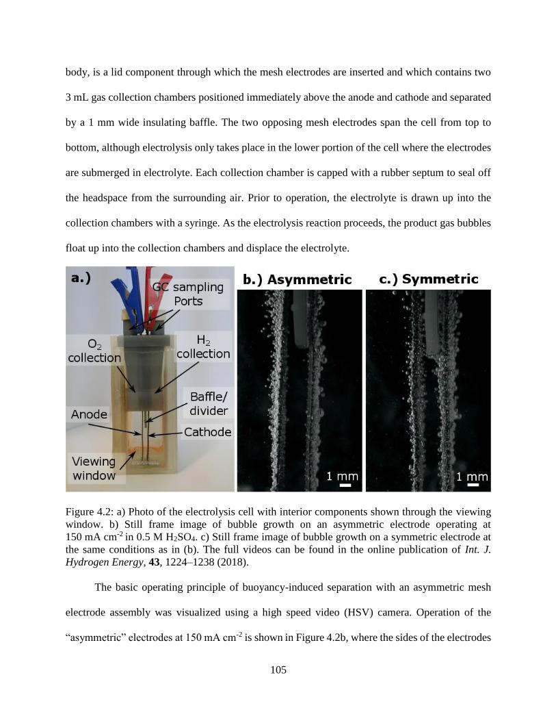
105

body, is a lid component through which the mesh electrodes are inserted and which contains two

3 mL gas collection chambers positioned immediately above the anode and cathode and separated

by a 1 mm wide insulating baffle. The two opposing mesh electrodes span the cell from top to

bottom, although electrolysis only takes place in the lower portion of the cell where the electrodes

are submerged in electrolyte. Each collection chamber is capped with a rubber septum to seal off

the headspace from the surrounding air. Prior to operation, the electrolyte is drawn up into the

collection chambers with a syringe. As the electrolysis reaction proceeds, the product gas bubbles

float up into the collection chambers and displace the electrolyte.

Figure 4.2: a) Photo of the electrolysis cell with interior components shown through the viewing

window. b) Still frame image of bubble growth on an asymmetric electrode operating at

150 mA cm-2 in 0.5 M H2SO4. c) Still frame image of bubble growth on a symmetric electrode at

the same conditions as in (b). The full videos can be found in the online publication of Int. J.

Hydrogen Energy, 43, 1224–1238 (2018).

The basic operating principle of buoyancy-induced separation with an asymmetric mesh

electrode assembly was visualized using a high speed video (HSV) camera. Operation of the

“asymmetric” electrodes at 150 mA cm-2 is shown in Figure 4.2b, where the sides of the electrodes

106

coated with the Pt electrocatalyst face outwards. So long as the electrolyte is sufficiently

conductive and the gap between the two electrodes is small, low solution resistance can be

achieved with this electrode geometry because dissolved ionic species—which do not experience

buoyancy forces— may easily pass through the holes in the mesh electrode. Figure 4.2b shows

that bubble nucleation is primarily confined to the outside faces of the asymmetric electrodes.

Once a bubble grows to a size where the buoyancy force exceeds the adhesion forces that keep it

attached to the electrode surface, the bubble detaches from the electrode and floats upward into

the overhead collection chamber. By this means, a passive membraneless electrolyzer based on

asymmetric mesh electrodes can operate with minimal product “cross-over”, which we define here

to be a process or event in which product generated at one electrode is transported across the

electrode gap and collected in the opposite overhead collection chamber. Figure 4.2c shows a still

frame image of bubble formation on a symmetric electrode, which has Pt catalyst deposited on

both sides of the electrode. Whereas bubble growth on the asymmetric electrodes is primarily

limited to the outside surfaces, bubbles readily grow and detach from both sides of the symmetric

electrodes. When bubbles reach the interior region between the electrodes, variations in local

convection can cause the bubbles to float up into either collection chamber, resulting in higher

cross-over rates and decreased product purity. The HSVs of asymmetric and symmetric electrodes

in operation are available in the online publication of Int. J. Hydrogen Energy, 43, 1224–1238

(2018).

The voltage efficiency associated with electrolysis can be determined from the 2-electrode

current-voltage (IV) curves. In order for the reaction to proceed, the applied cell voltage must be

greater than the difference in the reversible potentials of the oxygen evolution reaction (OER) and

hydrogen evolution reaction (HER), Δ𝐸0, which is equal to 1.23 V at standard conditions when

107

based on the lower heating value (LHV) of H2 (-237.1 kJ mole-1). The voltage efficiency of the

electrolyzer is equal to Δ𝐸0 divided by the operating voltage. Figure 4.3a compares the IV

characteristics of parallel (θ = 0°) asymmetric and symmetric electrodes operating in 0.5 M H2SO4.

At an operating current density of 100 mA cm-2, the electrolysis efficiencies for the asymmetric

and symmetric electrodes are 50.6% and 53.4%, respectfully. The slightly higher efficiency for the

symmetric electrodes can be attributed to the fact that they have twice as much electrochemically

active surface area. When accounting for the differences in platinum surface area, the IV-curves

for the asymmetric and symmetric electrodes collapse on top of each other (Figure 4.3b). Figure

4.3c shows the IV characteristics for asymmetric electrodes at varying angles of separation. When

operating at a current density of 100 mA cm-2, the electrolyzer efficiency decreases to 48.8% for

an electrode angle of 30°. This loss in efficiency with increasing electrode separation angle can be

attributed to an increase in the solution resistance, which increases as the average electrode

separation distance increases. Figure 4.3d shows the ohmic resistance of the cell determined by

EIS as a function of electrode separation angle. If the LSVs are corrected for ohmic resistance

using these values, the traces collapse into a single curve, as expected (See Appendix B,

Section 4.5.1. Figure 4.11).

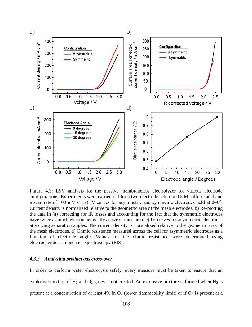
108

Figure 4.3: LSV analysis for the passive membraneless electrolyzer for various electrode

configurations. Experiments were carried out for a two-electrode setup in 0.5 M sulfuric acid and

a scan rate of 100 mV s-1. a) IV curves for asymmetric and symmetric electrodes held at θ=0⁰. Current density is normalized relative to the geometric area of the mesh electrodes. b) Re-plotting

the data in (a) correcting for IR losses and accounting for the fact that the symmetric electrodes

have twice as much electrochemically active surface area. c) IV curves for asymmetric electrodes

at varying separation angles. The current density is normalized relative to the geometric area of

the mesh electrodes. d) Ohmic resistance measured across the cell for asymmetric electrodes as a

function of electrode angle. Values for the ohmic resistance were determined using

electrochemical impedance spectroscopy (EIS).

4.3.2 Analyzing product gas cross-over

In order to perform water electrolysis safely, every measure must be taken to ensure that an

explosive mixture of H2 and O2 gases is not created. An explosive mixture is formed when H2 is

present at a concentration of at least 4% in O2 (lower flammability limit) or if O2 is present at a

109

concentration of at least 5% in H2 (upper flammability limit).38 Therefore, it is crucial to

demonstrate that the proposed electrolyzer design is able to efficiently collect the product gasses

with minimal cross-over of those products into the opposing collection chambers. To quantify

cross-over experimentally, the cell was operated at a constant current until ≈ 3 mL of product was

collected in the cathode chamber. The collected gas was then analyzed using gas chromatography

as described in Appendix B, Section 4.5.2. HSV was also recorded during operation to visually

inspect the dynamics of bubble evolution.

Cross-over behavior was systematically studied as a function of electrode angle and applied

current density for both symmetric and asymmetric electrodes. Figure 4.4 compares the percent

cross-over of H2 into the anode collection chamber for electrolysis experiments run at various

electrode angles and current densities. In Figure 4.4a, the percent H2 cross-over values for

asymmetric and symmetric electrodes are compared for different separation angles operating at a

current density of 20 mA cm-2, where the current density was calculated by dividing the total

applied current divided by the 2D area of the immersed electrode. As expected, lower cross-over

rates were measured for electrolysis with the asymmetric electrodes at all current densities, and

both electrode configurations showed lower rates of H2 cross-over as the electrode separation angle

was increased. Figure 4.4b shows the percent H2 cross-over recorded for the asymmetric electrodes

in response to the electrode separation angle and applied current density. Overall, the same trend

exists where increasing the electrode angle decreases the percentage of H2 cross-over.

Interestingly, the percent cross-over was found to decrease with increasing current density over

the ranges tested. The lowest percent H2 cross-over achieved for the asymmetric electrodes was

1%, and was recorded at an electrode separation angle of 30° and a current density of 40 mA cm-

2. A similar relationship between cross-over, electrode angle, and current density was found for

110

the symmetric electrodes, with the lowest percent cross-over recorded at 7% (See Appendix B,

Section 4.5.2 Figure 4.13).

Figure 4.4: Percent H2 cross-over into the O2 collection chamber of the static electrolyzer measured

by gas chromatography. Experiments were carried out in 0.5 M sulfuric acid at a constant applied

current. a) Comparing the percent H2 cross-over recorded for symmetric and asymmetric

electrodes at varying angles and operating at 20 mA cm-2, where the current density is reported

with respect to the geometric area of the electrodes. b) Percent H2 cross-over measured for

asymmetric electrodes at varying electrode angles and current densities.

As indicated by the results in Figure 4.4, asymmetric electrodes can be effective for

mitigating cross-over, but they do not eliminate it entirely. The gap spacing in the mesh can still

allow small bubbles to pass through, and collisions between rising bubbles combined with bubble-

induced local advection can result in lateral motion. Both of these factors can lead to cross-over.

By placing the electrodes at an angle to each other, the product bubbles are more likely to float

upwards unimpeded without being bumped, for example, by local bubble-induced turbulence into

the gap between the two mesh electrodes. Figure 4.5a-c shows schematic side views of three

possible mechanisms by which product gas can be transported across the gap between the two

angled electrodes. The first case is direct cross-over (Figure 4.5a), whereby a bubble from one

electrode travels directly through the opposing mesh electrode and into the opposite overhead

111

collection chamber. Based on HSV analysis, direct cross-over was seen to occur most frequently

when the electrodes were parallel to each other, but was very rarely observed as the angle between

the electrodes was increased to 5° or larger. A second mechanism by which cross-over can occur

was observed for electrode angles up to 15° and involved indirect cross-over through the formation

of a large, merged bubble that becomes pinned on the central baffle that divides the two mesh

electrodes (Figure 4.5b). Depending on the electrode type and angle, bubbles of this nature were

observed to grow for long time periods before randomly detaching into either of the two adjacent

collection chambers. When the asymmetric electrodes are operated at a 30° angle, neither the direct

nor indirect bubble cross-over is observed. However, cross-over can still occur in the form of

dissolved gas diffusion (Figure 4.5c). Cross-over of dissolved gas is most likely to occur after long

periods of operation when the electrolyte becomes saturated with dissolved gas, H2(aq) and O2(aq),

which can diffuse freely throughout the cell. The cross-over of dissolved gas is also assisted by

the local convection fields formed by the detached bubbles as they float upwards. When the

dissolved gas reaches the opposite side of the cell from which it formed, it can equilibrate with the

headspace above that chamber and/or the bubbles in the opposite chamber that will eventually float

up into the headspace. Although high speed video can be used to observe direct bubble cross-over

(Figure 4.5d) and indirect bubble cross-over (Figure 4.5e), it cannot directly observe cross-over of

dissolved H2(aq) and O2(aq).

112

Figure 4.5: Mechanisms of product gas cross-over in a static fluid electrolyzer. a) Direct bubble

cross-over: bubbles from one electrode detach and migrate to the opposite collection chamber. b)

Indirect bubble cross-over: bubbles from both electrodes accumulate on the central baffle, forming

a mixed gas bubble which can detach and travel into either collection chamber. c) Dissolved gas

cross-over: the electrolyte becomes saturated with dissolved product gas which can diffuse over

to the opposing electrode. The dissolved gas can equilibrate with bubbles as they float upwards to

the collection chamber. For simplicity, dissolution and diffusion was only shown for dissolved H2.

Still frame images taken from high speed video measurements showing instances of d) direct

bubble cross-over recorded for parallel asymmetric electrodes and e) indirect bubble cross-over

recorded for asymmetric electrodes at a 30 degree angle and 100 mA cm-2.

In order to visualize cross-over by dissolved H2 and O2, electrolysis was conducted in a pH

neutral 0.5 M NaCl electrolyte containing 17 % vol. universal pH indicator. The unbuffered, pH-

neutral solution allows for visualization of the spatio-temporal evolution of the dissolved-product

species because the HER and OER reactions lead to the build-up of hydroxyls at the cathode and

113

protons at the anode, respectively. When exposed to an alkaline pH, the universal pH indicator dye

quickly turns dark purple, and by tracking the movement of this purple plume it is possible to

monitor the progression of the dissolved reduction products as they migrate away from the cathode.

Technically, the color change is directly tied to OH- concentration, but it is a reasonable

assumption in these experiments that the plume of H2(aq) closely overlays that of the generated

hydroxyls. Figure 4.6 contains side-view photographs that show the progression of the alkaline

product plume as it spreads away from an asymmetric mesh cathode while operating at 40 mA cm-

2 and an electrode separation angle of 30°. Within 10-30 seconds of the start of electrolysis, the

product plume reaches the anode, proving that dissolved species transport between the two angled

electrodes can occur at reasonably high rates within the time scales of the experiments in Figure

4.5. At these time and length scales, transport must be dominated by convection that results from

bubble-induced fluid flow within the electrolyte.

114

Figure 4.6: Visualization of dissolved species cross-over during electrolysis in 0.5 M NaCl solution

with universal pH indicator. The indicator turns from red to dark purple in the presence of the

hydroxyls generated at the cathode. The experiment was carried out with asymmetric electrodes

operating at a current density of 40 mA cm-2.

The pH indicator dye experiment provides strong evidence that the cross-over of dissolved

gas is likely responsible for the H2 signal measured by GC in the anode compartment after

operation at lower current densities. Cross-over of dissolved H2(aq) may also explain the trend of

decreasing cross-over rates with increasing current density that was reported in Figure 4.4b. When

lower current densities are applied, a larger fraction of the product gas remains dissolved in the

aqueous phase. Operating at a lower current density also requires a longer time for the collection

chambers to fill up. While the time to fill the chamber during electrolysis at 40 mA cm-2 was only

4 minutes, experiments at 10 mA cm-2 required 16 minutes. Longer experiments allow more time

for gas to saturate the electrolyte, distribute across the electrolyte reservoir, and equilibrate in the

115

opposite collection chambers. However, the rate of dissolved gas cross-over is limited by the

solubility of the gasses in solution. Thus, operating at high current density at steady state can result

in a higher fraction of the products entering the gas phase (i.e. bubbles) rather than the dissolved

phase. Additionally, the rate of equilibration between the dissolved gasses and the headspace can

be minimized by further optimizing the geometry of the electrolysis cell. For example, the contact

area between the electrolyte and the headspace could be decreased. If the electrolyzer was

operating in an open body of water, the dissolved anode products would also be able to diffuse

away from the device, as opposed to being constrained to the enclosed reservoir of the current

design.

In addition to equilibrating with the opposing collection chamber, it is also possible for the

dissolved gasses to participate in a back reaction. For example, H2 evolved at the cathode can be

transported over to the anode, where it is oxidized back into protons through the hydrogen

oxidation reaction (HOR). Similarly, O2 evolved at the anode can be reduced back to water at the

cathode through the oxygen reduction reaction (ORR). Both of these so-called “back reaction”

processes result in lower Faradaic efficiencies for the OER and HER reactions, thereby decreasing

electrolysis efficiency. Fortunately, the magnitude of the back reactions is limited by the solubility

and mass transport of H2 and O2 gasses across the electrolyte gap between the anode and cathode.

In order to quantify the rate of the HOR back reaction at the anode used in the passive

membraneless electrolyzer, an auxiliary Pt-coated mesh electrode was used as an electrochemical

sensor. As illustrated in Figure 4.7a, this sensor electrode was positioned in between the anode and

cathode mesh electrodes and held parallel to the anode electrode. During electrolysis, the sensor

electrode was held at a potential of 0.8 V vs. Ag/AgCl, where it has ample overpotential to oxidize

H2 crossing over from the cathode, but the overpotential is insufficient to reduce O2.4 By this

116

means, the auxiliary electrode can serve as a H2 sensor that can selectively and quantitatively

measure the flux of dissolved H2 that would normally be oxidized at the OER anode.

Figure 4.7: a.) Schematic of a modified electrolysis cell involving a sensor electrode that is used

to measure current efficiency losses due to the HOR of H2 at the anode. b) Average losses in

current efficiency due to HOR during constant current electrolysis while holding the applied

potential of the sensing electrode at +0.8 V vs. Ag/AgCl. The current efficiency loss was calculated

by dividing the total integrated charge recorded by the sensing electrode by the total charge passed

between the anode and cathode throughout the electrolysis experiment. Measurements were

recorded for a 30° electrode angle in 0.5 M H2SO4.

Back reaction experiments utilizing the auxiliary electrode were performed using

asymmetric electrodes angled at 30⁰ and operated at constant current densities of 20 mA cm-2, 30

mA cm-2, and 40 mA cm-2 until the H2 collection chamber was filled. An Ag|AgCl reference

electrode was also present in the experimental set-up, and a bipotentiostat was used to apply a

constant potential of +0.8 V vs. Ag|AgCl to the sensor electrode while water electrolysis was

carried out between the anode and cathode of the electrolyzer cell. The results of the back reaction

experiments are shown in Figure 4.7b, where the Faradaic efficiency loss due to oxidation of H2

117

that crossed-over from the cathode is plotted as a function of the operating current density of the

electrolysis cell. This Faradaic efficiency loss is given by the percentage of H2 lost due to the HOR

back reaction, and was calculated by dividing the net charge passed through the sensing electrode

by the net charge passed between the anode and cathode over the duration of the experiment. As

expected, the largest fractional loss of H2, 3.5%, was measured for electrolysis at the lowest

operating current density, 10 mA cm-2, for which the lower rate of H2 generation allows a higher

percentage of the generated H2 to dissolve into the electrolyte and oxidize at the sensor electrode.

As the current density increased to 40 mA cm-2, the percent loss of H2 through the back reaction

decreased down to 1.5% as a larger fraction of the generated H2 was converted into gas bubbles

that were soon collected in the overhead collection chambers. Depending on the relative prices of

electricity and H2, back-reaction losses of 1.5%-3.5% can be tolerable in real devices if electricity

prices and capital costs of the membraneless system are sufficiently low.7 Although these

experiments only quantified the losses in Faradaic efficiency due to H2 oxidation at the cathode, it

is expected that the losses from oxygen reduction at the anode would be approximately the same

magnitude due to the similar transport pathways, solubility and diffusivity of aqueous O2.

Beyond efficiency losses due to back reaction, bubble cross-over can also impact device

performance by increasing the ohmic resistance for ion transport between the two electrodes.

When gas phase bubbles enter the spacing between electrodes, they behave as insulators which

inhibit ionic conduction.39 Fortunately, the bubbles largely remain on the outside of the asymmetric

electrodes where they do not significantly affect ion conduction between the two electrodes.

4.3.3 Measuring product collection efficiencies

The product collection efficiency can be defined as the percentage of generated H2 that is

successfully collected and removed from the electrolyzer. The collection efficiency can be less

118

than 100% for several reasons, including dissolution losses, back reaction losses, and losses

associated with H2 bubbles that never reach the desired collection chamber or apparatus. In this

study, the H2 collection efficiency of the membraneless electrolyzer was determined by measuring

the volumetric rate of H2 collected in the overhead collection chambers. These experiments were

performed using a specialized lid that was printed with graduated lines to read the height of the

electrolyte displaced during electrolysis (Appendix B, Section 4.5.3 Figure 4.14). Figure 4.8a

shows the recorded volume of H2 and O2 collected in the lid as a function of time during a constant

current electrolysis at 40 mA cm-2 with asymmetric electrodes held at a separation angle of 30°.

The error bars designate a 95% confidence interval around the average time of collection over

three separate trials. As predicted from the stoichiometry, the relative rates of H2 and O2 collection

are at approximately a 2:1 ratio. The solid lines on the plot represent the theoretical rate of

volumetric generation predicted from Faraday’s Law and the ideal gas law. When comparing the

slopes of the experimental and predicted data, the volumetric collection efficiencies for H2 and O2

were found to be 83.0% and 83.8%, respectively.

Figure 4.8: a) Volume of product gas collected as a function of time. Data was recorded for a 30°

electrode separation angle and an operating current density of 40 mA cm-2. The error bars

correspond to a 95% confidence interval for data averaged over three trials. The solid lines

represent the theoretical volumetric collection based on Faraday’s law and the Ideal gas law. b)

119

Mole balance on H2 generated during electrolysis with an electrode angle of 30° and operating at

40 mA cm-2 for 3.9 minutes.

By knowing the product collection efficiency, it is furthermore possible to close the mass

balance on the H2 generated by the membraneless electrolyzer. Figure 4.8b shows the resulting

balance of H2 for electrolyzer operation at 40 mA cm-2, which includes the collected H2, H2 lost to

the back reaction, H2 loss to cross-over to the anode collection stream, and “uncollected H2“ that

is still present in the system but did not reach the collection chamber. The percent H2 collected

was determined directly from the volumetric collection efficiency experiments described above,

and the percent H2 loss due to back reaction was determined from the results of the sensor electrode

experiments shown in Figure 4.7b. The percent H2 loss due to cross-over was determined from the

gas chromatography experiments shown in Figure 4.4b. From the analysis shown in Figure 4.8b,

14.1% of the generated H2 predicted from Faraday’s law remains uncollected. The uncollected H2

can be primarily attributed to H2 lost to dissolution in the liquid electrolyte and, to a smaller extent,

H2(g) bubbles that remain uncollected in the electrolysis cell. Based on the net amount of H2

generated during the electrolysis experiment, the volume of electrolyte within the cell, and the

solubility limit of H2, up to 12% of the generated H2 may have been dissolved in the electrolyte.

After experiments, some bubbles remained adhered to the reactor walls and sides of the electrodes,

likely accounting for the remaining ≈2 % of uncollected H2. For longer operating times over which

large amounts of H2 are produced, it is expected that the uncollected H2 losses will go towards 0%

because dissolved H2 and uncollected gas bubbles will be very small compared to the total amount

of H2 generated. In this case, the collection efficiency should only be limited by the back reaction

and dissolved gas cross-over to the opposite gas collection chamber.

120

4.3.4 Demonstration of a floating PV-electrolysis module

Having demonstrated that buoyancy driven product separation is possible with acceptable rates of

cross-over, we devote the remainder of the discussion to integrating the membraneless design into

a bench scale floating PV-electrolysis module. As illustrated schematically in Figure 4.9a, this

module contains two sets of asymmetric electrodes angled at 30°. The electrodes were wired

parallel to each other and connected to four parallel-connected c-Si PV panels, each of which

consisted of 6 sub-cells that are connected in series. A wiring diagram of the PV panels and

electrolyzers is shown in the Appendix B, Section 4.5.4 Figure 4.15. The entire module was then

placed in a 1 L reservoir of 0.5 M H2SO4 (Figure 4.9b), where it floats on the surface of the

electrolyte thanks to the high buoyancy of the void-containing 3D-printed raft. The purity of the

H2 collected in the interior reservoir was sampled through a sealed port for GC analysis after

completion of the electrolysis experiment.

121

Figure 4.9: a) Schematic side-view of the floating PV-electrolysis module, which is based on two

sets of asymmetric mesh electrodes that are wired in parallel to each other and to four PV panels.

The module floats in a reservoir of sulfuric acid. Hydrogen evolved at the cathode is collected

underneath the PV panels while the oxygen is allowed to vent to the atmosphere. b) Photo of the

PV-electrolyzer module floating in a sulfuric acid reservoir. c) I-V curve matching for the

electrolyzer and PV cells. The electrolyzer curve is for 6 cm2 of asymmetric mesh electrodes

submerged in 0.5 M sulfuric acid and was recorded at a scan rate of 10 mV s-1. The PV curve is

the combined I-V response for four PVs wired in parallel under a lamp calibrated to the AM 1.5G

intensity, and was recorded at a scan rate of 100 mV s-1. The intersection of these curves predicts

the operating current of the device when the PV panels and electrolyzer are connected to each

other. d) Operating current of the floating PV-electrolysis unit as a function of time during

unassisted water electrolysis under the same illumination conditions as described for the

measurements in c.).

Figure 4.9c shows the predicted performance of the PV-electrolyzer, which can be estimated

from the intersection of the individually tested IV curves of the electrolyzer and the PV panels.40

122

For these measurements, the two pairs of asymmetric electrodes were connected in parallel, and

the four PV panels were also connected in parallel. The performance of the four PV panels

connected in parallel was measured under illumination by an unfiltered halogen work lamp with

irradiance calibrated to match the solar AM 1.5 power intensity (100 mW cm-2). The resulting IV

curve is characterized by an open circuit voltage (Voc) of 3.127 V, a short circuit current (Jsc) of

256.2 mA, a fill factor (FF) of 72.1%, and a photovoltaic efficiency (ηPV) at max power point of

10.0 %. 𝜂𝑃𝑉 was calculated based on the cumulative PV cell area of 57.6 cm2 and incident light

intensity of 100 mW cm-2. The 2-electrode IV curve for the two pairs of asymmetric electrodes

shows that water electrolysis begins to take place above an applied voltage of ≈ 1.7 V, followed

by an exponential rise in current as voltage is increased further. From the intersection of the two

IV curves (I= 238.3 mA, V= 2.263 V), the electrolyzer efficiency (𝜂𝑒), coupling efficiency (𝜂𝑐),

and the solar–to-hydrogen (STH) efficiency (𝜂𝑆𝑇𝐻) may be determined. At the predicted operating

voltage, the electrolyzer efficiency is calculated to be 𝜂𝑒 =54%. The coupling efficiency, defined

as the device power at the operating point divided by the max power that can be produced by the

PV cells,40 is calculated to be 98%. This indicates that the PV and electrode arrangements are

almost perfectly matched. Combining the PV, electrolysis, and coupling efficiencies, the solar-to-

hydrogen conversion efficiency (ηSTH) is predicted to be 𝜂𝑆𝑇𝐻 = 𝜂𝑃𝑉𝜂𝑒𝜂𝑐= 5.3%. It should be

noted that 𝜂𝑃𝑉 was calculated based on the area of the PV cells, not the area of the entire PV-

electrolysis module. In an optimized PV-electrolyzer, the percentage of area occupied by PV

panels would be maximized such that the PV area is similar to the module area.

After measuring the IV curves for the individual components, the floating PV-electrolysis

module was tested under continuous illumination in 0.5 M H2SO4 for 75 min. Figure 4.9d shows

the measured operating current of the floating PV-electrolysis device as a function of time,

123

revealing stable operation. The average current of the device was found to be in good agreement

with the predicted operating point in Figure 4.6c. During operation, H2 was collected underneath

the central lid while O2 was allowed to vent to the atmosphere. After filling the collection chamber,

the gas was analyzed with GC. After subtracting out O2 signal associated with air (based on an

N2:O2 ratio of 79:21), the purity of the collected product gas was determined to be 98% H2.

4.3.5 Challenges for Seawater Electrolysis

Although this study has demonstrated that a membraneless, floating PV-electrolysis module can

generate and collect H2 with reasonable efficiency, many challenges for seawater electrolysis must

still be overcome41–43 before the solar fuels rig concept in Figure 4.1 can be realized. Future

demonstrations of devices for seawater electrolysis should report on their stability in electrolytes

that more realistically simulate seawater. Laboratory electrolytes are typically prepared from

reagent grade NaCl, H2SO4, and 18 MΩ DI water, and are free of contaminants which could cause

scaling or biofouling by micro- or macro-organisms. Biofouling, or the adhesion of micro- or

macro- organisms on a surface, has been found to be highly detrimental to membranes in reverse-

osmosis (RO)-based desalination devices.44,45 A simple way to overcome this deficiency in an

electrolysis device is to operate without a membrane, although the electrodes themselves may be

prone to biofouling as well. However, there is evidence to suggest that electrochemical reactions

at the anode can generate reactive oxides and hypochlorites that act as a protective antimicrobial

agents,46,47 and a recent study by our group has demonstrated the possibility of designing “impurity

tolerant” catalysts for water splitting.48 Inorganic scaling can also degrade the performance of the

electrodes, with Mg(OH)2 and Ca(OH)2 precipitating out of the electrolyte in alkaline conditions

and blocking electrochemically active sites.42,49 For proper operation of Nafion membranes in

chlor-alkali cells, brine purification is required to reduce the concentration of magnesium and

124

calcium ions below 50 parts per billion;50 by comparison seawater typically contains ≈1300 ppm

of Mg2+ and ≈400 ppm of Ca2+.51

In addition to challenges with long term stability, seawater electrolysis faces a number of

efficiency drawbacks when compared to concentrated acid or alkaline electrolysis. The electrolysis

of a pH neutral electrolyte tends to have more sluggish kinetics,52 and additional thermodynamic

penalties arise from pH gradients that form across the cell as the reaction proceeds.53 Natural

seawater is less conductive than acidic solutions such as 0.5 M H2SO4, which results in a larger

solution resistance. All of these factors require that a larger cell voltage be applied between the

electrodes to achieve a given current density, which generally requires more PV cells to be

connected in series and thereby decreases the solar-to–hydrogen conversion efficiency.40

In order to get an estimate of typical efficiency losses for electrolysis in seawater, 2-

electrode IV curves were measured with parallel asymmetric electrodes operating in 0.5 M H2SO4

and a synthetic seawater comprised of 0.6 M NaCl. The salinity of seawater is typically around

3.5% by mass,54 making 0.6 M NaCl a simple electrolyte with similar conductivity to seawater.

These IV curves are provided in Figure 4.10, showing that significantly larger voltages are required

to achieve the same electrolysis current density in the NaCl solution compared to the sulfuric acid

solution. For example, voltages of 2.44 V and 3.68 V are required to operate at a current density

of 100 mA cm-2 in the 0.5 M H2SO4 and 0.6 M NaCl solutions, respectively. This increase in

operating voltage of 1.24 V results in a decrease in the electrolysis efficiency from ηe = 50.4% in

0.5 M H2SO4 and ηe = 33.4% in 0.6 M NaCl. Based on the measured solution resistances and

electrode arrangement, 0.41 V of this extra voltage requirement can be attributed to the increased

solution resistance of the synthetic seawater electrolyte. More voltage is also required to overcome

the Nernstian penalty that arises from the pH gradients that develop at the anode and cathode. If

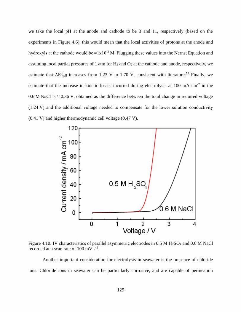
125

we take the local pH at the anode and cathode to be 3 and 11, respectively (based on the

experiments in Figure 4.6), this would mean that the local activities of protons at the anode and

hydroxyls at the cathode would be ≈1x10-3 M. Plugging these values into the Nernst Equation and

assuming local partial pressures of 1 atm for H2 and O2 at the cathode and anode, respectively, we

estimate that ΔEocell increases from 1.23 V to 1.70 V, consistent with literature.53 Finally, we

estimate that the increase in kinetic losses incurred during electrolysis at 100 mA cm-2 in the

0.6 M NaCl is ≈ 0.36 V, obtained as the difference between the total change in required voltage

(1.24 V) and the additional voltage needed to compensate for the lower solution conductivity

(0.41 V) and higher thermodynamic cell voltage (0.47 V).

Figure 4.10: IV characteristics of parallel asymmetric electrodes in 0.5 M H2SO4 and 0.6 M NaCl

recorded at a scan rate of 100 mV s-1.

Another important consideration for electrolysis in seawater is the presence of chloride

ions. Chloride ions in seawater can be particularly corrosive, and are capable of permeation

126

through protective layers.55 Additionally, the oxygen evolution reaction (Eo=+1.23 V NHE) must

compete with the evolution of chlorine (Cl2) gas (Eo=+1.36 V NHE). Cl2 has commercial value,

being produced by the Chlor-alkali process at 50-60 mton per year globally,56 so there may be

some interest in capturing Cl2 as a value-added side product during seawater electrolysis. However,

it is important to note that Cl2 is a toxic chemical that introduces health and environmental risks.57

In the present PV-electrolyzer design, the O2 product generated at the anode is simply vented to

the atmosphere, but this would not be acceptable in the case of Cl2. If it were desirable to avoid

Cl2 evolution, developing an anode catalyst that would be selective for the OER over Cl2 evolution

would be one solution. Fujimera et al. have demonstrated MnO2 OER electrocatalysts capable of

100% faradaic efficiency during electrolysis in an alkaline NaCl solution, although it’s behavior

was not reported for an acidic electrolyte that would be encountered at the anode during seawater

electrolysis.58

Besides developing catalysts that would be compatible with seawater, many other

challenges would need to be overcome at the device and plant-level. The corrosive environment

of seawater also poses problems for other components of a solar fuels rig (piping, storage vessels,

solar panels, pumps, etc), and there are many open questions relating to process engineering and

rig construction. What sort of rig size makes economic sense, and at what pressure should the H2

be stored? Should the rig be anchored to the sea floor, or be a free floating vessel that could move

between markets and out of the way of storms? As the concept of seawater electrolysis with stand-

along rigs gains more and more attention, engineering system- and plant-level solutions will be of

great importance.

127

4.4 Conclusions

This study has demonstrated a novel electrode architecture for water electrolysis whereby

high purity (≈99% pure) H2 can be produced without a membrane and without the actively pumped

electrolyte. Instead, this design relies on the use of buoyancy-driven separation of H2 and O2 gas

bubbles that are generated at so called “asymmetric” mesh electrodes with active catalyst deposited

onto only their outer surfaces. This arrangement is scalable and enables efficient electrolysis with

minimal ohmic resistance losses so long as the electrolyte is sufficiently conductive. By

systematically changing the mesh electrode angle and operating current density, the rate of product

gas cross-over between the anode and cathode chambers was observed qualitatively using high

speed video and quantitatively using gas chromatography. It was shown that the asymmetric mesh

electrodes significantly decrease H2 cross-over rates under all conditions that were tested, with the

lowest percent H2 cross-over found to be 1%. For cases when no direct cross-over of bubbles was

observed, in situ videos of electrolysis in the presence of color-changing dyes indicated that the

convective transport of dissolved H2 between chambers is the primary mechanism of product

cross-over. This study also showed that this membraneless electrode architecture can be easily

integrated into a 3D printed, floating PV-electrolysis module, which was used to produce H2 with

a solar-to-hydrogen efficiency of 5.3% in 0.5 M H2SO4. This demonstration was inspired by the

idea of seawater electrolysis, which represents an intriguing approach to the renewable generation

of fuel using non-agricultural space and non-drinking water. However, significant challenges in

catalysis, reactor design, and plant design will need to be overcome for economical seawater

electrolysis to become a reality.

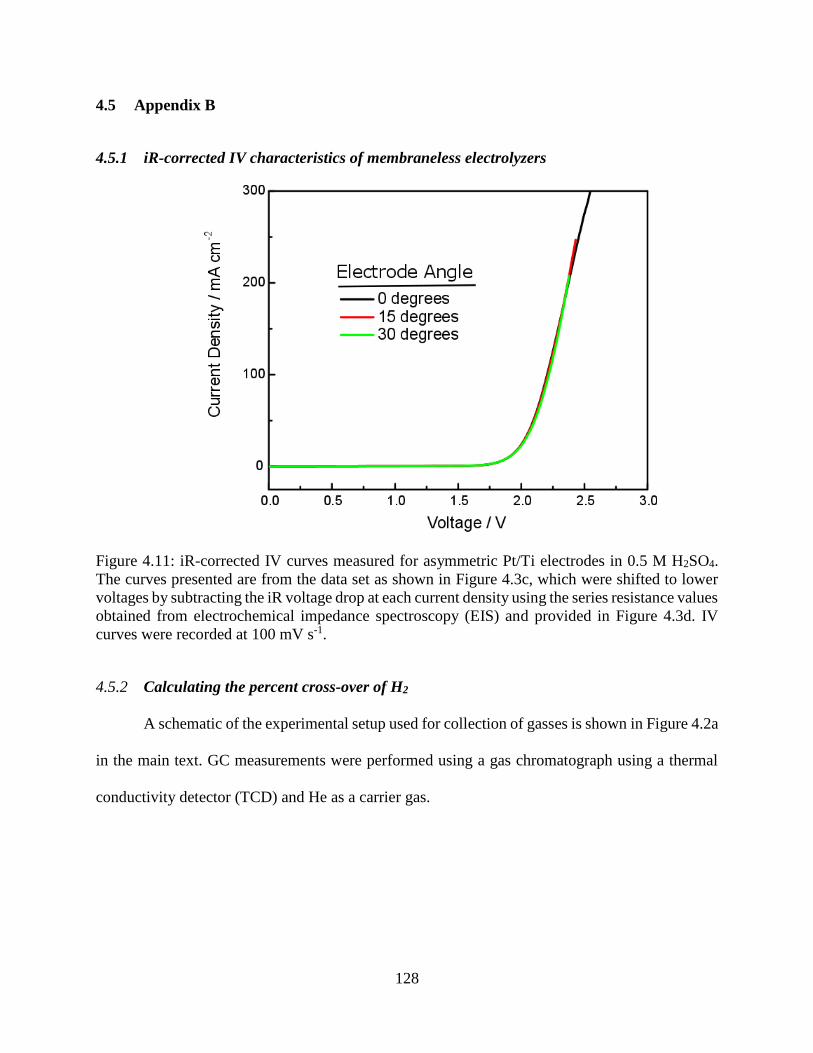
128

4.5 Appendix B

4.5.1 iR-corrected IV characteristics of membraneless electrolyzers

Figure 4.11: iR-corrected IV curves measured for asymmetric Pt/Ti electrodes in 0.5 M H2SO4.

The curves presented are from the data set as shown in Figure 4.3c, which were shifted to lower

voltages by subtracting the iR voltage drop at each current density using the series resistance values

obtained from electrochemical impedance spectroscopy (EIS) and provided in Figure 4.3d. IV

curves were recorded at 100 mV s-1.

4.5.2 Calculating the percent cross-over of H2

A schematic of the experimental setup used for collection of gasses is shown in Figure 4.2a

in the main text. GC measurements were performed using a gas chromatograph using a thermal

conductivity detector (TCD) and He as a carrier gas.

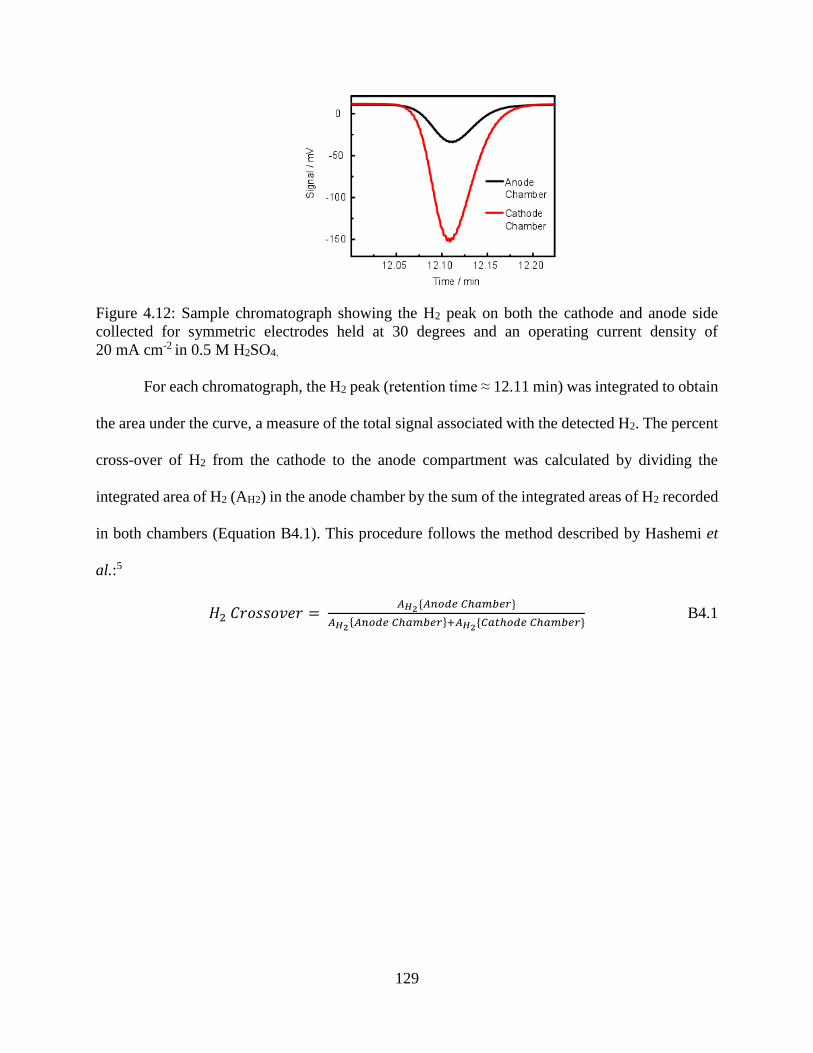
129

Figure 4.12: Sample chromatograph showing the H2 peak on both the cathode and anode side

collected for symmetric electrodes held at 30 degrees and an operating current density of

20 mA cm-2 in 0.5 M H2SO4.

For each chromatograph, the H2 peak (retention time ≈ 12.11 min) was integrated to obtain

the area under the curve, a measure of the total signal associated with the detected H2. The percent

cross-over of H2 from the cathode to the anode compartment was calculated by dividing the

integrated area of H2 (AH2) in the anode chamber by the sum of the integrated areas of H2 recorded

in both chambers (Equation B4.1). This procedure follows the method described by Hashemi et

al.:5

𝐻2 𝐶𝑟𝑜𝑠𝑠𝑜𝑣𝑒𝑟 = 𝐴𝐻2𝐴𝑛𝑜𝑑𝑒 𝐶ℎ𝑎𝑚𝑏𝑒𝑟

𝐴𝐻2𝐴𝑛𝑜𝑑𝑒 𝐶ℎ𝑎𝑚𝑏𝑒𝑟+𝐴𝐻2𝐶𝑎𝑡ℎ𝑜𝑑𝑒 𝐶ℎ𝑎𝑚𝑏𝑒𝑟

B4.1

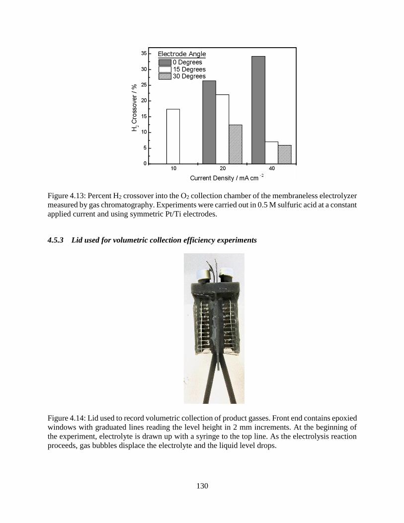
130

Figure 4.13: Percent H2 crossover into the O2 collection chamber of the membraneless electrolyzer

measured by gas chromatography. Experiments were carried out in 0.5 M sulfuric acid at a constant

applied current and using symmetric Pt/Ti electrodes.

4.5.3 Lid used for volumetric collection efficiency experiments

Figure 4.14: Lid used to record volumetric collection of product gasses. Front end contains epoxied

windows with graduated lines reading the level height in 2 mm increments. At the beginning of

the experiment, electrolyte is drawn up with a syringe to the top line. As the electrolysis reaction

proceeds, gas bubbles displace the electrolyte and the liquid level drops.

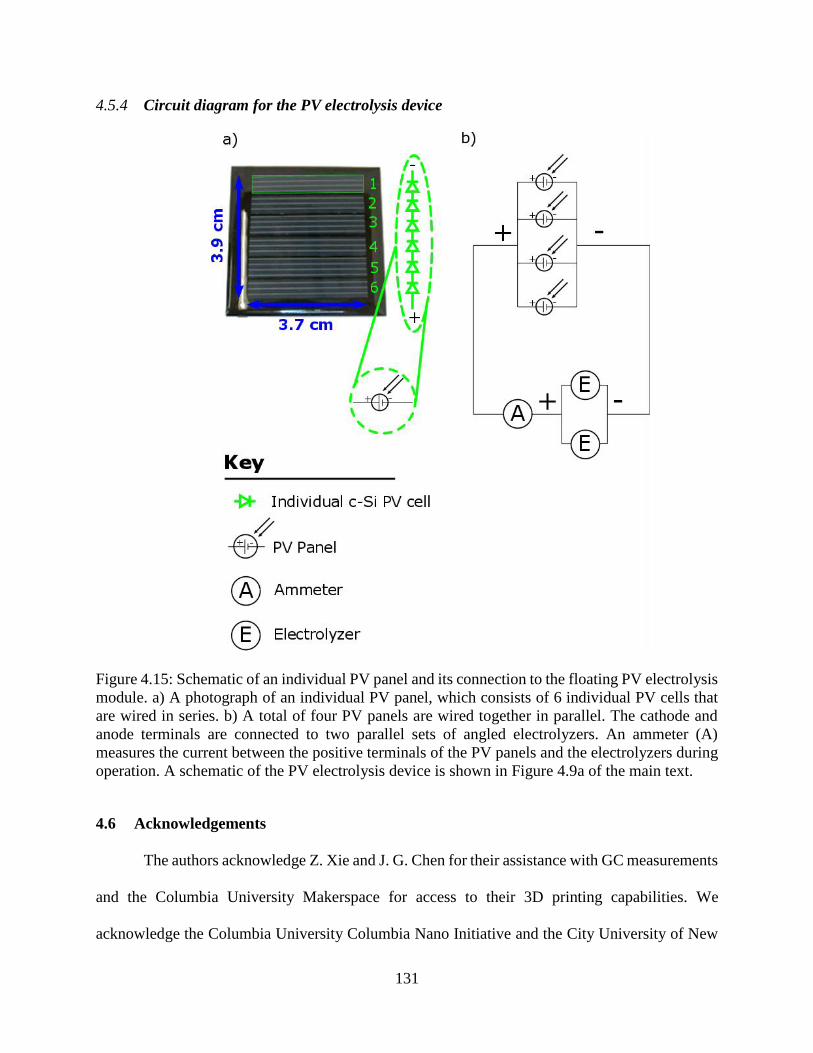
131

4.5.4 Circuit diagram for the PV electrolysis device

Figure 4.15: Schematic of an individual PV panel and its connection to the floating PV electrolysis

module. a) A photograph of an individual PV panel, which consists of 6 individual PV cells that

are wired in series. b) A total of four PV panels are wired together in parallel. The cathode and

anode terminals are connected to two parallel sets of angled electrolyzers. An ammeter (A)

measures the current between the positive terminals of the PV panels and the electrolyzers during

operation. A schematic of the PV electrolysis device is shown in Figure 4.9a of the main text.

4.6 Acknowledgements

The authors acknowledge Z. Xie and J. G. Chen for their assistance with GC measurements

and the Columbia University Makerspace for access to their 3D printing capabilities. We

acknowledge the Columbia University Columbia Nano Initiative and the City University of New

132

York Advanced Science Research Center for use of the physical vapor deposition equipment.

D.V.E. and J.T.D. acknowledge Columbia University for startup funding.

4.7 References

1. Carmo, M., Fritz, D. L., Mergel, J. & Stolten, D. A comprehensive review on PEM water

electrolysis. Int. J. Hydrogen Energy 38, 4901–4934 (2013).

2. Zeng, K. & Zhang, D. Recent progress in alkaline water electrolysis for hydrogen

production and applications. Prog. Energy Combust. Sci. 36, 307–326 (2010).

3. Millet, P., Ngameni, R., Grigoriev, S. A. & Fateev, V. N. Scientific and engineering issues

related to PEM technology: Water electrolysers, fuel cells and unitized regenerative

systems. Int. J. Hydrogen Energy 36, 4156–4163 (2011).

4. O’Neil, G. D., Christian, C. D., Brown, D. E. & Esposito, D. V. Hydrogen Production with

a Simple and Scalable Membraneless Electrolyzer. J. Electrochem. Soc. 163, F3012–F3019

(2016).

5. Hashemi, S. M. H., Modestino, M. A. & Psaltis, D. A membrane-less electrolyzer for

hydrogen production across the pH scale. Energy Environ. Sci. 8, 2003–2009 (2015).

6. Gillespie, M. I., van der Merwe, F. & Kriek, R. J. Performance evaluation of a

membraneless divergent electrode-flow-through (DEFT) alkaline electrolyser based on

optimisation of electrolytic flow and electrode gap. J. Power Sources 293, 228–235 (2015).

7. Esposito, D. V. Membraneless Electrolyzers for Low-Cost Hydrogen Production in a

Renewable Energy Future. Joule 1–15

8. Kim, S. et al. A Highly Versatile and Adaptable Artificial Leaf with Floatability and Planar

Compact Design Applicable in Various Natural Environments. Adv. Mater. 29, 1702431

(2017).

133

9. Rarotra, S., Mandal, T. K. & Bandyopadhyay, D. Microfluidic Electrolyzers for Production

and Separation of Hydrogen from Sea Water using Naturally Abundant Solar Energy.

Energy Technol. 781039, 1–11 (2017).

10. Jia, J. et al. Solar water splitting by photovoltaic-electrolysis with a solar-to-hydrogen

efficiency over 30%. Nat. Commun. 7, 13237 (2016).

11. Shapiro, D., Duffy, J., Kimble, M. & Pien, M. Solar-powered regenerative PEM

electrolyzer/fuel cell system. Sol. Energy 79, 544–550 (2005).

12. Barbir, F. PEM electrolysis for production of hydrogen from renewable energy sources. Sol.

Energy 78, 661–669 (2005).

13. Kumari, S., Turner White, R., Kumar, B. & Spurgeon, J. M. Solar hydrogen production

from seawater vapor electrolysis. Energy Environ. Sci. 9, 1725–1733 (2016).

14. Yilanci, A., Dincer, I. & Ozturk, H. K. A review on solar-hydrogen/fuel cell hybrid energy

systems for stationary applications. Prog. Energy Combust. Sci. 35, 231–244 (2009).

15. Khaselev, O. High-efficiency integrated multijunction photovoltaic/electrolysis systems for

hydrogen production. Int. J. Hydrogen Energy 26, 127–132 (2001).

16. Peharz, G., Dimroth, F. & Wittstadt, U. Solar hydrogen production by water splitting with

a conversion efficiency of 18%. Int. J. Hydrogen Energy 32, 3248–3252 (2007).

17. Luo, J. et al. Bipolar Membrane-Assisted Solar Water Splitting in Optimal pH. Adv. Energy

Mater. 6, 1600100 (2016).

18. Tachibana, Y., Vayssieres, L. & Durrant, J. R. Artificial photosynthesis for solar water-

splitting. Nat. Photonics 6, 511–518 (2012).

19. Choi, M. et al. Bioresource Technology Effects of biofouling on ion transport through

cation exchange membranes and microbial fuel cell performance. Bioresour. Technol. 102,

134

298–303 (2011).

20. Ping, Q., Cohen, B., Dosoretz, C. & He, Z. Long-term investigation of fouling of cation and

anion exchange membranes in microbial desalination cells. Desalination 325, 48–55

(2013).

21. Xuan, J., Leung, D. Y. C., Leung, M. K. H., Wang, H. & Ni, M. Chaotic flow-based fuel

cell built on counter-flow microfluidic network: Predicting the over-limiting current

behavior. J. Power Sources 196, 9391–9397 (2011).

22. Nasharudin, M. N., Kamarudin, S. K., Hasran, U. A. & Masdar, M. S. Mass transfer and

performance of membrane-less micro fuel cell: A review. Int. J. Hydrogen Energy 39,

1039–1055 (2014).

23. Mousavi Shaegh, S. A., Nguyen, N. T. & Chan, S. H. A review on membraneless laminar

flow-based fuel cells. Int. J. Hydrogen Energy 36, 5675–5694 (2011).

24. Ferrigno, R., Stroock, A. D., Clark, T. D., Mayer, M. & Whitesides, G. M. Membraneless

vanadium redox fuel cell using laminar flow. J. Am. Chem. Soc. 124, 12930–12931 (2002).

25. Choban, E., Markoski, L., Wieckowski, A. & Kenis, P. Microfluidic fuel cell based on

laminar flow. J. Power Sources 128, 54–60 (2004).

26. Braff, W. a, Bazant, M. Z. & Buie, C. R. Membrane-less hydrogen bromine flow battery.

Nat. Commun. 4, 2346 (2013).

27. Modestino, M. A., Fernandez Rivas, D., Hashemi, S. M. H., Gardeniers, J. G. E. & Psaltis,

D. The potential for microfluidics in electrochemical energy systems. Energy Environ. Sci.

9, 3381–3391 (2016).

28. Hartvigsen, J., Smith, J. & Dogan, F. New Low to Medium Temperature Electrolyte

Separation Method and System for Alkaline Water Electrolysis. ECS Trans. 68, 133–137

135

(2015).

29. Talabi, O. O., Dorfi, A. E., O’Neil, G. D. & Esposito, D. V. Membraneless electrolyzers for

the simultaneous production of acid and base. Chem. Commun. 53, 8006–8009 (2017).

30. Ruiz-Morales, J. C. et al. Three dimensional printing of components and functional devices

for energy and environmental applications. Energy Environ. Sci. (2017).

doi:10.1039/C6EE03526D

31. Symes, M. D. et al. Integrated 3D-printed reactionware for chemical synthesis and analysis.

Nat. Chem. 4, 349–354 (2012).

32. Ambrosi, A. & Pumera, M. 3D-printing technologies for electrochemical applications.

Chem. Soc. Rev. 45, 2740–2755 (2016).

33. Erkal, J. L. et al. 3D printed microfluidic devices with integrated versatile and reusable

electrodes. Lab Chip 14, 2023–32 (2014).

34. Sun, K. et al. 3D printing of interdigitated Li-ion microbattery architectures. Adv. Mater.

25, 4539–4543 (2013).

35. Chisholm, G., Kitson, P. J., Kirkaldy, N. D., Bloor, L. G. & Cronin, L. 3D printed flow

plates for the electrolysis of water: an economic and adaptable approach to device

manufacture. Energy Environ. Sci. 7, 3026–3032 (2014).

36. Davis, J. T. & Esposito, D. V. Limiting photocurrent analysis of a wide channel

photoelectrochemical flow reactor. J. Phys. D. Appl. Phys. 50, 084002 (2017).

37. Horn, T. J. & Harrysson, O. L. A. Overview of current additive manufacturing technologies

and selected applications. Sci. Prog. 95, 255–282 (2012).

38. Kumar, R. K. Flammability Limits of Hydrogen-Oxygen-Diluent Mixtures. J. Fire Sci. 3,

245–262 (1985).

136

39. Tobias, C. W. Effect of Gas Evolution on Current Distribution and Ohmic Resistance in

Electrolyzers. J. Electrochem. Soc. 106, 833 (1959).

40. Winkler, M. T., Cox, C. R., Nocera, D. G. & Buonassisi, T. Modeling integrated

photovoltaic-electrochemical devices using steady-state equivalent circuits. Proc. Natl.

Acad. Sci. 110, E1076–E1082 (2013).

41. Zohdy, K. M. & Kareem, M. A. Hydrogen Production Using Sea Water Electrolysis. Open

Fuel Cells J. 3, 1–7 (2010).

42. Kirk, D. W. & Ledas, A. E. Precipitate formation during sea water electrolysis. Int. J.

Hydrogen Energy 7, 925–932 (1982).

43. ABDELAAL, H. & HUSSEIN, I. Parametric study for saline water electrolysis: Part I—

hydrogen production. Int. J. Hydrogen Energy 18, 485–489 (1993).

44. Herzberg, M. & Elimelech, M. Biofouling of reverse osmosis membranes: Role of biofilm-

enhanced osmotic pressure. J. Memb. Sci. 295, 11–20 (2007).

45. Flemming, H.-C., Schaule, G., Griebe, T., Schmitt, J. & Tamachkiarowa, A. Biofouling—

the Achilles heel of membrane processes. Desalination 113, 215–225 (1997).

46. Wake, H. et al. Development of an electrochemical antifouling system for seawater cooling

pipelines of power plants using titanium. Biotechnol. Bioeng. 95, 468–473 (2006).

47. Pérez-Roa, R. E., Anderson, M. A., Rittschof, D., Hunt, C. G. & Noguera, D. R.

Involvement of reactive oxygen species in the electrochemical inhibition of barnacle (

Amphibalanus amphitrite ) settlement. Biofouling 25, 563–571 (2009).

48. Labrador, N. Y., Songcuan, E., De Silva, C. & Esposito, D. V. Hydrogen evolution

performance of membrane coated electrocatalysts based on well-defined silica-coated

platinum thin films (Manuscript Submitted). (2017).

137

49. Baniasadi, E., Dincer, I. & Naterer, G. F. Electrochemical analysis of seawater electrolysis

with molybdenum-oxo catalysts. Int. J. Hydrogen Energy 38, 2589–2595 (2013).

50. Bergner, D. Membrane cells for chlor-alkali electrolysis. J. Appl. Electrochem. 12, 631–644

(1982).

51. Kester, D. R., Duedall, I. W., Connors, D. N. & Pytkowicz, R. M. Preparation of Artificial

Seawater. Limnol. Oceanogr. 12, 176–179 (1967).

52. Xiang, C., Papadantonakis, K. M. & Lewis, N. S. Principles and implementations of

electrolysis systems for water splitting. Mater. Horiz. 3, 169–173 (2016).

53. Singh, M. R., Papadantonakis, K. M., Xiang, C. & Lewis, N. An Electrochemical

Engineering Assessment of the Operational Conditions and Constraints for Solar-Driven

Water-Splitting Systems at Near-Neutral pH. Energy Environ. Sci. 8, 2760–2767 (2015).

54. Poisson, A., Périé, M., Périé, J. & Chemla, M. Individual equivalent conductances of the

major ions in seawater. J. Solution Chem. 8, 377–394 (1979).

55. Shreir, L. L., Jarman, R. A. & Burstein, G. T. Corrosion. (Elsevier, 1994).

56. Karlsson, R. K. B. & Cornell, A. Selectivity between Oxygen and Chlorine Evolution in the

Chlor-Alkali and Chlorate Processes. Chem. Rev. 116, 2982–3028 (2016).

57. Zillich, J. a. Toxicity of combined chlorine residuals to freshwater fish. J. Water Pollut.

Control Fed. 44, 212–220 (1972).

58. Fujimura, K. et al. Anodically deposited manganese-molybdenum oxide anodes with high

selectivity for evolving oxygen in electrolysis of seawater. J. Appl. Electrochem. 29, 765–

771 (1999).

138

LIMITING PHOTOCURRENT ANALYSIS OF A WIDE CHANNEL

PHOTOELECTROCHEMICAL FLOW REACTOR

In this chapter, we extend our analysis of reactor designs to photoelectrochemical (PEC)

cells – semiconductor devices which are able to both directly capture sunlight and drive an

electrolytic process. The development of efficient and scalable PEC reactors is of great importance

for the eventual commercialization of solar fuels technology. This chapter presents a systematic

study of the influence of convective mass transport and light intensity on the performance of a 3D-

printed PEC flow cell reactor based on a wide channel, parallel plate geometry. Using this design,

the limiting current density generated from the hydrogen evolution reaction at a p-Si metal-

insulator-semiconductor (MIS) photocathode was investigated under varied reactant

concentration, fluid velocity, and light intensity. Additionally, a simple model is introduced to

predict the range of operating conditions (reactant concentration, light intensity, fluid velocity) for

which the photocurrent generated in a parallel plate PEC flow cell is limited by light absorption or

mass transport. This model can serve as a useful guide for the design and operation of wide-channel

PEC flow reactors. The results of this study have important implications for PEC reactors operating

in electrolytes with dilute reactant concentrations and/or under high light intensities where high

fluid velocities are required in order to avoid operation in the mass transport-limited regime.

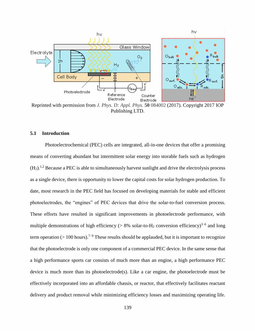
139

Reprinted with permission from J. Phys. D: Appl. Phys. 50 084002 (2017). Copyright 2017 IOP

Publishing LTD.

5.1 Introduction

Photoelectrochemical (PEC) cells are integrated, all-in-one devices that offer a promising

means of converting abundant but intermittent solar energy into storable fuels such as hydrogen

(H2).1,2 Because a PEC is able to simultaneously harvest sunlight and drive the electrolysis process

as a single device, there is opportunity to lower the capital costs for solar hydrogen production. To

date, most research in the PEC field has focused on developing materials for stable and efficient

photoelectrodes, the “engines” of PEC devices that drive the solar-to-fuel conversion process.

These efforts have resulted in significant improvements in photoelectrode performance, with

multiple demonstrations of high efficiency (> 8% solar-to-H2 conversion efficiency)3–6 and long

term operation (> 100 hours).7–9 These results should be applauded, but it is important to recognize

that the photoelectrode is only one component of a commercial PEC device. In the same sense that

a high performance sports car consists of much more than an engine, a high performance PEC

device is much more than its photoelectrode(s). Like a car engine, the photoelectrode must be

effectively incorporated into an affordable chassis, or reactor, that effectively facilitates reactant

delivery and product removal while minimizing efficiency losses and maximizing operating life.

140

As photoelectrode technology continues to improve, the task of developing efficient and scalable

PEC reactors will become even more crucial to the commercialization of PEC technology.10

The majority of photoelectrode-based PEC reactor designs that have been reported in

literature can be generally classified into one of three broad categories: batch, semi-batch, or

continuous. Most bench scale PEC device designs demonstrated to date are operated as semi-batch

reactors under 1 sun illumination intensity in a stagnant (non-pumped, non-stirred) electrolyte that

may be resupplied or topped off on an as needed basis.11–17 Less commonly explored are PEC

continuous flow reactors, in which electrolyte is continuously and actively pumped through the

reactor.18–22 PEC flow cells, or reactors, such as that illustrated in Figure 5.1 can offer several

advantages over passive semi-batch PEC reactors. First, flow cells can enable more efficient PEC

operation by enhancing transport of reactants to the photoelectrode surface.23 This benefit is

particularly important for reactions involving low concentrations of reactants such as CO2, which

has a solubility limit in water of only 34 mM at 298 K.24 Similarly, flowing electrolyte can enhance

PEC performance by facilitating removal of gaseous product species (i.e. bubbles) that would

otherwise accumulate on the photoelectrode surface and decrease its efficiency. Both of these

benefits are highly useful, and in many cases required, for PEC operation under concentrated solar

illumination whereby photocurrents may exceed the maximum rate of reactant mass transport even

for concentrated electrolytes. In solar concentrating reactors, lenses or mirrors are employed to

increase the light intensity incident on the photoelectrode and thereby reduce its required area (and

associated cost) for a given rate of product generation.5,6,25 Seger et al. have demonstrated that

flowing electrolyte can be beneficial in a parallel plate-like proton exchange membrane PEC

cell,18,26 but there has been a lack of quantitative analysis on the operating limits of PEC flow

reactors.

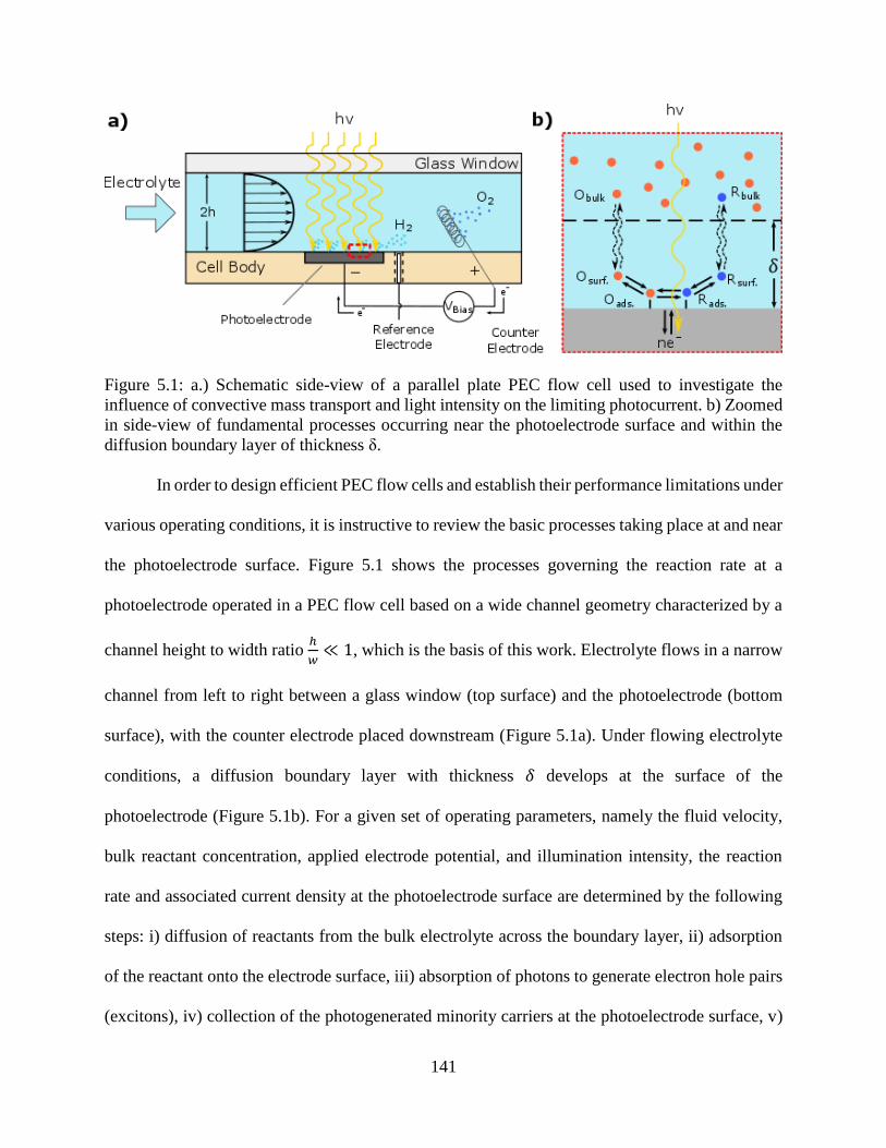
141

Figure 5.1: a.) Schematic side-view of a parallel plate PEC flow cell used to investigate the

influence of convective mass transport and light intensity on the limiting photocurrent. b) Zoomed

in side-view of fundamental processes occurring near the photoelectrode surface and within the

diffusion boundary layer of thickness δ.

In order to design efficient PEC flow cells and establish their performance limitations under

various operating conditions, it is instructive to review the basic processes taking place at and near

the photoelectrode surface. Figure 5.1 shows the processes governing the reaction rate at a

photoelectrode operated in a PEC flow cell based on a wide channel geometry characterized by a

channel height to width ratio ℎ

𝑤≪ 1, which is the basis of this work. Electrolyte flows in a narrow

channel from left to right between a glass window (top surface) and the photoelectrode (bottom

surface), with the counter electrode placed downstream (Figure 5.1a). Under flowing electrolyte

conditions, a diffusion boundary layer with thickness 𝛿 develops at the surface of the

photoelectrode (Figure 5.1b). For a given set of operating parameters, namely the fluid velocity,

bulk reactant concentration, applied electrode potential, and illumination intensity, the reaction

rate and associated current density at the photoelectrode surface are determined by the following

steps: i) diffusion of reactants from the bulk electrolyte across the boundary layer, ii) adsorption

of the reactant onto the electrode surface, iii) absorption of photons to generate electron hole pairs

(excitons), iv) collection of the photogenerated minority carriers at the photoelectrode surface, v)

142

electrochemical reaction of surface species, and vi) desorption and diffusion of product species

away from the electrode surface. Depending on the relative rates of all of these processes, the

limiting current of the photoelectrode can be described as photo-limited, mass transport-limited,

kinetically-limited, or a combination of the three conditions.

The primary objective of this study to establish a quantitative understanding of the limiting

photocurrent behavior for a photoelectrode operated in a wide channel flow cell under photo- or

mass transport-limiting conditions. Such conditions are achieved when sufficient potential is

applied or photovoltage generated to ensure that the photoelectrode current is not limited by

reaction kinetics. Thus, this study does not delve into the detailed effects of flowing electrolyte on

kinetics, but seeks to quantitatively understand the upper-limit of photocurrent that can be

generated when kinetics are not limiting. As a basis for this study, water electrolysis was performed

using a p-Si photocathode possessing a metal-insulator-semiconductor (MIS) architecture.27,28

With this configuration, the photo-absorber, p-type silicon, is separated from the electrolyte by a

≈1.5 nm thick insulating layer of native silicon dioxide and semitransparent layers of titanium and

platinum that were deposited as a continuous bi-layer by physical vapor deposition. The electric

field across the MIS junction allows for photogenerated carriers to be collected at the metallic Pt

layer, which also catalyzes the hydrogen evolution reaction. Overall, the p-Si based MIS

photocathode is a stable photoelectrode capable of high photocurrents, making it an excellent

baseline electrode to investigate in PEC flow cells.

The remainder of the chapter is organized as follows. After describing the design and

operation of the MIS photocathode in the PEC flow cell, a range of bulk reactant concentrations,

flow velocities, and illumination intensities are explored in order to map out the boundaries

between mass transport-limited and photo-limited operating regimes. Example measurements are

143

provided that clearly illustrate the characteristics of mass transport- and photo-limiting current

behavior, as well as the transition between the two operating regimes. Based on the mass transport

properties of the wide channel cell, a simple model is presented to predict the limiting current as a

function of fluid velocity for higher reactant concentrations and solar insolation. Finally, the

implications of this analysis for the design and operation of efficient PEC flow reactors are

discussed.

5.2 Experimental

Chemicals- Electrolyte solutions were prepared from concentrated sulfuric acid (Certified

ACS plus, Fischer Scientific), 18 MΩ cm deionized water, and sodium sulfate (ACS Reagent

grade, Sigma Aldrich) supporting electrolyte. The amount of sulfuric acid varied between

solutions, but the sodium sulfate concentration was always kept constant at 1 M.

Photoelectrode fabrication- All photoelectrodes consisted of an MIS structure in which

semitransparent 3 nm Pt and 10 nm Ti layers were deposited sequentially by e-beam evaporation

onto Si(100) substrates obtained from WRS Materials. Prime-grade p-Si(100) wafers with

resistivity of 1-5 Ω-cm were used for photoelectrodes, while degenerate p-Si(100) wafers with

resistivity of < 0.005 Ω-cm were used as metallic control samples. Indium back contacts were

soldered onto the back of the samples after fabrication of the front MIS junction, and were verified

to have an ohmic resistance of less than 10 Ω as determined by impedance spectroscopy. Exposed

electrode areas of ≈ 0.24 cm2 were defined by a square opening in 3M Electroplater’s tape. A black

metal foil mask having the identical shape and area as the exposed electrode area was aligned on

top of the PEC window to ensure that the illuminated area on the electrode was equal to the area

exposed to the electrolyte.

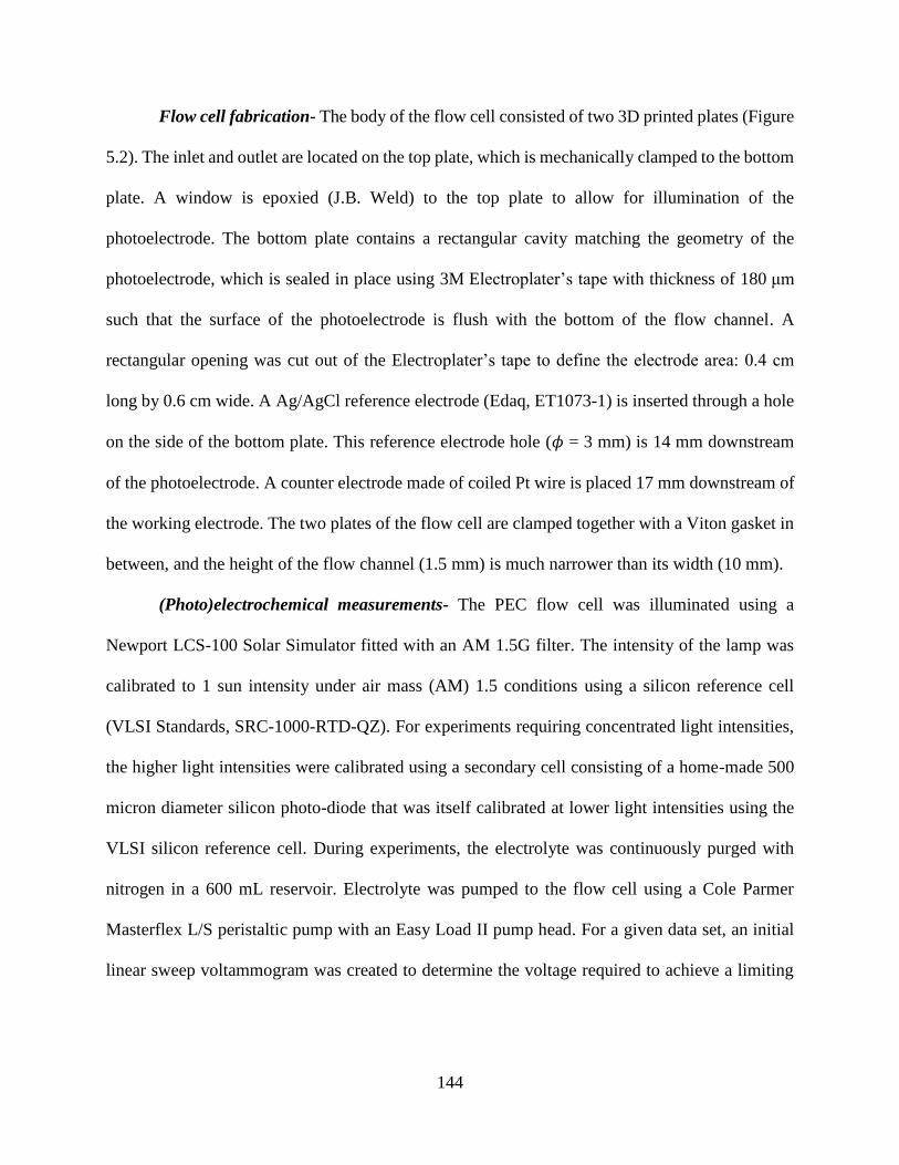
144

Flow cell fabrication- The body of the flow cell consisted of two 3D printed plates (Figure

5.2). The inlet and outlet are located on the top plate, which is mechanically clamped to the bottom

plate. A window is epoxied (J.B. Weld) to the top plate to allow for illumination of the

photoelectrode. The bottom plate contains a rectangular cavity matching the geometry of the

photoelectrode, which is sealed in place using 3M Electroplater’s tape with thickness of 180 μm

such that the surface of the photoelectrode is flush with the bottom of the flow channel. A

rectangular opening was cut out of the Electroplater’s tape to define the electrode area: 0.4 cm

long by 0.6 cm wide. A Ag/AgCl reference electrode (Edaq, ET1073-1) is inserted through a hole

on the side of the bottom plate. This reference electrode hole (𝜙 = 3 mm) is 14 mm downstream

of the photoelectrode. A counter electrode made of coiled Pt wire is placed 17 mm downstream of

the working electrode. The two plates of the flow cell are clamped together with a Viton gasket in

between, and the height of the flow channel (1.5 mm) is much narrower than its width (10 mm).

(Photo)electrochemical measurements- The PEC flow cell was illuminated using a

Newport LCS-100 Solar Simulator fitted with an AM 1.5G filter. The intensity of the lamp was

calibrated to 1 sun intensity under air mass (AM) 1.5 conditions using a silicon reference cell

(VLSI Standards, SRC-1000-RTD-QZ). For experiments requiring concentrated light intensities,

the higher light intensities were calibrated using a secondary cell consisting of a home-made 500

micron diameter silicon photo-diode that was itself calibrated at lower light intensities using the

VLSI silicon reference cell. During experiments, the electrolyte was continuously purged with

nitrogen in a 600 mL reservoir. Electrolyte was pumped to the flow cell using a Cole Parmer

Masterflex L/S peristaltic pump with an Easy Load II pump head. For a given data set, an initial

linear sweep voltammogram was created to determine the voltage required to achieve a limiting

145

current. Three successive chronoamperometry experiments were then held at this potential in order

to record an average value of the limiting current.

Figure 5.2: a) Exploded view of 3D printed PEC flow cell assembly. b) Photograph of PEC flow

cell. c) Simplified flow diagram of experimental set-up.

5.3 Results and discussion

5.3.1 Description of PEC flow cell and its operation

The wide-channel PEC flow cell and measurement set-up used as the basis for this study

are shown in Figure 5.2. An exploded view of the flow cell components is provided in Figure 5.2a

and a picture of the assembled device in operation is shown in Figure 5.2b. Within this parallel

plate flow cell, the photoelectrode is integrated into the bottom plate, while the reference and

146

counter electrodes are incorporated downstream of the photoelectrode as shown in Figure 5.2a and

described in the experimental section. A glass window in the top plate of the reactor allows for

light to be transmitted downward onto the exposed photoelectrode surface, which is mounted

horizontally within the cell. The small cross sectional area of the flow channel (0.15 cm2) permits

the flow cell to achieve a maximum fluid velocity of 82 cm s-1 with the peristaltic pump used in

this study. This fluid velocity corresponds to a Reynolds number (Re) of 1225, meaning that

laminar flow was established for all measurements. The rectangular flow channel is 8.5 cm long,

with the photoelectrode placed halfway downstream. A parabolic velocity flow profile typical of

flow through parallel plates can be assumed for this flow channel given that the channel’s height

is much less than its width (ℎ/𝑤 = 0.15) and the electrode is placed in the center of the channel,

more than 1 characteristic length away from the corners.29

Once the photoelectrode was assembled into the flow cell, its performance was evaluated

using linear sweep voltammetry (LSV) and chronoamperometry (CA). Figure 5.3 shows a typical

LSV curve for the standard p-Si MIS photocathodes measured in 200 mM H2SO4 and 1 M Na2SO4

under simulated AM 1.5 illumination, illustrating three different operating potential regimes. At

positive applied potentials under illumination (Region I in Figure 5.3), no current is measured

because too little photovoltage is generated to simultaneously achieve a high carrier collection

efficiency and drive HER kinetics. As the potential is scanned more negative, a photo-reduction

current becomes apparent around 0.32 V vs. NHE, corresponding to a potential known as the

photocurrent onset potential (Vonset). Scanning further, there is a sharp increase in photocurrent

until about -0.24 V. vs. NHE. In the absence of significant ohmic losses, current in this portion of

the LSV curve (Region II) is primarily dominated by reaction kinetics. Eventually, the

photocurrent becomes relatively constant, with no substantial change observed as the potential is

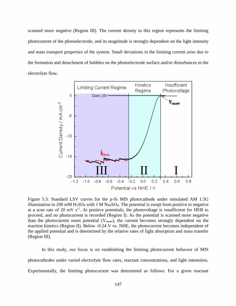
147

scanned more negative (Region III). The current density in this region represents the limiting

photocurrent of the photoelectrode, and its magnitude is strongly dependent on the light intensity

and mass transport properties of the system. Small deviations in the limiting current arise due to

the formation and detachment of bubbles on the photoelectrode surface and/or disturbances in the

electrolyte flow.

Figure 5.3: Standard LSV curves for the p-Si MIS photocathode under simulated AM 1.5G

illumination in 200 mM H2SO4 with 1 M Na2SO4. The potential is swept from positive to negative

at a scan rate of 20 mV s-1. At positive potentials, the photovoltage is insufficient for HER to

proceed, and no photocurrent is recorded (Region I). As the potential is scanned more negative

than the photocurrent onset potential (Vonset), the current becomes strongly dependent on the

reaction kinetics (Region II). Below -0.24 V vs. NHE, the photocurrent becomes independent of

the applied potential and is determined by the relative rates of light absorption and mass transfer

(Region III).

In this study, our focus is on establishing the limiting photocurrent behavior of MIS

photocathodes under varied electrolyte flow rates, reactant concentrations, and light intensities.

Experimentally, the limiting photocurrent was determined as follows: For a given reactant

148

concentration and illumination intensity, an LSV was performed to determine the applied potential

or voltage that is required for operation in Region III, the limiting current regime. CA was then

conducted at a potential that was 0.2 V to 0.3 V negative of the transition between Region II and

Region III. Each CA trial lasted for 20 s, and the overall limiting current determined by the average

value over three trials. In the following subsections, we explore cases where the photocurrent is

limited entirely by light, entirely by mass transport, or a combination of the two.

5.3.2 Light limited photocurrent

PEC device operation is said to be light- or photo-limited when the rate limiting step in the

sequence of processes illustrated in Figure 5.1b is the flux of photons to the photoelectrode. Under

such conditions, the current density, 𝑖, is highly sensitive to the spectral irradiance, 𝐼0, and often

varies linearly with it as described by Equation 5.1:

𝑖 =𝑞

ℎ𝑐∫ 𝐼0(𝜆)(100% − 𝑅(𝜆) − 𝐴𝑚(𝜆)) 𝐼𝑄𝐸(𝜆) 𝜆 𝑑𝜆

𝜆𝐸𝑔

0

5.1

where q is the elementary charge, h is the Planck constant, c is the speed of light, 𝜆𝐸𝐺 is

the bandgap energy of the semiconductor, R is the reflectivity of the photoelectrode surface, Am is

the absorptance of the metal bi-layer, and 𝐼𝑄𝐸(𝜆) is the internal quantum efficiency, defined as

the fraction of photons absorbed by the photoelectrode that result in a collected photocurrent.

Equation 5.1 is typically integrated over all wavelengths exceeding the bandgap energy where IQE

is non-zero.

In the lab, PECs are typically tested under illumination sources having a spectrum that is

modified to match the power density and spectral characteristics of the sun such as the standard

air mass 1.5 global (AM 1.5G) spectrum. Assuming that a light source having AM 1.5 spectral

149

characteristics is being employed, Equation 5.1 can be integrated and simplified to obtain the

following expression for photo-limited current density:

𝑖 = 𝑞Γ𝜙𝐴𝑀 1.5𝑋 5.2

Where 𝜙𝐴𝑀1.5 is the total photon flux from an AM 1.5 solar source incident on the PEC

reactor and Γ is the fraction of incident photons that result in electrochemical current. X is the solar

concentration factor, defined as the ratio of the photon flux incident on the PEC device to that

received under one sun illumination at AM 1.5. A practical upper limit on the solar concentrating

factor for a PEC has been suggested at 100 suns,6,30 and a recent technoeconomic analysis of solar

concentrated PECs used a base case of 10 suns.30,31

The LSVs shown in Figure 5.4a are for a photoelectrode operated in 200 mM sulfuric acid

under different light intensities. Under one sun illumination, the photo-limited current was

measured to be ≈ 16 mA cm-2, substantially less than the theoretical maximum photocurrent of

43 mA cm-2 for crystalline Si under AM 1.5G illumination.32 As shown in Appendix C, section

5.5.1, Figure 5.7, this difference can be primarily attributed to the high reflectance and absorbance

losses associated with the relatively thick Pt/Ti metal bilayer that was deposited on top of the MIS

photoelectrodes in this study. In Figure 5.4b, the average limiting currents are plotted as a function

of solar concentration factor, revealing that the photo-limited current recorded in 200 mM H2SO4

scales linearly with solar concentration factor. This observation is consistent with the classical

behavior predicted by Equation 5.2, and is commonly observed in other studies where the current

is photo-limited.3 By contrast, the photocurrent is nearly independent of light intensity when the

sulfuric acid concentration was decreased to 4 mM, where the photocurrent becomes mass

transport-limited and primarily depends on the delivery of reactants to the surface. Although not

observed in this work, it is worth noting that some lower-quality materials can exhibit sub-linear

150

dependence of photocurrent on light intensity due to higher carrier recombination rates at high

light intensity.33

Figure 5.4: Photo-limited PEC operation. a) Linear sweep voltammetry (LSV) curves recorded for

a p-Si MIS photocathode under varying solar concentrating factors. All scans were swept from

positive to negative potential at a rate of 10 mV s-1 in 200 mM H2SO4 flowing at an average

velocity of 22 cm s-1. b) Limiting photocurrent densities recorded for a p-Si MIS photocathode

under varied solar concentration factors in weakly and strongly acidic electrolytes flowing at an

average velocity of 22 cm s-1.

5.3.3 Mass transport-limited photocurrent

When the diffusion of reactants across the diffusion boundary layer is the slowest process

illustrated in Figure 5.1b, the current generated by the PEC is limited by mass transport. In this

case, the maximum flux of reactant species to the photoelectrode surface is less than the flux of

photo-generated carriers to the photoelectrode surface. Usually, mass transport becomes limiting

when there is a low concentration of reactant in the electrolyte. Such conditions are commonly

encountered for photoelectrochemical and electrochemical CO2 reduction, where the solubility of

the reactant, CO2, limits its concentration in aqueous electrolytes to approximately 34 mM at

298 K. At such low concentrations, PEC operation in a stagnant electrolyte can greatly reduce the

151

limiting photocurrent because the concentration of the reactant species is quickly depleted near the

photoelectrode surface, resulting in the development of a concentration gradient across the

diffusion boundary layer that is insufficient to induce a flux of reactants equivalent to the photon

flux. However, flow cells overcome this issue through forced convection of the liquid electrolyte,

which decreases the thickness of the diffusion boundary layer across which reactants must diffuse

in order to reach the photoelectrode surface. In flow cells, increasing the fluid velocity decreases

the diffusion boundary layer thickness, and therefore increases the maximum diffusive flux across

it.

Figure 5.5a shows LSV curves for a photoelectrode operating under 1 sun illumination in

4 mM sulfuric acid, a relatively dilute concentration for which mass transport-limited behavior is

expected. The mass transport limitations are confirmed by the sensitivity of the limiting current to

the electrolyte flow velocity (Figure 5.5b). As the electrolyte flows faster, the limiting current

density increases due to the decreasing boundary layer thickness, which in turn causes the diffusive

flux across it to increase. Because diffusion is a slow mode of transport relative to convection, the

thickness of the diffusion boundary layer strongly affects the mass transport-limiting current. The

relationship between a forced convection velocity field and the diffusion boundary layer thickness

can be described by a mass transport correlation that relates the Sherwood number (Sh=L/δ),

Reynolds number (𝑅𝑒 =𝑈𝐿

𝜈), and the Schmidt number (𝑆𝑐 =

𝜈

𝐷). The Reynolds number is the ratio

between inertial and viscous forces, where 𝑈 is the average fluid velocity, 𝐿 is the characteristic

length, and 𝜈 is the kinematic viscosity. The Schmidt number is the ratio between the kinematic

viscosity and the diffusivity 𝐷. For a given geometry, the Sherwood number is a function of Re

and Sc.

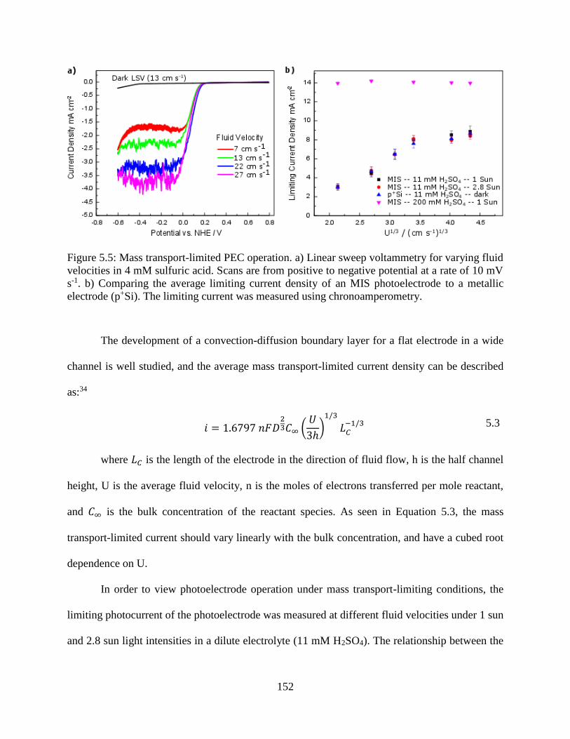
152

Figure 5.5: Mass transport-limited PEC operation. a) Linear sweep voltammetry for varying fluid

velocities in 4 mM sulfuric acid. Scans are from positive to negative potential at a rate of 10 mV

s-1. b) Comparing the average limiting current density of an MIS photoelectrode to a metallic

electrode (p+Si). The limiting current was measured using chronoamperometry.

The development of a convection-diffusion boundary layer for a flat electrode in a wide

channel is well studied, and the average mass transport-limited current density can be described

as:34

𝑖 = 1.6797 𝑛𝐹𝐷

23𝐶∞ (

𝑈

3ℎ)

1/3

𝐿𝐶−1/3

5.3

where 𝐿𝐶 is the length of the electrode in the direction of fluid flow, h is the half channel

height, U is the average fluid velocity, n is the moles of electrons transferred per mole reactant,

and 𝐶∞ is the bulk concentration of the reactant species. As seen in Equation 5.3, the mass

transport-limited current should vary linearly with the bulk concentration, and have a cubed root

dependence on U.

In order to view photoelectrode operation under mass transport-limiting conditions, the

limiting photocurrent of the photoelectrode was measured at different fluid velocities under 1 sun

and 2.8 sun light intensities in a dilute electrolyte (11 mM H2SO4). The relationship between the

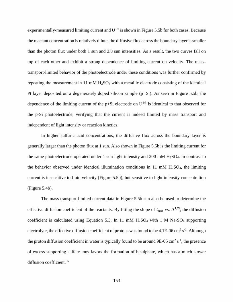
153

experimentally-measured limiting current and U1/3 is shown in Figure 5.5b for both cases. Because

the reactant concentration is relatively dilute, the diffusive flux across the boundary layer is smaller

than the photon flux under both 1 sun and 2.8 sun intensities. As a result, the two curves fall on

top of each other and exhibit a strong dependence of limiting current on velocity. The mass-

transport-limited behavior of the photoelectrode under these conditions was further confirmed by

repeating the measurement in 11 mM H2SO4 with a metallic electrode consisting of the identical

Pt layer deposited on a degenerately doped silicon sample (p+ Si). As seen in Figure 5.5b, the

dependence of the limiting current of the p+Si electrode on U1/3 is identical to that observed for

the p-Si photoelectrode, verifying that the current is indeed limited by mass transport and

independent of light intensity or reaction kinetics.

In higher sulfuric acid concentrations, the diffusive flux across the boundary layer is

generally larger than the photon flux at 1 sun. Also shown in Figure 5.5b is the limiting current for

the same photoelectrode operated under 1 sun light intensity and 200 mM H2SO4. In contrast to

the behavior observed under identical illumination conditions in 11 mM H2SO4, the limiting

current is insensitive to fluid velocity (Figure 5.5b), but sensitive to light intensity concentration

(Figure 5.4b).

The mass transport-limited current data in Figure 5.5b can also be used to determine the

effective diffusion coefficient of the reactants. By fitting the slope of 𝑖𝑙𝑖𝑚 vs. 𝑈1/3, the diffusion

coefficient is calculated using Equation 5.3. In 11 mM H2SO4 with 1 M Na2SO4 supporting

electrolyte, the effective diffusion coefficient of protons was found to be 4.1E-06 cm2 s-1. Although

the proton diffusion coefficient in water is typically found to be around 9E-05 cm2 s-1, the presence

of excess supporting sulfate ions favors the formation of bisulphate, which has a much slower

diffusion coefficient.35

154

The mass transport-limiting current behavior of the parallel plate flow cell is similar to

what others have observed for electrochemical proton reduction on a metallic rotating disc

electrode (RDE).36 While RDEs are not commonly used for studying photoelectrodes, the parallel

plate design is convenient for aligning the photoelectrode with the illumination source, an integral

part of this study. One can extend this analysis to other device geometries as well, provided that

the appropriate mass transfer correlations for that geometry are available and used. Besides the

correlation used here for the parallel plate geometry, other correlations are available in literature.37

Finally, we note that this analysis of mass transfer effects on PEC operation has focused

on the transport of reactant species to the photoelectrode surface, but the transport and subsequent

collection of product species would also be of great importance for practical PEC reactors. In the

present parallel plate configuration, one possible solution would be to incorporate a

semitransparent counter electrode where the front window is currently located, and utilize flow-

induced product separation to sweep the product gasses down two separate effluent channels as

has been demonstrated for laminar flow cell fuel cells,38,39 batteries,40 and electrolyzers.41

5.3.4 Predicting limiting photocurrent operating regimes

In the previous two sections, photoelectrode operation was described for operating

conditions under which the photocurrent was solely limited by mass transport or illumination

intensity. We now focus discussion on identifying and predicting the transition between these two

operating behaviors and using that information to map out the operating conditions for which the

photocurrent is expected to be limited by mass transport or illumination intensity. The basis of this

analysis is the assumption that the transition between mass transport- and photo-limiting behavior

occurs when the maximum flux of reactants to the surface is stoichiometrically equal to the

maximum flux of photogenerated carriers to the electrode surface. To minimize the presence and

155

impact of bubbles for this analysis, the limiting current was determined directly from LSVs at a

moderately fast scan rate of 40 mV s-1 whereby the limiting current can be achieved quickly before

the onset of significant product bubble growth.

An example illustrating the transition between mass transport- to photo-limiting behavior

for a photoelectrode is provided in Figure 5.6a, which shows the limiting photocurrent of an MIS

photocathode in varying H2SO4 concentrations under 1 sun illumination as a function of fluid

velocity. In 500 mM H2SO4, equivalent proton concentration of 1000 mM, the current is photo-

limited at all flow velocities. As the reactant concentration decreases, higher velocities are required

to achieve the photo-limited current. For example, in 33 mM H2SO4, equivalent proton

concentration of 66 mM, the limiting photocurrent is highly dependent on flow velocity up until

30 cm s-1, indicating that it is primarily limited by mass transport in this region of operation. At

flow velocities beyond 30 cm s-1, the limiting photocurrent plateaus to the one sun limit, indicating

that the photoelectrode has now become limited by light.

Mathematically, the transition between the mass transport and light-limiting photocurrent

can be described by setting Equation 5.2 (describing the maximum flux of photo-generated carriers

to the electrode surface) equal to Equation 5.3 (describing the maximum reactant flux). For a given

light intensity and flow velocity, the bulk reactant concentration, 𝐶∞, at which the photo-limiting

and mass transport-limiting processes are balanced is given by Equation 5.4:

𝐶∞ =0.858

𝑁𝐴∗

Γ𝜙𝐴𝑀 1.5𝑋

𝑛𝜓 5.4

where 𝜓 = (𝐷2𝑈

ℎ𝐿𝐶)

1/3

. The numerator of Equation 5.4, Γ𝜙𝐴𝑀 1.5𝑋, is the maximum photon flux,

while the denominator 𝑛𝜓 contains the parameters governing the mass transport properties of the

system and has dimensions of velocity. 𝑁𝐴 is Avagadro’s number. In Figure 5.6b, 𝐶∞ calculated

156

from Equation 5.4 is plotted against 𝜓 based on the PEC flow cell geometry and operating

parameters employed for the measurements shown in in Figure 5.6a. The value of Γ was set to be

0.42, which corresponds to a photo-limited current density of 18 mA cm-2 under 1 sun intensity as

was observed for the sample used for these measurements. The solar concentration factor X was

set to 1 sun. The channel half height h was 0.75 mm, and the electrode length was 4.0 mm. An

effective proton diffusion coefficient of 4.1E-06 cm2 s-1 was found for H2SO4 in 1.0 M Na2SO4

and was determined experimentally from the slope of the Levich plot in Figure 5.5b. For a given

coordinate pair of 𝜓 and reactant concentration, the curve plotted in Figure 5.6b represents a tie

line where operating points that lay above the curve are photo-limited, while points that lay below

the curve are limited by mass transport. Ideally, a PEC system would be designed to operate just

above the tie line to ensure operation in a photo-limited regime. Increasing the fluid velocity, and

therefore 𝜓, to excessively high levels can result in efficiency losses due to pump energy

requirements as well as dilution of the products. Unnecessarily high flow rates can also result in

undesirable mixing of the products downstream as well as dilution of the product species.

Therefore, it is advisable to set the operating fluid velocity high enough to ensure that the current

is not limited by mass transport, but not so high that large pumping and downstream separation

costs will be incurred.

157

Figure 5.6: Predicting the boundary between photo-limited and mass transport-limited PEC

operation. a) The limiting current of a photoelectrode operated in varying H2SO4 concentration

under 1 sun illumination. At low fluid velocities the current is mass transport-limited, but

increasing the flow velocity allows the current to reach the 1 sun photo-limited value, which is

equal to the limiting current in 500 mM H2SO4 ([H+] = 1000 mM). b) Predicted boundary between

photo-limited and mass transport-limited current at 1 sun. Individual data points on the plot

correspond to the same experimental data points shown in a). The tie line was calculated using

Equation 5.4, and 𝜓 is defined in the text. c) Predicted boundary at higher levels of solar

concentration for a reaction with n= 1 mole of electrons transferred per mole reactant. d) Predicted

boundary for reactions involving n= 8 moles of electrons transferred per mole reactant.

158

Also plotted in Figure 5.6b are the individual operating points corresponding to the

electrolyte concentration and flow velocities that were used in the measurements reported in Figure

5.6a. As the bulk proton concentration of the electrolyte increases, lower values of 𝜓, and thus

lower flow velocities, are required to achieve a photo-limited current. At a bulk proton

concentration of 56 mM, the transition from mass transport-limited to photo-limited operation is

expected at 𝜓 = 0.0029, corresponding to flow velocities greater than 40 cm s-1 and in agreement

with Figure 5.6a. Although reasonable agreement between the predicted and observed limiting

current transition is also demonstrated at a bulk proton concentration of 66 mM, the transition is

not as clear at a proton concentration of 80 mM. This observation of a blurred transition between

mass- and light-limited photocurrent most likely results because the predicted transition flow

velocity, 13 cm s-1, is too slow to remove the hydrogen bubbles adsorbed to the surface, resulting

in additional mass transport and optical losses.

The analysis described above based on Equation 5.4 and illustrated in Figure 5.6b can be

expanded upon to predict the limiting current over much wider ranges of light intensities, reactant

concentrations, and fluid velocities. Figure 5.6c shows the predicted boundary between photo-

limited and mass transport-limited currents for four different photo-limited current densities

(𝑞Γ𝜙𝐴𝑀 1.5𝑋). If a photoelectrode has an expected photo-limited current density of 15 mA cm-2 at

one sun intensity, then the photo-limited current density at ten suns can be estimated to be

150 mA cm-2. The tie lines in Figure 5.6c assume a reaction stoichiometry where one electron is

transferred per mole of reactant. As the solar concentration factor increases, the device requires

more concentrated electrolyte to avoid mass transport limitations. For example, under 20 sun

illumination, (𝑞Γ𝜙𝐴𝑀 1.5𝑋 = 300 mA cm-2) a system with a 1000 mM proton concentration is likely

to be mass transport-limited. By increasing the proton concentration to 1500 mM, or by increasing

159

the electrolyte flow velocity to 30 cm s-1 (𝜓 = 0.0028 cm s-1), the system becomes photo-limited.

In the cases where the reactant concentration cannot be increased – for example, due to a solubility

limit – increasing the flow rate of the electrolyte can be a practical solution to overcoming mass

transport limitations. This analysis can be extended to systems where multiple electrons are

transferred per reactant such that the electron transfer number, n, is > 1. Figure 5.6d shows the tie

lines for a hypothetical reaction where n = 8. As the value of n increases, the bulk reactant

concentration required to achieve a photo-limited current density decreases because each reactant

molecule reaching the photoelectrode surface is capable of accepting multiple photo-generated e-.

Using an analysis such as that shown in Figure 5.6 to map out the expected limiting cases

of operation can be very useful for both the design of PEC reactors and choosing operating

conditions. While HER was used as a model reaction to describe the mass transport characteristics

of the wide channel cell, these concepts can be applied to other reactions and reactor designs as

well. The range of values for 𝜓 will depend on the geometry of the flow cell, as well as the

diffusion coefficient(s) of reactant species. Figure 5.6c and Figure 5.6d illustrate that the number

of electrons transferred per mole of reactant formed in the reaction is also important for

determining the optimal operating conditions for a PEC flow reactor.42 For HER, one electron is

transferred per proton, but for CO2 reduction, the number of electrons transferred depends on what

products are formed – in the case of reduction to methane, 8 mole e- are transferred per mole of

reactant. Consequently, the system reaches a photo-limited current at lower reactant

concentrations.

While the present analysis provides a useful framework for understanding limiting

photocurrent behavior of photoelectrodes operating under a large applied bias, it must be

recognized that photoelectrodes in stand-alone PEC devices will likely operate at potentials for

160

which kinetic and ohmic losses will also be important. This is especially true at high reactant

concentrations, light intensities, and flow rates for which the high current densities will likely

necessitate photoelectrode operation at a potential for which the current is affected by the reaction

kinetics and/or ohmic resistances associated with the electrode, electrolyte, and membrane (if

present). These ohmic losses are not considered in Figure 5.6c, but are likely very important at

solar concentrating factors exceeding 10-20 suns. As an example, consider a PEC flow cell

containing a semitransparent counter electrode and a photoelectrode in parallel-plate configuration

with a 2 mm separation distance operating in 0.5 M H2SO4 (conductivity ≈0.21 S cm-1). If the

device current density at 1 sun intensity is 10 mA cm-2, its operating current density at 50 sun

intensity would be expected to be around 500 mA cm-2. Assuming Tafel kinetics for state of the

art Pt hydrogen evolution catalysts and IrO2 oxygen evolution catalysts,11,43 such a current density

would require HER and OER kinetic overpotential losses of 62 mV and 387 mV, respectively. The

ohmic voltage drop would be ≈ 475 mV. This simple exercise highlights the challenges associated

with operating any PEC reactor at high light intensities. For a stand-alone PEC device capable of

unassisted electrolysis, it will be essential that these losses are also accounted for in the design and

optimization of both the photoelectrode(s) and PEC reactor.

Another assumption of this analysis is that migration, or ionic transport due to the gradient

in the electric field, does not affect the mass transport limited current. This is a good assumption

to make in the current study because the relatively low concentrations of H2SO4 ensures that most

of the migration current is carried by the Na+, SO4-2, and HSO4

- ions in the supporting electrolyte.

At higher H2SO4 concentrations, the free protons carry a larger fraction of the migration current,

and the effect of migration cannot be entirely ignored. Thus, the predicted boundary between

photo-limited and mass transport-limited currents shown in Figure 5.6c at high reactant

161

concentrations and illumination intensity will likely deviate from what would be observed

experimentally.

5.4 Conclusions

This chapter has systematically investigated the limiting photocurrent behavior of a wide

channel PEC flow cell containing a p-Si MIS photocathode under varying electrolyte

concentrations, flow velocities, and illumination intensities. When the maximum flux of

photogenerated carriers to the electrode surface exceeds the flux of reactants across the diffusion

boundary layer, increasing the fluid velocity can have a huge effect on the limiting photocurrent,

and thus the overall solar-to-fuel conversion efficiency of the PEC device. For this reason,

understanding the boundary between mass transport and photo-limited operating regimes is of

great importance for optimizing PEC performance. These operating regimes for a given reactor

geometry can be predicted and modeled if the relationship between flow velocity and diffusion

boundary layer thickness is known. By balancing the photogenerated carrier flux with the diffusive

flux of the reactants, one can determine the minimum flow velocity required to achieve a photo-

limited current. Importantly, the methodologies and analysis introduced in this paper can be

extended to other PEC systems based on different photoelectrodes, optical concentration factors,

and dilute reactant concentrations.

5.5 Appendix C

5.5.1 UV-Vis analysis of photoelectrode optical losses

The maximum theoretical photocurrent generated by a single-junction solar cell based on

crystalline silicon (c-Si) is 43 mA cm-2 under AM 1.5G illumination.32 In reality, the observed

photocurrent is less than this amount due to optical and/or electronic losses. In the metal-insulator-

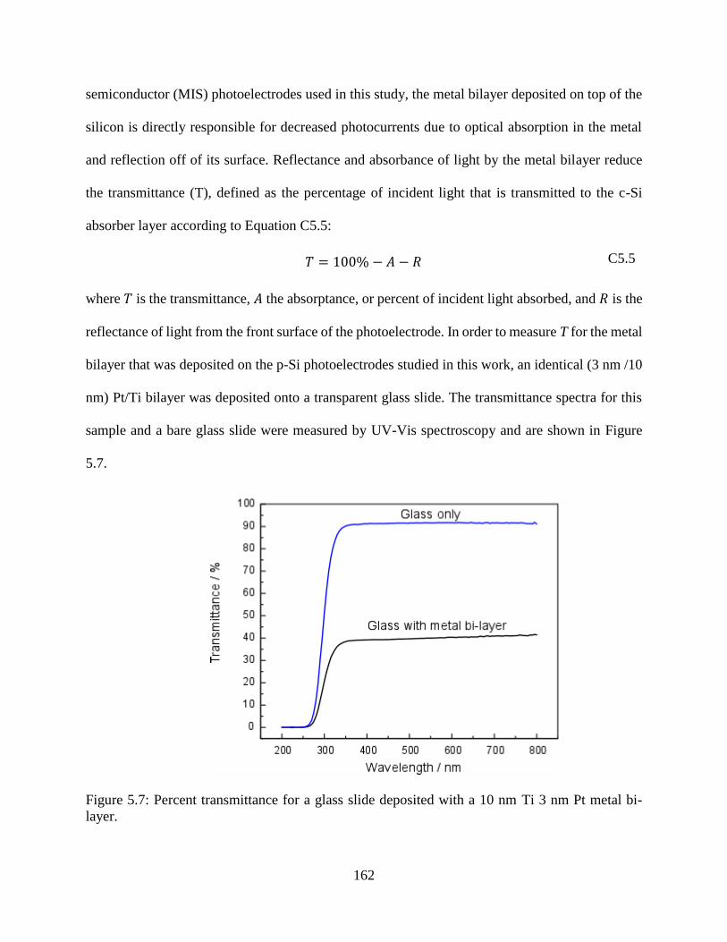
162

semiconductor (MIS) photoelectrodes used in this study, the metal bilayer deposited on top of the

silicon is directly responsible for decreased photocurrents due to optical absorption in the metal

and reflection off of its surface. Reflectance and absorbance of light by the metal bilayer reduce

the transmittance (T), defined as the percentage of incident light that is transmitted to the c-Si

absorber layer according to Equation C5.5:

𝑇 = 100% − 𝐴 − 𝑅 C5.5

where 𝑇 is the transmittance, 𝐴 the absorptance, or percent of incident light absorbed, and 𝑅 is the

reflectance of light from the front surface of the photoelectrode. In order to measure T for the metal

bilayer that was deposited on the p-Si photoelectrodes studied in this work, an identical (3 nm /10

nm) Pt/Ti bilayer was deposited onto a transparent glass slide. The transmittance spectra for this

sample and a bare glass slide were measured by UV-Vis spectroscopy and are shown in Figure

5.7.

Figure 5.7: Percent transmittance for a glass slide deposited with a 10 nm Ti 3 nm Pt metal bi-

layer.

163

The bare glass slide is highly transparent, allowing ≈ 90% of photons to be transmitted

across the visible spectrum. The metal bi-layer causes the transmitted light to drop significantly,

and the average transmittance between 300 and 800 nm for the metal-bilayer on glass substrate is

39.5%. Applying this average transmittance to the AM 1.5 spectrum, the maximum photo-

generated current for a silicon absorber is (39.5%)x(43 mA cm-2)= 17.0 mA cm-2. Comparing this

value to the 16 mA cm-2 photocurrent generated at AM 1.5G conditions by the MIS

photoelectrodes in this study, it can be concluded that most of the losses in the photolimited current

result from optical losses associated with the Pt/Ti bilayer.

It should be noted that the 1 sun photolimited current reported in Figure 5.6 is 18

mA cm-2, which is higher than the photolimited current reported in Figure 5.4. This can be

attributed to slight differences in the metal bi-layer thickness of the photoelectrodes used in these

experiments. Although the photoelectrodes were created during the same metal deposition process,

local variations in metal thickness can still arise, resulting in varied optical losses associated

with 𝐴𝑚.

5.6 Acknowledgements

The authors acknowledge Columbia University for funding and Dr. Alan West for helpful

discussions.

5.7 References

1. Grätzel, M. Photoelectrochemical Cells. Nature 414, 338–344 (2001).

2. Ager, J. W., Shaner, M. R., Walczak, K. A., Sharp, I. D. & Ardo, S. Experimental

Demonstrations of Spontaneous, Solar-Driven Photoelectrochemical Water Splitting.

Energy Environ. Sci. 8, 2811–2824 (2015).

3. Sun, K. et al. A Stabilized, Intrinsically Safe, 10% Efficient, Solar-Driven Water-Splitting

164

Cell Incorporating Earth-Abundant Electrocatalysts with Steady-State pH Gradients and

Product Separation Enabled by a Bipolar Membrane. Adv. Energy Mater. 2, 1–7 (2016).

4. Kainthla, R. C., Zelenay, B. & Bockris, J. O. Significant Efficiency Increase in Self-Driven

Photoelectrochemical Cell for Water Photoelectrolysis. J. Electrochem. Soc. 134, 841–845

(1987).

5. May, M. M., Lewerenz, H., Lackner, D., Dimroth, F. & Hannappel, T. Efficient direct solar-

to-hydrogen conversion by in situ interface transformation of a tandem structure. Nat.

Commun. 6, 1–7 (2015).

6. Khaselev, O. & Turner, J. a. A Monolithic Photovoltaic-Photoelectrochemical Device for

Hydrogen Production via Water Splitting. Science (80-. ). 280, 425–427 (1998).

7. Lichterman, M. F. et al. Stabilization of n-cadmium telluride photoanodes for water

oxidation to O 2 (g) in aqueous alkaline electrolytes using amorphous TiO 2 films formed

by atomic-layer deposition. Energy Environ. Sci. 7, 3334–3337 (2014).

8. Shaner, M. R., Hu, S., Sun, K. & Lewis, N. S. Stabilization of Si microwire arrays for solar-

driven H2O oxidation to O2(g) in 1.0 M KOH(aq) using conformal coatings of amorphous

TiO2. Energy Environ. Sci. 8, 203–207 (2015).

9. Dias, P., Vilanova, A., Lopes, T., Andrade, L. & Mendes, A. Extremely stable bare hematite

photoanode for solar water splitting. Nano Energy 23, 70–79 (2016).

10. Modestino, M. A. & Haussener, S. An Integrated Device View on Photo-Electrochemical

Solar-Hydrogen Generation. Annu. Rev. Chem. Biomol. Eng. 6, 13–34 (2015).

11. Walczak, K. et al. Modeling, Simulation, and Fabrication of a Fully Integrated, Acid-Stable,

Scalable Solar-Driven Water Splitting System. ChemSusChem 8, 544–551 (2015).

12. Singh, M. R., Papadantonakis, K., Xiang, C. & Lewis, N. S. An electrochemical engineering

165

assessment of the operational conditions and constraints for solar-driven water-splitting

systems at near-neutral pH. Energy Environ. Sci. 8, 2760–2767 (2015).

13. Verlage, E. et al. A monolithically integrated, intrinsically safe, 10% efficient, solar-driven

water-splitting system based on active, stable earth-abundant electrocatalysts in conjunction

with tandem III–V light absorbers protected by amorphous TiO2 films. Energy Environ.

Sci. 8, 3166–3172 (2015).

14. Minggu, L. J., Wan Daud, W. R. & Kassim, M. B. An overview of photocells and

photoreactors for photoelectrochemical water splitting. Int. J. Hydrogen Energy 35, 5233–

5244 (2010).

15. Kelly, N. a. & Gibson, T. L. Design and characterization of a robust photoelectrochemical

device to generate hydrogen using solar water splitting. Int. J. Hydrogen Energy 31, 1658–

1673 (2006).

16. Xing, Z., Zong, X., Pan, J. & Wang, L. On the engineering part of solar hydrogen production

from water splitting: Photoreactor design. Chem. Eng. Sci. 104, 125–146 (2013).

17. Jin, J. et al. An Experimental and Modeling/Simulation- Based Evaluation of the Efficiency

and Operational Performance Characteristics of an Integrated, Membrane-Free, Neutral pH

Solar-Driven Water-Splitting System. Energy Environ. Sci. 7, 3371–3380 (2014).

18. Seger, B. & Kamat, P. V. Fuel Cell Geared in Reverse: Photocatalytic Hydrogen Production

Using a TiO 2 /Nafion/Pt Membrane Assembly with No Applied Bias. J. Phys. Chem. C.

113, 18946–18952 (2009).

19. Rongé, J., Nijs, D., Kerkhofs, S., Masschaele, K. & Martens, J. a. Chronoamperometric

study of membrane electrode assembly operation in continuous flow photoelectrochemical

water splitting. Phys. Chem. Chem. Phys. 15, 9315 (2013).

166

20. Carver, C. et al. Modelling and development of photoelectrochemical reactor for H 2

production. Int. J. Hydrogen Energy 37, 2911–2923 (2012).

21. Homayoni, H., Chanmanee, W., de Tacconi, N. R., Dennis, B. H. & Rajeshwar, K.

Continuous Flow Photoelectrochemical Reactor for Solar Conversion of Carbon Dioxide to

Alcohols. J. Electrochem. Soc. 162, E115–E122 (2015).

22. Liao, S. et al. Integrating a dual-silicon photoelectrochemical cell into a redox flow battery

for unassisted photocharging. Nat. Commun. 7, 11474 (2016).

23. Modestino, M. A., Hashemi, S. M. H. & Haussener, S. Mass transport aspects of

electrochemical solar-hydrogen generation. Energy Environ. Sci. 9, 1533–1551 (2016).

24. Carroll, J. J., Slupsky, J. D. & Mather, A. E. The Solubility of Carbon Dioxide in Water at

Low Pressure. J. Phys. Chem. Ref. Data 20, 1201–1209 (1991).

25. Green, M. A., Emery, K., Hishikawa, Y., Warta, W. & Dunlop, E. D. Solar cell efficiency

tables (version 47). Prog. Photovoltaics Res. Appl. 24, 3–11 (2016).

26. Seger, B., Qing, G. (Max) & Wang, L. Electrical power and hydrogen production from a

photo-fuel cell using formic acid and other single-carbon organics. J. Mater. Chem. 22,

10709–10715 (2012).

27. Esposito, D. V, Levin, I., Moffat, T. P. & Talin, a A. H2 evolution at Si-based metal-

insulator-semiconductor photoelectrodes enhanced by inversion channel charge collection

and H spillover. Nat. Mater. 12, 562–8 (2013).

28. Chen, Y. W. et al. Atomic layer-deposited tunnel oxide stabilizes silicon photoanodes for

water oxidation. Nat. Mater. 10, 539–544 (2011).

29. Deen, W. M. Analysis of Transport Phenomena. (Oxford University Press, 2012).

30. Pinaud, B. A. et al. Technical and economic feasibility of centralized facilities for solar

167

hydrogen production via photocatalysis and photoelectrochemistry. Energy Environ. Sci. 6,

1983–2002 (2013).

31. Stevens, J. C. & Weber, A. Z. A Computational Study of Optically Concentrating, Solar-

Fuels Generators from Annual Thermal- and Fuel-Production Efficiency Perspectives. J.

Electrochem. Soc. 163, H475–H484 (2016).

32. Rühle, S. Tabulated values of the Shockley–Queisser limit for single junction solar cells.

Sol. Energy 130, 139–147 (2016).

33. Bell, S., Will, G. & Bell, J. Light intensity effects on photocatalytic water splitting with a

titania catalyst. Int. J. Hydrogen Energy 38, 6938–6947 (2013).

34. West, A. C. Electrochemistry and Electrochemical Engineering: An Introduction. (2012).

35. Pirogov, B. Y. & Zelinskii, A. G. Mass transport and effective diffusion coefficient in the

reduction of hydrogen ions from aqueous sulfuric acid solutions: Numerical modeling. Russ.

J. Electrochem. 45, 336–344 (2009).

36. Auinger, M. et al. Near-surface ion distribution and buffer effects during electrochemical

reactions. Phys. Chem. Chem. Phys. 13, 16384 (2011).

37. Newman, J. S. & Thomas-Alyea, K. E. Electrochemical Systems. (John Wiley & Sons,

2012).

38. Kjeang, E., Michel, R., Harrington, D. a., Djilali, N. & Sinton, D. A microfluidic fuel cell

with flow-through porous electrodes. J. Am. Chem. Soc. 130, 4000–4006 (2008).

39. Choban, E., Markoski, L., Wieckowski, A. & Kenis, P. Microfluidic fuel cell based on

laminar flow. J. Power Sources 128, 54–60 (2004).

40. Braff, W. a, Bazant, M. Z. & Buie, C. R. Membrane-less hydrogen bromine flow battery.

Nat. Commun. 4, 2346 (2013).

168

41. Hashemi, S. M. H., Modestino, M. A. & Psaltis, D. A membrane-less electrolyzer for

hydrogen production across the pH scale. Energy Environ. Sci. 8, 2003–2009 (2015).

42. Shaner, M. R., Atwater, H. A., Lewis, N. S. & McFarland, E. W. A comparative

technoeconomic analysis of renewable hydrogen production using solar energy. Energy

Environ. Sci. 9, 2354–2371 (2016).

43. McCrory, C. C. L. et al. Benchmarking Hydrogen Evolving Reaction and Oxygen Evolving

Reaction Electrocatalysts for Solar Water Splitting Devices. J. Am. Chem. Soc. 137, 4347–

4357 (2015).

169

CONCLUSIONS AND FUTURE DIRECTIONS

Membraneless electrolyzers are an emerging reactor design for water electrolysis which

have the potential to reduce the capital costs for H2 production. These devices achieve product

separation by carefully regulating the transport of the electrochemically generated gas bubbles as

they detach from the electrodes and flow through a liquid electrolyte. The efficiency of a

membraneless electrolyzer is strongly dependent on the electrode separation distance. Narrower

electrode separation distances decrease the ohmic resistance of the electrolyte, but increase the risk

of cross-over of the product gases. Through high speed video (HSV) imaging experiments, the

bubble formation processes on the electrode surfaces could be directly observed and quantified.

HSV analysis indicates that as much as 50% of the electrochemically generated H2 remains

dissolved in the aqueous electrolyte. Future designs of membraneless electrolyzers need to account

for dissolved species transport mechanisms and encourage better phase separation of the H2

downstream.

Controlling the size and position of the electrochemically generated H2 bubbles is also

important for determining the purity of H2 collected. In Chapter 4 it was demonstrated that

asymmetric electrocatalyst placement on a mesh flow-through electrode can suppress cross-over

to be as low as 1% in the absence of forced convection. Direct observation of the dissolved species

transport using an indicator dye suggests that dissolved species cross-over is greatly enhanced by

free convection caused by local turbulence at the electrode generated by bubble detachment events.

As a result, the 1% cross-over rate is thought to be largely attributed to the uncontrolled transport

of the dissolved H2. Using asymmetric electrodes in conjunction with forced convection of the

electrolyte could help to suppress the H2 cross-over percentage to even lower values.

170

This dissertation also demonstrates how 3D printing can be leveraged to create new device

concepts and experimental setups. The 3D printed imaging cell used in Chapter 3 was the first of

its kind to combine high speed imaging of bubble flows with an image processing algorithm to

reliably quantify the gas evolution efficiency and the current distribution based on the size and

positions of the detected bubbles. In Chapter 4, the asymmetric flow-through electrodes were

incorporated into a 3D printed collection apparatus for the first ever demonstration of a floating

PV-electrolyzer device. This so-called solar fuel rig draws inspiration from the floating oil rig

platforms deployed in the oceans today. Membraneless electrolyzers could be particularly well

suited for unfiltered seawater electrolysis, where the presence of trace calcium and magnesium

ions would readily degrade the performance of a membrane-based device. Lastly, a 3D printed

PEC flow cell was demonstrated as a first of its kind parallel plate cell for enhanced mass transport

to a photoelectrode. This concept is highly relevant to scaled up PEC reactor designs, where

product and reactant transport are not often considered. If a PEC device was to be placed under an

array of concentrating mirrors and lenses, extremely high current densities are expected. In these

scaled up scenarios, the photocurrent may not be limited by the intensity of light, but rather the

transport of the reactants and products. A membraneless PEC flow cell could help facilitate product

transport and collection while also allowing the device to operate at the maximum possible

photocurrent.

More broadly, the insights for membraneless electrolyzer operation and design that were

developed in this dissertation could be applied to other electrochemical systems involving

multiphase flows, such as electrochemical CO2 reduction or ammonia synthesis. However, the

initial conclusions of this dissertation also suggest that the phase equilibrium at gas evolving

electrodes is nontrivial, and additional research is necessary to fully understand gas bubble

171

formation and transport throughout the electrolyzer. The remainder of this chapter is devoted to

the discussion of future research directions which can build upon the present understanding of gas

transport in electrochemical cells.

6.1 Modeling multiphase flows in membraneless electrochemical cells

Using computational fluid dynamics (CFD) to model the transport of gas bubbles in a

membraneless electrolyzer is a logical extension of the work presented in this dissertation. Past

CFD studies of bubbly flows have been conducted for electrochemical systems, but the emphasis

of these studies was on the removal of bubbles to improve the overall ohmic resistance of the

electrolyzer.1–7 A rigorous CFD study relating the forces exerted on bubbles to their downstream

separation has yet to be demonstrated.

The focus of a combined CFD and experimental study should be to determine the scaling

rules for membraneless electrochemical cells. Theoretically predicted cross-over percentages

could be compared to experimental measurements through gas chromatography of the product

collection streams. High speed video experiments could also be used to validate CFD predictions

for the trajectories and spatial variation of electrochemically generated bubbles flowing in the bulk

electrolyte. After establishing a solid intuition of the governing physics of multiphase flows, a

successful CFD study should be able to determine the reasonable limits for electrode lengths and

separation distances in membraneless electrolyzers.

A significant challenge for multiphase flow models is the amount of computing power

required. Ideally, a simulation would account for the total force balance on every bubble in the

system, but for an electrolyzer which can generate tens of thousands of bubbles at once, this can

be impractical.8 Grid generation for the simulation can also be challenging when boundaries are

moving as a function of time. Nonetheless, computational studies tracking large numbers of

172

particles do exist. Takeuchi et al. applied a discrete element method to track ~30,000 particles with

a uniform diameter of 2.4 mm.9 It should be noted that these particles were modeled as rigid

spheres, and therefore do not necessarily have the same types of interactions as bubbles. In an

electrochemical cell, bubbles can collide, grow, dissolve, coalesce, nucleate, and wet a surface.

Eularian type models can reduce the computational demands of a CFD simulation by assuming the

bubbles behave as a pseudo-continuous phase.10 However, doing so also compresses information

about the behavior of discrete bubbles, and may not be able to characterize stochastic cross-over

events. A compromise may be to limit simulations to a handful of bubbles to describe their

interactions with each other. Studies of individual or pairs of bubbles can also be useful for

describing how they interact with the electrode surface, which is another important question for

future research to address.

6.2 Engineering the electrode surface tension

Related to the CFD modeling of membraneless electrolyzers are the physical properties of

the bubbles themselves. In Chapter 3, it was reported that a wide distribution of bubble diameters

were detected on a mesh flow through electrode. It was hypothesized that these bubble diameters

were likely related to both the surface tension and geometry of the mesh wires. Designing

electrodes which can produce bubbles of consistent size could help control the flow of bubbles in

the bulk electrolyte as well as simplify the analysis in CFD simulations.

Bubble formation and departure is a function of both the flow properties of the electrolyzer,

the local current density at the electrodes, and the surface tension on the electrode. Historically,

bubbles adsorbed to the electrode surface were of interest because they can increase the overall

ohmic resistance of the electrolyzer as well as the kinetic overpotential of the half reaction.11

Although these effects can be of interest for describing the overall efficiency, the objective of

173

studying bubble dynamics in a membraneless electrolyzer is to better understand their impact on

cross-over rates, and therefore the purity of collected gas.

Improved understanding of the bubble formation mechanisms can also improve the quality

of phase separation. Zhang, et al. have reported on modifying the surface wettability of graphene

electrodes to improve the rate of gas evolution.12 Yu, et al. reported on a Janus mesh structure,

with asymmetric surface wettability on each side of a mesh wire to control how and where bubbles

rest on the surface.13 These Janus mesh structures are reminiscent of the mesh electrodes with

asymmetric catalyst placement reported on in Chapter 4 of this dissertation. One could imagine

both of these techniques incorporated into a single mesh electrode to both control where the

electrochemical reaction occurs and where bubble nucleation occurs.

Hypothetically, the site of the electrochemical reaction does not have to be the site of

bubble nucleation and departure. From a design perspective, it would be easier to model a

membraneless electrolyzer where all the electrogenerated product is in the dissolved phase. One

could then imagine a downstream process, even if just a few centimeters away from the electrode,

where gas bubbles are allowed to nucleate and separate from the electrolyte without risk of cross-

over. On the other hand, engineering an electrode surface which has a higher gas evolution

efficiency could mitigate inefficiencies and losses due to dissolution of the product gas. In the next

section, improvements to the overall phase separation and gas collection in a membraneless

electrolyzer are discussed.

6.3 Improving downstream phase separation

Managing the dissolution of H2 and O2 gases is a significant challenge for membraneless

electrolyzers. The amount of H2 dissolved in the electrolyte is often times at super saturation levels.

In the HSV study in Chapter 3, the gas evolution efficiency for H2 in the region immediately

174

downstream of a flow through electrode was approximately 50%. As the bubbles continue to rise

in the effluent stream, however, they are expected to ripen and extract additional H2 from the super

saturated electrolyte. In Chapter 4, the evolved gas was directly collected in the headspace above

the cathode, and the gas collection efficiency was measured to be approximately 83%. In a study

at similar current densities by O’Neil, et al., the collection efficiency was approximately 90% after

letting the H2 bubbles float upwards in a 12-inch collection column.14

In a scaled-up device, the separation of dissolved H2 from the electrolyte must be further

optimized. Engineered surfaces could encourage nucleation of H2 to force the gas out of solution.

Another option could be to modify the gas solubility of the electrolyte by adjusting the temperature

or pressure. Given that the Henry’s law constant for gas solubility is temperature dependent,

performing electrolysis at a higher temperature would decrease the saturation concentration of H2,

thereby promoting additional gas separation from the electrolyte. However, this approach should

only be pursued if the enhancement in H2 capture exceeds the energy penalty for heating the

electrolyte.

In any case, the electrolyte must eventually be recycled back to the inlet of the electrolyzer.

If the electrolyte is unable to sufficiently degas before recycle, then at steady state the electrolyzer

will be saturated with both H2 and O2 gases. On the one hand this guarantees that there will be no

additional losses due to solvation of the product gases. However, this also guarantees that the

dissolved gases will cross-over and mix in the opposing collection chambers, decreasing the

overall purity of gas collected. In many scaled up devices some amount of gas crossover is

tolerable, and catalytic converters are used to back-oxidize H2 or reduce O2 in a controllable

manner.15 A similar implementation could be used in a membraneless electrolyzer, but more

information is needed regarding large scale designs.

175

6.4 Scale-up of membraneless electrolyzers

Eventually, the research goal for membraneless electrolyzers is to demonstrate H2

production at larger scales without compromising efficiencies and product purities achieved at

smaller scales. Before demonstrating a large scale membraneless electrolyzer, it is important to

develop an understanding of the product transport fundamentals through CFD modeling. Working

with larger scale H2 generation can present serious safety hazards which must be taken very

seriously.15 CFD modeling can help serve as a guiding tool to understand exactly how a device is

supposed to operate without having to engage in the safety risks of an experimental study.

Once CFD simulations are validated for bench scale experiments, larger devices can start

to be tested. Large-scale experiments should also be validated using CFD, and some model

parameters may need to be adjusted. The performance of a scaled up membraneless electrolyzer

should also be compared directly to the performance of a scaled-up PEM electrolyzer. Do both

devices operate at comparable efficiency, capacity, and product purity? A more detailed techno-

economic analysis based on the results could directly compare the capital costs of the devices and

address necessary design changes in order for the technologies to be competitive.

6.5 Membraneless electrolyzers for CO2 reduction

Although the focus of this dissertation has been on membraneless electrolyzers for H2

production, they can also be used for the electrochemical reduction of CO2 to carbon-based fuels.

A significant body of work has focused on the electrode materials for CO2 reduction, for which a

wide array of products can be made.16–24 One challenge for CO2 reduction is achieving high

Faradaic efficiency, which becomes challenging due to competition with the hydrogen evolution

reaction. Ongoing research is devoted to identifying electrocatalyst materials for CO2 reduction

that are active, selective, and stable. Most demonstrations of CO2 electrolysis are limited to C1 or

176

C2 products such as CO or ethylene,25,26 but recent developments have also shown that C3 and

even C4 products are possible.27 However, an important question to raise is the role the reactor

design can play in synthesizing longer chain products. Enhanced mass transport in a membraneless

electrolyzer could also improve the limiting current of a CO2 electrolysis device, which depends

on the solubility limit of CO2 in the aqueous electrolyte. Much is unknown as to what a scaled CO2

reduction reactor would look like, and the design space is wide open. Product separation in a CO2

reduction reactor is non-trivial,28 but initial studies in a membraneless electrolyzer could give

powerful insight on the relationship between the bulk fluid transport and the overall performance

of the device.

More broadly, membraneless electrolyzers have the potential to reduce the capital costs of

electrochemical fuel generation. Personal transportation vehicles are beginning to transition to

hydrogen and electrical power sources, but longer chain hydro

carbon fuels will continue to be relevant in heavy transportation sectors such as the

shipping or airline industry. In a renewable energy economy that relies heavily on electricity from

solar or wind energy, membraneless electrolyzers can be a powerful, low cost technology to

convert electricity into storable chemical energy.

6.6 References

1. Jupudi, R. S., Zhang, H., Zappi, G. & Bourgeois, R. Modeling Bubble Flow and Current

Density Distribution in an Alkaline Electrolysis Cell. J. Comput. Multiph. Flows 1, 341–

347 (2009).

2. El-Askary, W. A., Sakr, I. M., Ibrahim, K. A. & Balabel, A. Hydrodynamics characteristics

of hydrogen evolution process through electrolysis: Numerical and experimental studies.

Energy 90, 722–737 (2015).

177

3. Hreiz, R., Abdelouahed, L., Fünfschilling, D. & Lapicque, F. Electrogenerated bubbles

induced convection in narrow vertical cells: A review. Chem. Eng. Res. Des. 100, 268–281

(2015).

4. Aldas, K. Application of a two-phase flow model for hydrogen evolution in an

electrochemical cell. Appl. Math. Comput. 154, 507–519 (2004).

5. Aldas, K., Pehlivanoglu, N. & Mat, M. D. Numerical and experimental investigation of two-

phase flow in an electrochemical cell. Int. J. Hydrogen Energy 33, 3668–3675 (2008).

6. Nagai, N., Takeuchi, M. & Nakao, M. Effects of Generated Bubbles Between Electrodes on

Efficiency of Alkaline Water Electrolysis. JSME Int. J. Ser. B 46, 549–556 (2003).

7. Mat, M. D., Aldas, K. & Ilegbusi, O. J. A two-phase flow model for hydrogen evolution in

an electrochemical cell. Int. J. Hydrogen Energy 29, 1015–1023 (2004).

8. Crowe, C., Schwarzkopf, J., Sommerfeld, M. & Tsuji, Y. Multiphase Flows with Droplets

and Particles, Second Edition. (CRC Press, 2011). doi:10.1201/b11103

9. Takeuchi, S., Wang, S. & Rhodes, M. Discrete element method simulation of three-

dimensional conical-base spouted beds. Powder Technol. 184, 141–150 (2008).

10. Ferziger, J. H. & Perić, M. Computational Methods for Fluid Dynamics. (Springer Berlin

Heidelberg, 2002). doi:10.1007/978-3-642-56026-2

11. Vogt, H. The actual current density of gas-evolving electrodes - Notes on the bubble

coverage. Electrochim. Acta 78, 183–187 (2012).

12. Zhang, J. J. et al. Engineering the Interfaces of Superadsorbing Graphene-Based Electrodes

with Gas and Electrolyte to Boost Gas Evolution and Activation Reactions. ChemSusChem

11, 2306–2309 (2018).

13. Yu, C., Zhang, P., Wang, J. & Jiang, L. Superwettability of Gas Bubbles and Its Application:

178

From Bioinspiration to Advanced Materials. Adv. Mater. 29, 1–13 (2017).

14. O’Neil, G. D., Christian, C. D., Brown, D. E. & Esposito, D. V. Hydrogen Production with

a Simple and Scalable Membraneless Electrolyzer. J. Electrochem. Soc. 163, F3012–F3019

(2016).

15. Grigoriev, S. A. et al. Hydrogen safety aspects related to high-pressure polymer electrolyte

membrane water electrolysis. Int. J. Hydrogen Energy 34, 5986–5991 (2009).

16. Mao, X. & Hatton, T. A. Recent Advances in Electrocatalytic Reduction of Carbon Dioxide

Using Metal-Free Catalysts. Ind. Eng. Chem. Res. 54, 4033–4042 (2015).

17. Schouten, K. J. P., Qin, Z., Gallent, E. P. & Koper, M. T. M. Two pathways for the

formation of ethylene in CO reduction on single-crystal copper electrodes. J. Am. Chem.

Soc. 134, 9864–9867 (2012).

18. Min, X. & Kanan, M. W. Pd-Catalyzed Electrohydrogenation of Carbon Dioxide to

Formate: High Mass Activity at Low Overpotential and Identification of the Deactivation

Pathway. J. Am. Chem. Soc. 137, 4701–4708 (2015).

19. Sequeira, C. A. C. & Santos, D. M. F. Electrochemical routes for industrial synthesis. J.

Braz. Chem. Soc. 20, 387–406 (2009).

20. Botte, G. G. Electrochemical Manufacturing in the Chemical Industry. Electrochem. Soc.

Interface Fall, 49–50 (2014).

21. Gattrell, M., Gupta, N. & Co, A. A review of the aqueous electrochemical reduction of CO2

to hydrocarbons at copper. J. Electroanal. Chem. 594, 1–19 (2006).

22. Shibata, H., Moulijn, J. A. & Mul, G. Enabling electrocatalytic Fischer-Tropsch synthesis

from carbon dioxide over copper-based electrodes. Catal. Letters 123, 186–192 (2008).

23. Kuhl, K. P., Cave, E. R., Abram, D. N. & Jaramillo, T. F. New insights into the

179

electrochemical reduction of carbon dioxide on metallic copper surfaces. Energy Environ.

Sci. 5, 7050–7059 (2012).

24. Qiao, J., Liu, Y., Hong, F. & Zhang, J. A review of catalysts for the electroreduction of

carbon dioxide to produce low-carbon fuels. Chem. Soc. Rev. 43, 631–675 (2014).

25. Lu, Q. & Jiao, F. Electrochemical CO2 reduction: Electrocatalyst, reaction mechanism, and

process engineering. Nano Energy (2015). doi:10.1016/j.nanoen.2016.04.009

26. Dinh, C. et al. Sustained high-selectivity CO2 electroreduction to ethylene via hydroxide-

mediated catalysis at an abrupt reaction interface. Submitted to. Science (80-. ). 787, 783–

787 (2018).

27. Calvinho, K. U. D. et al. Selective CO2 reduction to C3 and C4 oxyhydrocarbons on nickel

phosphides at overpotentials as low as 10 mV. Energy Environ. Sci. 11, 2550–2559 (2018).

28. Greenblatt, J. B., Miller, D. J., Ager, J. W., Houle, F. A. & Sharp, I. D. The Technical and

Energetic Challenges of Separating (Photo)Electrochemical Carbon Dioxide Reduction

Products. Joule 2, 381–420 (2018).