Measurement of the production cross-sections of π ± in p–C and π ± –C interactions at 12...
46
arXiv:0802.0657v1 [astro-ph] 5 Feb 2008 Measurement of the production cross-sections of π ± in p-C and π ± -C interactions at 12 GeV/c HARP Collaboration February 20, 2013 Abstract The results of the measurements of the double-differential production cross-sections of pions, d 2 σ π /dpdΩ, in p-C and π ± -C interactions using the forward spectrometer of the HARP experiment are presented. The incident particles are 12 GeV/c protons and charged pions directed onto a carbon target with a thickness of 5% of a nuclear interaction length. For p-C interactions the analysis is performed using 100 035 reconstructed secondary tracks, while the corresponding numbers of tracks for π - -C and π + -C analyses are 106 534 and 10 122 respectively. Cross-section results are presented in the kinematic range 0.5 GeV/c ≤ pπ < 8 GeV/c and 30 mrad ≤ θπ < 240 mrad in the laboratory frame. The measured cross-sections have a direct impact on the precise calculation of atmospheric neutrino fluxes and on the improved reliability of extensive air shower simulations by reducing the uncertainties of hadronic interaction models in the low energy range.
-
Upload
independent -
Category
Documents
-
view
1 -
download
0
Transcript of Measurement of the production cross-sections of π ± in p–C and π ± –C interactions at 12...

arX
iv:0
802.
0657
v1 [
astr
o-ph
] 5
Feb
200
8
Measurement of the production cross-sections of π±
in p-C and π±-C interactions at 12 GeV/c
HARP Collaboration
February 20, 2013
Abstract
The results of the measurements of the double-differential production cross-sections of pions, d2σπ/dpdΩ,
in p-C and π±-C interactions using the forward spectrometer of the HARP experiment are presented. The
incident particles are 12 GeV/c protons and charged pions directed onto a carbon target with a thickness of
5% of a nuclear interaction length. For p-C interactions the analysis is performed using 100 035 reconstructed
secondary tracks, while the corresponding numbers of tracks for π−-C and π+-C analyses are 106 534 and
10 122 respectively. Cross-section results are presented in the kinematic range 0.5 GeV/c ≤ pπ < 8 GeV/c
and 30 mrad ≤ θπ < 240 mrad in the laboratory frame. The measured cross-sections have a direct impact
on the precise calculation of atmospheric neutrino fluxes and on the improved reliability of extensive air
shower simulations by reducing the uncertainties of hadronic interaction models in the low energy range.

HARP collaboration
M.G. Catanesi, E. Radicioni
Universita degli Studi e Sezione INFN, Bari, Italy
R. Edgecock, M. Ellis1, S. Robbins2,3, F.J.P. Soler4
Rutherford Appleton Laboratory, Chilton, Didcot, UK
C. Goßling
Institut fur Physik, Universitat Dortmund, Germany
S. Bunyatov, A. Krasnoperov, B. Popov5, V. Tereshchenko
Joint Institute for Nuclear Research, JINR Dubna, Russia
E. Di Capua, G. Vidal–Sitjes6
Universita degli Studi e Sezione INFN, Ferrara, Italy
A. Artamonov7, S. Giani, S. Gilardoni, P. Gorbunov7, A. Grant, A. Grossheim10, P. Gruber11, V. Ivanchenko12,
A. Kayis-Topaksu13, J. Panman, I. Papadopoulos, E. Tcherniaev, I. Tsukerman7, R. Veenhof, C. Wiebusch14,
P. Zucchelli9,15
CERN, Geneva, Switzerland
A. Blondel, S. Borghi16, M. Campanelli, M.C. Morone17, G. Prior18, R. Schroeter
Section de Physique, Universite de Geneve, Switzerland
R. Engel, C. Meurer
Forschungszentrum Karlsruhe, Institut fur Kernphysik, Karlsruhe, Germany
I. Kato10,20
University of Kyoto, Japan
U. Gastaldi
Laboratori Nazionali di Legnaro dell’ INFN, Legnaro, Italy
G. B. Mills20
Los Alamos National Laboratory, Los Alamos, USA
J.S. Graulich21, G. Gregoire
Institut de Physique Nucleaire, UCL, Louvain-la-Neuve, Belgium
M. Bonesini, F. Ferri
Universita degli Studi e Sezione INFN, Milano, Italy
M. Kirsanov
Institute for Nuclear Research, Moscow, Russia
A. Bagulya, V. Grichine, N. Polukhina
P. N. Lebedev Institute of Physics (FIAN), Russian Academy of Sciences, Moscow, Russia
V. Palladino
Universita “Federico II” e Sezione INFN, Napoli, Italy
L. Coney21, D. Schmitz21
Columbia University, New York, USA
G. Barr, A. De Santo22, C. Pattison, K. Zuber23
Nuclear and Astrophysics Laboratory, University of Oxford, UK
F. Bobisut, D. Gibin, A. Guglielmi, M. Mezzetto
Universita degli Studi e Sezione INFN, Padova, Italy
J. Dumarchez, F. Vannucci
LPNHE, Universites de Paris VI et VII, Paris, France
U. Dore
Universita “La Sapienza” e Sezione INFN Roma I, Roma, Italy
D. Orestano, F. Pastore, A. Tonazzo, L. Tortora
Universita degli Studi e Sezione INFN Roma III, Roma, Italy
C. Booth, L. Howlett
Dept. of Physics, University of Sheffield, UK
M. Bogomilov, M. Chizhov, D. Kolev, R. Tsenov
Faculty of Physics, St. Kliment Ohridski University, Sofia, Bulgaria

S. Piperov, P. Temnikov
Institute for Nuclear Research and Nuclear Energy, Academy of Sciences, Sofia, Bulgaria
M. Apollonio, P. Chimenti, G. Giannini, G. Santin24
Universita degli Studi e Sezione INFN, Trieste, Italy
J. Burguet–Castell, A. Cervera–Villanueva, J.J. Gomez–Cadenas, J. Martın–Albo, P. Novella, M. Sorel
Instituto de Fısica Corpuscular, IFIC, CSIC and Universidad de Valencia, Spain
1Now at FNAL, Batavia, Illinois, USA.2Jointly appointed by Nuclear and Astrophysics Laboratory, University of Oxford, UK.3Now at Codian Ltd., Langley, Slough, UK.4Now at University of Glasgow, UK.5Also supported by LPNHE, Universites de Paris VI et VII, Paris, France.6Now at Imperial College, University of London, UK.7ITEP, Moscow, Russian Federation.8Permanently at Instituto de Fısica de Cantabria, Univ. de Cantabria, Santander, Spain.9Now at SpinX Technologies, Geneva, Switzerland.
10Now at TRIUMF, Vancouver, Canada.11Now at University of St. Gallen, Switzerland.12On leave of absence from Ecoanalitica, Moscow State University, Moscow, Russia.13Now at Cukurova University, Adana, Turkey.14Now at III Phys. Inst. B, RWTH Aachen, Aachen, Germany.15On leave of absence from INFN, Sezione di Ferrara, Italy.16Now at CERN, Geneva, Switzerland.17Now at Univerity of Rome Tor Vergata, Italy.18Now at Lawrence Berkeley National Laboratory, Berkeley, California, USA.19K2K Collaboration.20MiniBooNE Collaboration.21Now at Section de Physique, Universite de Geneve, Switzerland, Switzerland.22Now at Royal Holloway, University of London, UK.23Now at University of Sussex, Brighton, UK.24Now at ESA/ESTEC, Noordwijk, The Netherlands.

1 Introduction 4
1 Introduction
The HARP experiment [1, 2] at the CERN PS was designed to make measurements of hadron yields from
a large range of nuclear targets and for incident particle momenta from 1.5 GeV/c to 15 GeV/c. The main
motivations are the measurement of pion yields for a quantitative design of the proton driver of a future
neutrino factory [3], a substantial improvement in the calculation of the atmospheric neutrino fluxes [4] and
the measurement of particle yields as input for the flux calculation of accelerator neutrino experiments, such as
K2K [5, 6], MiniBooNE [7] and SciBooNE [8].
The first HARP physics publication [9] reported measurements of the π+ production cross-section from an
aluminum target at 12.9 GeV/c proton momentum. This corresponds to the energy of the KEK PS and the
target material used by the K2K experiment. The results obtained in Ref. [9] were subsequently applied to the
final neutrino oscillation analysis of K2K [6], allowing a significant reduction of the dominant systematic error
associated with the calculation of the so-called far-to-near ratio (see [9] and [6] for a detailed discussion) and
thus an increased K2K sensitivity to the oscillation signal.
Our next goal was to contribute to the understanding of the MiniBooNE and SciBooNE neutrino fluxes. They
are both produced by the Booster Neutrino Beam at Fermilab which originates from protons accelerated to
8.9 GeV/c by the booster before being collided against a beryllium target. As was the case for the K2K beam,
a fundamental input for the calculation of the resulting neutrino flux is the measurement of the π+ production
cross-sections from a beryllium target at 8.9 GeV/c proton momentum, which is presented in [10].
We have also performed measurements with the HARP detector of the double-differential cross-section for π±
production at large angles by protons in the momentum range of 3–12.9 GeV/c impinging on different thin
5% nuclear interaction length (λI) targets [12, 13, 14]. These measurements are of special interest for target
materials used in conventional accelerator neutrino beams and in neutrino factory designs.
In this paper we address one of the other main motivations of the HARP experiment: the measurement of
the yields of positive and negative pions relevant for a precise calculation of the atmospheric neutrino fluxes
and improved modeling of extended air showers (EAS). We present measurements of the double-differential
cross-section, d2σπ/dpdΩ for π± production (in the kinematic range 0.5 GeV/c ≤ pπ < 8 GeV/c and 30 mrad
≤ θπ < 240 mrad) by protons and charged pions of 12 GeV/c momentum impinging on a thin carbon target
of 5% λI. These measurements are performed using the forward spectrometer of the HARP detector. HARP
results on the measurement of the double-differential π± production cross-section in proton–carbon collisions
in the range of pion momentum 100 MeV/c ≤ pπ < 800 MeV/c and angle 0.35 rad ≤ θπ < 2.15 rad obtained
with the HARP large-angle spectrometer are presented in a separate article [13].
The existing world data for π± production on light targets in the low energy region of incoming beam (≤25 GeV)
are rather limited. A number of fixed target measurements with a good phase space coverage exist for beryllium
targets and low energy proton beams [15, 16, 17, 18, 19, 20]. However, in general these data are often restricted
to a few fixed angles and have limited statistics. The work of Eichten et al. [19] has become a widely used
standard reference dataset. This experiment used a proton beam with energy of 24 GeV and a beryllium
target. The secondary particles (pions, kaons, protons) were measured in a broad angular range (17 mrad
< θ < 127 mrad) and in momentum region from 4 GeV/c up to 18 GeV/c. A measurement of inclusive pion
production in proton-beryllium interactions at 6.4, 12.3, and 17.5 GeV/c proton beam momentum has been
published recently by the E910 experiment at BNL [21]. In this work the differential π+ and π− production
cross-sections have been measured up to 400 mrad in θπ and up to 6 GeV/c in pπ. We should stress, however,
that the data for pion projectiles are still very scarce.

1.1 Experimental apparatus 5
TPC and RPCs insolenoidal magnet
zy
x
Drift ChambersTOFW
ECAL
CHEDipole magnet
FTP and RPCsT9 beam
NDC1
NDC2
NDC5
NDC3
NDC4
BMI
Figure 1: Schematic layout of the HARP detector. The convention for the coordinate system is shown in the
lower-right corner.
Carbon is isoscalar and so are nitrogen and oxygen, so the extrapolation to air is the most straightforward.
Unfortunately, the existing data for a carbon target at low energies are very scarce. The only measurement of
p-C collisions, which was not limited to a fixed angle, was the experiment done by Barton et al. [22]. These data
were collected using the Fermilab Single Arm Spectrometer facility in the M6E beam line. A proton beam with
a momentum of 100 GeV/c and a thin 2% λI (1.37 g/cm2) carbon target was used. However, the phase space
of the secondary particles (pions, kaons, protons) covers only a very small part of the phase space of interest to
the calculation of the atmospheric neutrino fluxes and to EAS modeling.
Recently the p-C data at 158 GeV/c provided by the NA49 experiment at CERN SPS in a large acceptance range
have become available [23]. The relevant data are expected also from the MIPP experiment at Fermilab [24]. We
would like to mention that the NA61 experiment [25] took first p-C data at 30 GeV/c in autumn of 2007. The
foreseen measurements of importance for astroparticle physics are studies of p-C interactions at the incoming
beam momenta 30, 40, 50 GeV/c and π±-C interactions at 158 and 350 GeV/c.
1.1 Experimental apparatus
The HARP experiment [1, 2] makes use of a large-acceptance spectrometer consisting of a forward and large-
angle detection system. The HARP detector is shown in Fig. 1. A detailed description of the experimental
apparatus can be found in Ref. [2]. The forward spectrometer is based on five modules of large area drift
chambers (NDC1-5) [26] and a dipole magnet complemented by a set of detectors for particle identification
(PID): a time-of-flight wall (TOFW) [27], a large Cherenkov detector (CHE) and an electromagnetic calorimeter
(ECAL). It covers polar angles up to 250 mrad. The muon contamination of the beam is measured with a muon
identifier consisting of thick iron absorbers and scintillation counters. The large-angle spectrometer – based on
a Time Projection Chamber (TPC) and Resistive Plate Chambers (RPCs) located inside a solenoidal magnet
– has a large acceptance in the momentum and angular range for the pions relevant to the production of the
muons in a neutrino factory (see the corresponding HARP publications [12, 13, 14]). For the analysis described
here we use the forward spectrometer and the beam instrumentation.

1.1 Experimental apparatus 6
target
FTP
ITC
TPC
RPC
TOF−BTOF−A
HALO−A
TDS
HALO−B1 4 2 3
BS MWPC
BC BBC Abeam
Figure 2: Schematic view of the trigger and beam equipment. The description is given in the text. The beam
enters from the left. The MWPCs are numbered: 1, 4, 2, 3 from left to right. On the right, the position of the
target inside the inner field cage of the TPC is shown.
The HARP experiment, located in the T9 beam of the CERN PS, took data in 2001 and 2002. The momentum
definition of the T9 beam is known with a precision of the order of 1% [28].
The target is placed inside the inner field cage (IFC) of the TPC. The cylindrical carbon target used for the
measurements reported here has a purity of 99.99%, a thickness of 18.94 mm, a diameter of 30.26 mm and a mass
of 25.656 g. The corresponding density of the target is 1.88 g/cm3 (for comparison the density of graphite is
2.27 g/cm3). The thickness of the carbon target is equivalent to 5% of a nuclear interaction length (3.56 g/cm2).
A sketch of the equipment in the beam line is shown in Fig. 2. A set of four multi-wire proportional chambers
(MWPCs) measures the position and direction of the incoming beam particles with an accuracy of ≈1 mm
in position and ≈0.2 mrad in angle per projection. A beam time-of-flight system (BTOF) measures the time
difference of particles over a 21.4 m path-length. It is made of two identical scintillation hodoscopes, TOFA
and TOFB (originally built for the NA52 experiment [29]), which, together with a small target-defining trigger
counter (TDS, also used for the trigger and described below), provide particle identification at low energies.
This provides separation of pions, kaons and protons up to 5 GeV/c and determines the initial time at the
interaction vertex (t0). The timing resolution of the combined BTOF system is about 70 ps. A system of two
N2-filled Cherenkov detectors (BCA and BCB) is used to tag electrons at low energies and pions at higher
energies. The electron and pion tagging efficiency is found to be close to 100%. At the beam energy used for
this analysis the Cherenkov counters are used to descriminate between protons and lighter particles, while the
BTOF is used to reject ions.
A set of trigger detectors completes the beam instrumentation: a thin scintillator slab covering the full aperture
of the last quadrupole magnet in the beam line is used to start the trigger logic decision (BS); a small scintillator
disk, TDS mentioned above, positioned upstream of the target to ensure that only particles hitting the target
cause a trigger; and ‘halo’ counters (scintillators with a hole to let the beam particles pass) to veto particles too
far away from the beam axis. The TDS is designed to have a very high efficiency (measured to be 99.9% [30]).
The trigger signal was formed by a logical OR of four photo-multipliers which viewed the side of the disk from
four sides through light-guides. The distribution of multiplicity of the signals of the four photo-multipliers could
be used to infer the overall efficiency. It is located as near as possible to the entrance of the TPC and has a
20 mm diameter, smaller than the target diameter of 30 mm. Its time resolution (∼ 130 ps) is sufficiently good
to be used as an additional detector for the BTOF system.

1.2 Experimental techniques for the HARP forward spectrometer 7
A downstream trigger in the forward trigger plane (FTP) was required to record the event. The FTP is a double
plane of scintillation counters covering the full aperture of the spectrometer magnet except a 60 mm central
hole for allowing non-interacting beam particles to pass. The efficiency is measured using tracks recognized by
the pattern recognition in the NDC’s in a sample of events taken with a beam-trigger only and with a trigger
based on signals in the Cherenkov detector. Accepting only tracks with a trajectory outside the central hole,
the efficiency of the FTP is measured to be >99.8%.
The track reconstruction and particle identification algorithms as well as the calculation of reconstruction
efficiencies are described in details in [9, 10, 11].
1.2 Experimental techniques for the HARP forward spectrometer
A detailed description of established experimental techniques for the data analysis in the HARP forward spec-
trometer can be found in Ref. [9, 11].
With respect to our first published paper on pion production in p–Al interactions [9], a number of improvements
to the analysis techniques and detector simulation have been made. The present results are based on the same
event reconstruction as described in Ref. [10]. The most important improvements introduced in this analysis
compared with the one presented in Ref. [9] are:
• An increase of the track reconstruction efficiency which is now constant over a much larger kinematic
range and a better momentum resolution coming from improvements in the tracking algorithm.
• Better understanding of the momentum scale and resolution of the detector, based on data, which was
then used to tune the simulation. The empty-target data (which is used as a “test beam” exposure for the
dipole spectrometer), elastic scattering data using a liquid hydrogen target and a method of comparison
with the measurement of the particle velocity in the TOFW were used to study the momentum calibration.
This results in smaller systematic errors associated with the unsmearing corrections determined from the
Monte Carlo simulation.
• New particle identification hit selection algorithms both in the TOFW and in the CHE resulting in much
reduced background and negligible efficiency losses. The PID algorithms developed for the HARP forward
spectrometer are described in details in Ref. [9, 11] and the recent improvements are reported in Ref. [10].
In the kinematic range of the current analysis, the pion identification efficiency is about 98%, while the
background from mis-identified protons is well below 1%.
• Significant increases in Monte Carlo production have also reduced uncertainties from Monte Carlo statistics
and allowed studies which have reduced certain systematics.
Further details of the improved analysis techniques can be found in [10]. For the current analysis we have used
identical reconstruction and PID algorithms, while at the final stage of the analysis the unfolding technique
introduced as UFO in [9] has been applied. The application of this technique has already been described in
Ref. [12].
The absolute normalization of the number of incident protons was performed using ‘incident-proton’ triggers.
These are triggers where the same selection on the beam particle was applied but no selection on the interaction
was performed. The rate of this trigger was down-scaled by a factor 64.
The muon contamination in the beam was measured by the beam muon identifier (BMI) located downstream of
the calorimeter (see Fig. 1). The BMI is a 1.40 m wide structure placed in the horizontal direction asymmetrically

2 Analysis of charged pion production in p-C and π±-C interactions 8
with respect to the beamline, in order to intercept all the beam muons which are horizontally deflected by the
spectrometer magnet. It consists of a passive 0.40 m layer of iron followed by an iron-scintillator sandwich with
five planes of six scintillators each, read out at both sides, giving a total of 6.4 λint.
In section 2 we present the analysis procedure. Physics results are presented in section 3 together with a
discussion on the relevance of these results to atmospheric neutrino flux calculations and to extensive air shower
simulations. Finally, a summary is presented in section 4.
2 Analysis of charged pion production in p-C and π±-C interactions
2.1 Data selection
The datasets used for the measurements of the production cross-sections of positive and negative pions in p-C
and π±-C interactions at 12 GeV/c were taken during two short run periods (only two days long for each beam
polarity) in June and September 2002. Over one million events with positive beam and more than half a million
events with negative beam were collected. For detailed event statistics see Table 1.
2.1.1 Beam particle selection and interaction selection
At the first stage of the analysis a favoured beam particle type is selected using the beam time of flight system
(TOF-A, TOF-B) and the Cherenkov counters (BCA, BCB) as described in section 1.1. A value of the pulse
height consistent with the pedestal in both beam Cherenkov detectors distinguishes protons from electrons and
pions. We also ask for time measurements in TOF-A, TOF-B and/or TDS which are needed for calculating the
arrival time of the beam proton at the target. The beam TOF system is used to reject ions, such as deuterons,
but at 12 GeV/c is not used to separate protons from pions.
The set of criteria for selecting beam protons for this analysis is as follows: we require ADC counts to be less
than 130 in BCA and less than 125 in BCB (see [2, 9] for more details). The beam pions are selected by applying
cuts on the ADC counts in BCA and BCB to be outside the range accepted for protons in both Cherenkov
counters.
In the 12 GeV/c beam setting the nitrogen pressure in the beam Cherenkov counters was too low for kaons to
be above the threshold. Kaons are thus a background to the proton sample. However, the fraction of kaons has
been measured in the 12.9 GeV/c beam configuration which is expected to be very similar to the beam used
in the present measurement. In the 12.9 GeV/c beam the fraction of kaons compared to protons was found to
be 0.5%. Electrons radiate in the Cherenkov counters and would be counted as pions. In the 3 GeV/c beam
electrons are identified by both BCA and BCB, since the pressure was such that pions remained below threshold.
In the 5 GeV/c beam electrons could be tagged by BCB only; in BCA pions were already above threshold. The
e/π fraction was measured to be 1% in the 3 GeV/c beam and < 10−3 in the 5 GeV/c beam. By extrapolation
from the lower-energy beam settings this electron contamination can be estimated to be negligible (< 10−3).
In addition to the momentum-selected beam of protons and pions originating from the T9 production target one
expects also the presence of muons from pion decay both downstream and upstream of the beam momentum
selection. Therefore, precise absolute knowledge of the pion rate incident on the HARP targets is required when
measurements of particle production with incident pions are performed. The particle identification detectors
in the beam do not distinguish muons from pions. A separate measurement of the muon component has been
performed using datasets without target (“empty-target datasets”) both for Monte Carlo and real data. Since

2.1 Data selection 9
the empty-target data were taken with the same beam parameter settings as the data taken with targets, the
beam composition can be measured in the empty-target runs and then used as an overall correction for the
counting of pions in the runs with targets.
Muons are recognized by their longer range in the BMI. The punch-through background in the BMI is measured
counting the protons (identified with the beam detectors) thus mis-identified as muons by the BMI. A comparison
of the punch-through rate between simulated incoming pions and protons was used to determine a correction for
the difference between pions and protons and to determine the systematic error. This difference is the dominant
systematic error in the beam composition measurement. The aim was to determine the composition of the beam
as it strikes the target, thus muons produced in pion decays after the HARP target should be considered as a
background to the measurement of muons in the beam. The rate of these background muons, which depends
mainly on the total inelastic cross-section and pion decay, was calculated by a Monte Carlo simulation using
GEANT4 [31]. The muon fraction in the beam (at the target) is obtained taking into account the efficiency
of the BMI selection criteria as well as the punch-through and decay backgrounds. The result of this analysis
for the 12 GeV/c beam is R = µ/(µ + π) = (2.8 ± 1.0)%, where the quoted error includes both statistical and
systematic errors.
Summarizing, the purity of the proton beam is better than 99%, with the main background formed by kaons
estimated to be 0.5%. This impurity is neglected in the analysis. The pion beam has a negligible electron
contamination and a muon contamination of almost 3%. The muon contamination is taken into account in the
normalization of the pion beam.
The distribution of the position of beam particles reconstructed in MWPCs and extrapolated to the target is
shown in Fig. 3. The position of the positive-charge selected beam is shifted by about 5 mm in the y-direction
with respect to the nominal position (x = 0; y = 0) and covers a circular area of about 8 mm in diameter.
In the case of negatively charged beam particles the beam hits the target more centrally but it has a broader
distribution of about 14 mm width in the y-direction. The distributions shown in Fig. 3 are obtained using
“unbiased” beam triggers where the requirement of the TDS hit and the veto in the halo counters are not
applied. Also no requirement on an interaction seen in the spectrometers was made. Under these conditions the
full width of the beam is recorded including particles which would not hit the target. The latter are removed
by the standard selection criteria. To keep the selection efficiency high and to exclude interactions at the target
edge only the beam particles within a radius of 12 mm with respect to the nominal beam axis are accepted
for the analysis. In addition, the MWPC track is required to have a measured direction within 5 mrad of the
nominal beam direction to further reduce halo particles. After these criteria the remaining number of events for
datasets with positive and negative beam are summarized in Table 1. At 12 GeV/c the negative beam consists
only of e− and π− (with a dominant fraction of π−), while the positive beam is dominated by protons (with a
small admixture of π+). This explains a significantly different statistics of the π−-C and π+-C datasets. Note
that in the analysis the measured beam profiles are used in the MC simulations.
2.1.2 Secondary track selection
Secondary track selection criteria are optimized to ensure the quality of momentum reconstruction and a clean
time-of-flight measurement while maintaining a high reconstruction efficiency. There are two kinds of acceptance
criteria concerning the track reconstruction quality and the characteristics of the tracks relative to the geometry
of the forward spectrometer. These criteria are described in what follows and a summary of track statistics for
the three different datasets (p-C, π+-C, π−-C) is given in Table 2. About 5% to 6% of all reconstructed tracks
in accepted events are used for the final analysis. The sample of reconstructed tracks contains also large-angle
and/or low momentum tracks which are only seen in the drift chamber module upstream of the dipole magnet.

2.1 Data selection 10
-20.0 -10.0 0.0 10.0 20.0-20.0
-10.0
0.0
10.0
20.0
x (mm)
y (m
m)
5% C Target
-20.0 -10.0 0.0 10.0 20.0-20.0
-10.0
0.0
10.0
20.0
x (mm)
y (m
m)
5% C Target
Positive beam Negative beam
Figure 3: Reconstructed position of positively (left panel) and negatively (right panel) charged beam particles
at the target plane. The solid circle gives the position and size of the carbon target (diameter: 30.26 mm), the
dashed circle indicates the region which corresponds to the accepted beam particles (diameter: 24 mm).
Table 1: Total number of events in 12 GeV/c carbon target and empty target datasets and in corresponding
Monte Carlo simulations (see section 2.4). The total number also includes triggers taken for normalization,
calibration and for cross-section measurements in the large-angle spectrometer.
Selection Carbon data Empty target data Monte Carlo
Positive beam 1 062 k 886 k
p-C 467 k 287 k 20.3 M
π+-C 40 k 25 k 20.8 M
Negative beam 646 k 531 k
π−-C 350 k 214 k 20.8 M
The following reconstruction quality criteria have been applied:
• Successful momentum reconstruction of secondary particle (momentum estimator p2, see Ref. [9] for
details). The above momentum measurement is obtained by extrapolating the segment of the track
downstream of the dipole magnet to the point defined by the position where the beam particle track
traverses the longitudinal mid-plane of the target. Thus the position of the hits measured in the upstream
drift chamber (NDC1) is not used for the momentum reconstruction.
• More than three hits on the track in NDC2 and at least five hits in a road around the particle trajectory 1
in one of the drift chamber modules NDC3, 4, or 5 or at least three hits on the track in one of the modules
NDC3, 4, 5 and more than five hits in a road around the particle trajectory in NDC2.
• A loose criterion requiring more than three hits in a road around the trajectory in NDC1 and average
χ2 ≤ 30 for these hits with respect to the track in NDC1 in order to reduce non-target interaction
1The algorithm looks for drift chamber hits in a tube around the trajectory and places a cut on the matching χ2.

2.2 Empty target subtraction 11
Table 2: Number of tracks in accepted events before and after the selection criteria for secondary tracks are
applied. About 5% to 6% of all tracks are used for the final analysis.
Selection Number of reconstructed tracks Number of selected tracks
p-C 2 057420 100 035
π+-C 192976 10 122
π−-C 1 701 041 106 534
backgrounds.
• The track has a matched TOFW hit. Hits are matched based on the χ2 of the extrapolation of the
trajectory to the TOFW. When more particles share the same TOFW hit, the hit is assigned to the track
with the best matching χ2. When more TOFW hits are consistent with the trajectory, the one with
the earliest time measurement is chosen. Hits have to pass a minimum pulse height requirement in the
photo-multipliers on both ends of the scintillator to be accepted.
The criteria on track geometry are:
• The angle θ of a secondary particle with respect to the beam axis is required to be less than 300 mrad.
The distribution of θ is shown in Fig. 4 (left panel). Only tracks with θ < 240 mrad are retained in the
final analysis.
• The y-component θy of the angle θ is required to be between −100 mrad and 100 mrad, see Fig. 4 (right
panel). This cut is imposed by the vertical dipole magnet aperture2.
• The extrapolation of a secondary track should point to the nominal beam axis on the target plane within
a radius of 200 mm.
• Only tracks which bend towards the beam axis are accepted as shown in Fig. 5. This is the case if the
product of charge and θx is negative. This criterion is applied to avoid the positive θx region for positively
charged secondary particles and the negative θx region for negatively charged particles where the efficiency
is momentum dependent due to the defocusing effect of the dipole magnet (see [9] for more details).
2.2 Empty target subtraction
There is a background induced by interactions of beam particles in the materials outside the target. This back-
ground is measured experimentally by taking data without a target in the target holder. These measurements
are called “empty target data”. The “empty target data” are also subject to the event and track selection
criteria like the standard carbon datasets. The event statistics of these data samples are given in Table 1.
To take into account this background the number of particles of the observed type (π+, π−) in the “empty
target data” are subtracted bin-by-bin (momentum and angular bins) from the number of particles of the same
type in the carbon data. The average empty-target subtraction amounts to ≈20%. The uncertainty induced by
this method is discussed in section 2.5 and labeled “empty target subtraction”.
2In previous publications, the more conservative requirement −80 mrad ≤ θy ≤ 80 mrad was applied. No degradation of
efficiency, momentum resolution and PID performance was observed in the larger vertical angle acceptance region.

2.2 Empty target subtraction 12
0.0 0.1 0.2 0.3
101.0
102.0
103.0
104.0
θ (rad)
even
ts
-0.2 -0.1 0.0 0.1 0.2100.0
101.0
102.0
103.0
104.0
θy (rad)
even
ts
Figure 4: Distribution of θ (left panel) and θy (right panel) for reconstructed tracks. The acceptance criteria
for these observables are indicated by dashed lines.
Figure 5: Top view of the HARP forward spectrometer. Only tracks which bend towards the beam axis are
accepted. This means the product of charge and θx must be negative.

2.3 Calculation of cross-section 13
2.3 Calculation of cross-section
The goal of this analysis is to measure the double-differential inclusive production cross-section of negative and
positive pions in p-C, π+-C and π−-C interactions at 12 GeV/c in a broad range of secondary pion momentum
and angle. The cross-section is calculated as follows
d2σα
dpdΩ(pi, θj) =
A
NAρt· 1
Npot
· 1
∆pi∆Ωj
·∑
p′
i,θ′
j,α′
Mcorpiθjαp′
iθ′
jα′ · Nα′
(p′i, θ′
j) , (1)
where
• d2σα
dpdΩ(pi, θj) is the cross-section in mb/(GeV/c sr) for the particle type α (p, π+or π−) for each momentum
and angle bin (pi, θj) covered in this analysis;
• Nα′
(p′i, θ′j) is the number of particles of type α in bins of reconstructed momentum p′i and angle θ′j in the
raw data after empty target subtraction;
• Mcorpθαp′θ′α′ is the correction matrix which accounts for efficiency and resolution of the detector;
• ANAρt
, 1Npot
and 1∆pi∆Ωj
are normalization factors, namely:
NAρtA
is the number of target nuclei per unit area 3;
Npot is the number of incident beam particles on target (particles on target);
∆pi and ∆Ωj are the bin sizes in momentum and solid angle, respectively 4.
We do not make a correction for the attenuation of the proton beam in the target, so that strictly speaking the
cross-sections are valid for a λI = 5% target.
2.4 Calculation of the correction matrix
A calculation of the correction matrix M corpiθjαp′
iθ′
jα′ is a rather difficult task. Various techniques are described in
the literature to obtain this matrix. As discussed in Ref. [9] for the p-Al analysis of HARP data at 12.9 GeV/c,
two complementary analyses have been performed to cross-check internal consistency and possible biases in the
respective procedures. A comparison of both analyses shows that the results are consistent within the overall
systematic error [9].
In the first method – called “Atlantic” in [9] – the correction matrix M corpiθjαp′
iθ′
jα′ is decomposed into distinct
independent contributions, which are computed mostly using the data themselves. The second method – called
UFO in [9] – is the unfolding method introduced by D’Agostini [32]. It is based on the Bayesian unfolding
technique. In this case a simultaneous (three dimensional) unfolding of momentum p, angle θ and particle type
α is performed. The correction matrix is computed using a Monte Carlo simulation. This method has been
used in recent HARP publications [12, 13, 14] and it is also applied in the analysis described here (see [33] for
additional information).
3A - atomic mass, NA - Avogadro number, ρ - target density and t - target thickness4∆pi = pmax
i − pmini , ∆Ωj = 2π(cos(θmin
j ) − cos(θmaxj ))

2.4 Calculation of the correction matrix 14
2.4.1 Unfolding technique
Caused by various error sources (biases and resolutions) and limited acceptance and efficiency of an experiment,
no measured observable represents the “true” physical value. The unfolding method tries to solve this problem
and to find the corresponding true distribution from a distribution in the measured observable. The main
assumption is that the probability distribution function in the “true” physical parameters can be approximated
by a histogram with discrete bins. Then the relation between the vector ~x of the true physical parameter and
the vector ~y of the measured observable can be described by a matrix Mmig which represents the mapping from
the true value to the measured one. This matrix is called the migration (or smearing) matrix
~y = Mmig · ~x . (2)
In our case these ~x and ~y vectors contain particle momentum, polar angle and particle type.
The goal of the unfolding procedure is to determine a transformation for the measurement to obtain the expected
values for ~x using the relation (2), see e.g. [34]. The most simple and obvious solution is the matrix inversion.
But this method often provides unstable results. Large correlations between bins lead to large off-diagonal
elements in the migration matrix Mmig and, thus, the result is dominated by very large variances and strong
negative correlation between neighbouring bins.
In the method of D’Agostini [32], the unfolding is performed by the calculation of the unfolding matrix MUFO =
Mcor in an iterative way which is used instead of M−1mig. Here MUFO is a two-dimensional matrix connecting
the measurement space (effects) with the space of the true values (causes). Expected causes and measured
effects are represented by one-dimensional vectors with entries xexp(Ci) and y(Ej) for each cause and effect bin
Ci and Ej , respectively:
xexp(Ci) =∑
j
MUFOij y(Ej) . (3)
The Bayes’ theorem provides the conditional probability P (Ci|Ej) for effect Ej to be caused by cause Ci
P (Ci|Ej) = P (Ej |Ci) · P (Ci) , (4)
where P (Ej |Ci) is the probability for cause Ci to produce effect Ej which corresponds to the migration matrix
and could be calculated from Monte Carlo, P (Ci) is the probability for cause Ci to happen. The Eq. (4) is
solved in an iterative process. The initial probability P0(Ci) could be assumed to be a uniform distribution.
The P (Ci|Ej) found is used as the unfolding matrix in the first interaction step and leads to a first estimation
of the expected values for causes
xexp(Ci) =∑
j
P (Ci|Ej) y(Ej) . (5)
From xexp(Ci) a new probability P1(Ci) for cause Ci is calculated and inserted in Eq. (4) for the next iteration
step. Before this, the distribution of P1(Ci) can optionally be smoothed to reduce oscillations due to statistical
fluctuations. Between two consecutive iteration steps a χ2-test is applied. The iteration process is terminated
when the difference of χ2 between consecutive iteration steps is small. This procedure was tested on distributions
obtained with simulated data and verified to yield results consistent with the “true input” distributions. The
final result of this method is the unfolded distribution of xexp(Ci) and its covariance matrix. We have also
checked that starting with flat priors at the first iteration does not introduce any biases in the final result.
The original unfolding program provided by D’Agostini is used in this analysis: P0(Ci) is assumed to be a
uniform distribution, while P (Ej |Ci) is calculated from the Monte Carlo simulation. In [30] it is shown that

2.4 Calculation of the correction matrix 15
smoothing the distribution of Pn(Ci) before inserting in the next iteration step does not lead to better (smoother)
results than without smoothing. Therefore the smoothing process is not applied in this analysis. The process
converges and the iterations are stopped when the changes are smaller than the errors (which typically happens
after about four iterations). The entries of the one-dimensional vectors ~x and ~y as well as the entries of the
two-dimensional matrix MUFO carry the information on angle, momentum and particle type.
The Monte Carlo simulation of the HARP setup is based on GEANT4 [31]. The detector materials are accurately
described in this simulation as well as the relevant features of the detector response and the digitization process.
All relevant physics processes are considered, including multiple scattering, energy loss, absorption and re-
interactions. The simulation is independent of the beam particle type because it only generates for each event
exactly one secondary particle of a specific particle type inside the target material and propagates it through the
complete detector. Owing to this fact the same simulation can be used for the three analyses of p-C, π+-C and
π−-C at 12 GeV/c. A small difference (at the few percent level) is observed between the efficiency calculated
for events simulated with the single-particle Monte Carlo and with a simulation using a multi-particle hadron-
production model. A similar difference is seen between the single-particle Monte Carlo and the efficiencies
measured directly from the data. A momentum-dependent correction factor determined using the efficiency
measured with the data is applied to take this into account. The track reconstruction used in this analysis and
the simulation are identical to the ones used for the π+ production in p-Be collisions [10]. A detailed description
of the corrections and their magnitude can be found there.
The reconstruction efficiency (inside the geometrical acceptance) is larger than 95% above 1.5 GeV/c and drops
to 80% at 0.5 GeV/c. The requirement of a match with a TOFW hit has an efficiency between 90% and 95%
independent of momentum. The electron veto rejects about 1% of the pions and protons below 3 GeV/c with a
remaining background of less than 0.5%. Below Cherenkov threshold the TOFW separates pions and protons
with negligible background and an efficiency of ≈98% for pions. Above Cherenkov threshold the efficiency for
pions is greater than 99% with only 1.5% of the protons mis-identified as a pion. The kaon background in the
pion spectra is smaller than 1% and were subtracted assuming a similar angular and momentum distribution
of kaons and pions.
The absorption and decay of particles is simulated by the Monte Carlo. The generated single particle can re-
interact and produce background particles by hadronic or electromagnetic processes, thus giving rise to tracks
in the dipole spectrometer. In such cases also the additional measurements are entered into the migration
matrix thereby taking into account the combined effect of the generated particle and any secondaries it creates.
The absorption correction is on average 20%, approximately independent of momentum. Uncertainties in the
absorption of secondaries in the dipole spectrometer material are taken into account by a variation of 10% of
this effect in the simulation. The effect of pion decay is treated in the same way as the absorption and is 20%
at 500 MeV/c and negligible at 3 GeV/c.
The uncertainty in the production of background due to tertiary particles is larger. The average correction
is ≈10% and up to 20% at 1 GeV/c. The correction includes reinteractions in the detector material as well
as a small component coming from reinteractions in the target. The validity of the generators used in the
simulation was checked by an analysis of HARP data with incoming protons, and charged pions on aluminium
and carbon targets at lower momenta (3 GeV/c and 5 GeV/c). A 30% uncertainty of the secondary production
was considered.
The unfolding matrix for the p-C analysis calculated this way is shown in Fig. 6 in the left upper panel. The
very good separation in the three particle types (π−, π+ and proton) can be clearly seen. The angular (right
upper panel) and momentum (lower panels) unfolding matrices have a nearly diagonal structure as expected.
The binning chosen for these matrices is the same as the one used for the particle spectra (see section 3). The

2.4 Calculation of the correction matrix 16
causes bins0 200 400 600 800 1000 1200
effe
ct b
ins
0
500
1000
1500
-π
+π
p
(rad)causθ0.05 0.1 0.15 0.2
(ra
d)
eff
θ0.05
0.1
0.15
0.2
-π
(MeV/c)caus
p2000 4000 6000 8000
(M
eV/c
)ef
fp
2000
4000
6000
8000-π
(MeV/c)caus
p2000 4000 6000 8000
(M
eV/c
)ef
fp
2000
4000
6000
8000+π
Figure 6: Graphical representation of migration matrices calculated for p-C analysis. The left upper panel shows
the original migration matrix where the three dimensions (angle, momentum and particle type) are merged into
one dimension as nθ,p,α = nθ + np · nmaxθ + nα · nmax
θ · nmaxp , where nθ,p,α is the bin number in the final
vectors and in the unfolding matrix; nθ, np and nα are the bin numbers in the three dimensions θ, p and α,
respectively; nmaxθ and nmax
p are the total number of bins in the observables p and α. The upper right panel
shows an example of the angular migration matrix for π− in one momentum causes-effects cell. The momentum
migration matrices integrated over θ for π− (left) and π+ (right) are shown in the two lower panels.

2.5 Error estimation 17
unfolding matrices for the two other analyses (π+-C and π−-C) are by construction very similar as the same
Monte Carlo tracks are used, only the binning is different.
Owing to the large redundancy of the tracking system downstream of the target the detection efficiency is very
robust under the usual variations of the detector performance during the long data taking periods. Since the
momentum is reconstructed without making use of the upstream drift chamber (which is more sensitive in its
performance to the beam intensity) the reconstruction efficiency is uniquely determined by the downstream
system. No variation of the overall efficiency has been observed. The performance of the TOFW and CHE
system have been monitored to be constant for the data taking periods used in this analysis. The calibration
of the detectors was performed on a day-by-day basis.
2.5 Error estimation
The total statistical error of the corrected data is composed of the statistical error of the raw data, but also of the
statistical error of the unfolding procedure, because the unfolding matrix is obtained from the data themselves
and hence contributes also to the statistical error. The statistical error provided by the unfolding program is
equivalent to the propagated statistical error of the raw data. In order to calculate the statistical error of the
unfolding procedure a separate analysis following [30] is applied. It is briefly described below. The p-C dataset
is divided into two independent data samples a and b, one sample contains all events with odd and the other
all events with even event numbers. These data samples are unfolded in three different ways: 1) both samples
are unfolded separately using the individually calculated unfolding matrix for each sample (set1); 2) each of the
two samples are unfolded with the unfolding matrix calculated by using the whole dataset (set2); 3) the whole
dataset is unfolded twice, using the unfolding matrices generated for each part of the split dataset (set3). For
all three sets the same Monte Carlo input is applied. Since the statistics of the Monte Carlo sample is much
larger compared to the statistics of the raw data, the statistical error related to the Monte Carlo is negligible.
Set1 leads to the total statistical error of the unfolding result, set2 - to the statistical error of the raw data and
set3 - to the statistical error of the unfolding matrix. For all sets the difference between the unfolded result of
data sample a and b is calculated and divided by the propagated statistical error of the raw data a and b for
each bin i in the effects space,
∆abi=
ai − bi√
σ2ai
+ σ2bi
. (6)
The distribution of ∆abishows for all three sets a Gaussian shape with a mean close to zero. The width of
the distribution of ∆ab for set1 is k(σstat) = 2.0, for set2 k(σdatastat ) = 0.98 and for set3 k(σUFO
stat ) = 1.77. A
consistency check gives
k(σstat) =
√
k2(σdatastat ) + k2(σUFO
stat ) −→ 2.0 ≃√
0.982 + 1.772 .
In conclusion, the statistical error provided by the unfolding procedure has to be multiplied globally by a factor
of 2, which is done for the three analyses (p-C, π+-C and π−-C) described here. This factor is somewhat
dependent on the shape of the distributions. For example a value 1.7 was found for the analysis reported in
Ref. [12].
The calculated statistical errors for each momentum–angle bin for all three datasets and separately for secondary
π− and π+ are given in [33]. Due to the high statistics of the dataset, the momentum binning for the p-C dataset
is chosen finer than for the other datasets. The limited statistics of the π+-C data is reflected in a relatively
large statistical error. Generally, the statistical error increases slightly with larger angle and significantly with

2.5 Error estimation 18
increasing momentum. The binning for the π−-C dataset is chosen to be the same as for the π+-C data to
make a direct comparison possible. The behaviour of statistical error as a function of momentum is shown in
Fig. 7(left).
Different sources of systematic errors are considered in the analysis. Namely they are track yield corrections,
particle identification, momentum and angular reconstruction. Following mainly [12], the strategy to calculate
these systematic errors is to find different solutions of the unfolding problem, i.e. different ’causes’ result
vectors. The difference vector is used to create a covariance matrix for a specific systematic error. Three
different methods are applied to calculate these different causes vectors: 1) variation of the normalization of the
causes vector; 2) variation of the unfolding matrix; 3) variation of the raw data. The first method is used for
the estimation of the systematic error of the track reconstruction efficiency. The uncertainties in the efficiency
are estimated from the small differences observed between the data and the simulation.
The second method is applied for most of the systematic error estimations. The loss of secondary particles has
to be considered due to particle decay and absorption in the detector materials as well as additional background
particles generated in secondary reactions. These effects are simulated by Monte Carlo: two single-particle
Monte Carlo simulations are generated, in the first simulation these effects are taken into account while not in
the second one. Both Monte Carlo simulations are used for unfolding data, then the results are compared. The
uncertainties in the absorption are estimated by a variation of 10% and the uncertainty in the production of
background particle due to tertiary particles by a 30% variation [10]. The performance of particle identifica-
tion, momentum and angular measurements are correlated due to the simultaneous unfolding process of these
observables as described in section 2.4. The calculation of systematic errors of particle identification, angular
and momentum resolution as well as of momentum scale is done by varying the acceptance criteria for these
observables in the raw data and in the Monte Carlo. For the momentum resolution possible discrepancies up to
10% of the resolution are taken into account [10]. The systematic uncertainty in the momentum determination
is estimated to be of the order of 2% using the elastic scattering analysis [10]. The angular scale was varied by
1%.
The third method is introduced for the estimation of the systematic error of the empty target subtraction. In
addition to the standard empty target subtraction only 95% of the calculated empty target value is subtracted
from the raw data5. The systematic error is taken from the difference of these two results. The statistical error
of the empty target subtraction is taken into account as a diagonal statistical error in Nα′
(p′i, θ′j) by simple
error propagation.
Due to the fact that kaons are not considered by the particle identification method in the current analysis [11]
misidentified secondary kaons form an additional error source. To reduce this effect a specific Monte Carlo
simulation only with secondary kaons is generated. Simulated kaons are classified as pions or protons according
to the same PID criteria as applied to the data. The remaining mis-identified kaons are then subtracted
assuming a 50% uncertainty on the K/π ratio. The central value of the K/π ratio was taken from Ref. [35].
This procedure also takes into account that decay muons from kaons produced in the target can be identified
as pions in the spectrometer; these are subtracted by this procedure. We do not make an explicit correction for
pions coming from decays of other particles created in the target. Pions created in strong decays are considered
to be part of the inclusive production cross-sections. A small background coming from weak decays other than
from charged kaons is neglected (such as K0’s and Λ0’s). These pions have a very small efficiency given the cuts
applied in this analysis.
Following Ref. [12] the overall normalization of the results is calculated relative to the number of incident beam
particles accepted by the selection. The uncertainty is 2% and 3% for incident protons and pions, respectively.
5the maximum effect of the 5% λI target is to “absorb” 5% of the beam particles
2.5 Error estimation 19
p (MeV/c)0 2000 4000 6000 8000
sta
t. e
rro
r o
f cr
oss
se
ctio
n (
%)
0
10
20
30
40
50-π
+π
p (MeV/c)0 2000 4000 6000 8000
syst
. e
rro
r o
f cr
oss
se
ctio
n (
%)
0
10
20
30
40
50
p (MeV/c)0 2000 4000 6000 8000
sta
t. e
rro
r o
f cr
oss
se
ctio
n (
%)
0
10
20
30
40
50
p (MeV/c)0 2000 4000 6000 8000
syst
. e
rro
r o
f cr
oss
se
ctio
n (
%)
0
10
20
30
40
50
p (MeV/c)0 2000 4000 6000 8000
sta
t. e
rro
r o
f cr
oss
se
ctio
n (
%)
0
10
20
30
40
50
p (MeV/c)0 2000 4000 6000 8000
syst
. e
rro
r o
f cr
oss
se
ctio
n (
%)
0
10
20
30
40
50
Statistical errors Systematic errors
p-C p-C
π+-C π
+-C
π−-C π
−-C
Figure 7: Statistical (left) and total systematic (right) errors of π−(filled circles) and π+(open circles) as a
function of momentum integrated over θ from 0.03 rad to 0.24 rad. Top: p-C, middle: π+-C, bottom: π−-C.

2.5 Error estimation 20
As a result of these systematic error studies each error source can be represented by a covariance matrix. The
sum of these matrices describes the total systematic error. Detailed information about the diagonal elements
of the covariance matrix of the total systematic error for each momentum–angular bin can be found in [33].
In Fig. 7(right) the total systematic error integrated over angle is shown as a function of momentum. For the
π+-C and π−-C datasets the systematic error has a nearly flat distribution and is approximately 6%. For the
p-C dataset the systematic error increases for higher momenta but also stays nearly constant around 8% below
6 GeV/c.
The dimensionless quantity δdiff , expressing the typical error on the double-differential cross-section, is defined
as follows
δdiff =
∑
i(δ[d2σπ/(dpdΩ)])i
∑
i(d2σπ/(dpdΩ))i
, (7)
where i labels a given momentum–angular bin (p, θ), (d2σπ/(dpdΩ))i is the central value for the double-
differential cross-section measurement in that bin, and (δ[d2σπ/(dpdΩ)])i is the error associated with this
measurement.
The dimensionless quantity δint is defined, expressing the fractional error on the integrated pion cross-section
σπ in the momentum range 0.5 GeV/c< p <8.0 GeV/c and the angular range 0.03 rad< θ <0.24 rad for the
p-C data and in the angular range 0.03 rad< θ <0.21 rad for the π±-C data6, as follows
δint =
√
∑
i,j(∆p∆Ω)iCij(∆p∆Ω)j
∑
i(d2σπ/dpdΩ)i(∆p∆Ω)i
, (8)
where (d2σπ/dpdΩ)i is the double-differential cross-section in bin i, (∆p∆Ω)i is the corresponding phase space
element, and Cij is the covariance matrix of the double-differential cross-section. Then√
Cii corresponds to the
error (δ[d2σπ/(dpdΩ)])i in Eq. (7).
The values of δdiff and δint are summarized for all specific systematic error sources in Table 3 for p-C data, in
Table 4 for π+-C data and in Table 5 for π−-C data. The systematic errors are of the same order for all three
datasets, δdiff = 9%-11% and δint = 5%-8%. The dominant error sources are given by particle absorption and the
subtraction of tertiary particles. The decay correction is technically made as part of the absorption correction
and reported under “absorption”. The errors of momentum and angular reconstruction are less important and
the errors caused by the particle misidentification are negligible. For the datasets with positively charged beam
the systematic error is smaller for π+ and for π−-C dataset it is smaller for π−.
Systematic and statistical errors are of the same order for the p-C and the π−-C data. For the π+-C dataset
the statistical error is dominating the total error. The π−-C data have the smallest total error due to the data
statistics and chosen bin width.
There is a certain amount of correlation between the systematic errors in the different spectra. In the comparison
of production spectra of the same secondary particle type by different incoming particles, the absorption and
decay errors cancel. One also expects the tertiary subtraction uncertainty to cancel partially, although this
depends on the details of the production models. (For example, the uncertainty in the background in the π+
spectra measured in the π+ beam is expected to be correlated to the background for π− in the π− beam, but
less so for opposite charges.) Of the other relatively important errors the systematic component of the empty
target subtraction and the momentum scale error cancel between the datasets. The overall normalization errors
are largely independent.
6The binning of the π± data was chosen to accommodate the lower statistics of the π+ data and is only determined for
θ <0.21 rad.

2.5 Error estimation 21
Table 3: Summary of the uncertainties affecting the double-differential and integrated cross-section measure-
ments of p-C data.
Error category Error source δπ−
diff(%) δπ−
int (%) δπ+
diff(%) δπ+
int (%)
Statistical Data statistics 12.8 3.2 10.8 2.5
Track yield corrections Reconstruction efficiency 1.6 1.3 1.1 0.5
Pion, proton absorption 4.2 3.7 3.7 3.2
Tertiary subtraction 9.8 4.2 8.6 3.7
Empty target subtraction 1.2 1.2 1.2 1.2
Subtotal 10.8 5.9 9.5 5.1
Particle identification Electron veto < 0.1 < 0.1 < 0.1 < 0.1
Pion, proton ID correction < 0.1 0.1 0.1 0.1
Kaon subtraction < 0.1 < 0.1 < 0.1 < 0.1
Subtotal 0.1 0.1 0.1 0.1
Momentum reconstruction Momentum scale 2.6 0.4 2.8 0.3
Momentum resolution 0.7 0.2 0.8 0.3
Subtotal 2.7 0.5 2.9 0.4
Angle reconstruction Angular scale 0.5 0.1 1.3 0.5
Systematic error Subtotal 11.2 5.9 10.0 5.1
Overall normalization Subtotal 2.0 2.0 2.0 2.0
All Total 17.1 7.0 14.9 6.1
Table 4: Summary of the uncertainties affecting the double-differential and integrated cross-section measure-
ments of π+-C data.
Error category Error source δπ−
diff(%) δπ−
int (%) δπ+
diff(%) δπ+
int (%)
Statistical Data statistics 41.8 6.4 34.5 7.2
Track yield corrections Reconstruction efficiency 1.4 0.7 0.9 0.5
Pion, proton absorption 4.0 2.1 3.3 2.7
Tertiary subtraction 9.3 4.7 7.6 6.3
Empty target subtraction 1.0 0.7 1.0 1.0
Subtotal 10.3 5.2 8.4 6.9
Particle identification Electron veto < 0.1 < 0.1 < 0.1 < 0.1
Pion, proton ID correction 0.1 < 0.1 0.2 0.2
Kaon subtraction < 0.1 < 0.1 < 0.1 < 0.1
Subtotal 0.1 0.1 0.2 0.2
Momentum reconstruction Momentum scale 3.2 0.2 3.6 0.5
Momentum resolution 0.9 0.2 1.1 0.3
Subtotal 3.3 0.3 3.8 0.6
Angle reconstruction Angular scale 1.7 0.1 1.3 0.5
Systematic error Subtotal 10.9 5.3 9.2 7.0
Overall normalization Subtotal 3.0 3.0 3.0 3.0
All Total 43.7 8.5 35.8 10.2

3 Results 22
Table 5: Summary of the uncertainties affecting the double-differential and integrated cross-section measure-
ments of π−-C data.
Error category Error source δπ−
diff(%) δπ−
int (%) δπ+
diff(%) δπ+
int (%)
Statistical Data statistics 8.5 2.2 10.0 1.9
Track yield corrections Reconstruction efficiency 1.3 1.1 0.7 0.4
Pion, proton absorption 3.5 3.1 3.8 2.3
Tertiary subtraction 7.9 6.8 9.0 5.3
Empty target subtraction 0.9 0.8 0.9 0.6
Subtotal 8.8 7.6 9.8 5.8
Particle identification Electron veto < 0.1 < 0.1 < 0.1 < 0.1
Pion, proton ID correction 0.1 0.1 0.1 0.1
Kaon subtraction < 0.1 < 0.1 < 0.1 < 0.1
Subtotal 0.1 0.1 0.1 0.1
Momentum reconstruction Momentum scale 2.3 0.7 2.7 0.3
Momentum resolution 0.6 0.2 0.5 0.2
Subtotal 2.4 0.7 2.7 0.4
Angle reconstruction Angular scale 0.6 0.3 0.7 < 0.1
Systematic error Subtotal 9.1 7.6 10.2 5.8
Overall normalization Subtotal 3.0 3.0 3.0 3.0
All Total 12.6 8.2 14.4 6.5
3 Results
The results of the measurements of the double-differential cross-sections for positive and negative pions in p-C,
π+-C and π−-C interactions at 12 GeV/c in the laboratory system are presented as a function of momentum
for various angular bins in Figs. 8, 9 and 10, respectively. The central values and square-root of the diagonal
elements of the covariance matrix are listed in Tables 10-12 in Appendix A. The kinematic range of the
measurements covers the momentum region from 0.5 GeV/c to 8.0 GeV/c and the angular range from 0.03 rad
to 0.24 rad for p-C and from 0.03 rad to 0.21 rad for π+-C and π−-C data. The error bars correspond to the
combined statistical and systematic errors as described in section 2.5. The overall normalization error of 2%
and 3% for the normalization of incident protons and pions, respectively, is not shown.
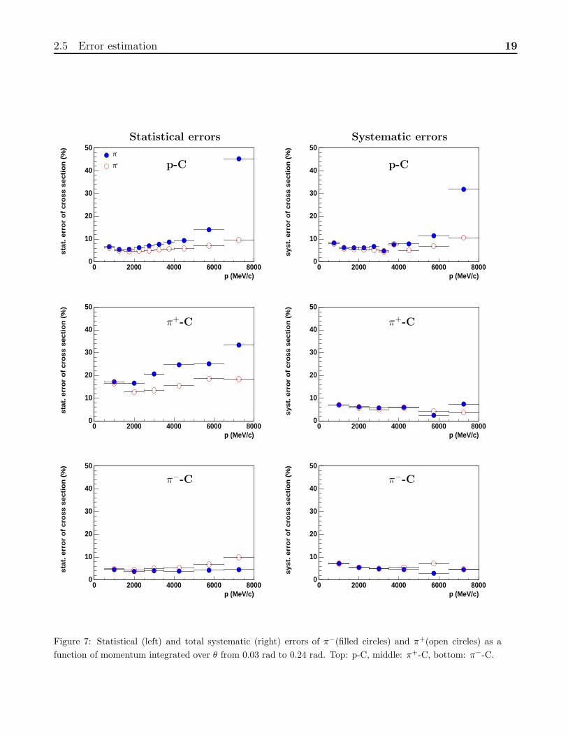
The shapes of the production cross-sections are similar for secondary π+ and π− as well as for different datasets.
For larger angles the spectra are softer and show a leading particle effect for produced π+ in p-C and π+-C
reactions and for π− in π−-C reactions. The distribution of secondary π+ in π+-C reactions show a very similar
behaviour as the distribution of secondary π− in π−-C reactions as expected because of the isospin symmetry
of π+ + C → π+ + X and π− + C → π− + X reactions. The corresponding behaviour can be seen for π− in
π+-C interactions and for π+ in π−-C interactions. The π+/π− ratio is larger than unity in the positive particle
beams and smaller than unity in the π− beam.
In section 3.1 the measured cross-sections are fitted to a Sanford-Wang parametrization while in section 3.2 a
comparison of HARP p-C data with predictions of different hadronic interaction models is shown.

3 Results 23
Figure 8: Measurement of the double-differential production cross-section of positive (open circles) and negative
(filled circles) pions from 12 GeV/c protons on carbon as a function of pion momentum, p, in bins of pion angle, θ,
in the laboratory frame. Seven panels show different angular bins from 30 mrad to 240 mrad (the corresponding
angular interval is printed on each panel). The error bars shown include statistical errors and all (diagonal)
systematic errors. The curves show the Sanford-Wang parametrization of Eq. 9 with parameter values given in
Table 6.

3 Results 24
Figure 9: Measurement of the double-differential production cross-section of positive (open circles) and negative
(filled circles) pions from 12 GeV/c π+ on carbon as a function of pion momentum, p, in bins of pion angle, θ,
in the laboratory frame. Six panels show different angular bins from 30 mrad to 210 mrad (the corresponding
angular interval is printed on each panel). The error bars shown include statistical errors and all (diagonal)
systematic errors. The curves show the Sanford-Wang parametrization of Eq. 9 with parameter values given in
Table 8.
3 Results 25
Figure 10: Measurement of the double-differential production cross-section of positive (open circles) and negative
(filled circles) pions from 12 GeV/c π− on carbon as a function of pion momentum, p, in bins of pion angle, θ,
in the laboratory frame. Six panels show different angular bins from 30 mrad to 210 mrad (the corresponding
angular interval is printed on each panel). The error bars shown include statistical errors and all (diagonal)
systematic errors. The curves show the Sanford-Wang parametrization of Eq. 9 with parameter values given in
Table 8.

3.1 Sanford-Wang parametrization 26
Table 6: Sanford-Wang parameters and errors obtained by fitting the p–C dataset.
p–C
Param π− π+
c1 144.46 ± 65.593 214.92 ± 93.307
c2 0.60749 ± 0.34902 0.95748 ± 0.44512
c3 16.947 ± 10.876 3.0906 ± 1.2601
c4=c5 3.2512 ± 1.3657 1.6876 ± 1.5230
c6 5.9304 ± 1.2561 5.5728 ± 0.71771
c7 0.17152 ± 0.074772 0.15597 ± 0.06683
c8 27.241 ± 12.232 30.873 ± 13.388
χ2/NDF 95.6/63 147.7/63
3.1 Sanford-Wang parametrization
Sanford and Wang [37] have developed an empirical parametrization for describing the production cross-sections
of mesons in proton-nucleus interactions. This parametrization has the functional form:
d2σπ
dpdΩ(p, θ) = c1p
c2
(
1 − p
pbeam
)
exp
[
−c3
pc4
pc5
beam
− c6θ (p − c7pbeam cosc8 θ)
]
, (9)
where
• d2σπ
dpdΩ(p, θ) is the cross-section in mb/(GeV/c sr) for secondary pions as a function of momentum p (in
GeV/c) and angle θ (in radians) of the secondary particles;
• pbeam is the beam momentum in GeV/c;
• c1, ..., c8 are free parameters obtained from fits to meson production data.
The parameter c1 is an overall normalization factor, the four parameters c2, c3, c4, c5 can be interpreted as
describing the momentum distribution of the secondary pions in the forward direction, and the three parameters
c6, c7, c8 as describing the angular distribution for fixed secondary and beam momenta, p and pbeam.
This empirical formula has been fitted to the measured π+ and π− production spectra in p–C, π+–C and π−–C
reactions at 12 GeV/c reported here. As initial values for these fits the parameters of the Sanford-Wang fit of
the p–Al HARP analysis at 12.9 GeV/c are taken from [9]. The original Sanford-Wang parametrization has
been proposed to describe incoming proton data. We apply the same parametrization also to the π+–C and
π−–C datasets.
In the χ2 minimization procedure the full error matrix is used. For these fits the Sanford-Wang parametrization
has been integrated over momentum and angular bin widths of the data. However, the results are nearly
identical to the fit results without integration over individual bins. Concerning the parameters estimation, the
best-fit values of the Sanford-Wang parameter set discussed above are reported in Tables 6 and 8, together with
their errors. Since for some fits the c3 parameter tends to zero, we decided to fix this parameter and to set it
to zero. For these fits the c4 and c5 parameters are irrelevant (see Eq. 9). The correlation coefficients among
the Sanford-Wang parameters are shown in Tables 7 and 9. The fit parameter errors are estimated by requiring
∆χ2 ≡ χ2 − χ2min = 8.18 (5.89), corresponding to the 68.27% confidence level region for seven (five) variable
parameters. Some parameters are strongly correlated resulting in large errors of the extracted parameters.

3.1 Sanford-Wang parametrization 27
Table 7: Correlation coefficients among the Sanford-Wang parameters, obtained by fitting the p–C dataset.
π−
Parameter c1 c2 c3 c4 = c5 c6 c7 c8
c1 1.000
c2 -0.433 1.000
c3 -0.041 -0.548 1.000
c4 = c5 -0.113 -0.535 0.950 1.000
c6 -0.535 0.622 -0.035 0.127 1.000
c7 -0.837 0.121 0.024 0.050 0.214 1.000
c8 -0.206 -0.316 0.028 -0.025 -0.360 0.611 1.000
π+
Parameter c1 c2 c3 c4 = c5 c6 c7 c8
c1 1.000
c2 0.151 1.000
c3 0.061 -0.151 1.000
c4 = c5 -0.461 -0.860 0.351 1.000
c6 -0.544 0.248 -0.373 0.065 1.000
c7 -0.790 -0.004 -0.168 0.115 0.333 1.000
c8 -0.083 -0.275 0.092 0.080 -0.416 0.488 1.000
The measurements for π− and π+ in p–C, π+–C and π−–C reactions are compared to the Sanford-Wang
parametrizations in Figs. 8, 9 and 10, respectively. One notes that the Sanford-Wang parametrization is not
able to describe some of the data spectral features especially at low and high momenta. The goodness-of-fit
of the Sanford-Wang parametrization hypothesis can be assessed by considering χ2 per number of degrees of
freedom (NDF) given in Tables 6 and 8. Especially for the π− data one finds a high value of χ2. This may not
be surprising since the parametrization was developed for pion production by incoming protons rather than by
incoming pions. The π− data with their high statistics are more likely to reveal discrepancies than the π+ data
which have much lower statistical significance.
For tuning and modifying models, often a parametrization of data like the Sanford-Wang formula is used. This
can be a suitable method to interpolate between measured energy and phase space regions. However, this
method has some shortcomings. By construction, the reliability of parametrizations for extrapolating to energy
Table 8: Sanford-Wang parameters and errors obtained by fitting the π+–C and π−–C datasets.
π+–C π−–C
Param π− π+ π− π+
c1 41.448 ± 45.572 109.24± 114.73 156.49 ± 56.132 78.963 ± 34.332
c2 1.8316 ± 0.61113 1.2130 ± 0.57892 1.1673 ± 0.17019 1.3561 ± 0.21690
c3 0. (fixed) 0. (fixed) 0. (fixed) 7.1493 ± 28.024
c4=c5 — — — 5.1098 ± 7.2508
c6 10.074 ± 1.8426 5.7823 ± 1.9875 5.6525 ± 0.54217 8.0965 ± 0.73121
c7 0.22877 ± 0.098638 0.25667 ± 0.17396 0.19908 ± 0.06052 0.21960 ± 0.055566
c8 18.056 ± 15.934 36.139 ± 25.437 30.368 ± 9.9403 25.561 ± 9.1022
χ2/NDF 37.4/31 18.5/31 133.6/31 136.7/29
3.2 Comparison of p–C HARP data at 12 GeV/c with model predictions 28
and phase space regions where no data are available is limited (see [33] for a more detailed discussion).
Detailed inspection of Figs. 8, 9 and 10 allows us to conclude that at high momenta and in particular at large
angles the parametrization does not describe the data well enough. Especially for π+ momentum spectra at
angles larger than 0.18 rad, the Sanford-Wang fit deviates considerably from the data and it should not be used
in the angular range above 0.18 rad.
3.2 Comparison of p–C HARP data at 12 GeV/c with model predictions
A comparison of π− and π+ production in p–C reactions at 12 GeV/c with different model predictions is
shown in Figs. 11 and 12. The three hadronic interaction models used for this comparison are GHEISHA [38],
UrQMD [39] and DPMJET-III [40]. These are the models typically used in air shower simulations. The
GHEISHA and UrQMD are implemented in CORSIKA [36] as low energy models (below 80 GeV), whereas
the DPMJET-III is mostly used at higher energies but it is also able to make predictions at lower energies.
Comparing the predictions of these models to the measured data, distinct discrepancies at low and high momenta
become visible. Especially the decrease of the cross-section at very low momenta is not well described by the
models. For π+, the prediction of the DPMJET-III seems relatively good, however, this model underestimates
the π− production at low momenta. At large momenta the predictions of the three models are similar to each
other, but none of them provides an acceptable description of the data.
We have also compared our measurements with predictions of GEANT4 [31] models relevant in the energy
domain studied here (FTFP [41], QGSP [41, 42] and LHEP [31, 43]). The corresponding plots are presented
in Figs. 13 and 14 (for incoming protons), in Figs. 15 and 16 (for incoming π+) and in Figs. 17 and 18 (for
incoming π−). From these plots one can conclude that the predictions of FTFP and QGSP models are closer
to the HARP data compared to the LHEP model. For the π− and π+ data the DPMJET-III model is shown
in the same figure. The predictions of the latter model are very close to those of the FTFP model.
We have made a χ2 comparison between the HARP data and all the models shown here. The full HARP error
matrix has been used, and MC statistical errors (small but non-negligible) have been also taken into account.
The conclusions of this study are given below. None of the models describe our data accurately. However,
in general these models tend to describe the π+ production more correctly than π− production for all three
incoming particle types. Different models are preferable, depending on projectile type and on the charge of the
pion produced. In particular,
• for proton projectiles and π+ production, UrQMD, FTFP and GHEISHA give the best results;
• for proton projectiles and π− production, FTFP is preferable;
• for π+ projectiles and π+ production and for π− projectiles and π− production, DPMJET-III is best;
• for π+ projectiles and π− production and for π− projectiles and π+ production, QGSP describes the data
best.
4 Summary and conclusions
The results reported in this article contribute to the precise calculations of atmospheric neutrino fluxes and to the
improvement of our understanding of extended air shower simulations and hadronic interactions at low energies.

4 Summary and conclusions 29
Figure 11: Comparison of the measured double-differential production cross-section of π− in p–C reactions at
12 GeV/c (points with error bars) with GHEISHA, UrQMD and DPMJET-III model predictions. Seven panels
show different angular bins from 30 mrad to 240 mrad (the corresponding angular interval is printed on each
panel).

4 Summary and conclusions 30
Figure 12: Comparison of the measured double-differential production cross-section of π+ in p–C reactions at
12 GeV/c (points with error bars) with GHEISHA, UrQMD and DPMJET-III model predictions. Seven panels
show different angular bins from 30 mrad to 240 mrad (the corresponding angular interval is printed on each
panel).

4 Summary and conclusions 31
Figure 13: Comparison of the measured double-differential production cross-section of π− in p–C reactions at
12 GeV/c (points with error bars) with predictions of relevant GEANT4 models. Seven panels show different
angular bins from 30 mrad to 240 mrad (the corresponding angular interval is printed on each panel).

4 Summary and conclusions 32
Figure 14: Comparison of the measured double-differential production cross-section of π+ in p–C reactions at
12 GeV/c (points with error bars) with predictions of relevant GEANT4 models. Seven panels show different
angular bins from 30 mrad to 240 mrad (the corresponding angular interval is printed on each panel).

4 Summary and conclusions 33
Figure 15: Comparison of the measured double-differential production cross-section of π− in π+–C reactions at
12 GeV/c (points with error bars) with predictions of relevant GEANT4 and DPMJET-III models. Six panels
show different angular bins from 30 mrad to 210 mrad (the corresponding angular interval is printed on each
panel).

4 Summary and conclusions 34
Figure 16: Comparison of the measured double-differential production cross-section of π+ in π+–C reactions at
12 GeV/c (points with error bars) with predictions of relevant GEANT4 and DPMJET-III models. Six panels
show different angular bins from 30 mrad to 210 mrad (the corresponding angular interval is printed on each
panel).

4 Summary and conclusions 35
Figure 17: Comparison of the measured double-differential production cross-section of π− in π−–C reactions at
12 GeV/c (points with error bars) with predictions of relevant GEANT4 and DPMJET-III models. Six panels
show different angular bins from 30 mrad to 210 mrad (the corresponding angular interval is printed on each
panel).

4 Summary and conclusions 36
Figure 18: Comparison of the measured double-differential production cross-section of π+ in π−–C reactions at
12 GeV/c (points with error bars) with predictions of relevant GEANT4 and DPMJET-III models. Six panels
show different angular bins from 30 mrad to 210 mrad (the corresponding angular interval is printed on each
panel).

5 Acknowledgments 37
A detailed description of uncertainties in atmospheric neutrino flux calculations due to hadron production can
be found in e.g. [44].
Simulations show that collisions of protons with a carbon target are very similar to proton interactions with
air. That is why these datasets can be used for tuning models needed in astroparticle physics simulations.
In this paper we presented measurements of the double-differential production cross-section of pions in the
collisions of 12 GeV/c protons and charged pions with a carbon 5% nuclear interaction length target. The data
were reported in bins of pion momentum and angle in the kinematic range from 0.5 GeV/c ≤ pπ < 8 GeV/c and
0.030 rad ≤ θπ < 0.240 rad. A detailed error analysis has been performed yielding integral errors (statistical
+ systematic) of 6.1% and 7.0% for π+ and π− in p-C interactions (10.2% and 8.5% for π+ and π− in π+-C
interactions; 6.5% and 8.2% for π+ and π− in π−-C interactions) and an overall normalization error of 2% for
the proton beam and 3% for the pion beams.
We should stress that the HARP incoming charged pion data are the first precision measurements in this
kinematic region.
To check the reliability of hadronic interaction models which are used for air shower simulations, the HARP
measurements have been compared to predictions of these models. Our conclusion is that none of the models
is able to describe satisfactorily and in detail the measured spectra. Discrepancies are found especially at low
and high momenta.
Several models rely on parametrizations of existing accelerator data. Therefore a Sanford-Wang parametrization
is given for all measured spectra. The parametrization is, however, not a good description of the data in the
full phase space region. From the comparison of the Sanford-Wang fits with model predictions we can conclude
that such parametrizations have to be used with caution, especially if these parametrizations are extrapolated
to regions where no data are available.
5 Acknowledgments
We gratefully acknowledge the help and support of the PS beam staff and of the numerous technical collabora-
tors who contributed to the detector design, construction, commissioning and operation. In particular, we would
like to thank G. Barichello, R. Brocard, K. Burin, V. Carassiti, F. Chignoli, D. Conventi, G. Decreuse, M. De-
lattre, C. Detraz, A. Domeniconi, M. Dwuznik, F. Evangelisti, B. Friend, A. Iaciofano, I. Krasin, D. Lacroix,
J.-C. Legrand, M. Lobello, M. Lollo, J. Loquet, F. Marinilli, J. Mulon, L. Musa, R. Nicholson, A. Pepato,
P. Petev, X. Pons, I. Rusinov, M. Scandurra, E. Usenko, and R. van der Vlugt, for their support in the
construction of the detector. The collaboration acknowledges the major contributions and advice of M. Baldo-
Ceolin, L. Linssen, M.T. Muciaccia and A. Pullia during the construction of the experiment. The collaboration
is indebted to V. Ableev, F. Bergsma, P. Binko, E. Boter, M. Calvi, C. Cavion, A. Chukanov, M. Doucet,
D. Dullmann, V. Ermilova, W. Flegel, Y. Hayato, A. Ichikawa, A. Ivanchenko, O. Klimov, T. Kobayashi,
D. Kustov, M. Laveder, M. Mass, H. Meinhard, A. Menegolli, T. Nakaya, K. Nishikawa, M. Pasquali, M. Pla-
centino, V. Serdiouk, S. Simone, S. Troquereau, S. Ueda and A. Valassi for their contributions to the experiment.
We acknowledge the contributions of V. Ammosov, G. Chelkov, D. Dedovich, F. Dydak, M. Gostkin, A. Guskov,
D. Khartchenko, V. Koreshev, Z. Kroumchtein, I. Nefedov, A. Semak, J. Wotschack, V. Zaets and A. Zhem-
chugov to the work described in this paper.
The experiment was made possible by grants from the Institut Interuniversitaire des Sciences Nucleaires and
the Interuniversitair Instituut voor Kernwetenschappen (Belgium), Ministerio de Educacion y Ciencia, Grant

5 Acknowledgments 38
FPA2003-06921-c02-02 and Generalitat Valenciana, grant GV00-054-1, CERN (Geneva, Switzerland), the Ger-
man Bundesministerium fur Bildung und Forschung (Germany), the Istituto Nazionale di Fisica Nucleare (Italy),
INR RAS (Moscow) and the Particle Physics and Astronomy Research Council (UK). We gratefully acknowledge
their support.
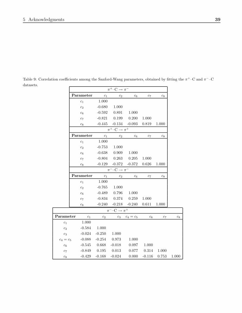
5 Acknowledgments 39
Table 9: Correlation coefficients among the Sanford-Wang parameters, obtained by fitting the π+–C and π−–C
datasets.π+–C → π−
Parameter c1 c2 c6 c7 c8
c1 1.000
c2 -0.680 1.000
c6 -0.592 0.891 1.000
c7 -0.821 0.199 0.200 1.000
c8 -0.445 -0.134 -0.093 0.819 1.000
π+–C → π+
Parameter c1 c2 c6 c7 c8
c1 1.000
c2 -0.753 1.000
c6 -0.638 0.909 1.000
c7 -0.804 0.263 0.205 1.000
c8 -0.129 -0.372 -0.372 0.626 1.000
π−–C → π−
Parameter c1 c2 c6 c7 c8
c1 1.000
c2 -0.765 1.000
c6 -0.489 0.796 1.000
c7 -0.834 0.374 0.259 1.000
c8 -0.240 -0.218 -0.240 0.611 1.000
π−–C → π+
Parameter c1 c2 c3 c4 = c5 c6 c7 c8
c1 1.000
c2 -0.584 1.000
c3 -0.024 -0.250 1.000
c4 = c5 -0.088 -0.254 0.973 1.000
c6 -0.545 0.668 -0.018 0.097 1.000
c7 -0.849 0.195 0.013 0.077 0.314 1.000
c8 -0.429 -0.168 -0.024 0.000 -0.116 0.753 1.000

A Cross-section data 40
A Cross-section data
Table 10: HARP results for the double-differential π+ and π− production cross-section in the laboratory system,
d2σπ/(dpdΩ), for p-C interactions at 12 GeV/c. Each row refers to a different (pmin ≤ p < pmax, θmin ≤ θ <
θmax) bin, where p and θ are the pion momentum and polar angle, respectively. The central value as well as
the square-root of the diagonal elements of the covariance matrix are given.
θmin θmax pmin pmax d2σπ+
/(dpdΩ) d2σπ−
/(dpdΩ)
(mrad) (mrad) (GeV/c) (GeV/c) (mb/(GeV/c sr)) (mb/(GeV/c sr))
30 60 0.5 1.0 198.5 ± 40.8 135.4 ± 30.5
1.0 1.5 245.8 ± 35.0 212.5 ± 30.8
1.5 2.0 248.2 ± 31.1 230.6 ± 32.1
2.0 2.5 227.9 ± 31.0 113.6 ± 21.9
2.5 3.0 331.6 ± 34.2 122.6 ± 22.6
3.0 3.5 258.2 ± 31.4 98.1 ± 18.9
3.5 4.0 214.1 ± 30.5 82.3 ± 14.8
4.0 5.0 133.5 ± 15.1 57.5 ± 10.4
5.0 6.5 102.6 ± 11.0 23.2 ± 6.2
6.5 8.0 45.2 ± 7.8 5.1 ± 4.3
60 90 0.5 1.0 191.7 ± 29.1 151.3 ± 24.9
1.0 1.5 243.2 ± 25.4 180.6 ± 22.0
1.5 2.0 284.9 ± 27.9 191.6 ± 21.3
2.0 2.5 284.4 ± 24.3 158.2 ± 18.0
2.5 3.0 214.9 ± 19.8 101.7 ± 14.0
3.0 3.5 163.1 ± 15.8 85.1 ± 12.0
3.5 4.0 148.4 ± 15.2 64.5 ± 12.2
4.0 5.0 91.4 ± 9.3 37.2 ± 5.5
5.0 6.5 36.9 ± 5.0 12.5 ± 2.8
6.5 8.0 15.6 ± 2.7 1.8 ± 1.0
90 120 0.5 1.0 204.0 ± 27.8 217.4 ± 31.2
1.0 1.5 243.7 ± 26.2 204.7 ± 23.2
1.5 2.0 269.4 ± 27.7 185.1 ± 21.0
2.0 2.5 221.3 ± 23.4 132.1 ± 16.5
2.5 3.0 168.0 ± 17.0 91.8 ± 13.8
3.0 3.5 140.5 ± 15.2 60.5 ± 9.2
3.5 4.0 94.8 ± 15.6 30.7 ± 5.1
4.0 5.0 50.2 ± 6.3 24.4 ± 5.2
5.0 6.5 18.0 ± 2.9 3.1 ± 1.1
6.5 8.0 4.7 ± 1.2 0.1 ± 0.1

A Cross-section data 41
θmin θmax pmin pmax d2σπ+
/(dpdΩ) d2σπ−
/(dpdΩ)
(mrad) (mrad) (GeV/c) (GeV/c) (mb/(GeV/c sr)) (mb/(GeV/c sr))
120 150 0.5 1.0 218.8 ± 30.6 230.5 ± 34.5
1.0 1.5 200.6 ± 23.4 198.9 ± 23.7
1.5 2.0 271.3 ± 28.5 130.7 ± 17.4
2.0 2.5 194.3 ± 21.6 79.7 ± 12.7
2.5 3.0 115.7 ± 15.6 66.7 ± 11.3
3.0 3.5 71.0 ± 10.7 52.5 ± 9.6
3.5 4.0 43.4 ± 7.4 24.9 ± 5.2
4.0 5.0 29.9 ± 5.0 14.0 ± 3.5
5.0 6.5 7.9 ± 2.1 3.1 ± 1.3
6.5 8.0 1.1 ± 0.4 0.3 ± 0.2
150 180 0.5 1.0 238.9 ± 34.1 193.4 ± 28.9
1.0 1.5 257.5 ± 26.9 142.8 ± 20.0
1.5 2.0 173.7 ± 20.8 137.6 ± 19.3
2.0 2.5 121.3 ± 16.7 82.1 ± 13.1
2.5 3.0 67.9 ± 11.8 60.2 ± 11.2
3.0 3.5 39.7 ± 7.4 27.3 ± 6.2
3.5 4.0 28.9 ± 6.3 17.9 ± 5.0
4.0 5.0 14.1 ± 3.5 9.8 ± 3.3
5.0 6.5 3.1 ± 1.2 0.8 ± 0.7
6.5 8.0 0.5 ± 0.3 —
180 210 0.5 1.0 280.1 ± 38.2 242.0 ± 35.1
1.0 1.5 121.0 ± 18.2 134.0 ± 19.8
1.5 2.0 91.8 ± 14.2 107.6 ± 16.8
2.0 2.5 42.0 ± 9.1 63.7 ± 11.9
2.5 3.0 29.3 ± 7.1 28.4 ± 7.2
3.0 3.5 22.2 ± 6.1 14.4 ± 4.6
3.5 4.0 15.1 ± 4.5 7.4 ± 3.4
4.0 5.0 8.9 ± 2.9 2.0 ± 1.3
5.0 6.5 5.6 ± 2.3 0.3 ± 0.4
6.5 8.0 0.7 ± 0.6 —
210 240 0.5 1.0 175.8 ± 29.2 119.4 ± 21.3
1.0 1.5 87.9 ± 16.8 85.4 ± 14.9
1.5 2.0 82.8 ± 17.1 92.6 ± 18.4
2.0 2.5 49.1 ± 11.7 40.3 ± 10.6
2.5 3.0 29.9 ± 8.2 15.5 ± 5.4
3.0 3.5 18.3 ± 6.1 8.7 ± 4.2
3.5 4.0 7.0 ± 3.1 3.1 ± 2.3
4.0 5.0 3.5 ± 2.2 1.6 ± 1.6
5.0 6.5 0.8 ± 0.8 0.2 ± 0.4
6.5 8.0 0.1 ± 0.2 —

A Cross-section data 42
Table 11: HARP results for the double-differential π+ and π− production cross-section in the laboratory system,
d2σπ/(dpdΩ), for π+-C interactions at 12 GeV/c. Each row refers to a different (pmin ≤ p < pmax, θmin ≤ θ <
θmax) bin, where p and θ are the pion momentum and polar angle, respectively. The central value as well as
the square-root of the diagonal elements of the covariance matrix are given.
θmin θmax pmin pmax d2σπ+
/(dpdΩ) d2σπ−
/(dpdΩ)
(mrad) (mrad) (GeV/c) (GeV/c) (mb/(GeV/c sr)) (mb/(GeV/c sr))
30 60 0.50 1.50 191.5 ± 85.0 136.7 ± 66.4
1.50 2.50 173.0 ± 65.1 177.6 ± 71.3
2.50 3.50 354.0 ± 88.4 193.3 ± 70.2
3.50 5.00 302.1 ± 63.6 129.0 ± 47.4
5.00 6.50 177.8 ± 46.9 106.1 ± 38.3
6.50 8.00 196.8 ± 48.5 94.8 ± 34.4
60 90 0.50 1.50 259.1 ± 70.7 161.9 ± 60.5
1.50 2.50 337.1 ± 65.8 166.2 ± 50.2
2.50 3.50 243.0 ± 53.9 140.6 ± 42.4
3.50 5.00 179.4 ± 37.4 88.2 ± 26.4
5.00 6.50 149.7 ± 32.9 54.1 ± 18.8
6.50 8.00 49.7 ± 15.3 12.6 ± 10.0
90 120 0.50 1.50 268.2 ± 64.9 197.6 ± 57.5
1.50 2.50 332.0 ± 65.3 107.3 ± 34.6
2.50 3.50 237.4 ± 47.4 222.3 ± 55.1
3.50 5.00 153.1 ± 34.5 35.8 ± 15.5
5.00 6.50 60.2 ± 18.9 34.4 ± 15.2
6.50 8.00 23.0 ± 9.7 10.1 ± 7.0
120 150 0.50 1.50 178.9 ± 54.8 147.4 ± 57.8
1.50 2.50 264.2 ± 61.8 146.7 ± 51.6
2.50 3.50 178.2 ± 46.3 88.3 ± 33.0
3.50 5.00 73.0 ± 26.3 54.3 ± 28.1
5.00 6.50 31.8 ± 15.5 3.7 ± 5.9
6.50 8.00 7.8 ± 7.0 —
150 180 0.50 1.50 181.1 ± 56.3 213.8 ± 66.6
1.50 2.50 165.7 ± 53.6 173.5 ± 53.7
2.50 3.50 136.2 ± 44.0 44.0 ± 28.4
3.50 5.00 25.7 ± 16.0 9.5 ± 14.2
5.00 6.50 21.3 ± 17.0 3.8 ± 10.2
6.50 8.00 4.5 ± 7.3 —
180 210 0.50 1.50 219.0 ± 73.4 248.5 ± 76.1
1.50 2.50 77.1 ± 35.6 127.8 ± 49.5
2.50 3.50 81.2 ± 42.1 40.9 ± 32.6
3.50 5.00 29.6 ± 24.6 4.4 ± 11.6
5.00 6.50 8.4 ± 13.8 0.0 ± 0.3
6.50 8.00 0.4 ± 3.0 —

A Cross-section data 43
Table 12: HARP results for the double-differential π+ and π− production cross-section in the laboratory system,
d2σπ/(dpdΩ), for π−-C interactions at 12 GeV/c. Each row refers to a different (pmin ≤ p < pmax, θmin ≤ θ <
θmax) bin, where p and θ are the pion momentum and polar angle, respectively. The central value as well as
the square-root of the diagonal elements of the covariance matrix are given.
θmin θmax pmin pmax d2σπ+
/(dpdΩ) d2σπ−
/(dpdΩ)
(mrad) (mrad) (GeV/c) (GeV/c) (mb/(GeV/c sr)) (mb/(GeV/c sr))
30 60 0.50 1.50 198.1 ± 28.7 189.6 ± 28.7
1.50 2.50 206.8 ± 24.2 284.9 ± 31.4
2.50 3.50 182.0 ± 22.2 263.8 ± 27.1
3.50 5.00 138.0 ± 15.3 242.0 ± 19.6
5.00 6.50 98.4 ± 11.4 257.7 ± 22.1
6.50 8.00 74.4 ± 10.4 260.9 ± 17.4
60 90 0.50 1.50 201.9 ± 21.7 249.0 ± 26.6
1.50 2.50 189.2 ± 18.1 302.4 ± 24.5
2.50 3.50 163.1 ± 14.6 247.5 ± 18.8
3.50 5.00 94.6 ± 9.1 200.3 ± 13.6
5.00 6.50 58.5 ± 7.1 129.2 ± 9.4
6.50 8.00 18.4 ± 3.6 81.1 ± 8.2
90 120 0.50 1.50 254.2 ± 26.1 317.1 ± 33.1
1.50 2.50 226.4 ± 20.4 325.5 ± 27.5
2.50 3.50 169.0 ± 16.0 263.9 ± 22.0
3.50 5.00 88.4 ± 10.0 146.9 ± 12.6
5.00 6.50 24.4 ± 4.1 70.1 ± 7.3
6.50 8.00 3.0 ± 0.8 29.0 ± 4.3
120 150 0.50 1.50 195.2 ± 21.6 267.8 ± 29.9
1.50 2.50 177.4 ± 19.0 235.3 ± 22.1
2.50 3.50 97.1 ± 11.9 159.9 ± 16.6
3.50 5.00 56.2 ± 7.7 87.1 ± 10.3
5.00 6.50 10.1 ± 2.8 29.6 ± 5.0
6.50 8.00 1.1 ± 0.5 8.7 ± 2.3
150 180 0.50 1.50 198.9 ± 23.2 267.8 ± 30.7
1.50 2.50 173.1 ± 19.3 233.1 ± 23.7
2.50 3.50 82.6 ± 11.8 89.4 ± 12.0
3.50 5.00 19.0 ± 4.6 48.9 ± 7.4
5.00 6.50 1.5 ± 1.0 11.8 ± 2.9
6.50 8.00 — 3.6 ± 1.3
180 210 0.50 1.50 175.1 ± 22.0 246.9 ± 29.6
1.50 2.50 112.6 ± 15.5 106.1 ± 14.3
2.50 3.50 43.7 ± 9.0 51.4 ± 8.7
3.50 5.00 9.1 ± 3.3 17.2 ± 3.8
5.00 6.50 1.2 ± 1.1 7.4 ± 2.4
6.50 8.00 — 2.4 ± 1.0

REFERENCES 44
References
[1] M. G. Catanesi et al., HARP Collaboration, “Proposal to study hadron production for the neutrino factory
and for the atmospheric neutrino flux”, CERN-SPSC/99-35 (1999).
[2] M. G. Catanesi et al. [HARP Collaboration], “The HARP Detector at the CERN PS”, Nucl. Instrum.
Meth. A 571 (2007) 527.
[3] M. Apollonio et al., “Oscillation Physics with a Neutrino Factory”, CERN TH2002-208,
[arXiv:hep-ph/0210192];
A. Baldini et al., BENE Steering Group, CERN-2006-005;
A. Blondel et al., CERN-2004-002, ECFA/04/230.
[4] M. Honda, T. Kajita, K. Kasahara and S. Midorikawa, Phys. Rev. D 70 (2004) 043008; Phys. Rev. D 75
(2007) 043005 [arXiv:astro-ph/0611201].
M. Honda, T. Kajita, K. Kasahara, S. Midorikawa and T. Sanuki, Phys. Rev. D 75 (2007) 043006
[arXiv:astro-ph/0611418].
G. D. Barr, T. K. Gaisser, P. Lipari, S. Robbins and T. Stanev, Phys. Rev. D 70 (2004) 023006.
G. Battistoni, A. Ferrari, T. Montaruli and P. R. Sala, [arXiv:hep-ph/0305208]
G. Battistoni, A. Ferrari, T. Montaruli and P. R. Sala, Astropart. Phys. 19 (2003) 269 [Erratum-ibid. 19
(2003) 291]
G. Battistoni, A. Ferrari, P. Lipari, T. Montaruli, P. R. Sala and T. Rancati, Astropart. Phys. 12 (2000)
315
[5] E. Aliu et al. [K2K Collaboration], “Evidence for muon neutrino oscillation in an accelerator-based ex-
periment,” Phys. Rev. Lett. 94 (2005) 081802 [arXiv:hep-ex/0411038].
[6] M. H. Ahn et al. [K2K Collaboration], “Measurement of neutrino oscillation by the K2K experiment”,
Phys. Rev. D 74 (2006) 072003 [arXiv:hep-ex/0606032].
[7] E. Church et al. [BooNe Collaboration], “A proposal for an experiment to measure muon-neutrino
→ electron-neutrino oscillations and muon-neutrino disappearance at the Fermilab Booster: BooNE”,
FERMILAB-PROPOSAL-0898.
A. A. Aguilar-Arevalo et al. [MiniBooNE Collaboration], arXiv:0704.1500 [hep-ex].
[8] A. A. Aguilar-Arevalo et al. [SciBooNE Collaboration], “Bringing the SciBar detector to the Booster
neutrino beam”, [arXiv:hep-ex/0601022].
[9] M. G. Catanesi et al. [HARP Collaboration], “Measurement of the production cross-section of positive
pions in p-Al collisions at 12.9 GeV/c”, Nucl. Phys. B 732 (2006) 1 [arXiv:hep-ex/0510039].
[10] M. G. Catanesi et al., [HARP Collaboration], “Measurement of the production cross-section of pos-
itive pions in the collision of 8.9 GeV/c protons on beryllium”, Eur. Phys. J. C 52 (2007) 29
[arXiv:hep-ex/0702024].
[11] M. G. Catanesi et al. [HARP Collaboration], “Particle identification algorithms for the HARP forward
spectrometer”, Nucl. Instrum. Meth. A 572 (2007) 899.
[12] M. G. Catanesi et al., [HARP Collaboration], “Measurement of the Production of charged Pions by
Protons on a Tantalum Target”, Eur. Phys. J. C 51 (2007) 787, arXiv:0706.1600 [hep-ex].
[13] M. G. Catanesi et al., [HARP Collaboration], “Large-angle production of charged pions by 3 GeV/c–
12 GeV/c protons on carbon, copper and tin targets”, Eur. Phys. J. C 53 (2008) 177, arXiv:0709.3464
[hep-ex].

REFERENCES 45
[14] M. G. Catanesi et al., [HARP Collaboration], “Large-angle production of charged pions by 3 GeV/c–
12.9 GeV/c protons on beryllium, aluminium and lead targets”, arXiv:0709.3458 [hep-ex], to be published
in European Physical Journal C.
[15] W. F. Baker et al., Phys. Rev. Lett. 7 (1961) 101.
[16] D. Dekkers et al., Phys. Rev. 137 (1965) B962.
[17] J. V. Allaby et al., CERN Yellow Report 70-12, 1970.
[18] Y. Cho et al., Phys. Rev. D 4 (1971) 1967.
[19] T. Eichten et al., Nucl. Phys. B 44 (1972) 333.
[20] D. Antreasyan et al., Phys. Rev. D 19 N3 (1979) 764.
[21] I. Chemakin et al. [E910 Collaboration], Phys. Rev. C 77 (2008) 015209, arXiv:0707.2375 [nucl-ex].
[22] D. S. Barton et al., Phys. Rev. D 27 (1983) 2580.
[23] C. Alt et al. [NA49 Collaboration], Eur. Phys. J. C 49 (2007) 897 [arXiv:hep-ex/0606028].
[24] H. Meyer [MIPP Collaboration], J. Phys. Conf. Ser. 69 (2007) 012025.
R. Raja, Nucl. Instrum. Meth. A 553 (2005) 225 [arXiv:hep-ex/0501005].
[25] N. Antoniou et al. [NA61 Collaboration], “Study of hadron production in hadron nucleus and nucleus
nucleus collisions at the CERN SPS”, CERN-SPSC-P-330, CERN-SPSC-2006-043, CERN-SPSC-2007-
004, CERN-SPSC-2007-019.
[26] M. Anfreville et al., “The drift chambers of the NOMAD experiment”, Nucl. Instrum. Meth. A 481 (2002)
339 [arXiv:hep-ex/0104012].
[27] M. Baldo-Ceolin et al., “The Time-Of-Flight TOFW Detector Of The HARP Experiment: Construction
And Performance”, Nucl. Instrum. Meth. A 532 (2004) 548.
[28] L. Durieu, A. Mueller and M. Martini, PAC-2001-TPAH142 Presented at IEEE Particle Accelerator Con-
ference (PAC2001), Chicago, Illinois, 18-22 Jun 2001;
L. Durieu et al., Proceedings of PAC’97, Vancouver, (1997);
L. Durieu, O. Fernando, CERN PS/PA Note 96-38.
[29] K. Pretzl et al., Invited talk at the “International Symposium on Strangeness and Quark Matter”, Crete,
(1999) 230.
[30] A. Grossheim, “Particle production yields induced by multi-GeV protons on nuclear targets”, Ph.D. thesis,
University of Dortmund, Germany, 2003, CERN-THESIS-2004-010.
[31] S. Agostinelli et al. [GEANT4 Collaboration], “GEANT4: A simulation toolkit”, Nucl. Instrum. Meth. A
506 (2003) 250.
[32] G. D’Agostini, DESY 94-099, ISSN 0418-9833, 1994.
G. D’Agostini, Nucl. Instrum. Meth. A 362 (1995) 487.
[33] Christine Meurer, “Muon production in extensive air showers and fixed target accelerator data”, Ph.D.
thesis, Karlsruhe, Germany, 2007, CERN-THESIS-2007-078.
[34] V. Blobel and E. Lohrmann, ”Statistische und numerische Methoden der Datenanalyse”, Stuttgart: Teub-
ner, 1998, ISBN 3-519-03243-0.

REFERENCES 46
[35] M. Kliemant, B. Lungwitz, and M. Gazdzicki, Phys. Rev. C 69 (2004) 044903.
[36] D. Heck et al., Report FZKA 6019 (1998)
[37] J. R. Sanford and C. L. Wang, ”Empirical formulas for particle production in p-Be collisions between 10
and 35 BeV/c”, Brookhaven National Loboratory, AGS internal report (1967).
[38] H. Fesefeldt, report PITHA-85/02, RWTH Aachen, 1985.
[39] M. Bleicher et al., J. Phys. G: Nucl. Part. Phys. 25 (1999) 1859.
[40] S. Roesler, R. Engel, and J. Ranft, in Proc. of Int. Conf. on Advanced Monte Carlo for Radiation Physics,
Particle Transport Simulation and Applications (MC 2000), Lisbon, Portugal, 23-26 Oct 2000, A. Kling,
F. Barao, M. Nakagawa, L. Tavora, P. Vaz eds., Springer-Verlag Berlin, p. 1033-1038 (2001), 2000.
[41] G. Folger and H. P. Wellisch, String parton models in Geant4, CHEP’03 (La Jolla, California, USA, 24-28
March 2003); Preprints CHEP-2003-MOMT007, e-Print physics/0306007
[42] D. H. Wright, T. Koi, G. Folger, V. Ivanchenko, M. Kossov, N. Starkov, A. Heikkinen and H. P. Wellisch,
2007 AIP Conf. Proc. 896 11
[43] D. H. Wright, T. Koi, G. Folger, V. Ivanchenko, M. Kossov, N. Starkov, A. Heikkinen and H. P. Wellisch,
2006 AIP Conf. Proc. 867 479
[44] G. D. Barr, T. K. Gaisser, S. Robbins and T. Stanev, Phys. Rev. D 74 (2006) 094009
[arXiv:astro-ph/0611266].


![Κ. Π. Καβάφης, Η ποιητική του μεταιχμίου (με υποσημειώσεις) [C. P. Cavafy, The Poetics of Middle Ground (with footnotes)]](https://static.fdokumen.com/doc/165x107/6333bb7cb94d62384202583b/k-kvis-i-poiitiki-tou-metimiou-me-uposimeioseis.jpg)