arX

iv:h

ep-e

x/05

1003

9 v1

14

Oct

200

5

Measurement of the production cross-section of

positive pions in p–Al collisions at 12.9 GeV/c

HARP Collaboration

October 17, 2005

Abstract

A precision measurement of the double-differential production cross-section, d2σπ+

/dpdΩ, for

pions of positive charge, performed in the HARP experiment is presented. The incident particles are

protons of 12.9 GeV/c momentum impinging on an aluminium target of 5% nuclear interaction length.

The measurement of this cross-section has a direct application to the calculation of the neutrino flux of

the K2K experiment. After cuts, 210 000 secondary tracks reconstructed in the forward spectrometer

were used in this analysis. The results are given for secondaries within a momentum range from

0.75 GeV/c to 6.5 GeV/c, and within an angular range from 30 mrad to 210 mrad. The absolute

normalization was performed using prescaled beam triggers counting protons on target. The overall

scale of the cross-section is known to better than 6%, while the average point-to-point error is 8.2%.

Accepted for publication in Nucl. Phys. B

1

HARP collaboration

M.G. Catanesi, M.T. Muciaccia, E. Radicioni, S. Simone

Universita degli Studi e Sezione INFN, Bari, ItalyR. Edgecock, M. Ellis1, S. Robbins2,3, F.J.P. Soler4

Rutherford Appleton Laboratory, Chilton, Didcot, UKC. Goßling, M. Mass

Institut fur Physik, Universitat Dortmund, GermanyS. Bunyatov, A. Chukanov, D. Dedovitch, A. Elagin, M. Gostkin, A. Guskov, D. Khartchenko, O. Klimov,

A. Krasnoperov, D. Kustov, K. Nikolaev, B. Popov5, V. Serdiouk, V. Tereshchenko, A. Zhemchugov

Joint Institute for Nuclear Research, JINR Dubna, RussiaE. Di Capua, G. Vidal–Sitjes6,1

Universita degli Studi e Sezione INFN, Ferrara, ItalyA. Artamonov7, P. Arce8, S. Giani, S. Gilardoni6, P. Gorbunov7, A. Grant, A. Grossheim6, P. Gruber6,

V. Ivanchenko9, A. Kayis-Topaksu10, L. Linssen, J. Panman, I. Papadopoulos, J. Pasternak6, E. Tcherniaev,

I. Tsukerman7, R. Veenhof, C. Wiebusch3, P. Zucchelli11,12

CERN, Geneva, SwitzerlandA. Blondel, S. Borghi, M. Campanelli, A. Cervera–Villanueva, M.C. Morone, G. Prior6,13, R. Schroeter

Section de Physique, Universite de Geneve, SwitzerlandI. Kato14, T. Nakaya14, K. Nishikawa14, S. Ueda14

University of Kyoto, JapanV. Ableev, U. Gastaldi

Laboratori Nazionali di Legnaro dell’ INFN, Legnaro, ItalyG. B. Mills15

Los Alamos National Laboratory, Los Alamos, USAJ.S. Graulich16, G. Gregoire

Institut de Physique Nucleaire, UCL, Louvain-la-Neuve, BelgiumM. Bonesini, M. Calvi, A. De Min, F. Ferri, M. Paganoni, F. Paleari

Universita degli Studi e Sezione INFN, Milano, ItalyM. Kirsanov

Institute for Nuclear Research, Moscow, RussiaA. Bagulya, V. Grichine, N. Polukhina

P. N. Lebedev Institute of Physics (FIAN), Russian Academy of Sciences, Moscow, RussiaV. Palladino

Universita “Federico II” e Sezione INFN, Napoli, ItalyL. Coney15, D. Schmitz15

Columbia University, New York, USAG. Barr, A. De Santo17, C. Pattison, K. Zuber18

Nuclear and Astrophysics Laboratory, University of Oxford, UKF. Bobisut, D. Gibin, A. Guglielmi, M. Laveder, A. Menegolli, M. Mezzetto

Universita degli Studi e Sezione INFN, Padova, ItalyJ. Dumarchez, S. Troquereau, F. Vannucci

LPNHE, Universites de Paris VI et VII, Paris, FranceV. Ammosov, V. Gapienko, V. Koreshev, A. Semak, Yu. Sviridov, V. Zaets

Institute for High Energy Physics, Protvino, RussiaU. Dore

Universita “La Sapienza” e Sezione INFN Roma I, Roma, ItalyD. Orestano, M. Pasquali, F. Pastore, A. Tonazzo, L. Tortora

Universita degli Studi e Sezione INFN Roma III, Roma, ItalyC. Booth, C. Buttar4, P. Hodgson, L. Howlett

Dept. of Physics, University of Sheffield, UKM. Bogomilov, M. Chizhov, D. Kolev, R. Tsenov

Faculty of Physics, St. Kliment Ohridski University, Sofia, BulgariaS. Piperov, P. Temnikov

Institute for Nuclear Research and Nuclear Energy, Academy of Sciences, Sofia, BulgariaM. Apollonio, P. Chimenti, G. Giannini, G. Santin19

Universita degli Studi e Sezione INFN, Trieste, ItalyY. Hayato14, A. Ichikawa14, T. Kobayashi14

KEK, Tsukuba, JapanJ. Burguet–Castell, J.J. Gomez–Cadenas, P. Novella, M. Sorel, A. Tornero

Instituto de Fisica Corpuscular, IFIC, CSIC and Universidad de Valencia, Spain

2

1Now at Imperial College, University of London, UK.2Now at Bergische Universitat Wuppertal, Germany.3Jointly appointed by Nuclear and Astrophysics Laboratory, University of Oxford, UK.4Now at University of Glasgow, UK.5Also supported by LPNHE (Paris).6Supported by the CERN Doctoral Student Programme.7Permanently at ITEP, Moscow, Russian Federation.8Permanently at Instituto de Fısica de Cantabria, Univ. de Cantabria, Santander, Spain.9On leave of absence from the Budker Institute for Nuclear Physics, Novosibirsk, Russia.

10On leave of absence from Cukurova University, Adana, Turkey.11On leave of absence from INFN, Sezione di Ferrara, Italy.12Now at SpinX Technologies, Geneva, Switzerland.13Now at Lawrence Berkeley National Laboratory, Berkeley, USA.14K2K Collaboration.15MiniBooNE Collaboration.16Now at Section de Physique, Universite de Geneve, Switzerland, Switzerland.17Now at Royal Holloway, University of London, UK.18Now at University of Sussex, Brighton, UK.19Now at ESA/ESTEC, Noordwijk, The Netherlands.

3

1 Introduction

The objective of the HARP experiment is a systematic study of hadron production for beam momentafrom 1.5 GeV/c to 15 GeV/c for a large range of target nuclei [1]. The main motivations are: a) tomeasure pion yields for a quantitative design of the proton driver of a future neutrino factory, b) toimprove substantially the calculation of the atmospheric neutrino flux and c) to provide input for theflux calculation of accelerator neutrino experiments, such as K2K and MiniBooNE.

The measurement described in this paper is of particular relevance in the context of the recent resultspresented by the K2K experiment [2, 3], which have shown evidence for neutrino oscillations at a con-fidence level of four standard deviations. The K2K experiment uses an accelerator-produced νµ beamwith an average energy of 1.3 GeV directed at the Super-Kamiokande detector. The K2K analysis com-pares the observed νµ spectrum in Super-Kamiokande, located at a distance of about 250 km from theneutrino source, with the predicted spectrum in the absence of oscillations. This, in turn, is computedby multiplying the observed spectrum at the near detector (located at 300 m from the neutrino source)by the so-called ‘far–near ratio’, R, defined as the ratio between the predicted flux at the far and neardetectors. This factor corrects for the fact that at the near detector, the neutrino source is not point-like,but sensitive to effects such as the finite size of the decay tunnel, etc., whereas at the Super-Kamiokandesite the neutrino source can be considered as point-like. According to the neutrino oscillation parametersmeasured in atmospheric neutrino experiments [4] the distortion of the spectrum measured with the fardetector is predicted to be maximal in the energy range between 0.5 and 1 GeV. The determination ofR is the leading energy-dependent systematic error in the K2K analysis [2, 3].

The HARP experiment has a large acceptance in the momentum and angular range relevant for K2Kneutrino flux. It covers 80% of the total neutrino flux in the near detector and in the relevant region forneutrino oscillations. Thus, it can provide an independent, and more precise, measurement of the pionyield needed as input to the calculation of the K2K far–near ratio than that currently available.

The neutrino beam of the K2K experiment originates from the decay of light hadrons, produced byexposing an aluminium target to a proton beam of momentum 12.9 GeV/c. In this paper, the mea-

surement of the double-differential cross-section, d2σπ+

/dpdΩ of positive pion production for protons of12.9 GeV/c momentum impinging on a thin Al target of 5% nuclear interaction length (λI) is presented,i.e. reproducing closely the conditions of the K2K beam-line for the production of secondaries.

The HARP apparatus [1, 5] is a large-acceptance spectrometer consisting of a forward and large-angledetection system. The forward spectrometer covers polar angles up to 250 mrad which is well matchedto the angular range of interest for the K2K beam line.

The results reported here are based on data taken in 2002 in the T9 beam of the CERN PS. About3.4 million incoming protons were selected. After cuts, 209 929 secondary tracks reconstructed in theforward spectrometer were used in this analysis. The results are given in the region relevant for K2K,that is the momentum range from 0.75 GeV/c to 6.5 GeV/c and within an angular range from 30 mradto 210 mrad. The absolute normalization was performed using 280 542 ‘minimum-bias’ triggers.

This paper is organized as follows. The experimental apparatus is outlined in Section 2. Section 3describes tracking with the forward spectrometer. Section 4 discusses the calculation of the reconstructionefficiency. Section 5 summarizes the particle identification (PID) capabilities of the spectrometer anddescribes the PID algorithm. Sections 6 and 7 give details of the cross-section calculation. Resultsare discussed in Section 8. A comparison with previous data is presented in Section 9. An illustrativecalculation of the K2K far–near ratio is shown in Section 10. A summary is given in Section 11.

2 Experimental apparatus

The HARP detector, shown in Fig. 1, consists of forward and large-angle detection systems. The con-vention used for the coordinate system is also given in the Figure. In the large-angle region a TPCpositioned in a solenoidal magnet is used for tracking. The forward spectrometer is built around a dipole

4

TPC and RPCs insolenoidal magnet

zy

x

Drift ChambersTOFW

ECAL

CHEDipole magnet

FTP and RPCsT9 beam

NDC1

NDC2

NDC5

NDC3

NDC4

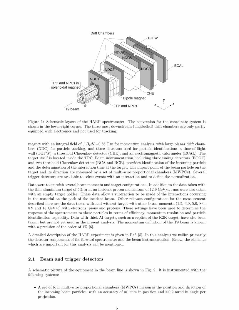
Figure 1: Schematic layout of the HARP spectrometer. The convention for the coordinate system isshown in the lower-right corner. The three most downstream (unlabelled) drift chambers are only partlyequipped with electronics and not used for tracking.

magnet with an integral field of∫

BydL=0.66 T m for momentum analysis, with large planar drift cham-bers (NDC) for particle tracking, and three detectors used for particle identification: a time-of-flightwall (TOFW), a threshold Cherenkov detector (CHE), and an electromagnetic calorimeter (ECAL). Thetarget itself is located inside the TPC. Beam instrumentation, including three timing detectors (BTOF)and two threshold Cherenkov detectors (BCA and BCB), provides identification of the incoming particleand the determination of the interaction time at the target. The impact point of the beam particle on thetarget and its direction are measured by a set of multi-wire proportional chambers (MWPCs). Severaltrigger detectors are available to select events with an interaction and to define the normalization.

Data were taken with several beam momenta and target configurations. In addition to the data taken withthe thin aluminium target of 5% λI at an incident proton momentum of 12.9 GeV/c, runs were also takenwith an empty target holder. These data allow a subtraction to be made of the interactions occurringin the material on the path of the incident beam. Other relevant configurations for the measurementdescribed here are the data taken with and without target with other beam momenta (1.5, 3.0, 5.0, 8.0,8.9 and 15 GeV/c) with electrons, pions and protons. These settings have been used to determine theresponse of the spectrometer to these particles in terms of efficiency, momentum resolution and particleidentification capability. Data with thick Al targets, such as a replica of the K2K target, have also beentaken, but are not yet used in the present analysis. The momentum definition of the T9 beam is knownwith a precision of the order of 1% [6].

A detailed description of the HARP experiment is given in Ref. [5]. In this analysis we utilize primarilythe detector components of the forward spectrometer and the beam instrumentation. Below, the elementswhich are important for this analysis will be mentioned.

2.1 Beam and trigger detectors

A schematic picture of the equipment in the beam line is shown in Fig. 2. It is instrumented with thefollowing systems:

• A set of four multi-wire proportional chambers (MWPCs) measures the position and direction ofthe incoming beam particles, with an accuracy of ≈1 mm in position and ≈0.2 mrad in angle perprojection.

5

target

FTP

ITC

TPC

RPC

TOF B TOF A

HALO A

TDS

HALO B 1423

BSMWPC

BC B BC A

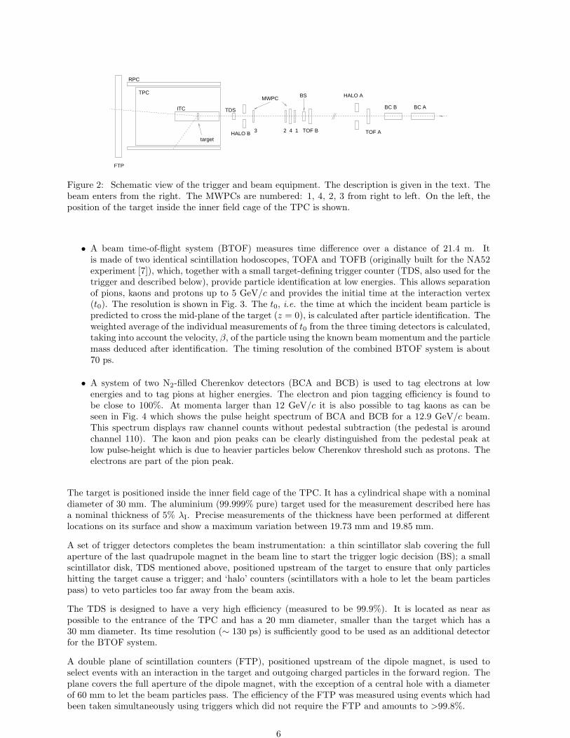
Figure 2: Schematic view of the trigger and beam equipment. The description is given in the text. Thebeam enters from the right. The MWPCs are numbered: 1, 4, 2, 3 from right to left. On the left, theposition of the target inside the inner field cage of the TPC is shown.

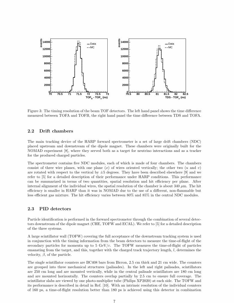
• A beam time-of-flight system (BTOF) measures time difference over a distance of 21.4 m. Itis made of two identical scintillation hodoscopes, TOFA and TOFB (originally built for the NA52experiment [7]), which, together with a small target-defining trigger counter (TDS, also used for thetrigger and described below), provide particle identification at low energies. This allows separationof pions, kaons and protons up to 5 GeV/c and provides the initial time at the interaction vertex(t0). The resolution is shown in Fig. 3. The t0, i.e. the time at which the incident beam particle ispredicted to cross the mid-plane of the target (z = 0), is calculated after particle identification. Theweighted average of the individual measurements of t0 from the three timing detectors is calculated,taking into account the velocity, β, of the particle using the known beam momentum and the particlemass deduced after identification. The timing resolution of the combined BTOF system is about70 ps.

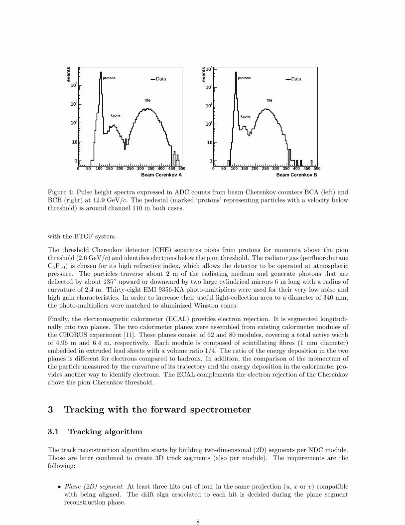
• A system of two N2-filled Cherenkov detectors (BCA and BCB) is used to tag electrons at lowenergies and to tag pions at higher energies. The electron and pion tagging efficiency is found tobe close to 100%. At momenta larger than 12 GeV/c it is also possible to tag kaons as can beseen in Fig. 4 which shows the pulse height spectrum of BCA and BCB for a 12.9 GeV/c beam.This spectrum displays raw channel counts without pedestal subtraction (the pedestal is aroundchannel 110). The kaon and pion peaks can be clearly distinguished from the pedestal peak atlow pulse-height which is due to heavier particles below Cherenkov threshold such as protons. Theelectrons are part of the pion peak.

The target is positioned inside the inner field cage of the TPC. It has a cylindrical shape with a nominaldiameter of 30 mm. The aluminium (99.999% pure) target used for the measurement described here hasa nominal thickness of 5% λI. Precise measurements of the thickness have been performed at differentlocations on its surface and show a maximum variation between 19.73 mm and 19.85 mm.

A set of trigger detectors completes the beam instrumentation: a thin scintillator slab covering the fullaperture of the last quadrupole magnet in the beam line to start the trigger logic decision (BS); a smallscintillator disk, TDS mentioned above, positioned upstream of the target to ensure that only particleshitting the target cause a trigger; and ‘halo’ counters (scintillators with a hole to let the beam particlespass) to veto particles too far away from the beam axis.

The TDS is designed to have a very high efficiency (measured to be 99.9%). It is located as near aspossible to the entrance of the TPC and has a 20 mm diameter, smaller than the target which has a30 mm diameter. Its time resolution (∼ 130 ps) is sufficiently good to be used as an additional detectorfor the BTOF system.

A double plane of scintillation counters (FTP), positioned upstream of the dipole magnet, is used toselect events with an interaction in the target and outgoing charged particles in the forward region. Theplane covers the full aperture of the dipole magnet, with the exception of a central hole with a diameterof 60 mm to let the beam particles pass. The efficiency of the FTP was measured using events which hadbeen taken simultaneously using triggers which did not require the FTP and amounts to >99.8%.

6

(ns)A - TOFBTOF70 70.5 71 71.5 72 72.5 73

even

ts

0

2000

4000

6000

8000

10000

12000

14000DataMC

(ns)ATDS - TOF79.5 80 80.5 81 81.5 82 82.5

even

ts

0

2000

4000

6000

8000

10000

12000

14000DataMC

Figure 3: The timing resolution of the beam TOF detectors. The left hand panel shows the time differencemeasured between TOFA and TOFB, the right hand panel the time difference between TDS and TOFA.

2.2 Drift chambers

The main tracking device of the HARP forward spectrometer is a set of large drift chambers (NDC)placed upstream and downstream of the dipole magnet. These chambers were originally built for theNOMAD experiment [8], where they served both as a target for neutrino interactions and as a trackerfor the produced charged particles.

The spectrometer contains five NDC modules, each of which is made of four chambers. The chambersconsist of three wire planes, with one plane (x) of wires oriented vertically; the other two (u and v)are rotated with respect to the vertical by ±5 degrees. They have been described elsewhere [9] and werefer to [5] for a detailed description of their performance under HARP conditions. This performancecan be summarized in terms of two quantities, spatial resolution and hit efficiency per plane. Afterinternal alignment of the individual wires, the spatial resolution of the chamber is about 340 µm. The hitefficiency is smaller in HARP than it was in NOMAD due to the use of a different, non-flammable butless efficient gas mixture. The hit efficiency varies between 80% and 85% in the central NDC modules.

2.3 PID detectors

Particle identification is performed in the forward spectrometer through the combination of several detec-tors downstream of the dipole magnet (CHE, TOFW and ECAL). We refer to [5] for a detailed descriptionof the three systems.

A large scintillator wall (TOFW) covering the full acceptance of the downstream tracking system is usedin conjunction with the timing information from the beam detectors to measure the time-of-flight of thesecondary particles for momenta up to 5 GeV/c. The TOFW measures the time-of-flight of particlesemanating from the target, and this, together with the charged track trajectory length, l, determines thevelocity, β, of the particle.

The single scintillator counters are BC408 bars from Bicron, 2.5 cm thick and 21 cm wide. The countersare grouped into three mechanical structures (palisades). In the left and right palisades, scintillatorsare 250 cm long and are mounted vertically, while in the central palisade scintillators are 180 cm longand are mounted horizontally. The counters overlap partially by 2.5 cm to ensure full coverage. Thescintillator slabs are viewed by one photo-multiplier tube (Philips XP2020) at each side. The TOFW andits performance is described in detail in Ref. [10]. With an intrinsic resolution of the individual countersof 160 ps, a time-of-flight resolution better than 180 ps is achieved using this detector in combination

7

Beam Cerenkov A0 50 100 150 200 250 300 350 400 450 500

even

ts

1

10

210

310

410Dataprotons

kaons

/eπ

Beam Cerenkov B0 50 100 150 200 250 300 350 400 450 500

even

ts

1

10

210

310

410

510

Dataprotons

kaons

/eπ

Figure 4: Pulse height spectra expressed in ADC counts from beam Cherenkov counters BCA (left) andBCB (right) at 12.9 GeV/c. The pedestal (marked ‘protons’ representing particles with a velocity belowthreshold) is around channel 110 in both cases.

with the BTOF system.

The threshold Cherenkov detector (CHE) separates pions from protons for momenta above the pionthreshold (2.6 GeV/c) and identifies electrons below the pion threshold. The radiator gas (perfluorobutaneC4F10) is chosen for its high refractive index, which allows the detector to be operated at atmosphericpressure. The particles traverse about 2 m of the radiating medium and generate photons that aredeflected by about 135 upward or downward by two large cylindrical mirrors 6 m long with a radius ofcurvature of 2.4 m. Thirty-eight EMI 9356-KA photo-multipliers were used for their very low noise andhigh gain characteristics. In order to increase their useful light-collection area to a diameter of 340 mm,the photo-multipliers were matched to aluminized Winston cones.

Finally, the electromagnetic calorimeter (ECAL) provides electron rejection. It is segmented longitudi-nally into two planes. The two calorimeter planes were assembled from existing calorimeter modules ofthe CHORUS experiment [11]. These planes consist of 62 and 80 modules, covering a total active widthof 4.96 m and 6.4 m, respectively. Each module is composed of scintillating fibres (1 mm diameter)embedded in extruded lead sheets with a volume ratio 1/4. The ratio of the energy deposition in the twoplanes is different for electrons compared to hadrons. In addition, the comparison of the momentum ofthe particle measured by the curvature of its trajectory and the energy deposition in the calorimeter pro-vides another way to identify electrons. The ECAL complements the electron rejection of the Cherenkovabove the pion Cherenkov threshold.

3 Tracking with the forward spectrometer

3.1 Tracking algorithm

The track reconstruction algorithm starts by building two-dimensional (2D) segments per NDC module.Those are later combined to create 3D track segments (also per module). The requirements are thefollowing:

• Plane (2D) segment: At least three hits out of four in the same projection (u, x or v) compatiblewith being aligned. The drift sign associated to each hit is decided during the plane segmentreconstruction phase.

8

• Track (3D) segment: Two or three plane segments of different projections, whose intersection definesa 3D straight line. In the case where only two plane segments are found, an additional hit in theremaining projection is required. This hit must intersect the 3D straight line defined by the othertwo projections.

Consequently, to form a track segment at least seven hits (from a total of 12 measurement planes) areneeded within the same NDC module. Once track segments are formed in the individual modules theyare combined (downstream of the dipole magnet) to obtain longer track segments. Finally, downstreamtracks are connected with either the interaction vertex or a 3D track segment in NDC1 (the NDC moduleupstream the dipole magnet, see Fig. 1) to measure the momentum. All these tasks are performed by asophisticated fitting, extrapolation and matching package called RecPack [12], which is based on the wellknown Kalman Filter technique [13].

The interaction vertex in this analysis is well defined. The transverse coordinates (x, y) are obtained byextrapolating the trajectory of the incoming beam particle, measured with the MWPCs (with an error ofthe order of 1 mm), and the z coordinate can be taken as that of the nominal plane of the target (whichis 19.80 mm thick).

Consequently, the momentum of a track can be determined by imposing the constraint that it emanatesfrom the vertex, that is, by connecting a 3D segment downstream the dipole magnet with a 3D pointupstream the magnet. Tracks of this type are called ‘VERTEX2 tracks’, and the estimator of the mo-mentum obtained by connecting a 3D segment with the vertex 3D point is denoted ‘p2’. Specifically, thisis done by extrapolating the downstream 3D segment to the nominal plane of the target, and imposingthat the distance between the transverse coordinates thus obtained (xs, ys) and the (x, y) coordinatesdefined above is less than 10 cm (in practice one builds a χ2 which also takes into account the measure-ment errors). Tracks which extrapolate to distances larger than 10 cm are not considered (in fact, theinefficiency of the p2 algorithm, a few percent comes almost exclusively from this source).

Alternatively, one can measure the momentum connecting a 3D segment downstream of the dipole witha 3D segment in the NDC1 module. These are called ‘VERTEX4 tracks’, and the estimator of themomentum is denoted ‘p4’. The way a downstream segment is connected with a NDC1 3D segment isdescribed with some detail below. In essence, one requires a reasonable collinearity in the non-bendingplane and obtains the momentum from the curvature in the bending plane.

The availability of two independent momentum estimators allows the tracking efficiency to be measuredfrom the data themselves. This is possible, since, a) the reconstruction methods providing the estimatorsp2 and p4 are independent b) p2 and p4 have a Gaussian distribution around the true momentum p(The distribution is expected to be Gaussian in the variable 1/p rather than p. With the relatively goodresolution the difference is negligible.) This makes it possible to use one of the estimators (p2) to measurethe yields while the other (p4) is used to measure tracking efficiency. The estimator p2 is preferred tomeasure yields since it does not involve the use of the NDC1 module, where tracking efficiency is lowerthan in the downstream modules (see the discussion on tracking efficiency in Section 4).

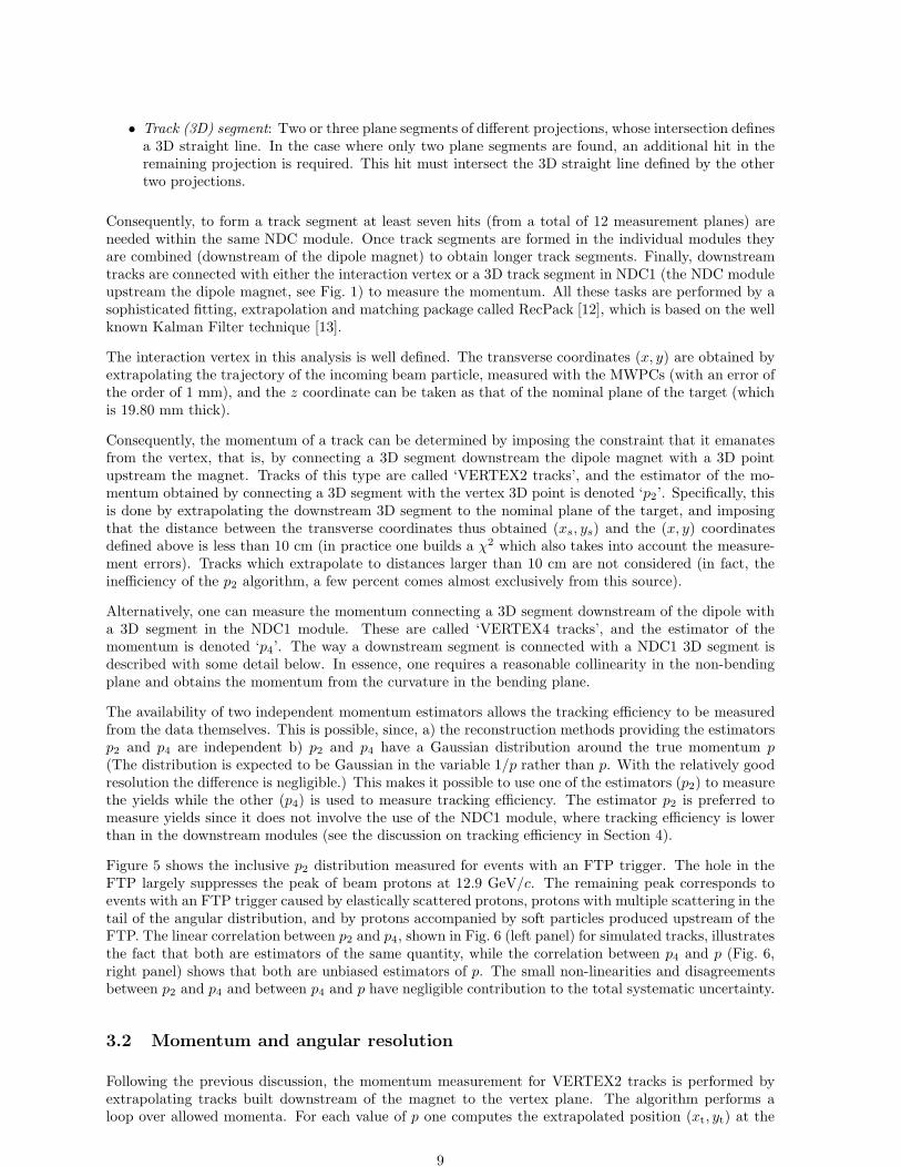
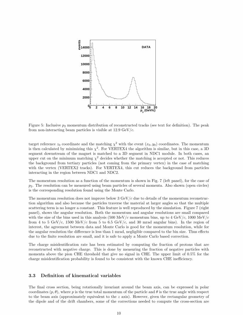
Figure 5 shows the inclusive p2 distribution measured for events with an FTP trigger. The hole in theFTP largely suppresses the peak of beam protons at 12.9 GeV/c. The remaining peak corresponds toevents with an FTP trigger caused by elastically scattered protons, protons with multiple scattering in thetail of the angular distribution, and by protons accompanied by soft particles produced upstream of theFTP. The linear correlation between p2 and p4, shown in Fig. 6 (left panel) for simulated tracks, illustratesthe fact that both are estimators of the same quantity, while the correlation between p4 and p (Fig. 6,right panel) shows that both are unbiased estimators of p. The small non-linearities and disagreementsbetween p2 and p4 and between p4 and p have negligible contribution to the total systematic uncertainty.

3.2 Momentum and angular resolution

Following the previous discussion, the momentum measurement for VERTEX2 tracks is performed byextrapolating tracks built downstream of the magnet to the vertex plane. The algorithm performs aloop over allowed momenta. For each value of p one computes the extrapolated position (xt, yt) at the

9

(GeV/c)2

p0 2 4 6 8 10 12 14 16 18 20

even

ts

0

2000

4000

6000

8000

10000

12000

14000 DATA

Figure 5: Inclusive p2 momentum distribution of reconstructed tracks (see text for definition). The peakfrom non-interacting beam particles is visible at 12.9 GeV/c.

target reference z0 coordinate and the matching χ2 with the event (x0, y0) coordinates. The momentumis then calculated by minimizing this χ2. For VERTEX4 the algorithm is similar, but in this case, a 3Dsegment downstream of the magnet is matched to a 3D segment in NDC1 module. In both cases, anupper cut on the minimum matching χ2 decides whether the matching is accepted or not. This reducesthe background from tertiary particles (not coming from the primary vertex) in the case of matchingwith the vertex (VERTEX2 tracks). For VERTEX4, this cut reduces the background from particlesinteracting in the region between NDC1 and NDC2.

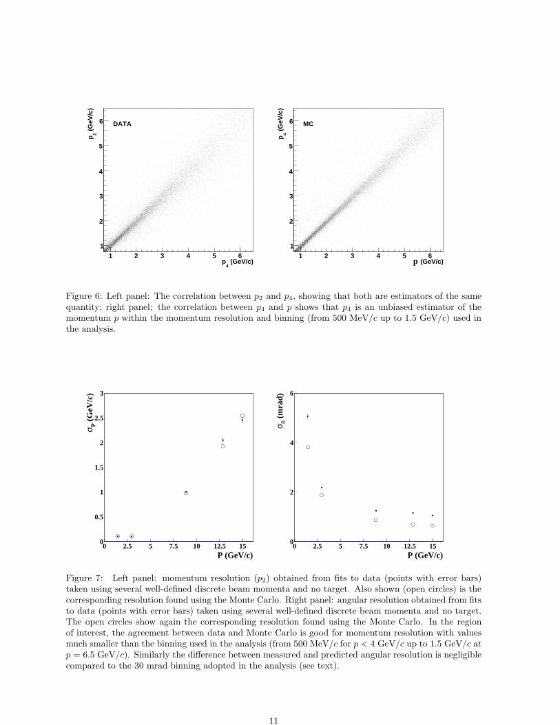
The momentum resolution as a function of the momentum is shown in Fig. 7 (left panel), for the case ofp2. The resolution can be measured using beam particles of several momenta. Also shown (open circles)is the corresponding resolution found using the Monte Carlo.

The momentum resolution does not improve below 3 GeV/c due to details of the momentum reconstruc-tion algorithm and also because the particles traverse the material at larger angles so that the multiplescattering term is no longer a constant. This feature is well reproduced by the simulation. Figure 7 (rightpanel), shows the angular resolution. Both the momentum and angular resolutions are small comparedwith the size of the bins used in this analysis (500 MeV/c momentum bins, up to 4 GeV/c, 1000 MeV/cfrom 4 to 5 GeV/c, 1500 MeV/c from 5 to 6.5 GeV/c, and 30 mrad angular bins). In the region ofinterest, the agreement between data and Monte Carlo is good for the momentum resolution, while forthe angular resolution the difference is less than 1 mrad, negligible compared to the bin size. Thus effectsdue to the finite resolution are small, and it is safe to apply a Monte Carlo based correction.

The charge misidentification rate has been estimated by computing the fraction of protons that arereconstructed with negative charge. This is done by measuring the fraction of negative particles withmomenta above the pion CHE threshold that give no signal in CHE. The upper limit of 0.5% for thecharge misidentification probability is found to be consistent with the known CHE inefficiency.

3.3 Definition of kinematical variables

The final cross section, being rotationally invariant around the beam axis, can be expressed in polarcoordinates (p, θ), where p is the true total momentum of the particle and θ is the true angle with respectto the beam axis (approximately equivalent to the z axis). However, given the rectangular geometry ofthe dipole and of the drift chambers, some of the corrections needed to compute the cross-section are

10

(GeV/c)4

p1 2 3 4 5 6

(G

eV/c

)2

p

1

2

3

4

5

6 DATA

(GeV/c)true

p1 2 3 4 5 6

(G

eV/c

)4

p

1

2

3

4

5

6 MC

p

Figure 6: Left panel: The correlation between p2 and p4, showing that both are estimators of the samequantity; right panel: the correlation between p4 and p shows that p4 is an unbiased estimator of themomentum p within the momentum resolution and binning (from 500 MeV/c up to 1.5 GeV/c) used inthe analysis.

0

0.5

1

1.5

2

2.5

3

0 2.5 5 7.5 10 12.5 15P (GeV/c)

σ P (

GeV

/c)

0

2

4

6

0 2.5 5 7.5 10 12.5 15P (GeV/c)

σ θ (m

rad)

Figure 7: Left panel: momentum resolution (p2) obtained from fits to data (points with error bars)taken using several well-defined discrete beam momenta and no target. Also shown (open circles) is thecorresponding resolution found using the Monte Carlo. Right panel: angular resolution obtained from fitsto data (points with error bars) taken using several well-defined discrete beam momenta and no target.The open circles show again the corresponding resolution found using the Monte Carlo. In the regionof interest, the agreement between data and Monte Carlo is good for momentum resolution with valuesmuch smaller than the binning used in the analysis (from 500 MeV/c for p < 4 GeV/c up to 1.5 GeV/c atp = 6.5 GeV/c). Similarly the difference between measured and predicted angular resolution is negligiblecompared to the 30 mrad binning adopted in the analysis (see text).

11

most naturally expressed in terms of (p, θx, θy), where θx = arctan(px/pz) and θy = arctan(py/pz). Thusthe conversion from rectangular to polar coordinates is carried out at a later stage of the analysis.

4 Track reconstruction efficiency

The track reconstruction efficiency, εtrack(p, θx, θy), is defined as the fraction of tracked particles (withposition and momentum measured) N track with respect to the total number of particles Nparts reachingthe fiducial volume of the HARP spectrometer as a function of the true momentum, p, and angles, θx, θy:

εtrack(p, θx, θy) =N track(p, θx, θy)

Nparts(p, θx, θy). (1)

The track reconstruction efficiency can be computed using the redundancy of the drift chambers takingadvantage of the multiple techniques used for the track reconstruction. The rest of this section detailsthe steps leading to this calculation. The efficiency was calculated for positively charged particles only.

4.1 The use of the p4 estimator to measure tracking efficiencies

The calculation of the cross-section requires the knowledge of tracking efficiency and acceptance in termsof the true kinematical variables of the particle. Strictly speaking, this is only possible if one uses theMonte Carlo to compute these quantities. This would make the calculation sensitive to the details of theMonte Carlo simulation of the spectrometer.

The existence of two independent estimators of the momentum allows the tracking efficiency to be mea-sured in terms of p4, taking advantage of the fact that it is Gaussian distributed around p and thereforecan be used to approximate the latter.

Therefore, a sample of p4 tracks is selected with well measured momentum imposing the additionalconstraint that the tracks emanate from the primary vertex. This is achieved by requiring that thedistance of the track extrapolation to the MWPC vertex is smaller than 10 mm. By construction, thevertex of VERTEX2 tracks clusters at a small radius around the nominal vertex origin (defined by theMWPC resolution) which is fully covered by these VERTEX4 tracks.

4.2 Module efficiency

Using the selected sample of VERTEX4 tracks, one can measure the tracking efficiency and acceptanceof individual NDC modules in terms of VERTEX4 kinematical quantities.

The measurement of p2 requires a downstream segment which is then connected to the event vertex. Inturn, a downstream segment can be made of a segment in NDC2, or a segment in any of the modulesdownstream NDC2 (that is NDC3, NDC4 and NDC5, see Fig. 8). For the purpose of the analysis onecan treat conceptually those three NDC modules as a single module which we call back-plane. Thus,a downstream segment is defined as a NDC2 segment, a back-plane segment or a long segment whichcombines both NDC2 and back-plane. In all cases the measurement of p2 requires that the true particlehas crossed NDC2. By definition the control sample of VERTEX4 tracks verifies that the true particlecrossed NDC2 (since the measurement of p4 requires a downstream segment connected to NDC1), butnot necessarily that a segment was reconstructed in NDC2 (since a good VERTEX4 track can be builtwith a back-plane segment and a segment in NDC1). In practice, the required condition is that at leastsix hits are found inside the road defined by the extrapolation of the downstream track to NDC2. It wasverified that this condition has a negligible effect on the efficiency determination.

The NDC2 efficiency ε2 is defined as the number of segments reconstructed in NDC2 (in terms of VER-TEX4 kinematical quantities, p, θx, θy) divided by the number of tracks in the VERTEX4 control sample.

12

NDC2 NDC5

NDC3

NDC4

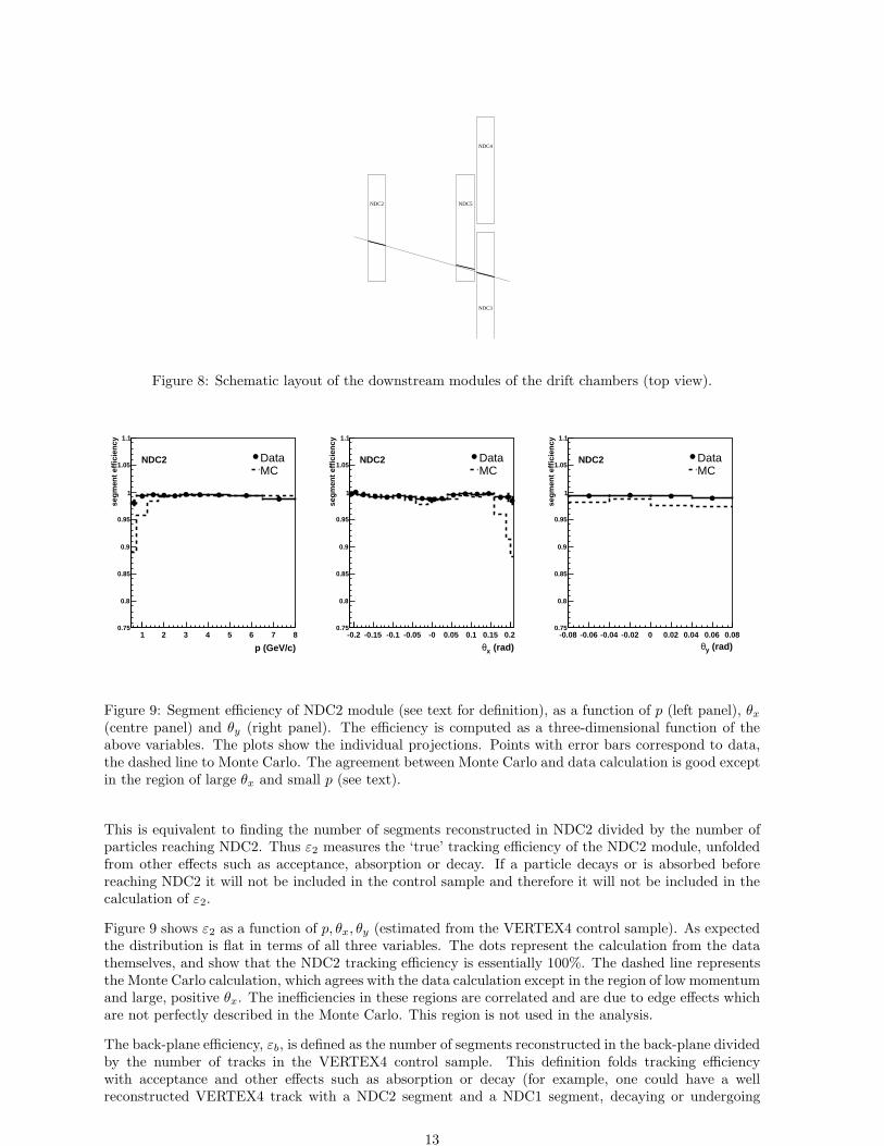
Figure 8: Schematic layout of the downstream modules of the drift chambers (top view).

p (GeV/c)1 2 3 4 5 6 7 8

seg

men

t ef

fici

ency

0.75

0.8

0.85

0.9

0.95

1

1.05

1.1

DataMC

NDC2

(rad)xθ-0.2 -0.15 -0.1 -0.05 -0 0.05 0.1 0.15 0.2

seg

men

t ef

fici

ency

0.75

0.8

0.85

0.9

0.95

1

1.05

1.1

DataMC

NDC2

(rad)yθ-0.08 -0.06 -0.04 -0.02 0 0.02 0.04 0.06 0.08

seg

men

t ef

fici

ency

0.75

0.8

0.85

0.9

0.95

1

1.05

1.1

DataMC

NDC2

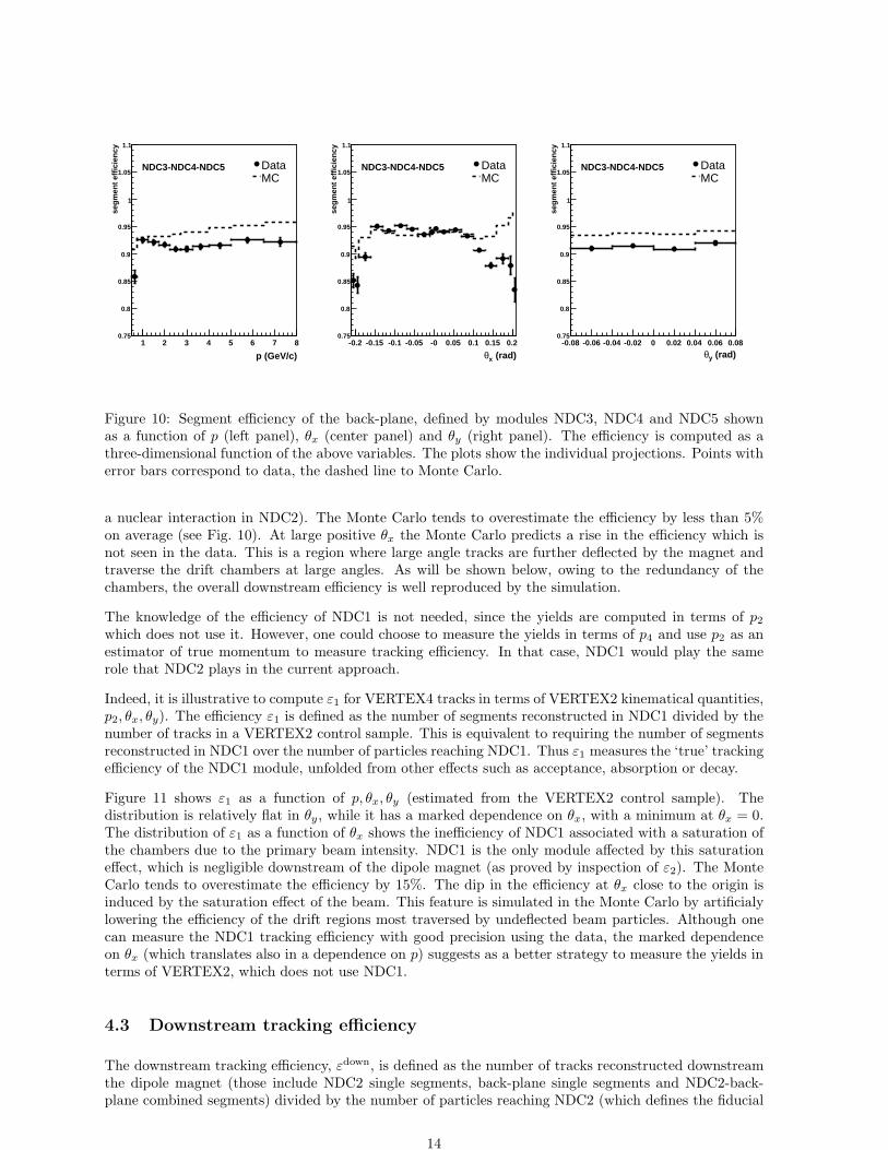
Figure 9: Segment efficiency of NDC2 module (see text for definition), as a function of p (left panel), θx

(centre panel) and θy (right panel). The efficiency is computed as a three-dimensional function of theabove variables. The plots show the individual projections. Points with error bars correspond to data,the dashed line to Monte Carlo. The agreement between Monte Carlo and data calculation is good exceptin the region of large θx and small p (see text).

This is equivalent to finding the number of segments reconstructed in NDC2 divided by the number ofparticles reaching NDC2. Thus ε2 measures the ‘true’ tracking efficiency of the NDC2 module, unfoldedfrom other effects such as acceptance, absorption or decay. If a particle decays or is absorbed beforereaching NDC2 it will not be included in the control sample and therefore it will not be included in thecalculation of ε2.

Figure 9 shows ε2 as a function of p, θx, θy (estimated from the VERTEX4 control sample). As expectedthe distribution is flat in terms of all three variables. The dots represent the calculation from the datathemselves, and show that the NDC2 tracking efficiency is essentially 100%. The dashed line representsthe Monte Carlo calculation, which agrees with the data calculation except in the region of low momentumand large, positive θx. The inefficiencies in these regions are correlated and are due to edge effects whichare not perfectly described in the Monte Carlo. This region is not used in the analysis.

The back-plane efficiency, εb, is defined as the number of segments reconstructed in the back-plane dividedby the number of tracks in the VERTEX4 control sample. This definition folds tracking efficiencywith acceptance and other effects such as absorption or decay (for example, one could have a wellreconstructed VERTEX4 track with a NDC2 segment and a NDC1 segment, decaying or undergoing

13

p (GeV/c)1 2 3 4 5 6 7 8

seg

men

t ef

fici

ency

0.75

0.8

0.85

0.9

0.95

1

1.05

1.1

DataMC

NDC3-NDC4-NDC5

(rad)xθ-0.2 -0.15 -0.1 -0.05 -0 0.05 0.1 0.15 0.2

seg

men

t ef

fici

ency

0.75

0.8

0.85

0.9

0.95

1

1.05

1.1

DataMC

NDC3-NDC4-NDC5

(rad)yθ-0.08 -0.06 -0.04 -0.02 0 0.02 0.04 0.06 0.08

seg

men

t ef

fici

ency

0.75

0.8

0.85

0.9

0.95

1

1.05

1.1

DataMC

NDC3-NDC4-NDC5

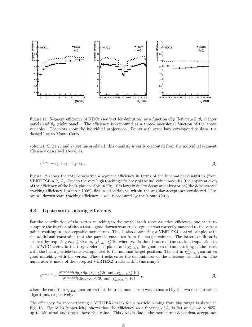
Figure 10: Segment efficiency of the back-plane, defined by modules NDC3, NDC4 and NDC5 shownas a function of p (left panel), θx (center panel) and θy (right panel). The efficiency is computed as athree-dimensional function of the above variables. The plots show the individual projections. Points witherror bars correspond to data, the dashed line to Monte Carlo.

a nuclear interaction in NDC2). The Monte Carlo tends to overestimate the efficiency by less than 5%on average (see Fig. 10). At large positive θx the Monte Carlo predicts a rise in the efficiency which isnot seen in the data. This is a region where large angle tracks are further deflected by the magnet andtraverse the drift chambers at large angles. As will be shown below, owing to the redundancy of thechambers, the overall downstream efficiency is well reproduced by the simulation.

The knowledge of the efficiency of NDC1 is not needed, since the yields are computed in terms of p2

which does not use it. However, one could choose to measure the yields in terms of p4 and use p2 as anestimator of true momentum to measure tracking efficiency. In that case, NDC1 would play the samerole that NDC2 plays in the current approach.

Indeed, it is illustrative to compute ε1 for VERTEX4 tracks in terms of VERTEX2 kinematical quantities,p2, θx, θy). The efficiency ε1 is defined as the number of segments reconstructed in NDC1 divided by thenumber of tracks in a VERTEX2 control sample. This is equivalent to requiring the number of segmentsreconstructed in NDC1 over the number of particles reaching NDC1. Thus ε1 measures the ‘true’ trackingefficiency of the NDC1 module, unfolded from other effects such as acceptance, absorption or decay.

Figure 11 shows ε1 as a function of p, θx, θy (estimated from the VERTEX2 control sample). Thedistribution is relatively flat in θy, while it has a marked dependence on θx, with a minimum at θx = 0.The distribution of ε1 as a function of θx shows the inefficiency of NDC1 associated with a saturation ofthe chambers due to the primary beam intensity. NDC1 is the only module affected by this saturationeffect, which is negligible downstream of the dipole magnet (as proved by inspection of ε2). The MonteCarlo tends to overestimate the efficiency by 15%. The dip in the efficiency at θx close to the origin isinduced by the saturation effect of the beam. This feature is simulated in the Monte Carlo by artificialylowering the efficiency of the drift regions most traversed by undeflected beam particles. Although onecan measure the NDC1 tracking efficiency with good precision using the data, the marked dependenceon θx (which translates also in a dependence on p) suggests as a better strategy to measure the yields interms of VERTEX2, which does not use NDC1.

4.3 Downstream tracking efficiency

The downstream tracking efficiency, εdown, is defined as the number of tracks reconstructed downstreamthe dipole magnet (those include NDC2 single segments, back-plane single segments and NDC2-back-plane combined segments) divided by the number of particles reaching NDC2 (which defines the fiducial

14

p (GeV/c)1 2 3 4 5 6 7 8

seg

men

t ef

fici

ency

0.3

0.4

0.5

0.6

0.7

0.8

0.9

1

1.1

DataMC

NDC1

(rad)xθ-0.2 -0.15 -0.1 -0.05 -0 0.05 0.1 0.15 0.2

seg

men

t ef

fici

ency

0.3

0.4

0.5

0.6

0.7

0.8

0.9

1

1.1

DataMC

NDC1

(rad)yθ-0.08 -0.06 -0.04 -0.02 0 0.02 0.04 0.06 0.08

seg

men

t ef

fici

ency

0.3

0.4

0.5

0.6

0.7

0.8

0.9

1

1.1

DataMC

NDC1

Figure 11: Segment efficiency of NDC1 (see text for definition) as a function of p (left panel), θx (centerpanel) and θy (right panel). The efficiency is computed as a three-dimensional function of the abovevariables. The plots show the individual projections. Points with error bars correspond to data, thedashed line to Monte Carlo.

volume). Since ε2 and εb are uncorrelated, this quantity is easily computed from the individual segmentefficiency described above, as:

εdown = ε2 + εb − ε2 · εb . (2)

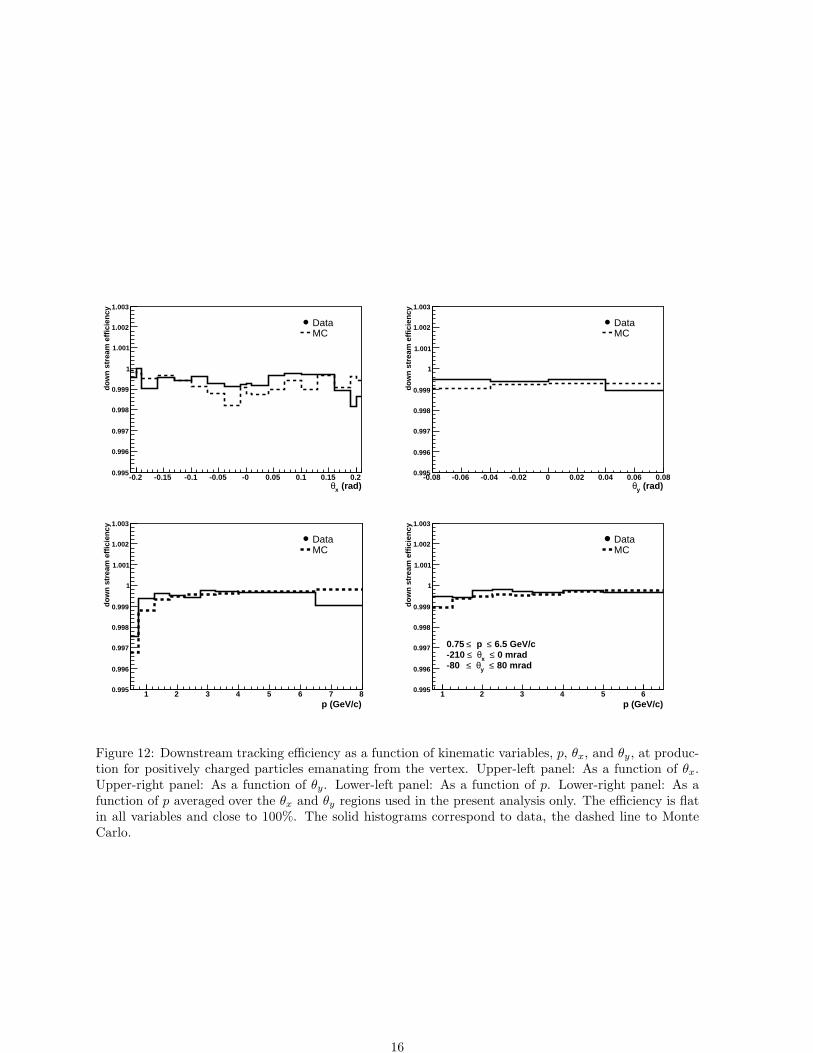
Figure 12 shows the total downstream segment efficiency in terms of the kinematical quantities (fromVERTEX4) p, θx, θy. Due to the very high tracking efficiency of the individual modules (the apparent dropof the efficiency of the back-plane visible in Fig. 10 is largely due to decay and absorption) the downstreamtracking efficiency is almost 100%, flat in all variables, within the angular acceptance considered. Theoverall downstream tracking efficiency is well reproduced by the Monte Carlo.

4.4 Upstream tracking efficiency

For the contribution of the vertex matching to the overall track reconstruction efficiency, one needs tocompute the fraction of times that a good downstream track segment was correctly matched to the vertexpoint resulting in an acceptable momentum. This is also done using a VERTEX4 control sample, withthe additional constraint that the particle emanates from the target volume. The latter condition isensured by requiring rV4 ≤ 30 mm, χ2

match ≤ 10, where rV4 is the distance of the track extrapolation tothe MWPC vertex in the target reference plane, and χ2

match the goodness of the matching of the trackwith the beam particle track extrapolated to the nominal target position. The cut in χ2

match guaranteesgood matching with the vertex. These tracks enter the denominator of the efficiency calculation. Thenumerator is made of the accepted VERTEX2 tracks within this sample:

εvertex2 =Nvertex2(∃p2; ∃p4, rV4 ≤ 30 mm, χ2

match ≤ 10)

Nvertex4(∃p4, rV4 ≤ 30 mm, χ2match ≤ 10)

, (3)

where the condition ∃p4(2) guarantees that the track momentum was estimated by the two reconstructionalgorithms, respectively.

The efficiency for reconstructing a VERTEX2 track for a particle coming from the target is shown inFig. 13. Figure 13 (upper-left), shows that the efficiency as a function of θx is flat and close to 95%,up to 150 mrad and drops above this value. This drop is due a the momentum-dependent acceptance

15

(rad)xθ-0.2 -0.15 -0.1 -0.05 -0 0.05 0.1 0.15 0.2

do

wn

str

eam

eff

icie

ncy

0.995

0.996

0.997

0.998

0.999

1

1.001

1.002

1.003

DataMC

(rad)yθ-0.08 -0.06 -0.04 -0.02 0 0.02 0.04 0.06 0.08

do

wn

str

eam

eff

icie

ncy

0.995

0.996

0.997

0.998

0.999

1

1.001

1.002

1.003

DataMC

p (GeV/c)1 2 3 4 5 6 7 8

do

wn

str

eam

eff

icie

ncy

0.995

0.996

0.997

0.998

0.999

1

1.001

1.002

1.003

DataMC

p (GeV/c)1 2 3 4 5 6

do

wn

str

eam

eff

icie

ncy

0.995

0.996

0.997

0.998

0.999

1

1.001

1.002

1.003

DataMC

6.5 GeV/c≤ p ≤0.75 0 mrad≤ xθ ≤-210 80 mrad≤ yθ ≤-80

Figure 12: Downstream tracking efficiency as a function of kinematic variables, p, θx, and θy, at produc-tion for positively charged particles emanating from the vertex. Upper-left panel: As a function of θx.Upper-right panel: As a function of θy. Lower-left panel: As a function of p. Lower-right panel: As afunction of p averaged over the θx and θy regions used in the present analysis only. The efficiency is flatin all variables and close to 100%. The solid histograms correspond to data, the dashed line to MonteCarlo.

16

(rad)xθ-0.2 -0.15 -0.1 -0.05 -0 0.05 0.1 0.15 0.2

trac

kin

g e

ffic

ien

cy

0

0.2

0.4

0.6

0.8

1

1.2 DataMC

(rad)yθ-0.08 -0.06 -0.04 -0.02 0 0.02 0.04 0.06 0.08

trac

kin

g e

ffic

ien

cy

0

0.2

0.4

0.6

0.8

1

1.2 DataMC

p (GeV/c)1 2 3 4 5 6 7 8

trac

kin

g e

ffic

ien

cy

0

0.2

0.4

0.6

0.8

1

1.2 DataMC

p (GeV/c)1 2 3 4 5 6

trac

kin

g e

ffic

ien

cy

0

0.2

0.4

0.6

0.8

1

1.2 DataMC

6.5 GeV/c≤ p ≤0.75 0 mrad≤ xθ ≤-210 80 mrad≤ yθ ≤-80

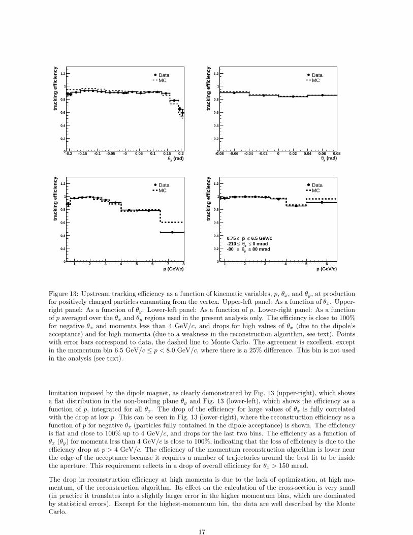
Figure 13: Upstream tracking efficiency as a function of kinematic variables, p, θx, and θy, at productionfor positively charged particles emanating from the vertex. Upper-left panel: As a function of θx. Upper-right panel: As a function of θy. Lower-left panel: As a function of p. Lower-right panel: As a functionof p averaged over the θx and θy regions used in the present analysis only. The efficiency is close to 100%for negative θx and momenta less than 4 GeV/c, and drops for high values of θx (due to the dipole’sacceptance) and for high momenta (due to a weakness in the reconstruction algorithm, see text). Pointswith error bars correspond to data, the dashed line to Monte Carlo. The agreement is excellent, exceptin the momentum bin 6.5 GeV/c ≤ p < 8.0 GeV/c, where there is a 25% difference. This bin is not usedin the analysis (see text).

limitation imposed by the dipole magnet, as clearly demonstrated by Fig. 13 (upper-right), which showsa flat distribution in the non-bending plane θy and Fig. 13 (lower-left), which shows the efficiency as afunction of p, integrated for all θx. The drop of the efficiency for large values of θx is fully correlatedwith the drop at low p. This can be seen in Fig. 13 (lower-right), where the reconstruction efficiency as afunction of p for negative θx (particles fully contained in the dipole acceptance) is shown. The efficiencyis flat and close to 100% up to 4 GeV/c, and drops for the last two bins. The efficiency as a function ofθx (θy) for momenta less than 4 GeV/c is close to 100%, indicating that the loss of efficiency is due to theefficiency drop at p > 4 GeV/c. The efficiency of the momentum reconstruction algorithm is lower nearthe edge of the acceptance because it requires a number of trajectories around the best fit to be insidethe aperture. This requirement reflects in a drop of overall efficiency for θx > 150 mrad.

The drop in reconstruction efficiency at high momenta is due to the lack of optimization, at high mo-mentum, of the reconstruction algorithm. Its effect on the calculation of the cross-section is very small(in practice it translates into a slightly larger error in the higher momentum bins, which are dominatedby statistical errors). Except for the highest-momentum bin, the data are well described by the MonteCarlo.

17

4.5 Total reconstruction efficiency

The total tracking efficiency, εtrack, can be expressed as the product of two factors. One factor representsthe downstream (of the dipole magnet) tracking efficiency and the other represents the efficiency formatching a downstream segment to a vertex (for tracks originating inside the target volume):

εtrack =Ndown

Nparts· Nvertex2

Ndown= εdown · εvertex2 , (4)

where Nvertex2 is the number of VERTEX2 tracks, which corresponds to N track in Eq. 1. In the momentumrange of interest for this analysis, a good time-of-flight measurement is essential for particle identification.Therefore, one also requires a good TOFW hit matched to the track. In addition to selecting thescintillator slab hit by the particle, this matching consists of a cut in the matching χ2 of the track withthe TOFW hit coordinate that is measured by the time difference of the signals at the two sides of thescintillators.

The TOFW hit matching efficiency was computed using the same track sample as in the previous section:

εToF =NToF(∃ToF; ∃p4, rV4 ≤ 30 mm, χ2

match ≤ 10)

Nvertex4(∃p4, rV4 ≤ 30 mm, χ2match ≤ 10)

, (5)

where the condition ∃ToF guarantees that a TOFW hit was associated with the track, and the totalreconstruction efficiency is found from:

εrecon = εtrack · εToF . (6)

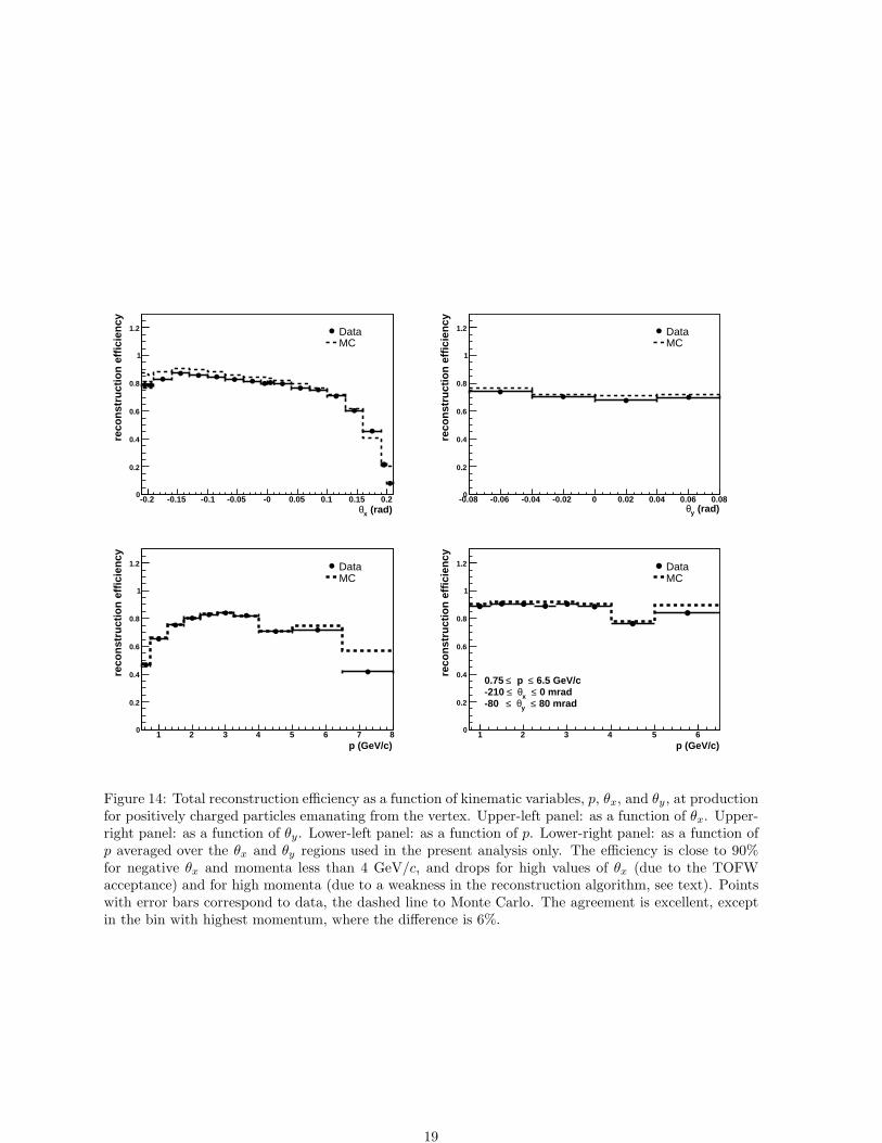
The total reconstruction efficiency is shown in Fig. 14. The inclusion of the TOF wall enhances themomentum-dependent acceptance cut (due to the fact that the TOF wall has a smaller geometricalacceptance than the NDC back-plane). The total reconstruction efficiency as a function of θx has aslight slope and drops for positive θx above 100 mrad. The total reconstruction efficiency as a functionof p for negative θx is flat (and about 90%) for momenta below 4 GeV/c. The drop to 90% is due tothe inefficiency in matching tracks to a TOFW hit. The agreement between data and Monte Carlo forthe total reconstruction efficiency is excellent, except in the last momentum bin, where there is a 25%difference, reflecting the same effect already observed in the upstream efficiency.

5 Particle identification

A set of efficient PID algorithms to select pions and reject other particles is required for the currentanalysis. A Monte Carlo prediction of the differential yields of the various particle types shows that thepion production cross-section is small above 6.5 GeV/c, which is set as the upper limit of this analysis.The electron distribution peaks at low energy, while the proton background increases with momentum.The kaon yield is expected to be only a small fraction of the pion yield. In the momentum and angularrange covered by the present measurements the proton yield is of a similar order of magnitude as thepion yield.

The PID strategy is based on the expectation of the yields of different particle types predicted by theMonte Carlo, and also on the momentum regions covered by the available PID detectors. The time-of-flight measurement with the combination of BTOF and TOFW systems (referred to as the TOFW mea-surement in what follows) allows pion–kaon and pion–proton separation to be performed up to 3 GeV/cand beyond 5 GeV/c respectively. The Cherenkov is used for hadron-electron separation below 2.5 GeV/cand pion–proton/kaon separation above 2.5 GeV/c in conjunction with the TOFW. The ECAL is usedonly to separate hadrons from electrons below 2.5 GeV/c to study the Cherenkov performance.

As mentioned above, the electron(positron) background is concentrated at low momentum (p < 2.5 GeV/c).It can be suppressed to negligible level with an upper limit on the CHE signal, given the fact that electrons

18

(rad)xθ-0.2 -0.15 -0.1 -0.05 -0 0.05 0.1 0.15 0.2

reco

nst

ruct

ion

eff

icie

ncy

0

0.2

0.4

0.6

0.8

1

1.2 DataMC

(rad)yθ-0.08 -0.06 -0.04 -0.02 0 0.02 0.04 0.06 0.08

reco

nst

ruct

ion

eff

icie

ncy

0

0.2

0.4

0.6

0.8

1

1.2 DataMC

p (GeV/c)1 2 3 4 5 6 7 8

reco

nst

ruct

ion

eff

icie

ncy

0

0.2

0.4

0.6

0.8

1

1.2 DataMC

p (GeV/c)1 2 3 4 5 6

reco

nst

ruct

ion

eff

icie

ncy

0

0.2

0.4

0.6

0.8

1

1.2 DataMC

6.5 GeV/c≤ p ≤0.75 0 mrad≤ xθ ≤-210 80 mrad≤ yθ ≤-80

Figure 14: Total reconstruction efficiency as a function of kinematic variables, p, θx, and θy, at productionfor positively charged particles emanating from the vertex. Upper-left panel: as a function of θx. Upper-right panel: as a function of θy. Lower-left panel: as a function of p. Lower-right panel: as a function ofp averaged over the θx and θy regions used in the present analysis only. The efficiency is close to 90%for negative θx and momenta less than 4 GeV/c, and drops for high values of θx (due to the TOFWacceptance) and for high momenta (due to a weakness in the reconstruction algorithm, see text). Pointswith error bars correspond to data, the dashed line to Monte Carlo. The agreement is excellent, exceptin the bin with highest momentum, where the difference is 6%.

19

are the only particles giving signal in the Cherenkov below the pion Cherenkov light emission threshold,which is equal to 2.6 GeV/c for the gas mixture used in HARP. In practice, any particle that has amomentum below 2.5 GeV/c and a signal in the CHE exceeding 15 photo-electrons is called an electron.In the following we will refer to this cut as the e-veto cut. The remaining electron background after thee-veto cut is negligible as studied in Ref. [14].

Having applied the e-veto cut to reject electrons and keeping in mind that there is a small fraction ofkaons, one builds PID estimators for protons and pions by combining the information from TOFW andCHE using likelihood techniques (Sec. 5.2). Then, a cut on these PID estimators is applied to selectpions or protons. The selected samples (raw pion and proton samples) will contain a small fraction ofkaons, which can be estimated from the data, as described in Ref. [14]. This background is subtractedfrom the dominant yields of pions and protons.

The quantities that enter the cross-section calculation are the raw pion and proton yields and the PIDefficiencies and purities (PID corrections) obtained by the application of the e-veto cut and cuts in thePID estimators. The PID corrections include the e-veto efficiencies, the kaon subtraction corrections andthe pion-proton efficiency matrix (M id, described in Sec. 6.4). A precise knowledge of these quantities(as a function of momentum and angle) requires the understanding of the responses of different PIDdetectors to the particle types considered. This is studied in detail using the data, taking advantage ofthe redundancy between the PID detectors.

These steps are explained briefly in the following sections. More details are given in Ref. [14].

5.1 Response of the PID detectors

The TOFW–CHE Probability Density Function (PDF), P (β, Nphe|i, p, θ), describes the probability thata particle of type i (pion or proton) with momentum p and polar angle θ results in simultaneous measure-ments β in TOFW and Nphe in CHE. The latter comes directly from the calibrated CHE signal, while β isthe particle velocity, computed as β = ltof/(ttof ·c), where ltof is the track length measured from the nomi-nal vertex position to the TOFW hit position, ttof is the measured time-of-flight and c is the speed of light.Assuming that the PID from both detectors are independent1 the TOFW–CHE PDFs can be factorizedin independent TOFW and CHE PDFs, such that P (β, Nphe|i, p, θ) = P (β|i, p, θ) · P (Nphe|i, p, θ).

5.1.1 TOFW response

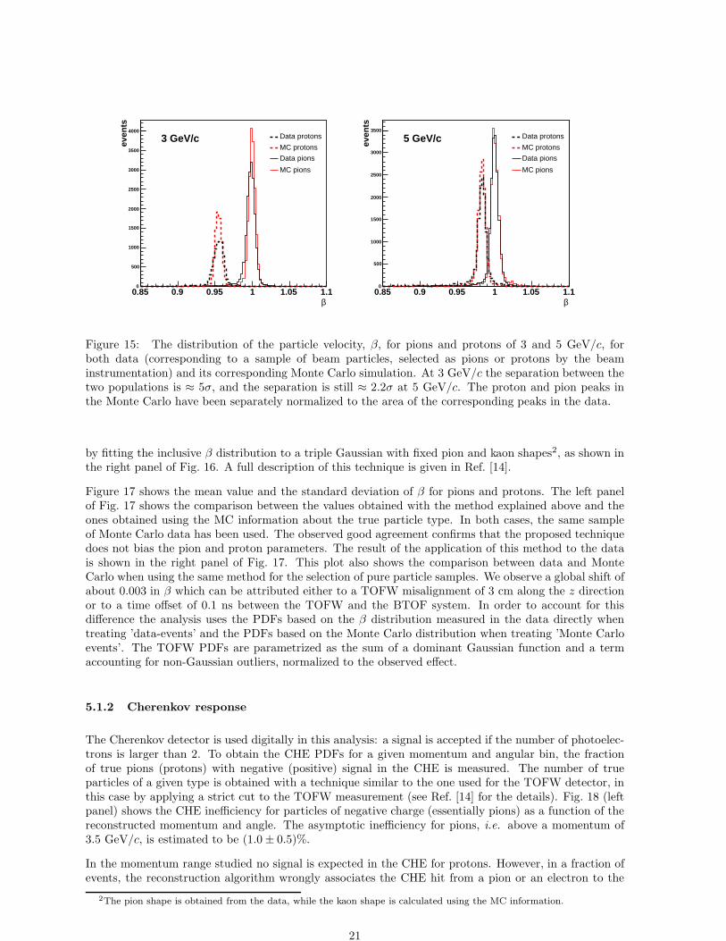
The use of the particle velocity, β, to characterize the TOFW response has several advantages. Itsdistribution is nearly Gaussian–the agreement between data and Monte Carlo is sufficient for the currentanalysis–and it discriminates very effectively between pions and protons up to momenta around 5 GeV/c(at this energy the separation between the average values of the proton and pion Gaussians is around2.2σ). These points are illustrated in Fig. 15.

To build the TOFW PDFs one should know the β distribution of pions and protons as a function of theparticle momentum and angle. In order to maximize the efficiency of the selection algorithm and to avoidany possible bias in the PID corrections related with a data–MC disagreement, those distributions havebeen measured from the data. This requires the ability to select pure and unbiased samples of pions andprotons from the data. Samples of pions with negligible contamination from other species can be obtainedselecting particles of negative charge passing the e-veto cut (Fig. 16, left panel). At low momentum, theproton parameters can be obtained by simply fitting to a Gaussian the proton part of the β distribution,since this is well separated from pions (Fig. 16, central panel). At large momentum (> 2.5 GeV/c), theproton and pion distributions overlap significantly. In this case, pions are rejected to the 1% level by acut on the CHE signal (Sec. 5.1.2). The resulting sample contains a majority of protons and residualcontaminations from pions and kaons. In this momentum range the proton parameters can be obtained

1The use of the reconstructed momentum instead of the true momentum in the probability density functionP (β, Nphe|i, p, θ) introduces a small correlation between TOFW and CHE. However, the good momentum resolution ofthe forward spectrometer (σp/p < 10%) makes this correlation very small. At the level of precision required by this analysisthis effect can be neglected.

20

β0.85 0.9 0.95 1 1.05 1.1

even

ts

0

500

1000

1500

2000

2500

3000

3500

4000Data protons

MC protons

Data pions

MC pions

3 GeV/c

β0.85 0.9 0.95 1 1.05 1.1

even

ts

0

500

1000

1500

2000

2500

3000

3500Data protons

MC protons

Data pions

MC pions

5 GeV/c

Figure 15: The distribution of the particle velocity, β, for pions and protons of 3 and 5 GeV/c, forboth data (corresponding to a sample of beam particles, selected as pions or protons by the beaminstrumentation) and its corresponding Monte Carlo simulation. At 3 GeV/c the separation between thetwo populations is ≈ 5σ, and the separation is still ≈ 2.2σ at 5 GeV/c. The proton and pion peaks inthe Monte Carlo have been separately normalized to the area of the corresponding peaks in the data.

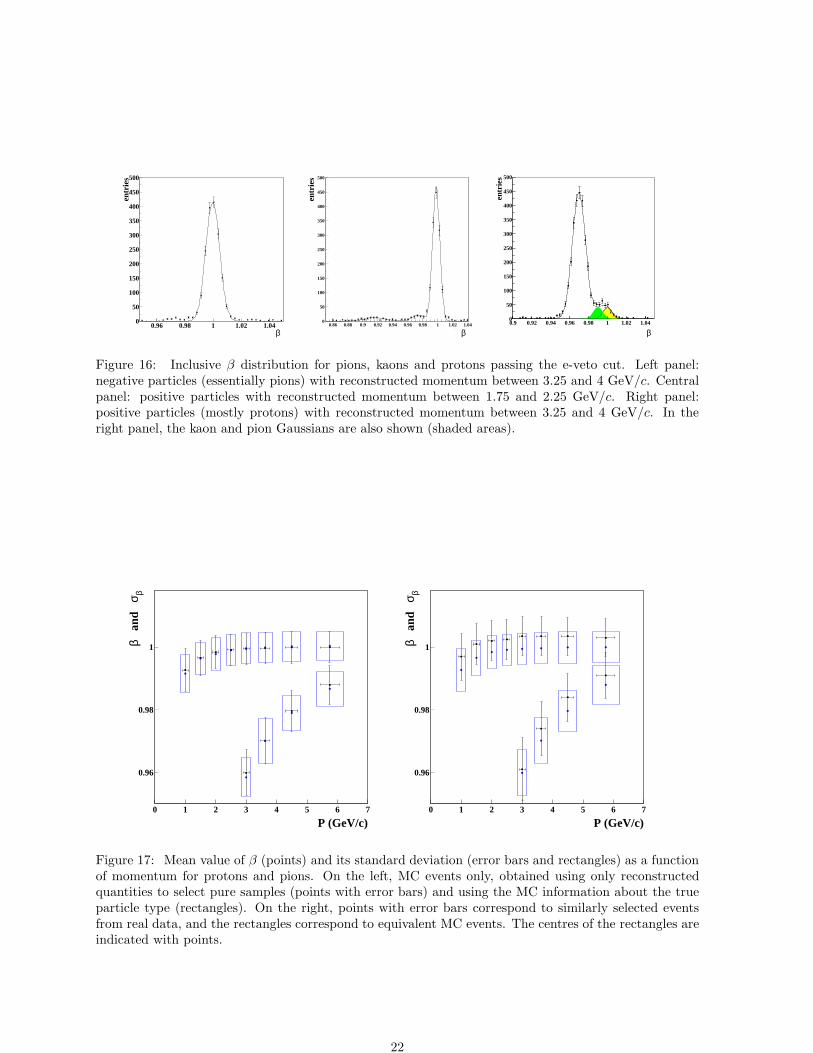
by fitting the inclusive β distribution to a triple Gaussian with fixed pion and kaon shapes2, as shown inthe right panel of Fig. 16. A full description of this technique is given in Ref. [14].

Figure 17 shows the mean value and the standard deviation of β for pions and protons. The left panelof Fig. 17 shows the comparison between the values obtained with the method explained above and theones obtained using the MC information about the true particle type. In both cases, the same sampleof Monte Carlo data has been used. The observed good agreement confirms that the proposed techniquedoes not bias the pion and proton parameters. The result of the application of this method to the datais shown in the right panel of Fig. 17. This plot also shows the comparison between data and MonteCarlo when using the same method for the selection of pure particle samples. We observe a global shift ofabout 0.003 in β which can be attributed either to a TOFW misalignment of 3 cm along the z directionor to a time offset of 0.1 ns between the TOFW and the BTOF system. In order to account for thisdifference the analysis uses the PDFs based on the β distribution measured in the data directly whentreating ’data-events’ and the PDFs based on the Monte Carlo distribution when treating ’Monte Carloevents’. The TOFW PDFs are parametrized as the sum of a dominant Gaussian function and a termaccounting for non-Gaussian outliers, normalized to the observed effect.

5.1.2 Cherenkov response

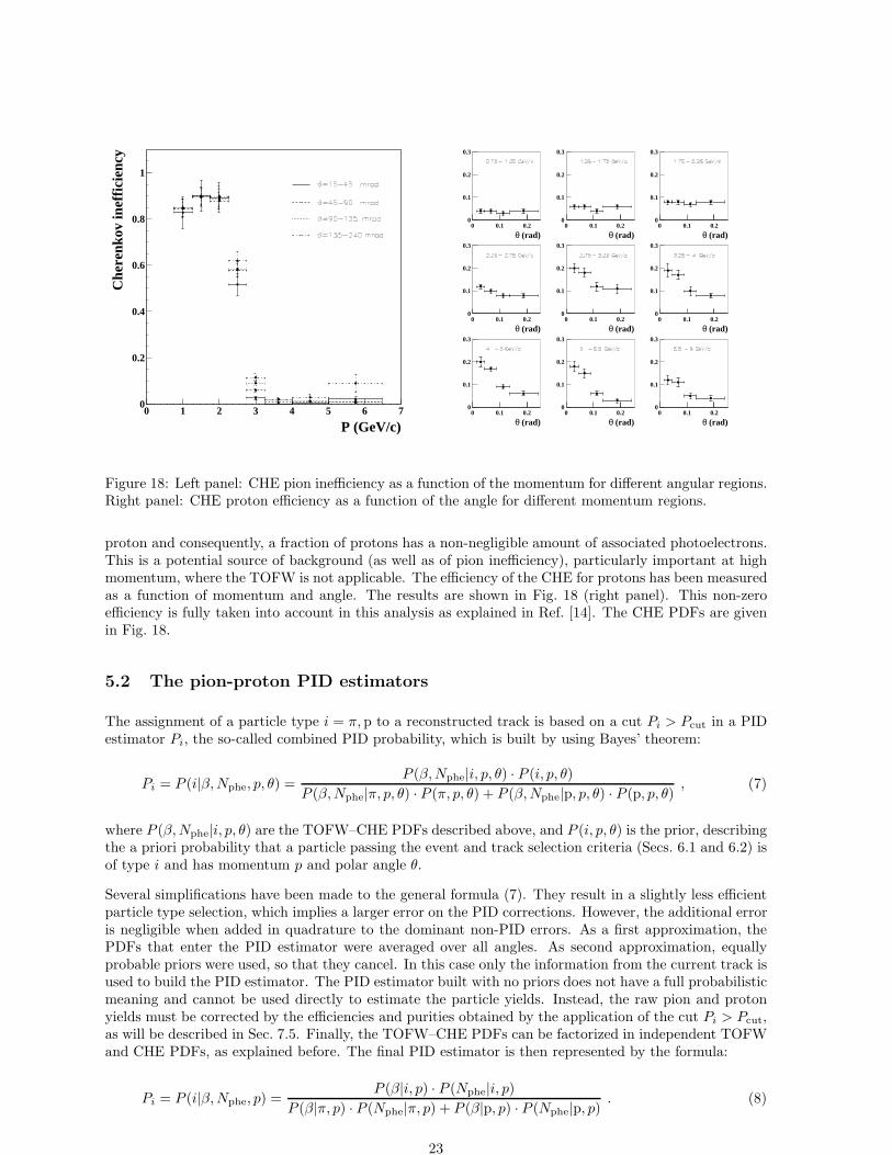
The Cherenkov detector is used digitally in this analysis: a signal is accepted if the number of photoelec-trons is larger than 2. To obtain the CHE PDFs for a given momentum and angular bin, the fractionof true pions (protons) with negative (positive) signal in the CHE is measured. The number of trueparticles of a given type is obtained with a technique similar to the one used for the TOFW detector, inthis case by applying a strict cut to the TOFW measurement (see Ref. [14] for the details). Fig. 18 (leftpanel) shows the CHE inefficiency for particles of negative charge (essentially pions) as a function of thereconstructed momentum and angle. The asymptotic inefficiency for pions, i.e. above a momentum of3.5 GeV/c, is estimated to be (1.0 ± 0.5)%.

In the momentum range studied no signal is expected in the CHE for protons. However, in a fraction ofevents, the reconstruction algorithm wrongly associates the CHE hit from a pion or an electron to the

2The pion shape is obtained from the data, while the kaon shape is calculated using the MC information.

21

0

50

100

150

200

250

300

350

400

450

500

0.96 0.98 1 1.02 1.04beta

entr

ies

β0

50

100

150

200

250

300

350

400

450

500

0.86 0.88 0.9 0.92 0.94 0.96 0.98 1 1.02 1.04

beta

entr

ies

β

0

50

100

150

200

250

300

350

400

450

500

0.9 0.92 0.94 0.96 0.98 1 1.02 1.04

beta

entr

ies

β

Figure 16: Inclusive β distribution for pions, kaons and protons passing the e-veto cut. Left panel:negative particles (essentially pions) with reconstructed momentum between 3.25 and 4 GeV/c. Centralpanel: positive particles with reconstructed momentum between 1.75 and 2.25 GeV/c. Right panel:positive particles (mostly protons) with reconstructed momentum between 3.25 and 4 GeV/c. In theright panel, the kaon and pion Gaussians are also shown (shaded areas).

0.96

0.98

1

0 1 2 3 4 5 6 7

P (GeV/c)

β a

nd

σ β

0.96

0.98

1

0 1 2 3 4 5 6 7

P (GeV/c)

β a

nd

σ β

Figure 17: Mean value of β (points) and its standard deviation (error bars and rectangles) as a functionof momentum for protons and pions. On the left, MC events only, obtained using only reconstructedquantities to select pure samples (points with error bars) and using the MC information about the trueparticle type (rectangles). On the right, points with error bars correspond to similarly selected eventsfrom real data, and the rectangles correspond to equivalent MC events. The centres of the rectangles areindicated with points.

22

0

0.2

0.4

0.6

0.8

1

0 1 2 3 4 5 6 7

P (GeV/c)

Che

renk

ov in

effi

cien

cy

0

0.1

0.2

0.3

0 0.1 0.2

θ (rad)

0

0.1

0.2

0.3

0 0.1 0.2

θ (rad)

0

0.1

0.2

0.3

0 0.1 0.2

θ (rad)

0

0.1

0.2

0.3

0 0.1 0.2

θ (rad)

0

0.1

0.2

0.3

0 0.1 0.2

θ (rad)

0

0.1

0.2

0.3

0 0.1 0.2

θ (rad)

0

0.1

0.2

0.3

0 0.1 0.2

θ (rad)

0

0.1

0.2

0.3

0 0.1 0.2

θ (rad)

0

0.1

0.2

0.3

0 0.1 0.2

θ (rad)

Figure 18: Left panel: CHE pion inefficiency as a function of the momentum for different angular regions.Right panel: CHE proton efficiency as a function of the angle for different momentum regions.

proton and consequently, a fraction of protons has a non-negligible amount of associated photoelectrons.This is a potential source of background (as well as of pion inefficiency), particularly important at highmomentum, where the TOFW is not applicable. The efficiency of the CHE for protons has been measuredas a function of momentum and angle. The results are shown in Fig. 18 (right panel). This non-zeroefficiency is fully taken into account in this analysis as explained in Ref. [14]. The CHE PDFs are givenin Fig. 18.

5.2 The pion-proton PID estimators

The assignment of a particle type i = π, p to a reconstructed track is based on a cut Pi > Pcut in a PIDestimator Pi, the so-called combined PID probability, which is built by using Bayes’ theorem:

Pi = P (i|β, Nphe, p, θ) =P (β, Nphe|i, p, θ) · P (i, p, θ)

P (β, Nphe|π, p, θ) · P (π, p, θ) + P (β, Nphe|p, p, θ) · P (p, p, θ), (7)

where P (β, Nphe|i, p, θ) are the TOFW–CHE PDFs described above, and P (i, p, θ) is the prior, describingthe a priori probability that a particle passing the event and track selection criteria (Secs. 6.1 and 6.2) isof type i and has momentum p and polar angle θ.

Several simplifications have been made to the general formula (7). They result in a slightly less efficientparticle type selection, which implies a larger error on the PID corrections. However, the additional erroris negligible when added in quadrature to the dominant non-PID errors. As a first approximation, thePDFs that enter the PID estimator were averaged over all angles. As second approximation, equallyprobable priors were used, so that they cancel. In this case only the information from the current track isused to build the PID estimator. The PID estimator built with no priors does not have a full probabilisticmeaning and cannot be used directly to estimate the particle yields. Instead, the raw pion and protonyields must be corrected by the efficiencies and purities obtained by the application of the cut Pi > Pcut,as will be described in Sec. 7.5. Finally, the TOFW–CHE PDFs can be factorized in independent TOFWand CHE PDFs, as explained before. The final PID estimator is then represented by the formula:

Pi = P (i|β, Nphe, p) =P (β|i, p) · P (Nphe|i, p)

P (β|π, p) · P (Nphe|π, p) + P (β|p, p) · P (Nphe|p, p). (8)

23

6 Calculation of the cross-section

The double-differential cross-section for the production of a particle of type α can be expressed in thelaboratory system as:

d2σα

dpidθj

=1

Npot

A

NAρtM−1

ijαi′j′α′ · Nα′

i′j′ , (9)

where d2σα

dpidθjis expressed in bins of true momentum (pi), angle (θj) and particle type (α), and the terms

on the right-hand side of the equation are:

• Nα′

i′j′ is the number of particles of observed type α′ in bins of reconstructed momentum (pi′ ) andangle (θj′ ). These particles must satisfy the event, track and PID selection criteria, explained below.This is the so called ‘raw yield’.

• M−1ijαi′j′α′ is a correction matrix which corrects for finite efficiency and resolution of the detector. It

unfolds the true variables ijα from the reconstructed variables i′j′α′ and corrects the observed num-ber of particles to take into account effects such as reconstruction efficiency, acceptance, absorption,pion decay, tertiary production, PID efficiency and PID misidentification rate.

• ANAρt

is the inverse of the number of target nuclei per unit area (A is the atomic mass, NA is the

Avogadro number, ρ and t are the target density and thickness).

• Npot is the number of incident protons on target.

The summation over reconstructed indices i′j′α′ is implied in the equation. It should be noted that theexperimental procedure bins the result initially in terms of the angular variable θ, while the final resultwill be expressed in terms of the solid angle Ω. Since the background from misidentified protons in thepion sample is not negligible, the pion and proton raw yields (Nα′

i′j′ , for α′ = π, p) have to be measuredsimultaneously.

For practical reasons, the background due to interactions of the primary proton outside the target (called‘Empty target background’) has been taken out of the correction matrix M−1. Instead, a subtractionterm is introduced in Eq. 9:

d2σα

dpidθj

=1

Npot

A

NAρtM−1

ijαi′j′α′ ·[

Nα′

i′j′(T) − Nα′

i′j′(E)]

, (10)

where (T) refers to the data taken with the aluminium target and (E) refers to the data taken with notarget (Empty target).

The event, track and particle identification selection criteria will be described first, then the method usedto obtain the cross-section and each of the corrections will be described in more detail.

6.1 Event Selection

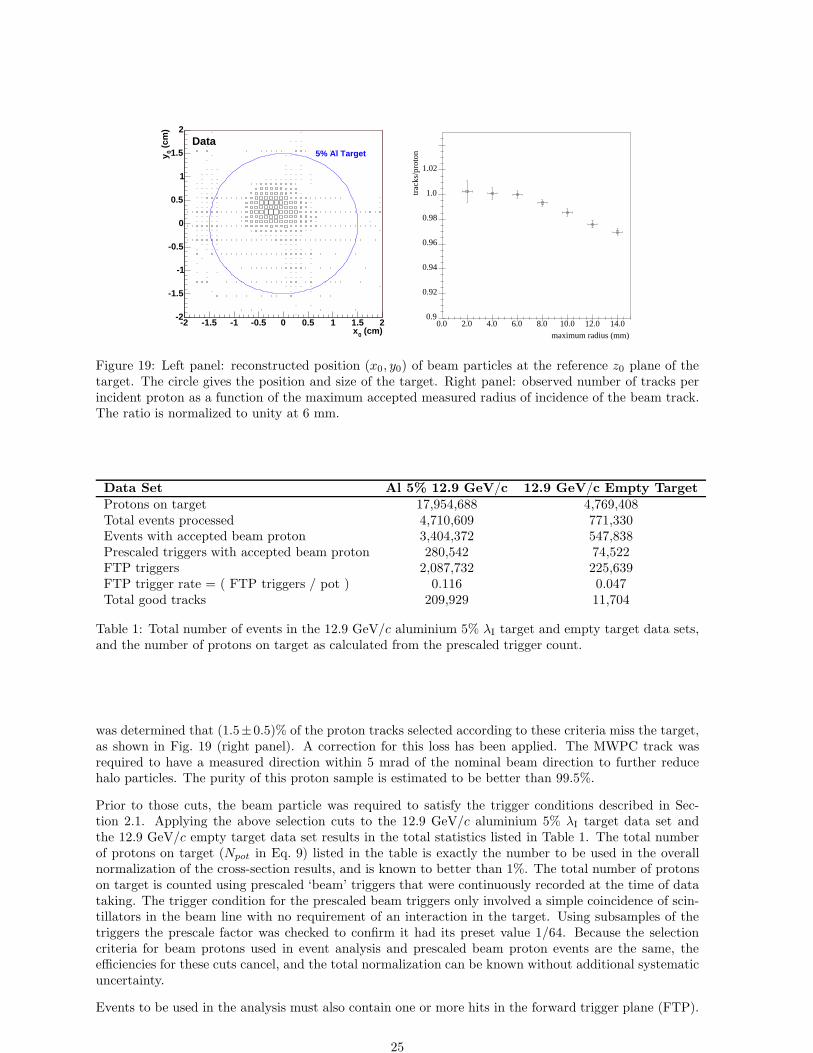
In the 12.9 GeV/c beam protons are selected by vetoing particles which give a signal in any of the beamCherenkov detectors. Only particles which give a good timing signal in all three beam timing detectors,leave a single track in the MWPCs, and are not seen in the halo detectors are accepted. A good timingmeasurement is defined as a set of three hits, one in each of the timing detectors, with their relative timedifference consistent with a beam particle. The distribution of the position of beam particles extrapolatedto the target is shown in Fig. 19 (left panel). The size of the target is indicated by a circle. Only particlesextrapolated within a radius of 10 mm are accepted. By evaluating the number of tracks reconstructedin the spectrometer as a function of the extrapolated impact point of the MWPC track to the target, it

24

(cm)0x-2 -1.5 -1 -0.5 0 0.5 1 1.5 2

(cm

)0y

-2

-1.5

-1

-0.5

0

0.5

1

1.5

2Target Position

Data5% Al Target

maximum radius (mm)

14.012.010.08.06.04.02.00.00.9

0.92

0.94

0.96

0.98

1.0

1.02

trac

ks/p

roto

n

Figure 19: Left panel: reconstructed position (x0, y0) of beam particles at the reference z0 plane of thetarget. The circle gives the position and size of the target. Right panel: observed number of tracks perincident proton as a function of the maximum accepted measured radius of incidence of the beam track.The ratio is normalized to unity at 6 mm.

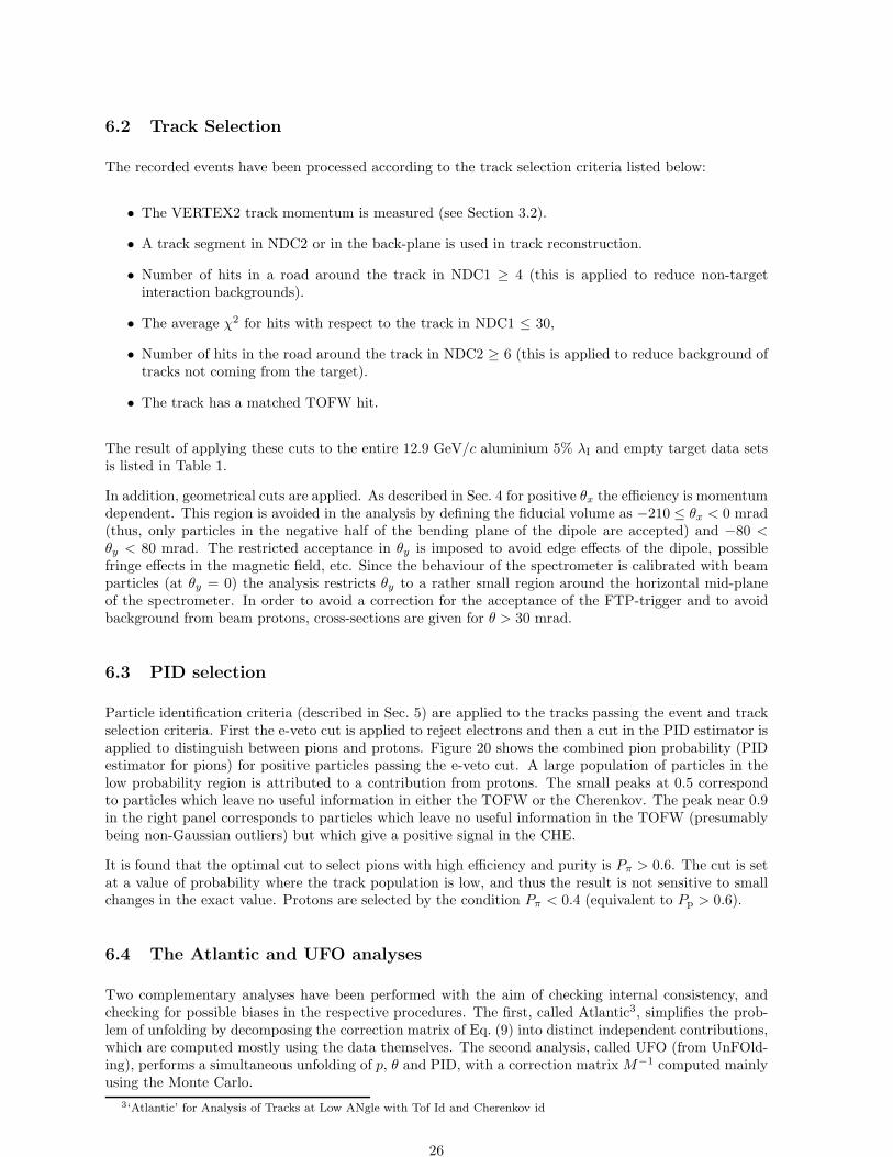
Data Set Al 5% 12.9 GeV/c 12.9 GeV/c Empty Target

Protons on target 17,954,688 4,769,408Total events processed 4,710,609 771,330Events with accepted beam proton 3,404,372 547,838Prescaled triggers with accepted beam proton 280,542 74,522FTP triggers 2,087,732 225,639FTP trigger rate = ( FTP triggers / pot ) 0.116 0.047Total good tracks 209,929 11,704

Table 1: Total number of events in the 12.9 GeV/c aluminium 5% λI target and empty target data sets,and the number of protons on target as calculated from the prescaled trigger count.

was determined that (1.5±0.5)% of the proton tracks selected according to these criteria miss the target,as shown in Fig. 19 (right panel). A correction for this loss has been applied. The MWPC track wasrequired to have a measured direction within 5 mrad of the nominal beam direction to further reducehalo particles. The purity of this proton sample is estimated to be better than 99.5%.

Prior to those cuts, the beam particle was required to satisfy the trigger conditions described in Sec-tion 2.1. Applying the above selection cuts to the 12.9 GeV/c aluminium 5% λI target data set andthe 12.9 GeV/c empty target data set results in the total statistics listed in Table 1. The total numberof protons on target (Npot in Eq. 9) listed in the table is exactly the number to be used in the overallnormalization of the cross-section results, and is known to better than 1%. The total number of protonson target is counted using prescaled ‘beam’ triggers that were continuously recorded at the time of datataking. The trigger condition for the prescaled beam triggers only involved a simple coincidence of scin-tillators in the beam line with no requirement of an interaction in the target. Using subsamples of thetriggers the prescale factor was checked to confirm it had its preset value 1/64. Because the selectioncriteria for beam protons used in event analysis and prescaled beam proton events are the same, theefficiencies for these cuts cancel, and the total normalization can be known without additional systematicuncertainty.

Events to be used in the analysis must also contain one or more hits in the forward trigger plane (FTP).

25

6.2 Track Selection

The recorded events have been processed according to the track selection criteria listed below:

• The VERTEX2 track momentum is measured (see Section 3.2).

• A track segment in NDC2 or in the back-plane is used in track reconstruction.

• Number of hits in a road around the track in NDC1 ≥ 4 (this is applied to reduce non-targetinteraction backgrounds).

• The average χ2 for hits with respect to the track in NDC1 ≤ 30,

• Number of hits in the road around the track in NDC2 ≥ 6 (this is applied to reduce background oftracks not coming from the target).

• The track has a matched TOFW hit.

The result of applying these cuts to the entire 12.9 GeV/c aluminium 5% λI and empty target data setsis listed in Table 1.

In addition, geometrical cuts are applied. As described in Sec. 4 for positive θx the efficiency is momentumdependent. This region is avoided in the analysis by defining the fiducial volume as −210 ≤ θx < 0 mrad(thus, only particles in the negative half of the bending plane of the dipole are accepted) and −80 <θy < 80 mrad. The restricted acceptance in θy is imposed to avoid edge effects of the dipole, possiblefringe effects in the magnetic field, etc. Since the behaviour of the spectrometer is calibrated with beamparticles (at θy = 0) the analysis restricts θy to a rather small region around the horizontal mid-planeof the spectrometer. In order to avoid a correction for the acceptance of the FTP-trigger and to avoidbackground from beam protons, cross-sections are given for θ > 30 mrad.

6.3 PID selection

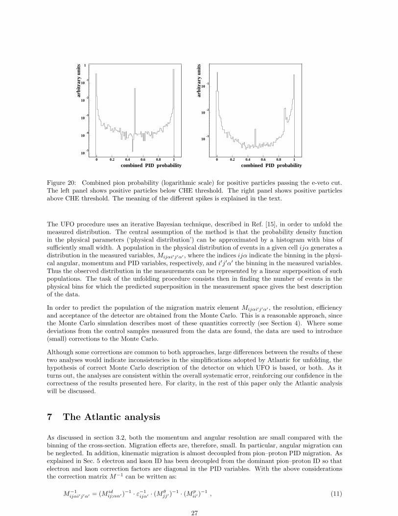
Particle identification criteria (described in Sec. 5) are applied to the tracks passing the event and trackselection criteria. First the e-veto cut is applied to reject electrons and then a cut in the PID estimator isapplied to distinguish between pions and protons. Figure 20 shows the combined pion probability (PIDestimator for pions) for positive particles passing the e-veto cut. A large population of particles in thelow probability region is attributed to a contribution from protons. The small peaks at 0.5 correspondto particles which leave no useful information in either the TOFW or the Cherenkov. The peak near 0.9in the right panel corresponds to particles which leave no useful information in the TOFW (presumablybeing non-Gaussian outliers) but which give a positive signal in the CHE.

It is found that the optimal cut to select pions with high efficiency and purity is Pπ > 0.6. The cut is setat a value of probability where the track population is low, and thus the result is not sensitive to smallchanges in the exact value. Protons are selected by the condition Pπ < 0.4 (equivalent to Pp > 0.6).

6.4 The Atlantic and UFO analyses

Two complementary analyses have been performed with the aim of checking internal consistency, andchecking for possible biases in the respective procedures. The first, called Atlantic3, simplifies the prob-lem of unfolding by decomposing the correction matrix of Eq. (9) into distinct independent contributions,which are computed mostly using the data themselves. The second analysis, called UFO (from UnFOld-ing), performs a simultaneous unfolding of p, θ and PID, with a correction matrix M−1 computed mainlyusing the Monte Carlo.

3‘Atlantic’ for Analysis of Tracks at Low ANgle with Tof Id and Cherenkov id

26

10-5

10-4

10-3

10-2

10-1

1

0 0.2 0.4 0.6 0.8 1

combined PID probability

arbi

trar

y un

its

10-3

10-2

10-1

0 0.2 0.4 0.6 0.8 1

combined PID probability

arbi

trar

y un

its

Figure 20: Combined pion probability (logarithmic scale) for positive particles passing the e-veto cut.The left panel shows positive particles below CHE threshold. The right panel shows positive particlesabove CHE threshold. The meaning of the different spikes is explained in the text.

The UFO procedure uses an iterative Bayesian technique, described in Ref. [15], in order to unfold themeasured distribution. The central assumption of the method is that the probability density functionin the physical parameters (‘physical distribution’) can be approximated by a histogram with bins ofsufficiently small width. A population in the physical distribution of events in a given cell ijα generates adistribution in the measured variables, Mijαi′j′α′ , where the indices ijα indicate the binning in the physi-cal angular, momentum and PID variables, respectively, and i′j′α′ the binning in the measured variables.Thus the observed distribution in the measurements can be represented by a linear superposition of suchpopulations. The task of the unfolding procedure consists then in finding the number of events in thephysical bins for which the predicted superposition in the measurement space gives the best descriptionof the data.

In order to predict the population of the migration matrix element Mijαi′j′α′ , the resolution, efficiencyand acceptance of the detector are obtained from the Monte Carlo. This is a reasonable approach, sincethe Monte Carlo simulation describes most of these quantities correctly (see Section 4). Where somedeviations from the control samples measured from the data are found, the data are used to introduce(small) corrections to the Monte Carlo.

Although some corrections are common to both approaches, large differences between the results of thesetwo analyses would indicate inconsistencies in the simplifications adopted by Atlantic for unfolding, thehypothesis of correct Monte Carlo description of the detector on which UFO is based, or both. As itturns out, the analyses are consistent within the overall systematic error, reinforcing our confidence in thecorrectness of the results presented here. For clarity, in the rest of this paper only the Atlantic analysiswill be discussed.

7 The Atlantic analysis

As discussed in section 3.2, both the momentum and angular resolution are small compared with thebinning of the cross-section. Migration effects are, therefore, small. In particular, angular migration canbe neglected. In addition, kinematic migration is almost decoupled from pion–proton PID migration. Asexplained in Sec. 5 electron and kaon ID has been decoupled from the dominant pion–proton ID so thatelectron and kaon correction factors are diagonal in the PID variables. With the above considerationsthe correction matrix M−1 can be written as:

M−1ijαi′j′α′ = (M id

ij;αα′ )−1 · ε−1ijα′ · (Mθ

jj′ )−1 · (Mp

ii′)−1 , (11)

27

where again reconstructed indices are indicated with a prime. The corrections are applied in the orderfrom right to left as they appear in the equation. The symbols in Eq. (11) have the following meaning:

ε−1ijα′ is the collection of factors applying the corrections that are diagonal in the PID indices:

reconstruction efficiency, acceptance, physical loss of particles (absorption, decay), backgroundfrom tertiary interactions, e-veto efficiency and kaon subtraction;

(Mpii′)

−1 is the simplified unfolding matrix correcting for the momentum smearing which onlydepends of the indices i and i′ representing the true and reconstructed momentum bins, respectively;

(Mθjj′ )

−1 is the identity matrix, representing the assumption that the smearing effect in the angularmeasurement is negligible; and

(M idij;αα′)−1 is the matrix which corrects for pion–proton PID inefficiency and migration, which is

diagonal in i, i′ and j, j′, but built of two–by–two sub-matrices, each different and non-diagonal inthe PID variables α, α′.

The diagonal efficiency correction

ε−1ijα′ = wrecon

ij · waccij · wabsorption

ijα′ · wtertiariesijα′ · ηK

ijα′ · ηeijα′ (12)

is composed of the following factors:

wreconij the correction for the overall reconstruction efficiency;

waccij the correction for the acceptance;

wabsorptionijα′ the correction for the loss of particles due to absorption and decay;

wtertiariesijα′ the correction for the background of tertiary particles generated by the secondaries pro-

duced in the target;

ηKijα′ is the factor correcting for the kaon background; and

ηeijα′ is the factor correcting for the effects of the electron veto.

The first two corrections are the same for pions and protons while the latter four also depend on theparticle type. It is worth noting that the efficiency correction is expressed in terms of the true momentumand angle, and in terms of the reconstructed particle type (α′). This is because these corrections areapplied before PID unfolding, as explained below.

As advanced in Sec. 3.3, some of the above corrections are computed as a function of p, θx and θy, whilesome others are directly expressed in the final variables (p, θ). In the first case, the transformation topolar coordinates (p, θ) is done integrating over all θx and θy resulting in a given θ bin. In particular,the four first corrections of Eq. (12), denoted by w, are computed as a function of (p, θx, θy).

Each of the above corrections will be described in the sections below.

7.1 Reconstruction and acceptance corrections

The correction for the total reconstruction efficiency, requiring a momentum measured and a matchedTOFW hit (computed in Sec. 4), is introduced as a weight wrecon

ij = [εrecon(p, θx, θy)]−1.

It is necessary to correct for the restricted definition of fiducial volume. Inside the θy acceptance (thatis, below the vertical cutoff at θy = ±80 mrad) the correction is a simple factor of 2 due to the fact thattracks with θx > 0 are not used. For values of θ above the θy cutoff, the correction is:

εacc(p, θx, θy) =1

π· arcsin

(

tan(θcuty )

tan(θ)

)

, (13)

28

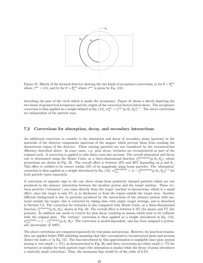
θx

b) a)

Figure 21: Sketch of the forward detector showing the two kinds of acceptance corrections, a) for θ < θcuty

where εacc = 0.5, and b) for θ > θcuty where εacc is given by Eq. (13).

describing the part of the circle which is inside the acceptance. Figure 21 shows a sketch depicting thetwo forms of geometrical acceptance and the origins of the correction factors listed above. The acceptancecorrection is then applied as a weight defined in Eq. (12), wacc

ij = [εacc(p, θx, θy)]−1. The above correctionsare independent of the particle type.

7.2 Corrections for absorption, decay, and secondary interactions

An additional correction to consider is the absorption and decay of secondary pions (protons) in thematerials of the detector components upstream of the magnet which prevent them from reaching thedownstream region of the detector. These missing particles are not considered by the reconstructionefficiency described above. In some cases, e.g. pion decay, tertiaries are reconstructed as part of theoriginal track. A correction is applied to take these cases into account. The overall absorption and decayrate is determined using the Monte Carlo, as a three-dimensional function εabsorption

α (p, θx, θy), whoseprojections are shown in Fig. 22. The overall effect is between 10% and 30% depending on p and θx.This effect is verified to be correct within 10% of its magnitude using beam particles. The ‘absorption’correction is then applied as a weight introduced in Eq. (12), wabsorption

ijα = [1− εabsorptionα (p, θx, θy)]−1 for

both particle types separately.

A correction of opposite sign to the one above stems from positively charged particles which are notproduced in the primary interaction between the incident proton and the target nucleus. These ter-tiary particles (‘tertiaries’) can come directly from the target (nuclear re-interactions, which is a smalleffect, since the target is only 5% λI in thickness) or from the region outside the target area. Anotherdifferent background is due to particles produced by the interactions of the primary proton with ma-terial outside the target; this is corrected by taking data with empty target settings, and is describedin Section 7.3. The correction for tertiaries is also computed with Monte Carlo, as a three-dimensionalfunction εtertiaries

α (p, θx, θy), shown in Fig. 23. The overall effect is between 2–3% (for pions) and 7% (forprotons). In addition one needs to correct for pion decay resulting in muons which tend to be collinearwith the original pion. The ‘tertiary’ correction is then applied as a weight introduced in Eq. (12),wtertiaries

ijα = 1 − εtertiariesα (p, θx, θy). The correction is model-dependent, and has been assigned a system-

atic uncertainty of 100%.

The above corrections are computed separately for true pions and protons. However, for practical reasons,they are applied before PID unfolding assuming that they correspond to reconstructed pions and protons(hence the index α′ in Eq. 12). The bias introduced by this approximation is negligible since pion–protonmixing is very small ( < 5%), as demonstrated in Fig. 26, and these corrections are either small (< 7% fortertiaries) or similar for both particle types (the absorption is similar while the decay of pions introducesa relatively small correction). Thus, the maximum bias would be of the order of 0.4%.

29

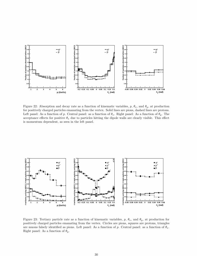
p (GeV/c)1 2 3 4 5 6

frac

tio

n o

f p

arti

cles

ab

sorb

ed b

efo

re N

DC

2

0

0.05

0.1

0.15

0.2

0.25

0.3

0.35

0.4

0.45

0.5

+πp

(rad)xθ-0.2 -0.15 -0.1 -0.05 -0 0.05 0.1 0.15 0.2

frac

tio

n o

f p

arti

cles

ab

sorb

ed b

efo

re N

DC

2

0

0.05

0.1

0.15

0.2

0.25

0.3

0.35

0.4

0.45

0.5

+πp

(rad)yθ-0.08 -0.06 -0.04 -0.02 0 0.02 0.04 0.06 0.08

frac

tio

n o

f p

arti

cles

ab

sorb

ed b

efo

re N

DC

2

0

0.05

0.1

0.15

0.2

0.25

0.3

0.35

0.4

0.45

0.5

+πp

Figure 22: Absorption and decay rate as a function of kinematic variables, p, θx, and θy, at productionfor positively charged particles emanating from the vertex. Solid lines are pions, dashed lines are protons.Left panel: As a function of p. Central panel: as a function of θx. Right panel: As a function of θy. Theacceptance effects for positive θx due to particles hitting the dipole walls are clearly visible. This effectis momentum dependent, as seen in the left panel.

p (GeV/c)1 2 3 4 5 6

# te

rtia

ries

arr

ivin

g N

DC

2 / #

to

tal p

arti

cles

arr

ivin

g N

DC

2

0

0.01

0.02

0.03

0.04

0.05

0.06

0.07

0.08

0.09

0.1

+π+µ

p

(rad)xθ-0.2 -0.15 -0.1 -0.05 -0 0.05 0.1 0.15 0.2

# te

rtia

ries

arr

ivin

g N

DC

2 / #

to

tal p

arti

cles

arr

ivin

g N

DC

2

0

0.01

0.02

0.03

0.04

0.05

0.06

0.07

0.08

0.09

0.1

+π+µ

p

(rad)yθ-0.08 -0.06 -0.04 -0.02 0 0.02 0.04 0.06 0.08

# te

rtia

ries

arr

ivin

g N

DC

2 / #

to

tal p

arti

cles

arr

ivin

g N

DC

2

0

0.01

0.02

0.03

0.04

0.05

0.06

0.07

0.08

0.09

0.1

+π+µ

p

Figure 23: Tertiary particle rate as a function of kinematic variables, p, θx, and θy, at production forpositively charged particles emanating from the vertex. Circles are pions, squares are protons, trianglesare muons falsely identified as pions. Left panel: As a function of p. Central panel: as a function of θx.Right panel: As a function of θy.

30

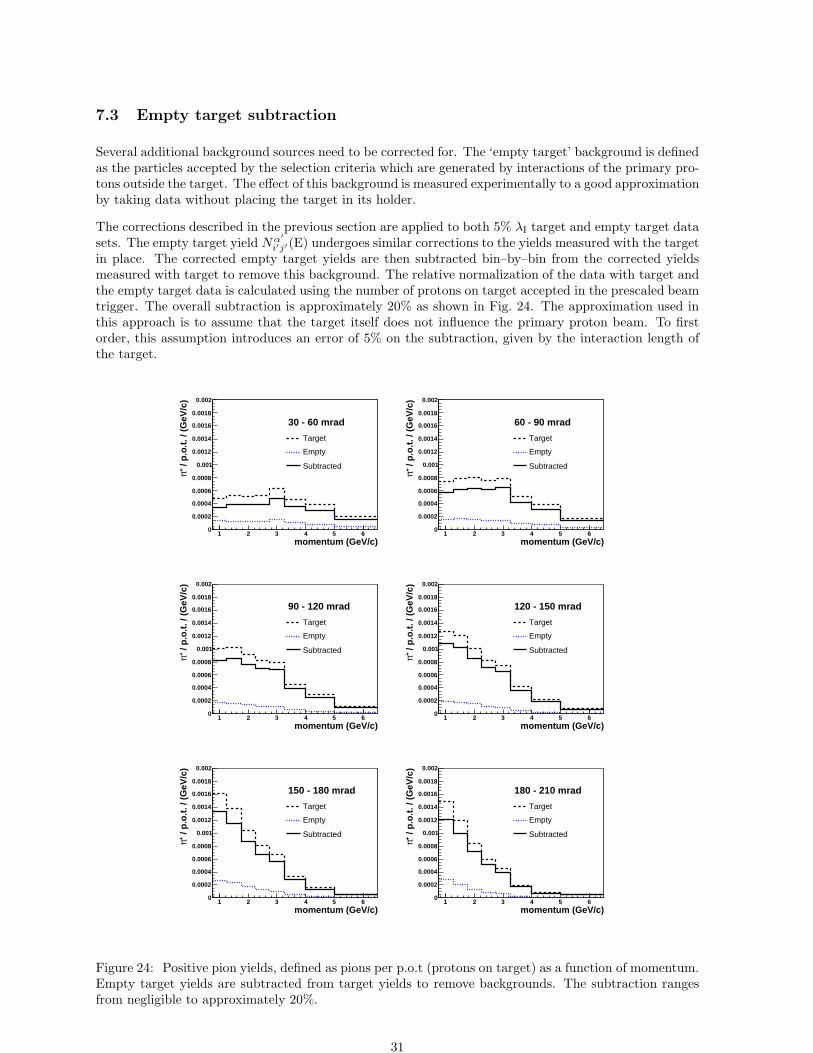
7.3 Empty target subtraction

Several additional background sources need to be corrected for. The ‘empty target’ background is definedas the particles accepted by the selection criteria which are generated by interactions of the primary pro-tons outside the target. The effect of this background is measured experimentally to a good approximationby taking data without placing the target in its holder.

The corrections described in the previous section are applied to both 5% λI target and empty target datasets. The empty target yield Nα′

i′j′(E) undergoes similar corrections to the yields measured with the targetin place. The corrected empty target yields are then subtracted bin–by–bin from the corrected yieldsmeasured with target to remove this background. The relative normalization of the data with target andthe empty target data is calculated using the number of protons on target accepted in the prescaled beamtrigger. The overall subtraction is approximately 20% as shown in Fig. 24. The approximation used inthis approach is to assume that the target itself does not influence the primary proton beam. To firstorder, this assumption introduces an error of 5% on the subtraction, given by the interaction length ofthe target.

momentum (GeV/c)1 2 3 4 5 6

/ p

.o.t

. / (

GeV

/c)

+ π

0

0.0002

0.0004

0.0006

0.0008

0.001

0.0012

0.0014

0.0016

0.0018

0.002

30 - 60 mrad

Target

Empty

Subtracted

momentum (GeV/c)1 2 3 4 5 6

/ p

.o.t

. / (

GeV

/c)

+ π

0

0.0002

0.0004

0.0006

0.0008

0.001

0.0012

0.0014

0.0016

0.0018

0.002

60 - 90 mrad

Target

Empty

Subtracted

momentum (GeV/c)1 2 3 4 5 6

/ p

.o.t

. / (

GeV

/c)

+ π

0

0.0002

0.0004

0.0006

0.0008

0.001

0.0012

0.0014

0.0016

0.0018

0.002

90 - 120 mrad

Target

Empty

Subtracted

momentum (GeV/c)1 2 3 4 5 6

/ p

.o.t

. / (

GeV

/c)

+ π

0

0.0002

0.0004

0.0006

0.0008

0.001

0.0012

0.0014

0.0016

0.0018

0.002

120 - 150 mrad

Target

Empty

Subtracted

momentum (GeV/c)1 2 3 4 5 6

/ p

.o.t

. / (

GeV

/c)

+ π

0

0.0002

0.0004

0.0006

0.0008

0.001

0.0012

0.0014

0.0016

0.0018

0.002

150 - 180 mrad

Target

Empty

Subtracted

momentum (GeV/c)1 2 3 4 5 6

/ p

.o.t

. / (

GeV

/c)

+ π

0

0.0002

0.0004

0.0006

0.0008

0.001

0.0012

0.0014

0.0016

0.0018

0.002

180 - 210 mrad

Target

Empty

Subtracted

Figure 24: Positive pion yields, defined as pions per p.o.t (protons on target) as a function of momentum.Empty target yields are subtracted from target yields to remove backgrounds. The subtraction rangesfrom negligible to approximately 20%.

31

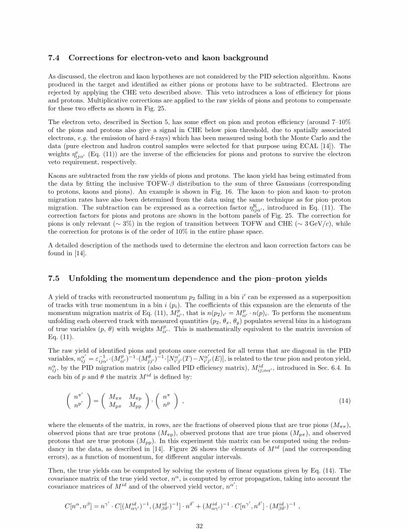
7.4 Corrections for electron-veto and kaon background

As discussed, the electron and kaon hypotheses are not considered by the PID selection algorithm. Kaonsproduced in the target and identified as either pions or protons have to be subtracted. Electrons arerejected by applying the CHE veto described above. This veto introduces a loss of efficiency for pionsand protons. Multiplicative corrections are applied to the raw yields of pions and protons to compensatefor these two effects as shown in Fig. 25.

The electron veto, described in Section 5, has some effect on pion and proton efficiency (around 7–10%of the pions and protons also give a signal in CHE below pion threshold, due to spatially associatedelectrons, e.g. the emission of hard δ-rays) which has been measured using both the Monte Carlo and thedata (pure electron and hadron control samples were selected for that purpose using ECAL [14]). Theweights ηe

ijα′ (Eq. (11)) are the inverse of the efficiencies for pions and protons to survive the electronveto requirement, respectively.

Kaons are subtracted from the raw yields of pions and protons. The kaon yield has being estimated fromthe data by fitting the inclusive TOFW-β distribution to the sum of three Gaussians (correspondingto protons, kaons and pions). An example is shown in Fig. 16. The kaon–to–pion and kaon–to–protonmigration rates have also been determined from the data using the same technique as for pion–protonmigration. The subtraction can be expressed as a correction factor ηK

ijα′ , introduced in Eq. (11). Thecorrection factors for pions and protons are shown in the bottom panels of Fig. 25. The correction forpions is only relevant (∼ 3%) in the region of transition between TOFW and CHE (∼ 3 GeV/c), whilethe correction for protons is of the order of 10% in the entire phase space.

A detailed description of the methods used to determine the electron and kaon correction factors can befound in [14].

7.5 Unfolding the momentum dependence and the pion–proton yields

A yield of tracks with reconstructed momentum p2 falling in a bin i′ can be expressed as a superpositionof tracks with true momentum in a bin i (pi). The coefficients of this expansion are the elements of themomentum migration matrix of Eq. (11), Mp

ii′ , that is n(p2)i′ = Mpii′ · n(p)i. To perform the momentum

unfolding each observed track with measured quantities (p2, θx, θy) populates several bins in a histogramof true variables (p, θ) with weights Mp

ii′ . This is mathematically equivalent to the matrix inversion ofEq. (11).

The raw yield of identified pions and protons once corrected for all terms that are diagonal in the PIDvariables, nα′

ij = ε−1ijα′ ·(Mp

ii′)−1 ·(Mθ

jj′ )−1 ·[Nα′

i′j′(T )−Nα′

i′j′(E)], is related to the true pion and proton yield,

nαij , by the PID migration matrix (also called PID efficiency matrix), M id

ij;αα′ , introduced in Sec. 6.4. In

each bin of p and θ the matrix M id is defined by:

(

nπ′

np′

)

=

(

Mππ Mπp

Mpπ Mpp

)

·(

nπ

np

)

, (14)

where the elements of the matrix, in rows, are the fractions of observed pions that are true pions (Mππ),observed pions that are true protons (Mπp), observed protons that are true pions (Mpπ), and observedprotons that are true protons (Mpp). In this experiment this matrix can be computed using the redun-dancy in the data, as described in [14]. Figure 26 shows the elements of M id (and the correspondingerrors), as a function of momentum, for different angular intervals.

Then, the true yields can be computed by solving the system of linear equations given by Eq. (14). Thecovariance matrix of the true yield vector, nα, is computed by error propagation, taking into account thecovariance matrices of M id and of the observed yield vector, nα′

:

C[nα, nβ ] = nγ′ · C[(M idαγ′)−1, (M id

βδ′)−1] · nδ′

+ (M idαγ′)−1 · C[nγ′

, nδ′

] · (M idβδ′)−1 ,

32

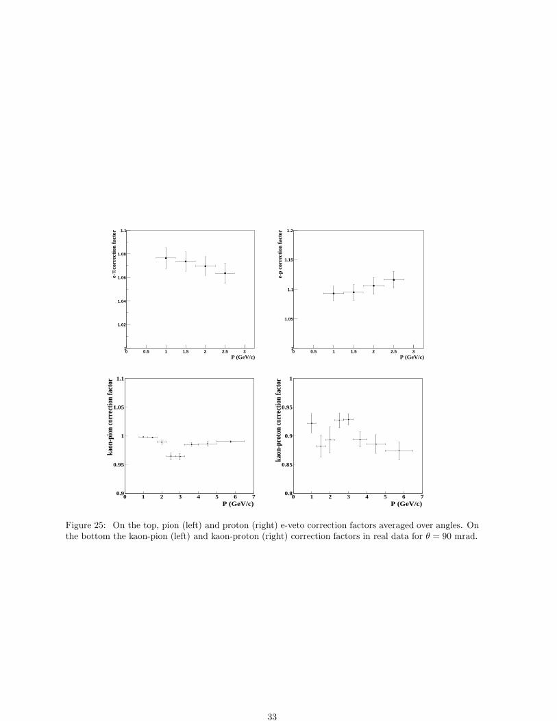
P (GeV/c)0 0.5 1 1.5 2 2.5 3

cor

rect

ion

fact

orπ

e-

1

1.02

1.04

1.06

1.08

1.1

P (GeV/c)0 0.5 1 1.5 2 2.5 3

e-p

corr

ecti

on fa

ctor

1

1.05

1.1

1.15

1.2

0.9

0.95

1

1.05

1.1

0 1 2 3 4 5 6 7P (GeV/c)

kaon

-pio

n co

rrec

tion

fact

or

0.8

0.85

0.9

0.95

1

0 1 2 3 4 5 6 7P (GeV/c)

kaon

-pro

ton

corr

ectio

n fa

ctor

Figure 25: On the top, pion (left) and proton (right) e-veto correction factors averaged over angles. Onthe bottom the kaon-pion (left) and kaon-proton (right) correction factors in real data for θ = 90 mrad.

33

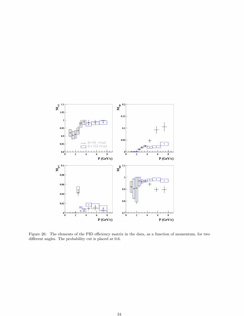
0.8

0.85

0.9

0.95

1

1.05

1.1

0 2 4 6 8

P (GeV/c)

Mπ

π

0

0.05

0.1

0.15

0.2

0 2 4 6 8

P (GeV/c)

Mπp

0

0.02

0.04

0.06

0.08

0.1

0 2 4 6 8

P (GeV/c)

Mpπ

0.7

0.8

0.9

1

1.1

0 2 4 6 8

P (GeV/c)

Mpp

Figure 26: The elements of the PID efficiency matrix in the data, as a function of momentum, for twodifferent angles. The probability cut is placed at 0.6.

34

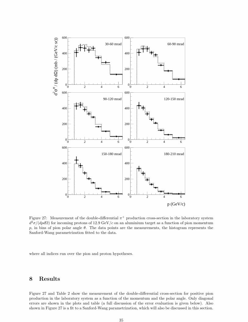
0

200

400

600

0 2 4 6

d2 σπ / (d

p dΩ

) (m

b / (

GeV

/c s

r))

30-60 mrad

0

200

400

600

0 2 4 6

60-90 mrad

0

200

400

600

0 2 4 6

90-120 mrad

0

200

400

600

0 2 4 6

120-150 mrad

0

200

400

600

0 2 4 6

150-180 mrad

0

200

400

600

0 2 4 6

p (GeV/c)

180-210 mrad

Figure 27: Measurement of the double-differential π+ production cross-section in the laboratory systemd2σ/(dpdΩ) for incoming protons of 12.9 GeV/c on an aluminium target as a function of pion momentump, in bins of pion polar angle θ. The data points are the measurements, the histogram represents theSanford-Wang parametrization fitted to the data.

where all indices run over the pion and proton hypotheses.

8 Results

Figure 27 and Table 2 show the measurement of the double-differential cross-section for positive pionproduction in the laboratory system as a function of the momentum and the polar angle. Only diagonalerrors are shown in the plots and table (a full discussion of the error evaluation is given below). Alsoshown in Figure 27 is a fit to a Sanford-Wang parametrization, which will also be discussed in this section.

35

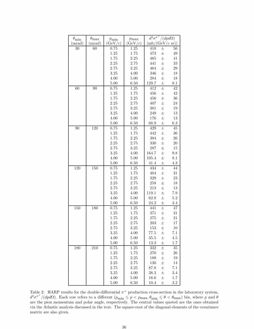
θmin θmax pmin pmax d2σπ+

/(dpdΩ)(mrad) (mrad) (GeV/c) (GeV/c) (mb/(GeV/c sr))

30 60 0.75 1.25 410 ± 561.25 1.75 473 ± 491.75 2.25 465 ± 412.25 2.75 441 ± 332.75 3.25 464 ± 293.25 4.00 346 ± 184.00 5.00 284 ± 185.00 6.50 129.7 ± 8.1

60 90 0.75 1.25 412 ± 421.25 1.75 456 ± 421.75 2.25 456 ± 362.25 2.75 407 ± 242.75 3.25 381 ± 193.25 4.00 249 ± 134.00 5.00 176 ± 135.00 6.50 68.9 ± 6.3

90 120 0.75 1.25 429 ± 451.25 1.75 442 ± 361.75 2.25 384 ± 262.25 2.75 330 ± 202.75 3.25 287 ± 153.25 4.00 164.7 ± 9.84.00 5.00 105.4 ± 8.15.00 6.50 41.4 ± 4.3

120 150 0.75 1.25 434 ± 441.25 1.75 404 ± 311.75 2.25 329 ± 232.25 2.75 258 ± 182.75 3.25 213 ± 133.25 4.00 119.1 ± 7.94.00 5.00 62.8 ± 5.25.00 6.50 24.2 ± 3.4

150 180 0.75 1.25 441 ± 471.25 1.75 371 ± 311.75 2.25 275 ± 212.25 2.75 203 ± 172.75 3.25 153 ± 103.25 4.00 77.5 ± 7.14.00 5.00 35.5 ± 4.55.00 6.50 13.3 ± 1.7

180 210 0.75 1.25 332 ± 351.25 1.75 270 ± 261.75 2.25 189 ± 192.25 2.75 130 ± 142.75 3.25 87.8 ± 7.13.25 4.00 38.3 ± 3.44.00 5.00 16.6 ± 1.75.00 6.50 10.4 ± 3.2

Table 2: HARP results for the double-differential π+ production cross-section in the laboratory system,d2σπ+

/(dpdΩ). Each row refers to a different (pmin ≤ p < pmax, θmin ≤ θ < θmax) bin, where p and θare the pion momentum and polar angle, respectively. The central values quoted are the ones obtainedvia the Atlantic analysis discussed in the text. The square-root of the diagonal elements of the covariancematrix are also given.

36

8.1 Error estimates

A detailed error analysis has been performed to evaluate the accuracy of the pion cross-section measure-ment. The main errors entering in this measurement are listed below.

First, the statistical uncertainties associated with the track yields measured from the aluminium targetsetting and from the empty target setting (needed for subtraction, as explained above) have been includedin the pion production cross-section uncertainty estimates.

Second, several uncertainties associated with the corrections needed to convert the measured track yieldsto true track yields have been evaluated. The track reconstruction efficiency correction is based on thecombination of thin target aluminium and beryllium data sets. The main error associated with thiscomputation is given by the size of the statistical sample. The correction to the pion and proton yieldsdue to absorption or decay is computed via a Monte Carlo simulation. An uncertainty of 10% for bothproton and pion yields has been assumed for this correction, in addition to the uncertainty due to thefinite size of the simulated data sample used to estimate this correction. Similarly, simulated data (andtheir associated uncertainties) were used to estimate the correction for the contamination in the sampledue to tertiary particles that are not produced in the target, but rather by the decay of secondaries, orby the interaction of secondaries in the spectrometer material. An uncertainty of 100% has been assumedfor this subtraction, for both proton and pion yields. Furthermore, an uncertainty has been assigned tothe empty target subtraction, in order to account for the effect of the target itself which attenuates theproton beam.

Third, uncertainties associated with the particle identification of tracks, and with the corrections neededto convert yields of tracks identified as pions to true pion yields, have been included. Among the severalerror sources associated with the pion–proton PID selection, the dominant one is due to the uncertaintyin the (small) fraction of pions and protons with an associated anomalous TOFW β measurement, thatis a β measurement which exhibits a non-Gaussian behaviour. Estimates of the uncertainty in the kaoncontamination and in the correction for the electron veto have been obtained from an analysis of the dataas explained in Section 5. The robustness of the pion PID selection and its associated correction has beenevaluated by performing the analysis with tighter and looser PID probability cuts with respect to theirnominal values, while correcting for the PID efficiency and migration corresponding to the probabilitycuts.

Fourth, we have included uncertainties associated with the momentum reconstruction performance ofthe spectrometer, and with the corrections needed to convert the measured momenta to ‘true’ momenta.Concerning the momentum, biases and resolution effects are taken into account using both real andsimulated data. It was found that momentum biases do not exceed the 5% level from a study of beamparticles at different momenta and from a comparison between the reconstructed momenta and themomenta inferred from β measurements with the TOFW and the threshold curves in the Cherenkov.

Finally, an overall normalization uncertainty of 4% has been estimated. The dominant sources for thisuncertainty are the targeting efficiency uncertainty, which is deduced from the measurement of transversebeam spot size on target, as well as the reconstruction and PID uncertainties that are fully correlatedacross different (p, θ) pion bins, and which are not included in the above evaluation. On the otherhand, the aluminium target thickness and density were carefully measured, and the effect on the overallcross-section normalization due to these uncertainties is negligible.

8.2 Results of the Error Evaluation

The impact of the error sources discussed in the previous section on the final cross-section measurementhas been evaluated, either by analytic error propagation, or by Monte Carlo techniques. Correlationeffects among different particle types, and among different (p, θ) bins, have also been taken into account.

The cross-section uncertainty level is quantified by adopting two different conventions. The rationaleis that both the errors on the ‘point–to–point’, double-differential cross-section, and the error on thecross-section integrated over the entire pion phase space measured, might be of interest.

37

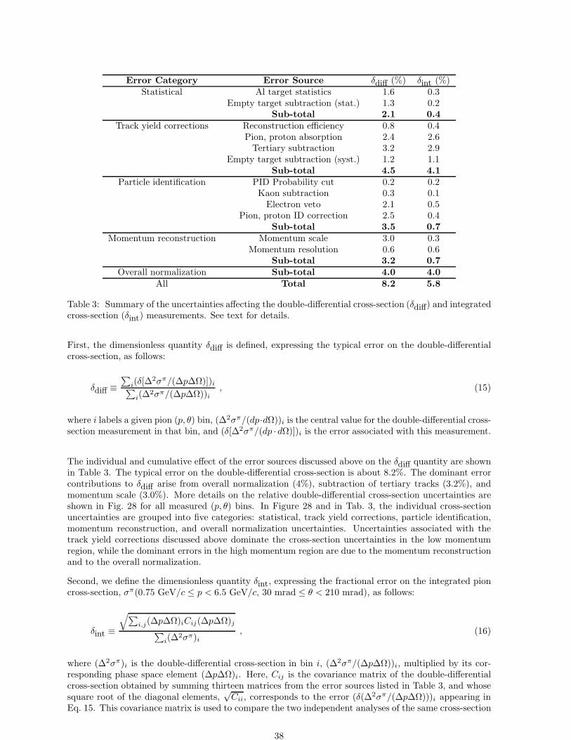
Error Category Error Source δdiff (%) δint (%)Statistical Al target statistics 1.6 0.3

Empty target subtraction (stat.) 1.3 0.2Sub-total 2.1 0.4

Track yield corrections Reconstruction efficiency 0.8 0.4Pion, proton absorption 2.4 2.6

Tertiary subtraction 3.2 2.9Empty target subtraction (syst.) 1.2 1.1

Sub-total 4.5 4.1

Particle identification PID Probability cut 0.2 0.2Kaon subtraction 0.3 0.1

Electron veto 2.1 0.5Pion, proton ID correction 2.5 0.4

Sub-total 3.5 0.7

Momentum reconstruction Momentum scale 3.0 0.3Momentum resolution 0.6 0.6

Sub-total 3.2 0.7

Overall normalization Sub-total 4.0 4.0

All Total 8.2 5.8

Table 3: Summary of the uncertainties affecting the double-differential cross-section (δdiff) and integratedcross-section (δint) measurements. See text for details.

First, the dimensionless quantity δdiff is defined, expressing the typical error on the double-differentialcross-section, as follows:

δdiff ≡∑

i(δ[∆2σπ/(∆p∆Ω)])i

∑

i(∆2σπ/(∆p∆Ω))i

, (15)

where i labels a given pion (p, θ) bin, (∆2σπ/(dp·dΩ))i is the central value for the double-differential cross-section measurement in that bin, and (δ[∆2σπ/(dp ·dΩ)])i is the error associated with this measurement.

The individual and cumulative effect of the error sources discussed above on the δdiff quantity are shownin Table 3. The typical error on the double-differential cross-section is about 8.2%. The dominant errorcontributions to δdiff arise from overall normalization (4%), subtraction of tertiary tracks (3.2%), andmomentum scale (3.0%). More details on the relative double-differential cross-section uncertainties areshown in Fig. 28 for all measured (p, θ) bins. In Figure 28 and in Tab. 3, the individual cross-sectionuncertainties are grouped into five categories: statistical, track yield corrections, particle identification,momentum reconstruction, and overall normalization uncertainties. Uncertainties associated with thetrack yield corrections discussed above dominate the cross-section uncertainties in the low momentumregion, while the dominant errors in the high momentum region are due to the momentum reconstructionand to the overall normalization.

Second, we define the dimensionless quantity δint, expressing the fractional error on the integrated pioncross-section, σπ(0.75 GeV/c ≤ p < 6.5 GeV/c, 30 mrad ≤ θ < 210 mrad), as follows:

δint ≡

√

∑

i,j(∆p∆Ω)iCij(∆p∆Ω)j

∑

i(∆2σπ)i

, (16)

where (∆2σπ)i is the double-differential cross-section in bin i, (∆2σπ/(∆p∆Ω))i, multiplied by its cor-responding phase space element (∆p∆Ω)i. Here, Cij is the covariance matrix of the double-differentialcross-section obtained by summing thirteen matrices from the error sources listed in Table 3, and whosesquare root of the diagonal elements,

√Cii, corresponds to the error (δ(∆2σπ/(∆p∆Ω)))i appearing in

Eq. 15. This covariance matrix is used to compare the two independent analyses of the same cross-section

38

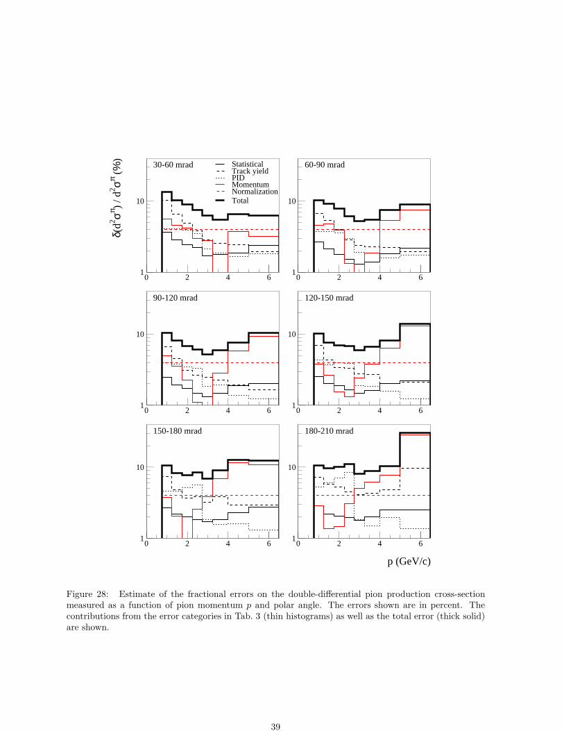
1

10

0 2 4 6

δ(d2 σπ )

/ d2 σπ (

%)

30-60 mrad StatisticalTrack yieldPIDMomentumNormalizationTotal

1

10

0 2 4 6

60-90 mrad

1

10

0 2 4 6

90-120 mrad

1

10

0 2 4 6

120-150 mrad

1

10

0 2 4 6

150-180 mrad

1

10

0 2 4 6

p (GeV/c)

180-210 mrad

Figure 28: Estimate of the fractional errors on the double-differential pion production cross-sectionmeasured as a function of pion momentum p and polar angle. The errors shown are in percent. Thecontributions from the error categories in Tab. 3 (thin histograms) as well as the total error (thick solid)are shown.

39

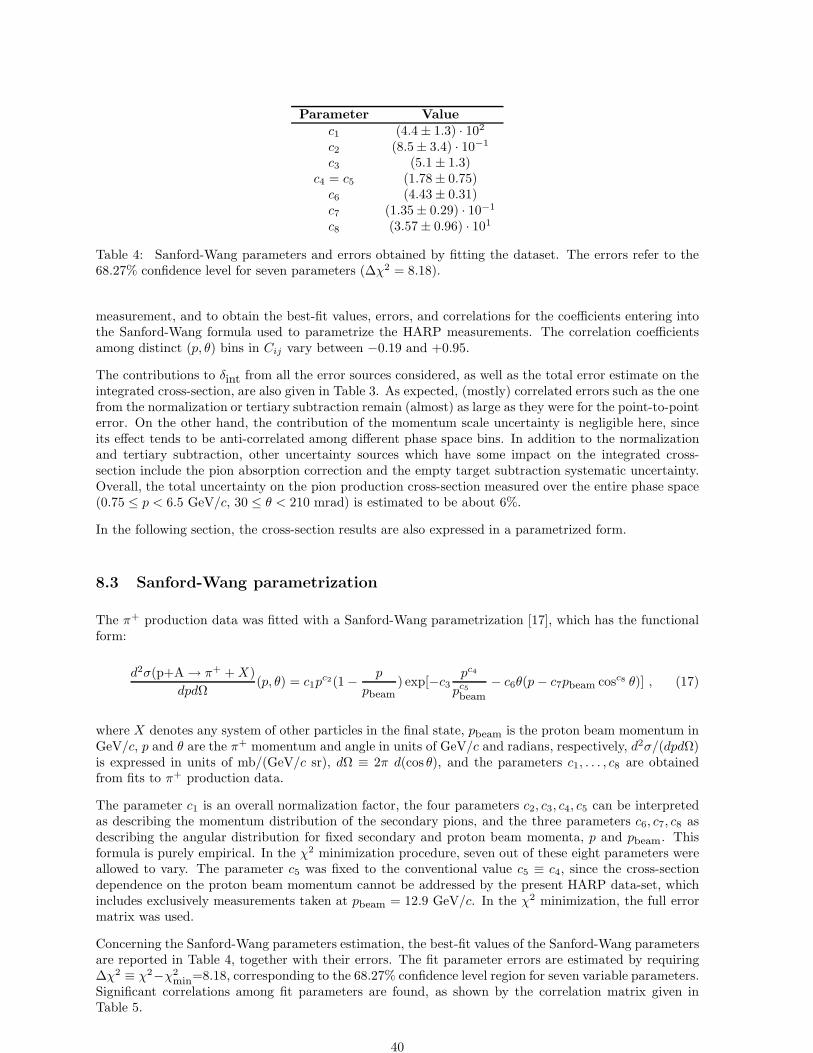
Parameter Value

c1 (4.4 ± 1.3) · 102

c2 (8.5 ± 3.4) · 10−1

c3 (5.1 ± 1.3)c4 = c5 (1.78 ± 0.75)

c6 (4.43 ± 0.31)c7 (1.35 ± 0.29) · 10−1

c8 (3.57 ± 0.96) · 101

Table 4: Sanford-Wang parameters and errors obtained by fitting the dataset. The errors refer to the68.27% confidence level for seven parameters (∆χ2 = 8.18).

measurement, and to obtain the best-fit values, errors, and correlations for the coefficients entering intothe Sanford-Wang formula used to parametrize the HARP measurements. The correlation coefficientsamong distinct (p, θ) bins in Cij vary between −0.19 and +0.95.

The contributions to δint from all the error sources considered, as well as the total error estimate on theintegrated cross-section, are also given in Table 3. As expected, (mostly) correlated errors such as the onefrom the normalization or tertiary subtraction remain (almost) as large as they were for the point-to-pointerror. On the other hand, the contribution of the momentum scale uncertainty is negligible here, sinceits effect tends to be anti-correlated among different phase space bins. In addition to the normalizationand tertiary subtraction, other uncertainty sources which have some impact on the integrated cross-section include the pion absorption correction and the empty target subtraction systematic uncertainty.Overall, the total uncertainty on the pion production cross-section measured over the entire phase space(0.75 ≤ p < 6.5 GeV/c, 30 ≤ θ < 210 mrad) is estimated to be about 6%.

In the following section, the cross-section results are also expressed in a parametrized form.

8.3 Sanford-Wang parametrization

The π+ production data was fitted with a Sanford-Wang parametrization [17], which has the functionalform:

d2σ(p+A → π+ + X)

dpdΩ(p, θ) = c1p

c2(1 − p

pbeam) exp[−c3

pc4

pc5

beam

− c6θ(p − c7pbeam cosc8 θ)] , (17)

where X denotes any system of other particles in the final state, pbeam is the proton beam momentum inGeV/c, p and θ are the π+ momentum and angle in units of GeV/c and radians, respectively, d2σ/(dpdΩ)is expressed in units of mb/(GeV/c sr), dΩ ≡ 2π d(cos θ), and the parameters c1, . . . , c8 are obtainedfrom fits to π+ production data.

The parameter c1 is an overall normalization factor, the four parameters c2, c3, c4, c5 can be interpretedas describing the momentum distribution of the secondary pions, and the three parameters c6, c7, c8 asdescribing the angular distribution for fixed secondary and proton beam momenta, p and pbeam. Thisformula is purely empirical. In the χ2 minimization procedure, seven out of these eight parameters wereallowed to vary. The parameter c5 was fixed to the conventional value c5 ≡ c4, since the cross-sectiondependence on the proton beam momentum cannot be addressed by the present HARP data-set, whichincludes exclusively measurements taken at pbeam = 12.9 GeV/c. In the χ2 minimization, the full errormatrix was used.

Concerning the Sanford-Wang parameters estimation, the best-fit values of the Sanford-Wang parametersare reported in Table 4, together with their errors. The fit parameter errors are estimated by requiring∆χ2 ≡ χ2−χ2

min=8.18, corresponding to the 68.27% confidence level region for seven variable parameters.Significant correlations among fit parameters are found, as shown by the correlation matrix given inTable 5.

40

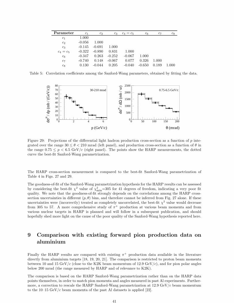
Parameter c1 c2 c3 c4 = c5 c6 c7 c8

c1 1.000c2 -0.056 1.000c3 -0.145 -0.691 1.000

c4 = c5 -0.322 -0.890 0.831 1.000c6 -0.347 0.263 -0.252 -0.067 1.000c7 -0.740 0.148 -0.067 0.077 0.326 1.000c8 0.130 -0.044 0.205 -0.040 -0.650 0.189 1.000

Table 5: Correlation coefficients among the Sanford-Wang parameters, obtained by fitting the data.

0

10

20

30

40

50

60

70

80

0 2 4 6

p (GeV/c)

dσπ /

dp (

mb

/ (G

eV/c

))

30-210 mrad

0

500

1000

1500

2000

2500

0 50 100 150 200

θ (mrad)

dσπ /

dΩ (

mb

/ sr)

0.75-6.5 GeV/c

Figure 29: Projections of the differential light hadron production cross-section as a function of p inte-grated over the range 30 ≤ θ < 210 mrad (left panel), and production cross-section as a function of θ inthe range 0.75 ≤ p < 6.5 GeV/c (right panel). The points show the HARP measurements, the dottedcurve the best-fit Sanford-Wang parametrization.

The HARP cross-section measurement is compared to the best-fit Sanford-Wang parametrization ofTable 4 in Figs. 27 and 29.

The goodness-of-fit of the Sanford-Wang parametrization hypothesis for the HARP results can be assessedby considering the best-fit χ2 value of χ2

min=305 for 41 degrees of freedom, indicating a very poor fitquality. We note that the goodness-of-fit strongly depends on the correlations among the HARP cross-section uncertainties in different (p, θ) bins, and therefore cannot be inferred from Fig. 27 alone. If theseuncertainties were (incorrectly) treated as completely uncorrelated, the best-fit χ2 value would decreasefrom 305 to 57. A more comprehensive study of π+ production at various beam momenta and fromvarious nuclear targets in HARP is planned and will follow in a subsequent publication, and shouldhopefully shed more light on the cause of the poor quality of the Sanford-Wang hypothesis reported here.

9 Comparison with existing forward pion production data on

aluminium

Finally the HARP results are compared with existing π+ production data available in the literaturedirectly from aluminium targets [18, 19, 20, 21]. The comparison is restricted to proton beam momentabetween 10 and 15 GeV/c (close to the K2K beam momentum of 12.9 GeV/c), and for pion polar anglesbelow 200 mrad (the range measured by HARP and of relevance to K2K).

The comparison is based on the HARP Sanford-Wang parametrization rather than on the HARP datapoints themselves, in order to match pion momenta and angles measured in past Al experiments. Further-more, a correction to rescale the HARP Sanford-Wang parametrization at 12.9 GeV/c beam momentumto the 10–15 GeV/c beam momenta of the past Al datasets is applied [22].

41

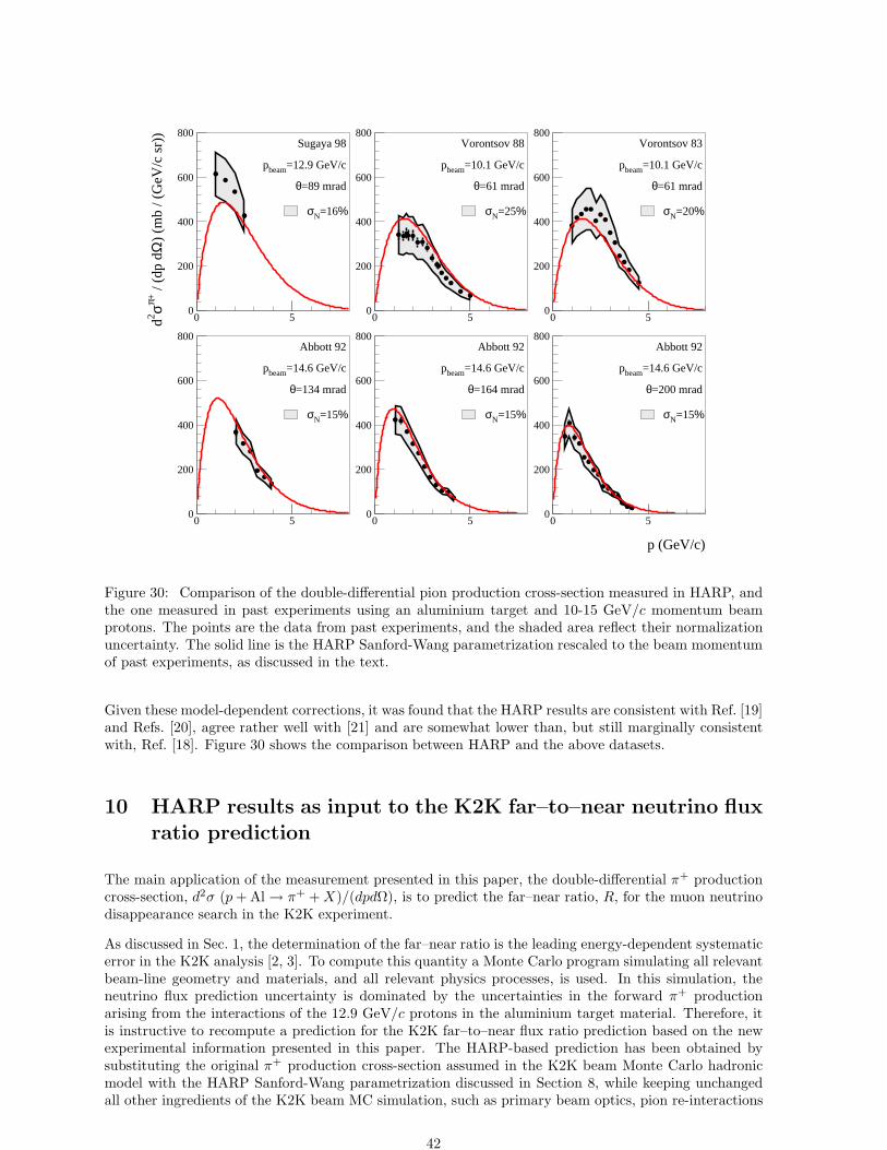
0

200

400

600

800

0 5d2 σπ+ /

(dp

dΩ)

(mb

/ (G

eV/c

sr)

)Sugaya 98

pbeam=12.9 GeV/c

θ=89 mrad

σN=16%

0

200

400

600

800

0 5

Vorontsov 88

pbeam=10.1 GeV/c

θ=61 mrad

σN=25%

0

200

400

600

800

0 5

Vorontsov 83

pbeam=10.1 GeV/c

θ=61 mrad

σN=20%

0

200

400

600

800

0 5

Abbott 92

pbeam=14.6 GeV/c

θ=134 mrad

σN=15%

0

200

400

600

800

0 5

Abbott 92

pbeam=14.6 GeV/c

θ=164 mrad

σN=15%

0

200

400

600

800

0 5

Abbott 92

pbeam=14.6 GeV/c

θ=200 mrad

σN=15%

p (GeV/c)

Figure 30: Comparison of the double-differential pion production cross-section measured in HARP, andthe one measured in past experiments using an aluminium target and 10-15 GeV/c momentum beamprotons. The points are the data from past experiments, and the shaded area reflect their normalizationuncertainty. The solid line is the HARP Sanford-Wang parametrization rescaled to the beam momentumof past experiments, as discussed in the text.

Given these model-dependent corrections, it was found that the HARP results are consistent with Ref. [19]and Refs. [20], agree rather well with [21] and are somewhat lower than, but still marginally consistentwith, Ref. [18]. Figure 30 shows the comparison between HARP and the above datasets.

10 HARP results as input to the K2K far–to–near neutrino flux

ratio prediction

The main application of the measurement presented in this paper, the double-differential π+ productioncross-section, d2σ (p + Al → π+ + X)/(dpdΩ), is to predict the far–near ratio, R, for the muon neutrinodisappearance search in the K2K experiment.

As discussed in Sec. 1, the determination of the far–near ratio is the leading energy-dependent systematicerror in the K2K analysis [2, 3]. To compute this quantity a Monte Carlo program simulating all relevantbeam-line geometry and materials, and all relevant physics processes, is used. In this simulation, theneutrino flux prediction uncertainty is dominated by the uncertainties in the forward π+ productionarising from the interactions of the 12.9 GeV/c protons in the aluminium target material. Therefore, itis instructive to recompute a prediction for the K2K far–to–near flux ratio prediction based on the newexperimental information presented in this paper. The HARP-based prediction has been obtained bysubstituting the original π+ production cross-section assumed in the K2K beam Monte Carlo hadronicmodel with the HARP Sanford-Wang parametrization discussed in Section 8, while keeping unchangedall other ingredients of the K2K beam MC simulation, such as primary beam optics, pion re-interactions

42

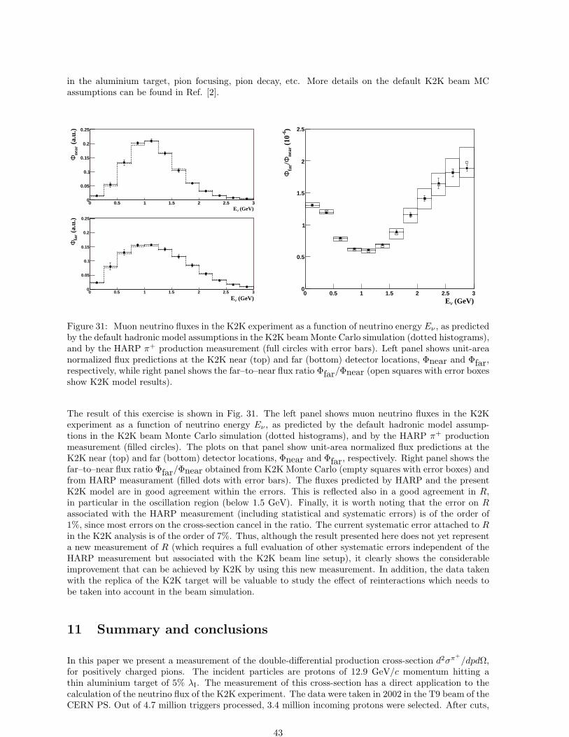
in the aluminium target, pion focusing, pion decay, etc. More details on the default K2K beam MCassumptions can be found in Ref. [2].

(GeV)νE0 0.5 1 1.5 2 2.5 3

(a.

u.)

near

Φ

0

0.05

0.1

0.15

0.2

0.25

(GeV)νE0 0.5 1 1.5 2 2.5 3

(a.

u.)

far

Φ

0

0.05

0.1

0.15

0.2

0.25

(GeV)νE0 0.5 1 1.5 2 2.5 3

)-6

(10

near

Φ/fa

rΦ

0

0.5

1

1.5

2

2.5

Figure 31: Muon neutrino fluxes in the K2K experiment as a function of neutrino energy Eν , as predictedby the default hadronic model assumptions in the K2K beam Monte Carlo simulation (dotted histograms),and by the HARP π+ production measurement (full circles with error bars). Left panel shows unit-areanormalized flux predictions at the K2K near (top) and far (bottom) detector locations, Φnear and Φfar,respectively, while right panel shows the far–to–near flux ratio Φfar/Φnear (open squares with error boxesshow K2K model results).

The result of this exercise is shown in Fig. 31. The left panel shows muon neutrino fluxes in the K2Kexperiment as a function of neutrino energy Eν , as predicted by the default hadronic model assump-tions in the K2K beam Monte Carlo simulation (dotted histograms), and by the HARP π+ productionmeasurement (filled circles). The plots on that panel show unit-area normalized flux predictions at theK2K near (top) and far (bottom) detector locations, Φnear and Φfar, respectively. Right panel shows thefar–to–near flux ratio Φfar/Φnear obtained from K2K Monte Carlo (empty squares with error boxes) andfrom HARP measurament (filled dots with error bars). The fluxes predicted by HARP and the presentK2K model are in good agreement within the errors. This is reflected also in a good agreement in R,in particular in the oscillation region (below 1.5 GeV). Finally, it is worth noting that the error on Rassociated with the HARP measurement (including statistical and systematic errors) is of the order of1%, since most errors on the cross-section cancel in the ratio. The current systematic error attached to Rin the K2K analysis is of the order of 7%. Thus, although the result presented here does not yet representa new measurement of R (which requires a full evaluation of other systematic errors independent of theHARP measurement but associated with the K2K beam line setup), it clearly shows the considerableimprovement that can be achieved by K2K by using this new measurement. In addition, the data takenwith the replica of the K2K target will be valuable to study the effect of reinteractions which needs tobe taken into account in the beam simulation.

11 Summary and conclusions

In this paper we present a measurement of the double-differential production cross-section d2σπ+

/dpdΩ,for positively charged pions. The incident particles are protons of 12.9 GeV/c momentum hitting athin aluminium target of 5% λI. The measurement of this cross-section has a direct application to thecalculation of the neutrino flux of the K2K experiment. The data were taken in 2002 in the T9 beam of theCERN PS. Out of 4.7 million triggers processed, 3.4 million incoming protons were selected. After cuts,

43

around 210 000 secondary tracks reconstructed in the forward spectrometer were used in this analysis.These high statistics results were corrected for measurement resolutions. These data were fitted with aSanford-Wang parametrization. The results are given for positively charged pions within a momentumrange from 0.75 GeV/c to 6.5 GeV/c, and within an angular range from 30 mrad to 210 mrad. Theaverage statistical error is 1.6% per point. The absolute normalization was performed using prescaledbeam triggers. The overall efficiency for track reconstruction and particle identification is known to betterthan 6%, while the average point-to-point error is 8.2%.

12 Acknowledgements

We gratefully acknowledge the help and support of the PS beam staff and of the numerous technicalcollaborators who contributed to the detector design, construction, commissioning and operation. Inparticular, we would like to thank G. Barichello, R. Broccard, K. Burin, V. Carassiti, F. Chignoli,G. Decreuse, C. Detraz, M. Dwuznik, F. Evangelisti, B. Friend, A. Iaciofano, I. Krasin, J.-C. Legrand,M. Lobello, F. Marinilli, J. Mulon, R. Nicholson, A. Pepato, P. Petev, X. Pons, I. Rusinov, M. Scandurra,E. Usenko, and R. van der Vlugt, for their support in the construction of the detector. The collaborationis indebted to M. Baldo Ceolin, P. Binko, E. Boter, M. Doucet, D. Dullmann, V. Ermilova, A. Pullia andA. Valassi for their contributions to the experiment.

We are indebted to the K2K collaboration who made available their beam-line simulation for the calcu-lation of the predicted far–to–near neutrino flux ratio.

The experiment was made possible by grants from the Institut Interuniversitaire des Sciences Nucleair-es and the Interuniversitair Instituut voor Kernwetenschappen (Belgium), Ministerio de Educacion yCiencia, Grant FPA2003-06921-c02-02 and Generalitat Valenciana, grant GV00-054-1, CERN (Geneva,Switzerland), the German Bundesministerium fur Bildung und Forschung (Germany), the Istituto Na-zionale di Fisica Nucleare (Italy), INR RAS (Moscow) and the Particle Physics and Astronomy ResearchCouncil (UK). We gratefully acknowledge their support.

44

References

[1] M.G Catanesi et al., HARP Collaboration, “Proposal to study hadron production for the neutrinofactory and for the atmospheric neutrino flux”, CERN-SPSC/99-35, 15 November 1999.

[2] M. H. Ahn et al. [K2K Collaboration], Phys. Rev. Lett. 90 (2003) 041801 [arXiv:hep-ex/0212007].

S. H. Ahn et al. [K2K Collaboration], Phys. Lett. B 511 (2001) 178 [arXiv:hep-ex/0103001].

[3] E. Aliu et al. [K2K Collaboration], Phys. Rev. Lett. 94 (2005) 081802 [arXiv:hep-ex/0411038].

[4] Y. Ashie et al. [Super-Kamiokande Collaboration], Phys. Rev. D 71 (2005) 112005[arXiv:hep-ex/0501064].

[5] HARP Collaboration, “The HARP detector at the CERN PS”, (paper in preparation).

[6] L. Durieu et al., Optic Studies for the T9 Beam Line in the Cern PS East Area Secondary BeamFacility, CERN/PS 2001-037; L. Durieu, O. Fernando, Design of the T9 (ATLAS/CMS) for EHNL,CERN PS/PA Note 96-38.

[7] K. Pretzl et al., Invited talk at the “International Symposium on Strangeness and Quark Matter”,Crete, 230 (1999).

[8] J. Altegoer et al. [NOMAD Collaboration], Nucl. Instrum. Meth. A 404 (1998) 96.

[9] M. Anfreville et al., Nucl. Instrum. Meth. A 481 (2002) 339 [arXiv:hep-ex/0104012].

[10] M. Baldo-Ceolin et al., Nucl. Instrum. Meth. A 532 (2004) 548.

[11] S. Buontempo et al., Nucl. Instrum. Meth. A 349 (1994) 70.

E. Di Capua et al., Nucl. Instrum. Meth. A 378 (1996) 221.

[12] A. Cervera-Villanueva, J. J. Gomez-Cadenas and J. A. Hernando, Nucl. Instrum. Meth. A 534

(2004) 180.

[13] P. Billoir, Nucl. Instrum. Meth. A 225 (1984) 352.

P. Billoir, R. Fruhwirth and M. Regler, Nucl. Instrum. Meth. A 241 (1985) 115.

R. Fruhwirth, Nucl. Instrum. Meth. A 262 (1987) 444.

R. Fruhwirth, “Application of Filter Methods to the Reconstruction of Tracks And Vertices inEvents of Experimental High Energy Physics”, HEPHY-PUB 516/88 Vienna, December 1988.

[14] HARP Collaboration, “Particle identification algorithms for the HARP forward spectrometer”,(paper in preparation).

[15] G. D’Agostini, Nucl. Instrum. Meth. A 362 (1995) 487.

[16] A. Grossheim, Ph.D. thesis, University of Dortmund, Germany, 2003, CERN-THESIS-2004-010.

[17] J. R. Sanford and C. L. Wang, Brookhaven National Laboratory, AGS internal report, 1967 (un-published); C. L. Wang, Phys. Rev. Letters 25, 1068 (1970); ibid. 25, 1536(E) (1970).

[18] Y. Sugaya et al., Nucl. Phys. A 634 (1998) 115.

[19] I. A. Vorontsov et al., ITEP-11-1988.

[20] I. A. Vorontsov et al., ITEP-85-1983.

[21] T. Abbott et al., E-802 Collaboration, Phys. Rev. D 45 (1992) 3906.

[22] Y. Cho et al., Phys. Rev. D 4 (1971) 1967.

45