Computational Statistics & Data Analysis 51 (2007) 3703–3717www.elsevier.com/locate/csda

Computational aspects of order �ps sampling schemesAlina Matei∗, Yves Tillé

Institute of Statistics, University of Neuchâtel, Pierre à Mazel, 7, 2000 Neuchâtel, Switzerland

Received 3 May 2006; received in revised form 11 December 2006; accepted 11 December 2006Available online 19 December 2006

Abstract

In an order sampling a finite population of size N has its units ordered by a ranking variable and then, a sample of the first nunits is drawn. For order �ps sampling, the target inclusion probabilities � = (�k)

Nk=1 are computed using a measure of size which

is correlated with a variable of interest. The quantities �k , however, are different from the true inclusion probabilities �k . Firstly, anew, simple method to compute �k from �k is presented, and it is used to compute the inclusion probabilities of order �ps samplingschemes (uniform, exponential and Pareto). Secondly, given two positively co-ordinated samples drawn with order �ps sampling,the joint inclusion probability of a unit in both samples is approximated. This approximation can be used to derive the expectedoverlap or to construct an estimate of the covariance on these two samples. All presented methods use numerical integration.© 2007 Elsevier B.V. All rights reserved.

Keywords: Sample survey; �ps sampling; Unequal probabilities; Fixed sample size; Order statistics; Permanent random numbers; Co-ordinationover time; Numerical integration

1. Introduction

1.1. Notation and basic concepts

Let U = {1, . . . , k, . . . , N} be a finite population, where k is the reference unit, and N denotes the population size.A sample s is a subset of U . We consider sampling without replacement and with fixed sample size n. Let Sn be thesample support, which is the set of all samples without replacement of size n drawn from U . Let p(.) be a probabilitydistribution on Sn. Given p(.), the inclusion probability of unit k to be in a sample is

�k = Pr(k ∈ s) =∑s�k

s∈Sn

p(s).

For each k ∈ U , the quantity �k denotes the first-order inclusion probability. Similarly, the second-order inclusionprobabilities are defined as

�k� = Pr(k ∈ s, � ∈ s) =∑s�k,�s∈Sn

p(s) if k �= � and �kk = �k otherwise.

∗ Corresponding author.E-mail addresses: alina.matei@unine.ch (A. Matei), yves.tille@unine.ch (Y. Tillé).

0167-9473/$ - see front matter © 2007 Elsevier B.V. All rights reserved.doi:10.1016/j.csda.2006.12.026

3704 A. Matei, Y. Tillé / Computational Statistics & Data Analysis 51 (2007) 3703–3717

When the sample size n is fixed, the inclusion probabilities satisfy the conditions∑k∈U

�k = n,∑�∈U��=k

�k� = (n − 1)�k for all k ∈ U .

Let y = (y1, . . . , yN) be the variable of interest, and let s ∈ Sn. The values of y are known only for the units k ∈ s.The Horvitz–Thompson estimator of the population total ty , where ty =∑

k∈U yk , is defined as

tHT =∑k∈s

yk

�k

. (1)

When an auxiliary variable z = (zk)Nk=1, with zk > 0, ∀k ∈ U , related to y is available for all units in the popula-

tion, unequal probability sampling is frequently used to increase the efficiency of the estimation (generally using theHorvitz–Thompson estimator). In this case, for a sampling design with fixed sample size n, the first-order inclusionprobability of unit k is equal to nzk/

∑�∈U z�, and the sampling is denoted as �ps sampling.

1.2. Order �ps sampling

The order sampling designs form a class of sampling schemes developed by Rosén (1997a, b), and adhere to thefollowing basic idea. Suppose we have N independent random variables X1, . . . , Xk, . . . , XN , where each variableis associated to a unit; these variables are usually referred to as ‘ordering variables’ or ‘ranking variables’. EachXk has a continuous cumulative distribution function (cdf) Fk defined on [0, ∞), and a probability density functionfk, k = 1, . . . , N . Order sampling with fixed sample size n and order distributions

F = (F1, . . . , Fk, . . . , FN)

is obtained by ordering the values of Xk by increasing magnitude and taking from U the first n units in this or-der. The sample obtained in this way is a random sample without replacement and has fixed size n. The variablesX1, . . . , Xk, . . . , XN follow the same type of distribution, but are not always identically distributed. When Xk’s areidentically distributed, a simple random sampling without replacement is obtained, and the inclusion probabilities areequal. Otherwise, the inclusion probabilities are unequal.

We focus on the �ps sampling, where the quantities �k (called ‘target inclusion probabilities’) are computed accordingto

�k = nzk∑N�=1 z�

, k = 1, . . . , N .

The quantity zk > 0 represents auxiliary information associated to unit k which is known for all units in the population.We assume that 0 < �k < 1, ∀k = 1, . . . , N .

Rosén (1997a) defined the order �ps sampling design with fixed distribution shape H and target inclusion probabilities� = (�k)

Nk=1 by setting

Fk(t) = H [tH−1(�k)],and

Xk = H−1(�k)

H−1(�k),

where H is a distribution function defined on [0, ∞), and � = (�k)Nk=1 is a vector of independent and identically

distributed U [0, 1] random variables. This type of sampling is known as asymptotically �ps sampling (Rosén, 1997a).Different distributions Fk lead to various types of order sampling. In particular, we have

1. Uniform order �ps sampling or sequential Poisson sampling (Ohlsson, 1990, 1998), which uses uniform orderingdistribution. In this case,

Xk = �k

�k

, Fk(t) = min(t�k, 1) ∀k ∈ U . (2)

A. Matei, Y. Tillé / Computational Statistics & Data Analysis 51 (2007) 3703–3717 3705

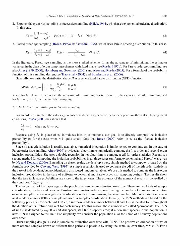
2. Exponential order �ps sampling or successive sampling (Hájek, 1964), which uses exponential ordering distribution.In this case,

Xk = ln(1 − �k)

ln(1 − �k), Fk(t) = 1 − (1 − �k)

t ∀k ∈ U . (3)

3. Pareto order �ps sampling (Rosén, 1997a, b; Saavedra, 1995), which uses Pareto ordering distribution. In this case,

Xk = �k/(1 − �k)

�k/(1 − �k), Fk(t) = t�k

1 − �k + t�k

∀k ∈ U . (4)

In the literature, Pareto �ps sampling is the most studied scheme. It has the advantage of minimizing the estimatorvariances in the class of order sampling schemes with fixed shape (see Rosén, 1997b). For Pareto order �ps sampling, seealso Aires (1999, 2000), Holmberg and Swensson (2001) and Aires and Rosén (2005). For a formula of the probabilityfunction of this sampling design, see Traat et al. (2004) and Bondesson et al. (2006).

Generally, we write the distribution shape H as a generalized Pareto distribution (GPD) function

GPD(t, a, b) ={

1 − (1 − bta)1/b b �= 0,

1 − exp(− ta) b = 0,

(5)

where for b = 1, a = 1, we obtain the uniform order sampling; for b = 0, a = 1, the exponential order sampling; andfor b = −1, a = 1, the Pareto order sampling.

1.3. Inclusion probabilities for order �ps sampling

For an ordered sample s, the values �k do not coincide with �k because the latter depends on the ranks. Under generalconditions, Rosén (2000) has shown that

�k

�k

→ 1 when n, N → ∞.

Because using �k in place of �k introduces bias in estimations, our goal is to directly compute the inclusionprobability �k for the case when n is quite small. Note that Rosén (2000) refers to �k as the ‘factual inclusionprobability’.

Since no analytic solution is readily available, numerical integration is implemented to compute �k . In the case ofPareto order �ps sampling, Aires (1999) provided an algorithm to numerically compute the first-order and second-orderinclusion probabilities. She uses a double recursion in her algorithm to compute a cdf for order statistics. Recently, asecond method for computing the inclusion probabilities in all three cases (uniform, exponential and Pareto) was givenby Ng and Donadio (2006). Extending on these results, we develop a new, simple method to compute �k based on theformula provided by Cao and West (1997). A simple recursion is used to compute the cdf of the kth order statistic inthe case of independent, but not identically distributed random variables. We use this method to compute the first-orderinclusion probabilities in the case of uniform, exponential and Pareto order �ps sampling designs. The results showthat the true inclusion probabilities are close to the target ones. The accuracy of the numerical results is controlled bythe condition

∑k∈U �k = n.

The second part of the paper regards the problem of sample co-ordination over time. There are two kinds of sampleco-ordination: positive and negative. Positive co-ordination refers to maximizing the number of common units in twoor more samples, whereas negative co-ordination refers to minimizing the same number. Methods based on perma-nent random number (PRN) principle are used in sample co-ordination. Usually, the PRN methods are based on thefollowing principle: for each unit k ∈ U , a uniform random number between 0 and 1 is associated to it throughoutthe duration of its lifetime and kept for each survey. For this reason, these numbers are called ‘permanent’. The PRNof unit k is denoted by �k . If a unit disappears, its PRN disappears too; if a new unit appears in the population, anew PRN is assigned to this unit. For simplicity, we consider the population U as the union of all survey populationsover time.

Order sampling design is used in sample co-ordination over time with PRNs. The positive co-ordination of two ormore ordered samples drawn at different time periods is possible by using the same �k over time, ∀ k ∈ U . For a

3706 A. Matei, Y. Tillé / Computational Statistics & Data Analysis 51 (2007) 3703–3717

negative co-ordination, the quantities 1 − �k (for only two surveys) or (�k + c) mod 1, for a fixed c ∈ (0, 1), aretaken into account instead of �k in the formula of Xk in (2)–(4). Note that the sequential Poisson sampling was usedin sample co-ordination in the Swedish Consumer Price Index survey (see Ohlsson, 1990).

In Section 3, we derive an approximation of the expected overlap of two samples drawn with order �ps sampling thathave positive sample co-ordination. More exactly, letting s1 and s2 be two such samples and �1,2

k = Pr(k ∈ s1, k ∈ s2),

the expected overlap of s1 and s2 is∑

k∈U �1,2k . We derive an approximation of �1,2

k . This approximation gives an ideaabout the magnitude of the expected overlap, and can be used to construct an estimate of the covariance computed ons1 and s2.

The presented algorithms are implemented in C + + language. The tests are executed on a Pentium 4, 2.8 GHzcomputer processor. The numerical integrations are realized using the Simpson method.

The article is organized as follows. Section 2 describes the computation of �k given �k . The same section remindsthe recurrence formula for the cdf of order statistics derived from independent and not identically distributed randomvariables (Cao and West, 1997). The inverse method to compute �k from �k is also given. Section 3 presents an algorithmto compute an approximation of �1,2

k . Simulation results are presented to compare the proposed approximation withthe simulated values. Section 4 draws concluding remarks.

2. Computation of the first-order inclusion probabilities

Let X(1), . . . , X(k), . . . , X(N) denote the order statistics of X1, . . . , Xk, . . . XN , F(k) the cdf of the kth order statisticX(k), and f(k) its probability density function for k = 1, . . . , N . Also let XN−1

(n),k denote the nth order statistic out of

N − 1 random variables X1, . . . , Xk−1, Xk+1, . . . , XN (computed without Xk); its cdf is FN−1(n),k .

In order to compute the first-order inclusion probability �k = Pr(k ∈ s), where s is an ordered sample of fixed sizen, we use the relation given in Aires (1999):

�k = Pr(k ∈ s) = Pr(Xk < XN−1(n),k ) =

∫ ∞

0[1 − FN−1

(n),k (t)]fk(t) dt . (6)

Since the random variables Xk and XN−1(n),k are independent, the convolution evaluated at a particular value of the

argument is given in Eq. (6).

2.1. Recurrence relations on the cdf of order statistics

In Eq. (6) it is necessary to compute FN−1(n),k (t) by using an efficient algorithm. Unlike in the usual case of independent

and identically distributed random variables, there are considerable computational complications when calculating thecdf of order statistics for independent, but not identically distributed random variables. In the latter case, Cao and West(1997) provide a recurrence formula for the cdf computation:

F(r)(t) = F(r−1)(t) − Jr(t)[1 − F(1)(t)] for r = 2, . . . , N , (7)

where

F(1)(t) = 1 −N∏

�=1

F�(t), Jr (t) = 1

r − 1

r−1∑i=1

(−1)i+1Li(t)Jr−i (t), (8)

and

Li(t) =N∑

�=1

[F�(t)

F �(t)

]i

with J1(t) = 1, and F�(t) = 1 − F�(t). (9)

This cdf computation method can be applied to any distribution type of X1, . . . , XN .

A. Matei, Y. Tillé / Computational Statistics & Data Analysis 51 (2007) 3703–3717 3707

2.2. The proposed algorithm and some implementation details

Since no analytic solution is readily available, numerical integration is used to compute �k . Eq. (6) can be rewrittenas follows:

�k = 1 −∫ 1

0FN−1

(n),k

[F−1

k (t)]

dt (10)

= 1 −∫ 1

0FN−1

(n),k

[g(t)

g(�k)

]dt , (11)

where g = H−1 depends on the sampling:

• in the uniform case

g(t) = t ,

• in the exponential case

g(t) = − ln(1 − t),

• in the Pareto case

g(t) = t

1 − t.

Algorithm 1 gives the general framework for computing �k .

Algorithm 1. First-order inclusion probabilities.

1: for k = 1, . . . , N do2: Use numerical approximations to evaluate

�k = 1 −∫ 1

0FN−1

(n),k

[g(t)

g(�k)

]dt ,

with the corresponding g, and using the next computations at each pointyj , j = 1, . . . , p, of the applied numerical method:

3: Compute tj = g(yj )/g(�k);4: Compute F1(tj ), . . . , Fk−1(tj ), Fk+1(tj ), ..., FN(tj );5: Compute

FN−1(1),k (tj ) = 1 −

N∏i=1,i �=k

[1 − Fi(tj )];

6: Compute

Jr,k(tj ) = 1

r − 1

r−1∑i=1

(−1)i+1Li,k(tj )Jr−i,k(tj ) for r = 2, . . . , n,

where

Li,k(tj ) =N∑

�=1,��=k

[F�(tj )

1 − F�(tj )

]i

and J1,k(tj ) = 1;

3708 A. Matei, Y. Tillé / Computational Statistics & Data Analysis 51 (2007) 3703–3717

7: Compute

FN−1(n),k (tj ) = FN−1

(1),k (tj ) − [1 − FN−1(1),k (tj )]

n∑r=2

Jr,k(tj );

8: end for.

Remark 1. The computation of the inclusion probabilities is useful in the case where the sample size n is quite smallsince, under general conditions, �k/�k → 1 when n, N → ∞ (Rosén, 2000). In the same paper, Rosén emphasizesthat: (a) ‘For uniform, exponential and Pareto order �ps, inclusion probabilities approach target values fast as thesample size increases, fastest for Pareto �ps.’ (b) ‘For Pareto �ps, target and factual inclusion probabilities differ onlynegligibly at least if min(n, N −n)�5. ’See Example 1 for an application of Algorithm 1 in all three cases, i.e. uniform,exponential, Pareto; observe that our results agree with points (a) and (b) from Rosén.

Remark 2. The formulae used in Algorithm 1 are mathematically correct (for a proof, see the original article of Caoand West, 1997). Since FN−1

(n),k is a cdf, the integral in (11) must be in the range of [0, 1]. Due to the possible numericalerrors in the computation of expression (11), the resulting �k may lie outside the range of [0, 1]. Thus, to check theaccuracy of the results one can directly use the condition 0��k �1. To maintain an overall accuracy, the condition∑

k∈U�k = n is used. The number of points p in the numerical method is also very important since it provides accuratenumerical approximations for integrals.

Remark 3. In our examples, the Simpson method was used to numerically compute the integral in (11). The accuracyof the results and the time performance of Algorithm 1 can be improved using other numerical methods such as theadaptive Gaussian quadrature.

Remark 4. In expression (11), there is a problem concerning the domain of definition of the integrating function. Toavoid this problem, the interval [0, 1] was translated to [1e−9, 0.999999999]. Moreover, in practice, the interval [0, 1]is split into p very small equal intervals. The question is: how large must p be to have a good precision? The answerdepends on the integrating function. In the examples below, p = 400.

Remark 5. Since the terms in the formula of Jr(t) in (8) have opposite signs, the computation of Jr(t) can benumerically unstable and, thus, produce cancellation errors. To reduce these errors, Jr(t) can be computed such thatpositive and negative terms are added in ascending order of their absolute values.

Remark 6. Cao and West (1997) noted that the evaluation of the terms F�(t)/F �(t) in the expression of Li(t) in(9) ‘may require care in tails if over—or under—flows are to be avoided. Direct development of appropriate analyticapproximations (such as Mills’ ratio) can be used.’

Example 1. Let N = 10, n= 3. Table 1 gives the values of �k in the case of uniform, exponential and Pareto order �pssampling computed from �k using Algorithm 1. The values �k are given in the first column of this table. The values�k are randomly generated U [0, 1] values, and normalized so that their sum equals 3. The execution time in secondsis also given (p = 400). For another example (not shown here) with N = 1000, n = 25, the execution times for theuniform, exponential, and Pareto case are 179.07, 223.83, and 13.98 s, respectively, for p = 400.

2.3. Comparison with other methods

As already mentioned in Section 1.3, there are two methods given in the literature for computing the first-orderinclusion probabilities (�k)

Nk=1: the method of Aires (1999) and the method of Ng and Donadio (2006). Aires applied

her method for Pareto order �ps sampling, but her method also applies to the uniform and exponential cases. In ouropinion, the Aires’ method is computationally intensive since it uses a double recursion to compute the cdf of X(k). Ngand Donadio provide a different method for each of the three cases of order �ps sampling (uniform, exponential andPareto). According to these authors their approach is more combinatoric than the Aires’ method and is computationally

A. Matei, Y. Tillé / Computational Statistics & Data Analysis 51 (2007) 3703–3717 3709

Table 1Values of �k derived from �k , N = 10, n = 3

k �k �k

Uniform Exponential Pareto

1 0.3669 0.3635 0.3673 0.36622 0.0614 0.0549 0.0573 0.06083 0.3552 0.3503 0.3549 0.35444 0.7035 0.7366 0.7145 0.70845 0.3689 0.3658 0.3695 0.36836 0.0781 0.0701 0.0732 0.07727 0.4209 0.4272 0.4252 0.42158 0.4185 0.4243 0.4226 0.41919 0.1616 0.1489 0.1546 0.159810 0.0652 0.0583 0.0609 0.0645

Total 3 3 3 3

Execution 0.015 0.015 ≈ 0time in s

more efficient. Our method avoids the double recursion in the cdf computation and is based on a single algorithm forall three cases. Thus the method is simple to apply. It is currently unclear, however, which of the three methods produceaccurate results in general. For this reason, an analytical and universal method for computing �k is desired, and maybe realizable.

2.4. Method to obtain � from �

In practice, the first-order inclusion probabilities � = (�k)Nk=1 are fixed, and the goal is to compute � from �.

Knowledge of � enables us to draw an ordered sample. Let �(�) = �. Thus � = (�1, . . . ,�k, . . . ,�N) where

�k(�) = �k = 1 −∫ 1

0FN−1

(n),k

[g(t)

g(�k)

]dt .

Using the Newton method, an iterative solution for � is constructed according to

�(i) = �(i−1) − D−1�(�(i−1))[�(�(i−1)) − �], (12)

with D−1� being the inverse of the Jacobian of �. The choice of �(0) = � as the starting point in this iterative processassures a fast convergence in (12). The iterative process in (12) is applied until the convergence is attained.

The efficiency of the method above can be improved. Since � and � are nearly equal, one may set �(�) �, in orderto avoid lengthy D−1� computation. Thus D−1� is approximated by the identity matrix. In this case, expression (12)reduces to

�(i) = �(i−1) − �(�(i−1)) + �. (13)

Unfortunately, for the method given in (13), we do not have a mathematical proof demonstrating its conver-gence. According to our practical experience, the method given in (13) converges quickly. We show this methodin Example 2.

Example 2. Table 2 gives the values of �k computed from �k using Eq. (13) in all three cases. The values of �k aregiven in the first column of Table 2. We have arbitrarily taken the values of �k from Example 1 (see Pareto case). Theexecution time is also specified. It is larger than in Table 1 due to the number of iterations in the Newton method. Forthis example, the value of the convergence tolerance in the Newton method was fixed at 10−6, and p=400. The numberof iterations in the Newton method was 5 in each presented case.

3710 A. Matei, Y. Tillé / Computational Statistics & Data Analysis 51 (2007) 3703–3717

Table 2Values of �k derived from �k , N = 10, n = 3

k �k �k

Uniform Exponential Pareto

1 0.3662 0.3696 0.3658 0.36692 0.0608 0.0680 0.0652 0.06143 0.3544 0.3594 0.3547 0.35514 0.7084 0.6611 0.6949 0.70205 0.3683 0.3713 0.3676 0.37366 0.0772 0.0859 0.0825 0.07887 0.4215 0.4150 0.4166 0.42438 0.4191 0.4131 0.4144 0.42119 0.1598 0.1735 0.1672 0.162510 0.0645 0.0720 0.0691 0.0652

Total 3 2.9889 2.9981 3.0108

Execution 0.031 0.078 0.093time in s

3. Extension to sampling on two occasions

Statistical agencies commonly conduct surveys that are repeated over time. Sample co-ordination consists in creatinga dependence between two or more samples drawn in repeated surveys. It is either positive or negative. While in theformer the expected overlap of two or more samples is maximized, in the latter, it is minimized. The Eurostat Conceptsand Definitions Database1 gives the following definition: ‘A positive coordination is often searched in repeated surveysover time in order to obtain a better accuracy of statistics depending on correlated variables from two surveys.A negativecoordination is used in order to share more equally the response burden among responding units when statistics fromsurveys are not used together or are not correlated.’

As previously mentioned, order �ps sampling is used in sample co-ordination with PRN. Suppose that the finitepopulation U is surveyed two times. For these two time occasions, which we call, respectively, the previous (1) and thecurrent (2) occasions, let us denote the ranking variables as Xk and Yk, k = 1, . . . , N . The cdfs are denoted as Fk forXk and Gk for Yk . On the previous occasion a sample s1 is drawn from U with fixed size n1. On the current occasion asample s2 is drawn from U with fixed size n2. Both s1 and s2 are ordered samples of the same family (both are uniform,exponential or Pareto ordered samples). The target inclusion probabilities are denoted as �1 and �2, respectively. Xk

and Yk are dependent random variables since

Xk = g(�k)

g(�1k)

, Yk = g(�k)

g(�2k)

,

with �k ∼ U [0, 1]. The co-ordination of s1 and s2 is possible since the same PRN �k is used in each occasion for allk ∈ U .

Let �1,2k = Pr(k ∈ s1, k ∈ s2) be the joint inclusion probability of unit k in both samples. Let �1

k = Pr(k ∈ s1) and�2

k = Pr(k ∈ s2). We are interested in positive co-ordination. Let n12 be the overlap of s1 and s2. The expectation ofn12 is defined as

E(n12) =∑k∈U

�1,2k .

Due to the Fréchet upper bound we have∑k∈U

�1,2k �

∑k∈U

min(�1k, �

2k). (14)

1 http://forum.europa.eu.int/irc/dsis/coded/info/data/coded/en/gl007214.htm

A. Matei, Y. Tillé / Computational Statistics & Data Analysis 51 (2007) 3703–3717 3711

We call the quantity∑

k∈U min(�1k, �

2k) the absolute upper bound. The empirical results on order �ps sampling designs

show that∑

k∈U�1,2k approaches the absolute upper bound, but does not necessarily achieve it. Necessary and sufficient

conditions to reach the absolute upper bound for two sampling designs are given in Matei and Tillé (2005). In the caseof equality in relation (14) we say the absolute upper bound is reached.

3.1. Approximation of �1,2k

Our goal is to give an approximation of �1,2k for positive sample co-ordination with order �ps sampling since an

exact expression is not available. Generally, for a random variable Z we denote by FZ its cdf, and by fZ its probabilitydensity function. We have

�1,2k = P(k ∈ s1, k ∈ s2)

= P(Xk < XN−1(n1),k

, Yk < YN−1(n2),k

) (15)

= P[g(�k) < min(g(�1

k)XN−1(n1),k

, g(�2k)Y

N−1(n2),k

)]

=∫ ∞

0[1 − Fmin(g(�1

k)XN−1(n1),k

,g(�2k)Y

N−1(n2),k

)(t)]fg(�k)(t) dt . (16)

As in Section 2, XN−1(n1),k

denotes the n1th order statistic out of N − 1 random variables X1, . . . , Xk−1, Xk+1, . . . , XN

(without Xk), and YN−1(n2),k

denotes the n2th order statistic out of N − 1 random variables Y1, . . . , Yk−1, Yk+1, . . . , YN

(without Yk). For simplicity, let Z1k = g(�1

k)XN−1(n1),k

and Z2k = g(�2

k)YN−1(n2),k

. Expression (16) is rewritten as

�1,2k = 1 −

∫ 1

0Fmin(Z1

k ,Z2k )[F−1

g(�k)(t)] dt , (17)

where F−1g(�k)

denotes the inverse of Fg(�k). Fmin(Z1k ,Z2

k ) is difficult to compute since Z1k and Z2

k are dependent andnon-identically distributed random variables.

Let F(1) and F(2) be the cdf of min(Z1k , Z

2k ) and max(Z1

k , Z2k ), respectively. Observe that

F(1)(t) = FZ1k(t) + FZ2

k(t) − F(2)(t). (18)

Empirical results on order �ps sampling show that E(n12) is nearly equal to∑

k∈U min(�1k, �

2k). When the absolute

upper bound is reached,

F(2)(t) = min(FZ1k(t), FZ2

k(t)).

In this case, from (18), we have

F(1)(t) = max(FZ1k(t), FZ2

k(t)). (19)

Based on these empirical results, one can use relation (19) to compute F(1)(t).Let us now consider our approximation. We can approximate

Ck = (Xk < XN−1(n1),k

, Yk < YN−1(n2),k

)

with

(max(Xk, Yk) < min(XN−1(n1),k

, YN−1(n2),k

)). (20)

Thus, using Eq. (15), an approximation of �1,2k is

�1,2k ≈ 1 −

∫ 1

0Fmin(XN−1

(n1),k,YN−1

(n2),k)(F−1

max(Xk,Yk)(t)) dt . (21)

3712 A. Matei, Y. Tillé / Computational Statistics & Data Analysis 51 (2007) 3703–3717

SinceXN−1(n1),k

andYN−1(n2),k

are dependent and non-identically distributed random variables, computingFmin(XN−1(n1),k

,YN−1(n2),k

)(t)

is non-trivial. In this context, we take

Fmin(XN−1(n1),k

,YN−1(n2),k

)(t) = max(F

XN−1(n1),k

(t), FYN−1

(n2),k(t)), (22)

as in (19), so as to reach the absolute upper bound. The approximation of Ck given by (20) is realized to compensatefor the choice taken by Fmin(XN−1

(n1),k,YN−1

(n2),k)(t) as in expression (22).

FXN−1

(n1),kand F

YN−1(n2),k

are computed using the same method as in Algorithm 1 (see Section 2.2). Relation (21) thus

reduces to

�1,2k ≈ 1 −

∫ 1

0max(F

XN−1(n1),k

, FYN−1

(n2),k)(F−1

max(Xk,Yk)(t)) dt . (23)

The computation of F−1max(Xk,Yk)

(the inverse of the cdf of max(Xk, Yk)) uses the relationship between Xk and Yk via�k . Thus we have

• for the uniform case

F−1max(Xk,Yk)

(t) = min

(1,

t

min(�1k, �

2k)

),

• for the exponential case

F−1max(Xk,Yk)

(t) = ln(1 − t)

max(ln(1 − �1k), ln(1 − �2

k)),

• for the Pareto case

F−1max(Xk,Yk)

(t) = t

1 − t

(1 − min(�1

k, �2k)

min(�1k, �

2k)

).

Algorithm 2 gives the general framework for approximating �1,2k . The approximation in (23) gives results very close

to the values obtained by simulation for any type of population (see Section 3.3).Similar to the computation of �k (see Remark 2 in Section 2.2), expression (23) can produce �1,2

k values out of the

range of [0, 1] due to numerical errors. In order to check the accuracy of the results, the direct condition 0��1,2k �1 is

used. Unfortunately, an overall condition taking into account∑

k∈U �1,2k is not possible since n12 is random.

Algorithm 2. Approximation of �1,2k .

1: for k = 1, . . . , N do2: Evaluate by numerical approximations the integral in (23) using the next

computations at each point yj , j = 1, . . . , p, of the applied numericalmethod:

3: Compute

tj = F−1max(Xk,Yk)

(yj );

4: Compute using the same method as in Algorithm 1

FXN−1

(n1),k(tj ), F

YN−1(n2),k

(tj ),

A. Matei, Y. Tillé / Computational Statistics & Data Analysis 51 (2007) 3703–3717 3713

and compute

max(FXN−1

(n1),k(tj ), FYN−1

(n2),k(tj ));

5: end for

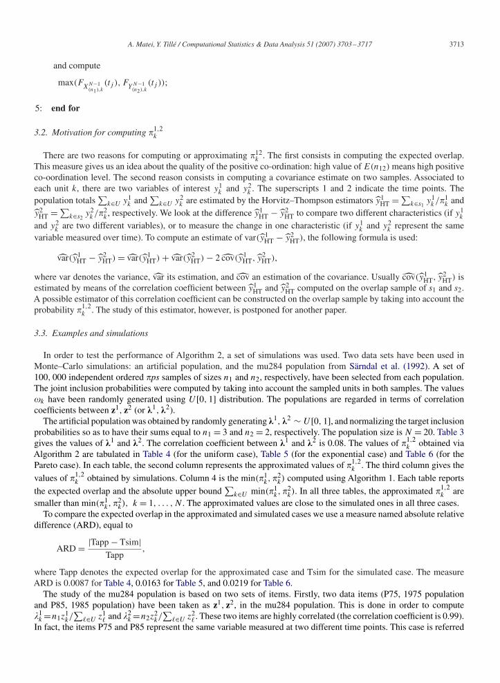
3.2. Motivation for computing �1,2k

There are two reasons for computing or approximating �12k . The first consists in computing the expected overlap.

This measure gives us an idea about the quality of the positive co-ordination: high value of E(n12) means high positiveco-oordination level. The second reason consists in computing a covariance estimate on two samples. Associated toeach unit k, there are two variables of interest y1

k and y2k . The superscripts 1 and 2 indicate the time points. The

population totals∑

k∈U y1k and

∑k∈U y2

k are estimated by the Horvitz–Thompson estimators y1HT =∑

k∈s1y1k /�1

k andy2

HT =∑k∈s2

y2k /�2

k , respectively. We look at the difference y1HT − y2

HT to compare two different characteristics (if y1k

and y2k are two different variables), or to measure the change in one characteristic (if y1

k and y2k represent the same

variable measured over time). To compute an estimate of var(y1HT − y2

HT), the following formula is used:

var(y1HT − y2

HT) = var(y1HT) + var(y2

HT) − 2 cov(y1HT, y2

HT),

where var denotes the variance, var its estimation, and cov an estimation of the covariance. Usually cov(y1HT, y2

HT) isestimated by means of the correlation coefficient between y1

HT and y2HT computed on the overlap sample of s1 and s2.

A possible estimator of this correlation coefficient can be constructed on the overlap sample by taking into account theprobability �1,2

k . The study of this estimator, however, is postponed for another paper.

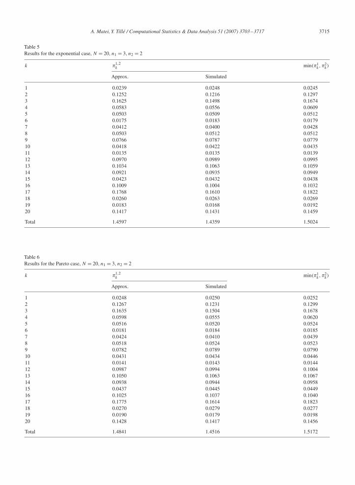
3.3. Examples and simulations

In order to test the performance of Algorithm 2, a set of simulations was used. Two data sets have been used inMonte–Carlo simulations: an artificial population, and the mu284 population from Särndal et al. (1992). A set of100, 000 independent ordered �ps samples of sizes n1 and n2, respectively, have been selected from each population.The joint inclusion probabilities were computed by taking into account the sampled units in both samples. The values�k have been randomly generated using U [0, 1] distribution. The populations are regarded in terms of correlationcoefficients between z1, z2 (or �1, �2).

The artificial population was obtained by randomly generating �1, �2 ∼ U [0, 1], and normalizing the target inclusionprobabilities so as to have their sums equal to n1 = 3 and n2 = 2, respectively. The population size is N = 20. Table 3gives the values of �1 and �2. The correlation coefficient between �1 and �2 is 0.08. The values of �1,2

k obtained viaAlgorithm 2 are tabulated in Table 4 (for the uniform case), Table 5 (for the exponential case) and Table 6 (for thePareto case). In each table, the second column represents the approximated values of �1,2

k . The third column gives the

values of �1,2k obtained by simulations. Column 4 is the min(�1

k, �2k) computed using Algorithm 1. Each table reports

the expected overlap and the absolute upper bound∑

k∈U min(�1k, �

2k). In all three tables, the approximated �1,2

k aresmaller than min(�1

k, �2k), k = 1, . . . , N . The approximated values are close to the simulated ones in all three cases.

To compare the expected overlap in the approximated and simulated cases we use a measure named absolute relativedifference (ARD), equal to

ARD = |Tapp − Tsim|Tapp

,

where Tapp denotes the expected overlap for the approximated case and Tsim for the simulated case. The measureARD is 0.0087 for Table 4, 0.0163 for Table 5, and 0.0219 for Table 6.

The study of the mu284 population is based on two sets of items. Firstly, two data items (P75, 1975 populationand P85, 1985 population) have been taken as z1, z2, in the mu284 population. This is done in order to compute�1k =n1z

1k/∑

�∈U z1� and �2

k =n2z2k/∑

�∈U z2� . These two items are highly correlated (the correlation coefficient is 0.99).

In fact, the items P75 and P85 represent the same variable measured at two different time points. This case is referred

3714 A. Matei, Y. Tillé / Computational Statistics & Data Analysis 51 (2007) 3703–3717

Table 3Values of �1

k, �2k, N = 20, n1 = 3, n2 = 2

k �1k �2

k

1 0.1722 0.02522 0.1997 0.13013 0.1680 0.22234 0.0833 0.06225 0.0525 0.23116 0.0185 0.16157 0.0440 0.08678 0.2251 0.05259 0.2556 0.079210 0.0841 0.044711 0.1221 0.014412 0.2268 0.100613 0.2414 0.106914 0.1915 0.096115 0.1148 0.045016 0.2486 0.104217 0.1824 0.230618 0.0998 0.027819 0.0198 0.033320 0.2499 0.1458

Table 4Results for the uniform case, N = 20, n1 = 3, n2 = 2

k �1,2k min(�1

k,�2k)

Approx. Simulated

1 0.0232 0.0234 0.02382 0.1232 0.1232 0.12873 0.1609 0.1474 0.16644 0.0568 0.0540 0.05955 0.0490 0.0493 0.05016 0.0170 0.0178 0.01757 0.0401 0.0387 0.04188 0.0488 0.0505 0.05009 0.0747 0.0765 0.076410 0.0406 0.0423 0.042411 0.0131 0.0137 0.013512 0.0950 0.0969 0.098013 0.1014 0.1029 0.104514 0.0901 0.0940 0.093415 0.0411 0.0425 0.042716 0.0990 0.1004 0.101817 0.1756 0.1610 0.181618 0.0252 0.0270 0.026119 0.0178 0.0178 0.018720 0.1400 0.1410 0.1454

Total 1.4326 1.4202 1.4825

to below as ‘mu284 I’. For the second set of items, we have retained the variables P75 for z1, but we have used theitem CS82 (number of Conservative seats in municipal council) instead of P85 to compute z2. Now the correlationcoefficient is 0.62. This case is referred to below as ‘mu284 II’.

For the mu284 population the units are stratified according to region (geographic region indicator; there are eightregions). Some units were removed in order to ensure �k < 1 : one unit in strata 1, 4 and 5, and three units in

A. Matei, Y. Tillé / Computational Statistics & Data Analysis 51 (2007) 3703–3717 3715

Table 5Results for the exponential case, N = 20, n1 = 3, n2 = 2

k �1,2k min(�1

k,�2k)

Approx. Simulated

1 0.0239 0.0248 0.02452 0.1252 0.1216 0.12973 0.1625 0.1498 0.16744 0.0583 0.0556 0.06095 0.0503 0.0509 0.05126 0.0175 0.0183 0.01797 0.0412 0.0400 0.04288 0.0503 0.0512 0.05129 0.0766 0.0787 0.077910 0.0418 0.0422 0.043511 0.0135 0.0135 0.013912 0.0970 0.0989 0.099513 0.1034 0.1063 0.105914 0.0921 0.0935 0.094915 0.0423 0.0432 0.043816 0.1009 0.1004 0.103217 0.1768 0.1610 0.182218 0.0260 0.0263 0.026919 0.0183 0.0168 0.019220 0.1417 0.1431 0.1459

Total 1.4597 1.4359 1.5024

Table 6Results for the Pareto case, N = 20, n1 = 3, n2 = 2

k �1,2k min(�1

k,�2k)

Approx. Simulated

1 0.0248 0.0250 0.02522 0.1267 0.1231 0.12993 0.1635 0.1504 0.16784 0.0598 0.0555 0.06205 0.0516 0.0520 0.05246 0.0181 0.0184 0.01857 0.0424 0.0410 0.04398 0.0518 0.0524 0.05239 0.0782 0.0789 0.079010 0.0431 0.0434 0.044611 0.0141 0.0143 0.014412 0.0987 0.0994 0.100413 0.1050 0.1063 0.106714 0.0938 0.0944 0.095815 0.0437 0.0445 0.044916 0.1025 0.1037 0.104017 0.1775 0.1614 0.182318 0.0270 0.0279 0.027719 0.0190 0.0179 0.019820 0.1428 0.1417 0.1456

Total 1.4841 1.4516 1.5172

3716 A. Matei, Y. Tillé / Computational Statistics & Data Analysis 51 (2007) 3703–3717

Table 7Expected overlap by stratum for mu284 I, N = 278, n1 = 4, n2 = 6

Stratum N Uniform Exponential Pareto

Tapp Tsim Tapp Tsim Tapp Tsim

1 24 3.84 3.98 3.90 3.98 3.95 3.982 48 3.87 3.99 3.91 3.99 3.94 3.983 32 3.88 3.99 3.92 3.99 3.95 3.994 37 3.88 3.99 3.90 3.99 3.93 3.995 55 3.86 3.99 3.88 3.99 3.90 3.996 41 3.87 3.99 3.89 3.99 3.93 3.987 12 3.89 3.99 3.98 3.99 3.99 3.988 29 3.82 3.99 3.92 3.97 3.99 3.95

Table 8Expected overlap by stratum for mu284 II, N = 278, n1 = 4, n2 = 6

Stratum N Uniform Exponential Pareto

Tapp Tsim Tapp Tsim Tapp Tsim

1 24 3.65 3.64 3.70 3.66 3.73 3.672 48 3.58 3.50 3.57 3.53 3.56 3.553 32 3.64 3.59 3.64 3.62 3.65 3.644 37 3.17 3.14 3.18 3.14 3.17 3.155 55 3.53 3.49 3.54 3.51 3.54 3.526 41 3.59 3.54 3.60 3.56 3.62 3.577 12 3.58 3.57 3.57 3.58 3.60 3.578 29 3.52 3.41 3.50 3.45 3.50 3.47

stratum 7. That is, the population size is N = 278. In each stratum, two ordered samples were drawn with sizes n1 = 4and n2 = 6. The strata are the same in the first and second design.

To save space in our tables, only the expected overlaps are reported in the case of the mu284 population.Tables 7 and 8 summarize the results by indicating the expected overlap by stratum for the approximated (Tapp)and simulated cases (Tsim). The number of units in each stratum is given in the second column of each table. Inmu284 I, our approximation performs better in the exponential and the Pareto cases. For the uniform case, ARDtakes values between 0.02 (in stratum 4) and 0.04 (in stratum 8). For the exponential case, ARD takes values be-tween 0.002 (in stratum 7) and 0.02 (in stratum 5). For the Pareto case, we have ARD between 0.002 (in stratum7) and 0.02 (in stratum 5). Similar results are given by mu284 II example. The ARD values for the uniform caselie between 0.002 (in stratum 7) and 0.03 (in stratum 8). For the exponential case we have ARD between 0.002 (instratum 7) and 0.01 (in stratum 8), and for the Pareto case, ARD takes values between 0.002 (in stratum 3) and 0.01(in stratum 1).

The following conclusions are made from the results of the empirical study:

(a) the approximated and the simulated values of �1,2k are close to one another, regardless of the correlation coefficient

between �1 and �2;(b) for the artificial population, the values of ARD lie between 0.008 and 0.02, and the best case appears to be the

uniform one;(c) for the mu284 population (mu284I and mu284II together), the values of ARD lie between 0.002 and 0.04, and

show no special behavior from one sampling design to another (uniform, exponential or Pareto).

A. Matei, Y. Tillé / Computational Statistics & Data Analysis 51 (2007) 3703–3717 3717

4. Conclusions

Improved numerical algorithms render possible various types of computation in order �ps sampling design withfixed order distribution shape. It is possible to compute the first-order inclusion probabilities in the case of uniform,exponential and Pareto order �ps sampling designs in a reasonable execution time using a simple method as shownin this paper. An approximation of the joint inclusion probability of a unit in two co-ordinated ordered samples isalso given. Empirical results show that this approximation gives values which are close to the simulated ones. Thesealgorithms facilitate the study and the use of order �ps sampling designs.

Acknowledgments

We would like to thank the Editor, Associate Editor, and the anonymous referees for their suggestions that led to animproved version of the paper. We would also like to thank Tanya Pamela Garcia for her helpful comments.

References

Aires, N., 1999. Algorithms to find exact inclusion probabilities for conditional Poisson sampling and Pareto �ps sampling designs. Methodol.Comput. Appl. Probab. 4, 457–469.

Aires, N., 2000. Comparisons between conditional Poisson sampling and Pareto �ps sampling designs. J. Statist. Plann. Inference 88 (1), 133–147.Aires, N., Rosén, B., 2005. On inclusion probabilities and relative estimator bias for Pareto �ps sampling. J. Statist. Plann. Inference 128 (2),

543–566.Bondesson, L., Traat, I., Lundqvist, A., 2006. Pareto sampling versus Sampford and Conditional Poisson sampling. Scand. J. Stat. 33 (4), 699–720.Cao, G., West, M., 1997. Computing distributions of order statistics. Comm. Statist. Theory Methods 26 (3), 755–764.Hájek, J., 1964. Asymptotic theory of rejective sampling with varying probabilities from a finite population. Ann. Math. Statist. 35, 1491–1523.Holmberg, A., Swensson, B., 2001. On Pareto �ps sampling: reflections on unequal probability sampling strategies. Theory Stoch. Process. 7(23)

(1–2), 142–155.Matei, A., Tillé, Y., 2005. Maximal and minimal sample co-ordination. Sankhya 67 (3), 590–612.Ng, M., Donadio, M., 2006. Computing inclusion probabilities for order sampling. J. Statist. Plann. Inference 136 (11), 4026–4042.Ohlsson, E., 1990. Sequential Poisson sampling from a business register and its application to the Swedish Consumer Price Index. R&D Report

1990:6, Statistics Sweden.Ohlsson, E., 1998. Sequential Poisson sampling. J. Official Statist. 14, 149–162.Rosén, B., 1997a. Asymptotic theory for order sampling. J. Statist. Plann. Inference 62, 135–158.Rosén, B., 1997b. On sampling with probability proportional to size. J. Statist. Plann. Inference 62, 159–191.Rosén, B., 2000. On inclusion probabilties for order �ps sampling. J. Statist. Plann. Inference 90, 117–143.Saavedra, P., 1995. Fixed sample size PPS approximations with a permanent random number. In: Proceedings of the Section on Survey Research

Methods.American Statistical Association, pp. 697–700.Särndal, C.-E., Swensson, B., Wretman, J., 1992. Model Assisted Survey Sampling. Springer, New York.Traat, I., Bondesson, L., Meister, K., 2004. Sampling design and sample selection through distribution theory. J. Statist. Plann. Inference 123,

395–413.