Measurement and modeling of exposure to selected air toxics for health effects studies and...

Janu

ary 2004

R e s e a R c h R e p o R t

H E A L T HE F F E CTSINSTITUTE

101 Federal Street, Suite 500

Boston, MA 02110, USA

+1-617-488-2300

www.healtheffects.org

R e s e a R c hR e p o R t


Number 143

June 2009

Number 143June 2009

WEBVERSIONPostedJuly 7, 2009

Measurement and Modeling of Exposure to Selected Air Toxics for Health Effects Studies and Verification by Biomarkers

Roy M. Harrison, Juana Maria Delgado-Saborit, Stephen J. Baker, Noel Aquilina, Claire Meddings, Stuart Harrad, Ian Matthews, Sotiris Vardoulakis, and H. Ross Anderson

Measurement and Modeling of Exposure to Selected Air Toxics for Health Effects Studies and

Verification by Biomarkers

Roy M. Harrison, Juana Maria Delgado-Saborit, Stephen J. Baker, Noel Aquilina, Claire Meddings, Stuart Harrad, Ian Matthews,

Sotiris Vardoulakis, and H. Ross Anderson

with a Critique by the HEI Health Review Committee

Research Report 143

Health Effects Institute

Boston, Massachusetts

Trusted Science

·

Cleaner Air

·

Better Health

Publishing history: The Web version of this document was posted at


in June 2009 andthen finalized for print.

Citation for whole document:

Harrison RM, Delgado-Saborit JM, Baker SJ, Aquilina N, Meddings C, Harrad S, Matthews I, Vardoulakis S, Anderson HR. 2009. Measurement and Modeling of Exposure to Selected Air Toxics for Health Effects Studies and Verification by Biomarkers. HEI Research Report 143. Health Effects Institute, Boston, MA.

When specifying a section of this report, cite it as a chapter of the whole document.

© 2009 Health Effects Institute, Boston, Mass., U.S.A. Asterisk Typographics, Barre, Vt., Compositor. Printed by Recycled Paper Printing, Boston, Mass. Library of Congress Catalog Number for the HEI Report Series: WA 754 R432.

Cover paper: made with at least 50% recycled content, of which at least 25% is post-consumer waste; freeof acid and elemental chlorine. Text paper: made with 100% post-consumer recycled product, acid free; nochlorine used in processing. The book is printed with soy-based inks and is of permanent archival quality.

C O N T E N T S

About HEI

v

About This Report

vii

Preface

ix

HEI STATEMENT

1

INVESTIGATORS’ REPORT

by Harrison et al.

3

ABSTRACT 3

INTRODUCTION 4

SPECIFIC AIMS 6

Overall Aim

7

Specific Goals

7

METHODS AND STUDY DESIGN 7

Recruitment of Subjects

7

Sampling Methods

9

Sampling Programs

11

Data Collection

14

Analytical Methods

15

Database Design

17

QA–QC and Record Keeping

17

STATISTICAL METHODS AND DATA ANALYSIS 19

Characterization of Personal Exposures and Microenvironmental Concentrations

19

Characterization of Urinary Biomarkers and Correlation with Personal Exposures to Selected Air Toxics

20

Source Apportionment

20

Development of the Personal Exposure Model

20

Validation of the Personal Exposure Model

22

Percent Contribution of Various Microenvironments to Overall Personal Exposures

23

RESULTS 23

Study Population

23

Behavioral Information

25

Presentation of Personal Exposure and Microenvironmental Concentration Data

25

Personal Exposures

26

Microenvironmental Concentrations

27

Summary of Personal Exposures and Microenvironmental Concentrations

30

Urinary Biomarkers

30

Correlations Between the VOC and PAH Data Sets

33

Source Apportionment

33

Development of the Personal Exposure Model

34


36

Research Report 143

Categorization of Low and High Personal Exposures

38

Percent Contributions of Various Microenvironments to Overall Personal Exposures

38

DISCUSSION 38

Study Population

38


45

Personal Exposures

49


57

Summary of Personal Exposures and Microenvironmental Concentrations

69

Urinary Biomarkers

71

Correlations Within and Between the VOC and PAH Databases

73

Source Apportionment by Factor Analysis

74

Performance of the Personal Exposure Model

74


80

Categorization of Low and High Personal Exposures

80

Percent Contributions of Various Microenvironmentsto Overall Personal Exposures to VOCs

81

SUMMARY 82


82

Personal Exposures

82


82

Urinary Biomarkers

83

Correlations

83

Source Apportionment by Factor Analysis

83

VOC and PAH Model Development

84

Personal Exposure Validation

84

Personal Exposure Categorization

84

Assessing Microenvironmental Contributionsto Personal Exposures

85

CONCLUSIONS 85

ACKNOWLEDGMENTS 86

REFERENCES 86

APPENDICES AVAILABLE ON THE WEB 94

ABOUT THE AUTHORS 94

OTHER PUBLICATIONS RESULTING FROM THIS RESEARCH 95

ABBREVIATIONS AND OTHER TERMS 96

CRITIQUE

by the Health Review Committee

97

RELATED HEI PUBLICATIONS

101

HEI BOARD, COMMITTEES, AND STAFF

103

A B O U T H E I

v

The Health Effects Institute is a nonprofit corporation chartered in 1980 as an independent research organization to provide high-quality, impartial, and relevant science on the effects of air pollution on health. To accomplish its mission, the institute

• Identifies the highest-priority areas for health effects research;

• Competitively funds and oversees research projects;

• Provides intensive independent review of HEI-supported studies and related research;

• Integrates HEI’s research results with those of other institutions into broader evaluations; and

• Communicates the results of HEI research and analyses to public and private decision makers.

HEI receives half of its core funds from the U.S. Environmental Protection Agency and half from the worldwide motor vehicle industry. Frequently, other public and private organizations in the United States and around the world also support major projects or certain research programs. HEI has funded more than 280 research projects in North America, Europe, Asia, and Latin America, the results of which have informed decisions regarding carbon monoxide, air toxics, nitrogen oxides, diesel exhaust, ozone, particulate matter, and other pollutants. These results have appeared in the peer-reviewed literature and in more than 200 comprehensive reports published by HEI.

HEI’s independent Board of Directors consists of leaders in science and policy who are committed to fostering the public–private partnership that is central to the organization. The Health Research Committee solicits input from HEI sponsors and other stakeholders and works with scientific staff to develop a Five-Year Strategic Plan, select research projects for funding, and oversee their conduct. The Health Review Committee, which has no role in selecting or overseeing studies, works with staff to evaluate and interpret the results of funded studies and related research.

All project results and accompanying comments by the Health Review Committee are widely disseminated through HEI’s Web site (


), printed reports, newsletters, and other publications, annual conferences, and presentations to legislative bodies and public agencies.

A B O U T T H I S R E P O R T

vii

Research Report 143,


, presents a research project funded by the Health Effects Institute and conducted by Dr. Roy M. Harrison of the Division of Environmental Health and Risk Management, University of Birmingham, Birmingham, United Kingdom, and his colleagues. This report contains three main sections.

The HEI Statement

, prepared by staff at HEI, is a brief, nontechnical summary of the study and its findings; it also briefly describes the Health Review Committee’s comments on the study.

The Investigators’ Report

, prepared by Harrison et al., describes the scientific background, aims, methods, results, and conclusions of the study.

The Critique

is prepared by members of the Health Review Committee with the assistance of HEI staff; it places the study in a broader scientific context, points out its strengths and limitations, and discusses remaining uncertainties and implications of the study’s findings for public health and future research.

This report has gone through HEI’s rigorous review process. When an HEI-funded study is completed, the investigators submit a draft final report presenting the background and results of the study. This draft report is first examined by outside technical reviewers and a biostatistician. The report and the reviewers’ comments are then evaluated by members of the Health Review Committee, an independent panel of distinguished scientists who have no involvement in selecting or overseeing HEI studies. During the review process, the investigators have an opportunity to exchange comments with the Review Committee and, as necessary, to revise their report. The Critique reflects the information provided in the final version of the report.

P R E F A C E

Health Effects Institute Research Report 143 © 2009

ix

HEI’s Research Program on Air Toxics Hot Spots

Air toxics comprise a large and diverse group of airpollutants that, with sufficient exposure, are known orsuspected to cause adverse effects on human health,including illness and death. These compounds areemitted by a variety of indoor and outdoor sources.Even though the ambient levels of air toxics are gener-ally low, the compounds are a cause for public healthconcern because large numbers of people are ex-posed to them over long periods. Tools and techniquesfor assessing specific health effects of air toxics are verylimited, in part because of the generally low ambientlevels of the compounds.

Air toxics are not regulated by the U.S. Environmen-tal Protection Agency (EPA) under the National Ambi-ent Air Quality Standards, but the EPA is requiredunder the Clean Air Act and its amendments to char-acterize, prioritize, and address the effects of air toxicson public health and the environment, and EPA has thestatutory authority to control and reduce the releaseof air toxics in the environment. The law also requiresthe EPA to regulate or consider regulating air toxicsfrom motor vehicles in the form of standards for fuels,vehicle emissions, or both. HEI has recently publisheda critical review of the literature on exposure andhealth effects associated with high-priority air toxicsfrom mobile sources (HEI Special Report 16, 2007).

In trying to understand the potential health effectsof exposure to toxic compounds, scientists often turnfirst to evaluating responses in highly exposed popula-tions, such as occupationally exposed workers. How-ever, workers and their on-the-job exposures are notrepresentative of the general population, and there-fore such studies may be somewhat limited in value.Another strategy is to study populations living in areasthought to have high concentrations of these pollut-ants (so-called hot spots). Such areas offer the poten-tial to conduct health investigations in groups that aremore similar to the general population.

Hot spots are generally specific areas that areexpected to have elevated levels of one or more air

toxics owing to their proximity to one or moresources. Some hot spots may have sufficiently highpollutant concentrations that they may be studied todetermine whether there is a link between exposureto air toxics and an adverse health outcome. Beforehealth effects studies can be initiated, however, actualexposures to pollutants in such hot-spot areas mustfirst be characterized — including their spatial andtemporal distributions. Understanding exposures inhot spots, as well as the sources of these exposures,will improve our ability to select the most appropriatesites, populations, and end points for subsequenthealth studies.

In January 2003, HEI issued a Request for Applica-tions (RFA 03-1) entitled “Assessing Exposure to AirToxics.” The main goal of the RFA was to suppor tresearch to identify and characterize exposure to airtoxics from a variety of sources in areas or situationswhere concentrations of air toxics are elevated. HEIwas particularly interested in studies that focused onair toxics emitted from mobile sources. Five studies,chosen to represent a diversity of sites and toxic com-pounds, were funded under this RFA. The study byHarrison and colleagues — presented in this ResearchReport — is the first of the five studies to be published.The remaining studies have been completed and arecurrently at varying stages of the HEI review and pub-lications process. All are expected to be releasedwithin the next year.

“Measurement and Modeling of Exposure to Air Toxics and Verification by Biomarker,” Roy M. Harrison, University of Birmingham, Birmingham, United Kingdom (Principal Investigator)

In the study presented in this report (HEI ResearchReport 143), Roy M. Harrison and colleagues investi-gated personal exposure to a broad range of air toxics,with the goal of developing detailed personal exposuremodels that would take various microenvironments

x

Preface

into account. Repeated measurements of exposure toselected air toxics were made for each of 100 healthynonsmoking adults who resided in urban, suburban,or rural areas of the United Kingdom, among whichexposures to traffic were expected to differ ; repeatedurine samples were also collected for analysis. Harrisonand colleagues developed models to predict personalexposure on the basis of microenvironmental concen-trations and data from time–activity diaries; they thencompared measured personal exposure with modeledestimates of exposure.

“Assessing Exposure to Air Toxics,” Eric Fujita, Desert Research Institute, Reno, Nevada (Principal Investigator)

The study by Fujita and colleagues assessed air tox-ics concentrations on major California freeways andcompared them with corresponding measurementsobtained at fixed monitoring stations. The diurnal andseasonal variations in concentrations of selected pol-lutants and the contribution of diesel- and gasoline-powered vehicles to selected air toxics and elementalcarbon were also determined.

“Assessing Personal Exposure to Air Toxics in Camden, New Jersey,” Paul Lioy, Environmental and Occupational Health Sciences Institute, Piscataway, New Jersey (Principal Investigator)

Lioy and colleagues measured personal and ambientresidential concentrations of air toxics and fine partic-ulate matter in two areas of Camden, New Jersey. Onesite was a potential hot spot with mobile sources and ahigh density of industrial facilities, and the other neigh-borhood was considered an urban reference site. Si-multaneous measurements were made of air toxics inpersonal air samples for 107 nonsmoking participantsand in air samples from fixed monitoring sites in thetwo areas. The degree of variation in the ambient con-centrations of air toxics was assessed during three sam-pling periods. In addition to the measurements of ac-tual ambient and personal exposures, the investigators

used modeling to estimate the contribution of ambientsources to personal exposure.

“Air Toxics Exposure from Vehicular Emissions at a U.S. Border Crossing,” John Spengler, Harvard School of Public Health, Boston, Massachusetts (Principal Investigator)

The study by Spengler and colleagues assessed con-centrations of mobile-source air toxics surrounding thePeace Bridge Plaza, a major border crossing betweenthe United States and Canada, located in Buffalo, NewYork. Three fixed monitoring sites were used to com-pare concentrations upwind and downwind of theplaza. Meteorologic measurements and hourly countsof trucks and cars were used to examine the relation-ship between the concentrations of air toxics and traf-fic density. To study spatial patterns, staff memberswalked along four established routes in a residentialneighborhood in West Buffalo while making measure-ments with mobile instruments and global positioningsystem (GPS)

devices.

“Air Toxics Hot Spots in Industrial Parks and Traffic,” Thomas Smith, Harvard School of Public Health, Boston, Massachusetts (Principal Investigator)

The study by Smith and colleagues was added to anongoing study, funded by the National Cancer Institute,of the relationship between exposure to dieselexhaust and mortality from lung cancer among dock-workers and truck drivers at more than 200 truck ter-minals in the United States. With support from HEI,Smith and colleagues measured levels of air toxics andparticulate matter in truck cabins and in 15 truck ter-minals throughout the United States. Twelve-hourmeasurements were made at upwind and downwindlocations around the perimeter of each terminal and atloading docks. The degree of variation among terminalsat various locations and the influence of wind directionwere evaluated with the goal of identifying the poten-tial impact of truck terminals on the surrounding areas.Continuous sampling was performed inside GPS-equipped truck cabins while they were being driven.

Synopsis of Research Report 143

H E I S T A T E M E N T

This Statement, prepared by the Health Effects Institute, summarizes a research project funded by HEI and conducted by Dr. Roy M. Harrisonat University of Birmingham, Division of Environmental Health and Risk Management, Birmingham, U.K., and colleagues. Research Report143 contains both the detailed Investigators’ Report and a Critique of the study prepared by the Institute’s Health Review Committee.

1

Measurement and Modeling of Exposure to Selected Air Toxics

BACKGROUND

Air toxics are a diverse group of air pollutants thatare known or suspected, with sufficient exposure,to cause adverse health effects including cancer,damage to the immune, neurologic, reproductive,developmental, or respiratory systems, or other healthproblems. Limited monitoring has been performedby some state and local agencies, but substantialuncertainty regarding exposure to air toxics remains,largely because of their presence in the ambientenvironment at low concentrations. Although envi-ronmental exposures to air toxics are generallylow, the potential for widespread chronic exposureand the large number of people who are exposedhave led to concerns regarding their impact on pub-lic health. Estimation of the health risks of expo-sure to air toxics is complicated by the fact thatthere are multiple sources of air toxics. Thesemay be outdoor and indoor (e.g., environmental to-bacco smoke, building materials, consumer prod-ucts, and cooking).

APPROACH

Dr. Roy Harrison investigated personal exposuresto a broad group of air toxics, with the goal of devel-oping detailed personal exposure models that takevarious microenvironments into account. In orderto provide important information on personal expo-sures to air toxics, the study was designed to captureadequate variation in exposure concentrations.Repeated measurements of exposure to selected airtoxics were made for each of 100 healthy adult non-smoking participants residing in urban, suburban,and rural areas of the United Kingdom expectedto have different traffic exposures. Measurementsincluded five repeated 24-hour measurements ofpersonal exposure to volatile organic compounds

(VOCs; including 1,3-butadiene) per participant; fiveurine samples collected to test for urinary biomarkers(polycyclic aromatic hydrocarbon [PAH] metabolites,cotinine, and

trans

-3

�

-hydroxycotinine) per partici-pant; and one 24-hour measurement of particle-phasePAHs per participant; plus concurrent measurementof microenvironmental exposures at participants’homes and workplaces — a total of 200 VOC, 1901,3-butadiene, and 168 PAH samples, as well asmeasurements in other major microenvironments.

Dr. Harrison developed models to predict per-sonal exposures on the basis of microenviron-mental concentrations and data from time–activitydiaries, and compared measured personal expo-sures with modeled estimates of exposure. Thegoal was to use these data to produce a scheme forcategorizing exposure (by compound) according tothe location of residence and other lifestyle andexposure factors, including environmental tobaccosmoke, for use in the design of health studies ofcancer incidence.

RESULTS AND IMPLICATIONS

This study serves as a rich source of recent infor-mation on personal exposures to selected air toxicsacross a range of residential locations and exposuresto non-traffic sources, with attention to spatial vari-ation and areas in which air toxics exposures werelikely to be elevated. However, most participants inthe study were young adults, thus limiting the study’sgeneralizability to other age groups. Also, owing tochallenges in recruitment, the study sample wasnot balanced.

Personal exposures were most heavily influencedby the home microenvironment and were higher inthe presence of fossil fuel combustion, environ-mental tobacco smoke, solvent use, use of selected

Research Report 143

2

consumer products, and commuting. After the homemicroenvironment, the workplace and commutingwere the largest contributors to personal exposure.The reported concentrations of selected air toxics andlevels of personal exposure were somewhat lowerthan those observed in other studies.

Harrison and colleagues used an innovativeapproach to modeling to predict personal exposureson the basis of microenvironmental concentrationdata and time–activity diaries, with the idea thatmodels could inform the design of future healthstudies. The most predictive statistical models didonly a fair-to-moderate job of predicting personalexposures, however. Statistical models based on

microenvironmental factors and lifestyle were ableto explain a fair amount of the variance in personalexposures for selected VOCs but were less predic-tive of PAH exposures. While part of the inability toeffectively model exposures may be due to the lackof measured characteristics of home ventilation,particularly air exchange rates in the home, thisstudy underscores the challenges of accurately pre-dicting personal exposures. Personal exposure mon-itoring requires extensive time and equipment, butthe science is not yet at a point at which exposuresto VOCs and PAHs can be reliably predicted fromtime–activity patterns and microenvironmental con-centrations alone.

Health Effects Institute Research Report 143 © 2009 3

INVESTIGATORS’ REPORT



Division of Environmental Health and Risk Management, University of Birmingham, Birmingham (R.M.H., J.M.D.-S., S.J.B., N.A., C.M., S.H.); Department of Epidemiology, Statistics, and Public Health, Cardiff University, Cardiff (I.M.); Public and Environmental Health Research Unit, London School of Hygiene and Tropical Medicine (S.V.); Department of Community Health Sciences, St. George’s Hospital Medical School, London (H.R.A.) — all in the United Kingdom.

ABSTRACT

The overall aim of our investigation was to quantify themagnitude and range of individual personal exposures to avariety of air toxics and to develop models for exposureprediction on the basis of time–activity diaries. The spe-cific research goals were (1) to use personal monitoring ofnon-smokers at a range of residential locations and expo-sures to non-traffic sources to assess daily exposures to arange of air toxics, especially volatile organic compounds(VOCs*) including 1,3-butadiene and particulate poly-cyclic aromatic hydrocarbons (PAHs); (2) to determinemicroenvironmental concentrations of the same air toxics,taking account of spatial and temporal variations and hotspots; (3) to optimize a model of personal exposure usingmicroenvironmental concentration data and time–activitydiaries and to compare modeled exposures with exposuresindependently estimated from personal monitoring data;(4) to determine the relationships of urinary biomarkerswith the environmental exposures to the correspondingair toxic.

Personal exposure measurements were made using anactively pumped personal sampler enclosed in a briefcase.Five 24-hour integrated personal samples were collectedfrom 100 volunteers with a range of exposure patterns foranalysis of VOCs and 1,3-butadiene concentrations ofambient air. One 24-hour integrated PAH personal expo-sure sample was collected by each subject concurrentlywith 24 hours of the personal sampling for VOCs. Duringthe period when personal exposures were being measured,workplace and home concentrations of the same air toxicswere being measured simultaneously, as were seasonallevels in other microenvironments that the subjects visitduring their daily activities, including street microenvi-ronments, transport microenvironments, indoor environ-ments, and other home environments. Information aboutsubjects’ lifestyles and daily activities were recorded bymeans of questionnaires and activity diaries.

VOCs were collected in tubes packed with the adsorbentresins Tenax GR and Carbotrap, and separate tubes for thecollection of 1,3-butadiene were packed with Carbopack Band Carbosieve S-III. After sampling, the tubes were ana-lyzed by means of a thermal desorber interfaced with agas chromatograph–mass spectrometer (GC–MS). Particle-phase PAHs collected onto a quartz-fiber filter wereextracted with solvent, purified, and concentrated beforebeing analyzed with a GC–MS. Urinary biomarkers wereanalyzed by liquid chromatography–tandem mass spec-trometry (LC–MS–MS).

Both the environmental concentrations and personalexposure concentrations measured in this study are lowerthan those in the majority of earlier published work, whichis consistent with the reported application of abatementmeasures to the control of air toxics emissions. The environ-mental concentration data clearly demonstrate the influenceof traffic sources and meteorologic conditions leading tohigher air toxics concentrations in the winter and during

This Investigators’ Report is one part of Health Effects Institute ResearchReport 143, which also includes a Critique by the Health Review Commit-tee and an HEI Statement about the research project. Correspondence con-cerning the Investigators’ Report may be addressed to Dr. Roy Harrison,University of Birmingham, Division of Environmental Health and RiskManagement, Edgbaston Park Road, School of Geography, Earth, and Envi-ronmental Sciences, Birmingham B15 2TT, United Kingdom, [email protected].

Although this document was produced with partial funding by the UnitedStates Environmental Protection Agency under Assistance Award CR–83234701 to the Health Effects Institute, it has not been subjected to theAgency’s peer and administrative review and therefore may not necessarilyreflect the views of the Agency, and no official endorsement by it should beinferred. The contents of this document also have not been reviewed byprivate party institutions, including those that support the Health EffectsInstitute; therefore, it may not reflect the views or policies of these parties,and no endorsement by them should be inferred.

*A list of abbreviations and other terms appears at the end of the Investiga-tors’ Report.

4


peak-traffic hours. The seasonal effect was also observed inindoor environments, where indoor sources add to theeffects of the previously identified outdoor sources.

The variability of personal exposure concentrations ofVOCs and PAHs mainly reflects the range of activities thesubjects engaged in during the five-day period of sampling.A number of generic factors have been identified to influ-ence personal exposure concentrations to VOCs, such asthe presence of an integral garage (attached to the home),exposure to environmental tobacco smoke (ETS), use ofsolvents, and commuting. In the case of the medium- andhigh-molecular-weight PAHs, traffic and ETS are impor-tant contributions to personal exposure. Personal exposureconcentrations generally exceed home indoor concentra-tions, which in turn exceed outdoor concentrations. Thehome microenvironment is the dominant individual con-tributor to personal exposure. However, for those subjectswith particularly high personal exposures, activities withinthe home and exposure to ETS play a major role in deter-mining exposure.

Correlation analysis and principal components analysis(PCA) have been performed to identify groups of com-pounds that share common sources, common chemistry, orcommon transport or meteorologic patterns. We used thesemethods to identify four main factors determining themakeup of personal exposures: fossil fuel combustion, useof solvents, ETS exposure, and use of consumer products.

Concurrent with sampling of the selected air toxics, atotal of 500 urine samples were collected, one for each ofthe 100 subjects on the day after each of the five days onwhich the briefcases were carried for personal exposuredata collection. From the 500 samples, 100 were selectedto be analyzed for PAHs and ETS-related urinary bio-markers. Results showed that urinary biomarkers of ETSexposure correlated strongly with the gas-phase markers ofETS and 1,3-butadiene. The urinary ETS biomarkers alsocorrelated strongly with high-molecular-weight PAHs inthe personal exposure samples.

Five different approaches have been taken to model per-sonal exposure to VOCs and PAHs, using 75% of the mea-sured personal exposure data set to develop the modelsand 25% as an independent check on the model perfor-mance. The best personal exposure model, based on mea-sured microenvironmental concentrations and lifestylefactors, is able to account for about 50% of the variance inmeasured personal exposure to benzene and a higher pro-portion of the variance for some other compounds (e.g.,75% of the variance in 3-ethenylpyridine exposure). In thecase of the PAHs, the best model for benzo[

a

]pyrene is ableto account for about 35% of the variance among exposures,with a similar result for the rest of the PAH compounds.

The models developed were validated by the independentdata set for almost all the VOC compounds. The modelsdeveloped for PAHs explain some of the variance in the in-dependent data set and are good indicators of the sourcesaffecting PAH concentrations but could not be validatedstatistically, with the exception of the model for pyrene.

A proposal for categorizing personal exposures as lowor high is also presented, according to exposure thresh-olds. For both VOCs and PAHs, low exposures are cor-rectly classified for the concentrations predicted by theproposed models, but higher exposures were less success-fully classified.

INTRODUCTION

The term “air toxics” embraces a range of gaseous or par-ticulate pollutants that are present in the air in low con-centrations and have characteristics such as toxicity orpersistence such that they are a hazard to human, plant, oranimal life. VOCs and PAHs are among the several catego-ries of compounds considered to be air toxics.

VOCs and PAHs are emitted into ambient air from awide range of sources. Major anthropogenic sources ofVOCs in ambient air include industrial processes, fossilfuel combustion for purposes of transportation, domesticheating and electricity generation, fuel distribution, sol-vent use, and landfills and waste treatment plants. Withregard to indoor air, primary sources of VOCs includeoutdoor air, ETS, fuel combustion, building materials,furnishings, furniture and carpet adhesives, paints andsolvents, cleaning agents, air fresheners, and cosmetics(Jurvelin 2003). PAHs are produced by high-temperaturereactions such as incomplete combustion and pyrolysis offossil fuels and other organic materials (Harrison et al.1996). Major anthropogenic sources of ambient-air PAHsinclude heating (with coal, oil, or wood), refuse burning,coke production, industrial processes, and operation ofmotor vehicles (Benner et al. 1989). In indoor environ-ments, PAHs are generated from cooking, smoking, and theburning of natural gas, wood, candles, or incense, as wellas being transported from the outdoors (Chuang et al. 1991;Naumova et al. 2002).

Air toxics are ubiquitous in outdoor and indoor air andare therefore of public health concern. There is evidencethat cancer, birth defects, genetic damage (InternationalAgency for Research on Cancer 1982), immunodeficiency(U.S. Environmental Protection Agency [EPA] 2007), respi-ratory disorders, (Andersson et al. 1997) and nervous sys-tem disorders (EPA 2007) can be linked to exposure tooccupational levels of air toxics. The International Agency

5

R.M. Harrison et al.

for Research on Cancer (2006) classifies 1,3-butadiene,benzene, and benzo[

a

]pyrene as known human carcino-gens; dibenz[

a,h

]anthracene as probably carcinogenic tohumans; and ethylbenzene, styrene, naphthalene, benzo[

a

]-anthracene, benzo[

b

]fluoranthene, benzo[

k

]fluoranthene,and indeno[1,2,3-

cd

]pyrene as possibly carcinogenic tohumans. Therefore, although air toxics may be associatedwith a number of adverse health outcomes, the mostimportant, especially in the public mind, is likely to becancer. Currently, however, evidence for carcinogenicityderives primarily from epidemiologic studies of occupa-tionally exposed individuals (Armstrong et al. 2004), oreven from laboratory studies of animal models. In the caseof pollutants such as benzene and the PAHs, for which theevidence for carcinogenicity from occupational exposuresis very strong, the exposures greatly exceed typical envi-ronmental concentrations to which the general public isexposed, and therefore evaluation of carcinogenic risk bymeans other than extrapolation is very difficult.

There is growing international recognition of the poten-tial health risks associated with exposure to air toxics andthe need for action to minimize these risks. Recently, thecontribution of indoor air to the exposure of an individualto pollutants has been increasingly recognized as being ofimportance (Samet and Spengler 2003; Adgate et al.2004a,b; Phillips et al. 2005). The determination of an in-dividual’s exposure to air pollution depends on the indi-vidual and his or her activity patterns, which are reflectedin the time spent in various microenvironments (Harrisonet al. 2002). Numerous international studies have reportedthat people spend 80–93% of their time indoors, 1–7% intransit in an enclosed vehicle, and 2–7% outdoors (Jenkinset al. 1992; Hinwood et al. 2003; Brunekreef et al. 2005;Koutrakis et al. 2005). It has been estimated that of the timespent indoors, approximately 60–70% is spent in the home(Thatcher and Layton 1995; Hinwood et al. 2003), whichsuggests that significant exposures may occur in the home.In addition, other indoor microenvironments, and particu-larly the workplace, are important determinants of overallpersonal exposure to air toxics (Harrison et al. 2002).

Despite the research community recognizing the impor-tance of indoor environments in personal exposure, policymakers have focused their attention on outdoor air quality.Environmental laws, standards, and other regulations havetraditionally focused on the release of pollution into the envi-ronment, and on outdoor concentrations, rather than on theextent of human exposure caused by the release. For this rea-son, the amounts of environmental pollutants to which gen-eral populations are actually exposed are rarely quantified.

Non-occupational air pollution regulations have typi-cally been applied to outdoor rather than indoor air, which

means that toxic pollutants emitted from indoor sourceshave been ignored (Ott and Roberts 1998; Jurvelin 2003).In addition, monitoring for compliance with ambient airquality standards is limited to a relatively small number ofstationary outdoor monitoring sites. Given the likely spa-tial variation in air toxics concentrations in ambient air, itis questionable to what extent such a monitoring strategyrepresents an accurate reflection of personal exposure (Kimet al. 2002). Furthermore, since people in developed coun-tries spend most of their time indoors, it can be argued thatfixed monitoring should not be used in risk assessmentfor personal exposures, as individual exposures are notwell represented.

Current assessments of public exposure to atmosphericpollutants have found that the personal exposures of theurban population to many airborne pollutants are vastlydifferent from, and often greater than, the outdoor air con-centrations measured at fixed monitoring stations (Michaelet al. 1990; Hartwell et al. 1992; Edwards et al. 2001a,b;Kim et al. 2002; Adgate et al. 2004a,b; Lai et al. 2004;Payne-Sturges et al. 2004; Phillips et al. 2005). Therefore,risk estimates based on ambient measurements may mis-estimate risks, leading to ineffective or inefficient manage-ment strategies (Payne-Sturges et al. 2004). Consequently,personal exposures cannot be determined directly fromambient background measurements from fixed monitoringstations. The alternative is personal exposure monitoring,which takes into account the mobility of people across var-ious microenvironments, according to their daily activities(Carrer et al. 2000). Personal exposure monitoring canoccur either via direct or indirect measurement. Directmeasurement is undertaken by means of personal samplers,whereas indirect exposure is determined by time–activitydiaries and microenvironmental measurements (Ott 1985).

To date, even though the study of personal exposureto air pollution is a rather well-developed science, it hasbeen restricted to a relatively limited range of pollutants.Among the air toxics, benzene has been heavily studied(Wallace 1989b; Lofgren et al. 1991; Edwards and Jantunen2001), and benzene, toluene, and the xylenes have beenthe focus for many studies of environmental concentra-tions. Edwards and colleagues (2001), as part of the AirPollution Exposure Distributions of Adult Urban Popula-tions in Europe (EXPOLIS)–Helsinki study, reported micro-environmental and personal exposure concentrations of 30target VOCs, finding ETS to be an important factor in expo-sure. Studies have also been conducted in Germany (Hoff-mann et al. 2000; Ilgen et al. 2001a), the United Kingdom(Kim et al. 2002), the United States (Wallace et al. 1985;Pellizzari et al. 1995; Turpin et al. 2007), Asia (Baek et al.1997; Chang et al. 2005), and Australia (Hinwood et al.2003). Studies assessing personal exposures to PAHs are

6


few, however (Georgiadis et al. 2001; Levy et al. 2001; Reffet al. 2005; Loh et al. 2007; Turpin et al. 2007).

In addition, for certain air toxics (e.g., 1,3-butadiene andstyrene), the extent of data from outdoor measurements isquite limited, and those from indoor measurements gener-ally even more limited, despite their carcinogenicity andhigher unit risk factor. Furthermore, the available data for1,3-butadiene are limited to specific microenvironmentssuch as automobiles, buses, homes, or workplaces (Heav-ner et al. 1996; Duffy and Nelson 1997; Kim et al. 1999,2001b; Klepeis et al. 2001). In previous studies, extensivemeasurement programs were carried out, determining con-centrations of 15 VOCs in a wide range of urban micro-environments including homes, offices, restaurants, pubs,department stores, bus and train stations, cinemas, librar-ies, perfume shops, heavily trafficked roadside locations,buses, trains and automobiles (Kim et al. 2001a; Fedorukand Kerger 2003; Lau and Chan 2003; Guo et al. 2004a). Yetthe number of measurements of VOCs and especially PAHsis still insufficient to allow for exposure estimations repre-sentative of various microenvironments. Finally, most pre-vious studies of personal exposure have been limited to1–2 days of sampling per subject (Hartwell et al. 1987;Hartwell et al. 1992; Leung and Harrison 1998; Jurvelin etal. 2001), with some exceptions, in which diurnal variationsin concentrations in individual exposures were studied for5–10 days (Kim et al. 2002; Koutrakis et al. 2005). As aresult, daily variations in exposure of individuals to VOCshave not been evaluated extensively. Thus, our study willconsiderably strengthen the database of VOC and PAH per-sonal exposure and microenvironmental measurements bygenerating new data via direct measurements.

Personal exposure can also be estimated via indirect mea-surements. An earlier study (Leung and Harrison 1998)showed that personal exposures modeled from microenvi-ronmental concentrations and personal-activity diaries canprovide a good prediction of overall measured personalexposure. Microenvironmental modeling offers an effec-tive means of estimating population exposures to pollut-ants without the considerable logistical difficulties ofpersonal sampling. This approach would be improved bydetermining the range of variability in pollutant concen-trations over space and time for key microenvironments,allowing a probabilistic approach to be taken in the use ofthese models (Harrison et al. 2002). Activity patterns havea significant influence on personal exposure. Therefore, astudy of the typical means and ranges of activity patternsof susceptible groups would permit microenvironmentalmodels to be included in probabilistic models (Harrisonet al. 2002). The power of this approach can be strength-ened by measuring exposures of more individuals and inmicroenvironments under various conditions.

Although previous studies have shed light on the distri-bution of concentrations seen in personal exposures and invarious microenvironments, and much work has been con-ducted with the aim of modeling population exposures toair pollutants using information collected in time–activitydiaries and using microenvironmental concentrations, verylittle has been done toward validating such models at thelevel of the individual. The present study aimed to determinethe statistical confidence with which personal exposurescan be reconstructed using measured microenvironmentalconcentrations, to demonstrate the confidence with whichindividual personal exposures can be categorized as low-risk or high-risk on the basis of limited lifestyle informa-tion such as that which can be collected in a questionnaire.

Finally, a major goal of environmental epidemiology isto establish quantitative relationships between exposuresto air toxics and the associated risks of disease. Biologicalmonitoring has been increasingly viewed as a desirablealternative to air sampling for characterizing environmen-tal exposures, not only because it accounts for all possibleexposure routes but also because it covers unexpected oraccidental exposures and reflects inter-individual differ-ences in uptake or genetic susceptibility (Lin et al. 2005).Urinary biomarkers have been widely used for assessingoccupational exposure to air toxic concentrations becausethe dose–response relationship between air toxics in suchexposures and biomarkers is of importance in settingthreshold values (Jacob et al. 2007). Nevertheless, to datethere are few studies in which urinary biomarkers havebeen used to assess non-occupational exposures (Buckleyet al. 1995; Scherer et al. 1999; Scherer et al. 2000; Hu et al.2006). In this study, we aimed to collect urine samples,analyze urinary metabolites, and relate them to corre-sponding air toxic exposures to establish the exposure–response relationship in non-occupational environmentalexposures.

This study seeks to lead to advances in understandingthe causes and magnitudes of exposures to relevant airtoxic substances — 15 VOCs and 16 PAHs — and to estab-lish whether collecting lifestyle information and/or urinarybiomarker data is sufficient to model personal exposuresreliably, as compared with collecting independent data onexposures by using personal samplers, for a range of airtoxic substances.

SPECIFIC AIMS

This research is concerned primarily with the issue ofquantifying personal exposures to air toxics according tothe location of documented exposure and associated emis-sions from specific sources such as road traffic and ETS.

7


The aim is to provide a validated approach to the estima-tion of personal exposure to determine whether personalexposures can be predicted using data from a lifestyle ques-tionnaire, allowing individuals to be differentiated into arange of personal exposure groupings that could be used ina subsequent epidemiological study of either a case–controlor ecological (spatial analysis) design.

Since air toxic substances are not emitted uniformlyfrom a single source, their concentrations may not corre-late among various exposure environments; therefore, itwould be desirable to measure microenvironmental con-centrations of a wide range of air toxics to establish theinter-relationships among them while also determiningthe relationships between microenvironmental concentra-tions and personal exposures through direct measurementsand modeling.

OVERALL AIM

To quantify the magnitude and range of individual per-sonal exposures to a group of selected air toxics and todevelop models for exposure prediction on the basis oftime–activity diaries.

SPECIFIC GOALS

The specific goals of this research were as follows:

• To use personal monitoring of volunteer nonsmokerswith a range of residential locations and exposures tonon-traffic sources to assess daily exposures.

• To determine microenvironmental concentrations ofa range of air toxics, taking spatial and temporal vari-ations and hot spots into account.

• To study the trend in the relationship of environmen-tal exposures to selected air toxics and urinary bio-marker levels.

• To optimize a model of personal exposures based onmicroenvironmental concentration data and time–activity diaries and to compare modeled exposureswith exposures independently estimated from per-sonal monitoring data.

• To produce a method for categorizing exposures (onthe basis of compound) according to location of resi-dence and other lifestyle and exposure factors (e.g.,ETS) for use in the design of case–control and ecolog-ical studies of cancer incidence.

The targeted air toxics were categorized into three groupsthat require different methods of sampling and analysis.

1. VOCs excluding 1,3-butadiene: Benzene, ethylbenzene,

n

-hexane, naphthalene, styrene, toluene,

o-

xylene,

m-

xylene,

p-

xylene, 1,3,5-trimethylbenzene, 1,2,4-trimethylbenzene,

p-

isopropyltoluene, pyridine, and3-ethenylpyridine. (Note that naphthalene wasgrouped with the VOCs for purposes of sampling andanalysis, despite being the most abundant PAH in thegas phase.)

2. 1,3-Butadiene. (Because of its high volatility, 1,3-butadiene was considered separately from the rest ofthe VOCs for sampling and analysis, but it is groupedwith the VOCs throughout this Investigators’ Report.)

3. PAHs: Acenaphthylene, acenaphthene, fluorene, phe-nanthrene, anthracene, fluoranthene, pyrene,benzo[

a

]anthracene, chrysene, benzo[

b

]fluoranthene,benzo[

j


k


a

]-pyrene, indeno[1,2,3-

cd

]pyrene, benzo[

g,h,i

]perylene,dibenz[

a,h

]anthracene, and coronene.

METHODS AND STUDY DESIGN

RECRUITMENT OF SUBJECTS

We recruited 100 healthy adult volunteers for mea-surement of personal exposure and indoor microenviron-mental (home and office) concentrations. Selection wasperformed without regard to age, sex, or ethnic back-ground. Potential subjects were excluded if they weresmokers, under 18 years old, unhealthy (e.g., had chronicrespiratory or coronary disease or cancer), unable to carrythe personal sampler for any reason, or exposed to PAHs orVOCs at work or if they traveled more than 2 hours per dayin the course of their work, their commute from work tohome was more than 2 hours in duration, or the distancefrom home to the workplace was more than 20 miles.

Subjects resided in three different areas of the UnitedKingdom: London (11 volunteers), where some of thehighest traffic exposures were anticipated; West Midlands(79 volunteers), where traffic exposures were expected tobe intermediate; and South Wales (10 volunteers), whichhas a broad gradient between clean rural areas and moreheavily contaminated urban environments.

After applying the exclusion criteria, we used four keydeterminants to further define our selection of subjects,including the number of subjects we sought to enroll ineach category:

1. Location: Urban (40 subjects in London and Bir-mingham, the urban center of West Midlands), sub-urban (40 subjects in suburban Birmingham, WestMidlands), or rural (20 subjects in rural West Midlandsand South Wales).

8


2. Exposure to ETS: No (> 80 subjects), or yes (< 20subjects).

3. Integral garage: No (70–80 subjects) or yes (20–30subjects).

4. Proximity to major road: Within the first line of prop-erties (50 subjects) or beyond the first line (50 sub-jects). Homes were considered as first-line propertiesif they were located on an A-class road (a road de-signed for large volumes of traffic and heavy vehicles)running through an urban or suburban area, on a roadtraveled by more than 20,000 vehicles per day, on abusy A road in rural area, or on a busy B-class road (aroad designed for lower volumes of traffic includingheavy vehicles) in an urban or suburban area.

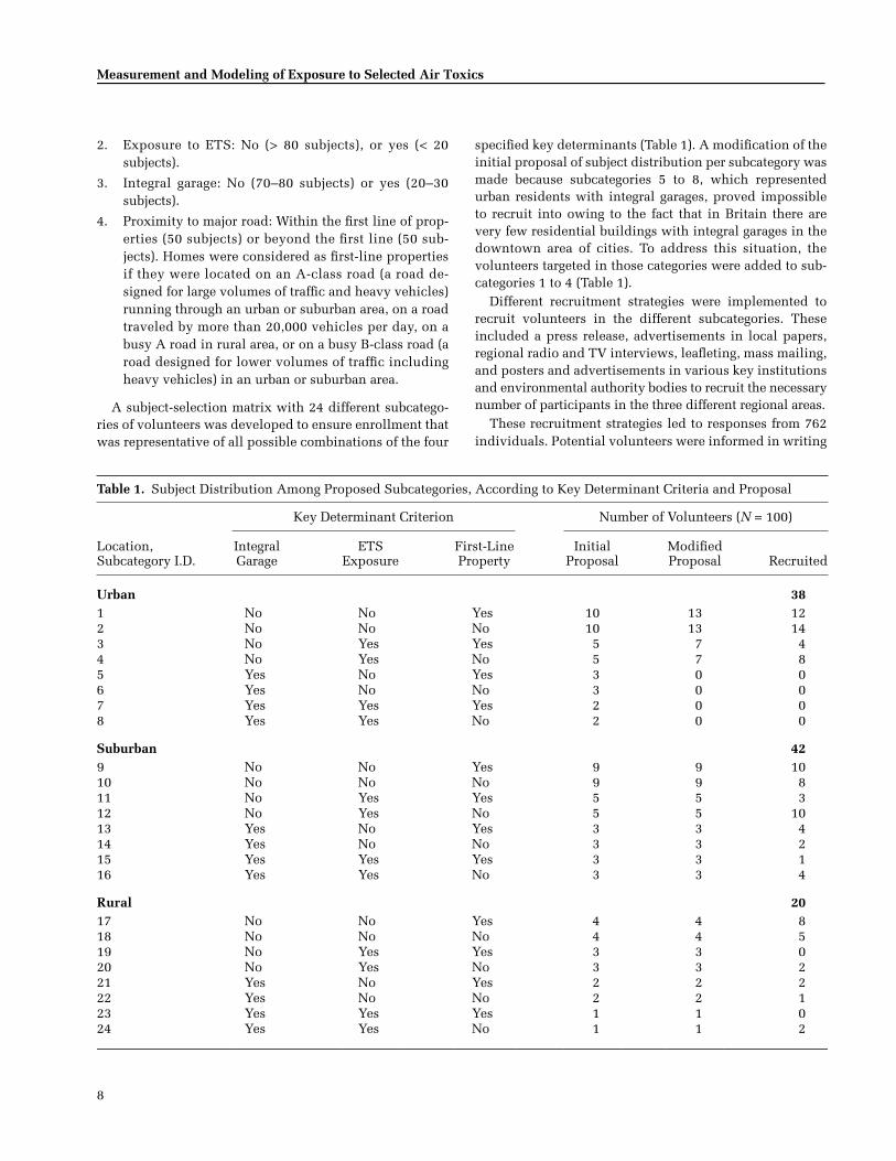
A subject-selection matrix with 24 different subcatego-ries of volunteers was developed to ensure enrollment thatwas representative of all possible combinations of the four

specified key determinants (Table 1). A modification of theinitial proposal of subject distribution per subcategory wasmade because subcategories 5 to 8, which representedurban residents with integral garages, proved impossibleto recruit into owing to the fact that in Britain there arevery few residential buildings with integral garages in thedowntown area of cities. To address this situation, thevolunteers targeted in those categories were added to sub-categories 1 to 4 (Table 1).

Different recruitment strategies were implemented torecruit volunteers in the different subcategories. Theseincluded a press release, advertisements in local papers,regional radio and TV interviews, leafleting, mass mailing,and posters and advertisements in various key institutionsand environmental authority bodies to recruit the necessarynumber of participants in the three different regional areas.

These recruitment strategies led to responses from 762individuals. Potential volunteers were informed in writing

Table 1.

Subject Distribution Among Proposed Subcategories, According to Key Determinant Criteria and Proposal

Location, Subcategory I.D.

Key Determinant Criterion Number of Volunteers (

N

= 100)

Integral Garage

ETSExposure

First-LineProperty

InitialProposal

ModifiedProposal Recruited

Urban 38

1 No No Yes 10 13 122 No No No 10 13 143 No Yes Yes 5 7 44 No Yes No 5 7 85 Yes No Yes 3 0 06 Yes No No 3 0 07 Yes Yes Yes 2 0 08 Yes Yes No 2 0 0

Suburban 42

9 No No Yes 9 9 1010 No No No 9 9 811 No Yes Yes 5 5 312 No Yes No 5 5 1013 Yes No Yes 3 3 414 Yes No No 3 3 215 Yes Yes Yes 3 3 116 Yes Yes No 3 3 4

Rural 20

17 No No Yes 4 4 818 No No No 4 4 519 No Yes Yes 3 3 020 No Yes No 3 3 221 Yes No Yes 2 2 222 Yes No No 2 2 123 Yes Yes Yes 1 1 0

24

Yes

Yes

No

1

1

2

9


of the aims of the study and of the activities that wereexpected of them, none of which required any change inthe normal pattern of activities; hence, they were exposedto no additional risks. Volunteers were asked to complete ascreening questionnaire containing information about per-sonal data, the key determinant criteria, and exclusion cri-teria in order to be classified into subcategories. They werealso asked to give their consent to participate in the study,which was required for recruitment. The subject infor-mation sheets and screening questionnaires, as well asthe consent forms, were approved by the Local ResearchEthics Committee for South Birmingham. Among the orig-inal 762 respondents, 49 were unable to be contacted, 252did not return their screening questionnaire and consentform, 51 met one or more of the exclusion criteria, and 14expressed their wish to no longer participate in the study.Therefore, the final number of volunteers suitable forrecruitment was 396. The numbers of subjects recruitedwith each method is summarized in Table 2.

Although overall we had a large number of people inter-ested in participating in the project, our requirement ofgrouping them into 20 specific subcategories relating to thelocation of their home, proximity to a busy road, presence orabsence of integral garage, and exposure to ETS meant thatwe had certain subcategories such as 12 and 17 (see Table 1)with large number of volunteers but other subcategoriessuch as 15, 19, and 23 which had few or no volunteers.

The main concern for recruitment of participants wasexposure to ETS. This criterion could not be specifically

evaluated during the recruitment process, unlike whetherthe home was a first-line property or had an integral garage.Although we had plenty of volunteers who met a givenrequirement, finding those who met some combinations ofrequirements (e.g., having an integral garage and a first-line home in a rural location and being exposed to ETS) wasproblematic. Because of such difficulties in recruitment,after exhausting all the recruitment methods, the final dis-tribution of subjects per subcategory was slightly differentthan that initially proposed (Table 1). Only 16 recruitedsubjects had integral garages, when initially the proposalwas to recruit 20–30 such subjects; a total of 34 subjectswere exposed to ETS on at least one day, when initially theproposal was to recruit 30–40 subjects; and finally, 44 sub-jects lived on a busy road (resided in a first-line property),when the proposal was 50 subjects. Nevertheless, the over-all balance among the various key factors was not compro-mised and the subjects recruited represent a wide range ofresidential locations with varying degrees of automotivepollution, ETS exposures, and concentrations of selectedair toxics, which enabled the work to proceed.

SAMPLING METHODS

Sampling Devices

Adsorption tubes were used for collection of VOC com-pounds including 1,3-butadiene, whereas quartz-fiber filterswere the sampling medium used to collect particle-phasePAHs. The sorbent tubes used for VOC and 1,3-butadienesampling were stainless-steel tubes 17.8 cm (7 inches) inlength, 0.6 cm (0.25 inches) in external diameter, and 0.49 cm(0.20 inches) in internal diameter. The tubes were packedwith a dual-adsorbent bed separated and plugged withunsilanised glass wool, fitted with appropriate ferrules andSwagelok caps, and conditioned at the University of Bir-mingham. Different adsorbents were used for sampling themain group of VOC compounds and 1,3-butadiene (Table 3).

Table 2.

Suitable Volunteers Recruited, According to Recruitment Method

Method of RecruitmentNumber of Volunteers

Media (local press, radio, and TV) 229Newspaper article 1/17/2006 17Posters 2Referrals 12Leafleting in West Midlands 23Leafleting in Wales 16E-mail distribution in London

(via environment authority bodies) 13Leafleting in London 0Mass mailing 62MATCH Internet site 1Active recruitment by Swansea

city council 20Active recruitment by Birmingham

city council 1

Total

396

Table 3.

Sorbent Tubes Used for VOC Sampling

VOC Sorbent Material

Quantityof SorbentMaterial

(mg)

Any studied, except1,3-butadiene

Tenax

®

GR (60/80 mesh) 300Carbotrap™ (20/40 mesh) 600

1,3-Butadiene Carbopack™ B (60/80 mesh) 1000

Carbosieve™ SIII (60/80 mesh)

150

10


The adsorbent materials were purchased from Supelco(Dorset, United Kingdom). Tubes were conditioned withhelium for one hour at 275

�

C for use in sampling VOCs andat 360

�

C for 1,3-butadiene, either before use or after theanalysis of highly polluted samples. Conditioned sorbenttubes were stored, wrapped in aluminum foil, inside air-tight metal tins at 4

�

C in a refrigerator.

All collected samples were kept under refrigeration aftersampling and before analysis. Tubes containing sampleswere stored, wrapped in aluminum foil, inside metal tinsin a refrigerator dedicated to either 1,3-butadiene or allother sampled VOCs.

The sampling material used to collect PAHs was filtermedia. For the first 33 subjects, glass-fiber filters were used(Whatman GF/A glass microfiber filter, 47 mm in diameter);sampling for the remaining subjects was performed withpreconditioned quartz-fiber filters (Millipore AQFA rein-forced quartz fiber filter, 47 mm in diameter). This changein filter media occurred after the method for extraction andanalysis of PAHs from filters was developed and validatedduring the second year of the project. The method devel-oped showed that the best filter on which to collect PAHswas the quartz-fiber filter, pre-baked for 48 hours at 400

�

C.Before sampling, the pre-treated filters were stored insidemetal tins that were wrapped in aluminum foil and placedin an airtight glass jar. All filters that contained sampleswere individually stored inside metal tins wrapped in alu-minum foil, in a separate freezer.

Personal Exposures

Personal exposure to selected air toxics was monitoredby using actively pumped personal sampling devices tocollect the following air toxics:

1. VOCs excluding 1,3-butadiene: Benzene, ethylben-zene,

n-

hexane, naphthalene, styrene, toluene,

o-

xylene,

m-

xylene,

p-

xylene, 1,3,5-trimethylbenzene, 1,2,4-trimethylbenzene,

p-

isopropyltoluene, pyridine, and3-ethenylpyridine.

2. 1,3-Butadiene.

3. PAHs (particle phase only): Acenaphthylene, acenaph-thene, fluorene, phenanthrene, anthracene, fluoran-thene, pyrene, benzo[

a

]anthracene, chrysene,benzo[

b


j


k

]-fluoranthene, benzo[

a

]pyrene, indeno[1,2,3-

cd

]-pyrene, benzo[

g,h,i

]perylene, dibenz[

a,h

]anthracene,and coronene.

The design of the personal exposure sampler involved adirect-current personal sampler pump (SKC model 224-PCXR8) connected to the sorbent tubes and a second DCpump connected to the PAH filter. The setup was fitted in

small aluminum briefcases (Figure A1.1, Appendix 1; allappendices are available on the HEI Web site) and extrapower was supplied via additional batteries containedwithin the briefcase. The personal exposure sampler mon-itored air toxics with the following design conditions:

1.

VOCs in the gas phase, excluding 1,3-butadiene

: Thesampling method (Kim et al. 2001a) involved drawingair, at 40 mL min

�

1

, through an adsorbent tube.

2.

1,3-Butadiene in the gas phase

: 1,3-Butadiene wascollected, at a flow rate of 30 mL min

�

1

, on an adsor-bent tube (Kim et al. 1999).

3.

PAHs in the particulate phase

: Particle-phase PAHswere collected onto a quartz-fiber filter at a flow rateof 3 L min

�

1

(Lim et al. 1999).

The setup of the sampling equipment was optimized tominimize noise and temperature levels, as well as weight.Samplers proved robust and fit for our purposes. Therecruited subjects were generally happy to carry their per-sonal samplers at all times. They carried the briefcaseseither from the handle, with the inlets at hip height, orwith the use of a strap carried over the shoulder.

Subject-Related Microenvironments

Microenvironmental samplers (ME samplers) were de-signed and constructed (Figure A1.2, Appendix 1) to mea-sure selected air toxics at each volunteer’s home andworkplace. The sampler was alternating current–powered,programmable, and was designed to collect two consecu-tive samples.

The ME samplers were designed to monitor air toxicsunder the following conditions:

1.


:VOCs were collected at 80 mL min

�

1

for 12 hours inthe home and at 120 mL min

�

1

for 8 hours in theworkplace.

2.

1,3-Butadiene in the gas phase:

1,3-Butadiene wascollected at 60 mL min

�

1

for 12 hours in the homeand at 90 mL min

�

1

for 8 hours in the workplace.

3.

PAHs in the particulate phase:

Particle-phase PAHswere collected onto a quartz-fiber filter at a flow rateof 6 L min

�

1

for 12 hours in the home and at a flowrate of 9 L min

�

1

for 8 hours in the workplace.

Other Microenvironments

An “other microenvironmental” (OME) sampler wasalso designed and constructed, powered by direct cur-rent, to be used in microenvironments where no powersupply was available for sampling during short time peri-ods (2 hours or less).

11


The OME sampler (Figure A1.3, Appendix 1) wasdesigned to monitor air toxics as follows:

1.


:VOCs were collected at 480 mL min

�

1

for 2 hours.

2.

1,3-Butadiene in the gas phase

: 1,3-Butadiene wascollected at 360 mL min

�

1

for 2 hours.

3.

PAHs in the particulate phase

: Particle-phase PAHswere collected onto a quartz-fiber filter at a flow rateof 12 L min

�

1

for 2 hours.

Urine Sampling

Urine samples were collected with the purpose of ana-lyzing urinary biomarkers related to the selected air toxicsunder study. The first midstream urine sample in themorning was collected every day for each volunteer foranalysis of the urinary biomarkers corresponding to theprevious 24 hours of sampling. Urine samples were col-lected in 100-mL polypropylene cups and transferred tothe laboratory in portable coolers containing ice packs.Once in the laboratory, 30 mL of the urine sample wastransferred to smaller polypropylene vials, which werestored in the freezer at

�

20

�

C. After a short time, the frozenurine samples were stored in a

�

80

�

C freezer.

A total of 500 urine samples were collected, five for eachof the 100 subjects. From among those samples, 100 werechosen for analysis. They had to have been either collectedon the morning after days where subjects were exposed totobacco smoke or after days when PAHs were sampled.About 15 mL of each urine sample was sent in dry ice to theDivision of Clinical Pharmacology at the University of Cali-fornia, San Francisco. In the research facilities of the groupled by Dr. Peyton Jacob III, urine samples were analyzedfor the ETS metabolites cotinine and

trans

-3

�

-hydroxy-cotinine and the PAH metabolites 1-hydroxyfluorene, 2-hydroxyfluorene, 3-hydroxyfluorene, 1-hydroxyphenan-threne, 2-hydroxyphenanthrene, 3+4-hydroxyphenanthrene,and 1-hydroxypyrene.

SAMPLING PROGRAMS

Personal Exposures

With the personal exposure sampler, the exposure of eachvolunteer was sampled for VOCs (including 1,3-butadiene)for a total of five consecutive 24-hour periods. In addition,particle-phase PAHs were sampled during one 24-hourperiod for 95 of the 100 volunteers.

Collection of the samples was spread over two years,from May 2005 to May 2007. Subjects in London weresampled in spring and summer (May–June 2006), subjectsin Wales were sampled in winter (October 2006–February

2007) and subjects in West Midlands were sampledthroughout the four seasons (May 2005–May 2007).

Duplicate samples were taken for 3% of the study popu-lation, and in 3%, weekend samples were obtained. A totalof 521 samples were collected for VOCs and 1,3-butadiene,and 99 samples were collected for particle-phase PAHs.

Subject-Related Microenvironments

During the period when personal exposure was mea-sured, there was a simultaneous program of measurementof subject-related microenvironments such as in the work-place and the home. Detailed information on the sam-pling days, which were concurrent with those for personalsampling, and background pollutant levels is available inAppendix 2.

VOC, 1,3-butadiene, and PAH samples were collected inthe subjects’ homes (as two 12-hour samples, one during theday and the other at night). The preferred place to locatethe ME sampler was the living room, where the subjectsspent most of their active time at home. Samples of VOCs,1,3-butadiene, and PAHs were also collected in some of thesubjects’ workplaces, concurrently with personal exposuresamples for eight hours. As most of the volunteers wereoffice workers, most of the workplaces were offices. Otherworkplaces that were sampled were a health center, a nurs-ery/playschool, a laboratory and a garden center. The num-bers of samples collected in the home and workplace arelisted in Table 4.

Other Microenvironments

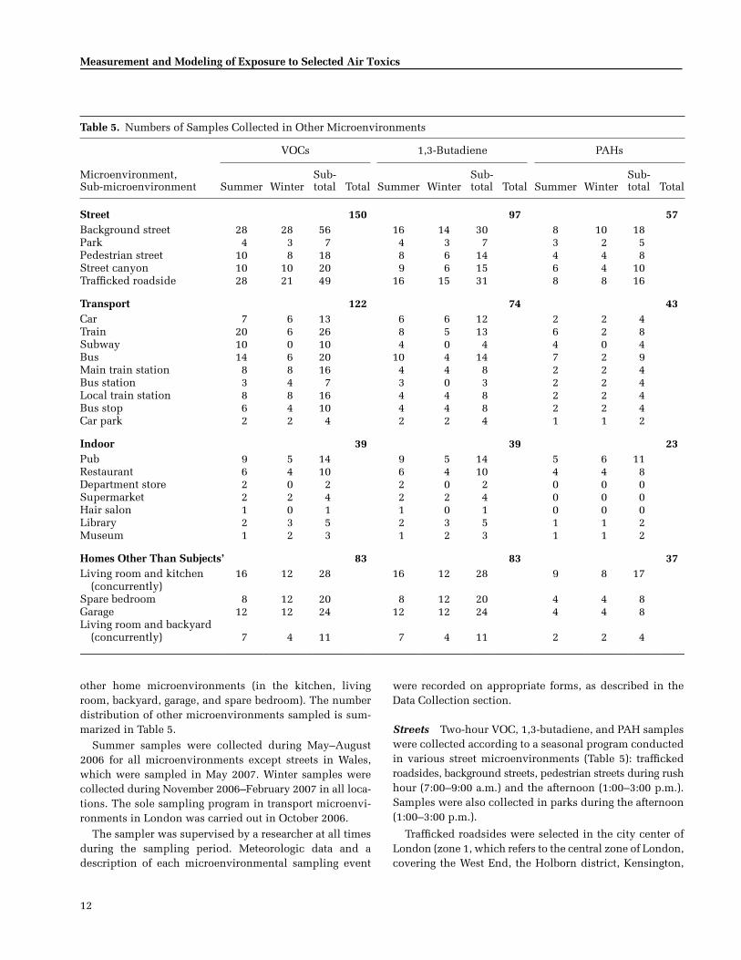
In addition to the sampling of subject-related microenvi-ronments, we carried out a seasonal program of measure-ment of other microenvironments that the public visits inthe course of their daily activities. These other microenvi-ronmental measurements were independent from the sub-ject’s sampling program. The locales sampled includedstreet microenvironments (e.g., trafficked roadside loca-tions, background streets, and parks), transport microenvi-ronments (e.g., cars, trains, buses, and bus stations), indoormicroenvironments (e.g., restaurants and libraries) and

Table 4.

Numbers of Samples Collected in Subject-Related Microenvironments

Air ToxicHome,

DayHome,Night Workplace Total

VOCs 80 80 40 2001,3-Butadiene 76 76 38 190

PAHs

66

66

36

168

12


other home microenvironments (in the kitchen, livingroom, backyard, garage, and spare bedroom). The numberdistribution of other microenvironments sampled is sum-marized in Table 5.

Summer samples were collected during May–August2006 for all microenvironments except streets in Wales,which were sampled in May 2007. Winter samples werecollected during November 2006–February 2007 in all loca-tions. The sole sampling program in transport microenvi-ronments in London was carried out in October 2006.

The sampler was supervised by a researcher at all timesduring the sampling period. Meteorologic data and adescription of each microenvironmental sampling event

were recorded on appropriate forms, as described in theData Collection section.

Streets

Two-hour VOC, 1,3-butadiene, and PAH sampleswere collected according to a seasonal program conductedin various street microenvironments (Table 5): traffickedroadsides, background streets, pedestrian streets during rushhour (7:00–9:00 a.m.) and the afternoon (1:00–3:00 p.m.).Samples were also collected in parks during the afternoon(1:00–3:00 p.m.).

Trafficked roadsides were selected in the city center ofLondon (zone 1, which refers to the central zone of London,covering the West End, the Holborn district, Kensington,

Table 5.

Numbers of Samples Collected in Other Microenvironments

Microenvironment,Sub-microenvironment

VOCs 1,3-Butadiene PAHs

Summer WinterSub-total Total Summer Winter

Sub-total Total Summer Winter

Sub-total Total

Street 150 97 57

Background street 28 28 56 16 14 30 8 10 18Park 4 3 7 4 3 7 3 2 5Pedestrian street 10 8 18 8 6 14 4 4 8Street canyon 10 10 20 9 6 15 6 4 10Trafficked roadside 28 21 49 16 15 31 8 8 16

Transport 122 74 43

Car 7 6 13 6 6 12 2 2 4Train 20 6 26 8 5 13 6 2 8Subway 10 0 10 4 0 4 4 0 4Bus 14 6 20 10 4 14 7 2 9Main train station 8 8 16 4 4 8 2 2 4Bus station 3 4 7 3 0 3 2 2 4Local train station 8 8 16 4 4 8 2 2 4Bus stop 6 4 10 4 4 8 2 2 4Car park 2 2 4 2 2 4 1 1 2

Indoor 39 39 23

Pub 9 5 14 9 5 14 5 6 11Restaurant 6 4 10 6 4 10 4 4 8Department store 2 0 2 2 0 2 0 0 0Supermarket 2 2 4 2 2 4 0 0 0Hair salon 1 0 1 1 0 1 0 0 0Library 2 3 5 2 3 5 1 1 2Museum 1 2 3 1 2 3 1 1 2

Homes Other Than Subjects’ 83 83 37Living room and kitchen

(concurrently)16 12 28 16 12 28 9 8 17

Spare bedroom 8 12 20 8 12 20 4 4 8Garage 12 12 24 12 12 24 4 4 8Living room and backyard

(concurrently) 7 4 11 7 4 11 2 2 4

13


Paddington, and the city of London) and the city centerand suburban areas of West Midlands and among traf-ficked rural roads crossing through a village (A roads) inWales. Background streets were selected in the city centerof London (zone 1); in the city center and suburban areasof Birmingham, and in a rural village in Wales. Pedestrianstreets were located in the city centers of London and Bir-mingham as well as in a suburban area in Birmingham.Parks were located in the city center of London and in sub-urban areas in Birmingham.

Samples were collected mainly in Birmingham, forlogistical reasons. However, samples from trafficked road-sides and background streets were also collected in Londonand Wales, in two different locations, during each seasonand each time period mentioned above. One sample from apedestrian street and one from a park were collected inLondon for each season and each time period.

The OME sampler was located on top of a portable tableon the curb, with the inlets facing the road or street. Thesampler was placed in the same position and locationevery time a given site was sampled, regardless of time ofday or season. In the case of the park and the pedestrianstreet, the sampler was located away from local sourcesand trees or walls, to avoid shadowing effects.

Transport Microenvironments Two-hour VOC, 1,3-buta-diene, and PAH samples were collected in the West Mid-lands area in a seasonal program in various mobile trans-port microenvironments (Table 5), namely bus, train, andcar during rush hour (7:00–9:00 a.m.) and the afternoon(1:00–3:00 p.m.). Samples were also collected in Londontransport systems in one sampling event carried out in theautumn, in which samples were collected in two differentbuses, two trains, and two subway trains at rush hour andin the afternoon.

The buses and trains sampled covered linear routesfrom the city center outward into suburban areas, and viceversa, with an average traveled distance of 30 miles perleg. The car samples were taken in Birmingham city centerand suburban areas with typical traffic patterns for citiesand suburban areas, respectively.

Sampling in vehicles was performed with the samplersecured with ropes to the passenger seat. The inlets facedthe center of the car or the aisle of the train or bus. In double-decker buses, the sampler was located on the bottom deck.

In addition, 2-hour VOC, 1,3-butadiene, and PAH sam-ples were collected during a seasonal program at varioustransport stations (Table 5). Two samples were collected insummer and in winter during rush hour and in the after-noon, as defined above, at main train stations, local trainstations, and local bus stops. Obtaining permission forsampling in bus stations proved to be very difficult, and

only one location could be sampled at the two proposedtimes in summer and winter. In the case of the car parks,two samples were taken in two different locations in bothseasons, in the afternoon.

Main train and bus stations were located in the city cen-ters of Birmingham and London, respectively. The localbus stops and train stations were located in suburban areasof Birmingham. The car parks were multi-storey buildingslocated in the city center of Birmingham. The samplerswere placed on a portable table in the main passenger areas:the waiting area of the bus stations, the platform of thetrain stations, on the curb at local bus stops, and in a park-ing space within the car parks. The inlets faced the flow oftraffic, and the position was replicated each time a givenlocation was sampled.

Indoor Areas To assess air toxic levels in indoor loca-tions other than homes and workplaces, a seasonal programwas designed to measure VOC and PAH concentrations invarious indoor environments (Table 5). Pubs, restaurants,libraries, museums, supermarkets, department stores, andhair salons were the indoor microenvironments chosen toreflect common places frequented by people during theirnormal day-to-day activities.

A total of 24 VOC and 1,3-butadiene samples and 19 PAHsamples were collected in pubs and restaurants. FifteenVOC and 1,3-butadiene samples were monitored in otherindoor environments, whereas just four PAH samples wereobtained from a library and museum (Table 5). All sampleswere collected during daytime hours over 2-hour intervals,preferably from 1:00–3:00 p.m., although some pub sam-ples were collected during the evening (6:00–8:00 p.m.).Because of the difficulty in getting permission to measureindoor microenvironments, just two libraries, one museum,and one supermarket were sampled during both seasons.We obtained permission from managers of one departmentstore and one hair salon to collect one sample during thesummer. On the other hand, permission was given by man-agers of five pubs and four restaurants for sampling in theirpremises in summer and winter.

All these indoor microenvironments were sampled in Bir-mingham. The pubs and restaurants were located in urban,suburban, and rural areas. The other indoor environmentswere located mainly in a suburban area. The sampler wasplaced on a table with the inlets facing the center of themicroenvironment in a location representative of the envi-ronment (e.g., a table for customers in a pub).

Homes Other Than Subjects’ Residences VOC, 1,3-buta-diene, and PAH samples were collected as part of a sea-sonal program in homes other than subjects’ home, mainly

14


in suburban areas, in various home microenvironments suchas kitchens, living rooms, spare bedrooms, and garages.This sampling was conducted over 12-hour periods duringthe day and 12-hour periods during the night (Table 5).Samples were also collected in backyards (over 6-hourdaytime periods). Some of these microenvironments weresampled concurrently, such as living rooms and kitchensor living rooms and backyards.

DATA COLLECTION

Subject-Related Information

First, to enable reconstruction of exposures from micro-environmental measurements, the subjects kept activitydiaries in which they recorded their location and mode ofactivity every 30 minutes. If a number of activities wereconducted within the sampling day, they were asked to listthese. Basic lifestyle information and important factorsinfluencing exposure, including the presence of a smoker,the degree of ventilation, and the presence of an integralgarage at the home, were also recorded by subjects, as wasthe precise location of residence and workplace and theirproximity to neighboring highways and busy roads. Theinformation collected from the subjects was recorded inthe following forms (Appendix 3).

• The time–activity diaries gave information, for every30 minutes, about where the volunteers had been,what they were doing, whether there was ventilation,and whether there were people smoking.

• The traveling description sheet gave information aboutthe trips the subjects took every day (e.g., means oftransport, time spent traveling, state of the roads, andplaces traveled through).

• The location description sheet gave information aboutthe places the subjects visited (e.g., the location, timespent in each microenvironment, state of the nearbyroads, and previous redecoration).

• The activity questionnaires gave detailed informationabout different activities performed during the daythat could affect the personal exposure (e.g., use ofaerosols and perfumes, use of a photocopier, refuelingof a car, and home repair and improvement).

• The storage questionnaire gave information aboutproducts that the volunteers stored in their homesand/or garages that could affect their personal expo-sure. This questionnaire was implemented after thestart of the study, used by the 27th recruited subjectonwards.

• The home questionnaire gave basic informationabout the home of each subject, the heating and cook-ing system used, the ventilation, redecoration events,

integral garages, and smoking events that might haveaffected the interior air.

• The screening questionnaire gave general informationabout each volunteer, the location of the home andwork with reference to busy roads, traveling patterns,and presence or absence of an integral garage at thehome and a source of ETS.

• The ETS questionnaire gave information about thesmoking events that the volunteers had been exposedto during a specific day. This questionnaire wasimplemented for the last 50 volunteers.

Compliance of the volunteers with the instructions forcompleting the forms was assessed every sampling day bythe researcher in charge. The assessment consisted of check-ing the filled-out forms and checking whether there wasany situation precluding the subject from carrying thebriefcase (and if so, noting that in the activity diary). Accu-racy of the filled forms was also assessed, involving check-ing that the complementary information entered in differentforms was consistent and detailed (e.g., if a subject reportedexposure to ETS in the activity diary, the researcher had tomake sure that an appropriate ETS form had been com-pleted). On the other hand, the fact that the forms werefocused more on collecting information by location thanby activity reduced the discrepancies between activity pat-terns and reported activity diaries (Robinson 1988).

Microenvironmental Data

Each time a microenvironment was monitored, informa-tion was recorded to describe the microenvironment andto aid the interpretation of the results at a later stage. Forhome and workplace microenvironments, a photographwas taken or a schematic of the location of the sampler inthe room was drawn. In addition, the position of the MEsampler with respect to walls, windows, doors, and heat-ing systems was recorded. For the last 40 volunteers re-cruited, meteorologic conditions such as temperature andrelative humidity were also collected.

In the case of samples from microenvironments other thanthose related to the subjects, a series of description sheetswas developed to collect information about the samplingconditions representative of the various microenviron-ments such as street, transport, and indoor environments.In those forms, information about the microenvironmentallocation, the state of the roads, smoking events, weatherconditions, ventilation, and redecoration was recorded. Inall cases photographs were taken or schematics weredrawn. Meteorologic conditions (temperature and relativehumidity) were recorded in all cases. Wind speed was alsorecorded in outdoor microenvironments.

A copy of each form is presented in Appendix 4.

15


ANALYTICAL METHODS

Analysis of VOCs

All the VOCs samples were analyzed at the University ofBirmingham according to standard operating proceduresbased on a previously described method (Kim 2001; Kim etal. 2001a). Briefly, the method comprises the thermal de-sorption of the compounds from sampling tubes and sub-sequent analysis with a GC–MS.

Sampled tubes loaded on the thermal desorption unit(Aerotrap 6016 Autosampler, Tekmar) were heated to 250�Cfor 20 minutes to allow for the complete release of the tar-get compounds from the adsorbent. Released compoundswere transferred in the carrier gas to a liquid nitrogen–cooled cryotrap (Aerotrap Desorber 6000, Tekmar) con-taining Tenax GR, cooled to �30�C. When desorption wascompleted, the cryotrap was heated to 250�C for 4 minutes,releasing the trapped compounds onto the GC column,where they were separated and identified using a MSdetector. After desorption, the tube was baked at 275�C for10 minutes to condition the tube for subsequent sampling.

Compounds were separated using a column (VarianCP7723 CP Wax 52CB column, 50 m in length � 0.25 mmin internal diameter � 0.20 µm in film thickness), a GCoven (Agilent Technologies 6890 N Network GC System)and a MS detector (Agilent Technologies 5973 NetworkMass Selective Detector). Samples were injected at a splitratio of 100:1 at 250�C. The initial temperature of the GCoven was held at 40�C for 5 minutes, then ramped up at5�C per minute to a final temperature of 180�C, held for1 minute. The carrier gas was helium, with a constant flowrate of 1 mL min�1.

The detector was set to quantify the analytes in singleion monitoring mode, covering specific masses rangingfrom 43.1–128 atomic mass units with a single ion moni-toring of 50–100 milliseconds per ion. The MS quad andsource temperatures were 150�C and 230�C, respectively.The analysis time per sample was 34 minutes.

After the sample was analyzed with a GC–MS, eachchromatogram was checked using MSD ChemStation soft-ware and the data were transferred to an Excel file toenable the concentration of each target VOC in the samplesto be calculated. The samples were analyzed and quanti-fied using a minimum-five-point calibration graph of con-centration against peak area, using linear regression. Thecalibration graphs were determined for each VOC with theuse of tubes spiked with known concentrations of standardsolutions prepared in methanol from commercially pur-chased, certified, standard solutions of the target com-pounds (LGC Promochem, Greyhound Chemservice, andUltraScientific). This procedure was carried out each timethe column was replaced on the GC.

Quality assurance (QA) and quality control (QC) duringanalysis of the VOCs included an instrument performancecheck and tuning before initial calibration, preparation ofan initial five-point calibration curve, analysis of labora-tory blanks at the beginning of a batch run, standard checkat the beginning and end of each batch run, re-conditioningof highly exposed tubes, and analysis of randomly selectedduplicate standards.

Analysis of 1,3-Butadiene

1,3-Butadiene was sampled and analyzed separately fromthe other VOCs because of its high volatility. All 1,3-butadiene samples were analyzed at the University of Bir-mingham, according to a standard operating procedurebased on a technique previously developed and validatedin our laboratory (Kim et al. 1999). Briefly, the methodcomprises the thermal desorption of the 1,3-butadiene fromthe sampling tube and subsequent analysis on a GC–MS.

Sampled tubes loaded on the thermal desorption unitwere heated to 350�C for 15 minutes to allow for the com-plete release of 1,3-butadiene from the adsorbent. Thereleased gas was transferred and trapped at �60�C onTenax GR in the liquid nitrogen–cooled cryotrap. Whendesorption was complete, the cryotrap was heated to 350�Cfor 5 minutes, releasing the 1,3-butadiene onto the GC col-umn. After desorption, the tube was baked at 360�C for10 minutes to condition the tube for subsequent sampling.

Two columns were used to analyze 1,3-butadiene. Sam-ples quantified before March 2006 were analyzed using acapillary column (Varian CP7552 CP-PoraPLOT Q; 52.5 min length � 0.32 mm in internal diameter � 10 µm in filmthickness), and the remaining samples were quantifiedusing a different column (Varian CP7352 CP-PoraBOND Q;50.0 m in length � 0.32 mm in internal diameter � 5 µm infilm thickness). The change in the capillary column wasbased on the criteria of using the best available capillarycolumn for 1,3-butadiene separation, after a crack wasdiscovered in the PoraPLOT column. Results were com-pared between the two capillary columns, and the newPoraBOND column was validated for the analysis of 1,3-butadiene using the same analytical methods.

1,3-Butadiene was isolated using the same GC (AgilentTechnologies 6890 N Network GC System) and MS detec-tor (Agilent Technologies 5973 Network Mass SelectiveDetector) as for the VOC samples. Samples were injected ata split ratio of 50:1 at 250�C. The initial temperature was heldat 90�C for 3 minutes, then ramped up at 8�C per minute toa final temperature of 220�C, held for 3 minutes. The carriergas was helium, with a constant flow rate of 1 mL min�1.

The detector was set to quantify 1,3-butadiene in singleion monitoring mode, covering the specific masses 39.0,

16


53.1, and 54.1 atomic mass units, with a dwell time of100 milliseconds per ion. The MS quad and source tem-peratures were 150�C and 230�C, respectively. The analysistime per sample was 32 minutes.

Each chromatogram was checked using MSD Chem-Station software and the data were transferred to an Excelfile to enable the concentration of 1,3-butadiene in thesamples to be calculated. The samples were analyzed andquantified using a six-point calibration graph of concentra-tion against peak area, using linear regression. Standardtubes were prepared by injecting an appropriate amount ofa certified 1,3-butadiene sample into a nitrogen standardgas mixture (Restek Corporation) by means of a valve and asample loop. This procedure was carried out each time thecolumn was replaced in the GC–MS.

QA and QC during the 1,3-butadiene analysis includedan instrument performance check and tuning before initialcalibration, preparation of an initial six-point calibrationcurve, analysis of a laboratory blank at the beginning of abatch run, a standard check at the beginning and end ofeach batch run, re-conditioning of highly exposed tubes,and analysis of randomly selected duplicate standards.

Analysis of PAHs

All the PAH samples were analyzed at the Universityof Birmingham, according to a standard operating proce-dure based on a method specifically developed and vali-dated in this study. Briefly, the method comprises theextraction, concentration, and purification of the PAHcompounds from the filter media and subsequent analysiswith a GC–MS.

PAH filters were spiked with internal standards beforeextraction, to enable monitoring of the extraction proce-dure. Filters were placed in conical flasks with 15 mL ofdichloromethane (high-performance liquid chromatography[HPLC] grade) and were shaken for 15 minutes at 1400 rev-olutions per minute. The extract was pre-concentrated toapproximately 0.5 mL by blowing down with nitrogenand was subsequently dried and cleaned by removing theremaining filter fiber with a chromatography column filledwith anhydrous sodium sulfate. The cleaned extract wasthen further concentrated by blowing down with nitrogento 25 µL. The solvent was changed from dichloromethaneto nonane (purum, 99%; Sigma-Aldrich Company) with afinal volume of 25 µL. Extracted samples were stored in GCvials in a freezer at �20�C. Before analysis, 25 µL of recov-ery standard was spiked into the insert vial to monitor theextraction process with regard to the recovery of the inter-nal standards. Samples were stirred to allow for mixing ofthe recovery standard into the sample and were then placedon the GC autosampler (Agilent 7683 Series Autosampler).

A 1-µL aliquot of sample was injected in a splitless andnon-pulsed injection mode at 300�C. Compounds wereseparated using a column (Agilent HP-5MS column; 30 min length � 0.25 mm in internal diameter � 0.25 µm infilm thickness), a GC oven (Agilent Technologies 6890 NNetwork GC System) and a MS detector (Agilent Technol-ogies 5973 Network Mass Selective Detector). The initialtemperature was held at 120�C for 2 minutes, then rampedup at 4�C per minute to a final temperature of 300�C, heldfor 10 minutes. The carrier gas was helium, with a constantflow rate of 1 mL min�1. The solvent delay time was set to3.8 minutes.

The detector was set to quantify the analytes in singleion monitoring mode covering specific masses rangingfrom 122–300 atomic mass units, with a dwell time of 75–100 milliseconds per ion. The mass spectrometer quad andsource temperatures were 150�C and 230�C, respectively.The analysis time per sample was 57 minutes.

Each chromatogram was checked using MSD Chem-Station software and the data were transferred to an Excelfile to enable the concentration of each target PAH in thesample to be calculated.

The samples were analyzed and quantified using a six-point calibration graph of the concentration ratio of theanalyte and the internal standard against the correspond-ing peak area ratios, using linear regression. This procedurecurve was performed every time the column was replacedin the GC or when routine maintenance (e.g., source clean-ing) was carried out in the GC–MS. The calibration graphswere determined for each PAH with the use of standardsolutions prepared in nonane (purum, 99%) containing thecertified standard 16 EPA Priority PAHs in toluene (LGCPromochem), coronene standard solution in toluene (Grey-hound ChemService), nine deuterium-labeled internalstandards (Greyhound ChemService and UltraScientific)and p-terphenyl-D14 in methylene chloride as recoverystandard (UltraScientific).

QA and QC during the PAH analysis included an instru-ment performance check and tuning before initial calibra-tion, preparation of an initial six-point calibration curve,analysis of laboratory method blanks after every 10 sam-ples had been run, a standard check at the beginning andend of each batch run as well as after every 10 samples hadbeen run, and the extraction and analysis of standard refer-ence material 1649a (Greyhound ChemService) after every25 samples had been run.

Analysis of Urinary Biomarkers

Analysis of urinary biomarkers was performed by theresearch group led by Dr. Peyton Jacob III in the Division of

17


Clinical Pharmacology at the University of California, SanFrancisco.

PAH metabolites in human urine, such as monophe-nolic metabolites of naphthalene (2-naphthol), fluorene(1-hydroxyfluorene, 2-hydroxyfluorene, 3-hydroxyfluorene),phenanthrene (1-hydroxyphenanthrene, 2-hydroxyphenan-threne, 3+4-hydroxyphenanthrene), and pyrene (1-hydroxy-pyrene) were analyzed with LC–MS–MS. This analyticalmethod involves conversion of the metabolites to thepentafluorobenzyl ether derivatives, in order to enhance sen-sitivity by making use of the electron-capture atmospheric-pressure chemicalionization technique. LC–MS–MS analyseswere carried out with a Surveyor HPLC instrument inter-faced to a TSQ Quantum Ultra triple-stage quadrupole massspectrometer (Thermo-Finnigan, San Jose, CA). A PAHGreen column (4.6 � 150 mm; Thermo-Hypersil-Keystone,Bellefonte, PA) was used for the chromatography (Jacobet al. 2007).

Concentrations of cotinine and trans-3�-hydroxycotininein urine were determined using LC–MS–MS. The methodis similar to a published method for determining cotinineconcentrations in plasma of non-smokers (Bernert et al.1997). Deuterium-labeled internal standards, cotinine-D9and trans-3�-hydroxycotinine-D9, were used as internalstandards. The MS is operated in the positive ion modeusing atmospheric pressure chemical ionization. Quantita-tion is achieved using selected reaction monitoring of thetransitions from the mass-to-charge ratio (m/z) of 177 tom/z 80 for cotinine, m/z 193 to m/z 80 for trans-3�-hydroxy-cotinine, and m/z 186 to m/z 84 and m/z 202 to m/z 84 forthe respective internal standards (P. Jacob, personal com-munication, April 2006).

DATABASE DESIGN

All data collected in the Measurement and Modelling ofExposure to Air Toxic Concentrations for Health EffectStudies (MATCH) study was input into and stored in a cus-tom database. The MATCH database was developed usingMicrosoft Access (version 2007). The goals of the databasewere to store all data collected, to identify all data with aunique code, to link appropriately the data stored in vari-ous tables to facilitate data entry and data recovery, to haveprocedures to check the correctness and completeness ofdata entry, and to protect the privacy of the volunteers.

Data stored in the MATCH database included all theinformation from volunteers, after being made anonymous,from the eight forms used, the VOC and PAH personal expo-sure concentrations, urine biomarker concentrations, micro-environmental data collected on the four forms accordingto microenvironment type, the VOC and PAH microenvi-ronmental concentrations, and meteorologic information.

QA–QC AND RECORD KEEPING

Standard Operating Procedures

Standard operating procedures were developed to facil-itate the homogeneity, reproducibility, and accuracy of thesampling and analysis for the following major activities:

• Subject screening and sampling visits,

• Preparation of sampling tubes for VOCs and 1,3-buta-diene,

• Personal exposure monitoring,

• Microenvironmental monitoring in subject-relatedareas,

• Microenvironmental monitoring in other areas,

• Sampling of urine and storage of these samples,

• Analysis of VOCs using a GC–MS,

• Analysis of 1,3-butadiene using a GC–MS,

• Analysis of PAHs using a GC–MS, and

• Extraction of PAHs.

Besides the standard operating procedures, some instruc-tions were developed to cover specific activities that requireddetailed information:

• Changing the column in the GC–MS,

• Filling the nitrogen vessel connected to the thermaldesorption unit,

• Loading the thermal desorption unit and running theGC–MS,

• Conditioning the sampling tubes for the analysis ofVOCs and 1,3-butadiene in air, and

• Setting up, running the samplers within, and disman-tling the briefcase.

Finally, some of the standard operating procedures andinstructions were accompanied by checklists to ensurethat all the steps were followed and all the parameterswere checked when carrying out certain activities as wellas when sampling away from the research center in Lon-don and Wales. Checklists were written for:

• Loading the thermal desorption unit with 1,3-butadi-ene tubes and running the GC–MS,

• Loading the thermal desorption unit with VOC tubesand running the GC–MS,

• Sampling personal exposures (general procedures),

• Sampling personal exposures in London and Wales,and

• Sampling exposures in microenvironments other thansubject-related areas, in London and Wales.

18


QA–QC During Sampling

Blanks For QA purposes, enough blanks were preparedto be equivalent in number to 6% of the total number ofsamples obtained during both the personal exposure andthe microenvironmental sampling. The types of blankscollected were travel blanks, travel and exposure blanks,and travel and environment blanks.

A travel blank was a clean sample (e.g., a conditionedfilter or sampling tube) that was carried to the samplingsite, returned to the laboratory without being opened, andtreated as an environmental sample. In this study, a travelblank was a capped sorbent tube or a filter enclosed in ametal tin that was placed in the air sampler during theperiod of travel to the site but was not placed in the brief-case during the period of sampling.

A travel and environment blank was a clean sample car-ried to the sampling site, exposed to sampling conditionswithout being opened, returned to the laboratory, andtreated as an environmental sample. In this study, a traveland environment blank was a sorbent tube or a filterenclosed in a metal tin that was placed in the air samplerat the same time as the normal sample but was kept closedduring the preparation and sampling periods.

A field blank was a clean sample that was calibrated,closed, carried to the sampling site, exposed to samplingconditions without being opened, returned to the labora-tory, and treated as an environmental sample. In this study,a field blank was a sorbent tube or a filter placed in the airsampler, calibrated, closed later with cap locks (if a sorbenttube) or enclosed in a metal tin (if a PAH filter), placed inthe air sampler for the same time as normal samples, butkept closed during the sampling time.

Duplicates For assessing the precision of measurements,duplicate samples were collected for 3% of the measure-ments. Duplicate samples were two samples taken withtwo identical samplers in the same environment during thesame time period. Duplicate samples were carried throughall the steps of sampling and analysis in an identical man-ner. Therefore, they were used to assess the total varianceof the sampling and analytical procedures.

Calibration of Flow Rates The flow rates of all the pumpsused in sampling (personal and microenvironmental) werecalibrated with rotameters covering the appropriate rangeof values before and after the sampling period; flow rateswere calculated as the average of both values. All the rota-meters were calibrated regularly using an air flow calibra-tion system (Gilibrator) that, in turn, was calibrated andserviced annually. All pumps were serviced and calibratedby the supplier annually.

Tests of Stability of Sample Storage An experiment wasconducted to test the stability of sampled VOC and 1,3-butadiene tubes stored in the refrigerator before analysis.Sets of VOC and 1,3-butadiene standards were preparedwith a midrange standard concentration, with target prep-aration times of 8, 6, 4, 2 and 0 weeks before analysis.

Owing to the technical problems with the GC–MS sys-tem at the time of the tests of sample storage stability, itwas not possible to analyze the test tubes for VOCs at thetarget times; instead, storage times of 21, 19, 17, 15, and0 weeks before analysis were used. Fortunately, the 1,3-butadiene stability tests could be performed on the targettimescale.

A second storage stability test was performed for 1,3-butadiene tubes. In this case, six samples were collected ina high-pollution environment, and another six in a low-pollution environment. Half of each set of samples wereanalyzed immediately after sampling, and the other half20 weeks after collection. In addition, two replicate stan-dard tubes were spiked with medium concentrations of1,3-butadiene and two with high concentrations; thesewere stored 20 weeks before analysis.

QA–QC During Analysis

The QA–QC protocol for the analysis was developed onthe basis of guidelines already in place within our researchgroup (Harrad 2005). QA–QC results are presented inAppendix 5.

Blanks For QA–QC purposes, enough laboratory methodblanks were prepared to be equivalent in number to 10%of the total number of analyzed samples. A laboratorymethod blank was a tube or filter that was not removedfrom the laboratory and that underwent the same analyti-cal procedure as a field sample.

GC–MS Performance Check and Method CalibrationDuring the analysis stage, before performing the methodcalibration, the GC–MS system was checked against themass spectral ion abundance criteria for the instrumentperformance check standard containing perfluorotributyl-amine. After these criteria had been met, the GC–MS sys-tem was fully calibrated with standards that spanned themonitoring range of interest. The method-calibration se-quence was used to determine the instrument sensitivityand the linearity of GC–MS response to the target com-pound concentrations. Calibration curves were constructedby plotting the concentration versus the peak area of theanalyte for five data points for VOCs and six points for 1,3-butadiene, using linear regression. In the case of PAHs, cal-ibration curves of six points were constructed by plotting

19


concentrations against peak area ratios of the analyte andits internal standard. Analytical methods for urinary bio-markers also involved calibration with standards.

Standard Check During the analysis stage, standardchecks were conducted to monitor the performance of theGC–MS system. In the case of VOCs and 1,3-butadiene,one midrange standard was placed at the front of eachbatch, immediately after the laboratory method blank, anda second standard was placed at the end of the batch. Eachbatch of VOC or 1,3-butadiene samples contained a maxi-mum of 10 samples. PAH sample batches were consider-ably larger, and therefore a midrange standard was run atthe beginning and end of the batch run as well as afterevery ten samples.

Limits of Detection Two categories of limits of detectionwere calculated for all the analytical methods used: theinstrument detection limit and the sample detection limit.

The instrument detection limit was defined as thatamount of pollutant that gives a signal-to-noise ratio of3:1. It was best determined by calculating the signal-to-noise ratio for the pollutant with the lowest concentrationin the calibration standard. The sample detection limitwas defined as the instrument detection limit divided bythe sample size.

Precision The precision was calculated for all methodsused. Precision was defined as the relative standard devia-tion of concentrations obtained from replicate analyses (n)of the same sample (i.e., 100 � �n�1/average). In the caseof the VOC and 1,3-butadiene methods, precision wascalculated from replicate standard tubes. For the PAHmethod, precision was calculated from replicate standardsolutions and from the replicate analysis of standard refer-ence material.

Accuracy Accuracy of the VOC and 1,3-butadiene meth-ods was determined via analysis of standard tubes pre-pared from certified standard solutions. Accuracy was cal-culated as the difference between the value given in theanalysis and the nominal value of the standard, divided bythe nominal value of the standard. Accuracy of the PAHmethod was calculated in two ways: via the analysis ofstandards prepared from certified standard solutions, andvia analysis of standard reference material 1649a.

Recovery of Internal Standards All PAH samples werespiked with deuterated internal standards before the extrac-tion was performed, and with a deuterated recovery stan-dard after the extraction was performed, to monitor theperformance of the extraction.

Data Integrity and Record Keeping

Protocols for data integrity, data traceability, sample refer-encing, and making the subject data anonymous were pre-pared. The requirements of the relevant European Unionlegislation (Directive 95/46/EC on the protection of individ-uals with regard to the processing of personal data and onthe free movement of such data) were taken into account.

STATISTICAL METHODS AND DATA ANALYSIS

Data were analyzed using SPSS (version 15.0 for Win-dows; SPSS Inc. 1989–2006), Excel (version 2002; Micro-soft Corporation, 1985–2001) and Access (version 2007;Microsoft Corporation, 2006). The main components of thedata analysis presented:

• Characterization of personal exposure and microenvi-ronmental concentrations of VOCs, including 1,3-butadiene, and PAHs.

• Characterization of urinary biomarkers and examina-tion of the correlation of biomarker concentrationswith personal exposure to selected air toxics.

• Source apportionment of the data set of personalexposure and microenvironmental concentrations.

• Development and validation of a predictive model ofpersonal exposure for selected air toxics.

CHARACTERIZATION OF PERSONAL EXPOSURES AND MICROENVIRONMENTAL CONCENTRATIONS

Personal exposure and microenvironmental concentra-tions were tested for normality using the skewness sta-tistic. Concentrations of all the VOCs tested, including1,3-butadiene, and PAHs were found to have right-skeweddistributions. For this reason, the VOC and PAH data werelog10-transformed, geometric means (GMs) and geometricstandard deviations (GSDs) were calculated, and measuresof association were characterized by Pearson correlationcoefficients (R) for both the transformed and nontrans-formed data.

Personal exposures and microenvironmental concentra-tions were characterized using descriptive statistics andgraphical analysis. The techniques used include univariatedistribution analysis and graphical distribution analysisusing bar charts to characterize data sets and Pearson cor-relation analysis to assess relations between compounds.Univariate distribution analysis reported medians, 25thand 75th percentiles, and arithmetic means and standarddeviations (SDs), GMs and GSDs, and maxima and min-ima for all pollutant concentrations. Summaries of thesevalues are reported in Appendices 4 through 12. Personal

20


exposure and microenvironmental concentrations are pre-sented here as arithmetic means ± SDs, with the GM inparentheses.

Statistical differences between two strata were tested inthe log10-transformed database with a t test for equality ofmeans and Kolmogorov–Smirnov test in cases in which thevariance was heterogeneous. Analyses of variance performedon the log10-transformed database were used to assess dif-ferences among more than two strata in cases in which thevariance was homogeneous, whereas the Kruskal–Wallischi-square statistic was also used for the log10-transformeddatabase in cases in which the variance was heteroge-neous. For personal exposure values, statistical differenceswere calculated among the five-day average concentrationlevels (N = 100) and also the individual concentration levels(N = 500). Results were considered significant if P valueswere < 0.05, and all P values < 0.10 were reported. Vari-ance was considered homogeneous provided that P > 0.05from the Levene test. In the case of personal exposure, onlyP values from tests involving the five-day average concen-trations are discussed here. The results of these analysesare presented in Appendices 7 through 13.

As a consequence of the air toxic concentrations havinglog10-normal distributions, bar graphs with a log scale wereused to present GMs and error bars representing the 95%confidence intervals. If fewer than five data points werevalid for a compound, confidence intervals were not shown.

The analyses were done on a compound-by-compoundbasis. In addition to the analysis of all the data, pooled,analyses were done according to several stratifying vari-ables. For the personal exposure and home microenviron-mental data set, the strata were locations of the residences(i.e., urban, suburban, or rural), presence or absence ofintegral garages, presence or absence of ETS exposures,first-line or non–first-line properties, and city. The samestrata, plus daytime or nighttime, were used to analyzedata collected from home microenvironments. For the restof the microenvironmental data set, the strata were season,daytime vs. nighttime, the presence or absence of ETSexposures, and sub-microenvironment type (as describedin Table 5). For simplicity, multivariable analyses to esti-mate mutually adjusted effects of characteristics were notundertaken.

The statistical inference we used ignores, for simplic-ity’s sake, some of the correlation expected among thedata, in particular between repeated measurements fromthe same subject on different days. Including this type ofcorrelation would have resulted in confidence intervalsthat were somewhat too narrow and P values that were toolow. We have addressed the omission by being cautious inour interpretation.

Concentrations of VOCs, including 1,3-butadiene, arereported in micrograms per cubic meter, whereas PAHconcentrations are reported in nanograms per cubic meter.Data below the detection limit (for a summary of these, seeTable A14.9, Appendix 14) were replaced with half thevalue of the detection limit for the purpose of statisticalanalysis. When duplicate samples were collected, the aver-age of both measurements was used in the data analyses.Personal exposure data were considered for inclusion inthe analysis only if the sampling time was over 1100 min-utes, therefore avoiding all the data collected with faultybattery pumps. In the same way, data for which the finalflow rate could not be measured owing to a rotameterbreakage were not included in analyses.

CHARACTERIZATION OF URINARY BIOMARKERS AND CORRELATION WITH PERSONAL EXPOSURES TO SELECTED AIR TOXICS

Urinary biomarker concentrations were characterizedusing univariate distribution analysis reporting medians,25th and 75th percentiles, and arithmetic means and SDs,GMs and GSDs, and maxima and minima for each biomarker.

The urinary biomarker distribution was right-skewed,so the data were log10-transformed for most analyses. Toassess relations between urinary biomarkers and concen-trations of the parent compounds, bivariate scatterplottingwas used, as well as Pearson correlation coefficients (R) intransformed data and nontranformed data.

SOURCE APPORTIONMENT

PCA was the technique used to assess source apportion-ment of VOC and PAH samples. As the data set was foundto be not normally distributed, PCA was performed on thenatural-log–transformed concentration data set. Analyseswere done in SPSS (version 15.0 for Windows), using theVarimax rotation method.

Data below the detection limit were replaced with halfthe value of the detection limit. Species for which morethan 20% of the data were below detection limits were notincluded in the PCA. Absolute factor-loading coefficientsof < 0.40 have been omitted from tables to facilitate identi-fication of sources.

DEVELOPMENT OF THE PERSONAL EXPOSURE MODEL

The personal exposure data were split into two differentand independent data sets. The first set contains 75% ofthe data and was used for “training” the model. The other25% of the data was saved as an independent-contrast val-idation data set to check and validate the model developed

21


with the training data set. Samples included in each dataset (training and validation) were chosen among all per-son-days in order to ensure an equal distribution of highand low concentrations in each data set.

Various models were implemented and tested to developand identify the model that best predicts personal expo-sure to selected air toxics.

Model 1

Model 1 assesses associations between personal expo-sure and microenvironmental concentrations, as measuredin homes and workplaces directly related to each subject.The equations used in model 1 are:

Log(Yi) = � + � � log(Xi, home) + i (1.1)

and

Log(Yi) = � + � � log(Xi, workplace) + i (1.2)

where Yi is the five-day average measured personal expo-sure for a subject i, � is the intercept of the model, � is theslope of the model, Xi, home is the average home concentra-tion for subject i and Xi, workplace is the workplace concen-tration for subject i. The i terms account for random error.Equations 1.1 and 1.2 were fitted to the data separately.

Model 2

Model 2 predicts the personal exposure, integrating thefraction of time spent in each microenvironment multi-plied by the concentration in each microenvironment vis-ited, as reflected in equation 2:

(2)

where Yij is the predicted personal exposure for a subject ion a day j, tijk is the time spent in microenvironment k bysubject i on a day j, Xik is the concentration representativeof microenvironment k for subject i, and Tij is the total timespent in all microenvironments by subject i on a day j,which in turn is the same as the sampling time for subjecti on a day j.

The microenvironmental concentrations used in model2 for homes and workplaces were the data collecteddirectly in each volunteer’s home and workplace. For thevolunteers with no data for home or work available, andfor the non–subject-related microenvironments (streets,transport settings, and other indoor microenvironments),an average concentration representative of each micro-environment was used. The concentration value for eachmicroenvironment was obtained by averaging the concen-trations measured in each specific microenvironment (e.g.,

Yij = tijk Xik�

Tij-----------------------�

taking the arithmetic mean of all measurements in pubs, torepresent the pub concentration in model 2). The tablecontaining these representative concentrations is availablein Appendix 19 (Table A19.1).

Model 3

Model 3 predicts the personal exposure by integratingthe fraction of time spent in each microenvironment mul-tiplied by the concentration in each microenvironmentvisited, as reflected in equation 3. Model 3 differs frommodel 2 in that the microenvironmental concentrationsused in model 3 for homes and workplaces were not thedata collected directly in each volunteer’s home and work-place but instead a pooled value representative of themicroenvironment. That is:

(3)

with the variables the same as those defined above forequation 2, except that Xk is used (the concentration repre-sentative of microenvironment k, without specific regardto subject i). For equation 3, a detailed list of stratifiedmicroenvironmental concentrations was developed forall the microenvironments — homes, workplaces, streets,transport, and other indoor microenvironments — takinginto account various strata such as location, season, trafficexposure, ETS exposure, and time of day, as appropriate.The concentration value for each stratum was the arith-metic mean of all the concentrations measured with regardto that stratum. The list of concentrations can be found inAppendix 19 (Tables A19.2 and A19.3).

Model 4

Model 4 predicts the personal exposure by integratingthe fraction of time spent in each microenvironment, mul-tiplied by the concentration in each microenvironmentvisited, and by accounting for external factors that mightaffect exposure, as add-on variables:

(4)

where Y�ij is the observed personal exposure for a subject ion a day j, � is the coefficient associated with personalexposure, Yij is the personal exposure predicted for a sub-ject i on a day j as calculated with model 3, Am is anexplanatory variable describing activities performed on aday j by a subject i or characteristics associated to a volun-teer i, �m is the coefficient associated with the explanatoryvariable Am, Fn represents the time spent doing variousactivities, and n is the coefficient associated with Fn.

Values of the explanatory variable Am, related to activitiessuch as burning incense, being exposed to ETS, or living in

Yij = tijk Xk�

Tij----------------------�

Y �ij = � Y� ij + ��mAm + �nFn

22


a house with integral garage, was extracted from the time–activity diary, the ETS questionnaire, and the activityquestionnaire. The explanatory variables related to char-acteristics were extracted from the home questionnaire,storage questionnaire, and the screening questionnaire.The explanatory variables were assigned a value of 1 if theactivity was performed or the characteristic is present, and0 if not.

The variables representing the time associated with var-ious activities, Fn, were measured in minutes and wereextracted from the time–activity diaries and location sheetsfor traveling. Examples of this sort of variable are “timeexposed to ETS” or “time spent in a car.”

A total of 112 add-on variables, Am and Fn, extractedfrom the collected information were included in themodel. The list of the add-on variables included, and theirmeanings, can be found in Table A21.3 in Appendix 21.

The model was developed and run with SPSS (version15.0) in three steps:

• Step 1. Development of the model using the Stepwiseoption from the Linear Regression Menu. This optiongave the optimum number of variables to yield thehighest correlation coefficient. The criterion for enter-ing new variables was a probability of F � 0.05. Thecriterion for removal of variables was a probability ofF 0.10.

• Step 2. The variables selected automatically by theSPSS program were reviewed according to criteria ofscientific meaning and to try to explain as much vari-ation using the least number of variables.

• Step 3. A new model with the variables selected inStep 2 was run with the SPSS program using the Enteroption from the Linear Regression Menu.

Model 5

Model 5 predicts the personal exposure by focusingexplicitly on the factors initially set as key determinants:traffic effects (first-line property or not), having an integralgarage at home or not, being exposed to ETS or not, andliving in an urban, suburban, or rural area. The equationwas as follows:

(5)

where Yij is the observed personal exposure for a subject ion a day j, a is a constant, Dl is the key determinant, and �lis the coefficient associated with key determinant Dl.

The model was developed with the SPSS (version15.0) program using the Stepwise option from the LinearRegression Menu. This option gave the optimum numberof variables to get the highest correlation coefficient. The

Yij = a + ��lDl

criterion for entering new variables was a probability ofF � 0.05. The criterion for removing variables was a prob-ability of F 0.10.

To assess the improvements made in the method devel-opment and the bias in the prediction, we used linearregression to compare the measured personal exposureversus the predicted personal exposure in the training set;scatterplots of predicted versus measured data were pre-sented, and the Pearson correlation coefficient (R) and thestandard error of the estimate were calculated and analysisof variance of the regression was performed.

VALIDATION OF THE PERSONAL EXPOSURE MODEL

The best model developed with the training set was latervalidated with the independent data set. Therefore, theselected prediction model (i.e., the model with the regres-sion coefficients obtained in the training data set) was usedto predict concentrations in the validation data set. Wecalculated the Pearson correlation coefficient (R), the nor-malized mean bias, the mean fractional bias, and the per-centages of predicted values that reflected a differencebetween the predicted and measured values within a fac-tor of 2 and within a factor of 3 were calculated.

The normalized mean bias was calculated as follows:

(6)

where NMB (%) is the percentage of the normalized meanbias, YPredicted is the concentration of the air toxic as pre-dicted by the selected model, YMeasured is the concentra-tion of the air toxic as measured, and N is the total numberof cases in the validation data set.

The fractional bias was calculated as follows:

(7)

where FrB is the fractional bias, YPredicted is the concentra-tion of the air toxic as predicted by the selected model andYMeasured is the concentration of the air toxic as measured.

The mean fractional bias is calculated by averaging thefractional bias, as follows:

(8)

where MFB (%) is the mean fractional bias, YPredicted is theconcentration of air toxic as predicted by the selected model,

NMB(%) =

YPredicted YMeasured�( )i=1

N

�

YMeasuredi=1

N

�----------------------------------------------------------------------- 100�

FrB = 2 YPredicted YMeasured�( )�

YPredicted + YMeasured( )--------------------------------------------------------------------------

MFB(%) = 1N----

2 YPredicted YMeasured�( )�

YPredicted + YMeasured( )-------------------------------------------------------------------------- 100�

i=1

N

�

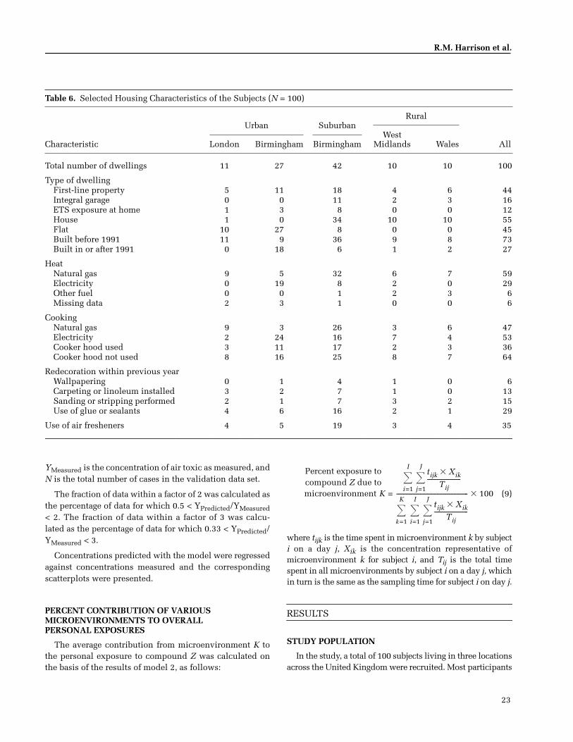
23


YMeasured is the concentration of air toxic as measured, andN is the total number of cases in the validation data set.

The fraction of data within a factor of 2 was calculated asthe percentage of data for which 0.5 < YPredicted/YMeasured< 2. The fraction of data within a factor of 3 was calcu-lated as the percentage of data for which 0.33 < YPredicted/YMeasured < 3.

Concentrations predicted with the model were regressedagainst concentrations measured and the correspondingscatterplots were presented.

PERCENT CONTRIBUTION OF VARIOUS MICROENVIRONMENTS TO OVERALL PERSONAL EXPOSURES

The average contribution from microenvironment K tothe personal exposure to compound Z was calculated onthe basis of the results of model 2, as follows:

where tijk is the time spent in microenvironment k by subjecti on a day j, Xik is the concentration representative ofmicroenvironment k for subject i, and Tij is the total timespent in all microenvironments by subject i on a day j, whichin turn is the same as the sampling time for subject i on day j.

RESULTS

STUDY POPULATION

In the study, a total of 100 subjects living in three locationsacross the United Kingdom were recruited. Most participants

microenvironment K =

tijk Xik�

Tij------------------------

j=1

J

�i=1

I

�

tijk Xik�

Tij------------------------

j=1

J

�i=1

I

�k=1

K

�--------------------------------------------------- 100�

Percent exposure to compound Z due to

Table 6. Selected Housing Characteristics of the Subjects (N = 100)

Characteristic

Urban SuburbanRural

AllWest

Midlands WalesLondon Birmingham Birmingham

Total number of dwellings 11 27 42 10 10 100

Type of dwellingFirst-line property 5 11 18 4 6 44Integral garage 0 0 11 2 3 16ETS exposure at home 1 3 8 0 0 12House 1 0 34 10 10 55Flat 10 27 8 0 0 45Built before 1991 11 9 36 9 8 73Built in or after 1991 0 18 6 1 2 27

HeatNatural gas 9 5 32 6 7 59Electricity 0 19 8 2 0 29Other fuel 0 0 1 2 3 6Missing data 2 3 1 0 0 6

CookingNatural gas 9 3 26 3 6 47Electricity 2 24 16 7 4 53Cooker hood used 3 11 17 2 3 36Cooker hood not used 8 16 25 8 7 64

Redecoration within previous yearWallpapering 0 1 4 1 0 6Carpeting or linoleum installed 3 2 7 1 0 13Sanding or stripping performed 2 1 7 3 2 15Use of glue or sealants 4 6 16 2 1 29

Use of air fresheners 4 5 19 3 4 35

(9)

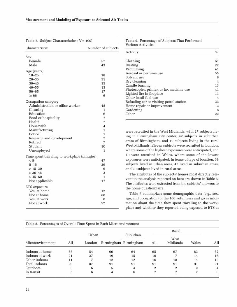
24


were recruited in the West Midlands, with 27 subjects liv-ing in Birmingham city center, 42 subjects in suburbanareas of Birmingham, and 10 subjects living in the ruralWest Midlands. Eleven subjects were recruited in London,where some of the highest exposures were anticipated, and10 were recruited in Wales, where some of the lowestexposures were anticipated. In terms of type of location, 38subjects lived in urban areas, 42 lived in suburban areas,and 20 subjects lived in rural areas.

The attributes of the subjects’ homes most directly rele-vant to the analysis reported on here are shown in Table 6.The attributes were extracted from the subjects’ answers tothe home questionnaire.

Table 7 summarizes some demographic data (e.g., sex,age, and occupation) of the 100 volunteers and gives infor-mation about the time they spent traveling to the work-place and whether they reported being exposed to ETS at

Table 7. Subject Characteristics (N = 100)

Characteristic Number of subjects

SexFemale 57Male 43

Age (years)18–25 1826–35 3136–45 1546–55 1356–65 17 66 6

Occupation categoryAdministration or office worker 48Cleaning 1Education 6Food or hospitality 7Health 7Housewife 4Manufacturing 1Police 1Research and development 7Retired 7Student 10Unemployed 1

Time spent traveling to workplace (minutes)< 5 475–15 26> 15–30 6> 30–45 3> 45–60 1Not applicable 17

ETS exposureYes, at home 12Not at home 88Yes, at work 8Not at work 92

Table 8. Percentages of Overall Time Spent in Each Microenvironment

Microenvironment

Urban SuburbanRural

AllAllWest

Midlands WalesAll London Birmingham Birmingham

Indoors at home 58 54 60 64 65 67 63 62Indoors at work 21 27 19 15 10 7 14 16Other indoors 11 7 12 12 16 18 14 12Total indoors 90 87 91 91 91 91 91 91Outdoors 5 6 5 4 2 2 2 4In transit 5 6 4 6 7 7 7 6

Table 9. Percentage of Subjects That Performed Various Activities

Activity %

Cleaning 61Dusting 27Vacuuming 41Aerosol or perfume use 55Solvent use 8Dry cleaning 4Candle burning 13Photocopier, printer, or fax machine use 41Lighted fire in fireplace 11Other fossil fuel use 4Refueling car or visiting petrol station 23Home repair or improvement 12Gardening 8Other 22

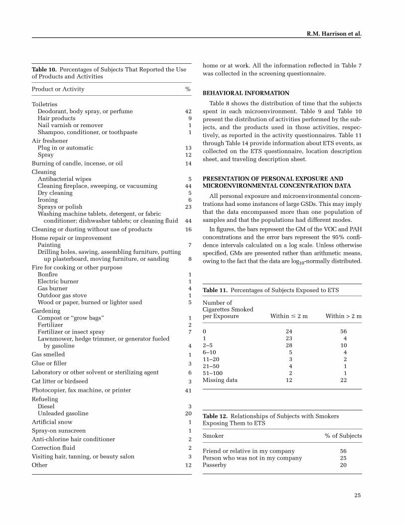
25


home or at work. All the information reflected in Table 7was collected in the screening questionnaire.

BEHAVIORAL INFORMATION

Table 8 shows the distribution of time that the subjectsspent in each microenvironment. Table 9 and Table 10present the distribution of activities performed by the sub-jects, and the products used in those activities, respec-tively, as reported in the activity questionnaires. Table 11through Table 14 provide information about ETS events, ascollected on the ETS questionnaire, location descriptionsheet, and traveling description sheet.

PRESENTATION OF PERSONAL EXPOSURE AND MICROENVIRONMENTAL CONCENTRATION DATA

All personal exposure and microenvironmental concen-trations had some instances of large GSDs. This may implythat the data encompassed more than one population ofsamples and that the populations had different modes.

In figures, the bars represent the GM of the VOC and PAHconcentrations and the error bars represent the 95% confi-dence intervals calculated on a log scale. Unless otherwisespecified, GMs are presented rather than arithmetic means,owing to the fact that the data are log10-normally distributed.

Table 10. Percentages of Subjects That Reported the Use of Products and Activities

Product or Activity %

ToiletriesDeodorant, body spray, or perfume 42Hair products 9Nail varnish or remover 1Shampoo, conditioner, or toothpaste 1

Air freshenerPlug in or automatic 13Spray 12

Burning of candle, incense, or oil 14Cleaning

Antibacterial wipes 5Cleaning fireplace, sweeping, or vacuuming 44Dry cleaning 5Ironing 6Sprays or polish 23Washing machine tablets, detergent, or fabric

conditioner; dishwasher tablets; or cleaning fluid 44Cleaning or dusting without use of products 16Home repair or improvement

Painting 7Drilling holes, sawing, assembling furniture, putting

up plasterboard, moving furniture, or sanding 8Fire for cooking or other purpose

Bonfire 1Electric burner 1Gas burner 4Outdoor gas stove 1Wood or paper, burned or lighter used 5

GardeningCompost or “grow bags” 1Fertilizer 2Fertilizer or insect spray 7Lawnmower, hedge trimmer, or generator fueled

by gasoline 4Gas smelled 1Glue or filler 3Laboratory or other solvent or sterilizing agent 6Cat litter or birdseed 3Photocopier, fax machine, or printer 41Refueling

Diesel 3Unleaded gasoline 20

Artificial snow 1Spray-on sunscreen 1Anti-chlorine hair conditioner 2Correction fluid 2Visiting hair, tanning, or beauty salon 3Other 12

Table 11. Percentages of Subjects Exposed to ETS

Number of Cigarettes Smokedper Exposure Within � 2 m Within > 2 m

0 24 561 23 42–5 28 106–10 5 411–20 3 221–50 4 151–100 2 1Missing data 12 22

Table 12. Relationships of Subjects with Smokers Exposing Them to ETS

Smoker % of Subjects

Friend or relative in my company 56Person who was not in my company 25Passerby 20

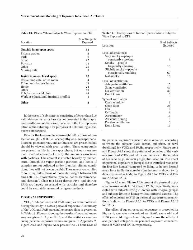
26


In the cases of sub-samples consisting of fewer than fivevalid data points, error bars are not presented in the graphsand results are not discussed, because of the low represen-tation of the subsample for purposes of determining subse-quent comparisons.

Data for the lower-molecular-weight PAHs (those of mo-lecular weight < 200, i.e., acenaphthylene, acenaphthene,fluorene, phenanthrene, and anthracene) are presented butshould be viewed with great caution. These compoundsare present mainly in the vapor phase, but our measure-ment method accounts for only the amounts associatedwith particles. This amount is affected heavily by temper-ature, through the vapor–particle partition, and hence ifsamples are not collected under identical climate condi-tions, they will not be comparable. The same caveat appliesto four-ring PAHs (those of molecular weight between 200and 228; i.e., fluoranthene, pyrene, benzo[a]anthracene,and chrysene), albeit to a lesser degree. Five- and six-ringPAHs are largely associated with particles and thereforecould be accurately measured using our methods.

PERSONAL EXPOSURES

VOC, 1,3-butadiene, and PAH samples were collectedduring the study to assess personal exposure. A summaryof the VOC and PAH personal exposure data is presentedin Table 15. Figures showing the results of personal expo-sure are given in Appendix 6, and the statistics summa-rizing personal exposure values are given in Appendix 7.Figure A6.1 and Figure A6.6 present the 24-hour GMs of

the personal exposure concentrations obtained, accordingto where the subjects lived (urban, suburban, or ruraldwellings) for VOCs and PAHs, respectively. Figure A6.2and Figure A6.7 show the patterns of behavior of the vari-ous groups of VOCs and PAHs, on the basis of the numberof benzene rings, in each geographic location. The effecton personal exposure of living close to trafficked roadsides(in first-line homes) compared to living in homes locatedaway from traffic (in non–first-line homes) is shown (withdata expressed as GMs) in Figure A6.3 for VOCs and Fig-ure A6.8 for PAHs.

Figure A6.4 and Figure A6.9 present the personal expo-sure measurements for VOCs and PAHs, respectively, asso-ciated with subjects living in homes with integral garagesand subjects living in homes without integral garages. Theeffect of exposure to ETS on personal exposure concentra-tions is shown in Figure A6.5 for VOCs and Figure A6.10for PAHs.

The effect of age on personal exposures is presented inFigure 1; age was categorized as 18–65 years old and 66 years old. Figure 2 and Figure 3 show the effects ofoccupational categories on personal exposure concentra-tions of VOCs and PAHs, respectively.

Table 13. Places Where Subjects Were Exposed to ETS

Location% of Subjects

Exposed

Outside in an open space 31Private garden 8Park 6Street 47Bus stop 11Other 25Missing data 3

Inside in an enclosed space 67Restaurant, café, or tea room 4Friend or relative’s house 13Home 24Other 13Pub, bar, or social club 44Work or educational institute or office 1

Other 2

Table 14. Descriptions of Indoor Spaces Where Subjects Were Exposed to ETS

Location% of Subjects

Exposed

Level of smokinessVery smoky — people

constantly smoking 7Smoky — people

frequently smoking 18Slightly smoky — people

occasionally smoking 60Not smoky 15

Level of ventilationAdequate ventilation 15Some ventilation 44No ventilation 35Don’t know 6

Type of ventilationOpen window 2Open door 38Fan 9Ceiling fan 4Air extractor 14Air conditioning 3Passive ventilation 0Don’t know 13

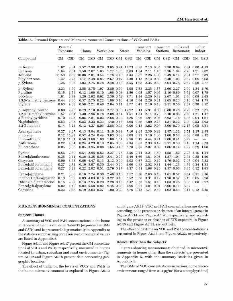
27


MICROENVIRONMENTAL CONCENTRATIONS

Subjects’ Homes

A summary of VOC and PAH concentrations in the homemicroenvironment is shown in Table 15 (expressed as GMsand GSDs) and is presented diagramatically in Appendix 6;the statistics summarizing home microenvironmental valuesare listed in Appendix 8.

Figure A6.11 and Figure A6.17 present the GM concentra-tions of VOCs and PAHs, respectively, measured in homeslocated in urban, suburban and rural environments; Fig-ure A6.12 and Figure A6.18 present data concerning geo-graphic location.

The effect of traffic on the levels of VOCs and PAHs inthe home microenvironment is explored in Figure A6.13

and Figure A6.19. VOC and PAH concentrations are shownaccording to the presence or absence of an integral garage inFigure A6.14 and Figure A6.20, respectively, and accord-ing to the presence or absence of ETS exposure in FigureA6.15 and Figure A6.21, respectively.

The effect of daytime on VOC and PAH concentrations ispresented in Figure A6.16 and Figure A6.22, respectively.

Homes Other than the Subjects’

Figures showing measurements obtained in microenvi-ronments in homes other than the subjects’ are presentedin Appendix 6, with the summary statistics given inAppendix 9.

The GMs of VOC concentrations in various home micro-environments ranged from 0.04 µg/m3 (for 3-ethenylpyridine)

Table 15. Personal Exposure and Microenvironmental Concentrations of VOCs and PAHs

Compound

PersonalExposure Home Workplace Street

TransportVehicles

TransportStations

Pubs andRestaurants

OtherIndoor

GM GSD GM GSD GM GSD GM GSD GM GSD GM GSD GM GSD GM GSD

n-Hexane 1.67 3.04 1.57 2.90 0.79 3.05 0.24 12.73 0.92 2.13 0.65 2.98 0.94 2.04 0.80 4.19Benzene 1.64 2.01 1.50 2.07 1.05 1.77 1.05 2.83 1.84 2.11 1.43 2.36 1.94 2.78 1.21 2.02Toluene 11.53 2.65 10.88 2.81 3.54 1.76 2.48 3.44 6.82 2.26 4.06 2.49 6.14 2.64 3.77 2.89Ethylbenzene 1.47 2.72 1.17 2.49 0.85 2.67 0.47 3.30 1.13 2.13 0.66 2.40 1.03 2.57 0.69 2.68p-Xylene 1.26 3.06 1.03 2.75 0.78 2.48 0.43 3.55 1.08 2.35 0.60 2.64 0.78 2.62 0.50 2.77

m-Xylene 3.23 3.00 2.55 2.75 1.97 2.89 0.99 4.05 2.88 2.25 1.55 2.69 2.27 2.90 1.34 2.70Pyridine 0.15 2.56 0.12 1.99 0.10 1.96 0.03 2.56 0.05 1.57 0.05 2.16 0.89 5.52 0.07 1.75o-Xylene 1.61 2.83 1.29 2.62 0.92 2.39 0.52 3.71 1.44 2.20 0.82 2.67 1.01 2.60 0.68 2.451,3,5-Trimethylbenzene 0.44 2.80 0.37 2.75 0.22 1.86 0.13 4.16 0.34 2.28 0.21 2.65 0.23 3.18 0.34 1.75Styrene 0.63 2.38 0.58 2.21 0.48 2.04 0.11 2.77 0.43 2.19 0.18 2.11 0.56 2.87 0.38 3.52

p-Isopropyltoluene 0.80 2.28 0.79 2.18 0.33 2.77 0.00 15.92 0.11 5.91 0.00 20.80 0.78 2.76 0.22 2.211,2,4-Trimethylbenzene 1.57 2.94 1.30 2.96 0.78 2.08 0.41 4.51 1.34 2.14 0.78 2.40 0.96 2.89 1.21 1.473-Ethenylpyridine 0.10 3.95 0.05 2.81 0.03 2.68 0.02 3.26 0.06 1.94 0.05 2.93 1.16 6.36 0.04 1.61Naphthalene 0.53 2.03 0.52 2.33 0.33 1.49 0.15 2.65 0.56 1.99 0.23 1.81 0.32 2.09 0.53 2.931,3-Butadiene 0.14 5.24 0.12 4.37 0.05 2.85 0.04 6.06 0.13 3.62 0.09 3.06 0.70 12.18 0.05 8.81

Acenaphthene 0.27 3.67 0.13 5.84 0.11 3.16 0.44 7.16 2.63 2.30 0.43 1.97 1.22 3.51 1.15 2.35Fluorene 0.12 15.93 0.52 4.24 0.44 3.63 0.38 8.69 0.33 3.10 1.00 1.00 0.53 3.09 0.88 3.32Phenanthrene 0.16 11.31 0.58 3.60 1.00 1.00 1.54 9.96 0.19 4.44 0.21 2.06 0.41 5.22 — —Anthracene 0.22 2.64 0.24 4.23 0.19 2.05 0.50 3.34 0.83 2.33 0.49 2.11 0.50 3.13 1.14 3.23Fluoranthene 0.05 3.08 0.05 3.95 0.08 1.65 0.10 2.78 0.25 2.87 0.09 1.86 0.14 1.97 0.29 1.68

Pyrene 0.56 2.30 0.54 2.95 0.82 2.27 1.76 2.56 2.41 2.21 1.50 1.58 1.62 2.28 2.16 1.54Benzo[a]anthracene 0.35 2.41 0.36 3.35 0.35 2.41 0.77 2.49 1.66 1.81 0.95 1.87 1.04 2.34 0.85 1.30Chrysene 0.09 3.63 0.06 4.47 0.13 3.12 0.09 4.02 0.37 3.31 0.12 1.79 0.32 7.07 0.04 5.32Benzo[b]fluoranthene 0.27 2.74 0.19 3.07 0.30 2.44 0.26 2.60 0.88 2.52 0.31 1.44 1.23 4.74 0.34 1.33Benzo[k]fluoranthene 0.27 3.29 0.22 2.82 0.51 2.79 0.17 3.37 0.51 1.98 0.26 1.37 0.66 3.65 0.12 1.95

Benzo[a]pyrene 0.21 3.06 0.18 2.74 0.30 2.46 0.16 3.17 0.36 2.63 0.16 1.61 0.57 3.54 0.11 2.16Indeno[1,2,3-cd]pyrene 0.13 3.65 0.09 4.03 0.16 3.22 0.13 2.52 0.28 3.31 0.12 1.98 0.37 5.13 0.05 2.98Dibenz[a,h]anthracene 0.16 2.97 0.13 2.95 0.20 2.28 0.15 2.42 0.23 1.61 0.18 1.63 0.26 3.08 0.08 2.92Benzo[g,h,i]perylene 0.02 5.49 0.02 5.58 0.02 9.45 0.02 3.96 0.02 4.01 0.01 2.06 0.11 5.47 — —Coronene 0.22 2.66 0.19 2.63 0.27 1.99 0.20 2.76 0.43 1.71 0.30 1.62 0.53 3.14 0.12 2.45

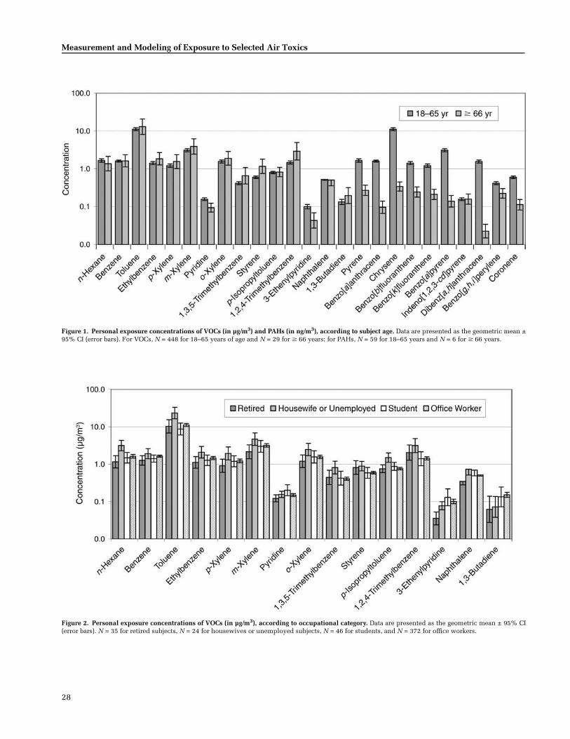
28


Figure 1. Personal exposure concentrations of VOCs (in µg/m3) and PAHs (in ng/m3), according to subject age. Data are presented as the geometric mean ±95% CI (error bars). For VOCs, N = 448 for 18–65 years of age and N = 29 for 66 years; for PAHs, N = 59 for 18–65 years and N = 6 for 66 years.

Figure 2. Personal exposure concentrations of VOCs (in µg/m3), according to occupational category. Data are presented as the geometric mean ± 95% CI(error bars). N = 35 for retired subjects, N = 24 for housewives or unemployed subjects, N = 46 for students, and N = 372 for office workers.

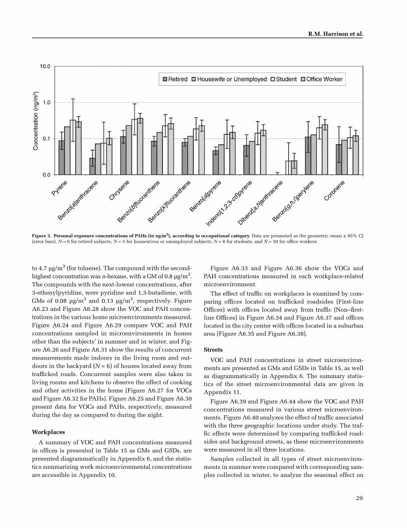
29


to 4.7 µg/m3 (for toluene). The compound with the second-highest concentration was n-hexane, with a GM of 0.8 µg/m3.The compounds with the next-lowest concentrations, after3-ethenylpyridine, were pyridine and 1,3-butadiene, withGMs of 0.08 µg/m3 and 0.13 µg/m3, respectively. FigureA6.23 and Figure A6.28 show the VOC and PAH concen-trations in the various home microenvironments measured.Figure A6.24 and Figure A6.29 compare VOC and PAHconcentrations sampled in microenvironments in homesother than the subjects’ in summer and in winter, and Fig-ure A6.26 and Figure A6.31 show the results of concurrentmeasurements made indoors in the living room and out-doors in the backyard (N = 6) of houses located away fromtrafficked roads. Concurrent samples were also taken inliving rooms and kitchens to observe the effect of cookingand other activities in the home (Figure A6.27 for VOCsand Figure A6.32 for PAHs). Figure A6.25 and Figure A6.30present data for VOCs and PAHs, respectively, measuredduring the day as compared to during the night.

Workplaces

A summary of VOC and PAH concentrations measuredin offices is presented in Table 15 as GMs and GSDs, arepresented diagrammatically in Appendix 6, and the statis-tics summarizing work microenvironmental concentrationsare accessible in Appendix 10.

Figure A6.33 and Figure A6.36 show the VOCs andPAH concentrations measured in each workplace-relatedmicroenvironment.

The effect of traffic on workplaces is examined by com-paring offices located on trafficked roadsides (First-lineOffices) with offices located away from traffic (Non–first-line Offices) in Figure A6.34 and Figure A6.37 and officeslocated in the city center with offices located in a suburbanarea (Figure A6.35 and Figure A6.38).

Streets

VOC and PAH concentrations in street microenviron-ments are presented as GMs and GSDs in Table 15, as wellas diagrammatically in Appendix 6. The summary statis-tics of the street microenvironmental data are given inAppendix 11.

Figure A6.39 and Figure A6.44 show the VOC and PAHconcentrations measured in various street microenviron-ments. Figure A6.40 analyzes the effect of traffic associatedwith the three geographic locations under study. The traf-fic effects were determined by comparing trafficked road-sides and background streets, as these microenvironmentswere measured in all three locations.

Samples collected in all types of street microenviron-ments in summer were compared with corresponding sam-ples collected in winter, to analyze the seasonal effect on

Figure 3. Personal exposure concentrations of PAHs (in ng/m3), according to occupational category. Data are presented as the geometric mean ± 95% CI(error bars). N = 6 for retired subjects, N = 5 for housewives or unemployed subjects, N = 6 for students, and N = 50 for office workers.

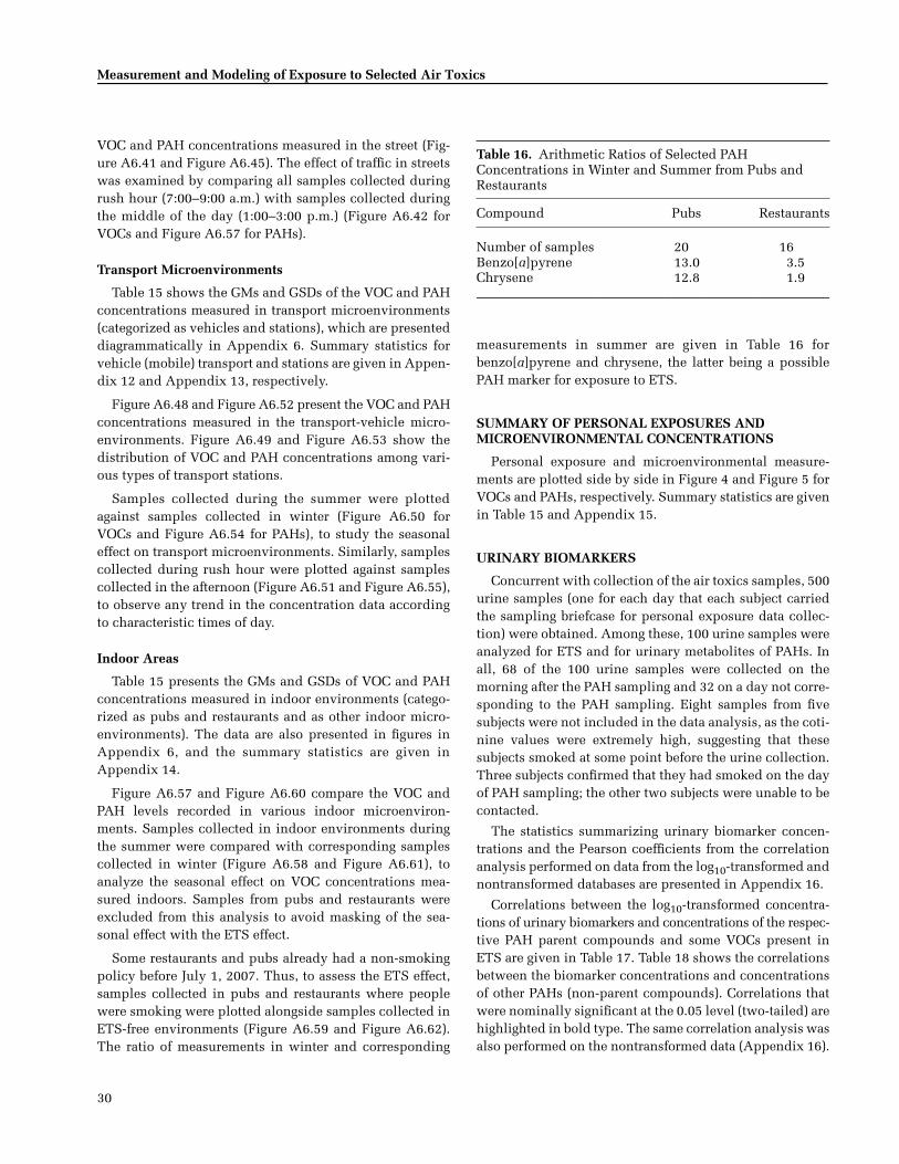
30


VOC and PAH concentrations measured in the street (Fig-ure A6.41 and Figure A6.45). The effect of traffic in streetswas examined by comparing all samples collected duringrush hour (7:00–9:00 a.m.) with samples collected duringthe middle of the day (1:00–3:00 p.m.) (Figure A6.42 forVOCs and Figure A6.57 for PAHs).

Transport Microenvironments

Table 15 shows the GMs and GSDs of the VOC and PAHconcentrations measured in transport microenvironments(categorized as vehicles and stations), which are presenteddiagrammatically in Appendix 6. Summary statistics forvehicle (mobile) transport and stations are given in Appen-dix 12 and Appendix 13, respectively.

Figure A6.48 and Figure A6.52 present the VOC and PAHconcentrations measured in the transport-vehicle micro-environments. Figure A6.49 and Figure A6.53 show thedistribution of VOC and PAH concentrations among vari-ous types of transport stations.

Samples collected during the summer were plottedagainst samples collected in winter (Figure A6.50 forVOCs and Figure A6.54 for PAHs), to study the seasonaleffect on transport microenvironments. Similarly, samplescollected during rush hour were plotted against samplescollected in the afternoon (Figure A6.51 and Figure A6.55),to observe any trend in the concentration data accordingto characteristic times of day.

Indoor Areas

Table 15 presents the GMs and GSDs of VOC and PAHconcentrations measured in indoor environments (catego-rized as pubs and restaurants and as other indoor micro-environments). The data are also presented in figures inAppendix 6, and the summary statistics are given inAppendix 14.

Figure A6.57 and Figure A6.60 compare the VOC andPAH levels recorded in various indoor microenviron-ments. Samples collected in indoor environments duringthe summer were compared with corresponding samplescollected in winter (Figure A6.58 and Figure A6.61), toanalyze the seasonal effect on VOC concentrations mea-sured indoors. Samples from pubs and restaurants wereexcluded from this analysis to avoid masking of the sea-sonal effect with the ETS effect.

Some restaurants and pubs already had a non-smokingpolicy before July 1, 2007. Thus, to assess the ETS effect,samples collected in pubs and restaurants where peoplewere smoking were plotted alongside samples collected inETS-free environments (Figure A6.59 and Figure A6.62).The ratio of measurements in winter and corresponding

Table 16. Arithmetic Ratios of Selected PAH Concentrations in Winter and Summer from Pubs and Restaurants

Compound Pubs Restaurants

Number of samples 20 16Benzo[a]pyrene 13.0 3.5Chrysene 12.8 1.9

measurements in summer are given in Table 16 forbenzo[a]pyrene and chrysene, the latter being a possiblePAH marker for exposure to ETS.

SUMMARY OF PERSONAL EXPOSURES AND MICROENVIRONMENTAL CONCENTRATIONS

Personal exposure and microenvironmental measure-ments are plotted side by side in Figure 4 and Figure 5 forVOCs and PAHs, respectively. Summary statistics are givenin Table 15 and Appendix 15.

URINARY BIOMARKERS

Concurrent with collection of the air toxics samples, 500urine samples (one for each day that each subject carriedthe sampling briefcase for personal exposure data collec-tion) were obtained. Among these, 100 urine samples wereanalyzed for ETS and for urinary metabolites of PAHs. Inall, 68 of the 100 urine samples were collected on themorning after the PAH sampling and 32 on a day not corre-sponding to the PAH sampling. Eight samples from fivesubjects were not included in the data analysis, as the coti-nine values were extremely high, suggesting that thesesubjects smoked at some point before the urine collection.Three subjects confirmed that they had smoked on the dayof PAH sampling; the other two subjects were unable to becontacted.

The statistics summarizing urinary biomarker concen-trations and the Pearson coefficients from the correlationanalysis performed on data from the log10-transformed andnontransformed databases are presented in Appendix 16.

Correlations between the log10-transformed concentra-tions of urinary biomarkers and concentrations of the respec-tive PAH parent compounds and some VOCs present inETS are given in Table 17. Table 18 shows the correlationsbetween the biomarker concentrations and concentrationsof other PAHs (non-parent compounds). Correlations thatwere nominally significant at the 0.05 level (two-tailed) arehighlighted in bold type. The same correlation analysis wasalso performed on the nontransformed data (Appendix 16).

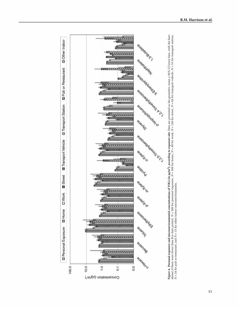
31


Fig

ure

4.

Per

son

al e

xpos

ure

an

d m

icro

envi

ron

men

tal

con

cen

trat

ion

s of

VO

Cs

(in

µg/

m3 )

, acc

ord

ing

to e

xpos

ure

sit

e. D

ata

are

pre

sen

ted

as

the

geom

etri

c m

ean

± 9

5% C

I (e

rror

bar

s, w

ith

th

e ba

rsab

sen

t if

th

ere

wer

e fe

wer

th

an fi

ve d

ata

poi

nts

). N

= 5

00 f

or p

erso

nal

exp

osu

re, N

= 1

60 f

or h

ome,

N =

40

for

wor

k, N

= 1

50 f

or s

tree

t, N

= 6

9 fo

r tr

ansp

ort

veh

icle

, N =

53

for

tran

spor

t st

atio

n,

N =

24

for

pu

b or

res

tau

ran

t, a

nd

N =

15

for

oth

er i

nd

oor

mic

roen

viro

nm

ents

.

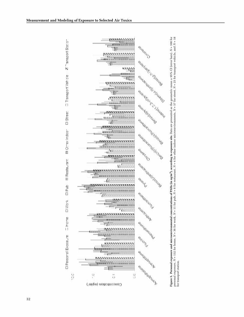
32


Fig

ure

5.

Per

son

al e

xpos

ure

an

d m

icro

envi

ron

men

tal

con

cen

trat

ion

s of

PA

Hs

(in

ng/

m3 )

, acc

ord

ing

to e

xpos

ure

sit

e. D

ata

are

pre

sen

ted

as

the

geom

etri

c m

ean

± 9

5% C

I (e

rror

bar

s). N

= 1

00 f

orp

erso

nal

exp

osu

re, N

= 1

32 f

or h

ome,

N =

36

for

wor

k, N

= 1

1 fo

r p

ub,

N =

8 f

or r

esta

ura

nt,

N =

4 f

or o

ther

in

doo

r m

icro

envi

ron

men

ts, N

= 5

7 fo

r st

reet

, N =

25

for

tran

spor

t ve

hic

le, a

nd

N =

18

for

tran

spor

t st

atio

n.

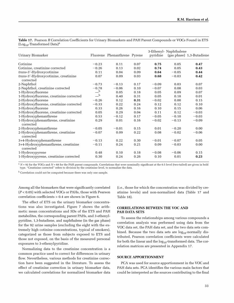
33


Table 17. Pearson R Correlation Coefficients for Urinary Biomarkers and PAH Parent Compounds or VOCs Found in ETS (Log10-Transformed Data)a

Urinary Biomarker Fluorene Phenanthrene Pyrene3-Ethenyl-pyridine

Naphthalene(gas phase) 1,3-Butadiene

Cotinine �0.23 0.11 0.07 0.75 0.05 0.47Cotinine, creatinine corrected �0.26 0.13 0.02 0.74 0.05 0.43trans-3�-Hydroxycotinine 0.11 0.04 0.09 0.64 �0.05 0.44trans-3�-Hydroxycotinine, creatinine

corrected0.07 0.09 0.03 0.68 �0.03 0.42

2-Naphthol �0.73 �0.13 0.17 �0.09 0.03 0.072-Naphthol, creatinine corrected �0.78 �0.06 0.10 �0.07 0.08 0.031-Hydroxyfluorene —b 0.05 0.18 0.05 0.09 0.071-Hydroxyfluorene, creatinine corrected —b 0.40 0.31 0.05 0.18 0.012-Hydroxyfluorene �0.26 0.12 0.31 �0.02 0.00 0.152-Hydroxyfluorene, creatinine corrected �0.33 0.22 0.24 0.12 0.12 0.103-Hydroxyfluorene 0.33 0.26 0.16 0.10 0.15 0.063-Hydroxyfluorene, creatinine corrected 0.05 0.29 0.04 0.11 0.12 �0.031-Hydroxyphenanthrene 0.53 �0.12 0.17 �0.05 �0.10 �0.031-Hydroxyphenanthrene, creatinine

corrected0.29 0.01 0.16 �0.02 �0.13 �0.09

2-Hydroxyphenanthrene �0.05 �0.01 0.15 0.01 �0.20 0.002-Hydroxyphenanthrene, creatinine

corrected�0.07 0.09 0.22 0.08 �0.02 �0.06

3+4-Hydroxyphenanthrene �0.13 0.22 0.30 �0.01 �0.07 0.053+4-Hydroxyphenanthrene, creatinine

corrected�0.11 0.24 0.21 0.09 �0.03 0.00

1-Hydroxypyrene 0.48 0.10 0.18 �0.08 �0.06 0.151-Hydroxypyrene, creatinine corrected 0.30 0.24 0.26 0.10 0.01 0.23

a N = 92 for the VOCs and N = 68 for the PAH parent compounds. Correlations that were nominally significant at the 0.5 level (two-tailed) are given in bold type. “Creatinine corrected” refers to division by the creatinine level, to normalize the data.

b Correlation could not be computed because there was only one sample.

Among all the biomarkers that were significantly correlated(P < 0.05) with selected VOCs or PAHs, those with Pearsoncorrelation coefficients > 0.4 are shown in Figure 6.

The effect of ETS on the urinary biomarker concentra-tions was also investigated. Figure 7 shows the arith-metic mean concentrations and SDs of the ETS and PAHmetabolites, the corresponding parent PAHs, and 3-ethenyl-pyridine, 1,3-butadiene, and naphthalene (in the gas phase)for the 92 urine samples (excluding the eight with the ex-tremely high cotinine concentrations, typical of smokers),categorized as those from subjects exposed to ETS andthose not exposed, on the basis of the measured personalexposures to 3-ethenylpyridine.

Normalizing data to the creatinine concentration is acommon practice used to correct for differences in urinaryflow. Nevertheless, various methods for creatinine correc-tion have been suggested in the literature. To assess theeffect of creatinine correction in urinary biomarker data,we calculated correlations for normalized biomarker data

(i.e., those for which the concentration was divided by cre-atinine levels) and non-normalized data (Table 17 andTable 18).

CORRELATIONS BETWEEN THE VOC AND PAH DATA SETS

To assess the relationships among various compounds acorrelation analysis was performed using data from theVOC data set, the PAH data set, and the two data sets com-bined. Because the two data sets are log10-normally dis-tributed, Pearson correlation coefficients were calculatedfor both the linear and the log10-transformed data. The cor-relation matrices are presented in Appendix 17.

SOURCE APPORTIONMENT

PCA was used for source apportionment in the VOC andPAH data sets. PCA identifies the various main factors thatcould be interpreted as the sources contributing to the final

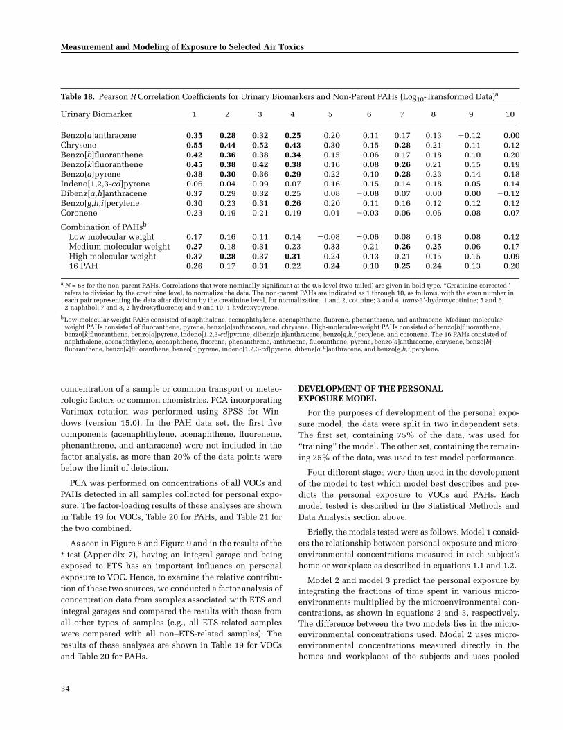
34


Table 18. Pearson R Correlation Coefficients for Urinary Biomarkers and Non-Parent PAHs (Log10-Transformed Data)a

Urinary Biomarker 1 2 3 4 5 6 7 8 9 10

Benzo[a]anthracene 0.35 0.28 0.32 0.25 0.20 0.11 0.17 0.13 �0.12 0.00Chrysene 0.55 0.44 0.52 0.43 0.30 0.15 0.28 0.21 0.11 0.12Benzo[b]fluoranthene 0.42 0.36 0.38 0.34 0.15 0.06 0.17 0.18 0.10 0.20Benzo[k]fluoranthene 0.45 0.38 0.42 0.38 0.16 0.08 0.26 0.21 0.15 0.19Benzo[a]pyrene 0.38 0.30 0.36 0.29 0.22 0.10 0.28 0.23 0.14 0.18Indeno[1,2,3-cd]pyrene 0.06 0.04 0.09 0.07 0.16 0.15 0.14 0.18 0.05 0.14Dibenz[a,h]anthracene 0.37 0.29 0.32 0.25 0.08 �0.08 0.07 0.00 0.00 �0.12Benzo[g,h,i]perylene 0.30 0.23 0.31 0.26 0.20 0.11 0.16 0.12 0.12 0.12Coronene 0.23 0.19 0.21 0.19 0.01 �0.03 0.06 0.06 0.08 0.07

Combination of PAHsb

Low molecular weight 0.17 0.16 0.11 0.14 �0.08 �0.06 0.08 0.18 0.08 0.12Medium molecular weight 0.27 0.18 0.31 0.23 0.33 0.21 0.26 0.25 0.06 0.17High molecular weight 0.37 0.28 0.37 0.31 0.24 0.13 0.21 0.15 0.15 0.0916 PAH 0.26 0.17 0.31 0.22 0.24 0.10 0.25 0.24 0.13 0.20

a N = 68 for the non-parent PAHs. Correlations that were nominally significant at the 0.5 level (two-tailed) are given in bold type. “Creatinine corrected” refers to division by the creatinine level, to normalize the data. The non-parent PAHs are indicated as 1 through 10, as follows, with the even number in each pair representing the data after division by the creatinine level, for normalization: 1 and 2, cotinine; 3 and 4, trans-3�-hydroxycotinine; 5 and 6, 2-naphthol; 7 and 8, 2-hydroxyfluorene; and 9 and 10, 1-hydroxypyrene.

bLow-molecular-weight PAHs consisted of naphthalene, acenaphthylene, acenaphthene, fluorene, phenanthrene, and anthracene. Medium-molecular-weight PAHs consisted of fluoranthene, pyrene, benzo[a]anthracene, and chrysene. High-molecular-weight PAHs consisted of benzo[b]fluoranthene, benzo[k]fluoranthene, benzo[a]pyrene, indeno[1,2,3-cd]pyrene, dibenz[a,h]anthracene, benzo[g,h,i]perylene, and coronene. The 16 PAHs consisted of naphthalene, acenaphthylene, acenaphthene, fluorene, phenanthrene, anthracene, fluoranthene, pyrene, benzo[a]anthracene, chrysene, benzo[b]-fluoranthene, benzo[k]fluoranthene, benzo[a]pyrene, indeno[1,2,3-cd]pyrene, dibenz[a,h]anthracene, and benzo[g,h,i]perylene.

concentration of a sample or common transport or meteo-rologic factors or common chemistries. PCA incorporatingVarimax rotation was performed using SPSS for Win-dows (version 15.0). In the PAH data set, the first fivecomponents (acenaphthylene, acenaphthene, fluorenene,phenanthrene, and anthracene) were not included in thefactor analysis, as more than 20% of the data points werebelow the limit of detection.

PCA was performed on concentrations of all VOCs andPAHs detected in all samples collected for personal expo-sure. The factor-loading results of these analyses are shownin Table 19 for VOCs, Table 20 for PAHs, and Table 21 forthe two combined.

As seen in Figure 8 and Figure 9 and in the results of thet test (Appendix 7), having an integral garage and beingexposed to ETS has an important influence on personalexposure to VOC. Hence, to examine the relative contribu-tion of these two sources, we conducted a factor analysis ofconcentration data from samples associated with ETS andintegral garages and compared the results with those fromall other types of samples (e.g., all ETS-related sampleswere compared with all non–ETS-related samples). Theresults of these analyses are shown in Table 19 for VOCsand Table 20 for PAHs.

DEVELOPMENT OF THE PERSONAL EXPOSURE MODEL

For the purposes of development of the personal expo-sure model, the data were split in two independent sets.The first set, containing 75% of the data, was used for“training” the model. The other set, containing the remain-ing 25% of the data, was used to test model performance.

Four different stages were then used in the developmentof the model to test which model best describes and pre-dicts the personal exposure to VOCs and PAHs. Eachmodel tested is described in the Statistical Methods andData Analysis section above.

Briefly, the models tested were as follows. Model 1 consid-ers the relationship between personal exposure and micro-environmental concentrations measured in each subject’shome or workplace as described in equations 1.1 and 1.2.

Model 2 and model 3 predict the personal exposure byintegrating the fractions of time spent in various micro-environments multiplied by the microenvironmental con-centrations, as shown in equations 2 and 3, respectively.The difference between the two models lies in the micro-environmental concentrations used. Model 2 uses micro-environmental concentrations measured directly in thehomes and workplaces of the subjects and uses pooled

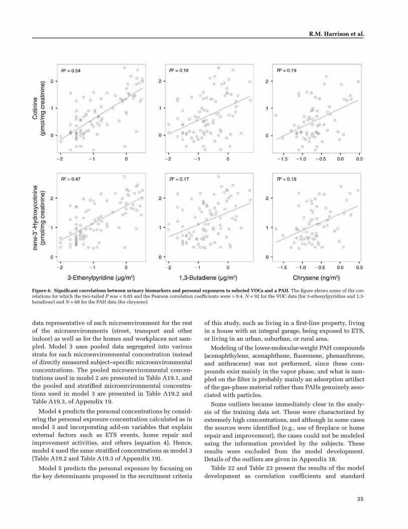
35


Figure 6. Significant correlations between urinary biomarkers and personal exposures to selected VOCs and a PAH. The figure shows some of the cor-relations for which the two-tailed P was < 0.05 and the Pearson correlation coefficients were > 0.4. N = 92 for the VOC data (for 3-ethenylpyridine and 1,3-butadiene) and N = 68 for the PAH data (for chrysene).

data representative of each microenvironment for the restof the microenvironments (street, transport and otherindoor) as well as for the homes and workplaces not sam-pled. Model 3 uses pooled data segregated into variousstrata for each microenvironmental concentration insteadof directly measured subject–specific microenvironmentalconcentrations. The pooled microenvironmental concen-trations used in model 2 are presented in Table A19.1, andthe pooled and stratified microenvironmental concentra-tions used in model 3 are presented in Table A19.2 andTable A19.3, of Appendix 19.

Model 4 predicts the personal concentrations by consid-ering the personal exposure concentration calculated as inmodel 3 and incorporating add-on variables that explainexternal factors such as ETS events, home repair andimprovement activities, and others (equation 4). Hence,model 4 used the same stratified concentrations as model 3(Table A19.2 and Table A19.3 of Appendix 19).

Model 5 predicts the personal exposure by focusing onthe key determinants proposed in the recruitment criteria

of this study, such as living in a first-line property, livingin a house with an integral garage, being exposed to ETS,or living in an urban, suburban, or rural area.

Modeling of the lower-molecular-weight PAH compounds(acenaphthylene, acenaphthene, fluorenene, phenanthrene,and anthracene) was not performed, since these com-pounds exist mainly in the vapor phase, and what is sam-pled on the filter is probably mainly an adsorption artifactof the gas-phase material rather than PAHs genuinely asso-ciated with particles.

Some outliers became immediately clear in the analy-sis of the training data set. These were characterized byextremely high concentrations, and although in some casesthe sources were identified (e.g., use of fireplace or homerepair and improvement), the cases could not be modeledusing the information provided by the subjects. Theseresults were excluded from the model development.Details of the outliers are given in Appendix 18.

Table 22 and Table 23 present the results of the modeldevelopment as correlation coefficients and standard

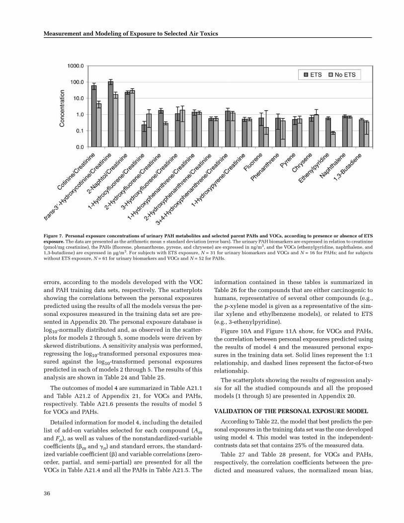
36


errors, according to the models developed with the VOCand PAH training data sets, respectively. The scatterplotsshowing the correlations between the personal exposurespredicted using the results of all the models versus the per-sonal exposures measured in the training data set are pre-sented in Appendix 20. The personal exposure database islog10-normally distributed and, as observed in the scatter-plots for models 2 through 5, some models were driven byskewed distributions. A sensitivity analysis was performed,regressing the log10-transformed personal exposures mea-sured against the log10-transformed personal exposurespredicted in each of models 2 through 5. The results of thisanalysis are shown in Table 24 and Table 25.

The outcomes of model 4 are summarized in Table A21.1and Table A21.2 of Appendix 21, for VOCs and PAHs,respectively. Table A21.6 presents the results of model 5for VOCs and PAHs.

Detailed information for model 4, including the detailedlist of add-on variables selected for each compound (Amand Fn), as well as values of the nonstandardized-variablecoefficients (�m and n) and standard errors, the standard-ized variable coefficient (�) and variable correlations (zero-order, partial, and semi-partial) are presented for all theVOCs in Table A21.4 and all the PAHs in Table A21.5. The

information contained in these tables is summarized inTable 26 for the compounds that are either carcinogenic tohumans, representative of several other compounds (e.g.,the p-xylene model is given as a representative of the sim-ilar xylene and ethylbenzene models), or related to ETS(e.g., 3-ethenylpyridine).

Figure 10A and Figure 11A show, for VOCs and PAHs,the correlation between personal exposures predicted usingthe results of model 4 and the measured personal expo-sures in the training data set. Solid lines represent the 1:1relationship, and dashed lines represent the factor-of-tworelationship.

The scatterplots showing the results of regression analy-sis for all the studied compounds and all the proposedmodels (1 through 5) are presented in Appendix 20.


According to Table 22, the model that best predicts the per-sonal exposures in the training data set was the one developedusing model 4. This model was tested in the independent-contrasts data set that contains 25% of the measured data.

Table 27 and Table 28 present, for VOCs and PAHs,respectively, the correlation coefficients between the pre-dicted and measured values, the normalized mean bias,

Figure 7. Personal exposure concentrations of urinary PAH metabolites and selected parent PAHs and VOCs, according to presence or absence of ETSexposure. The data are presented as the arithmetic mean ± standard deviation (error bars). The urinary PAH biomarkers are expressed in relation to creatinine(pmol/mg creatinine), the PAHs (fluorene, phenanthrene, pyrene, and chrysene) are expressed in ng/m3, and the VOCs (ethenylpyridine, naphthalene, and1,3-butadiene) are expressed in µg/m3. For subjects with ETS exposure, N = 31 for urinary biomarkers and VOCs and N = 16 for PAHs; and for subjectswithout ETS exposure, N = 61 for urinary biomarkers and VOCs and N = 52 for PAHs.

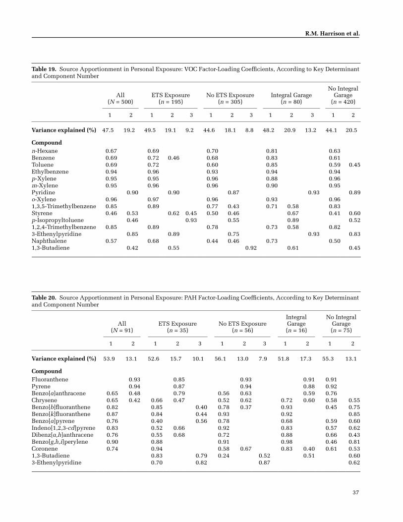
37


Table 19. Source Apportionment in Personal Exposure: VOC Factor-Loading Coefficients, According to Key Determinant and Component Number

All(N = 500)

ETS Exposure(n = 195)

No ETS Exposure(n = 305)

Integral Garage(n = 80)

No Integral Garage

(n = 420)

1 2 1 2 3 1 2 3 1 2 3 1 2

Variance explained (%) 47.5 19.2 49.5 19.1 9.2 44.6 18.1 8.8 48.2 20.9 13.2 44.1 20.5

Compoundn-Hexane 0.67 0.69 0.70 0.81 0.63Benzene 0.69 0.72 0.46 0.68 0.83 0.61Toluene 0.69 0.72 0.60 0.85 0.59 0.45Ethylbenzene 0.94 0.96 0.93 0.94 0.94p-Xylene 0.95 0.95 0.96 0.88 0.96m-Xylene 0.95 0.96 0.96 0.90 0.95Pyridine 0.90 0.90 0.87 0.93 0.89o-Xylene 0.96 0.97 0.96 0.93 0.961,3,5-Trimethylbenzene 0.85 0.89 0.77 0.43 0.71 0.58 0.83Styrene 0.46 0.53 0.62 0.45 0.50 0.46 0.67 0.41 0.60p-Isopropyltoluene 0.46 0.93 0.55 0.89 0.521,2,4-Trimethylbenzene 0.85 0.89 0.78 0.73 0.58 0.823-Ethenylpyridine 0.85 0.89 0.75 0.93 0.83Naphthalene 0.57 0.68 0.44 0.46 0.73 0.501,3-Butadiene 0.42 0.55 0.92 0.61 0.45

Table 20. Source Apportionment in Personal Exposure: PAH Factor-Loading Coefficients, According to Key Determinant and Component Number

All(N = 91)

ETS Exposure(n = 35)

No ETS Exposure(n = 56)

Integral Garage(n = 16)

No Integral Garage(n = 75)

1 2 1 2 3 1 2 3 1 2 1 2

Variance explained (%) 53.9 13.1 52.6 15.7 10.1 56.1 13.0 7.9 51.8 17.3 55.3 13.1

CompoundFluoranthene 0.93 0.85 0.93 0.91 0.91Pyrene 0.94 0.87 0.94 0.88 0.92Benzo[a]anthracene 0.65 0.48 0.79 0.56 0.63 0.59 0.76Chrysene 0.65 0.42 0.66 0.47 0.52 0.62 0.72 0.60 0.58 0.55Benzo[b]fluoranthene 0.82 0.85 0.40 0.78 0.37 0.93 0.45 0.75Benzo[k]fluoranthene 0.87 0.84 0.44 0.93 0.92 0.85Benzo[a]pyrene 0.76 0.40 0.56 0.78 0.68 0.59 0.60Indeno[1,2,3-cd]pyrene 0.83 0.52 0.66 0.92 0.83 0.57 0.62Dibenz[a,h]anthracene 0.76 0.55 0.68 0.72 0.88 0.66 0.43Benzo[g,h,i]perylene 0.90 0.88 0.91 0.98 0.46 0.81Coronene 0.74 0.94 0.58 0.67 0.83 0.40 0.61 0.531,3-Butadiene 0.83 0.79 0.24 0.52 0.51 0.603-Ethenylpyridine 0.70 0.82 0.87 0.62

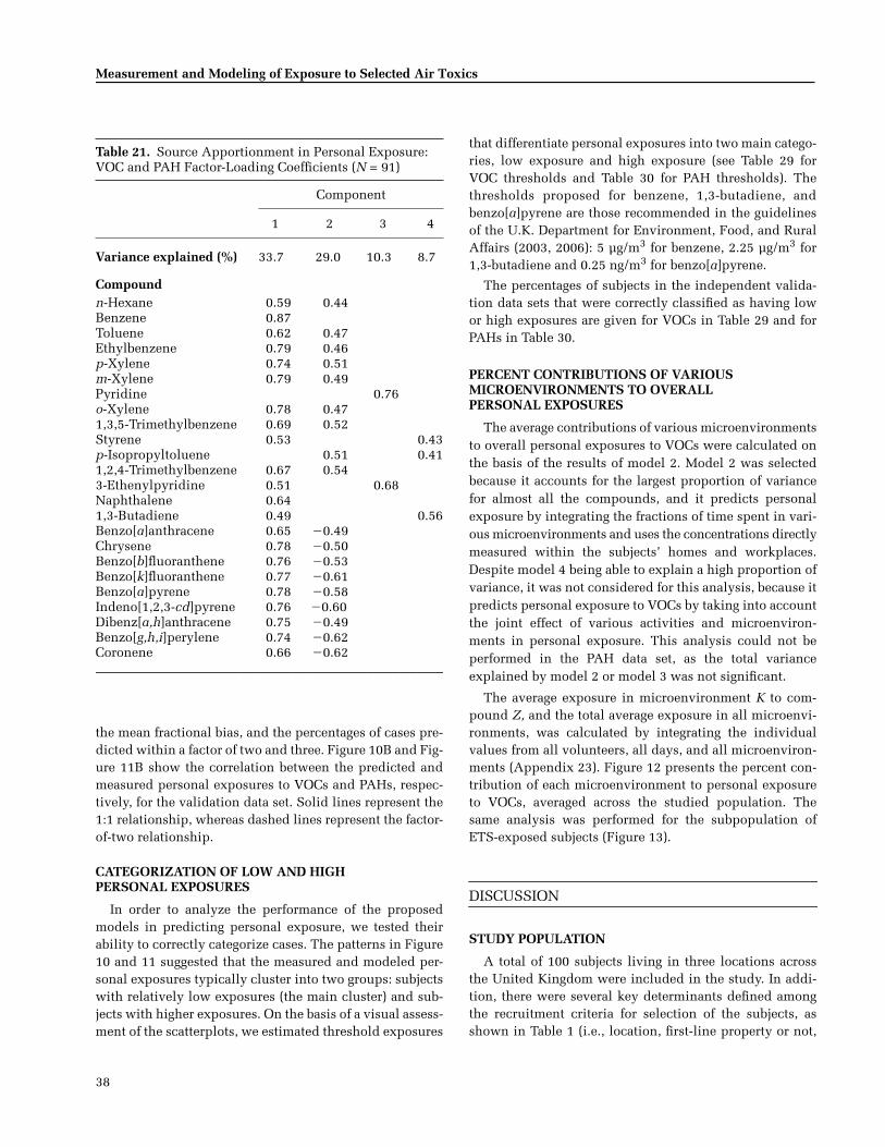
38


that differentiate personal exposures into two main catego-ries, low exposure and high exposure (see Table 29 forVOC thresholds and Table 30 for PAH thresholds). Thethresholds proposed for benzene, 1,3-butadiene, andbenzo[a]pyrene are those recommended in the guidelinesof the U.K. Department for Environment, Food, and RuralAffairs (2003, 2006): 5 µg/m3 for benzene, 2.25 µg/m3 for1,3-butadiene and 0.25 ng/m3 for benzo[a]pyrene.

The percentages of subjects in the independent valida-tion data sets that were correctly classified as having lowor high exposures are given for VOCs in Table 29 and forPAHs in Table 30.

PERCENT CONTRIBUTIONS OF VARIOUS MICROENVIRONMENTS TO OVERALL PERSONAL EXPOSURES

The average contributions of various microenvironmentsto overall personal exposures to VOCs were calculated onthe basis of the results of model 2. Model 2 was selectedbecause it accounts for the largest proportion of variancefor almost all the compounds, and it predicts personalexposure by integrating the fractions of time spent in vari-ous microenvironments and uses the concentrations directlymeasured within the subjects’ homes and workplaces.Despite model 4 being able to explain a high proportion ofvariance, it was not considered for this analysis, because itpredicts personal exposure to VOCs by taking into accountthe joint effect of various activities and microenviron-ments in personal exposure. This analysis could not beperformed in the PAH data set, as the total varianceexplained by model 2 or model 3 was not significant.

The average exposure in microenvironment K to com-pound Z, and the total average exposure in all microenvi-ronments, was calculated by integrating the individualvalues from all volunteers, all days, and all microenviron-ments (Appendix 23). Figure 12 presents the percent con-tribution of each microenvironment to personal exposureto VOCs, averaged across the studied population. Thesame analysis was performed for the subpopulation ofETS-exposed subjects (Figure 13).

DISCUSSION

STUDY POPULATION

A total of 100 subjects living in three locations acrossthe United Kingdom were included in the study. In addi-tion, there were several key determinants defined amongthe recruitment criteria for selection of the subjects, asshown in Table 1 (i.e., location, first-line property or not,

Table 21. Source Apportionment in Personal Exposure: VOC and PAH Factor-Loading Coefficients (N = 91)

Component

1 2 3 4

Variance explained (%) 33.7 29.0 10.3 8.7

Compoundn-Hexane 0.59 0.44Benzene 0.87Toluene 0.62 0.47Ethylbenzene 0.79 0.46p-Xylene 0.74 0.51m-Xylene 0.79 0.49Pyridine 0.76o-Xylene 0.78 0.471,3,5-Trimethylbenzene 0.69 0.52Styrene 0.53 0.43p-Isopropyltoluene 0.51 0.411,2,4-Trimethylbenzene 0.67 0.543-Ethenylpyridine 0.51 0.68Naphthalene 0.641,3-Butadiene 0.49 0.56Benzo[a]anthracene 0.65 �0.49Chrysene 0.78 �0.50Benzo[b]fluoranthene 0.76 �0.53Benzo[k]fluoranthene 0.77 �0.61Benzo[a]pyrene 0.78 �0.58Indeno[1,2,3-cd]pyrene 0.76 �0.60Dibenz[a,h]anthracene 0.75 �0.49Benzo[g,h,i]perylene 0.74 �0.62Coronene 0.66 �0.62

the mean fractional bias, and the percentages of cases pre-dicted within a factor of two and three. Figure 10B and Fig-ure 11B show the correlation between the predicted andmeasured personal exposures to VOCs and PAHs, respec-tively, for the validation data set. Solid lines represent the1:1 relationship, whereas dashed lines represent the factor-of-two relationship.

CATEGORIZATION OF LOW AND HIGH PERSONAL EXPOSURES

In order to analyze the performance of the proposedmodels in predicting personal exposure, we tested theirability to correctly categorize cases. The patterns in Figure10 and 11 suggested that the measured and modeled per-sonal exposures typically cluster into two groups: subjectswith relatively low exposures (the main cluster) and sub-jects with higher exposures. On the basis of a visual assess-ment of the scatterplots, we estimated threshold exposures

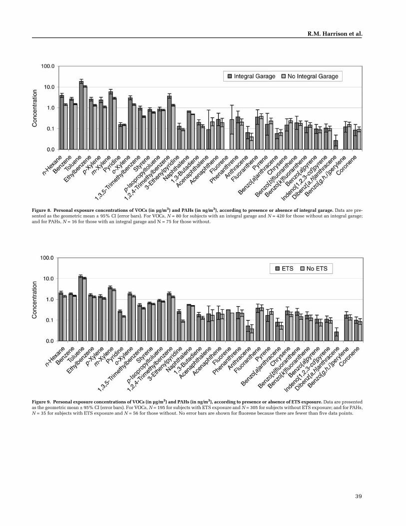
39


Figure 8. Personal exposure concentrations of VOCs (in µg/m3) and PAHs (in ng/m3), according to presence or absence of integral garage. Data are pre-sented as the geometric mean ± 95% CI (error bars). For VOCs, N = 80 for subjects with an integral garage and N = 420 for those without an integral garage;and for PAHs, N = 16 for those with an integral garage and N = 75 for those without.

Figure 9. Personal exposure concentrations of VOCs (in µg/m3) and PAHs (in ng/m3), according to presence or absence of ETS exposure. Data are presentedas the geometric mean ± 95% CI (error bars). For VOCs, N = 195 for subjects with ETS exposure and N = 305 for subjects without ETS exposure; and for PAHs,N = 35 for subjects with ETS exposure and N = 56 for those without. No error bars are shown for fluorene because there are fewer than five data points.

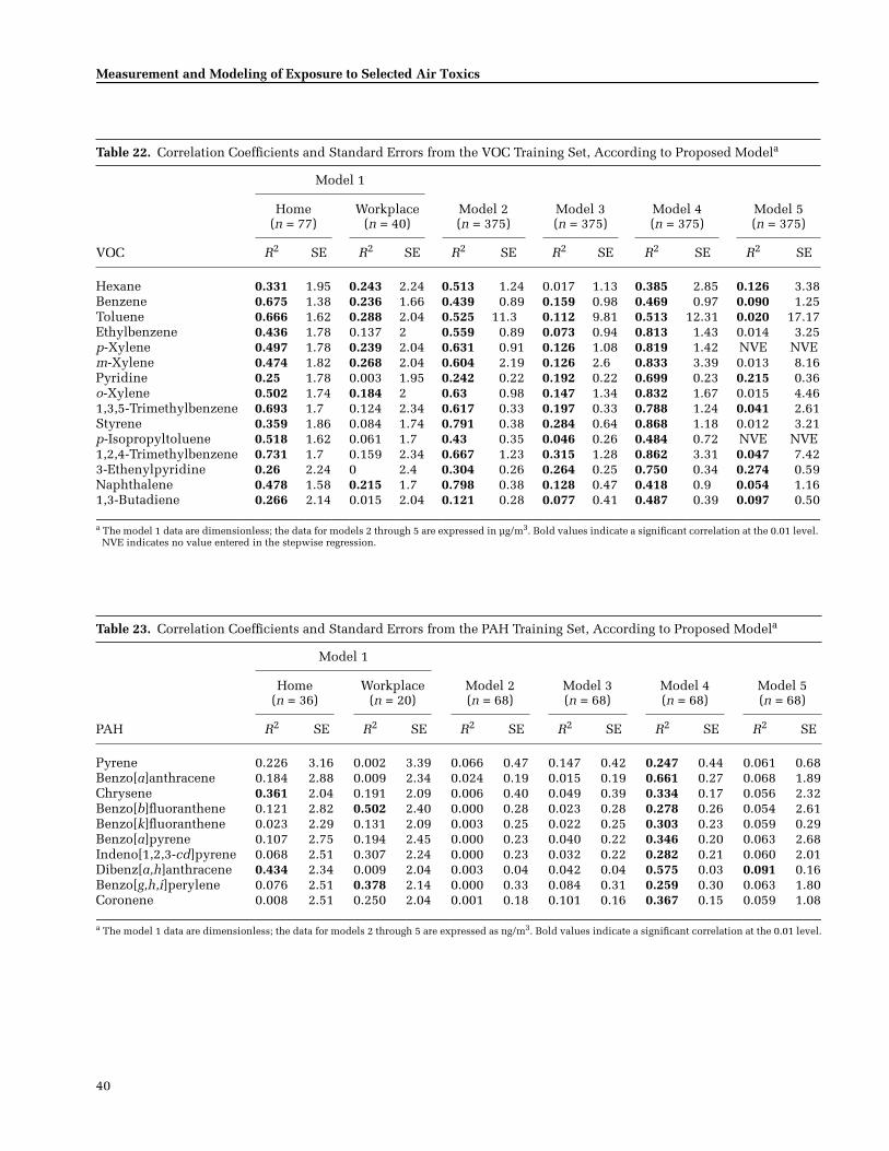
40


Table 22. Correlation Coefficients and Standard Errors from the VOC Training Set, According to Proposed Modela

VOC

Model 1

Model 2(n = 375)

Model 3(n = 375)

Model 4(n = 375)

Model 5(n = 375)

Home(n = 77)

Workplace(n = 40)

R2 SE R2 SE R2 SE R2 SE R2 SE R2 SE

Hexane 0.331 1.95 0.243 2.24 0.513 1.24 0.017 1.13 0.385 2.85 0.126 3.38Benzene 0.675 1.38 0.236 1.66 0.439 0.89 0.159 0.98 0.469 0.97 0.090 1.25Toluene 0.666 1.62 0.288 2.04 0.525 11.3 0.112 9.81 0.513 12.31 0.020 17.17Ethylbenzene 0.436 1.78 0.137 2 0.559 0.89 0.073 0.94 0.813 1.43 0.014 3.25p-Xylene 0.497 1.78 0.239 2.04 0.631 0.91 0.126 1.08 0.819 1.42 NVE NVEm-Xylene 0.474 1.82 0.268 2.04 0.604 2.19 0.126 2.6 0.833 3.39 0.013 8.16Pyridine 0.25 1.78 0.003 1.95 0.242 0.22 0.192 0.22 0.699 0.23 0.215 0.36o-Xylene 0.502 1.74 0.184 2 0.63 0.98 0.147 1.34 0.832 1.67 0.015 4.461,3,5-Trimethylbenzene 0.693 1.7 0.124 2.34 0.617 0.33 0.197 0.33 0.788 1.24 0.041 2.61Styrene 0.359 1.86 0.084 1.74 0.791 0.38 0.284 0.64 0.868 1.18 0.012 3.21p-Isopropyltoluene 0.518 1.62 0.061 1.7 0.43 0.35 0.046 0.26 0.484 0.72 NVE NVE1,2,4-Trimethylbenzene 0.731 1.7 0.159 2.34 0.667 1.23 0.315 1.28 0.862 3.31 0.047 7.423-Ethenylpyridine 0.26 2.24 0 2.4 0.304 0.26 0.264 0.25 0.750 0.34 0.274 0.59Naphthalene 0.478 1.58 0.215 1.7 0.798 0.38 0.128 0.47 0.418 0.9 0.054 1.161,3-Butadiene 0.266 2.14 0.015 2.04 0.121 0.28 0.077 0.41 0.487 0.39 0.097 0.50

a The model 1 data are dimensionless; the data for models 2 through 5 are expressed in µg/m3. Bold values indicate a significant correlation at the 0.01 level. NVE indicates no value entered in the stepwise regression.

Table 23. Correlation Coefficients and Standard Errors from the PAH Training Set, According to Proposed Modela

PAH

Model 1

Model 2(n = 68)

Model 3(n = 68)

Model 4(n = 68)

Model 5(n = 68)

Home(n = 36)

Workplace(n = 20)

R2 SE R2 SE R2 SE R2 SE R2 SE R2 SE

Pyrene 0.226 3.16 0.002 3.39 0.066 0.47 0.147 0.42 0.247 0.44 0.061 0.68Benzo[a]anthracene 0.184 2.88 0.009 2.34 0.024 0.19 0.015 0.19 0.661 0.27 0.068 1.89Chrysene 0.361 2.04 0.191 2.09 0.006 0.40 0.049 0.39 0.334 0.17 0.056 2.32Benzo[b]fluoranthene 0.121 2.82 0.502 2.40 0.000 0.28 0.023 0.28 0.278 0.26 0.054 2.61Benzo[k]fluoranthene 0.023 2.29 0.131 2.09 0.003 0.25 0.022 0.25 0.303 0.23 0.059 0.29Benzo[a]pyrene 0.107 2.75 0.194 2.45 0.000 0.23 0.040 0.22 0.346 0.20 0.063 2.68Indeno[1,2,3-cd]pyrene 0.068 2.51 0.307 2.24 0.000 0.23 0.032 0.22 0.282 0.21 0.060 2.01Dibenz[a,h]anthracene 0.434 2.34 0.009 2.04 0.003 0.04 0.042 0.04 0.575 0.03 0.091 0.16Benzo[g,h,i]perylene 0.076 2.51 0.378 2.14 0.000 0.33 0.084 0.31 0.259 0.30 0.063 1.80Coronene 0.008 2.51 0.250 2.04 0.001 0.18 0.101 0.16 0.367 0.15 0.059 1.08

a The model 1 data are dimensionless; the data for models 2 through 5 are expressed as ng/m3. Bold values indicate a significant correlation at the 0.01 level.

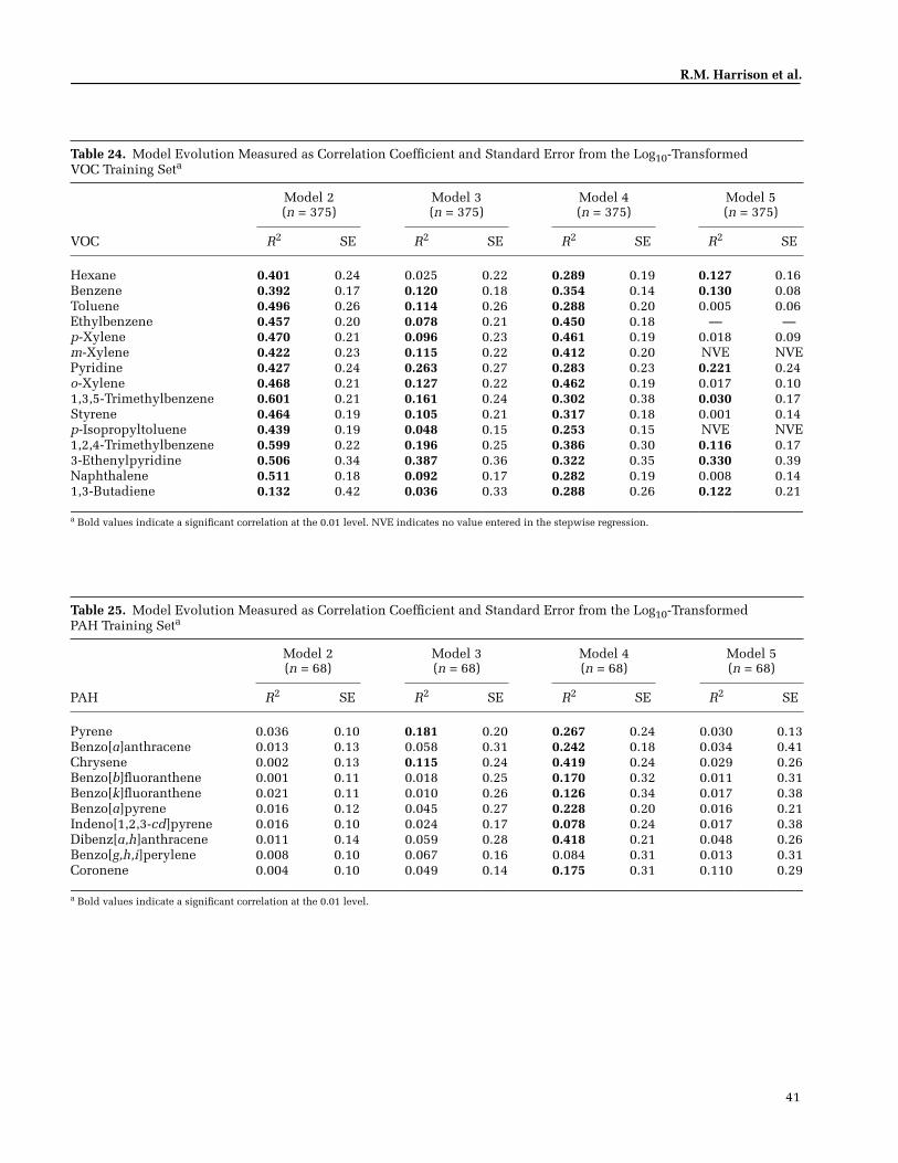
41


Table 24. Model Evolution Measured as Correlation Coefficient and Standard Error from the Log10-Transformed VOC Training Seta

VOC

Model 2(n = 375)

Model 3(n = 375)

Model 4(n = 375)

Model 5(n = 375)

R2 SE R2 SE R2 SE R2 SE

Hexane 0.401 0.24 0.025 0.22 0.289 0.19 0.127 0.16Benzene 0.392 0.17 0.120 0.18 0.354 0.14 0.130 0.08Toluene 0.496 0.26 0.114 0.26 0.288 0.20 0.005 0.06Ethylbenzene 0.457 0.20 0.078 0.21 0.450 0.18 — —p-Xylene 0.470 0.21 0.096 0.23 0.461 0.19 0.018 0.09m-Xylene 0.422 0.23 0.115 0.22 0.412 0.20 NVE NVEPyridine 0.427 0.24 0.263 0.27 0.283 0.23 0.221 0.24o-Xylene 0.468 0.21 0.127 0.22 0.462 0.19 0.017 0.101,3,5-Trimethylbenzene 0.601 0.21 0.161 0.24 0.302 0.38 0.030 0.17Styrene 0.464 0.19 0.105 0.21 0.317 0.18 0.001 0.14p-Isopropyltoluene 0.439 0.19 0.048 0.15 0.253 0.15 NVE NVE1,2,4-Trimethylbenzene 0.599 0.22 0.196 0.25 0.386 0.30 0.116 0.173-Ethenylpyridine 0.506 0.34 0.387 0.36 0.322 0.35 0.330 0.39Naphthalene 0.511 0.18 0.092 0.17 0.282 0.19 0.008 0.141,3-Butadiene 0.132 0.42 0.036 0.33 0.288 0.26 0.122 0.21

a Bold values indicate a significant correlation at the 0.01 level. NVE indicates no value entered in the stepwise regression.

Table 25. Model Evolution Measured as Correlation Coefficient and Standard Error from the Log10-Transformed PAH Training Seta

PAH

Model 2(n = 68)

Model 3(n = 68)

Model 4(n = 68)

Model 5(n = 68)

R2 SE R2 SE R2 SE R2 SE

Pyrene 0.036 0.10 0.181 0.20 0.267 0.24 0.030 0.13Benzo[a]anthracene 0.013 0.13 0.058 0.31 0.242 0.18 0.034 0.41Chrysene 0.002 0.13 0.115 0.24 0.419 0.24 0.029 0.26Benzo[b]fluoranthene 0.001 0.11 0.018 0.25 0.170 0.32 0.011 0.31Benzo[k]fluoranthene 0.021 0.11 0.010 0.26 0.126 0.34 0.017 0.38Benzo[a]pyrene 0.016 0.12 0.045 0.27 0.228 0.20 0.016 0.21Indeno[1,2,3-cd]pyrene 0.016 0.10 0.024 0.17 0.078 0.24 0.017 0.38Dibenz[a,h]anthracene 0.011 0.14 0.059 0.28 0.418 0.21 0.048 0.26Benzo[g,h,i]perylene 0.008 0.10 0.067 0.16 0.084 0.31 0.013 0.31Coronene 0.004 0.10 0.049 0.14 0.175 0.31 0.110 0.29

a Bold values indicate a significant correlation at the 0.01 level.

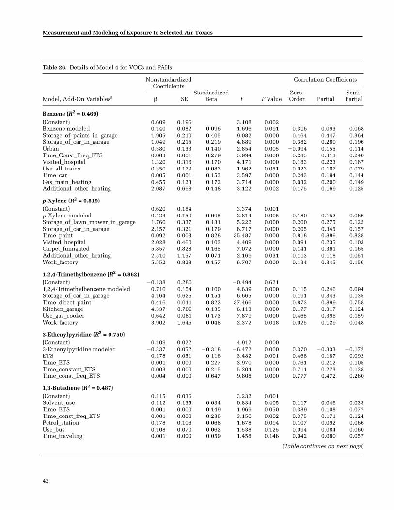
42


Table 26. Details of Model 4 for VOCs and PAHs

Model, Add-On Variablesa

NonstandardizedCoefficients

StandardizedBeta t P Value

Correlation Coefficients

Zero-Order Partial

Semi-Partial� SE

Benzene (R2 = 0.469)(Constant) 0.609 0.196 3.108 0.002Benzene modeled 0.140 0.082 0.096 1.696 0.091 0.316 0.093 0.068Storage_of_paints_in_garage 1.905 0.210 0.405 9.082 0.000 0.464 0.447 0.364Storage_of_car_in_garage 1.049 0.215 0.219 4.889 0.000 0.382 0.260 0.196Urban 0.380 0.133 0.140 2.854 0.005 �0.094 0.155 0.114Time_Const_Freq_ETS 0.003 0.001 0.279 5.994 0.000 0.285 0.313 0.240Visited_hospital 1.320 0.316 0.170 4.171 0.000 0.183 0.223 0.167Use_all_trains 0.350 0.179 0.083 1.962 0.051 0.023 0.107 0.079Time_car 0.005 0.001 0.153 3.597 0.000 0.243 0.194 0.144Gas_main_heating 0.455 0.123 0.172 3.714 0.000 0.032 0.200 0.149Additional_other_heating 2.087 0.668 0.148 3.122 0.002 0.175 0.169 0.125

p-Xylene (R2 = 0.819)(Constant) 0.620 0.184 3.374 0.001p-Xylene modeled 0.423 0.150 0.095 2.814 0.005 0.180 0.152 0.066Storage_of_lawn_mower_in_garage 1.760 0.337 0.131 5.222 0.000 0.200 0.275 0.122Storage_of_car_in_garage 2.157 0.321 0.179 6.717 0.000 0.205 0.345 0.157Time_paint 0.092 0.003 0.828 35.487 0.000 0.818 0.889 0.828Visited_hospital 2.028 0.460 0.103 4.409 0.000 0.091 0.235 0.103Carpet_fumigated 5.857 0.828 0.165 7.072 0.000 0.141 0.361 0.165Additional_other_heating 2.510 1.157 0.071 2.169 0.031 0.113 0.118 0.051Work_factory 5.552 0.828 0.157 6.707 0.000 0.134 0.345 0.156

1,2,4-Trimethylbenzene (R2 = 0.862)(Constant) �0.138 0.280 �0.494 0.6211,2,4-Trimethylbenzene modeled 0.716 0.154 0.100 4.639 0.000 0.115 0.246 0.094Storage_of_car_in_garage 4.164 0.625 0.151 6.665 0.000 0.191 0.343 0.135Time_direct_paint 0.416 0.011 0.822 37.466 0.000 0.873 0.899 0.758Kitchen_garage 4.337 0.709 0.135 6.113 0.000 0.177 0.317 0.124Use_gas_cooker 0.642 0.081 0.173 7.879 0.000 0.465 0.396 0.159Work_factory 3.902 1.645 0.048 2.372 0.018 0.025 0.129 0.048

3-Ethenylpyridine (R2 = 0.750)(Constant) 0.109 0.022 4.912 0.0003-Ethenylpyridine modeled �0.337 0.052 �0.318 �6.472 0.000 0.370 �0.333 �0.172ETS 0.178 0.051 0.116 3.482 0.001 0.468 0.187 0.092Time_ETS 0.001 0.000 0.227 3.970 0.000 0.761 0.212 0.105Time_constant_ETS 0.003 0.000 0.215 5.204 0.000 0.711 0.273 0.138Time_const_freq_ETS 0.004 0.000 0.647 9.808 0.000 0.777 0.472 0.260

1,3-Butadiene (R2 = 0.487)(Constant) 0.115 0.036 3.232 0.001Solvent_use 0.112 0.135 0.034 0.834 0.405 0.117 0.046 0.033Time_ETS 0.001 0.000 0.149 1.969 0.050 0.389 0.108 0.077Time_const_freq_ETS 0.001 0.000 0.236 3.150 0.002 0.375 0.171 0.124Petrol_station 0.178 0.106 0.068 1.678 0.094 0.107 0.092 0.066Use_bus 0.108 0.070 0.062 1.538 0.125 0.094 0.084 0.060Time_traveling 0.001 0.000 0.059 1.458 0.146 0.042 0.080 0.057

(Table continues on next page)

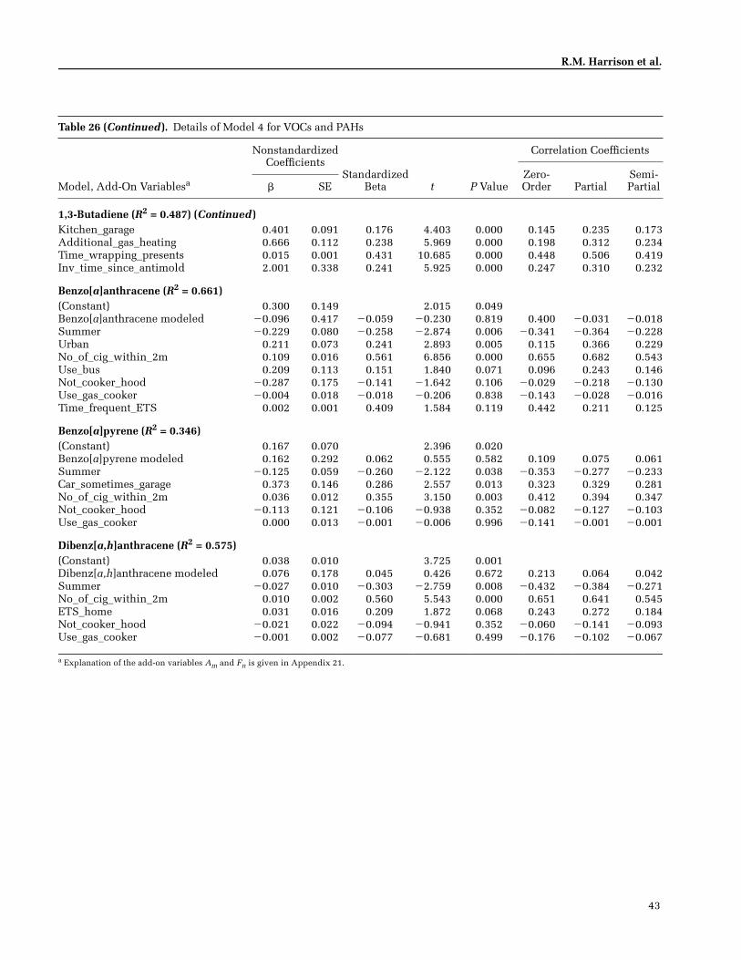
43


Table 26 (Continued). Details of Model 4 for VOCs and PAHs

Model, Add-On Variablesa

NonstandardizedCoefficients

StandardizedBeta t P Value

Correlation Coefficients

Zero-Order Partial

Semi-Partial� SE

1,3-Butadiene (R2 = 0.487) (Continued)Kitchen_garage 0.401 0.091 0.176 4.403 0.000 0.145 0.235 0.173Additional_gas_heating 0.666 0.112 0.238 5.969 0.000 0.198 0.312 0.234Time_wrapping_presents 0.015 0.001 0.431 10.685 0.000 0.448 0.506 0.419Inv_time_since_antimold 2.001 0.338 0.241 5.925 0.000 0.247 0.310 0.232

Benzo[a]anthracene (R2 = 0.661)(Constant) 0.300 0.149 2.015 0.049Benzo[a]anthracene modeled �0.096 0.417 �0.059 �0.230 0.819 0.400 �0.031 �0.018Summer �0.229 0.080 �0.258 �2.874 0.006 �0.341 �0.364 �0.228Urban 0.211 0.073 0.241 2.893 0.005 0.115 0.366 0.229No_of_cig_within_2m 0.109 0.016 0.561 6.856 0.000 0.655 0.682 0.543Use_bus 0.209 0.113 0.151 1.840 0.071 0.096 0.243 0.146Not_cooker_hood �0.287 0.175 �0.141 �1.642 0.106 �0.029 �0.218 �0.130Use_gas_cooker �0.004 0.018 �0.018 �0.206 0.838 �0.143 �0.028 �0.016Time_frequent_ETS 0.002 0.001 0.409 1.584 0.119 0.442 0.211 0.125

Benzo[a]pyrene (R2 = 0.346)(Constant) 0.167 0.070 2.396 0.020Benzo[a]pyrene modeled 0.162 0.292 0.062 0.555 0.582 0.109 0.075 0.061Summer �0.125 0.059 �0.260 �2.122 0.038 �0.353 �0.277 �0.233Car_sometimes_garage 0.373 0.146 0.286 2.557 0.013 0.323 0.329 0.281No_of_cig_within_2m 0.036 0.012 0.355 3.150 0.003 0.412 0.394 0.347Not_cooker_hood �0.113 0.121 �0.106 �0.938 0.352 �0.082 �0.127 �0.103Use_gas_cooker 0.000 0.013 �0.001 �0.006 0.996 �0.141 �0.001 �0.001

Dibenz[a,h]anthracene (R2 = 0.575)(Constant) 0.038 0.010 3.725 0.001Dibenz[a,h]anthracene modeled 0.076 0.178 0.045 0.426 0.672 0.213 0.064 0.042Summer �0.027 0.010 �0.303 �2.759 0.008 �0.432 �0.384 �0.271No_of_cig_within_2m 0.010 0.002 0.560 5.543 0.000 0.651 0.641 0.545ETS_home 0.031 0.016 0.209 1.872 0.068 0.243 0.272 0.184Not_cooker_hood �0.021 0.022 �0.094 �0.941 0.352 �0.060 �0.141 �0.093Use_gas_cooker �0.001 0.002 �0.077 �0.681 0.499 �0.176 �0.102 �0.067

a Explanation of the add-on variables Am and Fn is given in Appendix 21.

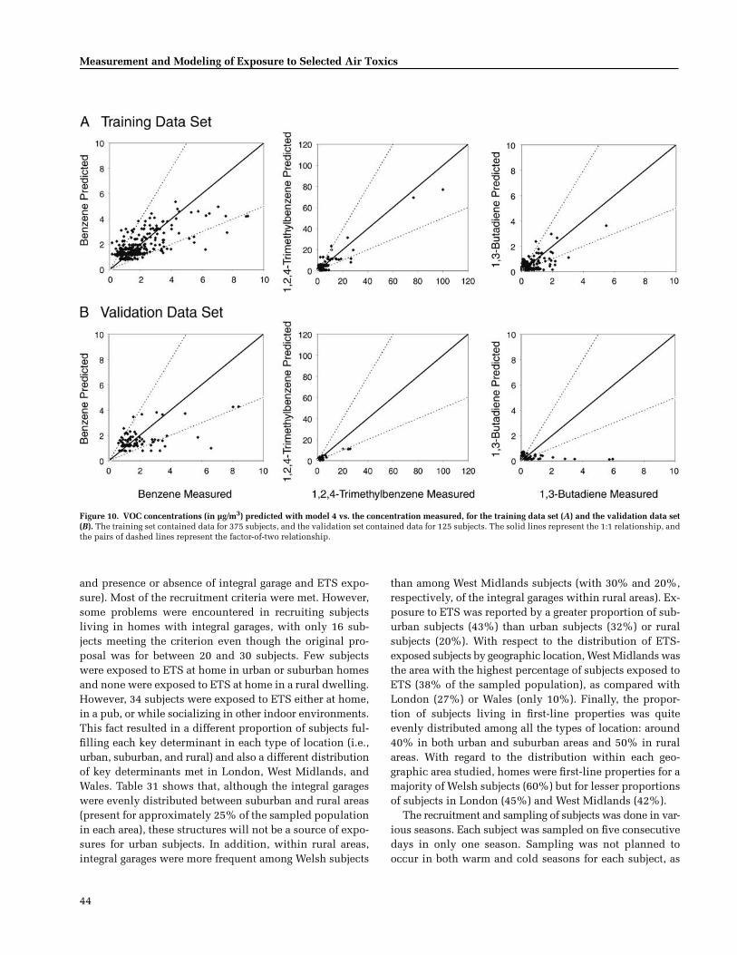
44


Figure 10. VOC concentrations (in µg/m3) predicted with model 4 vs. the concentration measured, for the training data set (A) and the validation data set(B). The training set contained data for 375 subjects, and the validation set contained data for 125 subjects. The solid lines represent the 1:1 relationship, andthe pairs of dashed lines represent the factor-of-two relationship.

and presence or absence of integral garage and ETS expo-sure). Most of the recruitment criteria were met. However,some problems were encountered in recruiting subjectsliving in homes with integral garages, with only 16 sub-jects meeting the criterion even though the original pro-posal was for between 20 and 30 subjects. Few subjectswere exposed to ETS at home in urban or suburban homesand none were exposed to ETS at home in a rural dwelling.However, 34 subjects were exposed to ETS either at home,in a pub, or while socializing in other indoor environments.This fact resulted in a different proportion of subjects ful-filling each key determinant in each type of location (i.e.,urban, suburban, and rural) and also a different distributionof key determinants met in London, West Midlands, andWales. Table 31 shows that, although the integral garageswere evenly distributed between suburban and rural areas(present for approximately 25% of the sampled populationin each area), these structures will not be a source of expo-sures for urban subjects. In addition, within rural areas,integral garages were more frequent among Welsh subjects

than among West Midlands subjects (with 30% and 20%,respectively, of the integral garages within rural areas). Ex-posure to ETS was reported by a greater proportion of sub-urban subjects (43%) than urban subjects (32%) or ruralsubjects (20%). With respect to the distribution of ETS-exposed subjects by geographic location, West Midlands wasthe area with the highest percentage of subjects exposed toETS (38% of the sampled population), as compared withLondon (27%) or Wales (only 10%). Finally, the propor-tion of subjects living in first-line properties was quiteevenly distributed among all the types of location: around40% in both urban and suburban areas and 50% in ruralareas. With regard to the distribution within each geo-graphic area studied, homes were first-line properties for amajority of Welsh subjects (60%) but for lesser proportionsof subjects in London (45%) and West Midlands (42%).

The recruitment and sampling of subjects was done in var-ious seasons. Each subject was sampled on five consecutivedays in only one season. Sampling was not planned tooccur in both warm and cold seasons for each subject, as

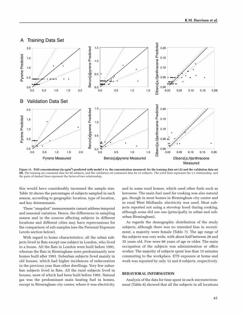
45


this would have considerably increased the sample size.Table 32 shows the percentages of subjects sampled in eachseason, according to geographic location, type of location,and key determinants.

These “snapshot” measurements cannot address temporaland seasonal variation. Hence, the differences in samplingseason and in the sources affecting subjects in differentlocations and different cities may have repercussions forthe comparison of sub-samples (see the Personal ExposureLevels section below).

With regard to home characteristics, all the urban sub-jects lived in flats except one subject in London, who livedin a house. All the flats in London were built before 1991,whereas the flats in Birmingham were predominantly newhomes built after 1991. Suburban subjects lived mainly inold houses, which had higher incidences of redecorationin the previous year than other dwellings. Very few subur-ban subjects lived in flats. All the rural subjects lived inhouses, most of which had been built before 1991. Naturalgas was the predominant main heating fuel in homes,except in Birmingham city center, where it was electricity,

and in some rural homes, which used other fuels such askerosene. The main fuel used for cooking was also naturalgas, though in most homes in Birmingham city center andin rural West Midlands, electricity was used. Most sub-jects reported not using a stovetop hood during cooking,although some did use one (principally in urban and sub-urban Birmingham).

As regards the demographic distribution of the studysubjects, although there was no intended bias in recruit-ment, a majority were female (Table 7). The age range ofthe subjects was very wide, with about half between 26 and35 years old. Few were 66 years of age or older. The mainoccupation of the subjects was administration or officeworker. The majority of subjects spent less than 15 minutescommuting to the workplace. ETS exposure at home andwork was reported by only 12 and 8 subjects, respectively.


Analysis of the data for time spent in each microenviron-ment (Table 8) showed that all the subjects in all locations

Figure 11. PAH concentrations (in ng/m3) predicted with model 4 vs. the concentration measured, for the training data set (A) and the validation data set(B). The training set contained data for 68 subjects, and the validation set contained data for 23 subjects. The solid lines represent the 1:1 relationship, andthe pairs of dashed lines represent the factor-of-two relationship.

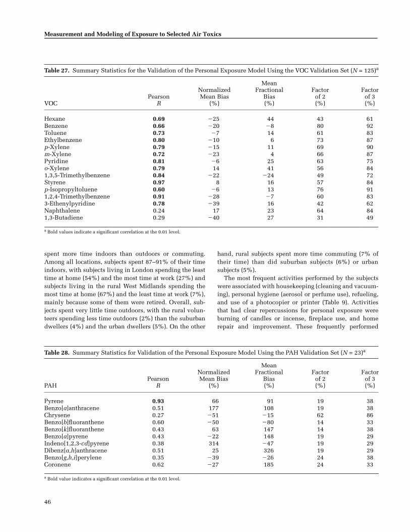
46


spent more time indoors than outdoors or commuting.Among all locations, subjects spent 87–91% of their timeindoors, with subjects living in London spending the leasttime at home (54%) and the most time at work (27%) andsubjects living in the rural West Midlands spending themost time at home (67%) and the least time at work (7%),mainly because some of them were retired. Overall, sub-jects spent very little time outdoors, with the rural volun-teers spending less time outdoors (2%) than the suburbandwellers (4%) and the urban dwellers (5%). On the other

hand, rural subjects spent more time commuting (7% oftheir time) than did suburban subjects (6%) or urbansubjects (5%).

The most frequent activities performed by the subjectswere associated with housekeeping (cleaning and vacuum-ing), personal hygiene (aerosol or perfume use), refueling,and use of a photocopier or printer (Table 9). Activitiesthat had clear repercussions for personal exposure wereburning of candles or incense, fireplace use, and homerepair and improvement. These frequently performed

Table 27. Summary Statistics for the Validation of the Personal Exposure Model Using the VOC Validation Set (N = 125)a

VOCPearson

R

NormalizedMean Bias

(%)

MeanFractional

Bias(%)

Factorof 2(%)

Factorof 3(%)

Hexane 0.69 �25 44 43 61Benzene 0.66 �20 �8 80 92Toluene 0.73 �7 14 61 83Ethylbenzene 0.80 �10 6 73 87p-Xylene 0.79 �15 11 69 90m-Xylene 0.72 �23 4 66 87Pyridine 0.81 �6 25 63 75o-Xylene 0.79 14 41 56 841,3,5-Trimethylbenzene 0.84 �22 �24 49 72Styrene 0.97 8 16 57 84p-Isopropyltoluene 0.60 �6 13 76 911,2,4-Trimethylbenzene 0.91 �28 �7 60 833-Ethenylpyridine 0.78 �39 16 42 62Naphthalene 0.24 17 23 64 841,3-Butadiene 0.29 �40 27 31 49

a Bold values indicate a significant correlation at the 0.01 level.

Table 28. Summary Statistics for Validation of the Personal Exposure Model Using the PAH Validation Set (N = 23)a

PAHPearson

R

NormalizedMean Bias

(%)

MeanFractional

Bias(%)

Factorof 2(%)

Factorof 3(%)

Pyrene 0.93 66 91 19 38Benzo[a]anthracene 0.51 177 108 19 38Chrysene 0.27 �51 �15 62 86Benzo[b]fluoranthene 0.60 �50 �80 14 33Benzo[k]fluoranthene 0.43 63 147 14 38Benzo[a]pyrene 0.43 �22 148 19 29Indeno[1,2,3-cd]pyrene 0.38 314 �47 19 29Dibenz[a,h]anthracene 0.51 25 326 19 29Benzo[g,h,i]perylene 0.35 �39 �26 24 38Coronene 0.62 �27 185 24 33

a Bold value indicates a significant correlation at the 0.01 level.

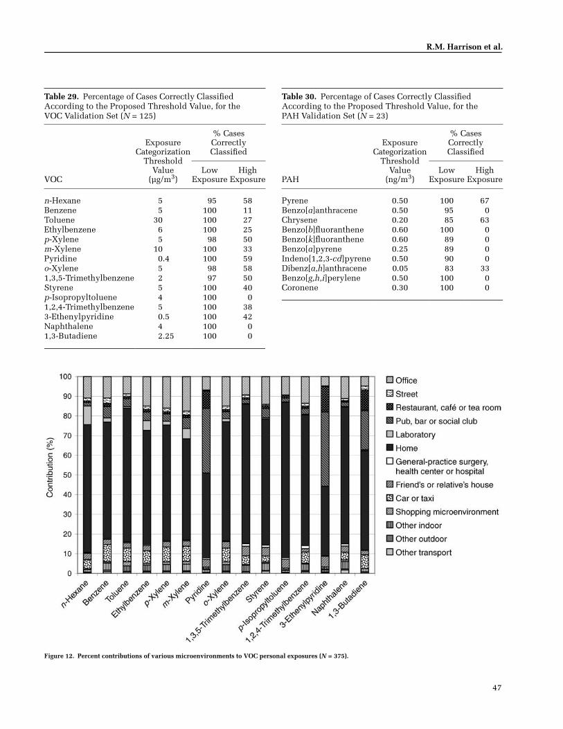
47


Table 29. Percentage of Cases Correctly Classified According to the Proposed Threshold Value, for the VOC Validation Set (N = 125)

VOC

ExposureCategorization

ThresholdValue

(µg/m3)

% CasesCorrectlyClassified

LowExposure

HighExposure

n-Hexane 5 95 58Benzene 5 100 11Toluene 30 100 27Ethylbenzene 6 100 25p-Xylene 5 98 50m-Xylene 10 100 33Pyridine 0.4 100 59o-Xylene 5 98 581,3,5-Trimethylbenzene 2 97 50Styrene 5 100 40p-Isopropyltoluene 4 100 01,2,4-Trimethylbenzene 5 100 383-Ethenylpyridine 0.5 100 42Naphthalene 4 100 01,3-Butadiene 2.25 100 0

Table 30. Percentage of Cases Correctly Classified According to the Proposed Threshold Value, for the PAH Validation Set (N = 23)

PAH

ExposureCategorization

ThresholdValue

(ng/m3)

% CasesCorrectlyClassified

LowExposure

HighExposure

Pyrene 0.50 100 67Benzo[a]anthracene 0.50 95 0Chrysene 0.20 85 63Benzo[b]fluoranthene 0.60 100 0Benzo[k]fluoranthene 0.60 89 0Benzo[a]pyrene 0.25 89 0Indeno[1,2,3-cd]pyrene 0.50 90 0Dibenz[a,h]anthracene 0.05 83 33Benzo[g,h,i]perylene 0.50 100 0Coronene 0.30 100 0

Figure 12. Percent contributions of various microenvironments to VOC personal exposures (N = 375).

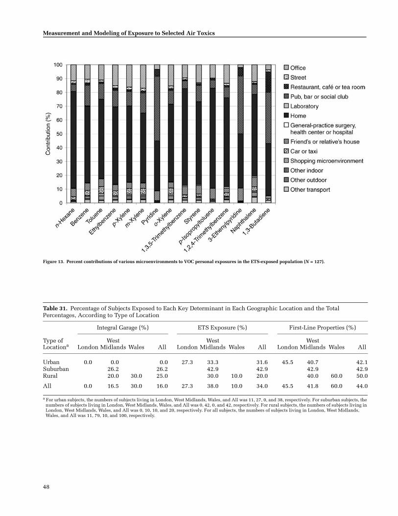
48


Figure 13. Percent contributions of various microenvironments to VOC personal exposures in the ETS-exposed population (N = 127).

Table 31. Percentage of Subjects Exposed to Each Key Determinant in Each Geographic Location and the Total Percentages, According to Type of Location

Type of Locationa

Integral Garage (%) ETS Exposure (%) First-Line Properties (%)

LondonWest

Midlands Wales All LondonWest

Midlands Wales All LondonWest

Midlands Wales All

Urban 0.0 0.0 0.0 27.3 33.3 31.6 45.5 40.7 42.1Suburban 26.2 26.2 42.9 42.9 42.9 42.9Rural 20.0 30.0 25.0 30.0 10.0 20.0 40.0 60.0 50.0

All 0.0 16.5 30.0 16.0 27.3 38.0 10.0 34.0 45.5 41.8 60.0 44.0

a For urban subjects, the numbers of subjects living in London, West Midlands, Wales, and All was 11, 27, 0, and 38, respectively. For suburban subjects, the numbers of subjects living in London, West Midlands, Wales, and All was 0, 42, 0, and 42, respectively. For rural subjects, the numbers of subjects living in London, West Midlands, Wales, and All was 0, 10, 10, and 20, respectively. For all subjects, the numbers of subjects living in London, West Midlands, Wales, and All was 11, 79, 10, and 100, respectively.

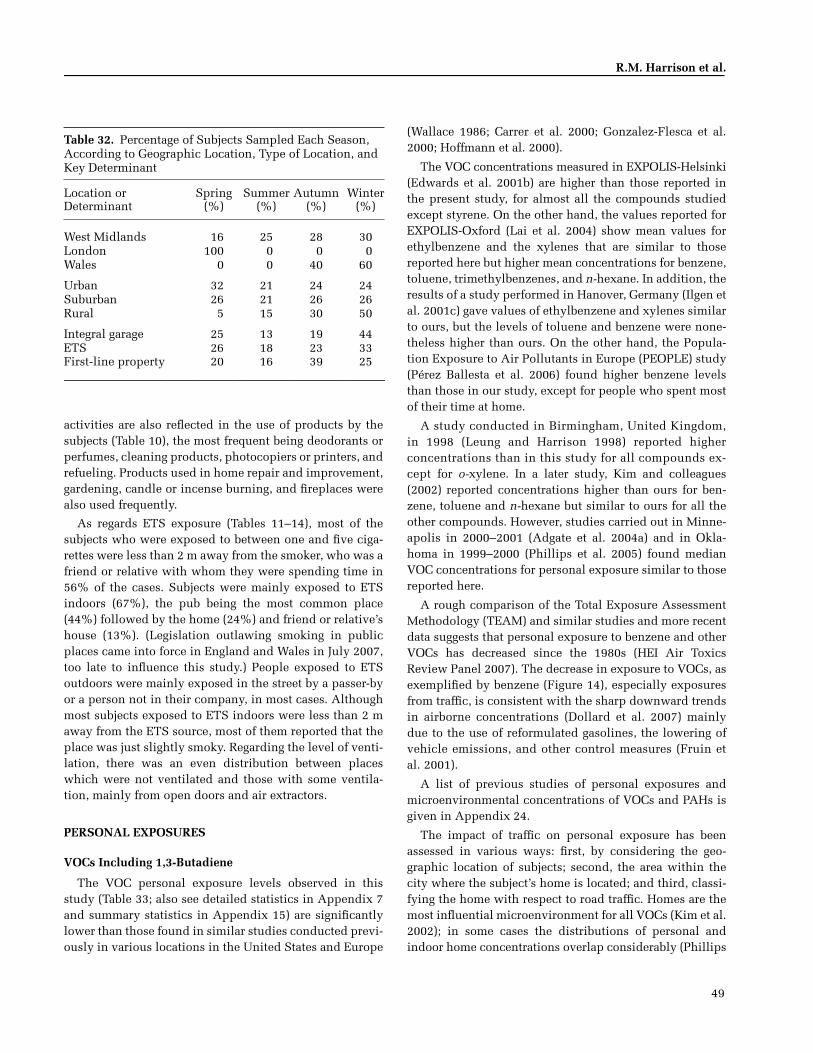
49


activities are also reflected in the use of products by thesubjects (Table 10), the most frequent being deodorants orperfumes, cleaning products, photocopiers or printers, andrefueling. Products used in home repair and improvement,gardening, candle or incense burning, and fireplaces werealso used frequently.

As regards ETS exposure (Tables 11–14), most of thesubjects who were exposed to between one and five ciga-rettes were less than 2 m away from the smoker, who was afriend or relative with whom they were spending time in56% of the cases. Subjects were mainly exposed to ETSindoors (67%), the pub being the most common place(44%) followed by the home (24%) and friend or relative’shouse (13%). (Legislation outlawing smoking in publicplaces came into force in England and Wales in July 2007,too late to influence this study.) People exposed to ETSoutdoors were mainly exposed in the street by a passer-byor a person not in their company, in most cases. Althoughmost subjects exposed to ETS indoors were less than 2 maway from the ETS source, most of them reported that theplace was just slightly smoky. Regarding the level of venti-lation, there was an even distribution between placeswhich were not ventilated and those with some ventila-tion, mainly from open doors and air extractors.

PERSONAL EXPOSURES

VOCs Including 1,3-Butadiene

The VOC personal exposure levels observed in thisstudy (Table 33; also see detailed statistics in Appendix 7and summary statistics in Appendix 15) are significantlylower than those found in similar studies conducted previ-ously in various locations in the United States and Europe

(Wallace 1986; Carrer et al. 2000; Gonzalez-Flesca et al.2000; Hoffmann et al. 2000).

The VOC concentrations measured in EXPOLIS-Helsinki(Edwards et al. 2001b) are higher than those reported inthe present study, for almost all the compounds studiedexcept styrene. On the other hand, the values reported forEXPOLIS-Oxford (Lai et al. 2004) show mean values forethylbenzene and the xylenes that are similar to thosereported here but higher mean concentrations for benzene,toluene, trimethylbenzenes, and n-hexane. In addition, theresults of a study performed in Hanover, Germany (Ilgen etal. 2001c) gave values of ethylbenzene and xylenes similarto ours, but the levels of toluene and benzene were none-theless higher than ours. On the other hand, the Popula-tion Exposure to Air Pollutants in Europe (PEOPLE) study(Pérez Ballesta et al. 2006) found higher benzene levelsthan those in our study, except for people who spent mostof their time at home.

A study conducted in Birmingham, United Kingdom,in 1998 (Leung and Harrison 1998) reported higherconcentrations than in this study for all compounds ex-cept for o-xylene. In a later study, Kim and colleagues(2002) reported concentrations higher than ours for ben-zene, toluene and n-hexane but similar to ours for all theother compounds. However, studies carried out in Minne-apolis in 2000–2001 (Adgate et al. 2004a) and in Okla-homa in 1999–2000 (Phillips et al. 2005) found medianVOC concentrations for personal exposure similar to thosereported here.

A rough comparison of the Total Exposure AssessmentMethodology (TEAM) and similar studies and more recentdata suggests that personal exposure to benzene and otherVOCs has decreased since the 1980s (HEI Air ToxicsReview Panel 2007). The decrease in exposure to VOCs, asexemplified by benzene (Figure 14), especially exposuresfrom traffic, is consistent with the sharp downward trendsin airborne concentrations (Dollard et al. 2007) mainlydue to the use of reformulated gasolines, the lowering ofvehicle emissions, and other control measures (Fruin etal. 2001).

A list of previous studies of personal exposures andmicroenvironmental concentrations of VOCs and PAHs isgiven in Appendix 24.

The impact of traffic on personal exposure has beenassessed in various ways: first, by considering the geo-graphic location of subjects; second, the area within thecity where the subject’s home is located; and third, classi-fying the home with respect to road traffic. Homes are themost influential microenvironment for all VOCs (Kim et al.2002); in some cases the distributions of personal andindoor home concentrations overlap considerably (Phillips

Table 32. Percentage of Subjects Sampled Each Season, According to Geographic Location, Type of Location, and Key Determinant

Location or Determinant

Spring(%)

Summer(%)

Autumn(%)

Winter(%)

West Midlands 16 25 28 30London 100 0 0 0Wales 0 0 40 60

Urban 32 21 24 24Suburban 26 21 26 26Rural 5 15 30 50

Integral garage 25 13 19 44ETS 26 18 23 33First-line property 20 16 39 25

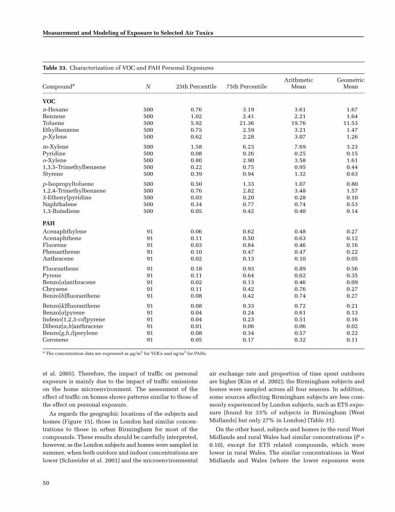
50


et al. 2005). Therefore, the impact of traffic on personalexposure is mainly due to the impact of traffic emissionson the home microenvironment. The assessment of theeffect of traffic on homes shows patterns similar to those ofthe effect on personal exposure.

As regards the geographic locations of the subjects andhomes (Figure 15), those in London had similar concen-trations to those in urban Birmingham for most of thecompounds. These results should be carefully interpreted,however, as the London subjects and homes were sampled insummer, when both outdoor and indoor concentrations arelower (Schneider et al. 2001) and the microenvironmental

air exchange rate and proportion of time spent outdoorsare higher (Kim et al. 2002); the Birmingham subjects andhomes were sampled across all four seasons. In addition,some sources affecting Birmingham subjects are less com-monly experienced by London subjects, such as ETS expo-sure (found for 33% of subjects in Birmingham [WestMidlands] but only 27% in London) (Table 31).

On the other hand, subjects and homes in the rural WestMidlands and rural Wales had similar concentrations (P >0.10), except for ETS related compounds, which werelower in rural Wales. The similar concentrations in WestMidlands and Wales (where the lower exposures were

Table 33. Characterization of VOC and PAH Personal Exposures

Compounda N 25th Percentile 75th PercentileArithmetic

MeanGeometric

Mean

VOCn-Hexane 500 0.76 3.19 3.61 1.67Benzene 500 1.02 2.41 2.21 1.64Toluene 500 5.92 21.36 19.76 11.53Ethylbenzene 500 0.75 2.59 3.21 1.47p-Xylene 500 0.62 2.28 3.07 1.26

m-Xylene 500 1.58 6.23 7.69 3.23Pyridine 500 0.08 0.26 0.25 0.15o-Xylene 500 0.80 2.90 3.58 1.611,3,5-Trimethylbenzene 500 0.22 0.75 0.95 0.44Styrene 500 0.39 0.94 1.32 0.63

p-Isopropyltoluene 500 0.50 1.33 1.07 0.801,2,4-Trimethylbenzene 500 0.76 2.82 3.48 1.573-Ethenylpyridine 500 0.03 0.20 0.28 0.10Naphthalene 500 0.34 0.77 0.74 0.531,3-Butadiene 500 0.05 0.42 0.40 0.14

PAHAcenaphthylene 91 0.06 0.62 0.48 0.27Acenaphthene 91 0.11 0.50 0.63 0.12Fluorene 91 0.03 0.84 0.46 0.16Phenanthrene 91 0.10 0.47 0.47 0.22Anthracene 91 0.02 0.13 0.10 0.05

Fluoranthene 91 0.18 0.93 0.89 0.56Pyrene 91 0.11 0.64 0.62 0.35Benzo[a]anthracene 91 0.02 0.13 0.46 0.09Chrysene 91 0.11 0.42 0.76 0.27Benzo[b]fluoranthene 91 0.08 0.42 0.74 0.27

Benzo[k]fluoranthene 91 0.08 0.33 0.72 0.21Benzo[a]pyrene 91 0.04 0.24 0.61 0.13Indeno[1,2,3-cd]pyrene 91 0.04 0.23 0.51 0.16Dibenz[a,h]anthracene 91 0.01 0.06 0.06 0.02Benzo[g,h,i]perylene 91 0.08 0.34 0.57 0.22Coronene 91 0.05 0.17 0.32 0.11

a The concentration data are expressed as µg/m3 for VOCs and ng/m3 for PAHs.

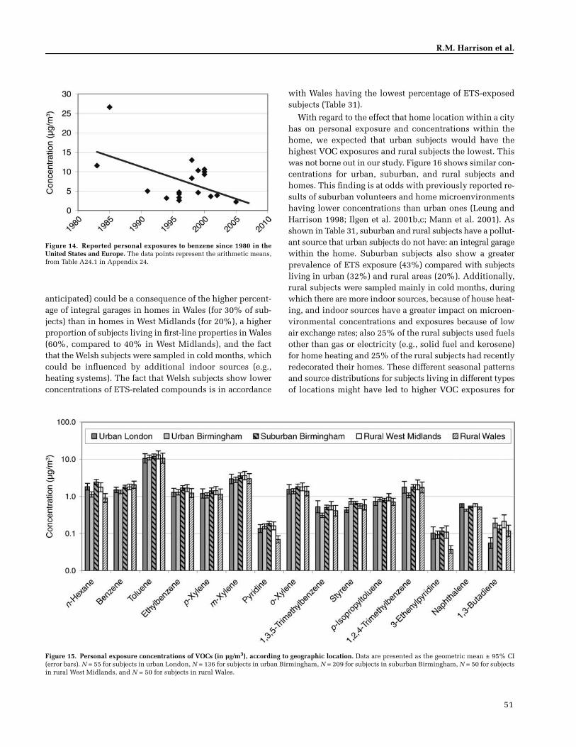
51


anticipated) could be a consequence of the higher percent-age of integral garages in homes in Wales (for 30% of sub-jects) than in homes in West Midlands (for 20%), a higherproportion of subjects living in first-line properties in Wales(60%, compared to 40% in West Midlands), and the factthat the Welsh subjects were sampled in cold months, whichcould be influenced by additional indoor sources (e.g.,heating systems). The fact that Welsh subjects show lowerconcentrations of ETS-related compounds is in accordance

with Wales having the lowest percentage of ETS-exposedsubjects (Table 31).

With regard to the effect that home location within a cityhas on personal exposure and concentrations within thehome, we expected that urban subjects would have thehighest VOC exposures and rural subjects the lowest. Thiswas not borne out in our study. Figure 16 shows similar con-centrations for urban, suburban, and rural subjects andhomes. This finding is at odds with previously reported re-sults of suburban volunteers and home microenvironmentshaving lower concentrations than urban ones (Leung andHarrison 1998; Ilgen et al. 2001b,c; Mann et al. 2001). Asshown in Table 31, suburban and rural subjects have a pollut-ant source that urban subjects do not have: an integral garagewithin the home. Suburban subjects also show a greaterprevalence of ETS exposure (43%) compared with subjectsliving in urban (32%) and rural areas (20%). Additionally,rural subjects were sampled mainly in cold months, duringwhich there are more indoor sources, because of house heat-ing, and indoor sources have a greater impact on microen-vironmental concentrations and exposures because of lowair exchange rates; also 25% of the rural subjects used fuelsother than gas or electricity (e.g., solid fuel and kerosene)for home heating and 25% of the rural subjects had recentlyredecorated their homes. These different seasonal patternsand source distributions for subjects living in different typesof locations might have led to higher VOC exposures for

Figure 14. Reported personal exposures to benzene since 1980 in theUnited States and Europe. The data points represent the arithmetic means,from Table A24.1 in Appendix 24.

Figure 15. Personal exposure concentrations of VOCs (in µg/m3), according to geographic location. Data are presented as the geometric mean ± 95% CI(error bars). N = 55 for subjects in urban London, N = 136 for subjects in urban Birmingham, N = 209 for subjects in suburban Birmingham, N = 50 for subjectsin rural West Midlands, and N = 50 for subjects in rural Wales.

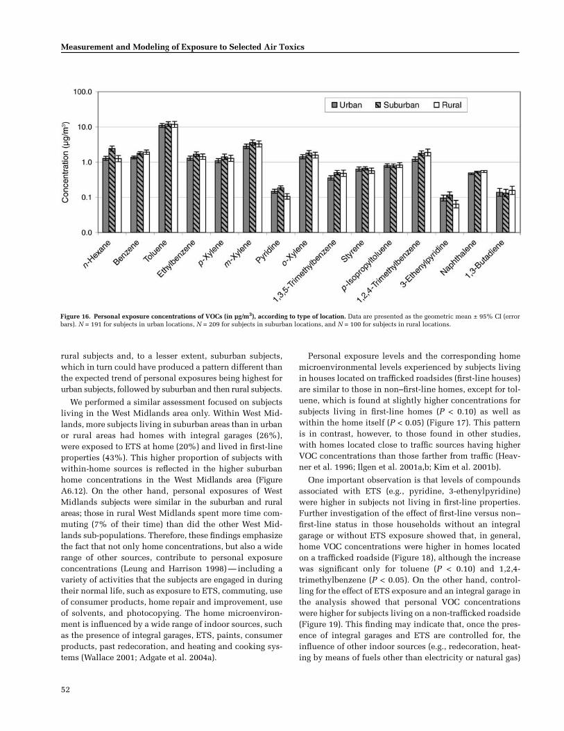
52


rural subjects and, to a lesser extent, suburban subjects,which in turn could have produced a pattern different thanthe expected trend of personal exposures being highest forurban subjects, followed by suburban and then rural subjects.

We performed a similar assessment focused on subjectsliving in the West Midlands area only. Within West Mid-lands, more subjects living in suburban areas than in urbanor rural areas had homes with integral garages (26%),were exposed to ETS at home (20%) and lived in first-lineproperties (43%). This higher proportion of subjects withwithin-home sources is reflected in the higher suburbanhome concentrations in the West Midlands area (FigureA6.12). On the other hand, personal exposures of WestMidlands subjects were similar in the suburban and ruralareas; those in rural West Midlands spent more time com-muting (7% of their time) than did the other West Mid-lands sub-populations. Therefore, these findings emphasizethe fact that not only home concentrations, but also a widerange of other sources, contribute to personal exposureconcentrations (Leung and Harrison 1998) — including avariety of activities that the subjects are engaged in duringtheir normal life, such as exposure to ETS, commuting, useof consumer products, home repair and improvement, useof solvents, and photocopying. The home microenviron-ment is influenced by a wide range of indoor sources, suchas the presence of integral garages, ETS, paints, consumerproducts, past redecoration, and heating and cooking sys-tems (Wallace 2001; Adgate et al. 2004a).

Personal exposure levels and the corresponding homemicroenvironmental levels experienced by subjects livingin houses located on trafficked roadsides (first-line houses)are similar to those in non–first-line homes, except for tol-uene, which is found at slightly higher concentrations forsubjects living in first-line homes (P < 0.10) as well aswithin the home itself (P < 0.05) (Figure 17). This patternis in contrast, however, to those found in other studies,with homes located close to traffic sources having higherVOC concentrations than those farther from traffic (Heav-ner et al. 1996; Ilgen et al. 2001a,b; Kim et al. 2001b).

One important observation is that levels of compoundsassociated with ETS (e.g., pyridine, 3-ethenylpyridine)were higher in subjects not living in first-line properties.Further investigation of the effect of first-line versus non–first-line status in those households without an integralgarage or without ETS exposure showed that, in general,home VOC concentrations were higher in homes locatedon a trafficked roadside (Figure 18), although the increasewas significant only for toluene (P < 0.10) and 1,2,4-trimethylbenzene (P < 0.05). On the other hand, control-ling for the effect of ETS exposure and an integral garage inthe analysis showed that personal VOC concentrationswere higher for subjects living on a non-trafficked roadside(Figure 19). This finding may indicate that, once the pres-ence of integral garages and ETS are controlled for, theinfluence of other indoor sources (e.g., redecoration, heat-ing by means of fuels other than electricity or natural gas)

Figure 16. Personal exposure concentrations of VOCs (in µg/m3), according to type of location. Data are presented as the geometric mean ± 95% CI (errorbars). N = 191 for subjects in urban locations, N = 209 for subjects in suburban locations, and N = 100 for subjects in rural locations.

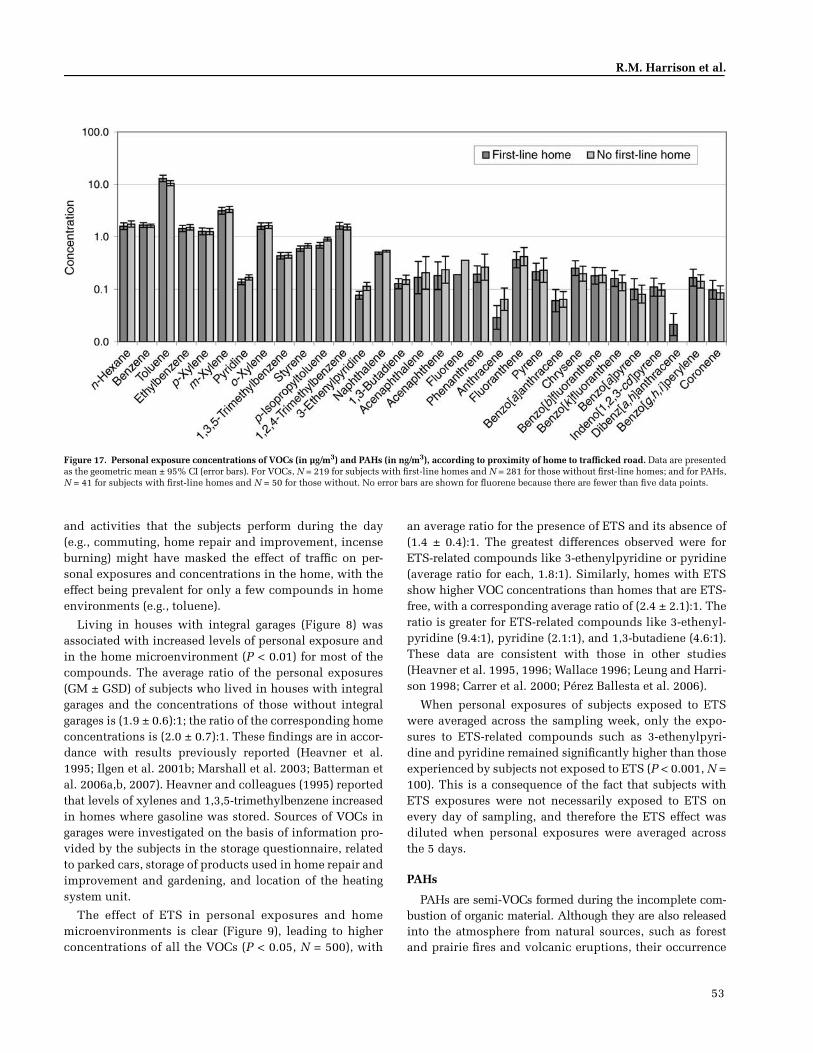
53


and activities that the subjects perform during the day(e.g., commuting, home repair and improvement, incenseburning) might have masked the effect of traffic on per-sonal exposures and concentrations in the home, with theeffect being prevalent for only a few compounds in homeenvironments (e.g., toluene).

Living in houses with integral garages (Figure 8) wasassociated with increased levels of personal exposure andin the home microenvironment (P < 0.01) for most of thecompounds. The average ratio of the personal exposures(GM ± GSD) of subjects who lived in houses with integralgarages and the concentrations of those without integralgarages is (1.9 ± 0.6):1; the ratio of the corresponding homeconcentrations is (2.0 ± 0.7):1. These findings are in accor-dance with results previously reported (Heavner et al.1995; Ilgen et al. 2001b; Marshall et al. 2003; Batterman etal. 2006a,b, 2007). Heavner and colleagues (1995) reportedthat levels of xylenes and 1,3,5-trimethylbenzene increasedin homes where gasoline was stored. Sources of VOCs ingarages were investigated on the basis of information pro-vided by the subjects in the storage questionnaire, relatedto parked cars, storage of products used in home repair andimprovement and gardening, and location of the heatingsystem unit.

The effect of ETS in personal exposures and homemicroenvironments is clear (Figure 9), leading to higherconcentrations of all the VOCs (P < 0.05, N = 500), with

an average ratio for the presence of ETS and its absence of(1.4 ± 0.4):1. The greatest differences observed were forETS-related compounds like 3-ethenylpyridine or pyridine(average ratio for each, 1.8:1). Similarly, homes with ETSshow higher VOC concentrations than homes that are ETS-free, with a corresponding average ratio of (2.4 ± 2.1):1. Theratio is greater for ETS-related compounds like 3-ethenyl-pyridine (9.4:1), pyridine (2.1:1), and 1,3-butadiene (4.6:1).These data are consistent with those in other studies(Heavner et al. 1995, 1996; Wallace 1996; Leung and Harri-son 1998; Carrer et al. 2000; Pérez Ballesta et al. 2006).

When personal exposures of subjects exposed to ETSwere averaged across the sampling week, only the expo-sures to ETS-related compounds such as 3-ethenylpyri-dine and pyridine remained significantly higher than thoseexperienced by subjects not exposed to ETS (P < 0.001, N =100). This is a consequence of the fact that subjects withETS exposures were not necessarily exposed to ETS onevery day of sampling, and therefore the ETS effect wasdiluted when personal exposures were averaged acrossthe 5 days.

PAHs

PAHs are semi-VOCs formed during the incomplete com-bustion of organic material. Although they are also releasedinto the atmosphere from natural sources, such as forestand prairie fires and volcanic eruptions, their occurrence

Figure 17. Personal exposure concentrations of VOCs (in µg/m3) and PAHs (in ng/m3), according to proximity of home to trafficked road. Data are presentedas the geometric mean ± 95% CI (error bars). For VOCs, N = 219 for subjects with first-line homes and N = 281 for those without first-line homes; and for PAHs,N = 41 for subjects with first-line homes and N = 50 for those without. No error bars are shown for fluorene because there are fewer than five data points.

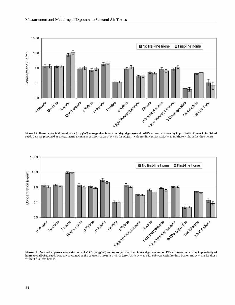
54


Figure 18. Home concentrations of VOCs (in µg/m3) among subjects with no integral garage and no ETS exposure, according to proximity of home to traffickedroad. Data are presented as the geometric mean ± 95% CI (error bars). N = 56 for subjects with first-line homes and N = 47 for those without first-line homes.

Figure 19. Personal exposure concentrations of VOCs (in µg/m3) among subjects with no integral garage and no ETS exposure, according to proximity ofhome to trafficked road. Data are presented as the geometric mean ± 95% CI (error bars). N = 128 for subjects with first-line homes and N = 111 for thosewithout first-line homes.

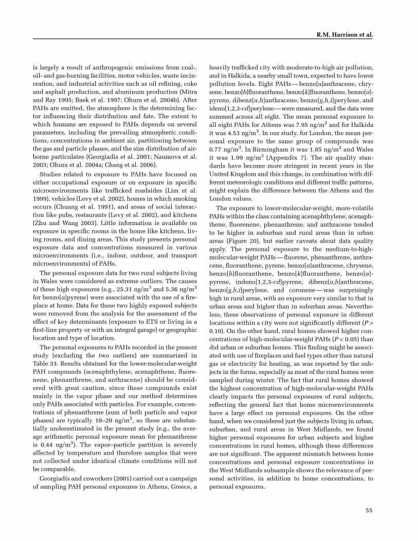
55


is largely a result of anthropogenic emissions from coal-,oil- and gas-burning facilities, motor vehicles, waste incin-eration, and industrial activities such as oil refining, cokeand asphalt production, and aluminum production (Mitraand Ray 1995; Baek et al. 1997; Ohura et al. 2004b). AfterPAHs are emitted, the atmosphere is the determining fac-tor influencing their distribution and fate. The extent towhich humans are exposed to PAHs depends on severalparameters, including the prevailing atmospheric condi-tions, concentrations in ambient air, partitioning betweenthe gas and particle phases, and the size distribution of air-borne particulates (Georgiadis et al. 2001; Naumova et al.2003; Ohura et al. 2004a; Chang et al. 2006).

Studies related to exposure to PAHs have focused oneither occupational exposure or on exposure in specificmicroenvironments like trafficked roadsides (Lim et al.1999), vehicles (Levy et al. 2002), homes in which smokingoccurs (Chuang et al. 1991), and areas of social interac-tion like pubs, restaurants (Levy et al. 2002), and kitchens(Zhu and Wang 2003). Little information is available onexposure in specific rooms in the home like kitchens, liv-ing rooms, and dining areas. This study presents personalexposure data and concentrations measured in variousmicroenvironments (i.e., indoor, outdoor, and transportmicroenvironments) of PAHs.

The personal exposure data for two rural subjects livingin Wales were considered as extreme outliers. The causesof these high exposures (e.g., 25.31 ng/m3 and 5.36 ng/m3

for benzo[a]pyrene) were associated with the use of a fire-place at home. Data for these two highly exposed subjectswere removed from the analysis for the assessment of theeffect of key determinants (exposure to ETS or living in afirst-line property or with an integral garage) or geographiclocation and type of location.

The personal exposures to PAHs recorded in the presentstudy (excluding the two outliers) are summarized inTable 33. Results obtained for the lower-molecular-weightPAH compounds (acenaphthylene, acenaphthene, fluore-nene, phenanthrene, and anthracene) should be consid-ered with great caution, since these compounds existmainly in the vapor phase and our method determinesonly PAHs associated with particles. For example, concen-trations of phenanthrene (sum of both particle and vaporphases) are typically 10–20 ng/m3, so these are substan-tially underestimated in the present study (e.g., the aver-age arithmetic personal exposure mean for phenanthreneis 0.44 ng/m3). The vapor–particle partition is severelyaffected by temperature and therefore samples that werenot collected under identical climate conditions will notbe comparable.

Georgiadis and coworkers (2001) carried out a campaignof sampling PAH personal exposures in Athens, Greece, a

heavily trafficked city with moderate-to-high air pollution,and in Halkida, a nearby small town, expected to have lowerpollution levels. Eight PAHs — benzo[a]anthracene, chry-sene, benzo[b]fluoranthene, benzo[k]fluoranthene, benzo[a]-pyrene, dibenz[a,h]anthracene, benzo[g,h,i]perylene, andideno[1,2,3-cd]perylene—were measured, and the data weresummed across all eight. The mean personal exposure toall eight PAHs for Athens was 7.95 ng/m3 and for Halkidait was 4.53 ng/m3. In our study, for London, the mean per-sonal exposure to the same group of compounds was0.77 ng/m3. In Birmingham it was 1.85 ng/m3 and Walesit was 1.99 ng/m3 (Appendix 7). The air quality stan-dards have become more stringent in recent years in theUnited Kingdom and this change, in combination with dif-ferent meteorologic conditions and different traffic patterns,might explain the difference between the Athens and theLondon values.

The exposure to lower-molecular-weight, more-volatilePAHs within the class containing acenaphthylene, acenaph-thene, fluorenene, phenanthrene, and anthracene tendedto be higher in suburban and rural areas than in urbanareas (Figure 20), but earlier caveats about data qualityapply. The personal exposure to the medium-to-high-molecular-weight PAHs — fluorene, phenanthrene, anthra-cene, fluoranthene, pyrene, benzo[a]anthracene, chrysene,benzo[b]fluoranthene, benzo[k]fluoranthene, benzo[a]-pyrene, indeno[1,2,3-cd]pyrene, dibenz[a,h]anthracene,benzo[g,h,i]perylene, and coronene — was surprisinglyhigh in rural areas, with an exposure very similar to that inurban areas and higher than in suburban areas. Neverthe-less, these observations of personal exposure in differentlocations within a city were not significantly different (P >0.10). On the other hand, rural homes showed higher con-centrations of high-molecular-weight PAHs (P < 0.05) thandid urban or suburban homes. This finding might be associ-ated with use of fireplaces and fuel types other than naturalgas or electricity for heating, as was reported by the sub-jects in the forms, especially as most of the rural homes weresampled during winter. The fact that rural homes showedthe highest concentration of high-molecular-weight PAHsclearly impacts the personal exposures of rural subjects,reflecting the general fact that home microenvironmentshave a large effect on personal exposures. On the otherhand, when we considered just the subjects living in urban,suburban, and rural areas in West Midlands, we foundhigher personal exposures for urban subjects and higherconcentrations in rural homes, although these differencesare not significant. The apparent mismatch between homeconcentrations and personal exposure concentrations inthe West Midlands subsample shows the relevance of per-sonal activities, in addition to home concentrations, topersonal exposures.

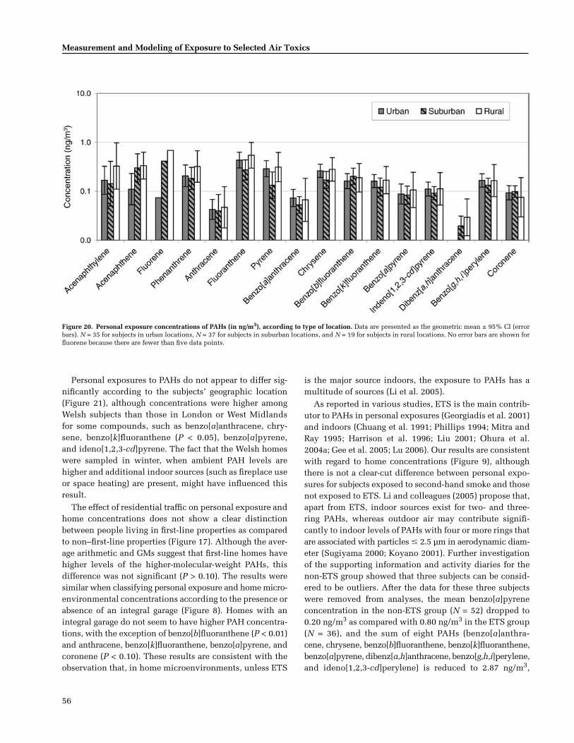
56


Personal exposures to PAHs do not appear to differ sig-nificantly according to the subjects’ geographic location(Figure 21), although concentrations were higher amongWelsh subjects than those in London or West Midlandsfor some compounds, such as benzo[a]anthracene, chry-sene, benzo[k]fluoranthene (P < 0.05), benzo[a]pyrene,and ideno[1,2,3-cd]pyrene. The fact that the Welsh homeswere sampled in winter, when ambient PAH levels arehigher and additional indoor sources (such as fireplace useor space heating) are present, might have influenced thisresult.

The effect of residential traffic on personal exposure andhome concentrations does not show a clear distinctionbetween people living in first-line properties as comparedto non–first-line properties (Figure 17). Although the aver-age arithmetic and GMs suggest that first-line homes havehigher levels of the higher-molecular-weight PAHs, thisdifference was not significant (P > 0.10). The results weresimilar when classifying personal exposure and home micro-environmental concentrations according to the presence orabsence of an integral garage (Figure 8). Homes with anintegral garage do not seem to have higher PAH concentra-tions, with the exception of benzo[b]fluoranthene (P < 0.01)and anthracene, benzo[k]fluoranthene, benzo[a]pyrene, andcoronene (P < 0.10). These results are consistent with theobservation that, in home microenvironments, unless ETS

is the major source indoors, the exposure to PAHs has amultitude of sources (Li et al. 2005).

As reported in various studies, ETS is the main contrib-utor to PAHs in personal exposures (Georgiadis et al. 2001)and indoors (Chuang et al. 1991; Phillips 1994; Mitra andRay 1995; Harrison et al. 1996; Liu 2001; Ohura et al.2004a; Gee et al. 2005; Lu 2006). Our results are consistentwith regard to home concentrations (Figure 9), althoughthere is not a clear-cut difference between personal expo-sures for subjects exposed to second-hand smoke and thosenot exposed to ETS. Li and colleagues (2005) propose that,apart from ETS, indoor sources exist for two- and three-ring PAHs, whereas outdoor air may contribute signifi-cantly to indoor levels of PAHs with four or more rings thatare associated with particles � 2.5 µm in aerodynamic diam-eter (Sugiyama 2000; Koyano 2001). Further investigationof the supporting information and activity diaries for thenon-ETS group showed that three subjects can be consid-ered to be outliers. After the data for these three subjectswere removed from analyses, the mean benzo[a]pyreneconcentration in the non-ETS group (N = 52) dropped to0.20 ng/m3 as compared with 0.80 ng/m3 in the ETS group(N = 36), and the sum of eight PAHs (benzo[a]anthra-cene, chrysene, benzo[b]fluoranthene, benzo[k]fluoranthene,benzo[a]pyrene, dibenz[a,h]anthracene, benzo[g,h,i]perylene,and ideno[1,2,3-cd]perylene) is reduced to 2.87 ng/m3,

Figure 20. Personal exposure concentrations of PAHs (in ng/m3), according to type of location. Data are presented as the geometric mean ± 95% CI (errorbars). N = 35 for subjects in urban locations, N = 37 for subjects in suburban locations, and N = 19 for subjects in rural locations. No error bars are shown forfluorene because there are fewer than five data points.

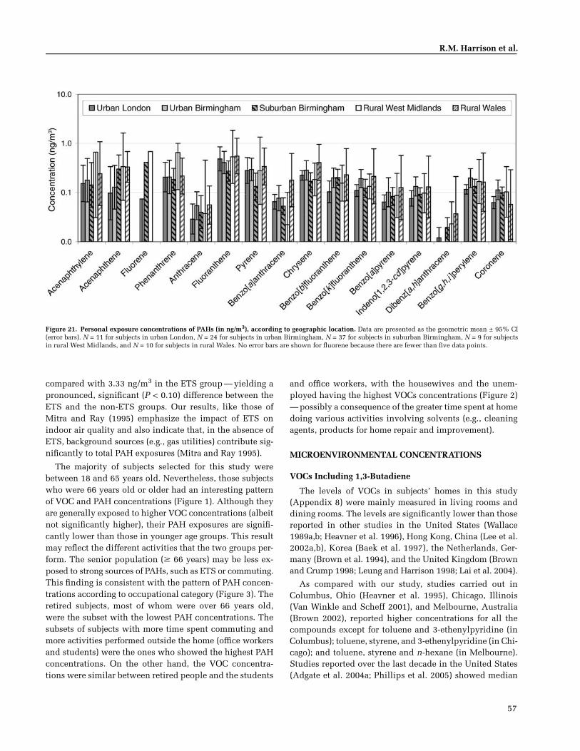
57


compared with 3.33 ng/m3 in the ETS group — yielding apronounced, significant (P < 0.10) difference between theETS and the non-ETS groups. Our results, like those ofMitra and Ray (1995) emphasize the impact of ETS onindoor air quality and also indicate that, in the absence ofETS, background sources (e.g., gas utilities) contribute sig-nificantly to total PAH exposures (Mitra and Ray 1995).

The majority of subjects selected for this study werebetween 18 and 65 years old. Nevertheless, those subjectswho were 66 years old or older had an interesting patternof VOC and PAH concentrations (Figure 1). Although theyare generally exposed to higher VOC concentrations (albeitnot significantly higher), their PAH exposures are signifi-cantly lower than those in younger age groups. This resultmay reflect the different activities that the two groups per-form. The senior population ( 66 years) may be less ex-posed to strong sources of PAHs, such as ETS or commuting.This finding is consistent with the pattern of PAH concen-trations according to occupational category (Figure 3). Theretired subjects, most of whom were over 66 years old,were the subset with the lowest PAH concentrations. Thesubsets of subjects with more time spent commuting andmore activities performed outside the home (office workersand students) were the ones who showed the highest PAHconcentrations. On the other hand, the VOC concentra-tions were similar between retired people and the students

and office workers, with the housewives and the unem-ployed having the highest VOCs concentrations (Figure 2)— possibly a consequence of the greater time spent at homedoing various activities involving solvents (e.g., cleaningagents, products for home repair and improvement).


VOCs Including 1,3-Butadiene

The levels of VOCs in subjects’ homes in this study(Appendix 8) were mainly measured in living rooms anddining rooms. The levels are significantly lower than thosereported in other studies in the United States (Wallace1989a,b; Heavner et al. 1996), Hong Kong, China (Lee et al.2002a,b), Korea (Baek et al. 1997), the Netherlands, Ger-many (Brown et al. 1994), and the United Kingdom (Brownand Crump 1998; Leung and Harrison 1998; Lai et al. 2004).

As compared with our study, studies carried out inColumbus, Ohio (Heavner et al. 1995), Chicago, Illinois(Van Winkle and Scheff 2001), and Melbourne, Australia(Brown 2002), reported higher concentrations for all thecompounds except for toluene and 3-ethenylpyridine (inColumbus); toluene, styrene, and 3-ethenylpyridine (in Chi-cago); and toluene, styrene and n-hexane (in Melbourne).Studies reported over the last decade in the United States(Adgate et al. 2004a; Phillips et al. 2005) showed median

Figure 21. Personal exposure concentrations of PAHs (in ng/m3), according to geographic location. Data are presented as the geometric mean ± 95% CI(error bars). N = 11 for subjects in urban London, N = 24 for subjects in urban Birmingham, N = 37 for subjects in suburban Birmingham, N = 9 for subjectsin rural West Midlands, and N = 10 for subjects in rural Wales. No error bars are shown for fluorene because there are fewer than five data points.

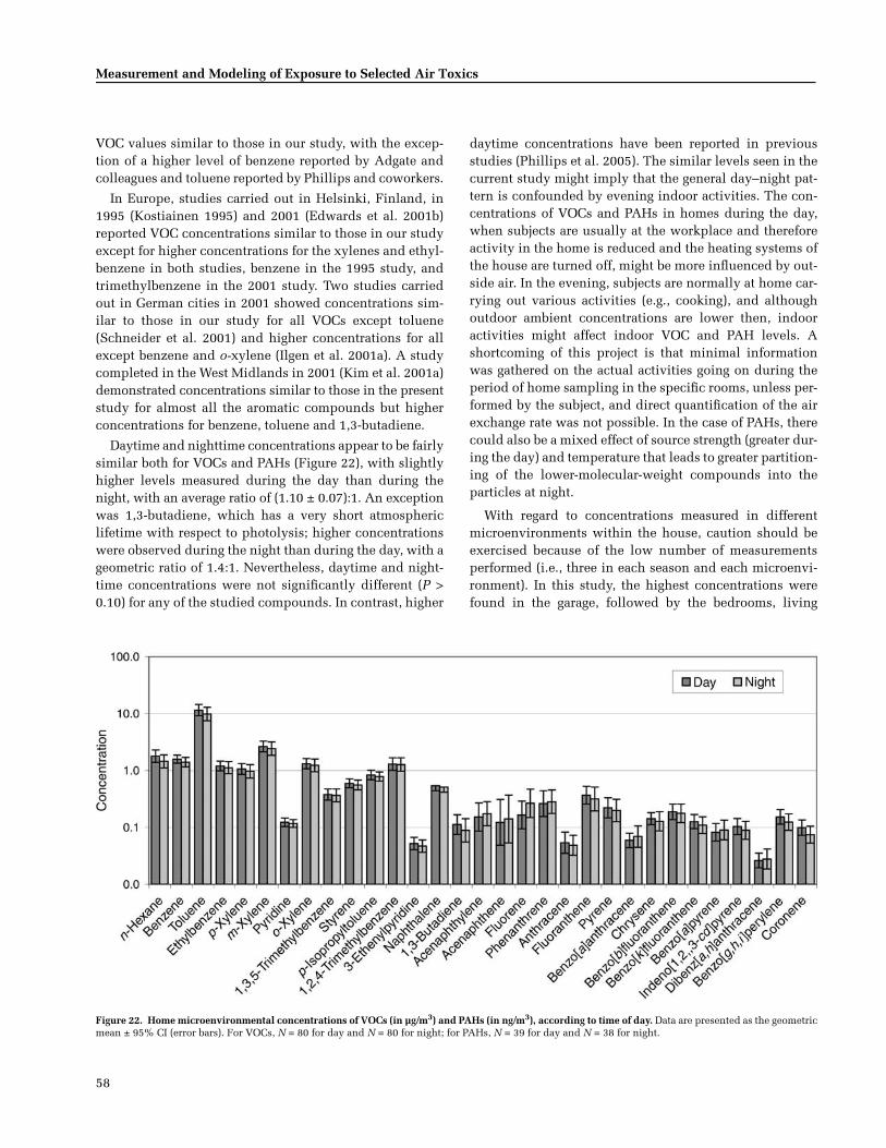
58


VOC values similar to those in our study, with the excep-tion of a higher level of benzene reported by Adgate andcolleagues and toluene reported by Phillips and coworkers.

In Europe, studies carried out in Helsinki, Finland, in1995 (Kostiainen 1995) and 2001 (Edwards et al. 2001b)reported VOC concentrations similar to those in our studyexcept for higher concentrations for the xylenes and ethyl-benzene in both studies, benzene in the 1995 study, andtrimethylbenzene in the 2001 study. Two studies carriedout in German cities in 2001 showed concentrations sim-ilar to those in our study for all VOCs except toluene(Schneider et al. 2001) and higher concentrations for allexcept benzene and o-xylene (Ilgen et al. 2001a). A studycompleted in the West Midlands in 2001 (Kim et al. 2001a)demonstrated concentrations similar to those in the presentstudy for almost all the aromatic compounds but higherconcentrations for benzene, toluene and 1,3-butadiene.

Daytime and nighttime concentrations appear to be fairlysimilar both for VOCs and PAHs (Figure 22), with slightlyhigher levels measured during the day than during thenight, with an average ratio of (1.10 ± 0.07):1. An exceptionwas 1,3-butadiene, which has a very short atmosphericlifetime with respect to photolysis; higher concentrationswere observed during the night than during the day, with ageometric ratio of 1.4:1. Nevertheless, daytime and night-time concentrations were not significantly different (P >0.10) for any of the studied compounds. In contrast, higher

daytime concentrations have been reported in previousstudies (Phillips et al. 2005). The similar levels seen in thecurrent study might imply that the general day–night pat-tern is confounded by evening indoor activities. The con-centrations of VOCs and PAHs in homes during the day,when subjects are usually at the workplace and thereforeactivity in the home is reduced and the heating systems ofthe house are turned off, might be more influenced by out-side air. In the evening, subjects are normally at home car-rying out various activities (e.g., cooking), and althoughoutdoor ambient concentrations are lower then, indooractivities might affect indoor VOC and PAH levels. Ashortcoming of this project is that minimal informationwas gathered on the actual activities going on during theperiod of home sampling in the specific rooms, unless per-formed by the subject, and direct quantification of the airexchange rate was not possible. In the case of PAHs, therecould also be a mixed effect of source strength (greater dur-ing the day) and temperature that leads to greater partition-ing of the lower-molecular-weight compounds into theparticles at night.

With regard to concentrations measured in differentmicroenvironments within the house, caution should beexercised because of the low number of measurementsperformed (i.e., three in each season and each microenvi-ronment). In this study, the highest concentrations werefound in the garage, followed by the bedrooms, living

Figure 22. Home microenvironmental concentrations of VOCs (in µg/m3) and PAHs (in ng/m3), according to time of day. Data are presented as the geometricmean ± 95% CI (error bars). For VOCs, N = 80 for day and N = 80 for night; for PAHs, N = 39 for day and N = 38 for night.

59


room, and kitchen. The levels in these microenvironmentsare lower than those reported in other studies to date, suchas those carried out in Helsinki, Finland (Edwards et al.2001a), Avon, United Kingdom (Mann et al. 2001), Han-over, Germany (Ilgen et al. 2001b), and Hong Kong, China(Lee et al. 2002b).

Despite the levels recorded in the garages being thehighest in the home microenvironment, these levels are farbelow those reported in the United States (Batterman et al.2006a,b, 2007) and previously in the United Kingdom(Mann et al. 2001). A possible explanation may be the factthat, much of the time, cars are not parked in the sampledgarages. This idea is consistent with the findings of Ilgenand associates (2001b), who found that garages had verylow concentrations of VOCs when no cars or solventswere stored inside, as compared with periods when carswere parked and solvents were kept inside the garages.

The levels of VOCs in living rooms in this study werehigher than the levels in kitchens, except for n-hexane and1,3-butadiene. The ratio of GM concentrations in livingrooms and kitchens, for all compounds, is (1.4 ± 0.5):1,and the ratio for 1,3-butadiene alone is 0.35:1. Thereappears to be an ETS effect on the living room:kitchenratio, as evidenced by the data for pyridine and 3-ethenyl-pyridine, which obscures the usefulness of the ratio. Otherstudies performed in Hong Kong, however, have reportedhigher concentrations of VOCs in kitchens than in livingrooms (Lee et al. 2002a,b). This difference might be a con-sequence of the reported presence of ETS in the livingroom and the fact that, in our study, cooking was notoccurring in several sampled kitchens. Other determinantssuch as ventilation patterns, cooking styles, and kitchenmaterials used may differ between the United Kingdomand Hong Kong, influencing the results. On the other hand,the higher levels of 1,3-butadiene recorded in the kitchenthan in the living room might be a consequence of the com-bustion that occurs in the kitchen during cooking. Simi-larly, the higher levels of n-hexane in the kitchen might beattributable to the presence of sealants and the storage ofpaints (Scorecard 2006) in the kitchen.

An unexpected result is that high concentrations ofbenzene, toluene, ethylbenzene and the xylenes werefound in yard samples. This result should be viewed withcaution, owing to the low number of samples collected andalso because one yard was the site of construction (of anaddition to the house and a new conservatory). The causeof this high level of benzene, toluene, ethylbenzene andthe xylenes in yards could also be explained by the use ofa gasoline-fueled lawnmower in the subject’s or a neigh-bor’s yard.

The results of several concurrent samples collected out-doors in the backyard and indoors in the living or dining

room of homes located away from traffic show a clear pat-tern, with higher concentrations indoors than outdoors forall VOC compounds. Figure A6.26 (Appendix 6) clearlyshows that concentrations indoors are higher, with anaverage ratio of (3.6 ± 5.3):1. The same pattern is observedwhen comparing concentrations measured in street micro-environments and any indoor microenvironment. Thisfinding is largely supported in the literature (Brown et al.1994; Wallace 1996; Baek et al. 1997; Edwards et al. 2001b;Ilgen et al. 2001a; Schneider et al. 2001; Phillips et al.2005; Batterman et al. 2007). However, some other studiesof certain subpopulations reported indoor:outdoor ratiosclose to, or less than, unity for benzene, ethylbenzene, ando-xylene (Wallace et al. 1988). The indoor-air loading ofbenzene, toluene, and the xylenes in homes originates inpart from the outdoors. Another source is human activitiesperformed indoors, such as smoking, cooking, heating,cleaning, redecoration, fumigation, and the use of varnishand solvents. Other sources of benzene, toluene, and thexylenes may be residues in furniture and floor and wallcoverings (Schneider et al. 2001). Therefore, the higherconcentrations indoors are a consequence of a higher num-ber of indoor VOC sources that contribute to the outdoorbackground VOC level.

Levels of VOC compounds recorded in workplaces(Appendix 10) are lower than personal exposure and homemicroenvironmental levels. As with personal and homeconcentrations, VOC levels measured in the present studyare lower than those from earlier studies in the West Mid-lands (Leung and Harrison 1998), England (Brown andCrump 1998; Lai et al. 2004), Europe (Carrer et al. 2000;Ilgen et al. 2001c), the United States (Heavner et al. 1996),and Singapore (Zuraimi et al. 2006). A study performed inWest Midlands offices in late 1990s showed similar con-centrations of the xylenes, trimethylbenzenes, styrene, andp-isopropyltoluene but higher concentrations of benzene,toluene, ethylbenzene, n-hexane, naphthalene, and 1,3-butadiene (Kim et al. 2001a).

The effect of traffic on workplace microenvironmentscan be examined by comparing offices located on traffickedroadsides with offices located away from traffic and officeslocated in the city center with those located in a suburbanarea. Although values are similar in first-line offices to non–first-line offices and in urban offices and suburban offices,compounds like toluene and 1,2,4-trimethylbenzene havehigher concentrations in the locations more affected bytraffic. This observation could not be proven statistically,however (P > 0.10).

Street levels of VOCs recorded in the present study(Appendix 11) are mostly lower than those reported instudies carried out in the United States (Wallace 1996),Europe (Pérez Ballesta et al. 2006), Germany (Ilgen et al.

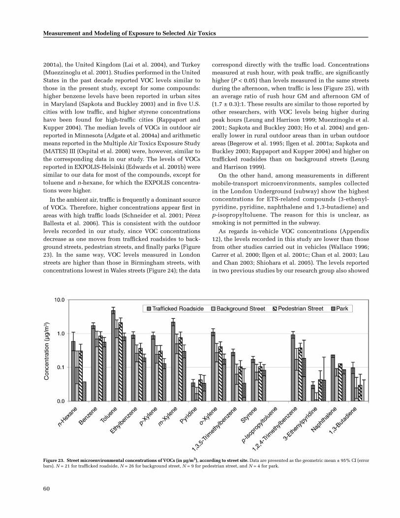
60


Figure 23. Street microenvironmental concentrations of VOCs (in µg/m3), according to street site. Data are presented as the geometric mean ± 95% CI (errorbars). N = 21 for trafficked roadside, N = 26 for background street, N = 9 for pedestrian street, and N = 4 for park.

2001a), the United Kingdom (Lai et al. 2004), and Turkey(Muezzinoglu et al. 2001). Studies performed in the UnitedStates in the past decade reported VOC levels similar tothose in the present study, except for some compounds:higher benzene levels have been reported in urban sitesin Maryland (Sapkota and Buckley 2003) and in five U.S.cities with low traffic, and higher styrene concentrationshave been found for high-traffic cities (Rappaport andKupper 2004). The median levels of VOCs in outdoor airreported in Minnesota (Adgate et al. 2004a) and arithmeticmeans reported in the Multiple Air Toxics Exposure Study(MATES) III (Ospital et al. 2008) were, however, similar tothe corresponding data in our study. The levels of VOCsreported in EXPOLIS-Helsinki (Edwards et al. 2001b) weresimilar to our data for most of the compounds, except fortoluene and n-hexane, for which the EXPOLIS concentra-tions were higher.

In the ambient air, traffic is frequently a dominant sourceof VOCs. Therefore, higher concentrations appear first inareas with high traffic loads (Schneider et al. 2001; PérezBallesta et al. 2006). This is consistent with the outdoorlevels recorded in our study, since VOC concentrationsdecrease as one moves from trafficked roadsides to back-ground streets, pedestrian streets, and finally parks (Figure23). In the same way, VOC levels measured in Londonstreets are higher than those in Birmingham streets, withconcentrations lowest in Wales streets (Figure 24); the data

correspond directly with the traffic load. Concentrationsmeasured at rush hour, with peak traffic, are significantlyhigher (P < 0.05) than levels measured in the same streetsduring the afternoon, when traffic is less (Figure 25), withan average ratio of rush hour GM and afternoon GM of(1.7 ± 0.3):1. These results are similar to those reported byother researchers, with VOC levels being higher duringpeak hours (Leung and Harrison 1999; Muezzinoglu et al.2001; Sapkota and Buckley 2003; Ho et al. 2004) and gen-erally lower in rural outdoor areas than in urban outdoorareas (Begerow et al. 1995; Ilgen et al. 2001a; Sapkota andBuckley 2003; Rappaport and Kupper 2004) and higher ontrafficked roadsides than on background streets (Leungand Harrison 1999).

On the other hand, among measurements in differentmobile-transport microenvironments, samples collectedin the London Underground (subway) show the highestconcentrations for ETS-related compounds (3-ethenyl-pyridine, pyridine, naphthalene and 1,3-butadiene) andp-isopropyltoluene. The reason for this is unclear, assmoking is not permitted in the subway.

As regards in-vehicle VOC concentrations (Appendix12), the levels recorded in this study are lower than thosefrom other studies carried out in vehicles (Wallace 1996;Carrer et al. 2000; Ilgen et al. 2001c; Chan et al. 2003; Lauand Chan 2003; Shiohara et al. 2005). The levels reportedin two previous studies by our research group also showed

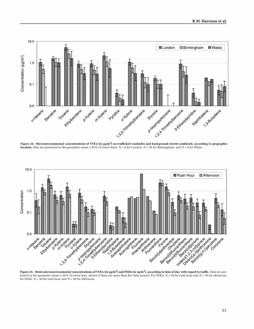
61


Figure 25. Street microenvironmental concentrations of VOCs (in µg/m3) and PAHs (in ng/m3), according to time of day with regard to traffic. Data are pre-sented as the geometric mean ± 95% CI (error bars, shown if there are more than five data points). For VOCs, N = 50 for rush hour and N = 70 for afternoon;for PAHs, N = 30 for rush hour and N = 30 for afternoon.

Figure 24. Microenvironmental concentrations of VOCs (in µg/m3) on trafficked roadsides and background streets combined, according to geographiclocation. Data are presented as the geometric mean ± 95% CI (error bars). N = 8 for London, N = 39 for Birmingham, and N = 8 for Wales.

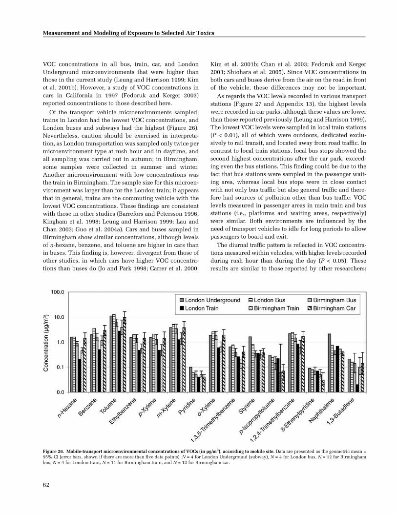
62


VOC concentrations in all bus, train, car, and LondonUnderground microenvironments that were higher thanthose in the current study (Leung and Harrison 1999; Kimet al. 2001b). However, a study of VOC concentrations incars in California in 1997 (Fedoruk and Kerger 2003)reported concentrations to those described here.

Of the transport vehicle microenvironments sampled,trains in London had the lowest VOC concentrations, andLondon buses and subways had the highest (Figure 26).Nevertheless, caution should be exercised in interpreta-tion, as London transportation was sampled only twice permicroenvironment type at rush hour and in daytime, andall sampling was carried out in autumn; in Birmingham,some samples were collected in summer and winter.Another microenvironment with low concentrations wasthe train in Birmingham. The sample size for this microen-vironment was larger than for the London train; it appearsthat in general, trains are the commuting vehicle with thelowest VOC concentrations. These findings are consistentwith those in other studies (Barrefors and Petersson 1996;Kingham et al. 1998; Leung and Harrison 1999; Lau andChan 2003; Guo et al. 2004a). Cars and buses sampled inBirmingham show similar concentrations, although levelsof n-hexane, benzene, and toluene are higher in cars thanin buses. This finding is, however, divergent from those ofother studies, in which cars have higher VOC concentra-tions than buses do (Jo and Park 1998; Carrer et al. 2000;

Kim et al. 2001b; Chan et al. 2003; Fedoruk and Kerger2003; Shiohara et al. 2005). Since VOC concentrations inboth cars and buses derive from the air on the road in frontof the vehicle, these differences may not be important.

As regards the VOC levels recorded in various transportstations (Figure 27 and Appendix 13), the highest levelswere recorded in car parks, although these values are lowerthan those reported previously (Leung and Harrison 1999).The lowest VOC levels were sampled in local train stations(P < 0.01), all of which were outdoors, dedicated exclu-sively to rail transit, and located away from road traffic. Incontrast to local train stations, local bus stops showed thesecond highest concentrations after the car park, exceed-ing even the bus stations. This finding could be due to thefact that bus stations were sampled in the passenger wait-ing area, whereas local bus stops were in close contactwith not only bus traffic but also general traffic and there-fore had sources of pollution other than bus traffic. VOClevels measured in passenger areas in main train and busstations (i.e., platforms and waiting areas, respectively)were similar. Both environments are influenced by theneed of transport vehicles to idle for long periods to allowpassengers to board and exit.

The diurnal traffic pattern is reflected in VOC concentra-tions measured within vehicles, with higher levels recordedduring rush hour than during the day (P < 0.05). Theseresults are similar to those reported by other researchers:

Figure 26. Mobile-transport microenvironmental concentrations of VOCs (in µg/m3), according to mobile site. Data are presented as the geometric mean ±95% CI (error bars, shown if there are more than five data points). N = 4 for London Underground (subway), N = 4 for London bus, N = 12 for Birminghambus, N = 4 for London train, N = 11 for Birmingham train, and N = 12 for Birmingham car.

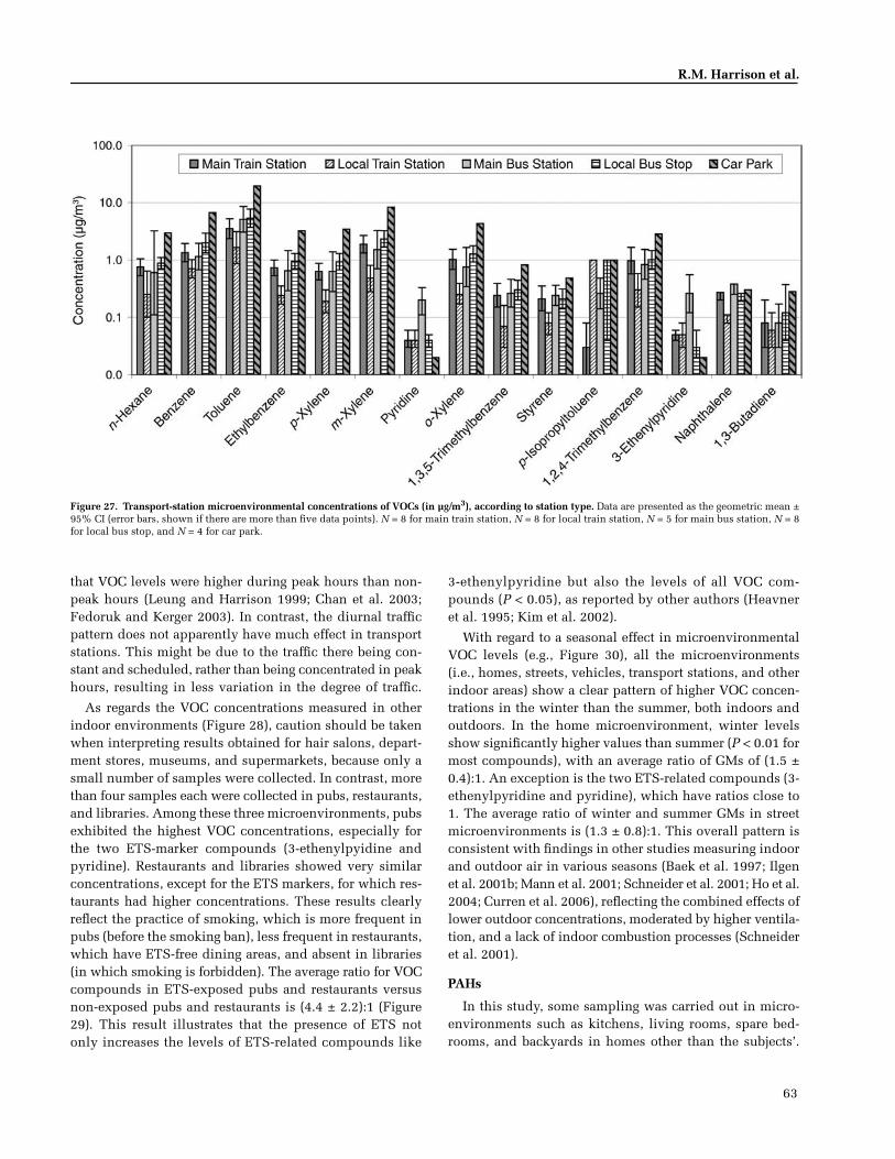
63


Figure 27. Transport-station microenvironmental concentrations of VOCs (in µg/m3), according to station type. Data are presented as the geometric mean ±95% CI (error bars, shown if there are more than five data points). N = 8 for main train station, N = 8 for local train station, N = 5 for main bus station, N = 8for local bus stop, and N = 4 for car park.

that VOC levels were higher during peak hours than non-peak hours (Leung and Harrison 1999; Chan et al. 2003;Fedoruk and Kerger 2003). In contrast, the diurnal trafficpattern does not apparently have much effect in transportstations. This might be due to the traffic there being con-stant and scheduled, rather than being concentrated in peakhours, resulting in less variation in the degree of traffic.

As regards the VOC concentrations measured in otherindoor environments (Figure 28), caution should be takenwhen interpreting results obtained for hair salons, depart-ment stores, museums, and supermarkets, because only asmall number of samples were collected. In contrast, morethan four samples each were collected in pubs, restaurants,and libraries. Among these three microenvironments, pubsexhibited the highest VOC concentrations, especially forthe two ETS-marker compounds (3-ethenylpyidine andpyridine). Restaurants and libraries showed very similarconcentrations, except for the ETS markers, for which res-taurants had higher concentrations. These results clearlyreflect the practice of smoking, which is more frequent inpubs (before the smoking ban), less frequent in restaurants,which have ETS-free dining areas, and absent in libraries(in which smoking is forbidden). The average ratio for VOCcompounds in ETS-exposed pubs and restaurants versusnon-exposed pubs and restaurants is (4.4 ± 2.2):1 (Figure29). This result illustrates that the presence of ETS notonly increases the levels of ETS-related compounds like

3-ethenylpyridine but also the levels of all VOC com-pounds (P < 0.05), as reported by other authors (Heavneret al. 1995; Kim et al. 2002).

With regard to a seasonal effect in microenvironmentalVOC levels (e.g., Figure 30), all the microenvironments(i.e., homes, streets, vehicles, transport stations, and otherindoor areas) show a clear pattern of higher VOC concen-trations in the winter than the summer, both indoors andoutdoors. In the home microenvironment, winter levelsshow significantly higher values than summer (P < 0.01 formost compounds), with an average ratio of GMs of (1.5 ±0.4):1. An exception is the two ETS-related compounds (3-ethenylpyridine and pyridine), which have ratios close to1. The average ratio of winter and summer GMs in streetmicroenvironments is (1.3 ± 0.8):1. This overall pattern isconsistent with findings in other studies measuring indoorand outdoor air in various seasons (Baek et al. 1997; Ilgenet al. 2001b; Mann et al. 2001; Schneider et al. 2001; Ho et al.2004; Curren et al. 2006), reflecting the combined effects oflower outdoor concentrations, moderated by higher ventila-tion, and a lack of indoor combustion processes (Schneideret al. 2001).

PAHs

In this study, some sampling was carried out in micro-environments such as kitchens, living rooms, spare bed-rooms, and backyards in homes other than the subjects’.

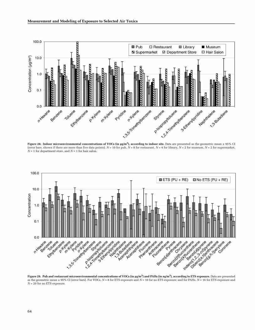
64


Figure 29. Pub and restaurant microenvironmental concentrations of VOCs (in µg/m3) and PAHs (in ng/m3), according to ETS exposure. Data are presentedas the geometric mean ± 95% CI (error bars). For VOCs, N = 8 for ETS exposure and N = 10 for no ETS exposure; and for PAHs, N = 16 for ETS exposure andN = 20 for no ETS exposure.

Figure 28. Indoor microenvironmental concentrations of VOCs (in µg/m3), according to indoor site. Data are presented as the geometric mean ± 95% CI(error bars, shown if there are more than five data points). N = 10 for pub, N = 8 for restaurant, N = 4 for library, N = 2 for museum, N = 2 for supermarket,N = 1 for department store, and N = 1 for hair salon.

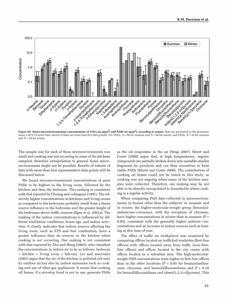
65


The sample size for each of these microenvironments wassmall and cooking was not occurring in some of the kitchenssampled; therefore extrapolation to general home micro-environments might not be possible. Results of subsets ofdata with more than four representative data points will bediscussed below.

We found microenvironmental concentrations of mostPAHs to be highest in the living room, followed by thekitchen and then the bedroom. This ranking is consistentwith that reported by Chuang and colleagues (1991). The rel-atively higher concentrations in kitchens and living roomsas compared to the bedrooms probably result from a lessersource influence in the bedrooms and the greater height ofthe bedrooms above traffic sources (Ilgen et al. 2001a). Theranking of the indoor concentrations is influenced by dif-ferent ventilation conditions, house age, and indoor activ-ities; it clearly indicates that indoor sources affecting theliving room, such as ETS and fuel combustion, have agreater influence than do sources in the kitchen whencooking is not occurring. Our ranking is not consistentwith that reported by Zhu and Wang (2003), who classifiedthe concentrations in indoor air to be as follows: bedroom> kitchen > living room > balcony. Liu and associates(2001) argue that the air of the kitchen is polluted not onlyby outdoor air but also by indoor emissions such as cook-ing and use of other gas appliances. It seems that cookingoil fumes, if a stovetop hood is not in use, generate PAHs

as the oil evaporates in the air (Srogi 2007). Moret andConte (2000) argue that, at high temperatures, organiccompounds are partially broken down into unstable smallerfragments by pyrolysis and can then recombine to formstable PAHs (Moret and Conte 2000). The contribution ofcooking oil fumes could not be tested in this study, ascooking was not ongoing when many of the kitchen sam-ples were collected. Therefore, our ranking may be notable to be directly extrapolated to households where cook-ing is a regular activity.

When comparing PAH data collected in microenviron-ments in homes other than the subjects’ in summer andin winter, the higher-molecular-weight group (benzo[a]-anthracene–coronene), with the exception of chrysene,have higher concentrations in winter than in summer (P <0.05), consistent with the generally higher ambient con-centrations and an increase in indoor sources such as heat-ing at this time of year.

The effect of traffic on workplaces was examined bycomparing offices located on trafficked roadsides (first-lineoffices) with offices located away from traffic (non–first-line offices) and offices located in the city center withoffices located in a suburban area. The high-molecular-weight PAH concentrations were higher in first-line officesthan in the other locations (P < 0.05 for benzo[a]anthra-cene, chrysene, and benzo[k]fluoranthene and P < 0.10for benzo[b]fluoranthene and ideno[1,2,3-cd]pyrene). This

Figure 30. Street microenvironmental concentrations of VOCs (in µg/m3) and PAHs (in ng/m3), according to season. Data are presented as the geometricmean ± 95% CI (error bars, shown if there are more than five data points). For VOCs, N = 60 for summer and N = 60 for winter; and PAHs, N = 30 for summerand N = 30 for winter.

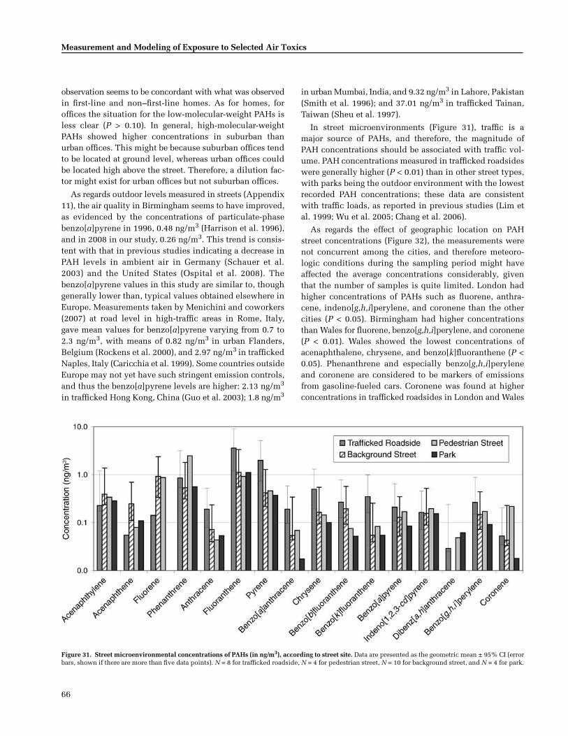
66


observation seems to be concordant with what was observedin first-line and non–first-line homes. As for homes, foroffices the situation for the low-molecular-weight PAHs isless clear (P > 0.10). In general, high-molecular-weightPAHs showed higher concentrations in suburban thanurban offices. This might be because suburban offices tendto be located at ground level, whereas urban offices couldbe located high above the street. Therefore, a dilution fac-tor might exist for urban offices but not suburban offices.

As regards outdoor levels measured in streets (Appendix11), the air quality in Birmingham seems to have improved,as evidenced by the concentrations of particulate-phasebenzo[a]pyrene in 1996, 0.48 ng/m3 (Harrison et al. 1996),and in 2008 in our study, 0.26 ng/m3. This trend is consis-tent with that in previous studies indicating a decrease inPAH levels in ambient air in Germany (Schauer et al.2003) and the United States (Ospital et al. 2008). Thebenzo[a]pyrene values in this study are similar to, thoughgenerally lower than, typical values obtained elsewhere inEurope. Measurements taken by Menichini and coworkers(2007) at road level in high-traffic areas in Rome, Italy,gave mean values for benzo[a]pyrene varying from 0.7 to2.3 ng/m3, with means of 0.82 ng/m3 in urban Flanders,Belgium (Rockens et al. 2000), and 2.97 ng/m3 in traffickedNaples, Italy (Caricchia et al. 1999). Some countries outsideEurope may not yet have such stringent emission controls,and thus the benzo[a]pyrene levels are higher: 2.13 ng/m3

in trafficked Hong Kong, China (Guo et al. 2003); 1.8 ng/m3

in urban Mumbai, India, and 9.32 ng/m3 in Lahore, Pakistan(Smith et al. 1996); and 37.01 ng/m3 in trafficked Tainan,Taiwan (Sheu et al. 1997).

In street microenvironments (Figure 31), traffic is amajor source of PAHs, and therefore, the magnitude ofPAH concentrations should be associated with traffic vol-ume. PAH concentrations measured in trafficked roadsideswere generally higher (P < 0.01) than in other street types,with parks being the outdoor environment with the lowestrecorded PAH concentrations; these data are consistentwith traffic loads, as reported in previous studies (Lim etal. 1999; Wu et al. 2005; Chang et al. 2006).

As regards the effect of geographic location on PAHstreet concentrations (Figure 32), the measurements werenot concurrent among the cities, and therefore meteoro-logic conditions during the sampling period might haveaffected the average concentrations considerably, giventhat the number of samples is quite limited. London hadhigher concentrations of PAHs such as fluorene, anthra-cene, indeno[g,h,i]perylene, and coronene than the othercities (P < 0.05). Birmingham had higher concentrationsthan Wales for fluorene, benzo[g,h,i]perylene, and coronene(P < 0.01). Wales showed the lowest concentrations ofacenaphthalene, chrysene, and benzo[k]fluoranthene (P <0.05). Phenanthrene and especially benzo[g,h,i]peryleneand coronene are considered to be markers of emissionsfrom gasoline-fueled cars. Coronene was found at higherconcentrations in trafficked roadsides in London and Wales

Figure 31. Street microenvironmental concentrations of PAHs (in ng/m3), according to street site. Data are presented as the geometric mean ± 95% CI (errorbars, shown if there are more than five data points). N = 8 for trafficked roadside, N = 4 for pedestrian street, N = 10 for background street, and N = 4 for park.

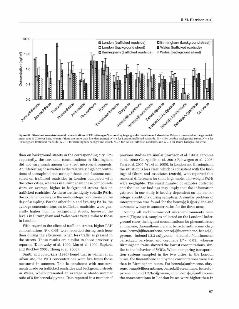
67


than on background streets in the corresponding city. Un-expectedly, the coronene concentrations in Birminghamdid not vary much among the street microenvironments.An interesting observation is the relatively high concentra-tions of acenaphthalene, acenaphthene, and fluorene mea-sured on trafficked roadsides in London compared withthe other cities, whereas in Birmingham these compoundswere, on average, higher in background streets than ontrafficked roadsides. As these are the highly volatile PAHs,the explanation may be the meteorologic conditions on theday of sampling. For the other four- and five-ring PAHs, theaverage concentrations on trafficked roadsides were gen-erally higher than in background streets; however, thelevels in Birmingham and Wales were very similar to thosein London.

With regard to the effect of traffic in streets, higher PAHconcentrations (P < 0.05) were recorded during rush hourthan during the afternoon, when less traffic is present inthe streets. These results are similar to those previouslyreported (Dubowsky et al. 1999; Lim et al. 1999; Sapkotaand Buckley 2003; Chang et al. 2006).

Smith and coworkers (1996) found that in winter, at anurban site, the PAH concentrations were five times thosemeasured in summer. This is consistent with measure-ments made on trafficked roadsides and background streetsin Wales, which presented an average winter-to-summerratio of 5 for benzo[a]pyrene. Data reported in a number of

previous studies are similar (Harrison et al. 1996a; Frommeet al. 1998; Georgiadis et al. 2001; Rehwagen et al. 2005;Tang et al. 2005; Wu et al. 2005). In London and Birmingham,the situation is less clear, which is consistent with the find-ings of Ohura and associates (2004b), who reported thatseasonal differences for some high-molecular-weight PAHswere negligible. The small number of samples collectedand the unclear findings may imply that the informationgathered in our study is heavily dependent on the meteo-rologic conditions during sampling. A similar problem ofinterpretation was found for the benzo[g,h,i]perylene andcoronene winter-to-summer ratios for the three areas.

Among all mobile-transport microenvironments mea-sured (Figure 33), samples collected on the London Under-ground show the highest concentrations for phenanthrene,anthracene, fluoranthene, pyrene, benzo[a]anthracene, chry-sene, benzo[b]fluoranthene, benzo[k]fluoranthene, benzo[a]-pyrene, indeno[1,2,3-cd]pyrene, dibenz[a,h]anthracene,benzo[g,h,i]perylene, and coronene (P < 0.01), whereasBirmingham trains showed the lowest concentrations, sim-ilar to the behavior of VOCs. When comparing transporta-tion systems sampled in the two cities, in the Londonbuses, the fluoranthene and pyrene concentrations were lessthan in Birmingham buses. For benzo[a]anthracene, chry-sene, benzo[b]fluoranthene, benzo[k]fluoranthene, benzo[a]-pyrene, indeno[1,2,3-cd]pyrene, and dibenz[a,h]anthracene,the concentrations in London buses were higher than in

Figure 32. Street microenvironmental concentrations of PAHs (in ng/m3), according to geographic location and street site. Data are presented as the geometricmean ± 95% CI (error bars, shown if there are more than five data points). N = 8 for London trafficked roadside, N = 4 for London background street, N = 8 forBirmingham trafficked roadside, N = 10 for Birmingham background street, N = 4 for Wales trafficked roadside, and N = 4 for Wales background street.

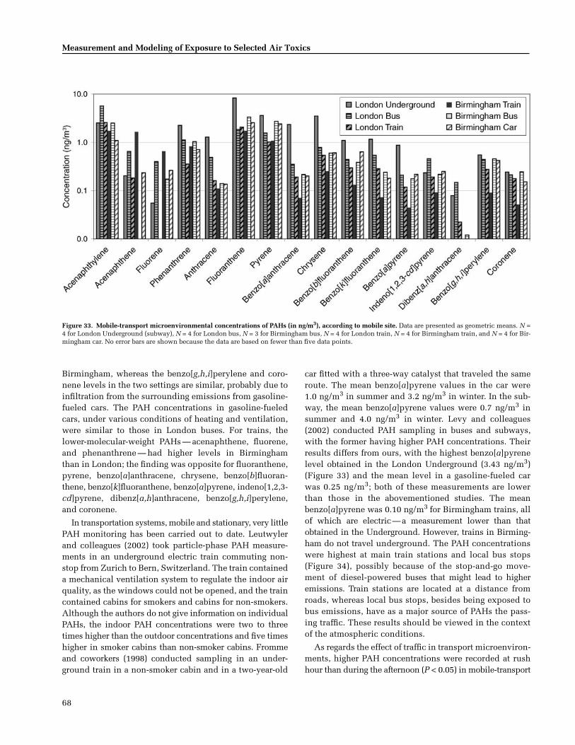
68


Birmingham, whereas the benzo[g,h,i]perylene and coro-nene levels in the two settings are similar, probably due toinfiltration from the surrounding emissions from gasoline-fueled cars. The PAH concentrations in gasoline-fueledcars, under various conditions of heating and ventilation,were similar to those in London buses. For trains, thelower-molecular-weight PAHs — acenaphthene, fluorene,and phenanthrene — had higher levels in Birminghamthan in London; the finding was opposite for fluoranthene,pyrene, benzo[a]anthracene, chrysene, benzo[b]fluoran-thene, benzo[k]fluoranthene, benzo[a]pyrene, indeno[1,2,3-cd]pyrene, dibenz[a,h]anthracene, benzo[g,h,i]perylene,and coronene.

In transportation systems, mobile and stationary, very littlePAH monitoring has been carried out to date. Leutwylerand colleagues (2002) took particle-phase PAH measure-ments in an underground electric train commuting non-stop from Zurich to Bern, Switzerland. The train containeda mechanical ventilation system to regulate the indoor airquality, as the windows could not be opened, and the traincontained cabins for smokers and cabins for non-smokers.Although the authors do not give information on individualPAHs, the indoor PAH concentrations were two to threetimes higher than the outdoor concentrations and five timeshigher in smoker cabins than non-smoker cabins. Frommeand coworkers (1998) conducted sampling in an under-ground train in a non-smoker cabin and in a two-year-old

car fitted with a three-way catalyst that traveled the sameroute. The mean benzo[a]pyrene values in the car were1.0 ng/m3 in summer and 3.2 ng/m3 in winter. In the sub-way, the mean benzo[a]pyrene values were 0.7 ng/m3 insummer and 4.0 ng/m3 in winter. Levy and colleagues(2002) conducted PAH sampling in buses and subways,with the former having higher PAH concentrations. Theirresults differs from ours, with the highest benzo[a]pyrenelevel obtained in the London Underground (3.43 ng/m3)(Figure 33) and the mean level in a gasoline-fueled carwas 0.25 ng/m3; both of these measurements are lowerthan those in the abovementioned studies. The meanbenzo[a]pyrene was 0.10 ng/m3 for Birmingham trains, allof which are electric—a measurement lower than thatobtained in the Underground. However, trains in Birming-ham do not travel underground. The PAH concentrationswere highest at main train stations and local bus stops(Figure 34), possibly because of the stop-and-go move-ment of diesel-powered buses that might lead to higheremissions. Train stations are located at a distance fromroads, whereas local bus stops, besides being exposed tobus emissions, have as a major source of PAHs the pass-ing traffic. These results should be viewed in the contextof the atmospheric conditions.

As regards the effect of traffic in transport microenviron-ments, higher PAH concentrations were recorded at rushhour than during the afternoon (P < 0.05) in mobile-transport

Figure 33. Mobile-transport microenvironmental concentrations of PAHs (in ng/m3), according to mobile site. Data are presented as geometric means. N =4 for London Underground (subway), N = 4 for London bus, N = 3 for Birmingham bus, N = 4 for London train, N = 4 for Birmingham train, and N = 4 for Bir-mingham car. No error bars are shown because the data are based on fewer than five data points.

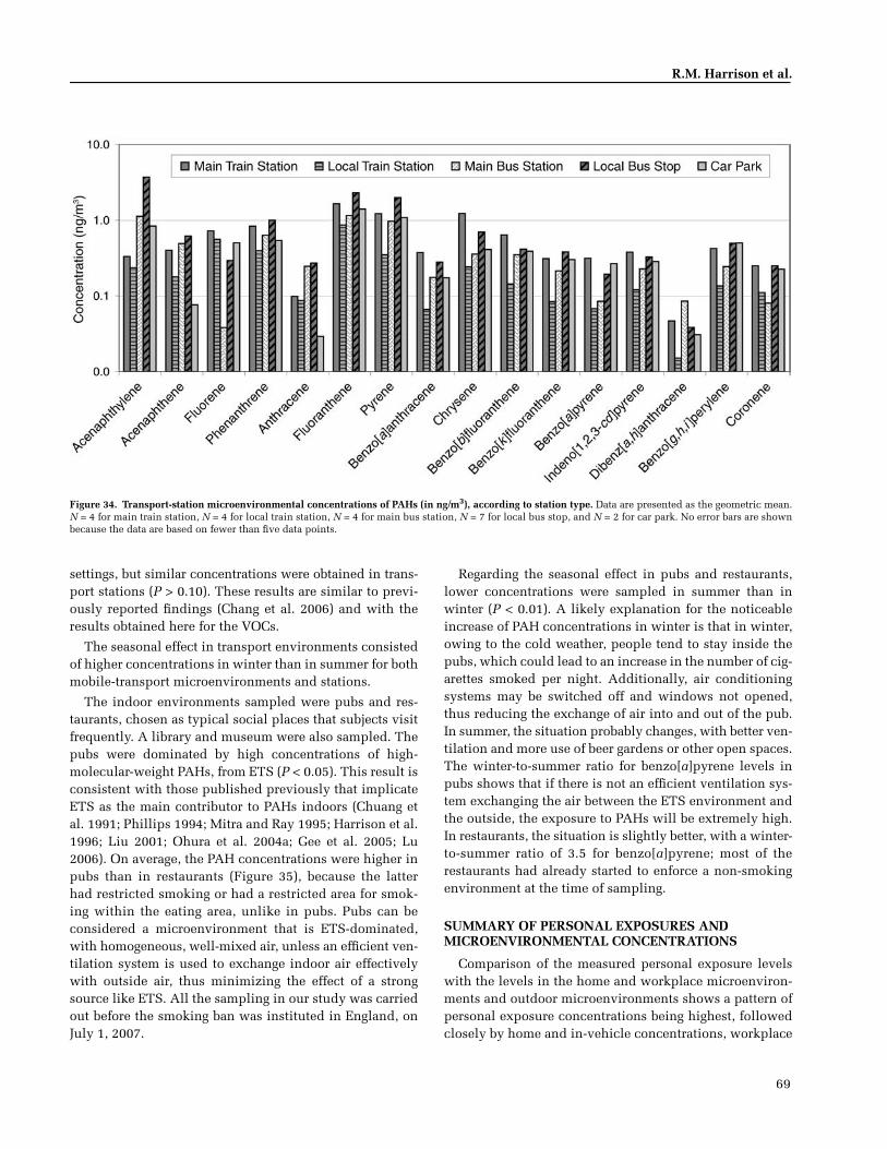
69


settings, but similar concentrations were obtained in trans-port stations (P > 0.10). These results are similar to previ-ously reported findings (Chang et al. 2006) and with theresults obtained here for the VOCs.

The seasonal effect in transport environments consistedof higher concentrations in winter than in summer for bothmobile-transport microenvironments and stations.

The indoor environments sampled were pubs and res-taurants, chosen as typical social places that subjects visitfrequently. A library and museum were also sampled. Thepubs were dominated by high concentrations of high-molecular-weight PAHs, from ETS (P < 0.05). This result isconsistent with those published previously that implicateETS as the main contributor to PAHs indoors (Chuang etal. 1991; Phillips 1994; Mitra and Ray 1995; Harrison et al.1996; Liu 2001; Ohura et al. 2004a; Gee et al. 2005; Lu2006). On average, the PAH concentrations were higher inpubs than in restaurants (Figure 35), because the latterhad restricted smoking or had a restricted area for smok-ing within the eating area, unlike in pubs. Pubs can beconsidered a microenvironment that is ETS-dominated,with homogeneous, well-mixed air, unless an efficient ven-tilation system is used to exchange indoor air effectivelywith outside air, thus minimizing the effect of a strongsource like ETS. All the sampling in our study was carriedout before the smoking ban was instituted in England, onJuly 1, 2007.

Regarding the seasonal effect in pubs and restaurants,lower concentrations were sampled in summer than inwinter (P < 0.01). A likely explanation for the noticeableincrease of PAH concentrations in winter is that in winter,owing to the cold weather, people tend to stay inside thepubs, which could lead to an increase in the number of cig-arettes smoked per night. Additionally, air conditioningsystems may be switched off and windows not opened,thus reducing the exchange of air into and out of the pub.In summer, the situation probably changes, with better ven-tilation and more use of beer gardens or other open spaces.The winter-to-summer ratio for benzo[a]pyrene levels inpubs shows that if there is not an efficient ventilation sys-tem exchanging the air between the ETS environment andthe outside, the exposure to PAHs will be extremely high.In restaurants, the situation is slightly better, with a winter-to-summer ratio of 3.5 for benzo[a]pyrene; most of therestaurants had already started to enforce a non-smokingenvironment at the time of sampling.

SUMMARY OF PERSONAL EXPOSURES AND MICROENVIRONMENTAL CONCENTRATIONS

Comparison of the measured personal exposure levelswith the levels in the home and workplace microenviron-ments and outdoor microenvironments shows a pattern ofpersonal exposure concentrations being highest, followedclosely by home and in-vehicle concentrations, workplace

Figure 34. Transport-station microenvironmental concentrations of PAHs (in ng/m3), according to station type. Data are presented as the geometric mean.N = 4 for main train station, N = 4 for local train station, N = 4 for main bus station, N = 7 for local bus stop, and N = 2 for car park. No error bars are shownbecause the data are based on fewer than five data points.

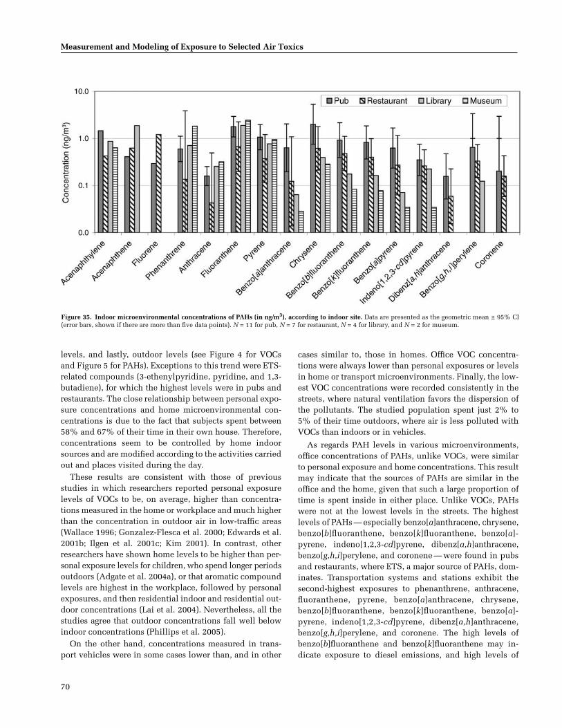
70


levels, and lastly, outdoor levels (see Figure 4 for VOCsand Figure 5 for PAHs). Exceptions to this trend were ETS-related compounds (3-ethenylpyridine, pyridine, and 1,3-butadiene), for which the highest levels were in pubs andrestaurants. The close relationship between personal expo-sure concentrations and home microenvironmental con-centrations is due to the fact that subjects spent between58% and 67% of their time in their own house. Therefore,concentrations seem to be controlled by home indoorsources and are modified according to the activities carriedout and places visited during the day.

These results are consistent with those of previousstudies in which researchers reported personal exposurelevels of VOCs to be, on average, higher than concentra-tions measured in the home or workplace and much higherthan the concentration in outdoor air in low-traffic areas(Wallace 1996; Gonzalez-Flesca et al. 2000; Edwards et al.2001b; Ilgen et al. 2001c; Kim 2001). In contrast, otherresearchers have shown home levels to be higher than per-sonal exposure levels for children, who spend longer periodsoutdoors (Adgate et al. 2004a), or that aromatic compoundlevels are highest in the workplace, followed by personalexposures, and then residential indoor and residential out-door concentrations (Lai et al. 2004). Nevertheless, all thestudies agree that outdoor concentrations fall well belowindoor concentrations (Phillips et al. 2005).

On the other hand, concentrations measured in trans-port vehicles were in some cases lower than, and in other

cases similar to, those in homes. Office VOC concentra-tions were always lower than personal exposures or levelsin home or transport microenvironments. Finally, the low-est VOC concentrations were recorded consistently in thestreets, where natural ventilation favors the dispersion ofthe pollutants. The studied population spent just 2% to5% of their time outdoors, where air is less polluted withVOCs than indoors or in vehicles.

As regards PAH levels in various microenvironments,office concentrations of PAHs, unlike VOCs, were similarto personal exposure and home concentrations. This resultmay indicate that the sources of PAHs are similar in theoffice and the home, given that such a large proportion oftime is spent inside in either place. Unlike VOCs, PAHswere not at the lowest levels in the streets. The highestlevels of PAHs — especially benzo[a]anthracene, chrysene,benzo[b]fluoranthene, benzo[k]fluoranthene, benzo[a]-pyrene, indeno[1,2,3-cd]pyrene, dibenz[a,h]anthracene,benzo[g,h,i]perylene, and coronene — were found in pubsand restaurants, where ETS, a major source of PAHs, dom-inates. Transportation systems and stations exhibit thesecond-highest exposures to phenanthrene, anthracene,fluoranthene, pyrene, benzo[a]anthracene, chrysene,benzo[b]fluoranthene, benzo[k]fluoranthene, benzo[a]-pyrene, indeno[1,2,3-cd]pyrene, dibenz[a,h]anthracene,benzo[g,h,i]perylene, and coronene. The high levels ofbenzo[b]fluoranthene and benzo[k]fluoranthene may in-dicate exposure to diesel emissions, and high levels of

Figure 35. Indoor microenvironmental concentrations of PAHs (in ng/m3), according to indoor site. Data are presented as the geometric mean ± 95% CI(error bars, shown if there are more than five data points). N = 11 for pub, N = 7 for restaurant, N = 4 for library, and N = 2 for museum.

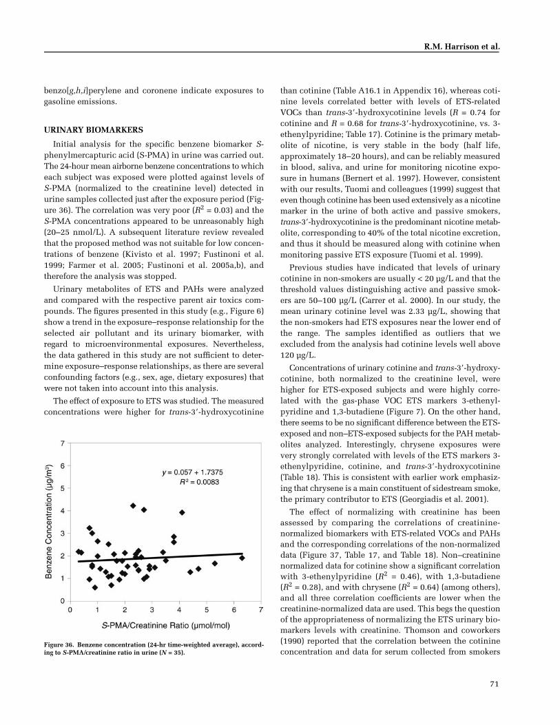
71


benzo[g,h,i]perylene and coronene indicate exposures togasoline emissions.

URINARY BIOMARKERS

Initial analysis for the specific benzene biomarker S-phenylmercapturic acid (S-PMA) in urine was carried out.The 24-hour mean airborne benzene concentrations to whicheach subject was exposed were plotted against levels ofS-PMA (normalized to the creatinine level) detected inurine samples collected just after the exposure period (Fig-ure 36). The correlation was very poor (R2 = 0.03) and theS-PMA concentrations appeared to be unreasonably high(20–25 nmol/L). A subsequent literature review revealedthat the proposed method was not suitable for low concen-trations of benzene (Kivisto et al. 1997; Fustinoni et al.1999; Farmer et al. 2005; Fustinoni et al. 2005a,b), andtherefore the analysis was stopped.

Urinary metabolites of ETS and PAHs were analyzedand compared with the respective parent air toxics com-pounds. The figures presented in this study (e.g., Figure 6)show a trend in the exposure–response relationship for theselected air pollutant and its urinary biomarker, withregard to microenvironmental exposures. Nevertheless,the data gathered in this study are not sufficient to deter-mine exposure–response relationships, as there are severalconfounding factors (e.g., sex, age, dietary exposures) thatwere not taken into account into this analysis.

The effect of exposure to ETS was studied. The measuredconcentrations were higher for trans-3�-hydroxycotinine

than cotinine (Table A16.1 in Appendix 16), whereas coti-nine levels correlated better with levels of ETS-relatedVOCs than trans-3�-hydroxycotinine levels (R = 0.74 forcotinine and R = 0.68 for trans-3�-hydroxycotinine, vs. 3-ethenylpyridine; Table 17). Cotinine is the primary metab-olite of nicotine, is very stable in the body (half life,approximately 18–20 hours), and can be reliably measuredin blood, saliva, and urine for monitoring nicotine expo-sure in humans (Bernert et al. 1997). However, consistentwith our results, Tuomi and colleagues (1999) suggest thateven though cotinine has been used extensively as a nicotinemarker in the urine of both active and passive smokers,trans-3�-hydroxycotinine is the predominant nicotine metab-olite, corresponding to 40% of the total nicotine excretion,and thus it should be measured along with cotinine whenmonitoring passive ETS exposure (Tuomi et al. 1999).

Previous studies have indicated that levels of urinarycotinine in non-smokers are usually < 20 µg/L and that thethreshold values distinguishing active and passive smok-ers are 50–100 µg/L (Carrer et al. 2000). In our study, themean urinary cotinine level was 2.33 µg/L, showing thatthe non-smokers had ETS exposures near the lower end ofthe range. The samples identified as outliers that weexcluded from the analysis had cotinine levels well above120 µg/L.

Concentrations of urinary cotinine and trans-3�-hydroxy-cotinine, both normalized to the creatinine level, werehigher for ETS-exposed subjects and were highly corre-lated with the gas-phase VOC ETS markers 3-ethenyl-pyridine and 1,3-butadiene (Figure 7). On the other hand,there seems to be no significant difference between the ETS-exposed and non–ETS-exposed subjects for the PAH metab-olites analyzed. Interestingly, chrysene exposures werevery strongly correlated with levels of the ETS markers 3-ethenylpyridine, cotinine, and trans-3�-hydroxycotinine(Table 18). This is consistent with earlier work emphasiz-ing that chrysene is a main constituent of sidestream smoke,the primary contributor to ETS (Georgiadis et al. 2001).

The effect of normalizing with creatinine has beenassessed by comparing the correlations of creatinine-normalized biomarkers with ETS-related VOCs and PAHsand the corresponding correlations of the non-normalizeddata (Figure 37, Table 17, and Table 18). Non–creatininenormalized data for cotinine show a significant correlationwith 3-ethenylpyridine (R2 = 0.46), with 1,3-butadiene(R2 = 0.28), and with chrysene (R2 = 0.64) (among others),and all three correlation coefficients are lower when thecreatinine-normalized data are used. This begs the questionof the appropriateness of normalizing the ETS urinary bio-markers levels with creatinine. Thomson and coworkers(1990) reported that the correlation between the cotinineconcentration and data for serum collected from smokers

Figure 36. Benzene concentration (24-hr time-weighted average), accord-ing to S-PMA/creatinine ratio in urine (N = 35).

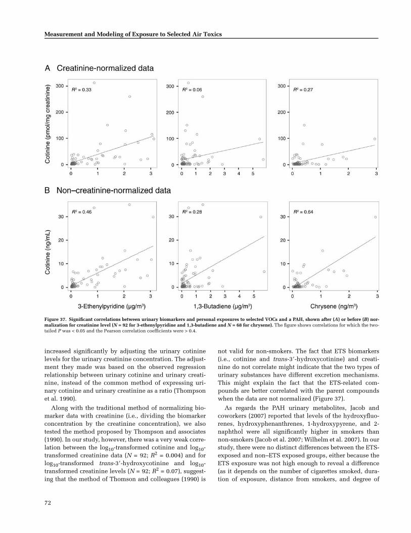
72


increased significantly by adjusting the urinary cotininelevels for the urinary creatinine concentration. The adjust-ment they made was based on the observed regressionrelationship between urinary cotinine and urinary creati-nine, instead of the common method of expressing uri-nary cotinine and urinary creatinine as a ratio (Thompsonet al. 1990).

Along with the traditional method of normalizing bio-marker data with creatinine (i.e., dividing the biomarkerconcentration by the creatinine concentration), we alsotested the method proposed by Thompson and associates(1990). In our study, however, there was a very weak corre-lation between the log10-transformed cotinine and log10-transformed creatinine data (N = 92; R2 = 0.004) and forlog10-transformed trans-3�-hydroxycotinine and log10-transformed creatinine levels (N = 92; R2 = 0.07), suggest-ing that the method of Thomson and colleagues (1990) is

not valid for non-smokers. The fact that ETS biomarkers(i.e., cotinine and trans-3�-hydroxycotinine) and creati-nine do not correlate might indicate that the two types ofurinary substances have different excretion mechanisms.This might explain the fact that the ETS-related com-pounds are better correlated with the parent compoundswhen the data are not normalized (Figure 37).

As regards the PAH urinary metabolites, Jacob andcoworkers (2007) reported that levels of the hydroxyfluo-renes, hydroxyphenanthrenes, 1-hydroxypyrene, and 2-naphthol were all significantly higher in smokers thannon-smokers (Jacob et al. 2007; Wilhelm et al. 2007). In ourstudy, there were no distinct differences between the ETS-exposed and non–ETS exposed groups, either because theETS exposure was not high enough to reveal a difference(as it depends on the number of cigarettes smoked, dura-tion of exposure, distance from smokers, and degree of

Figure 37. Significant correlations between urinary biomarkers and personal exposures to selected VOCs and a PAH, shown after (A) or before (B) nor-malization for creatinine level (N = 92 for 3-ethenylpyridine and 1,3-butadiene and N = 68 for chrysene). The figure shows correlations for which the two-tailed P was < 0.05 and the Pearson correlation coefficients were > 0.4.

73


ventilation) or because other sources of PAHs contribute tohigher exposure in the non-exposed group (Figure 7). Norwas there a correlation between the abovementioned metab-olites and the ETS metabolites or the ETS VOC markers,perhaps because the subjects in our study who were ETS-exposed had far lower exposures than smokers have, andthis study did not include smokers. However, cotinine andtrans-3�-hydroxycotinine levels showed a correlation (P <0.05) with exposures to the low-molecular-weight PAHs(naphthalene, acenaphthylene, acenaphthene, fluorene,phenanthrene, and anthracene), which include the PAHparent compounds.

It is unfortunate that the PAH metabolites measured inurine derive from the low-molecular-weight compoundsfor which our exposure data are not reliable, as the sam-pling technique collects data on the particle phase only,and these compounds are mainly found in the gas phase.Therefore, we observed little correlation of PAH urinarymetabolites and parent compounds. The personal exposuredata for naphthalene should be reliable, as it was measuredwith the VOCs. The relatively weak correlation betweennaphthalene exposures and the 2-naphthol data (normal-ized to creatinine) is probably due to other, non-respiratorysources of naphthalene exposure, of which there are many(Price and Jayjock 2008). Dietary exposure to PAHs may bea greater source of PAH intake into the body than is expo-sure to airborne PAHs, as the estimated average adultdietary intake of benzo[a]pyrene and benzo[a]anthracenewas 1.6 and 0.8 ng/kg of body weight per day, respectively,in 2000 in the United Kingdom (Food Standards Agency2002). The U.K. air quality standard for benzo[a]pyrene is0.25 ng/m3; thus, assuming a 70-kg person inhales 20 m3 ofair daily, benzo[a]pyrene intake from the atmosphere is muchlower than the estimate, at 0.07 ng/kg body weight per day.

On the other hand, high correlations were observed be-tween the ETS urinary biomarkers and the low-molecular-weight PAH compounds (Table 18). This finding maysuggest that the ETS urinary biomarkers studied are goodbiological indicators of personal exposure to some PAHs.

CORRELATIONS WITHIN AND BETWEEN THE VOC AND PAH DATABASES

Correlations among various VOCs and PAHs were exam-ined for both personal exposures and microenvironments(Appendix 17). These correlations might suggest somesources.

Generally, personal exposures and home and workplacemicroenvironments all showed similar correlations amongthe compounds. The strongest correlations were betweenethylbenzene and the xylenes (R > 0.9) and between thetwo trimethylbenzenes and the two ETS markers (R > 0.94).

The strength of the correlations may be the result of asso-ciations with traffic, use of solvents, and ETS. AlthoughVOC concentrations were elevated in smoking environments,only pyridine was correlated significantly with 3-ethenyl-pyridine, as was reported by Heavner and colleagues (1995).The correlation between pyridine and 3-ethenylpyridinewas not found in workplaces, however, where smoking isforbidden. High correlations were observed among thehigh-molecular-weight PAHs (R > 0.8), which could be inassociation with traffic or combustion sources. When ana-lyzing the correlations among VOCs and PAHs in the per-sonal exposure data set, we found correlations betweenbenzene and the high-molecular-weight PAHs; between m-xylene and the low-molecular-weight PAHs; between3-ethenylpyridine and compounds such as benzo[a]-anthracene, chrysene, benzo[b]fluoranthene and benzo[a]-pyrene; and between 1,3-butadiene and phenanthrene,anthracene, benzo[a]anthracene, and chrysene. Benzeneand naphthalene correlate with the high-molecular-weightPAHs, and in the office microenvironment, so do ethylben-zene, the xylenes, and styrene. These correlations suggestthat the high-molecular-weight PAHs and benzene may sharethe same source, which the literature suggests is traffic(Lim et al. 1999; Ho and Lee 2002) or combustion processes(Levy et al. 2002; Lung et al. 2003) such as ETS (McBride etal. 1999; Georgiadis et al. 2001; Levy et al. 2001).

The street and all transport microenvironments had anincreased number of correlating compounds, includingbenzene, toluene, ethylbenzene, and the xylenes being cor-related with the trimethylbenzenes, n-hexane, styrene, andnaphthalene (e.g., 0.85 < R < 0.99 in street and R > 0.75 inmobile-transport settings). This correlation among VOCs isattributed to traffic (Kim et al. 2001b). The correlationbetween the high-molecular-weight PAHs was, however,lower than that seen for personal exposures and indoorsamples. Correlations between VOC and PAH compoundswere stronger, including among the high-molecular-weightPAH compounds and the VOCs well known to be gener-ated from gasoline and diesel combustion, a finding con-sistent with traffic being a single source (Lim et al. 1999;Dimashki et al. 2001; Levy et al. 2001; Sakai et al. 2002).

The correlations observed among the PAHs were weakerin street microenvironments than in all the indoor micro-environments studied. This may be a consequence of theinfluence of regional atmospheric transport and dilutionon outdoor PAH concentrations. A weaker correlation wasalso observed in transport-station microenvironmentswithin the PAH data set, possibly due to the effect of ven-tilation and the distance between the source and the sam-pling point.

Correlations found in ETS-influenced indoor environ-ments clearly showed the influence of tobacco smoke. VOCs

74


were well correlated, with R > 0.7 (P < 0.05). Specifically,benzene and toluene were correlated; toluene, ethyl-benzene, and the xylenes were correlated with trimethyl-benzenes; 3-ethenylpyridine was correlated with pyridine;and naphthalene was correlated with xylenes and styrene.All the high-molecular-weight PAHs were correlated not onlywith one another (R > 0.75) but also with VOCs (R > 0.75).This suggests a similar predominant source of both pollut-ant types, namely ETS (McBride et al. 1999; Georgiadis etal. 2001; Levy et al. 2001).

SOURCE APPORTIONMENT BY FACTOR ANALYSIS

Three potential sources of VOCs affecting personal expo-sure were studied: traffic, ETS, and integral garages. Aspreviously discussed, having an integral garage at homeand being exposed to ETS leads to an increase in personalexposure to VOCs; hence, these two sources have beenevaluated.

Although a number of factors were extracted from ourdata, here we discuss, and use for source apportionment,only the factors that explained most of the variance in theoriginal data set. Factor analysis performed on all pooledpersonal exposure data for VOCs reveals two factors (Table19). High loadings of benzene, toluene, ethylbenzene, thexylenes, trimethylbenzenes, n-hexane, styrene, and naph-thalene are associated with a mix of sources such as vehi-cle use and solvents, the first factor (Mukund et al. 1996;Hinwood et al. 2006; Brown et al. 2007; Song et al. 2007).The second factor is associated with ETS, owing to thehigh loadings of the ETS markers 3-ethenylpyridine andpyridine (Kim et al. 2002).

The same two factors were present in other factor analy-ses performed on other subsets of the VOC database, dem-onstrating the importance of fossil fuel combustion, solventuse, and ETS in everyday personal exposures. Analysisaccording to the presence of integral garages revealed athird significant factor, with high loadings of trimethylben-zenes, styrene, p-isopropyltoluene, and 1,3-butadiene.

As regards the PAH data set, factor analysis performedon all pooled personal exposure data revealed two factors(Table 20). Factor 1 presented high loadings of all the high-molecular-weight PAHs (benzo[a]anthracene, chrysene,benzo[b]fluoranthene, benzo[k]fluoranthene, benzo[a]pyrene,indeno[1,2,3-cd]pyrene, dibenz[a,h]anthracene, benzo[g,h,i]-perylene, and coronene), which could be associated withgasoline emissions and combustion sources (Lim et al.1999; Chang et al. 2006). Factor 2 could be associated withcooking (Oanh et al. 2000; Zhu and Wang 2003) or diesel-vehicle emissions (Chang et al. 2006), because of the highloadings of low-molecular-weight PAHs.

The same two factors were present in other factor analy-ses performed on other PAH data sets (related to ETS andintegral garages), demonstrating the importance of traffic,combustion sources, and cooking on personal exposureto PAHs.

On the other hand, when performing factor analysis onthe combined VOC and PAH database (Table 21), the previ-ous factor 1 identified in the VOC data set, which explained48% of the variance and was associated with a mixture offuel combustion and use of solvents, was now broken intotwo different factors explaining 34% and 30% of the vari-ance in the combined data set. The new factor 1 in thecombined data set is related to fossil fuel combustion, as ithas high loadings of most aromatic compounds and all thePAHs. This factor is consistent with suggestions in the lit-erature (Lim et al. 1999; Ho and Lee 2002; Kim et al. 2002;Levy et al. 2002; Sakai et al. 2002). The second new factoris associated with the use of solvents, as it has high load-ings of aromatic hydrocarbons but negative loadings forPAHs, as reported by others (Watson et al. 2001; Choi andEhrman 2004; Guo et al. 2004b). Factor 3 is related to ETS,as it groups pyridine and 3-ethenylpyridine, whereas fac-tor 4 appears to be linked with use of consumer products.

PERFORMANCE OF THE PERSONAL EXPOSURE MODEL

In this study, we obtained measurements of VOCs andPAHs for both personal exposures and in various micro-environments. We also gathered personal lifestyle infor-mation. This information has been incorporated intoseveral models to predict the personal exposure of a non-occupationally exposed population to a selected group ofVOCs and PAHs.

There are several considerations regarding the quantityor quality of the information provided by the subjectswhose data have been used to develop the model:

• The factors covered by the storage questionnaire forsubjects 1 through 27 were estimated from informa-tion available from photographs, other questionnaires,and researchers’ knowledge of the subjects, becausewhen those subjects were sampled, the storage ques-tionnaire had not been prepared.

• No specific information on ETS as regards the numberof cigarettes smoked or the relationship of the subjectto the smoker is available for subjects 1 through 50,because for those subjects a separate ETS question-naire was not used. This information therefore couldnot be entered into the model.

• The volunteer’s perception of ETS is subjective. Forexample, some volunteers, in the company of a relative

75


or friend who might have smoked just one cigarette,describe the environment as being “slightly smoky —people are smoking occasionally” on the ETS ques-tionnaire or location description sheet. This closeETS event may have created a greater ETS concentra-tion in the area of the subject than if the smoker werenot a person in their company.

• Some subjects were active smokers but did not declarethis at the outset. Data from these subjects were con-sidered outliers during model development and vali-dation and have been removed.

• Information on some activities or characteristics thatmay have affected the measured concentrations wasnot collected. This information includes time spentphotocopying, type of paint used, and the presence ofnew furniture in the home or office.

• Some subjects gave inadequate information aboutwhere they were or what they were doing, making itdifficult to interpret some of the high concentrationsrecorded.

• Some of the high concentrations whose causes havebeen identified were difficult to enter into the model,because there were many variables that could havehad an effect and that could not be controlled (e.g.,location of the briefcase with reference to the pollut-ant source, ventilation in the building, activities per-formed by other dwellers or co-workers not recordedon the forms).

• Sampling periods that were < 1100 minutes and there-fore did not include the nighttime were not enteredinto the model, as the resulting concentrations werenot comparable with concentrations of samples col-lected over 1400 minutes (covering the daytime andnighttime).

The information extracted from the performance ofmodel 1 (Table 22) gives valuable information in terms ofevaluating the influence that the two microenvironmentswhere people spent most of their time have on personalexposure. The model that correlates personal exposure withhome microenvironment explains most of the variance inpersonal exposure, generating, in some cases, R2 valuesof 0.7, such as for benzene, toluene, and the trimethyl-benzenes. Other compounds for which home microenvi-ronments are a good predictor of personal exposures arep-isopropyltoluene, naphthalene, and the xylenes, with R2

around 0.5, and ethylbenzene (with R2 = 0.4). These obser-vations are confirmed by the scatterplots of the personalexposures predicted by the model versus the personal expo-sures measured (presented in Appendix 20). In severalcontexts — when subjects spent a large amount of time athome, there is little ventilation at home, there are additional

indoor sources (e.g., heating systems or cleaning productsin use), or there are strong indoor sources (e.g., ETS athome or recent redecoration) — the home contribution isexpected to impact greatly on the personal exposure, andhence home microenvironmental concentrations will be agood predictor of personal exposures.

On the other hand, the model correlating personal expo-sure with the workplace explains less of the variance inpersonal exposure, presenting correlation coefficients inthe range of 0.15–0.28 for most of the compounds. Fromthe performance of both models, it is clear that the homemicroenvironment affects personal exposure the most, withsubjects spending an average of 62% of their time at home.Personal exposure to all compounds was therefore domi-nated by the contribution from the home (Kim et al. 2002;Adgate et al. 2004a).

The time-weighted model, which used specific subject-related information when available and pooled data other-wise (model 2), explained more variability in personalexposure than did the model using the home measurementsalone, except for benzene and toluene. Similar results werereported for benzene by Adgate and colleagues (2004a) andfor other compounds by Kim and associates (2002). Never-theless, direct measurements in the subjects’ own loca-tions are required for this model.

On the other hand, model 3 uses generic stratified micro-environmental concentrations for all the microenvironmentsthat the subjects visit, in conjunction with the informa-tion extracted from the time–activity diaries. Therefore,no direct measurements are required to predict personalexposure. The performance of this model is lesser than forthe other tested models. This is a consequence of the diffi-culties in adequately stratifying home microenvironments,given the modest number of samples collected as well asthe home-to-home variation in concentrations. Even if thenumber of samples is large (N = 160), the large number ofstrata (e.g., integral garage, ETS exposure, first-line prop-erty, or type of location) reduces considerably the samplesize per stratum. The range of activities in which the sub-jects are engaged in their normal life was reflected in thespecific home and workplace levels and therefore wasaccounted for well in models 1 and 2. This was accountedfor less well in model 3, however, because the genericstratified microenvironmental concentrations used in themodel do not contain specific information about each sub-ject’s microenvironment. Nevertheless, the scatterplots ofthe measured personal exposures versus the predictedexposures (Appendix 20) show that the model predicts theconcentrations well, except in some cases where concen-trations are typically under-predicted. Further study showsthat these cases are linked to activities such as exposure toETS, home repair and improvement, photocopying, and

76


use of solvents. Therefore, model 3 predicts the concen-tration well in most instances but does not perform wellwhen the subjects engage in an activity that presumablyresults in a substantial increase in VOC exposure.

To address this difficulty, model 4 uses the concentrationsas calculated in model 3 but includes a range of add-onvariables that represent activities and home characteristicsthat could not be reflected in the stratified data and thatlead to an increase in VOC levels. This approach betterreflects the VOC concentrations, explaining higher levelsof variance: 80% for ethylbenzene, xylenes, styrene, andtrimethylbenzenes and around 50% for compounds suchas benzene, toluene, and 1,3-butadiene. The amount ofvariance left unexplained by model 4 (e.g., 51% for 1,3-butadiene) must be due to the fact that the sources of suchcompounds were not well captured in the proposed micro-environmental concentrations or add-on variables.

Table 22 shows that the model that best predicts the per-sonal exposure is model 4. The same comparison of pre-dicted versus measured concentrations was performedusing the log10-transformed database, showing in all casescorrelation coefficients lower than for the nontransformeddata (i.e., R2 ranging from 0.25 for p-isopropyltoluene to0.46 for p-xylene and o-xylene).

However, some compounds, such as benzene and tolu-ene, are best predicted by model 1, in which personalexposures are predicted directly from home exposures. Itappears that, for these two compounds, representation ofother microenvironments visited (as in model 2 and model3) or other activities performed during the day (as in model4) does not improve the prediction of personal exposures;rather, it increases the uncertainty not accounted for by themodel (e.g., for benzene, model 1 [home] explains 67% ofthe variability but models 2 and 4 explain only 44% and47%, respectively). As observed, most of the variation forthese two components arises from the home concentra-tions. On the other hand, the other microenvironments oractivities that contribute to the personal exposure couldnot be captured by the other proposed models (models 2through 5). This suggests that more detailed information isneeded to fully understand the non-home sources contrib-uting to benzene and toluene concentrations and that theestimates of home microenvironmental concentrationsused in models 3 and 4 do not fully reflect the behavior ofthese two compounds, thus requiring further study.

Regarding the performance of model 1 for the PAH dataset, home microenvironmental levels could explain 36%and 43% of the variance for chrysene and dibenz[a,h]-anthracene, respectively. Workplace concentrations couldexplain 50% and 38% of the variance for benzo[b]fluoran-thene and benzo[g,h,i]perylene, respectively. Contrary to

the observations for the VOC data set, PAH concentrationsat home do not always dominate personal exposures andhence, they are not good predictors of personal exposure,suggesting that activities or sources outside the home con-tribute largely to PAH personal exposures.

On the other hand, contrary to previously reportedresults (Ohura et al. 2005), neither of the two proposedtime-weighted models (model 2 and model 3), which con-sider only time spent in various microenvironments, couldexplain the variance for the PAH compounds. Model 4,however, was able to explain 25–66% of the variance forthe PAH compounds (e.g., 35% of variance for benzo[a]-pyrene). This improvement was a consequence of includ-ing add-on variables accounting for various activities inthe proposed time-weighted model (see Appendix 21 fordetailed add-on variables and model coefficients). There-fore, the evolution of model development for the PAHdatabase suggests that the home microenvironment aloneis not a good predictor for personal exposures, and there-fore model 1 does not perform well. It also suggests thatincluding information about other microenvironments vis-ited during the day does not improve the prediction of per-sonal exposures (model 2 and 3) and also highlights thestrong influence of the add-on variables, which reflectactivities, to predict the PAHs personal concentrations, asshown by the improvement of the R2 values seen for model4. Hence, the sources that mainly affect PAHs are not gen-erally found at home or in any other particular microenvi-ronment but are mostly a consequence of various activitiesthat the subjects perform.

Although model 4 is the best-performing model as aconsequence of the introduction of the add-on variablesthat account for various activities, such as exposure to ETSor commuting, it is not able to predict the personal expo-sures to PAH as well as the personal exposures to VOCs.This might suggest that the PAH database was not bigenough to allow the model to be trained with a signifi-cant number of cases across the exposure range; either thePAH exposures in the database were very similar andtherefore there was low variability in important predic-tors in the sample (e.g., commuting and ETS exposure),there was variability introduced by activities not recordedin the time–activity diaries, or the information captured inthe time–activity diaries needed to be more exhaustive toenter more detailed information into the model.

A correlation analysis of the variables entered into model4 for each VOC and PAH was performed to assess any col-linearity of the variables selected (Appendix 22). Severalvariables were identified as correlating with one anotherwith a Pearson R > 0.8. This was the case with “Time spentwhile others were painting” (Time_Indirect_Paint) and

77


“Time spent in contact with paint” (Time_Paint), whichare included in the o-xylene and the m-xylene models. Asimilar situation occurs between the variables “Time ex-posed to Frequent ETS” and “Pyridine Modeled” in model3, which affects the pyridine model; and also between thevariables “Time spent in Frequent and Constant ETS” and“Time spent in contact with ETS,” which were enteredas variables in the models of 3-ethenylpyridine and 1,3-butadiene. These findings imply that there is a degree ofoverlap within each of these pairs of variables. Neverthe-less, one of the identified variables was dropped from themodel if any of the Pearson R values exceeded 0.9 and thevariance inflation factor for these variables in their respec-tive models was greater than 10.

Some of the models presented in this study were drivenby skewed distributions. A sensitivity analysis was per-formed, which consisted of performing the same com-parisons of predicted versus measured data from thelog10-transformed database (Table 23 and Table 25 for VOCsand PAHs, respectively), showing in all cases R2 valueslower than were found for the nontranformed data (e.g., formodel 4, 25% for p-isopropyltoluene to 46% for p-xyleneand o-xylene in the VOC data set and 42% for chrysene to13% for benzo[k]fluoranthene in the PAH data set). How-ever, the sensitivity analysis also confirmed that model 4 isable to predict significant personal exposures for all thestudied compounds except benzo[g,h,i]perylene. Theseconclusions are in contrast with the similar results foundfor the log10-transformed and non-transformed data for thetwo best performing models: model 4, which predicts per-sonal exposures using a stratified, independent concentra-tions database and a lifestyle questionnaire, and model 2,which depends on direct measurements from the subject’shome and workplace. In the case of benzene, ethylbenzene,and the xylenes, model 4 performs similarly to model 2; forETS compounds, trimethylbenzenes, and toluene, model 4performs slightly worse than model 2; and for all the PAHs,model 4 performs considerably better.

The influences of several activities on the PAH and VOClevels can be assessed from the information listed in Table26 (see Table A21.4 and Table A21.5 for the complete list ofVOCs and PAHs). ETS exposure is important for 3-ethenyl-pyridine, pyridine, and 1,3-butadiene, as anticipated. Traf-fic is a good predictor for compounds such as benzene,toluene, 1,3-butadiene, and benzo[a]anthracene, as for allthese compounds, model 4 contains traffic-related vari-ables. However, toluene was the only compound for whichlevels were higher for personal exposures and home micro-environments at trafficked roadsides than those awayfrom trafficked roadsides. The use of paints is an activityimpacting the levels of ethylbenzene, the xylenes, and thetrimethylbenzenes. Similarly, storing paints in an integral

garage increases the levels of n-hexane, benzene, tolueneand ethylbenzene. In line with activities related to the inte-gral garage, parking the car in the garage raises the levels ofbenzene, toluene, ethylbenzene, the xylenes, and the tri-methylbenzenes. The use of fuels other than natural gas forheating increases the concentrations of n-hexane, benzene,ethylbenzene and p-xylene.

For the PAH database, the seasonal effect was consid-ered in the model, as all PAHs except coronene were foundat lower concentrations in summer than in winter. ETSwas identified as an important contributor, increasing thelevels of almost all the compounds, especially for subjectsin close proximity to a smoker. Other situations identifiedas important contributors to PAH levels are the use of a gascooker and the absence of a stovetop hood.

Detailed information about which activities and situa-tions affect each compound are summarized in Table 26(with complete information given in Table A21.4 for VOCsand in Table A21.5 for PAHs) is given below.

The n-hexane multivariate model explains the personalexposure levels by including variables such as storage ofpaints in the garage, ETS-related activities, use of addi-tional heating other than by gas or electricity, occupation-ally related variables such as working in a laboratory orfactory, and other activities such as visiting a hospital. Thismodel accounts for 35% of the variance in personal expo-sure. Storage of paints in the garage was identified as thestrongest predictor (standardized coefficient beta = 0.52),working in a laboratory was the second-strongest predictor(beta = 0.24), and other predictors had a similar influenceon n-hexane concentrations (0.1 < beta < 0.18). The vari-ables chosen are supported by the literature. n-Hexane isfound in a wide range of household products such as adhe-sive-related products, oils, greases and lubricants, automo-bile products, paint-related products, and householdcleaners and polishes (Edwards et al. 2005), as well as incarpet glues, wallpaper, chipboard, insulation foam, andnewly painted surfaces (Zuraimi et al. 2006).

The benzene model explains 47% of the total variancein personal exposure. This model takes into account theexistence of an integral garage where paints and the car arekept; traffic variables such as living in an urban area, use oftrains, and time spent commuting by car; ETS exposure;variables related to heating; and other variables linked toactivities such as working in a hospital. Storage of paintsin the garage was again identified as the strongest predictor(beta = 0.41), followed by time exposed to constant and fre-quent ETS (beta = 0.28), and storage of car in the garage(beta = 0.22). Predictors related to traffic had standardizedcoefficients 0.15–0.08 and those related to heating hadbeta values around 0.17–0.15. Higher benzene levels havebeen related to the presence of integral garages (Fruin et al.

78


2001; Marshall et al. 2003; Batterman et al. 2006b; Jia et al.2008), ETS (Heavner et al. 1995), and traffic (Edwards etal. 2005; Pérez Ballesta et al. 2006). A previous study thatattempted to model benzene levels explained only 28%of the variance (Heavner et al. 1995). Apparently the totalsum of all other unidentified benzene sources in themodel of Heavner and coworkers (1995) exerted an over-all greater effect on benzene concentrations than thevariables applied in that model, which is consistent withour findings. Pérez Ballesta and colleagues (2008) mod-eled benzene from information in time–microenvironment–activity diaries, reporting an R2 value of 0.47, which issimilar to the value reported here, although those re-searchers did not verify their model results with an inde-pendent data set.

The proposed multivariate model for toluene has thehighest number of input variables. A total of 51% of thevariance in toluene levels is explained by variables such ashome characteristics (e.g., open-plan kitchen, location inLondon), activities performed in the house (e.g., incenseburning, drawing or painting, having a manicure, wrap-ping presents, spraying artificial snow) or outside (e.g.,working in a hospital or factory), and finally by the storageof paints and a car in the integral garage. The main predic-tor of toluene was the duration of exposure to solvents(e.g., glues, manicure products, garden products), with astandardized coefficient of 0.48. Working in a hospital(beta = 0.25) and wrapping presents and using artificialsnow (beta = 0.23) were identified as the second and thirdmain predictors. Predictors with less influence on tolueneconcentrations were the use of additional gas heating (beta= 0.06), working in a factory (beta = 0.06), and burningincense (beta = 0.03). Toluene has been associated withemissions from carpet or vinyl flooring (Zuraimi et al.2006) and with wood boards and wood-based furniture(Saarela 1999), which might explain the fact that an open-plan kitchen was associated with higher concentrations oftoluene than traditional kitchens. Toluene is also emittedfrom transport sources (Hinwood et al. 2006; Na and Kim2007; Song et al. 2007), evaporation of gasoline (Song et al.2007), paints (Na et al. 2004; Song et al. 2007), newspapersand adhesive sprays (Saarela 1999), integral garages (Jia etal. 2008), and solvents (Choi and Ehrman 2004; Brown etal. 2007; Na and Kim 2007; Song et al. 2007). Other authorswho attempted to model toluene on the basis of informa-tion collected in time–activity diaries reported R2 valueslower than those in our study (Pérez Ballesta et al. 2008).

Ethylbenzene and the xylenes are estimated with fourmodels that take into account the same variables: carpetfumigation, activities performed indoors such as paintingor outside the house such as visiting a hospital or workingin a factory, and parking the car in the integral garage. The

proposed multivariate model explains an average of 80%of the total variance of each compound. The p-xylene ando-xylene models also include as an explanatory variablethe storage of a gasoline lawnmower in the garage and thetime spent in place while others were painting, respec-tively. In the case of ethylbenzene, two unique variablesare storage of paints in the garage and having a new carpet.Time spent in contact with fresh paint has been identifiedas the main predictor for ethylbenzene and the xylenes, withstandardized coefficients (beta) ranging from 0.68 for ethyl-benzene to 1.30 for o-xylene. In the case of ethylbenzene,another important predictor is having the carpet fumigated(beta = 0.55); the remaining predictors have standardizedcoefficients ranging from 0.07 to 1.52. For m-xylene ando-xylene, the second-strongest predictor is time spent in aplace while others were painting (beta = �0.53 and �0.60,respectively). These negative coefficients appear to be anartifact of the model. Storing the car in the garage (beta =0.22) was also identified as a main predictor for m-xylene.The remaining predictors for all the xylenes had similarstandardized coefficient values (0.07–0.18). Evaporationof solvents represents another important source for C8-aromatic hydrocarbons and may explain why these com-pounds are found in particularly high concentrations inthe indoor air of homes (Ilgen et al. 2001c). Ethylben-zene and xylenes are reported to be emitted from traffic(Mukund et al. 1996), insecticides (Yang et al. 2002;Scorecard 2006), and paints, industrial solvents, naturalgas, and ETS (Song et al. 2007). o-Xylene is also emittedfrom dry-process photocopiers (Zuraimi et al. 2006), andm-xylene from printers (Watson et al. 2001). Pérez Ballestaand associates (2008) modeled ethylbenzene and m,p-xylene exposures using variables derived from time–microenvironment–activity diaries and reported R2 valuesof 0.27 and 0.56, respectively, which are lower than thosereported in the present study.

Both trimethylbenzenes were correlated in multivari-ate models with the same explanatory variables. Themodel developed explains 79% of the variance for 1,3,5-trimethylbenzene and 87% for 1,2,4-trimethylbenzene.The explanatory variables were parking the car in the inte-gral garage, time spent painting, and house characteristicssuch as location of the door connecting the garage to thekitchen, use of a gas cooker, and working in a factory. Themain predictor was time spent painting, with standardizedcoefficients of 0.78 for 1,3,5-trimethylbenzene and 0.80 for1,2,4-trimethylbenzene. The remaining predictors had, inboth cases, coefficients between 0.03 and 0.16. Trimethyl-benzene levels have previously been significantly corre-lated with increasing duration of painting (Lai et al. 2004).Other sources include traffic, use of solvents (Watson et al.2001), ETS (Hinwood et al. 2006), heating systems (Kim

79


et al. 2002), integral garages (Jia et al. 2008) and printers(Watson et al. 2001).

The model adopted to predict styrene concentrationsexplained 87% of the variance with just 3 variables, whichwere the personal exposure concentration calculated inmodel 3 (beta = 0.06), burning wood (beta = 0.10) andhaving the carpet fumigated (beta = 0.93) which was thestrongest predictor. These results are consistent with theliterature, where styrene was associated with carpet orvinyl flooring emissions (Edwards et al. 2001a; Zuraimi etal. 2006), traffic (Hinwood et al. 2006), industrial solvents(Brown et al. 2007), wood burning (Austin et al. 2001) andETS (Hinwood et al. 2006).

A total of 48% of the variance in p-isopropyltoluenepersonal exposure levels is explained by the model wedeveloped. Ten variables accounted for the variability:incense burning, redecoration of the home, time spentpainting, use of chiropody solvents, drawing, painting,time spent in the gym, use of additional gas heating, cook-ing without a stovetop hood, and removal of mold fromwithin the house. The two main predictors were timespent painting (beta = 0.45) and use of chiropody solvents(beta = 0.35). The third main predictor was the inverse ofthe time since removal of mold from within the house(beta = 0.26). The remaining predictors had standardizedcoefficients between 0.05 and 0.16. Sources of p-isopropyl-toluene include paints, wood office furniture, and con-sumer products (Scorecard 2006).

Both pyridine and 3-ethenylpyridine, the vapor-phaseETS marker, had a significant correlation with all fivesmoking-activity variables. The variability explained bythe model for pyridine and 3-ethenylpyridine is 70% and75%, respectively. The main predictors in both cases wastime spent in constant and frequent ETS microenviron-ments (beta = 0.65 for 3-ethenylpyridine and beta = 0.54for pyridine). Time spent in frequent ETS microenviron-ments was also a strong predictor for pyridine (beta =0.54). The other predictors had beta values of �0.32 to 0.22for 3-ethenylpyridine and �0.29 to 0.21 for pyridine, withthe first variable being identified as the compound mod-eled in model 3 and the second the variable representingthe total time spent in ETS environments. This result ispartially supported by the work of Heavner and coworkers(1995), who found a significant correlation for 3-ethenyl-pyridine only.

The multiple regression analysis for naphthalene wasable to account for 42% of the variance in personal expo-sures, consistent with other studies (Edwards et al. 2005).The strongest predictor was the use of naphthalene as amoth repellent (beta = 0.60). The second-highest standard-ized coefficient was related to burning incense (beta = 0.17).

Other coefficients were related to the use of gas heating(beta = 0.11) (Edwards et al. 2005), the inverse of the timesince new carpet was installed (beta = 0.06), and the pres-ence of photocopiers and printers within the home (beta =0.10), which could be due to the ink used. Naphthaleneappears to be present in solvents used in domestic paintsand dyes. Crystalline naphthalene is used as a moth repel-lent and as a solid block deodorizer for toilets (Edwards etal. 2005). Naphthalene has been also reported to be emit-ted from dry-process photocopiers (Zuraimi et al. 2006).

The model proposed to estimate 1,3-butadiene levels inpersonal exposures explains 49% of the total variance, using10 variables. These variables are use of solvents, ETS-related variables, visiting a gas station, time since carpetwas installed in the living room, time spent commuting,location of the door connecting the integral garage to thekitchen, use of additional heating other than by natural gasor electricity, time spent using artificial snow, time spentwrapping presents, and time since mold was removedfrom the house. The main predictor was time spent wrap-ping presents and spraying artificial snow (beta = 0.43).Other important predictors were time spent in constantand frequent ETS environments, using gas for additionalheating, and time since mold was removed from the house(beta = 0.24 for all three). The remaining predictors hadbeta values ranging from 0.03 to 1.5. Area sources of 1,3-butadiene include prescribed burning, residential and com-mercial space heating, fuel and gasoline distribution, andthe burning of other materials (e.g., cigarettes). Mobilesources include on- and off-road motor vehicles, aircraft,rail vehicles, and marine vessels (Curren et al. 2006). 1,3-Butadiene has previously been linked to ETS exposure(Kim et al. 2001b; Kim et al. 2002; Hinwood et al. 2006).

The models proposed to estimate PAH concentrationsinvolved add-on variables related to ETS (e.g., number ofcigarettes smoked within 2 meters of the subject), combus-tion (e.g., incense burning) and traffic (e.g., use of bus).The same sources have been largely attributed to PAHs inthe literature (Chuang et al. 1991; Harrison et al. 1996;Dubowsky et al. 1999; Lim et al. 1999; Levy et al. 2001; Wuet al. 2005). Georgiadis and colleagues (2001) designed amultiple linear regression model in which total PAH levelsin winter were correlated at the P < 0.05 level only withthe declared time of exposure to ETS.

Model 5, which attempts to predict personal exposureson the basis of selected key determinants such as living ina first-line property, living in a house with integral garage,being exposed to ETS, and living in an urban, suburban, orrural location was the model that explained the least vari-ance. Model 5 was a good predictor of compounds that areETS related, such as 3-ethenylpyridine and pyridine (for

80


which 27% and 21% of the variance is explained). Amongthe PAHs, model 5 explained only 9% of the variation fordibenz[a,h]anthracene, which is associated with living inrural places.


Direct measurement of human exposure to VOCs viapersonal monitoring is the most accurate method of expo-sure assessment currently available. However, wide-scaleapplication of this method to evaluate exposures at thepopulation level is prohibitive both in terms of cost andtime. Consequently, indirect measurements via a combina-tion of microenvironmental monitoring and use of personal-activity diaries represent a potentially useful alternative. Ifindirect exposure estimates are to be routinely used, thenit is important that they are evaluated by means of compar-ison with direct measurements.

Such a comparison was conducted in the present study,with the conclusion that, with some exceptions (naphtha-lene and 1,3-butadiene), there is good agreement betweenthe indirect and direct methods for the VOCs. This conclu-sion is supported by four main findings: (1) the correlationcoefficients for the plots of the direct and indirect expo-sure estimates tested in a separate and independent valida-tion data set, which range from 0.4 for benzene to 0.9 forstyrene; (2) the absolute value of the normalized mean biasis less than 25% for most compounds; (3) the mean frac-tional bias is below 25% for most compounds; and (4) 60%of the concentrations are predicted within a factor of two,and this percentage increases to approximately 80% forprediction within a factor of three, for most of the VOCs(Table 27).

In the case of the PAHs, the models developed, althoughexplaining some of the variance in the independent data setand being good indicators of the sources affecting PAHconcentrations, could not be validated statistically, probablybecause the PAH validation data set is too small. The cor-relation coefficient was significant only for pyrene, the nor-malized bias mean was above 50% for most PAHs, themean fractional bias was greater than 100% for most, andaround 20% of PAHs were predicted within a factor of twoand 35% were predicted within a factor of three (Table 28).

The correlation coefficients (R2) were similar in both thetraining and validation data set for compounds such asn-hexane, benzene, toluene, pyridine, and the trimethyl-benzenes, and the coefficient for styrene was better in thevalidation set than in the training set. Nevertheless, othercompounds performed worse in the validation data set,such as ethylbenzene, the xylenes, p-isopropyltoluene,and 3-ethenylpyridine. For naphthalene and 1,3-butadiene,no correlation was found between the predicted exposures

and the measured exposures in the validation data set. Inthe case of the PAH models, the correlation coefficients aregenerally lower in the validation data set than in the train-ing data set, except for pyrene, for which it is considerablyhigher in the validation data set.

The normalized mean bias in the VOC data set showsthat most of the compounds (except o-xylene, styrene,and naphthalene) are under-predicted by the model by< 25%. This observation is confirmed by the negative meanfractional bias for compounds such as benzene and thetrimethylbenzenes. As regards the PAH data set, some com-pounds (e.g., pyrene) are over-estimated by the proposedmodel, whereas others (e.g., benzo[a]pyrene) are under-predicted. Although the normalized bias of the model isgenerally above 50%, compounds such as benzo[a]pyrene,dibenz[a,h]anthracene, and coronene are predicted with anormalized bias of < 30%. The mean fractional bias for thePAH validation data set is generally above 100% for mostof the compounds.

The percentage of predicted values within a factor oftwo is around 60% in the VOC validation data set. Thispercentage increases to 80% if a factor of three is consid-ered. Nevertheless, this is not the case for 1,3-butadiene,for which the factor-of-two value is 31% and the factor-of-three value is 49%. For the PAH data set, 20% of the valuesare predicted within a factor of two for most of the com-pounds, and this percentage increases to around 40% whenconsidering a factor of three. The same trend of high per-centages of predicted values within a factor of two forVOCs and low percentages for PAHs is visible in Figure 10and Figure 11, respectively.

CATEGORIZATION OF LOW AND HIGH PERSONAL EXPOSURES

As regards the performance of the model in the categori-zation of personal exposures according to the proposedthreshold values in the validation data set, the model issuccessful in correctly classifying cases of low exposure,with 95% to 100% of cases classified correctly (Table 29)for VOCs and 83% to 100% for PAHs (Table 30). Neverthe-less, the success rate decreases for high exposures, with11% to 60% of cases classified correctly (for benzene andpyridine, respectively) in the VOC data set and 33% to67% (for dibenz[a,h]anthracene and pyrene, respectively)in the PAH data set. This result is not unexpected, as allthe models show a tendency to underestimate personalexposure levels. For three VOCs (i.e., p-isopropyltoluene,naphthalene, and 1,3-butadiene) and most PAHs, none ofthe high personal exposures were classified correctly.Again, this is not surprising, as these data have higherslopes and intercepts and these are the compounds forwhich the model could not be validated.

81


The models developed with the training data set for VOCcompounds have been validated using the independentdata. The models developed for the PAHs could not be val-idated statistically for most of the compounds. Neverthe-less, the models proposed explain some of the variance inthe independent data set and are good indicators of thesources affecting PAH concentrations. Differences betweenthe absolute values of directly and indirectly obtained esti-mates of exposure were not unexpected and were consis-tent with previous reports (Heavner et al. 1995; Leung andHarrison 1998; Edwards et al. 2001b; Kim et al. 2002). Inessence, the differences we observed are a consequence ofthe dynamic nature of the source–receptor relationship,which implies that the sampling of air at stationary moni-toring locations may not accurately reflect the contaminantcomposition of the air inhaled by individuals, except if thelevel of a contaminant is spatially uniform or the individ-uals are relatively stationary (Kim et al. 2002).

PERCENT CONTRIBUTIONS OF VARIOUS MICROENVIRONMENTS TO OVERALL PERSONAL EXPOSURES TO VOCs

The assessment of percent contributions of each micro-environment to personal exposure to VOCs (Figure 12)gives us very useful information for assessing the mostinfluential microenvironments in personal exposures. Theaverage contribution of the home microenvironment to per-sonal exposures varies from 80% for p-isopropyltoluene to50% for m-xylene or 1,3-butadiene. In the case of ETS-related compounds, the home contribution is lower (e.g.,35% for 3-ethenylpyridine), as other microenvironmentssuch as pubs are important contributors (e.g., 38% for 3-ethenylpyridine). In the general population, the contribu-tion of the workplace is less important than that of thehome for all the VOC compounds; the percent contributionof the workplace averages 15% for ethylbenzene, the xylenes,and the trimethylbenzenes and around 8% for the others.The contribution of commuting is the third in importance,although the contribution is small (5–9%) compared withthe home contribution. The percentage of personal expo-sures not attributable to the home, workplace, or commut-ing is around 18%, which can be accounted for by pubs,restaurants, other indoor environments, and the outdoors.

Thus, for the general population, the home is on averagethe dominant microenvironment affecting personal expo-sure levels (average contribution, 64%), followed by theworkplace (13%) and commuting by car (6%). However,caution should be exercised in interpreting these data, asthere is error associated with the calculated percentages,indicated by the amount of unexplained variance in model2. The contributions of the three main microenvironments

to personal exposures are highly correlated with the frac-tion of time that subjects spent in them (e.g., around 60%at home, 18% at work, and 6% commuting; Table 8). Al-though in-vehicle concentrations are normally high com-pared with other microenvironmental concentrations (PérezBallesta et al. 2006; HEI Air Toxics Review Panel 2007), inthis study, in-vehicle concentrations were generally simi-lar to the concentrations found at home. Because time spentin-vehicle is tenfold lower than the time spent at home, thecontribution of commuting to personal exposures is pro-portionally reduced. This finding of a large contribution ofthe home microenvironment to personal exposures is con-sistent, however, with the results obtained in model 1,where personal exposures were well predicted from homeconcentrations, as well as being consistent with previousstudies that reported daily exposures to VOCs that werealmost completely determined by indoor exposure at homeand in the office, with a minor contribution during trans-port (Leung and Harrison 1998; Carrer et al. 2000; Ilgen etal. 2001c; Kim et al. 2002). In the case of ETS-related com-pounds such as 3-ethenylpyridine, pyridine, and 1,3-buta-diene, the contribution of the home microenvironment tothe exposure of the entire population decreases to 43%,and pubs become one of the largest contributors (30%).(Sampling occurred before July 1, 2007, when the smokingban came into effect.) However, because the variabilityexplained by model 2 for these three compounds is verylow, the findings should be interpreted with caution.

For the subjects that were exposed to ETS, the contribu-tion of ETS-polluted environments, such as pubs and thehomes of friends or relatives who smoke, gain importance.Figure 13 shows that, in this subgroup, the relative contri-bution of the home microenvironment for the VOC com-pounds (60%) is lower than for the general population,ranging from 70% for p-isopropyltoluene, n-hexane, and1,3,5-trimethylbenzene to 50% for m-xylene. In turn, thecontribution of the pub microenvironment is increased fornearly all the compounds, especially the ETS-associatedsubstances, for which the contribution is approximately42%. Another microenvironment that gains importance forthe ETS-exposed population is friends’ or relatives’ houses(5%), where ETS generation is more frequent than in theoverall population. A study performed in southern Califor-nia between 1989 and 1997 reported that passive smokingaccounted for one fourth of all the exposure to benzeneamong adult non-smokers, whereas in-transit microenvi-ronments accounted for 15% (Fruin et al. 2001). Thisresult for the ETS contribution is consistent with our resultof 22% for benzene, which is the value resulting from theaddition of places identified as the main ETS-influencedmicroenvironments as reported by ETS subjects (i.e., pubs,restaurants, and relatives’ or friends’ homes). The value of

82


in-transit contribution in our study is half that reported byFruin and associates (2001), which may reflect a reductionin traffic emissions or the different location of sampling.

Figure 12 attributes a significant proportion of exposureto certain VOCs to the laboratory environment. Our studysubjects included a number of laboratory workers. Conse-quently, this result is unlikely to extrapolate well to thewider community. Similarly, as most of our subjects wereoffice workers (purposefully recruited as such), their datamay also not be representative of the general population.

SUMMARY


• Subjects participating in this study spent 91% of timeindoors, 4% outdoors and 6% in transit.

• Most of the time spent indoors was at home (62%).

• Activities such as candle or incense burning, fireplaceuse, and home repair and improvement activities per-formed by the subjects influence personal exposures,as demonstrated by the developed model.

• Patterns of exposure to ETS were identified. A totalof 67% of subjects exposed to ETS were exposedindoors in places such as pubs (before the U.K. smok-ing ban), the home, and a friend or relative’s homes(in decreasing order of importance).

PERSONAL EXPOSURES

• Personal exposure levels in this study are generallylower than those reported in similar studies conductedpreviously in the United States and Europe.

• The personal exposure concentrations presented in thisstudy do not generally show significant differencesaccording to geographic location or type of location(urban, suburban, or rural) for either VOCs or PAHs.

• Personal exposure levels were compared with levelsmeasured in microenvironments, showing that per-sonal exposures exceed in-home and in-vehicle con-centrations, with outdoor concentrations being thelowest. An exception to this trend was ETS-relatedcompounds, which were at highest concentrationsin pubs.

• Subjects living in houses located on trafficked roadsidesdo not have significantly different personal exposuresthan those living away from traffic, except for tolueneand the high-molecular-weight PAH compounds.

• Subjects living in houses with integral garages hadhigher personal exposures to almost all VOCs butnot PAHs.

• Subjects living in houses with ETS had higher con-centrations for almost all the VOCs and PAHs.

• The highest PAH levels were measured for subjectswho used a fireplace at home.

• The senior subpopulation ( 66 years old) had a sig-nificant pattern of reduced exposure to PAHs.


Subjects’ Homes

• Levels measured at home in this study were generallylower than those previously reported in Europe andthe United States.

• The home microenvironmental concentrations do notgenerally show significant differences according togeographic location or type of location (urban, subur-ban, or rural) for VOCs.

• However, the concentrations of high-molecular-weightPAHs were highest in rural homes, followed by sub-urban and urban homes, probably because of a sea-sonal effect as well as fireplace and fuel usage.

• Similarly, homes located in Wales (rural homes)had the highest PAH concentrations, followed byhomes in West Midlands (rural, suburban, and urban)and homes in London (urban). This trend mightalso be affected by season and use of fireplaces forspace heating.

• Homes located on trafficked roadsides and homeslocated away from traffic had similar concentrations foralmost all VOCs and for the high-molecular-weightPAHs, except toluene, which was significantly higherin first-line homes.

• Concentrations measured in houses with integralgarages showed higher concentrations for almost allthe VOCs but not the PAHs.

• Homes where ETS was present had higher concentra-tions of almost all VOCs and PAHs than did homeswithout ETS.

• No significant difference between daytime and night-time concentrations was found.

Homes Other Than the Subjects’

• Within the home, VOC concentrations were highestin the garage and PAH concentrations were highest inthe living room.

• Samples collected in winter had higher concentra-tions of both VOC and PAH compounds than thosecollected in summer.

• Samples collected concurrently indoors and outdoors(i.e., in the living room and backyard) in homes

83


located away from traffic showed higher levels in-doors, and samples collected concurrently in the liv-ing room and kitchen showed lower concentrations inthe kitchen.

• No significant difference between daytime and night-time concentrations was found for either VOCs or PAHs.

Workplaces

• The effect of traffic was assessed by comparison ofoffices located close to and those located far from traf-ficked roadsides. First-line offices showed higher con-centrations for some VOCs (not significantly higher)and for some high-molecular-weight PAHs (P < 0.05).

• The influence of office location within the city wasalso assessed, with urban and suburban offices havingsimilar concentrations, for both VOCs and PAHs.

Streets

• VOC and PAH levels measured in this study are gen-erally lower than those reported by others elsewhere.

• The various street microenvironmental samplesshowed higher concentrations in association withhigher traffic loads (trafficked roadsides > backgroundstreets > pedestrian streets > parks).

• Similarly, samples collected during rush hour showedhigher VOC and PAH concentrations than those sam-pled during the afternoon.

• Samples collected during winter had higher concen-trations than those collected in summer.

Transport Microenvironments

• Among all the mobile-transport microenvironmentalsamples, those collected in London buses and theLondon Underground (subway) showed the highestVOC and PAH concentrations, respectively, with Lon-don trains having lower concentrations.

• High VOC concentrations were measured in car parksand high PAH concentrations were generally found inmain train stations.

• Samples collected in mobile-transport microenviron-ments during rush hour had higher VOC and PAH con-centrations than those collected during the afternoon.

• In contrast, samples collected in transport stations hadsimilar concentrations throughout the day.


Indoor Areas

• Various indoor microenvironments were sampled, withthe highest VOC and PAH levels recorded in pubswhere ETS was present.

• VOC and PAH levels sampled in other indoor environ-ments (e.g., libraries and museums) were generallylower than those in pubs and restaurants.

• The influence of ETS was further assessed in pubsand restaurants, showing higher VOC and PAH con-centrations in pubs and restaurants where ETS waspresent than in those in which it was absent.


URINARY BIOMARKERS

• ETS urinary biomarkers were significantly correlatedwith ETS-related VOCs such as 3-ethenylpyridine and1,3-butadiene.

• ETS urinary biomarkers were significantly correlatedwith high–molecular-weight PAH compounds.

• PAH urinary biomarkers did not show significantcorrelations with the respective PAH parent com-pounds, possibly owing to a sampling artifact for thelow-molecular-weight PAHs or the ETS-related VOCcompounds.

• Urinary 3-naphthol did not show a significant corre-lation with naphthalene in the gas phase, which maybe a consequence of the different pathways of naph-thalene intake.

CORRELATIONS

• Strong correlations were observed between ethylben-zene and the xylenes, the two trimethylbenzenes, thetwo ETS markers, and all the high-molecular-weightPAHs in the personal exposure, home, and workplacedatabases.

• An increased number of VOC compounds correlatedwith one another for the street and transport microen-vironments, suggesting a common source, which wasidentified to be traffic.

• This was not the case for PAH compounds, whichmay be a consequence of the influence of regionalatmospheric transport and dilution. However, thecombined VOC and PAH data collected in street andtransport microenvironments showed stronger corre-lations than for personal exposures or home andworkplace microenvironments.

• Correlations found in ETS-influenced environmentsclearly showed the influence of tobacco smoke onVOC and PAH levels.

SOURCE APPORTIONMENT BY FACTOR ANALYSIS

• Factor analysis performed on PAH personal exposuredata showed that two factors explained most of the

84


personal variance, with the first factor being associ-ated with gasoline emission and combustion sources(explaining 54% of the variance) and the second withcooking or diesel vehicle emissions (explaining 13%of the variance).

• Factor analysis performed on VOC personal exposuredata also revealed two factors: the first, a mix of sol-vent use and combustion sources (48%), and the sec-ond associated with ETS (20%).

• Combining the VOC and PAH databases allowed forthe separation of the two sources previously reportedas factor 1 in the VOC data set, with 34% of the vari-ance now allocated to fossil fuel combustion and 30%to solvent use. The third factor was identified as ETS(10%) and a fourth factor emerged, related to con-sumer products (9%).

VOC AND PAH MODEL DEVELOPMENT

• Five different models were developed to predict per-sonal exposures.

• The modeling suggested that individual-level activityand microenvironmental data are needed for develop-ing good predictive models (model 4).

• In the case of benzene and toluene, personal expo-sures were better predicted from concentrations mea-sured at home (model 1.1).

• Personal exposures modeled on the basis of housingcharacteristics (i.e., first-line properties, ETS exposureat home, having an integral garage, and geographicand urban, suburban, or rural location) were not veryaccurate, giving the worst predictions among all themodels proposed (model 5).

• The influences of several activities on VOC levelswere assessed from information in the models:

� ETS exposure is important for predicting 3-ethenyl-pyridine, pyridine, and 1,3-butadiene exposures, asanticipated.

� Traffic is a good predictor of exposure to com-pounds such as benzene, toluene, 1,3-butadiene,and benzo[a]anthracene.

� The use of paints is an activity impacting the levelsof ethylbenzene, the xylenes, and the trimethyl-benzenes; storing paints in an integral garage in-creases the levels of n-hexane, benzene, toluene,and ethylbenzene.

� Activities related to the integral garage, such asparking a car in it, increases the levels of benzene,toluene, ethylbenzene, the xylenes, and the tri-methylbenzenes.

� The use of fuels other than natural gas for heatingincreases the concentrations of n-hexane, benzene,ethylbenzene, and p-xylene.

• Activities that affect personal exposures to PAHs havealso been identified during model development:� Season affects all the PAHs (except coronene), with

lower concentrations in summer than winter.� ETS is an important contributor to PAH personal

exposure levels.� Other situations influencing PAH exposures are the

use of a gas cooker and the absence of a stovetop hood.� The use of a fireplace is a source of PAHs in personal

exposures, but this variable could not be includedin the model development, owing to an insufficientnumber of cases.

• Recommendations for further model developmentinclude:� Use of a larger data set for personal exposures, espe-

cially for the PAH model.� Use of a larger data set for microenvironmental con-

centrations, to perform accurate and detailed strati-fication of the microenvironments entered into themodel.

� Increased variability among the personal exposuresand that captured by the important predictors.

� Recording of more detailed information in the ques-tionnaires about activities performed and microen-vironments visited by the subjects.

� Inclusion of meteorologic variables.

PERSONAL EXPOSURE VALIDATION

• The model developed from activity information andmicroenvironmental concentrations (model 4), whichwas the best-performing model, was tested in a valida-tion data set (an independent set of 25% of the data).

• There is good agreement between the values predictedby model 4 and the measured values in the validationdata set for most of the VOC compounds, except naph-thalene and 1,3-butadiene.

• For the PAHs, although the model could explain someof the variance, it could only be validated for pyrene.This implies that further study is required to providepredictive capability for PAH concentrations in thegeneral population.

PERSONAL EXPOSURE CATEGORIZATION

• A model for categorizing lower and higher exposures,defined on the basis of exposure thresholds, has beenproposed.

85


• The model correctly classifies the lower exposures toVOCs and PAHs, but the success rate is decreased forhigher exposures.

ASSESSING MICROENVIRONMENTAL CONTRIBUTIONS TO PERSONAL EXPOSURES

• The home microenvironment was the microenviron-ment that contributed most to personal exposure, withcontributions ranging from 50–80%.

• The second-largest contribution was from the work-place (8–15%), followed by commuting by car (5–9%).

• For subjects exposed to ETS, the contribution of micro-environments where ETS is present gained impor-tance for exposures to all compounds, at the expenseof the contribution of the home microenvironment,especially for the ETS-related compounds.

CONCLUSIONS

Both the environmental concentrations and personalexposure concentrations measured in this study are lowerthan those reported in the majority of earlier publishedwork. This is consistent with the application of abatementmeasures to control air toxics emissions, which in inde-pendent data sets have been shown to have been very suc-cessful in reducing ambient concentrations.

Outdoor, indoor, and transport concentrations werefound to be higher in the winter than the summer, and out-door and in-vehicle concentrations were higher during themorning rush hour than in the afternoon, demonstratingthe impact of traffic sources.

Personal exposure concentrations exceeded home indoorconcentrations, which in turn exceeded outdoor concen-trations. This pattern of concentration ranking, togetherwith the pattern of time spent in each of those microenvi-ronments, allows for calculation of the contribution ofindividual microenvironments to personal exposures. Thehome microenvironment is the dominant individual con-tributor to personal exposure, followed by the workplaceand, to a lesser extent, commuting by car. However, forsubjects exposed to ETS, microenvironments in whichETS is present gain importance as personal exposure con-tributors, in some cases becoming similar to home contri-butions for ETS-related compounds.

A number of generic factors have been shown to be asso-ciated with personal exposure concentrations. The pres-ence of an integral garage within the home is associatedwith both home indoor and personal exposure concentra-tions for VOCs but not for PAHs. When the home is a first-line property, there is, on average, a small positive increment

in VOC concentrations within the home and a clearerassociation with the high-molecular-weight PAH concen-trations. There are marked differences in both personalexposures and home concentrations between situationsinfluenced by ETS and those free of ETS. The highest PAHlevels in personal exposures and home microenvironmentswere found when fireplaces had been used. Additionally,source apportionment identified a number of sources thatcontribute to personal exposures. These are fossil fuelcombustion, use of solvents, ETS exposure, and use ofconsumer products.

Several subjects with particularly high personal expo-sures were identified in this study. The high exposures wereattributable to activities within the home and exposures toETS, which play a major role in determining exposure. Forthis high-exposure subgroup, the results clearly indicatethat outdoor pollution sources make only a modest contri-bution to personal exposure. Therefore, efforts to reducethe high personal exposures should focus on regulatinghigh-emission household products and exposure to tobaccosmoke. On the other hand, the majority of the subjects havelower personal exposures, deriving largely from indoor con-centrations, which in turn are related to outdoor sourcesvia infiltration and air exchange. For the general popula-tion, abatement measures relating to outdoor sources willhave a large relative impact. Since most of the general pop-ulation is not in the high-exposure category, the population-wide health benefits, especially for non-threshold levels ofair toxics, deriving from abatement of outdoor sources maybe appreciable. It should also be noted that a reduction inthe VOC content of products used in the home and in ETSexposures would have a major benefit in reducing expo-sures in the general and high-exposure groups.

Urinary biomarkers of ETS exposure correlated stronglywith the gas-phase markers of ETS (3-ethenylpyridine andpyridine) and 1,3-butadiene. The urinary ETS biomarkersalso correlated strongly with high-molecular-weight PAHsin the personal exposure samples.

Several models have been developed for predicting per-sonal exposures, and validation of the models with anindependent data set suggests that individual-level activ-ity and microenvironmental data are needed for goodmodel performance. In contrast, personal exposures mod-eled using housing characteristics (e.g., having an integralgarage) are not very accurate and had the worst perfor-mance of the models tested.

The data extracted from the models are indicative of anumber of sources making important contributions to theconcentrations of air toxics. In the case of VOCs, road traf-fic, solvents, and ETS are important contributors, whereasfor medium- and high-molecular-weight PAHs, traffic and

86


ETS contributions are important. ETS present in any envi-ronment causes increases in the exposure concentrationsof a wide range of VOCs and PAHs. Specific activities ofthe subjects and those around them can lead to elevatedexposures, many of which have been identified. However,even when these are included in models of personal expo-sure, they do not account for all of the exposure to somecompounds; hence, some exposure sources appear not tohave been recognized.

On the other hand, although the proposed models iden-tify the most important non–weather-related variables forVOCs and some of the factors that affect PAH personal con-centrations, the use of such models in various geographicregions, countries, climates, and locations with markedlydifferent sources of pollutants will require caution. Never-theless, the models presented in this study will serve as abase and will guide the design of studies to develop spe-cific models for a variety of locations.

This study has focused mainly on active adults. Othermembers of the public who may have greater susceptibili-ties were not studied. For accurate assessment of the per-sonal exposures of these other populations, it would benecessary to collect information related to lifestyle andactivity. Although the models are anticipated to be broadlyapplicable, this would need to be tested in practice.

ACKNOWLEDGMENTS

We thank all 100 subjects who participated in theMATCH study. We acknowledge the support provided byenvironmental agencies in London (Environment Agencyand the Department for Environment, Food and RuralAffairs), the Birmingham and Swansea City Councils, andthe local media to recruit volunteers; the technicians fromthe Biosciences Workshop at the University of Birminghamfor all the support provided in designing and maintainingthe sampling equipment, the managers of the various micro-environmental locations (transport, parks, and indoorsites) who allowed staff of the MATCH project to sample intheir premises; the Westminster, Birmingham and SwanseaCity Councils for facilitating permission to sample on thestreets; and the M.Sc. and M.Phil. students from the Uni-versity of Birmingham who participated in the samplingcampaigns. We acknowledge the support and help providedby Dr. Colvile, Dr. Clemitshaw, and the M.Sc. studentsfrom Imperial College during the sampling campaigns inLondon. We thank the group led by Dr. Jacob of the Divi-sion of Clinical Pharmacology at the University of Cali-fornia, San Francisco, for collaborating with the MATCHstaff to perform the urinary biomarkers analysis. We areespecially grateful to Dr. Ben Armstrong for his extensiveadvice on statistical issues.

REFERENCES

Adgate JL, Church TR, Ryan AD, Ramachandran G, Fre-drickson AL, Stock TH, Morandi MT, Sexton K. 2004a.Outdoor, indoor, and personal exposure to VOCs in chil-dren. Environ Health Perspect 112:1386–1392.

Adgate JL, Eberly LE, Stroebel C, Pellizzari ED, Sexton K.2004b. Personal, indoor, and outdoor VOC exposures ina probability sample of children. J Expo Anal EnvironEpidemiol 14:S4–S13.

Andersson K, Bakke JV, Bjorseth O, Bornehag CG, ClausenG, Hongslo JK, Kjellman M, Kjaergaard S, Levy F, MolhaveL, Skerfving S, Sundell J. 1997. TVOC and health in non-industrial indoor environments: Report from a Nordic sci-entific consensus meeting at Langholmen in Stockholm,1996. Indoor Air 7:78–91.

Armstrong B, Hutchinson E, Unwin J, Fletcher T. 2004.Lung cancer risk after exposure to polycyclic aromatichydrocarbons: A review and meta-analysis. Environ HealthPerspect 112:970–978.

Austin CC, Wang D, Ecobichon DJ, Dussault G. 2001. Char-acterization of volatile organic compounds in smoke atexperimental fires. J Toxicol Environ Health A 63:191–206.

Baek SO, Kim YS, Perry R. 1997. Indoor air quality inhomes, offices and restaurants in Korean urban areas:Indoor/outdoor relationships. Atmos Environ 31:529–544.

Barrefors G, Petersson G. 1996. Exposure to volatile hydro-carbons in commuter trains and diesel buses. EnvironTechnol 17:643–647.

Batterman S, Hatzvasilis G, Jia CR. 2006a. Concentrationsand emissions of gasoline and other vapors from residen-tial vehicle garages. Atmos Environ 40:1828–1844.

Batterman S, Jia C, Hatzivasilis G. 2007. Migration of vola-tile organic compounds from attached garages to residences:A major exposure source. Environ Res 104:224–240.

Batterman S, Jia C, Hatzivasilis G, Godwin C. 2006b.Simultaneous measurement of ventilation using tracer gastechniques and VOC concentrations in homes, garages, andvehicles. J Environ Monit 8:249–256.

Begerow J, Jermann E, Keles T, Ranft U, Dunemann L.1995. Passive sampling for volatile organic-compounds(VOCs) in air at environmentally relevant concentrationlevels. Fresenius Z Anal Chem 351:549–554.

Benner BA, Gordon GE, Wise SA. 1989. Mobile sources ofatmospheric polycyclic aromatic-hydrocarbons: A road-way tunnel study. Environ Sci Technol 23:1269–1278.

87


Bernert JT Jr, Turner WE, Pirkle JL, Sosnoff CS, Akins JR,Waldrep MK, Ann Q, Covey TR, Whitfield WE, Gunter EW,Miller BB, Patterson DG Jr, Needham LL, Hannon WH,Sampson EJ. 1997. Development and validation of sen-sitive method for determination of serum cotinine insmokers and nonsmokers by liquid chromatography atmo-spheric pressure ionization tandem mass spectrometry.Clin Chem 43:2281–2291.

Brown SG, Frankel A, Hafner HR. 2007. Source appor-tionment of VOCs in the Los Angeles area using positivematrix factorization. Atmos Environ 41:227–237.

Brown SK. 2002. Volatile organic pollutants in new andestablished buildings in Melbourne, Australia. Indoor Air12:55–63.

Brown SK, Sim MR, Abramson MJ, Gray CN. 1994. Con-centrations of volatile organic compounds in indoor air: Areview. Indoor Air 4:123–134.

Brown VM, Crump DR. 1998. Diffusive sampling of vola-tile organic compounds in ambient air. Environ MonitAssess 52:43–55.

Brunekreef B, Janssen NAH, de Hartog JJ, Oldenwening M,Meliefste K, Hoek G, Lanki T, Timonen KL, Vallius M,Pekkanen J, Van Grieken R. 2005. Personal, Indoor, and Out-door Exposures to PM2.5 and Its Components for Groupsof Cardiovascular Patients in Amsterdam and Helsinki.Research Report 127. Health Effects Institute, Boston, MA.

Buckley TJ, Waldman JM, Dhara R, Greenberg A, OuyangZ, Lioy PJ. 1995. An assessment of a urinary biomarker fortotal human environmental exposure to benzo[a]pyrene.Int Arch Occup Environ Health 67:257–266.

Cambridge University Press. 2008. Cambridge AdvancedLearner’s Dictionary CD-ROM. Cambridge, United Kingdom.

Caricchia AM, Chiavarini S, Pezza M. 1999. Polycyclicaromatic hydrocarbons in the urban particulate matter inthe city of Naples (Italy). Atmos Environ 33:3731–3738.

Carrer P, Maroni M, Alcini D, Cavallo D, Fustinoni S,Lovato L, Visigalli F. 2000. Assessment through environ-mental and biological measurements of total daily expo-sure to volatile organic compounds of office workers inMilan, Italy. Indoor Air 10:258–268.

Chan LY, Lau WL, Wang XM, Tang JH. 2003. Preliminarymeasurements of aromatic VOCs in public transportationmodes in Guangzhou, China. Environ Int 29:429–435.

Chang KF, Fang CG, Chen JC, Wu JS. 2006. Atmosphericpolycyclic aromatic hydrocarbons (PAHs) in Asia: A reviewfrom 1999 to 2004. Environ Pollut 142:388–396.

Chang KH, Chen TF, Huang HC. 2005. Estimation of bio-genic volatile organic compounds emissions in subtropicalisland: Taiwan. Sci Total Environ 346:184–199.

Choi YJ, Ehrman SH. 2004. Investigation of sources of vol-atile organic carbon in the Baltimore area using highlytime-resolved measurements. Atmos Environ 38:775–791.

Chuang JC, Mack GA, Kuhlman MR, Wilson NK. 1991.Polycyclic aromatic hydrocarbons and their derivatives inindoor and outdoor air in an 8-home study. Atmos EnvironPart B–Urban Atmosphere 25:369–380.

Curren KC, Dann TF, Wang DK. 2006. Ambient air 1,3-butadiene concentrations in Canada (1995-2003): seasonal,day of week variations, trends, and source influences.Atmos Environ 40:170–181.

Department for Environment, Food and Rural Affairs. 2003.Part IV of the Environment Act 1995. Local Air QualityManagement. Technical Guidance LAQM.TG(03). Depart-ment for Environment, Food and Rural Affairs, London,England.

Department for Environment, Food and Rural Affairs.2006. The Air Quality Strategy for England, Scotland,Wales and Northern Ireland. A Consultation Document onOptions for Further Improvements in Air Quality. Volume1. London, Department for Environment, Food and RuralAffairs, London, England.

Dimashki ML, Lim H, Harrison RM, Harrad S. 2001. Tem-poral trends, temperature dependence, and relative reac-tivity of atmospheric polycyclic aromatic hydrocarbons.Environ Sci Technol 35:2264–2267.

Dollard GJ, Dumitrean P, Telling S, Dixon J, Derwent RG.2007. Observed trends in ambient concentrations of C-2-C-8 hydrocarbons in the United Kingdom over the periodfrom 1993 to 2004. Atmos Environ 41:2559–2569.

Dubowsky SD, Wallace LA, Buckley TJ. 1999. The contri-bution of traffic to indoor concentrations of polycyclic aro-matic hydrocarbons. J Expo Anal Environ Epidemiol 9:312–321.

Duffy BL, Nelson PF. 1997. Exposure to emissions of 1,3-butadiene and benzene in the cabins of moving motorvehicles and buses in Sydney, Australia. Atmos Environ31:3877–3885.

Edwards RD, Jantunen MJ. 2001. Benzene exposure in Hel-sinki, Finland. Atmos Environ 35:1411–1420.

Edwards RD, Jurvelin J, Koistinen K, Saarela K, Jantunen M.2001a. VOC source identification from personal and resi-dential indoor, outdoor and workplace microenvironment

88


samples in EXPOLIS: Helsinki, Finland. Atmos Environ35:4829–4841.

Edwards RD, Jurvelin J, Saarela K, Jantunen M. 2001b.VOC concentrations measured in personal samples andresidential indoor, outdoor and workplace microenviron-ments in EXPOLIS: Helsinki, Finland. Atmos Environ35:4531–4543.

Edwards RD, Schweizer C, Jantunen M, Lai HK, Bayer-Oglesby L, Katsouyanni K, Nieuwenhuijsen M, Saarela K,Sram R, Kunzli N. 2005. Personal exposures to VOC in theupper end of the distribution: Relationships to indoor, out-door and workplace concentrations. Atmos Environ 39:2299–2307.

Environmental Protection Agency. 2007. Technology Trans-fer Network Air Toxics Web Site (last updated June 6th,2007). www.epa.gov/ttn/atw/. Accessed 1/29/08.

Farmer PB, Kaur B, Roach J, Levy L, Consonni D, BertazziPA, Pesatori A, Fustinoni S, Buratti M, Bonzini M,Colombi A, Popov T, Cavallo D, Desideri A, Valerio F, PalaM, Bolognesi C, Merlo F. 2005. The use of S-phenylmer-capturic acid as a biomarker in molecular epidemiologystudies of benzene. Chem Biol Interact 153:97–102.

Fedoruk MJ, Kerger BD. 2003. Measurement of volatile or-ganic compounds inside automobiles. J Expo Anal EnvironEpidemiol 13:31–41.

Food Standards Agency. 2002. PAHs in the UK diet: 2000Total diet study samples. Food Standard Office, London,United Kingdom.

Fromme H, Oddoy A, Piloty M, Krause M, Lahrz T. 1998.Polycyclic aromatic hydrocarbons (PAH) and diesel engineemission (elemental carbon) inside a car and a subwaytrain. Sci Total Environ 217:165–173.

Fruin SA, St Denis MJ, Winer AM, Colome SD, LurmannFW. 2001. Reductions in human benzene exposure in theCalifornia South Coast Air Basin. Atmos Environ 35:1069–1077.

Fustinoni S, Buratti M, Campo L, Colombi A, Consonni D,Pesatori AC, Bonzini M, Farmer P, Garte S, Valerio F,Merlo DF, Bertazzi PA. 2005a. Urinary t,t-muconic acid,S-phenylmercapturic acid and benzene as biomarkers oflow benzene exposure. Chem Biol Interact 153:253–256.

Fustinoni S, Consonni D, Campo L, Buratti M, Colombi A,Pesatori AC, Bonzini M, Bertazzi PA, Foà V, Garte S,Farmer PB, Levy LS, Pala M, Valerio F, Fontana V, DesideriA, Merlo DF. 2005b. Monitoring low benzene exposure:Comparative evaluation of urinary biomarkers, influence

of cigarette smoking, and genetic polymorphisms. CancerEpidemiol Biomarkers Prev 14:2237–2244.

Fustinoni S, Giampiccolo R, Pulvirenti S, Buratti M,Colombi A. 1999. Headspace solid-phase microextractionfor the determination of benzene, toluene, ethylbenzeneand xylenes in urine. J Chromatogr B Biomed Sci Appl723:105–115.

Gee IL, Watson AFR, Tavernier G, Stewart LJ, Fletcher G,McL Niven R. 2005. Indoor air quality, environmental to-bacco smoke and asthma: A case control study of asthma ina community population. Indoor Built Environ 14:215–219.

Georgiadis P, Stoikidou M, Topinka J, Kaila S, Gioka M,Katsouyanni K, Sram R, Kyrtopoulos SA. 2001. Personalexposures to PM2.5 and polycyclic aromatic hydrocarbonsand their relationship to environmental tobacco smoke attwo locations in Greece. J Expo Anal Environ Epidemiol11:169–183.

Gonzalez-Flesca N, Bates MS, Delmas V, Cocheo V. 2000.Benzene exposure assessment at indoor, outdoor and per-sonal levels. The French contribution to the life MACBETHprogramme. Environ Monit Assess 65:59–67.

Guo H, Lee SC, Chan LY, Li WM. 2004a. Risk assessmentof exposure to volatile organic compounds in differentindoor environments. Environ Res 94:57–66.

Guo H, Wang T, Simpson IJ, Blake DR, Yu XM, Kwok YH,Li YS. 2004b. Source contributions to ambient VOCs andCO at a rural site in Eastern China. Atmos Environ 38:4551–4560.

Guo ZG, Sheng LF, Feng JL, Fang M. 2003. Seasonal varia-tion of solvent extractable organic compounds in the aero-sols in Qingdao, China. Atmos Environ 37:1825–1834.

Harrad S. 2005. Summary of Analytical Methods andAssociated Quality Assurance/Quality Control (QA/QC)Procedures for Semi-Volatile Organic Compounds. Divi-sion of Environmental Health & Risk Management, Schoolof Geography, Earth & Environmental Sciences, Universityof Birmingham, Birmingham, United Kingdom.

Harrison RM, Smith DJT, Luhana L. 1996. Source appor-tionment of atmospheric polycyclic aromatic hydrocarbonscollected from an urban location in Birmingham, U.K.Environ Sci Technol 30:825–832.

Harrison RM, Thornton CA, Lawrence RG, Mark D,Kinnersley RP, Ayres JG. 2002. Personal exposure moni-toring of particulate matter, nitrogen dioxide, and carbonmonoxide, including susceptible groups. Occup EnvironMed 59:671–679.

89


Hartwell TD, Pellizzari ED, Perritt RL, Whitmore RW,Zelon HA, Wallace L. 1987. Comparison of volatile organiclevels between sites and seasons for the Total ExposureAssessment Methodology (TEAM) study. Atmos Environ21:2413–2424.

Hartwell TD, Perritt RL, Pellizzari ED, Michael LC. 1992.Results from the 1987 Total Exposure Assessment Method-ology (TEAM) study in Southern California. Atmos EnvironPart A–General Topics 26:1519–1527.

Heavner DL, Morgan WT, Ogden MW. 1995. Determinationof volatile organic compounds and ETS apportionment in49 homes. Environ Int 21:3–21.

Heavner DL, Morgan WT, Ogden MW. 1996. Determinationof volatile organic compounds and respirable suspendedparticulate matter in New Jersey and Pennsylvania homesand workplaces. Environ Int 22:159–183.

HEI Air Toxics Review Panel. 2007. Mobile-Source AirToxics: A Critical Review of the Literature on Exposureand Health Effects. Special Report 16. Health Effects Insti-tute, Boston, MA.

Hinwood AL, Berko HN, Farrar D, Galbally IE, WeeksIA. 2006. Volatile organic compounds in selected micro-environments. Chemosphere 63:421–429.

Hinwood AL, Farrar D, Berko HN, Runnion T, Galbally IE,Weeks IA, Gillet R, Powell J, Glass D, Denison L, SheppeardV, Eiser C, Whitworth T, Edwards J, Horton A, Murray F,Fritschi L, Bulsara M, Dworjanyn P. 2003. Technical Re-port No. 6: BTEX Personal Exposure Monitoring in FourAustralian Cities, Environment Australia, Canberra.

Ho KF, Lee SC. 2002. Identification of atmospheric volatileorganic compounds (VOCs), polycyclic aromatic hydro-carbons (PAHs) and carbonyl compounds in Hong Kong.Sci Total Environ 289:145–158.

Ho KF, Lee SC, Guo H, Tsai W. 2004. Seasonal and diurnalvariations of volatile organic compounds (VOCs) in theatmosphere of Hong Kong. Sci Total Environ 322:155–166.

Hoffmann K, Krause C, Seifert B, Ullrich D. 2000. The Ger-man Environmental Survey 1990/92 (GerES II): Sources ofpersonal exposure to volatile organic compounds. J ExpoAnal Environ Epidemiol 10:115–125.

Hu Y, Zhou Z, Xue X, Li A, Fu J, Cohen B, Melikian AA,Desai M, Tang MS, Huang X, Roy N, Sun J, Nan P, Qu Q.2006. Sensitive biomarker of polycyclic aromatic hydro-carbons (PAHs): Urinary 1-hydroxyprene glucuronide inrelation to smoking and low ambient levels of exposure.Biomarkers 11:306–318.

Ilgen E, Karfich N, Levsen K, Angerer J, Schneider P,Heinrich J, Wichmann HE, Dunemann L, Begerow J. 2001a.Aromatic hydrocarbons in the atmospheric environment:Part I. Indoor versus outdoor sources, the influence of traf-fic. Atmos Environ 35:1235–1252.

Ilgen E, Levsen K, Angerer J, Schneider P, Heinrich J,Wichmann HE. 2001b. Aromatic hydrocarbons in theatmospheric environment: Part II. Univariate and multi-variate analysis and case studies of indoor concentrations.Atmos Environ 35:1253–1264.

Ilgen E, Levsen K, Angerer J, Schneider P, Heinrich J,Wichmann HE. 2001c. Aromatic hydrocarbons in theatmospheric environment. Part III. Personal monitoring.Atmos Environ 35:1265–1279.

International Agency for Research on Cancer. 1982. Sup-plement 4. Chemicals, Industrial Processes and IndustriesAssociated with Cancer in Humans. IARC Monographs onthe Evaluation of Carcinogenic Risks to Humans. Vols. 1–29. IARC, Lyon, France.

International Agency for Research on Cancer. 2009. IARCMonographs on the Evaluation of Carcinogenic Risks toHumans. Complete List of Agents Evaluated and TheirClassification. IARC, Lyon, France. Available from http://monographs.iarc.fr/ENG/Classification/index.php. Accessed9/21/08.

Jacob P, Wilson M, Benowitz NL. 2007. Determination ofphenolic metabolites of polycyclic aromatic hydrocarbonsin human urine as their pentafluorobenzyl ether deriva-tives using liquid chromatography-tandem mass spectrom-etry. Anal Chem 79:587–598.

Jenkins PL, Phillips TJ, Mulberg EJ, Hui SP. 1992. Activitypatterns of Californians: Use of and proximity to indoorpollutant sources. Atmos Environ Part A–General Topics26:2141–2148.

Jia C, Batterman S, Godwin C. 2008. VOCs in industrial,urban and suburban neighbourhoods: Part 2. Factors affect-ing indoor and outdoor concentrations. Atmos Environ 42:2101–2116.

Jo WK, Park KH. 1998. Concentrations of volatile organiccompounds in automobiles’ cabins while commuting alonga Korean urban area. Environ Int 24:259–265.

Jurvelin J. 2003. Personal Exposure to Volatile OrganicCompounds and Carbonyls: Relationship to Microenvi-ronment Concentrations and Analysis of Sources. Depart-ment of Environmental Health, Laboratory of Air Hygiene,National Public Health Institute Helsinki, Finland.

90


Jurvelin J, Edwards R, Saarela K, Laine-Ylijoki J, De BortoliM, Oglesby L, Schlapfer K, Georgoulis L, Tischerova E,Hanninen O, Jantunen M. 2001. Evaluation of VOC mea-surements in the EXPOLIS study. J Environ Monit 3:159–165.

Kim YM. 2001. Human Exposure via Inhalation to VolatileOrganic Compounds: Sources, Levels and Significance ofDifferent Microenvironments. Division of EnvironmentalHealth and Risk Management, the University of Birming-ham, Birmingham, United Kingdom.

Kim, YM, Harrad S, Harrison R. 2001a. Concentrations andsources of volatile organic compounds in urban domesticand public microenvironments. Indoor Built Environ 10:147–153.

Kim YM, Harrad S, Harrison RM. 1999. An improvedmethod for the determination of 1,3-butadiene in non-occupational environments. Environ Sci Technol 33:4342–4345.

Kim YM, Harrad S, Harrison RM. 2001b. Concentrationsand sources of VOCs in urban domestic and public micro-environments. Environ Sci Technol 35:997–1004.

Kim YM, Harrad S, Harrison RM. 2002. Levels and sourcesof personal inhalation exposure to volatile organic com-pounds. Environ Sci Technol 36:5405–5410.

Kingham S, Meaton J, Sheard A, Lawrenson O. 1998.Assessment of exposure to traffic-related fumes during thejourney to work. Transportation Research Part D 3:271–274.

Kivisto H, Pekari K, Peltonen K, Svinhufvud J, VeidebaumT, Sorsa M, Aitio A. 1997. Biological monitoring of expo-sure to benzene in the production of benzene and in a cok-ery. Sci Total Environ 199:49–63.

Klepeis NE, Nelson WC, Ott WR, Robinson JP, Tsang AM,Switzer P, Behar JV, Hern SC, Engelmann WH. 2001. TheNational Human Activity Pattern Survey (NHAPS): Aresource for assessing exposure to environmental pollut-ants. J Expo Anal Environ Epidemiol 11:231–252.

Kostiainen R. 1995. Volatile organic compounds in theindoor air of normal and sick houses. Atmos Environ 29:693–702.

Koutrakis P, Suh HH, Sarnat JA, Brown KW, Coull BA,Schwartz J. 2005. Characterization of Particulate and GasExposures of Sensitive Subpopulations Living in Baltimoreand Boston. Research Report 131. Health Effects Institute,Boston, MA.

Koyano M, Mineki S, Tsunoda Y, Endo O, Goto S, Ishii T.2001. Suspended particulate matter in indoor air. J HealthSci 47:452–459.

Lai HK, Kendall M, Ferrier H, Lindup I, Alm S, Han-ninen O, Jantunen M, Mathys P, Colvile R, Ashmore MR,Cullinan P, Nieuwenhuijsen MJ. 2004. Personal expo-sures and microenvironment concentrations of PM2.5,VOC, NO2 and CO in Oxford, UK. Atmos Environ 38:6399–6410.

Lau WL, Chan LY. 2003. Commuter exposure to aromaticVOCs in public transportation modes in Hong Kong. SciTotal Environ 308:143–155.

Lee SC, Guo H, Li WM, Chan LY. 2002a. Inter-comparisonof air pollutant concentrations in different indoor environ-ments in Hong Kong. Atmos Environ 36:1929–1940.

Lee SC, Li WM, Ao CH. 2002b. Investigation of indoor airquality at residential homes in Hong Kong — case study.Atmos Environ 36:225–237.

Leung PL, Harrison PM. 1998. Evaluation of personalexposure to monoaromatic hydrocarbons. Occup EnvironMed 55:249–257.

Leung PL, Harrison RM. 1999. Roadside and in-vehicle con-centrations of monoaromatic hydrocarbons. Atmos Environ33:191–204.

Leutwyler M, Siegmann K, Monn C. 2002. Suspended par-ticulate matter in railway coaches. Atmos Environ 36:1–7.

Levy JI, Dumyahn T, Spengler JD. 2002. Particulate matterand polycyclic aromatic hydrocarbon concentrations inindoor and outdoor microenvironments in Boston, Massa-chusetts. J Expo Anal Environ Epidemiol 12:104–114.

Levy JI, Houseman EA, Spengler JD, Loh P, Ryan L. 2001.Fine particulate matter and polycyclic aromatic hydrocar-bon concentration patterns in Roxbury, Massachusetts: Acommunity-based GIS analysis. Environ Health Perspect109:341–347.

Li A, Schoonover TM, Zou Q, Norlock F, Conroy LM,Scheff PA, Wadden RA. 2005. Polycyclic aromatic hydro-carbons in residential air of ten Chicago area homes: Con-centrations and influencing factors. Atmos Environ 39:3491–3501.

Lim LH, Harrison RM, Harrad S. 1999. The contribution oftraffic to atmospheric concentrations of polycyclic aro-matic hydrocarbons. Environ Sci Technol 33:3538–3542.

Lin YS, Kupper LL, Rappaport SM. 2005. Air samples versusbiomarkers for epidemiology. Occup Environ Med 62: 750.

91


Liu KS, Alevantis LE, Offermann FJ. 2001. A survey ofenvironmental tobacco smoke controls in California officebuildings. Indoor Air 11:16–34.

Lofgren L, Persson K, Stromvall AM, Petersson G. 1991.Exposure of commuters to volatile aromatic-hydrocarbonsfrom petrol exhaust. Sci Total Environ 108:225–233.

Loh MM, Levy JI, Spengler JD, Houseman EA, Bennett DH.2007. Ranking cancer risks of organic hazardous air pollut-ants in the United States. Environ Health Perspect 115:1160–1168.

Lu H, Zhu L. 2006. Pollution patterns of polycyclic aro-matic hydrocarbons in tobacco smoke. J Hazard Mater 2007;139:193–198. Epub June 10, 2006.

Lung SC, Kao MC, Hu SC. 2003. Contribution of incenseburning to indoor PM10 and particle-bound polycyclicaromatic hydrocarbons under two ventilation conditions.Indoor Air 13:194–199.

Mann HS, Crump D, Brown V. 2001. Personal exposure tobenzene and the influence of attached and integral garages.J R Soc Health 121:38–46.

Marshall JD, Riley WJ, McKone TE, Nazaroff WW. 2003.Intake fraction of primary pollutants: motor vehicle emis-sions in the South Coast Air Basin. Atmos Environ 37:3455–3468.

McBride SJ, Ferro AR, Ott WR, Switzer P, Hildemann LM.1999. Investigations of the proximity effect for pollutantsin the indoor environment. J Expo Anal Environ Epidemiol9:602–621.

Menichini E, Lacovella N, Monfredini F, Turrio-BaldassarriL. 2007. Relationships between indoor and outdoor airpollution by carcinogenic PAHs and PCBs. Atmos Environ41:9518–9529.

Michael LC, Pellizzari ED, Perritt RL, Hartwell TD, Wester-dahl D, Nelson WC. 1990. Comparison of indoor, backyard,and centralized air monitoring strategies for assessing per-sonal exposure to volatile organic-compounds. EnvironSci Technol 24:996–1003.

Mitra S, Ray B. 1995. Patterns and sources of PolycylicAromatic Hydrocarbons and their derivatives in indoor air.Atmos Environ 29:3345–3356.

Moret S, Conte LS. 2000. Polycyclic Aromatic Hydro-carbons in edible fats and oils: Occurrence and analyticalmethods. J Chromatogr A 882:245–253.

Muezzinoglu A, Odabasi M, Onat L. 2001. Volatile organiccompounds in the air of Izmir, Turkey. Atmos Environ 35:753–760.

Mukund R, Kelly TJ, Spicer CW. 1996. Source attributionof ambient air toxic and other VOCs in Columbus, Ohio.Atmos Environ 30:3457–3470.

Na K, Kim YP. 2007. Chemical mass balance receptor modelapplied to ambient C2-C9 VOC concentration in Seoul,Korea: Effect of chemical reaction losses. Atmos EnvironPart A–General Topics 41:6715–6728.

Na K, Kim YP, Moon I, Moon KC. 2004. Chemical compo-sition of major VOC emission sources in the Seoul atmo-sphere. Chemosphere 55:585–594.

Naumova YY, Eisenreich SJ, Turpin BJ, Weisel CP,Morandi MT, Colome SD, Totten LA, Stock TH, Winer AM,Alimokhtari S, Kwon J, Shendell D, Jones J, Maberti S,Wall SJ. 2002. Polycyclic aromatic hydrocarbons in theindoor and outdoor air of three cities in the US. EnvironSci Technol 36:2552–2559.

Naumova YY, Offenberg JH, Eisenreich SJ, Meng QY, Poli-dori A, Turpin BJ, Weisel CP, Morandi MT, Colome SD,Stock TH, Winer AM, Alimokhtari S, Kwon J, Maberti S,Shendell D, Jones J, Farrar C. 2003. Gas/particle distribu-tion of polycyclic aromatic hydrocarbons in coupled out-door/indoor atmospheres. Atmos Environ 37:703–719.

Oanh NTK, Reutergardh LB, Dung NT, Yu MH, Yao WX, CoHX. 2000. Polycyclic aromatic hydrocarbons in the air-borne particulate matter at a location 40 km north of Bang-kok, Thailand. Atmos Environ 34:4557–4563.

Ohura T, Amagai T, Fusaya M, Matsushita H. 2004a. Poly-cyclic Aromatic Hydrocarbons in indoor and outdoorenvironments and factors affecting their concentrations.Environ Sci Technol 38:77–83.

Ohura T, Amagai T, Sugiyama T, Fusaya M, Matsushita H.2004b. Characteristics of particle matter and associatedpolycyclic aromatic hydrocarbons in indoor and outdoorair in two cities in Shizuoka, Japan. Atmos Environ 38:2045–2054.

Ohura T, Noda T, Amagai T, Fusaya M. 2005. Prediction ofpersonal exposure to PM2.5 and carcinogenic polycyclicaromatic hydrocarbons by their concentrations in residen-tial microenvironments. Environ Sci Technol 39:5592–5599.

Ospital J, Cassmassi J, Chico T. 2008. Multiple Air ToxicsExposure Study in the South Coast Air Basin. MATES IIIDraft Final Report. South Coast Air Quality ManagementDistrict, Diamond Bar, CA.

Ott WR. 1985. Total Human Exposure. Environ Sci Technol19:880–886.

Ott WR, Roberts JW. 1998. Everyday exposure to toxic pol-lutants. Scientific American 278:86–91.

92


Payne-Sturges DC, Burke A, Breysse P, Diener-West M,Buckley TJ. 2004. Personal exposure meets risk assessment:A comparison of measured and modeled exposures andrisks in an urban community. Environ Health Perspect112:589–598.

Pellizzari E, Lioy P, Quackenboss J, Whitmore R, ClaytonA, Freeman N, Waldman J, Thomas K, Rodes C, WilcoskyT. 1995. Population-based exposure measurements in EPAregion-5: A phase-i field-study in support of the nationalhuman exposure assessment survey. J Expo Anal EnvironEpidemiol 5:327–358.

Pérez Ballesta P, Field RA, Connolly R, Cao N, Caracena AB,De Saeger E. 2006. Population exposure to benzene: Oneday cross-sections in six European cities. Atmos Environ40:3355–3366.

Pérez Ballesta P, Field RA, Fernandez-Patier R, Galan-Madruga D, Connolly R, Caracena AB, De Saeger E. 2008.An approach for the evaluation of exposure patterns ofurban populations to air pollution. Atmos Environ 42:5350–5364.

Phillips K, Howard DA, Browne D, Lewsley JM. 1994.Assessment of personal exposure to environmental tobaccosmoke in British nonsmokers. Environ Int 20:693–712.

Phillips ML, Esmen NA, Hall TA, Lynch R. 2005. Determi-nants of exposure to volatile organic compounds in fourOklahoma cities. J Expo Anal Environ Epidemiol 15:35–46.

Price PS, Jayjock MA. 2008. Available data on naphtha-lene exposures: Strengths and limitations. Regul ToxicolPharmacol 51:S15–S21.

Rappaport SM, Kupper LL. 2004. Variability of environ-mental exposures to volatile organic compounds. J ExpoAnal Environ Epidemiol 14:92–107.

Reff A, Turpin BJ, Porcja RJ, Giovennetti R, Cui W, WeiselCP, Zhang J, Kwon J, Alimokhtari S, Morandi M, Stock T,Maberti S, Colome S, Winer A, Shendell D, Jones J, FarrarC. 2005. Functional group characterization of indoor, out-door, and personal PM2.5: Results from RIOPA. Indoor Air15:53–61.

Rehwagen M, Muller A, Massolo L, Herbarth O, Ronco A.2005. Polycyclic aromatic hydrocarbons associated withparticles in ambient air from urban and industrial areas.Sci Total Environ 348:199–210.

Robinson JP. 1988. Time-diary research and human exposureassessment: Some methodological considerations. AtmosEnviron 22:2085–2092.

Rockens E, Dumollin J, Matheeussen C. 2000. PM10 dustand chemical characterisation of aerosols in Flanders, Bel-gium. Adv Air Pollut 8:699–707.

Saarela K. 1999. Organic Indoor Air Pollutants: Occur-rence, Measurement, Evaluation. Wiley-VCH, Weinheim,Germany.

Sakai R, Siegmann HC, Sato H, Voorhees S. 2002. Partic-ulate matter and particle-attached polycyclic aromatichydrocarbons in the indoor and outdoor air of Tokyo mea-sured with personal monitors. Environ Res 89:66–71.

Samet JM, Spengler JD. 2003. Indoor environments andhealth: Moving into the 21st century. Am J Public Health93:1489–1493.

Sapkota A, Buckley TJ. 2003. The mobile source effect oncurbside 1,3-butadiene, benzene, and particle-bound poly-cyclic aromatic hydrocarbons assessed at a tollbooth. AirWaste 53:740–748.

Schauer C, Niessner R, Poschl U. 2003. Polycyclic aromatichydrocarbons in urban air particulate matter: Decadal andseasonal trends, chemical degradation, and sampling arti-facts. Environ Sci Technol 37:2861–2868.

Scherer G, Frank S, Riedel K, Meger-Kossien I, Renner T.2000. Biomonitoring of exposure to polycyclic aromatichydrocarbons of nonoccupationally exposed persons. Can-cer Epidemiol Biomarkers Prev 9:373–380.

Scherer G, Meger-Kossien I, Riedel K, Renner T, Meger M.1999. Assessment of the exposure of children to environ-mental tobacco smoke (ETS) by different methods. HumExp Toxicol 18:297–301.

Schneider P, Gebefugi I, Richter K, Wolke G, Schnelle J,Wichmann HE, Heinrich J. 2001. Indoor and outdoor BTXlevels in German cities. Sci Total Environ 267:41–51.

Scorecard: the Pollution Information Site. Chemical profiles.Available from http://www.scorecard.org/chemical-profiles/index.tcl. Accessed 10/3/06.

Sheu HL, Lee WJ, Lin SJ, Fang GC, Chang HC, You WC.1997. Particle-bound PAH content in ambient air. EnvironPollut 96:369–382.

Shiohara N, Fernandez-Bremauntz AA, Jimenez SB,Yanagisawa Y. 2005. The commuters’ exposure to volatilechemicals and carcinogenic risk in Mexico City. AtmosEnviron 39:3481–3489.

Smith DJT, Harrison RM, Luhana L, Pio CC, Castro ML,Tariq MN, Hayat S, Quraishi T. 1996. Concentrations ofparticulate airborne polycyclic aromatic hydrocarbons and

93


metals collected in Lahore, Pakistan. Atmos Environ 30:4031–4040.

Song Y, Shao M, Liu Y, Lu SH, Kuster W, Goldan P, Xie SD.2007. Source apportionment of ambient volatile organiccompounds in Beijing. Environ Sci Technol 41:4348–4353.

Srogi K. 2007. Monitoring of environmental exposure topolycyclic aromatic hydrocarbons: A review. Environ ChemLett 5:169–195.

Sugiyama T, Amagai T, Matsushita H, Soma M. 2000. Sizedistribution of polycyclic aromatic hydrocarbons in indoorairborne particulates. Indoor Built Environ 9:265–276.

Tang N, Hattori T, Taga R, Igarashi K, Yang XY, Tamura K,Kakimoto H, Mishukov VF, Toriba A, Kizu R, Hayakawa K.2005. Polycyclic aromatic hydrocarbons and nitropoly-cyclic aromatic hydrocarbons in urban air particulates andtheir relationship to emission sources in the Pan-Japan Seacountries. Atmos Environ 39:5817–5826.

Thatcher TL, Layton DW. 1995. Deposition, resuspension,and penetration of particles within a residence. AtmosEnviron 29:1487–1497.

Thompson SG, Barlow RD, Wald NJ, Vanvunakis H. 1990.How should urinary cotinine concentrations be adjustedfor urinary creatinine concentration. Clin Chim Acta 187:289–296.

Tuomi T, Johnsson T, Reijula K. 1999. Analysis of nicotine,3-hydroxycotinine, cotinine, and caffeine in urine of pas-sive smokers by HPLC-tandem mass spectrometry. ClinChem 45:2164–2172.

Turpin BJ, Weisel CP, Morandi M, Colome S, Stock T,Eisenreich S, Buckley B. 2007. Relationships of Indoor, Out-door, and Personal Air (RIOPA): Part II. Analyses of Con-centrations of Particulate Matter Species. HEI ResearchReport 130; NUATRC Research Report 10. Health EffectsInstitute, Boston MA, and Mickey Leland National UrbanAir Toxics Research Center, Houston TX.

Van Winkle MR, Scheff PA. 2001. Volatile organic com-pounds, polycyclic aromatic hydrocarbons and elementsin the air of ten urban homes. Indoor Air 11:49–64.

Wallace L. 1996. Environmental exposure to benzene: Anupdate. Environ Health Perspect 104:1129–1136.

Wallace LA. 1986. Personal exposures, indoor and outdoorair concentrations, and exhaled breath concentrations of

selected volatile organic compounds measured for 600 res-idents of New Jersey, North Dakota, North Carolina andCalifornia. Toxicol Environ Chem 12:215–236.

Wallace LA. 1989a. The exposure of the general-populationto benzene. Cell Biol Toxicol 5:297–314.

Wallace LA. 1989b. Major sources of benzene exposure.Environ Health Perspect 82:165–169.

Wallace LA. 2001. Human exposure to volatile organicpollutants: Implications for indoor air studies. Annu RevEnergy Env 26:269–301.

Wallace LA, Pellizzari ED, Hartwell TD, Sparacino CM,Sheldon LS, Zelon H. 1985. Personal exposures, indoor out-door relationships, and breath levels of toxic air-pollutantsmeasured for 355 persons in New Jersey. Atmos Environ19:1651–1661.

Wallace LA, Pellizzari ED, Hartwell TD, Whitmore R,Zelon H, Perritt R, Sheldon L. 1988. The California teamstudy: Breath concentrations and personal exposures to 26volatile compounds in air and drinking-water of 188 resi-dents of Los-Angeles, Antioch, and Pittsburg, CA. AtmosEnviron 22:2141–2163.

Watson JG, Chow JC, Fujita EM. 2001. Review of volatileorganic compound source apportionment by chemicalmass balance. Atmos Environ 35:1567–1584.

Wilhelm M, Ewers U, Wittsiepe J, Furst P, Holzer J, Eber-wein G, Angerer J, Marczynski B, Ranft U. 2007. Humanbiomonitoring studies in North Rhine-Westphalia, Germany.Int J Hyg Environ Health 210:307–318.

Wu SP, Tao S, Zhang ZH, Lan T, Zuo Q. 2005. Distributionof particle-phase hydrocarbons, PAHs and OCPs in Tian-jin, China. Atmos Environ 39:7420–7432.

Yang PY, Lin JL, Hall AH, Tsao TCY, Chern MS. 2002.Acute ingestion poisoning with insecticide formulationscontaining the pyrethroid permethrin, xylene, and surfac-tant: A review of 48 cases. J Toxicol Clin Toxicol 40:107–113.

Zhu LZ, Wang J. 2003. Sources and patterns of polycyclicaromatic hydrocarbons pollution in kitchen air, China.Chemosphere 50:611–618.

Zuraimi MS, Roulet CA, Tham KW, Sekhar SC, CheongKWD, Wong NH, Lee KH. 2006. A comparative study ofVOCs in Singapore and European office buildings. Build-ing and Environment 41:316–329.

94


APPENDICES AVAILABLE ON THE WEB

The following materials are available on the HEI Web sitehttp://pubs.healtheffects.org. They may also be requestedby contacting the Health Effects Institute at 101 FederalStreet, Suite 500, Boston, MA 02110, +1-617-488-2300, fax+1-488-2335, or e-mail ([email protected]). Please give(1) the first author, full title, and number of the ResearchReport and (2) the title of the appendix requested.

Appendix 1. Sample PicturesAppendix 2. Personal Exposure, Home and Workplace

Measuring CircumstancesAppendix 3. Subject Related FormsAppendix 4. Microenvironment Related FormsAppendix 5. Quality Assurance–Quality Control

ResultsAppendix 6. Personal Exposure and Microenviron-

ment Concentration Result FiguresAppendix 7. Personal Exposure Statistics SummaryAppendix 8. Home Microenvironment Statistics Sum-

maryAppendix 9. Other Home Microenvironment Statistics

SummaryAppendix 10. Workplace Microenvironment Statistics

SummaryAppendix 11. Street Microenvironment Statistics

SummaryAppendix 12. Mobile Transport Microenvironment

Statistics SummaryAppendix 13. Transport–Station Microenvironment

Statistics SummaryAppendix 14. Other Indoors Microenvironment Statis-

tics SummaryAppendix 15. Personal Exposure and Microenviron-

ment Average Concentrations Statistics SummaryAppendix 16. Urinary Biomarkers Concentrations Sta-

tistics SummaryAppendix 17. VOC and PAH Database CorrelationAppendix 18. Model Development and Validation

Outlier CasesAppendix 19. Microenvironment Concentrations Used

in Model DevelopmentAppendix 20. Model Scatter PlotsAppendix 21. Model 4 and 5 Modelling Regression

ResultsAppendix 22. Assessment of Collinearity in Model 4Appendix 23. Percentage Contribution of Microenvi-

ronment to Personal ExposureAppendix 24. Comparison Tables

ABOUT THE AUTHORS

Roy Harrison, B.Sc., Ph.D., D.Sc., the principal investiga-tor for this project, is a professor of environmental healthand head of the Division of Environmental Health and RiskManagement at the University of Birmingham. He leads alarge research group studying issues relating to air qualityand health.

Juana Maria Delgado-Saborit, M.Eng., M.Sc., Ph.D., thecoordinator for this project, is a research fellow at the Uni-versity of Birmingham. Her current research interests arethe characterization and assessment of air quality, the sam-pling and modeling of personal exposure to air pollutants,and the study of sources and processes determining air-borne pollutant concentrations in indoor and ambient air.

Stephen J. Baker, B.Sc., Ph.D., was a research fellow onthis project, carrying out the analysis of VOCs, 1,3-buta-diene, and PAHs with a GC–MS. He is now an analyticalchemistry technician in the School of Geography, Earth,and Environmental Sciences at the University of Birming-ham, working on trace metal analysis with an inductivelycoupled plasma–MS.

Noel Aquilina, B.Sc., M.Sc., Ph.D., was the Ph.D. studentin this project, working on analysis of PAHs with focus onETS. He is now a physics lecturer at the University ofMalta in the atmospheric physics research group. His mainresearch interests are personal exposure to PAHs, dynamicsof ETS, indoor air quality, vehicular emissions and disper-sion modeling, and regional climate change modeling.

Claire Meddings, B.Sc., was the research associate for thisproject, responsible for the recruitment of the study partic-ipants and personal exposure sampling. She is currentlyan environmental scientist (specifically, an air quality con-sultant). Her professional interest is air quality impactassessment.

Stuart Harrad, B.Sc., M.Sc., Ph.D., is a reader in environ-mental chemistry at the University of Birmingham. Hisresearch interests center on experimental studies and math-ematical modeling of the sources, environmental fate, andbehavior of toxic organic chemicals (principally poly-chlorinated biphenyls, brominated flame retardants,PAHs, phthalates, VOCs and organochlorine pesticides),with particular reference to human exposure.

Ian Matthews, B.Sc., M.Sc., Ph.D., is a professor of envi-ronmental epidemiology in the Department of PrimaryCare and Public Health at Cardiff University. His currentresearch interests are the effects of nanoparticles on car-diovascular health, changes in gene and protein expression

95


in human lung tissue consequent to exposure to ambientnanoparticles, the effect of indoor biologicals on asthma,and testing interventions to eliminate biological reservoirsin the home as measures to prevent asthma.

Sotiris Vardoulakis, B.Sc., M.Sc., Ph.D., is a lecturer inenvironmental exposure assessment in the Public andEnvironmental Health Research Unit at the London Schoolof Hygiene and Tropical Medicine. His research interestslie within the wide area of air pollution, extending fromsampling and dispersion modeling techniques to air qual-ity management, personal exposure, and health impactassessment.

H. Ross Anderson, M.Sc., M.D., is a professor of epidemi-ology and public health at St. George’s Hospital MedicalSchool, University of London. His main research interestsare the epidemiology of asthma and the health effects of airpollution. He is a member of the steering group of the Euro-pean Union–funded multi-city European study of the acuteeffects of air pollution on health (the Air Pollution andHealth: A European Approach [APHEA] project) and of theInternational Study of Asthma and Allergies in Child-hood. He is a member of the U.K. Committee on the Medi-cal Effects of Air Pollution (COMEAP), the Expert Panel onAir Quality Standards, the HEI Review Committee, and anumber of World Health Organization working groups.

OTHER PUBLICATIONS RESULTING FROM THIS RESEARCH

Brennan M, Vardoulakis S, Harrison RM, Harrad S, DelgadoJM, Aquilina N, Baker S, Meddings C. 2006. Indoor air pol-lution: Developing the evidence base for risk assessment.In: Proceedings of the 9th World Congress on Environmen-tal Health. June 19–23, Dublin, Ireland.

Delgado-Saborit JM, Aquilina N, Baker S, Meddings C, Har-rad S, Matthews I, Anderson R, Armstrong B, Vardoulakis

S, Harrison RM. 2007. Measurement and modelling ofexposure to air toxic concentrations for health effect studies(MATCH Project). In: Proceedings of the Tenth Annual UKReview Meeting on Outdoor and Indoor Air PollutionResearch. May 1–2, Cranfield, United Kingdom.

Delgado-Saborit JM, Aquilina N, Baker S, Meddings C,Harrad S, Matthews I, Vardoulakis S, Harrison RM. 2008.Measurement and modelling of exposure to air toxic con-centrations for health effect studies and verification bybiomarker (MATCH study). Epidemiology 19:S26-S27.

Delgado-Saborit JM, Aquilina N, Baker S, Meddings C,Harrad S, Vardoulakis S, Harrison RM. 2008. Model de-velopment and validation of personal exposure to VOCconcentrations (MATCH Project). In: Proceedings of theEleventh Annual UK Review Meeting on Outdoor andIndoor Air Pollution Research. April 15–16, Cranfield,United Kingdom.

Delgado-Saborit JM, Aquilina N, Meddings C, Baker S,Vardoulakis S, Harrison RM. 2009. Measurement of per-sonal exposure to volatile organic compounds and particleassociated PAH in three UK regions. Environ Sci Technol,Articles ASAP. Available from http://pubs.acs.org/doi/abs/10.1021/es9005042.

Delgado-Saborit JM, Aquilina N, Stark C, Baker S, MeddingsC, Harrison RM. In press. Health implications of poly-cyclic aromatic hydrocarbons in indoor environments. In:Proceedings of the Twelfth Annual UK Review Meeting onOutdoor and Indoor Air Pollution Research. April 20–21,Cranfield, United Kingdom.

Harrison RM, Harrad S, Vardoulakis S, Delgado J-M, BakerS, Meddings C, Aquilina N, Matthews I, Anderson R,Armstrong B. 2005. Measurement and modelling of expo-sure to air toxics and verification by biomarker. In: Pro-ceedings of the Ninth Annual UK Review Meeting onOutdoor and Indoor Air Pollution Research. April 20–21,Leicester, United Kingdom.

96


ABBREVIATIONS AND OTHER TERMS

AER air exchange rate

EPA Environment Protection Agency

ETS environmental tobacco smoke

EXPOLIS Air Pollution Exposure Distributions of Adult Urban Populations in Europe

GC gas chromatograph

GM geometric mean

GSD geometric standard deviation

HPLC High-performance liquid chromatography

LC–MS–MS liquid chromatography–tandem mass spectrometry

m/z mass-to-charge ratio

MATCH Measurement and Modelling of Exposure to Air Toxic Concentrations for Health Effect Studies

ME sampler microenvironmental sampler (for subject-related microenvironments)

MS mass spectrometer

OME sampler other microenvironmental sampler (for non–subject-related microenvironments)

PAH polycyclic aromatic hydrocarbon

PCA principal components analysis

QA quality assurance

QC quality control

R Pearson correlation coefficient

R2 correlation coefficient

RFA Request for Application

SD standard deviation

S-PMA S-phenylmercapturic acid

VOC volatile organic compound

Health Effects Institute Research Report 143 © 2009 97

CRITIQUEHealth Review Committee

Research Report 143,


, R.M. Harrison et al.

INTRODUCTION

Air toxics are a diverse group of air pollutants that areknown or suspected, with sufficient exposure, to causeadverse health effects including cancer, damage to theimmune, neurologic, reproductive, developmental, or res-piratory systems, or other health problems. Monitoring hasbeen performed by some state and local agencies (HealthEffects Institute 2000), but substantial uncertainty regard-ing exposure to air toxics remains, largely because of theirpresence in the ambient environment at low concentra-tions. Although environmental exposures to air toxics aregenerally low, the potential for widespread chronic expo-sure and the large number of people who are exposed haveled to concerns regarding their impact on public health.Estimation of the health risks of exposure to air toxics iscomplicated by the fact that there are multiple sources ofair toxics. These may be outdoor and indoor (e.g., environ-mental tobacco smoke [ETS*], building materials, con-sumer products, and cooking).

One strategy for understanding potential health effectsfrom exposure to toxic pollutants is to study populationsliving in areas with high concentrations of these pollutants(areas often referred to as hot spots). Because hot spotshave levels higher than those to which the general publicis exposed, these areas offer the opportunity to assessexposure and potential health effects in smaller popula-tions. In 2003, HEI issued Request for Applications (RFA)03-01, “Assessing Exposure to Air Toxics,” which soughtstudies to assess ambient concentrations and personal expo-sure in areas likely to have elevated concentrations of airtoxics. The specific pollutants focused on in the RFA were

derived from the priority lists of mobile-source and urbanair toxics developed by the U.S. Environmental ProtectionAgency (1999, 2001b); all are produced by mobile sources,and many are also produced by other sources, includingindoor sources (Health Effects Institute 2003).

In response to RFA 03-1, Dr. Roy Harrison of the Univer-sity of Birmingham submitted an application for a three-year study, “Measuring and Modeling of Exposure to AirToxics and Verification by Biomarker.” He proposed to in-vestigate personal exposures to a broad group of air toxics,with the goal of developing detailed personal exposuremodels that take various microenvironments into account.The HEI Research Committee recommended Dr. Harrison’sapplication for funding because the study had the poten-tial to capture adequate variation in exposure concentra-tions and thus provide important information on personalexposures to air toxics.

APPROACH

The specific aims of the study were to:

1. Use personal monitoring and measurement of urinarybiomarkers to assess daily exposures to a selection ofair toxics—volatile organic compounds (VOCs), includ-ing 1,3-butadiene, and polycyclic aromatic hydrocar-bons (PAHs) — among 100 healthy adult non-smokerswith a range of residential locations and exposures tonon-traffic sources.

2. Determine microenvironmental concentrations of agroup of air toxics, with an emphasis on spatial andtemporal variations in concentrations.

3. Develop models to predict personal exposures on thebasis of microenvironmental concentrations and datafrom time–activity diaries and compare measured per-sonal exposures with modeled estimates of exposure.

4. Produce a scheme for categorizing exposure (by com-pound) according to the location of residence andother lifestyle and exposure factors, including ETS,for use in the design of future case–control and eco-logic studies of cancer incidence.

Participants were 100 healthy adult non-smokers resid-ing in the United Kingdom in an urban area (London orBirmingham, and the urban center of West Midlands), a

Dr. Harrison’s 3-year study, “Measuring and Modeling of Exposure to AirToxics and Verification by Biomarker,” began in December 2004. Totalexpenditures were $978,382. The draft Investigators’ Report from Harrisonand colleagues was received for review in April 2008. A revised report,received in September 2008, was accepted for publication in October 2008.During the review process, the HEI Health Review Committee and theinvestigators had the opportunity to exchange comments and to clarifyissues in both the Investigators’ Report and in the Review Committee’sCritique.

This document has not been reviewed by public or private party institu-tions, including those that support the Health Effects Institute; therefore, itmay not reflect the views of these parties, and no endorsements by themshould be inferred.

* A list of abbreviations and other terms appears at the end of the Investi-gators’ Report.

98

Critique of Investigators’ Report by Harrison et al.

suburban area (suburban West Midlands), and a rural area(rural West Midlands and South Wales) that were expectedto have different traffic exposures: high traffic, intermedi-ate traffic, and a gradient between light and heavy traffic,respectively. The strategy of subject selection incorporatedinformation on urban, suburban, or rural location; ETSexposure; presence or absence of an integral garage at theresidence (generally referred to as an “attached” garage, inthe United States); and proximity to a major road.

Repeated measurements of exposure to selected air toxicswere made for each participant and also for major micro-environments, including the home and workplace. Mea-surements included five repeated 24-hour measurementsof personal exposure to VOCs (including 1,3-butadiene)per participant, five urine samples collected to test for uri-nary biomarkers (PAH metabolites, cotinine, and

trans

-3

�

-hydroxycotinine) per participant, and one 24-hourmeasurement of particle-phase PAHs per participant, plusconcurrent measurement of microenvironmental expo-sures at participants’ homes and workplaces, for a total of200 VOC, 190 1,3-butadiene, and 168 PAH samples, aswell as measurements in other major microenvironments.

BRIEF SUMMARY OF RESULTS

Measured environmental and personal concentrationswere on the lower end of those in the previously publishedliterature (Wallace 1989 a,b; Brown et al. 1994; Leung andHarrison 1998; Edwards et al. 2001; HEI Air Toxics ReviewPanel 2007). Environmental concentrations were influ-enced by traffic and season (with higher concentrations inthe winter). The presence of an integral garage resulted inhigher indoor concentrations in the home and higher per-sonal exposures to VOCs but not PAHs.

Consistent with other research, personal exposures gen-erally exceeded indoor concentrations, which in turn ex-ceeded outdoor concentrations (Turpin et al. 2007). Per-sonal exposures were most heavily influenced by the homemicroenvironment and were higher in the presence of fos-sil fuel combustion, exposure to ETS, solvent use, use ofselected consumer products, and commuting. After the homemicroenvironment, the workplace and commuting werethe largest contributors to personal exposure. Urinary bio-markers were strongly correlated with gas-phase markersof ETS and 1,3-butadiene, as well as high-molecular-weightPAHs, in personal samples.

Statistical models based on microenvironmental factorsand lifestyle were able to explain a fair amount of the vari-ance in personal exposures for selected VOCs (approxi-mately 50% of the variance in benzene exposures and75% of that in 3-ethenylpyridine exposures) but were less

predictive of PAH exposures (with the best model forbenzo[

a

]pyrene explaining only 35% of the variance).Models could be statistically validated for nearly all VOCsbut, with the exception of pyrene, could not be validatedfor PAHs.

CRITIQUE

This study serves as a rich source of recent informationon personal exposures to selected air toxics across a rangeof residential locations and exposures to non-traffic sources,with attention to spatial variation and areas in which airtoxics exposures were likely to be elevated. Harrison et al.collected an impressive amount of data, which were ana-lyzed carefully and subjected to stringent quality-assuranceand quality-control procedures. Using appropriate methodsof microenvironmental and personal monitoring and ofmeasuring urinary biomarkers, they assessed daily expo-sures to over 30 air toxics, several of which are known tobe hazardous to human health, with a focus on VOCs andPAHs. Overall, measured concentrations of the selected airtoxics and personal exposures to them were somewhatlower than those reported in previous studies (HEI AirToxics Review Panel 2007).

The sampling frame was designed to capture a range ofexposures among healthy residents of urban, suburban,and rural populations. Challenges in the recruitment pro-cess resulted in a somewhat unbalanced sample, however,and a very small number of participants in some sub-groups. Thus, although the authors reported all results thatwere based on four or more data points, some of these find-ings should be interpreted with caution. For example, fewsubjects in urban and suburban homes, and none in ruralhomes, were exposed to ETS at home. In addition, integralgarages were present in 25% of both rural and suburbanhomes but were an uncommon source of exposure forurban residents; all but one of the London residents livedin flats.

Most of the participants were young adults (26–35 yearsof age) who reported spending little time commuting towork each day (the vast majority, <

15 minutes) but a sub-stantial amount of time (mean, 86 minutes each day) intransit overall. The authors did find differences in the levelsof personal exposure on the basis of age (18–65 years vs.

�

66 years) and professional status (retired vs. unemployed,or housewife vs. student vs. office workers), but again,definitive conclusions cannot be made, as the data arebased on very small numbers of participants in some ofthe subgroups. The large proportion of young adults in thestudy also limits the ability to generalize results to moresusceptible populations, such as children and the elderly.

99

Health Review Committee

Information on key determinants of exposure, includingproximity to traffic, presence or absence of an integralgarage, exposure to ETS, and extent of urbanization wereidentified by the authors largely on the basis of priorresearch. Harrison et al. did a thorough job of assessing theimpact of nonresidential exposures, including proximityto known sources and specific activities, on personal expo-sures. For example, they hypothesized that those livingwithin 20 meters of a heavily trafficked highway and thoseexposed to household ETS would be exposed to elevatedlevels of air toxics; indeed, living close to a heavily traf-ficked highway contributed to elevated PAH and tolueneconcentrations and ETS did affect VOC and PAH expo-sures. Nevertheless, with participants spending more thanhalf of their time indoors at home, the home environ-ment remained the biggest contributor to personal expo-sures (responsible for 50–80%); the second-largest contrib-utor, the workplace, contributed only 8–15%.

Home air exchange rate (AER), a major determinant ofexposure with large seasonal variability, was not explicitlyevaluated, however. The authors chose to focus their effortson the collection of additional microenvironmental sam-ples, rather than direct measurements of home AER, asthey felt microenvironmental data would better inform theprediction of personal exposures. However, they did collectdata on qualitative indicators of AER, such as the degree ofventilation, the use or nonuse of air conditioning, and thepresence or absence of open windows.

Harrison et al. endeavored to develop models to predictpersonal exposures on the basis of microenvironmentalconcentration data and time–activity diaries, with the ideathat these models could inform the design of future healthstudies. They used an innovative approach to modeling, inwhich models were fitted using 75% of the data and werethen validated on a test set comprising the remaining 25%of the data. Yet the model developed to explain the vari-ance in personal exposures on the basis of a priori determi-nants of exposure did not yield very predictive results.Indeed, the most predictive statistical models did only afair-to-moderate job of predicting personal exposures. Partof the inability to effectively model exposures using hous-ing characteristics may be due to the lack of measuredcharacteristics of home ventilation, particularly AER inthe home; the addition of qualitative indicators of AER didnot improve model predictions.

Harrison et al. initially intended to evaluate the exposure–response relationships of urinary biomarkers and corre-sponding air toxics in environmental exposures. Urine sam-ples collected concurrently with air toxics samples wereanalyzed for urinary metabolites of ETS and PAHs, and thebiomarker data were plotted against concentrations of

selected VOCs and PAHs in personal exposures. Becauseseveral potentially confounding factors (such as sex, age,and dietary exposures) were not taken into account, theanalysis as presented is more descriptive than a full char-acterization of potential exposure–response relationships.

In summary, this report underscores the challenges ofaccurately predicting personal exposures. Harrison et al.collected an impressive amount of high-quality data onpersonal exposures, microenvironmental concentrations,residential characteristics, and time–activity data. Theyapplied appropriate approaches to predicting personalexposures with these data, and yet the resulting modelshad only limited accuracy. This is most likely due to acombination of factors, including the lack of data on AER,as well as the inherent variability in personal activitiesand resulting exposures. Moreover, although the modelsidentified the most important non–weather-related vari-ables predicting exposure, particularly to VOCs, the trans-ferability of these models to other settings, particularly inthe absence of data on meteorologic characteristics, is some-what limited. These limitations suggest that even thoughpersonal exposure monitoring requires extensive time andequipment, the science is not yet at a point at which expo-sures to VOCs and PAHs can be reliably predicted fromtime–activity patterns and microenvironmental concentra-tions alone.

ACKNOWLEDGMENTS

The Health Review Committee thanks the ad hocreviewers for their help in evaluating the scientific merit ofthe Investigators’ Report. The Committee is also grateful toDr. Debra Kaden for her oversight of the study, to Dr. SumiMehta for her assistance in preparing its Critique, to JennyLamont for science editing of this Report and its Critique,and to Melissa Norcross, Flannery McDermott, and FredHowe for their roles in preparing this Research Reportfor publication.

REFERENCES

Brown SK, Sim MR, Abramson MJ, Gray CN. 1994. Con-centrations of volatile organic-compounds in indoor air —a Review. Indoor Air 4:123–134.

Edwards RD, Jurvelin J, Saarela K, Jantunen M. 2001. VOCconcentrations measured in personal samples and residen-tial indoor, outdoor, and workplace microenvironmentsin EXPOLIS — Helsinki, Finland. Atmos Environ 35:4531–4543.

100

Critique of Investigators’ Report by Harrison et al.

Health Effects Institute. 2000. Workshop on Mobile SourceAir Toxics (February 8, 2000). Health Effects Institute, Bos-ton, MA. www.healtheffects.org/Airtoxics/airtoxics-letter.html.

Health Effects Institute. 2003. Request for Applications 03-1:Assessing Exposure to Air Toxics. Health Effects Institute,Boston, MA.

HEI Air Toxics Review Panel. 2007. Mobile-Source AirToxics: A Critical Review of the Literature on Exposureand Health Effects. Special Report 16. Health Effects Insti-tute, Boston, MA.

Leung PL, Harrison RM. 1998. Evaluation of personal expo-sure to monoaromatic hydrocarbons. Occup Environ Med55:249–257.

Turpin BJ, Weisel CP, Morandi M, Colome S, Stock T,Eisenreich S, Buckley B. 2007. Relationships of Indoor,

Outdoor, and Personal Air (RIOPA): Part II. Analyses of Con-centrations of Particulate Matter Species. HEI ResearchReport 130; NUATRC Research Report 10. Health EffectsInstitute, Boston MA, and Mickey Leland National UrbanAir Toxics Research Center, Houston TX.

U.S. Environmental Protection Agency. 1999. National AirToxics Program: The integrated urban strategy; Notice. 40CFR, Parts 80 and 86. Fed Regist 64:38706–38740.

U.S. Environmental Protection Agency. 2001b. Control ofemissions of hazardous air pollutants from mobile sources;Final rule. 40 CFR, Parts 80 and 86. Fed Regist 66:17230–17273.

Wallace LA. 1989a. The exposure of the general-populationto benzene. Cell Biol Toxicol 5:297–314.

Wallace LA. 1989b. Major sources of benzene exposure.Environ Health Perspect 82:165–169.

* Reports published since 1998. Copies of these reports can be obtained from the Health Effects Institute and many are available at

pubs.healtheffects.org.

Principal

Number Title Investigator Date*

RELATED HEI PUBLICATIONS:

AIR

TOXICS

AND

RISK

ASSESSMENT

101

Research Reports

Genotoxicity of 1,3-Butadiene and Its Epoxy Intermediates VE Walker In Press

132 An Updated Study of Mortality among North American Synthetic Rubber E Delzell 2006Industry Workers

130 Relationships of Indoor, Outdoor, and Personal Air (RIOPA)

Part I.

Collection Methods and Descriptive Analyses CP Weisel 2005

Part II.

Analyses of Concentrations of Particulate Matter Species BJ Turpin 2007

116 Biomarkers in Czech Workers Exposed to 1,3-Butadiene: RJ Albertini 2003A Transitional Epidemiologic Study

115 Validation and Evaluation of Biomarkers in Workers Exposed to Benzene in China Q Qu 2003

113 Benzene Metabolism in Rodents at Doses Relevant to Human Exposure KW Turteltaub 2003from Urban Air

108 Case-Cohort Study of Styrene Exposure and Ischemic Heart Disease GM Matanoski 2002

103 Characterization and Mechanisms of Chromosomal Alterations Induced by Benzene D Eastmond 2001in Mice and Humans

101 Respiratory Epithelial Penetration and Clearance of Particle-Borne Benzo[

a

]pyrene P Gerde 2001

92 1,3-Butadiene: Cancer, Mutations, and Adducts 2000

Part I.

Carcinogenicity of 1,2,3,4-Diepoxybutane RF Henderson

Part II.

Roles of Two Metabolites of 1,3-Butadiene in Mediating Its L Recioin Vivo Genotoxicity

Part III.

In Vivo Mutation of the Endogenous

hprt

Genes of Mice and Rats by VE Walker1,3-Butadiene and Its Metabolites

Part IV.

Molecular Dosimetry of 1,3-Butadiene IA Blair

Part V.

Hemoglobin Adducts as Biomarkers of 1,3-Butadiene Exposure JA Swenbergand Metabolism

87 Development of Liquid Chromatography–Electrospray Ionization–Tandem AA Melikian 1999Mass Spectrometry Methods for Determination of Urinary Metabolites of Benzenein Humans

84 Evaluation of the Potential Health Effects of the Atmospheric Reaction Products AJ Grosovsky 1999of Polycyclic Aromatic Hydrocarbons

Continued

RELATED HEI PUBLICATIONS:

AIR

TOXICS

AND

RISK

ASSESSMENT

Principal

Number Title Investigator Date*

* Reports published since 1998. Copies of these reports can be obtained from the Health Effects Institute and many are available at

pubs.healtheffects.org.

102

HEI Communications

7 Diesel Workshop: Building a Research Strategy to Improve Risk Assessment 1999

6 A Partnership to Examine Emerging Health Effects: EC/HEI Workshop on 1,3-Butadiene 1999

HEI Program Summaries

Research on Air Toxics 1999

HEI Special Reports

17 A Critical Review of the Health Effects of Traffic-Related Air Pollution In Press

16 Mobile-Source Air Toxics: A Critical Review of the Literature on Exposure and Health Effects 2007

Research Directions to Improve Estimates of Human Exposure HEI Diesel Epidemiology 2002and Risk from Diesel Exhaust Working Group

Part I.

Report of the Diesel Epidemiology Working Group

Part II.

Investigators’ Reports

Cancer Risk from Diesel Emissions Exposure in Central and Eastern Europe: P BoffettaA Feasibility Study

Cancer Risk from Diesel Exhaust Exposure in the Canadian Railroad MM FinkelsteinIndustry: A Feasibility Study

Quantitative Assessment of Lung Cancer Risk from Diesel Exhaust Exposure E Garshickin the US Trucking Industry: A Feasibility Study

Measurement of Diesel Aerosol Exposure: A Feasibility Study DB Kittelson

Measuring Diesel Emissions Exposure in Underground Mines: B ZielinskaA Feasibility Study

Diesel Emissions and Lung Cancer: Epidemiology and Quantitative HEI Diesel Epidemology 1999Risk Assessment Expert Panel

H E I B OA R D, C O M M I T T E E S , a n d S TA F F

103

Board of Directors

Richard F. Celeste, Chair

President, Colorado College

Enriqueta Bond

President Emeritus, Burroughs Wellcome Fund

Michael T. Clegg

Professor of Biological Sciences, University of California–Irvine

Purnell W. Choppin

President Emeritus, Howard Hughes Medical Institute

Jared L. Cohon

President, Carnegie Mellon University

Stephen Corman

President, Corman Enterprises

Gowher Rizvi

Vice Provost of International Programs, University of Virginia

Linda Rosenstock

Dean, School of Public Health, University of California–Los Angeles

Warren M. Washington

Head, Climate Change Research, National Center for Atmospheric Research

Archibald Cox, Founding Chair

1980–2001

Donald Kennedy, Vice Chair Emeritus

Editor-in-Chief Emeritus,

Science;

President Emeritus and Bing Professor of Biological Sciences, Stanford University

Health Research Committee

Mark J. Utell, Chair

Professor of Medicine and Environmental Medicine, University of Rochester Medical Center

Kenneth L. Demerjian

Ray Falconer Endowed Chair, Director and Professor, Atmospheric Sciences Research Center and Department of Atmospheric and Environmental Sciences, University at Albany, State University of New York

Joe G.N. Garcia

Lowell T. Coggeshall Professor of Medicine, University of Chicago

Uwe Heinrich

Professor, Medical School Hannover; Executive Director, Fraunhofer Institute for Toxicology and Experimental Medicine, Hannover, Germany

Grace LeMasters

Professor of Epidemiology and Environmental Health, University of Cincinnati College of Medicine

Sylvia Richardson

Professor of Biostatistics, Department of Epidemiology and Public Health, Imperial College School of Medicine, London, United Kingdom

Howard E. Rockette

Professor, Department of Biostatistics, Graduate School of Public Health, University of Pittsburgh

James A. Swenberg

Kenan Distinguished Professor of Environmental Sciences, Department of Environmental Sciences and Engineering, University of North Carolina–Chapel Hill

Ira B. Tager

Professor of Epidemiology, School of Public Health, University of California–Berkeley

H E I B OA R D, C O M M I T T E E S , a n d S TA F F

104

Health Review Committee

Homer A. Boushey, Chair

Professor of Medicine, Department of Medicine, University of California–San Francisco

Ben Armstrong

Reader in Epidemiological Statistics, Public and Environmental Health Research Unit, Department of Public Health and Policy, London School of Hygiene and Tropical Medicine, United Kingdom

Michael Brauer

Professor, School of Environmental Health, University of British Columbia, Canada

Bert Brunekreef

Professor of Environmental Epidemiology, Institute of Risk Assessment Sciences, University of Utrecht, the Netherlands

Alan Buckpitt

Professor of Toxicology, Department of Molecular Biosciences, School of Veterinary Medicine, University of California–Davis

John R. Hoidal

Professor of Medicine, Clarence M. and Ruth N. Birrer Presidential Endowed Chair, Department of Medicine, University of Utah Health Sciences

Stephanie London

Senior Investigator, Epidemiology Branch, National Institute of Environmental Health Sciences

William N. Rom

Sol and Judith Bergstein Professor of Medicine and Environmental Medicine and Director of Pulmonary and Critical Care Medicine, New York University Medical Center

Armistead Russell

Georgia Power Distinguished Professor of Environmental Engineering, School of Civil and Environmental Engineering, Georgia Institute of Technology

Lianne Sheppard

Professor of Biostatistics, School of Public Health, University of Washington–Seattle

Officers and Staff

Daniel S. Greenbaum

President

Robert M. O’Keefe

Vice President

Rashid Shaikh

Director of Science

Barbara Gale

Director of Publications

Jacqueline C. Rutledge

Director of Finance and Administration

Helen I. Dooley

Corporate Secretary

Kate Adams

Staff Scientist

Marian Berkowitz

Research Associate

Aaron J. Cohen

Principal Scientist

Maria G. Costantini

Principal Scientist

Philip J. DeMarco

Compliance Manager

Terésa Fasulo

Science Administration Manager

Hope Green

Editorial Assistant (part time)

L. Virgi Hepner

Senior Science Editor

Anny Luu

Administrative Assistant

Francine Marmenout

Senior Executive Assistant

Flannery Carey McDermott

Editorial Assistant

Teresina McGuire

Accounting Assistant

Sumi Mehta Senior ScientistNicholas Moustakas Policy AssociateTiffany North Research AssociateKelly Pitts Research AssistantHilary Selby Polk Science EditorRobert A. Shavers Operations ManagerGeoffrey H. Sunshine Senior ScientistAnnemoon M.M. van Erp Senior ScientistKatherine Walker Senior Scientist

R e s e a R c h R e p o R t


Includes a Commentary by the Institute’s Health Review Committee

101 Federal Street, Suite 500

Boston, MA 02110, USA

+1-617-488-2300


R e s e a R c hR e p o R t


Number 143

June 2009

Number 143June 2009

WEBVERSIONPostedJuly 7, 2009



Measurement and modeling of exposure to selected air toxics for health effects studies and...

Documents

Transcript of Measurement and modeling of exposure to selected air toxics for health effects studies and...