Mechanical Verification of a Garbage Collector

Klaus Havelund

NASA Ames Research CenterRecom Technologies

Moffett Field, California, USAhavelund@ptolemy.arc.nasa.gov

http://ic-www.arc.nasa.gov/ic/projects/amphion

Abstract. We describe how the PVS verification system has been used to ver-ify a safety property of a garbage collection algorithm, originally suggested byBen-Ari. The safety property basically says that “nothing but garbage is ever col-lected”. Although the algorithm is relatively simple, its parallel composition witha “user” program that (nearly) arbitrarily modifies the memory makes the veri-fication quite challenging. The garbage collection algorithm and its compositionwith the user program is regarded as a concurrent system with two processesworking on a shared memory. Such concurrent systems can be encoded in PVSas state transition systems, very similar to the models of, for example, UNITYand TLA. The algorithm is an excellent test-case for formal methods, be theybased on theorem proving or model checking. Various hand-written proofs of thealgorithm have been developed, some of which are wrong. David Russinoff hasverified the algorithm in the Boyer-Moore prover, and our proof is an adaptionof this proof to PVS. We also model check a finite state version of the algorithmin the Stanford model checker Murphi, and we compare the result with the PVSverification.

1 Introduction

In [18], Russinoff uses the Boyer-Moore theorem prover to verify a safety property ofa garbage collection algorithm, originally suggested by Ben-Ari [1]. We will describehow the same algorithm can be formulated in the PVS verification system [16], andwe demonstrate how the safety property can be verified. An earlier related experimentwhere we verified a communication protocol in PVS is reported in [11].

The garbage collection algorithm, the collector, and its composition with a userprogram, the mutator, is regarded as a concurrent system with (these) two processesworking on a shared memory. The memory is basically a structure of nodes, each point-ing to other nodes. Some of the nodes are defined as roots, which are always accessibleto the mutator. Any node that can be reached from a root, chasing pointers, is definedas accessible to the mutator. The mutator changes pointers nearly arbitrarily, while thecollector continuously collects garbage (not accessible) nodes, and puts them into a freelist. The collector uses a colouring technique for bookkeeping purposes: each node hasa colour field associated with it, which is either coloured black if the node is accessi-ble or white if not. In order to cope with interference between the two processes, themutator colours the target node of the redirection black after the redirection. The safety

property basically says that nothing but garbage is ever collected. Although the collec-tor algorithm is relatively simple, its parallel composition with the mutator makes theverification quite challenging.

An initial version of the algorithm was first proposed by Dijkstra, Lamport, et al.[7] as an exercise in organizing and verifying the cooperation of concurrent processes.They described their experience as follows, citing [18]:

Our exercise has not only been very instructive, but at times even humiliating,as we have fallen into nearly every logical trap possible . . . It was only tooeasy to design what looked – sometimes even for weeks and to many people– like a perfectly valid solution, until the effort to prove it correct revealed a(sometimes deep) bug.

Their solution involves three colours. Ben-Ari’s later solution is based on the samealgorithm, but it only uses two colours, and the proof is therefore simpler. Alternativeproofs of Ben-Ari’s algorithm were then later published by Van de Snepscheut [6] andPixley [17]. All of these proofs were informal pencil and paper proofs. Ben-Ari defendsthis as follows:

So as not to obscure the main ideas, the exposition is limited to the criticalfacets of the proof. A mechanically verifiable proof would need all sorts oftrivial invariants . . . and elementary transformations of our invariants (. . . withappropriate adjustments of the indices).

These four pieces of work, however, indeed show the problem with handwrittenproofs, as pointed out by Russinoff [18]; the story goes as follows. Dijkstra, Lamportet al. [7] explained how they (as an example of a “logical trap”) originally proposed amodification to the algorithm where the mutator instructions were executed in reverseorder (colouring before pointer redirection). This claim was, however, wrong, but wasdiscovered by the authors before the proof reached publication. Ben-Ari then later againproposed this modification and argued for its correctness without discovering its flaw.Counter examples were later given in [17] and [6].

Furthermore, although Ben-Ari’s algorithm (which is the one we verify in PVS) iscorrect, his proof of the safety property was flawed. This flaw was essentially repeatedin [17] where it yet again survived the review process, and was only discovered 10 yearsafter when Russinoff detected the flaw during his mechanical proof [18]. As if the storywas not illustrative enough, Ben-Ari also gave a proof of a liveness property (everygarbage node will eventually be collected), and again: this was flawed as later observedin [6]. To put this story of flawed proofs into a context, we shall cite [18]:

Our summary of the story of this problem is not intended as a negative com-mentary on the capability of those who have contributed to its solution, all ofwhom are distinguished scientists. Rather, we present this example as an illus-tration of the inevitability of human error in the analysis of detailed argumentsand as an opportunity to demonstrate the viability of mechanical program ver-ification as an alternative to informal proof.

We first informally describe the algorithm. Then we formalize it in PVS as a statetransition system similar to the models of, for example, UNITY [5] and TLA [14].We then outline the PVS proof of the safety property; the paper contains the completeset of invariants and lemmas needed, some of which appear in appendix A. The proofresembles closely the proof in [18] and has the same invariants. We have also verifieda finite state version of the garbage collector in the Stanford Murphi model checker[15], and we comment on this extra experiment. The full Murphi code is contained inappendix B.

A main observation is that the PVS proof is surprisingly complex compared to thesize of the algorithm proved. It is therefore an excellent case study for the developmentof techniques that are supposed to automate theorem proving, for example invariantstrengthening techniques [4, 3], and abstraction techniques [2, 8]. In [12] we have doc-umented a refinement proof in PVS of the same algorithm. Another observation is thatMurphi’s execution model forced us to take some concrete design decisions, that couldbe left undecided and abstract in the PVS specification and proof. Also, we could onlyverify the algorithm for a particular very small memory with fixed bounds. The fact thatthe verification of such a small memory causes state explosion also seems a challenge.The advantage of Murphi is of course that it is automatic.

2 Informal Specification

In this section we informally describe the garbage collection algorithm. As illustratedin figure 1, the system consists of two processes, the mutator and the collector, workingon a shared memory.

Mutator Collector

123

0

4

0 1 2 3

3

1 4NODES = 5

SONS = 4

ROOTS = 2

Fig. 1. The Mutator, Collector and Shared Memory

The Memory

The memory is a fixed size array of nodes. In the figure there are 5 nodes (rows) num-bered 0 – 4. Associated with each node is an array of uniform length of cells. In the

figure there are 4 cells per node, numbered 0 – 3. A cell is hence identified by a pairof integers ( � ,

�) where � is a node number and where

�is called the index. Each cell

contains a pointer to a node, called the son. In the case of a LISP system, there are forexample two cells per node. In the figure we assume that all empty cells contain theNIL value 0, hence points to node 0. In addition, node 0 points to node 3 (because cell(0,0) does so), which in turn points to nodes 1 and 4. Hence the memory can be thoughtof as a two-dimensional array, the size of which is determined by the positive integerconstants NODES and SONS. To each node is associated a colour, black or white, whichis used by the collector in identifying garbage nodes.

A pre-determined number of nodes, defined by the positive integer constant ROOTS,is defined as the roots, and these are kept in the initial part of the array (they may bethought of as static program variables). In the figure there are two such roots, separatedfrom the rest with a dotted line. A node is accessible if it can be reached from a root byfollowing pointers, and a node is garbage if it is not accessible. In the figure nodes 0,1, 3 and 4 are therefore accessible, and 2 is garbage.There are only three operations by which the memory structure can be modified:

– Redirect a pointer towards an accessible node.– Change the colour of a node.– Append a garbage node to the free list.

In the initial state, all pointers are assumed to be 0, and nothing is assumed about thecolours.

The Mutator

The mutator corresponds to the user program and performs the main computation. Froman abstract point of view, it continuously changes pointers in the memory; the changesbeing arbitrary except for the fact that a cell can only be set to point to an alreadyaccessible node. In changing a pointer the “previously pointed-to” node may becomegarbage, if it is not accessible from the roots in some alternative way. In the figure,any cell can hence be modified by the mutator to point to anything else than 2. Oneshould think that only accessible cells could be modified, but the algorithm can in factbe proved safe without that restriction. Hence the less restricted context as possible ischosen. The algorithm is as follows:

1. Select a node � , an index�, and an accessible node � , and assign � to cell ( � ,

�).

2. Colour node � black. Return to step 1.

Each of the two steps are regarded as atomic instructions.

The Collector

The collector’s purpose is purely to collect garbage nodes, and put them into a free list,from which the mutator may then remove them as they are needed during dynamic stor-age allocation. Associated with each node is a colour field, that is used by the collector

during it’s identification of garbage nodes. Basically it colours accessible nodes black,and at a certain point it collects all white nodes, which are then garbage, and puts theminto the free list. Figure 1 illustrates a situation at such a point: only node 2 is whitesince only this one is garbage. The collector algorithm is as follows:

1. Colour each root black.2. Examine each pointer in succession. If the source is black and the target is white,

colour the target black.3. Count the black nodes. If the result exceeds the previous count (or if there was no

previous count), return to step 2.4. Examine each node in succession. If a node is white, append it to the free list; if it

is black, colour it white. Then return to step 1.

Steps 1–3 constitutes the marking phase and it’s purpose is to blacken all accessiblenodes. Each iteration within each step is regarded as an atomic instruction. Hence, forexample, step two consists of several atomic instructions, each counting (or not) a singlenode.

The Correctness Criteria

The safety property we want to verify is the following: No accessible node is ever ap-pended to the free list. In [18], the following liveness property is also verified: Everygarbage node is eventually collected. As in our previous work with a protocol verifica-tion in PVS and Murphi [11], we have focused only on safety, since already this requiresan effort worth reducing.

3 Formalization in PVS

We have followed the formalization of the algorithm in [18] as much as possible; wehave for example used the same names for most of the concepts introduced. This wasdone in order to create a better basis for comparison, and to avoid introducing errorsourself. We did in fact consider reducing the number of atomic instructions in Rusinoff’sformalization, since there seems to be more than in the informal algorithm (some ofthem are “just” test-and-goto instructions). However, with no changes we feel being on“safe ground”.

3.1 The Memory

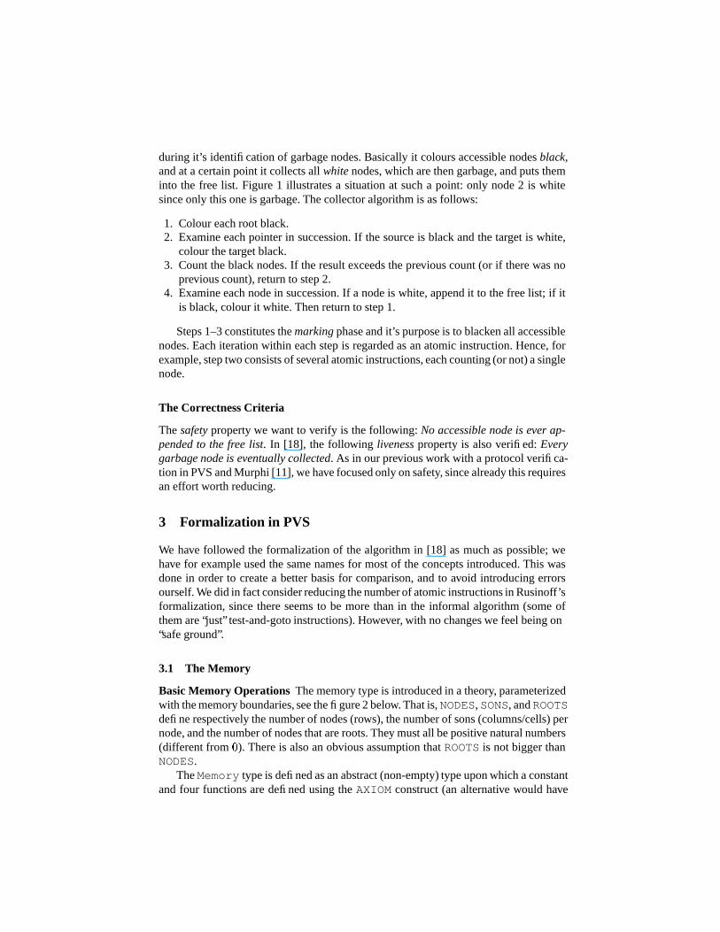
Basic Memory Operations The memory type is introduced in a theory, parameterizedwith the memory boundaries, see the figure 2 below. That is, NODES, SONS, and ROOTSdefine respectively the number of nodes (rows), the number of sons (columns/cells) pernode, and the number of nodes that are roots. They must all be positive natural numbers(different from � ). There is also an obvious assumption that ROOTS is not bigger thanNODES.

The Memory type is defined as an abstract (non-empty) type upon which a constantand four functions are defined using the AXIOM construct (an alternative would have

Memory[NODES:posnat,SONS:posnat,ROOTS:posnat] : THEORYBEGINASSUMINGroots_within : ASSUMPTION ROOTS <= NODES

ENDASSUMING

Memory : TYPE+NODE : TYPE = natINDEX : TYPE = natNode : TYPE = � n : NODE | n < NODES �Index : TYPE = � i : INDEX | i < SONS �Root : TYPE = � r : NODE | r < ROOTS �Colour : TYPE = bool

null_array : Memorycolour : [NODE -> [Memory -> Colour]]set_colour : [NODE,Colour -> [Memory -> Memory]]son : [NODE,INDEX -> [Memory -> NODE]]set_son : [NODE,INDEX,NODE -> [Memory -> Memory]]

m : VAR Memoryn,n1,n2,k : VAR Nodei,i1,i2 : VAR Indexc : VAR Colour

mem_ax1 : AXIOM son(n,i)(null_array) = 0

mem_ax2 : AXIOM colour(n1)(set_colour(n2,c)(m)) =IF n1=n2 THEN c ELSE colour(n1)(m) ENDIF

mem_ax3 : AXIOM colour(n1)(set_son(n2,i,k)(m)) = colour(n1)(m)

mem_ax4 : AXIOM son(n1,i1)(set_son(n2,i2,k)(m)) =IF n1=n2 AND i1=i2 THEN k ELSE son(n1,i1)(m) ENDIF

mem_ax5 : AXIOM son(n1,i)(set_colour(n2,c)(m)) = son(n1,i)(m)END Memory

Fig. 2. The Memory

been to define the memory explicitly as a function from pairs of nodes and indexes tonodes). First, however, some types of nodes, indexes and roots are defined. The typesNODE and INDEX are defined just by the natural numbers. Our functions will be appliedto arguments of these types.

The types Node and Index are the constrained versions where only natural num-bers below respectively NODES and SONS are considered. These latter constrainedtypes are used in axioms where universally quantified variables range over them: weonly want our functions to behave correctly within the boundaries of the memory. Inaddition the type Colour represents black with TRUE and white with FALSE.

The reason for not using the constrained types in the signatures of functions is thatif we did, the PVS type checker would generate TCC’s that we could not prove withoutconsidering the execution traces that lead to the application of these functions. In fact,some of the invariants that we shall later prove states exactly that these functions areindeed only applied to values that lie within the constrained types. If one really wantsto catch such “errors” using type checking, then one needs to define a subtype of well-formed states of the state type that we later will introduce. This, however, is not simple,

and may involve strengthening of this well-formedness predicate during the proof ofTCC’s. We rather prefer to have a PVS specification type checked quickly without toodeep proofs.

The memory is read and modified via four functions, and a constant null arrayrepresents the initial memory containing 0 in all memory cells (axiom mem ax1). Thefunction colour returns the colour of a node. The function set colour assigns acolour to a node. The function son returns the pointer contained in a particular cell.That is, the expression son(n,i)(m) returns the pointer contained in the cell identi-fied by node n and index i. Finally, the function set son assigns a pointer to a cell.That is, the expression set son(n,i,k)(m) returns the memory m updated in cell(n,i) to contain (a pointer to node) k.

Accessible Nodes In this section we define what it means for a node to be accessible.First, however, we introduce some functions on lists (figure 3).

List_Functions[T:TYPE+] : THEORYBEGINlast(l:list[T]|cons?(l)) : RECURSIVE T =IF length(l)=1 THEN car(l) ELSE last(cdr(l)) ENDIFMEASURE length(l)

last_index(l:list[T]|cons?(l)) : nat = length(l)-1

suffix(l:list[T],n:nat |n < length(l)) : RECURSIVE list[T] =IF n=0 THEN l ELSE suffix(cdr(l),n-1) ENDIFMEASURE length(l)

last_occurrence(x:T,l:list[T] | member(x,l)):nat =epsilon! (idx:nat):idx <= last_index(l) AND nth(l,idx) = x AND(idx < last_index(l) IMPLIES NOT member(x,suffix(l,idx+1)))

END List_Functions

Fig. 3. List Functions

The function last returns the last element of a non-empty list, while the func-tion last index returns the index of the last element in a list. So for example if l =cons(5,cons(7,cons(9,null))), then last(l) = 9 andlast index(l)= 2. The other two functions are used only in the proof: one taking the suffix of a listand the other returning the index of the last occurrence of a given element in a list,assuming it exists. The next theory (figure 4) defines the function accessible.

The function points to defines what it means for one node, n1, to point to an-other, n2, in the memory m. The function pointed is a predicate on lists of nodes, andis TRUE for a list if for any two successive nodes in the list, the first points to the nextin the memory. The function path is also a predicate on lists of nodes, and is TRUE fora list if that list represents a non-empty pointed list starting with a root. Finally, a nodeis accessible if it is the last element in some path.

Memory_Functions[NODES:posnat,SONS:posnat,ROOTS:posnat] : THEORYBEGINASSUMINGroots_within : ASSUMPTION ROOTS <= NODES

ENDASSUMINGIMPORTING List_FunctionsIMPORTING Memory[NODES,SONS,ROOTS]

m : VAR Memory

points_to(n1,n2:NODE)(m):bool =n1 < NODES AND n2 < NODES AND EXISTS (i:Index): son(n1,i)(m)=n2

pointed(p:list[Node])(m):bool =length(p) >= 2 IMPLIES

FORALL (i:nat|i<last_index(p)): points_to(nth(p,i),nth(p,i+1))(m)

path(p:list[Node])(m):bool =cons?(p) AND car(p) < ROOTS AND pointed(p)(m)

accessible(n:NODE)(m):bool =EXISTS (p:list[Node]) : path(p)(m) AND last(p) = n

...END Memory_Functions

Fig. 4. The Predicate accessible

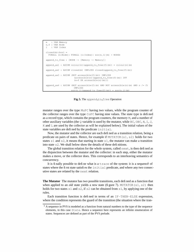
Appending Garbage Nodes In this section we define the operation for appendinga garbage node to the list of free nodes, that can be allocated by the mutator. Thisoperation will be defined abstractly, assuming as little as possible about it’s behavior.Note that, since the free list is supposed to be part of the memory, we could easilyhave defined this operation in terms of the functions son and set son, but this wouldhave required that we took some design decisions as to how the list was represented(for example where the head of the list should be and whether new elements should beadded first or last).

The definitions in figure 5 belong to the theory Memory Functions that we in-troduced part of in figure 4.

First of all, the predicate closed holds for a memory, if no pointer points outsidethe memory. The function append to free is defined by four axioms, having thefollowing informal explanation:

append ax1 The appending operation leaves colours unchanged.append ax2 The appending operation returns a closed memory when applied to a such.append ax3 In appending a garbage node, only that node becomes accessible, and the

accessibility of all other nodes stay unchanged.append ax4 In appending a garbage node, no pointer from any other garbage node is

altered.

3.2 The Mutator and the Collector

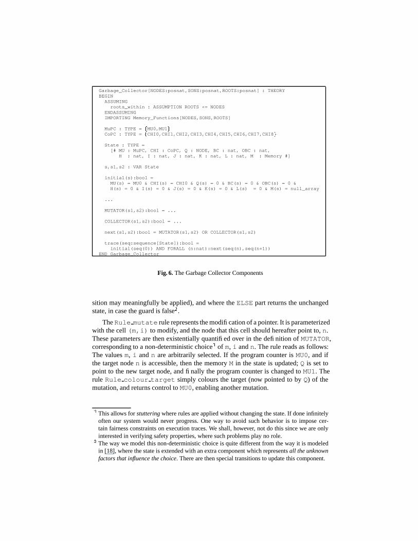
The mutator and the collector are introduced in the theory Garbage Collector infigure 6. First of all, each process has a program counter; the program counter of the

m : VAR Memoryn,f : VAR Nodei : VAR Index

closed(m):bool =FORALL (n:Node): FORALL (i:Index): son(n,i)(m) < NODES

append_to_free : [NODE -> [Memory -> Memory]]

append_ax1 : AXIOM colour(n)(append_to_free(f)(m)) = colour(n)(m)

append_ax2 : AXIOM closed(m) IMPLIES closed(append_to_free(f)(m))

append_ax3 : AXIOM (NOT accessible(f)(m)) IMPLIES(accessible(n)(append_to_free(f)(m)) IFF(n=f OR accessible(n)(m)))

append_ax4 : AXIOM (NOT accessible(f)(m) AND NOT accessible(n)(m) AND n /= f)IMPLIES

son(n,i)(append_to_free(f)(m)) = son(n,i)(m)

Fig. 5. The append to free Operation

mutator ranges over the type MuPC having two values, while the program counter ofthe collector ranges over the type CoPC having nine values. The state type is definedas a record type, which contains the program counters, the memory M, and a number ofother auxiliary variables (the Q variable is used by the mutator, while BC, OBC, H, I, J,K and L are used by the collector as will be explained below). The initial values of thestate variables are defined by the predicate initial.

Now, the mutator and the collector are each defined as a transition relation, being apredicate on pairs of states. Hence, for example if MUTATOR(s1,s2) holds for twostates s1 and s2, it means that starting in state s1, the mutator can make a transitioninto state s2. We shall below show the details of these definitions.

The global transition relation for the whole system, called next, is then defined asthe disjunction between the mutator and the collector: in each step, either the mutatormakes a move, or the collector does. This corresponds to an interleaving semantics ofconcurrency.

It is finally possible to define what is a trace of the system: it is a sequence� ofstates where the first state satisfies the initial predicate, and where any two consec-utive states are related by the next relation.

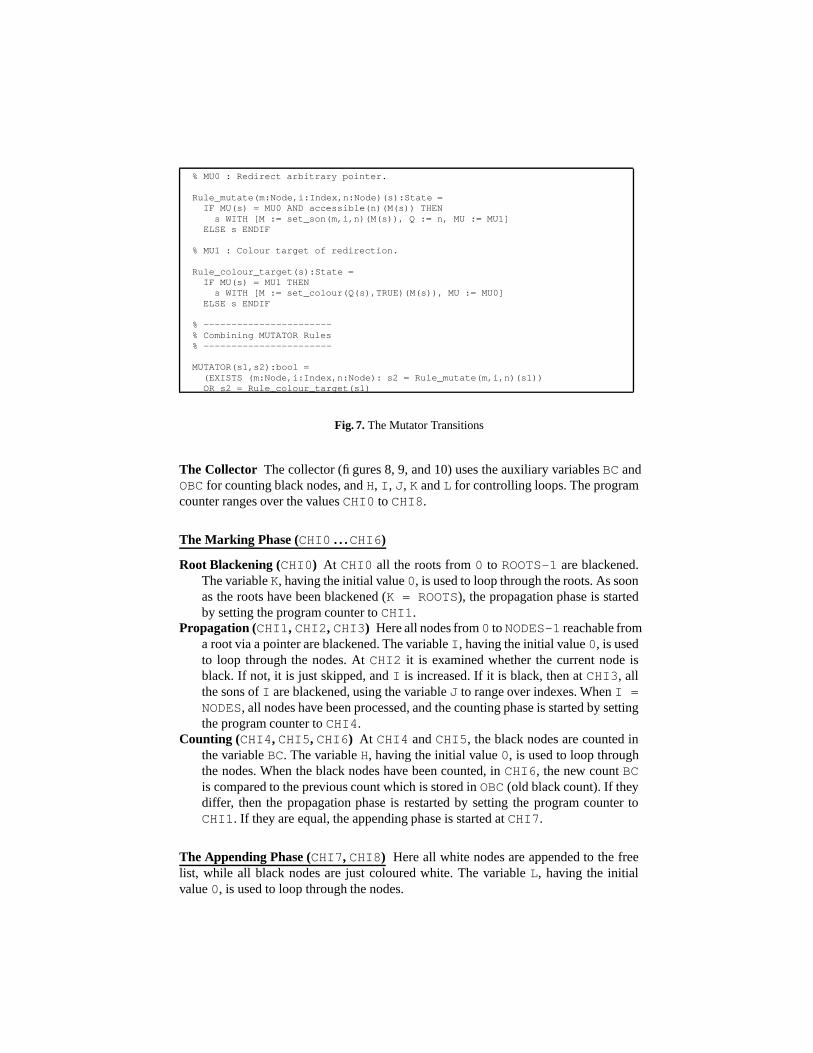
The Mutator The mutator has two possible transitions, each defined as a function thatwhen applied to an old state yields a new state (figure 7). MUTATOR(s1,s2) thenholds for two states s1 and s2, if s2 can be obtained from s1, by applying one of therules.

Each transition function is defined in terms of an IF-THEN-ELSE expression,where the condition represents the guard of the transition (the situation where the tran-

�A sequence in PVS is modeled as a function from natural numbers to the type of the sequenceelements, in this case State. Hence a sequence here represents an infinite enumeration ofstates. Sequences are defined as part of the PVS prelude.

Garbage_Collector[NODES:posnat,SONS:posnat,ROOTS:posnat] : THEORYBEGINASSUMINGroots_within : ASSUMPTION ROOTS <= NODES

ENDASSUMINGIMPORTING Memory_Functions[NODES,SONS,ROOTS]

MuPC : TYPE = � MU0,MU1 �CoPC : TYPE = � CHI0,CHI1,CHI2,CHI3,CHI4,CHI5,CHI6,CHI7,CHI8 �

State : TYPE =[# MU : MuPC, CHI : CoPC, Q : NODE, BC : nat, OBC : nat,

H : nat, I : nat, J : nat, K : nat, L : nat, M : Memory #]

s,s1,s2 : VAR State

initial(s):bool =MU(s) = MU0 & CHI(s) = CHI0 & Q(s) = 0 & BC(s) = 0 & OBC(s) = 0 &H(s) = 0 & I(s) = 0 & J(s) = 0 & K(s) = 0 & L(s) = 0 & M(s) = null_array

...

MUTATOR(s1,s2):bool = ...

COLLECTOR(s1,s2):bool = ...

next(s1,s2):bool = MUTATOR(s1,s2) OR COLLECTOR(s1,s2)

trace(seq:sequence[State]):bool =initial(seq(0)) AND FORALL (n:nat):next(seq(n),seq(n+1))

END Garbage_Collector

Fig. 6. The Garbage Collector Components

sition may meaningfully be applied), and where the ELSE part returns the unchangedstate, in case the guard is false

�

.

The Rule mutate rule represents the modification of a pointer. It is parameterizedwith the cell (m,i) to modify, and the node that this cell should hereafter point to, n.These parameters are then existentially quantified over in the definition of MUTATOR,corresponding to a non-deterministic choice

�

of m, i and n. The rule reads as follows:The values m, i and n are arbitrarily selected. If the program counter is MU0, and ifthe target node n is accessible, then the memory M in the state is updated; Q is set topoint to the new target node, and finally the program counter is changed to MU1. Therule Rule colour target simply colours the target (now pointed to by Q) of themutation, and returns control to MU0, enabling another mutation.

�

This allows for stuttering where rules are applied without changing the state. If done infinitelyoften our system would never progress. One way to avoid such behavior is to impose cer-tain fairness constraints on execution traces. We shall, however, not do this since we are onlyinterested in verifying safety properties, where such problems play no role.

�

The way we model this non-deterministic choice is quite different from the way it is modeledin [18], where the state is extended with an extra component which represents all the unknownfactors that influence the choice. There are then special transitions to update this component.

% MU0 : Redirect arbitrary pointer.

Rule_mutate(m:Node,i:Index,n:Node)(s):State =IF MU(s) = MU0 AND accessible(n)(M(s)) THENs WITH [M := set_son(m,i,n)(M(s)), Q := n, MU := MU1]

ELSE s ENDIF

% MU1 : Colour target of redirection.

Rule_colour_target(s):State =IF MU(s) = MU1 THEN

s WITH [M := set_colour(Q(s),TRUE)(M(s)), MU := MU0]ELSE s ENDIF

% -----------------------% Combining MUTATOR Rules% -----------------------

MUTATOR(s1,s2):bool =(EXISTS (m:Node,i:Index,n:Node): s2 = Rule_mutate(m,i,n)(s1))OR s2 = Rule_colour_target(s1)

Fig. 7. The Mutator Transitions

The Collector The collector (figures 8, 9, and 10) uses the auxiliary variables BC andOBC for counting black nodes, and H, I, J, K and L for controlling loops. The programcounter ranges over the values CHI0 to CHI8.

The Marking Phase (CHI0 . . .CHI6)

Root Blackening (CHI0) At CHI0 all the roots from 0 to ROOTS-1 are blackened.The variable K, having the initial value 0, is used to loop through the roots. As soonas the roots have been blackened (K = ROOTS), the propagation phase is startedby setting the program counter to CHI1.

Propagation (CHI1, CHI2, CHI3) Here all nodes from 0 to NODES-1 reachable froma root via a pointer are blackened. The variable I, having the initial value 0, is usedto loop through the nodes. At CHI2 it is examined whether the current node isblack. If not, it is just skipped, and I is increased. If it is black, then at CHI3, allthe sons of I are blackened, using the variable J to range over indexes. When I =NODES, all nodes have been processed, and the counting phase is started by settingthe program counter to CHI4.

Counting (CHI4, CHI5, CHI6) At CHI4 and CHI5, the black nodes are counted inthe variable BC. The variable H, having the initial value 0, is used to loop throughthe nodes. When the black nodes have been counted, in CHI6, the new count BCis compared to the previous count which is stored in OBC (old black count). If theydiffer, then the propagation phase is restarted by setting the program counter toCHI1. If they are equal, the appending phase is started at CHI7.

The Appending Phase (CHI7, CHI8) Here all white nodes are appended to the freelist, while all black nodes are just coloured white. The variable L, having the initialvalue 0, is used to loop through the nodes.

% -------------% Blacken Roots% -------------

% CHI0 : Blacken.

Rule_stop_blacken(s):State =IF CHI(s) = CHI0 AND K(s) = ROOTS THENs WITH [I := 0, CHI := CHI1]

ELSE s ENDIF

Rule_blacken(s):State =IF CHI(s) = CHI0 AND K(s) /= ROOTS THENs WITH [M := set_colour(K(s),TRUE)(M(s)), K := K(s) + 1, CHI := CHI0]

ELSE s ENDIF

% -------------------% Propagate Colouring% -------------------

% CHI1 : Decide whether to continue propagating.

Rule_stop_propagate(s):State =IF CHI(s) = CHI1 AND I(s) = NODES THENs WITH [BC := 0, H := 0, CHI := CHI4]

ELSE s ENDIF

Rule_continue_propagate(s):State =IF CHI(s) = CHI1 AND I(s) /= NODES THENs WITH [CHI := CHI2]

ELSE s ENDIF

% CHI2 : (Continue) Check whether node is black.

Rule_white_node(s):State =IF CHI(s) = CHI2 AND NOT colour(I(s))(M(s)) THENs WITH [I := I(s) + 1, CHI := CHI1]

ELSE s ENDIF

Rule_black_node(s):State =IF CHI(s) = CHI2 AND colour(I(s))(M(s)) THENs WITH [J := 0, CHI := CHI3]

ELSE s ENDIF

% CHI3 : (Node is black) Colour each son.

Rule_stop_colouring_sons(s):State =IF CHI(s) = CHI3 AND J(s) = SONS THENs WITH [I := I(s) + 1, CHI := CHI1]

ELSE s ENDIF

Rule_colour_son(s):State =IF CHI(s) = CHI3 AND J(s) /= SONS THENs WITH [M := set_colour(son(I(s),J(s))(M(s)),TRUE)(M(s)),

J := J(s) + 1, CHI := CHI3]ELSE s ENDIF

% -----------------% Count Black Nodes% -----------------

Fig. 8. Collector Transitions (a)

% CHI4 : Decide whether to continue counting.

Rule_stop_counting(s):State =IF CHI(s) = CHI4 AND H(s) = NODES THENs WITH [CHI := CHI6]

ELSE s ENDIF

Rule_continue_counting(s):State =IF CHI(s) = CHI4 AND H(s) /= NODES THENs WITH [CHI := CHI5]

ELSE s ENDIF

% CHI5 : (Continue) Count one up if black.

Rule_skip_white(s):State =IF CHI(s) = CHI5 AND NOT colour(H(s))(M(s)) THENs WITH [H := H(s) + 1, CHI := CHI4]

ELSE s ENDIF

Rule_count_black(s):State =IF CHI(s) = CHI5 AND colour(H(s))(M(s)) THENs WITH [BC := BC(s) + 1, H := H(s) + 1, CHI := CHI4]

ELSE s ENDIF

% CHI6 : Compare BC and OBC.

Rule_redo_propagation(s):State =IF CHI(s) = CHI6 AND BC(s) /= OBC(s) THENs WITH [OBC := BC(s), I := 0, CHI := CHI1]

ELSE s ENDIF

Rule_quit_propagation(s):State =IF CHI(s) = CHI6 AND BC(s) = OBC(s) THENs WITH [L := 0, CHI := CHI7]

ELSE s ENDIF

% -------------------% Append to Free List% -------------------

% CHI7 : Decide whether to continue appending.

Rule_stop_appending(s):State =IF CHI(s) = CHI7 AND L(s) = NODES THENs WITH [BC := 0, OBC := 0, K := 0, CHI := CHI0]

ELSE s ENDIF

Rule_continue_appending(s):State =IF CHI(s) = CHI7 AND L(s) /= NODES THENs WITH [CHI := CHI8]

ELSE s ENDIF

% CHI8 : (Continue) Append if white.

Rule_black_to_white(s):State =IF CHI(s) = CHI8 AND colour(L(s))(M(s)) THENs WITH [M := set_colour(L(s),FALSE)(M(s)), L := L(s) + 1,CHI := CHI7]

ELSE s ENDIF

Rule_append_white(s):State =IF CHI(s) = CHI8 AND NOT colour(L(s))(M(s)) THENs WITH [M := append_to_free(L(s))(M(s)), L := L(s) + 1, CHI := CHI7]

ELSE s ENDIF

Fig. 9. Collector Transitions (b)

% -------------------------% Combining COLLECTOR Rules% -------------------------

COLLECTOR(s1,s2):bool =s2 = Rule_stop_blacken(s1)

OR s2 = Rule_blacken(s1)OR s2 = Rule_stop_propagate(s1)OR s2 = Rule_continue_propagate(s1)OR s2 = Rule_white_node(s1)OR s2 = Rule_black_node(s1)OR s2 = Rule_stop_colouring_sons(s1)OR s2 = Rule_colour_son(s1)OR s2 = Rule_stop_counting(s1)OR s2 = Rule_continue_counting(s1)OR s2 = Rule_skip_white(s1)OR s2 = Rule_count_black(s1)OR s2 = Rule_redo_propagation(s1)OR s2 = Rule_quit_propagation(s1)OR s2 = Rule_stop_appending(s1)OR s2 = Rule_continue_appending(s1)OR s2 = Rule_black_to_white(s1)OR s2 = Rule_append_white(s1)

Fig. 10. Collector Transitions (c)

4 Theorem Proving in PVS

In this section we outline the proof of correctness for the garbage collector algorithm.First, we formulate in PVS what it means for the collector to be safe. We then outline thetechnique we have applied to master the relatively big size of the proof. This techniqueseems general and useful for verifying safety properties since it divides the proof intomanageable lemmas. Then we introduce some auxiliary functions (concepts) that areneeded during the proof; and finally, we outline the proof itself by listing the neededinvariants.

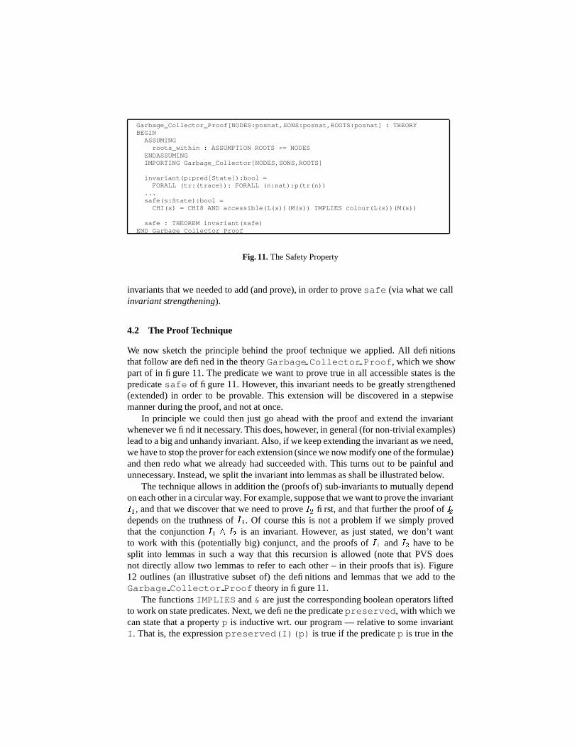
4.1 Formulating the Safety Property

Let us recall the safety property: no accessible node is ever appended to the free list. Ascan be seen from the collector algorithm in figure 9, the append to free operationis only applied at location CHI8 (in the rule Rule append white). It is applied tothe node L(s), but only if this node is white: NOT colour(L(s))(M(s)). Hence,the correctness criteria can be stated as: Whenever the program counter is CHI8, andL is accessible, then L is black (and will hence not be appended). This is stated in thetheory in figure 11.

The theory defines two predicates and a theorem: the correctness criteria. The pred-icate invariant takes as argument a predicate p on states (pred[State] is shortfor the function space [State -> bool]). It returns TRUE if for any executiontrace tr of the program: the predicate p holds in every position of that trace. The safetyproperty we want to verify is defined by the predicate safe. The correctness criteria isthen defined by the theorem named safe. The dots ... in the theory refers to extra

Garbage_Collector_Proof[NODES:posnat,SONS:posnat,ROOTS:posnat] : THEORYBEGINASSUMINGroots_within : ASSUMPTION ROOTS <= NODES

ENDASSUMINGIMPORTING Garbage_Collector[NODES,SONS,ROOTS]

invariant(p:pred[State]):bool =FORALL (tr:(trace)): FORALL (n:nat):p(tr(n))

...safe(s:State):bool =CHI(s) = CHI8 AND accessible(L(s))(M(s)) IMPLIES colour(L(s))(M(s))

safe : THEOREM invariant(safe)END Garbage_Collector_Proof

Fig. 11. The Safety Property

invariants that we needed to add (and prove), in order to prove safe (via what we callinvariant strengthening).

4.2 The Proof Technique

We now sketch the principle behind the proof technique we applied. All definitionsthat follow are defined in the theory Garbage Collector Proof, which we showpart of in figure 11. The predicate we want to prove true in all accessible states is thepredicate safe of figure 11. However, this invariant needs to be greatly strengthened(extended) in order to be provable. This extension will be discovered in a stepwisemanner during the proof, and not at once.

In principle we could then just go ahead with the proof and extend the invariantwhenever we find it necessary. This does, however, in general (for non-trivial examples)lead to a big and unhandy invariant. Also, if we keep extending the invariant as we need,we have to stop the prover for each extension (since we now modify one of the formulae)and then redo what we already had succeeded with. This turns out to be painful andunnecessary. Instead, we split the invariant into lemmas as shall be illustrated below.

The technique allows in addition the (proofs of) sub-invariants to mutually dependon each other in a circular way. For example, suppose that we want to prove the invariant

�

� , and that we discover that we need to prove�

� first, and that further the proof of�

�

depends on the truthness of�

� . Of course this is not a problem if we simply provedthat the conjunction

�

�� �

� is an invariant. However, as just stated, we don’t wantto work with this (potentially big) conjunct, and the proofs of

�

� and�

� have to besplit into lemmas in such a way that this recursion is allowed (note that PVS doesnot directly allow two lemmas to refer to each other – in their proofs that is). Figure12 outlines (an illustrative subset of) the definitions and lemmas that we add to theGarbage Collector Proof theory in figure 11.

The functions IMPLIES and & are just the corresponding boolean operators liftedto work on state predicates. Next, we define the predicate preserved, with which wecan state that a property p is inductive wrt. our program — relative to some invariantI. That is, the expression preserved(I)(p) is true if the predicate p is true in the

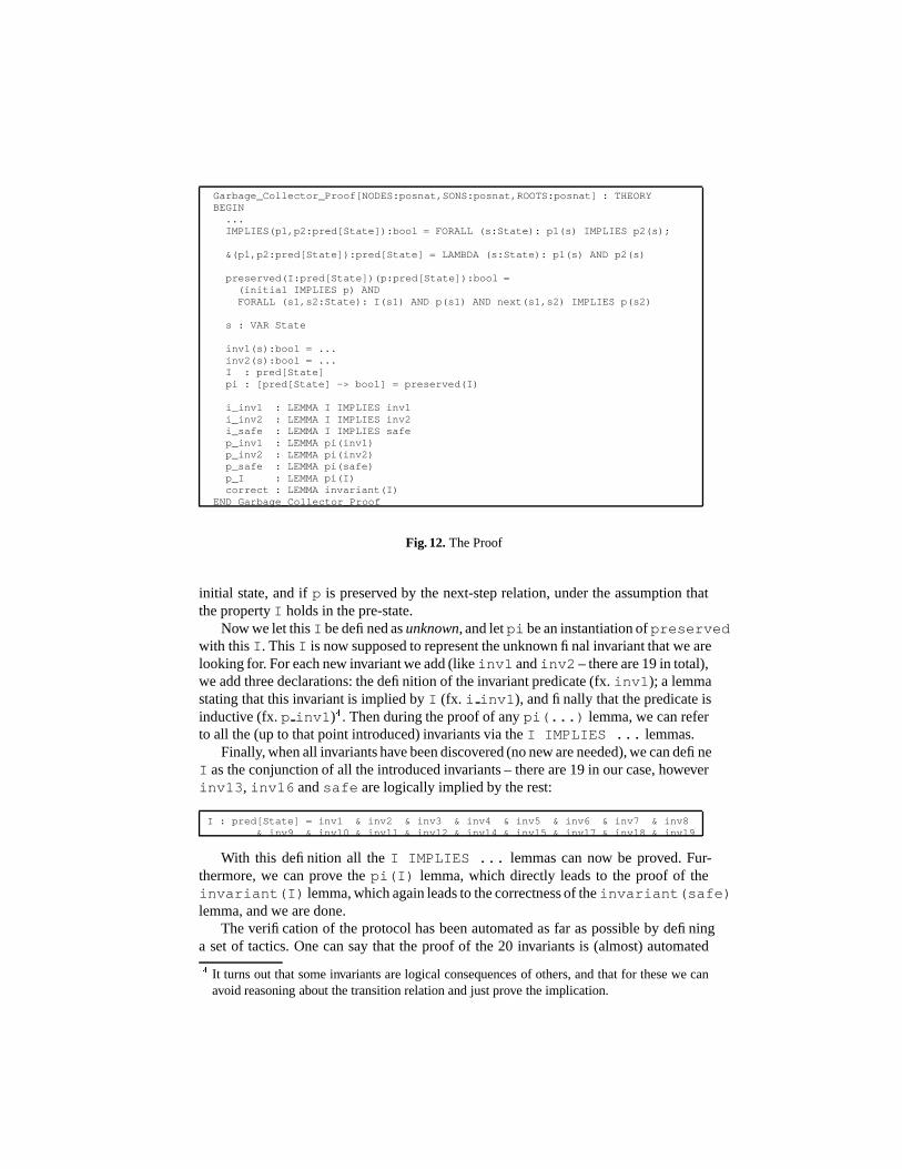
Garbage_Collector_Proof[NODES:posnat,SONS:posnat,ROOTS:posnat] : THEORYBEGIN...IMPLIES(p1,p2:pred[State]):bool = FORALL (s:State): p1(s) IMPLIES p2(s);

&(p1,p2:pred[State]):pred[State] = LAMBDA (s:State): p1(s) AND p2(s)

preserved(I:pred[State])(p:pred[State]):bool =(initial IMPLIES p) ANDFORALL (s1,s2:State): I(s1) AND p(s1) AND next(s1,s2) IMPLIES p(s2)

s : VAR State

inv1(s):bool = ...inv2(s):bool = ...I : pred[State]pi : [pred[State] -> bool] = preserved(I)

i_inv1 : LEMMA I IMPLIES inv1i_inv2 : LEMMA I IMPLIES inv2i_safe : LEMMA I IMPLIES safep_inv1 : LEMMA pi(inv1)p_inv2 : LEMMA pi(inv2)p_safe : LEMMA pi(safe)p_I : LEMMA pi(I)correct : LEMMA invariant(I)

END Garbage_Collector_Proof

Fig. 12. The Proof

initial state, and if p is preserved by the next-step relation, under the assumption thatthe property I holds in the pre-state.

Now we let this I be defined as unknown, and let pi be an instantiation of preservedwith this I. This I is now supposed to represent the unknown final invariant that we arelooking for. For each new invariant we add (like inv1 and inv2 – there are 19 in total),we add three declarations: the definition of the invariant predicate (fx. inv1); a lemmastating that this invariant is implied by I (fx. i inv1), and finally that the predicate isinductive (fx. p inv1) � . Then during the proof of any pi(...) lemma, we can referto all the (up to that point introduced) invariants via the I IMPLIES ... lemmas.

Finally, when all invariants have been discovered (no new are needed), we can defineI as the conjunction of all the introduced invariants – there are 19 in our case, howeverinv13, inv16 and safe are logically implied by the rest:

I : pred[State] = inv1 & inv2 & inv3 & inv4 & inv5 & inv6 & inv7 & inv8& inv9 & inv10 & inv11 & inv12 & inv14 & inv15 & inv17 & inv18 & inv19

With this definition all the I IMPLIES ... lemmas can now be proved. Fur-thermore, we can prove the pi(I) lemma, which directly leads to the proof of theinvariant(I) lemma, which again leads to the correctness of the invariant(safe)lemma, and we are done.

The verification of the protocol has been automated as far as possible by defininga set of tactics. One can say that the proof of the 20 invariants is (almost) automated

�It turns out that some invariants are logical consequences of others, and that for these we canavoid reasoning about the transition relation and just prove the implication.

“up to” lemmas. That is: if some invariant is provable given explicitly as assumptionsthe other invariants and lemmas it depends on, then it is proved automatically usinga single tactic. The obtained level of automatization could be achieved only becauseof the flexibility provided by the PVS decision procedures. When we say almost auto-mated, it means that in some few cases, we needed to assist the prover – always becausethe PVS (inst?) command did not get instantiations right. The program contains 20transitions, and with 20 invariants this gives 400 (20*20) proofs, and of these 6 neededmanual assistance (two transitions in the proof of inv15 and four in inv17), corre-sponding to

�������% automatization. It should though be said that the proofs of lemmas

about auxiliary functions were in general not automatic.

Memory_Observers[NODES:posnat,SONS:posnat,ROOTS:posnat] : THEORYBEGINASSUMINGroots_within : ASSUMPTION ROOTS <= NODES

ENDASSUMINGIMPORTING Memory_Functions[NODES,SONS,ROOTS]

m : VAR Memory

<(p1,p2:[NODE,INDEX]):bool =LET n1 = PROJ_1(p1), i1 = PROJ_2(p1), n2 = PROJ_1(p2), i2 = PROJ_2(p2) IN

n1 < n2 OR (n1 = n2 AND i1 < i2);

<=(p1,p2:[NODE,INDEX]):bool = p1 < p2 OR p1 = p2

blacks(l,u:NODE)(m) : RECURSIVE nat =IF l < u AND l < NODES THEN

IF colour(l)(m) THEN 1 ELSE 0 ENDIF + blacks(l+1,u)(m)ELSE 0 ENDIFMEASURE abs(u-l)

black_roots(u:NODE)(m):bool = FORALL (r:Root| r < u): colour(r)(m)

bw(n:NODE,i:INDEX)(m):bool =n < NODES AND i < SONS AND colour(n)(m) AND NOT colour(son(n,i)(m))(m)

exists_bw(n1:NODE,i1:INDEX,n2:NODE,i2:INDEX)(m):bool =EXISTS (n:Node,i:Index):bw(n,i)(m) AND NOT (n,i) < (n1,i1) AND (n,i) < (n2,i2)

propagated(m):bool = NOT exists_bw(0,0,NODES,0)(m)

blackened(l:NODE)(m):bool =FORALL (n:Node|l <= n): accessible(n)(m) IMPLIES colour(n)(m)

END Memory_Observers

Fig. 13. Auxiliary Functions

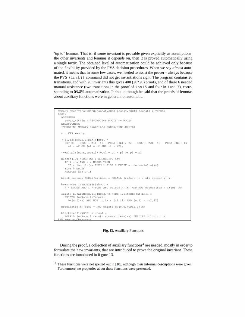
During the proof, a collection of auxiliary functions � are needed, mostly in order toformulate the new invariants, that are introduced to prove the original invariant. Thesefunctions are introduced in figure 13.

�These functions were not spelled out in [18], although their informal descriptions were given.Furthermore, no properties about these functions were presented.

inv1(s) :bool = I(s) <= NODES AND ((CHI(s)=CHI2 OR CHI(s)=CHI3)IMPLIES I(s) < NODES)

inv2(s) :bool = J(s) <= SONS

inv3(s) :bool = K(s) <= ROOTS

inv4(s) :bool = H(s) <= NODES AND (CHI(s)=CHI5 IMPLIES H(s) < NODES) AND(CHI(s)=CHI6 IMPLIES H(s) = NODES)

inv5(s) :bool = L(s) <= NODES AND (CHI(s)=CHI8 IMPLIES L(s) < NODES)

inv6(s) :bool = Q(s) < NODES

inv7(s) :bool = closed(M(s))

inv8(s) :bool = (CHI(s)=CHI4 OR CHI(s)=CHI5)IMPLIES BC(s) <= blacks(0,H(s))(M(s))

inv9(s) :bool = CHI(s)=CHI6 IMPLIES BC(s) <= blacks(0,NODES)(M(s))

inv10(s):bool = (CHI(s)=CHI0 OR CHI(s)=CHI1 OR CHI(s)=CHI2 OR CHI(s)=CHI3)IMPLIES OBC(s) <= blacks(0,NODES)(M(s))

inv11(s):bool = (CHI(s)=CHI4 OR CHI(s)=CHI5 OR CHI(s)=CHI6)IMPLIES OBC(s) <= BC(s) + blacks(H(s),NODES)(M(s))

inv12(s):bool = BC(s) <= NODES

inv13(s):bool = CHI(s)=CHI6 IMPLIES OBC(s) <= BC(s)

inv14(s):bool = (CHI(s)=CHI0 OR CHI(s)=CHI1 OR CHI(s)=CHI2 OR CHI(s)=CHI3 ORCHI(s)=CHI4 OR CHI(s)=CHI5 OR CHI(s)=CHI6) IMPLIESblack_roots(IF CHI(s)=CHI0 THEN K(s) ELSE ROOTS ENDIF)(M(s))

inv15(s):bool = FORALL (n:Node,i:Index):(((CHI(s)=CHI1 OR CHI(s)=CHI2 OR CHI(s)=CHI3) ANDblacks(0,NODES)(M(s)) = OBC(s) AND(n,i) < (I(s),IF CHI(s)=CHI3 THEN J(s) ELSE 0 ENDIF) ANDbw(n,i)(M(s)))IMPLIES (MU(s)=MU1 AND son(n,i)(M(s))=Q(s)))

inv16(s):bool = ((CHI(s)=CHI1 OR CHI(s)=CHI2 OR CHI(s)=CHI3) ANDblacks(0,NODES)(M(s)) = OBC(s) ANDexists_bw(0,0,I(s),IF CHI(s)=CHI3 THEN J(s) ELSE 0 ENDIF)(M(s)))IMPLIES MU(s)=MU1

inv17(s):bool = ((CHI(s)=CHI1 OR CHI(s)=CHI2 OR CHI(s)=CHI3) ANDblacks(0,NODES)(M(s)) = OBC(s) ANDexists_bw(0,0,I(s),IF CHI(s)=CHI3 THEN J(s) ELSE 0 ENDIF)(M(s)))IMPLIES

exists_bw(I(s),IF CHI(s)=CHI3 THEN J(s)ELSE 0 ENDIF,NODES,0)(M(s))

inv18(s):bool = ((CHI(s)=CHI4 OR CHI(s)=CHI5 OR CHI(s)=CHI6) ANDOBC(s) = BC(s) + blacks(H(s),NODES)(M(s)))IMPLIES blackened(0)(M(s))

inv19(s):bool = (CHI(s)=CHI7 OR CHI(s)=CHI8) IMPLIES blackened(L(s))(M(s))

Fig. 14. Invariants

The predicates < and <= define lexicographic ordering on node-index pairs, whereeach such pair identifies a cell in our memory. The projection function PROJ i (for i ���������

) selects the i’th component of a tuple. Hence, for example (2,3) < (3,0).The rest of the functions are explained as follows. The expressionblacks(l,u)(m)

returns the number of black nodes between l (included) and u (excluded). In particu-lar, blacks(0,NODES)(m) represents the total number of black nodes in the mem-ory m. The expression black roots(u)(m) returns true if all the nodes below uare black. In particular, black roots(ROOTS)(m) if all roots are black. The ex-pression bw(n,i)(m) returns true if node n is black and the son of cell (n,i) iswhite. The expression exists bw(n1,i1,n2,i2)(m) returns true if there existsa pointer between (n1,i1) and (n2,i2) from a black node to a white node. Theexpression propagated(m) returns true if no black node points to a white node. Fi-nally, blackened(l)(m) returns true if all nodes above (and including) l are blackif they are accessible.

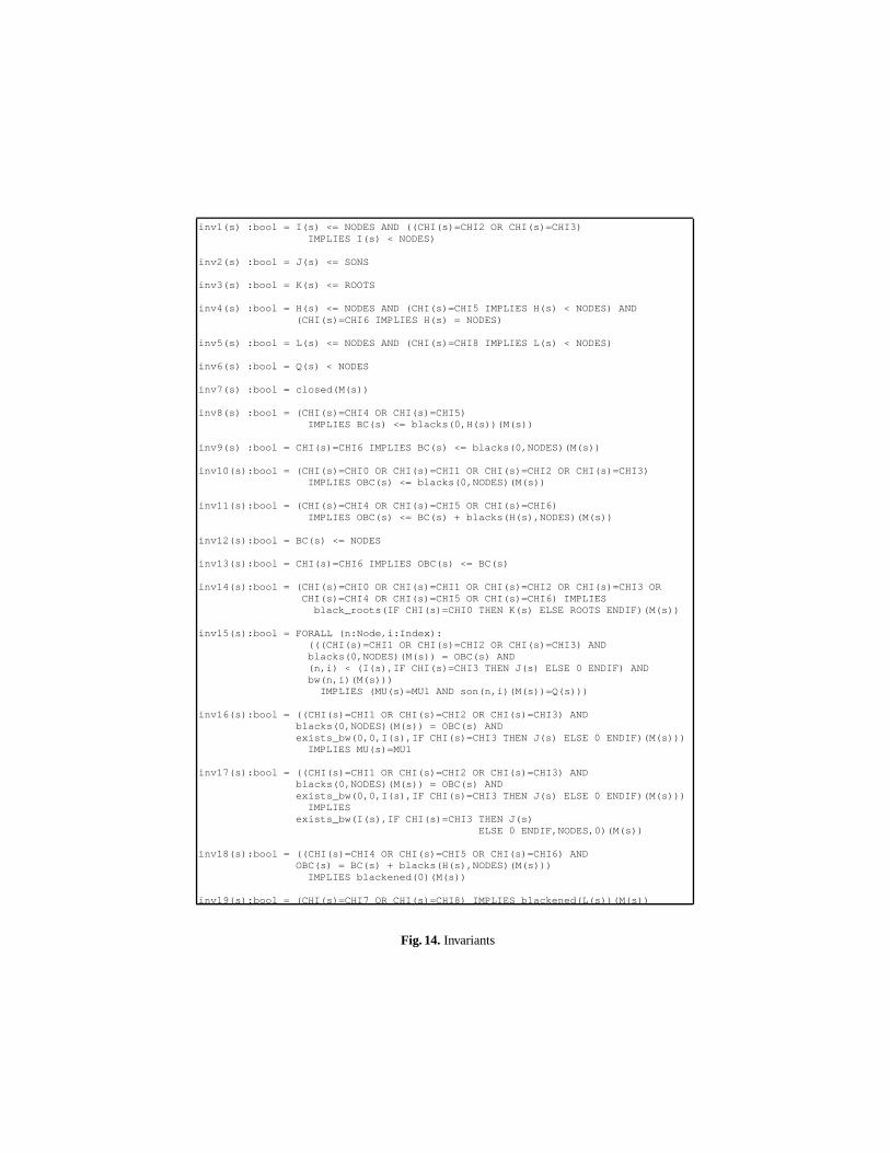
55 lemmas are needed (and proved) about these functions in order to carry out theproof of the safety property. In addition, 15 lemmas about various general list processingfunctions are needed. These lemmas are given in appendix A. This should be comparedto Russinoff’s ”over one hundred lemmas characterizing the behavior of relevant func-tions” in [18]. The invariants defined and proved are given in figure 14. These are thesame as in [18]. The proof took 1.5 months of effort.

5 Model Checking in Murphi

In this section, we shortly outline our experience with encoding the garbage collectorin the Murphi model checker [15]. The full formal Murphi program is contained inappendix B.

Murphi uses a program model that is similar to those of UNITY [5] and TLA [14],hence the one we have used in our PVS specification. A Murphi program has threecomponents: a declaration of the global variables, a description of the initial state, anda collection of transition rules. Each transition rule is a guarded command that consistsof a boolean guard expression over the global variables, and a deterministic statementthat changes the global variables. In addition, one can state invariant conditions to beverified.

An execution of a Murphi program is obtained by repeatedly (1) arbitrarily select-ing one of the transition rules where the boolean guard is true in the current state;(2) executing the statement of the chosen transition rule. The statement is executedatomically: no other transition rules are executed in parallel. Thus state transitions areinterleaving and processes communicate via shared variables. The notion of process isnot formally supported, but may be thought of as a subset of the transition rules. TheMurphi verifier tries to explore all reachable states in order to ensure that all invariantshold. If a violation is detected, Murphi generates a violating trace.

The reader is referred to the appendix for the details of the model. Here we shallfocus on the differences between the PVS model and the Murphi model. The two prin-cipal advantages of PVS are that (1): in PVS we can verify a parameterized program,whereas in Murphi we are limited to a finite state program; and: (2) in PVS we can

be abstract at the algorithmic level, whereas in Murphi we have to make certain designchoices. The advantage of Murphi is that verification is automatic, whereas in PVS wehave to manually assist the proof.

Infinite Versus Finite State

The first obvious difference concerns the size of the memory. In PVS, the boundaries(NODES, SONS and ROOTS) are unspecified parameters (figure 2), hence the correct-ness does not depend on their specific values. The garbage collector is therefore verifiedfor any size of memory. In the Murphi program, on the other hand, we have to fix theboundaries to particular natural numbers. In our case, we verified the algorithm with thefollowing values: NODES = 3, SONS = 2 and ROOTS = 1 (figure 15). In this context,Murphi used 803 seconds to verify the invariant, exploring 415633 states. It turned outthat Murphi was unable to verify bigger memories within reasonable time (24 hours).An experiment with 4 nodes, two sons and two roots had not terminated after 25 hoursand over 5 million states visited.

ConstNODES : 3; SONS : 2; ROOTS : 1;

TypeNode : 0..NODES-1; Index : 0..SONS-1; Colour : boolean;NodeStruct : Record colour : Colour; cells : Array[Index] Of Node; End;

VarM : Array[Node] Of NodeStruct;

Function colour(n:Node):Colour;Begin Return M[n].colour; End;

Procedure set_colour(n:Node;c:Colour);Begin M[n].colour := c; End;

Function son(n:Node;i:Index):Node;Begin Return M[n].cells[i]; End;

Procedure set_son(n:Node;i:Index;k:Node);Begin M[n].cells[i] := k; End;

Fig. 15. The Memory

Abstractness of Memory

The PVS memory is abstractly specified in terms of a set of axioms (figure 2). Althoughwe think of the memory as an array of two dimensions, this is in fact not required byan implementation. In the Murphi program, on the other hand, we need to choose animplementation of the memory, and we have chosen to model it as a two dimensionalarray as illustrated in figure 15.

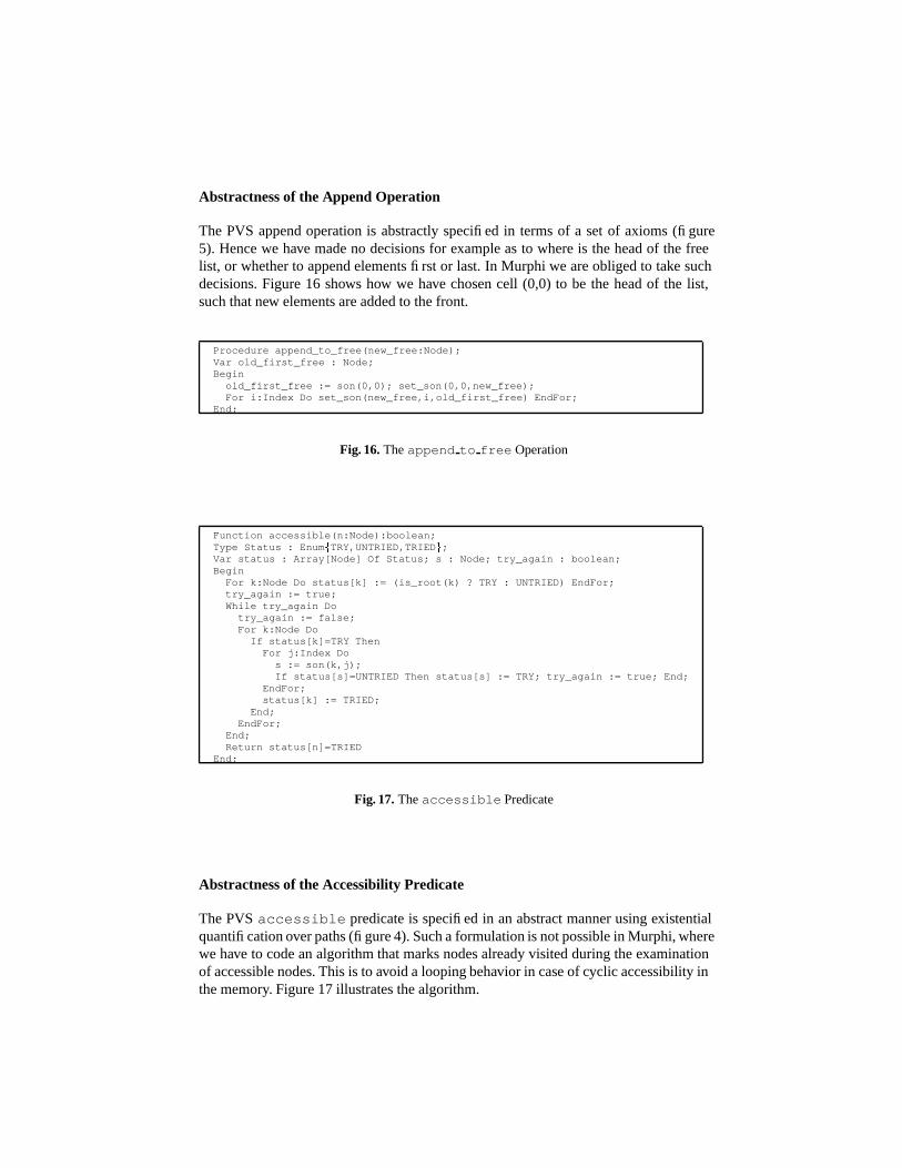
Abstractness of the Append Operation

The PVS append operation is abstractly specified in terms of a set of axioms (figure5). Hence we have made no decisions for example as to where is the head of the freelist, or whether to append elements first or last. In Murphi we are obliged to take suchdecisions. Figure 16 shows how we have chosen cell (0,0) to be the head of the list,such that new elements are added to the front.

Procedure append_to_free(new_free:Node);Var old_first_free : Node;Beginold_first_free := son(0,0); set_son(0,0,new_free);For i:Index Do set_son(new_free,i,old_first_free) EndFor;

End;

Fig. 16. The append to free Operation

Function accessible(n:Node):boolean;Type Status : Enum � TRY,UNTRIED,TRIED � ;Var status : Array[Node] Of Status; s : Node; try_again : boolean;BeginFor k:Node Do status[k] := (is_root(k) ? TRY : UNTRIED) EndFor;try_again := true;While try_again Do

try_again := false;For k:Node Do

If status[k]=TRY ThenFor j:Index Do

s := son(k,j);If status[s]=UNTRIED Then status[s] := TRY; try_again := true; End;

EndFor;status[k] := TRIED;

End;EndFor;

End;Return status[n]=TRIED

End;

Fig. 17. The accessible Predicate

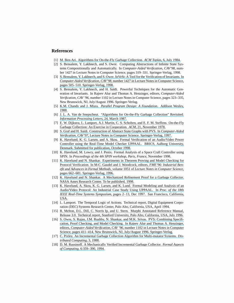
Abstractness of the Accessibility Predicate

The PVS accessible predicate is specified in an abstract manner using existentialquantification over paths (figure 4). Such a formulation is not possible in Murphi, wherewe have to code an algorithm that marks nodes already visited during the examinationof accessible nodes. This is to avoid a looping behavior in case of cyclic accessibility inthe memory. Figure 17 illustrates the algorithm.

6 Observations

The properties that we formulated and proved in PVS can be divided into two classes:invariants and properties about auxiliary functions; we call the latter just lemmas. Therewere 20 invariants, the same as in [18], and there were 70 lemmas, whereas [18] hasover 100. It’s however not clear what the reason for this reduction is, since [18] doesnot contain the lemmas. 98.5% of our invariant proofs were automatic, once the lemmasand other invariants needed as assumptions were identified. That is, observing that theprogram has 20 possible transitions and that there were 20 invariants, there were hence20*20 = 400 transition proofs, whereof 6 needed manual assistance. The assistance al-ways consisted of guiding the instantiation of universally quantified assumptions whenthe PVS (inst?) command did not succeed in finding the right instantiations. Manyof the lemmas needed manual assistance.

The general approach to the proof of an invariant was as follows. The proof wouldtypically fail, the result being a set of unproved sequents. Basically, a generalization ofthe conjunction of these sequents would form the new invariant to prove, and the processcontinued. This style of proof was also applied in [11] to a communications protocol. Aparticular hard problem seems to be the occurrence of loops in this strengthening pro-cess, implying possibly infinite strengthening. Here is where generalization is neededin terms of introducing quantifiers into the invariant. The PVS proof took 1.5 months ofeffort.

Murphi performed the proof automatically in less than 14 minutes, but we had to fixthe boundaries of the memory, and we had to make concrete implementation choices atthe algorithmic level as well as at the data type level. The size of the memory for whichthe garbage collector could be model checked was so small that it could represent aboarder case (three nodes, two sons per node, and one root), which hence may give lessconfidence in what to conclude from the verification result.

We believe that this example provides a good case study for efforts to improvetheorem proving techniques as well as model checking techniques. This is mainly dueto its small size (lines of code) combined with the difficulty to prove it. The exampleis in particular a challenge to invariant strengthening techniques such as [4, 3], andabstraction techniques such as [2, 8].

Acknowledgments. Therese Hardin provided a stimulating environment at Laboratoired’Informatique de Paris 6, France, where a major part of the work was carried out. JohnRushby, Natarajan Shankar and Sam Owre received me well during my long term visitto SRI, California, USA, and provided me with valuable comments. The Human CapitalMobility grant through which this work was funded came into existence partly due toPatrick Cousot (Ecole Normale Superieure, Paris). Recently SeungJoon Park (NASAAmes Research Center) has provided comments on using symmetry and abstraction toreduce the state space of the Murphi model.

References

[1] M. Ben-Ari. Algorithms for On-the-Fly Garbage Collection. ACM Toplas, 6, July 1984.[2] S. Bensalem, Y. Lakhnech, and S. Owre. Computing Abstractions of Infinite State Sys-

tems Compositionally and Automatically. In Computer-Aided Verification, CAV’98, num-ber 1427 in Lecture Notes in Computer Science, pages 319–331. Springer-Verlag, 1998.

[3] S. Bensalem, Y. Lakhnech, and S. Owre. InVeSt: A Tool for the Verification of Invariants. InComputer-Aided Verification, CAV’98, number 1427 in Lecture Notes in Computer Science,pages 505–510. Springer-Verlag, 1998.

[4] S. Bensalem, Y. Lakhnech, and H. Saıdi. Powerful Techniques for the Automatic Gen-eration of Invariants. In Rajeev Alur and Thomas A. Henzinger, editors, Computer-AidedVerification, CAV ’96, number 1102 in Lecture Notes in Computer Science, pages 323–335,New Brunswick, NJ, July/August 1996. Springer-Verlag.

[5] K.M. Chandy and J. Misra. Parallel Program Design: A Foundation. Addison Wesley,1988.

[6] J. L. A. Van de Snepscheut. “Algorithms for On-the-Fly Garbage Collection” Revisited.Information Processing Letters, 24, March 1987.

[7] E. W. Dijkstra, L. Lamport, A.J. Martin, C. S. Scholten, and E. F. M. Steffens. On-the-FlyGarbage Collection: An Exercise in Cooperation. ACM, 21, November 1978.

[8] S. Graf and H. Saidi. Construction of Abstract State Graphs with PVS. In Computer-AidedVerification, CAV’97, Lecture Notes in Computer Science. Springer-Verlag, 1997.

[9] K. Havelund, K. G. Larsen, and A. Skou. Formal Verification of an Audio/Video PowerController using the Real-Time Model Checker UPPAAL. BRICS, Aalborg University,Denmark. Submitted for publication, October 1998.

[10] K. Havelund, M. Lowry, and J. Penix. Formal Analysis of a Space Craft Controller usingSPIN. In Proceedings of the 4th SPIN workshop, Paris, France, November 1998.

[11] K. Havelund and N. Shankar. Experiments in Theorem Proving and Model Checking forProtocol Verification. In M-C. Gaudel and J. Woodcock, editors, FME’96: Industrial Ben-efit and Advances in Formal Methods, volume 1051 of Lecture Notes in Computer Science,pages 662–681. Springer-Verlag, 1996.

[12] K. Havelund and N. Shankar. A Mechanized Refinement Proof for a Garbage Collector.NASA Ames Research Center. To be published, 1998.

[13] K. Havelund, A. Skou, K. G. Larsen, and K. Lund. Formal Modeling and Analysis of anAudio/Video Protocol: An Industrial Case Study Using UPPAAL. In Proc. of the 18thIEEE Real-Time Systems Symposium, pages 2–13, Dec 1997. San Francisco, California,USA.

[14] L. Lamport. The Temporal Logic of Actions. Technical report, Digital Equipment Corpo-ration (DEC) Systems Research Center, Palo Alto, California, USA, April 1994.

[15] R. Melton, D.L. Dill, C. Norris Ip, and U. Stern. Murphi Annotated Reference Manual,Release 3.0. Technical report, Stanford University, Palo Alto, California, USA, July 1996.

[16] S. Owre, S. Rajan, J.M. Rushby, N. Shankar, and M.K. Srivas. PVS: Combining Specifi-cation, Proof Checking, and Model Checking. In Rajeev Alur and Thomas A. Henzinger,editors, Computer-Aided Verification, CAV ’96, number 1102 in Lecture Notes in ComputerScience, pages 411–414, New Brunswick, NJ, July/August 1996. Springer-Verlag.

[17] C. Pixley. An Incremental Garbage Collection Algorithm for Multi-mutator Systems. Dis-tributed Computing, 3, 1988.

[18] D. M. Russinoff. A Mechanically Verified Incremental Garbage Collector. Formal Aspectsof Computing, 6:359–390, 1994.

A PVS Lemmas aboutAuxiliary Functions

List_Properties[T:TYPE+] : THEORYBEGINIMPORTING List_Functions[T]

e : VAR Tl,l1,l2 : VAR list[T]p : VAR pred[T]n,k : VAR nat

length1 : LEMMAcons?(l) IMPLIES length(cdr(l)) = length(l)-1

length2 : LEMMAlength(append(l1,l2)) = length(l1) + length(l2)

member1 : LEMMAmember(e,l) =EXISTS n : (n < length(l) AND nth(l,n)=e)

member2 : LEMMAmember(e,l) IMPLIESEXISTS (x: nat):

x <= last_index(l) AND nth(l,x) = e AND(x < last_index(l) IMPLIES

NOT member(e,suffix(l,x+1)))

car1 : LEMMAcons?(l1) IMPLIES car(append(l1,l2)) = car(l1)

last1 : LEMMAlength(l)>=2 IMPLIES last(l)=last(cdr(l))

last2 : LEMMAlast(cons(e,null)) = e

last3 : LEMMA(length(l) >=2 AND p(car(l)) AND NOT p(last(l)))IMPLIES

EXISTS (i:nat|i<last_index(l)):p(nth(l,i)) AND NOT p(nth(l,i+1))

last4 : LEMMAcons?(l2) IMPLIESlast(append(l1,l2)) = last(l2)

last5 : LEMMAcons?(l) IMPLIES nth(l,last_index(l)) = last(l)

suffix1 : LEMMA(length(l) > 0 AND n <= last_index(l))IMPLIES cons?(suffix(l, n))

suffix2 : LEMMA(length(l) > 0 AND n <= last_index(l))IMPLIES car(suffix(l,n)) = nth(l,n)

suffix3 : LEMMA(length(l) > 0 AND n <= last_index(l))

IMPLIESlast(suffix(l,n)) = last(l)

suffix4 : LEMMAn < length(l) IMPLIESlength(suffix(l,n)) = length(l) - n

suffix5 : LEMMAn+k < length(l) IMPLIESnth(suffix(l,n),k) = nth(l,n+k)

END List_Properties

Memory_Properties[NODES : posnat,SONS : posnat,ROOTS : posnat] : THEORY

BEGINASSUMINGroots_within : ASSUMPTION ROOTS <= NODES

ENDASSUMINGIMPORTING List_PropertiesIMPORTING Memory_Functions[NODES,SONS,ROOTS]IMPORTING Memory_Observers[NODES,SONS,ROOTS]

abs(i:int):nat = IF i < 0 THEN -i ELSE i ENDIF

m : VAR Memoryn,n1,n2,k : VAR Nodei,i1,i2,j : VAR Indexc : VAR Colourx : VAR natN,N1,N2 : VAR NODE

I,I1,I2 : VAR INDEXl,l1,l2 : VAR list[Node]

smaller1 : LEMMANOT (n,i) < (0,0)

smaller2 : LEMMA(NOT (n,i) < (k,0) AND (n,i) < (k+1,0))

IMPLIES n = k

smaller3 : LEMMA(n,i) < (k,SONS) IFF (n,i) < (k+1,0)

smaller4 : LEMMA(NOT (n,i) < (k,j) AND (n,i) < (k,j+1)) IMPLIES(n,i)=(k,j)

closed1 : LEMMAclosed(null_array)

closed2 : LEMMAclosed(set_colour(n,c)(m)) = closed(m)

closed3 : LEMMAclosed(m) IMPLIES closed(set_son(n,i,k)(m))

closed4 : LEMMAclosed(m) IMPLIES son(n,i)(m) < NODES

blacks1 : LEMMAblacks(N1,N2)(set_son(n,i,k)(m)) =blacks(N1,N2)(m)

blacks2 : LEMMAblacks(N1,N2)(m) <=blacks(N1,N2)(set_colour(n,TRUE)(m))

blacks3 : LEMMANOT colour(n2)(m) IMPLIES

blacks(n1,n2+1)(m) = blacks(n1,n2)(m)

blacks4 : LEMMAn1<=n2 AND colour(n2)(m) IMPLIES

blacks(n1,n2+1)(m) = blacks(n1,n2)(m) + 1

blacks5 : LEMMANOT colour(n1)(m) IMPLIES

blacks(n1,N2)(m) = blacks(n1+1,N2)(m)

blacks6 : LEMMA(n1<N2 AND colour(n1)(m)) IMPLIES

blacks(n1,N2)(m) = blacks(n1+1,N2)(m) + 1

blacks7 : LEMMAN1 <= N2 IMPLIES blacks(N1,N2)(m) <= N2-N1

blacks8 : LEMMA(n < N1 OR n >= N2) IMPLIESblacks(N1,N2)(set_colour(n,c)(m)) =blacks(N1,N2)(m)

blacks9 : LEMMA(n >= N1 AND n < N2 AND NOT colour(n)(m))

IMPLIESblacks(N1,N2)(set_colour(n,TRUE)(m)) =blacks(N1,N2)(m) + 1

blacks10 : LEMMA(blacks(0,NODES)(set_colour(n,TRUE)(m)) =blacks(0,NODES)(m))IMPLIES colour(n)(m)

blacks11 : LEMMAblacks(N,N)(m) = 0

black_roots1 : LEMMAblack_roots(0)(m)

black_roots2 : LEMMAblack_roots(N)(set_son(n,i,k)(m)) =black_roots(N)(m)

black_roots3 : LEMMAblack_roots(N)(m) IMPLIESblack_roots(N)(set_colour(n,TRUE)(m))

black_roots4 : LEMMAblack_roots(n+1)(set_colour(n,TRUE)(m)) =black_roots(n)(m)

bw1 : LEMMAclosed(m) IMPLIES(NOT bw(n1,i1)(m) ANDbw(n1,i1)(set_son(n2,i2,k)(m)))IMPLIES

(n1,i1)=(n2,i2)

bw2 : LEMMAclosed(m) IMPLIES(NOT bw(n,i)(m) ANDbw(n,i)(set_colour(k,TRUE)(m)))IMPLIES

(n=k AND NOT colour(n)(m))

bw3 : LEMMAbw(n,i)(m) IMPLIEScolour(n)(m) AND NOT colour(son(n,i)(m))(m)

exists_bw1 : LEMMAexists_bw(N1,I1,N2,I2)(m) IMPLIESEXISTS (n:Node,i:Index):bw(n,i)(m) ANDNOT (n,i) < (N1,I1) AND(n,i) < (N2,I2)

exists_bw2 : LEMMAclosed(m) IMPLIES(NOT exists_bw(0,0,N2,I2)(m) ANDexists_bw(0,0,N2,I2)(set_son(n,i,k)(m)))IMPLIES

(NOT colour(k)(m) AND (n,i) < (N2,I2))

exists_bw3 : LEMMA(accessible(n)(m) ANDNOT colour(n)(m) ANDblack_roots(ROOTS)(m))IMPLIES

exists_bw(0,0,NODES,0)(m)

exists_bw4 : LEMMAexists_bw(0,0,NODES,0)(m) IMPLIESexists_bw(0,0,N,I)(m) ORexists_bw(N,I,NODES,0)(m)

exists_bw5 : LEMMAclosed(m) IMPLIES(exists_bw(N,I,NODES,0)(m) AND (n,i) < (N,I))

IMPLIESexists_bw(N,I,NODES,0)(set_son(n,i,k)(m))

exists_bw6 : LEMMAclosed(m) AND colour(n)(m) IMPLIESexists_bw(N1,I1,N2,I2)(set_colour(n,TRUE)(m))= exists_bw(N1,I1,N2,I2)(m)

exists_bw7 : LEMMAexists_bw(0,0,N+1,0)(m) IMPLIESexists_bw(0,0,N,SONS)(m)

exists_bw8 : LEMMAexists_bw(N,SONS,NODES,0)(m) IMPLIESexists_bw(N+1,0,NODES,0)(m)

exists_bw9 : LEMMA(NOT colour(n)(m) AND exists_bw(0,0,n+1,0)(m))IMPLIES

exists_bw(0,0,n,0)(m)

exists_bw10 : LEMMA(NOT colour(n)(m) AND exists_bw(n,0,NODES,0)(m))IMPLIES

exists_bw(n+1,0,NODES,0)(m)

exists_bw11 : LEMMA(colour(son(n,i)(m))(m) ANDexists_bw(0,0,n,i+1)(m))IMPLIES

exists_bw(0,0,n,i)(m)

exists_bw12 : LEMMA(colour(son(n,i)(m))(m) ANDexists_bw(n,i,NODES,0)(m))IMPLIES

exists_bw(n,i+1,NODES,0)(m)

exists_bw13 : LEMMANOT exists_bw(N,I,N,I)(m)

points_to1 : LEMMA(k /= n2 ANDpoints_to(n1,n2)(set_son(n,i,k)(m)))IMPLIES

points_to(n1,n2)(m)

pointed1 : LEMMA(NOT member(k,l) ANDpointed(l)(set_son(n,i,k)(m)))IMPLIES

pointed(l)(m)

pointed2 : LEMMA(pointed(l)(m) AND cons?(l) ANDx <= last_index(l))IMPLIES

pointed(suffix(l,x))(m)

pointed3 : LEMMApointed(cons(n,l))(m) IMPLIES pointed(l)(m)

pointed4 : LEMMA(cons?(l) AND points_to(n,car(l))(m) ANDpointed(l)(m))IMPLIES

pointed(cons(n,l))(m)

pointed5 : LEMMA(cons?(l1) AND cons?(l2) ANDpoints_to(last(l1),car(l2))(m) ANDpointed(l1)(m) AND pointed(l2)(m))

IMPLIESpointed(append(l1,l2))(m)

path1 : LEMMA(path(l1)(m) ANDcons?(l2) ANDpoints_to(last(l1),car(l2))(m) ANDpointed(l2)(m))IMPLIES

path(append(l1,l2))(m)

accessible1 : LEMMA(accessible(k)(m) ANDaccessible(n1)(set_son(n,i,k)(m)))IMPLIES

accessible(n1)(m)

propagated1 : LEMMA(cons?(l) AND pointed(l)(m) ANDcolour(car(l))(m) AND propagated(m))

IMPLIEScolour(last(l))(m)

propagated2 : LEMMApropagated(m) = NOT exists_bw(0,0,NODES,0)(m)

blackened1 : LEMMA(accessible(k)(m) AND blackened(N)(m))

IMPLIESblackened(N)(set_son(n,i,k)(m))

blackened2 : LEMMAblackened(N)(m) IMPLIESblackened(N)(set_colour(n,TRUE)(m))

blackened3 : LEMMA(black_roots(ROOTS)(m) AND propagated(m))

IMPLIESblackened(0)(m)

blackened4 : LEMMAblackened(n)(m) IMPLIESblackened(n+1)(set_colour(n,FALSE)(m))

blackened5 : LEMMA(NOT accessible(n)(m) AND blackened(n)(m))

IMPLIESblackened(n+1)(append_to_free(n)(m))

blackened6 : LEMMA(blackened(n)(m) AND accessible(n)(m)) IMPLIEScolour(n)(m)

END Memory_Properties

B Murphi FormalizationConstNODES : 3; MAX_NODE : NODES-1;SONS : 2; MAX_SON : SONS-1 ;ROOTS : 1; MAX_ROOT : ROOTS-1;

TypeNumberOfNodes : 0..NODES;Colour : boolean;Node : 0..MAX_NODE;Index : 0..MAX_SON;Root : 0..MAX_ROOT;NodeStruct :Recordcolour : Colour;cells : Array[Index] Of Node;

End;

VarMU : Enum � MU0,MU1 � ;CHI : Enum � CHI0,CHI1,CHI2,CHI3,CHI4,

CHI5,CHI6,CHI7,CHI8 � ;Q : Node;

BC : NumberOfNodes; OBC : NumberOfNodes;I,L,H : 0..NODES;J : 0..SONS; K : 0..ROOTS;

Var M : Array[Node] Of NodeStruct;

Function colour(n:Node):Colour;Begin Return M[n].colour; End;

Procedure set_colour(n:Node;c:Colour);Begin M[n].colour := c; End;

Function son(n:Node;i:Index):Node;Begin Return M[n].cells[i]; End;

Procedure set_son(n:Node;i:Index;k:Node);Begin M[n].cells[i] := k; End;

Function is_root(n:Node):boolean;Begin Return n < ROOTS; End;

Function accessible(n:Node):boolean;TypeStatus : Enum � TRY,UNTRIED,TRIED � ;

Varstatus : Array[Node] Of Status;s : Node; try_again : boolean;

BeginFor k:Node Do

status[k] :=(is_root(k) ? TRY : UNTRIED)

EndFor;try_again := true;While try_again Do

try_again := false;For k:Node DoIf status[k]=TRY Then

For j:Index Dos := son(k,j);If status[s]=UNTRIED Then

status[s] := TRY;try_again := true;

End;EndFor;status[k] := TRIED;

End;EndFor;

End;Return status[n]=TRIED

End;

Procedure append_to_free(new_free:Node);Varold_first_free : Node;

Beginold_first_free := son(0,0);set_son(0,0,new_free);For i:Index Do

set_son(new_free,i,old_first_free)EndFor;

End;

Procedure initialise_memory();BeginFor n:Node Do

set_colour(n,false);For i:Index Do set_son(n,i,0); EndFor;

EndFor;End;

StartstateBeginMU := MU0; CHI := CHI0;clear Q; clear BC; OBC := 0;clear I; clear J; K := 0;clear L; clear H;initialise_memory();

End;

-- The Mutator Process --

Ruleset m:Node; i:Index; n: Node DoRule "mutate"

MU = MU0 & accessible(n) ==>set_son(m,i,n); Q := n; MU := MU1;

End;End;

Rule "colour_target"MU = MU1 ==>set_colour(Q,true); MU := MU0;

End;

-- The Collector Process --

Rule "stop_blacken"CHI = CHI0 & K = ROOTS ==>

I := 0; CHI := CHI1;End;

Rule "blacken"CHI = CHI0 & K != ROOTS ==>set_colour(K,true);K := K+1; CHI := CHI0;

End;

Rule "stop_propagate"CHI = CHI1 & I = NODES ==>BC := 0; H := 0; CHI := CHI4;

End;

Rule "continue_propagate"CHI = CHI1 & I != NODES ==>CHI := CHI2;

End;

Rule "white_node"CHI = CHI2 & !colour(I) ==>I := I+1; CHI := CHI1;

End;

Rule "black_node"CHI = CHI2 & colour(I) ==>J := 0; CHI := CHI3;

End;

Rule "stop_colouring_sons"CHI = CHI3 & J = SONS ==>I := I+1; CHI := CHI1;

End;

Rule "colour_son"CHI = CHI3 & J != SONS ==>set_colour(son(I,J),true);J := J+1; CHI := CHI3;

End;

Rule "stop_counting"CHI = CHI4 & H = NODES ==>CHI := CHI6

End;

Rule "continue_counting"CHI = CHI4 & H != NODES ==>CHI := CHI5;

End;

Rule "skip_white"CHI = CHI5 & !colour(H) ==>H := H+1; CHI := CHI4;

End;

Rule "count_black"CHI = CHI5 & colour(H) ==>BC := BC+1; H := H+1; CHI := CHI4;

End;

Rule "redo_propagation"CHI = CHI6 & BC != OBC ==>OBC := BC; I := 0; CHI := CHI1;

End;

Rule "quit_propagation"CHI = CHI6 & BC = OBC ==>L := 0; CHI := CHI7;

End;

Rule "stop_appending"CHI = CHI7 & L = NODES ==>BC := 0; OBC := 0; K := 0;CHI := CHI0;

End;

Rule "continue_appending"CHI = CHI7 & L != NODES ==>CHI := CHI8

End;

Rule "black_to_white"CHI = CHI8 & colour(L) ==>set_colour(L,false);L := L+1; CHI := CHI7;

End;

Rule "append_white"CHI = CHI8 & !colour(L) ==>append_to_free(L);L := L+1; CHI := CHI7

End;

-- Specification --

Invariant "safe"CHI = CHI8 & accessible(L) -> colour(L);