McXtrace : a Monte Carlo software package for simulating X-ray optics, beamlines and experiments

research papers

J. Appl. Cryst. (2013). 46, 679–696 doi:10.1107/S0021889813007991 679

Journal of

AppliedCrystallography

ISSN 0021-8898

Received 3 December 2012

Accepted 22 March 2013

# 2013 International Union of Crystallography

Printed in Singapore – all rights reserved

McXtrace: a Monte Carlo software package forsimulating X-ray optics, beamlines and experiments

Erik Bergback Knudsen,a Andrea Prodi,b,c,d Jana Baltser,b,c Maria Thomsen,b,e Peter

Kjær Willendrup,a Manuel Sanchez del Rio,d Claudio Ferrero,d Emmanuel Farhi,f

Kristoffer Haldrup,a Anette Vickery,b Robert Feidenhans’l,b Kell Mortensen,b

Martin Meedom Nielsen,a Henning Friis Poulsen,a Søren Schmidta* and Kim

Lefmannb,c*

aDepartment of Physics, Technical University of Denmark, Building 307, 2800 Kongens Lyngby,

Denmark, bNanoscience Center, Niels Bohr Institute, Copenhagen University, Universitetsparken 5,

2100 Copenhagen, Denmark, ceScience Center, Niels Bohr Institute, Copenhagen University,

Universitetsparken 5, 2100 Copenhagen, Denmark, dEuropean Synchrotron Radiation Facility, 6

Rue Jules Horowitz, Grenoble, France, eNovo Nordisk A/S, Denmark, and fInstitut Laue–Langevin,

6 Rue Jules Horowitz, Grenoble, France. Correspondence e-mail: [email protected],

[email protected]

This article presents the Monte Carlo simulation package McXtrace, intended

for optimizing X-ray beam instrumentation and performing virtual X-ray

experiments for data analysis. The system shares a structure and code base with

the popular neutron simulation code McStas and is a good complement to the

standard X-ray simulation software SHADOW. McXtrace is open source,

licensed under the General Public License, and does not require the user to have

access to any proprietary software for its operation. The structure of the

software is described in detail, and various examples are given to showcase the

versatility of the McXtrace procedure and outline a possible route to using

Monte Carlo simulations in data analysis to gain new scientific insights. The

studies performed span a range of X-ray experimental techniques: absorption

tomography, powder diffraction, single-crystal diffraction and pump-and-probe

experiments. Simulation studies are compared with experimental data and

theoretical calculations. Furthermore, the simulation capabilities for computing

coherent X-ray beam properties and a comparison with basic diffraction theory

are presented.

1. Introduction

As the complexity of experimental equipment increases so

does the complexity of the physical models describing it and

the demand for methods to optimize the use of the often

expensive equipment. Such demand, coupled with the ever

rapidly increasing power of computers, means that the rele-

vance and importance of computer simulations of X-ray

equipment increases proportionally.

This development is further accentuated by the construc-

tion of new X-ray sources, such as free-electron lasers (FELs;

LCLS, 2012; SCALA, 2012; European XFEL, 2012) and next

generation synchrotrons (ultimate storage rings), opening

routes into uncharted territories of possible experiments. For

instance, in order to handle the unprecedented flux levels

available at FELs, the experimental equipment has to be

designed carefully, and having appropriate design tools is

imperative. In addition, the coherent nature of FEL X-ray

beams (Gutt et al., 2012) and of nanofocused synchrotron

radiation beams challenges X-ray instrumentation in quite

different ways than before. This evolution requires that

simulation tools also evolve alongside the new sources.

Whilst the generic and most prominent use of simulation

tools is anticipating what to expect from an experimental

arrangement and optimizing it, simulation tools may also be

used for data analysis. To first order these tools may be used to

correct data for instrumental imperfections, but by including

sophisticated sample models one may use simulations to

determine the validity of the models, by matching experi-

mental to simulated data. Another application of simulation

tools is in automatic beamline alignment (ABA) schemes, such

as the one described by Svensson & Pugliese (1998). Since

ABA requires that the simulation tool is closely linked to, for

example, beamline control, the structure of the simulation tool

also needs to be highly flexible from a computer science point

of view.

Currently, a number of tools are available for simulating

X-ray instrumentation and experiments, each with their own

focus and characteristics, be they ray-tracing- or wavefront-

propagation-based tools. SHADOW (Welnak et al., 1994;

http://scripts.iucr.org/cgi-bin/cr.cgi?rm=pdfbb&cnor=he5585&bbid=BB59


http://crossmark.crossref.org/dialog/?doi=10.1107/S0021889813007991&domain=pdf&date_stamp=2013-04-18

Sanchez del Rio et al., 2011) and Ray (Schafers, 2008) are

acclaimed ray-tracing-based simulation engines. SHADOW, in

particular, has a large user base. At present SRW (Chubar &

Elleaume, 1998) is the most used wavefront-propagation-

based tool. Furthermore, the hybrid package Phase (Bahrdt et

al., 2011) is able to perform either wavefront propagation or

ray tracing. Whilst all of these packages have their strengths, it

can be difficult for the user community to drive the further

development according to their needs. This is a compelling

reason for introducing McXtrace, which aims to include the

community in its mission to provide a practical and reliable

platform into which instrumentation specialists may easily

inject their knowledge for their own benefit and for that of the

community as a whole.

McXtrace was built on the very successful McStas Monte

Carlo-based tool (Lefmann & Nielsen, 1999; McStas, 2012) for

ray tracing of neutron beams. The working principles of

McStas have been consolidated numerous times in validation

experiments (Hugouvieux et al., 2007; Farhi et al., 2009; Udby

et al., 2011) and cross-comparisons (Seeger et al., 2002) with

other neutron ray-tracing packages (Zsigmond et al., 2002;

Seeger & Daemen, 2004; Saroun & Kulda, 1997). McXtrace

(like McStas) has an open modular structure specifically

designed to enable users to target the capabilities of the

package precisely to their requirements. One upshot of this

modular structure is that it is quite simple to design interfaces

to existing tools; interfaces for interacting with SHADOW

already exist and an SRW interface is under development.

Another effect of the modular structure is that, although the

basic principle is ray tracing, it is possible to dynamically

switch to another propagation scheme, in which wavefront

propagation is used locally before switching back to ray

tracing.

McXtrace is an open-source project, which runs on all major

platforms from high-end supercomputers via desktops to

smartphones. In line with the open-source philosophy, users

are encouraged but not required to take active part in the

further development of the framework. To get on board, users

should simply download and install the software package from

the McXtrace web site (McXtrace, 2012). The software bundle

includes source code, documentation and example simulations

to get started. With everything in place and armed with the

knowledge of which devices go where in the beamline of

interest, a user can quickly build a complete model of a

beamline with source, optics, sample and detectors in it. The

library of devices included in the package covers most devices

found in beamlines and is continuously growing. To take an

active part in the development of McXtrace, a user needs a

working knowledge of the C programming language

(Kernighan & Ritchie, 1988), but no additional knowledge or

tools are required.

Ray tracing of instrumentation in general is often closely

associated with large-scale facilities. On the other hand, new

instrumentation with novel properties also appears regularly

in laboratory-based equipment, which may also benefit from

the evolution in computer hardware to maximize output and

avoid losses of the (much) more limited flux. A flexible

simulation tool could be of great use for the laboratory X-ray

community.

In this paper we will present the basic physical and

computational principles behind McXtrace; we will show how

to use the program and show a series of examples of beamlines

and experiments already simulated. We will end with a

description of the current development directions and a call

for user contributions to the ongoing development and testing

of this simulation package.

2. Core concepts of Monte Carlo ray tracing

X-ray beamlines generally consist of a (long) series of devices,

ranging from the source through optics and samples to

detectors, where each element modifies the characteristics of

the beam. This introduces intercorrelations between devices,

which significantly increases the complexity of the system. In

all but a few rare cases, the complexity makes an analytical

model of a full beamline impossible. On the other hand,

analytical models of single discrete devices quite often exist. A

very powerful and extremely flexible technique to connect

such models, and thereby get a handle on the complex

problem of optimizing a full beamline for data quality

purposes, is the Monte Carlo method.

2.1. The Monte Carlo method

The Monte Carlo (MC) method (Metropolis & Ulam, 1949),

originally used in the Manhattan project, has been used over

some decades for simulating X-ray instrumentation. The idea

is to replace deterministic branches in the system with prob-

abilities. For example, instead of calculating the full diffraction

of a crystal illuminated by an X-ray beam, we define prob-

abilities for diffracting ‘on’ the possible reflection planes in the

crystal (usually denoted by Miller indices, hkl), and then

generate a large number of random events. By integrating

these events we can estimate the measurable features of the

X-ray beam.

From a mathematical point of view, the MC method relies

on the law of large numbers, which may be formulated as

follows: The probability that the average of a set of n obser-

vations �uun of a stochastic variable U is equal to the expected

value u approaches 1 as the number of observations approa-

ches infinity:

limn!1

P �uun � u�� <"� �

¼ 1; 8"> 0: ð1Þ

As a consequence, for any integrable function f ðuÞ (James,

1980)

limn!1

1

n

Xn

i¼1

f ðuiÞ

" #¼

1

ðb� aÞ

Zb

a

f ðuÞ du: ð2Þ

This latter form is known as MC integration. This is the form

actually used in the crystal diffraction example mentioned

above and in McXtrace simulations in general.

research papers

680 Erik Bergback Knudsen et al. � McXtrace J. Appl. Cryst. (2013). 46, 679–696

2.2. Weight factor

The MC method cast in the form of X-ray tracing for a

beamline amounts to generating a very large number of

numerical photons at the source and tracing their flight paths

through a beamline model, until the numerical photons are

either detected or absorbed. In practice, each numerical

photon is initially assigned a location and a wavevector. These

parameters are then continuously updated as the numerical

photon is traced through the model. To highlight the distinc-

tion and avoid confusion we will in the following use the terms

‘numerical photon’ or simply ray to denote MC numerical

photons and the term ‘physical photon’ to denote real photons

where the difference is significant.

When performing simulation studies it is often the case that

there is a preferred direction of interest. For instance, in one

case the intensity scattered from a sample may be the point of

interest, whereas in another case the part of the beam missing

the sample may be the interesting quantity.

Ray tracing, albeit simple and straightforward, results in

spending an amount of computational resources on a branch

of a simulation that is proportional to the probability of the

branch. This may be an issue if a part or branch of the simu-

lation is of little or no interest, or if a branch under study is

comparatively unlikely. Let us consider a mirror with reflec-

tivity R ¼ 0:6, with an absorbing shielding behind it. This

essentially means that 40% of the rays randomly arriving at

the mirror are terminated and all computations leading up to

the mirror are wasted computational effort. This example is

extreme, in the sense that the transmission branch leads to

termination of the numerical photon. In other cases, branches

should not simply be ignored, but may still not require as

accurate results.

In order to shift computational power to the points of

interest, we may introduce a concept known as weight factors.

Each numerical photon is assigned a weight p, and instead of

being reflected or transmitted with a probability based on the

physical properties of the surface, the numerical photon’s

initial weight factor p0 is multiplied by a factor �0 2 ½0; 1� (in

our example �0 ¼ 0:6) and the numerical photon is auto-

matically reflected. The weight factors ensure that the beam is

propagated correctly through the simulation. Thus, in our

example, 40% of the flux is lost at the mirror site even though

we automatically reflect all rays. Note that, instead of auto-

matically reflecting the numerical photon, it may also be

reflected with an arbitrary probability, provided that the

weight factor is adjusted accordingly.

After passing through a sequence of n devices the overall

weight pn becomes

pn ¼ p0

Qni¼0

�n; ð3Þ

where the numerical photon’s initial weight factor p0 is set

according to the physical conditions when the photon is

generated. The multipliers �n need not be restricted to occur

on a per device level. Instead they may rather correspond to

any physical process that changes the state of the numerical

photon. Thus a single device may be associated with several

multipliers. As an example let us consider a powder sample,

where it makes sense to have one multiplier to handle struc-

ture factors and another to handle the absorption process.

Physically, the weight of a numerical photon may be thought

of as a statistical number of physical photons in a bunch

represented by the numerical photon. In our example the

weight reduction implied by the factor �0 ¼ 0:6 is analogous

to removing 40% of the physical photons from the bunch. As

the bunch is considered an atomistic unit traversing the

beamline model it follows that the unit of the weight factor is

that of flux, i.e. photons per second.

One conclusion from this example is that the number of

physical photons in a bunch is not restricted to integers. In

fact, it is often the case for the initial weight that p0 � 1, and/

or for the resulting weight recorded at the end of a beamline

that pn < 1. The latter may seem counter intuitive but merely

reflects the fact that the simulated results are statistical esti-

mates that should be scaled according to source flux and

counting time in order to be directly comparable to actual

detector counts.

Suppose now that rays transmitted through the mirror of

our example are not absorbed and should not be completely

ignored. In such situations it may be advantageous to intro-

duce an MC choice. This allows steering of the available

computational effort towards the process of interest while not

completely ignoring the others. Instead of automatically

reflecting the ray in the mirror we may randomly choose to

reflect for instance nine out of ten rays, by adjusting the weight

multiplication factor according to equation (4), where fMC is

the probability of choosing a particular process:

�0 fMC ¼ Preal: ð4Þ

Continuing with the mirror example, if the MC probability fMC

for reflection is set to 0.9 and the real reflection probability

Preal is 0.6, this results in a weight multiplication factor

�0 ¼ 0:54. Note that the analogous procedure applies if the

wanted effect is to steer computational effort towards the

more unlikely branch – transmission in our example. For ray-

tracing simulations of protein crystals, often with >10 0000

branches to choose from, this is important in order to keep the

problem tractable without requiring high-performance

computer hardware.

2.3. Directional sampling

The concept of weight factor transformations may easily be

extended to directions (James, 1980). For instance, if there is

an aperture downstream from a source, it would be wasted

effort to simulate rays that end up being absorbed in the

aperture walls. If, instead, rays are emitted only in the solid

angle � subtended by the aperture as seen from the source

and the weight factor p1 is computed from the initial weight

factor p0 according to

p1 ¼�

4�p0; ð5Þ

research papers

J. Appl. Cryst. (2013). 46, 679–696 Erik Bergback Knudsen et al. � McXtrace 681

we get correct estimates of the beam without the overhead of

tracing rays that will never have an impact on the simulation

results. Equation (5) holds for an isotropic spatial distribution.

In other cases, such as for a synchrotron insertion device which

is highly directional in nature, the weight will be a less simple

function, but the principle is identical. In particular, simula-

tions based on sources such as laboratory X-ray tubes, which

are not directional in nature, benefit from this procedure.

Among others, the simulation in x5.1 makes use of this

concept.

2.4. Error estimates

Typically, what is recorded in a detector is the intensity I

averaged over some time. In an MC ray-tracing scheme this is

equivalent to summing the weights of the rays hitting the

detector:

I ¼PNj¼1

pj ¼ N �pp; ð6Þ

where �pp is the average weight factor and N is the number of

rays in the simulation. The central limit theorem for stochastic

variables (see for instance Roe, 2001) states that the sum of a

set of independent stochastic variables approximately follows

a normal distribution. If we regard pi as an observation of a

stochastic variable, Pi, then the variance of the sum may be

estimated according to (Roe, 2001)

� pð Þ2¼1

N � 1

XN

j¼1

pj � �pp� �2

’1

N

XN

j¼1

p2j �

1

N2

XN

j¼1

pj

!2

: ð7Þ

The latter expression of equation (7) is well suited for MC,

since it only requires keeping track of running sums of p0j , p1

j

and p2j .

2.5. X-ray propagation

A ray-tracing procedure inherently treats physical photons

as particles. This does not mean that it is impossible to

investigate wave-optical phenomena such as coherence and

polarization. In McXtrace, whenever a numerical photon is to

be propagated a distance dl, the spatial coordinates of the

numerical photon are updated along a linear path given by the

numerical photon’s wavevector and the speed of light. In

addition, the numerical photon is assigned a phase, ’, a time, t,

and a polarization vector, E ¼ ðEx;Ey;EzÞ, all of which are

also updated along the path, where appropriate.

If, at any point in the simulation, the polarization of the

beam is to be reconstructed, we must collect all rays. The beam

polarization vector is simply reconstructed as a weighted sum

of single polarization vectors, each with its own weight factor

pj. Similarly, a wavefront may be reconstructed from indivi-

dual numerical photons through a complex number summa-

tion of weight factors using the phases as argument. This is

used in the examples of x6.

2.6. Positioning

In order to propagate X-rays between devices, the device

positions need to be established. As noted, the coordinate

system used in McXtrace is in its initial unrotated state: by

convention, a right-handed one with the z axis along the beam

axis (i.e. toward the next object) and the y axis opposite to

gravity. The x axis is then fixed by the right handedness.

There are two modes of positioning: relative and absolute.

Most often, the first component is the only one with absolute

coordinates – subsequent components are positioned relative

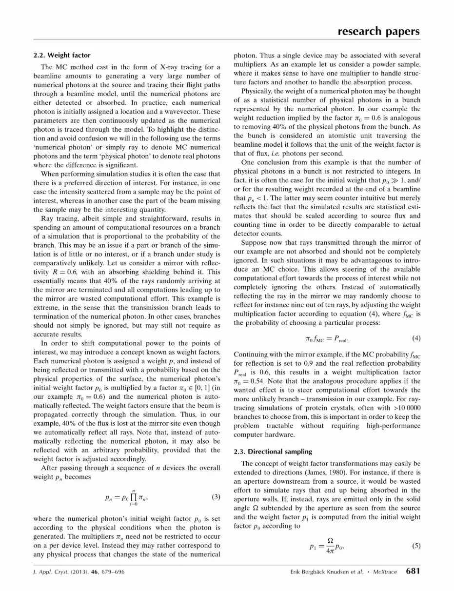
to a preceding component. As illustrated by Fig. 1, which

shows a set of crystals in a double-bounce monochromator

arrangement, an object may be rotated, thereby also changing

the location of subsequent devices placed relative to the

former object. This yields an intuitive beamline description

which follows the beam from the source to the detector. For

instance, the relative scheme makes positioning mirrors in a

KB (Kirkpatrick & Baez, 1948) configuration quite straight-

forward.

3. Running McXtrace

The general procedure for performing a McXtrace simulation

is to describe the beamline or experiment in the specific

McXtrace language. This description is contained in a file

which by convention is generally referred to as the instrument

file. We will stick to this convention for the remainder of the

paper. See the supplementary information1 for a detailed

tutorial example or the manual (Bergback Knudsen et al.,

2012b) for details on how to write the instrument file.

The McXtrace language is based on the C programming

language (Kernighan & Ritchie, 1988). In fact, the user has

access to the full programming language, should he/she wish to

extend the capabilities of McXtrace. McXtrace parses the

instrument file to run a simulation and generates a C program,

which in turn is compiled into an executable module. This

module may then be run to generate actual results. Among

others, this process has the advantage that the simulation code

research papers


Figure 1Sketch of the McXtrace positioning mechanism. By convention, the z axispoints downstream along the beam, the y axis is directed ‘up’ and the xaxis is given by the right-handed coordinate system. Components may bepositioned and/or rotated relative to any other preceding component orin absolute coordinates. In the sketch the dashed coordinate systems arethe default orientations for relative positioning. If one is rotated, such as‘Crystal 1’, subsequent relative coordinate systems rotate with it asindicated.

1 Supplementary material for this paper is available from the IUCr electronicarchives (Reference: HE5585). Services for accessing this material aredescribed at the back of the journal.

is inherently optimized, since it is compiled on the machine

where it is run and only includes the component code required

to describe the beamline at hand. We will investigate this

process in more detail in x4.

3.1. User interface

The McXtrace user interface reflects its portability oriented

design: it should be practical to run it on a remote server as

well on the user’s local desktop. Whereas a graphical user

interface (GUI) is often not desired on a remote desktop, it

comes in handy when running the code locally.

3.1.1. Graphical user interface. To address these twofold

and often conflicting requests, we provide a GUI written in an

interpreted scripting language, and utilities to simplify term-

inal-based command-line operations. Indeed, the GUI itself

uses the utility scripts to operate. We would like to emphasize

that the scripting language (at present Perl; Wall et al., 2000)

and the utilities are not required to run McXtrace. A C

compiler and a text editor are sufficient.

research papers


Figure 2Some examples of windows encountered in the McXtrace graphical user interface, as seen on a stock Ubuntu installation. (a) The main window. (b) Theincluded editor. (c) Device insertion dialogue. (d) The simulation run window.

When running the McXtrace GUI the user is presented with

the main window (shown in Fig. 2a). The GUI has a built-in

editor (shown in Fig. 2b), which helps the user generate the

instrument file. From the editor window the user may compose

the instrument file by choosing beamline devices from the

component library and choose parameters assisted by

dialogue widgets (an example is shown in Fig. 2c). Finally,

when the user is ready to trace rays through the beamline he/

she is presented with the run window (shown in Fig. 2d), where

runtime parameters such as the number of numerical photons

and the number of MPI cores to use may be specified.

3.1.2. Command-line interface. A list of commands that

McXtrace exposes to the shell is given in Table 1. The main

command mcxtrace translates an instrument file into a C

program, which may be compiled by using e.g. gcc (http://

gcc.gnu.org/). The generated executable may then be run with

a series of command-lines options. As an example a session in

a shell could look like

Most other commands are utility scripts that automate

certain common tasks. For instance, the utility mxrun checks

the time stamps of instrument files, executable files and

generated source code to control which steps are necessary for

a new run, before running the actual simulation. It also has an

interface for pointwise scanning of simulation input para-

meters etc. The second most used command is mxplot, which

shows interactive overview plots of simulation results.

Furthermore, the command mxdisplay generates the dynamic

visual ray-tracing interface where the trajectory of each

numerical photon is drawn alongside the illustrations of the

various beamline components. This is very useful, for example,

for debugging the beamline description.

4. Software structure

In this section we present a more detailed view of the structure

of McXtrace and its inner workings. At its inception McStas

(McStas, 2012), and hence McXtrace, was designed for speed

and portability. The former is achieved by parallelism

combined with selective code generation and local optimiza-

tion, the latter by keeping strictly to standards and only relying

on the presence of a C compiler for basic functionality.

4.1. Code features

The McXtrace code is structured in three different code sets

at different levels of abstraction: the instrument file, the

component library and the kernel. Their relationships are

indicated graphically in Fig. 3.

A user would mainly be concerned with the highest level of

abstraction: the instrument file. As mentioned previously, this

is a description of the beamline to be simulated, where all

devices are positioned in relation to each other, but this

description may also include additional code. One example of

this is the code to compute the positions of the individual

crystals in a double-bounce monochromator (see x5.5). From

the perspective of the instrument a beamline consists of a

research papers


Table 1The main commands that McXtrace exposes to the shell of the user’s system.

Note that, except for compilation and the McXtrace executable, these are Perl scripts that depend on the installed interpreter. The interpreter is supplied with theWindows installation executable; it is otherwise available on every major platform.

Command Action

mxgui Starts the McXtrace GUI.mcxtrace a.instr Interprets the instrument file a.instr and outputs a compliant C program in the file a.c.mxrun a.instr Performs a number of tasks:

(1) Checks whether the file a.out does not exist or is older than a.instr. If this is the case (a) runs mcxtrace ona.instr to produce a.c and (b) compiles a.c to a.out using the chosen C compiler.

(2) Runs the simulation using 106 numerical photons (the default value), and prompts the user for input values.mxrun a.instr par1 = 12 Similar to the former but sets the value of the input parameter par1 to 12 and uses the default values for all other

input parameters, i.e. it does not prompt the user for further input parameters.mxrun a.instr -N 11 par1 = 10,14 Performs an 11-point scan of the input parameter par1 from 10 to 14. This is equivalent to setting par1 to 10,

10.25, . . . manually and running simulations one by one.mxplot Produces an interactive overview plot of the monitors in the working directory.mxplot dir Generates an overview plot of data in directory dir.mxdisplay a.instr Similar to mxrun but carries out visual tracing of numerical photons using the default plotting back end (default is

PGPLOT; Pearson, 2001).mxdisplay -format = MATLAB a.instr Performs visual tracing using the MATLAB (The MathWorks Inc., Natick, MA, USA) back end (when present).

Figure 3Schematic drawing of the McXtrace code structure. The user describes theexperiment/beamline in the instrument file. The McXtrace systemgenerates a monolithic simulation code in C by collecting componentcode corresponding to the devices described in the instrument file andrelevant runtime libraries. The generated simulation code may thus beseen as the intersection of the three sets (or levels) of code.

connected set of black-box devices. These boxes may be of

many different kinds and all have different parameters.

During a simulation, each numerical photon is passed from

one device to another until it is terminated, for example

because it has been scattered beyond a beamline boundary or

absorbed by an attenuating medium. The McXtrace kernel

automatically handles the book-keeping associated with the

numerical photon passing from one object to another.

The second level of abstraction (the component library)

regards events such as numerical photons interacting with

matter, getting reflected or monitored etc. Users may adapt

existing components to their specific needs. Each component

is an independent entity which ‘knows’ nothing about other

components. Colloquially speaking, a component takes up a

numerical photon, modifies its state according to the compo-

nent model and releases the numerical photon. This concept

ensures the modularity of the system and keeps the compo-

nent-related code small and simple. As a result a component

typically contains �300 lines of code including in-line docu-

mentation.

The kernel, the third and lowest level, is invisible when

using McXtrace and, to a large extent, when writing compo-

nents. Suffice it to say that it contains a runtime library of

functions which, among other things, handle the propagation

of numerical photons between components, the orientation of

components relative to each other, random numbers, input/

output (I/O) and mathematical operations.

For a particular simulation McXtrace generates C code

corresponding to the intersection of the three code sets.

4.2. Inner workings

When a user runs McXtrace several things happen:

(1) The instrument file is analysed and a monolithic C code

is assembled containing the component code corresponding to

the devices found in the beamline description, the runtime

libraries and the necessary ‘glue’ to manage the name spaces

of the independent components, I/O directives, process split-

ting mechanisms across multiple processors and so on. Only

the code relevant to the beamline is included and hence,

although it is a single block of C code in one file, it is

comparatively small. As an example the full simulation code

of the Max IV Laboratory 711 beamline presented in x5.4

contains �16 000 lines of code, of which >4000 are macro

definitions that will be removed by the C preprocessor.

(2) The generated C code is compiled by a stock C compiler.

No external libraries need to be included.

(3) The compiled executable is run on the target system

specifying runtime settings for the simulation. Such settings

include the number of numerical photons to trace through the

beamline and any other user-defined parameters. The

numerical photon states at the sites of the monitors included

in the beamline are recorded as appropriate and saved into

files. These data files may now be processed and analysed

almost as if they were recorded on a real-world beamline, the

simple difference being that count times in a simulation and at

a real beamline are completely uncorrelated. In addition,

simulations yield counts that may be non-integer.

Firstly, as each numerical photon is independent of the

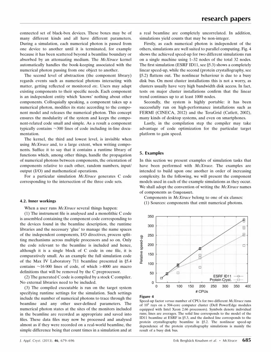
others, simulations are well suited to parallel computing. Fig. 4

shows the achieved speed-up for two different simulations run

on a single machine using 1–32 nodes of the total 32 nodes.

The first simulation (ESRF ID11, see x5.3) shows a completely

linear speed-up, while the second (protein crystallography, see

x5.2) flattens out. The nonlinear behaviour is due to a busy

disk bus. On most cluster installations this is not a worry, as

clusters usually have very high bandwidth disk access. In fact,

tests on major cluster installations confirm that the linear

trend continues up to at least 1000 nodes.

Secondly, the system is highly portable: it has been

successfully run on high-performance installations such as

FERMI (CINECA, 2012) and the TeraGrid (Catlett, 2002),

many kinds of desktop systems, and even on smartphones.

Lastly, in the compilation step the compiler may take

advantage of code optimization for the particular target

platform to gain speed.

5. Examples

In this section we present examples of simulation tasks that

have been performed with McXtrace. The examples are

intended to build upon one another in order of increasing

complexity. In the following, we will present the component

models used in each of the example simulations as they occur.

We shall adopt the convention of writing the McXtrace names

of components as Component.

Components in McXtrace belong to one of six classes:

(1) Sources: components that emit numerical photons.

research papers


Figure 4Speed-up factor versus number of CPUs for two different McXtrace runsof 109 rays on a 504-core computer cluster (Dell PowerEdge modulesequipped with Intel Xeon 2.66 processors). Symbols denote individualruns; lines are averages. The solid line corresponds to the model of theID11 beamline at ESRF in x5.3, and the dashed line corresponds to theprotein crystallography beamline in x5.2. The nonlinear speed-updependence of the protein crystallography simulations is mainly theresult of a busy disk bus.

(2) Monitors: components that detect the numerical photon

state parameters or a subset or function thereof under various

conditions. Most monitors behave like ideal probes, in that

they register the photon state without influencing it, but are

nonetheless used for modelling detectors. Components

modelling physical detectors including effects such as non-

uniform efficiency also belong to this category.

(3) Optics: optical components that influence the numerical

photon state: lenses, mirrors, apertures etc.

(4) Samples: optically active objects, generally used as

samples. Note that these components may also be used as

more general material models, for example, using the

McXtrace powder diffraction component PowderN to simulate

background contributions from other objects in the beamline.

(5) Contrib: components that have been contributed by the

user community. Although these components are not actively

supported by the McXtrace team, they have been tested.

(6) Misc: simulation-specific components which have no

physical counterparts, e.g. the simulation status tracker called

Progress_bar.

The above classification has no technical significance. It

merely exists to help users find their way in the component

catalogue.

5.1. Tomography

This example is motivated by the need to correct for beam-

hardening effects when performing tomographic studies of

insulin injections in biological tissue in order to estimate the

spatial concentration distribution of insulin inside the tissue.

The ‘real’ situation we attempt to simulate is shown schema-

tically in Fig. 5. For simplicity and clarity we restrict ourselves

to phantom samples in our simulations, and refer to a forth-

coming paper for details (Thomsen et al., 2013).

5.1.1. Point source and laboratory source. In McXtrace an

X-ray tube may be modelled using the source component

Source_pt, which represents a mathematical point source

emitting numerical photons in 4� steradians. To avoid tracing

rays that will inevitably be discarded later on, we employ

directional sampling (x2.3) and only emit numerical photons

that will pass through a rectangle of xwidth � yheight m posi-

tioned dist metres further downstream. The weight factor of

each numerical photon is adjusted accordingly (x2.2). The

source model may be supplied with a measured spectrum. The

input spectrum should be normalized to represent the emitted

raw flux uninhibited by apertures, filters etc. Examples of

spectra measured from an X-ray tube with a molybdenum

anode can be seen in Fig. 6.

If measured spectra are not available, the component

Source_lab may be used instead, where theoretical approx-

imations (Kramers, 1923; Honkimaki et al., 1990) and tabu-

lated values (Bearden, 1967; Krause & Oliver, 1979) are used

to generate spectral flux distributions from which rays can be

sampled. Rays are generated from a slab of the anode target

material. A rectangular area in the slab is illuminated by an

electron beam, and the underlying volume acts as a starting

point for emitted rays. The weight factor of the ray is corrected

for the length of the anode target material traversed on the

way to the exit window of the source. Spectra generated with

Source_lab may be found in Fig. 6. We find a reasonable

qualitative agreement between simulated and measured

spectra, apart from a scaling factor. Taking the scaling factor

into account, integrated absolute intensities (both character-

istic radiation and Bremsstrahlung) agree to within 10 and

30%. Simulated spectra consistently show narrower line

widths and overestimate absorption in the target at low

energies.

The source model has a few noteworthy limitations. Firstly,

absorption in the exit window, for example, a Be window, is

not included, nor is absorption in the air traversed from anode

to exit window. Secondly, the line widths of the characteristic

radiation are the natural widths of the excitation spectrum

from free atoms. Several effects contribute to broadening of

radiation peaks, such as multiplet splitting and chemical

bonding (Krause & Oliver, 1979).

research papers


Figure 6Measured and simulated (via the Source_lab component) spectral fluxversus X-ray energy for an Mo rotating-anode source hit by electronssubmitted to the acceleration from voltages of 40 kV (measured: bluecircles; simulated: red down triangles) and 80 kV (measured: black uptriangles; simulated: magenta diamonds). The 80 kV curves have beendisplaced by 0.5 along the y axis for the sake of clarity. The peaks in thespectrum correspond to K�1;2 and K� as K�1 and K�2 are not resolved.

Figure 5Sketch of a laboratory tomography setup, mimicking one at TechnischeUniversitat Munchen. A sample is mounted on a rotation stage; otherwisethe beamline consists of a succession of filters. A discrete air filter isincluded to correct for nonzero absorption effects in air, where the airdensity has been increased by a factor of ten to reproduce more realisticbeamline conditions.

In addition we only have limited knowledge of the rotating-

anode source parameters. This is in conjunction with the

model limitations, which may explain the differences between

measured and simulated flux; work is ongoing to close the gap

between experimental and simulated spectral characteristics.

5.1.2. Slits and apertures. Although rays are only emitted

toward the sampling window, it may be important to include

an aperture that models the aperture present in the laboratory

machine. Apertures are simulated using the Slit component.

This may take the form of either a rectangular or a circular

aperture of any size. It consists of a hole in an infinitely thin

slab of perfectly absorbing material, i.e. any ray with a

trajectory towards the aperture is allowed through unaffected,

whereas all other rays are absorbed. To include effects such as

slit scattering and non-ideal slit absorption, the individual slit

blades may be modelled as individual PowderN or Single_

crystal components, whichever is more appropriate. See

xx5.4 and 5.2 for more details on these components.

5.1.3. Filters. In a laboratory there are often a certain

number of optional filters that may be put into the beam to

absorb long-wavelength photons. In McXtrace the filters are

rectangular blocks of material that decrement the numerical

photon weight by exp½��ð�Þ dl �, where dl is the distance

travelled through the filter block along the ray trajectory. The

attenuation coefficient �ð�Þ is computed by interpolating

between tabulated values (Chantler, 1995, 2000).

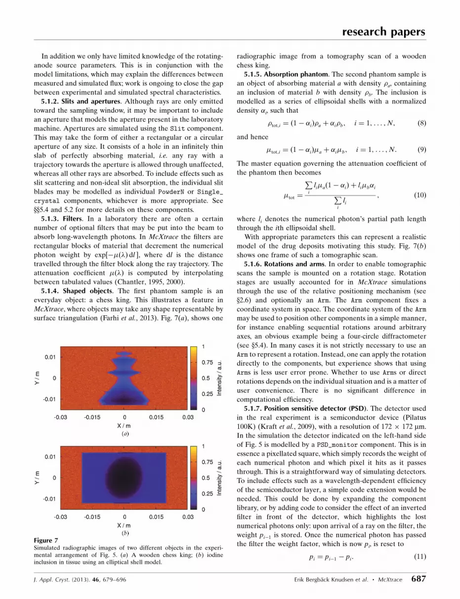
5.1.4. Shaped objects. The first phantom sample is an

everyday object: a chess king. This illustrates a feature in

McXtrace, where objects may take any shape representable by

surface triangulation (Farhi et al., 2013). Fig. 7(a), shows one

radiographic image from a tomography scan of a wooden

chess king.

5.1.5. Absorption phantom. The second phantom sample is

an object of absorbing material a with density �a, containing

an inclusion of material b with density �b. The inclusion is

modelled as a series of ellipsoidal shells with a normalized

density �i, such that

�tot;i ¼ 1� �ið Þ�a þ �i�b; i ¼ 1; . . . ;N; ð8Þ

and hence

�tot;i ¼ 1� �ið Þ�a þ �i�b; i ¼ 1; . . . ;N: ð9Þ

The master equation governing the attenuation coefficient of

the phantom then becomes

�tot ¼

Pi

li�að1� �iÞ þ li�b�iPi

li

; ð10Þ

where li denotes the numerical photon’s partial path length

through the ith ellipsoidal shell.

With appropriate parameters this can represent a realistic

model of the drug deposits motivating this study. Fig. 7(b)

shows one frame of such a tomographic scan.

5.1.6. Rotations and arms. In order to enable tomographic

scans the sample is mounted on a rotation stage. Rotation

stages are usually accounted for in McXtrace simulations

through the use of the relative positioning mechanism (see

x2.6) and optionally an Arm. The Arm component fixes a

coordinate system in space. The coordinate system of the Arm

may be used to position other components in a simple manner,

for instance enabling sequential rotations around arbitrary

axes, an obvious example being a four-circle diffractometer

(see x5.4). In many cases it is not strictly necessary to use an

Arm to represent a rotation. Instead, one can apply the rotation

directly to the components, but experience shows that using

Arms is less user error prone. Whether to use Arms or direct

rotations depends on the individual situation and is a matter of

user convenience. There is no significant difference in

computational efficiency.

5.1.7. Position sensitive detector (PSD). The detector used

in the real experiment is a semiconductor device (Pilatus

100K) (Kraft et al., 2009), with a resolution of 172 � 172 mm.

In the simulation the detector indicated on the left-hand side

of Fig. 5 is modelled by a PSD_monitor component. This is in

essence a pixellated square, which simply records the weight of

each numerical photon and which pixel it hits as it passes

through. This is a straightforward way of simulating detectors.

To include effects such as a wavelength-dependent efficiency

of the semiconductor layer, a simple code extension would be

needed. This could be done by expanding the component

library, or by adding code to consider the effect of an inverted

filter in front of the detector, which highlights the lost

numerical photons only: upon arrival of a ray on the filter, the

weight pi�1 is stored. Once the numerical photon has passed

the filter the weight factor, which is now pi, is reset to

pi ¼ pi�1 � pi: ð11Þ

research papers


Figure 7Simulated radiographic images of two different objects in the experi-mental arrangement of Fig. 5. (a) A wooden chess king; (b) iodineinclusion in tissue using an elliptical shell model.

This is to exemplify the versatility of the system, where the

effect of components may easily be altered using a few simple

additions. The related code may be found in Listing 1,

Appendix A. In this way, the thickness of the scintillation layer

seen by a numerical photon automatically becomes dependent

on the angle of incidence, as does the apparent pixel size. On

the other hand, the numerical photon will be registered at its

position after traversing the scintillation layer. To allow

intensity to be deposited in more than one pixel along the

trajectory of the numerical photon requires extension to the

monitor model.

5.2. Protein crystallography

In the following we sketch how to build a model of a generic

beamline designed for protein crystallography measurements.

The setup of this kind of beamline tends to be conceptually

simple and its automated operation is typically very advanced.

A generic model is hence quite simple and illustrative of the

way of building functional blocks within the McXtrace

framework. Let us, however, bear in mind that in order to

perform virtual experiments (VE), as defined by Lefmann et

al. (2008), a more sophisticated beamline model with a closer

match to reality is necessary.

In our case study the beamline consists of a photon source, a

sample and a movable PSD, both mounted on rotation stages.

In the McXtrace system these are represented by the

components Source_gaussian, Single_crystal and PSD_

monitor, respectively. Furthermore, the rotation stages on

which sample and detector are mounted to form a four-circle

diffractometer are configured using several instances of the

Arm component.

5.2.1. Gaussian cross section source. The Gaussian source

component (Source_gaussian) emits photons from a two-

dimensional Gaussian distribution on a plane surface

perpendicular to the beam direction. Numerical photons are

emitted with a given uniform divergence profile. This is a good

and effective model when a beamline is fed by a synchrotron

source. Moreover, the numerical photons emitted may be

taken from an arbitrary energy spectrum. The spatial distri-

bution of numerical photons is assumed to be independent of

the wavelength distribution. This approximation is valid only

when considering photons in a narrow wavelength band. For

other types of experiments, where a wider bandwidth is

required, a more sophisticated approach is warranted.

5.2.2. Single crystal. The Single_crystal component is by

far the largest component in the package in terms of lines of

code. The module simulates the diffraction pattern from a

single crystal where the line broadening is dominated by

crystal mosaicity, i.e. the crystal is ideally imperfect. The

Single_crystal component needs as input a list of reflections

and their corresponding crystallographic structure factors, F ,

the crystal orientation, absorption cross sections etc. For an

example of an input file please see the supplementary mate-

rial.

Briefly, when a numerical photon arrives on the crystal, the

reflection list is analysed using the Ewald sphere concept to

find which reflections, if any, are possible at that photon

energy and at the given crystal mosaicity. The coherent elastic

scattering cross section in the crystal is governed by the master

equation

�coh;s ¼

ZEwald

Nð2�Þ3

V0

Gðs� jÞjFj2 d�: ð12Þ

Here j is the scattering vector, s the lattice vector, V0 the unit-

cell volume and F the crystallographic structure factor asso-

ciated with the lattice vector. Integration is performed over

the Ewald sphere. G denotes a three-dimensional Gaussian

function modelling crystal mosaicity as

GðyÞ ¼1

ð2�Þ3=2

1

�1�2�3

expf�½Uðyþ sÞ�TD½Uðyþ sÞ�g; ð13Þ

where U ¼ ðu1; u2; u3Þ is a 3� 3 matrix forming a basis for the

three-dimensional Gaussian function. By convention, �1 is

parallel to s and is proportional to the standard deviation in

relative lattice spacing. �2, �3 are perpendicular to s and hence

proportional to the standard deviation in crystal orientation.

This model implies that the spherical caps generated by

rotations of the reciprocal lattice vectors are approximated by

research papers


Figure 8Top and skew view of a Laue diffraction camera with square areadetectors (black and gray squares) set around a sample to approximate asingle spherical detector. The recorded diffraction signal from a crystal ofan l-leucine ligand is only shown on some of the screens to avoidcluttering. The bottom-left orange ellipsoid indicates the location of thesource model, the central gray cube indicates the l-leucine crystal, blacksquares indicate area detectors on the front end of the sphere and graysquares detectors on the back end of the sphere. Red lines indicate a fewscattered X-rays. The arrangement is set up in McXtrace using a set ofArms to place the area detectors. This way we may use simulations togenerate virtual data, as close to a real detector arrangement as possible.

planar circles. In principle this approximation is valid when

�1 6� �2;3.

The total interaction cross section consisting of absorption,

coherent scattering and incoherent scattering yields a relative

scattering probability. If scattering is selected by an MC

choice, then one of the possible reflections is chosen randomly

and a scattering direction is computed using the crystal

mosaicity as an uncertainty parameter. The scattered numer-

ical photon, which now has an altered wavevector, is rein-

jected into the scattering algorithm to allow multiple

scattering events. For more details see the component manual

(Bergback Knudsen et al., 2012a).

The beamline is completed by putting a number of area

detectors (PSDs) around the sample which record the

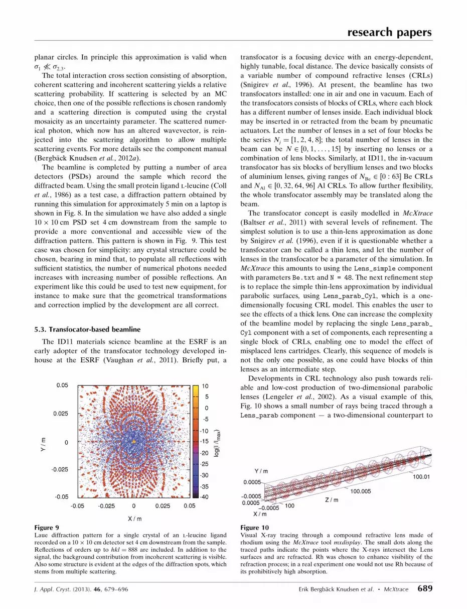
diffracted beam. Using the small protein ligand l-leucine (Coll

et al., 1986) as a test case, a diffraction pattern obtained by

running this simulation for approximately 5 min on a laptop is

shown in Fig. 8. In the simulation we have also added a single

10� 10 cm PSD set 4 cm downstream from the sample to

provide a more conventional and accessible view of the

diffraction pattern. This pattern is shown in Fig. 9. This test

case was chosen for simplicity: any crystal structure could be

chosen, bearing in mind that, to populate all reflections with

sufficient statistics, the number of numerical photons needed

increases with increasing number of possible reflections. An

experiment like this could be used to test new equipment, for

instance to make sure that the geometrical transformations

and correction implied by the development are all correct.

5.3. Transfocator-based beamline

The ID11 materials science beamline at the ESRF is an

early adopter of the transfocator technology developed in-

house at the ESRF (Vaughan et al., 2011). Briefly put, a

transfocator is a focusing device with an energy-dependent,

highly tunable, focal distance. The device basically consists of

a variable number of compound refractive lenses (CRLs)

(Snigirev et al., 1996). At present, the beamline has two

transfocators installed: one in air and one in vacuum. Each of

the transfocators consists of blocks of CRLs, where each block

has a different number of lenses inside. Each individual block

may be inserted in or retracted from the beam by pneumatic

actuators. Let the number of lenses in a set of four blocks be

the series Nj ¼ ½1; 2; 4; 8�; the total number of lenses in the

beam can be N 2 ½0; 1; . . . ; 15� by inserting no lenses or a

combination of lens blocks. Similarly, at ID11, the in-vacuum

transfocator has six blocks of beryllium lenses and two blocks

of aluminium lenses, giving ranges of NBe 2 ½0 : 63� Be CRLs

and NAl 2 ½0; 32; 64; 96� Al CRLs. To allow further flexibility,

the whole transfocator assembly may be translated along the

beam.

The transfocator concept is easily modelled in McXtrace

(Baltser et al., 2011) with several levels of refinement. The

simplest solution is to use a thin-lens approximation as done

by Snigirev et al. (1996), even if it is questionable whether a

transfocator can be called a thin lens, and let the number of

lenses in the transfocator be a parameter of the simulation. In

McXtrace this amounts to using the Lens_simple component

with parameters Be.txt and N = 48. The next refinement step

is to replace the simple thin-lens approximation by individual

parabolic surfaces, using Lens_parab_Cyl, which is a one-

dimensionally focusing CRL model. This enables the user to

see the effects of a thick lens. One can increase the complexity

of the beamline model by replacing the single Lens_parab_

Cyl component with a set of components, each representing a

single block of CRLs, enabling one to model the effect of

misplaced lens cartridges. Clearly, this sequence of models is

not the only one possible, as one could have blocks of thin

lenses as an intermediate step.

Developments in CRL technology also push towards reli-

able and low-cost production of two-dimensional parabolic

lenses (Lengeler et al., 2002). As a visual example of this,

Fig. 10 shows a small number of rays being traced through a

Lens_parab component — a two-dimensional counterpart to

research papers


Figure 9Laue diffraction pattern for a single crystal of an l-leucine ligandrecorded on a 10� 10 cm detector set 4 cm downstream from the sample.Reflections of orders up to hkl ¼ 888 are included. In addition to thesignal, the background contribution from incoherent scattering is visible.Also some structure is evident at the edges of the diffraction spots, whichstems from multiple scattering.

Figure 10Visual X-ray tracing through a compound refractive lens made ofrhodium using the McXtrace tool mxdisplay. The small dots along thetraced paths indicate the points where the X-rays intersect the Lenssurfaces and are refracted. Rh was chosen to enhance visibility of therefraction process; in a real experiment one would not use Rh because ofits prohibitively high absorption.

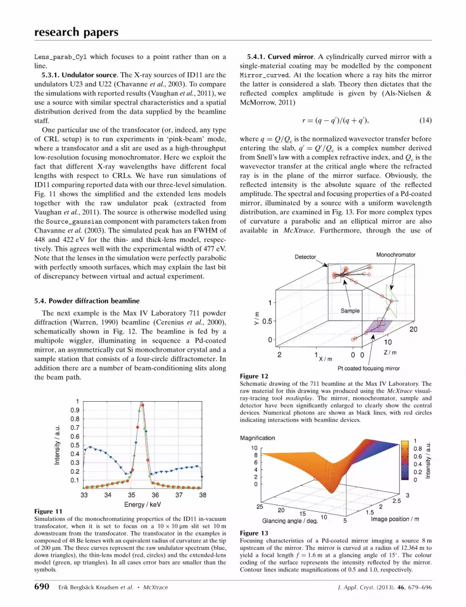
Lens_parab_Cyl which focuses to a point rather than on a

line.

5.3.1. Undulator source. The X-ray sources of ID11 are the

undulators U23 and U22 (Chavanne et al., 2003). To compare

the simulations with reported results (Vaughan et al., 2011), we

use a source with similar spectral characteristics and a spatial

distribution derived from the data supplied by the beamline

staff.

One particular use of the transfocator (or, indeed, any type

of CRL setup) is to run experiments in ‘pink-beam’ mode,

where a transfocator and a slit are used as a high-throughput

low-resolution focusing monochromator. Here we exploit the

fact that different X-ray wavelengths have different focal

lengths with respect to CRLs. We have run simulations of

ID11 comparing reported data with our three-level simulation.

Fig. 11 shows the simplified and the extended lens models

together with the raw undulator peak (extracted from

Vaughan et al., 2011). The source is otherwise modelled using

the Source_gaussian component with parameters taken from

Chavanne et al. (2003). The simulated peak has an FWHM of

448 and 422 eV for the thin- and thick-lens model, respec-

tively. This agrees well with the experimental width of 477 eV.

Note that the lenses in the simulation were perfectly parabolic

with perfectly smooth surfaces, which may explain the last bit

of discrepancy between virtual and actual experiment.

5.4. Powder diffraction beamline

The next example is the Max IV Laboratory 711 powder

diffraction (Warren, 1990) beamline (Cerenius et al., 2000),

schematically shown in Fig. 12. The beamline is fed by a

multipole wiggler, illuminating in sequence a Pd-coated

mirror, an asymmetrically cut Si monochromator crystal and a

sample station that consists of a four-circle diffractometer. In

addition there are a number of beam-conditioning slits along

the beam path.

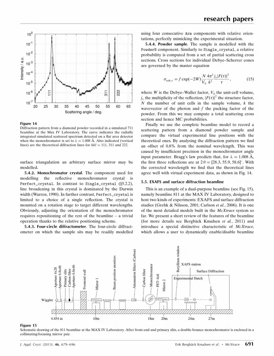
5.4.1. Curved mirror. A cylindrically curved mirror with a

single-material coating may be modelled by the component

Mirror_curved. At the location where a ray hits the mirror

the latter is considered a slab. Theory then dictates that the

reflected complex amplitude is given by (Als-Nielsen &

McMorrow, 2011)

r ¼ ðq� q0Þ=ðqþ q0Þ; ð14Þ

where q ¼ Q=Qc is the normalized wavevector transfer before

entering the slab, q0 ¼ Q0=Qc is a complex number derived

from Snell’s law with a complex refractive index, and Qc is the

wavevector transfer at the critical angle where the refracted

ray is in the plane of the mirror surface. Obviously, the

reflected intensity is the absolute square of the reflected

amplitude. The spectral and focusing properties of a Pd-coated

mirror, illuminated by a source with a uniform wavelength

distribution, are examined in Fig. 13. For more complex types

of curvature a parabolic and an elliptical mirror are also

available in McXtrace. Furthermore, through the use of

research papers


Figure 12Schematic drawing of the 711 beamline at the Max IV Laboratory. Theraw material for this drawing was produced using the McXtrace visual-ray-tracing tool mxdisplay. The mirror, monochromator, sample anddetector have been significantly enlarged to clearly show the centraldevices. Numerical photons are shown as black lines, with red circlesindicating interactions with beamline devices.

Figure 11Simulations of the monochromatizing properties of the ID11 in-vacuumtransfocator, when it is set to focus on a 10� 10 mm slit set 10 mdownstream from the transfocator. The transfocator in the examples iscomposed of 48 Be lenses with an equivalent radius of curvature at the tipof 200 mm. The three curves represent the raw undulator spectrum (blue,down triangles), the thin-lens model (red, circles) and the extended-lensmodel (green, up triangles). In all cases error bars are smaller than thesymbols.

Figure 13Focusing characteristics of a Pd-coated mirror imaging a source 8 mupstream of the mirror. The mirror is curved at a radius of 12.364 m toyield a focal length f ¼ 1:6 m at a glancing angle of 15. The colourcoding of the surface represents the intensity reflected by the mirror.Contour lines indicate magnifications of 0.5 and 1.0, respectively.

surface triangulation an arbitrary surface mirror may be

modelled.

5.4.2. Monochromator crystal. The component used for

modelling the reflective monochromator crystal is

Perfect_crystal. In contrast to Single_crystal (x5.2.2),

line broadening in this crystal is dominated by the Darwin

width (Warren, 1990). In further contrast, Perfect_crystal is

limited to a choice of a single reflection. The crystal is

mounted on a rotation stage to target different wavelengths.

Obviously, adjusting the orientation of the monochromator

requires repositioning of the rest of the beamline – a trivial

operation thanks to the relative positioning scheme.

5.4.3. Four-circle diffractometer. The four-circle diffract-

ometer on which the sample sits may be readily modelled

using four consecutive Arm components with relative orien-

tations, perfectly mimicking the experimental situation.

5.4.4. Powder sample. The sample is modelled with the

PowderN component. Similarly to Single_crystal, a relative

probability is computed from a set of partial scattering cross

sections. Cross sections for individual Debye–Scherrer cones

are governed by the master equation

�coh; ¼ f expð�2WÞN

V0

4�3

k2

jjFðÞj2

; ð15Þ

where W is the Debye–Waller factor, V0 the unit-cell volume,

j the multiplicity of the reflection, jFðÞj2 the structure factor,

N the number of unit cells in the sample volume, k the

wavevector of the photon and f the packing factor of the

powder. From this we may compute a total scattering cross

section and hence MC probabilities.

Finally we use the complete beamline model to record a

scattering pattern from a diamond powder sample and

compare the virtual experimental line positions with the

theoretical ones. By analysing the diffraction pattern we find

an offset of 0.8% from the nominal wavelength. This was

caused by insufficient precision in the monochromator angle

input parameter. Bragg’s law predicts that, for � ¼ 1:008 A,

the first three reflections are at 2 ¼ ½28:3; 55:9; 58:6�. With

the corrected wavelength we find that the theoretical lines

agree well with virtual experiment data, as shown in Fig. 14.

5.5. EXAFS and surface diffraction beamline

This is an example of a dual-purpose beamline (see Fig. 15),

namely beamline 811 at the MAX IV Laboratory, designed to

host two kinds of experiments: EXAFS and surface diffraction

studies (Grehk & Nilsson, 2001; Carlson et al., 2006). It is one

of the most detailed models built in the McXtrace system so

far. We present a short review of the features of the beamline

(for more details see Bergback Knudsen et al., 2011) and

introduce a special distinctive characteristic of McXtrace,

which allows a user to dynamically enable/disable beamline

research papers


Figure 14Diffraction pattern from a diamond powder recorded in a simulated 711beamline at the Max IV Laboratory. The curve indicates the radiallyintegrated simulated scattered spectrum detected on a flat area detectorwhen the monochromator is set to � ¼ 1:008 A. Also indicated (verticallines) are the theoretical diffraction lines for hkl ¼ 111, 311 and 222.

Figure 15Schematic drawing of the 811 beamline at the MAX IV Laboratory. After front-end and primary slits, a double-bounce monochromator is enclosed in acollimating/focusing mirror pair.

devices. The central part of the beamline includes a colli-

mating/focusing mirror pair surrounding a double-bounce Si

monochromator (see for instance Shvyd’ko, 2004). The role of

the collimating mirror is to diffuse the heat load on the first

monochromator crystal. As the curvatures of the mirrors are

independent, the second mirror can counteract the first and

focus on either of the two sample stations. Positioning of

mirrors and crystals may appear complicated in an absolute

frame, but bearing in mind that in McXtrace the default

positioning scheme refers to the previous element, modelling a

setup like this becomes quite straightforward.

The mirrors may be removed for some applications, in

which case the monochromator crystals should be moved and

a set of attenuating C filters may be inserted, instead, to avoid

heat load issues. Rather than having separate beamline

descriptions for the two versions, features like this may be

modelled dynamically in McXtrace using the WHEN keyword

(see Listing 3, Appendix A).

5.5.1. Double-bounce monochromator. Similarly to x5.4,

the Perfect_crystal component may be used for modelling

a double-bounce monochromator. The two crystals are set on

a common rotation axis with an additional translation for the

second crystal (Grehk & Nilsson, 2001). In reality, the beam-

line control system computes the rotation angles and positions

of the two crystals given an operating wavelength. Following

the methodology of VE (Lefmann et al., 2008) in McXtrace,

automatic positioning of the crystals may be implemented in

the INITIALIZE section of the instrument file, as shown in

Listing 2, Appendix A. Fig. 16 shows the spectral character-

istics of the beamline at the source, after the front-end filters

and after the monochromator.

5.6. Time-resolved studies

When tracing X-rays through a beamline model, McXtrace

also keeps track of the flight time of the numerical photons. As

a consequence, it is also possible to model time-resolved

studies, such as pump-and-probe experiments. To illustrate

this, we have set up a model experiment using an ideal

chopper and a sample component Molecule_2state. This

component models a molecule in solution that can be in either

of two states. In either of the two states the resulting scattering

cross section is given by the master equation (Debye, 1915)

�� ¼ �r0

XN

j¼1

f0;jð�Þ�� 2þ2

XN

k¼jþ1

sin � rk � rj

�� rk � rj

�� f0;j f0;k

" #; ð16Þ

where f0;j is the atomic form factor for the jth atom in the

molecule, rj is the position vector of the jth atom (similarly for

rk), r0 is the Thomson scattering length and � is the wavevector

transfer.

Now, let one state be the excited state and the other the

ground state, and let the probability of finding a molecule in

the excited state be

P ¼� exp �ðt � t0Þ=trelax

� �; t t0;

0; t< t0;

�ð17Þ

where � is an excitation fraction (typically around 20%), t the

arrival time of the X-ray numerical photon on the sample, t0

the time at which the sample is excited by some external

means and trelax the relaxation time of the sample. This models

a generic pump-and-probe experiment where a sample is

excited by, for example, a laser pulse and later probed by a

pulsed X-ray beam. Following Haldrup et al. (2012), let the

sample be a solution of tris(2,20-bipyridine)iron (shown in

Fig. 17) with a relaxation time of trelax ¼ 600 ps, excite it by a

laser pulse of 2 s duration at t0 ¼ 0, and probe it by 100 ps

X-ray pulses at txray ¼ �2 ns and 100 ps. A negative txray < 0

means the X-ray pulse arrives before the laser pulse, which

guarantees that the sample is in its relaxed state. The scattered

simulated intensity recorded on a banana-shaped detector is

shown in Fig. 18. Generally it is of interest to study the

research papers


Figure 16Spectral characteristics of the simulated beamline 811 at the MAX IVLaboratory. The curves refer to the raw wiggler spectrum (red), thespectrum after front-end apertures and filters (magenta), and thespectrum after the double-bounce monochromator (blue). The insetshows a blow-up of the monochromated spectrum.

Figure 17Fe(2,20-bipyridine)3 molecule. Such molecules in solution are used forscattering in x5.6. The colours denote the kind of atom in the complex(red: iron; blue: nitrogen; gray: carbon). For the sake of clarity, H atomshave been excluded. When the molecule is optically excited the N—Febond length increases.

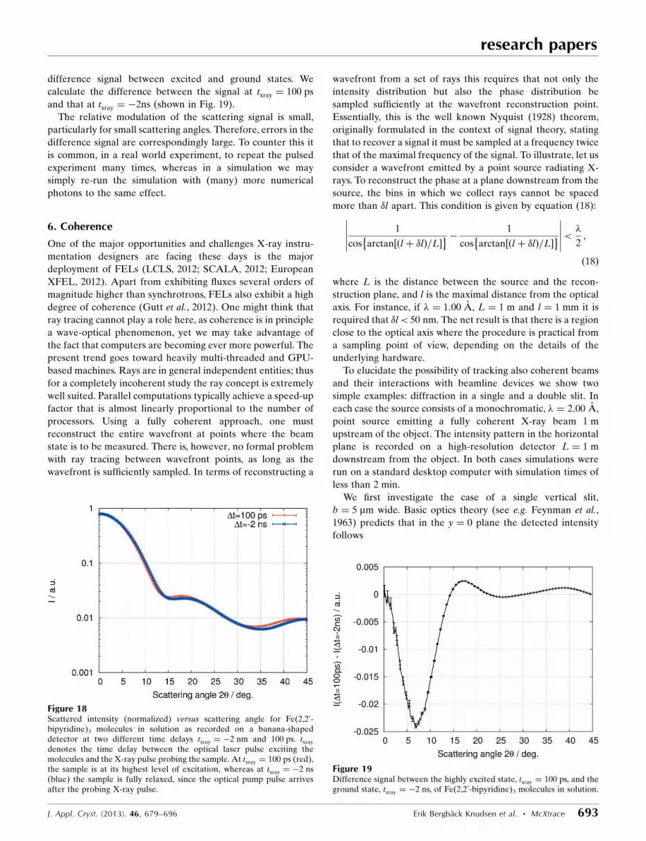
difference signal between excited and ground states. We

calculate the difference between the signal at txray ¼ 100 ps

and that at txray ¼ �2ns (shown in Fig. 19).

The relative modulation of the scattering signal is small,

particularly for small scattering angles. Therefore, errors in the

difference signal are correspondingly large. To counter this it

is common, in a real world experiment, to repeat the pulsed

experiment many times, whereas in a simulation we may

simply re-run the simulation with (many) more numerical

photons to the same effect.

6. Coherence

One of the major opportunities and challenges X-ray instru-

mentation designers are facing these days is the major

deployment of FELs (LCLS, 2012; SCALA, 2012; European

XFEL, 2012). Apart from exhibiting fluxes several orders of

magnitude higher than synchrotrons, FELs also exhibit a high

degree of coherence (Gutt et al., 2012). One might think that

ray tracing cannot play a role here, as coherence is in principle

a wave-optical phenomenon, yet we may take advantage of

the fact that computers are becoming ever more powerful. The

present trend goes toward heavily multi-threaded and GPU-

based machines. Rays are in general independent entities; thus

for a completely incoherent study the ray concept is extremely

well suited. Parallel computations typically achieve a speed-up

factor that is almost linearly proportional to the number of

processors. Using a fully coherent approach, one must

reconstruct the entire wavefront at points where the beam

state is to be measured. There is, however, no formal problem

with ray tracing between wavefront points, as long as the

wavefront is sufficiently sampled. In terms of reconstructing a

wavefront from a set of rays this requires that not only the

intensity distribution but also the phase distribution be

sampled sufficiently at the wavefront reconstruction point.

Essentially, this is the well known Nyquist (1928) theorem,

originally formulated in the context of signal theory, stating

that to recover a signal it must be sampled at a frequency twice

that of the maximal frequency of the signal. To illustrate, let us

consider a wavefront emitted by a point source radiating X-

rays. To reconstruct the phase at a plane downstream from the

source, the bins in which we collect rays cannot be spaced

more than l apart. This condition is given by equation (18):

1

cos arctan ðl þ lÞ=L½ �� 1

cos arctan ðl þ lÞ=L½ ��

��< �

2;

ð18Þ

where L is the distance between the source and the recon-

struction plane, and l is the maximal distance from the optical

axis. For instance, if � ¼ 1:00 A, L ¼ 1 m and l ¼ 1 mm it is

required that l< 50 nm. The net result is that there is a region

close to the optical axis where the procedure is practical from

a sampling point of view, depending on the details of the

underlying hardware.

To elucidate the possibility of tracking also coherent beams

and their interactions with beamline devices we show two

simple examples: diffraction in a single and a double slit. In

each case the source consists of a monochromatic, � ¼ 2:00 A,

point source emitting a fully coherent X-ray beam 1 m

upstream of the object. The intensity pattern in the horizontal

plane is recorded on a high-resolution detector L ¼ 1 m

downstream from the object. In both cases simulations were

run on a standard desktop computer with simulation times of

less than 2 min.

We first investigate the case of a single vertical slit,

b ¼ 5 mm wide. Basic optics theory (see e.g. Feynman et al.,

1963) predicts that in the y ¼ 0 plane the detected intensity

follows

research papers


Figure 18Scattered intensity (normalized) versus scattering angle for Fe(2,20-bipyridine)3 molecules in solution as recorded on a banana-shapeddetector at two different time delays txray ¼ �2 nm and 100 ps. txray

denotes the time delay between the optical laser pulse exciting themolecules and the X-ray pulse probing the sample. At txray ¼ 100 ps (red),the sample is at its highest level of excitation, whereas at txray ¼ �2 ns(blue) the sample is fully relaxed, since the optical pump pulse arrivesafter the probing X-ray pulse.

Figure 19Difference signal between the highly excited state, txray ¼ 100 ps, and theground state, txray ¼ �2 ns, of Fe(2,20-bipyridine)3 molecules in solution.

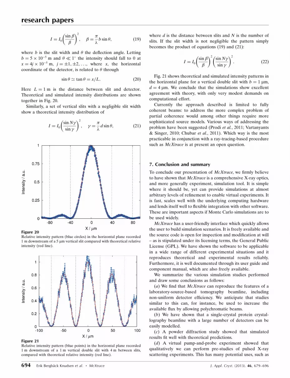
I ¼ I0

sin �

�

�2

; � ¼�

�b sin ; ð19Þ

where b is the slit width and the deflection angle. Letting

b ¼ 5� 10�5 m and � 1 the intensity should fall to 0 at

x ¼ 4j� 10�5 m, j ¼ �1;�2; . . ., where x, the horizontal

coordinate of the detector, is related to through

sin ’ tan ¼ x=L: ð20Þ

Here L ¼ 1 m is the distance between slit and detector.

Theoretical and simulated intensity distributions are shown

together in Fig. 20.

Similarly, a set of vertical slits with a negligible slit width

show a theoretical intensity distribution of

I ¼ I0

sin N�

sin �

�2

; � ¼�

�d sin ; ð21Þ

where d is the distance between slits and N is the number of

slits. If the slit width is not negligible the pattern simply

becomes the product of equations (19) and (21):

I ¼ I0

sin �

�

�2sin N�

sin �

�2

: ð22Þ

Fig. 21 shows theoretical and simulated intensity patterns in

the horizontal plane for a vertical double slit with b ¼ 1 mm,

d ¼ 4 mm. We conclude that the simulations show excellent

agreement with theory, with only very modest demands on

computational effort.

Currently the approach described is limited to fully

coherent beams: to address the more complex problem of

partial coherence would among other things require more

sophisticated source models. Various ways of addressing the

problem have been suggested (Prodi et al., 2011; Vartanyants

& Singer, 2010; Chubar et al., 2011). Which way is the most

practicable in conjunction with a ray-tracing-based procedure

such as McXtrace is at present an open question.

7. Conclusion and summary

To conclude our presentation of McXtrace, we firmly believe

to have shown that McXtrace is a comprehensive X-ray optics,

and more generally experiment, simulation tool. It is simple

where it should be, yet can provide simulations at almost

arbitrary levels of refinement to enable virtual experiments. It

is fast, scales well with the underlying computing hardware

and lends itself well to flexible integration with other software.

These are important aspects if Monte Carlo simulations are to

be used widely.

McXtrace has a user-friendly interface which quickly allows

the user to build simulation scenarios. It is freely available and

the source code is open for inspection and modification at will

– as is stipulated under its licensing terms, the General Public

License (GPL). We have shown the software to be applicable

in a wide range of different experimental situations and it

reproduces theoretical and experimental results reliably.

Furthermore, it is well documented through its user guide and

component manual, which are also freely available.

We summarize the various simulation studies performed

and draw some conclusions as follows:

(a) We find that McXtrace can reproduce the features of a

laboratory-source-based tomography beamline, including

non-uniform detector efficiency. We anticipate that studies

similar to this can, for instance, be used to increase the

available flux by allowing polychromatic beams.

(b) We have shown that a single-crystal protein crystal-

lography beamline with a large number of detectors can be

easily modelled.

(c) A powder diffraction study showed that simulated

results fit well with theoretical predictions.

(d) A virtual pump-and-probe experiment showed that

qualitatively we can perform pre-studies of pulsed X-ray

scattering experiments. This has many potential uses, such as

research papers


Figure 20Relative intensity pattern (blue circles) in the horizontal plane recorded1 m downstream of a 5 mm vertical slit compared with theoretical relativeintensity (red line).

Figure 21Relative intensity pattern (blue points) in the horizontal plane recorded1 m downstream of a 1 m vertical double slit with 4 m between slits,compared with theoretical relative intensity (red line).

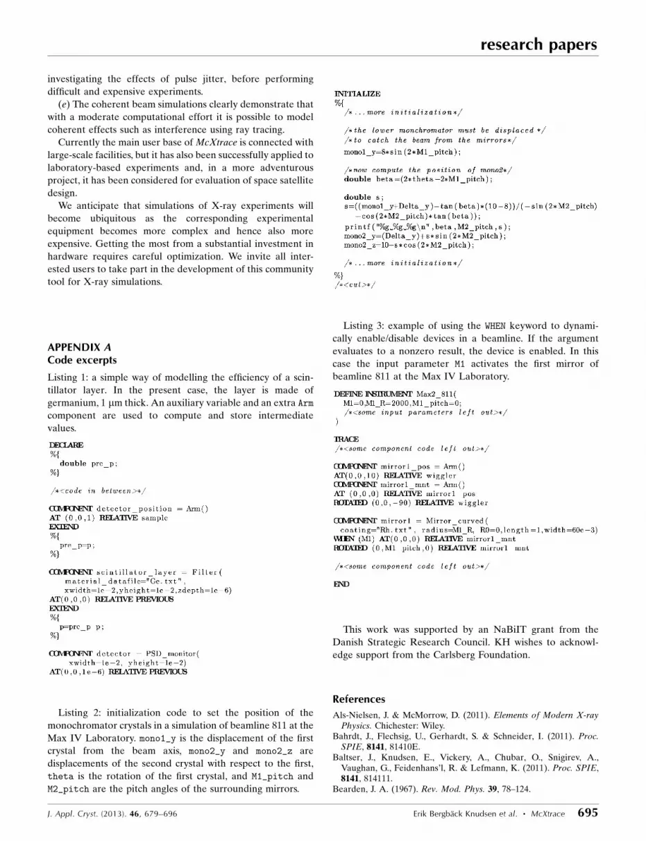
investigating the effects of pulse jitter, before performing

difficult and expensive experiments.

(e) The coherent beam simulations clearly demonstrate that

with a moderate computational effort it is possible to model

coherent effects such as interference using ray tracing.

Currently the main user base of McXtrace is connected with

large-scale facilities, but it has also been successfully applied to

laboratory-based experiments and, in a more adventurous

project, it has been considered for evaluation of space satellite

design.

We anticipate that simulations of X-ray experiments will

become ubiquitous as the corresponding experimental

equipment becomes more complex and hence also more

expensive. Getting the most from a substantial investment in

hardware requires careful optimization. We invite all inter-

ested users to take part in the development of this community

tool for X-ray simulations.

APPENDIX ACode excerpts

Listing 1: a simple way of modelling the efficiency of a scin-

tillator layer. In the present case, the layer is made of

germanium, 1 mm thick. An auxiliary variable and an extra Arm

component are used to compute and store intermediate

values.

Listing 2: initialization code to set the position of the

monochromator crystals in a simulation of beamline 811 at the

Max IV Laboratory. mono1_y is the displacement of the first

crystal from the beam axis, mono2_y and mono2_z are

displacements of the second crystal with respect to the first,

theta is the rotation of the first crystal, and M1_pitch and

M2_pitch are the pitch angles of the surrounding mirrors.

Listing 3: example of using the WHEN keyword to dynami-

cally enable/disable devices in a beamline. If the argument

evaluates to a nonzero result, the device is enabled. In this

case the input parameter M1 activates the first mirror of

beamline 811 at the Max IV Laboratory.

This work was supported by an NaBiIT grant from the

Danish Strategic Research Council. KH wishes to acknowl-

edge support from the Carlsberg Foundation.

References

Als-Nielsen, J. & McMorrow, D. (2011). Elements of Modern X-rayPhysics. Chichester: Wiley.

Bahrdt, J., Flechsig, U., Gerhardt, S. & Schneider, I. (2011). Proc.SPIE, 8141, 81410E.

Baltser, J., Knudsen, E., Vickery, A., Chubar, O., Snigirev, A.,Vaughan, G., Feidenhans’l, R. & Lefmann, K. (2011). Proc. SPIE,8141, 814111.

Bearden, J. A. (1967). Rev. Mod. Phys. 39, 78–124.

research papers










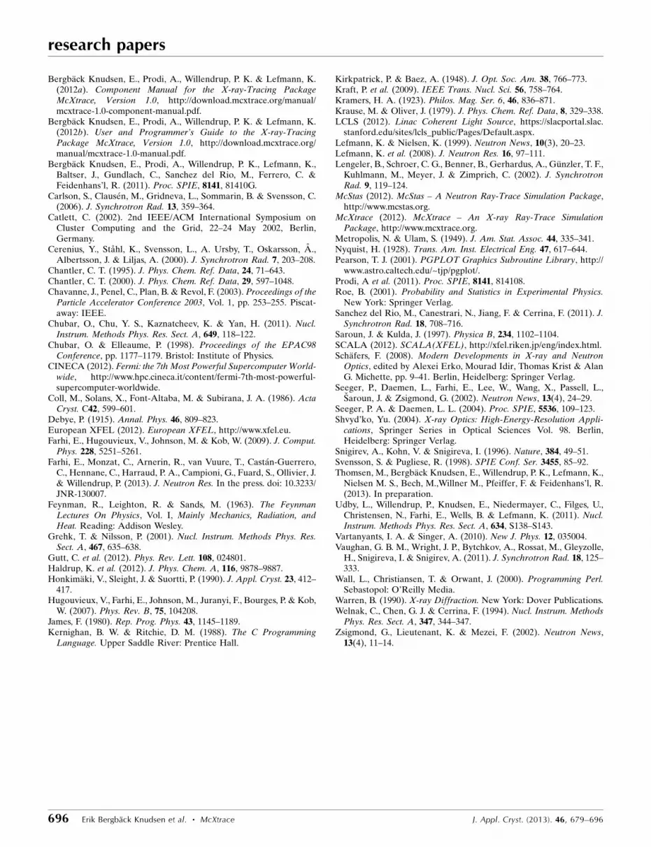
Bergback Knudsen, E., Prodi, A., Willendrup, P. K. & Lefmann, K.(2012a). Component Manual for the X-ray-Tracing PackageMcXtrace, Version 1.0, http://download.mcxtrace.org/manual/mcxtrace-1.0-component-manual.pdf.

Bergback Knudsen, E., Prodi, A., Willendrup, P. K. & Lefmann, K.(2012b). User and Programmer’s Guide to the X-ray-TracingPackage McXtrace, Version 1.0, http://download.mcxtrace.org/manual/mcxtrace-1.0-manual.pdf.

Bergback Knudsen, E., Prodi, A., Willendrup, P. K., Lefmann, K.,Baltser, J., Gundlach, C., Sanchez del Rio, M., Ferrero, C. &Feidenhans’l, R. (2011). Proc. SPIE, 8141, 81410G.

Carlson, S., Clausen, M., Gridneva, L., Sommarin, B. & Svensson, C.(2006). J. Synchrotron Rad. 13, 359–364.

Catlett, C. (2002). 2nd IEEE/ACM International Symposium onCluster Computing and the Grid, 22–24 May 2002, Berlin,Germany.

Cerenius, Y., Stahl, K., Svensson, L., A. Ursby, T., Oskarsson, A.,Albertsson, J. & Liljas, A. (2000). J. Synchrotron Rad. 7, 203–208.

Chantler, C. T. (1995). J. Phys. Chem. Ref. Data, 24, 71–643.Chantler, C. T. (2000). J. Phys. Chem. Ref. Data, 29, 597–1048.Chavanne, J., Penel, C., Plan, B. & Revol, F. (2003). Proceedings of the

Particle Accelerator Conference 2003, Vol. 1, pp. 253–255. Piscat-away: IEEE.

Chubar, O., Chu, Y. S., Kaznatcheev, K. & Yan, H. (2011). Nucl.Instrum. Methods Phys. Res. Sect. A, 649, 118–122.

Chubar, O. & Elleaume, P. (1998). Proceedings of the EPAC98Conference, pp. 1177–1179. Bristol: Institute of Physics.

CINECA (2012). Fermi: the 7th Most Powerful Supercomputer World-wide, http://www.hpc.cineca.it/content/fermi-7th-most-powerful-supercomputer-worldwide.

Coll, M., Solans, X., Font-Altaba, M. & Subirana, J. A. (1986). ActaCryst. C42, 599–601.

Debye, P. (1915). Annal. Phys. 46, 809–823.European XFEL (2012). European XFEL, http://www.xfel.eu.Farhi, E., Hugouvieux, V., Johnson, M. & Kob, W. (2009). J. Comput.

Phys. 228, 5251–5261.Farhi, E., Monzat, C., Arnerin, R., van Vuure, T., Castan-Guerrero,

C., Hennane, C., Harraud, P. A., Campioni, G., Fuard, S., Ollivier, J.& Willendrup, P. (2013). J. Neutron Res. In the press. doi: 10.3233/JNR-130007.

Feynman, R., Leighton, R. & Sands, M. (1963). The FeynmanLectures On Physics, Vol. I, Mainly Mechanics, Radiation, andHeat. Reading: Addison Wesley.

Grehk, T. & Nilsson, P. (2001). Nucl. Instrum. Methods Phys. Res.Sect. A, 467, 635–638.

Gutt, C. et al. (2012). Phys. Rev. Lett. 108, 024801.Haldrup, K. et al. (2012). J. Phys. Chem. A, 116, 9878–9887.Honkimaki, V., Sleight, J. & Suortti, P. (1990). J. Appl. Cryst. 23, 412–

417.Hugouvieux, V., Farhi, E., Johnson, M., Juranyi, F., Bourges, P. & Kob,

W. (2007). Phys. Rev. B, 75, 104208.James, F. (1980). Rep. Prog. Phys. 43, 1145–1189.Kernighan, B. W. & Ritchie, D. M. (1988). The C Programming

Language. Upper Saddle River: Prentice Hall.

Kirkpatrick, P. & Baez, A. (1948). J. Opt. Soc. Am. 38, 766–773.Kraft, P. et al. (2009). IEEE Trans. Nucl. Sci. 56, 758–764.Kramers, H. A. (1923). Philos. Mag. Ser. 6, 46, 836–871.Krause, M. & Oliver, J. (1979). J. Phys. Chem. Ref. Data, 8, 329–338.LCLS (2012). Linac Coherent Light Source, https://slacportal.slac.

stanford.edu/sites/lcls_public/Pages/Default.aspx.Lefmann, K. & Nielsen, K. (1999). Neutron News, 10(3), 20–23.Lefmann, K. et al. (2008). J. Neutron Res. 16, 97–111.Lengeler, B., Schroer, C. G., Benner, B., Gerhardus, A., Gunzler, T. F.,

Kuhlmann, M., Meyer, J. & Zimprich, C. (2002). J. SynchrotronRad. 9, 119–124.

McStas (2012). McStas – A Neutron Ray-Trace Simulation Package,http://www.mcstas.org.

McXtrace (2012). McXtrace – An X-ray Ray-Trace SimulationPackage, http://www.mcxtrace.org.

Metropolis, N. & Ulam, S. (1949). J. Am. Stat. Assoc. 44, 335–341.Nyquist, H. (1928). Trans. Am. Inst. Electrical Eng. 47, 617–644.Pearson, T. J. (2001). PGPLOT Graphics Subroutine Library, http://

www.astro.caltech.edu/~tjp/pgplot/.Prodi, A et al. (2011). Proc. SPIE, 8141, 814108.Roe, B. (2001). Probability and Statistics in Experimental Physics.

New York: Springer Verlag.Sanchez del Rio, M., Canestrari, N., Jiang, F. & Cerrina, F. (2011). J.

Synchrotron Rad. 18, 708–716.Saroun, J. & Kulda, J. (1997). Physica B, 234, 1102–1104.SCALA (2012). SCALA(XFEL), http://xfel.riken.jp/eng/index.html.Schafers, F. (2008). Modern Developments in X-ray and Neutron

Optics, edited by Alexei Erko, Mourad Idir, Thomas Krist & AlanG. Michette, pp. 9–41. Berlin, Heidelberg: Springer Verlag.

Seeger, P., Daemen, L., Farhi, E., Lee, W., Wang, X., Passell, L.,Saroun, J. & Zsigmond, G. (2002). Neutron News, 13(4), 24–29.

Seeger, P. A. & Daemen, L. L. (2004). Proc. SPIE, 5536, 109–123.Shvyd’ko, Yu. (2004). X-ray Optics: High-Energy-Resolution Appli-

cations, Springer Series in Optical Sciences Vol. 98. Berlin,Heidelberg: Springer Verlag.

Snigirev, A., Kohn, V. & Snigireva, I. (1996). Nature, 384, 49–51.Svensson, S. & Pugliese, R. (1998). SPIE Conf. Ser. 3455, 85–92.Thomsen, M., Bergback Knudsen, E., Willendrup, P. K., Lefmann, K.,

Nielsen M. S., Bech, M.,Willner M., Pfeiffer, F. & Feidenhans’l, R.(2013). In preparation.

Udby, L., Willendrup, P., Knudsen, E., Niedermayer, C., Filges, U.,Christensen, N., Farhi, E., Wells, B. & Lefmann, K. (2011). Nucl.Instrum. Methods Phys. Res. Sect. A, 634, S138–S143.

Vartanyants, I. A. & Singer, A. (2010). New J. Phys. 12, 035004.Vaughan, G. B. M., Wright, J. P., Bytchkov, A., Rossat, M., Gleyzolle,

H., Snigireva, I. & Snigirev, A. (2011). J. Synchrotron Rad. 18, 125–333.

Wall, L., Christiansen, T. & Orwant, J. (2000). Programming Perl.Sebastopol: O’Reilly Media.

Warren, B. (1990). X-ray Diffraction. New York: Dover Publications.Welnak, C., Chen, G. J. & Cerrina, F. (1994). Nucl. Instrum. Methods

Phys. Res. Sect. A, 347, 344–347.Zsigmond, G., Lieutenant, K. & Mezei, F. (2002). Neutron News,

13(4), 11–14.

research papers














































































































McXtrace : a Monte Carlo software package for simulating X-ray optics, beamlines and experiments

Documents

Transcript of McXtrace : a Monte Carlo software package for simulating X-ray optics, beamlines and experiments