Matrix analysis of metamorphic mineral assemblages and reactions

Contrib Mineral Petrol (1989) 102:69-77 Contributions to Mineralogy and Petrology �9 Springer-Verlag 1989

Matrix analysis of metamorphic mineral assemblages George W. Fisher Department of Earth and Planetary Sciences, Johns Hopkins University, Baltimore, MD 21218, USA

and reactions

Abstract. Assemblage diagrams are widely used in interpreting metamorphic mineral assemblages. In simple systems, they can help to identify assemblages which may represent equilibrium states; to determine whether differences between assemblages reflect changes in metamorphic grade or variations in bulk composition; and to characterize isograd reactions. In multicomponent assemblages these questions can be approached by investigating the rank, composition space (range) and reaction space (null-space) of a matrix representing the compositions of the phases involved. Singular value decomposition (SVD) provides an elegant way of (1) finding the rank of a matrix and determining orthonormal bases for both the composition space and the reaction space needed to represent an assemblage or pair of assemblages; and (2) finding a model matrix of specified rank which is closest in a least squares sense to an observed assemblage. Although closely related to least squares techniques, the SVD approach has the advantages that it tolerates errors in all observations and is computationally simpler and more stable than non-linear least squares algorithms. Models of this sort can be used to interpret multicomponent mineral assemblages by straightfor- ward generalizations of the methods used to interpret assemblage diagrams in simpler systems. SVD analysis of mineral assemblages described by Lang and Rice (1985) demonstrates the utility of the approach.

Introduction

In the 32 years since Thompson (1957) developed the AFM projection, metamorphic petrologists have used graphical analysis extensively in interpreting mineral assemblages. Phase diagrams have proven invaluable in identifying assemblages which may represent equilibrium states, in determining whether local differences between assemblages reflect changes in metamorphic grade or variations in bulk compositions, and in characterizing metamorphic isograd reactions.

Graphical methods for interpreting mineral assemblages are based on equilibrium thermodynamics, which requires that a set of assemblages equilibrated under arbitrary values of P, T, and externally fixed activities must exhibit a unique relation between bulk composition and mineral assemblage; every point in a phase diagram of such a set must correspond to a unique mineral assemblage, characterized by a single set of minerals with definite compositions and proportions (Korzhinskii 1959, p. 62). This fact leads immedi- ately to the two basic rules for interpreting assemblage dia-

grams: (1)An assemblage which contains intersecting tie lines in a valid phase diagram cannot represent equilibrium under arbitrary conditions; the compositions at each intersection are represented by two possible pairs of minerals, which can have equilibrated only along univariant curves. (2) If elements of two equilibrium assemblages intersect, the assemblages must have equilibrated under different external conditions, and their differences cannot be attributed solely to variations in bulk composition (Greenwood 1967); in many cases, the nature of the reaction relating the assemblages can be deduced from the change in topology of the assemblage diagram (Thompson 1957).

These rules are easy to apply in simple systems, but many rocks contain too many components for rigorous graphical representation, making it difficult to distinguish valid intersections from artifacts of the projection. Realiz- ing that matrix techniques provide an escape from the limi- tations of two-dimensional plots, Greenwood (1967, 1968) pointed out that linear algebraic dependencies between minerals in multicomponent assemblages are entirely equivalent to graphical intersections in simple phase diagrams, and developed techniques designed to detect linear dependencies in multicomponent systems using linear programming and regression analysis.

Regression analysis has proven particularly useful in interpreting mineral assemblages (e.g., Pigage 1976; Fletcher and Greenwood 1979; Lang and Rice 1985). However, the formulation of the regression problem generally used in metamorphic petrology (Albarede and Provost 1977) is based on non-linear least squares methods, an approach which involves a number of computational difficulties. Re- cent work in matrix analysis (Golub and Van Loan 1980, 1983; Van Huffel 1987) has lead to development of a more effective approach to such problems based on singular value decomposition (SVD).

This paper reviews the analysis of mineral assemblages by matrix methods, shows how the SVD approach can simplify analysis of mineral assemblages, and compares results of the SVD approach with those of non-linear regression techniques. Computer programs written to implement the approaches discussed are listed in Appendix I.

Matrix methods for analysis of metamorphic assemblages

Some basic principles

To see how matrix techniques can be used to analyze mineral assemblages, consider an assemblage containing m minerals whose compositions are given by n suitable components. The operation

70

of projecting this assemblage into a suitable composition diagram corresponds to the matrix operation

A x = b , (1)

where A is an n by m matrix, the rows of which represent the n components and the columns of which specify the compositions of the m minerals; x is a vector giving the composition of the assemblage in terms of the molar proportions of the m minerals; and b is a vector giving its composition in terms of the n system components. This equation projects the elements of x into a space called the range of A, which includes the vector b, and corresponds to the Cartesian composition space of Spear et al. (1982). The number of dimensions in composition space, and the number of elements of x which can be uniquely projected into it are both given by the rank of A. Provided that the components used in defining A are linearly independent, the rank of A is n. If m > n the projection loses m - n pieces of information, because an n- dimensional vector space cannot contain a space of more than n dimensions. However, the missing m - n pieces of information are not lost irretrievably. They project into an additional vector space, called the null space, which corresponds closely to the reaction space of Thompson (1982) 1 , and they represent phase reactions (in the terminology of Thompson 1988). Together, composition space and reaction space can uniquely represent mineral assemblages of any complexity.

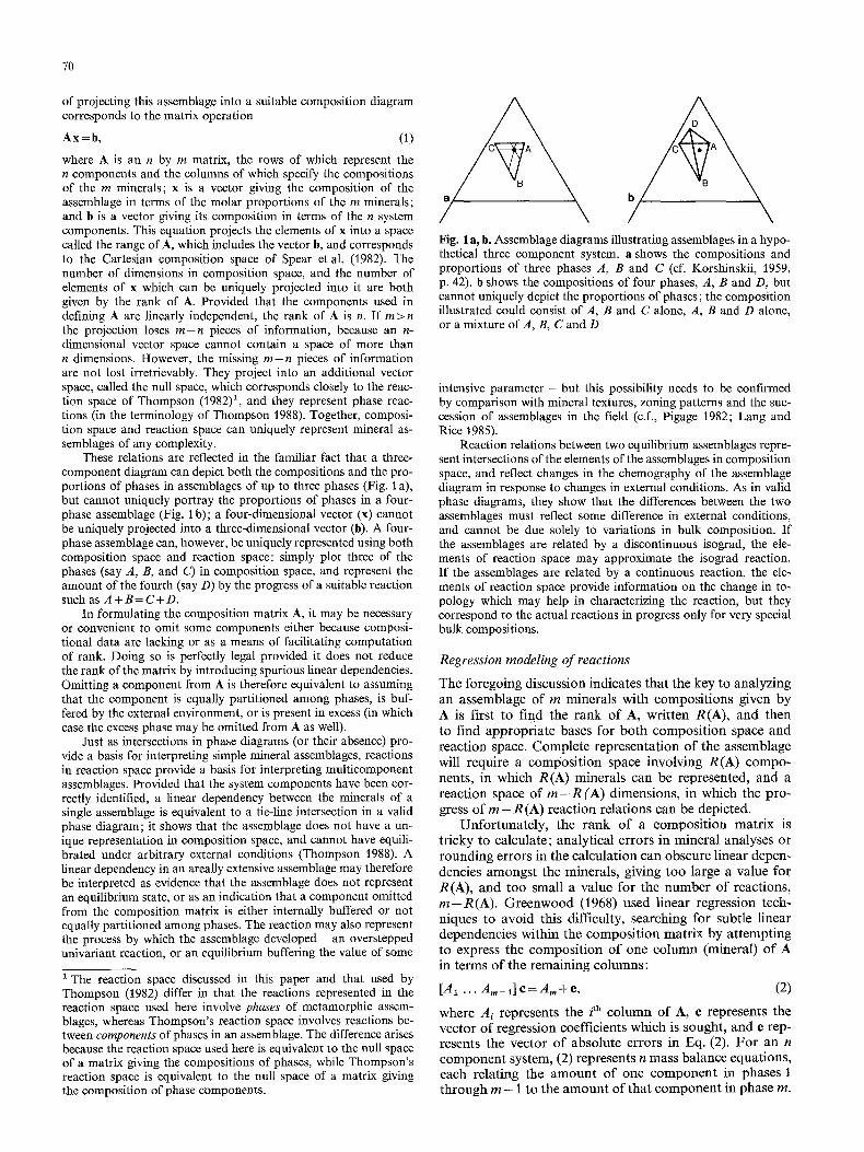
These relations are reflected in the familiar fact that a three- component diagram can depict both the compositions and the proportions of phases in assemblages of up to three phases (Fig. 1 a), but cannot uniquely portray the proportions of phases in a four- phase assemblage (Fig. 1 b); a four-dimensional vector (x) cannot be uniquely projected into a three-dimensional vector (b). A four- phase assemblage can, however, be uniquely represented using both composition space and reaction space: simply plot three of the phases (say A, B, and C) in composition space, and represent the amount of the fourth (say D) by the progress of a suitable reaction such as A + B = C + D .

In formulating the composition matrix A, it may be necessary or convenient to omit some components either because compositional data are lacking or as a means of facilitating computation of rank. Doing so is perfectly legal provided it does not reduce the rank of the matrix by introducing spurious linear dependencies. Omitting a component from A is therefore equivalent to assuming that the component is equally partitioned among phases, is buffered by the external environment, or is present in excess (in which case the excess phase may be omitted from A as well).

Just as intersections in phase diagrams (or their absence) provide a basis for interpreting simple mineral assemblages, reactions in reaction space provide a basis for interpreting multieomponent assemblages. Provided that the system components have been cor- rectly identified, a linear dependency between the minerals of a single assemblage is equivalent to a tie-line intersection in a valid phase diagram; it shows that the assemblage does not have a unique representation in composition space, and cannot have equilibrated under arbitrary external conditions (Thompson 1988). A linear dependency in an areally extensive assemblage may therefore be interpreted as evidence that the assemblage does not represent an equilibrium state, or as an indication that a component omitted from the composition matrix is either internally buffered or not equally partitioned among phases. The reaction may also represent the process by which the assemblage developed - an overstepped univariant reaction, or an equilibrium buffering the value of some

1 The reaction space discussed in this paper and that used by Thompson (1982) differ in that the reactions represented in the reaction space used here involve phases of metamorphic assemblages, whereas Thompson's reaction space involves reactions between components of phases in an assemblage. The difference arises because the reaction space used here is equivalent to the null space of a matrix giving the compositions of phases, while Thompson's reaction space is equivalent to the null space of a matrix giving the composition of phase components.

Fig. 1 a, b. Assemblage diagrams illustrating assemblages in a hypothetical three component system, a shows the compositions and proportions of three phases A, B and C (cf. Korshinskii, 1959, p. 42). b shows the compositions of four phases, A, B and D, but cannot uniquely depict the proportions of phases; the composition illustrated could consist of A, B and C alone, A, B and D alone, or a mixture of A, B, C and D

intensive parameter - but this possibility needs to be confirmed by comparison with mineral textures, zoning patterns and the suc- cession of assemblages in the field (c.f., Pigage 1982; Lang and Rice 1985).

Reaction relations between two equilibrium assemblages represent intersections of the elements of the assemblages in composition space, and reflect changes in the chemography of the assemblage diagram in response to changes in external conditions. As in valid phase diagrams, they show that the differences between the two assemblages must reflect some difference in external conditions, and cannot be due solely to variations in bulk composition. If the assemblages are related by a discontinuous isograd, the elements of reaction space may approximate the isograd reaction. If the assemblages are related by a continuous reaction, the elements of reaction space provide information on the change in topology which may help in characterizing the reaction, but they correspond to the actual reactions in progress only for very special bulk compositions.

Regression modeling o f reactions

The foregoing discussion indicates that the key to analyzing an assemblage of m minerals with compositions given by A is first to find the rank of A, written R(A), and then to find appropriate bases for both composition space and reaction space. Complete representation of the assemblage will require a composition space involving R(A) components, in which R(A) minerals can be represented, and a reaction space of m - R (A) dimensions, in which the progress of m - R (A) reaction relations can be depicted.

Unfortunately, the rank of a composition matrix is tricky to calculate; analytical errors in mineral analyses or rounding errors in the calculation can obscure linear dependencies amongst the minerals, giving too large a value for R (A), and too small a value for the number of reactions, m - R ( A ) . Greenwood (1968) used linear regression techniques to avoid this difficulty, searching for subtle linear dependencies within the composition matrix by attempting to express the composition of one column (mineral) of A in terms of the remaining columns:

[A1 ... A, ,- 1] e = A m + e , (2)

where Ai represents the t ~h column of A, e represents the vector of regression coefficients which is sought, and e represents the vector of absolute errors in Eq. (2). For an n component system, (2) represents n mass balance equations, each relating the amount of one component in phases 1 through m - 1 to the amount of that component in phase m.

Classical regression analysis assumes that the terms on the lefthand side of (2), the "independent variables", are known exactly, and that only the terms on the right hand side, the "dependent variables", are subject to error. This approach is clearly inappropriate for analysis of mineral assemblages, where we must model one mineral composition in terms of others which are subject to comparable analytical uncertainty. Reid et al. (1973) and Albarede and Provost (1977) circumvented this problem by weighting Eq. (2) with the reciprocal of the overall error for each mass balance equation. Unfortunately, the overall errors depend upon the solution to the regression problem, neces- sitating an iterative approach based upon non-linear root- finding techniques. The algorithm developed by Albarede and Provost (1977) served as the basis for the program PROTEUS, which was developed and refined by Green- wood and his students (Pigage 1976; Fletcher and Green- wood 1979), and is now representative of approaches used in metamorphic petrology (e.g., Lang and Rice 1985).

Although serviceable, the Albarede-Provost algorithm has several disadvantages. It is complex and difficult to code efficiently. Like any non-linear root-finding technique, it can mislead the user by finding false minima in the residu- al surface. The values found for the minimum may depend upon the trial values used in the first iteration. And like any regression technique, it requires the user to decide in advance which mineral to treat as a dependent variable and which as independent variables. This restriction is in- consequential in analyzing a single assemblage, but can prove cumbersome in searching for a linear dependency between the minerals of two separate assemblages. The regression approach requires that the number of components exceed the number of minerals, which commonly means that regression analysis must be applied to a series of subsets of the minerals from the two assemblages. The search for subtle intersections between assemblages requires that all possible sub-sets be considered, a time-consuming and error-prone process.

Recent work on problems in which all variables are subject to experimental error (referred to as total least squares problems in the matrix analysis literature) has lead to an approach based on singular value decomposition which avoids most of the difficulties of conventional regression methods (Golub and Van Loan 1980, 1983; Van Huffel 1987; Van Huffel and Vandewalle 1988). The following sec- tions outline techniques for analyzing mineral assemblages using this approach. Initially I will assume that all compositions are known with comparable uncertainty; in a later section I will present methods of weighting the composition matrix so as to allow for variable uncertainties.

Singular value decomposition in matrix analys&

Singular value decomposition (SVD) is based upon a theo- rem of matrix analysis which states that any m by n matrix M can be expressed as the product of a column orthogonal matrix U, a diagonal n by n matrix W, and the transpose of an orthogonal n by n matrix V,

M = UW V t. (3)

This decomposition is extremely useful for our purposes because it gives the three elements essential to analyzing mineral assemblages in a single operation: the number of non-zero diagonal terms in W gives the rank of M; the

71

columns of U corresponding to the non-zero terms in W constitute an orthonormal basis for the range (composition space) of M; and the columns of V corresponding to the zero diagonal elements of W provide an orthonormal basis for the null space (reaction space) of M (Golub and Van Loan 1983, p. 16-20). The SVD of a matrix can be easily computed using software routines available in most matrix manipulation packages (e.g., Press et al. 1986, p. 52 64). Programs designed for SVD analysis of assemblages are listed in Appendix I.

As an example, consider the matrix

1.00 1.00 1.00 n = 0.00 0.25 0.50

0.00 0.75 1.50,

in which the rows represent the components 8i02, MgO and FeO and the columns give the compositions of quartz, an orthopyroxene (of composition Fs75), and an olivine (Fa7s), in moles of oxide components. Taking the SVD ofMgives

2.33132 0.00000 0.00000 W= 0.00000 0.83064 0.00000

0.00000 0.00000 0.00000,

-0.69773 0.71636 0.00000 U= -0.22653 -0.22064 -0.94868

-0.67960 -0.66193 0.31623,

-0.29929 0.86242 0.40825 V= -0.54221 0.19835 -0.81650

-0.78513 -0.46572 0.40825.

W has two non-zero diagonal elements, so the rank of M is two, reflecting the fact that the orthopyroxene and the olivine have the same Fe/Mg ratio. The first two columns of U can be used as an orthonormal basis for composition space (admittedly not a very convenient one) and the last column of V provides a basis vector for reaction space; normalizing to one formula unit of quartz, the reaction is

2 orthopyroxene = 1 quartz + 1 olivine,

which indicates that the orthopyroxene point intersects the quartz olivine tie line, and that the assemblage therefore cannot have equilibrated at arbitrary P and T.

Now suppose that we were given chemical analyses of these minerals, reduced to the following compositions expressed in oxide components:

0.990 1.010 1.005 M' = 0.000 0.251 0.498

0.000 0.748 1.502.

The differences between M and M' reflect hypothetical analytical errors on the order of 1%. The SVD of M' is

2.33587 0.00000 0.00000 W= 0.00000 0.82490 0.00000

0.00000 0.00000 0.00231,

-0.69845 0.71566 --0.00098 U= --0.22585 -0.21913 0.94920

--0.67909 -0.66318 --0.31468,

-0.29602 0.85890 -0.41794 V= --0.54373 0.20822 0.81302

--0.78532 -0.46791 --0.40537,

and the fact that W now has three non-zero elements shows that the analytical errors have removed the linear depen-

72

dency between the minerals. However, inspection of the singular values (the diagonal elements of W) shows that W[3,3] is much smaller than the other two, and hence that M is close to a matrix of rank two.

We can find a model matrix of rank exactly 2, M", by setting W[3,3]=0.000, and using Eq. (3) to form the matrix

M r ' = U W V t '

giving

0.99000 1.01000 t.00500 M" = 0.00092 0.24922 0.49889

- 0.00030 0.74859 1.50171 .

To assess how well M" approximates the measured matrix M', we form the matrix difference

0.00000 0.00000 0.00000 M ' - M ' = 0.00092 -0.00178 0.00089

-- 0.00030 0.00059 -- 0.00029 ;

the residuals are well within the expected analytical uncertainty, showing that M' is indistinguishable from a matrix of rank 2. Taking the SVD of M" we get

2.33587 0.00000 0.00000 W= 0.00000 0.82490 0.00000

0.00000 0.00000 0.00000,

-0.69845 0.71566 -0.00098 U= -0.22585 -0.21913 0.94920

-0.67909 -0.66318 -0.31468,

-0.29602 0.85890 0.41794 V= -0.54373 0.20822 -0.81302

-0.78532 -0.46791 0.40537,

confirming that M " is indeed of rank 2, and that (except for trivial changes in sign) its SVD is the same as that of M'. Because the rank of M" is less than 3, it contains [ 3 - R (M")] = 1 reaction relation, with coefficients given by the third column of V,

1.945 orthopyroxene = 1.000 quartz + 0.970 olivine,

a reasonable approximation to the reaction implied by matrix M.

The process can be taken one step further by setting W[2,2] =0.000, calculating a matrix of rank 1, and testing to see whether or not it too provides a good approximation of M'. Doing so results in residuals on the order of 0.1-0.5, proving that M' is indeed significantly different from a matrix of rank 1.

We have thus shown that M' is analytically indistinguishable from a matrix of rank 2 containing an orthopyroxene that is collinear with quartz and orthopyroxene, implying that the assemblage can be interpreted as representing eqnilibrium only if that equilibrium is construed as being univariant.

This example shows how SVD can be used to search for possible reactions within a single sample: use SVD techniques to model the measured composition matrix with matrices of successively lower rank, selecting the model of lowest rank which approximates the observed mineral compositions within reasonable analytical uncertainty. The rank of this model matrix gives the number of components in the sample, and the vectors of V corresponding to zero diagonal terms in W provide an orthonormal basis for reactions between the minerals of the sample. Program SVDMOD (Ap-

m 2 / /

I I I I

ml

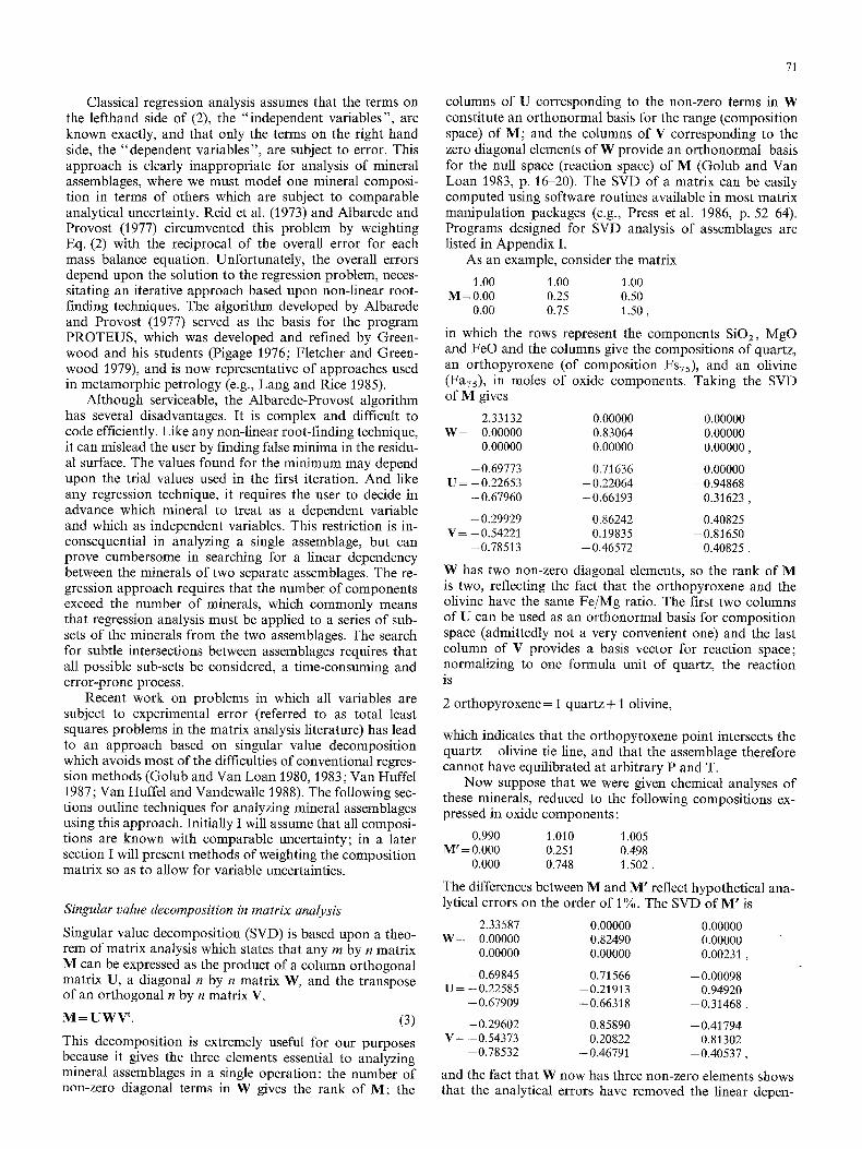
Fig. 2. Plot showing measurements of the content of five components from two hypothetical minerals, ml and m2. The heavy line illustrates a vector fitted to the observed compositional points; conventional least squares finds the line which minimizes the sum of squares of the residuals represented by dotted lines, while SVD analysis minimizes the sum of squares of the residuals represented by light solid lines

pendix I) can be used to perform these operations directly. As in the hypothetical case just discussed, decisions on which model to accept are generally easy to make, because the compositions given by model matrices vary considerably with rank; generally, one model matrix will fit the observed compositions with clearly acceptable residuals, while the model of next lower rank leads to residuals which are ob- viously unacceptable.

Stewart (1973, p. 322) has shown that the process outlined above finds the matrix of desired rank which is closest to an observed matrix in the sense that the sum of the squares of the residuals is minimized. The procedure is perfectly general, and can be used to approximate any matrix of mineral analyses by matrices of lower rank.

Golub and Van Loan (1980) make this same point in a more geometric context, which also serves to highlight the distinction between SVD and classical least squares analysis. To paraphrase their conclusion, SVD will find the hypersurface of chosen rank which minimizes the sum of the squares of the perpendicular distances to the analyzed compositions in multicomponent composition space. For example, consider an assemblage containing two phases of similar composition, ml and m2. We can test whether or not the difference in composition is significant by attempting to fit a matrix of rank 1 (a vector) to the appropriate composition matrix. SVD will find the line which minimizes the sum of the squares of the perpendicular distances to the composition data (Fig. 2, solid lines). Classical least squares analysis will find the line which minimizes sum of the squares of the composition residuals for one mineral, holding the composition of the other mineral at the observed values (Fig. 2, dotted lines).

Examining relationships between two or more assemblages

The techniques outlined above can be extended to determine whether or not two equilibrium assemblages are related by a reaction relation, using a two-step procedure:

1) Form a composite matrix composed of the minerals from the two assemblages to be compared, and use SVD

Table 1. Compositions of hypothetical mineral assemblages

qz op ol

M1 : SiOz 1.000 1.000 MgO 0.600 0.900 FeO 0.380 1.045 MnO 0.020 0.055

M2: SiO2 1.000 1.000 1.000 MgO 0.000 0.500 0.800 FeO 0.000 0.475 1.140 MnO 0.000 0.025 0.060

M 3 : SiO2 1.000 1.000 MgO 0.450 0.700 FeO 0.523 1.235 MnO 0.027 0.065

73

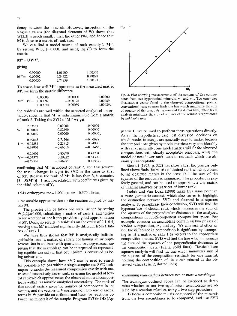
assemblages into the system S i O 2 - F e O - M g O suggests that M1 differs significantly in bulk composi t ion from both M2 and M3 and could have crystall ized under the same condit ions as either, but that M2 and M3 intersect and cannot have equil ibrated under the same condit ions (Fig. 3). Our problem is to assess the influence of MnO on these conclusions: does it consti tute an " e x t r a " component, el iminating the intersection between M2 and M3 and implying that they might have formed under the same conditions ?

We begin by forming a matr ix representing the composite assemblage M2M3, based on the composi t ions in Ta- ble 1 :

M 2 M 3

qz op ol op ol qz quartz; op orthopyroxene, and ol olivine

SiO 2 1.00000 1.00000 ] .00000 1.00000 1.00000 MgO 0.00000 0.50000 0.80000 0.45000 0.70000 FeO 0.00000 0.47500 1.14000 0.52300 1.23500 MnO 0.00000 0.02500 0.06000 0.02700 0.06500.

The SVD of this composi te gives the matrices

3.01819 0.0 0.0 0.0 0.0 0.0 0.88004 0.0 0.0 0.0

W = 0.0 0.0 0.17812 0.0 0.0 0.0 0.0 0.0 0.00045 0.0 0.0 0.0 0.0 0.0 0.00000

-0.71244 0.69683 -0.08281 -0.00000 0.00000 -0.40367 -0.31043 0.86063 -0.00057 -0.00000

U= -0.57321 -0.64568 -0.50172 0.05296 0.00000 -0.03010 -0.03413 -0.02709 -0.99860 0.00000 - 0 . 0 0 0 0 0 - 0 . 0 0 0 0 0 - 0 . 0 0 0 0 0 0.00000 - I . 0 0 0 0 0

MgO FeO --0.23605 0.79182 --0.46493 --0.21351 --0.23570 Fig. 3. Assemblage diagram projecting assemblages described by -0.39338 0.26597 0.60918 -0.42566 0.47140 matrices M1, M2, and M3 of Table 1 into the simplified composi- V= -0.56015 -0.32912 0.18023 -0.21314 -0.70711 tional space SiO2--FeO--MgO; qz quartz; op orthopyroxene; ol -0.39583 0 .24831 0.23208 0.85311 -0.00000 olivine. See text for discussion -0.56487 -0.36374 -0.57131 -0.00080 0.47140.

techniques to fit the composi te with a model matr ix having the lowest rank compat ib le with reasonable analytical uncertainty. The rank of the model matr ix gives the number of independent chemical components in the composite, and the vectors of V corresponding to zero diagonal terms in W provide an o r thonormal basis for reactions between the minerals o f the composite.

2) Determine whether or not the react ion space described by these basis vectors includes any reactions for which the minerals of one assemblage are reactants, and the minerals of the other assemblage are products . Any such reactions represent intersections of the assemblages in composi t ion space, and indicate that the two assemblages cannot have equil ibrated under the same external conditions. I f no such reactions are found, the assemblages occupy different regions of composi t ion space, and could have equil ibrated under the same external conditions. Program M U L T I (Appendix I) was writ ten to generate all univar iant reactions within the react ion space of a matr ix of mineral composit ions, and to detect those which represent incompatibilities.

To see how this approach works, consider matrices M1, M2, and M3, representing three different hypothet ical equi- l ibrium assemblages composed of quartz (qz), or thopyrox- ene (op) and olivine (ol) in the system SiO2 - M g O - F e O - MnO (Table 1). An assemblage d iagram project ing these

W[4,4] and W[5,5] are significantly less than the first three singular values, implying that M2M3 is close to a matr ix of rank three; setting W[4,4] and W[5,5]=0.0 , we generate a model matr ix with rank exac t l y three by using Eq. 3 to form the matr ix product U W V , giving

1.00000 1.00000 1.00000 1.00000 1.00000 --0.00000 0.50000 0.80000 0.45000 0.70000

0.00000 0 . 4 7 5 0 1 1 . 1 4 0 0 1 0.52298 1.23500 --0.00000 0 . 0 2 4 8 1 0.05990 0.02738 0.06500.

The residuals representing the differences between this model matr ix and M2M3,

-0.00000 -0.00000 -0.00000 0.00000 -0.00000 -0.00000 -0.00000 -0.00000 0.00000 -0.00000

0.00000 0.00000 0.00000 - 0.00000 0.00000 - 0.00000 - 0.00019 - 0.00000 0.00038 - 0.00000,

are well within analytical uncertainty, demonstra t ing that M2M3 is indist inguishable from a matr ix of rank three. Therefore, these five minerals do all lie in a three-component space, and the presence of MnO does not impose an addi t ional dimension.

Next, we must determine whether or not the reaction space associated with this composi te contains a reaction representing an incompat ibi l i ty between the two assemblages. The last two columns of V (corresponding to the two zero singular values of our model matrix) provide an or thonormal basis for all possible reactions between these

74

five phases. The two given directly by V are

0.214 qz + 0.426 opM2 + 0.213 o1~2 + 0.001 olM3 = 0.853 OpM 3 (V4)

0.236 qz + 0.707 olMz = 0.471 opt2 + 0.471 o1~3. (V5)

M2 and M3 minerals both occur on the left of V4 and on the right of V5, so neither represents an incompatibility between the two assemblages. But we need to know whether or not the reaction space defined by V4 and V5 (that is, the set of linear combinations of V4 and V5) contains any reactions representing an incompatibility.

We can explore this reaction space by writting all possible univariant reactions involving the five phases in the model three-component system, using the methods o f Korz- hinskii (1959, p. 103ff.) or the program M U L T I (Appen- dix I):

qz OpM2 01M2 OpM3 OIM3

0.000 - 1.993 0.999 1.994 - 1.000 [1] 1.003 0.000 2.004 - 2.007 - 1.000 [2]

- 0.997 - 3.974 0.000 5.971 - 1.000 [3] 0.500 - 1.000 1.500 0.000 - 1.000 [4] 0.251 0.498 0.251 - 1.000 0.000. [5]

Of these five reactions, [2] and [5] do indeed represent incompatibilities, because each has the minerals of one assemblage as reactants (negative coefficients) and the minerals of the other as products (positive coefficients). Conse- quently these assemblages intersect in composition space, and cannot have equilibrated under the same (arbitrary) conditions.

Reactions [2] and [5] should be interpreted as algebraic representations of the intersections between elements of M2 and M3 in composition space (Fig. 3), reflecting changes in chemography caused by the change in conditions from those under which M2 equilibrated to those under which M3 equilibrated. They represent the actual reactions involved in transforming M2 to M3 only in the very special case where M2 and M3 have the same bulk composition, and where that bulk composition lies along the M3 tie line between the opM3 point and the intersection of that tie line and the qz-olMz tie line.

In using these techniques to test for reactions indicating incompatibilities between assemblages, it is essential to ex- amine the reaction space associated with the model composition matrix. The measured compositions in this example define a matrix which has rank four (though small, W [4,4] in the SVD of the original matrix is greater than zero), and consequently give only a single reaction, which involves members of both assemblages as reactants and therefore does not represent an incompatibility.

Applying the same process to M1 and M2 we again find that all five minerals of the two assemblages lie in a single three-component composition space, and involve a reaction space of two dimensions. But the model minerals yield five reactions,

qz OpM2 01M2 opM1 O1M1

0.000 -- 1.000 1.000 1.000 -- 1.000 [1'] -- 0 .250 0 .000 0.750 0 .500 -- 1.000 [2'] - 1.000 3.000 0.000 -- 1.000 - 1.000 [3'] - 0.500 1.000 0.500 0.000 -- 1.000 [4'] - 0.500 2.000 - 0.500 -- 1.000 0.000, [5']

each of which involves minerals of both assemblages as reactants (negative coefficients) or products (positive coeffi-

cients) and so do not represent incompatibilities. Conse- quently M1 and M2 do indeed occupy different regions of composition space and may have equilibrated under the same external conditions, as suggested by Fig. 3.

The difference between reaction sets [1] ... [5] and [1'] ... [5'] reflects the change in composition of the olivine and pyroxene in the assemblages being compared with M2, which causes a change in the stoichiometry of [2] and [5] from reactions reflecting the intersection of elements of M2 and M3 to petrologically meaningless algebraic relations between nearby elements of M1 and M2.

Weighting the terms of composition matrices

Thus far we have assumed that all mineral compositions are known with comparable uncertainty. But in any real problem, some data will be more accurate than others, and accordingly it is necessary to weight the terms of matrix A prior to analysis by SVD. Weighting can be accomplished by pre-multiplying A by an n by n diagonal matrix whose elements weight the rows of A, and postmultiplying the result by an m by m diagonal matrix, whose elements weight the columns of A (Golub and Van Loan 1980, p. 884).

The row weights should be chosen so as to reflect the user's confidence in the accuracy of the figures for each component in A, based upon an assessment of the accuracy of the analyses available, the amount of zoning in the minerals, the grain-to-grain variation in composition, and an evaluation of any retrograde effects (cf., Lang and Rice 1985, p. 874). Similarly, the column weights should be chosen to reflect the user's confidence in the composition of the phases in A. Program C A L C W T (Appendix A) was written to calculate row and column weight vectors from estimates of mineral composition uncertainties. For cases where the composition of one or more phases (quartz, for example, or a phase component in a solid solution) is known exactly, Van Huffel (1987, p. 54-55) and Van Huffel and Vandewalle (1988) have developed procedures for im- posing exact column compositions on the solution. But in most cases it suffices to weight stoichiometric phases with column weights approximately ten times those of minerals of variable composition.

Though simple to apply, this technique for weighting the composition matrix is not ideal; only rarely will the matrix of estimated uncertainties have the structure of a product of two diagonal matrices. Further research into techniques of weighting the composition matrix seems desir- able.

Application to natural examples

In order to evaluate the effectiveness of the SVD method outlined above, it is helpful to reexamine problems which have been studied using established regression techniques. Lang and Rice (1985) included unusually complete data on mineral compositions and uncertainties in their regression study of progressively metamorphosed pelitic rocks, ranging from chlorite - biotite - muscovite argillites to kyanite - staurolite - garnet - biotite - muscovite schist; their data provide an excellent basis for comparing the two techniques. I have repeated most of the calculations reported by Lang and Rice using SVD methods. My results are generally similar to theirs, but some differences illustrate the usefulness of the SVD approach. The following discussion highlights some of the more interesting comparisons.

75

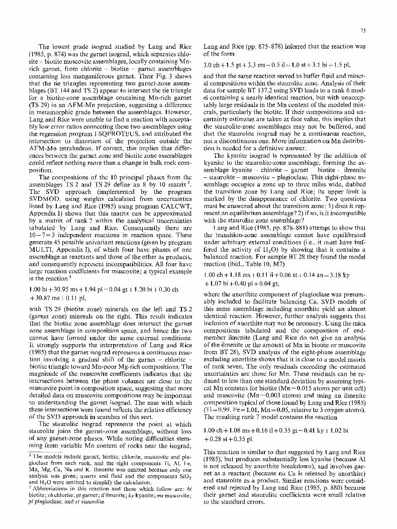
The lowest grade isograd studied by Lang and Rice (1985, p. 874) was the garnet isograd, which separates chlorite - biotite muscovite assemblages, locally containing Mn- rich garnet, from chlorite - biotite - garnet assemblages containing less manganiferous garnet. Their Fig. 3 shows that the tie triangles representing two garnet-zone assemblages (BT 144 and TS 2) appear to intersect the tie triangle for a biotite-zone assemblage containing Mn-rich garnet (TS 29) in an AFM-Mn projection, suggesting a difference in metamorphic grade between the assemblages. However, Lang and Rice were unable to find a reaction with accepta- bly low error ratios connecting these two assemblages using the regression program LSQPROTEUS, and attributed the intersection to distortion of the projection outside the AFM-Mn tetrahedron. If correct, this implies that differences between the garnet zone and biotite zone assemblages could reflect nothing more than a change in bulk rock composition.

The compositions of the 10 principal phases from the assemblages TS 2 and TS 29 define an 8 by 10 matrix 2. The SVD approach (implemented by the program SVDMOD, using weights calculated from uncertainties listed by Lang and Rice (1985) using program CALCWT, Appendix I) shows that this matrix can be approximated by a matrix of rank 7 within the analytical uncertainties tabulated by Lang and Rice. Consequently there are 1 0 - 7 = 3 independent reactions in reaction space. These generate 45 possible univariant reactions (given by program MULTI, Appendix I), of which four have phases of one assemblage as reactants and those of the other as products, and consequently represent incompatibilities. All four have large reaction coefficients for muscovite; a typical example is the reaction 3

1.00 bi + 30.95 ms + 1.94 pl = 0.04 gt + 1.20 bi + 0.30 ch 430.87 ms+0.11 pl,

with TS 29 (biotite zone) minerals on the left and TS 2 (garnet zone) minerals on the right. This result indicates that the biotite zone assemblage does intersect the garnet zone assemblage in composition space, and hence the two cannot have formed under the same external conditions. It strongly supports the interpretation of Lang and Rice (1985) that the garnet isograd represents a continuous reaction involving a gradual shift of the garnet chlorite - biotite triangle toward Mn-poor Mg-rich compositions. The magnitude of the muscovite coefficients indicates that the intersections between the phase volumes are close to the muscovite point in composition space, suggesting that more detailed data on muscovite compositions may be important to understanding the garnet isograd. The ease with which these intersections were found reflects the relative efficiency of the SVD approach in searches of this sort.

The staurolite isograd represents the point at which staurolite joins the garnet-zone assemblage, without loss of any garnet-zone phases. While noting difficulties stem- ming from variable Mn content of rocks near the isograd,

z The models include garnet, biotite, chlorite, muscovite and plagioclase from each rock, and the eight components Ti, A1, Fe, Mn, Mg, Ca, Na and K. Ilmenite was omitted because only one analysis was given; quartz and fluid and the components SiO2 and H20 were omitted to simplify the calculation. 3 Abbreviations in this reaction and those which follow are: bi biotite; ch chlorite; gt garnet; il ilmenite; Icy kyanite; ms muscovite; pl plagioclase, and st staurolite

Lang and Rice (pp. 875-878) inferred that the reaction was of the form

3.0 ch+ 1.5 g t+ 3.3 ms+0.5 i l= 1.0 s t+ 3.1 b i+ 1.5 pl,

and that the same reaction served to buffer fluid and mineral compositions within the staurolite zone. Analysis of their data for sample BT 137.2 using SVD leads to a rank 6 model containing a nearly identical reaction, but with unaccep- tably large residuals in the Mn content of the modeled minerals, particularly the biotite. I f their compositions and uncertainty estimates are taken at face value, this implies that the staurolite-zone assemblages may not be buffered, and that the staurolite isograd may be a continuous reaction, not a discontinuous one. More information on Mn distribution is needed for a definitive answer.

The kyanite isograd is represented by the addition of kyanite to the staurolite-zone assemblage, forming the assemblage kyanite - chlorite - garnet - biotite - ilmenite

staurolite - muscovite - plagioclase. This eight-phase assemblage occupies a zone up to three miles wide, dubbed the transition zone by Lang and Rice; its upper limit is marked by the disappearance of chlorite. Two questions must be answered about the transition zone: 1) does it represent an equilibrium assemblage ? 2) if so, is it incompatible with the staurolite zone assemblage?

Lang and Rice (1985, pp. 878-881) attempt to show that the transition-zone assemblage cannot have equilibrated under arbitrary external conditions (i.e., it must have buffered the activity of H20) by showing that it contains a balanced reaction. For sample BT 28 they found the model reaction (ibid., Table 10, M7)

1.00 ch+ 1.18 ms+0.11 i1+0.06 st+0.14 an=3.18 ky + 1.07 bi + 0.40 pl + 0.04 gt,

where the anorthite component of plagioclase was presumably included to facilitate balancing Ca. SVD models of this same assemblage including anorthite yield an almost identical reaction. However, further analysis suggests that inclusion of anorthite may not be necessary. Using the mica compositions tabulated and the composition of end- member ilmenite (Lang and Rice do not give an analysis of the ilmenite or the amount of Mn in biotite or muscovite from BT 28), SVD analysis of the eight-phase assemblage excluding anorthite shows that it is close to a model matrix of rank seven. The only residuals exceeding the estimated uncertainties are those for Mn. These residuals can be reduced to less than one standard deviation by assuming typical Mn contents for biotite (Mn = 0.015 atoms per unit cell) and muscovite (Mn=0.003 atoms) and using an ilmenite composition typical of those found by Lang and Rice (1985) (Ti = 0.99, Fe = 1.01, Mn = 0.05, relative to 3 oxygen atoms). The resulting rank 7 model contains the reaction

1.00 ch+ 1.08 ms+0.16 i1+0.35 gt =0.41 k y + 1.02 bi +0.28 st+0.35 pl.

This reaction is similar to that suggested by Lang and Rice (1985), but produces substantially less kyanite (because A1 is not released by anorthite breakdown), and involves garnet as a reactant (because no Ca is released by anorthite) and staurolite as a product. Similar reactions were considered and rejected by Lang and Rice (1985, p. 880) because their garnet and staurolite coefficients were small relative to the standard errors.

76

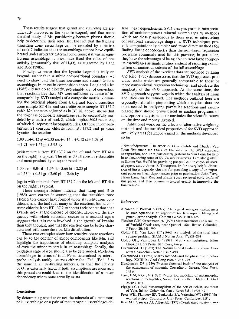
These results suggest that garnet and staurolite are significantly involved in the kyanite isograd, and that more detailed study of Mn partitioning between phases should help to determine their roles. But the fact that the 8 phase transition zone assemblage can be modeled by a matrix of rank 7 indicates that the assemblage cannot have equilibrated under arbitrary external conditions; if it was an equilibrium assemblage, it must have fixed the value of one activity (presumably that of H20), as suggested by Lang and Rice (1985).

Finally, to prove that the kyanite isograd is truly an isograd, rather than a subtle compositional boundary, we need to show that the transition-zone and staurolite-zone assemblages intersect in composition space. Lang and Rice (1985) did not do so directly, presumably out of conviction that reactions like their M7 were sufficient evidence of incompatibility. SVD analysis of a composite matrix containing the principal phases from Lang and Rice's transition zone sample BT 41 a and staurolite zone sample BT 137.2 (with Mn contents adjusted as in BT 28, above) shows that the 15-phase composite assemblage can be successfully modeled by a matrix o f rank 8, which implies 5005 reactions, of which 51 represent incompatibilities. Of these incompatibilities, 21 consume chlorite from BT 137.2 and produce kyanite; the reaction

1.00 ch+0 .12 g t + 1.33 ms +0.14 i1+0.12 s t + 1.09 pl

=1.21 b i+ 1.67 p1+3.93 ky

(with minerals from BT 137.2 on the left and from BT 41 a on the right) is typical. The other 30 all consume staurolite and most produce kyanite; the reaction

1.00 m s + 0.04 i l+ 1.36 s t + 3.66 b i + 2.25 pl

=4.53 bi+0.51 g t+2 .60 p l + 12.46 ky

(again with minerals from BT 137.2 on the left and BT 41 a on the right) is typical.

These incompatibilities indicate that Lang and Rice (1985) were correct in assuming that the transition zone assemblages cannot have formed under staurolite zone conditions; and the fact that many of the reactions found consume chlorite from BT 137.2 supports their contention that kyanite grew at the expense of chlorite. However, the fre- quency with which staurolite occurs as a reactant again suggests that it is more involved in the growth of kyanite than they thought, and that the reaction can be better characterized with more data on Mn distribution.

These two examples show how sensitive phase reactions can be to the content of minor components like Mn, and highlight the importance of obtaining complete analyses of even the minor minerals in an assemblage. Ideally, the oxidation state of iron should also be determined. Modeling assemblages in terms of total Fe as determined by microprobe analysis tacitly assumes either that Fe + +/Fe +++ is the same in all Fe-bearing minerals, or that the activity of 02 is externally fixed; if both assumptions are incorrect, this procedure could lead to the identification of a linear dependency where none actually exists.

Conclusions

By determining whether or not the minerals of a metamorphic assemblage or a pair of metamorphic assemblages de-

fine linear dependencies, SVD analysis permits interpretation of multicomponent mineral assemblages by methods which are closely analogous to those used in interpreting conventional assemblage diagrams. SVD techniques provide computationally simpler and more direct methods for finding linear dependencies than the non-linear regression programs commonly used for this purpose; in particular, they have the advantage of being able to treat large composite assemblages as single entities, instead of requiring exami- nation of numerous subsets of the full assemblage.

SVD analysis of the excellent data set provided by Lang and Rice (1985) demonstrates that the SVD approach provides results which are generally comparable to those of more conventional regression techniques, and illustrate the simplicity of the SVD approach. At the same time, the SVD approach suggests ways in which the analysis of Lang and Rice can be refined. The methods outlined here are especially helpful in pinpointing which analytical data are most needed in analyzing particular reactions and assemblages; they should prove useful in guiding programs of microprobe analysis so as to maximize the scientific return on the time and money invested.

Additional work on the effects of alternative weighting methods and the statistical properties of the SVD approach are likely areas for improvement in the methods developed so far.

Acknowledgements. The work of Gene Golub and Charles Van Loan first made me aware of the value of the SVD approach to regression, and I am particularly grateful to Van Loan for help in understanding some of SVD's subtler aspects. I am also grateful to Sabine Van Huffel for providing pre-publication copies of several papers, and to James B. Thompson, Jr. for a very helpful discussion of linear dependencies and for providing a copy of an important paper on linear dependencies prior to publication. John Ferry, Helen Lang, Jack Rice and Frank Spear reviewed early drafts of this paper, and their comments helped greatly in improving the final version.

References

Albarede F, Provost A (1977) Petrological and geochemical mass balance equations: an algorithm for least-square fitting and general error analysis. Comput Geosci 3 : 309-326

Fletcher CJN, Greenwood HJ (1979) Metamorphism and structure of Penfold Creek area, near Quesnel Lake, British Columbia. J Petrol 20 : 743 790

Golub GH, Van Loan CF (1980) An analysis of the total least squares problem. SIAM J Numer Anal 17:883-893

Golub GH, Van Loan CF (1983) Matrix computations. Johns Hopkins Univ Press, Baltimore, 476 p

Greenwood HJ (1967) The N-dimensional tie-line problem. Geo- china Cosmochim Acta 31:467~490

Greenwood HJ (1968) Matrix methods and the phase rule in petrology. XXIII Int Geol Cong Proc 6: 267-279

Korzhinskii DS (1959) Physico-chemical basis of the analysis of the paragenesis of minerals. Consultants Bureau, New York, 142 p

Lang HM, Rice JM (1985) Regression modeling of metamorphic reactions in metapelites, Snow Peak, northern Idaho. J Petrol 26: 857-887

Pigage LC (1976) Metamorphism of the Settler Schist, southeast of Yale, British Columbia. Can J Earth Sci 13:405-421

Press WH, Flannery BP, Teukolsky SA, Vettering WT (1986) Nu- merical recipes. Cambridge Univ Press, Cambridge, 818 p

Reid MJ, Gancarz AJ, Albee AL (1973) Constrained least-squares

77

analysis of petrologic problems with an application to lunar sample 12040; Earth Planet Sci Lett 17: 433~445

Spear FS, Rumble D, Ferry JM (1982) Linear algebraic manipulation of n-dimensional composition space. Min Soc Am Rev Mineral 10:53-104

Stewart GW (1973) Introduction to matrix computations. Academ- ic Press, New York, 441 p

Thompson JB (1957) The graphical analysis of mineral assemblages in pelitic schists. Am Mineral 42:842 858

Thompson JB (1982) Reaction space: an algebraic and geometric approach. Mineral Soc Am Rev Mineral 10:33-52

Thompson JB (1988) Paul Niggli and petrology; order out of chaos. Min Schweiz Pet (in press)

Van Huffel S (1987) Analysis of the total least squares problem and its use in parameter estimation; doctoral thesis submitted to the Department of Electrical Engineering, Catholic Univ of Leuven, Belgium, 370 p

Van Huffel S, Vandewalle J (1988) Analysis and properties of the generalized total least squares problem AX = B when some or all columns in A are subject to error. SIAM J Matrix Anal Appl (in press)

Received October 1, 1988 / Accepted February 21, 1989 Editorial responsibility: T. Grove

Appendix I

Programs for analysis of mineral assemblages by singular value decomposition

In order to facilitate use of the techniques described in this paper, I have written a set of Pascal computer programs suitable for analysis of mineral assemblages by singular value decomposition on an IBM PC or compatible. The following programs are available for distribution free to interested users; those desiring copies are asked to send a formatted IBM 51/4 inch diskette to the author with their request.

CALCWT. A program which calculates row and column weighting vectors for use with SVDMOD, using estimates of mineral compositional uncertainties as input; the weight vectors consist of the geometric mean of the inverse of the compositional uncertainty for each row and column.

MATRIX. A general purpose matrix manipulation program for performing most matrix algebra operations, including singular value decomposition.

MULTI. A program to generate all univariant reactions possible within the reaction space of a matrix of mineral compositions.

SVDMOD. A program to model mineral assemblages with matrices of arbitrary rank, using singular value decomposition.

Matrix analysis of metamorphic mineral assemblages and reactions

Documents

Transcript of Matrix analysis of metamorphic mineral assemblages and reactions