San Jose State University San Jose State University

SJSU ScholarWorks SJSU ScholarWorks

Master's Projects Master's Theses and Graduate Research

Spring 5-20-2019

JavaScript Metamorphic Malware Detection Using Machine JavaScript Metamorphic Malware Detection Using Machine

Learning Techniques Learning Techniques

Aakash Wadhwani San Jose State University

Follow this and additional works at: https://scholarworks.sjsu.edu/etd_projects

Part of the Artificial Intelligence and Robotics Commons, and the Information Security Commons

Recommended Citation Recommended Citation Wadhwani, Aakash, "JavaScript Metamorphic Malware Detection Using Machine Learning Techniques" (2019). Master's Projects. 688. DOI: https://doi.org/10.31979/etd.8rtn-buzk https://scholarworks.sjsu.edu/etd_projects/688

This Master's Project is brought to you for free and open access by the Master's Theses and Graduate Research at SJSU ScholarWorks. It has been accepted for inclusion in Master's Projects by an authorized administrator of SJSU ScholarWorks. For more information, please contact scholarworks@sjsu.edu.

JavaScript Metamorphic Malware Detection Using Machine Learning Techniques

A Project

Presented to

The Faculty of the Department of Computer Science

San José State University

In Partial Fulfillment

of the Requirements for the Degree

Master of Science

by

Aakash Wadhwani

May 2019

© 2019

Aakash Wadhwani

ALL RIGHTS RESERVED

The Designated Project Committee Approves the Project Titled

JavaScript Metamorphic Malware Detection Using Machine Learning Techniques

by

Aakash Wadhwani

APPROVED FOR THE DEPARTMENT OF COMPUTER SCIENCE

SAN JOSÉ STATE UNIVERSITY

May 2019

Dr. Thomas Austin Department of Computer Science

Prof. Mark Stamp Department of Computer Science

Prof. Philip Heller Department of Computer Science

ABSTRACT

JavaScript Metamorphic Malware Detection Using Machine Learning Techniques

by Aakash Wadhwani

Various factors like defects in the operating system, email attachments from

unknown sources, downloading and installing a software from non-trusted sites make

computers vulnerable to malware attacks. Current antivirus techniques lack the

ability to detect metamorphic viruses, which vary the internal structure of the original

malware code across various versions, but still have the exact same behavior throughout.

Antivirus software typically relies on signature detection for identifying a virus, but

code morphing evades signature detection quite effectively.

JavaScript is used to generate metamorphic malware by changing the code’s

Abstract Syntax Tree without changing the actual functionality, making it very

difficult to detect by antivirus software. As JavaScript is prevalent almost everywhere,

it becomes an ideal candidate language for spreading malware.

This research aims to detect metamorphic malware using various machine learning

models like K Nearest Neighbors, Random Forest, Support Vector Machine, and Naïve

Bayes. It also aims to test the effectiveness of various morphing techniques that

can be used to reduce the accuracy of the classification model. Thus, this involves

improvement on both fronts of generation and detection of the malware helping

antivirus software detect morphed codes with better accuracy. In this research,

JavaScript based metamorphic engine reduces the accuracy of a trained malware

detector. While N-gram frequency based feature vectors give good accuracy results

for classifying metamorphic malware, HMM feature vectors provide the best results.

ACKNOWLEDGMENTS

I would like to thank my project advisor Prof. Thomas Austin. Without his

constant support and guidance, this project would not have been possible.

I would also like to thank my committee members Prof. Mark Stamp and

Prof. Philip Heller for monitoring my progress throughout and guiding me with their

expertise in the field of Machine Learning and Information Security.

v

TABLE OF CONTENTS

CHAPTER

1 Introduction . . . . . . . . . . . . . . . . . . . . . . . . . . . . . . . . 1

2 Background . . . . . . . . . . . . . . . . . . . . . . . . . . . . . . . . 3

2.1 Malware . . . . . . . . . . . . . . . . . . . . . . . . . . . . . . . . 3

2.2 Malware Types . . . . . . . . . . . . . . . . . . . . . . . . . . . . 4

2.2.1 Virus . . . . . . . . . . . . . . . . . . . . . . . . . . . . . . 4

2.2.2 Worms . . . . . . . . . . . . . . . . . . . . . . . . . . . . . 5

2.2.3 Trojan . . . . . . . . . . . . . . . . . . . . . . . . . . . . . 5

2.2.4 Backdoor . . . . . . . . . . . . . . . . . . . . . . . . . . . 6

2.3 Detection Techniques . . . . . . . . . . . . . . . . . . . . . . . . . 6

2.3.1 Signature Detection . . . . . . . . . . . . . . . . . . . . . . 6

2.3.2 Behavioral Detection . . . . . . . . . . . . . . . . . . . . . 7

2.3.3 Anomaly Detection . . . . . . . . . . . . . . . . . . . . . . 7

2.3.4 Hidden Markov Model (HMM) . . . . . . . . . . . . . . . . 8

3 Related Work . . . . . . . . . . . . . . . . . . . . . . . . . . . . . . . 11

4 Morphing Engine . . . . . . . . . . . . . . . . . . . . . . . . . . . . . 12

4.1 Abstract Syntax Tree . . . . . . . . . . . . . . . . . . . . . . . . . 12

4.2 Engine Implementation Details . . . . . . . . . . . . . . . . . . . 14

4.3 Architecture Overview . . . . . . . . . . . . . . . . . . . . . . . . 15

4.4 Techniques Used . . . . . . . . . . . . . . . . . . . . . . . . . . . 16

4.4.1 Variable Renaming . . . . . . . . . . . . . . . . . . . . . . 16

vi

vii

4.4.2 Dead Code Insertion . . . . . . . . . . . . . . . . . . . . . 17

4.4.3 Instruction Reordering . . . . . . . . . . . . . . . . . . . . 17

4.4.4 Function Reordering . . . . . . . . . . . . . . . . . . . . . 18

4.4.5 Instruction Substitution . . . . . . . . . . . . . . . . . . . 19

5 Rhino . . . . . . . . . . . . . . . . . . . . . . . . . . . . . . . . . . . . 21

5.1 Architecture . . . . . . . . . . . . . . . . . . . . . . . . . . . . . . 21

5.2 Steps . . . . . . . . . . . . . . . . . . . . . . . . . . . . . . . . . . 24

6 Detecting Metamorphic JavaScript . . . . . . . . . . . . . . . . . 26

6.1 Dataset . . . . . . . . . . . . . . . . . . . . . . . . . . . . . . . . 26

6.2 Preprocessing . . . . . . . . . . . . . . . . . . . . . . . . . . . . . 27

6.3 Feature Extraction . . . . . . . . . . . . . . . . . . . . . . . . . . 28

6.3.1 N-gram Extraction . . . . . . . . . . . . . . . . . . . . . . 28

6.3.2 HMM feature extraction . . . . . . . . . . . . . . . . . . . 30

6.4 Training using N-gram . . . . . . . . . . . . . . . . . . . . . . . . 30

6.4.1 SVM . . . . . . . . . . . . . . . . . . . . . . . . . . . . . . 30

6.4.2 Random Forest . . . . . . . . . . . . . . . . . . . . . . . . 31

6.4.3 K Nearest Neighbors . . . . . . . . . . . . . . . . . . . . . 31

6.4.4 Naive Bayes . . . . . . . . . . . . . . . . . . . . . . . . . . 31

6.5 HMM . . . . . . . . . . . . . . . . . . . . . . . . . . . . . . . . . . 31

6.5.1 Training . . . . . . . . . . . . . . . . . . . . . . . . . . . . 32

6.5.2 Classification using HMM vectors . . . . . . . . . . . . . . 32

7 Experiments . . . . . . . . . . . . . . . . . . . . . . . . . . . . . . . . 34

7.1 Setup . . . . . . . . . . . . . . . . . . . . . . . . . . . . . . . . . . 34

viii

7.2 Results . . . . . . . . . . . . . . . . . . . . . . . . . . . . . . . . . 35

7.2.1 Reducing the accuracy of malware detector . . . . . . . . . 35

7.2.2 Building a metamorphic detector . . . . . . . . . . . . . . 40

8 Conclusion and Future Work . . . . . . . . . . . . . . . . . . . . . 46

LIST OF REFERENCES . . . . . . . . . . . . . . . . . . . . . . . . . . . 48

APPENDIX

Appendix A . . . . . . . . . . . . . . . . . . . . . . . . . . . . . . . . . . . 52

A.1 HMM for detecting metamorphic malware with N=3, M=26,T=50,000 . . . . . . . . . . . . . . . . . . . . . . . . . . . . . 52

A.2 HMM for detecting metamorphic malware with N=5, M=26,T=50,000 . . . . . . . . . . . . . . . . . . . . . . . . . . . . . 53

A.3 K-Nearest Neighbors for metamorphic malware detection usingN-gram features with K=[3,7,11] . . . . . . . . . . . . . . . . 54

A.4 Random Forest for metamorphic malware detection using N-gramfeatures with Trees=[200,300] . . . . . . . . . . . . . . . . . . 55

LIST OF TABLES

1 HMM Notations [1] . . . . . . . . . . . . . . . . . . . . . . . . . . 8

2 Host Machine Specifications . . . . . . . . . . . . . . . . . . . . . 34

3 Guest Machine Specifications . . . . . . . . . . . . . . . . . . . . 35

4 Accuracy Drop . . . . . . . . . . . . . . . . . . . . . . . . . . . . 38

ix

LIST OF FIGURES

1 New Malware programs in last 10 years [2] . . . . . . . . . . . . . 3

2 Generic view of Hidden Markov Model [1] . . . . . . . . . . . . . 9

3 Abstract Syntax Tree using esprima . . . . . . . . . . . . . . . . 13

4 Morphing Engine Architecture . . . . . . . . . . . . . . . . . . . . 15

5 Rhino Block Diagram [3] . . . . . . . . . . . . . . . . . . . . . . . 22

6 Abstract Syntax Tree [3] . . . . . . . . . . . . . . . . . . . . . . . 23

7 rhinoFile.js Bytecode . . . . . . . . . . . . . . . . . . . . . . . . . 25

8 Example sequence file . . . . . . . . . . . . . . . . . . . . . . . . 28

9 Random Forest . . . . . . . . . . . . . . . . . . . . . . . . . . . . 36

10 K Nearest Neighbours . . . . . . . . . . . . . . . . . . . . . . . . 37

11 Support Vector Machine . . . . . . . . . . . . . . . . . . . . . . . 37

12 Naïve Bayes . . . . . . . . . . . . . . . . . . . . . . . . . . . . . . 38

13 Accuracy Drop Graph . . . . . . . . . . . . . . . . . . . . . . . . 39

14 Accuracy Drop - Dead Code . . . . . . . . . . . . . . . . . . . . . 40

15 Random Forest using N-grams . . . . . . . . . . . . . . . . . . . 41

16 K Nearest Neighbours using N-grams . . . . . . . . . . . . . . . . 41

17 Support Vector Machine using N-grams . . . . . . . . . . . . . . 42

18 Naive Bayes using N-grams . . . . . . . . . . . . . . . . . . . . . 42

19 Random Forest using HMM vectors . . . . . . . . . . . . . . . . . 43

20 K Nearest Neighbours using HMM vectors . . . . . . . . . . . . . 44

21 Support Vector Machine using HMM vectors . . . . . . . . . . . . 44

x

xi

22 Naive Bayes using HMM vectors . . . . . . . . . . . . . . . . . . 45

A.23 HMM with N=3, M=26, T=50,000 . . . . . . . . . . . . . . . . . 52

A.24 HMM with N=5, M=26, T=50,000 . . . . . . . . . . . . . . . . . 53

A.25 N-grams with K-Nearest Neighbor (KNN) as classifier . . . . . . 54

A.26 N-grams with Random Forest as classifier . . . . . . . . . . . . . 55

CHAPTER 1

Introduction

Malware is computer software that is developed with the intention of infiltrating

a computer system without the user’s consent. The main purpose of a malware is

to extract critical information from one’s system and access confidential resources

without a user’s permission. This malware can delete files from a user’s computer

and infect them with malicious code, thereby stealing private information from a user

or causing a computer to cease to work normally. These codes stop the execution of

non-malicious code or run beside them to harm the host computer.

There are millions of services and web applications on the web, such as social

networking websites, content distribution websites, entertainment, and academic sites

making the internet a core part of our daily lives. With its ubiquity and popularity,

the web has become an integral platform for malware creators. Malware seeks to evade

security mechanisms by performing activities like getting access to the user’s computer

and its resources, delaying services provided by users through denial of service(DoS)

attacks, and unwanted spamming. It becomes very difficult for the end user to protect

their system from malware, since most of them lack the expertise. There is no central

authority to ensure security as the web is a vast distributed system.

While there are few ways to introduce malware using HTML, Javascript enables

the malware writers to download and run malicious code by making the victim

browse any website. Bugs in Javascript or incorrect implementations could introduce

backdoors which can be exploited by attackers. The ubiquitous nature of JavaScript

across the web makes the users vulnerable to many attacks. Even a small amount

of Javascript code inside a HTML file is enough to record any activity on a website

without having to submit anything. The activities like scrolling, cursor movements,

keystrokes can be recorded for the purposes of understanding user’s behavior without

1

their consent. One of the possibilities of JavaScript is cross-site scripting(XSS). Cross

side scripting enables hackers to embed malicious Javascript based code inside a

legitimate web page. This will make the end user get affected by malwares even by

visiting the trusted websites. Server-side malware involves malware scripts that casuse

Denial of Service attacks, backdoors, web-shells, and bruteforce attacks [4].

Over the years, several techniques have been introduced for the detection of

this malware. Signature detection is used by various antivirus software which detect

the malware based on the physical structure of the virus code. The major problem

with this detection technique is that when the virus code is morphed, providing

a newer version of the same code, it fails to detect the malware. This limitation

motivates the introduction of malware detection using machine learning techniques

like K Nearest Neighbors, Support Vector Machine, Random Forest, Naïve Bayes and

Hidden Markov Models (HMM). HMM is a statistical model which uses probability

distribution amongst the observation sequences containing malware and benign codes

to detect malwares.

In this research, we build a malware classifier and analyze various Javascript

code morphing techniques to deteriorate the accuracy of the classifier. Later, we

experiment on different machine learning techniques to better detect these morphed

malware files.

The chapters are organized in the following manner: Chapter 2 gives background

on malware and explains why it is important to detect them; Chapter 3 explains

the related work on malware detection; Chapter 4 explains the metamorphic engine

used to reduce the classification accuracy of a malware detector. Chapter 5 explains

the usage of Rhino JavsScript Engine to extract opcode sequences from source code.

Chapter 6 explains approaches to detect metamorphic malware files; and chapter 7

explain the experiments carried out to detect metamorphic malware.

2

CHAPTER 2

Background2.1 Malware

Malware is software written to cause damage to any system on or off the

computer network. Much of the earlier malware were written with the inten-

tion of pranks or, in some cases Digital Rights Management (DRM). Sony Mu-

sic Compact discs installed a rootkit on buyers systems for preventing piracy,

but this gave access to unauthorized access to user’s listening habits lead-

ing to security vulnerabilities [5]. A security report by AV-Test [2] found

the drastic increase in development of new malware programs from 2007-2017.

Figure 1: New Malware programs in last 10 years [2]

The x-axis denotes the years from 2007-2018 and the y-axis denotes the number of

new malware programs. We can see the spike in 2014 where the number increased

from 83.2 million to 143.1 million. Thus, there is an aggressive need to solve malware

detection problem with such a huge rate in increase of new malware programs.

3

2.2 Malware Types

Malware is a superset of all kinds of viruses families, Trojans, backdoor virus,

adware, worms, etc [6].

2.2.1 Virus

A virus is a type of malware which has the property of self-replication to spread

itself to other executable programs [7]. In turn, these affected executable programs

spread the infection to other benign files. The virus can live anywhere in the system

like in the executable files, data files, hidden files or even the boot sector. As explained

in [8] [7] [9], virus can exist before any antivirus program boots up or any other

operating system based security is enabled. Thus, the antivirus would be in no state

to prevent virus from infecting the system as even before the antivirus boots up, the

virus would have infected the system. The virus can also prevent the antivirus from

booting all together. This virus can then be spread across various means like email,

external storage devices like hard disk drives, pen drives, floppy drives, etc.

2.2.1.1 Encrypted virus

The initial approach to detect any virus was to store the signature of the virus,

in which an instruction sequence or a pattern is stored against each virus so that

next time same virus attempts to defect the system it can be detected [7] [9]. To go

around this trivial detection mechanism, malware writers introduced encrypted viruses

where a malware is encrypted with an encryption technique and key. Thus, signature

detection becomes difficult. The problem with this is that the code to decrypt is

also attached along with the encrypted malware’s body. But, it is still possible to

search and store encrypted pattern similar to storing a malware signature. And thus,

it can be still detected using signature detection. The decryptor loop is constant in

the encrypted virus and hence can be detected easily. Next logical approach [8] is to

4

change the decryptor loop with each version of the virus.

2.2.1.2 Polymorphic Virus

The decryptor loop being constant in encrypted virus, makes it easier for detection.

There was a need to hide the decryption code and hence the inception of Polymorphic

malware [10]. With every version of the virus, the decrypted code is encrypted

too [7] [9]. Thus, with infinite possibilities of decryptor loop variations, it makes it

very difficult to detect Polymorphic virus by listing all possible combinations of the

decryptor loop [8]. Morphing of the decryptor loop is done in such a way that the the

code looks completely different but is logically the same [11].

2.2.1.3 Metamorphic Virus

In metamorphic virus, the entire body of the virus is morphed before affecting the

system [11] [7] [9]. Thus, it becomes very difficult to detect any metamorphic virus.

The appearance of the virus completely changes and hence it is very challenging to

detect these types of virus files [12] [13].

2.2.2 Worms

A worm is similar to a virus by having a property of self-replication to other

computers in the network [14]. The primary difference between a worm and a virus is

that the worm does not need a host file to rely on and can be an independent file that

damages other files [9] [7]. Worms can replicate rapidly and damage any system by

saturating it.

2.2.3 Trojan

Unlike a virus, A Trojan does not self-replicate. It acts as a harmless program

in the system. When the user click on these programs, the Trojans install harmful

programs in the system causing damage [8]. Trojans could delete files, remove any

data from the hard disk drive, open backdoors which act as security vulnerabilities in

5

the system[9] [7]. They act as legitimate functions but instead drop malicious payloads

into the system.

2.2.4 Backdoor

The backdoor is a program that will allow other malicious programs to carry

out damage to the system [8]. The other user programs compromise the end users

confidential resources [7] [9]. Backdoors allow malicious programs to have damaging

consequences on the host computer like deleting all the files, stealing confidential

information, it also lets open communication ports allowing other computer systems

have remote control over the host computer.

2.3 Detection Techniques

In this section, we will look at the various detection techniques based on static

analysis like some pattern matching inside malware and dynamic analysis like behaviour

of the malware. Most antivirus software depend on signature based detection of

malware [15]. The dynamic analysis can be done by models like Hidden Markov

Models(HMM).

2.3.1 Signature Detection

Signature based detection is the most common technique in antivirus software

programs [16]. Signature detection is based on pattern matching, where a sequence of

bits against a malware program is stored on a malware database. When the antivirus

scans the system it searches for programs having the signatures in the malware

database. If any file gets matched with the files in the malware database it is marked

as a malware too and hence used later for malware signature matching.

The advantages of using signature based detection is speed and accuracy. With

this, the disadvantages of using signature based detection are that it only compares

the malware from the malware database. Any new malware files would never be

6

detected by such static detection mechanisms. Thus, the malware database needs to

be constantly updated. Even a small obfuscation will cause this detection technique

to break. Thus, dynamic analysis is required for dynamic behaviors of the virus.

2.3.2 Behavioral Detection

Behavior based detection works on dynamic behavior of the files instead of the

static signature based analysis [17] [18]. The dynamic behavior of the file is extracted

by running a file in an emulated environment [7] [19]. The main purpose of this is

that even if the virus would look like a legitimate program, its functionality would

explain that it is actually a malware program. Behavior analysis along with machine

learning is used [20] to classify a file into a malware or a benign file. The emulator

would generate a report on each file, explaining the API features involved in the file.

These features are then used in the training phase and the files are classified into

malware or benign.

2.3.3 Anomaly Detection

Anomaly detection works on the approach of detecting if the file given follows

a normal behavior [7]. It overcomes the limitations of signature based detection by

using heuristic based approaches to detect normal behavior. Any file that doesn’t

classify as normal is then classified as a malware. The definition of anomalous and

normal is user defined, so it doesn’t provide a lot of accuracy in classification.

In [21], a malware detector was developed to classify the input files into classes

based on structure of the files. A test file which needs classification is given as an

input to the detector. The file is classified as anomalous if it looks like one, else it is

marked as benign. After classification, it is reviewed to determine if it was a malware

file or it was just a false positive case [16]. Anomaly detection might have a lot of

false positives or false negatives [16]. This is the reason Anomaly detection is used

7

with Signature detection to provide higher accuracy.

2.3.4 Hidden Markov Model (HMM)

HMM is a statistical model which depends on the probability distribution of

the data and are well suited for statistical pattern analysis [1] [22] [23]. HMM is

a state machine which means that it can be in one of the set number of states

depending on the previous state and the present value of its input. In HMM, the

states are not visible to the user (hidden), hence is a special type of Markov model

and consequently named as Hidden Markov Models. In HMM, every state has a

probability distribution to observe a set of observation symbols and the transition

from one state to another has fixed probabilities. We can match the trained HMM

sequence against the test sequence/observation sequence. If the probability is high,

we can say that the observation sequence is similar to trained HMM sequence [1].

The following notations in Table 1 are used in HMM [1]:

Table 1: HMM Notations [1]

Symbol Definition

T length of the observation sequenceN number of states in the modelM number of distinct observation symbolsQ distinct states of the Markov ModelV set of possible observationsA state transition probability matrixB observation probability matrix𝜋 initial state distributionO observation sequence

A HMM is defined by the matrices A, B and 𝜋.

An HMM is denoted as 𝜆 = (A, B, 𝜋).

The Generic view of Hidden Markov Model [1] is explained in Figure 2 Hidden

Markov Model solve three types of problems.

8

Figure 2: Generic view of Hidden Markov Model [1]

Problem 1: Given a model 𝜆 = (A, B, 𝜋) and an observation sequence O, we need

to find P(O|𝜆). So, we need to find an observation sequence that fits well to a given

model.

Problem 2: Given a model 𝜆 = (A, B, 𝜋) and an observation sequence O, most

likely hidden state sequence can be determined for the model.

Problem 3: Given O, N, M, we can find a model 𝜆 that maximizes probability of

O. That is we train the model in order to best fit an observation sequence [1].

In this project, Problem 3 is used. Problem 3 is used when we train the model

using the malware source code observation sequence and later files are scored against

this model using machine learning classification. If the observation sequence is close

to the trained model, we say it is also a malware, otherwise it is not.

Problem 1, Problem 2 and Problem 3 are solved by Forward Algorithm, Backward

Algorithm, Baum-Welch re-estimation algorithm.

The forward algorithm determines P(O|𝜆) [1] which is the probability of being in

a state 𝑞𝑖 given an observation sequence O [1].

Baum-Welch algorithm is described in [1] [7] and explained as follows:

9

1. Initialize 𝜆 = (A, B, 𝜋) with random values for A, B and 𝜋 and making the

matrices row stochastic.

2. Compute 𝛼𝑡(𝑖), 𝛽𝑡(𝑖), 𝛾𝑡(𝑖) and 𝛾𝑡(𝑖, 𝑗) Equation for digammas:

𝛾𝑡(𝑖, 𝑗) =𝛼𝑡(𝑖)𝑎𝑖,𝑗𝑏𝑗(𝑂𝑡+1)𝛽𝑡+1(𝑗)

𝑃 (𝑂|𝜆) (1)

3. 𝛾𝑡(𝑖) and 𝛾𝑡(𝑖, 𝑗) relation:

𝛾𝑡(𝑖) =𝑁−1∑︁𝑗=0

𝛾𝑡(𝑖, 𝑗) (2)

4. Re-estimate: For i = 0, 1, . . . , N - 1 let

𝜋𝑖 = 𝛾0(𝑖) (3)

5. For i = 0, 1, . . . , N - 1 and j = 0, 1, . . . , N - 1, compute

𝑎𝑖,𝑗 =𝑇−2∑︁𝑡=0

𝛾𝑡(𝑖, 𝑗)/𝑇−2∑︁𝑡=0

𝛾𝑡(𝑖) (4)

6. For j = 0, 1, . . . , N - 1 and k = 0, 1, . . . , M - 1, compute

𝑏𝑗(𝑘) =∑︁

𝑡∈(0,1,....𝑇−2),𝑂𝑡=𝑘

𝛾𝑡(𝑗)/𝑇−2∑︁𝑡=0

𝛾𝑡(𝑗) (5)

7. for increase in P(O|𝜆) go to step 3.

10

CHAPTER 3

Related Work

Machine Learning has been long involved in malware detection. Naïve Bayes is

a model that works on the likelihood of certain features in the model. This model

is introduced by Schultz et al [24] for malware detection. If certain features occur

in a malware, the probability of these featues occurring in any test file is taken and

predicted if the given file is a malware. The cons of this approach is that if the features

are changed, the model will fail to detect malware files. Heuristic based machine

learning is introduced by Bazrafshan et al [15] for malware detection. To overcome

the limitation of Naïve Bayes, Hidden Markov Model (HMM) for malware detection

is introduced by Rezaei et al [25].

Sridhara [26] explains opcode extraction from a source code as features for the

purpose of training an HMM on those opcodes. Hidden Markov Model performs much

better as compared to signature-based detection when it comes to unseen malware.

As compared to behavior based detection [18], HMM is much faster as it doesn’t take

time to run the malware to verify its intent. According to Rezaei et al. [25], HMM

provides more than 70% of malware detection which is 15% more than any other

antivirus techniques.

11

CHAPTER 4

Morphing Engine

The idea of the morphing engine is to morph the Javascript code into another

form of code, which would have different physical appearance, but would be logically

the same. In this research, we will look at morphing code at the Abstract Syntax

Tree (AST) level [27].

4.1 Abstract Syntax Tree

Abstract Syntax Tree is a representation of source code in a hierarchical format

according to the programming language grammar [28]. Irrespective of the programming

language used, the source code needs to parsed as plain text and converted into an

Abstract Syntax Tree data structure (AST). The software that parses the plain text

and converts it into a logical grammar can be a compiler(C, JAVA, RUST) or an

interpreter(JavaScript, Python, Ruby). The role of the Abstract Syntax Tree along

with presenting the code in a structured format, is to also help in semantic analysis

of the code, resulting in validating the correctness of the language used. ASTs are

also used to generate bytecode or machine code going forward. Applications of AST

include language transpilation. For example, we could represent a Python based code

into its AST and that will be used to generate JavaScript based code or reverse.

In compiler design [29], after tokenization, the parsing phase will take those tokens

and generate an Abstract Syntax Tree (AST). It converts the plain text code into

a logical structure as understood by the language, and it will skip spaces, new lines,

and comments to create that logical structure and hence prefixed as "Abstract". The

parser will attempt to match tokens to pre-defined pattern of tokens. For example,

assignment = identifier, equals, identifier ;

Given a simple code like in the Listing 4.1, we get the Abstract syntax Tree as given

in Figure 3

12

Listing 4.1: Sample Codefunc t i on function_1 ( ){

var a = 2 ;var b = a ;

}

Figure 3: Abstract Syntax Tree using esprimaThis is an example of Abstract Syntax Tree of a very simple JavaScript code.

This tree is later converted into assembly code. Our focus is on morphing using the

AST. Since we have the logical structure of the code, we can morph the variable names,

the way that program is written, have different permutations and combinations of

the functions/variables, etc.

13

4.2 Engine Implementation Details

For morphing, certain steps are followed for each source code:

• Convert Code To AST:

The user inputs the JavaScript code which is converted to an abstract syntax

tree using the nodeJS module Esprima [30]. The abstract syntax tree is a tree

representation of the abstract syntactic structure of the source code. This is

useful because it abstracts the details of the programming language for us and

gives us essential information about instruction required to morph the code.

• Morphing:

The provided AST is then morphed with the techniques explained in 4.4. Esprima

provides the AST in a JSON format and morphing the JSON would refer to

changing the values at certain keys and rearranging certain key-value pairs.

• Convert AST to Code: The abstract syntax tree after morphing is converted

back to JavaScript code using the module escodegen [31]. Escodegen [31] has

the reverse functionality of esprima where it converts the AST back to its code.

Thus, the end result of this would be a morphed code. With every iteration we

can morph with different permutations of the techniques mentioned and provide

with a different version of the same code everytime.

14

4.3 Architecture Overview

Figure 4: Morphing Engine ArchitectureIn the architecture, JavaScript code can be morphed to many levels. The original

code is morphed using the techniques explained in 4.4 and converted back to a

JavaScript code. Again, this code can be morphed further with the same set of

techniques providing different levels of morphing. This will eventually make the

code extremely hard for detection. Even though, with introducing such high level of

morphing, the code would logically be the same. Just that, with every new generation

it would have a different physical appearance.

15

Listing 4.2: Original Codefunc t i on morphEngine ( ){

var a = 2 ;func t i on morphEngineInner ( ){

var a = 24 ;}

}

4.4 Techniques Used

This is the heart of the architecture, where the code is actually obfuscated.

Morphing is done on the Abstract Syntax Tree provided by esprima. The following

techniques are performed on the recieved AST JSON.

4.4.1 Variable Renaming

Variable renaming refers to changing the name of the variable in the entire code

and maintaining a representation of a scope. In JavaScript we can have functions

inside a function having same named variables. We need to keep track of the scope

we are in to change any variable names. The data structure used is a stack. With

every scope, we add the variables on the top of the stack contained in the current

scope. We then change variables inside that scope using the variables on top of the

stack. While parsing the AST, we only change the Variable declarations in the code.

A new generated variable is assigned to respective variables for which a key-value pair

is maintained.

In the Listing 4.2, the variable "a" above is declared in different functional scopes

and hence will have different definitions of the variable. We need to account for both

these variables. Listing 4.3 is the code after morphing.

16

Listing 4.3: Variable Renamingfunc t i on morphEngine ( ){

var xyz = 2 ;func t i on morphEngineInner ( ){

var pqr = 24 ;}

}

Listing 4.4: Original Codefunc t i on morphEngine ( ){

var xyz = 2 ;}

4.4.2 Dead Code Insertion

In this technique we insert pieces of code in the original code that changes the

signature of the original code without changing its functionality. In our implementation

we count the number of instructions and use that number as a seed to generate a

random number, which decides the number of times the dead code will be inserted and

the position of the insertion of the code is also randomized. This will ensure that there

is no pattern that can be found using subsequent morphed codes. In our example,

I have inserted no-operation instructions like empty function, empty console.log,

empty setTimeout functions, etc. as explained in the Listing 4.4

Thus, in this we have inserted setTimeout, console.log. This does change the

signature as it looks different than the original code. But these code will not include

any logical changes as explained in Listing 4.5

4.4.3 Instruction Reordering

For this morphing technique we find out variable declaration instructions from

the abstract syntax tree. We make sure that the instructions are independent and

17

Listing 4.5: Dead Code Insertionfunc t i on morphEngine ( ){

setTimeout ( func t i on ( ) { } ) ;var xyz = 2 ;setTimeout ( func t i on ( ) { } ) ;c on so l e . l og ( " " ) ;

}

Listing 4.6: Original Codefunc t i on morphEngine ( ){

var a = 2 ;var b = 5 ;

}

continuous to minimize the risk of introduction of bugs. Once such instructions are

identified we swap them. This will swap the order of the declaration of the variable

and help in changing the signature of the code as explained in Listing 4.6. After

instruction reordering, we get the code in Listing 4.7. This doesn’t change the logical

structure of the code, but only permutes various variable declarations.

4.4.4 Function Reordering

Similar to instruction reordering, functions can be reordered in various permuta-

tions and combinations. Suppose, with n different functions, we can arrange it in n!

different ways giving n! different morphed generations of the code [9] as explained in

Listing 4.8. Permutations are done on this code, since there are 2 functions, it can be

Listing 4.7: Instruction Reorderingfunc t i on morphEngine ( ){

var b = 5 ;var a = 2 ;

}

18

Listing 4.8: Original Codefunc t i on function_1 ( ){

var b = 5 ;var a = 2 ;

}func t i on function_2 ( ){

conso l e . l og (" Cal led func t i on number 2 " ) ;}

Listing 4.9: Function reorderingfunc t i on function_2 ( ){

conso l e . l og (" Cal led func t i on number 2 " ) ;}func t i on function_1 ( ){

var b = 5 ;var a = 2 ;

}

arranged in 2! = 2 ways. Thus, the resulting code would look like in Listing 4.9

4.4.5 Instruction Substitution

Arithmetic instruction substitution is done in which the arithmetic operators

are substituted with other operators. Best example is when we add 2 numbers, for

example, if we have an expression var a = 2 + 2, it will be replaced with var a =

2 - -2 which would result in the same result. The Original code is given in Listing

4.10 and it will be replaced by code in Listing 4.11.

With these techniques, the end result will be a completely morphed code, with

completely different physical structure but will be logically the same. This morphing

can be applied many times over the same code or on morphed code to provide different

physical structures.

19

Listing 4.10: Original Codefunc t i on i n s t r u c t i o nSub s t i t u t i o n ( ){

var a = 5 + 5 ;var b = 2 − 2 ;var c = 2 ∗ 6 ;var d = 4/2 ;

}

Listing 4.11: Instruction Substitutionfunc t i on i n s t r u c t i o nSub s t i t u t i o n ( ){

var a = 5 − −5;var b = 2 + −2;var c = 2 ∗ 12/2 ;var d = 4 ∗ 1/2 ;

}

20

CHAPTER 5

Rhino

Netscape created a project called as Rhino which is a Javscript Engine written

in Java. Rhino can be used to convert JavaScript code to Java classes and run in

one of the two modes - compiled or interpreted. Javascript code is converted to Java

bytecode and then run as a Java program to improve the execution time of Javascript.

5.1 Architecture

Rhino is based on a four step process:

• Parser

• Bytecode generator

• Interpreter

• JIT

The first phase is parsing where the code is converted into an Abstract Syntax

Tree (AST). In second phase, this AST is given to a Bytecode generator, which

generates a JAVA bytecode. The Rhino Interpreter then takes this bytecode as an

input and converts it into a machine code with the help of JIT. This machine code is

then executed.

Block diagram [3] of Rhino JavaScript can be used for reference.

21

Figure 5: Rhino Block Diagram [3]

Parser: Parser has information of all the Javascript literals. It will tokenize the

Javascript code and use it to generate AST. In the generated syntax tree, each leaf

node represent the operands and each non-leaf node represents the operation like

subtraction, comparison, addition, equivalence, etc. Greatest Common Divisor(GCD)

example by binary algorithm [9] is given in Listing 5.1. The AST for the Listing 5.1

is given in Figure 6

22

Listing 5.1: GCD example [9]f unc t i on GCD ( num1 , num2 ){

i f ( num2 > num1 ){var temp = num1 ;num1 = num2 ;num2 = temp ;

}whi le ( t rue ) {

num1 %= num2 ;i f ( num1 == 0) re turn num2 ;num2 %= num1 ;i f ( num2 == 0) re turn num1 ;

}}

Figure 6: Abstract Syntax Tree [3]

23

Bytecode Generator: AST as given as an input to the Bytecode generator. The

Bytecode generator converts AST into bytecode.

For example, if there are two variables that need to be added, the generator will

select that block from the AST and convert it into bytecode.

iload_1

iload_2

iadd 3

istore 3

These are explained as load first and second variable at offset 1 and 2 in the

register. Add those two values and store it at offset 3.

Interpreter: The Interpreter converts the bytecode generated by the Bytecode

generator as input. This bytecode is then converted to machine level code with the

help of JIT which is executed at runtime. For example, the above bytecode is given

as:

MOV EAX 0xFF20

MOV EBX 0xFF24

SUB EAX EBX

MOV ECX EAX

5.2 Steps

Consider a file named as test.js. The contents of the file are:

Listing 5.2: test.js

f unc t i on rh i n oF i l e ( ){

var a = 5 + 5 ;

}

24

This Javascript file can be converted to Java bytecode representation using the

following command:

java -cp /Users/awadhwani/Downloads/rhino1_7R4/js.jar

org.mozilla.javascript.tools.jsc.Main rhinoFile.js

This gives a rhinoFile.class file which can be then used to convert to bytecode

by using:

javap -c rhinoFile.class

The output of this command gives the following result:

Figure 7: rhinoFile.js Bytecode

25

CHAPTER 6

Detecting Metamorphic JavaScript

The primary purpose is to detect metamorphic malware from a set of given files.

The purpose of metamorphism is to reduce the accuracy of the classifier to detect it

as a malware. If for example a classifier clearly understands the difference between a

malware and benign file, introducing metamorphism will break the model’s accuracy

and thus the model would misclassify malware files as benign. The aim here is to

detect such malware files that are classified as benign, basically we want to detect

false negatives that are introduced because of the morphing engine.

We want to classify the morphed code from the original code to be able to tell

that the given file is still a malware file. Section 6.1 gives information about the

dataset used. Section 6.2 explains the preprocessing required on the source code to

extract features explained in section 6.3. Section 6.4 is used for training on the features

extracted and running machine learning classification to classify morphed and non

morphed source code.

6.1 Dataset

The benign dataset [32] is a set of 150K benign JavaScript files. These files are

collected from GitHub repositories and are filtered and processed by removing all the

duplicate files, removing project forks and keeping the programs that can be parsed.

As part of the malware dataset, we use 40,000 malware samples from a github

repository of JavaScript malware collection [33]. These files are parsed from github

repository and it consists of JavaScript files from standard libraries and frameworks

present on github. We have used entire 40,000 malware samples from the mentioned

repository for malware samples and 40,000 benign samples from the benign dataset.

All files from both the dataset are of the .js format.

For the purpose of having a morphed dataset, we use the morphing engine

26

mentioned in Chapter 4. The malware dataset is morphed using the techniques like

variable renaming, dead code insertion, function reordering, instruction substitution

and instruction substitution and generated newer versions of the files which can reduce

the accuracy of the classification model explained in Chapter 7. Thus, we generate

40,000 morphed samples of malware.

6.2 Preprocessing

The source code cannot be directly compared to the other source code to determine

if the given file is harmful or not. The given input file is a .js format file and has to

be preprocessed to generate features that a machine learning classifier will train on.

Bytecodes are extracted from Rhino Javascript Engine explained in Chapter 5. Figure

7 shows sample bytecode file extracted from Javascript code in Section 5.2. After

extraction of bytecode files, opcode sequences in those files are extracted. According to

the official documentation of JAVA SE [34], a JVM instruction consist of an opcode,

which specifies the operation to be performed. The opcode is followed by zero or

more operands which are values that are to be operated upon. Examples of opcode

are aload_0, iload_3, aload_2, tableswitch. The complete list of opcodes are

specified in the official Oracle docs of JAVA SE [34]. These opcodes are extracted

from the bytecode sequence for every file and placed in a sequence file where every

line represents a file. Figure 8 shows the sequence file snippet.

Every line in the file is a sequence of opcodes present in the bytecode of the

file. Thus, opcode sequence files are generated for benign, malware and morphed

dataset. Post creation of these files, we extract the features explained in section 6.3.

27

Figure 8: Example sequence file

6.3 Feature Extraction

With the sequence file as input we need to extract features to be trained into a

machine learning model [35]. Feature extraction is done in two ways.

1. One way is to extract n-grams [36] [26] from the sequence file, in which the

value of N can vary. The process of extracting features from n-grams is explained

in 6.3.1.

2. Second way is to extract HMM A, B and 𝜋 matrix for each file from the sequence

file. This approach is explained in the section 6.5

6.3.1 N-gram Extraction

N-grams are a set of words occurring together in a given window size. We move

one word at each window and take the next set of words. N-grams are used in text

mining and Natural language processing tasks [37]. Since N-grams are based on

sequence of the words, it is the right fit in source code features [38].

Following is an example of N-grams extracted from a sequence file:

For N=5, the N-gram features can be:

28

(sipush, sipush, invokevirtual, getfield, tableswitch) ,

(sipush, invokevirtual, getfield, tableswitch, aload) ,

(invokevirtual, getfield, tableswitch, aload, getfield) ,

....

If we are planning to classify between morphed and non-morphed code. The

process of extracting feature vectors would be as follows:

1. Extract N-grams from both the given sequence files (morphed and non-morphed).

2. Find out the count of all N-grams present in both files.

3. Take highest K occurring N-grams as the ground truth for generating feature

vectors.

4. Create vector with size K for every line in the individual sequence file.

5. Loop for all the lines in the file and mark the index as frequency of the n-gram

on that index is present in highest K n-gram vector, otherwise 0.

6. Consider the final vector array as feature vectors to be given for classification.

For example, we take top 100 N-grams with the value of N=5, frequency wise from the

entire dataset containing morphed and non-morphed files. Each line in the sequence

files is a 100 size vector with value on a index is the frequency of the N-gram in that

line, otherwise 0. Similar work for malware classification is done using n-grams in [39]

So, feature vector may look like:

[12,4,5,33,78,0,1,...........12,3] - Line 1 of morphed file ,

[2,55,25,36,9,0,0,...........0,9] - Line 2 of morphed file

Length of feature vector = 100 These feature vectors are then given to machine

learning models for classification.

29

6.3.2 HMM feature extraction

Another approach to extract features is by training the HMM model on an

observation sequence. In this method, we take top 26 occurring opcodes from the

dataset. In our example, when we take top occurring opcodes we get:

[’invokestatic’, ’sipush’, ’putstatic’, ’ldc_w’, ’invokespecial’, ..]

These opcodes are then represented in numbers starting from 0.

So, invokestatic = 0, sipush = 1, putstatic = 2 and so on. Thus, non-

morphed and morphed sequence files are replaced by numeric mappings of the opcodes

given in the map formed. We only take top 26 occurring opcodes, rest every other

opcode is taken as other = 26 Thus, eventually an observation sequence file would

look like:

[1, 5, 18, 3, 3, 0, 11, 7, ....]

This observation sequence is extracted for both types of sequence files and taken

as input for HMM models.

6.4 Training using N-gram

Post feature extraction, we train the machine learning models explained in the

below sections. These models take N-gram generated feature vectors and train on

them. Cross-validation with 80-20 split is applied.

6.4.1 SVM

SVMs is a supervised learning model. SVM algorithm finds a hyperplane in a

N-dimensional space that would separate points of different classes [40]. Data points

can come on either side of the hyperplane and the objective is to maximize the distance

between data points and the hyperplane. Thus, by separating the points we can have

achive classification between the data points. It is well suited for malware detection

as explained in [20].

30

6.4.2 Random Forest

Random forest is a supervised learning algorithm. In Random Forest, we have

many decision trees working in parallel. A decision tree is a machine learning model

in which decisions are taken at attributes and a tree like structure is created which

eventually holds a class. The basic structure of Random Forest is when we merge

many decision trees [40]. The idea behind this is that we can combine decision tree

models to increase the overall accuracy of the model.

6.4.3 K Nearest Neighbors

In k-nearest neighbor, a class of a point in Euclidean space is determined by

calculating distance between every other point [40]. Majority of the top k classes

distance wise are taken for the point in question. In voting process, whatever majority

of the classes are for the k points, that class is assigned to that point. Value of k is

taken to be odd, since there should never be a tie.

6.4.4 Naive Bayes

Naive Bayes works on definition the probability of features in all the classes with

having classes from c_0 through c_k and features from x_0 through x_n. Using this,

it will determine the class of the point in question. For this, we use the Bayes rule

[41].

𝑃 (A|B) = 𝑃 (A)𝑃 (B|A)

𝑃 (B)(6)

6.5 HMM

As explained in section 6.3.2, we extract observation sequence for morphed as well

as non morphed dataset. Using these observation sequences, multiple experiments are

run on it. We change the value of N with every experiment and observe the results.

31

6.5.1 Training

The training phase of HMM is explained as Problem 3 in section 2.3.4. Using the

dataset explained in section 6.1 for both malware non-morphed and malware morphed,

we strip out T = 50,000 opcodes and train the HMM with 1000 iterations. The value

of M is taken as 26 since we have 26 top occurring opcode symbols and N is taken

as [2, 3, 5] for experimentation. A, B and 𝜋 matrix are initialized randomly making

them row stochastic.

The HMM follows the estimate and maximize(EM) algorithm [42]. In the maxi-

mize step the observation vector is aligned with the state in that model and the log

likelihood is maximized. The estimate step estimates the parameters for vectors that

are aligned to the state and the state transition probabilities. There is a maximize

and estimate step for each iteration. This repeats for all iterations mentioned in the

model.

6.5.2 Classification using HMM vectors

As explained in the section 6.4, N-gram vectors are used to train the machine

learning models like SVM, Random Forest, K Nearest Neighbors, Feed forward Neural

Network. Though these provide good accuracy in terms of detection as mentioned in

the 7 section. We could have different set of feature vectors which are explained in

section 6.3.2.

Each HMM run gives a A, B and 𝜋 matrix. These values could be merged together

and used as feature vectors. So for each HMM with N=2, we get a 2 × 2 A matrix

and a 2 × 26 B matrix. If we merge these two together we get a 2 × 28 matrix which

can be then flattened and used as a feature vector. Thus, our feature vector here

would be a 1 × 56 vector for each HMM run. As the HMM is run for both types of

sequence files - morphed and non morphed, we get feature vectors for both the classes.

32

For example, consider A matrix as[︂𝑎11 𝑎12𝑎21 𝑎22

]︂Consider B matrix as [︂

𝑏11 𝑏12 𝑏13 . . . 𝑏126𝑏21 𝑏22 𝑏23 . . . 𝑏226

]︂When we merge these two and flatten we get,

[︀𝑎11 𝑎12 𝑏11 𝑏12 . . . 𝑏126 𝑎21 𝑎22 𝑏21 𝑏22 . . . 𝑏226

]︀This matrix is then used as a feature vector for one HMMs that run on 50,000 opcodes

from one type of sequence file. The process is explained in section 6.5. Non morphed

sequence file HMM feature vectors are given a class 0, representing non-morph class

and Morphed sequence file HMM feature vectors are given a class 1, representing

morph class. After this, it is a standard machine learning classification problem. After

we receive these feature vectors, we can use all the classification models explained in

6.4. It is observed that these features give better accuracy as compared to N-gram

features as explained in 7.

33

CHAPTER 7

Experiments

This chapter concentrates on the experiments carried out and results of those

experiments covered in 7.2. It also explains the setup used for these experiments in

section 7.1.

The focus of the experiments is two-fold:

1. First part concentrates on reducing the accuracy of a malware detector by

inducing code morphing.

2. The second part concentrates on increasing the accuracy of morph code detector.

7.1 Setup

A virtual machine is used for training malware samples. Oracle VirtualBox is used

for maintaining a virtual machine. Table 2 explains the host machine specifications

and Table 3 explains the guest machine specifications.

Feature extraction for N-grams and HMM feature vectors is done using the guest

machine as we deal with malware files. After we extract the feature vectors, we predict

the results on the host machine. The classification based on machine learning models

and prediction is done on the host machine.

Attribute Specification

Model MacBook Pro (Retina, 15-inch, Mid 2015)Processor 2.5 GHz Intel Core i7Memory 16 GB 1600 MHz DDR3

System Type 64-bit OSOperating System macOs Mojave 10.14.3

Table 2: Host Machine Specifications

34

Attribute Specification

Software Oracle VirtualBox Version 6.0.4 r128413Base memory 4096 MB

Processors 4System Type 64-bit OS

Operating System Linux Ubuntu 12.04.3 LTS

Table 3: Guest Machine Specifications

7.2 Results

The first section focuses on reducing the accuracy of existing malware detectors.

The next section focuses on building a morphed code detector using N-gram frequency

and HMM vector as features.

7.2.1 Reducing the accuracy of malware detector

The primary purpose of this section is to explain how code morphing can reduce

the accuracy of an existing malware detector. These techniques are explained in

Chapter 4. The techniques implemented are:

• Inserting No-operation instruction.

• Variable Renaming

• Instruction Reordering

• Function Reordering

The malware detector is trained on malware and benign dataset explained in section

6.1. Various machine learning models are used for the classification.

• K Nearest Neighbours

• Random Forest

• Support Vector Machine

• Naive Bayes

These models with varied parameters are trained with malware and benign dataset.

35

Accuracy is taken as a measure of comparison. Classifcation models are judged by

plotting Receiver Operating Characteristics curve [43]. Area under the curve explains

the correctness of classification models.

a) Random Forest

Random Forest achieves the AUC-ROC of 0.93 with 100 trees in the forest.

Figure 9: Random Forest

36

b) K Nearest Neighbours

K Nearest Neighbors achieves AUC-ROC of 0.94. This is with value of K = 5

Figure 10: K Nearest Neighbours

c) Support Vector Machine

Support Vector Machine achieves AUC-ROC of 0.96. Kernel used is linear

Figure 11: Support Vector Machine

37

d) Naïve Bayes - AUC-ROC - 0.94

Figure 12: Naïve Bayes

In the results above, SVM with linear kernel gives the best results of malware

detection with accuracy of 95.25%. For SVM, post application of the morphing

techniques, the accuracy of the model is degraded to 73.3%. Table 4 depict the

degraded accuracy’s of various models. These results are obtained with one level of

morphing. K-Nearest Neighbor has the max accuracy drop of 37.3%.

Table 4: Accuracy Drop

Model Accuracy Morphed Accuracy Accuracy Drop

KNN 93.5% 56.2% 37.3%Random Forest 86.5% 54.55% 31.95%

SVM 95.25% 73.3% 21.95%Naïve Bayes 85.75% 49% 36.75%

38

Figure 13: Accuracy Drop Graph

Figure 13 shows the accuracy drop, the x-axis represents the four classifiers: Random

Forest, Naïve Bayes, K Nearest Neighbors, and Support Vector Machine. The y-axis

shows the accuracy for all the classifiers. The yellow bars show the original accuracy

and the green bars show the morphed accuracy after applying morphing techniques

explained in Section 4. Figure 14 shows the effect of dead code on accuracy. On the

x-axis we have percentage of dead code added in the files, on y-axis we have accuracy.

So, as and when we increase the amount of dead code, the accuracy keeps decreasing.

For 75% of dead code, accuracy drops till 47%.

Thus, classifiers accuracy can be dropped significantly using code morphing. The

next section concentrates on training the model to learn morphing using the same

machine learning models and also using HMM. As explained in the section 2.3.4, HMM

is a statistical model well suited for sequential analysis. Thus, experiments are done

39

using HMM and are explained in the next section.

Figure 14: Accuracy Drop - Dead Code

7.2.2 Building a metamorphic detector

Morphing malware have reduced the significance of signature based detection as

it becomes very difficult to know each variant of the morphed code [44]. Thus, it is

very important to experiment on techniques that could detect metamorphic malware.

The experiments in this section involve using machine learning models explained in

chapter 6.

We will first experiment by using feature vectors explained in section 6.3.1. These

features are created from the idea of the existence of top n-grams available in a file.

The idea is that if a malware file consists of a given set of common n-grams, and if

the file in question has a majority of them, we classify that file as malware. Even

after morphing techniques like introducing new code, changing variables would not

change the entire flow of opcodes.

40

a) Random Forest using N-grams with N=5

Random Forest achieves the AUC-ROC of 0.97 with 100 trees in the forest.

Figure 15: Random Forest using N-grams

b) K-Nearest Neighbours using N-grams with N=5, K=5

K Nearest Neighbors achieves AUC-ROC of 0.99. This is with value of K = 5

Figure 16: K Nearest Neighbours using N-grams

41

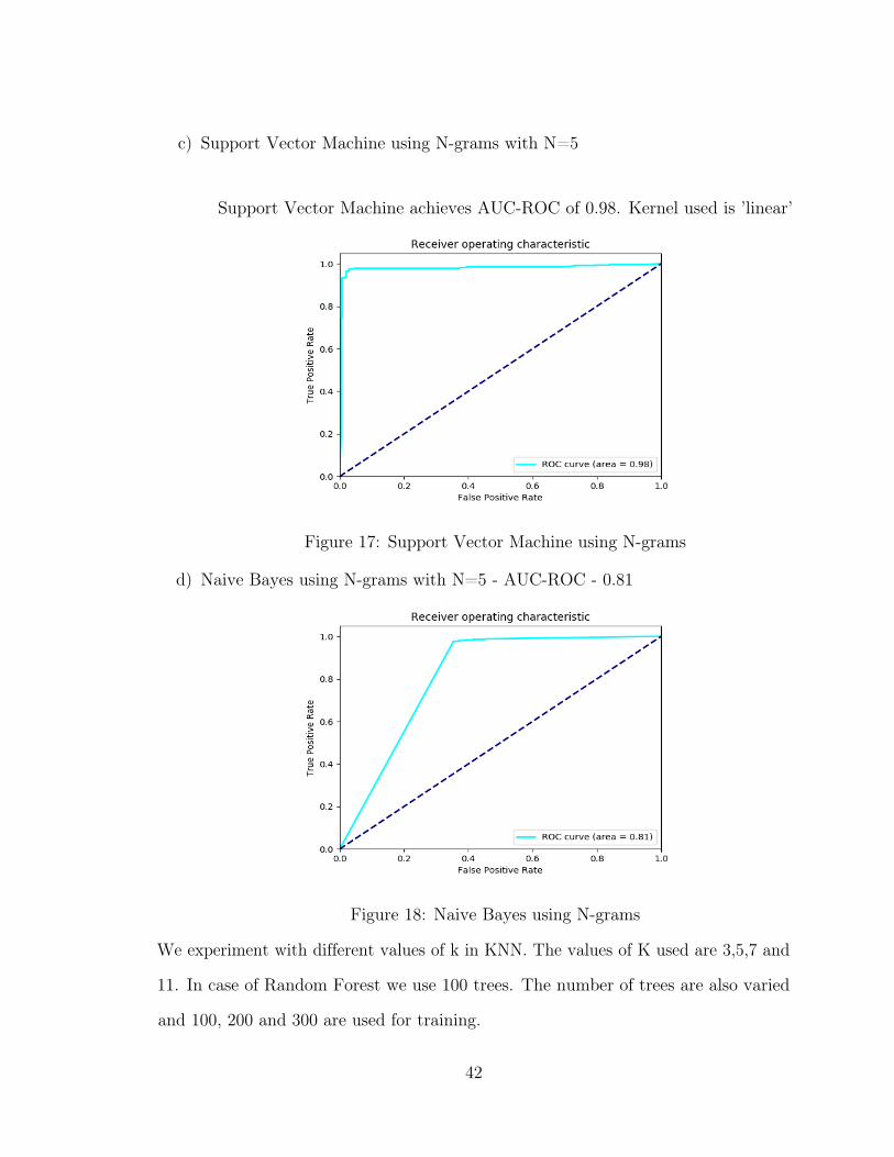
c) Support Vector Machine using N-grams with N=5

Support Vector Machine achieves AUC-ROC of 0.98. Kernel used is ’linear’

Figure 17: Support Vector Machine using N-grams

d) Naive Bayes using N-grams with N=5 - AUC-ROC - 0.81

Figure 18: Naive Bayes using N-grams

We experiment with different values of k in KNN. The values of K used are 3,5,7 and

11. In case of Random Forest we use 100 trees. The number of trees are also varied

and 100, 200 and 300 are used for training.

42

The second approach is to use HMM to train on morphed sequences. We use

two HMM models in which one we train on a malware opcode sequence from 40,000

files and the other one we train on morphed malware opcode sequences from 40,000

morphed samples. The HMM specifications used are N = [2,3,5], M = 26, iterations

= 1000 and random row stochastic values for A, B and 𝜋 matrix. The HMM is run

on T = 50,000 opcode sequences from the two sequence files. The two HMM models

provide final A, B and 𝜋 matrix for both type of sequence files. Thus, as explained in

section 6.3.2, we merge the A, B and 𝜋 matrix to get a feature vector and we can run

classification on them.

After we receive feature vectors, it becomes a machine learning classification

problem. Thus we can apply standard machine learning techniques to classify on

the basis of the feature vectors. The following experiments are performed with N=2.

Experiments with varied values of N is presented in Appendix A

a) Random Forest using HMM vectors with N=2

Random Forest achieves the AUC-ROC of 0.99 with 100 trees in the forest.

Figure 19: Random Forest using HMM vectors

43

b) K Nearest Neighbours using HMM vectors with N=2

K Nearest Neighbors achieves AUC-ROC of 0.86. This is with value of K = 5

Figure 20: K Nearest Neighbours using HMM vectors

c) Support Vector Machine using HMM vectors with N=2

Support Vector Machine achieves AUC-ROC of 0.97. Kernel used is ’linear’

Figure 21: Support Vector Machine using HMM vectors

44

d) Naive Bayes using HMM vectors with N=2

Naive Bayes performs the worst with AUC-ROC as 0.88

Figure 22: Naive Bayes using HMM vectors

45

CHAPTER 8

Conclusion and Future Work

In this project, the aim was to detect metamorphic malware. We first introduced

the metamorphic engine to morph the JavaScript based code. The techniques used are

variable renaming, function reordering, instruction reordering, dead code insertion and

instruction substitution. These techniques when used together provide great levels of

code obfuscation. As discussed in the project, major anti-virus software programs use

signature based detection for detecting malwares which would eventually fail because

of code obfuscation. We are using NodeJS esprima and escodegen to convert the

code to and from Abstract Syntax Tree of that code. Abstract Syntax Trees are used

to morph the code by changing the logical structure using the techniques mentioned

above. With this we achieve a 21.95% drop from 95.25% to 73.3% when using SVM as

a malware detector with max accuracy drop of 37.3% while using K-Nearest Neighbor.

The next part of the project is to detect metamorphic code. Since we have the

source code, we cannot directly compare the source files to classify malware files. Thus,

we converted it into meaningful feature vectors. First approach was to use N-gram

feature vectors on bytecode files of those JavaScript source codes. We use Rhino

JavaScript engine to convert JavaScript code to JAVA bytecodes. The bytecode file

is then used to extract opcodes from. The sequence of opcode symbols are important

in the experiment rather than the entire source file. We remove opcodes from all the

files and place it in a sequence file where every line of opcodes represents a file. Thus

for detecting metamorphic malware, we have sequence files for malware as well as

morphed malware. We then take out N-gram frequency features and apply machine

learning models like SVM, Random Forest, Naive Bayes and K Nearest Neighbor.

From this, Support Vector Machine gives the best accuracy of 97% and AUC-ROC of

46

0.98.

We also experimented using HMM feature vectors. In the same sequence files for

malware and morphed malware, instead of the opcodes, we represent the opcodes

in numeric format. We calculate the frequency of the opcodes in the sequence files

and keep only top 26 opcode symbols. Using N = [2,3,5], M = 26, T = 50,000 and

iterations = 1000 we train the HMM model and extract A, B and 𝜋 matrix for each

HMM output for 50,000 opcodes. These matrices are merged together and form a

feature vector for classification models. After we get the feature vectors of 1 × 56

dimension. We use it for classification with the same machine learning models used

for N-gram feature vectors. Using HMM feature vectors, SVM performs the best with

96.8% accuracy with KNN being on the second position with 96.38% accuracy.

The main purpose of these approaches is that if a malware file is morphed, it can

act as benign in most of the malware detectors. Thus, to catch such type of malware

we have a metamorphic detector which would determine that there is some morphing

involved in the file and needs to be scrutinized again. Thus, we mark such files as

a potential candidate of being a malware. As part of future work, we can combine

this approach along with dynamic analysis where we run a sandbox to understand

the behavior of the files and detect malware files easily. As we followed a two-fold

process by degrading the accuracy of a detector thereby increasing accuracy for morph

code detection, we could experiment in the field of Malware GAN [45] where there are

two neural networks that compete with each other to improve metamorphic malware

creation. One neural network aims to create newer versions of malware to beat the

other network which tries to differentiate between two classes. It will be an interesting

field of research. We could also try to detect Transcriptase [46] malware.

47

LIST OF REFERENCES

[1] M. Stamp, ‘‘A revealing introduction to Hidden Markov Models,’’ Department ofComputer Science San Jose State University, pp. 26--56, 2004.

[2] M. Statistics, ‘‘Trends report| av-test,’’ 2017. [Online]. Avail-able: https://www.av-test.org/fileadmin/pdf/security_report/AV-TEST_Security_Report_2017-2018.pdf

[3] A. Prabhu, ‘‘Working of rhino.’’ [Online]. Available: http://www.quora.com/JavaScript-programming-language/How-does-a-JavaScript-engine-work

[4] ‘‘Greg zemskov.’’ [Online]. Available: https://www.plesk.com/blog/product-technology/hidden-website-threats-deal-with-site-malware

[5] Wikipedia contributors, ‘‘Sony bmg copy protection rootkit scandal ---Wikipedia, the free encyclopedia,’’ 2019, [Online; accessed 18-April-2019].[Online]. Available: https://en.wikipedia.org/w/index.php?title=Sony_BMG_copy_protection_rootkit_scandal&oldid=881854109

[6] ‘‘Panda security (n.d.). virus, worms, trojans and backdoors: Other harmfulrelatives of viruses.’’ [Online]. Available: http://www.pandasecurity.com/homeusers-cms3/security-info/about-malware/generalconcep

[7] C. Annachhatre, T. H. Austin, and M. Stamp, ‘‘Hidden markov models formalware classification,’’ Journal of Computer Virology and Hacking Techniques,vol. 11, no. 2, pp. 59--73, 2015.

[8] J. Aycock, Computer Viruses and Malware. Springer US, 2006.

[9] M. Musale, T. H. Austin, and M. Stamp, ‘‘Hunting for metamorphic javascriptmalware,’’ Journal of Computer Virology and Hacking Techniques, vol. 11, no. 2,pp. 89--102, 2015.

[10] X. Li, P. K. Loh, and F. Tan, ‘‘Mechanisms of polymorphic and metamorphicviruses,’’ in 2011 European intelligence and security informatics conference.IEEE, 2011, pp. 149--154.

[11] B. B. Rad, M. Masrom, and S. Ibrahim, ‘‘Camouflage in malware: from encryptionto metamorphism,’’ International Journal of Computer Science and NetworkSecurity, vol. 12, no. 8, pp. 74--83, 2012.

48

[12] A. S. Bist, ‘‘Detection of metamorphic viruses: A survey,’’ in 2014 Interna-tional Conference on Advances in Computing, Communications and Informatics(ICACCI). IEEE, 2014, pp. 1559--1565.

[13] I. You and K. Yim, ‘‘Malware obfuscation techniques: A brief survey,’’ in 2010International conference on broadband, wireless computing, communication andapplications. IEEE, 2010, pp. 297--300.

[14] V. S. Koganti, L. K. Galla, and N. Nuthalapati, ‘‘Internet worms and its de-tection,’’ in 2016 International Conference on Control, Instrumentation, Com-munication and Computational Technologies (ICCICCT). IEEE, 2016, pp.64--73.

[15] Z. Bazrafshan, H. Hashemi, S. M. H. Fard, and A. Hamzeh, ‘‘A survey onheuristic malware detection techniques,’’ in The 5th Conference on Informationand Knowledge Technology. IEEE, 2013, pp. 113--120.

[16] M. Stamp, Information security: principles and practice. John Wiley & Sons,2011.

[17] W. Liu, P. Ren, K. Liu, and H.-x. Duan, ‘‘Behavior-based malware analysisand detection,’’ in 2011 First International Workshop on Complexity and DataMining. IEEE, 2011, pp. 39--42.

[18] G. Hăjmăşan, A. Mondoc, and O. Creț, ‘‘Dynamic behavior evaluation formalware detection,’’ in 2017 5th International Symposium on Digital Forensicand Security (ISDFS). IEEE, 2017, pp. 1--6.

[19] S. Priyadarshi, ‘‘Metamorphic detection via emulation,’’ 2011.

[20] I. Firdausi, A. Erwin, A. S. Nugroho, et al., ‘‘Analysis of machine learningtechniques used in behavior-based malware detection,’’ in 2010 second interna-tional conference on advances in computing, control, and telecommunicationtechnologies. IEEE, 2010, pp. 201--203.

[21] W.-J. Li, K. Wang, S. J. Stolfo, and B. Herzog, ‘‘Fileprints: Identifying filetypes by n-gram analysis,’’ in Proceedings from the Sixth Annual IEEE SMCInformation Assurance Workshop. IEEE, 2005, pp. 64--71.

[22] T. H. Austin, E. Filiol, S. Josse, and M. Stamp, ‘‘Exploring hidden markov modelsfor virus analysis: a semantic approach,’’ in 2013 46th Hawaii InternationalConference on System Sciences. IEEE, 2013, pp. 5039--5048.

[23] A. Krogh, ‘‘An introduction to hidden markov models for biological sequences.’’

49

[24] M. G. Schultz, E. Eskin, F. Zadok, and S. J. Stolfo, ‘‘Data mining methods fordetection of new malicious executables,’’ in Proceedings 2001 IEEE Symposiumon Security and Privacy. S&P 2001. IEEE, 2001, pp. 38--49.

[25] F. Rezaei, M. K. Nezhad, S. Rezaei, and A. Payandeh, ‘‘Detecting encryptedmetamorphic viruses by hidden markov models,’’ in 2014 11th InternationalConference on Fuzzy Systems and Knowledge Discovery (FSKD). IEEE, 2014,pp. 973--977.

[26] S. M. Sridhara and M. Stamp, ‘‘Metamorphic worm that carries its own morphingengine,’’ Journal of Computer Virology and Hacking Techniques, vol. 9, no. 2,pp. 49--58, 2013.

[27] G. Blanc, D. Miyamoto, M. Akiyama, and Y. Kadobayashi, ‘‘Characterizingobfuscated javascript using abstract syntax trees: Experimenting with mali-cious scripts,’’ in 2012 26th International Conference on Advanced InformationNetworking and Applications Workshops. IEEE, 2012, pp. 344--351.

[28] Wikipedia contributors, ‘‘Abstract syntax tree --- Wikipedia, the freeencyclopedia,’’ 2019, [Online; accessed 18-April-2019]. [Online]. Available: https://en.wikipedia.org/w/index.php?title=Abstract_syntax_tree&oldid=891491683

[29] J. Picado, ‘‘Abstract syntax trees on javascript.’’ [Online]. Available: https://medium.com/@jotadeveloper/abstract-syntax-trees-on-javascript-534e33361fc7

[30] A. Hidayat, ‘‘Esprima npm.’’ [Online]. Available: https://www.npmjs.com/package/esprima

[31] Y. Suzuki, ‘‘Escodegen npm.’’ [Online]. Available: https://www.npmjs.com/package/escodegen

[32] V. Raychev, P. Bielik, M. Vechev, and A. Krause, ‘‘Learning programs from noisydata,’’ in ACM SIGPLAN Notices, vol. 51, no. 1. ACM, 2016, pp. 761--774.

[33] H. Petrak, ‘‘github repo: javascript-malware-collection.’’ [Online]. Available:https://github.com/HynekPetrak/javascript-malware-collection

[34] Oracle, ‘‘Jvm instruction set.’’ [Online]. Available: https://docs.oracle.com/javase/specs/jvms/se7/html/jvms-6.html

[35] S. Ranveer and S. Hiray, ‘‘Comparative analysis of feature extraction methods ofmalware detection,’’ International Journal of Computer Applications, vol. 120,no. 5, 2015.

[36] J. Z. Kolter and M. A. Maloof, ‘‘Learning to detect and classify maliciousexecutables in the wild,’’ Journal of Machine Learning Research, vol. 7, no. Dec,pp. 2721--2744, 2006.

50

[37] I. Santos, Y. K. Penya, J. Devesa, and P. G. Bringas, ‘‘N-grams-based filesignatures for malware detection.’’ ICEIS (2), vol. 9, pp. 317--320, 2009.

[38] S. Jain and Y. K. Meena, ‘‘Byte level n--gram analysis for malware detection,’’ inInternational Conference on Information Processing. Springer, 2011, pp. 51--59.

[39] Z. Fuyong and Z. Tiezhu, ‘‘Malware detection and classification based on n-gramsattribute similarity,’’ in 2017 IEEE International Conference on ComputationalScience and Engineering (CSE) and IEEE International Conference on Embeddedand Ubiquitous Computing (EUC), vol. 1. IEEE, 2017, pp. 793--796.

[40] A. Singh, N. Thakur, and A. Sharma, ‘‘A review of supervised machine learningalgorithms,’’ in 2016 3rd International Conference on Computing for SustainableGlobal Development (INDIACom). IEEE, 2016, pp. 1310--1315.

[41] H. Zhang and D. Li, ‘‘Naïve bayes text classifier,’’ in 2007 IEEE InternationalConference on Granular Computing (GRC 2007). IEEE, 2007, pp. 708--708.

[42] J. M. (https://stats.stackexchange.com/users/44603/jeffm), ‘‘Training ahidden markov model, multiple training instances,’’ Cross Validated,uRL:https://stats.stackexchange.com/q/95553 (version: 2014-04-29). [Online].Available: https://stats.stackexchange.com/q/95553

[43] A. P. Bradley, ‘‘The use of the area under the roc curve in the evaluation ofmachine learning algorithms,’’ Pattern recognition, vol. 30, no. 7, pp. 1145--1159,1997.

[44] S. Choudhary and M. D. Vidyarthi, ‘‘A simple method for detection of meta-morphic malware using dynamic analysis and text mining,’’ Procedia ComputerScience, vol. 54, pp. 265--270, 2015.

[45] W. Hu and Y. Tan, ‘‘Generating adversarial malware examples for black-boxattacks based on gan,’’ arXiv preprint arXiv:1702.05983, 2017.

[46] F. Di Troia, C. A. Visaggio, T. H. Austin, and M. Stamp, ‘‘Advanced transcriptasefor javascript malware,’’ in 2016 11th International Conference on Malicious andUnwanted Software (MALWARE). IEEE, 2016, pp. 1--8.

51

APPENDIX

Appendix AA.1 HMM for detecting metamorphic malware with N=3, M=26,

T=50,000

(a) (b)

(c) (d)

Figure A.23: HMM with N=3, M=26, T=50,000 (a) Naïve Bayes; (b) K-NearestNeighbor; (c) Support Vector Machine; (d) Random Forest

52

A.2 HMM for detecting metamorphic malware with N=5, M=26,T=50,000

(a) (b)

(c) (d)

Figure A.24: HMM with N=5, M=26, T=50,000 (a) Naïve Bayes; (b) K-NearestNeighbor; (c) Support Vector Machine; (d) Random Forest

53

A.3 K-Nearest Neighbors for metamorphic malware detection using N-gram features with K=[3,7,11]

(a) (b)

(c)

Figure A.25: N-grams with K-Nearest Neighbor (KNN) as classifier (a) KNN withN=3; (b) KNN with N=7; (c) KNN with N=11;

54

A.4 Random Forest for metamorphic malware detection using N-gramfeatures with Trees=[200,300]

(a) (b)

Figure A.26: N-grams with Random Forest as classifier (a) Random Forest withTrees=200; (b) Random Forest with Trees=300;

55