Matlab 2: 2D and 3D Graph | NMSL@NTHU

Matlab2:2Dand3DGraph

Cheng-HsinHsuNa#onalTsingHuaUniversity

DepartmentofComputerScience

SlidesarebasedonthematerialsfromProf.RogerJang

CS3330Scien@ficCompu@ng 1

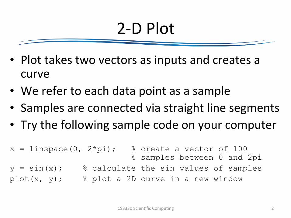
2-DPlot

•  Plottakestwovectorsasinputsandcreatesacurve

•  Werefertoeachdatapointasasample•  Samplesareconnectedviastraightlinesegments•  Trythefollowingsamplecodeonyourcomputer x = linspace(0, 2*pi); % create a vector of 100 % samples between 0 and 2pi

y = sin(x); % calculate the sin values of samples plot(x, y); % plot a 2D curve in a new window


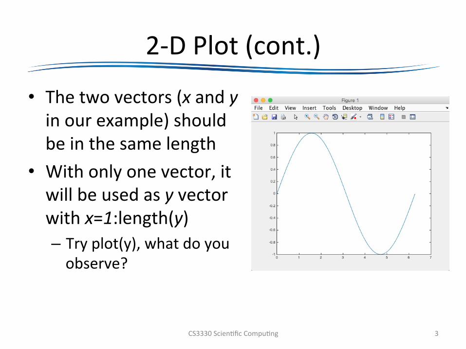
2-DPlot(cont.)

•  Thetwovectors(xandyinourexample)shouldbeinthesamelength

•  Withonlyonevector,itwillbeusedasyvectorwithx=1:length(y)–  Tryplot(y),whatdoyouobserve?


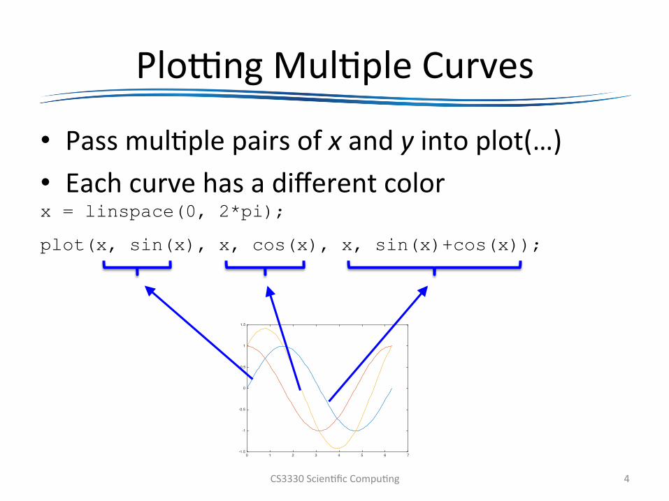
PloQngMul@pleCurves

•  Passmul@plepairsofxandyintoplot(…)•  Eachcurvehasadifferentcolor x = linspace(0, 2*pi);

plot(x, sin(x), x, cos(x), x, sin(x)+cos(x));


0 1 2 3 4 5 6 7-1.5

-1

-0.5

0

0.5

1

1.5

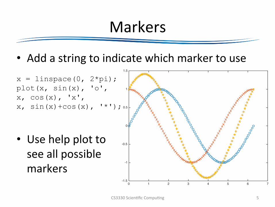
Markers

•  Addastringtoindicatewhichmarkertouse x = linspace(0, 2*pi); plot(x, sin(x), 'o', x, cos(x), 'x', x, sin(x)+cos(x), '*');

•  Usehelpplottoseeallpossiblemarkers


0 1 2 3 4 5 6 7-1.5

-1

-0.5

0

0.5

1

1.5

0 5 10 15 20 25 30 35 40 45 50-8

-6

-4

-2

0

2

4

6

8

10

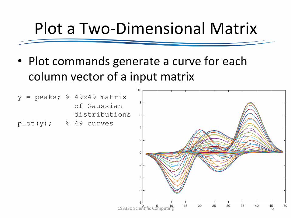
PlotaTwo-DimensionalMatrix

•  Plotcommandsgenerateacurveforeachcolumnvectorofainputmatrix

y = peaks; % 49x49 matrix

of Gaussian distributions

plot(y); % 49 curves


-8 -6 -4 -2 0 2 4 6 8 10-8

-6

-4

-2

0

2

4

6

8

10

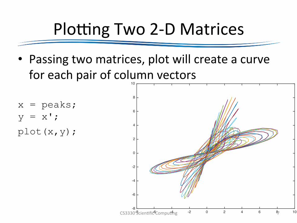
PloQngTwo2-DMatrices•  Passingtwomatrices,plotwillcreateacurveforeachpairofcolumnvectors

x = peaks; y = x';

plot(x,y);


Conven@onsinMatlab

•  Matlabtreatseach2-Dmatrixasasubsetofcolumnvectors

•  Passinga2-Dmatrixtoafunc@on,suchasmax,min,andmean),thefunc@onitera@velyprocesseseachcolumnvector

>> mean(magic(5))

ans =

13 13 13 13 13


PloQngComplexNumbers

•  Foravectorofcomplexnumbers,plot(z)isthesameasplot(real(z),imag(z))

x = randn(30); % 30×30 random numbers (Gaussian)z = eig(x); % calculate eigenvalues plot(z, 'o') grid on % add grids


PloQngComplexNumbers(cont.)

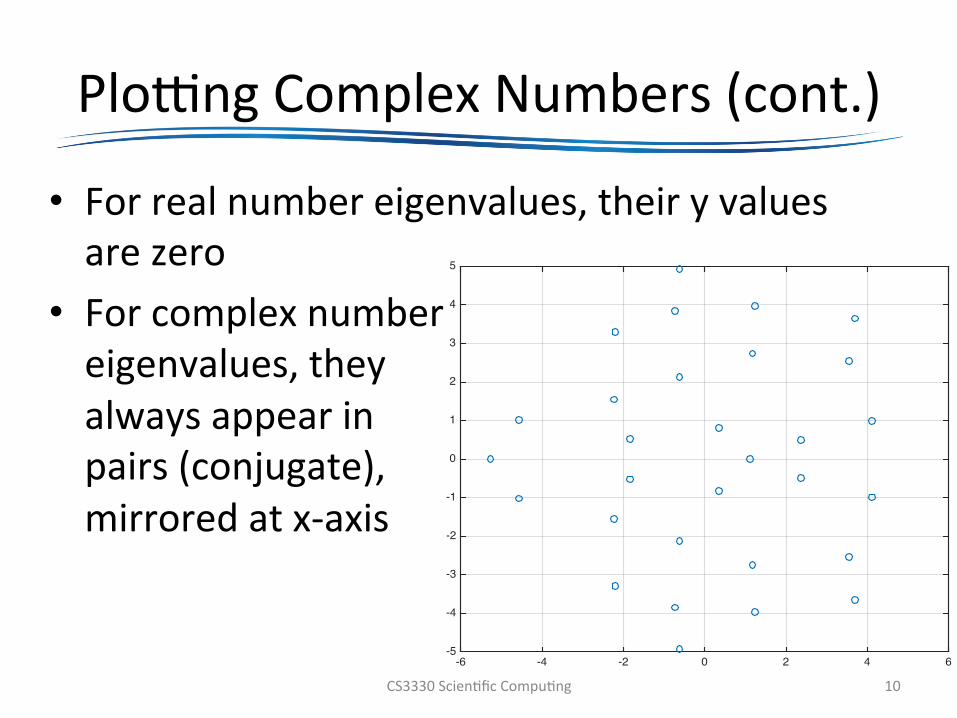
•  Forrealnumbereigenvalues,theiryvaluesarezero

•  Forcomplexnumbereigenvalues,theyalwaysappearinpairs(conjugate),mirroredatx-axis


-6 -4 -2 0 2 4 6-5

-4

-3

-2

-1

0

1

2

3

4

5

More2DPlotCommands

•  plot:bothxandyaxesarelinear•  loglog:bothxandyaxesarelogarithmic•  semilogx:xaxisislogarithmic,whileyaxisislinear•  semilogy:yaxisislogarithmic,whilexaxisislinear•  plotyy:createtwoyaxes(leaandright)


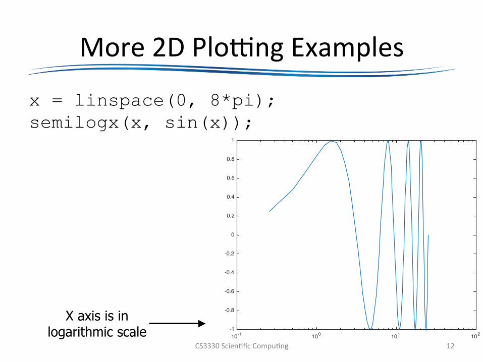
More2DPloQngExamples

x = linspace(0, 8*pi);semilogx(x, sin(x));

CS3330Scien@ficCompu@ng 1210-1 100 101 102-1

-0.8

-0.6

-0.4

-0.2

0

0.2

0.4

0.6

0.8

1

X axis is in logarithmic scale

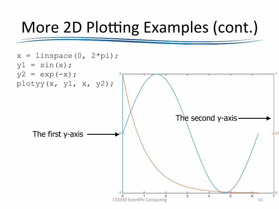
More2DPloQngExamples(cont.)x = linspace(0, 2*pi); y1 = sin(x); y2 = exp(-x); plotyy(x, y1, x, y2);

CS3330Scien@ficCompu@ng 130 1 2 3 4 5 6 7

-1

0

1

0

0.5

1

The first y-axis

The second y-axis

ControltheCurves

•  Recallthatweassignmarkerstocurvesusingastring

•  Syntax:plot(x,y,‘CLM’)– C:colorofthecurveßred,blue,andsoon– L:linestylesßsolid,dash,dots,andetc.– M:markerßcircle,asterisk,diamond,andsoon


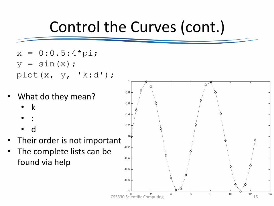
ControltheCurves(cont.)x = 0:0.5:4*pi; y = sin(x); plot(x, y, 'k:d');


-1

-0.8

-0.6

-0.4

-0.2

0

0.2

0.4

0.6

0.8

1

•  Whatdotheymean?•  k•  :•  d

•  Theirorderisnotimportant•  Thecompletelistscanbe

foundviahelp

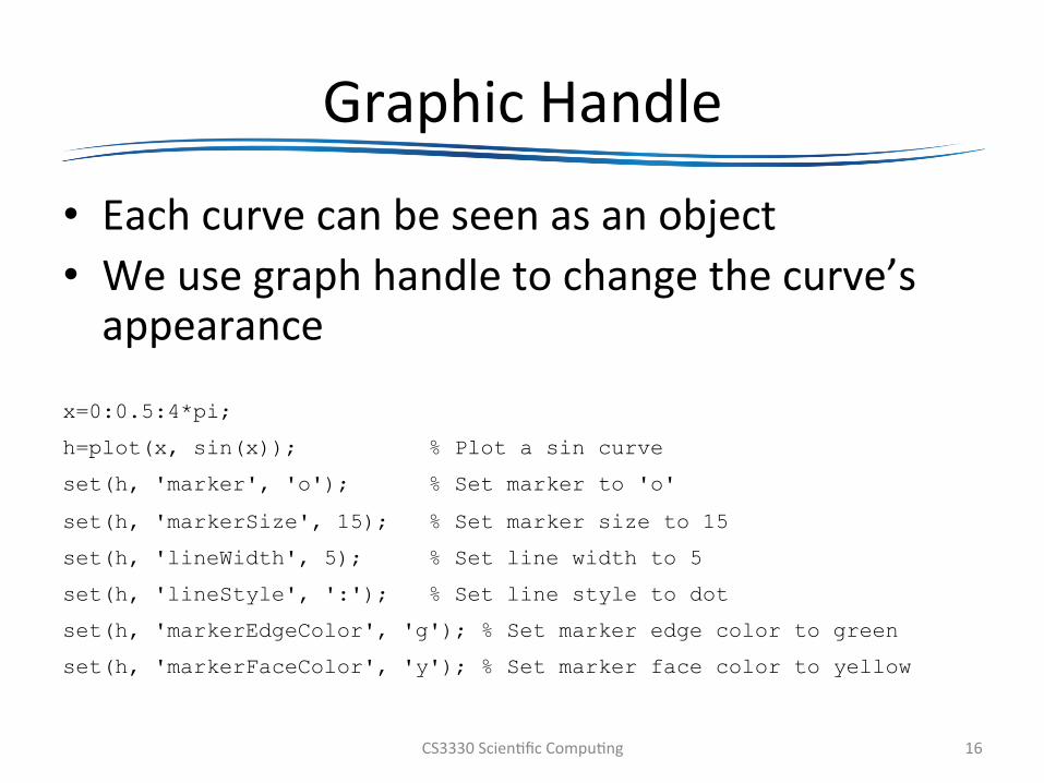
GraphicHandle

•  Eachcurvecanbeseenasanobject•  Weusegraphhandletochangethecurve’sappearance

x=0:0.5:4*pi;

h=plot(x, sin(x)); % Plot a sin curve

set(h, 'marker', 'o'); % Set marker to 'o'

set(h, 'markerSize', 15); % Set marker size to 15

set(h, 'lineWidth', 5); % Set line width to 5

set(h, 'lineStyle', ':'); % Set line style to dot

set(h, 'markerEdgeColor', 'g'); % Set marker edge color to green

set(h, 'markerFaceColor', 'y'); % Set marker face color to yellow


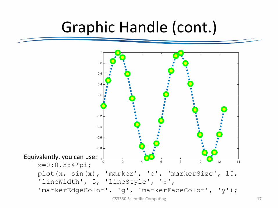
GraphicHandle(cont.)


0 2 4 6 8 10 12 14-1

-0.8

-0.6

-0.4

-0.2

0

0.2

0.4

0.6

0.8

1

Equivalently,youcanuse:x=0:0.5:4*pi; plot(x, sin(x), 'marker', 'o', 'markerSize', 15, 'lineWidth', 5, 'lineStyle', ':', 'markerEdgeColor', 'g', 'markerFaceColor', 'y');

Adjus@ngtheRangesofAxes

•  Matlabassignsdefaultxlimandylimheuris@cally

•  OrseQngthemmanually– axis([xmin,xmax,ymin,ymax])– xlim([xmin,xmax])– ylim([ymin,ymax])


Adjus@ngtheRangesofAxes(cont.)

x = 0:0.1:4*pi; y = sin(x); plot(x, y); axis([-inf, inf, 0, 1]); % inf means the extreme values of samples

CS3330Scien@ficCompu@ng 190 2 4 6 8 10 120

0.1

0.2

0.3

0.4

0.5

0.6

0.7

0.8

0.9

1

Adjus@ngTicksandGridsx = 0:0.1:4*pi; plot(x, sin(x)+sin(3*x)) set(gca, 'ytick', [-1 -0.3 0.1 1]); grid on; % gca returns the current axes, as an object


-1

-0.3

0.1

1

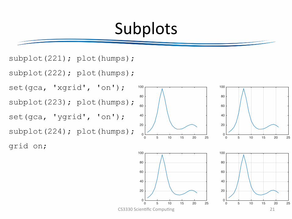
Subplotssubplot(221); plot(humps);

subplot(222); plot(humps);

set(gca, 'xgrid', 'on');


set(gca, 'ygrid', 'on');


grid on;


0 5 10 15 20 250

20

40

60

80

100

0 5 10 15 20 250

20

40

60

80

100

0 5 10 15 20 250

20

40

60

80

100

0 5 10 15 20 250

20

40

60

80

100

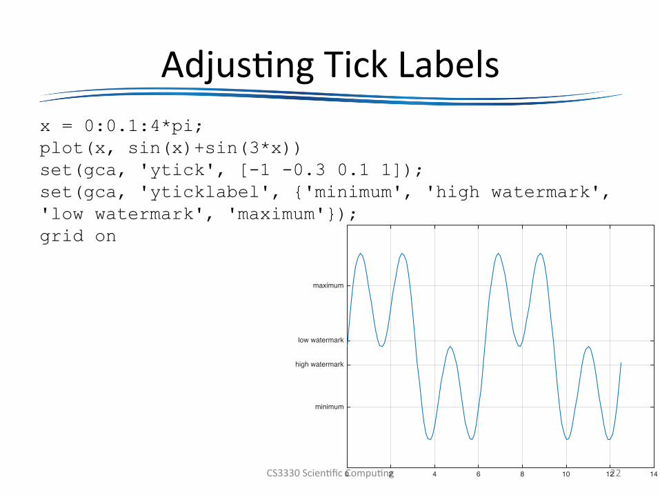
Adjus@ngTickLabelsx = 0:0.1:4*pi; plot(x, sin(x)+sin(3*x)) set(gca, 'ytick', [-1 -0.3 0.1 1]); set(gca, 'yticklabel', {'minimum', 'high watermark', 'low watermark', 'maximum'}); grid on


minimum

high watermark

low watermark

maximum

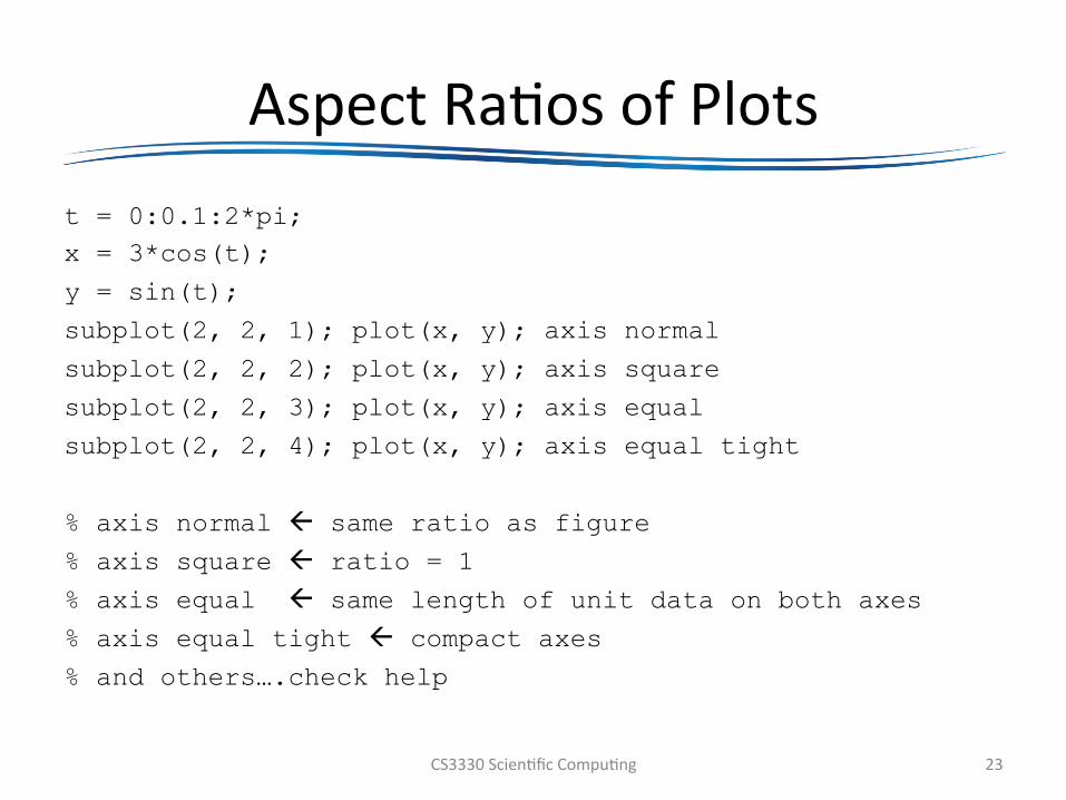
AspectRa@osofPlotst = 0:0.1:2*pi; x = 3*cos(t);

y = sin(t);

subplot(2, 2, 1); plot(x, y); axis normal

subplot(2, 2, 2); plot(x, y); axis square

subplot(2, 2, 3); plot(x, y); axis equal

subplot(2, 2, 4); plot(x, y); axis equal tight

% axis normal ß same ratio as figure

% axis square ß ratio = 1

% axis equal ß same length of unit data on both axes

% axis equal tight ß compact axes % and others….check help


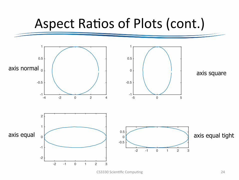
AspectRa@osofPlots(cont.)


-4 -2 0 2 4-1

-0.5

0

0.5

1

-5 0 5-1

-0.5

0

0.5

1

-2 -1 0 1 2 3

-2

-1

0

1

2

-2 -1 0 1 2 3

-0.50

0.5

axis normal

axis equal

axis square

axis equal tight

Addi@onalControls

•  colordefwhiteßwhiteaxes’background•  colordefblack•  gridon•  gridoff•  boxonßboundingboxoftheaxes•  boxoff


CommandstoAddDescrip@veTexts

•  @tle:figure@tle•  xlabel:x-axistext•  ylabel:y-axistext•  zlabel:z-axistext•  legend:descrip@onsofindividualcurves•  text:annota@ons•  gtext:annota@onsplacedbymouseclicks


ExampleofTexts

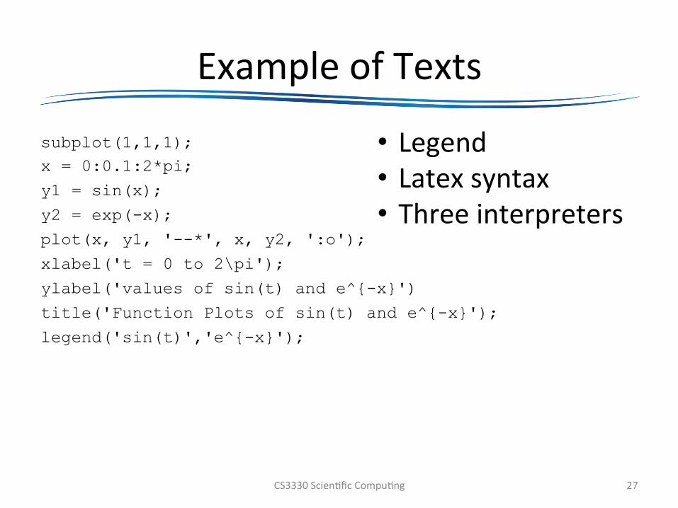
subplot(1,1,1); x = 0:0.1:2*pi;

y1 = sin(x);

y2 = exp(-x);

plot(x, y1, '--*', x, y2, ':o');

xlabel('t = 0 to 2\pi');

ylabel('values of sin(t) and e^{-x}')

title('Function Plots of sin(t) and e^{-x}');

legend('sin(t)','e^{-x}');


•  Legend•  Latexsyntax•  Threeinterpreters

ExampleofTexts(cont.)

CS3330Scien@ficCompu@ng 28t = 0 to 2:

0 1 2 3 4 5 6 7

valu

es o

f sin

(t) a

nd e

-x

-1

-0.8

-0.6

-0.4

-0.2

0

0.2

0.4

0.6

0.8

1Function Plots of sin(t) and e-x

sin(t)e -x

0 1 2 3 4 5 6 7-1

-0.8

-0.6

-0.4

-0.2

0

0.2

0.4

0.6

0.8

1

A sin(:/4) = 0.707

cos(5:/4) = -0.707!

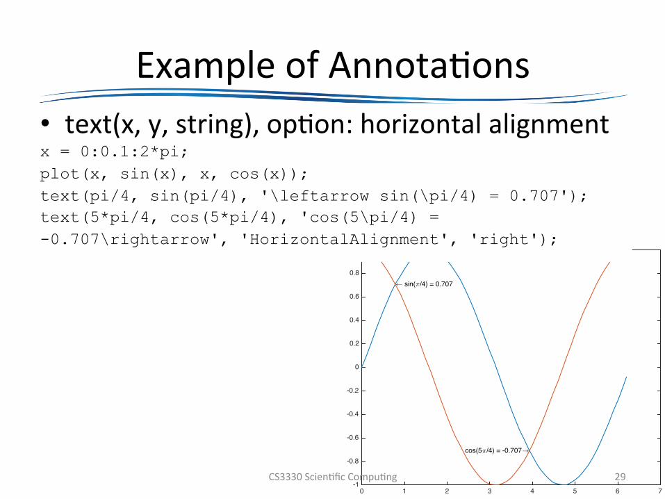
ExampleofAnnota@ons•  text(x,y,string),op@on:horizontalalignmentx = 0:0.1:2*pi; plot(x, sin(x), x, cos(x)); text(pi/4, sin(pi/4), '\leftarrow sin(\pi/4) = 0.707'); text(5*pi/4, cos(5*pi/4), 'cos(5\pi/4) = -0.707\rightarrow', 'HorizontalAlignment', 'right');


ExampleofAnnota@ons(cont.)

•  gtext(string)ßtryitonyourcomputer•  Aaerissuingthiscommand,usemouseclicktoplacethestring

•  Onlyworksin2-Dgraphs


SomeOther2-DGraphCommands

•  errorbar:curveswitherrorintervals•  fplot,ezplot:ploQngwithadap@vexsampling•  polar,ezpolar:ploQngwithpolarcoordinates•  hist:histogram•  rose:anglehistogram


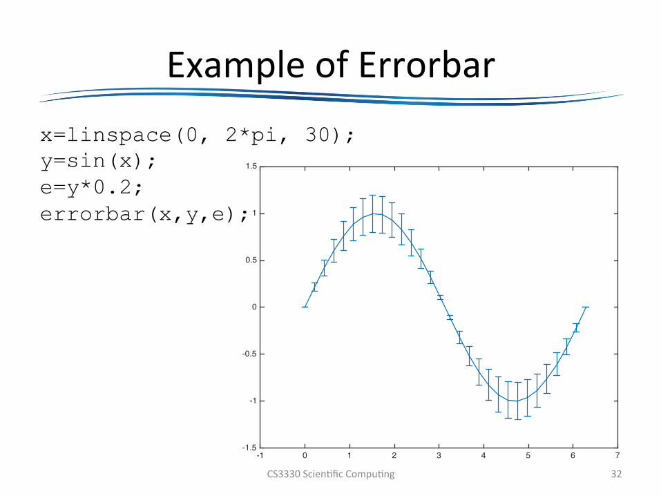
ExampleofErrorbarx=linspace(0, 2*pi, 30); y=sin(x); e=y*0.2; errorbar(x,y,e);


-1 0 1 2 3 4 5 6 7-1.5

-1

-0.5

0

0.5

1

1.5

Exampleoffplot•  Problemwithx=0.02:0.01:0.4; y=sin(1./x); plot(x,y)?

•  fplot('sin(1/x)', [0.02, 0.4])ßadap@velypicksamples

CS3330Scien@ficCompu@ng 330.05 0.1 0.15 0.2 0.25 0.3 0.35 0.4-1

-0.8

-0.6

-0.4

-0.2

0

0.2

0.4

0.6

0.8

1

More samples in this area

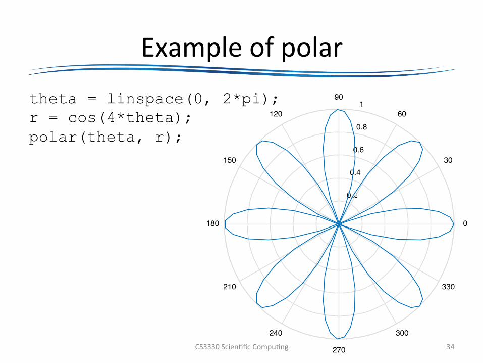
Exampleofpolartheta = linspace(0, 2*pi); r = cos(4*theta); polar(theta, r);


0.2

0.4

0.6

0.8

1

30

210

60

240

90

270

120

300

150

330

180 0

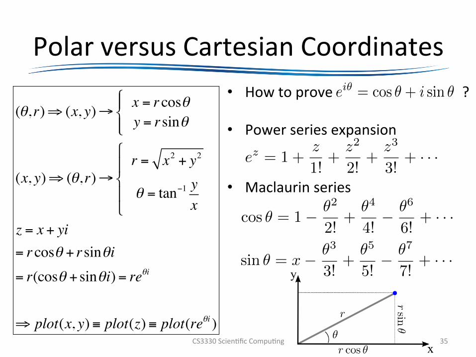
PolarversusCartesianCoordinates


(θ, r)⇒ (x, y)→ x = rcosθy = rsinθ

⎧⎨⎪

⎩⎪

(x, y)⇒ (θ, r)→r = x2 + y2

θ = tan−1 yx

⎧

⎨⎪

⎩⎪

z = x + yi= rcosθ + rsinθi= r(cosθ + sinθi) = reθi

⇒ plot(x, y) ≡ plot(z) ≡ plot(reθi )

•  Howtoprove?

•  Powerseriesexpansion

•  Maclaurinseries

ei✓ = cos ✓ + i sin ✓

ez = 1 +z

1!+

z2

2!+

z3

3!+ · · ·

cos ✓ = 1� ✓2

2!

+

✓4

4!

� ✓6

6!

+ · · ·

sin ✓ = x� ✓

3

3!+

✓

5

5!� ✓

7

7!+ · · ·

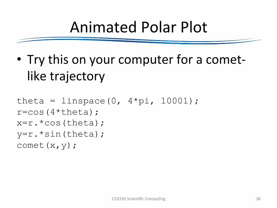
AnimatedPolarPlot

•  Trythisonyourcomputerforacomet-liketrajectory

theta = linspace(0, 4*pi, 10001); r=cos(4*theta); x=r.*cos(theta); y=r.*sin(theta); comet(x,y);


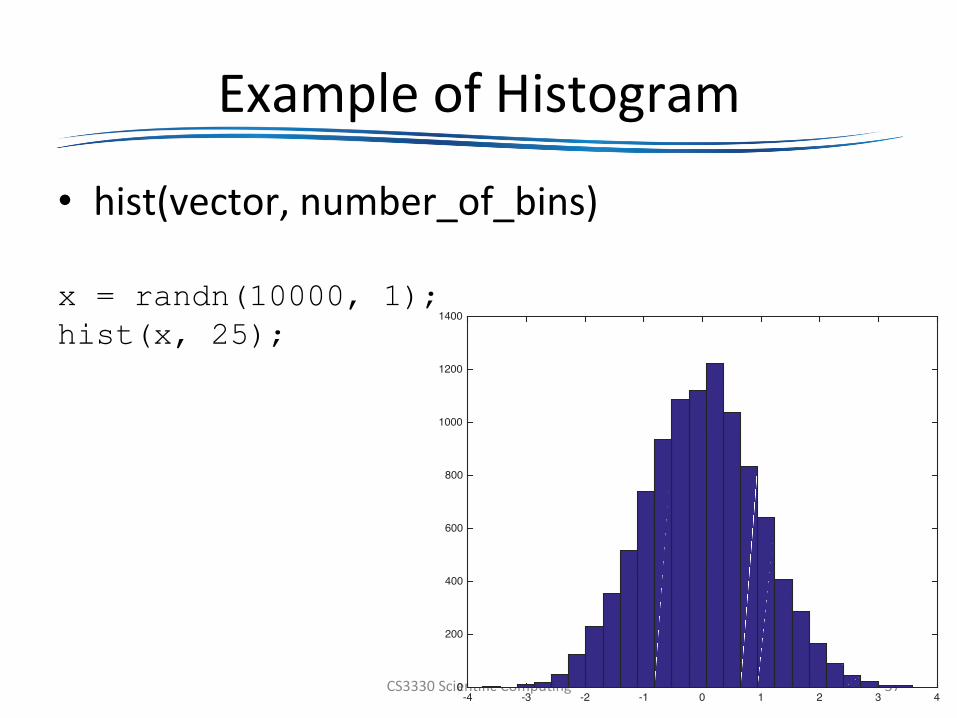
ExampleofHistogram

•  hist(vector,number_of_bins)x = randn(10000, 1); hist(x, 25);

CS3330Scien@ficCompu@ng 37-4 -3 -2 -1 0 1 2 3 40

200

400

600

800

1000

1200

1400

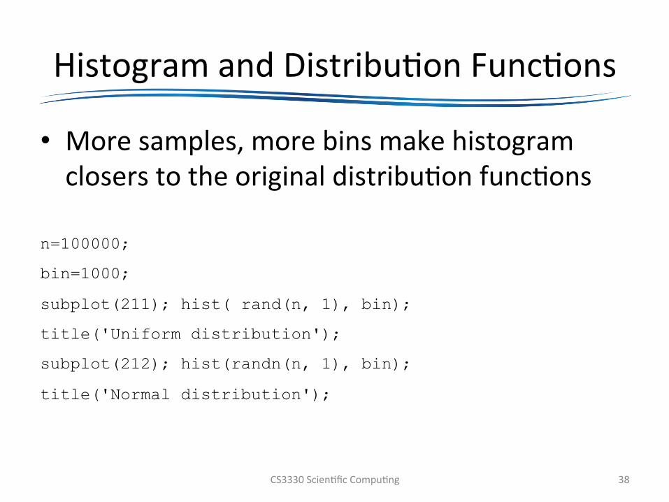
HistogramandDistribu@onFunc@ons

•  Moresamples,morebinsmakehistogramcloserstotheoriginaldistribu@onfunc@ons

n=100000;

bin=1000;

subplot(211); hist( rand(n, 1), bin);

title('Uniform distribution');

subplot(212); hist(randn(n, 1), bin);

title('Normal distribution');


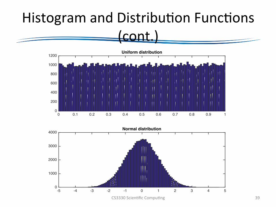
HistogramandDistribu@onFunc@ons(cont.)


0 0.1 0.2 0.3 0.4 0.5 0.6 0.7 0.8 0.9 10

200

400

600

800

1000

1200Uniform distribution

-5 -4 -3 -2 -1 0 1 2 3 4 50

1000

2000

3000

4000Normal distribution

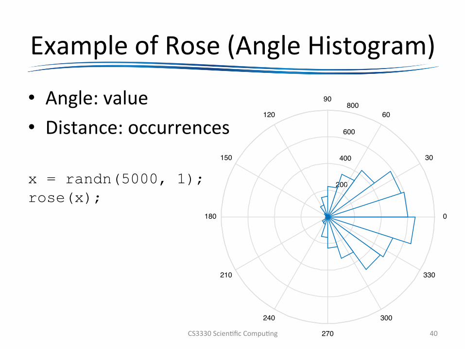
ExampleofRose(AngleHistogram)

•  Angle:value•  Distance:occurrences

x = randn(5000, 1); rose(x);


200

400

600

800

30

210

60

240

90

270

120

300

150

330

180 0

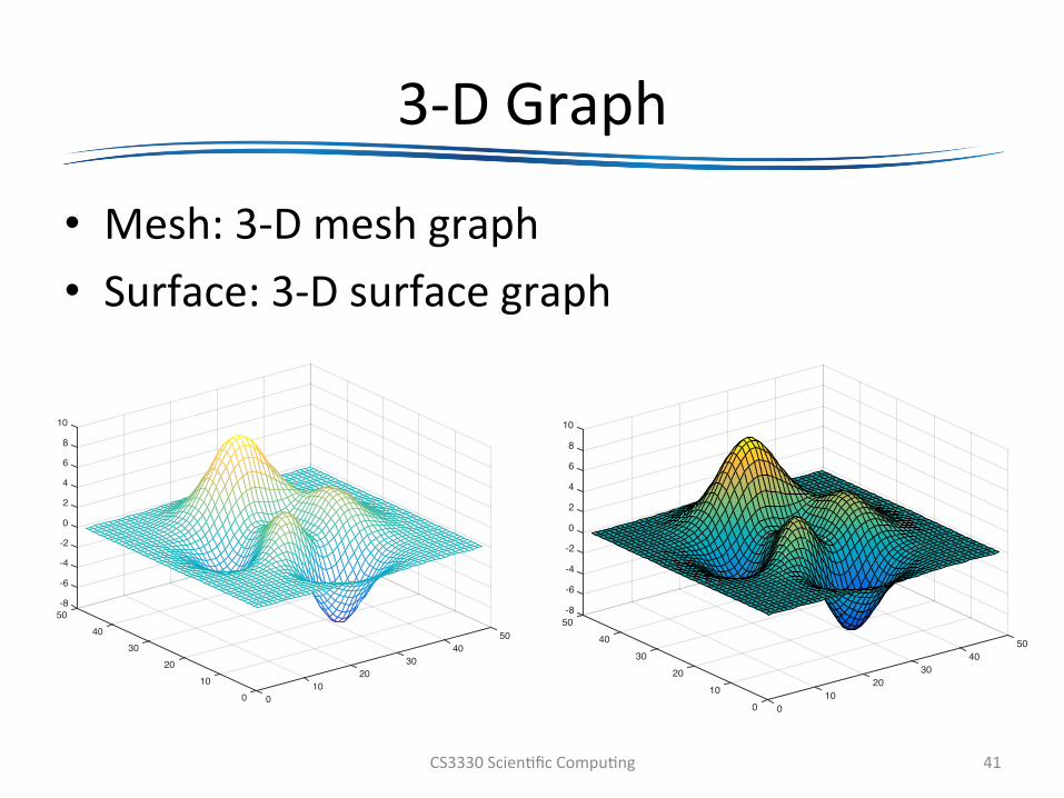
3-DGraph

•  Mesh:3-Dmeshgraph•  Surface:3-Dsurfacegraph


5040

3020

1000

1020

3040

8

-8

-6

-4

-2

0

6

2

4

10

50

5040

3020

1000

1020

3040

8

-8

-6

-4

-2

0

10

2

4

6

50

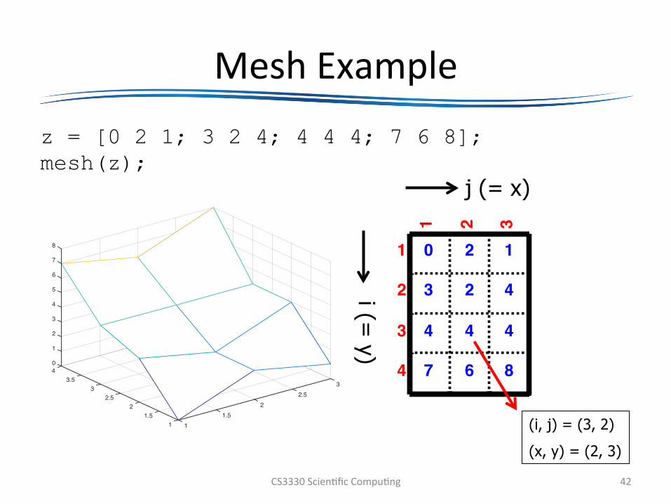
MeshExamplez = [0 2 1; 3 2 4; 4 4 4; 7 6 8]; mesh(z);


0 2 1

3 2 4

4 4 4

7 6 8

1

2

3

4

1 2 3

i (= y)

j (= x)

(i, j) = (3, 2)

(x, y) = (2, 3)

32.5

21.5

111.5

22.5

33.5

7

8

0

1

2

3

4

5

6

4

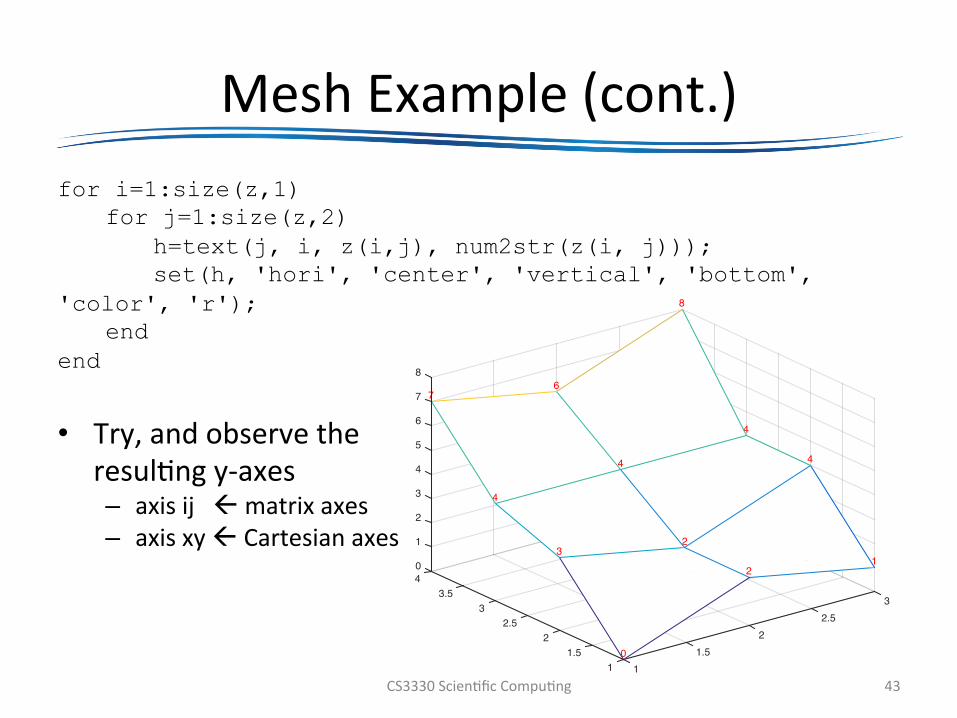
MeshExample(cont.)for i=1:size(z,1)

for j=1:size(z,2) h=text(j, i, z(i,j), num2str(z(i, j))); set(h, 'hori', 'center', 'vertical', 'bottom',

'color', 'r'); end

end

•  Try,andobservethe

resul@ngy-axes–  axisijßmatrixaxes–  axisxyßCartesianaxes


3

1

2.5

4

2

2

4

1.5

2

8

10

4

11.5

3

6

22.5

4

33.5

77

0

1

2

3

4

8

5

6

4

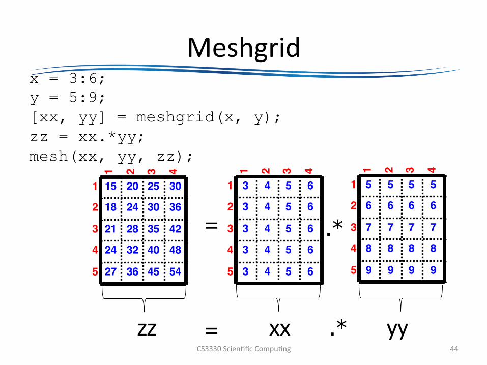
Meshgridx = 3:6; y = 5:9; [xx, yy] = meshgrid(x, y); zz = xx.*yy; mesh(xx, yy, zz);


3 4 5 6

3 4 5 6

3 4 5 6

3 4 5 6

3 4 5 6

1

2

3

4

5

1 2 3 4

5 5 5 5

6 6 6 6

7 7 7 7

8 8 8 8

9 9 9 9

1

2

3

4

5

1 2 3 4

15 20 25 30

18 24 30 36

21 28 35 42

24 32 40 48

27 36 45 54

1

2

3

4

5

1 2 3 4

zz xx yy = .*

= .*

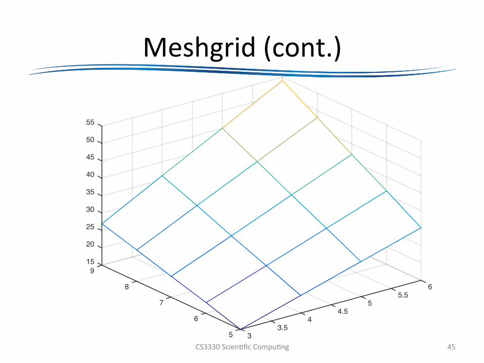
Meshgrid(cont.)


65.5

54.5

43.5

35

6

7

8

35

15

20

30

25

55

50

45

40

9

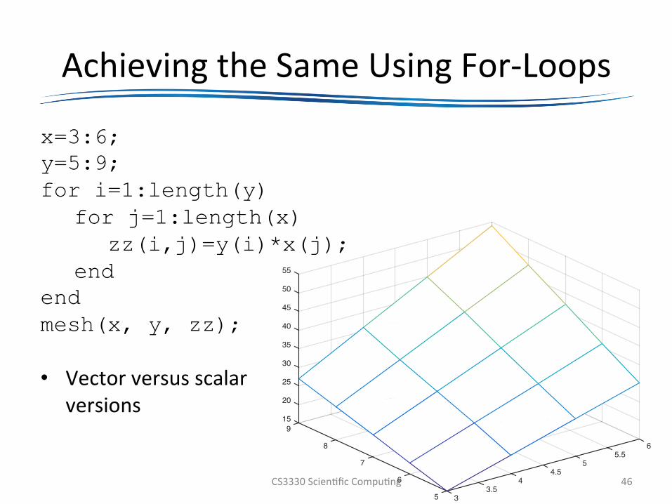
AchievingtheSameUsingFor-Loops

x=3:6; y=5:9; for i=1:length(y) for j=1:length(x) zz(i,j)=y(i)*x(j); end

end mesh(x, y, zz); •  Vectorversusscalar

versions


65.5

54.5

43.5

35

6

7

8

35

15

20

30

25

55

50

45

40

9

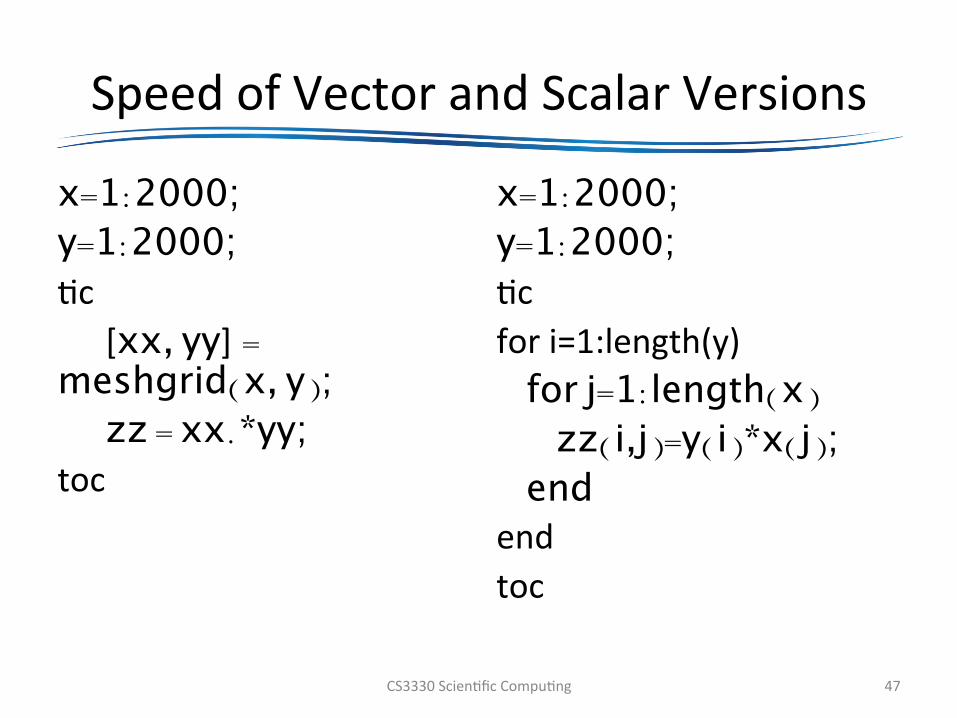
SpeedofVectorandScalarVersions

x=1:2000;y=1:2000;@c

[xx, yy] = meshgrid(x, y);

zz = xx.*yy; toc

x=1:2000;y=1:2000;@cfori=1:length(y) for j=1:length(x) zz(i,j)=y(i)*x(j); endendtoc


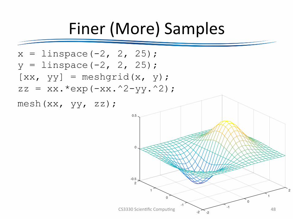
Finer(More)Samplesx = linspace(-2, 2, 25); y = linspace(-2, 2, 25); [xx, yy] = meshgrid(x, y); zz = xx.*exp(-xx.^2-yy.^2);

mesh(xx, yy, zz);


21

0-1

-2-2

-1

0

1

0.5

-0.5

0

2

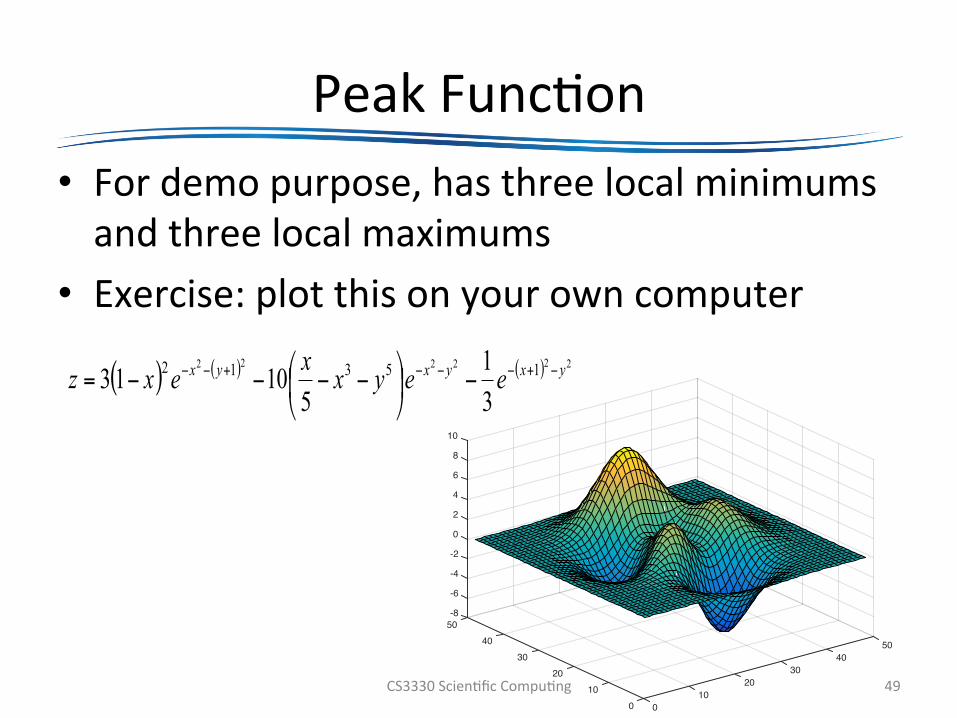
PeakFunc@on•  Fordemopurpose,hasthreelocalminimumsandthreelocalmaximums

•  Exercise:plotthisonyourowncomputer


5040

3020

1000

1020

3040

8

-8

-6

-4

-2

0

10

2

4

6

50

( ) ( ) ( ) 222222 15312

31

51013 yxyxyx eeyxxexz −+−−−+−− −⎟

⎠

⎞⎜⎝

⎛ −−−−=

Meshz


5040

3020

1000

1020

3040

0

-2

-4

-6

2

-8

4

6

8

10

50

Waterfall


5040

3020

1000

1020

3040

10

8

6

4

2

0

-2

-4

-6

-850

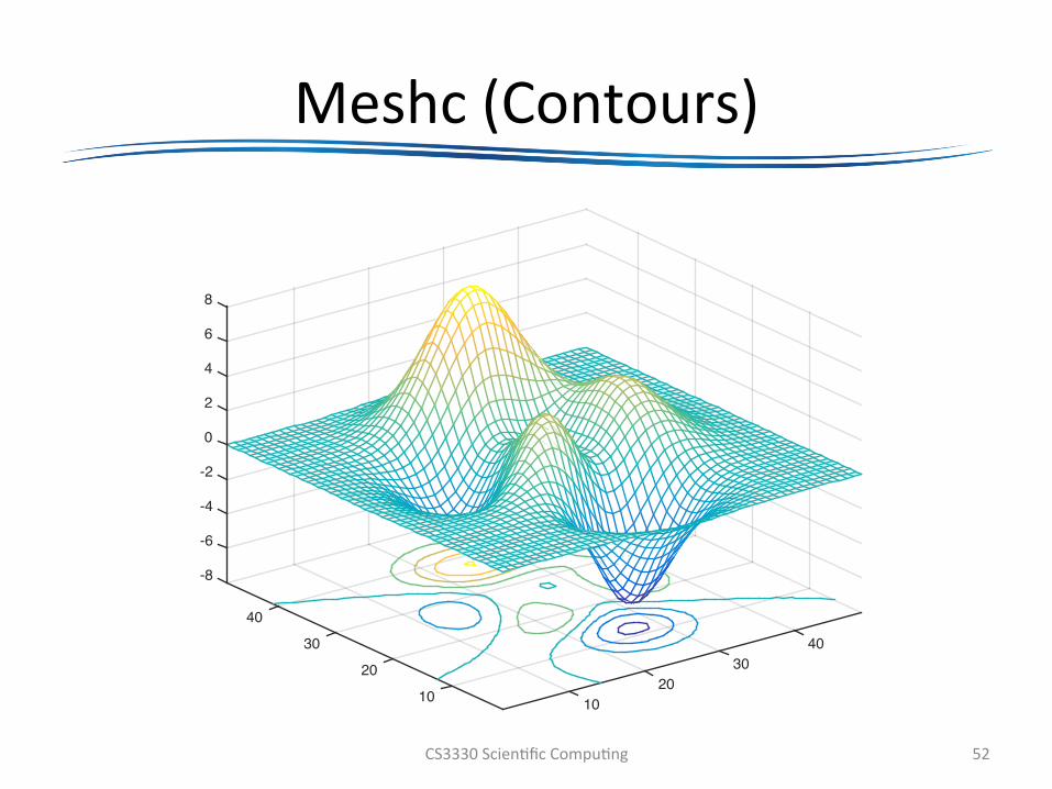
Meshc(Contours)


4030

201010

20

30

40

6

-8

8

-4

-2

0

2

4

-6

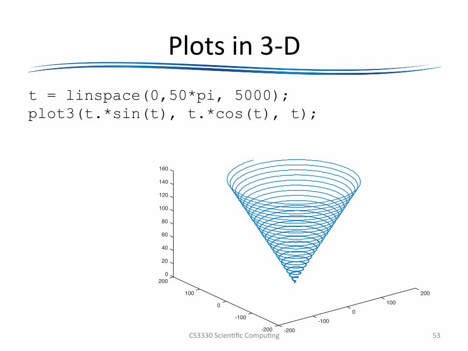
Plotsin3-Dt = linspace(0,50*pi, 5000); plot3(t.*sin(t), t.*cos(t), t);


200100

0-100

-200-200

-100

0

100

160

140

120

100

80

60

40

20

0200

OtherUsagesofPlot3D

t = linspace(0, 10*pi, 501); plot3(t.*sin(t), t.*cos(t), t, t.*sin(t), t.*cos(t), -t);


3020

100

-10-20

-30-40

-20

0

20

30

40

-40

-30

-20

-10

0

10

20

40

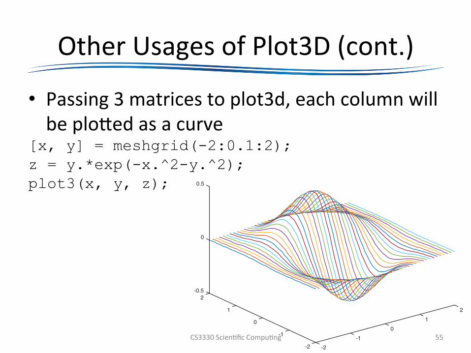
OtherUsagesofPlot3D(cont.)

•  Passing3matricestoplot3d,eachcolumnwillbeploledasacurve

[x, y] = meshgrid(-2:0.1:2); z = y.*exp(-x.^2-y.^2); plot3(x, y, z);


21

0-1

-2-2

-1

0

1

-0.5

0

0.5

2

Interpola@onUsingGriddatax = 6*rand(100,1)-3;

y = 6*rand(100,1)-3; z = peaks(x, y);

[X, Y] = meshgrid(-3:0.1:3);

Z = griddata(x, y, z, X, Y, 'cubic');

mesh(X, Y, Z);

hold on plot3(x, y, z, '.', 'MarkerSize', 16);


32

10

-1-2

-3-3-2

-10

12

6

-4

8

-2

0

2

4

3

Griddatasupportsvariousinterpola@onalgorithm,thedefaultislinear

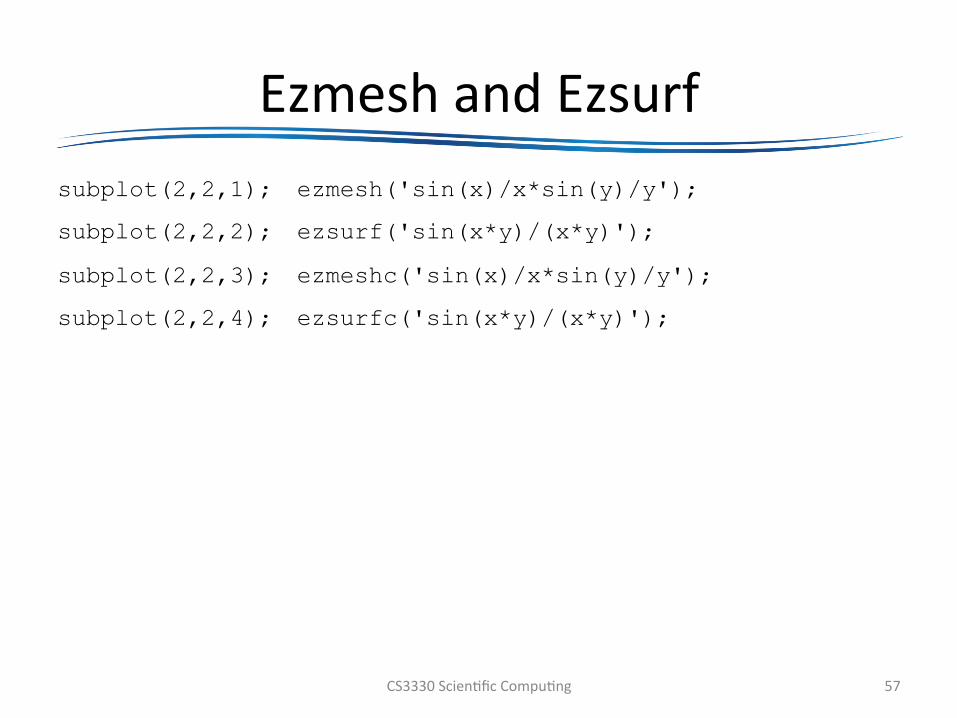
EzmeshandEzsurfsubplot(2,2,1); ezmesh('sin(x)/x*sin(y)/y');

subplot(2,2,2); ezsurf('sin(x*y)/(x*y)');

subplot(2,2,3); ezmeshc('sin(x)/x*sin(y)/y');

subplot(2,2,4); ezsurfc('sin(x*y)/(x*y)');


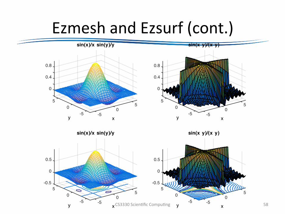
EzmeshandEzsurf(cont.)


50

x

sin(x)/x sin(y)/y

-5-5y

05

0.8

0

0.4

50

x

sin(x y)/(x y)

-5-5y

05

0.8

0

0.4

50

x

sin(x)/x sin(y)/y

-5-5y

05

0.5

-0.5

0

50

x

sin(x y)/(x y)

-5-5y

05

-0.5

0.5

0

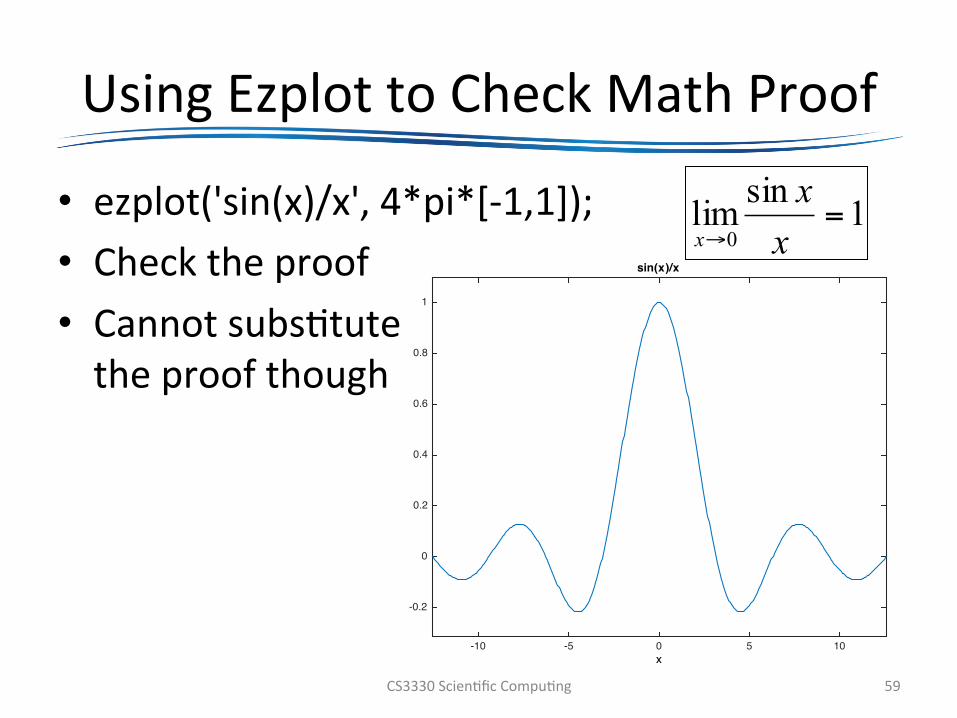
UsingEzplottoCheckMathProof

•  ezplot('sin(x)/x',4*pi*[-1,1]);•  Checktheproof•  Cannotsubs@tutetheproofthough


1sinlim0

=→ x

xx

x-10 -5 0 5 10

-0.2

0

0.2

0.4

0.6

0.8

1

sin(x)/x

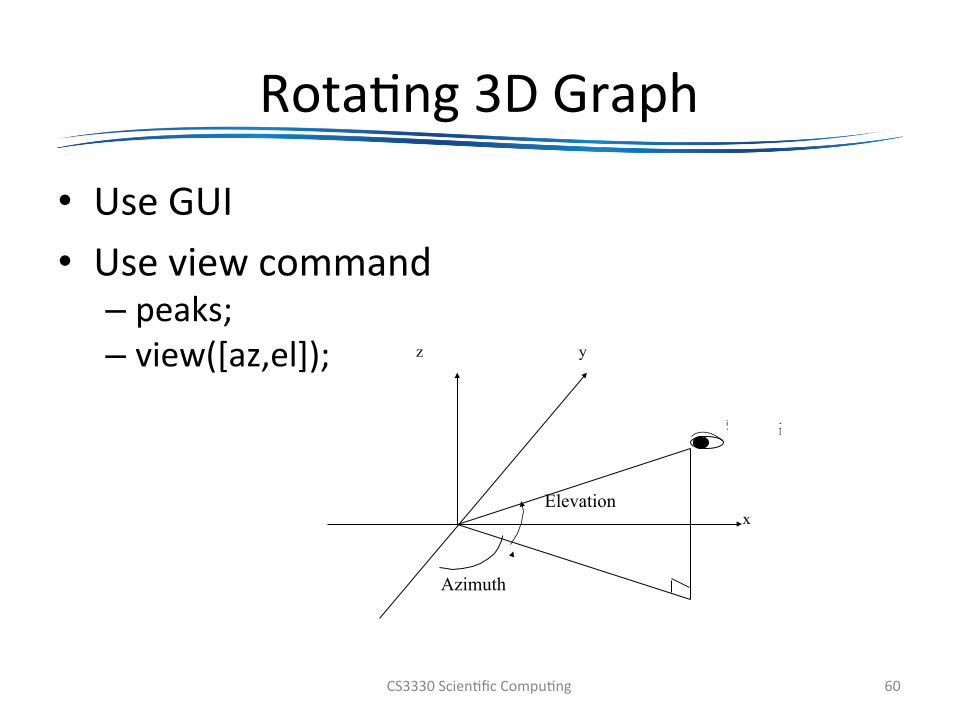
Rota@ng3DGraph

•  UseGUI•  Useviewcommand

– peaks;– view([az,el]);


Elevation

Azimuth

觀測點

原點

x

z y

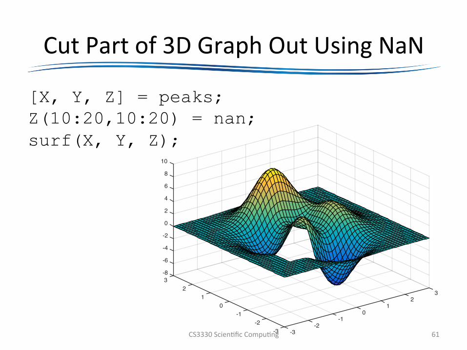
CutPartof3DGraphOutUsingNaN

[X, Y, Z] = peaks; Z(10:20,10:20) = nan; surf(X, Y, Z);


32

10

-1-2

-3-3-2

-10

12

10

8

6

4

2

0

-2

-4

-6

-83

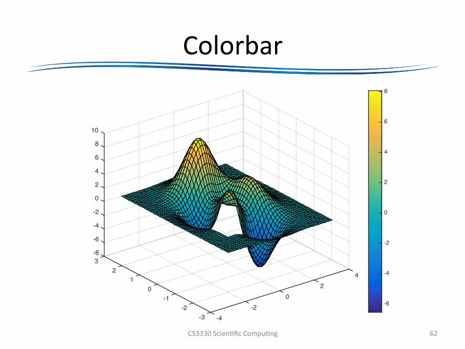
Colorbar


42

0-2

-4-3-2

-10

12

10

-8

-6

-4

-2

0

2

4

6

8

3

-6

-4

-2

0

2

4

6

8

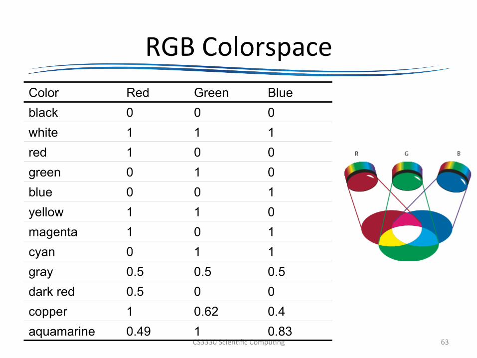
RGBColorspace


Color Red Green Blue black 0 0 0 white 1 1 1 red 1 0 0 green 0 1 0 blue 0 0 1 yellow 1 1 0 magenta 1 0 1 cyan 0 1 1 gray 0.5 0.5 0.5 dark red 0.5 0 0 copper 1 0.62 0.4 aquamarine 0.49 1 0.83

Colormap

•  cm=colormap;•  size(cm)•  ans=643

•  In3Dfigures,thelowestzsurfacehasthecolorspecifiedinrow1ofcm

•  Thereare64zsurfaces


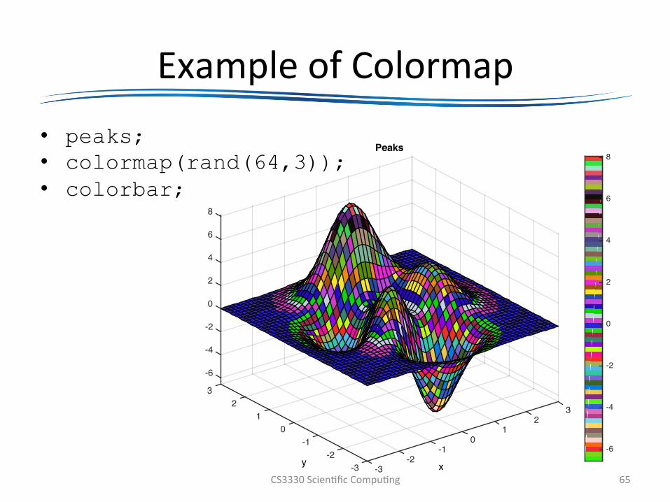
ExampleofColormap•  peaks; •  colormap(rand(64,3)); •  colorbar;


32

10

-1

x-2

Peaks

-3-3-2

-1

y

01

2

8

6

4

2

0

-2

-4

-6

3

-6

-4

-2

0

2

4

6

8

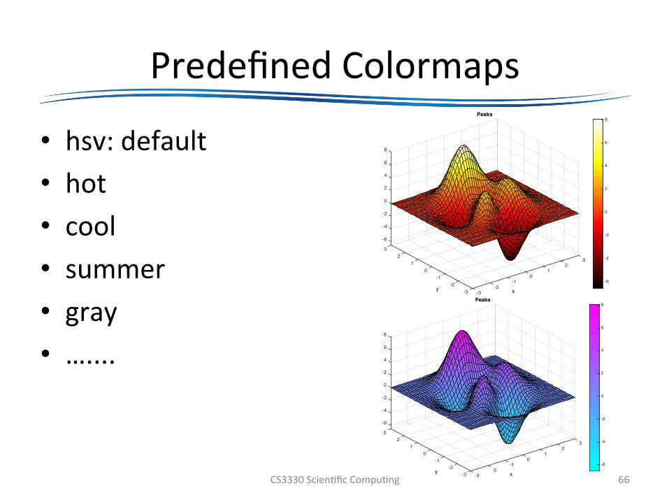
PredefinedColormaps

•  hsv:default•  hot•  cool•  summer•  gray•  …....


32

10

-1

x-2

Peaks

-3-3-2

-1

y

01

2

8

6

4

2

0

-2

-4

-6

3

-6

-4

-2

0

2

4

6

8

32

10

-1

x-2

Peaks

-3-3-2

-1

y

01

2

8

6

4

2

0

-2

-4

-6

3

-6

-4

-2

0

2

4

6

8

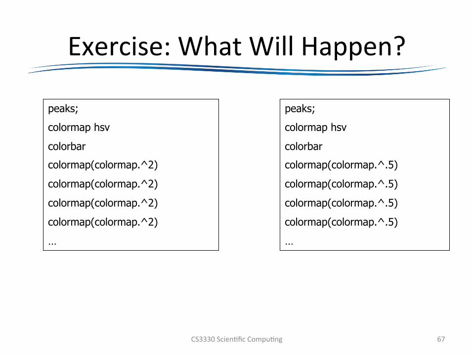
Exercise:WhatWillHappen?


peaks;

colormap hsv

colorbar

colormap(colormap.^2)




…

peaks;

colormap hsv

colorbar

colormap(colormap.^.5)




…

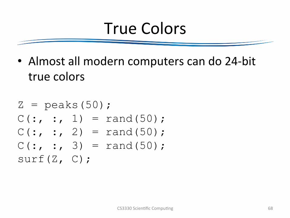
TrueColors

•  Almostallmoderncomputerscando24-bittruecolors

Z = peaks(50); C(:, :, 1) = rand(50); C(:, :, 2) = rand(50); C(:, :, 3) = rand(50); surf(Z, C);


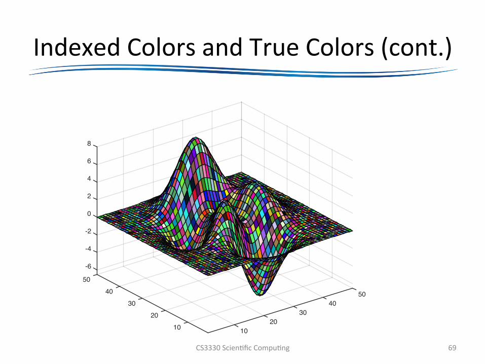
IndexedColorsandTrueColors(cont.)


5040

3020

101020

3040

8

6

4

2

0

-2

-4

-6

50

0.1

0.2

0.3

0.4

0.5

0.6

0.7

0.8

0.9

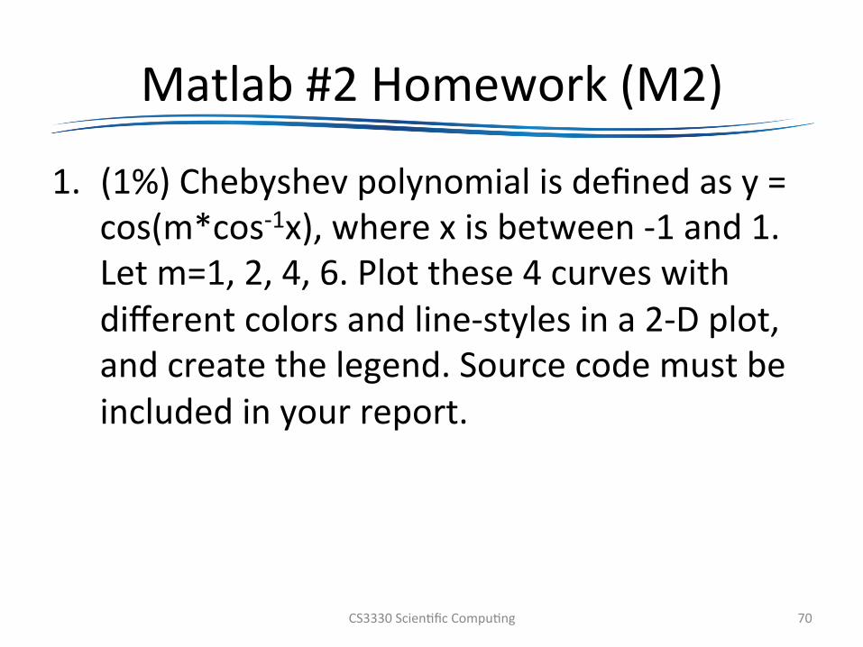
Matlab#2Homework(M2)

1.  (1%)Chebyshevpolynomialisdefinedasy=cos(m*cos-1x),wherexisbetween-1and1.Letm=1,2,4,6.Plotthese4curveswithdifferentcolorsandline-stylesina2-Dplot,andcreatethelegend.Sourcecodemustbeincludedinyourreport.


Matlab#2Homework(M2)cont.

2.  (1%)Plotaspirallikethis.Itisoktohavex,andyaxes,andotherstandardMatlabfigurecomponents.


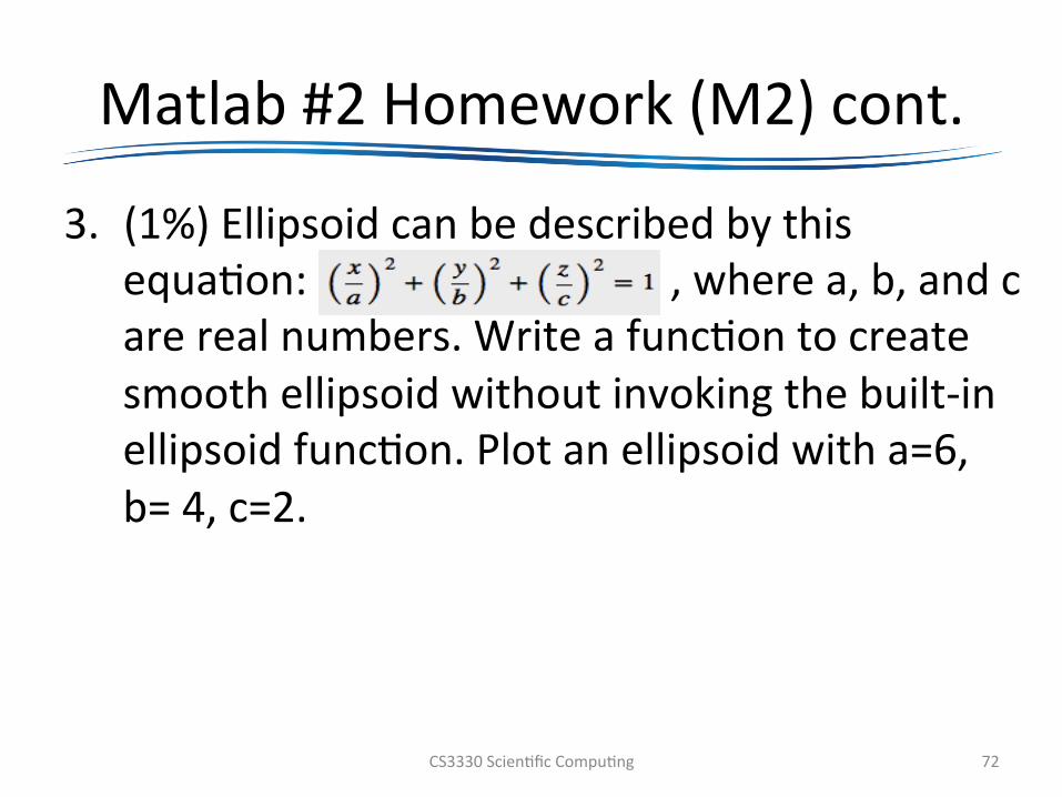
Matlab#2Homework(M2)cont.

3.  (1%)Ellipsoidcanbedescribedbythisequa@on:,wherea,b,andcarerealnumbers.Writeafunc@ontocreatesmoothellipsoidwithoutinvokingthebuilt-inellipsoidfunc@on.Plotanellipsoidwitha=6,b=4,c=2.


Matlab 2: 2D and 3D Graph | NMSL@NTHU

Documents

Transcript of Matlab 2: 2D and 3D Graph | NMSL@NTHU