Guia matlab de neurona
406
Neural Network Toolbox™ User's Guide R2014b Mark Hudson Beale Martin T. Hagan Howard B. Demuth
-
Upload
independent -
Category
Documents
-
view
0 -
download
0
Transcript of Guia matlab de neurona

Neural Network Toolbox™
User's Guide
R2014b
Mark Hudson BealeMartin T. HaganHoward B. Demuth
How to Contact MathWorks
Latest news: www.mathworks.com
Sales and services: www.mathworks.com/sales_and_services
User community: www.mathworks.com/matlabcentral
Technical support: www.mathworks.com/support/contact_us
Phone: 508-647-7000
The MathWorks, Inc.3 Apple Hill DriveNatick, MA 01760-2098
Neural Network Toolbox™ User's Guide© COPYRIGHT 1992–2014 by The MathWorks, Inc.The software described in this document is furnished under a license agreement. The software may be usedor copied only under the terms of the license agreement. No part of this manual may be photocopied orreproduced in any form without prior written consent from The MathWorks, Inc.FEDERAL ACQUISITION: This provision applies to all acquisitions of the Program and Documentationby, for, or through the federal government of the United States. By accepting delivery of the Programor Documentation, the government hereby agrees that this software or documentation qualifies ascommercial computer software or commercial computer software documentation as such terms are usedor defined in FAR 12.212, DFARS Part 227.72, and DFARS 252.227-7014. Accordingly, the terms andconditions of this Agreement and only those rights specified in this Agreement, shall pertain to andgovern the use, modification, reproduction, release, performance, display, and disclosure of the Programand Documentation by the federal government (or other entity acquiring for or through the federalgovernment) and shall supersede any conflicting contractual terms or conditions. If this License failsto meet the government's needs or is inconsistent in any respect with federal procurement law, thegovernment agrees to return the Program and Documentation, unused, to The MathWorks, Inc.
Trademarks
MATLAB and Simulink are registered trademarks of The MathWorks, Inc. Seewww.mathworks.com/trademarks for a list of additional trademarks. Other product or brandnames may be trademarks or registered trademarks of their respective holders.Patents
MathWorks products are protected by one or more U.S. patents. Please seewww.mathworks.com/patents for more information.

Revision History
June 1992 First printingApril 1993 Second printingJanuary 1997 Third printingJuly 1997 Fourth printingJanuary 1998 Fifth printing Revised for Version 3 (Release 11)September 2000 Sixth printing Revised for Version 4 (Release 12)June 2001 Seventh printing Minor revisions (Release 12.1)July 2002 Online only Minor revisions (Release 13)January 2003 Online only Minor revisions (Release 13SP1)June 2004 Online only Revised for Version 4.0.3 (Release 14)October 2004 Online only Revised for Version 4.0.4 (Release 14SP1)October 2004 Eighth printing Revised for Version 4.0.4March 2005 Online only Revised for Version 4.0.5 (Release 14SP2)March 2006 Online only Revised for Version 5.0 (Release 2006a)September 2006 Ninth printing Minor revisions (Release 2006b)March 2007 Online only Minor revisions (Release 2007a)September 2007 Online only Revised for Version 5.1 (Release 2007b)March 2008 Online only Revised for Version 6.0 (Release 2008a)October 2008 Online only Revised for Version 6.0.1 (Release 2008b)March 2009 Online only Revised for Version 6.0.2 (Release 2009a)September 2009 Online only Revised for Version 6.0.3 (Release 2009b)March 2010 Online only Revised for Version 6.0.4 (Release 2010a)September 2010 Online only Revised for Version 7.0 (Release 2010b)April 2011 Online only Revised for Version 7.0.1 (Release 2011a)September 2011 Online only Revised for Version 7.0.2 (Release 2011b)March 2012 Online only Revised for Version 7.0.3 (Release 2012a)September 2012 Online only Revised for Version 8.0 (Release 2012b)March 2013 Online only Revised for Version 8.0.1 (Release 2013a)September 2013 Online only Revised for Version 8.1 (Release 2013b)March 2014 Online only Revised for Version 8.2 (Release 2014a)October 2014 Online only Revised for Version 8.2.1 (Release 2014b)

v
Contents
Neural Network Toolbox Design Book
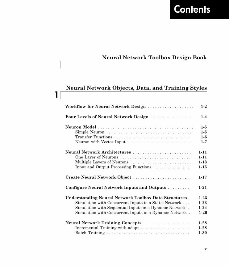
Neural Network Objects, Data, and Training Styles1
Workflow for Neural Network Design . . . . . . . . . . . . . . . . . . . 1-2
Four Levels of Neural Network Design . . . . . . . . . . . . . . . . . 1-4
Neuron Model . . . . . . . . . . . . . . . . . . . . . . . . . . . . . . . . . . . . . . . 1-5Simple Neuron . . . . . . . . . . . . . . . . . . . . . . . . . . . . . . . . . . . 1-5Transfer Functions . . . . . . . . . . . . . . . . . . . . . . . . . . . . . . . . 1-6Neuron with Vector Input . . . . . . . . . . . . . . . . . . . . . . . . . . . 1-7
Neural Network Architectures . . . . . . . . . . . . . . . . . . . . . . . . 1-11One Layer of Neurons . . . . . . . . . . . . . . . . . . . . . . . . . . . . . 1-11Multiple Layers of Neurons . . . . . . . . . . . . . . . . . . . . . . . . . 1-13Input and Output Processing Functions . . . . . . . . . . . . . . . 1-15
Create Neural Network Object . . . . . . . . . . . . . . . . . . . . . . . 1-17
Configure Neural Network Inputs and Outputs . . . . . . . . . 1-21
Understanding Neural Network Toolbox Data Structures . 1-23Simulation with Concurrent Inputs in a Static Network . . . 1-23Simulation with Sequential Inputs in a Dynamic Network . 1-24Simulation with Concurrent Inputs in a Dynamic Network . 1-26
Neural Network Training Concepts . . . . . . . . . . . . . . . . . . . 1-28Incremental Training with adapt . . . . . . . . . . . . . . . . . . . . 1-28Batch Training . . . . . . . . . . . . . . . . . . . . . . . . . . . . . . . . . . 1-30

vi Contents
Training Feedback . . . . . . . . . . . . . . . . . . . . . . . . . . . . . . . 1-33
Multilayer Neural Networks and BackpropagationTraining
2Multilayer Neural Networks and Backpropagation
Training . . . . . . . . . . . . . . . . . . . . . . . . . . . . . . . . . . . . . . . . . . 2-2
Multilayer Neural Network Architecture . . . . . . . . . . . . . . . . 2-4Neuron Model (logsig, tansig, purelin) . . . . . . . . . . . . . . . . . . 2-4Feedforward Neural Network . . . . . . . . . . . . . . . . . . . . . . . . 2-5
Prepare Data for Multilayer Neural Networks . . . . . . . . . . . 2-8
Choose Neural Network Input-Output ProcessingFunctions . . . . . . . . . . . . . . . . . . . . . . . . . . . . . . . . . . . . . . . . 2-9
Representing Unknown or Don't-Care Targets . . . . . . . . . . 2-11
Divide Data for Optimal Neural Network Training . . . . . . . 2-12
Create, Configure, and Initialize Multilayer NeuralNetworks . . . . . . . . . . . . . . . . . . . . . . . . . . . . . . . . . . . . . . . . 2-14
Other Related Architectures . . . . . . . . . . . . . . . . . . . . . . . . 2-15Initializing Weights (init) . . . . . . . . . . . . . . . . . . . . . . . . . . 2-15
Train and Apply Multilayer Neural Networks . . . . . . . . . . . 2-17Training Algorithms . . . . . . . . . . . . . . . . . . . . . . . . . . . . . . 2-18Training Example . . . . . . . . . . . . . . . . . . . . . . . . . . . . . . . . 2-20Use the Network . . . . . . . . . . . . . . . . . . . . . . . . . . . . . . . . . 2-22
Analyze Neural Network Performance After Training . . . . 2-23Improving Results . . . . . . . . . . . . . . . . . . . . . . . . . . . . . . . . 2-28
Limitations and Cautions . . . . . . . . . . . . . . . . . . . . . . . . . . . . 2-29

vii
Dynamic Neural Networks3
Introduction to Dynamic Neural Networks . . . . . . . . . . . . . . 3-2
How Dynamic Neural Networks Work . . . . . . . . . . . . . . . . . . 3-3Feedforward and Recurrent Neural Networks . . . . . . . . . . . . 3-3Applications of Dynamic Networks . . . . . . . . . . . . . . . . . . . 3-11Dynamic Network Structures . . . . . . . . . . . . . . . . . . . . . . . 3-11Dynamic Network Training . . . . . . . . . . . . . . . . . . . . . . . . . 3-12
Design Time Series Time-Delay Neural Networks . . . . . . . . 3-14Prepare Input and Layer Delay States . . . . . . . . . . . . . . . . 3-18
Design Time Series Distributed Delay Neural Networks . . 3-20
Design Time Series NARX Feedback Neural Networks . . . . 3-23Multiple External Variables . . . . . . . . . . . . . . . . . . . . . . . . 3-30
Design Layer-Recurrent Neural Networks . . . . . . . . . . . . . . 3-31
Create Reference Model Controller with MATLAB Script . 3-34
Multiple Sequences with Dynamic Neural Networks . . . . . 3-41
Neural Network Time-Series Utilities . . . . . . . . . . . . . . . . . . 3-42
Train Neural Networks with Error Weights . . . . . . . . . . . . . 3-44
Normalize Errors of Multiple Outputs . . . . . . . . . . . . . . . . . 3-47
Multistep Neural Network Prediction . . . . . . . . . . . . . . . . . 3-52Set Up in Open-Loop Mode . . . . . . . . . . . . . . . . . . . . . . . . . 3-52Multistep Closed-Loop Prediction From Initial Conditions . . 3-53Multistep Closed-Loop Prediction Following Known
Sequence . . . . . . . . . . . . . . . . . . . . . . . . . . . . . . . . . . . . . 3-53Following Closed-Loop Simulation with Open-Loop
Simulation . . . . . . . . . . . . . . . . . . . . . . . . . . . . . . . . . . . . 3-54
viii Contents
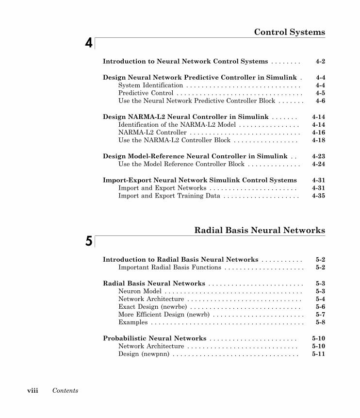
Control Systems4
Introduction to Neural Network Control Systems . . . . . . . . 4-2
Design Neural Network Predictive Controller in Simulink . 4-4System Identification . . . . . . . . . . . . . . . . . . . . . . . . . . . . . . 4-4Predictive Control . . . . . . . . . . . . . . . . . . . . . . . . . . . . . . . . . 4-5Use the Neural Network Predictive Controller Block . . . . . . . 4-6
Design NARMA-L2 Neural Controller in Simulink . . . . . . . 4-14Identification of the NARMA-L2 Model . . . . . . . . . . . . . . . . 4-14NARMA-L2 Controller . . . . . . . . . . . . . . . . . . . . . . . . . . . . . 4-16Use the NARMA-L2 Controller Block . . . . . . . . . . . . . . . . . 4-18
Design Model-Reference Neural Controller in Simulink . . 4-23Use the Model Reference Controller Block . . . . . . . . . . . . . . 4-24
Import-Export Neural Network Simulink Control Systems 4-31Import and Export Networks . . . . . . . . . . . . . . . . . . . . . . . 4-31Import and Export Training Data . . . . . . . . . . . . . . . . . . . . 4-35
Radial Basis Neural Networks5
Introduction to Radial Basis Neural Networks . . . . . . . . . . . 5-2Important Radial Basis Functions . . . . . . . . . . . . . . . . . . . . . 5-2
Radial Basis Neural Networks . . . . . . . . . . . . . . . . . . . . . . . . . 5-3Neuron Model . . . . . . . . . . . . . . . . . . . . . . . . . . . . . . . . . . . . 5-3Network Architecture . . . . . . . . . . . . . . . . . . . . . . . . . . . . . . 5-4Exact Design (newrbe) . . . . . . . . . . . . . . . . . . . . . . . . . . . . . 5-6More Efficient Design (newrb) . . . . . . . . . . . . . . . . . . . . . . . . 5-7Examples . . . . . . . . . . . . . . . . . . . . . . . . . . . . . . . . . . . . . . . . 5-8
Probabilistic Neural Networks . . . . . . . . . . . . . . . . . . . . . . . 5-10Network Architecture . . . . . . . . . . . . . . . . . . . . . . . . . . . . . 5-10Design (newpnn) . . . . . . . . . . . . . . . . . . . . . . . . . . . . . . . . . 5-11
ix
Generalized Regression Neural Networks . . . . . . . . . . . . . . 5-13Network Architecture . . . . . . . . . . . . . . . . . . . . . . . . . . . . . 5-13Design (newgrnn) . . . . . . . . . . . . . . . . . . . . . . . . . . . . . . . . 5-15
Self-Organizing and Learning Vector QuantizationNetworks
6Introduction to Self-Organizing and LVQ . . . . . . . . . . . . . . . 6-2
Important Self-Organizing and LVQ Functions . . . . . . . . . . . 6-2
Cluster with a Competitive Neural Network . . . . . . . . . . . . . 6-3Architecture . . . . . . . . . . . . . . . . . . . . . . . . . . . . . . . . . . . . . 6-3Create a Competitive Neural Network . . . . . . . . . . . . . . . . . 6-4Kohonen Learning Rule (learnk) . . . . . . . . . . . . . . . . . . . . . . 6-5Bias Learning Rule (learncon) . . . . . . . . . . . . . . . . . . . . . . . . 6-5Training . . . . . . . . . . . . . . . . . . . . . . . . . . . . . . . . . . . . . . . . 6-6Graphical Example . . . . . . . . . . . . . . . . . . . . . . . . . . . . . . . . 6-8
Cluster with Self-Organizing Map Neural Network . . . . . . . 6-9Topologies (gridtop, hextop, randtop) . . . . . . . . . . . . . . . . . . 6-11Distance Functions (dist, linkdist, mandist, boxdist) . . . . . . 6-14Architecture . . . . . . . . . . . . . . . . . . . . . . . . . . . . . . . . . . . . . 6-17Create a Self-Organizing Map Neural Network (selforgmap) 6-18Training (learnsomb) . . . . . . . . . . . . . . . . . . . . . . . . . . . . . . 6-19Examples . . . . . . . . . . . . . . . . . . . . . . . . . . . . . . . . . . . . . . . 6-22
Learning Vector Quantization (LVQ) Neural Networks . . . 6-34Architecture . . . . . . . . . . . . . . . . . . . . . . . . . . . . . . . . . . . . . 6-34Creating an LVQ Network . . . . . . . . . . . . . . . . . . . . . . . . . 6-35LVQ1 Learning Rule (learnlv1) . . . . . . . . . . . . . . . . . . . . . . 6-38Training . . . . . . . . . . . . . . . . . . . . . . . . . . . . . . . . . . . . . . . 6-39Supplemental LVQ2.1 Learning Rule (learnlv2) . . . . . . . . . 6-41
x Contents
Adaptive Filters and Adaptive Training7
Adaptive Neural Network Filters . . . . . . . . . . . . . . . . . . . . . . 7-2Adaptive Functions . . . . . . . . . . . . . . . . . . . . . . . . . . . . . . . . 7-2Linear Neuron Model . . . . . . . . . . . . . . . . . . . . . . . . . . . . . . 7-3Adaptive Linear Network Architecture . . . . . . . . . . . . . . . . . 7-3Least Mean Square Error . . . . . . . . . . . . . . . . . . . . . . . . . . . 7-6LMS Algorithm (learnwh) . . . . . . . . . . . . . . . . . . . . . . . . . . . 7-7Adaptive Filtering (adapt) . . . . . . . . . . . . . . . . . . . . . . . . . . . 7-7
Advanced Topics8
Neural Networks with Parallel and GPU Computing . . . . . . 8-2Modes of Parallelism . . . . . . . . . . . . . . . . . . . . . . . . . . . . . . . 8-2Distributed Computing . . . . . . . . . . . . . . . . . . . . . . . . . . . . . 8-3Single GPU Computing . . . . . . . . . . . . . . . . . . . . . . . . . . . . . 8-5Distributed GPU Computing . . . . . . . . . . . . . . . . . . . . . . . . . 8-8Parallel Time Series . . . . . . . . . . . . . . . . . . . . . . . . . . . . . . . 8-9Parallel Availability, Fallbacks, and Feedback . . . . . . . . . . 8-10
Optimize Neural Network Training Speed and Memory . . . 8-12Memory Reduction . . . . . . . . . . . . . . . . . . . . . . . . . . . . . . . 8-12Fast Elliot Sigmoid . . . . . . . . . . . . . . . . . . . . . . . . . . . . . . . 8-12
Choose a Multilayer Neural Network Training Function . . 8-16SIN Data Set . . . . . . . . . . . . . . . . . . . . . . . . . . . . . . . . . . . 8-17PARITY Data Set . . . . . . . . . . . . . . . . . . . . . . . . . . . . . . . . 8-19ENGINE Data Set . . . . . . . . . . . . . . . . . . . . . . . . . . . . . . . . 8-21CANCER Data Set . . . . . . . . . . . . . . . . . . . . . . . . . . . . . . . 8-23CHOLESTEROL Data Set . . . . . . . . . . . . . . . . . . . . . . . . . 8-25DIABETES Data Set . . . . . . . . . . . . . . . . . . . . . . . . . . . . . . 8-27Summary . . . . . . . . . . . . . . . . . . . . . . . . . . . . . . . . . . . . . . . 8-29
Improve Neural Network Generalization and AvoidOverfitting . . . . . . . . . . . . . . . . . . . . . . . . . . . . . . . . . . . . . . 8-31
Retraining Neural Networks . . . . . . . . . . . . . . . . . . . . . . . . 8-32Multiple Neural Networks . . . . . . . . . . . . . . . . . . . . . . . . . . 8-34

xi
Early Stopping . . . . . . . . . . . . . . . . . . . . . . . . . . . . . . . . . . 8-35Index Data Division (divideind) . . . . . . . . . . . . . . . . . . . . . . 8-36Random Data Division (dividerand) . . . . . . . . . . . . . . . . . . 8-36Block Data Division (divideblock) . . . . . . . . . . . . . . . . . . . . 8-36Interleaved Data Division (divideint) . . . . . . . . . . . . . . . . . 8-37Regularization . . . . . . . . . . . . . . . . . . . . . . . . . . . . . . . . . . . 8-37Summary and Discussion of Early Stopping and
Regularization . . . . . . . . . . . . . . . . . . . . . . . . . . . . . . . . . 8-40Posttraining Analysis (regression) . . . . . . . . . . . . . . . . . . . . 8-42
Create and Train Custom Neural Network Architectures . 8-44Custom Network . . . . . . . . . . . . . . . . . . . . . . . . . . . . . . . . . 8-44Network Definition . . . . . . . . . . . . . . . . . . . . . . . . . . . . . . . 8-45Network Behavior . . . . . . . . . . . . . . . . . . . . . . . . . . . . . . . . 8-54
Custom Neural Network Helper Functions . . . . . . . . . . . . . 8-57
Automatically Save Checkpoints During Neural NetworkTraining . . . . . . . . . . . . . . . . . . . . . . . . . . . . . . . . . . . . . . . . . 8-58
Deploy Neural Network Functions . . . . . . . . . . . . . . . . . . . . 8-60Deployment Functions and Tools . . . . . . . . . . . . . . . . . . . . 8-60Generate Neural Network Functions for Application
Deployment . . . . . . . . . . . . . . . . . . . . . . . . . . . . . . . . . . . 8-61Generate Simulink Diagrams . . . . . . . . . . . . . . . . . . . . . . . 8-63
Historical Neural Networks9
Historical Neural Networks Overview . . . . . . . . . . . . . . . . . . 9-2
Perceptron Neural Networks . . . . . . . . . . . . . . . . . . . . . . . . . . 9-3Neuron Model . . . . . . . . . . . . . . . . . . . . . . . . . . . . . . . . . . . . 9-3Perceptron Architecture . . . . . . . . . . . . . . . . . . . . . . . . . . . . 9-5Create a Perceptron . . . . . . . . . . . . . . . . . . . . . . . . . . . . . . . 9-6Perceptron Learning Rule (learnp) . . . . . . . . . . . . . . . . . . . . 9-8Training (train) . . . . . . . . . . . . . . . . . . . . . . . . . . . . . . . . . . 9-10Limitations and Cautions . . . . . . . . . . . . . . . . . . . . . . . . . . 9-15
xii Contents
Linear Neural Networks . . . . . . . . . . . . . . . . . . . . . . . . . . . . . 9-18Neuron Model . . . . . . . . . . . . . . . . . . . . . . . . . . . . . . . . . . . 9-18Network Architecture . . . . . . . . . . . . . . . . . . . . . . . . . . . . . 9-19Least Mean Square Error . . . . . . . . . . . . . . . . . . . . . . . . . . 9-22Linear System Design (newlind) . . . . . . . . . . . . . . . . . . . . . 9-23Linear Networks with Delays . . . . . . . . . . . . . . . . . . . . . . . 9-24LMS Algorithm (learnwh) . . . . . . . . . . . . . . . . . . . . . . . . . . 9-26Linear Classification (train) . . . . . . . . . . . . . . . . . . . . . . . . 9-28Limitations and Cautions . . . . . . . . . . . . . . . . . . . . . . . . . . 9-30
Hopfield Neural Network . . . . . . . . . . . . . . . . . . . . . . . . . . . . 9-32Fundamentals . . . . . . . . . . . . . . . . . . . . . . . . . . . . . . . . . . . 9-32Architecture . . . . . . . . . . . . . . . . . . . . . . . . . . . . . . . . . . . . . 9-32Design (newhop) . . . . . . . . . . . . . . . . . . . . . . . . . . . . . . . . . 9-34Summary . . . . . . . . . . . . . . . . . . . . . . . . . . . . . . . . . . . . . . . 9-38
Neural Network Object Reference10
Neural Network Object Properties . . . . . . . . . . . . . . . . . . . . 10-2General . . . . . . . . . . . . . . . . . . . . . . . . . . . . . . . . . . . . . . . . 10-2Architecture . . . . . . . . . . . . . . . . . . . . . . . . . . . . . . . . . . . . . 10-2Subobject Structures . . . . . . . . . . . . . . . . . . . . . . . . . . . . . . 10-6Functions . . . . . . . . . . . . . . . . . . . . . . . . . . . . . . . . . . . . . . . 10-8Weight and Bias Values . . . . . . . . . . . . . . . . . . . . . . . . . . 10-11
Neural Network Subobject Properties . . . . . . . . . . . . . . . . 10-14Inputs . . . . . . . . . . . . . . . . . . . . . . . . . . . . . . . . . . . . . . . . 10-14Layers . . . . . . . . . . . . . . . . . . . . . . . . . . . . . . . . . . . . . . . . 10-16Outputs . . . . . . . . . . . . . . . . . . . . . . . . . . . . . . . . . . . . . . . 10-22Biases . . . . . . . . . . . . . . . . . . . . . . . . . . . . . . . . . . . . . . . . 10-24Input Weights . . . . . . . . . . . . . . . . . . . . . . . . . . . . . . . . . . 10-25Layer Weights . . . . . . . . . . . . . . . . . . . . . . . . . . . . . . . . . . 10-26

xiii
Bibliography11
Neural Network Toolbox Bibliography . . . . . . . . . . . . . . . . . 11-2
Mathematical NotationA
Mathematics and Code Equivalents . . . . . . . . . . . . . . . . . . . . A-2Mathematics Notation to MATLAB Notation . . . . . . . . . . . . A-2Figure Notation . . . . . . . . . . . . . . . . . . . . . . . . . . . . . . . . . . A-2
Neural Network Blocks for the SimulinkEnvironment
BNeural Network Simulink Block Library . . . . . . . . . . . . . . . . B-2
Transfer Function Blocks . . . . . . . . . . . . . . . . . . . . . . . . . . . B-2Net Input Blocks . . . . . . . . . . . . . . . . . . . . . . . . . . . . . . . . . B-3Weight Blocks . . . . . . . . . . . . . . . . . . . . . . . . . . . . . . . . . . . . B-3Processing Blocks . . . . . . . . . . . . . . . . . . . . . . . . . . . . . . . . . B-4
Deploy Neural Network Simulink Diagrams . . . . . . . . . . . . . B-5Example . . . . . . . . . . . . . . . . . . . . . . . . . . . . . . . . . . . . . . . . B-5Suggested Exercises . . . . . . . . . . . . . . . . . . . . . . . . . . . . . . . B-7Generate Functions and Objects . . . . . . . . . . . . . . . . . . . . . . B-8
Code NotesC
Neural Network Toolbox Data Conventions . . . . . . . . . . . . . C-2Dimensions . . . . . . . . . . . . . . . . . . . . . . . . . . . . . . . . . . . . . . C-2Variables . . . . . . . . . . . . . . . . . . . . . . . . . . . . . . . . . . . . . . . C-2

xiv

i
Neural Network Toolbox Design BookThe developers of the Neural Network Toolbox™ software have written a textbook,Neural Network Design (Hagan, Demuth, and Beale, ISBN 0-9717321-0-8). Thebook presents the theory of neural networks, discusses their design and application,and makes considerable use of the MATLAB® environment and Neural NetworkToolbox software. Example programs from the book are used in various sections of thisdocumentation. (You can find all the book example programs in the Neural NetworkToolbox software by typing nnd.)
Obtain this book from John Stovall at (303) 492-3648, or by email [email protected].
The Neural Network Design textbook includes:
• An Instructor's Manual for those who adopt the book for a class• Transparency Masters for class use
If you are teaching a class and want an Instructor's Manual (with solutionsto the book exercises), contact John Stovall at (303) 492-3648, or by email [email protected]
To look at sample chapters of the book and to obtain Transparency Masters, go directly tothe Neural Network Design page at:
http://hagan.okstate.edu/nnd.html
From this link, you can obtain sample book chapters in PDF format and you candownload the Transparency Masters by clicking Transparency Masters (3.6MB).
You can get the Transparency Masters in PowerPoint or PDF format.

ii

1
Neural Network Objects, Data, andTraining Styles
• “Workflow for Neural Network Design” on page 1-2• “Four Levels of Neural Network Design” on page 1-4• “Neuron Model” on page 1-5• “Neural Network Architectures” on page 1-11• “Create Neural Network Object” on page 1-17• “Configure Neural Network Inputs and Outputs” on page 1-21• “Understanding Neural Network Toolbox Data Structures” on page 1-23• “Neural Network Training Concepts” on page 1-28

1 Neural Network Objects, Data, and Training Styles
1-2
Workflow for Neural Network Design
The work flow for the neural network design process has seven primary steps. Referencedtopics discuss the basic ideas behind steps 2, 3, and 5.
1 Collect data2 Create the network — “Create Neural Network Object” on page 1-173 Configure the network — “Configure Neural Network Inputs and Outputs” on page
1-214 Initialize the weights and biases5 Train the network — “Neural Network Training Concepts” on page 1-286 Validate the network7 Use the network
Data collection in step 1 generally occurs outside the framework of Neural NetworkToolbox software, but it is discussed in general terms in “Multilayer Neural Networksand Backpropagation Training”. Details of the other steps and discussions of steps 4, 6,and 7, are discussed in topics specific to the type of network.
The Neural Network Toolbox software uses the network object to store all of theinformation that defines a neural network. This topic describes the basic components of aneural network and shows how they are created and stored in the network object.
After a neural network has been created, it needs to be configured and then trained.Configuration involves arranging the network so that it is compatible with the problemyou want to solve, as defined by sample data. After the network has been configured,the adjustable network parameters (called weights and biases) need to be tuned, so thatthe network performance is optimized. This tuning process is referred to as training thenetwork. Configuration and training require that the network be provided with exampledata. This topic shows how to format the data for presentation to the network. It alsoexplains network configuration and the two forms of network training: incrementaltraining and batch training.
More About• “Four Levels of Neural Network Design” on page 1-4• “Neuron Model” on page 1-5• “Neural Network Architectures” on page 1-11

Workflow for Neural Network Design
1-3
• “Understanding Neural Network Toolbox Data Structures” on page 1-23

1 Neural Network Objects, Data, and Training Styles
1-4
Four Levels of Neural Network Design
There are four different levels at which the Neural Network Toolbox software can beused. The first level is represented by the GUIs that are described in “Getting Startedwith Neural Network Toolbox”. These provide a quick way to access the power of thetoolbox for many problems of function fitting, pattern recognition, clustering and timeseries analysis.
The second level of toolbox use is through basic command-line operations. The command-line functions use simple argument lists with intelligent default settings for functionparameters. (You can override all of the default settings, for increased functionality.)This topic, and the ones that follow, concentrate on command-line operations.
The GUIs described in Getting Started can automatically generate MATLAB code fileswith the command-line implementation of the GUI operations. This provides a niceintroduction to the use of the command-line functionality.
A third level of toolbox use is customization of the toolbox. This advanced capabilityallows you to create your own custom neural networks, while still having access to thefull functionality of the toolbox.
The fourth level of toolbox usage is the ability to modify any of the code files containedin the toolbox. Every computational component is written in MATLAB code and is fullyaccessible.
The first level of toolbox use (through the GUIs) is described in Getting Started whichalso introduces command-line operations. The following topics will discuss the command-line operations in more detail. The customization of the toolbox is described in “DefineNeural Network Architectures”.
More About• “Workflow for Neural Network Design” on page 1-2
Neuron Model
1-5
Neuron Model
In this section...
“Simple Neuron” on page 1-5“Transfer Functions” on page 1-6“Neuron with Vector Input” on page 1-7
Simple Neuron
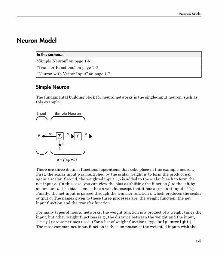
The fundamental building block for neural networks is the single-input neuron, such asthis example.
There are three distinct functional operations that take place in this example neuron.First, the scalar input p is multiplied by the scalar weight w to form the product wp,again a scalar. Second, the weighted input wp is added to the scalar bias b to form thenet input n. (In this case, you can view the bias as shifting the function f to the left byan amount b. The bias is much like a weight, except that it has a constant input of 1.)Finally, the net input is passed through the transfer function f, which produces the scalaroutput a. The names given to these three processes are: the weight function, the netinput function and the transfer function.
For many types of neural networks, the weight function is a product of a weight times theinput, but other weight functions (e.g., the distance between the weight and the input,|w − p|) are sometimes used. (For a list of weight functions, type help nnweight.)The most common net input function is the summation of the weighted inputs with the
1 Neural Network Objects, Data, and Training Styles
1-6
bias, but other operations, such as multiplication, can be used. (For a list of net inputfunctions, type help nnnetinput.) “Introduction to Radial Basis Neural Networks”discusses how distance can be used as the weight function and multiplication can be usedas the net input function. There are also many types of transfer functions. Examplesof various transfer functions are in “Transfer Functions” on page 1-6. (For a list oftransfer functions, type help nntransfer.)
Note that w and b are both adjustable scalar parameters of the neuron. The central ideaof neural networks is that such parameters can be adjusted so that the network exhibitssome desired or interesting behavior. Thus, you can train the network to do a particularjob by adjusting the weight or bias parameters.
All the neurons in the Neural Network Toolbox software have provision for a bias, anda bias is used in many of the examples and is assumed in most of this toolbox. However,you can omit a bias in a neuron if you want.
Transfer Functions
Many transfer functions are included in the Neural Network Toolbox software.
Two of the most commonly used functions are shown below.
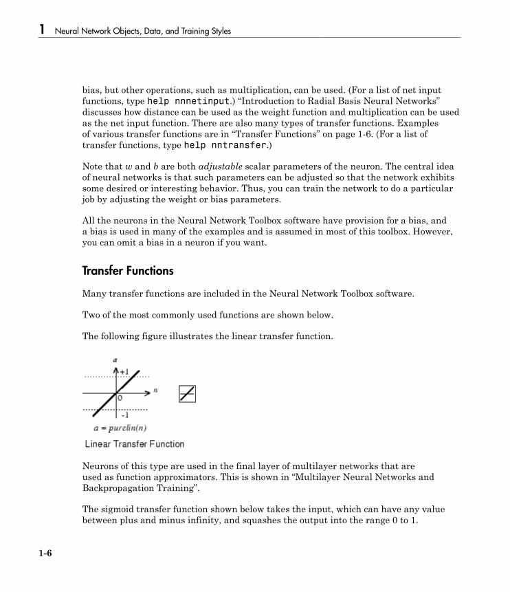
The following figure illustrates the linear transfer function.
Neurons of this type are used in the final layer of multilayer networks that areused as function approximators. This is shown in “Multilayer Neural Networks andBackpropagation Training”.
The sigmoid transfer function shown below takes the input, which can have any valuebetween plus and minus infinity, and squashes the output into the range 0 to 1.
Neuron Model
1-7
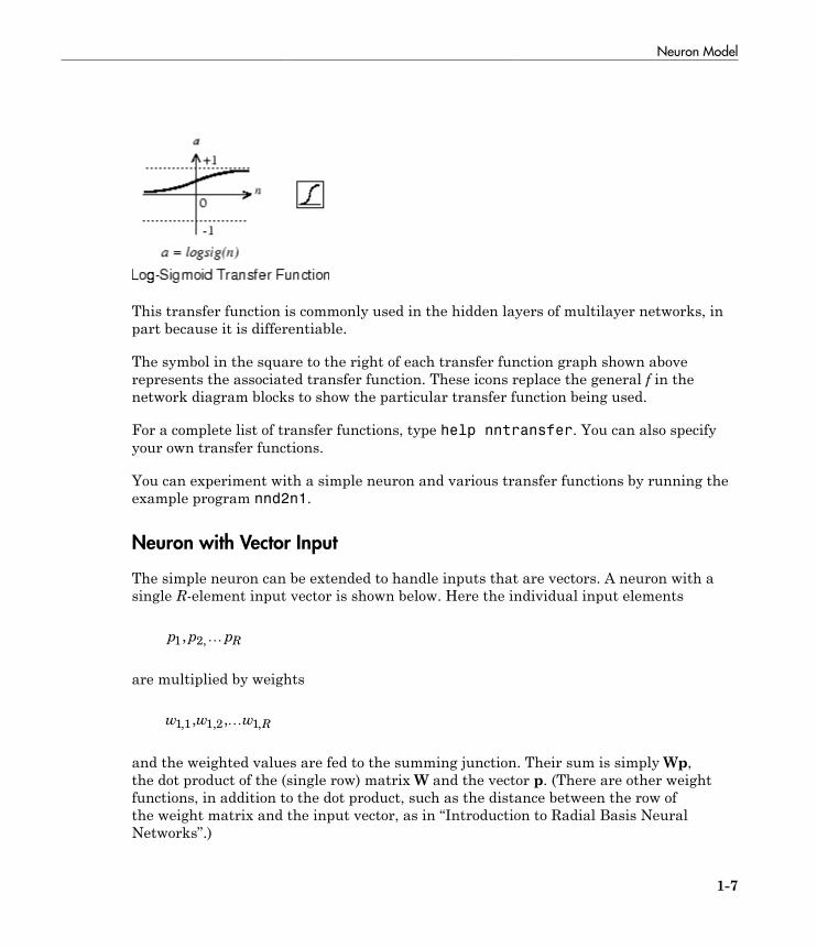
This transfer function is commonly used in the hidden layers of multilayer networks, inpart because it is differentiable.
The symbol in the square to the right of each transfer function graph shown aboverepresents the associated transfer function. These icons replace the general f in thenetwork diagram blocks to show the particular transfer function being used.
For a complete list of transfer functions, type help nntransfer. You can also specifyyour own transfer functions.
You can experiment with a simple neuron and various transfer functions by running theexample program nnd2n1.
Neuron with Vector Input
The simple neuron can be extended to handle inputs that are vectors. A neuron with asingle R-element input vector is shown below. Here the individual input elements
p p pR1 2, ,…
are multiplied by weights
w w w R1 1 1 2 1, , ,, ,…
and the weighted values are fed to the summing junction. Their sum is simply Wp,the dot product of the (single row) matrix W and the vector p. (There are other weightfunctions, in addition to the dot product, such as the distance between the row ofthe weight matrix and the input vector, as in “Introduction to Radial Basis NeuralNetworks”.)

1 Neural Network Objects, Data, and Training Styles
1-8
The neuron has a bias b, which is summed with the weighted inputs to form the netinput n. (In addition to the summation, other net input functions can be used, such as themultiplication that is used in “Introduction to Radial Basis Neural Networks”.) The netinput n is the argument of the transfer function f.
n w p w p w p bR R= + + + +1 1 1 1 2 2 1, , ,…
This expression can, of course, be written in MATLAB code as
n = W*p + b
However, you will seldom be writing code at this level, for such code is already built intofunctions to define and simulate entire networks.
Abbreviated Notation
The figure of a single neuron shown above contains a lot of detail. When you considernetworks with many neurons, and perhaps layers of many neurons, there is so muchdetail that the main thoughts tend to be lost. Thus, the authors have devised anabbreviated notation for an individual neuron. This notation, which is used later incircuits of multiple neurons, is shown here.

Neuron Model
1-9
Here the input vector p is represented by the solid dark vertical bar at the left. Thedimensions of p are shown below the symbol p in the figure as R × 1. (Note that a capitalletter, such as R in the previous sentence, is used when referring to the size of a vector.)Thus, p is a vector of R input elements. These inputs postmultiply the single-row, R-column matrix W. As before, a constant 1 enters the neuron as an input and is multipliedby a scalar bias b. The net input to the transfer function f is n, the sum of the bias band the product Wp. This sum is passed to the transfer function f to get the neuron'soutput a, which in this case is a scalar. Note that if there were more than one neuron, thenetwork output would be a vector.
A layer of a network is defined in the previous figure. A layer includes the weights, themultiplication and summing operations (here realized as a vector product Wp), the biasb, and the transfer function f. The array of inputs, vector p, is not included in or called alayer.
As with the “Simple Neuron” on page 1-5, there are three operations that take placein the layer: the weight function (matrix multiplication, or dot product, in this case), thenet input function (summation, in this case), and the transfer function.
Each time this abbreviated network notation is used, the sizes of the matrices are shownjust below their matrix variable names. This notation will allow you to understand thearchitectures and follow the matrix mathematics associated with them.
As discussed in “Transfer Functions” on page 1-6, when a specific transfer functionis to be used in a figure, the symbol for that transfer function replaces the f shown above.Here are some examples.

1 Neural Network Objects, Data, and Training Styles
1-10
You can experiment with a two-element neuron by running the example programnnd2n2.
More About• “Neural Network Architectures” on page 1-11• “Workflow for Neural Network Design” on page 1-2

Neural Network Architectures
1-11
Neural Network Architectures
In this section...
“One Layer of Neurons” on page 1-11“Multiple Layers of Neurons” on page 1-13“Input and Output Processing Functions” on page 1-15
Two or more of the neurons shown earlier can be combined in a layer, and a particularnetwork could contain one or more such layers. First consider a single layer of neurons.
One Layer of Neurons
A one-layer network with R input elements and S neurons follows.
In this network, each element of the input vector p is connected to each neuron inputthrough the weight matrix W. The ith neuron has a summer that gathers its weightedinputs and bias to form its own scalar output n(i). The various n(i) taken together forman S-element net input vector n. Finally, the neuron layer outputs form a column vectora. The expression for a is shown at the bottom of the figure.
1 Neural Network Objects, Data, and Training Styles
1-12
Note that it is common for the number of inputs to a layer to be different from thenumber of neurons (i.e., R is not necessarily equal to S). A layer is not constrained tohave the number of its inputs equal to the number of its neurons.
You can create a single (composite) layer of neurons having different transfer functionssimply by putting two of the networks shown earlier in parallel. Both networks wouldhave the same inputs, and each network would create some of the outputs.
The input vector elements enter the network through the weight matrix W.
W =
È
Î
ÍÍÍÍÍ
˘
˚
˙˙˙˙˙
w w w
w w w
w w w
R
R
S S S R
1 1 1 2 1
2 1 2 2 2
1 2
, , ,
, , ,
, , ,
…
…
…
Note that the row indices on the elements of matrix W indicate the destination neuronof the weight, and the column indices indicate which source is the input for that weight.Thus, the indices in w1,2 say that the strength of the signal from the second inputelement to the first (and only) neuron is w1,2.
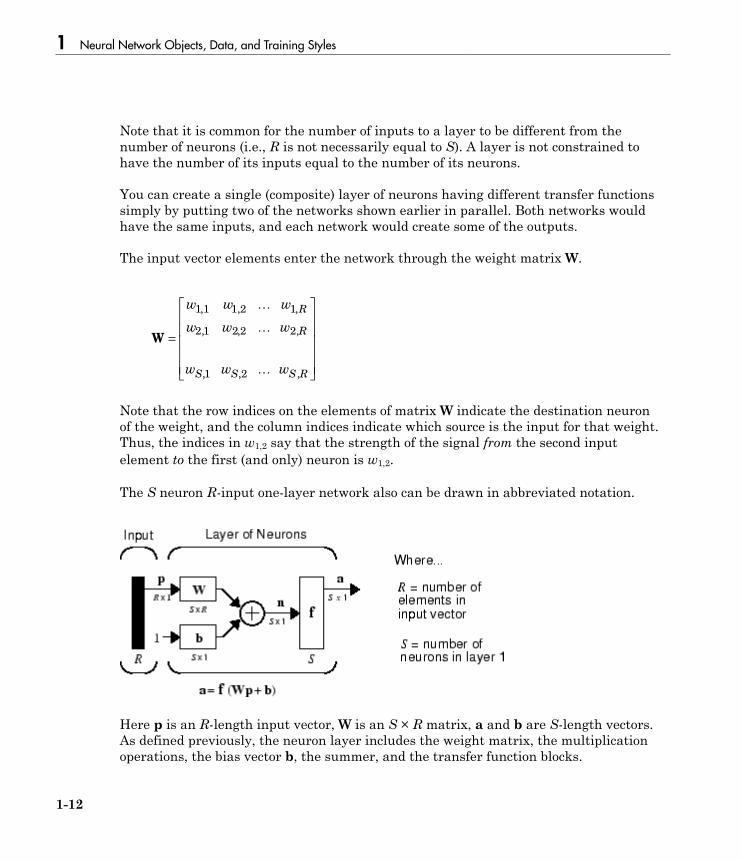
The S neuron R-input one-layer network also can be drawn in abbreviated notation.
Here p is an R-length input vector, W is an S × R matrix, a and b are S-length vectors.As defined previously, the neuron layer includes the weight matrix, the multiplicationoperations, the bias vector b, the summer, and the transfer function blocks.
Neural Network Architectures
1-13
Inputs and Layers
To describe networks having multiple layers, the notation must be extended. Specifically,it needs to make a distinction between weight matrices that are connected to inputs andweight matrices that are connected between layers. It also needs to identify the sourceand destination for the weight matrices.
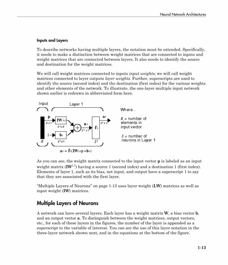
We will call weight matrices connected to inputs input weights; we will call weightmatrices connected to layer outputs layer weights. Further, superscripts are used toidentify the source (second index) and the destination (first index) for the various weightsand other elements of the network. To illustrate, the one-layer multiple input networkshown earlier is redrawn in abbreviated form here.
As you can see, the weight matrix connected to the input vector p is labeled as an inputweight matrix (IW1,1) having a source 1 (second index) and a destination 1 (first index).Elements of layer 1, such as its bias, net input, and output have a superscript 1 to saythat they are associated with the first layer.
“Multiple Layers of Neurons” on page 1-13 uses layer weight (LW) matrices as well asinput weight (IW) matrices.
Multiple Layers of Neurons
A network can have several layers. Each layer has a weight matrix W, a bias vector b,and an output vector a. To distinguish between the weight matrices, output vectors,etc., for each of these layers in the figures, the number of the layer is appended as asuperscript to the variable of interest. You can see the use of this layer notation in thethree-layer network shown next, and in the equations at the bottom of the figure.
1 Neural Network Objects, Data, and Training Styles
1-14
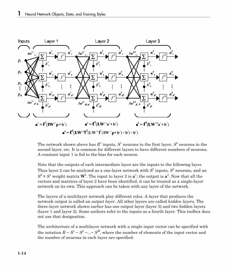
The network shown above has R1 inputs, S1 neurons in the first layer, S2 neurons in thesecond layer, etc. It is common for different layers to have different numbers of neurons.A constant input 1 is fed to the bias for each neuron.
Note that the outputs of each intermediate layer are the inputs to the following layer.Thus layer 2 can be analyzed as a one-layer network with S1 inputs, S2 neurons, and anS2 × S1 weight matrix W2. The input to layer 2 is a1; the output is a2. Now that all thevectors and matrices of layer 2 have been identified, it can be treated as a single-layernetwork on its own. This approach can be taken with any layer of the network.
The layers of a multilayer network play different roles. A layer that produces thenetwork output is called an output layer. All other layers are called hidden layers. Thethree-layer network shown earlier has one output layer (layer 3) and two hidden layers(layer 1 and layer 2). Some authors refer to the inputs as a fourth layer. This toolbox doesnot use that designation.
The architecture of a multilayer network with a single input vector can be specified withthe notation R − S1 − S2 −...− SM, where the number of elements of the input vector andthe number of neurons in each layer are specified.

Neural Network Architectures
1-15
The same three-layer network can also be drawn using abbreviated notation.
Multiple-layer networks are quite powerful. For instance, a network of two layers, wherethe first layer is sigmoid and the second layer is linear, can be trained to approximateany function (with a finite number of discontinuities) arbitrarily well. This kind of two-layer network is used extensively in “Multilayer Neural Networks and BackpropagationTraining”.
Here it is assumed that the output of the third layer, a3, is the network output ofinterest, and this output is labeled as y. This notation is used to specify the output ofmultilayer networks.
Input and Output Processing Functions
Network inputs might have associated processing functions. Processing functionstransform user input data to a form that is easier or more efficient for a network.
For instance, mapminmax transforms input data so that all values fall into the interval[−1, 1]. This can speed up learning for many networks. removeconstantrows removesthe rows of the input vector that correspond to input elements that always have thesame value, because these input elements are not providing any useful information tothe network. The third common processing function is fixunknowns, which recodesunknown data (represented in the user's data with NaN values) into a numerical form forthe network. fixunknowns preserves information about which values are known andwhich are unknown.
Similarly, network outputs can also have associated processing functions. Outputprocessing functions are used to transform user-provided target vectors for network use.

1 Neural Network Objects, Data, and Training Styles
1-16
Then, network outputs are reverse-processed using the same functions to produce outputdata with the same characteristics as the original user-provided targets.
Both mapminmax and removeconstantrows are often associated with network outputs.However, fixunknowns is not. Unknown values in targets (represented by NaN values)do not need to be altered for network use.
Processing functions are described in more detail in “Choose Neural Network Input-Output Processing Functions” on page 2-9.
More About• “Neuron Model” on page 1-5• “Workflow for Neural Network Design” on page 1-2
Create Neural Network Object
1-17
Create Neural Network Object
This topic is part of the design workflow described in “Workflow for Neural NetworkDesign” on page 1-2.
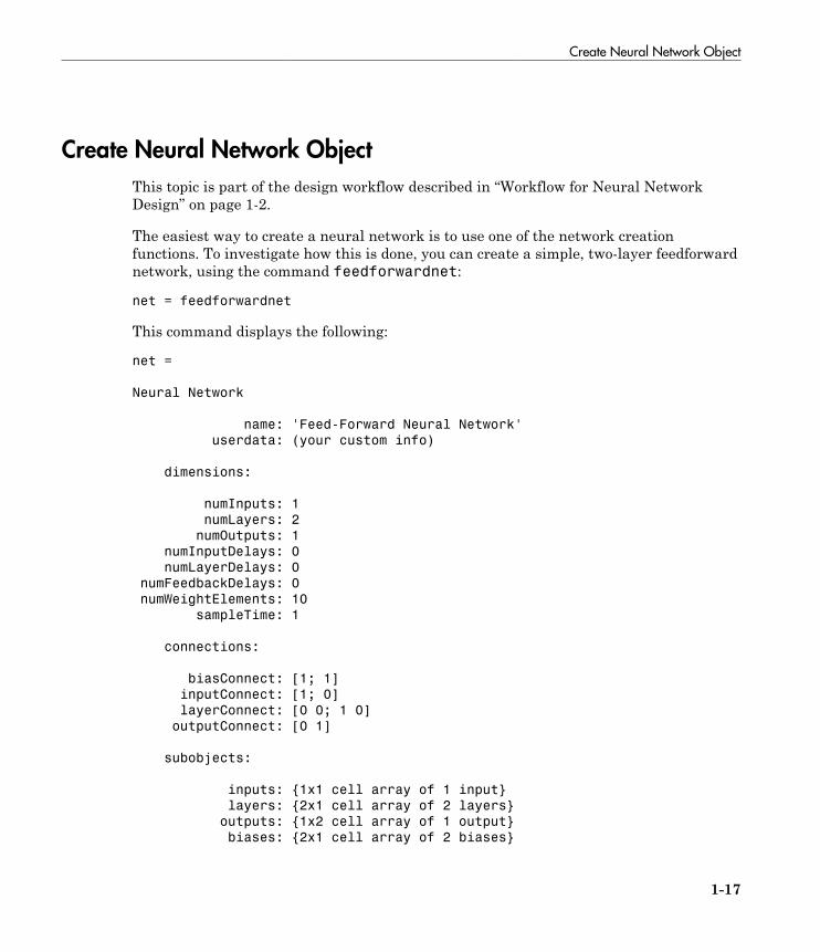
The easiest way to create a neural network is to use one of the network creationfunctions. To investigate how this is done, you can create a simple, two-layer feedforwardnetwork, using the command feedforwardnet:
net = feedforwardnet
This command displays the following:
net =
Neural Network
name: 'Feed-Forward Neural Network'
userdata: (your custom info)
dimensions:
numInputs: 1
numLayers: 2
numOutputs: 1
numInputDelays: 0
numLayerDelays: 0
numFeedbackDelays: 0
numWeightElements: 10
sampleTime: 1
connections:
biasConnect: [1; 1]
inputConnect: [1; 0]
layerConnect: [0 0; 1 0]
outputConnect: [0 1]
subobjects:
inputs: {1x1 cell array of 1 input}
layers: {2x1 cell array of 2 layers}
outputs: {1x2 cell array of 1 output}
biases: {2x1 cell array of 2 biases}

1 Neural Network Objects, Data, and Training Styles
1-18
inputWeights: {2x1 cell array of 1 weight}
layerWeights: {2x2 cell array of 1 weight}
functions:
adaptFcn: 'adaptwb'
adaptParam: (none)
derivFcn: 'defaultderiv'
divideFcn: 'dividerand'
divideParam: .trainRatio, .valRatio, .testRatio
divideMode: 'sample'
initFcn: 'initlay'
performFcn: 'mse'
performParam: .regularization, .normalization
plotFcns: {'plotperform', plottrainstate, ploterrhist,
plotregression}
plotParams: {1x4 cell array of 4 params}
trainFcn: 'trainlm'
trainParam: .showWindow, .showCommandLine, .show, .epochs,
.time, .goal, .min_grad, .max_fail, .mu, .mu_dec,
.mu_inc, .mu_max
weight and bias values:
IW: {2x1 cell} containing 1 input weight matrix
LW: {2x2 cell} containing 1 layer weight matrix
b: {2x1 cell} containing 2 bias vectors
methods:
adapt: Learn while in continuous use
configure: Configure inputs & outputs
gensim: Generate Simulink model
init: Initialize weights & biases
perform: Calculate performance
sim: Evaluate network outputs given inputs
train: Train network with examples
view: View diagram
unconfigure: Unconfigure inputs & outputs
evaluate: outputs = net(inputs)
Create Neural Network Object
1-19
This display is an overview of the network object, which is used to store all of theinformation that defines a neural network. There is a lot of detail here, but there are afew key sections that can help you to see how the network object is organized.
The dimensions section stores the overall structure of the network. Here you can seethat there is one input to the network (although the one input can be a vector containingmany elements), one network output and two layers.
The connections section stores the connections between components of the network.For example, here there is a bias connected to each layer, the input is connected tolayer 1, and the output comes from layer 2. You can also see that layer 1 is connectedto layer 2. (The rows of net.layerConnect represent the destination layer, and thecolumns represent the source layer. A one in this matrix indicates a connection, anda zero indicates a lack of connection. For this example, there is a single one in the 2,1element of the matrix.)
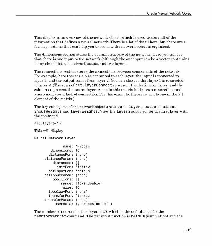
The key subobjects of the network object are inputs, layers, outputs, biases,inputWeights and layerWeights. View the layers subobject for the first layer withthe command
net.layers{1}
This will display
Neural Network Layer
name: 'Hidden'
dimensions: 10
distanceFcn: (none)
distanceParam: (none)
distances: []
initFcn: 'initnw'
netInputFcn: 'netsum'
netInputParam: (none)
positions: []
range: [10x2 double]
size: 10
topologyFcn: (none)
transferFcn: 'tansig'
transferParam: (none)
userdata: (your custom info)
The number of neurons in this layer is 20, which is the default size for thefeedforwardnet command. The net input function is netsum (summation) and the

1 Neural Network Objects, Data, and Training Styles
1-20
transfer function is the tansig. If you wanted to change the transfer function to logsig,for example, you could execute the command:
net.layers{1}.transferFcn = 'logsig';
To view the layerWeights subobject for the weight between layer 1 and layer 2, use thecommand:
net.layerWeights{2,1}
This produces the following response.
Neural Network Weight
delays: 0
initFcn: (none)
initConfig: .inputSize
learn: true
learnFcn: 'learngdm'
learnParam: .lr, .mc
size: [0 10]
weightFcn: 'dotprod'
weightParam: (none)
userdata: (your custom info)
The weight function is dotprod, which represents standard matrix multiplication (dotproduct). Note that the size of this layer weight is 0-by-20. The reason that we have zerorows is because the network has not yet been configured for a particular data set. Thenumber of output neurons is determined by the number of elements in your target vector.During the configuration process, you will provide the network with example inputs andtargets, and then the number of output neurons can be assigned.
This gives you some idea of how the network object is organized. For many applications,you will not need to be concerned about making changes directly to the network object,since that is taken care of by the network creation functions. It is usually only when youwant to override the system defaults that it is necessary to access the network objectdirectly. Later topics will show how this is done for particular networks and trainingmethods.
If you would like to investigate the network object in more detail, you will find thatthe object listings, such as the one shown above, contains links to help files on eachsubobject. Just click the links, and you can selectively investigate those parts of theobject that are of interest to you.
Configure Neural Network Inputs and Outputs
1-21
Configure Neural Network Inputs and Outputs
This topic is part of the design workflow described in “Workflow for Neural NetworkDesign” on page 1-2.
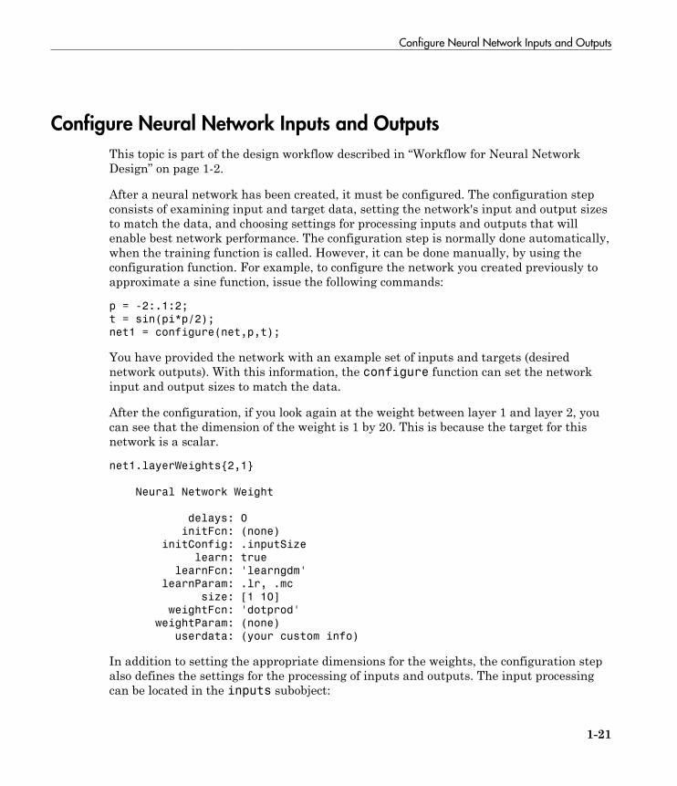
After a neural network has been created, it must be configured. The configuration stepconsists of examining input and target data, setting the network's input and output sizesto match the data, and choosing settings for processing inputs and outputs that willenable best network performance. The configuration step is normally done automatically,when the training function is called. However, it can be done manually, by using theconfiguration function. For example, to configure the network you created previously toapproximate a sine function, issue the following commands:
p = -2:.1:2;
t = sin(pi*p/2);
net1 = configure(net,p,t);
You have provided the network with an example set of inputs and targets (desirednetwork outputs). With this information, the configure function can set the networkinput and output sizes to match the data.
After the configuration, if you look again at the weight between layer 1 and layer 2, youcan see that the dimension of the weight is 1 by 20. This is because the target for thisnetwork is a scalar.
net1.layerWeights{2,1}
Neural Network Weight
delays: 0
initFcn: (none)
initConfig: .inputSize
learn: true
learnFcn: 'learngdm'
learnParam: .lr, .mc
size: [1 10]
weightFcn: 'dotprod'
weightParam: (none)
userdata: (your custom info)
In addition to setting the appropriate dimensions for the weights, the configuration stepalso defines the settings for the processing of inputs and outputs. The input processingcan be located in the inputs subobject:
1 Neural Network Objects, Data, and Training Styles
1-22
net1.inputs{1}
Neural Network Input
name: 'Input'
feedbackOutput: []
processFcns: {'removeconstantrows', mapminmax}
processParams: {1x2 cell array of 2 params}
processSettings: {1x2 cell array of 2 settings}
processedRange: [1x2 double]
processedSize: 1
range: [1x2 double]
size: 1
userdata: (your custom info)
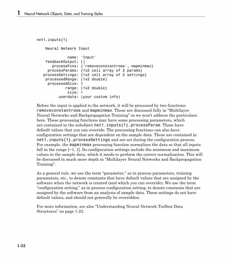
Before the input is applied to the network, it will be processed by two functions:removeconstantrows and mapminmax. These are discussed fully in “MultilayerNeural Networks and Backpropagation Training” so we won't address the particularshere. These processing functions may have some processing parameters, whichare contained in the subobject net1.inputs{1}.processParam. These havedefault values that you can override. The processing functions can also haveconfiguration settings that are dependent on the sample data. These are contained innet1.inputs{1}.processSettings and are set during the configuration process.For example, the mapminmax processing function normalizes the data so that all inputsfall in the range [−1, 1]. Its configuration settings include the minimum and maximumvalues in the sample data, which it needs to perform the correct normalization. This willbe discussed in much more depth in “Multilayer Neural Networks and BackpropagationTraining”.
As a general rule, we use the term “parameter,” as in process parameters, trainingparameters, etc., to denote constants that have default values that are assigned by thesoftware when the network is created (and which you can override). We use the term“configuration setting,” as in process configuration setting, to denote constants that areassigned by the software from an analysis of sample data. These settings do not havedefault values, and should not generally be overridden.
For more information, see also “Understanding Neural Network Toolbox DataStructures” on page 1-23.

Understanding Neural Network Toolbox Data Structures
1-23
Understanding Neural Network Toolbox Data Structures
In this section...
“Simulation with Concurrent Inputs in a Static Network” on page 1-23“Simulation with Sequential Inputs in a Dynamic Network” on page 1-24“Simulation with Concurrent Inputs in a Dynamic Network” on page 1-26
This topic discusses how the format of input data structures affects the simulation ofnetworks. It starts with static networks, and then continues with dynamic networks.The following section describes how the format of the data structures affects networktraining.
There are two basic types of input vectors: those that occur concurrently (at the sametime, or in no particular time sequence), and those that occur sequentially in time. Forconcurrent vectors, the order is not important, and if there were a number of networksrunning in parallel, you could present one input vector to each of the networks. Forsequential vectors, the order in which the vectors appear is important.
Simulation with Concurrent Inputs in a Static Network
The simplest situation for simulating a network occurs when the network to be simulatedis static (has no feedback or delays). In this case, you need not be concerned aboutwhether or not the input vectors occur in a particular time sequence, so you can treat theinputs as concurrent. In addition, the problem is made even simpler by assuming thatthe network has only one input vector. Use the following network as an example.
1 Neural Network Objects, Data, and Training Styles
1-24
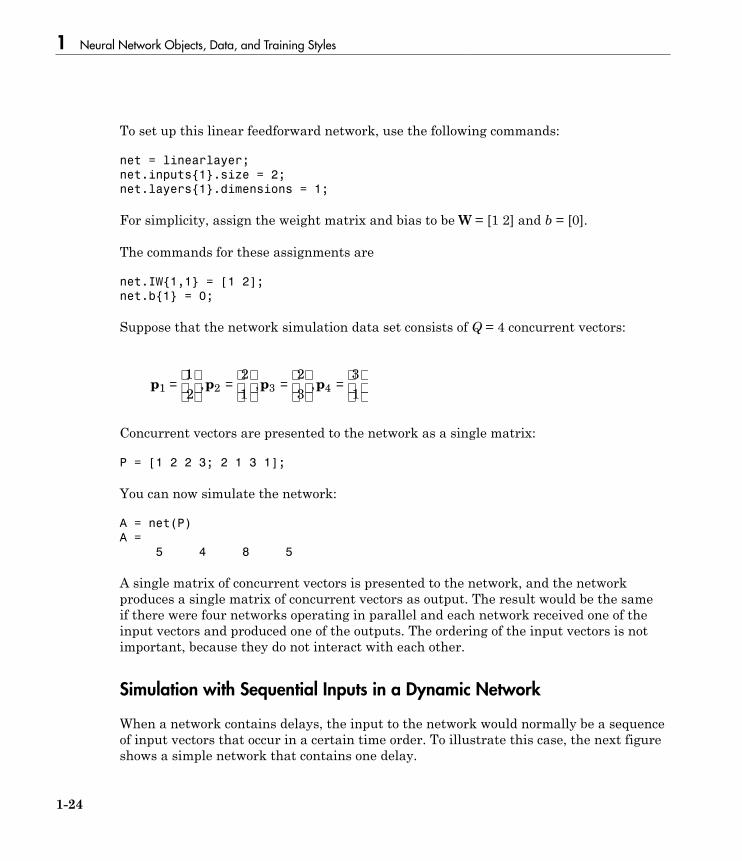
To set up this linear feedforward network, use the following commands:
net = linearlayer;
net.inputs{1}.size = 2;
net.layers{1}.dimensions = 1;
For simplicity, assign the weight matrix and bias to be W = [1 2] and b = [0].
The commands for these assignments are
net.IW{1,1} = [1 2];
net.b{1} = 0;
Suppose that the network simulation data set consists of Q = 4 concurrent vectors:
p p p p1 2 3 4
1
2
2
1
2
3
3
1=
=
=
=
, , ,
Concurrent vectors are presented to the network as a single matrix:
P = [1 2 2 3; 2 1 3 1];
You can now simulate the network:
A = net(P)
A =
5 4 8 5
A single matrix of concurrent vectors is presented to the network, and the networkproduces a single matrix of concurrent vectors as output. The result would be the sameif there were four networks operating in parallel and each network received one of theinput vectors and produced one of the outputs. The ordering of the input vectors is notimportant, because they do not interact with each other.
Simulation with Sequential Inputs in a Dynamic Network
When a network contains delays, the input to the network would normally be a sequenceof input vectors that occur in a certain time order. To illustrate this case, the next figureshows a simple network that contains one delay.

Understanding Neural Network Toolbox Data Structures
1-25
The following commands create this network:
net = linearlayer([0 1]);
net.inputs{1}.size = 1;
net.layers{1}.dimensions = 1;
net.biasConnect = 0;
Assign the weight matrix to be W = [1 2].
The command is:
net.IW{1,1} = [1 2];
Suppose that the input sequence is:
p p p p1 2 3 41 2 3 4= [ ] = [ ] = [ ] = [ ], , ,
Sequential inputs are presented to the network as elements of a cell array:
P = {1 2 3 4};
You can now simulate the network:
A = net(P)
A =
[1] [4] [7] [10]
You input a cell array containing a sequence of inputs, and the network produces a cellarray containing a sequence of outputs. The order of the inputs is important when theyare presented as a sequence. In this case, the current output is obtained by multiplying
1 Neural Network Objects, Data, and Training Styles
1-26
the current input by 1 and the preceding input by 2 and summing the result. If you wereto change the order of the inputs, the numbers obtained in the output would change.
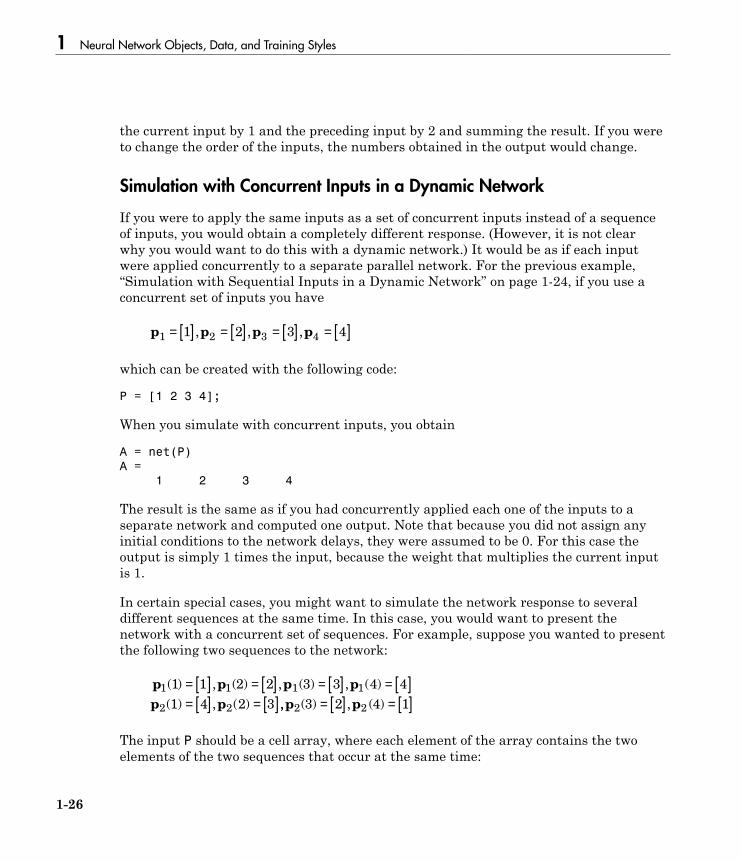
Simulation with Concurrent Inputs in a Dynamic Network
If you were to apply the same inputs as a set of concurrent inputs instead of a sequenceof inputs, you would obtain a completely different response. (However, it is not clearwhy you would want to do this with a dynamic network.) It would be as if each inputwere applied concurrently to a separate parallel network. For the previous example,“Simulation with Sequential Inputs in a Dynamic Network” on page 1-24, if you use aconcurrent set of inputs you have
p p p p1 2 3 41 2 3 4= [ ] = [ ] = [ ] = [ ], , ,
which can be created with the following code:
P = [1 2 3 4];
When you simulate with concurrent inputs, you obtain
A = net(P)
A =
1 2 3 4
The result is the same as if you had concurrently applied each one of the inputs to aseparate network and computed one output. Note that because you did not assign anyinitial conditions to the network delays, they were assumed to be 0. For this case theoutput is simply 1 times the input, because the weight that multiplies the current inputis 1.
In certain special cases, you might want to simulate the network response to severaldifferent sequences at the same time. In this case, you would want to present thenetwork with a concurrent set of sequences. For example, suppose you wanted to presentthe following two sequences to the network:
p p p p
p p
1 1 1 1
2 2
1 1 2 2 3 3 4 4
1 4 2 3
( ) , ( ) , ( ) , ( )
( ) , ( )
= [ ] = [ ] = [ ] = [ ]= [ ] = [ ],, ( ) , ( )p p2 23 2 4 1= [ ] = [ ]
The input P should be a cell array, where each element of the array contains the twoelements of the two sequences that occur at the same time:

Understanding Neural Network Toolbox Data Structures
1-27
P = {[1 4] [2 3] [3 2] [4 1]};
You can now simulate the network:
A = net(P);
The resulting network output would be
A = {[1 4] [4 11] [7 8] [10 5]}
As you can see, the first column of each matrix makes up the output sequence producedby the first input sequence, which was the one used in an earlier example. The secondcolumn of each matrix makes up the output sequence produced by the second inputsequence. There is no interaction between the two concurrent sequences. It is as if theywere each applied to separate networks running in parallel.
The following diagram shows the general format for the network input P when there areQ concurrent sequences of TS time steps. It covers all cases where there is a single inputvector. Each element of the cell array is a matrix of concurrent vectors that correspond tothe same point in time for each sequence. If there are multiple input vectors, there willbe multiple rows of matrices in the cell array.
In this topic, you apply sequential and concurrent inputs to dynamic networks. In“Simulation with Concurrent Inputs in a Static Network” on page 1-23, you appliedconcurrent inputs to static networks. It is also possible to apply sequential inputsto static networks. It does not change the simulated response of the network, but itcan affect the way in which the network is trained. This will become clear in “NeuralNetwork Training Concepts” on page 1-28.
See also “Configure Neural Network Inputs and Outputs” on page 1-21.
1 Neural Network Objects, Data, and Training Styles
1-28
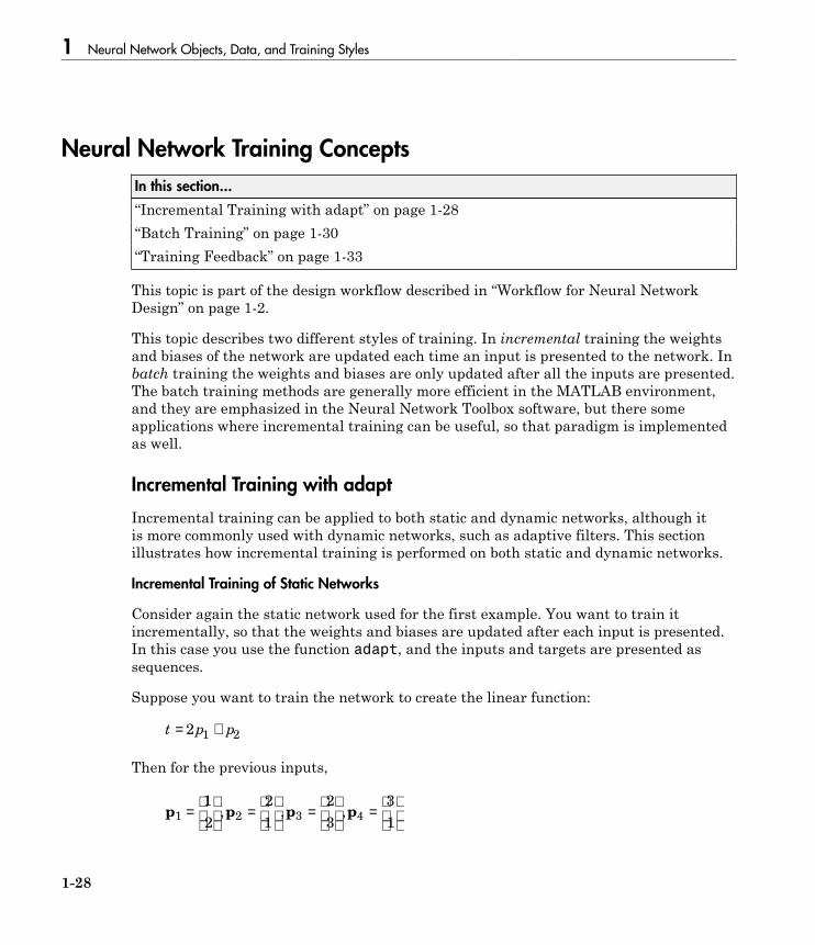
Neural Network Training Concepts
In this section...
“Incremental Training with adapt” on page 1-28“Batch Training” on page 1-30“Training Feedback” on page 1-33
This topic is part of the design workflow described in “Workflow for Neural NetworkDesign” on page 1-2.
This topic describes two different styles of training. In incremental training the weightsand biases of the network are updated each time an input is presented to the network. Inbatch training the weights and biases are only updated after all the inputs are presented.The batch training methods are generally more efficient in the MATLAB environment,and they are emphasized in the Neural Network Toolbox software, but there someapplications where incremental training can be useful, so that paradigm is implementedas well.
Incremental Training with adapt
Incremental training can be applied to both static and dynamic networks, although itis more commonly used with dynamic networks, such as adaptive filters. This sectionillustrates how incremental training is performed on both static and dynamic networks.
Incremental Training of Static Networks
Consider again the static network used for the first example. You want to train itincrementally, so that the weights and biases are updated after each input is presented.In this case you use the function adapt, and the inputs and targets are presented assequences.
Suppose you want to train the network to create the linear function:
t p p= +21 2
Then for the previous inputs,
p p p p1 2 3 4
1
2
2
1
2
3
3
1=
=
=
=
, , ,
Neural Network Training Concepts
1-29
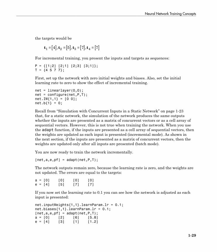
the targets would be
t t t t1 2 3 44 5 7 7= [ ] = [ ] = [ ] = [ ], , ,
For incremental training, you present the inputs and targets as sequences:
P = {[1;2] [2;1] [2;3] [3;1]};
T = {4 5 7 7};
First, set up the network with zero initial weights and biases. Also, set the initiallearning rate to zero to show the effect of incremental training.
net = linearlayer(0,0);
net = configure(net,P,T);
net.IW{1,1} = [0 0];
net.b{1} = 0;
Recall from “Simulation with Concurrent Inputs in a Static Network” on page 1-23that, for a static network, the simulation of the network produces the same outputswhether the inputs are presented as a matrix of concurrent vectors or as a cell array ofsequential vectors. However, this is not true when training the network. When you usethe adapt function, if the inputs are presented as a cell array of sequential vectors, thenthe weights are updated as each input is presented (incremental mode). As shown inthe next section, if the inputs are presented as a matrix of concurrent vectors, then theweights are updated only after all inputs are presented (batch mode).
You are now ready to train the network incrementally.
[net,a,e,pf] = adapt(net,P,T);
The network outputs remain zero, because the learning rate is zero, and the weights arenot updated. The errors are equal to the targets:
a = [0] [0] [0] [0]
e = [4] [5] [7] [7]
If you now set the learning rate to 0.1 you can see how the network is adjusted as eachinput is presented:
net.inputWeights{1,1}.learnParam.lr = 0.1;
net.biases{1,1}.learnParam.lr = 0.1;
[net,a,e,pf] = adapt(net,P,T);
a = [0] [2] [6] [5.8]
e = [4] [3] [1] [1.2]
1 Neural Network Objects, Data, and Training Styles
1-30
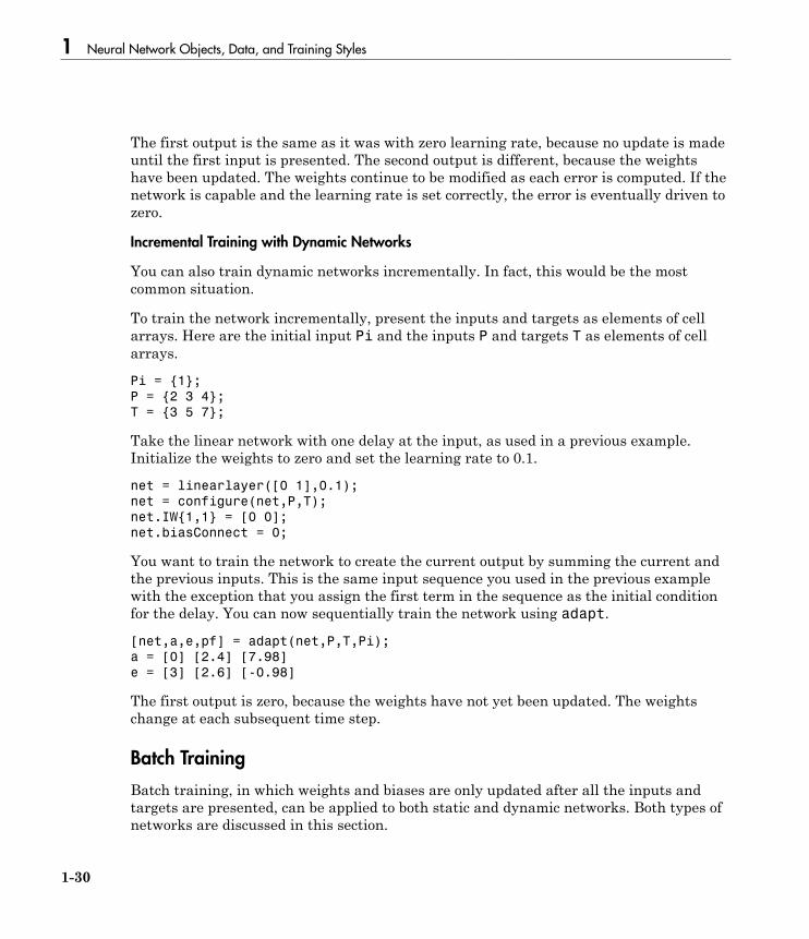
The first output is the same as it was with zero learning rate, because no update is madeuntil the first input is presented. The second output is different, because the weightshave been updated. The weights continue to be modified as each error is computed. If thenetwork is capable and the learning rate is set correctly, the error is eventually driven tozero.
Incremental Training with Dynamic Networks
You can also train dynamic networks incrementally. In fact, this would be the mostcommon situation.
To train the network incrementally, present the inputs and targets as elements of cellarrays. Here are the initial input Pi and the inputs P and targets T as elements of cellarrays.
Pi = {1};
P = {2 3 4};
T = {3 5 7};
Take the linear network with one delay at the input, as used in a previous example.Initialize the weights to zero and set the learning rate to 0.1.
net = linearlayer([0 1],0.1);
net = configure(net,P,T);
net.IW{1,1} = [0 0];
net.biasConnect = 0;
You want to train the network to create the current output by summing the current andthe previous inputs. This is the same input sequence you used in the previous examplewith the exception that you assign the first term in the sequence as the initial conditionfor the delay. You can now sequentially train the network using adapt.
[net,a,e,pf] = adapt(net,P,T,Pi);
a = [0] [2.4] [7.98]
e = [3] [2.6] [-0.98]
The first output is zero, because the weights have not yet been updated. The weightschange at each subsequent time step.
Batch Training
Batch training, in which weights and biases are only updated after all the inputs andtargets are presented, can be applied to both static and dynamic networks. Both types ofnetworks are discussed in this section.

Neural Network Training Concepts
1-31
Batch Training with Static Networks
Batch training can be done using either adapt or train, although train is generallythe best option, because it typically has access to more efficient training algorithms.Incremental training is usually done with adapt; batch training is usually done withtrain.
For batch training of a static network with adapt, the input vectors must be placed inone matrix of concurrent vectors.
P = [1 2 2 3; 2 1 3 1];
T = [4 5 7 7];
Begin with the static network used in previous examples. The learning rate is set to 0.01.
net = linearlayer(0,0.01);
net = configure(net,P,T);
net.IW{1,1} = [0 0];
net.b{1} = 0;
When you call adapt, it invokes trains (the default adaption function for the linearnetwork) and learnwh (the default learning function for the weights and biases). trainsuses Widrow-Hoff learning.
[net,a,e,pf] = adapt(net,P,T);
a = 0 0 0 0
e = 4 5 7 7
Note that the outputs of the network are all zero, because the weights are not updateduntil all the training set has been presented. If you display the weights, you find
net.IW{1,1}
ans = 0.4900 0.4100
net.b{1}
ans =
0.2300
This is different from the result after one pass of adapt with incremental updating.
Now perform the same batch training using train. Because the Widrow-Hoff rule canbe used in incremental or batch mode, it can be invoked by adapt or train. (There areseveral algorithms that can only be used in batch mode (e.g., Levenberg-Marquardt), sothese algorithms can only be invoked by train.)
1 Neural Network Objects, Data, and Training Styles
1-32
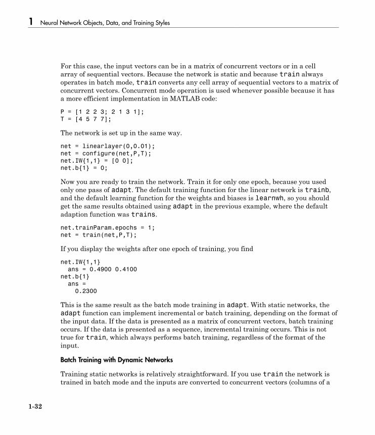
For this case, the input vectors can be in a matrix of concurrent vectors or in a cellarray of sequential vectors. Because the network is static and because train alwaysoperates in batch mode, train converts any cell array of sequential vectors to a matrix ofconcurrent vectors. Concurrent mode operation is used whenever possible because it hasa more efficient implementation in MATLAB code:
P = [1 2 2 3; 2 1 3 1];
T = [4 5 7 7];
The network is set up in the same way.
net = linearlayer(0,0.01);
net = configure(net,P,T);
net.IW{1,1} = [0 0];
net.b{1} = 0;
Now you are ready to train the network. Train it for only one epoch, because you usedonly one pass of adapt. The default training function for the linear network is trainb,and the default learning function for the weights and biases is learnwh, so you shouldget the same results obtained using adapt in the previous example, where the defaultadaption function was trains.
net.trainParam.epochs = 1;
net = train(net,P,T);
If you display the weights after one epoch of training, you find
net.IW{1,1}
ans = 0.4900 0.4100
net.b{1}
ans =
0.2300
This is the same result as the batch mode training in adapt. With static networks, theadapt function can implement incremental or batch training, depending on the format ofthe input data. If the data is presented as a matrix of concurrent vectors, batch trainingoccurs. If the data is presented as a sequence, incremental training occurs. This is nottrue for train, which always performs batch training, regardless of the format of theinput.
Batch Training with Dynamic Networks
Training static networks is relatively straightforward. If you use train the network istrained in batch mode and the inputs are converted to concurrent vectors (columns of a
Neural Network Training Concepts
1-33
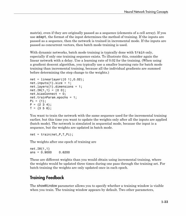
matrix), even if they are originally passed as a sequence (elements of a cell array). If youuse adapt, the format of the input determines the method of training. If the inputs arepassed as a sequence, then the network is trained in incremental mode. If the inputs arepassed as concurrent vectors, then batch mode training is used.
With dynamic networks, batch mode training is typically done with train only,especially if only one training sequence exists. To illustrate this, consider again thelinear network with a delay. Use a learning rate of 0.02 for the training. (When usinga gradient descent algorithm, you typically use a smaller learning rate for batch modetraining than incremental training, because all the individual gradients are summedbefore determining the step change to the weights.)
net = linearlayer([0 1],0.02);
net.inputs{1}.size = 1;
net.layers{1}.dimensions = 1;
net.IW{1,1} = [0 0];
net.biasConnect = 0;
net.trainParam.epochs = 1;
Pi = {1};
P = {2 3 4};
T = {3 5 6};
You want to train the network with the same sequence used for the incremental trainingearlier, but this time you want to update the weights only after all the inputs are applied(batch mode). The network is simulated in sequential mode, because the input is asequence, but the weights are updated in batch mode.
net = train(net,P,T,Pi);
The weights after one epoch of training are
net.IW{1,1}
ans = 0.9000 0.6200
These are different weights than you would obtain using incremental training, wherethe weights would be updated three times during one pass through the training set. Forbatch training the weights are only updated once in each epoch.
Training Feedback
The showWindow parameter allows you to specify whether a training window is visiblewhen you train. The training window appears by default. Two other parameters,
1 Neural Network Objects, Data, and Training Styles
1-34
showCommandLine and show, determine whether command-line output is generated andthe number of epochs between command-line feedback during training. For instance, thiscode turns off the training window and gives you training status information every 35epochs when the network is later trained with train:
net.trainParam.showWindow = false;
net.trainParam.showCommandLine = true;
net.trainParam.show= 35;
Sometimes it is convenient to disable all training displays. To do that, turn off both thetraining window and command-line feedback:
net.trainParam.showWindow = false;
net.trainParam.showCommandLine = false;
The training window appears automatically when you train. Use the nntraintoolfunction to manually open and close the training window.
nntraintool
nntraintool('close')
2
Multilayer Neural Networks andBackpropagation Training
• “Multilayer Neural Networks and Backpropagation Training” on page 2-2• “Multilayer Neural Network Architecture” on page 2-4• “Prepare Data for Multilayer Neural Networks” on page 2-8• “Choose Neural Network Input-Output Processing Functions” on page 2-9• “Divide Data for Optimal Neural Network Training” on page 2-12• “Create, Configure, and Initialize Multilayer Neural Networks” on page 2-14• “Train and Apply Multilayer Neural Networks” on page 2-17• “Analyze Neural Network Performance After Training” on page 2-23• “Limitations and Cautions” on page 2-29

2 Multilayer Neural Networks and Backpropagation Training
2-2
Multilayer Neural Networks and Backpropagation Training
The multilayer feedforward neural network is the workhorse of the Neural NetworkToolbox software. It can be used for both function fitting and pattern recognitionproblems. With the addition of a tapped delay line, it can also be used for predictionproblems, as discussed in “Design Time Series Time-Delay Neural Networks” on page3-14. This topic shows how you can use a multilayer network. It also illustrates thebasic procedures for designing any neural network.
Note The training functions described in this topic are not limited to multilayernetworks. They can be used to train arbitrary architectures (even custom networks), aslong as their components are differentiable.
The work flow for the general neural network design process has seven primary steps:
1 Collect data2 Create the network3 Configure the network4 Initialize the weights and biases5 Train the network6 Validate the network (post-training analysis)7 Use the network
Step 1 might happen outside the framework of Neural Network Toolbox software, butthis step is critical to the success of the design process.
Details of this workflow are discussed in these sections:
• “Multilayer Neural Network Architecture” on page 2-4• “Prepare Data for Multilayer Neural Networks” on page 2-8• “Create, Configure, and Initialize Multilayer Neural Networks” on page 2-14• “Train and Apply Multilayer Neural Networks” on page 2-17• “Analyze Neural Network Performance After Training” on page 2-23• “Use the Network” on page 2-22• “Limitations and Cautions” on page 2-29
Multilayer Neural Networks and Backpropagation Training
2-3
Optional workflow steps are discussed in these sections:
• “Choose Neural Network Input-Output Processing Functions” on page 2-9• “Divide Data for Optimal Neural Network Training” on page 2-12• “Neural Networks with Parallel and GPU Computing” on page 8-2
For time series, dynamic modeling, and prediction, see this section:
• “How Dynamic Neural Networks Work” on page 3-3
2 Multilayer Neural Networks and Backpropagation Training
2-4
Multilayer Neural Network Architecture
In this section...
“Neuron Model (logsig, tansig, purelin)” on page 2-4“Feedforward Neural Network” on page 2-5
This topic presents part of a typical multilayer network workflow. For more informationand other steps, see “Multilayer Neural Networks and Backpropagation Training” onpage 2-2.
Neuron Model (logsig, tansig, purelin)
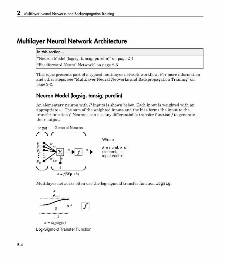
An elementary neuron with R inputs is shown below. Each input is weighted with anappropriate w. The sum of the weighted inputs and the bias forms the input to thetransfer function f. Neurons can use any differentiable transfer function f to generatetheir output.
Multilayer networks often use the log-sigmoid transfer function logsig.

Multilayer Neural Network Architecture
2-5
The function logsig generates outputs between 0 and 1 as the neuron's net input goesfrom negative to positive infinity.
Alternatively, multilayer networks can use the tan-sigmoid transfer function tansig.
Sigmoid output neurons are often used for pattern recognition problems, while linearoutput neurons are used for function fitting problems. The linear transfer functionpurelin is shown below.
The three transfer functions described here are the most commonly used transferfunctions for multilayer networks, but other differentiable transfer functions can becreated and used if desired.
Feedforward Neural Network
A single-layer network of S logsig neurons having R inputs is shown below in full detailon the left and with a layer diagram on the right.

2 Multilayer Neural Networks and Backpropagation Training
2-6
Feedforward networks often have one or more hidden layers of sigmoid neurons followedby an output layer of linear neurons. Multiple layers of neurons with nonlinear transferfunctions allow the network to learn nonlinear relationships between input and outputvectors. The linear output layer is most often used for function fitting (or nonlinearregression) problems.
On the other hand, if you want to constrain the outputs of a network (such as between 0and 1), then the output layer should use a sigmoid transfer function (such as logsig).This is the case when the network is used for pattern recognition problems (in which adecision is being made by the network).
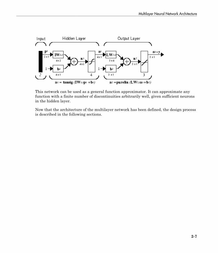
For multiple-layer networks the layer number determines the superscript on the weightmatrix. The appropriate notation is used in the two-layer tansig/purelin networkshown next.
Multilayer Neural Network Architecture
2-7
This network can be used as a general function approximator. It can approximate anyfunction with a finite number of discontinuities arbitrarily well, given sufficient neuronsin the hidden layer.
Now that the architecture of the multilayer network has been defined, the design processis described in the following sections.

2 Multilayer Neural Networks and Backpropagation Training
2-8
Prepare Data for Multilayer Neural Networks
This topic presents part of a typical multilayer network workflow. For more informationand other steps, see “Multilayer Neural Networks and Backpropagation Training” onpage 2-2.
Before beginning the network design process, you first collect and prepare sample data.It is generally difficult to incorporate prior knowledge into a neural network, thereforethe network can only be as accurate as the data that are used to train the network.
It is important that the data cover the range of inputs for which the network will beused. Multilayer networks can be trained to generalize well within the range of inputsfor which they have been trained. However, they do not have the ability to accuratelyextrapolate beyond this range, so it is important that the training data span the fullrange of the input space.
After the data have been collected, there are two steps that need to be performed beforethe data are used to train the network: the data need to be preprocessed, and they needto be divided into subsets.
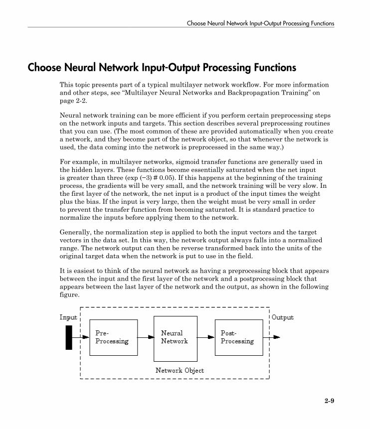
Choose Neural Network Input-Output Processing Functions
2-9
Choose Neural Network Input-Output Processing Functions
This topic presents part of a typical multilayer network workflow. For more informationand other steps, see “Multilayer Neural Networks and Backpropagation Training” onpage 2-2.
Neural network training can be more efficient if you perform certain preprocessing stepson the network inputs and targets. This section describes several preprocessing routinesthat you can use. (The most common of these are provided automatically when you createa network, and they become part of the network object, so that whenever the network isused, the data coming into the network is preprocessed in the same way.)
For example, in multilayer networks, sigmoid transfer functions are generally used inthe hidden layers. These functions become essentially saturated when the net inputis greater than three (exp (−3) ≅ 0.05). If this happens at the beginning of the trainingprocess, the gradients will be very small, and the network training will be very slow. Inthe first layer of the network, the net input is a product of the input times the weightplus the bias. If the input is very large, then the weight must be very small in orderto prevent the transfer function from becoming saturated. It is standard practice tonormalize the inputs before applying them to the network.
Generally, the normalization step is applied to both the input vectors and the targetvectors in the data set. In this way, the network output always falls into a normalizedrange. The network output can then be reverse transformed back into the units of theoriginal target data when the network is put to use in the field.
It is easiest to think of the neural network as having a preprocessing block that appearsbetween the input and the first layer of the network and a postprocessing block thatappears between the last layer of the network and the output, as shown in the followingfigure.

2 Multilayer Neural Networks and Backpropagation Training
2-10
Most of the network creation functions in the toolbox, including the multilayer networkcreation functions, such as feedforwardnet, automatically assign processing functionsto your network inputs and outputs. These functions transform the input and targetvalues you provide into values that are better suited for network training.
You can override the default input and output processing functions by adjusting networkproperties after you create the network.
To see a cell array list of processing functions assigned to the input of a network, accessthis property:
net.inputs{1}.processFcns
where the index 1 refers to the first input vector. (There is only one input vector for thefeedforward network.) To view the processing functions returned by the output of a two-layer network, access this network property:
net.outputs{2}.processFcns
where the index 2 refers to the output vector coming from the second layer. (For thefeedforward network, there is only one output vector, and it comes from the final layer.)You can use these properties to change the processing functions that you want yournetwork to apply to the inputs and outputs. However, the defaults usually provideexcellent performance.
Several processing functions have parameters that customize their operation. You canaccess or change the parameters of the ith input processing function for the networkinput as follows:
net.inputs{1}.processParams{i}
You can access or change the parameters of the ith output processing function for thenetwork output associated with the second layer, as follows:
net.outputs{2}.processParams{i}
For multilayer network creation functions, such as feedforwardnet, the default inputprocessing functions are removeconstantrows and mapminmax. For outputs, thedefault processing functions are also removeconstantrows and mapminmax.
The following table lists the most common preprocessing and postprocessing functions. Inmost cases, you will not need to use them directly, since the preprocessing steps become
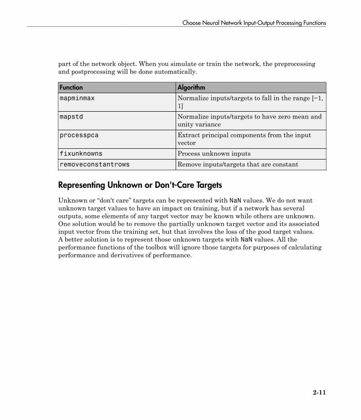
Choose Neural Network Input-Output Processing Functions
2-11
part of the network object. When you simulate or train the network, the preprocessingand postprocessing will be done automatically.
Function Algorithm
mapminmax Normalize inputs/targets to fall in the range [−1,1]
mapstd Normalize inputs/targets to have zero mean andunity variance
processpca Extract principal components from the inputvector
fixunknowns Process unknown inputsremoveconstantrows Remove inputs/targets that are constant
Representing Unknown or Don't-Care Targets
Unknown or “don't care” targets can be represented with NaN values. We do not wantunknown target values to have an impact on training, but if a network has severaloutputs, some elements of any target vector may be known while others are unknown.One solution would be to remove the partially unknown target vector and its associatedinput vector from the training set, but that involves the loss of the good target values.A better solution is to represent those unknown targets with NaN values. All theperformance functions of the toolbox will ignore those targets for purposes of calculatingperformance and derivatives of performance.
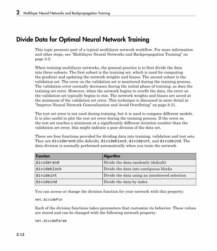
2 Multilayer Neural Networks and Backpropagation Training
2-12
Divide Data for Optimal Neural Network Training
This topic presents part of a typical multilayer network workflow. For more informationand other steps, see “Multilayer Neural Networks and Backpropagation Training” onpage 2-2.
When training multilayer networks, the general practice is to first divide the datainto three subsets. The first subset is the training set, which is used for computingthe gradient and updating the network weights and biases. The second subset is thevalidation set. The error on the validation set is monitored during the training process.The validation error normally decreases during the initial phase of training, as does thetraining set error. However, when the network begins to overfit the data, the error onthe validation set typically begins to rise. The network weights and biases are saved atthe minimum of the validation set error. This technique is discussed in more detail in“Improve Neural Network Generalization and Avoid Overfitting” on page 8-31.
The test set error is not used during training, but it is used to compare different models.It is also useful to plot the test set error during the training process. If the error onthe test set reaches a minimum at a significantly different iteration number than thevalidation set error, this might indicate a poor division of the data set.
There are four functions provided for dividing data into training, validation and test sets.They are dividerand (the default), divideblock, divideint, and divideind. Thedata division is normally performed automatically when you train the network.
Function Algorithm
dividerand Divide the data randomly (default)divideblock Divide the data into contiguous blocksdivideint Divide the data using an interleaved selectiondivideind Divide the data by index
You can access or change the division function for your network with this property:
net.divideFcn
Each of the division functions takes parameters that customize its behavior. These valuesare stored and can be changed with the following network property:
net.divideParam

Divide Data for Optimal Neural Network Training
2-13
The divide function is accessed automatically whenever the network is trained, and isused to divide the data into training, validation and testing subsets. If net.divideFcnis set to 'dividerand' (the default), then the data is randomly divided into thethree subsets using the division parameters net.divideParam.trainRatio,net.divideParam.valRatio, and net.divideParam.testRatio. The fractionof data that is placed in the training set is trainRatio/(trainRatio+valRatio+testRatio), with a similar formula for the other two sets. The default ratios fortraining, testing and validation are 0.7, 0.15 and 0.15, respectively.
If net.divideFcn is set to 'divideblock', then the data is divided into three subsetsusing three contiguous blocks of the original data set (training taking the first block,validation the second and testing the third). The fraction of the original data thatgoes into each subset is determined by the same three division parameters used fordividerand.
If net.divideFcn is set to 'divideint', then the data is divided by an interleavedmethod, as in dealing a deck of cards. It is done so that different percentages of datago into the three subsets. The fraction of the original data that goes into each subset isdetermined by the same three division parameters used for dividerand.
When net.divideFcn is set to 'divideind', the data is dividedby index. The indices for the three subsets are defined by the divisionparameters net.divideParam.trainInd, net.divideParam.valInd andnet.divideParam.testInd. The default assignment for these indices is the null array,so you must set the indices when using this option.

2 Multilayer Neural Networks and Backpropagation Training
2-14
Create, Configure, and Initialize Multilayer Neural Networks
In this section...
“Other Related Architectures” on page 2-15“Initializing Weights (init)” on page 2-15
This topic presents part of a typical multilayer network workflow. For more informationand other steps, see “Multilayer Neural Networks and Backpropagation Training” onpage 2-2.
After the data has be collected, the next step in training a network is to create thenetwork object. The function feedforwardnet creates a multilayer feedforwardnetwork. If this function is invoked with no input arguments, then a default networkobject is created that has not been configured. The resulting network can then beconfigured with the configure command.
As an example, the file housing.mat contains a predefined set of input and targetvectors. The input vectors define data regarding real-estate properties and the targetvalues define relative values of the properties. Load the data using the followingcommand:
load house_dataset
Loading this file creates two variables. The input matrix houseInputs consists of 506column vectors of 13 real estate variables for 506 different houses. The target matrixhouseTargets consists of the corresponding 506 relative valuations.
The next step is to create the network. The following call to feedforwardnet creates atwo-layer network with 10 neurons in the hidden layer. (During the configuration step,the number of neurons in the output layer is set to one, which is the number of elementsin each vector of targets.)
net = feedforwardnet;
net = configure(net,houseInputs,houseTargets);
Optional arguments can be provided to feedforwardnet. For instance, the firstargument is an array containing the number of neurons in each hidden layer. (Thedefault setting is 10, which means one hidden layer with 10 neurons. One hidden layergenerally produces excellent results, but you may want to try two hidden layers, if theresults with one are not adequate. Increasing the number of neurons in the hiddenlayer increases the power of the network, but requires more computation and is more
Create, Configure, and Initialize Multilayer Neural Networks
2-15
likely to produce overfitting.) The second argument contains the name of the trainingfunction to be used. If no arguments are supplied, the default number of layers is 2, thedefault number of neurons in the hidden layer is 10, and the default training function istrainlm. The default transfer function for hidden layers is tansig and the default forthe output layer is purelin.
The configure command configures the network object and also initializes the weightsand biases of the network; therefore the network is ready for training. There are timeswhen you might want to reinitialize the weights, or to perform a custom initialization.“Initializing Weights (init)” on page 2-15 explains the details of the initializationprocess. You can also skip the configuration step and go directly to training the network.The train command will automatically configure the network and initialize the weights.
Other Related Architectures
While two-layer feedforward networks can potentially learn virtually any input-outputrelationship, feedforward networks with more layers might learn complex relationshipsmore quickly. For most problems, it is best to start with two layers, and then increase tothree layers, if the performance with two layers is not satisfactory.
The function cascadeforwardnet creates cascade-forward networks. These aresimilar to feedforward networks, but include a weight connection from the input toeach layer, and from each layer to the successive layers. For example, a three-layernetwork has connections from layer 1 to layer 2, layer 2 to layer 3, and layer 1 to layer3. The three-layer network also has connections from the input to all three layers. Theadditional connections might improve the speed at which the network learns the desiredrelationship.
The function patternnet creates a network that is very similar to feedforwardnet,except that it uses the tansig transfer function in the last layer. This network isgenerally used for pattern recognition. Other networks can learn dynamic or time-seriesrelationships.
Initializing Weights (init)
Before training a feedforward network, you must initialize the weights and biases. Theconfigure command automatically initializes the weights, but you might want toreinitialize them. You do this with the init command. This function takes a networkobject as input and returns a network object with all weights and biases initialized. Hereis how a network is initialized (or reinitialized):

2 Multilayer Neural Networks and Backpropagation Training
2-16
net = init(net);
Train and Apply Multilayer Neural Networks
2-17
Train and Apply Multilayer Neural Networks
In this section...
“Training Algorithms” on page 2-18“Training Example” on page 2-20“Use the Network” on page 2-22
This topic presents part of a typical multilayer network workflow. For more informationand other steps, see “Multilayer Neural Networks and Backpropagation Training” onpage 2-2.
When the network weights and biases are initialized, the network is ready for training.The multilayer feedforward network can be trained for function approximation(nonlinear regression) or pattern recognition. The training process requires a set ofexamples of proper network behavior—network inputs p and target outputs t.
The process of training a neural network involves tuning the values of the weightsand biases of the network to optimize network performance, as defined by the networkperformance function net.performFcn. The default performance function forfeedforward networks is mean square error mse—the average squared error between thenetwork outputs a and the target outputs t. It is defined as follows:
F mseN
eN
t ai
i
N
i i
i
N
= = = −= =∑ ∑1 12
1
2
1
( ) ( )
(Individual squared errors can also be weighted. See “Train Neural Networks withError Weights” on page 3-44.) There are two different ways in which training canbe implemented: incremental mode and batch mode. In incremental mode, the gradientis computed and the weights are updated after each input is applied to the network.In batch mode, all the inputs in the training set are applied to the network beforethe weights are updated. This topic describes batch mode training with the traincommand. Incremental training with the adapt command is discussed in “IncrementalTraining with adapt” on page 1-28. For most problems, when using the Neural NetworkToolbox software, batch training is significantly faster and produces smaller errors thanincremental training.
For training multilayer feedforward networks, any standard numerical optimizationalgorithm can be used to optimize the performance function, but there are a few key ones

2 Multilayer Neural Networks and Backpropagation Training
2-18
that have shown excellent performance for neural network training. These optimizationmethods use either the gradient of the network performance with respect to the networkweights, or the Jacobian of the network errors with respect to the weights.
The gradient and the Jacobian are calculated using a technique called thebackpropagation algorithm, which involves performing computations backward throughthe network. The backpropagation computation is derived using the chain rule of calculusand is described in Chapters 11 (for the gradient) and 12 (for the Jacobian) of [HDB96].
Training Algorithms
As an illustration of how the training works, consider the simplest optimizationalgorithm — gradient descent. It updates the network weights and biases in the directionin which the performance function decreases most rapidly, the negative of the gradient.One iteration of this algorithm can be written as
x x gk k k k+ = −1
a
where xk is a vector of current weights and biases, gk is the current gradient, and αk isthe learning rate. This equation is iterated until the network converges.
A list of the training algorithms that are available in the Neural Network Toolboxsoftware and that use gradient- or Jacobian-based methods, is shown in the followingtable.
For a detailed description of several of these techniques, see also Hagan, M.T., H.B.Demuth, and M.H. Beale, Neural Network Design, Boston, MA: PWS Publishing, 1996,Chapters 11 and 12.
Function Algorithm
trainlm Levenberg-Marquardttrainbr Bayesian Regularizationtrainbfg BFGS Quasi-Newtontrainrp Resilient Backpropagationtrainscg Scaled Conjugate Gradienttraincgb Conjugate Gradient with Powell/Beale Restartstraincgf Fletcher-Powell Conjugate Gradient
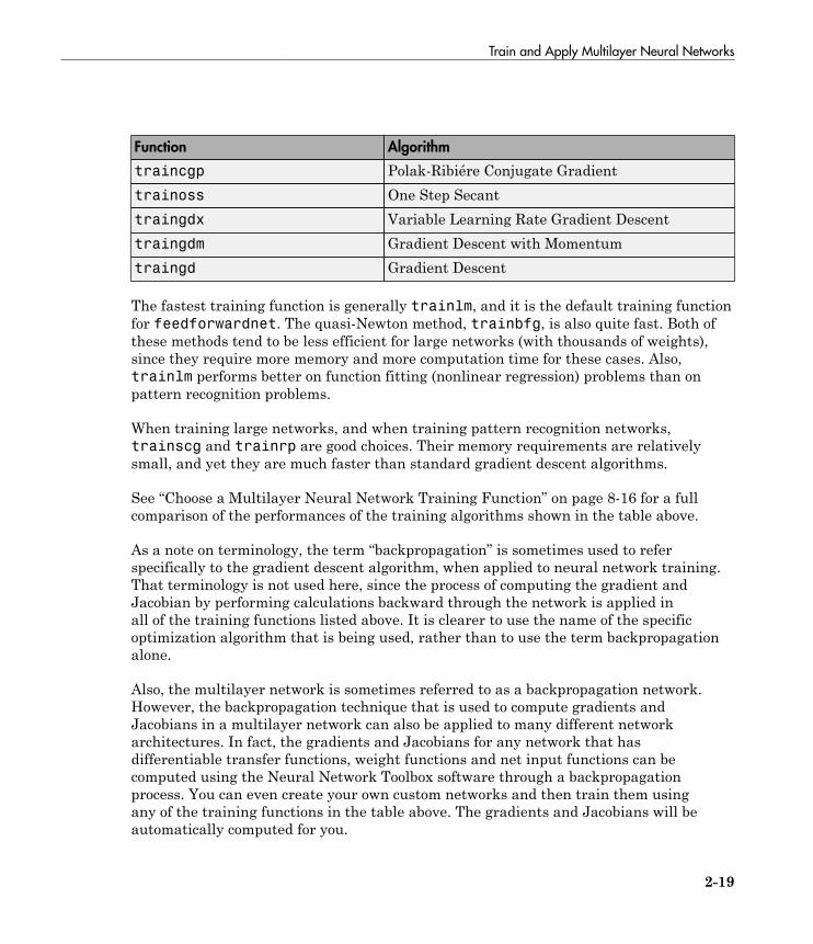
Train and Apply Multilayer Neural Networks
2-19
Function Algorithm
traincgp Polak-Ribiére Conjugate Gradienttrainoss One Step Secanttraingdx Variable Learning Rate Gradient Descenttraingdm Gradient Descent with Momentumtraingd Gradient Descent
The fastest training function is generally trainlm, and it is the default training functionfor feedforwardnet. The quasi-Newton method, trainbfg, is also quite fast. Both ofthese methods tend to be less efficient for large networks (with thousands of weights),since they require more memory and more computation time for these cases. Also,trainlm performs better on function fitting (nonlinear regression) problems than onpattern recognition problems.
When training large networks, and when training pattern recognition networks,trainscg and trainrp are good choices. Their memory requirements are relativelysmall, and yet they are much faster than standard gradient descent algorithms.
See “Choose a Multilayer Neural Network Training Function” on page 8-16 for a fullcomparison of the performances of the training algorithms shown in the table above.
As a note on terminology, the term “backpropagation” is sometimes used to referspecifically to the gradient descent algorithm, when applied to neural network training.That terminology is not used here, since the process of computing the gradient andJacobian by performing calculations backward through the network is applied inall of the training functions listed above. It is clearer to use the name of the specificoptimization algorithm that is being used, rather than to use the term backpropagationalone.
Also, the multilayer network is sometimes referred to as a backpropagation network.However, the backpropagation technique that is used to compute gradients andJacobians in a multilayer network can also be applied to many different networkarchitectures. In fact, the gradients and Jacobians for any network that hasdifferentiable transfer functions, weight functions and net input functions can becomputed using the Neural Network Toolbox software through a backpropagationprocess. You can even create your own custom networks and then train them usingany of the training functions in the table above. The gradients and Jacobians will beautomatically computed for you.
2 Multilayer Neural Networks and Backpropagation Training
2-20
Training Example
To illustrate the training process, execute the following commands:
load house_dataset
net = feedforwardnet(20);
[net,tr] = train(net,houseInputs,houseTargets);
Notice that you did not need to issue the configure command, because theconfiguration is done automatically by the train function. The training windowwill appear during training, as shown in the following figure. (If you do notwant to have this window displayed during training, you can set the parameternet.trainParam.showWindow to false. If you want training information displayed inthe command line, you can set the parameter net.trainParam.showCommandLine totrue.)
This window shows that the data has been divided using the dividerand function,and the Levenberg-Marquardt (trainlm) training method has been used with themean square error performance function. Recall that these are the default settings forfeedforwardnet.
During training, the progress is constantly updated in the training window. Of mostinterest are the performance, the magnitude of the gradient of performance and thenumber of validation checks. The magnitude of the gradient and the number of validationchecks are used to terminate the training. The gradient will become very small as thetraining reaches a minimum of the performance. If the magnitude of the gradient is lessthan 1e-5, the training will stop. This limit can be adjusted by setting the parameternet.trainParam.min_grad. The number of validation checks represents the numberof successive iterations that the validation performance fails to decrease. If this numberreaches 6 (the default value), the training will stop. In this run, you can see that thetraining did stop because of the number of validation checks. You can change thiscriterion by setting the parameter net.trainParam.max_fail. (Note that your resultsmay be different than those shown in the following figure, because of the random settingof the initial weights and biases.)

Train and Apply Multilayer Neural Networks
2-21
There are other criteria that can be used to stop network training. They are listed in thefollowing table.
Parameter Stopping Criteria
min_grad Minimum Gradient Magnitudemax_fail Maximum Number of Validation Increasestime Maximum Training Timegoal Minimum Performance Valueepochs Maximum Number of Training Epochs (Iterations)
The training will also stop if you click the Stop Training button in the training window.You might want to do this if the performance function fails to decrease significantly overmany iterations. It is always possible to continue the training by reissuing the train
2 Multilayer Neural Networks and Backpropagation Training
2-22
command shown above. It will continue to train the network from the completion of theprevious run.
From the training window, you can access four plots: performance, training state, errorhistogram, and regression. The performance plot shows the value of the performancefunction versus the iteration number. It plots training, validation, and test performances.The training state plot shows the progress of other training variables, such as thegradient magnitude, the number of validation checks, etc. The error histogram plotshows the distribution of the network errors. The regression plot shows a regressionbetween network outputs and network targets. You can use the histogram and regressionplots to validate network performance, as is discussed in “Analyze Neural NetworkPerformance After Training” on page 2-23.
Use the Network
After the network is trained and validated, the network object can be used to calculatethe network response to any input. For example, if you want to find the network responseto the fifth input vector in the building data set, you can use the following
a = net(houseInputs(:,5))
a =
34.3922
If you try this command, your output might be different, depending on the state of yourrandom number generator when the network was initialized. Below, the network object iscalled to calculate the outputs for a concurrent set of all the input vectors in the housingdata set. This is the batch mode form of simulation, in which all the input vectors areplaced in one matrix. This is much more efficient than presenting the vectors one at atime.
a = net(houseInputs);
Each time a neural network is trained, can result in a different solution due to differentinitial weight and bias values and different divisions of data into training, validation,and test sets. As a result, different neural networks trained on the same problem cangive different outputs for the same input. To ensure that a neural network of goodaccuracy has been found, retrain several times.
There are several other techniques for improving upon initial solutions if higher accuracyis desired. For more information, see “Improve Neural Network Generalization and AvoidOverfitting” on page 8-31.
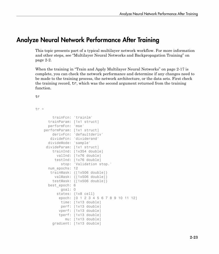
Analyze Neural Network Performance After Training
2-23
Analyze Neural Network Performance After Training
This topic presents part of a typical multilayer network workflow. For more informationand other steps, see “Multilayer Neural Networks and Backpropagation Training” onpage 2-2.
When the training in “Train and Apply Multilayer Neural Networks” on page 2-17 iscomplete, you can check the network performance and determine if any changes need tobe made to the training process, the network architecture, or the data sets. First checkthe training record, tr, which was the second argument returned from the trainingfunction.
tr
tr =
trainFcn: 'trainlm'
trainParam: [1x1 struct]
performFcn: 'mse'
performParam: [1x1 struct]
derivFcn: 'defaultderiv'
divideFcn: 'dividerand'
divideMode: 'sample'
divideParam: [1x1 struct]
trainInd: [1x354 double]
valInd: [1x76 double]
testInd: [1x76 double]
stop: 'Validation stop.'
num_epochs: 12
trainMask: {[1x506 double]}
valMask: {[1x506 double]}
testMask: {[1x506 double]}
best_epoch: 6
goal: 0
states: {1x8 cell}
epoch: [0 1 2 3 4 5 6 7 8 9 10 11 12]
time: [1x13 double]
perf: [1x13 double]
vperf: [1x13 double]
tperf: [1x13 double]
mu: [1x13 double]
gradient: [1x13 double]
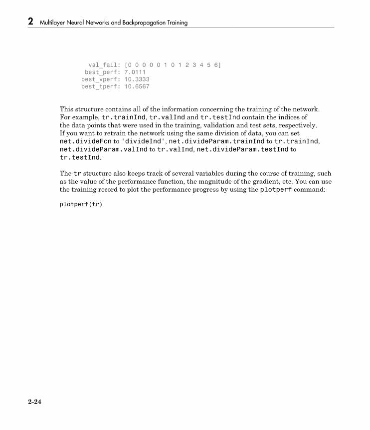
2 Multilayer Neural Networks and Backpropagation Training
2-24
val_fail: [0 0 0 0 0 1 0 1 2 3 4 5 6]
best_perf: 7.0111
best_vperf: 10.3333
best_tperf: 10.6567
This structure contains all of the information concerning the training of the network.For example, tr.trainInd, tr.valInd and tr.testInd contain the indices ofthe data points that were used in the training, validation and test sets, respectively.If you want to retrain the network using the same division of data, you can setnet.divideFcn to 'divideInd', net.divideParam.trainInd to tr.trainInd,net.divideParam.valInd to tr.valInd, net.divideParam.testInd totr.testInd.
The tr structure also keeps track of several variables during the course of training, suchas the value of the performance function, the magnitude of the gradient, etc. You can usethe training record to plot the performance progress by using the plotperf command:
plotperf(tr)

Analyze Neural Network Performance After Training
2-25
The property tr.best_epoch indicates the iteration at which the validationperformance reached a minimum. The training continued for 6 more iterations before thetraining stopped.
This figure does not indicate any major problems with the training. The validation andtest curves are very similar. If the test curve had increased significantly before thevalidation curve increased, then it is possible that some overfitting might have occurred.
The next step in validating the network is to create a regression plot, which shows therelationship between the outputs of the network and the targets. If the training wereperfect, the network outputs and the targets would be exactly equal, but the relationshipis rarely perfect in practice. For the housing example, we can create a regression plotwith the following commands. The first command calculates the trained network
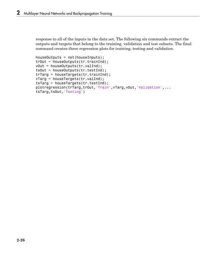
2 Multilayer Neural Networks and Backpropagation Training
2-26
response to all of the inputs in the data set. The following six commands extract theoutputs and targets that belong to the training, validation and test subsets. The finalcommand creates three regression plots for training, testing and validation.
houseOutputs = net(houseInputs);
trOut = houseOutputs(tr.trainInd);
vOut = houseOutputs(tr.valInd);
tsOut = houseOutputs(tr.testInd);
trTarg = houseTargets(tr.trainInd);
vTarg = houseTargets(tr.valInd);
tsTarg = houseTargets(tr.testInd);
plotregression(trTarg,trOut,'Train',vTarg,vOut,'Validation',...
tsTarg,tsOut,'Testing')
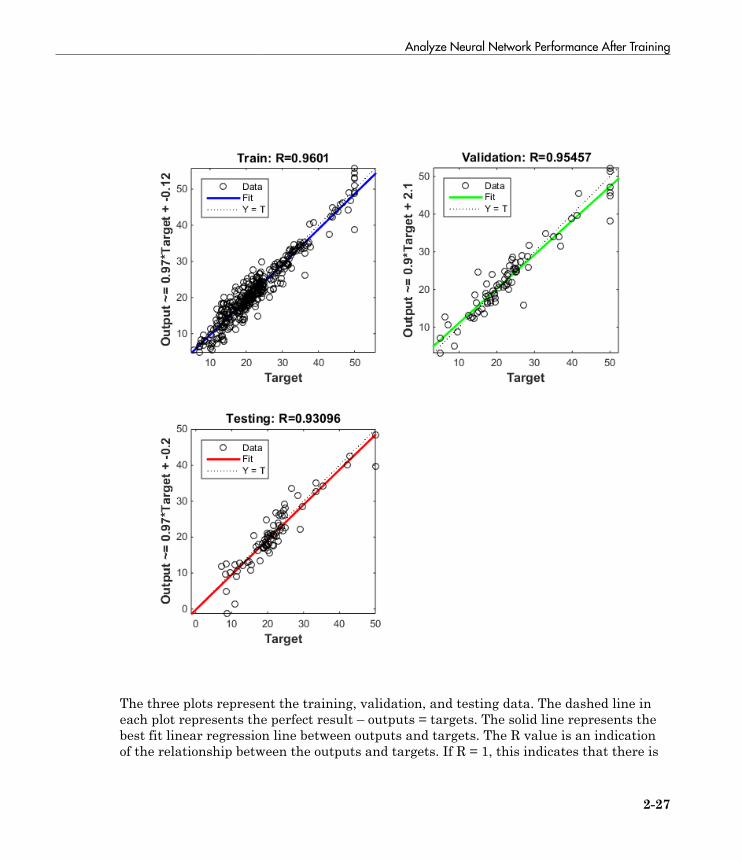
Analyze Neural Network Performance After Training
2-27
The three plots represent the training, validation, and testing data. The dashed line ineach plot represents the perfect result – outputs = targets. The solid line represents thebest fit linear regression line between outputs and targets. The R value is an indicationof the relationship between the outputs and targets. If R = 1, this indicates that there is
2 Multilayer Neural Networks and Backpropagation Training
2-28
an exact linear relationship between outputs and targets. If R is close to zero, then thereis no linear relationship between outputs and targets.
For this example, the training data indicates a good fit. The validation and test resultsalso show R values that greater than 0.9. The scatter plot is helpful in showing thatcertain data points have poor fits. For example, there is a data point in the test set whosenetwork output is close to 35, while the corresponding target value is about 12. The nextstep would be to investigate this data point to determine if it represents extrapolation(i.e., is it outside of the training data set). If so, then it should be included in the trainingset, and additional data should be collected to be used in the test set.
Improving Results
If the network is not sufficiently accurate, you can try initializing the network and thetraining again. Each time your initialize a feedforward network, the network parametersare different and might produce different solutions.
net = init(net);
net = train(net,houseInputs,houseTargets);
As a second approach, you can increase the number of hidden neurons above 20. Largernumbers of neurons in the hidden layer give the network more flexibility because thenetwork has more parameters it can optimize. (Increase the layer size gradually. If youmake the hidden layer too large, you might cause the problem to be under-characterizedand the network must optimize more parameters than there are data vectors to constrainthese parameters.)
A third option is to try a different training function. Bayesian regularization trainingwith trainbr, for example, can sometimes produce better generalization capability thanusing early stopping.
Finally, try using additional training data. Providing additional data for the network ismore likely to produce a network that generalizes well to new data.

Limitations and Cautions
2-29
Limitations and Cautions
You would normally use Levenberg-Marquardt training for small and medium sizenetworks, if you have enough memory available. If memory is a problem, then there area variety of other fast algorithms available. For large networks you will probably want touse trainscg or trainrp.
Multilayer networks are capable of performing just about any linear or nonlinearcomputation, and they can approximate any reasonable function arbitrarily well.However, while the network being trained might theoretically be capable of performingcorrectly, backpropagation and its variations might not always find a solution. See page12-8 of [HDB96] for a discussion of convergence to local minimum points.
The error surface of a nonlinear network is more complex than the error surface of alinear network. To understand this complexity, see the figures on pages 12-5 to 12-7of [HDB96], which show three different error surfaces for a multilayer network. Theproblem is that nonlinear transfer functions in multilayer networks introduce manylocal minima in the error surface. As gradient descent is performed on the error surface,depending on the initial starting conditions, it is possible for the network solution tobecome trapped in one of these local minima. Settling in a local minimum can be good orbad depending on how close the local minimum is to the global minimum and how low anerror is required. In any case, be cautioned that although a multilayer backpropagationnetwork with enough neurons can implement just about any function, backpropagationdoes not always find the correct weights for the optimum solution. You might want toreinitialize the network and retrain several times to guarantee that you have the bestsolution.
Networks are also sensitive to the number of neurons in their hidden layers. Too fewneurons can lead to underfitting. Too many neurons can contribute to overfitting, inwhich all training points are well fitted, but the fitting curve oscillates wildly betweenthese points. Ways of dealing with various of these issues are discussed in “ImproveNeural Network Generalization and Avoid Overfitting” on page 8-31. This topic isalso discussed starting on page 11-21 of [HDB96].
For more information about the workflow with multilayer networks, see “MultilayerNeural Networks and Backpropagation Training” on page 2-2.

2-30
3
Dynamic Neural Networks
• “Introduction to Dynamic Neural Networks” on page 3-2• “How Dynamic Neural Networks Work” on page 3-3• “Design Time Series Time-Delay Neural Networks” on page 3-14• “Design Time Series Distributed Delay Neural Networks” on page 3-20• “Design Time Series NARX Feedback Neural Networks” on page 3-23• “Design Layer-Recurrent Neural Networks” on page 3-31• “Create Reference Model Controller with MATLAB Script” on page 3-34• “Multiple Sequences with Dynamic Neural Networks” on page 3-41• “Neural Network Time-Series Utilities” on page 3-42• “Train Neural Networks with Error Weights” on page 3-44• “Normalize Errors of Multiple Outputs” on page 3-47• “Multistep Neural Network Prediction” on page 3-52
3 Dynamic Neural Networks
3-2
Introduction to Dynamic Neural Networks
Neural networks can be classified into dynamic and static categories. Static (feedforward)networks have no feedback elements and contain no delays; the output is calculateddirectly from the input through feedforward connections. In dynamic networks, theoutput depends not only on the current input to the network, but also on the current orprevious inputs, outputs, or states of the network.
Details of this workflow are discussed in the following sections:
• “Design Time Series Time-Delay Neural Networks” on page 3-14• “Prepare Input and Layer Delay States” on page 3-18• “Design Time Series Distributed Delay Neural Networks” on page 3-20• “Design Time Series NARX Feedback Neural Networks” on page 3-23• “Design Layer-Recurrent Neural Networks” on page 3-31
Optional workflow steps are discussed in these sections:
• “Choose Neural Network Input-Output Processing Functions” on page 2-9• “Divide Data for Optimal Neural Network Training” on page 2-12• “Train Neural Networks with Error Weights” on page 3-44

How Dynamic Neural Networks Work
3-3
How Dynamic Neural Networks Work
In this section...
“Feedforward and Recurrent Neural Networks” on page 3-3“Applications of Dynamic Networks” on page 3-11“Dynamic Network Structures” on page 3-11“Dynamic Network Training” on page 3-12
Feedforward and Recurrent Neural Networks
Dynamic networks can be divided into two categories: those that have only feedforwardconnections, and those that have feedback, or recurrent, connections. To understandthe differences between static, feedforward-dynamic, and recurrent-dynamic networks,create some networks and see how they respond to an input sequence. (First, you mightwant to review “Simulation with Sequential Inputs in a Dynamic Network” on page1-24.)
The following commands create a pulse input sequence and plot it:
p = {0 0 1 1 1 1 0 0 0 0 0 0};
stem(cell2mat(p))
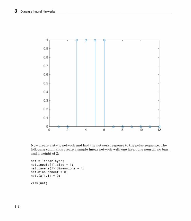
3 Dynamic Neural Networks
3-4
Now create a static network and find the network response to the pulse sequence. Thefollowing commands create a simple linear network with one layer, one neuron, no bias,and a weight of 2:
net = linearlayer;
net.inputs{1}.size = 1;
net.layers{1}.dimensions = 1;
net.biasConnect = 0;
net.IW{1,1} = 2;
view(net)

How Dynamic Neural Networks Work
3-5
You can now simulate the network response to the pulse input and plot it:
a = net(p);
stem(cell2mat(a))
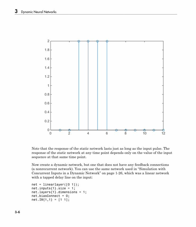
3 Dynamic Neural Networks
3-6
Note that the response of the static network lasts just as long as the input pulse. Theresponse of the static network at any time point depends only on the value of the inputsequence at that same time point.
Now create a dynamic network, but one that does not have any feedback connections(a nonrecurrent network). You can use the same network used in “Simulation withConcurrent Inputs in a Dynamic Network” on page 1-26, which was a linear networkwith a tapped delay line on the input:
net = linearlayer([0 1]);
net.inputs{1}.size = 1;
net.layers{1}.dimensions = 1;
net.biasConnect = 0;
net.IW{1,1} = [1 1];
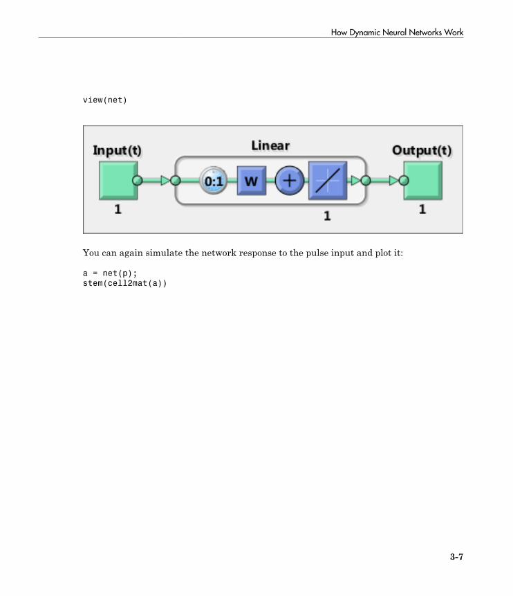
How Dynamic Neural Networks Work
3-7
view(net)
You can again simulate the network response to the pulse input and plot it:
a = net(p);
stem(cell2mat(a))

3 Dynamic Neural Networks
3-8
The response of the dynamic network lasts longer than the input pulse. The dynamicnetwork has memory. Its response at any given time depends not only on the currentinput, but on the history of the input sequence. If the network does not have anyfeedback connections, then only a finite amount of history will affect the response. In thisfigure you can see that the response to the pulse lasts one time step beyond the pulseduration. That is because the tapped delay line on the input has a maximum delay of 1.
Now consider a simple recurrent-dynamic network, shown in the following figure.
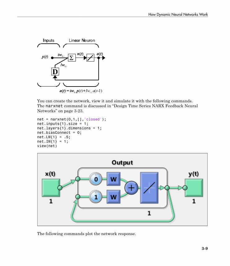
How Dynamic Neural Networks Work
3-9
You can create the network, view it and simulate it with the following commands.The narxnet command is discussed in “Design Time Series NARX Feedback NeuralNetworks” on page 3-23.
net = narxnet(0,1,[],'closed');
net.inputs{1}.size = 1;
net.layers{1}.dimensions = 1;
net.biasConnect = 0;
net.LW{1} = .5;
net.IW{1} = 1;
view(net)
The following commands plot the network response.
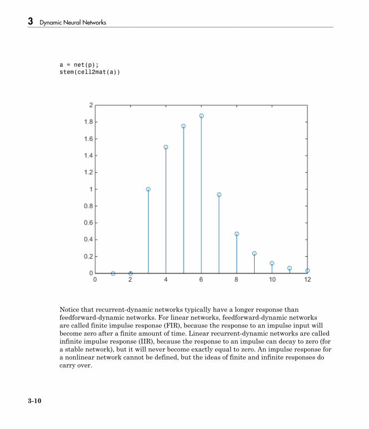
3 Dynamic Neural Networks
3-10
a = net(p);
stem(cell2mat(a))
Notice that recurrent-dynamic networks typically have a longer response thanfeedforward-dynamic networks. For linear networks, feedforward-dynamic networksare called finite impulse response (FIR), because the response to an impulse input willbecome zero after a finite amount of time. Linear recurrent-dynamic networks are calledinfinite impulse response (IIR), because the response to an impulse can decay to zero (fora stable network), but it will never become exactly equal to zero. An impulse response fora nonlinear network cannot be defined, but the ideas of finite and infinite responses docarry over.

How Dynamic Neural Networks Work
3-11
Applications of Dynamic Networks
Dynamic networks are generally more powerful than static networks (althoughsomewhat more difficult to train). Because dynamic networks have memory, they canbe trained to learn sequential or time-varying patterns. This has applications in suchdisparate areas as prediction in financial markets [RoJa96], channel equalizationin communication systems [FeTs03], phase detection in power systems [KaGr96],sorting [JaRa04], fault detection [ChDa99], speech recognition [Robin94], and even theprediction of protein structure in genetics [GiPr02]. You can find a discussion of manymore dynamic network applications in [MeJa00].
One principal application of dynamic neural networks is in control systems. Thisapplication is discussed in detail in “Neural Network Control Systems”. Dynamicnetworks are also well suited for filtering. You will see the use of some linear dynamicnetworks for filtering in and some of those ideas are extended in this topic, usingnonlinear dynamic networks.
Dynamic Network Structures
The Neural Network Toolbox software is designed to train a class of network calledthe Layered Digital Dynamic Network (LDDN). Any network that can be arranged inthe form of an LDDN can be trained with the toolbox. Here is a basic description of theLDDN.
Each layer in the LDDN is made up of the following parts:
• Set of weight matrices that come into that layer (which can connect from other layersor from external inputs), associated weight function rule used to combine the weightmatrix with its input (normally standard matrix multiplication, dotprod), andassociated tapped delay line
• Bias vector• Net input function rule that is used to combine the outputs of the various weight
functions with the bias to produce the net input (normally a summing junction,netprod)
• Transfer function
The network has inputs that are connected to special weights, called input weights, anddenoted by IWi,j (net.IW{i,j} in the code), where j denotes the number of the inputvector that enters the weight, and i denotes the number of the layer to which the weightis connected. The weights connecting one layer to another are called layer weights and

3 Dynamic Neural Networks
3-12
are denoted by LWi,j (net.LW{i,j} in the code), where j denotes the number of the layercoming into the weight and i denotes the number of the layer at the output of the weight.
The following figure is an example of a three-layer LDDN. The first layer has threeweights associated with it: one input weight, a layer weight from layer 1, and a layerweight from layer 3. The two layer weights have tapped delay lines associated with them.
The Neural Network Toolbox software can be used to train any LDDN, so long as theweight functions, net input functions, and transfer functions have derivatives. Mostwell-known dynamic network architectures can be represented in LDDN form. In theremainder of this topic you will see how to use some simple commands to create andtrain several very powerful dynamic networks. Other LDDN networks not covered in thistopic can be created using the generic network command, as explained in “Define NeuralNetwork Architectures”.
Dynamic Network Training
Dynamic networks are trained in the Neural Network Toolbox software using the samegradient-based algorithms that were described in “Multilayer Neural Networks andBackpropagation Training”. You can select from any of the training functions that werepresented in that topic. Examples are provided in the following sections.

How Dynamic Neural Networks Work
3-13
Although dynamic networks can be trained using the same gradient-based algorithmsthat are used for static networks, the performance of the algorithms on dynamicnetworks can be quite different, and the gradient must be computed in a more complexway. Consider again the simple recurrent network shown in this figure.
The weights have two different effects on the network output. The first is the directeffect, because a change in the weight causes an immediate change in the output at thecurrent time step. (This first effect can be computed using standard backpropagation.)The second is an indirect effect, because some of the inputs to the layer, such as a(t −1), are also functions of the weights. To account for this indirect effect, you must usedynamic backpropagation to compute the gradients, which is more computationallyintensive. (See [DeHa01a], [DeHa01b] and [DeHa07].) Expect dynamic backpropagationto take more time to train, in part for this reason. In addition, the error surfaces fordynamic networks can be more complex than those for static networks. Training is morelikely to be trapped in local minima. This suggests that you might need to train thenetwork several times to achieve an optimal result. See [DHH01] and [HDH09] for somediscussion on the training of dynamic networks.
The remaining sections of this topic show how to create, train, and apply certain dynamicnetworks to modeling, detection, and forecasting problems. Some of the networks requiredynamic backpropagation for computing the gradients and others do not. As a user,you do not need to decide whether or not dynamic backpropagation is needed. Thisis determined automatically by the software, which also decides on the best form ofdynamic backpropagation to use. You just need to create the network and then invokethe standard train command.
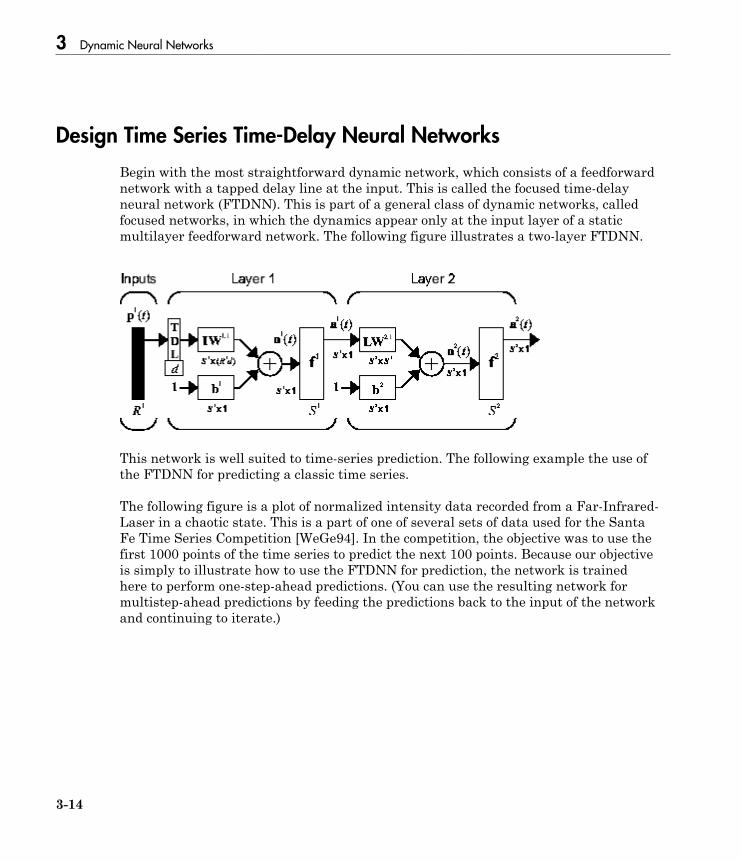
3 Dynamic Neural Networks
3-14
Design Time Series Time-Delay Neural Networks
Begin with the most straightforward dynamic network, which consists of a feedforwardnetwork with a tapped delay line at the input. This is called the focused time-delayneural network (FTDNN). This is part of a general class of dynamic networks, calledfocused networks, in which the dynamics appear only at the input layer of a staticmultilayer feedforward network. The following figure illustrates a two-layer FTDNN.
This network is well suited to time-series prediction. The following example the use ofthe FTDNN for predicting a classic time series.
The following figure is a plot of normalized intensity data recorded from a Far-Infrared-Laser in a chaotic state. This is a part of one of several sets of data used for the SantaFe Time Series Competition [WeGe94]. In the competition, the objective was to use thefirst 1000 points of the time series to predict the next 100 points. Because our objectiveis simply to illustrate how to use the FTDNN for prediction, the network is trainedhere to perform one-step-ahead predictions. (You can use the resulting network formultistep-ahead predictions by feeding the predictions back to the input of the networkand continuing to iterate.)
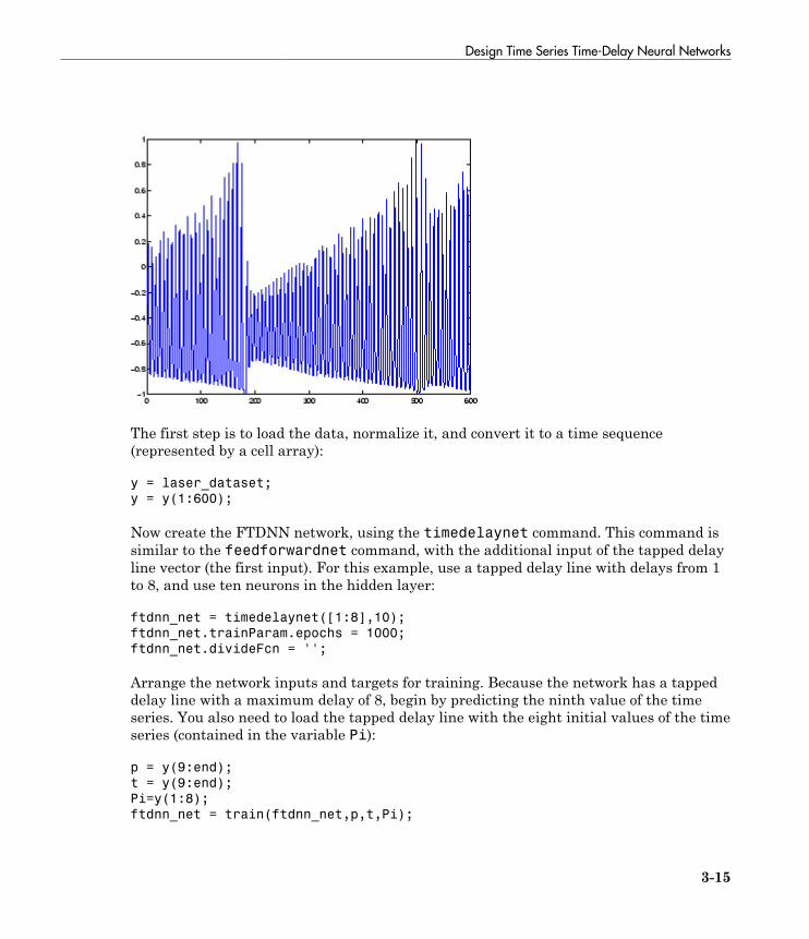
Design Time Series Time-Delay Neural Networks
3-15
The first step is to load the data, normalize it, and convert it to a time sequence(represented by a cell array):
y = laser_dataset;
y = y(1:600);
Now create the FTDNN network, using the timedelaynet command. This command issimilar to the feedforwardnet command, with the additional input of the tapped delayline vector (the first input). For this example, use a tapped delay line with delays from 1to 8, and use ten neurons in the hidden layer:
ftdnn_net = timedelaynet([1:8],10);
ftdnn_net.trainParam.epochs = 1000;
ftdnn_net.divideFcn = '';
Arrange the network inputs and targets for training. Because the network has a tappeddelay line with a maximum delay of 8, begin by predicting the ninth value of the timeseries. You also need to load the tapped delay line with the eight initial values of the timeseries (contained in the variable Pi):
p = y(9:end);
t = y(9:end);
Pi=y(1:8);
ftdnn_net = train(ftdnn_net,p,t,Pi);

3 Dynamic Neural Networks
3-16
Notice that the input to the network is the same as the target. Because the network hasa minimum delay of one time step, this means that you are performing a one-step-aheadprediction.
During training, the following training window appears.
Training stopped because the maximum epoch was reached. From this window, you candisplay the response of the network by clicking Time-Series Response. The followingfigure appears.

Design Time Series Time-Delay Neural Networks
3-17
Now simulate the network and determine the prediction error.
yp = ftdnn_net(p,Pi);
e = gsubtract(yp,t);
rmse = sqrt(mse(e))
rmse =
0.9740
(Note that gsubtract is a general subtraction function that can operate on cell arrays.)This result is much better than you could have obtained using a linear predictor. Youcan verify this with the following commands, which design a linear filter with the sametapped delay line input as the previous FTDNN.
lin_net = linearlayer([1:8]);
lin_net.trainFcn='trainlm';
[lin_net,tr] = train(lin_net,p,t,Pi);
lin_yp = lin_net(p,Pi);
lin_e = gsubtract(lin_yp,t);
lin_rmse = sqrt(mse(lin_e))
3 Dynamic Neural Networks
3-18
lin_rmse =
21.1386
The rms error is 21.1386 for the linear predictor, but 0.9740 for the nonlinear FTDNNpredictor.
One nice feature of the FTDNN is that it does not require dynamic backpropagation tocompute the network gradient. This is because the tapped delay line appears only at theinput of the network, and contains no feedback loops or adjustable parameters. For thisreason, you will find that this network trains faster than other dynamic networks.
If you have an application for a dynamic network, try the linear network first(linearlayer) and then the FTDNN (timedelaynet). If neither network issatisfactory, try one of the more complex dynamic networks discussed in the remainder ofthis topic.
Each time a neural network is trained, can result in a different solution due to differentinitial weight and bias values and different divisions of data into training, validation,and test sets. As a result, different neural networks trained on the same problem cangive different outputs for the same input. To ensure that a neural network of goodaccuracy has been found, retrain several times.
There are several other techniques for improving upon initial solutions if higher accuracyis desired. For more information, see “Improve Neural Network Generalization and AvoidOverfitting” on page 8-31.
Prepare Input and Layer Delay States
You will notice in the last section that for dynamic networks there is a significantamount of data preparation that is required before training or simulating the network.This is because the tapped delay lines in the network need to be filled with initialconditions, which requires that part of the original data set be removed and shifted.(You can see the steps for doing this “Design Time Series Time-Delay Neural Networks”on page 3-14.) There is a toolbox function that facilitates the data preparation fordynamic (time series) networks - preparets. For example, the following lines:
p = y(9:end);
t = y(9:end);
Pi = y(1:8);
can be replaced with
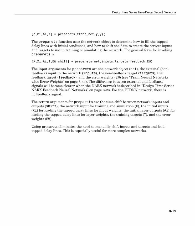
Design Time Series Time-Delay Neural Networks
3-19
[p,Pi,Ai,t] = preparets(ftdnn_net,y,y);
The preparets function uses the network object to determine how to fill the tappeddelay lines with initial conditions, and how to shift the data to create the correct inputsand targets to use in training or simulating the network. The general form for invokingpreparets is
[X,Xi,Ai,T,EW,shift] = preparets(net,inputs,targets,feedback,EW)
The input arguments for preparets are the network object (net), the external (non-feedback) input to the network (inputs), the non-feedback target (targets), thefeedback target (feedback), and the error weights (EW) (see “Train Neural Networkswith Error Weights” on page 3-44). The difference between external and feedbacksignals will become clearer when the NARX network is described in “Design Time SeriesNARX Feedback Neural Networks” on page 3-23. For the FTDNN network, there isno feedback signal.
The return arguments for preparets are the time shift between network inputs andoutputs (shift), the network input for training and simulation (X), the initial inputs(Xi) for loading the tapped delay lines for input weights, the initial layer outputs (Ai) forloading the tapped delay lines for layer weights, the training targets (T), and the errorweights (EW).
Using preparets eliminates the need to manually shift inputs and targets and loadtapped delay lines. This is especially useful for more complex networks.

3 Dynamic Neural Networks
3-20
Design Time Series Distributed Delay Neural Networks
The FTDNN had the tapped delay line memory only at the input to the first layer of thestatic feedforward network. You can also distribute the tapped delay lines throughoutthe network. The distributed TDNN was first introduced in [WaHa89] for phonemerecognition. The original architecture was very specialized for that particular problem.The following figure shows a general two-layer distributed TDNN.
This network can be used for a simplified problem that is similar to phoneme recognition.The network will attempt to recognize the frequency content of an input signal. Thefollowing figure shows a signal in which one of two frequencies is present at any giventime.

Design Time Series Distributed Delay Neural Networks
3-21
The following code creates this signal and a target network output. The target output is 1when the input is at the low frequency and -1 when the input is at the high frequency.
time = 0:99;
y1 = sin(2*pi*time/10);
y2 = sin(2*pi*time/5);
y = [y1 y2 y1 y2];
t1 = ones(1,100);
t2 = -ones(1,100);
t = [t1 t2 t1 t2];
Now create the distributed TDNN network with the distdelaynet function. The onlydifference between the distdelaynet function and the timedelaynet function is thatthe first input argument is a cell array that contains the tapped delays to be used in eachlayer. In the next example, delays of zero to four are used in layer 1 and zero to threeare used in layer 2. (To add some variety, the training function trainbr is used in thisexample instead of the default, which is trainlm. You can use any training functiondiscussed in “Multilayer Neural Networks and Backpropagation Training”.)
d1 = 0:4;
d2 = 0:3;
p = con2seq(y);
t = con2seq(t);
dtdnn_net = distdelaynet({d1,d2},5);
dtdnn_net.trainFcn = 'trainbr';
dtdnn_net.divideFcn = '';
dtdnn_net.trainParam.epochs = 100;
dtdnn_net = train(dtdnn_net,p,t);
yp = sim(dtdnn_net,p);
plotresponse(t,yp)
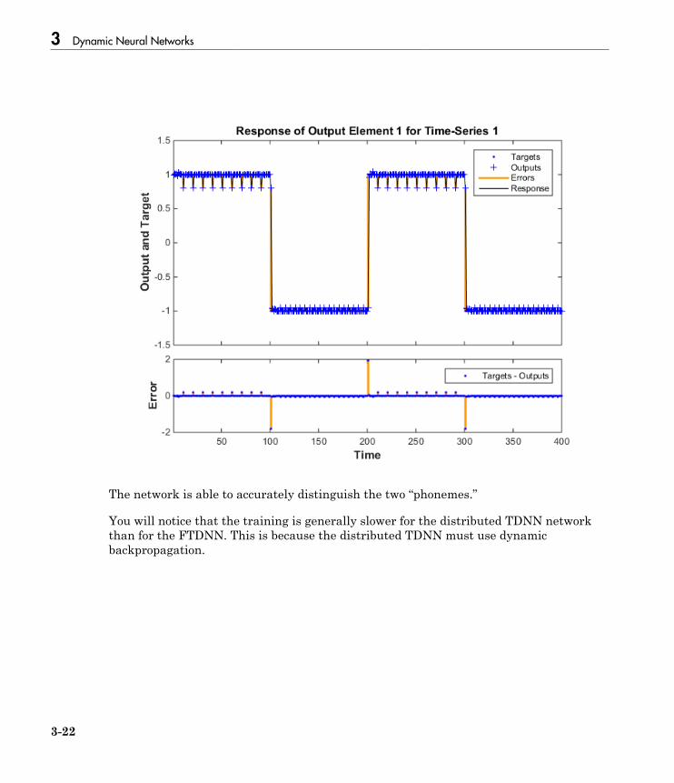
3 Dynamic Neural Networks
3-22
The network is able to accurately distinguish the two “phonemes.”
You will notice that the training is generally slower for the distributed TDNN networkthan for the FTDNN. This is because the distributed TDNN must use dynamicbackpropagation.

Design Time Series NARX Feedback Neural Networks
3-23
Design Time Series NARX Feedback Neural Networks
All the specific dynamic networks discussed so far have either been focused networks,with the dynamics only at the input layer, or feedforward networks. The nonlinearautoregressive network with exogenous inputs (NARX) is a recurrent dynamic network,with feedback connections enclosing several layers of the network. The NARX model isbased on the linear ARX model, which is commonly used in time-series modeling.
The defining equation for the NARX model is
y t f y t y t y t n u t u t u t ny u( ) ( ( ), ( ), , ( ), ( ), ( ), , ( ))= − − − − − −1 2 1 2… …
where the next value of the dependent output signal y(t) is regressed on previous valuesof the output signal and previous values of an independent (exogenous) input signal. Youcan implement the NARX model by using a feedforward neural network to approximatethe function f. A diagram of the resulting network is shown below, where a two-layerfeedforward network is used for the approximation. This implementation also allows for avector ARX model, where the input and output can be multidimensional.
There are many applications for the NARX network. It can be used as a predictor, topredict the next value of the input signal. It can also be used for nonlinear filtering, inwhich the target output is a noise-free version of the input signal. The use of the NARXnetwork is shown in another important application, the modeling of nonlinear dynamicsystems.
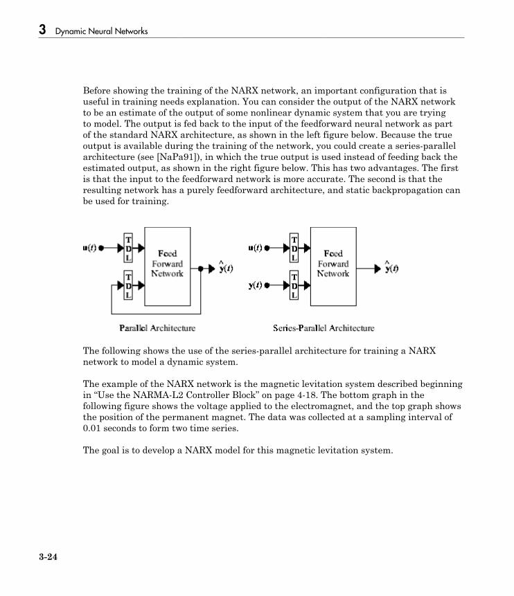
3 Dynamic Neural Networks
3-24
Before showing the training of the NARX network, an important configuration that isuseful in training needs explanation. You can consider the output of the NARX networkto be an estimate of the output of some nonlinear dynamic system that you are tryingto model. The output is fed back to the input of the feedforward neural network as partof the standard NARX architecture, as shown in the left figure below. Because the trueoutput is available during the training of the network, you could create a series-parallelarchitecture (see [NaPa91]), in which the true output is used instead of feeding back theestimated output, as shown in the right figure below. This has two advantages. The firstis that the input to the feedforward network is more accurate. The second is that theresulting network has a purely feedforward architecture, and static backpropagation canbe used for training.
The following shows the use of the series-parallel architecture for training a NARXnetwork to model a dynamic system.
The example of the NARX network is the magnetic levitation system described beginningin “Use the NARMA-L2 Controller Block” on page 4-18. The bottom graph in thefollowing figure shows the voltage applied to the electromagnet, and the top graph showsthe position of the permanent magnet. The data was collected at a sampling interval of0.01 seconds to form two time series.
The goal is to develop a NARX model for this magnetic levitation system.

Design Time Series NARX Feedback Neural Networks
3-25
First, load the training data. Use tapped delay lines with two delays for both the inputand the output, so training begins with the third data point. There are two inputs to theseries-parallel network, the u(t) sequence and the y(t) sequence.
load magdata
y = con2seq(y);
u = con2seq(u);
Create the series-parallel NARX network using the function narxnet. Use 10 neurons inthe hidden layer and use trainlm for the training function, and then prepare the datawith preparets:
d1 = [1:2];
d2 = [1:2];
narx_net = narxnet(d1,d2,10);
narx_net.divideFcn = '';
narx_net.trainParam.min_grad = 1e-10;
[p,Pi,Ai,t] = preparets(narx_net,u,{},y);
(Notice that the y sequence is considered a feedback signal, which is an input that isalso an output (target). Later, when you close the loop, the appropriate output will beconnected to the appropriate input.) Now you are ready to train the network.
narx_net = train(narx_net,p,t,Pi);
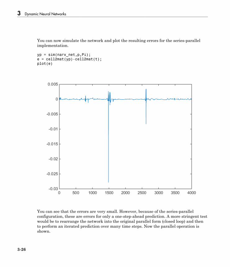
3 Dynamic Neural Networks
3-26
You can now simulate the network and plot the resulting errors for the series-parallelimplementation.
yp = sim(narx_net,p,Pi);
e = cell2mat(yp)-cell2mat(t);
plot(e)
You can see that the errors are very small. However, because of the series-parallelconfiguration, these are errors for only a one-step-ahead prediction. A more stringent testwould be to rearrange the network into the original parallel form (closed loop) and thento perform an iterated prediction over many time steps. Now the parallel operation isshown.

Design Time Series NARX Feedback Neural Networks
3-27
There is a toolbox function (closeloop) for converting NARX (and other) networks fromthe series-parallel configuration (open loop), which is useful for training, to the parallelconfiguration (closed loop), which is useful for multi-step-ahead prediction. The followingcommand illustrates how to convert the network that you just trained to parallel form:
narx_net_closed = closeloop(narx_net);
To see the differences between the two networks, you can use the view command:
view(narx_net)
view(narx_net_closed)

3 Dynamic Neural Networks
3-28
All of the training is done in open loop (also called series-parallel architecture), includingthe validation and testing steps. The typical workflow is to fully create the network inopen loop, and only when it has been trained (which includes validation and testingsteps) is it transformed to closed loop for multistep-ahead prediction. Likewise, the Rvalues in the GUI are computed based on the open-loop training results.
You can now use the closed-loop (parallel) configuration to perform an iterated predictionof 900 time steps. In this network you need to load the two initial inputs and the twoinitial outputs as initial conditions. You can use the preparets function to prepare thedata. It will use the network structure to determine how to divide and shift the dataappropriately.
y1 = y(1700:2600);
u1 = u(1700:2600);
[p1,Pi1,Ai1,t1] = preparets(narx_net_closed,u1,{},y1);
yp1 = narx_net_closed(p1,Pi1,Ai1);
TS = size(t1,2);
plot(1:TS,cell2mat(t1),'b',1:TS,cell2mat(yp1),'r')

Design Time Series NARX Feedback Neural Networks
3-29
The figure illustrates the iterated prediction. The blue line is the actual position of themagnet, and the red line is the position predicted by the NARX neural network. Eventhough the network is predicting 900 time steps ahead, the prediction is very accurate.
In order for the parallel response (iterated prediction) to be accurate, it is important thatthe network be trained so that the errors in the series-parallel configuration (one-step-ahead prediction) are very small.
You can also create a parallel (closed loop) NARX network, using the narxnet commandwith the fourth input argument set to 'closed', and train that network directly.Generally, the training takes longer, and the resulting performance is not as good as thatobtained with series-parallel training.
3 Dynamic Neural Networks
3-30
Each time a neural network is trained, can result in a different solution due to differentinitial weight and bias values and different divisions of data into training, validation,and test sets. As a result, different neural networks trained on the same problem cangive different outputs for the same input. To ensure that a neural network of goodaccuracy has been found, retrain several times.
There are several other techniques for improving upon initial solutions if higher accuracyis desired. For more information, see “Improve Neural Network Generalization and AvoidOverfitting” on page 8-31.
Multiple External Variables
The maglev example showed how to model a time series with a single external inputvalue over time. But the NARX network will work for problems with multiple externalinput elements and predict series with multiple elements. In these cases, the input andtarget consist of row cell arrays representing time, but with each cell element being an N-by-1 vector for the N elements of the input or target signal.
For example, here is a dataset which consists of 2-element external variables predicting a1-element series.
[X,T] = ph_dataset;
The external inputs X are formatted as a row cell array of 2-element vectors, with eachvector representing acid and base solution flow. The targets represent the resulting pH ofthe solution over time.
You can reformat your own multi-element series data from matrix form to neuralnetwork time-series form with the function con2seq.
The process for training a network proceeds as it did above for the maglev problem.
net = narxnet(10);
[x,xi,ai,t] = preparets(net,X,{},T);
net = train(net,x,t,xi,ai);
y = net(x,xi,ai);
e = gsubtract(t,y);
To see examples of using NARX networks being applied in open-loop form, closed-loop form and open/closed-loop multistep prediction see “Multistep Neural NetworkPrediction” on page 3-52.
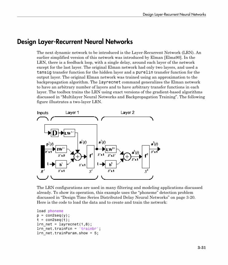
Design Layer-Recurrent Neural Networks
3-31
Design Layer-Recurrent Neural Networks
The next dynamic network to be introduced is the Layer-Recurrent Network (LRN). Anearlier simplified version of this network was introduced by Elman [Elma90]. In theLRN, there is a feedback loop, with a single delay, around each layer of the networkexcept for the last layer. The original Elman network had only two layers, and used atansig transfer function for the hidden layer and a purelin transfer function for theoutput layer. The original Elman network was trained using an approximation to thebackpropagation algorithm. The layrecnet command generalizes the Elman networkto have an arbitrary number of layers and to have arbitrary transfer functions in eachlayer. The toolbox trains the LRN using exact versions of the gradient-based algorithmsdiscussed in “Multilayer Neural Networks and Backpropagation Training”. The followingfigure illustrates a two-layer LRN.
The LRN configurations are used in many filtering and modeling applications discussedalready. To show its operation, this example uses the “phoneme” detection problemdiscussed in “Design Time Series Distributed Delay Neural Networks” on page 3-20.Here is the code to load the data and to create and train the network:
load phoneme
p = con2seq(y);
t = con2seq(t);
lrn_net = layrecnet(1,8);
lrn_net.trainFcn = 'trainbr';
lrn_net.trainParam.show = 5;
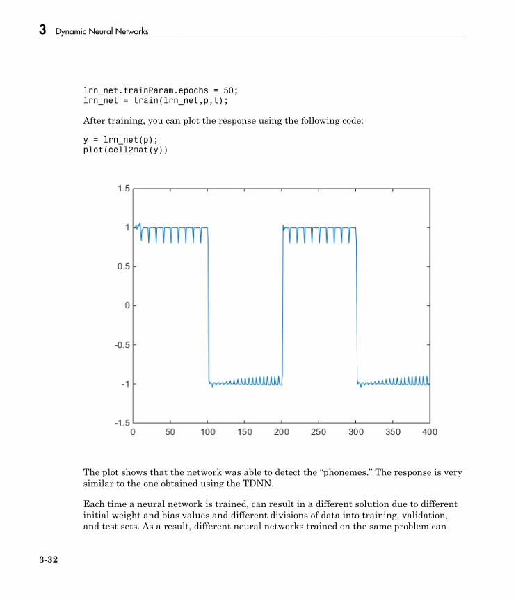
3 Dynamic Neural Networks
3-32
lrn_net.trainParam.epochs = 50;
lrn_net = train(lrn_net,p,t);
After training, you can plot the response using the following code:
y = lrn_net(p);
plot(cell2mat(y))
The plot shows that the network was able to detect the “phonemes.” The response is verysimilar to the one obtained using the TDNN.
Each time a neural network is trained, can result in a different solution due to differentinitial weight and bias values and different divisions of data into training, validation,and test sets. As a result, different neural networks trained on the same problem can

Design Layer-Recurrent Neural Networks
3-33
give different outputs for the same input. To ensure that a neural network of goodaccuracy has been found, retrain several times.
There are several other techniques for improving upon initial solutions if higher accuracyis desired. For more information, see “Improve Neural Network Generalization and AvoidOverfitting” on page 8-31.

3 Dynamic Neural Networks
3-34
Create Reference Model Controller with MATLAB Script
So far, this topic has described the training procedures for several specific dynamicnetwork architectures. However, any network that can be created in the toolbox canbe trained using the training functions described in “Multilayer Neural Networks andBackpropagation Training” so long as the components of the network are differentiable.This section gives an example of how to create and train a custom architecture. Thecustom architecture you will use is the model reference adaptive control (MRAC) systemthat is described in detail in “Design Model-Reference Neural Controller in Simulink” onpage 4-23.
As you can see in “Design Model-Reference Neural Controller in Simulink” on page4-23, the model reference control architecture has two subnetworks. One subnetworkis the model of the plant that you want to control. The other subnetwork is thecontroller. You will begin by training a NARX network that will become the plant modelsubnetwork. For this example, you will use the robot arm to represent the plant, asdescribed in “Design Model-Reference Neural Controller in Simulink” on page 4-23.The following code will load data collected from the robot arm and create and train aNARX network. For this simple problem, you do not need to preprocess the data, and allof the data can be used for training, so no data division is needed.
[u,y] = robotarm_dataset;
d1 = [1:2];
d2 = [1:2];
S1 = 5;
narx_net = narxnet(d1,d2,S1);
narx_net.divideFcn = '';
narx_net.inputs{1}.processFcns = {};
narx_net.inputs{2}.processFcns = {};
narx_net.outputs{2}.processFcns = {};
narx_net.trainParam.min_grad = 1e-10;
[p,Pi,Ai,t] = preparets(narx_net,u,{},y);
narx_net = train(narx_net,p,t,Pi);
narx_net_closed = closeloop(narx_net);
view(narx_net_closed)
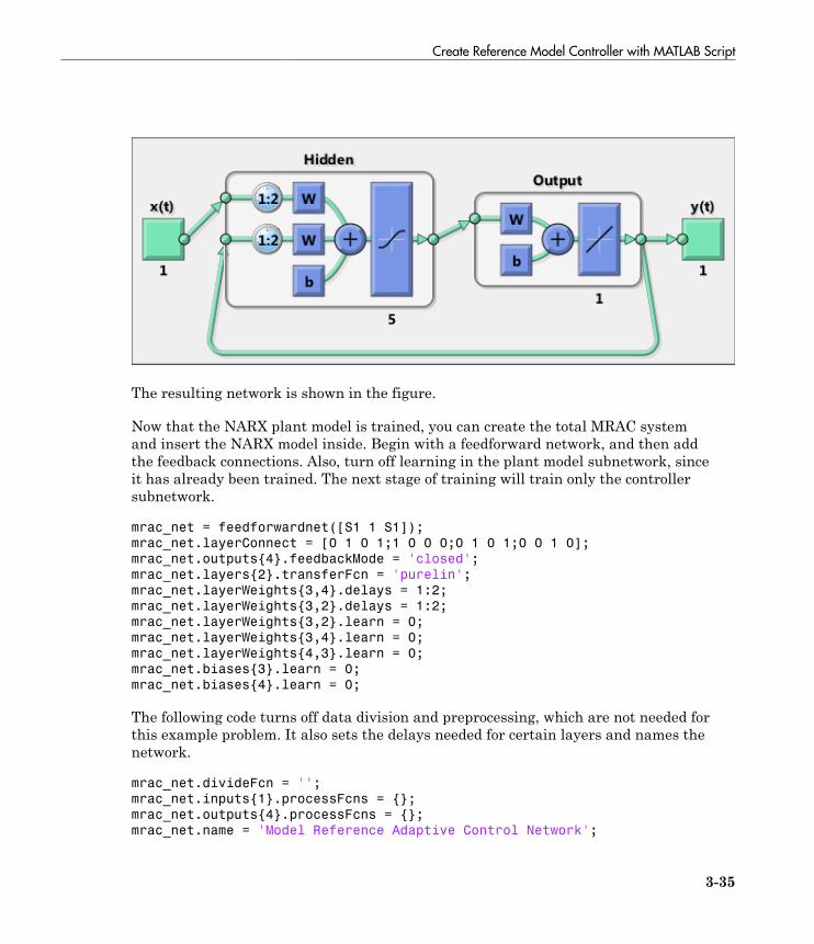
Create Reference Model Controller with MATLAB Script
3-35
The resulting network is shown in the figure.
Now that the NARX plant model is trained, you can create the total MRAC systemand insert the NARX model inside. Begin with a feedforward network, and then addthe feedback connections. Also, turn off learning in the plant model subnetwork, sinceit has already been trained. The next stage of training will train only the controllersubnetwork.
mrac_net = feedforwardnet([S1 1 S1]);
mrac_net.layerConnect = [0 1 0 1;1 0 0 0;0 1 0 1;0 0 1 0];
mrac_net.outputs{4}.feedbackMode = 'closed';
mrac_net.layers{2}.transferFcn = 'purelin';
mrac_net.layerWeights{3,4}.delays = 1:2;
mrac_net.layerWeights{3,2}.delays = 1:2;
mrac_net.layerWeights{3,2}.learn = 0;
mrac_net.layerWeights{3,4}.learn = 0;
mrac_net.layerWeights{4,3}.learn = 0;
mrac_net.biases{3}.learn = 0;
mrac_net.biases{4}.learn = 0;
The following code turns off data division and preprocessing, which are not needed forthis example problem. It also sets the delays needed for certain layers and names thenetwork.
mrac_net.divideFcn = '';
mrac_net.inputs{1}.processFcns = {};
mrac_net.outputs{4}.processFcns = {};
mrac_net.name = 'Model Reference Adaptive Control Network';
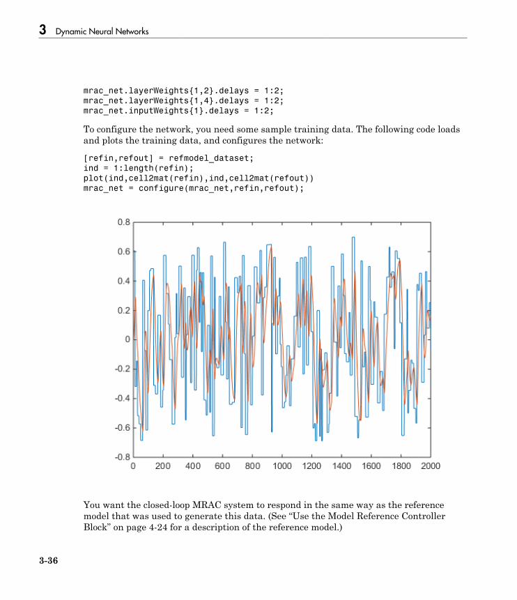
3 Dynamic Neural Networks
3-36
mrac_net.layerWeights{1,2}.delays = 1:2;
mrac_net.layerWeights{1,4}.delays = 1:2;
mrac_net.inputWeights{1}.delays = 1:2;
To configure the network, you need some sample training data. The following code loadsand plots the training data, and configures the network:
[refin,refout] = refmodel_dataset;
ind = 1:length(refin);
plot(ind,cell2mat(refin),ind,cell2mat(refout))
mrac_net = configure(mrac_net,refin,refout);
You want the closed-loop MRAC system to respond in the same way as the referencemodel that was used to generate this data. (See “Use the Model Reference ControllerBlock” on page 4-24 for a description of the reference model.)
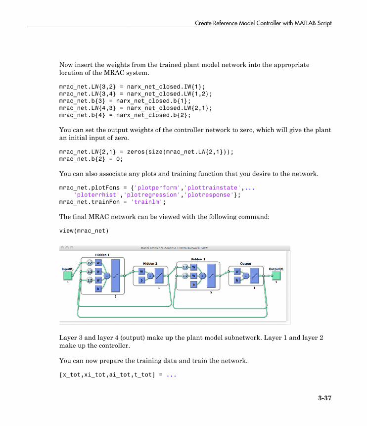
Create Reference Model Controller with MATLAB Script
3-37
Now insert the weights from the trained plant model network into the appropriatelocation of the MRAC system.
mrac_net.LW{3,2} = narx_net_closed.IW{1};
mrac_net.LW{3,4} = narx_net_closed.LW{1,2};
mrac_net.b{3} = narx_net_closed.b{1};
mrac_net.LW{4,3} = narx_net_closed.LW{2,1};
mrac_net.b{4} = narx_net_closed.b{2};
You can set the output weights of the controller network to zero, which will give the plantan initial input of zero.
mrac_net.LW{2,1} = zeros(size(mrac_net.LW{2,1}));
mrac_net.b{2} = 0;
You can also associate any plots and training function that you desire to the network.
mrac_net.plotFcns = {'plotperform','plottrainstate',...
'ploterrhist','plotregression','plotresponse'};
mrac_net.trainFcn = 'trainlm';
The final MRAC network can be viewed with the following command:
view(mrac_net)
Layer 3 and layer 4 (output) make up the plant model subnetwork. Layer 1 and layer 2make up the controller.
You can now prepare the training data and train the network.
[x_tot,xi_tot,ai_tot,t_tot] = ...
3 Dynamic Neural Networks
3-38
preparets(mrac_net,refin,{},refout);
mrac_net.trainParam.epochs = 50;
mrac_net.trainParam.min_grad = 1e-10;
[mrac_net,tr] = train(mrac_net,x_tot,t_tot,xi_tot,ai_tot);
Note Notice that you are using the trainlm training function here, but any of thetraining functions discussed in “Multilayer Neural Networks and BackpropagationTraining” could be used as well. Any network that you can create in the toolbox can betrained with any of those training functions. The only limitation is that all of the parts ofthe network must be differentiable.
You will find that the training of the MRAC system takes much longer that the trainingof the NARX plant model. This is because the network is recurrent and dynamicbackpropagation must be used. This is determined automatically by the toolbox softwareand does not require any user intervention. There are several implementations ofdynamic backpropagation (see [DeHa07]), and the toolbox software automaticallydetermines the most efficient one for the selected network architecture and trainingalgorithm.
After the network has been trained, you can test the operation by applying a test inputto the MRAC network. The following code creates a skyline input function, which is aseries of steps of random height and width, and applies it to the trained MRAC network.
testin = skyline(1000,50,200,-.7,.7);
testinseq = con2seq(testin);
testoutseq = mrac_net(testinseq);
testout = cell2mat(testoutseq);
figure
plot([testin' testout'])

Create Reference Model Controller with MATLAB Script
3-39
From the figure, you can see that the plant model output does follow the reference inputwith the correct critically damped response, even though the input sequence was not thesame as the input sequence in the training data. The steady state response is not perfectfor each step, but this could be improved with a larger training set and perhaps morehidden neurons.
The purpose of this example was to show that you can create your own custom dynamicnetwork and train it using the standard toolbox training functions without anymodifications. Any network that you can create in the toolbox can be trained with thestandard training functions, as long as each component of the network has a definedderivative.

3 Dynamic Neural Networks
3-40
It should be noted that recurrent networks are generally more difficult to train thanfeedforward networks. See [HDH09] for some discussion of these training difficulties.
Multiple Sequences with Dynamic Neural Networks
3-41
Multiple Sequences with Dynamic Neural Networks
There are times when time-series data is not available in one long sequence, but ratheras several shorter sequences. When dealing with static networks and concurrent batchesof static data, you can simply append data sets together to form one large concurrentbatch. However, you would not generally want to append time sequences together, sincethat would cause a discontinuity in the sequence. For these cases, you can create aconcurrent set of sequences, as described in “Understanding Neural Network ToolboxData Structures” on page 1-23.
When training a network with a concurrent set of sequences, it is required that eachsequence be of the same length. If this is not the case, then the shorter sequenceinputs and targets should be padded with NaNs, in order to make all sequences thesame length. The targets that are assigned values of NaN will be ignored during thecalculation of network performance.
The following code illustrates the use of the function catsamples to combine severalsequences together to form a concurrent set of sequences, while at the same time paddingthe shorter sequences.
load magmulseq
y_mul = catsamples(y1,y2,y3,'pad');
u_mul = catsamples(u1,u2,u3,'pad');
d1 = [1:2];
d2 = [1:2];
narx_net = narxnet(d1,d2,10);
narx_net.divideFcn = '';
narx_net.trainParam.min_grad = 1e-10;
[p,Pi,Ai,t] = preparets(narx_net,u_mul,{},y_mul);
narx_net = train(narx_net,p,t,Pi);
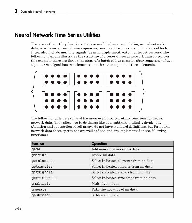
3 Dynamic Neural Networks
3-42
Neural Network Time-Series Utilities
There are other utility functions that are useful when manipulating neural networkdata, which can consist of time sequences, concurrent batches or combinations of both.It can also include multiple signals (as in multiple input, output or target vectors). Thefollowing diagram illustrates the structure of a general neural network data object. Forthis example there are three time steps of a batch of four samples (four sequences) of twosignals. One signal has two elements, and the other signal has three elements.
The following table lists some of the more useful toolbox utility functions for neuralnetwork data. They allow you to do things like add, subtract, multiply, divide, etc.(Addition and subtraction of cell arrays do not have standard definitions, but for neuralnetwork data these operations are well defined and are implemented in the followingfunctions.)
Function Operation
gadd Add neural network (nn) data.gdivide Divide nn data.getelements Select indicated elements from nn data.getsamples Select indicated samples from nn data.getsignals Select indicated signals from nn data.gettimesteps Select indicated time steps from nn data.gmultiply Multiply nn data.gnegate Take the negative of nn data.gsubtract Subtract nn data.
Neural Network Time-Series Utilities
3-43
Function Operation
nndata Create an nn data object of specified size, wherevalues are assigned randomly or to a constant.
nnsize Return number of elements, samples, time stepsand signals in an nn data object.
numelements Return the number of elements in nn data.numsamples Return the number of samples in nn data.numsignals Return the number of signals in nn data.numtimesteps Return the number of time steps in nn data.setelements Set specified elements of nn data.setsamples Set specified samples of nn data.setsignals Set specified signals of nn data.settimesteps Set specified time steps of nn data.
There are also some useful plotting and analysis functions for dynamic networks that arelisted in the following table. There are examples of using these functions in the “GettingStarted with Neural Network Toolbox”.
Function Operation
ploterrcorr Plot the autocorrelation function of the error.plotinerrcorr Plot the crosscorrelation between the error and the
input.plotresponse Plot network output and target versus time.

3 Dynamic Neural Networks
3-44
Train Neural Networks with Error Weights
In the default mean square error performance function (see “Train and Apply MultilayerNeural Networks” on page 2-17), each squared error contributes the same amount to theperformance function as follows:
F mseN
eN
t ai
i
N
i i
i
N
= = = -
= =
 Â1 12
1
2
1
( ) ( )
However, the toolbox allows you to weight each squared error individually as follows:
F mseN
w eN
w t ai
e
i
i
N
i
e
i i
i
N
= = = -
= =
 Â1 12
1
2
1
( ) ( )
The error weighting object needs to have the same dimensions as the target data. Inthis way, errors can be weighted according to time step, sample number, signal numberor element number. The following is an example of weighting the errors at the end of atime sequence more heavily than errors at the beginning of a time sequence. The errorweighting object is passed as the last argument in the call to train.
y = laser_dataset;
y = y(1:600);
ind = 1:600;
ew = 0.99.^(600-ind);
figure
plot(ew)
ew = con2seq(ew);
ftdnn_net = timedelaynet([1:8],10);
ftdnn_net.trainParam.epochs = 1000;
ftdnn_net.divideFcn = '';
[p,Pi,Ai,t,ew1] = preparets(ftdnn_net,y,y,{},ew);
[ftdnn_net1,tr] = train(ftdnn_net,p,t,Pi,Ai,ew1);
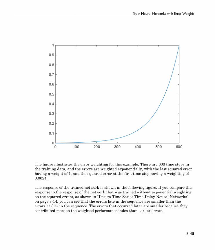
Train Neural Networks with Error Weights
3-45
The figure illustrates the error weighting for this example. There are 600 time steps inthe training data, and the errors are weighted exponentially, with the last squared errorhaving a weight of 1, and the squared error at the first time step having a weighting of0.0024.
The response of the trained network is shown in the following figure. If you compare thisresponse to the response of the network that was trained without exponential weightingon the squared errors, as shown in “Design Time Series Time-Delay Neural Networks”on page 3-14, you can see that the errors late in the sequence are smaller than theerrors earlier in the sequence. The errors that occurred later are smaller because theycontributed more to the weighted performance index than earlier errors.

3 Dynamic Neural Networks
3-46
Normalize Errors of Multiple Outputs
3-47
Normalize Errors of Multiple Outputs
The most common performance function used to train neural networks is mean squarederror (mse). However, with multiple outputs that have different ranges of values,training with mean squared error tends to optimize accuracy on the output element withthe wider range of values relative to the output element with a smaller range.
For instance, here two target elements have very different ranges:
x = -1:0.01:1;
t1 = 100*sin(x);
t2 = 0.01*cos(x);
t = [t1; t2];
The range of t1 is 200 (from a minimum of -100 to a maximum of 100), while the rangeof t2 is only 0.02 (from -0.01 to 0.01). The range of t1 is 10,000 times greater than therange of t2.
If you create and train a neural network on this to minimize mean squared error,training favors the relative accuracy of the first output element over the second.
net = feedforwardnet(5);
net1 = train(net,x,t);
y = net1(x);
Here you can see that the network has learned to fit the first output element very well.
figure(1)
plot(x,y(1,:),x,t(1,:))
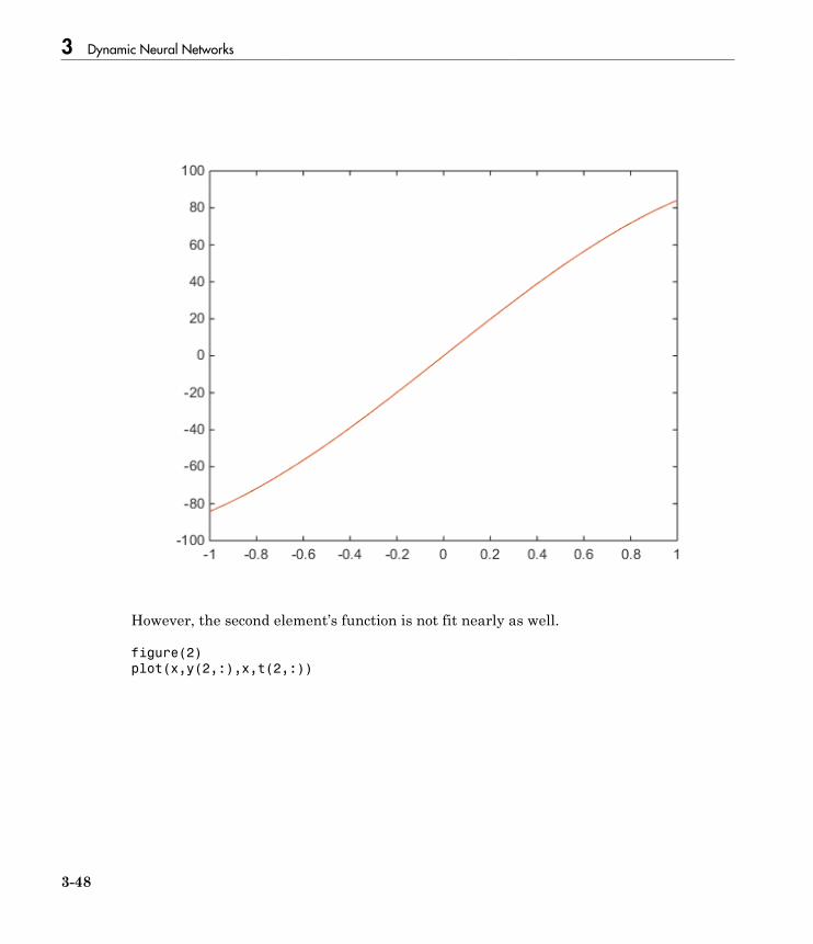
3 Dynamic Neural Networks
3-48
However, the second element’s function is not fit nearly as well.
figure(2)
plot(x,y(2,:),x,t(2,:))
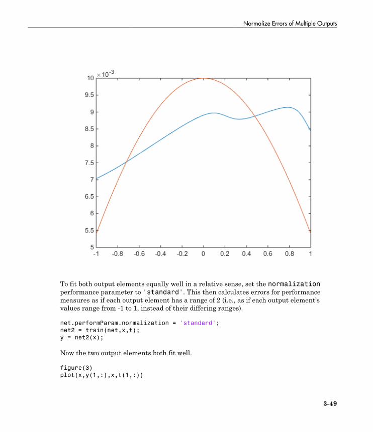
Normalize Errors of Multiple Outputs
3-49
To fit both output elements equally well in a relative sense, set the normalizationperformance parameter to 'standard'. This then calculates errors for performancemeasures as if each output element has a range of 2 (i.e., as if each output element’svalues range from -1 to 1, instead of their differing ranges).
net.performParam.normalization = 'standard';
net2 = train(net,x,t);
y = net2(x);
Now the two output elements both fit well.
figure(3)
plot(x,y(1,:),x,t(1,:))
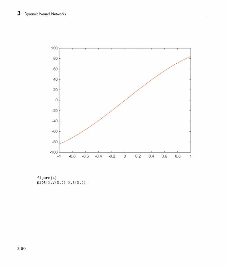
3 Dynamic Neural Networks
3-50
figure(4)
plot(x,y(2,:),x,t(2,:))

Normalize Errors of Multiple Outputs
3-51
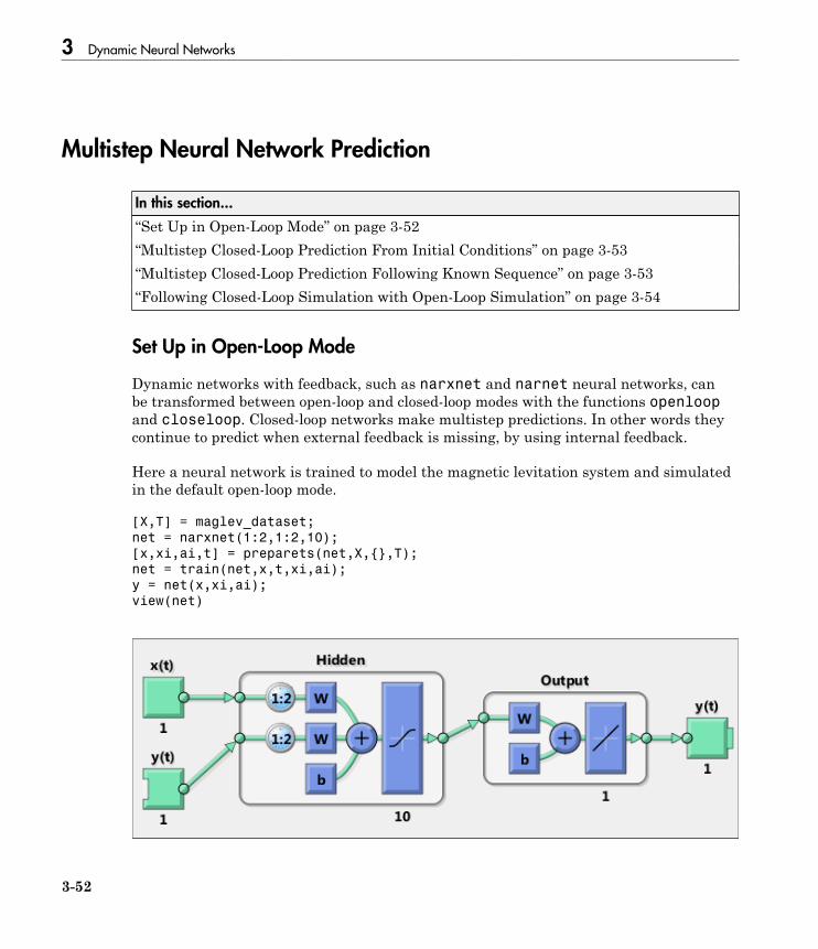
3 Dynamic Neural Networks
3-52
Multistep Neural Network Prediction
In this section...
“Set Up in Open-Loop Mode” on page 3-52“Multistep Closed-Loop Prediction From Initial Conditions” on page 3-53“Multistep Closed-Loop Prediction Following Known Sequence” on page 3-53“Following Closed-Loop Simulation with Open-Loop Simulation” on page 3-54
Set Up in Open-Loop Mode
Dynamic networks with feedback, such as narxnet and narnet neural networks, canbe transformed between open-loop and closed-loop modes with the functions openloopand closeloop. Closed-loop networks make multistep predictions. In other words theycontinue to predict when external feedback is missing, by using internal feedback.
Here a neural network is trained to model the magnetic levitation system and simulatedin the default open-loop mode.
[X,T] = maglev_dataset;
net = narxnet(1:2,1:2,10);
[x,xi,ai,t] = preparets(net,X,{},T);
net = train(net,x,t,xi,ai);
y = net(x,xi,ai);
view(net)
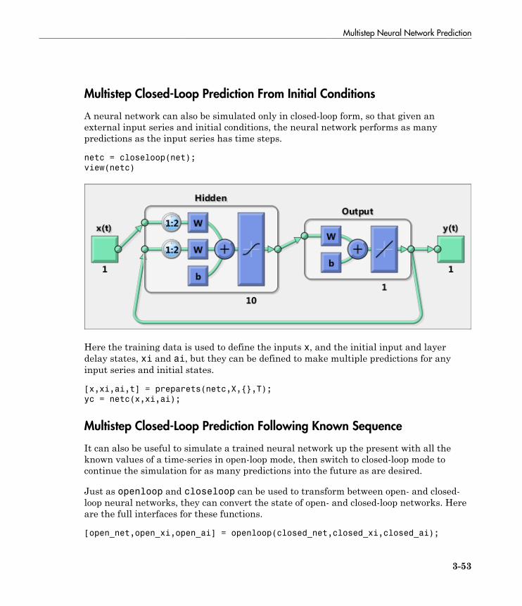
Multistep Neural Network Prediction
3-53
Multistep Closed-Loop Prediction From Initial Conditions
A neural network can also be simulated only in closed-loop form, so that given anexternal input series and initial conditions, the neural network performs as manypredictions as the input series has time steps.
netc = closeloop(net);
view(netc)
Here the training data is used to define the inputs x, and the initial input and layerdelay states, xi and ai, but they can be defined to make multiple predictions for anyinput series and initial states.
[x,xi,ai,t] = preparets(netc,X,{},T);
yc = netc(x,xi,ai);
Multistep Closed-Loop Prediction Following Known Sequence
It can also be useful to simulate a trained neural network up the present with all theknown values of a time-series in open-loop mode, then switch to closed-loop mode tocontinue the simulation for as many predictions into the future as are desired.
Just as openloop and closeloop can be used to transform between open- and closed-loop neural networks, they can convert the state of open- and closed-loop networks. Hereare the full interfaces for these functions.
[open_net,open_xi,open_ai] = openloop(closed_net,closed_xi,closed_ai);
3 Dynamic Neural Networks
3-54
[closed_net,closed_xi,closed_ai] = closeloop(open_net,open_xi,open_ai);
Consider the case where you might have a record of the Maglev’s behavior for 20 timesteps, and you want to predict ahead for 20 more time steps.
First, define the first 20 steps of inputs and targets, representing the 20 time steps wherethe known output is defined by the targets t. With the next 20 time steps of the input aredefined, use the network to predict the 20 outputs using each of its predictions feedbackto help the network perform the next prediction.
x1 = x(1:20);
t1 = t(1:20);
x2 = x(21:40);
The open-loop neural network is then simulated on this data.
[x,xi,ai,t] = preparets(net,x1,{},t1);
[y1,xf,af] = net(x,xi,ai);
Now the final input and layer states returned by the network are converted to closed-loop form along with the network. The final input states xf and layer states af of theopen-loop network become the initial input states xi and layer states ai of the closed-loop network.
[netc,xi,ai] = closeloop(net,xf,af);
Typically use preparets to define initial input and layer states. Since these havealready been obtained from the end of the open-loop simulation, you do not needpreparets to continue with the 20 step predictions of the closed-loop network.
[y2,xf,af] = netc(x2,xi,ai);
Note that you can set x2 to different sequences of inputs to test different scenarios forhowever many time steps you would like to make predictions. For example, to predict themagnetic levitation system’s behavior if 10 random inputs are used:
x2 = num2cell(rand(1,10));
[y2,xf,af] = netc(x2,xi,ai);
Following Closed-Loop Simulation with Open-Loop Simulation
If after simulating the network in closed-loop form, you can continue the simulation fromthere in open-loop form. Here the closed-loop state is converted back to open-loop state.

Multistep Neural Network Prediction
3-55
(You do not have to convert the network back to open-loop form as you already have theoriginal open-loop network.)
[~,xi,ai] = openloop(netc,xf,af);
Now you can define continuations of the external input and open-loop feedback, andsimulate the open-loop network.
x3 = num2cell(rand(2,10));
y3 = net(x,xi,ai);
In this way, you can switch simulation between open-loop and closed-loop manners.One application for this is making time-series predictions of a sensor, where the lastsensor value is usually known, allowing open-loop prediction of the next step. But onsome occasions the sensor reading is not available, or known to be erroneous, requiring aclosed-loop prediction step. The predictions can alternate between open-loop and closed-loop form, depending on the availability of the last step’s sensor reading.

3-56

4
Control Systems
• “Introduction to Neural Network Control Systems” on page 4-2• “Design Neural Network Predictive Controller in Simulink” on page 4-4• “Design NARMA-L2 Neural Controller in Simulink” on page 4-14• “Design Model-Reference Neural Controller in Simulink” on page 4-23• “Import-Export Neural Network Simulink Control Systems” on page 4-31
4 Control Systems
4-2
Introduction to Neural Network Control Systems
Neural networks have been applied successfully in the identification and control ofdynamic systems. The universal approximation capabilities of the multilayer perceptronmake it a popular choice for modeling nonlinear systems and for implementing general-purpose nonlinear controllers [HaDe99]. This topic introduces three popular neuralnetwork architectures for prediction and control that have been implemented in theNeural Network Toolbox software, and presents brief descriptions of each of thesearchitectures and shows how you can use them:
• Model Predictive Control• NARMA-L2 (or Feedback Linearization) Control• Model Reference Control
There are typically two steps involved when using neural networks for control:
1 System identification2 Control design
In the system identification stage, you develop a neural network model of the plant thatyou want to control. In the control design stage, you use the neural network plant modelto design (or train) the controller. In each of the three control architectures described inthis topic, the system identification stage is identical. The control design stage, however,is different for each architecture:
• For model predictive control, the plant model is used to predict future behavior of theplant, and an optimization algorithm is used to select the control input that optimizesfuture performance.
• For NARMA-L2 control, the controller is simply a rearrangement of the plant model.• For model reference control, the controller is a neural network that is trained to
control a plant so that it follows a reference model. The neural network plant model isused to assist in the controller training.
The next three sections discuss model predictive control, NARMA-L2 control, and modelreference control. Each section consists of a brief description of the control concept,followed by an example of the use of the appropriate Neural Network Toolbox function.These three controllers are implemented as Simulink® blocks, which are contained in theNeural Network Toolbox blockset.

Introduction to Neural Network Control Systems
4-3
To assist you in determining the best controller for your application, the following listsummarizes the key controller features. Each controller has its own strengths andweaknesses. No single controller is appropriate for every application.
• Model Predictive Control — This controller uses a neural network model to predictfuture plant responses to potential control signals. An optimization algorithm thencomputes the control signals that optimize future plant performance. The neuralnetwork plant model is trained offline, in batch form. (This is true for all three controlarchitectures.) The controller, however, requires a significant amount of onlinecomputation, because an optimization algorithm is performed at each sample time tocompute the optimal control input.
• NARMA-L2 Control — This controller requires the least computation of thesethree architectures. The controller is simply a rearrangement of the neural networkplant model, which is trained offline, in batch form. The only online computation is aforward pass through the neural network controller. The drawback of this method isthat the plant must either be in companion form, or be capable of approximation bya companion form model. (“Identification of the NARMA-L2 Model” on page 4-14describes the companion form model.)
• Model Reference Control — The online computation of this controller, likeNARMA-L2, is minimal. However, unlike NARMA-L2, the model referencearchitecture requires that a separate neural network controller be trained offline, inaddition to the neural network plant model. The controller training is computationallyexpensive, because it requires the use of dynamic backpropagation [HaJe99]. Onthe positive side, model reference control applies to a larger class of plant than doesNARMA-L2 control.
4 Control Systems
4-4
Design Neural Network Predictive Controller in Simulink
In this section...
“System Identification” on page 4-4“Predictive Control” on page 4-5“Use the Neural Network Predictive Controller Block” on page 4-6
The neural network predictive controller that is implemented in the Neural NetworkToolbox software uses a neural network model of a nonlinear plant to predict futureplant performance. The controller then calculates the control input that will optimizeplant performance over a specified future time horizon. The first step in model predictivecontrol is to determine the neural network plant model (system identification). Next,the plant model is used by the controller to predict future performance. (See the ModelPredictive Control Toolbox™ documentation for complete coverage of the application ofvarious model predictive control strategies to linear systems.)
The following section describes the system identification process. This is followed bya description of the optimization process. Finally, it discusses how to use the modelpredictive controller block that is implemented in the Simulink environment.
System Identification
The first stage of model predictive control is to train a neural network to represent theforward dynamics of the plant. The prediction error between the plant output and theneural network output is used as the neural network training signal. The process isrepresented by the following figure:

Design Neural Network Predictive Controller in Simulink
4-5
The neural network plant model uses previous inputs and previous plant outputs topredict future values of the plant output. The structure of the neural network plantmodel is given in the following figure.
This network can be trained offline in batch mode, using data collected from theoperation of the plant. You can use any of the training algorithms discussed in“Multilayer Neural Networks and Backpropagation Training” for network training. Thisprocess is discussed in more detail in following sections.
Predictive Control
The model predictive control method is based on the receding horizon technique[SoHa96]. The neural network model predicts the plant response over a specified timehorizon. The predictions are used by a numerical optimization program to determine
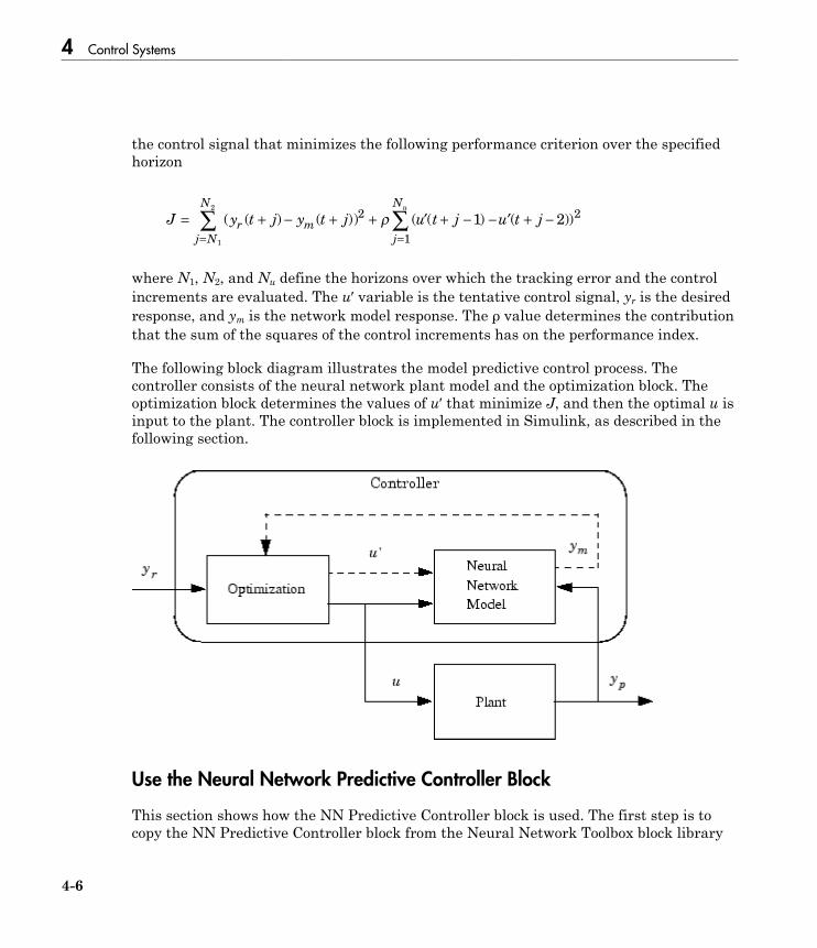
4 Control Systems
4-6
the control signal that minimizes the following performance criterion over the specifiedhorizon
J y t j y t j u t j u t jr m
j
N
j N
N u
= + - + + + - - + -
==ÂÂ ( ( ) ( )) ( ( ) ( ))
2 2
1
1 2
1
2
r ¢ ¢
where N1, N2, and Nu define the horizons over which the tracking error and the controlincrements are evaluated. The u′ variable is the tentative control signal, yr is the desiredresponse, and ym is the network model response. The ρ value determines the contributionthat the sum of the squares of the control increments has on the performance index.
The following block diagram illustrates the model predictive control process. Thecontroller consists of the neural network plant model and the optimization block. Theoptimization block determines the values of u′ that minimize J, and then the optimal u isinput to the plant. The controller block is implemented in Simulink, as described in thefollowing section.
Use the Neural Network Predictive Controller Block
This section shows how the NN Predictive Controller block is used. The first step is tocopy the NN Predictive Controller block from the Neural Network Toolbox block library

Design Neural Network Predictive Controller in Simulink
4-7
to the Simulink Editor. See the Simulink documentation if you are not sure how to dothis. This step is skipped in the following example.
An example model is provided with the Neural Network Toolbox software to show theuse of the predictive controller. This example uses a catalytic Continuous Stirred TankReactor (CSTR). A diagram of the process is shown in the following figure.
The dynamic model of the system is
dh t
dtw t w t h t
dC t
dtC C t
w t
h t
bb b
( )( ) ( ) . ( )
( )( ( ))
( )
( )(
= + −
= − +
1 2
11
0 2
CC C tw t
h t
k C t
k C tb b
b
b
22 1
22
1− −
+( ))
( )
( )
( )
( ( ))
where h(t) is the liquid level, Cb(t) is the product concentration at the output of theprocess, w1(t) is the flow rate of the concentrated feed Cb1, and w2(t) is the flow rate ofthe diluted feed Cb2. The input concentrations are set to Cb1 = 24.9 and Cb2 = 0.1. Theconstants associated with the rate of consumption are k1 = 1 and k2 = 1.
The objective of the controller is to maintain the product concentration by adjustingthe flow w1(t). To simplify the example, set w2(t) = 0.1. The level of the tank h(t) is notcontrolled for this experiment.
To run this example:
1 Start MATLAB.2 Type predcstr in the MATLAB Command Window. This command opens the
Simulink Editor with the following model.

4 Control Systems
4-8
The Plant block contains the Simulink CSTR plant model. The NN PredictiveController block signals are connected as follows:
• Control Signal is connected to the input of the Plant model.• The Plant Output signal is connected to the Plant block output.• The Reference is connected to the Random Reference signal.
3 Double-click the NN Predictive Controller block. This opens the following windowfor designing the model predictive controller. This window enables you to changethe controller horizons N2 and Nu. (N1 is fixed at 1.) The weighting parameter ρ,described earlier, is also defined in this window. The parameter α is used to controlthe optimization. It determines how much reduction in performance is required fora successful optimization step. You can select which linear minimization routine isused by the optimization algorithm, and you can decide how many iterations of theoptimization algorithm are performed at each sample time. The linear minimizationroutines are slight modifications of those discussed in “Multilayer Neural Networksand Backpropagation Training”.
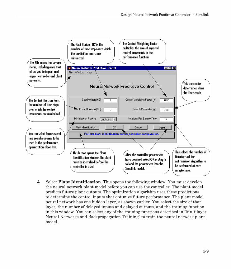
Design Neural Network Predictive Controller in Simulink
4-9
4 Select Plant Identification. This opens the following window. You must developthe neural network plant model before you can use the controller. The plant modelpredicts future plant outputs. The optimization algorithm uses these predictionsto determine the control inputs that optimize future performance. The plant modelneural network has one hidden layer, as shown earlier. You select the size of thatlayer, the number of delayed inputs and delayed outputs, and the training functionin this window. You can select any of the training functions described in “MultilayerNeural Networks and Backpropagation Training” to train the neural network plantmodel.

4 Control Systems
4-10
5 Click Generate Training Data. The program generates training data by applyinga series of random step inputs to the Simulink plant model. The potential trainingdata is then displayed in a figure similar to the following.
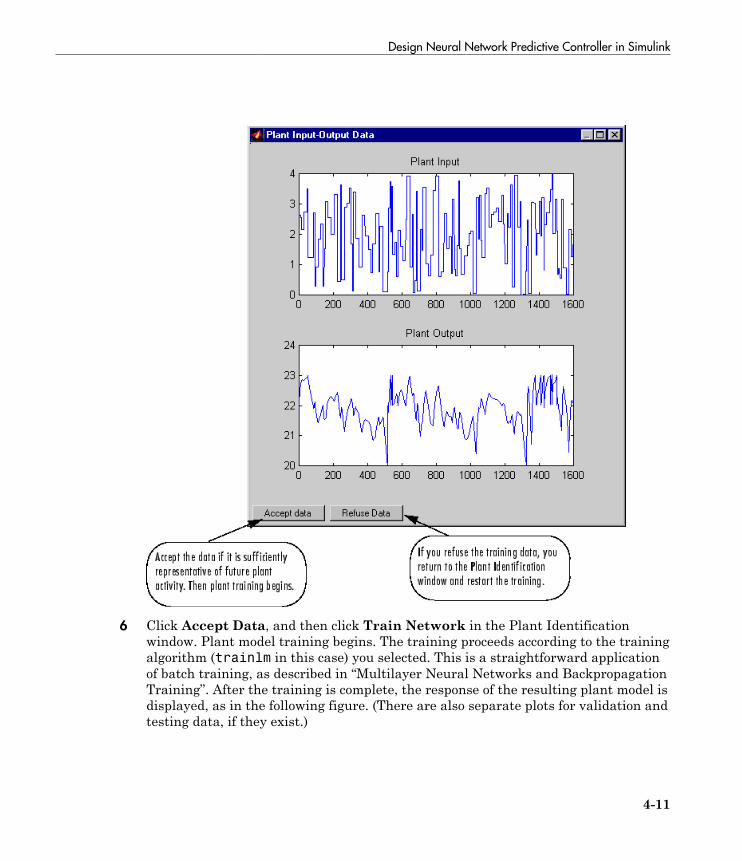
Design Neural Network Predictive Controller in Simulink
4-11
6 Click Accept Data, and then click Train Network in the Plant Identificationwindow. Plant model training begins. The training proceeds according to the trainingalgorithm (trainlm in this case) you selected. This is a straightforward applicationof batch training, as described in “Multilayer Neural Networks and BackpropagationTraining”. After the training is complete, the response of the resulting plant model isdisplayed, as in the following figure. (There are also separate plots for validation andtesting data, if they exist.)

4 Control Systems
4-12
You can then continue training with the same data set by selecting Train Networkagain, you can Erase Generated Data and generate a new data set, or you canaccept the current plant model and begin simulating the closed loop system. For thisexample, begin the simulation, as shown in the following steps.
7 Select OK in the Plant Identification window. This loads the trained neural networkplant model into the NN Predictive Controller block.
8 Select OK in the Neural Network Predictive Control window. This loads thecontroller parameters into the NN Predictive Controller block.
9 Return to the Simulink Editor and start the simulation by choosing the menu optionSimulation > Run. As the simulation runs, the plant output and the referencesignal are displayed, as in the following figure.

Design Neural Network Predictive Controller in Simulink
4-13

4 Control Systems
4-14
Design NARMA-L2 Neural Controller in Simulink
In this section...
“Identification of the NARMA-L2 Model” on page 4-14“NARMA-L2 Controller” on page 4-16“Use the NARMA-L2 Controller Block” on page 4-18
The neurocontroller described in this section is referred to by two different names:feedback linearization control and NARMA-L2 control. It is referred to as feedbacklinearization when the plant model has a particular form (companion form). It is referredto as NARMA-L2 control when the plant model can be approximated by the same form.The central idea of this type of control is to transform nonlinear system dynamics intolinear dynamics by canceling the nonlinearities. This section begins by presenting thecompanion form system model and showing how you can use a neural network to identifythis model. Then it describes how the identified neural network model can be used todevelop a controller. This is followed by an example of how to use the NARMA-L2 Controlblock, which is contained in the Neural Network Toolbox blockset.
Identification of the NARMA-L2 Model
As with model predictive control, the first step in using feedback linearization (orNARMA-L2) control is to identify the system to be controlled. You train a neural networkto represent the forward dynamics of the system. The first step is to choose a modelstructure to use. One standard model that is used to represent general discrete-timenonlinear systems is the nonlinear autoregressive-moving average (NARMA) model:
y k d N y k y k y k n u k u k u k n( ) [ ( ), ( ), , ( ), ( ), ( ), , ( )]+ = − − + − − +1 1 1 1… …
where u(k) is the system input, and y(k) is the system output. For the identificationphase, you could train a neural network to approximate the nonlinear function N. This isthe identification procedure used for the NN Predictive Controller.
If you want the system output to follow some reference trajectoryy(k + d) = yr(k + d), the next step is to develop a nonlinear controller of the form:
u k G y k y k y k n y k d u k u k mr( ) [ ( ), ( ), , ( ), ( ), ( ), , ( )]= − − + + − − +1 1 1 1… …

Design NARMA-L2 Neural Controller in Simulink
4-15
The problem with using this controller is that if you want to train a neural networkto create the function G to minimize mean square error, you need to use dynamicbackpropagation ([NaPa91] or [HaJe99]). This can be quite slow. One solution, proposedby Narendra and Mukhopadhyay [NaMu97], is to use approximate models to representthe system. The controller used in this section is based on the NARMA-L2 approximatemodel:
ˆ( ) [ ( ), ( ), , ( ), ( ), , ( )]
[ ( )
y k d f y k y k y k n u k u k m
g y k
+ = - - + - - +
+
1 1 1 1… …
,, ( ), , ( ), ( ), , ( )] ( )y k y k n u k u k m u k- - + - - + ◊1 1 1 1… …
This model is in companion form, where the next controller input u(k) is not containedinside the nonlinearity. The advantage of this form is that you can solve for the controlinput that causes the system output to follow the reference y(k + d) = yr(k + d). Theresulting controller would have the form
u ky k d f y k y k y k n u k u k n
gr( )( ) [ ( ), ( ), , ( ), ( ), , ( )]
[=
+ − − − + − − +1 1 1 1… …
yy k y k y k n u k u k n( ), ( ), , ( ), ( ), , ( )]− − + − − +1 1 1 1… …
Using this equation directly can cause realization problems, because you must determinethe control input u(k) based on the output at the same time, y(k). So, instead, use themodel
y k d f y k y k y k n u k u k u k n
g
( ) [ ( ), ( ), , ( ), ( ), ( ), , ( )]
[
+ = - - + - - +
+
1 1 1 1… …
yy k y k n u k u k n u k( ), , ( ), ( ), , ( )] ( )… …- + - + ◊ +1 1 1
where d ≥ 2. The following figure shows the structure of a neural network representation.

4 Control Systems
4-16
NARMA-L2 Controller
Using the NARMA-L2 model, you can obtain the controller
u ky k d f y k y k n u k u k n
g y kr( )( ) [ ( ), , ( ), ( ), , ( )]
[ ( ), ,+ =
+ − − + − +1
1 1… …
… yy k n u k u k n( ), ( ), , ( )]− + − +1 1…
which is realizable for d ≥ 2. The following figure is a block diagram of the NARMA-L2controller.

Design NARMA-L2 Neural Controller in Simulink
4-17
This controller can be implemented with the previously identified NARMA-L2 plantmodel, as shown in the following figure.

4 Control Systems
4-18
Use the NARMA-L2 Controller Block
This section shows how the NARMA-L2 controller is trained. The first step is to copythe NARMA-L2 Controller block from the Neural Network Toolbox block library to theSimulink Editor. See the Simulink documentation if you are not sure how to do this. Thisstep is skipped in the following example.
An example model is provided with the Neural Network Toolbox software to show the useof the NARMA-L2 controller. In this example, the objective is to control the position of amagnet suspended above an electromagnet, where the magnet is constrained so that itcan only move in the vertical direction, as in the following figure.
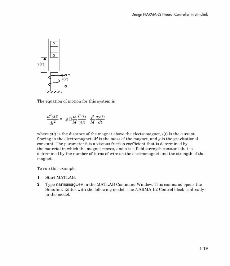
Design NARMA-L2 Neural Controller in Simulink
4-19
The equation of motion for this system is
d y t
dtg
M
i t
y t M
dy t
dt
2
2
2( ) ( )
( )
( )= − + −a b
where y(t) is the distance of the magnet above the electromagnet, i(t) is the currentflowing in the electromagnet, M is the mass of the magnet, and g is the gravitationalconstant. The parameter β is a viscous friction coefficient that is determined bythe material in which the magnet moves, and α is a field strength constant that isdetermined by the number of turns of wire on the electromagnet and the strength of themagnet.
To run this example:
1 Start MATLAB.2 Type narmamaglev in the MATLAB Command Window. This command opens the
Simulink Editor with the following model. The NARMA-L2 Control block is alreadyin the model.
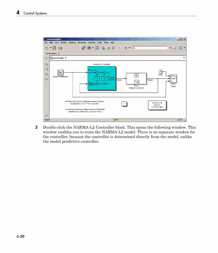
4 Control Systems
4-20
3 Double-click the NARMA-L2 Controller block. This opens the following window. Thiswindow enables you to train the NARMA-L2 model. There is no separate window forthe controller, because the controller is determined directly from the model, unlikethe model predictive controller.

Design NARMA-L2 Neural Controller in Simulink
4-21
4 This window works the same as the other Plant Identification windows, so thetraining process is not repeated. Instead, simulate the NARMA-L2 controller.
5 Return to the Simulink Editor and start the simulation by choosing the menu optionSimulation > Run. As the simulation runs, the plant output and the referencesignal are displayed, as in the following figure.
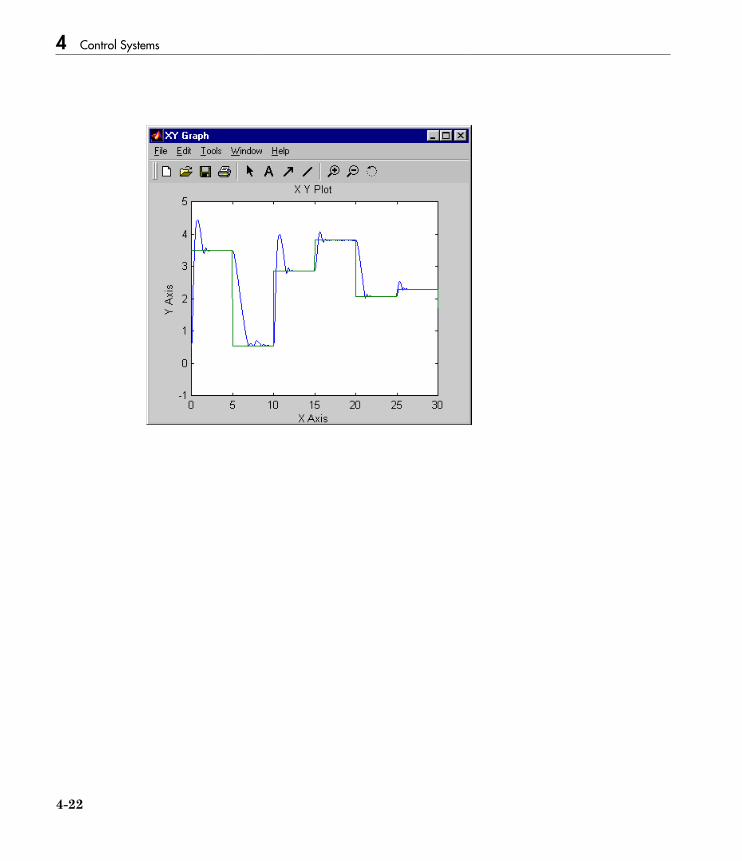
4 Control Systems
4-22
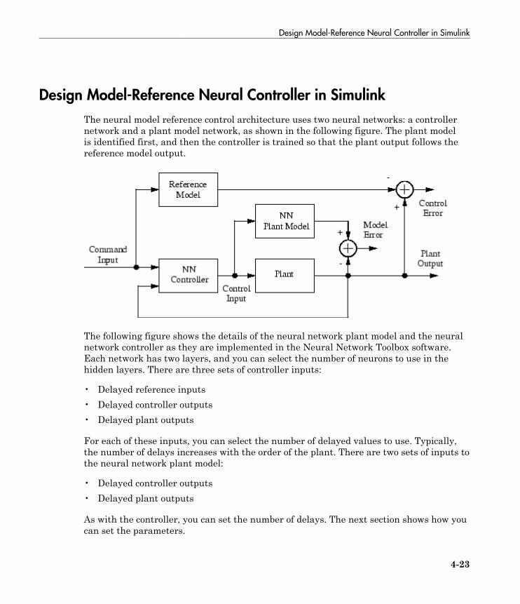
Design Model-Reference Neural Controller in Simulink
4-23
Design Model-Reference Neural Controller in Simulink
The neural model reference control architecture uses two neural networks: a controllernetwork and a plant model network, as shown in the following figure. The plant modelis identified first, and then the controller is trained so that the plant output follows thereference model output.
The following figure shows the details of the neural network plant model and the neuralnetwork controller as they are implemented in the Neural Network Toolbox software.Each network has two layers, and you can select the number of neurons to use in thehidden layers. There are three sets of controller inputs:
• Delayed reference inputs• Delayed controller outputs• Delayed plant outputs
For each of these inputs, you can select the number of delayed values to use. Typically,the number of delays increases with the order of the plant. There are two sets of inputs tothe neural network plant model:
• Delayed controller outputs• Delayed plant outputs
As with the controller, you can set the number of delays. The next section shows how youcan set the parameters.
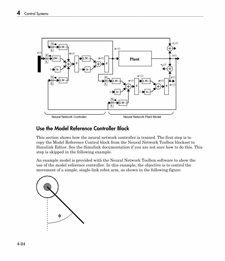
4 Control Systems
4-24
Use the Model Reference Controller Block
This section shows how the neural network controller is trained. The first step is tocopy the Model Reference Control block from the Neural Network Toolbox blockset toSimulink Editor. See the Simulink documentation if you are not sure how to do this. Thisstep is skipped in the following example.
An example model is provided with the Neural Network Toolbox software to show theuse of the model reference controller. In this example, the objective is to control themovement of a simple, single-link robot arm, as shown in the following figure:

Design Model-Reference Neural Controller in Simulink
4-25
The equation of motion for the arm is
d
dt
d
dtu
2
210 2
ff
f= − − +sin
where ≅ is the angle of the arm, and u is the torque supplied by the DC motor.
The objective is to train the controller so that the arm tracks the reference model
d y
dty
dy
dtrr
rr
2
29 6 9= − − +
where yr is the output of the reference model, and r is the input reference signal.
This example uses a neural network controller with a 5-13-1 architecture. The inputs tothe controller consist of two delayed reference inputs, two delayed plant outputs, and onedelayed controller output. A sampling interval of 0.05 seconds is used.
To run this example:
1 Start MATLAB.2 Type mrefrobotarm in the MATLAB Command Window. This command opens the
Simulink Editor with the Model Reference Control block already in the model.
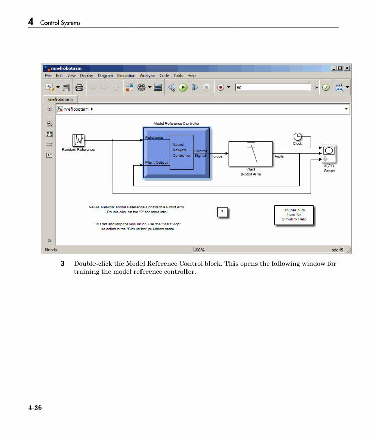
4 Control Systems
4-26
3 Double-click the Model Reference Control block. This opens the following window fortraining the model reference controller.
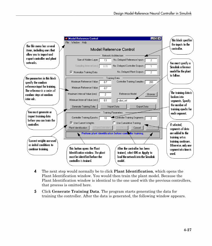
Design Model-Reference Neural Controller in Simulink
4-27
4 The next step would normally be to click Plant Identification, which opens thePlant Identification window. You would then train the plant model. Because thePlant Identification window is identical to the one used with the previous controllers,that process is omitted here.
5 Click Generate Training Data. The program starts generating the data fortraining the controller. After the data is generated, the following window appears.
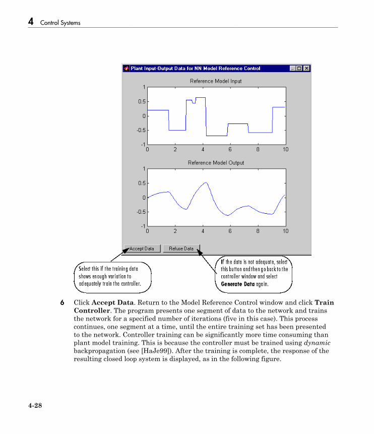
4 Control Systems
4-28
6 Click Accept Data. Return to the Model Reference Control window and click TrainController. The program presents one segment of data to the network and trainsthe network for a specified number of iterations (five in this case). This processcontinues, one segment at a time, until the entire training set has been presentedto the network. Controller training can be significantly more time consuming thanplant model training. This is because the controller must be trained using dynamicbackpropagation (see [HaJe99]). After the training is complete, the response of theresulting closed loop system is displayed, as in the following figure.
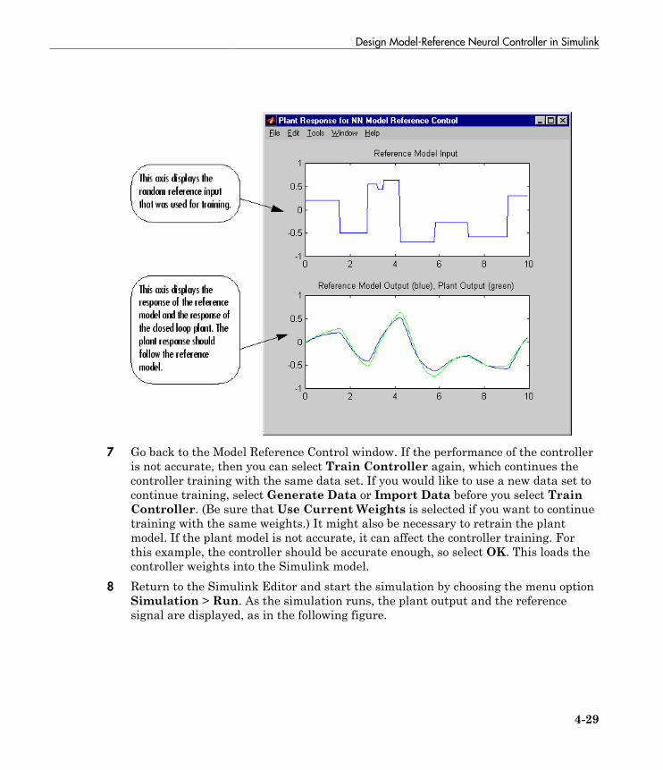
Design Model-Reference Neural Controller in Simulink
4-29
7 Go back to the Model Reference Control window. If the performance of the controlleris not accurate, then you can select Train Controller again, which continues thecontroller training with the same data set. If you would like to use a new data set tocontinue training, select Generate Data or Import Data before you select TrainController. (Be sure that Use Current Weights is selected if you want to continuetraining with the same weights.) It might also be necessary to retrain the plantmodel. If the plant model is not accurate, it can affect the controller training. Forthis example, the controller should be accurate enough, so select OK. This loads thecontroller weights into the Simulink model.
8 Return to the Simulink Editor and start the simulation by choosing the menu optionSimulation > Run. As the simulation runs, the plant output and the referencesignal are displayed, as in the following figure.
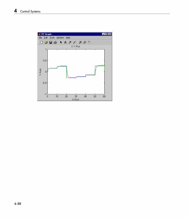
4 Control Systems
4-30

Import-Export Neural Network Simulink Control Systems
4-31
Import-Export Neural Network Simulink Control Systems
In this section...
“Import and Export Networks” on page 4-31“Import and Export Training Data” on page 4-35
Import and Export Networks
The controller and plant model networks that you develop are stored within Simulinkcontroller blocks. At some point you might want to transfer the networks into otherapplications, or you might want to transfer a network from one controller block toanother. You can do this by using the Import Network and Export Network menuoptions. The following example leads you through the export and import processes. (TheNARMA-L2 window is used for this example, but the same procedure applies to all thecontrollers.)
1 Repeat the first three steps of the NARMA-L2 example in “Use the NARMA-L2Controller Block” on page 4-18. The NARMA-L2 Plant Identification window shouldnow be open.
2 Select File > Export Network, as shown below.
This opens the following window.

4 Control Systems
4-32
3 Select Export to Disk. The following window opens. Enter the file name test inthe box, and select Save. This saves the controller and plant networks to disk.
4 Retrieve that data with the Import menu option. Select File > Import Network, asin the following figure.
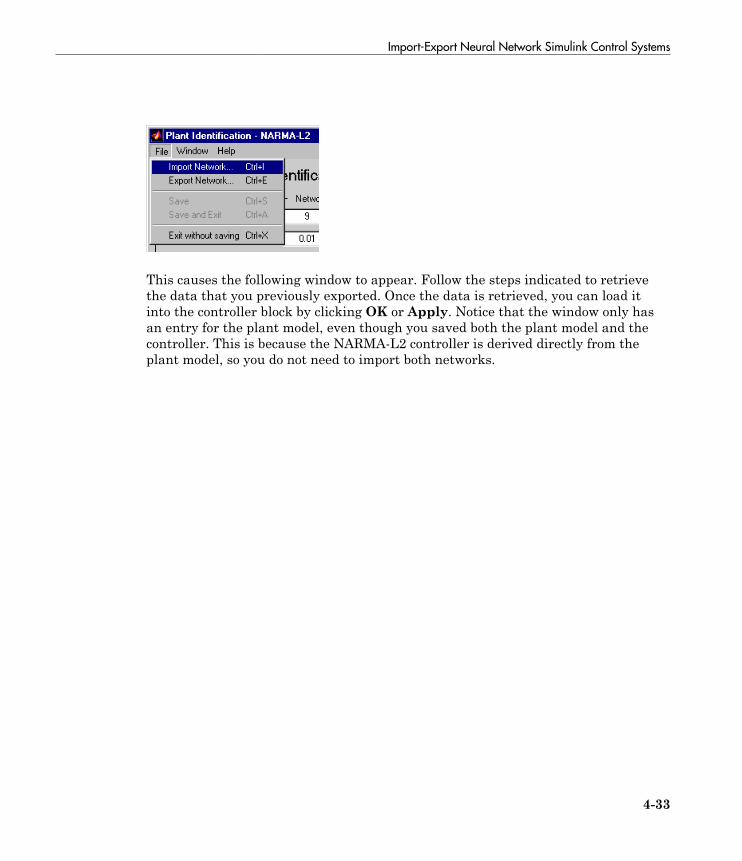
Import-Export Neural Network Simulink Control Systems
4-33
This causes the following window to appear. Follow the steps indicated to retrievethe data that you previously exported. Once the data is retrieved, you can load itinto the controller block by clicking OK or Apply. Notice that the window only hasan entry for the plant model, even though you saved both the plant model and thecontroller. This is because the NARMA-L2 controller is derived directly from theplant model, so you do not need to import both networks.
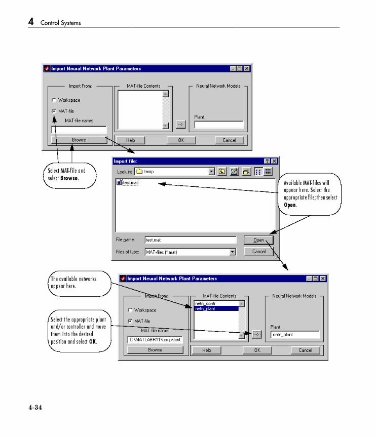
4 Control Systems
4-34

Import-Export Neural Network Simulink Control Systems
4-35
Import and Export Training Data
The data that you generate to train networks exists only in the corresponding plantidentification or controller training window. You might want to save the training datato the workspace or to a disk file so that you can load it again at a later time. You mightalso want to combine data sets manually and then load them back into the trainingwindow. You can do this by using the Import and Export buttons. The followingexample leads you through the import and export processes. (The NN Predictive Controlwindow is used for this example, but the same procedure applies to all the controllers.)
1 Repeat the first five steps of the NN Predictive Control example in “Use the NeuralNetwork Predictive Controller Block” on page 4-6. Then select Accept Data. ThePlant Identification window should then be open, and the Import and Exportbuttons should be active.
2 Click Export to open the following window.
3 Click Export to Disk. The following window opens. Enter the filename testdat inthe box, and select Save. This saves the training data structure to disk.
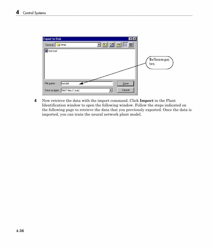
4 Control Systems
4-36
4 Now retrieve the data with the import command. Click Import in the PlantIdentification window to open the following window. Follow the steps indicated onthe following page to retrieve the data that you previously exported. Once the data isimported, you can train the neural network plant model.
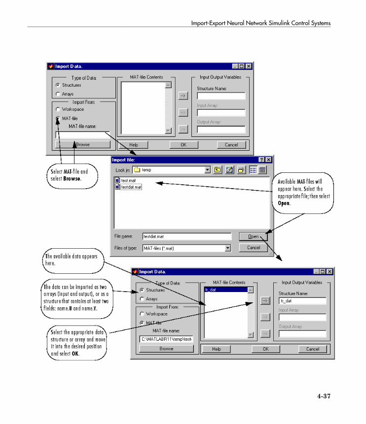
Import-Export Neural Network Simulink Control Systems
4-37

4-38

5
Radial Basis Neural Networks
• “Introduction to Radial Basis Neural Networks” on page 5-2• “Radial Basis Neural Networks” on page 5-3• “Probabilistic Neural Networks” on page 5-10• “Generalized Regression Neural Networks” on page 5-13
5 Radial Basis Neural Networks
5-2
Introduction to Radial Basis Neural Networks
Radial basis networks can require more neurons than standard feedforwardbackpropagation networks, but often they can be designed in a fraction of the time ittakes to train standard feedforward networks. They work best when many trainingvectors are available.
You might want to consult the following paper on this subject: Chen, S., C.F.N. Cowan,and P.M. Grant, “Orthogonal Least Squares Learning Algorithm for Radial BasisFunction Networks,” IEEE Transactions on Neural Networks, Vol. 2, No. 2, March 1991,pp. 302–309.
This topic discusses two variants of radial basis networks, generalized regressionnetworks (GRNN) and probabilistic neural networks (PNN). You can read about themin P.D. Wasserman, Advanced Methods in Neural Computing, New York: Van NostrandReinhold, 1993, on pp. 155–61 and pp. 35–55, respectively.
Important Radial Basis Functions
Radial basis networks can be designed with either newrbe or newrb. GRNNs and PNNscan be designed with newgrnn and newpnn, respectively.

Radial Basis Neural Networks
5-3
Radial Basis Neural Networks
In this section...
“Neuron Model” on page 5-3“Network Architecture” on page 5-4“Exact Design (newrbe)” on page 5-6“More Efficient Design (newrb)” on page 5-7“Examples” on page 5-8
Neuron Model
Here is a radial basis network with R inputs.
Notice that the expression for the net input of a radbas neuron is different from that ofother neurons. Here the net input to the radbas transfer function is the vector distancebetween its weight vector w and the input vector p, multiplied by the bias b. (The ||dist || box in this figure accepts the input vector p and the single row input weightmatrix, and produces the dot product of the two.)
The transfer function for a radial basis neuron is
radbas n en
( ) = − 2
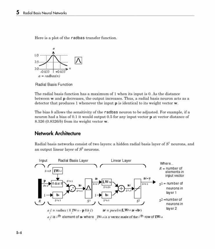
5 Radial Basis Neural Networks
5-4
Here is a plot of the radbas transfer function.
The radial basis function has a maximum of 1 when its input is 0. As the distancebetween w and p decreases, the output increases. Thus, a radial basis neuron acts as adetector that produces 1 whenever the input p is identical to its weight vector w.
The bias b allows the sensitivity of the radbas neuron to be adjusted. For example, if aneuron had a bias of 0.1 it would output 0.5 for any input vector p at vector distance of8.326 (0.8326/b) from its weight vector w.
Network Architecture
Radial basis networks consist of two layers: a hidden radial basis layer of S1 neurons, andan output linear layer of S2 neurons.

Radial Basis Neural Networks
5-5
The || dist || box in this figure accepts the input vector p and the input weight matrixIW1,1, and produces a vector having S1 elements. The elements are the distances betweenthe input vector and vectors iIW1,1 formed from the rows of the input weight matrix.
The bias vector b1 and the output of || dist || are combined with the MATLABoperation .* , which does element-by-element multiplication.
The output of the first layer for a feedforward network net can be obtained with thefollowing code:
a{1} = radbas(netprod(dist(net.IW{1,1},p),net.b{1}))
Fortunately, you won't have to write such lines of code. All the details of designing thisnetwork are built into design functions newrbe and newrb, and you can obtain theiroutputs with sim.
You can understand how this network behaves by following an input vector p throughthe network to the output a2. If you present an input vector to such a network, eachneuron in the radial basis layer will output a value according to how close the inputvector is to each neuron's weight vector.
Thus, radial basis neurons with weight vectors quite different from the input vector phave outputs near zero. These small outputs have only a negligible effect on the linearoutput neurons.
In contrast, a radial basis neuron with a weight vector close to the input vector pproduces a value near 1. If a neuron has an output of 1, its output weights in the secondlayer pass their values to the linear neurons in the second layer.
In fact, if only one radial basis neuron had an output of 1, and all others had outputs of0s (or very close to 0), the output of the linear layer would be the active neuron's outputweights. This would, however, be an extreme case. Typically several neurons are alwaysfiring, to varying degrees.
Now look in detail at how the first layer operates. Each neuron's weighted input is thedistance between the input vector and its weight vector, calculated with dist. Eachneuron's net input is the element-by-element product of its weighted input with its bias,calculated with netprod. Each neuron's output is its net input passed through radbas.If a neuron's weight vector is equal to the input vector (transposed), its weighted inputis 0, its net input is 0, and its output is 1. If a neuron's weight vector is a distance of
5 Radial Basis Neural Networks
5-6
spread from the input vector, its weighted input is spread, its net input is sqrt(−log(.5))(or 0.8326), therefore its output is 0.5.
Exact Design (newrbe)
You can design radial basis networks with the function newrbe. This function canproduce a network with zero error on training vectors. It is called in the following way:
net = newrbe(P,T,SPREAD)
The function newrbe takes matrices of input vectors P and target vectors T, and a spreadconstant SPREAD for the radial basis layer, and returns a network with weights andbiases such that the outputs are exactly T when the inputs are P.
This function newrbe creates as many radbas neurons as there are input vectors in P,and sets the first-layer weights to P'. Thus, there is a layer of radbas neurons in whicheach neuron acts as a detector for a different input vector. If there are Q input vectors,then there will be Q neurons.
Each bias in the first layer is set to 0.8326/SPREAD. This gives radial basis functions thatcross 0.5 at weighted inputs of +/− SPREAD. This determines the width of an area in theinput space to which each neuron responds. If SPREAD is 4, then each radbas neuronwill respond with 0.5 or more to any input vectors within a vector distance of 4 fromtheir weight vector. SPREAD should be large enough that neurons respond strongly tooverlapping regions of the input space.
The second-layer weights IW 2,1 (or in code, IW{2,1}) and biases b2 (or in code, b{2})are found by simulating the first-layer outputs a1 (A{1}), and then solving the followinglinear expression:
[W{2,1} b{2}] * [A{1}; ones(1,Q)] = T
You know the inputs to the second layer (A{1}) and the target (T), and the layer is linear.You can use the following code to calculate the weights and biases of the second layer tominimize the sum-squared error.
Wb = T/[A{1}; ones(1,Q)]
Here Wb contains both weights and biases, with the biases in the last column. The sum-squared error is always 0, as explained below.

Radial Basis Neural Networks
5-7
There is a problem with C constraints (input/target pairs) and each neuron has C +1variables (the C weights from the C radbas neurons, and a bias). A linear problem withC constraints and more than C variables has an infinite number of zero error solutions.
Thus, newrbe creates a network with zero error on training vectors. The only conditionrequired is to make sure that SPREAD is large enough that the active input regions of theradbas neurons overlap enough so that several radbas neurons always have fairly largeoutputs at any given moment. This makes the network function smoother and resultsin better generalization for new input vectors occurring between input vectors used inthe design. (However, SPREAD should not be so large that each neuron is effectivelyresponding in the same large area of the input space.)
The drawback to newrbe is that it produces a network with as many hidden neurons asthere are input vectors. For this reason, newrbe does not return an acceptable solutionwhen many input vectors are needed to properly define a network, as is typically thecase.
More Efficient Design (newrb)
The function newrb iteratively creates a radial basis network one neuron at a time.Neurons are added to the network until the sum-squared error falls beneath an errorgoal or a maximum number of neurons has been reached. The call for this function is
net = newrb(P,T,GOAL,SPREAD)
The function newrb takes matrices of input and target vectors P and T, and designparameters GOAL and SPREAD, and returns the desired network.
The design method of newrb is similar to that of newrbe. The difference is that newrbcreates neurons one at a time. At each iteration the input vector that results in loweringthe network error the most is used to create a radbas neuron. The error of the newnetwork is checked, and if low enough newrb is finished. Otherwise the next neuron isadded. This procedure is repeated until the error goal is met or the maximum number ofneurons is reached.
As with newrbe, it is important that the spread parameter be large enough that theradbas neurons respond to overlapping regions of the input space, but not so large thatall the neurons respond in essentially the same manner.
Why not always use a radial basis network instead of a standard feedforward network?Radial basis networks, even when designed efficiently with newrbe, tend to have many
5 Radial Basis Neural Networks
5-8
times more neurons than a comparable feedforward network with tansig or logsigneurons in the hidden layer.
This is because sigmoid neurons can have outputs over a large region of the input space,while radbas neurons only respond to relatively small regions of the input space. Theresult is that the larger the input space (in terms of number of inputs, and the rangesthose inputs vary over) the more radbas neurons required.
On the other hand, designing a radial basis network often takes much less time thantraining a sigmoid/linear network, and can sometimes result in fewer neurons' beingused, as can be seen in the next example.
Examples
The example demorb1 shows how a radial basis network is used to fit a function. Herethe problem is solved with only five neurons.
Examples demorb3 and demorb4 examine how the spread constant affects the designprocess for radial basis networks.
In demorb3, a radial basis network is designed to solve the same problem as in demorb1.However, this time the spread constant used is 0.01. Thus, each radial basis neuronreturns 0.5 or lower for any input vector with a distance of 0.01 or more from its weightvector.
Because the training inputs occur at intervals of 0.1, no two radial basis neurons have astrong output for any given input.
demorb3 showed that having too small a spread constant can result in a solution thatdoes not generalize from the input/target vectors used in the design. Example demorb4shows the opposite problem. If the spread constant is large enough, the radial basisneurons will output large values (near 1.0) for all the inputs used to design the network.
If all the radial basis neurons always output 1, any information presented to the networkbecomes lost. No matter what the input, the second layer outputs 1's. The function newrbwill attempt to find a network, but cannot because of numerical problems that arise inthis situation.
The moral of the story is, choose a spread constant larger than the distance betweenadjacent input vectors, so as to get good generalization, but smaller than the distanceacross the whole input space.

Radial Basis Neural Networks
5-9
For this problem that would mean picking a spread constant greater than 0.1, theinterval between inputs, and less than 2, the distance between the leftmost andrightmost inputs.
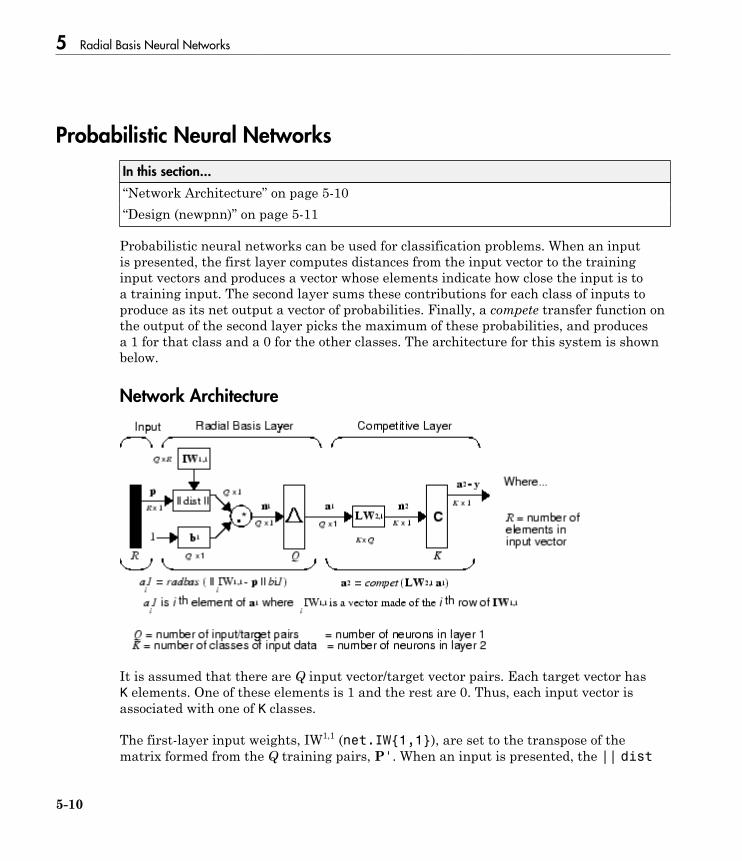
5 Radial Basis Neural Networks
5-10
Probabilistic Neural Networks
In this section...
“Network Architecture” on page 5-10“Design (newpnn)” on page 5-11
Probabilistic neural networks can be used for classification problems. When an inputis presented, the first layer computes distances from the input vector to the traininginput vectors and produces a vector whose elements indicate how close the input is toa training input. The second layer sums these contributions for each class of inputs toproduce as its net output a vector of probabilities. Finally, a compete transfer function onthe output of the second layer picks the maximum of these probabilities, and producesa 1 for that class and a 0 for the other classes. The architecture for this system is shownbelow.
Network Architecture
It is assumed that there are Q input vector/target vector pairs. Each target vector hasK elements. One of these elements is 1 and the rest are 0. Thus, each input vector isassociated with one of K classes.
The first-layer input weights, IW1,1 (net.IW{1,1}), are set to the transpose of thematrix formed from the Q training pairs, P'. When an input is presented, the || dist

Probabilistic Neural Networks
5-11
|| box produces a vector whose elements indicate how close the input is to the vectors ofthe training set. These elements are multiplied, element by element, by the bias and sentto the radbas transfer function. An input vector close to a training vector is representedby a number close to 1 in the output vector a1. If an input is close to several trainingvectors of a single class, it is represented by several elements of a1 that are close to 1.
The second-layer weights, LW1,2 (net.LW{2,1}), are set to the matrix T of targetvectors. Each vector has a 1 only in the row associated with that particular class ofinput, and 0s elsewhere. (Use function ind2vec to create the proper vectors.) Themultiplication Ta1 sums the elements of a1 due to each of the K input classes. Finally,the second-layer transfer function, compet, produces a 1 corresponding to the largestelement of n2, and 0s elsewhere. Thus, the network classifies the input vector into aspecific K class because that class has the maximum probability of being correct.
Design (newpnn)
You can use the function newpnn to create a PNN. For instance, suppose that seveninput vectors and their corresponding targets are
P = [0 0;1 1;0 3;1 4;3 1;4 1;4 3]'
which yields
P =
0 1 0 1 3 4 4
0 1 3 4 1 1 3
Tc = [1 1 2 2 3 3 3]
which yields
Tc =
1 1 2 2 3 3 3
You need a target matrix with 1s in the right places. You can get it with the functionind2vec. It gives a matrix with 0s except at the correct spots. So execute
T = ind2vec(Tc)
which gives
T =
(1,1) 1
5 Radial Basis Neural Networks
5-12
(1,2) 1
(2,3) 1
(2,4) 1
(3,5) 1
(3,6) 1
(3,7) 1
Now you can create a network and simulate it, using the input P to make sure that itdoes produce the correct classifications. Use the function vec2ind to convert the outputY into a row Yc to make the classifications clear.
net = newpnn(P,T);
Y = sim(net,P);
Yc = vec2ind(Y)
This produces
Yc =
1 1 2 2 3 3 3
You might try classifying vectors other than those that were used to design the network.Try to classify the vectors shown below in P2.
P2 = [1 4;0 1;5 2]'
P2 =
1 0 5
4 1 2
Can you guess how these vectors will be classified? If you run the simulation and plot thevectors as before, you get
Yc =
2 1 3
These results look good, for these test vectors were quite close to members of classes 2,1, and 3, respectively. The network has managed to generalize its operation to properlyclassify vectors other than those used to design the network.
You might want to try demopnn1. It shows how to design a PNN, and how the networkcan successfully classify a vector not used in the design.
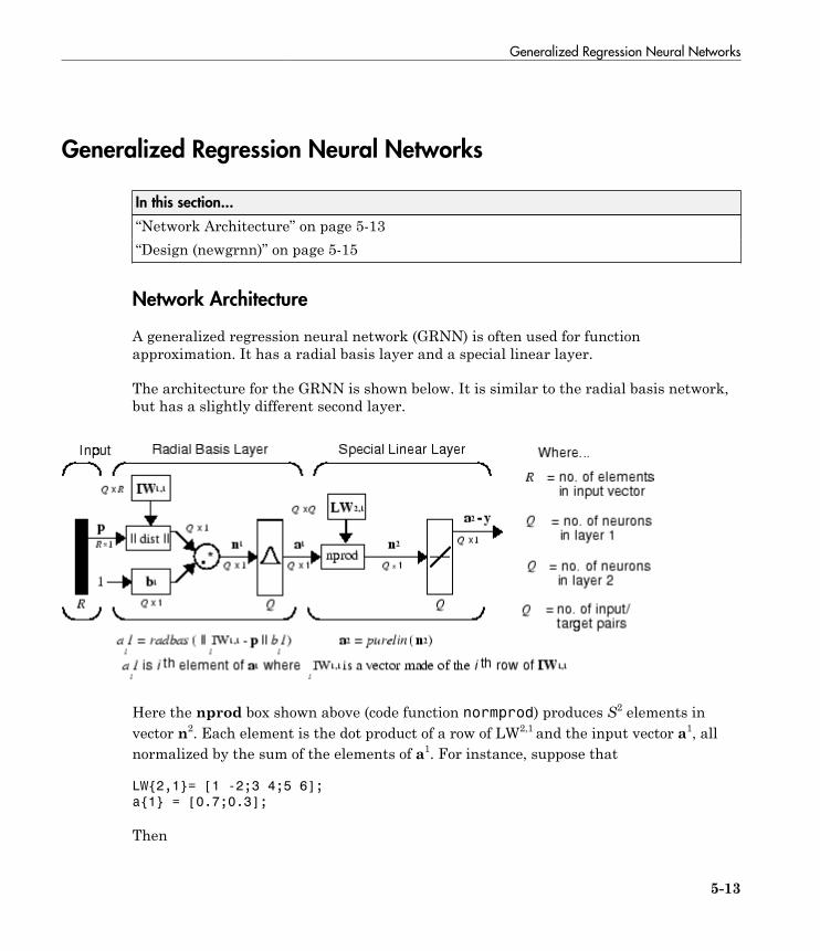
Generalized Regression Neural Networks
5-13
Generalized Regression Neural Networks
In this section...
“Network Architecture” on page 5-13“Design (newgrnn)” on page 5-15
Network Architecture
A generalized regression neural network (GRNN) is often used for functionapproximation. It has a radial basis layer and a special linear layer.
The architecture for the GRNN is shown below. It is similar to the radial basis network,but has a slightly different second layer.
Here the nprod box shown above (code function normprod) produces S2 elements invector n2. Each element is the dot product of a row of LW2,1 and the input vector a1, allnormalized by the sum of the elements of a1. For instance, suppose that
LW{2,1}= [1 -2;3 4;5 6];
a{1} = [0.7;0.3];
Then
5 Radial Basis Neural Networks
5-14
aout = normprod(LW{2,1},a{1})
aout =
0.1000
3.3000
5.3000
The first layer is just like that for newrbe networks. It has as many neurons as there areinput/ target vectors in P. Specifically, the first-layer weights are set to P'. The bias b1 isset to a column vector of 0.8326/SPREAD. The user chooses SPREAD, the distance an inputvector must be from a neuron's weight vector to be 0.5.
Again, the first layer operates just like the newrbe radial basis layer describedpreviously. Each neuron's weighted input is the distance between the input vector andits weight vector, calculated with dist. Each neuron's net input is the product of itsweighted input with its bias, calculated with netprod. Each neuron's output is its netinput passed through radbas. If a neuron's weight vector is equal to the input vector(transposed), its weighted input will be 0, its net input will be 0, and its output will be1. If a neuron's weight vector is a distance of spread from the input vector, its weightedinput will be spread, and its net input will be sqrt(−log(.5)) (or 0.8326). Therefore itsoutput will be 0.5.
The second layer also has as many neurons as input/target vectors, but here LW{2,1} isset to T.
Suppose you have an input vector p close to pi, one of the input vectors among the inputvector/target pairs used in designing layer 1 weights. This input p produces a layer 1 ai
output close to 1. This leads to a layer 2 output close to ti, one of the targets used to formlayer 2 weights.
A larger spread leads to a large area around the input vector where layer 1 neurons willrespond with significant outputs. Therefore if spread is small the radial basis functionis very steep, so that the neuron with the weight vector closest to the input will have amuch larger output than other neurons. The network tends to respond with the targetvector associated with the nearest design input vector.
As spread becomes larger the radial basis function's slope becomes smoother andseveral neurons can respond to an input vector. The network then acts as if it is takinga weighted average between target vectors whose design input vectors are closest to thenew input vector. As spread becomes larger more and more neurons contribute to theaverage, with the result that the network function becomes smoother.
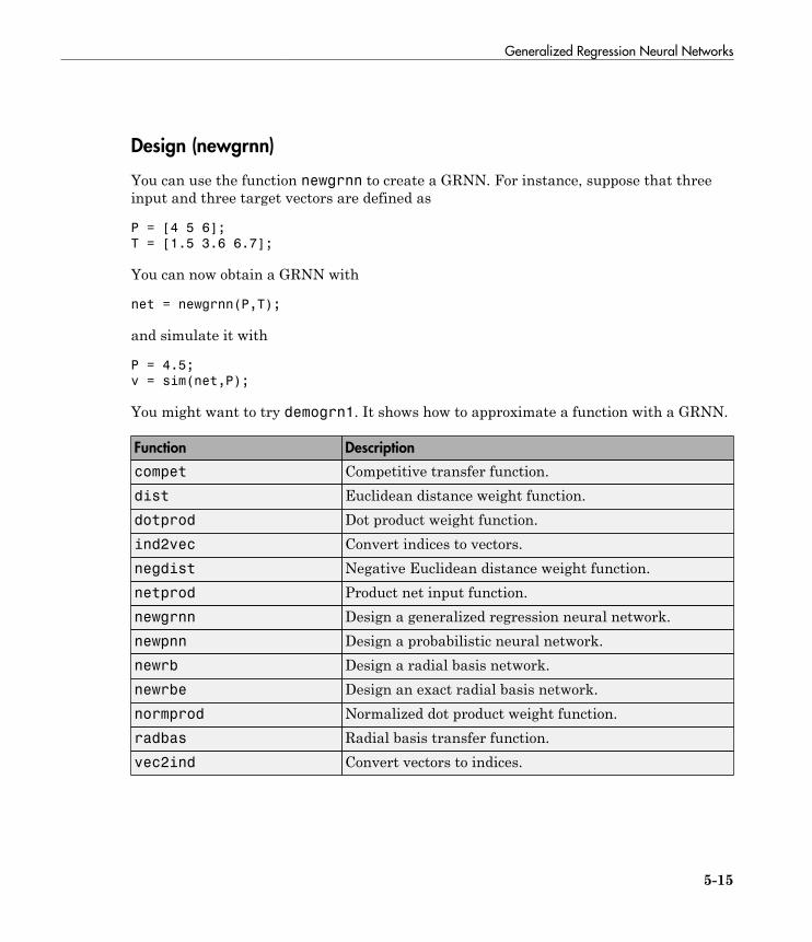
Generalized Regression Neural Networks
5-15
Design (newgrnn)
You can use the function newgrnn to create a GRNN. For instance, suppose that threeinput and three target vectors are defined as
P = [4 5 6];
T = [1.5 3.6 6.7];
You can now obtain a GRNN with
net = newgrnn(P,T);
and simulate it with
P = 4.5;
v = sim(net,P);
You might want to try demogrn1. It shows how to approximate a function with a GRNN.
Function Description
compet Competitive transfer function.dist Euclidean distance weight function.dotprod Dot product weight function.ind2vec Convert indices to vectors.negdist Negative Euclidean distance weight function.netprod Product net input function.newgrnn Design a generalized regression neural network.newpnn Design a probabilistic neural network.newrb Design a radial basis network.newrbe Design an exact radial basis network.normprod Normalized dot product weight function.radbas Radial basis transfer function.vec2ind Convert vectors to indices.

5-16

6
Self-Organizing and Learning VectorQuantization Networks
• “Introduction to Self-Organizing and LVQ” on page 6-2• “Cluster with a Competitive Neural Network” on page 6-3• “Cluster with Self-Organizing Map Neural Network” on page 6-9• “Learning Vector Quantization (LVQ) Neural Networks” on page 6-34
6 Self-Organizing and Learning Vector Quantization Networks
6-2
Introduction to Self-Organizing and LVQ
Self-organizing in networks is one of the most fascinating topics in the neural networkfield. Such networks can learn to detect regularities and correlations in their inputand adapt their future responses to that input accordingly. The neurons of competitivenetworks learn to recognize groups of similar input vectors. Self-organizing maps learnto recognize groups of similar input vectors in such a way that neurons physically neareach other in the neuron layer respond to similar input vectors. Self-organizing maps donot have target vectors, since their purpose is to divide the input vectors into clusters ofsimilar vectors. There is no desired output for these types of networks.
Learning vector quantization (LVQ) is a method for training competitive layers in asupervised manner (with target outputs). A competitive layer automatically learnsto classify input vectors. However, the classes that the competitive layer finds aredependent only on the distance between input vectors. If two input vectors are verysimilar, the competitive layer probably will put them in the same class. There is nomechanism in a strictly competitive layer design to say whether or not any two inputvectors are in the same class or different classes.
LVQ networks, on the other hand, learn to classify input vectors into target classeschosen by the user.
You might consult the following reference: Kohonen, T., Self-Organization andAssociative Memory, 2nd Edition, Berlin: Springer-Verlag, 1987.
Important Self-Organizing and LVQ Functions
You can create competitive layers and self-organizing maps with competlayer andselforgmap, respectively.
You can create an LVQ network with the function lvqnet.
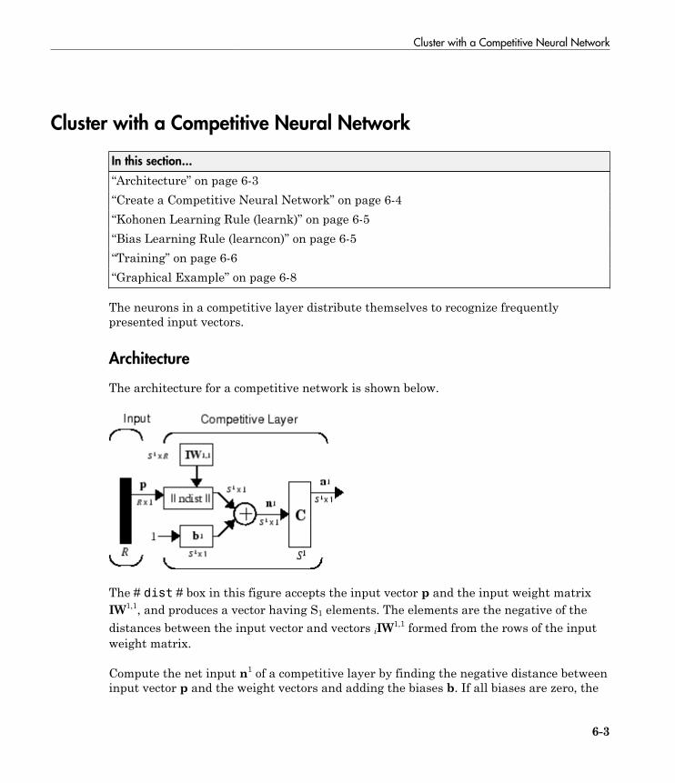
Cluster with a Competitive Neural Network
6-3
Cluster with a Competitive Neural Network
In this section...
“Architecture” on page 6-3“Create a Competitive Neural Network” on page 6-4“Kohonen Learning Rule (learnk)” on page 6-5“Bias Learning Rule (learncon)” on page 6-5“Training” on page 6-6“Graphical Example” on page 6-8
The neurons in a competitive layer distribute themselves to recognize frequentlypresented input vectors.
Architecture
The architecture for a competitive network is shown below.
The ≅ dist ≅ box in this figure accepts the input vector p and the input weight matrixIW1,1, and produces a vector having S1 elements. The elements are the negative of thedistances between the input vector and vectors iIW1,1 formed from the rows of the inputweight matrix.
Compute the net input n1 of a competitive layer by finding the negative distance betweeninput vector p and the weight vectors and adding the biases b. If all biases are zero, the
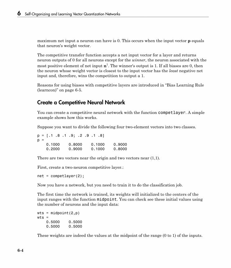
6 Self-Organizing and Learning Vector Quantization Networks
6-4
maximum net input a neuron can have is 0. This occurs when the input vector p equalsthat neuron's weight vector.
The competitive transfer function accepts a net input vector for a layer and returnsneuron outputs of 0 for all neurons except for the winner, the neuron associated with themost positive element of net input n1. The winner's output is 1. If all biases are 0, thenthe neuron whose weight vector is closest to the input vector has the least negative netinput and, therefore, wins the competition to output a 1.
Reasons for using biases with competitive layers are introduced in “Bias Learning Rule(learncon)” on page 6-5.
Create a Competitive Neural Network
You can create a competitive neural network with the function competlayer. A simpleexample shows how this works.
Suppose you want to divide the following four two-element vectors into two classes.
p = [.1 .8 .1 .9; .2 .9 .1 .8]
p =
0.1000 0.8000 0.1000 0.9000
0.2000 0.9000 0.1000 0.8000
There are two vectors near the origin and two vectors near (1,1).
First, create a two-neuron competitive layer.:
net = competlayer(2);
Now you have a network, but you need to train it to do the classification job.
The first time the network is trained, its weights will initialized to the centers of theinput ranges with the function midpoint. You can check see these initial values usingthe number of neurons and the input data:
wts = midpoint(2,p)
wts =
0.5000 0.5000
0.5000 0.5000
These weights are indeed the values at the midpoint of the range (0 to 1) of the inputs.
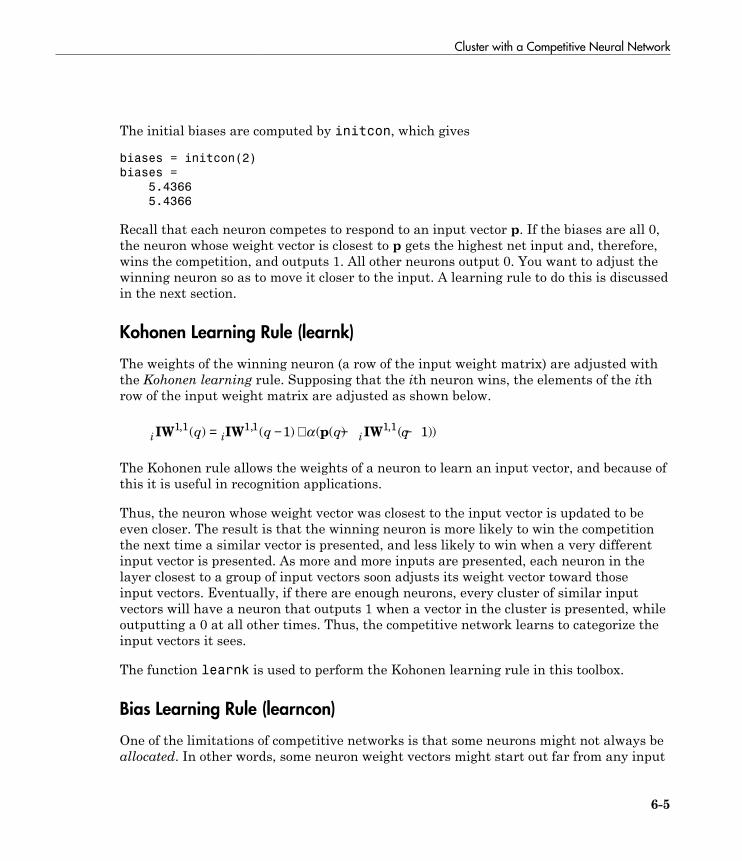
Cluster with a Competitive Neural Network
6-5
The initial biases are computed by initcon, which gives
biases = initcon(2)
biases =
5.4366
5.4366
Recall that each neuron competes to respond to an input vector p. If the biases are all 0,the neuron whose weight vector is closest to p gets the highest net input and, therefore,wins the competition, and outputs 1. All other neurons output 0. You want to adjust thewinning neuron so as to move it closer to the input. A learning rule to do this is discussedin the next section.
Kohonen Learning Rule (learnk)
The weights of the winning neuron (a row of the input weight matrix) are adjusted withthe Kohonen learning rule. Supposing that the ith neuron wins, the elements of the ithrow of the input weight matrix are adjusted as shown below.
i i iq q q qIW IW p IW1 1 1 1 1 11 1, , ,( ) ( ) ( ( ) ( ))= − + − −a
The Kohonen rule allows the weights of a neuron to learn an input vector, and because ofthis it is useful in recognition applications.
Thus, the neuron whose weight vector was closest to the input vector is updated to beeven closer. The result is that the winning neuron is more likely to win the competitionthe next time a similar vector is presented, and less likely to win when a very differentinput vector is presented. As more and more inputs are presented, each neuron in thelayer closest to a group of input vectors soon adjusts its weight vector toward thoseinput vectors. Eventually, if there are enough neurons, every cluster of similar inputvectors will have a neuron that outputs 1 when a vector in the cluster is presented, whileoutputting a 0 at all other times. Thus, the competitive network learns to categorize theinput vectors it sees.
The function learnk is used to perform the Kohonen learning rule in this toolbox.
Bias Learning Rule (learncon)
One of the limitations of competitive networks is that some neurons might not always beallocated. In other words, some neuron weight vectors might start out far from any input
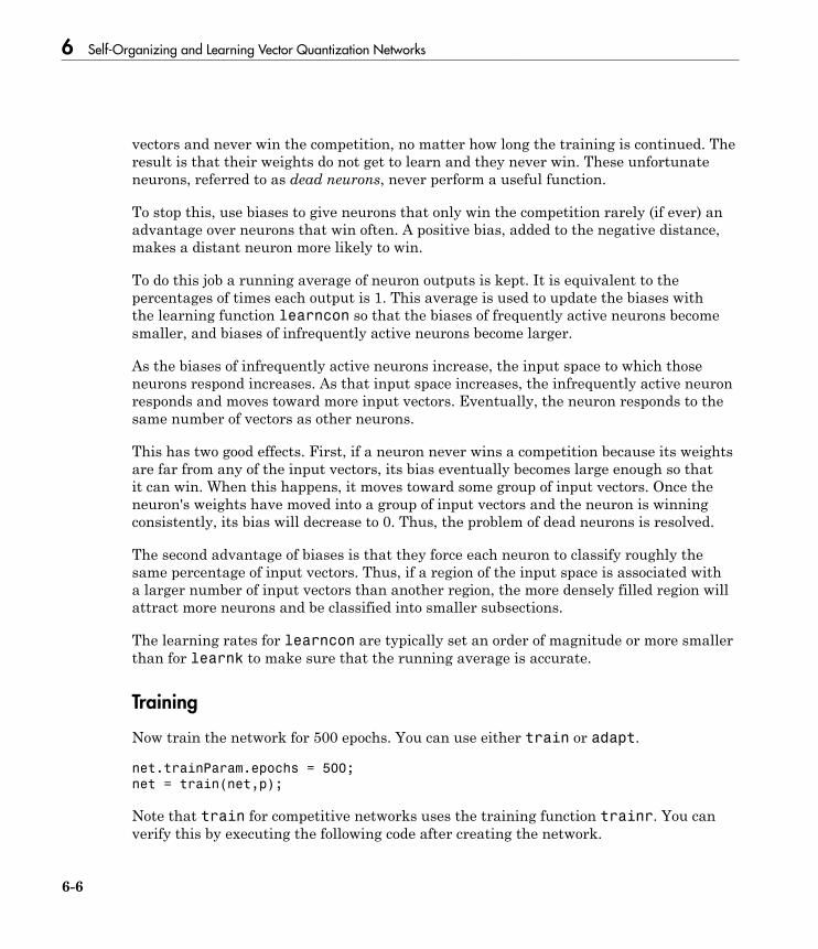
6 Self-Organizing and Learning Vector Quantization Networks
6-6
vectors and never win the competition, no matter how long the training is continued. Theresult is that their weights do not get to learn and they never win. These unfortunateneurons, referred to as dead neurons, never perform a useful function.
To stop this, use biases to give neurons that only win the competition rarely (if ever) anadvantage over neurons that win often. A positive bias, added to the negative distance,makes a distant neuron more likely to win.
To do this job a running average of neuron outputs is kept. It is equivalent to thepercentages of times each output is 1. This average is used to update the biases withthe learning function learncon so that the biases of frequently active neurons becomesmaller, and biases of infrequently active neurons become larger.
As the biases of infrequently active neurons increase, the input space to which thoseneurons respond increases. As that input space increases, the infrequently active neuronresponds and moves toward more input vectors. Eventually, the neuron responds to thesame number of vectors as other neurons.
This has two good effects. First, if a neuron never wins a competition because its weightsare far from any of the input vectors, its bias eventually becomes large enough so thatit can win. When this happens, it moves toward some group of input vectors. Once theneuron's weights have moved into a group of input vectors and the neuron is winningconsistently, its bias will decrease to 0. Thus, the problem of dead neurons is resolved.
The second advantage of biases is that they force each neuron to classify roughly thesame percentage of input vectors. Thus, if a region of the input space is associated witha larger number of input vectors than another region, the more densely filled region willattract more neurons and be classified into smaller subsections.
The learning rates for learncon are typically set an order of magnitude or more smallerthan for learnk to make sure that the running average is accurate.
Training
Now train the network for 500 epochs. You can use either train or adapt.
net.trainParam.epochs = 500;
net = train(net,p);
Note that train for competitive networks uses the training function trainr. You canverify this by executing the following code after creating the network.
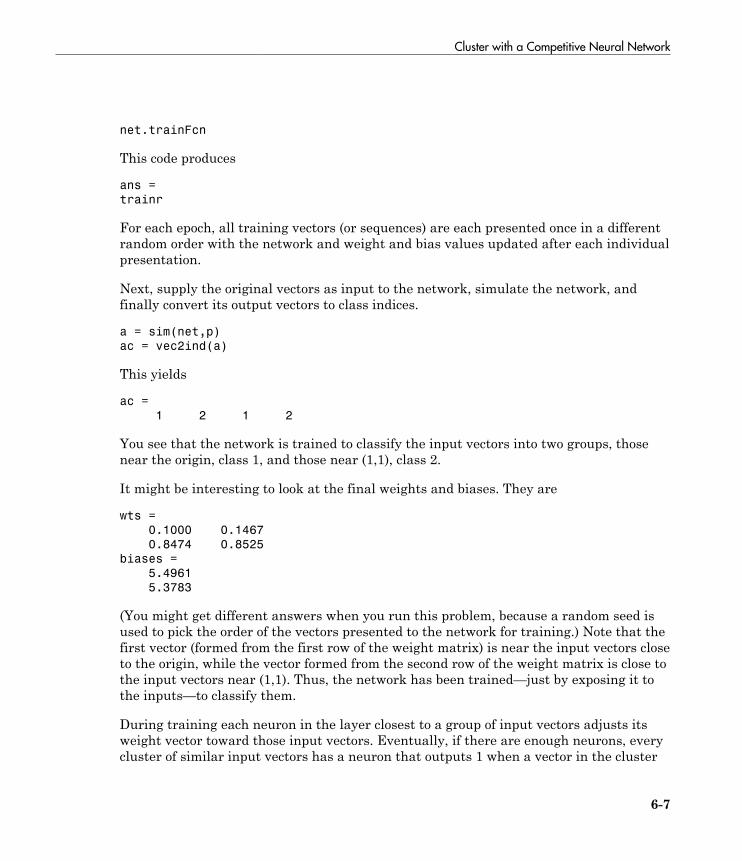
Cluster with a Competitive Neural Network
6-7
net.trainFcn
This code produces
ans =
trainr
For each epoch, all training vectors (or sequences) are each presented once in a differentrandom order with the network and weight and bias values updated after each individualpresentation.
Next, supply the original vectors as input to the network, simulate the network, andfinally convert its output vectors to class indices.
a = sim(net,p)
ac = vec2ind(a)
This yields
ac =
1 2 1 2
You see that the network is trained to classify the input vectors into two groups, thosenear the origin, class 1, and those near (1,1), class 2.
It might be interesting to look at the final weights and biases. They are
wts =
0.1000 0.1467
0.8474 0.8525
biases =
5.4961
5.3783
(You might get different answers when you run this problem, because a random seed isused to pick the order of the vectors presented to the network for training.) Note that thefirst vector (formed from the first row of the weight matrix) is near the input vectors closeto the origin, while the vector formed from the second row of the weight matrix is close tothe input vectors near (1,1). Thus, the network has been trained—just by exposing it tothe inputs—to classify them.
During training each neuron in the layer closest to a group of input vectors adjusts itsweight vector toward those input vectors. Eventually, if there are enough neurons, everycluster of similar input vectors has a neuron that outputs 1 when a vector in the cluster
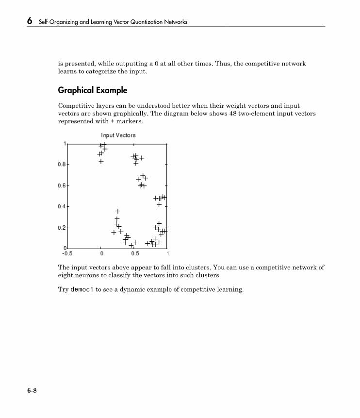
6 Self-Organizing and Learning Vector Quantization Networks
6-8
is presented, while outputting a 0 at all other times. Thus, the competitive networklearns to categorize the input.
Graphical Example
Competitive layers can be understood better when their weight vectors and inputvectors are shown graphically. The diagram below shows 48 two-element input vectorsrepresented with + markers.
The input vectors above appear to fall into clusters. You can use a competitive network ofeight neurons to classify the vectors into such clusters.
Try democ1 to see a dynamic example of competitive learning.

Cluster with Self-Organizing Map Neural Network
6-9
Cluster with Self-Organizing Map Neural Network
In this section...
“Topologies (gridtop, hextop, randtop)” on page 6-11“Distance Functions (dist, linkdist, mandist, boxdist)” on page 6-14“Architecture” on page 6-17“Create a Self-Organizing Map Neural Network (selforgmap)” on page 6-18“Training (learnsomb)” on page 6-19“Examples” on page 6-22
Self-organizing feature maps (SOFM) learn to classify input vectors according tohow they are grouped in the input space. They differ from competitive layers in thatneighboring neurons in the self-organizing map learn to recognize neighboring sections ofthe input space. Thus, self-organizing maps learn both the distribution (as do competitivelayers) and topology of the input vectors they are trained on.
The neurons in the layer of an SOFM are arranged originally in physical positionsaccording to a topology function. The function gridtop, hextop, or randtop canarrange the neurons in a grid, hexagonal, or random topology. Distances betweenneurons are calculated from their positions with a distance function. There are fourdistance functions, dist, boxdist, linkdist, and mandist. Link distance is the mostcommon. These topology and distance functions are described in “Topologies (gridtop,hextop, randtop)” on page 6-11 and “Distance Functions (dist, linkdist, mandist,boxdist)” on page 6-14.
Here a self-organizing feature map network identifies a winning neuron i* using thesame procedure as employed by a competitive layer. However, instead of updating onlythe winning neuron, all neurons within a certain neighborhood Ni* (d) of the winningneuron are updated, using the Kohonen rule. Specifically, all such neurons i ≅ Ni* (d) areadjusted as follows:
i i iq q q qw w p w( ) ( ) ( ( ) ( ))= − + − −1 1a
or
i iq q qw w p( ) ( ) ( ) ( )= − − +1 1a a
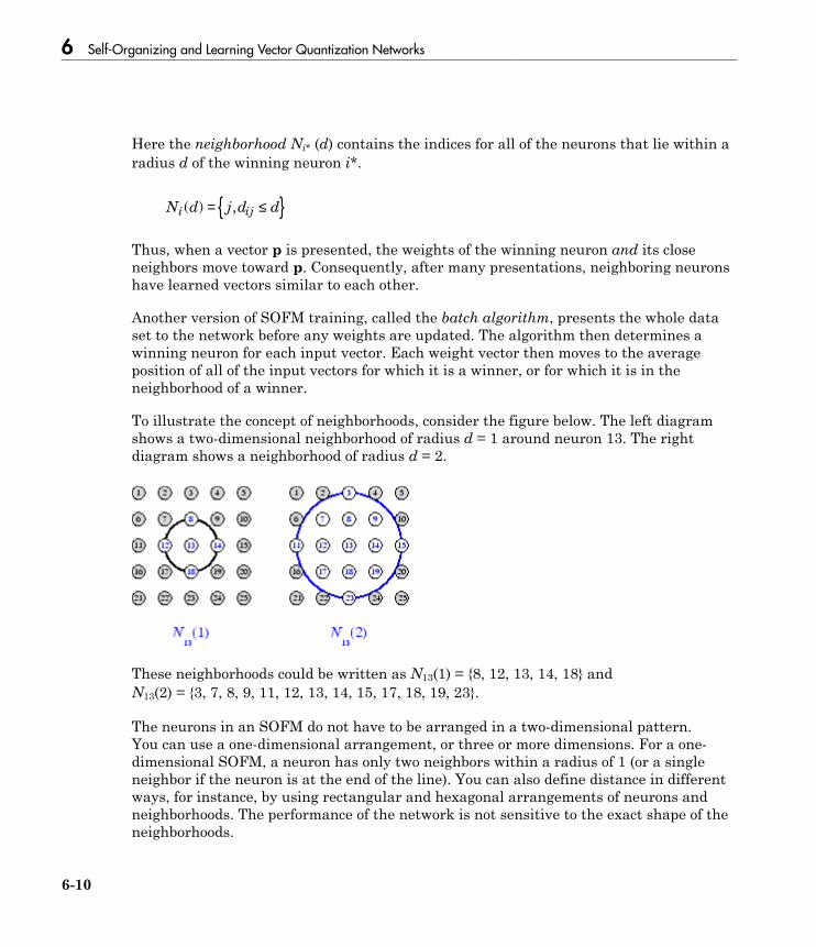
6 Self-Organizing and Learning Vector Quantization Networks
6-10
Here the neighborhood Ni* (d) contains the indices for all of the neurons that lie within aradius d of the winning neuron i*.
N d j d di ij( ) ,= ≤{ }
Thus, when a vector p is presented, the weights of the winning neuron and its closeneighbors move toward p. Consequently, after many presentations, neighboring neuronshave learned vectors similar to each other.
Another version of SOFM training, called the batch algorithm, presents the whole dataset to the network before any weights are updated. The algorithm then determines awinning neuron for each input vector. Each weight vector then moves to the averageposition of all of the input vectors for which it is a winner, or for which it is in theneighborhood of a winner.
To illustrate the concept of neighborhoods, consider the figure below. The left diagramshows a two-dimensional neighborhood of radius d = 1 around neuron 13. The rightdiagram shows a neighborhood of radius d = 2.
These neighborhoods could be written as N13(1) = {8, 12, 13, 14, 18} andN13(2) = {3, 7, 8, 9, 11, 12, 13, 14, 15, 17, 18, 19, 23}.
The neurons in an SOFM do not have to be arranged in a two-dimensional pattern.You can use a one-dimensional arrangement, or three or more dimensions. For a one-dimensional SOFM, a neuron has only two neighbors within a radius of 1 (or a singleneighbor if the neuron is at the end of the line). You can also define distance in differentways, for instance, by using rectangular and hexagonal arrangements of neurons andneighborhoods. The performance of the network is not sensitive to the exact shape of theneighborhoods.
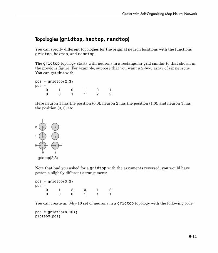
Cluster with Self-Organizing Map Neural Network
6-11
Topologies (gridtop, hextop, randtop)
You can specify different topologies for the original neuron locations with the functionsgridtop, hextop, and randtop.
The gridtop topology starts with neurons in a rectangular grid similar to that shown inthe previous figure. For example, suppose that you want a 2-by-3 array of six neurons.You can get this with
pos = gridtop(2,3)
pos =
0 1 0 1 0 1
0 0 1 1 2 2
Here neuron 1 has the position (0,0), neuron 2 has the position (1,0), and neuron 3 hasthe position (0,1), etc.
Note that had you asked for a gridtop with the arguments reversed, you would havegotten a slightly different arrangement:
pos = gridtop(3,2)
pos =
0 1 2 0 1 2
0 0 0 1 1 1
You can create an 8-by-10 set of neurons in a gridtop topology with the following code:
pos = gridtop(8,10);
plotsom(pos)
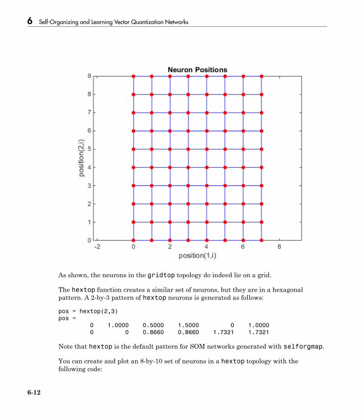
6 Self-Organizing and Learning Vector Quantization Networks
6-12
As shown, the neurons in the gridtop topology do indeed lie on a grid.
The hextop function creates a similar set of neurons, but they are in a hexagonalpattern. A 2-by-3 pattern of hextop neurons is generated as follows:
pos = hextop(2,3)
pos =
0 1.0000 0.5000 1.5000 0 1.0000
0 0 0.8660 0.8660 1.7321 1.7321
Note that hextop is the default pattern for SOM networks generated with selforgmap.
You can create and plot an 8-by-10 set of neurons in a hextop topology with thefollowing code:

Cluster with Self-Organizing Map Neural Network
6-13
pos = hextop(8,10);
plotsom(pos)
pos = hextop(8,10);
plotsom(pos)
Note the positions of the neurons in a hexagonal arrangement.
Finally, the randtop function creates neurons in an N-dimensional random pattern. Thefollowing code generates a random pattern of neurons.
pos = randtop(2,3)
pos =
0 0.7620 0.6268 1.4218 0.0663 0.7862
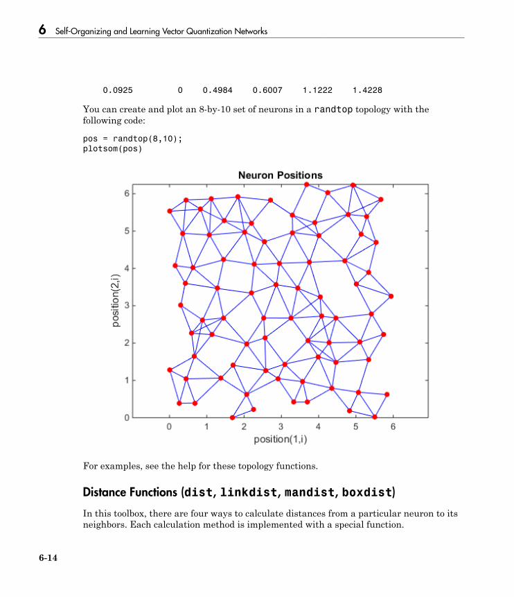
6 Self-Organizing and Learning Vector Quantization Networks
6-14
0.0925 0 0.4984 0.6007 1.1222 1.4228
You can create and plot an 8-by-10 set of neurons in a randtop topology with thefollowing code:
pos = randtop(8,10);
plotsom(pos)
For examples, see the help for these topology functions.
Distance Functions (dist, linkdist, mandist, boxdist)
In this toolbox, there are four ways to calculate distances from a particular neuron to itsneighbors. Each calculation method is implemented with a special function.
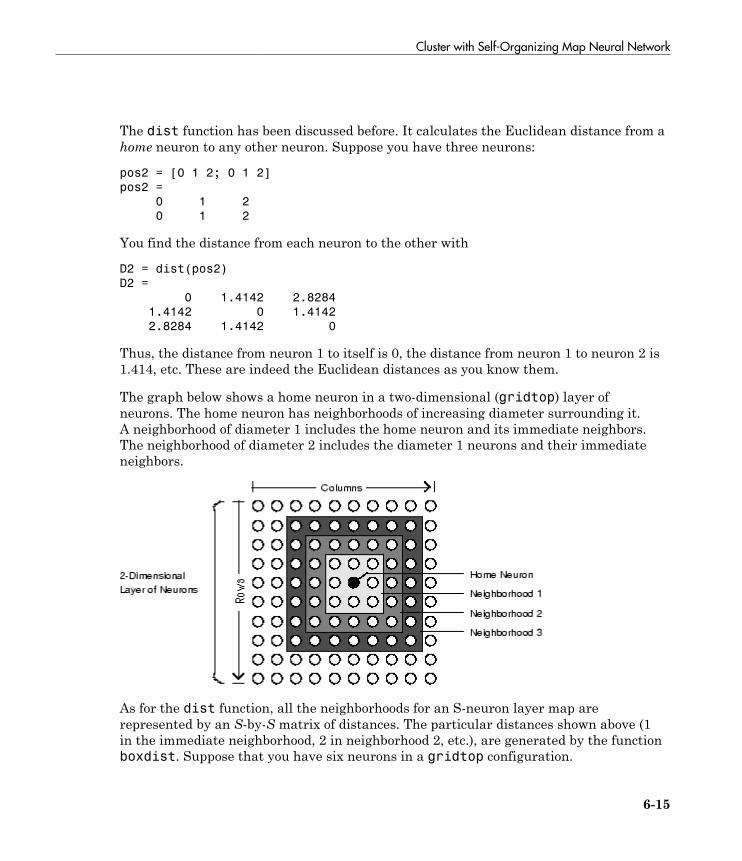
Cluster with Self-Organizing Map Neural Network
6-15
The dist function has been discussed before. It calculates the Euclidean distance from ahome neuron to any other neuron. Suppose you have three neurons:
pos2 = [0 1 2; 0 1 2]
pos2 =
0 1 2
0 1 2
You find the distance from each neuron to the other with
D2 = dist(pos2)
D2 =
0 1.4142 2.8284
1.4142 0 1.4142
2.8284 1.4142 0
Thus, the distance from neuron 1 to itself is 0, the distance from neuron 1 to neuron 2 is1.414, etc. These are indeed the Euclidean distances as you know them.
The graph below shows a home neuron in a two-dimensional (gridtop) layer ofneurons. The home neuron has neighborhoods of increasing diameter surrounding it.A neighborhood of diameter 1 includes the home neuron and its immediate neighbors.The neighborhood of diameter 2 includes the diameter 1 neurons and their immediateneighbors.
As for the dist function, all the neighborhoods for an S-neuron layer map arerepresented by an S-by-S matrix of distances. The particular distances shown above (1in the immediate neighborhood, 2 in neighborhood 2, etc.), are generated by the functionboxdist. Suppose that you have six neurons in a gridtop configuration.

6 Self-Organizing and Learning Vector Quantization Networks
6-16
pos = gridtop(2,3)
pos =
0 1 0 1 0 1
0 0 1 1 2 2
Then the box distances are
d = boxdist(pos)
d =
0 1 1 1 2 2
1 0 1 1 2 2
1 1 0 1 1 1
1 1 1 0 1 1
2 2 1 1 0 1
2 2 1 1 1 0
The distance from neuron 1 to 2, 3, and 4 is just 1, for they are in the immediateneighborhood. The distance from neuron 1 to both 5 and 6 is 2. The distance from both 3and 4 to all other neurons is just 1.
The link distance from one neuron is just the number of links, or steps, that must betaken to get to the neuron under consideration. Thus, if you calculate the distances fromthe same set of neurons with linkdist, you get
dlink =
0 1 1 2 2 3
1 0 2 1 3 2
1 2 0 1 1 2
2 1 1 0 2 1
2 3 1 2 0 1
3 2 2 1 1 0
The Manhattan distance between two vectors x and y is calculated as
D = sum(abs(x-y))
Thus if you have
W1 = [1 2; 3 4; 5 6]
W1 =
1 2
3 4
5 6
and

Cluster with Self-Organizing Map Neural Network
6-17
P1 = [1;1]
P1 =
1
1
then you get for the distances
Z1 = mandist(W1,P1)
Z1 =
1
5
9
The distances calculated with mandist do indeed follow the mathematical expressiongiven above.
Architecture
The architecture for this SOFM is shown below.
This architecture is like that of a competitive network, except no bias is used here. Thecompetitive transfer function produces a 1 for output element a1
i corresponding to i*, thewinning neuron. All other output elements in a1 are 0.
Now, however, as described above, neurons close to the winning neuron are updatedalong with the winning neuron. You can choose from various topologies of neurons.Similarly, you can choose from various distance expressions to calculate neurons that areclose to the winning neuron.
6 Self-Organizing and Learning Vector Quantization Networks
6-18
Create a Self-Organizing Map Neural Network (selforgmap)
You can create a new SOM network with the function selforgmap. This function definesvariables used in two phases of learning:
• Ordering-phase learning rate• Ordering-phase steps• Tuning-phase learning rate• Tuning-phase neighborhood distance
These values are used for training and adapting.
Consider the following example.
Suppose that you want to create a network having input vectors with two elements, andthat you want to have six neurons in a hexagonal 2-by-3 network. The code to obtain thisnetwork is:
net = selforgmap([2,3]);
Suppose that the vectors to train on are:
P = [.1 .3 1.2 1.1 1.8 1.7 .1 .3 1.2 1.1 1.8 1.7;...
0.2 0.1 0.3 0.1 0.3 0.2 1.8 1.8 1.9 1.9 1.7 1.8];
You can configure the network to input the data and plot all of this with:
net = configure(net,P);
plotsompos(net,P)

Cluster with Self-Organizing Map Neural Network
6-19
The green spots are the training vectors. The initialization for selforgmap spreads theinitial weights across the input space. Note that they are initially some distance from thetraining vectors.
When simulating a network, the negative distances between each neuron’s weight vectorand the input vector are calculated (negdist) to get the weighted inputs. The weightedinputs are also the net inputs (netsum). The net inputs compete (compet) so that onlythe neuron with the most positive net input will output a 1.
Training (learnsomb)
The default learning in a self-organizing feature map occurs in the batch mode(trainbu). The weight learning function for the self-organizing map is learnsomb.

6 Self-Organizing and Learning Vector Quantization Networks
6-20
First, the network identifies the winning neuron for each input vector. Each weightvector then moves to the average position of all of the input vectors for which it is awinner or for which it is in the neighborhood of a winner. The distance that defines thesize of the neighborhood is altered during training through two phases.
Ordering Phase
This phase lasts for the given number of steps. The neighborhood distance starts at agiven initial distance, and decreases to the tuning neighborhood distance (1.0). As theneighborhood distance decreases over this phase, the neurons of the network typicallyorder themselves in the input space with the same topology in which they are orderedphysically.
Tuning Phase
This phase lasts for the rest of training or adaption. The neighborhood size has decreasedbelow 1 so only the winning neuron learns for each sample.
Now take a look at some of the specific values commonly used in these networks.
Learning occurs according to the learnsomb learning parameter, shown here with itsdefault value.
Learning Parameter Default Value Purpose
LP.init_neighborhood 3 Initial neighborhood sizeLP.steps 100 Ordering phase steps
The neighborhood size NS is altered through two phases: an ordering phase and a tuningphase.
The ordering phase lasts as many steps as LP.steps. During this phase, the algorithmadjusts ND from the initial neighborhood size LP.init_neighborhood down to 1. It isduring this phase that neuron weights order themselves in the input space consistentwith the associated neuron positions.
During the tuning phase, ND is less than 1. During this phase, the weights are expectedto spread out relatively evenly over the input space while retaining their topologicalorder found during the ordering phase.
Thus, the neuron's weight vectors initially take large steps all together toward thearea of input space where input vectors are occurring. Then as the neighborhood size
Cluster with Self-Organizing Map Neural Network
6-21
decreases to 1, the map tends to order itself topologically over the presented inputvectors. Once the neighborhood size is 1, the network should be fairly well ordered. Thetraining continues in order to give the neurons time to spread out evenly across the inputvectors.
As with competitive layers, the neurons of a self-organizing map will order themselveswith approximately equal distances between them if input vectors appear with evenprobability throughout a section of the input space. If input vectors occur with varyingfrequency throughout the input space, the feature map layer tends to allocate neurons toan area in proportion to the frequency of input vectors there.
Thus, feature maps, while learning to categorize their input, also learn both the topologyand distribution of their input.
You can train the network for 1000 epochs with
net.trainParam.epochs = 1000;
net = train(net,P);
plotsompos(net,P)

6 Self-Organizing and Learning Vector Quantization Networks
6-22
You can see that the neurons have started to move toward the various training groups.Additional training is required to get the neurons closer to the various groups.
As noted previously, self-organizing maps differ from conventional competitive learningin terms of which neurons get their weights updated. Instead of updating only thewinner, feature maps update the weights of the winner and its neighbors. The result isthat neighboring neurons tend to have similar weight vectors and to be responsive tosimilar input vectors.
Examples
Two examples are described briefly below. You also might try the similar examplesdemosm1 and demosm2.
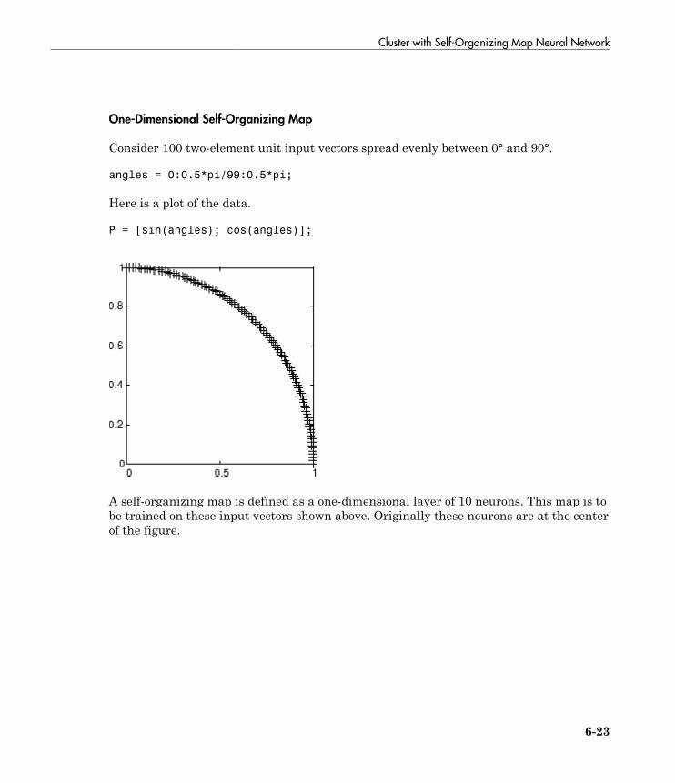
Cluster with Self-Organizing Map Neural Network
6-23
One-Dimensional Self-Organizing Map
Consider 100 two-element unit input vectors spread evenly between 0° and 90°.
angles = 0:0.5*pi/99:0.5*pi;
Here is a plot of the data.
P = [sin(angles); cos(angles)];
A self-organizing map is defined as a one-dimensional layer of 10 neurons. This map is tobe trained on these input vectors shown above. Originally these neurons are at the centerof the figure.

6 Self-Organizing and Learning Vector Quantization Networks
6-24
Of course, because all the weight vectors start in the middle of the input vector space, allyou see now is a single circle.
As training starts the weight vectors move together toward the input vectors. They alsobecome ordered as the neighborhood size decreases. Finally the layer adjusts its weightsso that each neuron responds strongly to a region of the input space occupied by inputvectors. The placement of neighboring neuron weight vectors also reflects the topology ofthe input vectors.
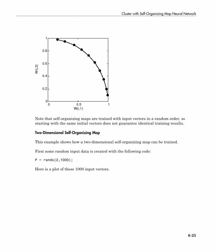
Cluster with Self-Organizing Map Neural Network
6-25
Note that self-organizing maps are trained with input vectors in a random order, sostarting with the same initial vectors does not guarantee identical training results.
Two-Dimensional Self-Organizing Map
This example shows how a two-dimensional self-organizing map can be trained.
First some random input data is created with the following code:
P = rands(2,1000);
Here is a plot of these 1000 input vectors.
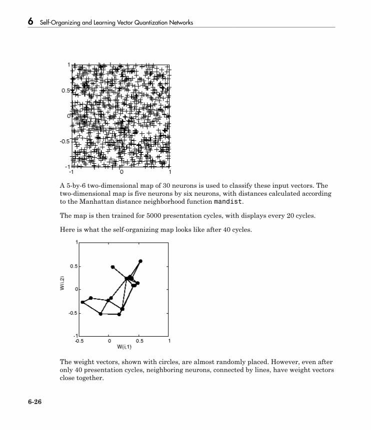
6 Self-Organizing and Learning Vector Quantization Networks
6-26
A 5-by-6 two-dimensional map of 30 neurons is used to classify these input vectors. Thetwo-dimensional map is five neurons by six neurons, with distances calculated accordingto the Manhattan distance neighborhood function mandist.
The map is then trained for 5000 presentation cycles, with displays every 20 cycles.
Here is what the self-organizing map looks like after 40 cycles.
The weight vectors, shown with circles, are almost randomly placed. However, even afteronly 40 presentation cycles, neighboring neurons, connected by lines, have weight vectorsclose together.
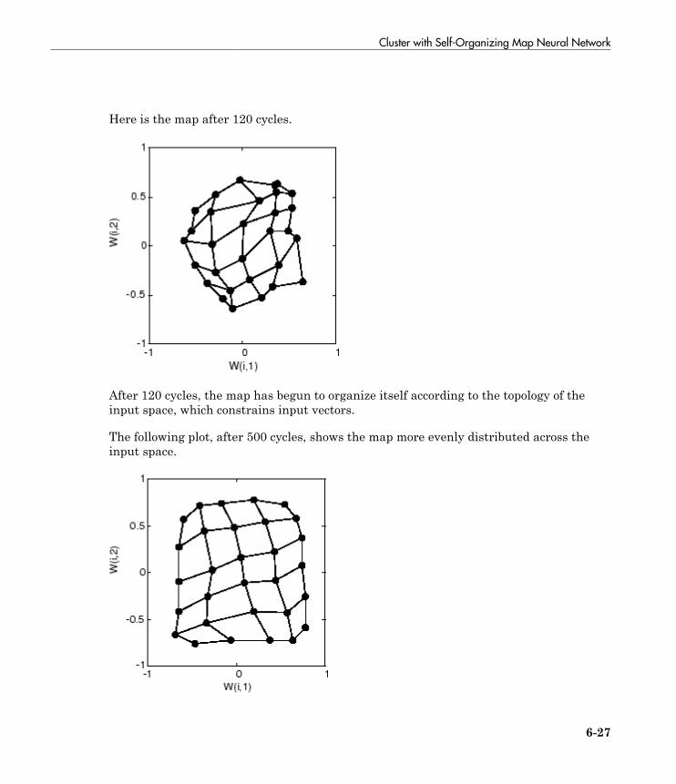
Cluster with Self-Organizing Map Neural Network
6-27
Here is the map after 120 cycles.
After 120 cycles, the map has begun to organize itself according to the topology of theinput space, which constrains input vectors.
The following plot, after 500 cycles, shows the map more evenly distributed across theinput space.
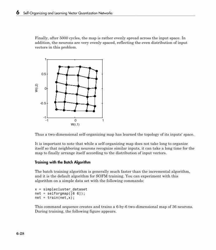
6 Self-Organizing and Learning Vector Quantization Networks
6-28
Finally, after 5000 cycles, the map is rather evenly spread across the input space. Inaddition, the neurons are very evenly spaced, reflecting the even distribution of inputvectors in this problem.
Thus a two-dimensional self-organizing map has learned the topology of its inputs' space.
It is important to note that while a self-organizing map does not take long to organizeitself so that neighboring neurons recognize similar inputs, it can take a long time for themap to finally arrange itself according to the distribution of input vectors.
Training with the Batch Algorithm
The batch training algorithm is generally much faster than the incremental algorithm,and it is the default algorithm for SOFM training. You can experiment with thisalgorithm on a simple data set with the following commands:
x = simplecluster_dataset
net = selforgmap([6 6]);
net = train(net,x);
This command sequence creates and trains a 6-by-6 two-dimensional map of 36 neurons.During training, the following figure appears.
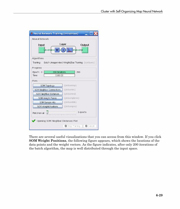
Cluster with Self-Organizing Map Neural Network
6-29
There are several useful visualizations that you can access from this window. If you clickSOM Weight Positions, the following figure appears, which shows the locations of thedata points and the weight vectors. As the figure indicates, after only 200 iterations ofthe batch algorithm, the map is well distributed through the input space.
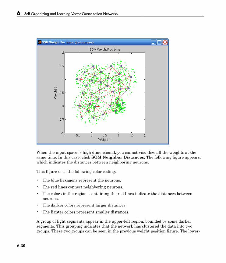
6 Self-Organizing and Learning Vector Quantization Networks
6-30
When the input space is high dimensional, you cannot visualize all the weights at thesame time. In this case, click SOM Neighbor Distances. The following figure appears,which indicates the distances between neighboring neurons.
This figure uses the following color coding:
• The blue hexagons represent the neurons.• The red lines connect neighboring neurons.• The colors in the regions containing the red lines indicate the distances between
neurons.• The darker colors represent larger distances.• The lighter colors represent smaller distances.
A group of light segments appear in the upper-left region, bounded by some darkersegments. This grouping indicates that the network has clustered the data into twogroups. These two groups can be seen in the previous weight position figure. The lower-
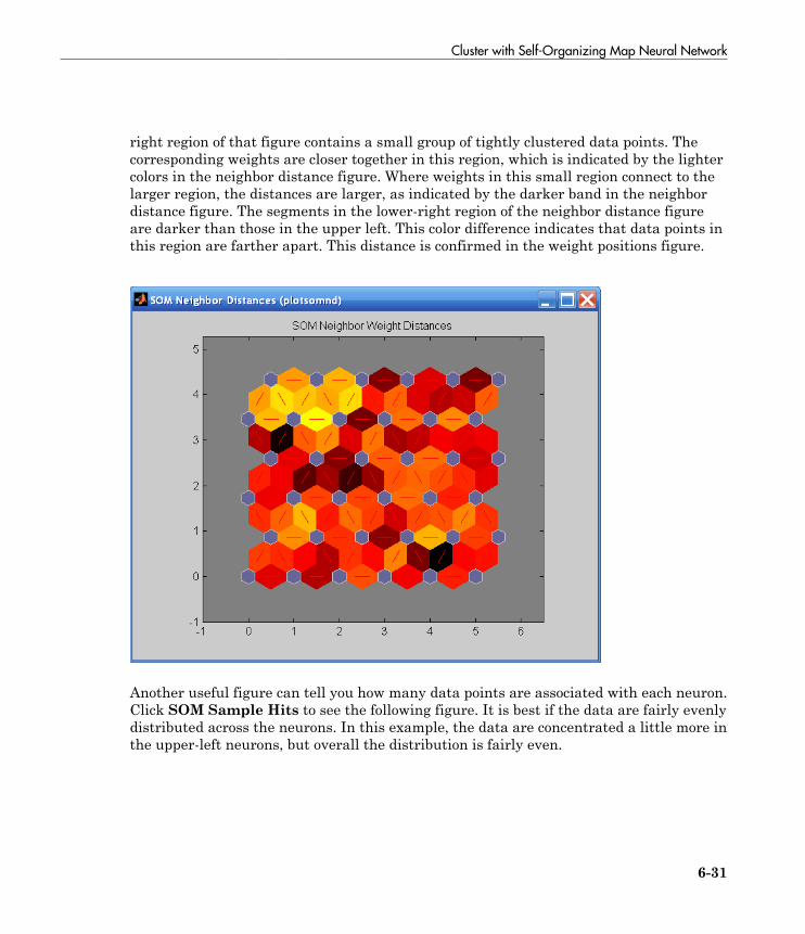
Cluster with Self-Organizing Map Neural Network
6-31
right region of that figure contains a small group of tightly clustered data points. Thecorresponding weights are closer together in this region, which is indicated by the lightercolors in the neighbor distance figure. Where weights in this small region connect to thelarger region, the distances are larger, as indicated by the darker band in the neighbordistance figure. The segments in the lower-right region of the neighbor distance figureare darker than those in the upper left. This color difference indicates that data points inthis region are farther apart. This distance is confirmed in the weight positions figure.
Another useful figure can tell you how many data points are associated with each neuron.Click SOM Sample Hits to see the following figure. It is best if the data are fairly evenlydistributed across the neurons. In this example, the data are concentrated a little more inthe upper-left neurons, but overall the distribution is fairly even.
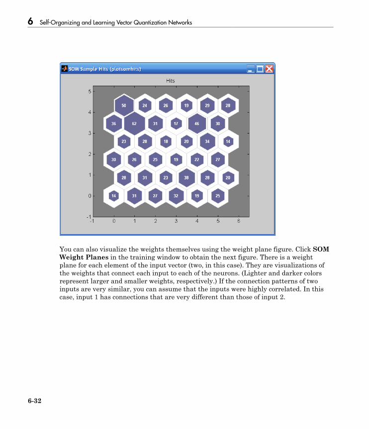
6 Self-Organizing and Learning Vector Quantization Networks
6-32
You can also visualize the weights themselves using the weight plane figure. Click SOMWeight Planes in the training window to obtain the next figure. There is a weightplane for each element of the input vector (two, in this case). They are visualizations ofthe weights that connect each input to each of the neurons. (Lighter and darker colorsrepresent larger and smaller weights, respectively.) If the connection patterns of twoinputs are very similar, you can assume that the inputs were highly correlated. In thiscase, input 1 has connections that are very different than those of input 2.
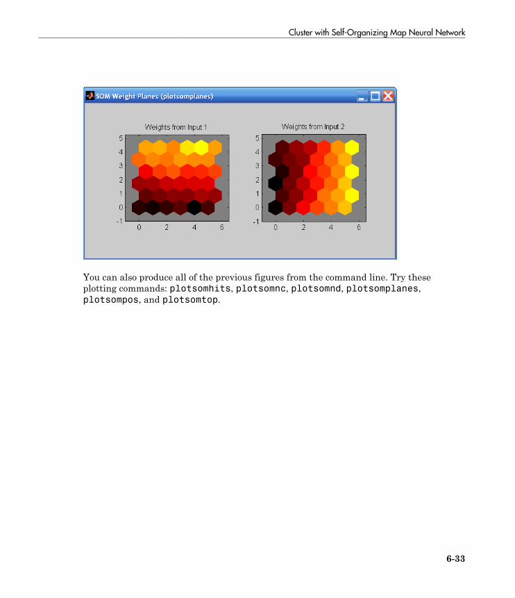
Cluster with Self-Organizing Map Neural Network
6-33
You can also produce all of the previous figures from the command line. Try theseplotting commands: plotsomhits, plotsomnc, plotsomnd, plotsomplanes,plotsompos, and plotsomtop.
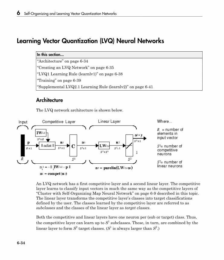
6 Self-Organizing and Learning Vector Quantization Networks
6-34
Learning Vector Quantization (LVQ) Neural Networks
In this section...
“Architecture” on page 6-34“Creating an LVQ Network” on page 6-35“LVQ1 Learning Rule (learnlv1)” on page 6-38“Training” on page 6-39“Supplemental LVQ2.1 Learning Rule (learnlv2)” on page 6-41
Architecture
The LVQ network architecture is shown below.
An LVQ network has a first competitive layer and a second linear layer. The competitivelayer learns to classify input vectors in much the same way as the competitive layers of“Cluster with Self-Organizing Map Neural Network” on page 6-9 described in this topic.The linear layer transforms the competitive layer’s classes into target classificationsdefined by the user. The classes learned by the competitive layer are referred to assubclasses and the classes of the linear layer as target classes.
Both the competitive and linear layers have one neuron per (sub or target) class. Thus,the competitive layer can learn up to S1 subclasses. These, in turn, are combined by thelinear layer to form S2 target classes. (S1 is always larger than S2.)

Learning Vector Quantization (LVQ) Neural Networks
6-35
For example, suppose neurons 1, 2, and 3 in the competitive layer all learn subclasses ofthe input space that belongs to the linear layer target class 2. Then competitive neurons1, 2, and 3 will have LW2,1 weights of 1.0 to neuron n2 in the linear layer, and weightsof 0 to all other linear neurons. Thus, the linear neuron produces a 1 if any of the threecompetitive neurons (1, 2, or 3) wins the competition and outputs a 1. This is how thesubclasses of the competitive layer are combined into target classes in the linear layer.
In short, a 1 in the ith row of a1 (the rest to the elements of a1 will be zero) effectivelypicks the ith column of LW2,1 as the network output. Each such column contains a single1, corresponding to a specific class. Thus, subclass 1s from layer 1 are put into variousclasses by the LW2,1a1 multiplication in layer 2.
You know ahead of time what fraction of the layer 1 neurons should be classified intothe various class outputs of layer 2, so you can specify the elements of LW2,1 at the start.However, you have to go through a training procedure to get the first layer to produce thecorrect subclass output for each vector of the training set. This training is discussed in“Training” on page 6-6. First, consider how to create the original network.
Creating an LVQ Network
You can create an LVQ network with the function lvqnet,
net = lvqnet(S1,LR,LF)
where
• S1 is the number of first-layer hidden neurons.• LR is the learning rate (default 0.01).• LF is the learning function (default is learnlv1).
Suppose you have 10 input vectors. Create a network that assigns each of these inputvectors to one of four subclasses. Thus, there are four neurons in the first competitivelayer. These subclasses are then assigned to one of two output classes by the two neuronsin layer 2. The input vectors and targets are specified by
P = [-3 -2 -2 0 0 0 0 2 2 3; 0 1 -1 2 1 -1 -2 1 -1 0];
and
Tc = [1 1 1 2 2 2 2 1 1 1];

6 Self-Organizing and Learning Vector Quantization Networks
6-36
It might help to show the details of what you get from these two lines of code.
P,Tc
P =
-3 -2 -2 0 0 0 0 2 2 3
0 1 -1 2 1 -1 -2 1 -1 0
Tc =
1 1 1 2 2 2 2 1 1 1
A plot of the input vectors follows.
As you can see, there are four subclasses of input vectors. You want a network thatclassifies p1, p2, p3, p8, p9, and p10 to produce an output of 1, and that classifies vectorsp4, p5, p6, and p7 to produce an output of 2. Note that this problem is nonlinearlyseparable, and so cannot be solved by a perceptron, but an LVQ network has nodifficulty.
Next convert the Tc matrix to target vectors.
T = ind2vec(Tc);
This gives a sparse matrix T that can be displayed in full with
targets = full(T)
which gives
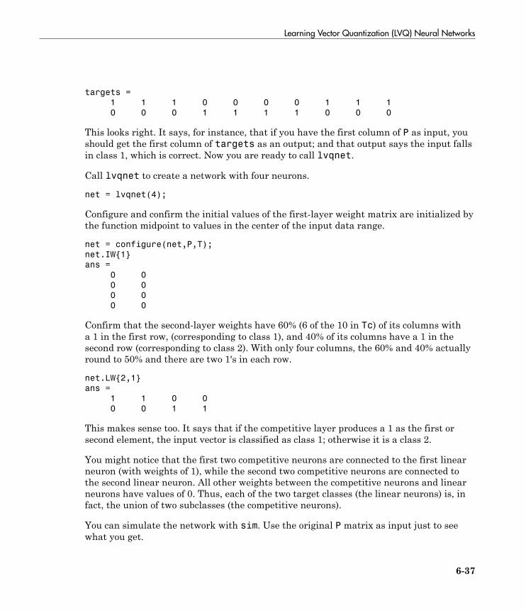
Learning Vector Quantization (LVQ) Neural Networks
6-37
targets =
1 1 1 0 0 0 0 1 1 1
0 0 0 1 1 1 1 0 0 0
This looks right. It says, for instance, that if you have the first column of P as input, youshould get the first column of targets as an output; and that output says the input fallsin class 1, which is correct. Now you are ready to call lvqnet.
Call lvqnet to create a network with four neurons.
net = lvqnet(4);
Configure and confirm the initial values of the first-layer weight matrix are initialized bythe function midpoint to values in the center of the input data range.
net = configure(net,P,T);
net.IW{1}
ans =
0 0
0 0
0 0
0 0
Confirm that the second-layer weights have 60% (6 of the 10 in Tc) of its columns witha 1 in the first row, (corresponding to class 1), and 40% of its columns have a 1 in thesecond row (corresponding to class 2). With only four columns, the 60% and 40% actuallyround to 50% and there are two 1's in each row.
net.LW{2,1}
ans =
1 1 0 0
0 0 1 1
This makes sense too. It says that if the competitive layer produces a 1 as the first orsecond element, the input vector is classified as class 1; otherwise it is a class 2.
You might notice that the first two competitive neurons are connected to the first linearneuron (with weights of 1), while the second two competitive neurons are connected tothe second linear neuron. All other weights between the competitive neurons and linearneurons have values of 0. Thus, each of the two target classes (the linear neurons) is, infact, the union of two subclasses (the competitive neurons).
You can simulate the network with sim. Use the original P matrix as input just to seewhat you get.

6 Self-Organizing and Learning Vector Quantization Networks
6-38
Y = net(P);
Yc = vec2ind(Y)
Yc =
1 1 1 1 1 1 1 1 1 1
The network classifies all inputs into class 1. Because this is not what you want, youhave to train the network (adjusting the weights of layer 1 only), before you can expecta good result. The next two sections discuss two LVQ learning rules and the trainingprocess.
LVQ1 Learning Rule (learnlv1)
LVQ learning in the competitive layer is based on a set of input/target pairs.
p t p t p t1 1 2 2, , , , ,{ } { } { }… Q Q
Each target vector has a single 1. The rest of its elements are 0. The 1 tells the properclassification of the associated input. For instance, consider the following training pair.
p t1 1
2
1
0
0
0
1
0
= −
=
,
Here there are input vectors of three elements, and each input vector is to be assignedto one of four classes. The network is to be trained so that it classifies the input vectorshown above into the third of four classes.
To train the network, an input vector p is presented, and the distance from p to eachrow of the input weight matrix IW1,1 is computed with the function negdist. The hiddenneurons of layer 1 compete. Suppose that the ith element of n1 is most positive, andneuron i* wins the competition. Then the competitive transfer function produces a 1 asthe i*th element of a1. All other elements of a1 are 0.
When a1 is multiplied by the layer 2 weights LW2,1, the single 1 in a1 selects the class k*associated with the input. Thus, the network has assigned the input vector p to class k*and α2
k* will be 1. Of course, this assignment can be a good one or a bad one, for tk* can be1 or 0, depending on whether the input belonged to class k* or not.

Learning Vector Quantization (LVQ) Neural Networks
6-39
Adjust the i*th row of IW1,1 in such a way as to move this row closer to the input vectorp if the assignment is correct, and to move the row away from p if the assignment isincorrect. If p is classified correctly,
ak kt∗ ∗= =( )21
compute the new value of the i*th row of IW1,1 as
i i iq q q q∗ ∗ ∗= − + − −IW IW p IW1 1 1 1 1 11 1, , ,( ) ( ) ( ( ) ( ))a
On the other hand, if p is classified incorrectly,
ak kt∗ ∗= ≠ =( )21 0
compute the new value of the i*th row of IW1,1 as
i i iq q q q∗ ∗ ∗= − − − −IW IW p IW1 1 1 1 1 11 1, , ,( ) ( ) ( ( ) ( ))a
You can make these corrections to the i*th row of IW1,1 automatically, without affectingother rows of IW1,1, by back-propagating the output errors to layer 1.
Such corrections move the hidden neuron toward vectors that fall into the class for whichit forms a subclass, and away from vectors that fall into other classes.
The learning function that implements these changes in the layer 1 weights in LVQnetworks is learnlv1. It can be applied during training.
Training
Next you need to train the network to obtain first-layer weights that lead to the correctclassification of input vectors. You do this with train as with the following commands.First, set the training epochs to 150. Then, use train:
net.trainParam.epochs = 150;
net = train(net,P,T);
Now confirm the first-layer weights.
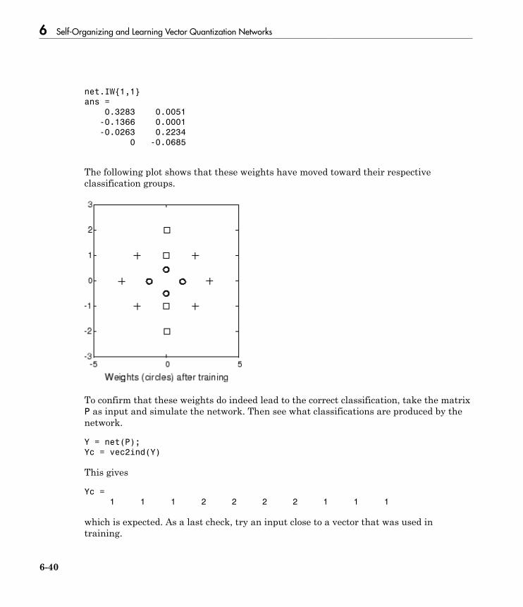
6 Self-Organizing and Learning Vector Quantization Networks
6-40
net.IW{1,1}
ans =
0.3283 0.0051
-0.1366 0.0001
-0.0263 0.2234
0 -0.0685
The following plot shows that these weights have moved toward their respectiveclassification groups.
To confirm that these weights do indeed lead to the correct classification, take the matrixP as input and simulate the network. Then see what classifications are produced by thenetwork.
Y = net(P);
Yc = vec2ind(Y)
This gives
Yc =
1 1 1 2 2 2 2 1 1 1
which is expected. As a last check, try an input close to a vector that was used intraining.
Learning Vector Quantization (LVQ) Neural Networks
6-41
pchk1 = [0; 0.5];
Y = net(pchk1);
Yc1 = vec2ind(Y)
This gives
Yc1 =
2
This looks right, because pchk1 is close to other vectors classified as 2. Similarly,
pchk2 = [1; 0];
Y = net(pchk2);
Yc2 = vec2ind(Y)
gives
Yc2 =
1
This looks right too, because pchk2 is close to other vectors classified as 1.
You might want to try the example program demolvq1. It follows the discussion oftraining given above.
Supplemental LVQ2.1 Learning Rule (learnlv2)
The following learning rule is one that might be applied after first applying LVQ1. It canimprove the result of the first learning. This particular version of LVQ2 (referred to asLVQ2.1 in the literature [Koho97]) is embodied in the function learnlv2. Note againthat LVQ2.1 is to be used only after LVQ1 has been applied.
Learning here is similar to that in learnlv2 except now two vectors of layer 1 thatare closest to the input vector can be updated, provided that one belongs to the correctclass and one belongs to a wrong class, and further provided that the input falls into a“window” near the midplane of the two vectors.
The window is defined by
min ,d
d
d
dsi
j
j
i
>

6 Self-Organizing and Learning Vector Quantization Networks
6-42
where
s
w
w
≡−+
1
1
(where di and dj are the Euclidean distances of p from i*IW1,1 and j*IW1,1, respectively).Take a value for w in the range 0.2 to 0.3. If you pick, for instance, 0.25, then s = 0.6. Thismeans that if the minimum of the two distance ratios is greater than 0.6, the two vectorsare adjusted. That is, if the input is near the midplane, adjust the two vectors, providedalso that the input vector p and j*IW1,1 belong to the same class, and p and i*IW1,1 do notbelong in the same class.
The adjustments made are
i i iq q q q∗ ∗ ∗= − − − −IW IW p IW1 1 1 1 1 11 1, , ,( ) ( ) ( ( ) ( ))a
and
j j jq q q q∗ ∗ ∗= − + − −IW IW p IW1 1 1 1 1 11 1, , ,( ) ( ) ( ( ) ( ))a
Thus, given two vectors closest to the input, as long as one belongs to the wrong class andthe other to the correct class, and as long as the input falls in a midplane window, thetwo vectors are adjusted. Such a procedure allows a vector that is just barely classifiedcorrectly with LVQ1 to be moved even closer to the input, so the results are more robust.
Function Description
competlayer Create a competitive layer.learnk Kohonen learning rule.selforgmap Create a self-organizing map.learncon Conscience bias learning function.boxdist Distance between two position vectors.dist Euclidean distance weight function.linkdist Link distance function.mandist Manhattan distance weight function.gridtop Gridtop layer topology function.
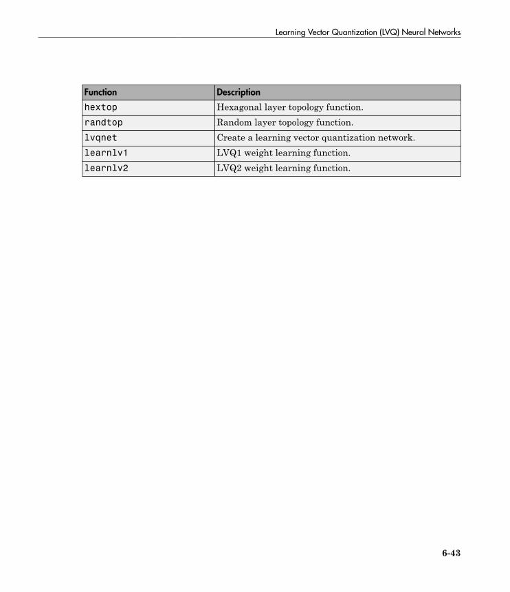
Learning Vector Quantization (LVQ) Neural Networks
6-43
Function Description
hextop Hexagonal layer topology function.randtop Random layer topology function.lvqnet Create a learning vector quantization network.learnlv1 LVQ1 weight learning function.learnlv2 LVQ2 weight learning function.

6-44
7
Adaptive Filters and AdaptiveTraining
7 Adaptive Filters and Adaptive Training
7-2
Adaptive Neural Network Filters
In this section...
“Adaptive Functions” on page 7-2“Linear Neuron Model” on page 7-3“Adaptive Linear Network Architecture” on page 7-3“Least Mean Square Error” on page 7-6“LMS Algorithm (learnwh)” on page 7-7“Adaptive Filtering (adapt)” on page 7-7
The ADALINE (adaptive linear neuron) networks discussed in this topic are similarto the perceptron, but their transfer function is linear rather than hard-limiting. Thisallows their outputs to take on any value, whereas the perceptron output is limited toeither 0 or 1. Both the ADALINE and the perceptron can solve only linearly separableproblems. However, here the LMS (least mean squares) learning rule, which is muchmore powerful than the perceptron learning rule, is used. The LMS, or Widrow-Hoff,learning rule minimizes the mean square error and thus moves the decision boundariesas far as it can from the training patterns.
In this section, you design an adaptive linear system that responds to changes in itsenvironment as it is operating. Linear networks that are adjusted at each time stepbased on new input and target vectors can find weights and biases that minimize thenetwork's sum-squared error for recent input and target vectors. Networks of this sortare often used in error cancelation, signal processing, and control systems.
The pioneering work in this field was done by Widrow and Hoff, who gave the nameADALINE to adaptive linear elements. The basic reference on this subject is Widrow, B.,and S.D. Sterns, Adaptive Signal Processing, New York, Prentice-Hall, 1985.
The adaptive training of self-organizing and competitive networks is also considered inthis section.
Adaptive Functions
This section introduces the function adapt, which changes the weights and biases of anetwork incrementally during training.
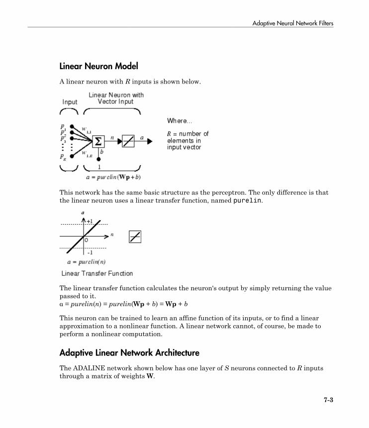
Adaptive Neural Network Filters
7-3
Linear Neuron Model
A linear neuron with R inputs is shown below.
This network has the same basic structure as the perceptron. The only difference is thatthe linear neuron uses a linear transfer function, named purelin.
The linear transfer function calculates the neuron's output by simply returning the valuepassed to it.α = purelin(n) = purelin(Wp + b) = Wp + b
This neuron can be trained to learn an affine function of its inputs, or to find a linearapproximation to a nonlinear function. A linear network cannot, of course, be made toperform a nonlinear computation.
Adaptive Linear Network Architecture
The ADALINE network shown below has one layer of S neurons connected to R inputsthrough a matrix of weights W.

7 Adaptive Filters and Adaptive Training
7-4
This network is sometimes called a MADALINE for Many ADALINEs. Note that thefigure on the right defines an S-length output vector a.
The Widrow-Hoff rule can only train single-layer linear networks. This is not much of adisadvantage, however, as single-layer linear networks are just as capable as multilayerlinear networks. For every multilayer linear network, there is an equivalent single-layerlinear network.
Single ADALINE (linearlayer)
Consider a single ADALINE with two inputs. The following figure shows the diagram forthis network.
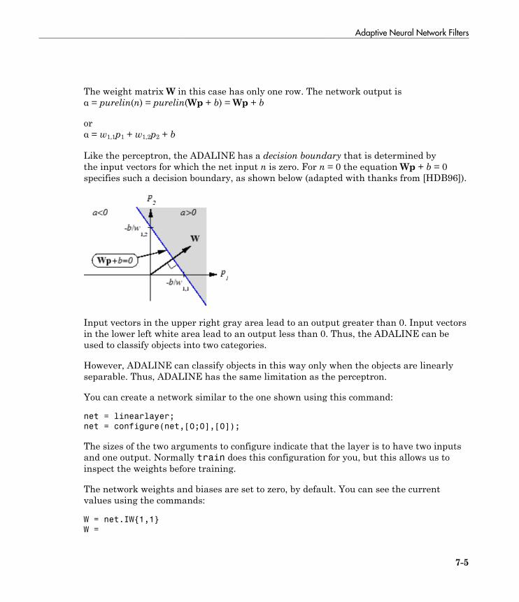
Adaptive Neural Network Filters
7-5
The weight matrix W in this case has only one row. The network output isα = purelin(n) = purelin(Wp + b) = Wp + b
orα = w1,1p1 + w1,2p2 + b
Like the perceptron, the ADALINE has a decision boundary that is determined bythe input vectors for which the net input n is zero. For n = 0 the equation Wp + b = 0specifies such a decision boundary, as shown below (adapted with thanks from [HDB96]).
Input vectors in the upper right gray area lead to an output greater than 0. Input vectorsin the lower left white area lead to an output less than 0. Thus, the ADALINE can beused to classify objects into two categories.
However, ADALINE can classify objects in this way only when the objects are linearlyseparable. Thus, ADALINE has the same limitation as the perceptron.
You can create a network similar to the one shown using this command:
net = linearlayer;
net = configure(net,[0;0],[0]);
The sizes of the two arguments to configure indicate that the layer is to have two inputsand one output. Normally train does this configuration for you, but this allows us toinspect the weights before training.
The network weights and biases are set to zero, by default. You can see the currentvalues using the commands:
W = net.IW{1,1}
W =
7 Adaptive Filters and Adaptive Training
7-6
0 0
and
b = net.b{1}
b =
0
You can also assign arbitrary values to the weights and bias, such as 2 and 3 for theweights and −4 for the bias:
net.IW{1,1} = [2 3];
net.b{1} = -4;
You can simulate the ADALINE for a particular input vector.
p = [5; 6];
a = sim(net,p)
a =
24
To summarize, you can create an ADALINE network with linearlayer, adjust itselements as you want, and simulate it with sim.
Least Mean Square Error
Like the perceptron learning rule, the least mean square error (LMS) algorithm is anexample of supervised training, in which the learning rule is provided with a set ofexamples of desired network behavior.
p t p t p t1 1 2 2, , , , ,{ } { } { }… Q Q
Here pq is an input to the network, and tq is the corresponding target output. As eachinput is applied to the network, the network output is compared to the target. The erroris calculated as the difference between the target output and the network output. Thegoal is to minimize the average of the sum of these errors.
mseQ
e kQ
t k k
k
Q
k
Q
= = −= =∑ ∑1 12
1
2
1
( ) ( ) ( ))a
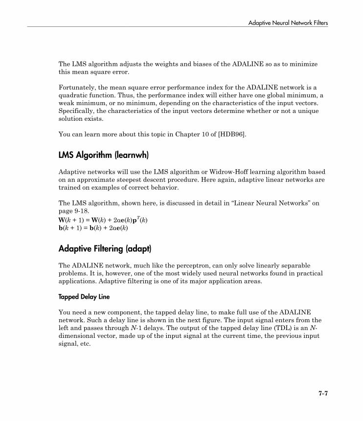
Adaptive Neural Network Filters
7-7
The LMS algorithm adjusts the weights and biases of the ADALINE so as to minimizethis mean square error.
Fortunately, the mean square error performance index for the ADALINE network is aquadratic function. Thus, the performance index will either have one global minimum, aweak minimum, or no minimum, depending on the characteristics of the input vectors.Specifically, the characteristics of the input vectors determine whether or not a uniquesolution exists.
You can learn more about this topic in Chapter 10 of [HDB96].
LMS Algorithm (learnwh)
Adaptive networks will use the LMS algorithm or Widrow-Hoff learning algorithm basedon an approximate steepest descent procedure. Here again, adaptive linear networks aretrained on examples of correct behavior.
The LMS algorithm, shown here, is discussed in detail in “Linear Neural Networks” onpage 9-18.W(k + 1) = W(k) + 2αe(k)pT(k)b(k + 1) = b(k) + 2αe(k)
Adaptive Filtering (adapt)
The ADALINE network, much like the perceptron, can only solve linearly separableproblems. It is, however, one of the most widely used neural networks found in practicalapplications. Adaptive filtering is one of its major application areas.
Tapped Delay Line
You need a new component, the tapped delay line, to make full use of the ADALINEnetwork. Such a delay line is shown in the next figure. The input signal enters from theleft and passes through N-1 delays. The output of the tapped delay line (TDL) is an N-dimensional vector, made up of the input signal at the current time, the previous inputsignal, etc.
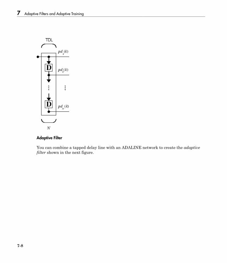
7 Adaptive Filters and Adaptive Training
7-8
Adaptive Filter
You can combine a tapped delay line with an ADALINE network to create the adaptivefilter shown in the next figure.
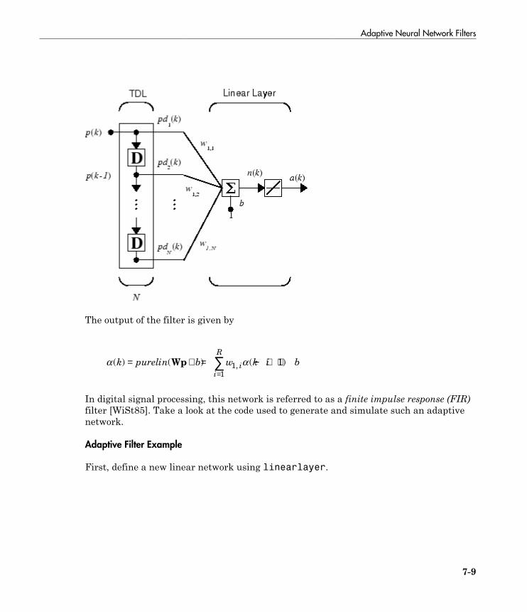
Adaptive Neural Network Filters
7-9
The output of the filter is given by
a a( ) ( ) ( ),k purelin b w k i bii
R
= + = − + +=∑Wp 1
1
1
In digital signal processing, this network is referred to as a finite impulse response (FIR)filter [WiSt85]. Take a look at the code used to generate and simulate such an adaptivenetwork.
Adaptive Filter Example
First, define a new linear network using linearlayer.
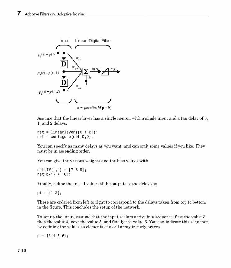
7 Adaptive Filters and Adaptive Training
7-10
Assume that the linear layer has a single neuron with a single input and a tap delay of 0,1, and 2 delays.
net = linearlayer([0 1 2]);
net = configure(net,0,0);
You can specify as many delays as you want, and can omit some values if you like. Theymust be in ascending order.
You can give the various weights and the bias values with
net.IW{1,1} = [7 8 9];
net.b{1} = [0];
Finally, define the initial values of the outputs of the delays as
pi = {1 2};
These are ordered from left to right to correspond to the delays taken from top to bottomin the figure. This concludes the setup of the network.
To set up the input, assume that the input scalars arrive in a sequence: first the value 3,then the value 4, next the value 5, and finally the value 6. You can indicate this sequenceby defining the values as elements of a cell array in curly braces.
p = {3 4 5 6};
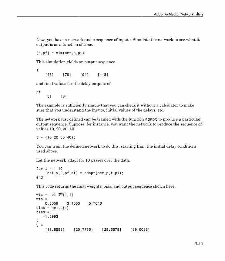
Adaptive Neural Network Filters
7-11
Now, you have a network and a sequence of inputs. Simulate the network to see what itsoutput is as a function of time.
[a,pf] = sim(net,p,pi)
This simulation yields an output sequence
a
[46] [70] [94] [118]
and final values for the delay outputs of
pf
[5] [6]
The example is sufficiently simple that you can check it without a calculator to makesure that you understand the inputs, initial values of the delays, etc.
The network just defined can be trained with the function adapt to produce a particularoutput sequence. Suppose, for instance, you want the network to produce the sequence ofvalues 10, 20, 30, 40.
t = {10 20 30 40};
You can train the defined network to do this, starting from the initial delay conditionsused above.
Let the network adapt for 10 passes over the data.
for i = 1:10
[net,y,E,pf,af] = adapt(net,p,t,pi);
end
This code returns the final weights, bias, and output sequence shown here.
wts = net.IW{1,1}
wts =
0.5059 3.1053 5.7046
bias = net.b{1}
bias =
-1.5993
y
y =
[11.8558] [20.7735] [29.6679] [39.0036]

7 Adaptive Filters and Adaptive Training
7-12
Presumably, if you ran additional passes the output sequence would have been evencloser to the desired values of 10, 20, 30, and 40.
Thus, adaptive networks can be specified, simulated, and finally trained with adapt.However, the outstanding value of adaptive networks lies in their use to perform aparticular function, such as prediction or noise cancelation.
Prediction Example
Suppose that you want to use an adaptive filter to predict the next value of a stationaryrandom process, p(t). You can use the network shown in the following figure to do thisprediction.
The signal to be predicted, p(t), enters from the left into a tapped delay line. The previoustwo values of p(t) are available as outputs from the tapped delay line. The network usesadapt to change the weights on each time step so as to minimize the error e(t) on the farright. If this error is 0, the network output a(t) is exactly equal to p(t), and the networkhas done its prediction properly.
Given the autocorrelation function of the stationary random process p(t), you cancalculate the error surface, the maximum learning rate, and the optimum values of theweights. Commonly, of course, you do not have detailed information about the randomprocess, so these calculations cannot be performed. This lack does not matter to thenetwork. After it is initialized and operating, the network adapts at each time step tominimize the error and in a relatively short time is able to predict the input p(t).
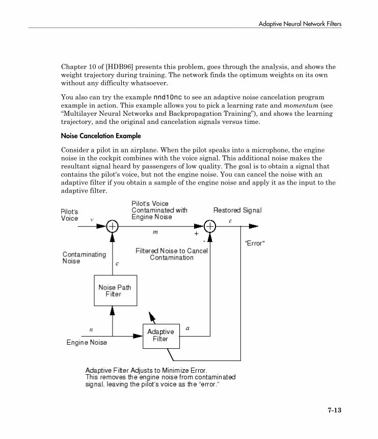
Adaptive Neural Network Filters
7-13
Chapter 10 of [HDB96] presents this problem, goes through the analysis, and shows theweight trajectory during training. The network finds the optimum weights on its ownwithout any difficulty whatsoever.
You also can try the example nnd10nc to see an adaptive noise cancelation programexample in action. This example allows you to pick a learning rate and momentum (see“Multilayer Neural Networks and Backpropagation Training”), and shows the learningtrajectory, and the original and cancelation signals versus time.
Noise Cancelation Example
Consider a pilot in an airplane. When the pilot speaks into a microphone, the enginenoise in the cockpit combines with the voice signal. This additional noise makes theresultant signal heard by passengers of low quality. The goal is to obtain a signal thatcontains the pilot's voice, but not the engine noise. You can cancel the noise with anadaptive filter if you obtain a sample of the engine noise and apply it as the input to theadaptive filter.
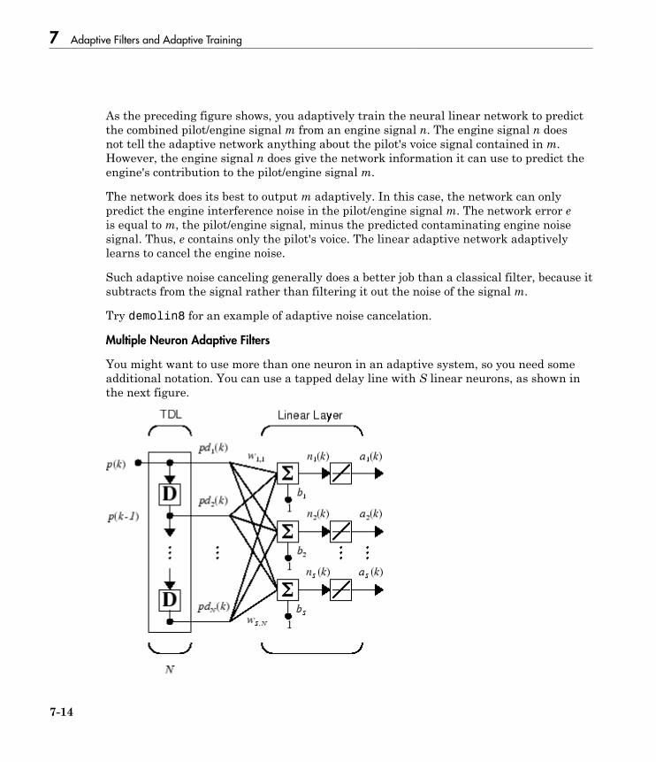
7 Adaptive Filters and Adaptive Training
7-14
As the preceding figure shows, you adaptively train the neural linear network to predictthe combined pilot/engine signal m from an engine signal n. The engine signal n doesnot tell the adaptive network anything about the pilot's voice signal contained in m.However, the engine signal n does give the network information it can use to predict theengine's contribution to the pilot/engine signal m.
The network does its best to output m adaptively. In this case, the network can onlypredict the engine interference noise in the pilot/engine signal m. The network error eis equal to m, the pilot/engine signal, minus the predicted contaminating engine noisesignal. Thus, e contains only the pilot's voice. The linear adaptive network adaptivelylearns to cancel the engine noise.
Such adaptive noise canceling generally does a better job than a classical filter, because itsubtracts from the signal rather than filtering it out the noise of the signal m.
Try demolin8 for an example of adaptive noise cancelation.
Multiple Neuron Adaptive Filters
You might want to use more than one neuron in an adaptive system, so you need someadditional notation. You can use a tapped delay line with S linear neurons, as shown inthe next figure.
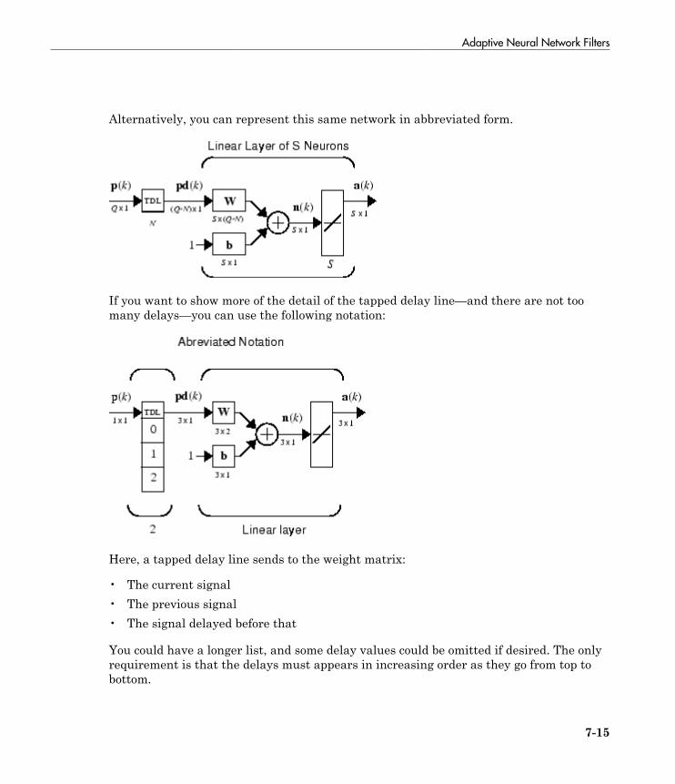
Adaptive Neural Network Filters
7-15
Alternatively, you can represent this same network in abbreviated form.
If you want to show more of the detail of the tapped delay line—and there are not toomany delays—you can use the following notation:
Here, a tapped delay line sends to the weight matrix:
• The current signal• The previous signal• The signal delayed before that
You could have a longer list, and some delay values could be omitted if desired. The onlyrequirement is that the delays must appears in increasing order as they go from top tobottom.

7-16
8
Advanced Topics
• “Neural Networks with Parallel and GPU Computing” on page 8-2• “Optimize Neural Network Training Speed and Memory” on page 8-12• “Choose a Multilayer Neural Network Training Function” on page 8-16• “Improve Neural Network Generalization and Avoid Overfitting” on page 8-31• “Create and Train Custom Neural Network Architectures” on page 8-44• “Custom Neural Network Helper Functions” on page 8-57• “Automatically Save Checkpoints During Neural Network Training” on page 8-58• “Deploy Neural Network Functions” on page 8-60

8 Advanced Topics
8-2
Neural Networks with Parallel and GPU Computing
In this section...
“Modes of Parallelism” on page 8-2“Distributed Computing” on page 8-3“Single GPU Computing” on page 8-5“Distributed GPU Computing” on page 8-8“Parallel Time Series” on page 8-9“Parallel Availability, Fallbacks, and Feedback” on page 8-10
Modes of Parallelism
Neural networks are inherently parallel algorithms. Multicore CPUs, graphicalprocessing units (GPUs), and clusters of computers with multiple CPUs and GPUs cantake advantage of this parallelism.
Parallel Computing Toolbox™, when used in conjunction with Neural Network Toolbox,enables neural network training and simulation to take advantage of each mode ofparallelism.
For example, the following shows a standard single-threaded training and simulationsession:
[x,t] = house_dataset;
net1 = feedforwardnet(10);
net2 = train(net1,x,t);
y = net2(x);
The two steps you can parallelize in this session are the call to train and the implicitcall to sim (where the network net2 is called as a function).
In Neural Network Toolbox you can divide any data, such as x and t in the previousexample code, across samples. If x and t contain only one sample each, there is noparallelism. But if x and t contain hundreds or thousands of samples, parallelism canprovide both speed and problem size benefits.

Neural Networks with Parallel and GPU Computing
8-3
Distributed Computing
Parallel Computing Toolbox allows neural network training and simulation to run acrossmultiple CPU cores on a single PC, or across multiple CPUs on multiple computers on anetwork using MATLAB Distributed Computing Server™.
Using multiple cores can speed calculations. Using multiple computers can allow you tosolve problems using data sets too big to fit in the RAM of a single computer. The onlylimit to problem size is the total quantity of RAM available across all computers.
To manage cluster configurations, use the Cluster Profile Manager from the MATLABHome tab Environment menu Parallel > Manage Cluster Profiles.
To open a pool of MATLAB workers using the default cluster profile, which is usually thelocal CPU cores, use this command:
pool = parpool
Starting parallel pool (parpool) using the 'local' profile ... connected to 4 workers.
When parpool runs, it displays the number of workers available in the pool. Anotherway to determine the number of workers is to query the pool:
pool.NumWorkers
4
Now you can train and simulate the neural network with data split by sample across allthe workers. To do this, set the train and sim parameter 'useParallel' to 'yes'.
net2 = train(net1,x,t,'useParallel','yes')
y = net2(x,'useParallel','yes')
Use the 'showResources' argument to verify that the calculations ran across multipleworkers.
net2 = train(net1,x,t,'useParallel','yes','showResources','yes');
y = net2(x,'useParallel','yes','showResources','yes');
MATLAB indicates which resources were used. For example:
Computing Resources:
Parallel Workers
Worker 1 on MyComputer, MEX on PCWIN64
8 Advanced Topics
8-4
Worker 2 on MyComputer, MEX on PCWIN64
Worker 3 on MyComputer, MEX on PCWIN64
Worker 4 on MyComputer, MEX on PCWIN64
When train and sim are called, they divide the input matrix or cell array data intodistributed Composite values before training and simulation. When sim has calculated aComposite, this output is converted back to the same matrix or cell array form before it isreturned.
However, you might want to perform this data division manually if:
• The problem size is too large for the host computer. Manually defining the elements ofComposite values sequentially allows much bigger problems to be defined.
• It is known that some workers are on computers that are faster or have more memorythan others. You can distribute the data with differing numbers of samples perworker. This is called load balancing.
The following code sequentially creates a series of random datasets and saves them toseparate files:
pool = gcp;
for i=1:pool.NumWorkers
x = rand(2,1000);
save(['inputs' num2str(i)],'x');
t = x(1,:) .* x(2,:) + 2 * (x(1,:) + x(2,:));
save(['targets' num2str(i)],'t');
clear x t
end
Because the data was defined sequentially, you can define a total dataset larger than canfit in the host PC memory. PC memory must accommodate only a sub-dataset at a time.
Now you can load the datasets sequentially across parallel workers, and train andsimulate a network on the Composite data. When train or sim is called with Compositedata, the 'useParallel' argument is automatically set to 'yes'. When usingComposite data, configure the network’s input and outputs to match one of the datasetsmanually using the configure function before training.
xc = Composite;
tc = Composite;
for i=1:pool.NumWorkers
data = load(['inputs' num2str(i)],'x');
xc{i} = data.x;
Neural Networks with Parallel and GPU Computing
8-5
data = load(['targets' num2str(i)],'t');
tc{i} = data.t;
clear data
end
net2 = configure(net1,xc{1},tc{1});
net2 = train(net2,xc,tc);
yc = net2(xc);
To convert the Composite output returned by sim, you can access each of its elements,separately if concerned about memory limitations.
for i=1:pool.NumWorkers
yi = yc{i}
end
Combined the Composite value into one local value if you are not concerned aboutmemory limitations.
y = {yc{:}};
When load balancing, the same process happens, but, instead of each dataset having thesame number of samples (1000 in the previous example), the numbers of samples can beadjusted to best take advantage of the memory and speed differences of the worker hostcomputers.
It is not required that each worker have data. If element i of a Composite value isundefined, worker i will not be used in the computation.
Single GPU Computing
The number of cores, size of memory, and speed efficiencies of GPU cards are growingrapidly with each new generation. Where video games have long benefited from improvedGPU performance, these cards are now flexible enough to perform general numericalcomputing tasks like training neural networks.
For the latest GPU requirements, see the web page for Parallel Computing Toolbox;or query MATLAB to determine whether your PC has a supported GPU. This functionreturns the number of GPUs in your system:
count = gpuDeviceCount
count =

8 Advanced Topics
8-6
1
If the result is one or more, you can query each GPU by index for its characteristics. Thisincludes its name, number of multiprocessors, SIMDWidth of each multiprocessor, andtotal memory.
gpu1 = gpuDevice(1)
gpu1 =
CUDADevice with properties:
Name: 'GeForce GTX 470'
Index: 1
ComputeCapability: '2.0'
SupportsDouble: 1
DriverVersion: 4.1000
MaxThreadsPerBlock: 1024
MaxShmemPerBlock: 49152
MaxThreadBlockSize: [1024 1024 64]
MaxGridSize: [65535 65535 1]
SIMDWidth: 32
TotalMemory: 1.3422e+09
AvailableMemory: 1.1056e+09
MultiprocessorCount: 14
ClockRateKHz: 1215000
ComputeMode: 'Default'
GPUOverlapsTransfers: 1
KernelExecutionTimeout: 1
CanMapHostMemory: 1
DeviceSupported: 1
DeviceSelected: 1
The simplest way to take advantage of the GPU is to specify call train and sim with theparameter argument 'useGPU' set to 'yes' ('no' is the default).
net2 = train(net1,x,t,'useGPU','yes')
y = net2(x,'useGPU','yes')
If net1 has the default training function trainlm, you see a warning that GPUcalculations do not support Jacobian training, only gradient training. So the trainingfunction is automatically changed to the gradient training function trainscg. To avoidthe notice, you can specify the function before training:
net1.trainFcn = 'trainscg';

Neural Networks with Parallel and GPU Computing
8-7
To verify that the training and simulation occur on the GPU device, request that thecomputer resources be shown:
net2 = train(net1,x,t,'useGPU','yes','showResources','yes')
y = net2(x,'useGPU','yes','showResources','yes')
Each of the above lines of code outputs the following resources summary:
Computing Resources:
GPU device #1, GeForce GTX 470
Many MATLAB functions automatically execute on a GPU when any of the inputarguments is a gpuArray. Normally you move arrays to and from the GPU with thefunctions gpuArray and gather. However, for neural network calculations on a GPUto be efficient, matrices need to be transposed and the columns padded so that the firstelement in each column aligns properly in the GPU memory. Neural Network Toolboxprovides a special function called nndata2gpu to move an array to a GPU and properlyorganize it:
xg = nndata2gpu(x);
tg = nndata2gpu(t);
Now you can train and simulate the network using the converted data already on theGPU, without having to specify the 'useGPU' argument. Then convert and return theresulting GPU array back to MATLAB with the complementary function gpu2nndata.
Before training with gpuArray data, the network’s input and outputs must be manuallyconfigured with regular MATLAB matrices using the configure function:net2 = configure(net1,x,t); % Configure with MATLAB arrays
net2 = train(net2,xg,tg); % Execute on GPU with NNET formatted gpuArrays
yg = net2(xg); % Execute on GPU
y = gpu2nndata(yg); % Transfer array to local workspace
On GPUs and other hardware where you might want to deploy your neural networks, itis often the case that the exponential function exp is not implemented with hardware,but with a software library. This can slow down neural networks that use the tansigsigmoid transfer function. An alternative function is the Elliot sigmoid function whoseexpression does not include a call to any higher order functions:
(equation) a = n / (1 + abs(n))
Before training, the network’s tansig layers can be converted to elliotsig layers asfollows:
8 Advanced Topics
8-8
for i=1:net.numLayers
if strcmp(net.layers{i}.transferFcn,'tansig')
net.layers{i}.transferFcn = 'elliotsig';
end
end
Now training and simulation might be faster on the GPU and simpler deploymenthardware.
Distributed GPU Computing
Distributed and GPU computing can be combined to run calculations across multipleCPUs and/or GPUs on a single computer, or on a cluster with MATLAB DistributedComputing Server.
The simplest way to do this is to specify train and sim to do so, using the parallel pooldetermined by the cluster profile you use. The 'showResources' option is especiallyrecommended in this case, to verify that the expected hardware is being employed:net2 = train(net1,x,t,'useParallel','yes','useGPU','yes','showResources','yes')
y = net2(x,'useParallel','yes','useGPU','yes','showResources','yes')
These lines of code use all available workers in the parallel pool. One worker for eachunique GPU employs that GPU, while other workers operate as CPUs. In some cases, itmight be faster to use only GPUs. For instance, if a single computer has three GPUs andfour workers each, the three workers that are accelerated by the three GPUs might bespeed limited by the fourth CPU worker. In these cases, you can specify that train andsim use only workers with unique GPUs.net2 = train(net1,x,t,'useParallel','yes','useGPU','only','showResources','yes')
y = net2(x,'useParallel','yes','useGPU','only','showResources','yes')
As with simple distributed computing, distributed GPU computing can benefit frommanually created Composite values. Defining the Composite values yourself lets youindicate which workers to use, how many samples to assign to each worker, and whichworkers use GPUs.
For instance, if you have four workers and only three GPUs, you can define largerdatasets for the GPU workers. Here, a random dataset is created with different sampleloads per Composite element:
numSamples = [1000 1000 1000 300];
xc = Composite;
Neural Networks with Parallel and GPU Computing
8-9
tc = Composite;
for i=1:4
xi = rand(2,numSamples(i));
ti = xi(1,:).^2 + 3*xi(2,:);
xc{i} = xi;
tc{i} = ti;
end
You can now specify that train and sim use the three GPUs available:
net2 = configure(net1,xc{1},tc{1});
net2 = train(net2,xc,tc,'useGPU','yes','showResources','yes');
yc = net2(xc,'showResources','yes');
To ensure that the GPUs get used by the first three workers, manually converting eachworker’s Composite elements to gpuArrays. Each worker performs this transformationwithin a parallel executing spmd block.
spmd
if labindex <= 3
xc = nndata2gpu(xc);
tc = nndata2gpu(tc);
end
end
Now the data specifies when to use GPUs, so you do not need to tell train and sim to doso.
net2 = configure(net1,xc{1},tc{1});
net2 = train(net2,xc,tc,'showResources','yes');
yc = net2(xc,'showResources','yes');
Ensure that each GPU is used by only one worker, so that the computations are mostefficient. If multiple workers assign gpuArray data on the same GPU, the computationwill still work but will be slower, because the GPU will operate on the multiple workers’data sequentially.
Parallel Time Series
For time series networks, simply use cell array values for x and t, and optionally includeinitial input delay states xi and initial layer delay states ai, as required.
net2 = train(net1,x,t,xi,ai,'useGPU','yes')

8 Advanced Topics
8-10
y = net2(x,xi,ai,'useParallel','yes','useGPU','yes')
net2 = train(net1,x,t,xi,ai,'useParallel','yes')
y = net2(x,xi,ai,'useParallel','yes','useGPU','only')
net2 = train(net1,x,t,xi,ai,'useParallel','yes','useGPU','only')
y = net2(x,xi,ai,'useParallel','yes','useGPU','only')
Note that parallelism happens across samples, or in the case of time series acrossdifferent series. However, if the network has only input delays, with no layer delays, thedelayed inputs can be precalculated so that for the purposes of computation, the timesteps become different samples and can be parallelized. This is the case for networkssuch as timedelaynet and open-loop versions of narxnet and narnet. If a network haslayer delays, then time cannot be “flattened” for purposes of computation, and so singleseries data cannot be parallelized. This is the case for networks such as layrecnet andclosed-loop versions of narxnet and narnet. However, if the data consists of multiplesequences, it can be parallelized across the separate sequences.
Parallel Availability, Fallbacks, and Feedback
As mentioned previously, you can query MATLAB to discover the current parallelresources that are available.
To see what GPUs are available on the host computer:
gpuCount = gpuDeviceCount
for i=1:gpuCount
gpuDevice(i)
end
To see how many workers are running in the current parallel pool:
poolSize = pool.NumWorkers
To see the GPUs available across a parallel pool running on a PC cluster using MATLABDistributed Computing Server:
spmd
worker.index = labindex;
worker.name = system('hostname');
worker.gpuCount = gpuDeviceCount;
try
worker.gpuInfo = gpuDevice;

Neural Networks with Parallel and GPU Computing
8-11
catch
worker.gpuInfo = [];
end
worker
end
When 'useParallel' or 'useGPU' are set to 'yes', but parallel or GPU workersare unavailable, the convention is that when resources are requested, they are used ifavailable. The computation is performed without error even if they are not. This processof falling back from requested resources to actual resources happens as follows:
• If 'useParallel' is 'yes' but Parallel Computing Toolbox is unavailable, or aparallel pool is not open, then computation reverts to single-threaded MATLAB.
• If 'useGPU' is 'yes' but the gpuDevice for the current MATLAB session isunassigned or not supported, then computation reverts to the CPU.
• If 'useParallel' and 'useGPU' are 'yes', then each worker with a unique GPUuses that GPU, and other workers revert to CPU.
• If 'useParallel' is 'yes' and 'useGPU' is 'only', then workers with uniqueGPUs are used. Other workers are not used, unless no workers have GPUs. In thecase with no GPUs, all workers use CPUs.
When unsure about what hardware is actually being employed, check gpuDeviceCount,gpuDevice, and pool.NumWorkers to ensure the desired hardware is available, andcall train and sim with 'showResources' set to 'yes' to verify what resources wereactually used.
8 Advanced Topics
8-12
Optimize Neural Network Training Speed and Memory
In this section...
“Memory Reduction” on page 8-12“Fast Elliot Sigmoid” on page 8-12
Memory Reduction
Depending on the particular neural network, simulation and gradient calculations canoccur in MATLAB or MEX. MEX is more memory efficient, but MATLAB can be mademore memory efficient in exchange for time.
To determine whether MATLAB or MEX is being used, use the 'showResources'option, as shown in this general form of the syntax:
net2 = train(net1,x,t,'showResources','yes')
If MATLAB is being used and memory limitations are a problem, the amount oftemporary storage needed can be reduced by a factor of N, in exchange for performing thecomputations N times sequentially on each of N subsets of the data.
net2 = train(net1,x,t,'reduction',N);
This is called memory reduction.
Fast Elliot Sigmoid
Some simple computing hardware might not support the exponential function directly,and software implementations can be slow. The Elliot sigmoid elliotsig functionperforms the same role as the symmetric sigmoid tansig function, but avoids theexponential function.
Here is a plot of the Elliot sigmoid:
n = -10:0.01:10;
a = elliotsig(n);
plot(n,a)

Optimize Neural Network Training Speed and Memory
8-13
Next, elliotsig is compared with tansig.
a2 = tansig(n);
h = plot(n,a,n,a2);
legend(h,'elliotsig','tansig','Location','NorthWest')

8 Advanced Topics
8-14
To train a neural network using elliotsig instead of tansig, transform the network’stransfer functions:
[x,t] = house_dataset;
net = feedforwardnet;
view(net)
net.layers{1}.transferFcn = 'elliotsig';
view(net)
net = train(net,x,t);
y = net(x)
Here, the times to execute elliotsig and tansig are compared. elliotsig isapproximately four times faster on the test system.
n = rand(1000,1000);

Optimize Neural Network Training Speed and Memory
8-15
tic,for i=1:100,a=tansig(n); end, tansigTime = toc;
tic,for i=1:100,a=elliotsig(n); end, elliotTime = toc;
speedup = tansigTime / elliotTime
speedup =
4.1406
However, while simulation is faster with elliotsig, training is not guaranteed to befaster, due to the different shapes of the two transfer functions. Here, 10 networks areeach trained for tansig and elliotsig, but training times vary significantly even onthe same problem with the same network.
[x,t] = house_dataset;
tansigNet = feedforwardnet;
tansigNet.trainParam.showWindow = false;
elliotNet = tansigNet;
elliotNet.layers{1}.transferFcn = 'elliotsig';
for i=1:10, tic, net = train(tansigNet,x,t); tansigTime = toc, end
for i=1:10, tic, net = train(elliotNet,x,t), elliotTime = toc, end

8 Advanced Topics
8-16
Choose a Multilayer Neural Network Training Function
In this section...
“SIN Data Set” on page 8-17“PARITY Data Set” on page 8-19“ENGINE Data Set” on page 8-21“CANCER Data Set” on page 8-23“CHOLESTEROL Data Set” on page 8-25“DIABETES Data Set” on page 8-27“Summary” on page 8-29
It is very difficult to know which training algorithm will be the fastest for a givenproblem. It depends on many factors, including the complexity of the problem, thenumber of data points in the training set, the number of weights and biases in thenetwork, the error goal, and whether the network is being used for pattern recognition(discriminant analysis) or function approximation (regression). This section compares thevarious training algorithms. Feedforward networks are trained on six different problems.Three of the problems fall in the pattern recognition category and the three others fallin the function approximation category. Two of the problems are simple “toy” problems,while the other four are “real world” problems. Networks with a variety of differentarchitectures and complexities are used, and the networks are trained to a variety ofdifferent accuracy levels.
The following table lists the algorithms that are tested and the acronyms used to identifythem.
Acronym Algorithm Description
LM trainlm Levenberg-MarquardtBFG trainbfg BFGS Quasi-NewtonRP trainrp Resilient BackpropagationSCG trainscg Scaled Conjugate GradientCGB traincgb Conjugate Gradient with Powell/Beale RestartsCGF traincgf Fletcher-Powell Conjugate GradientCGP traincgp Polak-Ribiére Conjugate Gradient

Choose a Multilayer Neural Network Training Function
8-17
Acronym Algorithm Description
OSS trainoss One Step SecantGDX traingdx Variable Learning Rate Backpropagation
The following table lists the six benchmark problems and some characteristics of thenetworks, training processes, and computers used.
Problem Title Problem Type NetworkStructure
Error Goal Computer
SIN Functionapproximation
1-5-1 0.002 Sun Sparc 2
PARITY Pattern recognition 3-10-10-1 0.001 Sun Sparc 2ENGINE Function
approximation2-30-2 0.005 Sun Enterprise 4000
CANCER Pattern recognition 9-5-5-2 0.012 Sun Sparc 2CHOLESTEROL Function
approximation21-15-3 0.027 Sun Sparc 20
DIABETES Pattern recognition 8-15-15-2 0.05 Sun Sparc 20
SIN Data Set
The first benchmark data set is a simple function approximation problem. A 1-5-1network, with tansig transfer functions in the hidden layer and a linear transferfunction in the output layer, is used to approximate a single period of a sine wave. Thefollowing table summarizes the results of training the network using nine differenttraining algorithms. Each entry in the table represents 30 different trials, wheredifferent random initial weights are used in each trial. In each case, the network istrained until the squared error is less than 0.002. The fastest algorithm for this problemis the Levenberg-Marquardt algorithm. On the average, it is over four times faster thanthe next fastest algorithm. This is the type of problem for which the LM algorithm isbest suited—a function approximation problem where the network has fewer than onehundred weights and the approximation must be very accurate.
Algorithm Mean Time (s) Ratio Min. Time (s) Max. Time (s) Std. (s)
LM 1.14 1.00 0.65 1.83 0.38BFG 5.22 4.58 3.17 14.38 2.08
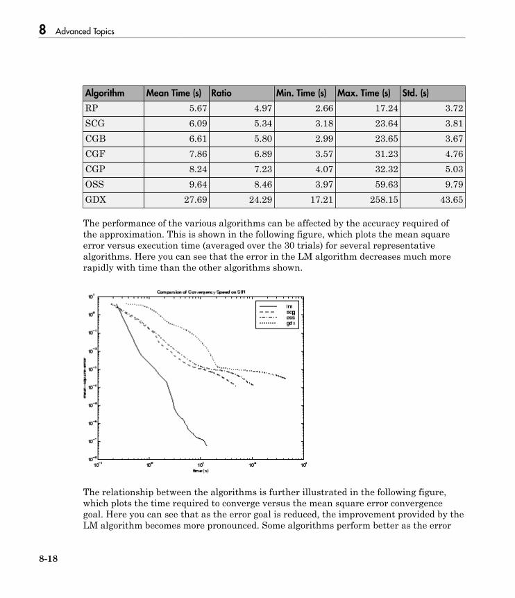
8 Advanced Topics
8-18
Algorithm Mean Time (s) Ratio Min. Time (s) Max. Time (s) Std. (s)
RP 5.67 4.97 2.66 17.24 3.72SCG 6.09 5.34 3.18 23.64 3.81CGB 6.61 5.80 2.99 23.65 3.67CGF 7.86 6.89 3.57 31.23 4.76CGP 8.24 7.23 4.07 32.32 5.03OSS 9.64 8.46 3.97 59.63 9.79GDX 27.69 24.29 17.21 258.15 43.65
The performance of the various algorithms can be affected by the accuracy required ofthe approximation. This is shown in the following figure, which plots the mean squareerror versus execution time (averaged over the 30 trials) for several representativealgorithms. Here you can see that the error in the LM algorithm decreases much morerapidly with time than the other algorithms shown.
The relationship between the algorithms is further illustrated in the following figure,which plots the time required to converge versus the mean square error convergencegoal. Here you can see that as the error goal is reduced, the improvement provided by theLM algorithm becomes more pronounced. Some algorithms perform better as the error

Choose a Multilayer Neural Network Training Function
8-19
goal is reduced (LM and BFG), and other algorithms degrade as the error goal is reduced(OSS and GDX).
PARITY Data Set
The second benchmark problem is a simple pattern recognition problem—detect theparity of a 3-bit number. If the number of ones in the input pattern is odd, then thenetwork should output a 1; otherwise, it should output a -1. The network used for thisproblem is a 3-10-10-1 network with tansig neurons in each layer. The following tablesummarizes the results of training this network with the nine different algorithms. Eachentry in the table represents 30 different trials, where different random initial weightsare used in each trial. In each case, the network is trained until the squared error isless than 0.001. The fastest algorithm for this problem is the resilient backpropagationalgorithm, although the conjugate gradient algorithms (in particular, the scaledconjugate gradient algorithm) are almost as fast. Notice that the LM algorithm does notperform well on this problem. In general, the LM algorithm does not perform as well onpattern recognition problems as it does on function approximation problems. The LMalgorithm is designed for least squares problems that are approximately linear. Becausethe output neurons in pattern recognition problems are generally saturated, you will notbe operating in the linear region.
Algorithm Mean Time (s) Ratio Min. Time (s) Max. Time (s) Std. (s)
RP 3.73 1.00 2.35 6.89 1.26
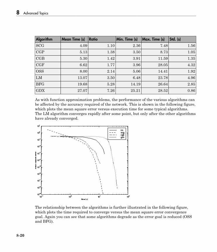
8 Advanced Topics
8-20
Algorithm Mean Time (s) Ratio Min. Time (s) Max. Time (s) Std. (s)
SCG 4.09 1.10 2.36 7.48 1.56CGP 5.13 1.38 3.50 8.73 1.05CGB 5.30 1.42 3.91 11.59 1.35CGF 6.62 1.77 3.96 28.05 4.32OSS 8.00 2.14 5.06 14.41 1.92LM 13.07 3.50 6.48 23.78 4.96BFG 19.68 5.28 14.19 26.64 2.85GDX 27.07 7.26 25.21 28.52 0.86
As with function approximation problems, the performance of the various algorithms canbe affected by the accuracy required of the network. This is shown in the following figure,which plots the mean square error versus execution time for some typical algorithms.The LM algorithm converges rapidly after some point, but only after the other algorithmshave already converged.
The relationship between the algorithms is further illustrated in the following figure,which plots the time required to converge versus the mean square error convergencegoal. Again you can see that some algorithms degrade as the error goal is reduced (OSSand BFG).
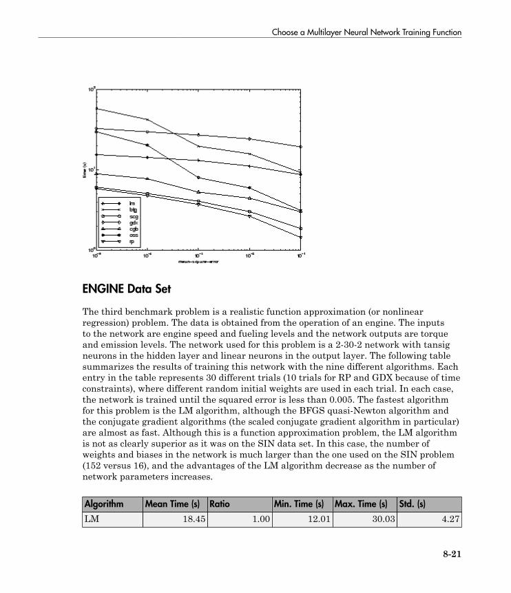
Choose a Multilayer Neural Network Training Function
8-21
ENGINE Data Set
The third benchmark problem is a realistic function approximation (or nonlinearregression) problem. The data is obtained from the operation of an engine. The inputsto the network are engine speed and fueling levels and the network outputs are torqueand emission levels. The network used for this problem is a 2-30-2 network with tansigneurons in the hidden layer and linear neurons in the output layer. The following tablesummarizes the results of training this network with the nine different algorithms. Eachentry in the table represents 30 different trials (10 trials for RP and GDX because of timeconstraints), where different random initial weights are used in each trial. In each case,the network is trained until the squared error is less than 0.005. The fastest algorithmfor this problem is the LM algorithm, although the BFGS quasi-Newton algorithm andthe conjugate gradient algorithms (the scaled conjugate gradient algorithm in particular)are almost as fast. Although this is a function approximation problem, the LM algorithmis not as clearly superior as it was on the SIN data set. In this case, the number ofweights and biases in the network is much larger than the one used on the SIN problem(152 versus 16), and the advantages of the LM algorithm decrease as the number ofnetwork parameters increases.
Algorithm Mean Time (s) Ratio Min. Time (s) Max. Time (s) Std. (s)
LM 18.45 1.00 12.01 30.03 4.27

8 Advanced Topics
8-22
Algorithm Mean Time (s) Ratio Min. Time (s) Max. Time (s) Std. (s)
BFG 27.12 1.47 16.42 47.36 5.95SCG 36.02 1.95 19.39 52.45 7.78CGF 37.93 2.06 18.89 50.34 6.12CGB 39.93 2.16 23.33 55.42 7.50CGP 44.30 2.40 24.99 71.55 9.89OSS 48.71 2.64 23.51 80.90 12.33RP 65.91 3.57 31.83 134.31 34.24GDX 188.50 10.22 81.59 279.90 66.67
The following figure plots the mean square error versus execution time for some typicalalgorithms. The performance of the LM algorithm improves over time relative to theother algorithms.
The relationship between the algorithms is further illustrated in the following figure,which plots the time required to converge versus the mean square error convergencegoal. Again you can see that some algorithms degrade as the error goal is reduced (GDXand RP), while the LM algorithm improves.
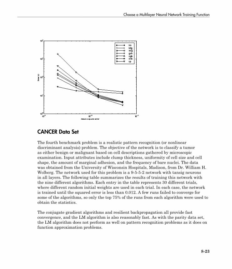
Choose a Multilayer Neural Network Training Function
8-23
CANCER Data Set
The fourth benchmark problem is a realistic pattern recognition (or nonlineardiscriminant analysis) problem. The objective of the network is to classify a tumoras either benign or malignant based on cell descriptions gathered by microscopicexamination. Input attributes include clump thickness, uniformity of cell size and cellshape, the amount of marginal adhesion, and the frequency of bare nuclei. The datawas obtained from the University of Wisconsin Hospitals, Madison, from Dr. William H.Wolberg. The network used for this problem is a 9-5-5-2 network with tansig neuronsin all layers. The following table summarizes the results of training this network withthe nine different algorithms. Each entry in the table represents 30 different trials,where different random initial weights are used in each trial. In each case, the networkis trained until the squared error is less than 0.012. A few runs failed to converge forsome of the algorithms, so only the top 75% of the runs from each algorithm were used toobtain the statistics.
The conjugate gradient algorithms and resilient backpropagation all provide fastconvergence, and the LM algorithm is also reasonably fast. As with the parity data set,the LM algorithm does not perform as well on pattern recognition problems as it does onfunction approximation problems.
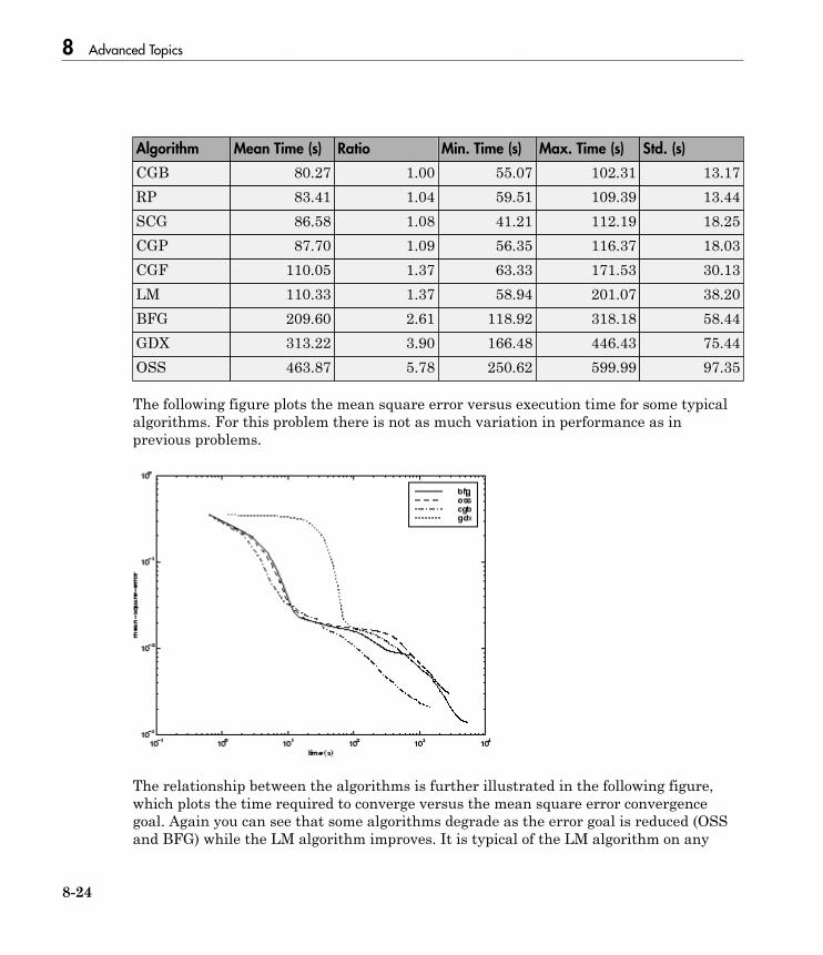
8 Advanced Topics
8-24
Algorithm Mean Time (s) Ratio Min. Time (s) Max. Time (s) Std. (s)
CGB 80.27 1.00 55.07 102.31 13.17RP 83.41 1.04 59.51 109.39 13.44SCG 86.58 1.08 41.21 112.19 18.25CGP 87.70 1.09 56.35 116.37 18.03CGF 110.05 1.37 63.33 171.53 30.13LM 110.33 1.37 58.94 201.07 38.20BFG 209.60 2.61 118.92 318.18 58.44GDX 313.22 3.90 166.48 446.43 75.44OSS 463.87 5.78 250.62 599.99 97.35
The following figure plots the mean square error versus execution time for some typicalalgorithms. For this problem there is not as much variation in performance as inprevious problems.
The relationship between the algorithms is further illustrated in the following figure,which plots the time required to converge versus the mean square error convergencegoal. Again you can see that some algorithms degrade as the error goal is reduced (OSSand BFG) while the LM algorithm improves. It is typical of the LM algorithm on any
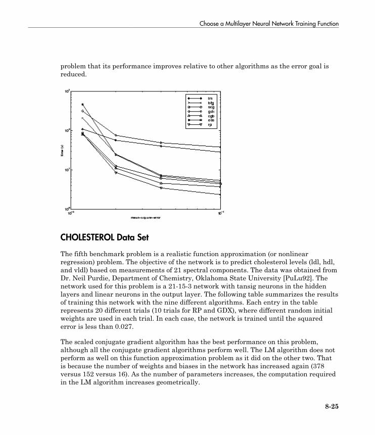
Choose a Multilayer Neural Network Training Function
8-25
problem that its performance improves relative to other algorithms as the error goal isreduced.
CHOLESTEROL Data Set
The fifth benchmark problem is a realistic function approximation (or nonlinearregression) problem. The objective of the network is to predict cholesterol levels (ldl, hdl,and vldl) based on measurements of 21 spectral components. The data was obtained fromDr. Neil Purdie, Department of Chemistry, Oklahoma State University [PuLu92]. Thenetwork used for this problem is a 21-15-3 network with tansig neurons in the hiddenlayers and linear neurons in the output layer. The following table summarizes the resultsof training this network with the nine different algorithms. Each entry in the tablerepresents 20 different trials (10 trials for RP and GDX), where different random initialweights are used in each trial. In each case, the network is trained until the squarederror is less than 0.027.
The scaled conjugate gradient algorithm has the best performance on this problem,although all the conjugate gradient algorithms perform well. The LM algorithm does notperform as well on this function approximation problem as it did on the other two. Thatis because the number of weights and biases in the network has increased again (378versus 152 versus 16). As the number of parameters increases, the computation requiredin the LM algorithm increases geometrically.

8 Advanced Topics
8-26
Algorithm Mean Time (s) Ratio Min. Time (s) Max. Time (s) Std. (s)
SCG 99.73 1.00 83.10 113.40 9.93CGP 121.54 1.22 101.76 162.49 16.34CGB 124.06 1.2 107.64 146.90 14.62CGF 136.04 1.36 106.46 167.28 17.67LM 261.50 2.62 103.52 398.45 102.06OSS 268.55 2.69 197.84 372.99 56.79BFG 550.92 5.52 471.61 676.39 46.59RP 1519.00 15.23 581.17 2256.10 557.34GDX 3169.50 31.78 2514.90 4168.20 610.52
The following figure plots the mean square error versus execution time for sometypical algorithms. For this problem, you can see that the LM algorithm is able to drivethe mean square error to a lower level than the other algorithms. The SCG and RPalgorithms provide the fastest initial convergence.
The relationship between the algorithms is further illustrated in the following figure,which plots the time required to converge versus the mean square error convergencegoal. You can see that the LM and BFG algorithms improve relative to the otheralgorithms as the error goal is reduced.
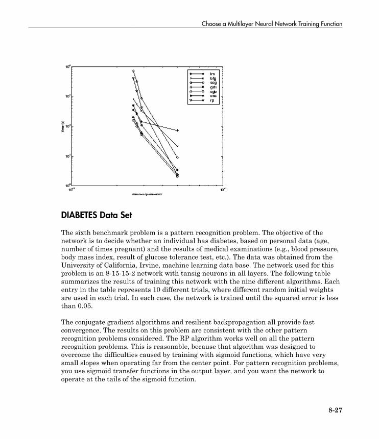
Choose a Multilayer Neural Network Training Function
8-27
DIABETES Data Set
The sixth benchmark problem is a pattern recognition problem. The objective of thenetwork is to decide whether an individual has diabetes, based on personal data (age,number of times pregnant) and the results of medical examinations (e.g., blood pressure,body mass index, result of glucose tolerance test, etc.). The data was obtained from theUniversity of California, Irvine, machine learning data base. The network used for thisproblem is an 8-15-15-2 network with tansig neurons in all layers. The following tablesummarizes the results of training this network with the nine different algorithms. Eachentry in the table represents 10 different trials, where different random initial weightsare used in each trial. In each case, the network is trained until the squared error is lessthan 0.05.
The conjugate gradient algorithms and resilient backpropagation all provide fastconvergence. The results on this problem are consistent with the other patternrecognition problems considered. The RP algorithm works well on all the patternrecognition problems. This is reasonable, because that algorithm was designed toovercome the difficulties caused by training with sigmoid functions, which have verysmall slopes when operating far from the center point. For pattern recognition problems,you use sigmoid transfer functions in the output layer, and you want the network tooperate at the tails of the sigmoid function.

8 Advanced Topics
8-28
Algorithm Mean Time (s) Ratio Min. Time (s) Max. Time (s) Std. (s)
RP 323.90 1.00 187.43 576.90 111.37SCG 390.53 1.21 267.99 487.17 75.07CGB 394.67 1.22 312.25 558.21 85.38CGP 415.90 1.28 320.62 614.62 94.77OSS 784.00 2.42 706.89 936.52 76.37CGF 784.50 2.42 629.42 1082.20 144.63LM 1028.10 3.17 802.01 1269.50 166.31BFG 1821.00 5.62 1415.80 3254.50 546.36GDX 7687.00 23.73 5169.20 10350.00 2015.00
The following figure plots the mean square error versus execution time for some typicalalgorithms. As with other problems, you see that the SCG and RP have fast initialconvergence, while the LM algorithm is able to provide smaller final error.
The relationship between the algorithms is further illustrated in the following figure,which plots the time required to converge versus the mean square error convergencegoal. In this case, you can see that the BFG algorithm degrades as the error goal isreduced, while the LM algorithm improves. The RP algorithm is best, except at thesmallest error goal, where SCG is better.

Choose a Multilayer Neural Network Training Function
8-29
Summary
There are several algorithm characteristics that can be deduced from the experimentsdescribed. In general, on function approximation problems, for networks that containup to a few hundred weights, the Levenberg-Marquardt algorithm will have the fastestconvergence. This advantage is especially noticeable if very accurate training is required.In many cases, trainlm is able to obtain lower mean square errors than any of the otheralgorithms tested. However, as the number of weights in the network increases, theadvantage of trainlm decreases. In addition, trainlm performance is relatively poor onpattern recognition problems. The storage requirements of trainlm are larger than theother algorithms tested. By adjusting the mem_reduc parameter, discussed earlier, thestorage requirements can be reduced, but at the cost of increased execution time.
The trainrp function is the fastest algorithm on pattern recognition problems. However,it does not perform well on function approximation problems. Its performance alsodegrades as the error goal is reduced. The memory requirements for this algorithm arerelatively small in comparison to the other algorithms considered.
The conjugate gradient algorithms, in particular trainscg, seem to perform well overa wide variety of problems, particularly for networks with a large number of weights.The SCG algorithm is almost as fast as the LM algorithm on function approximationproblems (faster for large networks) and is almost as fast as trainrp on pattern
8 Advanced Topics
8-30
recognition problems. Its performance does not degrade as quickly as trainrpperformance does when the error is reduced. The conjugate gradient algorithms haverelatively modest memory requirements.
The performance of trainbfg is similar to that of trainlm. It does not require as muchstorage as trainlm, but the computation required does increase geometrically with thesize of the network, because the equivalent of a matrix inverse must be computed at eachiteration.
The variable learning rate algorithm traingdx is usually much slower than the othermethods, and has about the same storage requirements as trainrp, but it can still beuseful for some problems. There are certain situations in which it is better to convergemore slowly. For example, when using early stopping you can have inconsistent results ifyou use an algorithm that converges too quickly. You might overshoot the point at whichthe error on the validation set is minimized.

Improve Neural Network Generalization and Avoid Overfitting
8-31
Improve Neural Network Generalization and Avoid Overfitting
In this section...
“Retraining Neural Networks” on page 8-32“Multiple Neural Networks” on page 8-34“Early Stopping” on page 8-35“Index Data Division (divideind)” on page 8-36“Random Data Division (dividerand)” on page 8-36“Block Data Division (divideblock)” on page 8-36“Interleaved Data Division (divideint)” on page 8-37“Regularization” on page 8-37“Summary and Discussion of Early Stopping and Regularization” on page 8-40“Posttraining Analysis (regression)” on page 8-42
One of the problems that occur during neural network training is called overfitting. Theerror on the training set is driven to a very small value, but when new data is presentedto the network the error is large. The network has memorized the training examples, butit has not learned to generalize to new situations.
The following figure shows the response of a 1-20-1 neural network that has been trainedto approximate a noisy sine function. The underlying sine function is shown by thedotted line, the noisy measurements are given by the + symbols, and the neural networkresponse is given by the solid line. Clearly this network has overfitted the data and willnot generalize well.

8 Advanced Topics
8-32
One method for improving network generalization is to use a network that is just largeenough to provide an adequate fit. The larger network you use, the more complex thefunctions the network can create. If you use a small enough network, it will not haveenough power to overfit the data. Run the Neural Network Design example nnd11gn[HDB96] to investigate how reducing the size of a network can prevent overfitting.
Unfortunately, it is difficult to know beforehand how large a network should be for aspecific application. There are two other methods for improving generalization that areimplemented in Neural Network Toolbox software: regularization and early stopping.The next sections describe these two techniques and the routines to implement them.
Note that if the number of parameters in the network is much smaller than the totalnumber of points in the training set, then there is little or no chance of overfitting. Ifyou can easily collect more data and increase the size of the training set, then there isno need to worry about the following techniques to prevent overfitting. The rest of thissection only applies to those situations in which you want to make the most of a limitedsupply of data.
Retraining Neural Networks
Typically each backpropagation training session starts with different initial weightsand biases, and different divisions of data into training, validation, and test sets. Thesedifferent conditions can lead to very different solutions for the same problem.
Improve Neural Network Generalization and Avoid Overfitting
8-33
It is a good idea to train several networks to ensure that a network with goodgeneralization is found.
Here a dataset is loaded and divided into two parts: 90% for designing networks and 10%for testing them all.
[x,t] = house_dataset;
Q = size(x,2);
Q1 = floor(Q*0.90);
Q2 = Q-Q1;
ind = randperm(Q);
ind1 = ind(1:Q1);
ind2 = ind(Q1+(1:Q2));
x1 = x(:,ind1);
t1 = t(:,ind1);
x2 = x(:,ind2);
t2 = t(:,ind2);
Next a network architecture is chosen and trained ten times on the first part of thedataset, with each network’s mean square error on the second part of the dataset.
net = feedforwardnet(10);
numNN = 10;
NN = cell(1,numNN);
perfs = zeros(1,numNN);
for i=1:numNN
disp(['Training ' num2str(i) '/' num2str(numNN)])
NN{i} = train(net,x1,t1);
y2 = NN{i}(x2);
perfs(i) = mse(net,t2,y2);
end
Each network will be trained starting from different initial weights and biases, and witha different division of the first dataset into training, validation, and test sets. Note thatthe test sets are a good measure of generalization for each respective network, but notfor all the networks, because data that is a test set for one network will likely be usedfor training or validation by other neural networks. This is why the original dataset wasdivided into two parts, to ensure that a completely independent test set is preserved.
The neural network with the lowest performance is the one that generalized best to thesecond part of the dataset.

8 Advanced Topics
8-34
Multiple Neural Networks
Another simple way to improve generalization, especially when caused by noisy data or asmall dataset, is to train multiple neural networks and average their outputs.
For instance, here 10 neural networks are trained on a small problem and their meansquared errors compared to the means squared error of their average.
First, the dataset is loaded and divided into a design and test set.
[x,t] = house_dataset;
Q = size(x,2);
Q1 = floor(Q*0.90);
Q2 = Q-Q1;
ind = randperm(Q);
ind1 = ind(1:Q1);
ind2 = ind(Q1+(1:Q2));
x1 = x(:,ind1);
t1 = t(:,ind1);
x2 = x(:,ind2);
t2 = t(:,ind2);
Then, ten neural networks are trained.
net = feedforwardnet(10);
numNN = 10;
nets = cell(1,numNN);
for i=1:numNN
disp(['Training ' num2str(i) '/' num2str(numNN)])
nets{i} = train(net,x1,t1);
end
Next, each network is tested on the second dataset with both individual performancesand the performance for the average output calculated.
perfs = zeros(1,numNN);
y2Total = 0;
for i=1:numNN
neti = nets{i};
y2 = neti(x2);
perfs(i) = mse(neti,t2,y2);
y2Total = y2Total + y2;
end
perfs
Improve Neural Network Generalization and Avoid Overfitting
8-35
y2AverageOutput = y2Total / numNN;
perfAveragedOutputs = mse(nets{1},t2,y2AverageOutput)
The mean squared error for the average output is likely to be lower than most of theindividual performances, perhaps not all. It is likely to generalize better to additionalnew data.
For some very difficult problems, a hundred networks can be trained and the averageof their outputs taken for any input. This is especially helpful for a small, noisy datasetin conjunction with the Bayesian Regularization training function trainbr, describedbelow.
Early Stopping
The default method for improving generalization is called early stopping. This techniqueis automatically provided for all of the supervised network creation functions, includingthe backpropagation network creation functions such as feedforwardnet.
In this technique the available data is divided into three subsets. The first subset isthe training set, which is used for computing the gradient and updating the networkweights and biases. The second subset is the validation set. The error on the validationset is monitored during the training process. The validation error normally decreasesduring the initial phase of training, as does the training set error. However, whenthe network begins to overfit the data, the error on the validation set typically beginsto rise. When the validation error increases for a specified number of iterations(net.trainParam.max_fail), the training is stopped, and the weights and biases atthe minimum of the validation error are returned.
The test set error is not used during training, but it is used to compare different models.It is also useful to plot the test set error during the training process. If the error inthe test set reaches a minimum at a significantly different iteration number than thevalidation set error, this might indicate a poor division of the data set.
There are four functions provided for dividing data into training, validation and test sets.They are dividerand (the default), divideblock, divideint, and divideind. Youcan access or change the division function for your network with this property:
net.divideFcn
Each of these functions takes parameters that customize its behavior. These values arestored and can be changed with the following network property:
8 Advanced Topics
8-36
net.divideParam
Index Data Division (divideind)
Create a simple test problem. For the full data set, generate a noisy sine wave with 201input points ranging from −1 to 1 at steps of 0.01:
p = [-1:0.01:1];
t = sin(2*pi*p)+0.1*randn(size(p));
Divide the data by index so that successive samples are assigned to the training set,validation set, and test set successively:
trainInd = 1:3:201
valInd = 2:3:201;
testInd = 3:3:201;
[trainP,valP,testP] = divideind(p,trainInd,valInd,testInd);
[trainT,valT,testT] = divideind(t,trainInd,valInd,testInd);
Random Data Division (dividerand)
You can divide the input data randomly so that 60% of the samples are assigned to thetraining set, 20% to the validation set, and 20% to the test set, as follows:
[trainP,valP,testP,trainInd,valInd,testInd] = dividerand(p);
This function not only divides the input data, but also returns indices so that you candivide the target data accordingly using divideind:
[trainT,valT,testT] = divideind(t,trainInd,valInd,testInd);
Block Data Division (divideblock)
You can also divide the input data randomly such that the first 60% of the samples areassigned to the training set, the next 20% to the validation set, and the last 20% to thetest set, as follows:
[trainP,valP,testP,trainInd,valInd,testInd] = divideblock(p);
Divide the target data accordingly using divideind:
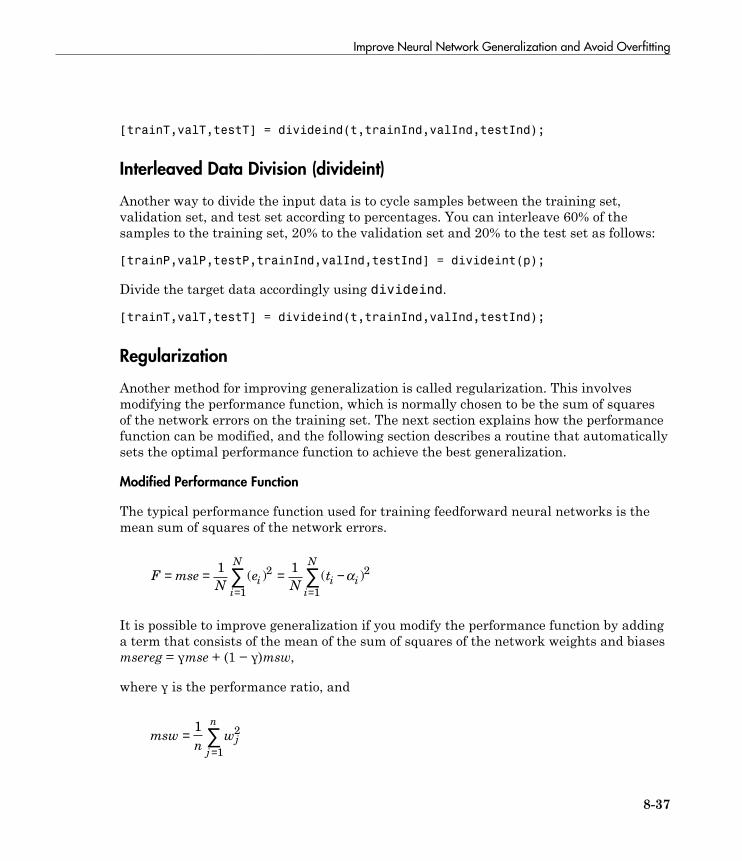
Improve Neural Network Generalization and Avoid Overfitting
8-37
[trainT,valT,testT] = divideind(t,trainInd,valInd,testInd);
Interleaved Data Division (divideint)
Another way to divide the input data is to cycle samples between the training set,validation set, and test set according to percentages. You can interleave 60% of thesamples to the training set, 20% to the validation set and 20% to the test set as follows:
[trainP,valP,testP,trainInd,valInd,testInd] = divideint(p);
Divide the target data accordingly using divideind.
[trainT,valT,testT] = divideind(t,trainInd,valInd,testInd);
Regularization
Another method for improving generalization is called regularization. This involvesmodifying the performance function, which is normally chosen to be the sum of squaresof the network errors on the training set. The next section explains how the performancefunction can be modified, and the following section describes a routine that automaticallysets the optimal performance function to achieve the best generalization.
Modified Performance Function
The typical performance function used for training feedforward neural networks is themean sum of squares of the network errors.
F mseN
eN
ti
i
N
i i
i
N
= = = −= =∑ ∑1 12
1
2
1
( ) ( )a
It is possible to improve generalization if you modify the performance function by addinga term that consists of the mean of the sum of squares of the network weights and biasesmsereg = γmse + (1 − γ)msw,
where γ is the performance ratio, and
mswn
wj
j
n
==∑1 2
1
8 Advanced Topics
8-38
Using this performance function causes the network to have smaller weights and biases,and this forces the network response to be smoother and less likely to overfit.
The following code reinitializes the previous network and retrains it using the BFGSalgorithm with the regularized performance function. Here the performance ratio is setto 0.5, which gives equal weight to the mean square errors and the mean square weights.(Data division is cancelled by setting net.divideFcn so that the effects of msereg areisolated from early stopping.)
[x,t] = simplefit_dataset;
net = feedforwardnet(10,'trainbfg');
net.divideFcn = '';
net.trainParam.epochs = 300;
net.trainParam.goal = 1e-5;
net.performParam.regularization = 0.5;
net = train(net,x,t);
The problem with regularization is that it is difficult to determine the optimum valuefor the performance ratio parameter. If you make this parameter too large, you mightget overfitting. If the ratio is too small, the network does not adequately fit the trainingdata. The next section describes a routine that automatically sets the regularizationparameters.
Automated Regularization (trainbr)
It is desirable to determine the optimal regularization parameters in an automatedfashion. One approach to this process is the Bayesian framework of David MacKay[MacK92]. In this framework, the weights and biases of the network are assumed to berandom variables with specified distributions. The regularization parameters are relatedto the unknown variances associated with these distributions. You can then estimatethese parameters using statistical techniques.
A detailed discussion of Bayesian regularization is beyond the scope of this user guide. Adetailed discussion of the use of Bayesian regularization, in combination with Levenberg-Marquardt training, can be found in [FoHa97].
Bayesian regularization has been implemented in the function trainbr. The followingcode shows how you can train a 1-20-1 network using this function to approximatethe noisy sine wave shown in the figure in “Improve Neural Network Generalizationand Avoid Overfitting” on page 8-31. (Data division is cancelled by settingnet.divideFcn so that the effects of trainbr are isolated from early stopping.)
Improve Neural Network Generalization and Avoid Overfitting
8-39
x = -1:0.05:1;
t = sin(2*pi*x) + 0.1*randn(size(x));
net = feedforwardnet(20,'trainbr');
net = train(net,x,t);
One feature of this algorithm is that it provides a measure of how many networkparameters (weights and biases) are being effectively used by the network. In this case,the final trained network uses approximately 12 parameters (indicated by #Par in theprintout) out of the 61 total weights and biases in the 1-20-1 network. This effectivenumber of parameters should remain approximately the same, no matter how large thenumber of parameters in the network becomes. (This assumes that the network has beentrained for a sufficient number of iterations to ensure convergence.)
The trainbr algorithm generally works best when the network inputs and targetsare scaled so that they fall approximately in the range [−1,1]. That is the case for thetest problem here. If your inputs and targets do not fall in this range, you can use thefunction mapminmax or mapstd to perform the scaling, as described in “Choose NeuralNetwork Input-Output Processing Functions” on page 2-9. Networks created withfeedforwardnet include mapminmax as an input and output processing function bydefault.
The following figure shows the response of the trained network. In contrast to theprevious figure, in which a 1-20-1 network overfits the data, here you see that thenetwork response is very close to the underlying sine function (dotted line), and,therefore, the network will generalize well to new inputs. You could have tried an evenlarger network, but the network response would never overfit the data. This eliminatesthe guesswork required in determining the optimum network size.
When using trainbr, it is important to let the algorithm run until the effective numberof parameters has converged. The training might stop with the message "Maximum MUreached." This is typical, and is a good indication that the algorithm has truly converged.You can also tell that the algorithm has converged if the sum squared error (SSE) andsum squared weights (SSW) are relatively constant over several iterations. When thisoccurs you might want to click the Stop Training button in the training window.

8 Advanced Topics
8-40
Summary and Discussion of Early Stopping and Regularization
Early stopping and regularization can ensure network generalization when you applythem properly.
For early stopping, you must be careful not to use an algorithm that converges toorapidly. If you are using a fast algorithm (like trainlm), set the training parametersso that the convergence is relatively slow. For example, set mu to a relatively largevalue, such as 1, and set mu_dec and mu_inc to values close to 1, such as 0.8 and 1.5,respectively. The training functions trainscg and trainbr usually work well withearly stopping.
With early stopping, the choice of the validation set is also important. The validation setshould be representative of all points in the training set.
When you use Bayesian regularization, it is important to train the network until itreaches convergence. The sum-squared error, the sum-squared weights, and the effectivenumber of parameters should reach constant values when the network has converged.
With both early stopping and regularization, it is a good idea to train the networkstarting from several different initial conditions. It is possible for either method to failin certain circumstances. By testing several different initial conditions, you can verifyrobust network performance.

Improve Neural Network Generalization and Avoid Overfitting
8-41
When the data set is small and you are training function approximation networks,Bayesian regularization provides better generalization performance than early stopping.This is because Bayesian regularization does not require that a validation data set beseparate from the training data set; it uses all the data.
To provide some insight into the performance of the algorithms, both early stopping andBayesian regularization were tested on several benchmark data sets, which are listed inthe following table.
Data Set Title Number ofPoints
Network Description
BALL 67 2-10-1 Dual-sensor calibration for a ball positionmeasurement
SINE (5% N) 41 1-15-1 Single-cycle sine wave with Gaussian noise at 5%level
SINE (2% N) 41 1-15-1 Single-cycle sine wave with Gaussian noise at 2%level
ENGINE (ALL) 1199 2-30-2 Engine sensor—full data setENGINE (1/4) 300 2-30-2 Engine sensor—1/4 of data setCHOLEST (ALL) 264 5-15-3 Cholesterol measurement—full data setCHOLEST (1/2) 132 5-15-3 Cholesterol measurement—1/2 data set
These data sets are of various sizes, with different numbers of inputs and targets. Withtwo of the data sets the networks were trained once using all the data and then retrainedusing only a fraction of the data. This illustrates how the advantage of Bayesianregularization becomes more noticeable when the data sets are smaller. All the datasets are obtained from physical systems except for the SINE data sets. These two wereartificially created by adding various levels of noise to a single cycle of a sine wave. Theperformance of the algorithms on these two data sets illustrates the effect of noise.
The following table summarizes the performance of early stopping (ES) and Bayesianregularization (BR) on the seven test sets. (The trainscg algorithm was used for theearly stopping tests. Other algorithms provide similar performance.)
Mean Squared Test Set Error
Method Ball Engine (All) Engine(1/4)
Choles(All)
Choles(1/2)
Sine (5%N)
Sine (2%N)
ES 1.2e-1 1.3e-2 1.9e-2 1.2e-1 1.4e-1 1.7e-1 1.3e-1

8 Advanced Topics
8-42
Method Ball Engine (All) Engine(1/4)
Choles(All)
Choles(1/2)
Sine (5%N)
Sine (2%N)
BR 1.3e-3 2.6e-3 4.7e-3 1.2e-1 9.3e-2 3.0e-2 6.3e-3ES/BR 92 5 4 1 1.5 5.7 21
You can see that Bayesian regularization performs better than early stopping in mostcases. The performance improvement is most noticeable when the data set is small, or ifthere is little noise in the data set. The BALL data set, for example, was obtained fromsensors that had very little noise.
Although the generalization performance of Bayesian regularization is often betterthan early stopping, this is not always the case. In addition, the form of Bayesianregularization implemented in the toolbox does not perform as well on patternrecognition problems as it does on function approximation problems. This is becausethe approximation to the Hessian that is used in the Levenberg-Marquardt algorithm isnot as accurate when the network output is saturated, as would be the case in patternrecognition problems. Another disadvantage of the Bayesian regularization method isthat it generally takes longer to converge than early stopping.
Posttraining Analysis (regression)
The performance of a trained network can be measured to some extent by the errors onthe training, validation, and test sets, but it is often useful to investigate the networkresponse in more detail. One option is to perform a regression analysis between thenetwork response and the corresponding targets. The routine regression is designed toperform this analysis.
The following commands illustrate how to perform a regression analysis on a networktrained.
x = [-1:.05:1];
t = sin(2*pi*x)+0.1*randn(size(x));
net = feedforwardnet(10);
net = train(net,x,t);
y = net(x);
[r,m,b] = regression(t,y)
r =
0.9935
m =
0.9874

Improve Neural Network Generalization and Avoid Overfitting
8-43
b =
-0.0067
The network output and the corresponding targets are passed to regression. It returnsthree parameters. The first two, m and b, correspond to the slope and the y-intercept ofthe best linear regression relating targets to network outputs. If there were a perfect fit(outputs exactly equal to targets), the slope would be 1, and the y-intercept would be 0.In this example, you can see that the numbers are very close. The third variable returnedby regression is the correlation coefficient (R-value) between the outputs and targets.It is a measure of how well the variation in the output is explained by the targets. If thisnumber is equal to 1, then there is perfect correlation between targets and outputs. Inthe example, the number is very close to 1, which indicates a good fit.
The following figure illustrates the graphical output provided by regression. Thenetwork outputs are plotted versus the targets as open circles. The best linear fit isindicated by a dashed line. The perfect fit (output equal to targets) is indicated by thesolid line. In this example, it is difficult to distinguish the best linear fit line from theperfect fit line because the fit is so good.

8 Advanced Topics
8-44
Create and Train Custom Neural Network Architectures
In this section...
“Custom Network” on page 8-44“Network Definition” on page 8-45“Network Behavior” on page 8-54
Neural Network Toolbox software provides a flexible network object type that allowsmany kinds of networks to be created and then used with functions such as init, sim,and train.
Type the following to see all the network creation functions in the toolbox.
help nnnetwork
This flexibility is possible because networks have an object-oriented representation. Therepresentation allows you to define various architectures and assign various algorithmsto those architectures.
To create custom networks, start with an empty network (obtained with the networkfunction) and set its properties as desired.
net = network
The network object consists of many properties that you can set to specify the structureand behavior of your network.
The following sections show how to create a custom network by using these properties.
Custom Network
Before you can build a network you need to know what it looks like. For dramaticpurposes (and to give the toolbox a workout) this section leads you through the creationof the wild and complicated network shown below.
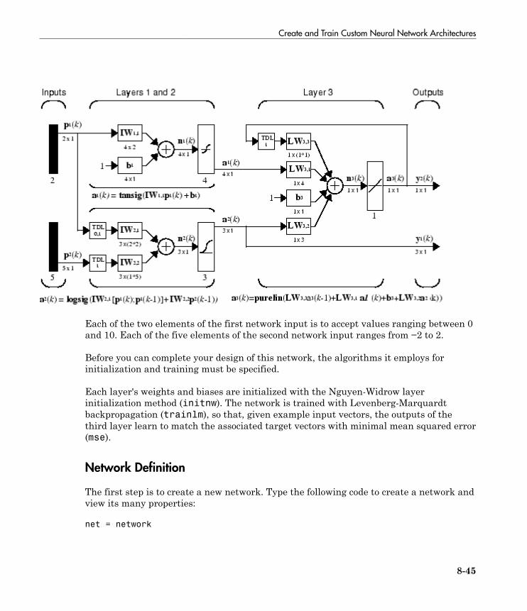
Create and Train Custom Neural Network Architectures
8-45
Each of the two elements of the first network input is to accept values ranging between 0and 10. Each of the five elements of the second network input ranges from −2 to 2.
Before you can complete your design of this network, the algorithms it employs forinitialization and training must be specified.
Each layer's weights and biases are initialized with the Nguyen-Widrow layerinitialization method (initnw). The network is trained with Levenberg-Marquardtbackpropagation (trainlm), so that, given example input vectors, the outputs of thethird layer learn to match the associated target vectors with minimal mean squared error(mse).
Network Definition
The first step is to create a new network. Type the following code to create a network andview its many properties:
net = network

8 Advanced Topics
8-46
Architecture Properties
The first group of properties displayed is labeled architecture properties. Theseproperties allow you to select the number of inputs and layers and their connections.Number of Inputs and Layers
The first two properties displayed in the dimensions group are numInputs andnumLayers. These properties allow you to select how many inputs and layers you wantthe network to have.
net =
dimensions:
numInputs: 0
numLayers: 0
...
Note that the network has no inputs or layers at this time.
Change that by setting these properties to the number of inputs and number of layers inthe custom network diagram.
net.numInputs = 2;
net.numLayers = 3;
net.numInputs is the number of input sources, not the number of elements in an inputvector (net.inputs{i}.size).Bias Connections
Type net and press Enter to view its properties again. The network now has two inputsand three layers.
net =
Neural Network:
dimensions:
numInputs: 2
numLayers: 3
Examine the next four properties in the connections group:
biasConnect: [0; 0; 0]
inputConnect: [0 0; 0 0; 0 0]
layerConnect: [0 0 0; 0 0 0; 0 0 0]
outputConnect: [0 0 0]
Create and Train Custom Neural Network Architectures
8-47
These matrices of 1s and 0s represent the presence and absence of bias, input weight,layer weight, and output connections. They are currently all zeros, indicating that thenetwork does not have any such connections.
The bias connection matrix is a 3-by-1 vector. To create a bias connection to the ith layeryou can set net.biasConnect(i) to 1. Specify that the first and third layers are tohave bias connections, as the diagram indicates, by typing the following code:
net.biasConnect(1) = 1;
net.biasConnect(3) = 1;
You could also define those connections with a single line of code.
net.biasConnect = [1; 0; 1];
Input and Layer Weight Connections
The input connection matrix is 3-by-2, representing the presence of connectionsfrom two sources (the two inputs) to three destinations (the three layers). Thus,net.inputConnect(i,j) represents the presence of an input weight connection goingto the ith layer from the jth input.
To connect the first input to the first and second layers, and the second input to thesecond layer (as indicated by the custom network diagram), type
net.inputConnect(1,1) = 1;
net.inputConnect(2,1) = 1;
net.inputConnect(2,2) = 1;
or this single line of code:
net.inputConnect = [1 0; 1 1; 0 0];
Similarly, net.layerConnect(i.j) represents the presence of a layer-weightconnection going to the ith layer from the jth layer. Connect layers 1, 2, and 3 to layer 3as follows:
net.layerConnect = [0 0 0; 0 0 0; 1 1 1];
Output Connections
The output connections are a 1-by-3 matrix, indicating that they connect to onedestination (the external world) from three sources (the three layers).
To connect layers 2 and 3 to the network output, type
8 Advanced Topics
8-48
net.outputConnect = [0 1 1];
Number of Outputs
Type net and press Enter to view the updated properties. The final three architectureproperties are read-only values, which means their values are determined by the choicesmade for other properties. The first read-only property in the dimension group is thenumber of outputs:
numOutputs: 2
By defining output connection from layers 2 and 3, you specified that the network hastwo outputs.
Subobject Properties
The next group of properties in the output display is subobjects:
subobjects:
inputs: {2x1 cell array of 2 inputs}
layers: {3x1 cell array of 3 layers}
outputs: {1x3 cell array of 2 outputs}
biases: {3x1 cell array of 2 biases}
inputWeights: {3x2 cell array of 3 weights}
layerWeights: {3x3 cell array of 3 weights}
Inputs
When you set the number of inputs (net.numInputs) to 2, the inputs property becomesa cell array of two input structures. Each ith input structure (net.inputs{i}) containsadditional properties associated with the ith input.
To see how the input structures are arranged, type
net.inputs
ans =
[1x1 nnetInput]
[1x1 nnetInput]
To see the properties associated with the first input, type
net.inputs{1}
The properties appear as follows:
ans =
Create and Train Custom Neural Network Architectures
8-49
name: 'Input'
feedbackOutput: []
processFcns: {}
processParams: {1x0 cell array of 0 params}
processSettings: {0x0 cell array of 0 settings}
processedRange: []
processedSize: 0
range: []
size: 0
userdata: (your custom info)
If you set the exampleInput property, the range, size, processedSize, andprocessedRange properties will automatically be updated to match the properties of thevalue of exampleInput.
Set the exampleInput property as follows:
net.inputs{1}.exampleInput = [0 10 5; 0 3 10];
If you examine the structure of the first input again, you see that it now has new values.
The property processFcns can be set to one or more processing functions. Type helpnnprocess to see a list of these functions.
Set the second input vector ranges to be from −2 to 2 for five elements as follows:
net.inputs{1}.processFcns = {'removeconstantrows','mapminmax'};
View the new input properties. You will see that processParams, processSettings,processedRange and processedSize have all been updated to reflect that inputswill be processed using removeconstantrows and mapminmax before being given tothe network when the network is simulated or trained. The property processParamscontains the default parameters for each processing function. You can alter these values,if you like. See the reference page for each processing function to learn more about theirparameters.
You can set the size of an input directly when no processing functions are used:
net.inputs{2}.size = 5;
Layers
When you set the number of layers (net.numLayers) to 3, the layers property becomesa cell array of three-layer structures. Type the following line of code to see the propertiesassociated with the first layer.
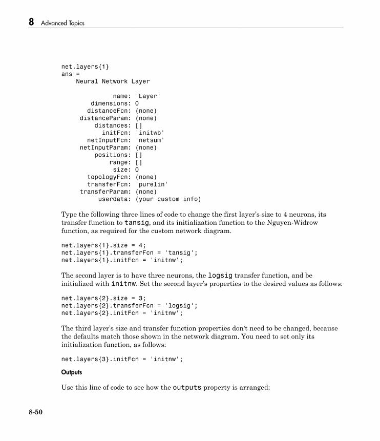
8 Advanced Topics
8-50
net.layers{1}
ans =
Neural Network Layer
name: 'Layer'
dimensions: 0
distanceFcn: (none)
distanceParam: (none)
distances: []
initFcn: 'initwb'
netInputFcn: 'netsum'
netInputParam: (none)
positions: []
range: []
size: 0
topologyFcn: (none)
transferFcn: 'purelin'
transferParam: (none)
userdata: (your custom info)
Type the following three lines of code to change the first layer’s size to 4 neurons, itstransfer function to tansig, and its initialization function to the Nguyen-Widrowfunction, as required for the custom network diagram.
net.layers{1}.size = 4;
net.layers{1}.transferFcn = 'tansig';
net.layers{1}.initFcn = 'initnw';
The second layer is to have three neurons, the logsig transfer function, and beinitialized with initnw. Set the second layer’s properties to the desired values as follows:
net.layers{2}.size = 3;
net.layers{2}.transferFcn = 'logsig';
net.layers{2}.initFcn = 'initnw';
The third layer’s size and transfer function properties don't need to be changed, becausethe defaults match those shown in the network diagram. You need to set only itsinitialization function, as follows:
net.layers{3}.initFcn = 'initnw';
Outputs
Use this line of code to see how the outputs property is arranged:
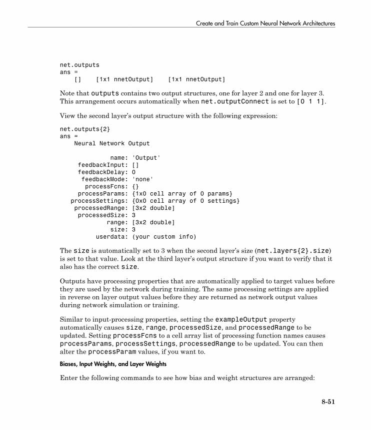
Create and Train Custom Neural Network Architectures
8-51
net.outputs
ans =
[] [1x1 nnetOutput] [1x1 nnetOutput]
Note that outputs contains two output structures, one for layer 2 and one for layer 3.This arrangement occurs automatically when net.outputConnect is set to [0 1 1].
View the second layer’s output structure with the following expression:
net.outputs{2}
ans =
Neural Network Output
name: 'Output'
feedbackInput: []
feedbackDelay: 0
feedbackMode: 'none'
processFcns: {}
processParams: {1x0 cell array of 0 params}
processSettings: {0x0 cell array of 0 settings}
processedRange: [3x2 double]
processedSize: 3
range: [3x2 double]
size: 3
userdata: (your custom info)
The size is automatically set to 3 when the second layer’s size (net.layers{2}.size)is set to that value. Look at the third layer’s output structure if you want to verify that italso has the correct size.
Outputs have processing properties that are automatically applied to target values beforethey are used by the network during training. The same processing settings are appliedin reverse on layer output values before they are returned as network output valuesduring network simulation or training.
Similar to input-processing properties, setting the exampleOutput propertyautomatically causes size, range, processedSize, and processedRange to beupdated. Setting processFcns to a cell array list of processing function names causesprocessParams, processSettings, processedRange to be updated. You can thenalter the processParam values, if you want to.
Biases, Input Weights, and Layer Weights
Enter the following commands to see how bias and weight structures are arranged:
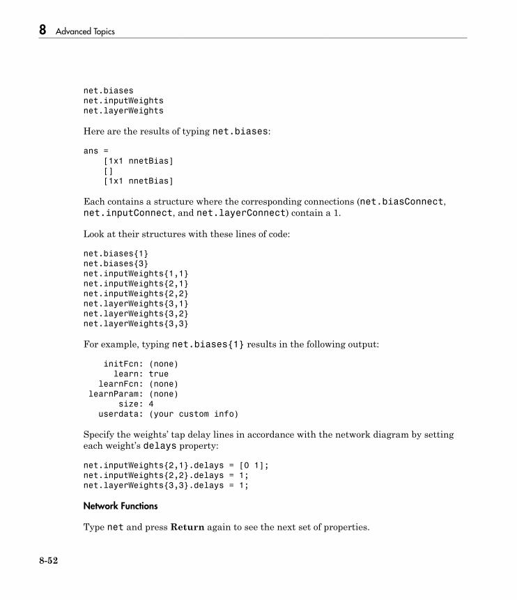
8 Advanced Topics
8-52
net.biases
net.inputWeights
net.layerWeights
Here are the results of typing net.biases:
ans =
[1x1 nnetBias]
[]
[1x1 nnetBias]
Each contains a structure where the corresponding connections (net.biasConnect,net.inputConnect, and net.layerConnect) contain a 1.
Look at their structures with these lines of code:
net.biases{1}
net.biases{3}
net.inputWeights{1,1}
net.inputWeights{2,1}
net.inputWeights{2,2}
net.layerWeights{3,1}
net.layerWeights{3,2}
net.layerWeights{3,3}
For example, typing net.biases{1} results in the following output:
initFcn: (none)
learn: true
learnFcn: (none)
learnParam: (none)
size: 4
userdata: (your custom info)
Specify the weights’ tap delay lines in accordance with the network diagram by settingeach weight’s delays property:
net.inputWeights{2,1}.delays = [0 1];
net.inputWeights{2,2}.delays = 1;
net.layerWeights{3,3}.delays = 1;
Network Functions
Type net and press Return again to see the next set of properties.

Create and Train Custom Neural Network Architectures
8-53
functions:
adaptFcn: (none)
adaptParam: (none)
derivFcn: 'defaultderiv'
divideFcn: (none)
divideParam: (none)
divideMode: 'sample'
initFcn: 'initlay'
performFcn: 'mse'
performParam: .regularization, .normalization
plotFcns: {}
plotParams: {1x0 cell array of 0 params}
trainFcn: (none)
trainParam: (none)
Each of these properties defines a function for a basic network operation.
Set the initialization function to initlay so the network initializes itself accordingto the layer initialization functions already set to initnw, the Nguyen-Widrowinitialization function.
net.initFcn = 'initlay';
This meets the initialization requirement of the network.
Set the performance function to mse (mean squared error) and the training function totrainlm (Levenberg-Marquardt backpropagation) to meet the final requirement of thecustom network.
net.performFcn = 'mse';
net.trainFcn = 'trainlm';
Set the divide function to dividerand (divide training data randomly).
net.divideFcn = 'dividerand';
During supervised training, the input and target data are randomly divided intotraining, test, and validation data sets. The network is trained on the training datauntil its performance begins to decrease on the validation data, which signals thatgeneralization has peaked. The test data provides a completely independent test ofnetwork generalization.
Set the plot functions to plotperform (plot training, validation and test performance)and plottrainstate (plot the state of the training algorithm with respect to epochs).
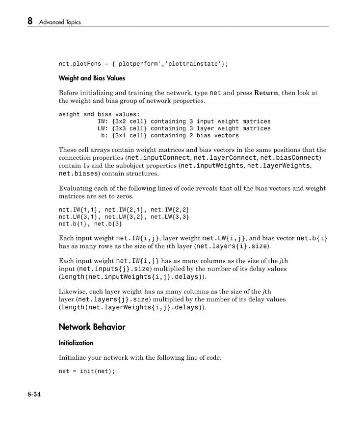
8 Advanced Topics
8-54
net.plotFcns = {'plotperform','plottrainstate'};
Weight and Bias Values
Before initializing and training the network, type net and press Return, then look atthe weight and bias group of network properties.
weight and bias values:
IW: {3x2 cell} containing 3 input weight matrices
LW: {3x3 cell} containing 3 layer weight matrices
b: {3x1 cell} containing 2 bias vectors
These cell arrays contain weight matrices and bias vectors in the same positions that theconnection properties (net.inputConnect, net.layerConnect, net.biasConnect)contain 1s and the subobject properties (net.inputWeights, net.layerWeights,net.biases) contain structures.
Evaluating each of the following lines of code reveals that all the bias vectors and weightmatrices are set to zeros.
net.IW{1,1}, net.IW{2,1}, net.IW{2,2}
net.LW{3,1}, net.LW{3,2}, net.LW{3,3}
net.b{1}, net.b{3}
Each input weight net.IW{i,j}, layer weight net.LW{i,j}, and bias vector net.b{i}has as many rows as the size of the ith layer (net.layers{i}.size).
Each input weight net.IW{i,j} has as many columns as the size of the jthinput (net.inputs{j}.size) multiplied by the number of its delay values(length(net.inputWeights{i,j}.delays)).
Likewise, each layer weight has as many columns as the size of the jthlayer (net.layers{j}.size) multiplied by the number of its delay values(length(net.layerWeights{i,j}.delays)).
Network Behavior
Initialization
Initialize your network with the following line of code:
net = init(net);
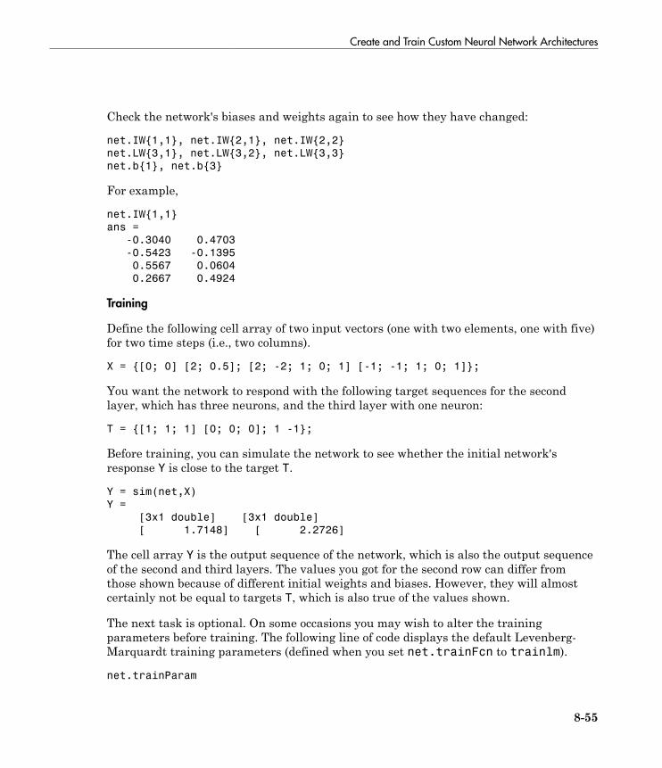
Create and Train Custom Neural Network Architectures
8-55
Check the network's biases and weights again to see how they have changed:
net.IW{1,1}, net.IW{2,1}, net.IW{2,2}
net.LW{3,1}, net.LW{3,2}, net.LW{3,3}
net.b{1}, net.b{3}
For example,
net.IW{1,1}
ans =
-0.3040 0.4703
-0.5423 -0.1395
0.5567 0.0604
0.2667 0.4924
Training
Define the following cell array of two input vectors (one with two elements, one with five)for two time steps (i.e., two columns).
X = {[0; 0] [2; 0.5]; [2; -2; 1; 0; 1] [-1; -1; 1; 0; 1]};
You want the network to respond with the following target sequences for the secondlayer, which has three neurons, and the third layer with one neuron:
T = {[1; 1; 1] [0; 0; 0]; 1 -1};
Before training, you can simulate the network to see whether the initial network'sresponse Y is close to the target T.
Y = sim(net,X)
Y =
[3x1 double] [3x1 double]
[ 1.7148] [ 2.2726]
The cell array Y is the output sequence of the network, which is also the output sequenceof the second and third layers. The values you got for the second row can differ fromthose shown because of different initial weights and biases. However, they will almostcertainly not be equal to targets T, which is also true of the values shown.
The next task is optional. On some occasions you may wish to alter the trainingparameters before training. The following line of code displays the default Levenberg-Marquardt training parameters (defined when you set net.trainFcn to trainlm).
net.trainParam

8 Advanced Topics
8-56
The following properties should be displayed.
ans =
Show Training Window Feedback showWindow: true
Show Command Line Feedback showCommandLine: false
Command Line Frequency show: 25
Maximum Epochs epochs: 1000
Maximum Training Time time: Inf
Performance Goal goal: 0
Minimum Gradient min_grad: 1e-07
Maximum Validation Checks max_fail: 6
Mu mu: 0.001
Mu Decrease Ratio mu_dec: 0.1
Mu Increase Ratio mu_inc: 10
Maximum mu mu_max: 10000000000
You will not often need to modify these values. See the documentation for the trainingfunction for information about what each of these means. They have been initialized withdefault values that work well for a large range of problems, so there is no need to changethem here.
Next, train the network with the following call:
net = train(net,X,T);
Training launches the neural network training window. To open the performance andtraining state plots, click the plot buttons.
After training, you can simulate the network to see if it has learned to respond correctly:
Y = sim(net,X)
[3x1 double] [3x1 double]
[ 1.0000] [ -1.0000]
The second network output (i.e., the second row of the cell array Y), which is also thethird layer’s output, matches the target sequence T.

Custom Neural Network Helper Functions
8-57
Custom Neural Network Helper Functions
The toolbox allows you to create and use your own custom functions. This gives youa great deal of control over the algorithms used to initialize, simulate, and train yournetworks.
Be aware, however, that custom functions may need updating to remain compatible withfuture versions of the software. Backward compatibility of custom functions cannot beguaranteed.
Template functions are available for you to copy, rename and customize, to create yourown versions of these kinds of functions. You can see the list of all template functions bytyping the following:
help nncustom
Each template is a simple version of a different type of function that you can use withyour own custom networks.
For instance, make a copy of the file tansig.m with the new name mytransfer.m.Start editing the new file by changing the function name a the top from tansig tomytransfer.
You can now edit each of the sections of code that make up a transfer function, using thehelp comments in each of those sections to guide you.
Once you are done, store the new function in your working folder, and assign the name ofyour transfer function to the transferFcn property of any layer of any network object toput it to use.

8 Advanced Topics
8-58
Automatically Save Checkpoints During Neural Network TrainingDuring neural network training, intermediate results can be periodically saved to aMAT file for recovery if the computer fails or you kill the training process. This helpsprotect the value of long training runs, which if interrupted would need to be completelyrestarted otherwise.
This feature is especially useful for long parallel training sessions, which are more likelyto be interrupted by computing resource failures. You can stop these training sessionsonly with a Ctrl+C break, because the nntraintool GUI (with its Stop button) is notavailable during parallel training.
Checkpoint saves are enabled with the optional 'CheckpointFile' training argumentfollowed by the checkpoint file name or path. If you specify only a file name, the file isplaced in the working directory by default. The file must have the .mat file extension,but if this is not specified it is automatically appended. In this example, checkpoint savesare made to the file called MyCheckpoint.mat in the current working directory.
[x,t] = house_dataset;
net = feedforwardnet(10);
net2 = train(net,x,t,'CheckpointFile','MyCheckpoint.mat');
22-Mar-2013 04:49:05 First Checkpoint #1: /WorkingDir/MyCheckpoint.mat
22-Mar-2013 04:49:06 Final Checkpoint #2: /WorkingDir/MyCheckpoint.mat
By default, checkpoint saves occur at most once every 60 seconds. For the previous shorttraining example, this results in only two checkpoint saves: one at the beginning and oneat the end of training.
The optional training argument 'CheckpointDelay' can change the frequency of saves.For example, here the minimum checkpoint delay is set to 10 seconds for a time-seriesproblem where a neural network is trained to model a levitated magnet.[x,t] = maglev_dataset;
net = narxnet(1:2,1:2,10);
[X,Xi,Ai,T] = preparets(net,x,{},t);
net2 = train(net,X,T,Xi,Ai,'CheckpointFile','MyCheckpoint.mat','CheckpointDelay',10);
22-Mar-2013 04:59:28 First Checkpoint #1: /WorkingDir/MyCheckpoint.mat
22-Mar-2013 04:59:38 Write Checkpoint #2: /WorkingDir/MyCheckpoint.mat
22-Mar-2013 04:59:48 Write Checkpoint #3: /WorkingDir/MyCheckpoint.mat
22-Mar-2013 04:59:58 Write Checkpoint #4: /WorkingDir/MyCheckpoint.mat
22-Mar-2013 05:00:08 Write Checkpoint #5: /WorkingDir/MyCheckpoint.mat
22-Mar-2013 05:00:09 Final Checkpoint #6: /WorkingDir/MyCheckpoint.mat
After a computer failure or training interruption, you can reload the checkpoint structurecontaining the best neural network obtained before the interruption, and the training
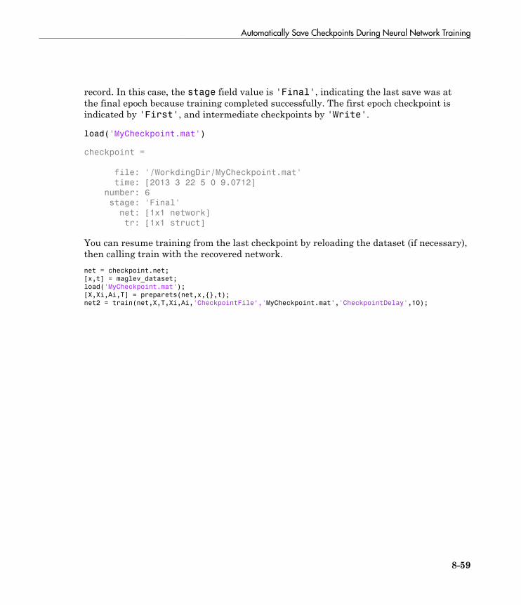
Automatically Save Checkpoints During Neural Network Training
8-59
record. In this case, the stage field value is 'Final', indicating the last save was atthe final epoch because training completed successfully. The first epoch checkpoint isindicated by 'First', and intermediate checkpoints by 'Write'.
load('MyCheckpoint.mat')
checkpoint =
file: '/WorkdingDir/MyCheckpoint.mat'
time: [2013 3 22 5 0 9.0712]
number: 6
stage: 'Final'
net: [1x1 network]
tr: [1x1 struct]
You can resume training from the last checkpoint by reloading the dataset (if necessary),then calling train with the recovered network.net = checkpoint.net;
[x,t] = maglev_dataset;
load('MyCheckpoint.mat');
[X,Xi,Ai,T] = preparets(net,x,{},t);
net2 = train(net,X,T,Xi,Ai,'CheckpointFile’,'MyCheckpoint.mat','CheckpointDelay',10);

8 Advanced Topics
8-60
Deploy Neural Network FunctionsIn this section...
“Deployment Functions and Tools” on page 8-60“Generate Neural Network Functions for Application Deployment” on page 8-61“Generate Simulink Diagrams” on page 8-63
Deployment Functions and Tools
The function genFunction allows stand-alone MATLAB functions for a trained neuralnetwork. The generated code contains all the information needed to simulate a neuralnetwork, including settings, weight and bias values, module functions, and calculations.
The generated MATLAB function can be used to inspect the exact simulation calculationsthat a particular neural network performs, and makes it easier to deploy neuralnetworks for many purposes with a wide variety of MATLAB deployment products andtools.
The function genFunction is introduced in the deployment panels in the tools nftool,nctool, nprtool and ntstool. For information on these tool features, see “Fit Datawith a Neural Network”, “Classify Patterns with a Neural Network”, “Cluster Data witha Self-Organizing Map”, and “Neural Network Time Series Prediction and Modeling”.
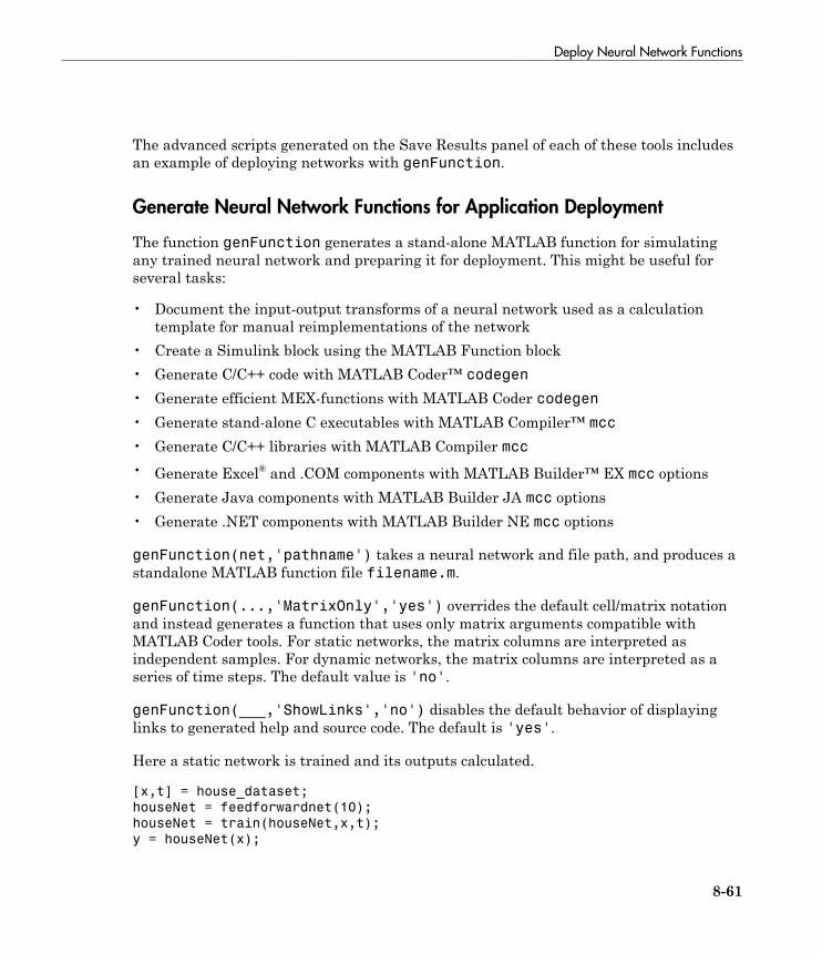
Deploy Neural Network Functions
8-61
The advanced scripts generated on the Save Results panel of each of these tools includesan example of deploying networks with genFunction.
Generate Neural Network Functions for Application Deployment
The function genFunction generates a stand-alone MATLAB function for simulatingany trained neural network and preparing it for deployment. This might be useful forseveral tasks:
• Document the input-output transforms of a neural network used as a calculationtemplate for manual reimplementations of the network
• Create a Simulink block using the MATLAB Function block• Generate C/C++ code with MATLAB Coder™ codegen• Generate efficient MEX-functions with MATLAB Coder codegen• Generate stand-alone C executables with MATLAB Compiler™ mcc• Generate C/C++ libraries with MATLAB Compiler mcc• Generate Excel® and .COM components with MATLAB Builder™ EX mcc options• Generate Java components with MATLAB Builder JA mcc options• Generate .NET components with MATLAB Builder NE mcc options
genFunction(net,'pathname') takes a neural network and file path, and produces astandalone MATLAB function file filename.m.
genFunction(...,'MatrixOnly','yes') overrides the default cell/matrix notationand instead generates a function that uses only matrix arguments compatible withMATLAB Coder tools. For static networks, the matrix columns are interpreted asindependent samples. For dynamic networks, the matrix columns are interpreted as aseries of time steps. The default value is 'no'.
genFunction(___,'ShowLinks','no') disables the default behavior of displayinglinks to generated help and source code. The default is 'yes'.
Here a static network is trained and its outputs calculated.
[x,t] = house_dataset;
houseNet = feedforwardnet(10);
houseNet = train(houseNet,x,t);
y = houseNet(x);

8 Advanced Topics
8-62
The following code generates, tests, and displays a MATLAB function with the sameinterface as the neural network object.
genFunction(houseNet,'houseFcn');
y2 = houseFcn(x);
accuracy2 = max(abs(y-y2))
edit houseFcn
You can compile the new function with the MATLAB Compiler tools (license required) toa shared/dynamically linked library with mcc.
mcc -W lib:libHouse -T link:lib houseFcn
The next code generates another version of the MATLAB function that supports onlymatrix arguments (no cell arrays). This function is tested. Then it is used to generate aMEX-function with the MATLAB Coder tool codegen (license required), which is alsotested.genFunction(houseNet,'houseFcn','MatrixOnly','yes');
y3 = houseFcn(x);
accuracy3 = max(abs(y-y3))
x1Type = coder.typeof(double(0),[13 Inf]); % Coder type of input 1
codegen houseFcn.m -config:mex -o houseCodeGen -args {x1Type}
y4 = houseCodeGen(x);
accuracy4 = max(abs(y-y4))
Here a dynamic network is trained and its outputs calculated.
[x,t] = maglev_dataset;
maglevNet = narxnet(1:2,1:2,10);
[X,Xi,Ai,T] = preparets(maglevNet,x,{},t);
maglevNet = train(maglevNet,X,T,Xi,Ai);
[y,xf,af] = maglevNet(X,Xi,Ai);
Next a MATLAB function is generated and tested. The function is then used to create ashared/dynamically linked library with mcc.
genFunction(maglevNet,'maglevFcn');
[y2,xf,af] = maglevFcn(X,Xi,Ai);
accuracy2 = max(abs(cell2mat(y)-cell2mat(y2)))
mcc -W lib:libMaglev -T link:lib maglevFcn
The following code generates another version of the MATLAB function that supports onlymatrix arguments (no cell arrays). This function is tested. Then it is used to generate aMEX-function with the MATLAB Coder tool codegen, which is also tested.
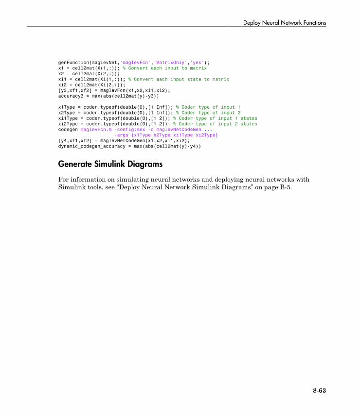
Deploy Neural Network Functions
8-63
genFunction(maglevNet,'maglevFcn','MatrixOnly','yes');
x1 = cell2mat(X(1,:)); % Convert each input to matrix
x2 = cell2mat(X(2,:));
xi1 = cell2mat(Xi(1,:)); % Convert each input state to matrix
xi2 = cell2mat(Xi(2,:));
[y3,xf1,xf2] = maglevFcn(x1,x2,xi1,xi2);
accuracy3 = max(abs(cell2mat(y)-y3))
x1Type = coder.typeof(double(0),[1 Inf]); % Coder type of input 1
x2Type = coder.typeof(double(0),[1 Inf]); % Coder type of input 2
xi1Type = coder.typeof(double(0),[1 2]); % Coder type of input 1 states
xi2Type = coder.typeof(double(0),[1 2]); % Coder type of input 2 states
codegen maglevFcn.m -config:mex -o maglevNetCodeGen ...
-args {x1Type x2Type xi1Type xi2Type}
[y4,xf1,xf2] = maglevNetCodeGen(x1,x2,xi1,xi2);
dynamic_codegen_accuracy = max(abs(cell2mat(y)-y4))
Generate Simulink Diagrams
For information on simulating neural networks and deploying neural networks withSimulink tools, see “Deploy Neural Network Simulink Diagrams” on page B-5.

8-64
9
Historical Neural Networks
• “Historical Neural Networks Overview” on page 9-2• “Perceptron Neural Networks” on page 9-3• “Linear Neural Networks” on page 9-18• “Hopfield Neural Network” on page 9-32
9 Historical Neural Networks
9-2
Historical Neural Networks Overview
This section covers networks that are of historical interest, but that are not as activelyused today as networks presented in other sections. Two of the networks are single-layernetworks that were the first neural networks for which practical training algorithmswere developed: perceptron networks and ADALINE networks. This section also coversrecurrent Hopfield networks.
The perceptron network is a single-layer network whose weights and biases can betrained to produce a correct target vector when presented with the correspondinginput vector. This perceptron rule was the first training algorithm developed forneural networks. The original book on the perceptron is Rosenblatt, F., Principles ofNeurodynamics, Washington D.C., Spartan Press, 1961 [Rose61].
At about the same time that Rosenblatt developed the perceptron network, Widrow andHoff developed a single-layer linear network and associated learning rule, which theycalled the ADALINE (Adaptive Linear Neuron). This network was used to implementadaptive filters, which are still actively used today. The original paper describing thisnetwork is Widrow, B., and M.E. Hoff, “Adaptive switching circuits,” 1960 IRE WESCONConvention Record, New York IRE, 1960, pp. 96–104.
The Hopfield network is used to store one or more stable target vectors. These stablevectors can be viewed as memories that the network recalls when provided with similarvectors that act as a cue to the network memory. You might want to peruse a basic paperin this field:
Li, J., A.N. Michel, and W. Porod, “Analysis and synthesis of a class of neural networks:linear systems operating on a closed hypercube,” IEEE Transactions on Circuits andSystems, Vol. 36, No. 11, November 1989, pp. 1405–1422.

Perceptron Neural Networks
9-3
Perceptron Neural Networks
In this section...
“Neuron Model” on page 9-3“Perceptron Architecture” on page 9-5“Create a Perceptron” on page 9-6“Perceptron Learning Rule (learnp)” on page 9-8“Training (train)” on page 9-10“Limitations and Cautions” on page 9-15
Rosenblatt [Rose61] created many variations of the perceptron. One of the simplestwas a single-layer network whose weights and biases could be trained to produce acorrect target vector when presented with the corresponding input vector. The trainingtechnique used is called the perceptron learning rule. The perceptron generated greatinterest due to its ability to generalize from its training vectors and learn from initiallyrandomly distributed connections. Perceptrons are especially suited for simple problemsin pattern classification. They are fast and reliable networks for the problems they cansolve. In addition, an understanding of the operations of the perceptron provides a goodbasis for understanding more complex networks.
The discussion of perceptrons in this section is necessarily brief. For a more thoroughdiscussion, see Chapter 4, “Perceptron Learning Rule,” of [HDB1996], which discussesthe use of multiple layers of perceptrons to solve more difficult problems beyond thecapability of one layer.
Neuron Model
A perceptron neuron, which uses the hard-limit transfer function hardlim, is shownbelow.
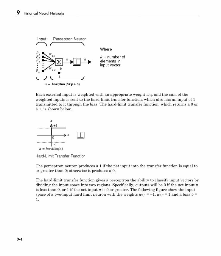
9 Historical Neural Networks
9-4
Each external input is weighted with an appropriate weight w1j, and the sum of theweighted inputs is sent to the hard-limit transfer function, which also has an input of 1transmitted to it through the bias. The hard-limit transfer function, which returns a 0 ora 1, is shown below.
The perceptron neuron produces a 1 if the net input into the transfer function is equal toor greater than 0; otherwise it produces a 0.
The hard-limit transfer function gives a perceptron the ability to classify input vectors bydividing the input space into two regions. Specifically, outputs will be 0 if the net input nis less than 0, or 1 if the net input n is 0 or greater. The following figure show the inputspace of a two-input hard limit neuron with the weights w1,1 = −1, w1,2 = 1 and a bias b =1.
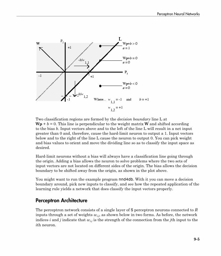
Perceptron Neural Networks
9-5
Two classification regions are formed by the decision boundary line L atWp + b = 0. This line is perpendicular to the weight matrix W and shifted accordingto the bias b. Input vectors above and to the left of the line L will result in a net inputgreater than 0 and, therefore, cause the hard-limit neuron to output a 1. Input vectorsbelow and to the right of the line L cause the neuron to output 0. You can pick weightand bias values to orient and move the dividing line so as to classify the input space asdesired.
Hard-limit neurons without a bias will always have a classification line going throughthe origin. Adding a bias allows the neuron to solve problems where the two sets ofinput vectors are not located on different sides of the origin. The bias allows the decisionboundary to be shifted away from the origin, as shown in the plot above.
You might want to run the example program nnd4db. With it you can move a decisionboundary around, pick new inputs to classify, and see how the repeated application of thelearning rule yields a network that does classify the input vectors properly.
Perceptron Architecture
The perceptron network consists of a single layer of S perceptron neurons connected to Rinputs through a set of weights wi,j, as shown below in two forms. As before, the networkindices i and j indicate that wi,j is the strength of the connection from the jth input to theith neuron.
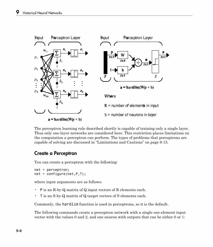
9 Historical Neural Networks
9-6
The perceptron learning rule described shortly is capable of training only a single layer.Thus only one-layer networks are considered here. This restriction places limitations onthe computation a perceptron can perform. The types of problems that perceptrons arecapable of solving are discussed in “Limitations and Cautions” on page 9-15.
Create a Perceptron
You can create a perceptron with the following:
net = perceptron;
net = configure(net,P,T);
where input arguments are as follows:
• P is an R-by-Q matrix of Q input vectors of R elements each.• T is an S-by-Q matrix of Q target vectors of S elements each.
Commonly, the hardlim function is used in perceptrons, so it is the default.
The following commands create a perceptron network with a single one-element inputvector with the values 0 and 2, and one neuron with outputs that can be either 0 or 1:

Perceptron Neural Networks
9-7
P = [0 2];
T = [0 1];
net = perceptron;
net = configure(net,P,T);
You can see what network has been created by executing the following command:
inputweights = net.inputweights{1,1}
which yields
inputweights =
delays: 0
initFcn: 'initzero'
learn: true
learnFcn: 'learnp'
learnParam: (none)
size: [1 1]
weightFcn: 'dotprod'
weightParam: (none)
userdata: (your custom info)
The default learning function is learnp, which is discussed in “Perceptron LearningRule (learnp)” on page 9-8. The net input to the hardlim transfer function isdotprod, which generates the product of the input vector and weight matrix and addsthe bias to compute the net input.
The default initialization function initzero is used to set the initial values of theweights to zero.
Similarly,
biases = net.biases{1}
gives
biases =
initFcn: 'initzero'
learn: 1
learnFcn: 'learnp'
learnParam: []
size: 1
userdata: [1x1 struct]
You can see that the default initialization for the bias is also 0.
9 Historical Neural Networks
9-8
Perceptron Learning Rule (learnp)
Perceptrons are trained on examples of desired behavior. The desired behavior can besummarized by a set of input, output pairs
p t p t p t1 1 2 1, , ,… Q Q
where p is an input to the network and t is the corresponding correct (target) output.The objective is to reduce the error e, which is the difference t − a between the neuronresponse a and the target vector t. The perceptron learning rule learnp calculatesdesired changes to the perceptron's weights and biases, given an input vector p andthe associated error e. The target vector t must contain values of either 0 or 1, becauseperceptrons (with hardlim transfer functions) can only output these values.
Each time learnp is executed, the perceptron has a better chance of producing thecorrect outputs. The perceptron rule is proven to converge on a solution in a finitenumber of iterations if a solution exists.
If a bias is not used, learnp works to find a solution by altering only the weight vector wto point toward input vectors to be classified as 1 and away from vectors to be classifiedas 0. This results in a decision boundary that is perpendicular to w and that properlyclassifies the input vectors.
There are three conditions that can occur for a single neuron once an input vector p ispresented and the network's response a is calculated:
CASE 1. If an input vector is presented and the output of the neuron is correct (a = t ande = t – a = 0), then the weight vector w is not altered.
CASE 2. If the neuron output is 0 and should have been 1 (a = 0 and t = 1, and e =t – a = 1), the input vector p is added to the weight vector w. This makes the weightvector point closer to the input vector, increasing the chance that the input vector will beclassified as a 1 in the future.
CASE 3. If the neuron output is 1 and should have been 0 (a = 1 and t = 0, and e = t – a= –1), the input vector p is subtracted from the weight vector w. This makes the weightvector point farther away from the input vector, increasing the chance that the inputvector will be classified as a 0 in the future.
The perceptron learning rule can be written more succinctly in terms of the error e = t –a and the change to be made to the weight vector Δw:
Perceptron Neural Networks
9-9
CASE 1. If e = 0, then make a change Δw equal to 0.
CASE 2. If e = 1, then make a change Δw equal to pT.
CASE 3. If e = –1, then make a change Δw equal to –pT.
All three cases can then be written with a single expression:
∆w p p= − =( )t eT T
a
You can get the expression for changes in a neuron's bias by noting that the bias issimply a weight that always has an input of 1:
∆b t e= − =( )( )a 1
For the case of a layer of neurons you have
∆W t a p e p= − =( )( ) ( )T T
and
∆b t a= − =( ) e
The perceptron learning rule can be summarized as follows:
W W epnew old T= +
and
b b enew old= +
where e = t – a.
Now try a simple example. Start with a single neuron having an input vector with justtwo elements.
net = perceptron;
net = configure(net,[0;0],0);
To simplify matters, set the bias equal to 0 and the weights to 1 and -0.8:
9 Historical Neural Networks
9-10
net.b{1} = [0];
w = [1 -0.8];
net.IW{1,1} = w;
The input target pair is given by
p = [1; 2];
t = [1];
You can compute the output and error with
a = net(p)
a =
0
e = t-a
e =
1
and use the function learnp to find the change in the weights.
dw = learnp(w,p,[],[],[],[],e,[],[],[],[],[])
dw =
1 2
The new weights, then, are obtained as
w = w + dw
w =
2.0000 1.2000
The process of finding new weights (and biases) can be repeated until there are no errors.Recall that the perceptron learning rule is guaranteed to converge in a finite number ofsteps for all problems that can be solved by a perceptron. These include all classificationproblems that are linearly separable. The objects to be classified in such cases can beseparated by a single line.
You might want to try the example nnd4pr. It allows you to pick new input vectors andapply the learning rule to classify them.
Training (train)
If sim and learnp are used repeatedly to present inputs to a perceptron, and to changethe perceptron weights and biases according to the error, the perceptron will eventually
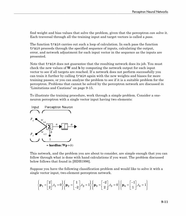
Perceptron Neural Networks
9-11
find weight and bias values that solve the problem, given that the perceptron can solve it.Each traversal through all the training input and target vectors is called a pass.
The function train carries out such a loop of calculation. In each pass the functiontrain proceeds through the specified sequence of inputs, calculating the output,error, and network adjustment for each input vector in the sequence as the inputs arepresented.
Note that train does not guarantee that the resulting network does its job. You mustcheck the new values of W and b by computing the network output for each inputvector to see if all targets are reached. If a network does not perform successfully youcan train it further by calling train again with the new weights and biases for moretraining passes, or you can analyze the problem to see if it is a suitable problem for theperceptron. Problems that cannot be solved by the perceptron network are discussed in“Limitations and Cautions” on page 9-15.
To illustrate the training procedure, work through a simple problem. Consider a one-neuron perceptron with a single vector input having two elements:
This network, and the problem you are about to consider, are simple enough that you canfollow through what is done with hand calculations if you want. The problem discussedbelow follows that found in [HDB1996].
Suppose you have the following classification problem and would like to solve it with asingle vector input, two-element perceptron network.
p p p1 1 2 2 3
2
20
1
21
2
2=
È
ÎÍ
˘
˚˙ =
¸˝Ô
Ô=
-
È
ÎÍ
˘
˚˙ =
ÏÌÔ
ÓÔ
¸˝Ô
Ô=
-È
ÎÍ
˘, ,t t
˚˙ =
ÏÌÔ
ÓÔ
¸˝Ô
Ô=
-È
ÎÍ
˘
˚˙
ÏÌÔ
ÓÔ=
ÏÌÔ
ÓÔ
¸˝Ô
Ô, ,t t3 4 40
1
11p
9 Historical Neural Networks
9-12
Use the initial weights and bias. Denote the variables at each step of this calculationby using a number in parentheses after the variable. Thus, above, the initial values areW(0) and b(0).
w( ) ( )0 0 0 0 0= [ ] =b
Start by calculating the perceptron's output a for the first input vector p1, using theinitial weights and bias.
a = +
= [ ]
+
=
hardlim b
hardlim hardlim
( ( ) ( ))W p0 0
0 02
20
1
(( )0 1=
The output a does not equal the target value t1, so use the perceptron rule to find theincremental changes to the weights and biases based on the error.
e t
e
b e
T
= − = − = −
= = − [ ] = − −[ ]= = − = −
1
1
0 1 1
1 2 2 2 2
1 1
a
∆
∆
W p ( )
( )
You can calculate the new weights and bias using the perceptron update rules.
W W ep Wnew old T
new oldb b e
= + = [ ] + − −[ ] = − −[ ] =
= + = + − = −
0 0 2 2 2 2 1
0 1 1
( )
( ) == b( )1
Now present the next input vector, p2. The output is calculated below.
a = +
= − −[ ] −−
−
=
hardlim b
hardlim har
( ( ) ( ))W p1 1
2 22
21
2
ddlim( )1 1=
On this occasion, the target is 1, so the error is zero. Thus there are no changes inweights or bias, so W(2) = W(1) = [−2 −2] and p(2) = p(1) = −1.
You can continue in this fashion, presenting p3 next, calculating an output and the error,and making changes in the weights and bias, etc. After making one pass through all of
Perceptron Neural Networks
9-13
the four inputs, you get the values W(4) = [−3 −1] and b(4) = 0. To determine whether asatisfactory solution is obtained, make one pass through all input vectors to see if they allproduce the desired target values. This is not true for the fourth input, but the algorithmdoes converge on the sixth presentation of an input. The final values areW(6) = [−2 −3] and b(6) = 1.
This concludes the hand calculation. Now, how can you do this using the train function?
The following code defines a perceptron.
net = perceptron;
Consider the application of a single input
p = [2; 2];
having the target
t = [0];
Set epochs to 1, so that train goes through the input vectors (only one here) just onetime.
net.trainParam.epochs = 1;
net = train(net,p,t);
The new weights and bias are
w = net.iw{1,1}, b = net.b{1}
w =
-2 -2
b =
-1
Thus, the initial weights and bias are 0, and after training on only the first vector, theyhave the values [−2 −2] and −1, just as you hand calculated.
Now apply the second input vector p2. The output is 1, as it will be until the weightsand bias are changed, but now the target is 1, the error will be 0, and the change will bezero. You could proceed in this way, starting from the previous result and applying a newinput vector time after time. But you can do this job automatically with train.
Apply train for one epoch, a single pass through the sequence of all four input vectors.Start with the network definition.

9 Historical Neural Networks
9-14
net = perceptron;
net.trainParam.epochs = 1;
The input vectors and targets are
p = [[2;2] [1;-2] [-2;2] [-1;1]]
t = [0 1 0 1]
Now train the network with
net = train(net,p,t);
The new weights and bias are
w = net.iw{1,1}, b = net.b{1}
w =
-3 -1
b =
0
This is the same result as you got previously by hand.
Finally, simulate the trained network for each of the inputs.
a = net(p)
a =
0 0 1 1
The outputs do not yet equal the targets, so you need to train the network for more thanone pass. Try more epochs. This run gives a mean absolute error performance of 0 aftertwo epochs:
net.trainParam.epochs = 1000;
net = train(net,p,t);
Thus, the network was trained by the time the inputs were presented on the third epoch.(As you know from hand calculation, the network converges on the presentation of thesixth input vector. This occurs in the middle of the second epoch, but it takes the thirdepoch to detect the network convergence.) The final weights and bias are
w = net.iw{1,1}, b = net.b{1}
w =
-2 -3
b =
1
Perceptron Neural Networks
9-15
The simulated output and errors for the various inputs are
a = net(p)
a =
0 1 0 1
error = a-t
error =
0 0 0 0
You confirm that the training procedure is successful. The network converges andproduces the correct target outputs for the four input vectors.
The default training function for networks created with newp is trainc. (You canfind this by executing net.trainFcn.) This training function applies the perceptronlearning rule in its pure form, in that individual input vectors are applied individually,in sequence, and corrections to the weights and bias are made after each presentation ofan input vector. Thus, perceptron training with train will converge in a finite number ofsteps unless the problem presented cannot be solved with a simple perceptron.
The function train can be used in various ways by other networks as well. Type helptrain to read more about this basic function.
You might want to try various example programs. For instance, demop1 illustratesclassification and training of a simple perceptron.
Limitations and Cautions
Perceptron networks should be trained with adapt, which presents the input vectorsto the network one at a time and makes corrections to the network based on the resultsof each presentation. Use of adapt in this way guarantees that any linearly separableproblem is solved in a finite number of training presentations.
As noted in the previous pages, perceptrons can also be trained with the function train.Commonly when train is used for perceptrons, it presents the inputs to the networkin batches, and makes corrections to the network based on the sum of all the individualcorrections. Unfortunately, there is no proof that such a training algorithm converges forperceptrons. On that account the use of train for perceptrons is not recommended.
Perceptron networks have several limitations. First, the output values of a perceptroncan take on only one of two values (0 or 1) because of the hard-limit transfer function.Second, perceptrons can only classify linearly separable sets of vectors. If a straight line

9 Historical Neural Networks
9-16
or a plane can be drawn to separate the input vectors into their correct categories, theinput vectors are linearly separable. If the vectors are not linearly separable, learningwill never reach a point where all vectors are classified properly. However, it hasbeen proven that if the vectors are linearly separable, perceptrons trained adaptivelywill always find a solution in finite time. You might want to try demop6. It shows thedifficulty of trying to classify input vectors that are not linearly separable.
It is only fair, however, to point out that networks with more than one perceptron canbe used to solve more difficult problems. For instance, suppose that you have a set offour vectors that you would like to classify into distinct groups, and that two lines can bedrawn to separate them. A two-neuron network can be found such that its two decisionboundaries classify the inputs into four categories. For additional discussion aboutperceptrons and to examine more complex perceptron problems, see [HDB1996].
Outliers and the Normalized Perceptron Rule
Long training times can be caused by the presence of an outlier input vector whose lengthis much larger or smaller than the other input vectors. Applying the perceptron learningrule involves adding and subtracting input vectors from the current weights and biasesin response to error. Thus, an input vector with large elements can lead to changes in theweights and biases that take a long time for a much smaller input vector to overcome.You might want to try demop4 to see how an outlier affects the training.
By changing the perceptron learning rule slightly, you can make training timesinsensitive to extremely large or small outlier input vectors.
Here is the original rule for updating weights:
∆w p p= − =( )t eT T
a
As shown above, the larger an input vector p, the larger its effect on the weight vectorw. Thus, if an input vector is much larger than other input vectors, the smaller inputvectors must be presented many times to have an effect.
The solution is to normalize the rule so that the effect of each input vector on the weightsis of the same magnitude:
∆wp
p
p
p= − =( )t e
T T
a

Perceptron Neural Networks
9-17
The normalized perceptron rule is implemented with the function learnpn, which iscalled exactly like learnp. The normalized perceptron rule function learnpn takesslightly more time to execute, but reduces the number of epochs considerably if thereare outlier input vectors. You might try demop5 to see how this normalized training ruleworks.
9 Historical Neural Networks
9-18
Linear Neural Networks
In this section...
“Neuron Model” on page 9-18“Network Architecture” on page 9-19“Least Mean Square Error” on page 9-22“Linear System Design (newlind)” on page 9-23“Linear Networks with Delays” on page 9-24“LMS Algorithm (learnwh)” on page 9-26“Linear Classification (train)” on page 9-28“Limitations and Cautions” on page 9-30
The linear networks discussed in this section are similar to the perceptron, but theirtransfer function is linear rather than hard-limiting. This allows their outputs to takeon any value, whereas the perceptron output is limited to either 0 or 1. Linear networks,like the perceptron, can only solve linearly separable problems.
Here you design a linear network that, when presented with a set of given input vectors,produces outputs of corresponding target vectors. For each input vector, you can calculatethe network's output vector. The difference between an output vector and its targetvector is the error. You would like to find values for the network weights and biases suchthat the sum of the squares of the errors is minimized or below a specific value. Thisproblem is manageable because linear systems have a single error minimum. In mostcases, you can calculate a linear network directly, such that its error is a minimum forthe given input vectors and target vectors. In other cases, numerical problems prohibitdirect calculation. Fortunately, you can always train the network to have a minimumerror by using the least mean squares (Widrow-Hoff) algorithm.
This section introduces newlin, a function that creates a linear layer, and newlind, afunction that designs a linear layer for a specific purpose.
Neuron Model
A linear neuron with R inputs is shown below.
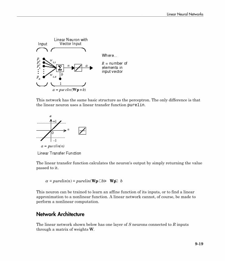
Linear Neural Networks
9-19
This network has the same basic structure as the perceptron. The only difference is thatthe linear neuron uses a linear transfer function purelin.
The linear transfer function calculates the neuron's output by simply returning the valuepassed to it.
a = = + = +purelin n purelin b b( ) ( )Wp Wp
This neuron can be trained to learn an affine function of its inputs, or to find a linearapproximation to a nonlinear function. A linear network cannot, of course, be made toperform a nonlinear computation.
Network Architecture
The linear network shown below has one layer of S neurons connected to R inputsthrough a matrix of weights W.
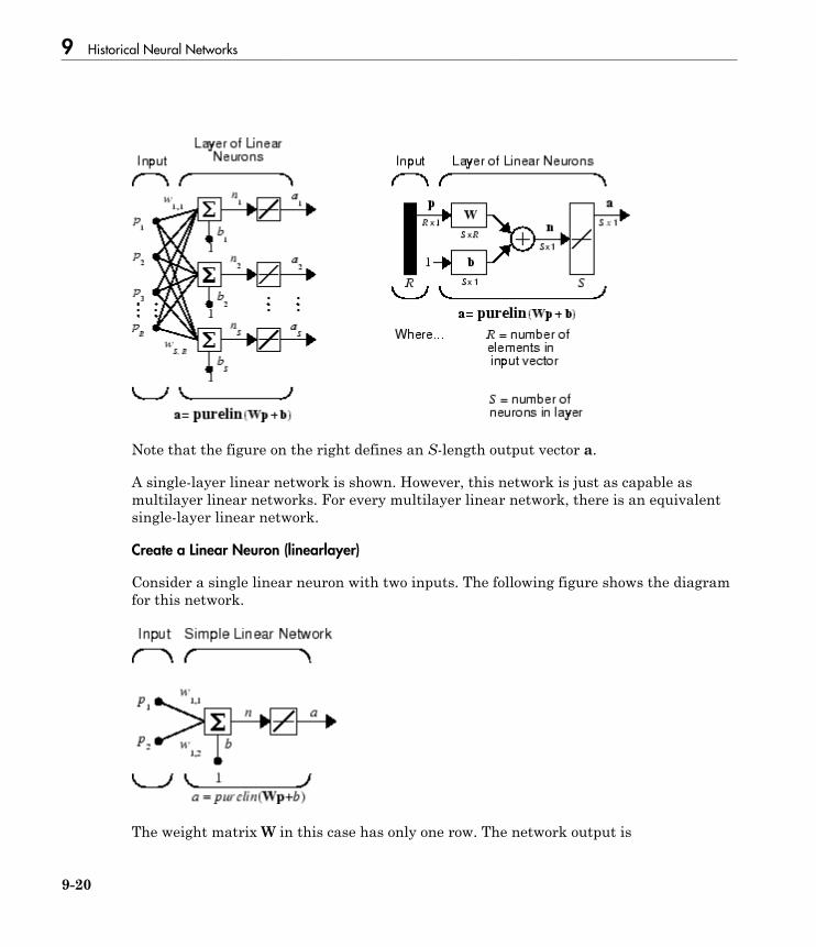
9 Historical Neural Networks
9-20
Note that the figure on the right defines an S-length output vector a.
A single-layer linear network is shown. However, this network is just as capable asmultilayer linear networks. For every multilayer linear network, there is an equivalentsingle-layer linear network.
Create a Linear Neuron (linearlayer)
Consider a single linear neuron with two inputs. The following figure shows the diagramfor this network.
The weight matrix W in this case has only one row. The network output is

Linear Neural Networks
9-21
a = = + = +purelin n purelin b b( ) ( )Wp Wp
or
a = + +w p w p b1 1 1 1 2 2, ,
Like the perceptron, the linear network has a decision boundary that is determined bythe input vectors for which the net input n is zero. For n = 0 the equation Wp + b = 0specifies such a decision boundary, as shown below (adapted with thanks from [HDB96]).
Input vectors in the upper right gray area lead to an output greater than 0. Input vectorsin the lower left white area lead to an output less than 0. Thus, the linear network can beused to classify objects into two categories. However, it can classify in this way only if theobjects are linearly separable. Thus, the linear network has the same limitation as theperceptron.
You can create this network using linearlayer, and configure its dimensions with twovalues so the input has two elements and the output has one.
net = linearlayer;
net = configure(net,[0;0],0);
The network weights and biases are set to zero by default. You can see the current valueswith the commands
W = net.IW{1,1}
W =
0 0

9 Historical Neural Networks
9-22
and
b= net.b{1}
b =
0
However, you can give the weights any values that you want, such as 2 and 3,respectively, with
net.IW{1,1} = [2 3];
W = net.IW{1,1}
W =
2 3
You can set and check the bias in the same way.
net.b{1} = [-4];
b = net.b{1}
b =
-4
You can simulate the linear network for a particular input vector. Try
p = [5;6];
You can find the network output with the function sim.
a = net(p)
a =
24
To summarize, you can create a linear network with newlin, adjust its elements asyou want, and simulate it with sim. You can find more about newlin by typing helpnewlin.
Least Mean Square Error
Like the perceptron learning rule, the least mean square error (LMS) algorithm is anexample of supervised training, in which the learning rule is provided with a set ofexamples of desired network behavior:
p t p t p t1 1 2 2, , , , ,{ } { } { }… Q Q
Linear Neural Networks
9-23
Here pq is an input to the network, and tq is the corresponding target output. As eachinput is applied to the network, the network output is compared to the target. The erroris calculated as the difference between the target output and the network output. Thegoal is to minimize the average of the sum of these errors.
mseQ
e kQ
t k k
k
Q
k
Q
= = −= =∑ ∑1 12
1
2
1
( ) ( ( ) ( ))a
The LMS algorithm adjusts the weights and biases of the linear network so as tominimize this mean square error.
Fortunately, the mean square error performance index for the linear network is aquadratic function. Thus, the performance index will either have one global minimum, aweak minimum, or no minimum, depending on the characteristics of the input vectors.Specifically, the characteristics of the input vectors determine whether or not a uniquesolution exists.
You can find more about this topic in Chapter 10 of [HDB96].
Linear System Design (newlind)
Unlike most other network architectures, linear networks can be designed directly ifinput/target vector pairs are known. You can obtain specific network values for weightsand biases to minimize the mean square error by using the function newlind.
Suppose that the inputs and targets are
P = [1 2 3];
T= [2.0 4.1 5.9];
Now you can design a network.
net = newlind(P,T);
You can simulate the network behavior to check that the design was done properly.
Y = net(P)
Y =
2.0500 4.0000 5.9500
Note that the network outputs are quite close to the desired targets.

9 Historical Neural Networks
9-24
You might try demolin1. It shows error surfaces for a particular problem, illustrates thedesign, and plots the designed solution.
You can also use the function newlind to design linear networks having delays in theinput. Such networks are discussed in “Linear Networks with Delays” on page 9-24.First, however, delays must be discussed.
Linear Networks with Delays
Tapped Delay Line
You need a new component, the tapped delay line, to make full use of the linear network.Such a delay line is shown below. There the input signal enters from the left and passesthrough N-1 delays. The output of the tapped delay line (TDL) is an N-dimensionalvector, made up of the input signal at the current time, the previous input signal, etc.
Linear Filter
You can combine a tapped delay line with a linear network to create the linear filtershown.
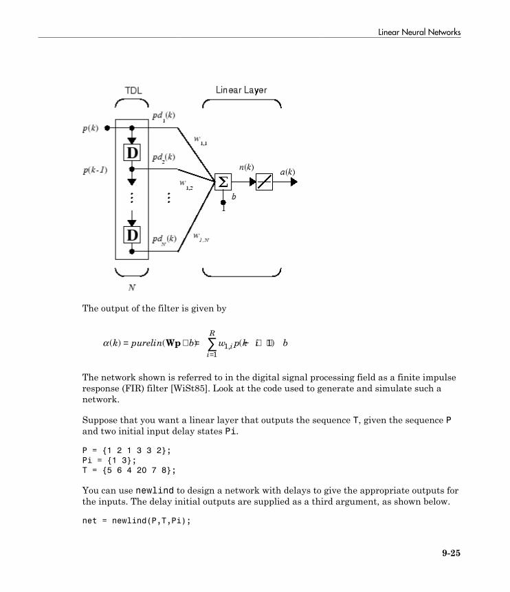
Linear Neural Networks
9-25
The output of the filter is given by
a ( ) ( ) ( ),k purelin b w p k i bii
R
= + = − + +=∑Wp 1
1
1
The network shown is referred to in the digital signal processing field as a finite impulseresponse (FIR) filter [WiSt85]. Look at the code used to generate and simulate such anetwork.
Suppose that you want a linear layer that outputs the sequence T, given the sequence Pand two initial input delay states Pi.
P = {1 2 1 3 3 2};
Pi = {1 3};
T = {5 6 4 20 7 8};
You can use newlind to design a network with delays to give the appropriate outputs forthe inputs. The delay initial outputs are supplied as a third argument, as shown below.
net = newlind(P,T,Pi);
9 Historical Neural Networks
9-26
You can obtain the output of the designed network with
Y = net(P,Pi)
to give
Y = [2.7297] [10.5405] [5.0090] [14.9550] [10.7838] [5.9820]
As you can see, the network outputs are not exactly equal to the targets, but they areclose and the mean square error is minimized.
LMS Algorithm (learnwh)
The LMS algorithm, or Widrow-Hoff learning algorithm, is based on an approximatesteepest descent procedure. Here again, linear networks are trained on examples ofcorrect behavior.
Widrow and Hoff had the insight that they could estimate the mean square error byusing the squared error at each iteration. If you take the partial derivative of the squarederror with respect to the weights and biases at the kth iteration, you have
∂∂
= ∂∂
e k
we k
e k
wj j
2
1 1
2( )
( )( )
, ,
for j = 1,2,…,R and
∂∂
=∂∂
e k
be k
e k
b
2
2( )
( )( )
Next look at the partial derivative with respect to the error.
∂∂
= ∂ −∂
= ∂∂
− +e k
w
t k k
w wt k k b
j j j
( ) [ ( ) ( )][ ( ) ( ( ) )]
, , ,1 1 1
aWp
or
∂∂
=∂
∂− +
=
∑e k
w wt k w p k b
j ji i
i
R( )( ) ( )
, ,,
1 11
1
Linear Neural Networks
9-27
Here pi(k) is the ith element of the input vector at the kth iteration.
This can be simplified to
∂∂
= −e k
wp k
jj
( )( )
,1
and
∂∂
= −e k
b
( )1
Finally, change the weight matrix, and the bias will be2αe(k)p(k)
and2αe(k)
These two equations form the basis of the Widrow-Hoff (LMS) learning algorithm.
These results can be extended to the case of multiple neurons, and written in matrix formas
W W e p
b b e
( ) ( ) ( ) ( )
( ) ( ) ( )
k k k k
k k k
T+ = ++ = +
1 2
1 2
a
a
Here the error e and the bias b are vectors, and α is a learning rate. If α is large, learningoccurs quickly, but if it is too large it can lead to instability and errors might evenincrease. To ensure stable learning, the learning rate must be less than the reciprocal ofthe largest eigenvalue of the correlation matrix pTp of the input vectors.
You might want to read some of Chapter 10 of [HDB96] for more information about theLMS algorithm and its convergence.
Fortunately, there is a toolbox function, learnwh, that does all the calculation for you. Itcalculates the change in weights as
dw = lr*e*p'
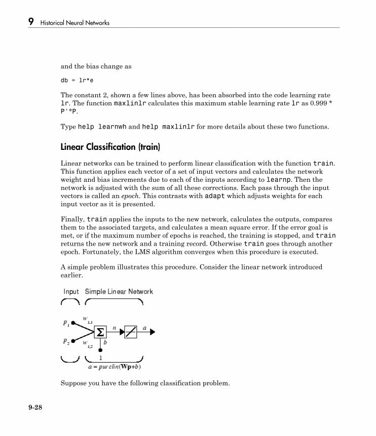
9 Historical Neural Networks
9-28
and the bias change as
db = lr*e
The constant 2, shown a few lines above, has been absorbed into the code learning ratelr. The function maxlinlr calculates this maximum stable learning rate lr as 0.999 *P'*P.
Type help learnwh and help maxlinlr for more details about these two functions.
Linear Classification (train)
Linear networks can be trained to perform linear classification with the function train.This function applies each vector of a set of input vectors and calculates the networkweight and bias increments due to each of the inputs according to learnp. Then thenetwork is adjusted with the sum of all these corrections. Each pass through the inputvectors is called an epoch. This contrasts with adapt which adjusts weights for eachinput vector as it is presented.
Finally, train applies the inputs to the new network, calculates the outputs, comparesthem to the associated targets, and calculates a mean square error. If the error goal ismet, or if the maximum number of epochs is reached, the training is stopped, and trainreturns the new network and a training record. Otherwise train goes through anotherepoch. Fortunately, the LMS algorithm converges when this procedure is executed.
A simple problem illustrates this procedure. Consider the linear network introducedearlier.
Suppose you have the following classification problem.

Linear Neural Networks
9-29
p p p1 1 2 2 3
2
20
1
21
2
2=
È
ÎÍ
˘
˚˙ =
¸˝Ô
Ô=
-
È
ÎÍ
˘
˚˙ =
ÏÌÔ
ÓÔ
¸˝Ô
Ô=
-È
ÎÍ
˘, ,t t
˚˙ =
ÏÌÔ
ÓÔ
¸˝Ô
Ô=
-È
ÎÍ
˘
˚˙
ÏÌÔ
ÓÔ=
ÏÌÔ
ÓÔ
¸˝Ô
Ô, ,t t3 4 40
1
11p
Here there are four input vectors, and you want a network that produces the outputcorresponding to each input vector when that vector is presented.
Use train to get the weights and biases for a network that produces the correct targetsfor each input vector. The initial weights and bias for the new network are 0 by default.Set the error goal to 0.1 rather than accept its default of 0.
P = [2 1 -2 -1;2 -2 2 1];
T = [0 1 0 1];
net = linearlayer;
net.trainParam.goal= 0.1;
net = train(net,P,T);
The problem runs for 64 epochs, achieving a mean square error of 0.0999. The newweights and bias are
weights = net.iw{1,1}
weights =
-0.0615 -0.2194
bias = net.b(1)
bias =
[0.5899]
You can simulate the new network as shown below.
A = net(P)
A =
0.0282 0.9672 0.2741 0.4320
You can also calculate the error.
err = T - sim(net,P)
err =
-0.0282 0.0328 -0.2741 0.5680
Note that the targets are not realized exactly. The problem would have run longerin an attempt to get perfect results had a smaller error goal been chosen, but in thisproblem it is not possible to obtain a goal of 0. The network is limited in its capability.See “Limitations and Cautions” on page 9-30 for examples of various limitations.

9 Historical Neural Networks
9-30
This example program, demolin2, shows the training of a linear neuron and plots theweight trajectory and error during training.
You might also try running the example program nnd10lc. It addresses a classicand historically interesting problem, shows how a network can be trained to classifyvarious patterns, and shows how the trained network responds when noisy patterns arepresented.
Limitations and Cautions
Linear networks can only learn linear relationships between input and output vectors.Thus, they cannot find solutions to some problems. However, even if a perfect solutiondoes not exist, the linear network will minimize the sum of squared errors if the learningrate lr is sufficiently small. The network will find as close a solution as is possible giventhe linear nature of the network's architecture. This property holds because the errorsurface of a linear network is a multidimensional parabola. Because parabolas haveonly one minimum, a gradient descent algorithm (such as the LMS rule) must produce asolution at that minimum.
Linear networks have various other limitations. Some of them are discussed below.
Overdetermined Systems
Consider an overdetermined system. Suppose that you have a network to be trainedwith four one-element input vectors and four targets. A perfect solution to wp + b = t foreach of the inputs might not exist, for there are four constraining equations, and onlyone weight and one bias to adjust. However, the LMS rule still minimizes the error. Youmight try demolin4 to see how this is done.
Underdetermined Systems
Consider a single linear neuron with one input. This time, in demolin5, train it on onlyone one-element input vector and its one-element target vector:
P = [1.0];
T = [0.5];
Note that while there is only one constraint arising from the single input/target pair,there are two variables, the weight and the bias. Having more variables than constraintsresults in an underdetermined problem with an infinite number of solutions. You can trydemolin5 to explore this topic.

Linear Neural Networks
9-31
Linearly Dependent Vectors
Normally it is a straightforward job to determine whether or not a linear network cansolve a problem. Commonly, if a linear network has at least as many degrees of freedom(S *R + S = number of weights and biases) as constraints (Q = pairs of input/targetvectors), then the network can solve the problem. This is true except when the inputvectors are linearly dependent and they are applied to a network without biases. In thiscase, as shown with the example demolin6, the network cannot solve the problem withzero error. You might want to try demolin6.
Too Large a Learning Rate
You can always train a linear network with the Widrow-Hoff rule to find the minimumerror solution for its weights and biases, as long as the learning rate is small enough.Example demolin7 shows what happens when a neuron with one input and a bias istrained with a learning rate larger than that recommended by maxlinlr. The network istrained with two different learning rates to show the results of using too large a learningrate.
9 Historical Neural Networks
9-32
Hopfield Neural Network
In this section...
“Fundamentals” on page 9-32“Architecture” on page 9-32“Design (newhop)” on page 9-34“Summary” on page 9-38
Fundamentals
The goal here is to design a network that stores a specific set of equilibrium points suchthat, when an initial condition is provided, the network eventually comes to rest at sucha design point. The network is recursive in that the output is fed back as the input,once the network is in operation. Hopefully, the network output will settle on one of theoriginal design points.
The design method presented is not perfect in that the designed network can havespurious undesired equilibrium points in addition to the desired ones. However, thenumber of these undesired points is made as small as possible by the design method.Further, the domain of attraction of the designed equilibrium points is as large aspossible.
The design method is based on a system of first-order linear ordinary differentialequations that are defined on a closed hypercube of the state space. The solutions existon the boundary of the hypercube. These systems have the basic structure of the Hopfieldmodel, but are easier to understand and design than the Hopfield model.
The material in this section is based on the following paper: Jian-Hua Li, Anthony N.Michel, and Wolfgang Porod, “Analysis and synthesis of a class of neural networks: linearsystems operating on a closed hypercube,” IEEE Trans. on Circuits and Systems, Vol. 36,No. 11, November 1989, pp. 1405–22.
For further information on Hopfield networks, read Chapter 18 of the Hopfield Network[HDB96].
Architecture
The architecture of the Hopfield network follows.

Hopfield Neural Network
9-33
As noted, the input p to this network merely supplies the initial conditions.
The Hopfield network uses the saturated linear transfer function satlins.
For inputs less than −1 satlins produces −1. For inputs in the range −1 to +1 it simplyreturns the input value. For inputs greater than +1 it produces +1.
This network can be tested with one or more input vectors that are presented as initialconditions to the network. After the initial conditions are given, the network produces anoutput that is then fed back to become the input. This process is repeated over and overuntil the output stabilizes. Hopefully, each output vector eventually converges to one ofthe design equilibrium point vectors that is closest to the input that provoked it.
9 Historical Neural Networks
9-34
Design (newhop)
Li et al. [LiMi89] have studied a system that has the basic structure of the Hopfieldnetwork but is, in Li's own words, “easier to analyze, synthesize, and implement thanthe Hopfield model.” The authors are enthusiastic about the reference article, as it hasmany excellent points and is one of the most readable in the field. However, the designis mathematically complex, and even a short justification of it would burden this guide.Thus the Li design method is presented, with thanks to Li et al., as a recipe that is foundin the function newhop.
Given a set of target equilibrium points represented as a matrix T of vectors, newhopreturns weights and biases for a recursive network. The network is guaranteed to havestable equilibrium points at the target vectors, but it could contain other spuriousequilibrium points as well. The number of these undesired points is made as small aspossible by the design method.
Once the network has been designed, it can be tested with one or more input vectors.Hopefully those input vectors close to target equilibrium points will find their targets.As suggested by the network figure, an array of input vectors is presented one at a timeor in a batch. The network proceeds to give output vectors that are fed back as inputs.These output vectors can be can be compared to the target vectors to see how the solutionis proceeding.
The ability to run batches of trial input vectors quickly allows you to check the designin a relatively short time. First you might check to see that the target equilibrium pointvectors are indeed contained in the network. Then you could try other input vectors todetermine the domains of attraction of the target equilibrium points and the locations ofspurious equilibrium points if they are present.
Consider the following design example. Suppose that you want to design a network withtwo stable points in a three-dimensional space.
T = [-1 -1 1; 1 -1 1]'
T =
-1 1
-1 -1
1 1
You can execute the design with
net = newhop(T);
Hopfield Neural Network
9-35
Next, check to make sure that the designed network is at these two points, as follows.Because Hopfield networks have no inputs, the second argument to the network is anempty cell array whose columns indicate the number of time steps.
Ai = {T};
[Y,Pf,Af] = net(cell(1,2),{},Ai);
Y{2}
This gives you
-1 1
-1 -1
1 1
Thus, the network has indeed been designed to be stable at its design points. Next youcan try another input condition that is not a design point, such as
Ai = {[-0.9; -0.8; 0.7]};
This point is reasonably close to the first design point, so you might anticipate that thenetwork would converge to that first point. To see if this happens, run the following code.
[Y,Pf,Af] = net(cell(1,5),{},Ai);
Y{end}
This produces
-1
-1
1
Thus, an original condition close to a design point did converge to that point.
This is, of course, the hope for all such inputs. Unfortunately, even the best knownHopfield designs occasionally include spurious undesired stable points that attract thesolution.
Example
Consider a Hopfield network with just two neurons. Each neuron has a bias and weightsto accommodate two-element input vectors weighted. The target equilibrium points aredefined to be stored in the network as the two columns of the matrix T.
T = [1 -1; -1 1]'
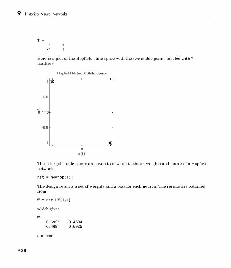
9 Historical Neural Networks
9-36
T =
1 -1
-1 1
Here is a plot of the Hopfield state space with the two stable points labeled with *markers.
These target stable points are given to newhop to obtain weights and biases of a Hopfieldnetwork.
net = newhop(T);
The design returns a set of weights and a bias for each neuron. The results are obtainedfrom
W = net.LW{1,1}
which gives
W =
0.6925 -0.4694
-0.4694 0.6925
and from
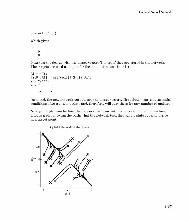
Hopfield Neural Network
9-37
b = net.b{1,1}
which gives
b =
0
0
Next test the design with the target vectors T to see if they are stored in the network.The targets are used as inputs for the simulation function sim.
Ai = {T};
[Y,Pf,Af] = net(cell(1,2),{},Ai);
Y = Y{end}
ans =
1 -1
-1 1
As hoped, the new network outputs are the target vectors. The solution stays at its initialconditions after a single update and, therefore, will stay there for any number of updates.
Now you might wonder how the network performs with various random input vectors.Here is a plot showing the paths that the network took through its state space to arriveat a target point.
9 Historical Neural Networks
9-38
This plot show the trajectories of the solution for various starting points. You can try theexample demohop1 to see more of this kind of network behavior.
Hopfield networks can be designed for an arbitrary number of dimensions. You can trydemohop3 to see a three-dimensional design.
Unfortunately, Hopfield networks can have both unstable equilibrium points andspurious stable points. You can try examples demohop2 and demohop4 to investigatethese issues.
Summary
Hopfield networks can act as error correction or vector categorization networks. Inputvectors are used as the initial conditions to the network, which recurrently updates untilit reaches a stable output vector.
Hopfield networks are interesting from a theoretical standpoint, but are seldom usedin practice. Even the best Hopfield designs may have spurious stable points that leadto incorrect answers. More efficient and reliable error correction techniques, such asbackpropagation, are available.
Functions
This topic introduces the following functions:
Function Description
newhop Create a Hopfield recurrent network.satlins Symmetric saturating linear transfer function.

10
Neural Network Object Reference
• “Neural Network Object Properties” on page 10-2• “Neural Network Subobject Properties” on page 10-14
10 Neural Network Object Reference
10-2
Neural Network Object Properties
In this section...
“General” on page 10-2“Architecture” on page 10-2“Subobject Structures” on page 10-6“Functions” on page 10-8“Weight and Bias Values” on page 10-11
These properties define the basic features of a network. “Neural Network SubobjectProperties” on page 10-14 describes properties that define network details.
General
Here are the general properties of neural networks.
net.name
This property consists of a string defining the network name. Network creation functions,such as feedforwardnet, define this appropriately. But it can be set to any string asdesired.
net.userdata
This property provides a place for users to add custom information to a network object.Only one field is predefined. It contains a secret message to all Neural Network Toolboxusers:
net.userdata.note
Architecture
These properties determine the number of network subobjects (which include inputs,layers, outputs, targets, biases, and weights), and how they are connected.
net.numInputs
This property defines the number of inputs a network receives. It can be set to 0 or apositive integer.

Neural Network Object Properties
10-3
Clarification
The number of network inputs and the size of a network input are not the same thing.The number of inputs defines how many sets of vectors the network receives as input.The size of each input (i.e., the number of elements in each input vector) is determined bythe input size (net.inputs{i}.size).
Most networks have only one input, whose size is determined by the problem.
Side Effects
Any change to this property results in a change in the size of the matrix definingconnections to layers from inputs, (net.inputConnect) and the size of the cell array ofinput subobjects (net.inputs).
net.numLayers
This property defines the number of layers a network has. It can be set to 0 or a positiveinteger.
Side Effects
Any change to this property changes the size of each of these Boolean matrices thatdefine connections to and from layers:
net.biasConnect
net.inputConnect
net.layerConnect
net.outputConnect
and changes the size of each cell array of subobject structures whose size depends on thenumber of layers:
net.biases
net.inputWeights
net.layerWeights
net.outputs
and also changes the size of each of the network's adjustable parameter's properties:
net.IW
net.LW
net.b
10 Neural Network Object Reference
10-4
net.biasConnect
This property defines which layers have biases. It can be set to any N-by-1 matrix ofBoolean values, where Nl is the number of network layers (net.numLayers). Thepresence (or absence) of a bias to the ith layer is indicated by a 1 (or 0) at
net.biasConnect(i)
Side Effects
Any change to this property alters the presence or absence of structures in the cell arrayof biases (net.biases) and, in the presence or absence of vectors in the cell array, ofbias vectors (net.b).
net.inputConnect
This property defines which layers have weights coming from inputs.
It can be set to any Nl × Ni matrix of Boolean values, where Nl is the number of networklayers (net.numLayers), and Ni is the number of network inputs (net.numInputs).The presence (or absence) of a weight going to the ith layer from the jth input is indicatedby a 1 (or 0) at net.inputConnect(i,j).
Side Effects
Any change to this property alters the presence or absence of structures in the cell arrayof input weight subobjects (net.inputWeights) and the presence or absence of matricesin the cell array of input weight matrices (net.IW).
net.layerConnect
This property defines which layers have weights coming from other layers. It can beset to any Nl × Nl matrix of Boolean values, where Nl is the number of network layers(net.numLayers). The presence (or absence) of a weight going to the ith layer from thejth layer is indicated by a 1 (or 0) at
net.layerConnect(i,j)
Side Effects
Any change to this property alters the presence or absence of structures in the cell arrayof layer weight subobjects (net.layerWeights) and the presence or absence of matricesin the cell array of layer weight matrices (net.LW).
Neural Network Object Properties
10-5
net.outputConnect
This property defines which layers generate network outputs. It can be set to any 1 × Nlmatrix of Boolean values, where Nl is the number of network layers (net.numLayers).The presence (or absence) of a network output from the ith layer is indicated by a 1 (or 0)at net.outputConnect(i).Side Effects
Any change to this property alters the number of network outputs (net.numOutputs)and the presence or absence of structures in the cell array of output subobjects(net.outputs).
net.numOutputs (read only)
This property indicates how many outputs the network has. It is always equal to thenumber of 1s in net.outputConnect.
net.numInputDelays (read only)
This property indicates the number of time steps of past inputs that must be supplied tosimulate the network. It is always set to the maximum delay value associated with any ofthe network's input weights:
numInputDelays = 0;
for i=1:net.numLayers
for j=1:net.numInputs
if net.inputConnect(i,j)
numInputDelays = max( ...
[numInputDelays net.inputWeights{i,j}.delays]);
end
end
end
net.numLayerDelays (read only)
This property indicates the number of time steps of past layer outputs that must besupplied to simulate the network. It is always set to the maximum delay value associatedwith any of the network's layer weights:
numLayerDelays = 0;
for i=1:net.numLayers
for j=1:net.numLayers
if net.layerConnect(i,j)
numLayerDelays = max( ...
10 Neural Network Object Reference
10-6
[numLayerDelays net.layerWeights{i,j}.delays]);
end
end
end
net.numWeightElements (read only)
This property indicates the number of weight and bias values in the network. It is thesum of the number of elements in the matrices stored in the two cell arrays:
net.IW
new.b
Subobject Structures
These properties consist of cell arrays of structures that define each of the network'sinputs, layers, outputs, targets, biases, and weights.
The properties for each kind of subobject are described in “Neural Network SubobjectProperties” on page 10-14.
net.inputs
This property holds structures of properties for each of the network's inputs. It is alwaysan Ni × 1 cell array of input structures, where Ni is the number of network inputs(net.numInputs).
The structure defining the properties of the ith network input is located at
net.inputs{i}
If a neural network has only one input, then you can access net.inputs{1} without thecell array notation as follows:
net.input
Input Properties
See “Inputs” on page 10-14 for descriptions of input properties.
net.layers
This property holds structures of properties for each of the network's layers. It is alwaysan Nl × 1 cell array of layer structures, where Nl is the number of network layers(net.numLayers).
Neural Network Object Properties
10-7
The structure defining the properties of the ith layer is located at net.layers{i}.Layer Properties
See “Layers” on page 10-16 for descriptions of layer properties.
net.outputs
This property holds structures of properties for each of the network's outputs.It is always a 1 × Nl cell array, where Nl is the number of network outputs(net.numOutputs).
The structure defining the properties of the output from the ith layer (or a null matrix[]) is located at net.outputs{i} if net.outputConnect(i) is 1 (or 0).
If a neural network has only one output at layer i, then you can access net.outputs{i}without the cell array notation as follows:
net.output
Output Properties
See “Outputs” on page 10-22 for descriptions of output properties.
net.biases
This property holds structures of properties for each of the network's biases. It is alwaysan Nl × 1 cell array, where Nl is the number of network layers (net.numLayers).
The structure defining the properties of the bias associated with the ith layer (or a nullmatrix []) is located at net.biases{i} if net.biasConnect(i) is 1 (or 0).Bias Properties
See “Biases” on page 10-24 for descriptions of bias properties.
net.inputWeights
This property holds structures of properties for each of the network's input weights.It is always an Nl × Ni cell array, where Nl is the number of network layers(net.numLayers), and Ni is the number of network inputs (net.numInputs).
The structure defining the properties of the weight going to the ith layer fromthe jth input (or a null matrix []) is located at net.inputWeights{i,j} ifnet.inputConnect(i,j) is 1 (or 0).
10 Neural Network Object Reference
10-8
Input Weight Properties
See “Input Weights” on page 10-25 for descriptions of input weight properties.
net.layerWeights
This property holds structures of properties for each of the network's layer weights. It isalways an Nl ×Nl cell array, where Nl is the number of network layers (net.numLayers).
The structure defining the properties of the weight going to the ith layer fromthe jth layer (or a null matrix []) is located at net.layerWeights{i,j} ifnet.layerConnect(i,j) is 1 (or 0).
Layer Weight Properties
See “Layer Weights” on page 10-26 for descriptions of layer weight properties.
Functions
These properties define the algorithms to use when a network is to adapt, is to beinitialized, is to have its performance measured, or is to be trained.
net.adaptFcn
This property defines the function to be used when the network adapts. It can be set tothe name of any network adapt function. The network adapt function is used to performadaption whenever adapt is called.
[net,Y,E,Pf,Af] = adapt(NET,P,T,Pi,Ai)
For a list of functions, type help nntrain.
Side Effects
Whenever this property is altered, the network's adaption parameters(net.adaptParam) are set to contain the parameters and default values of the newfunction.
net.adaptParam
This property defines the parameters and values of the current adapt function. Call helpon the current adapt function to get a description of what each field means:
help(net.adaptFcn)
Neural Network Object Properties
10-9
net.derivFcn
This property defines the derivative function to be used to calculate error gradientsand Jacobians when the network is trained using a supervised algorithm, such asbackpropagation. You can set this property to the name of any derivative function.
For a list of functions, type help nnderivative.
net.divideFcn
This property defines the data division function to be used when the network is trainedusing a supervised algorithm, such as backpropagation. You can set this property to thename of a division function.
For a list of functions, type help nndivision.
Side Effects
Whenever this property is altered, the network's adaption parameters(net.divideParam) are set to contain the parameters and default values of the newfunction.
net.divideParam
This property defines the parameters and values of the current data-division function. Toget a description of what each field means, type the following command:
help(net.divideParam)
net.divideMode
This property defines the target data dimensions which to divide up when the datadivision function is called. Its default value is 'sample' for static networks and 'time'for dynamic networks. It may also be set to 'sampletime' to divide targets by bothsample and timestep, 'all' to divide up targets by every scalar value, or 'none' to notdivide up data at all (in which case all data is used for training, none for validation ortesting).
net.initFcn
This property defines the function used to initialize the network's weight matrices andbias vectors. . The initialization function is used to initialize the network whenever initis called:
10 Neural Network Object Reference
10-10
net = init(net)
Side Effects
Whenever this property is altered, the network's initialization parameters(net.initParam) are set to contain the parameters and default values of the newfunction.
net.initParam
This property defines the parameters and values of the current initialization function.Call help on the current initialization function to get a description of what each fieldmeans:
help(net.initFcn)
net.performFcn
This property defines the function used to measure the network’s performance. Theperformance function is used to calculate network performance during training whenevertrain is called.
[net,tr] = train(NET,P,T,Pi,Ai)
For a list of functions, type help nnperformance.
Side Effects
Whenever this property is altered, the network's performance parameters(net.performParam) are set to contain the parameters and default values of the newfunction.
net.performParam
This property defines the parameters and values of the current performance function.Call help on the current performance function to get a description of what each fieldmeans:
help(net.performFcn)
net.plotFcns
This property consists of a row cell array of strings, defining the plot functions associatedwith a network. The neural network training window, which is opened by the train

Neural Network Object Properties
10-11
function, shows a button for each plotting function. Click the button during or aftertraining to open the desired plot.
net.plotParams
This property consists of a row cell array of structures, defining the parameters andvalues of each plot function in net.plotFcns. Call help on the each plot function to geta description of what each field means:
help(net.plotFcns{i})
net.trainFcn
This property defines the function used to train the network. It can be set to the nameof any of the training functions, which is used to train the network whenever train iscalled.
[net,tr] = train(NET,P,T,Pi,Ai)
For a list of functions, type help nntrain.
Side Effects
Whenever this property is altered, the network's training parameters (net.trainParam)are set to contain the parameters and default values of the new function.
net.trainParam
This property defines the parameters and values of the current training function. Callhelp on the current training function to get a description of what each field means:
help(net.trainFcn)
Weight and Bias Values
These properties define the network's adjustable parameters: its weight matrices andbias vectors.
net.IW
This property defines the weight matrices of weights going to layers from networkinputs. It is always an Nl × Ni cell array, where Nl is the number of network layers(net.numLayers), and Ni is the number of network inputs (net.numInputs).
10 Neural Network Object Reference
10-12
The weight matrix for the weight going to the ith layer from the jth input (or a nullmatrix []) is located at net.IW{i,j} if net.inputConnect(i,j) is 1 (or 0).
The weight matrix has as many rows as the size of the layer it goes to(net.layers{i}.size). It has as many columns as the product of the input size withthe number of delays associated with the weight:
net.inputs{j}.size * length(net.inputWeights{i,j}.delays)
These dimensions can also be obtained from the input weight properties:
net.inputWeights{i,j}.size
net.LW
This property defines the weight matrices of weights going to layers from otherlayers. It is always an Nl × Nl cell array, where Nl is the number of network layers(net.numLayers).
The weight matrix for the weight going to the ith layer from the jth layer (or a nullmatrix []) is located at net.LW{i,j} if net.layerConnect(i,j) is 1 (or 0).
The weight matrix has as many rows as the size of the layer it goes to(net.layers{i}.size). It has as many columns as the product of the size of the layer itcomes from with the number of delays associated with the weight:
net.layers{j}.size * length(net.layerWeights{i,j}.delays)
These dimensions can also be obtained from the layer weight properties:
net.layerWeights{i,j}.size
net.b
This property defines the bias vectors for each layer with a bias. It is always an Nl × 1cell array, where Nl is the number of network layers (net.numLayers).
The bias vector for the ith layer (or a null matrix []) is located at net.b{i} ifnet.biasConnect(i) is 1 (or 0).
The number of elements in the bias vector is always equal to the size of the layer it isassociated with (net.layers{i}.size).
This dimension can also be obtained from the bias properties:

Neural Network Object Properties
10-13
net.biases{i}.size
10 Neural Network Object Reference
10-14
Neural Network Subobject Properties
These properties define the details of a network's inputs, layers, outputs, targets, biases,and weights.
In this section...
“Inputs” on page 10-14“Layers” on page 10-16“Outputs” on page 10-22“Biases” on page 10-24“Input Weights” on page 10-25“Layer Weights” on page 10-26
Inputs
These properties define the details of each ith network input.
net.inputs{1}.name
This property consists of a string defining the input name. Network creation functions,such as feedforwardnet, define this appropriately. But it can be set to any string asdesired.
net.inputs{i}.feedbackInput (read only)
If this network is associated with an open-loop feedback output, then this property willindicate the index of that output. Otherwise it will be an empty matrix.
net.inputs{i}.processFcns
This property defines a row cell array of processing function names to be used by ithnetwork input. The processing functions are applied to input values before the networkuses them.
Side Effects
Whenever this property is altered, the input processParams are set to defaultvalues for the given processing functions, processSettings, processedSize, and

Neural Network Subobject Properties
10-15
processedRange are defined by applying the process functions and parameters toexampleInput.
For a list of processing functions, type help nnprocess.
net.inputs{i}.processParams
This property holds a row cell array of processing function parameters to be used by ithnetwork input. The processing parameters are applied by the processing functions toinput values before the network uses them.Side Effects
Whenever this property is altered, the input processSettings, processedSize,and processedRange are defined by applying the process functions and parameters toexampleInput.
net.inputs{i}.processSettings (read only)
This property holds a row cell array of processing function settings to be used by ithnetwork input. The processing settings are found by applying the processing functionsand parameters to exampleInput and then used to provide consistent results to newinput values before the network uses them.
net.inputs{i}.processedRange (read only)
This property defines the range of exampleInput values after they have been processedwith processingFcns and processingParams.
net.inputs{i}.processedSize (read only)
This property defines the number of rows in the exampleInput values after they havebeen processed with processingFcns and processingParams.
net.inputs{i}.range
This property defines the range of each element of the ith network input.
It can be set to any Ri × 2 matrix, where Ri is the number of elements in the input(net.inputs{i}.size), and each element in column 1 is less than the element next toit in column 2.
Each jth row defines the minimum and maximum values of the jth input element, in thatorder:

10 Neural Network Object Reference
10-16
net.inputs{i}(j,:)
Uses
Some initialization functions use input ranges to find appropriate initial values for inputweight matrices.
Side Effects
Whenever the number of rows in this property is altered, the input size,processedSize, and processedRange change to remain consistent. The sizes of anyweights coming from this input and the dimensions of the weight matrices also change.
net.inputs{i}.size
This property defines the number of elements in the ith network input. It can be set to 0or a positive integer.
Side Effects
Whenever this property is altered, the input range, processedRange, andprocessedSize are updated. Any associated input weights change size accordingly.
net.inputs{i}.userdata
This property provides a place for users to add custom information to the ith networkinput.
Layers
These properties define the details of each ith network layer.
net.layers{i}.name
This property consists of a string defining the layer name. Network creation functions,such as feedforwardnet, define this appropriately. But it can be set to any string asdesired.
net.layers{i}.dimensions
This property defines the physical dimensions of the ith layer's neurons. Being able toarrange a layer's neurons in a multidimensional manner is important for self-organizingmaps.
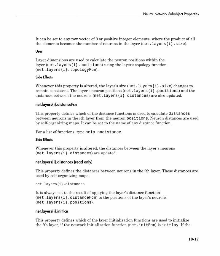
Neural Network Subobject Properties
10-17
It can be set to any row vector of 0 or positive integer elements, where the product of allthe elements becomes the number of neurons in the layer (net.layers{i}.size).
Uses
Layer dimensions are used to calculate the neuron positions within thelayer (net.layers{i}.positions) using the layer's topology function(net.layers{i}.topologyFcn).
Side Effects
Whenever this property is altered, the layer's size (net.layers{i}.size) changes toremain consistent. The layer's neuron positions (net.layers{i}.positions) and thedistances between the neurons (net.layers{i}.distances) are also updated.
net.layers{i}.distanceFcn
This property defines which of the distance functions is used to calculate distancesbetween neurons in the ith layer from the neuron positions. Neuron distances are usedby self-organizing maps. It can be set to the name of any distance function.
For a list of functions, type help nndistance.
Side Effects
Whenever this property is altered, the distances between the layer's neurons(net.layers{i}.distances) are updated.
net.layers{i}.distances (read only)
This property defines the distances between neurons in the ith layer. These distances areused by self-organizing maps:
net.layers{i}.distances
It is always set to the result of applying the layer's distance function(net.layers{i}.distanceFcn) to the positions of the layer's neurons(net.layers{i}.positions).
net.layers{i}.initFcn
This property defines which of the layer initialization functions are used to initializethe ith layer, if the network initialization function (net.initFcn) is initlay. If the

10 Neural Network Object Reference
10-18
network initialization is set to initlay, then the function indicated by this property isused to initialize the layer's weights and biases.
net.layers{i}.netInputFcn
This property defines which of the net input functions is used to calculate the ith layer'snet input, given the layer's weighted inputs and bias during simulating and training.
For a list of functions, type help nnnetinput.
net.layers{i}.netInputParam
This property defines the parameters of the layer's net input function. Call help on thecurrent net input function to get a description of each field:
help(net.layers{i}.netInputFcn)
net.layers{i}.positions (read only)
This property defines the positions of neurons in the ith layer. These positions are usedby self-organizing maps.
It is always set to the result of applying the layer's topology function(net.layers{i}.topologyFcn) to the positions of the layer's dimensions(net.layers{i}.dimensions).
Plotting
Use plotsom to plot the positions of a layer's neurons.
For instance, if the first-layer neurons of a network are arranged withdimensions (net.layers{1}.dimensions) of [4 5], and the topology function(net.layers{1}.topologyFcn) is hextop, the neurons' positions can be plotted asfollows:
plotsom(net.layers{1}.positions)
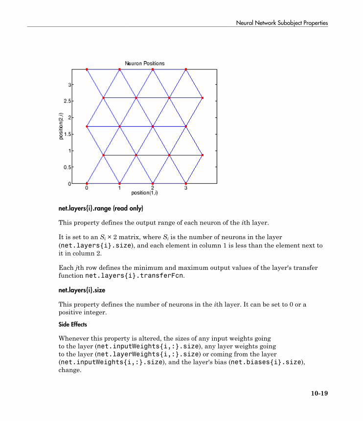
Neural Network Subobject Properties
10-19
net.layers{i}.range (read only)
This property defines the output range of each neuron of the ith layer.
It is set to an Si × 2 matrix, where Si is the number of neurons in the layer(net.layers{i}.size), and each element in column 1 is less than the element next toit in column 2.
Each jth row defines the minimum and maximum output values of the layer's transferfunction net.layers{i}.transferFcn.
net.layers{i}.size
This property defines the number of neurons in the ith layer. It can be set to 0 or apositive integer.
Side Effects
Whenever this property is altered, the sizes of any input weights goingto the layer (net.inputWeights{i,:}.size), any layer weights goingto the layer (net.layerWeights{i,:}.size) or coming from the layer(net.inputWeights{i,:}.size), and the layer's bias (net.biases{i}.size),change.

10 Neural Network Object Reference
10-20
The dimensions of the corresponding weight matrices (net.IW{i,:}, net.LW{i,:},net.LW{:,i}), and biases (net.b{i}) also change.
Changing this property also changes the size of the layer's output(net.outputs{i}.size) and target (net.targets{i}.size) if they exist.
Finally, when this property is altered, the dimensions of the layer's neurons(net.layers{i}.dimension) are set to the same value. (This results in a one-dimensional arrangement of neurons. If another arrangement is required, set thedimensions property directly instead of using size.)
net.layers{i}.topologyFcn
This property defines which of the topology functions are used to calculate the ithlayer's neuron positions (net.layers{i}.positions) from the layer's dimensions(net.layers{i}.dimensions).
For a list of functions, type help nntopology.
Side Effects
Whenever this property is altered, the positions of the layer's neurons(net.layers{i}.positions) are updated.
Use plotsom to plot the positions of the layer neurons. For instance, if the first-layerneurons of a network are arranged with dimensions (net.layers{1}.dimensions)of [8 10] and the topology function (net.layers{1}.topologyFcn) is randtop, theneuron positions are arranged to resemble the following plot:
plotsom(net.layers{1}.positions)
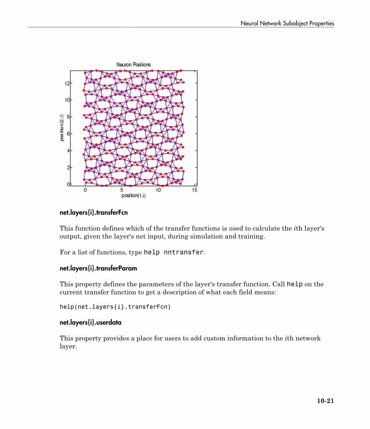
Neural Network Subobject Properties
10-21
net.layers{i}.transferFcn
This function defines which of the transfer functions is used to calculate the ith layer'soutput, given the layer's net input, during simulation and training.
For a list of functions, type help nntransfer.
net.layers{i}.transferParam
This property defines the parameters of the layer's transfer function. Call help on thecurrent transfer function to get a description of what each field means:
help(net.layers{i}.transferFcn)
net.layers{i}.userdata
This property provides a place for users to add custom information to the ith networklayer.

10 Neural Network Object Reference
10-22
Outputs
net.outputs{i}.name
This property consists of a string defining the output name. Network creation functions,such as feedforwardnet, define this appropriately. But it can be set to any string asdesired.
net.outputs{i}.feedbackInput
If the output implements open-loop feedback (net.outputs{i}.feedbackMode= 'open'), then this property indicates the index of the associated feedback input,otherwise it will be an empty matrix.
net.outputs{i}.feedbackDelay
This property defines the timestep difference between this output and network inputs.Input-to-output network delays can be removed and added with removedelay andadddelay functions resulting in this property being incremented or decrementedrespectively. The difference in timing between inputs and outputs is used by preparetsto properly format simulation and training data, and used by closeloop to add thecorrect number of delays when closing an open-loop output, and openloop to removedelays when opening a closed loop.
net.outputs{i}.feedbackMode
This property is set to the string 'none' for non-feedback outputs. For feedback outputsit can either be set to 'open' or 'closed'. If it is set to 'open', then the output willbe associated with a feedback input, with the property feedbackInput indicating theinput's index.
net.outputs{i}.processFcns
This property defines a row cell array of processing function names to be used by theith network output. The processing functions are applied to target values before thenetwork uses them, and applied in reverse to layer output values before being returnedas network output values.Side Effects
When you change this property, you also affect the following settings: the outputparameters processParams are modified to the default values of the specifiedprocessing functions; processSettings, processedSize, and processedRange

Neural Network Subobject Properties
10-23
are defined using the results of applying the process functions and parameters toexampleOutput; the ith layer size is updated to match the processedSize.
For a list of functions, type help nnprocess.
net.outputs{i}.processParams
This property holds a row cell array of processing function parameters to be used byith network output on target values. The processing parameters are applied by theprocessing functions to input values before the network uses them.Side Effects
Whenever this property is altered, the output processSettings, processedSizeand processedRange are defined by applying the process functions and parameters toexampleOutput. The ith layer's size is also updated to match processedSize.
net.outputs{i}.processSettings (read only)
This property holds a row cell array of processing function settings to be used by ithnetwork output. The processing settings are found by applying the processing functionsand parameters to exampleOutput and then used to provide consistent results to newtarget values before the network uses them. The processing settings are also applied inreverse to layer output values before being returned by the network.
net.outputs{i}.processedRange (read only)
This property defines the range of exampleOutput values after they have beenprocessed with processingFcns and processingParams.
net.outputs{i}.processedSize (read only)
This property defines the number of rows in the exampleOutput values after they havebeen processed with processingFcns and processingParams.
net.outputs{i}.size (read only)
This property defines the number of elements in the ith layer's output. It is always set tothe size of the ith layer (net.layers{i}.size).
net.outputs{i}.userdata
This property provides a place for users to add custom information to the ith layer'soutput.

10 Neural Network Object Reference
10-24
Biases
net.biases{i}.initFcn
This property defines the weight and bias initialization functions used to set the ithlayer's bias vector (net.b{i}) if the network initialization function is initlay and theith layer's initialization function is initwb.
net.biases{i}.learn
This property defines whether the ith bias vector is to be altered during training andadaption. It can be set to 0 or 1.
It enables or disables the bias's learning during calls to adapt and train.
net.biases{i}.learnFcn
This property defines which of the learning functions is used to update the ith layer'sbias vector (net.b{i}) during training, if the network training function is trainb,trainc, or trainr, or during adaption, if the network adapt function is trains.
For a list of functions, type help nnlearn.Side Effects
Whenever this property is altered, the biases learning parameters(net.biases{i}.learnParam) are set to contain the fields and default values of thenew function.
net.biases{i}.learnParam
This property defines the learning parameters and values for the current learningfunction of the ith layer's bias. The fields of this property depend on the current learningfunction. Call help on the current learning function to get a description of what eachfield means.
net.biases{i}.size (read only)
This property defines the size of the ith layer's bias vector. It is always set to the size ofthe ith layer (net.layers{i}.size).
net.biases{i}.userdata
This property provides a place for users to add custom information to the ith layer's bias.

Neural Network Subobject Properties
10-25
Input Weights
net.inputWeights{i,j}.delays
This property defines a tapped delay line between the jth input and its weight to the ithlayer. It must be set to a row vector of increasing values. The elements must be either 0or positive integers.Side Effects
Whenever this property is altered, the weight's size (net.inputWeights{i,j}.size)and the dimensions of its weight matrix (net.IW{i,j}) are updated.
net.inputWeights{i,j}.initFcn
This property defines which of the Weight and Bias Initialization Functions is used toinitialize the weight matrix (net.IW{i,j}) going to the ith layer from the jth input, ifthe network initialization function is initlay, and the ith layer's initialization functionis initwb. This function can be set to the name of any weight initialization function.
net.inputWeights{i,j}.initSettings (read only)
This property is set to values useful for initializing the weight as part of theconfiguration process that occurs automatically the first time a network is trained, orwhen the function configure is called on a network directly.
net.inputWeights{i,j}.learn
This property defines whether the weight matrix to the ith layer from the jth input is tobe altered during training and adaption. It can be set to 0 or 1.
net.inputWeights{i,j}.learnFcn
This property defines which of the learning functions is used to update the weight matrix(net.IW{i,j}) going to the ith layer from the jth input during training, if the networktraining function is trainb, trainc, or trainr, or during adaption, if the networkadapt function is trains. It can be set to the name of any weight learning function.
For a list of functions, type help nnlearn.
net.inputWeights{i,j}.learnParam
This property defines the learning parameters and values for the current learningfunction of the ith layer's weight coming from the jth input.

10 Neural Network Object Reference
10-26
The fields of this property depend on the current learning function(net.inputWeights{i,j}.learnFcn). Evaluate the above reference to see the fields ofthe current learning function.
Call help on the current learning function to get a description of what each field means.
net.inputWeights{i,j}.size (read only)
This property defines the dimensions of the ith layer's weight matrix from the jthnetwork input. It is always set to a two-element row vector indicating the number of rowsand columns of the associated weight matrix (net.IW{i,j}). The first element is equalto the size of the ith layer (net.layers{i}.size). The second element is equal to theproduct of the length of the weight's delay vectors and the size of the jth input:
length(net.inputWeights{i,j}.delays) * net.inputs{j}.size
net.inputWeights{i,j}.userdata
This property provides a place for users to add custom information to the (i,j)th inputweight.
net.inputWeights{i,j}.weightFcn
This property defines which of the weight functions is used to apply the ith layer's weightfrom the jth input to that input. It can be set to the name of any weight function. Theweight function is used to transform layer inputs during simulation and training.
For a list of functions, type help nnweight.
net.inputWeights{i,j}.weightParam
This property defines the parameters of the layer's net input function. Call help on thecurrent net input function to get a description of each field.
Layer Weights
net.layerWeights{i,j}.delays
This property defines a tapped delay line between the jth layer and its weight to the ithlayer. It must be set to a row vector of increasing values. The elements must be either 0or positive integers.

Neural Network Subobject Properties
10-27
net.layerWeights{i,j}.initFcn
This property defines which of the weight and bias initialization functions is used toinitialize the weight matrix (net.LW{i,j}) going to the ith layer from the jth layer, ifthe network initialization function is initlay, and the ith layer's initialization functionis initwb. This function can be set to the name of any weight initialization function.
net.layerWeights{i,j}.initSettings (read only)
This property is set to values useful for initializing the weight as part of theconfiguration process that occurs automatically the first time a network is trained, orwhen the function configure is called on a network directly.
net.layerWeights{i,j}.learn
This property defines whether the weight matrix to the ith layer from the jth layer is tobe altered during training and adaption. It can be set to 0 or 1.
net.layerWeights{i,j}.learnFcn
This property defines which of the learning functions is used to update the weight matrix(net.LW{i,j}) going to the ith layer from the jth layer during training, if the networktraining function is trainb, trainc, or trainr, or during adaption, if the networkadapt function is trains. It can be set to the name of any weight learning function.
For a list of functions, type help nnlearn.
net.layerWeights{i,j}.learnParam
This property defines the learning parameters fields and values for the current learningfunction of the ith layer's weight coming from the jth layer. The fields of this propertydepend on the current learning function. Call help on the current net input function toget a description of each field.
net.layerWeights{i,j}.size (read only)
This property defines the dimensions of the ith layer's weight matrix from the jth layer.It is always set to a two-element row vector indicating the number of rows and columnsof the associated weight matrix (net.LW{i,j}). The first element is equal to the size ofthe ith layer (net.layers{i}.size). The second element is equal to the product of thelength of the weight's delay vectors and the size of the jth layer.

10 Neural Network Object Reference
10-28
net.layerWeights{i,j}.userdata
This property provides a place for users to add custom information to the (i,j)th layerweight.
net.layerWeights{i,j}.weightFcn
This property defines which of the weight functions is used to apply the ith layer's weightfrom the jth layer to that layer's output. It can be set to the name of any weight function.The weight function is used to transform layer inputs when the network is simulated.
For a list of functions, type help nnweight.
net.layerWeights{i,j}.weightParam
This property defines the parameters of the layer's net input function. Call help on thecurrent net input function to get a description of each field.

11
Bibliography
11 Bibliography
11-2
Neural Network Toolbox Bibliography
[Batt92] Battiti, R., “First and second order methods for learning: Between steepestdescent and Newton's method,” Neural Computation, Vol. 4, No. 2, 1992, pp. 141–166.
[Beal72] Beale, E.M.L., “A derivation of conjugate gradients,” in F.A. Lootsma, Ed.,Numerical methods for nonlinear optimization, London: Academic Press, 1972.
[Bren73] Brent, R.P., Algorithms for Minimization Without Derivatives, EnglewoodCliffs, NJ: Prentice-Hall, 1973.
[Caud89] Caudill, M., Neural Networks Primer, San Francisco, CA: Miller FreemanPublications, 1989.
This collection of papers from the AI Expert Magazine gives an excellent introduction tothe field of neural networks. The papers use a minimum of mathematics to explain themain results clearly. Several good suggestions for further reading are included.
[CaBu92] Caudill, M., and C. Butler, Understanding Neural Networks: ComputerExplorations, Vols. 1 and 2, Cambridge, MA: The MIT Press, 1992.
This is a two-volume workbook designed to give students “hands on” experience withneural networks. It is written for a laboratory course at the senior or first-year graduatelevel. Software for IBM PC and Apple Macintosh computers is included. The materialis well written, clear, and helpful in understanding a field that traditionally has beenburied in mathematics.
[Char92] Charalambous, C.,“Conjugate gradient algorithm for efficient training ofartificial neural networks,” IEEE Proceedings, Vol. 139, No. 3, 1992, pp. 301–310.
[ChCo91] Chen, S., C.F.N. Cowan, and P.M. Grant, “Orthogonal least squares learningalgorithm for radial basis function networks,” IEEE Transactions on Neural Networks,Vol. 2, No. 2, 1991, pp. 302–309.
This paper gives an excellent introduction to the field of radial basis functions. Thepapers use a minimum of mathematics to explain the main results clearly. Several goodsuggestions for further reading are included.
[ChDa99] Chengyu, G., and K. Danai, “Fault diagnosis of the IFAC BenchmarkProblem with a model-based recurrent neural network,” Proceedings of the 1999 IEEEInternational Conference on Control Applications, Vol. 2, 1999, pp. 1755–1760.
Neural Network Toolbox Bibliography
11-3
[DARP88] DARPA Neural Network Study, Lexington, MA: M.I.T. Lincoln Laboratory,1988.
This book is a compendium of knowledge of neural networks as they were known to1988. It presents the theoretical foundations of neural networks and discusses theircurrent applications. It contains sections on associative memories, recurrent networks,vision, speech recognition, and robotics. Finally, it discusses simulation tools andimplementation technology.
[DeHa01a] De Jesús, O., and M.T. Hagan, “Backpropagation Through Time for aGeneral Class of Recurrent Network,” Proceedings of the International Joint Conferenceon Neural Networks, Washington, DC, July 15–19, 2001, pp. 2638–2642.
[DeHa01b] De Jesús, O., and M.T. Hagan, “Forward Perturbation Algorithm for aGeneral Class of Recurrent Network,” Proceedings of the International Joint Conferenceon Neural Networks, Washington, DC, July 15–19, 2001, pp. 2626–2631.
[DeHa07] De Jesús, O., and M.T. Hagan, “Backpropagation Algorithms for a BroadClass of Dynamic Networks,” IEEE Transactions on Neural Networks, Vol. 18, No. 1,January 2007, pp. 14 -27.
This paper provides detailed algorithms for the calculation of gradients and Jacobians forarbitrarily-connected neural networks. Both the backpropagation-through-time and real-time recurrent learning algorithms are covered.
[DeSc83] Dennis, J.E., and R.B. Schnabel, Numerical Methods for UnconstrainedOptimization and Nonlinear Equations, Englewood Cliffs, NJ: Prentice-Hall, 1983.
[DHH01] De Jesús, O., J.M. Horn, and M.T. Hagan, “Analysis of Recurrent NetworkTraining and Suggestions for Improvements,” Proceedings of the International JointConference on Neural Networks, Washington, DC, July 15–19, 2001, pp. 2632–2637.
[Elma90] Elman, J.L., “Finding structure in time,” Cognitive Science, Vol. 14, 1990, pp.179–211.
This paper is a superb introduction to the Elman networks described in Chapter 10,“Recurrent Networks.”
[FeTs03] Feng, J., C.K. Tse, and F.C.M. Lau, “A neural-network-based channel-equalization strategy for chaos-based communication systems,” IEEE Transactions onCircuits and Systems I: Fundamental Theory and Applications, Vol. 50, No. 7, 2003,pp. 954–957.

11 Bibliography
11-4
[FlRe64] Fletcher, R., and C.M. Reeves, “Function minimization by conjugate gradients,”Computer Journal, Vol. 7, 1964, pp. 149–154.
[FoHa97] Foresee, F.D., and M.T. Hagan, “Gauss-Newton approximation to Bayesianregularization,” Proceedings of the 1997 International Joint Conference on NeuralNetworks, 1997, pp. 1930–1935.
[GiMu81] Gill, P.E., W. Murray, and M.H. Wright, Practical Optimization, New York:Academic Press, 1981.
[GiPr02] Gianluca, P., D. Przybylski, B. Rost, P. Baldi, “Improving the prediction ofprotein secondary structure in three and eight classes using recurrent neural networksand profiles,” Proteins: Structure, Function, and Genetics, Vol. 47, No. 2, 2002, pp. 228–235.
[Gros82] Grossberg, S., Studies of the Mind and Brain, Drodrecht, Holland: ReidelPress, 1982.
This book contains articles summarizing Grossberg's theoretical psychophysiology workup to 1980. Each article contains a preface explaining the main points.
[HaDe99] Hagan, M.T., and H.B. Demuth, “Neural Networks for Control,” Proceedings ofthe 1999 American Control Conference, San Diego, CA, 1999, pp. 1642–1656.
[HaJe99] Hagan, M.T., O. De Jesus, and R. Schultz, “Training Recurrent Networksfor Filtering and Control,” Chapter 12 in Recurrent Neural Networks: Design andApplications, L. Medsker and L.C. Jain, Eds., CRC Press, pp. 311–340.
[HaMe94] Hagan, M.T., and M. Menhaj, “Training feed-forward networks with theMarquardt algorithm,” IEEE Transactions on Neural Networks, Vol. 5, No. 6, 1999, pp.989–993, 1994.
This paper reports the first development of the Levenberg-Marquardt algorithm forneural networks. It describes the theory and application of the algorithm, which trainsneural networks at a rate 10 to 100 times faster than the usual gradient descentbackpropagation method.
[HaRu78] Harrison, D., and Rubinfeld, D.L., “Hedonic prices and the demand for cleanair,” J. Environ. Economics & Management, Vol. 5, 1978, pp. 81-102.
This data set was taken from the StatLib library, which is maintained at CarnegieMellon University.
Neural Network Toolbox Bibliography
11-5
[HDB96] Hagan, M.T., H.B. Demuth, and M.H. Beale, Neural Network Design, Boston,MA: PWS Publishing, 1996.
This book provides a clear and detailed survey of basic neural network architectures andlearning rules. It emphasizes mathematical analysis of networks, methods of trainingnetworks, and application of networks to practical engineering problems. It has exampleprograms, an instructor’s guide, and transparency overheads for teaching.
[HDH09] Horn, J.M., O. De Jesús and M.T. Hagan, “Spurious Valleys in the ErrorSurface of Recurrent Networks - Analysis and Avoidance,” IEEE Transactions on NeuralNetworks, Vol. 20, No. 4, pp. 686-700, April 2009.
This paper describes spurious valleys that appear in the error surfaces of recurrentnetworks. It also explains how training algorithms can be modified to avoid becomingstuck in these valleys.
[Hebb49] Hebb, D.O., The Organization of Behavior, New York: Wiley, 1949.
This book proposed neural network architectures and the first learning rule. Thelearning rule is used to form a theory of how collections of cells might form a concept.
[Himm72] Himmelblau, D.M., Applied Nonlinear Programming, New York: McGraw-Hill, 1972.
[HuSb92] Hunt, K.J., D. Sbarbaro, R. Zbikowski, and P.J. Gawthrop, Neural Networksfor Control System — A Survey,” Automatica, Vol. 28, 1992, pp. 1083–1112.
[JaRa04] Jayadeva and S.A.Rahman, “A neural network with O(N) neurons for rankingN numbers in O(1/N) time,” IEEE Transactions on Circuits and Systems I: RegularPapers, Vol. 51, No. 10, 2004, pp. 2044–2051.
[Joll86] Jolliffe, I.T., Principal Component Analysis, New York: Springer-Verlag, 1986.
[KaGr96] Kamwa, I., R. Grondin, V.K. Sood, C. Gagnon, Van Thich Nguyen, and J.Mereb, “Recurrent neural networks for phasor detection and adaptive identificationin power system control and protection,” IEEE Transactions on Instrumentation andMeasurement, Vol. 45, No. 2, 1996, pp. 657–664.
[Koho87] Kohonen, T., Self-Organization and Associative Memory, 2nd Edition, Berlin:Springer-Verlag, 1987.
This book analyzes several learning rules. The Kohonen learning rule is then introducedand embedded in self-organizing feature maps. Associative networks are also studied.
11 Bibliography
11-6
[Koho97] Kohonen, T., Self-Organizing Maps, Second Edition, Berlin: Springer-Verlag,1997.
This book discusses the history, fundamentals, theory, applications, and hardware of self-organizing maps. It also includes a comprehensive literature survey.
[LiMi89] Li, J., A.N. Michel, and W. Porod, “Analysis and synthesis of a class of neuralnetworks: linear systems operating on a closed hypercube,” IEEE Transactions onCircuits and Systems, Vol. 36, No. 11, 1989, pp. 1405–1422.
This paper discusses a class of neural networks described by first-order linear differentialequations that are defined on a closed hypercube. The systems considered retain thebasic structure of the Hopfield model but are easier to analyze and implement. The paperpresents an efficient method for determining the set of asymptotically stable equilibriumpoints and the set of unstable equilibrium points. Examples are presented. The method ofLi, et. al., is implemented in Advanced Topics in the User’s Guide.
[Lipp87] Lippman, R.P., “An introduction to computing with neural nets,” IEEE ASSPMagazine, 1987, pp. 4–22.
This paper gives an introduction to the field of neural nets by reviewing six neuralnet models that can be used for pattern classification. The paper shows how existingclassification and clustering algorithms can be performed using simple components thatare like neurons. This is a highly readable paper.
[MacK92] MacKay, D.J.C., “Bayesian interpolation,” Neural Computation, Vol. 4, No. 3,1992, pp. 415–447.
[Marq63] Marquardt, D., “An Algorithm for Least-Squares Estimation of NonlinearParameters,” SIAM Journal on Applied Mathematics, Vol. 11, No. 2, June 1963, pp. 431–441.
[McPi43] McCulloch, W.S., and W.H. Pitts, “A logical calculus of ideas immanent innervous activity,” Bulletin of Mathematical Biophysics, Vol. 5, 1943, pp. 115–133.
A classic paper that describes a model of a neuron that is binary and has a fixedthreshold. A network of such neurons can perform logical operations.
[MeJa00] Medsker, L.R., and L.C. Jain, Recurrent neural networks: design andapplications, Boca Raton, FL: CRC Press, 2000.
[Moll93] Moller, M.F., “A scaled conjugate gradient algorithm for fast supervisedlearning,” Neural Networks, Vol. 6, 1993, pp. 525–533.
Neural Network Toolbox Bibliography
11-7
[MuNe92] Murray, R., D. Neumerkel, and D. Sbarbaro, “Neural Networks forModeling and Control of a Non-linear Dynamic System,” Proceedings of the 1992 IEEEInternational Symposium on Intelligent Control, 1992, pp. 404–409.
[NaMu97] Narendra, K.S., and S. Mukhopadhyay, “Adaptive Control Using NeuralNetworks and Approximate Models,” IEEE Transactions on Neural Networks, Vol. 8,1997, pp. 475–485.
[NaPa91] Narendra, Kumpati S. and Kannan Parthasarathy, “Learning AutomataApproach to Hierarchical Multiobjective Analysis,” IEEE Transactions on Systems, Manand Cybernetics, Vol. 20, No. 1, January/February 1991, pp. 263–272.
[NgWi89] Nguyen, D., and B. Widrow, “The truck backer-upper: An example of self-learning in neural networks,” Proceedings of the International Joint Conference on NeuralNetworks, Vol. 2, 1989, pp. 357–363.
This paper describes a two-layer network that first learned the truck dynamics and thenlearned how to back the truck to a specified position at a loading dock. To do this, theneural network had to solve a highly nonlinear control systems problem.
[NgWi90] Nguyen, D., and B. Widrow, “Improving the learning speed of 2-layerneural networks by choosing initial values of the adaptive weights,” Proceedings of theInternational Joint Conference on Neural Networks, Vol. 3, 1990, pp. 21–26.
Nguyen and Widrow show that a two-layer sigmoid/linear network can be viewed asperforming a piecewise linear approximation of any learned function. It is shown thatweights and biases generated with certain constraints result in an initial network betterable to form a function approximation of an arbitrary function. Use of the Nguyen-Widrow (instead of purely random) initial conditions often shortens training time bymore than an order of magnitude.
[Powe77] Powell, M.J.D., “Restart procedures for the conjugate gradient method,”Mathematical Programming, Vol. 12, 1977, pp. 241–254.
[Pulu92] Purdie, N., E.A. Lucas, and M.B. Talley, “Direct measure of total cholesteroland its distribution among major serum lipoproteins,” Clinical Chemistry, Vol. 38, No. 9,1992, pp. 1645–1647.
[RiBr93] Riedmiller, M., and H. Braun, “A direct adaptive method for fasterbackpropagation learning: The RPROP algorithm,” Proceedings of the IEEE InternationalConference on Neural Networks, 1993.
11 Bibliography
11-8
[Robin94] Robinson, A.J., “An application of recurrent nets to phone probabilityestimation,” IEEE Transactions on Neural Networks, Vol. 5 , No. 2, 1994.
[RoJa96] Roman, J., and A. Jameel, “Backpropagation and recurrent neural networksin financial analysis of multiple stock market returns,” Proceedings of the Twenty-NinthHawaii International Conference on System Sciences, Vol. 2, 1996, pp. 454–460.
[Rose61] Rosenblatt, F., Principles of Neurodynamics, Washington, D.C.: Spartan Press,1961.
This book presents all of Rosenblatt's results on perceptrons. In particular, it presents hismost important result, the perceptron learning theorem.
[RuHi86a] Rumelhart, D.E., G.E. Hinton, and R.J. Williams, “Learning internalrepresentations by error propagation,” in D.E. Rumelhart and J.L. McClelland, Eds.,Parallel Data Processing, Vol. 1, Cambridge, MA: The M.I.T. Press, 1986, pp. 318–362.
This is a basic reference on backpropagation.
[RuHi86b] Rumelhart, D.E., G.E. Hinton, and R.J. Williams, “Learning representationsby back-propagating errors,” Nature, Vol. 323, 1986, pp. 533–536.
[RuMc86] Rumelhart, D.E., J.L. McClelland, and the PDP Research Group, Eds.,Parallel Distributed Processing, Vols. 1 and 2, Cambridge, MA: The M.I.T. Press, 1986.
These two volumes contain a set of monographs that present a technical introduction tothe field of neural networks. Each section is written by different authors. These workspresent a summary of most of the research in neural networks to the date of publication.
[Scal85] Scales, L.E., Introduction to Non-Linear Optimization, New York: Springer-Verlag, 1985.
[SoHa96] Soloway, D., and P.J. Haley, “Neural Generalized Predictive Control,”Proceedings of the 1996 IEEE International Symposium on Intelligent Control, 1996, pp.277–281.
[VoMa88] Vogl, T.P., J.K. Mangis, A.K. Rigler, W.T. Zink, and D.L. Alkon, “Acceleratingthe convergence of the backpropagation method,” Biological Cybernetics, Vol. 59, 1988,pp. 256–264.
Backpropagation learning can be speeded up and made less sensitive to small featuresin the error surface such as shallow local minima by combining techniques such asbatching, adaptive learning rate, and momentum.
Neural Network Toolbox Bibliography
11-9
[WaHa89] Waibel, A., T. Hanazawa, G. Hilton, K. Shikano, and K. J. Lang, “Phonemerecognition using time-delay neural networks,” IEEE Transactions on Acoustics, Speech,and Signal Processing, Vol. 37, 1989, pp. 328–339.
[Wass93] Wasserman, P.D., Advanced Methods in Neural Computing, New York: VanNostrand Reinhold, 1993.
[WeGe94] Weigend, A. S., and N. A. Gershenfeld, eds., Time Series Prediction:Forecasting the Future and Understanding the Past, Reading, MA: Addison-Wesley, 1994.
[WiHo60] Widrow, B., and M.E. Hoff, “Adaptive switching circuits,” 1960 IRE WESCONConvention Record, New York IRE, 1960, pp. 96–104.
[WiSt85] Widrow, B., and S.D. Sterns, Adaptive Signal Processing, New York: Prentice-Hall, 1985.
This is a basic paper on adaptive signal processing.

11-10

A
Mathematical Notation
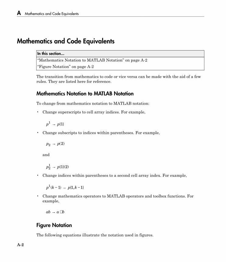
A Mathematics and Code Equivalents
A-2
Mathematics and Code Equivalents
In this section...
“Mathematics Notation to MATLAB Notation” on page A-2“Figure Notation” on page A-2
The transition from mathematics to code or vice versa can be made with the aid of a fewrules. They are listed here for reference.
Mathematics Notation to MATLAB Notation
To change from mathematics notation to MATLAB notation:
• Change superscripts to cell array indices. For example,
p p1
1→ { }
• Change subscripts to indices within parentheses. For example,
p p2 2→ ( )
and
p p21
1 2→ { }( )
• Change indices within parentheses to a second cell array index. For example,
p k p k1 1 1 1( ) { , }− → −
• Change mathematics operators to MATLAB operators and toolbox functions. Forexample,
ab a b→ ∗
Figure Notation
The following equations illustrate the notation used in figures.
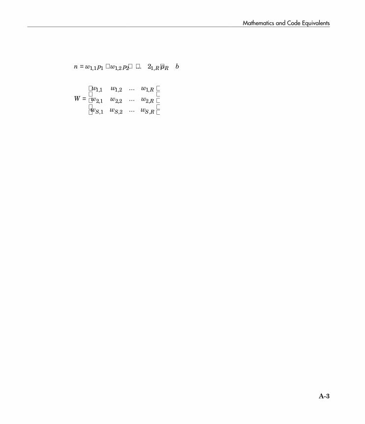
Mathematics and Code Equivalents
A-3
n w p w p p bR R= + + + +1 1 1 1 2 2 12, , ,...
W
w w w
w w w
w w w
R
R
S S S R
=
1 1 1 2 1
2 1 2 2 2
1 2
, , ,
, , ,
, , ,
...
...
...

A-4
B
Neural Network Blocks for the SimulinkEnvironment

B Neural Network Simulink Block Library
B-2
Neural Network Simulink Block Library
In this section...
“Transfer Function Blocks” on page B-2“Net Input Blocks” on page B-3“Weight Blocks” on page B-3“Processing Blocks” on page B-4
The Neural Network Toolbox product provides a set of blocks you can use to build neuralnetworks using Simulink software, or that the function gensim can use to generate theSimulink version of any network you have created using MATLAB software.
Open the Neural Network Toolbox block library with the command:
neural
This opens a library window that contains five blocks. Each of these blocks containsadditional blocks.
Transfer Function Blocks
Double-click the Transfer Functions block in the Neural library window to open a windowcontaining several transfer function blocks.

Neural Network Simulink Block Library
B-3
Each of these blocks takes a net input vector and generates a corresponding outputvector whose dimensions are the same as the input vector.
Net Input Blocks
Double-click the Net Input Functions block in the Neural library window to open awindow containing two net-input function blocks.
Each of these blocks takes any number of weighted input vectors, weight layer outputvectors, and bias vectors, and returns a net-input vector.
Weight Blocks
Double-click the Weight Functions block in the Neural library window to open a windowcontaining three weight function blocks.
Each of these blocks takes a neuron’s weight vector and applies it to an input vector (or alayer output vector) to get a weighted input value for a neuron.

B Neural Network Simulink Block Library
B-4
It is important to note that these blocks expect the neuron’s weight vector to be definedas a column vector. This is because Simulink signals can be column vectors, but cannotbe matrices or row vectors.
It is also important to note that because of this limitation you have to create S weightfunction blocks (one for each row), to implement a weight matrix going to a layer with Sneurons.
This contrasts with the other two kinds of blocks. Only one net input function and onetransfer function block are required for each layer.
Processing Blocks
Double-click the Processing Functions block in the Neural library window to open awindow containing processing blocks and their corresponding reverse-processing blocks.
Each of these blocks can be used to preprocess inputs and postprocess outputs.
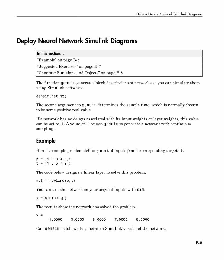
Deploy Neural Network Simulink Diagrams
B-5
Deploy Neural Network Simulink Diagrams
In this section...
“Example” on page B-5“Suggested Exercises” on page B-7“Generate Functions and Objects” on page B-8
The function gensim generates block descriptions of networks so you can simulate themusing Simulink software.
gensim(net,st)
The second argument to gensim determines the sample time, which is normally chosento be some positive real value.
If a network has no delays associated with its input weights or layer weights, this valuecan be set to -1. A value of -1 causes gensim to generate a network with continuoussampling.
Example
Here is a simple problem defining a set of inputs p and corresponding targets t.
p = [1 2 3 4 5];
t = [1 3 5 7 9];
The code below designs a linear layer to solve this problem.
net = newlind(p,t)
You can test the network on your original inputs with sim.
y = sim(net,p)
The results show the network has solved the problem.
y =
1.0000 3.0000 5.0000 7.0000 9.0000
Call gensim as follows to generate a Simulink version of the network.

B Deploy Neural Network Simulink Diagrams
B-6
gensim(net,-1)
The second argument is -1, so the resulting network block samples continuously.
The call to gensim opens the following Simulink Editor, showing a system consisting ofthe linear network connected to a sample input and a scope.
To test the network, double-click the input Constant x1 block on the left.
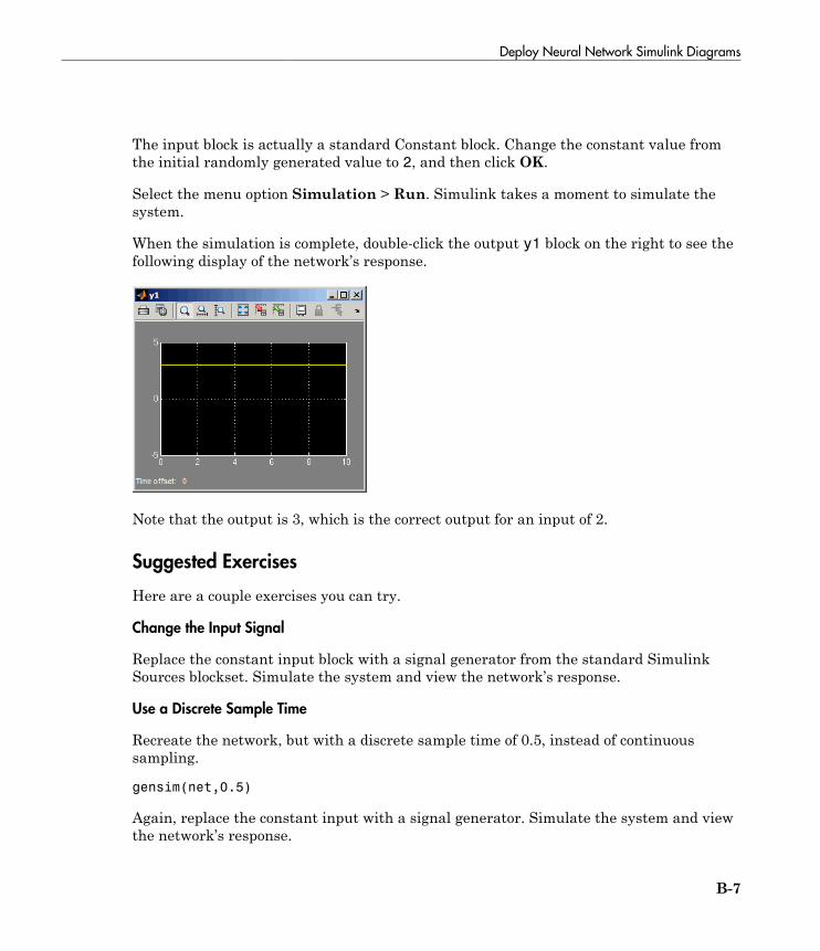
Deploy Neural Network Simulink Diagrams
B-7
The input block is actually a standard Constant block. Change the constant value fromthe initial randomly generated value to 2, and then click OK.
Select the menu option Simulation > Run. Simulink takes a moment to simulate thesystem.
When the simulation is complete, double-click the output y1 block on the right to see thefollowing display of the network’s response.
Note that the output is 3, which is the correct output for an input of 2.
Suggested Exercises
Here are a couple exercises you can try.
Change the Input Signal
Replace the constant input block with a signal generator from the standard SimulinkSources blockset. Simulate the system and view the network’s response.
Use a Discrete Sample Time
Recreate the network, but with a discrete sample time of 0.5, instead of continuoussampling.
gensim(net,0.5)
Again, replace the constant input with a signal generator. Simulate the system and viewthe network’s response.

B Deploy Neural Network Simulink Diagrams
B-8
Generate Functions and Objects
For information on simulating and deploying neural networks with MATLAB functions,see “Deploy Neural Network Functions” on page 8-60.

C
Code Notes

C Neural Network Toolbox Data Conventions
C-2
Neural Network Toolbox Data Conventions
In this section...
“Dimensions” on page C-2“Variables” on page C-2
Dimensions
The following code dimensions are used in describing both the network signals that userscommonly see, and those used by the utility functions:
Ni = Number of network inputs = net.numInputs
Ri = Number of elements in input i = net.inputs{i}.size
Nl = Number of layers = net.numLayers
Si = Number of neurons in layer i = net.layers{i}.size
Nt = Number of targetsVi = Number of elements in target i,equal to Sj, where j is the ith layerwith a target. (A layer n has a target ifnet.targets(n) == 1.)No = Number of network outputsUi = Number of elements in output i,equal to Sj, where j is the ith layer withan output (A layer n has an output ifnet.outputs(n) == 1.)ID = Number of input delays = net.numInputDelays
LD = Number of layer delays = net.numLayerDelays
TS = Number of time stepsQ = Number of concurrent vectors orsequences
Variables
The variables a user commonly uses when defining a simulation or training session are
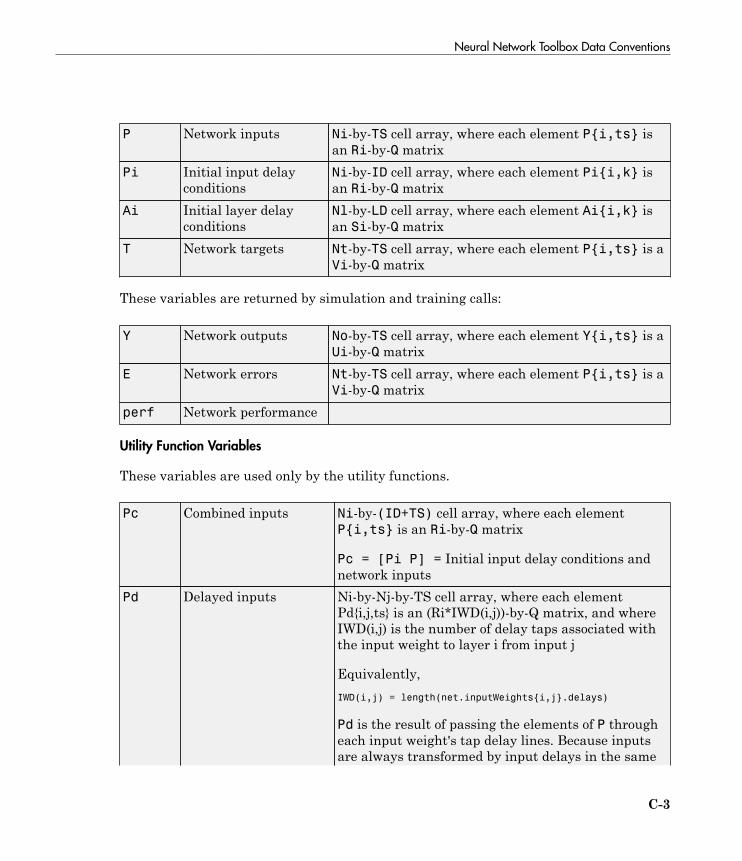
Neural Network Toolbox Data Conventions
C-3
P Network inputs Ni-by-TS cell array, where each element P{i,ts} isan Ri-by-Q matrix
Pi Initial input delayconditions
Ni-by-ID cell array, where each element Pi{i,k} isan Ri-by-Q matrix
Ai Initial layer delayconditions
Nl-by-LD cell array, where each element Ai{i,k} isan Si-by-Q matrix
T Network targets Nt-by-TS cell array, where each element P{i,ts} is aVi-by-Q matrix
These variables are returned by simulation and training calls:
Y Network outputs No-by-TS cell array, where each element Y{i,ts} is aUi-by-Q matrix
E Network errors Nt-by-TS cell array, where each element P{i,ts} is aVi-by-Q matrix
perf Network performance
Utility Function Variables
These variables are used only by the utility functions.
Pc Combined inputs Ni-by-(ID+TS) cell array, where each elementP{i,ts} is an Ri-by-Q matrix
Pc = [Pi P] = Initial input delay conditions andnetwork inputs
Pd Delayed inputs Ni-by-Nj-by-TS cell array, where each elementPd{i,j,ts} is an (Ri*IWD(i,j))-by-Q matrix, and whereIWD(i,j) is the number of delay taps associated withthe input weight to layer i from input j
Equivalently,IWD(i,j) = length(net.inputWeights{i,j}.delays)
Pd is the result of passing the elements of P througheach input weight's tap delay lines. Because inputsare always transformed by input delays in the same
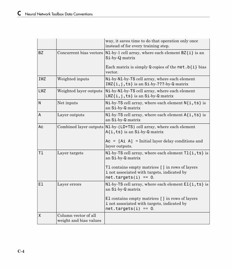
C Neural Network Toolbox Data Conventions
C-4
way, it saves time to do that operation only onceinstead of for every training step.
BZ Concurrent bias vectors Nl-by-1 cell array, where each element BZ{i} is anSi-by-Q matrix
Each matrix is simply Q copies of the net.b{i} biasvector.
IWZ Weighted inputs Ni-by-Nl-by-TS cell array, where each elementIWZ{i,j,ts} is an Si-by-???-by-Q matrix
LWZ Weighted layer outputs Ni-by-Nl-by-TS cell array, where each elementLWZ{i,j,ts} is an Si-by-Q matrix
N Net inputs Ni-by-TS cell array, where each element N{i,ts} isan Si-by-Q matrix
A Layer outputs Nl-by-TS cell array, where each element A{i,ts} isan Si-by-Q matrix
Ac Combined layer outputs Nl-by-(LD+TS) cell array, where each elementA{i,ts} is an Si-by-Q matrix
Ac = [Ai A] = Initial layer delay conditions andlayer outputs.
Tl Layer targets Nl-by-TS cell array, where each element Tl{i,ts} isan Si-by-Q matrix
Tl contains empty matrices [] in rows of layersi not associated with targets, indicated bynet.targets(i) == 0.
El Layer errors Nl-by-TS cell array, where each element El{i,ts} isan Si-by-Q matrix
El contains empty matrices [] in rows of layersi not associated with targets, indicated bynet.targets(i) == 0.
X Column vector of allweight and bias values