Mathematical Models and State Observation of the Glucose-Insulin Homeostasis

MATHEMATICAL MODELS AND STATE OBSERVATION OF THE GLUCOSE-INSULIN HOMEOSTASIS

Andrea De Gaetano IASI-CNR BioMatLab, Universitd Cattolica del Sacro Cuore, Largo A. Gemelli 8, 00168 Roma, Italy [email protected]

Domenico Di Martino Istituto di Analisi dei Sistemi ed Informatica (IASI-CNR), Viale Manzoni 30, 00185 Roma, Italy

Alfredo Germani Dipartimento di Ingegneria Elettrica, Universitd degli Studi dell'Aquila, Monteluco di Roio, 67040 L'Aquila, Italy [email protected]

Costanzo Manes Dipartimento di Ingegneria Elettrica, Universitd degli Studi delllAquila, Monteluco di Roio, 67040 L'Aquila, Italy

Abstract This paper explores the possibility of using an asymptotic state observer for the real-time reconstruction of insulin blood concentration in an individual by using only measurements of the glucose blood concentration. The interest in this topic relies on the fact that the glucose measurements are much more economical and faster then the insulin measurements. An algorithm providing reliable insulin concentrations in real-time is essential for the realization of an "artificial pancreas", an automatic device aimed to infuse the required amount of insulin into the circulatory system of a diabetic patient. An important issue for a good observer design is the determination of satisfactory models of the

SYSTEM MODELING AND OPTIMIZATION

glucose-insulin homeostasis. Different models have been considered and discussed in this paper. For all models presented an asymptotic state observer has been constructed and numerical simulations have been suc- cessfully carried out.

Keywords: Homeostasis, nonlinear systems, state observer, drift-observability

Introduction It is well-known that glucose and insulin blood concentrations are two

extremely important variables in a diabetic individual. Unfortunately, only glucose blood concentration can be easily monitored in real-time, while the measurement of the insulin concentration is expensive and not immediate. In many control applications, when not all the variables of a system can be directly measured, an "asymptotic state observer" is used, which is an algorithm that processes the available measurements and provides estimates of all the system variables, with an error that asymptotically converges to zero. This fact suggests the use of a state observer for the reconstruction of the insulin blood concentration using only glucose concentration data. This paper investigates the use of the observers presented in [13] and [6], that under some conditions guarantee exponential decay of the estimation error. The design of a good observer requires the knowledge of a good model of the system under investigation. The problem of developing satisfactory models of the glucose-insulin homeostasis has been widely investigated by many authors in the last two decades (see [7], [16], [LO], [9], [2], [5], [ll], [15], [4]). At today the most used model in physiological research on glucose metabolism is the so called Minimal Model [2], originally proposed for the interpretation of the glucose and insulin plasma concentrations following the intra-venous glucose tolerance test (IVGTT). In the Minimal Model two dynamic subsystems can be singled out. The parameters of each subsystem can be evaluated using glucose and insulin data in a separate identification procedures. In [7] the authors showed that in some situations the coupling of the two subsystems does not admit an equilibrium and the concentration of active insulin in the "distant" compartment increases without bounds. For this reason, in this paper two modifications of the Minimal Model are considered. For each model an asymptotic state observer is computed and verified through numerical simulations.

Models and Observation of the Glucose-Insulin Homeostasis

1. Asymptotic State Observers

Consider a dynamic system described, for t 2 0, by nonlinear differential equations of the form

k(t) = f (44) + g(x(t))u(t) , (1)

y (t) = h ( ~ ( t ) ) , (2)

where x(t) E X C Rn is the system state, u(t) E U C_ R is the input function and y (t) E R is the output, f (x) and g(x) are Ck (x) vector fields, with k an integer allowing all differentiations needed.

In most applications the input u(t) and the output y(t) of the system are the only quantities available through measurements, while the system state x(t) remains unaccessible. An important issue in systems and control theory is the problem of state reconstruction through on line processing of the measured input and output signals. An algorithm that asymptotically reconstructs the state is called an asymptotic state observer, and is usually described by differential equations. The existence of an asymptotic observer depends on the observability properties of the system. A system is said drift-observable if it is such that, when the input is identically zero, different states produce different outputs (see [6]). Such property depends only on the pair (f (x), h(x)) , and claims the theoretical possibility of the state reconstruction from the measured output data, when u(t) ZE 0. A system is said uniformly observable when different states produce different outputs, for any input function u(t) (see [12]). This is a rather strong property for nonlinear systems, and depends on the triple (f (x), g(x), h(x)) . A weaker property is the almost-uniform observability, that characterizes systems such that different states produce different outputs, for any constant input (see [13]). The study of the drift-observability and of the almost-uniform observability of nonlinear systems is made through the construction of suitable vector functions that map the system state at a given time t into the output and its derivatives at the same time t.

The following two square maps can be defined for system (1)-(2)

where L ? ~ ( x ) denotes the k-th order repeated Lie derivative of the function h(x) along the field f (x), and in the same way, ~ ) + ~ , h ( x ) denotes

284 SYSTEM MODELING AND OPTIMIZATION

repeated Lie derivative of h(x) along f (x) + g(x)u, with u constant parameter. Formally

L?h(x) = h(x), L ? + g u h ( ~ ) = h b ) , d ~ ) h

~ ;+ 'h (x )= - f ( z ) , L;;iuh(x)= dx

dL?+guh (f (x) + g(z)u), dx

(4) Recall that the observation relative degree of a triple (f (x), g(x), h(x)) in a set R C !Rn is an integer r 5 n such that

The observation relative degree is said full or mazimal if it is equal to n. Quite obviously, when u = 0 the two maps (3) coincide, so that @(x) = !P(x,O). Moreover, it is not difficult to show that if the relative degree is maximal it follows that !P(x, u) = @(x). Let z(t) be the vector made of the output and its derivatives up to order n - 1, i.e.

It can be easily checked that when u(t) - 0 or the relative degree is maximal it is z(t) = @(x(t)), while if u(t) r fi it is z(t) = !P(x(t), a). The map @(x) is named drift-obseruability map. The drift-observability property in an open set R E !Rn implies that in R there exists the inverse map x = @ - l ( z ) . This means that when u(t) 3 0 or when the relative degree is full the state can be reconstructed from the knowledge of the output, at least from a theoretical point of view. In the same way, the uniform-observability in R x U implies the existence of the inverse x = !Pli- '(z,~), forall x E R and fi E U . This means that the state can be reconstructed from the knowledge of the output and of the constant input ti.

Let Q(x) and Q(x, u) denote the Jacobians

Drift-observability of the system (1)-(2) in a set R implies nonsingularity of Q(x) in 0, and allows the construction of the asymptotic observer presented in [6], described by the differential equation

Models and Observation of the Glucose-Insulin Homeostasis 285

Almost-uniform observability in a set S2 x U implies invertibility of Q(x, u) for all (x, u) E S2 x U, and allows the construction of the following asymptotic observer

presented in [13]. In both observers (8)-(9) the constant vector K is the observer gain, and is a design parameter. In [6, 131 it is shown that, under suitable assumptions, there exists a choice for K such that (8) or (9) are exponential observers for system (1)-(2), i.e. there exist positive constants ,u and cu such that

In the case of observer (8) the convergence is guaranteed if the system has relative degree n and the input u(t) is bounded. If the system relative degree is smaller than n, (8) is still an exponential observer for (1)-(2), provided that the amplitude of the input u(t) satisfies a specific bound (for more details see [6]). For systems with generic relative degree (9) is an exponential observer provided that the input derivative satisfies a specific bound (slowly varying input, for more details see [13]). A strategy for the choice of the gain vector K is described in the convergence proofs reported in [6, 131. In particular, K should be chosen such to assign eigenvalues to the matrix Ab - KCb, where (Ab, Cb) define a Brunowski pair of dimension n.

In this paper the state observers (8) and (9) are applied for the reconstruction of the blood insulin concentration through on-line processing of the measured blood glucose concentration (the system output y(t)).

2 . The Minimal Model

There are two main experimental procedures currently in use for the estimation of the insulin sensitivity in a subject: the euglycemic hyper- insulinemic clamp (EHC) [8] and the intra venous glucose tolerance test (IVGTT) [2]. With respect to the EHC, the IVGTT is easier to execute and provides more informations. The test consists of injecting 1.V. a bolus of glucose and frequently sampling the glucose and insulin plasma concentrations afterwards, for a period of about three hours. The physiological model most used in the interpretation of the IVGTT is known as the Minimal Model [2]:


where [ a ] + denotes the positive part of its argument, and

G(t) [mg/dl] is the blood glucose concentration at time t [min];

I ( t ) [pUI/ml] is the blood insulin concentration;

X (t) [min-'1 is an auxiliary function representing insulin-excitable tissue glucose uptake activity, proportional to insulin concentration in a "distant" compartment;

Gb [mgldl] is the subject's baseline glycemia;

Ib [pUI/ml] is the subject's baseline insulinemia;

po [mgldl] is the theoretical glycemia at time 0 after the instanta- neous glucose bolus;

pl [min-'1 is the glucose "mass action" rate constant, i.e. the insulin-independent rate constant of tissue glucose uptake, "glucose effectiveness" ;

p2 [min-'1 is the rate constant expressing the spontaneous decrease of tissue glucose uptake ability;

p3 [ m i n - 2 ( p ~ ~ / m l ) - 1 ] is the insulin-dependent rate of increase in tissue glucose uptake ability, per unit of insulin concentration excess over baseline insulin;

p4 [ ( p ~ l / r n l ) - ' (mg/dl)-'min-2] is the rate of pancreatic release of insulin after the bolus, per minute and per mgldl of glucose concentration above the "target" glycemia;

pg [mg/dl] is the pancreatic "target glycemia" (pancreas produces insulin as long as G(t) > pg);

p6 [min-'1 is the first order decay rate constant for plasma insulin;

p7 = pUI/ml is the theoretical plasma insulin concentration at time 0, above basal insulinemia, immediately after the glucose bolus.

Parameters po, pl , p4, pg , p6 and p7 are usually referred to in the liter- ature as Go, SG, y, h, n and Io, respectively, while the insulin sensitivity index SI is computed as p3/p2.

The Minimal Model was conceived as composed of two parts. The first one, made of eq.'s (11)-(12), describes the time course of plasma glucose concentration as a function of the circulating insulin, treated as a forcing


function, known from measurements. The second part consists of eq. (13) and describes the time course of plasma insulin concentration accounting for the dynamics of pancreatic insulin release in response to the glucose stimulus regarded as a forcing function, known from measurements. In this way the problem of model parameter fitting can be separated into two separate subproblems. However, some stability problems of the Minimal Model have been revealed in [7]. The main reason of instability is a term in the third equation that linearly grows with time.

The injection into the bloodstream of a subject of a bolus of glucose during the IVGTT induces an impulsive increase in the plasma glucose concentration G(t) and a corresponding increase of the plasma concentration of insulin I ( t ) , secreted by the pancreas. These concentrations are measured during a three hour time interval beginning at the bolus injection. Note that in eq. (13) the positive part of G(t) - ps multiplies the time t to model the hypothesis that the effect of circulating hyperglycemia on the rate of pancreatic secretion of insulin is proportional both to the hyperglycemia and to the time elapsed from the glucose stimulus [16]. However the multiplication by t in (13) introduces an ori- gin for time, making the model non stationary and binding the model to the IVGTT experimental procedure.

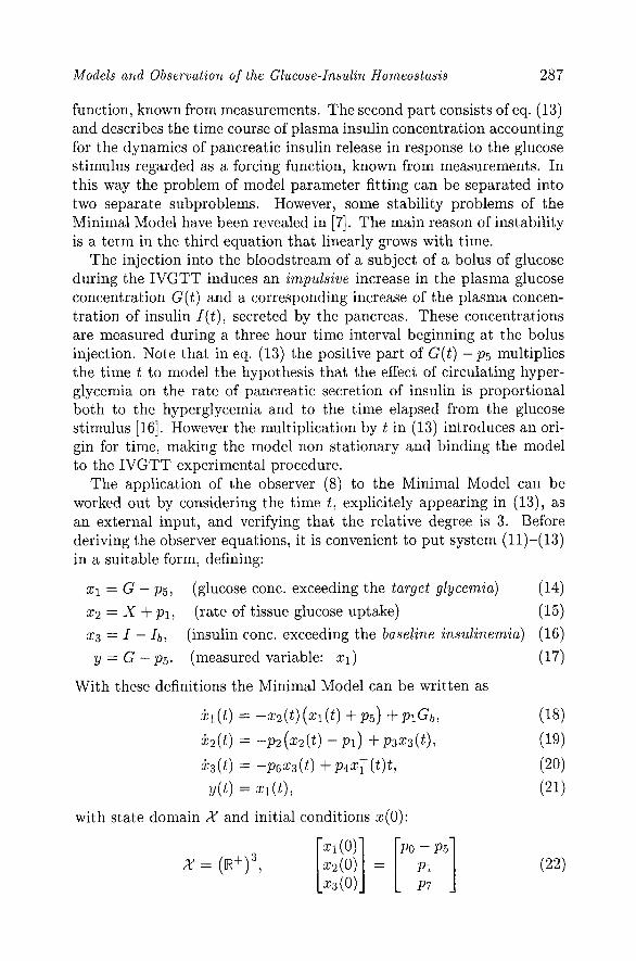
The application of the observer (8) to the Minimal Model can be worked out by considering the time t , explicitely appearing in (13), as an external input, and verifying that the relative degree is 3. Before deriving the observer equations, it is convenient to put system (11)-(13) in a suitable form, defining:

XI = G - p5, (glucose conc. exceeding the target glycemia) (14)

2 2 = X + pl, (rate of tissue glucose uptake) (15) 2 3 = I - Ib, (insulin conc, exceeding the baseline insulinemia) (16) y = G - pg. (measured variable: xl) (17)

With these definitions the Minimal Model can be written as

with state domain X and initial conditions x(0):


True (continuous line) and obsened (dotted) blood glucose concentratlon

C

40. 60 00 120 ?rue (continuous Ilne) and observed (dotted) a u x R r y functlon u(A

O O ~ ~ - - - - - - - - - . - - - - - - - - - - - - - - - - - - - - - - - - - - - - - - - - - - - - - - - - - - - - - - - - - - - - - - - - - - - - - .

-0.05 1 I I I I I I 0 40 80 100

T??e (continuous line) and obsene8qdotted) blood nsul ln concentratlon 120

Time t [mln]

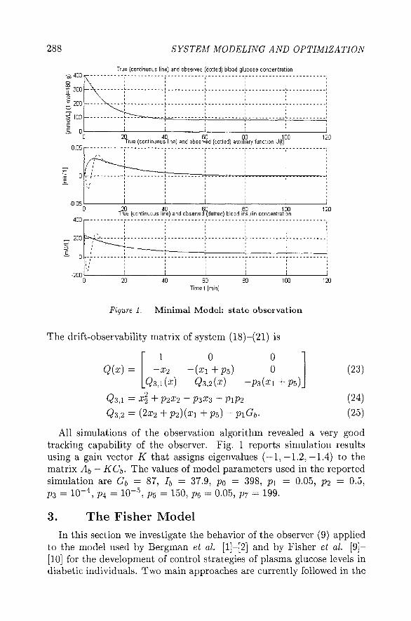
Figure 1 . Minimal Model: state observation

The drift-observability matrix of system (18)-(21) is

All simulations of the observation algorithm revealed a very good tracking capability of the observer. Fig. 1 reports simulation results using a gain vector K that assigns eigenvalues (- 1, -1.2, -1.4) to the matrix Ab - KCb. The values of model parameters used in the reported simulation are Gb = 87, Ib = 37.9, po = 398, pl = 0.05, pz = 0 , 5

5 p3 = lo-*, p4 = 10- , p5 = 150, p~ = 0.05, p7 = 199.

3. The Fisher Model

In this section we investigate the behavior of the observer (9) applied to the model used by Bergman et al. [I]-[2] and by Fisher e t al. 191- [lo] for the development of control strategies of plasma glucose levels in diabetic individuals. Two main approaches are currently followed in the


development of insulin infusion programs: open-loop methods, devoted to the computation of a predetermined amount of insulin to be deliv- ered to a patient, and closed-loop methods, often referred to as artificial beta cells or artificial pancreas. Closed-loop methods require continuous monitoring of blood glucose levels and can involve quite sophisticated and costly apparatus. An intermediate approach is followed by semi closed-loop methods ([5], [9], [lo]), based on intermittent blood glucose sampling. Optimization techniques are used to calculate insulin infusion programs for the correction of hyperglycemia. The semi closed-loop algorithm proposed in [ll] is based on three hourly plasma glucose samples and combines a single injection with continuous infusion of insulin.

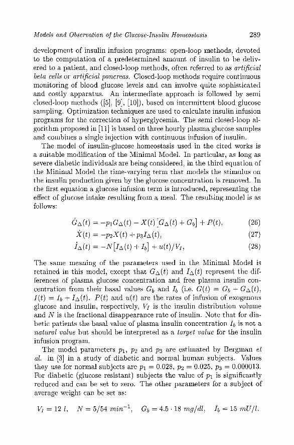
The model of insulin-glucose homeostasis used in the cited works is a suitable modification of the Minimal Model. In particular, as long as severe diabetic individuals are being considered, in the third equation of the Minimal Model the time-varying term that models the stimulus on the insulin production given by the glucose concentration is removed. In the first equation a glucose infusion term is introduced, representing the effect of glucose intake resulting from a meal. The resulting model is as follows:

The same meaning of the parameters used in the Minimal Model is retained in this model, except that GA(t) and IA( t ) represent the dif- ferences of plasma glucose concentration and free plasma insulin concentration from their basal values Gb and Ib (i.e. G(t) = Gb + GA(t) , I ( t ) = Ib + IA(t) . P ( t ) and u(t) are the rates of infusion of exogenous glucose and insulin, respectively, VI is the insulin distribution volume and N is the fractional disappearance rate of insulin. Note that for diabetic patients the basal value of plasma insulin concentration Ib is not a natural va lue but should be interpreted as a target va lue for the insulin infusion program.

The model parameters pl , pz and p3 are estimated by Bergman e t al, in [3] in a study of diabetic and normal human subjects. Values they use for normal subjects are pl = 0.028, p:! = 0.025, ps = 0.000013. For diabetic (glucose resistant) subjects the value of pl is significantly reduced and can be set to zero. The other parameters for a subject of average weight can be set as:


The value of Ib is typical of free insulin levels of controlled diabetic subjects under steady-state conditions. The steady-state in the model corresponds to a constant insulin infusion rate of u = NVIIb [ m u . min-'1. This is consistent with observations of the infusion rates that are required to maintain steady-state plasma glucose levels of severe diabetics at the basal values of normal subjects.

In the design of an observer for the model (26)-(28) we assume that oral glucose infusion starts at t = 0 prior to which plasma glucose and insulin are at their fasting levels. The term P( t ) in (26) represents the rate at which glucose enters the blood from intestinal absorption following a meal. In oral glucose tests it is observed that the plasma glucose level rises from the rest level to a maximum in less than 30 min. In normal subjects the glucose level falls to the base level after about 2 - 3 hours. A function that produces this kind of desired behavior in the mode1 (26)-(28) is

where B depends on the amount of glucose ingested during the meal, and k is the rate constant of glucose delivery to the blood circulatory system. A good value for k in normal subjects is k = 0.05 min-l, while for a medium meal B = 0.5 mg/(min.dl). The introduction of the term (29) in the model (26)-(28) requires an additional differential equation

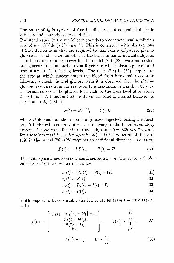
The state space dimension now has dimension n = 4. The state variables considered for the observer design are

With respect to these variable the Fisher Model takes the form (1)-(2) with

Models and Observation of the Glucose-Insulin Homeostasis

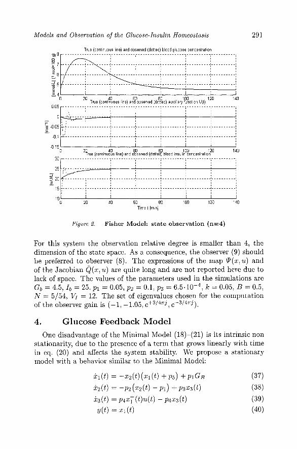
Figure 2. Fisher Model: state observation (n=4)

For this system the observation relative degree is smaller than 4, the dimension of the state space. As a consequence, the observer (9) should be preferred to observer (8). The expressions of the map @(x, u) and of the Jacobian Q(x, u) are quite long and are not reported here due to lack of space. The values of the parameters used in the simulations are Gb = 4.5, Ib = 25, pl = 0.05, p2 = 0.1, p3 = 6.5.1oP4, k = 0.05, B = 0.5, N = 5/54, VI = 12. The set of eigenvalues chosen for the computation of the observer gain is (-1, -1.05, e+3/4"jj, e33/4Tj >.

4. Glucose Feedback Model One disadvantage of the Minimal Model (18)-(21) is its intrinsic non

stationarity, due to the presence of a term that grows linearly with time in eq. (20) and affects the system stability. We propose a stationary model with a behavior similar to the Minimal Model:


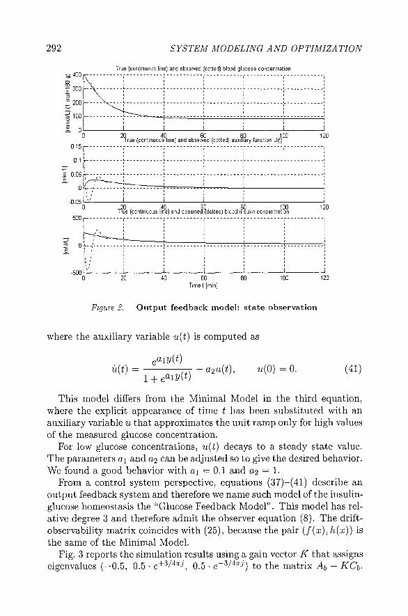
Figure 3. Output feedback model: state observation

where the auxiliary variable u(t) is computed as

This model differs from the Minimal Model in the third equation, where the explicit appearance of time t has been substituted with an auxiliary variable u that approximates the unit ramp only for high values of the measured glucose concentration.

For low glucose concentrations, u(t) decays to a steady state value. The parameters a1 and a2 can be adjusted so to give the desired behavior. We found a good behavior with a1 = 0.1 and a2 = 1.

From a control system perspective, equations (37)-(41) describe an output feedback system and therefore we name such model of the insulin- glucose homeostasis the "Glucose Feedback Model". This model has relative degree 3 and therefore admit the observer equation (8). The drift- observability matrix coincides with (25), because the pair (f (x), h(x)) is the same of the Minimal Model.

Fig. 3 reports the simulation results using a gain vector K that assigns eigenvalues (-0.5, 0.5 . e+3/4Tj, 0.5 . e-3/4nj) to the matrix Ab - KCb.


The values of the model parameters are the same used in the simulation of the Minimal Model.

5. Conclusions and Future Developments

This work explores the use of nonlinear state observers for real-time monitoring of the insulin blood concentration using only measurements of blood glucose concentration. Three models of the glucose-insulin homeostasis have been presented here, on which asymptotic observers have been constructed. The clinical validation of the proposed observers using experimental data will be the object of a future research. In future work, also the delay-differential models presented in [7] will be considered for state observation, using the observer developed in [14].

References [I] R. N. Bergman, D. T. Finegood, and M. Ader. Assessment of insulin sensitivity

in vivo. Endocrine Rev., 6:45-86, 1985.

[2] R. N. Bergman, Y. Z. Ider, C. R. Bowden, and C. Cobelli. Quantitative estimation of insulin sensitivity. Amer. Journal of Physiology, 236:E667-677, 1979.

[3] R. N. Bergman, L. S. Phillips, and C. Cobelli. Physiological evaluation of factors controlling glucose tolerance in man: measurement of insulin sensitivity and P- cell glucose sensitivity from the response to intravenous glucose. Journal Clin. Invest., 68:1456-1467, 1981.

[4] B. Candas and J. Radziuk. An adaptive plasma glucose controller based on a nonlinear insulin/glucose model, IEEE Transactions on Biomedical Engineering, 41:-, 1994.

[5] D. J. Chisolm, E. W. Kraegen, D. J. Bell, and D. R. Chipps. A semi-closed loop computer-assisted insulin infusion system. Med. Journal Aust., 141:784-789, 1984.

[6] M. Dalla Mora, A. Germani, and C. Manes. Design of state observers from a drift-observability property. IEEE Transactions on Automatic Control, 45:1536- 1540, 2000.

[7] A. De Gaetano and 0 . Arino. Mathematical modelling of the intravenous glucose tolerance test. Journal of Mathematical Biology, 40:136-168, 2000.

[8] R.A. Defronzo, J.D. Tobin, and R. Andreas. Glucose clamp technique: a method for quantifying insulin secretion and resistance. Am. Journal of Physiology, 237:E214-E223, 1979.

[9] M. E. Fisher and Kok Lay Teo. Optimal insulin infusion resulting from a mathematical model of blood glucose dynamics. IEEE Transactions on Biomedical Engineering, 36:479-485, 1989.

[lo] M.E. Fisher. A semiclosed-loop for the control of blood glucose levels in diabetics. IEEE Transactions on Biomedical Engineering, 38:57-61, 1991.

[ll] S. M. Furler, E. W. Kraegen, R. H. Smallwood, and D. J. Chisolm. Blood glucose control by intermittent loop closure in the basal mode: computer simulation studies with a diabetic model. Diabetes Care, 8:553-561, 1985.

294 S Y S T E M MODELING AND OPTIMIZATION

[12] J.P. Gauthier, and G. Bornard, Observability for any u(t) of a class of nonlinear systems. IEEE Transactions on Automatic Control, 26:922-926, 1981.

[13] A. Germani and C. Manes. State observers for nonlinear systems with slowly varying inputs. 36th IEEE Conf. on Decision and Control (CDC197), S. Diego, Ca., 5:5054-5059, 1997.

[14] A. Germani, C. Manes, and P. Pepe. An asymptotic state observer for a class of nonlinear delay systems. Kybernetyka, 37:459-478, 2001.

[15] R.S. Parker, F .J . Doyle 111, and N.A. Peppas. A model-based algorithm for blood glucose control in type i diabetic patients. IEEE Transactions on Biomedical Engineering, 46:-, 1999.

[16] G. Toffolo, R.N. Bergman, D.T. Finegood, C.R. Bowden, and C. Cobelli. Quan- titative estimation of beta cell sensitivity to glucose in the intact organism: a minimal model of insulin kinetics in the dog. Diabetes, 29:979-990, 1980.

Mathematical Models and State Observation of the Glucose-Insulin Homeostasis

Documents

Transcript of Mathematical Models and State Observation of the Glucose-Insulin Homeostasis