LAPPEENRANTA UNIVERSITY OF TECHNOLOGY

LUT School of Energy Systems

LUT Mechanical Engineering

Suraj Jaiswal

MODELING CONFIGURATOR FOR REAL-TIME SIMULATOR OF A TRACTOR

Examiner(s): Professor Aki Mikkola

D. Sc. (Tech.) Kimmo Kerkkänen

ABSTRACT

Lappeenranta University of Technology

LUT School of Energy Systems

LUT Mechanical Engineering

Suraj Jaiswal

Modeling configurator for real-time simulator of a tractor

Master’s thesis

2017

71 pages, 39 figures, 4 table and 2 appendices

Examiners: Professor Aki Mikkola

D. Sc. (Tech.) Kimmo Kerkkänen

Keywords: Modeling configurator, Tractor Simulator, SIM platform, Real-time simulation,

Multibody system dynamics.

The foundation of this research work was laid by the vision of a tractor simulator where the

users can generate their customized tractor model with the help of just a user-interface. The

aim of this paper was to modify the attributes of the tractor simulation model. For the same

reason, a modeling configurator was developed for the tractor model in python programming

language with a user-friendly interface designed over Microsoft excel. This research work

reports the effort in the development of modeling configurator for parameterizing a tractor

model.

The modeling configurator has been designed in such a way that the users can select their

choices just from a drop down menu in the user-interface. The attributes that can be

parameterized are maximum torque of the engine, maximum braking torque for the engine,

number of forward and reverse gears. For tyre modeling, special attention was paid as the

modeling configurator allowed users to select only from the standard tyres available, whose

width and diameter are predefined. The mass and number of tyres can also be modified. At

last, additional equipment that can be used in farming was also modeled as an assembly file.

For additional equipment, only trailer has been covered within the scope of this research

work whose mass is predefined. The modeling configurator was validated by selecting

different options in the user-interface and then running the simulation file and noting down

the differences. Some differences can be visualized like the number of tyres and attached

trailer, while other differences can be seen with the help of plots like maximum torque of

the engine, gear index, and tyre profiles. For the masses of the tyres, user can only feel the

difference while running the simulator in real-time. At the end of the research, scope for

future work is also suggested based on the limitations of this research work.

ACKNOWLEDGEMENTS

I would like to take this opportunity to thank Professor Aki Mikkola for believing in me at

the first place and handing over the responsibility of this research work to me. I will always

be grateful to him for his constant faith in me. His vision of having the SIM studio at

Lappeenranta University of technology laid the foundation for this research work. He

constantly encouraged me for the effort and was very supportive in situations where I needed

his help. This work would never have been possible without him. He is definitely a source

of inspiration and a role model. I acknowledge him from the deepest core of my heart.

Along the journey, there were couple of other persons like Professor Jussi Sopanen, Kimmo

Kerkkänen, and Jarkko Nokka, who are acknowledged as well for their support in providing

data for designing the simulation model and demonstrating the already existing MeVEA

simulator at the University. Also, the support staff from MeVEA Oy is worth mentioning for

arranging few workshops in order to demonstrate the MeVEA simulation software.

Suraj Jaiswal

Suraj Jaiswal

Lappeenranta 28.2.2017

4

TABLE OF CONTENTS

ABSTRACT

ACKNOWLEDGEMENTS

TABLE OF CONTENTS

LIST OF SYMBOLS AND ABBREVIATIONS

1 INTRODUCTION ....................................................................................................... 8

1.1 Introduction to SIM platform ................................................................................. 8

1.2 Motivation behind the research and research problem .......................................... 9

1.3 Research questions ............................................................................................... 11

1.4 Aim and objectives of the research ...................................................................... 12

1.5 Research methods ................................................................................................ 13

2 LITERATURE REVIEW OF MODELING CONFIGURATORS ...................... 14

2.1 Systematic literature review methodology .......................................................... 14

2.2 Findings from systematic literature review ......................................................... 17

3 TOOLS AND METHODOLOGIES ........................................................................ 23

3.1 Commercial softwares or online open source applications ................................. 26

3.2 XML mapping using Microsoft excel .................................................................. 27

3.3 Programming language softwares ........................................................................ 27

4 CASE STUDY FOR TRACTOR SIMULATOR .................................................... 29

4.1 Construction of the vehicle .................................................................................. 32

4.2 Power transmission system .................................................................................. 37

4.3 Method applied in this case study ........................................................................ 40

4.4 Sub-divisions of the tractor for modeling configurator ....................................... 40

4.5 Engine modeling .................................................................................................. 41

4.6 Gearbox modeling ................................................................................................ 44

4.7 Tyre modeling ...................................................................................................... 45

4.8 Equipment modeling ............................................................................................ 49

4.9 User-interface: data collection for the model ...................................................... 51

4.10 Connection between user-interface and MeVEA: modeling configurator .......... 51

4.11 Simulating the model in MeVEA ........................................................................ 53

5 RESULTS AND ANALYSIS .................................................................................... 55

5

5.1 Flow of information ............................................................................................. 55

5.2 Engine parameterization ...................................................................................... 56

5.3 Gearbox parameterization .................................................................................... 58

5.4 Tyre parameterization .......................................................................................... 59

5.5 Additional equipment parameterization ............................................................... 61

6 CONCLUSION .......................................................................................................... 62

7 SCOPE OF FUTURE WORK .................................................................................. 65

7.1 Length of coding .................................................................................................. 65

7.2 User-interface ....................................................................................................... 65

7.3 Visualization effect .............................................................................................. 66

7.4 Increasing feasible choices .................................................................................. 66

LIST OF REFERENCES .................................................................................................. 67

APPENDIX

Appendix I: Detailed overview of systematic literature review.

Appendix II: Python script used for developing the modeling configurator.

6

LIST OF SYMBOLS AND ABBREVIATIONS

𝐴 Scale

𝐵 Offset

𝐷𝑧 Dead zone

𝐹𝑛 Normal force

𝐹𝑠 Frictional force

𝑔 Friction

𝑛 Number of generalized coordinates

𝑛𝑐 Number of constraints

𝑠𝑔𝑛 Sign function

𝑟 Radius of the tyre

𝑣 Linear velocity of the tyre

𝑣𝑟 Relative velocity between two sliding surfaces

𝑣𝑠 Stribeck relative velocity

𝑥 Raw input

𝑦 Output

𝑧 Bristle deformation

𝜇𝑐 Normalized coulomb friction

𝜇𝑠 Normalized static friction

𝜎0 Longitudinal lumped stiffness of the rubber

𝜎1 Longitudinal lumped damping coefficient

𝜎2 Relative viscous damping

𝜔 Angular velocity of the tyre

API Application programming interface

ASP Active Server Pages

CAD Computer-aided design

DTD Document Type Definition

FE Finite element

HTML HyperText Markup Language

I-EGR Internal Exhaust Gas Recirculation

7

IGES Initial graphics exchange specification

SIM Sustainable product processes through simulation

X3D eXtensible 3D

XHTML Extensible Hypertext Markup Language

XML Extensible Markup Language

8

1 INTRODUCTION

Simulation can be described as a process of imitating the actions of a physical world, process,

or system over a period of time. Majority of the real-world systems are so complex that their

prototypes are either difficult or impossible to manufacture for testing the real time

performance. This is where simulation comes in handy. For simulating any process or

system, first it is required to build its simulation model, which represents the main

characteristics of the selected process or system. The simulation model for a complex

process or system can most of the times be constructed and tested for its performance

characteristics. The model is simulated to create a set of statistics of the sample histories,

which helps in analyzing the performance of the system under a given set of parameters, so

that one can optimize the best set of parameters required for the real-world system (Altiok

& Melamed 2007, p. 3).

Simulation is used in many perspectives like simulating a technology to optimize its

performance, education, video games, safety purposes, training, testing et cetera (Pat. US

20160092628 2016, p. 1). Until the late nineties, the simulation process was quite expensive

as well as time consuming, but with the evolution of computers, the application of simulation

modeling has been greatly enhanced (Altiok et al. 2007, p. 4). In the recent years, the

application area of simulation is becoming wider every-day and it covers versatile fields

across industries. Right from manufacturing environments to supply chains, from computer

information to transportation systems, it has valuable impact on almost every aspect of

modern technology. (Altiok et al. 2007, p. 1.) As the application area of simulation is huge,

so simulation of mobile working machines is only covered within the scope of this research

work.

1.1 Introduction to SIM platform

SIM (Sustainable product processes through simulation) platform, is one of the research

platforms of LUT (Lappeenranta University of Technology), Finland that aims to take

today’s simulator driven design and manufacturing all together to a next level by presenting

community-based tools for real-time simulations, replicating the functionalities of a real-

world (SIM platform). Traditionally, in product development work, digital tools like finite

9

element method and multibody system dynamics are used to speed up the design processes

and also to ensure that a product will have the targeted technical features for the users as

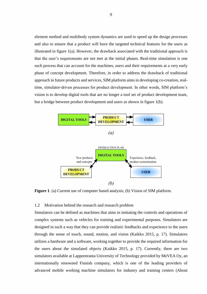
illustrated in figure 1(a). However, the drawback associated with the traditional approach is

that the user’s requirements are not met at the initial phases. Real-time simulation is one

such process that can account for the machines, users and their requirements at a very early

phase of concept development. Therefore, in order to address the drawback of traditional

approach in future products and services, SIM platform aims in developing co-creation, real-

time, simulator-driven processes for product development. In other words, SIM platform’s

vision is to develop digital tools that are no longer a tool set of product development team,

but a bridge between product development and users as shown in figure 1(b).

Figure 1. (a) Current use of computer based analysis; (b) Vision of SIM platform.

1.2 Motivation behind the research and research problem

Simulators can be defined as machines that aims in imitating the controls and operations of

complex systems such as vehicles for training and experimental purposes. Simulators are

designed in such a way that they can provide realistic feedbacks and experience to the users

through the sense of touch, sound, motion, and vision (Kaikko 2015, p. 17). Simulators

utilizes a hardware and a software, working together to provide the required information for

the users about the simulated objects (Kaikko 2015, p. 17). Currently, there are two

simulators available at Lappeenranta University of Technology provided by MeVEA Oy, an

internationally renowned Finnish company, which is one of the leading providers of

advanced mobile working machine simulators for industry and training centers (About

10

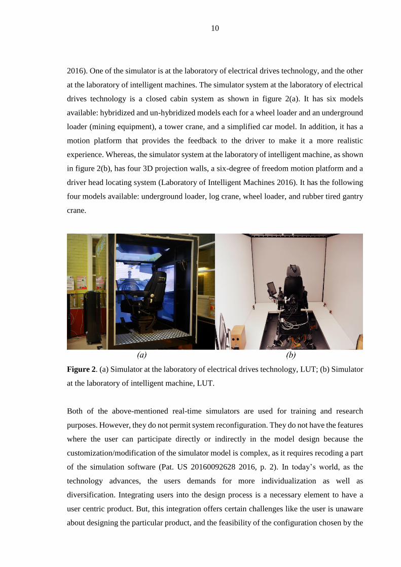
2016). One of the simulator is at the laboratory of electrical drives technology, and the other

at the laboratory of intelligent machines. The simulator system at the laboratory of electrical

drives technology is a closed cabin system as shown in figure 2(a). It has six models

available: hybridized and un-hybridized models each for a wheel loader and an underground

loader (mining equipment), a tower crane, and a simplified car model. In addition, it has a

motion platform that provides the feedback to the driver to make it a more realistic

experience. Whereas, the simulator system at the laboratory of intelligent machine, as shown

in figure 2(b), has four 3D projection walls, a six-degree of freedom motion platform and a

driver head locating system (Laboratory of Intelligent Machines 2016). It has the following

four models available: underground loader, log crane, wheel loader, and rubber tired gantry

crane.

Figure 2. (a) Simulator at the laboratory of electrical drives technology, LUT; (b) Simulator

at the laboratory of intelligent machine, LUT.

Both of the above-mentioned real-time simulators are used for training and research

purposes. However, they do not permit system reconfiguration. They do not have the features

where the user can participate directly or indirectly in the model design because the

customization/modification of the simulator model is complex, as it requires recoding a part

of the simulation software (Pat. US 20160092628 2016, p. 2). In today’s world, as the

technology advances, the users demands for more individualization as well as

diversification. Integrating users into the design process is a necessary element to have a

user centric product. But, this integration offers certain challenges like the user is unaware

about designing the particular product, and the feasibility of the configuration chosen by the

11

user is also a matter of concern. In addition, the choices made by the user must be optimized

for performance. To overcome these difficulties, the design tools and methodologies should

be altered or new tool-sets should be develop to communicate with the users in order to

collect the crucial information about customization. Therefore, the research problem for this

thesis is concerning the incorporation of user specific designs into simulation models by

using some altered or new tool-sets. (Ninan & Siddique 2004, p. 4317.)

1.3 Research questions

In order to address the research problem and simultaneously to achieve the vision of utilizing

digital tools to bridge the gap between product development and users, SIM platform plans

to set-up a user interactive SIM studio at LUT, Finland in collaboration with MeVEA Oy.

The vision is that the users can customize the simulation model according to their own

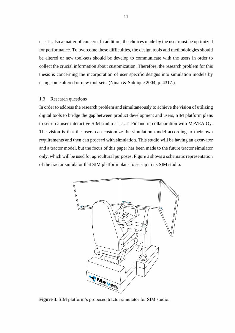
requirements and then can proceed with simulation. This studio will be having an excavator

and a tractor model, but the focus of this paper has been made to the future tractor simulator

only, which will be used for agricultural purposes. Figure 3 shows a schematic representation

of the tractor simulator that SIM platform plans to set-up in its SIM studio.

Figure 3. SIM platform’s proposed tractor simulator for SIM studio.

12

The SIM studio will be made available round the clock for students, staff, and all the

personnel of LUT. Therefore, anyone having access to the university can access this studio

and can simulate the machine based on their own requirements. This vision can be achieved

by developing a user-friendly interface or a modeling configurator that can communicate

with users, who are often laymen in a non-technical perspective, to collect their

requirements. The user-interface/modeling configurator could be integrated with the

simulation software (MeVEA Modeller) in order to reflect the changes in the system design,

in a real-time environment. However, this approach leads to a number of questions that will

be answered with the help of this research work. The research questions are:

(i) How can the modeling configurator be created and linked to the simulation software?

(ii) Why this cannot be done by the traditional approach of design/modeling tools?

(iii) Which parameters/attributes can the users customize?

(iv) What is the maximum number of options provided to the users for each attributes?

(v) Is a feasible configuration selected by the users?

1.4 Aim and objectives of the research

Traditional simulation modeling techniques typically requires an expert’s knowledge and

supervision for carrying out the development and the modification of a simulation model.

Also, it takes a good amount of time for verifying and validating such a model. (Wang et al.

2011, p. 765.) In order to overcome these drawbacks, Kaikko (2015, p. 12) stated that a

modeling process can be divided into three phases: (i) Collecting the information from the

user, (ii) Building the model according to the choices, and (iii) Simulating the model. By

doing so, the users are able to express their needs in a clear technical manner and this in turn

will help the users to modify the model quickly.

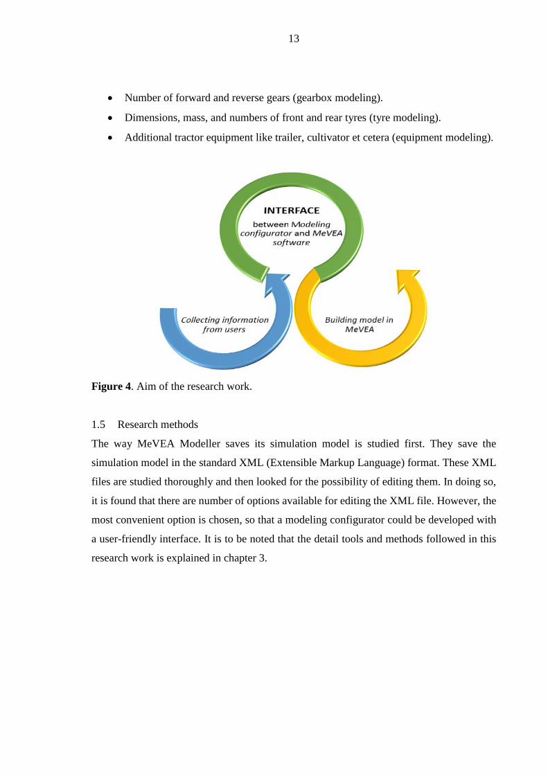
The main aim of this research is to develop a modeling configurator that will collect the

parameter requirements for the agricultural tractor model from the user, and accordingly, it

will process the required information in MeVEA Modeller to generate the customized

simulation model as explain in figure 4. There are a number of parameters/attributes that

could be modified for a tractor. However, the objective of this research paper is to modify

the following attributes for the tractor simulator:

Maximum torque of the engine (engine modeling).

Maximum braking torque for the engine (engine modeling).

13

Number of forward and reverse gears (gearbox modeling).

Dimensions, mass, and numbers of front and rear tyres (tyre modeling).

Additional tractor equipment like trailer, cultivator et cetera (equipment modeling).

Figure 4. Aim of the research work.

1.5 Research methods

The way MeVEA Modeller saves its simulation model is studied first. They save the

simulation model in the standard XML (Extensible Markup Language) format. These XML

files are studied thoroughly and then looked for the possibility of editing them. In doing so,

it is found that there are number of options available for editing the XML file. However, the

most convenient option is chosen, so that a modeling configurator could be developed with

a user-friendly interface. It is to be noted that the detail tools and methods followed in this

research work is explained in chapter 3.

14

2 LITERATURE REVIEW OF MODELING CONFIGURATORS

In order to embark the development of any new idea, it is always a good practice to figure-

out that, what has been already researched in the specific area of interest. This approach

helps in analyzing and understanding the various concepts and approaches that has already

being tested. Accordingly, the results of the previous findings can be used to further enhance

and develop the model in this research work.

In this chapter, the overview and advancement of modeling configurators should have been

considered. But, as modeling configurators are too broad a topic to be reviewed, so in order

to make this review a more focused one, literature review of modeling configurators for

mobile vehicles has been carried out. This was made achievable by following a systematic

literature review procedure. In the following sub-sections, the methodology for performing

a systematic literature review and the findings by applying this methodology will be

discussed.

2.1 Systematic literature review methodology

In this section, the method to perform a systematic literature review is presented so that a

relevant set of documents with the prime objective of finding the working principle of the

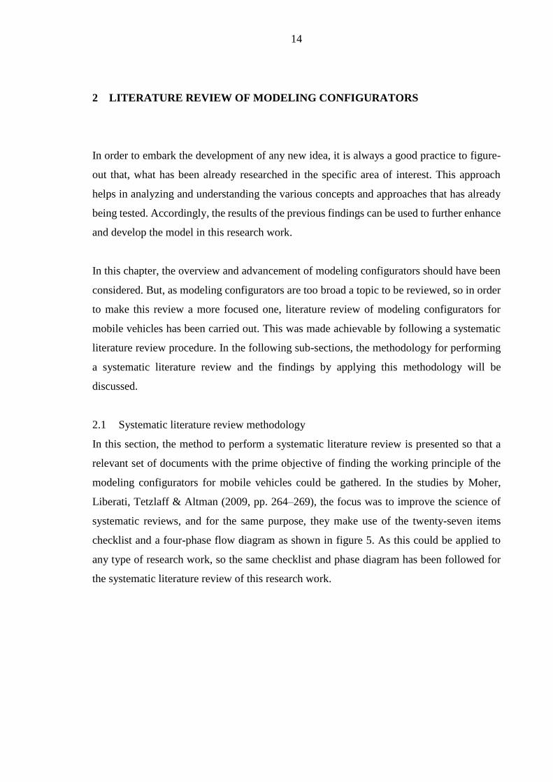
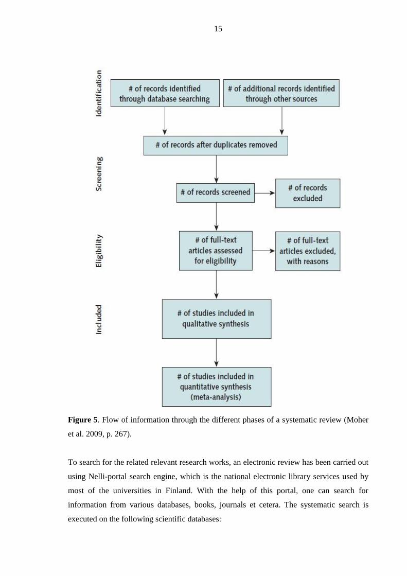
modeling configurators for mobile vehicles could be gathered. In the studies by Moher,

Liberati, Tetzlaff & Altman (2009, pp. 264–269), the focus was to improve the science of

systematic reviews, and for the same purpose, they make use of the twenty-seven items

checklist and a four-phase flow diagram as shown in figure 5. As this could be applied to

any type of research work, so the same checklist and phase diagram has been followed for

the systematic literature review of this research work.

15

Figure 5. Flow of information through the different phases of a systematic review (Moher

et al. 2009, p. 267).

To search for the related relevant research works, an electronic review has been carried out

using Nelli-portal search engine, which is the national electronic library services used by

most of the universities in Finland. With the help of this portal, one can search for

information from various databases, books, journals et cetera. The systematic search is

executed on the following scientific databases:

16

- ABI/INFORM Global(ProQuest XML)

- DOAB - Directory of Open Access Books

- DOAJ Directory of Open Access Journals

- Ebook Library (EBL)

- EBSCO - Academic Search Elite

- Emerald Journals (Emerald)

- Espacenet Patent search-English

- FreePatentsOnline

- IEEE

- LUTPub / Doria (LUT's e-publications)

- ProQuest Technology Collection

- ScienceDirect - All Subscribed Content (Elsevier API)

- SCOPUS (Elsevier API)

- SpringerLink eJournals

- Springer eBooks

- Web of Science (WOS) - Cross Search

- Wiley Blackwell Online Library

During the search in the above-mentioned databases, there are number of criteria that has

been followed. These criteria are as follows:

(i) The keywords that has been used are “modeling” AND “tool” AND “mobile vehicle”

/ “vehicle” (refer to appendix I, where the keywords for each databases are

mentioned).

(ii) Scientific articles, conference papers, patents, and other relevant documents from the

database’s search results has been considered for the scope of this review.

(iii) Only English language has been selected for performing the search as most of the

authors and organizations around the world make use of English language in their

publications.

(iv) It has also been considered that the publication dates are not older than 10 years for

a better and updated scientific contribution. However, in some cases an exception

has been made where the idea or the basic concept of the research article is not being

affected by the time frame.

17

By following the systematic approach as shown in figure 5 above, the initial results obtained

from all the databases are screened for choosing a specific number of full-text articles. Now,

the abstract is read thoroughly in order to remove duplicacy and the most eligible articles

are chosen for the review. As per requirement, the introduction and the result sections are

also screened to have a better picture of the articles. As a part of the systematic approach,

the references of the selected articles from the previous step are also screened in order to

search for any missing article in the process. Also, for the better search of literature, relevant

articles from other sources like google scholar were also included. In this way, all the four

phases namely identification phase, screening phase, eligibility phase, and inclusion phase

of the systematic flow diagram has been covered. Finally, the scientific documents retrieved,

as a result of above methodology, are sorted and their significance is taken into consideration

in section 2.2.

2.2 Findings from systematic literature review

This section is dedicated for briefing the results of the systematic literature review applied

in this research work. According to the present knowledge of the author, this is one amongst

the first reports of its kind where the findings from the scientific databases on the modeling

tool for mobile vehicles has been considered.

An electronic search has been carried out in Nelli-portal search engine on the list of databases

mentioned in last section based on the search criteria, which is also mentioned in the last

section. In order to follow the detailed overview on all the databases, one may refer to

appendix I, where the number of records retrieval, exclusion, and inclusion along with the

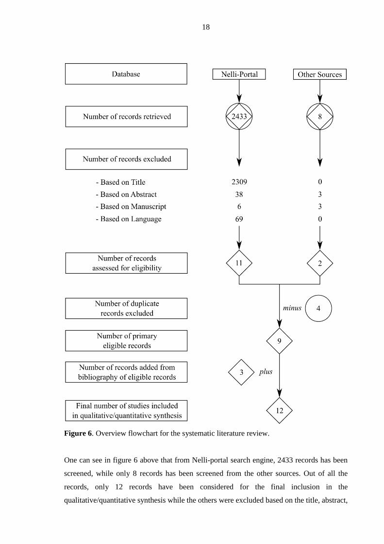
keywords for each databases are listed. However, the brief result has been shown in figure 6

in the form of a flowchart along with the results from other sources like google scholar as

well.

18

Figure 6. Overview flowchart for the systematic literature review.

One can see in figure 6 above that from Nelli-portal search engine, 2433 records has been

screened, while only 8 records has been screened from the other sources. Out of all the

records, only 12 records have been considered for the final inclusion in the

qualitative/quantitative synthesis while the others were excluded based on the title, abstract,

19

manuscript, language, and duplicacy. With the help of this systematic review, the literatures

of the relevant topics has been summarized in the following paragraphs.

Mackulak & Cochran (1990, pp. 82–87) concluded from the IntelliSim project that 45% of

the total efforts required for a simulation project are consumed in formulating and modeling

phase. Mackulak, Lawrence & Colvin (1998, pp. 979–984) figured out that a bug-free

(accurate) model can be quickly constructed and reused only if one uses a generic simulation

model. So, in order to have a generic model which could be applied to many systems to save

significant amount of simulation study time, Steele, Mollaghasemi, Rabadi & Cates (2002,

pp. 747–753) focused on developing a generic simulation model that can be populated with

system-specific information to obtain a more reliable system-specific model with the desired

results. Here, the user-interface for such a generic model allows only the system’s experts to

feed in the required information into the generic simulation model by using their own

terminologies (Steele et al. 2002, pp. 747–753). Also, due to large amount of market

competitions, even the manufacturing industry demanded for a less time consuming and

error-free simulation model of manufacturing systems. So, Wy et al. (2011, pp. 138–147)

focused on a generic simulation modeling framework for logistic-embedded assembly

manufacturing line consisting of a data-driven generic simulation model and a layout

modeling software in order to reduce the build-up time for such a simulation model. Zhao,

Guo, Xu & Guo (2013, pp. 2287–2290) showed the significance of automatic drivetrain

modeling by focusing on modeling and simulating the automatic transmission assembly. As

there was a great demand for generic real-time models drivetrain topologies, so Schwarz,

Bachinger, Stolz & Watzenig (2015, pp. 1–5) proposed a novel tool for automatic

parametrization that helps in designing mainly all types of gear transmission (drivetrain)

topologies by non-experts. Even, Kaikko (2015, pp. 1–77) focused on developing a generic

simulation model for robust simulation providing electric drive solutions for the mobile

working machines, which can also be used for marketing and development purposes.

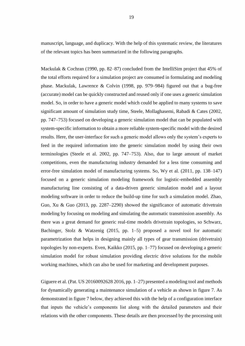
Giguere et al. (Pat. US 20160092628 2016, pp. 1–27) presented a modeling tool and methods

for dynamically generating a maintenance simulation of a vehicle as shown in figure 7. As

demonstrated in figure 7 below, they achieved this with the help of a configuration interface

that inputs the vehicle’s components list along with the detailed parameters and their

relations with the other components. These details are then processed by the processing unit

20

and helps in generating the maintenance simulation which comprises the collection of all the

transition states amongst the components into a global state machine. (Pat. US 20160092628

2016, pp. 1–27.)

Figure 7. A modeling tool for dynamically generating a maintenance simulation of a vehicle

(mod. Pat. US 20160092628 2016).

Mitrev & Tudjarov (2014, pp. 268–273) also proposed and developed a web-based tool for

reconstructing accident in a web-based environment which is otherwise, a time consuming

process. They make use of X3D (eXtensible 3D) language in order to showcase the

visualization for the web-based simulation where the 3D scene and vehicle’s animation after

the impact is being automatically generated based on the results of the solution of modeled

differential equations of the system (Mitrev & Tudjarov 2014, pp. 268–273).

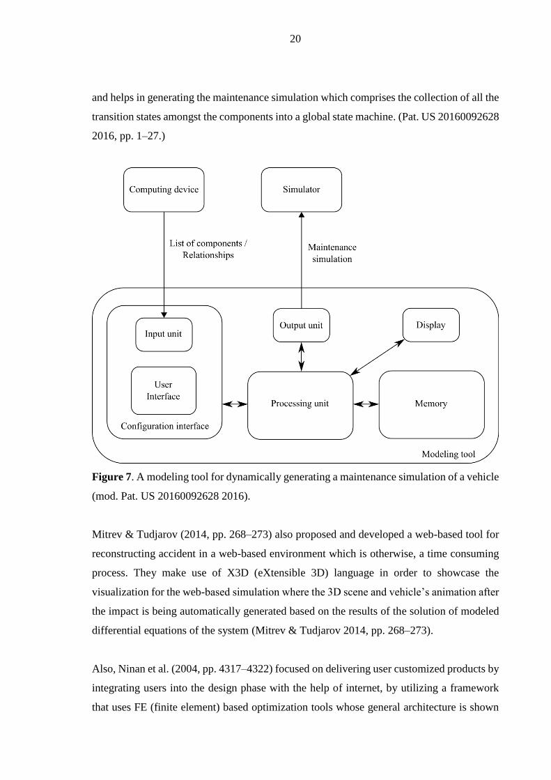
Also, Ninan et al. (2004, pp. 4317–4322) focused on delivering user customized products by

integrating users into the design phase with the help of internet, by utilizing a framework

that uses FE (finite element) based optimization tools whose general architecture is shown

21

in figure 8. As shown in figure 8 below, the parameters selected by the users are categorized

as geometric and structured parameters or their combinations. The API (application

programming interface) of the CAD (computer-aided design) system inputs the geometric

parameters and builds the solid model of the customized product that is being saved as an

IGES (initial graphics exchange specification) file into the common database which is later

being utilized by the FE software. (Ninan et al. 2004, p. 4319.)

Figure 8. System architecture for internet based framework for customer centric design and

optimization (Ninan et al. 2004, p. 4319).

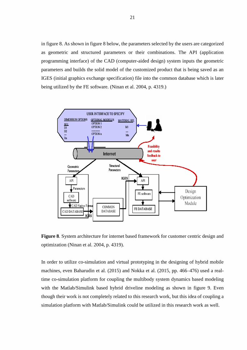
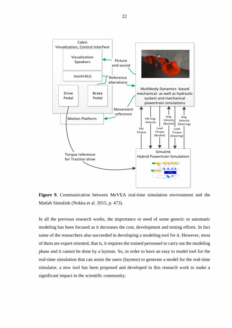
In order to utilize co-simulation and virtual prototyping in the designing of hybrid mobile

machines, even Baharudin et al. (2015) and Nokka et al. (2015, pp. 466–476) used a real-

time co-simulation platform for coupling the multibody system dynamics based modeling

with the Matlab/Simulink based hybrid driveline modeling as shown in figure 9. Even

though their work is not completely related to this research work, but this idea of coupling a

simulation platform with Matlab/Simulink could be utilized in this research work as well.

22

CabinVisualization, Control Interface

Drive Pedal

Brake Pedal

Joystick(s)

Multibody Dynamics -based mechanical- as well as hydraulic

system and mechanical powertrain simulations

Reference alterations

VisualizationSpeakers Picture

and sound

Motion Platform

Movement reference

SimulinkHybrid Powertrain Simulation

Torque referencefor Traction drive

EMTorque

EM Ang. Velocity

LoadTorque

(Bucket)

Ang. Velocity(Bucket)

LoadTorque

(Steering)

Ang. Velocity

(Steering)

Figure 9. Communication between MeVEA real-time simulation environment and the

Matlab Simulink (Nokka et al. 2015, p. 473).

In all the previous research works, the importance or need of some generic or automatic

modeling has been focused as it decreases the cost, development and testing efforts. In fact

some of the researchers also succeeded in developing a modeling tool for it. However, most

of them are expert oriented, that is, it requires the trained personnel to carry out the modeling

phase and it cannot be done by a layman. So, in order to have an easy to model tool for the

real-time simulation that can assist the users (laymen) to generate a model for the real-time

simulator, a new tool has been proposed and developed in this research work to make a

significant impact in the scientific community.

23

3 TOOLS AND METHODOLOGIES

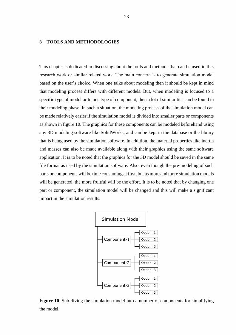
This chapter is dedicated in discussing about the tools and methods that can be used in this

research work or similar related work. The main concern is to generate simulation model

based on the user’s choice. When one talks about modeling then it should be kept in mind

that modeling process differs with different models. But, when modeling is focused to a

specific type of model or to one type of component, then a lot of similarities can be found in

their modeling phase. In such a situation, the modeling process of the simulation model can

be made relatively easier if the simulation model is divided into smaller parts or components

as shown in figure 10. The graphics for these components can be modeled beforehand using

any 3D modeling software like SolidWorks, and can be kept in the database or the library

that is being used by the simulation software. In addition, the material properties like inertia

and masses can also be made available along with their graphics using the same software

application. It is to be noted that the graphics for the 3D model should be saved in the same

file format as used by the simulation software. Also, even though the pre-modeling of such

parts or components will be time consuming at first, but as more and more simulation models

will be generated, the more fruitful will be the effort. It is to be noted that by changing one

part or component, the simulation model will be changed and this will make a significant

impact in the simulation results.

Figure 10. Sub-diving the simulation model into a number of components for simplifying

the model.

24

Also, the first simulation model must be made available beforehand as a reference for the

users, so that the users do not have to make the simulation model from scratch. The users

will just have the option of changing the various components of the model by choosing the

appropriate choices made available in the modeling configurator. The simulation software

will utilize its database where all the different choices of components are made available,

and depending upon the choices selected by the users, the simulation software is going to

create the simulation model with those choices. Every time the user makes a new selection,

the previous simulation model will be overwritten (updated) with the new choices, leading

to a new simulation model. One of the possible advantage of this approach is the significant

reduction in the simulation study time as the simulation model need not be modeled from

scratch, rather it only needs to be populated with the new data from the users. However, as

this approach is more general, so extra care must be taken in the study of the simulation

software and its working principle for developing the modeling configurator so that it is

applicable to all the instances of the chosen domain. The software application used for

simulation in this research work is decided before hand and the selection of MeVEA as the

simulation software is a natural choice, as the project is in close collaboration with MeVEA

Oy. Therefore, study of MeVEA simulation software has been done thoroughly.

MeVEA simulation software is based on multibody system dynamics. It utilizes global and

body reference coordinate system for determining the location and orientation of the bodies.

All the bodies have their own body reference coordinate system, but their location and

orientation can also be defined using the body reference coordinate system of other bodies.

Here, the bodies are connected with each other with the help of constraints, which can be in

the form of translational joints, revolute joints, spherical joints, cylindrical joints, hinge

joints, universal joints and/or fixed joints. Bodies can also be fixed with one another or onto

the same plane. This constraint’s definition helps in defining the relative movement of the

bodies. Here, also the mass, inertia and forces of the bodies affects the body’s movement

and in turn the response of the entire system. (MeVEA Modeller [simulation program]

2017b, pp. 1–206.)

In addition, when a model is made using MeVEA Modeller, then it generates two “.xml”

files and one “.mvs” file. The first “.xml” file, which is being saved as “ModelName.xml”,

comprises of details like model properties and all the simulation components. Whereas, the

25

second “.xml” file, which is being saved as “ModelName_world.xml”, comprises of details

concerning the world properties such as lights, cameras, effects et cetera. Now, the role of

the “.mvs” file, which is being saved as “ModelName.mvs”, is to connect the above two

“.xml” files, namely, “ModelName.xml” and “ModelName_world.xml”, and it also contains

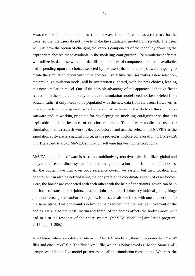
some additional settings. (MeVEA Modeller [simulation program] 2017a, pp. 7–8.) Here,

the aim is to modify the XML file named “ModelName.xml”, which contain details of all

the simulation components and the properties of the model with the help of the modeling

configurator. Since, only the model needs to be changed and not the effects like camera and

lights, so the “ModelName_world.xml” file will remain unaltered. Finally, the

“ModelName.mvs” file should be able to execute the modified XML and the world XML

file and generate the required model that is able to simulate. Figure 11 shows an example of

such “.mvs” file, where it links “Tractor_Model.xml” file and “Tractor_Model_world.xml”

file, and executes the simulation.

Figure 11. Contents of the “.mvs” file used in MeVEA simulation software.

26

XML documents are structured documents and when it comes to editing or authoring them,

then care must be taken so that later the simulation software can utilize them. This can be

done in a number of ways, but the aim is to modify it using a web-based tool or modeling

configurator where the users can enter their own choices or select the pre-existing ones. In

the following sub-sections, there are different methods explained that can be implied for

carrying out the desired action.

3.1 Commercial softwares or online open source applications

Many of the popular XML editors are mostly text editors that makes use of their XML syntax

knowledge and follow the provided XML schema or DTD (Document Type Definition). For

editing/authoring a complex XML file, there are number of commercial softwares available

like Altova XMLSpy (XML Editor 2016a), EditiX XML Editor (Home 2016), Oxygen XML

Editor (XML Editor 2016b) and many more. The possible advantage of using such softwares

could be that the desired changes in the file can be done rather quickly if one knows the

structure/pattern of the file. Whereas, the possible disadvantage could be that it may disrupt

the structure or the format of the XML file and then later it may become non-readable for

the simulation software. In addition, another possible disadvantage could be that handling

such softwares by layman could be challenging and may require experts for the task.

Also, unlike the generic tools (mentioned above) that can work with any type of documents,

there are also tools available like Mozilla Composer or DreamWeaver, that are specialized

to handle only the single document type such as HTML (HyperText Markup Language) or

XHTML (Extensible Hypertext Markup Language). As they are for single document type,

so they do not require any schema or DTD because the code of such tools already contains

information about its DTD or schema. The advantage of using such tools is that it hides the

complexity of structured documents by behaving like work processors as much as possible.

This helps the naive users in creating and modifying a complex document by using a normal-

view in the tool. However, possible disadvantage of such a tool is that they demand the users

to have some knowledge about the markup language or the structured documents. (Quint &

Vatton 2004, p. 116.)

In addition, there are many open source applications available online like “Online XML

Editor”, which is a browser based cross-platform editor having a graphical user-interface for

27

editing or viewing. It represents the XML file in a grid view and does not require any special

plugins. All the parsing, mapping, data representation and editing is being done in the user’s

computer, and only a small amount of time is required by the server for preparing the desired

XML file that can be saved in the desired directory for the simulation software. (Frequently

Asked Questions 2016.) The possible advantage for such an online tool is that everything

can be done without the knowledge of markup languages or structured documents in a

significantly small amount of time. However, there is also a possible disadvantage that all

the fields of the file are editable, which may not be desired. In addition, when editing a

simulation XML file, the users should also have knowledge about how different attributes

of the XML file are related to each other.

3.2 XML mapping using Microsoft excel

Another possible method of editing XML documents is with the help of Microsoft excel.

Excel could be used to map the XML file into an excel file (.xlsx file). The excel file (.xlsx

file) refers the XML schema from the XML file itself. Then, this same excel file could be

saved as an editable “.htm” or “.html” file where any changes made into the webpage could

be reflected into the excel file and the same can be exported into the desired XML file, which

will be used by the simulation software. (Map XML elements to cells in an XML Map 2016.)

The possible advantage of such an approach is that only the desired fields of the xml file can

be edited using the web page. Whereas, the possible disadvantage is that while editing and

exporting the data back into the XML file, some of the data like forces, volume definitions

et cetera may get lost, making the final simulation behave in the most unpredictable way.

3.3 Programming language softwares

Another possible method is to make use of the programming language software for

writing/editing files (XML file in this case) for the simulation software. Kaikko (2015, pp.

1–77) made a generic simulation model using python programming language that was used

to make scripts that helped to build “.xml” file and various “.mva” files for the simulation

software. Similarly, python can be used as one of the tools for the problem in hand. Python

is an un-compiled or interpreted language that is dynamically typed and it is a white space

language. The idea here is to handle the XML document according to semantics. The

possible advantage of using python is that it is a versatile and open source software, so the

desired action can be achieved. However, the possible disadvantage of using such a

28

programming language software is that it cannot be used by a layman as it is not a user-

friendly application. Another possible option could be MATLAB/Simulink as well, but it

may have the same disadvantage.

So, in order to make use of this method, additional applications can be used to input the data

from the users into python script using user-friendly interfaces. The idea here is to hide the

sophisticated script/system behind those user-friendly interfaces. One possible option is to

make use of the editable “.htm” or “.html” files as explained in section 3.2. The choices from

the user can be saved into the webpage which in turn will save it in an excel datasheet, and

the same datasheet can be used by the python script. Also, in this approach, the introduction

of partial interactive autonomy would considerably enhance its performance. Partial

interactive autonomy can be introduced by using ASP (Active Server Pages) technology that

can build web-based user-interface. ASP can act as an agent between the user and the

simulation software, and the information from the user passes through them.

29

4 CASE STUDY FOR TRACTOR SIMULATOR

A case study of agricultural tractor simulator is covered in this chapter based on one of the

methods from the last chapter. To start with, a tractor simulator can be seen as a simulator

that imitates the working of an actual tractor. Tractors can be defined as mobile working

machines that helps in carrying out the agricultural activities like ploughing, shoveling,

transporting et cetera. However, these agricultural activities seem deemed possible till the

time one does not have an efficient machine. Only with the advent of tractors, all the farming

activities could be accelerated and became much more efficient than before. (Tractor

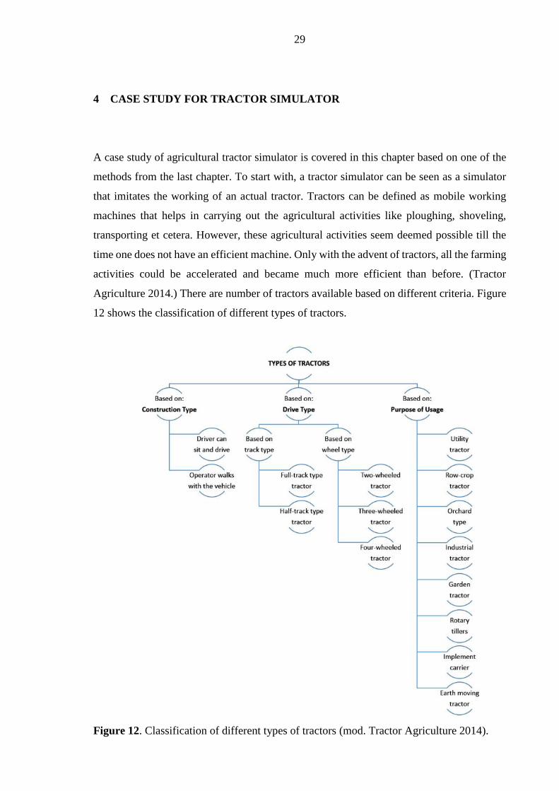
Agriculture 2014.) There are number of tractors available based on different criteria. Figure

12 shows the classification of different types of tractors.

Figure 12. Classification of different types of tractors (mod. Tractor Agriculture 2014).

30

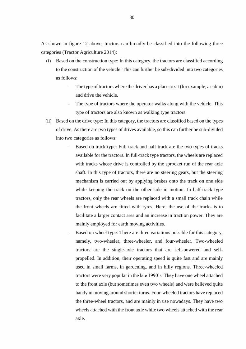
As shown in figure 12 above, tractors can broadly be classified into the following three

categories (Tractor Agriculture 2014):

(i) Based on the construction type: In this category, the tractors are classified according

to the construction of the vehicle. This can further be sub-divided into two categories

as follows:

- The type of tractors where the driver has a place to sit (for example, a cabin)

and drive the vehicle.

- The type of tractors where the operator walks along with the vehicle. This

type of tractors are also known as walking type tractors.

(ii) Based on the drive type: In this category, the tractors are classified based on the types

of drive. As there are two types of drives available, so this can further be sub-divided

into two categories as follows:

- Based on track type: Full-track and half-track are the two types of tracks

available for the tractors. In full-track type tractors, the wheels are replaced

with tracks whose drive is controlled by the sprocket run of the rear axle

shaft. In this type of tractors, there are no steering gears, but the steering

mechanism is carried out by applying brakes onto the track on one side

while keeping the track on the other side in motion. In half-track type

tractors, only the rear wheels are replaced with a small track chain while

the front wheels are fitted with tyres. Here, the use of the tracks is to

facilitate a larger contact area and an increase in traction power. They are

mainly employed for earth moving activities.

- Based on wheel type: There are three variations possible for this category,

namely, two-wheeler, three-wheeler, and four-wheeler. Two-wheeled

tractors are the single-axle tractors that are self-powered and self-

propelled. In addition, their operating speed is quite fast and are mainly

used in small farms, in gardening, and in hilly regions. Three-wheeled

tractors were very popular in the late 1990’s. They have one wheel attached

to the front axle (but sometimes even two wheels) and were believed quite

handy in moving around shorter turns. Four-wheeled tractors have replaced

the three-wheel tractors, and are mainly in use nowadays. They have two

wheels attached with the front axle while two wheels attached with the rear

axle.

31

(iii) Based on the purpose of usage: In this category, the tractors are classified according

to their purpose of use. Depending upon the usage of the vehicle, this category can

further be divided. According to Tractor Agriculture (2014), “They are further

divided into broad categories listed below:

1. Utility Tractors

2. Row Crop Tractor

3. Orchard Type

4. Industrial Tractor

5. Garden Tractor

6. Rotary Tillers

7. Implement Carrier

8. Earth Moving Tractors”

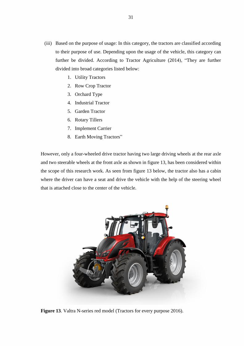
However, only a four-wheeled drive tractor having two large driving wheels at the rear axle

and two steerable wheels at the front axle as shown in figure 13, has been considered within

the scope of this research work. As seen from figure 13 below, the tractor also has a cabin

where the driver can have a seat and drive the vehicle with the help of the steering wheel

that is attached close to the center of the vehicle.

Figure 13. Valtra N-series red model (Tractors for every purpose 2016).

32

4.1 Construction of the vehicle

The development of modeling configurator depends completely on how the tractor has been

modeled in MeVEA Modeller. Therefore, construction of the tractor in MeVEA is one of

the important steps in developing the modeling configurator. When the modeling is focused

completely on tractor simulator as in this research work, then many similarities can be found

in modeling the variations (types and sizes) of the same components. This particular fact has

been used in order to model the tractor simulator and the same advantage is being utilized in

developing the modeling configurator. As a result of this, different simulation models for

the tractor are easily generated in a considerably less amount of time, like in a couple of

seconds or maximum one minute.

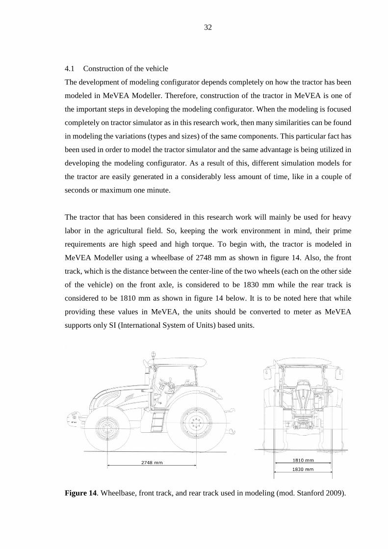
The tractor that has been considered in this research work will mainly be used for heavy

labor in the agricultural field. So, keeping the work environment in mind, their prime

requirements are high speed and high torque. To begin with, the tractor is modeled in

MeVEA Modeller using a wheelbase of 2748 mm as shown in figure 14. Also, the front

track, which is the distance between the center-line of the two wheels (each on the other side

of the vehicle) on the front axle, is considered to be 1830 mm while the rear track is

considered to be 1810 mm as shown in figure 14 below. It is to be noted here that while

providing these values in MeVEA, the units should be converted to meter as MeVEA

supports only SI (International System of Units) based units.

Figure 14. Wheelbase, front track, and rear track used in modeling (mod. Stanford 2009).

33

It is to be noted that this research work is meant for academic purpose, so the construction

of the vehicle including the mass of the vehicle, mass distribution et cetera has been assumed

as an example for demonstration purposes only. As, the Valtra T-series tractors have a

weight of 7300 kg without considering the extra weights (Compare Valtra models 2017). So,

the current model is assumed to have a total weight of 7300 kg. It is to be noted that the

model in hand is designed in accordance with the Valtra T-series tractors as much as

possible, and that too specifically, T144, T154, and T174e, as they all share some common

features like weights and dimensions. The static weight distribution between the front and

rear axle (which is also defined as weight split) is assumed to be 55/45 for academic purposes

only. So, 55% of the tractor’s weight goes to the front axle while the remaining 45% goes to

the rear axle. However, the tractor considered in this research work (with no implements or

additional weights) normally has weight distribution in such a way that the rear axle has a

higher mass than the front axle. But, the weight distribution of 55/45 considered in this

research work is assumed for academic purposes only. Therefore, 4015 kg (55% of 7300 kg)

goes to the front axle, while 3285 kg (45% of 7300 kg) goes to the rear axle. But, as tyres

are already attached to the axles and the total weight of the front tyres is 150*2 = 300 kg,

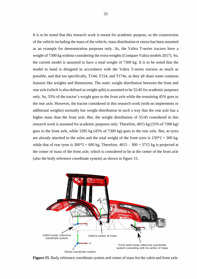
while that of rear tyres is 300*2 = 600 kg. Therefore, 4015 – 300 = 3715 kg is projected at

the center of mass of the front axle, which is considered to be at the center of the front axle

(also the body reference coordinate system) as shown in figure 15.

Figure 15. Body reference coordinate system and center of mass for the cabin and front axle.

34

Whereas, 3285 – 600 = 2685 kg is projected at the center of mass of the cabin (as cabin and

rear axle together is assumed to be a single body, otherwise, it is always projected at the

center of the rear axle), which is at a distance of (1080, 300, 0) mm from the body reference

coordinate system of the cabin. Also, the body reference coordinate system of the cabin is at

a distance of (0, 980, 0) mm with respect to the ground (global coordinate system) as shown

in figure 15 above. It is to be noted here that the mass distribution projected over the center

of masses is just used as a demonstration for academic purposes. However, the main aim of

this research is to develop the modeling configurator.

Then, there are two pivots which are attached to both ends of the front axle. The position of

the right pivot is (0, -13, 915) mm with respect to the front axle, whereas, the position of the

left pivot is (0, -13, -915) mm with respect to the front axle. The front tyres are attached to

these pivots. The position of the tie rod, which is used to design the steering mechanism, is

(-292, 0, 0) mm with respect to the front axle.

In order to calculate the moments and products of inertia, the inertia calculator of MeVEA

Modeller, as shown in figure 16, has been utilized. It is only required to choose the shape of

the body and then provide the necessary dimensions and mass, the inertia calculator will then

provide the necessary values for the moments and products of inertia. The moments and

products of inertia for the cabin has been calculated by assuming it to be a cube with a

dimension of x = 5800 mm, y = 1075.2 mm, and z = 2550 mm as almost all the weight is

concentrated to the lower portion of the cabin, while the upper portion is mainly an empty

space. Also, the mass considered for the cabin is 2685 kg as already explained above. For

the front axle, it is assumed to have a shape of horizontal cylinder, whose length is 1830 mm

and radius is 26 mm. Also, as already explained above, the mass considered for the front

axle is 3715 kg.

35

Figure 16. Inertia calculator of MeVEA Modeller utilized to calculate moments and

products of inertia.

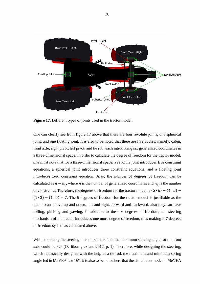
In the tractor model, the bodies are constrained with a number of joints. The different types

of joints used in the model are as shown in figure 17. The tractor’s cabin is constrained with

the ground by utilizing a floating joint at a location of (100, 300, 0) mm with respect to the

global coordinate system. The front axle in turn is constrained with the cabin by utilizing a

revolute joint at a location of (2748, -182.5, 0) mm with respect to the cabin’s body reference

coordinate system. The right and the left pivots are connected to the front axle with the help

of revolute joints at a location of (0, 0, 915) mm and (0, 0, -915) mm respectively with

respect to the front axle, and (0, 13, 0) mm and (0, 13, 0) mm with respect to the pivots

respectively. The tie rod, which is used to model the steering mechanism, is connected to the

left pivot with the help of a spherical joint at a location of (-292, 0, 16.3) mm with respect

to the left pivot and (0, 0, -898.7) mm with respect to the tie rod. Whereas, with the right

pivot, the tie rod is connected with the help of a revolute joint at a location of (-292, 0, -16.3)

mm with respect to the right pivot and (0, 0, 898.7) mm with respect to the tie rod.

36

Figure 17. Different types of joints used in the tractor model.

One can clearly see from figure 17 above that there are four revolute joints, one spherical

joint, and one floating joint. It is also to be noted that there are five bodies, namely, cabin,

front axle, right pivot, left pivot, and tie rod, each introducing six generalized coordinates in

a three-dimensional space. In order to calculate the degree of freedom for the tractor model,

one must note that for a three-dimensional space, a revolute joint introduces five constraint

equations, a spherical joint introduces three constraint equations, and a floating joint

introduces zero constraint equation. Also, the number of degrees of freedom can be

calculated as 𝑛 − 𝑛𝑐, where 𝑛 is the number of generalized coordinates and 𝑛𝑐 is the number

of constraints. Therefore, the degrees of freedom for the tractor model is (5 ∙ 6) − (4 ∙ 5) −

(1 ∙ 3) − (1 ∙ 0) = 7. The 6 degrees of freedom for the tractor model is justifiable as the

tractor can move up and down, left and right, forward and backward, also they can have

rolling, pitching and yawing. In addition to these 6 degrees of freedom, the steering

mechanism of the tractor introduces one more degree of freedom, thus making it 7 degrees

of freedom system as calculated above.

While modeling the steering, it is to be noted that the maximum steering angle for the front

axle could be 32° (Oerlikon graziano 2017, p. 1). Therefore, while designing the steering,

which is basically designed with the help of a tie rod, the maximum and minimum spring

angle fed in MeVEA is ± 16°. It is also to be noted here that the simulation model in MeVEA

37

is completely a mathematical model and the graphics are just for the visualization of the

components. As MeVEA does not allow designing the graphics, so the graphics are imported

from other designing softwares like Blender, SolidWorks et cetera in the specific file format

(mostly “.3ds” file format). However, graphics does not possess any properties other than its

position and orientation. Their only role is to make the components visible and they moves

along with the components. The graphics used in designing the tractor model are provided

by the Machine Dynamics research group at LUT School of Energy Systems. The list of

graphics provided by the Machine Dynamics research group includes cabin and outer frame

as well as its collision graphics, front axle, mudguards, tie rod, and front and rear tyres.

4.2 Power transmission system

Power transmission system can be defined as the driveline that plays a key role in modeling

the vehicle. It is basically a combination of shafts in sequence and can also be referred as the

speed reduction mechanism. It comprises of various components that helps in transmitting

the torque from the engine (where the torque is being generated) to the driving wheels. As it

also helps in changing the torque, so it is even utilized in changing the rotating direction of

the driving wheels.

This section deals with the power transmission system that has been used in modeling the

tractor simulator model. It is to be noted that as this research work is meant for academic

purpose, so the power transmission system utilized is for demonstration use only. The power

transmission system is modeled in a generic way such that it allows to drive the tractor

model. Otherwise, it is not the realistic construction of the Valtra tractor’s power

transmission system. The schematic diagram of the power transmission system used in

designing the tractor model in MeVEA Modeller is shown in figure 18. Broadly, it comprises

of engine, clutch, gearbox, differential gearboxes, reduction gears, axles and wheels. Here,

engine is the prime mover, which generates the torque that needs to be transmitted. In

MeVEA Modeller, it is being modeled with the help of spline curve. Then comes the clutch

that helps in connecting or disconnecting the engine with the rest of the transmission system.

It helps in transmitting the torque from the engine to the gearbox. Also, when the gear needs

to be changed, then the power to the gearbox is cut-off from the engine with the help of

clutch otherwise the gear tooth can be damaged. Here, the clutch is modeled with the help

of friction that allows the gripping action to take place by making use of frictional force

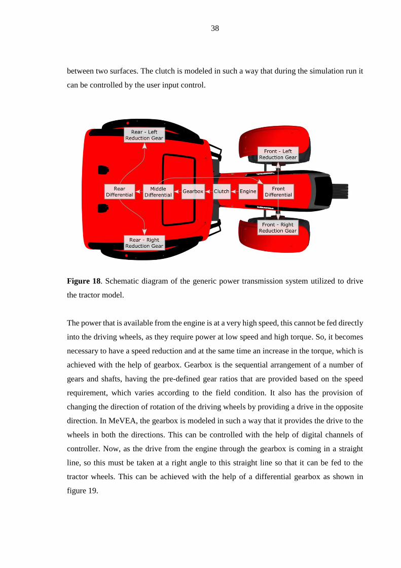
38

between two surfaces. The clutch is modeled in such a way that during the simulation run it

can be controlled by the user input control.

Figure 18. Schematic diagram of the generic power transmission system utilized to drive

the tractor model.

The power that is available from the engine is at a very high speed, this cannot be fed directly

into the driving wheels, as they require power at low speed and high torque. So, it becomes

necessary to have a speed reduction and at the same time an increase in the torque, which is

achieved with the help of gearbox. Gearbox is the sequential arrangement of a number of

gears and shafts, having the pre-defined gear ratios that are provided based on the speed

requirement, which varies according to the field condition. It also has the provision of

changing the direction of rotation of the driving wheels by providing a drive in the opposite

direction. In MeVEA, the gearbox is modeled in such a way that it provides the drive to the

wheels in both the directions. This can be controlled with the help of digital channels of

controller. Now, as the drive from the engine through the gearbox is coming in a straight

line, so this must be taken at a right angle to this straight line so that it can be fed to the

tractor wheels. This can be achieved with the help of a differential gearbox as shown in

figure 19.

39

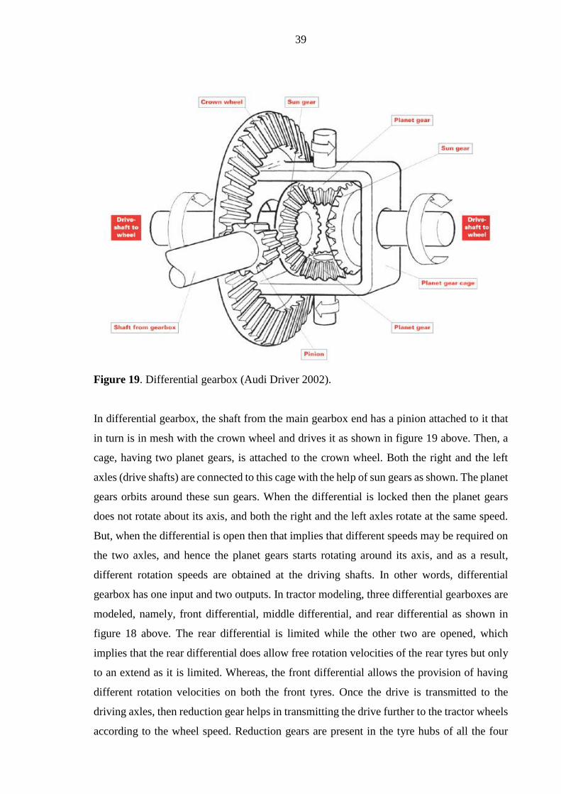
Figure 19. Differential gearbox (Audi Driver 2002).

In differential gearbox, the shaft from the main gearbox end has a pinion attached to it that

in turn is in mesh with the crown wheel and drives it as shown in figure 19 above. Then, a

cage, having two planet gears, is attached to the crown wheel. Both the right and the left

axles (drive shafts) are connected to this cage with the help of sun gears as shown. The planet

gears orbits around these sun gears. When the differential is locked then the planet gears

does not rotate about its axis, and both the right and the left axles rotate at the same speed.

But, when the differential is open then that implies that different speeds may be required on

the two axles, and hence the planet gears starts rotating around its axis, and as a result,

different rotation speeds are obtained at the driving shafts. In other words, differential

gearbox has one input and two outputs. In tractor modeling, three differential gearboxes are

modeled, namely, front differential, middle differential, and rear differential as shown in

figure 18 above. The rear differential is limited while the other two are opened, which

implies that the rear differential does allow free rotation velocities of the rear tyres but only

to an extend as it is limited. Whereas, the front differential allows the provision of having

different rotation velocities on both the front tyres. Once the drive is transmitted to the

driving axles, then reduction gear helps in transmitting the drive further to the tractor wheels

according to the wheel speed. Reduction gears are present in the tyre hubs of all the four

40

wheels and are epicyclic gear packs in this case. Here, the drive is provided on all the four

wheels of the tractor as a four-wheel drive tractor has been considered in this research work.

This way, the entire drive is transmitted right from the engine all the way to the tractor

wheels.

4.3 Method applied in this case study

In order to develop the modeling configurator, the method listed in section 3.3, that is,

utilizing programming language softwares has been used in this research work. Python

programming language has been used in the present study and for the user-interface,

Microsoft excel has been employed. Here, the python script, which is also referred to as the

modeling configurator, is used to access the only “.xml” file of the tractor model that

contains all the model properties and carry out the desire modifications.

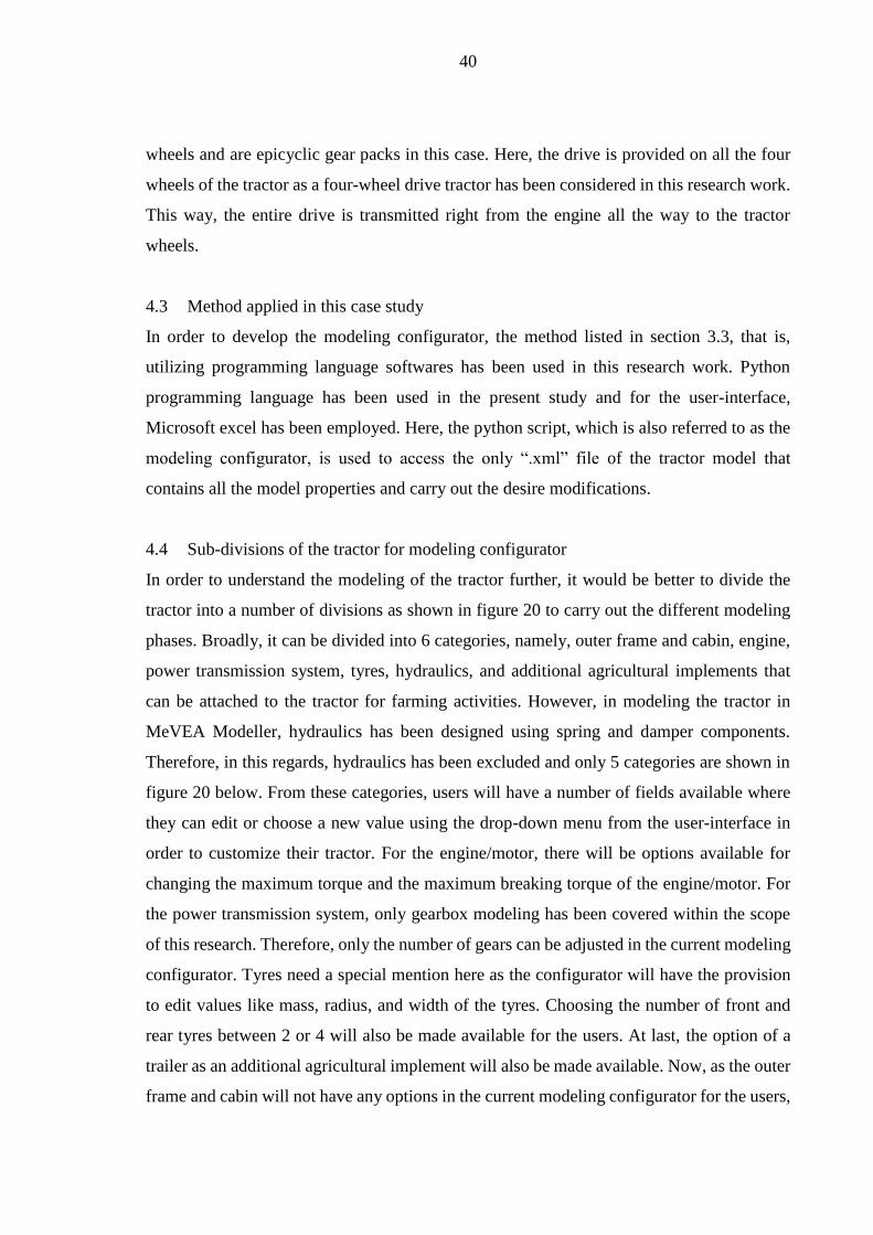
4.4 Sub-divisions of the tractor for modeling configurator

In order to understand the modeling of the tractor further, it would be better to divide the

tractor into a number of divisions as shown in figure 20 to carry out the different modeling

phases. Broadly, it can be divided into 6 categories, namely, outer frame and cabin, engine,

power transmission system, tyres, hydraulics, and additional agricultural implements that

can be attached to the tractor for farming activities. However, in modeling the tractor in

MeVEA Modeller, hydraulics has been designed using spring and damper components.

Therefore, in this regards, hydraulics has been excluded and only 5 categories are shown in

figure 20 below. From these categories, users will have a number of fields available where

they can edit or choose a new value using the drop-down menu from the user-interface in

order to customize their tractor. For the engine/motor, there will be options available for

changing the maximum torque and the maximum breaking torque of the engine/motor. For

the power transmission system, only gearbox modeling has been covered within the scope

of this research. Therefore, only the number of gears can be adjusted in the current modeling

configurator. Tyres need a special mention here as the configurator will have the provision

to edit values like mass, radius, and width of the tyres. Choosing the number of front and

rear tyres between 2 or 4 will also be made available for the users. At last, the option of a

trailer as an additional agricultural implement will also be made available. Now, as the outer

frame and cabin will not have any options in the current modeling configurator for the users,

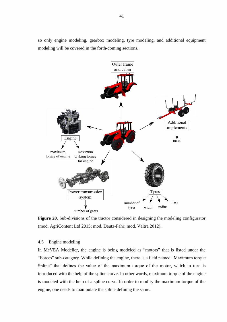
41

so only engine modeling, gearbox modeling, tyre modeling, and additional equipment

modeling will be covered in the forth-coming sections.

Figure 20. Sub-divisions of the tractor considered in designing the modeling configurator

(mod. AgriContent Ltd 2015; mod. Deutz-Fahr; mod. Valtra 2012).

4.5 Engine modeling

In MeVEA Modeller, the engine is being modeled as “motors” that is listed under the

“Forces” sub-category. While defining the engine, there is a field named “Maximum torque

Spline” that defines the value of the maximum torque of the motor, which in turn is

introduced with the help of the spline curve. In other words, maximum torque of the engine

is modeled with the help of a spline curve. In order to modify the maximum torque of the

engine, one needs to manipulate the spline defining the same.

42

In real world, the tractor type considered in this research work utilizes engines from AGCO

Power. But as an academic research approach, the engines used in this research work as an

example is just for demonstration purposes. So, the engines that are used for the tractor

model are the Volvo’s V-ACT Tier 3/Stage IIIA approved 6-cylinder straight turbocharged

diesel engine with a capacity of 6 liters. These engines have a common rail for fuel injection

system as well as switchable I-EGR (Internal Exhaust Gas Recirculation) system. Within the

scope of this research work, the modeling configurator is designed in such a way that it

provide options for selecting between three different Volvo diesel engine models, namely,

Volvo D6E LAE3, Volvo D6E LBE3, and Volvo D6E LCE3. The specifications for these

three models are listed in table 1.

Table 1. Specification of different models of Volvo diesel engine (mod. Volvo 2009, p. 22).

MODEL Volvo D6E LAE3 Volvo D6E LBE3 Volvo D6E LCE3

Net power 128 kw (172 hp) 125 kw (168 hp) 114 kw (153 hp)

Gross power 129 kw (173 hp) 126 kw (169 hp) 115 kw (154 hp)

Power measured at 1700 rpm 1700 rpm 1700 rpm

Displacement 5.7 L (348 cu in) 5.7 L (348 cu in) 5.7 L (348 cu in)

Max Torque 770 Nm (570 lb ft) 750 Nm (550 lb ft) 680 Nm (500 lb ft)

Torque measured at 1600 rpm 1600 rpm 1600 rpm

Number of Cylinders 6 6 6

Aspiration Turbocharged Turbocharged Turbocharged

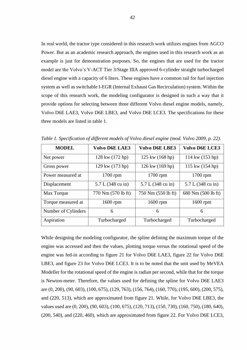
While designing the modeling configurator, the spline defining the maximum torque of the

engine was accessed and then the values, plotting torque versus the rotational speed of the

engine was fed-in according to figure 21 for Volvo D6E LAE3, figure 22 for Volvo D6E

LBE3, and figure 23 for Volvo D6E LCE3. It is to be noted that the unit used by MeVEA

Modeller for the rotational speed of the engine is radian per second, while that for the torque

is Newton-meter. Therefore, the values used for defining the spline for Volvo D6E LAE3

are (0, 200), (90, 603), (100, 675), (129, 763), (156, 764), (160, 770), (195, 600), (200, 575),

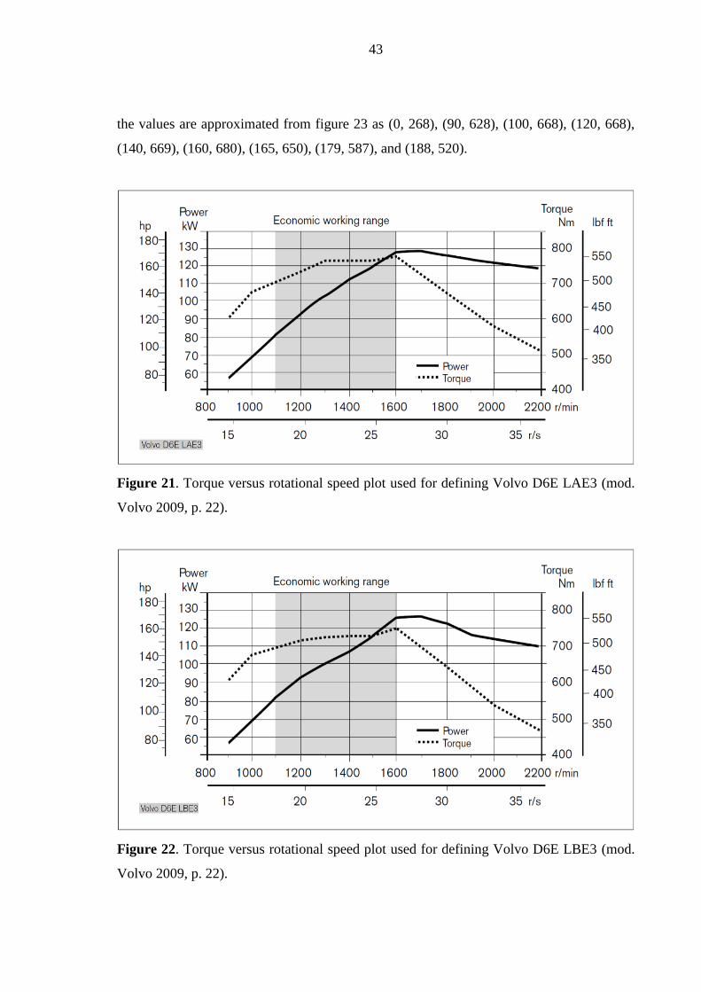
and (220, 513), which are approximated from figure 21. While, for Volvo D6E LBE3, the

values used are (0, 200), (90, 603), (100, 675), (120, 713), (150, 730), (160, 750), (180, 640),

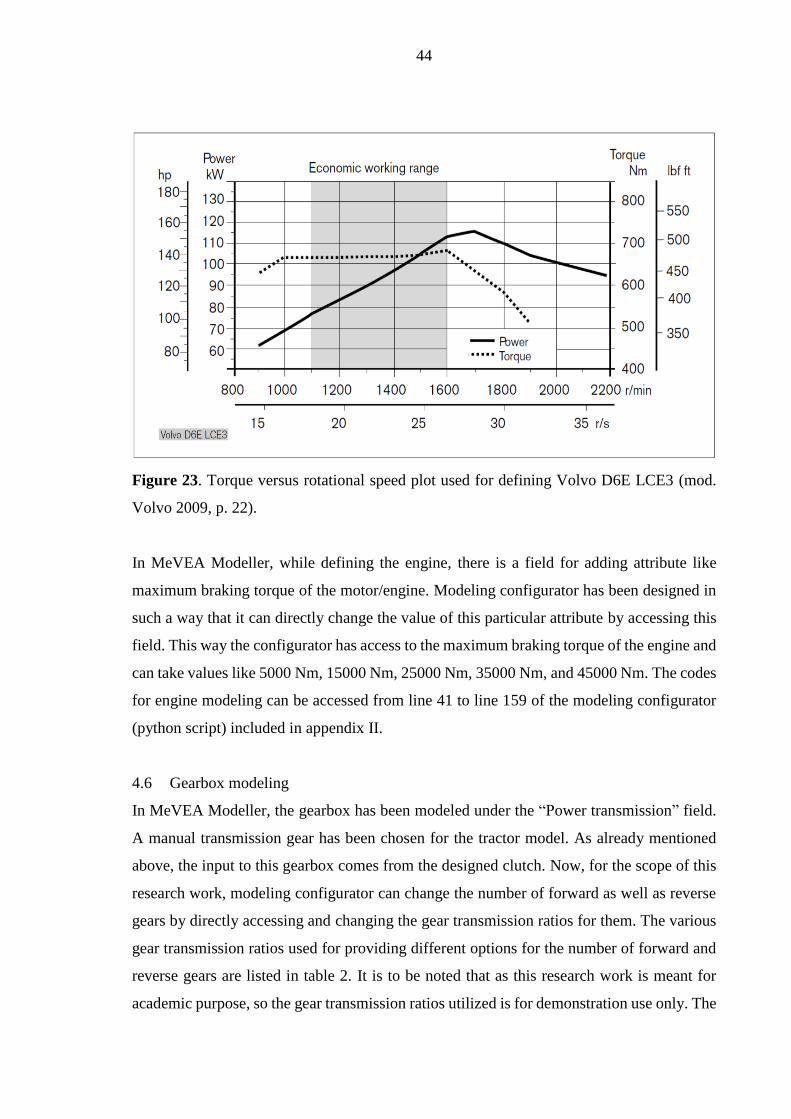
(200, 540), and (220, 460), which are approximated from figure 22. For Volvo D6E LCE3,

43

the values are approximated from figure 23 as (0, 268), (90, 628), (100, 668), (120, 668),

(140, 669), (160, 680), (165, 650), (179, 587), and (188, 520).

Figure 21. Torque versus rotational speed plot used for defining Volvo D6E LAE3 (mod.

Volvo 2009, p. 22).

Figure 22. Torque versus rotational speed plot used for defining Volvo D6E LBE3 (mod.

Volvo 2009, p. 22).

44

Figure 23. Torque versus rotational speed plot used for defining Volvo D6E LCE3 (mod.

Volvo 2009, p. 22).

In MeVEA Modeller, while defining the engine, there is a field for adding attribute like

maximum braking torque of the motor/engine. Modeling configurator has been designed in

such a way that it can directly change the value of this particular attribute by accessing this

field. This way the configurator has access to the maximum braking torque of the engine and

can take values like 5000 Nm, 15000 Nm, 25000 Nm, 35000 Nm, and 45000 Nm. The codes

for engine modeling can be accessed from line 41 to line 159 of the modeling configurator

(python script) included in appendix II.

4.6 Gearbox modeling

In MeVEA Modeller, the gearbox has been modeled under the “Power transmission” field.

A manual transmission gear has been chosen for the tractor model. As already mentioned

above, the input to this gearbox comes from the designed clutch. Now, for the scope of this

research work, modeling configurator can change the number of forward as well as reverse

gears by directly accessing and changing the gear transmission ratios for them. The various

gear transmission ratios used for providing different options for the number of forward and

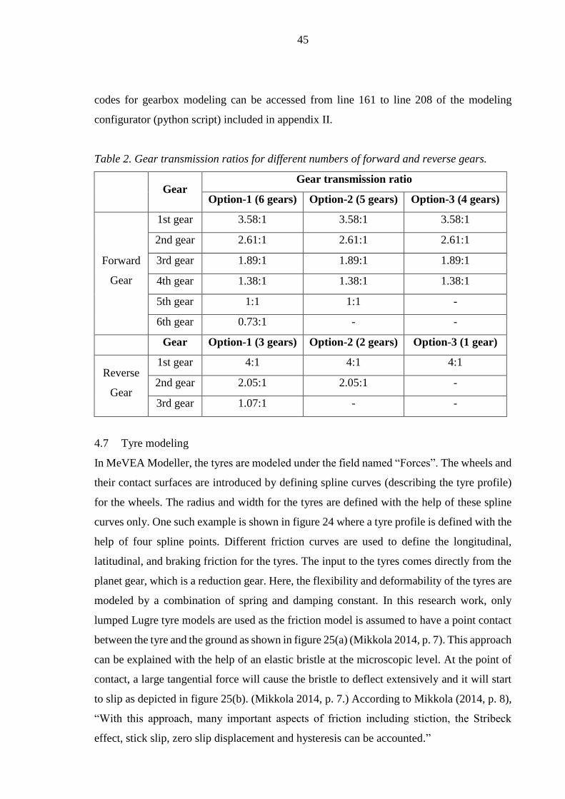
reverse gears are listed in table 2. It is to be noted that as this research work is meant for

academic purpose, so the gear transmission ratios utilized is for demonstration use only. The

45

codes for gearbox modeling can be accessed from line 161 to line 208 of the modeling

configurator (python script) included in appendix II.

Table 2. Gear transmission ratios for different numbers of forward and reverse gears.

Gear Gear transmission ratio

Option-1 (6 gears) Option-2 (5 gears) Option-3 (4 gears)

Forward

Gear

1st gear 3.58:1 3.58:1 3.58:1

2nd gear 2.61:1 2.61:1 2.61:1

3rd gear 1.89:1 1.89:1 1.89:1

4th gear 1.38:1 1.38:1 1.38:1

5th gear 1:1 1:1 -

6th gear 0.73:1 - -

Gear Option-1 (3 gears) Option-2 (2 gears) Option-3 (1 gear)

Reverse

Gear

1st gear 4:1 4:1 4:1

2nd gear 2.05:1 2.05:1 -

3rd gear 1.07:1 - -

4.7 Tyre modeling

In MeVEA Modeller, the tyres are modeled under the field named “Forces”. The wheels and

their contact surfaces are introduced by defining spline curves (describing the tyre profile)

for the wheels. The radius and width for the tyres are defined with the help of these spline

curves only. One such example is shown in figure 24 where a tyre profile is defined with the

help of four spline points. Different friction curves are used to define the longitudinal,

latitudinal, and braking friction for the tyres. The input to the tyres comes directly from the

planet gear, which is a reduction gear. Here, the flexibility and deformability of the tyres are

modeled by a combination of spring and damping constant. In this research work, only

lumped Lugre tyre models are used as the friction model is assumed to have a point contact

between the tyre and the ground as shown in figure 25(a) (Mikkola 2014, p. 7). This approach

can be explained with the help of an elastic bristle at the microscopic level. At the point of

contact, a large tangential force will cause the bristle to deflect extensively and it will start

to slip as depicted in figure 25(b). (Mikkola 2014, p. 7.) According to Mikkola (2014, p. 8),

“With this approach, many important aspects of friction including stiction, the Stribeck

effect, stick slip, zero slip displacement and hysteresis can be accounted.”

46

Figure 24. Example of a tyre profile created with the help of spline points (mod. MeVEA

Modeller [simulation program] 2017a, p. 37).

Figure 25. (a) Friction description for lumped Lugre model; (b) Deformation of a bristle

during acceleration. (mod. Mikkola 2014, p. 6 & p. 8.)

47

The bristle will start deflecting with respect to time when the tyre starts rotating and this

bristle deflection, which is denoted by 𝑧 in figure 25(b) above, can be calculated as (Mikkola

2014, p. 8):

𝑑𝑧

𝑑𝑡= 𝑣𝑟 −

𝜎0|𝑣𝑟|

𝑔𝑧 (1)

where, 𝜎0 is the longitudinal lumped stiffness of the rubber, 𝑣𝑟 = 𝑟𝜔 − 𝑣 is the relative

velocity between two sliding surfaces with 𝑟 as the radius, 𝜔 as the angular velocity, and 𝑣

as the linear velocity of the tyre. Also, in equation 1, 𝑔 is the friction, which must always

be positive, and is dependent on material properties, lubricants, temperature et cetera.

(Mikkola 2014, pp. 8–9.) The friction 𝑔 can also be written as (Mikkola 2014, p. 8):

𝑔 = 𝜇𝑐 + (𝜇𝑠 − 𝜇𝑐)𝑒

−|𝑣𝑟𝑣𝑠|−12

(2)

where, 𝜇𝑐 is the normalized coulomb friction, 𝜇𝑠 is the normalized static friction, and 𝑣𝑠 is

the Stribeck relative velocity (Mikkola 2014, p. 9). Based on the lumped Lugre model, the

frictional force 𝐹𝑠 can be written as (Mikkola 2014, p. 9):

𝐹𝑠 = (𝜎0𝑧 + 𝜎1𝑑𝑧

𝑑𝑡+ 𝜎2𝑣𝑟) 𝐹𝑛 (3)

where, 𝜎1 is the longitudinal lumped damping coefficient, 𝜎2 is the relative viscous damping,

and 𝐹𝑛 is the normal force as shown in figure 25 above. Now, for the steady state

characteristics of the model, translational and angular velocities are assumed to be constant,

and 𝑑𝑧 𝑑𝑡⁄ is made equal to zero. Thus, from equation 1 above, 𝑧 = (𝑔 𝜎0⁄ )𝑠𝑔𝑛(𝑣𝑟), where

𝑠𝑔𝑛 is the sign function. (Mikkola 2014, p. 9.) Now, by putting these values in equation 3

above, the frictional force in steady state can be obtained as (Mikkola 2014, p. 9):

𝐹𝑠 = (𝑔 𝑠𝑔𝑛(𝑣𝑟) + 𝜎2𝑣𝑟)𝐹𝑛 (4)

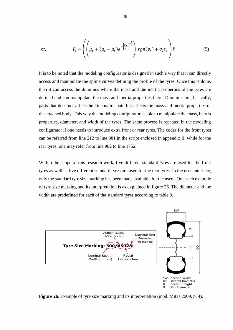
48

or, 𝐹𝑠 = ((𝜇𝑐 + (𝜇𝑠 − 𝜇𝑐)𝑒−|𝑣𝑟𝑣𝑠|−12

) 𝑠𝑔𝑛(𝑣𝑟) + 𝜎2𝑣𝑟)𝐹𝑛 (5)

It is to be noted that the modeling configurator is designed in such a way that it can directly

access and manipulate the spline curves defining the profile of the tyres. Once this is done,

then it can access the dummies where the mass and the inertia properties of the tyres are

defined and can manipulate the mass and inertia properties there. Dummies are, basically,

parts that does not affect the kinematic chain but affects the mass and inertia properties of

the attached body. This way the modeling configurator is able to manipulate the mass, inertia

properties, diameter, and width of the tyres. The same process is repeated in the modeling

configurator if one needs to introduce extra front or rear tyres. The codes for the front tyres

can be referred from line 212 to line 981 in the script enclosed in appendix II, while for the

rear tyres, one may refer from line 982 to line 1752.

Within the scope of this research work, five different standard tyres are used for the front

tyres as well as five different standard tyres are used for the rear tyres. In the user-interface,

only the standard tyre size marking has been made available for the users. One such example

of tyre size marking and its interpretation is as explained in figure 26. The diameter and the

width are predefined for each of the standard tyres according to table 3.

Figure 26. Example of tyre size marking and its interpretation (mod. Mitas 2009, p. 4).

49

Table 3. Diameter and width of different available tyre options in modeling configurator.

Tyre Tyre Size Marking Diameter Width

Front Tyres

600/70R28 1552 mm 600 mm

420/85R28 1426 mm 440 mm

480/70R28 1424 mm 482 mm

540/65R28 1414 mm 540 mm

600/65R28 1492 mm 600 mm

Rear Tyres

520/85R38 1850 mm 536 mm

580/70R38 1852 mm 594 mm

650/65R38 1830 mm 620 mm

650/85R38 2072 mm 650 mm

710/70R38 1960 mm 710 mm

The different mass options available for each of the front and rear tyres are listed in table 4.

Also, while calculating the moments and products of inertia with the help of inertia calculator

in MeVEA Modeller, the shape of the tyre is assumed to be horizontal hollow cylinder. In

addition, the inner diameter is assumed to be the nominal diameter of the rim, while the outer

diameter is considered as shown in table 3 above.

Table 4. Different available mass options for each of the front and rear tyres.

Options Front tyre Rear tyre

Option-1 150 kg 300 kg

Option-2 175 kg 325 kg

Option-3 200 kg 350 kg

Option-4 225 kg 375 kg

Option-5 250 kg 400 kg

4.8 Equipment modeling

Agriculture equipment can be defined as a machinery that is used on the agricultural field to

help in farming. There are number of additional implements that can be used along with the

tractor like cultivator, harrow, chisel plow, trailer et cetera. However, only a trailer has been

covered within the scope of this research work. The trailer is modeled using three bodies,

50

namely, trailer’s body, left axle, and right axle. The tyres are attached to these left and right

axles. The trailer is attached to the rear end of the tractor. The body reference coordinate

system of the trailer’s body is at a distance of (0, 100, 0) mm with respect to the body

reference coordinate system of the tractor’s cabin. The mass of the trailer’s body is assumed

to be 500 kg that is directed to its center of mass, which is at a distance of (4250, 0, 0) mm

with respect to the body reference coordinate system of the trailer’s body. The left axle is

located at a distance of (-4290, -276, -468) mm with respect to the body reference coordinate

system of the trailer’s body. Whereas, the right axle is located at a distance of (-4290, -276,

468) mm with respect to the trailer’s body. Here, the trailer’s body is constrained with the

tractor’s cabin by using a spherical joint, whereas the left and the right axles are constrained

with the trailer’s body by utilizing revolute joints. Also, the graphics for the trailer’s body,

axles, and wheels are provided by the Machine Dynamics research group at LUT School of

Energy Systems.

The modeling configurator is designed in such a way that through the user-interface, one is

allowed to select only trailer as the additional implement whose mass is predefined. So, the

users are not provided with the option of altering the weight of the trailer within the scope

of this research work. The trailer presented in this research work is modeled using the

assembly option in MeVEA Modeller. This is carried out by modeling all the

parameters/attributes defining the trailer in a separate “.mva” file, which is an assembly file

for the trailer that is named as “Trailer.mva”. This “.mva” file is also like an XML file that

contains all the data required for modeling a trailer including the number of bodies,

constraints definition, graphics, tyres definition, spline, dummies, and collision definitions.

The role of the modeling configurator is to access the main XML file of the tractor model

and in the field of “FileName” for the assembly attribute, it will only call the “Trailer.mva”

file if a trailer is selected in the user-interface or it will keep that field blank if nothing is

selected in the user-interface. The codes for equipment modeling can be accessed from line

1754 to line 1762 of the modeling configurator (python script) included in appendix II.

Likewise, more such assembly files of various additional implements can be modeled, and

accordingly, they can be assembled with the tractor in the near future. It is to be noted that

the “Trailer.mva” file is modeled beforehand as already illustrated above and is kept in the

same folder as the main tractor model.

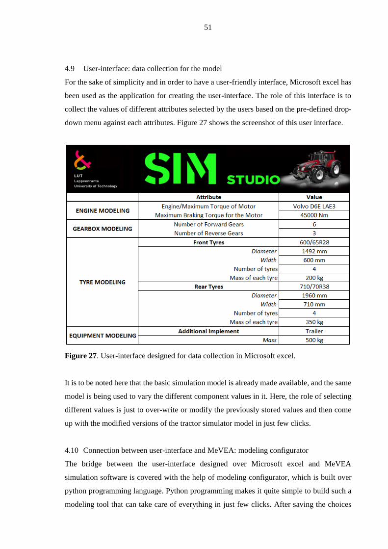
51

4.9 User-interface: data collection for the model

For the sake of simplicity and in order to have a user-friendly interface, Microsoft excel has

been used as the application for creating the user-interface. The role of this interface is to

collect the values of different attributes selected by the users based on the pre-defined drop-

down menu against each attributes. Figure 27 shows the screenshot of this user interface.

Figure 27. User-interface designed for data collection in Microsoft excel.

It is to be noted here that the basic simulation model is already made available, and the same

model is being used to vary the different component values in it. Here, the role of selecting

different values is just to over-write or modify the previously stored values and then come

up with the modified versions of the tractor simulator model in just few clicks.

4.10 Connection between user-interface and MeVEA: modeling configurator

The bridge between the user-interface designed over Microsoft excel and MeVEA

simulation software is covered with the help of modeling configurator, which is built over

python programming language. Python programming makes it quite simple to build such a

modeling tool that can take care of everything in just few clicks. After saving the choices

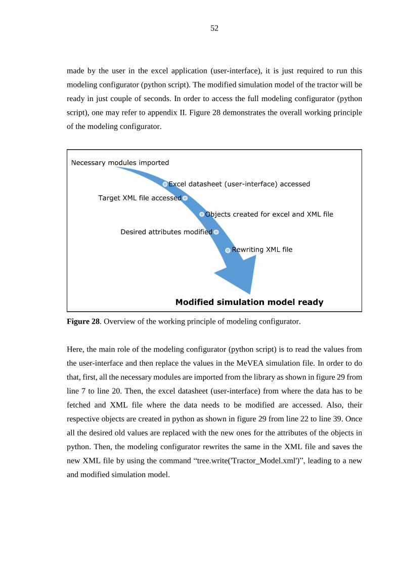
52

made by the user in the excel application (user-interface), it is just required to run this

modeling configurator (python script). The modified simulation model of the tractor will be

ready in just couple of seconds. In order to access the full modeling configurator (python

script), one may refer to appendix II. Figure 28 demonstrates the overall working principle

of the modeling configurator.

Figure 28. Overview of the working principle of modeling configurator.

Here, the main role of the modeling configurator (python script) is to read the values from

the user-interface and then replace the values in the MeVEA simulation file. In order to do

that, first, all the necessary modules are imported from the library as shown in figure 29 from

line 7 to line 20. Then, the excel datasheet (user-interface) from where the data has to be

fetched and XML file where the data needs to be modified are accessed. Also, their

respective objects are created in python as shown in figure 29 from line 22 to line 39. Once

all the desired old values are replaced with the new ones for the attributes of the objects in

python. Then, the modeling configurator rewrites the same in the XML file and saves the

new XML file by using the command “tree.write('Tractor_Model.xml')”, leading to a new

and modified simulation model.

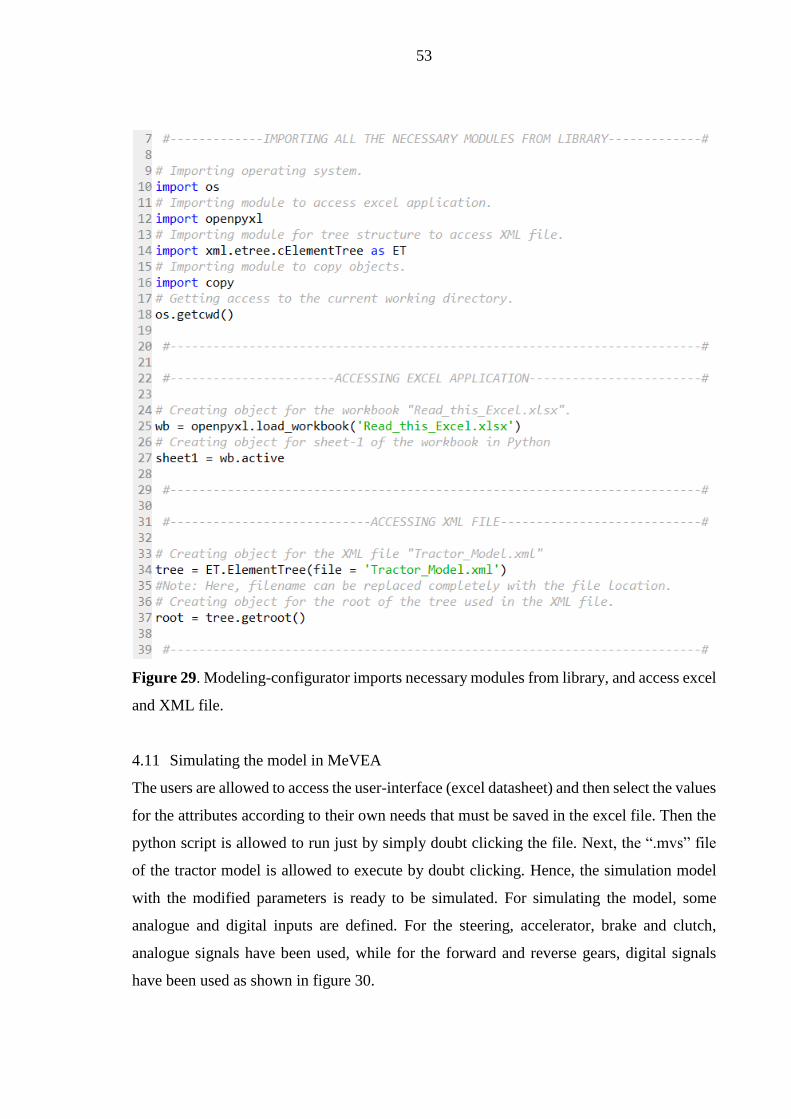
53

Figure 29. Modeling-configurator imports necessary modules from library, and access excel

and XML file.

4.11 Simulating the model in MeVEA

The users are allowed to access the user-interface (excel datasheet) and then select the values

for the attributes according to their own needs that must be saved in the excel file. Then the

python script is allowed to run just by simply doubt clicking the file. Next, the “.mvs” file

of the tractor model is allowed to execute by doubt clicking. Hence, the simulation model

with the modified parameters is ready to be simulated. For simulating the model, some

analogue and digital inputs are defined. For the steering, accelerator, brake and clutch,

analogue signals have been used, while for the forward and reverse gears, digital signals

have been used as shown in figure 30.

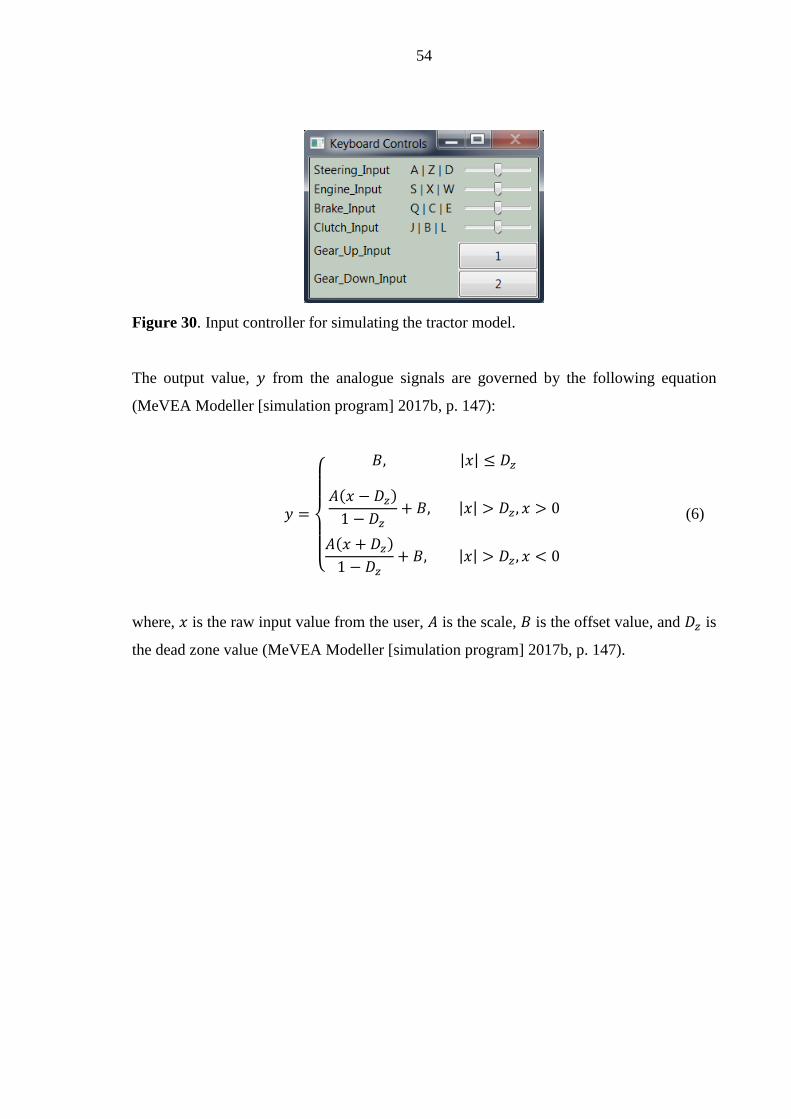
54

Figure 30. Input controller for simulating the tractor model.

The output value, 𝑦 from the analogue signals are governed by the following equation

(MeVEA Modeller [simulation program] 2017b, p. 147):

𝑦 =

{

𝐵, |𝑥| ≤ 𝐷𝑧

𝐴(𝑥 − 𝐷𝑧)

1 − 𝐷𝑧+ 𝐵, |𝑥| > 𝐷𝑧 , 𝑥 > 0

𝐴(𝑥 + 𝐷𝑧)

1 − 𝐷𝑧+ 𝐵, |𝑥| > 𝐷𝑧 , 𝑥 < 0

(6)

where, 𝑥 is the raw input value from the user, 𝐴 is the scale, 𝐵 is the offset value, and 𝐷𝑧 is

the dead zone value (MeVEA Modeller [simulation program] 2017b, p. 147).

55

5 RESULTS AND ANALYSIS

On December 27, 2016, the SIM studio, as proposed by the SIM platform, was setup at

Lappeenranta University of Technology, Finland. The studio has two real-time simulators,

one for the excavator while the other one for the tractor. The image on the right-hand side of

figure 31 shows the tractor simulator. The initial goal has already been achieved with this

SIM studio. The main aim of this research was to integrate users in the product development

phase with the help of digital tools. For this purpose, a modeling configurator has been

developed with the help of python programming language, and a user-friendly interface

(designed over Microsoft excel) has been made available for the users. This chapter is mainly

focused on discussing the outcomes of this modeling configurator in order to achieve the

objectives of this research paper. The following sub-sections covers the flow of information

in the process, and the results of selecting different options for engine modeling, gearbox

modeling, tyre modeling and additional equipment modeling.

Figure 31. Tractor simulator (on the right) at SIM studio, Lappeenranta University of

Technology.

5.1 Flow of information

The modeling configurator developed in this research work is tailor-made for the case study

of tractor simulation model in hand. The modeling configurator cannot be generalized

because the coding will differ with how different the components are being modeled in

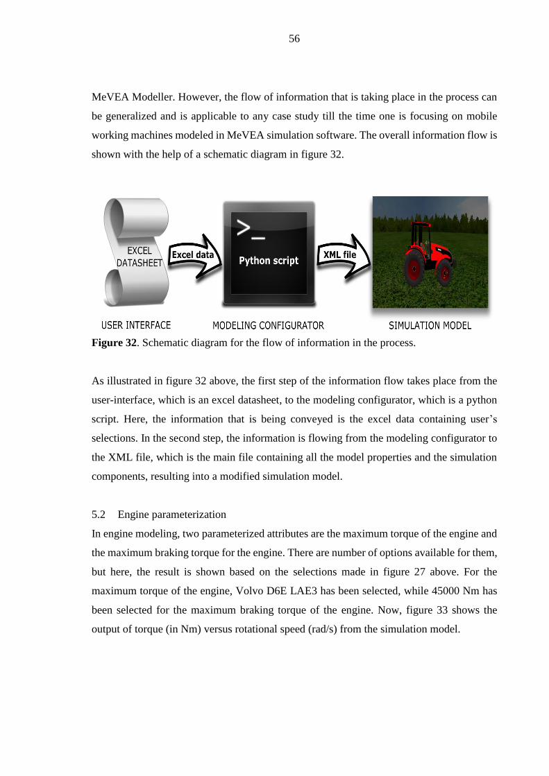
56

MeVEA Modeller. However, the flow of information that is taking place in the process can

be generalized and is applicable to any case study till the time one is focusing on mobile

working machines modeled in MeVEA simulation software. The overall information flow is

shown with the help of a schematic diagram in figure 32.

Figure 32. Schematic diagram for the flow of information in the process.

As illustrated in figure 32 above, the first step of the information flow takes place from the

user-interface, which is an excel datasheet, to the modeling configurator, which is a python

script. Here, the information that is being conveyed is the excel data containing user’s

selections. In the second step, the information is flowing from the modeling configurator to

the XML file, which is the main file containing all the model properties and the simulation

components, resulting into a modified simulation model.

5.2 Engine parameterization

In engine modeling, two parameterized attributes are the maximum torque of the engine and

the maximum braking torque for the engine. There are number of options available for them,

but here, the result is shown based on the selections made in figure 27 above. For the

maximum torque of the engine, Volvo D6E LAE3 has been selected, while 45000 Nm has

been selected for the maximum braking torque of the engine. Now, figure 33 shows the

output of torque (in Nm) versus rotational speed (rad/s) from the simulation model.

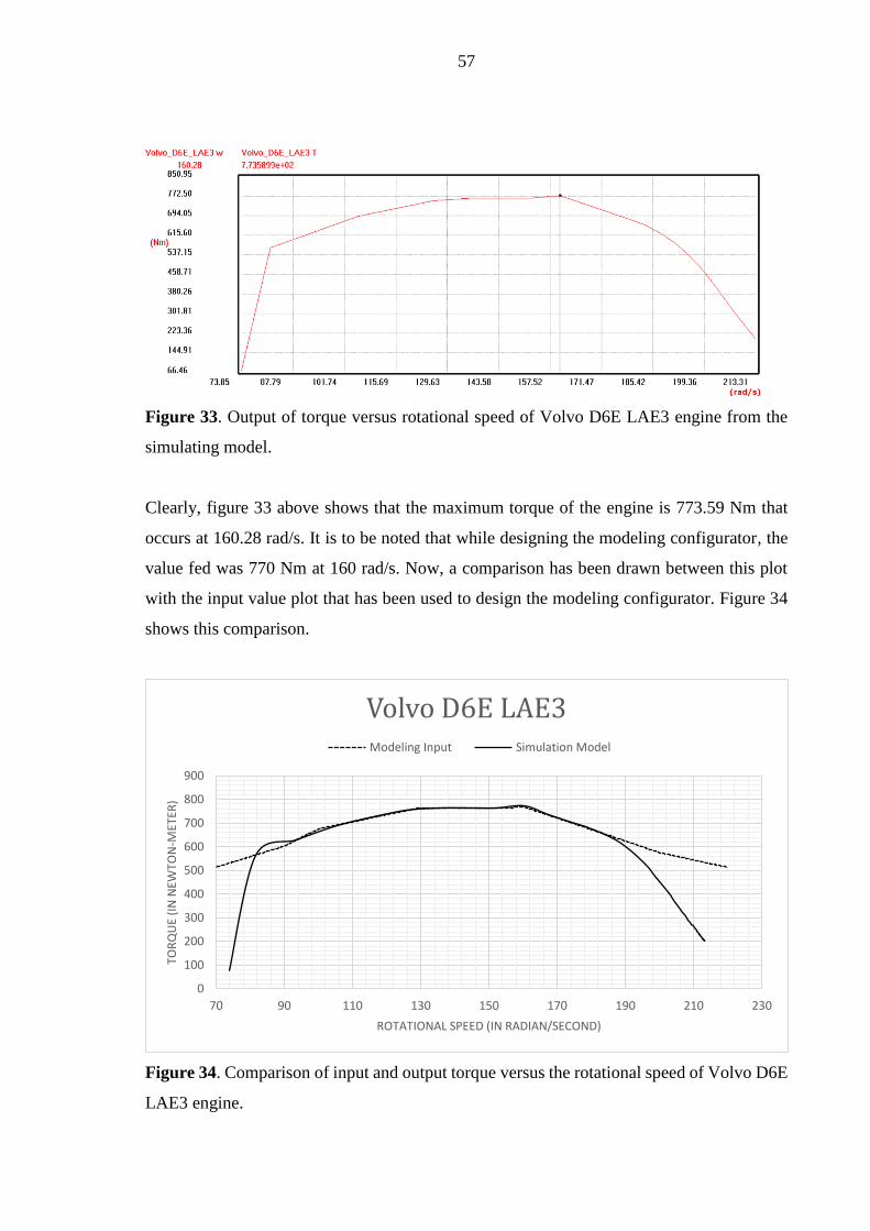
57

Figure 33. Output of torque versus rotational speed of Volvo D6E LAE3 engine from the

simulating model.

Clearly, figure 33 above shows that the maximum torque of the engine is 773.59 Nm that

occurs at 160.28 rad/s. It is to be noted that while designing the modeling configurator, the

value fed was 770 Nm at 160 rad/s. Now, a comparison has been drawn between this plot

with the input value plot that has been used to design the modeling configurator. Figure 34

shows this comparison.

Figure 34. Comparison of input and output torque versus the rotational speed of Volvo D6E

LAE3 engine.

0

100

200

300

400

500

600

700

800

900

70 90 110 130 150 170 190 210 230

TOR

QU

E (I

N N

EWTO

N-M

ETER

)

ROTATIONAL SPEED (IN RADIAN/SECOND)

Volvo D6E LAE3Modeling Input Simulation Model

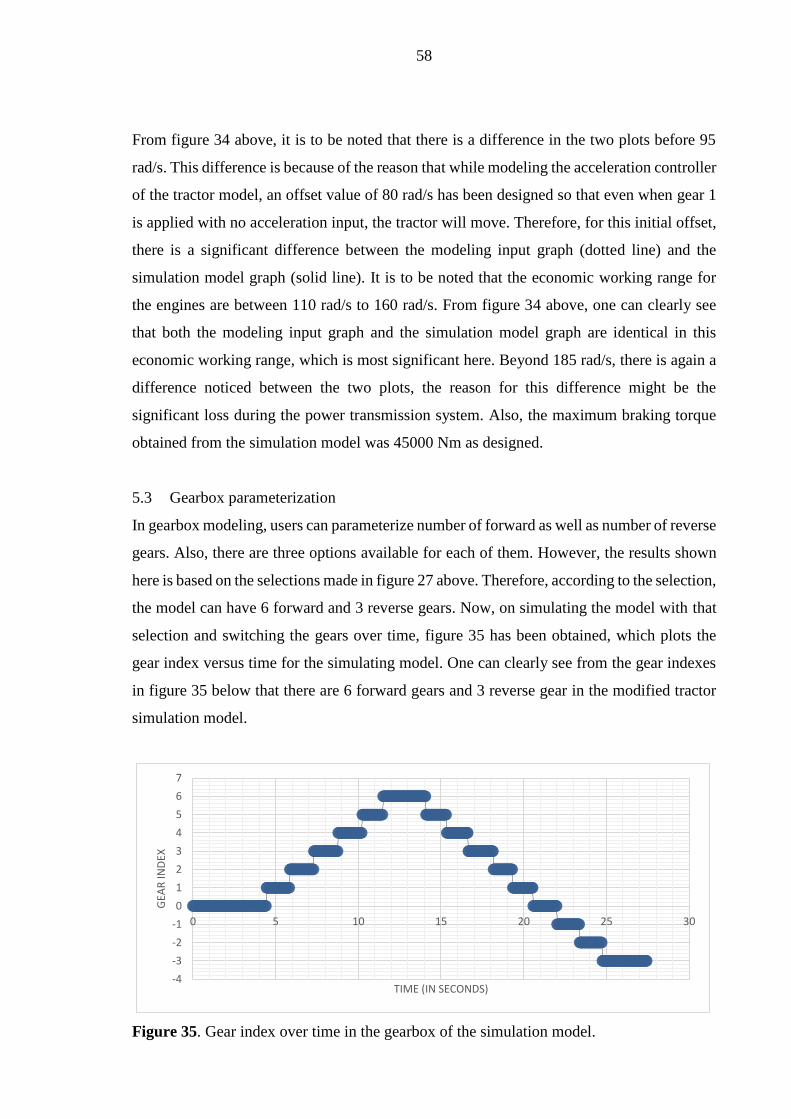
58

From figure 34 above, it is to be noted that there is a difference in the two plots before 95

rad/s. This difference is because of the reason that while modeling the acceleration controller

of the tractor model, an offset value of 80 rad/s has been designed so that even when gear 1

is applied with no acceleration input, the tractor will move. Therefore, for this initial offset,

there is a significant difference between the modeling input graph (dotted line) and the

simulation model graph (solid line). It is to be noted that the economic working range for

the engines are between 110 rad/s to 160 rad/s. From figure 34 above, one can clearly see

that both the modeling input graph and the simulation model graph are identical in this

economic working range, which is most significant here. Beyond 185 rad/s, there is again a

difference noticed between the two plots, the reason for this difference might be the

significant loss during the power transmission system. Also, the maximum braking torque

obtained from the simulation model was 45000 Nm as designed.

5.3 Gearbox parameterization

In gearbox modeling, users can parameterize number of forward as well as number of reverse

gears. Also, there are three options available for each of them. However, the results shown

here is based on the selections made in figure 27 above. Therefore, according to the selection,

the model can have 6 forward and 3 reverse gears. Now, on simulating the model with that

selection and switching the gears over time, figure 35 has been obtained, which plots the

gear index versus time for the simulating model. One can clearly see from the gear indexes

in figure 35 below that there are 6 forward gears and 3 reverse gear in the modified tractor

simulation model.

Figure 35. Gear index over time in the gearbox of the simulation model.

-4

-3

-2

-1

0

1

2

3

4

5

6

7

0 5 10 15 20 25 30

GEA

R IN

DEX

TIME (IN SECONDS)

59

5.4 Tyre parameterization

In tyre modeling, number of tyres, diameter, width, and mass can be parameterized. There

are number of options available for the tyres. Only tyre size marking is made available for

the users. The width and diameter of the tyres are pre-defined. The results shown here is

based on the selection made in figure 27 above. For the front tyres, 600/65R28 tyre has been

selected whose diameter is 1492 mm while width is 600 mm. For the rear tyres, 710/70R38

tyre has been selected whose diameter is 1960 mm and width is 710 mm. After this selection

has been done in the user-interface, the modeling configurator is executed.

Now, when the simulation model is analyzed in MeVEA Modeller, the tyre profiles are

studied. One can clearly see from figure 36, which represents the front tyres profile, that the

width of the front tyres is 0.6 m (600 mm) and their radius is 0.746 m (1492/2 = 746 mm).

In addition, on manually checking the mass for each of the front tyres, it resulted to be 200

kg as selected in figure 27 above. The users can only experience the mass of the tyres during

real-time simulation.

Figure 36. Front tyre profile in the simulation model.

Also, figure 37 represents the profile of the rear tyres. It can be seen from figure 37 below

that the width of the rear tyres is 0.71 m (710 mm), while their radius is 0.98 m (1960/2 =

980 mm). The mass for each of the rear tyres was found to be 350 kg as already selected in

0

0,0746

0,1492

0,2238

0,2984

0,373

0,4476

0,5222

0,5968

0,6714

0,746

0,8206

-0,4 -0,3 -0,2 -0,1 0 0,1 0,2 0,3 0,4

TYR

E R

AD

IUS

(IN

MET

ER)

TYRE WIDTH (IN METER)

Front Tyre Profile

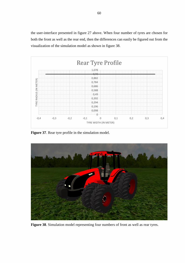
60

the user-interface presented in figure 27 above. When four number of tyres are chosen for

both the front as well as the rear end, then the differences can easily be figured out from the

visualization of the simulation model as shown in figure 38.

Figure 37. Rear tyre profile in the simulation model.

Figure 38. Simulation model representing four numbers of front as well as rear tyres.

0

0,098

0,196

0,294

0,392

0,49

0,588

0,686

0,784

0,882

0,98

1,078

-0,4 -0,3 -0,2 -0,1 0 0,1 0,2 0,3 0,4

TYR

E R

AD

IUS

(IN

MET

ER)

TYRE WIDTH (IN METER)

Rear Tyre Profile

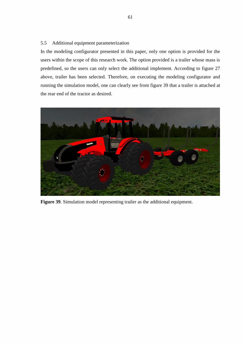
61

5.5 Additional equipment parameterization

In the modeling configurator presented in this paper, only one option is provided for the

users within the scope of this research work. The option provided is a trailer whose mass is

predefined, so the users can only select the additional implement. According to figure 27

above, trailer has been selected. Therefore, on executing the modeling configurator and

running the simulation model, one can clearly see from figure 39 that a trailer is attached at

the rear end of the tractor as desired.

Figure 39. Simulation model representing trailer as the additional equipment.

62

6 CONCLUSION

The foundation of this research work was laid by the vision of a tractor simulator where the

users can customize the simulation model according to their own requirements and then can

proceed with simulation. As already shown in chapter 5 that a tractor simulator was setup

at SIM studio, Lappeenranta University of Technology, Finland on December 27, 2016. This

vision has also lead to the development of modeling configurator for the tractor model, which

was the main aim of this research work. Also, at the start of this research work, there were

couple of research questions like:

(i) How can the modeling configurator be created and linked to the simulation software?

(ii) Why this cannot be done by the traditional approach of design/modeling tools?

(iii) Which parameters/attributes can the users customize?

(iv) What is the maximum number of options provided to the users for each attributes?

(v) Is a feasible configuration selected by the users?

This paper clearly answers all the research questions that were introduced at the start of this

research work. The modeling configurator has been developed using python programming

language. Also, for a user-friendly interface, Microsoft excel has been used. The role of the

modeling configurator is to read the options selected by the users in the user-interface (excel

datasheet). Then accordingly, the modeling configurator will access and modify the required

fields from the main XML file of the simulation model, which contains all the detailed model

properties and simulation components for the tractor model. Therefore, this clearly answers

the first research question.

Traditional design/modeling tools usually requires appropriate skills or expert supervision

to design such a tractor simulation model. In addition, if a modeling configurator needs to

be made from them, then for modifying the appropriate XML file of the simulation model,

one needs to know completely about the different modeling steps for the tractor model. They

also need to know that how different components are related to each other. XML file is

already too complex for a layman to understand, and then modifying the same would just

end up in a modeling failure. So, when the end user is a layman then traditional design or

63

modeling tools cannot be employed. Hence, this clearly answers the second research

question.

As already discussed from section 4.5 to 4.8, the modeling configurator is developed to

parameterize the engine, gearbox, tyres and additional equipment. The users can customize

the maximum torque of the engine, maximum braking torque for the engine, number of

forward as well as number of reverse gears. Also, changing the diameter, width, and mass

of both the front and rear tyres are possible. In addition, users can even select four front and

four rear tyres. For additional equipment, there is only one option made available for the

users that is a trailer attached at the rear end of the tractor. With this, even the third research

question has been answered.

While developing the modeling configurator, each of the parameterized attributes are

provided with a number of options. In engine modeling, three options, namely: Volvo D6E

LAE3, Volvo D6E LBE3, and Volvo D6E LCE3, are provided for the maximum torque of

the engine. Whereas, five options, namely: 5000 Nm, 15000 Nm, 25000 Nm, 35000 Nm,

and 45000 Nm, are provided for the maximum braking torque of the engine. In gearbox

modeling, three options are provided for each of the forward as well as the reverse gears.

For forward gears, the users can select between 4, 5, or 6 gears, while for reverse gears, they

can choose from 1, 2, or 3 gears. In the case of tyre modeling, five different standard tyres

have been used for both the front as well as the rear tyres in the modeling configurator. Only

the tyre size marking is made available for the users, the diameter and width are predefined

according to the standard size. The options available for the front tyres are 600/70R28,

420/85R28, 480/70R28, 540/65R28, and 600/65R28. Whereas, the options available for the

rear tyres are 520/85R38, 580/70R38, 650/65R38, 650/85R38, and 710/70R38. Also, five

different mass options are available for each of the front and rear tyres. The different mass

options for each front tyres are 150 kg, 175 kg, 200 kg, 225 kg, and 250 kg. Whereas, for

each rear tyres, the different mass options are 300 kg, 325 kg, 350 kg, 375 kg, and 400 kg.

For both the front and rear tyres, users can select between 2 or 4 tyres, so the modeling

configurator even have the provision of modeling extra tyres. In additional equipment

modeling, only one option is made available, which is a trailer whose mass is predefined.

Therefore, this paper even answers the fourth research question.

64

For the fifth research question, it is to be note that the modeling configurator is developed in

such a way that it utilizes all the standard components in its options. So, the users are left

with selecting just the standard alternatives that are pre-modeled in the modeling

configurator. In addition, the modeling configurator has been modeled based on the

feasibility of these standard components only. Therefore, no matter which combination of

options are chosen by the users, the selected configuration will always be feasible.

To conclude, this research work reports the effort in the development of a modeling

configurator for parameterization. This paper has achieved all the objectives set at the

beginning of the research work. It is also able to answer all the research questions. All the

attributes mentioned above can easily be parameterized. Every time a new selection is made,

the simulation model is overwritten with the new model. Therefore, the modeling

configurator developed, can produce accurate simulation models within fraction of seconds.

65

7 SCOPE OF FUTURE WORK

To the present knowledge of the author, the work carried out in this paper has served all the

aims and objectives of the research. However, there are certain areas, which still shows some

scope of improvement that may lead to some future research activities in this field. The focus

of this chapter has been laid on the loopholes or drawbacks of this research work and how

one can overcome them in the near future. One of the major setback for this research work

is that the present modeling configurator cannot be generalized. It can particularly be used

for the current tractor model designed in MeVEA Modeller. The reason for this is that the

codes in the python script depends completely on how the simulation model is being

designed and modeled in MeVEA, so accordingly the codes will differ.

7.1 Length of coding

One of the possible drawback with the present modeling configurator is the length of the

code. For this research work, two thousand lines of coding has been done, also, the length

will increase if more attributes needs to be parameterized. One possibility of avoiding this

in the future work can be the use of functions within the code, which might decrease the

number of lines of coding. This will also save a lot of manual effort in coding such a

modeling configurator.

7.2 User-interface

At present, the user-interface used with the modeling configurator is basically an excel

datasheet and the users have to save their options every time a new selection is made. There

is a scope of improvement in this area where instead of the excel sheet, the user-interface

can be designed in MeVEA Launcher and then programmes can be written in order to

execute everything from the launcher. The launcher may ask the users for their possible

choices and then will save their choices in the required XML file based on the new program

that connects the MeVEA Launcher and the simulation model. So in this way, the user’s

experience can be made more automatic and friendly.

66

7.3 Visualization effect

Another possible area of improvement is the graphics. The number of graphics provided for

this research work was minimal, for example, just one-set of graphics was made available

for the tyres. So, every time user selects a new option for the tyres with different width and

diameter, the real-feel of visualizing the modified dimension of the tyre is missing in the

current model as only one-set of tyre graphics has been used. This can be improved if one

can model different tyres with different graphics according to its diameter and width. Even

though the graphics does not play any role in the simulation as the entire model in MeVEA

is a mathematical model, but the use of different graphics will give more realistic feel to the

users.

7.4 Increasing feasible choices

In this research work, the users are provided with a limited number of options (between one

to five) for all the attributes including engine modeling, gearbox modeling, tyre modeling,

and additional equipment modeling. These numbers can be increased significantly,

providing more number of options for the users if one is provided with the appropriate data

for modeling the different choices of the attributes. However, at the same time, the length of

the code must also be kept in mind and in order to provide more options the coding process

must include some functions where the number of choices can be increased without

significantly increasing the lines of coding.

67

LIST OF REFERENCES

About. 2016. [Mevea Simulation solutions webpage]. [Referred 16.9.2016]. Available:

http://mevea.com/about/

AgriContent Ltd. 2015. Michelin: Innovative tractor tyre tread pattern concept unveiled.

[What’s new in farming webpage]. Updated March 15, 2015. [Referred 9.12.2016].

Available: http://www.wnif.co.uk/2015/03/michelin-innovative-tractor-tyre-tread-pattern-

concept-unveiled/

Altiok, T. & Melamed, B. 2007. [Chapter 1:] Introduction to Simulation Modeling. In: T.

Altiok & B. Melamed. Simulation Modeling and Analysis with Arena. [Burlington:]

Academic Press. 2007. Pp. 1–10.

Audi Driver. 2002. Finding traction. [Referred 08.12.2016]. Available:

http://www.urquattro.fr/Web/Pages/Journaux/audidriver/AD22.html#anchor2

Baharudin, E., Nokka, J., Montonen, H., Immonen, P., Rouvinen, A., Laurila, L., Lindh, T.,

Mikkola, A., Sopanen, J. & Pyrhönen, J. 2015. Simulation Environment for the Real-Time

Dynamic Analysis of Hybrid Mobile Machines. Proceedings of the ASME 2015

International Design Engineering Technical Conferences and Computers and Information in

Engineering Conference. Boston, Massachusetts, USA. 2-5.8.2015. Boston, Massachusetts,

USA: American Society of Mechanical Engineers. 11 p.

Compare Valtra models. 2017. [Valtra webpage]. [Referred 22.2.2017]. Available:

http://www.valtra.com/productcompare.aspx?models=T144+Active,T154+Active,T174e+

Active,T194+Active,T214+Active,T234+Active,T144+Direct,T154+Direct,T174e+Direct,

T194+Direct,T214+Direct,T144+Versu,T154+Versu,T174e+Versu,T194+Versu,T214+Ve

rsu,T234+Versu,T144+HiTech+5,T154+HiTech+5,T174e+HiTech+5,T194+HiTech+5,T2

14+HiTech+5,T234+HiTech+5

68

Deutz-Fahr. Agrofarm G 410 | 430. [web document]. [Referred 9.12.2016]. Available:

http://www.deutz-fahr.com/en-eu/products/tractors/882-agrofarm-g

Frequently Asked Questions. 2016. [XmlGrid.net Online XML Editor webpage]. [Referred

4.11.2016]. Available: http://xmlgrid.net/faq.html

Home. 2016. [EditiX XML Editor webpage]. Updated 2016. [Referred 4.11.2016].

Available: https://www.altova.com/xml-editor/

Kaikko, E. P. 2015. Development of Generic Simulation Model for Mobile Working

Machines. Master’s thesis. Lappeenranta University of Technology. LUT Mechanical

Engineering. 77 p.

Laboratory of Intelligent Machines. [Lappeenranta University of Technology webpage].

[Referred 23.9.2016]. Available: http://www.lut.fi/web/en/school-of-energy-

systems/research/intelligent-machines

Mackulak, G. T. & Cochran, J. K. 1990. The Generic-Specific Modeling Approach: An

Application of Artificial Intelligence to Simulation. 1990 IIE Integrated Systems Conference

& Society for Integrated Manufacturing Conference Proceedings. San Antonio, TX, USA:

IIE. P. 82–87.

Mackulak, G. T., Lawrence, F. P. & Colvin, T. 1998. Effective simulation model reuse: a

case study for AMHS modeling. Proceedings of the 30th conference on Winter simulation.

Washington, D.C., USA. 13-16.12.1998. Los Alamitos, California, USA: IEEE Computer

Society Press. P 979–984.

Map XML elements to cells in an XML Map. 2016. [Microsoft webpage]. Updated 2016.

[Referred 4.11.2016]. Available: https://support.office.com/en-us/article/Map-XML-

elements-to-cells-in-an-XML-Map-ddb23edf-f5c5-4fbf-b736-b3bf977a0c53?ui=en-

US&rs=en-US&ad=US

69

MeVEA Modeller [simulation program]. 2017a. Version 2.2.567. Mevea Modeller:

Beginner tutorials, Version 2.0 (help menu: Show tutorials). 52 p.

MeVEA Modeller [simulation program]. 2017b. Version 2.2.567. Reference Manual for

Solver Library 7.70. (help menu: Mevea Solver reference manual). 206 p.

Mikkola, A. 2014. Lugre tire model for HMMWV [web document]. Madison: October 2014

[Referred 12.3.2017]. Technical report TR-2014-15. University of Wisconsin-Madison,

Simulation-Based Engineering Laboratory. 15 p. Available in PDF-file:

http://sbel.wisc.edu/documents/TR-2014-15.pdf

Mitas. 2009. Agricultural Tyres, Technical Information 2009. [web document]. Prague,

Czech Republic: 2009 [Referred 23.1.2017]. 39 p. Available in PDF-file:

http://www.agricultural-tyres.com/Mitas-databook-en-09.pdf

Mitrev, R. & Tudjarov, B. 2014. Web based tool for Modeling and Simulation of Vehicles

Collisions. 10th France-Japan/ 8th Europe-Asia Congress on Mecatronics

(MECATRONICS2014- Tokyo). Tokyo, Japan. 27-29.11.2014. IEEE. P. 268–273.

Moher, D., Liberati, A., Tetzlaff, J. & Altman, D.G. 2009. Preferred reporting items for

systematic reviews and meta-analyses: the PRISMA statement. Annals of internal medicine,

151: 4. Pp. 264–269.

Ninan, J. & Siddique, Z. 2004. Internet Based Automated Design Optimization Setup to

Support Integration of Customer in the Design of User Customizable Products. 10th

AIAA/ISSMO Multidisciplinary Analysis and Optimization Conference. Albany, New

York, USA. 30.8-1.9.2004. Reston, Virginia, USA: American Institute of Aeronautics and

Astronautics. P. 4317–4322.

Nokka, J.I., Montonen, J.H., Baharudin, E.B., Immonen, P., Rouvinen, A., Laurila, L.,

Lindh, T., Mikkola, A., Sopanen, J. & Pyrhönen, J. 2015. Multi-Body Simulation Based

Development Environment for Hybrid Working Machines. International Review on

Modelling and Simulations (IREMOS), 8: 4. Pp. 466–476.

70

Oerlikon graziano. 2017. Front & Rear Steering Axles, designed for Agricultural Tractors.

[web document]. [Referred 22.2.2017]. 1 p. Available in PDF-file:

https://www.oerlikon.com/ecomaXL/files/oerlikon_EN_AG_front_and_rear_steering_axle

s.pdf

Pat. US 20160092628. 2016. Modeling tool, method and computer program product for

dynamically generating a maintenance simulation of a vehicle. Cae Inc. (Giguere, G., Vo,

T.H., Nejelski, M., Cayer, C. & Harvey, E.) Appl. US 496995, 2014-09-25. Publ. 2016-03-

31. 27 p.

Quint, V. & Vatton, I. 2004. Techniques for authoring complex XML documents.

Proceedings of the 2004 ACM symposium on Document engineering. Milwaukee,

Wisconsin, USA. 28-30.10.2004. New York, NY, USA: Association for Computing

Machinery. P. 115–123.

Schwarz, C., Bachinger, M., Stolz, M. & Watzenig, D. 2015. Tool-driven Design and

Automated Parameterization for Real-time Generic Drivetrain Models. MATEC Web of

Conferences, 28: 03001. Pp. 1–5.

SIM platform. [Lappeenranta University of Technology webpage]. [Referred 20.9.2016].

Available: http://www.lut.fi/web/en/research/platforms/sim

Stanford, A. 2009. Llandini Powermax Tractor. [web document]. Published 2009, updated

7.8.2009. [Referred 21.2.2017]. Available: http://www.the-blueprints.com/

blueprints/trucks/trucks-cars/33947/view/llandini_powermax_tractor/

Steele, M.J., Mollaghasemi, M., Rabadi, G. & Cates, G. 2002. Generic simulation models of

reusable launch vehicles. Proceedings of the 2002 Winter Simulation Conference. USA. 8-

11.12.2002. Los Alamitos, California, USA: IEEE Computer Society Press. P 747–753.

Tractor Agriculture. 2014. Types of Tractors. [web document]. Updated 30.6.2014.

[Referred 17.11.2016]. Available: http://www.tractoragriculture.com/types-of-tractors/

71

Tractors for every purpose. 2016. [Valtra webpage]. [Referred 7.12.2016]. Available:

http://www.valtra.com/images/Valtra_N4_Red.jpg

Valtra. 2012. Uusi voimansiirto Valtran N-sarjaan. [web document]. Updated 26.3.2012.

[Referred 9.12.2016]. Available: http://www.valtra.fi/231.aspx

Volvo. 2009. Volvo Wheel Loaders L60F, L70F, L90F. [web document]. Sweden: August

2009 [Referred 24.2.2017]. 36 p. Available in PDF-file:

https://www.volvoce.com/SiteCollectionDocuments/VCE/Documents%20Global/wheel%2

0loaders/ProductBrochure_L60FtoL90F_EN_21D1002737_2009-08.pdf

Wang, J., Chang, Q., Xiao, G., Wang, N. & Li, S. 2011. Data driven production modeling

and simulation of complex automobile general assembly plant. Computers in Industry, 62:

7. Pp. 765–775.

Wy, J., Jeong, S., Kim, B.I., Park, J., Shin, J., Yoon, H. & Lee, S. 2011. A data-driven generic

simulation model for logistics-embedded assembly manufacturing lines. Computers &

Industrial Engineering, 60: 1. Pp. 138–147.

XML Editor. 2016a. [Altova webpage]. Updated 2016. [Referred 4.11.2016]. Available:

https://www.altova.com/xml-editor/

XML Editor. 2016b. [Oxygen XML Editor webpage]. Updated October 18, 2016. [Referred

4.11.2016]. Available: https://www.oxygenxml.com/xml_editor.html

Zhao, S., Guo, R., Xu, L. & Guo, X.L. 2013. Modeling and Simulation of the Automatic

Transmission Assembly Using Matlab/Simulink. Tang, X., Chen, X., Dong, Y., Wei, X. &

Yang, Q. Applied Mechanics and Materials, 291-294. Pp. 2287–2290.

APPENDIX I, 1

Table below shows the detailed overview of all the databases for retrieving the most eligible

documents by following a systematic literature review.

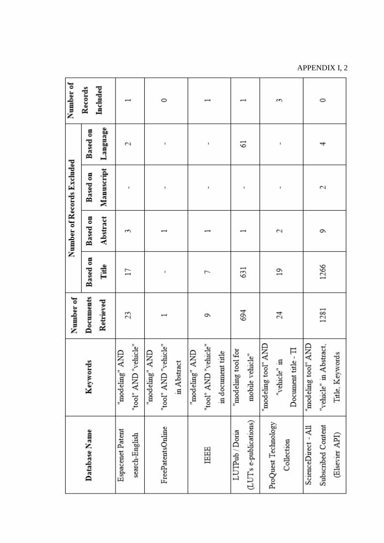
APPENDIX I, 2

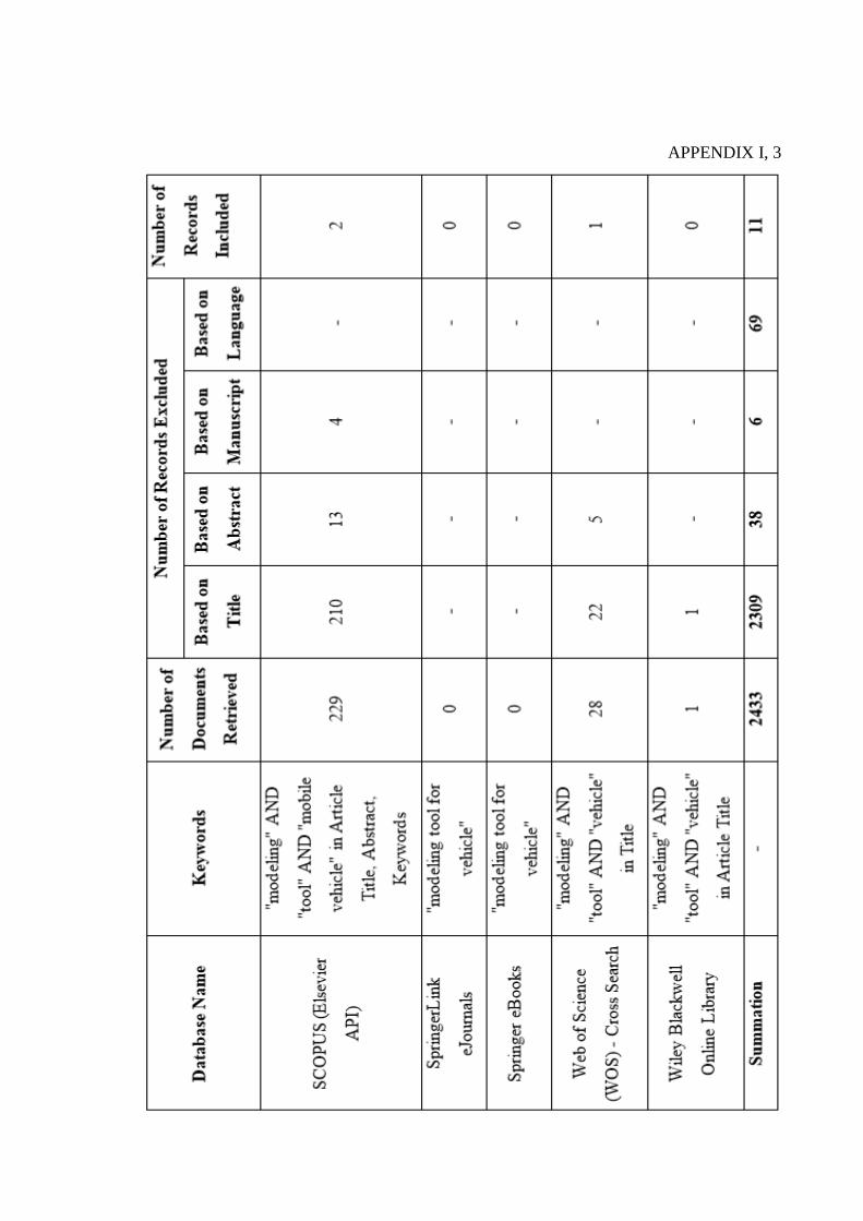
APPENDIX I, 3

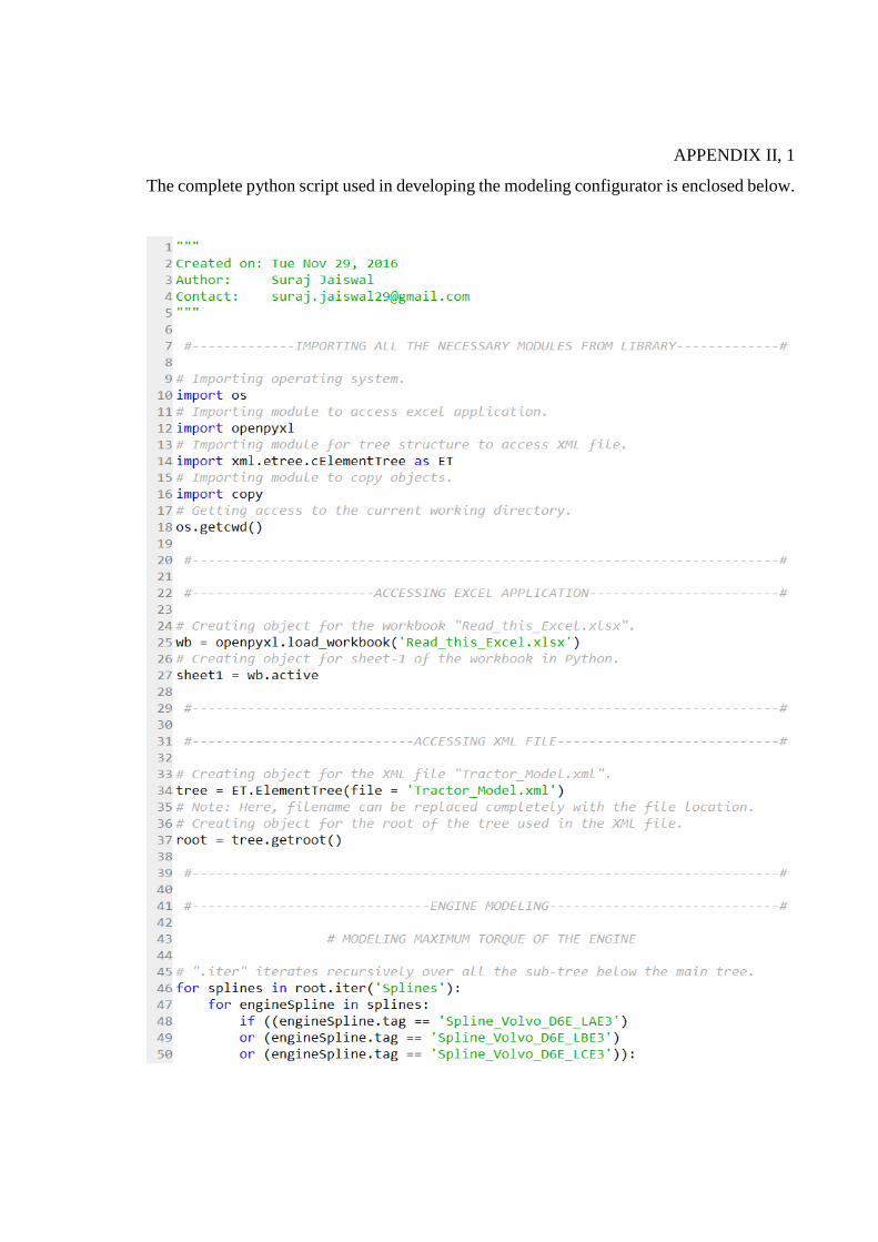
APPENDIX II, 1

The complete python script used in developing the modeling configurator is enclosed below.

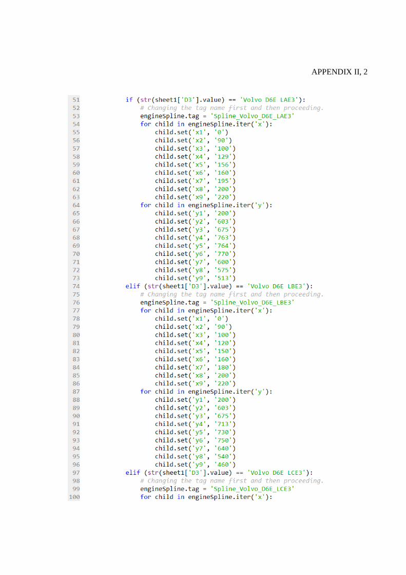
APPENDIX II, 2

APPENDIX II, 3

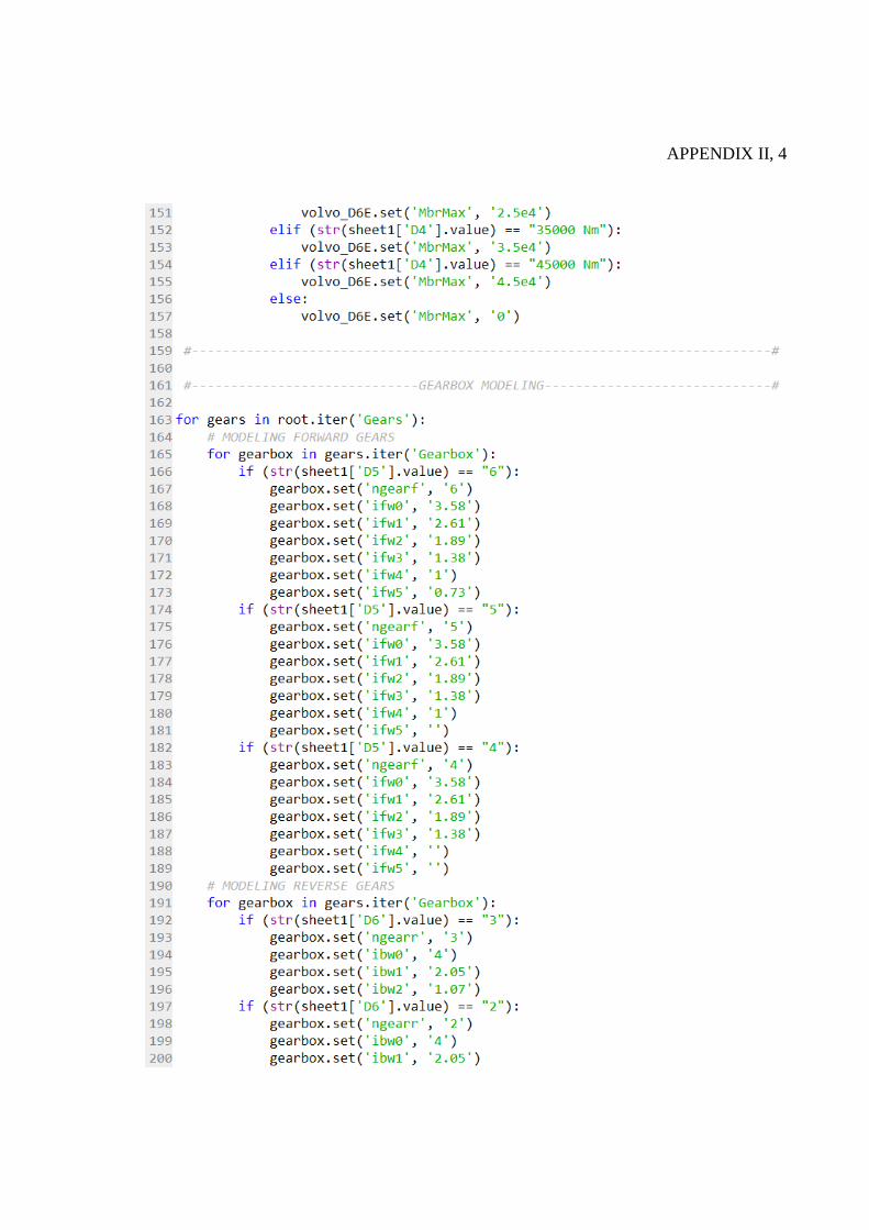
APPENDIX II, 4

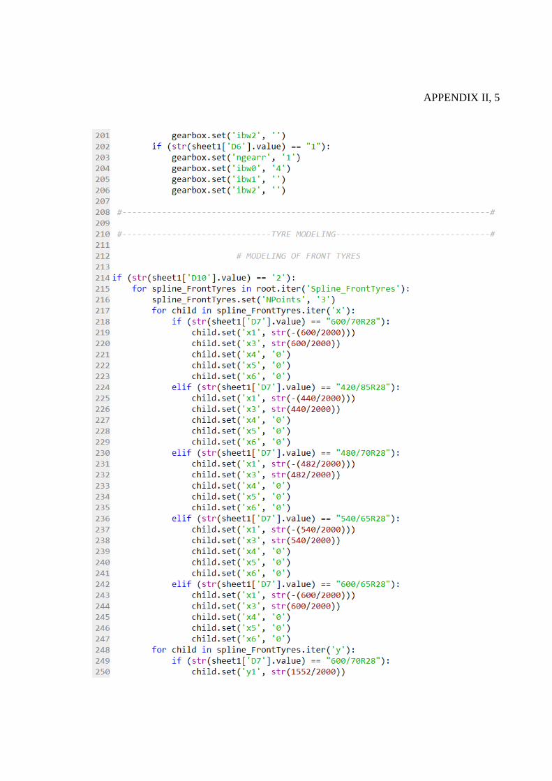
APPENDIX II, 5

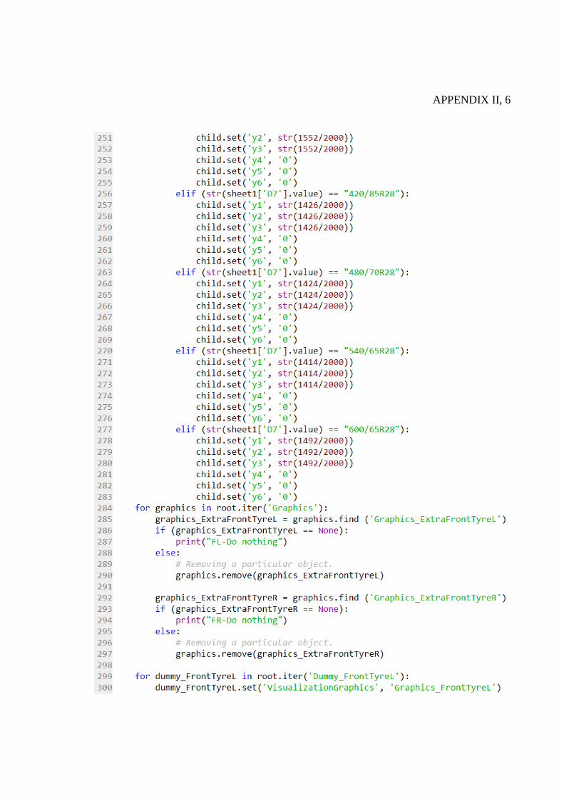
APPENDIX II, 6

APPENDIX II, 7

APPENDIX II, 8

APPENDIX II, 9

APPENDIX II, 10

APPENDIX II, 11

APPENDIX II, 12

APPENDIX II, 13

APPENDIX II, 14

APPENDIX II, 15

APPENDIX II, 16

APPENDIX II, 17

APPENDIX II, 18

APPENDIX II, 19

APPENDIX II, 20

APPENDIX II, 21

APPENDIX II, 22

APPENDIX II, 23

APPENDIX II, 24

APPENDIX II, 25

APPENDIX II, 26

APPENDIX II, 27

APPENDIX II, 28

APPENDIX II, 29

APPENDIX II, 30

APPENDIX II, 31

APPENDIX II, 32

APPENDIX II, 33

APPENDIX II, 34

APPENDIX II, 35

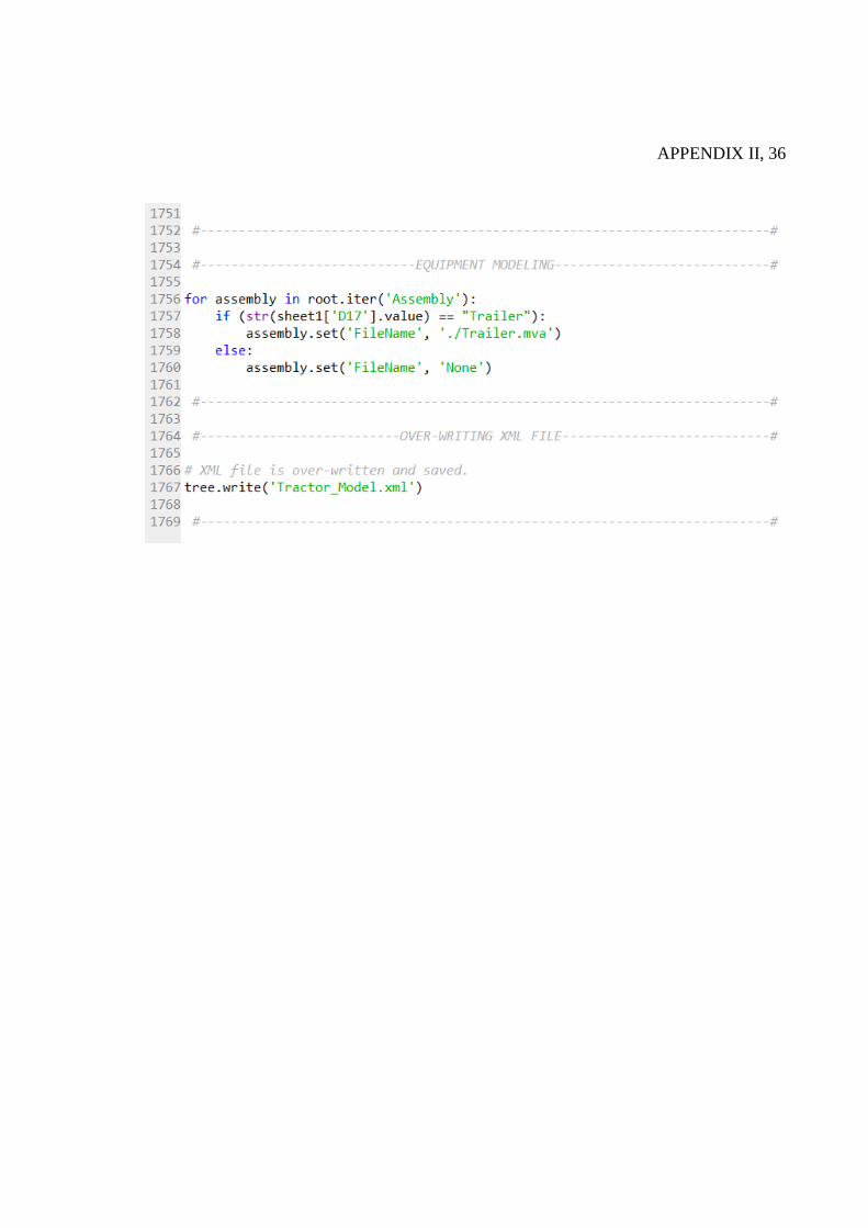
APPENDIX II, 36