Master equation and conversion of environmental heat into coherent electromagnetic energy
60
Progress in Quantum Electronics 34 (2010) 349–408 Review Master equation and conversion of environmental heat into coherent electromagnetic energy Eliade Stefanescu Center of Advanced Studies in Physics at the Institute of Mathematics Simion Stoilow of the Romanian Academy, 13 Calea 13 Septembrie, 050711 Bucharest S5, Romania Abstract We derive a non-Markovian master equation for the long-time dynamics of a system of Fermions interacting with a coherent electromagnetic field, in an environment of other Fermions, Bosons, and free electromagnetic field. This equation is applied to a superradiant p–i–n semiconductor heterostructure with quantum dots in a Fabry–Perot cavity, we recently proposed for converting environmental heat into coherent electromagnetic energy. While a current is injected in the device, a superradiant field is generated by quantum transitions in quantum dots, through the very thin i-layers. Dissipation is described by correlated transitions of the system and environment particles, transitions of the system particles induced by the thermal fluctuations of the self-consistent field of the environment particles, and non-local in time effects of these fluctuations. We show that, for a finite spectrum of states and a sufficiently weak dissipative coupling, this equation preserves the positivity of the density matrix during the whole evolution of the system. The preservation of the positivity is also guaranteed in the rotating-wave approximation. For a rather short fluctuation time on the scale of the system dynamics, these fluctuations tend to wash out the non-Markovian integral in a long-time evolution, this integral remaining significant only during a rather short memory time. We derive explicit expressions of the superradiant power for two possible configurations of the superradiant device: (1) a longitudinal device, with the superradiant mode propagating in the direction of the injected current, i.e. perpendicularly to the semiconductor structure, and (2) a transversal device, with the superradiant mode propagating perpendicularly to the injected current, i.e. in the plane of the semiconductor structure. The active electrons, tunneling through the i-zone between the two quantum dot arrays, are coupled to a coherent superradiant mode, and to a dissipative environment including four components, namely: (1) the quasi-free electrons of the conduction n-region, (2) the quasi-free holes of the conduction p-region, (3) the vibrations of the crystal lattice, and (4) the free electromagnetic field. To diminish the coupling of the active electrons to the quasi-free conduction electrons and holes, the quantum dot arrays are separated from the two www.elsevier.com/locate/pquantelec 0079-6727/$ - see front matter & 2010 Elsevier Ltd. All rights reserved. doi:10.1016/j.pquantelec.2010.06.003 Tel.: þ40 726398719; fax: þ40 213196505. E-mail address: [email protected]
Transcript of Master equation and conversion of environmental heat into coherent electromagnetic energy

Progress in Quantum Electronics 34 (2010) 349–408
0079-6727/$ -
doi:10.1016/j
�Tel.: þ40E-mail ad
www.elsevier.com/locate/pquantelec
Review
Master equation and conversion of environmentalheat into coherent electromagnetic energy
Eliade Stefanescu�
Center of Advanced Studies in Physics at the Institute of Mathematics Simion Stoilow of the Romanian Academy,
13 Calea 13 Septembrie, 050711 Bucharest S5, Romania
Abstract
We derive a non-Markovian master equation for the long-time dynamics of a system of Fermions
interacting with a coherent electromagnetic field, in an environment of other Fermions, Bosons, and
free electromagnetic field. This equation is applied to a superradiant p–i–n semiconductor
heterostructure with quantum dots in a Fabry–Perot cavity, we recently proposed for converting
environmental heat into coherent electromagnetic energy. While a current is injected in the device,
a superradiant field is generated by quantum transitions in quantum dots, through the very thin
i-layers. Dissipation is described by correlated transitions of the system and environment particles,
transitions of the system particles induced by the thermal fluctuations of the self-consistent field of
the environment particles, and non-local in time effects of these fluctuations. We show that, for a
finite spectrum of states and a sufficiently weak dissipative coupling, this equation preserves the
positivity of the density matrix during the whole evolution of the system. The preservation of the
positivity is also guaranteed in the rotating-wave approximation. For a rather short fluctuation time
on the scale of the system dynamics, these fluctuations tend to wash out the non-Markovian integral
in a long-time evolution, this integral remaining significant only during a rather short memory time.
We derive explicit expressions of the superradiant power for two possible configurations of the
superradiant device: (1) a longitudinal device, with the superradiant mode propagating in the
direction of the injected current, i.e. perpendicularly to the semiconductor structure, and (2) a
transversal device, with the superradiant mode propagating perpendicularly to the injected current,
i.e. in the plane of the semiconductor structure. The active electrons, tunneling through the i-zone
between the two quantum dot arrays, are coupled to a coherent superradiant mode, and to a
dissipative environment including four components, namely: (1) the quasi-free electrons of the
conduction n-region, (2) the quasi-free holes of the conduction p-region, (3) the vibrations of the
crystal lattice, and (4) the free electromagnetic field. To diminish the coupling of the active electrons
to the quasi-free conduction electrons and holes, the quantum dot arrays are separated from the two
see front matter & 2010 Elsevier Ltd. All rights reserved.
.pquantelec.2010.06.003
726398719; fax: þ40 213196505.
dress: [email protected]
E. Stefanescu / Progress in Quantum Electronics 34 (2010) 349–408350
n and p conduction regions by potential barriers, which bound the two-well potential corresponding
to these arrays. We obtain analytical expressions of the dissipation coefficients, which include simple
dependences on the parameters of the semiconductor device, and are transparent to physical
interpretations. We describe the dynamics of the system by non-Markovian optical equations with
additional terms for the current injection, the radiation of the field, and the dissipative processes. We
study the dependence of the dissipative coefficients on the physical parameters of the system, and the
operation performances as functions of these parameters. We show that the decay rate of
the superradiant electrons due to the coupling to the conduction electrons and holes is lower than the
decay rate due to the coupling to the crystal vibrations, while the decay due to the coupling to the free
electromagnetic field is quite negligible. According to the non-Markovian term arising in the optical
equations, the system dynamics is significantly influenced by the thermal fluctuations of the self-
consistent field of the quasi-free electrons and holes in the conduction regions n and p, respectively.
We study the dependence of the superradiant power on the injected current, and the effects of the
non-Markovian fluctuations. In comparison with a longitudinal device, a transversal device has a
lower increase of the superradiant power with the injected current, but also a lower threshold current
and a lesser sensitivity to thermal fluctuations.
& 2010 Elsevier Ltd. All rights reserved.
Keywords: Non-Markovian quantum master equation; Superradiance; Correlated transitions; Semiconductor
heterostructure; Photon; Phonon
Contents
1. Introduction . . . . . . . . . . . . . . . . . . . . . . . . . . . . . . . . . . . . . . . . . . . . . . . . . . . . . . 350
2. Quantum master equation for a matter-field system and the positivity of the
density matrix . . . . . . . . . . . . . . . . . . . . . . . . . . . . . . . . . . . . . . . . . . . . . . . . . . . . . 354
3. Long-time evolution . . . . . . . . . . . . . . . . . . . . . . . . . . . . . . . . . . . . . . . . . . . . . . . . 360
4. Superradiant dynamics . . . . . . . . . . . . . . . . . . . . . . . . . . . . . . . . . . . . . . . . . . . . . . . 362
5. Steady state . . . . . . . . . . . . . . . . . . . . . . . . . . . . . . . . . . . . . . . . . . . . . . . . . . . . . . 367
6. System structure and microscopic model . . . . . . . . . . . . . . . . . . . . . . . . . . . . . . . . . . 370
7. Wave functions and dipole moments of the system . . . . . . . . . . . . . . . . . . . . . . . . . . . 376
8. Coupling to the conduction electrons . . . . . . . . . . . . . . . . . . . . . . . . . . . . . . . . . . . . 380
9. Coupling to the crystal vibrations and the free electromagnetic field. . . . . . . . . . . . . . . 386
10. Superradiant semiconductor device . . . . . . . . . . . . . . . . . . . . . . . . . . . . . . . . . . . . . . 390
11. Operation conditions for the device parameters . . . . . . . . . . . . . . . . . . . . . . . . . . . . . 393
12. Operation conditions for the separation barriers. . . . . . . . . . . . . . . . . . . . . . . . . . . . . 395
13. Dissipative coefficients and stationary regime . . . . . . . . . . . . . . . . . . . . . . . . . . . . . . . 396
14. Non-Markovian fluctuations. . . . . . . . . . . . . . . . . . . . . . . . . . . . . . . . . . . . . . . . . . . 403
15. Discussion and concluding remarks. . . . . . . . . . . . . . . . . . . . . . . . . . . . . . . . . . . . . . 404
References . . . . . . . . . . . . . . . . . . . . . . . . . . . . . . . . . . . . . . . . . . . . . . . . . . . . . . . 407
1. Introduction
The dissipative dynamics, as a characteristic of any realistic system, is an interesting fieldof research [1–4], especially due to the difficulties raised by a correct description of thedissipative coupling [5]. Important applications where dissipation cannot be neglected aregiven in [6–10]. The dissipative coupling is essential for a device we recently proposed for

E. Stefanescu / Progress in Quantum Electronics 34 (2010) 349–408 351
converting the environmental heat into usable energy, called quantum heat converter[11–14]. In the most general form, such a coupling can be described by an additional,dissipation term, in the dynamic equation of the density matrix that, with this, becomes amaster equation [15–17].
A generalization of the Schrodinger equation of a closed system, to a master equationdescribing an openness of this system, has been performed by taking into account variousarguments [18]. In [15], the dynamic equation of a harmonic oscillator is generalized byconsidering the canonical coordinates as being complex quantities, with imaginary partsdepending on noise operators. When an equation for the real coordinate and momentum isderived from the dynamic equation with a noisy effective Hamiltonian, a quantum masterequation is obtained. In [16], the total system composed of a harmonic oscillator of interestand an environment of other harmonic oscillators is quantized, and the reduced dynamicsis obtained in the framework of the path integral theory.
In [17], Lindblad adopts a quite radical approach of the problem, by using amathematical generalization of the dynamic group of the quantum states of a system to atime-dependent semigroup, having in view only the positivity preservation of the densitymatrix. Ten years later, this equation has been put into a form with friction and diffusioncoefficients, for a harmonic oscillator [19]. For the dissipative coefficients, althoughunspecified in this framework, fundamental constraints are obtained from theirdependence on Lindblad’s axiomatic coefficients. These relations are in agreement withthe well-known theorem of dissipation and fluctuations. The essential merit of thisequation in comparison with the previous ones is the full agreement with the quantum-mechanical principles: the positivity of the density matrix during the whole evolution of thesystem and the uncertainty relation. When the matrix elements of the openness operatorssatisfy certain conditions depending on temperature, Lindblad’s master equation is inagreement also with the detailed balance principle [20]. For a harmonic oscillator at quasi-equilibrium, the dissipative parameters reduce to only two, the two diffusion coefficients ofcoordinate and momentum becoming functions of the friction coefficient and temperature.Important efforts continued to improving existing models, or developing new physicalmodels [21–38].
By a procedure previously used in [39], in this paper we calculate the long-time reduceddynamics of a system of Fermions, interacting with a coherent electromagnetic field, in adissipative environment of other Fermions, Bosons, and a free electromagnetic field, bytaking into account correlated transitions of the system and environment particles, andrandom fluctuations of the self-consistent field of the environmental Fermions. We derive amaster equation including a phase-operator fðtÞ, which describes fluctuations of thedensity matrix due to the thermal fluctuations of the self-consistent field of theenvironment particles, and a memory time t, much longer than the fluctuation time ofthis field, but much shorter than the decay time. This equation also includes a fluctuationHamiltonian ‘ zijc
þi cj, which is similar to the hopping Hamiltonian (3) in [40]. Besides this
fluctuation Hamiltonian, a non-Markovian term of the second-order in the fluctuationmatrix elements zij arises [39], from the dissipative quantum dynamics in theapproximation of a weak dissipative coupling [28]. We derive conditions for thepreservation of the positivity of the density matrix.
We apply this master equation to a superradiant n–i–p semiconductor heterostructurerepresented in Fig. 1, as a basic element of a quantum heat converter [11–14], whichworks on the principle of the photon-assisted tunneling [41–45]. This device consists in a
AD
LD
n
ND Ne
i na
pa
Ne
p n na i p
a p
NA NAND Ne Ne
n−i−p junction 1 n−i−p junction 2 n−i−p junction Nt
nb pb
nb
pb
N3 N4 N3 N4
•I I
x
y
z
LongitudinalRadiation Field
TransversalRadiation Field
◦ • ◦
• ◦• ◦
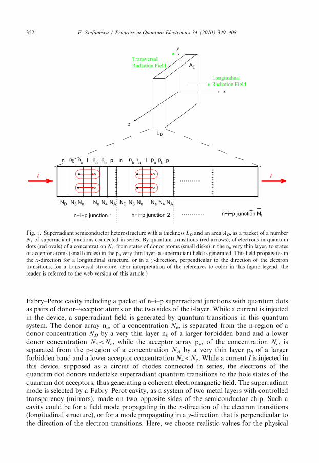
Fig. 1. Superradiant semiconductor heterostructure with a thickness LD and an area AD, as a packet of a number
N t of superradiant junctions connected in series. By quantum transitions (red arrows), of electrons in quantum
dots (red ovals) of a concentration Ne, from states of donor atoms (small disks) in the na very thin layer, to states
of acceptor atoms (small circles) in the pa very thin layer, a superradiant field is generated. This field propagates in
the x-direction for a longitudinal structure, or in a y-direction, perpendicular to the direction of the electron
transitions, for a transversal structure. (For interpretation of the references to color in this figure legend, the
reader is referred to the web version of this article.)
E. Stefanescu / Progress in Quantum Electronics 34 (2010) 349–408352
Fabry–Perot cavity including a packet of n–i–p superradiant junctions with quantum dotsas pairs of donor–acceptor atoms on the two sides of the i-layer. While a current is injectedin the device, a superradiant field is generated by quantum transitions in this quantumsystem. The donor array na, of a concentration Ne, is separated from the n-region of adonor concentration ND by a very thin layer nb of a larger forbidden band and a lowerdonor concentration N3oNe, while the acceptor array pa, of the concentration Ne, isseparated from the p-region of a concentration NA by a very thin layer pb of a largerforbidden band and a lower acceptor concentration N4oNe. While a current I is injected inthis device, supposed as a circuit of diodes connected in series, the electrons of thequantum dot donors undertake superradiant quantum transitions to the hole states of thequantum dot acceptors, thus generating a coherent electromagnetic field. The superradiantmode is selected by a Fabry–Perot cavity, as a system of two metal layers with controlledtransparency (mirrors), made on two opposite sides of the semiconductor chip. Such acavity could be for a field mode propagating in the x-direction of the electron transitions(longitudinal structure), or for a mode propagating in a y-direction that is perpendicular tothe direction of the electron transitions. Here, we choose realistic values for the physical

E. Stefanescu / Progress in Quantum Electronics 34 (2010) 349–408 353
parameters, and study the dissipation coefficients and the superradiant power as functionsof these parameters.
The superradiation process [46–48] is usually described by using optical equations for a two-level atom interacting with a single mode of the electromagnetic field [49–51]. These equationsdescribe the time-evolution of a Bloch vector ~s in the space ðsx;sy;szÞ of the pseudo-spin, as a
geometrical representation of the population difference sz, and polarization sx þ isy [49].
When the system is closed, this vector rapidly rotates around the sz-axes with the resonancefrequency o0. It is remarkable that, when the system is open, the Bloch vector has a quitedifferent evolution, which essentially depends on the perturbing coupling to the environment[52–57]. Really, since in a closed system the atom continuously changes energy with the field,
the population difference sz and the amplitude of the polarizationffiffiffiffiffiffiffiffiffiffiffiffiffiffiffiffis2x þ s2y
qslowly oscillate
between �1 and 1 with the Rabi frequency, while the polarization components sx;sy rapidly
oscillate with the frequency o0. When the system is open, as long as no electromagnetic fieldexists, the component sz takes a constant value sz0 according to the detailed balance principle,while the polarization components sx, sy vanish. While a quasi-resonant electromagnetic field
arises, after a transitory time, the amplitudes of the Bloch vector components sx, sy, sz take
constant values, depending on the coupling coefficients of the system to the field and to thedissipative environment. In this case, the energy absorbed by the atom from the field isdissipated by the environment. Thus, we notice that dissipation plays a central role in theatom-field interaction. Important efforts have been devoted to the microscopic description ofthe dissipative processes in the atom-field interaction [40,58–60]. In [40] a many-electronmicroscopic model, including a hopping Hamiltonian, an electron–electron Coulombinteraction, and an electron–phonon interaction, is developed.
The atom-field dissipative dynamics gets a more systematic approach in the frameworkof the quantum theory of open systems, where the diagonal elements of the density matrixare the populations of the states, while the non-diagonal ones represent polarizations infield equations [7–10,61–65]. In [66], we found that, besides the well-known decay anddephasing rates of the optical equations, Lindblad’s master equation [17] produces anadditional term, describing a coupling of the polarization to the population through theenvironment. It is remarkable that this coupling is somehow similar to the couplingproduced by an electromagnetic field. For certain values of the atomic detuning, thiscoupling leads to negative values of the absorption coefficient, which means a slightamplification of the electromagnetic field on the account of the environment energy.
In this paper we present a physical principle and a semiconductor superradiant deviceconverting the environmental heat in coherent electromagnetic energy with a highefficiency [11–14]. In Section 2, we obtain a non-Markovian quantum master equationwith explicit microscopic coefficients, describing the long-time dynamics of this device. Weshow that for a finite spectrum of states and a sufficiently weak dissipative coupling, thepositivity of the density matrix is preserved, the tendency of the non-Markovian term tocarry the density out from its positivity domain being canceled by the Markovian term,bringing it back into this domain. In Section 3, we derive equations for the matrixelements. In the rotating-wave approximation [58,67,68], for the diagonal matrix elementswe obtain equations preserving the positivity. We describe the long-time dynamicsof the system, by introducing a memory time in the non-Markovian integral, and aphase fluctuation operator in the exponentials under this integral. In Section 4, forthe usual model of an assembly of two-level systems in a Fabry–Perot cavity, we derive

E. Stefanescu / Progress in Quantum Electronics 34 (2010) 349–408354
non-Markovian equations for polarization, population, and field, with additional termsfor the injected current and the field radiation and dissipation. In Section 5, we find thatthe time non-local equations do not have stationary solutions. However, since thecontributions of the non-Markovian terms consist only in oscillations round theMarkovian solution, we consider this solution as describing the stationary regime of thisdevice. In the Markovian approximation, we derive expressions of the superradiant poweras functions of the coupling, dissipation, and radiation characteristics.In Section 6, we present the microscopic model of the device superradiant junction, and
calculate the energy levels as functions of impurity concentrations. We obtain explicitexpressions of the electric dissipative coefficients, as functions of electric materialcharacteristics and matrix elements of the two-body potentials between the electrons ofthe superradiant system and the conduction electrons and holes. In Section 7, we derivewave-functions and transition dipole moments. These moments mainly depend on theoverlap in the i-layer of the wave-functions of the active electrons in the two states ofthe superradiant system. In Section 8, we calculate the matrix elements for the coupling tothe quasi-free electrons and holes, and derive the electric dissipative coefficients as functionsof physical characteristics of the semiconductor structure. These coefficients depend on thetransition dipole moments, the transition energy, the donor and acceptor concentrations,and the thicknesses of the separation barriers. In Section 9, we derive the phonon dissipativecoefficients, which depend on the transition energy and the sound velocity in the crystal. Wealso derive the decay rates due to the coupling to the free electromagnetic field, whichdepend only on physical constants and the transition dipole moment.In Section 10, we present the basic idea of a quantum heat converter, and the physical
models for two possible versions, which depend on the position of the semiconductor structurein the Fabry–Perot cavity, i.e. on the surfaces of the structure which the mirror metalizationsare made on: (1) a longitudinal device with the superradiant field propagating in the directionof the injection current, which is perpendicular to the semiconductor layers, and (2) atransversal device with the superradiant field propagating perpendicularly to the direction ofthe injection current, which is in the plane of the semiconductor layers. In Section 11, we getexplicit expressions for the coefficients of the optical equations, as depending only on physicalcharacteristics of the system. We discuss the dependences on these characteristics of thesuperradiant power, threshold currents, and operation conditions. In Section 12, we deriveconditions for the separation barriers to provide the necessary injection current. In Section 13,we give a numerical example, and study the dependence on the i-zone thickness of the deviceparameters that mainly depend on this thickness: dissipation rates, coupling coefficients,threshold currents, and the quantum dot density necessary for entirely including the internalfield in the quantum dot region. We find that, due to the separation barriers, the electriccoupling to the conduction electrons gets weaker than the phonon coupling to the crystallattice. We study the dependence of the dissipation coefficients and superradiant power onphysical characteristics of the system. In Section 14, we study the effects of the thermalfluctuations on the superradiation process for the two versions of the device. In Section 15 wediscuss the results and give some conclusions.
2. Quantum master equation for a matter-field system and the positivity of the density matrix
The dissipative dynamics of a system of Fermions interacting with an electromagneticfield, in an environment of other Fermions, Bosons, and a free electromagnetic field, has

E. Stefanescu / Progress in Quantum Electronics 34 (2010) 349–408 355
been previously described by a quantum master equation with a Markovian term for thecorrelated transitions of the system and environment particles [29–31]. Recently, we havetaken into account the presence of a self-consistent field of the environment Fermions,described in the master equation by a non-Markovian term [39]. We notice that all thesecouplings are essential for the superradiant dynamics of a semiconductor structure, which,besides the active quantum system, includes a complex environment of quasi-free electronsand holes, and vibrations of the crystal lattice. For the total system, we consider thegeneral quantum dynamical equation:
d
dt~wðtÞ ¼ �
i
‘e ~V ðtÞ þ e ~V
EðtÞ; ~wðtÞ
h i; ð1Þ
where VE is the potential of interaction of the system of interest with the environment,while V is the potential of interaction from the Hamiltonian of the system of interest
H ¼ HS0 þHF þ V ; ð2Þ
which includes the terms
HS0 ¼
Xk
ekcþk ck ð3Þ
for the system of Fermions, and HF for the electromagnetic field. In this equation, tildedenotes operators in the interaction picture, e.g.
~wðtÞ ¼ ei=‘ ðHEþHS0þHF ÞtwðtÞe�i=‘ ðHFþHS
0þHE Þt; ð4Þ
where HE is the Hamiltonian of the environment. According to a general proceduredisclosed in [28], we take a total density of the form
~wðtÞ ¼ R ~rðtÞ þ e ~wð1ÞðtÞ þ e2 ~wð2ÞðtÞ þ � � � ; ð5Þ
where rðtÞ is the reduced density matrix of the system of Fermions and electromagneticfield, while R is the density of the dissipative environment at the initial momentof time, t=0, the time-evolution of environment being taken into account by the higher-order terms ~wð1ÞðtÞ; ~wð2ÞðtÞ; � � �. The parameter e is introduced to handle the ordersof the terms in this expansion, and is set to 1 in the final results. The reduced density of thesystem is
~rðtÞ ¼ TrEf ~wðtÞg; ð6Þ
while the higher-order terms of the total density have the property:
TrEf ~wð1Þg ¼ TrEf ~wð2Þg ¼ � � � ¼ 0: ð7Þ
If initially the environment is in the equilibrium state R, the initial density matrix wðtÞ of thetotal system is of the form wð0Þ ¼ Rrð0Þ. We suppose that at the moment t=0, due to theinteraction V of the system of Fermions with the electromagnetic field, or due to a non-equilibrium initial state rð0ÞarT , a time-evolution begins, while the reduced densitysatisfies a quantum dynamical equation of the form
d
dt~rðtÞ ¼ e ~B
ð1Þð ~rðtÞ;tÞ þ e2 ~B
ð2Þð ~rðtÞ;tÞ þ � � � : ð8Þ
We take the equilibrium density matrix of the environment
R ¼ RF � RB � RFE ð9Þ
E. Stefanescu / Progress in Quantum Electronics 34 (2010) 349–408356
as including the density matrix
RF ¼Xab
RFabcþa cb ð10Þ
of the Fermi component, and similar expressions for the Bose and the free electromagneticfield components. In this case, the perturbation term
V E ¼ ‘X
ij
Gijcþi cj ð11Þ
includes operators
Gij ¼ GFij þ GB
ij þ GFEij ; ð12Þ
with terms for the Fermion part of the environment
GFij ¼
1
‘
Xab
/aijVF jbjScþa cb; ð13Þ
and similar expressions for the Boson part and for the free electromagnetic field. Here, wetake into account only the dissipative coupling of the system of Fermions, since thedissipation of the field is a well-known problem. That means that the interaction with theelectromagnetic field is described only by the Hamiltonian term, while the field dissipationcan be taken into account merely introducing the dissipative terms of the correspondingharmonic oscillator [39]. In the density matrix (5) of the total system, we distinguish thefirst term, which describes the evolution of the system of interest while the state of theenvironment remains unchanged (Markov approximation). The higher-order terms of thisseries expansion describe the evolution of the environment correlated with the evolution ofthe system. In the second-order approximation, these terms are
~wð1ÞðtÞ ¼ �i
‘R
Z t
0
½ ~V ðt0Þ; ~rðt0Þ� dt0�R
Z t
0
~Bð1Þ½ ~rðt0Þ;t0� dt0�i
Xij
Z t
0
½ ~Gijðt0Þ~cþi ðt
0Þ~cjðt0Þ;R ~rðt0Þ� dt0;
ð14aÞ
~wð2ÞðtÞ ¼ �i
‘
Z t
0
½ ~V ðt0Þ; ~wð1Þðt0Þ� dt0�R
Z t
0
~Bð2Þ½ ~rðt0Þ;t0� dt0�i
Xij
Z t
0
½ ~Gijðt0Þ~cþi ðt
0Þ~cjðt0Þ; ~wð1Þðt0Þ� dt0;
ð14bÞ
while for the reduced dynamics of the system we get the terms:
~Bð1Þ½ ~rðtÞ;t� ¼ �
i
‘½ ~V ðtÞ; ~rðtÞ��i
Xij
TrE ½ ~G ijðtÞ~cþi ðtÞ~cjðtÞ;R ~rðtÞ�; ð15aÞ
~Bð2Þ½ ~rðtÞ;t� ¼ �i
Xij
TrE ½ ~GijðtÞ~cþi ðtÞ~cjðtÞ; ~wð1ÞðtÞ�: ð15bÞ
In these equations we consider the reduced density matrix in the interaction picture ~rðtÞ asslowly varying in time. We assume the time-symmetry, which means that the time-integralsdo not depend on the origin of time, but only on the relative intervals t�t0 between the
E. Stefanescu / Progress in Quantum Electronics 34 (2010) 349–408 357
actual time t and the past time t0. With the transition operators in the interaction picture,
~cþi ðtÞ~cjðtÞ ¼ eioij tcþi cj ;oij ¼ei�ej
‘; ð16Þ
we obtain:
~Bð1Þ½ ~rðtÞ;t� ¼ �
i
‘½ ~V ðtÞ; ~rðtÞ��i
Xij
zij0½~cþi ðtÞ~cjðtÞ; ~rðtÞ�; ð17aÞ
~Bð2Þ½ ~rðtÞ;t� ¼
Xij
lijf½cþi cj ~rðtÞ;cþj ci� þ ½c
þi cj ; ~rðtÞcþj ci�g
þXijkl
zij0zkl0
Z t
0
½~cþi ðtÞ~cjðtÞ;½~cþk ðt0Þ~clðt
0Þ; ~rðt0Þ�� dt0: ð17bÞ
These equations include two families of dissipative coefficients: the matrix elements of theself-consistent field of the environment particles
zij0 ¼
1
‘Y F
ZðaÞ/aijVF jajSf F
a ðeaÞgFa ðeaÞ dea ð18Þ
and the decay rates
lFij ¼
p‘Y F
ZðbÞj/aijV F jbjSj2½1�f F
a ðeaÞ�fFb ðebÞg
Fa ðeaÞg
Fb ðebÞjoab¼oji
deb; ð19aÞ
lBij ¼
p‘Y B
ZðbÞj/aijV BjbjSj2½1þ f B
a ðeaÞ�fBb ðebÞg
Ba ðeaÞg
Bb ðebÞjoab¼oji
deb ð19bÞ
for the coupling with the system of Fermions and with the system of Bosons, respectively.In these expressions, YF, YB represent the total numbers of the environment Fermions andBosons, in the quantization volumes of these particles. Although, by diagonalizing thepotential VF in (18) the transition elements zij
0 vanish, such transitions continue to begenerated by the thermal fluctuations of the environment particles over the states jaS. Wetake into account these fluctuations by considering in (18) the variances of the potential VF:
zij0�!zij ¼
1
‘
ffiffiffiffiffiffiffiffiffiffiffiffiffiffiffiffiffiffiffiffiffiffiffiffiffiffiffiffiffiffiffiffiffiffiffiffiffiffiffiffiffiffiffiffiffiffiffiffiffiffiffiffiffiffiffiffiffiffiffiffiffiffiffiffiffiffiffiffiffiffiffiffiffiffiffi1
Y F
ZðaÞ/aijðV F Þ
2jajSf F
a ðeaÞgFa ðeaÞ dea
s: ð20Þ
Using the transition operators (16) with the resonance condition oab ¼ oji, and the seriesexpansion (8) with the terms (17), in the second-order approximation of the dissipativecoupling we obtain the non-Markovian quantum master equation [39]:
d
dtrðtÞ ¼ �
i
‘½H;rðtÞ��i
Xij
zij½cþi cj ;rðtÞ� þ
Xij
lijð½cþi cjrðtÞ;cþj ci� þ ½c
þi cj ;rðtÞcþj ci�Þ
þXijkl
zijzkl
Z t
0
½cþi cj ;e�i=‘HS
0ðt�t0Þ½cþk cl ;rðt0Þ�ei=‘HS
0ðt�t0Þ� dt0: ð21Þ
The dissipative generator of this equation is composed of a Hamiltonian part with thematrix elements zij, which describe transitions stimulated by the fluctuations of the self-consistent field of the environment particles, a Markovian part, of Lindblad’s form, withthe decay rates lij, which describe correlated transitions of the system and environment

E. Stefanescu / Progress in Quantum Electronics 34 (2010) 349–408358
particles, and a non-Markovian part, as a time-integral of the system operators, describingmemory effects, which are proportional to the fluctuations of the self-consistent field of the
environment particles. We do not diagonalize the dissipative HamiltonianP
ijzijcþi cj, since
the matrix elements zij describe fluctuations that arise in any basis of states. The dissipative
coefficients of the Markovian part
lij ¼ lFij þ lB
ij þ gij ð22Þ
include explicit terms for the coupling to an environment of Fermions, Bosons and the freeelectromagnetic field. These terms depend on the dissipative two-body potentials VF, VB,
the densities of the environment states gFa ðeaÞ; g
Ba ðeaÞ, the occupation probabilities of these
states f Fa ðeaÞ; f
Ba ðeaÞ; and temperature T. For a rather low temperature, T5eji; j4i, these
terms become
lFij ¼
p‘j/aijV F jbjSj2½1�f F
a ðejiÞ�gFa ðejiÞ; ð23aÞ
lFji ¼
p‘j/aijV F jbjSj2f F
a ðejiÞgFa ðejiÞ ð23bÞ
for the Fermi environment,
lBij ¼
p‘j/aijV BjbjSj2½1þ f B
a ðejiÞ�gBa ðejiÞ; ð24aÞ
lBji ¼
p‘j/aijV BjbjSj2f B
a ðejiÞgBa ðejiÞ ð24bÞ
for the Bose environment, and
gij ¼2a
c2‘ 3~r2ije
3ji 1þ
1
eeji=T�1
� �ð25Þ
for the Bose environment of the free electromagnetic field, where~rij are the transition dipole
moments. The terms of the master Eq. (21), with the dissipative coefficients (22)–(25),describe single-particle transitions of the system and environment, with energy conserva-tion, eji ¼ eab, in agreement with the quantum-mechanical principles, and with the detailed
balance principle [32]. The non-Markovian part of this equation takes into account thefluctuations of the self-consistent field of the environment Fermions, with the coefficients
(20), where Y F is the total number of these particles occupying the states jaS in aquantization volume.Since the master Eq. (21) is derived as a second-order approximation of the total
dynamics, we investigate the preservation of the positivity of the density matrix generatedby this equation. We consider that at the initial moment of time t=0, the density matrix ispositive and, consequently, can be diagonalized:
rð0Þ ¼X
i
licþi ci; riið0Þ ¼ li40: ð26Þ
Introducing this expression in the master equation (21), and using the commutation relations
eð�i=‘ ÞHS0tcþk ¼ eð�i=‘ Þektcþk eð�i=‘ ÞH
S0t; ð27aÞ
ckeði=‘ ÞHS0t ¼ eði=‘ Þekteði=‘ ÞH
S0tck; ð27bÞ

E. Stefanescu / Progress in Quantum Electronics 34 (2010) 349–408 359
we get the evolution of the diagonal matrix elements riiðtÞ in a very short interval of time t, asdepending on the whole energy spectrum ej:
d
dtriiðtÞ
����t¼t¼ 2X
j
lij�‘ jzijj
2
ej�ei
sin½ðej�eiÞt�
!lj� lji�
‘ jzijj2
ej�ei
sin½ðej�eiÞt�
!li
" #:
ð28Þ
According to (22)–(25), for a finite energy spectrum, the decay/excitation coefficients takenon-zero, positive values, lij ; lji40, which means that, for a rather small but non-zerointerval of time t, the coefficients of Eq. (28) also remain positive:
lij�jzijj2t40; lji�jzijj
2t40: ð29Þ
When a diagonal element riiðtÞ 2 ½0; 1�, of the density matrix, approaches one of its limits, thevariation of this element gets a sign bringing it back to the inner of its definition domain:
riiðtÞ-0)d
dtriiðtÞ
���t¼t¼ 2X
j
ðlij�jzijj2tÞlj40; ð30aÞ
riiðtÞ-1)d
dtriiðtÞ
���t¼t¼ �2
Xj
ðlji�jzijj2tÞlio0: ð30bÞ
However, if we consider a time interval t satisfying the uncertainty relation ðej�eiÞt4‘ ,for a finite spectrum of states we get the positivity conditions
‘ jzijj2
jej�eijolij ;
‘ jzijj2
jej�eijolji; ð31Þ
depending on the decay rates lij and the excitation rates lji. From (30) and (31), we noticethat, although the non-Markovian fluctuation rates zij of this equation have the tendency toalter the positivity of the density matrix, for a finite spectrum of states and a sufficiently weakdissipative coupling, the positivity is still preserved, this tendency being canceled by the decay/excitation rates lij ; lji. In the following, we derive explicit expressions for these coefficients, asfunctions of the physical parameters of the system.
We notice that Eq. (28) of the diagonal matrix elements includes only non-diagonalmatrix elements zij . From (20) and (23b), we notice that the excitation matrix elements lji
and the non-diagonal fluctuation matrix elements zij could be considered approximately ofthe same order of magnitude, which means that the conditions (31) reduce to the conditionthat these elements are much smaller than the distance between the energy levels of thesystem:
‘ jzijj5jej�eij: ð32Þ
These conditions are always satisfied in the assumption of a weak dissipative coupling,when the density matrix elements have slowly varying amplitudes:
rjiðtÞ ¼ ~rjiðtÞe�ioji t: ð33Þ

E. Stefanescu / Progress in Quantum Electronics 34 (2010) 349–408360
3. Long-time evolution
From the master Eq. (21) we derive equations for the density matrix elements that, withthe matrix elements of the transition operators /kjcþi cjjlS ¼ dkidjl , take the form
d
dtrjiðtÞ ¼ �iojirjiðtÞ�
i
‘
Xk
½VjkðtÞrkiðtÞ�rjkðtÞVkiðtÞ�
�iX
k
½zjkrkiðtÞ�rjkðtÞzki� þX
k
½2dijljkrkkðtÞ�ðlki þ lkjÞrjiðtÞ�
þX
kl
Z t
0
fzjk½zklrliðt0Þ�rklðt
0Þzli�eioikðt�t0Þ�½zjkrklðt
0Þ�rjkðt0Þzkl �zlie
iolj ðt�t0Þg dt0:
ð34Þ
In these equations, we introduce density matrix elements of the form (33), and neglect therapidly varying terms in the amplitudes ~rjiðtÞ (rotating-wave approximation). Thus, for theslowly varying amplitudes ~rjiðtÞ, we get the equations
d
dt~rjiðtÞ ¼ �
i
‘
Xk
½VjkðtÞrkiðtÞ�rjkðtÞVkiðtÞ�eioji t þ
Xk
½2dijljkrkkðtÞeioji t�ðlki þ lkjÞ ~rjiðtÞ�
�iX
k
½zjk ~rkiðtÞe�iokit� ~rjkðtÞe
�iojktzki�eioji t
þX
kl
Z t
0
fzjk½zkl ~rliðt0Þe�ioli t
0
� ~rklðt0Þe�iokl t
0
zli�eioji teioikðt�t0Þ
�½zjk ~rklðt0Þe�iokl t
0
� ~rjkðt0Þe�iojkt0zkl �zlie
ioji teiolj ðt�t0Þg dt0; ð35Þ
where we neglect the rapidly oscillating terms. From these equations we obtain non-Markovian equations for the non-diagonal matrix elements
d
dtrjiðtÞ ¼ �i½oji þ ðzjj�ziiÞ�rjiðtÞ�
i
‘
Xk
½VjkðtÞrkiðtÞ�rjkðtÞVkiðtÞ�
�X
k
ðlki þ lkjÞrjiðtÞ þ ðzjj�ziiÞ2e�ioji t
Z t
0
~rjiðt0Þ dt0; ð36Þ
and Markovian equations for the diagonal ones:
d
dtrjjðtÞ ¼ �
i
‘
Xk
½VjkðtÞrkjðtÞ�rjkðtÞVkjðtÞ��2X
k
½lkjrjjðtÞ�ljkrkkðtÞ�: ð37Þ
That means that in the rotating-wave approximation the non-Markovian component ofthe dissipative dynamics does not alter the quantum and statistical properties of the densitymatrix, as the normalization, positivity, and detailed balance. We notice that the non-diagonal elements rjiðtÞ of the density matrix does not depend on the non-diagonalelements of the field fluctuations, but only on the diagonal elements zjj and zii of thesefluctuations, which means that, in this case, the positivity conditions (31) and (32) arealways satisfied in the rotating-wave approximation.These equations take a simpler form for a two-level system with a transition frequency
o0 � o10, interacting with an electromagnetic field with an amplitude EðtÞ and a frequencyo, which is not very far from resonance (o � o0). Using the notations SðtÞ for the

E. Stefanescu / Progress in Quantum Electronics 34 (2010) 349–408 361
polarization of the system as a slowly varying amplitude of the non-diagonal element ofthe density matrix,
r10ðtÞ ¼12SðtÞe�iot; ð38Þ
and
wðtÞ ¼ r11ðtÞ�r00ðtÞ with the condition ð39aÞ
1 ¼ r11ðtÞ þ r00ðtÞ ð39bÞ
for the population difference, we obtain
d
dtSðtÞ ¼ �g?ð1�idoÞSðtÞ þ igEðtÞwðtÞ þ g2n
Z t
0
Sðt0Þeiðo�o0Þðt�t0Þ dt0; ð40aÞ
d
dtwðtÞ ¼ �gJ½wðtÞ�wT ��i
g
2½EðtÞS�ðtÞ�E�ðtÞSðtÞ�: ð40bÞ
The coefficients of these equations are the damping rate of the polarization (dephasingrate)
g? ¼ l01 þ l10 þ l00 þ l11; ð41Þ
the decay rate of the population difference
gJ ¼ 2ðl01 þ l10Þ; ð42Þ
the fluctuation rate of the self-consistent field of the environment particles (non-Markovian coefficient)
gn � jz11�z00j; ð43Þ
the relative atomic detuning
do ¼o�o0�gn
g?; ð44Þ
the equilibrium population difference
wT ¼ �l01�l10l01 þ l10
; ð45Þ
and the coupling coefficient of the system with the coherent electromagnetic field
g ¼e
‘~r01~1E ð46Þ
as a function of the transition dipole moment~r01 and the polarization vector of the field ~1E .The non-Markovian term of Eq. (40a) describes the effects of the fluctuations of the self-consistent field of the environment particles on the system polarization SðtÞ, cumulated duringthe whole history of the system from t0 ¼ 0 to t0 ¼ t. This description is certainly valid for ashort pulse of the field EðtÞ interacting with the system. For a longer time, we have to take intoaccount that the term gn in the exponential factor ðo�o0Þðt�t0Þ ¼ ðg?doþ gnÞðt�t0Þ of thenon-Markovian integral is the mean-value of a fluctuation. Thus, in system (40) we introduce a

E. Stefanescu / Progress in Quantum Electronics 34 (2010) 349–408362
random phase fnðt0Þ 2 ½0; 2p� with a fluctuation time tn ¼ 1=gn:
d
dtSðtÞ ¼ �g?ð1�idoÞSðtÞ þ igEðtÞwðtÞ þ g2n
Z t
0
Sðt0Þei½fnðt0Þþðo�o0Þðt�t0Þ� dt0; ð47aÞ
d
dtwðtÞ ¼ �gJ½wðtÞ�wT ��i
g
2½EðtÞS�ðtÞ�E�ðtÞSðtÞ�: ð47bÞ
In the following, by numerical calculations it will be found that the fluctuation time 1=gn
is very short on the scale of the time-evolution of the system. Thus, during a long-timeevolution t�t0bt4tn, these fluctuations have the tendency to washing out the term under theintegral, the non-Markovian term remaining significant only during a rather short memorytime t. That means that, for a long-time evolution, the quantum master Eq. (21) takes thegeneral form:
d
dtrðtÞ ¼ �
i
‘½H;rðtÞ��i
Xij
zij½cþi cj ;rðtÞ� þ
Xij
lijð½cþi cjrðtÞ;cþj ci� þ ½c
þi cj ;rðtÞcþj ci�Þ
þXijkl
zijzkl
Z t
t�t½cþi cj ;e
�i½fðt0Þþð1=‘ ÞHS0ðt�t0Þ�½cþk cl ;rðt0Þ�ei½fðt
0Þþð1=‘ ÞHS0ðt�t0Þ�� dt0;
ð48Þ
where fðt0Þ is a phase fluctuation operator. With this operator, in Eqs. (34) of the matrixelements, any memory phase oikðt�t0Þ is altered by a fluctuation phase fikðt
0Þ: oikðt�t0Þ-fikðt
0Þ þ oikðt�t0Þ. In this equation, fðt0Þ describes thermal fluctuations induced by the self-consistent field of the environment particles, while t is a memory time, which is much longerthan the fluctuation time of this field. In the following, we find that, for realistic values of thephysical parameters, the memory time t is much shorter than the decay/excitation times andthe period of the Rabi oscillation that characterizes the Hamiltonian dynamics. We notice thatthe fluctuation Hamiltonian ‘ zijc
þi cj in (48) is similar to the hopping Hamiltonian (3) in [40].
Besides this fluctuation Hamiltonian, a non-Markovian term of the second-order in thefluctuation matrix elements zij arises from the dissipative dynamics (1)–(8) in the approximationof a weak dissipative coupling.
4. Superradiant dynamics
We apply the master Eq. (48) to a superradiant n–i–p semiconductor heterostructure,working on the principle of the photon-assisted tunneling [41–45], as is represented inFig. 1. We consider this system as an assembly of AD Ne N t two-level quantumsystems, with an area AD and a length LD in a Fabry–Perot cavity, coupled to the twocounter-propagating modes of the electromagnetic field in this cavity, as is represented inFig. 2. This matter-field system is described by the Hamiltonian (2), including theHamiltonian (3) for the system of electrons, the Hamiltonian
HF ¼ ‘oðaþþaþ þ aþ�a� þ 1Þ ð49Þ
for the two counter-propagating waves of the electromagnetic field in the Fabry–Perotcavity, and the interaction potential
V ¼e
M~p~A: ð50Þ

√ AD
√ AD
LD
1
2
√ NeAD
1
2
√ NeAD
1 Nt
√
√ 1−
0=0
2
Fig. 2. Model of an assembly of N t of superradiant junctions, of area AD ¼ffiffiffiffiffiffiffiAD
p
ffiffiffiffiffiffiffiAD
pand length LD. These
junctions are conceived as square arrays with Ne ¼ffiffiffiffiffiffiNe
p
ffiffiffiffiffiffiNe
ptwo-level quantum dots per square meter,
coupled to an electromagnetic field with two counter propagating waves G,ffiffiffiffiffiffiffiffiffiffi1�Tp
G, existing in a Fabry–Perot
cavity with the transmission coefficient T of the output mirror.
E. Stefanescu / Progress in Quantum Electronics 34 (2010) 349–408 363
This potential depends on the momentum of the system
~p ¼ iMX
ij
oij~rijcþi cj ð51Þ
and the potential vector
~A ¼‘e~K ðaþeikx þ aþþe�ikx þ a�e�ikx þ aþ�eikxÞ ð52Þ
for the electric field
~E ¼ i‘oe~K ðaþeikx�aþþe�ikx þ a�e�ikx�aþ�eikxÞ ð53Þ
propagating in the x-direction. In these expressions, M is the mass of the electron, ‘oij ¼
ei�ej is the energy of a transition j jS-jiS,~rij is the dipole moment of this transition, and~K ¼ ~1y
ffiffiffiffiffiffiffiffiffiffiffiffiffiffiaðl=VÞ
pis a vector in the y-direction of the field, depending on the fine-structure
E. Stefanescu / Progress in Quantum Electronics 34 (2010) 349–408364
constant a ¼ e2=4pe‘ c � 1137
, the field wavelength l ¼ 2p=k, and the quantization volumeof the electromagnetic field V.From the master Eq. (48) for a two-level system, we derive optical equations in the
approximation of the slowly varying amplitudes. We consider the non-diagonal matrixelements in the mean-field approximation
r10ðtÞ ¼ r�01ðtÞ ¼12½SþðtÞeikx þ S�ðtÞe�ikx�e�iot; ð54Þ
and of the population difference
wðtÞ ¼ r11ðtÞ�r00ðtÞ with the normalization condition; ð55aÞ
1 ¼ r11ðtÞ þ r00ðtÞ: ð55bÞ
Calculating the matrix elements of the two-level system, and averaging over the field states,from Eq. (48) we get
d
dtr10ðtÞ ¼ �½l01 þ l10 þ iðo0 þ z11�z00Þ�r10ðtÞ
þ~K ½ð/aþSþ/aþ�SÞeikx þ ð/aþþSþ/a�SÞe�ikx�o0~r10½r00ðtÞ�r11ðtÞ�
þðz11�z00Þ2
Z t
t�tr10ðt
0Þe�i½f10ðt0Þþo0ðt�t0Þ�dt0; ð56aÞ
d
dtr11ðtÞ ¼ �
d
dtr00ðtÞ ¼ 2½l10r00�l01r11�
þ~K ½ð/aþSþ/aþ�SÞeikx þ ð/aþþSþ/a�SÞe�ikx�o0~r10½r10ðtÞ þ r01ðtÞ�:
ð56bÞ
Since the mean-values of the annihilation operators of the superradiant field are of theform
/aþS ¼ ~aþðtÞe�iot; ð57aÞ
/a�S ¼ ~a�ðtÞe�iot; ð57bÞ
the mean-value of the electric field of the superradiant mode is
/~ES ¼ 12½~E ðtÞe�iot þ ~E�ðtÞeiot�; ð58Þ
with the slowly varying in time amplitudes
~E ðtÞ ¼ ~EþðtÞeikx þ ~E�ðtÞe�ikx; ð59Þ
and the slowly varying in space amplitudes
~EþðtÞ ¼ 2i‘oe~K ~aþðtÞ; ð60aÞ
~E�ðtÞ ¼ 2i‘oe~K ~a�ðtÞ: ð60bÞ
In this description we neglect the variation of the amplitudes inside the cavity, by takinginto account these two amplitudes only as mean-values over the space coordinate, relatedby the boundary condition for the output mirror of transmission coefficient T :
~E�ðtÞ ¼ �ffiffiffiffiffiffiffiffiffiffi1�Tp
~EþðtÞ: ð61Þ

E. Stefanescu / Progress in Quantum Electronics 34 (2010) 349–408 365
With the notations
~g ¼e
‘~r10 ð62Þ
for the coupling coefficient,
g? ¼ l01 þ l10 ð63Þ
for the dephasing rate,
gJ ¼ 2ðl01 þ l10Þ ð64Þ
for the decay rate,
gn ¼ jz11�z00j ð65Þ
for the fluctuation rate of the self-consistent field, and
wT ¼ �l01�l10l01 þ l10
; ð66Þ
from (54) to (61) we obtain equations for the slowly varying amplitudes
d
dtSþðtÞ ¼ �½g? þ iðo0 þ gn�oÞ�SþðtÞ þ i~g~EþðtÞwðtÞ
þ g2n
Z t
t�tSþðt0Þei½�f10ðt
0Þþðo�o0Þðt�t0Þ� dt0; ð67aÞ
d
dtwðtÞ ¼ �gJ½wðtÞ�wT � þ ð2�T Þi~g
1
2½~E�þðtÞSþðtÞ�~EþðtÞS�þðtÞ�: ð67bÞ
In Eq. (67b) we have taken into account that the term
FþðtÞ ¼ i~g12½~E�þðtÞSþðtÞ�~EþðtÞS�þðtÞ� ð68Þ
is a particle flow due to the forward electromagnetic wave propagating in the cavity, while
F�ðtÞ ¼ i~g12½~E��ðtÞS�ðtÞ�~E�ðtÞS��ðtÞ� ð69Þ
is a particle flow due to the backward electromagnetic wave, which means that the twoflows satisfy the boundary condition for the energy flow of the electromagnetic field
F�ðtÞ ¼ ð1�T ÞFþðtÞ: ð70Þ
At the same time, calculating the mean-value of the field operator a, averaging over thestates of the two-level system, and taking into account the relation
/cþi cjS ¼ rjiðtÞ; ð71Þ
from Eq. (48) we get the field equation
d
dt/aþS ¼ �io/aþSþ ~Ko0~r10½r10ðtÞ�r01ðtÞ�e
�ikx: ð72Þ
Thus, with (54), (57) and (60), we get a field equation for slowly varying amplitudes
d
dt~EþðtÞ ¼ �io0
‘oe~K ð~K~r10ÞSþðtÞ: ð73Þ

E. Stefanescu / Progress in Quantum Electronics 34 (2010) 349–408366
We consider this equation for the components u(t) and v(t) of the polarization amplitude
SþðtÞ ¼ uðtÞ�ivðtÞ; ð74Þ
and F ðtÞ and GðtÞ of the electromagnetic field
EþðtÞ ¼ F ðtÞ þ iGðtÞ; ð75Þ
and take into account the field dissipation described by the dissipation rate gF . We get
d
dtF ðtÞ ¼ �gFF ðtÞ�g
‘o0
2eV vðtÞ; ð76aÞ
d
dtGðtÞ ¼ �gFGðtÞ�g
‘o0
2eV uðtÞ: ð76bÞ
We consider these equations for the electromagnetic energy in the quantization volume V,and introduce the energy flow through the surface A of this volume:
d
dtV 12eF 2ðtÞ
� �¼ �T c
1
2eF 2ðtÞA�gFVeF 2ðtÞ�g
‘o0
2FvðtÞ; ð77aÞ
d
dtV 12eG2ðtÞ
� �¼ �T c
1
2eG2ðtÞA�gFVeG2ðtÞ�g
‘o0
2GuðtÞ: ð77bÞ
At the same time, from (67b) with (74) and (75), we derive the equation for the populationdifference (55a), and introduce the particle flow I in a two-level system, due to the electriccurrent I ¼ eADNeI injected in the device:
d
dtwðtÞ ¼ �gF ½wðtÞ�wT � þ 2I þ ð2�T Þg½F ðtÞvðtÞ þ GðtÞuðtÞ�: ð78Þ
From (77) and (78) with (55), we get an equation of energy conservation:
‘o0I ¼d
dt‘o0r11ðtÞ þ ð2�T ÞV
1
2e½F 2ðtÞ þ G2ðtÞ�
� þ gJ r11ðtÞ�
1þ wT
2
� �‘o0
þð2�T Þ T cAV þ 2gF
� �V 12e½F 2ðtÞ þ G2ðtÞ�: ð79Þ
This equation describes the transition power ‘o0I of the active system as providing thetransfers of energy involved in the dissipative superradiant decay: (1) the energy variation ofthe electron-field system, (2) the dissipative decay of the electron energy, proportional to gJ,(3) the radiation of the field energy, proportional to the light velocity c and the transmissioncoefficient T of the output mirror, and (4) the dissipation of the field energy, proportionalto gF . In this equation, both waves leaving the quantum system and propagating in thecavity, the forward wave with an amplitude coefficient 1 and the backward wave with anamplitude coefficient R ¼ 1�T , are taken into account with the coefficient 1þR ¼ 2�T .From the polarization Eq. (67a) with (74) and (75), the population Eq. (78), and the field
Eqs. (77), we obtain the equations of the slowly varying amplitudes of the system:
d
dtuðtÞ ¼ �g?½uðtÞ�dovðtÞ��gGðtÞwðtÞ
þg2n
Z t
t�tfuðt0Þcos½fnðt
0Þ þ ðo�o0Þðt�t0Þ� þ vðt0Þsin½fnðt0Þ þ ðo�o0Þðt�t0Þ�g dt0;
ð80aÞ

E. Stefanescu / Progress in Quantum Electronics 34 (2010) 349–408 367
d
dtvðtÞ ¼ �g?½vðtÞ þ douðtÞ��gF ðtÞwðtÞ
þg2n
Z t
t�tfvðt0Þcos½fnðt
0Þ þ ðo�o0Þðt�t0Þ��uðt0Þsin½fnðt0Þ þ ðo�o0Þðt�t0Þ�g dt0; ð80bÞ
d
dtwðtÞ ¼ �gJ½wðtÞ�wT � þ 2I þ ð2�T Þg½GðtÞuðtÞ þ F ðtÞvðtÞ�; ð80cÞ
d
dtF ðtÞ ¼ � 1
2T cAV F ðtÞ�gFF ðtÞ�g
‘o0
2eV vðtÞ; ð80dÞ
d
dtGðtÞ ¼ � 1
2T cAV GðtÞ�gFGðtÞ�g
‘o0
2eV uðtÞ; ð80eÞ
where fnðt0Þ � f01ðt
0Þ � �f10ðt0Þ is the phase fluctuation with a fluctuation time tn ¼ 1=gn,
and
do ¼o�o0�gn
g?ð81Þ
is the relative detuning. In these equations, the coupling of the electron system to theelectromagnetic field is described by a coupling coefficient for the electric dipole interaction(46). These equations also describe a dissipative decay of the electron system by thecoefficients gJ, g?, non-Markovian effects by time-integrals in the polarization Eqs. (80a),(80b), a decrease of the electron-field coupling due to the field radiation by the termproportional to the coefficient ð2�T Þ in (80c), and a decrease of field by the radiationterms proportional to the product cT in (80d), (80e), and by the terms proportional to thedecay rate gF .
5. Steady state
The dynamic Eqs. (80) take a simpler form in a stationary regime when the timederivatives become zero and the polarizations can be taken out from the integrals.Considering an integration over a fluctuation time tn ¼ 1=gn, we get
� g?�g2n
sin½ðo�o0Þ=gn�
o�o0
� �uþ g?doþ g2n
sin2½ðo�o0Þ=ð2gnÞ�
ðo�o0Þ=2
� �v�gGw ¼ 0; ð82aÞ
� g?doþ g2nsin2½ðo�o0Þ=ð2gnÞ�
ðo�o0Þ=2
� �u� g?�g
2n
sin½ðo�o0Þ=gn�
o�o0
� �v�gFw ¼ 0; ð82bÞ
�gJðw�wT Þ þ 2I þ ð2�T ÞgðGuþ FvÞ ¼ 0; ð82cÞ
�1
2T cAV þ gF
� �F�g
‘o0
2eV v ¼ 0; ð82dÞ
�1
2T cAV þ gF
� �G�g
‘o0
2eV u ¼ 0: ð82eÞ

E. Stefanescu / Progress in Quantum Electronics 34 (2010) 349–408368
From Eqs. (82a)–(82b) and (82d)–(82e), we get the existence condition of a quasi-stationary solution ðF ;GÞ of the field:
g?�gG
GF
w�g2nsin½ðo�o0Þ=gn�
o�o0
� �2
þ g?doþ g2nsin2½ðo�o0Þ=ð2gnÞ�
ðo�o0Þ=2
� �2
¼ 0; ð83Þ
where we used the notations:
G ¼ g‘o0
2eV ; ð84aÞ
GF ¼1
2T cAV þ gF : ð84bÞ
Generally, this condition cannot be fulfilled, that means that such a solution in fact doesnot exist, i.e. the system continuously oscillates under the influence of the fluctuations ofthe environment particles.In the following we solve Eqs. (82) in the Markovian approximation. Thus, instead of
Eqs. (82a) and (82b), we obtain the Markovian polarization equations:
�g?½u�dov��gGw ¼ 0; ð85aÞ
�g?½vþ dou��gFw ¼ 0: ð85bÞ
From the system of Eqs. (85a)–(85b) for the resonance case ðdo ¼ 0Þ and (82c)–(82e), wecalculate the flow density of the electromagnetic energy radiated by the device:
S ¼ T c12eðF 2 þ G2Þ: ð86Þ
We get
S ¼
‘o0
ð2�T ÞA
1þ2gFVT cA
I� �wT
gJ2þ
1
2T cAV þ gF
g2‘o0
g?gJeV
0BB@
1CCA
2664
3775: ð87Þ
We notice that this expression of the flow density S has a nice physical interpretation beingproportional to the product of the transition energy ‘o0, divided to the radiation areaof a quantum dot A, with the difference between the particle flow I and a thresholdvalue depending on the coupling, radiation, and dissipation coefficients. This expressionis valid when the quantization volume V of the field corresponds to the electromagneticenergy delivered by the whole system of NeNt quantum dots to a volume unit, whichmeans
V½m3� ¼1
Ne½m�2�Nt½m�1�; ð88Þ
where Ne[m�2] is the number of quantum dots per area unit, and Nt[m
�1] is the number ofsuperradiant junctions per length unit. For a longitudinal device, the N t (dimensionless)quantum dots in the x-direction, radiate through an area 1=Ne½m
�2�, which means
AL½m2� ¼
1
Ne½m�2�N t
; ð89Þ

E. Stefanescu / Progress in Quantum Electronics 34 (2010) 349–408 369
while for a transversal device, theffiffiffiffiffiffiffiffiffiffiffiffiffiffiffiffiffiffiffiffiffiffiffiffiffiffiffiffiffiffiffiNe½m�2�AD½m2�
pquantum dots in the y-direction,
radiate through an area ðLD½m�=N tÞð1=ffiffiffiffiffiffiffiffiffiffiffiffiffiffiffiffiffiNe½m�2�
pÞ, which means
AT ½m2� ¼
LD½m�
Ne½m�2�N t
ffiffiffiffiffiffiffiffiffiffiffiffiffiffiffiAD½m2�
p : ð90Þ
With the radiation area AL (AT ) of a quantum dot, from (87) we derive the flow density SL
(ST), and the total flow of the electromagnetic field radiated by the device in the twoversions:
FL ¼ ADSL; ð91aÞ
FT ¼ LD
ffiffiffiffiffiffiffiAD
pST : ð91bÞ
We obtain
FL ¼N t
ð2�T Þ 1þ 21LgF
T c
� � � ‘o0
eðI�I0LÞ; ð92aÞ
FT ¼N t
ð2�T Þ 1þ 21LgF
T c
A1=2D
LD
! � ‘o0
eðI�I0T Þ ð92bÞ
as a function of the injected current I and the threshold currents
I0L ¼1
2eNeADgJ �wT þ
eg?g2
L‘o0NeN t
ðT cþ 2 � 1LgF Þ
� �; ð93aÞ
I0T ¼1
2eNeADgJ �wT þ
eg?g2
T‘o0NeN t
T cLD
A1=2D
þ 2 � 1LgF
!" #; ð93bÞ
where we used the notation 1L ¼ N t=Nt for the length unit. The threshold current isproportional to the threshold population, which includes three terms for the threedissipative processes that must be balanced by current injection for creating a coherentelectromagnetic field: (1) the threshold value �wT, necessary to reach an inversion state ofpopulation, (2) the population inversion proportional to the light velocity c and thetransmission coefficient T , necessary to balance the radiation of the field, and (3) thepopulation inversion proportional to decay rate gF , necessary to balance the dissipation ofthe field in the cavity. The second term arises only due to the openness of the cavity, whilefor a closed cavity, when T ¼ 0 and no energy is lost by radiation, this term vanishes.
From (82c) and (92), we notice that when the injection current I ¼ eNeADI is under thethreshold value I0L (I0T), the radiation field is F þ iG ¼ 0, while the population differencew increases with this current. When the injection current I reaches the threshold current I0L
(I0T), the population difference w reaches the radiation value
wR ¼
T cAV þ 2gF
g2‘o0
g?eV
: ð94Þ

E. Stefanescu / Progress in Quantum Electronics 34 (2010) 349–408370
Increasing the injection current I beyond the threshold value I0L (I0T), the populationdifference keeps this value, while the superradiant field and the polarization variables
u ¼ �g
g?wRG; ð95aÞ
v ¼ �g
g?wRF ð95bÞ
increase with this current according to (92) with (86) and (91). However, the polarization(u, v) cannot increase indefinitely, being constrained by the condition of the Bloch vectorlength:
ð2�T Þðu2 þ v2Þ þ w2rw2T : ð96Þ
For the maximum value (uM, vM) of the polarization, while u2M þ v2M ¼ ðw
2T�w2
RÞ=ð2�T Þ,the superradiant field reaches its maximum flow density
SM ¼T ce
2ð2�T Þ w2T
g2‘2o2
0
e2V2
T cAV þ 2gF
� �2�g2?g2
26664
37775: ð97Þ
From this equation with Eq. (87) for S=SM, we get the value IM ¼ eNeADIM of theinjection current producing the maximum flow of the electromagnetic energy. Increasingthe injection current beyond this value, the polarization (u, v) will not increase any more,but the population will increase, leading to a rapid decrease of the polarization due to thecondition (96). Neglecting the current increase from IM to the value I 0M when thepolarization vanishes, from Eq. (82c) with w=�wT and u=v=0, we get a simple,approximate expression
IM � I 0M ¼12eNeADgJð�wT�wT Þ; ð98Þ
which can be compared with (93). Thus, from the operation condition I0L, I0ToIM , we getconditions for the coupling, dissipation, and radiation coefficients. These conditions will bederived as functions of the physical characteristics of the system, and will be studied bynumerical calculations.
6. System structure and microscopic model
We consider a superradiant semiconductor heterostructure, as an assembly of n–i–psemiconductor junctions as represented in Fig. 1. Such a junction contains four GaAs-layers, with a narrower forbidden band, for the two conduction zones n and p, and for thetwo narrow quantum wells determining the quantum zone with two energy levels E1 and E0
(Fig. 3). The potentials Uc and Uv of the two conduction regions n and p depend on theconcentrations of donors ND and acceptors NA of these regions. Between these twoconduction regions there is an active quantum region separated by potential barriersformed by two very thin slightly doped layers of Alx Ga1�xAs. The active quantum regionhas two states separated by a very thin i-layer of Alx Ga1�xAs with a larger forbiddenband. The active quantum region is composed of pairs of donors and acceptors (quantumdots) of concentration Ne, placed in two GaAs layers na and pa neighboring the i-layer. For
Uc
U3
i n
E1
E0
U1
U2
U0
U00
U4
Uv
p
Ie
Ih
U
0
y z
− √1−
√
x3 x1 x3 x2 x4 x5 x
0=0 T
GaAs
GaAs GaAs
AlxGa1−xAs
AlxGa1−xAs
AlxGa1−xAs
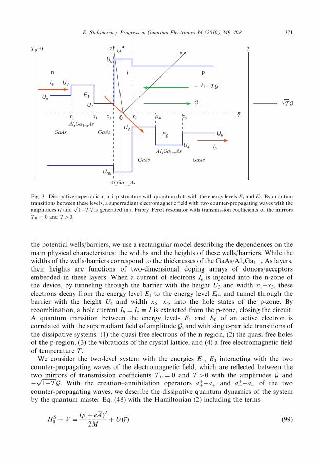
GaAs
Fig. 3. Dissipative superradiant n–i–p structure with quantum dots with the energy levels E1 and E0. By quantum
transitions between these levels, a superradiant electromagnetic field with two counter-propagating waves with the
amplitudes G andffiffiffiffiffiffiffiffiffiffi1�Tp
G is generated in a Fabry–Perot resonator with transmission coefficients of the mirrors
T 0 ¼ 0 and T40.
E. Stefanescu / Progress in Quantum Electronics 34 (2010) 349–408 371
the potential wells/barriers, we use a rectangular model describing the dependences on themain physical characteristics: the widths and the heights of these wells/barriers. While thewidths of the wells/barriers correspond to the thicknesses of the GaAs/AlxGa1�x As layers,their heights are functions of two-dimensional doping arrays of donors/acceptorsembedded in these layers. When a current of electrons Ie is injected into the n-zone ofthe device, by tunneling through the barrier with the height U3 and width x1�x3, theseelectrons decay from the energy level E1 to the energy level E0, and tunnel through thebarrier with the height U4 and width x5�x4, into the hole states of the p-zone. Byrecombination, a hole current Ih ¼ Ie � I is extracted from the p-zone, closing the circuit.A quantum transition between the energy levels E1 and E0 of an active electron iscorrelated with the superradiant field of amplitude G, and with single-particle transitions ofthe dissipative systems: (1) the quasi-free electrons of the n-region, (2) the quasi-free holesof the p-region, (3) the vibrations of the crystal lattice, and (4) a free electromagnetic fieldof temperature T.
We consider the two-level system with the energies E1, E0 interacting with the twocounter-propagating waves of the electromagnetic field, which are reflected between thetwo mirrors of transmission coefficients T 0 ¼ 0 and T40 with the amplitudes G and�
ffiffiffiffiffiffiffiffiffiffi1�Tp
G. With the creation–annihilation operators aþþ�aþ and a�
þ�a� of the two
counter-propagating waves, we describe the dissipative quantum dynamics of the systemby the quantum master Eq. (48) with the Hamiltonian (2) including the terms
HS0 þ V ¼
ð~p þ e~AÞ2
2MþUð~rÞ ð99Þ

E. Stefanescu / Progress in Quantum Electronics 34 (2010) 349–408372
and (49), which depend on the potential Uð~rÞ, the potential vector ~A of the superradiantfield, and the potential of interaction V of an active electron with this field. In aweak-field approximation, when the term in ~A
2can be neglected, we get the interaction
potential (50) as a product of the two operators (51) and (52), for a field propagatingin the x-direction, where ‘oij ¼ ei�ej , a ¼ e2=4pe‘ c � 1=137, l ¼ 2p=k is the radiationwavelength, and V is the quantization volume of the electromagnetic field. We notice thatthe momentum (51) is non-diagonal, while the square of this momentum with thematrix elements
/mj~p2jnS ¼
M2
‘ 2
Xj
ðej�emÞðej�enÞ~rmj~rnj ; m;n;j ¼ 0;1 ð100Þ
is diagonal for a two-level system. Thus, we obtain non-diagonal two-body potentials that,due to the momentum conservation, are proportional to ~p, and diagonal fluctuations ofthese potentials, which are proportional to ~p2.We calculate the decay/excitation rates by using the general expressions (23)–(25) for
non-diagonal matrix elements of the dissipative potential, and the diagonal elements zii byusing the general expression (20). From Eqs. (36) to (37), we notice that these elementsdetermine entirely the dynamics of the system. With the assumption that in a quantizationvolume Vn (Vp), of a conduction region n (p), any electron (hole) is a quasi-free particlewith a kinetic energy Ea, we get the density of states [69]
gðnÞa ðEaÞ ¼ Vn
ffiffiffi2p
M3=2n
p2‘ 3
ffiffiffiffiffiffiEa
p; ð101aÞ
gðpÞa ðEaÞ ¼ Vp
ffiffiffi2p
M3=2p
p2‘ 3
ffiffiffiffiffiffiEa
p; ð101bÞ
where Mn (Mp) is the effective mass. For the two conduction regions n and p, we considerthe non-degenerate case, when the donor and acceptor concentrations ND and NA aresufficiently low to approximate the Fermi–Dirac distributions of electrons and holes withBoltzmann distributions:
f ðnÞa ðEaÞ ¼1
eðUcþEaÞ=T þ 1� e�ðUcþEaÞ=T ; ð102aÞ
f ðpÞa ðEaÞ ¼1
eð�UvþEaÞ=T þ 1� e�ð�UvþEaÞ=T ; ð102bÞ
where Ea is the kinetic energy in the conduction or valence band. Integrating the particlenumbers (102) over the states with the densities (101), we obtain the number of particles inthe quantization volume:Z 1
0
f ðnÞa ðEaÞgðnÞa ðEaÞ dEa ¼ VnND; ð103aÞ
Z 10
f ðpÞa ðEaÞgðpÞa ðEaÞdEa ¼ VpNA; ð103bÞ
where ND is the concentration of donors in the n-region and NA is the concentration ofacceptors in the p-region. With the approximate expressions (102), in Eqs. (103) we get an
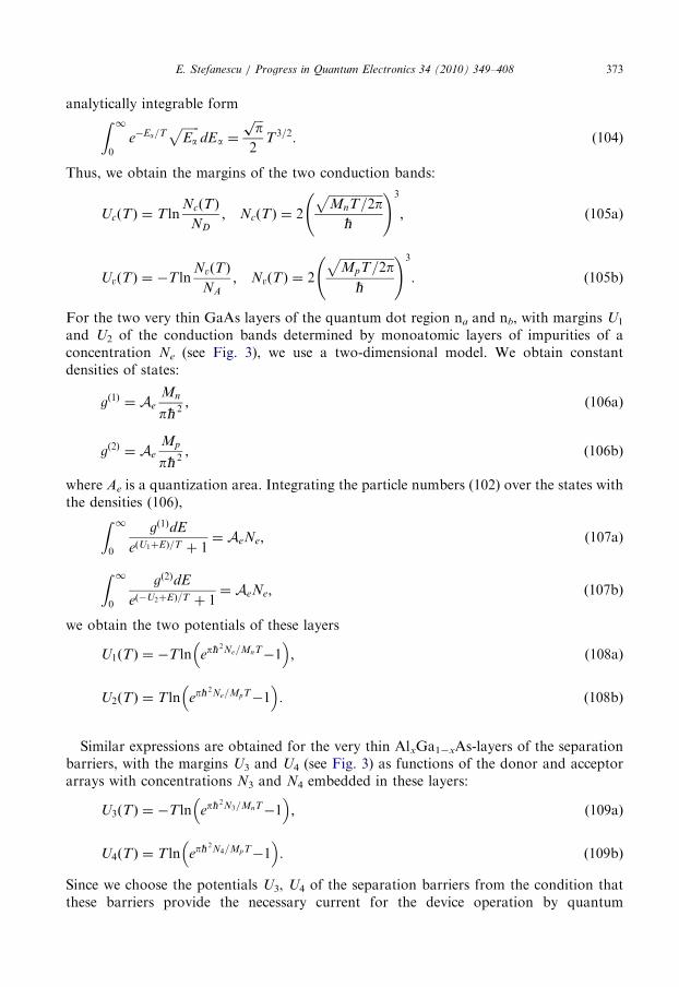
E. Stefanescu / Progress in Quantum Electronics 34 (2010) 349–408 373
analytically integrable formZ 10
e�Ea=TffiffiffiffiffiffiEa
pdEa ¼
ffiffiffipp
2T3=2: ð104Þ
Thus, we obtain the margins of the two conduction bands:
UcðTÞ ¼ T lnNcðTÞ
ND
; NcðTÞ ¼ 2
ffiffiffiffiffiffiffiffiffiffiffiffiffiffiffiffiffiffiMnT=2p
p‘
!3
; ð105aÞ
UvðTÞ ¼ �T lnNvðTÞ
NA
; NvðTÞ ¼ 2
ffiffiffiffiffiffiffiffiffiffiffiffiffiffiffiffiffiffiMpT=2p
p‘
!3
: ð105bÞ
For the two very thin GaAs layers of the quantum dot region na and nb, with margins U1
and U2 of the conduction bands determined by monoatomic layers of impurities of aconcentration Ne (see Fig. 3), we use a two-dimensional model. We obtain constantdensities of states:
gð1Þ ¼ Ae
Mn
p‘ 2; ð106aÞ
gð2Þ ¼ Ae
Mp
p‘ 2; ð106bÞ
where Ae is a quantization area. Integrating the particle numbers (102) over the states withthe densities (106),Z 1
0
gð1ÞdE
eðU1þEÞ=T þ 1¼ AeNe; ð107aÞ
Z 10
gð2ÞdE
eð�U2þEÞ=T þ 1¼ AeNe; ð107bÞ
we obtain the two potentials of these layers
U1ðTÞ ¼ �T ln ep‘2Ne=MnT�1
�; ð108aÞ
U2ðTÞ ¼ T ln ep‘2Ne=MpT�1
�: ð108bÞ
Similar expressions are obtained for the very thin AlxGa1�xAs-layers of the separationbarriers, with the margins U3 and U4 (see Fig. 3) as functions of the donor and acceptorarrays with concentrations N3 and N4 embedded in these layers:
U3ðTÞ ¼ �T ln ep‘2N3=MnT�1
�; ð109aÞ
U4ðTÞ ¼ T ln ep‘2N4=MpT�1
�: ð109bÞ
Since we choose the potentials U3, U4 of the separation barriers from the condition thatthese barriers provide the necessary current for the device operation by quantum

E. Stefanescu / Progress in Quantum Electronics 34 (2010) 349–408374
tunneling, we use the inverse relations to calculate the corresponding concentrations:
N3 ¼MnT
p‘ 2lnð1þ e�U3=T Þ; ð110aÞ
N4 ¼MpT
p‘ 2lnð1þ eU4=T Þ: ð110bÞ
From (23) and (20) with the densities of states (101), and the occupation probabilities ofthese state (102), we calculate the dissipation coefficients of the coupling to an n-clusterwith a quantization volume Vn
lðVnÞ
01 ð~R0Þ ¼
M3=2n
ffiffiffiffiffiffiffiffi2e10p
p‘ 4½e�ðUcþe10Þ=T þ 1�
j/a0jV ðnÞð~R0Þjb1Sj2Vn; ð111aÞ
lðVnÞ
10 ð~R0Þ ¼
M3=2n
ffiffiffiffiffiffiffiffi2e10p
p‘ 4½eðUcþe10Þ=T þ 1�
j/a0jV ðnÞð~R0Þjb1Sj2Vn; ð111bÞ
½zðVnÞ
ii ð~R0Þ�
2 ¼M
3=2n T3=2
pffiffiffiffiffiffi2pp
‘ 5e�Uc=T/ij½V ðnÞð~R0Þ�
2jiSVn; i ¼ 0;1; ð111cÞ
and to a p-cluster with a quantization volume Vp
lðVpÞ
01 ð~R0Þ ¼
M3=2p
ffiffiffiffiffiffiffiffi2e10p
p‘ 4½e�ð�Uvþe10Þ=T þ 1�
j/a0jV ðpÞð~R0Þjb1Sj2Vp; ð112aÞ
lðVpÞ
10 ð~R0Þ ¼
M3=2p
ffiffiffiffiffiffiffiffi2e10p
p‘ 4½eð�Uvþe10Þ=T þ 1�
j/a0jV ðpÞð~R0Þjb1Sj2Vp; ð112bÞ
½zðVpÞ
ii ð~R0Þ�
2 ¼M
3=2p T3=2
pffiffiffiffiffiffi2pp
‘ 5eUv=T/ij½V ðpÞð~R0Þ�
2jiSVp; i ¼ 0;1; ð112cÞ
where e10 ¼ E1�E0 � ‘o0 is the transition energy of the system, ~R0 is the coordinate of adissipative cluster with the volume Vn (Vp), and V ðnÞ (~R0) ðV
ðpÞ ð~R0ÞÞ is the two-bodypotential of interaction with an electron of the n-conduction region (a hole of thep-conduction region) (Fig. 4). In (111a), (111b), (112a), and (112b), the initial, lower quasi-free state jbS corresponds to an energy that we approximate as Eb ¼ T=2, while thefinal, higher quasi-free state jaS corresponds to the excitation energy Ea ¼ Eb þ e10. In(111c) and (112c) we neglected the dimensions of a dissipative cluster in comparisonwith the distance ~R0, which means /aij½V ðnÞð~R0Þ�
2jaiS ¼ /ajaS/ij½V ðnÞð~R0Þ�2jiS ¼
/ij½V ðnÞð~R0Þ�2jiS, and a similar relation for V(p).
We take into account that the dissipation coefficients lij represent transition
probabilities due to the coupling to the environment particles, and zii fluctuations ofthe self-consistent field of these particles. That means that the total probability of atransition due to the coupling to the environment is a sum of transitions probabilitiesdue to the couplings to the components of this environment. At the same time, a

n-region-quasi-free electrons
p-region-quasi-free holes
quantumdots
R0
kP
kFEF
α0|V (n) (R0)|β1 α0|V (p) (R0)|β1
Eβ
Eα
Eα
Eβ
E1
E0
n p
−Lp / 2 Lp / 20−Lp / 2 Lp / 20
n p
Fig. 4. Dissipative couplings of an active electron to the environment. A decay j1S-j0S of the electron of a
quantum dot is correlated with: (1) a transition jbS-jaS of a quasi-free electron in a quantization volume Vn, (2)
a transition jbS-jaS of a quasi-free hole in a quantization volume Vp, (3) a phonon creation with a wave vector~kP, and (4) a photon creation with a wave vector ~kFEF .
E. Stefanescu / Progress in Quantum Electronics 34 (2010) 349–408 375
fluctuation of the total environment is the quadratic sum of the fluctuations ofthe components of this environment. Thus, we take the dissipative coefficients of thecoupling to the entire system of the conduction electrons and holes as integrals of the
components (111) and (112) with the quantization volumes as differentials d3~R0 ¼ Vn, Vp.
We obtain
lE01 ¼ lðnÞ01 þ lðpÞ01 ; ð113aÞ
lE10 ¼ lðnÞ10 þ lðpÞ10 ; ð113bÞ
z2ii ¼ ½zðnÞii �
2 þ ½zðpÞii �2; i ¼ 0;1; ð113cÞ
with the components
lðnÞ01 ¼M
3=2n
ffiffiffiffiffiffiffiffi2e10p
p‘ 4½e�ðUcþe10Þ=T þ 1�
ZðnÞ
j/a0jV ðnÞð~R0Þjb1Sj2 d3~R0; ð114aÞ
lðnÞ10 ¼M
3=2n
ffiffiffiffiffiffiffiffi2e10p
p‘ 4½eðUcþe10Þ=T þ 1�
ZðnÞ
j/a0jV ðnÞð~R0Þjb1Sj2 d3~R0; ð114bÞ
½zðnÞii �2 ¼
M3=2n T3=2
pffiffiffiffiffiffi2pp
‘ 5e�Uc=T
ZðnÞ
/ij½V ðnÞð~R0Þ�2jiSSnð~R0Þ d
3~R0; i ¼ 0;1 ð114cÞ

E. Stefanescu / Progress in Quantum Electronics 34 (2010) 349–408376
for the coupling to the conduction electrons in the n-zone, and
lðpÞ01 ¼M
3=2p
ffiffiffiffiffiffiffiffi2e10p
p‘ 4½e�ð�Uvþe10Þ=T þ 1�
ZðpÞ
j/a0jV ðpÞð~R0Þjb1Sj2 d3~R0 ð115aÞ
lðpÞ10 ¼M
3=2p
ffiffiffiffiffiffiffiffi2e10p
p‘ 4½eð�Uvþe10Þ=T þ 1�
ZðpÞ
j/a0jV ðpÞð~R0Þjb1Sj2 d3~R0 ð115bÞ
½zðpÞii �2 ¼
M3=2p T3=2
pffiffiffiffiffiffi2pp
‘ 5eUv=T
ZðpÞ
/ij½V ðpÞð~R0Þ�2jiSSpð~R0Þ d
3~R0; i ¼ 0;1 ð115cÞ
for the coupling to the holes in the p-zone. In (114c) and (115c) we introduced the
screening functions Snð~R0Þ and Spð~R0Þ, which take into account that a field fluctuation
generated inside the n (p) layer is mostly absorbed in its propagation toward the outside.To calculate the matrix elements in these expressions, in the next section we derive thewave-functions.
7. Wave functions and dipole moments of the system
A wave-function c1ðxÞ (c0ðxÞ), with the energy E1 (E0), is considered extended only inthe barriers bounding the corresponding potential well, i.e. the tails of the wave-functionbeyond these barriers are neglected. Thus, we get
c1ðxÞ ¼ A1 cos k1ðx0�xÞ�arctana1k1
� �; x1rxrx0; ð116aÞ
c1ðxÞ ¼ A1
ffiffiffiffiffiffiffiffiffiffiffiffiffiffiffiE1�U1
U0�U1
re�a1ðx�x0Þ; x0rxrx2; ð116bÞ
c1ðxÞ ¼ A1
ffiffiffiffiffiffiffiffiffiffiffiffiffiffiffiE1�U1
U3�U1
re�a3ðx1�xÞ; x3rxrx1 ð116cÞ
for the firs well, and
c0ðxÞ ¼ A0 cos k0ðx�x2Þ�arctana0k0
� �; x2rxrx4; ð117aÞ
c0ðxÞ ¼ A0
ffiffiffiffiffiffiffiffiffiffiffiffiffiffiffiffiffiU2�E0
U2�U00
re�a0ðx2�xÞ; x0rxrx2; ð117bÞ
c0ðxÞ ¼ A0
ffiffiffiffiffiffiffiffiffiffiffiffiffiffiffiU2�E0
U2�U4
re�a4ðx�x4Þ; x4rxrx5 ð117cÞ
for the second well. These wave-functions depend on the wave-vectors in the two wells
k1 ¼1
‘
ffiffiffiffiffiffiffiffiffiffiffiffiffiffiffiffiffiffiffiffiffiffiffiffiffiffiffi2MnðE1�U1Þ
p; ð118aÞ
k0 ¼1
‘
ffiffiffiffiffiffiffiffiffiffiffiffiffiffiffiffiffiffiffiffiffiffiffiffiffiffiffi2MpðU2�E0Þ
p; ð118bÞ

E. Stefanescu / Progress in Quantum Electronics 34 (2010) 349–408 377
on the attenuation coefficients in the corresponding barriers
a1 ¼1
‘
ffiffiffiffiffiffiffiffiffiffiffiffiffiffiffiffiffiffiffiffiffiffiffiffiffiffiffi2MnðU0�E1Þ
p; ð119aÞ
a0 ¼1
‘
ffiffiffiffiffiffiffiffiffiffiffiffiffiffiffiffiffiffiffiffiffiffiffiffiffiffiffiffiffi2MpðE0�U00Þ
p; ð119bÞ
a3 ¼1
‘
ffiffiffiffiffiffiffiffiffiffiffiffiffiffiffiffiffiffiffiffiffiffiffiffiffiffiffi2MnðU3�E1Þ
p; ð119cÞ
a4 ¼1
‘
ffiffiffiffiffiffiffiffiffiffiffiffiffiffiffiffiffiffiffiffiffiffiffiffiffiffiffi2MpðE0�U4Þ
p; ð119dÞ
and on the normalization factors
A1 ¼ffiffiffi2p
x0�x1 þ‘ffiffiffiffiffiffiffiffiffiffi2Mn
p1ffiffiffiffiffiffiffiffiffiffiffiffiffiffiffi
U0�E1
p þ1ffiffiffiffiffiffiffiffiffiffiffiffiffiffiffi
U3�E1
p
� �� ��1=2; ð120aÞ
A0 ¼ffiffiffi2p
x4�x2 þ‘ffiffiffiffiffiffiffiffiffiffi2Mp
p 1ffiffiffiffiffiffiffiffiffiffiffiffiffiffiffiffiffiE0�U00
p þ1ffiffiffiffiffiffiffiffiffiffiffiffiffiffiffi
E0�U4
p
� �" #�1=2: ð120bÞ
We obtain the energy levels E1 and E0 as solutions of the equations:
E1�U1 ¼‘ 2
2Mnðx0�x1Þ2
arctan
ffiffiffiffiffiffiffiffiffiffiffiffiffiffiffiU0�E1
E1�U1
rþ arctan
ffiffiffiffiffiffiffiffiffiffiffiffiffiffiffiU3�E1
E1�U1
r� �2
; ð121aÞ
U2�E0 ¼‘ 2
2Mpðx4�x2Þ2
arctan
ffiffiffiffiffiffiffiffiffiffiffiffiffiffiffiffiffiE0�U00
U2�E0
rþ arctan
ffiffiffiffiffiffiffiffiffiffiffiffiffiffiffiE0�U4
U2�E0
r� �2
: ð121bÞ
Thus, the wave functions c1ðxÞ and c0ðxÞ are defined in the domains (x3,x2) and (x0,x5),respectively, their tails outside these domains being neglected. Due to the overlap of thesewave-functions in the domain (x0,x2) of the i-layer, a tunneling through this layer takesplace. The overlap function depends on the wave numbers (118), the attenuationcoefficients (119), and the normalization factors (120), as functions of the energy levelsgiven by (121). This tunneling is not a simple quantum process, due only to an overlap, buta complex process, including other processes of superradiance and dissipation in thesemiconductor structure and the Fabry–Perot cavity.
Two superradiant modes are possible: (1) a longitudinal mode, propagating in thetunneling direction, i.e. perpendicularly to the quantum dot layers, and (2) a transversalmode, propagating perpendicularly to the tunneling direction, i.e. in the plan of thequantum dot layers (Fig. 1). At this point, we have to take into account that while in thex-direction an electron is confined in the potential represented in Fig. 3, in the y, z-directionsthe electron moves quasi-freely with wave-numbers knðTÞ ¼ ð1=‘ Þ
ffiffiffiffiffiffiffiffiffiffiffiffiffiffiffiffiffiffiffiffiffiffi2MnEnðTÞ
p�
ð1=‘ ÞffiffiffiffiffiffiffiffiffiffiffiMnTp
in the n-zone and kpðTÞ ¼ ð1=‘ Þffiffiffiffiffiffiffiffiffiffiffiffiffiffiffiffiffiffiffiffiffiffiffiffiffi�2MpEpðTÞ
p� ð1=‘ Þ
ffiffiffiffiffiffiffiffiffiffiffiMpT
pin the p-zone,
corresponding to temperature T of the system (Fig. 5). Thus, the total wave-functions of thesystem are of the form
C1ðx;y;zÞ ¼ c1ðxÞf1ðyÞw1ðzÞ; ð122aÞ
C0ðx;y;zÞ ¼ c0ðxÞf0ðyÞw0ðzÞ: ð122bÞ

x
y
z
1/√N e
1/√N
e
Electron Hole
kn
kp
na pai
E1 E0
Fig. 5. Quantum dot with an electron confined in the x-direction by the n-type active layer na, and a hole confined
in this direction by the p-type active layer pa. While an electron decays from the higher energy E1 in the na-layer to
the lower energy E0 in the pa-layer, recombining with a hole, these particles move quasi-freely in the plane (y, z) of
the two layers, with the wave vectors ~knðTÞ, ~kpðTÞ corresponding to temperature T of these layers.
E. Stefanescu / Progress in Quantum Electronics 34 (2010) 349–408378
With the overlap functions
cðxÞ01 ¼
Z x2
x0
c0ðxÞc1ðxÞ dx
��������; ð123aÞ
cðyÞ01 ¼
Z y2
y1
f0ðyÞf1ðyÞ dy
��������; ð123bÞ
cðzÞ01 ¼
Z z2
z1
w0ðzÞw1ðzÞ dz
��������; ð123cÞ
and the dipole moments
x01 ¼
Z x2
x0
c0ðxÞxc1ðxÞ dx
��������; ð124aÞ
y01 ¼
Z y2
y1
f0ðyÞyf1ðyÞ dy
��������; ð124bÞ
z01 ¼
Z z2
z1
w0ðzÞzw1ðzÞ dz
��������; ð124cÞ
we obtain the total dipole moments corresponding to a transition through the i-layer:
xðCÞ01 ¼ x01c
ðyÞ01 cðzÞ01 ; ð125aÞ
yðCÞ01 ¼ c
ðxÞ01 y01c
ðzÞ01 ; ð125bÞ
zðCÞ01 ¼ c
ðxÞ01 cðyÞ01 z01: ð125cÞ

E. Stefanescu / Progress in Quantum Electronics 34 (2010) 349–408 379
Using (116)–(120), we obtain the overlap functions
cðxÞ01 ¼
A1A0
a0�a1
ffiffiffiffiffiffiffiffiffiffiffiffiffiffiffiffiffiffiffiffiffiffiffiffiffiffiffiffiffiffiffiffiffiffiffiffiffiffiffiðE1�U1ÞðU2�E0Þ
ðU0�U1ÞðU2�U00Þ
sðe�a1ðx2�x0Þ�e�a0ðx2�x0ÞÞ; ð126aÞ
cðyÞ01 ¼ c
ðzÞ01 ¼ 1; ð126bÞ
corresponding to transitions with momentum conservation kn ¼ kp � k, which is observedin a weak-field approximation of the superradiant tunneling. In such a transition, the totalenergy, including the crystal lattice motion that is responsible for the effective mass variationfrom Mn to Mp, is conserved, while, due this mass variation, the particle energy is notconserved. In this case, a part of the initial energy ‘ 2k2=ð2MnÞ ¼ T is taken by the crystallattice, while the final energy of the particle takes a smaller value ‘ 2k2=ð2MpÞ ¼ ðMn=MpÞT .Only by a subsequent relaxation process, the particle takes its thermal value‘ 2k2
pT=ð2MpÞ ¼ T . We notice that the overlap function in the x-direction has a simpledependence on the ratios of the two zero-point vibration energies to the correspondingbarrier heights (E1�U1)/(U0�U1) and (U2�E0)/(U2�U00), and on the i-layer thicknessx2�x0. For transitions between the states (116) and (117) in the x-direction, and thermalstates of the form
f1ðyÞ ¼ffiffiffi2pA�1=4 cos½knðTÞy�; ð127aÞ
f0ðyÞ ¼ �ffiffiffi2pA�1=4 sin½kpðTÞy� ð127bÞ
in a quantization area A, we obtain the dipole moments
y01 ¼ z01 ¼‘
2ffiffiffiffiffiffiffiffiffiffiffiffiffiffiffi2MnEn
p ‘
2ffiffiffiffiffiffiffiffiffiffiffiMnTp ; ð128aÞ
y10 ¼ z10 ¼‘
2ffiffiffiffiffiffiffiffiffiffiffiffiffiffiffiffiffiffi�2MpEp
p ‘
2ffiffiffiffiffiffiffiffiffiffiffiMpT
p : ð128bÞ
With these expressions, we get the total dipole moments
xðCÞ01 ¼ c
ðxÞ01
x2�x0
2�
1
a0�a1
� �; ð129aÞ
yðCÞ01 ¼ z
ðCÞ01 ¼ c
ðxÞ01
‘
2ffiffiffiffiffiffiffiffiffiffiffiffiffiffiffi2MnEn
p cðxÞ01
‘
2ffiffiffiffiffiffiffiffiffiffiffiMnTp ; ð129bÞ
yðCÞ10 ¼ z
ðCÞ10 ¼ c
ðxÞ01
‘
2ffiffiffiffiffiffiffiffiffiffiffiffiffiffiffiffiffiffi�2MpEp
p cðxÞ01
‘
2ffiffiffiffiffiffiffiffiffiffiffiMpT
p : ð129cÞ
We notice that the longitudinal x-dipole moment is given by the half-thickness of thei-zone x2�x0, diminished with the attenuation width 1=ða0�a1Þ, and multiplied by theoverlap function. The transversal y- and z-dipole moments are given by the half-widthsdefined as ‘ c=
ffiffiffiffiffiffiffiffiffiffiffiffiffiffiffiMnc2T
pand ‘ c=
ffiffiffiffiffiffiffiffiffiffiffiffiffiffiffiMpc2T
p, respectively, also multiplied by the overlap
function. Due to the variation of the effective mass, the transversal dipole moments of thetransition from the n-region to the p-region are higher than those of the inverse transitions,from the p-region to the n-region. This is because at the same energy, a lighter particle has alarger wavelength.
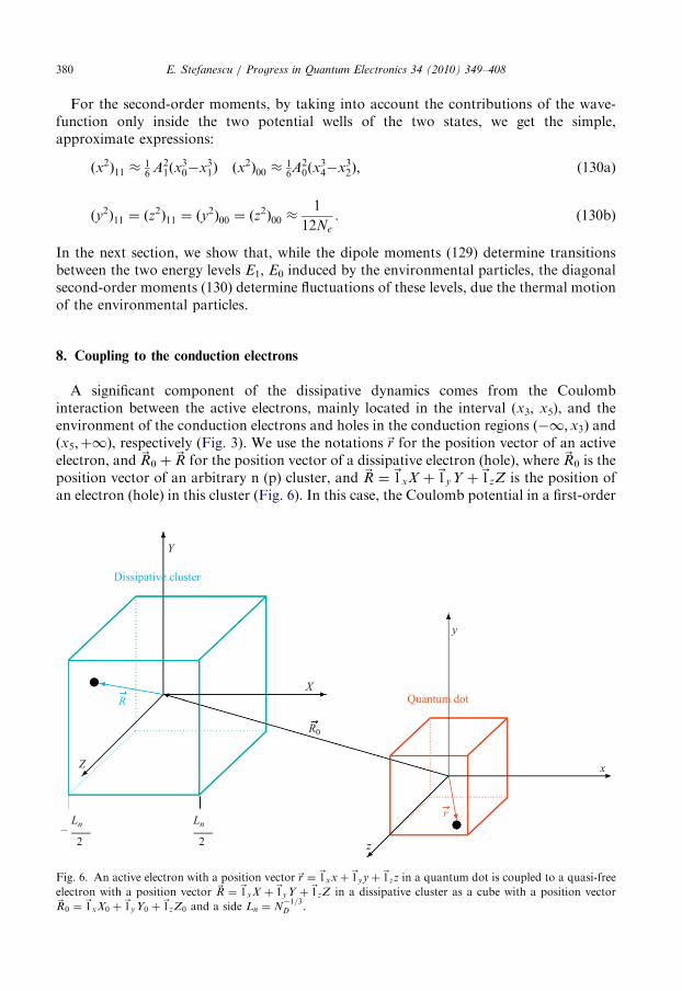
E. Stefanescu / Progress in Quantum Electronics 34 (2010) 349–408380
For the second-order moments, by taking into account the contributions of the wave-function only inside the two potential wells of the two states, we get the simple,approximate expressions:
ðx2Þ11 �16
A21ðx
30�x3
1Þ ðx2Þ00 �
16A2
0ðx34�x3
2Þ; ð130aÞ
ðy2Þ11 ¼ ðz2Þ11 ¼ ðy
2Þ00 ¼ ðz2Þ00 �
1
12Ne
: ð130bÞ
In the next section, we show that, while the dipole moments (129) determine transitionsbetween the two energy levels E1, E0 induced by the environmental particles, the diagonalsecond-order moments (130) determine fluctuations of these levels, due the thermal motionof the environmental particles.
8. Coupling to the conduction electrons
A significant component of the dissipative dynamics comes from the Coulombinteraction between the active electrons, mainly located in the interval (x3, x5), and theenvironment of the conduction electrons and holes in the conduction regions ð�1;x3Þ andðx5;þ1Þ, respectively (Fig. 3). We use the notations~r for the position vector of an activeelectron, and ~R0 þ ~R for the position vector of a dissipative electron (hole), where ~R0 is theposition vector of an arbitrary n (p) cluster, and ~R ¼ ~1xX þ~1yY þ~1zZ is the position ofan electron (hole) in this cluster (Fig. 6). In this case, the Coulomb potential in a first-order
Quantum dot
Dissipative cluster
−Ln
2
Ln
2
x
y
z
X
Y
Z
R0
r
R
Fig. 6. An active electron with a position vector~r ¼ ~1xxþ~1yyþ~1zz in a quantum dot is coupled to a quasi-free
electron with a position vector ~R ¼ ~1xX þ~1yY þ~1zZ in a dissipative cluster as a cube with a position vector~R0 ¼ ~1xX0 þ~1yY0 þ~1zZ0 and a side Ln ¼ N
�1=3D .

E. Stefanescu / Progress in Quantum Electronics 34 (2010) 349–408 381
approximation of the two-body term ~R~r ¼ Xxþ Yyþ Zz is
VCð~R;~rÞ ¼a‘ c
j~R0 þ ~R�~rj¼
a‘ c
j~R0j
ffiffiffiffiffiffiffiffiffiffiffiffiffiffiffiffiffiffiffiffiffiffiffiffiffiffiffiffiffiffiffiffiffiffiffiffiffiffiffiffiffiffiffiffiffiffiffiffiffiffiffiffiffiffiffiffiffiffiffiffiffiffiffiffi1þ
2~R0ð~R�~rÞ
j~R0j2þ~R
2�2~R~r þ~r2
j~R0j2
s
�a‘ c
j~R0j1þ
Xxþ Yyþ Zz
~R2
0
!: ð131Þ
From this expression, only the second term, bilinear in the coordinates of an activeelectron and of an electron (hole) of the environment, yields contributions in the transitionmatrix elements of the decay/excitation rates (23):
VF ð~R;~rÞ ¼a‘ c
j~R0j3ðXxþ Yyþ ZzÞ: ð132Þ
To obtain the dissipative coefficients for the coupling to the entire system of conductionelectrons and holes, we consider (114a)–(114b) and (115a)–(115b) with potentials of theform (132), V ðnÞ ¼ VF ;V ðpÞ ¼ �V F , and integrate with ~R0 over the n- and p-regions from aradius equal to the distance to the nearest cluster, RD=ND
�1/3/2-x3 for the n-region,and RA=NA
�1/3/2þx5 for the p-region, up to infinity (Fig. 7).With the notations
~rðCÞ01 ¼~1xx
ðCÞ01 þ
~1yyðCÞ01 þ
~1zzðCÞ01 ; ð133aÞ
~RðnÞ
ab ¼~1xX
ðnÞab þ
~1yYðnÞab þ
~1zZðnÞab ; ð133bÞ
~RðpÞ
ab ¼~1xX
ðpÞab þ
~1yYðpÞab þ
~1zZðpÞab ; ð133cÞ
we get the dissipative coefficients:
lðnÞ01 ¼a2c2ð2MnÞ
3=2e1=210
3‘ 2 N�1=3D
2�x3
!3�ð~RðnÞ
ab~rðCÞ01 Þð
~RðnÞ
ba~rðCÞ10 Þ
e�ðUcþe10Þ=T þ 1; ð134aÞ
lðnÞ10 ¼a2c2ð2MnÞ
3=2e1=210
3‘ 2 N-1=3D
2-x3
!3�ð~RðnÞ
ab~rðCÞ01 Þð
~RðnÞ
ba~rðCÞ10 Þ
eðUcþe10Þ=T þ 1ð134bÞ
for the coupling to the sea of electrons in the n-region, and
lðpÞ01 ¼a2c2ð2MpÞ
3=2e1=210
3‘ 2 N�1=3A
2þ x5
!3�ð~RðpÞ
ab~rðCÞ01 Þð
~RðpÞ
ba~rðCÞ10 Þ
e�ð�Uvþe10Þ=T þ 1; ð135aÞ

Quantum dot
n-dissipative clusters p-dissipative clusters
0x3−RD x5 RA
NA−1/3ND
−1/3
R0
Fig. 7. The electron of a quantum dot is coupled to the quasi-free electrons of the n-dissipative clusters (n-region)
and quasi-free holes of the p-dissipative clusters (p-region).
E. Stefanescu / Progress in Quantum Electronics 34 (2010) 349–408382
lðpÞ10 ¼a2c2ð2MpÞ
3=2e1=210
3‘ 2 N-1=3A
2þ x5
!3�ð~RðpÞ
ab~rðCÞ01 Þð
~RðpÞ
ba~rðCÞ10 Þ
eð-Uvþe10Þ=T þ 1ð135bÞ
for the coupling to the sea of holes in the p-region, where ND�1/3/2 and NA
�1/3/2 are thehalf-sides of the dissipative clusters of the n-region with the donor concentration ND andof the p-region with the acceptor concentration NA, respectively (see Fig. 7). Accordingto (129), and the discussion that follows regarding the effects of the different effectivemasses Mn and Mp of the particles in thermal motion, in (134) and (135) we have takeninto account different matrix elements for the transitions jb1S-ja0S and for thereverse ones. These expressions describe single-particle transitions of the systembetween the two states C1ðx; y; zÞ and C0ðx; y; zÞ, with dipole moments x
ðCÞ01 ; y
ðCÞ01 ; z
ðCÞ01 ,
correlated to single-particle transitions of an environmental cluster between two quasi-freestates
Cað~RÞ ¼ caðX ÞfaðY ÞwaðZÞ; ð136aÞ
Cbð~RÞ ¼ cbðX ÞfbðY ÞwbðZÞ; ð136bÞ

E. Stefanescu / Progress in Quantum Electronics 34 (2010) 349–408 383
with the dipole moments
Xab ¼
Z X2
X1
caðX ÞXcbðX Þ dX ; ð137aÞ
Yab ¼
Z Y2
Y1
faðY ÞYfbðY Þ dY ; ð137bÞ
Zab ¼
Z Z2
Z1
waðZÞZwbðZÞ dZ: ð137cÞ
That means that, while an active electron decays from C1ðx; y; zÞ to C0ðx; y; zÞ with acertain probability rate lðnÞ01 ðl
ðpÞ01 Þ, an electron (hole) in a n (p) dissipative cluster is excited
from a state CbðX ;Y ;ZÞ to a state CaðX ;Y ;ZÞ. We consider quasi-free states of differentparities in a quantization volume Vn ¼ L3
n:
cðnÞa ðX Þ ¼ �ffiffiffi2pV�1=6n sinðkðnÞa X Þ; kðnÞa ¼
1
‘
ffiffiffiffiffiffiffiffiffiffiffiffiffiffiffi2MnEa
p; ð138aÞ
cðnÞb ðX Þ ¼ffiffiffi2pV�1=6n cosðk
ðnÞb X Þ; k
ðnÞb ¼
1
‘
ffiffiffiffiffiffiffiffiffiffiffiffiffiffiffi2MnEb
pð138bÞ
for an initial energy Eb corresponding to the thermal motion, and the final energy Ea ¼
Eb þ e10 for an excitation with e10. With these states, we derive the dipole moments
XðnÞab � �2V
�1=3n
Z Ln=2
�Ln=2sinðkðnÞa X ÞXcosðk
ðnÞb X Þ dX
¼ L�1n Xcos½ðkðnÞa þ k
ðnÞb ÞX �
kðnÞa þ k
ðnÞb
þcos½ðkðnÞa �k
ðnÞb ÞX �
kðnÞa �k
ðnÞb
( )�����Ln=2
�Ln=2
�L�1n
Z Ln=2
�Ln=2
cos½ðkðnÞa þ kðnÞb ÞX �
kðnÞa þ k
ðnÞb
þcos½ðkðnÞa �k
ðnÞb ÞX �
kðnÞa �k
ðnÞb
( )dX : ð139Þ
We notice that the second term of this expression is an integral of a rapidlyoscillating function that can be neglected. This integral vanishes exactly with theboundary conditions
cos ðkðnÞa þ kðnÞb Þ
Ln
2
� �¼ 1; cos ðkðnÞa þ k
ðnÞb Þ�Ln
2
� �¼ 1; ð140aÞ
cos ðkðnÞa �kðnÞb Þ
Ln
2
� �¼ 1; cos ðkðnÞa �k
ðnÞb Þ�Ln
2
� �¼ 1 ð140bÞ
in the quantization volume Vn, while the first term yields
XðnÞab ¼
2kðnÞa
ðkðnÞa Þ
2�ðk
ðnÞb Þ
2: ð141Þ

E. Stefanescu / Progress in Quantum Electronics 34 (2010) 349–408384
With the initial and the final energies Eb ¼ T=2;Ea ¼ Eb þ e10 in the wave-numbers (138),we obtain the dipole moments for the n-zone
XðnÞab ¼ Y
ðnÞab ¼ Z
ðnÞab ¼
‘e10
ffiffiffiffiffiffiffiffiffiffiffiffiffiffiffiffiffiffi2e10 þ T
Mn
s; ð142Þ
and similar expressions for the p-zone:
XðpÞab ¼ Y
ðpÞab ¼ Z
ðpÞab ¼
‘e10
ffiffiffiffiffiffiffiffiffiffiffiffiffiffiffiffiffiffi2e10 þ T
Mp
s: ð143Þ
With the dipole moments (129) of the system and the dipole moments (142) and (143) ofthe conduction electrons and holes, the dissipative coefficients (134) and (135) take theexplicit form:
lðnÞ01 ¼4a2c2
ffiffiffiffiffiffiffiffiffiffi2Mn
pe10 þ
T
2
� �jcðxÞ01 j
2m201
3N�1=3D
2�x3
!3
e3=210 ðe�ðUcþe10Þ=T þ 1Þ
; ð144aÞ
lðnÞ10 ¼4a2c2
ffiffiffiffiffiffiffiffiffiffi2Mn
pe10 þ
T
2
� �jcðxÞ01 j
2m201
3N
-1=3D
2-x3
!3
e3=210 ðeðUcþe10Þ=T þ 1Þ
; ð144bÞ
lðpÞ01 ¼4a2c2
ffiffiffiffiffiffiffiffiffiffi2Mp
pe10 þ
T
2
� �jcðxÞ01 j
2m201
3N�1=3A
2þ x5
!3
e3=210 ðe�ð�Uvþe10Þ=T þ 1Þ
; ð144cÞ
lðpÞ10 ¼4a2c2
ffiffiffiffiffiffiffiffiffiffi2Mp
pe10 þ
T
2
� �jcðxÞ01 j
2m201
3N
-1=3A
2þ x5
!3
e3=210 ðeð-Uvþe10Þ=T þ 1Þ
; ð144dÞ
where
m201 ¼x2�x0
2�
1
a0�a1þ
‘ffiffiffiffiffiffiffiffiffiffiffiMnTp
� �x2�x0
2�
1
a0�a1þ
‘ffiffiffiffiffiffiffiffiffiffiffiMpT
p !
: ð145Þ
The dissipation coefficients of the coupling to the conduction electrons (holes) get largerwith the overlap function c01
(x), and smaller with the distance �x3 (x5) of separation fromthe conduction region. With these coefficients, from (113a) to (113b) we obtain the termslE01; l
E10 of the total decay rates that, according to the general Eqs. (22) applied to our
system, include terms for the couplings to the crystal lattice vibrations lP01, l
P10, and to the

Fluctuations of theself-consistent field
(Cn) (Cp)x
−RD RA0
x0 + x12
x2 + x42
ND−1/3
Fig. 8. Quantum dot in the self-consistent field fluctuations of the quasi-free electrons in the n-region and the
quasi-free holes in the p-region.
E. Stefanescu / Progress in Quantum Electronics 34 (2010) 349–408 385
free electromagnetic field g01, g10:
l01 ¼ lE01 þ lP
01 þ g01; ð146aÞ
l10 ¼ lE10 þ lP
10 þ g10: ð146bÞ
The electric decay/excitation processes, between the two quantum states j1S and j0S, ofthe coupling to the conduction electrons and holes, enter in competition with the processesof phonon creation/annihilation of the coupling to the crystal lattice, and with thesuperradiant processes. From (144), we notice that, for rather short separation distances�x3, x5, as is the case of a conventional light-emitting or laser diode, where the activetransitions are between conduction electrons and holes, the electric decay/excitation ratescan take very large values.
With (138), by neglecting the rapidly varying terms under the integrals of the second-order moments, we get
ðX 2Þn ¼ ðY2Þn ¼ ðZ
2Þn ¼ 2V�1=3n
Z Ln=2
�Ln=2X 2 cos2ðkðnÞa X Þ dX ¼
1
12N�2=3D ; ð147aÞ
ðX 2Þp ¼ ðY2Þp ¼ ðZ
2Þp ¼ 2V�1=3p
Z Lp=2
�Lp=2X 2 cos2ðkðpÞa X Þ dX ¼
1
12N�2=3A : ð147bÞ
We calculate the field fluctuations (114c) and (115c) considering that, due the planegeometry, the field fluctuations generated inside a conducting layer are emittedperpendicularly to this layer. We take into account this effect integrating not in thewhole n (p) region, but only in the cylinder Cn (Cp) of the neighboring clusters with anarea of the basis 1/Ne corresponding to the quantum dot area in the plane (y,z),and extended in the n (p) region from the nearest cluster up to infinity (Fig. 8). Due to thevery strong decrease with the distance j~R0j of the square of the potential (132), with power6 of this distance, in the integrals (114c) and (115c) we neglect the screening effect, i.e. we
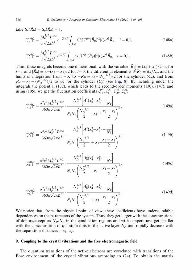
E. Stefanescu / Progress in Quantum Electronics 34 (2010) 349–408386
take Snð~R0Þ ¼ Spð~R0Þ ¼ 1:
½zðnÞii �2 ¼
M3=2n T3=2
pffiffiffiffiffiffi2pp
‘ 5e�Uc=T
ZðCnÞ
/ij½V ðnÞð~R0Þ�2jiSd3~R0; i ¼ 0;1; ð148aÞ
½zðpÞii �2 ¼
M3=2p T3=2
pffiffiffiffiffiffi2pp
‘ 5eUv=T
ZðCpÞ
/ij½V ðpÞð~R0Þ�2jiSd3~R0; i ¼ 0;1: ð148bÞ
Thus, these integrals become one-dimensional, with the variable j~R0j ¼ ðx0 þ x1Þ=2�x fori=1 and j~R0j ¼ x�ðx2 þ x4Þ=2 for i=0, the differential element is d3~R0 ¼ dx=Ne, and thelimits of integration from �1 to �RD ¼ x3�ðN
�1=3D Þ=2 for the cylinder (Cn), and from
RA ¼ x5 þ ðN�1=3A Þ=2 to 1 for the cylinder (Cp) (see Fig. 8). By including under the
integrals the potential (132), which leads to the second-order moments (130), (147), andusing (105), we get the fluctuation coefficients zðnÞ11 , z
ðpÞ11 , z
ðnÞ00 , z
ðpÞ00 :
½zðnÞ11 �2 ¼
a2c2M3=2n T3=2
360pffiffiffiffiffiffi2pp
‘ 3�
N1=3D A2
1ðx30�x3
1Þ þ1
Ne
� �
NeNc
N�1=3D
2�x3 þ
x0 þ x1
2
!5; ð149aÞ
½zðpÞ11 �2 ¼
a2c2M3=2p T3=2
360pffiffiffiffiffiffi2pp
‘ 3�
N1=3A A2
1ðx30�x3
1Þ þ1
Ne
� �
NeNv
N�1=3A
2þ x5�
x0 þ x1
2
!5; ð149bÞ
½zðnÞ00 �2 ¼
a2c2M3=2n T3=2
360pffiffiffiffiffiffi2pp
‘ 3�
N1=3D A2
0ðx34�x3
2Þ þ1
Ne
� �
NeNc
N�1=3D
2�x3 þ
x4 þ x2
2
!5; ð149cÞ
½zðpÞ00 �2 ¼
a2c2M3=2p T3=2
360pffiffiffiffiffiffi2pp
‘ 3�
N1=3A A2
0ðx34�x3
2Þ þ1
Ne
� �
NeNv
N�1=3A
2þ x5�
x4 þ x2
2
!5: ð149dÞ
We notice that, from the physical point of view, these coefficients have understandabledependences on the parameters of the system. Thus, they get larger with the concentrationsof donors/acceptors ND/NA in the conduction regions and with temperature, get smallerwith the concentration of quantum dots in the active layer Ne, and rapidly decrease withthe separation distances �x3, x5.
9. Coupling to the crystal vibrations and the free electromagnetic field
The quantum transitions of the active electrons are correlated with transitions of theBose environment of the crystal vibrations according to (24). To obtain the matrix

E. Stefanescu / Progress in Quantum Electronics 34 (2010) 349–408 387
elements in these expressions, we consider the electron system with the Hamiltonian (3)interacting with the phonon system with the Hamiltonian
HP ¼Xna
‘on aþnaana þ1
2
� �; ð150Þ
where a designates the polarization of a phonon mode. The process of a phonon creationby an electron decay, and an electron excitation by a phonon absorption, is described byan electron–phonon potential of the form:
VEP ¼X
ioj;n;a
ðV EPijnac
þi cja
þna þ V EP
jinacþj cianaÞ: ð151Þ
We consider the electron–phonon system with the Hamiltonian
HEPT ¼ HS
0 þHP þ V EP: ð152Þ
From the energy conservation of this system, according to Heisenberg’s equation ofmotion, we obtain
½V EP;HS0 � þ ½V
EP;HP� ¼ 0: ð153Þ
Of course, this equation does not describe the dynamics of our system of interest that hasmany other couplings, but it is used here only to derive the matrix elements of the electron–phonon potential (151). For a two-level system with the transition frequency o0, thisequation takes a formX
na
ðon�o0ÞðVEP01nac
þ0 c1aþna�VEP
10nacþ1 c0anaÞ ¼ 0; ð154Þ
which gives the resonant conditions:
on ¼ o0: ð155Þ
We take the momentum of the electron system (51), and the momentum of the phonon system
~P ¼ iXna
~1a
ffiffiffiffiffiffiffiffiffiffiffiffiffiffiffiM‘on
2
rðaþna�anaÞ; ð156Þ
whereM is the mass of a quantization volume VP of the phonon field in the crystal. FromHeisenberg’s equation of motion for the conservation of the total momentum~p þ ~P, we obtain
½HS0 þ V EP;~p� þ ½HP þ V EP;~P� ¼ 0: ð157Þ
With the resonance condition (155), this equation takes the explicit form:
M‘o20~r01
~1a þ VEP01a
ffiffiffiffiffiffiffiffiffiffiffiffiffiffiffiM‘o0
2
r !cþ0 c1 þ M‘o2
0~r01~1a þ V EP
10a
ffiffiffiffiffiffiffiffiffiffiffiffiffiffiffiM‘o0
2
r !cþ1 c0
þ‘o0
ffiffiffiffiffiffiffiffiffiffiffiffiffiffiffiM‘o0
2
r�
1
‘V EP
01aM~r01~1aðcþ1 c1�cþ0 c0Þ
" #aþa
(
�
ffiffiffiffiffiffiffiffiffiffiffiffiffiffiffiM‘o0
2
r�
1
‘VEP
10aM~r01~1aðcþ1 c1�cþ0 c0Þ
" #aa
)¼ 0: ð158Þ
Since the phonon creation–annihilation operators are non-diagonal in a particle numberrepresentation, from the mean-value of this equation over the phonon states we obtain the
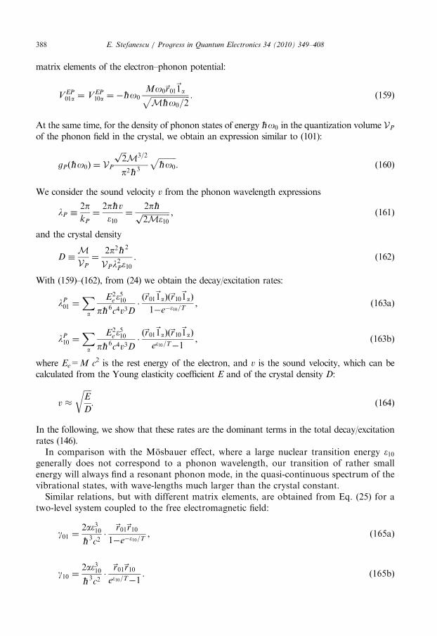
E. Stefanescu / Progress in Quantum Electronics 34 (2010) 349–408388
matrix elements of the electron–phonon potential:
V EP01a ¼ VEP
10a ¼ �‘o0Mo0~r01~1affiffiffiffiffiffiffiffiffiffiffiffiffiffiffiffiffiffiffiffiM‘o0=2
p : ð159Þ
At the same time, for the density of phonon states of energy ‘o0 in the quantization volume VP
of the phonon field in the crystal, we obtain an expression similar to (101):
gPð‘o0Þ ¼ VP
ffiffiffi2pM3=2
p2‘ 3
ffiffiffiffiffiffiffiffiffi‘o0
p: ð160Þ
We consider the sound velocity v from the phonon wavelength expressions
lP �2pkP
¼2p‘ v
e10¼
2p‘ffiffiffiffiffiffiffiffiffiffiffiffiffiffi2Me10p ; ð161Þ
and the crystal density
D �MVP
¼2p2‘ 2
VPl2Pe10
: ð162Þ
With (159)–(162), from (24) we obtain the decay/excitation rates:
lP01 ¼
Xa
E2e e
510
p‘ 6c4v3D�ð~r01~1aÞð~r10~1aÞ
1�e�e10=T; ð163aÞ
lP10 ¼
Xa
E2e e
510
p‘ 6c4v3D�ð~r01~1aÞð~r10~1aÞ
ee10=T�1; ð163bÞ
where Ee=M c2 is the rest energy of the electron, and v is the sound velocity, which can becalculated from the Young elasticity coefficient E and of the crystal density D:
v �
ffiffiffiffiE
D
r: ð164Þ
In the following, we show that these rates are the dominant terms in the total decay/excitationrates (146).In comparison with the Mosbauer effect, where a large nuclear transition energy e10
generally does not correspond to a phonon wavelength, our transition of rather smallenergy will always find a resonant phonon mode, in the quasi-continuous spectrum of thevibrational states, with wave-lengths much larger than the crystal constant.Similar relations, but with different matrix elements, are obtained from Eq. (25) for a
two-level system coupled to the free electromagnetic field:
g01 ¼2ae310‘ 3c2
�~r01~r10
1�e�e10=T; ð165aÞ
g10 ¼2ae310‘ 3c2
�~r01~r10
ee10=T�1: ð165bÞ
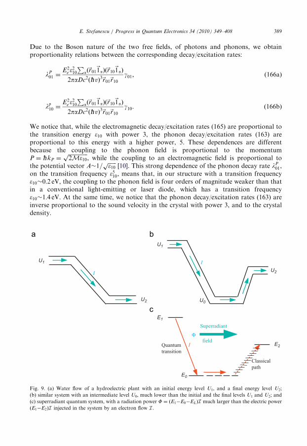
E. Stefanescu / Progress in Quantum Electronics 34 (2010) 349–408 389
Due to the Boson nature of the two free fields, of photons and phonons, we obtainproportionality relations between the corresponding decay/excitation rates:
lP01 ¼
E2e e
210
Pað~r01
~1aÞð~r10~1aÞ
2paDc2ð‘ vÞ3~r01~r10g01; ð166aÞ
lp10 ¼
E2e e
210
Pað~r01
~1aÞð~r10~1aÞ
2paDc2ð‘ vÞ3~r01~r10g10: ð166bÞ
We notice that, while the electromagnetic decay/excitation rates (165) are proportional tothe transition energy e10 with power 3, the phonon decay/excitation rates (163) areproportional to this energy with a higher power, 5. These dependences are differentbecause the coupling to the phonon field is proportional to the momentumP ¼ ‘kP ¼
ffiffiffiffiffiffiffiffiffiffiffiffiffiffi2Me10p
, while the coupling to an electromagnetic field is proportional tothe potential vector A1=
ffiffiffiffiffiffie10p
[10]. This strong dependence of the phonon decay rate lP01,
on the transition frequency e510, means that, in our structure with a transition frequencye100:2 eV, the coupling to the phonon field is four orders of magnitude weaker than thatin a conventional light-emitting or laser diode, which has a transition frequencye101:4 eV. At the same time, we notice that the phonon decay/excitation rates (163) areinverse proportional to the sound velocity in the crystal with power 3, and to the crystaldensity.
U1
U2
I
U1
U2
U0
I
E1
E2
E0
Quantumtransition
Classicalpath
Superradiant
field I
Φ
Fig. 9. (a) Water flow of a hydroelectric plant with an initial energy level U1, and a final energy level U2;
(b) similar system with an intermediate level U0, much lower than the initial and the final levels U1 and U2; and
(c) superradiant quantum system, with a radiation power F ¼ ðE1�E0�ELÞI much larger than the electric power
ðE1�E2ÞI injected in the system by an electron flow I .
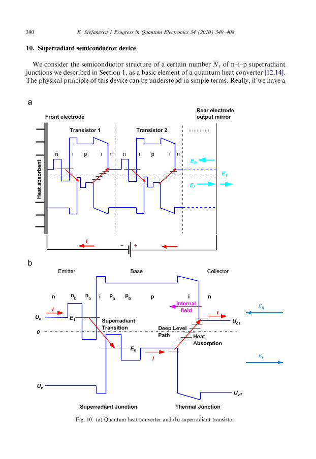
E. Stefanescu / Progress in Quantum Electronics 34 (2010) 349–408390
10. Superradiant semiconductor device
We consider the semiconductor structure of a certain number N t of n–i–p superradiantjunctions we described in Section 1, as a basic element of a quantum heat converter [12,14].The physical principle of this device can be understood in simple terms. Really, if we have a
Transistor 1 Transistor 2
n i p i n n i p i n
Hea
t abs
orbe
nt
Front electrode Rear electrodeoutput mirror
I − +
EI
ER
ET
Uc
0Deep LevelPath
Thermal Junction Superradiant Junction
Emitter Base Collector
Uv
Heat Absorption
E1
E0
Uc1
Uv1
SuperradiantTransition
I
I
I
n nb na pa pb p i i n Internal field
ER
EI
Fig. 10. (a) Quantum heat converter and (b) superradiant transistor.

E. Stefanescu / Progress in Quantum Electronics 34 (2010) 349–408 391
classical system as the water flow of a hydroelectric plant (Fig. 9a), we obtain a power
F ¼ ðU1�U2�ELÞI ; ð167Þ
as the product of the difference between the initial potential energy U1 and the finalpotential energy U2 of the mass unit with the mass flow I, while EL is an energy loss. If wetake a similar system with a much lower intermediate energy level U0oU1;U2 (Fig. 9b),nothing happens, the power being the same as is given by Eq. (167). However, if instead ofthe classical system in Fig. 9b, we consider a quantum system of electrons as is representedin Fig. 9c, something extraordinary might happen: by a quantum transition from theinitial energy level E1 to the much lower intermediate level E0, the large energyE1�E0 might be given to a photon of a superradiant field, which means an electromagneticpower
F ¼ ðE1�E0�ELÞI ð168Þ
much larger than the power ðE1�E2ÞI injected in the device to obtain the electron flow I ,while EL is a term taking into account that some transitions are lost by dissipation.
The actual device [12], represented in Fig. 10a, can be regarded as a succession of n–i–p–i–n superradiant transistors (Fig. 10b), with an electron transfer in two steps: (1) asuperradiant quantum transition from emitter to base, and (2) a classical transfer, withthermal excitation of electrons from base to collector. This process involves a quasi-ohmiccontact between base and collector, that means a deep-level path crossing the energy gap ofthe base-collector junction. On this deep level path, the electrons are carried up by theinternal field of the p–i–n base-collector junction, while the energy of this field is recoveredby heat absorption, when a kinetic energy is provided to the electrons building up the fieldby diffusion. This electron transfer by the internal field of a junction is similar to thetransistor effect [70], with the difference that in an ordinary bipolar transistor the electronscross the base-collector junction decaying through the conduction band, with energydissipation (Fig. 11), while in a superradiant transistor (Fig. 10b), the electrons go up,absorbing energy from the internal field, which is from the environment. This phenomenoncan be understood from statistical reasons. From Fig. 10b, we notice that the injectedcurrent I increases the population of the lower states and decreases the population of thehigher states of the deep level path. That means that this region becomes colder, absorbing
n n
Uc
Uv
IE
IB
ICUc1
Uv1
0
Internalfield
Emitter Collector Base
p
Fig. 11. Ordinary bipolar transistor: while a small current IB is injected in base, an important part IC of the
emitter current IE is carried through the base-collector junction by the internal field.

E. Stefanescu / Progress in Quantum Electronics 34 (2010) 349–408392
heat from the environment. This heat absorption has the tendency to remake the initialstatistical distribution, modified by current injection. In the following calculations weneglect the temperature variation due to the heat transfer throughout the semiconductorstructure. To take into account this temperature variation, one has to make corrections ofthe parameters, to obtain the same transition frequency on the whole chain of superradiantjunctions.
Uc
U3
i n
E1
E0
U1
U2
U0
U00
U4
Uv
p Ie
Ih
x
z U y
x1 x0 x2x3 x4 x50
− √1−√
I
M1( 0=0) M2( )
1 2
na
nb
AlxGa1−xAs
GaAs
GaAs GaAs
pa pbGaAs
AlxGa1−xAs
AlxGa1−xAs
Uc
U3
i n
E1
E0
U1
U2
U0
U00
U4
Uv
p
Ie
Ih
x
z U y
x1 x0 x2x3 x4 x50
− √1−TG
√
I
M1(T0=0)
M2( )
1 2
na
nb
AlxGa1−xAs
GaAs
GaAsGaAspa
pbGaAs
AlxGa1−xAs
AlxGa1−xAs
Fig. 12. Dissipative superradiant n–i–p device with two injection electrodes E1 and E2 and a Fabry–Perot cavity
with the mirrors M1 and M2 of transmission coefficients T 0 ¼ 0 and T , respectively, in two possible versions (a)
and (b). (a) Longitudinal superradiant device with the Fabry–Perot cavity oriented in the x-direction of the
injected current I=Ie=Ih, i.e. perpendicular to the semiconductor layers. (b) Transversal superradiant device with
the Fabry–Perot cavity oriented in the y-direction, perpendicular to the injected current I=Ie=Ih, i.e. in the plane
of the semiconductor layers.

E. Stefanescu / Progress in Quantum Electronics 34 (2010) 349–408 393
Such a device can be realized in two versions schematically represented in Fig. 12: (a) alongitudinal device with the two mirror metalizations M1 and M2 made on the two surfacesin the plane of the chip, of transmission coefficients T 0 ¼ 0 and T40, which form aFabry–Perot cavity coupling a superradiant mode that propagates in the x-direction of theinjection current; (b) a transversal device with the two mirror metalizations M1 and M2
made on two lateral surfaces of the chip, of transmission coefficients T 0 ¼ 0 and T40,which form a Fabry–Perot cavity coupling a superradiant mode that propagates in they-direction, perpendicular to the injection current. While in version (a) the roles of themirrors M1 and M2, and of the injection electrodes E1 and E2, are played by the samemetalizations, made on the two surfaces in the plane of the chip, in version (b) the mirrormetalizations M1 and M2, which are made on two lateral surfaces, are different from theelectrode metalizations E1 and E2.
The two devices have the same semiconductor structure, including layers of GaAs, with anarrower forbidden band and a heavier doping, for the quantum wells, and layers ofAlxGa1�xAs, with a larger forbidden band and a lighter doping, for the potentialbarriers. The margins of these bands are determined by the concentrations of the donors/acceptors embedded in the semiconductor layers. For the potential distribution, weconsider a simple rectangular model taking into account the essential characteristics ofthe system.
11. Operation conditions for the device parameters
We describe the superradiant dynamics of the systems represented in Fig. 12 by theoptical equations (80) with coefficients that take simple forms as functions of the physicalparameters of the system and temperature. These equations describe the coupling of asystem of electrons to the electromagnetic field, by a coupling coefficient for the electricdipole interaction, which according to (62) and (129), is
g ¼ gL ¼e
‘xðCÞ01 ¼
e
‘cðxÞ01
x2�x0
2�
1
a0�a1
� �ð169Þ
for a transversal device, while for a longitudinal device we take
g ¼ gT ¼e
‘
ffiffiffiffiffiffiffiffiffiffiffiffiffiffiffiffiyðCÞ01 y
ðCÞ10
q¼
e
‘cðxÞ01
‘
2ffiffiffiffiffiffiffiffiffiffiffiffiffiffiffiffiffiffiffiffiffiffiffiffiffiffiffiffiffiffiffiffiffiffiffiffi
MnMp
pT
q : ð170Þ
In Sections 8 and 9, we obtained explicit expressions of the decay and excitation rates l01and l10 of the electron system for three dissipative couplings. With these terms, from (42)and (146), we obtain the decay and dephasing rates
gJ ¼ 2g? ¼ gEJ þ gP
J þ gEMJ ; ð171Þ
where gEJ stands for the electric coupling to the conduction electrons, gP
J for the phononcoupling to the crystal lattice, and gEM
J for the coupling to the free electromagnetic field.The electric decay rate has two components for the interaction with the two conductionregions n and p:
gEJ ¼ gðnÞJ þ gðpÞJ : ð172Þ

E. Stefanescu / Progress in Quantum Electronics 34 (2010) 349–408394
From (42), for the two components n and p of the environment of conduction electronsand holes, with (144), we get
gðnÞJ ¼8a2c2
ffiffiffiffiffiffiffiffiffiffi2Mn
pe10 þ
T
2
� �jcðxÞ01 j
2m201
3N�1=3D
2�x3
!3
e3=210
; ð173Þ
and
gðpÞJ ¼8a2c2
ffiffiffiffiffiffiffiffiffiffi2Mp
pe10 þ
T
2
� �jcðxÞ01 j
2m201
3N�1=3A
2þ x5
!3
e3=210
: ð174Þ
These two expressions describe dipole-dipole couplings of an active electron to the quasi-free electrons and holes in the two conduction regions n and p, which are inverseproportional to the cubes of the separation distances N
�1=3D =2�x3 and N
�1=3A =2þ x5,
respectively. The electric decay rates (173) and (174) get lower with the transition energye10 ¼ E1�E0, an increase of this energy leading to transitions of the environment electrons/holes into states with wave-functions more rapidly varying in space, which form smallerdipole moments. From Eq. (42) for a phonon environment, with (165) and (166), we obtainthe phonon decay rate
gPJ ¼
Xa
2E2e e
510ð~r01
~1aÞð~r10~1aÞ
p‘ 6c4v3D�
ee10=T þ 1
ee10=T�1; ð175Þ
where Ee=M c2 is the rest energy of the electron, and ~1a are the polarization vectors of thephonon modes. We notice that the phonon decay rate gets higher with the transitionenergy e10 with power 5, with the dipole moments~r01,~r10, and with temperature T. At thesame time, it gets lower with the sound velocity with power 3, which, according to (164) is afunction of the Young elasticity coefficient E and the crystal density D. With (165), we getthe electromagnetic decay rate
gEMJ ¼
4ae310~r01~r10‘ 3c2
�ee10=T þ 1
ee10=T�1; ð176Þ
which also gets higher with the dipole moments ~r01, ~r10, and temperature T, but with thetransition energy e10 only with power 3. In the numerical case in Section 5, the phonondecay rate (175) dominates the electric decay rate (172)–(145), while the electromagneticdecay (176) is negligible. The non-Markovian coefficient (43), with the components (149),depends on the relative fluctuations between the two levels, induced by the twocomponents n and p of the environment that we add quadratically:
g2n ¼ffiffiffiffiffiffiffiffiffiffiffiffiffiffiffiffiffiffiffiffiffiffiffiffiffiffiffiffi½zðnÞ11 �
2 þ ½zðpÞ11 �2
q�
ffiffiffiffiffiffiffiffiffiffiffiffiffiffiffiffiffiffiffiffiffiffiffiffiffiffiffiffi½zðnÞ00 �
2 þ ½zðpÞ00 �2
q� �2
: ð177Þ
The non-Markovian coefficient (177) with the components (149) arises due to the distancedifference of the two states from the two conduction regions: the field fluctuations of aconduction region have a stronger influence on the closer state than on the farer one. It is
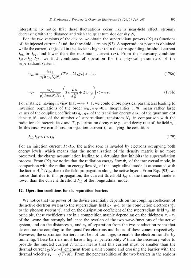
E. Stefanescu / Progress in Quantum Electronics 34 (2010) 349–408 395
interesting to notice that these fluctuations occur like a near-field effect, stronglydecreasing with the distance and with the quantum dot density Ne.
For the two versions of the device, we obtain the superradiant powers (92) as functionsof the injected current I and the threshold currents (93). A superradiant power is obtainedwhile the current I injected in the device is higher than the corresponding threshold currentI0L or I0T, and lower than the maximum current (98). From the necessary conditionIM4I0L; I0T , we find conditions of operation for the physical parameters of thesuperradiant system:
wIL ¼e0g?
g2L‘o0NeN t
ðT cþ 21LgF Þo�wT ð178aÞ
wIT ¼e0g?
g2T‘o0NeN t
T cLD
A1=2D
þ 21LgF
!o�wT : ð178bÞ
For instance, having in view that �wT � 1, we could chose physical parameters leading toinversion populations of the order wIL;wIT0:1. Inequalities (178) mean rather largevalues of the coupling coefficients gL, gT, of the transition energy ‘o0, of the quantum dotdensity Ne, and of the number of superradiant transistors N t, in comparison with theradiation characteristics c and T , polarization decay rate g?, and decay rate of the field gF .In this case, we can choose an injection current I, satisfying the condition
I0L;I0ToIoIM : ð179Þ
For an injection current I4IM , the active zone is invaded by electrons occupying bothenergy levels, which means that the normalization of the density matrix is no morepreserved, the charge accumulation leading to a detuning that inhibits the superradiationprocess. From (92), we notice that the radiation energy flow FT of the transversal mode, incomparison with the radiation energy flow FL of the longitudinal mode, is attenuated withthe factor A
1=2D =LD, due to the field propagation along the active layers. From Eqs. (93), we
notice that due to this propagation, the current threshold I0T of the transversal mode islower than the current threshold I0L of the longitudinal mode.
12. Operation conditions for the separation barriers
We notice that the power of the device essentially depends on the coupling coefficient ofthe active electron system to the superradiant field gL (gT), to the conduction electrons gE
J ,to the phonon system gP
J , and on the dissipation coefficient of the superradiant field gF . Inprinciple, these coefficients are in a competition mainly depending on the thickness x2�x0
of the i-zone that strongly influence the overlap of the two wave-functions of the activesystem, and on the distances x3 and x5 of separation from the two conduction zones thatdetermine the coupling to the quasi-free electrons and holes of these zones, respectively.However, the separation barriers must be not too large, to enable the electron transfer bytunneling. These barriers must have a higher penetrability P than the necessary value toprovide the injected current I, which means that this current must be smaller than thethermal current 1
6eNDvT P emergent from a unit volume and crossing the barrier with the
thermal velocity vT ¼ffiffiffiffiffiffiffiffiffiffiffiffiffiT=Mn
p. From the penetrabilities of the two barriers in the regions

E. Stefanescu / Progress in Quantum Electronics 34 (2010) 349–408396
n and p, P ¼ e�Bn ; e�Bp , we find the conditions:
BnoIn; ð180aÞ
BpoIp; ð180bÞ
for the barrier coefficients
Bn ¼1
‘
ffiffiffiffiffiffiffiffiffiffiffiffiffiffiffiffiffiffiffiffiffiffiffiffiffiffiffiffiffiffiffiffiffiffiffiffiffiffiffiffi2Mn U3�Uc�
T
2
� �sðx1�x3Þ;
Bp ¼1
‘
ffiffiffiffiffiffiffiffiffiffiffiffiffiffiffiffiffiffiffiffiffiffiffiffiffiffiffiffiffiffiffiffiffiffiffiffiffiffiffiffi2Mp Uv�U4�
T
2
� �sðx5�x4Þ; ð181Þ
and the injection coefficients
In ¼1
2ln
eNDAD
6I
ffiffiffiffiffiffiffiT
Mn
r� �;
Ip ¼1
2ln
eNAAD
6I
ffiffiffiffiffiffiffiT
Mp
s !: ð182Þ
These coefficients depend on the current ratios eNDAD c/I and eNAADc/I, and the energyratios T/(Mnc2) and T/(Mpc2) for the n and p regions, respectively. With (119c) and (119d),we get conditions for the attenuation coefficients of the wave-functions in the separationbarriers a3 ¼ ð1=‘ Þ
ffiffiffiffiffiffiffiffiffiffiffiffiffiffiffiffiffiffiffiffiffiffiffiffiffiffiffi2MnðU3�E1Þ
p, a4 ¼ ð1=‘ Þ
ffiffiffiffiffiffiffiffiffiffiffiffiffiffiffiffiffiffiffiffiffiffiffiffiffiffiffi2MpðE0�U4Þ
p, and the thicknesses of
these barriers:
a3ðx1�x3Þo1
2ln
eNDAD
6I
ffiffiffiffiffiffiffiT
Mn
r� �; ð183aÞ
a4ðx5�x4Þo1
2ln
eNAAD
6I
ffiffiffiffiffiffiffiT
Mp
s !: ð183bÞ
The thickness x2�x0 of the i-zone must be sufficiently small to obtain the necessarycoupling coefficients (169) and (170) with the overlap function (126a). However,diminishing this thickness, the dissipative coupling to the conduction electrons also gethigher. This dissipative coupling can be diminished by increasing the separation distancesx3, x5, but only in the limits imposed by inequalities (183). In the following section, weshow that, even with these limitations, a large radiation power can be obtained.
13. Dissipative coefficients and stationary regime
We consider a chip of a GaAs–Al0.37Ga0.63As semiconductor heterostructure, as asquare with a side of 2 cm and a thickness of 2mm (see Fig. 1), which comprise 1045superradiant n–i–p junctions with a thickness equal to the wavelength of the superradiantfield, which is l ¼ 1:914mm for the chosen parameters of the system (Fig. 12). In thefurther calculations, we use the relative effective masses Mnr=0.05 of the electron andMpr= 0.5 of the hole, the relative electric permittivity er ¼ 12, the mobilities mn ¼
8000 cm2=Vs of the electron and mp ¼ 400 cm2=Vs of the hole, a Young elasticity

E. Stefanescu / Progress in Quantum Electronics 34 (2010) 349–408 397
coefficient E ¼ C11 ¼ 5:38 1011 dyn=cm2, the thermal resistivity k ¼ 0:37 cal=ðcm s0 KÞ,and the crystal density D=5.317 g/cm3.
For the two GaAs conduction zones with the forbidden band Eg(GaAs)=1.426 eV wetake equal donor and acceptor concentrations ND ¼ NA ¼ 3:16 1016 cm�3. We considera temperature T ¼ 10ˆC, while from Eqs. (105), we get the margins of the conduction andvalence bands Uc=51.1meV and Uv=�135.4meV, respectively, which correspond toNc=2.57 1017 cm�3 and Nv=8.14 1018 cm�3. The quantum zone includes three layersof Al0.37Ga0.63As with the forbidden band Eg(Al0.37Ga0.63As)=1.92 eV: (1) the i-layer witha thickness that here is taken in the interval x2�x0 2 ð5; 10Þnm, in fact a weakly dopedlayer with the barrier height U0=0.5 eV, corresponding to an array of N0=6.4243 106
m�2 donors, (2) the nb barrier with a thickness x1�x3=10 nm and a heightU3=Ucþ0.05=0.1011 eV corresponding to an array of N3=8.01 1013m�2 donors, and(3) the pb barrier with a thickness x5�x4=3nm and a height U4=Uv�0.05=�0.1854 eV,corresponding to an array of N4=2.552 1013m�2 acceptors.
For a thickness of the i-layer x2�x0=5.5 nm and a density of quantum dots Ne ¼
1:476 1016 m�2 donors in the na–GaAs layer, and acceptors in the pa–GaAs layer, from(108), we get the potentials U1=�69.3meV and U2=�26.6meV. For energy levels of thetwo quantum dot wells equal to the margins of the two conduction and valence bands(E1=Uc and E0=Uv), from (121), we calculate the widths x0�x1=4.189 nm andx4�x2=1.576 nm of these wells, while, for the considered Ne-value, we get the internalfield entirely confined between the two quantum dot arrays. At the same time, thetransition energy is e10 � E1�E0 ¼ 0:1866 eV, the wavelength of the radiation in GaAstakes the value l ¼ 1:9158mm, while the dipole moments of coupling to the superradiant
field are xðCÞ01 ¼ 5:171 10�4 nm and
ffiffiffiffiffiffiffiffiffiffiffiffiffiffiffiffiyðCÞ01 y
ðCÞ10
q¼ 4:689 10�4 nm, for the transversal and
the longitudinal device, respectively. From Eqs. (144)–(145) and (163)–(164), we get the
dissipative coefficients of the electric interaction lðnÞ01 ¼ 5:4517 105 s�1, lðnÞ10 ¼ 32:0194 s�1,
lðpÞ01 ¼ 4:8894 106 s�1, lðpÞ10 ¼ 9:0810 s�1, and of the phonon interaction lP01 ¼ 1:8947
107 s�1, lP10 ¼ 9:0572 103 s�1. We notice that the electric decay rate is an order of
magnitude lower than the phonon decay rate.
For a transmission coefficient of the output mirror T ¼ 0:1, the threshold currents takerather large values I0L=24.1149A and I0T=23.4528A with a maximum currentIM=46.0995A. For the chosen separation barriers, even with a rather large injectioncurrent as, for instance I=45A, the necessary relations between the barrier and theinjection coefficients are satisfied: In=Bn ¼ 1:727641, Ip=Bn ¼ 1:548741. At the sametime, for the non-Markovian coefficient we get the value gn ¼ 3:8015 1011 s�1. Taking alength of the p-zone of l=4, the total series resistance is Rs ¼ 7:1mO, while the electricallydissipated power is Pel=14.3643W. For the longitudinal device, we obtain a totalsuperradiant power FL ¼ 1:2843 kW, which means a power density PL ¼ 3:2107MW=m2.For the transversal device, we obtain a total superradiant power FT ¼ 0:288 kW, i.e. apower density PT ¼ 0:720MW=m2.
In Fig. 13, we represent the components gEJ , g
PJ , g
EMJ of the decay rate gJ, and the non-
Markovian coefficient gn, as functions of the thickness x2�x0 of the i-zone that essentiallydetermines the overlap of the two wave functions of the initial and final states and, by this,the transition dipole moment (see Eqs. (126a)–(129)). First of all, we notice that theelectromagnetic decay rate gEM
J is negligible in comparison with the electric and phonon

5 6 7 8 9 10101
102
103
104
x2−x0[nm]
[m V
−1 s
−1]
gL
gT
Fig. 14. The dependence of the coupling coefficients on the thickness of the i-zone.
5 6 7 8 9 1010−2
10−1
100
101
102
103
x2−x0 [nm] x2−x0 [nm]
[A] IM
I0LI0T
5 6 7 8 9 1010−2
10−1
100
101
102
103
[A] IM
I0LI0T
Fig. 15. The dependence of the threshold currents on the thicknesses of the i-zone for two values of the
transmission coefficient of the output mirror: (a) T ¼ 0:1 and (b) T ¼ 0:5.
5 6 7 8 9 10
100
105
1010
x2−x0[nm]
[s−1
]
γn
γ||
γ||
γ||
P
E
EM
Fig. 13. The dependence of the dissipative coefficients on the thickness of the i-zone.
E. Stefanescu / Progress in Quantum Electronics 34 (2010) 349–408398

5 6 7 8 9 100.9
1
1.1
1.2
1.3
1.4
1.5
1.6 x 1016
x2−x0 [nm]
Ne
[m−2
]
Fig. 16. The dependence of the quantum dot density on the thickness of the i-zone.
E. Stefanescu / Progress in Quantum Electronics 34 (2010) 349–408 399
decay rates gEJ ; g
PJ , and that the phonon decay dominates the other decay processes. We
also notice that the variation of the decay rates with the thickness of the i-zone is verystrong, while the dependence of the non-Markovian coefficient gn is weak, this coefficientbeing essentially determined by the distance between the active electrons and the quasi-freeelectrons and holes in the conduction regions. The non-Markovian coefficient gn is muchlarger than the decay rates, this coefficient describing fluctuations of a mean-time 1=gn
much shorter than the decay time 1=gJ.In Fig. 14, we represent the dependence on the thickness x2�x0 of the coupling
coefficients gL, gT. As we can see from (169) to (170), since these coefficients areproportional to the dipole-moment, while the decay rates (173)–(175) are proportional tothe square of this moment, the inversion populations (178) do not depend strongly on these
coefficients and on the decay rates, but only on other parameters as Ne, N t, T and gF .From (169) and (170), it is interesting to notice that, although the two coefficients gL andgT have quite different expressions, depending on different parameters, they are of thesame order of magnitude. However, the dependence on x2�x0 of gT, which is proportional
to xðCÞ01 , is weaker than that gL, which is proportional to
ffiffiffiffiffiffiffiffiffiffiffiffiffiffiffiffiyðCÞ01 y
ðCÞ10
q.
In Fig. 15, we represent the dependence on the thickness x2�x0 of the threshold currents.According to (93), the decrease of these currents with the thickness x2�x0 is mainlydetermined by the decrease of the decay rate gJ, the inversion populations wIL, wIT in thesquare parentheses depending only weakly on this thickness. It is interesting that, as onecan notice from (92), (98), and (179), by increasing the dissipation rate gJ, one obtains ahigher radiation power, given by a higher current IoIM . The threshold current of atransversal device is lower than that of a longitudinal one, due to the factor LD=A
1=2D in the
radiation term of the inversion population (178b). From Fig. 15b, in comparison withFig. 15a, we notice that, although according to (93) the threshold current gets larger withthe transmission coefficient T , the operation conditions (178) are satisfied for large valuesof T .
In Fig. 16, we represent the dependence on the thickness x2�x0 of the quantum dotdensity Ne, obtained from the condition that the entire internal field between the two
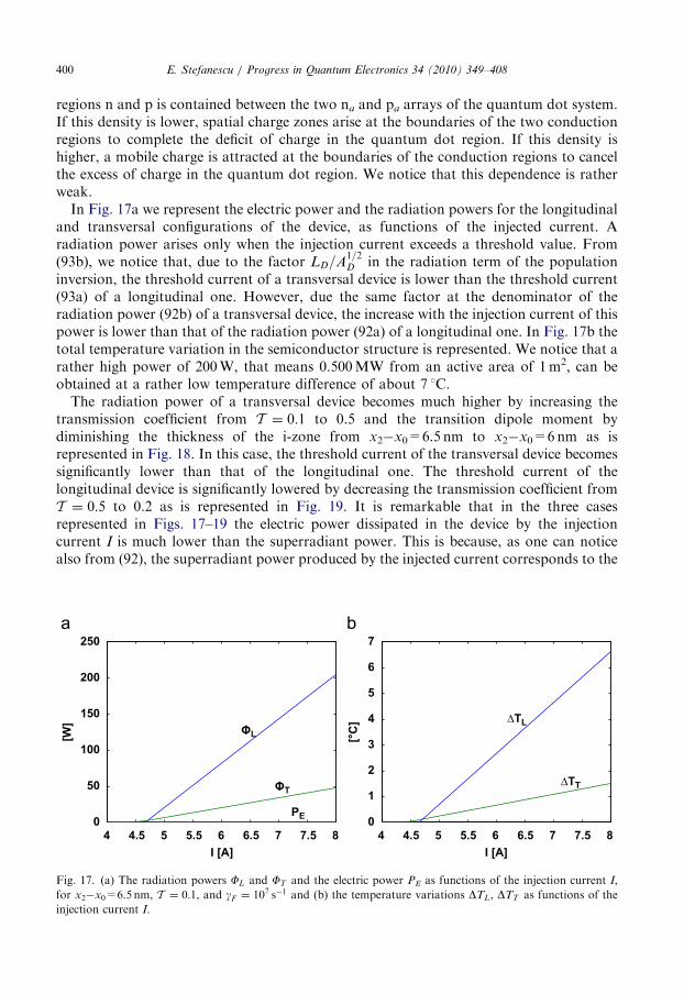
E. Stefanescu / Progress in Quantum Electronics 34 (2010) 349–408400
regions n and p is contained between the two na and pa arrays of the quantum dot system.If this density is lower, spatial charge zones arise at the boundaries of the two conductionregions to complete the deficit of charge in the quantum dot region. If this density ishigher, a mobile charge is attracted at the boundaries of the conduction regions to cancelthe excess of charge in the quantum dot region. We notice that this dependence is ratherweak.In Fig. 17a we represent the electric power and the radiation powers for the longitudinal
and transversal configurations of the device, as functions of the injected current. Aradiation power arises only when the injection current exceeds a threshold value. From(93b), we notice that, due to the factor LD=A
1=2D in the radiation term of the population
inversion, the threshold current of a transversal device is lower than the threshold current(93a) of a longitudinal one. However, due the same factor at the denominator of theradiation power (92b) of a transversal device, the increase with the injection current of thispower is lower than that of the radiation power (92a) of a longitudinal one. In Fig. 17b thetotal temperature variation in the semiconductor structure is represented. We notice that arather high power of 200W, that means 0.500MW from an active area of 1m2, can beobtained at a rather low temperature difference of about 7 1C.The radiation power of a transversal device becomes much higher by increasing the
transmission coefficient from T ¼ 0:1 to 0.5 and the transition dipole moment bydiminishing the thickness of the i-zone from x2�x0=6.5 nm to x2�x0=6 nm as isrepresented in Fig. 18. In this case, the threshold current of the transversal device becomessignificantly lower than that of the longitudinal one. The threshold current of thelongitudinal device is significantly lowered by decreasing the transmission coefficient fromT ¼ 0:5 to 0.2 as is represented in Fig. 19. It is remarkable that in the three casesrepresented in Figs. 17–19 the electric power dissipated in the device by the injectioncurrent I is much lower than the superradiant power. This is because, as one can noticealso from (92), the superradiant power produced by the injected current corresponds to the
4 4.5 5 5.5 6 6.5 7 7.5 80
50
100
150
200
250
I [A]
[W] ΦL
ΦT
PE
4 4.5 5 5.5 6 6.5 7 7.5 80
1
2
3
4
5
6
7
I [A]
[°C
] ∆TL
∆TT
Fig. 17. (a) The radiation powers FL and FT and the electric power PE as functions of the injection current I,
for x2�x0=6.5 nm, T ¼ 0:1, and gF ¼ 107 s�1 and (b) the temperature variations DTL, DTT as functions of the
injection current I.
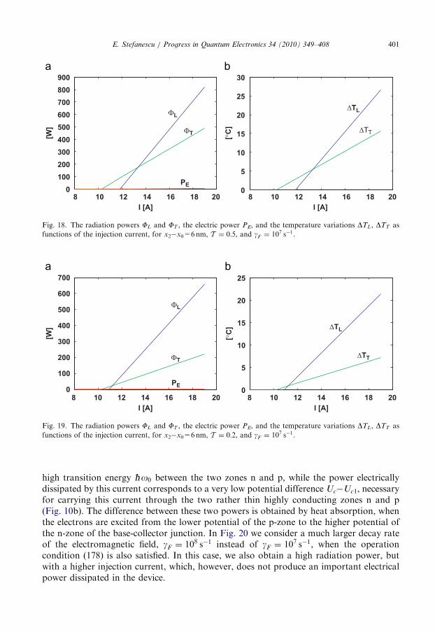
8 10 12 14 16 18 200
100
200
300
400
500
600
700
I [A]
[W]
PE
ΦT
ΦL
8 10 12 14 16 18 200
5
10
15
20
25
I [A]
[°C
]
ΔTT
ΔTL
Fig. 19. The radiation powers FL and FT , the electric power PE, and the temperature variations DTL, DTT as
functions of the injection current, for x2�x0=6nm, T ¼ 0:2, and gF ¼ 107 s�1.
0100200300400500600700800900
I [A]
[W]
PE
ΦT
ΦL
8 10 12 14 16 18 20 8 10 12 14 16 18 200
5
10
15
20
25
30
I [A]
[°C
] ΔTT
ΔTL
Fig. 18. The radiation powers FL and FT , the electric power PE, and the temperature variations DTL, DTT as
functions of the injection current, for x2�x0=6nm, T ¼ 0:5, and gF ¼ 107 s�1.
E. Stefanescu / Progress in Quantum Electronics 34 (2010) 349–408 401
high transition energy ‘o0 between the two zones n and p, while the power electricallydissipated by this current corresponds to a very low potential difference Uc�Uc1, necessaryfor carrying this current through the two rather thin highly conducting zones n and p(Fig. 10b). The difference between these two powers is obtained by heat absorption, whenthe electrons are excited from the lower potential of the p-zone to the higher potential ofthe n-zone of the base-collector junction. In Fig. 20 we consider a much larger decay rateof the electromagnetic field, gF ¼ 108 s�1 instead of gF ¼ 107 s�1, when the operationcondition (178) is also satisfied. In this case, we also obtain a high radiation power, butwith a higher injection current, which, however, does not produce an important electricalpower dissipated in the device.
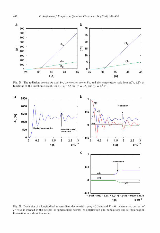
0 0.5 1 1.5 2 2.5 3x 10⁻⁷
0
500
1000
1500
2000
2500
t [s]
ΦL
[W]
Non−Markovianfluctuation
Markovian evolution
0 0.5 1 1.5 2 2.5 3x 10⁻⁷
−0.5
0
0.5
1
t [s]
w(t)
u(t)
v(t)
Fluctuaion
1.9176 1.9177 1.9177 1.9178 1.9178 1.9179 1.9179
x 10−7
−0.5
0
0.5
1
t [s]
Fluctuation
u(t)
w(t)
v(t)
Fig. 21. Dynamics of a longitudinal superradiant device with x2�x0=5.5 nm and T ¼ 0:1 when a step current of
I=45A is injected in the device: (a) superradiant power; (b) polarization and population; and (c) polarization
fluctuation in a short timescale.
25 30 35 40 450
100200300400500600700800900
I [A]
[W]
ΦL
PE
ΦT
25 30 35 40 450
5
10
15
20
25
30
I [A]
[°C
]
ΔTT
ΔTL
Fig. 20. The radiation powers FL and FT , the electric power PE, and the temperature variations DTL, DTT as
functions of the injection current, for x2�x0=5.5 nm, T ¼ 0:5, and gF ¼ 108 s�1.
E. Stefanescu / Progress in Quantum Electronics 34 (2010) 349–408402
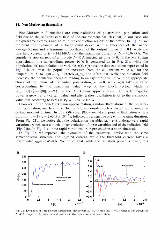
E. Stefanescu / Progress in Quantum Electronics 34 (2010) 349–408 403
14. Non-Markovian fluctuations
Non-Markovian fluctuations are time-evolutions of polarization, population andfield due to the self-consistent field of the environment particles that, in our case, arethe quasi-free electrons and holes in the conduction regions of the device. In Fig. 21, werepresent the dynamics of a longitudinal device with a thickness of the i-zonex2�x0=5.5 nm and a transmission coefficient of the output mirror T ¼ 0:1, while thethreshold current is I0L=24.1149A and the maximum current is IM=46.0995A. Weconsider a step current of amplitude I=45A injected at time t=0. In the Markovianapproximation, a superradiant power FLðtÞ is generated as in Fig. 21a, while thepopulation wðtÞ and polarization variables u(t), v(t) have the time-evolutions represented inFig. 21b. At t=0, the population increases from the equilibrium value wT for thetemperature T, to wð0Þ ¼ wT þ 2I=ðeNeADgJÞ and, after that, while the radiation fieldincreases, the population decreases tending to an asymptotic value. With an appropriatechoice of the phase of the initial polarization, v(0)=0, while u(0) takes a valuecorresponding to the maximum value �wT of the Bloch vector, which is
uð0Þ ¼ffiffiffiffiffiffiffiffiffiffiffiffiffiffiffiffiffiffiffiffiffiffiffiffiffiffiffiffiffiffiffiffiffiffiffiffiffiffiffi½w2
T�w2ð0Þ�=ð2�T Þp
. In the Markovian approximation, the electromagnetic
power is growing to a certain value, and after a short oscillation tends to the asymptotic
value that according to (92a) is FL ¼ 1:2843 103W.However, in the non-Markovian approximation, random fluctuations of the polariza-
tion, population, and field arise. In Fig. 21, we consider such a fluctuation arising at acertain moment of time. In Eqs. (80a) and (80b), we take a positive fluctuation with aduration tn ¼ 1=gn ¼ 2:6305 10�12 s, followed by a negative one with the same duration.From Fig. 21b, we notice that the polarization variables u(t), v(t) undergo very rapidvariations, which start a much longer evolution of these variables and of the radiation field(Fig. 21a). In Fig. 21c, these rapid variations are represented in a short timescale.
In Fig. 22, we represent the dynamics of the transversal device with the samesemiconductor structure and injected current, while the threshold current takes alower value I0T=23.4528A. We notice that, while the radiation power is lower, this
0 0.5 1 1.5 2 2.5x 10⁻⁷
0
50
100
150
200
250
300
350
t [s]
ΦT
[w]
Markovian evolution
Non−Markovian fluctuation
0 0.5 1 1.5 2 2.5x 10⁻⁷
−0.6
−0.4
−0.2
0
0.2
0.4
0.6
0.8
1
t [s]
Fluctuation
w(t)
u(t)
v(t)
Fig. 22. Dynamics of a transversal superradiant device with x2�x0=5.5 nm and T ¼ 0:1 when a step current of
I=45A is injected: (a) superradiant power and (b) population and polarization.

0 0.5 1 1.5 2 2.5x 10⁻⁷
0
50
100
150
200
250
300
350
t [s]
ΦL
[W]
Non−Markovianfluctuation
Markovian evolution
0 0.5 1 1.5 2 2.5x 10⁻⁷
−0.6
−0.4
−0.2
0
0.2
0.4
0.6
0.8
1
t [s]
w(t)
u(t)
v(t)
Fluctuation
Fig. 24. Dynamics of a transversal superradiant device with a negative fluctuation ðfn ¼ pÞ, followed by a
positive one ðfn ¼ 0Þ.
x 10−7
0
500
1000
1500
2000
2500
t [s]
ΦL
[W]
Markovian evolution
Non−Markovian fluctuation
0 0.5 1 1.5 2 2.5 3 0 0.5 1 1.5 2 2.5 3x 10⁻⁷
−0.5
0
0.5
1
t [s]
w(t)
u(t)
v(t)
Fluctuation
Fig. 23. Dynamics of a longitudinal superradiant device with a negative fluctuation ðfn ¼ pÞ, followed by a
positive one ðfn ¼ 0Þ.
E. Stefanescu / Progress in Quantum Electronics 34 (2010) 349–408404
device is much less sensitive to the thermal fluctuations described by the non-Markovianterm.In Figs. 21 and 22, we considered a positive fluctuation followed by a negative one, which
means an integration over a first interval of time tn ¼ 1=gn with a phase fn ¼ 0 followed byan integration over a second interval of time tn with a phase fn ¼ p in Eqs. (80a) and (80b).Changing the phases of the fluctuations, i.e. taking a negative fluctuation followed by apositive one (Figs. 23 and 24), we get similar evolutions but with opposite signs.
15. Discussion and concluding remarks
We obtained a non-Markovian master equation for a system of Fermions interactingwith an electromagnetic field, for the long-time dynamics of this system. By a Markovian
E. Stefanescu / Progress in Quantum Electronics 34 (2010) 349–408 405
term, this equation describes transitions of the system particles correlated with single-particle transitions of a complex environment of other Fermions, Bosons and freeelectromagnetic field. This equation also includes a hopping potential for the fluctuationsof the self-consistent field of the environmental Fermions and a time-integral for time non-local effects of these fluctuations. In comparison with the similar master equation wepreviously derived for short pulses, the new equation includes a memory time, and arandom phase in the non-Markovian integral. We found that the fluctuation time isabout three orders of magnitude shorter than the characteristic times of the Hamiltonianand Markovian evolutions. Taking into account such fluctuations during a long-timeevolution, we conceive this integral as being split into terms with short integration-timeintervals, and random phases of the harmonic functions under the integral. In along-time evolution, these terms cancel one-another, only the terms in a rather shortmemory-time remaining significant. We showed that, for a finite spectrum of states and asufficiently weak dissipative coupling, this equation preserves the positivity of the densitymatrix. In the rotating-wave approximation, the time non-local term affects only the non-diagonal elements of the density matrix, the diagonal ones remaining of Lindblad’s form.Thus, the fundamental physical properties guaranteed by the Lindbladian time local term,as positivity and detailed balance, remain untouched.
As an application, we considered a superradiant semiconductor n–i–p heterostructure,as a basic element of a device we recently proposed for the conversion of the environmentalheat into usable energy. We derived polarization equations with additional terms for thethermal fluctuations of the environment particles, a population equation with anadditional term for a current injected in the semiconductor structure, and field equationswith additional terms for the radiation of coherent field from the Fabry–Perot cavityincluding this structure. On this basis, one can study the competition of the superradiantprocess, which is useful in this application, against dissipative effects that could deterioratethe performances of the device.
In the framework of a two-level model, we calculated the dissipative coefficients,where we have taken into account the coupling of the active electrons to the conductionelectrons and holes, lattice vibrations, and the free electromagnetic field. We obtainedthe dependence of the dissipative coefficients on the physical parameters of the device asthe density of quantum dots, the thicknesses and the impurity concentrations of thesemiconductor zones, and temperature. Thus, for the coupling with the conductionelectrons and holes, we got a strong decrease of the of the corresponding decay rates andfluctuation coefficients with the thicknesses of the separation barriers, namely with thesethicknesses with powers 3, and 5
2, respectively. In comparison with a light-emitting or laserdiode, based on recombination processes between conduction flows of carriers that comevery close to one another, and with a transition energy of the order of the forbidden band,our device, with an active region separated from the conduction regions by potentialbarriers, and with a much smaller transition energy, is much less dissipative. At the sametime, for the coupling to the crystal lattice vibrations, we obtained a strong increase of thecorresponding decay rate with the transition energy, namely with this energy with power 5.
We performed numerical calculations for a realistic semiconductor device including anumber of n–i–p superradiant junctions connected in series. A superradiant power that issignificant for applications is obtained for quite feasible values of the device parameters.While a current is injected in the semiconductor structure, the most part of the transitionenergy is converted into coherent electromagnetic energy, a smaller part is transferred to

E. Stefanescu / Progress in Quantum Electronics 34 (2010) 349–408406
the crystal vibrations, a still smaller part is dissipated in the conduction regions, and aquite negligible part is emitted as thermal radiation. The electron transfer through thequasi-ohmic contacts between the superradiant junctions is provided with energy byheat absorption from the environment. The operation characteristics of the device asfunctions of its physical parameters can be understood by simple physical interpretations.Thus, the decrease of the electric decay rate with the transition energy is an effect of thedecrease of the dipole moment of the conduction electrons that, being excited at higherenergies in the conduction band, get wave functions more rapidly oscillating in space. Thisdecrease of the dipole moment with the transition energy dominates the increase of thedensity of states.The increase of the phonon decay rate with the transition energy can be understood
by the increase of the density of states and of the interaction potential. However, thedensity of these phonon states increases with the transition energy as long as theirwavelength is much longer than the distance between atoms. When the phonon wavelengthapproaches the distance between atoms, the density of phonon states can no morebe considered quasi-continuous. For energies that are not in resonance with the vibrationalmodes, the coupling begins to decrease, finally vanishing as in the Mosbauer effect. In ourcase of rather low transition energies, when the phonon spectrum of states can beconsidered quasi-continuous, an optimum value of the transition energy exists, whenthe decay rate and, consequently, the threshold injection current take the minimumvalue. However, this minimum value of the threshold current could not be veryadvantageous for a high superradiant power. A low value of the threshold current means asmall current injected in the device, which cannot be much larger than the threshold value.This current must be smaller than a maximum value IM, otherwise altering thenormalization of the active electron distribution in the two quantum states and, by this,dramatically altering the difference between the corresponding energy levels. A largerdecay rate enables a larger injected current and, consequently, a larger superradiant poweras long as the threshold current I0L (I0T) remains significantly lower than the maximumcurrent IM.We studied two versions of this superradiant device: (1) a longitudinal device, with the
superradiant field propagating in the direction of the injected current, i.e. perpendicularlyto the semiconductor structure, and (2) a transversal device, with the superradiant fieldpropagating perpendicularly to the direction of the injected current, i.e. in the plane of thesemiconductor structure. We derived analytical expressions of the superradiant power forthe two versions of the device working in stationary regime. The time-dependent equationsof population, polarization, and field, have been numerically solved in the Markovianapproximation. In these equations, the non-Markovian dynamics is described by a time-integral of the polarization variables multiplied by harmonic functions with a frequencyequal to the fluctuation rate gn, and a random phase with the fluctuation time tn ¼ 1=gn.For the physical system considered here, the fluctuation time is much shorter than thedecay time: tn51=gJ. When such a fluctuation arises at a certain moment of time, a long-standing non-Markovian evolution of the radiation power, population, and polarization isstarted. The amplitude of such a fluctuation of the superradiant power is far from beingnegligible, but consists only in an oscillation around the Markovian value. Thus, wedescribe the device operation as a Markovian evolution of the superradiant system ofelectrons, with a noise generated as a time non-local effect of the thermal fluctuations ofthe self-consistent field of the conduction electrons and holes.

E. Stefanescu / Progress in Quantum Electronics 34 (2010) 349–408 407
References
[1] R.P. Feynman, Statistical Mechanics, Addison-Wesley Publishing Company, Reading, MA, 1972.
[2] U. Weiss, Quantum Dissipative Systems, World Scientific, Singapore, 1999.
[3] H.-P. Breuer, F. Petruccione, The Theory of Open Quantum Systems, Oxford University Press, Oxford, 2002.
[4] R. Alicki, M. Fannes, Quantum Dynamical Systems, Oxford University Press, Oxford, 2001.
[5] I. Prigogine, Phys. Rept. 219 (1992) 93.
[6] P. Meystre, Phys. Rept. 219 (1992) 243.
[7] H. Carmichael, An Open Systems Approach to Quantum Optics, Springer-Verlag, Berlin, 1993.
[8] G. Mahler, V.A. Weberruß, Quantum Networks—Dynamics of Open Nanostructures, Springer-Verlag,
Berlin, 1995.
[9] C. Cohen-Tannoudji, J. Dupont-Roc, G. Grinberg, Atom–Photon Interactions, John Wiley & Sons, Inc.,
New York, 1992.
[10] M. Weissbluth, Photon–Atom Interactions, Academic Press, New York, 1989.
[11] E. Stefanescu, W. Scheid, Physica A 374 (2007) 203.
[12] E. Stefanescu, L.E. Cornescu, Longitudinal quantum heat converter, Patent US 2009/0007950 A1 (US Patent
Office, 01-08-2009).
[13] E. Stefanescu, L.E. Cornescu, Transversal quantum heat converter, Patent US 2010/0019618 A1 (US Patent
Office, 01-28-2010).
[14] E. Stefanescu, L.E. Cornescu, Quantum injection system, Patent US 2009/0007951 A1 (US Patent Office,
01-08-2009).
[15] H. Dekker, Phys. Rev. A 16 (1977) 2126.
[16] A.O. Caldeira, A.J. Leggett, Physica A 121 (1983) 587.
[17] G. Lindblad, Commun. Math. Phys. 48 (1976) 119.
[18] K.-H. Li, Phys. Rept. 134 (1986).
[19] A. Sandulescu, H. Scutaru, Ann. Phys. 173 (1987) 277.
[20] A.K. Rajagopal, Phys. Lett. A 246 (1998) 237.
[21] S. Gao, Phys. Rev. Lett. 79 (1997) 3101.
[22] B. Vacchini, Phys. Rev. Lett. 84 (2000) 1374.
[23] G.W. Ford, R.F. O’Connell, Phys. Rev. Lett. 82 (1999) 3376.
[24] S. Gao, Phys. Rev. Lett. 82 (1999) 3377.
[25] H.M. Wiseman, W.J. Munro, Phys. Rev. Lett. 80 (1998) 5702.
[26] R.F. O’Connell, Phys. Rev. Lett. 87 (2001) 028901.
[27] B. Vacchini, Phys. Rev. Lett. 87 (2001) 028902.
[28] G.W. Ford, J.T. Lewis, R.F. O’Connell, Ann. Phys. 252 (1996) 362.
[29] E. Stefanescu, A. Sandulescu, W. Scheid, Int. J. Mod. Phys. E 9 (2000) 17.
[30] E. Stefanescu, A. Sandulescu, Int. J. Mod. Phys. E 11 (2002) 119.
[31] E. Stefanescu, A. Sandulescu, Int. J. Mod. Phys. E 11 (2002) 379.
[32] E. Stefanescu, Physica A 350 (2005) 227.
[33] W.J. Munro, C.W. Gardiner, Phys. Rev. A 53 (1996) 2633.
[34] B.L. Hu, J. Pablo Paz, Y. Zhang, Phys. Rev. D 45 (1992) 2843.
[35] J.J. Halliwell, T. Yu, Phys. Rev. D 53 (1996) 2012.
[36] Z. Kanokov, Yu.V. Palchikov, G.G. Adamian, N.V. Antonenko, W. Scheid, Phys. Rev. E 71 (2005) 016121.
[37] Yu.V. Palchikov, Z. Kanokov, G.G. Adamian, N.V. Antonenko, W. Scheid, Phys. Rev. E 71 (2005) 016122.
[38] T. Grotz, L. Heaney, W.T. Strunz, Phys. Rev. A 74 (2006) 022102.
[39] E. Stefanescu, W. Scheid, A. Sandulescu, Ann. Phys. 323 (2008) 1168.
[40] V.M. Axt, S. Mukamel, Rev. Mod. Phys. 70 (1998) 145.
[41] M. Asada, J. Appl. Phys. 94 (2003) 677.
[42] H. Drexier, J.S. Scott, S.J. Allen, K.L. Campman, A.C. Gossard, Appl. Phys. Lett. 67 (1995) 2816.
[43] R.H. Blick, R.J. Haug, D.W. van der Weide, K. von Klitzing, K. Eberl, Appl. Phys. Lett. 67 (1995) 3924.
[44] J. Inarrea, J. Platero, Phys. Rev. B 50 (1994) 4581.
[45] L.P. Kouwenhoven, S. Jauhar, J. Orenstein, P.L. McEuen, Phys. Rev. Lett. 73 (1994) 3443.
[46] R.H. Dicke, Phys. Rev. 93 (1954) 99.
[47] F. Haake, R.J. Glauber, Phys. Rev. A 5 (1972) 1457.
[48] M. Gross, S. Haroche, Phys. Rept. 93 (1982) 301.

E. Stefanescu / Progress in Quantum Electronics 34 (2010) 349–408408
[49] R.P. Feynman, F.L. Vernon Jr., R.W. Hellwarth, J. Appl. Phys. 28 (1957) 49.
[50] H.-I. Yoo, J.H. Eberly, Phys. Rept. 118 (1985) 239.
[51] L. Allen, J.H. Eberly, Optical Resonance and Two-Level Atoms, Dover Publications, Inc., New York, 1987.
[52] B.R. Mollow, Phys. Rev. 188 (1969) 1969.
[53] R. Bonifacio, L.A. Lugiato, Phys. Rev. 11 (1975) 1507.
[54] R. Bonifacio, L.A. Lugiato, Phys. Rev. 12 (1975) 587.
[55] R. Bonifacio, M. Gronchi, L.A. Lugiato, Opt. Commun. 30 (1979).
[56] P. Meystre, Opt. Commun. 26 (1978) 277.
[57] H.J. Carmichael, Opt. Acta 27 (1980) 147.
[58] D. Polder, M.F.H. Schuurmans, Q.H.F. Vrehen, Phys. Rev. A 19 (1979) 1192.
[59] P.R. Berman, R.G. Brewer, Phys. Rev. A 32 (1985) 2784.
[60] M. Lindberg, S.W. Koch, Phys. Rev. B 38 (1988) 3342.
[61] L. Viola, S. Lloyd, Phys. Rev. A 58 (1998) 2733.
[62] C. Anastopoulos, B.L. Hu, Phys. Rev. A 62 (2000) 033821.
[63] R. Xu, Y.-J. Yan, Phys. Rev. A 65 (2002) 023807.
[64] P. Valente, H. Failache, A. Lezama, Phys. Rev. A 67 (2003) 013806.
[65] D.J. Atkins, H.M. Wiseman, P. Warszawski, Phys. Rev. A 67 (2003) 023802.
[66] A. Sandulescu, E. Stefanescu, Physica A 161 (1989) 252.
[67] C. Anastopoulos, B.L. Hu, Phys. Rev. A 62 (2000) 033821.
[68] G.W. Ford, J.T. Lewis, R.F. O’Connell, Phys. Rev. A 37 (1988) 4419.
[69] T. Fließbach, Statistische Physik, Lehrbuch zur Theoretischen Physik IV, Elsevier, Munchen, 2007.
[70] P.E. Gray, C.L. Searle, Electronic Principles: Physics, Models, and Circuits, John Wiley & Sons, Inc.,
New York, 1969.