
Mars Express - The Scientific Investigations - Freie Universität ...
294
→ MARS EXPRESS The Scientific Investigations
-
Upload
khangminh22 -
Category
Documents
-
view
3 -
download
0
Transcript of Mars Express - The Scientific Investigations - Freie Universität ...
→ MA
RS EXPRESS The Scientific InvestigationsSP-1291
ESA Member States
Austria
Belgium
Czech Republic
Denmark
Finland
France
Germany
Greece
Ireland
Italy
Luxembourg
Netherlands
Norway
Portugal
Spain
Sweden
Switzerland
United Kingdom
An ESA Communications ProductionCopyright © 2009 European Space Agency
European Space Agency
→ MARS EXPRESSThe Scientific Investigations


→ Mars ExprEssThe scientific Investigations
SP-1291June 2009

ii
Cover:An image taken by the High Resolution Stereo Camera (HRSC) on ESA’s Mars Express. See page viii for the full image. (ESA/DLR/FU Berlin/G. Neukum)
an Esa Communications production
Mars Express: The Scientific Investigations (ESA SP-1291, June 2009)
K. Fletcher
O. Witasse, Research & Scientific Support Dept., ESA
Contactivity bv, Leiden, the Netherlands
ESA Communication Production OfficeESTEC, PO Box 299, 2200 AG Noordwijk, the NetherlandsTel: +31 71 565 3408 Fax: +31 71 565 5433 www.esa.int
92-9221-975-8
978-92-9221-975-8
0379-6566
© 2009 European Space Agency
publication
project Leader
scientific Coordinator
Editing/Layout
publisher
IsBN-10
IsBN-13
IssN
Copyright
iii
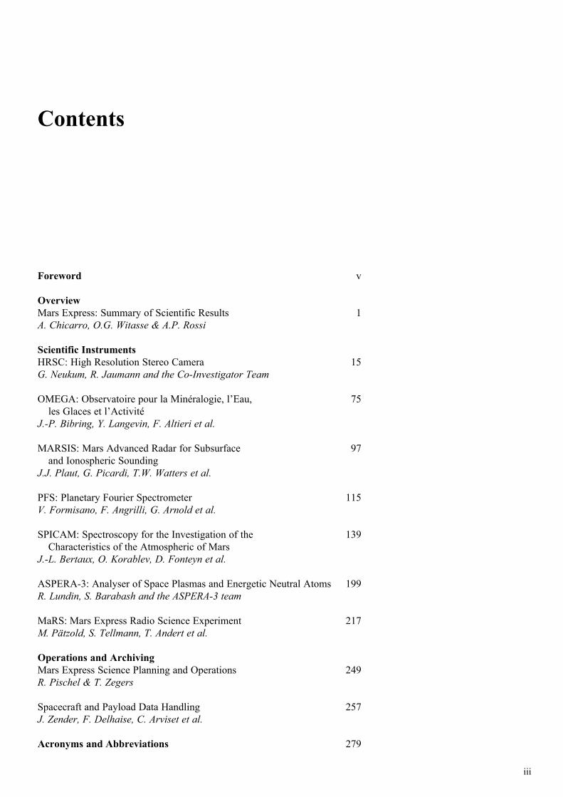
Foreword v
OverviewMars Express: Summary of Scientific Results 1A. Chicarro, O.G. Witasse & A.P. Rossi
Scientific InstrumentsHRSC: High Resolution Stereo Camera 15G. Neukum, R. Jaumann and the Co‑Investigator Team
OMEGA: Observatoire pour la Minéralogie, l’Eau, 75les Glaces et l’Activité
J.‑P. Bibring, Y. Langevin, F. Altieri et al.
MARSIS: Mars Advanced Radar for Subsurface 97and Ionospheric Sounding
J.J. Plaut, G. Picardi, T.W. Watters et al.
PFS: Planetary Fourier Spectrometer 115V. Formisano, F. Angrilli, G. Arnold et al.
SPICAM: Spectroscopy for the Investigation of the 139Characteristics of the Atmospheric of Mars
J.-L. Bertaux, O. Korablev, D. Fonteyn et al.
ASPERA-3: Analyser of Space Plasmas and Energetic Neutral Atoms 199R. Lundin, S. Barabash and the ASPERA-3 team
MaRS: Mars Express Radio Science Experiment 217M. Pätzold, S. Tellmann, T. Andert et al.
Operations and ArchivingMars Express Science Planning and Operations 249R. Pischel & T. Zegers
Spacecraft and Payload Data Handling 257J. Zender, F. Delhaise, C. Arviset et al.
Acronyms and Abbreviations 279
Contents


FOREWORD

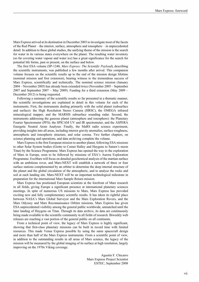
Mars Express arrived at its destination in December 2003 to investigate most of the facets of the Red Planet – the interior, surface, atmosphere and ionosphere – in unprecedented detail. In addition to these global studies, the unifying theme of the mission is the search for water in its various states everywhere on the planet. The resulting water inventory (so far covering water vapour and water ice) has a great significance for the search for potential life forms, past or present, on the surface and below.
The first ESA volume (SP-1240, Mars Express: The Scientific Payload), describing the scientific instruments, was published a few months after arrival. This companion volume focuses on the scientific results up to the end of the mission design lifetime (nominal mission and first extension), bearing witness to the tremendous success of Mars Express, scientifically and technically. The nominal science mission (January 2004 – November 2005) has already been extended twice (November 2005 – September 2007 and September 2007 – May 2009). Funding for a third extension (May 2009 – December 2012) is being requested.
Following a summary of the scientific results so far presented in a thematic manner, the scientific investigations are explained in detail in this volume for each of the instruments. First, the instruments dealing primarily with the solid planet (subsurface and surface): the High Resolution Stereo Camera (HRSC), the OMEGA infrared mineralogical mapper, and the MARSIS subsurface sounding radar. Second, the instruments addressing the gaseous planet (atmosphere and ionosphere): the Planetary Fourier Spectrometer (PFS), the SPICAM UV and IR spectrometer, and the ASPERA Energetic Neutral Atom Analyser. Finally, the MaRS radio science experiment, providing insights into all areas, including interior gravity anomalies, surface roughness, atmospheric and ionospheric structure, and solar corona. Two further chapters, on science planning and operations, and data archiving complete the volume.
Mars Express is the first European mission to another planet, following ESA missions to other Solar System bodies (Giotto to Comet Halley and Huygens to Saturn’s moon Titan) by the Science Programme. Mars Express has opened the way to the exploration of Mars in Europe, soon to be followed by missions of ESA’s Aurora Exploration Programme. ExoMars will focus on detailed geochemical analysis of the martian surface with an ambitious rover, and Mars-NEXT will establish a network of three or four surface stations complemented by an orbiter to determine the deep internal structure of the planet and the global circulation of the atmospheric, and to analyse the rocks and soil at each landing site. Mars-NEXT will be an important technological milestone in preparation for the international Mars Sample Return mission.
Mars Express has positioned European scientists at the forefront of Mars research in all fields, giving Europe a significant presence at international planetary sciences meetings. In spite of numerous US missions to Mars, Mars Express has provided exciting new and fully complementary scientific results. It has taken its rightful place between NASA’s Mars Global Surveyor and the Mars Exploration Rovers, and the Mars Odyssey and Mars Reconnaissance Orbiter missions. Mars Express has given ESA unprecedented visibility among the general public worldwide, unmatched until the later landing of Huygens on Titan. Through its data archive, its data are continuously being made available to the scientific community in all fields of research. Biweekly web releases are reaching a vast portion of the general public on all continents.
From a technical point of view, the legacy of Mars Express is highly significant, showing that first-class planetary missions can be built in record time with limited resources. This made Venus Express possible by using the same spacecraft design and more than half of the Mars Express instruments. From a scientific point of view, in addition to the outstanding results in all areas of Mars science, the legacy of the mission will be measured by the global imaging of its surface at high resolution, largely improving on the 1970s Viking coverage.
Agustin F. ChicarroMars Express Project Scientist
ESTEC, September 2008
vii
Mars Express: foreword
SP-1291
viii
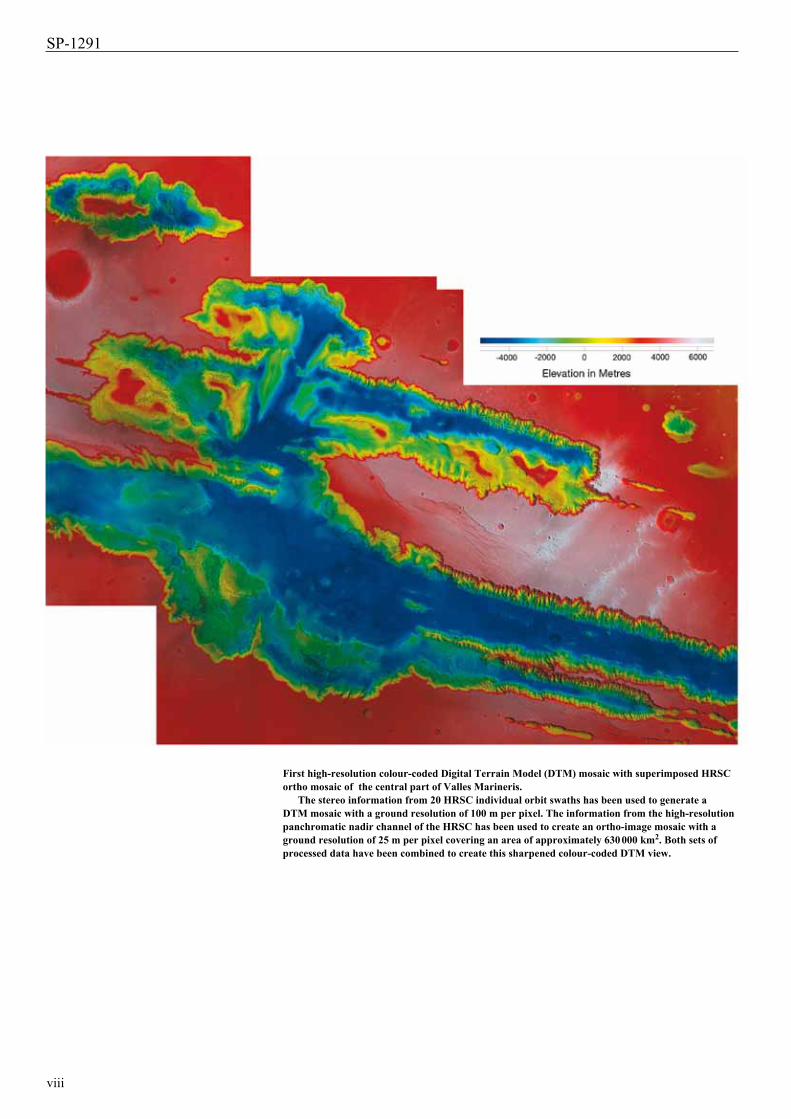
First high-resolution colour-coded Digital Terrain Model (DTM) mosaic with superimposed HRSC ortho mosaic of the central part of Valles Marineris.
The stereo information from 20 HRSC individual orbit swaths has been used to generate a DTM mosaic with a ground resolution of 100 m per pixel. The information from the high-resolution panchromatic nadir channel of the HRSC has been used to create an ortho-image mosaic with a ground resolution of 25 m per pixel covering an area of approximately 630 000 km2. Both sets of processed data have been combined to create this sharpened colour-coded DTM view.
Mars Express
ix
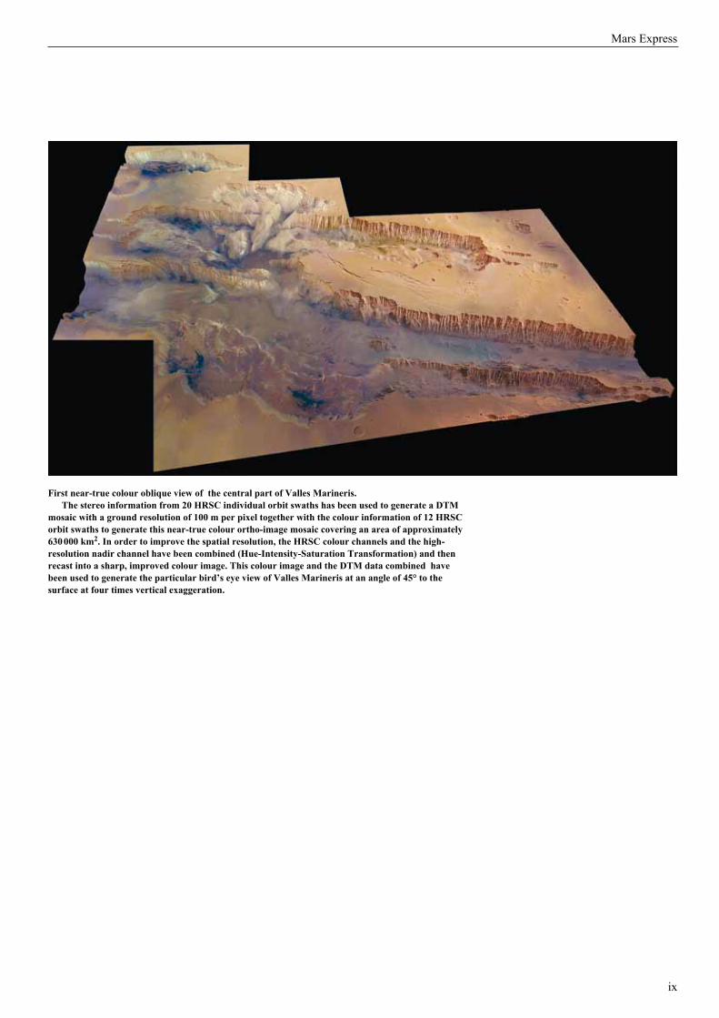
First near-true colour oblique view of the central part of Valles Marineris.The stereo information from 20 HRSC individual orbit swaths has been used to generate a DTM
mosaic with a ground resolution of 100 m per pixel together with the colour information of 12 HRSC orbit swaths to generate this near-true colour ortho-image mosaic covering an area of approximately 630 000 km2. In order to improve the spatial resolution, the HRSC colour channels and the high-resolution nadir channel have been combined (Hue-Intensity-Saturation Transformation) and then recast into a sharp, improved colour image. This colour image and the DTM data combined have been used to generate the particular bird’s eye view of Valles Marineris at an angle of 45° to the surface at four times vertical exaggeration.


1
Overview


3
A.F. Chicarro, O.G. Witasse & A. Pio Rossi
Mars express: Summary of Scientific results
Solar System Missions Division, Research & Scientific Support Department, ESA/ESTEC, PO Box 299, 2200 AG Noordwijk, the Netherlands Email: [email protected]
3
Mars express is the first european mission to another planet. it has opened the way to further european exploration of Mars with the exoMars rover and, one day, with a network of surface stations in preparation for the international Mars Sample return mission. The Mars express spacecraft has been orbiting the red Planet for more than five years, during which time it has investigated many scientific aspects of Mars in unprecedented detail, which are summarised in this chapter. Mars express has revolutionised our understanding of the planet’s geological evolution, allowing us to build a comprehensive and multidisciplinary view of Mars, including the surface geology and mineralogy, the subsurface structure, the state of the interior, the climate’s evolution, the atmospheric dynamics, composition and escape, the aeronomy and the ionospheric structure. Major advances have been made through discoveries such as the very recent (in geological timescales) occurrence of volcanic and glacial processes, the presence of water ice below the surface and the fine structure of the polar caps. The various types of ice in the polar regions have been mapped, and the history of water abundance on the surface of Mars has been determined in view of the alteration minerals formed at different epochs. The mission has revealed the unequivocal presence of methane in the atmosphere, the existence of nightglow, mid-latitude auroras above crustal magnetic fields in the southern highlands and very high-altitude CO2 clouds, as well as the solar wind scavenging of the upper atmosphere down to 270 km altitude and the current rate of atmospheric escape. Detailed studies have been made of the crustal gravity anomalies (and thus the properties of the interior), the surface roughness and the fine structure of the ionosphere. indeed, the presence of methane, independently confirmed by ground measurements, suggests that either volcanism or biological processes are currently active on Mars. either way, these breathtaking results have given us an entirely new view of the planet.
Mars Express has revolutionised our understanding of the planet’s geological evolution, in conjunction with the ‘ground truth’ provided by NASA’s rovers. A great wealth of data has been gathered, allowing us to build a comprehensive and multidisciplinary view of Mars, including the surface geology and mineralogy, the subsurface structure, the state of the interior, the climate’s evolution, the atmospheric dynamics, composition and escape, the aeronomy and the ionospheric structure. Major advances have been made, such as the discovery of water ice below the surface, mapping of the various types of ice in the polar regions, the history of water abundance on the surface of Mars in view of the minerals formed at different epochs, the presence of methane in the atmosphere, mid-latitude auroras above crustal magnetic fields, and much younger timescales for volcanism and glacial processes. Indeed, the presence
1. introduction

SP-1291
4
of methane, independently confirmed by ground measurements, suggests that either volcanism or biological processes are currently active on Mars.
The Mars Express spacecraft has now been orbiting the Red Planet for more than five years. Its High Resolution Stereo Colour Camera (HRSC) has provided breathtaking views of the planet covering both hemispheres, highlighting the very young glacial and volcanic features, from hundreds of thousands to a few million years old, respectively. The OMEGA infrared mineralogical mapping spectrometer has provided unprecedented maps of H2O ice and CO2 ice in the polar regions. It has also shown that the alteration of minerals in the early history of Mars reflect the abundance of liquid water, while the nature of minerals formed later suggest a colder, drier planet with only limited periods of surface water.
Also, high-altitude CO2 ice clouds have been detected in the equatorial region of Mars. The Planetary Fourier Spectrometer (PFS) has confirmed the presence of methane for the first time from orbit, pointing to current volcanic activity and/or biological processes. The SPICAM ultraviolet and infrared atmospheric spectrometer has provided the first complete vertical profiles of CO2 density and temperature. It has also discovered the existence of nightglow over the atmosphere’s nightside, as well as auroras over mid-latitude regions linked to crustal palaeomagnetic signatures, and very high-altitude CO2 clouds. The ASPERA energetic neutral atom analyser has found that the solar wind is slowly stripping off the high atmosphere down to 270 km altitude, and has measured the current rate of atmospheric escape. The MaRS radio science experiment has studied the surface roughness by pointing the spacecraft’s high-gain antenna at the planet and recording the echoes. Also, the martian interior has been probed by studying the gravity anomalies that affect the orbit, and a transient ionospheric layer due to meteors burning in the atmosphere has been identified. Finally, the MARSIS subsurface sounding radar has recorded strong echoes coming from the surface and the subsurface, allowing the identification of the very fine structure of the polar caps. Radar probing of the ionosphere has revealed a variety of echoes originating in areas of remnant magnetism.
One of the objectives of the Mars Radio Science (MaRS) experiment is to study the temporal and spatial variations of the martian gravity field. Gravity is measured by observing the acceleration of a test mass, which is in this case the Mars Express craft itself. For example, the mass excess of a volcano attracts the spacecraft, while the mass deficit of a large impact crater allows the spacecraft to drift away from Mars. Time variations in the gravity field also disturb the spacecraft’s orbit, although in a more complex way. The speed and position of Mars Express can be measured to within a few tens of metres by Earth antennas through the round-trip time and the Doppler frequency shift of the radio signal between Earth and the orbiter. It is then possible to compute precise orbits of Mars Express in order to estimate deviations of the path of the spacecraft with respect to the expected trajectory assuming a reference model of the gravity field. Moreover, flybys above specific targets at the surface of Mars are useful for determining the crustal density and the elastic thickness of the lithosphere. Scientists have focused on the volcanic Tharsis region, for which results point to a high loading density in comparison with the mean density of the martian crust. The trajectory of Mars Express is also disturbed by the mass of the Phobos and Deimos moons, enabling us to refine our estimates of the mass of each moon.
Real imaging of the Mars interior was impossible before Mars Express. Altimetry and radio science data from past NASA missions, as well as Mars Express, have provided indirect information about the internal structure of the planet, but the first ever direct subsurface sounding of any planet has been obtained by MARSIS. This multi-frequency synthetic aperture radar is capable of sounding both ionosphere and subsurface, and of detecting material discontinuities in the subsurface, enabling us to understand the distribution of water, both solid and liquid, in the upper crust. MARSIS has probed the polar layered deposits and investigated them down to their base, at a
2. Deep interior and Subsurface
5
Overview
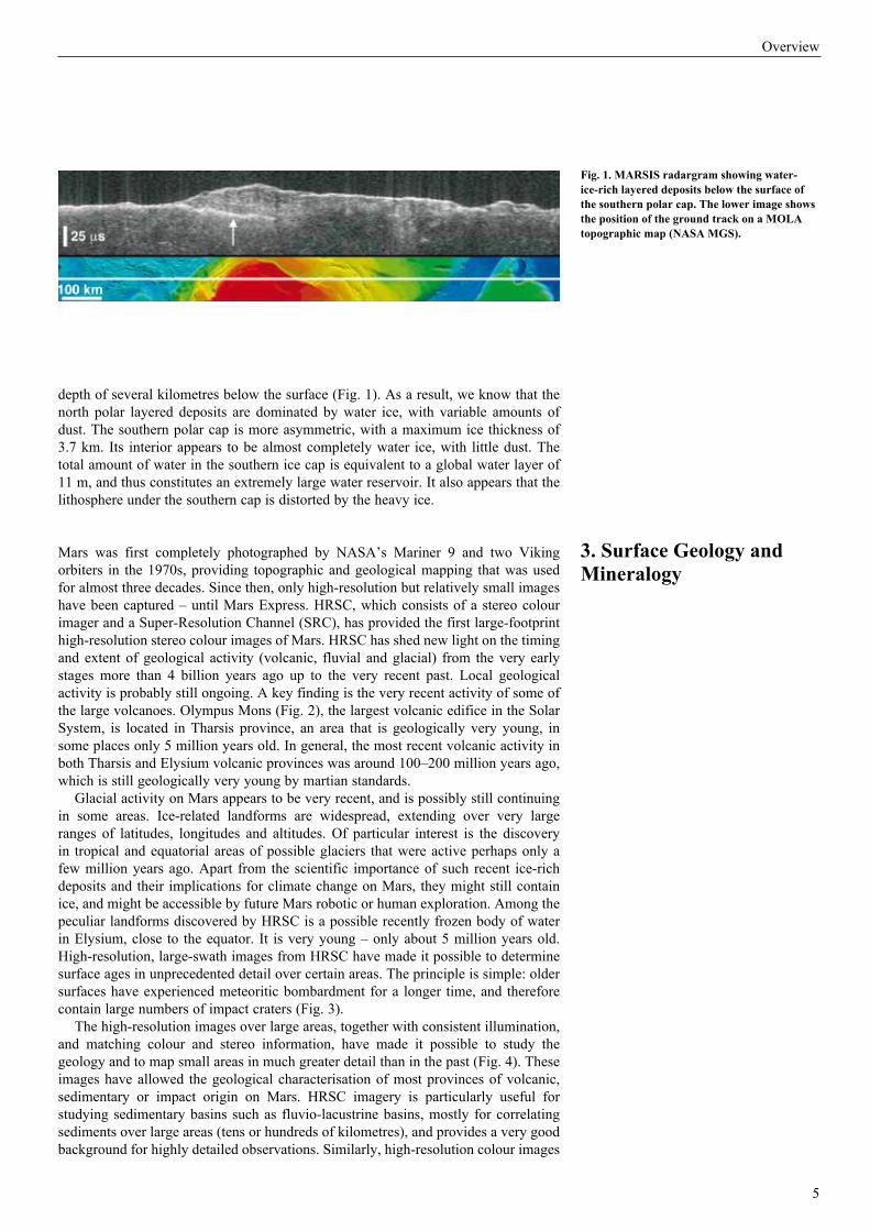
depth of several kilometres below the surface (Fig. 1). As a result, we know that the north polar layered deposits are dominated by water ice, with variable amounts of dust. The southern polar cap is more asymmetric, with a maximum ice thickness of 3.7 km. Its interior appears to be almost completely water ice, with little dust. The total amount of water in the southern ice cap is equivalent to a global water layer of 11 m, and thus constitutes an extremely large water reservoir. It also appears that the lithosphere under the southern cap is distorted by the heavy ice.
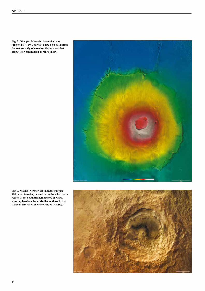
Mars was first completely photographed by NASA’s Mariner 9 and two Viking orbiters in the 1970s, providing topographic and geological mapping that was used for almost three decades. Since then, only high-resolution but relatively small images have been captured – until Mars Express. HRSC, which consists of a stereo colour imager and a Super-Resolution Channel (SRC), has provided the first large-footprint high-resolution stereo colour images of Mars. HRSC has shed new light on the timing and extent of geological activity (volcanic, fluvial and glacial) from the very early stages more than 4 billion years ago up to the very recent past. Local geological activity is probably still ongoing. A key finding is the very recent activity of some of the large volcanoes. Olympus Mons (Fig. 2), the largest volcanic edifice in the Solar System, is located in Tharsis province, an area that is geologically very young, in some places only 5 million years old. In general, the most recent volcanic activity in both Tharsis and Elysium volcanic provinces was around 100–200 million years ago, which is still geologically very young by martian standards.
Glacial activity on Mars appears to be very recent, and is possibly still continuing in some areas. Ice-related landforms are widespread, extending over very large ranges of latitudes, longitudes and altitudes. Of particular interest is the discovery in tropical and equatorial areas of possible glaciers that were active perhaps only a few million years ago. Apart from the scientific importance of such recent ice-rich deposits and their implications for climate change on Mars, they might still contain ice, and might be accessible by future Mars robotic or human exploration. Among the peculiar landforms discovered by HRSC is a possible recently frozen body of water in Elysium, close to the equator. It is very young – only about 5 million years old. High-resolution, large-swath images from HRSC have made it possible to determine surface ages in unprecedented detail over certain areas. The principle is simple: older surfaces have experienced meteoritic bombardment for a longer time, and therefore contain large numbers of impact craters (Fig. 3).
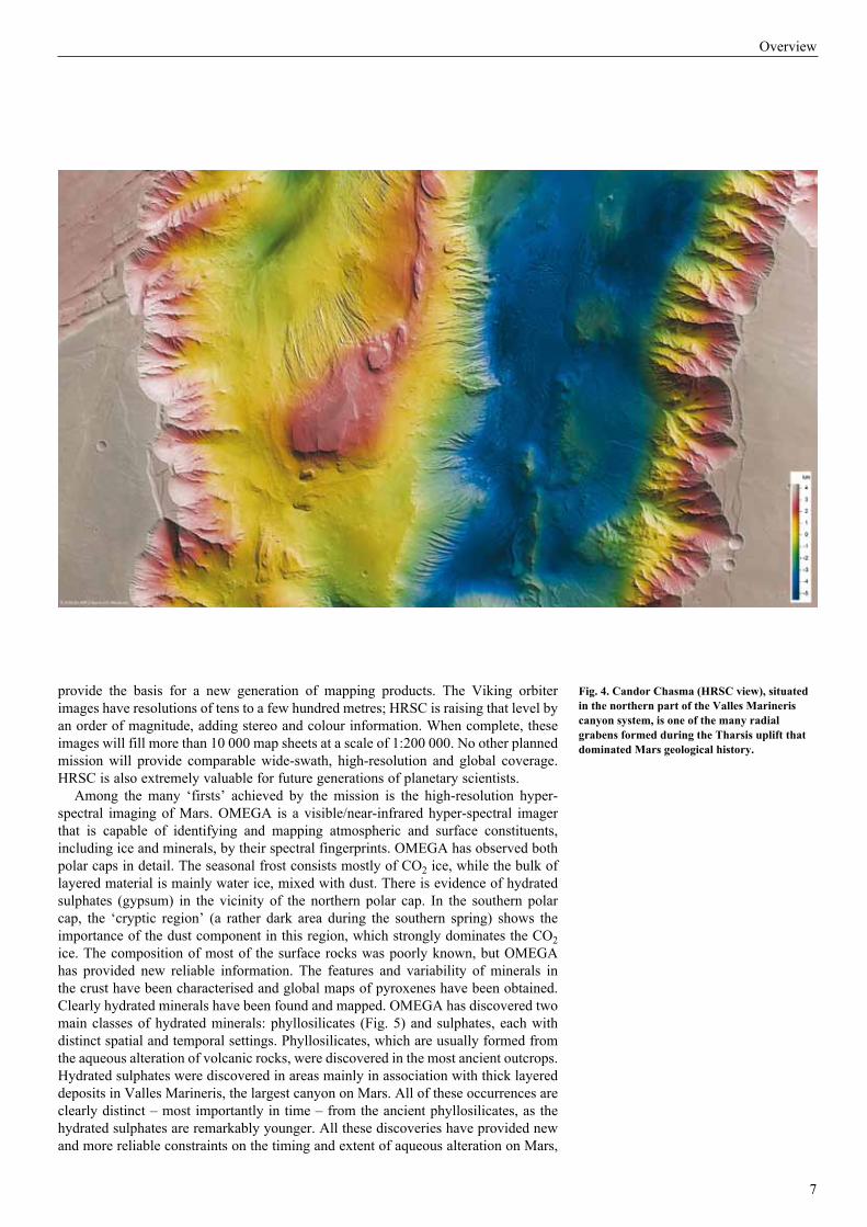
The high-resolution images over large areas, together with consistent illumination, and matching colour and stereo information, have made it possible to study the geology and to map small areas in much greater detail than in the past (Fig. 4). These images have allowed the geological characterisation of most provinces of volcanic, sedimentary or impact origin on Mars. HRSC imagery is particularly useful for studying sedimentary basins such as fluvio-lacustrine basins, mostly for correlating sediments over large areas (tens or hundreds of kilometres), and provides a very good background for highly detailed observations. Similarly, high-resolution colour images
3. Surface Geology and Mineralogy
Fig. 1. MArSiS radargram showing water-ice-rich layered deposits below the surface of the southern polar cap. The lower image shows the position of the ground track on a MOLA topographic map (NASA MGS).
6
SP-1291
Fig. 2. Olympus Mons (in false colour) as imaged by HrSC, part of a new high-resolution dataset recently released on the internet that allows the visualisation of Mars in 3D.
Fig. 3. Maunder crater, an impact structure 90 km in diameter, located in the Noachis Terra region of the southern hemisphere of Mars, showing barchan dunes similar to those in the African deserts on the crater floor (HrSC).
7
Overview
provide the basis for a new generation of mapping products. The Viking orbiter images have resolutions of tens to a few hundred metres; HRSC is raising that level by an order of magnitude, adding stereo and colour information. When complete, these images will fill more than 10 000 map sheets at a scale of 1:200 000. No other planned mission will provide comparable wide-swath, high-resolution and global coverage. HRSC is also extremely valuable for future generations of planetary scientists.
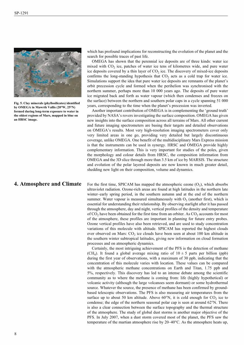
Among the many ‘firsts’ achieved by the mission is the high-resolution hyper-spectral imaging of Mars. OMEGA is a visible/near-infrared hyper-spectral imager that is capable of identifying and mapping atmospheric and surface constituents, including ice and minerals, by their spectral fingerprints. OMEGA has observed both polar caps in detail. The seasonal frost consists mostly of CO2 ice, while the bulk of layered material is mainly water ice, mixed with dust. There is evidence of hydrated sulphates (gypsum) in the vicinity of the northern polar cap. In the southern polar cap, the ‘cryptic region’ (a rather dark area during the southern spring) shows the importance of the dust component in this region, which strongly dominates the CO2 ice. The composition of most of the surface rocks was poorly known, but OMEGA has provided new reliable information. The features and variability of minerals in the crust have been characterised and global maps of pyroxenes have been obtained. Clearly hydrated minerals have been found and mapped. OMEGA has discovered two main classes of hydrated minerals: phyllosilicates (Fig. 5) and sulphates, each with distinct spatial and temporal settings. Phyllosilicates, which are usually formed from the aqueous alteration of volcanic rocks, were discovered in the most ancient outcrops. Hydrated sulphates were discovered in areas mainly in association with thick layered deposits in Valles Marineris, the largest canyon on Mars. All of these occurrences are clearly distinct – most importantly in time – from the ancient phyllosilicates, as the hydrated sulphates are remarkably younger. All these discoveries have provided new and more reliable constraints on the timing and extent of aqueous alteration on Mars,
Fig. 4. Candor Chasma (HrSC view), situated in the northern part of the valles Marineris canyon system, is one of the many radial grabens formed during the Tharsis uplift that dominated Mars geological history.
8
SP-1291
which has profound implications for reconstructing the evolution of the planet and the search for possible traces of past life.
OMEGA has shown that the perennial ice deposits are of three kinds: water ice mixed with CO2 ice, patches of water ice tens of kilometres wide, and pure water ice deposits covered by a thin layer of CO2 ice. The discovery of mixed-ice deposits confirms the long-standing hypothesis that CO2 acts as a cold trap for water ice. Simulations support the idea that pure water ice deposits are remnants of the planet’s orbit precession cycle and formed when the perihelion was synchronised with the northern summer, perhaps more than 10 000 years ago. The deposits of pure water ice migrated back and forth as water vapour (which then condenses and freezes on the surface) between the northern and southern polar caps in a cycle spanning 51 000 years, corresponding to the time when the planet’s precession was inverted.
Another important contribution of OMEGA is in complementing the ‘ground truth’ provided by NASA’s rovers investigating the surface composition. OMEGA has given new insights into the surface composition across all terrains of Mars. All other current and future imaging spectrometers are basing their targets and detailed observations on OMEGA’s results. Most very high-resolution imaging spectrometers cover only very limited areas in one go, providing very detailed but largely discontinuous coverage, unlike OMEGA. One benefit of the multidisciplinary Mars Express mission is that the instruments can be used in synergy. HRSC and OMEGA provide highly complementary information. This is very important for studies of the poles, given the morphology and colour details from HRSC, the composition information from OMEGA and the 3D slice through more than 3.5 km of ice by MARSIS. The structure and evolution of the polar layered deposits are now known in much greater detail, shedding new light on their composition, volume and dynamics.
For the first time, SPICAM has mapped the atmospheric ozone (O3), which absorbs ultraviolet radiation. Ozone-rich areas are found at high latitudes in the northern late winter–early spring period, in the southern autumn and at the end of the northern summer. Water vapour is measured simultaneously with O3 (another first), which is essential for understanding their relationship. By observing starlight after it has passed through the atmosphere, day and night, vertical profiles of the density and temperature of CO2 have been obtained for the first time from an orbiter. As CO2 accounts for most of the atmosphere, these profiles are important in planning for future entry probes. Ozone vertical profiles have also been retrieved, and are used to study concentration variations of this molecule with altitude. SPICAM has reported the highest clouds ever observed on Mars: CO2 ice clouds have been seen at about 100 km altitude in the southern winter subtropical latitudes, giving new information on cloud formation processes and on atmospheric dynamics.
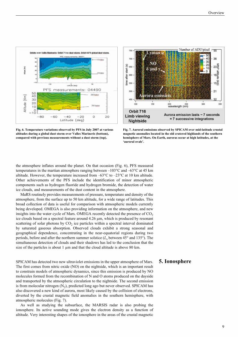
Certainly, the most intriguing achievement of the PFS is the detection of methane (CH4). It found a global average mixing ratio of 10 ± 5 parts per billion (ppb) during the first year of observations, with a maximum of 30 ppb, indicating that the concentration of this molecule varies with location. These values can be compared with the atmospheric methane concentrations on Earth and Titan, 1.75 ppb and 5%, respectively. This discovery has led to an intense debate among the scientific community as to where the methane is coming from: life (highly hypothetical) or volcanic activity (although the large volcanoes seem dormant) or some hydrothermal source. Whatever the source, the presence of methane has been confirmed by ground-based telescopic observations. The PFS is also measuring air temperatures from the surface up to about 50 km altitude. Above 60°N, it is cold enough for CO2 ice to condense; the edge of the northern seasonal polar cap is seen at around 62°N. There is also a clear connection between the surface topography and the thermal structure of the atmosphere. The study of global dust storms is another major objective of the PFS. In July 2007, when a dust storm covered most of the planet, the PFS saw the temperature of the martian atmosphere rise by 20–40°C. As the atmosphere heats up,
4. Atmosphere and Climate
Fig. 5. Clay minerals (phyllosilicates) identified by OMeGA in Mawrth vallis (20°w, 25°N) formed during long-term exposure to water in the oldest regions of Mars, mapped in blue on an HrSC image.
9
Overview
the atmosphere inflates around the planet. On that occasion (Fig. 6), PFS measured temperatures in the martian atmosphere ranging between –103°C and –63°C at 45 km altitude. However, the temperature increased from –63°C to –23°C at 10 km altitude. Other achievements of the PFS include the identification of minor atmospheric components such as hydrogen fluoride and hydrogen bromide, the detection of water ice clouds, and measurements of the dust content in the atmosphere.
MaRS routinely provides measurements of pressure, temperature and density of the atmosphere, from the surface up to 50 km altitude, for a wide range of latitudes. This broad collection of data is useful for comparison with atmospheric models currently being developed. OMEGA is also providing information on the atmosphere, and new insights into the water cycle of Mars. OMEGA recently detected the presence of CO2 ice clouds based on a spectral feature around 4.26 µm, which is produced by resonant scattering of solar photons by CO2 ice particles within a spectral interval dominated by saturated gaseous absorption. Observed clouds exhibit a strong seasonal and geographical dependence, concentrating in the near-equatorial regions during two periods, before and after the northern summer solstice (Ls between 45° and 135°). The simultaneous detection of clouds and their shadows has led to the conclusion that the size of the particles is about 1 µm and that the cloud altitude is above 80 km.
SPICAM has detected two new ultraviolet emissions in the upper atmosphere of Mars. The first comes from nitric oxide (NO) on the nightside, which is an important result to constrain models of atmospheric dynamics, since this emission is produced by NO molecules formed from the recombination of N and O atoms produced on the dayside and transported by the atmospheric circulation to the nightside. The second emission is from molecular nitrogen (N2), predicted long ago but never observed. SPICAM has also discovered a new kind of aurora, most likely caused by the collision of electrons, diverted by the crustal magnetic field anomalies in the southern hemisphere, with atmospheric molecules (Fig. 7).
As well as studying the subsurface, the MARSIS radar is also probing the ionosphere. Its active sounding mode gives the electron density as a function of altitude. Very interesting shapes of the ionosphere in the areas of the crustal magnetic
5. ionosphere
Fig. 6. Temperature variations observed by PFS in July 2007 at various altitudes during a global dust storm over valles Marineris (bottom), compared with previous measurements without a dust storm (top).
Fig. 7. Auroral emissions observed by SPiCAM over mid-latitude crustal magnetic anomalies located in the old cratered highlands of the southern hemisphere of Mars. On earth, auroras occur at high latitudes, at the ‘auroral ovals’.
10
SP-1291
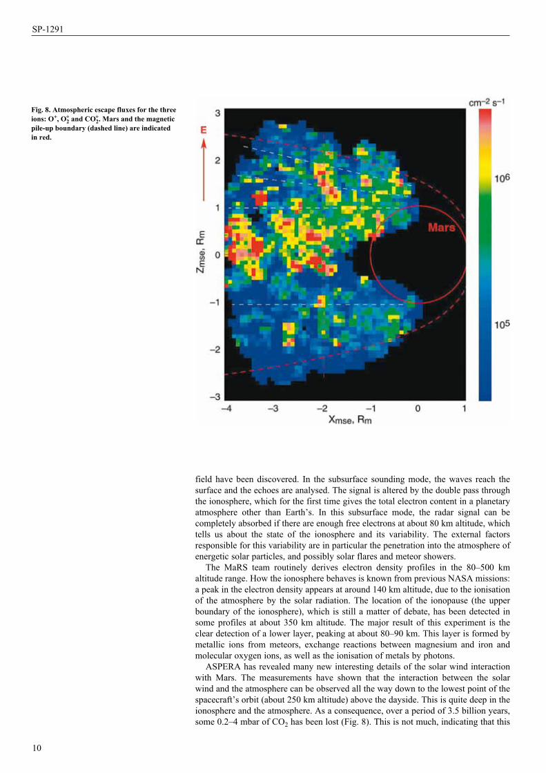
Fig. 8. Atmospheric escape fluxes for the three ions: O+, O2
+ and CO2+. Mars and the magnetic
pile-up boundary (dashed line) are indicated in red.
field have been discovered. In the subsurface sounding mode, the waves reach the surface and the echoes are analysed. The signal is altered by the double pass through the ionosphere, which for the first time gives the total electron content in a planetary atmosphere other than Earth’s. In this subsurface mode, the radar signal can be completely absorbed if there are enough free electrons at about 80 km altitude, which tells us about the state of the ionosphere and its variability. The external factors responsible for this variability are in particular the penetration into the atmosphere of energetic solar particles, and possibly solar flares and meteor showers.
The MaRS team routinely derives electron density profiles in the 80–500 km altitude range. How the ionosphere behaves is known from previous NASA missions: a peak in the electron density appears at around 140 km altitude, due to the ionisation of the atmosphere by the solar radiation. The location of the ionopause (the upper boundary of the ionosphere), which is still a matter of debate, has been detected in some profiles at about 350 km altitude. The major result of this experiment is the clear detection of a lower layer, peaking at about 80–90 km. This layer is formed by metallic ions from meteors, exchange reactions between magnesium and iron and molecular oxygen ions, as well as the ionisation of metals by photons.
ASPERA has revealed many new interesting details of the solar wind interaction with Mars. The measurements have shown that the interaction between the solar wind and the atmosphere can be observed all the way down to the lowest point of the spacecraft’s orbit (about 250 km altitude) above the dayside. This is quite deep in the ionosphere and the atmosphere. As a consequence, over a period of 3.5 billion years, some 0.2–4 mbar of CO2 has been lost (Fig. 8). This is not much, indicating that this

11
Overview
6. Concluding remarks
is not an efficient way for the atmosphere to escape. With its novel technique for measuring energetic neutral atoms (ENAs), ASPERA is exploring a new dimension of the interaction of the solar wind with planets that have no intrinsic magnetic field. Mars is ‘shining’ in ENAs. Part of this is caused by reflections of inflowing hydrogen ENAs from the solar wind, but a large fraction is emitted when hot plasma, from the solar and planetary winds, interacts with the upper atmosphere to create ENAs.
Mars Express has entirely revolutionised our understanding of the planet’s geological and climate history. The mission has allowed major discoveries to be made, including the very recent (in geological timescales) occurrence of volcanic and glacial processes, the presence of water ice below the surface and the fine structure of the polar caps. The various types of ice in the polar regions have been mapped, and the past water abundance on the surface has been determined in view of the alteration minerals formed at different epochs. The mission has revealed the unequivocal presence of methane in the atmosphere, the existence of nightglow, mid-latitude auroras above remnant magnetic fields in the southern highlands and very high-altitude CO2 clouds, as well as the solar wind scavenging of the upper atmosphere down to 270 km altitude and the current rate of atmospheric escape. Detailed studies have been made of the crustal gravity anomalies (and thus the properties of the interior), the surface roughness and the fine structure of the ionosphere.
New techniques used by state-of-the-art instruments have provided the first subsurface radar sounding of another planet, complete atmospheric density and temperature profiles up to 100 km altitude, stellar occultations, total electron content in the ionosphere and surface coverage at high resolution, in both stereo and colour. The coverage will eventually be global provided that the mission is sufficiently extended. The superb images have provided ESA with a significant tool for public outreach, and will also undoubtedly be the legacy of the mission for future generations of planetary scientists as well as the general public.
So far, the various Mars Express experiment teams have published over 250 refereed papers in scientific journals. The scientific data from the nominal mission is now available in the mission archive for further study by the public and scientists alike. The Principal Investigators and their large teams of co-investigators, together with the various ESA teams throughout almost all its establishments, have contributed to the tremendous success of this mission.
The nominal mission lifetime of the orbiter of one martian year (January 2004 to November 2005) has already been extended twice, up to May 2009. The extensions give priority to achieving the remaining goals of the nominal mission (including gravity measurements and seasonal coverage), to catch up with delayed MARSIS observations, and to complete global coverage of high-resolution imaging and spectroscopy. Other goals include subsurface sounding with the radar, observing atmospheric and variable phenomena, and revisiting areas of past discoveries. The scope of cooperation has been broadened, in particular with NASA’s Mars rovers Mars Odyssey and Mars Reconnaissance Orbiter, and with Venus Express, which is carrying the same instruments and provides a unique opportunity for comparing our nearest neighbours.
Finally, Mars Express is providing valuable data for preparing two planned missions of ESA’s Exploration Programme: ExoMars, which includes a rover for biological, geophysical and climatological investigations, and Mars-NEXT, which includes a network of three or four surface stations complemented by an orbiter for determining the internal structure, the global atmospheric circulation and the geology and geochemistry of the landing sites. In particular, the data from Mars Express are being used to establish a surface/subsurface geosciences database and to refine the existing atmospheric models, in order to identify potential landing sites of high scientific value, and to assess risks during atmospheric entry, descent and landing for the future exploration of Mars.
More detailed information about the Mars Express mission and its wealth of scientific results can be found at http://sci.esa.int/marsexpress


Scientific inStrumentS

15
G. Neukum1, R. Jaumann2,1, A.T. Basilevsky3, A. Dumke1, S. van Gasselt1, B. Giese2, E. Hauber2, J.W. Head, III4, C. Heipke5, N. Hoekzema6, H. Hoffmann2, R. Greeley7, K. Gwinner2, R. Kirk8, W. Markiewicz6, T.B. McCord9, G. Michael1, J.-P. Muller10, J. B. Murray11, J. Oberst12,2, P. Pinet13, R. Pischel14, T. Roatsch2, F. Scholten2, K. Willner2, the HRSC Co-Investigator Team15 and HRSC Associates
1 Freie Universität Berlin (FUB), Institute of Geosciences, Planetology and Remote Sensing, Berlin, Germany2 German Aerospace Center (DLR) Berlin, Institute of Planetary Research, Berlin, Germany3 Vernadsky Institute of Geochemistry and Analytical Chemistry, Russian Academy of Science, Moscow, Russia4 Brown University, Department of Geological Sciences, Providence, RI, USA5 Universität Hannover, Institut für Photogrammetrie und GeoInformation (IPI), Hannover, Germany6 Max Planck Institute for Solar System Research (MPS), Katlenburg-Lindau, Germany7 Arizona State University (ASU), School of Earth and Space Exploration (SESE), Tempe, AZ, USA8 US Geological Survey (USGS), Astrogeology Program, Flagstaff, AZ, USA9 Bear Fight Center, Space Science Institute, Winthrop, WA, USA10 UCL Mullard Space Science Laboratory, MSSL, Space and Climate Physics, Dorking, Surrey, UK11 The Open University, Department of Earth Sciences, Milton Keynes, UK12 Technical University of Berlin, Geodesy and Geoinformation Science, Planetary Geodesy, Berlin, Germany13 Laboratoire dynamique terrestre et planetaire de l’Observatoire de Midi-Pyrenees, Toulouse, France14 ESA Moscow, Moscow, Russia15 See Table 7
HrSc: High resolution Stereo camera
15
the High resolution Stereo camera (HrSc) on mars express has delivered a wealth of image data, amounting to over 2.5 tB from the start of the mapping phase in January 2004 to September 2008. in that time, more than a third of mars was covered at a resolution of 10–20 m/pixel in stereo and colour. After five years in orbit, HrSc is still in excellent shape, and it could continue to operate for many more years. HrSc has proven its ability to close the gap between the low-resolution Viking image data and the high-resolution mars Orbiter camera images, leading to a global picture of the geological evolution of mars that is now much clearer than ever before. Derived highest-resolution terrain model data have closed major gaps and provided an unprecedented insight into the shape of the surface, which is paramount not only for surface analysis and geological interpretation, but also for combination with and analysis of data from other instruments, as well as in planning for future missions.
this chapter presents the scientific output from data analysis and high-level data processing, complemented by a summary of how the experiment is conducted by the HrSc team members working in geoscience, atmospheric science, photogrammetry and spectrophotometry. many of these contributions have been or will be published in peer-reviewed journals and special issues. they form a cross-section of the scientific output, either by summarising the new geoscientific picture of mars provided by HrSc or by detailing some of the topics of data analysis concerning photogrammetry, cartography and spectral data analysis.

16
SP-1291
The HRSC experiment on Mars Express has delivered a wealth of data since the start of its orbital mapping phase in January 2004. At the time of writing, the goal of global coverage had been partially achieved, with 35% coverage at a resolution of 10–20 m/pixel in stereo and colour, and it is expected that ~60% coverage will have been achieved by the end of the present mission extension period (May 2009). Unfortunately, we will then still be some way from the primary goal of the HRSC to achieve 100% coverage at 10–20 m/pixel, but this is due to the much more limited operational performance of the spacecraft in terms of data acquisition and downlink capabilities than was envisaged in the original plans before launch. Nevertheless, the original coverage goal could be achieved with an appropriate further extension of the mission and the full operation of the HRSC.
Technically, there does not appear to be a problem with the HRSC; the instrument is in very good shape, and it could continue to operate for many more years. The scientific output from the analysis of the imagery over 3.5 years of operation is remarkable. The HRSC team has been slightly modified to include new scientists working in areas where it was realised that sufficient experience in data analysis was lacking in the original team, and it consists of 44 individual co-investigators from 26 institutions and 10 countries (Fig. 1). By 2009 several co-investigators will join or will have left the team (see Table 7). The team’s outputs so far include 60 refereed papers published in professional journals, as well as 120 extended abstracts (citable short papers) and 350 conference abstracts and related talks or posters. Also, seven young scientists associated with the team members have completed doctoral and diploma/master theses. Among the publications are landmark papers in prestigious journals such as Nature (Neukum et al., 2004a; Hauber et al., 2005a; Head et al., 2005a; Murray et al., 2005).
This chapter represents the first attempt to provide a comprehensive summary of the most important results of the HRSC CoI team as a ‘team effort’ covering all scientific areas relevant in the data analysis directly related and close in time to the data flow from the mission. These include results from the geosciences, atmospheric, photogrammetry and cartography, and spectrophotometry working groups. It should be noted that the HRSC dataset has to undergo a complicated data processing effort by a number of groups of the team, in particular the DLR group in Berlin and the other groups that handle the production of Digital Terrain Models (DTMs). At present, a new effort is under way to produce high-resolution archive-quality DTMs, financed by the DLR agency and concentrated at DLR Berlin and FU Berlin. This will significantly enhance the usability of the stereo data, and will probably have a very positive effect in the area of data analysis offline.
1. introduction
fig. 1. the HrSc team.

17
Scientific instruments
For readers who are familiar with the history of the exploration of Mars, the previously (before HRSC) available large-area coverage imagery and the previous interpretation of the geological evolution and history of Mars, this chapter will demonstrate that the HRSC experiment has opened up new domains of in-depth scientific interpretation, and is already is beginning to change our view of Mars considerably. To give just a few examples: the idea that Mars was wet and warm, with a thick atmosphere, early on, possibly lasting long into mid-martian history, is now questioned. Whether there was a global ocean for a long period of time early on seems rather unlikely on the basis of the analysis of the HRSC data (and OMEGA data). It is now becoming clear that the evolution of the martian surface was probably not steady over time but episodic. All of these questions will be addressed further in the course of the mission with additional HRSC data, and there may be many surprises in the future.
The HRSC (Fig. 2) represents a multi-sensor push-broom instrument comprising nine CCD line sensors mounted in parallel for simultaneous high-resolution stereo, multicolour and multi-phase imaging by delivering nine superimposed image swaths (Jaumann et al., 2007). The HRSC is designed to perform stereo imaging with triple to quintuple panchromatic along-track stereo, including a nadir-directed, forward and aft-looking (±18.9°), and two inner (±12.8°) stereo line sensors. Their spectral range covers 675 ± 90 nm (width at half-maximum). Multispectral imaging is realised by four line sensors in the blue, green, red and near-infrared colour ranges (440 ± 45, 530 ± 45, 750 ± 20 and 970 ± 45 nm). All nine line sensors have a cross-track field of view of ±6°. They are mounted behind one single transmission optics with a focal length of 175 mm and an aperture of f = 5.6. Each of the nine Thomson THX 7808B linear CCD arrays has 5184 active pixels 7 × 7 µm in size. An additional Super-Resolution Channel (SRC) provides frame images embedded in the basic HRSC swath at five times higher
2. HrSc experiment and Achievements
fig. 2. Operating principle and viewing geometry of the individual ccD sensors: nD, nadir channel; S1, S2, stereo 1 and stereo 2 (±18.9°); P1 and P2, photometry 1 and photometry 2 (±12.8°); ir, near-infrared channel (+15.9°); Gr, green channel (+3.3°); BL, blue channel (–3.3°); re, red channel (–15.9°). All nine lines sensors have a cross track field of view of ±6°. Src, Super-resolution channel (panchromatic).
18
SP-1291
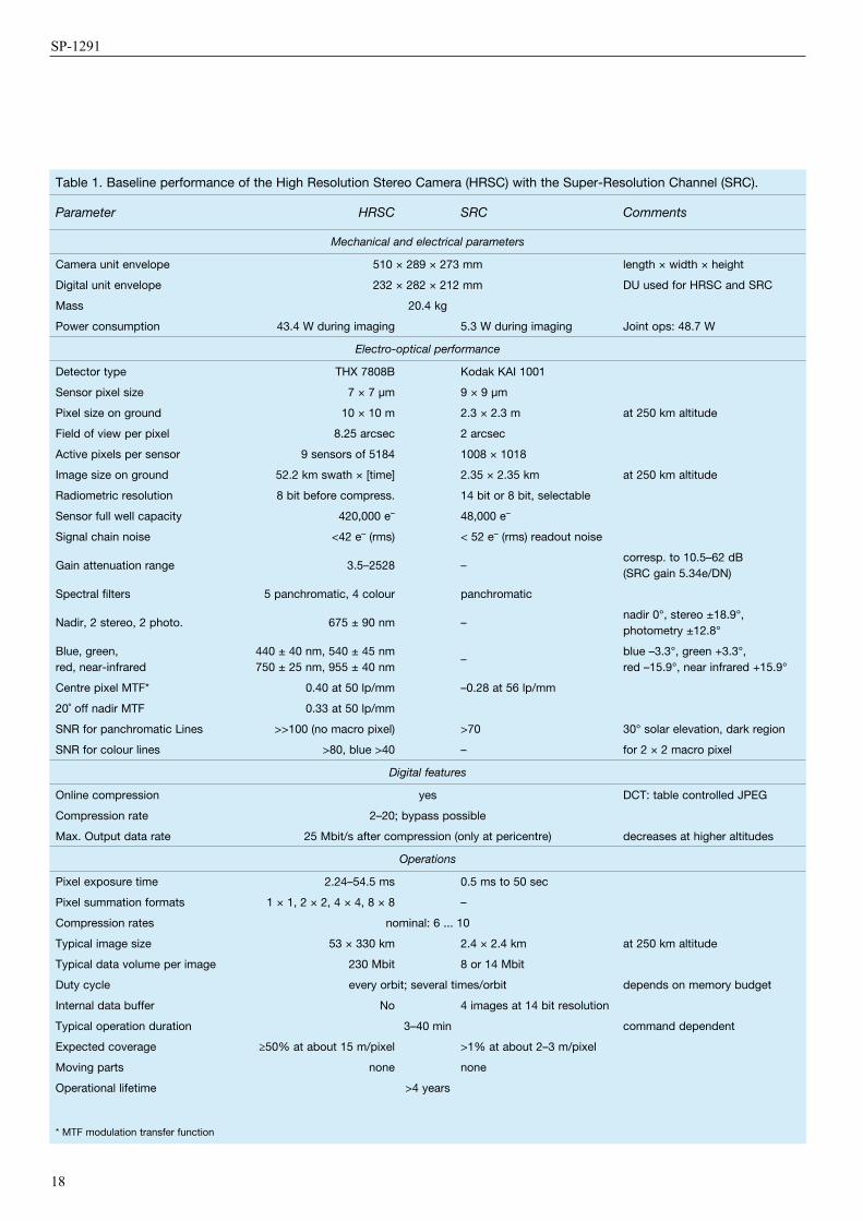
Table 1. Baseline performance of the High Resolution Stereo Camera (HRSC) with the Super-Resolution Channel (SRC).
Parameter HRSC SRC Comments
Mechanical and electrical parameters
Camera unit envelope 510 × 289 × 273 mm length × width × height
Digital unit envelope 232 × 282 × 212 mm DU used for HRSC and SRC
Mass 20.4 kg
Power consumption 43.4 W during imaging 5.3 W during imaging Joint ops: 48.7 W
Electro-optical performance
Detector type THX 7808B Kodak KAI 1001
Sensor pixel size 7 × 7 µm 9 × 9 µm
Pixel size on ground 10 × 10 m 2.3 × 2.3 m at 250 km altitude
Field of view per pixel 8.25 arcsec 2 arcsec
Active pixels per sensor 9 sensors of 5184 1008 × 1018
Image size on ground 52.2 km swath × [time] 2.35 × 2.35 km at 250 km altitude
Radiometric resolution 8 bit before compress. 14 bit or 8 bit, selectable
Sensor full well capacity 420,000 e– 48,000 e–
Signal chain noise <42 e– (rms) < 52 e– (rms) readout noise
Gain attenuation range 3.5–2528 –corresp. to 10.5–62 dB (SRC gain 5.34e/DN)
Spectral filters 5 panchromatic, 4 colour panchromatic
Nadir, 2 stereo, 2 photo. 675 ± 90 nm –nadir 0°, stereo ±18.9°, photometry ±12.8°
Blue, green, red, near-infrared
440 ± 40 nm, 540 ± 45 nm 750 ± 25 nm, 955 ± 40 nm
–blue –3.3°, green +3.3°, red –15.9°, near infrared +15.9°
Centre pixel MTF* 0.40 at 50 lp/mm –0.28 at 56 lp/mm
20˚ off nadir MTF 0.33 at 50 lp/mm
SNR for panchromatic Lines >>100 (no macro pixel) >70 30° solar elevation, dark region
SNR for colour lines >80, blue >40 – for 2 × 2 macro pixel
Digital features
Online compression yes DCT: table controlled JPEG
Compression rate 2–20; bypass possible
Max. Output data rate 25 Mbit/s after compression (only at pericentre) decreases at higher altitudes
Operations
Pixel exposure time 2.24–54.5 ms 0.5 ms to 50 sec
Pixel summation formats 1 × 1, 2 × 2, 4 × 4, 8 × 8 –
Compression rates nominal: 6 ... 10
Typical image size 53 × 330 km 2.4 × 2.4 km at 250 km altitude
Typical data volume per image 230 Mbit 8 or 14 Mbit
Duty cycle every orbit; several times/orbit depends on memory budget
Internal data buffer No 4 images at 14 bit resolution
Typical operation duration 3–40 min command dependent
Expected coverage ≥50% at about 15 m/pixel >1% at about 2–3 m/pixel
Moving parts none none
Operational lifetime >4 years
* MTF modulation transfer function
19
Scientific instruments
resolution. The SRC comprises a 1024 × 1024 CCD array and lightweight mirror optics with its optical axis parallel to that of the HRSC camera head. The total mass of the HRSC, including the SRC, is 20.4 kg. During imaging the total power consumption is 48.7 W. The focal plane temperature is kept within the range +7 to +17°C by camera internal heaters. The characteristic parameters of the instrument are given in Table 1.
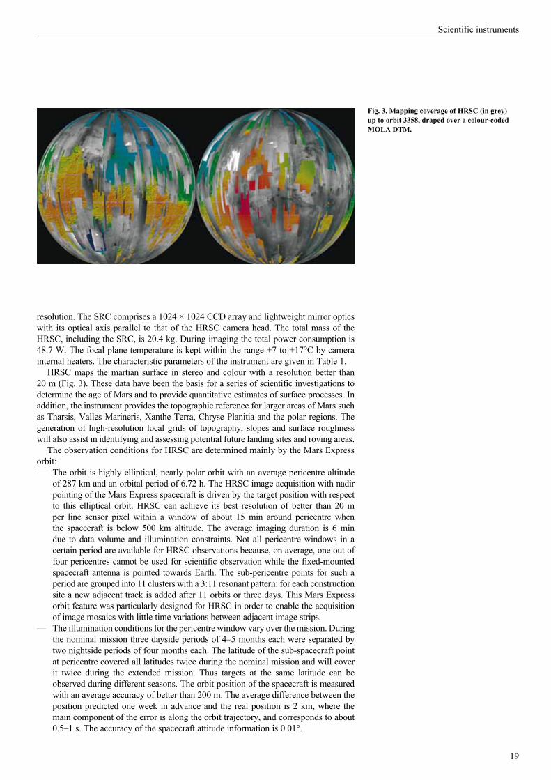
HRSC maps the martian surface in stereo and colour with a resolution better than 20 m (Fig. 3). These data have been the basis for a series of scientific investigations to determine the age of Mars and to provide quantitative estimates of surface processes. In addition, the instrument provides the topographic reference for larger areas of Mars such as Tharsis, Valles Marineris, Xanthe Terra, Chryse Planitia and the polar regions. The generation of high-resolution local grids of topography, slopes and surface roughness will also assist in identifying and assessing potential future landing sites and roving areas.
The observation conditions for HRSC are determined mainly by the Mars Express orbit:— The orbit is highly elliptical, nearly polar orbit with an average pericentre altitude
of 287 km and an orbital period of 6.72 h. The HRSC image acquisition with nadir pointing of the Mars Express spacecraft is driven by the target position with respect to this elliptical orbit. HRSC can achieve its best resolution of better than 20 m per line sensor pixel within a window of about 15 min around pericentre when the spacecraft is below 500 km altitude. The average imaging duration is 6 min due to data volume and illumination constraints. Not all pericentre windows in a certain period are available for HRSC observations because, on average, one out of four pericentres cannot be used for scientific observation while the fixed-mounted spacecraft antenna is pointed towards Earth. The sub-pericentre points for such a period are grouped into 11 clusters with a 3:11 resonant pattern: for each construction site a new adjacent track is added after 11 orbits or three days. This Mars Express orbit feature was particularly designed for HRSC in order to enable the acquisition of image mosaics with little time variations between adjacent image strips.
— The illumination conditions for the pericentre window vary over the mission. During the nominal mission three dayside periods of 4–5 months each were separated by two nightside periods of four months each. The latitude of the sub-spacecraft point at pericentre covered all latitudes twice during the nominal mission and will cover it twice during the extended mission. Thus targets at the same latitude can be observed during different seasons. The orbit position of the spacecraft is measured with an average accuracy of better than 200 m. The average difference between the position predicted one week in advance and the real position is 2 km, where the main component of the error is along the orbit trajectory, and corresponds to about 0.5–1 s. The accuracy of the spacecraft attitude information is 0.01°.
fig. 3. mapping coverage of HrSc (in grey) up to orbit 3358, draped over a colour-coded mOLA Dtm.
20
SP-1291
2.1 mapping and StatisticsAfter orbit insertion on 25 December 2003, HRSC made its first image in orbit 8, on 9 January 2004. Since then, HRSC acquired data during 1198 orbits and performed 1489 image observations until the Mars Express science operations had to stop for more than two months after orbit 3358, in mid-August 2006, due to the long duration of solar eclipses and the subsequent solar conjunction. HRSC collected a total of 817 GB of uncompressed data, which contributed to meeting the prime objective of HRSC to image and map the martian surface (Fig. 3).
With a total of 1258 surface observations, HRSC has so far covered about 64% of the martian surface at spatial resolutions ≤60 m/pixel, and 31% at ≤20 m/pixel (Table 2). These numbers refer to the mapping coverage, taking into account any overlap between adjacent image strips. A standard HRSC image comprises imaging with all nine channels, thus providing high-resolution, stereo and colour imagery at the same time. Along one orbit, the image length is restricted only by the available data storage and downlink capacities. Thus, HRSC images are several hundred to several thousand kilometres long. To obtain contiguous image coverage also in a cross-track direction at similar spatial resolution and observation conditions (i.e. atmospheric seeing and illumination), HRSC is aiming to operate in consecutive orbits for mosaicking image strips with an overlap of about 10%. The Mars Express orbit was optimised for this purpose in its longitudinal periapsis walk, which reaches the same area on Mars after 11 orbit revolutions and three days with a slight westward shift. Owing to technical constraints, however, such as Earth contact or spacecraft resources, as well as the
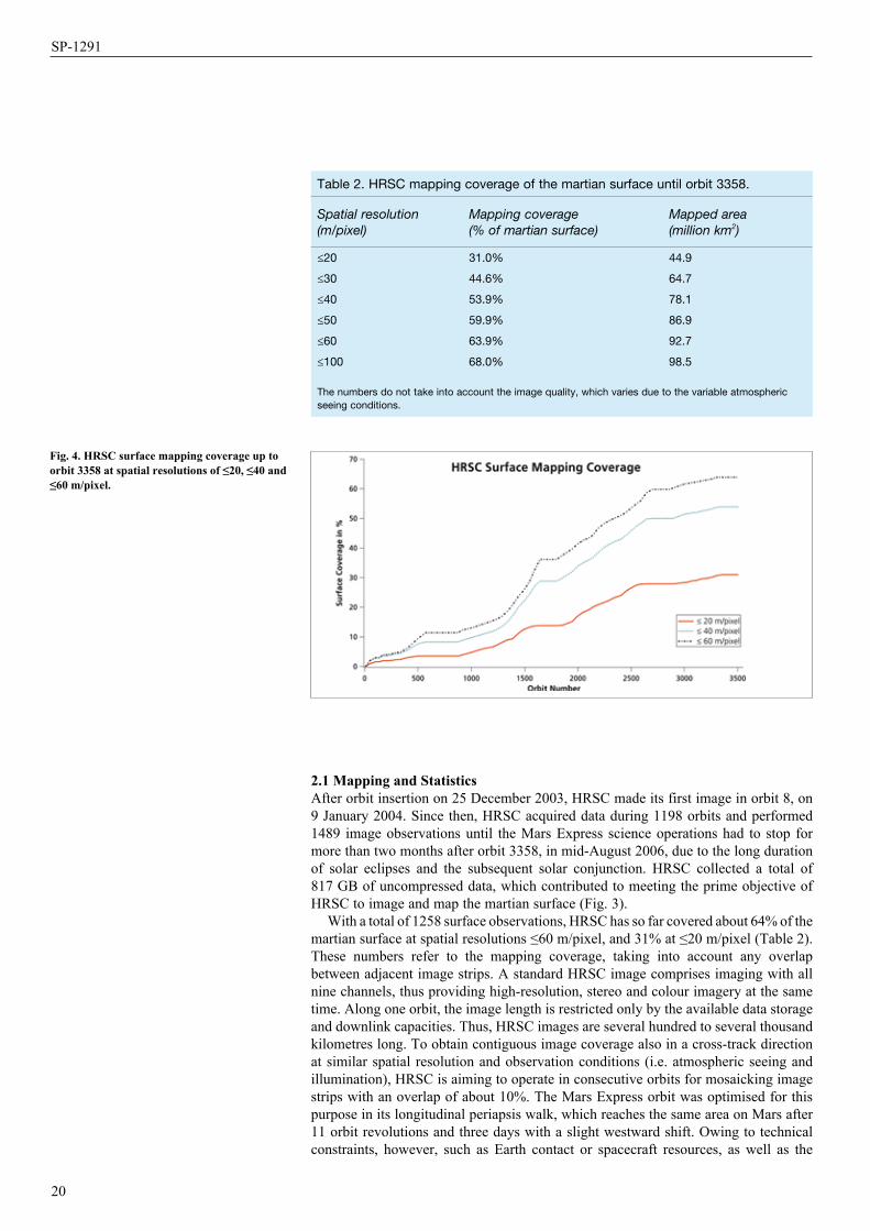
Table 2. HRSC mapping coverage of the martian surface until orbit 3358.
Spatial resolution (m/pixel)
Mapping coverage (% of martian surface)
Mapped area (million km2)
≤20 31.0% 44.9
≤30 44.6% 64.7
≤40 53.9% 78.1
≤50 59.9% 86.9
≤60 63.9% 92.7
≤100 68.0% 98.5
The numbers do not take into account the image quality, which varies due to the variable atmospheric seeing conditions.
fig. 4. HrSc surface mapping coverage up to orbit 3358 at spatial resolutions of ≤20, ≤40 and ≤60 m/pixel.
21
Scientific instruments
necessary sharing of resources among the different experiments on Mars Express with their specific needs for pointing at periapsis, only three to five orbits out of nine can be used for short-term mosaicking within a planning cycle of 100 orbits.
The development of the HRSC mapping coverage over the mission until August 2006 reflects the effect of the Mars Express data transfer capacity, which is determined by the distance between Mars and Earth and the availability of ground stations (Fig. 4). Major breaks in surface mapping are related to night-time periods, solar conjunction, and long solar eclipses. The periapsis went three times into the dark. At the beginning and end of such a period, however, HRSC still encounters acceptable observation conditions at higher altitudes, and the mapping coverage at lower spatial resolutions increases considerably compared with the high-resolution coverage of ≤20 m/pixel.
The secondary objectives of HRSC comprise observations for atmospheric sciences and of the martian moons. For studying atmospheric phenomena, HRSC has performed 70 limb soundings and 72 observations of the terminator and from high altitudes. Phobos has been imaged successfully 44 times and Deimos 18 times. HRSC has also succeeded in capturing the shadow of Phobos on the martian surface seven times. Finally, 28 data takes were conducted for in-flight calibration and testing, and during spot pointing.
2.2 HrSc in the context of other camera experimentsImaging is a major source of information for increasing our understanding of the evolution of the martian geology and climate. Consequently, since the beginning of exploration of the Red Planet, all Mars missions have been equipped with a camera instrument and have sent back a wealth of information. The basis for the ongoing Mars exploration effort was laid in the late 1970s by the Viking missions, which achieved a near-global coverage of the martian surface (95%) at 200 m/pixel, 28% coverage at ≤100 m/pixel, and 0.3% at ≤20 m/pixel (e.g. Neukum & Hoffmann, 2000). At present there are four missions operating in orbit around Mars, each of which carries a camera instrument and delivers imaging data back to Earth. The value of HRSC can only be assessed by putting it in context with the other imaging devices.
The Mars Observer Camera (MOC) on the Mars Global Surveyor (MGS) comprises two instruments. The wide-angle camera has covered the entire martian surface at 240 m/pixel and in two colours. It also monitors the martian weather at resolutions of a few kilometres. The narrow-angle camera has a spatial resolution of up to 1.4 m/pixel (Malin & Edgett, 2001) and has so far covered about 3% of the martian surface. By applying a slew manoeuvre of the spacecraft during imaging, the along-track pixel resolution could be improved to <1 m for selected observations. The small image size of a few kilometres causes problems in analysing the data in their broader geological context. Stereo observations are obtained for specific targets by pointing the spacecraft towards the same area in different orbits.
The Thermal Emission Imaging System (THEMIS) instrument on Mars Odyssey (MO) provides a spatial resolution of up to 18 m/pixel in the VIS (Christensen et al., 2004) and has covered 20% of the martian surface at ≤20 m/pixel and 35% at ≤50 m/pixel. The pointing capability of the spacecraft is limited and does not allow stereo observations. The camera has five colours but only very limited colour coverage. The typical image size is about 20 × 100 km.
The Mars Reconnaissance Orbiter (MRO) has just started its science operations and carries three camera experiments. Daily weather monitoring in the kilometre range is the task of the Mars Color Imager (MARCI), which has five colour filters in the VIS and two filters in the UV (www.msss.com/mro/marci/index.html ). The High Resolution Imaging Science Experiment (HiRISE) has a maximum spatial resolution of 0.3 m/pixel and is equipped with three colours (McEwen et al., 2007). During normal operations, the highest resolution will be achieved for the central part of the image swath, while a 4 × 4 pixel binning on the sides yields a spatial resolution of 1.2 m/pixel. It is planned to cover ~1% of the martian surface at ≤1.2 m/pixel, ~0.1% at 0.3 m/pixel, and ~0.1% in all three colours during the nominal mission. Each HiRISE image will be accompanied by an image of the Context Imager (CTX),
22
SP-1291
which obtains black-and-white images at a spatial resolution of 6 m/pixel (www.msss.com/mro/ctx/index.html). CTX is aiming to cover 15% of the martian surface. Stereo observations are envisaged by HiRISE for ~0.1% of the surface.
In comparison with the other camera instruments, the HRSC experiment has a number of unique features, including:
— Its unprecedented capability to provide wide-area contiguous coverage in colour at relatively high spatial resolution fills the gap between Viking, Mars Global Surveyor MOC and HiRISE on MRO, as well as relatively high-resolution global coverage.
— Its capability to produce stereo images in colour for geological interpretation in 3D, and for the derivation of high-resolution digital terrain models (DTMs). HRSC is the only dedicated stereo camera recording stereo information routinely for each observation nearly simultaneously and under the same observation conditions (atmospheric seeing, illumination).
— Its multiple-line concept with different viewing angles yields intrinsic geometric stability compared with the single-line imaging concept of the other cameras.
— The peculiar orbit of Mars Express and its pointing capabilities enable imaging at all times of day, whereas MGS, MO and MRO have Sun-synchronous, circular orbits, allowing imaging at fixed local times in the afternoon (15:00 and 14:00 h, respectively). HRSC is also the only instrument that can observe Phobos at high resolution due to the elliptical orbit.
In conclusion, the different camera experiments operating in orbit around Mars are highly complementary.
2.3 Data Distribution and Availability2.3.1 Data distribution via the ESA PSA and NASA PDSThe data acquired by the HRSC instrument have been released every six months to the ESA Planetary Science Archive. All the science data from the first 4479 orbits are available for public access.
Initially, the data were provided as radiometrically calibrated products (Level-2). Since 4 April 2006, they have also been made available as Level-3 (map-projected, ortho-rectified using the MOLA DTM). The data are validated, mainly by visual inspection, by the Co-I team, led by G. Neukum (FUB), H. Hoffmann (DLR), R. Greeley (ASU) and G. Ori (IRSPS). To date, a total of 1.4 Terabytes of radiometrically calibrated data have been released. The map-projected data volume is approximately the same. All products are formatted in accordance with PDS standards. Software for both the visualisation and the generation of map-projected data are provided together with the data release (xvd and hrortho/frameortho).
Detailed specifications of the archived HRSC data products are given in the instrument’s Experiment to Archive Interface Control Document (EAICD) (Roatsch, 2005), which is also available in the archive.
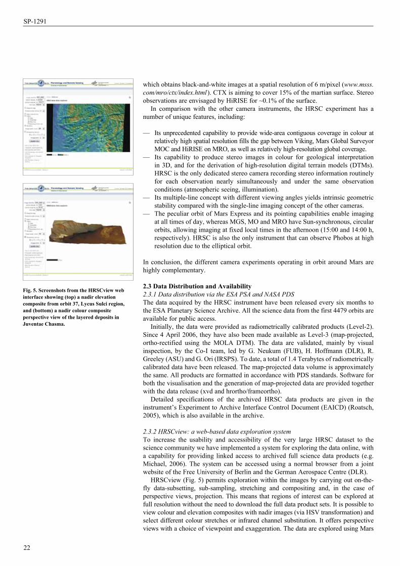
2.3.2 HRSCview: a web-based data exploration systemTo increase the usability and accessibility of the very large HRSC dataset to the science community we have implemented a system for exploring the data online, with a capability for providing linked access to archived full science data products (e.g. Michael, 2006). The system can be accessed using a normal browser from a joint website of the Free University of Berlin and the German Aerospace Centre (DLR).
HRSCview (Fig. 5) permits exploration within the images by carrying out on-the-fly data-subsetting, sub-sampling, stretching and compositing and, in the case of perspective views, projection. This means that regions of interest can be explored at full resolution without the need to download the full data product sets. It is possible to view colour and elevation composites with nadir images (via HSV transformation) and select different colour stretches or infrared channel substitution. It offers perspective views with a choice of viewpoint and exaggeration. The data are explored using Mars
fig. 5. Screenshots from the HrScview web interface showing (top) a nadir elevation composite from orbit 37, Lycus Sulci region, and (bottom) a nadir colour composite perspective view of the layered deposits in Juventae chasma.
23
Scientific instruments
surface coordinates, making it a simple matter to move between multiple images of the same location, and also to move from a global image footprint map directly into an HRSC image at a position of interest. The map scale of the view can be selected using the distance and elevation scale bars provided. Images can be accessed by orbit/image number as well as via the footprint map. In either case, a link is provided to a data product page, where header items describing the full map-projected science data product are displayed, and a link to the archived data products can be provided. HRSCview is currently being tested by the Co-I team, and will shortly be opened for public access. At present, the elevation composites are derived from the HRSC preliminary 200 m DTMs generated at DLR, which will not be available as separately downloadable data products. These DTMs will be progressively superseded by higher-resolution archival DTMs, also from DLR, which will be made available for download.
The service is distinct from that provided by the ESA PSA in that it provides a means to explore inside the individual (but very large) images, and to carry out a preliminary on-the-fly processing of the data. A more powerful version of the software, including tools for quantitative DTM analysis and intended for working with locally hosted HRSC data products, will be made available for work with the archived DTMs.
3.1 Photogrammetry3.1.1 Stereophotogrammetric Processing of HRSC dataThe multi-stereo and multi-spectral capabilities of HRSC enable high-resolution photogrammetric stereo analysis as well as orthoimage generation to derive valuable base products for a variety of geoscientific investigations. The methods employed are similar to those developed and applied within various airborne DLR projects in recent years (Neukum, 1999; Wewel et al., 2000; Gwinner et al., 2000).
DLR’s photogrammetric processing system, comprising digital terrain model (DTM) generation based multi-image matching, ortho-rectification and image mosaicking, represents the major aspect of the photogrammetric and cartographic activities and makes it possible to provide photogrammetric data products to the team. The operational and standardised generation of products is intended to improve the availability of higher-level data products (orthoimages and 3D surface descriptions are available within days; Scholten et al., 2005), to ensure the full exploitation of the entire HRSC potential (multi-stereo capability for reliable 3D modelling, as well as precise high-resolution and multi-spectral orthoimage generation), and comprises a high degree of automation. The preliminary products currently include HRSC DTMs on 200 m grids and orthoimages at resolutions of 12.5, 25.0 or 50.0 m/pixel of all sensors, derived using the corresponding HRSC DTM. Based on predicted pointing and reconstructed orbit data, the accuracies of these products are a few hundred metres for planimetry, and better than 100 m for height measurements.
Figure 6 indicates the quality of HRSC preliminary products compared with the topography described by the Mars Orbiter Laser Altimeter (MOLA). Besides the production of additional, more elaborate high-level data (Gwinner et al., 2005), adapting processing parameters to specific data characteristics), the described standardised processing also provides inputs to other photogrammetric investigations (Albertz et al., 2005). Finally, this system is designed to integrate the results of these investigations for the derivation of enhanced data products, such as high-quality regional or global image and DTM mosaics.
3.1.1.1 An Alternative Approach to Stereo Photogrammetric Processing of HRSC Data Based on ISIS and SOCET SETAlthough the primary role of the US Geological Survey, Flagstaff, USA, in the HRSC experiment is advisory rather than operational, this group has developed and demonstrated its own capability for stereo processing. The approach chosen was to integrate Level-2 (radiometrically calibrated, geometrically raw) HRSC and SRC images into the USGS planetary cartography software system ISIS (Torson & Becker,
3. Scientific Achievements

24
SP-1291
1997; Eliason, 1997; Eliason et al., 1997; Gaddis et al., 1997) and from there into the commercial photogrammetric software SOCET SET (www.baesystems.com; Miller & Walker, 1993). In addition, it was necessary to develop sensor models for the two cameras in the ISIS system; in SOCET SET, available ‘generic’ models could be used.
The benefits of this work include preparing the USGS to undertake systematic mapping if directed by NASA, providing capabilities for cartographic processing of HRSC data to the many researchers who use ISIS rather than VICAR, and bringing to bear on the images the largely unique ISIS capabilities for photometric function modelling, photometric correction of images and mosaics (Kirk et al., 2001), and topographic modelling by photoclinometry/shape-from-shading (Kirk et al., 2003).
Initial work (Kirk et al., 2004) has demonstrated the production of high-resolution DTMs from stereo pairs made up of HRSC-SRC and MGS MOC-NA images, by exploiting the multi-sensor capabilities of SOCET SET. Subsequent work (Kirk et al., 2006) undertaken as part of the HRSC DTM test (Heipke et al., 2006) has shown that DTMs can be produced from HRSC scanner data and can be used to do useful spectrophotometric processing. The quality of stereo DTMs is intermediate compared with the results obtained by other processing approaches, but refinement by photoclinometry can dramatically improve the geological detail at the limit of resolution while preserving absolute accuracy, even in areas of highly variable albedo.
3.1.1.2 Improving Position and Attitude of the HRSC cameraThe 3D orbit position and attitude of the HRSC are given by nominal values, which in the case of the orbit position are refined by Doppler shift measurements. For highly accurate photogrammetric applications, these values are often not accurate enough. Therefore, a photogrammetric approach to compute orbit and attitude improvements has been developed in close cooperation between the Leibniz University Hannover, the Technical University of Munich and DLR.
The approach consists of two independent steps. First, a large number of tie points between the multiple stereo strips is extracted by digital image matching (Heipke et al., 2004). Subsequently, a least-squares bundle-block adjustment (BBA) is performed to improve the exterior orientation (EO), using the generated tie points as direct observations for the unknown EO parameters. By introducing only a bias and a drift value for each orientation parameter per orbit, the BBA preserves the high relative accuracy of the available information, corrects for camera/spacecraft misalignment and improves the absolute accuracy significantly. In order to fit the matched HRSC
fig. 6. Subset of the mars express orbit 1070 (~7°S, 298°e). from left to right: standardised HrSc orthoimage 12.5 m/pixel, gridded mOLA Dtm (Smith et al., 2003); preliminary HrSc 200 m Dtm (Scholten et al., 2005); and high-resolution HrSc Dtm, 50 m grid (Gwinner et al., 2005).
25
Scientific instruments
points to the existing MOLA DTM (Smith et al., 2003; Neumann et al., 2003), which can be considered as a reference for Mars, further constraints are added to the BBA (Ebner et al., 2004).
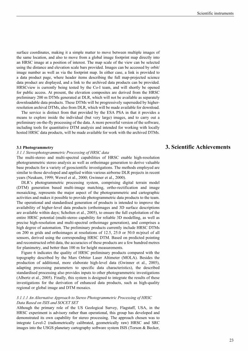
For more than 68% of the images (903 orbits) a successful BBA was achieved, and the remaining imagery was processed successfully to improve poor image quality. For reasons of brevity, we report here only results for a selected block comprising the orbits 894, 905 and 927 with a ground pixel size of approximately 15 m in the nadir channel. First, the EO was improved by BBA without taking into account the MOLA DTM. The theoretical standard deviations of the object points after BBA were improved by factors of 2 to 3, and lay in the range of about 5–7 m in the X (flight direction) and Y (across track) directions. The Z (height) accuracies of all orbits were about 11–16 m.
Next, the HRSC object points were tied to the MOLA DTM, resulting in statistically highly significant improvements for position and attitude. In addition, the root-mean-square (rms) differences between HRSC and MOLA DTM could be reduced by a factor of 3. Hence, we have reached a high consistency between HRSC points and the MOLA reference. This is clearly visible in Fig. 7, which compares the Z-differences before and after the BBA. With the resulting adjusted EO, high-quality products such as DTMs, orthoimages and shaded reliefs can be derived from the imagery.
3.1.1.3 Quality Assessment of HRSC Object Points and Improved DTM Generation The point cloud resulting from the standardised stereo-photogrammetric VICAR processing is dependent on albedo features. Generally, in rugged areas (e.g. craters, valleys, chaotic terrains) many high-quality points can be determined, whereas smooth areas are poorly described, with a high measurement noise and data gaps.
A point classification method developed by the group at the Vienna University of Technology has been applied iteratively to reduce the measurement noise (Attwenger & Neukum, 2005). The basic idea is to start from a coarse DTM and improve it from one iteration step to the next. HRSC points are either accepted or rejected depending on their distance from the intermediate DTM until a stable condition is reached. The initial DTM may be derived from a reduced HRSC data set or from MOLA data. The latter can also bridge large gaps in regions without points.
The results show the elimination of gross errors and a reduction of the mean measurement noise. Thus, features are better discernible in DTMs derived from the accepted points, and smaller grid widths can be used for DTM generation (Fig. 8). It should be noted that all employed points are original measurements. Thus, any
fig. 7. Differences between HrSc and mOLA points before (left) and after (right) BBA (in metres).
fig 8. test area (orbit 18). Left: shading based on the original point cloud; centre: shading based on the accepted point cloud; right: HrSc ortho-image.

26
SP-1291
interpolation algorithm (e.g. linear prediction with the capability for further noise filtering) can be applied to derive a regular, grid-based DTM from these points.
3.1.2 Improvement of Spatial Data by Shape from Shading Besides the USGS (see above) the Munich UniBw group has also refined the standard Level-4 digital elevation models (DEM) by means of shape-from-shading (SFS). Surface inclinations and elevations are derived from illumination-induced shading information in the HRSC images. SFS, although dependent on spatial and physical factors such as reflectance, surface albedo, shadows, light source distribution, image resolution, etc., is in principle not only capable of realistic interpolation into a coarse elevation grid but also guarantees conformity with photometric image information. This is prerequisite for subsequent modifications of image shades towards rigorous homogenisation and optimisation of relief shading in the final orthoimage maps (Dorrer et al., 2005; Albertz et al., 2005) (Fig. 9).
3.1.3 DTM Test Using HRSC ImageryAs described, automatic DTM generation from HRSC images by means of image matching has reached a very high level over the years. In addition to the systematic processing, several groups have been able to produce DTMs using different approaches, or have developed alternative modules for parts of the DTM generation process. It was therefore considered desirable to compare the individual approaches for deriving DTMs from HRSC images in order to assess their advantages and disadvantages (Heipke et al., 2006).
The key goals of the test were to reconstruct the fine details and the geometric accuracy of the DTMs. Fine detail was studied using a variety of qualitative assessments in small but representative areas, while geometric accuracy was analysed with respect to the MOLA DTM. All quality parameters were also related to operational aspects such as the computing effort of the applied method, and thus its applicability to generating DTMs of large areas (multiple orbits, potentially the whole HRSC dataset). The test was organised by the Photogrammetry and Cartography Working Group (PCWG) within the HRSC CoI team under the auspices of the ISPRS Working Group IV/7 on Extraterrestrial Mapping. IPI, Leibniz University of Hannover, and DLR Berlin–Adlershof acted as pilot centres for the test. Based on commonly agreed test datasets, including image orientations refined by bundle adjustment, a total of seven groups have derived DTMs. The pilot centres then analysed the data produced. To our knowledge this is the first multi-site test for DTM generation from planetary imagery.
The test was very successful and demonstrated that a number of methods can be used to generate high-quality DTMs from HRSC imagery. Nevertheless, there were notable differences between the participants’ results. Some approaches, not surprisingly those that were developed with planetary imagery in mind, yielded superior results, and have been extensively applied to planetary and in particular to HRSC image data in the past. Most operational methods, in terms of processing time, needed only a few hours. The best approaches yielded a DTM resolution of two
fig. 9. A 495 × 565 subsection from HrSc orbit 927 with 50 m ground pixel size (scene size 25 × 28 km). (a) Photometrically corrected irradiance of the original orthoimage derived from the corresponding HrSc nadir image and a standard Level-4 Dtm. (b) the modelled scene radiance of this obviously relatively crude Dtm. (c) the modelled scene radiance of the SfS-refined Dtm. the fact that (c) is almost indistinguishable from (a) demonstrates the potential of SfS.
27
Scientific instruments
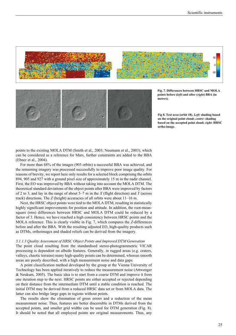
to three times that of the nadir image, and a geometric accuracy with respect to the MOLA DTM of one to two pixels in object space depending on the terrain difficulties, still provided operational production times of only a few days processing per orbit. Shape from shading is able to refine the matching DTM to a remarkable degree of detail. Furthermore, the test confirms previous findings that the DTMs generated from HRSC data, at least at lower latitudes, are clearly superior to the MOLA DTM in terms of resolution and visible fine detail.
On the basis of these results, some inferences can be made for further development of the matching algorithms:
— the use of multiple images instead of only the nadir and the two stereo channels often improves the results;
— the reduction of radiometric noise prior to image matching appears to carry a lot of promise (see also Gwinner et al., 2005; Schmidt et al., 2006);
— rectifying the images at least to a plane prior to matching is mandatory. More advantageous seems to be a rectification to a DTM such as the MOLA DTM or,
fig. 10. example of a sheet from ‘topographic image map mars 1:200 000’ showing the Hellas and centauri montes region.

28
SP-1291
even better, one generated within the matching process, in particular in areas with steep slopes;
— detecting and eliminating blunders must be seen as an essential sub-task at every step in the processing chain; and
— general purpose algorithms should be carefully adapted to the peculiarities of the HRSC sensor, e.g. the geometric sensor model, macro pixel formats and varying integration times. We were also able to demonstrate within the test that in order to generate consistent results a photogrammetric bundle adjustment using a sufficient number of tie points is necessary.
3.1.4 Mapping of the Martian Surface with HRSC DataThe cartographic standard product of the Mars Express mission is the ‘Topographic Image Map Mars 1:200 000’ (Albertz et al., 2004, 2005). This large-scale map series is compiled in equal-area map projections, i.e. the Sinusoidal projection between latitudes 85° north and south and the Lambert Azimuthal projection in the polar regions. Mars is covered by a total of 10 372 individual map sheets.
In order to automate the map generation process, the cartographic software package Planetary Image Mapper (PIMap; Gehrke et al., 2005) has been developed at Technische Universität Berlin. The software generates and/or compiles the topographic map content, i.e. the ortho-image basis, contour lines derived from HRSC DTM, topographic names and gridlines, as well as map titles and further marginal information. The resulting digital map sheets contain all raster and vector data in pdf format, and can be printed out on demand. Using PIMap, various sheets of the ‘Topographic Image Map Mars 1:200 000’ series, special target maps at larger scales, and thematic maps of different types have also been generated. An example is given in Fig. 10.
3.1.5 3D VisualisationFollowing the concept ‘from 3D camera to 3D image’ and based on the stereo-capability of HRSC, the 3D Visualisation Group of the Institute for Cartography of the Dresden University of Technology have developed an optimised cartographic true-3D display method by merging the well known principles of transparent prismatic microlens foils, which have been used for so-called ‘flip images’ and the lenticular foil technology, and so far have been used for displays with only a few discrete levels of depth. This approach allows the production of hardcopy displays that permit spontaneous, glasses-free viewing without artificial illumination by several individuals simultaneously. For the Mars surface, bitemporal ‘three-in-one’ scenes showing dynamic geological processes have been generated (see the cover page of the special issue of Photogrammetric Engineering & Remote Sensing on planetary mapping, October 2005). For background information about this method, see Buchroithner et al. (2005a, 2005b).
3.1.6 Automated Cartographic Feature Extraction from HRSC imageryThe production of global-scale DTMs with associated ortho-rectified high-resolution images opens up the potential to mine the resultant datasets for significant geomorphometric features such as craters, sand dunes, lava flows and hydrological remnants. Automated crater detection using image data-mining techniques has been described by Kim et al. (2005) and its reliability has been demonstrated with Viking orbiter, MOC and HRSC data to be over 85% (Kim et al., 2005). We show here some examples of the extension of this approach to the use of stereo fusion for both crater detection from multiple HRSC looks (Fig. 12), as well as the detailed geomorphometry of the crater shape (Fig. 11). It is planned to continue development of these data-mining techniques so that a much wider range of geologically important features can be automatically detected, leading in the very long term to the production of geological feature maps. These crater databases can also be employed for surface date aging (Kim et al., 2005) using size–frequency distribution (SFD).
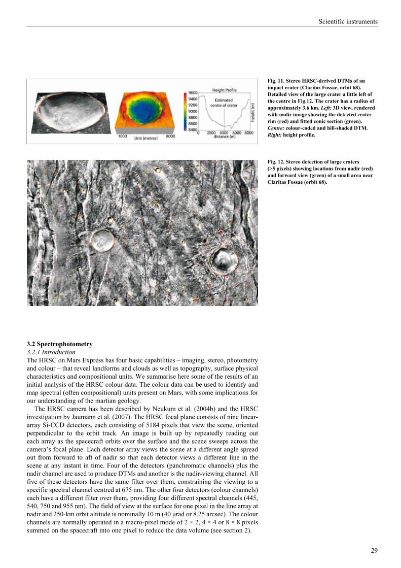
29
Scientific instruments
3.2 Spectrophotometry3.2.1 IntroductionThe HRSC on Mars Express has four basic capabilities – imaging, stereo, photometry and colour – that reveal landforms and clouds as well as topography, surface physical characteristics and compositional units. We summarise here some of the results of an initial analysis of the HRSC colour data. The colour data can be used to identify and map spectral (often compositional) units present on Mars, with some implications for our understanding of the martian geology.
The HRSC camera has been described by Neukum et al. (2004b) and the HRSC investigation by Jaumann et al. (2007). The HRSC focal plane consists of nine linear-array Si-CCD detectors, each consisting of 5184 pixels that view the scene, oriented perpendicular to the orbit track. An image is built up by repeatedly reading out each array as the spacecraft orbits over the surface and the scene sweeps across the camera’s focal plane. Each detector array views the scene at a different angle spread out from forward to aft of nadir so that each detector views a different line in the scene at any instant in time. Four of the detectors (panchromatic channels) plus the nadir channel are used to produce DTMs and another is the nadir-viewing channel. All five of these detectors have the same filter over them, constraining the viewing to a specific spectral channel centred at 675 nm. The other four detectors (colour channels) each have a different filter over them, providing four different spectral channels (445, 540, 750 and 955 nm). The field of view at the surface for one pixel in the line array at nadir and 250-km orbit altitude is nominally 10 m (40 μrad or 8.25 arcsec). The colour channels are normally operated in a macro-pixel mode of 2 × 2, 4 × 4 or 8 × 8 pixels summed on the spacecraft into one pixel to reduce the data volume (see section 2).
fig. 11. Stereo HrSc-derived Dtms of an impact crater (claritas fossae, orbit 68). Detailed view of the large crater a little left of the centre in fig.12. the crater has a radius of approximately 3.6 km. Left: 3D view, rendered with nadir image showing the detected crater rim (red) and fitted conic section (green). Centre: colour-coded and hill-shaded Dtm. Right: height profile.
fig. 12. Stereo detection of large craters (>5 pixels) showing locations from nadir (red) and forward view (green) of a small area near claritas fossae (orbit 68).

30
SP-1291
3.2.2 Colour Data CharacteristicsThe colour data characteristics have been investigated extensively in order to understand how the data may be used for studying spectral units and Mars’ geology and atmosphere, and a lengthy report on this study is given in McCord et al. (2006). In summary, these characteristics include the effects of data compression and of the different angles of viewing among the colour channels. The degree of data compression is different in each colour channel and from place to place on Mars, and this can affect the appearance of colour units. However, it is found that this effect is usually at the few-DN level and is worst where the surface has least albedo and colour features. The differing angles of observation for each colour channel have a more serious effect because the atmosphere can be highly scattering with directionality, and it can contribute considerably differently to each channel, depending on the solar illumination. The surface roughness also can cause different amounts of shadow to appear in each colour image with different viewing angles. Finally, differences in surface photometric functions can create false colour differences.
In addition, the HRSC observes such large swaths of latitude across Mars in each orbit that the solar illumination angle varies greatly within a swath and among swaths, including from equator to pole. McCord et al. (2006) report that applying a simple cosine brightness correction works surprisingly well for removing the first-order effects from the data, but a more complex correction should be attempted for some studies. Since the colour channels each observe the surface at different angles and times, the colour images must be spatially registered in order to construct colour unit maps. This registration process is difficult and resource consuming, so that misregistration and the associated colour artifacts are problematic, especially for topographically complex terrains, unless special efforts are made to register to a few tenths of a pixel dimension.
3.2.3 Comparison with OMEGA and Telescopic ObservationsAn extensive analysis was conducted (McCord et al., 2006) to compare HRSC spectrophotometric measurements with those of the same regions by other instruments. In summary, this study revealed that the HRSC blue, green and infrared channel I/F values agree with measurements by OMEGA visual channel and telescopic observations, but that the HRSC red channel I/F values are offset from these other measurements, with HRSC being higher in I/F. A search for the reasons for this offset has been inconclusive so far. Possible reasons include a basic error in the HRSC calibration or a change in its performance since ground calibration, an error in the OMEGA visual channel calibration, or an atmospheric or surface scattering effect due to the HRSC red and infrared channels being offset from each other in viewing angles by nearly 30°. Interestingly, a comparison of HRSC and OMEGA measurements for the small Mars satellite Phobos shows this effect but at an even greater size. Phobos has no atmosphere and is relatively dark, so this suggests a calibration error in one or both instruments. An analysis of the potential atmospheric effects on the HRSC spectrophotometric data, due to the differing viewing angles of the four colour channels, was conducted using radiation transfer calculations. This revealed that extra scattering contributions to the red channel could be expected under dusty atmospheric conditions. Further, examples were found where water clouds high in the atmosphere created just such an effect. However, an investigation searching for variations of this effect with solar phase angle revealed no conclusive dependence, in apparent contradiction with this explanation (McCord et al., 2006; Coombs & McCord, 2006).
In spite of these complications, the HRSC colour dataset is a powerful resource for studying Mars. The colour data have been demonstrated to be very good for defining the basic spectral components of Mars and showing their spatial distribution. Thus, HRSC spectral images are an important asset for photo interpretation and mapping. They also are the best link between OMEGA spectroscopy and photo interpretation. By showing that HRSC I/F spectra are consistent with, but slightly offset from, the same wavelengths of OMEGA, telescopic and laboratory spectra, we have validated that familiar compositional information is contained in the HRSC images. The HRSC spectral data, however, were

31
Scientific instruments
never intended for identifying composition. There are neither enough spectral bands nor broad enough spectral coverage. OMEGA data are intended for this purpose. The power of the HRSC colour data lies in having both high spatial resolution and broad spatial coverage in the four main colour bands. Combined with OMEGA, it is a unique dataset.
3.2.4 Reflectance SpectraIn spite of the complications described above, and the effects of the atmosphere, I/F values for the surface units can be calculated if one assumes knowledge of the spectrum of at least one unit in a scene. This approach was used by assuming the darkest units in each scene are composed of basalt and correcting the HRSC dark unit spectrum to match a laboratory spectrum of unweathered basalt and applying this correction to all other pixels in the scene. The example I/F spectra produced following this procedure, presented in Fig. 13(c), are for specific pixels and locations on Mars that were carefully selected to illustrate three different spectral units and probably classes of material (McCord et al., 2006).
fig. 13. HrSc four-colour spectra plotted for selected areas in several orbit image stripes, as designated in the legend by orbit number and spot name. (a) Spectra as delivered by HrSc after radiometric calibration. (b) Spectra after correcting for solar illumination angle according to a cosine function. (c) Spectra after also applying the corrections to force the HrSc spectra for dark material to agree with a laboratory basalt spectrum. (d) the basalt correction factors for each of the orbit scenes. (e) the basalt correction factors scaled to unity for the 750 nm channel (mccord et al., 2006).
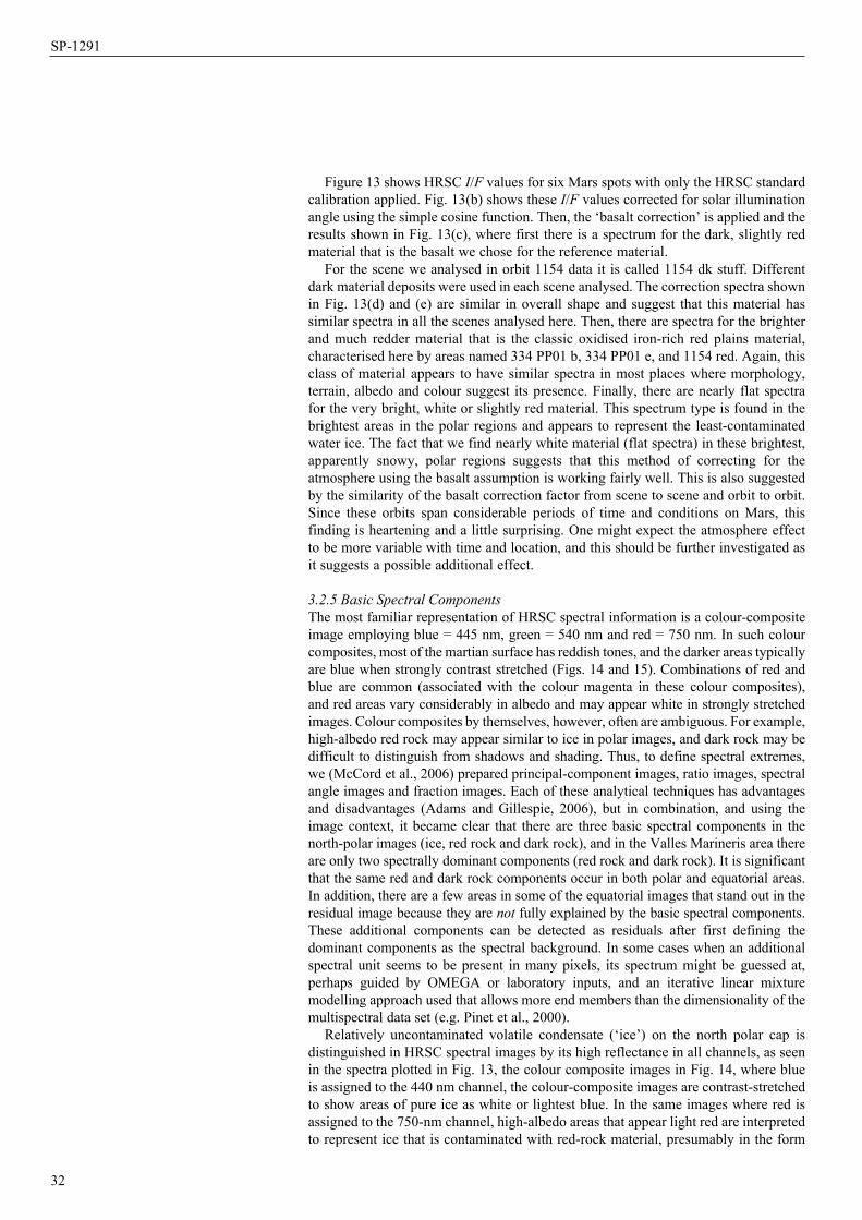
32
SP-1291
Figure 13 shows HRSC I/F values for six Mars spots with only the HRSC standard calibration applied. Fig. 13(b) shows these I/F values corrected for solar illumination angle using the simple cosine function. Then, the ‘basalt correction’ is applied and the results shown in Fig. 13(c), where first there is a spectrum for the dark, slightly red material that is the basalt we chose for the reference material.
For the scene we analysed in orbit 1154 data it is called 1154 dk stuff. Different dark material deposits were used in each scene analysed. The correction spectra shown in Fig. 13(d) and (e) are similar in overall shape and suggest that this material has similar spectra in all the scenes analysed here. Then, there are spectra for the brighter and much redder material that is the classic oxidised iron-rich red plains material, characterised here by areas named 334 PP01 b, 334 PP01 e, and 1154 red. Again, this class of material appears to have similar spectra in most places where morphology, terrain, albedo and colour suggest its presence. Finally, there are nearly flat spectra for the very bright, white or slightly red material. This spectrum type is found in the brightest areas in the polar regions and appears to represent the least-contaminated water ice. The fact that we find nearly white material (flat spectra) in these brightest, apparently snowy, polar regions suggests that this method of correcting for the atmosphere using the basalt assumption is working fairly well. This is also suggested by the similarity of the basalt correction factor from scene to scene and orbit to orbit. Since these orbits span considerable periods of time and conditions on Mars, this finding is heartening and a little surprising. One might expect the atmosphere effect to be more variable with time and location, and this should be further investigated as it suggests a possible additional effect.
3.2.5 Basic Spectral ComponentsThe most familiar representation of HRSC spectral information is a colour-composite image employing blue = 445 nm, green = 540 nm and red = 750 nm. In such colour composites, most of the martian surface has reddish tones, and the darker areas typically are blue when strongly contrast stretched (Figs. 14 and 15). Combinations of red and blue are common (associated with the colour magenta in these colour composites), and red areas vary considerably in albedo and may appear white in strongly stretched images. Colour composites by themselves, however, often are ambiguous. For example, high-albedo red rock may appear similar to ice in polar images, and dark rock may be difficult to distinguish from shadows and shading. Thus, to define spectral extremes, we (McCord et al., 2006) prepared principal-component images, ratio images, spectral angle images and fraction images. Each of these analytical techniques has advantages and disadvantages (Adams and Gillespie, 2006), but in combination, and using the image context, it became clear that there are three basic spectral components in the north-polar images (ice, red rock and dark rock), and in the Valles Marineris area there are only two spectrally dominant components (red rock and dark rock). It is significant that the same red and dark rock components occur in both polar and equatorial areas. In addition, there are a few areas in some of the equatorial images that stand out in the residual image because they are not fully explained by the basic spectral components. These additional components can be detected as residuals after first defining the dominant components as the spectral background. In some cases when an additional spectral unit seems to be present in many pixels, its spectrum might be guessed at, perhaps guided by OMEGA or laboratory inputs, and an iterative linear mixture modelling approach used that allows more end members than the dimensionality of the multispectral data set (e.g. Pinet et al., 2000).
Relatively uncontaminated volatile condensate (‘ice’) on the north polar cap is distinguished in HRSC spectral images by its high reflectance in all channels, as seen in the spectra plotted in Fig. 13, the colour composite images in Fig. 14, where blue is assigned to the 440 nm channel, the colour-composite images are contrast-stretched to show areas of pure ice as white or lightest blue. In the same images where red is assigned to the 750-nm channel, high-albedo areas that appear light red are interpreted to represent ice that is contaminated with red-rock material, presumably in the form
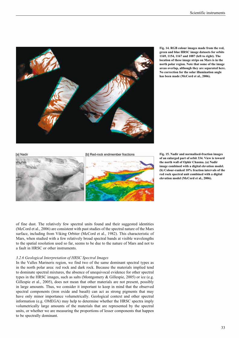
33
Scientific instruments
of fine dust. The relatively few spectral units found and their suggested identities (McCord et al., 2006) are consistent with past studies of the spectral nature of the Mars surface, including from Viking Orbiter (McCord et al., 1982). This characteristic of Mars, when studied with a few relatively broad spectral bands at visible wavelengths to the spatial resolution used so far, seems to be due to the nature of Mars and not to a fault in HRSC or other instruments.
3.2.6 Geological Interpretation of HRSC Spectral ImagesIn the Valles Marineris region, we find two of the same dominant spectral types as in the north polar area: red rock and dark rock. Because the materials implied tend to dominate spectral mixtures, the absence of unequivocal evidence for other spectral types in the HRSC images, such as salts (Montgomery & Gillespie, 2005) or ice (e.g. Gillespie et al., 2005), does not mean that other materials are not present, possibly in large amounts. Thus, we consider it important to keep in mind that the observed spectral components (iron oxide and basalt) can act as strong pigments that may have only minor importance volumetrically. Geological context and other spectral information (e.g. OMEGA) may help to determine whether the HRSC spectra imply volumetrically large amounts of the materials that are represented by the spectral units, or whether we are measuring the proportions of lesser components that happen to be spectrally dominant.
fig. 14. rGB colour images made from the red, green and blue HrSc image datasets for orbits 1169, 1154, 1167 and 1087 (left to right). the location of these image strips on mars is in the north polar region. note that some of the image areas overlap, although they are separated here. no correction for the solar illumination angle has been made (mccord et al., 2006).
fig. 15. nadir and normalised-fraction images of an enlarged part of orbit 334. View is toward the north wall of Ophir chasma. (a) nadir image combined with a digital elevation model. (b) colour-ranked 10% fraction intervals of the red rock spectral unit combined with a digital elevation model (mccord et al., 2006).

34
SP-1291
In the context of the HRSC images, the red and dark spectral types define two main geological units in the Valles Marineris region. In Fig. 15 we show an example map of the proportions of these two units. The red unit dominates the plains that surround the canyons, the upper parts of the canyon walls, and some of the islands within the larger chasmata. Local outcrops of the red unit occur within the dark unit on the valley floors. In HRSC nadir images and MOC images, some of these outcrops exhibit fine layering. The dark unit makes up most of the floors of the larger chasmata, where it occurs as extensive smooth plains, occasional dunes and uncommon layered deposits. It also occurs in conical depressions within the red unit, as talus slopes, and in a wide variety of irregular patches. The dark unit is locally present on the high plains near the rims of the chasmata. Although the red unit is topographically above the dark unit on a regional scale, the contact between the two is nearly everywhere broadly gradational, and, locally, dark material appears to have intruded and altered the red unit. Our spectral definitions of the red and dark units have potentially important implications for interpreting the geology of Valles Marineris. The high-albedo deposits within the chasmata are spectrally indistinguishable from the materials that comprise canyon walls, rims and the surrounding plains. If the high-albedo materials all have approximately the same composition, the interior deposits may be part of the Hesperian/Noachian ‘basement’ that comprises the canyon walls and plains, rather than younger deposits that lie unconformably on the basement, as proposed for example by Witbeck et al. (1991). Many workers have lumped the low-albedo materials in the chasmata together with the high-albedo materials as part of the younger, interior deposits.
Based on our spectral definition of units, however, the dark-material unit is compositionally distinct from the red, high-albedo material. Layers of the dark unit are present in the deepest parts of Mellas Chasma and may be stratigraphically below the red unit. We find no evidence that the red unit occurs stratigraphically below the dark unit, as would be implied if the Hesperian/Noachian basement materials had been down-faulted to form the floor on which younger, dark materials were deposited. Excluding dunes and dust deposits, the main interface between the red and the dark units in the chasmata is morphologically complex and extends over an altitude range of several kilometres. Furthermore, the contact is everywhere gradational. If the dark material is basaltic in composition, it is difficult to explain the observed complex and gradational zone as a depositional contact between dark flows/tephra and overlying lighter deposits. On the other hand, it does not appear that the dark unit is simply intrusive into the red one, although in places there is evidence that the dark material has followed fracture zones into the high-albedo material. We suggest that understanding the interface between the red and dark units is essential for understanding the origin of the Valles Marineris region, and HRSC colour data are well suited for this purpose.
3.2.7 SummaryWe have demonstrated that the HRSC colour data can contribute a better understanding of the geology of Mars. We find that only a few basic spectral and probably compositional units (red, iron-oxide-rich material; dark basalt; polar water ice) contribute to most pixels to the degree HRSC can sense them. There is evidence of several other units that are brighter and less blue than the other units, probably salts and possibly other materials, may also be detectable with HRSC. Reflectance spectra from HRSC can be calibrated to a level comparable with laboratory spectra and in agreement with OMEGA visual spectra, allowing compositional interpretations of HRSC spectra and extension and mapping of OMEGA compositional identifications to higher spatial resolution and extent than possible with OMEGA (or HRSC) alone. Our exploration of the bright red and dark apparently basalt units reveals that the unit distributions seem to disagree in important cases with existing geological interpretations exhibited in the published Mars geological maps. Thus, there is much geological exploration that can be
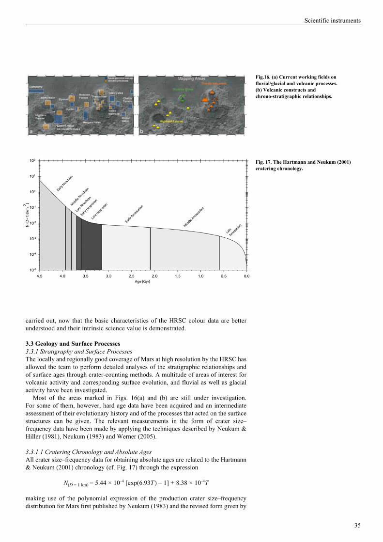
35
Scientific instruments
carried out, now that the basic characteristics of the HRSC colour data are better understood and their intrinsic science value is demonstrated.
3.3 Geology and Surface Processes3.3.1 Stratigraphy and Surface ProcessesThe locally and regionally good coverage of Mars at high resolution by the HRSC has allowed the team to perform detailed analyses of the stratigraphic relationships and of surface ages through crater-counting methods. A multitude of areas of interest for volcanic activity and corresponding surface evolution, and fluvial as well as glacial activity have been investigated.
Most of the areas marked in Figs. 16(a) and (b) are still under investigation. For some of them, however, hard age data have been acquired and an intermediate assessment of their evolutionary history and of the processes that acted on the surface structures can be given. The relevant measurements in the form of crater size–frequency data have been made by applying the techniques described by Neukum & Hiller (1981), Neukum (1983) and Werner (2005).
3.3.1.1 Cratering Chronology and Absolute AgesAll crater size–frequency data for obtaining absolute ages are related to the Hartmann & Neukum (2001) chronology (cf. Fig. 17) through the expression
N(D = 1 km) = 5.44 × 10⁻⁴ [exp(6.93T) – 1] + 8.38 × 10⁻⁴T
making use of the polynomial expression of the production crater size–frequency distribution for Mars first published by Neukum (1983) and the revised form given by
fig.16. (a) current working fields on fluvial/glacial and volcanic processes. (b) Volcanic constructs and chrono-stratigraphic relationships.
fig. 17. the Hartmann and neukum (2001) cratering chronology.

36
SP-1291
fig. 18. the martian size–frequency distribution (from Werner, 2005). (a) Assemblage of crater size–frequency measurements obtained for counts performed on HrSc, Src, Viking, tHemiS and mOc imagery. they represent typical crater size–frequency measurements of differently aged surfaces. the set of isochrones indicate the expected distribution applying the Hartmann–neukum chronology model for different ages, which makes it possible to derive crater retention ages from the measurements by way of visual interpretation of a graph (Hartmann & neukum, 2001). usually, we derive ages by fitting the crater production function to the measurements and obtain a numerical value n(1) for a reference crater diameter (usually 1 km). (b) the same assemblage of crater size–frequency measurements normalised to the utOPiA 15 m A+B measurement, which represents a measurement in the medium-sized crater diameter range. the black curve is the lunar crater production function transferred to martian conditions, representing a surface age of 3.25 Ga. the good fit strongly suggests that the impactor size–frequency distributions for the moon and mars are really the same, and that our previous procedure (neukum, 1983; neukum et al., 2001; ivanov, 2001) of transferring the lunar crater size–frequency distribution to mars was carried out correctly.
fig. 19. (a) isochrons according to Hartmann and neukum (2001), martian size–frequency distribution by ivanov (2001). (b) examples of recent impacts on mars (from malin et al., 2006). first column: before impact; second column: after impact (both mOc WA); third column: mOc nA image; fourth column: close-up image of impact site.
fig. 20. malin et al.’s (2006) measurements of recent impacts in comparison with the Hartmann & neukum (2001) chronology (isochrons and cumulative crater frequencies for craters >25 m).
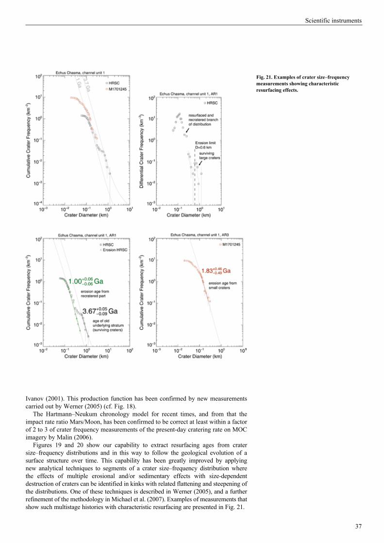
37
Scientific instruments
Ivanov (2001). This production function has been confirmed by new measurements carried out by Werner (2005) (cf. Fig. 18).
The Hartmann–Neukum chronology model for recent times, and from that the impact rate ratio Mars/Moon, has been confirmed to be correct at least within a factor of 2 to 3 of crater frequency measurements of the present-day cratering rate on MOC imagery by Malin (2006).
Figures 19 and 20 show our capability to extract resurfacing ages from crater size–frequency distributions and in this way to follow the geological evolution of a surface structure over time. This capability has been greatly improved by applying new analytical techniques to segments of a crater size–frequency distribution where the effects of multiple erosional and/or sedimentary effects with size-dependent destruction of craters can be identified in kinks with related flattening and steepening of the distributions. One of these techniques is described in Werner (2005), and a further refinement of the methodology in Michael et al. (2007). Examples of measurements that show such multistage histories with characteristic resurfacing are presented in Fig. 21.
fig. 21. examples of crater size–frequency measurements showing characteristic resurfacing effects.
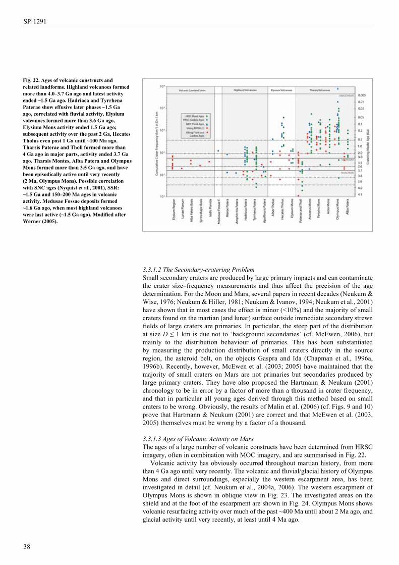
38
SP-1291
3.3.1.2 The Secondary-cratering ProblemSmall secondary craters are produced by large primary impacts and can contaminate the crater size–frequency measurements and thus affect the precision of the age determination. For the Moon and Mars, several papers in recent decades (Neukum & Wise, 1976; Neukum & Hiller, 1981; Neukum & Ivanov, 1994; Neukum et al., 2001) have shown that in most cases the effect is minor (<10%) and the majority of small craters found on the martian (and lunar) surface outside immediate secondary strewn fields of large craters are primaries. In particular, the steep part of the distribution at size D ≤ 1 km is due not to ‘background secondaries’ (cf. McEwen, 2006), but mainly to the distribution behaviour of primaries. This has been substantiated by measuring the production distribution of small craters directly in the source region, the asteroid belt, on the objects Gaspra and Ida (Chapman et al., 1996a, 1996b). Recently, however, McEwen et al. (2003; 2005) have maintained that the majority of small craters on Mars are not primaries but secondaries produced by large primary craters. They have also proposed the Hartmann & Neukum (2001) chronology to be in error by a factor of more than a thousand in crater frequency, and that in particular all young ages derived through this method based on small craters to be wrong. Obviously, the results of Malin et al. (2006) (cf. Figs. 9 and 10) prove that Hartmann & Neukum (2001) are correct and that McEwen et al. (2003, 2005) themselves must be wrong by a factor of a thousand.
3.3.1.3 Ages of Volcanic Activity on MarsThe ages of a large number of volcanic constructs have been determined from HRSC imagery, often in combination with MOC imagery, and are summarised in Fig. 22.
Volcanic activity has obviously occurred throughout martian history, from more than 4 Ga ago until very recently. The volcanic and fluvial/glacial history of Olympus Mons and direct surroundings, especially the western escarpment area, has been investigated in detail (cf. Neukum et al., 2004a, 2006). The western escarpment of Olympus Mons is shown in oblique view in Fig. 23. The investigated areas on the shield and at the foot of the escarpment are shown in Fig. 24. Olympus Mons shows volcanic resurfacing activity over much of the past ~400 Ma until about 2 Ma ago, and glacial activity until very recently, at least until 4 Ma ago.
fig. 22. Ages of volcanic constructs and related landforms. Highland volcanoes formed more than 4.0–3.7 Ga ago and latest activity ended ~1.5 Ga ago. Hadriaca and tyrrhena Paterae show effusive later phases ~1.5 Ga ago, correlated with fluvial activity. elysium volcanoes formed more than 3.6 Ga ago, elysium mons activity ended 1.5 Ga ago; subsequent activity over the past 2 Ga, Hecates tholus even past 1 Ga until ~100 ma ago. tharsis Paterae and tholi formed more than 4 Ga ago in major parts, activity ended 3.7 Ga ago. tharsis montes, Alba Patera and Olympus mons formed more than 3.5 Ga ago, and have been episodically active until very recently (2 ma, Olympus mons). Possible correlation with Snc ages (nyquist et al., 2001), SSr: ~1.5 Ga and 150–200 ma ages in volcanic activity. medusae fossae deposits formed ~1.6 Ga ago, when most highland volcanoes were last active (~1.5 Ga ago). modified after Werner (2005).
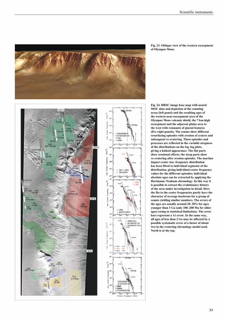
39
Scientific instruments
fig. 23. Oblique view of the western escarpment of Olympus mons.
fig. 24. HrSc image base map with nested mOc data and depiction of the counting areas (left panel) and the resulting ages of the western near-escarpment area of the Olympus mons volcanic shield, the 7 km-high escarpment and the adjacent plains area to the west with remnants of glacial features (five right panels). the counts show different resurfacing episodes with erosion of craters and subsequent re-cratering. these episodes and processes are reflected in the variable steepness of the distributions on the log–log plots, giving a kinked appearance. the flat parts show erosional effects; the steep parts show re-cratering after erosion episodes. the martian impact crater size–frequency distribution has been fitted to individual segments of the distribution, giving individual crater frequency values for the different episodes; individual absolute ages can be extracted by applying the Hartmann–neukum chronology. in this way it is possible to extract the evolutionary history of the area under investigation in detail. Here the fits to the crater frequencies partly have the character of average isochrons for a group of counts yielding similar numbers. the errors of the ages are usually around 20–30% for ages younger than 3 Ga (only 100–200 ma for older ages) owing to statistical limitations. the error bars represent a 1s error. in the same way, all ages of less than 2 Ga may be affected by a possible systematic error of a factor of about two in the cratering chronology model used. north is at the top.
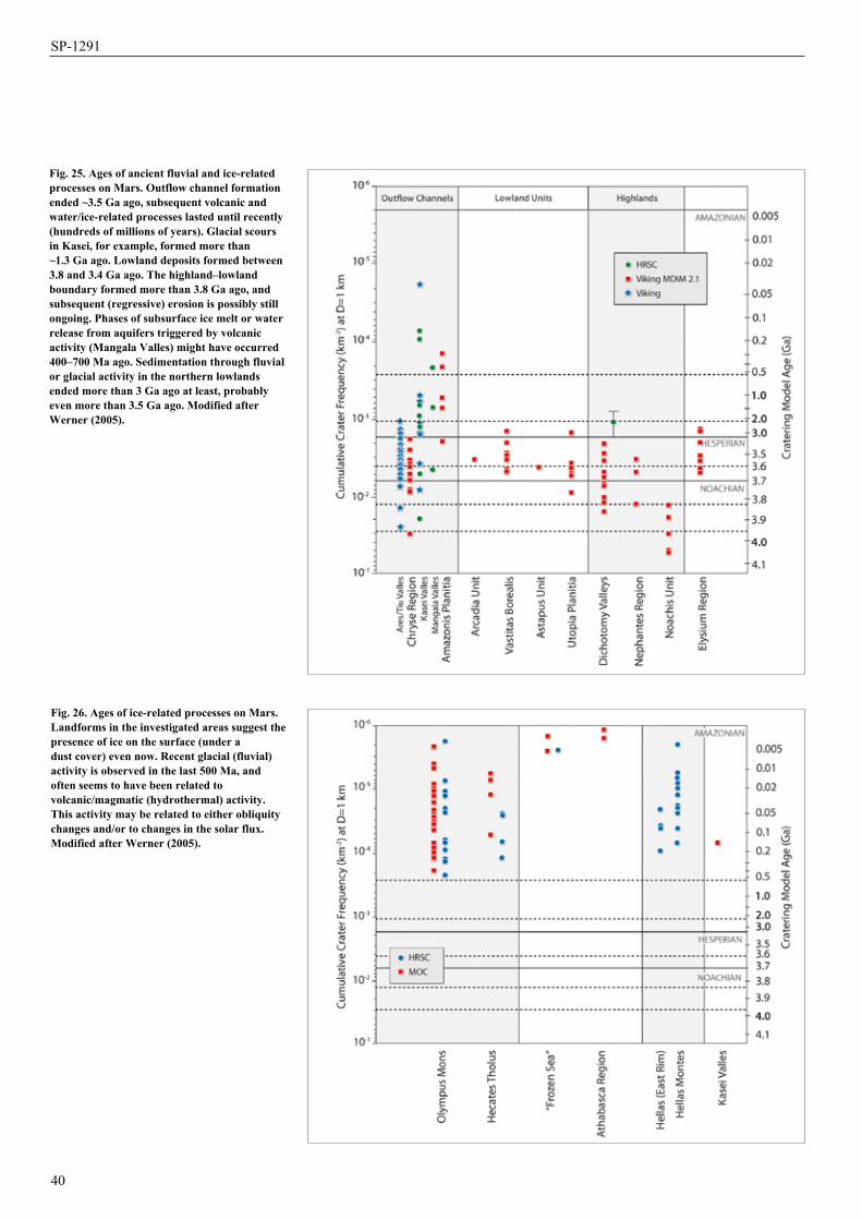
40
SP-1291
fig. 25. Ages of ancient fluvial and ice-related processes on mars. Outflow channel formation ended ~3.5 Ga ago, subsequent volcanic and water/ice-related processes lasted until recently (hundreds of millions of years). Glacial scours in Kasei, for example, formed more than ~1.3 Ga ago. Lowland deposits formed between 3.8 and 3.4 Ga ago. the highland–lowland boundary formed more than 3.8 Ga ago, and subsequent (regressive) erosion is possibly still ongoing. Phases of subsurface ice melt or water release from aquifers triggered by volcanic activity (mangala Valles) might have occurred 400–700 ma ago. Sedimentation through fluvial or glacial activity in the northern lowlands ended more than 3 Ga ago at least, probably even more than 3.5 Ga ago. modified after Werner (2005).
fig. 26. Ages of ice-related processes on mars. Landforms in the investigated areas suggest the presence of ice on the surface (under a dust cover) even now. recent glacial (fluvial) activity is observed in the last 500 ma, and often seems to have been related to volcanic/magmatic (hydrothermal) activity. this activity may be related to either obliquity changes and/or to changes in the solar flux. modified after Werner (2005).
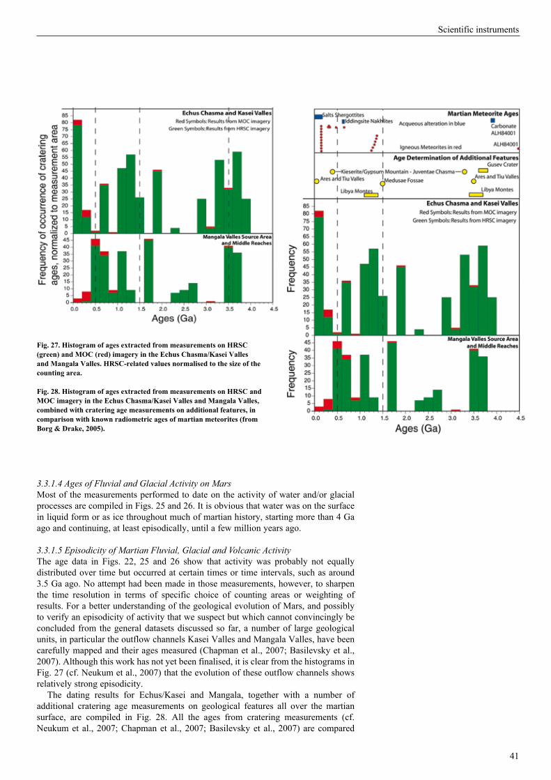
41
Scientific instruments
3.3.1.4 Ages of Fluvial and Glacial Activity on MarsMost of the measurements performed to date on the activity of water and/or glacial processes are compiled in Figs. 25 and 26. It is obvious that water was on the surface in liquid form or as ice throughout much of martian history, starting more than 4 Ga ago and continuing, at least episodically, until a few million years ago.
3.3.1.5 Episodicity of Martian Fluvial, Glacial and Volcanic ActivityThe age data in Figs. 22, 25 and 26 show that activity was probably not equally distributed over time but occurred at certain times or time intervals, such as around 3.5 Ga ago. No attempt had been made in those measurements, however, to sharpen the time resolution in terms of specific choice of counting areas or weighting of results. For a better understanding of the geological evolution of Mars, and possibly to verify an episodicity of activity that we suspect but which cannot convincingly be concluded from the general datasets discussed so far, a number of large geological units, in particular the outflow channels Kasei Valles and Mangala Valles, have been carefully mapped and their ages measured (Chapman et al., 2007; Basilevsky et al., 2007). Although this work has not yet been finalised, it is clear from the histograms in Fig. 27 (cf. Neukum et al., 2007) that the evolution of these outflow channels shows relatively strong episodicity.
The dating results for Echus/Kasei and Mangala, together with a number of additional cratering age measurements on geological features all over the martian surface, are compiled in Fig. 28. All the ages from cratering measurements (cf. Neukum et al., 2007; Chapman et al., 2007; Basilevsky et al., 2007) are compared
fig. 27. Histogram of ages extracted from measurements on HrSc (green) and mOc (red) imagery in the echus chasma/Kasei Valles and mangala Valles. HrSc-related values normalised to the size of the counting area.
fig. 28. Histogram of ages extracted from measurements on HrSc and mOc imagery in the echus chasma/Kasei Valles and mangala Valles, combined with cratering age measurements on additional features, in comparison with known radiometric ages of martian meteorites (from Borg & Drake, 2005).
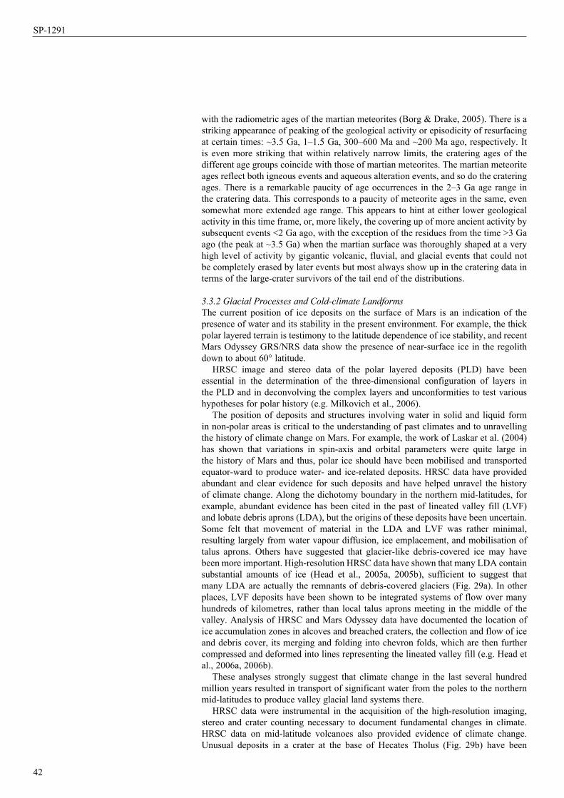
42
SP-1291
with the radiometric ages of the martian meteorites (Borg & Drake, 2005). There is a striking appearance of peaking of the geological activity or episodicity of resurfacing at certain times: ~3.5 Ga, 1–1.5 Ga, 300–600 Ma and ~200 Ma ago, respectively. It is even more striking that within relatively narrow limits, the cratering ages of the different age groups coincide with those of martian meteorites. The martian meteorite ages reflect both igneous events and aqueous alteration events, and so do the cratering ages. There is a remarkable paucity of age occurrences in the 2–3 Ga age range in the cratering data. This corresponds to a paucity of meteorite ages in the same, even somewhat more extended age range. This appears to hint at either lower geological activity in this time frame, or, more likely, the covering up of more ancient activity by subsequent events <2 Ga ago, with the exception of the residues from the time >3 Ga ago (the peak at ~3.5 Ga) when the martian surface was thoroughly shaped at a very high level of activity by gigantic volcanic, fluvial, and glacial events that could not be completely erased by later events but most always show up in the cratering data in terms of the large-crater survivors of the tail end of the distributions.
3.3.2 Glacial Processes and Cold-climate LandformsThe current position of ice deposits on the surface of Mars is an indication of the presence of water and its stability in the present environment. For example, the thick polar layered terrain is testimony to the latitude dependence of ice stability, and recent Mars Odyssey GRS/NRS data show the presence of near-surface ice in the regolith down to about 60° latitude.
HRSC image and stereo data of the polar layered deposits (PLD) have been essential in the determination of the three-dimensional configuration of layers in the PLD and in deconvolving the complex layers and unconformities to test various hypotheses for polar history (e.g. Milkovich et al., 2006).
The position of deposits and structures involving water in solid and liquid form in non-polar areas is critical to the understanding of past climates and to unravelling the history of climate change on Mars. For example, the work of Laskar et al. (2004) has shown that variations in spin-axis and orbital parameters were quite large in the history of Mars and thus, polar ice should have been mobilised and transported equator-ward to produce water- and ice-related deposits. HRSC data have provided abundant and clear evidence for such deposits and have helped unravel the history of climate change. Along the dichotomy boundary in the northern mid-latitudes, for example, abundant evidence has been cited in the past of lineated valley fill (LVF) and lobate debris aprons (LDA), but the origins of these deposits have been uncertain. Some felt that movement of material in the LDA and LVF was rather minimal, resulting largely from water vapour diffusion, ice emplacement, and mobilisation of talus aprons. Others have suggested that glacier-like debris-covered ice may have been more important. High-resolution HRSC data have shown that many LDA contain substantial amounts of ice (Head et al., 2005a, 2005b), sufficient to suggest that many LDA are actually the remnants of debris-covered glaciers (Fig. 29a). In other places, LVF deposits have been shown to be integrated systems of flow over many hundreds of kilometres, rather than local talus aprons meeting in the middle of the valley. Analysis of HRSC and Mars Odyssey data have documented the location of ice accumulation zones in alcoves and breached craters, the collection and flow of ice and debris cover, its merging and folding into chevron folds, which are then further compressed and deformed into lines representing the lineated valley fill (e.g. Head et al., 2006a, 2006b).
These analyses strongly suggest that climate change in the last several hundred million years resulted in transport of significant water from the poles to the northern mid-latitudes to produce valley glacial land systems there.
HRSC data were instrumental in the acquisition of the high-resolution imaging, stereo and crater counting necessary to document fundamental changes in climate. HRSC data on mid-latitude volcanoes also provided evidence of climate change. Unusual deposits in a crater at the base of Hecates Tholus (Fig. 29b) have been
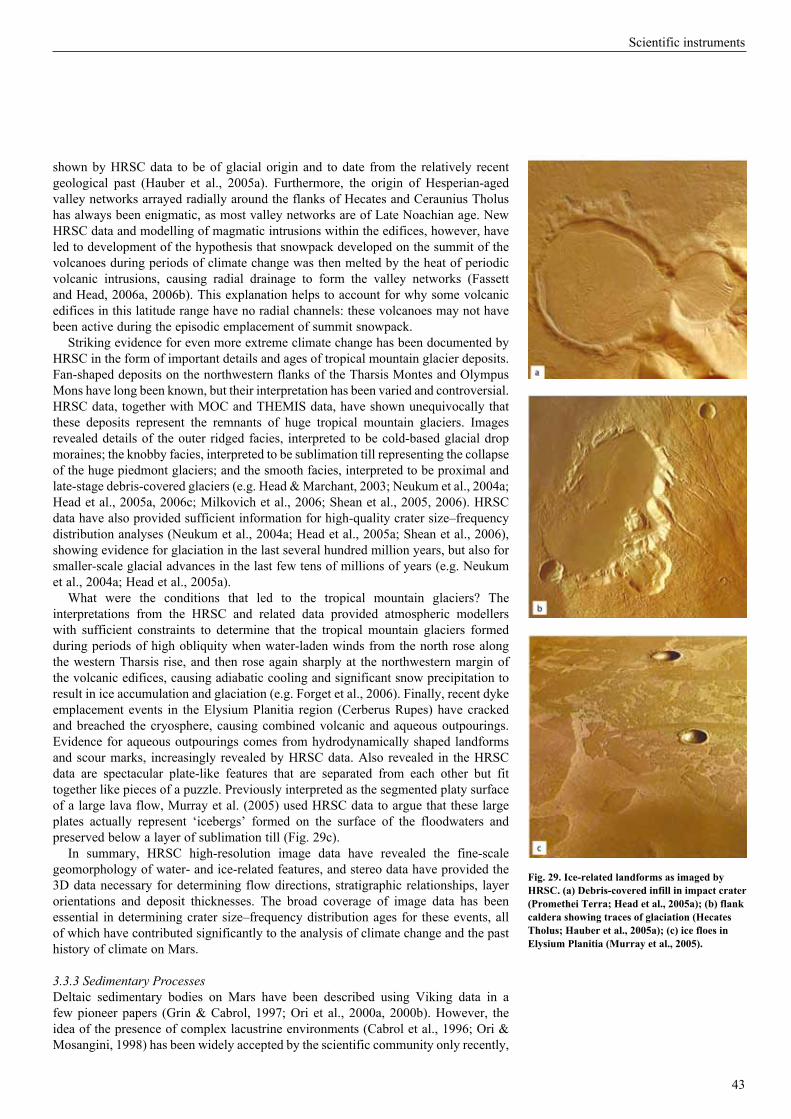
43
Scientific instruments
shown by HRSC data to be of glacial origin and to date from the relatively recent geological past (Hauber et al., 2005a). Furthermore, the origin of Hesperian-aged valley networks arrayed radially around the flanks of Hecates and Ceraunius Tholus has always been enigmatic, as most valley networks are of Late Noachian age. New HRSC data and modelling of magmatic intrusions within the edifices, however, have led to development of the hypothesis that snowpack developed on the summit of the volcanoes during periods of climate change was then melted by the heat of periodic volcanic intrusions, causing radial drainage to form the valley networks (Fassett and Head, 2006a, 2006b). This explanation helps to account for why some volcanic edifices in this latitude range have no radial channels: these volcanoes may not have been active during the episodic emplacement of summit snowpack.
Striking evidence for even more extreme climate change has been documented by HRSC in the form of important details and ages of tropical mountain glacier deposits. Fan-shaped deposits on the northwestern flanks of the Tharsis Montes and Olympus Mons have long been known, but their interpretation has been varied and controversial. HRSC data, together with MOC and THEMIS data, have shown unequivocally that these deposits represent the remnants of huge tropical mountain glaciers. Images revealed details of the outer ridged facies, interpreted to be cold-based glacial drop moraines; the knobby facies, interpreted to be sublimation till representing the collapse of the huge piedmont glaciers; and the smooth facies, interpreted to be proximal and late-stage debris-covered glaciers (e.g. Head & Marchant, 2003; Neukum et al., 2004a; Head et al., 2005a, 2006c; Milkovich et al., 2006; Shean et al., 2005, 2006). HRSC data have also provided sufficient information for high-quality crater size–frequency distribution analyses (Neukum et al., 2004a; Head et al., 2005a; Shean et al., 2006), showing evidence for glaciation in the last several hundred million years, but also for smaller-scale glacial advances in the last few tens of millions of years (e.g. Neukum et al., 2004a; Head et al., 2005a).
What were the conditions that led to the tropical mountain glaciers? The interpretations from the HRSC and related data provided atmospheric modellers with sufficient constraints to determine that the tropical mountain glaciers formed during periods of high obliquity when water-laden winds from the north rose along the western Tharsis rise, and then rose again sharply at the northwestern margin of the volcanic edifices, causing adiabatic cooling and significant snow precipitation to result in ice accumulation and glaciation (e.g. Forget et al., 2006). Finally, recent dyke emplacement events in the Elysium Planitia region (Cerberus Rupes) have cracked and breached the cryosphere, causing combined volcanic and aqueous outpourings. Evidence for aqueous outpourings comes from hydrodynamically shaped landforms and scour marks, increasingly revealed by HRSC data. Also revealed in the HRSC data are spectacular plate-like features that are separated from each other but fit together like pieces of a puzzle. Previously interpreted as the segmented platy surface of a large lava flow, Murray et al. (2005) used HRSC data to argue that these large plates actually represent ‘icebergs’ formed on the surface of the floodwaters and preserved below a layer of sublimation till (Fig. 29c).
In summary, HRSC high-resolution image data have revealed the fine-scale geomorphology of water- and ice-related features, and stereo data have provided the 3D data necessary for determining flow directions, stratigraphic relationships, layer orientations and deposit thicknesses. The broad coverage of image data has been essential in determining crater size–frequency distribution ages for these events, all of which have contributed significantly to the analysis of climate change and the past history of climate on Mars.
3.3.3 Sedimentary ProcessesDeltaic sedimentary bodies on Mars have been described using Viking data in a few pioneer papers (Grin & Cabrol, 1997; Ori et al., 2000a, 2000b). However, the idea of the presence of complex lacustrine environments (Cabrol et al., 1996; Ori & Mosangini, 1998) has been widely accepted by the scientific community only recently,
fig. 29. ice-related landforms as imaged by HrSc. (a) Debris-covered infill in impact crater (Promethei terra; Head et al., 2005a); (b) flank caldera showing traces of glaciation (Hecates tholus; Hauber et al., 2005a); (c) ice floes in elysium Planitia (murray et al., 2005).

44
SP-1291
when data from the new mission have provided other data. The contribution of the HRSC to our understanding the lacustrine sedimentary environments and associated deltas has been remarkable. The high-quality data with stereo capability allow detailed analysis of the sedimentary strata patterns, morphologies and even facies.
It is now clear that deltas exhibit a variety of facies associations, ranging from Gilbert-type deltas to shallow-water fluvial-dominated deltas. Gilbert-type deltas are simple bodies and form when short-headed fluvial systems debouch in a lacustrine basin with a steep margin. Shallow-water deltas are controlled by long fluvial systems and display a large number of distributary channels. The transition from the deltaic plain and the prodelta area is subtle due to the low gradient. Mouth bars are poorly developed. Between these end members there are a number of fan-shaped bodies that in places show distinct evidence of interaction with a standing body of water, but can often be ascribed to alluvial fans due the lack of evidence of a lacustrine environment.
HRSC images in combination with HRSC-based DTM and, at places, MOC narrow-angle images allow us to observe the outcrops with an Earth-like approach and in particular to describe the internal geometry of layered sequences. These observations are particularly important with respect to sedimentary bodies, because these systems display complex internal geometrical patterns. Delta-like deposits, wave-cut terraces, and shorelines are fundamental features to support the hypothesis of standing and long-lived water bodies on Mars. Intra-crater lakes, due to their relatively limited size and their strong climatic coupling, might allow the reconstruction of local hydrological cycles, which could help improve our understanding of the evolution of the martian climate.
Figure 30 presents an example from the Eberswalde fan delta, centred at 24.1°S and 326.4°E, located in one of the richest fluvial-related morphologies areas of Mars (e.g. Malin & Edgett, 2001). The delta is made of bright and dark interlayered deposits, which display a cyclic depositional pattern. The bright layers appear to be more resistant to weathering and erosion. Some of the bright layers consist of very poorly sorted material, with boulders up to 10 m in diameter floating in a finer matrix suggesting an emplacement as mass flows. Other layers consist of finer and better-sorted material. The sedimentary complex displays a low-dipping proximal area (1–2), a distal relatively high-dipping area (6–10) and a more distal low-dipping area (1–2), which gradually connects with the crater floor.
We interpret the low-dipping proximal part as delta plain facies consisting of distributary areas, mostly built by coalescing point bars, and interdistributary area, in which crevasse splays flood into the plain (Pondrelli et al., 2006). At places the topset–foreset–bottomset architecture typical of fan deltas is present, even if the foresets are just slightly inclined. We interpret the high-dipping part of the fan delta as delta front deposits (Pondrelli et al., 2006).
Along an erosional cut, a transgressive–regressive cycle has been observed, with layers at the base showing a retrogradational stacking pattern on top of which clinoforms suggesting a progradational stacking pattern develop forming an offlap surface. We interpret the retrogradational stacking pattern as formed during a transgressive system tract followed by a high stand system tract corresponding to the progradational stacking pattern. The transition among these systems is marked by a maximum flooding surface. This geometry suggests an allogenic control on the deposition.
A survey of the Xanthe Terra cratered terrains revealed several delta-like deposits inside impact craters (Subur, Sabrina, Nanedi and Tyras Vallis) and downstream of a widening of the valley floors (Hypanis Valles) (Di Achille et al., 2006a; Hauber et al., 2005b). In particular, the Tyras palaeolacustrine system, formed by the Tyras Vallis channel and an as yet unnamed Noachian complex crater (70 km in diameter) (Scott & Tanaka, 1986), has been studied in detail using high-resolution topography derived from HRSC stereo data (Di Achille et al., 2006a; Fig. 31a). This supports the recognition of the Tyras fan deposit and its morphometric description, which allows the reconstruction of the overall lacustrine depositional history from the parallel
fig. 30. the delta in the eberswalde crater (ca. 50 × 70 km). (a) Perspective 3D false-colour view of the eberswalde delta and the delta (arrow). to the left (=south), the rim of the large Holden crater is visible. Both craters have been proposed as future landing sites due to their spectacular fluvial and lacustrine landforms (HrSc image 511). (b) the delta in eberswalde crater seen in perspective view from the south. the delta is located at 24.1°S and 326.4°e and has a size of 12 × 12 km (detail of HrSc image 2013).
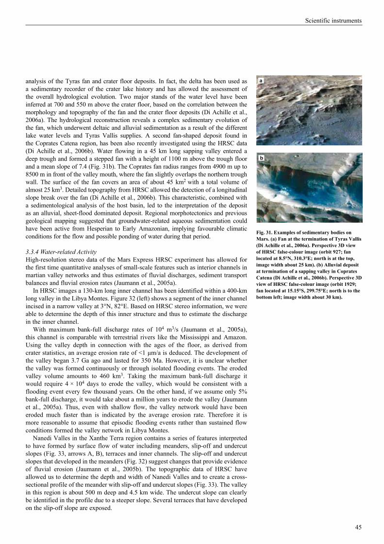
45
Scientific instruments
analysis of the Tyras fan and crater floor deposits. In fact, the delta has been used as a sedimentary recorder of the crater lake history and has allowed the assessment of the overall hydrological evolution. Two major stands of the water level have been inferred at 700 and 550 m above the crater floor, based on the correlation between the morphology and topography of the fan and the crater floor deposits (Di Achille et al., 2006a). The hydrological reconstruction reveals a complex sedimentary evolution of the fan, which underwent deltaic and alluvial sedimentation as a result of the different lake water levels and Tyras Vallis supplies. A second fan-shaped deposit found in the Coprates Catena region, has been also recently investigated using the HRSC data (Di Achille et al., 2006b). Water flowing in a 45 km long sapping valley entered a deep trough and formed a stepped fan with a height of 1100 m above the trough floor and a mean slope of 7.4 (Fig. 31b). The Coprates fan radius ranges from 4900 m up to 8500 m in front of the valley mouth, where the fan slightly overlaps the northern trough wall. The surface of the fan covers an area of about 45 km2 with a total volume of almost 25 km3. Detailed topography from HRSC allowed the detection of a longitudinal slope break over the fan (Di Achille et al., 2006b). This characteristic, combined with a sedimentological analysis of the host basin, led to the interpretation of the deposit as an alluvial, sheet-flood dominated deposit. Regional morphotectonics and previous geological mapping suggested that groundwater-related aqueous sedimentation could have been active from Hesperian to Early Amazonian, implying favourable climatic conditions for the flow and possible ponding of water during that period.
3.3.4 Water-related ActivityHigh-resolution stereo data of the Mars Express HRSC experiment has allowed for the first time quantitative analyses of small-scale features such as interior channels in martian valley networks and thus estimates of fluvial discharges, sediment transport balances and fluvial erosion rates (Jaumann et al., 2005a).
In HRSC images a 130-km long inner channel has been identified within a 400-km long valley in the Libya Montes. Figure 32 (left) shows a segment of the inner channel incised in a narrow valley at 3°N, 82°E. Based on HRSC stereo information, we were able to determine the depth of this inner structure and thus to estimate the discharge in the inner channel.
With maximum bank-full discharge rates of 104 m3/s (Jaumann et al., 2005a), this channel is comparable with terrestrial rivers like the Mississippi and Amazon. Using the valley depth in connection with the ages of the floor, as derived from crater statistics, an average erosion rate of <1 μm/a is deduced. The development of the valley began 3.7 Ga ago and lasted for 350 Ma. However, it is unclear whether the valley was formed continuously or through isolated flooding events. The eroded valley volume amounts to 460 km3. Taking the maximum bank-full discharge it would require 4 × 10⁴ days to erode the valley, which would be consistent with a flooding event every few thousand years. On the other hand, if we assume only 5% bank-full discharge, it would take about a million years to erode the valley (Jaumann et al., 2005a). Thus, even with shallow flow, the valley network would have been eroded much faster than is indicated by the average erosion rate. Therefore it is more reasonable to assume that episodic flooding events rather than sustained flow conditions formed the valley network in Libya Montes.
Nanedi Valles in the Xanthe Terra region contains a series of features interpreted to have formed by surface flow of water including meanders, slip-off and undercut slopes (Fig. 33, arrows A, B), terraces and inner channels. The slip-off and undercut slopes that developed in the meanders (Fig. 32) suggest changes that provide evidence of fluvial erosion (Jaumann et al., 2005b). The topographic data of HRSC have allowed us to determine the depth and width of Nanedi Valles and to create a cross-sectional profile of the meander with slip-off and undercut slopes (Fig. 33). The valley in this region is about 500 m deep and 4.5 km wide. The undercut slope can clearly be identified in the profile due to a steeper slope. Several terraces that have developed on the slip-off slope are exposed.
fig. 31. examples of sedimentary bodies on mars. (a) fan at the termination of tyras Vallis (Di Achille et al., 2006a). Perspective 3D view of HrSc false-colour image (orbit 927; fan located at 8.5°n, 310.3°e; north is at the top, image width about 25 km). (b) Alluvial deposit at termination of a sapping valley in coprates catena (Di Achille et al., 2006b). Perspective 3D view of HrSc false-colour image (orbit 1929; fan located at 15.15°S, 299.75°e; north is to the bottom left; image width about 30 km).
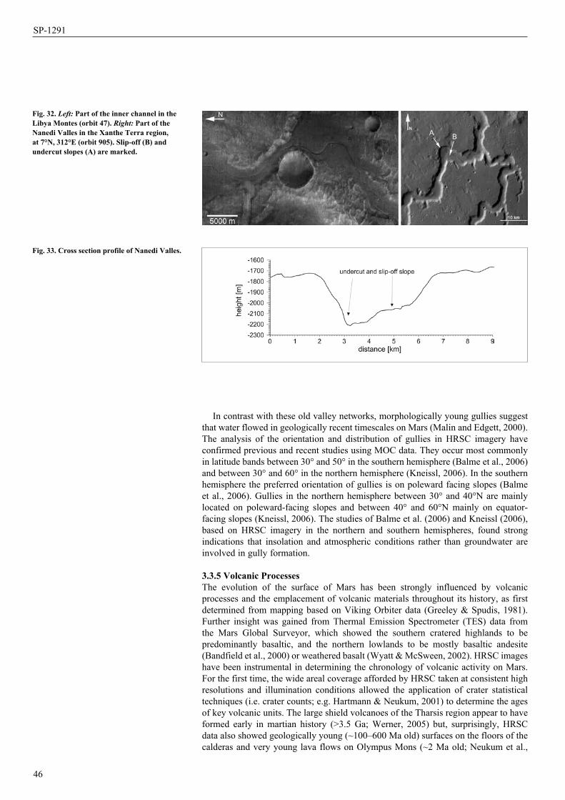
46
SP-1291
In contrast with these old valley networks, morphologically young gullies suggest that water flowed in geologically recent timescales on Mars (Malin and Edgett, 2000). The analysis of the orientation and distribution of gullies in HRSC imagery have confirmed previous and recent studies using MOC data. They occur most commonly in latitude bands between 30° and 50° in the southern hemisphere (Balme et al., 2006) and between 30° and 60° in the northern hemisphere (Kneissl, 2006). In the southern hemisphere the preferred orientation of gullies is on poleward facing slopes (Balme et al., 2006). Gullies in the northern hemisphere between 30° and 40°N are mainly located on poleward-facing slopes and between 40° and 60°N mainly on equator-facing slopes (Kneissl, 2006). The studies of Balme et al. (2006) and Kneissl (2006), based on HRSC imagery in the northern and southern hemispheres, found strong indications that insolation and atmospheric conditions rather than groundwater are involved in gully formation.
3.3.5 Volcanic ProcessesThe evolution of the surface of Mars has been strongly influenced by volcanic processes and the emplacement of volcanic materials throughout its history, as first determined from mapping based on Viking Orbiter data (Greeley & Spudis, 1981). Further insight was gained from Thermal Emission Spectrometer (TES) data from the Mars Global Surveyor, which showed the southern cratered highlands to be predominantly basaltic, and the northern lowlands to be mostly basaltic andesite (Bandfield et al., 2000) or weathered basalt (Wyatt & McSween, 2002). HRSC images have been instrumental in determining the chronology of volcanic activity on Mars. For the first time, the wide areal coverage afforded by HRSC taken at consistent high resolutions and illumination conditions allowed the application of crater statistical techniques (i.e. crater counts; e.g. Hartmann & Neukum, 2001) to determine the ages of key volcanic units. The large shield volcanoes of the Tharsis region appear to have formed early in martian history (>3.5 Ga; Werner, 2005) but, surprisingly, HRSC data also showed geologically young (~100–600 Ma old) surfaces on the floors of the calderas and very young lava flows on Olympus Mons (~2 Ma old; Neukum et al.,
fig. 32. Left: Part of the inner channel in the Libya montes (orbit 47). Right: Part of the nanedi Valles in the Xanthe terra region, at 7°n, 312°e (orbit 905). Slip-off (B) and undercut slopes (A) are marked.
fig. 33. cross section profile of nanedi Valles.
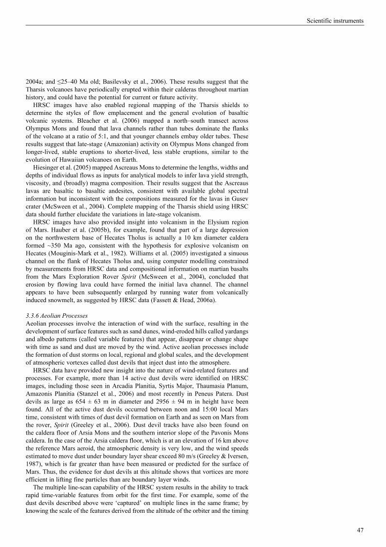
47
Scientific instruments
2004a; and ≤25–40 Ma old; Basilevsky et al., 2006). These results suggest that the Tharsis volcanoes have periodically erupted within their calderas throughout martian history, and could have the potential for current or future activity.
HRSC images have also enabled regional mapping of the Tharsis shields to determine the styles of flow emplacement and the general evolution of basaltic volcanic systems. Bleacher et al. (2006) mapped a north–south transect across Olympus Mons and found that lava channels rather than tubes dominate the flanks of the volcano at a ratio of 5:1, and that younger channels embay older tubes. These results suggest that late-stage (Amazonian) activity on Olympus Mons changed from longer-lived, stable eruptions to shorter-lived, less stable eruptions, similar to the evolution of Hawaiian volcanoes on Earth.
Hiesinger et al. (2005) mapped Ascreaus Mons to determine the lengths, widths and depths of individual flows as inputs for analytical models to infer lava yield strength, viscosity, and (broadly) magma composition. Their results suggest that the Ascreaus lavas are basaltic to basaltic andesites, consistent with available global spectral information but inconsistent with the compositions measured for the lavas in Gusev crater (McSween et al., 2004). Complete mapping of the Tharsis shield using HRSC data should further elucidate the variations in late-stage volcanism.
HRSC images have also provided insight into volcanism in the Elysium region of Mars. Hauber et al. (2005b), for example, found that part of a large depression on the northwestern base of Hecates Tholus is actually a 10 km diameter caldera formed ~350 Ma ago, consistent with the hypothesis for explosive volcanism on Hecates (Mouginis-Mark et al., 1982). Williams et al. (2005) investigated a sinuous channel on the flank of Hecates Tholus and, using computer modelling constrained by measurements from HRSC data and compositional information on martian basalts from the Mars Exploration Rover Spirit (McSween et al., 2004), concluded that erosion by flowing lava could have formed the initial lava channel. The channel appears to have been subsequently enlarged by running water from volcanically induced snowmelt, as suggested by HRSC data (Fassett & Head, 2006a).
3.3.6 Aeolian ProcessesAeolian processes involve the interaction of wind with the surface, resulting in the development of surface features such as sand dunes, wind-eroded hills called yardangs and albedo patterns (called variable features) that appear, disappear or change shape with time as sand and dust are moved by the wind. Active aeolian processes include the formation of dust storms on local, regional and global scales, and the development of atmospheric vortexes called dust devils that inject dust into the atmosphere.
HRSC data have provided new insight into the nature of wind-related features and processes. For example, more than 14 active dust devils were identified on HRSC images, including those seen in Arcadia Planitia, Syrtis Major, Thaumasia Planum, Amazonis Planitia (Stanzel et al., 2006) and most recently in Peneus Patera. Dust devils as large as 654 ± 63 m in diameter and 2956 ± 94 m in height have been found. All of the active dust devils occurred between noon and 15:00 local Mars time, consistent with times of dust devil formation on Earth and as seen on Mars from the rover, Spirit (Greeley et al., 2006). Dust devil tracks have also been found on the caldera floor of Arsia Mons and the southern interior slope of the Pavonis Mons caldera. In the case of the Arsia caldera floor, which is at an elevation of 16 km above the reference Mars aeroid, the atmospheric density is very low, and the wind speeds estimated to move dust under boundary layer shear exceed 80 m/s (Greeley & Iversen, 1987), which is far greater than have been measured or predicted for the surface of Mars. Thus, the evidence for dust devils at this altitude shows that vortices are more efficient in lifting fine particles than are boundary layer winds.
The multiple line-scan capability of the HRSC system results in the ability to track rapid time-variable features from orbit for the first time. For example, some of the dust devils described above were ‘captured’ on multiple lines in the same frame; by knowing the scale of the features derived from the altitude of the orbiter and the timing
48
SP-1291
between HRSC line array exposures, the speeds of the dust devils could be determined. Speeds were found to range from a few to about 25 m/s (Stanzel et al., 2006).
HRSC images enable an assessment of the detection of variable features as a function of imaging wavelength. Such features have been mapped on images from previous missions (primarily the Viking Orbiter) for comparison with predictions of near-surface winds as a function of season. Unfortunately, most of the previous mapping was conducted without regard to the filter through which the images were taken, potentially leading to erroneous correlations. Because HRSC data are taken through four colour filters almost simultaneously, the detection of variable features can be assessed consistently; the results show that most bright variable features (such as wind streaks) are best seen through the red filter.
Future work will involve studies of variable features in selected regions of Mars and analysis of dune fields for which HRSC and compositional data, as from the Omega instrument, are available. This work will allow us to trace potential source regions of the sands in the dune fields as part of the overall analysis of sediment transport pathways on Mars.
3.3.7 TectonismThe morphology of the martian surface displays clear and unambiguous evidence of tectonic processes (e.g. Carr, 1981; Banerdt et al., 1992). A variety of structural landforms suggests brittle failure of the crust and the lithosphere. The most frequent examples are extensional features (e.g. long and narrow simple grabens, rifts) and contractional features (wrinkle ridges, lobate scarps and fold belts; for a recent review see Mueller & Golombek, 2004). A critical aspect of any study of martian geodynamics based on the analysis of tectonic structures is the determination of the chronology. The relative ages of the features and, therefore, the processes responsible for their formation may be dated by structural mapping and crater counts, while additional information on topography and gravity is required to model loads and to derive stresses in the lithosphere (Golombek & Banerdt, 1999; Anderson et al., 2001). HRSC data were used for the investigation of extensional as well as contractional tectonic features.
On Earth, tectonic (continental) rifts are defined as ‘elongated tectonic depressions associated with which the entire lithosphere has been modified in extension’ (Olsen & Morgan, 1995: 4). Therefore, rifts provide information on significant crustal deformation and associated stress fields. Earlier studies by members of the HRSC team, but still without HRSC data, reported the identification of extensional structures on Mars that can be directly compared in several aspects with their terrestrial analogues, i.e. terrestrial continental rifts (Hauber & Kronberg, 2001, 2005c). The use of HRSC images has improved the situation in that they provide relatively high-resolution data (typically 10–20 m/pixel) over large areas. Such images are ideally suited for crater counting and, therefore, for the age determination of key surface units. Two martian rifts have been investigated with HRSC images so far: the Acheron Fossae and the Coracis Fossae rift systems.
The Acheron Fossae region is an ancient crustal block exposed in the northwestern Tharsis province on Mars. The extensional tectonics along the E–W-trending topographic high of Acheron Fossae is interpreted as a surface expression of upwelling asthenospheric material that initiated regional uplift, crustal extension and breakup, and associated volcanism in the Noachian period (Kronberg et al., 2006). The tectonic architecture and the dimensions of the extensional structures are comparable with those of terrestrial continental rifts (Fig. 34). An area of elevated topography and strong erosion in the eastern Acheron Fossae region is interpreted as a rift-related centre of volcanism. The extension across the Acheron Fossae reaches 1.2–8.7 km, comparable to young continental rifts on Earth. Crater statistics indicate an absolute cratering model age of between ~3.9 and 3.7 Ga for the rifting. The uplift observed on the rift flanks of the Acheron Fossae indicates a fairly thin and thus hot lithosphere. Using flexural analysis, Kronberg et al. (2006) have constrained the elastic lithosphere

49
Scientific instruments
thickness at the time of rifting to 8.9–11.3 km, corresponding to thermal gradients of between 28 and 41K/km. These heat flows are substantially larger than Noachian heat flow values previously reported, but are consistent with the presence of rift-related volcanism and a magmatically very active environment.
The Coracis Fossae are located in the southern Thaumasia region and cut the Thaumasia highland belt in the NE–SW direction. Their structural architecture is also similar to terrestrial continental rifts. Grott et al. (2005) have identified flexural uplift at the flanks of the central Coracis Fossae rift valley. Modelling the topography, the elastic thickness is constrained to 10.3–12.5 km; the corresponding mechanical thickness and thermal gradient are 15–19 km and 27–33K/km, respectively. These values are similar to those found for the Acheron Fossae region, which are similar in age. The time of rifting of the Coracis Fossae is dated by evaluating the crater size–frequency distribution of key surface units related to the rifting. Thus, the heat flux between 3.5 and 3.9 Ga ago is calculated to be 54–66 mW/m² . Furthermore, the stresses supported by the rift bounding faults are estimated to be below 5 MPa. We speculate that this weakness may be connected to the presence of water below the surface.
Contractional tectonic surface features on Mars include wrinkle ridges and lobate scarps (Mueller & Golombek, 2004). It is possible to gain insight into the state of the early martian lithosphere by modelling the topography above lobate scarps (surface breaking thrust faults). HRSC data and MOLA topography were used to analyse two thrust faults in the southern Thaumasia region (Grott et al., 2006). Crater counts of key surface units associated with the faulting indicate a scarp emplacement in the Late Noachian–Early Hesperian periods between 4.0 and 3.5 Ga. The seismogenic layer thickness at the time of faulting is constrained to 27–35 km and 21–28 km for the two scarps investigated, implying palaeo-geothermal gradients of 12–18 and 15–23K/km, corresponding to heat flows of 24–36 and 30–46 mW/m². The heat flow values obtained by Grott et al. (2006) are considerably lower than those derived from rift flank uplift at the nearby Coracis Fossae for a similar time period, indicating that surface heat flow is a strong function of regional setting. If viewed as representative of magmatically active and inactive regions, the thermal gradients at rifts and scarps
fig. 34. 3D perspective view of the eastern Acheron fossae region, based on HrSc colour and stereo data. the area is heavily fractured by extensional faults. the large elevated area in the foreground is interpreted to be a pre- or synrift volcanic region. two small cones in the middle left foreground may be volcanic edifices.

50
SP-1291
Table 3. Phobos encounters
Orbit Encounter times (UTC) Mean anomaly (deg) Flyby distance (km)
413 2004-05-18T08:34 32.02 1881
649 2004-07-23T12:40 185.11 1834
682 2004-08-01T18:35 178.02 1465
715 2004-08-11T00:30 171.36 1207
748 2004-08-20T06:25 164.77 1239
756 2004-08-22T12:06 169.14 147
1064 2004-11-16T14:21 114.14 4676
1163 2004-12-14T08:05 94.43 3815
1212 2004-12-28T02:52 91.70 1966
1558 2005-04-03T23:50 40.54 3598
1574 2005-04-08T11:20 53.57 3801
1607 2005-04-17T17:15 47.54 3988
1769 2005-06-02T03:40 202.77 1440
1901 2005-07-09T03:25 181.73 3109
2151 2005-09-16T23:24 136.73 3825
2192 2005-09-28T11:02 131.80 2924
2233 2005-10-09T22:29 127.02 2111
2381 2005-11-20T09:06 94.23 3169
2397 2005-11-24T20:38 100.80 1672
2405 2005-11-27T02:15 106.72 1426
2446 2005-12-08T13:44 96.60 2026
2463 2005-12-13T08:03 75.12 4233
2479 2005-12-17T19:26 83.87 2913
2487 2005-12-20T01:15 89.69 2571
2501 2005-12-24T00:50 272.40 4745
2583 2006-01-15T23:49 262.03 4141
2601 2006-01-20T23:07 103.40 5264
2643 2006-02-01T17:26 63.74 4189
2673 2006-02-10T04:40 262.97 2027
2682 2006-02-12T17:32 241.91 5149
2706 2006-02-19T10:24 256.23 2179
2739 2006-02-28T16:24 250.20 1783
2747 2006-03-02T22:04 252.95 1050
2756 2006-03-05T11:05 236.23 4168
2780 2006-03-12T04:03 246.45 606
2805 2006-03-19T04:19 238.99 1955
2813 2006-03-21T09:58 239.68 832
2846 2006-03-30T15:54 233.92 1328
2854 2006-04-01T21:30 237.83 973
2912 2006-04-18T03:46 223.28 2394
2979 2006-05-06T23:15 211.97 5092
3005 2006-05-13T23:41 208.94 5305
3245 2006-07-20T06:16 150.96 4942
3310 2006-08-07T10:50 161.70 606
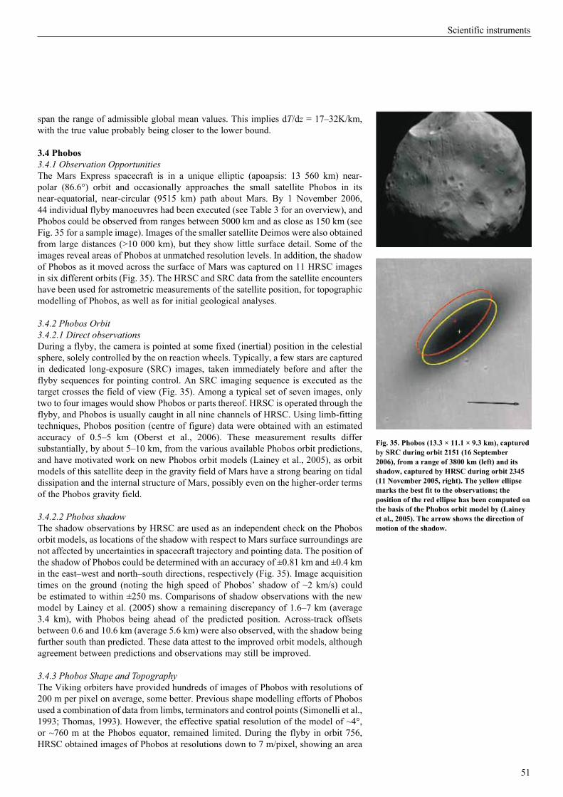
51
Scientific instruments
span the range of admissible global mean values. This implies dT/dz = 17–32K/km, with the true value probably being closer to the lower bound. 3.4 Phobos3.4.1 Observation OpportunitiesThe Mars Express spacecraft is in a unique elliptic (apoapsis: 13 560 km) near-polar (86.6°) orbit and occasionally approaches the small satellite Phobos in its near-equatorial, near-circular (9515 km) path about Mars. By 1 November 2006, 44 individual flyby manoeuvres had been executed (see Table 3 for an overview), and Phobos could be observed from ranges between 5000 km and as close as 150 km (see Fig. 35 for a sample image). Images of the smaller satellite Deimos were also obtained from large distances (>10 000 km), but they show little surface detail. Some of the images reveal areas of Phobos at unmatched resolution levels. In addition, the shadow of Phobos as it moved across the surface of Mars was captured on 11 HRSC images in six different orbits (Fig. 35). The HRSC and SRC data from the satellite encounters have been used for astrometric measurements of the satellite position, for topographic modelling of Phobos, as well as for initial geological analyses.
3.4.2 Phobos Orbit 3.4.2.1 Direct observationsDuring a flyby, the camera is pointed at some fixed (inertial) position in the celestial sphere, solely controlled by the on reaction wheels. Typically, a few stars are captured in dedicated long-exposure (SRC) images, taken immediately before and after the flyby sequences for pointing control. An SRC imaging sequence is executed as the target crosses the field of view (Fig. 35). Among a typical set of seven images, only two to four images would show Phobos or parts thereof. HRSC is operated through the flyby, and Phobos is usually caught in all nine channels of HRSC. Using limb-fitting techniques, Phobos position (centre of figure) data were obtained with an estimated accuracy of 0.5–5 km (Oberst et al., 2006). These measurement results differ substantially, by about 5–10 km, from the various available Phobos orbit predictions, and have motivated work on new Phobos orbit models (Lainey et al., 2005), as orbit models of this satellite deep in the gravity field of Mars have a strong bearing on tidal dissipation and the internal structure of Mars, possibly even on the higher-order terms of the Phobos gravity field.
3.4.2.2 Phobos shadowThe shadow observations by HRSC are used as an independent check on the Phobos orbit models, as locations of the shadow with respect to Mars surface surroundings are not affected by uncertainties in spacecraft trajectory and pointing data. The position of the shadow of Phobos could be determined with an accuracy of ±0.81 km and ±0.4 km in the east–west and north–south directions, respectively (Fig. 35). Image acquisition times on the ground (noting the high speed of Phobos’ shadow of ~2 km/s) could be estimated to within ±250 ms. Comparisons of shadow observations with the new model by Lainey et al. (2005) show a remaining discrepancy of 1.6–7 km (average 3.4 km), with Phobos being ahead of the predicted position. Across-track offsets between 0.6 and 10.6 km (average 5.6 km) were also observed, with the shadow being further south than predicted. These data attest to the improved orbit models, although agreement between predictions and observations may still be improved.
3.4.3 Phobos Shape and TopographyThe Viking orbiters have provided hundreds of images of Phobos with resolutions of 200 m per pixel on average, some better. Previous shape modelling efforts of Phobos used a combination of data from limbs, terminators and control points (Simonelli et al., 1993; Thomas, 1993). However, the effective spatial resolution of the model of ~4°, or ~760 m at the Phobos equator, remained limited. During the flyby in orbit 756, HRSC obtained images of Phobos at resolutions down to 7 m/pixel, showing an area
fig. 35. Phobos (13.3 × 11.1 × 9.3 km), captured by Src during orbit 2151 (16 September 2006), from a range of 3800 km (left) and its shadow, captured by HrSc during orbit 2345 (11 november 2005, right). the yellow ellipse marks the best fit to the observations; the position of the red ellipse has been computed on the basis of the Phobos orbit model by (Lainey et al., 2005). the arrow shows the direction of motion of the shadow.
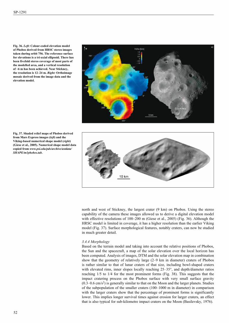
52
SP-1291
north and west of Stickney, the largest crater (9 km) on Phobos. Using the stereo capability of the camera these images allowed us to derive a digital elevation model with effective resolutions of 100–200 m (Giese et al., 2005) (Fig. 36). Although the HRSC model is limited in coverage, it has a higher resolution than the earlier Viking model (Fig. 37). Surface morphological features, notably craters, can now be studied in much greater detail.
3.4.4 MorphologyBased on the terrain model and taking into account the relative positions of Phobos, the Sun and the spacecraft, a map of the solar elevation over the local horizon has been computed. Analysis of images, DTM and the solar elevation map in combination show that the geometry of relatively large (2–9 km in diameter) craters of Phobos is rather similar to that of lunar craters of that size, including bowl-shaped craters with elevated rims, inner slopes locally reaching 25–35°, and depth/diameter ratios reaching 1/5 to 1/4 for the most prominent forms (Fig. 38). This suggests that the impact cratering process on the Phobos surface with very small surface gravity (0.3–0.6 cm/s2) is generally similar to that on the Moon and the larger planets. Studies of the subpopulation of the smaller craters (100–1000 m in diameter) in comparison with the larger craters show that the percentage of prominent forms is significantly lower. This implies longer survival times against erosion for larger craters, an effect that is also typical for sub-kilometre impact craters on the Moon (Basilevsky, 1976).
fig. 36. Left: colour-coded elevation model of Phobos derived from HrSc stereo images taken during orbit 756. the reference surface for elevations is a tri-axial ellipsoid. there has been fivefold stereo coverage of most parts of the modelled area, and a vertical resolution of ~6 m has been achieved. near Stickney, the resolution is 12–24 m. Right: Orthoimage mosaic derived from the image data and the elevation model.
fig. 37. Shaded relief maps of Phobos derived from mars express images (left) and the Viking-based numerical shape model (right) (Giese et al., 2005). numerical shape model data copied from www.psi.edu/pds/archive/astdata/SHAPE/m1phobos.tab.
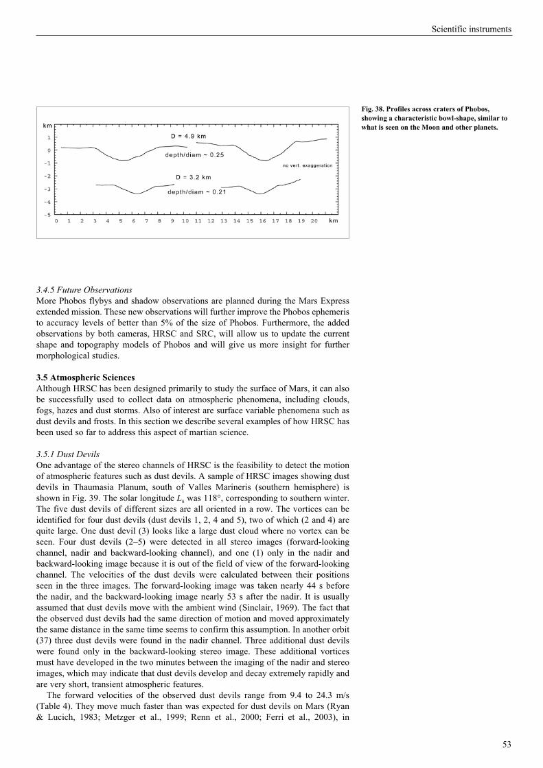
53
Scientific instruments
3.4.5 Future ObservationsMore Phobos flybys and shadow observations are planned during the Mars Express extended mission. These new observations will further improve the Phobos ephemeris to accuracy levels of better than 5% of the size of Phobos. Furthermore, the added observations by both cameras, HRSC and SRC, will allow us to update the current shape and topography models of Phobos and will give us more insight for further morphological studies.
3.5 Atmospheric SciencesAlthough HRSC has been designed primarily to study the surface of Mars, it can also be successfully used to collect data on atmospheric phenomena, including clouds, fogs, hazes and dust storms. Also of interest are surface variable phenomena such as dust devils and frosts. In this section we describe several examples of how HRSC has been used so far to address this aspect of martian science.
3.5.1 Dust DevilsOne advantage of the stereo channels of HRSC is the feasibility to detect the motion of atmospheric features such as dust devils. A sample of HRSC images showing dust devils in Thaumasia Planum, south of Valles Marineris (southern hemisphere) is shown in Fig. 39. The solar longitude Ls was 118°, corresponding to southern winter. The five dust devils of different sizes are all oriented in a row. The vortices can be identified for four dust devils (dust devils 1, 2, 4 and 5), two of which (2 and 4) are quite large. One dust devil (3) looks like a large dust cloud where no vortex can be seen. Four dust devils (2–5) were detected in all stereo images (forward-looking channel, nadir and backward-looking channel), and one (1) only in the nadir and backward-looking image because it is out of the field of view of the forward-looking channel. The velocities of the dust devils were calculated between their positions seen in the three images. The forward-looking image was taken nearly 44 s before the nadir, and the backward-looking image nearly 53 s after the nadir. It is usually assumed that dust devils move with the ambient wind (Sinclair, 1969). The fact that the observed dust devils had the same direction of motion and moved approximately the same distance in the same time seems to confirm this assumption. In another orbit (37) three dust devils were found in the nadir channel. Three additional dust devils were found only in the backward-looking stereo image. These additional vortices must have developed in the two minutes between the imaging of the nadir and stereo images, which may indicate that dust devils develop and decay extremely rapidly and are very short, transient atmospheric features.
The forward velocities of the observed dust devils range from 9.4 to 24.3 m/s (Table 4). They move much faster than was expected for dust devils on Mars (Ryan & Lucich, 1983; Metzger et al., 1999; Renn et al., 2000; Ferri et al., 2003), in
fig. 38. Profiles across craters of Phobos, showing a characteristic bowl-shape, similar to what is seen on the moon and other planets.
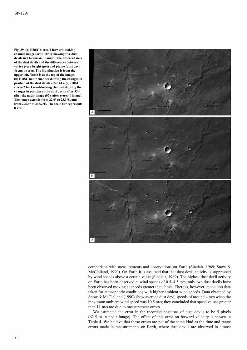
54
SP-1291
comparison with measurements and observations on Earth (Sinclair, 1969; Snow & McClelland, 1990). On Earth it is assumed that that dust devil activity is suppressed by wind speeds above a certain value (Sinclair, 1969). The highest dust devil activity on Earth has been observed at wind speeds of 0.5–4.5 m/s; only two dust devils have been observed moving at speeds greater than 9 m/s. There is, however, much less data taken for atmospheric conditions with higher ambient wind speeds. Data obtained by Snow & McClelland (1990) show average dust devil speeds of around 4 m/s when the maximum ambient wind speed was 10.5 m/s; they concluded that speed values greater than 11 m/s are due to measurement errors.
We estimated the error in the recorded positions of dust devils to be 5 pixels (62.5 m in nadir image). The effect of this error on forward velocity is shown in Table 4. We believe that these errors are not of the same kind as the time and range errors made in measurements on Earth, where dust devils are observed in almost
fig. 39. (a) HrSc stereo 1 forward-looking channel image (orbit 1081) showing five dust devils in thaumasia Planum. the different sizes of the dust devils and the differences between vortex (very bright spot) and plume (dust devil 4) can be seen. the illumination is from the upper left. north is at the top of the image. (b) HrSc nadir channel showing the changes in position of the dust devils after 44 s. (c) HrSc stereo 2 backward-looking channel showing the changes in position of the dust devils after 53 s after the nadir image (97 s after stereo 1 image). the image extends from 22.6° to 23.3°S, and from 296.6° to 298.2°e. the scale bar represents 8 km.
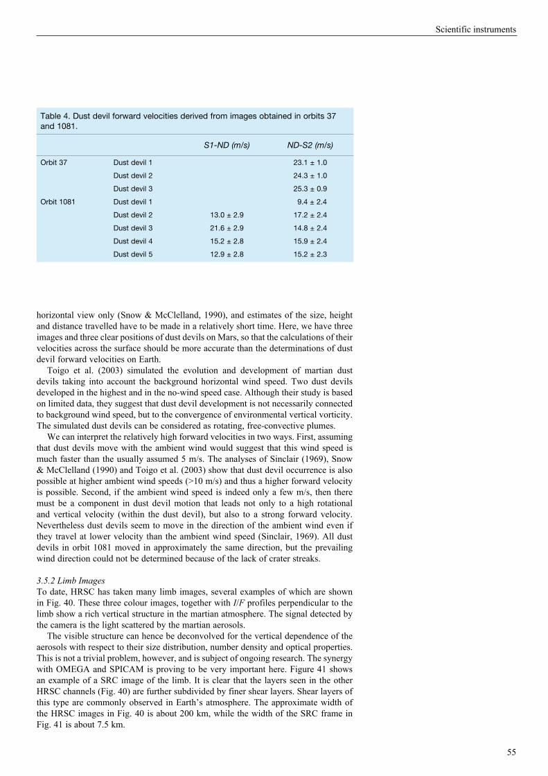
55
Scientific instruments
horizontal view only (Snow & McClelland, 1990), and estimates of the size, height and distance travelled have to be made in a relatively short time. Here, we have three images and three clear positions of dust devils on Mars, so that the calculations of their velocities across the surface should be more accurate than the determinations of dust devil forward velocities on Earth.
Toigo et al. (2003) simulated the evolution and development of martian dust devils taking into account the background horizontal wind speed. Two dust devils developed in the highest and in the no-wind speed case. Although their study is based on limited data, they suggest that dust devil development is not necessarily connected to background wind speed, but to the convergence of environmental vertical vorticity. The simulated dust devils can be considered as rotating, free-convective plumes.
We can interpret the relatively high forward velocities in two ways. First, assuming that dust devils move with the ambient wind would suggest that this wind speed is much faster than the usually assumed 5 m/s. The analyses of Sinclair (1969), Snow & McClelland (1990) and Toigo et al. (2003) show that dust devil occurrence is also possible at higher ambient wind speeds (>10 m/s) and thus a higher forward velocity is possible. Second, if the ambient wind speed is indeed only a few m/s, then there must be a component in dust devil motion that leads not only to a high rotational and vertical velocity (within the dust devil), but also to a strong forward velocity. Nevertheless dust devils seem to move in the direction of the ambient wind even if they travel at lower velocity than the ambient wind speed (Sinclair, 1969). All dust devils in orbit 1081 moved in approximately the same direction, but the prevailing wind direction could not be determined because of the lack of crater streaks.
3.5.2 Limb ImagesTo date, HRSC has taken many limb images, several examples of which are shown in Fig. 40. These three colour images, together with I/F profiles perpendicular to the limb show a rich vertical structure in the martian atmosphere. The signal detected by the camera is the light scattered by the martian aerosols.
The visible structure can hence be deconvolved for the vertical dependence of the aerosols with respect to their size distribution, number density and optical properties. This is not a trivial problem, however, and is subject of ongoing research. The synergy with OMEGA and SPICAM is proving to be very important here. Figure 41 shows an example of a SRC image of the limb. It is clear that the layers seen in the other HRSC channels (Fig. 40) are further subdivided by finer shear layers. Shear layers of this type are commonly observed in Earth’s atmosphere. The approximate width of the HRSC images in Fig. 40 is about 200 km, while the width of the SRC frame in Fig. 41 is about 7.5 km.
Table 4. Dust devil forward velocities derived from images obtained in orbits 37 and 1081.
S1-ND (m/s) ND-S2 (m/s)
Orbit 37 Dust devil 1 23.1 ± 1.0
Dust devil 2 24.3 ± 1.0
Dust devil 3 25.3 ± 0.9
Orbit 1081 Dust devil 1 9.4 ± 2.4
Dust devil 2 13.0 ± 2.9 17.2 ± 2.4
Dust devil 3 21.6 ± 2.9 14.8 ± 2.4
Dust devil 4 15.2 ± 2.8 15.9 ± 2.4
Dust devil 5 12.9 ± 2.8 15.2 ± 2.3
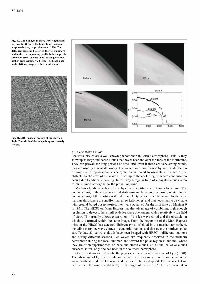
56
SP-1291
3.5.3 Lee Wave CloudsLee wave clouds are a well known phenomenon in Earth’s atmosphere. Usually they show up as large and dense clouds that hover near and over the tops of the mountains. They can prevail for long periods of time, and, even if there are very strong winds, they are usually almost stationary. Lee wave clouds are formed by vertical deflection of winds on a topographic obstacle; the air is forced to oscillate in the lee of the obstacle. In the crest of the wave air rises up to the cooler region where condensation occurs due to adiabatic cooling. In this way a regular train of elongated clouds often forms, aligned orthogonal to the prevailing wind.
Martian clouds have been the subject of scientific interest for a long time. The understanding of their appearance, distribution and behaviour is closely related to the understanding of the martian water, dust and CO2 cycles. Since lee wave clouds in the martian atmosphere are smaller than a few kilometres, and thus too small to be visible with ground-based observatories, they were observed for the first time by Mariner 9 in 1971. The HRSC on Mars Express has the advantage of combining high enough resolution to detect rather small-scale lee wave phenomena with a relatively wide field of view. This usually allows observation of the lee wave cloud and the obstacle on which it is formed within the same image. From the beginning of the Mars Express mission the HRSC has detected different types of cloud in the martian atmosphere, including many lee wave clouds in equatorial regions and also over the northern polar cap. To date 23 lee wave clouds have been imaged with HRSC in different locations and during different seasons. Lee waves are frequently observed in the northern hemisphere during the local summer, and toward the polar region in autumn, where they are often superimposed on haze and streak clouds. Of all the lee wave clouds observed so far, only one has been in the southern hemisphere.
One of first works to describe the physics of the lee waves was that of Lyra (1940). The advantage of Lyra’s formulation is that it gives a simple connection between the wavelength of produced lee wave and the horizontal wind speed. This means that we can estimate the wind speed directly from images of lee waves. An HRSC image taken
fig. 41. Src image of section of the martian limb. the width of the image is approximately 7.5 km.
fig. 40. Limb images in three wavelengths and I/F profiles through the limb. Limb position is approximately at pixel number 2000. the detached haze can be seen in the 750 nm image and in the corresponding profile between pixels 2300 and 2500. the width of the images at the limb is approximately 200 km. the black dots in the 440 nm image are due to saturation.
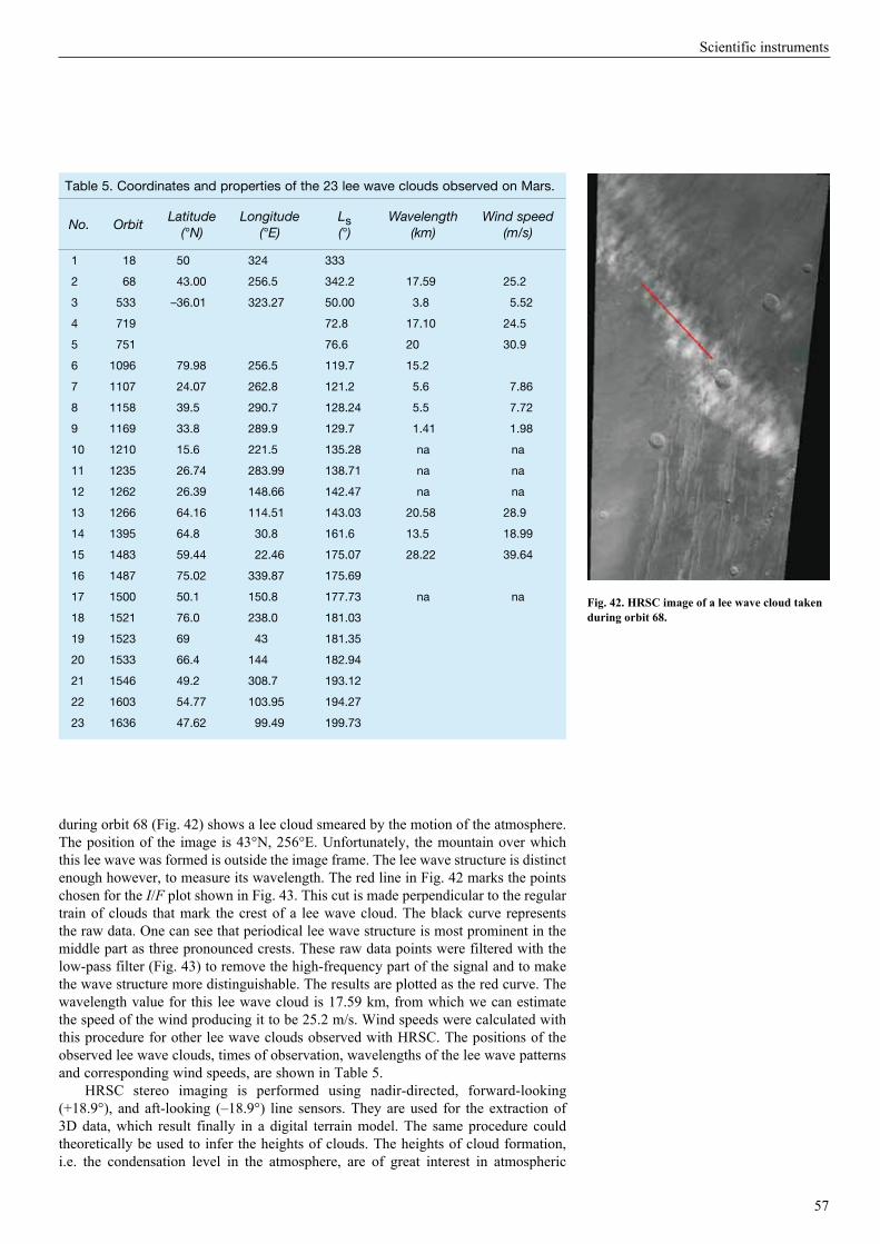
57
Scientific instruments
during orbit 68 (Fig. 42) shows a lee cloud smeared by the motion of the atmosphere. The position of the image is 43°N, 256°E. Unfortunately, the mountain over which this lee wave was formed is outside the image frame. The lee wave structure is distinct enough however, to measure its wavelength. The red line in Fig. 42 marks the points chosen for the I/F plot shown in Fig. 43. This cut is made perpendicular to the regular train of clouds that mark the crest of a lee wave cloud. The black curve represents the raw data. One can see that periodical lee wave structure is most prominent in the middle part as three pronounced crests. These raw data points were filtered with the low-pass filter (Fig. 43) to remove the high-frequency part of the signal and to make the wave structure more distinguishable. The results are plotted as the red curve. The wavelength value for this lee wave cloud is 17.59 km, from which we can estimate the speed of the wind producing it to be 25.2 m/s. Wind speeds were calculated with this procedure for other lee wave clouds observed with HRSC. The positions of the observed lee wave clouds, times of observation, wavelengths of the lee wave patterns and corresponding wind speeds, are shown in Table 5.
HRSC stereo imaging is performed using nadir-directed, forward-looking (+18.9°), and aft-looking (–18.9°) line sensors. They are used for the extraction of 3D data, which result finally in a digital terrain model. The same procedure could theoretically be used to infer the heights of clouds. The heights of cloud formation, i.e. the condensation level in the atmosphere, are of great interest in atmospheric
Table 5. Coordinates and properties of the 23 lee wave clouds observed on Mars.
No. OrbitLatitude
(°N)Longitude
(°E)Ls (°)
Wavelength (km)
Wind speed(m/s)
1 18 50.00 324 333
2 68 43.00 256.5 342.2 17.59 25.2
3 533 –36.01 323.27 50.00 03.8 05.52
4 719 72.8 17.10 24.5
5 751 76.6 20 30.9
6 1096 79.98 256.5 119.7 15.2
7 1107 24.07 262.8 121.2 05.6 07.86
8 1158 39.50 290.7 128.24 05.5 07.72
9 1169 33.80 289.9 129.7 01.41 01.98
10 1210 15.60 221.5 135.28 na na
11 1235 26.74 283.99 138.71 na na
12 1262 26.39 148.66 142.47 na na
13 1266 64.16 114.51 143.03 20.58 28.9
14 1395 64.80 030.8 161.6 13.5 18.99
15 1483 59.44 022.46 175.07 28.22 39.64
16 1487 75.02 339.87 175.69
17 1500 50.10 150.8 177.73 na na
18 1521 76.00 238.0 181.03
19 1523 69.00 043 181.35
20 1533 66.40 144 182.94
21 1546 49.20 308.7 193.12
22 1603 54.77 103.95 194.27
23 1636 47.62 099.49 199.73
fig. 42. HrSc image of a lee wave cloud taken during orbit 68.
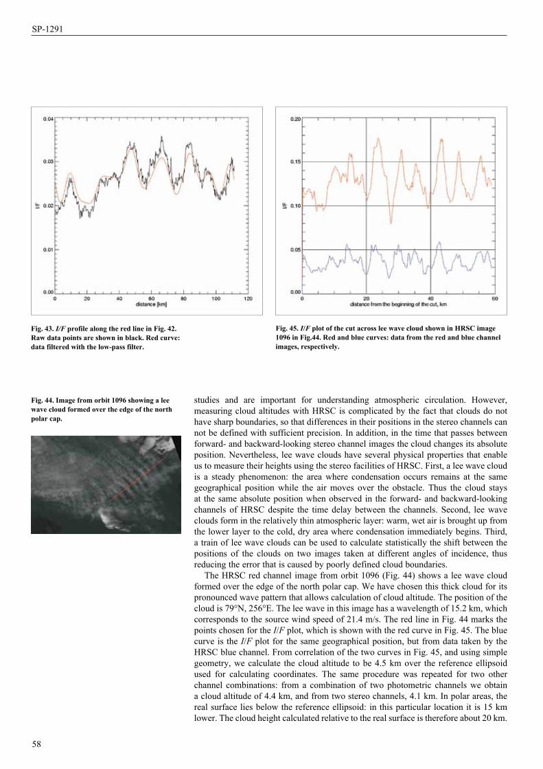
SP-1291
58
studies and are important for understanding atmospheric circulation. However, measuring cloud altitudes with HRSC is complicated by the fact that clouds do not have sharp boundaries, so that differences in their positions in the stereo channels can not be defined with sufficient precision. In addition, in the time that passes between forward- and backward-looking stereo channel images the cloud changes its absolute position. Nevertheless, lee wave clouds have several physical properties that enable us to measure their heights using the stereo facilities of HRSC. First, a lee wave cloud is a steady phenomenon: the area where condensation occurs remains at the same geographical position while the air moves over the obstacle. Thus the cloud stays at the same absolute position when observed in the forward- and backward-looking channels of HRSC despite the time delay between the channels. Second, lee wave clouds form in the relatively thin atmospheric layer: warm, wet air is brought up from the lower layer to the cold, dry area where condensation immediately begins. Third, a train of lee wave clouds can be used to calculate statistically the shift between the positions of the clouds on two images taken at different angles of incidence, thus reducing the error that is caused by poorly defined cloud boundaries.
The HRSC red channel image from orbit 1096 (Fig. 44) shows a lee wave cloud formed over the edge of the north polar cap. We have chosen this thick cloud for its pronounced wave pattern that allows calculation of cloud altitude. The position of the cloud is 79°N, 256°E. The lee wave in this image has a wavelength of 15.2 km, which corresponds to the source wind speed of 21.4 m/s. The red line in Fig. 44 marks the points chosen for the I/F plot, which is shown with the red curve in Fig. 45. The blue curve is the I/F plot for the same geographical position, but from data taken by the HRSC blue channel. From correlation of the two curves in Fig. 45, and using simple geometry, we calculate the cloud altitude to be 4.5 km over the reference ellipsoid used for calculating coordinates. The same procedure was repeated for two other channel combinations: from a combination of two photometric channels we obtain a cloud altitude of 4.4 km, and from two stereo channels, 4.1 km. In polar areas, the real surface lies below the reference ellipsoid: in this particular location it is 15 km lower. The cloud height calculated relative to the real surface is therefore about 20 km.
fig. 43. I/F profile along the red line in fig. 42. raw data points are shown in black. red curve: data filtered with the low-pass filter.
fig. 44. image from orbit 1096 showing a lee wave cloud formed over the edge of the north polar cap.
fig. 45. I/F plot of the cut across lee wave cloud shown in HrSc image 1096 in fig.44. red and blue curves: data from the red and blue channel images, respectively.
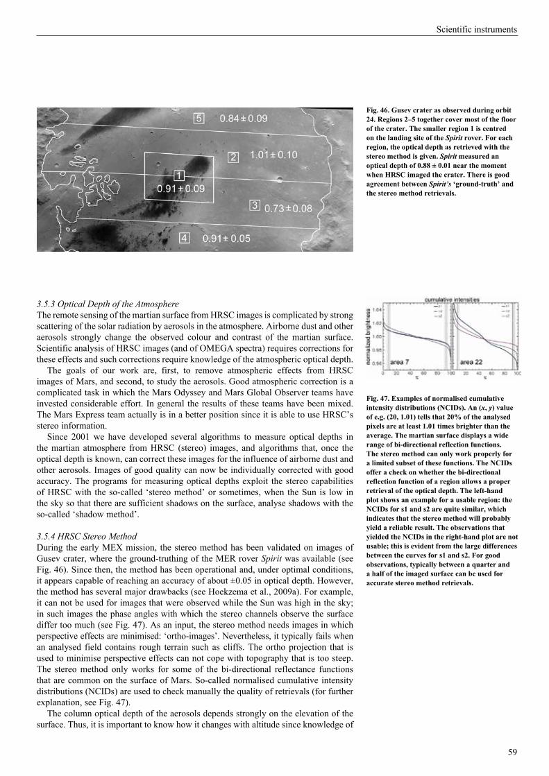
Scientific instruments
59
3.5.3 Optical Depth of the AtmosphereThe remote sensing of the martian surface from HRSC images is complicated by strong scattering of the solar radiation by aerosols in the atmosphere. Airborne dust and other aerosols strongly change the observed colour and contrast of the martian surface. Scientific analysis of HRSC images (and of OMEGA spectra) requires corrections for these effects and such corrections require knowledge of the atmospheric optical depth.
The goals of our work are, first, to remove atmospheric effects from HRSC images of Mars, and second, to study the aerosols. Good atmospheric correction is a complicated task in which the Mars Odyssey and Mars Global Observer teams have invested considerable effort. In general the results of these teams have been mixed. The Mars Express team actually is in a better position since it is able to use HRSC’s stereo information.
Since 2001 we have developed several algorithms to measure optical depths in the martian atmosphere from HRSC (stereo) images, and algorithms that, once the optical depth is known, can correct these images for the influence of airborne dust and other aerosols. Images of good quality can now be individually corrected with good accuracy. The programs for measuring optical depths exploit the stereo capabilities of HRSC with the so-called ‘stereo method’ or sometimes, when the Sun is low in the sky so that there are sufficient shadows on the surface, analyse shadows with the so-called ‘shadow method’.
3.5.4 HRSC Stereo MethodDuring the early MEX mission, the stereo method has been validated on images of Gusev crater, where the ground-truthing of the MER rover Spirit was available (see Fig. 46). Since then, the method has been operational and, under optimal conditions, it appears capable of reaching an accuracy of about ±0.05 in optical depth. However, the method has several major drawbacks (see Hoekzema et al., 2009a). For example, it can not be used for images that were observed while the Sun was high in the sky; in such images the phase angles with which the stereo channels observe the surface differ too much (see Fig. 47). As an input, the stereo method needs images in which perspective effects are minimised: ‘ortho-images’. Nevertheless, it typically fails when an analysed field contains rough terrain such as cliffs. The ortho projection that is used to minimise perspective effects can not cope with topography that is too steep. The stereo method only works for some of the bi-directional reflectance functions that are common on the surface of Mars. So-called normalised cumulative intensity distributions (NCIDs) are used to check manually the quality of retrievals (for further explanation, see Fig. 47).
The column optical depth of the aerosols depends strongly on the elevation of the surface. Thus, it is important to know how it changes with altitude since knowledge of
fig. 46. Gusev crater as observed during orbit 24. regions 2–5 together cover most of the floor of the crater. the smaller region 1 is centred on the landing site of the Spirit rover. for each region, the optical depth as retrieved with the stereo method is given. Spirit measured an optical depth of 0.88 ± 0.01 near the moment when HrSc imaged the crater. there is good agreement between Spirit’s ‘ground-truth’ and the stereo method retrievals.
fig. 47. examples of normalised cumulative intensity distributions (nciDs). An (x, y) value of e.g. (20, 1.01) tells that 20% of the analysed pixels are at least 1.01 times brighter than the average. the martian surface displays a wide range of bi-directional reflection functions. the stereo method can only work properly for a limited subset of these functions. the nciDs offer a check on whether the bi-directional reflection function of a region allows a proper retrieval of the optical depth. the left-hand plot shows an example for a usable region: the nciDs for s1 and s2 are quite similar, which indicates that the stereo method will probably yield a reliable result. the observations that yielded the nciDs in the right-hand plot are not usable; this is evident from the large differences between the curves for s1 and s2. for good observations, typically between a quarter and a half of the imaged surface can be used for accurate stereo method retrievals.

60
SP-1291
the altitude dependence makes it possible to extrapolate from a measured optical depth to the optical depth of close-by regions at different elevations. The stereo method was successfully used to study this correlation (see Fig. 48).
3.5.5 HRSC Digital Terrain Models and the shadow methodAt first glance, many images of Mars show frequent shadows on its surface. However, once HRSC’s digital terrain models (DTMs) became available, it became evident that many images show only shades, and hardly any true shadows. The detailed DTMs of HRSC show that on Mars, true shadows become common only when the Sun is quite low in the sky since steep slopes are quite rare on the planet. As a result, the shadow method is of limited use. In effect, it can only be used for images taken when the Sun is less than about 25° from the horizon. As a result it proved impossible to use the ground truth as measured by Spirit and Opportunity to validate the shadow method for HRSC images. There simply do not (yet) exist HRSC image sequences of the MER landing sites in Gusev and Meridiani that contain significant shadows. We expect such observations to be made during the extended mission.
3.5.6 Aerosol Scattering Properties The Pathfinder mission yielded accurate measurements of the local aerosol properties around the landing site. Thus, before the MEX mission, we expected to have sufficient knowledge about martian aerosols to do accurate atmospheric correction once an optical depth was known. However, the results of the MEX mission made it clear that the ‘Pathfinder’ aerosols are not the only common aerosols in the martian atmosphere. Sometimes Pathfinder aerosols do yield accurate results in our atmospheric correction software, but more often they do not. In some cases simulations with only Pathfinder aerosols yielded errors in the estimated surface albedo of more than 20%. In this respect, HRSC stereo imagery hints at the importance of high-altitude hazes. Such hazes are thin, but apparently can be important since the small (probably often icy) particles that make up such hazes show quite strong backscattering, whereas airborne dust does not.
3.5.7 Simultaneous Observations by OMEGA and HRSCOMEGA and HRSC usually measure reflectance simultaneously. HRSC provides very high spatial resolution images in nine channels from the VIS to the NIR, and OMEGA provides spectra from 0.36 to 5.2 µm, so these instruments complement each other. We are especially interested in these simultaneous measurements because they can help us to choose and rule out different sets of optical properties. Also, comparison of the datasets serves as a validation of the reflectance measurements. On top of that, OMEGA can detect water ice in the atmosphere (and differentiate it from that on the surface) from its measurements around 1.5 µm. All these analyses will be used to better determine the surface albedos.
With this aim in mind, we have often combined simultaneous HRSC and OMEGA measurements to determine, for instance, the composition of bright hazes detected in Valles Marineris and around volcanoes.
Simultaneous observations of HRSC and OMEGA of the Valles Marineris during the southern autumn show a dense haze inside the valley, which became thinner three days later and disappeared after nine. OMEGA spectra showed that, contrary to what one would guess from HRSC colour images, the haze contains only airborne dust and no measurable amount of ice.
Often, HRSC images show bright regions around volcanoes on Mars, probably clouds of water ice that evolve with time. Simultaneous OMEGA spectra indeed show the presence of water ice in these clouds. Figure 49 shows an example, here near the summit of Pavonis Mons, of such detection of water ice by OMEGA. The water ice is present mainly on the flank of the volcano, where the relative band depth reaches in some areas 10%. The analysis of the spectra around 3.5 μm suggests particles of the order of 2–3 μm, confirming that the absorption is due to water ice in the atmosphere. This kind of analysis helps to differentiate between atmospheric and surface ice.
fig. 48. Top: regions around contour lines (altitude ±500 m) on scree slopes in Valles marineris. the optical depths retrieved from these regions (bottom) reveal a scale height of dust that is almost equal to that of gas. this indicates that over the imaged regions the dust is well mixed into the atmosphere. Other walls of the Valles (not shown) offered examples of the opposite. for details of this analysis of the Valles and the implications for the scale height of dust, see Hoekzema et al. (2009b).
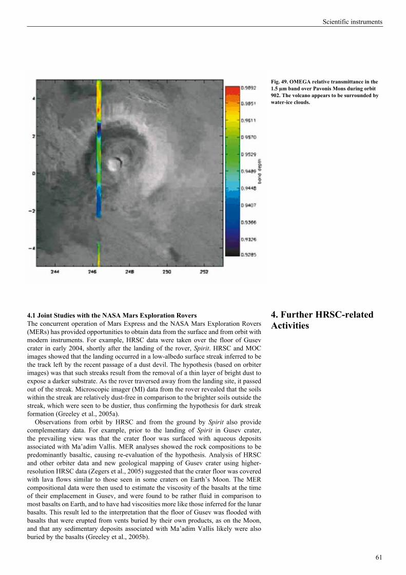
61
Scientific instruments
4.1 Joint Studies with the nASA mars exploration roversThe concurrent operation of Mars Express and the NASA Mars Exploration Rovers (MERs) has provided opportunities to obtain data from the surface and from orbit with modern instruments. For example, HRSC data were taken over the floor of Gusev crater in early 2004, shortly after the landing of the rover, Spirit. HRSC and MOC images showed that the landing occurred in a low-albedo surface streak inferred to be the track left by the recent passage of a dust devil. The hypothesis (based on orbiter images) was that such streaks result from the removal of a thin layer of bright dust to expose a darker substrate. As the rover traversed away from the landing site, it passed out of the streak. Microscopic imager (MI) data from the rover revealed that the soils within the streak are relatively dust-free in comparison to the brighter soils outside the streak, which were seen to be dustier, thus confirming the hypothesis for dark streak formation (Greeley et al., 2005a).
Observations from orbit by HRSC and from the ground by Spirit also provide complementary data. For example, prior to the landing of Spirit in Gusev crater, the prevailing view was that the crater floor was surfaced with aqueous deposits associated with Ma’adim Vallis. MER analyses showed the rock compositions to be predominantly basaltic, causing re-evaluation of the hypothesis. Analysis of HRSC and other orbiter data and new geological mapping of Gusev crater using higher-resolution HRSC data (Zegers et al., 2005) suggested that the crater floor was covered with lava flows similar to those seen in some craters on Earth’s Moon. The MER compositional data were then used to estimate the viscosity of the basalts at the time of their emplacement in Gusev, and were found to be rather fluid in comparison to most basalts on Earth, and to have had viscosities more like those inferred for the lunar basalts. This result led to the interpretation that the floor of Gusev was flooded with basalts that were erupted from vents buried by their own products, as on the Moon, and that any sedimentary deposits associated with Ma’adim Vallis likely were also buried by the basalts (Greeley et al., 2005b).
fig. 49. OmeGA relative transmittance in the 1.5 µm band over Pavonis mons during orbit 902. the volcano appears to be surrounded by water-ice clouds.
4. further HrSc-related Activities
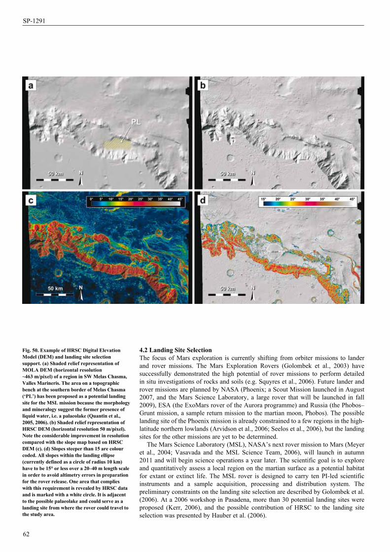
62
SP-1291
4.2 Landing Site SelectionThe focus of Mars exploration is currently shifting from orbiter missions to lander and rover missions. The Mars Exploration Rovers (Golombek et al., 2003) have successfully demonstrated the high potential of rover missions to perform detailed in situ investigations of rocks and soils (e.g. Squyres et al., 2006). Future lander and rover missions are planned by NASA (Phoenix; a Scout Mission launched in August 2007, and the Mars Science Laboratory, a large rover that will be launched in fall 2009), ESA (the ExoMars rover of the Aurora programme) and Russia (the Phobos–Grunt mission, a sample return mission to the martian moon, Phobos). The possible landing site of the Phoenix mission is already constrained to a few regions in the high-latitude northern lowlands (Arvidson et al., 2006; Seelos et al., 2006), but the landing sites for the other missions are yet to be determined.
The Mars Science Laboratory (MSL), NASA’s next rover mission to Mars (Meyer et al., 2004; Vasavada and the MSL Science Team, 2006), will launch in autumn 2011 and will begin science operations a year later. The scientific goal is to explore and quantitatively assess a local region on the martian surface as a potential habitat for extant or extinct life. The MSL rover is designed to carry ten PI-led scientific instruments and a sample acquisition, processing and distribution system. The preliminary constraints on the landing site selection are described by Golombek et al. (2006). At a 2006 workshop in Pasadena, more than 30 potential landing sites were proposed (Kerr, 2006), and the possible contribution of HRSC to the landing site selection was presented by Hauber et al. (2006).
fig. 50. example of HrSc Digital elevation model (Dem) and landing site selection support. (a) Shaded relief representation of mOLA Dem (horizontal resolution ~463 m/pixel) of a region in SW melas chasma, Valles marineris. the area on a topographic bench at the southern border of melas chasma (‘PL’) has been proposed as a potential landing site for the mSL mission because the morphology and mineralogy suggest the former presence of liquid water, i.e. a palaeolake (Quantin et al., 2005, 2006). (b) Shaded relief representation of HrSc Dem (horizontal resolution 50 m/pixel). note the considerable improvement in resolution compared with the slope map based on HrSc Dem (c). (d) Slopes steeper than 15 are colour coded. All slopes within the landing ellipse (currently defined as a circle of radius 10 km) have to be 15° or less over a 20–40 m length scale in order to avoid altimetry errors in preparation for the rover release. One area that complies with this requirement is revealed by HrSc data and is marked with a white circle. it is adjacent to the possible palaeolake and could serve as a landing site from where the rover could travel to the study area.
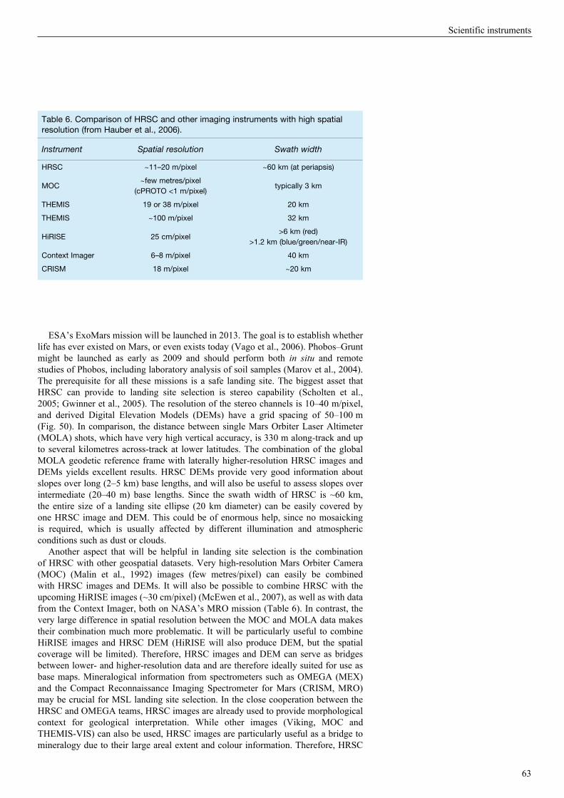
63
Scientific instruments
ESA’s ExoMars mission will be launched in 2013. The goal is to establish whether life has ever existed on Mars, or even exists today (Vago et al., 2006). Phobos–Grunt might be launched as early as 2009 and should perform both in situ and remote studies of Phobos, including laboratory analysis of soil samples (Marov et al., 2004). The prerequisite for all these missions is a safe landing site. The biggest asset that HRSC can provide to landing site selection is stereo capability (Scholten et al., 2005; Gwinner et al., 2005). The resolution of the stereo channels is 10–40 m/pixel, and derived Digital Elevation Models (DEMs) have a grid spacing of 50–100 m (Fig. 50). In comparison, the distance between single Mars Orbiter Laser Altimeter (MOLA) shots, which have very high vertical accuracy, is 330 m along-track and up to several kilometres across-track at lower latitudes. The combination of the global MOLA geodetic reference frame with laterally higher-resolution HRSC images and DEMs yields excellent results. HRSC DEMs provide very good information about slopes over long (2–5 km) base lengths, and will also be useful to assess slopes over intermediate (20–40 m) base lengths. Since the swath width of HRSC is ~60 km, the entire size of a landing site ellipse (20 km diameter) can be easily covered by one HRSC image and DEM. This could be of enormous help, since no mosaicking is required, which is usually affected by different illumination and atmospheric conditions such as dust or clouds.
Another aspect that will be helpful in landing site selection is the combination of HRSC with other geospatial datasets. Very high-resolution Mars Orbiter Camera (MOC) (Malin et al., 1992) images (few metres/pixel) can easily be combined with HRSC images and DEMs. It will also be possible to combine HRSC with the upcoming HiRISE images (~30 cm/pixel) (McEwen et al., 2007), as well as with data from the Context Imager, both on NASA’s MRO mission (Table 6). In contrast, the very large difference in spatial resolution between the MOC and MOLA data makes their combination much more problematic. It will be particularly useful to combine HiRISE images and HRSC DEM (HiRISE will also produce DEM, but the spatial coverage will be limited). Therefore, HRSC images and DEM can serve as bridges between lower- and higher-resolution data and are therefore ideally suited for use as base maps. Mineralogical information from spectrometers such as OMEGA (MEX) and the Compact Reconnaissance Imaging Spectrometer for Mars (CRISM, MRO) may be crucial for MSL landing site selection. In the close cooperation between the HRSC and OMEGA teams, HRSC images are already used to provide morphological context for geological interpretation. While other images (Viking, MOC and THEMIS-VIS) can also be used, HRSC images are particularly useful as a bridge to mineralogy due to their large areal extent and colour information. Therefore, HRSC
Table 6. Comparison of HRSC and other imaging instruments with high spatial resolution (from Hauber et al., 2006).
Instrument Spatial resolution Swath width
HRSC ~11–20 m/pixel ~60 km (at periapsis)
MOC~few metres/pixel
(cPROTO <1 m/pixel)typically 3 km
THEMIS 19 or 38 m/pixel 20 km
THEMIS ~100 m/pixel 32 km
HiRISE 25 cm/pixel>6 km (red)
>1.2 km (blue/green/near-IR)
Context Imager 6–8 m/pixel 40 km
CRISM 18 m/pixel ~20 km
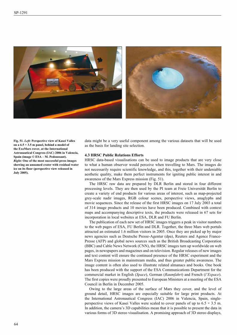
64
SP-1291
data might be a very useful component among the various datasets that will be used as the basis for landing site selection.
4.3 HrSc Public relations effortsHRSC data-based visualisations can be used to image products that are very close to what a human observer would perceive when travelling to Mars. The images do not necessarily require scientific knowledge, and this, together with their undeniable aesthetic quality, make them perfect instruments for igniting public interest in and awareness of the Mars Express mission (Fig. 51).
The HRSC raw data are prepared by DLR Berlin and stored in four different processing levels. They are then used by the PI team at Freie Universität Berlin to create a variety of end products for various areas of interest, such as map-projected grey-scale nadir images, RGB colour scenes, perspective views, anaglyphs and movie sequences. Since the release of the first HRSC images on 17 July 2003 a total of 314 image products and 10 movies have been produced. Combined with context maps and accompanying descriptive texts, the products were released in 67 sets for incorporation in local websites at ESA, DLR and FU Berlin.
The publication of each new set of HRSC images triggers a peak in visitor numbers to the web pages of ESA, FU Berlin and DLR. Together, the three Mars web portals attracted an estimated 1.6 million visitors in 2005. Once they are picked up by major news agencies such as Deutsche Presse-Agentur (dpa), Reuters and Agence France-Presse (AFP) and global news sources such as the British Broadcasting Corporation (BBC) and Cable News Network (CNN), the HRSC images turn up worldwide on web pages, in newspapers and magazines and on television. Regular releases of new images and text content will ensure the continued presence of the HRSC experiment and the Mars Express mission in mainstream media, and thus greater public awareness. The image content is often also used to illustrate related almanacs and books. One book has been produced with the support of the ESA Communications Department for the commercial market in English (Space), German (Raumfahrt) and French (l’Espace). The first copies were proudly presented to European Ministers at a meeting of the ESA Council in Berlin in December 2005.
Owing to the large areas of the surface of Mars they cover, and the level of ground detail, HRSC images are especially suitable for large print products. At the International Astronautical Congress (IAC) 2006 in Valencia, Spain, single-perspective views of Kasei Valles were scaled to cover panels of up to 6.5 × 3.5 m. In addition, the camera’s 3D capabilities mean that it is possible to present the data in various forms of 3D stereo visualisation. A promising approach of 3D stereo displays,
fig. 51. Left: Perspective view of Kasei Valles on a 6.5 × 3.5 m panel, behind a model of the exomars rover, at the international Astronautical congress (iAc) 2006 in Valencia, Spain (image © eSA – m. Pedoussaut). Right: One of the most successful press images showing an unnamed crater with residual water ice on its floor (perspective view released in July 2005).

65
Scientific instruments
which enable 3D perception without the need for additional devices such as glasses, has been developed in cooperation with mbm-Systems. The display panels range from postcard size to large displays 2.2 × 1 m. Exhibited in prominent places, these are always eye-catching features at the facilities of ESA, DLR and FU Berlin.
The three institutions are also using the material and its potential by participating in public events such as the ‘Night of Science’ in Berlin, and arranging open days at their facilities. There is also frequent support and guest lectures at observatories and cooperation with various science and space museums around the world. Most events are covered by TV and newspapers. HRSC images are exhibited at major scientific and industry events such as those of the European Geosciences Union (EGU), the Earth and Space Week (ESA/European Commission), the Farnborough International Airshow (UK), and the Berlin, Moscow and Paris air shows, to name but a few.
Probably the most successful direct contact with the public and policy makers can be attributed to the touring exhibition ‘A New Perspective on Mars’, prepared by DLR in cooperation with the HRSC team. Mounted at venues around the world, such as during the Germany–Japan year in Tokyo, at the University Museum in Kyoto, Japan, at the meeting of the Committee on the Peaceful Uses of Outer Space (COPUOS) in 2006 in Vienna, Austria, at the Deutsches Museum in Munich, Germany, and at the United Nations headquarters in New York, USA, in 2007, the exhibition attracted more than 500 000 visitors.
HRSC data have been used in many innovative ways, including to provide members of the public with the interactive experience of flying across the martian surface. The first opportunity was provided by DLR and the German company KUKA, who joined forces to build an unprecedented robotic flight simulator called Mars ‘Robodome’. It mimics the three-dimensional movements of a real spaceship in conjunction with a visualisation of the martian surface from HRSC data. The second opportunity was initiated by a cooperation of the Open University, University College London and Imperial College London, at the Royal Society Summer Science Exhibition in London in 2006. Visitors were able to interactively fly through martian landscapes generated using HRSC data, which were projected onto a Geowall 3D Display, giving the user a truly 3D experience.
Up to now, the HRSC data have provided extensive public relations materials, and have given access to and worldwide recognition of the HRSC experiment and the ESA Mars Express mission.
Adams, J.B. & Gillespie, A.R. (2006). Sensing of Landscapes with Spectral Images: A Physical Modeling Approach, Cambridge University Press.
Albertz, J., S. Gehrke, M. Wählisch, H. Lehmann, T. Schumacher, G. Neukum & the HRSC Co-Investigator Team (2004). Digital Cartography with HRSC on Mars Express, Int. Arch. Photogram. Rem. Sens. Spatial Inform. Sci. 35, 869–874.
Albertz, J., M. Attwenger, J. Barrett, S. Casley, P. Dorninger, E. Dorrer, H. Ebner, S. Gehrke, B. Giese, K. Gwinner, C. Heipke, E. Howington-Kraus, R. L. Kirk, H. Lehmann, H. Mayer, J.-P. Muller, J. Oberst, A. Ostrovskiy, J. Renter, S. Reznik, R. Schmidt, F. Scholten, M. Spiegel, M. Wählisch, G. Neukum & the HRSC Co-Investigator Team (2005). HRSC on Mars Express Photogrammetric and Cartographic Research, Photogram. Eng. Rem. Sens. 71, 1153–1166.
Anderson, R.C., J.M. Dohm, M.P. Golombek, A.F.C. Haldemann, B.J. Franklin, K.L. Tanaka, J. Lias & B. Peer (2001). Primary Centers and Secondary Concentrations of Tectonic Activity through Time in the Western Hemisphere of Mars, J. Geophys. Res. 106, 20563–20586.
Arvidson, R.E., L.M. Barge, J. Barnes, W.V. Boynton, J. Friedson, M.P. Golombek, J. Guinn, D.M. Kass, R. Kirk, M. Malin, M. Mellon, T. Michaels, D. Paige, T.J. Parker, S. Rafkin, K. Seelos, M.D. Smith, P.H. Smith, L. Tamppari & D. Tyler (2006). Overview of Mars Exploration Program 2007 Phoenix Mission Landing Site Selection, in 37th Lun. Planet. Sci. Conf. Abstract 1328 (CD-ROM), League City, Houston, Texas, USA.
references
66
SP-1291
Attwenger, M. & G. Neukum (2005). Klassifikation von HRSC-Objektpunkten zur Generierung hochwertiger Geländemodelle der Marsoberfläche (in German), Photogrammetrie, Fernerkundung, Geoinformation 5, 395–402.
Balme, M.R., N. Mangold, D. Baratoux, F. Costard, M. Gosselin, P. Masson, P. Pinet & G. Neukum (2006). Orientation and Distribution of Recent Gullies in the Southern Hemisphere of Mars: Observations from High Resolution Stereo Camera/Mars Express (HRSC/MEX) and Mars Orbiter Camera/Mars Global Surveyor (MOC/MGS) data, J. Geophys. Res. 111.
Bandfield, J.L., V.E. Hamilton & P.R. Christensen (2000). A Global View of Martian Surface Compositions from MGS-TES, Science 287, 1626–1630.
Banerdt, W.B., M.P. Golombek & K.L. Tanaka (1992). Stress and Tectonics on Mars, University of Arizona Press, pp.249–297.
Basilevsky, A. (1976). On the Evolution Rate of Small Lunar Craters, in Proc. 7th Lunar Sci. Conf., Pergamon Press, Oxford, UK, pp.1005–1020.
Basilevsky, A.T., S.C. Werner, G. Neukum, J.W. Head, S. van Gasselt, K. Gwinner & B.A. Ivanov (2006). Geologically Recent Tectonic, Volcanic and Fluvial Activity on the Eastern Flank of the Olympus Mons Volcano, Mars, Geophys. Res. Lett. 33, 13 201.
Basilevsky, A.T., G. Neukum, S.C. Werner, S. van Gasselt, A. Dumke, W. Zuschneid, M.G. Chapman & R. Greeley (2007). Geological Evolution of Mangala Valles, Mars: Analysis of the HRSC Image H0286, in 38th Lun. Planet. Sci. Conf., Lun. Planet. Inst., p.1338 (CD-ROM), League City, Houston, Texas, USA, 12–16 March.
Bleacher, J.E., R. Greeley, D.A. Williams, G. Neukum & the HRSC Co-Investigator Team (2006). Comparison of Effusive Volcanism at Olympus, Arsia, Pavonis and Ascraeus Montes, Mars from Lava Flow Mapping Using Mars Express HRSC Data, in 37th Lun. Planet. Sci. Conf. (Eds. S. Mackwell and E. Stansbery), p.1182.
Borg, L. & Drake M.J. (2005). A Review of Meteorite Evidence for the Timing of Magmatism and of Surface or Near-surface Liquid Water on Mars, J. Geophys. Res. 110, E12S03.
Buchroithner, M., T. Gründemann, K. Habermann, G. Neukum & the HRSC Co-Investigator Team (2005a). Multitemporale und grossformatige Echt-3D-Hartkopien der Marsoberfläche, Photogrammetrie, Fernerkundung, Geoinformation 5, 433–438.
Buchroithner, M.F., T. Gründemann, R.L. Kirk & K. Habermann (2005b). Three in One: Multiscale Hardcopy Depiction of the Mars Surface in True-3D, Photogram. Eng. Remote Sensing 71, 1105–1108.
Cabrol, N.A., E.A. Grin & G. Dawidowicz (1996). Ma’adim Vallis Revisited through New Topographic Data: Evidence for an Ancient Intravalley Lake, Icarus 123, 269–283.
Carr, M.H. (1981). The Surface of Mars, Yale University Press, New Haven, CT.Chapman, M.G., G. Neukum, S.C. Werner, S. van Gasselt, A. Dumke, W. Zuschneid &
G. Michael (2007). Echus Chasma and Kasei Valles, Mars: New Data and Geologic Interpretations, in: 38th Lun. Planet. Sci. Conf., Lun. Planet. Inst., #1407 (CD-ROM), League City, Houston, Texas, USA, 12–16 March.
Chapman, C.R., J. Veverka, M.J.S. Belton, G. Neukum & D. Morrison (1996a). Cratering on Gaspra, Icarus, 120(1), 231-245.
Chapman, C.R., E.V. Ryan, W. J. Merline, G. Neukum, R. Wagner, P.C. Thomas, J. Veverka & R.J. Sullivan (1996b). Cratering on Ida, Icarus 120(1), 77-86.
Christensen, P.R., B.M. Jakosky, H.H. Kieffer, M.C. Malin, H.Y. McSween, Jr., K. Nealson, G. L. Mehall, S.H. Silverman, S. Ferry, M. Caplinger & M. Ravine (2004). The Thermal Emission Imaging System (THEMIS) for the Mars 2001 Odyssey Mission, Space Sci. Rev. 110, 85–130.
Coomb, J.P. & T.B. McCord (2006). Investigation of the Spectrophotometric Measurements by the Mars Express HRSC and OMEGA instruments, Adv. Space Res., 43(1), 128–137.
Di Achille, G., L. Marinangeli, G.G. Ori, E. Hauber, K. Gwinner, D. Reiss & G. Neukum (2006a). Geological Evolution of the Tyras Vallis Paleolacustrine System, Mars, J. Geophys. Res. 111, 4003.
Di Achille, G., G.G. Ori, D. Reiss, E. Hauber, K. Gwinner, G. Michael & G. Neukum (2006b). A steep fan at Coprates Catena, Valles Marineris, Mars, as Seen by HRSC data, Geophys. Res. Lett. 33, 7204.

67
Scientific instruments
Dorrer, E., H. Mayer, Y. Haase, A. Ostrovskiy, J. Renter, M. Rentsch, S. Reznik, G. Neukum & the HRSC Co-Investigator Team (2005). Improvement of Spatial Data by Means of Shape-from-Shading (in German), Photogrammetrie, Fernerkundung, Geoinformation 5, 403–408.
Ebner, H., M. Spiegel, A. Baumgartner, B. Giese, G. Neukum & the HRSC Co-Investigator Team (2004). Improving the Exterior Orientation of Mars Express HRSC imagery, Int. Arch. Photogram. Rem. Sens. Spatial Inform. Sci. 35, 852–857.
Eliason, E. (1997). Production of Digital Image Models Using the ISIS System, Lun. Planet. Sci. Conf. Abstracts XXViii, p.331–332.
Eliason, E., T. Hare, H. Kieffer, E. Lee, J. Mathews, L. Soderblom, T. Sucharski & J. Torson (1997). An Overview of the Integrated Software for Imaging Spectrometers (ISIS), Lun. Planet. Sci. Conf. Abstracts XXViii, pp. 387–388.
Fassett, C.I. & J.W. Head (2006a). Valley Formation on Martian Volcanoes in the Hesperian: Evidence for Melting of Summit Snowpack, Caldera Lake Formation, Drainage and Erosion at Ceraunius Tholus, Icarus, 189, 118–135
Fassett, C.I. & J.W. Head, III (2006b). Valleys on Hecates Tholus, Mars: Origin by Basal Melting of Summit Snowpack, Planet. Space Sci. 54, 370–378.
Ferri, F., P.H. Smith, M. Lemmon & N.O. Renno (2003). Dust Devils as Observed by Mars Pathfinder, J. Geophys. Res. 108.
Forget, F., R.M. Haberle, F. Montmessin, B. Levrard & J.W. Head (2006). Formation of Glaciers on Mars by Atmospheric Precipitation at High Obliquity, Science 311, 368–371.
Gaddis, L., J. Anderson, K. Becker, T. Becker, D. Cook, K. Edwards, E. Eliason, T. Hare, H. Kieffer, E. Lee, J. Mathews, L. Soderblom, T. Sucharski, J. Torson, A. McEwen & M. Robinson (1997), An Overview of the Integrated Software for Imaging Spectrometers (ISIS), Lun. Planet. Sci. Conf. Abstracts XXViii, p.387–388.
Gehrke, S., M. Wählisch, H. Lehmann, J. Albertz & T. Roatsch (2005). Generation of Digital Topographic Maps of Planetary Bodies, Int. Arch. Photogram. Rem. Sens. Spatial Inform. Sci. 36.
Giese, B., J. Oberst, F. Scholten, H. Hoffmann, M. Spiegel, G. Neukum & the HRSC Co-Investigator Team (2005). Ein hoch auflösendFes digitales Oberflächenmodell des Marsmondes Phobos (in German), Photogrammetrie, Fernerkundung, Geoinformation 5, 435–440.
Gillespie, A.R., D.R. Montgomery & A. Mushkin (2005). Planetary Science: Are there Active Glaciers on Mars? Nature 438.
Golombek, M.P. & W.B. Banerdt (1999). Recent Advances in Mars Tectonics, in 5th Int. Conf. on Mars, Pasadena, CA.
Golombek, M.P., J.A. Grant, T.J. Parker, D.M. Kass, J.A. Crisp, S.W. Squyres, A.F.C. Haldemann, M. Adler, W.J. Lee, N.T. Bridges, R.E. Arvidson, M.H. Carr, R.L. Kirk, P.C. Knocke, R.B. Roncoli, C.M. Weitz, J.T. Schofield, R.W. Zurek, P.R. Christensen, R.L. Fergason, F.S. Anderson & J.W. Rice (2003). Selection of the Mars Exploration Rover Landing Sites, J. Geophys. Res. 108, 13–1.
Golombek, M., J. Grant, L. Lorenzoni, A. Steltzner, A. R. Vasavada, C. Voorhees & M. Watkins (2006). Preliminary Constraints and Plans for Mars Science Laboratory Landing Site Selection, in 37th Lun. Planet. Sci. Conf., #2172 (CD-ROM), League City, Houston, Texas.
Greeley, R. & J.D. Iversen (1987). Measurements of Wind Friction Speeds over Lava Surfaces and Assessment of Sediment Transport, Geophys. Res. Lett. 14, 925–928.
Greeley, R. & P.D. Spudis (1981). Volcanism on Mars, Rev. Geophys. Space Phys. 19, 13–41.Greeley, R., R. Arvidson, J.F. Bell, P. Christensen, D. Foley, A. Haldemann, R.O. Kuzmin,
G. Landis, L.D.V. Neakrase, G. Neukum, S. W. Squyres, R. Sullivan, S. D. Thompson, P.L. Whelley & D. Williams (2005a). Martian Variable Features: New Insight from the Mars Express Orbiter and the Mars Exploration Rover Spirit, J. Geophys. Res. 110, 6002.
Greeley, R., B.H. Foing, H.Y. McSween, G. Neukum, P. Pinet, M. van Kan, S.C. Werner, D. A. Williams & T.E. Zegers (2005b). Fluid Lava Flows in Gusev Crater, Mars, J. Geophys. Res. 110, 5008.
Greeley, R., R.E. Arvidson, P.W. Barlett, D. Blaney, N.A. Cabrol, P.R. Christensen, R.L. Fergason, M.P. Golombek, G.A. Landis, M.T. Lemmon, S.M. McLennan, J.N. Maki, T. Michaels, J.E. Moersch, L.D.V. Neakrase, S.C.R. Rafkin, L. Richter, S.W. Squyres, P.A.
68
SP-1291
de Souza, R.J. Sullivan, S.D. Thompson & P.L. Whelley (2006). Gusev Crater: Wind-related Features and Processes Observed by the Mars Exploration Rover Spirit, J. Geophys. Res. (Planets) 111.
Grin, E.A. & N.A. Cabrol (1997). Limnologic Analysis of Gusev Crater Paleolake, Mars, Icarus 130, 461–474.
Grott, M., E. Hauber, S. Werner, P. Kronberg & G. Neukum (2005). High Heat Flux on Ancient Mars: Evidence from Rift Flank Uplift at Coracis Fossae, Geophys. Res. Lett. 32, L21201.
Grott, M., E. Hauber, S.C. Werner, P. Kronberg & G. Neukum (2006). Mechanical Modeling of Thrust Faults in the Thaumasia Region, Mars and Implications for the Noachian Heat Flux, Icarus 186(2), 517–526.
Gwinner, K., E. Hauber, R. Jaumann & G. Neukum (2000). High-Resolution, Digital Photogrammetric Mapping: A Tool for Earth Science, Eos Trans. 81, 513–520.
Gwinner, K., F. Scholten, B. Giese, J. Oberst, R. Jaumann, M. Spiegel, R. Schmidt, G. Neukum & the HRSC Co-Investigator Team (2005). Hochauflösende Digitale Geländemodelle auf der Grundlage von Mars Express HRSC-Daten, (in German), Photogrammetrie, Fernerkundung, Geoinformation 5, 387–394.
Hartmann, W.K. & G. Neukum (2001). Cratering Chronology and the Evolution of Mars, Space Sci. Rev. 96(1–4), 165–194.
Hauber, E. & P. Kronberg (2001). Tempe Fossae, Mars: A Planetary Analogon to a Terrestrial Continental Rift? J. Geophys. Res. 106, 20 587–20 602.
Hauber, E. & P. Kronberg (2005). The Large Thaumasia Graben on Mars: Is it a Rift? J. Geophys. Res. 110, 7003.
Hauber, E., S. van Gasselt, B. Ivanov, S. Werner, J.W. Head, G. Neukum, R. Jaumann, R. Greeley, K.L. Mitchell, P. Muller & the HRSC Co-Investigator Team (2005a). Discovery of a Flank Caldera and Very Young Glacial Activity at Hecates Tholus, Mars, Nature 434, 356–361.
Hauber, E., K. Gwinner, D. Reiss, F. Scholten, G.G. Michael, R. Jaumann, G.G. Ori, L. Marinangeli, G. Neukum & the HRSC Co-Investigator Team (2005b). Delta-like Deposits in Xanthe Terra, Mars, as Seen with the High Resolution Stereo Camera (HRSC), in 36th Lun. Planet. Sci. Conf. (Eds. S. Mackwell & E. Stansbery), pp.1661.
Hauber, E., G. Neukum, R. Jaumann, K. Gwinner, F. Scholten, H. Hoffmann, S. van Gasselt & T. Duxbury (2006). The High Resolution Stereo Camera (HRSC): A Tool for Landing Site Selection, in 1st MSL Landing Site Workshop, Pasadena, California.
Head, J.W. & D.R. Marchant (2003). Cold-based Mountain Glaciers on Mars: Western Arsia Mons, Geology 31, 641–644.
Head, J.W., III & D.R. Marchant (2006). Evidence for Global-Scale Northern Mid-Latitude Glaciation in the Amazonian Period of Mars: Debris-covered Glacier and Valley Glacier Deposits in the 30–50°N Latitude Band, in 37th Ann. Lun. Planet. Sci. Conf. (Eds. S. Mackwell and E. Stansbery), pp.1127.
Head, J.W., G. Neukum, R. Jaumann, H. Hiesinger, E. Hauber, M. Carr, P. Masson, B. Foing, H. Hoffmann, M. Kreslavsky, S. Werner, S. Milkovich, S. van Gasselt & the HRSC Co-Investigator Team (2005a). Tropical to Mid-latitude Snow and Ice Accumulation, Flow and Glaciation on Mars, Nature 434, 346–351.
Head, J.W., G. Neukum, R. Jaumann, H. Hiesinger, E. Hauber, M. Carr, P. Masson, B. Foing, H. Hoffmann, M. Kreslavsky, S. Werner, S. Milkovich, S. van Gasselt & the HRSC Co-Investigator Team (2005b). Planetary Science: Are There Active Glaciers on Mars? (Reply), Nature 438.
Head, J.W., D.R. Marchant, M.C. Agnew, C.I. Fassett & M.A. Kreslavsky (2006a). Extensive Valley Glacier Deposits in the Northern Mid-latitudes of Mars: Evidence for Late Amazonian Obliquity-driven Climate Change, Earth Planet. Sci. Lett. 241, 663–671.
Head, J.W., A.L. Nahm, D.R. Marchant & G. Neukum (2006b). Modification of the Dichotomy Boundary on Mars by Amazonian Mid-latitude Regional Glaciation, Geophys. Res. Lett. 33, L08S03.
Heipke, C., R. Schmidt, R. Brand, J. Oberst, G. Neukum & the HRSC Co-Investigator Team (2004). Performance of Automatic Tie Point Extraction Using HRSC Imagery of the Mars Express Mission, Int. Arch. Photogram. Rem. Sens. Spatial Inform. Sci. 35, 846–851.

69
Scientific instruments
Heipke, C., J. Oberst, J. Albertz, M. Attwenger, P. Dorninger, E. Dorrer, M. Ewe, S. Gehrke, K. Gwinner, H. Hirschmller, J. R. Kim, R. L. Kirk, H. Mayer, R. Muller, J.-P.and Rengarajan, M. Rentsch, R. Schmidt, F. Scholten, J. Shan, M. Spiegel, M. Wählisch, G. Neukum & the HRSC Co-Investigator Team (2006). The HRSC DTM Test, Int. Arch. Photogram. Rem. Sens. Spatial Inform. Sci. 36, 311–325.
Hiesinger, H., J.W. Head, III, G. Neukum & the HRSC Co-Investigator Team (2005). Rheological Properties of Late-Stage Lava Flows on Ascraeus Mons: New Evidence from HRSC, in 36th Annual Lun. Planet. Sci. Conf. (Eds. S. Mackwell & E. Stansbery), pp. 1727.
Hoekzema, N.M., W.J. Markiewicz, B. Grieger, K. Gwinner, S. Hviid, H.U. Keller, H. Hoffmann, G. Neukum (2009a). Atmospheric Optical Depths from HRSC Stereo Images of Mars, Earth Planet. Sci. Lett. submitted.
Hoekzema, N.M., W.J. Markiewicz, B. Grieger, K. Gwinner, S. Hviid, H. U. Keller, H. Hoffmann, G. Neukum & the MER Co-Investigator Team (2009b). The Dust-scale Height of the Martian Atmosphere around Valles Marineris from HRSC Stereo Images, Earth Planet. Sci. Lett. submitted.
Ivanov, B.A. (2001). Mars/Moon Cratering Rate Ratio Estimates, Space Sci. Rev. 96(1/4), 87–104.
Jaumann, R., D. Reiss, S. Frei, G. Neukum, F. Scholten, K. Gwinner, T. Roatsch, K.-D. Matz, V. Mertens, E. Hauber, H. Hoffmann, U. Köhler, J. W. Head, H. Hiesinger & M. H. Carr (2005a). Interior Channels in Martian Valleys: Constraints on Fluvial Erosion by Measurements of the Mars Express High Resolution Stereo Camera, Geophys. Res. Lett. 32, 16, 203.
Jaumann, R., D. Reiss, S. Frei, F. Scholten, K. Gwinner, T. Roatsch, K.-D. Matz, E. Hauber, V. Mertens, H. Hoffmann, J.W. Head, III, H. Hiesinger, M.H. Carr, G. Neukum & the HRSC Co-Investigator Team (2005b). Martian Valley Networks and Associated Fluvial Features as Seen by the Mars Express High Resolution Stereo Camera (HRSC), in 36th Ann. Lun. Planet. Sci. Conf. (Eds. S. Mackwell & E. Stansbery), pp.1765.
Jaumann, R., G. Neukum, T. Behnke, T.C. Duxbury, J. Flohrer, S. van Gasselt, B. Giese, K. Gwinner, E. Hauber, H. Hoffmann, U. Köhler, K.-D. Matz, T.B. McCord, V. Mertens, J. Oberst, R. Pischel, D. Reiss, T. Roatsch, P. Saiger, F. Scholten, G. Schwarz, K. Stephan & M. Wählisch (2007). The High Resolution Stereo Camera (HRSC) Experiment on Mars Express: Instrument Aspects and Experiment Conduct from Interplanetary Cruise through the Nominal Mission, Planet. Space Sci. 55, 928–952.
Kerr, R. (2006). In Search of the Red Planet’s Sweet Spot, Science 312, 1588–1590. Kim, J.R., J.-P. Muller, S. van Gasselt, J.G. Morley, G. Neukum & the HRSC Co-Investigator
Team (2005). Automated Crater Detection, A New Tool for Mars Cartography and Chronology, Photogram. Eng. Rem. Sens. 71(10), 1205–1217.
Kirk, R., K. Thompson & E.M. Lee (2001). Photometry of the Martian Atmosphere: An Improved Practical Model for Cartography and Photoclinometry, in Lun. Planet. Sci. Conf. Abstracts, XXXii, abstract 1874 (CD–ROM).
Kirk, R., J. Barrett & L. Soderblom (2003). Photoclinometry Made Simple? in ISPRS-ET Working Group IV/9 Workshop ‘Advances in Planetary Mapping’.
Kirk, R.L., S.W. Squyres, G. Neukum & the MER Athena and MEX HRSC Science Teams (2004). Topographic Mapping of Mars: From Hectometer to Micrometer Scales, Int. Arch. Photogram. Rem. Sens. Spatial Inform. Sci. 35, 834–839.
Kirk, R., E. Howington-Kraus, D. Galuszka, B. Redding & T. Hare (2006). Topomapping of Mars with HRSC images, ISIS, and a Commercial Stereo Workstation, Int. Arch. Photogram. Rem. Sens. Spatial Inform. Sci. 36.
Kneissl, T. (2006). Verbreitung und Azimutabhängigkeiten von Erosionsrinnen in der nördlichen Hemisphäre des Mars, Master’s thesis, Martin–Luther–Universitaet, Halle Wittenberg.
Kronberg, P., E. Hauber, S. Werner, T. Schäfer, K. Gwinner, B. Giese, P. Masson & G. Neukum (2006). Acheron Fossae, Mars: Tectonic Rifting, Volcanism, and Implications for Lithospheric Thickness, J. Geophys. Res, 112, E04005.
Lainey, V., V. Dehant, J. Oberst & M. Pätzold (2005). New Ephemerides of the Martian Moons, Eos Trans. AGU 86, Fall Meeting, Suppl., Abstract G51A–0802.
70
SP-1291
Laskar, J., A.C.M. Correia, M. Gastineau, F. Joutel, B. Levrard & P. Robutel (2004). Long-term Evolution and Chaotic Diffusion of the Insolation Quantities of Mars, Icarus 170, 343–364.
Lyra, von G. (1940). Über den Einfluß von Bodenerhebungen auf die Strömung einer stabil geschichteten Atmosphäre, Beiträge zur Physik der freien Atmosphäre 26, 197–206.
McCord, T.B., R.B. Singer, B.R. Hawke, J.B. Adams, D.L. Evans, J.W. Head, P.J. Mouginis-Mark, C.M. Pieters, R.L. Huguenin & S.H. Zisk (1982). Mars: Definition and Characterization of Global Surface Units with Emphasis on Composition, J. Geophys. Res. 87, 10 129–10 148.
McCord, T.B., J.B. Adams, G. Bellucci, J.-P. Combe, A.R. Gillespie, G. Hansen, H. Hoffmann, R. Jaumann, G. Neukum, P. Pinet, F. Poulet, K. Stephan, the HRSC Spectrophotometric Working Group & the HRSC Co-Investigator Team (2006). The Mars Express High Resolution Stereo Camera Spectrophotometric Data: Characteristics and Science Analysis, J. Geophys. Res. 112, E06004.
McEwen, A.S. (2003). Secondary Cratering on Mars: Implications for Age Dating and Surface Properties, in: 6th Int. Conf. Mars, Lun. Planet. Inst., Pasadena, California, 20–25 July.
McEwen, A.S. (2006). Cratering Age Considerations for Young Terranes in the Inner Solar System, in: Lun. Planet. Sci. Conf., Lun. Planet. Inst., #6030 (CD-ROM), League City, Houston, Texas, USA.
McEwen, A.S., B.S. Preblich, E.P. Turtle, N.A. Artemieva, M.P. Golombek, M. Hurst, R.L. Kirk, D.M. Burr & P.R. Christensen (2005). The Rayed Crater Zunil and Interpretations of Small Impact Craters on Mars, Icarus 176(2), 351-381.
McEwen, A.S., E.M. Eliason, J.W. Bergstrom, N.T. Bridges, C.J. Hansen, W.A. Delamere, J.A. Grant, V.C. Gulick, K.E. Herkenhoff, L. Keszthelyi, R.L. Kirk, M.T. Mellon, S.W. Squyres, N. Thomas & C.M. Weitz (2007). MRO’s High Resolution Imaging Science Experiment (HiRISE), J. Geophys. Res, 112, E05S02.
McSween, H.Y., R.E. Arvidson, J.F. Bell, D. Blaney, N.A. Cabrol, P.R. Christensen, B.C. Clark, J.A. Crisp, L.S. Crumpler, D.J. Des Marais, J.D. Farmer, R. Gellert, A. Ghosh, S. Gorevan, T. Graff, J. Grant, L.A. Haskin, K.E. Herkenhoff, J.R. Johnson, B.L. Jolliff, G. Klingelhoefer, A.T. Knudson, S. McLennan, K.A. Milam, J.E. Moersch, R.V. Morris, R. Rieder, S.W. Ruff, P.A. de Souza, S.W. Squyres, H. Wänke, A. Wang, M.B. Wyatt, A. Yen & J. Zipfel (2004). Basaltic Rocks Analyzed by the Spirit Rover in Gusev Crater, Science 305, 842–845.
Malin, M.C. & K.S. Edgett (2000). Evidence for Recent Groundwater Seepage and Surface Runoff on Mars, Science, 288, 2330–2335.
Malin, M.C. & K.S. Edgett (2001). Mars Global Surveyor Mars Orbiter Camera: Interplanetary Cruise through Primary Mission, J. Geophys. Res. 106, 23 429–23 570.
Malin, M.C., G.E. Danielson, A.P. Ingersoll, H. Masursky, J. Veverka, M.A. Ravine & T.A. Soulanille (1992). Mars Observer Camera, J. Geophys. Res. 97, 7699–7718.
Malin, M.C., K.S. Edgett, L.V. Posiolova, S.M. McColley & E.Z.N. Dobrea (2006). Present-Day Impact Cratering Rate and Contemporary Gully Activity on Mars, Science, 314(5805), 1573–1577.
Marov, M.Y., V.S. Avduevsky, E.L. Akim, T.M. Eneev, R.S. Kremnev, S.D. Kulikov, K.M. Pichkhadze, G.A. Popov & G.N. Rogovsky (2004). Phobos-Grunt: Russian Sample Return Mission, Adv. Space Res. 33, 2276–2280.
Metzger, S.M., J.R. Carr, J.R. Johnson, T.J. Parker & M.T. Lemmon (1999). Dust Devil Vortices Seen by the Mars Pathfinder Camera, Geophys. Res. Lett. 26, 2781–2784.
Meyer, M., F. Palluconi & J. Rummel (2004). Mars Science Laboratory Goals and Challenges, in 35th COSPAR Scientific Assembly, abstract 3837, Paris.
Michael G., van Gasselt S., Walter S., Neukum G. & Jaumann R. (2006). HRSC View-Web: A Web-Based Exploration System for Mars Express HRSC images, in: 1st Europ. Planet. Sci. Conf., Berlin.
Michael, G. & G. Neukum (2007). Refinement of Cratering Model Age for the Case if Partial Resurfacing, in 38th Lun. Planet. Sci. Conf., Lun. Planet. Inst., League City, Houston, Texas, USA.
Milkovich, S.M., J.W. Head & D.R. Marchant (2006). Debris-covered Piedmont Glaciers along the Northwest Flank of the Olympus Mons Scarp: Evidence for Low-latitude Ice Accumulation during the Late Amazonian of Mars, Icarus 181, 388–407.
71
Scientific instruments
Miller, S.B. & A. Walker (1993). Further Developments of Leica Digital Photogrammetric Systems by Helava, in ACSM/ASPRS Ann. Convention and Exposition Technical Papers, 3, 256–263.
Montgomery, D.R. & A. Gillespie (2005). Formation of Valles Marineris and Associated Outflow Channels by Catastrophic Dewatering of Evaporite Deposits, Geology 33, 625–628.
Mouginis-Mark, P.J., J.W. Head, III & L. Wilson (1982). Explosive Volcanism on Hecates Tholus, Mars – Investigation of Eruption Conditions, J. Geophys. Res. 87, 9890–9904.
Mueller, K. & M. Golombek (2004). Compressional Structures on Mars, Ann. Rev. Earth Planet. Sci. 32.
Murray, J.B., J.-P. Muller, G. Neukum, S.C. Werner, S. van Gasselt, E. Hauber, W.J. Markiewicz, J.W. Head, B.H. Foing, D. Page, K.L. Mitchell, G. Portyankina & the HRSC Co-Investigator Team (205). Evidence from the Mars Express High Resolution Stereo Camera for a Frozen Sea Close to Mars’ Equator, Nature 434, 352–356.
Neukum, G. (1983). Meteoritenbombardement und Datierung planetarer Oberflächen, Habilitation thesis, Ludwig-Maximilians-Universität München, München.
Neukum, G. (1999). The Airborne HRSC-A: Performance Results and Application Potential, in Photogrammetric Week, D. Fritsch & R. Spiller, Eds., Wichmann, Stuttgart, Germany, pp.83–88.
Neukum, G. & K. Hiller (1981). Martian Ages, J. Geophys. Res. 86, 3097–3121.Neukum, G. &H. Hoffmann (2000). Imaging Mars, in Towards Mars (Eds. R. Pellinen &
P. Raudsepp), Oy Raud Publishing Ltd, Helsinki.Neukum, G. & B.A. Ivanov (1994). Crater Size Distributions and Impact Probabilities on Earth
from Lunar, Terrestrial-planet, and Asteroid Cratering Data, in Hazards Due to Comets and Asteroids (Eds. T. Gehrels, M.S. Matthews & A. Schumann), University Arizona Press, Tucson, AZ, p.359.
Neukum, G. & D.U. Wise (1976). Mars – A Standard Crater Curve and Possible New Time Scale, Science 194(4272), 1381–1387.
Neukum, G., B. A. Ivanov & W. K. Hartmann (2001). Cratering Records in the Inner Solar System in Relation to the Lunar Reference System, in: ISSI Workshop ‘Chronology and Evolution of Mars’, Space Sciences Series of ISSI, Bern, Switzerland, 10–14 April 2000, Kluwer Academic Publishers, pp.55–86.
Neukum, G., R. Jaumann, H. Hoffmann, E. Hauber, J.W. Head, A.T. Basilevsky, B.A. Ivanov, S.C. Werner, S. van Gasselt, J.B. Murray, T. McCord & the HRSC Co-Investigator Team (2004a). Recent and Episodic Volcanic and Glacial Activity on Mars Revealed by the High Resolution Stereo Camera, Nature 432, 971–979.
Neukum, G., R. Jaumann & the HRSC Team (2004b). HRSC: The High Resolution Stereo Camera of Mars Express, in Mars Express: The Scientific Payload, ESA SP-1240, ESA Publications Division, European Space Agency, Noordwijk, the Netherlands, pp.17–35.
Neukum, G., A.T. Basilevsky, S. van Gasselt, R. Greeley, E. Hauber, J.W. Head, H. Hoffmann, B.A. Ivanov, R. Jaumann, T.B. McCord, S. Preuschmann, S. Werner, D. A. Williams, U. Wolf & the HRSC Co-Investigator Team (2006). New Insights into the Geological Evolution of Mars through the Mars Express High Resolution Stereo Camera (HRSC), in: 37th Lun. Planet. Sci. Conf., Lun. Planet. Inst., #2379 (CD-ROM), League City, Houston, Texas, 13–17 March.
Neukum, G., A.T. Basilevsky, M.G. Chapman, S.C. Werner, S. van Gasselt, R. Jaumann, E. Hauber, H. Hoffmann, U. Wolf, J.W. Head, R. Greeley, T.B. McCord & the HRSC Co-Investigator Team (2007). The Geologic Evolution of Mars: Episodicity of Resurfacing Events and Ages from Cratering Analysis of Image Data and Correlation with Radiometric Ages of Martian Meteorites, in: 38th Lun. Planet. Sci. Conf., Lun. Planet. Inst., #2271 (CD-ROM), League City, Houston, Texas, 12–16 March.
L.E. Nyquist, D.D. Bogard, C.-Y. Shih, A. Greshake, D. Stöffler & O. Eugster (2001). Ages and Geologic Histories of Martian Meteorites. In: Chronology and Evolution of Mars (Eds. R. Kallenbach, J. Geiss & W.K. Hartmann), Kluwer, Dordrecht, pp.105–164.
Neumann, G., F. Lemoine, D. Smith & M. Zuber (2003). The Mars Obiter Laser Altimeter Archive: Final Precision Experiment Data Record Release and Status of Radiometry, Lun. Planet. Sci. Conf. Abstracts XXXiV, CD–ROM abstract #1978.

72
SP-1291
Oberst, J., K.-D. Matz., T. Roatsch, B. Giese, H. Hoffmann, T. Duxbury & G. Neukum (2006). Astrometric Observations of Phobos and Deimos with the SRC on Mars Express, Astron. Astrophys. 447, 1145–1151.
Olsen, K.H. & P. Morgan (1995). Introduction: Progress in Understanding Continental Rifts, in Continental Rifts: Evolution, Structure, Tectonics (Ed. K.H. Olsen), Elsevier: New York, pp.3–26.
Ori, G.G. & C. Mosangini (1998). Complex Depositional Systems in Hydraotes Chaos, Mars: An Example of Sedimentary Process Interactions in the Martian Hydrological Cycle, J. Geophys. Res. 103, 22713–22724.
Ori, G.G., L. Marinangeli & A. Baliva (2000a). Terraces and Gilbert-type Deltas in Crater Lakes in Ismenius Lacus and Memnonia (Mars), J. Geophys. Res. 105, 17629–17642.
Ori, G.G., L. Marinangeli & G. Komatsu (2000b). Martian Paleolacustrine Environments and their Geological Constraints on Drilling Operations for Exobiological Research, Planet. Space Sci. 48, 1027–1034.
Pinet, P.C., V.V. Shevchenko, D.D. Chevrel, Y.H. Daydou & C. Rosemberg (2000). Local and Regional Lunar Regolith Characteristics at Reiner Gamma Formation: Optical and Spectroscopic Properties from Clementine and Earth-based Data, J. Geophys. Res. 105, 9457–9475.
Pondrelli, M., A.P. Rossi, L. Marinangeli, G.G. Ori, S. di Lorenzo, A. Baliva, E. Hauber, G. Neukum & the HRSC Team (2006). Morphofacies Analysis of the Eberswalde Crater (Mars), in 37th Ann. Lun. Planet. Sci. Conf. (Eds. S. Mackwell & E. Stansbery), pp.1555.
Quantin, C., P. Allemand, N. Mangold, G. Dromart & C. Delacourt (2005). Fluvial and Lacustrine Activity on Layered Deposits in Melas Chasma, Valles Marineris, Mars, J. Geophys. Res. 110, 12.
Quantin, C., C. Weitz, R. Williams, G. Dromart & N. Mangold (2006). Paleo-lake in Melas Chasma (Valles Marineris) as a Potential Landing Site for MSL, in First MSL Landing Site Workshop, Pasadena.
Renn, N.O., A.A. Nash, J. Lunine & J. Murphy (2000). Martian and Terrestrial Dust Devils: Test of a Scaling Theory Using Pathfinder data, J. Geophys. Res. 105, 1859–1865.
Roatsch, T. (2005). MEX-HRSC to Planetary Science Archive Interface Control Document for Level-3 Data (EAICD), Tech. Rep. HRSC-DLR-TN-4200-008, German Aerospace Center (DLR).
Ryan, J.A. & R.D. Lucich (1999). Possible Dust Devils, Vortices on Mars, J. Geophys. Res. 88, 11 005–11 011.
Schmidt, R., C. Heipke, G. Neukum & the HRSC Co-Investigator Team (2006). Improving Tie Point Extraction by Anisotropic Diffusion, Int. Arch. Photogram. Rem. Sens. Spatial Inform. Sci. 36, 352–357.
Scholten, F., K. Gwinner, T. Roatsch, K.-D. Matz, M. Wählisch, B. Giese, J. Oberst, R. Jaumann, G. Neukum & the HRSC Co-Investigator Team (2005). Mars Express HRSC Data Processing Methods and Operational Aspects, Photogram. Eng. Rem. Sens. 71, 1143–1152.
Scott, D.H. & K. L. Tanaka (1986), Geologic Map of the Western Equatorial Region of Mars, US Geol. Surv. Misc. Invest. Series, Map I-1802A.
Seelos, K D., R.E. Arvidson, M. Golombek, T. Parker, L. Tamppari & P. Smith (2006). Geomorphology and Terrain Characterization of the 2007 Phoenix Mission Landing Sites in the Northern Plains of Mars, in 37th Lun. Planet. Sci. Conf. Abs. (CD-ROM), #2166, League City, Houston, Texas, USA.
Shean, D.E., J.W. Head & D.R. Marchant (2005). Origin and Evolution of a Cold-based Tropical Mountain Glacier on Mars: The Pavonis Mons Fan-shaped Deposit, J. Geophys. Res. 110, 5001.
Shean, D.E., J.W. Head, M. Kreslavsky, G. Neukum & the HRSC Co-Investigator Team (2006). When Were Glaciers Present in Tharsis? Constraining Age Estimates for the Tharsis Montes Fan-shaped Deposits, in 37th Lun. Planet. Sci. Conf. (Ed. S. Mackwell and E. Stansbery), p.2092.
Simonelli, D., P. Thomas, B. Carcich & J. Veverka (1993). The Generation and use of Numerical Shape Models for Irregular Solar System Objects, Icarus 103, 49–61.
Sinclair, P.C. (1969). General Characteristics of Dust Devils, J. Appl. Meteorol. 8, 32-45.

73
Scientific instruments
Smith, D., G. Neumann, R.E. Arvidson, E.A. Guinness & S. Slavney (2003). Mars Global Surveyor Laser Altimeter Mission Experiment Gridded Data Record, Tech. Rep. MGS-MMOLA-5-MEGDR-L3-V1.0, NASA Planetary Data System.
Snow, J.T. & T.M. McClelland (1990). Dust Devils at White Sands Missile Range, New Mexico 1. Temporal and Spatial Distributions, J. Geophys. Res. 95.
Squyres, S.W., A.H. Knoll, R.E. Arvidson, B.C. Clark, J.P. Grotzinger, B.L. Jolliff, S.M. McLennan, N. Tosca, J.F. Bell, W.M. Calvin, W.H. Farrand, T.D. Glotch, M.P. Golombek, K.E. Herkenhoff, J.R. Johnson, G. Klingelhöfer, H.Y. McSween & A.S. Yen (2006). Two Years at Meridiani Planum: Results from the Opportunity Rover, Science 313, 1403–1407.
Stanzel, C., M. Pätzold, R. Greeley, E. Hauber & G. Neukum (2006). Dust Devils on Mars Observed by the High Resolution Stereo Camera, Geophys. Res. Lett. 33, 11 202.
Thomas, P. (1993). Gravity, Tides, and Topography on Small Satellites and Asteroids: Application to Surface Features of the Martian Satellites, Icarus 105, 326–344.
Toigo, A.D., M.I. Richardson, S.P. Ewald & P.J. Gierasch (2003). Numerical Simulation of Martian Dust Devils, J. Geophys. Res. 108.
Torson, J. & K. Becker (1997). Isis – A Software Architecture for Processing Planetary Images, in Lun. Planet. Sci. Conf. Abs. XXViii, pp.1443–1444.
Vago, J., B. Gardini, G. Kminek, P. Baglioni, G. Gianfiglio, A. Santovincenzo, S. Bayon & M. Van Winnendael (2006). ExoMars: Searching for Life on the Red Planet, in ESA Bull. 126, 16–23.
Vasavada, A.R. & the MSL Science Team (2006). NASA’s 2009 Mars Science Laboratory: An Update, in 37th Lun. Planet. Sci. Conf. Abs., #1940 (CD-ROM), League City, Houston, Texas.
Werner, S.C. (2005). Major Aspects of the Chronostratigraphy and Geologic Evolutionary History of Mars, PhD thesis, Institute for Geosciences, Freie Universität Berlin.
Wewel, F., F. Scholten & K. Gwinner (2000). High Resolution Stereo Camera (HRSC) Multispectral 3D-Data Acquisition and Photogrammetric Data Processing, Can. J. Rem. Sens. 26, 466–474.
Williams, D.A., R. Greeley, E. Hauber, K. Gwinner & G. Neukum (2005). Erosion by Flowing Martian Lava: New Insights for Hecates Tholus from Mars Express and MER data, J. Geophys. Res. (Planets) 110, 5006.
Witbeck, N.E., K.L. Tanaka & D.H. Scott (1991). Geologic Map of the Valles Marineris Region of Mars, Map i-2010, Miscellaneous Investigation Series.
Wyatt, M.B. & H.Y. McSween (2002). Spectral Evidence for Weathered Basalt as an Alternative to Andesite in the Northern Lowlands of Mars, Nature 417, 263–266.
Zegers, T., B. Foing, M. van Kan, R. Pischel, P. Martin, R. Jaumann, P. Pinet, A. Jehl, S. Werner, G. Neukum & the HRSC Co-Investigator Team (2005). Geological Mapping and Structural Analysis of Gusev Area: A Record of 4 Ga of Martian History, in 1st Mars Express Sci. Conf., ESTEC, the Netherlands.
74
SP-1291
Table 7. HRSC Co-investigators.
J. Albertz**, Technische Universität Berlin, Photogrammetry and Cartography, EB 9, Berlin, Germany
A.T. Basilevsky, Vernadsky Institute of Geochemistry and Analytical Chemistry, Russian Academy of Science, Moscow, Russia
G. Bellucci, Inst. di Fisica dello Spazio Interplanetario (CNR/IFSI), Rome, Italy
J.-P. Bibring, Centre National de la Recherche Scientifique (CNRS), Institut d’Astrophysique Spatiale (IAS), Orsay, France
M. Buchroithner**, Technische Universität Dresden, Institute of Cartography, Dresden, Germany
M.H. Carr, U.S. Geological Survey, Menlo Park, CA, USA
M.G. Chapman*, U.S. Geological Survey, Astrogeology, Flagstaff, USA
E. Dorrer**, Universität der Bundeswehr München, Institut für Photogrammetrie und Kartographie (IPK), Munich, Germany
T.C. Duxbury, Jet Propulsion Laboratory (JPL), California Institute of Technology, Pasadena, CA, USA
H. Ebner**, Technische Universität München (TUM), Photogrammetrie und Fernerkundung, München, Germany
B.H. Foing, Research and Scientific Support Department, ESTEC/SCI-SR, Noordwijk, the Netherlands
S. van Gasselt*, Freie Universität Berlin (FUB), Institute of Geosciences, Planetology and Remote Sensing, Berlin, Germany
R. Greeley, Arizona State University (ASU), School of Earth and Space Exploration (SESE), Tempe, AZ, USA
W.K. Hartmann*, Planetary Science Institute, Tucson, AZ, USA
E. Hauber, German Aerospace Center (DLR) Berlin, Institute of Planetary Research, Berlin, Germany
J.W. Head, III, Brown University, Department of Geological Sciences, Providence, RI, USA
C. Heipke, Universität Hannover, Institut für Photogrammetrie und GeoInformation (IPI), Hannover, Germany
H. Hiesinger, Universität Münster, Institut für Planetologie, Münster, Germany
H. Hoffmann, German Aerospace Center (DLR) Berlin, Institute of Planetary Research, Berlin, Germany
A. Inada, California Institute of Technology, Pasadena, CA, USA
W.-H. Ip, Institute of Astronomy, National Central University (NCU), Taiwan
B.A. Ivanov, Institute of Dynamics of Geospheres (IDG), Russian Academy of Science, Moscow, Russia
J. Jansa, Technische Universität Wien (TUW), Institut für Photogrammetrie und Fernerkundung (IPF), Vienna, Austria
R. Jaumann, German Aerospace Center (DLR) Berlin, Institute of Planetary Research, Berlin, Germany
H.U. Keller, Max Planck Institute for Solar System Research (MPS), Katlenburg-Lindau, Germany
R. Kirk, US Geological Survey (USGS), Astrogeology Program, Flagstaff, AZ, USA
P. Kronberg, Technische Universität Clausthal (TUC), Clausthal-Zellerfeld, Germany
R. Kuzmin, Vernadsky Institute of Geochemistry and Analytical Chemistry, Russian Academy of Science, Moscow, Russia
Y. Langevin, Centre National de la Recherche Scientifique (CNRS), Institut d’Astrophysique Spatiale (IAS), Orsay, France
K. Lumme**, University of Helsinki, Observatory and Astrophysics Laboratory, Helsinki, Finland
W. Markiewicz, Max Planck Institute for Solar System Research (MPS), Katlenburg-Lindau, Germany
P. Masson, Laboratoire Orsay Terre (FRE CNRS 2566), Université Paris-Sud Bâtiment 509, Orsay, France
H. Mayer**, Universität der Bundeswehr München, Institut für Photogrammetrie und Kartographie, Neubiberg, Germany
T.B. McCord, Bear Fight Center, Space Science Institute, Winthrop, WA, USA
J.-P. Muller, UCL Mullard Space Science Laboratory, MSSL, Space and Climate Physics, Dorking, Surrey, UK
J.B. Murray, The Open University, Department of Earth Sciences, Milton Keynes, UK
F.M. Neubauer**, Universitüt Köln, Institut für Geophysik und Meteorologie, Cologne, Germany
J. Oberst, Technical University of Berlin, Geodesy and Geoinformation Science, Planetary Geodesy, Berlin, Germany
G.G. Ori, International Research School of Planetary Sciences (IRSPS), Universita’ d’Annunzio, Pescara, Italy
M. Pätzold, Universität Köln, Institut für Geophysik und Meteorologie, Cologne, Germany
P. Pinet, Laboratoire dynamique terrestre et planetaire de l’Observatoire de Midi-Pyrenees, Toulouse, France
R. Pischel, ESA Moscow, Moscow, Russia
F. Poulet, Centre National de la Recherche Scientifique (CNRS), Institut d’Astrophysique Spatiale (IAS), Orsay, France
J. Raitala, University of Oulu, Astronomy Space Institute, Oulu, Finland
G. Schwarz, German Aerospace Center (DLR) Oberpfaffenhofen, Institute of Remote Sensing Methods, Wessling, Germany
T. Spohn, German Aerospace Center (DLR) Berlin, Institute of Planetary Research, Berlin, Germany
S.W. Squyres, Cornell University, Department of Astronomy, Ithaca, NY, USA
U. Stilla**, Technische Universität München (TUM), Photogrammetrie und Fernerkundung, Munich, Germany
* Will have joined the team by 2009.
** Will leave the team by 2009.
75
J.-P. Bibring1, Y. Langevin1, F. Altieri3, R. Arvidson7, G. Belluci3, M. Berthé1, S. Douté8, P. Drossart2, T. Encrenaz2, F. Forget10, T. Fouchet2, A. Gendrin1, B. Gondet1, N. Mangold5, V. Moroz4, J. Mustard6, P. Pinet11, F. Poulet1, B. Schmitt8, C. Sotin9, A. Soufflot1, D. Titov4, L. Zasova4 and the OMEGA team
OMEGA: Observatoire pour la Minéralogie, l’Eau, les Glaces et l’Activité
1 Institut d’Astrophysique Spatiale, bâtiment 121, F-91405 Orsay, France Email: [email protected] Laboratoire d’Etudes Spatiales et d’Instrumentation en Astrophysique, Observatoire de Paris-Meudon, 5 Place Jules Janssen,
F-92195 Meudon, France3 Institute of Physics of Interplanetary Space, via del Fosso del Cavaliere 100, I-00044 Frascati, Italy4 Space Research Institute, 117997, 84/32 Profsoyuznaya Street, Moscow, Russia5 Interactions et Dynamique des Environnements de Surface, F-91405 Orsay, France6 Brown University, 324 Brook Street, Box 1846, Providence, RI 02912, USA7 Earth and Planetary Remote Sensing Laboratory, Washington University, St Louis, MO 63130-4899, USA8 Laboratoire de Planetologie de Grenoble, Domaine Universaire, Grenoble, France9 Laboratoire de Planétologie et Géodynamique, F-44322, Nantes, France10 Laboratoire de Meteorologie Dynamique du CNRS, Université Paris 6, BP 99, F-75252, Paris Cedex 05, France 11 Observatoire Midi Pyrénées, 14 Avenue Edouard Belin, F-31400 Toulouse, France
75
OMEGA is a VIS/NIR hyperspectral imager. It acquires images of the surface and atmosphere of Mars with a footprint ranging from 300 m to 5 km depending on the altitude of the spacecraft. On each pixel, it provides the spectrum in 352 spectral channels covering the range 0.35–5.1 µm. In this domain, most surface (minerals, frost, ice) and atmospheric (gas, aerosols, clouds) constituents have diagnostic features that enable their identification. Consequently, OMEGA can monitor their time and space dependence. As a major outcome, OMEGA can derive the evolution of Mars over all timescales, from geological and climatic to seasonal variations.
This chapter presents the main results obtained after four years of operation. The results are discussed in the framework of Mars history that they are likely to modify profoundly, in particular with regard to the role of water. A very early era of potential habitats has been identified, with the relevant terrains located and the environmental conditions deciphered. It is suggested that this era was followed by a period of global climatic change, towards a cold and dry environment that has lasted to the present day.
1. OMEGA InstrumentThe Observatoire pour la Minéralogie, l’Eau, les Glaces et l’Activité (OMEGA) instrument on Mars Express is a visible/near-infrared hyperspectral imager, built under the responsibility of the Institut d’Astrophysique Spatiale (IAS), Orsay, France (Principal Investigator, PI, and Project Manager, PM), and the Laboratoire d’Etudes Spatiales et d’Instrumentation en Astrophysique (LESIA), Meudon, France, in cooperation with the Istituto di Fisica dello Spazio Interplanetario (IFSI-INAF), Rome, Italy, and the Institute for Space Research (IKI), Moscow, Russia (Bibring et al., 2004a).
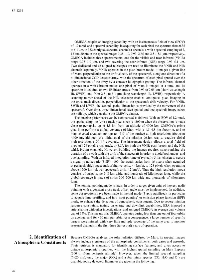
76
SP-1291
OMEGA couples an imaging capability, with an instantaneous field of view (IFOV) of 1.2 mrad, and a spectral capability, in acquiring for each pixel the spectrum from 0.35 to 5.1 µm, in 352 contiguous spectral channels (‘spectels’), with a spectral sampling of 7, 13 and 20 nm in the spectral ranges 0.35–1.0, 0.93–2.65 and 2.51–5.1 µm, respectively. OMEGA includes three spectrometers, one for the visible and near-infrared (VNIR) range 0.35–1.0 µm, and two covering the near-infrared (NIR) range 0.93–5.1 µm. Two dedicated and co-aligned telescopes are used to illuminate the VNIR and NIR channels separately. VNIR operates in the push-broom mode; it images a given line of Mars, perpendicular to the drift velocity of the spacecraft, along one direction of a bi-dimensional CCD detector array, with the spectrum of each pixel spread over the other direction of the array by a concave holographic grating. The infrared channel operates in a whisk-broom mode: one pixel of Mars is imaged at a time, and its spectrum is acquired on two IR linear arrays, from 0.93 to 2.65 µm (short-wavelength IR, SWIR), and from 2.51 to 5.1 µm (long-wavelength IR, LWIR), respectively. A scanning mirror ahead of the NIR telescope enables contiguous pixel imaging in the cross-track direction, perpendicular to the spacecraft drift velocity. For VNIR, SWIR and LWIR, the second spatial dimension is provided by the movement of the spacecraft. Over time, three-dimensional (two spatial and one spectral) image cubes are built up, which constitute the OMEGA dataset.
The imaging performance can be summarised as follows. With an IFOV of 1.2 mrad, the spatial sampling (cross-track pixel size) is ~300 m when the observation is made close to periapsis, up to 4.8 km from an altitude of 4000 km. OMEGA’s prime goal is to perform a global coverage of Mars with a 1.5–4.8 km footprint, and to map selected areas amounting to ~5% of the surface at high resolution (footprint <400 m), although the initial goal of the mission design was to acquire global high-resolution (100 m) coverage. The instrument design allows a total field of view of 128 pixels cross-track, or 8.8°, for both the VNIR push-broom and the NIR whisk-broom channels. However, building the images requires synchronising the duration of a swath with the drift of the spacecraft in order to avoid both under- and oversampling. With an infrared integration time of typically 5 ms, chosen to secure a signal to noise ratio (SNR) >100, the swath varies from 16 pixels when acquired at periapsis (high spacecraft orbital velocity, ~4 km/s), to 128 pixels when operating above 1500 km (slower spacecraft drift, <2 km/s). Thus the high-resolution mode consists of strips some 5–8 km wide, and hundreds of kilometres long, while the global coverage is made of strips 300–500 km wide and thousands of kilometres long.
The nominal pointing mode is nadir. In order to target given units of interest, nadir pointing with a constant cross-track offset angle must be implemented. In addition, some observations have been made in inertial mode (3-axis stabilised), in particular to acquire limb profiling, and in a ‘spot pointing’ or emission phase function (EPF) mode, to enhance the detection of atmospheric constituents. Due to severe mission resource constraints, mainly on energy and downlink capabilities, ESA imposed a strict sharing with other investigations, and assigned OMEGA an average data volume cap of 15%. This means that OMEGA operates during less than one out of four orbits on average, and for <60 min per orbit. As a consequence, a large number of specific targets were missed, with very little multiple coverage of the same area to monitor seasonal changes in the first three (terrestrial) years of operation.
Because OMEGA analyses the solar radiation diffused by Mars, its spectral images always include signatures of the atmospheric constituents, both gases and aerosols. Their retrieval is mandatory for identifying surface features, and gives access to unique atmospheric properties, with the highest spatial sampling on Mars Express (300 m from periapsis altitude). However, given the limited spectral sampling (7–20 nm), only the major (CO2) and a few minor species (CO, H2O and O2) are unambiguously detected. Examples are given in the following.
2. Identification of Atmospheric Constituents

77
Scientific instruments
2.1 CO2An accurate radiative transfer model devoted to the retrieval of the three components (surface, gas, aerosols) is essentially complex and iterative. At first order, it is possible to calculate the atmospheric absorption independently. A dedicated model has been built for this purpose (Melchiorri et al., 2006), which computes a multiplicative component in the synthetic spectrum representative of the main atmospheric contributions (CO2, H2O and CO) in the 1–2.7 µm range (corresponding to the SWIR-C channel). This model performs a line-by-line spectroscopic calculation of the atmospheric absorption, and a spectral atmospheric database is built up for each OMEGA session, with a one-to-one correspondence. A priori knowledge of the atmospheric pressure is taken from general circulation model (GCM) predictions (Forget et al., 1999), as well as a humidity factor and CO profile. Several spectra are calculated around the GCM-predicted position in parameter space, and a least-squares fit adjustment is made to retrieve the observed atmospheric pressure. Each calculation is performed at the exact illumination and elevation conditions corresponding to the OMEGA observations.
The pressure measured in this way is not the actual martian pressure, as at this stage no correction has been made for dust opacity. The ‘effective pressure’ measured in the model is nevertheless correlated with the actual pressure, in a way that can be constrained by a more sophisticated model, including the scattering which is developed as ‘second-order’ modelling (Forget et al., 2007).
Since pressure variations on Mars are primarily correlated with the altitude of the surface, CO2 being the dominant atmospheric compound, a first output of the model is an altimetry map along the OMEGA observations. These altimetry measurements can be checked against the Mars Orbiter Laser Altimeter (MOLA) measurements; effective pressure measurements are found to be accurate to 0.044 mbar (standard deviation), corresponding to an altimetry accuracy of 100 m (1s). The instrumental noise itself is estimated to about 200 m. Therefore, OMEGA atmospheric observation gives an altimetry measurement that is spatially better resolved than the a priori MOLA measurement, to an accuracy of a few hundred metres. This first step allows us to study pressure fluctuations beyond the altimetry variations. This second-order study enables us to search for global or local wave variations, at the 0.1 mbar pressure range, corresponding to the martian meteorology. Similar searches have been tentatively performed using Phobos imaging spectrometer (ISM) observations (Gendrin et al., 2003).
2.2 H2O and CO variations A second step in the study of atmospheric features from OMEGA observations is the H2O and CO retrieval. Despite faint absorption at OMEGA resolution, the sensitivity of the instrument gives access to a good accuracy of the column density of these minor constituents. The spatial variations in the abundance ratio of H2O and CO can therefore be studied, after a correction for the altitude of the surface is performed. The 2.6 µm band of H2O is used, and water vapour maps have been obtained, for Ls = 94–112°, corresponding to the sublimation of the northern polar cap. A mixing ratio of H2O in the range 2–3 × 10⁻⁴ is obtained at 40°N, corresponding to 25 pr-mm, and 5–10 × 10–4 at 60–80°N, corresponding to 40–60 pr-µm. These results are consistent with previous Mars Atmospheric Water Detector (MAWD/Viking) and Thermal Emission Spectrometer (TES/MGS) observations below 60°N (Encrenaz et al., 2005).
The CO abundance is measured with only a low accuracy, due to the low intensity of the (2–0) band at 2.3 µm. Nevertheless, spatial variations have been positively observed over Hellas at Ls = 130–150°, by a factor of 2 compared with Ls = 330–350° (Encrenaz et al., 2006). This result is consistent with GCM predictions (Forget et al., 2006), which indicate an enrichment of non-condensable species over Hellas during the southern winter, due to the effects of local topography on the global circulation. Similar variations in argon abundance have been observed on Hellas at similar Ls (Sprague et al., 2004).

78
SP-1291
2.3 CO2 fluorescence Strong non-LTE emissions of the martian atmosphere are observed above the limb in the OMEGA observations in 3-axis stabilised mode. These emissions are identified as CO2 at 4.3 µm, with a maximum at ~90 km altitude, and CO at 4.7 µm, with a peak emission at ~50 km. The CO2 emission is observed at altitudes well above any dust contamination, since dust opacity reflections typically occur well below 60 km. Although no direct observations of the CO2 emission in imaging mode had been made before Mars Express, its interpretation was well understood in advance from non-LTE modelling of the martian atmosphere, with models developed in particular for atmospheric profile accuracy measurements (Lopez-Valverde et al., 1998). An example of a spectrum of the fluorescence is given in Fig. 1(a), and the vertical variation in the integrated emissions in the CO2 and CO bands are plotted in Fig. 1(b). The main value of OMEGA observations is that they provide simultaneously the spectral information on CO2 and accurate imaging of the emissions. For the first time, the altitudes of these emissions can be directly evaluated from the spectral images, and compared with the model. The model has been improved to fit the data (Drossart et al., 2004).
2.4 Clouds and aerosolsOMEGA has clearly identified both H2O and CO2 clouds, through specific spectral features. In particular, high-altitude CO2 clouds show up via resonant absorption at 3.24 µm, within the otherwise saturated band; they also appear through enhanced reflection in the visible in both the OMEGA VNIR data, and HRSC coordinated observations. Their occurrence has been mapped over the entire planet and all seasons: these clouds are highly localised in both space and time, emphasising the coupled role of thermodynamics and nucleation processes to account for their formation (Montmessin, 2008). In parallel, Monte Carlo based modelling has been conducted to derive aerosol properties from the near-infrared spectra in a variety of areas observed under different dust opacities (Vincendon et al., 2007).
2.5 The O2 DayglowThe O2 emission at 1.27 μm was observed on the dayside by OMEGA in both nadir and inertial modes of observation. In spite of the limited spectral sampling, it is possible to monitor the O2 emission, as it does not overlap with emission or absorption features at a percent level. The O2 dayglow at 1.27 µm is excited by the photolysis of ozone. About 90% of O2 molecules are produced on the excited level a1Δg, which decays either by emitting 1.27 µm photons or by colliding with CO2 molecules. From
Fig. 1. (a) Average of OMEGA spectra taken at the limb over altitudes in the range 50–90 km, exhibiting the fluorescence of CO2 and CO in the martian atmosphere. (b) Integrated emission on the spectral bands for CO2, CO and the continuum, showing the maximum emission along the line of sight.
(a) (b)
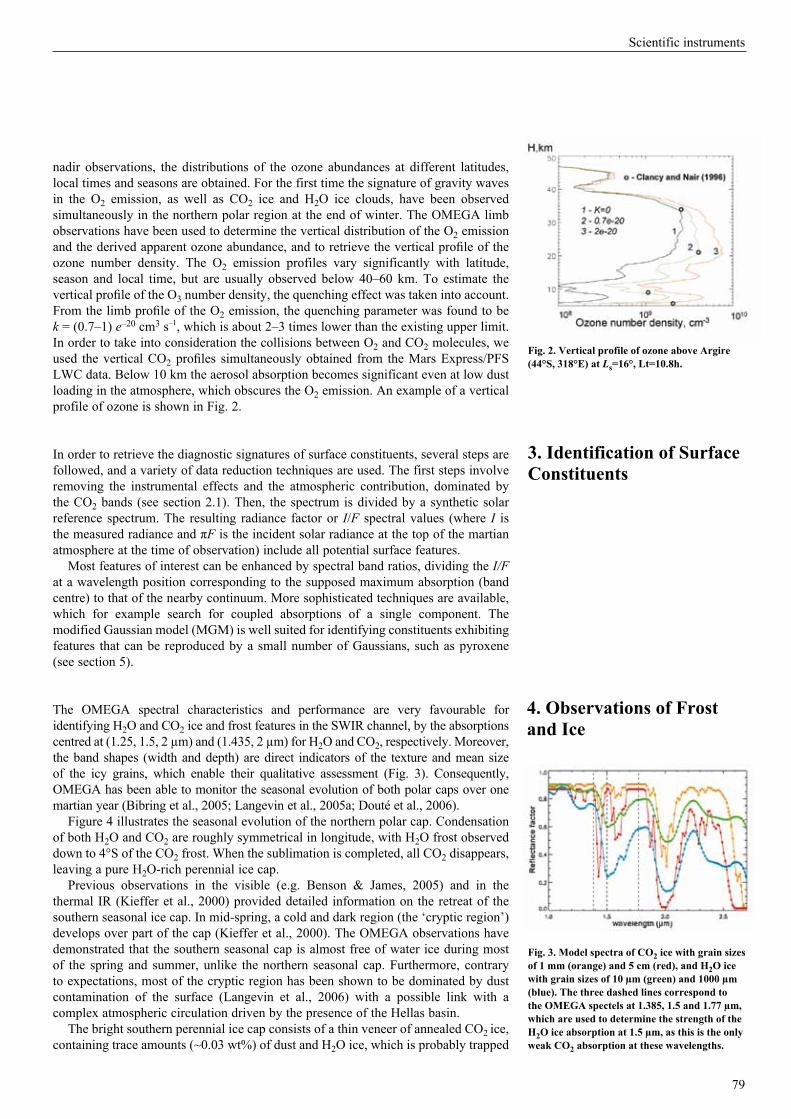
79
Scientific instruments
nadir observations, the distributions of the ozone abundances at different latitudes, local times and seasons are obtained. For the first time the signature of gravity waves in the O2 emission, as well as CO2 ice and H2O ice clouds, have been observed simultaneously in the northern polar region at the end of winter. The OMEGA limb observations have been used to determine the vertical distribution of the O2 emission and the derived apparent ozone abundance, and to retrieve the vertical profile of the ozone number density. The O2 emission profiles vary significantly with latitude, season and local time, but are usually observed below 40–60 km. To estimate the vertical profile of the O3 number density, the quenching effect was taken into account. From the limb profile of the O2 emission, the quenching parameter was found to be k = (0.7–1) e–20 cm3 s–1, which is about 2–3 times lower than the existing upper limit. In order to take into consideration the collisions between O2 and CO2 molecules, we used the vertical CO2 profiles simultaneously obtained from the Mars Express/PFS LWC data. Below 10 km the aerosol absorption becomes significant even at low dust loading in the atmosphere, which obscures the O2 emission. An example of a vertical profile of ozone is shown in Fig. 2.
In order to retrieve the diagnostic signatures of surface constituents, several steps are followed, and a variety of data reduction techniques are used. The first steps involve removing the instrumental effects and the atmospheric contribution, dominated by the CO2 bands (see section 2.1). Then, the spectrum is divided by a synthetic solar reference spectrum. The resulting radiance factor or I/F spectral values (where I is the measured radiance and πF is the incident solar radiance at the top of the martian atmosphere at the time of observation) include all potential surface features.
Most features of interest can be enhanced by spectral band ratios, dividing the I/F at a wavelength position corresponding to the supposed maximum absorption (band centre) to that of the nearby continuum. More sophisticated techniques are available, which for example search for coupled absorptions of a single component. The modified Gaussian model (MGM) is well suited for identifying constituents exhibiting features that can be reproduced by a small number of Gaussians, such as pyroxene (see section 5).
The OMEGA spectral characteristics and performance are very favourable for identifying H2O and CO2 ice and frost features in the SWIR channel, by the absorptions centred at (1.25, 1.5, 2 µm) and (1.435, 2 µm) for H2O and CO2, respectively. Moreover, the band shapes (width and depth) are direct indicators of the texture and mean size of the icy grains, which enable their qualitative assessment (Fig. 3). Consequently, OMEGA has been able to monitor the seasonal evolution of both polar caps over one martian year (Bibring et al., 2005; Langevin et al., 2005a; Douté et al., 2006).
Figure 4 illustrates the seasonal evolution of the northern polar cap. Condensation of both H2O and CO2 are roughly symmetrical in longitude, with H2O frost observed down to 4°S of the CO2 frost. When the sublimation is completed, all CO2 disappears, leaving a pure H2O-rich perennial ice cap.
Previous observations in the visible (e.g. Benson & James, 2005) and in the thermal IR (Kieffer et al., 2000) provided detailed information on the retreat of the southern seasonal ice cap. In mid-spring, a cold and dark region (the ‘cryptic region’) develops over part of the cap (Kieffer et al., 2000). The OMEGA observations have demonstrated that the southern seasonal cap is almost free of water ice during most of the spring and summer, unlike the northern seasonal cap. Furthermore, contrary to expectations, most of the cryptic region has been shown to be dominated by dust contamination of the surface (Langevin et al., 2006) with a possible link with a complex atmospheric circulation driven by the presence of the Hellas basin.
The bright southern perennial ice cap consists of a thin veneer of annealed CO2 ice, containing trace amounts (~0.03 wt%) of dust and H2O ice, which is probably trapped
Fig. 2. Vertical profile of ozone above Argire (44°S, 318°E) at Ls=16°, Lt=10.8h.
3. Identification of Surface Constituents
4. Observations of Frost and Ice
Fig. 3. Model spectra of CO2 ice with grain sizes of 1 mm (orange) and 5 cm (red), and H2O ice with grain sizes of 10 µm (green) and 1000 µm (blue). The three dashed lines correspond to the OMEGA spectels at 1.385, 1.5 and 1.77 µm, which are used to determine the strength of the H2O ice absorption at 1.5 µm, as this is the only weak CO2 absorption at these wavelengths.
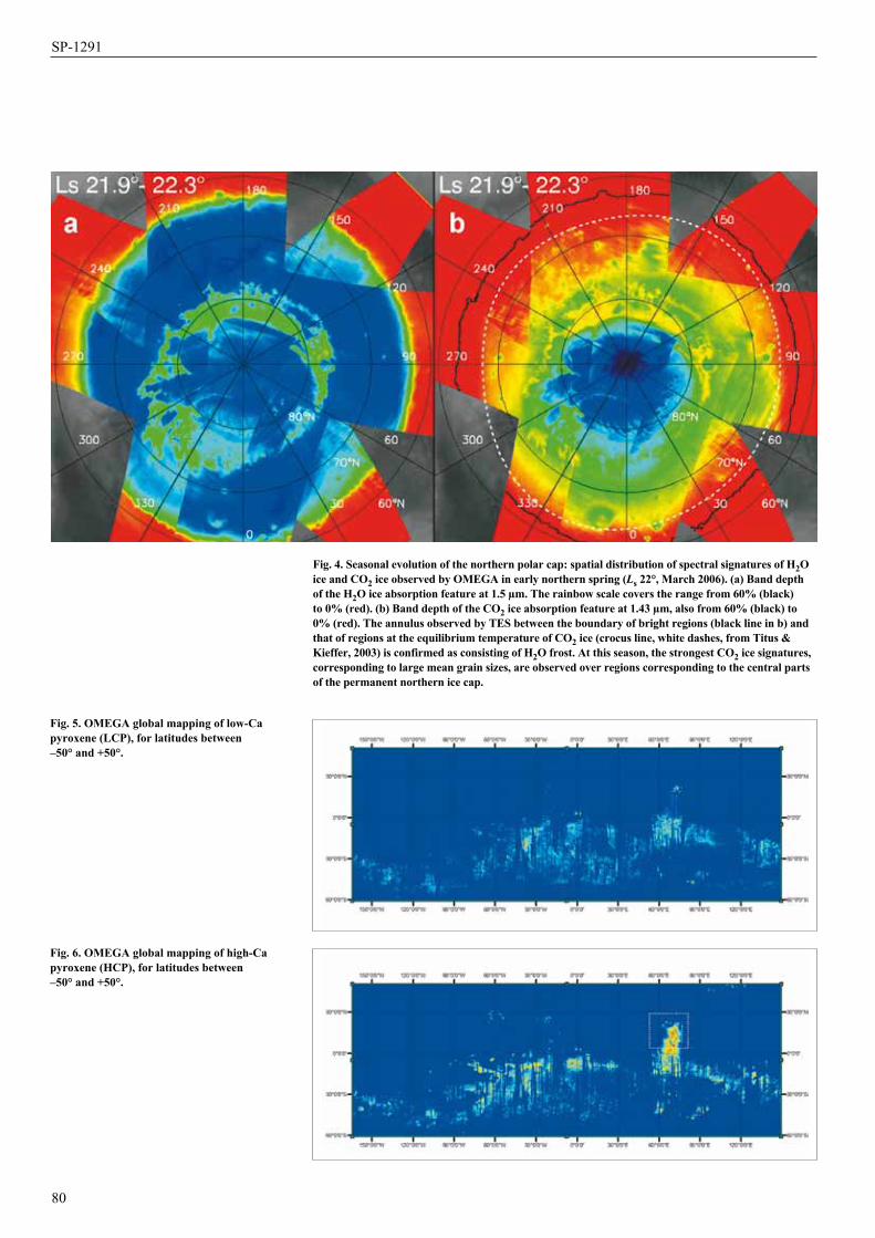
80
SP-1291
Fig. 4. Seasonal evolution of the northern polar cap: spatial distribution of spectral signatures of H2O ice and CO2 ice observed by OMEGA in early northern spring (Ls 22°, March 2006). (a) Band depth of the H2O ice absorption feature at 1.5 µm. The rainbow scale covers the range from 60% (black) to 0% (red). (b) Band depth of the CO2 ice absorption feature at 1.43 µm, also from 60% (black) to 0% (red). The annulus observed by TES between the boundary of bright regions (black line in b) and that of regions at the equilibrium temperature of CO2 ice (crocus line, white dashes, from Titus & Kieffer, 2003) is confirmed as consisting of H2O frost. At this season, the strongest CO2 ice signatures, corresponding to large mean grain sizes, are observed over regions corresponding to the central parts of the permanent northern ice cap.
Fig. 5. OMEGA global mapping of low-Ca pyroxene (LCP), for latitudes between –50° and +50°.
Fig. 6. OMEGA global mapping of high-Ca pyroxene (HCP), for latitudes between –50° and +50°.
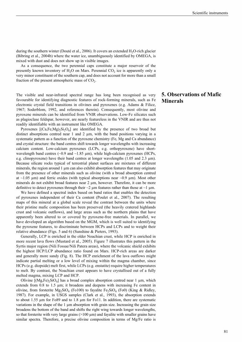
81
Scientific instruments
during the southern winter (Douté et al., 2006). It covers an extended H2O-rich glacier (Bibring et al., 2004b) where the water ice, unambiguously identified by OMEGA, is mixed with dust and does not show up in visible images.
As a consequence, the two perennial caps constitute a major reservoir of the presently known inventory of H2O on Mars. Perennial CO2 ice is apparently only a very minor constituent of the southern cap, and does not account for more than a small fraction of the present atmospheric mass of CO2.
The visible and near-infrared spectral range has long been recognised as very favourable for identifying diagnostic features of rock-forming minerals, such as Fe electronic crystal field transitions in olivines and pyroxenes (e.g. Adams & Filice, 1967; Soderblom, 1992, and references therein). Consequently, most olivine and pyroxene minerals can be identified from VNIR observations. Low-Fe silicates such as plagioclase feldspar, however, are nearly featureless in the VNIR and are thus not readily identifiable with an instrument like OMEGA.
Pyroxenes [(Ca,Fe,Mg)2Si2O6] are identified by the presence of two broad but distinct absorptions centred near 1 and 2 µm, with the band positions varying in a systematic pattern as a function of the pyroxene chemistry (Fe, Mg and Ca abundance) and crystal structure: the band centres shift towards longer wavelengths with increasing calcium content. Low-calcium pyroxenes (LCPs, e.g. orthopyroxene) have short-wavelength band centres (~0.9 and ~1.85 µm), while high-calcium pyroxenes (HCPs, e.g. clinopyroxene) have their band centres at longer wavelengths (1.05 and 2.3 µm). Because silicate rocks typical of terrestrial planet surfaces are mixtures of different minerals, the region around 1 µm can also exhibit absorption features that may originate from the presence of other minerals such as olivine (with a broad absorption centred at ~1.05 µm) and ferric oxides (with typical absorptions near ~0.9 µm). Most other minerals do not exhibit broad features near 2 µm, however. Therefore, it can be more definitive to detect pyroxenes through their ~2 µm features rather than those at ~1 µm.
We have defined a spectral index based on band ratios that enables the detection of pyroxenes independent of their Ca content (Poulet et al., 2007). The resulting maps of this mineral at a global scale reveal the contrast between the units where their pristine mafic composition has been preserved (the heavily cratered highlands crust and volcanic outflows), and large areas such as the northern plains that have apparently been altered to or covered by pyroxene-free materials. In parallel, we have developed an algorithm based on the MGM, which is well suited to identifying the pyroxene features, to discriminate between HCPs and LCPs and to weight their relative abundance (Figs. 5 and 6) (Sunshine & Pieters, 1993).
Generally, LCP is enriched in the older Noachian crust, while HCP is enriched in more recent lava flows (Mustard et al., 2005). Figure 7 illustrates this pattern in the Syrtis major region (Nili Fossae/Nili Patera areas), where the volcanic shield exhibits the highest HCP/LCP abundance ratio found on Mars. HCP-rich areas are darker and generally more sandy (Fig. 8). The HCP enrichment of the lava outflows might indicate partial melting or a low level of mixing within the magma chamber, since HCPs (e.g. diopside) melt first, while LCPs (e.g. enstatite) require higher temperatures to melt. By contrast, the Noachian crust appears to have crystallised out of a fully melted magma, mixing LCP and HCP.
Olivine [(Mg,Fe)2SiO4] has a broad complex absorption centred near 1 µm, which extends from 0.8 to 1.5 µm; it broadens and deepens with increasing Fe content in olivine, from forsterite Mg2SiO4 (Fo100) to fayalite Fe2SiO4 (Fo0) (King & Ridley, 1987). For example, in USGS samples (Clark et al., 1993), the absorption extends to about 1.55 µm for Fo89 and to 1.8 µm for Fo11. In addition, there are systematic variations in the shape of the 1 µm absorption with grain size. Increasing the grain size broadens the bottom of the band and shifts the right wing towards longer wavelengths, so that forsterite with very large grains (>100 µm) and fayalite with smaller grains have similar spectra. Therefore, a precise olivine composition in terms of Mg/Fe ratio is
5. Observations of Mafic Minerals
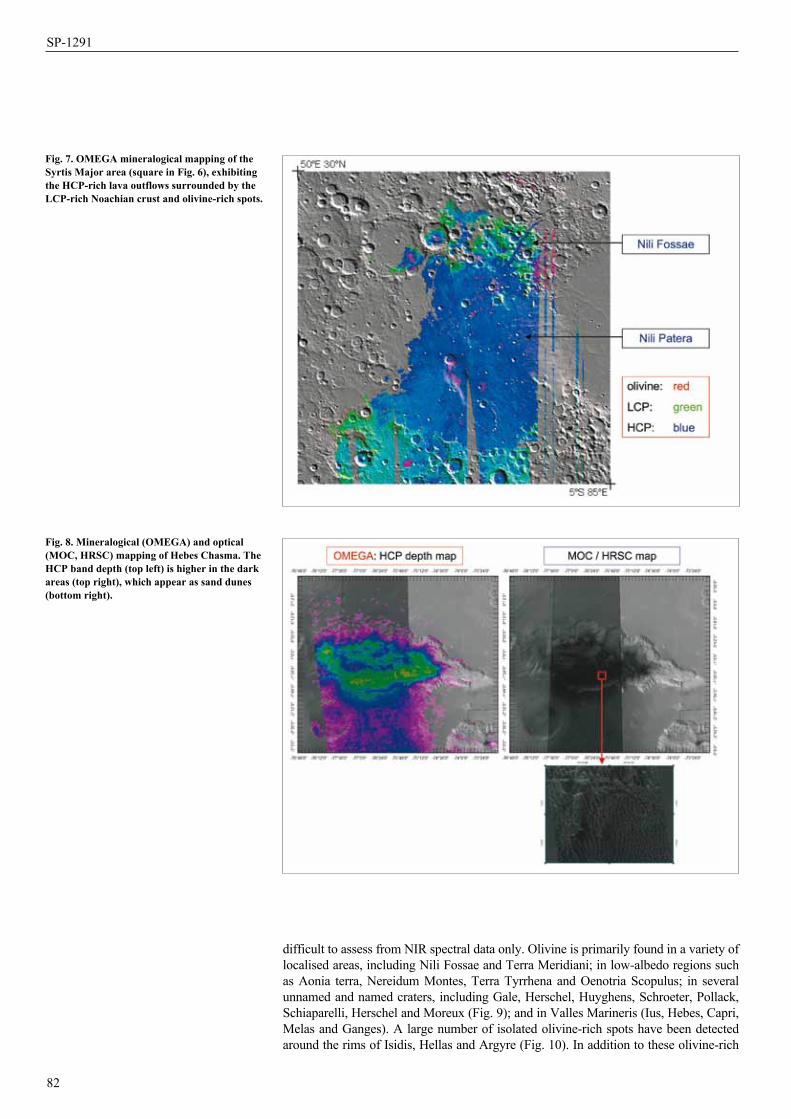
82
SP-1291
difficult to assess from NIR spectral data only. Olivine is primarily found in a variety of localised areas, including Nili Fossae and Terra Meridiani; in low-albedo regions such as Aonia terra, Nereidum Montes, Terra Tyrrhena and Oenotria Scopulus; in several unnamed and named craters, including Gale, Herschel, Huyghens, Schroeter, Pollack, Schiaparelli, Herschel and Moreux (Fig. 9); and in Valles Marineris (Ius, Hebes, Capri, Melas and Ganges). A large number of isolated olivine-rich spots have been detected around the rims of Isidis, Hellas and Argyre (Fig. 10). In addition to these olivine-rich
Fig. 7. OMEGA mineralogical mapping of the Syrtis Major area (square in Fig. 6), exhibiting the HCP-rich lava outflows surrounded by the LCP-rich Noachian crust and olivine-rich spots.
Fig. 8. Mineralogical (OMEGA) and optical (MOC, HRSC) mapping of Hebes Chasma. The HCP band depth (top left) is higher in the dark areas (top right), which appear as sand dunes (bottom right).
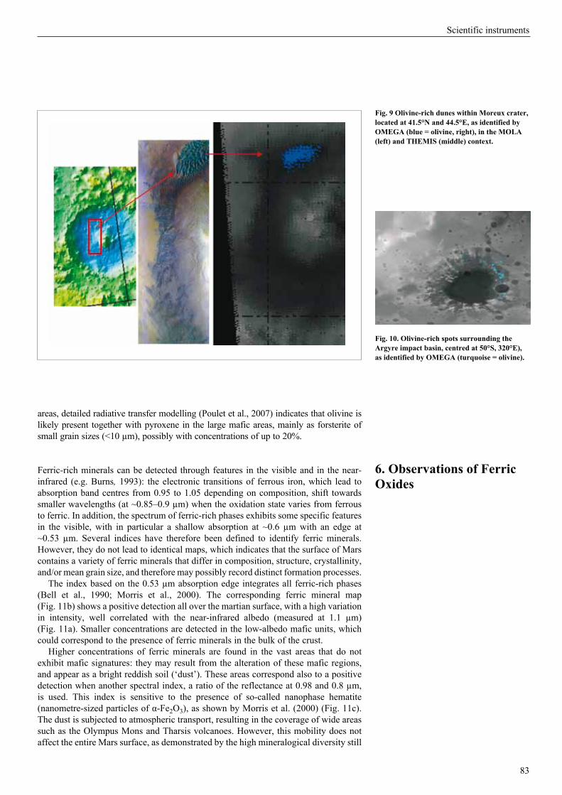
83
Scientific instruments
areas, detailed radiative transfer modelling (Poulet et al., 2007) indicates that olivine is likely present together with pyroxene in the large mafic areas, mainly as forsterite of small grain sizes (<10 µm), possibly with concentrations of up to 20%.
Ferric-rich minerals can be detected through features in the visible and in the near-infrared (e.g. Burns, 1993): the electronic transitions of ferrous iron, which lead to absorption band centres from 0.95 to 1.05 depending on composition, shift towards smaller wavelengths (at ~0.85–0.9 µm) when the oxidation state varies from ferrous to ferric. In addition, the spectrum of ferric-rich phases exhibits some specific features in the visible, with in particular a shallow absorption at ~0.6 µm with an edge at ~0.53 µm. Several indices have therefore been defined to identify ferric minerals. However, they do not lead to identical maps, which indicates that the surface of Mars contains a variety of ferric minerals that differ in composition, structure, crystallinity, and/or mean grain size, and therefore may possibly record distinct formation processes.
The index based on the 0.53 µm absorption edge integrates all ferric-rich phases (Bell et al., 1990; Morris et al., 2000). The corresponding ferric mineral map (Fig. 11b) shows a positive detection all over the martian surface, with a high variation in intensity, well correlated with the near-infrared albedo (measured at 1.1 µm) (Fig. 11a). Smaller concentrations are detected in the low-albedo mafic units, which could correspond to the presence of ferric minerals in the bulk of the crust.
Higher concentrations of ferric minerals are found in the vast areas that do not exhibit mafic signatures: they may result from the alteration of these mafic regions, and appear as a bright reddish soil (‘dust’). These areas correspond also to a positive detection when another spectral index, a ratio of the reflectance at 0.98 and 0.8 µm, is used. This index is sensitive to the presence of so-called nanophase hematite (nanometre-sized particles of α-Fe2O3), as shown by Morris et al. (2000) (Fig. 11c). The dust is subjected to atmospheric transport, resulting in the coverage of wide areas such as the Olympus Mons and Tharsis volcanoes. However, this mobility does not affect the entire Mars surface, as demonstrated by the high mineralogical diversity still
Fig. 9 Olivine-rich dunes within Moreux crater, located at 41.5°N and 44.5°E, as identified by OMEGA (blue = olivine, right), in the MOLA (left) and THEMIS (middle) context.
6. Observations of Ferric Oxides
Fig. 10. Olivine-rich spots surrounding the Argyre impact basin, centred at 50°S, 320°E), as identified by OMEGA (turquoise = olivine).
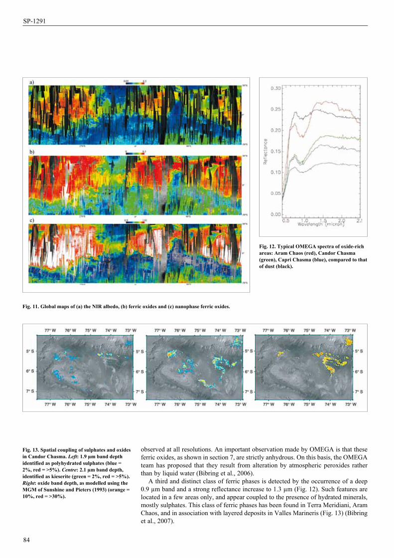
84
SP-1291
Fig. 11. Global maps of (a) the NIR albedo, (b) ferric oxides and (c) nanophase ferric oxides.
Fig. 12. Typical OMEGA spectra of oxide-rich areas: Aram Chaos (red), Candor Chasma (green), Capri Chasma (blue), compared to that of dust (black).
observed at all resolutions. An important observation made by OMEGA is that these ferric oxides, as shown in section 7, are strictly anhydrous. On this basis, the OMEGA team has proposed that they result from alteration by atmospheric peroxides rather than by liquid water (Bibring et al., 2006).
A third and distinct class of ferric phases is detected by the occurrence of a deep 0.9 µm band and a strong reflectance increase to 1.3 µm (Fig. 12). Such features are located in a few areas only, and appear coupled to the presence of hydrated minerals, mostly sulphates. This class of ferric phases has been found in Terra Meridiani, Aram Chaos, and in association with layered deposits in Valles Marineris (Fig. 13) (Bibring et al., 2007).
Fig. 13. Spatial coupling of sulphates and oxides in Candor Chasma. Left: 1.9 µm band depth identified as polyhydrated sulphates (blue = 2%, red = >5%). Centre: 2.1 µm band depth, identified as kieserite (green = 2%, red = >5%). Right: oxide band depth, as modelled using the MGM of Sunshine and Pieters (1993) (orange = 10%, red = >30%).
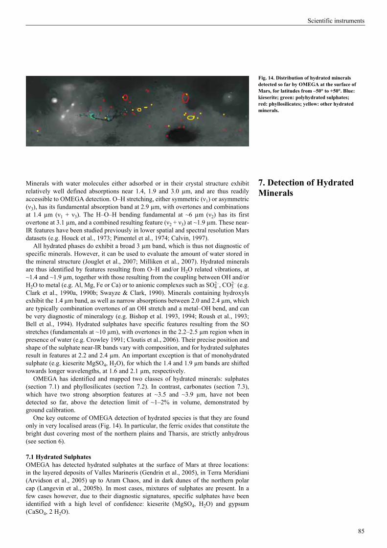
85
Scientific instruments
Minerals with water molecules either adsorbed or in their crystal structure exhibit relatively well defined absorptions near 1.4, 1.9 and 3.0 µm, and are thus readily accessible to OMEGA detection. O–H stretching, either symmetric (ν1) or asymmetric (ν3), has its fundamental absorption band at 2.9 µm, with overtones and combinations at 1.4 µm (ν1 + ν3). The H–O–H bending fundamental at ~6 µm (ν2) has its first overtone at 3.1 µm, and a combined resulting feature (ν2 + ν3) at ~1.9 µm. These near-IR features have been studied previously in lower spatial and spectral resolution Mars datasets (e.g. Houck et al., 1973; Pimentel et al., 1974; Calvin, 1997).
All hydrated phases do exhibit a broad 3 µm band, which is thus not diagnostic of specific minerals. However, it can be used to evaluate the amount of water stored in the mineral structure (Jouglet et al., 2007; Milliken et al., 2007). Hydrated minerals are thus identified by features resulting from O–H and/or H2O related vibrations, at ~1.4 and ~1.9 µm, together with those resulting from the coupling between OH and/or H2O to metal (e.g. Al, Mg, Fe or Ca) or to anionic complexes such as SO4
2–, CO32– (e.g.
Clark et al., 1990a, 1990b; Swayze & Clark, 1990). Minerals containing hydroxyls exhibit the 1.4 µm band, as well as narrow absorptions between 2.0 and 2.4 µm, which are typically combination overtones of an OH stretch and a metal–OH bend, and can be very diagnostic of mineralogy (e.g. Bishop et al. 1993, 1994; Roush et al., 1993; Bell et al., 1994). Hydrated sulphates have specific features resulting from the SO stretches (fundamentals at ~10 µm), with overtones in the 2.2–2.5 µm region when in presence of water (e.g. Crowley 1991; Cloutis et al., 2006). Their precise position and shape of the sulphate near-IR bands vary with composition, and for hydrated sulphates result in features at 2.2 and 2.4 µm. An important exception is that of monohydrated sulphate (e.g. kieserite MgSO4, H2O), for which the 1.4 and 1.9 µm bands are shifted towards longer wavelengths, at 1.6 and 2.1 µm, respectively.
OMEGA has identified and mapped two classes of hydrated minerals: sulphates (section 7.1) and phyllosilicates (section 7.2). In contrast, carbonates (section 7.3), which have two strong absorption features at ~3.5 and ~3.9 µm, have not been detected so far, above the detection limit of ~1–2% in volume, demonstrated by ground calibration.
One key outcome of OMEGA detection of hydrated species is that they are found only in very localised areas (Fig. 14). In particular, the ferric oxides that constitute the bright dust covering most of the northern plains and Tharsis, are strictly anhydrous (see section 6).
7.1 Hydrated SulphatesOMEGA has detected hydrated sulphates at the surface of Mars at three locations: in the layered deposits of Valles Marineris (Gendrin et al., 2005), in Terra Meridiani (Arvidson et al., 2005) up to Aram Chaos, and in dark dunes of the northern polar cap (Langevin et al., 2005b). In most cases, mixtures of sulphates are present. In a few cases however, due to their diagnostic signatures, specific sulphates have been identified with a high level of confidence: kieserite (MgSO4, H2O) and gypsum (CaSO4, 2 H2O).
7. Detection of Hydrated Minerals
Fig. 14. Distribution of hydrated minerals detected so far by OMEGA at the surface of Mars, for latitudes from –50° to +50°. Blue: kieserite; green: polyhydrated sulphates; red: phyllosilicates; yellow: other hydrated minerals.
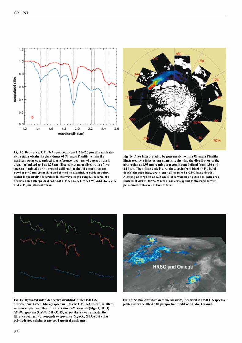
86
SP-1291
Fig. 15. Red curve: OMEGA spectrum from 1.2 to 2.6 µm of a sulphate-rich region within the dark dunes of Olympia Planitia, within the northern polar cap, ratioed to a reference spectrum of a nearby dark area, normalised to 1 at 1.25 µm. Blue curve: normalised ratio of two spectra obtained during ground calibration: that of a pure gypsum powder (<40 µm grain size) and that of an aluminium oxide powder, which is spectrally featureless in this wavelength range. Features are observed in both spectral ratios at 1.445, 1.535, 1.745, 1.94, 2.22, 2.26, 2.42 and 2.48 µm (dashed lines).
Fig. 16. Area interpreted to be gypsum rich within Olympia Planitia, illustrated by a false-colour composite showing the distribution of the absorption at 1.93 µm relative to a continuum defined from 1.86 and 2.14 µm. The colour code is a rainbow scale from black (<4% band depth) through blue, green and yellow to red (>25% band depth). A strong absorption at 1.93 µm is observed on an extended dark area centred at 240°E, 80°N. White areas correspond to the regions with permanent water ice at the surface.
Fig. 17. Hydrated sulphate spectra identified in the OMEGA observations. Green: library spectrum. Black: OMEGA spectrum. Blue: reference spectrum. Red: spectral ratio. Left: kieserite (MgSO4, H2O). Middle: gypsum (CaSO4, 2H2O). Right: polyhydrated sulphate; the library spectrum corresponds to epsomite (MgSO4, 7H2O) but other polyhydrated sulphates are good spectral analogues.
Fig. 18. Spatial distribution of the kieserite, identified in OMEGA spectra, plotted over the HRSC 3D perspective model of Candor Chasma.
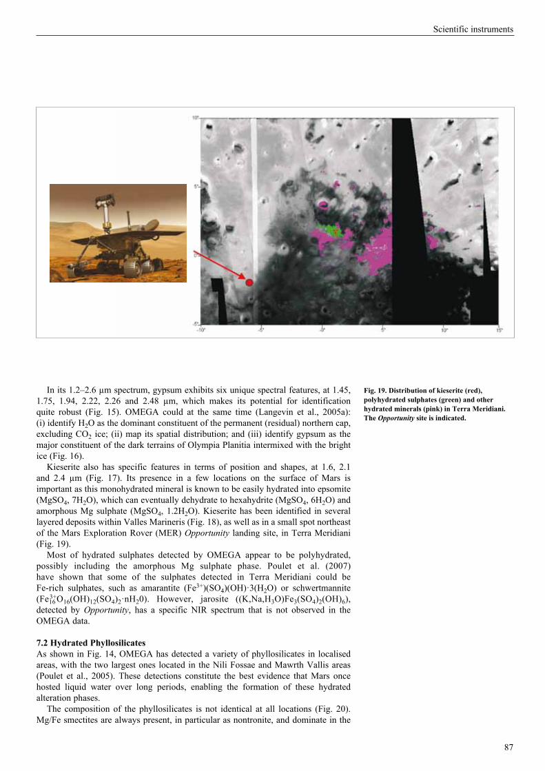
87
Scientific instruments
In its 1.2–2.6 µm spectrum, gypsum exhibits six unique spectral features, at 1.45, 1.75, 1.94, 2.22, 2.26 and 2.48 µm, which makes its potential for identification quite robust (Fig. 15). OMEGA could at the same time (Langevin et al., 2005a): (i) identify H2O as the dominant constituent of the permanent (residual) northern cap, excluding CO2 ice; (ii) map its spatial distribution; and (iii) identify gypsum as the major constituent of the dark terrains of Olympia Planitia intermixed with the bright ice (Fig. 16).
Kieserite also has specific features in terms of position and shapes, at 1.6, 2.1 and 2.4 µm (Fig. 17). Its presence in a few locations on the surface of Mars is important as this monohydrated mineral is known to be easily hydrated into epsomite (MgSO4, 7H2O), which can eventually dehydrate to hexahydrite (MgSO4, 6H2O) and amorphous Mg sulphate (MgSO4, 1.2H2O). Kieserite has been identified in several layered deposits within Valles Marineris (Fig. 18), as well as in a small spot northeast of the Mars Exploration Rover (MER) Opportunity landing site, in Terra Meridiani (Fig. 19).
Most of hydrated sulphates detected by OMEGA appear to be polyhydrated, possibly including the amorphous Mg sulphate phase. Poulet et al. (2007) have shown that some of the sulphates detected in Terra Meridiani could be Fe-rich sulphates, such as amarantite (Fe3+)(SO4)(OH)·3(H2O) or schwertmannite (Fe16
3+O16(OH)12(SO4)2·nH20). However, jarosite ((K,Na,H3O)Fe3(SO4)2(OH)6), detected by Opportunity, has a specific NIR spectrum that is not observed in the OMEGA data.
7.2 Hydrated PhyllosilicatesAs shown in Fig. 14, OMEGA has detected a variety of phyllosilicates in localised areas, with the two largest ones located in the Nili Fossae and Mawrth Vallis areas (Poulet et al., 2005). These detections constitute the best evidence that Mars once hosted liquid water over long periods, enabling the formation of these hydrated alteration phases.
The composition of the phyllosilicates is not identical at all locations (Fig. 20). Mg/Fe smectites are always present, in particular as nontronite, and dominate in the
Fig. 19. Distribution of kieserite (red), polyhydrated sulphates (green) and other hydrated minerals (pink) in Terra Meridiani. The Opportunity site is indicated.

88
SP-1291
Nili Fossae/Syrtis Major complex. Al-rich phyllosilicates, such as montmorillonite or chlorite, are also found, in particular in the Mawrth Vallis area. However, kaolinite appears to be rare. This is an indication that the process responsible for the formation of the phyllosilicates, although it implies liquid water likely over long periods, was characterised by a rather low level of leaching (Chevrier et al., 2007). With reference to conditions prevailing in terrestrial environments, or during laboratory simulations when similar minerals are formed, the martian fluids in which these smectites formed were neutral to alkaline rather than acidic at the time the aqueous alteration took place (Chevrier et al., 2007).
The sites where the phyllosilicates have been mapped are all very ancient, and have been exposed to the surface either by impact or erosion. In the Nili Fossae area (Mustard et al., 2007; Mangold et al., 2007), the phyllosilicate-rich terrains all appear to predate the first lava flows from Nili Patera and Syrtis Major Planum, dated early Hesperian by crater counting. Phyllosilicate-rich sites include both ancient heavily cratered terrains that have not been buried by the lava flows, and recently excavated ones (Fig. 21). Apparently the impact process did not destroy or dehydrate these minerals, but might rather have triggered their formation. It is important to note that by contrast, the lobate ejecta craters within the Nili Patera lava floor do not exhibit hydrated minerals, which strongly indicates that this lava material was essentially dry.
Fig. 20. Spectra of hydrated phyllosilicates, as detected by OMEGA, compared with laboratory spectra, showing the diagnostic shift of the M–OH feature from 2.2 µm for Al-rich (a,b) to 2.28 µm Fe-rich (c), and 2.35 µm Mg/Fe-rich (d) species.
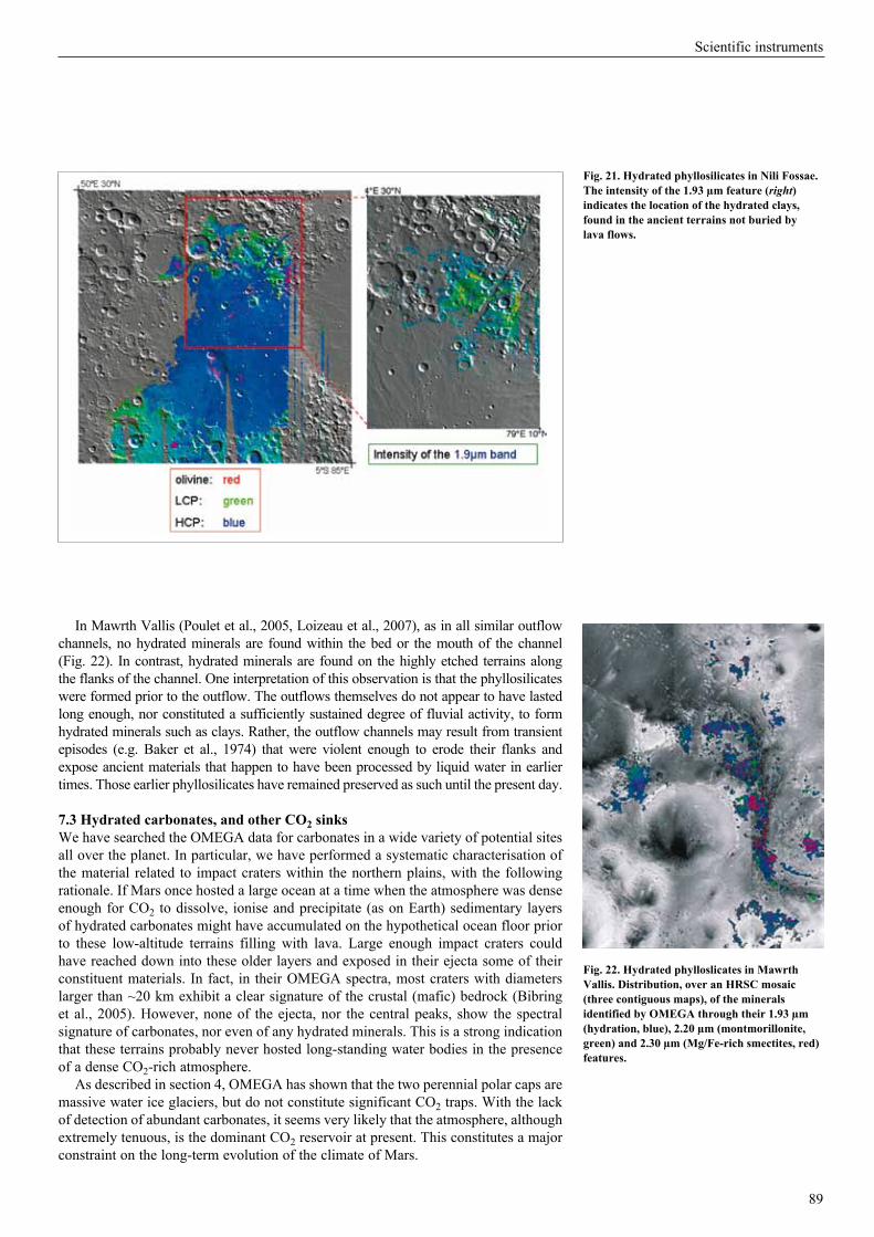
89
Scientific instruments
In Mawrth Vallis (Poulet et al., 2005, Loizeau et al., 2007), as in all similar outflow channels, no hydrated minerals are found within the bed or the mouth of the channel (Fig. 22). In contrast, hydrated minerals are found on the highly etched terrains along the flanks of the channel. One interpretation of this observation is that the phyllosilicates were formed prior to the outflow. The outflows themselves do not appear to have lasted long enough, nor constituted a sufficiently sustained degree of fluvial activity, to form hydrated minerals such as clays. Rather, the outflow channels may result from transient episodes (e.g. Baker et al., 1974) that were violent enough to erode their flanks and expose ancient materials that happen to have been processed by liquid water in earlier times. Those earlier phyllosilicates have remained preserved as such until the present day.
7.3 Hydrated carbonates, and other CO2 sinksWe have searched the OMEGA data for carbonates in a wide variety of potential sites all over the planet. In particular, we have performed a systematic characterisation of the material related to impact craters within the northern plains, with the following rationale. If Mars once hosted a large ocean at a time when the atmosphere was dense enough for CO2 to dissolve, ionise and precipitate (as on Earth) sedimentary layers of hydrated carbonates might have accumulated on the hypothetical ocean floor prior to these low-altitude terrains filling with lava. Large enough impact craters could have reached down into these older layers and exposed in their ejecta some of their constituent materials. In fact, in their OMEGA spectra, most craters with diameters larger than ~20 km exhibit a clear signature of the crustal (mafic) bedrock (Bibring et al., 2005). However, none of the ejecta, nor the central peaks, show the spectral signature of carbonates, nor even of any hydrated minerals. This is a strong indication that these terrains probably never hosted long-standing water bodies in the presence of a dense CO2-rich atmosphere.
As described in section 4, OMEGA has shown that the two perennial polar caps are massive water ice glaciers, but do not constitute significant CO2 traps. With the lack of detection of abundant carbonates, it seems very likely that the atmosphere, although extremely tenuous, is the dominant CO2 reservoir at present. This constitutes a major constraint on the long-term evolution of the climate of Mars.
Fig. 21. Hydrated phyllosilicates in Nili Fossae. The intensity of the 1.93 µm feature (right) indicates the location of the hydrated clays, found in the ancient terrains not buried by lava flows.
Fig. 22. Hydrated phylloslicates in Mawrth Vallis. Distribution, over an HRSC mosaic (three contiguous maps), of the minerals identified by OMEGA through their 1.93 µm (hydration, blue), 2.20 µm (montmorillonite, green) and 2.30 µm (Mg/Fe-rich smectites, red) features.

90
SP-1291
The identification and mapping of both primary igneous and secondary altered minerals, put into their geomorphological context, reveals some major features relevant to the history of Mars (Bibring et al., 2006). Well preserved mafic minerals are still observed on a wide scale, in the oldest crust and, in places, even in impact craters. By contrast, the northern lowlands are dominated by an alteration product (dust) characterised by anhydrous ferric oxide. Hydrated minerals have been detected, in a restricted number of localised areas. They consist of two classes, phyllosilicates and sulphates, which are found in distinct terrains, formed by distinct processes, at distinct times. They trace distinct eras, ‘phyllosian’ and theiikian’ respectively to reflect the names, in Greek, of their dominant minerals. Stratigraphic relationships suggest that the phyllosilicates formed first, in a neutral to alkaline environment, followed by the sulphates (theiikos in Greek), in an acidic environment. We are thus led to propose that in between the two eras, Mars underwent global-scale climatic change. We attribute this major environmental evolution to the volcanic activity that led to the building of Tharsis and the filling of the northern plains (Fig. 23).
Since phyllosilicates usually require water over long duration to form, Mars likely hosted conditions sustaining liquid water on geological timescales in its very early history. This in turn requires that there were abundant greenhouse gases, given the predicted low luminosity of the early Sun (e.g. Pollack et al., 1987). However, like most young stars, the early Sun was likely an extreme ultraviolet emitter, with high ionising efficiency, and with an intense solar wind. A planetary magnetic shield was thus critical to protect against atmospheric loss. As demonstrated by the findings of the Magnetometer and Electron Reflectometer (MAG/ER) investigation of remnant crustal magnetism on Mars Global Surveyor, early Mars appears to have supported a global dynamo, which could have efficiently protected its atmosphere. The absence of magnetised minerals over Tharsis and in the northern plains is a strong indication that this dynamo shut off before the onset of volcanism that raised Tharsis and filled the plains.
A possible explanation is that mantle convection could not sustain a sufficient temperature difference between the core and the mantle, required to maintain core convection: the dynamo and its associated magnetic shield dropped. Cold plumes could have started to form and to sink within the mantle and accumulate at the core/mantle boundary. This, in turn, could have triggered thermal instabilities, leading to the formation of degree 1 hot plumes, ascending to form Tharsis after some tens of millions years. In such a scheme, the formation of Tharsis would have happened long after the magnetic field had faded, and long after most of the atmosphere had been lost by solar wind erosion or other processes. In the tenuous resulting atmosphere, the massive outgassing coupled to the volcanic activity could have injected S-rich compounds as dominant species, which then rapidly oxidised into sulphuric compounds, leading the environment (including any groundwater) to become highly acidic. These S-rich species precipitated widely over the planet, possibly in the form of nanophase S-rich grains, accounting for the large concentration of S detected by elemental Alpha Particle X-ray Spectrometer (APXS) analyses at all rover and lander sites since Viking.
The present composition of the martian atmosphere has an N2/CO2 value close to those of both Venus and Earth (~3%), if one takes into account that most of the initial terrestrial CO2 is presently trapped as carbonates. The N2/CO2 ratio is consistent with such an early physical loss mechanism. If the initial volatile reservoirs of Mars, Venus and Earth were similar, and given that CO2 can be sequestered into carbonates whereas N2 hardly ever condenses into minerals, one would not expect a massive depletion of both constituents (more than 99.9%) with identical efficiencies (Bibring & Erard, 2001). OMEGA data support a model in which most of the atmosphere escaped prior to the Theiikian; today’s atmosphere would result from an equilibrium between the present (very limited) loss mechanisms, for example as measured by Mars Express/ASPERA (Barabash et al., 2007), and the supply of volatiles by residual internal activity.
8. A Derived Mars Mineralogical History:
Identification and Characterisation of an
Early Global Change

91
Scientific instruments
In such a model, the Phyllosian era would have ended when the surface water could no longer remain stable as a liquid, and instead evaporated and/or percolated and froze as subsurface permafrost. The large-scale tectonic effects that followed the building of Tharsis, such as the opening of Valles Marineris and the tilt of Terra Meridiani, as well as the localised rising of the geothermal water table, could have produced sequential supplies of liquid water to a variety of regions within these areas, for example, cementing the S-rich nanophase grains into large sulphate deposits. This process would not necessarily require surface liquid water to be long-lasting, since sulphates can sediment even while water is evaporating. During this period, sulphate layers would have grown where surface water was supplied, in spatial and time relation with the Tharsis rise. The Theiikian era would have ended rapidly, leading to a long era (Siderikian), lasting until the present, dominated by anhydrous surface oxidation and the creation of nanophase ferric oxides (siderikos in Greek) in a highly rarefied atmosphere. This oxidation likely results from a very slow process (time scales of Gyr) operating on the very superficial layers (sub-millimetre scale) of surface grains.
Although one could have expected that the global circulation of dust would preclude the identification of distinct units on the surface of Mars, the OMEGA investigation has demonstrated a high degree of mineralogical diversity down to a sub-kilometre scale. Units of all ages, from the most ancient to the most recently processed ones, have been identified by their composition. In particular, the oldest units, although subjected to a longer period of potential weathering, still preserve their igneous content. In parallel, the detection and mapping of alteration products provide key clues for deciphering the evolution of the Mars environment.
Two classes of hydrated phases have been identified. Placed in their geological context, and in relation to the in situ findings of the two NASA Mars Exploration Rovers, they enable a profoundly new model of the past martian climate to be envisioned. Thirty years after the pioneering measurements of the Viking landers, the OMEGA orbital near-infrared survey indicates that Mars might indeed have hosted, once in its earlier past, conditions that favoured liquid water to remain stable over long periods of time. The sites where one might search for these potential habitats are not necessarily located where the optical images would have led us to consider, since phyllosilicates are not directly associated with fluvial or other water-related landforms. OMEGA results so far suggest that the most favourable sites for preserving evidence of this early epoch are those characterised by a mineralogical signature of hydrated phyllosilicates. Most of the largest of these targets may have already been identified. A refined analysis by the Compact Reconnaissance Imaging Spectrometer for Mars (CRISM) instrument on the Mars Reconnaissance Orbiter mission, with
9. Summary
Fig. 23. OMEGA derived Mars mineralogical history.
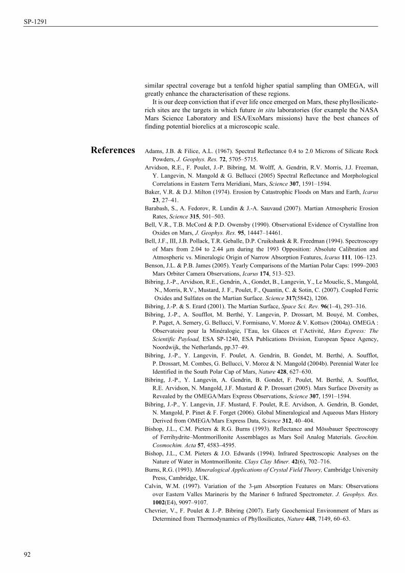
92
SP-1291
similar spectral coverage but a tenfold higher spatial sampling than OMEGA, will greatly enhance the characterisation of these regions.
It is our deep conviction that if ever life once emerged on Mars, these phyllosilicate-rich sites are the targets in which future in situ laboratories (for example the NASA Mars Science Laboratory and ESA/ExoMars missions) have the best chances of finding potential biorelics at a microscopic scale.
Adams, J.B. & Filice, A.L. (1967). Spectral Reflectance 0.4 to 2.0 Microns of Silicate Rock Powders, J. Geophys. Res. 72, 5705–5715.
Arvidson, R.E., F. Poulet, J.-P. Bibring, M. Wolff, A. Gendrin, R.V. Morris, J.J. Freeman, Y. Langevin, N. Mangold & G. Bellucci (2005) Spectral Reflectance and Morphological Correlations in Eastern Terra Meridiani, Mars, Science 307, 1591–1594.
Baker, V.R. & D.J. Milton (1974). Erosion by Catastrophic Floods on Mars and Earth, Icarus 23, 27–41.
Barabash, S., A. Fedorov, R. Lundin & J.-A. Sauvaud (2007). Martian Atmospheric Erosion Rates, Science 315, 501–503.
Bell, V.R., T.B. McCord & P.D. Owensby (1990). Observational Evidence of Crystalline Iron Oxides on Mars, J. Geophys. Res. 95, 14447–14461.
Bell, J.F., III, J.B. Pollack, T.R. Geballe, D.P. Cruikshank & R. Freedman (1994). Spectroscopy of Mars from 2.04 to 2.44 µm during the 1993 Opposition: Absolute Calibration and Atmospheric vs. Mineralogic Origin of Narrow Absorption Features, Icarus 111, 106–123.
Benson, J.L. & P.B. James (2005). Yearly Comparisons of the Martian Polar Caps: 1999–2003 Mars Orbiter Camera Observations, Icarus 174, 513–523.
Bibring, J.-P., Arvidson, R.E., Gendrin, A., Gondet, B., Langevin, Y., Le Mouelic, S., Mangold, N., Morris, R.V., Mustard, J. F., Poulet, F., Quantin, C. & Sotin, C. (2007). Coupled Ferric Oxides and Sulfates on the Martian Surface. Science 317(5842), 1206.
Bibring, J.-P. & S. Erard (2001). The Martian Surface, Space Sci. Rev. 96(1–4), 293–316. Bibring, J.-P., A. Soufflot, M. Berthé, Y. Langevin, P. Drossart, M. Bouyé, M. Combes,
P. Puget, A. Semery, G. Bellucci, V. Formisano, V. Moroz & V. Kottsov (2004a). OMEGA : Observatoire pour la Minéralogie, l’Eau, les Glaces et l’Activité, Mars Express: The Scientific Payload, ESA SP-1240, ESA Publications Division, European Space Agency, Noordwijk, the Netherlands, pp.37–49.
Bibring, J.-P., Y. Langevin, F. Poulet, A. Gendrin, B. Gondet, M. Berthé, A. Soufflot, P. Drossart, M. Combes, G. Bellucci, V. Moroz & N. Mangold (2004b). Perennial Water Ice Identified in the South Polar Cap of Mars, Nature 428, 627–630.
Bibring, J.-P., Y. Langevin, A. Gendrin, B. Gondet, F. Poulet, M. Berthé, A. Soufflot, R.E. Arvidson, N. Mangold, J.F. Mustard & P. Drossart (2005). Mars Surface Diversity as Revealed by the OMEGA/Mars Express Observations, Science 307, 1591–1594.
Bibring, J.-P., Y. Langevin, J.F. Mustard, F. Poulet, R.E. Arvidson, A. Gendrin, B. Gondet, N. Mangold, P. Pinet & F. Forget (2006). Global Mineralogical and Aqueous Mars History Derived from OMEGA/Mars Express Data, Science 312, 40–404.
Bishop, J.L., C.M. Pieters & R.G. Burns (1993). Reflectance and Mössbauer Spectroscopy of Ferrihydrite–Montmorillonite Assemblages as Mars Soil Analog Materials. Geochim. Cosmochim. Acta 57, 4583–4595.
Bishop, J.L., C.M. Pieters & J.O. Edwards (1994). Infrared Spectroscopic Analyses on the Nature of Water in Montmorillonite. Clays Clay Miner. 42(6), 702–716.
Burns, R.G. (1993). Mineralogical Applications of Crystal Field Theory, Cambridge University Press, Cambridge, UK.
Calvin, W.M. (1997). Variation of the 3-μm Absorption Features on Mars: Observations over Eastern Valles Marineris by the Mariner 6 Infrared Spectrometer. J. Geophys. Res. 1002(E4), 9097–9107.
Chevrier, V., F. Poulet & J.-P. Bibring (2007). Early Geochemical Environment of Mars as Determined from Thermodynamics of Phyllosilicates, Nature 448, 7149, 60–63.
References
93
Scientific instruments
Clark, R.N., G. A. Swayze, R. B. Singer, and J. B. Pollack (1990a). High resolution Reflectance Spectra of Mars in the 2.3-mm Region: Evidence for the Mineral Scapolite, J. Geophys. Res. 95, 14463–80.
Clark, R.N., T.V.V. King, M. Klejwa, G.A. Swayze & N. Vergo (1990b). High Spectral Resolution Reflectance Spectroscopy of Minerals. J. Geophys. Res. 95, 12653–12680.
Clark, R.N., G.A. Swayze, A. Gallagher, T.V.V. King & W.M. Calvin (1993). The USGS Digital Spectral Library: Version 1: 0.2 to 3.0 µm, USGS, Open File Report 93-592.
Crowley, J.K. (1991). Visible and Near-infrared (0.4–2.5 µm) Reflectance Spectra of Playa Evaporite Minerals. J. Geophys. Res. 96, 16 231–16 240.
Cloutis, E.A., F.C. Hawthorne, S.A. Mertzman, K. Krenn, M.A. Craig, D. Marcino, M. Methot, J. Strong, J.F. Mustard, D.L. Blaney, J.F. Bell III & F. Vilas (2006). Detection and Discrimination of Sulfate Minerals Using Reflectance Spectroscopy, Icarus 184, 121–157.
Drossart P., M. Combes, T. Encrenaz, R. Melchiorri, T. Fouchet, F. Forget, V. Moroz, N. Ignatiev, J.-P Bibring & Y. Langevin (2004). Mars atmosphere studies with the OMEGA/Mars Express experiment: I. Overview and detection of florescent emission by CO2. 35th COSPAR Scientific Assembly, vol.35, p.1798.
Douté, S., B. Schmitt, Y. Langevin, J.-P. Bibring, F. Altieri, G. Bellucci, B. Gondet & F. Poulet (2006). South Pole of Mars: Nature and Composition of the Icy Terrains from Mars Express OMEGA Observations, Planet. Space Sci.
Encrenaz, T., R. Melchiorri, T. Fouchet, P. Drossart, E. Lellouch, B. Gondet, J.-P. Bibring, Y. Langevin, D. Titov, N. Ignatiev & F. Forget (2005). A Mapping of Martian Water Sublimation during Early Northern Summer Using OMEGA/Mars, Astron. Astrophys. 441(3), L9–L12.
Encrenaz, T., T. Fouchet, R. Melchiorri, P. Drossart, B. Gondet, Y. Langevin, J.-P. Bibring, F. Forget & B. Bézard (2006). Seasonal Variations of the Martian CO over Hellas as Observed by OMEGA/Mars Express, Astron. Astrophys. 459(1), 265–270.
Forget, F., F. Hourdin, R. Fournier, C. Hourdin, O. Talagrand, M. Collins, S.R. Lewis, P.L. Read & J.-P. Huot (1999). Improved General Circulation Models of the Martian Atmosphere from the Surface to above 80 km, J. Geophys. Res. 104(E10), 24155–24176.
Forget, F., L. Montabone & S. Lebonnois (2006). Second International Workshop on Mars Atmosphere Modelling and Observations, Granada, 27 February–3 March 2006, Abstract 4.2.2.
Forget, F., Spiga A., Dolla S., Vinatier S., Melchiorri R., Drossart P., Gendrin A., Bibring J-P., Langevin Y. & Gondet B. (2007). Remote Sensing of Surface Pressure on Mars with the Mars Express/OMEGA Spectrometer: 1. Retrieval Method, J. Geophys. Res. 112(E08), E08S15
Gendrin, A., S. Erard, P. Drossart & R. Melchiorri (2003). Observation of Pressure Variations in the Martian Atmosphere, Geophys. Res. Lett. 30, 23, ASC14-1.
Gendrin, A., N. Mangold, J.-P. Bibring, Y. Langevin, B. Gondet, F. Poulet, G. Bonello, C. Quantin, J.F. Mustard, R.E. Arvidson & S. LeMouelic (2005). Sulfates in Martian Layered Terrains: The OMEGA/Mars Express View, Science 307, 1587–1591.
Houck, J.R., J.B. Pollack, C. Sagan, D. Schaack & J.A. Decker, Jr (1973). High Altitude Infrared Spectroscopic Evidence for Bound Water on Mars. Icarus 18, 470.
Jouglet, D., F. Poulet, R.E. Milliken, J.F. Mustard, J.-P. Bibring, Y. Langevin, B. Gondet & Gomez C., (2007). Hydration State of the Martian Surface as Seen by Mars Express OMEGA I: Analysis of the 3 µm Feature, J. Geophys. Res. 112, E08S06.
Kieffer, H.H., T.N. Titus, K.F. Mullins & P.R. Christensen (2000). Mars South Polar Spring and Summer Behavior Observed by TES: Seasonal Cap Evolution Controlled by Frost Grain Size, J. Geophys. Res. 105, 9653–9700.
King, T.V.V. & W.I. Ridley (1987). Relation of the Spectroscopic Reflectance of Olivine to Mineral Chemistry and Some Remote Sensing Implications, J. Geophys. Res. 92, 11457–11469.
Langevin, Y., S. Douté, M. Vincendon, F. Poulet, J.-P. Bibring, B. Gondet, B. Schmitt & F. Forget (2006). No Signature of Clear CO2 Ice from the ‘Cryptic’ Regions in Mars’ South Seasonal Polar Cap, Nature 442, 831–835.

94
SP-1291
Langevin, Y., F. Poulet, J.-P. Bibring, B. Schmitt, S. Douté & B. Gondet (2005a) Summer Evolution of the North Polar Cap of Mars as Observed by the OMEGA/Mars Express Observations, Science 307, 1581–1584.
Langevin, Y., F. Poulet, J.-P. Bibring & B. Gondet (2005b). Sulfates in the North Polar Region of Mars Detected by the OMEGA/Mars Express Observations, Science 307, 1584–1586.
Loizeau, D., N. Mangold, F. Poulet, J.-P. Bibring, A. Gendrin, V. Ansan, C. Gomez, Y. Langevin, B. Gondet, P. Masson & G. Neukum (2007). Phyllosilicates in the Mawrth Vallis region of Mars, J. Geophys. Res. 112, E08S08
López-Valverde, M.A., D.P. Edwards, M. López-Puertas & C. Roldán (1998). Non-local Thermodynamic Equilibrium in General Circulation Models of the Martian Atmosphere 1. Effects of the Local Thermodynamic Equilibrium Approximation on Thermal Cooling and Solar Heating, J. Geophys. Res. 103(E7), 16799–16812.
Mangold, N., F. Poulet, J.F. Mustard, J.-P. Bibring, B. Gondet, Y. Langevin, V. Ansan, P. Masson, C. Fassett, J.W. Head, H. Hoffmann & G. Neukum (2007). Mineralogy of the Nili Fossae Region with OMEGA/MEx data: 2. Aqueous Alteration of the Crust, J. Geophys. Res. 112, E08S04.
Melchiorri, R., P. Drossart, T. Fouchet, B. Bézard, F. Forget, A. Gendrin, J.-P. Bibring, N. Manaud & the OMEGA Team (2006). A Simulation of the OMEGA/Mars Express Observations: Analysis of the Atmospheric Contribution, Planet. Space Sci. 54, 774–783.
Milliken, R.E., J.F. Mustard, F. Poulet, D. Jouglet, J.-P. Bibring, B. Gondet & Y. Langevin (2007). Hydration State of the Martian Surface as Seen by Mars Express OMEGA II: H2O Content of the Surface, J. Geophys. Res. 112, E08S07.
Montmessin F., Gondet B. Määttänen A. Scholten F., Bibring J-P., Bertaux J-L. & Neukum G. (2008), CO2 Ice Clouds in the Upper Atmosphere of Mars: A Combined OMEGA and HRSC Data Analysis, 37th COSPAR Scientific Assembly, p.2092.
Morris, R.V., D.C. Golden, J.F. Bell, T.D. Shelfer, A.C. Scheinost, N.W. Hinman, G. Furniss, S.A. Mertzman, J.L. Bishop, D.W. Ming, C.C. Allen & D.T. Britt (2000). Mineralogy, Composition, and Alteration of Mars Pathfinder Rocks and Soils: Evidence from Multispectral, Elemental, and Magnetic Data on Terrestrial Analogue, SNC Meteorite, and Pathfinder Samples, J. Geophys. Res. 105(E1), 1757–1818.
Mustard, J.F., F. Poulet, A. Gendrin, J.-P. Bibring, Y. Langevin, B. Gondet, N. Mangold, G. Bellucci & F. Altieri (2005). Olivine and Pyroxene Diversity in the Crust of Mars, Science 307, 1594–1597.
Mustard, J.F., F. Poulet, J.W. Head, N. Mangold, J.-P. Bibring, S.M. Perkey, C. Fassett, Y. Langevin & G. Neukum (2007). Mineralogy of the Nili Fossae Region with OMEGA/MEx Data: 1. Ancient Impact Melt in the Isidis Basin and Implication for the Transition from the Noachian to Hesperian, J. Geophys. Res. 112, E08S03.
Pimentel, G.C., P.B. Forney & K.C. Herr (1974). Evidence about Hydrate and Solid Water in the Martian Surface from the 1969 Mariner Infrared Spectrometer. J. Geophys. Res. 79, 1623–1634.
Pollack, J.B., J.F. Kasting, S.M. Richardson & K. Poliakoff (1987). The Case for a Wet, Warm Climate on Mars, Icarus 71, 203–224.
Poulet, F., J.P. Bibring, J.F. Mustard, A. Gendrin, N. Mangold, Y. Langevin, R.E., Arvidson, B. Gondet & C. Gomez (2005). Phyllosilicates on Mars and Implications for Early Martian Climate, Nature 438, 623–628.
Poulet, F., C. Gomez, J.-P. Bibring, Y. Langevin, B. Gondet, P. Pinet, G. Bellucci & J.F. Mustard (2007). Martian Surface Mineralogy from OMEGA/MEx: Global Mineral Maps, J. Geophys. Res. 112, E08S02.
Roush, T.L., D.L. Blaney & R.B. Singer (1993) The Surface Composition of Mars as Inferred from Spectroscopic Observations. In Remote Geochemical Analysis: Elemental and Mineralogical Composition (Eds. C.M. Pieters and P.A.J. Englert), Cambridge University Press, Cambridge, UK, pp.367–393.
Soderblom, L. (1992) The Composition and Mineralogy of the Martian Surface from Spectroscopic Observations: 0.3 µm to 50 µm, in: Mars (Eds. H. Kieffer, B. Jakovsky, C. Snyder & M. Matthews), University of Arizona Press, Tucson, pp.557–597.

95
Scientific instruments
Sprague, A.L., W.V. Boynton, K.E. Kerry, D.M. Janes, D.M. Hunten, K.J. Kim, R.C. Reedy & A.E. Metzger (2004). Mars South Polar Ar Enhancement: A Tracer for South Polar Seasonal Meridional Mixing, Science 306, 1364–1367.
Sunshine J.M. & C.M. Pieters (1993). Estimating Modal Abundances from the Spectra of Natural and Laboratory Pyroxene Mixtures using the Modified Gaussian Model, J. Geophys. Res. 98, 9075–9087.
Swayze, G.A. & R.N. Clark (1990). Infrared Spectra and Crystal Chemistry of Scapolites: Implications for Martian Mineralogy. J. Geophys. Res. 95, 14 481–14 495.
Titus, T.N. & H.H. Kieffer (2002). A Comparison of the Mars South Polar Recession Rates between 1999 and 2001, Lunar Planet. Sci. Conf. 33, 2071.
Vincendon, M., Langevin, Y., Poulet, F., Bibring, J.-P. & Gondet, B. (2007). Recovery of Surface Reflectance Spectra and Evaluation of the Optical Depth of Aerosols in the Near-IR Using a Monte Carlo Approach: Application to the OMEGA Observations of High-latitude Regions of Mars. J. Geophys. Rev. 112, E08S13. DOI: 10.1029/2006JE002845.

97
J.J. Plaut1, G. Picardi2, T.W. Watters3, D.A. Gurnett4 and the MARSIS Science Team
MARSIS: Mars Advanced Radar for Subsurface and Ionospheric Sounding
97
1 Jet Propulsion Laboratory, California Institute of Technology, Pasadena, CA 91109, USA Email: [email protected] Infocom Department, ‘La Sapienza’ University of Rome, I-00184 Rome, Italy 3 Center for Earth and Planetary Studies, National Air and Space Museum, Smithsonian Institution, Washington, DC 20560, USA4 Department of Physics and Astronomy, University of Iowa, Iowa City, IA 52242, USA
We report the findings of MARSIS from the first several months of its science operations phase. Subsurface soundings were used to probe the north polar layered deposits to their base, up to 1.8 km deep. The base of the south polar layered deposits was mapped, and the volume of the deposits was measured. Radar penetration was observed in the equatorial Medusae Fossae formation, indicating the presence of low-density material that may include water ice. In the ionospheric sounding mode, several types of echo were observed, ranging from vertical echoes caused by specular reflection from the horizontally stratified ionosphere, to a wide variety of oblique and diffuse echoes. Echoes at the electron plasma frequency and the cyclotron period provide measurements of the local electron density and magnetic field strength.
The Mars Advanced Radar for Subsurface and Ionospheric Sounding (MARSIS) is the first radar to collect data from Mars orbit. MARSIS is a multi-frequency synthetic aperture orbital sounding radar (Picardi et al., 2004) that operates in two modes, subsurface sounding and ionospheric sounding. In both modes, MARSIS acquires data in the conventional fashion of a radar, in which pulses of electromagnetic radio waves are transmitted, interact with a target, and the echoes are received and recorded by the instrument. MARSIS differs from most orbital radars in the frequencies of the radar signal. MARSIS operates in the range 0.1–5.5 MHz, which corresponds to wavelengths of tens to hundreds of metres. These long wavelengths were chosen, in the case of the subsurface sounder, to maximise the penetration of the signal into the subsurface of Mars. In the case of the ionospheric sounder, the selected frequencies are in the range where some waves reflect from the topside of the ionosphere, depending on the electron plasma frequency, while others penetrate through to be reflected at the surface or subsurface.
The primary goal of the MARSIS subsurface experiment is to detect material discontinuities in the subsurface of Mars in order to understand the distribution of water, both solid and liquid, in the upper crust. The experiment is also probing for other discontinuities in the subsurface, related to geological units and structures. Finally, the subsurface mode obtains information in its surface echoes on the electromagnetic, topographic and roughness properties of the Mars surface. The goals of the ionospheric sounding experiment are to characterise the upper portions of the atmosphere (the ionosphere) and its interactions with solar radiation and particles.
1. Introduction
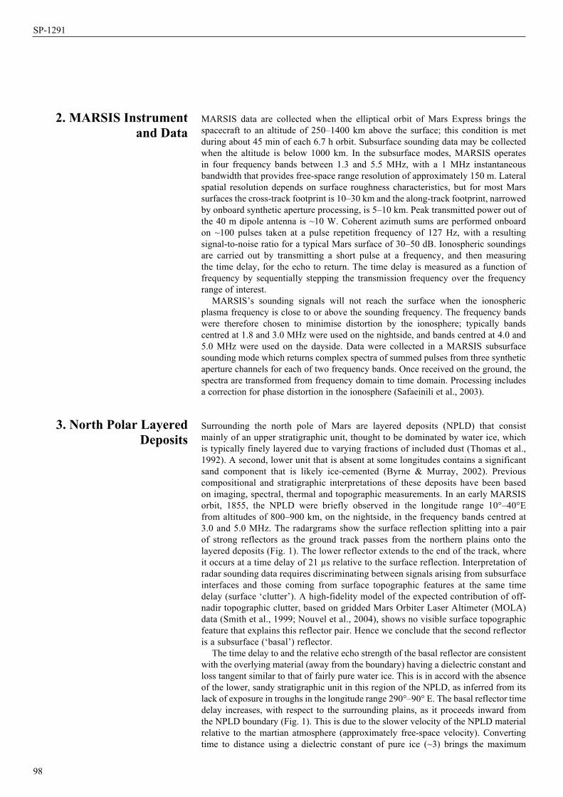
98
SP-1291
MARSIS data are collected when the elliptical orbit of Mars Express brings the spacecraft to an altitude of 250–1400 km above the surface; this condition is met during about 45 min of each 6.7 h orbit. Subsurface sounding data may be collected when the altitude is below 1000 km. In the subsurface modes, MARSIS operates in four frequency bands between 1.3 and 5.5 MHz, with a 1 MHz instantaneous bandwidth that provides free-space range resolution of approximately 150 m. Lateral spatial resolution depends on surface roughness characteristics, but for most Mars surfaces the cross-track footprint is 10–30 km and the along-track footprint, narrowed by onboard synthetic aperture processing, is 5–10 km. Peak transmitted power out of the 40 m dipole antenna is ~10 W. Coherent azimuth sums are performed onboard on ~100 pulses taken at a pulse repetition frequency of 127 Hz, with a resulting signal-to-noise ratio for a typical Mars surface of 30–50 dB. Ionospheric soundings are carried out by transmitting a short pulse at a frequency, and then measuring the time delay, for the echo to return. The time delay is measured as a function of frequency by sequentially stepping the transmission frequency over the frequency range of interest.
MARSIS’s sounding signals will not reach the surface when the ionospheric plasma frequency is close to or above the sounding frequency. The frequency bands were therefore chosen to minimise distortion by the ionosphere; typically bands centred at 1.8 and 3.0 MHz were used on the nightside, and bands centred at 4.0 and 5.0 MHz were used on the dayside. Data were collected in a MARSIS subsurface sounding mode which returns complex spectra of summed pulses from three synthetic aperture channels for each of two frequency bands. Once received on the ground, the spectra are transformed from frequency domain to time domain. Processing includes a correction for phase distortion in the ionosphere (Safaeinili et al., 2003).
Surrounding the north pole of Mars are layered deposits (NPLD) that consist mainly of an upper stratigraphic unit, thought to be dominated by water ice, which is typically finely layered due to varying fractions of included dust (Thomas et al., 1992). A second, lower unit that is absent at some longitudes contains a significant sand component that is likely ice-cemented (Byrne & Murray, 2002). Previous compositional and stratigraphic interpretations of these deposits have been based on imaging, spectral, thermal and topographic measurements. In an early MARSIS orbit, 1855, the NPLD were briefly observed in the longitude range 10°–40°E from altitudes of 800–900 km, on the nightside, in the frequency bands centred at 3.0 and 5.0 MHz. The radargrams show the surface reflection splitting into a pair of strong reflectors as the ground track passes from the northern plains onto the layered deposits (Fig. 1). The lower reflector extends to the end of the track, where it occurs at a time delay of 21 µs relative to the surface reflection. Interpretation of radar sounding data requires discriminating between signals arising from subsurface interfaces and those coming from surface topographic features at the same time delay (surface ‘clutter’). A high-fidelity model of the expected contribution of off-nadir topographic clutter, based on gridded Mars Orbiter Laser Altimeter (MOLA) data (Smith et al., 1999; Nouvel et al., 2004), shows no visible surface topographic feature that explains this reflector pair. Hence we conclude that the second reflector is a subsurface (‘basal’) reflector.
The time delay to and the relative echo strength of the basal reflector are consistent with the overlying material (away from the boundary) having a dielectric constant and loss tangent similar to that of fairly pure water ice. This is in accord with the absence of the lower, sandy stratigraphic unit in this region of the NPLD, as inferred from its lack of exposure in troughs in the longitude range 290°–90° E. The basal reflector time delay increases, with respect to the surrounding plains, as it proceeds inward from the NPLD boundary (Fig. 1). This is due to the slower velocity of the NPLD material relative to the martian atmosphere (approximately free-space velocity). Converting time to distance using a dielectric constant of pure ice (~3) brings the maximum
2. MARSIS Instrument and Data
3. North Polar Layered Deposits
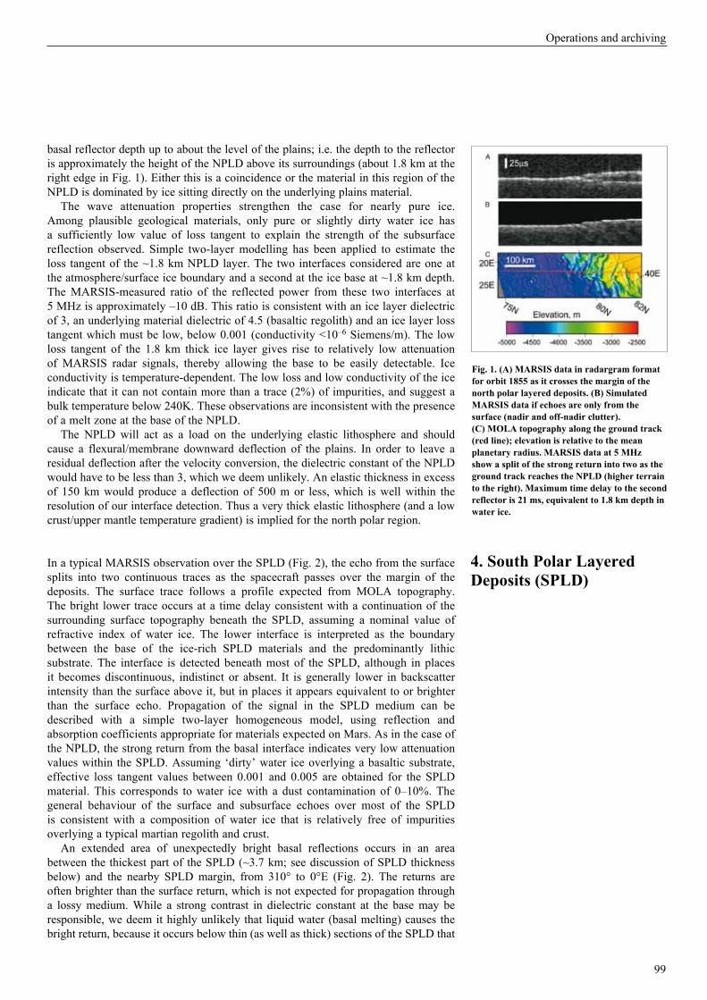
99
Operations and archiving
basal reflector depth up to about the level of the plains; i.e. the depth to the reflector is approximately the height of the NPLD above its surroundings (about 1.8 km at the right edge in Fig. 1). Either this is a coincidence or the material in this region of the NPLD is dominated by ice sitting directly on the underlying plains material.
The wave attenuation properties strengthen the case for nearly pure ice. Among plausible geological materials, only pure or slightly dirty water ice has a sufficiently low value of loss tangent to explain the strength of the subsurface reflection observed. Simple two-layer modelling has been applied to estimate the loss tangent of the ~1.8 km NPLD layer. The two interfaces considered are one at the atmosphere/surface ice boundary and a second at the ice base at ~1.8 km depth. The MARSIS-measured ratio of the reflected power from these two interfaces at 5 MHz is approximately –10 dB. This ratio is consistent with an ice layer dielectric of 3, an underlying material dielectric of 4.5 (basaltic regolith) and an ice layer loss tangent which must be low, below 0.001 (conductivity <10–6 Siemens/m). The low loss tangent of the 1.8 km thick ice layer gives rise to relatively low attenuation of MARSIS radar signals, thereby allowing the base to be easily detectable. Ice conductivity is temperature-dependent. The low loss and low conductivity of the ice indicate that it can not contain more than a trace (2%) of impurities, and suggest a bulk temperature below 240K. These observations are inconsistent with the presence of a melt zone at the base of the NPLD.
The NPLD will act as a load on the underlying elastic lithosphere and should cause a flexural/membrane downward deflection of the plains. In order to leave a residual deflection after the velocity conversion, the dielectric constant of the NPLD would have to be less than 3, which we deem unlikely. An elastic thickness in excess of 150 km would produce a deflection of 500 m or less, which is well within the resolution of our interface detection. Thus a very thick elastic lithosphere (and a low crust/upper mantle temperature gradient) is implied for the north polar region.
In a typical MARSIS observation over the SPLD (Fig. 2), the echo from the surface splits into two continuous traces as the spacecraft passes over the margin of the deposits. The surface trace follows a profile expected from MOLA topography. The bright lower trace occurs at a time delay consistent with a continuation of the surrounding surface topography beneath the SPLD, assuming a nominal value of refractive index of water ice. The lower interface is interpreted as the boundary between the base of the ice-rich SPLD materials and the predominantly lithic substrate. The interface is detected beneath most of the SPLD, although in places it becomes discontinuous, indistinct or absent. It is generally lower in backscatter intensity than the surface above it, but in places it appears equivalent to or brighter than the surface echo. Propagation of the signal in the SPLD medium can be described with a simple two-layer homogeneous model, using reflection and absorption coefficients appropriate for materials expected on Mars. As in the case of the NPLD, the strong return from the basal interface indicates very low attenuation values within the SPLD. Assuming ‘dirty’ water ice overlying a basaltic substrate, effective loss tangent values between 0.001 and 0.005 are obtained for the SPLD material. This corresponds to water ice with a dust contamination of 0–10%. The general behaviour of the surface and subsurface echoes over most of the SPLD is consistent with a composition of water ice that is relatively free of impurities overlying a typical martian regolith and crust.
An extended area of unexpectedly bright basal reflections occurs in an area between the thickest part of the SPLD (~3.7 km; see discussion of SPLD thickness below) and the nearby SPLD margin, from 310° to 0°E (Fig. 2). The returns are often brighter than the surface return, which is not expected for propagation through a lossy medium. While a strong contrast in dielectric constant at the base may be responsible, we deem it highly unlikely that liquid water (basal melting) causes the bright return, because it occurs below thin (as well as thick) sections of the SPLD that
4. South Polar Layered Deposits (SPLD)
Fig. 1. (A) MARSIS data in radargram format for orbit 1855 as it crosses the margin of the north polar layered deposits. (B) Simulated MARSIS data if echoes are only from the surface (nadir and off-nadir clutter). (C) MOLA topography along the ground track (red line); elevation is relative to the mean planetary radius. MARSIS data at 5 MHz show a split of the strong return into two as the ground track reaches the NPLD (higher terrain to the right). Maximum time delay to the second reflector is 21 ms, equivalent to 1.8 km depth in water ice.
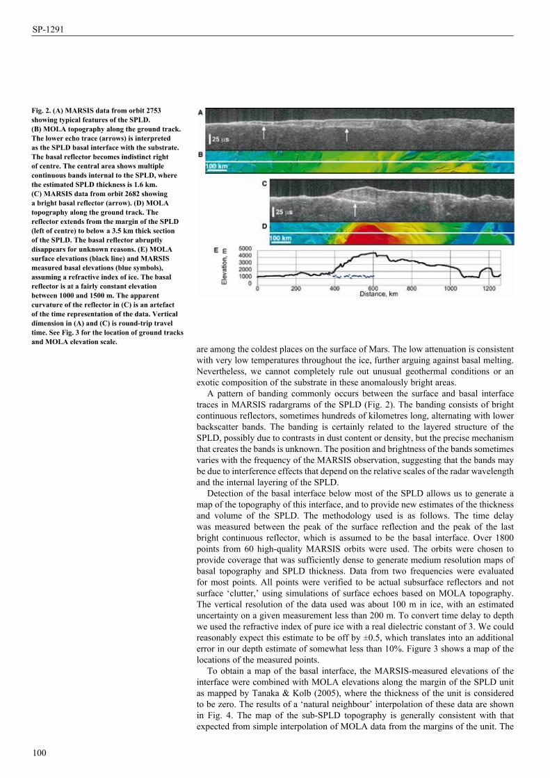
100
SP-1291
are among the coldest places on the surface of Mars. The low attenuation is consistent with very low temperatures throughout the ice, further arguing against basal melting. Nevertheless, we cannot completely rule out unusual geothermal conditions or an exotic composition of the substrate in these anomalously bright areas.
A pattern of banding commonly occurs between the surface and basal interface traces in MARSIS radargrams of the SPLD (Fig. 2). The banding consists of bright continuous reflectors, sometimes hundreds of kilometres long, alternating with lower backscatter bands. The banding is certainly related to the layered structure of the SPLD, possibly due to contrasts in dust content or density, but the precise mechanism that creates the bands is unknown. The position and brightness of the bands sometimes varies with the frequency of the MARSIS observation, suggesting that the bands may be due to interference effects that depend on the relative scales of the radar wavelength and the internal layering of the SPLD.
Detection of the basal interface below most of the SPLD allows us to generate a map of the topography of this interface, and to provide new estimates of the thickness and volume of the SPLD. The methodology used is as follows. The time delay was measured between the peak of the surface reflection and the peak of the last bright continuous reflector, which is assumed to be the basal interface. Over 1800 points from 60 high-quality MARSIS orbits were used. The orbits were chosen to provide coverage that was sufficiently dense to generate medium resolution maps of basal topography and SPLD thickness. Data from two frequencies were evaluated for most points. All points were verified to be actual subsurface reflectors and not surface ‘clutter,’ using simulations of surface echoes based on MOLA topography. The vertical resolution of the data used was about 100 m in ice, with an estimated uncertainty on a given measurement less than 200 m. To convert time delay to depth we used the refractive index of pure ice with a real dielectric constant of 3. We could reasonably expect this estimate to be off by ±0.5, which translates into an additional error in our depth estimate of somewhat less than 10%. Figure 3 shows a map of the locations of the measured points.
To obtain a map of the basal interface, the MARSIS-measured elevations of the interface were combined with MOLA elevations along the margin of the SPLD unit as mapped by Tanaka & Kolb (2005), where the thickness of the unit is considered to be zero. The results of a ‘natural neighbour’ interpolation of these data are shown in Fig. 4. The map of the sub-SPLD topography is generally consistent with that expected from simple interpolation of MOLA data from the margins of the unit. The
Fig. 2. (A) MARSIS data from orbit 2753 showing typical features of the SPLD. (B) MOLA topography along the ground track. The lower echo trace (arrows) is interpreted as the SPLD basal interface with the substrate. The basal reflector becomes indistinct right of centre. The central area shows multiple continuous bands internal to the SPLD, where the estimated SPLD thickness is 1.6 km. (C) MARSIS data from orbit 2682 showing a bright basal reflector (arrow). (D) MOLA topography along the ground track. The reflector extends from the margin of the SPLD (left of centre) to below a 3.5 km thick section of the SPLD. The basal reflector abruptly disappears for unknown reasons. (E) MOLA surface elevations (black line) and MARSIS measured basal elevations (blue symbols), assuming a refractive index of ice. The basal reflector is at a fairly constant elevation between 1000 and 1500 m. The apparent curvature of the reflector in (C) is an artefact of the time representation of the data. Vertical dimension in (A) and (C) is round-trip travel time. See Fig. 3 for the location of ground tracks and MOLA elevation scale.

101
Operations and archiving
Fig. 3. Topography of the south polar region of Mars from MGS MOLA data, with locations of MARSIS measurements of the SPLD thickness shown as open circles. The SPLD unit mapped by Tanaka and Kolb (2005) is outlined in black. Red lines indicate ground tracks of orbits in Fig. 2. Apparent gaps in coverage are due to the lack of a discernible basal interface, and not to gaps in observations. No MARSIS data are available poleward of 87°S (dark circle in upper centre).
surface is typically low in relief, with broad areas of higher and lower topography. A pronounced low area is seen near the SPLD margin around 72°–74°S, 130°–145°E, and elevated regions within the remnant Prometheus impact basin are seen to continue below the SPLD at 78°–82°S, 100°–130°E and from 70°–90°E poleward of about 83°S. An unexpected feature of the basal topography is a series of depressions at the highest latitudes (84°–87°S). These occur discontinuously from longitudes 95° to 295°E. The depressions range in width from 50 to 200 km, and reach a depth of as much as 1 km below the surrounding sub-SPLD topography. The basal reflection within the depressions is typically dimmer than under the rest of the SPLD. This, and the position of the depressions in the near-polar areas suggest there may be processes unique to this sub-SPLD area. The depressions may be the result of differential compaction of mega-regolith in response to the SPLD load. Alternatively they may be a group of buried impact craters or other pre-existing topography such as the ~km-deep pits (‘Cavi’) in the nearby plains. On a regional scale, the basal interface is relatively flat. The lack of evidence of regional downwarping in response to the SPLD load suggests the elastic lithosphere in the south polar region is very thick (>150 km), as was inferred for the north polar region.
A thickness map of the SPLD was generated by subtracting the elevations of the interpolated basal topography from the high-resolution MOLA surface topography (Fig. 5). The distribution of SPLD thickness reflects the asymmetry of the south polar geology, with the thickest portions offset from the pole near 0°E, and the much more areally extensive but thinner portion centred near 180°E. The newly discovered
Fig. 4. Same as Fig. 3, with topography at the SPLD basal interface shown, based on MARSIS measurements of SPLD thickness. A indicates a depression below a distal SPLD lobe. B indicates relative highs within the remnant Prometheus basin (basin rim indicated with arrows). C indicates depressions in the near-polar region.

102
SP-1291
near-polar depressions show clearly as anomalously thick areas, as do several of the distal lobes. The maximum measured thickness is 3.7 ± 0.4 km, under the highest elevations of the SPLD near 0°E. Our estimate of the integrated volume of the entire SPLD is 1.6 ± 0.2 × 10⁶ km3. This translates to an equivalent global water layer thickness of 11 ± 1.4 m (assuming an SPLD composition of nearly pure ice), and is within the range estimated by previous workers using MOLA data alone (Smith et al., 2001). Knowledge of the basal topography now allows us to estimate the volume with a much smaller range of uncertainty.
MARSIS data do not allow us to distinguish a component of CO2 ice in the SPLD material, but there is no corroborative evidence for such a component. Spectral and albedo observations of the surface of the SPLD indicate an optically thick lag of dust or rocky material, but this layer is ‘optically’ thin at MARSIS wavelengths. Similarly, MARSIS detects no difference in surface or subsurface echoes from areas covered by the residual (‘perennial’) CO2-rich ice unit, consistent with recent analyses indicating it is a deposit no more than a few tens of metres thick (Byrne & Ingersoll, 2003).
Units of the Medusae Fossae formation (MFF) occur discontinuously at equatorial latitudes along the boundary of the hemispheric dichotomy from Amazonis to Elysium Planitiae (~130°–240°E) (Scott & Tanaka, 1986; Greeley & Guest, 1987). The MFF may be among the youngest surficial deposits on Mars, unconformably overlying ancient Noachian heavily cratered highlands and young Amazonian lowlands (Bradley et al., 2002). The local topographic relief of the MFF units varies greatly, reaching a maximum of more than 3.5 km (Zimbelman et al., 1999; Hynek et al., 2003; Head & Kreslavsky, 2004). The morphology of the MFF units is complex and variable. Over large horizontal scales (tens of kilometres), the undulating hills of the MFF are relatively smooth (Fig. 6). At smaller scales, many of the MFF units are marked by systems of parallel ridges and grooves interpreted as yardangs (Fig. 7). Remnant yardangs and
5. Medusae Fossae Formation
Fig. 5. Map of the SPLD thickness, based on MARSIS measurements and MOLA surface topography. An anomalous thick section appears in lower right (see A in Fig. 4). The thickest areas occur beneath the highest elevations of the SPLD (red areas near top), and in association with the near-polar depressions (see C in Fig. 4).
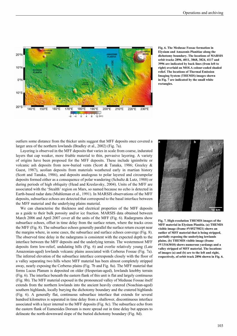
103
Operations and archiving
outliers some distance from the thicker units suggest that MFF deposits once covered a larger area of the northern lowlands (Bradley et al., 2002) (Fig. 7a).
Layering is observed in the MFF deposits that varies in scale from coarse, indurated layers that cap weaker, more friable material to thin, pervasive layering. A variety of origins have been proposed for the MFF deposits. These include ignimbrite or volcanic ash deposits from now-buried vents (Scott & Tanaka, 1986; Greeley & Guest, 1987), aeolian deposits from materials weathered early in martian history (Scott and Tanaka, 1986), and deposits analogous to polar layered and circumpolar deposits formed either as a consequence of polar wandering (Schultz & Lutz, 1988) or during periods of high obliquity (Head and Kreslavsky, 2004). Units of the MFF are associated with the ‘Stealth’ region on Mars, so named because no echo is detected in Earth-based radar data (Muhleman et al., 1991). In MARSIS observations of the MFF deposits, subsurface echoes are detected that correspond to the basal interface between the MFF material and the underlying plains material.
We can characterise the thickness and electrical properties of the MFF deposits as a guide to their bulk porosity and/or ice fraction. MARSIS data obtained between March 2006 and April 2007 cover all the units of the MFF (Fig. 6). Radargrams show subsurface echoes, offset in time delay from the surface return, where the tracks cross the MFF (Fig. 8). The subsurface echoes generally parallel the surface return except near the margins where, in some cases, the subsurface and surface echoes converge (Fig. 8). The observed time delay in the radargrams is consistent with the expected depth to the interface between the MFF deposits and the underlying terrain. The westernmost MFF deposits form low-relief, undulating hills (Fig. 6) and overlie relatively young (Late Amazonian-aged) lowlands volcanic plains associated with Cerberus Fossae (Fig. 7a). The inferred elevation of the subsurface interface corresponds closely with the floor of a valley separating two hills where MFF material has been almost completely stripped away, nearly exposing the Cerberus plains (Fig. 7b and Fig. 8a). The MFF material that forms Lucus Planum is deposited on older (Hesperian-aged), lowlands knobby terrain (Fig. 6). The interface beneath the eastern flank of this unit is flat and largely continuous (Fig. 8b). The MFF material exposed in the pronounced valley of Medusae Fossae itself extends from the northern lowlands into the ancient heavily cratered (Noachian-aged) southern highlands, locally burying the dichotomy boundary and the cratered highlands (Fig. 6). A generally flat, continuous subsurface interface that extends for several hundred kilometres is separated in time delay from a shallower, discontinuous interface associated with a layer internal to the MFF deposits (Fig. 8c). The subsurface echo from the eastern flank of Eumenides Dorsum is more spread out in time delay but appears to delineate the north-downward slope of the buried dichotomy boundary (Fig. 8d).
Fig. 6. The Medusae Fossae formation in Elysium and Amazonis Planitiae along the dichotomy boundary. The locations of MARSIS orbit tracks 2896, 4011, 3868, 3824, 4117 and 3996 are indicated by back lines (from left to right) overlaid on MOLA colour-coded shaded relief. The locations of Thermal Emission Imaging System (THEMIS) images shown in Fig. 7 are indicated by the small white rectangles.
Fig. 7. High-resolution THEMIS images of the MFF material in Elysium Planitia. (a) THEMIS visible image (frame #V05275021) shows an outlier of MFF material that is being stripped, partially exposing the underlying lowlands plains. (b) THEMIS visible image (frame #V13163010) shows numerous yardangs and a valley stripped of MFF material. The locations of images (a) and (b) are to the left and right, respectively, of orbit track 2896 shown in Fig. 6.
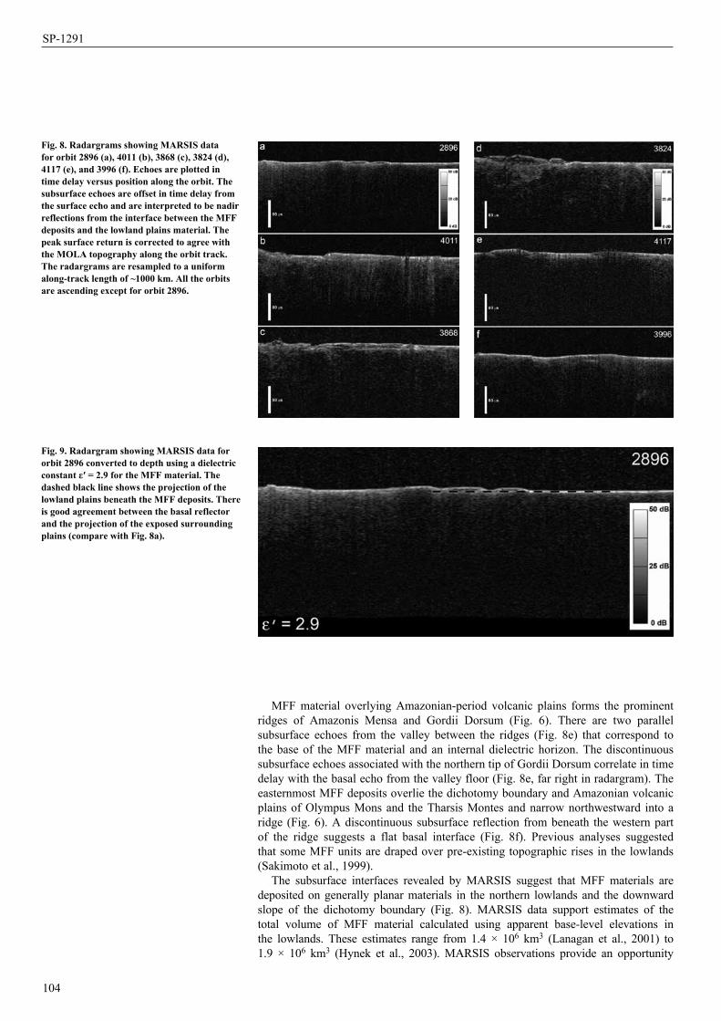
104
SP-1291
MFF material overlying Amazonian-period volcanic plains forms the prominent ridges of Amazonis Mensa and Gordii Dorsum (Fig. 6). There are two parallel subsurface echoes from the valley between the ridges (Fig. 8e) that correspond to the base of the MFF material and an internal dielectric horizon. The discontinuous subsurface echoes associated with the northern tip of Gordii Dorsum correlate in time delay with the basal echo from the valley floor (Fig. 8e, far right in radargram). The easternmost MFF deposits overlie the dichotomy boundary and Amazonian volcanic plains of Olympus Mons and the Tharsis Montes and narrow northwestward into a ridge (Fig. 6). A discontinuous subsurface reflection from beneath the western part of the ridge suggests a flat basal interface (Fig. 8f). Previous analyses suggested that some MFF units are draped over pre-existing topographic rises in the lowlands (Sakimoto et al., 1999).
The subsurface interfaces revealed by MARSIS suggest that MFF materials are deposited on generally planar materials in the northern lowlands and the downward slope of the dichotomy boundary (Fig. 8). MARSIS data support estimates of the total volume of MFF material calculated using apparent base-level elevations in the lowlands. These estimates range from 1.4 × 10⁶ km3 (Lanagan et al., 2001) to 1.9 × 10⁶ km3 (Hynek et al., 2003). MARSIS observations provide an opportunity
Fig. 8. Radargrams showing MARSIS data for orbit 2896 (a), 4011 (b), 3868 (c), 3824 (d), 4117 (e), and 3996 (f). Echoes are plotted in time delay versus position along the orbit. The subsurface echoes are offset in time delay from the surface echo and are interpreted to be nadir reflections from the interface between the MFF deposits and the lowland plains material. The peak surface return is corrected to agree with the MOLA topography along the orbit track. The radargrams are resampled to a uniform along-track length of ~1000 km. All the orbits are ascending except for orbit 2896.
Fig. 9. Radargram showing MARSIS data for orbit 2896 converted to depth using a dielectric constant ε′ = 2.9 for the MFF material. The dashed black line shows the projection of the lowland plains beneath the MFF deposits. There is good agreement between the basal reflector and the projection of the exposed surrounding plains (compare with Fig. 8a).
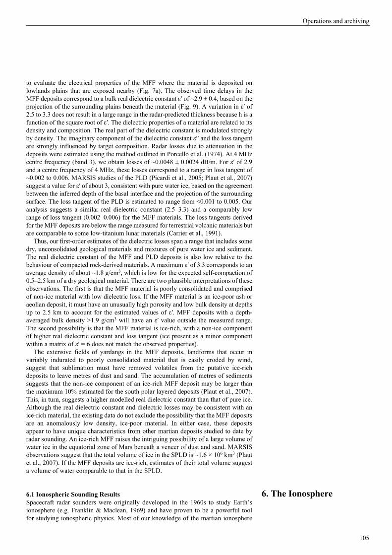
105
Operations and archiving
to evaluate the electrical properties of the MFF where the material is deposited on lowlands plains that are exposed nearby (Fig. 7a). The observed time delays in the MFF deposits correspond to a bulk real dielectric constant ε′ of ~2.9 ± 0.4, based on the projection of the surrounding plains beneath the material (Fig. 9). A variation in ε′ of 2.5 to 3.3 does not result in a large range in the radar-predicted thickness because h is a function of the square root of ε′. The dielectric properties of a material are related to its density and composition. The real part of the dielectric constant is modulated strongly by density. The imaginary component of the dielectric constant ε′′ and the loss tangent are strongly influenced by target composition. Radar losses due to attenuation in the deposits were estimated using the method outlined in Porcello et al. (1974). At 4 MHz centre frequency (band 3), we obtain losses of ~0.0048 ± 0.0024 dB/m. For ε′ of 2.9 and a centre frequency of 4 MHz, these losses correspond to a range in loss tangent of ~0.002 to 0.006. MARSIS studies of the PLD (Picardi et al., 2005; Plaut et al., 2007) suggest a value for ε′ of about 3, consistent with pure water ice, based on the agreement between the inferred depth of the basal interface and the projection of the surrounding surface. The loss tangent of the PLD is estimated to range from <0.001 to 0.005. Our analysis suggests a similar real dielectric constant (2.5–3.3) and a comparably low range of loss tangent (0.002–0.006) for the MFF materials. The loss tangents derived for the MFF deposits are below the range measured for terrestrial volcanic materials but are comparable to some low-titanium lunar materials (Carrier et al., 1991).
Thus, our first-order estimates of the dielectric losses span a range that includes some dry, unconsolidated geological materials and mixtures of pure water ice and sediment. The real dielectric constant of the MFF and PLD deposits is also low relative to the behaviour of compacted rock-derived materials. A maximum ε′ of 3.3 corresponds to an average density of about ~1.8 g/cm3, which is low for the expected self-compaction of 0.5–2.5 km of a dry geological material. There are two plausible interpretations of these observations. The first is that the MFF material is poorly consolidated and comprised of non-ice material with low dielectric loss. If the MFF material is an ice-poor ash or aeolian deposit, it must have an unusually high porosity and low bulk density at depths up to 2.5 km to account for the estimated values of ε′. MFF deposits with a depth-averaged bulk density >1.9 g/cm3 will have an ε′ value outside the measured range. The second possibility is that the MFF material is ice-rich, with a non-ice component of higher real dielectric constant and loss tangent (ice present as a minor component within a matrix of ε′ = 6 does not match the observed properties).
The extensive fields of yardangs in the MFF deposits, landforms that occur in variably indurated to poorly consolidated material that is easily eroded by wind, suggest that sublimation must have removed volatiles from the putative ice-rich deposits to leave metres of dust and sand. The accumulation of metres of sediments suggests that the non-ice component of an ice-rich MFF deposit may be larger than the maximum 10% estimated for the south polar layered deposits (Plaut et al., 2007). This, in turn, suggests a higher modelled real dielectric constant than that of pure ice. Although the real dielectric constant and dielectric losses may be consistent with an ice-rich material, the existing data do not exclude the possibility that the MFF deposits are an anomalously low density, ice-poor material. In either case, these deposits appear to have unique characteristics from other martian deposits studied to date by radar sounding. An ice-rich MFF raises the intriguing possibility of a large volume of water ice in the equatorial zone of Mars beneath a veneer of dust and sand. MARSIS observations suggest that the total volume of ice in the SPLD is ~1.6 × 10⁶ km3 (Plaut et al., 2007). If the MFF deposits are ice-rich, estimates of their total volume suggest a volume of water comparable to that in the SPLD.
6.1 Ionospheric Sounding ResultsSpacecraft radar sounders were originally developed in the 1960s to study Earth’s ionosphere (e.g. Franklin & Maclean, 1969) and have proven to be a powerful tool for studying ionospheric physics. Most of our knowledge of the martian ionosphere
6. The Ionosphere
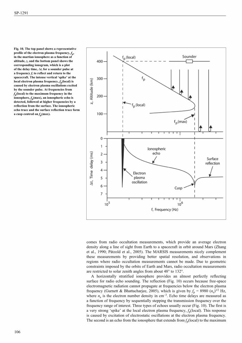
106
SP-1291
comes from radio occultation measurements, which provide an average electron density along a line of sight from Earth to a spacecraft in orbit around Mars (Zhang et al., 1990; Pätzold et al., 2005). The MARSIS measurements nicely complement these measurements by providing better spatial resolution, and observations in regions where radio occultation measurements cannot be made. Due to geometric constraints imposed by the orbits of Earth and Mars, radio occultation measurements are restricted to solar zenith angles from about 48° to 132°.
A horizontally stratified ionosphere provides an almost perfectly reflecting surface for radio echo sounding. The reflection (Fig. 10) occurs because free-space electromagnetic radiation cannot propagate at frequencies below the electron plasma frequency (Gurnett & Bhattacharjee, 2005), which is given by fp = 8980 (ne)1⁄2 Hz, where ne is the electron number density in cm–3. Echo time delays are measured as a function of frequency by sequentially stepping the transmission frequency over the frequency range of interest. Three types of echoes usually occur (Fig. 10). The first is a very strong ‘spike’ at the local electron plasma frequency, fp(local). This response is caused by excitation of electrostatic oscillations at the electron plasma frequency. The second is an echo from the ionosphere that extends from fp(local) to the maximum
Fig. 10. The top panel shows a representative profile of the electron plasma frequency, fp, in the martian ionosphere as a function of altitude, z, and the bottom panel shows the corresponding ionogram, which is a plot of the delay time, ∆t, for a sounder pulse at a frequency f, to reflect and return to the spacecraft. The intense vertical ‘spike’ at the local electron plasma frequency, fp(local) is caused by electron plasma oscillations excited by the sounder pulse. At frequencies from fp(local) to the maximum frequency in the ionosphere, fp(max), an ionospheric echo is detected, followed at higher frequencies by a reflection from the surface. The ionospheric echo trace and the surface reflection trace form a cusp centred on fp(max).
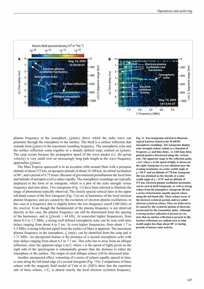
107
Operations and archiving
plasma frequency in the ionosphere, fp(max), above which the radio wave can penetrate through the ionosphere to the surface. The third is a surface reflection that extends from fp(max) to the maximum sounding frequency. The ionospheric echo and the surface reflection come together in a sharply defined cusp, centred on fp(max). The cusp occurs because the propagation speed of the wave packet (i.e. the group velocity) is very small over an increasingly long path length as the wave frequency approaches fp(max).
The Mars Express spacecraft is in an eccentric orbit around Mars with a periapsis altitude of about 275 km, an apoapsis altitude of about 10 100 km, an orbital inclination of 86°, and a period of 6.75 hours. Because of gravitational perturbations the local time and latitude of periapsis evolve rather rapidly. The ionospheric soundings are typically displayed in the form of an ionogram, which is a plot of the echo strength versus frequency and time delay. Two ionograms (Fig. 11) have been selected to illustrate the range of phenomena typically observed. The closely spaced vertical lines in the upper left-hand corner of the first ionogram (Fig. 11a) are at harmonics of the local electron plasma frequency and are caused by the excitation of electron plasma oscillations, in this case at a frequency that is slightly below the low-frequency cutoff (100 kHz) of the receiver. Even though the fundamental of the plasma frequency is not observed directly in this case, the plasma frequency can still be determined from the spacing of the harmonics, and is fp(local) = 44 kHz. At somewhat higher frequencies, from about 0.5 to 1.7 MHz, a strong well defined ionospheric echo can be seen with time delays ranging from about 4 to 5 ms. At even higher frequencies, from about 1.7 to 5.5 MHz, a strong reflected signal from the surface of Mars is apparent. The maximum plasma frequency in the ionosphere, fp (max), can be identified from the cusp and is 1.71 MHz. An unexpected feature is the presence of a second ionospheric echo with time delays ranging from about 6.3 to 7.1 ms. This echo has to arise from an oblique reflection, since the apparent range (c∆t/2, where c is the speed of light) given on the right side of the spectrogram is substantially greater than the distance to either the ionosphere or the surface. The origin of such oblique echoes will be discussed later.
Another unexpected effect, consisting of a series of echoes equally spaced in time, is seen along the left-hand edge of a second ionogram (Fig. 11b). Comparisons of these echoes with the magnetic field model of Cain et al. (2003) show that the repetition rate of these echoes, 1/Tc, is almost exactly the local electron cyclotron frequency,
Fig. 11. Two ionograms selected to illustrate typical features found in the MARSIS ionospheric soundings. The ionograms display echo strength (colour coded) as a function of frequency, f, and time delay, ∆t, with time delay plotted positive downward along the vertical axis. The apparent range to the reflection point, c∆t/2, where c is the speed of light, is shown on the right. Ionogram (A) was obtained near the evening terminator at a solar zenith angle of χ = 89.3° and an altitude of 778 km. Ionogram (B) was obtained on the dayside at a solar zenith angle of χ = 47.9° and an altitude of 573 km. Electron plasma oscillation harmonics can be seen in both ionograms, as well as strong echoes from the ionosphere. Ionogram (B) has a series of horizontal, equally spaced echoes along the left-hand side. These echoes occur at the electron cyclotron period, and are called electron cyclotron echoes. They are believed to be caused by the cyclotron motion of electrons accelerated by the transmitter pulse. Although a strong surface reflection is present in (A), note that no surface reflection is present in (B). Surface reflections are seldom seen at solar zenith angles less than about 40° or during periods of intense solar activity.

108
SP-1291
fc = 28 B Hz, where B is the magnetic field strength (in nT). Because of the close relationship to the electron cyclotron frequency, these echoes are called ‘electron cyclotron echoes’. Such echoes are very common and are usually present whenever the magnetic field strength is greater than a few tens of nT. We believe that these echoes are caused by electrons accelerated by the strong electric fields near the antenna during each cycle of the transmitter waveform. The cyclotron motion of the electrons in the local magnetic field then causes these electrons to periodically return to the vicinity of the antenna where they induce a signal on the antenna. For this process to occur, the magnetic field strength must be reasonably uniform over a spatial region comparable to the cyclotron radius. For a magnetic field strength of 100 nT, which is a typical crustal field strength at the spacecraft, and a voltage of 500 V, which is the typical antenna voltage, the cyclotron radius is about 1 km. Since the crustal magnetic fields have scale sizes of hundreds of kilometres, this condition is easily satisfied.
In contrast to the first ionogram (Fig. 11a), no surface reflection can be detected in the second ionogram (Fig. 11b). The intensity of the surface reflection is found to be highly variable, a topic of considerable importance for subsurface sounding. Some of this variability can be attributed to solar activity. For example, surface reflections disappeared completely about two days after a class X17 solar flare that occurred on 7 September 2005, and did not reappear until 23 September, nearly two weeks later. Although further analysis is needed, it seems almost certain that the absorption is caused by energetic charged particles produced by solar flares. The onset of the absorption is usually delayed by a day or more after a flare and tends to last many days, much longer than the typical time scale for decay of the ultraviolet and X-ray radiation associated with a flare. At Earth it is well known that energetic protons from solar flares cause enhanced ionisation and absorption of radio waves in the lower levels of the ionosphere, and a similar process may occur at Mars. In addition to the solar flare control, the absorption also appears to increase with decreasing solar zenith angle. Even during periods of low solar activity surface reflections are rarely observed when the solar zenith angle is less than about 40°.
6.2 Ionospheric Density ModelsIn order to compare the MARSIS ionospheric soundings with various ionospheric models, it is necessary to convert the soundings to usable electron density profiles. Although a rough estimate of the density profile can be obtained from the apparent range to the reflection point, for accurate measurements it is necessary to correct for dispersion, which is the effect the plasma has on the propagation speed of the wave. For vertical incidence on a horizontally stratified ionosphere the round-trip delay time as a function of frequency, ∆t(f), is given by the integral
where the integration is carried out from the reflection point altitude, z(fp), to the spacecraft altitude, zsc. Since ∆t(f) is known from the ionospheric echo trace, the basic problem is to invert the integral to obtain z(fp), i.e. the altitude of the reflection point as a function of the plasma frequency. Once this is known, the equation fp = 8980 (ne)1⁄2, can be used to obtain z(ne).
Although the mathematical techniques for carrying out this inversion are straightforward, there are sometimes practical difficulties. For example, the ionospheric echo trace often does not extend down to the local plasma frequency (Fig. 11). In such cases it is necessary to make a reasonable guess as to how the echo trace extends from the lowest frequency measured to the local plasma frequency. Normally the inversion is not very sensitive to this choice, since the correction to the propagation speed becomes quite small when the plasma frequency is well below the wave frequency.
ct f
ff z
dz2
1 pz f
z
2
2
p
sc
T =
-
^]
^
hg
h
# (1)
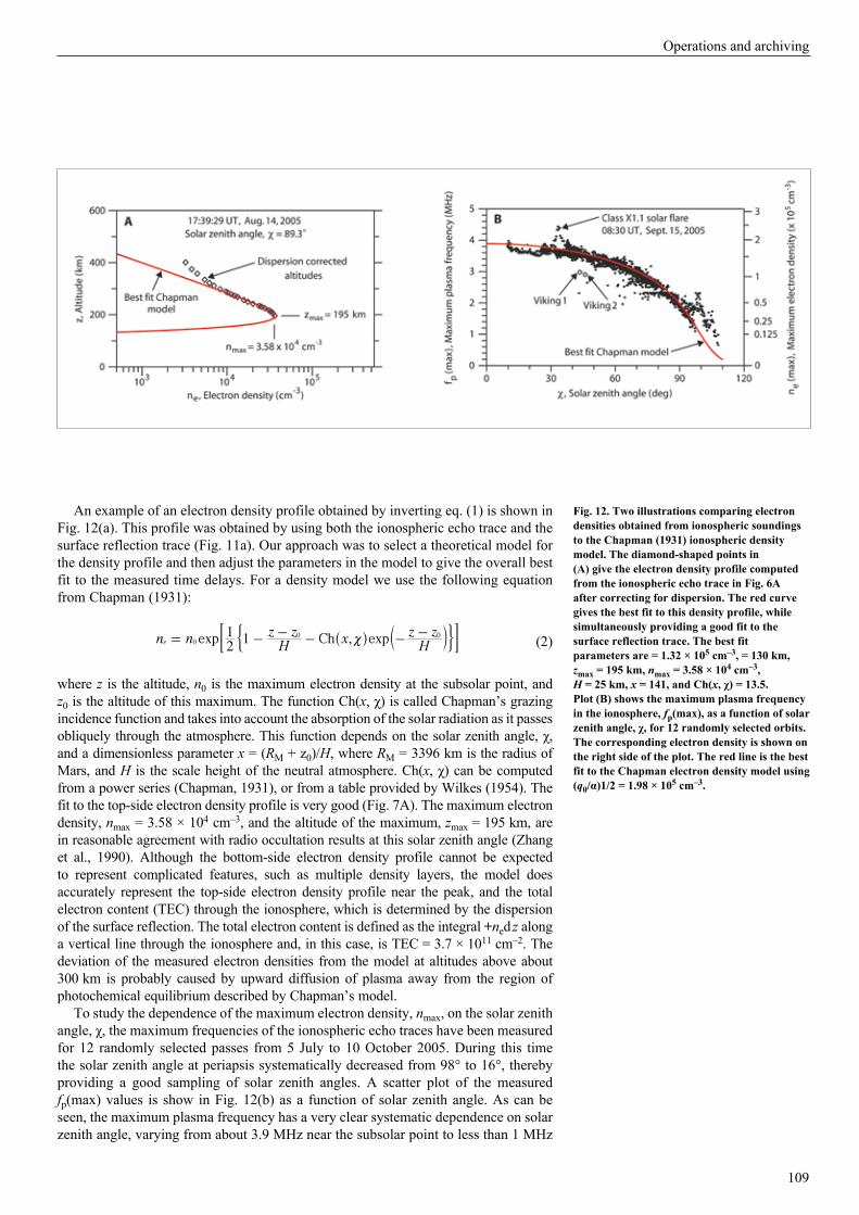
109
Operations and archiving
An example of an electron density profile obtained by inverting eq. (1) is shown in Fig. 12(a). This profile was obtained by using both the ionospheric echo trace and the surface reflection trace (Fig. 11a). Our approach was to select a theoretical model for the density profile and then adjust the parameters in the model to give the overall best fit to the measured time delays. For a density model we use the following equation from Chapman (1931):
where z is the altitude, n0 is the maximum electron density at the subsolar point, and z0 is the altitude of this maximum. The function Ch(x, χ) is called Chapman’s grazing incidence function and takes into account the absorption of the solar radiation as it passes obliquely through the atmosphere. This function depends on the solar zenith angle, χ, and a dimensionless parameter x = (RM + z0)/H, where RM = 3396 km is the radius of Mars, and H is the scale height of the neutral atmosphere. Ch(x, χ) can be computed from a power series (Chapman, 1931), or from a table provided by Wilkes (1954). The fit to the top-side electron density profile is very good (Fig. 7A). The maximum electron density, nmax = 3.58 × 104 cm–3, and the altitude of the maximum, zmax = 195 km, are in reasonable agreement with radio occultation results at this solar zenith angle (Zhang et al., 1990). Although the bottom-side electron density profile cannot be expected to represent complicated features, such as multiple density layers, the model does accurately represent the top-side electron density profile near the peak, and the total electron content (TEC) through the ionosphere, which is determined by the dispersion of the surface reflection. The total electron content is defined as the integral +ned z along a vertical line through the ionosphere and, in this case, is TEC = 3.7 × 1011 cm–2. The deviation of the measured electron densities from the model at altitudes above about 300 km is probably caused by upward diffusion of plasma away from the region of photochemical equilibrium described by Chapman’s model.
To study the dependence of the maximum electron density, nmax, on the solar zenith angle, χ, the maximum frequencies of the ionospheric echo traces have been measured for 12 randomly selected passes from 5 July to 10 October 2005. During this time the solar zenith angle at periapsis systematically decreased from 98° to 16°, thereby providing a good sampling of solar zenith angles. A scatter plot of the measured fp(max) values is show in Fig. 12(b) as a function of solar zenith angle. As can be seen, the maximum plasma frequency has a very clear systematic dependence on solar zenith angle, varying from about 3.9 MHz near the subsolar point to less than 1 MHz
Ch ,exp expn nH
z z xH
z z21 1 0 0
e 0= |- - - - -^ bh l; E& 0 (2)
Fig. 12. Two illustrations comparing electron densities obtained from ionospheric soundings to the Chapman (1931) ionospheric density model. The diamond-shaped points in (A) give the electron density profile computed from the ionospheric echo trace in Fig. 6A after correcting for dispersion. The red curve gives the best fit to this density profile, while simultaneously providing a good fit to the surface reflection trace. The best fit parameters are = 1.32 × 105 cm–3, = 130 km, zmax = 195 km, nmax = 3.58 × 104 cm–3, H = 25 km, x = 141, and Ch(x, χ) = 13.5. Plot (B) shows the maximum plasma frequency in the ionosphere, fp(max), as a function of solar zenith angle, χ, for 12 randomly selected orbits. The corresponding electron density is shown on the right side of the plot. The red line is the best fit to the Chapman electron density model using (q0/α)1/2 = 1.98 × 105 cm–3.
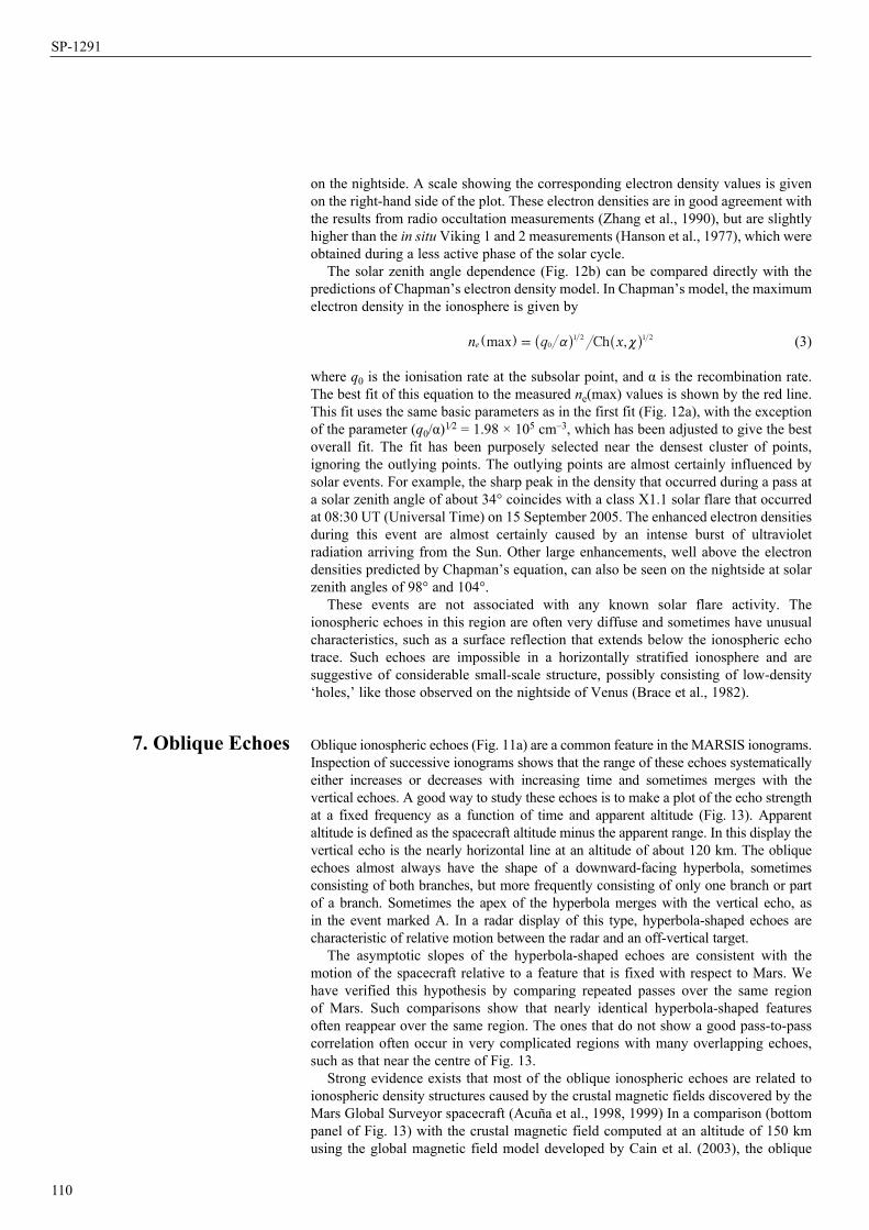
110
SP-1291
on the nightside. A scale showing the corresponding electron density values is given on the right-hand side of the plot. These electron densities are in good agreement with the results from radio occultation measurements (Zhang et al., 1990), but are slightly higher than the in situ Viking 1 and 2 measurements (Hanson et al., 1977), which were obtained during a less active phase of the solar cycle.
The solar zenith angle dependence (Fig. 12b) can be compared directly with the predictions of Chapman’s electron density model. In Chapman’s model, the maximum electron density in the ionosphere is given by
where q0 is the ionisation rate at the subsolar point, and α is the recombination rate. The best fit of this equation to the measured ne(max) values is shown by the red line. This fit uses the same basic parameters as in the first fit (Fig. 12a), with the exception of the parameter (q0/α)1⁄2 = 1.98 × 105 cm–3, which has been adjusted to give the best overall fit. The fit has been purposely selected near the densest cluster of points, ignoring the outlying points. The outlying points are almost certainly influenced by solar events. For example, the sharp peak in the density that occurred during a pass at a solar zenith angle of about 34° coincides with a class X1.1 solar flare that occurred at 08:30 UT (Universal Time) on 15 September 2005. The enhanced electron densities during this event are almost certainly caused by an intense burst of ultraviolet radiation arriving from the Sun. Other large enhancements, well above the electron densities predicted by Chapman’s equation, can also be seen on the nightside at solar zenith angles of 98° and 104°.
These events are not associated with any known solar flare activity. The ionospheric echoes in this region are often very diffuse and sometimes have unusual characteristics, such as a surface reflection that extends below the ionospheric echo trace. Such echoes are impossible in a horizontally stratified ionosphere and are suggestive of considerable small-scale structure, possibly consisting of low-density ‘holes,’ like those observed on the nightside of Venus (Brace et al., 1982).
Oblique ionospheric echoes (Fig. 11a) are a common feature in the MARSIS ionograms. Inspection of successive ionograms shows that the range of these echoes systematically either increases or decreases with increasing time and sometimes merges with the vertical echoes. A good way to study these echoes is to make a plot of the echo strength at a fixed frequency as a function of time and apparent altitude (Fig. 13). Apparent altitude is defined as the spacecraft altitude minus the apparent range. In this display the vertical echo is the nearly horizontal line at an altitude of about 120 km. The oblique echoes almost always have the shape of a downward-facing hyperbola, sometimes consisting of both branches, but more frequently consisting of only one branch or part of a branch. Sometimes the apex of the hyperbola merges with the vertical echo, as in the event marked A. In a radar display of this type, hyperbola-shaped echoes are characteristic of relative motion between the radar and an off-vertical target.
The asymptotic slopes of the hyperbola-shaped echoes are consistent with the motion of the spacecraft relative to a feature that is fixed with respect to Mars. We have verified this hypothesis by comparing repeated passes over the same region of Mars. Such comparisons show that nearly identical hyperbola-shaped features often reappear over the same region. The ones that do not show a good pass-to-pass correlation often occur in very complicated regions with many overlapping echoes, such as that near the centre of Fig. 13.
Strong evidence exists that most of the oblique ionospheric echoes are related to ionospheric density structures caused by the crustal magnetic fields discovered by the Mars Global Surveyor spacecraft (Acuña et al., 1998, 1999) In a comparison (bottom panel of Fig. 13) with the crustal magnetic field computed at an altitude of 150 km using the global magnetic field model developed by Cain et al. (2003), the oblique
Ch ,maxn q x01 2 1 2
e = a |] ^ ^g h h
7. Oblique Echoes
(3)
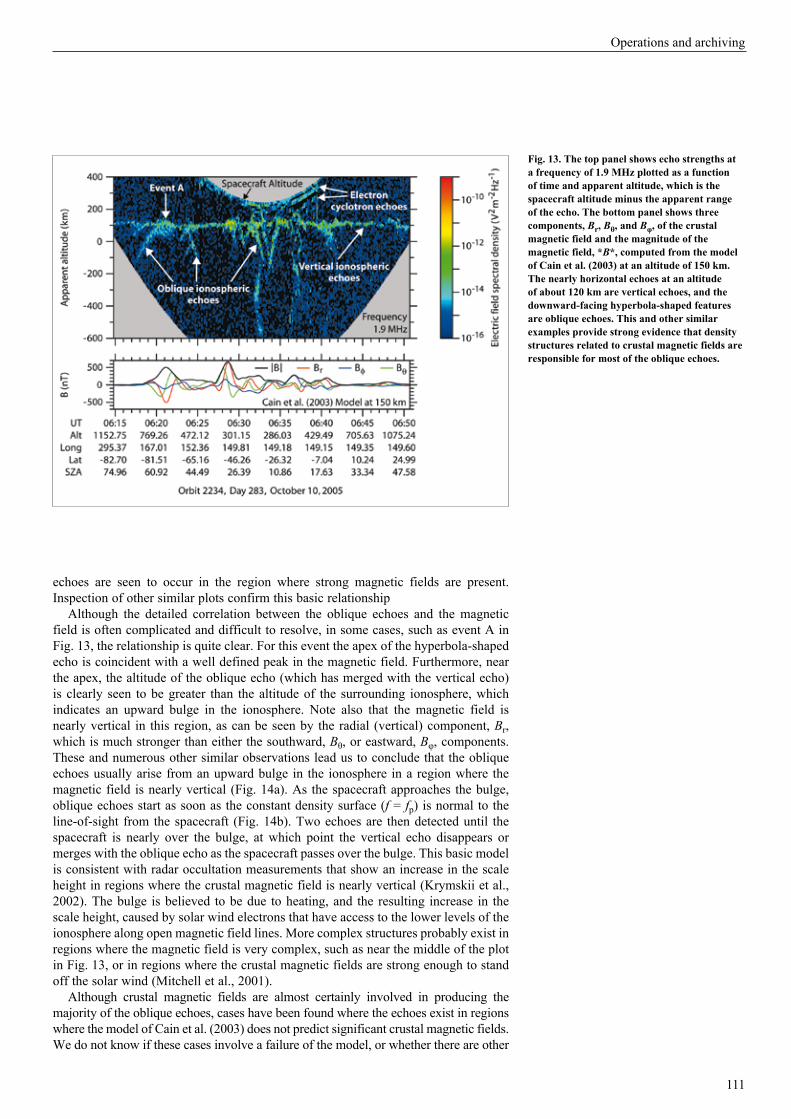
111
Operations and archiving
echoes are seen to occur in the region where strong magnetic fields are present. Inspection of other similar plots confirm this basic relationship
Although the detailed correlation between the oblique echoes and the magnetic field is often complicated and difficult to resolve, in some cases, such as event A in Fig. 13, the relationship is quite clear. For this event the apex of the hyperbola-shaped echo is coincident with a well defined peak in the magnetic field. Furthermore, near the apex, the altitude of the oblique echo (which has merged with the vertical echo) is clearly seen to be greater than the altitude of the surrounding ionosphere, which indicates an upward bulge in the ionosphere. Note also that the magnetic field is nearly vertical in this region, as can be seen by the radial (vertical) component, Br, which is much stronger than either the southward, Bθ, or eastward, Bφ, components. These and numerous other similar observations lead us to conclude that the oblique echoes usually arise from an upward bulge in the ionosphere in a region where the magnetic field is nearly vertical (Fig. 14a). As the spacecraft approaches the bulge, oblique echoes start as soon as the constant density surface (f = fp) is normal to the line-of-sight from the spacecraft (Fig. 14b). Two echoes are then detected until the spacecraft is nearly over the bulge, at which point the vertical echo disappears or merges with the oblique echo as the spacecraft passes over the bulge. This basic model is consistent with radar occultation measurements that show an increase in the scale height in regions where the crustal magnetic field is nearly vertical (Krymskii et al., 2002). The bulge is believed to be due to heating, and the resulting increase in the scale height, caused by solar wind electrons that have access to the lower levels of the ionosphere along open magnetic field lines. More complex structures probably exist in regions where the magnetic field is very complex, such as near the middle of the plot in Fig. 13, or in regions where the crustal magnetic fields are strong enough to stand off the solar wind (Mitchell et al., 2001).
Although crustal magnetic fields are almost certainly involved in producing the majority of the oblique echoes, cases have been found where the echoes exist in regions where the model of Cain et al. (2003) does not predict significant crustal magnetic fields. We do not know if these cases involve a failure of the model, or whether there are other
Fig. 13. The top panel shows echo strengths at a frequency of 1.9 MHz plotted as a function of time and apparent altitude, which is the spacecraft altitude minus the apparent range of the echo. The bottom panel shows three components, Br, Bθ, and Bφ, of the crustal magnetic field and the magnitude of the magnetic field, *B*, computed from the model of Cain et al. (2003) at an altitude of 150 km. The nearly horizontal echoes at an altitude of about 120 km are vertical echoes, and the downward-facing hyperbola-shaped features are oblique echoes. This and other similar examples provide strong evidence that density structures related to crustal magnetic fields are responsible for most of the oblique echoes.
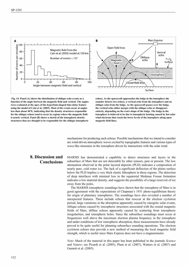
112
SP-1291
mechanisms for producing such echoes. Possible mechanisms that we intend to consider are wind-driven atmospheric waves excited by topographic features and various types of wave-like structures in the ionosphere driven by interactions with the solar wind.
MARSIS has demonstrated a capability to detect structures and layers in the subsurface of Mars that are not detectable by other sensors, past or present. The low attenuation observed in the polar layered deposits (PLD) indicates a composition of nearly pure, cold water ice. The lack of a significant deflection of the plains surface below the PLD implies a very thick elastic lithosphere in these regions. The detection of deep interfaces with minimal loss in the equatorial Medusae Fossae formation indicates a low material density, and suggests the possibility of a large reservoir of ice away from the poles.
The MARSIS ionospheric soundings have shown that the ionosphere of Mars is in good agreement with the expectations of Chapman’s 1931 photo-equilibrium theory for origin of planetary ionospheres. The soundings have also revealed a number of unexpected features. These include echoes that reoccur at the electron cyclotron period, large variations in the absorption apparently caused by energetic solar events, oblique echoes caused by ionospheric structures associated with the crustal magnetic fields of Mars, diffuse echoes apparently caused by scattering from ionospheric irregularities, and ionospheric holes. Since the subsurface soundings must occur at frequencies well above the maximum electron plasma frequency in the ionosphere and under conditions of low ionospheric absorption, these measurements have already proved to be quite useful for planning subsurface sounding operations. The electron cyclotron echoes also provide a new method of measuring the local magnetic field strength, which is useful since Mars Express does not have a magnetometer.
Note: Much of the material in this paper has been published in the journals Science and Nature; see Picardi et al. (2005), Plaut et al. (2007), Watters et al. (2007) and Gurnett et al. (2005).
8. Discussion and Conclusions
Fig. 14. Panel (A) shows the distribution of oblique echo events as a function of the angle between the magnetic field and vertical. The angles were evaluated at the apex of the hyperbola-shaped time delay feature using the model of Cain et al. (2003). Most of the events occur at angles less than about 40°E, indicating that the density structures responsible for the oblique echoes tend to occur in regions where the magnetic field is nearly vertical. Panel (B) shows a sketch of the ionospheric density structures that are thought to be responsible for the oblique ionospheric
echoes. As the spacecraft approaches the bulge in the ionosphere the sounder detects two echoes, a vertical echo from the ionosphere and an oblique echo from the bulge. As the spacecraft passes over the bulge, the vertical echo either merges with the oblique echo or disappears entirely, depending on the exact shape of the bulge. The bulge in the ionosphere is believed to be due to ionospheric heating caused by hot solar wind electrons that reach the lower levels of the ionosphere along open magnetic field lines.
113
Operations and archiving
Acuña, M.H., J.E.P. Connerney, P. Wasilewski, R.P. Lin, K.A. Anderson, C.W. Carlson, J. McFadden, D.W. Curtis, D. Mitchell, H. Reme, C. Mazelle, J.A. Sauvaud, C. d’Uston, A. Cros, J.L. Medale, S.J. Bauer, P. Cloutier, M. Mayhew, D. Winterhalter & N.F. Ness (1998). Magnetic Field and Plasma Observations at Mars: Initial Results of the Mars Global Surveyor Mission, Science 279, 167.
Acuña, M.H., J.E.P. Connerney, N.F. Ness, R.P. Lin, D. Mitchell, C.W. Carlson, J. McFadden, K.A. Anderson, H. Rème, C. Mazelle, D. Vignes, P. Wasilewski & P. Cloutier (1999). Global Distribution of Crustal Magnetization Discovered by the Mars Global Surveyor MAG/ER Experiment. Science 284, 790.
Brace, L., R. Theis, H. Mayr, S. Curtis & J. Luhmann (1982). Holes in the Nightside Ionosphere of Venus. J. Geophys. Res. 87, 199.
Bradley, B.A., S.E.H. Sakimoto, H.Frey & J.R. Zimbelman (2002). Medusae Fossae Formation: New Perspectives from Mars Global Surveyor. J. Geophys. Res. 107, 5058.
Byrne, S. & Ingersoll, A.P. (2003). A Sublimation Model for Martian South Polar Ice Features. Science 299, 1051. DOI: 10.1126/science.1080148.
Byrne, S. & Murray, B.C. (2002). North Polar Stratigraphy and the Paleo-erg of Mars. J. Geophys. Res. 107(E6), 5044. DOI : 10.1029/2001JE001615.
Cain J. C., B.B. Ferguson & D. Mozzoni (2003). An n = 90 Internal Potential Function of the Martian Crustal Magnetic Field. J. Geophys. Res. 108, 5008.
Carrier, W.D., G.R. Olhoeft & W. Mendell (1991), in Lunar Sourcebook. Cambridge University Press, New York, pp. 475–594.
Franklin, C.A. & M.A. Maclean (1969). The Design of Swept-frequency Topside Sounders. Proc. IEEE 57, 897.
Greeley, R. & J.E. Guest (1987). US Geol. Surv. Misc. Invest. Ser. Map, I-1802-B.Gurnett, D.A. & A. Bhattacharjee (2005). Introduction to Plasma Physics. Cambridge
University Press, Cambridge, p.114.Gurnett, D.A., Kirchner, D.L., Huff, R.L., Morgan, D.D., Persoon, A.M., Averkamp, T.F.,
Duru, F., Nielsen, E., Safaeinili, A., Plaut, J.J. & Picardi, G. (2005). Radar Soundings of the Ionosphere of Mars, Science 310, 1929–1933.
Hanson, W.B., S. Sanatani & D.R. Zuccaro (1977). The Martian Ionosphere as Observed by the Viking Retarding Potential Analyzers. J. Geophys. Res. 82, 4351.
Head, J.W. & M. Kreslavsky (2004). Medusae Fossae Formation: Ice-rich Airborne Dust Deposited during Periods of High Obliquity? Lunar Planet. Sci. 35, 1635 (abstract).
Hynek, B.M., R.J. Phillips, R.E. Arvidson (2003). Explosive Volcanism in the Tharsis Region: Global Evidence in the Martian Geologic Record, J. Geophys. Res. 108, 5111.
Krymskii A.M., T.K. Breus, N.F. Ness, M.H. Acuña, J.E.P. Connerney, D.H. Crider, D.L. Mitchell & S.J. Bauer (2002). Structure of the Magnetic Field Fluxes Connected with Crustal Magnetization and Topside Ionosphere at Mars. J. Geophys. Res. 107, 1245.
Lanagan, P., A. McEwen, L. Keszthelyi, and T. Thordarson (2001). Rootless Cones on Mars Indicating the Presence of Shallow Equatorial Ground Ice in Recent Times, Geophys. Res. Lett., 28(12), 2365-2367
Mitchell, D., R. Lin, C. Mazelle, H. Rème, P. Cloutier, J. Connerney, M. Acuna & N. Ness (2001). Probing Mars’ Crustal Magnetic Field and Ionosphere with the MGS Electron Reflectometer. J. Geophys. Res. 106, 23419.
Muhleman, D.O., B.J. Butler, A.W. Grossman & M.A. Slade (1991). Radar Images of Mars. Science 253, 1508.
Nouvel, J.-F., Herique, A., Kofman, W. & Safaeinili, A. (2004). Radar Signal Simulation: Surface Modeling with the Facet Method, Radio Sci. 39, RS1013. DOI: 10.1029/2003RS002903.
Pätzold, M., S. Tellmann, B. Häusler, D. Hinson, R. Schaa & G. L. Tyler (2005). A Sporadic Third Layer in the Ionosphere of Mars, Science 310, 837.
Picardi, G., Biccari, D., Seu, R., Plaut, J.J., Johnson, W.T.K., Jordan, R.L., Safaeinili, A., Gurnett, D.A., Huff, R., Orosei, R., Bombaci, O., Calabrese, D. & Zampolini, E. (2004). MARSIS: Mars Advanced Radar for Subsurface and Ionosphere Sounding, in Mars Express: The Scientific Payload, ESA SP-1240, ESA Publications Division, European Space Agency, Noordwijk, the Netherlands, pp.51–69.
References
114
SP-1291
Picardi, G., Plaut, J.J., Biccari, D., Bombaci, O., Calabrese, D., Cartacci, M., Cicchetti, A., Clifford, S.M., Edenhofer, P., Farrell, W.M., Federico, C., Frigeri, A., Gurnett, D.A., Hagfors, T., Heggy, E., Herique, A., Huff, R.L., Ivanov, A.B., Johnson, W.T.K., Jordan, R.L., Kirchner, D.L., Kofman, W., Leuschen, C.J., Nielsen, E., Orosei, R., Pettinelli, E., Phillips, R.J., Plettemeier, D., Safaeinili, A., Seu, R., Stofan, E.R., Vannaroni, G., Watters, T.R. & Zampolini, E. (2005). Radar Soundings of the Subsurface of Mars, Science 310, 1925–1928.
Plaut, J.J., Picardi, G., Safaeinili, A., Ivanov, A.B., Milkovich, S.M., Cicchetti, A., Kofman, W., Mouginot, J., Farrell, W.M., Phillips, R.J., Clifford, S.M., Frigeri, A., Orosei, R., Federico, C., Williams, I.P., Gurnett, D.A., Nielsen, E., Hagfors, T., Heggy, E., Stofan, E.R., Plettemeier, D., Watters, T.R., Leuschen, C.J. & Edenhofer, P. (2007). Subsurface Radar Sounding of the South Polar Layered Deposits of Mars, Science 315, 92–95, DOI: 10.1126/science.1139672.
Porcello, L.J., R.L. Jordan, J.S. Zelenka, G.F. Adams, R.J. Phillips, W.E. Brown, S.H. Ward, & P.L. Jackson (1974). The Apollo Lunar Sounder Radar System. Proc. IEEE 62, 769.
Safaeinili, A., W. Kofman, J.-F. Nouvel, A. Herique, & R.L. Jordan, R.L. (2003). Impact of Mars Ionosphere on Orbital Radar Sounder Operation and Data Processing, Planet. Space Sci. 51, 505.
Sakimoto, S.E.H., H.V. Frey, J. B. Garvin & J. H. Roark (1999). Topography, Roughness, Layering, and Slope Properties of the Medusae Fossae Formation from Mars Orbiter Laser Altimeter (MOLA) and Mars Orbiter Camera (MOC) data. J. Geophys. Res. 104, 24141.
Schultz, P.H. & A.B. Lutz (1988). Polar Wander of Mars. Icarus 73, 91.Scott, D.H. & K.L. Tanaka (1986). US Geol. Surv. Misc. Invest. Ser. Map, I-1802-A.Smith, D.E., Zuber, M.T., Solomon, S.C., Phillips, R.J., Head, J.W., Garvin, J.B., Banerdt,
W.B., Muhleman, D.O., Pettengill, G.H., Neumann, G.A., Lemoine, F.G., Abshire, J.B., Aharonson, O., Brown, C.D., Hauck, S.A., Ivanov, A.B., McGovern, P.J., Zwally, H.J. & Duxbury, T.C. (1999). The Global Topography of Mars and Implications for Surface Evolution, Science 284, 1495.
Tanaka, K. & E. Kolb (2005). Geologic Mapping of the Polar Regions of Mars: Preliminary Results and Climate Implications. US Geol. Surv. Open File Rept. 2005-1271.
Thomas, P.C., Squyres, S., Herkenhoff, K., Howard, A. & Murray, B. (1992) in Mars (Eds. H.H. Kieffer et al.), University of Arizona Press, Tucson, pp.767–795.
Watters, T.R., Campbell, B.A., Carter, L., Leuschen, C.J., Plaut, J.J., Picardi, G., Safaeinili, A., Clifford, S.M., Farrell, W.M., Ivanov, A.B., Phillips, R.J. & Stofan, E.R. (2007). Radar Sounding of the Medusae Fossae Formation Mars: Equatorial Ice or Dry, Low-Density Deposits? Science 318, 112. DOI: 10.1126/science.1148112.
Wilkes, M.V. (1954). A Table of Chapman’s Grazing Incidence Integral Ch(x, χ). Proc. R. Soc. B 67, 304.
Zhang, M.H.G., J.G. Luhmann & A.J. Kliore (1990). An Observational Study of the Nightside Ionospheres of Mars and Venus with Radio Occultation Methods. J. Geophys. Res. 95, 17095.
Zimbelman, J. et al. (1999). Medusae Fossae Formation, Mars: An Assessment of Possible Origins Utilizing Early Results from Mars Global Surveyor. Lunar Planet. Sci. 30, 1652 (abstr.)
This chapter reviews the first year of results from the Planetary Fourier Spectrometer (PFS) of Mars Express. An average global spectrum ranging from 200 cm–1 to 8200 cm–1 is compared with the martian spectrum from the Short Wavelength Spectrometer of the Infrared Space Observatory (ISO), and with the global synthetic spectrum computed using only the gases CO2, CO and H2O. PFS is able to measure the vertical temperature–pressure profile in the atmosphere and the temperature of the soil simultaneously with the dust and water-ice opacity. The short-wavelength channel shows the major CO2 bands at 4.3 µm and 2.7 µm. The bottom of the first band shows very clearly the non-local thermodynamic equilibrium emission of the high atmospheric CO2 gas, while the limb measurements show CO emission. All the isotopic CO2 molecules appear to be emitting at the same radiance level, implying strong energy pumping from the most abundant to the less abundant molecules. In one of the first passes over Olympus Mons, the temperature field shows abnormal adiabatic cooling in the atmosphere above the mountain, while the soil temperature of the volcano is higher than the latitudinal profile expectation because of illumination from the Sun. The descending branch of the Hadley cell circulation is studied in detail, with its adiabatic heating and formation of water-ice clouds. Of the many unidentified lines observed, a few have been studied and the presence of methane (10 ppbv), HF (200 ppbv) and HBr (150 ppbv) is reported here. PFS has allowed the study of the composition of the permanent south polar cap: an intimate
115
PFS: Planetary Fourier Spectrometer
V. Formisano1, F. Angrilli2, G. Arnold3, S. Atreya4, G. Bianchini2, D. Biondi1, M.I. Blecka6, A. Coradini1, L. Colangeli7, V. Cottini1, A. Ekonomov8, T. Encrenaz9, F. Esposito7, C. Fiorenza1, S. Fonti5, M. Giuranna1, D. Grassi1, V. Gnedykh8, A. Grigoriev8, G. Hansen10, H. Hirsh9, I. Khatuntsev8, N. Ignatiev8,1, A. Jurewicz6, E. Lellouch9, J. Lopez Moreno11, A. Mattana1, A. Maturilli1, M. Michalska6, B. Moshkin8, F. Nespoli1, R. Orfei1, P. Orleanski6, E. Palomba7, D. Patsaev8, G. Piccioni12, M. Rataj6, R. Rodrigo11, J. Rodriguez11, M. Rossi1, B. Saggin13, D. Titov8 & L. Zasova8,1
1 Istituto di Fisica dello Spazio Interplanetario INAF-IFSI, Via del Fosso del Cavaliere 100, I-00133 Roma, Italy Email: [email protected] Universita’ di Padova, CISAS, Via Venezia 1, I-35131 Padova, Italy3 German Aerospace Center (DLR), Optical Information System, Rutherfordstr. 2, D-12489 Berlin, Germany4 The University of Michigan, Dept. of Atmospheric, Oceanic and Space Sciences, Ann Arbor, MI 48109-2143, USA5 Universita’ degli Studi di Lecce, Dipartimento di Fisica, Via Arnesano, I-73100 Lecce, Italy.6 Space Research Centre of Polish Academy of Sciences (SRC PAS), Bartycka 18A, 00716 Warsaw, Poland 7 Osservatorio Astronomico di Capodimonte (INAF-OAC), Via Moiariello 16, I-80131 Napoli, Italy8 Space Research Institute of Russian Academy of Sciences (IKI), Profsojuznaja 84/32, 117997 Moscow, Russia9 Laboratoire d’Etudes Spatiales et d’Instrumentation en Astrophysique (LESIA), Observatoire de Paris, 5 Place Janssen, F-92195 Meudon,
France10 PlanetaryScienceInstitute,PacificNorthwestDivision,Dept.ofEarthandSpaceScience,Seattle,WA98195-1310,USA11 InstitutodeAstrofisicadeAndalusiaCSIC,POB3004,E-18080Granada,Spain12 IstitutoAstrofisicaSpazialeINAF-IASF,ViaFossodelCavaliere100,I-00133Roma,Italy13 Politecnico di Milano, Facoltà di Ing. Meccanica di Lecco, Corso Matteotti 3, I-23900 Lecco, Italy
mixture model of mostly CO2 ice, ppm of water ice and some dust fits the data very well. Almost pure water-ice and CO2-ice spectra have been observed in specific locations. Finally, many solar lines are being observed; a few are being studied and compared with ISO observations and the solar spectrum assembled for PFS. In certain spectral regions, Mars looks like a Lambertian screen, reflecting an almost unperturbed solar spectrum.
Following arrival in orbit around Mars on 25 December 2003, the Planetary Fourier Spectrometer (PFS) on Mars Express was activated on 10 January 2004. Routine operations for each orbit cover calibration, observation and then calibration again. The observed spectra, although showing evidence of the craft’s micro-vibrations, immediately gave the flavour of a dataset extremely rich in information. The team could immediately arrange for a number of publications describing the experiment, its performance and its scientific validation, in particular, Formisano et al. (2005a) for the experiment description and Giuranna et al. (2005a, b) for the calibrations. The method of retrieving the atmosphere’s temperature–pressure vertical profile is described in Grassi et al. (2005a); the method of fast synthetic spectra computation is presented in Ignatiev et al. (2005). A number of scientific results were also obtained, and they were highly appropriate for scientific validation of the experiment and of the data obtained. This chapter reviews some of the presented results (Formisano et al., 2005b; Grassi et al., 2005b; Zasova et al., 2005) and adds unpublished data, with the aim of bringing to the attention of the scientific community the characteristics of PFS data and stressing the importance of the information in the data.
1.1 Experiment Characteristics and Present Global CoveragePFS is an IR spectrometer optimised for atmospheric studies. It has a short-wavelength (SW) channel covering the spectral range 1700–8200 cm–1 (1.2–5.5 µm), and a long-wavelength (LW) channel covering 250–1700 cm–1 (5.5–45 µm). Both channels have a uniform spectral resolution of 1.3 cm–1, while the sampling is every 1 cm–1. The instrument Field of View (FOV) is about 1.6° Full Width Half Maximum (FWHM) for SW, and 2.8° FWHM for LW, which corresponds to spatial resolutions of 7 km and 12 km, respectively, when Mars is observed from a height of 250 km.
In comparison with the classical Michelson interferometer, the design (Formisano et al., 2005a) is highly robust against slight misalignments in harsh environments. Mechanical vibrations from the spacecraft affect the main radiation beam and the reference channels used to drive the experiment in the same way, so that meaningful measurements can still be taken. Double-sided interferograms are taken because they are relatively insensitive to phase errors – an important point for computing the martian spectrum.
Figure 1 shows the coverage of the planet achieved by April 2005, after more than a year of operations. By then, more than 190 000 measurements had been collected, each consisting of an LW interferogram and an SW interferogram. The coverage of the planet is very good; the extended mission aims to achieve four times this coverage. Figure 2 shows the north polar region coverage either illuminated (Fig. 2a) or not (Fig. 2b); it is evident that the coverage of the northern polar cap has been rather good when illuminated, but less so when not illuminated. Figure 3 presents the equivalent coverage of the southern polar cap. Owing to the season, the team has good coverage of the cap on the night side and limited coverage with solar illumination.
Figure 4 shows the latitude–local time coverage, an important aspect because the study of diurnal variation of several parameters is an important scientific objective. The local time coverage is rather good, but it is biased by season, i.e. season and local time are strongly linked. So far, there are no measurements of the equatorial region at midnight. It will be necessary to use the pointing mirror to fill this gap because the pericentre of the orbit, although it travels over all latitudes in time, will never reach the midnight regions at the equator.
116
SP-1291
1. Introduction
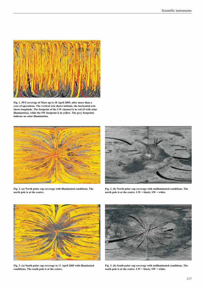
117
Scientific instruments
Fig. 1. PFS coverage of Mars up to 18 April 2005, after more than a year of operations. The vertical axis shows latitude, the horizontal axis shows longitude. The footprint of the LW channel is in red (if with solar illumination), while the SW footprint is in yellow. The grey footprints indicate no solar illumination.
Fig. 2. (a) North polar cap coverage with illuminated conditions. The north pole is at the centre.
Fig. 2. (b) North polar cap coverage with unilluminated conditions. The north pole is at the centre. LW = black; SW = white.
Fig. 3. (a) South polar cap coverage to 11 April 2005 with illuminated conditions. The south pole is at the centre.
Fig. 3. (b) South polar cap coverage with unilluminated conditions. The south pole is at the centre. LW = black; SW = white.
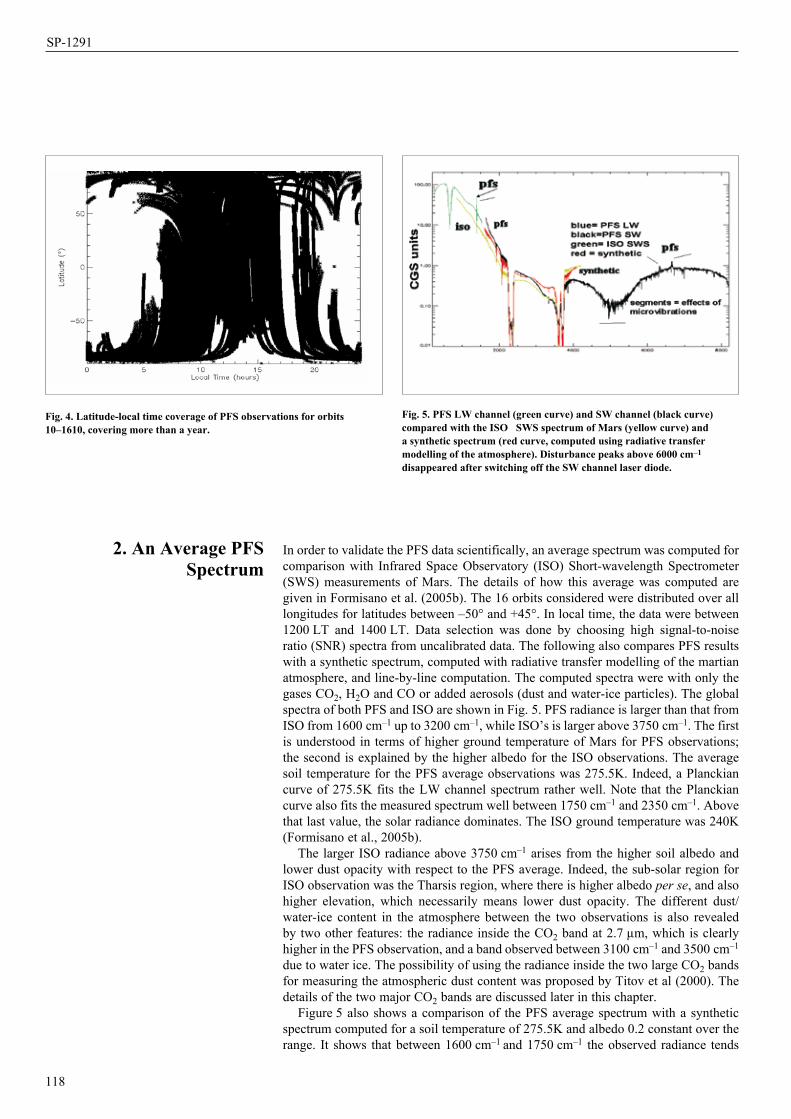
In order to validate the PFS data scientifically, an average spectrum was computed for comparison with Infrared Space Observatory (ISO) Short-wavelength Spectrometer (SWS) measurements of Mars. The details of how this average was computed are given in Formisano et al. (2005b). The 16 orbits considered were distributed over all longitudes for latitudes between –50° and +45°. In local time, the data were between 1200 LT and 1400 LT. Data selection was done by choosing high signal-to-noise ratio (SNR) spectra from uncalibrated data. The following also compares PFS results with a synthetic spectrum, computed with radiative transfer modelling of the martian atmosphere, and line-by-line computation. The computed spectra were with only the gases CO2, H2O and CO or added aerosols (dust and water-ice particles). The global spectra of both PFS and ISO are shown in Fig. 5. PFS radiance is larger than that from ISO from 1600 cm–1 up to 3200 cm–1, while ISO’s is larger above 3750 cm–1. The first is understood in terms of higher ground temperature of Mars for PFS observations; the second is explained by the higher albedo for the ISO observations. The average soil temperature for the PFS average observations was 275.5K. Indeed, a Planckian curve of 275.5K fits the LW channel spectrum rather well. Note that the Planckian curve also fits the measured spectrum well between 1750 cm–1 and 2350 cm–1. Above that last value, the solar radiance dominates. The ISO ground temperature was 240K (Formisano et al., 2005b).
The larger ISO radiance above 3750 cm–1 arises from the higher soil albedo and lower dust opacity with respect to the PFS average. Indeed, the sub-solar region for ISO observation was the Tharsis region, where there is higher albedo per se, and also higher elevation, which necessarily means lower dust opacity. The different dust/water-ice content in the atmosphere between the two observations is also revealed by two other features: the radiance inside the CO2 band at 2.7 µm, which is clearly higher in the PFS observation, and a band observed between 3100 cm–1 and 3500 cm–1 due to water ice. The possibility of using the radiance inside the two large CO2 bands for measuring the atmospheric dust content was proposed by Titov et al (2000). The details of the two major CO2 bands are discussed later in this chapter.
Figure 5 also shows a comparison of the PFS average spectrum with a synthetic spectrum computed for a soil temperature of 275.5K and albedo 0.2 constant over the range. It shows that between 1600 cm–1 and 1750 cm–1 the observed radiance tends
118
SP-1291
Fig. 5. PFS LW channel (green curve) and SW channel (black curve) compared with the ISO SWS spectrum of Mars (yellow curve) and a synthetic spectrum (red curve, computed using radiative transfer modelling of the atmosphere). Disturbance peaks above 6000 cm–1 disappeared after switching off the SW channel laser diode.
2. An Average PFS Spectrum
Fig. 4. Latitude-local time coverage of PFS observations for orbits 10–1610, covering more than a year.
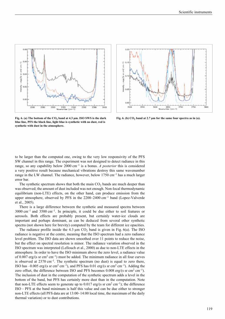
to be larger than the computed one, owing to the very low responsivity of the PFS SW channel in this range. The experiment was not designed to detect radiance in this range, so any capability below 2000 cm–1 is a bonus. A posterior this is considered a very positive result because mechanical vibrations destroy this same wavenumber range in the LW channel. The radiance, however, below 1750 cm–1 has a much larger error bar.
The synthetic spectrum shows that both the main CO2 bands are much deeper than was observed; the amount of dust included was not enough. Non-local thermodynamic equilibrium (non-LTE) effects, on the other hand, can produce emission from the upper atmosphere, observed by PFS in the 2200–2400 cm–1 band (Lopez-Valverde et al., 2005).
There is a large difference between the synthetic and measured spectra between 3000 cm–1 and 3500 cm–1. In principle, it could be due either to soil features or aerosols. Both effects are probably present, but certainly water-ice clouds are important and perhaps dominant, as can be deduced from several other synthetic spectra (not shown here for brevity) computed by the team for different ice opacities.
The radiance profile inside the 4.3 µm CO2 band is given in Fig. 6(a). The ISO radiance is negative at the centre, meaning that the ISO spectrum had a zero radiance level problem. The ISO data are shown smoothed over 11 points to reduce the noise, but the effect on spectral resolution is minor. The radiance variation observed in the ISO spectrum was interpreted (Lellouch et al., 2000) as due to non-LTE effects in the atmosphere. In order to have the ISO minimum above the zero level, a radiance value of 0.007 erg/(s sr cm2 cm–1) must be added. The minimum radiance in all four curves is observed at 2370 cm–1. The synthetic spectrum (no dust) is equal to zero there, ISO has –0.005 erg/(s sr cm2 cm–1), and PFS has 0.01 erg/(s sr cm2 cm–1). Adding the zero offset, the difference between ISO and PFS becomes 0.008 erg/(s sr cm2 cm–1). The inclusion of dust in the computation of the synthetic spectrum adds a level in the bottom of the band, but PFS has certainly more dust than in the computation. Note that non-LTE effects seem to generate up to 0.017 erg/(s sr cm2 cm–1); the difference ISO – PFS at the band minimum is half this value and can be due either to stronger non-LTE effects (all PFS data are at 13:00–14:00 local time, the maximum of the daily thermal variation) or to dust contributions.
119
Scientific instruments
Fig. 6. (b) CO2 band at 2.7 µm for the same four spectra as in (a).Fig. 6. (a) The bottom of the CO2 band at 4.3 µm. ISO SWS is the dark blue line, PFS the black line, light blue is synthetic with no dust, red is synthetic with dust in the atmosphere.
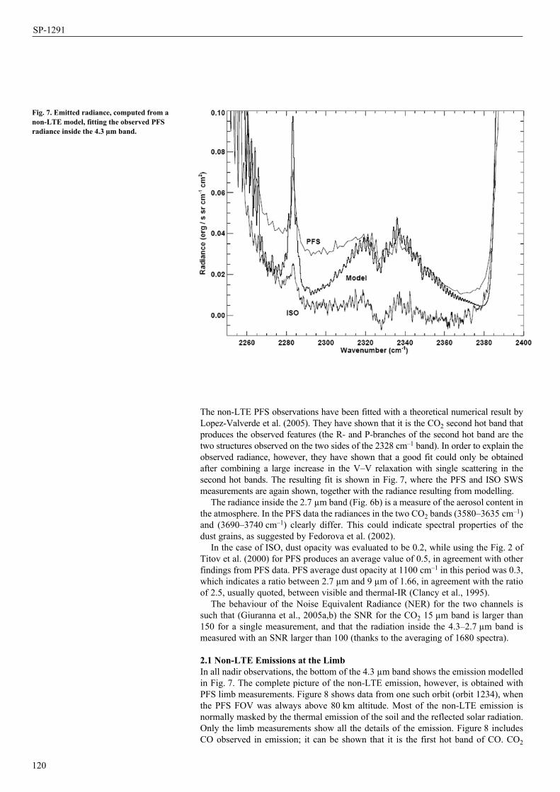
The non-LTE PFS observations have been fitted with a theoretical numerical result by Lopez-Valverde et al. (2005). They have shown that it is the CO2 second hot band that produces the observed features (the R- and P-branches of the second hot band are the two structures observed on the two sides of the 2328 cm–1 band). In order to explain the observed radiance, however, they have shown that a good fit could only be obtained after combining a large increase in the V–V relaxation with single scattering in the second hot bands. The resulting fit is shown in Fig. 7, where the PFS and ISO SWS measurements are again shown, together with the radiance resulting from modelling.
The radiance inside the 2.7 µm band (Fig. 6b) is a measure of the aerosol content in the atmosphere. In the PFS data the radiances in the two CO2 bands (3580–3635 cm–1) and (3690–3740 cm–1) clearly differ. This could indicate spectral properties of the dust grains, as suggested by Fedorova et al. (2002).
In the case of ISO, dust opacity was evaluated to be 0.2, while using the Fig. 2 of Titov et al. (2000) for PFS produces an average value of 0.5, in agreement with other findings from PFS data. PFS average dust opacity at 1100 cm–1 in this period was 0.3, which indicates a ratio between 2.7 µm and 9 µm of 1.66, in agreement with the ratio of 2.5, usually quoted, between visible and thermal-IR (Clancy et al., 1995).
The behaviour of the Noise Equivalent Radiance (NER) for the two channels is such that (Giuranna et al., 2005a,b) the SNR for the CO2 15 µm band is larger than 150 for a single measurement, and that the radiation inside the 4.3–2.7 µm band is measured with an SNR larger than 100 (thanks to the averaging of 1680 spectra).
2.1 Non-LTE Emissions at the LimbIn all nadir observations, the bottom of the 4.3 µm band shows the emission modelled in Fig. 7. The complete picture of the non-LTE emission, however, is obtained with PFS limb measurements. Figure 8 shows data from one such orbit (orbit 1234), when the PFS FOV was always above 80 km altitude. Most of the non-LTE emission is normally masked by the thermal emission of the soil and the reflected solar radiation. Only the limb measurements show all the details of the emission. Figure 8 includes CO observed in emission; it can be shown that it is the first hot band of CO. CO2
120
SP-1291
Fig. 7. Emitted radiance, computed from a non-LTE model, fitting the observed PFS radiance inside the 4.3 µm band.

emission shows a structure that, when studied in detail (Formisano et al., 2005c), can be interpreted as due to the isotopic molecules of CO2. The 636, 626 and 628 isotopic molecules are emitting at almost the same intensity, which implies a very strong pumping of energy from the main isotope 626 to the others via collisions. It can be shown that the 626 and 636 isotopic molecules are emitting the second hot band, while the 628 is emitting the third.
The LW channel covers the thermal region 250–1700 cm–1. Spectral resolution is of the order of 2 cm–1 for apodised spectra, sampled with a 1 cm–1 step. The instantaneous FOV of the channel has a diameter of 12.2 km at the nominal height of the 250 km pericentre. A complete description of the instrument and its radiometric performances can be found in Formisano et al. (2005a) and Giuranna et al. (2005a).
The PFS spectra can be analysed individually using the methods and tools presented by Grassi et al. (2005a). The algorithm computes the effects of multiple scattering by atmospheric aerosols. Retrieval of atmospheric fields is limited to surface temperature, air temperature vs. altitude (up to 45–50 km), dust and water-ice integrated contents. Dust concentration is assumed to scale exponentially with altitude, according a decay height of 10 km. Results presented in this work were achieved by assuming that the water-ice particle concentration vs. altitude is described by an exponential shape with a 10 km decay height.
An important problematic aspect of the temperature retrieval method arises from the assumptions made to define the value of Psurf (atmospheric pressure at the surface), to be adopted in the definition of a suitable temperature vs. pressure grid during evaluation of synthetic spectra. Values projected by models were used integrated with Mars Global Surveyor’s Mars Orbiter Laser Altimeter (MOLA) data (Smith et al., 2003). In the future, the SW channel data will be used to obtain the team’s own measured Psurf. The non-saturated CO2 bands at solar wavelengths (e.g. 5000, 6350 and 6950 cm–1) allow the retrieval of the integrated content of CO2 (i.e. Psurf), with an error of the order 0.25 mbar or lower.
121
Scientific instruments
Fig. 8. Limb observation of non-LTE emission from CO and CO2. The grey curve is the deep-space zero-radiance level.
3. Results from the LW Channel
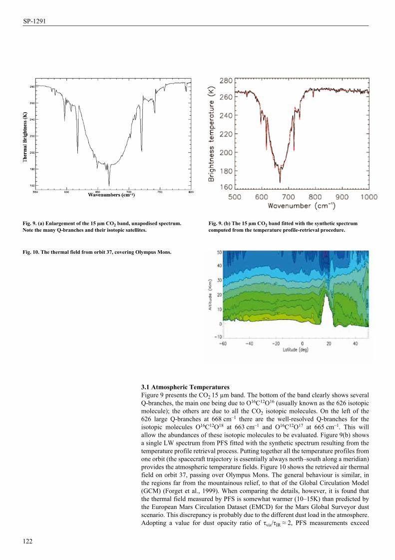
3.1 Atmospheric Temperatures Figure 9 presents the CO2 15 µm band. The bottom of the band clearly shows several Q-branches, the main one being due to O16C12O16 (usually known as the 626 isotopic molecule); the others are due to all the CO2 isotopic molecules. On the left of the 626 large Q-branches at 668 cm–1 there are the well-resolved Q-branches for the isotopic molecules O16C12O18 at 663 cm–1 and O16C12O17 at 665 cm–1. This will allow the abundances of these isotopic molecules to be evaluated. Figure 9(b) shows a single LW spectrum from PFS fitted with the synthetic spectrum resulting from the temperature profile retrieval process. Putting together all the temperature profiles from one orbit (the spacecraft trajectory is essentially always north–south along a meridian) provides the atmospheric temperature fields. Figure 10 shows the retrieved air thermal field on orbit 37, passing over Olympus Mons. The general behaviour is similar, in the regions far from the mountainous relief, to that of the Global Circulation Model (GCM) (Forget et al., 1999). When comparing the details, however, it is found that the thermal field measured by PFS is somewhat warmer (10–15K) than predicted by the European Mars Circulation Dataset (EMCD) for the Mars Global Surveyor dust scenario. This discrepancy is probably due to the different dust load in the atmosphere. Adopting a value for dust opacity ratio of τvis/τIR ≈ 2, PFS measurements exceed
122
SP-1291
Fig. 10. The thermal field from orbit 37, covering Olympus Mons.
Fig. 9. (b) The 15 µm CO2 band fitted with the synthetic spectrum computed from the temperature profile-retrieval procedure.
Fig. 9. (a) Enlargement of the 15 µm CO2 band, unapodised spectrum. Note the many Q-branches and their isotopic satellites.
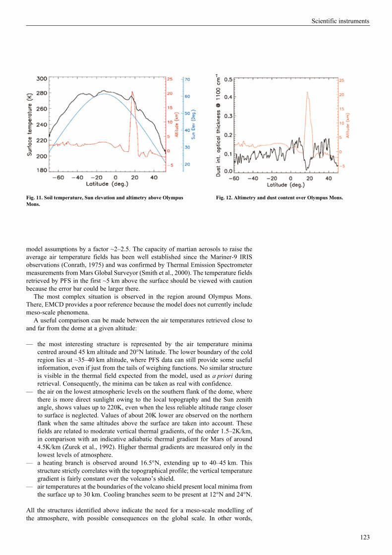
123
Scientific instruments
Fig. 12. Altimetry and dust content over Olympus Mons.Fig. 11. Soil temperature, Sun elevation and altimetry above Olympus Mons.
model assumptions by a factor ~2–2.5. The capacity of martian aerosols to raise the average air temperature fields has been well established since the Mariner-9 IRIS observations (Conrath, 1975) and was confirmed by Thermal Emission Spectrometer measurements from Mars Global Surveyor (Smith et al., 2000). The temperature fields retrieved by PFS in the first ~5 km above the surface should be viewed with caution because the error bar could be larger there.
The most complex situation is observed in the region around Olympus Mons. There, EMCD provides a poor reference because the model does not currently include meso-scale phenomena.
A useful comparison can be made between the air temperatures retrieved close to and far from the dome at a given altitude:
— the most interesting structure is represented by the air temperature minima centred around 45 km altitude and 20°N latitude. The lower boundary of the cold region lies at ~35–40 km altitude, where PFS data can still provide some useful information, even if just from the tails of weighing functions. No similar structure is visible in the thermal field expected from the model, used as a priori during retrieval. Consequently, the minima can be taken as real with confidence.
— the air on the lowest atmospheric levels on the southern flank of the dome, where there is more direct sunlight owing to the local topography and the Sun zenith angle, shows values up to 220K, even when the less reliable altitude range closer to surface is neglected. Values of about 20K lower are observed on the northern flank when the same altitudes above the surface are taken into account. These fields are related to moderate vertical thermal gradients, of the order 1.5–2K/km, in comparison with an indicative adiabatic thermal gradient for Mars of around 4.5K/km (Zurek et al., 1992). Higher thermal gradients are measured only in the lowest levels of atmosphere.
— a heating branch is observed around 16.5°N, extending up to 40–45 km. This structure strictly correlates with the topographical profile; the vertical tempera ture gradient is fairly constant over the volcano’s shield.
— air temperatures at the boundaries of the volcano shield present local minima from the surface up to 30 km. Cooling branches seem to be present at 12°N and 24°N.
All the structures identified above indicate the need for a meso-scale modelling of the atmosphere, with possible consequences on the global scale. In other words,
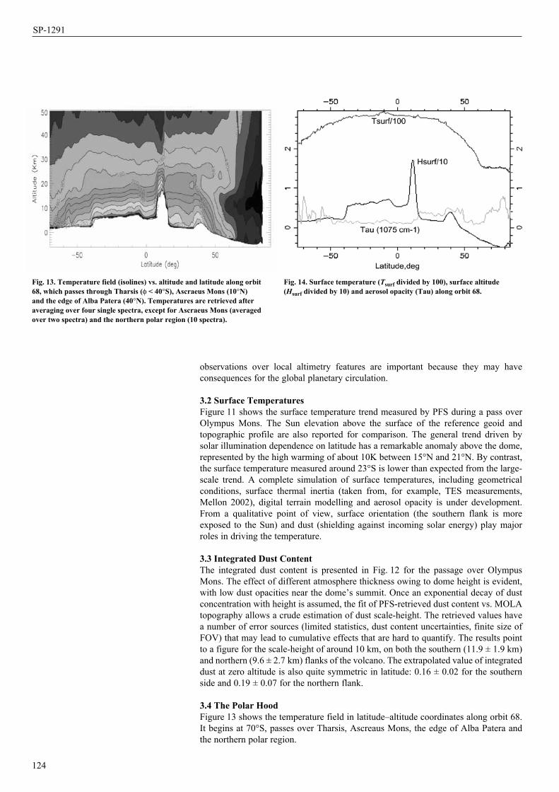
observations over local altimetry features are important because they may have consequences for the global planetary circulation.
3.2 Surface Temperatures Figure 11 shows the surface temperature trend measured by PFS during a pass over Olympus Mons. The Sun elevation above the surface of the reference geoid and topographic profile are also reported for comparison. The general trend driven by solar illumination dependence on latitude has a remarkable anomaly above the dome, represented by the high warming of about 10K between 15°N and 21°N. By contrast, the surface temperature measured around 23°S is lower than expected from the large-scale trend. A complete simulation of surface temperatures, including geometrical conditions, surface thermal inertia (taken from, for example, TES measurements, Mellon 2002), digital terrain modelling and aerosol opacity is under development. From a qualitative point of view, surface orientation (the southern flank is more exposed to the Sun) and dust (shielding against incoming solar energy) play major roles in driving the temperature.
3.3 Integrated Dust Content The integrated dust content is presented in Fig. 12 for the passage over Olympus Mons. The effect of different atmosphere thickness owing to dome height is evident, with low dust opacities near the dome’s summit. Once an exponential decay of dust concentration with height is assumed, the fit of PFS-retrieved dust content vs. MOLA topography allows a crude estimation of dust scale-height. The retrieved values have a number of error sources (limited statistics, dust content uncertainties, finite size of FOV) that may lead to cumulative effects that are hard to quantify. The results point to a figure for the scale-height of around 10 km, on both the southern (11.9 ± 1.9 km) and northern (9.6 ± 2.7 km) flanks of the volcano. The extrapolated value of integrated dust at zero altitude is also quite symmetric in latitude: 0.16 ± 0.02 for the southern side and 0.19 ± 0.07 for the northern flank.
3.4 The Polar HoodFigure 13 shows the temperature field in latitude–altitude coordinates along orbit 68. It begins at 70°S, passes over Tharsis, Ascreaus Mons, the edge of Alba Patera and the northern polar region.
124
SP-1291
Fig. 14. Surface temperature (Tsurf divided by 100), surface altitude (Hsurf divided by 10) and aerosol opacity (Tau) along orbit 68.
Fig. 13. Temperature field (isolines) vs. altitude and latitude along orbit 68, which passes through Tharsis (f < 40°S), Ascraeus Mons (10°N) and the edge of Alba Patera (40°N). Temperatures are retrieved after averaging over four single spectra, except for Ascraeus Mons (averaged over two spectra) and the northern polar region (10 spectra).
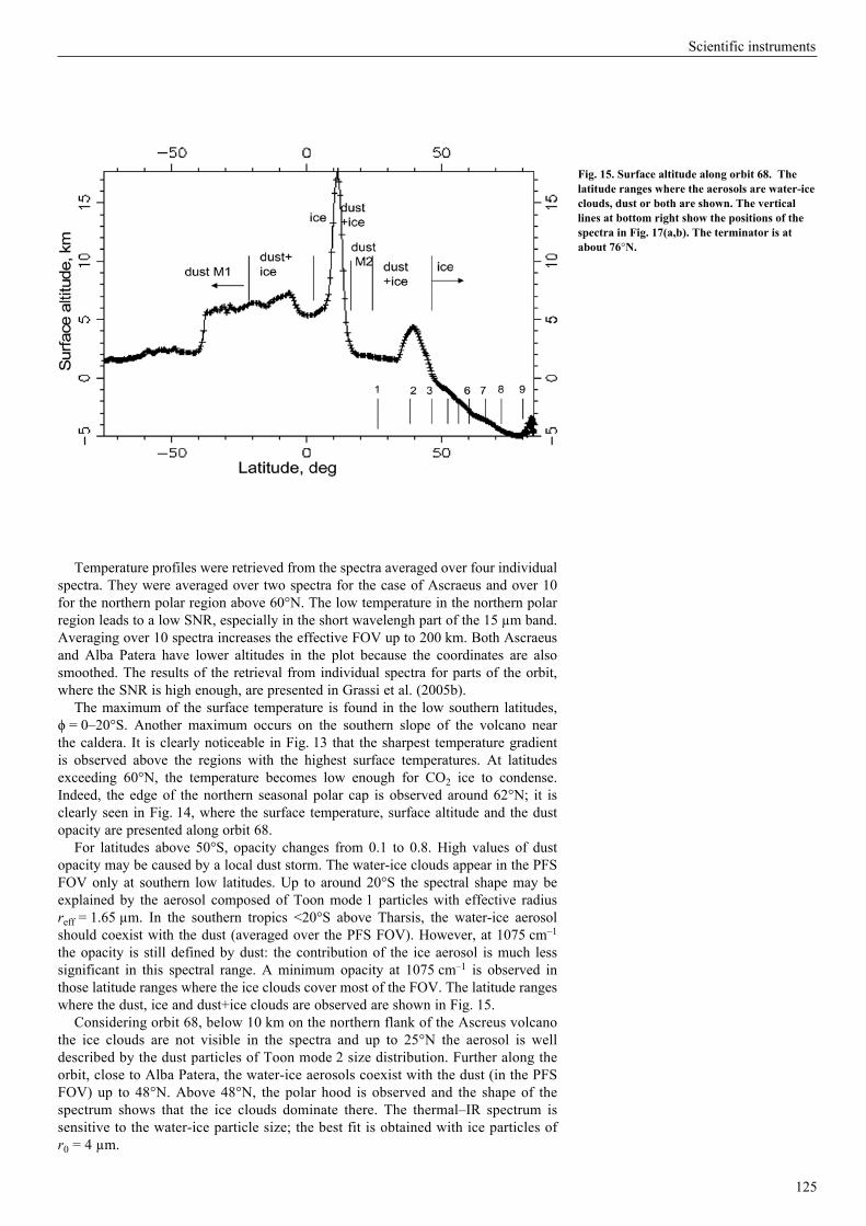
Temperature profiles were retrieved from the spectra averaged over four individual spectra. They were averaged over two spectra for the case of Ascraeus and over 10 for the northern polar region above 60°N. The low temperature in the northern polar region leads to a low SNR, especially in the short wavelengh part of the 15 µm band. Averaging over 10 spectra increases the effective FOV up to 200 km. Both Ascraeus and Alba Patera have lower altitudes in the plot because the coordinates are also smoothed. The results of the retrieval from individual spectra for parts of the orbit, where the SNR is high enough, are presented in Grassi et al. (2005b).
The maximum of the surface temperature is found in the low southern latitudes, ϕ = 0–20°S. Another maximum occurs on the southern slope of the volcano near the caldera. It is clearly noticeable in Fig. 13 that the sharpest temperature gradient is observed above the regions with the highest surface temperatures. At latitudes exceeding 60°N, the temperature becomes low enough for CO2 ice to condense. Indeed, the edge of the northern seasonal polar cap is observed around 62°N; it is clearly seen in Fig. 14, where the surface temperature, surface altitude and the dust opacity are presented along orbit 68.
For latitudes above 50°S, opacity changes from 0.1 to 0.8. High values of dust opacity may be caused by a local dust storm. The water-ice clouds appear in the PFS FOV only at southern low latitudes. Up to around 20°S the spectral shape may be explained by the aerosol composed of Toon mode 1 particles with effective radius reff = 1.65 µm. In the southern tropics <20°S above Tharsis, the water-ice aerosol should coexist with the dust (averaged over the PFS FOV). However, at 1075 cm–1
the opacity is still defined by dust: the contribution of the ice aerosol is much less significant in this spectral range. A minimum opacity at 1075 cm–1 is observed in those latitude ranges where the ice clouds cover most of the FOV. The latitude ranges where the dust, ice and dust+ice clouds are observed are shown in Fig. 15.
Considering orbit 68, below 10 km on the northern flank of the Ascreus volcano the ice clouds are not visible in the spectra and up to 25°N the aerosol is well described by the dust particles of Toon mode 2 size distribution. Further along the orbit, close to Alba Patera, the water-ice aerosols coexist with the dust (in the PFS FOV) up to 48°N. Above 48°N, the polar hood is observed and the shape of the spectrum shows that the ice clouds dominate there. The thermal–IR spectrum is sensitive to the water-ice particle size; the best fit is obtained with ice particles of r0 = 4 µm.
125
Scientific instruments
Fig. 15. Surface altitude along orbit 68. The latitude ranges where the aerosols are water-ice clouds, dust or both are shown. The vertical lines at bottom right show the positions of the spectra in Fig. 17(a,b). The terminator is at about 76°N.
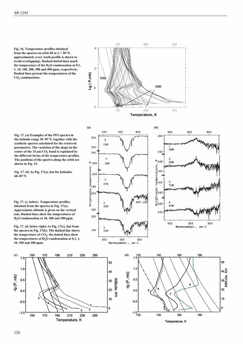
126
SP-1291
Fig. 17. (c, below) Temperature profiles obtained from the spectra in Fig. 17(a). Approximate altitude is given on the vertical axis. Dashed lines show the temperatures of H2O condensation at 10, 100 and 200 ppm.
Fig. 17. (d, below right) As Fig. 17(c), but from the spectra in Fig. 17(b). The dashed line shows the temperature of CO2; the dotted lines show the temperatures of H2O condensation at 0.1, 1, 10, 100 and 200 ppm.
Fig. 17. (a) Examples of the PFS spectra in the latitude range 30–55°N, together with the synthetic spectra calculated for the retrieved parameters. The variation of the shape in the centre of the 15 µm CO2 band is explained by the different forms of the temperature profiles. The positions of the spectra along the orbit are shown in Fig. 15.
Fig. 17. (b) As Fig. 17(a), but for latitudes 60–85°N.
Fig. 16. Temperature profiles obtained from the spectra on orbit 68 at f > 30°N; approximately every tenth profile is shown to avoid overlapping). Dashed-dotted lines mark the temperature of the H2O condensation at 0.1, 1, 10, 100, 200, 300 and 400 ppm, respectively. Dashed lines present the temperatures of the CO2 condensation.
(a) (b)
(c) (d)
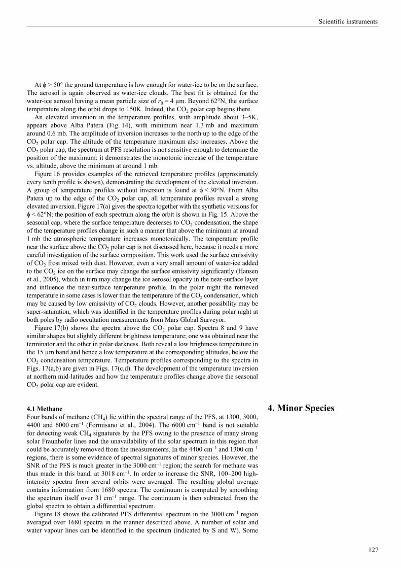
At ϕ > 50° the ground temperature is low enough for water-ice to be on the surface. The aerosol is again observed as water-ice clouds. The best fit is obtained for the water-ice aerosol having a mean particle size of r0 = 4 µm. Beyond 62°N, the surface temperature along the orbit drops to 150K. Indeed, the CO2 polar cap begins there.
An elevated inversion in the temperature profiles, with amplitude about 3–5K, appears above Alba Patera (Fig. 14), with minimum near 1.3 mb and maximum around 0.6 mb. The amplitude of inversion increases to the north up to the edge of the CO2 polar cap. The altitude of the temperature maximum also increases. Above the CO2 polar cap, the spectrum at PFS resolution is not sensitive enough to determine the position of the maximum: it demonstrates the monotonic increase of the temperature vs. altitude, above the minimum at around 1 mb.
Figure 16 provides examples of the retrieved temperature profiles (approximately every tenth profile is shown), demonstrating the development of the elevated inversion. A group of temperature profiles without inversion is found at ϕ < 30°N. From Alba Patera up to the edge of the CO2 polar cap, all temperature profiles reveal a strong elevated inversion. Figure 17(a) gives the spectra together with the synthetic versions for ϕ < 62°N; the position of each spectrum along the orbit is shown in Fig. 15. Above the seasonal cap, where the surface temperature decreases to CO2 condensation, the shape of the temperature profiles change in such a manner that above the minimum at around 1 mb the atmospheric temperature increases monotonically. The temperature profile near the surface above the CO2 polar cap is not discussed here, because it needs a more careful investigation of the surface composition. This work used the surface emissivity of CO2 frost mixed with dust. However, even a very small amount of water-ice added to the CO2 ice on the surface may change the surface emissivity significantly (Hansen et al., 2005), which in turn may change the ice aerosol opacity in the near-surface layer and influence the near-surface temperature profile. In the polar night the retrieved temperature in some cases is lower than the temperature of the CO2 condensation, which may be caused by low emissivity of CO2 clouds. However, another possibility may be super-saturation, which was identified in the temperature profiles during polar night at both poles by radio occultation measurements from Mars Global Surveyor.
Figure 17(b) shows the spectra above the CO2 polar cap. Spectra 8 and 9 have similar shapes but slightly different brightness temperature; one was obtained near the terminator and the other in polar darkness. Both reveal a low brightness temperature in the 15 µm band and hence a low temperature at the corresponding altitudes, below the CO2 condensation temperature. Temperature profiles corresponding to the spectra in Figs. 17(a,b) are given in Figs. 17(c,d). The development of the temperature inversion at northern mid-latitudes and how the temperature profiles change above the seasonal CO2 polar cap are evident.
4.1 MethaneFour bands of methane (CH4) lie within the spectral range of the PFS, at 1300, 3000, 4400 and 6000 cm–1 (Formisano et al., 2004). The 6000 cm–1 band is not suitable for detecting weak CH4 signatures by the PFS owing to the presence of many strong solar Fraunhofer lines and the unavailability of the solar spectrum in this region that could be accurately removed from the measurements. In the 4400 cm–1 and 1300 cm–1 regions, there is some evidence of spectral signatures of minor species. However, the SNR of the PFS is much greater in the 3000 cm–1 region; the search for methane was thus made in this band, at 3018 cm–1. In order to increase the SNR, 100–200 high-intensity spectra from several orbits were averaged. The resulting global average contains information from 1680 spectra. The continuum is computed by smoothing the spectrum itself over 31 cm–1 range. The continuum is then subtracted from the global spectra to obtain a differential spectrum.
Figure 18 shows the calibrated PFS differential spectrum in the 3000 cm–1 region averaged over 1680 spectra in the manner described above. A number of solar and water vapour lines can be identified in the spectrum (indicated by S and W). Some
127
Scientific instruments
4. Minor Species
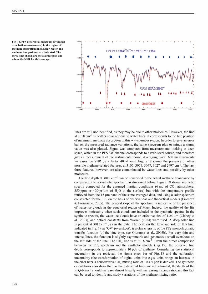
lines are still not identified, as they may be due to other molecules. However, the line at 3018 cm–1 is neither solar nor due to water lines; it corresponds to the line position of maximum methane absorption in this wavenumber region. In order to give an error bar on the measured radiance variations, the same spectrum plus or minus a sigma value was also plotted. Sigma was computed from measurements looking at deep space, which in the PFS SW channel corresponds to a zero-level source, and therefore gives a measurement of the instrumental noise. Averaging over 1680 measurements increases the SNR by a factor 40 at least. Figure 18 shows the presence of other possible methane-related features, at 3105, 3075, 3047, 3027 and 2997 cm–1. The last three features, however, are also contaminated by water lines and possibly by other molecules.
The line depth at 3018 cm–1 can be converted to the actual methane abundance by comparing it to a synthetic spectrum, as discussed below. Figure 19 shows synthetic spectra computed for the assumed martian conditions (6 mb of CO2 atmosphere, 350 ppm or ~30 pr-µm of H2O at the surface) but with the temperature profile retrieved from the 15 µm band of the same averaged data, and using a solar spectrum constructed for the PFS on the basis of observations and theoretical models (Fiorenza & Formisano, 2005). The general slope of the spectrum is indicative of the presence of water-ice clouds in the equatorial region of Mars. Indeed, the quality of the fits improves noticeably when such clouds are included in the synthetic spectra. In the synthetic spectra, the water-ice clouds have an effective size of 1.25 µm (Clancy et al., 2003), and optical constants from Warren (1984) were used. A deep solar line is present at 3012 cm–1, as in the data. The peak on the left-hand side of this line, indicated in Fig. 19 as ‘OV’ (overshoot), is a characteristic of the PFS monochromatic transfer function (of the sinc type, see Giuranna et al., 2005b). For very thin and intense lines, the function is slightly asymmetric and generates a small overshoot on the left side of the line. The CH4 line is at 3018 cm–1. From the direct comparison between the PFS spectrum and the synthetic models (Fig. 19), the observed line depth corresponds to approximately 10 ppb of methane. Considering the statistical uncertainty in the retrieval, the sigma error bar of Fig. 18 and the calibration uncertainty (the transformation of digital units into c.g.s. units brings an increase in the error bar), a conservative CH4 mixing ratio of 10 ± 5 ppb is derived. The synthetic calculations also show that, as the individual lines are not saturated, the depth of the n3 Q-branch should increase almost linearly with increasing mixing ratio, and this fact can be used to identify and study variations of the methane mixing ratio.
128
SP-1291
Fig. 18. PFS differential spectrum (averaged over 1680 measurements) in the region of methane absorption lines. Solar, water and methane line positions are indicated. The three lines shown are the average plus and minus the NER for this average.
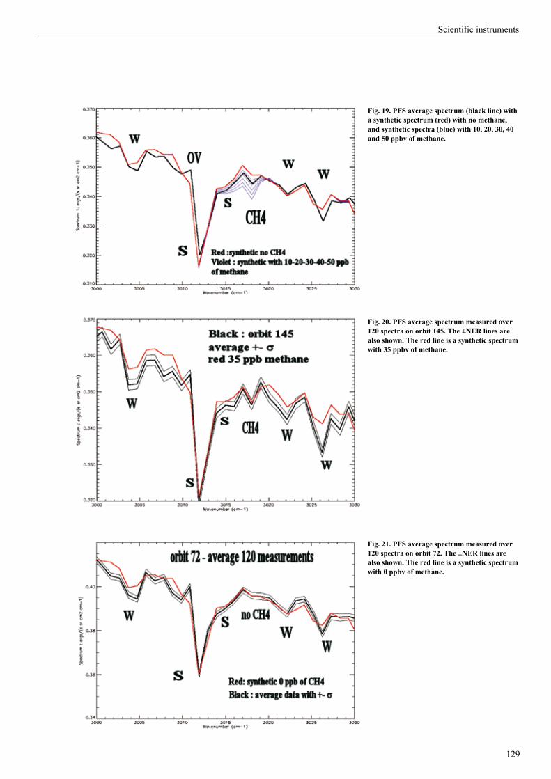
129
Scientific instruments
Fig. 21. PFS average spectrum measured over 120 spectra on orbit 72. The ±NER lines are also shown. The red line is a synthetic spectrum with 0 ppbv of methane.
Fig. 20. PFS average spectrum measured over 120 spectra on orbit 145. The ±NER lines are also shown. The red line is a synthetic spectrum with 35 ppbv of methane.
Fig. 19. PFS average spectrum (black line) with a synthetic spectrum (red) with no methane, and synthetic spectra (blue) with 10, 20, 30, 40 and 50 ppbv of methane.

An examination of orbits with higher airmass factor can provide greater confidence in the analysis, as the methane line depth should increase with increasing CH4 amounts along the line-of-sight. This is possible since Mars Express occasionally does not point to the nadir (its normal operation mode), but at a slant angle. This results in an increased air mass in the line-of-sight, which implies that the line-of-sight abundance of methane should also increase, while its mixing ratio is expected to remain unchanged. Figure 20 shows the average over 121 measurements taken during the pericentre pass of orbit 145, with an airmass factor of 1.12. In the figure, the black curve is the measured PFS spectrum with the ±σ thin lines, while the red line provides synthetic spectrum for 35 ppb of methane, but taking into account the airmass factor we obtain 30±5 ppb for the mixing ratio. The value obtained is higher than the global average value of 10 ppb, indicating that the methane mixing ratio may be variable. Motivated by this possibility, several other orbits were examined, including 68, 202 and 72, for which the airmass factors are, respectively, 1.03, 1.33 and 2.1. It was discovered that orbit 72, for which the airmass factor (2.1) was even greater than on orbit 145 (1.12), gives another extreme in CH4. Since the number of measurements for this case (120) is close to those in orbit 145, a similar sigma value is obtained. Figure 21 gives the average PFS spectrum for orbit 72. The uncertainty for this average is shown as ±σ lines. The spectrum is just like the others, with the water lines and the solar lines (together with overshooting) well evident and fitted. However, there is no indication of the methane line, and the synthetic spectrum with no CH4 fits the data nicely. As the synthetic spectrum fitting orbit 72 data was computed using the same solar spectrum as for the previous figures, it is also automatically demonstrated that the 3018 cm–1 line in the previous figures was not due to the Sun. From the four orbits 68, 145, 202 and 72, with respective airmass factors of 1.03, 1.12, 1.33 and 2.1, CH4 mixing ratios of 9, 30, 30 and 0 ppb are derived by comparing the observed methane line depth to synthetic spectra, after taking into account the airmass factors. In the case of orbit 72, it is concluded that the CH4 abundance is below the PFS detectability limit, i.e. lower than 5 ppb. The maximum value of methane is three times the global average value given above. Such behaviour seems to indicate CH4 variability over the planet.
4.2 HF and HClTwo other minor species, HF and HBr, have been identified tentatively. Both gases have a number of lines present in the PFS spectrum; some lines are clearly identified, while others may be masked by water or solar lines. For both gases, a number of lines
130
SP-1291
Fig. 22. Footprints of the PFS observations considered here, inserted into the OMEGA polar cap image. The different colours identify measurements averaged together in the study; data from three different orbits were considered.
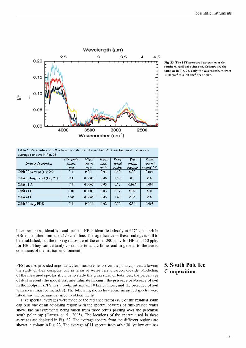
have been seen, identified and studied. HF is identified clearly at 4075 cm–1, while HBr is identified from the 2470 cm–1 line. The significance of these findings is still to be established, but the mixing ratios are of the order 200 ppbv for HF and 150 ppbv for HBr. They can certainly contribute to acidic brine, and in general to the acidic conditions of the martian environment.
PFS has also provided important, clear measurements over the polar cap ices, allowing the study of their compositions in terms of water versus carbon dioxide. Modelling of the measured spectra allow us to study the grain sizes of both ices, the percentage of dust present (the model assumes intimate mixing), the presence or absence of soil in the footprint (PFS has a footprint size of 10 km or more, and the presence of soil with no ice must be included). The following shows how some measured spectra were fitted, and the parameters used to obtain the fit.
Five spectral averages were made of the radiance factor (I/F) of the residual south cap plus one of an adjoining region with the spectral features of fine-grained water snow, the measurements being taken from three orbits passing over the perennial south polar cap (Hansen et al., 2005). The locations of the spectra used in these averages are depicted in Fig. 22. The average spectra from the different regions are shown in colour in Fig. 23. The average of 11 spectra from orbit 30 (yellow outlines
131
Scientific instruments
5. South Pole Ice Composition
Fig. 23. The PFS measured spectra over the southern residual polar cap. Colours are the same as in Fig. 22. Only the wavenumbers from 2000 cm–1 to 4350 cm–1 are shown.
Table 1. Parameters for CO2 frost models that fit specified PFS residual south polar cap averages shown in Fig. 25.
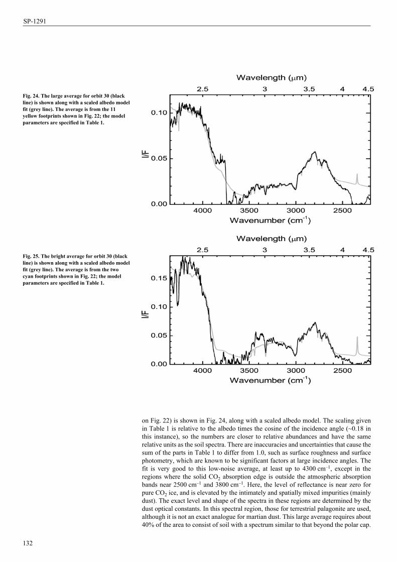
on Fig. 22) is shown in Fig. 24, along with a scaled albedo model. The scaling given in Table 1 is relative to the albedo times the cosine of the incidence angle (~0.18 in this instance), so the numbers are closer to relative abundances and have the same relative units as the soil spectra. There are inaccuracies and uncertainties that cause the sum of the parts in Table 1 to differ from 1.0, such as surface roughness and surface photometry, which are known to be significant factors at large incidence angles. The fit is very good to this low-noise average, at least up to 4300 cm–1, except in the regions where the solid CO2 absorption edge is outside the atmospheric absorption bands near 2500 cm–1 and 3800 cm–1. Here, the level of reflectance is near zero for pure CO2 ice, and is elevated by the intimately and spatially mixed impurities (mainly dust). The exact level and shape of the spectra in these regions are determined by the dust optical constants. In this spectral region, those for terrestrial palagonite are used, although it is not an exact analogue for martian dust. This large average requires about 40% of the area to consist of soil with a spectrum similar to that beyond the polar cap.
132
SP-1291
Fig. 25. The bright average for orbit 30 (black line) is shown along with a scaled albedo model fit (grey line). The average is from the two cyan footprints shown in Fig. 22; the model parameters are specified in Table 1.
Fig. 24. The large average for orbit 30 (black line) is shown along with a scaled albedo model fit (grey line). The average is from the 11 yellow footprints shown in Fig. 22; the model parameters are specified in Table 1.
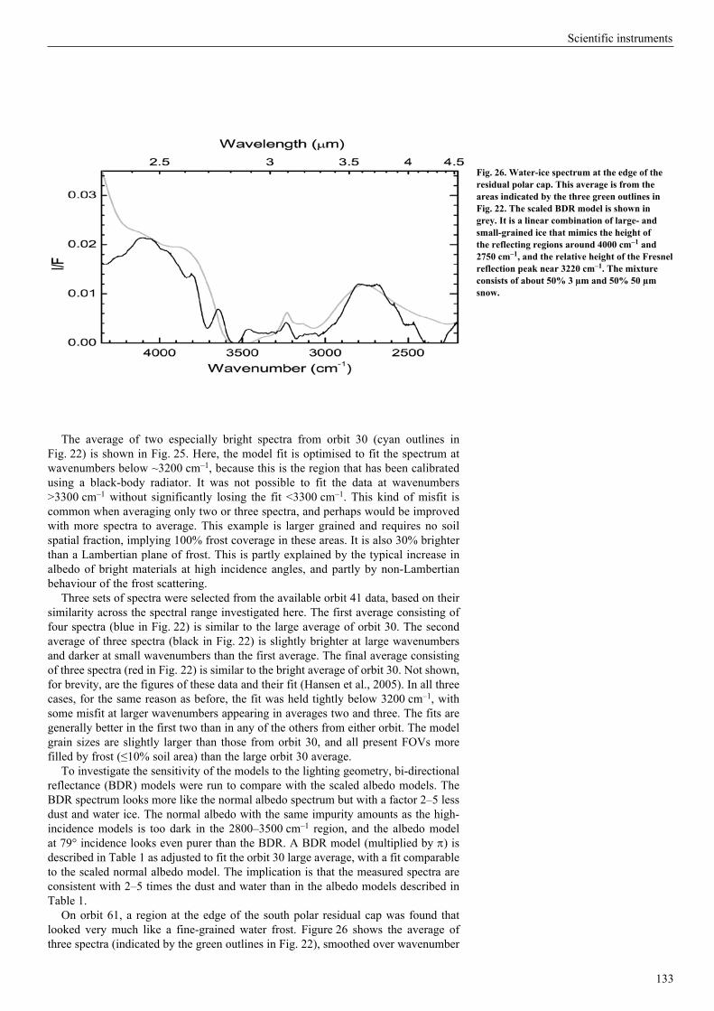
The average of two especially bright spectra from orbit 30 (cyan outlines in Fig. 22) is shown in Fig. 25. Here, the model fit is optimised to fit the spectrum at wavenumbers below ~3200 cm–1, because this is the region that has been calibrated using a black-body radiator. It was not possible to fit the data at wavenumbers >3300 cm–1 without significantly losing the fit <3300 cm–1. This kind of misfit is common when averaging only two or three spectra, and perhaps would be improved with more spectra to average. This example is larger grained and requires no soil spatial fraction, implying 100% frost coverage in these areas. It is also 30% brighter than a Lambertian plane of frost. This is partly explained by the typical increase in albedo of bright materials at high incidence angles, and partly by non-Lambertian behaviour of the frost scattering.
Three sets of spectra were selected from the available orbit 41 data, based on their similarity across the spectral range investigated here. The first average consisting of four spectra (blue in Fig. 22) is similar to the large average of orbit 30. The second average of three spectra (black in Fig. 22) is slightly brighter at large wavenumbers and darker at small wavenumbers than the first average. The final average consisting of three spectra (red in Fig. 22) is similar to the bright average of orbit 30. Not shown, for brevity, are the figures of these data and their fit (Hansen et al., 2005). In all three cases, for the same reason as before, the fit was held tightly below 3200 cm–1, with some misfit at larger wavenumbers appearing in averages two and three. The fits are generally better in the first two than in any of the others from either orbit. The model grain sizes are slightly larger than those from orbit 30, and all present FOVs more filled by frost (≤10% soil area) than the large orbit 30 average.
To investigate the sensitivity of the models to the lighting geometry, bi-directional reflectance (BDR) models were run to compare with the scaled albedo models. The BDR spectrum looks more like the normal albedo spectrum but with a factor 2–5 less dust and water ice. The normal albedo with the same impurity amounts as the high-incidence models is too dark in the 2800–3500 cm–1 region, and the albedo model at 79° incidence looks even purer than the BDR. A BDR model (multiplied by p) is described in Table 1 as adjusted to fit the orbit 30 large average, with a fit comparable to the scaled normal albedo model. The implication is that the measured spectra are consistent with 2–5 times the dust and water than in the albedo models described in Table 1.
On orbit 61, a region at the edge of the south polar residual cap was found that looked very much like a fine-grained water frost. Figure 26 shows the average of three spectra (indicated by the green outlines in Fig. 22), smoothed over wavenumber
133
Scientific instruments
Fig. 26. Water-ice spectrum at the edge of the residual polar cap. This average is from the areas indicated by the three green outlines in Fig. 22. The scaled BDR model is shown in grey. It is a linear combination of large- and small-grained ice that mimics the height of the reflecting regions around 4000 cm–1 and 2750 cm–1, and the relative height of the Fresnel reflection peak near 3220 cm–1. The mixture consists of about 50% 3 µm and 50% 50 µm snow.
because there are no fine-resolution features in the spectrum of water snow. Also shown in Fig. 26 is a model that fits it. The model is based on a bi-directional reflectance model of water snow at ~150K at the lighting geometry consistent with the observation. The model is adjusted to fit the peak reflection at 2800 cm–1 and 4000 cm–1, and the height of the Fresnel reflectance peak of water-ice at 3220 cm–1. The model consists of a spatial mixture of fine-grained water ice (to match the high reflectance) and large-grained water ice (to match the Fresnel peak). The relative abundances of fine-grained (r = 3 µm) snow and coarse-grained (r ≥ 50 µm) snow are about equal and the model is scaled by a factor of about 0.8 (implying a small amount of shadow in the footprints).
The model simulation of the PFS south polar cap spectra shows that the principal component of ice is, of course, solid carbon dioxide. However, best fits require some admixture, with water-ice amounting to (allowing for uncertainties owing to lighting geometry) not more than several tens of ppm by mass. The effective grain sizes are typically 5–10 mm, and the dust content is a few times 10– 4. These results are very similar to those from telescopic measurements of the mid-summer south polar cap in the same wavelength region (Glenar et al., 2005). A very different estimate of 15% for the H2O/CO2 mixing ratio was published by Bibring et al. (2004), on the basis of spectra obtained by OMEGA in the 2–2.6 µm wavelength range. It seems the discrepancy is related to the models rather than the data. The team’s assumption is that the CO2 and H2O are sufficiently different in volatility that they condense discretely and mix heterogeneously, like dust and ice. It is assumed that the water is mostly from atmospheric condensation and has grain sizes typical of atmospheric water-ice particles. The Bibring et al. (2004) model, on the other hand, assumes a molecular mixture of CO2 and H2O, which would be expected to produce different results to the grain mixture. The spots of high water-ice abundance in the OMEGA data, however, correspond well with the water-ice regions sampled by PFS on orbit 61 (Fig. 26). Finally, it should be stressed that only information about the composition of a thin layer can be derived from the IR spectra. What is below cannot be studied with IR remote-sensing techniques. But a predominantly CO2-covered residual south polar cap at a time when it is at its smallest extent (at the end of summer) proves from a spectroscopic point of view what thermal measurements have shown before: the persistence of CO2 is the normal state of affairs for the south over at least the last 30 years, even in the face of rapidly changing small-scale terrain features (Malin et al., 2001).
The intensities of 10 solar lines relative to the continuum, which is given in Table 1 in PFS units [erg/(s sr cm2 cm–1)], have been studied. The intensity of a solar line relative to the continuum should remain constant in time if the line is not variable (as assumed) and if there are no systematic errors in the measurements. The lines considered (Table 2) range from wavenumber 2468 cm–1 to 3012 cm–1. Their intensities with respect to the continuum span from 2.1% to 8.5%. Although there is a systematic difference in the continuum owing to higher soil temperature for PFS, the solar line intensities are essentially identical for PFS and ISO; indeed, the deviation on average seems to be only 0.02%. lt appears clear that the overshoot is present in the PFS data only for the most intense lines. If the average error on the line intensities is considered as due to noise, then there is an SNR of the order 3000 in the wavenumber range considered here (for this average of 1680 PFS measurements).The last column in Table 2 gives the FWHM of the lines studied. This quantity is useful for checking the spectral resolution of PFS; on average, the FWHM is of the order 1.5 cm–1. This does not disagree with the quoted spectral resolution of 1.3 cm resulting from studies of synthetic spectra fitting PFS measurements, because single solar lines were not necessarily selected. It may well be that some of the lines are multiple solar lines, in which case the FWHM would not be expected to be representative of the PFS spectral resolution.
134
SP-1291
6. Signatures of the Solar Spectrum
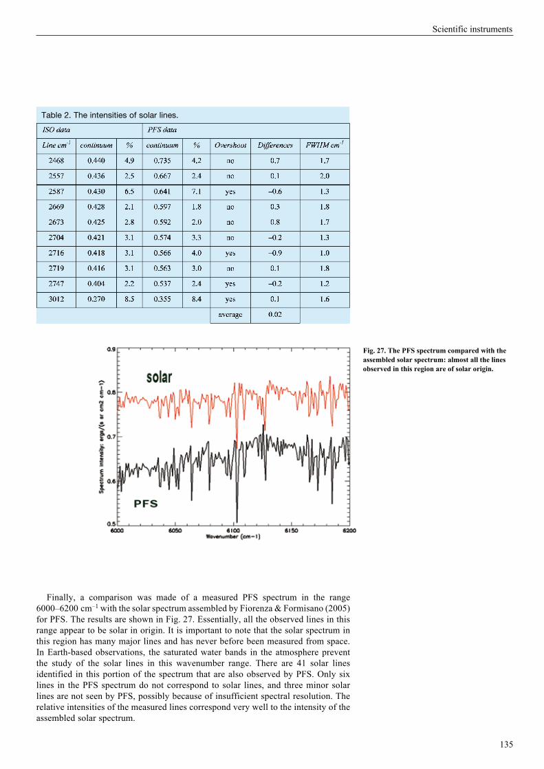
Table 2. The intensities of solar lines.
Finally, a comparison was made of a measured PFS spectrum in the range 6000–6200 cm–1 with the solar spectrum assembled by Fiorenza & Formisano (2005) for PFS. The results are shown in Fig. 27. Essentially, all the observed lines in this range appear to be solar in origin. It is important to note that the solar spectrum in this region has many major lines and has never before been measured from space. In Earth-based observations, the saturated water bands in the atmosphere prevent the study of the solar lines in this wavenumber range. There are 41 solar lines identified in this portion of the spectrum that are also observed by PFS. Only six lines in the PFS spectrum do not correspond to solar lines, and three minor solar lines are not seen by PFS, possibly because of insufficient spectral resolution. The relative intensities of the measured lines correspond very well to the intensity of the assembled solar spectrum.
135
Scientific instruments
Fig. 27. The PFS spectrum compared with the assembled solar spectrum: almost all the lines observed in this region are of solar origin.

The first PFS results have been reviewed here. PFS has worked well and produced interesting results for the range of wavenumbers explored. A comparison with the ISO SWS spectrum has been performed and has demonstrated good measurements to the lower radiance intensity level (fraction of the 0.1% level in the 1680-measurement average spectrum). The atmosphere is well studied by the LW channel; the SW channel adds minor-species composition, soil features and non-LTE emission. Finally, the details of the solar spectrum seem to appear clearly in the PFS spectrum, measured from space for the first time.
The PFS experiment was built at the Istituto di Fisica dello Spazio Interplanetario (IFSI) of the Istituto Nazionale di Astrofisica (INAF), and was funded by ASI in the context of the Italian participation in the Mars Express mission of ESA.
Bibring, J.-P., Langevin, Y., Poulet, F., Gendrin, A., Gondet, B., Berthe, M., Soufflot, A., Drossart, P., Combes, M., Bellucci, G., Maroz, V., Mangold, N. & Schmitt, B. (2004). Perennial water ice identified in the south polar cap of Mars. Nature 428, 6983–6986.
Clancy, R.T., Lee, S.W., Gladstone, G.R., McMillan, W.W. & Rousch, T. (1995). A new model for Mars atmospheric dust based upon analysis of ultraviolet through infrared observations from Mariner 9, Viking, and PHOBOS. J. Geophys. Res. 100(E3), 5251–5263.
Clancy, R.T., Wolff, M.J. & Christensen, P.R. (2003). Mars aerosol studies with the MGS TES emission phase function observations: optical depths, particle sizes, and ice cloud types versus latitude and solar longitude. J. Geophys. Res. 100(E9), 2–1, CiteID 5098, DOI: 10.1029/2003JE002058.
Conrath, B.J. (1975). Thermal structure of the martian atmosphere during the dissipation of the dust storm of 1971. Icarus 24, 36–46.
Fedorova, A.A., Leilouch, E., Titov, D.V., de Graauw, T. & Feuchtgruber, H. (2002). Remote sounding of the martian dust from ISO spectroscopy in the 2.7 µm bands. Planet. Space Sci. 50(1), 3–9.
Fiorenza, C. & Formisano, V. (2005). A solar spectrum for PFS data analysis. Planet. Space Sci.; in Press.
Forget, F., Hourdin, F., Fournier, R., Hourdin, C., Talagrand, O., Collins, M., Lewis, S.R., Read, P.L. & Huot, J. (1999). Improved general circulation models of the martian atmosphere from the surface to above 80 km. J. Geophys. Res. 100(E10), 24155–24176.
Formisano, V., Angrilli, F., Amold, G., Atreya, S., Bianchini, G., Biondi, D., Blanco, A., Blecka, M.I., Coradini, A., Colangeli, L., Ekonomov, A., Encrenaz, T., Esposito, F., Fonti, S., Giuranna, M., Grassi, D., Gnedykh, V., Grigoriev, A., Hansen, G., Hirsh, H., Khatuntsev, I., Kiselev, A., Ignatiev, N., Jurewicz, A., Lellouch, E., Lopez Moreno, J., Marten, A., Mattana, A., Maturilli, A., Mencarelli, E., Michalska, M., Moroz, V., Moshkin, B., Nespoli, F., Nikolsky, Y., Orfei, R., Orleanski, P., Orofino, V., Palomba, E., Patsaev, D., Piccioni, G., Rataj, M., Rodrigo, R., Rodriguez, J., Rossi, M., Saggin, B., Titov, D. & Zasova, L. (2005a). The Planetary Fourier Spectrometer (PFS) onboard the European Mars Express mission. Planet. Space Sci. 53, 963–974.
Formisano, V., Atreya, S., Encrenaz, T., Ignatiev, N. & Giuranna, M. (2004). Detection of methane in the atmosphere of Mars. Science 306, 1758.
Formisano, V., Encrenaz, T., Fonti, S., Giuranna, M., Grassi, D., Hirsh, H., Khatuntsev, I., Ignatiev, N., Lellouch, E., Maturilli, A., Moroz, M., Orleanski, P., Piccioni, G., Rataj, M., Saggin, B. & Zasova, L. (2005b). A martian PFS average spectrum: Comparison with ISO SWS. Planet. Space Sci. 53, 1043–1052.
Formisano, V., Maturilli, A., Giuranna, M., D’Aversa, E. & Lopez-Valverde, M.A. (2005c). PFS-MEX observations of non-LTE emission at 4–5 µm. Icarus (submitted).
Giuranna, M, Formisano, V., Biondi, D., Ekonomov, A., Fonti, S., Grassi, D., Flirsch, H., Khatuntsev, I., Ignatiev, N., Michalska, M., Mattana, A., Maturilli, A., Mencarelli, E., Nespoli, F., Orfei, R., Orleanski, P., Piccioni, G., Rataj, M., Saggin, B. & Zasova, L.
136
SP-1291
References
Acknowledgements
7. Conclusions

(2005a). Calibration of the Planetary Fourier Spectro meter Long Wavelength Channel. Planet. Space Sci. 53, 993–1007.
Giuranna, M, Formisano, V., Biondi, D., Ekonomov, A., Fonti, S., Grassi, D., Hirsch, H., Khatuntsev, I., Ignatiev, N., Michalska, M., Mattana, A., Maturilli, A., Mencarelli, E., Nespoli, F., Orfei, R., Orleanski, P., Piccioni, G., Rataj, M., Saggin, B. & Zasova, L. (2005b). Calibration of the Planetary Fourier Spectro meter Short Wavelength Channel. Planet. Space Sci. 53, 975–991.
Glenar, D.A., Hansen, G., Bjoraker, G., Smith, M., Pearl, J. & Blaney, D. (2005). Bright-region radiative properties within the Mars south polar cap (Ls=231) from near-infrared spectroscopic imaging. Icarus; in Press.
Grassi, D., Ignatiev, N.I., Zasova, L.V., Maturilli, A., Formisano, V., Bianchini, G.A. & Giuranna, M. (2005a). Methods for the analysis of data from the Planetary Fourier Spectrometer on board of the Mars Express mission. Planet. Space Sci. 53, 1017–1034.
Grassi, D., Fiorenza, C., Zasova, L.V., Ignatiev, N.I., Maturilli, A., Formisano, V. & Giuranna, M. (2005b). The martian atmosphere above great volcanoes: Early Planetary Fourier Spectrometer observations. Planet. Space Sci. 53, 1053–1064.
Hansen, G., Giuranna, M., Formisano, V., Fonti, S., Grassi, D., Hirsh, H., Ignatiev, N., Maturilli, A., Orleanski, P., Piccioni, G., Rataj, M., Saggin, B. & Zasova, L. (2005). PFS-MEX observations of ices in the residual south polar caps of Mars. Planet. Space Sci. 53, 1089–1095.
Ignatiev, N.I., Grassi, D. & Zasova, L.V. (2005). Planetary Fourier Spectrometer data analysis: fast radiative transfer models. Planet. Space Sci. 53, 1035–1042.
Lellouch, E., Encrenaz, T., de Graauw, T., Erard, S., Morris, P., Crovisier, J., Feucht gruber, H., Girard, T. & Burgdorf, M. (2000). The 2.4–45 µm spectrum of Mars observed with the Infrared Space Observatory. Planet. Space Sci. 48, 1393.
Lopez-Valverde, M.A., Lopez Puertas, M., Lopez Moreno, J.J., Formisano, V., Grassi, D., Maturilli, A., Lellouch, E. & Drossart, P. (2005). Simulation of non-LTE CO2 emissions at 4.3 µm in the martian atmosphere as observed by PFS/ Mars Express and SWS/ISO. Planet. Space Sci. 53, 1079–1087.
Malin, M.C., Caplinger, M.A. & Davis, S.D. (2001). Observational evidence for an active surface reservoir of solid carbon dioxide on Mars. Science 294, 2146–2148.
Mellon, M. (2002). TES thermal inertia global map. NASA Planetary Data System, GLOBAL_TI_60N_50S_8PPD.
Smith, D.E., Neumann, G., Arvidson, R.E., Guinness, E.A. & Slavney, S. (2003). Mars Global Surveyor laser altimeter mission experiment gridded data record. NASA Planetary Data System, MGS-M-MOLA-5-MEGDR-L3-V1.0.
Smith, M.D., Pearl, J.C., Conrath, B.J. & Christensen, P.R. (2000). Mars Global Surveyor Thermal Emission Spectrometer (TES) observations of dust opacity during aerobraking and science phasing. J. Geophys. Res. 105(E4), 9539–9552.
Titov, D.V., Fedorova, A.A. & Haus, R. (2000) A new method of remote sounding of the martian aerosols by means of spectroscopy in the 2.7 µm band. Planet. Space Sci. 48(1), 67–74.
Warren, S.G. (1984). Optical constants of ice from the ultraviolet to the microwave. Applied Optics 23, 1206–1225.
Zasova, L., Formisano, V., Moroz, V., Grassi, D., Ignatiev, N., Giuranna, M., Hansen, G., Blecka, M., Ekonomov, A., Lellouch, E., Fonti, S., Grigoriev, A., Hirsch, H., Khatuntsev, I., Mattana, A., Maturilli, A., Moshkin, B., Patsaev, D., Piccioni, G., Rataj, M. & Saggin, B. (2005). Water clouds and dust aerosols observa tions with PFS MEX at Mars. Planet. Space Sci. 53, 1065–1077.
Zurek, R.W., Barnes, J.R., Haberle, R.M., Pollack, J.B., Tillman, J.E. & Leovy, C.B. (1992). Dynamics of the atmosphere of Mars. In Mars (Eds. H.H. Kieffer, B.M. Jakowsky, C.W. Snyder & M.S. Matthews), The University of Arizona Press., Tucson, USA, pp835–933.
137
Scientific instruments

The SPICAM (Spectroscopy for the Investigation of the Characteristics of the Atmosphere of Mars) UV–IR dual spectrometer is dedicated to the study of the atmosphere of Mars. It is the first instrument to perform stellar occultations at Mars; its UV imaging spectrometer was designed primarily for atmospheric vertical profiling by stellar occultation. The IR spectrometer is dedicated to nadir measurements of H2O abundances simultaneously with UV ozone measurements, for a better understanding of the chemical coupling H2O–O3.
The principal SPICAM achievements are: the first vertical profile of density/ temperature of CO2 obtained from a planetary orbiter; numerous vertical profiles of ozone and cloud layers; the systematic measurement of total vertical ozone along-track on the dayside provides the first climatic map of ozone on Mars; the first simultaneous measurements of ozone and water vapour from an orbiter; the discovery of nightglow NO bands in UV; the discovery of auroral activity near the crustal remnant magnetic field; a thorough study of the ionosphere–upper atmosphere through high-altitude aeronomical observations of O, H, CO, CO+, and CO22
+; and the first measurement of H2O and CO2 ice albedo spectra (simultaneously with OMEGA and PFS). Other products of IR nadir observations are: surface albedo at various wavelengths; the intensity of O2(1Δg) emission due to photo-dissociation of ozone; the equivalent widths of carbon dioxide and water ice (on the surface and in aerosol layers); and water vapour total column amount.
All of these successes are the result of a highly versatile instrument, a highly capable spacecraft, and engineers and scientists dedicated to the design, building and testing of the instrument, integration on the spacecraft, and complex operations managed at ESTEC and ESOC.
139
SPICAM: Spectroscopy for the Investigation of the Characteristics of the Atmosphere of Mars
1 Service d’Aéronomie du CNRS/IPSL, BP3, F‑91371 Verrières‑le‑Buisson, France Email: jean‑[email protected] Space Research Institute (IKI), 84/32 Profsoyuznaya, 117810 Moscow, Russia 3 Belgian Institute for Space Aeronomy, 3 av. Circulaire, B‑1180 Brussels, Belgium4 Laboratoire de Météorologie Dynamique, 4 place Jussieu, F‑75252 Paris Cedex 05, Paris, France5 Lunar & Planetary Laboratory, 901 Gould Simpson Building, Univ. of Arizona, Tucson, AZ 85721, USA6 SouthWest Research Institute, 1050 Walnut Avenue, Suite 400, Boulder, CO 80302‑5143, USA7 Research & Scientific Support Department, ESTEC, Postbus 299, 2200 AG Noordwijk, the Netherlands8 Institut d’Astrophysique Spatiale, Orsay Campus, F‑91405 Orsay Cedex, France9 Finnish Meteorological Institute, PO Box 503 FIN‑00101 Helsinki, Finland
J.-L. Bertaux1, O. Korablev2, D. Fonteyn3, S. Perrier1, A. Fedorova2, F. Montmessin1, F. Leblanc1, S. Lebonnois4, F. Lefèvre1, E. Quémerais1, P. Rannou1, J.Y. Chaufray1, F. Forget4, B. Sandel5, A. Stern6, C. Muller3, E. Dimarellis1, J.P. Dubois1, S. Guibert1, G. Souchon1, M. Leclère1, F. Semelin1, A. Reberac1, M. Barthelemy1, J.C. Lebrun1, C. Taulemesse1, E. Van Ransbeeck1, B. Gondet8, A. Kiselev2, A. Rodin12, A. Stepanov2, Yu. Kalinnikov2, A. Grigoriev2, A. Hauchecorne1, M. Cabane1, E. Chassefière1, G. Cernogora1, A.C. Levasseur-Regourd1, M. De Maziere3, E. Neefs3, P.C. Simon3, D. Fussen3, D. Nevejans3, E. Arijs3, F. Hourdin4, O. Talagrand4, O. Witasse7, E. Kyrölä9 & J. Tamminen9

Mars Express is recovering most of the science lost with the launch failure in November 1996 of the Russian Mars-96 mission. SPICAM was dedicated to studying the atmosphere of Mars from top to bottom (Bertaux et al., 2000), in a variety of observing modes, including stellar occultations. It consisted of two packages: one for solar occultations, and one for stellar occultations and limb viewing. With the common electronic package, the total mass was 46 kg. Within the much more limited payload mass available on Mars Express, the design had to be radically modified. The strenuous efforts of the team produced a new instrument, called SPICAM Light, a 4.7 kg UV–IR instrument able to deliver most of the science of the Mars-96 version. The considerable mass saving was achieved by sacrificing all the visible part of the spectrum in the solar and stellar occultation sensors, and by removing all redundancy between the two sensors. Also, the pointing ability of Mars Express avoided the need for the instrument platforms of Mars-96. SPICAM Light was originally proposed to include the separate solar occultation IR sensor (SOIR) inherited from the solar package of SPICAM/Mars-96. This 3.8 kg sensor consisted of a grating spectrometer (1.2–4.8 µm, resolution 0.4–1 nm) for vertical profiling during solar occultations of H2O, CO2, CO, aerosols and exploration of carbon compounds such as methane (Bertaux et al., 2000). The severe mass constraints precluded its inclusion; instead, an extremely lightweight near-IR spectrometer based on acousto-optical tuneable filter (AOTF) technology, dedicated to water vapour measurements at 1.38 µm, and designed in Russia, was accepted by ESA.
This chapter presents an overview of the instruments, the modes of observations, some statistics on the number of observations, and a summary of the main scientific results. These results are discussed in much greater detail in several dedicated papers: the retrieval of occultation data (Quémerais et al., 2006), total ozone mapping (Perrier et al., 2006), ozone vertical profiling (Lebonnois et al., 2006), dust and aerosol vertical profiles (Montmessin et al., 2006), dayglow and nightglow (Leblanc et al., 2006), limb dust measurements (Rannou et al., 2006), and water vapour measurements (Fedorova et al., 2006). This chapter is based on material presented in Bertaux et al. (2006) and Korablev et al. (2006).
140
SP-1291
1. Introduction
Fig. 1. Mechanical layout of the SUV and SIR channels. The IR AOTF spectrometer is at the front; the UV spectrometer is at the rear. The common optical axis points to the right (the +Z axis of the spacecraft).
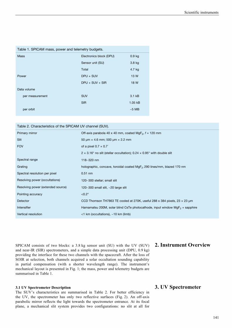
141
Scientific instruments
2. Instrument Overview
Table 2. Characteristics of the SPICAM UV channel (SUV).
Primary mirror Off-axis parabola 40 x 40 mm, coated MgF2, f = 120 mm
Slit 50 µm × 4.6 mm; 500 µm × 2.2 mm
FOV of a pixel 0.7 × 0.7´
2 × 3.16° no slit (stellar occultation); 0.24 × 0.95° with double slit
Spectral range 118–320 nm
Grating holographic, concave, toroidal coated MgF2, 290 lines/mm, blazed 170 nm
Spectral resolution per pixel 0.51 nm
Resolving power (occultations) 120–300 stellar; small slit
Resolving power (extended source) 120–300 small slit, ~20 large slit
Pointing accuracy <0.2°
Detector CCD Thomson TH7863 TE cooled at 270K, useful 288 x 384 pixels, 23 × 23 µm
Intensifier Hamamatsu 200M, solar blind CsTe photocathode, input window MgF2 + sapphire
Vertical resolution <1 km (occultations), ~10 km (limb)
Table 1. SPICAM mass, power and telemetry budgets.
Mass Electronics block (DPU) 0.9 kg
Sensor unit (SU) 3.8 kg
Total 4.7 kg
Power DPU + SUV 13 W
DPU + SUV + SIR 18 W
Data volume
per measurement SUV 3.1 kB
SIR 1.05 kB
per orbit ~5 MB
SPICAM consists of two blocks: a 3.8 kg sensor unit (SU) with the UV (SUV) and near-IR (SIR) spectrometers, and a simple data processing unit (DPU, 0.9 kg) providing the interface for these two channels with the spacecraft. After the loss of SOIR at selection, both channels acquired a solar occultation sounding capability in partial compensation (with a shorter wavelength range). The instrument’s mechanical layout is presented in Fig. 1; the mass, power and telemetry budgets are summarised in Table 1.
3.1 UV Spectrometer DescriptionThe SUV’s characteristics are summarised in Table 2. For better efficiency in the UV, the spectrometer has only two reflective surfaces (Fig. 2). An off-axis parabolic mirror reflects the light towards the spectrometer entrance. At its focal plane, a mechanical slit system provides two configurations: no slit at all for
3. UV Spectrometer

stellar occultations, and a slit for extended sources. The slit is divided into two, with different widths providing two spectral resolutions when observing extended sources. The 50 µm-wide slit provides good resolution at lower fluxes; the 500 µm slit offers more sensitivity at the expense of a coarser spectral resolution. The slit can be completely retracted, leaving a hole corresponding to the total useful field of view (FOV; 2 × 3.16°). This configuration is used in the stellar occultation mode with a dark limb when the spectrum of the star is recorded on a few lines of the CCD. The required pointing accuracy is 0.2°, but the achieved spacecraft pointing accuracy is often much better on Mars Express, after accounting for a small mechanical misalignment of SPICAM with the craft’s axis, which was measured in flight using star observations. It has been possible on some occasions to perform stellar occultations within the narrow part of the slit (0.02° wide), allowing some vertical profiling even on the dayside.
A holographic concave toroidal grating from Jobin–Yvon, ion-etched for efficiency, feeds the detection block. The image ratio is ~1, which means that a monochromatic image in the entrance of the spectrometer is conserved in the detector plane (Fig. 3). The spectral resolution for a point source determined by aberrations is about 1 nm. The CCD detector is a Thomson TH7863 with 288 × 384 useful pixels, and a masked zone of equivalent size. Pixel size is 23 × 23 µm. The detector is electrically cooled to ~0°C; at this temperature the dark current equals 800 electrons per pixel per second, or a few analogue to digital units (ADUs) only. By means of custom fibre optics, the CCD is coupled with the output window of the image intensifier (Hamamatsu type 200M). A solar-blind CsTe photocathode has zero quantum efficiency beyond 320 nm. The input window is made of MgF2 to reach down to Lyman-a wavelengths – an important target for SPICAM. A sapphire filter partially covers the window, preventing overlapping of diffraction orders and Lyman-a stray light.
For solar occultations, there is a 0.2 cm2 mirror at 90° to the main optical axis at the entrance pupil. During solar occultation measurements, the detector operates at the lowest gain and an integration time of 20 ms. The focal length of the telescope is such that one CCD pixel covers a FOV of 0.01 × 0.01°. The narrow part (0.02° wide by 1.9° long) of the spectrometer slit has a spectral resolution of 1.5 nm (about 3 CCD pixels), while the wide part (0.2° wide by 0.98° long) has a higher photometric sensitivity for extended sources (factor ~8), at the expense of a reduced spectral resolution (6 nm). In principle, SPICAM can record 288 spatially resolved spectra along its 2.88°-long
142
Nadirdirection
20
21
Ø30
12
789
10
1113
14
Sundirection
Nadirdirection
40x40
2
3
1
4
5
6
17
16
18
19
15
Fig. 2. Optical scheme of SPICAM’s UV and IR channels. 1: aperture blend of the UV channel; 2: off-axis parabolic mirror; 3: slit (can be changed from wide to narrow, by a mechanical actuator; see text); 4: concave UV grating; 5: intensifier; 6: CCD; 7: IR channel objective; 8: IR FOV diaphragm; 9/11: collimating lens; 10: AOTF crystal; 12: light trap for undiffracted light; 13: detector proximity lenses; 14: ‘extraordinary’ beam detector; 15: ‘ordinary’ beam detector; 16: solar opening (closed by shutter when not looking at Sun); 17/21: flat mirror; 18: IR solar entry; 19: optical fibre; 20: fibre collimator.
SP-1291

slit (i.e. each spatial element subtends 0.02 × 0.01° on the sky). However, in practice, only five spectra are transmitted for each 1 s measurement in order to save on data transmission. These spectra are formed differently for various modes of CCD readout (see Fig. 6). The most-used mode is such that each of the five spectra is a sum of N individual CCD line spectra (binned on chip in the readout line, before reading), with N = 2, 4, 8, 16 or 32, forming five adjacent spatial bins of variable extent (from 0.02° to 0.32°). Two other modes may be used for special purposes: a full imaging mode, when the whole CCD is read, five consecutive lines at each reading, with the first displaced by four lines; and a ‘progressive binning’ mode that provides a higher dynamic, since 2, 4, 8, 16 and 32 lines are binned together in the five spectra transmitted via telemetry (with the risk of saturation and overspilling of the register). This mode was useful at the beginning to optimise the gain level and integration time for nadir observations.
The gain of the Micro Channel Plate (MCP) of the image intensifier may be adjusted by telecommand with a high-voltage level of 500–900 V, commanded by a digital-level HT of 0–255. When a photoelectron is created in the photocathode (a photo-event), it results in a pulse of light from the phosphor, distributed over a few pixels of the CCD. It is detected by the CCD reading electronics by a number of ADUs. At HT = 20 (a typical low gain necessary to avoid saturation for dayside nadir observations), there are about 1.5 ADU created per photo-event; for HT = 200, there are ~40 ADU per photo-event. The absolute calibration of the instrument is well characterised by numerous observations of hot UV stars and comparison with previous International Ultraviolet Explorer (IUE) measurements.
There is a potential danger to activating the intensifier at a large gain with an intense source of light. This high gain has to be used cautiously on the dayside at high altitude, and on the nightside. A constraint of SPICAM operations is that the instrument parameters may not be changed during an observing period (ON–OFF). In particular, when a fixed inertial attitude of the spacecraft is chosen, it must be certain that the signal will not damage the detector if a high gain is used on a bright target.
3.2 Instrument Characteristics Measured on the GroundFigure 4 is an overall view of SPICAM. Figure 5 shows the detector illuminated through the optics by monochromatic light (Hg line emission at 253.7 nm). Some
143
Fig. 3. The SPICAM UV detector combines an image intensifier from Hamamatsu, transforming each UV photon at the entrance into a pulse of green light generated by the phosphor. The image is then conveyed through two blocks of fibre optics, one in the Hamamatsu detector, the other attached to the Thomson CCD. (W. Sandel, Lunar & Planetary Laboratory)
Scientific instruments
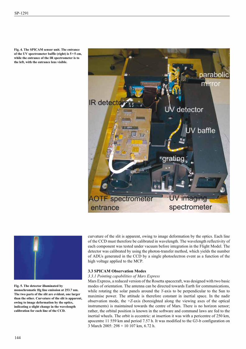
curvature of the slit is apparent, owing to image deformation by the optics. Each line of the CCD must therefore be calibrated in wavelength. The wavelength reflectivity of each component was tested under vacuum before integration in the Flight Model. The detector was calibrated by using the photon-transfer method, which yields the number of ADUs generated in the CCD by a single photoelectron event as a function of the high voltage applied to the MCP.
3.3 SPICAM Observation Modes3.3.1 Pointing capabilities of Mars ExpressMars Express, a reduced version of the Rosetta spacecraft, was designed with two basic modes of orientation. The antenna can be directed towards Earth for communications, while rotating the solar panels around the Y-axis to be perpendicular to the Sun to maximise power. The attitude is therefore constant in inertial space. In the nadir observation mode, the +Z-axis (boresighted along the viewing axes of the optical instruments) is maintained towards the centre of Mars. There is no horizon sensor; rather, the orbital position is known in the software and command laws are fed to the inertial wheels. The orbit is eccentric: at insertion it was with a pericentre of 250 km, apocentre 11 559 km and period 7.57 h. It was modified to the G3-b configuration on 3 March 2005: 298 × 10 107 km, 6.72 h.
144
Fig. 4. The SPICAM sensor unit. The entrance of the UV spectrometer baffle (right) is 5 × 5 cm, while the entrance of the IR spectrometer is to the left, with the entrance lens visible.
Fig. 5. The detector illuminated by monochromatic Hg line emission at 253.7 nm. The two parts of the slit are evident, one larger than the other. Curvature of the slit is apparent, owing to image deformation by the optics, indicating a slight change in the wavelength calibration for each line of the CCD.
SP-1291
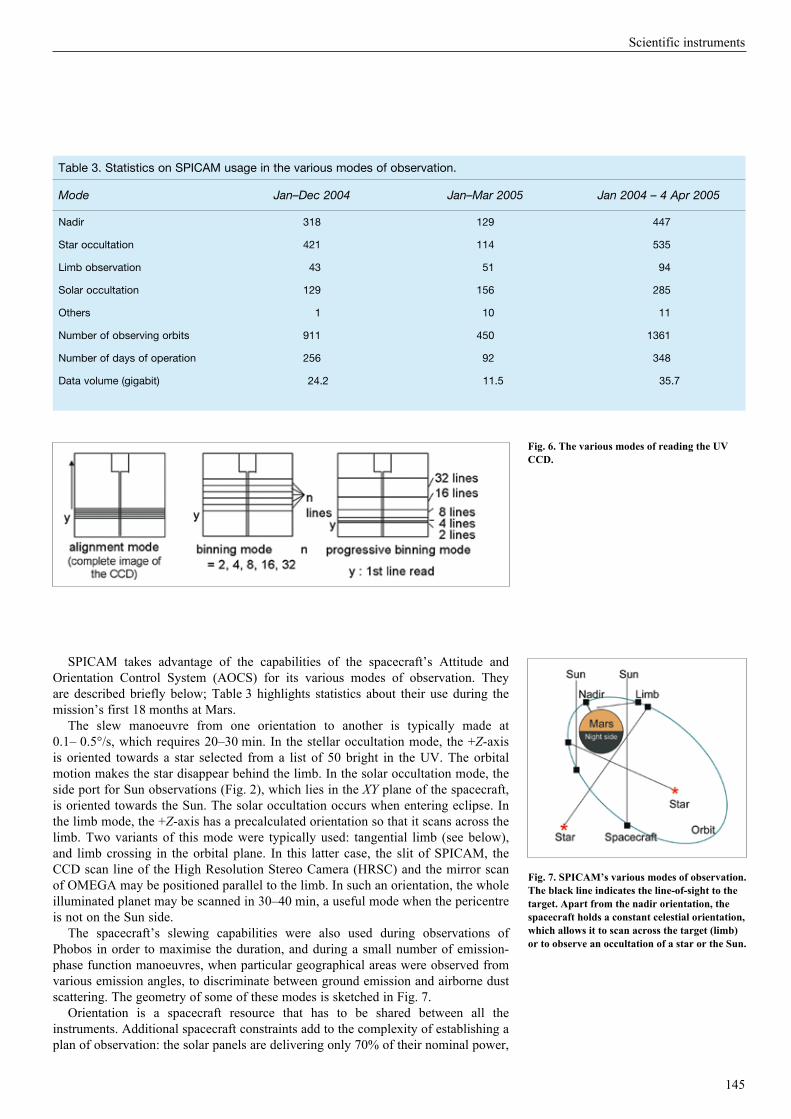
SPICAM takes advantage of the capabilities of the spacecraft’s Attitude and Orientation Control System (AOCS) for its various modes of observation. They are described briefly below; Table 3 highlights statistics about their use during the mission’s first 18 months at Mars.
The slew manoeuvre from one orientation to another is typically made at 0.1– 0.5°/s, which requires 20–30 min. In the stellar occultation mode, the +Z-axis is oriented towards a star selected from a list of 50 bright in the UV. The orbital motion makes the star disappear behind the limb. In the solar occultation mode, the side port for Sun observations (Fig. 2), which lies in the XY plane of the spacecraft, is oriented towards the Sun. The solar occultation occurs when entering eclipse. In the limb mode, the +Z-axis has a precalculated orientation so that it scans across the limb. Two variants of this mode were typically used: tangential limb (see below), and limb crossing in the orbital plane. In this latter case, the slit of SPICAM, the CCD scan line of the High Resolution Stereo Camera (HRSC) and the mirror scan of OMEGA may be positioned parallel to the limb. In such an orientation, the whole illuminated planet may be scanned in 30–40 min, a useful mode when the pericentre is not on the Sun side.
The spacecraft’s slewing capabilities were also used during observations of Phobos in order to maximise the duration, and during a small number of emission-phase function manoeuvres, when particular geographical areas were observed from various emission angles, to discriminate between ground emission and airborne dust scattering. The geometry of some of these modes is sketched in Fig. 7.
Orientation is a spacecraft resource that has to be shared between all the instruments. Additional spacecraft constraints add to the complexity of establishing a plan of observation: the solar panels are delivering only 70% of their nominal power,
145
Fig. 6. The various modes of reading the UV CCD.
Fig. 7. SPICAM’s various modes of observation. The black line indicates the line-of-sight to the target. Apart from the nadir orientation, the spacecraft holds a constant celestial orientation, which allows it to scan across the target (limb) or to observe an occultation of a star or the Sun.
Table 3. Statistics on SPICAM usage in the various modes of observation.
Mode Jan–Dec 2004 Jan–Mar 2005 Jan 2004 – 4 Apr 2005
Nadir 318 129 447
Star occultation 421 114 535
Limb observation 43 51 94
Solar occultation 129 156 285
Others 1 10 11
Number of observing orbits 911 450 1361
Number of days of operation 256 92 348
Data volume (gigabit) 24.2 11.5 35.7
Scientific instruments

the radiators cooling some instruments should not be illuminated by the Sun, and a window of 4 h per day is reserved for uplink telecommanding, among others. As a result, the plan adopted 3 months in advance of execution is a compromise between contradictory requirements from the various instruments and the spacecraft, usually resolved during lively animated teleconferences between ESA and the Principal Investigator teams. Table 3 indicates the type and number of observations obtained with SPICAM from orbit insertion (25 December 2003) to 4 April 2005.
3.3.2 Geometry of nightglow/dayglow limb observations: the tangential limb modeAirglow spectroscopy and radiometry are powerful methods for investigating the upper atmospheres of the terrestrial planets. After the pioneering work by the UV spectrometers of Mariner-6, -7 and -9 (Barth et al., 1971; 1992), this technique was neglected for the following 30 years at Mars, except for rare observations in the EUV with rockets and Earth-orbiting observatories.
While dayglow was clearly measured and identified in the Mariner observations, the first detection of nightglow in the atmosphere of Mars was made with SPICAM (Bertaux et al., 2005a). This was the result of SPICAM’s high sensitivity and the dedicated spacecraft operations to optimise the geometry of limb observations, yielding higher signals than the nominal nadir-looking geometry around pericentre. This geometry is illustrated in Fig. 8.
Planning a limb observation requires finding an inertial direction such that, during the orbital motion, the line-of-sight (LOS) scans across the limb. In order to maximise the duration of the observation, the LOS skims the limb tangentially, with a selectable minimum altitude. For any point M on the eccentric orbit, there are two LOS directions that will skim the limb tangentially, with a specified minimum altitude Zmin. They are contained in the two planes tangential to the sphere of radius RMars + Zmin, which also contain the tangent to the orbit at M (the velocity vector). One is selected to plan the observation, as well as the point M, according to the desired position of the tangent point at minimum altitude. One particularity of this kind of observation is
146
Fig. 8. The geometry of limb-grazing observations, which maximise the time spent observing the limb from an eccentric orbit. It was used successfully on Mars Express, and is also employed by Venus Express. The spacecraft is oriented with the +Z-axis (SPICAM line-of-sight) fixed inertially, scanning the limb twice. In this case, the line-of-sight was perpendicular to the velocity vector at pericentre, for optimum vertical resolution at the limb.
Fig. 9. Distribution of light over the whole detector when a star is observed without the slit. The intensity (in ADUs) is colour-coded. The spectrum is horizontal, along the CCD lines, parallel to the spacecraft Y-axis. Optical aberrations spread the spectrum over several lines of the CCD. The slit orientation is parallel to the spacecraft X-axis, along the column axis of the CCD (vertically on this figure). The ‘tapestry’ effect is a residual electronic noise (pseudo-periodic), after subtraction of offset and dark charge.
SP-1291

that several geometrical parameters of the LOS tangent point vary significantly and simultaneously during the observation: altitude, latitude and solar zenith angle. Given the success of this observation mode on Mars Express to detect weak emissions (two discoveries: NO bands at night, and aurora), it is also used on Venus Express.
3.4 Flight Performance of the UV Spectrometer3.4.1 Pointing qualityFor all SPICAM modes, the quality of the results depends on the pointing quality. The pointing accuracy of Mars Express is usually (but not always) much better than the specified 0.1°. Although in principle they are boresighted, there is some offset between the centre of SPICAM’s CCD detector and the +Z-axis: 0.17° in one direction (along the wavelength axis, parallel to the spacecraft’s Y-axis), and <0.01° in the perpendicular direction along the X-axis, as determined by star spectra during cruise and outside the atmosphere in the alignment mode, which provides a full image of the CCD (Fig. 9).
For a star observation, the spacecraft is requested to position the inertial direction of the star (α, δ) exactly along the Z-axis, or with some offset from the Z-axis, along a direction defined by two angles θ, ϕ, in the body axis reference frame. θ is the angle of the projection of this direction on the X,Y plane of the X‑axis, and ϕ is the angle of this projection with the direction.
Several offset angles were tried, projecting a test star’s spectrum in various places on the detector. Figure 10 shows the recorded spectrum of Sirius (41 times in total) in ADU units, on the same wavelength scale, obtained between orbits 906 and 1410 (spanning about 5 months). It shows the excellent stability of the instrument, with no sign of ageing. The curves are different between ~135 nm and 180 nm. This is the effect of the sapphire window, which protrudes into the middle of this wavelength interval for nominal pointing. The sensitivity is higher outside of the window than through it, because its transmission is <1. There is no abrupt change on the curve at the position of the sapphire edge because a point on the cathode at or around the edge ‘sees’ the grating over an angle of ~20°, partly through the window and partly outside, providing a continuous response to a continuous spectrum.
It was recently discovered that the pointing is not perfectly repeatable. With exactly the same offset angles (q, f) the spectrum of star Zeta Puppis should be at the same place on the detector, but it is not. As shown in Fig. 11, there are two places where it differs by about 0.1°, corresponding to about 6 nm in wavelength shift. At each position, all spectra of one class are precisely superimposed. This problem triggers two difficulties. The first is that the commanded offset pointing cannot be relied upon to establish the wavelength assignment of each pixel of the star spectrum, so the star spectrum recorded outside the atmosphere has to be examined carefully to determine exactly its wavelength assignment (the wavelength of each pixel). The second is that a number of star occultations with the slit in place have failed.
Star occultations are usually made without the slit, because a star is a point source. Some occultations were performed on the dayside with the slit, which partially eliminates the solar light scattered at the limb by dust and the atmosphere. Some were successful: the star signal has about half the strength than without the slit, because of optical aberrations in the off-axis parabolic mirror. Several others failed because of the pointing unrepeatability. This problem may affect other instruments. It comes from startracker A or the redundant startracker B not being perfectly co-aligned.
The pointing stability is quite good. When a star is observed outside of the atmosphere, the signal is usually recorded in five bands of eight CCD lines, the central band collecting >90 % of the total star signal (computed from Fig. 13). The signal in the central band does not show periodic fluctuations (at least before the deployment of MARSIS), which would be a sign of angular oscillations. All slew manoeuvres of the spacecraft (at a maximum 0.5°/s) are followed by a ‘tranquilisation’ period of about 10 min, before the spacecraft may be considered stable and SPICAM is switched ON. In fact, in order to monitor the spacecraft motions, dedicated observation of a
147
Fig. 10. Forty-one spectra of Sirius (O28 in the SPICAM star catalogue) recorded outside the atmosphere of Mars, between orbits 906 and 1410 (spanning 5 months). They are shown in ADU units, and on the same wavelength scale. The different offset pointings resulted in various positions on the detector. The excellent stability of the instrument is evident, with no sign of ageing. The curves differ between ~135 nm and 180 nm, resulting from the edge of the sapphire window, which is positioned in the middle of this wavelength interval for nominal pointing.
Scientific instruments
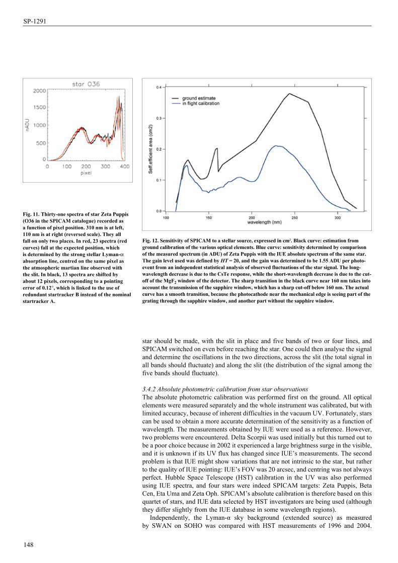
star should be made, with the slit in place and five bands of two or four lines, and SPICAM switched on even before reaching the star. One could then analyse the signal and determine the oscillations in the two directions, across the slit (the total signal in all bands should fluctuate) and along the slit (the distribution of the signal among the five bands should fluctuate).
3.4.2 Absolute photometric calibration from star observationsThe absolute photometric calibration was performed first on the ground. All optical elements were measured separately and the whole instrument was calibrated, but with limited accuracy, because of inherent difficulties in the vacuum UV. Fortunately, stars can be used to obtain a more accurate determination of the sensitivity as a function of wavelength. The measurements obtained by IUE were used as a reference. However, two problems were encountered. Delta Scorpii was used initially but this turned out to be a poor choice because in 2002 it experienced a large brightness surge in the visible, and it is unknown if its UV flux has changed since IUE’s measurements. The second problem is that IUE might show variations that are not intrinsic to the star, but rather to the quality of IUE pointing: IUE’s FOV was 20 arcsec, and centring was not always perfect. Hubble Space Telescope (HST) calibration in the UV was also performed using IUE spectra, and four stars were indeed SPICAM targets: Zeta Puppis, Beta Cen, Eta Uma and Zeta Oph. SPICAM’s absolute calibration is therefore based on this quartet of stars, and IUE data selected by HST investigators are being used (although they differ slightly from the IUE database in some wavelength regions).
Independently, the Lyman-α sky background (extended source) as measured by SWAN on SOHO was compared with HST measurements of 1996 and 2004.
148
Fig. 11. Thirty-one spectra of star Zeta Puppis (O36 in the SPICAM catalogue) recorded as a function of pixel position. 310 nm is at left, 110 nm is at right (reversed scale). They all fall on only two places. In red, 23 spectra (red curves) fall at the expected position, which is determined by the strong stellar Lyman-a absorption line, centred on the same pixel as the atmospheric martian line observed with the slit. In black, 13 spectra are shifted by about 12 pixels, corresponding to a pointing error of 0.12°, which is linked to the use of redundant startracker B instead of the nominal startracker A.
Fig. 12. Sensitivity of SPICAM to a stellar source, expressed in cm2. Black curve: estimation from ground calibration of the various optical elements. Blue curve: sensitivity determined by comparison of the measured spectrum (in ADU) of Zeta Puppis with the IUE absolute spectrum of the same star. The gain level used was defined by HT = 20, and the gain was determined to be 1.55 ADU per photo-event from an independent statistical analysis of observed fluctuations of the star signal. The long-wavelength decrease is due to the CsTe response, while the short-wavelength decrease is due to the cut-off of the MgF2 window of the detector. The sharp transition in the black curve near 160 nm takes into account the transmission of the sapphire window, which has a sharp cut-off below 160 nm. The actual curve has a smooth transition, because the photocathode near the mechanical edge is seeing part of the grating through the sapphire window, and another part without the sapphire window.
SP-1291

Throughout this period, the ageing of the SWAN sensors was monitored through observations of UV stars (Quémerais et al., 2006). Full consistency was found between the calibration factors found by comparing HST and SWAN measurements of the Lyman-α sky background after 8 years, and the ageing was determined by the SWAN star signal variation during the same period.
The IUE spectrum, given in erg/(cm2 s Å), is converted to a photon flux Φ (in photons/(cm2 s nm). SPICAM data are in ADU units, the output of CCD reading. As described above, the high voltage of the image intensifier may be adjusted to increase or reduce the ADUs per photo-event (one photoelectron created at the cathode of the image intensifier, creating a pulse of light in the CCD), a parameter designated as G, the gain of the detector system.
The calibration factor of SPICAM is therefore G Seff, where Seff is the ‘efficient area’ expressed in cm2, and defined in the relation:
Nphotev = Φ Seff
where Nphotev is the number of photo-events detected by SPICAM per second and per nanometre. There is also the relationship:
NADU = G Nphotev
resulting in the calibration equation:
G Seff = Φ / NADU
The gain G was determined on the ground for various levels of the voltage of the image intensifier. It varies from 1.0 to 79 in the whole range of possible commanded voltage levels, defined by the instrument parameter HT (from 1 to 255). The gain was also checked in flight by a statistical method, by determining the mean number of photo-events contained in the whole band devoted to the star signal outside of the atmosphere. The total ADU signal fluctuations were analysed, and the gain G determined as:
G = Var (SADU)/ (2 SADU)
where SADU is the mean value of a series of measurements, Var(SADU) is the variance of the series, and the factor 2 comes from the non-gaussian distribution of the number of electrons coming from a single photo-event (Sandel & Broadfoot, 1986).
Figure 12 shows the sensitivity of SPICAM to a stellar source, Seff (in cm2), as a function of wavelength. The drop at the short-wavelength cut-off is due to the opacity of the MgF2 window, while the drop at long wavelength is due to the drop-off of the CsTe cathode (the solar blind behaviour). This curve represents the sensitivity of the instrument for a star source placed at the ‘correct’ position, defined as the centre of the spectrometer slit. The nominal wavelength assignment is also defined as such, making it valid for all extended source measurements collected with the slit in place. Figure 10 indicates that, when the star is elsewhere, the sensitivity across the detector is similar (at least in the small region explored), except near the edge of the sapphire widow. Also, this curve is valid only when the star signal is integrated over 8 CCD lines (centred on CDD line 144), collecting 90% of the total signal.
When using this Seff curve for the calibration of extended source measurements (filling the whole slit), this 90% factor has to be taken into account (because the whole signal is collected with an extended source), along with the actual FOV of one CCD line: 50 µm (slit width) × 23 µm (CCD pixel size) and the focal length of 120 mm of the parabolic mirror. The solid angle dw subtended by one CCD line is therefore 7.986 × 10⁻⁸ sr. In Rayleigh airglow units, 1 R = 106 / 4p photons/(cm2 s sr), so an extended source with a brightness B of 1 R/nm would give:
149
Scientific instruments
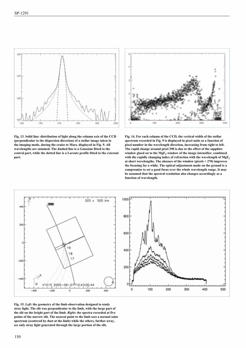
150
Fig. 13. Solid line: distribution of light along the column axis of the CCD (perpendicular to the dispersion direction) of a stellar image taken in the imaging mode, during the cruise to Mars, displayed in Fig. 9. All wavelengths are summed. The dashed line is a Gaussian fitted to the central part, while the dotted line is a Lorentz profile fitted to the external part.
Fig. 14. For each column of the CCD, the vertical width of the stellar spectrum recorded in Fig. 9 is displayed in pixel units as a function of pixel number in the wavelength direction, increasing from right to left. The rapid change around pixel 290 is due to the effect of the sapphire window glued on to the MgF2 window of the image intensifier, combined with the rapidly changing index of refraction with the wavelength of MgF2 at short wavelengths. The absence of the window (pixels > 270) improves the focusing for a while. The optical adjustment made on the ground is a compromise to set a good focus over the whole wavelength range. It may be assumed that the spectral resolution also changes accordingly as a function of wavelength.
Fig. 15. Left: the geometry of the limb observation designed to study stray light. The slit was perpendicular to the limb, with the large part of the slit on the bright part of the limb. Right: the spectra recorded at five points of the narrow slit. The nearest point to the limb sees a normal solar spectrum (scattered by dust at the limb) while the others, further away, see only stray light generated through the large portion of the slit.
SP-1291

NADUB = G B dw Seff / 0.9 = 1.06 × 10⁻² Seff
in ADU per second and per nm, for each line of the detector, at gain G = 1.5.When a star is observed without the slit, the light is spread over many CCD lines,
with a distribution perpendicular to the dispersion axis (along CCD columns), as shown in Fig. 13. When the usual configuration of five bands of eight CCD lines each is used, the relative content is 1, 3, 90, 5 and 1%, respectively, for bands 1 to 5. This spreading is most likely due to scattering on the surface of the grating, or within the MgF2 window of the detector. It is a sign of internal stray light, generated after the slit or focal plane of the mirror. Some photons are detected away from their nominal positions, both vertically and in wavelength. Analysis of solar light scattered at the limb (see below) determined the level of stray light, mainly from the large part of the slit, and allowed a systematic correction to be made for it.
On some rare occasions, evidence was found of external stray light, defined as detected photons coming from outside the nominal FOV defined by the slit at the focal plane of the parabolic mirror. This external stray light is still being characterised.
3.4.3 Internal stray light correctionKnowing that the light from a star is spread over a large area (Fig. 13), it was suspected that, when the whole slit is illuminated, the light entering the slit at places other than the lines of the CCD readout will spread over the whole CCD. In particular, a large contribution from the wide part of the slit might be expected.
This problem was resolved with the limb observation during orbit 1788 on 7 June 2005 (solar longitude 225.7°, distance to the Sun 1.39 AU); 1181 spectra were recorded in about 20 min. The observation was made with inertial pointing and grazing geometry, with a minimum altitude of 50 km below the limb, so the limb crossing was slow. The measuring lines were binned by four, covering lines 135 to 155, which are all on the narrow part of the slit, near the centre of the CCD (line 144). The distribution of dust-scattered light at the limb can be considered as a knife-edge to a first approximation: very bright below a certain altitude, with a very rapid drop above. The spacecraft was oriented with its X-axis (and slit direction) perpendicular to the limb, with the wide slit looking at lower altitudes than the narrow slit (Fig. 15). Scanning the whole limb up to 200 km (duration 200 s from 0 km to 200 km), there were times when only the wide slit was illuminated by the bright limb.
Figure 16 shows the mean light detected on the CCD as a function of time. The signals of the five bands are very similar, with the shift in time corresponding to the shift in altitude at the limb. The limb signal is expected to drop rapidly, but there is still a slow decrease after the initial fast reduction (between 700 s and 900 s after the beginning of the observation); this is suspected to be stray light from the wide slit. Indeed, the spectrum of this emission (Fig. 17) is completely different from the usual nadir or limb spectra (Fig. 20). There are no strong UV features of the solar UV spectrum. The fifth band, nearer the wide slit, detects more light than the first, which is further from the upper part of the CCD, where the wide slit is. This also confirms that, closer to the wide slit, more stray light is collected in the observed bands. This stray light represents around 10% of the signal. A detailed study was performed by Perrier (2005), yielding the contribution of stray light from all parts of the slit to the read bands. Assuming that the whole slit is illuminated by the same spectrum, it is then possible to subtract from each measurement the spectrum of stray light in Fig. 17 scaled by an appropriate factor, depending on the actual intensity recorded. This was done for the correction of the nadir data for the extraction of ozone content. When the scenery is not uniform over the slit FOV on the ground at a scale of a few km (as over the polar caps), the correction for stray light will not be so accurate.
151
Scientific instruments
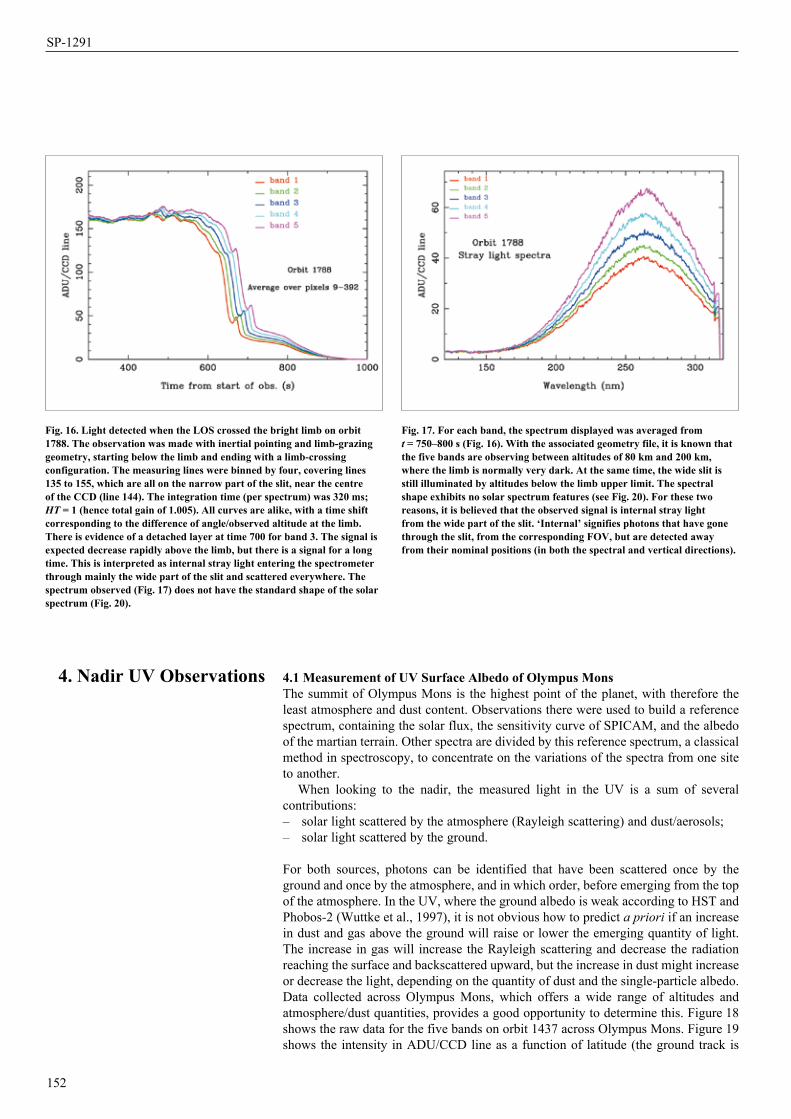
4.1 Measurement of UV Surface Albedo of Olympus MonsThe summit of Olympus Mons is the highest point of the planet, with therefore the least atmosphere and dust content. Observations there were used to build a reference spectrum, containing the solar flux, the sensitivity curve of SPICAM, and the albedo of the martian terrain. Other spectra are divided by this reference spectrum, a classical method in spectroscopy, to concentrate on the variations of the spectra from one site to another.
When looking to the nadir, the measured light in the UV is a sum of several contributions:– solar light scattered by the atmosphere (Rayleigh scattering) and dust/aerosols;– solar light scattered by the ground.
For both sources, photons can be identified that have been scattered once by the ground and once by the atmosphere, and in which order, before emerging from the top of the atmosphere. In the UV, where the ground albedo is weak according to HST and Phobos-2 (Wuttke et al., 1997), it is not obvious how to predict a priori if an increase in dust and gas above the ground will raise or lower the emerging quantity of light. The increase in gas will increase the Rayleigh scattering and decrease the radiation reaching the surface and backscattered upward, but the increase in dust might increase or decrease the light, depending on the quantity of dust and the single-particle albedo. Data collected across Olympus Mons, which offers a wide range of altitudes and atmosphere/dust quantities, provides a good opportunity to determine this. Figure 18 shows the raw data for the five bands on orbit 1437 across Olympus Mons. Figure 19 shows the intensity in ADU/CCD line as a function of latitude (the ground track is
152
4. Nadir UV Observations
Fig. 16. Light detected when the LOS crossed the bright limb on orbit 1788. The observation was made with inertial pointing and limb-grazing geometry, starting below the limb and ending with a limb-crossing configuration. The measuring lines were binned by four, covering lines 135 to 155, which are all on the narrow part of the slit, near the centre of the CCD (line 144). The integration time (per spectrum) was 320 ms; HT = 1 (hence total gain of 1.005). All curves are alike, with a time shift corresponding to the difference of angle/observed altitude at the limb. There is evidence of a detached layer at time 700 for band 3. The signal is expected decrease rapidly above the limb, but there is a signal for a long time. This is interpreted as internal stray light entering the spectrometer through mainly the wide part of the slit and scattered everywhere. The spectrum observed (Fig. 17) does not have the standard shape of the solar spectrum (Fig. 20).
Fig. 17. For each band, the spectrum displayed was averaged from t = 750–800 s (Fig. 16). With the associated geometry file, it is known that the five bands are observing between altitudes of 80 km and 200 km, where the limb is normally very dark. At the same time, the wide slit is still illuminated by altitudes below the limb upper limit. The spectral shape exhibits no solar spectrum features (see Fig. 20). For these two reasons, it is believed that the observed signal is internal stray light from the wide part of the slit. ‘Internal’ signifies photons that have gone through the slit, from the corresponding FOV, but are detected away from their nominal positions (in both the spectral and vertical directions).
SP-1291

climbing northward) for three different wavelengths: 210, 250 and 300 nm. Ground altitude is plotted in black, showing the strong relief of Olympus Mons around 17°N. There is a strong drop in intensity when the ground point is higher, stronger at 210 nm than at 250 nm and then at 300 nm, which is consistent with a reduction in Rayleigh scattering with higher altitude.
Figure 20 shows examples of spectra from the same orbit. The shapes reflect the solar flux scattered by the ground and atmosphere/dust, multiplied by the detector sensitivity and affected by the instrumental spectral resolution (both wavelength-dependent). Strong solar features structure the observed spectrum. The recorded intensity decreases below 220 nm and above 290 nm, so only the 220–290 nm range was kept in order to retrieve ozone quantities.
One way to derive the surface albedo is to study large topographic variations, providing large variations in surface pressure. This occurs above Olympus Mons: the surface pressure at the summit is ~1 mbar, while it is ~6 mbar at the base. Data were averaged from the five bands and within a range of ~5 nm around the selected wavelength, in order to increase the signal-to-noise ratio. From the absolute calibration of the instrument (Fig. 12), the measured radiance factor was derived and plotted in Fig. 21 as a function of the surface pressure predicted by the GCM of Forget et al. (1999). Data show a linear behaviour, which can be extrapolated down to zero surface pressure. The value obtained corresponds to the radiance factor if there were no atmosphere. In other words, it is the surface albedo, multiplied by the cosine of the solar zenith angle (SZA). The same method was applied to each wavelength, yielding the surface albedo of Olympus Mons as a function of wavelength (Fig. 22).
153
Fig. 18. The upper curves are raw data for the five bands of orbit 1437 across Olympus Mons (intensities integrated over the whole spectrum, dashed lines). The solid lines are after subtraction of offset, dark charge and internal stray light. After the correction, the five bands have exactly the same intensity.
Fig. 19. Intensity measured by SUV ( in ADU/CCD line) as a function of latitude during orbit 1437 over Olympus Mons at three wavelengths: 210, 250, 300 nm. The MGS/MOLA altitude of the ground observed at nadir is included in black (right scale). The signal falls at all wavelengths with increasing altitude on the flanks of Olympus Mons, but the relative decrease is larger at shorter wavelength. This is explained by more Rayleigh scattering at low altitudes (an effect clearly seen from aircraft on Earth: the ground looks blueish, except over high mountains).
Scientific instruments

In the radiative transfer modelling (see below), it was assumed that the surface albedo varyied linearly with wavelength, defined by its two values at 210 nm and 300 nm. For consistency, a linear fit to the observed albedo of Olympus Mons was obtained in the range 220–280 nm, where it is linear.
4.2 Ozone Retrieval MethodologyThe ozone absorption cross-section reaches maximum around 250 nm, showing a broad band with a characteristic shape. This absorption is imprinted in the solar UV radiation backscattered by the surface, the gas and atmospheric dust. The highly structured shape of the solar spectrum (Fig. 20) means that it is not easy to evaluate visually the quality of a fit of the recorded data by a model of what should be seen by SPICAM. Rather, the ratio of two recorded spectra will display much more clearly the absorption of ozone if their ozone contents are different. Therefore, all SPICAM nadir UV spectra have been divided by a data reference spectrum to yield an ensemble of relative spectra, to be fitted by a model. This method was also used by Barth et al. (1973) for ozone retrieval from the Mariner-9 UV spectrometer. The advantage of this ‘relative’ method is that it avoids the issue of the exact absolute calibration efficient area Seff and the gain G of the detector. Moreover, a simulated solar spectrum at the exact spectral resolution (variable with wavelength) of the instrument is not required in this method. Such a method thus prevents the results from being affected by instrumental calibrations and instrumental parameter uncertainties.
A data reference spectrum is first established, corresponding to an ozone-free atmosphere, with a minimal amount of dust and aerosols. These conditions are naturally realised above the highest mountain, Olympus Mons. The reference spectrum was defined as the average of spectra recorded above Olympus Mons during orbit 1448, near the top of the volcano (mean surface pressure P0 = 1.9 mbar); it is shown in green in Fig. 20. It is assumed that this reference spectrum is unaffected by ozone (as confirmed by GCM predictions) and dust (dust is minor at this altitude).
Taking the example of orbit 231, all recorded spectra were first divided by the data reference spectrum, and then averaged over the five bands and 50 s to obtain 35
154
Fig. 20. Examples of SPICAM-recorded spectra, in ADU. The shapes are dictated by solar features, detector sensitivity and instrument resolution. The spectra were averaged over the five bands and 20 s, i.e. 100 spectra averaged, and collected over Olympus Mons (OM). The spectrum at the summit (in green) is less intense and less violet than those from lower altitudes, before and after Olympus Mons; there is more Rayleigh scattering at lower latitudes.
Fig. 21. Radiance factor above Olympus Mons as a function of surface pressure (predicted by a GCM), at l = 250 nm. The linear fit is plotted in red, which yields the radiance factor from the surface only when extrapolated to zero pressure. When divided by cos(SZA), it gives the surface albedo. The green points are northward of the summit; blue points southward.
SP-1291

averaged relative spectra (a typical number for a standard orbit). Every other averaged relative spectrum is plotted in Fig. 23. The colour code varies with the SZA (red for a low SZA, blue for a high SZA). During this observation, the spacecraft was looking from low to high latitudes of the northern hemisphere, and the SZA was increasing with latitude. The further north Mars Express was, the more ozone absorption band at 250 nm appears in the data. The season was early spring (Ls = 8.6°); for the last spectra, the SZA is closer to 90° and the signal becomes rather low.
4.3 Radiative Transfer Model and Fitting MethodTo model UV spectra observed by SPICAM, a full radiative transfer code based on the Spherical Harmonic Discrete Ordinate Method (SHDOM) in a plane-parallel atmosphere and adapted to the atmosphere of Mars (Perrier et al., 2006) was built to simulate multiple scattering. The model was run once to simulate the data reference spectrum (DRS) over Olympus Mons, and to establish a model reference spectrum (MRS). Then, for each relative data spectrum to be fitted, the model was run for a variety of unknown parameters. The resulting simulated spectrum was divided by the MRS, to be compared with the relative data spectrum, as in Fig. 23.
The atmosphere is modelled over 0–100 km by 51 layers 2 km thick. The exact geometry corresponding to each spectrum (SZA, phase angle, emission angle between local vertical and SPICAM) was taken into account. The surface pressure was taken from the GCM by Forget et al. (1999), and the density of the atmosphere at the altitude of each layer was deduced from the hydrostatic equilibrium. The ground albedo is described by two parameters: its values at 210 nm and 300 nm, and a linear behaviour is assumed in the 210–300 nm range. The values at 210 nm and 300 nm were taken from the linear fit (Fig. 22) over the range 220–280 nm.
155
Fig. 22. The surface albedo (red) as a function of wavelength derived by extrapolation to zero altitude (Fig. 21) and division by cos(SZA). The exact value depends on the calibration curve of the instrument. Blue gives a linear fit of the albedo in the range 210–290 nm.
Fig. 23. Examples of relative spectra: spectra from orbit 231 divided by the reference spectrum above Olympus Mons. The colour code varies with SZA, from red for low SZA to blue for high SZA. The large trough centred at 255 nm is due to ozone absorption. During this observation, the spacecraft was looking from low latitudes of the northern hemisphere to high latitudes: as the SZA increases, the observed latitude increases. The trough depth of the ozone absorption band at 250 nm and the corresponding ozone quantity increases when going north. The fine-scale wavelength structure is not due to atmospheric components (the Hartley band of ozone absorption is broad and featureless at the resolution of the instrument) but to an instrumental effect (shift of wavelength scale) that was not not fully corrected.
Scientific instruments
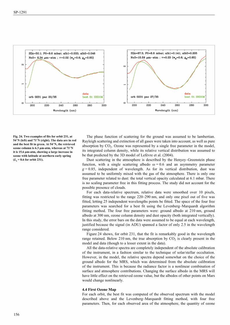
The phase function of scattering for the ground was assumed to be lambertian. Rayleigh scattering and extinction of all gases were taken into account, as well as pure absorption by CO2. Ozone was represented by a single free parameter in the model, its integrated column density, while its relative vertical distribution was assumed to be that predicted by the 3D model of Lefèvre et al. (2004).
Dust scattering in the atmosphere is described by the Henyey–Greenstein phase function, with a single scattering albedo w = 0.6 and an asymmetry parameter g = 0.85, independent of wavelength. As for its vertical distribution, dust was assumed to be uniformly mixed with the gas of the atmosphere. There is only one free parameter related to dust: the total vertical opacity calculated at 6.1 mbar. There is no scaling parameter free in this fitting process. The study did not account for the possible presence of clouds.
For each data-relative spectrum, relative data were smoothed over 10 pixels, fitting was restricted to the range 220–290 nm, and only one pixel out of five was fitted, letting 25 independent wavelengths points be fitted. The space of the four free parameters was searched for a best fit using the Levenberg–Marquardt algorithm fitting method. The four free parameters were: ground albedo at 210 nm, ground albedo at 300 nm, ozone column density and dust opacity (both integrated vertically). In this study, the error bars on the data were assumed to be equal at each wavelength, justified because the signal (in ADU) spanned a factor of only 2.5 in the wavelength range considered.
Figure 24 shows, for orbit 231, that the fit is remarkably good in the wavelength range retained. Below 210 nm, the true absorption by CO2 is clearly present in the model and data (though to a lesser extent in the data).
All the data-relative spectra are completely independent of the absolute calibration of the instrument, in a fashion similar to the technique of solar/stellar occultation. However, in the model, the relative spectra depend somewhat on the choice of the ground albedo for the MRS, which was determined from the absolute calibration of the instrument. This is because the radiance factor is a nonlinear combination of surface and atmosphere contributions. Changing the surface albedo in the MRS will have little effect on the retrieved ozone value, but the albedos of other points on Mars would change nonlinearly.
4.4 First Ozone MapFor each orbit, the best fit was computed of the observed spectrum with the model described above and the Levenberg–Marquardt fitting method, with four free parameters. Then, for each observed area of the atmosphere, the quantity of ozone
156
Fig. 24. Two examples of fits for orbit 231, at 54°N (left) and 71°N (right). The data are in red and the best fit in green. At 54°N, the retrieved ozone column is 6.3 µm-atm, whereas at 71°N it is 15.6 µm-atm, showing a large increase in ozone with latitude at northern early spring (Ls = 8.6 for orbit 231).
SP-1291

present at the instant of observation was obtained. It is convenient to represent the results in the (geographical) latitude versus solar longitude plane. This plane is divided into sectors of 1 square-degree. When one of these sectors had been observed several times, the average value of the ozone quantity was kept. As far as possible, values were interpolated in unobserved sectors along the latitude axis to complete the dataset. This then produces a map of the ozone quantity as a function of the latitude and the solar longitude. Figure 25 presents the first ozone map ever measured, in units of µm-atm (1 µm-atm = 2.689 × 10¹⁵ mol cm–2 = 0.1 Dobson units). The map covers only the column range (0–15 µm-atm) in order to improve the contrast for low ozone quantities, although in some places SPICAM was able to measure up to 30 µm-atm. Three ozone-rich regions are visible at high latitudes: in the northern late winter–early spring, during the autumn in the southern hemisphere, and at the end of the northern summer. There are also noticeable variations from day to day.
A noticeable point with the ozone map is the distribution of the available data. Few data are available at high latitudes. This is due both to the large solar zenith angle, and to the need to share observing time with other instruments: SPICAM is usually on at the same time as the imagers, around the pericentre, while the high latitudes can only be observed far from pericentre. There is a lack of data within Ls = 70–90° because of power limitations during solar eclipses. For these reasons, the coverage in season and latitude is highly variable.
Sharp variations are evident in the ozone quantity, depending on the latitude and season. There are three main ozone-rich regions visible on the latitude–season map: the high northern latitudes during late winter and early spring; the high southern latitudes during autumn, and the high northern latitudes during summer.
4.5 Comparison of Ozone Data with GCM PredictionsThe SPICAM results were compared (Fig. 26) with the 3D distribution of ozone computed by the GCM described by Lefèvre et al. (2004). For each orbit, the O3 column was extracted from the GCM for the same location and time as the measurements. All of the gross features of the data map were well-captured by the model, including the location of the three large maxima in the latitude–season maps, and the large day-to-day variability.
157
Fig. 25. The first Ls–latitude ozone map, from Ls = 330° to 180°. The dataset coverage in season and latitude is variable, depending on observational and technical constraints. Around Ls = 80° the pericentre was on the nightside and nadir dayside observations were very limited. Sharp variations were measured in the ozone column density.
Fig. 26. GCM ozone prediction compared with SPICAM data.
(a) (b)
Scientific instruments
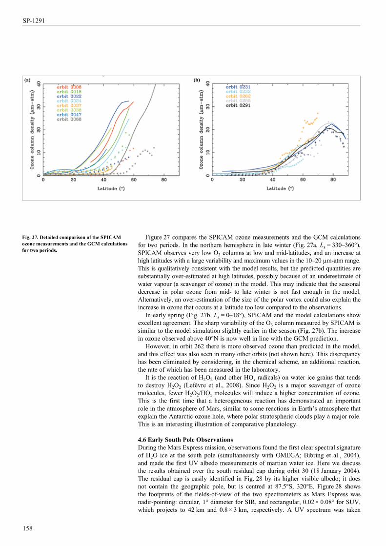
Figure 27 compares the SPICAM ozone measurements and the GCM calculations for two periods. In the northern hemisphere in late winter (Fig. 27a, Ls = 330–360°), SPICAM observes very low O3 columns at low and mid-latitudes, and an increase at high latitudes with a large variability and maximum values in the 10–20 µm-atm range. This is qualitatively consistent with the model results, but the predicted quantities are substantially over-estimated at high latitudes, possibly because of an underestimate of water vapour (a scavenger of ozone) in the model. This may indicate that the seasonal decrease in polar ozone from mid- to late winter is not fast enough in the model. Alternatively, an over-estimation of the size of the polar vortex could also explain the increase in ozone that occurs at a latitude too low compared to the observations.
In early spring (Fig. 27b, Ls = 0–18°), SPICAM and the model calculations show excellent agreement. The sharp variability of the O3 column measured by SPICAM is similar to the model simulation slightly earlier in the season (Fig. 27b). The increase in ozone observed above 40°N is now well in line with the GCM prediction.
However, in orbit 262 there is more observed ozone than predicted in the model, and this effect was also seen in many other orbits (not shown here). This discrepancy has been eliminated by considering, in the chemical scheme, an additional reaction, the rate of which has been measured in the laboratory.
It is the reaction of H2O2 (and other HOx radicals) on water ice grains that tends to destroy H2O2 (Lefèvre et al., 2008). Since H2O2 is a major scavenger of ozone molecules, fewer H2O2/HOx molecules will induce a higher concentration of ozone. This is the first time that a heterogeneous reaction has demonstrated an important role in the atmosphere of Mars, similar to some reactions in Earth’s atmosphere that explain the Antarctic ozone hole, where polar stratospheric clouds play a major role. This is an interesting illustration of comparative planetology.
4.6 Early South Pole ObservationsDuring the Mars Express mission, observations found the first clear spectral signature of H2O ice at the south pole (simultaneously with OMEGA; Bibring et al., 2004), and made the first UV albedo measurements of martian water ice. Here we discuss the results obtained over the south residual cap during orbit 30 (18 January 2004). The residual cap is easily identified in Fig. 28 by its higher visible albedo; it does not contain the geographic pole, but is centred at 87.5°S, 320°E. Figure 28 shows the footprints of the fields-of-view of the two spectrometers as Mars Express was nadir-pointing: circular, 1° diameter for SIR, and rectangular, 0.02 × 0.08° for SUV, which projects to 42 km and 0.8 × 3 km, respectively. A UV spectrum was taken
158
Fig. 27. Detailed comparison of the SPICAM ozone measurements and the GCM calculations for two periods.
(a) (b)
SP-1291

159
each second, with light integrated for 0.64 s; the FOV moved by about 2 km during this time. A full IR spectrum was acquired in 24 s, but each of the 3984 wavelength samples was acquired during 6 ms, giving a negligible spatial lag: each individual IR sample corresponded to a 1° circle, but since the SIR was sequentially sweeping the wavelengths the FOV was moving accordingly, along the trajectory shown in Fig. 28. The circles are given for the longest wavelength of each IR spectrum. (Also, Fig. 67, a typical SPICAM IR spectrum, clearly shows the water-ice signature).
The martian season of the SPICAM observations corresponds to Ls = 336°, late summer for the southern hemisphere: the seasonal CO2 cap was long gone and the pole was still illuminated by the Sun, which allows analysis of the spectrum of the backscattered solar light. Figure 29 plots the UV reflectance recorded to nadir as a function of acquisition time, showing very strong fluctuations only on the permanent polar cap, with deep troughs corresponding to low-albedo channels apparent in the Viking polar cap image (Fig. 28), identified by the letters a–g in Fig. 29.
Over the permanent cap, the UV reflectance is rather high (0.11), much higher than the 0.02–0.03 recorded beyond the polar cap. However, the high value is still much lower than laboratory measurements of pure H2O and CO2 ices (Hapke, 1981), indicating that there is also some dust mixed with the icy material, as might be expected from the ubiquitous dusty character of the martian atmosphere.
Beyond the cap (from around 210 s to 500 s after the start of observation; Fig. 29), the reflectances at 230 nm and 270 nm are almost the same, which means that ground albedo or dust do not cause strong variations in the spectral reflectance. Over the bright regions, the reflectance increases by a factor of 1.6 between 230 nm to 270 nm. It can be assumed that the dust/atmospheric conditions are the same between bright region 6 and region g just outside the cap: this implies that the strong reflectance variation over 230–270 nm is due to ground ice albedo variations with wavelength. Indeed, laboratory measurements of pure H2O and CO2 ices (Hapke, 1981) indicate a decrease in reflectance over 230–270 nm, but unfortunately for both types of ice. The reflectances at both wavelengths are the same in the holes a–f, which means no ice is seen in these regions, either because it is in shadow or because the ground is similar to that beyond the cap, where the ground albedoes are also identical at these two wavelengths.
Further systematic UV studies will extend to the north pole, and to the seasonal caps.
Fig. 28. A Viking map of of the south polar cap. The red line represents the SPICAM UV FOV ground track, and the yellow circles the SIR FOV during the nadir observations of 18 January 2004.
Scientific instruments
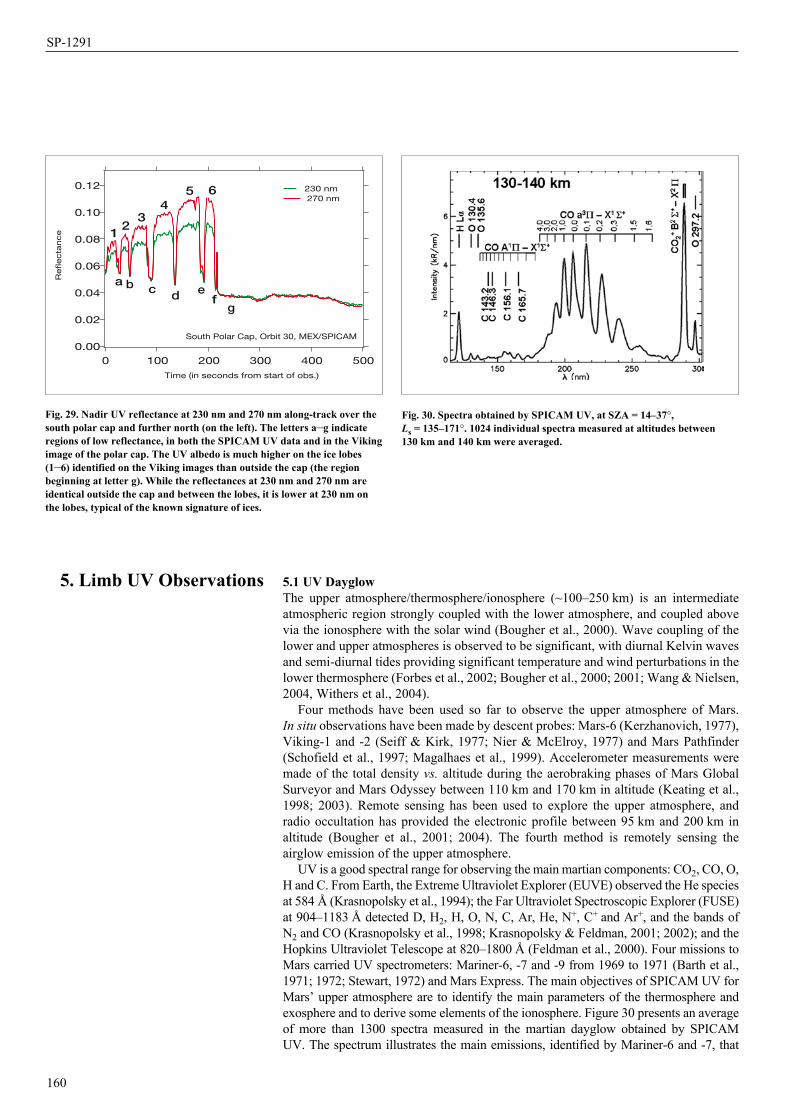
5.1 UV Dayglow The upper atmosphere/thermosphere/ionosphere (~100–250 km) is an intermediate atmospheric region strongly coupled with the lower atmosphere, and coupled above via the ionosphere with the solar wind (Bougher et al., 2000). Wave coupling of the lower and upper atmospheres is observed to be significant, with diurnal Kelvin waves and semi-diurnal tides providing significant temperature and wind perturbations in the lower thermosphere (Forbes et al., 2002; Bougher et al., 2000; 2001; Wang & Nielsen, 2004, Withers et al., 2004).
Four methods have been used so far to observe the upper atmosphere of Mars. In situ observations have been made by descent probes: Mars-6 (Kerzhanovich, 1977), Viking-1 and -2 (Seiff & Kirk, 1977; Nier & McElroy, 1977) and Mars Pathfinder (Schofield et al., 1997; Magalhaes et al., 1999). Accelerometer measurements were made of the total density vs. altitude during the aerobraking phases of Mars Global Surveyor and Mars Odyssey between 110 km and 170 km in altitude (Keating et al., 1998; 2003). Remote sensing has been used to explore the upper atmosphere, and radio occultation has provided the electronic profile between 95 km and 200 km in altitude (Bougher et al., 2001; 2004). The fourth method is remotely sensing the airglow emission of the upper atmosphere.
UV is a good spectral range for observing the main martian components: CO2, CO, O, H and C. From Earth, the Extreme Ultraviolet Explorer (EUVE) observed the He species at 584 Å (Krasnopolsky et al., 1994); the Far Ultraviolet Spectroscopic Explorer (FUSE) at 904–1183 Å detected D, H2, H, O, N, C, Ar, He, N+, C+ and Ar+, and the bands of N2 and CO (Krasnopolsky et al., 1998; Krasnopolsky & Feldman, 2001; 2002); and the Hopkins Ultraviolet Telescope at 820–1800 Å (Feldman et al., 2000). Four missions to Mars carried UV spectrometers: Mariner-6, -7 and -9 from 1969 to 1971 (Barth et al., 1971; 1972; Stewart, 1972) and Mars Express. The main objectives of SPICAM UV for Mars’ upper atmosphere are to identify the main parameters of the thermosphere and exosphere and to derive some elements of the ionosphere. Figure 30 presents an average of more than 1300 spectra measured in the martian dayglow obtained by SPICAM UV. The spectrum illustrates the main emissions, identified by Mariner-6 and -7, that
160
5. Limb UV Observations
Fig. 29. Nadir UV reflectance at 230 nm and 270 nm along-track over the south polar cap and further north (on the left). The letters a–g indicate regions of low reflectance, in both the SPICAM UV data and in the Viking image of the polar cap. The UV albedo is much higher on the ice lobes (1–6) identified on the Viking images than outside the cap (the region beginning at letter g). While the reflectances at 230 nm and 270 nm are identical outside the cap and between the lobes, it is lower at 230 nm on the lobes, typical of the known signature of ices.
0.12
0.10
0.08
0.06
0.04
0.02
0.00
Re�ecta
nce
5004003002001000 Time (in seconds from start of obs.)
230 nm 270 nm
a
b c d e f
g
1 2
3 4
5 6
South Polar Cap, Orbit 30, MEX/SPICAM
Fig. 30. Spectra obtained by SPICAM UV, at SZA = 14–37°, Ls = 135–171°. 1024 individual spectra measured at altitudes between 130 km and 140 km were averaged.
SP-1291
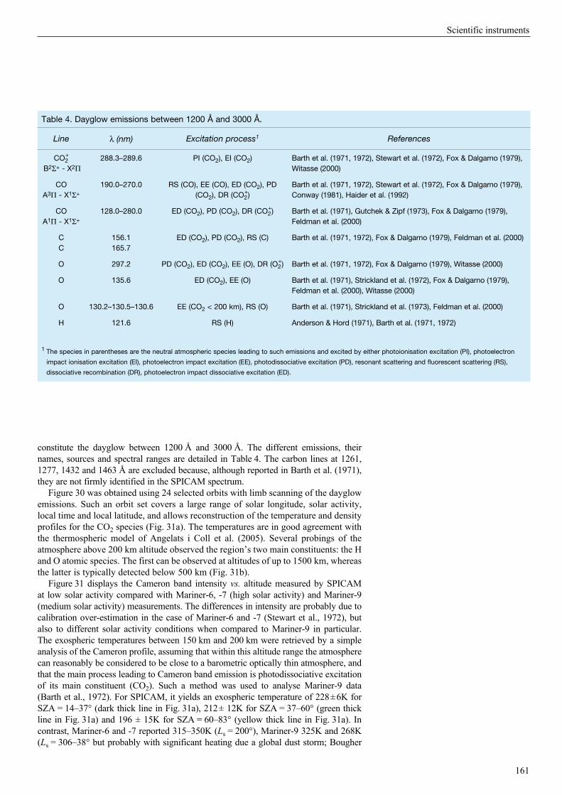
constitute the dayglow between 1200 Å and 3000 Å. The different emissions, their names, sources and spectral ranges are detailed in Table 4. The carbon lines at 1261, 1277, 1432 and 1463 Å are excluded because, although reported in Barth et al. (1971), they are not firmly identified in the SPICAM spectrum.
Figure 30 was obtained using 24 selected orbits with limb scanning of the dayglow emissions. Such an orbit set covers a large range of solar longitude, solar activity, local time and local latitude, and allows reconstruction of the temperature and density profiles for the CO2 species (Fig. 31a). The temperatures are in good agreement with the thermospheric model of Angelats i Coll et al. (2005). Several probings of the atmosphere above 200 km altitude observed the region’s two main constituents: the H and O atomic species. The first can be observed at altitudes of up to 1500 km, whereas the latter is typically detected below 500 km (Fig. 31b).
Figure 31 displays the Cameron band intensity vs. altitude measured by SPICAM at low solar activity compared with Mariner-6, -7 (high solar activity) and Mariner-9 (medium solar activity) measurements. The differences in intensity are probably due to calibration over-estimation in the case of Mariner-6 and -7 (Stewart et al., 1972), but also to different solar activity conditions when compared to Mariner-9 in particular. The exospheric temperatures between 150 km and 200 km were retrieved by a simple analysis of the Cameron profile, assuming that within this altitude range the atmosphere can reasonably be considered to be close to a barometric optically thin atmosphere, and that the main process leading to Cameron band emission is photodissociative excitation of its main constituent (CO2). Such a method was used to analyse Mariner-9 data (Barth et al., 1972). For SPICAM, it yields an exospheric temperature of 228 ± 6K for SZA = 14–37° (dark thick line in Fig. 31a), 212 ± 12K for SZA = 37–60° (green thick line in Fig. 31a) and 196 ± 15K for SZA = 60–83° (yellow thick line in Fig. 31a). In contrast, Mariner-6 and -7 reported 315–350K (Ls = 200°), Mariner-9 325K and 268K (Ls = 306–38° but probably with significant heating due a global dust storm; Bougher
161
Table 4. Dayglow emissions between 1200 Å and 3000 Å.
Line l (nm) Excitation process1 References
CO2+
B2S+ - X2P288.3–289.6 PI (CO2), EI (CO2) Barth et al. (1971, 1972), Stewart et al. (1972), Fox & Dalgarno (1979),
Witasse (2000)
CO A3P - X1S+
190.0–270.0 RS (CO), EE (CO), ED (CO2), PD (CO2), DR (CO2
+)Barth et al. (1971, 1972), Stewart et al. (1972), Fox & Dalgarno (1979), Conway (1981), Haider et al. (1992)
CO A1P - X1S+
128.0–280.0 ED (CO2), PD (CO2), DR (CO2+) Barth et al. (1971), Gutchek & Zipf (1973), Fox & Dalgarno (1979),
Feldman et al. (2000)
C C
156.1 165.7
ED (CO2), PD (CO2), RS (C) Barth et al. (1971, 1972), Fox & Dalgarno (1979), Feldman et al. (2000)
O 297.2 PD (CO2), ED (CO2), EE (O), DR (O2+) Barth et al. (1971, 1972), Fox & Dalgarno (1979), Witasse (2000)
O 135.6 ED (CO2), EE (O) Barth et al. (1971), Strickland et al. (1972), Fox & Dalgarno (1979), Feldman et al. (2000), Witasse (2000)
O 130.2–130.5–130.6 EE (CO2 < 200 km), RS (O) Barth et al. (1971), Strickland et al. (1973), Feldman et al. (2000)
H 121.6 RS (H) Anderson & Hord (1971), Barth et al. (1971, 1972)
1 The species in parentheses are the neutral atmospheric species leading to such emissions and excited by either photoionisation excitation (PI), photoelectron
impact ionisation excitation (EI), photoelectron impact excitation (EE), photodissociative excitation (PD), resonant scattering and fluorescent scattering (RS),
dissociative recombination (DR), photoelectron impact dissociative excitation (ED).
Scientific instruments
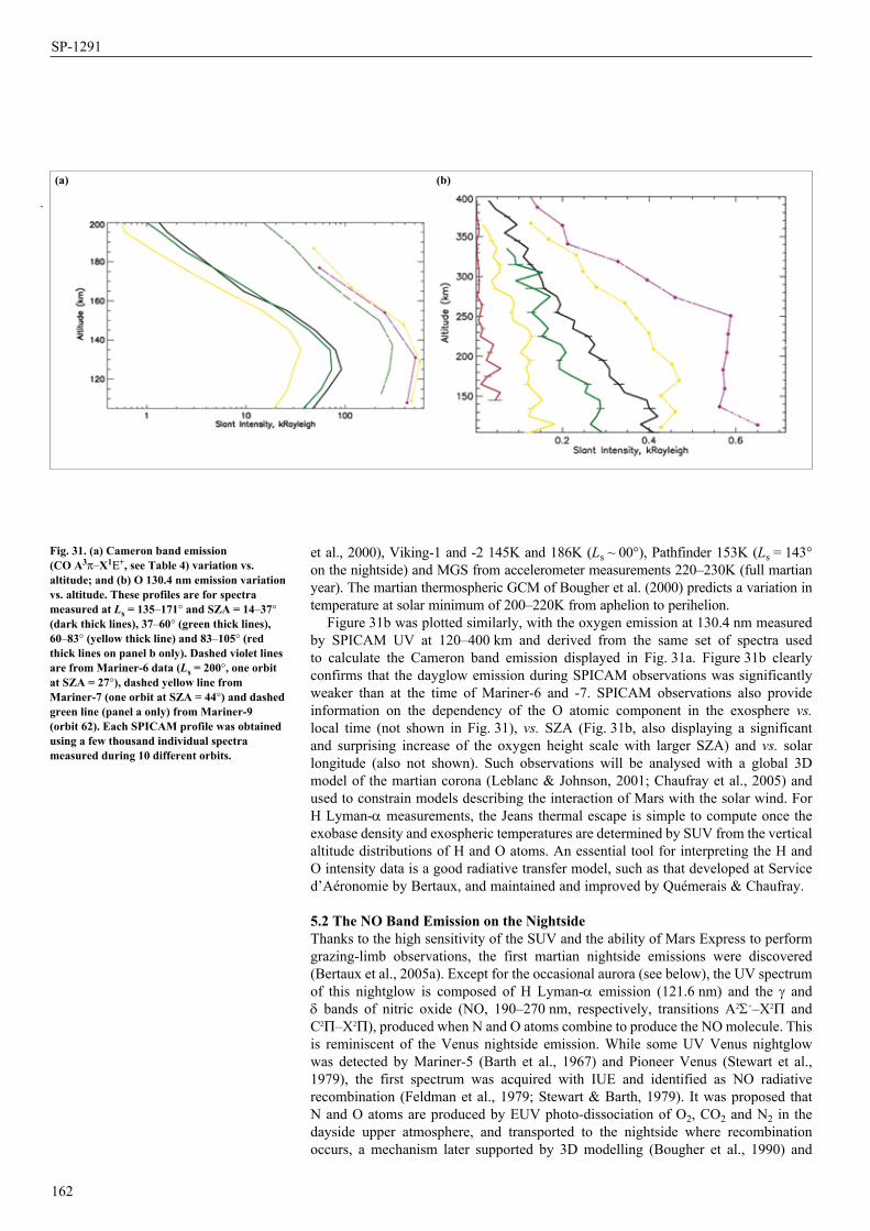
et al., 2000), Viking-1 and -2 145K and 186K (Ls ~ 00°), Pathfinder 153K (Ls = 143° on the nightside) and MGS from accelerometer measurements 220–230K (full martian year). The martian thermospheric GCM of Bougher et al. (2000) predicts a variation in temperature at solar minimum of 200–220K from aphelion to perihelion.
Figure 31b was plotted similarly, with the oxygen emission at 130.4 nm measured by SPICAM UV at 120–400 km and derived from the same set of spectra used to calculate the Cameron band emission displayed in Fig. 31a. Figure 31b clearly confirms that the dayglow emission during SPICAM observations was significantly weaker than at the time of Mariner-6 and -7. SPICAM observations also provide information on the dependency of the O atomic component in the exosphere vs. local time (not shown in Fig. 31), vs. SZA (Fig. 31b, also displaying a significant and surprising increase of the oxygen height scale with larger SZA) and vs. solar longitude (also not shown). Such observations will be analysed with a global 3D model of the martian corona (Leblanc & Johnson, 2001; Chaufray et al., 2005) and used to constrain models describing the interaction of Mars with the solar wind. For H Lyman-a measurements, the Jeans thermal escape is simple to compute once the exobase density and exospheric temperatures are determined by SUV from the vertical altitude distributions of H and O atoms. An essential tool for interpreting the H and O intensity data is a good radiative transfer model, such as that developed at Service d’Aéronomie by Bertaux, and maintained and improved by Quémerais & Chaufray.
5.2 The NO Band Emission on the Nightside Thanks to the high sensitivity of the SUV and the ability of Mars Express to perform grazing-limb observations, the first martian nightside emissions were discovered (Bertaux et al., 2005a). Except for the occasional aurora (see below), the UV spectrum of this nightglow is composed of H Lyman-a emission (121.6 nm) and the g and d bands of nitric oxide (NO, 190–270 nm, respectively, transitions A2S+–X2P and C2P–X2P), produced when N and O atoms combine to produce the NO molecule. This is reminiscent of the Venus nightside emission. While some UV Venus nightglow was detected by Mariner-5 (Barth et al., 1967) and Pioneer Venus (Stewart et al., 1979), the first spectrum was acquired with IUE and identified as NO radiative recombination (Feldman et al., 1979; Stewart & Barth, 1979). It was proposed that N and O atoms are produced by EUV photo-dissociation of O2, CO2 and N2 in the dayside upper atmosphere, and transported to the nightside where recombination occurs, a mechanism later supported by 3D modelling (Bougher et al., 1990) and
162
Fig. 31. (a) Cameron band emission (CO A3p–X1E+, see Table 4) variation vs. altitude; and (b) O 130.4 nm emission variation vs. altitude. These profiles are for spectra measured at Ls = 135–171° and SZA = 14–37° (dark thick lines), 37–60° (green thick lines), 60–83° (yellow thick line) and 83–105° (red thick lines on panel b only). Dashed violet lines are from Mariner-6 data (Ls = 200°, one orbit at SZA = 27°), dashed yellow line from Mariner-7 (one orbit at SZA = 44°) and dashed green line (panel a only) from Mariner-9 (orbit 62). Each SPICAM profile was obtained using a few thousand individual spectra measured during 10 different orbits.
(a) (b)
SP-1291
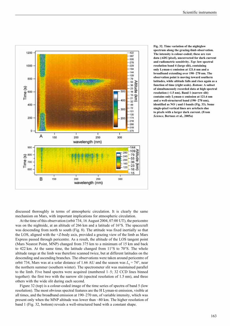
discussed thoroughly in terms of atmospheric circulation. It is clearly the same mechanism on Mars, with important implications for atmospheric circulation.
At the time of this observation (orbit 734, 16 August 2004, 07:00 UT), the pericentre was on the nightside, at an altitude of 266 km and a latitude of 16°S. The spacecraft was descending from north to south (Fig. 8). The attitude was fixed inertially so that the LOS, aligned with the +Z-body axis, provided a grazing view of the limb as Mars Express passed through pericentre. As a result, the altitude of the LOS tangent point (Mars Nearest Point, MNP) changed from 375 km to a minimum of 15 km and back to 422 km. At the same time, the latitude changed from 11°S to 70°S. The whole altitude range at the limb was therefore scanned twice, but at different latitudes on the descending and ascending branches. The observations were taken around pericentre of orbit 734, Mars was at a solar distance of 1.66 AU and the season was Ls = 74°, near the northern summer (southern winter). The spectrometer slit was maintained parallel to the limb. Five band spectra were acquired (numbered 1–5; 32 CCD lines binned together): the first two with the narrow slit (spectral resolution of 1.5 nm), and three others with the wide slit during each second.
Figure 32 (top) is a colour-coded image of the time series of spectra of band 5 (low resolution). The most obvious spectral features are the H Lyman-a emission, visible at all times, and the broadband emission at 190–270 nm, of variable intensity, which was present only when the MNP altitude was lower than ~80 km. The higher resolution of band 1 (Fig. 32, bottom) reveals a well-structured band with a constant shape.
163
Fig. 32. Time variation of the nightglow spectrum along the grazing-limb observation. The intensity is colour-coded; these are raw data (ADU/pixel), uncorrected for dark current and radiometric sensitivity. Top: low spectral resolution band 4 (large slit), containing only Lyman-a emission at 121.6 nm and a broadband extending over 190–270 nm. The observation point is moving toward southern latitudes, while altitude falls and rises again as a function of time (right scale). Bottom: A subset of simultaneously recorded data at high spectral resolution (~1.5 nm). Band 1 (narrow slit) contains only Lyman-a emission at 121.6 nm and a well-structured band (190–270 nm), identified as NO g and d bands (Fig. 33). Some single-pixel vertical lines are artefacts due to pixels with a larger dark current. (From Science, Bertaux et al., 2005a)
Scientific instruments
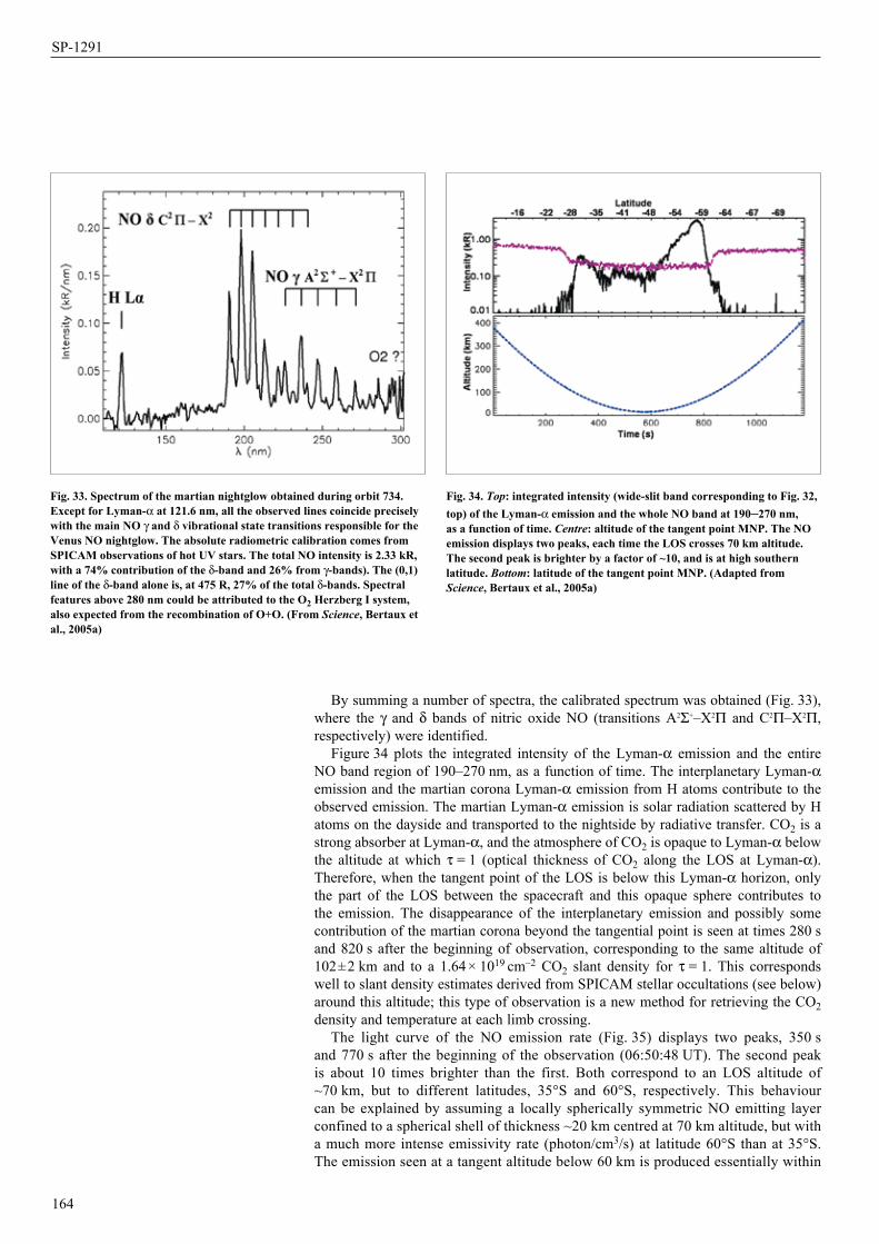
By summing a number of spectra, the calibrated spectrum was obtained (Fig. 33), where the g and d bands of nitric oxide NO (transitions A2S+–X2P and C2P–X2P, respectively) were identified.
Figure 34 plots the integrated intensity of the Lyman-a emission and the entire NO band region of 190–270 nm, as a function of time. The interplanetary Lyman-a emission and the martian corona Lyman-a emission from H atoms contribute to the observed emission. The martian Lyman-a emission is solar radiation scattered by H atoms on the dayside and transported to the nightside by radiative transfer. CO2 is a strong absorber at Lyman-a, and the atmosphere of CO2 is opaque to Lyman-a below the altitude at which t = 1 (optical thickness of CO2 along the LOS at Lyman-a). Therefore, when the tangent point of the LOS is below this Lyman-a horizon, only the part of the LOS between the spacecraft and this opaque sphere contributes to the emission. The disappearance of the interplanetary emission and possibly some contribution of the martian corona beyond the tangential point is seen at times 280 s and 820 s after the beginning of observation, corresponding to the same altitude of 102±2 km and to a 1.64 × 1019 cm–2 CO2 slant density for t = 1. This corresponds well to slant density estimates derived from SPICAM stellar occultations (see below) around this altitude; this type of observation is a new method for retrieving the CO2 density and temperature at each limb crossing.
The light curve of the NO emission rate (Fig. 35) displays two peaks, 350 s and 770 s after the beginning of the observation (06:50:48 UT). The second peak is about 10 times brighter than the first. Both correspond to an LOS altitude of ~70 km, but to different latitudes, 35°S and 60°S, respectively. This behaviour can be explained by assuming a locally spherically symmetric NO emitting layer confined to a spherical shell of thickness ~20 km centred at 70 km altitude, but with a much more intense emissivity rate (photon/cm3/s) at latitude 60°S than at 35°S. The emission seen at a tangent altitude below 60 km is produced essentially within
164
Fig. 33. Spectrum of the martian nightglow obtained during orbit 734. Except for Lyman-a at 121.6 nm, all the observed lines coincide precisely with the main NO g and d vibrational state transitions responsible for the Venus NO nightglow. The absolute radiometric calibration comes from SPICAM observations of hot UV stars. The total NO intensity is 2.33 kR, with a 74% contribution of the d-band and 26% from g-bands). The (0,1) line of the d-band alone is, at 475 R, 27% of the total d-bands. Spectral features above 280 nm could be attributed to the O2 Herzberg I system, also expected from the recombination of O+O. (From Science, Bertaux et al., 2005a)
Fig. 34. Top: integrated intensity (wide-slit band corresponding to Fig. 32, top) of the Lyman-a emission and the whole NO band at 190–270 nm, as a function of time. Centre: altitude of the tangent point MNP. The NO emission displays two peaks, each time the LOS crosses 70 km altitude. The second peak is brighter by a factor of ~10, and is at high southern latitude. Bottom: latitude of the tangent point MNP. (Adapted from Science, Bertaux et al., 2005a)
SP-1291
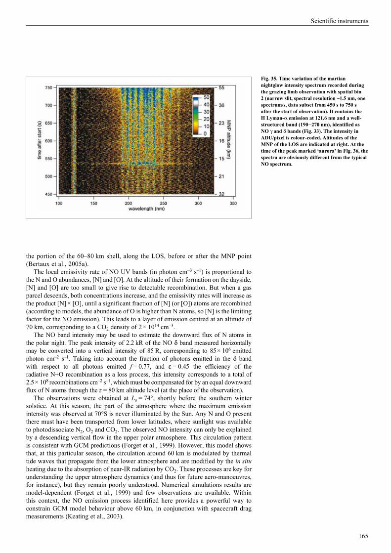
the portion of the 60–80 km shell, along the LOS, before or after the MNP point (Bertaux et al., 2005a).
The local emissivity rate of NO UV bands (in photon cm–3 s–1) is proportional to the N and O abundances, [N] and [O]. At the altitude of their formation on the dayside, [N] and [O] are too small to give rise to detectable recombination. But when a gas parcel descends, both concentrations increase, and the emissivity rates will increase as the product [N] × [O], until a significant fraction of [N] (or [O]) atoms are recombined (according to models, the abundance of O is higher than N atoms, so [N] is the limiting factor for the NO emission). This leads to a layer of emission centred at an altitude of 70 km, corresponding to a CO2 density of 2 × 1014 cm–3.
The NO band intensity may be used to estimate the downward flux of N atoms in the polar night. The peak intensity of 2.2 kR of the NO d band measured horizontally may be converted into a vertical intensity of 85 R, corresponding to 85 × 106 emitted photon cm–2 s–1. Taking into account the fraction of photons emitted in the d band with respect to all photons emitted f = 0.77, and e = 0.45 the efficiency of the radiative N+O recombination as a loss process, this intensity corresponds to a total of 2.5 × 10⁸ recombinations cm–2 s–1, which must be compensated for by an equal downward flux of N atoms through the z = 80 km altitude level (at the place of the observation).
The observations were obtained at Ls = 74°, shortly before the southern winter solstice. At this season, the part of the atmosphere where the maximum emission intensity was observed at 70°S is never illuminated by the Sun. Any N and O present there must have been transported from lower latitudes, where sunlight was available to photodissociate N2, O2 and CO2. The observed NO intensity can only be explained by a descending vertical flow in the upper polar atmosphere. This circulation pattern is consistent with GCM predictions (Forget et al., 1999). However, this model shows that, at this particular season, the circulation around 60 km is modulated by thermal tide waves that propagate from the lower atmosphere and are modified by the in situ heating due to the absorption of near-IR radiation by CO2. These processes are key for understanding the upper atmosphere dynamics (and thus for future aero-manoeuvres, for instance), but they remain poorly understood. Numerical simulations results are model-dependent (Forget et al., 1999) and few observations are available. Within this context, the NO emission process identified here provides a powerful way to constrain GCM model behaviour above 60 km, in conjunction with spacecraft drag measurements (Keating et al., 2003).
165
Fig. 35. Time variation of the martian nightglow intensity spectrum recorded during the grazing limb observation with spatial bin 2 (narrow slit, spectral resolution ~1.5 nm, one spectrum/s, data subset from 450 s to 750 s after the start of observation). It contains the H Lyman-a emission at 121.6 nm and a well-structured band (190–270 nm), identified as NO g and d bands (Fig. 33). The intensity in ADU/pixel is colour-coded. Altitudes of the MNP of the LOS are indicated at right. At the time of the peak marked ‘aurora’ in Fig. 36, the spectra are obviously different from the typical NO spectrum.
Scientific instruments
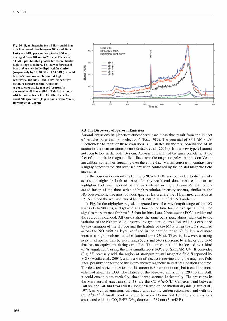
5.3 The Discovery of Auroral Emission Auroral emissions in planetary atmospheres ‘are those that result from the impact of particles other than photoelectrons’ (Fox, 1986). The potential of SPICAM’s UV spectrometer to monitor these emissions is illustrated by the first observation of an aurora in the martian atmosphere (Bertaux et al., 2005b). It is a new type of aurora not seen before in the Solar System. Auroras on Earth and the giant planets lie at the feet of the intrinsic magnetic field lines near the magnetic poles. Auroras on Venus are diffuse, sometimes spreading over the entire disc. Martian auroras, in contrast, are a highly concentrated and localised emission controlled by the crustal magnetic field anomalies.
In the observation on orbit 716, the SPICAM LOS was permitted to drift slowly across the nightside limb to search for any weak emission, because no martian nightglow had been reported before, as sketched in Fig. 7. Figure 35 is a colour-coded image of the time series of high-resolution intensity spectra, similar to the NO observations. The most obvious spectral features are the H Lyman-a emission at 121.6 nm and the well-structured band at 190–270 nm of the NO molecule.
In Fig. 36 the nightglow signal, integrated over the wavelength range of the NO bands (181–298 nm), is displayed as a function of time for the five spatial bins. The signal is more intense for bins 3–5 than for bins 1 and 2 because the FOV is wider and the source is extended. All curves show the same behaviour, almost identical to the variation of the NO emission observed 6 days later on orbit 734, which is explained by the variation of the altitude and the latitude of the MNP when the LOS scanned across the NO emitting layer, confined in the altitude range 60–80 km, and more intense at high southern latitudes (around time 750 s). There is, however, a strong peak in all spatial bins between times 533 s and 540 s (increase by a factor of 3 to 4) that has no equivalent during orbit 734. The emission could be located by a kind of ‘triangulation’, using the five simultaneous FOVs of SPICAM UV. It coincides (Fig. 37) precisely with the region of strongest crustal magnetic field B reported by MGS (Acuña et al., 2001), and is a sign of electrons moving along the magnetic field lines, possibly connected to the interplanetary magnetic field at this location and time. The detected horizontal extent of this aurora is 30 km minimum, but it could be more extended along the LOS. The altitude of the observed emission is 129 ± 13 km. Still, it could extend more vertically, since it was scanned horizontally. The emissions in the Mars auroral spectrum (Fig. 38) are the CO A3p–X1E* Cameron band between 180 nm and 240 nm (694 ± 50 R), long observed on the martian dayside (Barth et al., 1971), as well as emissions associated with atomic carbon resonances and with the CO A1p–X1E+ fourth positive group between 135 nm and 170 nm, and emissions associated with the CO2
+ B2Eu–X2pg doublet at 289 nm (71 ± 42 R).
166
Fig. 36. Signal intensity for all five spatial bins as a function of time between 200 s and 900 s. Units are ADU per spectral pixel = 0.54 nm, averaged from 181 nm to 298 nm. There are 40 ADU per detected photon for the particular high voltage used here. The curves for spatial bins 2–5 are vertically displaced for clarity (respectively by 10, 20, 30 and 60 ADU). Spatial bins 3–5 have low resolution but high sensitivity, and bins 1 and 2 are less sensitive but have higher spectral resolution. A conspicuous spike marked ‘Aurora’ is observed in all bins at 535 s. This is the time at which the spectra in Fig. 35 differ from the usual NO spectrum. (Figure taken from Nature, Bertaux et al., 2005b)
SP-1291

6.1 General PrinciplesThe occultation technique has been used to measure O3 in Earth’s atmosphere since the 1970s. Early attempts observed only one or two wavelengths at a time, making the identification of the absorber species uncertain. With the advent of multi-pixel detectors, the absorbing species in a multi-spectral occultation can be safely identified via their spectral signatures. There is also the potential to discover new, unexpected species in the atmosphere. The method of absorptive occultation spectroscopy was reviewed by Roscoe et al. (1994) and Smith & Hunten (1990). In terrestrial stratospheric research, it has become the most advanced method for long-term monitoring of ozone. The most remarkable results in the IR are from ATMOS/Atlas, which provided a set of high-resolution spectra of Earth’s atmosphere. In the UV–visible, SAGE-3 uses full wavelength coverage of the Sun. The Scanning Imaging Absorption Spectrometer for Atmospheric Chartography (SCIAMACHY) of Envisat (ESA, 2001) is performing solar occultation and nadir observations, while the Global Ozone Monitoring by Occultations of Stars (GOMOS) instrument is dedicated to monitoring ozone and other species by stellar occultations (more than 400 000 ozone, NO2 and NO3 profiles have been collected so far; Hauchecorne et al., 2005). SPICAM is thus in line with the most advanced instrumentation deployed for studying Earth’s atmosphere.
So far, the only solar occultation measurements at Mars were performed during the Phobos mission by the Auguste instrument (Blamont et al., 1989; Krasnopolsky et al., 1989). Although the mission was not fully successful, the solar occultation studies covered more than a month, significantly improving our knowledge of the martian water vapour profile (Krasnopolsky et al., 1991; Rodin et al., 1997), aerosol vertical distribution (Chassefière et al., 1992; Korablev et al., 1993) and ozone distribution (Blamont & Chassefière, 1993). The promising results were not fully developed because of the failure of the Mars-96 mission.
167
6. Atmospheric Vertical Profiling by Stellar Occultation in UV
Fig. 37. Radial B field component (nT) at 200 km altitude of the crustal field deduced from MGS aerobraking and science phasing orbits (Acuña et al., 2001). White dashed line: satellite position during orbit 716 (start at the top and end of the orbit at the bottom of the figure). White solid line: position of the MNP. Dark solid and dashed lines: orbit 734 during which no emission was recorded. Magenta dashed line: SPICAM LOS at 535 s; the dark rectangle on the line is an estimate of the extended emitting region. (From Nature, Bertaux et al., 2005b)
Fig. 38. Spectrum formed by averaging spectra obtained between observation times 541 s and 548 s, typical of the NO emission, which also contain the CO emission. (From Nature, Bertaux et al., 2005b)
Scientific instruments
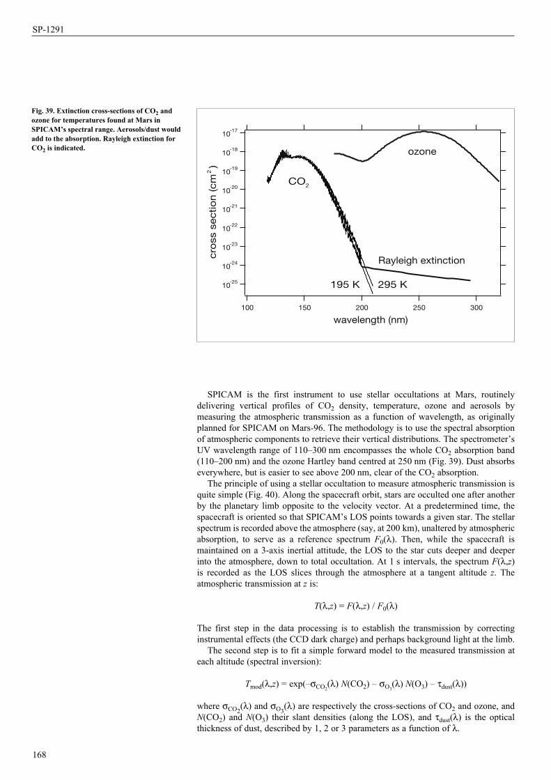
SPICAM is the first instrument to use stellar occultations at Mars, routinely delivering vertical profiles of CO2 density, temperature, ozone and aerosols by measuring the atmospheric transmission as a function of wavelength, as originally planned for SPICAM on Mars-96. The methodology is to use the spectral absorption of atmospheric components to retrieve their vertical distributions. The spectrometer’s UV wavelength range of 110–300 nm encompasses the whole CO2 absorption band (110–200 nm) and the ozone Hartley band centred at 250 nm (Fig. 39). Dust absorbs everywhere, but is easier to see above 200 nm, clear of the CO2 absorption.
The principle of using a stellar occultation to measure atmospheric transmission is quite simple (Fig. 40). Along the spacecraft orbit, stars are occulted one after another by the planetary limb opposite to the velocity vector. At a predetermined time, the spacecraft is oriented so that SPICAM’s LOS points towards a given star. The stellar spectrum is recorded above the atmosphere (say, at 200 km), unaltered by atmospheric absorption, to serve as a reference spectrum F0(l). Then, while the spacecraft is maintained on a 3-axis inertial attitude, the LOS to the star cuts deeper and deeper into the atmosphere, down to total occultation. At 1 s intervals, the spectrum F(l,z) is recorded as the LOS slices through the atmosphere at a tangent altitude z. The atmospheric transmission at z is:
T(l,z) = F(l,z) / F0(l)
The first step in the data processing is to establish the transmission by correcting instrumental effects (the CCD dark charge) and perhaps background light at the limb.
The second step is to fit a simple forward model to the measured transmission at each altitude (spectral inversion):
Tmod(l,z) = exp(–sCO2(l) N(CO2) – sO3
(l) N(O3) – tdust(l))
where sCO2(l) and sO3(l) are respectively the cross-sections of CO2 and ozone, and N(CO2) and N(O3) their slant densities (along the LOS), and tdust(l) is the optical thickness of dust, described by 1, 2 or 3 parameters as a function of l.
168
Fig. 39. Extinction cross-sections of CO2 and ozone for temperatures found at Mars in SPICAM’s spectral range. Aerosols/dust would add to the absorption. Rayleigh extinction for CO2 is indicated.
10-25
10-24
10-23
10-22
10-21
10-20
10-19
10-18
10-17
cro
ss s
ectio
n (cm
2)
300250200150100
wavelength (nm)
ozone
CO2
Rayleigh extinction
195 K 295 K
SP-1291
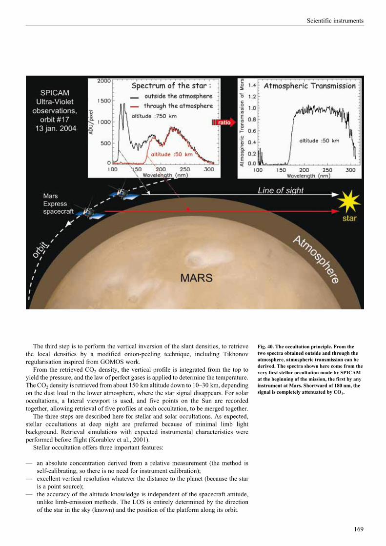
The third step is to perform the vertical inversion of the slant densities, to retrieve the local densities by a modified onion-peeling technique, including Tikhonov regularisation inspired from GOMOS work.
From the retrieved CO2 density, the vertical profile is integrated from the top to yield the pressure, and the law of perfect gases is applied to determine the temperature. The CO2 density is retrieved from about 150 km altitude down to 10–30 km, depending on the dust load in the lower atmosphere, where the star signal disappears. For solar occultations, a lateral viewport is used, and five points on the Sun are recorded together, allowing retrieval of five profiles at each occultation, to be merged together.
The three steps are described here for stellar and solar occultations. As expected, stellar occultations at deep night are preferred because of minimal limb light background. Retrieval simulations with expected instrumental characteristics were performed before flight (Korablev et al., 2001).
Stellar occultation offers three important features:
— an absolute concentration derived from a relative measurement (the method is self-calibrating, so there is no need for instrument calibration);
— excellent vertical resolution whatever the distance to the planet (because the star is a point source);
— the accuracy of the altitude knowledge is independent of the spacecraft attitude, unlike limb-emission methods. The LOS is entirely determined by the direction of the star in the sky (known) and the position of the platform along its orbit.
169
Fig. 40. The occultation principle. From the two spectra obtained outside and through the atmosphere, atmospheric transmission can be derived. The spectra shown here come from the very first stellar occultation made by SPICAM at the beginning of the mission, the first by any instrument at Mars. Shortward of 180 nm, the signal is completely attenuated by CO2.
Scientific instruments
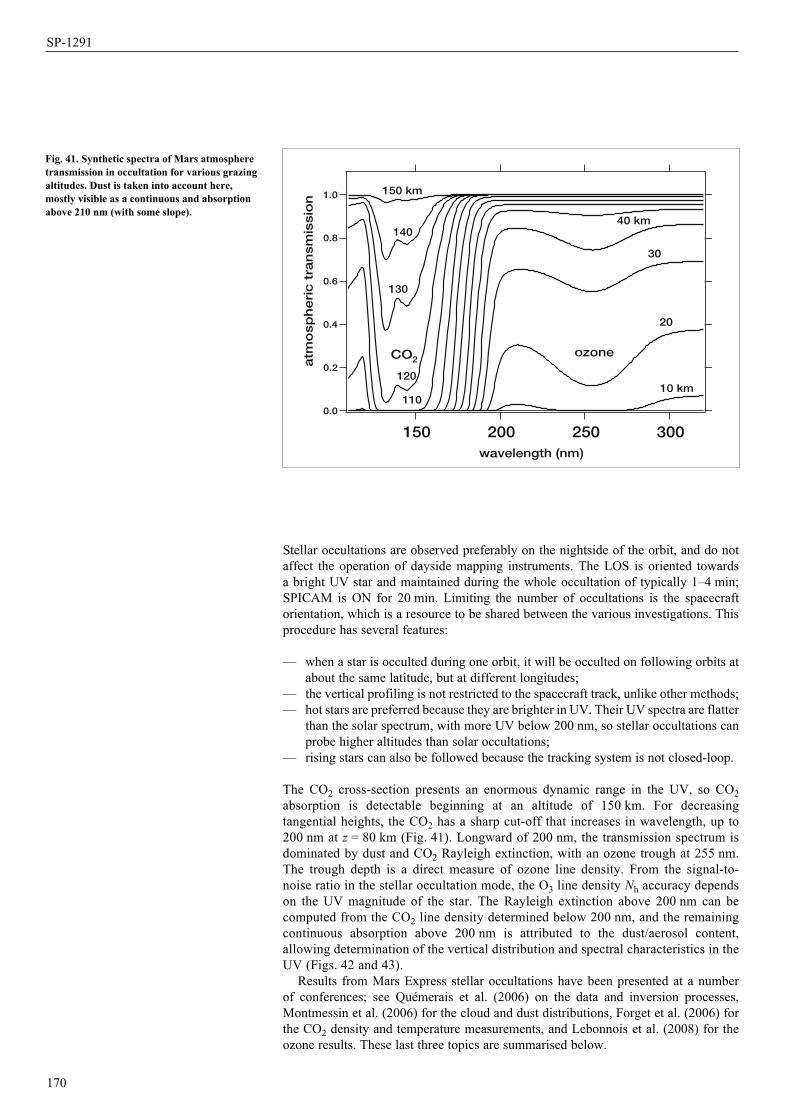
Stellar occultations are observed preferably on the nightside of the orbit, and do not affect the operation of dayside mapping instruments. The LOS is oriented towards a bright UV star and maintained during the whole occultation of typically 1–4 min; SPICAM is ON for 20 min. Limiting the number of occultations is the spacecraft orientation, which is a resource to be shared between the various investigations. This procedure has several features:
— when a star is occulted during one orbit, it will be occulted on following orbits at about the same latitude, but at different longitudes;
— the vertical profiling is not restricted to the spacecraft track, unlike other methods;— hot stars are preferred because they are brighter in UV. Their UV spectra are flatter
than the solar spectrum, with more UV below 200 nm, so stellar occultations can probe higher altitudes than solar occultations;
— rising stars can also be followed because the tracking system is not closed-loop.
The CO2 cross-section presents an enormous dynamic range in the UV, so CO2 absorption is detectable beginning at an altitude of 150 km. For decreasing tangential heights, the CO2 has a sharp cut-off that increases in wavelength, up to 200 nm at z = 80 km (Fig. 41). Longward of 200 nm, the transmission spectrum is dominated by dust and CO2 Rayleigh extinction, with an ozone trough at 255 nm. The trough depth is a direct measure of ozone line density. From the signal-to-noise ratio in the stellar occultation mode, the O3 line density Nh accuracy depends on the UV magnitude of the star. The Rayleigh extinction above 200 nm can be computed from the CO2 line density determined below 200 nm, and the remaining continuous absorption above 200 nm is attributed to the dust/aerosol content, allowing determination of the vertical distribution and spectral characteristics in the UV (Figs. 42 and 43).
Results from Mars Express stellar occultations have been presented at a number of conferences; see Quémerais et al. (2006) on the data and inversion processes, Montmessin et al. (2006) for the cloud and dust distributions, Forget et al. (2006) for the CO2 density and temperature measurements, and Lebonnois et al. (2008) for the ozone results. These last three topics are summarised below.
170
Fig. 41. Synthetic spectra of Mars atmosphere transmission in occultation for various grazing altitudes. Dust is taken into account here, mostly visible as a continuous and absorption above 210 nm (with some slope).
1.0
0.8
0.6
0.4
0.2
0.0
atm
osp
he
ric
tra
nsm
issio
n
300250200150 wavelength (nm)
150 km
140
130
120
110 10 km
CO2 ozone
20
30
40 km
SP-1291
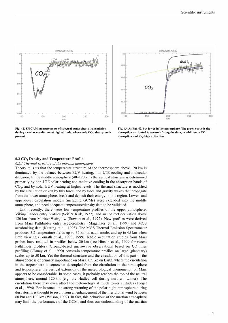
6.2 CO2 Density and Temperature Profile6.2.1 Thermal structure of the martian atmosphere Theory tells us that the temperature structure of the thermosphere above 120 km is dominated by the balance between EUV heating, non-LTE cooling and molecular diffusion. In the middle atmosphere (40–120 km) the vertical structure is determined primarily by non-LTE solar heating and radiative cooling in the absorption bands of CO2, and by solar EUV heating at higher levels. The thermal structure is modified by the circulation driven by this force, and by tides and gravity waves that propagate from the lower atmosphere, break and deposit their energy in this region. Lower- and upper-level circulation models (including GCMs) were extended into the middle atmosphere, and need adequate temperature/density data to be validated.
Until recently, there were few temperature profiles of the upper atmosphere: Viking Lander entry profiles (Seif & Kirk, 1977), and an indirect derivation above 120 km from Mariner-9 airglow (Stewart et al., 1972). New profiles were derived from Mars Pathfinder entry accelerometry (Magalhaes et al., 1999) and MGS aerobraking data (Keating et al., 1998). The MGS Thermal Emission Spectrometer produces 3D temperature fields up to 35 km in nadir mode, and up to 65 km when limb viewing (Conrath et al., 1998; 1999). Radio occultation studies from Mars probes have resulted in profiles below 20 km (see Hinson et al., 1999 for recent Pathfinder profiles). Ground-based microwave observations based on CO lines profiling (Clancy et al., 1990) constrain temperature profiles on large (planetary) scales up to 50 km. Yet the thermal structure and the circulation of this part of the atmosphere is of primary importance on Mars. Unlike on Earth, where the circulation in the troposphere is somewhat decoupled from the circulation in the stratosphere and troposphere, the vertical extension of the meteorological phenomenon on Mars appears to be considerable. In some cases, it probably reaches the top of the neutral atmosphere, around 120 km (e.g. the Hadley cell during northern winter). The circulation there may even affect the meteorology at much lower altitudes (Forget et al., 1996). For instance, the strong warming of the polar night atmosphere during dust storms is thought to result from an enhancement of the meridional wind between 60 km and 100 km (Wilson, 1997). In fact, this behaviour of the martian atmosphere may limit the performance of the GCMs and thus our understanding of the martian
171
Fig. 42. SPICAM measurements of spectral atmospheric transmission during a stellar occultation at high altitude, where only CO2 absorption is present.
Fig. 43. As Fig. 42, but lower in the atmosphere. The green curve is the absorption attributed to aerosols fitting the data, in addition to CO2 absorption and Rayleigh extinction.
Scientific instruments
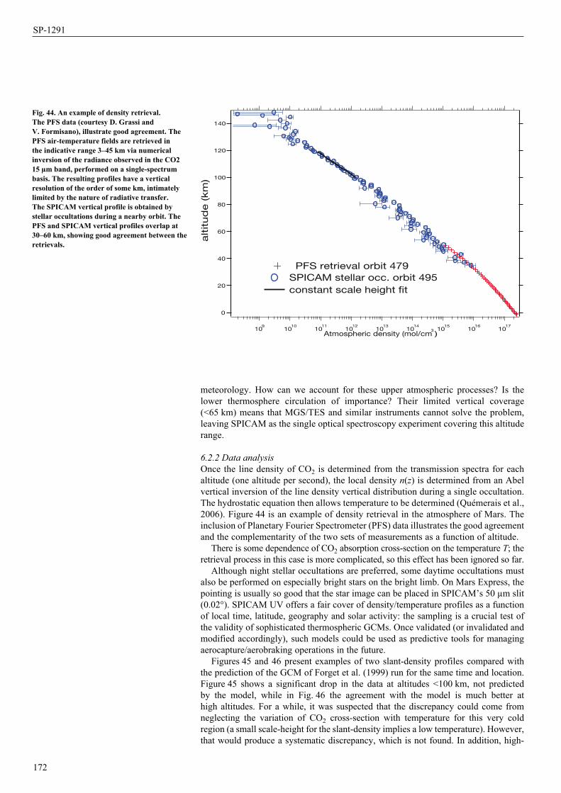
meteorology. How can we account for these upper atmospheric processes? Is the lower thermosphere circulation of importance? Their limited vertical coverage (<65 km) means that MGS/TES and similar instruments cannot solve the problem, leaving SPICAM as the single optical spectroscopy experiment covering this altitude range.
6.2.2 Data analysisOnce the line density of CO2 is determined from the transmission spectra for each altitude (one altitude per second), the local density n(z) is determined from an Abel vertical inversion of the line density vertical distribution during a single occultation. The hydrostatic equation then allows temperature to be determined (Quémerais et al., 2006). Figure 44 is an example of density retrieval in the atmosphere of Mars. The inclusion of Planetary Fourier Spectrometer (PFS) data illustrates the good agreement and the complementarity of the two sets of measurements as a function of altitude.
There is some dependence of CO2 absorption cross-section on the temperature T; the retrieval process in this case is more complicated, so this effect has been ignored so far.
Although night stellar occultations are preferred, some daytime occultations must also be performed on especially bright stars on the bright limb. On Mars Express, the pointing is usually so good that the star image can be placed in SPICAM’s 50 µm slit (0.02°). SPICAM UV offers a fair cover of density/temperature profiles as a function of local time, latitude, geography and solar activity: the sampling is a crucial test of the validity of sophisticated thermospheric GCMs. Once validated (or invalidated and modified accordingly), such models could be used as predictive tools for managing aerocapture/aerobraking operations in the future.
Figures 45 and 46 present examples of two slant-density profiles compared with the prediction of the GCM of Forget et al. (1999) run for the same time and location. Figure 45 shows a significant drop in the data at altitudes <100 km, not predicted by the model, while in Fig. 46 the agreement with the model is much better at high altitudes. For a while, it was suspected that the discrepancy could come from neglecting the variation of CO2 cross-section with temperature for this very cold region (a small scale-height for the slant-density implies a low temperature). However, that would produce a systematic discrepancy, which is not found. In addition, high-
172
140
120
100
80
60
40
20
0
altitud
e (km
)
109
1010
1011
1012
1013
1014
1015
1016
1017
Atmospheric density (mol/cm3)
PFS retrieval orbit 479 SPICAM stellar occ. orbit 495 constant scale height �t
Fig. 44. An example of density retrieval. The PFS data (courtesy D. Grassi and V. Formisano), illustrate good agreement. The PFS air-temperature fields are retrieved in the indicative range 3–45 km via numerical inversion of the radiance observed in the CO2 15 µm band, performed on a single-spectrum basis. The resulting profiles have a vertical resolution of the order of some km, intimately limited by the nature of radiative transfer. The SPICAM vertical profile is obtained by stellar occultations during a nearby orbit. The PFS and SPICAM vertical profiles overlap at 30–60 km, showing good agreement between the retrievals.
SP-1291

altitude clouds were detected on some occasions (see below), always connected to low temperatures at high altitude. The profile of Fig. 45 is therefore seen as realistic and is fully confirmed by the extensive analysis of CO2 and temperature profiles presented in Forget et al. (2008).
6.2.3 The case for molecular oxygenMolecular oxygen is the result of CO2 photo-dissociation. O2 provides in the Schumann–Runge bands (170–210 nm) an additional absorption that should be measurable. Calculations show that the difference in transmission between an atmosphere with O2 (O2/CO2 = 10–3) and one without O2 amounts to 2% around 80 km, in a bandwidth of about 20 nm around 190 nm. The absorption decreases somewhat below. In principle, one expects a constant mixing ratio of O2 in altitude and over the planet, inasmuch the chemical reactions that control this molecule are understood, constantly produced by photo-dissociation of CO2. The UV occultation technique is one way to access this important molecule. Although on Mars there is a conspicuous O2 emission at 1.27 µm, it is produced by photo-dissociation of ozone. It does not trace the density distribution of O2 as would the UV absorption seen in occultation. Some recent processing at LPL appears to have definitely found O2 UV absorption, with a mixing ratio of 0.7% (Lewis & Sandel, private communication). This is a high value compared to the adopted value of 0.13% derived from Viking measurements. If confirmed, it would be an important feature to reproduce in the modelling of photo-dissociation of CO2.
6.3 Ozone Vertical Profiles from Stellar OccultationsThe analysis of transmission spectra yields slant densities of CO2, dust and ozone as a function of altitude. Inversion of these vertical profiles allows us to retrieve vertical profiles of local densities, with an altitude resolution of close to 5 km. Before Mars Express, there was only a single ozone vertical profile, obtained by Blamont & Chassefière (1993) by solar occultation on the Phobos-2 mission. The quality was not excellent, partly because the ozone quantity was low at that season. For SPICAM’s numerous stellar occultations, some show no detectable ozone, but on others the UV absorption signature is quite conspicuous, as illustrated in Fig. 47.
173
Figs. 45 (left) and 46 (right). Comparison of measured slant-density profiles with the prediction of the GCM of Forget et al. (1999) run for the same time, geometry and location. The black line is the SPICAM data, with dotted lines at ± error bar. Several models are compared.
Blue curve: clear (no dust); green curve: MGS scenario; red curve: dusty atmosphere. There is a significant deficit of CO2 above 100 km in the data, which is not present on other orbits (Fig. 46, right). It must therefore be real, and indicates a low temperature in the region 100–110 km.
Fig. 47. Spectral transmission at 15 km altitude during orbit 174 (a single 1 s measurement). The ozone absorption trough is well seen, superimposed on the dust continuum above 200 nm wavelength.
Scientific instruments
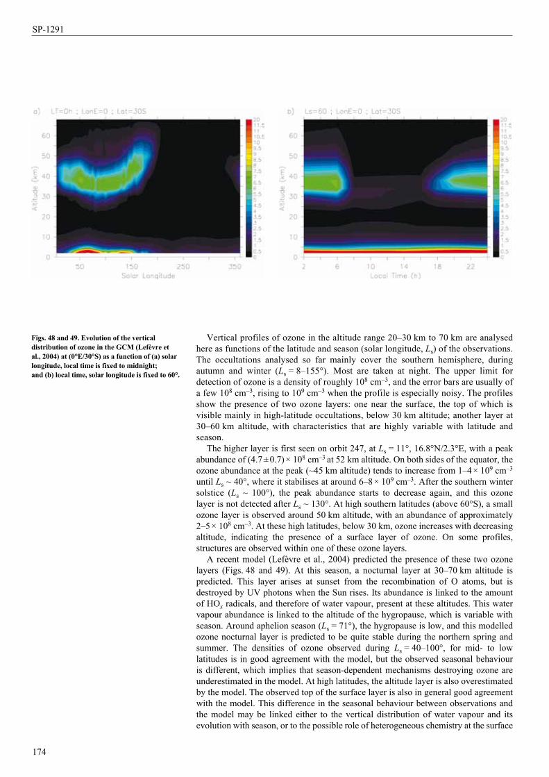
Vertical profiles of ozone in the altitude range 20–30 km to 70 km are analysed here as functions of the latitude and season (solar longitude, Ls) of the observations. The occultations analysed so far mainly cover the southern hemisphere, during autumn and winter (Ls = 8–155°). Most are taken at night. The upper limit for detection of ozone is a density of roughly 108 cm–3, and the error bars are usually of a few 108 cm–3, rising to 109 cm–3 when the profile is especially noisy. The profiles show the presence of two ozone layers: one near the surface, the top of which is visible mainly in high-latitude occultations, below 30 km altitude; another layer at 30–60 km altitude, with characteristics that are highly variable with latitude and season.
The higher layer is first seen on orbit 247, at Ls = 11°, 16.8°N/2.3°E, with a peak abundance of (4.7 ± 0.7) × 108 cm–3 at 52 km altitude. On both sides of the equator, the ozone abundance at the peak (~45 km altitude) tends to increase from 1–4 × 109 cm–3
until Ls ~ 40°, where it stabilises at around 6–8 × 109 cm–3. After the southern winter solstice (Ls ~ 100°), the peak abundance starts to decrease again, and this ozone layer is not detected after Ls ~ 130°. At high southern latitudes (above 60°S), a small ozone layer is observed around 50 km altitude, with an abundance of approximately 2–5 × 108 cm–3. At these high latitudes, below 30 km, ozone increases with decreasing altitude, indicating the presence of a surface layer of ozone. On some profiles, structures are observed within one of these ozone layers.
A recent model (Lefèvre et al., 2004) predicted the presence of these two ozone layers (Figs. 48 and 49). At this season, a nocturnal layer at 30–70 km altitude is predicted. This layer arises at sunset from the recombination of O atoms, but is destroyed by UV photons when the Sun rises. Its abundance is linked to the amount of HOx radicals, and therefore of water vapour, present at these altitudes. This water vapour abundance is linked to the altitude of the hygropause, which is variable with season. Around aphelion season (Ls = 71°), the hygropause is low, and this modelled ozone nocturnal layer is predicted to be quite stable during the northern spring and summer. The densities of ozone observed during Ls = 40–100°, for mid- to low latitudes is in good agreement with the model, but the observed seasonal behaviour is different, which implies that season-dependent mechanisms destroying ozone are underestimated in the model. At high latitudes, the altitude layer is also overestimated by the model. The observed top of the surface layer is also in general good agreement with the model. This difference in the seasonal behaviour between observations and the model may be linked either to the vertical distribution of water vapour and its evolution with season, or to the possible role of heterogeneous chemistry at the surface
174
Figs. 48 and 49. Evolution of the vertical distribution of ozone in the GCM (Lefèvre et al., 2004) at (0°E/30°S) as a function of (a) solar longitude, local time is fixed to midnight; and (b) local time, solar longitude is fixed to 60°.
SP-1291

of dust particles or water ice clouds. SPICAM observations have the potential to explore both hypotheses in more detail in future studies.
6.4 Stellar Occultation Results: Aerosol Vertical Profiles6.4.1 Impact of aerosols on the martian climate An important component of the martian atmosphere is dusty and volatile aerosols. The strong involvement of the aerosols in basic climate fields means that the lower atmosphere can be considered as a ‘dusty climate’ system. There is a permanent haze with a column optical depth of 0.1–1, depending on the season, with sporadic increases up to several units during dust storms, which is known to control temperatures in the troposphere and lower stratosphere. Heating and cooling by aerosols drive dynamical phenomena, varying in scale from general circulation to local waves that give rise to the atmospheric turbulence. The content and distribution of aerosols in the atmosphere are in turn controlled by atmospheric motion, as part of the complex feedback that makes the current climate extremely variable. Volatile aerosols also affect the thermal field by changing the optical properties and settling rates of particles. They therefore provide strongly nonlinear thermal feedback determined by the saturation curve, which is expected to be most significant during aphelion (Clancy et al., 1996; Rodin et al., 1999).
6.4.2 Observation descriptionWhile aerosols/dust may be observed on the dayside via their emission of scattered solar light, the stellar occultation technique remains unique for detecting condensation clouds during the night, in addition to plain dust particles. Figure 50A indicates the actual star spectrum signal as a function of MNP altitude and wavelength for a typical occultation. At high altitudes (z > 150 km), there is no absorption, and the structure of the signal is due to the spectrum of the star, with a strong peak at short wavelengths. The structure of CO2 absorption is clearly visible at 120–180 nm, with a fainter region of ozone absorption around 250 nm. Quantitatively, for each occultation, the ratio of spectra taken through and outside the atmosphere gives an atmospheric transmission at each altitude above the point on the surface that is closest to the slant. If there is any absorbing or/and scattering species along the optical path between the star and the spacecraft, photons are lost and the resulting transmissions are lower than 1. The fitting procedure of the measured transmission is based on a Levenberg–Marquardt algorithm that is fed with the LOS-integrated (slant) molecular concentrations of carbon dioxide, ozone and the opacity created by aerosols along the LOS. Values returned for each parameter are compiled to determine the resulting vertical profile of each species. Figure 50C compares a fitted transmission spectrum and transmission derived from the data. It illustrates the prominent signatures of CO2 and O3 and shows the transmission attenuation created by aerosols over the whole spectral range. The comparison of transmission vertical profiles at specific wavelengths (Fig. 50B) confirms the consistency of the fitting procedure.
6.4.3 Detection of a seasonal signalSince the very first occultation sequence made on 13 January 2004, more than 500 profiles have been collected by SPICAM. Some sequences were lost due to pixel saturation, or to a mispositioning of star image on the detector. A total of 412 could still be treated and yielded vertical profiles of atmospheric species, including aerosols (Fig. 51). The dataset spans a period between the end of the northern winter (at Ls = 330°, corresponding to the arrival of Mars Express) and the beginning of the northern autumn (Ls = 200°). Most observations were performed in the southern hemisphere.
Stellar occultation requires only the faint light of stars, so it offers coverage of night regions. On Mars, this is of particular interest because a crucial part of the climate is played out in the polar night regions where surface temperatures fall below the CO2 condensation point. CO2 condensed on the ground leads to significant seasonal variations in global pressure. Unfortunately, this aspect of the martian climate is incompletely documented. Temperatures have been retrieved from IR measurements,
175
Scientific instruments
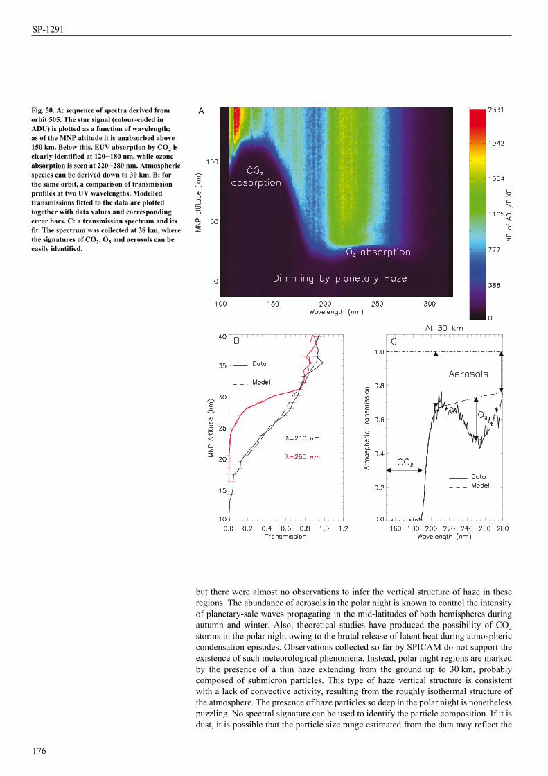
but there were almost no observations to infer the vertical structure of haze in these regions. The abundance of aerosols in the polar night is known to control the intensity of planetary-sale waves propagating in the mid-latitudes of both hemispheres during autumn and winter. Also, theoretical studies have produced the possibility of CO2 storms in the polar night owing to the brutal release of latent heat during atmospheric condensation episodes. Observations collected so far by SPICAM do not support the existence of such meteorological phenomena. Instead, polar night regions are marked by the presence of a thin haze extending from the ground up to 30 km, probably composed of submicron particles. This type of haze vertical structure is consistent with a lack of convective activity, resulting from the roughly isothermal structure of the atmosphere. The presence of haze particles so deep in the polar night is nonetheless puzzling. No spectral signature can be used to identify the particle composition. If it is dust, it is possible that the particle size range estimated from the data may reflect the
176
Fig. 50. A: sequence of spectra derived from orbit 505. The star signal (colour-coded in ADU) is plotted as a function of wavelength; as of the MNP altitude it is unabsorbed above 150 km. Below this, EUV absorption by CO2 is clearly identified at 120–180 nm, while ozone absorption is seen at 220–280 nm. Atmospheric species can be derived down to 30 km. B: for the same orbit, a comparison of transmission profiles at two UV wavelengths. Modelled transmissions fitted to the data are plotted together with data values and corresponding error bars. C: a transmission spectrum and its fit. The spectrum was collected at 38 km, where the signatures of CO2, O3 and aerosols can be easily identified.
A
SP-1291

177
Fig. 51. A set of aerosol profiles retrieved from SPICAM stellar occultations in the southern hemisphere around the northern summer solstice. Solid lines show the aerosol opacity along the LOS as a function of altitude (red horizontal bars indicate measurement uncertainties). Blue circles give the value of the Angström coefficient a (opacity varies as l–a; a is a parameter indicative of the particle size), on the same scale as opacity. Larger a means smaller particles. Values shown here suggest a particle size of <1 µm. The orbit number is at upper left; at top is the latitude and longitude of the occultation point and solar longitude Ls, and the local time. The atmosphere is clear above 30 km, which is rarely the case at other latitudes and seasons.
Scientific instruments
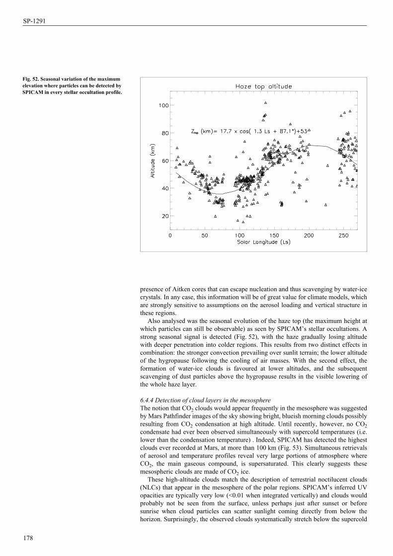
178
Fig. 52. Seasonal variation of the maximum elevation where particles can be detected by SPICAM in every stellar occultation profile.
presence of Aitken cores that can escape nucleation and thus scavenging by water-ice crystals. In any case, this information will be of great value for climate models, which are strongly sensitive to assumptions on the aerosol loading and vertical structure in these regions.
Also analysed was the seasonal evolution of the haze top (the maximum height at which particles can still be observable) as seen by SPICAM’s stellar occultations. A strong seasonal signal is detected (Fig. 52), with the haze gradually losing altitude with deeper penetration into colder regions. This results from two distinct effects in combination: the stronger convection prevailing over sunlit terrain; the lower altitude of the hygropause following the cooling of air masses. With the second effect, the formation of water-ice clouds is favoured at lower altitudes, and the subsequent scavenging of dust particles above the hygropause results in the visible lowering of the whole haze layer.
6.4.4 Detection of cloud layers in the mesosphereThe notion that CO2 clouds would appear frequently in the mesosphere was suggested by Mars Pathfinder images of the sky showing bright, blueish morning clouds possibly resulting from CO2 condensation at high altitude. Until recently, however, no CO2 condensate had ever been observed simultaneously with supercold temperatures (i.e. lower than the condensation temperature) . Indeed, SPICAM has detected the highest clouds ever recorded at Mars, at more than 100 km (Fig. 53). Simultaneous retrievals of aerosol and temperature profiles reveal very large portions of atmosphere where CO2, the main gaseous compound, is supersaturated. This clearly suggests these mesospheric clouds are made of CO2 ice.
These high-altitude clouds match the description of terrestrial noctilucent clouds (NLCs) that appear in the mesosphere of the polar regions. SPICAM’s inferred UV opacities are typically very low (<0.01 when integrated vertically) and clouds would probably not be seen from the surface, unless perhaps just after sunset or before sunrise when cloud particles can scatter sunlight coming directly from below the horizon. Surprisingly, the observed clouds systematically stretch below the supercold
SP-1291
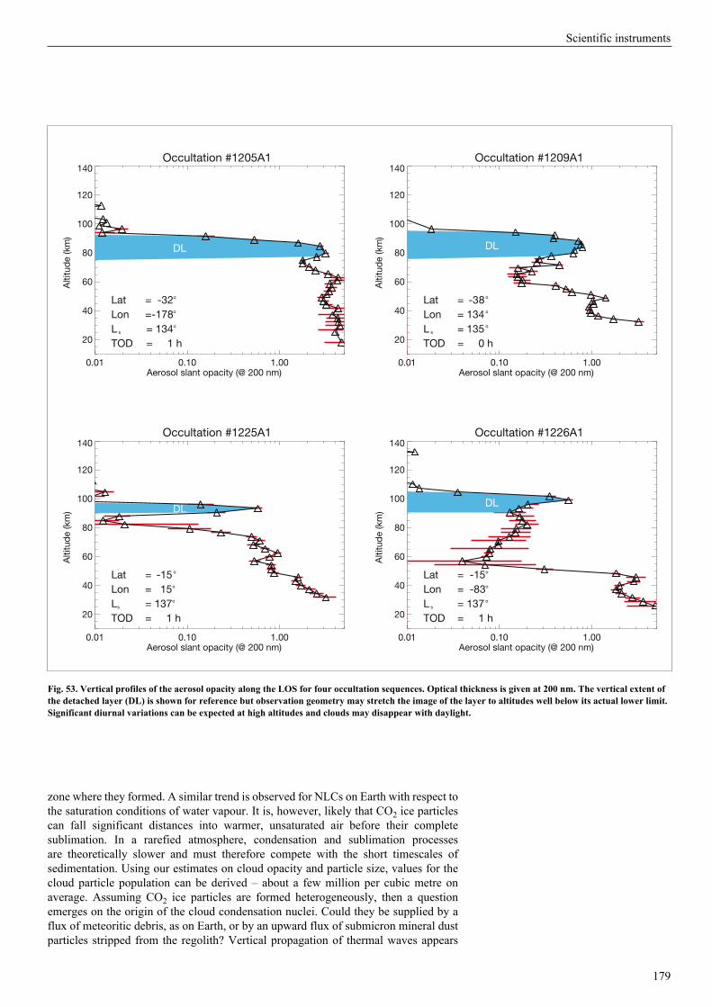
zone where they formed. A similar trend is observed for NLCs on Earth with respect to the saturation conditions of water vapour. It is, however, likely that CO2 ice particles can fall significant distances into warmer, unsaturated air before their complete sublimation. In a rarefied atmosphere, condensation and sublimation processes are theoretically slower and must therefore compete with the short timescales of sedimentation. Using our estimates on cloud opacity and particle size, values for the cloud particle population can be derived – about a few million per cubic metre on average. Assuming CO2 ice particles are formed heterogeneously, then a question emerges on the origin of the cloud condensation nuclei. Could they be supplied by a flux of meteoritic debris, as on Earth, or by an upward flux of submicron mineral dust particles stripped from the regolith? Vertical propagation of thermal waves appears
179
Fig. 53. Vertical profiles of the aerosol opacity along the LOS for four occultation sequences. Optical thickness is given at 200 nm. The vertical extent of the detached layer (DL) is shown for reference but observation geometry may stretch the image of the layer to altitudes well below its actual lower limit. Significant diurnal variations can be expected at high altitudes and clouds may disappear with daylight.
Occultation #1205A1
0.01 0.10 1.00Aerosol slant opacity (@ 200 nm)
20
40
60
80
100
120
140
Alti
tud
e (k
m)
LatLonL s
TOD
= -32o
=-178o
= 134o
= 1 h
DL
Occultation #1209A1
0.01 0.10 1.00Aerosol slant opacity (@ 200 nm)
20
40
60
80
100
120
140
Alti
tud
e (k
m)
LatLonL s
TOD
= -3 8o
= 134 o
= 135 o
= 0 h
DL
Occultation #1225A1
0.01 0.10 1.00Aerosol slant opacity (@ 200 nm)
20
40
60
80
100
120
140
Alti
tud
e (k
m)
LatLonLs
TOD
= -15 o
= 1 5o
= 137o
= 1 h
DL
Occultation #1226A1
0.01 0.10 1.00Aerosol slant opacity (@ 200 nm)
20
40
60
80
100
120
140
Alti
tud
e (k
m)
LatLonL s
TOD
= -1 5o
= -8 3o
= 137 o
= 1 h
DL
Scientific instruments

only partly buffered by the release of latent heat induced by CO2 condensation, as illustrated by the recurrent presence of supercold air pockets. As a result, the role played by microphysical processes, which control CO2 ice particle formation and evolution, is critical in regulating the thermal state of the upper atmosphere.
7.1 Technical Description The near-IR channel works in the spectral range 1–1.7 µm with a resolving power superior to 1800. It is a lightweight (0.8 kg) extension of the UV channel that was added at late stage of the mission, partly in order to demonstrate the capability of the new acousto-optic tuneable filter (AOTF) technology in deep space. Its principal goal is to measure water vapour in the atmosphere, spectrally analysing solar radiation reflected from the surface and modified by atmospheric absorptions. This channel and its expected science return were described in Bertaux et al. (2004) and Korablev et al. (2002a); a more detailed description of the hardware is presented in Korablev et al. (2002b). This section summarises the in-flight performance and presents an overview of the main scientific results.
A single-pixel detector of InGaAs, associated with an AOTF, allows the measurement of the H2O column at nadir with a very low-mass configuration. The AOTF device is based on the Bragg diffraction of an entrance beam by the ultrasonic acoustic wave excited within a crystal. It offers the potential to reach a resolving power, l/Dl, greater than 1000, which is ample to measure nadir H2O by scanning the absorption line at 1.38 µm in the reflected solar spectrum. There are no moving parts, such as a chopper. This new concept in IR spectroscopy had never flown on a civil spacecraft but SPICAM has demonstrated its maturity for space research; it should have a great future.
The spectrometer is included alongside the SUV (see Fig. 4); its optical scheme is shown in Fig. 2 and its main characteristics are summarised in Table 5. A 30 mm diameter lens telescope has a focal ratio of 1/1.9. A 1 mm diameter circular diaphragm
180
7. The SPICAM AOTF Near-IR Channel
Table 5. Characteristics of the SPICAM near-IR channel (SIR).
Spectral range 1.0–1.7 µm
Spectral resolution 0.5 nm at 1.0 µm; 0.95 nm at 1.5 µm
FOV 1°
Telescope Lens type, Ø 30 mm
AOTF TeO2, efficiency 70% (in polarised light), aperture 3.6 x 3.6 mm, ±3.5°
Detector 2 InGaAs PIN diodes (Hamamatsu G5832), Ø 1 mm
Transmission of optics 20%
NER ~5 x 10⁻⁹ W cm–2 sr–1
Gain control 4 pre-chosen gain values
Number of spectral points 2 spectra with different polarisations, 332–3984 points each
Dynamic range 216, rounded to 212
Power consumption 5 W average
Dimensions 220 x 85 x 65 mm
Mass 700 g
SP-1291
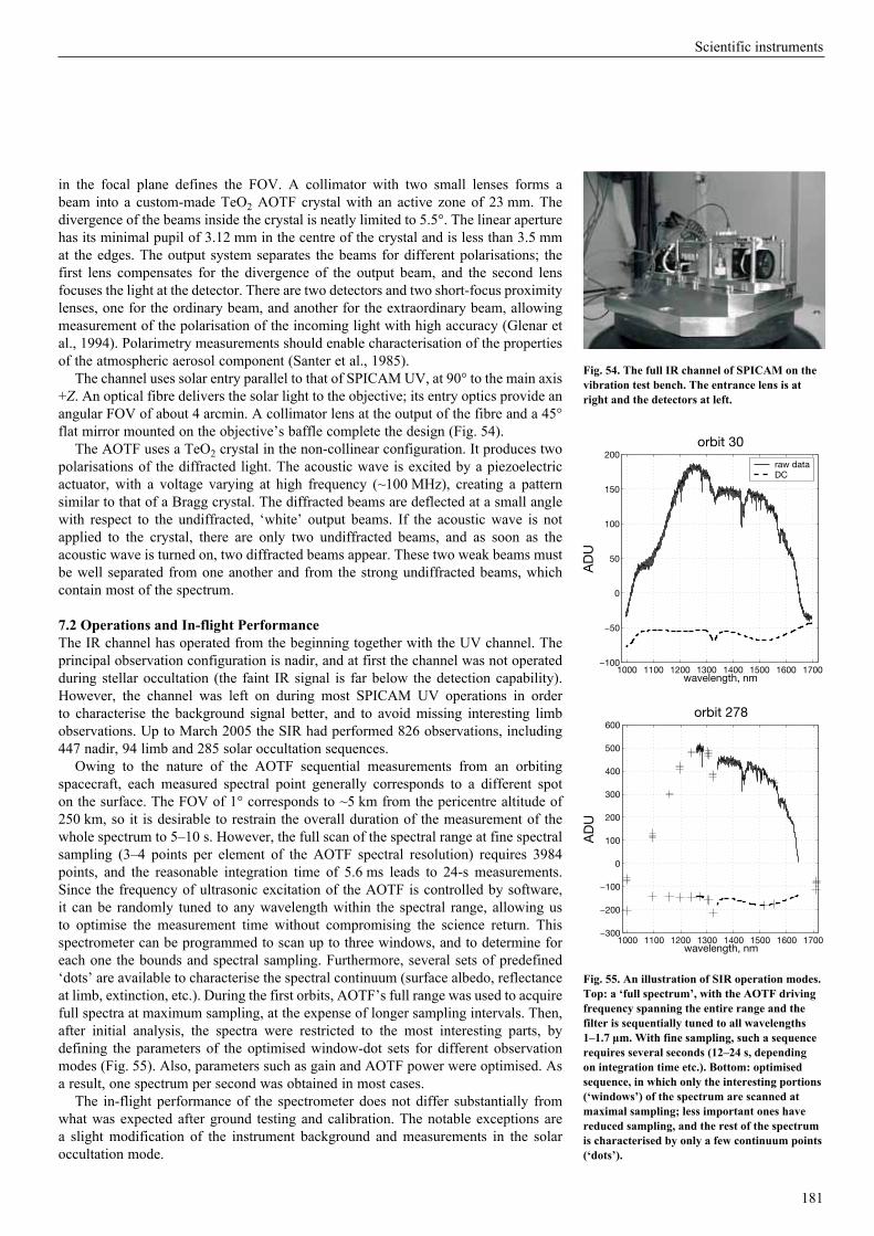
in the focal plane defines the FOV. A collimator with two small lenses forms a beam into a custom-made TeO2 AOTF crystal with an active zone of 23 mm. The divergence of the beams inside the crystal is neatly limited to 5.5°. The linear aperture has its minimal pupil of 3.12 mm in the centre of the crystal and is less than 3.5 mm at the edges. The output system separates the beams for different polarisations; the first lens compensates for the divergence of the output beam, and the second lens focuses the light at the detector. There are two detectors and two short-focus proximity lenses, one for the ordinary beam, and another for the extraordinary beam, allowing measurement of the polarisation of the incoming light with high accuracy (Glenar et al., 1994). Polarimetry measurements should enable characterisation of the properties of the atmospheric aerosol component (Santer et al., 1985).
The channel uses solar entry parallel to that of SPICAM UV, at 90° to the main axis +Z. An optical fibre delivers the solar light to the objective; its entry optics provide an angular FOV of about 4 arcmin. A collimator lens at the output of the fibre and a 45° flat mirror mounted on the objective’s baffle complete the design (Fig. 54).
The AOTF uses a TeO2 crystal in the non-collinear configuration. It produces two polarisations of the diffracted light. The acoustic wave is excited by a piezoelectric actuator, with a voltage varying at high frequency (~100 MHz), creating a pattern similar to that of a Bragg crystal. The diffracted beams are deflected at a small angle with respect to the undiffracted, ‘white’ output beams. If the acoustic wave is not applied to the crystal, there are only two undiffracted beams, and as soon as the acoustic wave is turned on, two diffracted beams appear. These two weak beams must be well separated from one another and from the strong undiffracted beams, which contain most of the spectrum.
7.2 Operations and In-flight Performance The IR channel has operated from the beginning together with the UV channel. The principal observation configuration is nadir, and at first the channel was not operated during stellar occultation (the faint IR signal is far below the detection capability). However, the channel was left on during most SPICAM UV operations in order to characterise the background signal better, and to avoid missing interesting limb observations. Up to March 2005 the SIR had performed 826 observations, including 447 nadir, 94 limb and 285 solar occultation sequences.
Owing to the nature of the AOTF sequential measurements from an orbiting spacecraft, each measured spectral point generally corresponds to a different spot on the surface. The FOV of 1° corresponds to ~5 km from the pericentre altitude of 250 km, so it is desirable to restrain the overall duration of the measurement of the whole spectrum to 5–10 s. However, the full scan of the spectral range at fine spectral sampling (3–4 points per element of the AOTF spectral resolution) requires 3984 points, and the reasonable integration time of 5.6 ms leads to 24-s measurements. Since the frequency of ultrasonic excitation of the AOTF is controlled by software, it can be randomly tuned to any wavelength within the spectral range, allowing us to optimise the measurement time without compromising the science return. This spectrometer can be programmed to scan up to three windows, and to determine for each one the bounds and spectral sampling. Furthermore, several sets of predefined ‘dots’ are available to characterise the spectral continuum (surface albedo, reflectance at limb, extinction, etc.). During the first orbits, AOTF’s full range was used to acquire full spectra at maximum sampling, at the expense of longer sampling intervals. Then, after initial analysis, the spectra were restricted to the most interesting parts, by defining the parameters of the optimised window-dot sets for different observation modes (Fig. 55). Also, parameters such as gain and AOTF power were optimised. As a result, one spectrum per second was obtained in most cases.
The in-flight performance of the spectrometer does not differ substantially from what was expected after ground testing and calibration. The notable exceptions are a slight modification of the instrument background and measurements in the solar occultation mode.
181
1000 1100 1200 1300 1400 1500 1600 1700−300
−200
−100
0
100
200
300
400
500
600
wavelength, nm
AD
U
orbit 278
1000 1100 1200 1300 1400 1500 1600 1700−100
−50
0
50
100
150
200orbit 30
AD
U
raw dataDC
wavelength, nm
Fig. 55. An illustration of SIR operation modes. Top: a ‘full spectrum’, with the AOTF driving frequency spanning the entire range and the filter is sequentially tuned to all wavelengths 1–1.7 µm. With fine sampling, such a sequence requires several seconds (12–24 s, depending on integration time etc.). Bottom: optimised sequence, in which only the interesting portions (‘windows’) of the spectrum are scanned at maximal sampling; less important ones have reduced sampling, and the rest of the spectrum is characterised by only a few continuum points (‘dots’).
Fig. 54. The full IR channel of SPICAM on the vibration test bench. The entrance lens is at right and the detectors at left.
1000 1100 1200 1300 1400 1500 1600 1700−300
−200
−100
0
100
200
300
400
500
600
wavelength, nm
AD
U
orbit 278
1000 1100 1200 1300 1400 1500 1600 1700−100
−50
0
50
100
150
200orbit 30
AD
U
raw dataDC
wavelength, nm
Scientific instruments
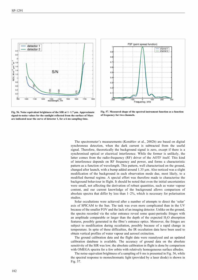
The spectrometer’s measurements (Korablev et al., 2002b) are based on digital synchronous detection, when the dark current is subtracted from the useful signal. Therefore, theoretically the background signal is zero, except if there is a synchronised optical or electrical interference. While the former is unlikely, the latter comes from the radio-frequency (RF) driver of the AOTF itself. This kind of interference depends on RF frequency and power, and forms a characteristic pattern as a function of wavelength. This pattern, well characterised on the ground, changed after launch, with a bump added around 1.35 µm. Also noticed was a slight modification of the background in each observation mode due, most likely, to a modified thermal regime. A special effort was therefore made to characterise the background behaviour in flight. It should be noted that even the initial uncertainties were small, not affecting the derivation of robust quantities, such as water vapour content, and our current knowledge of the background allows comparison of absolute spectra that differ by less than 1–2%, which is necessary for polarisation studies.
Solar occultations were achieved after a number of attempts to direct the ‘solar’ axis of SPICAM to the Sun. The task was even more complicated than in the UV because of the smaller FOV and the lack of an imaging detector. Unlike on the ground, the spectra recorded via the solar entrance reveal some quasi-periodic fringes with an amplitude comparable or larger than the depth of the expected H2O absorption features, possibly generated in the fibre’s entrance optics. Moreover, the fringes are subject to modification during occultation, possibly because of a rapid change in temperature. In spite of these difficulties, the IR occultation data have been used to obtain vertical profiles of water vapour and aerosol extinction.
The ground calibration data and the flight data were reanalysed and an updated calibration database is available. The accuracy of ground data on the absolute sensitivity of the SIR was low; the absolute calibration in flight is done by comparison with OMEGA spectra for a few orbits with relatively homogeneous surface albedos.
The noise-equivalent brightness of a sampling of 6 ms is presented in Fig. 56, while the spectral response to monochromatic light (provided by a laser diode) is shown in Fig. 57.
182
Fig. 56. Noise equivalent brightness of the SIR at 1–1.7 µm. Approximate signal-to-noise values for the sunlight reflected from the surface of Mars are indicated near the curve of detector 1, for a 6 ms sampling time.
Fig. 57. Measured shape of the spectral instrument function as a function of frequency for two channels.
SP-1291
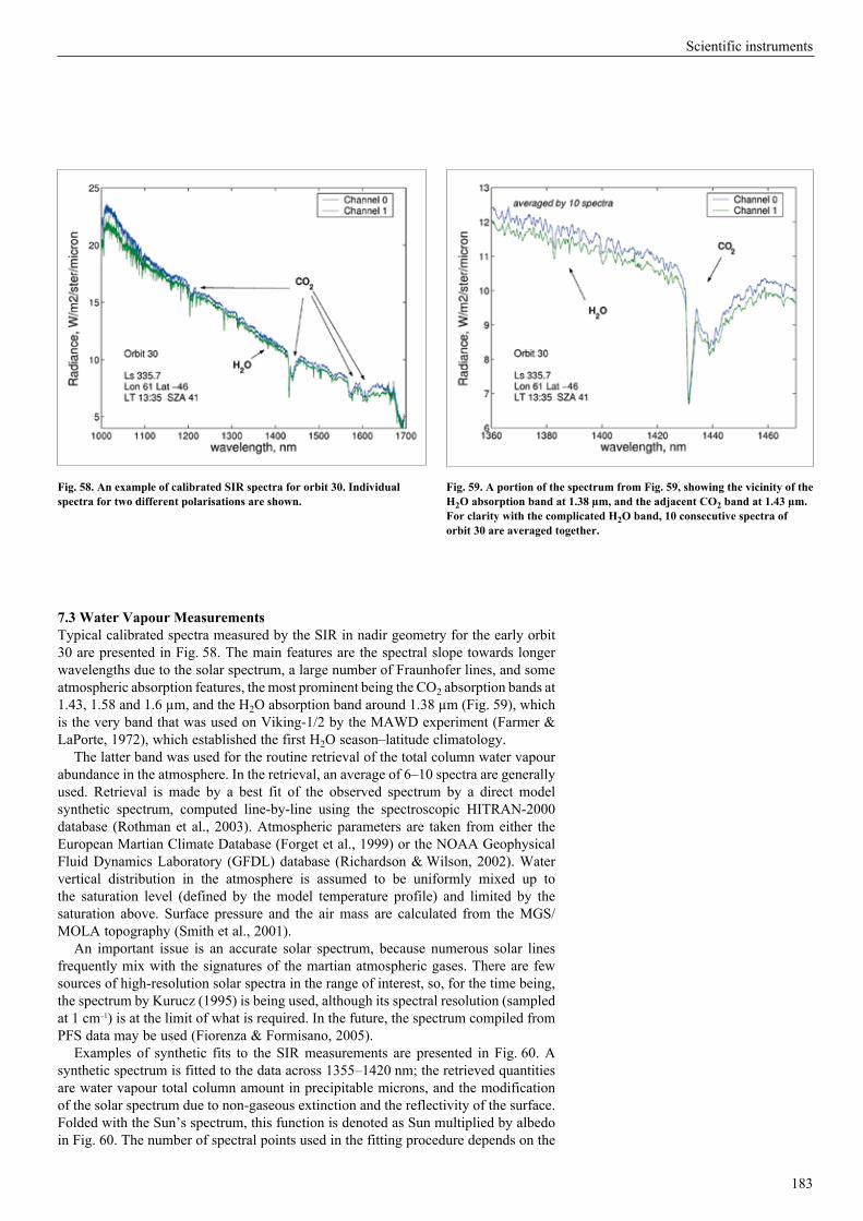
183
7.3 Water Vapour MeasurementsTypical calibrated spectra measured by the SIR in nadir geometry for the early orbit 30 are presented in Fig. 58. The main features are the spectral slope towards longer wavelengths due to the solar spectrum, a large number of Fraunhofer lines, and some atmospheric absorption features, the most prominent being the CO2 absorption bands at 1.43, 1.58 and 1.6 µm, and the H2O absorption band around 1.38 µm (Fig. 59), which is the very band that was used on Viking-1/2 by the MAWD experiment (Farmer & LaPorte, 1972), which established the first H2O season–latitude climatology.
The latter band was used for the routine retrieval of the total column water vapour abundance in the atmosphere. In the retrieval, an average of 6–10 spectra are generally used. Retrieval is made by a best fit of the observed spectrum by a direct model synthetic spectrum, computed line-by-line using the spectroscopic HITRAN-2000 database (Rothman et al., 2003). Atmospheric parameters are taken from either the European Martian Climate Database (Forget et al., 1999) or the NOAA Geophysical Fluid Dynamics Laboratory (GFDL) database (Richardson & Wilson, 2002). Water vertical distribution in the atmosphere is assumed to be uniformly mixed up to the saturation level (defined by the model temperature profile) and limited by the saturation above. Surface pressure and the air mass are calculated from the MGS/MOLA topography (Smith et al., 2001).
An important issue is an accurate solar spectrum, because numerous solar lines frequently mix with the signatures of the martian atmospheric gases. There are few sources of high-resolution solar spectra in the range of interest, so, for the time being, the spectrum by Kurucz (1995) is being used, although its spectral resolution (sampled at 1 cm–1) is at the limit of what is required. In the future, the spectrum compiled from PFS data may be used (Fiorenza & Formisano, 2005).
Examples of synthetic fits to the SIR measurements are presented in Fig. 60. A synthetic spectrum is fitted to the data across 1355–1420 nm; the retrieved quantities are water vapour total column amount in precipitable microns, and the modification of the solar spectrum due to non-gaseous extinction and the reflectivity of the surface. Folded with the Sun’s spectrum, this function is denoted as Sun multiplied by albedo in Fig. 60. The number of spectral points used in the fitting procedure depends on the
Fig. 58. An example of calibrated SIR spectra for orbit 30. Individual spectra for two different polarisations are shown.
Fig. 59. A portion of the spectrum from Fig. 59, showing the vicinity of the H2O absorption band at 1.38 µm, and the adjacent CO2 band at 1.43 µm. For clarity with the complicated H2O band, 10 consecutive spectra of orbit 30 are averaged together.
Scientific instruments
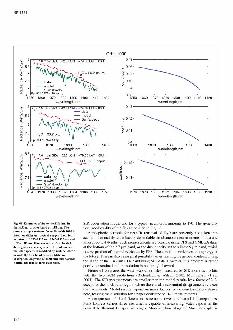
SIR observation mode, and for a typical nadir orbit amounts to 170. The generally very good quality of the fit can be seen in Fig. 60.
Atmospheric aerosols for near-IR retrieval of H2O are presently not taken into account, due mainly to the lack of dependable simultaneous measurements of dust and aerosol optical depths. Such measurements are possible using PFS and OMEGA data: at the bottom of the 2.7 µm band, or the dust opacity in the silicate 9 µm band, which is a by-product of thermal retrievals by PFS. The aim is to implement this synergy in the future. There is also a marginal possibility of estimating the aerosol contents fitting the shape of the 1.43 µm CO2 band using SIR data. However, this problem is rather poorly constrained and the solution is not straightforward.
Figure 61 compares the water vapour profiles measured by SIR along two orbits with the two GCM predictions (Richardson & Wilson, 2002; Montmessin et al., 2004). The SIR measurements are smaller than the model results by a factor of 2–3, except for the north polar region, where there is also substantial disagreement between the two models. Model results depend on many factors, so no conclusions are drawn here, leaving the discussion for a paper dedicated to H2O measurements.
A comparison of the different measurements reveals substantial discrepancies. Mars Express carries three instruments capable of measuring water vapour in the near-IR to thermal–IR spectral ranges. Modern climatology of Mars atmospheric
184
1350 1360 1370 1380 1390 1400 1410 14206.5
7
7.5
8
8.5
9
wavelength,nm
Rad
ianc
e, W
/m2/
µm
Orbit 1000
Sp. 001 / 97Avr 10 sp.
P0 = 7.0 mbar SZA = 62.3 LON = −79.5E LAT = 86.1
H2O = 29.2 pr.µm
datamodelSun*albedo
1350 1360 1370 1380 1390 1400 1410 14200.38
0.4
0.42
0.44
0.46
0.48
wavelength,nm
cont
inuu
m
1360 1370 1380 1390 14007
7.5
8
8.5
9
wavelength,nm
Rad
ianc
e, W
/m2/
µm
Sp. 001 / 97Avr 10 sp.
P0 = 7.0 mbar SZA = 62.3 LON = −79.5E LAT = 86.1
H2O = 33.7 pr.µm
datamodelSun*albedo
1360 1370 1380 1390 14000.4
0.41
0.42
0.43
wavelength,nm
cont
inuu
m
1376 1378 1380 1382 1384 1386 1388 13907
7.5
8
8.5
wavelength,nm
Rad
ianc
e, W
/m2/
µm
Sp. 001 / 97Avr 10 sp.
P0 = 7.0 mbar SZA = 62.3 LON = −79.5E LAT = 86.1
H2O = 35.6 pr.µm
datamodelSun*albedo
1376 1378 1380 1382 1384 1386 1388 1390
0.41
0.415
wavelength,nm
cont
inuu
m
Fig. 60. Examples of fits to the SIR data in the H2O absorption band at 1.38 µm. The same average spectrum for nadir orbit 1000 is fitted for different spectral ranges (from top to bottom): 1355–1412 nm, 1365–1395 nm and 1377–1389 nm. Blue curves: SIR calibrated data; green curves: synthetic fit; red curves: the solar spectrum modified by surface albedo (a wide H2O ice band causes additional absorption longward of 1420 nm) and possible continuum atmospheric extinction.
SP-1291
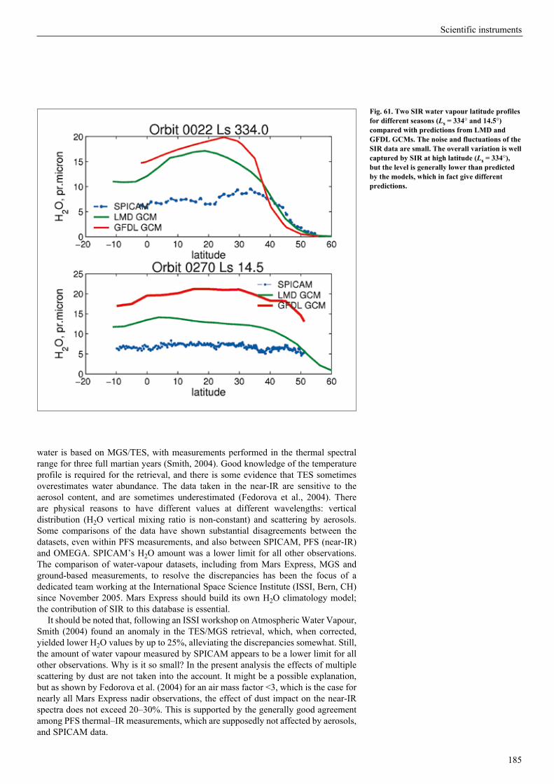
water is based on MGS/TES, with measurements performed in the thermal spectral range for three full martian years (Smith, 2004). Good knowledge of the temperature profile is required for the retrieval, and there is some evidence that TES sometimes overestimates water abundance. The data taken in the near-IR are sensitive to the aerosol content, and are sometimes underestimated (Fedorova et al., 2004). There are physical reasons to have different values at different wavelengths: vertical distribution (H2O vertical mixing ratio is non-constant) and scattering by aerosols. Some comparisons of the data have shown substantial disagreements between the datasets, even within PFS measurements, and also between SPICAM, PFS (near-IR) and OMEGA. SPICAM’s H2O amount was a lower limit for all other observations. The comparison of water-vapour datasets, including from Mars Express, MGS and ground-based measurements, to resolve the discrepancies has been the focus of a dedicated team working at the International Space Science Institute (ISSI, Bern, CH) since November 2005. Mars Express should build its own H2O climatology model; the contribution of SIR to this database is essential.
It should be noted that, following an ISSI workshop on Atmospheric Water Vapour, Smith (2004) found an anomaly in the TES/MGS retrieval, which, when corrected, yielded lower H2O values by up to 25%, alleviating the discrepancies somewhat. Still, the amount of water vapour measured by SPICAM appears to be a lower limit for all other observations. Why is it so small? In the present analysis the effects of multiple scattering by dust are not taken into the account. It might be a possible explanation, but as shown by Fedorova et al. (2004) for an air mass factor <3, which is the case for nearly all Mars Express nadir observations, the effect of dust impact on the near-IR spectra does not exceed 20–30%. This is supported by the generally good agreement among PFS thermal–IR measurements, which are supposedly not affected by aerosols, and SPICAM data.
185
Fig. 61. Two SIR water vapour latitude profiles for different seasons (Ls = 334° and 14.5°) compared with predictions from LMD and GFDL GCMs. The noise and fluctuations of the SIR data are small. The overall variation is well captured by SIR at high latitude (Ls = 334°), but the level is generally lower than predicted by the models, which in fact give different predictions.
Scientific instruments
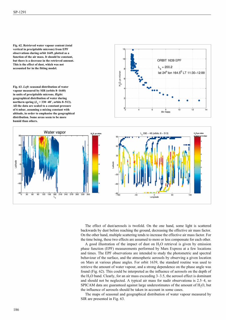
The effect of dust/aerosols is twofold. On the one hand, some light is scattered backwards by dust before reaching the ground, decreasing the effective air mass factor. On the other hand, multiple scattering tends to increase the effective air mass factor. For the time being, these two effects are assumed to more or less compensate for each other.
A good illustration of the impact of dust on H2O retrieval is given by emission phase function (EPF) measurements performed by Mars Express at a few locations and times. The EPF observations are intended to study the photometric and spectral behaviour of the surface, and the atmospheric aerosols by observing a given location on Mars at various phase angles. For orbit 1639, the standard routine was used to retrieve the amount of water vapour, and a strong dependence on the phase angle was found (Fig. 62). This could be interpreted as the influence of aerosols on the depth of the H2O band. Clearly, for an air mass exceeding 3–3.5, the aerosol effect is dominant and should not be neglected. A typical air mass for nadir observationa is 2.5–4, so SPICAM data are guaranteed against large underestimates of the amount of H2O, but the influence of aerosols should be taken in account in some cases.
The maps of seasonal and geographical distribution of water vapour measured by SIR are presented in Fig. 63.
186
Fig. 63. Left: seasonal distribution of water vapour measured by SIR (orbits 8–1640) in units of precipitable microns. Right: geographical distribution of water during northern spring (Ls = 330–48°, orbits 8–513). All the data are scaled to a constant pressure of 6 mbar, assuming a mixing constant with altitude, in order to emphasise the geographical distribution. Some areas seem to be more humid than others.
Fig. 62. Retrieved water vapour content (total vertical in precipitable microns) from EPF observations during orbit 1649, plotted as a function of the air mass. It should be constant, but there is a decrease in the retrieved amount. This is the effect of dust, which was not accounted for in the fitting model.
SP-1291
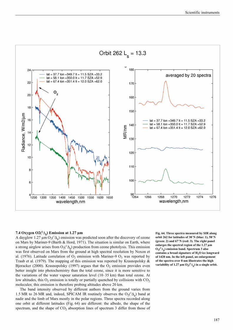
7.4 Oxygen O2(1∆g) Emission at 1.27 µmA dayglow 1.27 µm O2(1Dg) emission was predicted soon after the discovery of ozone on Mars by Mariner-9 (Barth & Hord, 1971). The situation is similar on Earth, where a strong airglow arises from O2(1Dg) production from ozone photolysis. This emission was first observed on Mars from the ground at high spectral resolution by Noxon et al. (1976). Latitude correlation of O2 emission with Mariner-9 O3 was reported by Traub et al. (1979). The mapping of this emission was reported by Krasnopolsky & Bjoracker (2000). Krasnopolsky (1997) argues that the O2 emission provides even better insight into photochemistry than the total ozone, since it is more sensitive to the variations of the water vapour saturation level (10–35 km) than total ozone. At low altitudes, this O2 emission is totally or partially quenched by collisions with CO2 molecules; this emission is therefore probing altitudes above 20 km.
The band intensity observed by different authors from the ground varies from 1.5 MR to 26 MR and, indeed, SPICAM IR routinely observes the O2(1Dg) band at nadir and the limb of Mars mostly in the polar regions. Three spectra recorded along one orbit at different latitudes (Fig. 64) are different: the albedo, the shape of the spectrum, and the shape of CO2 absorption lines of spectrum 3 differ from those of
187
Fig. 64. Three spectra measured by SIR along orbit 262 for latitudes of 38°N (blue: 1), 58°N (green: 2) and 67°N (red: 3). The right panel enlarges the spectral region of the 1.27 µm O2(1∆g) emission band. Spectrum 3 also contains a broad signature of H2O ice longward of 1420 nm. In the left panel, an enlargement of the spectra over 8 nm illustrates the high variability of 1.27 µm O2(1∆g) in a single orbit.
Scientific instruments
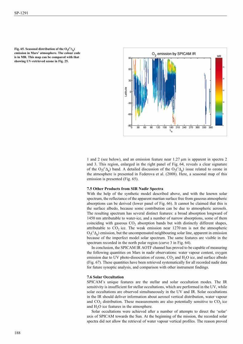
1 and 2 (see below), and an emission feature near 1.27 µm is apparent in spectra 2 and 3. This region, enlarged in the right panel of Fig. 64, reveals a clear signature of the O2(1Dg) band. A detailed discussion of the O2(1Dg) issue related to ozone in the atmosphere is presented in Federova et al. (2008). Here, a seasonal map of this emission is presented (Fig. 65).
7.5 Other Products from SIR Nadir Spectra With the help of the synthetic model described above, and with the known solar spectrum, the reflectance of the apparent martian surface free from gaseous atmospheric absorptions can be derived (lower panel of Fig. 66). It cannot be claimed that this is the surface albedo, because some contribution can be due to atmospheric aerosols. The resulting spectrum has several distinct features: a broad absorption longward of 1450 nm attributable to water-ice, and a number of narrow absorptions, some of them coinciding with gaseous CO2 absorption bands but with distinctly different shapes, attributable to CO2 ice. The weak emission near 1270 nm is not the atmospheric O2(1Dg) emission, but the uncompensated neighbouring solar line, apparent in emission because of the imperfect model solar spectrum. The same features are visible in the spectrum recorded in the north polar region (curve 3 in Fig. 64).
In conclusion, the SPICAM IR AOTF channel has proved to be capable of measuring the following quantities on Mars in nadir observations: water vapour content, oxygen emission due to UV photo-dissociation of ozone, CO2 and H2O ice, and surface albedo (Fig. 67). These quantities have been retrieved systematically for all recorded nadir data for future synoptic analysis, and comparison with other instrument findings.
7.6 Solar OccultationSPICAM’s unique features are the stellar and solar occultation modes. The IR sensitivity is insufficient for stellar occultations, which are performed in the UV, while solar occultations are observed simultaneously in the UV and IR. Solar occultations in the IR should deliver information about aerosol vertical distribution, water vapour and CO2 distribution. These measurements are also potentially sensitive to CO2 ice and H2O ice features in the atmosphere.
Solar occultations were achieved after a number of attempts to direct the ‘solar’ axis of SPICAM towards the Sun. At the beginning of the mission, the recorded solar spectra did not allow the retrieval of water vapour vertical profiles. The reason proved
188
Fig. 65. Seasonal distribution of the O2(1∆g) emission in Mars’ atmosphere. The colour code is in MR. This map can be compared with that showing UV-retrieved ozone in Fig. 25.
SP-1291
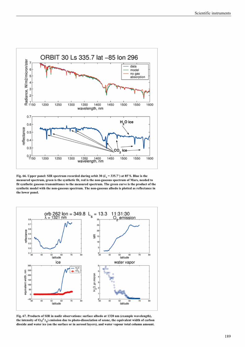
189
Fig. 66. Upper panel: SIR spectrum recorded during orbit 30 (Ls = 335.7°) at 85°S. Blue is the measured spectrum, green is the synthetic fit, red is the non-gaseous spectrum of Mars, needed to fit synthetic gaseous transmittance to the measured spectrum. The green curve is the product of the synthetic model with the non-gaseous spectrum. The non-gaseous albedo is plotted as reflectance in the lower panel.
Fig. 67. Products of SIR in nadir observations: surface albedo at 1320 nm (example wavelength), the intensity of O2(1∆g) emission due to photo-dissociation of ozone, the equivalent width of carbon dioxide and water ice (on the surface or in aerosol layers), and water vapour total column amount.
Scientific instruments
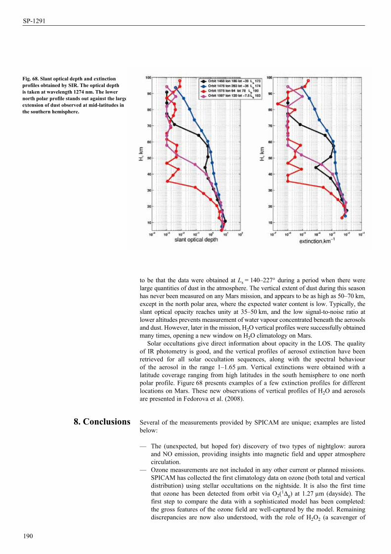
190
8. Conclusions
Fig. 68. Slant optical depth and extinction profiles obtained by SIR. The optical depth is taken at wavelength 1274 nm. The lower north polar profile stands out against the large extension of dust observed at mid-latitudes in the southern hemisphere.
to be that the data were obtained at Ls = 140–227° during a period when there were large quantities of dust in the atmosphere. The vertical extent of dust during this season has never been measured on any Mars mission, and appears to be as high as 50–70 km, except in the north polar area, where the expected water content is low. Typically, the slant optical opacity reaches unity at 35–50 km, and the low signal-to-noise ratio at lower altitudes prevents measurement of water vapour concentrated beneath the aerosols and dust. However, later in the mission, H2O vertical profiles were successfully obtained many times, opening a new window on H2O climatology on Mars.
Solar occultations give direct information about opacity in the LOS. The quality of IR photometry is good, and the vertical profiles of aerosol extinction have been retrieved for all solar occultation sequences, along with the spectral behaviour of the aerosol in the range 1–1.65 µm. Vertical extinctions were obtained with a latitude coverage ranging from high latitudes in the south hemisphere to one north polar profile. Figure 68 presents examples of a few extinction profiles for different locations on Mars. These new observations of vertical profiles of H2O and aerosols are presented in Fedorova et al. (2008).
Several of the measurements provided by SPICAM are unique; examples are listed below:
— The (unexpected, but hoped for) discovery of two types of nightglow: aurora and NO emission, providing insights into magnetic field and upper atmosphere circulation.
— Ozone measurements are not included in any other current or planned missions. SPICAM has collected the first climatology data on ozone (both total and vertical distribution) using stellar occultations on the nightside. It is also the first time that ozone has been detected from orbit via O2(1Dg) at 1.27 µm (dayside). The first step to compare the data with a sophisticated model has been completed: the gross features of the ozone field are well-captured by the model. Remaining discrepancies are now also understood, with the role of H2O2 (a scavenger of
SP-1291
ozone) destruction on water-ice grains in the clouds or on the ground (Lefèvre et al., 2008). Once the model is tuned to reproduce the data (validated), it will offer the extraordinary possibility to calculate with confidence a large number of other species that are difficult (H2O2) or impossible to measure directly (i.e. HOx radicals), for a full description of the martian environment. This is important for studies to assess the sustainability of life and human exploration.
— The density/temperature profiles obtained with SPICAM provide important constraints for building meteorological and dynamical atmospheric models, from the surface to the troposphere. SPICAM provides the only access by remote sensing to altitudes of 80–150 km, the region used for aerocapture and aerobraking. As predicted (Bertaux et al., 2004), stellar occultations gave a unique chance to detect clouds on the nightside, with the discovery of CO2 condensation clouds at 90 km.
— Remote sensing of the ionosphere from natural emissions and interaction with the solar wind is not included in other ongoing or planned missions.
— The mapping of H2O by the AOTF near-IR spectrometer has been fully demonstrated. With a mass of only 0.75 kg, this instrument should fly as a low-cost passenger on all future Mars missions.
SPICAM is applying to Mars the most successful methods for studying Earth’s atmosphere: backscatter UV and IR spectroscopy, and solar/stellar occultation limb sounding. The most remarkable thing is that all these results have been obtained with an instrument weighing only 4.7 kg. It is fair to say that the success of SPICAM is also due to the design of the Mars Express spacecraft, which has a marvellous capability for orientation in any direction, at almost any time.
It is already clear that the atmosphere of Mars, as well as that of Earth, experiences a strong inter-annual variability and its study must be pursued at every opportunity. The approved extension of the Mars Express mission for a full second Mars year is an excellent decision; it is hoped that further extensions will be possible.
The authors express their gratitude to all ESA members who participated in the successful Mars Express mission, in particular M. Denis and his team at ESOC for their delicate control of the spacecraft, and R. Pischel and T. Zeghers at ESTEC for careful planning exercises. They also thank Astrium for the design and construction of the spacecraft, and in particular A. Clochet, responsible for the scientific payload. They thank collaborators at the three institutes for the design and fabrication of the instrument (Service d’Aéronomie/France, BIRA/Belgium and IKI/Moscow). They thank CNRS and CNES for financing SPICAM in France, the Belgian government, and NASA for supporting US co-investigators. The Russian team acknowledges support of RFFI grant 04-02-16856-a. The authors express their gratitude to F. Rocard at CNES and are grateful to M.D. Smith for the TES water vapour profiles. They are grateful to E. Villard for special measurements on the second Flight Model of SPICAM, while preparing SPICAV for Venus Express. They also have a special thought for V.I. Moroz, a co-investigator, who promoted planetary exploration so much in the Soviet Union/Russia, and who passed away in 2004.
Acuña, M.H., Connerney, J.E.P., Wasilewski, P., Lin, R.P., Mitchell, D., Anderson, K.A., Carlson, C.W., McFadden, J., Rème, H., Mazelle, C., Vignes, D., Bauer, S.J., Cloutier, P. & Ness, N.F. (2001). Magnetic Field of Mars: Summary of Results from the Aerobraking and Mapping Orbits, J. Geophys. Res. 106, 23,403–23,417.
Anderson, D.E. & C.W. Hord (1972). Mariner 6 and 7 Ultraviolet Spectrometer Experiment: Analysis of Hydrogen Lyman-Alpha Data. J. Geophys. Res. 76, 6666–6673.
Angelats i Coll, M., F. Forget, M.A. Lopez-Valverde & F. Gonzalez-Galindo (2005). The First Mars Thermospheric General Circulation Model: The Martian Atmosphere from the Ground to 240 km. Geophys, Res. Letts. 32, L04201, doi:10.1029/2004GL021368.
191
Acknowledgements
References
Scientific instruments
Barth, C.A. & C.W. Hord (1971). Mariner Ultraviolet Spectrometer: Topography and Polar Cap. Science 173, 197-201.
Barth, C.A, J.B. Pearce, K.K. Kelly, L. Wallace & W.G. Fastie. (1967). Ultraviolet Emissions Observed near Venus from Mariner. Science 158, 1675-1678.
Barth, C.A., C.W. Hord, J.B. Pearce, K.K. Kelly, G.P. Anderson & A.I. Stewart (1971). Mariner 6 and 7 Ultraviolet Spectrometer Experiment: Upper Atmosphere Data. J. Geophys. Res. 76, 2213-2227.
Barth, C.A., A.I. Stewart, C.W. Hord & A.L. Lane (1972). Mariner 9 Ultraviolet Spectrometer Experiment: Mars Airglow Spectroscopy and Variations in Lyman Alpha. Icarus 17, 457-462.
Barth, C.A., C.W. Hord, A.I. Stewart, A.L. Lane, M.L. Duck & G.P. Anderson (1973). Mariner 9 Ultraviolet Spectrometer Experiment: Seasonal Variation of Ozone on Mars. Science 179, 795-796.
Barth, C.A., A.I.F. Stewart, S.W. Bougher, D.M. Hunten, S.J. Bauer & A.F. Nagy (1992). Aeronomy of the Current Martian Atmosphere. In Mars (Eds. Kieffer et al.), Univ. of Arizona Press, USA.
Bertaux, J.L., D. Fonteyn, O. Korablev, E. Chassefière, E. Dimarellis, J.P. Dubois, A. Hauchecorne, M. Cabane, P. Ranou, A.C. Levasseur-Regourd, G. Cernogora, E. Quemerais, C. Hermans, G. Kockarts, C. Lippens, M. De Maziere, D. Moreau, C. Muller, E. Neefs, P.C. Simon, F. Forget, F. Hourdin, O. Talagrand, V.I. Moroz, A. Rodin, B. Sandel & A. Stern (2000). The Study of the Martian Atmosphere from Top to Bottom with SPICAM Light on Mars Express. Planet. Space Sci. 48, 1303-1320.
Bertaux, J.L., D. Fonteyn, O. Korablev, E. Chassefiere, E. Dimarellis, J.P. Dubois, A. Hauchecorne, M. Cabane, P. Rannou, A.C. Levasseur-Regourd, G. Cernogora, E. Quemerais, C. Hermans, G. Kockarts, C. Lippens, M. De Maziere, D.Moreau, C. Muller, E. Neefs, P. Simon, F. Forget, F. Hourdin, O. Talagrand, V.I. Moroz, S. Rodin, B. Sandel & A. Stern (2004). SPICAM: Studying the Global Structure and Composition of the Martian Atmosphere. In Mars Express: The Scientific Payload (Ed. A. Wilson), SP-1240, ESA Publications Division, ESTEC, Noordwijk, The Netherlands, pp.95-120.
Bertaux, J.-L., F. Leblanc, S. Perrier, E. Quemerais, O. Korablev, E. Dimarellis, A. Reberac, F. Forget, P.C. Simon, A.S. Stern & B. Sandel. (2005a). First Observation of Nightglow in the Upper Atmosphere of Mars: the NO Bands in UV and Implications for Atmospheric Transport. Science 307, 566-569.
Bertaux, J.-L., F. Leblanc, O. Witasse, E. Quémerais, J. Lilensten, A.S. Stern, B. Sandel & O. Korablev (2005b). Discovery of Aurora on Mars. Nature 435, 790-794.
Bertaux, J-L., Korablev, O., Perrier, S., Quémerais, E., Montmessin, F., Leblanc, F., Lebonnois, S., Rannou, P., Lefèvre, F., Forget, F., Fedorova, A., Dimarellis, E., Reberac, A., Fonteyn, D., Chaufray, J-Y. & Guibert, S. (2006). SPICAM on Mars Express: Observing Modes and Overview of UV Spectrometer Data and Scientific Results. J. Geophys. Res. 111, E10S90, doi: 10.1029/2006JE002690
Bibring, J.P., Langevin, Y., Poulet, F., Gendrin, A., Gondet, B., Berthé, M., Soufflot, A., Drossart, P., Combes, M., Bellucci, G., Moroz, V.I., Mangold, N., Schmitt, B. and the OMEGA team (2004). Perennial Water Ice Identified in the South Polar Cap of Mars. Nature 428, 627-630.
Blamont, J.E. & E. Chassefière (1993). First Detection of Ozone in the Middle Atmosphere of Mars from Solar Occultation Measurements. Icarus 104, 324-336.
Blamont, J.E., E. Chassefière, J.P. Goutail, B. Mege, M. Nunes-Pinharanda, G. Soushon, V.A. Krasnopolsky, A.A. Krysko & V.I. Moroz (1989). Vertical Structure of Dust and Ozone in the Martian Atmosphere Deduced from Solar Occultation Measurements. Nature 341, 600-603.
Bougher, S.W., D.P. Hinson, J.M. Forbes & S. Engel (2001). MGS Radio Science Electron Density Profiles and Implications for the Neutral Atmosphere. Geophys. Res. Lett. 28, 3091-3094.
Bougher, S.W., S. Engel, R.G. Roble & B. Foster. (2000). Comparative Terrestrial Planet Thermospheres: 3. Solar Cycle Variation of Global Structure and Winds at Solstices. J. Geophys. Res. 105, 17,669-17,689.
192
SP-1291
Bougher, S.W., Roble, R.G., Ridley, E.C. & Dickinson, R.E. (1990). The Mars Thermosphere. II. General Circulation with Coupled Dynamics and Composition. J. Geophys. Res. 95, 14,811-14,827.
Bougher, S.W., S. Engel, D.P. Hinson & J.R. Murphy (2004). MGS Radio Science Electron Density Profiles: Interannual Variability and Implications for the Martian Neutral Atmosphere. J. Geophys. Res. 109, E03010, doi:10.1029/2003JE002154.
Chassefière, E., J.E. Blamont, V.A. Krasnopolsky, O.I. Korablev, S.K. Atreya & R.A. West (1992). Vertical Structure and Size Distributions of Martian Aerosols from Solar Occultation Measurements. Icarus 97, 46-69.
Chaufray, J.-Y., Modolo, R., Leblanc, F. & G. Chanteur (2005). Non Thermal Oxygen Escape at Mars at Low and High Solar Activities. Presented at IAGA poster session.
Clancy, R.T., A.W. Grossman, M.J. Wolff, P.B. James, D.J. Rudy, Y.N. Billawala, B.J. Sandor, S.W. Lee & D.O. Muhleman (1996). Water Vapor Saturation at Low Altitudes around Mars Aphelion: A Key to Mars Climate? Icarus 122, 36-62.
Conrath, B.J., J.C. Pearl, M.D. Smith & P.R. Christensen (1998). MGS TES Results: Characterization of the Martian Atmospheric Thermal Structure. DPS Meeting 30, #11.P06. Bull. Am. Astron. Soc. 30, 1031.
Conrath, B. J., J.C. Pearl, M.D. Smith, P.R. Christensen, 1999. Mars Global Surveyor TES Results: Atmospheric Thermal Structure Retrieved from Limb Measurements DPS Meeting 31, #49.08
Conway, R.R. (1981). Spectroscopy of the Cameron Bands in the Mars Airglow. J. Geophys. Res. 86, 4767-4775.
ESA (2001). GOMOS: An Instrument for Global Atmospheric Ozone Monitoring. ESA SP-1244, pp113.
Farmer, C.B. & D.D. LaPorte (1972). The Detection and Mapping of Water Vapor in the Martian Atmosphere. Icarus 16, 34-46.
Fedorova, A.A., A.V. Rodin & I.V. Baklanova (2004). MAWD Observations Revisited: Seasonal Behavior of Water Vapor in the Martian Atmosphere. Icarus 171, 54-67.
Fedorova, A., Korablev, O., Bertaux, J.-L., Rodin, A., Kiselev, A. & Perrier, S. (2006a). Mars Water Vapor Abundance from SPICAM IR Spectrometer: Seasonal and Geographic Distributions. J. Geophys. Res. 111, E09S08, doi:10.1029/2006 JE002695
Fedorova, A., Korablev, O., Perrier, S., Bertaux, J.L., Lefevre, F., Rodin, A. (2006b). Observation of O2 1.27 µm Dayglow by SPICAM IR: Seasonal Distribution for the First Martian Year of Mars-Express. J. Geophys. Rev. 111, E09S07, DOI: 10.1029/2006JE002694
Fedorova, A., Korablev, O.I., Bertaux, J-L., Rodin, A.V., Montmessin, F., Belyaev, D.A. & Reberac, A. (2008). Solar Infrared Occultations by SPICAM Experiment on Mars-Express: Simultaneous Observations of H2O, CO2 and Aerosol Vertical Distribution. Submitted to Icarus.
Feldman, P.D., Moos, H.W., Clarke, J.T. & Lane, L. (1979). Identification of the UV Nightglow from Venus. Nature 279, 221-222.
Feldman, P.D., E.B. Burgh, S.T. Durrance & A.F. Davidsen (2000). Far-Ultraviolet Spectroscopy of Venus and Mars at 4A Resolution with the Hopkins Ultraviolet Telescope on Astro-2. Astrophys. J. 538, 395-400.
Fiorenza, C. & V. Formisano (2005). A Solar Spectrum for PFS Data Analysis. Planet. Space Sci. 53, 1009-1016.
Forbes, J.M., A.F.C. Bridger, M.E. Hagan, S.W. Bougher, J.L. Hollingsworth, G.M. Keating & J.R. Murphy (2002). Nonmigrating Tides in the Thermosphere of Mars. J. Geophys. Res. 107 (E11), 5113, doi: 10.1029/2001JE001582.
Forget, F., F. Hourdin, R. Fournier, C. Hourdin, O. Talagrand, M. Collins, S.R. Lewis, P.L. Read & J.-P. Huot (1999). Improved General Circulation Models of the Martian Atmosphere from the Surface to above 80 km. J. Geophys. Res. 104(E10), 24,155-24,176.
Forget, F., F. Hourdin, and O. Talagrand, 1996, Simulation of the martian atmospheric polar warming with the LMD general circulation model, Ann. Geophys. 14, C797.
Forget F., Gonzalez-Galindo, F., Lebonnois, S., Quémerais, E., Bertaux, J.L., Montmessin, F., Reberac, A., Dimarellis, E. & Lopez Valverde, M.A. (2008). The Density and Temperatures
193
Scientific instruments
of the Upper Martian Atmosphere Measured by Stellar Occultations with Mars Express SPICAM. JGR Planets, in Press.
Fox, J.L. & A. Dalgarno (1979). Ionization, Luminosity, and Heating of the Upper Atmosphere of Mars. J. Geophys. Res. 84, 7315-7333.
Fox, J.L. (1986). Models for Aurora and Airglow Emissions from other Planetary Atmospheres. Can. J. Phys. 64, 1631-1656.
Glenar, D.A., J.J. Hillman, B. Saiff & J. Bergstralh (1994). Acouto-optic Imaging Spectropolarimery for Remote Sensing. Appl. Opt. 33, 7412-7424.
Gutchek, R.A. & E.C. Zipf (1973). Excitation of the CO Fourth Positive System by the Dissociative Recombination of CO2
+ Ions. J. Geophys. Res. 78, 5429-5436.Haider, S.A., J. Kim, A.F. Nagy, C.N. Keller, M.I. Verigin, K.I. Gringauz, N.M. Shutte,
K. Szego & P. Kiraly (1992). Calculated Ionization Rates, Ion Densities, and Airglow Emission Rates due to Precipitating Electrons in the Nightside Ionosphere of Mars. J. Geophys. Res. 97, 10,637-10,641.
Hapke, B. (1981). Bidirectional Reflectance Spectroscopy. I. Theory. J. Geophys. Res. 86, 3039-3054.
Hauchecorne, A., Bertaux, J.-L., Dalaudier, F., Cot, C., Lebrun, J.-C., Bekki, S., Marchand, M., Kyrölä, E., Tamminen, J., Sofieva, V., Fussen, D., Vanhellemont, F., Fanton d’Andon, O., Barrot, G., Mangin, A., Théodore, B., Guirlet, M., Snoeij, P., Koopman, R., Saavedra de Miguel, L., Fraisse, R. & Renard, J.-B. (2005). First Simultaneous Global Measurements of Nighttime Stratospheric NO2 and NO3 Observed by Global Ozone Monitoring by Occultation of Stars (GOMOS)/Envisat in 2003. J. Geophys. Res. 110, No. D18, D18301, doi: 10.1029/2004JD005711
Hinson, D.P., R.A. Simpson, J.D. Twicken, G.L. Tyler & F.M. Flasar (1999). Initial Results from Radio Occultation Measurements from Mars Global Surveyor. J. Geophys. Res. 104(E11), 26997-27012.
Keating, G.M., S.W. Bougher, R.W. Zurek, Tolson, R.H., Cancro, G.J., Noll, S.N., Parker, J.S., Schellenberg, T.J., Shane, R.W., Wilkerson, B.L., Murphy, J.R., Hollingsworth, J.L., Haberle, R.M., Joshi, M., Pearl, J.C., Conrath, B.J., Smith, M.D., Clancy, R.T., Blanchard, R.C., Wilmoth, R.G., Rault, D.F., Martin, T.Z., Lyons, D.T., Esposito, P.B., Johnston, M.D., Whetzel, C.W., Justus, C.G. & Babicke, J.M. (1998). The Structure of the Upper Atmosphere of Mars: In Situ Accelerometer Measurements from Mars Global Surveyor. Science 279, 1672-1676.
Keating G.M., M. Theriot, R. Tolson, S. Bougher, F. Forget & J. Forbes (2003). Global Measurement of the Mars Upper Atmosphere: In-situ Accelerometer Measurements from Mars Odyssey 2001 and Mars Global Surveyor. In Lunar and Planetary Science, 34th Ann.Lun. Planet. Sci.Conf., 17-21 March 2003, League City, Texas, USA, abstract no.1142.
Kerzhanovich, V. V. (1977). Mars 6: Improved Analysis of the Descent Module Measurements. Icarus 30, 1-25.
Korablev, O.I., V.A. Krasnopolsky, A.V. Rodin & E. Chassefière (1993). Vertical Structure of Martian Dust Measured by the Solar Occultation from Phobos Spacecraft. Icarus 102, 76-87.
Korablev, O., Bertaux, J-L., A. Grigoriev, E. Dimarellis, Yu. Kalinnikov, A. Rodin, C. Muller & D.Fonteyn (2002a). An AOTF-Based Spectrometer For the Studies of Mars Atmosphere for Mars Express Mission. Adv. Space Res. 29(2), 143-150,
Korablev, O.I., J.L. Bertaux, E. Dimarellis, A. Grigoriev, Yu. Kalinnikov, A. Step anov, & S. Guibert (2002b). AOTF-based Spectrometer for Mars Atmosphere Sounding. In Infrared Spaceborne Remote Sensing X. Proc. SPIE 4818 (Eds. M. Strojnik & B.F. Andresen), SPIE, 261-271.
Korablev, O.I., Bertaux, J.L., & Dubois, J.P. ( 2001). Occultation of Stars in the UV: Study of the Atmosphere of Mars. JGR Planets 106, 7597-7610.
Korablev, O., Bertaux, J-L., Fedorova, A., Fonteyn, D., Stepanov, A., Kalinnikov, Y., Kiselev, A., Grigoriev, A., Jegoulev, V., Perrier, S., Dimarellis, E., Dubois, J.P., Reberac, A., Van Ransbeeck, E., Gondet, B., Montmessin, F. & Rodin, A. (2006). SPICAM IR Acousto-optic Spectrometer Experiment on Mars Express. J. Geophys. Res. 111, E9, E09S03, doi: 10.1029/2006JE002696
194
SP-1291
Krasnopolsky, V.A. (1997). Photochemical Mapping of Mars. J. Geophys. Res. 102, 13,313-13,320.Krasnopolsky, V.A. & G.L. Bjoracker (2000). Mapping of Mars O2(1D) Dayglow. J. Geophys.
Res. 105, 20,179-20,188.Krasnopolsky, V.A. & P.D. Feldman (2001). Detection of Molecular Hydrogen in the
Atmosphere of Mars. Science 294, 1914-1917.Krasnopolsky, V.A. & Feldman, P.D. (2002). Far Ultraviolet Spectrum of Mars. Icarus 160, 86-94.Krasnopolsky, V.A., O.I. Korablev, V.I. Moroz, A.A. Krysko, J.E. Blamont & E. Chassefiere
(1991). Infrared Solar Occultation Sounding of the Martian Atmosphere by the Phobos Spacecraft. Icarus 94, 32-44.
Krasnopolsky, V. A., S. Bowyer, S. Chakrabarti, G.R. Gladstone & J.S. McDonald (1994). First Measurement of Helium on Mars: Implications for the Problem of Radiogenic Gases on the Terrestrial Planets. Icarus 109, 337-351.
Krasnopolsky, V.A., M.J. Mumma & G.R. Gladstone (1998). Detection of Atomic Deuterium in the Upper Atmosphere of Mars. Science 280, 1576-1580.
Krasnopolsky, V.A., V.I. Moroz, A.A. Krysko, O.I. Korablev, V.S. Zhegulev, A.V. Grigoriev, A.Yu. Tkachuk, V.A. Parshev, J.E. Blamont & J.-P. Goutail (1989). Phobos-2: Solar Occultation Spectroscopic Measurements of the Martian Atmosphere at 1.9 and 3.7 µm. Nature 341, 603-604.
Kurucz, R. (1995). The Solar Spectrum: Atlases and Line Identifications. In Workshop on Laboratory and Astronomical High resolution Spectra, Proc. ASP Conf., Brussels, Belgium, 29 August‑2 September 1994 (Eds. A.J. Saival, R. Blomme & N. Grevesse), San Francisco, ASP, 81, p.17-51.
Leblanc, F. & R.E. Johnson (2001). Sputtering of the Martian Atmosphere by Solar Wind Pick-up Ions. Planet. Space Sci. 49, 645-656.
Leblanc F., Chaufray, J.Y., Lilensten, J., Witasse, O. & Bertaux, J.-L. (2006). Martian Dayglow as Seen by the SPICAM UV Spectrograph on Mars Express. J. Geophys. Res. 111, E09S11, doi: 10.1029/2005JE002664
Lebonnois, S., Quémerais, E., Montmessin, F., Lefèvre, F., Perrier, S., Bertaux, J.-L. & Forget, F. (2006), Vertical Distribution of Ozone on Mars as Measured by SPICAM/Mars Express using Stellar Occultations. J. Geophys. Res. 111, E09S05, doi:10.1029/2005JE002643
Lefèvre, F., S. Lebonnois, F. Montmessin & F. Forget (2004). Three-dimensional Modelling of Ozone on Mars. J. Geophys. Res. 109, E07004, doi:10.1029/2004 JE002268
Lefèvre, F., Jean-Loup Bertaux, J.L., Clancy, R.T., Encrenaz, T., Fast, K., Forget, F., Lebonnois, S., Montmessin, F. & Perrier, S. (2008). Heterogeneous Chemistry in the Atmosphere of Mars. Nature, in press.
Magalhães, J.A., J.T. Schofield & A. Seiff (1999). Results of the Mars Pathfinder Atmospheric Structure Investigation. J. Geophys. Res. 104, 8943-8955.
Montmessin, F., Bertaux, J.L., Quémerais, E., Korablev, O., Rannou, P., Forget, F., Perrier, S., Fussen, D., Lebonnois, S., Reberac, A. & Dimarellis, E. (2006a). Sub-visible CO2 Ice Clouds Detected in the Mesosphere of Mars. Icarus 183(2), 403-410.
Montmessin, F., Quémerais, E., Bertaux, J.L., Korablev, O., Rannou, P. & Lebonnois, S. (2006b). Stellar Occultations at UV Wavelengths by the SPICAM Instrument: Retrieval and Analysis of Martian Haze Profiles. J. Geophys. Res. 111, E09S09, doi:10.1029/2005JE002662
Montmessin, F., F. Forget, P. Rannou, M. Cabane & R.M. Haberle (2004). Origin and Role of Water Ice Clouds in the Martian Water Cycle as Inferred from a General Circulation Model. J. Geophys. Res. 109, E10004, DOI: 10.1029/2004JE002284.
Nier, A.O. & M.B. McElroy (1977). Composition and Structure of Mars’ Upper Atmosphere: Results from the Neutral Mass Spectrometers on Viking 1 and 2. J. Geophys. Res. 82(28), 4341-4349.
Noxon, J.F., W.A. Traub, N.P. Carleton & P. Connes (1976). Detection of O2 Airglow Emission from Mars and the Martian Ozone Abundance. Astrophys. J. 207, 1025-1035.
Perrier, S., Bertaux, J.L., Lefèvre, F., Lebonnois, S., Korablev, O., Fedorova, A. & Montmessin, F. (2006). Global Distribution of Total Ozone on Mars from SPICAM/MEX UV Measurements. J. Geophys. Res. 111, E09S06, doi: 10.1029/2006JE002681
195
Scientific instruments

Quémerais, E., Bertaux, J.L., Korablev, O., Dimarellis, E., Cot, C., Sandel, B.R., & Fussen, D. (2006). Stellar Occultations Observed by SPICAM on Mars Express. J. Geophys. Rev. 111, E09S04, doi :10.1029/2005JE002604
Quémerais, E. & Bertaux, J.L. (2002). Radiometric Calibration of the SWAN Instrument. In ISSI Scientific Report SR‑002, The Radiometric Calibration of SOHO (Eds. A. Pauluhn, M.C.E. Huber & R. von Steiger), pp.203-210.
Rannou, P., Perrier, S., Bertaux, J.-L., Montmessin, F., Korablev, O. & Rébérac, A. (2006). Dust and Cloud Detection at Mars Limb from UV Scattered Sunlight with SPICAM. J. Geophys. Res. 111, E09S10, doi: 10.1029/2006JE002693
Richardson, M.I. & R.J. Wilson (2002). Investigation of the Nature and Stability of the Martian Seasonal Water Cycle with a General Circulation Model. J. Geophys. Res. 107, 10.1029/2001JE001536.
Rodin, A.V., O.I. Korablev & V.I. Moroz (1997). Vertical Distribution of Water in Near-Equatorial Troposphere of Mars: Water Vapor and Clouds. Icarus 125, 21-29.
Rodin, A.V., R.T. Clancy, R.J. Wilson, M. Richardson, M. Wolff & S. Woods (1999). Thermal Feedback between Dust and Water Ice Clouds in Mars Atmosphere: Implications for the Aphelion Climate. Icarus; in press.
Roscoe, H.K., R.A. Freshwater, R. Wolfenden, R.L. Jones, D.J. Fish, J.E. Harries & D.J. Oldham (1994). Using Stars for Remote Sensing of the Earth’s Stratosphere. Appl. Optics. 33, 7126-7131.
Rothman, L.S., Barbe, A., Benner, D., Brown, L.R., Camy-Peyret, C., Carleer, M.R., Chance, K., Clerbaux, C., Dana, V., Devi, V.M., Fayt, A., Flaud, J.-M., Gamache, R.R., Goldman, A., Jacquemart, D., Jucks, K.W., Lafferty, W.J., Mandin, J.-Y., Massie, S.T., Nemtchinov, V., Newnham, D.A., Perrin, A., Rinsland, C.P., Schroeder, J., Smith, K.M., Smith, M.A.H., Tang, K., Toth, R.A., Vander Auwera, J., Varanasi, P. & Yoshino, K. (2003). The Hitran Molecular Spectroscopic Database: Edition of 2000 including through 2001. J. Quant. Spectrosc. Rad. Transfer 82, 5-44.
Sandel, B.R. & A.L. Broadfoot (1986). Statistical Performance of the Intensified Charge Coupled Device. Appl. Optics 25, 4135-4140.
Santer, R., M. Deschamps, L.V. Ksanfomaliti & A. Dollfus (1985.) Photo polarimetric Analysis of the Martian Atmosphere by the Soviet MARS-5 Orbiter. I: White Clouds and Dust Veils. Astron. Astroph. 150(2), 217-228.
Schofield, J.T., J.R. Barnes, D. Crisp, R.M. Haberle, S. Larsen, J.A. Magalhães, J.R. Murphy, A. Seiff & G. Wilson (1977). The Mars Pathfinder Atmospheric Structure Investigation/Meteorology (ASI/MET) Experiment. Science 278, 1752-1758.
Seiff, A. & D.B. Kirk (1977). Structure of the Atmosphere of Mars in Summer in Mid-latitudes. J. Geophys. Res. 82, 4364-4378.
Smith, M.D. (2004). Interannual Variability in TES Atmospheric Observations of Mars during 1999-2003. Icarus 167, 148-165.
Smith, G.R. & D.M. Hunten (1990). Study of Planetary Atmospheres by Absorptive Occultations. Rev. Geophys. 28, 117-143.
Smith, D.E., M.T. Zuber, H.V. Frey, J.B. Garvin, J.W. Head, D.O. Muhleman, G.H. Petten gill, R.J. Phillips, S.C. Solomon, H.J. Zwally, W.B. Banerdt, T.C. Duxbury, M.P. Golombek, F.G. Lemoine, G.A. Neumann, D.D. Rowlands, O. Aharonson, P.G. Ford, A.B. Ivanov, P.J. McGovern, J.B.Abshire, R.S. Afzal, & X. Sun (2001). Mars Orbiter Laser Altimeter (MOLA): Experiment Summary after the First Year of Global Mapping of Mars. J. Geophys. Res. 106, 23,689-23,722.
Smith, M.D., J.C. Conrath, J. Barney & P.R. Christensen (2001). Thermal Emission Spectrometer Results: Mars Atmospheric Thermal Structure and Aerosol Distribution. J. Geophys. Res. 106, 23929-23945.
Stewart, A.I. (1972). Mariner 6 and 7 Ultraviolet Spectrometer Experiment: Implication of CO2+,
CO and O airglow. J. Geophys. Res. 77, 54-68. Stewart, A.I.F. & C.A. Barth (1979). Ultraviolet Night Airglow of Venus. Science 205, 59-62. Stewart, A.I.F, C.A. Barth, C.W. Hord & A.L. Lane (1972). Mariner 9 Ultraviolet Spectrometer
Experiment: Structure of Mars’ Upper Atmosphere. Icarus 17, 469-474.
196
SP-1291
Stewart, A.I.F., D.E. Anderson, Jr., L.W. Esposito & C.A. Barth (1979). Ultraviolet Spectroscopy of Venus: Initial Results from the Pioneer Venus Orbiter. Science 203, 777-779.
Strickland, D.J., G.E. Thomas & P.R. Sparks (1972). Mariner 6 and 7 Ultraviolet Spectrometer Experiment: Analysis of the OI 1304-1356-A Emissions. J. Geophys. Res. 77, 4052-4068.
Traub, W.A, N.P. Carleton, P. Connes & J.F. Noxon (1979). The Latitude Variation of O2 Airglow and O3 Abundance on Mars. Astrophys. J. 229, 846-850.
Wang, J.-S. & E. Nielsen (2004).Evidence for Topographic Effects on the Martian Ionosphere. Planet. Space Sci. 52, 881-886.
Wilson, R.J. (1997). A General Circulation Model Simulation of the Mars Polar Warming. Geophys. Res. Lett. 24, 123-126.
Witasse, O. (2000). Modélisation des ionospheres planétaires et de leur rayonnement: la Terre et Mars. PhD Thesis, Université Joseph Fourier, July 2000.
Withers, P., S.W. Bougher & G.M. Keating (2004). The Effects of Topographically-Controlled Thermal Tides in the Martian Upper Atmosphere as Seen by the MGS Accelerometer. Icarus 164, 14-32.
Wuttke, M.W., H.U. Keller, W.J. Markiewicz, E. Petrova, K. Richter & N. Thomas (1997). Properties of Dust in the Mars Atmosphere: A Revised Analysis of Phobos/KRFM Data. Planet. Space Sci. 45, 281-288.
197
Scientific instruments

199199
R. Lundin1, S. Barabash1 and the ASPERA-3 team: M. Holmström1, H. Andersson1, M. Yamauchi1, H. Nilsson1, A. Grigorev, D. Winningham2, R. Frahm2, J.R. Sharber2, J.-A. Sauvaud3, A. Fedorov3, E. Budnik3, J.-J. Thocaven3, K. Asamura4, H. Hayakawa4, A.J. Coates5, Y. Soobiah5 D.R. Linder5, D.O. Kataria5, C. Curtis6, K.C. Hsieh6, B.R. Sandel6, M. Grande7, M. Carter7, D.H. Reading7, H. Koskinen8, E. Kallio8, P. Riihela8, T. Säles8, J. Kozyra9, N. Krupp10, J. Woch10, M. Fraenz10, J. Luhmann11 , D. Brain11, S. McKenna-Lawler12, R. Cerulli-Irelli13, S. Orsini13, M. Maggi13, A. Milillo13, E. Roelof14, S. Livi14, P. Brandt14, P. Wurz15, P. Bochsler15 & A. Galli15
ASPERA-3: Analyser of Space Plasmas and Energetic Neutral Atoms
1 Swedish Institute of Space Physics, Box 812, S-98 128 Kiruna, Sweden2 Southwest Research Institute, San Antonio, TX 7228-0510, USA3 Centre d’Etude Spatiale des Rayonnements, BP-4346, F-31028 Toulouse, France4 Institute of Space and Astronautical Science, 3-1-1 Yoshinodai, Sagamichara, Japan5 Mullard Space Science Laboratory, University College London, Surrey RH5 6NT, UK6 University of Arizona, Tucson, AZ 85721, USA7 Rutherford Appleton Laboratory, Chilton, Didcot, Oxfordshire OX11 0QX, UK8 Finnish Meteorological Institute, Box 503, FIN-00101 Helsinki, Finland; and Department of Physical Sciences, PO Box 64,
University of Helsinki, FIN-00014 Helsinki, Finland9 Space Physics Research Laboratory, University of Michigan, Ann Arbor, MI 48109-2143, USA10 Max-Planck-Institut für Sonnensystemforschung, D-37191 Katlenburg-Lindau, Germany11 Space Science Laboratory, University of California at Berkeley, Berkeley, CA 94720-7450, USA12 Space Technology Ltd, National University of Ireland, Maynooth, Co. Kildare, Ireland13 Istituto di Fisica dello Spazio Interplanetario, I-00133 Rome, Italy14 Applied Physics Laboratory, Johns Hopkins University, Laurel, MD 20723-6099, USA15 University of Bern, Physikalisches Institut, CH-3012 Bern, Switzerland
The Analyser of Space Plasma and Energetic Neutral Atoms (ASPERA-3) on Mars Express (MEX) has now completed one martian year in orbit. The experiment has performed very well and has yielded many interesting findings about the interaction of the solar wind with the planet Mars. ASPERA-3 has revealed that solar wind plasma and accelerated ionospheric ions may be observed all the way down to the MEX pericentre (250–300 km) above the dayside planetary surface. This is quite deep in the ionosphere and atmosphere, implying strong solar wind plasma forcing. The low-altitude ion energisation and outflow near Mars is surprisingly similar to that over the strongly magnetised planet Earth – from narrow ‘mono-energetic’ ion beams to beams with a broad energy distribution. The distribution of the accelerated plasma suggests both a direct solar wind energy and momentum exchange, via for instance, waves produced by the shocked solar wind, and an indirect solar wind interaction inducing electric currents and fields in a magnetised plasma environment. In the latter case we also envisage parallel (to the magnetic field) electric currents and electric fields projected onto regions of crustal magnetisation in the nightside ionosphere of Mars.

200
SP-1291
Using a novel measurement technique for energetic neutral atoms (ENAs), ASPERA-3 is exploring a new dimension in the solar wind interaction with unmagnetised planets. Mars is ‘shining’ in energetic neutral atoms. Part of this is caused by reflections of inflowing hydrogen ENAs from the solar wind, but a large fraction is emitted via charge exchange when hot plasma, of solar wind and planetary wind origin, interacts with the upper atmosphere. In this chapter we briefly review three ENA phenomena related to Mars – ENA albedo, ENA jets and ENA occultation. We also discuss another, yet to be explained, source of ENAs in interplanetary space. This source is most likely related to the heliospheric boundaries, but other explanations should also be considered.
Solar forcing has a strong impact on Earth-like planets, on a long-term as well as short-term basis. The solar electromagnetic radiation, from X-rays to infrared, provides the highest input power to the planetary environment; for Mars, with its elliptical orbit, the power varies between ~90 and 720 W m–2. The corpuscular (particle flux) power from the solar wind is up to six orders of magnitude less than that. Yet, it is known that the solar wind plays an important, if not the major, role in the erosion of the martian atmosphere. The heating of the martian exosphere leads to a mass loss from Jeans (thermal) escape an order of magnitude less than nonthermal escape governed by the solar wind with an input power of just ~0.001 W m–2. This demonstrates that physical processes matter more than sheer power for the escape of planetary volatiles.
Thermal (Jeans) escape from an atmosphere is determined from a Maxwellian (thermalised) particle distribution, the escape rate given by the temperature of the distribution at the exobase and the escape velocity of the object at the exobase. Theoretically, all particles within a Maxwellian distribution of particles having velocities above the escape velocity will be lost. Nonthermal escape may be defined as all other processes where the energisation and escape of particles are related to (microscopic) nonthermal processes. In our case we define nonthermal escape as the result of external plasma (solar wind) forcing. All other processes of catastrophic nature, such as impact erosion by objects infalling from space, are excluded. Nonthermal escape is not unrelated to thermal escape, because most nonthermal escape processes are based on photoionisation, i.e. ionisation of the neutral upper atmosphere. The electromagnetic radiation from the Sun also determines the scale height of the atmosphere, and correspondingly also the ionosphere and target area for e.g. solar wind forcing. However, we separate these two mechanisms mainly because of their differences with respect to solar forcing.
A good illustration of nonthermal escape is the plasma (ion) tail of a comet. The plasma tail is due mainly to the interaction of the solar wind with ionised cometary matter. Despite general differences between a comet and a weakly magnetised planet like Mars, there are many similarities. The main difference between these objects is gravity. Mars has much stronger gravity that binds volatile substances for billions of years before being significantly eroded away by the solar wind. The low gravity of comets means that their atmosphere builds up and expands while approaching the Sun, leading to rapid erosion by the solar wind. Insertion in an Earth-like orbit would in fact completely empty a kilometre-sized comet of volatiles in typically one million years.
The direct interaction between the solar wind and the martian atmosphere contrasts with the indirect interaction of the solar wind with Earth. The radial standoff distance from Earth is typically 70 000 km in the subsolar region, while it is less than 1000 km for Mars (Gringauz, 1981). While solar wind energy has only limited access to Earth’s auroral region, it has access to essentially the entire dayside, and part of the nightside ionosphere and atmosphere of Mars. The rate of erosion of the ionospheric plasma is consequently lower for Earth than for Mars.
Phobos 2, launched in July 1988, was the first spacecraft that enabled a quantitative estimate of the volatile escape from Mars. Based on the energised outflow of H+,
1. Introduction
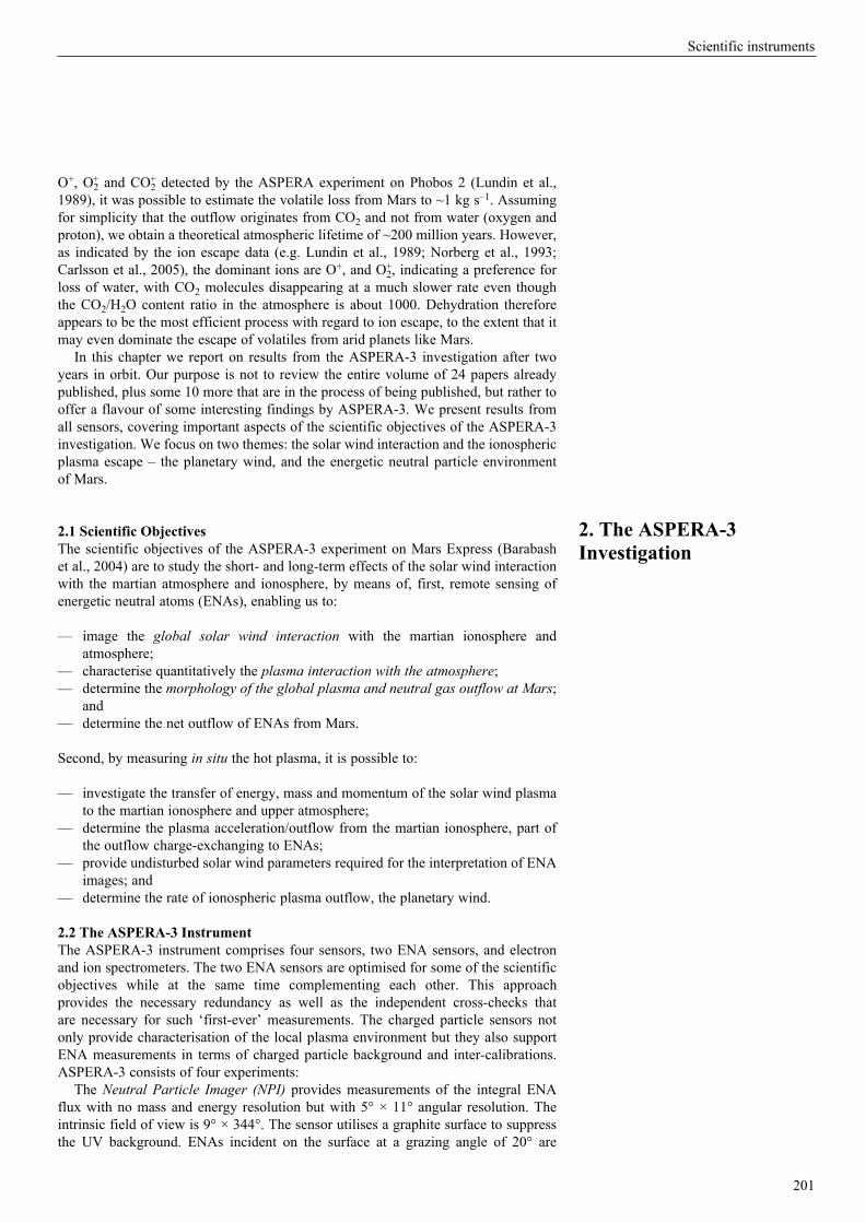
201
Scientific instruments
O+, O2+ and CO2
+ detected by the ASPERA experiment on Phobos 2 (Lundin et al., 1989), it was possible to estimate the volatile loss from Mars to ~1 kg s–1. Assuming for simplicity that the outflow originates from CO2 and not from water (oxygen and proton), we obtain a theoretical atmospheric lifetime of ~200 million years. However, as indicated by the ion escape data (e.g. Lundin et al., 1989; Norberg et al., 1993; Carlsson et al., 2005), the dominant ions are O+, and O2
+, indicating a preference for loss of water, with CO2 molecules disappearing at a much slower rate even though the CO2/H2O content ratio in the atmosphere is about 1000. Dehydration therefore appears to be the most efficient process with regard to ion escape, to the extent that it may even dominate the escape of volatiles from arid planets like Mars.
In this chapter we report on results from the ASPERA-3 investigation after two years in orbit. Our purpose is not to review the entire volume of 24 papers already published, plus some 10 more that are in the process of being published, but rather to offer a flavour of some interesting findings by ASPERA-3. We present results from all sensors, covering important aspects of the scientific objectives of the ASPERA-3 investigation. We focus on two themes: the solar wind interaction and the ionospheric plasma escape – the planetary wind, and the energetic neutral particle environment of Mars.
2.1 Scientific ObjectivesThe scientific objectives of the ASPERA-3 experiment on Mars Express (Barabash et al., 2004) are to study the short- and long-term effects of the solar wind interaction with the martian atmosphere and ionosphere, by means of, first, remote sensing of energetic neutral atoms (ENAs), enabling us to:
— image the global solar wind interaction with the martian ionosphere and atmosphere;
— characterise quantitatively the plasma interaction with the atmosphere;— determine the morphology of the global plasma and neutral gas outflow at Mars;
and — determine the net outflow of ENAs from Mars.
Second, by measuring in situ the hot plasma, it is possible to:
— investigate the transfer of energy, mass and momentum of the solar wind plasma to the martian ionosphere and upper atmosphere;
— determine the plasma acceleration/outflow from the martian ionosphere, part of the outflow charge-exchanging to ENAs;
— provide undisturbed solar wind parameters required for the interpretation of ENA images; and
— determine the rate of ionospheric plasma outflow, the planetary wind.
2.2 The ASPERA-3 InstrumentThe ASPERA-3 instrument comprises four sensors, two ENA sensors, and electron and ion spectrometers. The two ENA sensors are optimised for some of the scientific objectives while at the same time complementing each other. This approach provides the necessary redundancy as well as the independent cross-checks that are necessary for such ‘first-ever’ measurements. The charged particle sensors not only provide characterisation of the local plasma environment but they also support ENA measurements in terms of charged particle background and inter-calibrations. ASPERA-3 consists of four experiments:
The Neutral Particle Imager (NPI) provides measurements of the integral ENA flux with no mass and energy resolution but with 5° × 11° angular resolution. The intrinsic field of view is 9° × 344°. The sensor utilises a graphite surface to suppress the UV background. ENAs incident on the surface at a grazing angle of 20° are
2. The ASPERA-3 Investigation
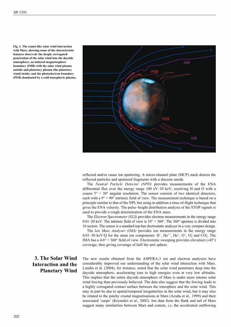
202
SP-1291
reflected and/or cause ion sputtering. A micro-channel plate (MCP) stack detects the reflected particles and sputtered fragments with a discrete anode.
The Neutral Particle Detector (NPD) provides measurements of the ENA differential flux over the energy range 100 eV–10 keV, resolving H and O with a coarse 5° × 30° angular resolution. The sensor consists of two identical detectors, each with a 9° × 90° intrinsic field of view. The measurement technique is based on a principle similar to that of the NPI, but using in addition a time-of-flight technique that gives the ENA velocity. The pulse–height distribution analysis of the STOP signals is used to provide a rough determination of the ENA mass.
The Electron Spectrometer (ELS) provides electron measurements in the energy range 0.01–20 keV. The intrinsic field of view is 10° × 360°. The 360° aperture is divided into 16 sectors. The sensor is a standard top-hat electrostatic analyser in a very compact design.
The Ion Mass Analyser (IMA) provides ion measurements in the energy range 0.01–30 keV/Q for the main ion components: H+, He++, He+, O+, O2
+ and CO2+. The
IMA has a 4.6° × 360° field of view. Electrostatic sweeping provides elevation (±45°) coverage, thus giving coverage of half the unit sphere.
The new results obtained from the ASPERA-3 ion and electron analysers have considerably improved our understanding of the solar wind interaction with Mars. Lundin et al. (2004), for instance, noted that the solar wind penetrates deep into the dayside atmosphere, accelerating ions to high energies even at very low altitudes. This implies that the entire dayside atmosphere of Mars is under more intense solar wind forcing than previously believed. The data also suggest that the forcing leads to a highly corrugated contact surface between the ionosphere and the solar wind. This may in part be due to spatial/temporal irregularities in the solar wind, but it may also be related to the patchy crustal magnetisations at Mars (Acuña et al., 1999) and their associated ‘cusps’ (Krymskii et al., 2002). Ion data from the flank and tail of Mars suggest many similarities between Mars and comets, i.e. the accelerated outflowing
3. The Solar Wind Interaction and the
Planetary Wind
Fig. 1. The comet-like solar wind interaction with Mars, showing some of the characteristic features observed: the deeply corrugated penetration of the solar wind into the dayside atmosphere; an induced magnetosphere boundary (IMB) with the solar wind plasma outside and planetary plasma (the planetary wind) inside; and the photoelectron boundary (PEB) dominated by a cold ionospheric plasma.
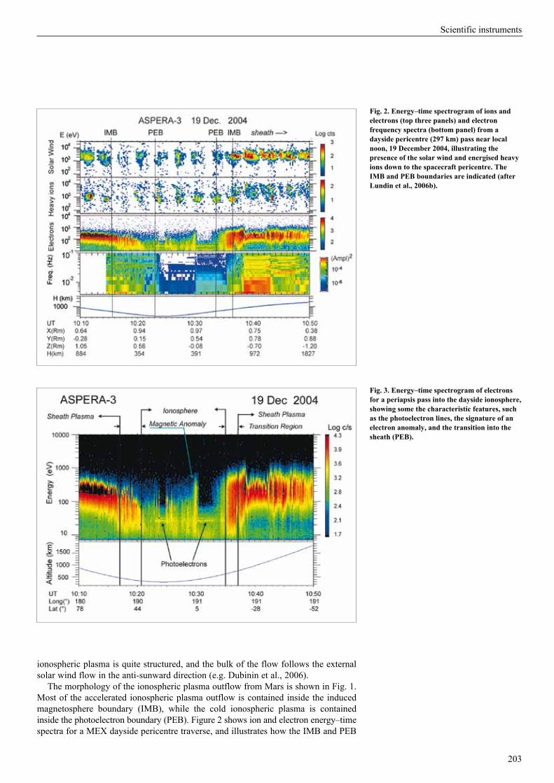
203
Scientific instruments
ionospheric plasma is quite structured, and the bulk of the flow follows the external solar wind flow in the anti-sunward direction (e.g. Dubinin et al., 2006).
The morphology of the ionospheric plasma outflow from Mars is shown in Fig. 1. Most of the accelerated ionospheric plasma outflow is contained inside the induced magnetosphere boundary (IMB), while the cold ionospheric plasma is contained inside the photoelectron boundary (PEB). Figure 2 shows ion and electron energy–time spectra for a MEX dayside pericentre traverse, and illustrates how the IMB and PEB
Fig. 2. Energy–time spectrogram of ions and electrons (top three panels) and electron frequency spectra (bottom panel) from a dayside pericentre (297 km) pass near local noon, 19 December 2004, illustrating the presence of the solar wind and energised heavy ions down to the spacecraft pericentre. The IMB and PEB boundaries are indicated (after Lundin et al., 2006b).
Fig. 3. Energy–time spectrogram of electrons for a periapsis pass into the dayside ionosphere, showing some the characteristic features, such as the photoelectron lines, the signature of an electron anomaly, and the transition into the sheath (PEB).

204
SP-1291
Fig. 4. Morphology of the planetary ion acceleration and outflow. MEX trajectory traces with observations of ion acceleration and outflow are depicted using a cylindrical coordinate system. IMB marks the average induced magnetosphere boundary.
Fig. 5. IMI and ELS data from a MEX pericentre pass on June 21 2004. Right panel, top: data (counts) of tailward-moving planetary ions (m/q=16–44 amu). Left panel, centre: downward-moving electron energy spectra (counts) and the frequency spectra of electrons, respectively. The ion and electron flux spectra in the right panel were taken at 12:56 UT (Lundin et al., 2006b).
Fig 6. (a) Energy–time spectrogram for electrons and ions showing plasma acceleration in the deep nightside. (b) Energy spectra of oppositely accelerated electron and ion fluxes in the central tail, taken at 06:55 UT (Lundin et al., 2006b).
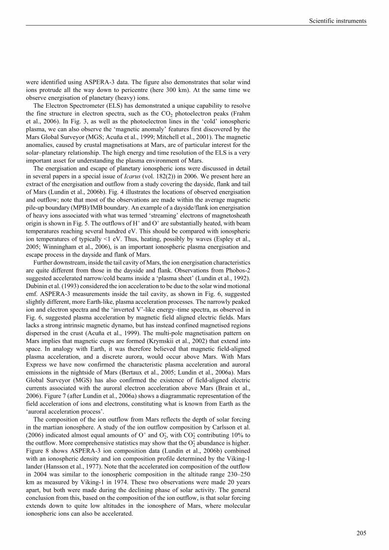
205
Scientific instruments
were identified using ASPERA-3 data. The figure also demonstrates that solar wind ions protrude all the way down to pericentre (here 300 km). At the same time we observe energisation of planetary (heavy) ions.
The Electron Spectrometer (ELS) has demonstrated a unique capability to resolve the fine structure in electron spectra, such as the CO2 photoelectron peaks (Frahm et al., 2006). In Fig. 3, as well as the photoelectron lines in the ‘cold’ ionospheric plasma, we can also observe the ‘magnetic anomaly’ features first discovered by the Mars Global Surveyor (MGS; Acuña et al., 1999; Mitchell et al., 2001). The magnetic anomalies, caused by crustal magnetisations at Mars, are of particular interest for the solar–planetary relationship. The high energy and time resolution of the ELS is a very important asset for understanding the plasma environment of Mars.
The energisation and escape of planetary ionospheric ions were discussed in detail in several papers in a special issue of Icarus (vol. 182(2)) in 2006. We present here an extract of the energisation and outflow from a study covering the dayside, flank and tail of Mars (Lundin et al., 2006b). Fig. 4 illustrates the locations of observed energisation and outflow; note that most of the observations are made within the average magnetic pile-up boundary (MPB)/IMB boundary. An example of a dayside/flank ion energisation of heavy ions associated with what was termed ‘streaming’ electrons of magnetosheath origin is shown in Fig. 5. The outflows of H+ and O+ are substantially heated, with beam temperatures reaching several hundred eV. This should be compared with ionospheric ion temperatures of typically <1 eV. Thus, heating, possibly by waves (Espley et al., 2005; Winningham et al., 2006), is an important ionospheric plasma energisation and escape process in the dayside and flank of Mars.
Further downstream, inside the tail cavity of Mars, the ion energisation characteristics are quite different from those in the dayside and flank. Observations from Phobos-2 suggested accelerated narrow/cold beams inside a ‘plasma sheet’ (Lundin et al., 1992). Dubinin et al. (1993) considered the ion acceleration to be due to the solar wind motional emf. ASPERA-3 measurements inside the tail cavity, as shown in Fig. 6, suggested slightly different, more Earth-like, plasma acceleration processes. The narrowly peaked ion and electron spectra and the ‘inverted V’-like energy–time spectra, as observed in Fig. 6, suggested plasma acceleration by magnetic field aligned electric fields. Mars lacks a strong intrinsic magnetic dynamo, but has instead confined magnetised regions dispersed in the crust (Acuña et al., 1999). The multi-pole magnetisation pattern on Mars implies that magnetic cusps are formed (Krymskii et al., 2002) that extend into space. In analogy with Earth, it was therefore believed that magnetic field-aligned plasma acceleration, and a discrete aurora, would occur above Mars. With Mars Express we have now confirmed the characteristic plasma acceleration and auroral emissions in the nightside of Mars (Bertaux et al., 2005; Lundin et al., 2006a). Mars Global Surveyor (MGS) has also confirmed the existence of field-aligned electric currents associated with the auroral electron acceleration above Mars (Brain et al., 2006). Figure 7 (after Lundin et al., 2006a) shows a diagrammatic representation of the field acceleration of ions and electrons, constituting what is known from Earth as the ‘auroral acceleration process’.
The composition of the ion outflow from Mars reflects the depth of solar forcing in the martian ionosphere. A study of the ion outflow composition by Carlsson et al. (2006) indicated almost equal amounts of O+ and O2
+, with CO2+ contributing 10% to
the outflow. More comprehensive statistics may show that the O2+ abundance is higher.
Figure 8 shows ASPERA-3 ion composition data (Lundin et al., 2006b) combined with an ionospheric density and ion composition profile determined by the Viking-1 lander (Hansson et al., 1977). Note that the accelerated ion composition of the outflow in 2004 was similar to the ionospheric composition in the altitude range 230–250 km as measured by Viking-1 in 1974. These two observations were made 20 years apart, but both were made during the declining phase of solar activity. The general conclusion from this, based on the composition of the ion outflow, is that solar forcing extends down to quite low altitudes in the ionosphere of Mars, where molecular ionospheric ions can also be accelerated.
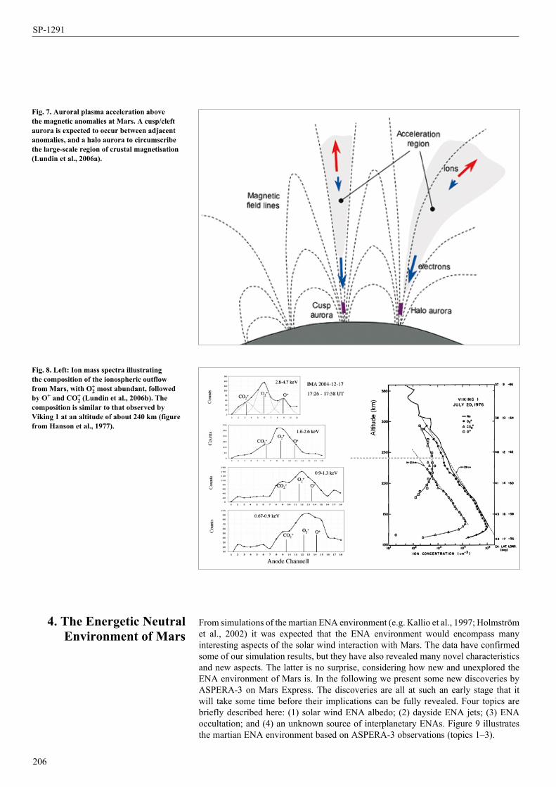
206
SP-1291
From simulations of the martian ENA environment (e.g. Kallio et al., 1997; Holmström et al., 2002) it was expected that the ENA environment would encompass many interesting aspects of the solar wind interaction with Mars. The data have confirmed some of our simulation results, but they have also revealed many novel characteristics and new aspects. The latter is no surprise, considering how new and unexplored the ENA environment of Mars is. In the following we present some new discoveries by ASPERA-3 on Mars Express. The discoveries are all at such an early stage that it will take some time before their implications can be fully revealed. Four topics are briefly described here: (1) solar wind ENA albedo; (2) dayside ENA jets; (3) ENA occultation; and (4) an unknown source of interplanetary ENAs. Figure 9 illustrates the martian ENA environment based on ASPERA-3 observations (topics 1–3).
Fig. 8. Left: Ion mass spectra illustrating the composition of the ionospheric outflow from Mars, with O2
+ most abundant, followed by O+ and CO2
+ (Lundin et al., 2006b). The composition is similar to that observed by Viking 1 at an altitude of about 240 km (figure from Hanson et al., 1977).
4. The Energetic Neutral Environment of Mars
Fig. 7. Auroral plasma acceleration above the magnetic anomalies at Mars. A cusp/cleft aurora is expected to occur between adjacent anomalies, and a halo aurora to circumscribe the large-scale region of crustal magnetisation (Lundin et al., 2006a).
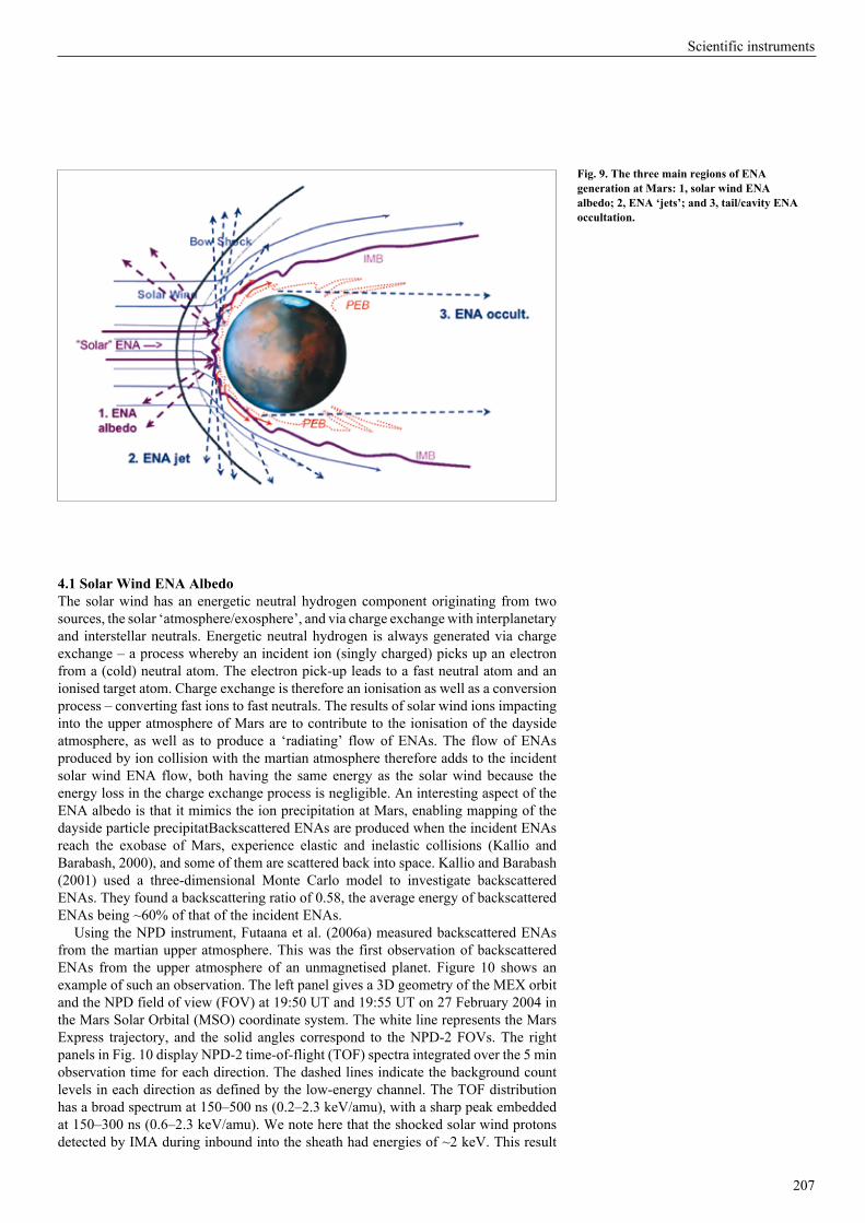
207
Scientific instruments
4.1 Solar Wind ENA AlbedoThe solar wind has an energetic neutral hydrogen component originating from two sources, the solar ‘atmosphere/exosphere’, and via charge exchange with interplanetary and interstellar neutrals. Energetic neutral hydrogen is always generated via charge exchange – a process whereby an incident ion (singly charged) picks up an electron from a (cold) neutral atom. The electron pick-up leads to a fast neutral atom and an ionised target atom. Charge exchange is therefore an ionisation as well as a conversion process – converting fast ions to fast neutrals. The results of solar wind ions impacting into the upper atmosphere of Mars are to contribute to the ionisation of the dayside atmosphere, as well as to produce a ‘radiating’ flow of ENAs. The flow of ENAs produced by ion collision with the martian atmosphere therefore adds to the incident solar wind ENA flow, both having the same energy as the solar wind because the energy loss in the charge exchange process is negligible. An interesting aspect of the ENA albedo is that it mimics the ion precipitation at Mars, enabling mapping of the dayside particle precipitatBackscattered ENAs are produced when the incident ENAs reach the exobase of Mars, experience elastic and inelastic collisions (Kallio and Barabash, 2000), and some of them are scattered back into space. Kallio and Barabash (2001) used a three-dimensional Monte Carlo model to investigate backscattered ENAs. They found a backscattering ratio of 0.58, the average energy of backscattered ENAs being ~60% of that of the incident ENAs.
Using the NPD instrument, Futaana et al. (2006a) measured backscattered ENAs from the martian upper atmosphere. This was the first observation of backscattered ENAs from the upper atmosphere of an unmagnetised planet. Figure 10 shows an example of such an observation. The left panel gives a 3D geometry of the MEX orbit and the NPD field of view (FOV) at 19:50 UT and 19:55 UT on 27 February 2004 in the Mars Solar Orbital (MSO) coordinate system. The white line represents the Mars Express trajectory, and the solid angles correspond to the NPD-2 FOVs. The right panels in Fig. 10 display NPD-2 time-of-flight (TOF) spectra integrated over the 5 min observation time for each direction. The dashed lines indicate the background count levels in each direction as defined by the low-energy channel. The TOF distribution has a broad spectrum at 150–500 ns (0.2–2.3 keV/amu), with a sharp peak embedded at 150–300 ns (0.6–2.3 keV/amu). We note here that the shocked solar wind protons detected by IMA during inbound into the sheath had energies of ~2 keV. This result
Fig. 9. The three main regions of ENA generation at Mars: 1, solar wind ENA albedo; 2, ENA ‘jets’; and 3, tail/cavity ENA occultation.

208
SP-1291
is consistent with the ENAs originating from the solar wind interaction with Mars. Futaana et al. (2006a) inferred on basis of their observations a global backscattered ENA emission of ~107 cm–2 s–1.
4.2 Dayside ENA JetsThe NPD and NPI sensors also detected a substantial flux of ENAs in the azimuthal direction (Gunell et al., 2006; Futaana et al., 2006b). They reported ENA signals coming from the dayside IMB–magnetosheath interface. By comparing the NPI data and an ENA generation model in the shocked solar wind, Kallio et al. (1997) concluded that they are the ENAs of shocked solar wind origin. On the other hand, Futaana et al. (2006b) measured the ENA flux emitted from the subsolar region using the NPD instrument, and named the outflow subsolar ENA jets, because the flux emission is highly directional from the subsolar region. Subsolar ENA jets may originate from two sources:
— Shocked solar wind protons charge-exchanging with planetary neutral atoms (Holmström et al., 2002) – the shocked solar wind is highly deflected in the subsolar region, and the velocity vector of the shocked solar wind flow points towards the azimuthal direction. When converted to ENAs, they form a subsolar ENA jet.
— Accelerated protons originating from hydrogen atoms in the martian upper atmosphere – the acceleration takes place in the exosphere by the solar wind interaction. The accelerated protons may subsequently charge-exchange back to ENAs (Lichtenegger et al., 2002).
In both cases, jets may be produced near local noon, in a region subject to head-on solar wind forcing. An opportunity to reveal in more detail the geometry and the cause of the ENA jets came during the passage of an interplanetary shock that displaced the ENA source region (Futaana et al., 2006c). During this event the NPD data exhibited an extremely high-flux ENA jet. The observed flux was approximately five times higher than typical fluxes, and decreased abruptly in a very short time, less than 10 s, when the spacecraft crossed an outer boundary of the ENA jet. The generation region of the subsolar ENA jet was pushed towards the planet by the interplanetary shock, as shown in Fig. 11. Mars Express subsequently went into and out of the ENA jet region
Fig. 10. Observations of backscattered ENAs (from Futaana et al., 2006b). Left panel: the MEX orbit and field of view of the NPD measurements. Right panels: TOF spectra for two directions integrated over the 5 min observation period.
Fig. 11. Geometry of the subsolar ENA jet. The subsolar jet can be detected when the sensor is within it (case a). As soon as the spacecraft leaves the jet (case b) the ENAs cannot be detected even though the instrument FOV covers the source region (Futaana et al., 2006b).
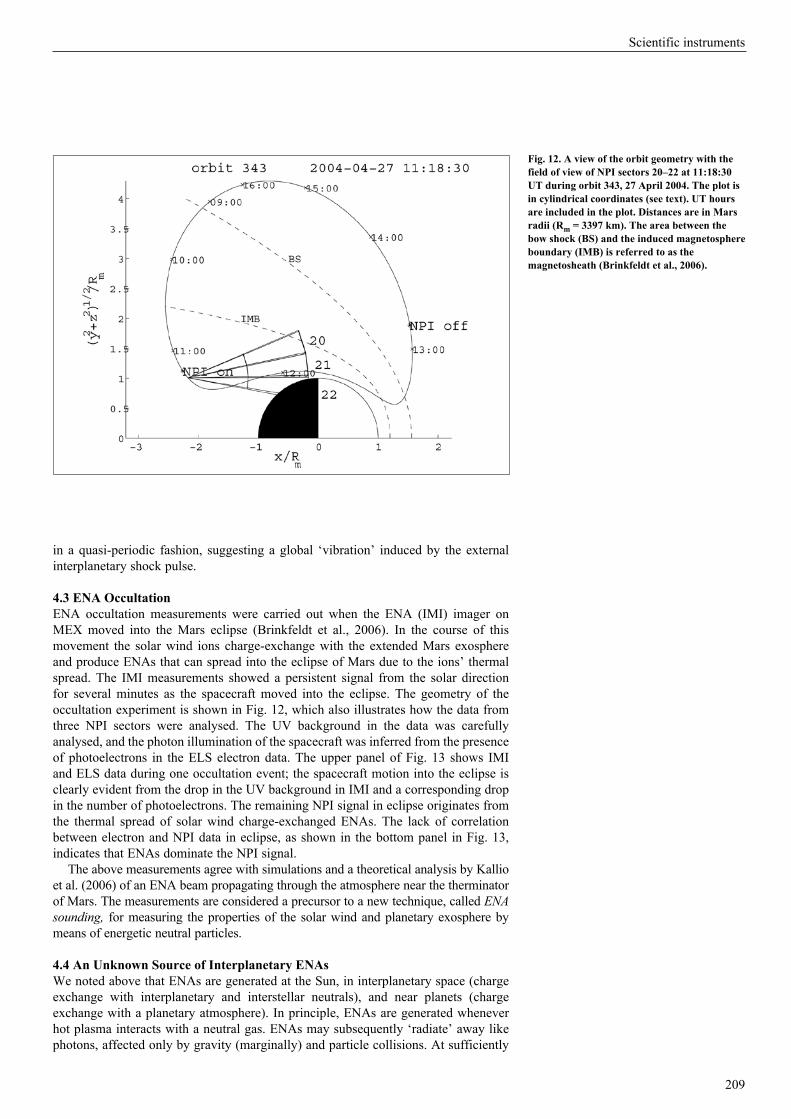
209
Scientific instruments
in a quasi-periodic fashion, suggesting a global ‘vibration’ induced by the external interplanetary shock pulse.
4.3 ENA OccultationENA occultation measurements were carried out when the ENA (IMI) imager on MEX moved into the Mars eclipse (Brinkfeldt et al., 2006). In the course of this movement the solar wind ions charge-exchange with the extended Mars exosphere and produce ENAs that can spread into the eclipse of Mars due to the ions’ thermal spread. The IMI measurements showed a persistent signal from the solar direction for several minutes as the spacecraft moved into the eclipse. The geometry of the occultation experiment is shown in Fig. 12, which also illustrates how the data from three NPI sectors were analysed. The UV background in the data was carefully analysed, and the photon illumination of the spacecraft was inferred from the presence of photoelectrons in the ELS electron data. The upper panel of Fig. 13 shows IMI and ELS data during one occultation event; the spacecraft motion into the eclipse is clearly evident from the drop in the UV background in IMI and a corresponding drop in the number of photoelectrons. The remaining NPI signal in eclipse originates from the thermal spread of solar wind charge-exchanged ENAs. The lack of correlation between electron and NPI data in eclipse, as shown in the bottom panel in Fig. 13, indicates that ENAs dominate the NPI signal.
The above measurements agree with simulations and a theoretical analysis by Kallio et al. (2006) of an ENA beam propagating through the atmosphere near the therminator of Mars. The measurements are considered a precursor to a new technique, called ENA sounding, for measuring the properties of the solar wind and planetary exosphere by means of energetic neutral particles.
4.4 An Unknown Source of Interplanetary ENAsWe noted above that ENAs are generated at the Sun, in interplanetary space (charge exchange with interplanetary and interstellar neutrals), and near planets (charge exchange with a planetary atmosphere). In principle, ENAs are generated whenever hot plasma interacts with a neutral gas. ENAs may subsequently ‘radiate’ away like photons, affected only by gravity (marginally) and particle collisions. At sufficiently
Fig. 12. A view of the orbit geometry with the field of view of NPI sectors 20–22 at 11:18:30 UT during orbit 343, 27 April 2004. The plot is in cylindrical coordinates (see text). UT hours are included in the plot. Distances are in Mars radii (Rm = 3397 km). The area between the bow shock (BS) and the induced magnetosphere boundary (IMB) is referred to as the magnetosheath (Brinkfeldt et al., 2006).
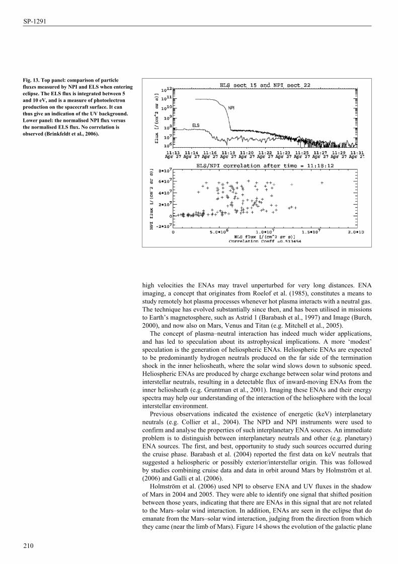
210
SP-1291
high velocities the ENAs may travel unperturbed for very long distances. ENA imaging, a concept that originates from Roelof et al. (1985), constitutes a means to study remotely hot plasma processes whenever hot plasma interacts with a neutral gas. The technique has evolved substantially since then, and has been utilised in missions to Earth’s magnetosphere, such as Astrid 1 (Barabash et al., 1997) and Image (Burch, 2000), and now also on Mars, Venus and Titan (e.g. Mitchell et al., 2005).
The concept of plasma–neutral interaction has indeed much wider applications, and has led to speculation about its astrophysical implications. A more ‘modest’ speculation is the generation of heliospheric ENAs. Heliospheric ENAs are expected to be predominantly hydrogen neutrals produced on the far side of the termination shock in the inner heliosheath, where the solar wind slows down to subsonic speed. Heliospheric ENAs are produced by charge exchange between solar wind protons and interstellar neutrals, resulting in a detectable flux of inward-moving ENAs from the inner heliosheath (e.g. Gruntman et al., 2001). Imaging these ENAs and their energy spectra may help our understanding of the interaction of the heliosphere with the local interstellar environment.
Previous observations indicated the existence of energetic (keV) interplanetary neutrals (e.g. Collier et al., 2004). The NPD and NPI instruments were used to confirm and analyse the properties of such interplanetary ENA sources. An immediate problem is to distinguish between interplanetary neutrals and other (e.g. planetary) ENA sources. The first, and best, opportunity to study such sources occurred during the cruise phase. Barabash et al. (2004) reported the first data on keV neutrals that suggested a heliospheric or possibly exterior/interstellar origin. This was followed by studies combining cruise data and data in orbit around Mars by Holmström et al. (2006) and Galli et al. (2006).
Holmström et al. (2006) used NPI to observe ENA and UV fluxes in the shadow of Mars in 2004 and 2005. They were able to identify one signal that shifted position between those years, indicating that there are ENAs in this signal that are not related to the Mars–solar wind interaction. In addition, ENAs are seen in the eclipse that do emanate from the Mars–solar wind interaction, judging from the direction from which they came (near the limb of Mars). Figure 14 shows the evolution of the galactic plane
Fig. 13. Top panel: comparison of particle fluxes measured by NPI and ELS when entering eclipse. The ELS flux is integrated between 5 and 10 eV, and is a measure of photoelectron production on the spacecraft surface. It can thus give an indication of the UV background. Lower panel: the normalised NPI flux versus the normalised ELS flux. No correlation is observed (Brinkfeldt et al., 2006).
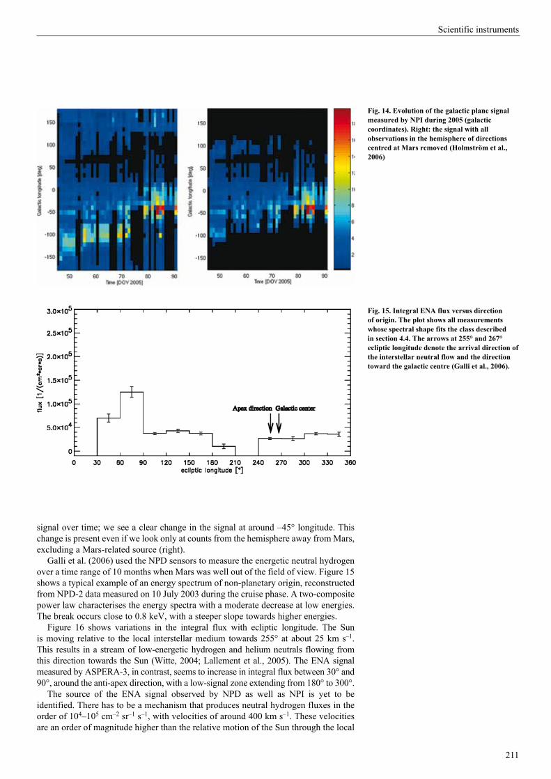
211
Scientific instruments
signal over time; we see a clear change in the signal at around –45° longitude. This change is present even if we look only at counts from the hemisphere away from Mars, excluding a Mars-related source (right).
Galli et al. (2006) used the NPD sensors to measure the energetic neutral hydrogen over a time range of 10 months when Mars was well out of the field of view. Figure 15 shows a typical example of an energy spectrum of non-planetary origin, reconstructed from NPD-2 data measured on 10 July 2003 during the cruise phase. A two-composite power law characterises the energy spectra with a moderate decrease at low energies. The break occurs close to 0.8 keV, with a steeper slope towards higher energies.
Figure 16 shows variations in the integral flux with ecliptic longitude. The Sun is moving relative to the local interstellar medium towards 255° at about 25 km s–1. This results in a stream of low-energetic hydrogen and helium neutrals flowing from this direction towards the Sun (Witte, 2004; Lallement et al., 2005). The ENA signal measured by ASPERA-3, in contrast, seems to increase in integral flux between 30° and 90°, around the anti-apex direction, with a low-signal zone extending from 180° to 300°.
The source of the ENA signal observed by NPD as well as NPI is yet to be identified. There has to be a mechanism that produces neutral hydrogen fluxes in the order of 104–105 cm–2 sr–1 s–1, with velocities of around 400 km s–1. These velocities are an order of magnitude higher than the relative motion of the Sun through the local
Fig. 14. Evolution of the galactic plane signal measured by NPI during 2005 (galactic coordinates). Right: the signal with all observations in the hemisphere of directions centred at Mars removed (Holmström et al., 2006)
Fig. 15. Integral ENA flux versus direction of origin. The plot shows all measurements whose spectral shape fits the class described in section 4.4. The arrows at 255° and 267° ecliptic longitude denote the arrival direction of the interstellar neutral flow and the direction toward the galactic centre (Galli et al., 2006).
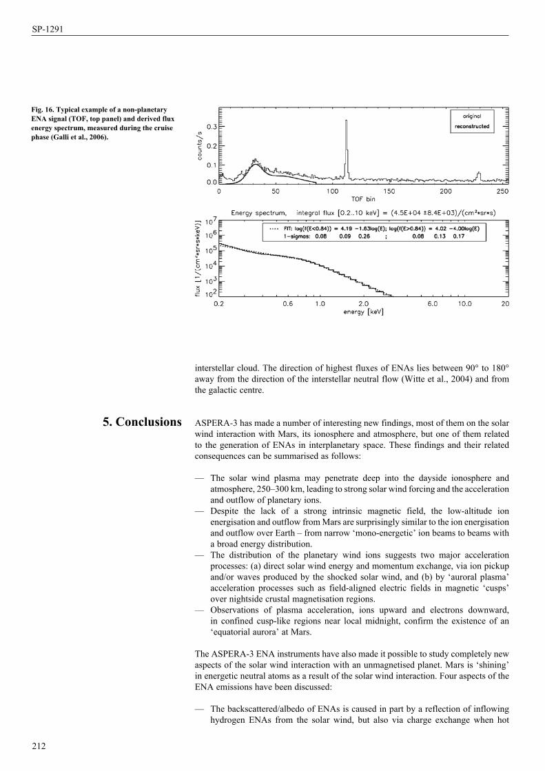
212
SP-1291
interstellar cloud. The direction of highest fluxes of ENAs lies between 90° to 180° away from the direction of the interstellar neutral flow (Witte et al., 2004) and from the galactic centre.
ASPERA-3 has made a number of interesting new findings, most of them on the solar wind interaction with Mars, its ionosphere and atmosphere, but one of them related to the generation of ENAs in interplanetary space. These findings and their related consequences can be summarised as follows:
— The solar wind plasma may penetrate deep into the dayside ionosphere and atmosphere, 250–300 km, leading to strong solar wind forcing and the acceleration and outflow of planetary ions.
— Despite the lack of a strong intrinsic magnetic field, the low-altitude ion energisation and outflow from Mars are surprisingly similar to the ion energisation and outflow over Earth – from narrow ‘mono-energetic’ ion beams to beams with a broad energy distribution.
— The distribution of the planetary wind ions suggests two major acceleration processes: (a) direct solar wind energy and momentum exchange, via ion pickup and/or waves produced by the shocked solar wind, and (b) by ‘auroral plasma’ acceleration processes such as field-aligned electric fields in magnetic ‘cusps’ over nightside crustal magnetisation regions.
— Observations of plasma acceleration, ions upward and electrons downward, in confined cusp-like regions near local midnight, confirm the existence of an ‘equatorial aurora’ at Mars.
The ASPERA-3 ENA instruments have also made it possible to study completely new aspects of the solar wind interaction with an unmagnetised planet. Mars is ‘shining’ in energetic neutral atoms as a result of the solar wind interaction. Four aspects of the ENA emissions have been discussed:
— The backscattered/albedo of ENAs is caused in part by a reflection of inflowing hydrogen ENAs from the solar wind, but also via charge exchange when hot
Fig. 16. Typical example of a non-planetary ENA signal (TOF, top panel) and derived flux energy spectrum, measured during the cruise phase (Galli et al., 2006).
5. Conclusions

213
Scientific instruments
plasma, of solar wind and planetary wind origin, interacts with the upper atmosphere.
— Subsolar ENA jets may originate from either shocked solar wind protons charge-exchanging with planetary neutral atoms, or accelerated protons originating from hydrogen atoms in the martian upper atmosphere.
— ENA occultation, representing a new technique called ENA sounding, can be used to measure solar wind and planetary exosphere properties by means of energetic neutral particles passing through the upper atmosphere/exosphere.
— Interplanetary/interstellar ENAs in the keV range, a completely new source of ENAs, are possibly generated in the heliosphere outside the termination shock. This observation introduces a new aspect of stellar objects in Universe, the possibility of these objects emitting, ‘shining’, substantial flows of energetic neutral atoms. This ‘ENA shine’ clearly must have an impact on astrophysics, and on how we conceive stellar objects in general and stellar spheres in particular.
In conclusion, we can now state that after two Earth-years in orbit around Mars, ASPERA-3 has been a great success. Since completion of this review, 22 papers based on ASPERA-3 data have been published in journals such as Science, Icarus, Planetary and Space Sciences and the Astrophysical Journal, and many more are pending. In view of the lead time involved, the number of publications after two years of data taking can be considered outstandingly high. ASPERA-3 has been a major success for its investigators, as well as for ESA and the Mars Express project.
The ASPERA-3 experiment on Mars Express is a joint effort involving 15 laboratories in 10 countries, all supported by their national agencies. We thank all of these agencies, as well as the various departments/institutes that are hosting these efforts. We wish to acknowledge in particular the Swedish National Space Board for its support for the main PI institute, and NASA for supporting its PI institute. Finally, we are indebted to European Space Agency for the tremendous success of MEX, the first ESA mission to the Red Planet.
Acuña, M.J., Connerey, J., Ness,N., Lin, R., Mitchell, D., Carlsson, C., McFadden, J., Anderson, K., Rème, H., Mazelle, C., Vignes, D. Wasilewski, P. & Cloutier, P. (1999). Global Distribution of Crustal Magnetization Discovered by Mars Global Surveyor MAG/ER Experiment. Science 284, 790–793.
Barabash, S., P.C. Brandt, O. Norberg, R. Lundin, E.C. Roelof, C.J. Chase, B.H. Mauk, H. Koskinen (1997). Energetic Neutral Atom Imaging by the Astrid Microsatellite, Adv. Space Res. 20, 1055–1060.
Barabash, S., R. Lundin, H. Andersson, M. Holmström & the ASPERA-3 team (2004). ASPERA-3: The Analyser of Space Plasmas and Energetic Atoms for Mars Express, In Mars Express: The Scientific Payload, ESA-SP-1240, ESA Publications Division, European Space Agency, Noordwijk, the Netherlands, p.121.
Barabash, S. & the ASPERA-3 team (2004). First Results of the Analyzer of Space Plasma and Energetic Neutral Atoms (ASPERA-3) on Board Mars Express, Invited presentation at the EGU Conference, Nice, France.
Bertaux, J.-L., F. Leblanc, O. Witasse, E. Quemerais, J. Lilensten, S.A. Stern, B. Sandel & O. Koalbev (2005). Discovery of an Aurora on Mars, Nature 435(9), 790–794.
Brain, D.A., Halekas, J.S., Peticolas, L.M., Lin, R.P., Luhmann, J.G., Mitchell, D.L., Delory, G.T., Bougher, S.W., Acuña, M.H. & Rème, H. (2006). On the Origin of Aurorae on Mars, Geophys. Res. Lett. DOI: 10.1029/2005GL024782.
Brinkfeld, K., H. Gunell, P.C. Brandt & the ASPERA-3 team (2006). First ENA observations at Mars: Observations of Energetic Neutral Atoms on the Nightside of Mars, Icarus 182(2), 439–447.
Acknowledgements
References
214
SP-1291
Burch, J.L. (2000). IMAGE Mission Overview, Space Sci. Rev. 91, 1–14. Carlsson, E., A. Fedorov, S. Barabash, R. Frahm, et al. (2006). Mass Composition of the
Escaping Plasma at Mars in the Energy Range of 0.6–2 keV, Icarus 182(2), 320–328. Collier M.R., T.E. Moore, D. Simpson, A. Roberts, A. Szabo, S. Fuselier, P. Wurz, M.A. Lee
& B.T. Tsurutani (2004). Adv. Space Res. 34(1), 166–171.Dubinin, E., R. Lundin , H. Koskinen & N. Pissarenko (1993). Ion Acceleration in the Martian
Tail: Phobos Observations, J. Geophys. Res. 98, 3991–3997. Dubinin, E., D. Winningham, M. Fränz & the ASPERA-3 team (2006). Solar Wind Plasma
Protrusion into the Martian Magnetosphere – ASPERA-3 observations, Icarus 182(2). Espley, J.R., P.A. Cloutier, D.H. Crider, D.A. Brain & M.H. Acuña (2005). Low-frequency
Plasma Oscillations at Mars during the October 2003 Solar Storm, J. Geophys. Res. 110, A09S33. DOI: 10.1029/2004JA010935.
Frahm, R., D. Winningham, J. Sharber & the ASPERA-3 team (2006). Carbon Dioxide Photoelectron Peaks at Mars, Icarus 182(2), 371–382.
Futaana, Y., S. Barabash, A. Grigoriev & the ASPERA-3 team (2006a). First ENA Observations at Mars: ENA Emissions from the Martian Upper Atmosphere, Icarus 182(2), 424–430.
Futaana, Y., S. Barabash, A. Grigoriev & the ASPERA-3 team (2006b). First ENA Observations at Mars: Sub-Solar ENA Jet , Icarus 182(2), 413–423.
Futaana, Y., S. Barabash, A. Grigoriev, D. Winningham, R. Frahm & R. Lundin (2006c). Global Response of Martian Plasma Environment to an Interplanetary Shock: From ENA and Plasma Observations at Mars, Space Sci. Rev. 126(1–4), 315–332.
Galli A., P. Wurz, S. Barabash, A. Grigoriev, R. Lundin, Y. Futaana, H. Gunell, M. Holmstöm, E.C. Roelof, C.C. Curtis, K.C. Hsieh, A. Fedorov, D. Winningham, R.A. Frahm, R. Cerulli-Irelli, P. Bochsler, N. Krupp, J. Woch & M. Fraenz (2006). Direct Measurements of Energetic Neutral Hydrogen in the Interplanetary Medium, Astrophys. J. 644(2).
Gringauz, K.I. (1981). A Comparison of the Magnetospheres of Mars, Venus and the Earth, Adv. Space Res. 1, 5–24.
Gruntman, M., Roelof, E.C., Mitchell, D.G., Fahr, H.-J., Funsten, H.O. & McComas, D.J. (2001). Energetic Neutral Atom Imaging of the Heliospheric Boundary Region, J. Geophys. Res. 106, 15767–15782.
Gunell, H., K. Brinkfeldt, M. Holmström & the ASPERA-3 team (2006). Measurements and Simulations of Energetic Neutral Atoms Produced by Charge Exchange at Mars, Icarus 182(2).
Hanson, W.B., Sanatani S. & Zuccaro D.R. (1977). The Martian Ionosphere as Observed by the Viking Retarding Potential Analyzer. J. Geophys. Res. 82, 4351–4363.
Holmström, M., S. Barabash & E. Kallio (2002). Energetic Neutral Atoms at Mars 1. Imaging of Solar Wind Protons, J. Geophys. Res. 107(A10), DOI: 10.1029/2001JA000325.
Holmström M., K. Brinkfeldt, S. Barabash & R. Lundin (2006). Observations in the Shadow of Mars by the Neutral Particle Imager, Adv. Geosci., World Scientific Publications.
Kallio, E. & S. Barabash (2000). On the Elastic and Inelastic Collisions between the Precipitating Energetic Hydrogen Atoms and the Martian Atmospheric Neutrals, J. Geophys. Res. 105(A11), 24973–24996.
Kallio, E. & S. Barabash (2001). Atmospheric Effects of Precipitating Energetic Hydrogen Atoms to the Martian Atmosphere, J. Geophys. Res. 106(1), 165–177.
Kallio, E., J.G. Luhmann & S. Barabash (1997). Charge Exchange near Mars: The Solar Wind Absorbtion and Energetic Neutral Atom Production, J. Geophys. Res. 102, 22183–22197.
Kallio, E., S. Barabash, K. Brinkfeldt & the ASPERA-3 team (2006). Energetic Neutral Atoms (ENA) at Mars: Properties of the Hydrogen Atoms Produced Upstream of the Martian Bow Shock and Implications for ENA Sounding Technique around Non-magnetized Planets, Icarus 182(2), 448–463.
Krymskii, A.M., Breus, T.K., Ness, N.F., Acuña, M.H., Connerney, J.E.P., Crider, D.H., Mitchell, D.L. & Bauer, S.J. (2002). Structure of the Magnetic Field Fluxes Connected with Crustal Magnetization and Topside Ionosphere at Mars. J. Geophys. Res. 107(A9), 1245. DOI: 10.1029/2001JA000239.
Holmström, M., S. Barabash & E. Kallio (2002). Energetic Neutral Atoms at Mars, 1: Imaging of Solar Wind Protons, J. Geophys. Res. 107(A10), 1277. DOI: 10.1029/2001JA000325.
215
Scientific instruments
Lallement, R., Qu’emerais, E., Bertaux, J.L., Ferron, S., Koutroumpa, D. & Pellinen, R. (2005). Deflection of the Interstellar Neutral Hydrogen Flow across the Heliospheric Interface, Science 307, 1447–1449.
Lichtenegger, H., H. Lammer & W. Stumptner (2002). Energetic Neutral Atoms at Mars, 3: Flux and Energy Distributions of Planetary Energetic H Atoms, J. Geophys. Res. 107(A10), 1279. DOI: 10.1029/2001JA000322.
Lundin, R., A., Zakharov, R. Pellinen, B. Hultqvist, H. Borg, E.M. Dubinin, S. Barabasj, N. Pissarenkon, H. Koskinen & I. Liede (1989). First Results of the Ionospheric Plasma Escape from Mars, Nature 341, 609–612.
Lundin, R., A. Zakharov, R. Pellinen, S.W. Barabasj, H. Borg, E.M. Dubinin, B. Hultqvist, H. Koskinen, I. Liede & N. Pissarenko (1990). ASPERA/Phobos Measurements of the Ion Outflow from the Martian Ionosphere, Geophys. Res. Lett. 17, 873–876 .
Lundin, R., E. Dubinin, O. Norberg & S. Barabash (1992). Mars Magnetospheric Boundaries and the Acceleration of Ions in the Martian Tail, in Proc. COSPAR Colloq. 4, Ann Arbor, MI, USA, pp.311–320.
Lundin, R., S. Barabash, H. Andersson, M. Holmström & the ASPERA-3 team (2004). Solar Wind Induced Atmospheric Erosion at Mars – First Results from ASPERA-3 on Mars Express, Science 305, 1933–1936.
Lundin R., D. Winningham, S. Barabash, R. Frahm, M. Holmström, J.-A. Sauvaud, A. Fedorov, K. Asamura, A.J. Coates, Y. Soobiah, K.C. Hsieh, M. Grande, H. Koskinen, E. Kallio, J. Kozyra, J. Woch, M. Fraenz, D. Brain, J. Luhmann, S. McKenna-Lawler, R. S. Orsini, P. Brandt & P. Wurz (2006a). Plasma Acceleration above Martian Magnetic Anomalies, Science 311, 980–985.
Lundin, R., D. Winningham, S. Barabash & the ASPERA-3 team (2006b). Ionospheric Plasma Acceleration at Mars: ASPERA-3 Results, Icarus 182(2), 308–319.
Mitchell, D.L., Lin, R.P., Mazelle, C. et al. (2001). Probing Mars’ Crustal Magnetic Field and Ionosphere with the MGS Electron Reflectometer. J. Geophys. Res. 106, 23419–23428.
Mitchell, D.G., Brandt,, P.C., Roelof, E.C., Dandouras, J., Krimigis, S.M. & Mauk, B.H. (2005). Energetic Neutral Atom Emissions from Titan Interaction with Saturn’s Magnetosphere, Science 308, 989–992.
Norberg, O., R. Lundin & S. Barabash (1993). Observation of Molecular Ions in the Martian Plasma Environment, in: Plasma Environments of Non-magnetic Planets (Ed. T.I. Gombosi), Proc. COSPAR Colloq. 4, Ann Arbor, MI, USA, pp.299–304.
Roelof, EC., D.G. Mitchell & D.J. Williams (1985). Energetic Neutral Atoms (E≈50 keV) from the Ring Current: IMP7/8 and ISEE 1, J. Geophys. Res. 90, 10991–11008.
Winningham, J.D., R. Frahm, J. Sharber & the ASPERA-3 team (2006). Electron Oscillations in the Induced Martian Magnetosphere, Icarus 182(2), 360–370.
Witte, M. (2004). Kinetic Parameters of Interstellar Neutral Helium: Review of Results Obtained during One Solar Cycle with the Ulysses/GAS-Instrument, Astron. Astrophys. 426, 835–844.
Witte, M., Banaszkiewicz, M., Rosenbauer, H. & McMullin, D. (2004). Kinetic Parameters of Interstellar Neutral Helium: Updated Results from the Ulysses/GAS-instrument, Adv. Space Res. 34, 61–65.

The Mars Express Radio Science Experiment (MaRS) started regular operations in April 2004. The experiment employed radio occultation during two occultation seasons in April-August 2004 and December 2004 to sound the neutral martian atmosphere to derive vertical density, pressure and temperature profiles as functions of height, and to sound the ionosphere to derive vertical ionospheric electron density profiles. Both profile types were monitored as functions of time in order to determine diurnal variations and, in the case of the ionosphere, dependence on solar wind conditions. MaRS also determined the dielectric and scattering properties of the martian surface in specific target areas by using bistatic radar, determining gravity anomalies during pericentre passes at altitudes of 250 km for investigations of the structure and evolution of the crust and lithosphere, and sounding the solar corona during the superior conjunction of Mars with the Sun from mid-August to mid-October 2004. This chapter gives, as intended by the project, an overview of the observations from April 2004 to mid-2005, and presents examples and first results.
Mars Express was injected into orbit around Mars on 25 December 2003; the science instrument commissioning phase began in January 2004, after arrival in the operational orbit, and lasted until June 2004. Since then, Mars Express has been conducting regular observations of the planet and environs. The primary mission, which ended in November 2005, was succeeded by an extended mission.
The Mars Express Orbiter Radio Science Experiment (MaRS) is employing radio occultation (i) to sound the neutral martian atmosphere to derive vertical density, pressure and temperature profiles as functions of height, and (ii) to sound the ionosphere to derive vertical ionospheric electron density profiles. Both types of profiles may be monitored as functions of time to determine diurnal and seasonal variations and, in the case of the ionosphere, dependence on solar wind conditions. MaRS is also (iii) determining the dielectric and scattering properties of the surface in specific target
217
MaRS: Mars Express Radio Science Experiment
M. Pätzold1, S. Tellmann1, T. Andert1, L. Carone1, M. Fels1, R. Schaa1, C. Stanzel1, I. Audenrieth-Kersten1, A. Gahr1, A.-L. Müller1, B. Stracke1, D. Stupar1, C. Walter1, B. Häusler2,S. Remus2, J. Selle2, H. Griebel2, W. Eidel2, S. Asmar3, G. Goltz3, D. Kahan3, J.-P. Barriot4, V. Dehant5, M. Beuthe5, P. Rosenblatt5, Ö. Karatekin5, V. Lainey5, G.L. Tyler6, D. Hinson6, R. Simpson6 & J. Twicken6
1 Institut für Geophysik und Meteorologie, Universität zu Köln, D-50923 Köln, Germany; now at Rheinisches Institut für Umweltforschung, Abt. Planetenforschung an der Universität zu Köln, D-50931, Germany
Email: [email protected] Institut für Raumfahrttechnik, Universität der Bundeswehr München, D-85577 Neubiberg, Germany3 Jet Propulsion Laboratory, California Institute of Technology, 4800 Oak Grove Drive, Pasadena,CA 91009, USA4 Observatoire Midi Pyrenees, F-31401 Toulouse, France 5 Observatoire Royal, B-1180 Brussels, Belgium6 Space, Telecommunication & Radioscience Laboratory, Department of Electrical Engineering, Stanford University, Stanford CA 95305, USA
1. Introduction
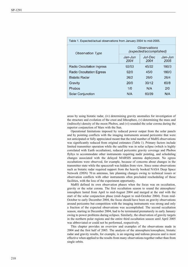
Table 1. Expected/actual observations from January 2004 to mid-2005.
areas by using bistatic radar, (iv) determining gravity anomalies for investigation of the structure and evolution of the crust and lithosphere, (v) determining the mass and (indirectly) density of the moon Phobos, and (vi) sounded the solar corona during the superior conjunction of Mars with the Sun.
Operational limitations imposed by reduced power output from the solar panels and by pointing conflicts with the imaging instruments around pericentre that were not anticipated or fully appreciated meant that the total number of MaRS observations was significantly reduced from original estimates (Table 1). Primary factors include limited transmitter operation while the satellite was in solar eclipse (which is highly correlated with Earth occultation), reduced pericentre gravity coverage and Phobos flybys to accommodate other instruments requiring nadir pointing, and scheduling changes associated with the delayed MARSIS antenna deployment. No egress occultations were observed, for example, because of concerns about changes in the transmitter state while the spacecraft was hidden from view. Since some observations such as bistatic radar required support from the heavily booked NASA Deep Space Network (DSN) 70 m antennas, late planning changes owing to technical issues or observation conflicts with other instruments often precluded rescheduling of those facilities, with the loss of the experiment opportunity.
MaRS defined its own observation phases when the focus was on occultation, gravity or the solar corona. The first occultation season to sound the atmosphere/ ionosphere lasted from April to mid-August 2004 and merged at the end with the start of the solar conjunction phase (mid-August to mid-October 2004). From mid-October to early December 2004, the focus should have been on gravity observations around pericentre but competition with the imaging instruments was strong and only a fraction of the expected observations was accomplished. The second occultation season, starting in December 2004, had to be terminated prematurely in early January owing to power problems during eclipses. Similarly, the observation of gravity targets in the northern polar regions and the entire third occultation season until April 2005 was abbreviated or could not be performed, respectively.
This chapter provides an overview and examples of the observations made in 2004 and the first half of 2005. The analysis of the atmosphere/ionosphere, bistatic radar and gravity results, for example, is an ongoing and tedious process and is most effective when applied to the results from many observations together rather than from single orbits.
218
SP-1291
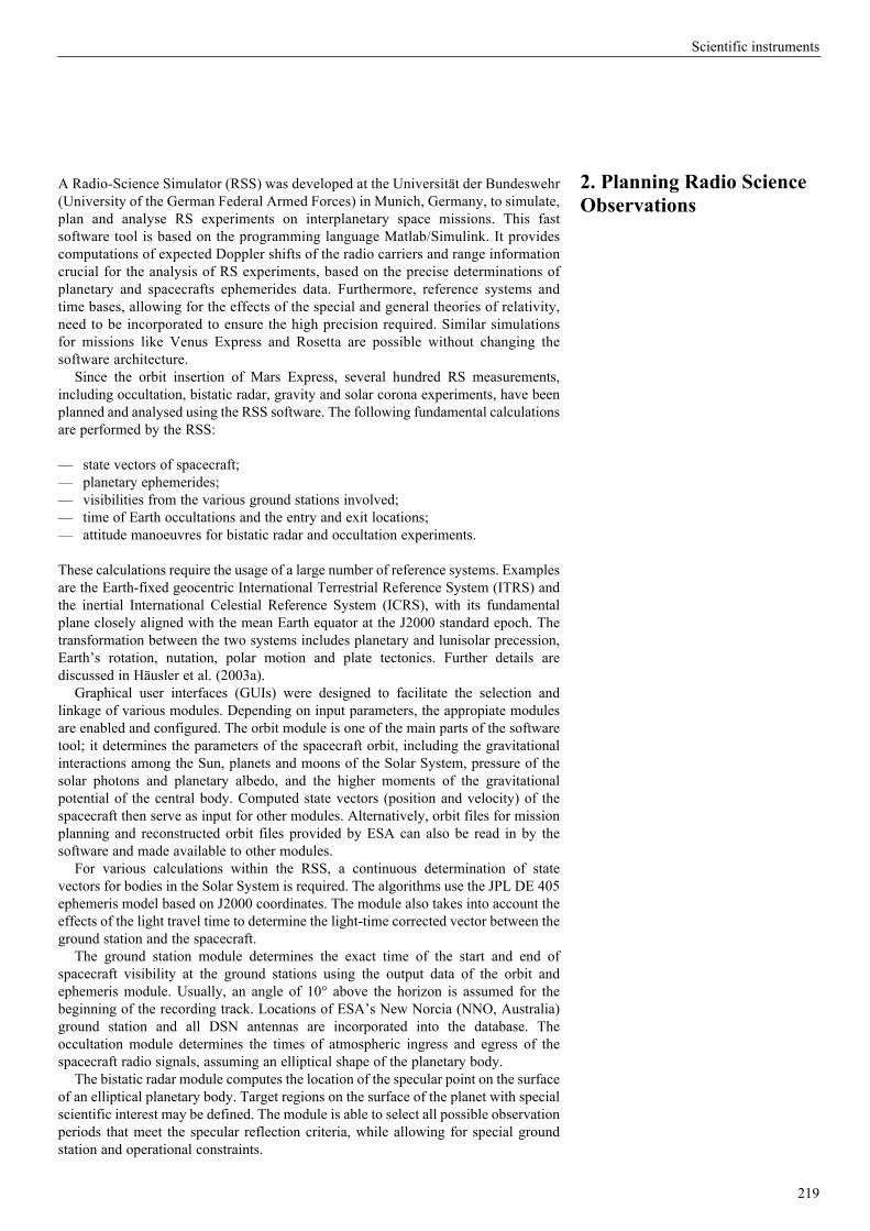
A Radio-Science Simulator (RSS) was developed at the Universität der Bundeswehr (University of the German Federal Armed Forces) in Munich, Germany, to simulate, plan and analyse RS experiments on interplanetary space missions. This fast software tool is based on the programming language Matlab/Simulink. It provides computations of expected Doppler shifts of the radio carriers and range information crucial for the analysis of RS experiments, based on the precise determinations of planetary and spacecrafts ephemerides data. Furthermore, reference systems and time bases, allowing for the effects of the special and general theories of relativity, need to be incorporated to ensure the high precision required. Similar simulations for missions like Venus Express and Rosetta are possible without changing the software architecture.
Since the orbit insertion of Mars Express, several hundred RS measurements, including occultation, bistatic radar, gravity and solar corona experiments, have been planned and analysed using the RSS software. The following fundamental calculations are performed by the RSS:
— state vectors of spacecraft;— planetary ephemerides;— visibilities from the various ground stations involved;— time of Earth occultations and the entry and exit locations;— attitude manoeuvres for bistatic radar and occultation experiments.
These calculations require the usage of a large number of reference systems. Examples are the Earth-fixed geocentric International Terrestrial Reference System (ITRS) and the inertial International Celestial Reference System (ICRS), with its fundamental plane closely aligned with the mean Earth equator at the J2000 standard epoch. The transformation between the two systems includes planetary and lunisolar precession, Earth’s rotation, nutation, polar motion and plate tectonics. Further details are discussed in Häusler et al. (2003a).
Graphical user interfaces (GUIs) were designed to facilitate the selection and linkage of various modules. Depending on input parameters, the appropiate modules are enabled and configured. The orbit module is one of the main parts of the software tool; it determines the parameters of the spacecraft orbit, including the gravitational interactions among the Sun, planets and moons of the Solar System, pressure of the solar photons and planetary albedo, and the higher moments of the gravitational potential of the central body. Computed state vectors (position and velocity) of the spacecraft then serve as input for other modules. Alternatively, orbit files for mission planning and reconstructed orbit files provided by ESA can also be read in by the software and made available to other modules.
For various calculations within the RSS, a continuous determination of state vectors for bodies in the Solar System is required. The algorithms use the JPL DE 405 ephemeris model based on J2000 coordinates. The module also takes into account the effects of the light travel time to determine the light-time corrected vector between the ground station and the spacecraft.
The ground station module determines the exact time of the start and end of spacecraft visibility at the ground stations using the output data of the orbit and ephemeris module. Usually, an angle of 10° above the horizon is assumed for the beginning of the recording track. Locations of ESA’s New Norcia (NNO, Australia) ground station and all DSN antennas are incorporated into the database. The occultation module determines the times of atmospheric ingress and egress of the spacecraft radio signals, assuming an elliptical shape of the planetary body.
The bistatic radar module computes the location of the specular point on the surface of an elliptical planetary body. Target regions on the surface of the planet with special scientific interest may be defined. The module is able to select all possible observation periods that meet the specular reflection criteria, while allowing for special ground station and operational constraints.
219
Scientific instruments
2. Planning Radio ScienceObservations

220
The output of the occultation, bistatic radar, gravity and solar corona modules is used to generate request files for Mission Operations in a format defined by ESA. The request files are checked and adjusted in a complicated and time-consuming process to meet the specific Mars Express mission constraints defined by ESA. The result is the input for the mission planning process (Fig. 1).
Frequency shifts in the one-way and two-way modes depend on the relative velocity between transmitter and receiver (Doppler effect), typically of the order of 30 km/s, on perturbations by gravity potentials, other non-gravitational forces acting on the spacecraft, and the effects from special and general relativity. The RSS Doppler module takes into account terms up to order (β2 = v/c)2 (Häusler et al., 2003a):
(1)
assuming a system S (spacecraft) is transmitting the frequency fS, and a system E (Earth ground station) receives the frequency fE. Here, we define â = v/c with n̂ being a unit vector pointing from (S) to (E), i.e. in the direction of the signal propagation at the time the signal is radiated. vS is the coordinate velocity of the spacecraft S and vE is the coordinate velocity of the ground station on Earth at the time of signal emission and reception, respectively. The coordinate system used is the Solar System barycentric system. All relative velocities must be Lorentz-transformed. ϕE and ϕS are the gravitational potentials of E and S, respectively. The potential of the ground station contains the centrifugal potential of Earth. For one-way propagation, the contribution of the gravitational potentials (gravitational redshift) can be significant and can reach approximately 30 Hz at the X-band. The Doppler predictions are compared with the received Doppler data, forming the Doppler residuals, which represent the basis for later scientific analysis, leading to planetary atmospheric parameters such as temperature, density and pressure.
More than a year of MaRS operations provides the opportunity to analyse the performance of the experiment by comparing the actual measurements during different time periods and at different Earth–spacecraft distances with predictions based on link analyses.
As extensively discussed in Pätzold et al. (2004), the performance of a radio science experiment at the radio frequency level can be expressed by two quantities: the Doppler frequency and the ranging values recorded at the ground station. The quality of these recordings determines the accuracy of sounding planetary atmospheres and ionospheres, the accuracy of the determination of planetary gravity field coefficients, and the detail of which effects of the propagation of radio wave propagation in the solar corona/solar wind plasma can be studied. Several parameters have to be carefully considered when making such a comparison: the spacecraft–Earth distance, the configurations of the onboard transponder and the ground station.
Data were studied from three time periods (June 2005, January 2005, August 2004), when the MaRS experiment was configured in the coherent TWOD mode (X-uplink, X- and S-downlink) for global gravity measurements at the orbit’s apocentre. The data were recorded at ESA’s NNO. The corresponding spacecraft–Earth distances were 1.1, 2.1 and 2.5 AU. The radio frequency parameters of the ground station and the spacecraft transponder are given in the MEX Space/Ground Interface Control Document SGICD (2003). The transponder phase noise and group delay performances as measured on the ground are summarised in Remus et al. (2001) and Häusler et al. (2003b).
Since the measurement made on 7 August 2004 near 2.5 AU took place only about a month before superior solar conjunction (17 September 2004), the contribution of the solar corona plasma to the Doppler measurement was substantial. A coarse
1 n a a n a n a n aff
c21 1
S
EE S S E S E S S E
2 2 2
2$ $ $ $. + +b b z z- - - - - -t t t t t t t t t] ^ ] ] ] ^g h g g g h
3. Assessment of Carrier Frequency and Range
Background Noise
Fig. 1. Planning tools and decision paths involved in the planning and operation of MaRS. The Principal Investigator initiates an experiment simulation at the Radio Science Simulator (RSS). The MaRS team generates with the Parsifal software (developed by the Payload Operations Service, POS) radio science specific request files (MREQs) for ESTEC for further coordination. The Mars Express (MEX) Instrument Resource Analyser (MIRA) software using the Flight Dynamics Events and Communications Skeleton (FECS) from ESOC was developed by POS to identify spacecraft resource and instrument conflict situations. In the ideal case, conflict-free experiment operations can be carried out by ESOC.
SP-1291

Table 2. Doppler velocity errors and Allan Deviation values for three passes at different Earth-Mars distances at X- and S-band in the TWOD mode.
estimate of the average solar contribution to the standard deviation of the Doppler measure ment error, which is based on the work of Woo & Armstrong (1979), is given in DSMS (2000) and was included in this analysis. The predicted Doppler and range values were substracted from the Doppler and group delay (ranging) measurements recorded at the ground station. These residuals were detrended and used in this analysis.
3.1 Doppler MeasurementsAs an example, Fig. 2 shows Doppler residuals taken from orbit 1775/1776 on day-of-year (DOY) 154 (3 June 2005) sampled at 1 s integration time over a time period of 1000 s.
The three sets of Doppler data for the above three passes were sampled at 1 s integration time for a time period of 5000 s per pass. Table 2 shows the correspondingly converted values of the standard deviation σV (μm s–1) of the velocity error. The Allan deviation values at 1, 10 and 100 s integration times are shown for completeness.
221
Fig. 2 X-band (upper panel) and S-band (lower panel) frequency residuals recorded in orbit 1775/1776 at orbit apocentre. The 1s standard deviation at 1 s integration time is 5.6 mHz at X-band and 9.4 mHz at S-band, which correspond to 201.8 μm/s and 1227.5 μm s‒1 Doppler velocity noise, respectively. See Table 1 for frequency stability.
Scientific instruments
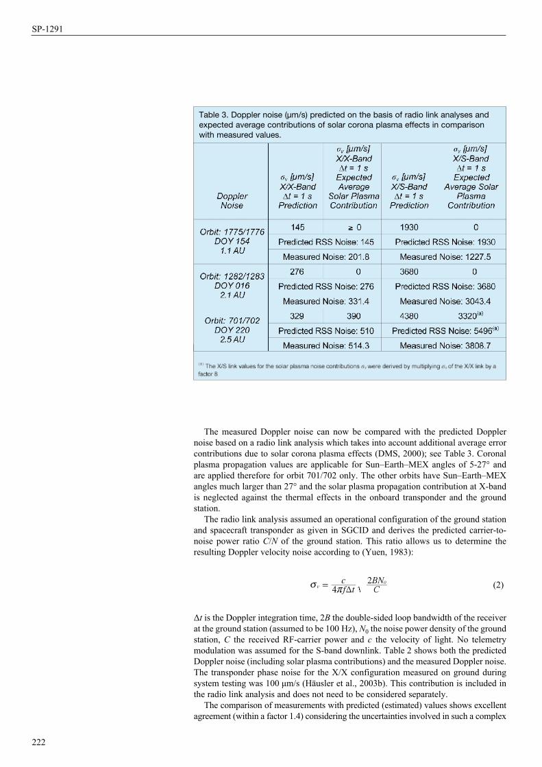
Table 3. Doppler noise (µm/s) predicted on the basis of radio link analyses andexpected average contributions of solar corona plasma effects in comparison with measured values.
The measured Doppler noise can now be compared with the predicted Doppler noise based on a radio link analysis which takes into account additional average error contributions due to solar corona plasma effects (DMS, 2000); see Table 3. Coronal plasma propagation values are applicable for Sun–Earth–MEX angles of 5-27° and are applied therefore for orbit 701/702 only. The other orbits have Sun–Earth–MEX angles much larger than 27° and the solar plasma propagation contribution at X-band is neglected against the thermal effects in the onboard transponder and the ground station.
The radio link analysis assumed an operational configuration of the ground station and spacecraft transponder as given in SGCID and derives the predicted carrier-to-noise power ratio C/N of the ground station. This ratio allows us to determine the resulting Doppler velocity noise according to (Yuen, 1983):
(2)
Δt is the Doppler integration time, 2B the double-sided loop bandwidth of the receiver at the ground station (assumed to be 100 Hz), N0 the noise power density of the ground station, C the received RF-carrier power and c the velocity of light. No telemetry modulation was assumed for the S-band downlink. Table 2 shows both the predicted Doppler noise (including solar plasma contributions) and the measured Doppler noise. The transponder phase noise for the X/X configuration measured on ground during system testing was 100 μm/s (Häusler et al., 2003b). This contribution is included in the radio link analysis and does not need to be considered separately.
The comparison of measurements with predicted (estimated) values shows excellent agreement (within a factor 1.4) considering the uncertainties involved in such a complex
222
f tc
CBN
42 0
v T=v r
SP-1291
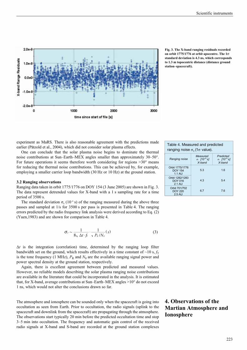
Table 4. Measured and predicted ranging noise στ (1σ value).
experiment as MaRS. There is also reasonable agreement with the predictions made earlier (Pätzold et al., 2004), which did not consider solar plasma effects.
One can conclude that the solar plasma noise begins to dominate the thermal noise contributions at Sun–Earth–MEX angles smaller than approximately 30–50°. For future operations it seems therefore worth considering for regions >30° means for reducing the thermal noise contributions. This can be achieved by, for example, employing a smaller carrier loop bandwidth (30 Hz or 10 Hz) at the ground station.
3.2 Ranging observationsRanging data taken in orbit 1775/1776 on DOY 154 (3 June 2005) are shown in Fig. 3. The data represent detrended values for X-band with a 1 s sampling rate for a time period of 3500 s.
The standard deviation στ (10–9 s) of the ranging measured during the above three passes and sampled at 1/s for 3500 s per pass is presented in Table 4. The ranging errors predicted by the radio frequency link analysis were derived according to Eq. (2) (Yuen,1983) and are shown for comparison in Table 4.
(3)
Δt is the integration (correlation) time, determined by the ranging loop filter bandwidth set on the ground, which results effectively in a time constant of ~10 s, fT is the tone frequency (1 MHz), PR and N0 are the available ranging signal power and power spectral density at the ground station, respectively.
Again, there is excellent agreement between predicted and measured values. However, no reliable models describing the solar plasma ranging noise contributions are available in the literature that could be incorporated in the analysis. It is estimated that, for X-band, average contributions at Sun–Earth–MEX angles >10° do not exceed 1 ns, which would not alter the conclusions drawn so far.
The atmosphere and ionosphere can be sounded only when the spacecraft is going into occultation as seen from Earth. Prior to occultation, the radio signals (uplink to the spacecraft and downlink from the spacecraft) are propagating through the atmosphere. The observations start typically 20 min before the predicted occultation time and stop 3–5 min into occultation. The frequency and automatic gain control of the received radio signals at X-band and S-band are recorded at the ground station complexes
223
ISSUE 1 10
Andy's HD:Users:andy:Documents:ANDY:sp1291MEX2:MaRS:RSIv1.docCreated on 11/21/05 4:21 PM
Table 4: Measured and predicted ranging noise st ( 1s - value) and predicted ranging
noise tr (1s - value )
Ranging noiseMeasuredστ [10–9 s]
X-band
Predictedστ [10–9 s]
X-band
Orbit 1775/1776DOY 1541.1 AU
5.3 1.6
Orbit 1282/1283DOY 0162.1 AU
4.3 5.4
Orbit 701/702DOY 2202.5 AU
6.7 7.6
Fig. 3. The X-band ranging residuals recorded on orbit 1775/1776 at orbit apocentre. The 1s standard deviation is 4.3 ns, which corresponds to 1.3 m topocentric distance (distance ground station–spacecraft).
/t f P Ns
8
1 1
T R O
r
$$
T+v ] g
4. Observations of theMartian Atmosphere and Ionosphere
Scientific instruments
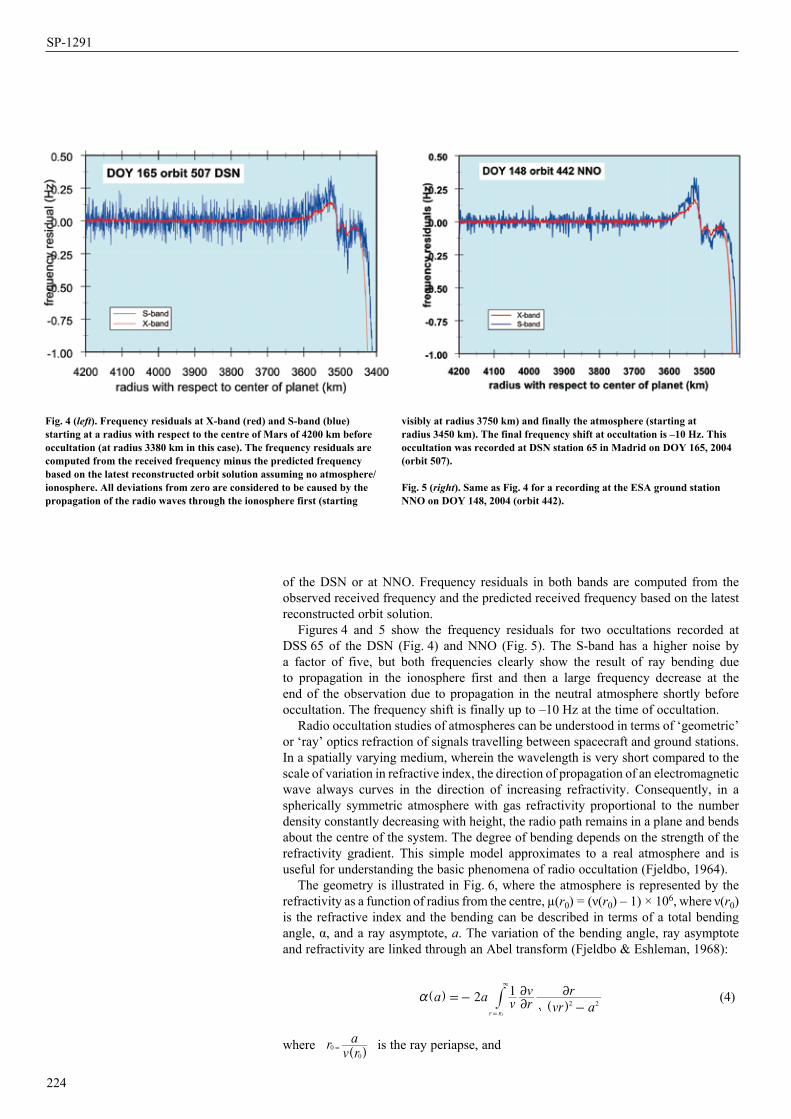
224
Fig. 4 (left). Frequency residuals at X-band (red) and S-band (blue) starting at a radius with respect to the centre of Mars of 4200 km before occultation (at radius 3380 km in this case). The frequency residuals are computed from the received frequency minus the predicted frequency based on the latest reconstructed orbit solution assuming no atmosphere/ionosphere. All deviations from zero are considered to be caused by the propagation of the radio waves through the ionosphere first (starting
visibly at radius 3750 km) and finally the atmosphere (starting at radius 3450 km). The final frequency shift at occultation is –10 Hz. This occultation was recorded at DSN station 65 in Madrid on DOY 165, 2004 (orbit 507).
Fig. 5 (right). Same as Fig. 4 for a recording at the ESA ground station NNO on DOY 148, 2004 (orbit 442).
of the DSN or at NNO. Frequency residuals in both bands are computed from the observed received frequency and the predicted received frequency based on the latest reconstructed orbit solution.
Figures 4 and 5 show the frequency residuals for two occultations recorded at DSS 65 of the DSN (Fig. 4) and NNO (Fig. 5). The S-band has a higher noise by a factor of five, but both frequencies clearly show the result of ray bending due to propagation in the ionosphere first and then a large frequency decrease at the end of the observation due to propagation in the neutral atmosphere shortly before occultation. The frequency shift is finally up to –10 Hz at the time of occultation.
Radio occultation studies of atmospheres can be understood in terms of ‘geometric’ or ‘ray’ optics refraction of signals travelling between spacecraft and ground stations. In a spatially varying medium, wherein the wavelength is very short compared to the scale of variation in refractive index, the direction of propagation of an electromagnetic wave always curves in the direction of increasing refractivity. Consequently, in a spherically symmetric atmosphere with gas refractivity proportional to the number density constantly decreasing with height, the radio path remains in a plane and bends about the centre of the system. The degree of bending depends on the strength of the refractivity gradient. This simple model approximates to a real atmosphere and is useful for understanding the basic phenomena of radio occultation (Fjeldbo, 1964).
The geometry is illustrated in Fig. 6, where the atmosphere is represented by the refractivity as a function of radius from the centre, µ(r0) = (ν(r0) – 1) × 106, where ν(r0) is the refractive index and the bending can be described in terms of a total bending angle, α, and a ray asymptote, a. The variation of the bending angle, ray asymptote and refractivity are linked through an Abel transform (Fjeldbo & Eshleman, 1968):
(4)
where is the ray periapse, and
a av r
v
vr a
r2 1
r r
2 2
0
22 2a =-
-
3
=
]]
gg
#
rv ra
0
0
= ] g
SP-1291
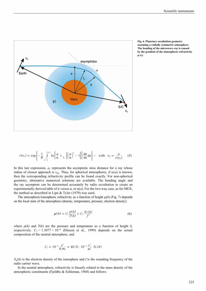
225
Fig. 6. Planetary occultation geometry assuming a radially symmetric atmosphere. The bending of the microwave ray is caused by the gradient of the atmospheric refractivity µ (r).
(5)
In this last expression, a1 represents the asymptotic miss distance for a ray whose radius of closest approach is r01. Thus, for spherical atmospheres, if a(a) is known, then the corresponding refractivity profile can be found exactly. For non-spherical geometry, alternative numerical solutions are available. The bending angle and the ray asymptote can be determined accurately by radio occultation to create an experimentally derived table of α versus α, or α(a). For the two-way case, as for MEX, the method as described in Lipa & Tyler (1979) was used.
The atmospheric/ionospheric refractivity as a function of height µ(h) (Fig. 7) depends on the local state of the atmosphere (density, temperature, pressure, electron density):
(6)
where p(h) and T(h) are the pressure and temperature as a function of height h, respectively. C1 = 1.3077 × 10⁻⁶ (Hinson et al., 1999) depends on the actual composition of the neutral atmosphere, and
Ne(h) is the electron density of the ionosphere and f is the sounding frequency of the radio carrier wave.
In the neutral atmosphere, refractivity is linearly related to the mass density of the atmospheric constituents (Fjeldbo & Eshleman, 1968) and follows
10 40.31 10Cme
ms N h3
6
0
26
3
2
ee$ $= =f
- - ] g
h CT h
p hC
fN he
1 3 2= +n]]] ]ggg g
dd d withexp lnv r
aa
aa
aa r
v ra1 1
a a
a
011 1
2
01
011
= + =ra
- - -
3
=
=
] b]
g lg
; E(* 2 4#
Scientific instruments
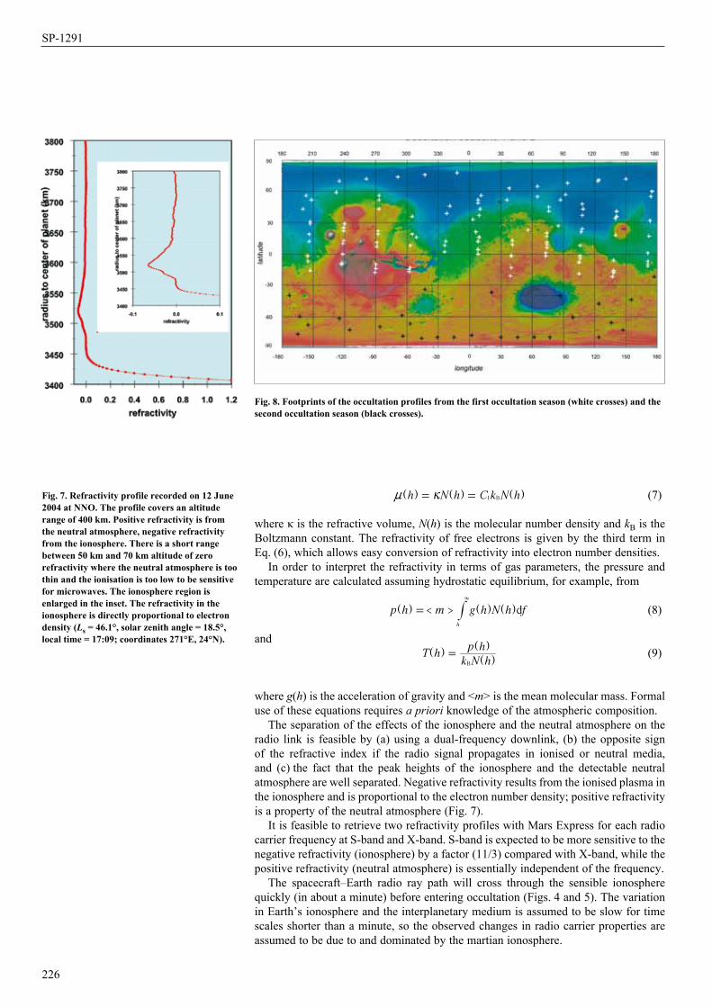
(7)
where κ is the refractive volume, N(h) is the molecular number density and kB is the Boltzmann constant. The refractivity of free electrons is given by the third term in Eq. (6), which allows easy conversion of refractivity into electron number densities.
In order to interpret the refractivity in terms of gas parameters, the pressure and temperature are calculated assuming hydrostatic equilibrium, for example, from
(8)
and (9)
where g(h) is the acceleration of gravity and <m> is the mean molecular mass. Formal use of these equations requires a priori knowledge of the atmospheric composition.
The separation of the effects of the ionosphere and the neutral atmosphere on the radio link is feasible by (a) using a dual-frequency downlink, (b) the opposite sign of the refractive index if the radio signal propagates in ionised or neutral media, and (c) the fact that the peak heights of the ionosphere and the detectable neutral atmosphere are well separated. Negative refractivity results from the ionised plasma in the ionosphere and is proportional to the electron number density; positive refractivity is a property of the neutral atmosphere (Fig. 7).
It is feasible to retrieve two refractivity profiles with Mars Express for each radio carrier frequency at S-band and X-band. S-band is expected to be more sensitive to the negative refractivity (ionosphere) by a factor (11/3) compared with X-band, while the positive refractivity (neutral atmosphere) is essentially independent of the frequency.
The spacecraft–Earth radio ray path will cross through the sensible ionosphere quickly (in about a minute) before entering occultation (Figs. 4 and 5). The variation in Earth’s ionosphere and the interplanetary medium is assumed to be slow for time scales shorter than a minute, so the observed changes in radio carrier properties are assumed to be due to and dominated by the martian ionosphere.
226
T hk N h
p h
B
=]]]
ggg
Fig. 8. Footprints of the occultation profiles from the first occultation season (white crosses) and the second occultation season (black crosses).
dp h m g h N h f< >h
=
3
] ] ]g g g#
h N h C k N h1 B= =n l] ] ]g g gFig. 7. Refractivity profile recorded on 12 June 2004 at NNO. The profile covers an altitude range of 400 km. Positive refractivity is from the neutral atmosphere, negative refractivity from the ionosphere. There is a short range between 50 km and 70 km altitude of zero refractivity where the neutral atmosphere is too thin and the ionisation is too low to be sensitive for microwaves. The ionosphere region is enlarged in the inset. The refractivity in the ionosphere is directly proportional to electron density (Ls = 46.1°, solar zenith angle = 18.5°, local time = 17:09; coordinates 271°E, 24°N).
SP-1291

During the first occultation season, from April to mid-August 2004, MaRS retrieved about 100 profiles of pressure, temperature, neutral number density from the neutral atmosphere and electron density from the ionosphere. Another 32 profiles were obtained during the second occultation season (Fig. 8).
The dataset from the first occultation season may be divided into two parts: 13 profiles obtained in April 2004 (solar longitudes Ls = 13–21°) covering solar zenith angles from 108° to 85° at local morning times of about 04:30 to 05:15, and a second part of about 86 profiles (Ls = 32–74°) covering solar zenith angles from 70° to 84° at local late afternoon times at about 17:00.
Thirty-two profiles of the second occultation season were observed from 8 December 2004 to 4 January 2005. The observations in this season had to be terminated prematurely owing to the eclipse situation; two-thirds of the maximal possible occultations could not be observed.
4.1 Profiles from the Neutral Atmosphere Vertical profiles of pressure, temperature and number-density of the neutral atmosphere from near to the surface to about 50 km altitude were obtained at 05:00 local time at high latitudes in the Northern Plains (Ls = 13–21°, early spring in the northern hemisphere) during sunrise and at local times of 17:00 from mid-latitudes in the northern hemisphere to the equator (Ls = 32–74°). MEX occultations therefore reach other latitudes and areas than Mars Global Surveyor (MGS) and provide valuable input for general circulation models (GCMs) of the atmosphere.
An example is shown in Fig. 9 from a low-latitude region at 74°E, 6.6°N in mid-spring at 17:30 local time. The profiles range from the surface at 3397 km radius to about 40 km altitude. There is a gradual decrease in temperature from 230K at the surface to 140K at 40 km altitude. The error bars mark the confidence limits from the derivation process. The relative error in general for all profiles is 0.1% at the surface (fractions of a kelvin) to 10% at the top of the profile (15K). The blue open circles in Fig. 9 are temperatures and number-densities from the GCM derived at Laboratoire Météorologique Dynamique (LMD) in Paris (Angelats i Coll et al., 2005). The LMD GCM follows the observations well for profiles from the equator to the mid-latitudes in both hemispheres.
Strong deviations from the GCM can be identified in all observed profiles at polar latitudes during both local spring over the northern hemisphere (Fig. 10) and local winter (polar night) over the southern hemisphere (Fig. 11). These first-ever observations of the high latitudes at different local times to MGS observations provide valuable information for improving the GCMs of the martian atmosphere. Two examples from the early morning during local spring and from the polar night during local deep winter, at high northern and southern latitudes, respectively, are discussed below.
The temperature profile in Fig. 10 from 290°E, 74.5°N in the Northern Plains at Ls = 21° and 05:17 local time shows a very cold near-surface temperature of 156K at 2 km altitude; the atmosphere warms up to 168K at 6 km. An inversion layer at that altitude is present. The GCM follows essentially the same trend but at temperatures of about 10K higher. At 35 km altitude, a strong depletion of CO2 is experienced, as seen from the comparison of the GCM with the observed neutral number density.
Figure 11 shows profiles from high southern latitudes (47°E, –81°S) at local winter (Ls = 136°) at 14:30 local time. This is the polar night; the Sun is below the horizon for the entire sol and the atmosphere cools extremely during the polar night. The temperature is almost constant at 142K from the surface up to 35 km altitude. However, it is warmer than the atmosphere in the early morning at local spring (Fig. 10) at altitudes above 15 km. The GCM does not reflect the situation at all.
4.2 Profiles from the IonosphereThe electron density profile of the ionosphere is easily converted from the refractivity (the third term in Eq. 6). One observes a stable two-layer ionospheric structure (Fig. 12) at peak altitudes of approximately 110 km and 130 km for the M1 and M2 layers (the designation of layers follows Rishbeth & Mendillo, 2003), respectively,
227
Scientific instruments
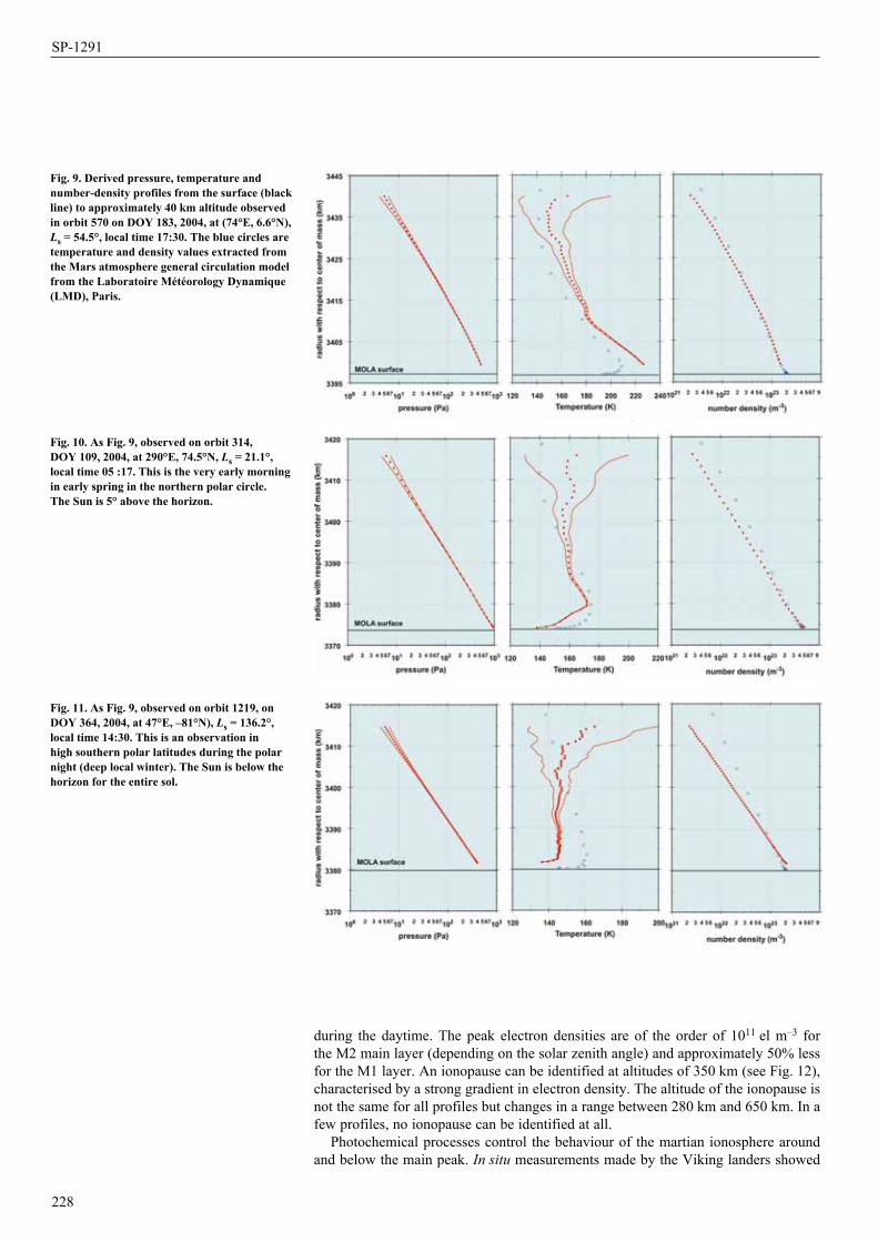
during the daytime. The peak electron densities are of the order of 1011 el m–3 for the M2 main layer (depending on the solar zenith angle) and approximately 50% less for the M1 layer. An ionopause can be identified at altitudes of 350 km (see Fig. 12), characterised by a strong gradient in electron density. The altitude of the ionopause is not the same for all profiles but changes in a range between 280 km and 650 km. In a few profiles, no ionopause can be identified at all.
Photochemical processes control the behaviour of the martian ionosphere around and below the main peak. In situ measurements made by the Viking landers showed
228
Fig. 11. As Fig. 9, observed on orbit 1219, on DOY 364, 2004, at 47°E, –81°N), Ls = 136.2°, local time 14:30. This is an observation in high southern polar latitudes during the polar night (deep local winter). The Sun is below the horizon for the entire sol.
Fig. 10. As Fig. 9, observed on orbit 314, DOY 109, 2004, at 290°E, 74.5°N, Ls = 21.1°, local time 05 :17. This is the very early morning in early spring in the northern polar circle. The Sun is 5° above the horizon.
Fig. 9. Derived pressure, temperature and number-density profiles from the surface (black line) to approximately 40 km altitude observed in orbit 570 on DOY 183, 2004, at (74°E, 6.6°N), Ls = 54.5°, local time 17:30. The blue circles are temperature and density values extracted from the Mars atmosphere general circulation model from the Laboratoire Météorology Dynamique (LMD), Paris.
SP-1291
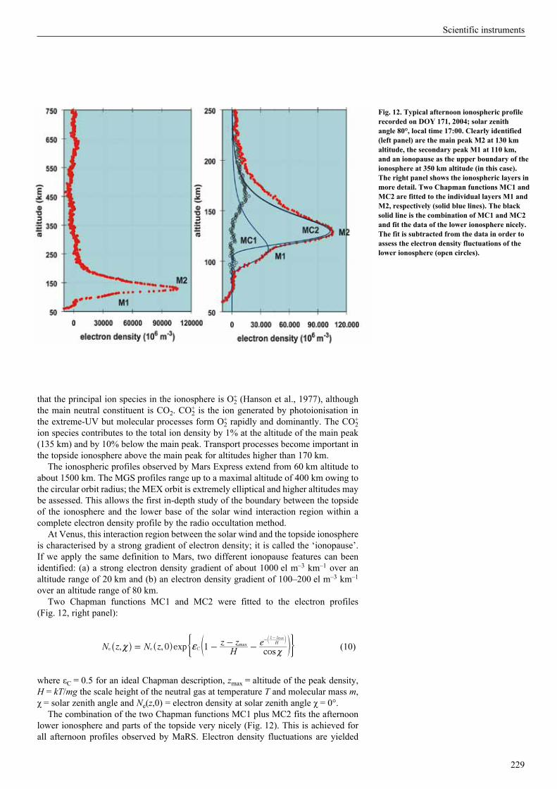
229
Fig. 12. Typical afternoon ionospheric profile recorded on DOY 171, 2004; solar zenith angle 80°, local time 17:00. Clearly identified (left panel) are the main peak M2 at 130 km altitude, the secondary peak M1 at 110 km, and an ionopause as the upper boundary of the ionosphere at 350 km altitude (in this case). The right panel shows the ionospheric layers in more detail. Two Chapman functions MC1 and MC2 are fitted to the individual layers M1 and M2, respectively (solid blue lines). The black solid line is the combination of MC1 and MC2 and fit the data of the lower ionosphere nicely. The fit is subtracted from the data in order to assess the electron density fluctuations of the lower ionosphere (open circles).
that the principal ion species in the ionosphere is O2+ (Hanson et al., 1977), although
the main neutral constituent is CO2. CO2+ is the ion generated by photoionisation in
the extreme-UV but molecular processes form O2+ rapidly and dominantly. The CO2
+ ion species contributes to the total ion density by 1% at the altitude of the main peak (135 km) and by 10% below the main peak. Transport processes become important in the topside ionosphere above the main peak for altitudes higher than 170 km.
The ionospheric profiles observed by Mars Express extend from 60 km altitude to about 1500 km. The MGS profiles range up to a maximal altitude of 400 km owing to the circular orbit radius; the MEX orbit is extremely elliptical and higher altitudes may be assessed. This allows the first in-depth study of the boundary between the topside of the ionosphere and the lower base of the solar wind interaction region within a complete electron density profile by the radio occultation method.
At Venus, this interaction region between the solar wind and the topside ionosphere is characterised by a strong gradient of electron density; it is called the ‘ionopause’. If we apply the same definition to Mars, two different ionopause features can been identified: (a) a strong electron density gradient of about 1000 el m–3 km–1 over an altitude range of 20 km and (b) an electron density gradient of 100–200 el m–3 km–1 over an altitude range of 80 km.
Two Chapman functions MC1 and MC2 were fitted to the electron profiles (Fig. 12, right panel):
(10)
where εC = 0.5 for an ideal Chapman description, zmax = altitude of the peak density, H = kT/mg the scale height of the neutral gas at temperature T and molecular mass m, χ = solar zenith angle and Ne(z,0) = electron density at solar zenith angle χ = 0°.
The combination of the two Chapman functions MC1 plus MC2 fits the afternoon lower ionosphere and parts of the topside very nicely (Fig. 12). This is achieved for all afternoon profiles observed by MaRS. Electron density fluctuations are yielded
, , expcos
N z N zH
z z e0 1Cmax H
z z
e e
max
= f|
| - - --
-
^ ^ ec
h h om
) 3
Scientific instruments
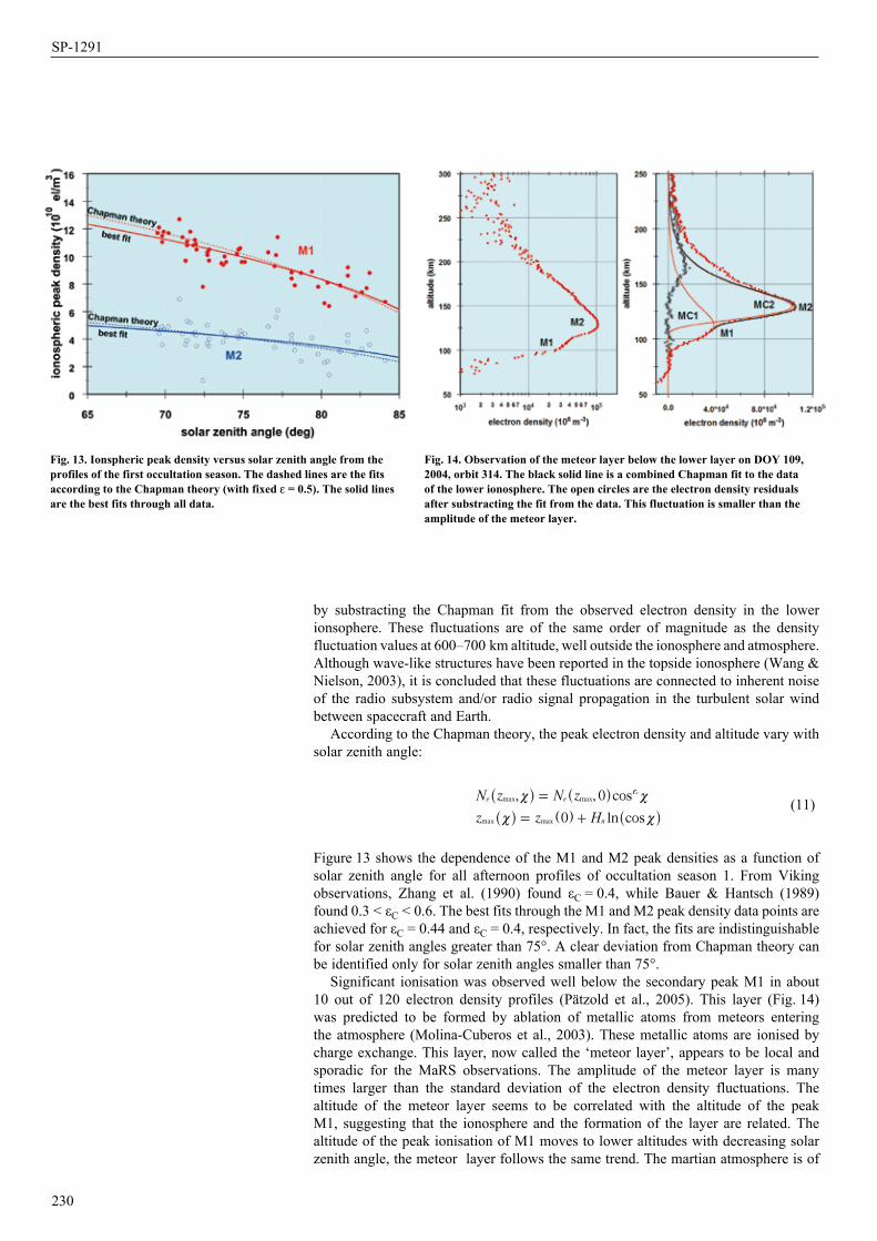
by substracting the Chapman fit from the observed electron density in the lower ionsophere. These fluctuations are of the same order of magnitude as the density fluctuation values at 600–700 km altitude, well outside the ionosphere and atmosphere. Although wave-like structures have been reported in the topside ionosphere (Wang & Nielson, 2003), it is concluded that these fluctuations are connected to inherent noise of the radio subsystem and/or radio signal propagation in the turbulent solar wind between spacecraft and Earth.
According to the Chapman theory, the peak electron density and altitude vary with solar zenith angle:
(11)
Figure 13 shows the dependence of the M1 and M2 peak densities as a function of solar zenith angle for all afternoon profiles of occultation season 1. From Viking observations, Zhang et al. (1990) found εC = 0.4, while Bauer & Hantsch (1989) found 0.3 < εC < 0.6. The best fits through the M1 and M2 peak density data points are achieved for εC = 0.44 and εC = 0.4, respectively. In fact, the fits are indistinguishable for solar zenith angles greater than 75°. A clear deviation from Chapman theory can be identified only for solar zenith angles smaller than 75°.
Significant ionisation was observed well below the secondary peak M1 in about 10 out of 120 electron density profiles (Pätzold et al., 2005). This layer (Fig. 14) was predicted to be formed by ablation of metallic atoms from meteors entering the atmosphere (Molina-Cuberos et al., 2003). These metallic atoms are ionised by charge exchange. This layer, now called the ‘meteor layer’, appears to be local and sporadic for the MaRS observations. The amplitude of the meteor layer is many times larger than the standard deviation of the electron density fluctuations. The altitude of the meteor layer seems to be correlated with the altitude of the peak M1, suggesting that the ionosphere and the formation of the layer are related. The altitude of the peak ionisation of M1 moves to lower altitudes with decreasing solar zenith angle, the meteor layer follows the same trend. The martian atmosphere is of
230
Fig. 13. Ionspheric peak density versus solar zenith angle from the profiles of the first occultation season. The dashed lines are the fits according to the Chapman theory (with fixed e = 0.5). The solid lines are the best fits through all data.
Fig. 14. Observation of the meteor layer below the lower layer on DOY 109, 2004, orbit 314. The black solid line is a combined Chapman fit to the data of the lower ionosphere. The open circles are the electron density residuals after substracting the fit from the data. This fluctuation is smaller than the amplitude of the meteor layer.
, , cos
ln cos
N z N z
z z H
0
0
max max
max max
ee
n
c=
= +
| |
| |
f^ ^
^ ] ^
h h
h g h
SP-1291
sufficient density between 70 km and 100 km altitude to provide drag needed to heat and ablate meteorites. The density in Earth’s atmosphere above 95 km, where the meteoritic layer has been found to be permanent (Kopp, 1997), is slightly higher than the neutral density of the martian atmosphere at 75 km and is an order of magnitude greater than the martian atmosphere at 95 km. This would explain the similar ablation effect of meteors on Mars and Earth. The slightly thinner atmosphere at this level on Mars implies that meteors of larger kinetic energies than on Earth are required for significant ablation to occur above 75 km. The latter would then explain the sporadic occurrence of the meteor layer at its observed altitude.
The gravity field of a planet is the result of its internal mass distribution and rotational state. Rapidly rotating planets bulge at the equator as a result of centrifugal forces. Consequently, the associated redistribution of mass to the equatorial plane results in a stronger gravitational acceleration of a spacecraft when it is near the pole than when it is at the same altitude over the equator. Similarly, anomalies in the internal distribution of mass are expressed as departures of the external gravitational field from that of a uniform sphere or a stratified spherical distribution. Space probes in the vicinity of planetary bodies follow trajectories that deviate from the ideal orbits described by Kepler’s laws in response to these gravity anomalies.
The goal of the gravity observations is the study of the state and evolution of the martian crust and lithosphere with important implications for the tectonic evolution and mantle convection of Mars. The targets of investigations are the hot-spot areas Tharsis and Elysium, large single volcanoes such as Alba Patera and Olympus Mons, the large impact craters and basins such as Huygens, Argyre and Hellas, respectively, rift structures like Tempe Fossae and Claritas Fossae, and the highland-lowland boundary. The investigation of impact basins must be viewed in the context of similar studies on other planetary bodies, including Earth, in the sense of comparative planetology and studies of the impact mechanisms that are not yet fully understood, especially for large basins. Studies of the highland-lowland boundary will contribute to the open question of this dichotomy.
Up to June 2005 there were 21 successful target gravity observations in total (Table 5 and Fig. 15). This low number results from the fact that the imaging instruments had priority for high-gain antenna Earth pointing and instrument nadir pointing when requesting the same pericentre target observation as radio science.
The gravity measurements consist of Doppler data along line-of-sight (LOS) near the pericentre above the selected target areas of geophysical interest (Pätzold et al., 2004), as summarised in Table 5. The altitude of Mars Express at pericentre, between 265 km and 330 km, is lower than the minimum altitude (370 km) of the circularised orbit of MGS (Lemoine et al., 2001; Yuan et al., 2001). Short-wavelength orbital perturbations due to gravity are thus significantly larger on MEX than on MGS, so that MEX gravity data are useful for improving knowledge of the short-wavelength gravity anomalies over the observed targets.
Starting from the observed Doppler shift frequencies, LOS Doppler velocity residuals were computed using the latest reconstructed orbit solution provided by ESA’s European Space Operations Centre (ESOC); see Fig. 16 for orbit 1144 over Olympus Mons as an example. Since the reconstructed orbit solution computed by ESOC is based on the global gravity field JGM85F02 up to degree and order 50, the resulting Doppler residuals do not include variations caused by gravity harmonics lower than degree and order 51.
The noise of the Doppler velocity residuals may be estimated from the high-altitude part of the pericentre pass where short-wavelength gravity anomalies have a negligible effect on the spacecraft orbit. For an integration time of 10 s, we obtain a mean value of 0.02 mm/s, which agrees well with the mean noise (0.03 mm/s) on the LOS velocity residuals during the Gravity Calibration Orbit of MGS. The signal-to-noise ratio is thus better than for the MGS LOS data. The pericentre pass is defined by an
231
5. Observations of theMartian Gravity Field
Scientific instruments
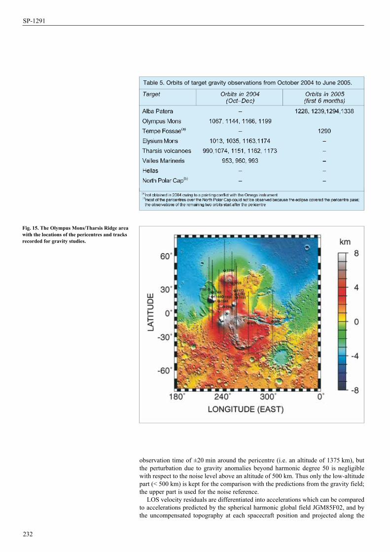
Table 5. Orbits of target gravity observations from October 2004 to June 2005.
observation time of ±20 min around the pericentre (i.e. an altitude of 1375 km), but the perturbation due to gravity anomalies beyond harmonic degree 50 is negligible with respect to the noise level above an altitude of 500 km. Thus only the low-altitude part (< 500 km) is kept for the comparison with the predictions from the gravity field; the upper part is used for the noise reference.
LOS velocity residuals are differentiated into accelerations which can be compared to accelerations predicted by the spherical harmonic global field JGM85F02, and by the uncompensated topography at each spacecraft position and projected along the
232
Fig. 15. The Olympus Mons/Tharsis Ridge area with the locations of the pericentres and tracks recorded for gravity studies.
SP-1291
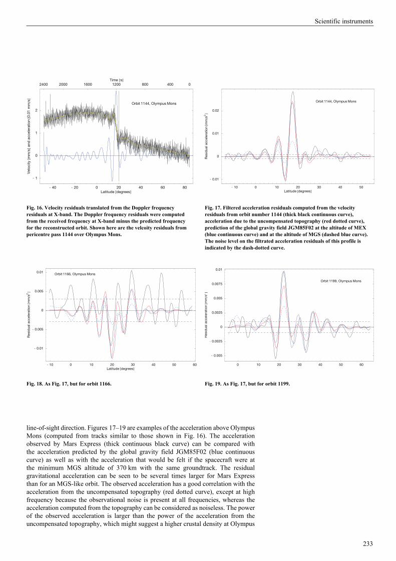
line-of-sight direction. Figures 17–19 are examples of the acceleration above Olympus Mons (computed from tracks similar to those shown in Fig. 16). The acceleration observed by Mars Express (thick continuous black curve) can be compared with the acceleration predicted by the global gravity field JGM85F02 (blue continuous curve) as well as with the acceleration that would be felt if the spacecraft were at the minimum MGS altitude of 370 km with the same groundtrack. The residual gravitational acceleration can be seen to be several times larger for Mars Express than for an MGS-like orbit. The observed acceleration has a good correlation with the acceleration from the uncompensated topography (red dotted curve), except at high frequency because the observational noise is present at all frequencies, whereas the acceleration computed from the topography can be considered as noiseless. The power of the observed acceleration is larger than the power of the acceleration from the uncompensated topography, which might suggest a higher crustal density at Olympus
233
0 10 20 30 40 50 60Latitude degrees
- 0.005
- 0.0025
0
0.0025
0.005
0.0075
0.01
Res
idua
lacc
eler
atio
nm
ms2
Orbit 1199, Olympus Mons
- 10 0 10 20 30 40 50 60Latitude degrees
- 0.01
- 0.005
0
0.005
0.01
Res
idua
lacc
eler
atio
nm
ms2
Orbit 1166, Olympus Mons
- 10 0 10 20 30 40 50Latitude degrees
- 0.01
0
0.01
0.02
Res
idua
lacc
eler
atio
nm
ms2
Orbit 1144, Olympus Mons
- 40 - 20 0 20 40 60 80Latitude degrees
- 1
0
1
2
Vel
ocity
mm
san
dac
cele
ratio
n0.
01m
ms
04008001200160020002400Time s
Orbit 1144, Olympus Mons
Fig. 19. As Fig. 17, but for orbit 1199.Fig. 18. As Fig. 17, but for orbit 1166.
Fig. 17. Filtered acceleration residuals computed from the velocity residuals from orbit number 1144 (thick black continuous curve), acceleration due to the uncompensated topography (red dotted curve), prediction of the global gravity field JGM85F02 at the altitude of MEX (blue continuous curve) and at the altitude of MGS (dashed blue curve). The noise level on the filtrated acceleration residuals of this profile is indicated by the dash-dotted curve.
Fig. 16. Velocity residuals translated from the Doppler frequency residuals at X-band. The Doppler frequency residuals were computed from the received frequency at X-band minus the predicted frequency for the reconstructed orbit. Shown here are the velcoity residuals from pericentre pass 1144 over Olympus Mons.
Scientific instruments

Mons. The confidence in such geophysical predictions is. however, limited by the presence of noise, and only the accumulation of several parallel orbits above a target improves the quality of the prediction by statistically decreasing the noise. In the three examples shown in Figs. 17-19, orbits 1144 and 1199 support the high crustal density hypothesis, whereas orbit 1166 has a too-high noise level to be useful.
In their analysis of MEX gravity data, Beuthe et al. (2005) performed a comparative spectral analysis of the MEX and MGS accelerations and the theoretical acceleration from a model of the topography. They computed the coherences between the MEX and topography accelerations, between the MGS and topography accelerations, and between the MEX and MGS accelerations. The average coherence MEX/topography is optimal down to a wavelength corresponding to the altitude of the spacecraft at pericentre; it rapidly decreases for much smaller wavelengths because of the presence of noise in the MEX residuals. This behaviour corresponds to expectations based on the rule of thumb that the smallest detectable wavelength is given by the minimum altitude of the spacecraft. The global MGS gravity solution shows a coherence with the topography comparable to MEX or better, because the global gravity field is obtained as a statistical average over thousands of MGS profiles. The MEX/MGS coherence is similar in shape to the MEX/topography coherence, though a little smaller at large wavelengths because of unmodelled effects in the MEX orbit. This coherence remains at a high level down to a wavelength of 300 km.
The gain factor between MEX and MGS is 1 within the error bars, except again at the largest wavelength, where the coherence is lower. This analysis of the coherence and gain factor shows that MEX can be used as an independent check on the quality of the existing gravity solutions such as JGM85F02 in the target regions analysed at an altitude lower than MGS orbits. Conversely, the good agreement between MEX and MGS also provides confidence in MEX gravity data.
Several parallel pericentre tracks over a target area, if available, will be used for a refined analysis of the local structure of the crust and the lithosphere, in order to obtain, for instance, the local crustal density. Just this local crust density has a very strong effect on the acceleration signal at short wavelengths and MEX is very sensitive to that.
In parallel, gravity data from MEX apocentre passes are used to derive temporal variations of the gravity field from seasonal mass exchange. A large amount of data is required in order to be able to observe seasonal effects. From October to December 2004, 36 passes of up to 3 h could be obtained, with another 135 passes in the first half year of 2005. These data are being processed with the GINS software package in Brussels and will be grouped and averaged in monthly or quaterly batches to derive a mean C2O and C3O over the respective time span. Changes in the averaged coefficients will give indications on seasonal mass exchange between the poles, and variations in rotation.
These apocentre data will also be used in an attempt to determine the k2 Love number. This number represents the non-rigid Mars response to the tidal potential and can be seen from the orbit of Mars Express. A strategy to separate the various parameters has been developed and will be applied to all data.
Two bistatic radar experiments were conducted during the first year of Mars Express operations. Four more were conducted during the first half of 2005, and others were made at the rate of approximately two per month through the remainder of 2005. The first was carried out on 21 January 2004 when the spacecraft was near apoapsis on orbit 36; it yielded no S-band surfaces echoes (12.6 cm wavelength) but had strong echoes at X-band (3.6 cm). Unfortunately, the ground calibrations failed, and it has been impossible to obtain results that are quantitatively meaningful. After overhauling the calibration procedures, the second experiment was conducted on 21 May 2004 (orbit 422). This yielded very weak S-band echoes despite an Earth-Mars distance of more than 2 AU, but there was nothing at X-band because of a receiver tuning error. No further experiments were attempted during the remainder of 2004 as Mars passed
234
6. Bistatic Radar Observations
SP-1291
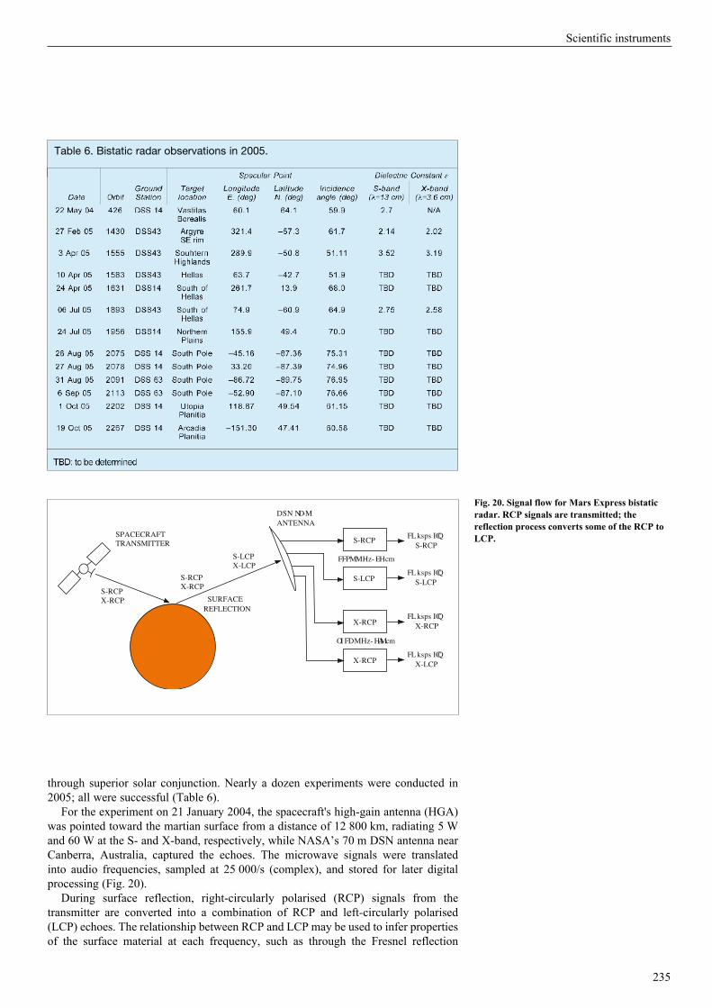
Table 6. Bistatic radar observations in 2005.
through superior solar conjunction. Nearly a dozen experiments were conducted in 2005; all were successful (Table 6).
For the experiment on 21 January 2004, the spacecraft's high-gain antenna (HGA) was pointed toward the martian surface from a distance of 12 800 km, radiating 5 W and 60 W at the S- and X-band, respectively, while NASA’s 70 m DSN antenna near Canberra, Australia, captured the echoes. The microwave signals were translated into audio frequencies, sampled at 25 000/s (complex), and stored for later digital processing (Fig. 20).
During surface reflection, right-circularly polarised (RCP) signals from the transmitter are converted into a combination of RCP and left-circularly polarised (LCP) echoes. The relationship between RCP and LCP may be used to infer properties of the surface material at each frequency, such as through the Fresnel reflection
235
Fig. 20. Signal flow for Mars Express bistatic radar. RCP signals are transmitted; the reflection process converts some of the RCP to LCP.
Scientific instruments
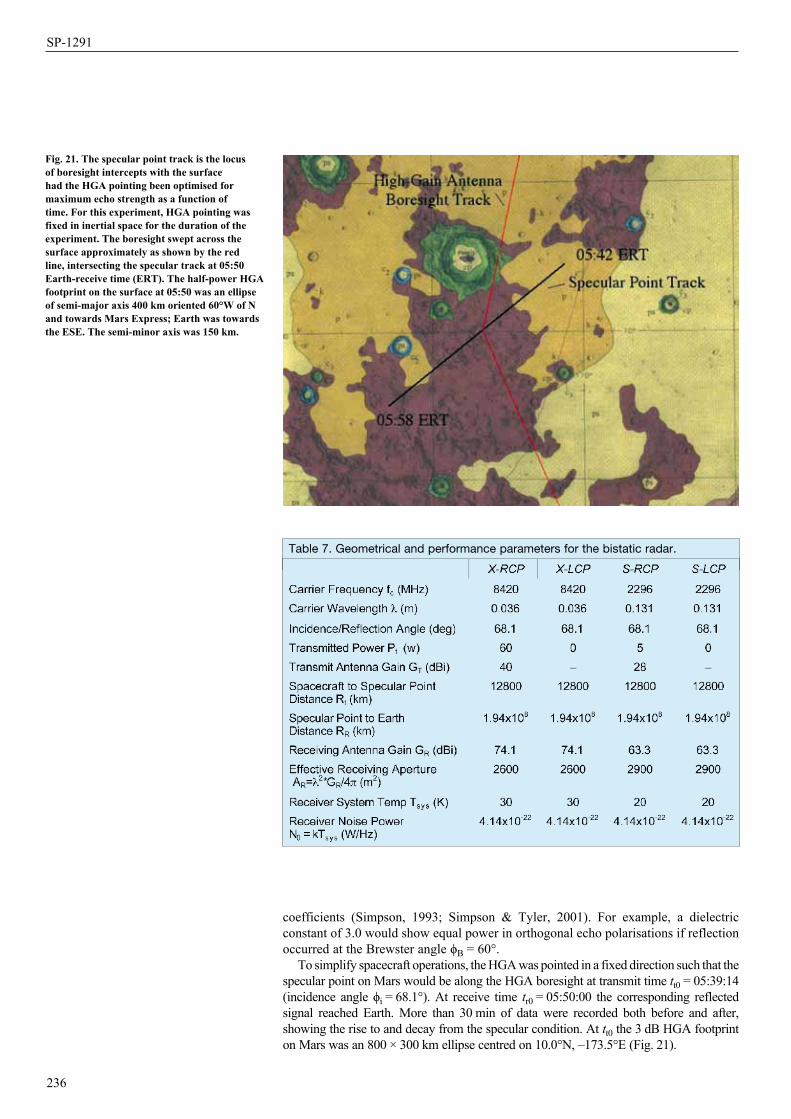
Table 7. Geometrical and performance parameters for the bistatic radar.
coefficients (Simpson, 1993; Simpson & Tyler, 2001). For example, a dielectric constant of 3.0 would show equal power in orthogonal echo polarisations if reflection occurred at the Brewster angle ϕB = 60°.
To simplify spacecraft operations, the HGA was pointed in a fixed direction such that the specular point on Mars would be along the HGA boresight at transmit time tt0 = 05:39:14 (incidence angle ϕi = 68.1°). At receive time tr0 = 05:50:00 the corresponding reflected signal reached Earth. More than 30 min of data were recorded both before and after, showing the rise to and decay from the specular condition. At tt0 the 3 dB HGA footprint on Mars was an 800 × 300 km ellipse centred on 10.0°N, –173.5°E (Fig. 21).
236
Fig. 21. The specular point track is the locus of boresight intercepts with the surface had the HGA pointing been optimised for maximum echo strength as a function of time. For this experiment, HGA pointing was fixed in inertial space for the duration of the experiment. The boresight swept across the surface approximately as shown by the red line, intersecting the specular track at 05:50 Earth-receive time (ERT). The half-power HGA footprint on the surface at 05:50 was an ellipse of semi-major axis 400 km oriented 60°W of N and towards Mars Express; Earth was towards the ESE. The semi-minor axis was 150 km.
SP-1291
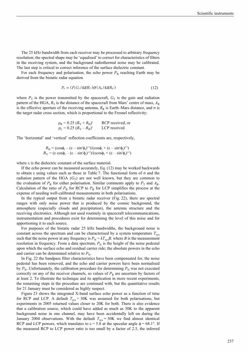
The 25 kHz bandwidth from each receiver may be processed to arbitrary frequency resolution; the spectral shape may be ‘equalised’ to correct for characteristics of filters in the receiving system, and the background radiothermal noise may be calibrated. The last step is critical to correct inference of the surface dielectric constant.
For each frequency and polarisation, the echo power PR reaching Earth may be derived from the bistatic radar equation
(12)
where PT is the power transmitted by the spacecraft, GT is the gain and radiation pattern of the HGA, RT is the distance of the spacecraft from Mars’ centre of mass, AR is the effective aperture of the receiving antenna, RR is Earth–Mars distance, and σ is the target radar cross section, which is proportional to the Fresnel reflectivity:
ρR = 0.25 (RV + RH)2 RCP received, or ρL = 0.25 (RV – RH)2 LCP received
The ‘horizontal’ and ‘vertical’ reflection coefficients are, respectively,
RH = (cosϕi – (ε – sin2ϕi)1/2)/(cosϕi + (ε – sin2ϕi)1/2) RV = (ε cosϕi – (ε – sin2ϕi)1/2)/(εcosϕi + (ε – sin2ϕi)1/2)
where ε is the dielectric constant of the surface material. If the echo power can be measured accurately, Eq. (12) may be worked backwards
to obtain ε using values such as those in Table 7. The functional form of σ and the radiation pattern of the HGA (GT) are not well known, but they are common to the evaluation of PR for either polarisation. Similar comments apply to PT and AR. Calculation of the ratio of PR for RCP to PR for LCP simplifies the process at the expense of needing well-calibrated measurements in both polarisations.
In the typical output from a bistatic radar receiver (Fig. 22), there are spectral ranges with only noise power that is produced by the cosmic background, the atmosphere (especially clouds and precipitation), the antenna structure and the receiving electronics. Although not used routinely in spacecraft telecommunications, instrumentation and procedures exist for determining the level of this noise and for apportioning it to each source.
For purposes of the bistatic radar 25 kHz bandwidths, the background noise is constant across the spectrum and can be characterised by a system temperature Tsys such that the noise power at any frequency is PN = kTsysB, where B is the measurement resolution in frequency. From a data spectrum, PN is the height of the noise pedestal upon which the surface echo and residual carrier ride; the absolute powers in the echo and carrier can be determined relative to PN.
In Fig. 22 the bandpass filter characteristics have been compensated for, the noise pedestal has been removed, and the echo and carrier powers have been normalised by PN. Unfortunately, the calibration procedure for determining PN was not executed correctly on any of the receiver channels, so values of PR are uncertain by factors of at least 2. To illustrate the technique and its application in more recent experiments, the remaining steps in the procedure are continued with, but the quantitative results for 21 January must be considered as highly suspect.
Figure 23 shows the integrated X-band surface echo power as a function of time for RCP and LCP. A default Tsys = 30K was assumed for both polarisations, but experiments in 2005 returned values closer to 20K for both. There is also evidence that a calibration source, which could have added as much as 30K to the apparent background noise in one channel, may have been accidentally left on during the January 2004 observations. With the default Tsys = 30K we find almost identical RCP and LCP powers, which translates to ε = 5.8 at the specular angle ϕ = 68.1°. If the measured RCP to LCP power ratio is too small by a factor of 2.5, the inferred
237
/4 /P P G R A R4R T T T R R2 2r v r= ] ]g g
Scientific instruments
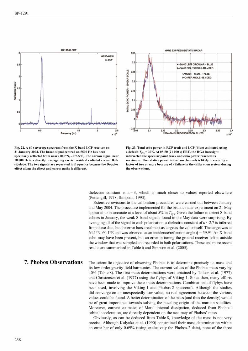
dielectric constant is ε ~ 3, which is much closer to values reported elsewhere (Pettengill, 1978; Simpson, 1993).
Extensive revisions to the calibration procedures were carried out between January and May 2004. The procedure implemented for the bistatic radar experiment on 21 May appeared to be accurate at a level of about 5% in Tsys. Given the failure to detect S-band echoes in January, the weak S-band signals found in the May data were surprising. By averaging all of the signal in each polarisation, a dielectric constant of ε ~ 2.7 is inferred from these data, but the error bars are almost as large as the value itself. The target was at 64.1°N, 60.1°E and was observed at an incidence/reflection angle ϕ = 59.9°. An X-band echo may have been present, but an error in tuning the ground receiver left it outside the window that was sampled and recorded in both polarisations. These and more recent results are summarised in Table 6 and Simpson et al. (2005).
The scientific objective of observing Phobos is to determine precisely its mass and its low-order gravity field harmonics. The current values of the Phobos mass vary by 40% (Table 8). The first mass determinations were obtained by Tolson et al. (1977) and Christensen et al. (1977) using the flybys of Viking-1. Since then, many efforts have been made to improve these mass determinations. Combinations of flybys have been used, involving the Viking-1 and Phobos-2 spacecraft. Although the studies did converge on an unexpectedly low value, no real agreement between the various values could be found. A better determination of the mass (and thus the density) would be of great importance towards solving the puzzling origin of the martian satellites. Moreover, current estimates of Mars’ internal dissipation, deduced from Phobos’ orbital acceleration, are directly dependent on the accuracy of Phobos’ mass.
Obviously, as can be deduced from Table 8, knowledge of the mass is not very precise. Although Kolyuka et al. (1990) constrained their mass determination within an error bar of only 0.69% (using exclusively the Phobos-2 data), none of the three
238
7. Phobos Observations
Fig. 23. Total echo power in RCP (red) and LCP (blue) estimated using a default Tsys = 30K. At 05:50 (21 000 s) ERT, the HGA boresight intersected the specular point track and echo power reached its maximum. The relative power in the two channels is likely in error by a factor of two or more because of a failure in the calibration system during the observations.
Fig. 22. A 60 s average spectrum from the X-band LCP receiver on 21 January 2004. The broad signal centred on 5500 Hz has been specularly reflected from near (10.0°N, –173.5°E); the narrow signal near 18 000 Hz is a directly propagating carrier residual radiated via an HGA sidelobe. The two signals are separated in frequency because the Doppler effect along the direct and carom paths is different.
SP-1291
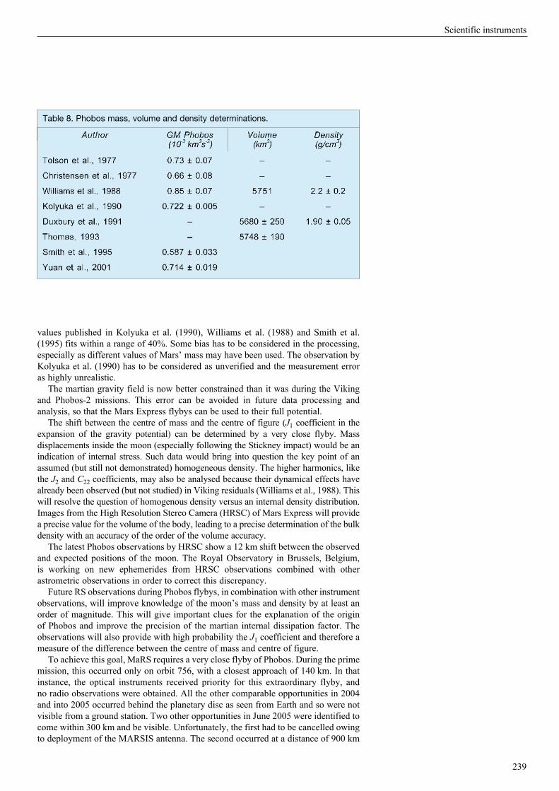
Table 8. Phobos mass, volume and density determinations.
values published in Kolyuka et al. (1990), Williams et al. (1988) and Smith et al. (1995) fits within a range of 40%. Some bias has to be considered in the processing, especially as different values of Mars’ mass may have been used. The observation by Kolyuka et al. (1990) has to be considered as unverified and the measurement error as highly unrealistic.
The martian gravity field is now better constrained than it was during the Viking and Phobos-2 missions. This error can be avoided in future data processing and analysis, so that the Mars Express flybys can be used to their full potential.
The shift between the centre of mass and the centre of figure (J1 coefficient in the expansion of the gravity potential) can be determined by a very close flyby. Mass displacements inside the moon (especially following the Stickney impact) would be an indication of internal stress. Such data would bring into question the key point of an assumed (but still not demonstrated) homogeneous density. The higher harmonics, like the J2 and C22 coefficients, may also be analysed because their dynamical effects have already been observed (but not studied) in Viking residuals (Williams et al., 1988). This will resolve the question of homogenous density versus an internal density distribution. Images from the High Resolution Stereo Camera (HRSC) of Mars Express will provide a precise value for the volume of the body, leading to a precise determination of the bulk density with an accuracy of the order of the volume accuracy.
The latest Phobos observations by HRSC show a 12 km shift between the observed and expected positions of the moon. The Royal Observatory in Brussels, Belgium, is working on new ephemerides from HRSC observations combined with other astrometric observations in order to correct this discrepancy.
Future RS observations during Phobos flybys, in combination with other instrument observations, will improve knowledge of the moon’s mass and density by at least an order of magnitude. This will give important clues for the explanation of the origin of Phobos and improve the precision of the martian internal dissipation factor. The observations will also provide with high probability the J1 coefficient and therefore a measure of the difference between the centre of mass and centre of figure.
To achieve this goal, MaRS requires a very close flyby of Phobos. During the prime mission, this occurred only on orbit 756, with a closest approach of 140 km. In that instance, the optical instruments received priority for this extraordinary flyby, and no radio observations were obtained. All the other comparable opportunities in 2004 and into 2005 occurred behind the planetary disc as seen from Earth and so were not visible from a ground station. Two other opportunities in June 2005 were identified to come within 300 km and be visible. Unfortunately, the first had to be cancelled owing to deployment of the MARSIS antenna. The second occurred at a distance of 900 km
239
Scientific instruments
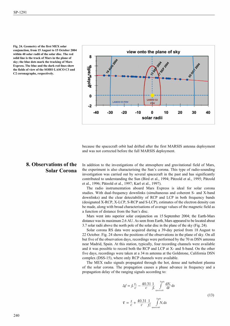
because the spacecraft orbit had drifted after the first MARSIS antenna deployment and was not corrected before the full MARSIS deployment.
In addition to the investigations of the atmosphere and gravitational field of Mars, the experiment is also characterising the Sun’s corona. This type of radio-sounding investigation was carried out by several spacecraft in the past and has significantly contributed to understanding the Sun (Bird et al., 1994; Pätzold et al., 1995; Pätzold et al., 1996; Pätzold et al., 1997; Karl et al., 1997).
The radio instrumentation aboard Mars Express is ideal for solar corona studies. With dual-frequency downlinks (simultaneous and coherent S- and X-band downlinks) and the clear detectability of RCP and LCP in both frequency bands (designated X-RCP, X-LCP, S-RCP and S-LCP), estimates of the electron density can be made, along with broad characterisations of average values of the magnetic field as a function of distance from the Sun’s disc.
Mars went into superior solar conjunction on 15 September 2004; the Earth-Mars distance was its maximum 2.6 AU. As seen from Earth, Mars appeared to be located about 3.7 solar radii above the north pole of the solar disc in the plane of the sky (Fig. 24).
Solar corona RS data were acquired during a 39-day period from 18 August to 22 October. Fig. 24 shows the positions of the observations in the plane of sky. On all but five of the observation days, recordings were performed by the 70 m DSN antenna near Madrid, Spain. At this station, typically, four recording channels were available and it was possible to record both the RCP and LCP at X- and S-band. On the other five days, recordings were taken at a 34 m antenna at the Goldstone, California DSN complex (DSS-15), where only RCP channels were available.
The MEX radio signals propagated through the hot, dense and turbulent plasma of the solar corona. The propagation causes a phase advance in frequency and a propagation delay of the ranging signals according to:
(13)
240
Fig. 24. Geometry of the first MEX solar conjunction, from 15 August to 15 October 2004 within 40 solar radii of the solar disc. The red solid line is the track of Mars in the plane of sky; the blue dots mark the tracking of Mars Express. The blue and the dark red lines show the fields of view of the SOHO LASCO C3 and C2 coronagraphs, respectively.
8. Observations of theSolar Corona
.dd d
. d
f fcv
c f tN s
cs
c fN s
40 31 1
40 31 1
pacecraft
Earth
spacecraft
Earth
r e
s
e
00
02
T =
= +x
- #
#
SP-1291

where Δf is the recorded Doppler shift consisting of the classical Doppler shift (first term) and the propagation in plasma (second term), t is the propagation time of the radio signal between the spacecraft and the ground station consisting of the vacuum light time (first term) and the propagation delay in plasma (second term), and Ne is the electron density in the solar corona, dNe/dt is the temporal change of electron density at time scales of the integrated sampling time, f0 is the radio carrier frequency, vr is the relative velocity between the receiver on Earth and the spacecraft transmitter, and s is the distance (range) between the ground station and the spacecraft.
By using two frequencies, e.g. X-band and S-band, simultaneously and forming the differential Doppler and differential range, the contribution of the plasma to the one-way downlink at the lower frequency is yielded, here at S-band
(14)
From the Ulysses superior solar conjunctions in 1991 and 1995 (Bird et al., 1994; Pätzold et al., 1995) and the experiences gained in these experiments, MaRS defined the solar conjunction phase within a range of 40 solar radii (10° elongation) about the solar disc in the plane of sky. Mars entered this range on 15 August and exited on 15 October 2004.
MaRS requested one tracking pass per day with the spacecraft transponder and ground station configured as S-band uplink, X-band and S-band simultaneous downlink; dual-frequency ranging where feasible (DSN only). Although the first passes in August were conducted at S-band uplink, ESOC switched back to X-band uplink for operational reasons after a few passes. The total number of passes was 34 (instead of the 60 projected), each of a few hours but sometimes only 20 min. They were performed exclusively by the DSN, with the majority at the 70 m station DSS-63 in Madrid. The recording bandwidth in DSN’s open-loop RS Receiver was 2 kHz, allowing capture of signal dynamics not modelled in the frequency predictions and signal broadening resulting from propagation through the solar corona.
Spacecraft signal parameters sensitive to changes in the propagation medium include frequency Doppler shift, ranging, bandwidth, amplitude/phase scintillations and Faraday rotation (Bird, 1982). The MEX 2004 solar corona experiment data will be processed in full to examine all these effects.
Figure 25 shows six SOHO LASCO C3 images centred about solar conjunction. The varying coronal structure with streamers and holes is prominent. The position of Mars is a faint spot indicated by arrows in the first and last two images. Mars entered and left the field of view of the LASCO C2 images (6 solar radii) on 11 September and 19 September, respectively. Figure 26 shows the four LASCO C2 images, which correspond to the four observations within 6 solar radii.
The change in electron content as a function of solar offset also clearly shows the sounding of coronal streamer and coronal hole structures (Fig. 27). From the SOHO images it can be seen that the position of Mars in the field of view coincided with streamer structures at distances between 20 and 10 solar radii during ingress. While passing over the northern pole within 10 solar radii, less plasma was found and the electron content decreased. This can be followed in Figs. 25 and 26. During superior conjunction, polar rays must have been sounded because the electron content increased again, only to drop again when another coronal hole was encountered (Fig. 26, lower row).
It is concluded from the signature in the differential Doppler and the electron content time series on 21 September 2004 that a coronal mass ejection (CME) may
241
.dd d
. d
f fc f f
ftN s
c f fN s
113 40 31 1 1
40 31 1 1
spacecraft
Earth
spacecraft
Earth
s x
s x
se
s x
s x
e
2 2
2 2
T T =
=x x
- - -
- -
'
'
1
1
#
#
Scientific instruments

have intersected the radio ray path. Unfortunately, no LASCO images were available for a period of 62 h from 20 September to 23 September to cover that event.
The CME signature is easily extracted from the X-band and S-band residuals and the differential Doppler (Fig. 28). A fast-moving plasma shock front crossing both uplink and downlink can be identified:
— in the downlinks because both frequencies are affected;— in the differential Doppler representing the downlink at S-band;— on the uplink at X-band and a time Dt later again on the X-band downlink
repeating the signal;— not on the S-band downlink after Dt seconds because the uplink frequency is
downconverted by a factor of 240/749.
The integration of the differential Doppler yields the change in electron content along the ray path since the start of the measurement. A strong increase in electron content by 8000 hexem can be seen for the duration of the signature at X-band starting at 1600 s (Fig. 28); this is in comparison to typical changes in electron content in the solar corona by a few hundred hexems.
With these data it is possible to study the morphologies of CMEs in the microwave bands, to determine the position where a CME hits the ray path, its speed and the density of the shock front. These studies continue.
The Mars Express Radio Science Experiment has shown that the spacecraft is an efficient and sensitive tool for gravity studies, atmospheric/ionospheric/coronal sounding and bistatic radar. The experiment has achieved outstanding results and made important discoveries despite operational constraints and pointing conflicts. Atmospheric and ionospheric sounding can be done at locations and local times on Mars that are inaccessible to MGS, thereby complementing the numerous MGS observations. The gravity signal is a factor of four stronger during MEX pericentre
242
9. Outlook for the Extended Mission
Fig. 26. LASCO C2 coronagraph images (FOV 6 solar radii) from 11–18 September, the four days when Mars Express was tracked within 6 solar radii. The location of Mars is indicated by arrows.
Fig. 25. LASCO C3 coronagraph images (FOV 30 solar radii) showing the coronal structure for the days noted. Mars is marked by arrows. On 13 and 17 September, Mars was behind the inner C3 cover that masks the solar disc. The bright spot in these images is Venus.
SP-1291

passes than for MGS. Bistatic radar observations were performed on a regular basis during 2005 and all show strong return echo signals.
The ambitious goals of the MaRS experiment, however, could not be met during the prime mission. This was firstly due to the power situation during eclipses, which resulted in a large number of lost occultations, and, secondly, to the pointing conflicts with the imaging instruments for pericentre gravity observations. The loss of all feasible Phobos observations due to these pointing conflicts was very disappointing.
The mission is in its second extension at the time of this publication, encompassing more occultation seasons and one solar conjunction in 2006. Gravity studies and bistatic radar experiments are being planned as individual events, hopefully at a higher rate than during the prime mission, although constraints and conflicts still remain.
Angelats i Coll, M., Fotget, F., Lopez-Valverde, M.A. & González-Galindo, F. (2005). The First Mars Thermospheric General Circulation Model: The Martian Atmosphere from the Ground to 240 km. Geophys. Res. Lett. 32(4), CiteID L04201.
Bauer, S.J. & Hantsch, M.H. (1989). Solar Cycle Variations of the Upper Atmosphere of Mars. Geophys. Res. Lett. 16, 373-376.
Bird, M.K. (1982). Coronal Investigations with Occulted Spacecraft Signals. Space Sci. Rev. 33, 99-126.
Bird, M.K., Volland, H., Pätzold, M., Edenhofer, P., Asmar, S.W. & Brenkle, J.P. (1994). The Coronal Electron Density Distribution Determined from Dual-Frequency Ranging Measurements during the 1991 Solar Conjunction of the Ulysses Spacecraft. Astrophys. J. 426, 373-381.
Beuthe, M., Rosenblatt, P., Dehant, V., Pätzold, M., Haeusler, B., Karatekin, O., Le Maistre, S., Van Hoolst, T. & Barriot, J.-P. (2005) Assessment of the Martian Global Gravity Field at Short Wavelength with Mars Express; Submitted for publication.
243
References
Fig. 28. X-band and S-band residuals (the two upper panels) from DOY 265, 2004 show the signature of a CME crossing the radio ray path. The lower panel is the change in electron content. A rapid rise in electron content starts with the high density shock front of the CME engulfing the ray path. After the passage of the front, the electron content decreases to normal values.
Fig. 27. Change in electron content from dual-frequency Doppler as a function of solar offset. The red circles are the average change in electron content; the error bar marks the maximal variation during the tracking pass. A CME and possibly a second show extreme values.
Scientific instruments

Christensen, E.J., Born, G.H., Hildebrand, C.E. & Williams, B.G. (1977). The Mass of PHOBOS from Viking Flybys. Geophys. Res. Lett. 4, 555-557.
DSMS Telecommunications Link Design Handbook 202 (2000). 34-m and 70-m Doppler, 810-005, Rev. E, 30 November 2000.
Fjeldbo, G. (1964). Bistatic Radar Methods for Studying Planetary Ionospheres and Surfaces. SU-SEL-64-025, Stanford Electronics Laboratory, Stanford University, USA.
Fjeldbo, G. & Eshleman, V.R. (1968). The Atmosphere of Mars Analyzed by Integral Inversion of the Mariner IV Occultation Data. Planet. Space Sci. 16, 1035-1059.
Häusler, B., Eidel, W., Hagl, D., Remus, S., Selle, J. & Pätzold, M. (2003a).Venus Express Radio Science Experiment VeRa, Reference Systems and Techniques Used for the Simulation and Prediction of Atmospheric and Ionospheric Sounding Measurements at Planet Venus. VEX-VERA-UBW-TN-3040, I2.5, 23.07.2004, also Forschungsbericht LRT-WE-9-FB-4, Universität der Bundeswehr München, Germany.
Häusler, B., Remus, S., Hagl, D. & Selle, J. (2003b). MaRS Experiment System Test Summary Report for FM Transponder, MEX-MRS-UBW-TR-4000, 07.03.2003b, Universität der Bundeswehr München, Germany.
Hanson, W.B., Sanatani, S. & Zuccaro, D.R. (1977). The Martian Ionosphere as Observed by the Viking Retarding Potential Analyzers. J. Geophys. Res. 82, 4351-4363.
Hinson, D.P., Simpson, R.A., Twicken, J.D., Tyler, G.L. & Flasar, F.M. (1999). Initial Results from Radio Occultation Measurements with Mars Global Surveyor. J. Geophys. Res. 104(E11), 29997-27012.
Karl, J., M. Pätzold & M.K. Bird (1997). Coronal Radio Sounding: Non-Gaussian Turbulence in the Source Regions of the Solar Wind. Geophys. Res. Lett. 24, 2881-2884.
Kolyuka, Y.F., Efimov, A.E., Kudryavtsev, S.M., Margorin, O.K., Tarasov, V.P. & Tikhonov, V.F. (1990). Refinement of the Gravitational Constant of Phobos from Phobos-2 Tracking Data. Soviet Astr. Lett. 16, 168-170.
Kopp, E. (1997). On the Abundance of Metal Ions in the Lower Ionosphere. J. Geophys. Res. 102(A5), 9667-9674.
Lemoine, F.G., Smith, D.E., Rowlands, D.D., Zuber, M.T., Neumann, G.A., Chinn, D.S. & Pavlis, D.E. (2001). An Improved Solution of the Gravity Field of Mars (GMM-2B) from Mars Global Surveyor. J. Geophys. Res. 106(E10), 23359-23376.
Lipa, B. & Tyler, G.L. (1979). Statistical and Computational Uncertainties in Atmospheric Profiles from Radio Occultation – Mariner 10 at Venus. Icarus 39, 192.
Molina-Cuberos, G.J., Witasse, O., Lebreton, J.-P., Rodrigo, R. & Lopez-Moreno, J.J. (2003). Meteoric Ions in the Atmosphere of Mars. Planet. Space Sci. 51, 239-249.
Pätzold, M., Karl, J. & Bird, M.K. (1996). Coronal Sounding with Ulysses: Phase Scintillation Spectra in Coronal Holes and Streamers. Astron. Astrophys. 316, 449-456.
Pätzold, M., Tsurutani, B.T. & Bird, M.K. (1997). An Estimate of Large-Scale Solar Wind Density and Velocity Profiles in a Coronal Hole and the Coronal Streamer Belt. J. Geophys. Res. 102, 24151-24160.
Pätzold, M., Neubauer, F.M., Carone, L., Hagermann, A., Stanzel, C., Häusler, B., Remus, S., Selle, J., Hagl, D., Hinson, D.P., Simpson, R.A., Tyler, G.L., Asmar, S.W., Axford, W.I., Hagfors, T., Barriot, J.-P., Cerisier, J.-C., Imamura, T., Oyama, K.-I., Janle, P., Kirchengast, G. & Dehant, V. (2004). MaRS: Mars Express Orbiter Radio Science. In Mars Express: The Scientific Payload (Ed. A. Wilson), ESA SP-1240, ESA Publications Division, ESTEC, Noordwijk, The Netherlands.
Pätzold, M., Tellmann, S., Häusler, B., Hinson, D., Schaa, R. & Tyler, G.L. (2005). A Sporadic and Local Third Layer in the Ionosphere of Mars. Science; in Press.
Pettengill, G.H. (1978). Physical Properties of the Planets and Satellites from Radar Observations. Ann. Revs. Astron. & Astrophys. 16, 265-292.
Remus, S., Häusler, B., Pätzold, M. & Wennmacher, A. (2001). Ergebnisse der Radio Science Testmessungen an den ESA Satelliten Rosetta und Mars Express. Deutscher Luft- und Raumfahrtkongress, DGLR-2001-022, 17-20 September, 2001.
Rishbeth, H. & Mendillo, M. (2003). Ionospheric Layers of Mars and Earth. Planet. Space Sci. 52, 849-832.
244
SP-1291
Scientific instruments
245
SGICD (2003). Mars Express Spacecraft/Ground Interface Document, ME-ESC-IF-5001, I 4.4, May 2003, ESA/ESOC.
Simpson, R.A. (1993). Spacecraft Studies of Planetary Surfaces using Bistatic Radar. IEEE Trans. Geosci. & Remote Sensing 31, 465-482.
Simpson, R.A. & Tyler, G.L. (2001). Mars Global Surveyor Bistatic Radar Probing of the MPL/DS2 Target Area. Icarus 152, 70-74.
Simpson, R.A., Tyler, G.L., Pätzold, M. & Häusler, B. (2005). Determination of Local Surface Properties using Mars Express Bistatic Radar. J. Geophys. Res.; submitted 2005.
Smith, D.E., Lemoine, F.G. & Zuber, M.T. (1995). Simultaneous Estimation of the Masses of Mars, Phobos, and Deimos using Spacecraft Distant Encounters. Geophys. Res. Lett. 22, 2171-2174.
Tolson, R.H., Blackshear, W.T., Mason, M.L. & Kelly, G.M. (1977). The Mass of Phobos. Geophys. Res. Lett. 4, 551-554.
Wang, J.-S. & Nielsen, E. (2003). Wavelike Structures in the Martian Topside Ionosphere observed by Mars Global Surveyor. J. Geophys. Res. 108(E7), 14-1, CiteID 5078, DOI 10.1029/2003JE002078.
Williams, B.G., Duxbury, T.C. & Hildebrand, C.E. (1988). Improved Determination of PHOBOS and Deimos Masses from Viking Fly-Bys. LPI Abstracts 19, 1274-1274.
Woo, R. & Armstrong, J.W. (1979). Spacecraft Radio Scattering Observations of the Power Spectrum of Electron Density Fluctuations in the Solar Wind. J. Geophys. Res. 84(A12), 7288-7296.
Yuan, D.-N., Sjogren, W.L., Konopliv, A.S. & Kucinskas, A.B. (2001). Gravity field of Mars: A 75th Degree and Order Model. J. Geophys. Res. 106(E10), 23377-23401.
Yuen, J.H. (1983). Deep Space Telecommunications System Engineering. Plenum Press, New York and London.
Zhang, M.H.G, Luhmann, J.G. & Kliore, A.J. (1990). An Observational Study of the Night Side Ionosphere of Mars and Venus with Radio Occultation Methods. J. Geophys. Res. 95, 17095-17102.


OperatiOns and archiving

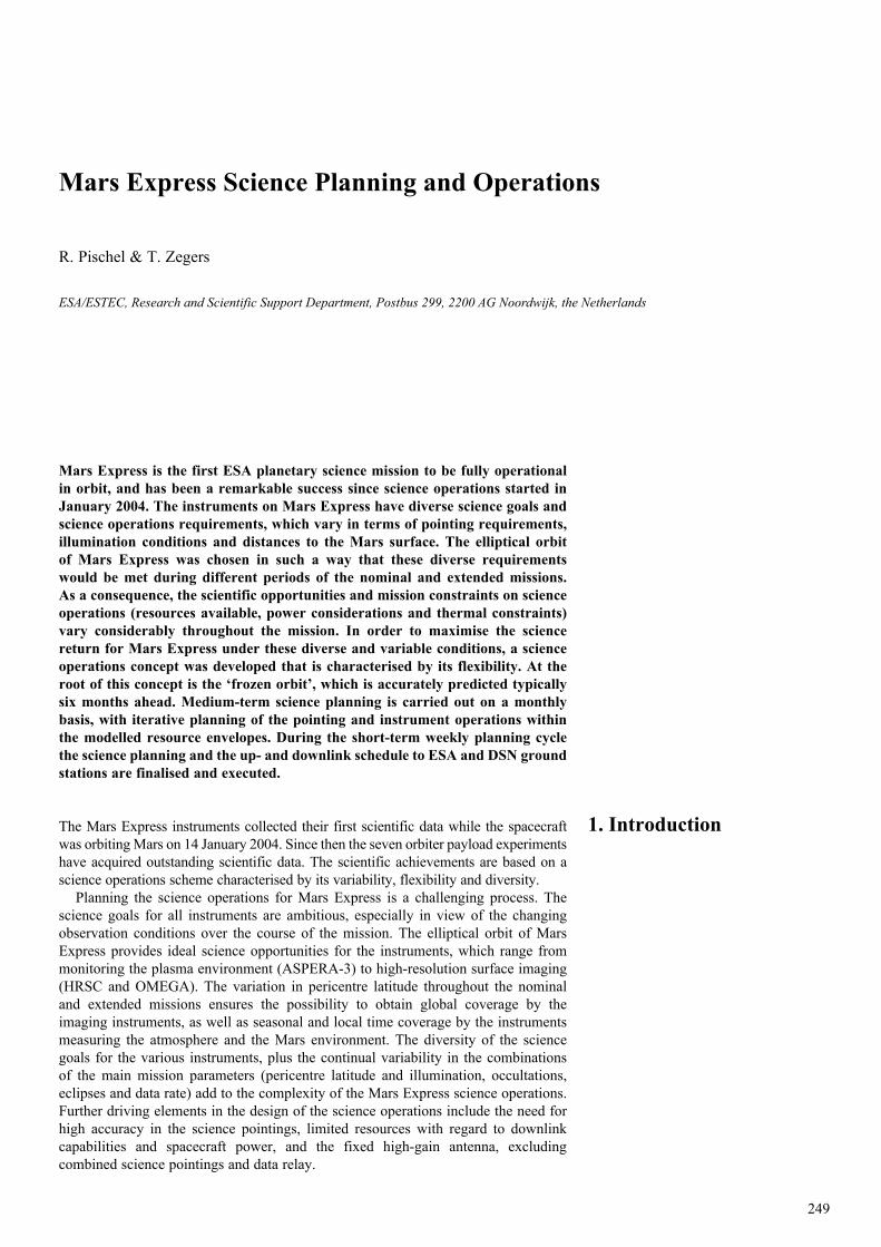
249
R. Pischel & T. Zegers
Mars express science planning and Operations
ESA/ESTEC, Research and Scientific Support Department, Postbus 299, 2200 AG Noordwijk, the Netherlands
249
Mars express is the first esa planetary science mission to be fully operational in orbit, and has been a remarkable success since science operations started in January 2004. the instruments on Mars express have diverse science goals and science operations requirements, which vary in terms of pointing requirements, illumination conditions and distances to the Mars surface. the elliptical orbit of Mars express was chosen in such a way that these diverse requirements would be met during different periods of the nominal and extended missions. as a consequence, the scientific opportunities and mission constraints on science operations (resources available, power considerations and thermal constraints) vary considerably throughout the mission. in order to maximise the science return for Mars express under these diverse and variable conditions, a science operations concept was developed that is characterised by its flexibility. at the root of this concept is the ‘frozen orbit’, which is accurately predicted typically six months ahead. Medium-term science planning is carried out on a monthly basis, with iterative planning of the pointing and instrument operations within the modelled resource envelopes. during the short-term weekly planning cycle the science planning and the up- and downlink schedule to esa and dsn ground stations are finalised and executed.
The Mars Express instruments collected their first scientific data while the spacecraft was orbiting Mars on 14 January 2004. Since then the seven orbiter payload experiments have acquired outstanding scientific data. The scientific achievements are based on a science operations scheme characterised by its variability, flexibility and diversity.
Planning the science operations for Mars Express is a challenging process. The science goals for all instruments are ambitious, especially in view of the changing observation conditions over the course of the mission. The elliptical orbit of Mars Express provides ideal science opportunities for the instruments, which range from monitoring the plasma environment (ASPERA-3) to high-resolution surface imaging (HRSC and OMEGA). The variation in pericentre latitude throughout the nominal and extended missions ensures the possibility to obtain global coverage by the imaging instruments, as well as seasonal and local time coverage by the instruments measuring the atmosphere and the Mars environment. The diversity of the science goals for the various instruments, plus the continual variability in the combinations of the main mission parameters (pericentre latitude and illumination, occultations, eclipses and data rate) add to the complexity of the Mars Express science operations. Further driving elements in the design of the science operations include the need for high accuracy in the science pointings, limited resources with regard to downlink capabilities and spacecraft power, and the fixed high-gain antenna, excluding combined science pointings and data relay.
1. introduction
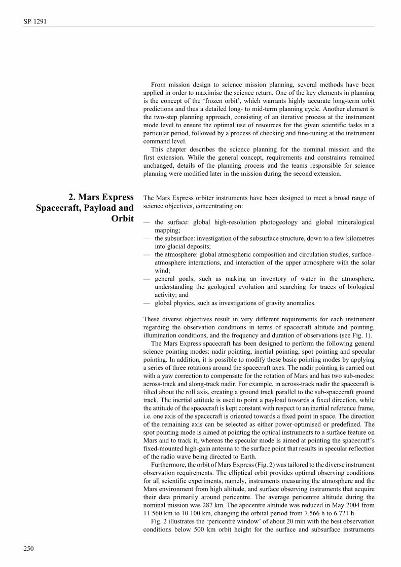
250
SP-1291
From mission design to science mission planning, several methods have been applied in order to maximise the science return. One of the key elements in planning is the concept of the ‘frozen orbit’, which warrants highly accurate long-term orbit predictions and thus a detailed long- to mid-term planning cycle. Another element is the two-step planning approach, consisting of an iterative process at the instrument mode level to ensure the optimal use of resources for the given scientific tasks in a particular period, followed by a process of checking and fine-tuning at the instrument command level.
This chapter describes the science planning for the nominal mission and the first extension. While the general concept, requirements and constraints remained unchanged, details of the planning process and the teams responsible for science planning were modified later in the mission during the second extension.
The Mars Express orbiter instruments have been designed to meet a broad range of science objectives, concentrating on:
— the surface: global high-resolution photogeology and global mineralogical mapping;
— the subsurface: investigation of the subsurface structure, down to a few kilometres into glacial deposits;
— the atmosphere: global atmospheric composition and circulation studies, surface–atmosphere interactions, and interaction of the upper atmosphere with the solar wind;
— general goals, such as making an inventory of water in the atmosphere, understanding the geological evolution and searching for traces of biological activity; and
— global physics, such as investigations of gravity anomalies.
These diverse objectives result in very different requirements for each instrument regarding the observation conditions in terms of spacecraft altitude and pointing, illumination conditions, and the frequency and duration of observations (see Fig. 1).
The Mars Express spacecraft has been designed to perform the following general science pointing modes: nadir pointing, inertial pointing, spot pointing and specular pointing. In addition, it is possible to modify these basic pointing modes by applying a series of three rotations around the spacecraft axes. The nadir pointing is carried out with a yaw correction to compensate for the rotation of Mars and has two sub-modes: across-track and along-track nadir. For example, in across-track nadir the spacecraft is tilted about the roll axis, creating a ground track parallel to the sub-spacecraft ground track. The inertial attitude is used to point a payload towards a fixed direction, while the attitude of the spacecraft is kept constant with respect to an inertial reference frame, i.e. one axis of the spacecraft is oriented towards a fixed point in space. The direction of the remaining axis can be selected as either power-optimised or predefined. The spot pointing mode is aimed at pointing the optical instruments to a surface feature on Mars and to track it, whereas the specular mode is aimed at pointing the spacecraft’s fixed-mounted high-gain antenna to the surface point that results in specular reflection of the radio wave being directed to Earth.
Furthermore, the orbit of Mars Express (Fig. 2) was tailored to the diverse instrument observation requirements. The elliptical orbit provides optimal observing conditions for all scientific experiments, namely, instruments measuring the atmosphere and the Mars environment from high altitude, and surface observing instruments that acquire their data primarily around pericentre. The average pericentre altitude during the nominal mission was 287 km. The apocentre altitude was reduced in May 2004 from 11 560 km to 10 100 km, changing the orbital period from 7.566 h to 6.721 h.
Fig. 2 illustrates the ‘pericentre window’ of about 20 min with the best observation conditions below 500 km orbit height for the surface and subsurface instruments
2. Mars express spacecraft, payload and
Orbit
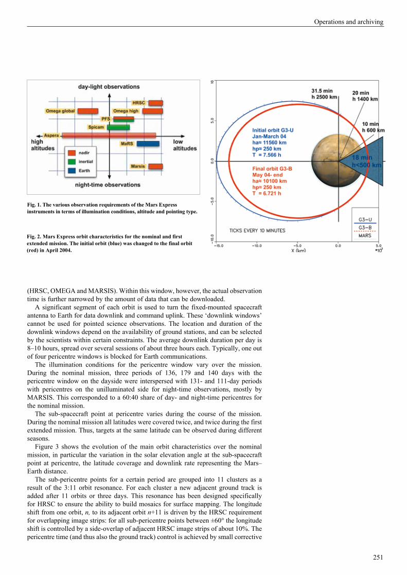
251
Operations and archiving
(HRSC, OMEGA and MARSIS). Within this window, however, the actual observation time is further narrowed by the amount of data that can be downloaded.
A significant segment of each orbit is used to turn the fixed-mounted spacecraft antenna to Earth for data downlink and command uplink. These ‘downlink windows’ cannot be used for pointed science observations. The location and duration of the downlink windows depend on the availability of ground stations, and can be selected by the scientists within certain constraints. The average downlink duration per day is 8–10 hours, spread over several sessions of about three hours each. Typically, one out of four pericentre windows is blocked for Earth communications.
The illumination conditions for the pericentre window vary over the mission. During the nominal mission, three periods of 136, 179 and 140 days with the pericentre window on the dayside were interspersed with 131- and 111-day periods with pericentres on the unilluminated side for night-time observations, mostly by MARSIS. This corresponded to a 60:40 share of day- and night-time pericentres for the nominal mission.
The sub-spacecraft point at pericentre varies during the course of the mission. During the nominal mission all latitudes were covered twice, and twice during the first extended mission. Thus, targets at the same latitude can be observed during different seasons.
Figure 3 shows the evolution of the main orbit characteristics over the nominal mission, in particular the variation in the solar elevation angle at the sub-spacecraft point at pericentre, the latitude coverage and downlink rate representing the Mars–Earth distance.
The sub-pericentre points for a certain period are grouped into 11 clusters as a result of the 3:11 orbit resonance. For each cluster a new adjacent ground track is added after 11 orbits or three days. This resonance has been designed specifically for HRSC to ensure the ability to build mosaics for surface mapping. The longitude shift from one orbit, n, to its adjacent orbit n+11 is driven by the HRSC requirement for overlapping image strips: for all sub-pericentre points between ±60° the longitude shift is controlled by a side-overlap of adjacent HRSC image strips of about 10%. The pericentre time (and thus also the ground track) control is achieved by small corrective
Fig. 1. the various observation requirements of the Mars express instruments in terms of illumination conditions, altitude and pointing type.
Fig. 2. Mars express orbit characteristics for the nominal and first extended mission. the initial orbit (blue) was changed to the final orbit (red) in april 2004.
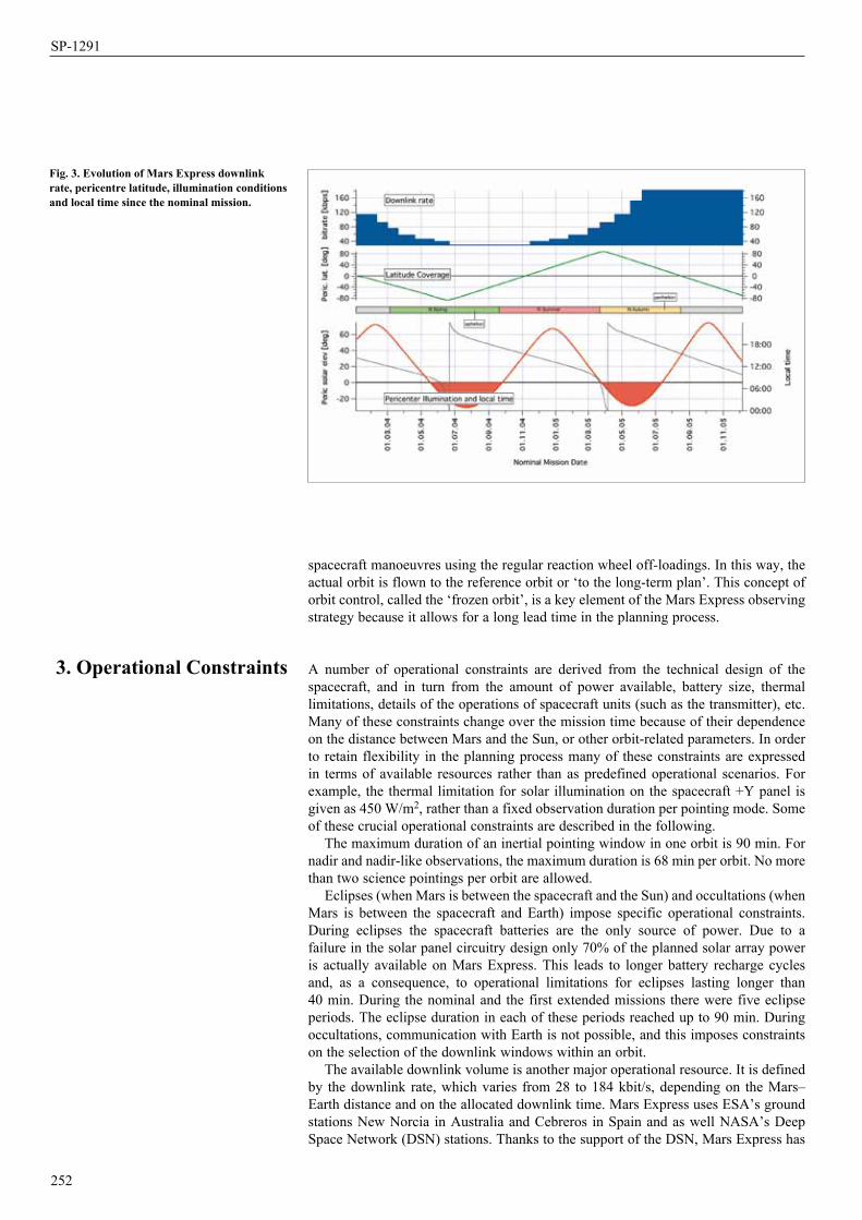
252
SP-1291
spacecraft manoeuvres using the regular reaction wheel off-loadings. In this way, the actual orbit is flown to the reference orbit or ‘to the long-term plan’. This concept of orbit control, called the ‘frozen orbit’, is a key element of the Mars Express observing strategy because it allows for a long lead time in the planning process.
A number of operational constraints are derived from the technical design of the spacecraft, and in turn from the amount of power available, battery size, thermal limitations, details of the operations of spacecraft units (such as the transmitter), etc. Many of these constraints change over the mission time because of their dependence on the distance between Mars and the Sun, or other orbit-related parameters. In order to retain flexibility in the planning process many of these constraints are expressed in terms of available resources rather than as predefined operational scenarios. For example, the thermal limitation for solar illumination on the spacecraft +Y panel is given as 450 W/m2, rather than a fixed observation duration per pointing mode. Some of these crucial operational constraints are described in the following.
The maximum duration of an inertial pointing window in one orbit is 90 min. For nadir and nadir-like observations, the maximum duration is 68 min per orbit. No more than two science pointings per orbit are allowed.
Eclipses (when Mars is between the spacecraft and the Sun) and occultations (when Mars is between the spacecraft and Earth) impose specific operational constraints. During eclipses the spacecraft batteries are the only source of power. Due to a failure in the solar panel circuitry design only 70% of the planned solar array power is actually available on Mars Express. This leads to longer battery recharge cycles and, as a consequence, to operational limitations for eclipses lasting longer than 40 min. During the nominal and the first extended missions there were five eclipse periods. The eclipse duration in each of these periods reached up to 90 min. During occultations, communication with Earth is not possible, and this imposes constraints on the selection of the downlink windows within an orbit.
The available downlink volume is another major operational resource. It is defined by the downlink rate, which varies from 28 to 184 kbit/s, depending on the Mars– Earth distance and on the allocated downlink time. Mars Express uses ESA’s ground stations New Norcia in Australia and Cebreros in Spain and as well NASA’s Deep Space Network (DSN) stations. Thanks to the support of the DSN, Mars Express has
3. Operational constraints
Fig. 3. evolution of Mars express downlink rate, pericentre latitude, illumination conditions and local time since the nominal mission.
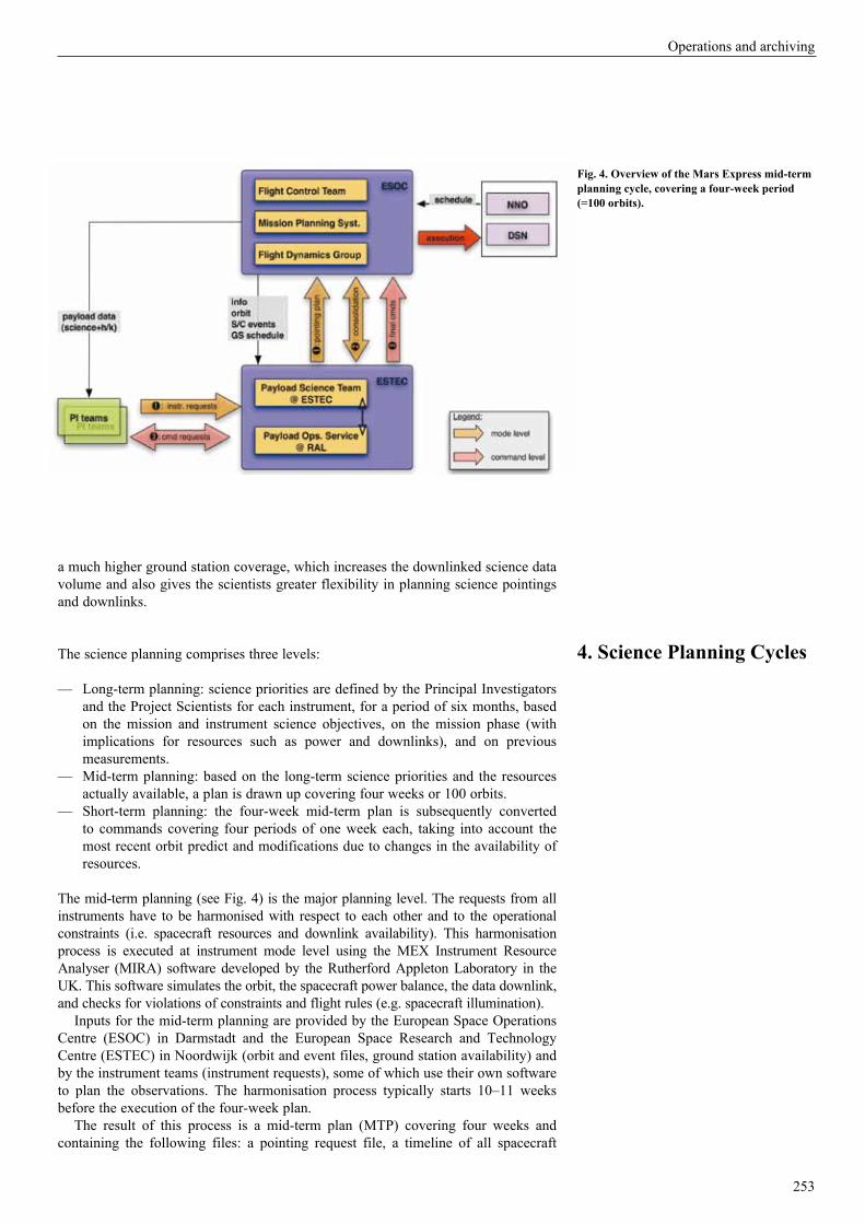
253
Operations and archiving
a much higher ground station coverage, which increases the downlinked science data volume and also gives the scientists greater flexibility in planning science pointings and downlinks.
The science planning comprises three levels:
— Long-term planning: science priorities are defined by the Principal Investigators and the Project Scientists for each instrument, for a period of six months, based on the mission and instrument science objectives, on the mission phase (with implications for resources such as power and downlinks), and on previous measurements.
— Mid-term planning: based on the long-term science priorities and the resources actually available, a plan is drawn up covering four weeks or 100 orbits.
— Short-term planning: the four-week mid-term plan is subsequently converted to commands covering four periods of one week each, taking into account the most recent orbit predict and modifications due to changes in the availability of resources.
The mid-term planning (see Fig. 4) is the major planning level. The requests from all instruments have to be harmonised with respect to each other and to the operational constraints (i.e. spacecraft resources and downlink availability). This harmonisation process is executed at instrument mode level using the MEX Instrument Resource Analyser (MIRA) software developed by the Rutherford Appleton Laboratory in the UK. This software simulates the orbit, the spacecraft power balance, the data downlink, and checks for violations of constraints and flight rules (e.g. spacecraft illumination).
Inputs for the mid-term planning are provided by the European Space Operations Centre (ESOC) in Darmstadt and the European Space Research and Technology Centre (ESTEC) in Noordwijk (orbit and event files, ground station availability) and by the instrument teams (instrument requests), some of which use their own software to plan the observations. The harmonisation process typically starts 10–11 weeks before the execution of the four-week plan.
The result of this process is a mid-term plan (MTP) covering four weeks and containing the following files: a pointing request file, a timeline of all spacecraft
4. science planning cycles
Fig. 4. Overview of the Mars express mid-term planning cycle, covering a four-week period (=100 orbits).

254
SP-1291
pointings, and a timeline of instrument requests at the mode level. This output is delivered to ESOC eight weeks before the execution of the four-week plan. ESOC checks the plan with more detailed models and implements changes if necessary. The mid-term plan is finally frozen four weeks before execution.
The updated and finally frozen mode level instrument plans are semi-automatically converted into instrument commands. This task is split up into four command periods of one week each. The instrument command file is generated by the Rutherford Appleton Laboratory in a feedback loop with the instrument teams so that they can confirm the final command files. Once confirmed, the instrument command files (covering one week) are sent to ESOC ten days before execution. ESOC integrates the payload and spacecraft commands. Up to this moment all instrument requests at mode and command levels were relative to pericentre. During the last processing steps ESOC converts these relative times to absolute times using the most recent orbit predict, which is typically 2–3 days ‘old’. The final combined command files are uploaded to the spacecraft 2–3 days before execution, and are then carried out in accordance with the time-tagged timeline. The process is depicted in Fig. 4.
In the period between its first full orbit around Mars on 4 January 2004 and 31 December 2006, the Mars Express spacecraft orbited the Red Planet 3832 times, with 3–4 orbits per day. Of these orbits, about 60% were used for science observations, 25% for communications, and 15% for specific spacecraft needs (commissioning, eclipses, conjunction, etc.).
During this period, 34 mid-term and four-week cycles were successfully planned. The mid-term planning concept proved to be effective and gave the instrument teams a very high level of control and flexibility in using spacecraft and ground station resources. The major resources such as the pericentre window time and the available downlink time were used close to 100%. In addition, new science pointing modes have been implemented that were not foreseen at the beginning of the mission, such as spot pointing, specular pointing, and the combination of more than one cross-pointing angle in a nadir pointing window. The original flight baseline has been expanded by controlling resources rather than using predefined scenarios. The problem of the 70% power has been fully incorporated into the mid-term planning process.
The Mars Express spacecraft has shown excellent performance that has partly exceeded the numbers originally specified:
— the orbit position of the spacecraft can be measured with an average accuracy of better than 200 m;
— the average difference between the position predicted one week in advance and the real position is 2 km, where the main component of the error is along the orbit trajectory and corresponds to about 0.5–1 s; and
— the attitude of the spacecraft is known to an accuracy of 0.01°.
In addition to the ‘nominal’ science plan, a number of special observations and activities have been conducted. These included observations of Phobos and Deimos and of the shadow of Phobos on the surface of Mars, communication tests and joint observations with NASA’s Mars Exploration Rovers Opportunity and Spirit, and the deployment of the MARSIS antenna after a year of routine operations.
During these 3800 orbits about 2300 Gbit of raw (for some instruments compressed) science data were acquired. These data were analysed by the instrument teams and can be accessed by the public via the ESA Planetary Science Archive. Since the arrival of Mars Express at Mars in December 2003, the instrument teams and their associated science teams have published more than 200 papers.
ESA approved the first Mars Express mission extension for a second Mars year until October 2007. The main science objectives were to accomplish the remaining global coverage, to achieve the original MARSIS science goals, to study periodic time
5. experiences and results
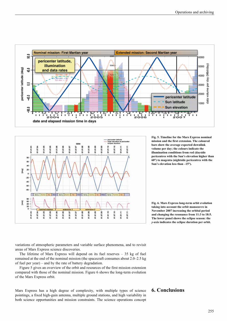
255
Operations and archiving
variations of atmospheric parameters and variable surface phenomena, and to revisit areas of Mars Express science discoveries.
The lifetime of Mars Express will depend on its fuel reserves – 35 kg of fuel remained at the end of the nominal mission (the spacecraft consumes about 2.0–2.5 kg of fuel per year) – and by the rate of battery degradation.
Figure 5 gives an overview of the orbit and resources of the first mission extension compared with those of the nominal mission. Figure 6 shows the long-term evolution of the Mars Express orbit.
Mars Express has a high degree of complexity, with multiple types of science pointings, a fixed high-gain antenna, multiple ground stations, and high variability in both science opportunities and mission constraints. The science operations concept
Fig. 5. timeline for the Mars express nominal mission and the first extension. the coloured bars show the average expected downlink volume per day; the colours indicate the illumination conditions from red (dayside pericentres with the sun’s elevation higher than 60°) to magenta (nightside pericentres with the sun’s elevation less than –15°).
Fig. 6. Mars express long-term orbit evolution taking into account the orbit manoeuvre in november 2007 increasing the orbital period and changing the resonance from 11:3 to 18:5. the lower panel shows the eclipse season: the y-axis indicates the eclipse duration per orbit.
6. conclusions

256
SP-1291
and practice for Mars Express have evolved into a highly flexible system. The flexibility is driven by the diverse science requirements and science opportunities (specific ground targets) of the instruments, and the high variability in the conditions (e.g. illumination) and the resource envelope (e.g. energy, data rate).
The excellent science return of Mars Express is the end result of close collaboration and interaction between the various teams (seven Principal Investigator teams, ESA science operations and operations teams, Rutherford Appleton Laboratories), all of whom aim to make the best possible scientific use of the Mars Express spacecraft.

257
J. Zender1, F. Delhaise2, C. Arviset3, D. Heather1, J. Diaz del Rio3, N. Manaud3, J. Vazquez Garcia3, J. Hernandez3, I. Ortiz3, J. Dowson3, S. Jeffers4, T. Roatsch5, K-D. Matz5, G. Poulleau6, Y. Langevin6, B. Gondet6, A. Reberac12, J.F. Daloze12, E. Dimarellis12, L. Carone7, C. Stanzel7, M. D’Amore8, R. Orosei9, R. Noschese10, M. Cartacci10, S. Giuppi10, R. Huff11, R. Johnson11, C. Acton13, B. Semenov13, E. Guinness14 & S. Slavney14
Spacecraft and Payload Data Handling
1 Research and Scientific Support Department, ESA/ESTEC, Noordwijk, the Netherlands Email: [email protected] Ground Systems Engineering Department, ESA/ESOC, Darmstadt, Germany3 Science Operations Department, ESA/ESAC, Villafranca del Castillo, Madrid, Spain4 Southwest Research Institute, San Antonio, TX 728-0510, USA5 German Aerospace Center (DLR), Rutherfordstrasse 2, D-12489 Berlin, Germany6 Institut d’Astrophysique Spatiale (IAS), Bâtiment 121, F-91405 Orsay Campus, France7 Rheinisches Institut für Umweltforschung an der Universität zu Köln, Abteilung Planetenforschung, D-50931 Cologne, Germany8 Istituto di Fisica dello Spazio Interplanetario CNR (IFSI), Via del Fosso del Cavaliere 100, I-00133 Rome, Italy9 Istituto di Astrofisica Spaziale e Fisica Cosmica (IASF), Istituto Nazionale di Astrofisica (INAF), Via del Fosso del Cavaliere 100,
I-00133 Rome, Italy10 Infocom Department, ‘La Sapienza’ University of Rome, Via Eudossiana 18, I-00184 Rome, Italy11 Department of Physics and Astronomy, University of Iowa, Iowa City, IA 52242-1447, USA12 Service d’Aéronomie (SA) du CNRS/IPSL, BP 3, F-91371, Verrières-le-Buisson, France13 Jet Propulsion Laboratory, 4800 Oak Grove Drive, Pasadena, CA 91109, USA14 Washington University, Department of Earth and Planetary Sciences, St Louis, MO 63130-4899, USA
257
The success of a scientific mission is determined by the quality of the scientific results. The prompt delivery of instrument and ancillary raw data to the instrument teams and of reduced and calibrated data to the scientific community is therefore a key element in the mission design. This chapter describes the flow of data from the spacecraft through the ground segment via the instrument teams to the final scientific archive. Several software tools and standards are used to support data dissemination. The functionality of the individual tools is explained, the interfaces to the individual groups are discussed, and examples of the graphical user interfaces are shown. Finally, the chapter provides a brief introduction to each of the currently available datasets.
A large number of teams and individuals are involved in processing data from the byte packages on the Mars Express (MEX) spacecraft, to provide scientifically useful, reviewed datasets to the scientific communities. Although the various teams have different responsibilities, all of them aim to deliver complete, accurate sets of information. The information dealt with is diverse, covering, for example:
— spacecraft and instrument documentation;— ancillary data such as spacecraft event information, instrument mounting
alignments;
1. Introduction
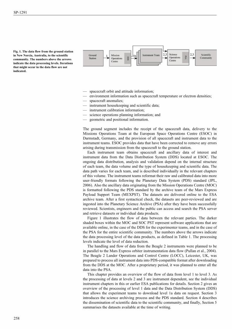
258
SP-1291
— spacecraft orbit and attitude information;— environment information such as spacecraft temperature or electron densities;— spacecraft anomalies;— instrument housekeeping and scientific data;— instrument calibration information;— science operations planning information; and— geometric and positional information.
The ground segment includes the receipt of the spacecraft data, delivery to the Missions Operations Team at the European Space Operations Centre (ESOC) in Darmstadt, Germany, and the provision of all spacecraft and instrument data to the instrument teams. ESOC provides data that have been corrected to remove any errors arising during transmission from the spacecraft to the ground station.
Each instrument team obtains spacecraft and ancillary data of interest and instrument data from the Data Distribution System (DDS) located at ESOC. The ongoing data distribution, analysis and validation depend on the internal structure of each team, the data volume and the type of housekeeping and scientific data. The data path varies for each team, and is described individually in the relevant chapters of this volume. The instrument teams reformat their raw and calibrated data into more user-friendly formats following the Planetary Data System (PDS) standard (JPL, 2006). Also the ancillary data originating from the Mission Operations Centre (MOC) is formatted following the PDS standard by the archive team of the Mars Express Payload Support Team (MEXPST). The datasets are delivered online to the ESA archive team. After a first syntactical check, the datasets are peer-reviewed and are ingested into the Planetary Science Archive (PSA) after they have been successfully reviewed. Scientists, engineers and the public can access and search the PSA server and retrieve datasets or individual data products.
Figure 1 illustrates the flow of data between the relevant parties. The darker shaded boxes within the MOC and SOC PST represent software applications that are available online, in the case of the DDS for the experimenter teams, and in the case of the PSA for the entire scientific community. The numbers above the arrows indicate the data processing level of the data products, as defined in Table 1. The processing levels indicate the level of data reduction.
The handling and flow of data from the Beagle 2 instruments were planned to be in parallel to the Mars Express orbiter instrumentation data flow (Pullan et al., 2004). The Beagle 2 Lander Operations and Control Centre (LOCC), Leicester, UK, was prepared to process all instrument data into PDS-compatible format after downloading from the DDS at the MOC. After a proprietary period, it was planned to enter all the data into the PSA.
This chapter provides an overview of the flow of data from level 1 to level 3. As the processing of data at levels 2 and 3 are instrument dependent, see the individual instrument chapters in this or earlier ESA publications for details. Section 2 gives an overview of the processing of level 1 data and the Data Distribution System (DDS) that allows the experiment teams to download level 1a data on request. Section 3 introduces the science archiving process and the PDS standard. Section 4 describes the dissemination of scientific data to the scientific community, and finally, Section 5 summarises the datasets available at the time of writing.
Fig. 1. The data flow from the ground station in New Norcia, Australia, to the scientific community. The numbers above the arrows indicate the data processing levels. Iterations that might occur in the data flow are not indicated.
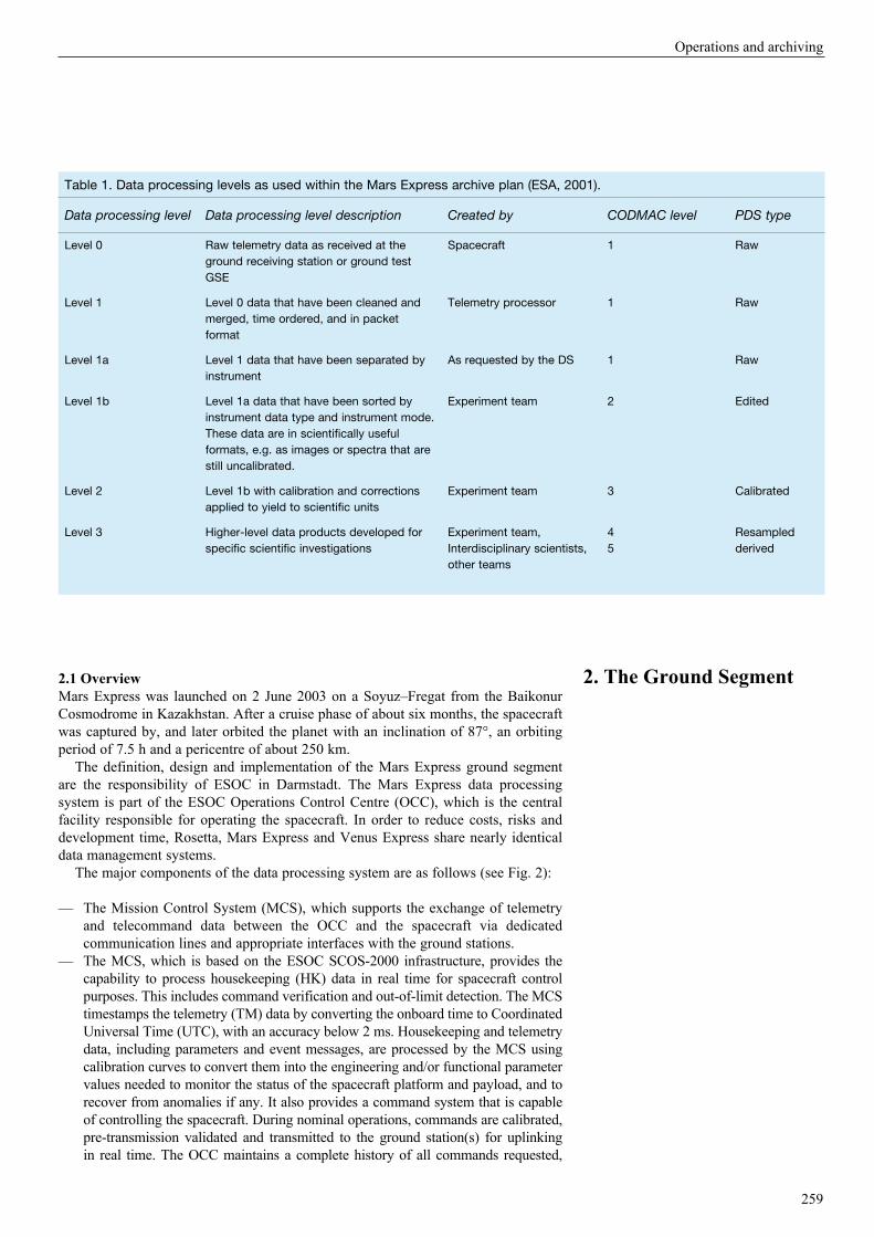
259
Operations and archiving
2.1 OverviewMars Express was launched on 2 June 2003 on a Soyuz–Fregat from the Baikonur Cosmodrome in Kazakhstan. After a cruise phase of about six months, the spacecraft was captured by, and later orbited the planet with an inclination of 87°, an orbiting period of 7.5 h and a pericentre of about 250 km.
The definition, design and implementation of the Mars Express ground segment are the responsibility of ESOC in Darmstadt. The Mars Express data processing system is part of the ESOC Operations Control Centre (OCC), which is the central facility responsible for operating the spacecraft. In order to reduce costs, risks and development time, Rosetta, Mars Express and Venus Express share nearly identical data management systems.
The major components of the data processing system are as follows (see Fig. 2):
— The Mission Control System (MCS), which supports the exchange of telemetry and telecommand data between the OCC and the spacecraft via dedicated communication lines and appropriate interfaces with the ground stations.
— The MCS, which is based on the ESOC SCOS-2000 infrastructure, provides the capability to process housekeeping (HK) data in real time for spacecraft control purposes. This includes command verification and out-of-limit detection. The MCS timestamps the telemetry (TM) data by converting the onboard time to Coordinated Universal Time (UTC), with an accuracy below 2 ms. Housekeeping and telemetry data, including parameters and event messages, are processed by the MCS using calibration curves to convert them into the engineering and/or functional parameter values needed to monitor the status of the spacecraft platform and payload, and to recover from anomalies if any. It also provides a command system that is capable of controlling the spacecraft. During nominal operations, commands are calibrated, pre-transmission validated and transmitted to the ground station(s) for uplinking in real time. The OCC maintains a complete history of all commands requested,
Table 1. Data processing levels as used within the Mars Express archive plan (ESA, 2001).
Data processing level Data processing level description Created by CODMAC level PDS type
Level 0 Raw telemetry data as received at the ground receiving station or ground test GSE
Spacecraft 1 Raw
Level 1 Level 0 data that have been cleaned and merged, time ordered, and in packet format
Telemetry processor 1 Raw
Level 1a Level 1 data that have been separated by instrument
As requested by the DS 1 Raw
Level 1b Level 1a data that have been sorted by instrument data type and instrument mode. These data are in scientifically useful formats, e.g. as images or spectra that are still uncalibrated.
Experiment team 2 Edited
Level 2 Level 1b with calibration and corrections applied to yield to scientific units
Experiment team 3 Calibrated
Level 3 Higher-level data products developed for specific scientific investigations
Experiment team, Interdisciplinary scientists, other teams
45
Resampled derived
2. The Ground Segment

260
SP-1291
transmitted and verified. The MCS also has facilities for managing the operational database and for maintaining the onboard software.
— The Data Distribution System (DDS) is based on the Generic Data Disposition System (GDDS), and allows remote access by the scientific community for the near-real-time and/or offline inspection of mission data. The system also provides facilities for the regular daily production of raw data media (RDM) for the permanent archiving of raw telemetry and auxiliary data. For Mars Express the DDS will be used to store instrument telemetry data on recordable compact discs (CD-Rs), which are sent to authorised members of the Mars Express scientific community. The DDS system is described in more detail below.
— The Mission Planning System (MPS) is an offline system that provides tools for the advance planning of the mission operations, based on inputs from the Principal Investigators, the Science Operations Centre (SOC) and the operations staff at ESOC. The final outputs of this system take the form of machine-readable schedules for commanding the spacecraft and the two ground stations. Unlike other data system components, the MPS is mission-specific.
— The Flight Operations Procedure (FOP) system is used by the Mission Operations Team to prepare spacecraft operational procedures and command sequences, which can then be imported into the operational database.
2.2 Collection of Telemetry DataThe Mission Control System interfaces with the ground stations to receive and transmit telemetry (TM) and telecommand (TC) data in a controlled and error-free manner. A no-break data link connection is always established when the ground station is in real-time contact with the spacecraft.
The Mars Express MCS receives the telemetry data from the ground stations via a generic infrastructure system called the Network Controller and Telemetry Receiver System (NCTRS), which serves as the ground station interface with the MCS.
The NCTRS receives the telemetry data as delivered by the ground station equipment, which has already performed some basic checks and has ‘time stamped’ it with Earth Reception Time (ERT). It then passes the housekeeping and science telemetry data to the relevant MCS for more specific processing and for archiving. The NCTRS gathers all the telecommands sent from the MCS and forwards them to the relevant ground station.
The NCTRS is also used for acquiring and locally storing tracking data such as antenna angles, range and Doppler measurements made at the ground station. These are then made available to the Flight Dynamics System via the File Transfer System (FTS) and to authorised Principal Investigators (PIs) via the DDS system.
The files generated by the OCC, such as antenna pointing information and ground station schedule files, are also transferred via the NCTRS to the ground station.
Fig. 2. The Mars Express Operations Control Centre (OCC).

261
Operations and archiving
2.3 Dissemination of Raw Data The Mars Express OCC offers telemetry, both housekeeping and scientific data, and auxiliary data in near-real-time and/or offline mode to the PIs. Following receipt or generation at the OCC, the data can be accessed from remote computers on a call-up basis.
Mission products include payload science data, all platform and payload housekeeping data and auxiliary data (e.g. TC history, station visibility, spacecraft orbital position, attitude, etc.; DDID, 2002). HK and science TM data (both real-time and playback) are extracted and stored as raw data, which are chronologically ordered and sorted by spacecraft and payload. They include quality data and additional timing data so that the PIs are able to correlate the data with respect to UTC.
In addition, the science data, housekeeping data and consolidated auxiliary data are transferred onto CD-ROMs, which are mailed to each PI on a weekly basis. A common data interchange standard based on the Standard Formatted Data Unit (SFDU) concept is used in order to allow for efficient data distribution.
Finally, the OCC archives all Mars Express level 1 data for all payloads for a period of ten years after the end of the mission. Archived data include all raw telemetry and auxiliary data.
The MCS is on the operational LAN and can be accessed by operational staff at ESOC (i.e. there is no remote access). External access to mission data is via the DDS, which allows a secure connection between the outside world (such as the Mars Express PIs) and the ESOC-protected operational LAN.
2.3.1 Dissemination of Mission Raw Data via the Mars Express DDSThe DDS is based on the Generic Data Disposition System (GDDS, 2002). It enables PIs and other external users to submit requests for data to be extracted from the mission archives supported by the SCOS-2000 spacecraft control system kernel. These requests are expressed in a format based on XML (extended mark-up language; Thompson et al., 2001). Figure 3 provides an overview of the GDDS.
The Mission Control System, based on SCOS-2000, maintains a mission archive comprising two main elements: a packet archive containing historical telemetry, telecommand and derived data, and a file archive that typically includes flight dynamics and planning data. A file generation process within SCOS-2000 can also be invoked to generate file-based summary data from packet data, e.g. command history reports.
Fig. 3. Generic Data Disposition System (GDDS) architecture.

262
SP-1291
Requests for data to be extracted from the mission archive may originate in three ways:
— scheduled ‘standing orders’;— submission via a web-based interface; or— request files sent using the File Transmission Protocol (FTP).
All requests comprise a list of items to be retrieved, and are expressed in a recursive query language defined in XML, which is used internally within the system, and also exposed to the user on the FTP interface. This allows multiple filters to be applied to the data being retrieved. The requested data can be from three sources: telemetry, auxiliary and catalogue data.
These requests are managed by a central DDS server, which interfaces with the MCS to initiate archive retrievals via a Common Object Request Broker Architecture (CORBA) based interface. Archive retrievals performed on the MCS interface are relatively low level, and several individual retrievals may be performed to satisfy a single request. The GDDS server maintains a request list, and collates the retrieved data for a single delivery in response to each request.
Requests must be identified as originating from a previously authorised external user. The DDS maintains a database of these authorised users, together with address information for the delivery of retrieved data.
Three methods of archive data delivery are supported: online via a web-based interface; via an FTP server; and on CD-ROM (only available for Mars Express PIs, and following agreed recording and distribution schemes).
The DDS web-based user interface is designed to allow authorised users to view the catalogue of data held in the mission archive, and to generate and submit retrieval requests, for delivery using the FTP server or online. Figure 4 shows a screenshot of a data request.
Fig. 4. Sample screenshot from the GDDS web interface.

263
Operations and archiving
All responses from the DDS server to the web-based interface are also transferred as XML files. These may include request acknowledgements, catalogue data and online data retrieval.
Online data retrieval is only available in response to a request originating from the web-based interface, and is designed for previewing small amounts of data only. This enables a user to verify that it is the required data, before requesting a full FTP transfer. The data are embedded as a byte stream in the XML response.
3.1 OverviewFollowing the success of the visits of the Giotto spacecraft to the comets P/Halley and P/Grigg–Skjellerup (during its extended mission), Rosetta, Mars Express and SMART-1 are ESA’s next planetary missions. All the data from the International Halley Watch campaign – including the Giotto data – have been archived using NASA’s Planetary Data System (PDS) standard. The PDS is the de facto standard for most US planetary missions. It was therefore decided early in the mission development to use the PDS standard for Rosetta, Mars Express and SMART-1.
To ensure maximum commonality, ESA has introduced the Planetary Science Archive (www.rssd.esa.int/PSA) for all planetary missions. The PSA is the official interface of all engineering, housekeeping and scientific data for the scientific community after the experimenters’ proprietary period has come to an end. All necessary services are offered to the scientific community via an online interface.
The initial requirements, system tests and further development of the PSA are basically driven by the PSA Scientific Advisory Group, a mission-independent group representing a range of instrument categories and disciplines within the European scientific community.
This section describes the PDS standard and the PSA system and gives an outline of the planned archive process.
3.2 The Planetary Data System (PDS) StandardThe PDS standard is a set of guidelines published in the PDS Data Standards Reference (JPL, 2006). The guidelines cover the archive process as well as details of predefined data types, an object description language, a data dictionary, rules on labelling data products, catalogue templates and the organisation of logical or physical volumes. The PDS standard is compliant with the reference model of the Open Archival Information System (OAIS; CCSDS, 1999).
As a general rule, each data product must be labelled and linked to a data file. The label is either attached to the data file itself or detached in a separate file, called a label file. Documents are classified as products and a label is required. Each self-contained unity, called a dataset, must contain a default set of documentation in ASCII format, referred to as catalogue files. Figure 5 sketches the parts of the standard, and indicates the hierarchical structure of the standard.
The glue for all data products is the standard grammar, the object description language (ODL). The ODL requires that all metadata be given as a keyword = value pair. For example,is a valid description of the spacecraft name. The keywords on the left side of the
3. Scientific Processing and Data Archive Preparation
INSTRUMENT_HOST_NAME = MARS_EXPRESS
pair must be defined in the Planetary Science Data Dictionary (PSDD; JPL, 2002). A lookup for the keyword instrument_host_name results in

264
SP-1291
The basic elements of the archive are of course the data products. The standard foresees a small number of simple, predefined data types for these products, but also allows the definition of user-defined structures or combined structures. Bearing in mind that one of the purposes of the archive is the long-term preservation of the data, the reduced number of available data types can seen as an advantage, as it enhances the simplicity of the data in the long term. Data producers are forced to design easy data types and structures, which in turn simplify access to data products. These data types include matrix, image, spectrum, table and histogram, to name just a few.
The standard description foresees a label for each data product. This label contains keyword = value pairs that describe the data type, structure and any another meta-
Fig. 5. Hierarchy of the Planetary Data System (PDS) standard.
NAME = INSTRUMENT_HOST_NAME STATUS_TYPE = APPROVED GENERAL_DATA_TYPE = CHARACTER UNIT_ID = NONE STANDARD_VALUE_TYPE = STATIC MAXIMUM_LENGTH = 60 DESCRIPTION = “ The instrument_host_name element provides the full name of the host on which an instrument is based. This host can be either a spacecraft or an earth base. Thus, the instrument_host_name element can contain values which are either spacecraft_name values or earth_base_name values.” STANDARD_VALUE_SET = { “ROSETTA”, “ROSETTA LANDER”, “MARS EXPRESS”, “BEAGLE 2”, “SMART 1”, “2001 MARS ODYSSEY”, “24-COLOR SURVEY”, “AMES MARS GENERAL CIRCULATION MODEL”, “ARECIBO OBSERVATORY”, “CLEMENTINE 1”, …. }
Stds

265
Operations and archiving
information necessary to access the data and to interpret it. The following block shows an excerpt from the OMEGA data product label:
The PDS standard also requires a set of catalogue files. A catalogue file is a label file that contains textual information in ASCII format for at least:
— dataset description (dataset catalogue file);— spacecraft description (instrument_host catalogue file);— instrument description (instrument catalogue file);— mission description (mission catalogue file);— references (reference catalogue file);— personnel information (personnel catalogue file);— dataset collection description (dataset collection catalogue file, optional); and— target information (target catalogue file, optional).
In addition, the standard requires a well defined directory structure. All catalogue files, for example, need to be accessible from a directory named CATALOG. The top-level directory must contain a file named VOLDESC.CAT that describes the whole archive volume. The next block gives an example of a typical VOLDESC.CAT file:
PRODUCT_ID = “ORB1879_2_DATA”PRODUCT_TYPE = EDRSTANDARD_DATA_PRODUCT_ID = “OMEGA DATA”PI_PDS_USER_ID = BIBRINGMISSION_NAME = “MARS EXPRESS”MISSION_PHASE_NAME = “MR Phase 6”INSTRUMENT_NAME = “Observatoire Mineralogie, Eau, Glaces, Activite”PRODUCER_INSTITUTION_NAME = “IAS”INSTRUMENT_ID = OMEGAINSTRUMENT_TYPE = “IMAGING SPECTROMETER”^INSTRUMENT_DESC = “OMEGA_DESC.TXT”^INSTRUMENT_CALIBRATION_DESC = “OMEGA_CALIBRATION_DESC.TXT” DATA_QUALITY_ID = 3DATA_QUALITY_DESC = “ from 0 to 3 depending on missing lines and compression errors” MISSING_SCAN_LINES = 0CHANNEL_ID = (IRC,IRL,VIS)SOFTWARE_VERSION_ID = “OMEGA 4.5”TARGET_NAME = MARSORBIT_NUMBER = 1879 PRODUCT_CREATION_TIME = 2005-09-14T23:57:13.000START_TIME = 2005-07-02T20:41:36.043STOP_TIME = 2005-07-02T20:51:38.091SPACECRAFT_CLOCK_START_COUNT = “68351355.13762”SPACECRAFT_CLOCK_STOP_COUNT = “68351957.00685” MAXIMUM_LATITUDE = -54.238MINIMUM_LATITUDE = -70.102EASTERNMOST_LONGITUDE = 184.354WESTERNMOST_LONGITUDE = 161.580SLANT_DISTANCE = 2526.525
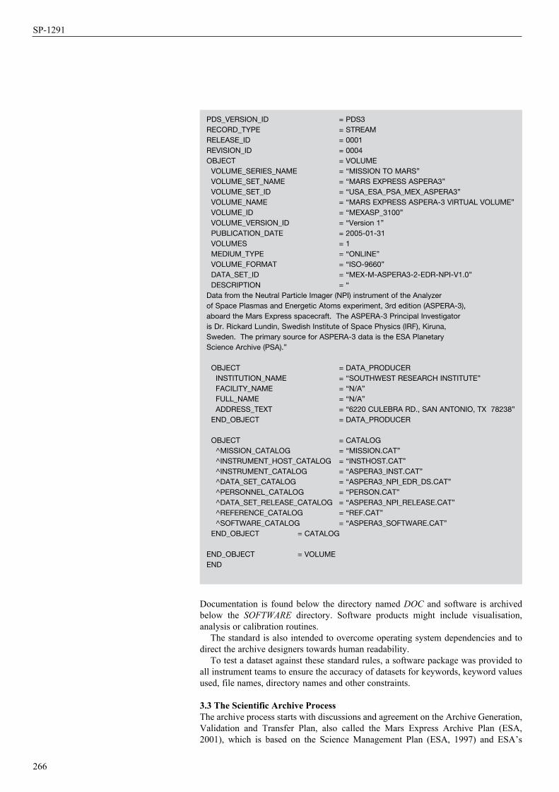
266
SP-1291
Documentation is found below the directory named DOC and software is archived below the SOFTWARE directory. Software products might include visualisation, analysis or calibration routines.
The standard is also intended to overcome operating system dependencies and to direct the archive designers towards human readability.
To test a dataset against these standard rules, a software package was provided to all instrument teams to ensure the accuracy of datasets for keywords, keyword values used, file names, directory names and other constraints.
3.3 The Scientific Archive ProcessThe archive process starts with discussions and agreement on the Archive Generation, Validation and Transfer Plan, also called the Mars Express Archive Plan (ESA, 2001), which is based on the Science Management Plan (ESA, 1997) and ESA’s
PDS_VERSION_ID = PDS3RECORD_TYPE = STREAMRELEASE_ID = 0001REVISION_ID = 0004OBJECT = VOLUME VOLUME_SERIES_NAME = “MISSION TO MARS” VOLUME_SET_NAME = “MARS EXPRESS ASPERA3” VOLUME_SET_ID = “USA_ESA_PSA_MEX_ASPERA3” VOLUME_NAME = “MARS EXPRESS ASPERA-3 VIRTUAL VOLUME” VOLUME_ID = “MEXASP_3100” VOLUME_VERSION_ID = “Version 1” PUBLICATION_DATE = 2005-01-31 VOLUMES = 1 MEDIUM_TYPE = “ONLINE” VOLUME_FORMAT = “ISO-9660” DATA_SET_ID = “MEX-M-ASPERA3-2-EDR-NPI-V1.0” DESCRIPTION = “ Data from the Neutral Particle Imager (NPI) instrument of the Analyzer of Space Plasmas and Energetic Atoms experiment, 3rd edition (ASPERA-3),aboard the Mars Express spacecraft. The ASPERA-3 Principal Investigatoris Dr. Rickard Lundin, Swedish Institute of Space Physics (IRF), Kiruna,Sweden. The primary source for ASPERA-3 data is the ESA PlanetaryScience Archive (PSA).”
OBJECT = DATA_PRODUCER INSTITUTION_NAME = “SOUTHWEST RESEARCH INSTITUTE” FACILITY_NAME = “N/A” FULL_NAME = “N/A” ADDRESS_TEXT = “6220 CULEBRA RD., SAN ANTONIO, TX 78238” END_OBJECT = DATA_PRODUCER
OBJECT = CATALOG ^MISSION_CATALOG = “MISSION.CAT” ^INSTRUMENT_HOST_CATALOG = “INSTHOST.CAT” ^INSTRUMENT_CATALOG = “ASPERA3_INST.CAT” ^DATA_SET_CATALOG = “ASPERA3_NPI_EDR_DS.CAT” ^PERSONNEL_CATALOG = “PERSON.CAT” ^DATA_SET_RELEASE_CATALOG = “ASPERA3_NPI_RELEASE.CAT” ^REFERENCE_CATALOG = “REF.CAT” ^SOFTWARE_CATALOG = “ASPERA3_SOFTWARE.CAT” END_OBJECT = CATALOG
END_OBJECT = VOLUMEEND

267
Operations and archiving
general archiving rules (ESA Council, 1989). The Archive Plan gives the scope of the scientific data archive in relation to the overall mission, and summarises the mission, experiments and groups involved in the archiving efforts. It lists the datasets that are produced by each team, together with contact information for the team members.
Within the Mars Express mission, the experimenters are responsible for the design and implementation of the scientific datasets. The initial version of the Mars Express Archive Plan, which contained a first draft of the data types and the expected data volume, was prepared by ESA’s archive team and was issued one year before launch.
As the PDS standard gives enough information for the experimenter teams to start preparing their archive design, the ESA archive team acts as a consultant for the experimenters. Each experimenter team defines its archive design in the Experimenter to Archive Interface Control Document (EAICD), which contains full details of the archive’s directory structure, the data types and the label keywords used. The EAICDs were issued soon after launch and updated when required.
Throughout the entire process of data preparation and archiving, members of the Data Archive Working Group (DAWG) hold regular meetings and teleconferences to discuss issues of common interest and to keep each other informed on the progress in design and implementation.
The volume of the scientific archive of Mars Express was originally estimated to be of the order of 1 terabyte (TB;109 bytes) for the nominal mission phase, but this has already grown to 2.5 TB.
Electronic data handling is the aim, for the ingestion of data from the experimenter teams into the PSA, and the delivery of data from the PSA to the scientific community.
The members of ESA’s archive team keep in close contact with their PDS colleagues in the United States. The PDS Geosciences Node in St Louis and the PDS Navigation and Ancillary Information Node (NAIF) at the Jet Propulsion Laboratory (JPL) in Pasadena, support MEX-related archive and ancillary activities. For Mars Express, the archive will contain the NAIF auxiliary data kernels that will be produced by NAIF software from the corresponding ESOC auxiliary files.
Besides the spacecraft data prepared by several teams at ESOC and the experimental scientific data, the PSA contains geometric, positional, illumination and mission phase information. Individual working groups discuss these topics, and agree on the content and format of corresponding data products, which are often implemented by the experimenter teams and delivered as part of their instrument datasets.
Because the continuous (e.g. daily) delivery of data from the instrument teams to the archive team would require tremendous technical and data validation efforts by all the parties involved, the delivery schedule is based on longer time periods. The three archive phases, as they are known, are the data collection, archive preparation and archive validation phases.
During the data collection phase, the experimenter teams receive their data from the DDS, distribute the data among their co-investigators and other team members, and perform data analysis and validation. The data collection phase will never be longer than the proprietary period, which is usually six months for ESA’s planetary missions. All the data from one collection phase are processed into PDS-compliant datasets over the next three months, the archive preparation phase. After automatic data pre-validation, the experimenter team will ingest its datasets electronically into the PSA. The ESA archive team will run software validation tools to check for syntax errors and ensure that the delivered datasets are complete. The archive team will also manually check the completeness of the delivered documentation and calibration information. For the first and last deliveries of a mission, a team of ESA internal and external scientists and engineers will be called in to conduct an independent scientific peer review of the completeness and accuracy of the delivered datasets. For intermediate deliveries, scientists will get together via teleconferences to conduct ad hoc reviews of individual deliveries. Three months after delivery to the PSA, the datasets will be made available to the scientific community. It will be obvious to scientific users of the PSA whether or not a dataset has been successfully peer reviewed.

268
SP-1291
The Planetary Science Archive (PSA) is an online archive where users can search for and access data via the internet.
Several experiment teams expressed the need to offer additional data services on top of the delivery of PDS-compliant datasets. Investigations into the potential of online data archiving showed that re-using the ISO and X-ray Multi-Mirror Mission (XMM–Newton) scientific data archive architecture would have several advantages. In particular, the architecture has been used for several years by hundreds of scientists around the world, and would cost considerably less than it would to develop a new one. Thus the decision was made in 2002 to build on the expertise of the Research and Scientific Support Department (RSSD) Science Archives Team at the European Space Astronomy Centre (ESAC) in Villafranca, Spain.
In April 2002, a PSA user requirements workshop was held for 2.5 days, resulting in a well defined set of requirements (PSA, 2002). To guarantee the balanced capture of the requirements of the different scientific fields involved in planetary missions, scientists and engineers from a range of disciplines were invited: spectroscopy, plasma, lander, radio science, radar, atmospheres, dust, imaging, probe/lander orbiter coordination and science operations. The members of the User Requirement Working Group will form the PSA Scientific Advisory Group.
The PSA will support several user groups. Standard users, typically scientists or engineers, can query the PSA to find data on a specific topic, a dedicated instrument keyword or a location on a planetary body. Standard users have full access to all public data in the database. Expert users can access a restricted set of scientific data, e.g. experimental data that are not yet open to the public, perhaps due to a proprietary period, for example, or uncertainties in the data validation. Potential expert users include members of experiment teams or of the Science Operations Team. The third group of potential users includes members of the general public who may be interested in using simple queries to find the most interesting and easy-to-interpret data. Educators are supported in this group of users.
Besides the technical objectives of the PSA – covering the electronic ingestion of data from the experimenter teams and the delivery of data to the scientific community – there are several major scientific objectives, including:
4. Planetary Science Archive Services
Fig. 6. The PSA query user interface. In this example the HRSC instrument is selected and all HRSC data covering the crater Pollack. Only map-projected data and data from the nadir channel are requested.
Fig. 7. The result of the query defined in Fig. 6. Product information is presented as a list of main label parameters, as well as an icon that gives immediate access to quicklook information. The data product can be downloaded directly from the ‘Retrieve’ option on the left.
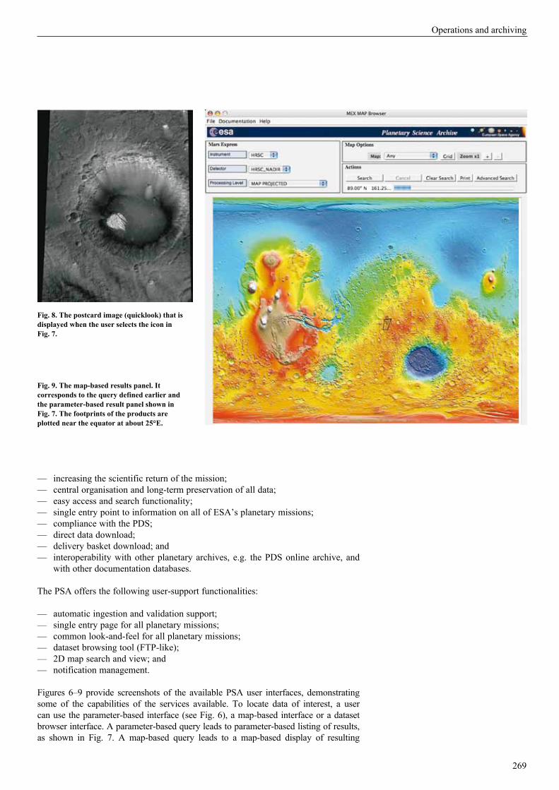
269
Operations and archiving
— increasing the scientific return of the mission;— central organisation and long-term preservation of all data;— easy access and search functionality;— single entry point to information on all of ESA’s planetary missions;— compliance with the PDS;— direct data download;— delivery basket download; and — interoperability with other planetary archives, e.g. the PDS online archive, and
with other documentation databases.
The PSA offers the following user-support functionalities:
— automatic ingestion and validation support;— single entry page for all planetary missions;— common look-and-feel for all planetary missions;— dataset browsing tool (FTP-like);— 2D map search and view; and— notification management.
Figures 6–9 provide screenshots of the available PSA user interfaces, demonstrating some of the capabilities of the services available. To locate data of interest, a user can use the parameter-based interface (see Fig. 6), a map-based interface or a dataset browser interface. A parameter-based query leads to parameter-based listing of results, as shown in Fig. 7. A map-based query leads to a map-based display of resulting
Fig. 8. The postcard image (quicklook) that is displayed when the user selects the icon in Fig. 7.
Fig. 9. The map-based results panel. It corresponds to the query defined earlier and the parameter-based result panel shown in Fig. 7. The footprints of the products are plotted near the equator at about 25°E.
270
SP-1291
footprints, as shown in Fig. 9. The user can toggle between the available result displays. If quicklook information is provided within a dataset, the individual quicklook images can be immediately accessed from the result panels. The dataset browser interface provides FTP-like access to all available Mars Express data. A more detailed user manual is available from the PSA web page.
5.1 General Dataset CharacteristicsAll datasets have an identical top-level directory structure as required by the PDS standard explained in section 3. Due to the common archive approach, including discussions and agreements with the instrument teams, a minimal set of keywords is used within all data labels.
The INDEX directory of each dataset contains a minimum set of ASCII index files formatted as PDS TABLE objects, to be used for information lookup or further data processing. The file INDEX.TAB contains a single line for each data product of a dataset, with basic identification information. The GEO_MARS.TAB file contains geometrical information for each data product, providing a representation/projection of each data product/observation on the surface of Mars (i.e. footprint). A common concept was developed for all instrument types (ESA, 2007) to allow uniform data retrieval. The BROWSE.TAB file is optional and present in case browse images are available in the dataset. It provides the mapping between the data products and their corresponding browse products.
The DOCUMENT directory of each dataset contains the Experiment to Archive Interface Control Document (EAICD). This is the basic document of each dataset and should be the entry point for new users. The file MEX_ORIENTATION_DESC.TXT defines the different orientations of the Mars Express spacecraft and their use within the datasets. The file MEX_POINTING_DESC.TXT defines the spacecraft pointing modes and their uses. Individual datasets might contain other documents; users are advised to read the EAICD for detailed information. The file AAREADME.TXT at the root of each dataset provides further high-level information, which new users are also advised to read.
Changes, updates, corrections of errors and other important information are documented at several locations, especially in the file ERRATA.TXT in the root directory of each dataset. Information is appended to the ERRATA.TXT to ensure that modifications to the dataset are fully transparent to users.
The planetocentric coordinate system is used for all Mars Express datasets, with longitudes increasing from 0° to 360°E, and latitudes between –90° and +90°. The reference frames of the spacecraft, instruments and detectors are defined in the frame kernels of the SPICE datasets (see section 5.8). In the following, the terms ‘reduced’ and ‘calibrated’ are used synonymously.
5.2 ASPERA-3 (Analyser of Space Plasmas and Energetic Neutral Atoms)ASPERA-3 comprises four sensors: the Electron Spectrometer (ELS), the Neutral Particle Imager (NPI), the Neutral Particle Detector (NPD), and the Ion Mass Analyser (IMA; Barabash et al., 2004). Data from each sensor are archived in individual datasets. The following datasets are currently available from ASPERA-3 and are produced at the Southwest Research Institute, San Antonio, Texas. All sensor data are stored in ASCII format with a varying, sometimes large, file sizes.
The dataset MEX-M-ASPERA3-2-EDR-ELS-V1.0 contains the raw experimental data records of the ELS sensor from launch to the end of the nominal mission. It provides the in situ electron measurements in the energy range 0.05–20 keV in two kinds of data product: the ELS Science low-range data and the ELS Science high-range data, both given in counts per accumulation unit. A data quality indicator based on the state of the instrument is available for each set of scan measurements. The data structure for all products is a spreadsheet in ASCII format, which is effectively a table containing comma-separated columns. The CALIBRATION directory contains
5. Available Mars Express Datasets
271
Operations and archiving
the high-range and low-range calibration tables providing for each ELS sensor the conversion values from counts to number fluxes. Deflection voltages to centre energies for the scan values are also given. The DOCUMENT directory contains supplementary information on flight performance, sensor frame definitions and usage, sensor numbering and calibration reports.
The dataset MEX-M-ASPERA3-3-RDR-ELS-V1.0 contains the reduced experimental data records of the ELS sensor from launch to the end of the nominal mission. The values are given as Differential Number Flux (DNF) as a SPREADSHEET object. The CALIB directory again contains the high- and low-range calibration tables with details explained in the file CALINFO.TXT.
The dataset MEX-M-ASPERA3-2/3-EDR/RDR-NPI-V1.0 contains the raw as well as the reduced experimental data records of the NPI sensor from launch to the end of the nominal mission. The measured energetic neutral atoms (ENA) count rates per second in the range 0.1–60 keV are given in a single type of data product, again using the SPREADSHEET structure. The provision of count rates allows for the analysis of the ENA as well as the UV signal, which are intermixed. The CALIBRATION directory contains a calibration table defining the values for converting from count rate to number fluxes for the ENA component only.
The dataset MEX-M-ASPERA3-2/3-EDR/RDR-NPI-EXT1-V1.0 contains the NPI data described above from the extended mission phase 1.
The dataset MEX-M-ASPERA3-2-EDR-IMA-V1.0 contains the raw experimental data records of the IMA sensor from launch to the end of the nominal mission. The measured ion count rates per accumulation are given in a SPREADSHEET structure. The CALIBRATION directory contains the mass channel data calibration table providing background noise values and the correction ratio for each of the mass channels. The energy step table provides the centre energy for each energy step, and the fraction of noise dependent on the energy step. The azimuth sector table provides the efficiencies and geometric factors for each of the sectors. The use of the calibration tables is described in the CALINFO.TXT file.
5.3 HRSC (High Resolution Stereo Camera)The HRSC instrument consists of two cameras, the Super-Resolution Camera (SRC) and the High Resolution Stereo Camera. The HRSC is a push-broom scanning instrument with nine CCD line detectors mounted in parallel in the focal plane (Neukum et al., 2004; Jaumann et al., 2007). The scan line data from each orbit and for each line detector are collected and stored in one IMAGE object.
The SRC is a framing device and the resulting observations are stored in an IMAGE object, one for each observation. All HRSC and SRC data are stored in VICAR format with an attached PDS label. The BROWSE directory contains a JPEG image of each data product. As the data products can be of considerable size (up to 5 GBytes), users are advised to check the browse images before downloading. All HRSC datasets contain this browse information.
All HRSC datasets are produced at the German Aerospace Center (DLR) in Berlin, Germany, in cooperation with the Department of Earth Sciences at the Freie Universität Berlin.
The dataset MEX-M-HRSC-3-RDR-V2.0 contains the radiometrically calibrated data from orbit 10 to the end of the first mission phase extension. The SOFTWARE directory contains the source code of MINIVICAR, a small subset of the VICAR image processing system with additions to allow for HRSC data processing. The MINIVICAR package provides a functionality to display the HRSC images, and convert them into other image file formats, and can process the radiometrically calibrated images to higher data processing levels.
The dataset MEX-M-HRSC-5-REFDR-MAPPROJECTED-V2.0 contains the geometrically calibrated and map projected data from orbit 10 to the end of the first mission phase extension. Images are presented in a sinusoidal equal-area map projection for latitudes between –85° and +85°E. Images at the poles are presented in
272
SP-1291
stereographic projection. More detailed information can be found in the file DSMAP.CAT in the CATALOG directory, and in the references provided there.
The dataset MEX-M-HRSC-5-REFDR-DTM.V1.0 contains the Digital Terrain Model (DTM) as 8-bit orthoimages for the nadir channel and the four colour channels, and 16-bit DTM, the latter with a height resolution of 1 m. The spatial resolution of the DTM is about twice the stereo resolution (up to 50 m). The map projection is polar-stereographic for polar areas, and sinusoidal elsewhere.
5.4 MaRS (Mars Express Radio Science) ExperimentThe dataset approach for the radio science experiment differs from those for the other instruments. The MaRS team provides one dataset including several data processing levels for each observation. For example, the dataset MEX-M-MRS-1-2-3-PRM-0117-V1.0 contains all data levels for an observation with sequence number 117 obtained during the nominal (prime, PRM) mission. Several hundreds of datasets are available for the nominal mission. More information about the MaRS experiment can be found in Pätzold et al. (2004).
The data processing levels provided in the datasets are as follows. The first data level contains the raw tracking data from either New Norcia or the Deep Space Network for both closed- and open-loop. The next data level contains the reformatted and further processed data in ASCII format. The third data level contains calibrated data products: distance to the target, observed and predicted frequencies, residuals of both frequencies, corrections for Earth’s atmosphere, signal level and the differential Doppler. For bistatic radar products coordinates are also available.
The data from each of the different processing levels, and from each of the ground stations used, are included in separate directories with appropriate naming.
The CALIBRATION directory contains calibration information for the ground stations used, both open- and closed-loop. The BROWSE directory contains JPEG images containing four-panel plots that allow preliminary data quality checks. The DOCUMENT directory contains a large amount of supplementary information ranging from the operational notebooks to ground station antenna documents.
5.5 OMEGA (Observatoire pour la Minéralogie, l’Eau, les Glaces et l’Activité)The dataset MEX-M-OMEGA-2-EDR-FLIGHT-V1.0 contains the raw experimental data records as well as geometry data from launch to the end of the nominal mission. The data records from the two mapping spectrometer channels (Bibring et al., 2004), the visible and near-infrared channel and the short-wavelength channel, are three dimensional and physically stored using the QUBE object comprising two spatial and one spectral dimension. The backplane of the QUBE contains dark current information for each CCD pixel. Several sideplanes of the QUBE contain supplementary instrument housekeeping information such as temperatures, voltages, scan mirror positions and more detailed timing information. One QUBE corresponds to one observation. A geometry data product is provided for each observation, providing the observation geometry of each pixel for each of the OMEGA channels. Explanations and definitions of the 51 geometry parameters can be found in the EAICD.
The SOFTWARE directory contains all versions of a data reduction pipeline to calibrate the raw data records into radiances and several other data structures. Users of OMEGA data are advised to check regularly for software updates. The software package contains necessary calibration data such as bias, flat field and photometric data, and explains instrument-specific and environmental aspects and takes them into account during the reduction.
The OMEGA dataset has been produced at the Institute d’Astrophysique Spatiale (IAS), Orsay, France.
5.6 PFS (Planetary Fourier Spectrometer)The dataset MEX-M-PFS-2-EDR-NOMINAL-V1.0 contains the raw experimental data records from the PFS spectrometer (Formisano et al., 2004) from launch to the

273
Operations and archiving
end of the nominal mission, produced at the Istituto Nazionale di Astrofisica (INAF-IFSI) in Rome, Italy. The data from the short-wavelength channel (SWC, 1.2–5 mm) and the long-wavelength channel (LWC, 5–45 mm), are contained in this dataset and separated via an appropriate directory naming scheme described in detail in the document MEX-PFS-PSA-ICD-25.pdf (EIACD for the PFS instrument).
The two channels can be operated in instrument calibration and instrument measurement modes. For each mode, the raw measurements, the housekeeping data and geometry information are provided in separate files using the TABLE structure. Data files, comprising calibration, housekeeping and measurements, from both the SWC and LWC, are stored in separated subdirectories of DATA directory, while the geometrical information for each scientific measurement is stored in the GEOMETRY directory, which has an identical structure.
The DOCUMENT directory contains extensive calibration documentation for both the SWC and the LWC. It discusses the calibration steps as well as external influences on the measurements, and includes the user manual for the PFS instrument.
5.7 SPICAM (Spectroscopy for Investigation of Characteristics of the Atmosphere of Mars)The raw data from the infrared (IR) and the ultraviolet (UV) spectrometers of SPICAM (Bertaux et al., 2004) are archived in two different datasets, all produced at the Service d’Aéronomie, IPSL, CNRS in Verrières-le-Buisson, France.
The datasets MEX-Y/M-SPI-2-UVEDR-RAWXCRU/MARS-V1.0 and MEX-Y/M-SPI-2-IREDR-RAWXCRU/MARS-V1.0 contain the raw experimental data records from the UV and IR channels, respectively, from launch to the end of the nominal mission. The instrument data are stored in an ARRAY of COLLECTIONS containing for each record a header and the data. The data part of a UV record represents five bands of the UV CCD, recorded during one measurement. The data part of an IR record represents the spectrum points recorded by each of the two detectors during one measurement cycle. The DOCUMENT directory contains a calibration document for each sensor, explaining how to process the data, and referring to the calibration files in the CALIB directory. The BROWSE directory contains PNG quicklook spectro-temporal images for each UV band and each IR detector. Both datasets provide further geometry parameters in the GEOMETRY directory for each observation. The parameters include, for example, line-of-sight information for specific CCD locations, specific operational modes and specific targets. Detailed information can be found in the SPICAM_GEOMETRY and SPICAM_POINTING files within the DOCUMENT directory.
5.8 MARSIS (Mars Advanced Radar for Subsurface and Ionosphere Sounding)The raw experimental data records of MARSIS (Picardi et al., 2004) are processed at the INFOCOM Department of the University of Rome ‘La Sapienza’ to produce the MEX-M-MARSIS-2-EDR-V1.0 dataset. This contains data that have been edited to remove corrupted or duplicated packets, and provides auxiliary information to locate them in space and time.
The data products in MEX-M-MARSIS-2-EDR-V1.0 are made by an aggregation of frames, which are a collection of received echoes with or without onboard processing applied. Each data product contains frames acquired through a single operational mode, instrument status and onboard processing scheme. The storage representation is a binary TABLE object containing timing, housekeeping and measurement values.
Users of this dataset are mainly radar scientists interested in redoing the entire processing of the received signal. The fact that unprocessed subsurface sounding echoes do not show any obvious indication of subsurface interfaces means that they are of little use to geologists.
Subsurface sounding data are further processed at the INFOCOM Department to produce the MEX-M-MARSIS-3-RDR-SS-V1.0 dataset, i.e. data that have been calibrated, range-compressed and corrected for ionospheric distortion. They are
274
SP-1291
therefore the dataset of choice for geological analysis of the structure and layering of the martian subsurface. Data products in this dataset have the same structure as those in the MEX-M-MARSIS-2-EDR-V1.0 dataset, with ground-processed frames substituted for instrument raw frames.
These datasets contain data from the deployment of the antenna in May 2005 to the end of the nominal mission. Data acquired in the extended phases of the mission are named MEX-M-MARSIS-2-EDR-EXTx-V1.0 for experiment data records and MEX-M-MARSIS-3-RDR-SS-EXTx-V1.0 for subsurface sounding processed frames, where ‘x’ denotes the number of the extension (‘1’ for the first extension, and so on).
The Department of Physics and Astronomy of the University of Iowa provides the calibrated data relating to the ionospheric soundings.
The data products of MEX-M-MARSIS-3-RDR-AIS-V1.0 are calibrated ionospheric sounding data stored in binary format using the TABLE object. One data product contains a list of vectors representing the power received by the instrument in time after transmission. The BROWSE directory contains one overview frequency–time spectrogram for each pericentre pass, as well as several delay time versus frequency plots covering all transmit/receive intervals of one pericentre pass.
5.9 SPICE (Navigational and Ancillary Information)The dataset MEX-M-SPICE-6-V1.0 contains navigation and ancillary data in the form of SPICE kernel files (Semenov et al., 2005). The instrument description kernels (IK) give descriptive and operational data for an instrument. I-kernels are available for all ASPERA-3 sensors, the HRSC camera, the OMEGA spectral imager and the PFS spectrometer. The frame definition kernels (FK) contain information to define reference frames, sources of frame orientation data and interconnections between these and other frames within the SPICE system. F-kernels are available for the Mars Express spacecraft, its instruments and most of its subsystems, such as the solar arrays and the high-gain antenna. The spacecraft clock kernel (SCLK) contains the onboard clock calibration data required to perform a mapping between ephemeris time and the onboard time. The leap seconds kernel (LSK) is a non-mission related kernel and provides the leap seconds and other constants required to perform transformations between UTC and ephemeris time.
The C-kernels describe the spacecraft pointing, containing a transformation traditionally called the C-Matrix, which is used to determine the time-tagged pointing angles. For Mars Express, the flight dynamics team provides one predicted attitude data file that is continuously updated in precision and time interval. Only in very rare cases is a reconstituted attitude file provided. These files are converted to C-kernels by the MEXPST team, with the support of the NAIF team. The filenames of these kernels are prefixed with ‘ATNM_P’. The reconstituted C-kernel is prefixed with ‘ATNM_RECONSTITUTED’.
SPK-kernels describe the ephemeris of one object against another. One SPK kernel prefixed with ‘ORHM’ describes the ephemeris of the spacecraft during cruise. During the nominal mission, there is typically one orbit file provided per month, prefixed with ‘ORMM’. Several Phobos and Deimos ephemeris kernels are provided, originating from ESOC, JPL or the HRSC instrument team. Ephemeris data for the ESA New Norcia station and the NASA DSN stations are also provided.
The DOCUMENT directory contains further information on the processing and use of the kernels provided.
The data flow and data integrity from the spacecraft to the payload team and to the scientific community are well defined. All the tools and services from the OCC to the PSA are operational, stable and in continuous use. The PSA released the first scientific data to the scientific community at large, and will provide a continuous support to scientists worldwide.
6. Conclusions
275
Operations and archiving
The data path from the spacecraft to the scientific users is accompanied by hundreds of engineers and scientists, including – and our apologies to those we have forgotten to mention – Pedro Osuna, Jesus Salgado, Guillermo San Miguel, Aurele Vrata Venet, Esther Parrila, Markus Fels, Phil Brabbin, Alessandro Ercolani, Angelo Rossi and Maud Barthelemy.
Barabash, S., Lundin, R. Anderson, H. et al. (2004). ASPERA-3: Analyser of Space Plasmas and Energetic Ions for Mars Express. In Mars Express: The Scientific Payload, ESA SP-1240, ESA Publications Division, European Space Agency, Noordwijk, the Netherlands.
Bertaux, J.-L. et al. (2004). SPICAM: Studying the Global Structure and Composition of the Martian Atmosphere. In Mars Express: The Scientific Payload, ESA SP-1240, ESA Publications Division, European Space Agency, Noordwijk, the Netherlands.
Bibring, J.-P., Soufflot, A., Berthé, M. et al. (2004). OMEGA: Observatoire pour la Minéralogie, l’Eau, les Glaces et l’Activité. In Mars Express: The Scientific Payload, ESA SP-1240, ESA Publications Division, European Space Agency, Noordwijk, the Netherlands.
CCSDS (1999). Reference Model for an Open Archival Information System (OAIS): Red Book, CCSDS 650.0-R-1.
DDID (2002). Rosetta/Mars Express Data Delivery Interface Document, RO-ESC-IF-5003. ESA Council (1989). Rules concerning Information and Data, ESA/C(89)95, rev.1, 21
December 1989.ESA (1997). Mars Express Science Management Plan. ESA/SPC(97)40, October 1997.ESA (2007). Planetary Science Data Archive Technical Note: Geometry and Position
Information, SOP-RSSD-TN-10, Issue 4.1, April 2007.ESA (2001). Mars Express Data Generation, Validation and Transfer Plan, EST-MEX-
TN-4009, Issue 1, 21 June 2001.Formisano, V., Grassi, D., Orfei, R. et al. (2004). PFS: The Planetary Fourier Spectrometer for
Mars Express. In Mars Express: The Scientific Payload, ESA SP-1240, ESA Publications Division, European Space Agency, Noordwijk, the Netherlands.
GDDS (2002). Operator User Manual, DTOS-INFR-UM-1001, Issue 1.1.Jaumann, R. et al. (2007). The High-resolution Stereo Camera (HRSC) Experiment on Mars
Express: Instrument Aspects and Experiment Conduct from Interplanetary Cruise through the Nominal Mission, Planet. Space Sci. 55, 28–952.
JPL (2002). Planetary Science Data Dictionary Document, JPL D-7116, Rev. E, 28 August 2002. http://pds.jpl.nasa.gov/documents/psdd/psdd.pdf
JPL (2006). Planetary Data System Data Standards Reference, Version 3.7, JPL D-7669, Part 2, 20 March 2006. http://pds.jpl.nasa.gov/documents/sr/index.html
Neukum, G., Jaumann, R. et al. (2004). HRSC: The High Resolution Stereo Camera of Mars Express. In Mars Express: The Scientific Payload, ESA SP-1240, ESA Publications Division, European Space Agency, Noordwijk, the Netherlands.
Pätzold, M., Tellmann, S., Anert, T. et al. (2004). MaRS: Mars Express Orbiter Radio Science Experiment. In Mars Express: The Scientific Payload. ESA SP-1240, ESA Publications Division, European Space Agency, Noordwijk, the Netherlands.
Picardi, G., Biccari, D., Seu R. et al. (2004). MARSIS: Mars Advanced Radar for Subsurface and Ionospheric Sounding. In Mars Express: The Scientific Payload. ESA SP-1240, ESA Publications Division, European Space Agency, Noordwijk, the Netherlands.
PSA (2002). PSA User Requirement Document, SOP-RSSD-RS-006, Issue 1, 17 April 2002. Pullan, D., Sims, M.R., Wright, I.P. et al. (2004). Beagle 2: The Exobiological Lander of
Mars Express. In Mars Express: The Scientific Payload. ESA SP-1240, ESA Publications Division, European Space Agency, Noordwijk, the Netherlands.
Semenov, B.V., Acton, C.H., Bachman, N.J., Elson, L.S. & Wright, E.D. (2005). Reducing Costs of Managing and Accessing Navigation and Ancillary Data by Relying on the Extensive Capabilities of NASA’s Spice System. In Proc. 6th Int. Symp. on Reducing the Costs of Spacecraft Ground Systems and Operations (RCSGSO), ESA/ESOC, Darmstadt, Germany, 14–17 June 2005. ESA SP-601, ESA Publications Division, European Space Agency, Noordwijk, the Netherlands.
Acknowledgements
References

276
SP-1291
Thompson, R.S., Cooper, S., Long, J.M. & Campbell, D. (2001). Application of XML in Space Data Systems: Science Systems Experience, Science Systems (Space) Ltd, XML Workshop, ESA/ESOC.

Acronyms And AbbreviAtions


279
ADU analogue to digital (conversion) unitAOCS Attitude and Orientation Control System AOTF acousto-optical tunable filterAPS Auxiliary Power SupplyAPXS Alpha Particle X-ray Spectrometer ASI Agenzia Spaziale Italiana ASPERA Analyser of Space Plasma and Energetic AtomsAU astronomical unit
BBA bundle block adjustmentBDR bi-directional reflectance BEE Back End Electronics
CCD Charge Coupled DeviceCDPU Command & Data Processing UnitCI Context ImagerCME coronal mass ejection CMOS Complementary Metal Oxide SemiconductorCNES Centre National d’Etudes SpatialesCNR Consiglio Nazionale della Ricercha (Italy)CNRS Centre National de la Recherche Scientifique
(France)Co-I Co-InvestigatorCORBA Common Object Request Broker Architecture COSPAR UN Committee on Space ResearchCRISM Compact Reconnaissance Imaging Spectrometer
for MarsCSW common softwareCTX Context ImagerCUL close-up lens
DAWG Data Archive Working Group DDS Data Distribution System (ESOC) DEM Digital Elevation ModelDES Digital Electronic SubsystemDESPA Observatoire de Paris, Département de
Recherches Spatiales (France)DHA Detector Head AssemblyDLR Deutsches Zentrum für Luft- und Raumfahrt
(German Aerospace Center )DM Development ModelDN Data Number (pixel intensity on a scale of
0–255)DNF Differential Number Flux DPU data processing unitDSN Deep Space Network (NASA)DTM Digital Terrain Model; data-transmission modeDVD digital video disc
EAICD Experimenter to Archive Interface Control Document
ELS Electron Spectrometer (ASPERA)ELM Electronics ModuleEMCD European Mars Climate DatabaseENA energetic neutral atom (ASPERA)EO exterior orientation
EPF emission phase functionEPROM erasable programmable read-only memoryEQM Electrical Qualification ModelERT Earth Reception Time ESA European Space Agency; electrostatic analyserESAC European Space Astronomy Centre, Villafranca
(Spain)ESOC European Space Operations Centre, Darmstadt
(Germany)ESS Environmental Sensor SuiteESTEC European Space Research and Technology
Centre, Noordwijk (the Netherlands)EUV extreme ultravioletEW equivalent width
FFT Fast Fourier TransformFIR far-infraredFM flight modelFOP Flight Operations Procedure FOV field of viewFTP File Transmission Protocol FTS File Transfer System FUV far-ultravioletFWHM full width at half maximum
GCM general circulation modelGC-MS gas chromatograph-mass spectrometerGDDS Generic Data Disposition System GDS global dust stormGFDL Geophysical Fluid Dynamics Laboratory (NOAA)GOMOS Global Ozone Monitoring by Occultations of
StarsGUI graphical user interface
HCP high-calcium pyroxeneHGA high-gain antennaHiRISE High Resolution Imaging Science Experiment HK housekeepingHRSC High Resolution Stereo Camera HST Hubble Space Telescope
IAS Institut d’Astrophysique Spatiale, Orsay (France)
ICA Ion Composition Analyser (Rosetta)ICD Interface Control DocumentICRS International Celestial Reference SystemIFSI Istituto di Fisica dello Spazio Interplanetario
(Italy)IKI Institute for Space Research (Russia)IFOV instantaneous field of viewIMA Ion Mass Analyser (ASPERA)IMB induced magnetosphere boundary IMEWG International Mars Exploration Working GroupINAF Istituto Nazionale di AstrofisicaIPSL Institut Pierre Simon Laplace (CNRS, France)
Operations and archiving

280
SP-1291
IR infraredIRIS Infrared Interferometer Spectrometer ISIS Integrated Scientific Information SystemISM imaging spectrometer (Phobos mission)ISO Infrared Space Observatory (ESA)ISSI International Space Science Institute
(Switzerland)ITRS International Terrestrial Reference SystemIUE International Ultraviolet Explorer
JPL Jet Propulsion Laboratory (NASA)
LAN local area networkLASCO Large Angle Spectrometric Coronagraph
(SOHO)LCP low-calcium pyroxene;
left-hand circular polarisationLDA lobate debris apronsLMD Laboratoire de Météorologie Dynamique (Paris)LOCC Lander Operations and Control Centre
(Beagle 2, Leicester, UK)LOS line of sightLTE local thermodynamic equilibriumLVF lineated valley fillLWC long-wavelength channel LWIR long-wavelength infraredLESIA Laboratoire d’Etudes Spatiales et
d’Instrumentation en Astrophysique (France)
MAG/ER Magnetometer and Electron Reflectometer MARCI Mars Color ImagerMaRS Mars Radio Science MARSIS Mars Advanced Radar for Subsurface and
Ionosphere Sounding MCO Mars Climate Orbiter (NASA)MCP micro-channel plateMEDUSA Miniaturized Electrostatic DUal-top-hat
Spherical AnalyzerMEP Mars Exploration Program (NASA)MER Mars Exploration Rover (NASA)MEX Mars Express MSG Meteosat Second Generation MGS Mars Global Surveyor (NASA)MI Microscopic Imager MIC microscopeMIPL Multimission Image Processing Laboratory
(JPL)MLI multi-layer insulationMMF Medusae Fossae formation MNP Mars nearest pointMO Mars OdysseyMOC Mission Operations Centre; Mars Observer
CameraMOLA Mars Orbiter Laser Altimeter (MGS)MoU Memorandum of UnderstandingMPB magnetic pile-up boundary
MPF Mars Pathfinder (NASA)MPS Mission Planning System MRO Mars Reconnaissance Orbiter MRS model reference spectrumMSO Mars Solar OrbitalMSM Mass Stiffness ModelMSL Mars Science Laboratory (NASA) MSP Master Science PlanMTF modulation transfer function
NCID normalised cumulative intensity distributionNCTRS Network Controller and Telemetry Receiver
System NEB noise equivalent brightnessNPD Neutral Particle Detector (ASPERA)NPI Neutral Particle Imager (ASPERA)NPLD north polar layered deposits
OAIS Open Archival Information System OBDM onboard data managementOCC Operations Control Centre (ESOC)ODL object description language OMEGA Observatoire pour la Minéralogie, l’Eau, les
Glaces et l’Activitié
PCWG Photogrammetry and Cartography Working Group
PDS Planetary Data System (NASA)PFS Planetary Fourier Spectrometer PI Principal InvestigatorPIMap Planetary Image Mapper PLD polar layered deposits PM Project Manager PEB photoelectron boundary POS Payload Operations ServicePRF Pulse Repetition FrequencyPROM programmable read-only memoryPSA Planetary Science ArchivePSDD Planetary Science Data Dictionary PSLA Project Service Level AgreementPSSL Planetary Science Sample Librarypx pixel
RCL Recognised Cooperating LaboratoryRCP right-hand circular polarisationRFS radio-frequency subsystemrms root mean squareRSS Radio Science Simulator
SCIAMACHY Scanning Imaging Absorption Spectrometer for Atmospheric Cartography (ESA)
SFD size–frequency distributionSFDU Standard Formatted Data Unit SFS shape from shadingSGICD Space/Ground Interface Control Document
(Mars Express)

281
SHDOM spherical harmonic discrete ordinate modelSIR SPICAM Infrared (channel)S/N; SNR signal-to-noise ratioSOC Science Operations Centre (ESOC) SOHO Solar and Heliospheric ObservatorySOWG Science Operations Working GroupSPICAM Spectroscopy for the Investigation of the
Characteristics of the Atmosphere of Mars SPLD south polar layered deposits SRC Super-Resolution Channel (HRSC)SST Science Support TaskSUV SPICAM UV (channel)SW short wavelengthSWIR short-wavelength infrared
SWS Short-Wavelength Spectrometer (ISO)SZA solar zenith angleTEC total electron content TES Thermal Emission Spectrometer TGCM thermospheric general circulation modelTHEMIS Thermal Emission Imaging System TOF time-of-flight
UTC Coordinated Universal Time USGS United States Geological SurveyUV–IR ultraviolet–infrared
VICAR Video Image Communication and RetrievalVIS/NIR; VNIR visible/near-infrared
Operations and archiving
→ MA
RS EXPRESS The Scientifi c InvestigationsSP-1291
ESA Member States
Austria
Belgium
Czech Republic
Denmark
Finland
France
Germany
Greece
Ireland
Italy
Luxembourg
Netherlands
Norway
Portugal
Spain
Sweden
Switzerland
United Kingdom
An ESA Communications ProductionCopyright © 2009 European Space Agency
European Space Agency
→ MARS EXPRESSThe Scientifi c Investigations
ESA0901_MEX_COVER.indd 1 2-7-2009 9:22:35