Manufacturing Flow Line Systems: A Review of Models and ...

Manufacturing Flow Line Systems:

A Review of Models and Analytical Results

Yves DalleryLaboratoire MASI (UA 818, CNRS)

Universite Pierre et Marie Curie4, Place Jussieu, 75252 Paris Cedex 05

Stanley B. GershwinLaboratory for Manufacturing and Productivity

Massachusetts Institute of TechnologyCambridge, Massachusetts 02139

Abstract

The most important models and results of the manufacturing flow line literature aredescribed. These include the major classes of models (asynchronous, synchronous, and con-tinuous); the major features (blocking, processing times, failures and repairs); the majorproperties (conservation of flow, flow rate-idle time, reversibility, and others); and the rela-tionships among different models. Exact and approximate methods for obtaining quantitativemeasures of performance are also reviewed. The exact methods are appropriate for smallsystems. The approximate methods, which are the only means available for large systems,are generally based on decomposition, and make use of the exact methods for small systems.Extensions are briefly discussed. Directions for future research are suggested.

Keywords: Manufacturing Flow Line Systems, Blocking, Failures, Modelling,Performance Evaluation, Analytical Methods, Exact Analysis, Approximate Anal-ysis.

0

1 INTRODUCTION 1

1 Introduction

1.1 Goals of the Paper

Manufacturing flow line systems consist of material, work areas, and storage areas. Materialflows from work area to storage area to work area; it visits each work and storage area exactlyonce in a fixed sequence; there is a first work area through which material enters and a lastwork area through which it leaves the system. The times that parts spend in work areas arerandom and this is the only source of randomness. This randomness may be due to randomprocessing times, random failure and repair events, or both. Storage areas can hold only a finiteamount of material. Machines are never allowed to be idle while they have parts to work onand space in which to put parts they have worked on. Manufacturing flow lines are also calledtransfer lines and production lines. In this paper, we mainly use the term ‘manufacturingflow lines’ or simply flow lines. The work areas are usually called machines. Storage areasare often called buffers. The material in most cases consists of discrete parts. There is onlya single kind of material in the system. Each piece of material travels the same sequence ofmachines and buffers, but each may experience different delays at each point in the system.Figure 1 depicts a five-machine flow line. A major example of the use of transfer lines is in thehigh volume production of metal parts of automobiles, but flow lines can be found throughoutmanufacturing industry. In the language of queuing theory, a flow line can be represented as afinite buffer, tandem queueing system. In that case, machines are called servers, storageareas are called buffers, and discrete parts are called customers, or jobs.

Our purposes are to survey the most widely known methods and publications in this area;to summarize the most important results and conjectures; to organize the great deal of workthat has been done; to show relationships among models; and to offer some opinions. We willtry to emphasize those papers that are most influential, those papers that are most well-known,or those papers that (in our opinion) should be. Like all fields, this one has fuzzy boundaries.We will try to focus on papers that are clearly in the flow line/transfer line/production lineliterature, and avoid those that belong in the much larger general queuing theory domain.

There are many different kinds of flow lines, and many different kinds of models in theliterature. The great variety of models in part reflects the variety of different kinds of systems;in part it reflects the fact that different models lend themselves to analysis more or less easilyfor different purposes. In what follows, we present or quote many mathematical results on thebehavior of these systems. The simple structure of a flow line permits very strong statements insome cases. Some of these statements (like conservation of flow) are quite general, and can bethought of as applying to actual systems. Others (such as methods for calculating productionrates) are specific to individual models.

Notation There have been many authors in this field, and almost as many different sets ofnotation. The present authors have therefore given up the notion of satisfying everyone, and havechosen their own earlier notation, with some modifications and compromises. Consequently, thesquares in Figure 1 represent machines and the circles represent buffers. Machines are numberedfrom 1 to K, where K is the number of machines in the system. There are K−1 buffers, and thebuffer between Machines Mi and Mi+1 is Bi,i+1. Parts flow from outside the system to Machine

1 INTRODUCTION 2

M1 M2 M3 M4 M5��

��

��

��

B1,2 B2,3 B3,4 B4,5- - - -- - - -

Figure 1: Five-Machine Flow Line

M1, then to Buffer B1,2, then to Machine M2, then to Buffer B2,3, and so on up to Machine MK

after which they leave the system. All the parts have to be processed on all the machines. Agreat deal of additional notation is defined throughout the paper.

Historically, this work has been aimed mostly at manufacturing systems. For that reason,there is a great emphasis on machine failures as the source of randomness. The goal has beenprimarily to calculate the maximum rate of flow of material through a production line. The max-imum flow rate is often called production rate, efficiency (in some models), or throughput.Thus, it is assumed that whenever a machine can do an operation, it does. Deliberate idlenessis not considered in these models. Other performance measures are also important, especiallythe average amount of material that is found in the buffers.

Whenever Machine Mi processes material, it reduces the level of Buffer Bi−1,i and it increasesthe level of Buffer Bi,i+1. On the other hand, when Machine Mi fails or takes an especially longtime to process a part, and its neighbors work normally, the level of Buffer Bi−1,i tends toincrease and the level of Buffer Bi,i+1 tends to decrease. If that persists, Buffer Bi−1,i mightbecome full or Buffer Bi,i+1 might become empty. In that case, one of the neighbors of Mi isnot able to operate; either Mi−1 is starved or Mi+1 is blocked (and is thus idle). Productionis then reduced because time is wasted. The isolated production rate of a machine is therate that it would operate at if it were not in a system with other machines and buffers.

The production rate of a line is limited in two ways. (1) The throughput can be no greaterthan that of the machine with the smallest isolated production rate. When the machines arevery different in their isolated production rates, the speeds of all but the slowest are largelywasted. (2) The unsynchronized disruptions that cause buffers to be empty or full also wastemachine capability. Buffers become empty or full because machines fail or take long times toprocess material at different times. If all machines could be perfectly synchronized, not only inperforming operations, but also in failing and getting repaired, buffers would not affect flow. Itis the lack of synchronization that causes machines to be starved or blocked, and thus to losethe opportunity to work.

Models, Reality, Mathematics, and Engineering Like all mathematical models, the mod-els in the flow line literature are compromises between fidelity to reality and tractability. All ofengineering requires the creative use of results that are based on simplifications of reality, andthe design of production systems is not an exception. It is not possible to prove a theorem onthe bounds of errors between a model and reality, since it is not possible to fully describe reality.Thus, in spite of the apparent restrictions on the class of systems we are considering, theseresults may be widely applicable. For example, although we have assumed that there is only

1 INTRODUCTION 3

a single part type, these methods may be usable for systems with many part types. If severalparts are produced in a line, and they require different lengths of time at each machine, thematerial may be treated as a single part type with random operation times. The distribution ofthe processing time then represents the differences of the processing times of the different partsand the randomness of the mixture of parts.

In addition, while we follow the literature and distinguish between reliable and unreliablesystems, it is sometimes useful to think of a failure as a long processing time, which occurs atrandom. Consequently, unreliable systems may be analyzed by methods designed for reliablesystems with random operation times, and vice versa.

1.2 Major Features and Properties of Real Manufacturing Flow Lines

Transfer and production lines are of great economic importance. Thus, much of the literaturethat we survey has practical value, as well as academic interest. In this section, we informallydiscuss some features of real systems. Mathematical models of these phenomena are definedmore precisely in Section 2. Much of the literature is aimed at developing ways of treating themore intractable features.

1.2.1 Synchronous/Asynchronous

Most real systems are unsynchronized. That is, the machines are not constrained to start orstop their operations at the same instant. Even when machines have fixed, equal cycle times(the times required for operations), the presence of buffers between them allows them to startand stop independently, as long as the intermediate buffers are neither empty nor full. In someapplications, the machines are not machines at all, but people. In others, the operation timescannot be fixed (for example when the parts are different, but treated as a single type). Finally,uncertain failure and repair times can lead to unsynchronized operation times.

Consequently, asynchronous systems form an important class of mathematical models inthe literature. However, it is very difficult to treat asynchronous systems with deterministicoperation times. This difficulty is generally met in one of three ways: (1) Asynchronous systemsare usually modeled with random operation times that have exponential, phase-type, or othertractable probability distribution. (2) Synchronous systems are defined, in which operationtimes are assumed to be deterministic and equal, and when machines are not under repair, theystart and stop at the same instant. Alternatively, one may view these models as having timediscretized, and it is not important when events occur during the time intervals; by convention,they are treated as though they occur at the beginnings or at the ends of the intervals. (3)Continuous material systems are defined; see Section 1.2.5.

1.2.2 Saturated/Non-saturated

Material arrives at and leaves from a factory in a variety of different ways. It is always possiblefor raw material to be absent, or for the means of removal of finished goods to fail. However, inthe literature, it is almost always assumed that the first machine is never starved and the lastis never blocked. Such models are called saturated models. Saturated models are of interestbecause a saturated model is appropriate for addressing the most important performance issue of

1 INTRODUCTION 4

a flow line, the maximal (average) number of parts that can be produced per unit of time. Thisquantity is referred to as the production rate of the flow line. However, the behavior of a flowline under a given input process and/or output process is also of interest. Thus, some authors,to represent the uncertain arrival and departure processes, add a buffer upstream of the firstmachine, with random arrivals to it, or a buffer downstream of the last machine, with randomdepartures from it. Often these buffers are infinite, while the others are finite. Such models arecalled unsaturated models. Another approach is simply to declare that the first machine of themodel represents the arrival process, and the second machine of the model corresponds to thefirst machine of the real system. That is, an unsaturated system can equivalently be representedby a saturated model. Because of the predominance of saturated models in the literature,and because of the relationship between saturated and unsaturated models, we concentrate onsaturated systems in this paper.

1.2.3 Blocking and Starvation and Decoupling

The function of a buffer is to decouple machines. If a machine is subject to a disruption (a failureor a long operation time), the machine upstream can still operate until the upstream bufferfills up, and the machine downstream can still operate until the downstream buffer becomesempty. The larger the buffers, the longer before the filling or emptying occur, and the larger theproduction rate. Zero buffers, or pairs of machines that have no storage space between them,have the greatest coupling; and infinite buffers, or storage areas that are never filled, have theleast. (Infinite buffers allow coupling when they become empty.)

1.2.4 Failures

Some models of flow lines have machines that can fail. When a failure occurs, a machine maynot process any material, so the buffer upstream cannot lose material and the buffer downstreamcannot gain material. A variety of assumptions about the conditions under which failure mayoccur, the time until a failure starts, the time that a failure lasts, and so forth, are consideredin the literature. In this paper, we call systems in which machines can fail Flow Lines withUnreliable Machines (FLUMs). Systems in which machines cannot fail are called FlowLines with Reliable Machines (FLRMs).

In FLRMs, all the randomness is due to the variability of the processing times. In FLUMs,some randomness is due to the failures of the machines and, in some models, some randomnessmay be due to variability of the processing times.

An important focus of the literature, and of this paper, are the up- and down-time distribu-tions, the probability distributions of the time between a repair and the next failure, and of thetime between a failure and the following repair. The most common assumption, and the mostmathematically tractable, is exponential. Reality is not always so convenient, so the literaturedescribes a variety of ways of treating non-exponential distributions for some classes of systems.

1.2.5 Discrete/Continuous

The literature described here is most often directed at manufacturing systems with discreteparts. That is, individual parts are treated, and each requires a non-zero, finite amount of

1 INTRODUCTION 5

time at each machine. On the other hand, systems that treat continuous material share somecharacteristics with these systems: in both, machines can fail, and finite buffers can becomeempty or full and thereby propagate disturbances and reduce production rates. Continuousmodels, in addition to describing real systems with continuous material, can also approximatediscrete systems.

1.2.6 Realistic Up-, Down-, and Operation Times

Transfer lines are artificial systems that are built for economic purposes. As a consequence,they have certain characteristics that are important for researchers to consider when developingmodels and approximation techniques. For example, in most real systems, the machines do notdiffer greatly from one another in their production rates. This is because the production rateof the system is limited by the slowest machine, and any investment in machines that are muchbetter than the slowest is wasted. This is made more precise, and other realistic characteristicsare described, in Section 3.10.

1.2.7 Operating Policy

In all models surveyed, machines are not allowed to be idle if they can be operated. That is,whenever a machine is neither blocked nor starved, it is used for an operation. Buzacott (1982)demonstrates that this is the optimal operating policy for a two-machine line when the systemproduction rate is the performance measure. He points out that other policies, such as keepingthe buffer level as close as possible to some intermediate value (to avoid blocking and starvation),have been used in practice.

There are good reasons for using other policies, however. Maximizing production rate doesnot take inventory costs into account. When inventory is expensive, it may be optimal to keepthe buffer level close to an intermediate value, and to use the buffer size to limit the deviationfrom that ideal level. Even still, it is useful to study systems operated in this way to determinetheir maximum possible production rates.

1.2.8 Non-Perishability

In the literature we survey, the material in buffers is assumed to be non-perishable. That is, itdoes not decay or lose value, no matter how long it waits.

1.3 Other Features

There are manufacturing systems that differ from those described in Section 1.2, but which areclose enough so that the methods and characteristics surveyed in this paper should, to someextend, be extendible to them. They include systems with:

machines in parallel Systems are built with machines in parallel for two reasons: eitherto achieve a greater production rate or to achieve a greater reliability. The first case is oftenobserved when some operation is inherently much slower than the others. The second case isencountered when some machine is much less reliable than the others.

1 INTRODUCTION 6

assembly operations In a flow line, each machine feeds a single buffer, and each buffer feedsa single machine. In assembly systems, however, two or more buffers can feed a single machine.The machine takes one part from each upstream buffer, and assembles a part from them. (Thiscan be generalized in a variety of ways, including disassembly.)

pallets Some systems require parts to be fitted onto pallets or fixtures before they are allowedto enter. In some cases, the fixtures allow for very precise location of holes. Because the numberof pallets is limited, parts must sometimes wait before they can be processed, even when thefirst machine is operational and not blocked. From the point of view of the pallets, such systemsare closed loops. In fact, one can calculate performance measures by ignoring the parts andmodeling only the movement of pallets.

1.4 Review of Reviews

Because of the economic and academic interest in this area, it has generated a great deal ofliterature, starting in the early 1950’s. That literature, in turn, has generated a large numberof reviews, which we review here. Because this survey emphasizes the most recent approachesand results, we do not cover all papers that have been devoted to flow lines. Many otherreferences are listed or described in these reviews. In addition, excellent surveys can be found intheses, including those by Ammar (1980), Anderson (1968), Boxma (1977), Buzacott (1967a),Dattatreya (1978), De Koster (1988a), Dudick (1979), Jafari (1982), Liu (1990), Schick (Schickand Gershwin, 1978), Sheskin (1974), Wiley (1981), as well as the monograph of Newell (1979).

Buzacott (1967a) describes the earliest Russian work. Because this work is difficult to obtain,and to translate, we quote from Buzacott (1967a):

It is not known when buffer stocks were first used to improve the efficiency of anautomatic transfer line. It seems to have been about 1946 in Russia. The earliesttheoretical papers were published there (Erpsher, 1952; Vladzievskii, 1952 and 1953).

Vladzievskii’s work is important as he was the first author to use probability the-ory to explain the behaviour of automatic transfer lines. In the 1953 paper he used aMarkov process approach to solve the case of two identical stages with identical expo-nential repair time distributions separated by a fixed capacity buffer... Vladzievskiihas subsequently written a book on automatic transfer lines (1958 — referred to inYu Retsker and Bunin, 1964)....

Yu Retsker and Bunin (1964) gives curves based on Vladzievskii’s work whichenable the economic optimum number of sections into which a line should be dividedto be found.

Koenigsberg (1959) begins his review by saying that the production line “has been all butneglected in the annals of operations research and management science.” This problem has beensubstantially remedied since then, as evidenced by the size of this paper and its reference list. Hesays that “Three major problems in the design and operation of production lines are concernedwith (a) the number of stages in the line, (b) the location of bunkers or pulsating stores [buffers],(c) the size of these pulsating stores.” Tools for the solution of these problems did not appear

1 INTRODUCTION 7

until the 1980’s. They are discussed in Section 5. Koenigsberg describes a number of differentapproaches and some systems that were in use in industry.

Buxey, Slack, and Wild (1973) survey a wider variety of phenomena than are found in mostof the papers described here. Papers they surveyed covered line balancing, flexibility (in thosedays called mixed-model production), human factors, parallel stations, allocation of part types toproduction lines, and the “launching” of work into lines. They consider conveyor belt systems,and they survey studies of the effect of belt speed. They also survey the literature to that dateon the effects of buffer stocks.

Buzacott and Hanifin (1978a) introduce the concepts of single station and total line failures,and operation dependent and time dependent failures. (See Section 2.1.3.) They provide simpleformulas to calculate the production rate of a line without buffers and with either time dependentand operation dependent failures. They describe the work of Vladzievskii (1953) (which isavailable only in Russian) and Sevast’yanov (1962) and other, more recent papers. They pointout that it would be easy to include the effects of total line failures on any of these models.Finally, they compared the performance prediction of one of Buzacott’s models with a simulationbased on real data, and they conclude that there are significant differences, which they attributeto the non-memoryless behavior of the repair and failure times. Buzacott and Hanifin (1978b)discuss the state of the art in transfer line design and modeling. They describe such physicaland mechanical issues as the transfer mechanism, shunt versus series banks (which determinewhether the material in buffers is moved according to FIFO or LIFO), and the design of theline to reduce cycle time, failure frequencies, and downtime duration. They discuss and critiqueboth the practice of simulation as a tool for the design of lines, and the existing analytic models.

Perros (1984) is simply a list of 75 relevant papers on queueing networks with blocking.Smunt and Perkins (1985) focus on “unpaced assembly lines with stochastic task times” —

roughly, what we call asynchronous flow lines with reliable machines. They are particularlyinterested in line design, the problem of locating and sizing buffers, and allocating tasks tostations. They review many simulation papers and they perform their own simulations to testHillier and Boling’s “bowl phenomenon.” They conclude that it is “highly situation specific.”

Awate and Sastry (1987) survey much of the transfer and flow line literature. They reviewthe solution methods of most of the important papers. Gun (1987) is a systematic descriptionof 23 of the major papers in this field. For each paper, the model, the performance measure,and the method are briefly sketched. Perros (1988) describes the literature of two-node queuingnetworks with blocking. Because this review is restricted to small systems, it is able to reporton many analytic solutions. It is restricted to asynchronous models. Perros (1989) surveys theliterature on queueing networks with blocking. It includes models with reliable or unreliablemachines, having tandem or more general topologies. He considers models useful for differentapplications: computer systems, communication networks, and production systems. Most of thepaper deals with approximate techniques. Onvural (1990) surveys closed queuing networks withfinite buffers. This paper is more concerned with computer systems than production systems,and, like Perros (1988), it emphasizes asynchronous models. A variety of blocking mechanismsand equivalences among network types are described. (See Section 2.1.1.)

Perros and Altiok (1989) is the proceedings of a conference on queuing networks with block-ing. It contains many papers on a variety of topics in this area.

2 FLOW LINE MODELS 8

1.5 Outline

In Section 2 we present the major classes of mathematical models of flow lines. We examinethe most important properties of flow lines, and the relationships among the models, in Section3. Methods that analyze systems exactly are explained in Section 4. Because of the finitenessof the buffers, only special systems have exact solutions. Approximate methods are shown inSection 5. The most important methods are decompositions, in which large systems are brokeninto a set of small systems. Extensions are considered in Section 6. Conclusions and directionsfor further research are presented in Section 7. Coxian and phase-type distributions, which areused extensively throughout the paper, are described in the appendix. Also, some mathematicalclaims are proved in the appendix.

2 Flow Line Models

In this section, we introduce three major classes of models that have been considered for theanalysis of tandem production lines. We describe assumptions that are made in most of theliterature. Some exceptions are summarized in Section 6.

2.1 Asynchronous Models

2.1.1 Blocking Issues

All real buffers have finite capacity. It is convenient to define the intermediate storagecapacity between Machines Mi and Mi+1, Ci,i+1, to be the total number of parts that can bestored between the two machines. We define the capacity or size Ni,i+1 of Buffer Bi,i+1 toinclude the space on Machine Mi+1. It satisfies Ni,i+1 = Ci,i+1 + 1. Let N = (N1,2, ..., NK−1,K)denote the buffer capacity vector. These quantities are constant system parameters. We alsodefine the buffer level ni,i+1 to be the random variable that indicates the number of parts inBuffer Bi,i+1 at any time, including the part on Machine Mi+1, if any. It satisfies

0 ≤ ni,i+1 ≤ Ni,i+1 (1)

Since the buffers have finite capacity, blocking may occur. Different types of blocking mech-anisms are of interest: blocking-after-service and blocking-before-service (Perros, 1989).Blocking-after-service (BAS) is also referred to as type-1 blocking (Onvural and Perros, 1986),manufacturing blocking, production blocking, transfer blocking, and non-immediateblocking (Gun and Makowski, 1989). BAS blocking occurs if, at the instant of completion of apart on Machine Mi, the downstream buffer, Bi,i+1, is full. In that case, the part stays on themachine until a space is available in Buffer Bi,i+1. During this time the machine is preventedfrom working and is said to be blocked. When a space becomes available in the downstreambuffer, the part is immediately transferred and the machine can start processing another part,if any.

Blocking-before-service (BBS), is also referred to as type-2 blocking (Onvural and Perros,1986), communication blocking, service blocking, and immediate blocking (Gun andMakowski, 1989). A machine can start processing a part only if there is a space available in


the downstream buffer. Otherwise, it has to wait until a space becomes available. MachineMi is said to be blocked when Buffer Bi,i+1 is full. BBS is further classified according towhether the position (space) on the machine may be occupied while the machine is blocked ornot. These two cases are referred to (Perros, 1989) as BBS-PO (blocking before servicewith position occupied while the machine is blocked) and BBS-PNO (blocking beforeservice with position non-occupied while the machine is blocked). Most often, productionlines operate under the BAS mechanism, and therefore most authors assume BAS.

Thus, when a machine is blocked, it is prevented from working. A machine may also beprevented from working because it has no material to work on. This phenomenon is starvation.In the case of BBS, starvation corresponds to the situation where the upstream buffer is empty.That is, Machine Mi is starved if ni−1,i = 0. In the case of BAS, starvation corresponds to thesituation where either the upstream buffer is empty, or it contains a single part whose processinghas already been completed. The second condition corresponds to the case where the part cannotbe transferred because the machine is blocked. In this case, although the buffer is not empty,the machine has no part to work on. (We note, however, that some authors define starvationsimply as the situation where the upstream buffer is empty.)

A machine is said to be idle if it is either starved or blocked. A machine may be simultane-ously starved and blocked.

Following the majority of papers in the literature, we assume that the first machine, M1, isnever starved. That is, there are always parts at the input of the system. Also, we assume thatthe last machine, MK , is never blocked. There are always spaces for Machine MK to deliver itsparts. In other words, we only consider saturated models. See Section 1.2.2.

The issue of blocking definition was first raised by Altiok and Stidham (1982) who criticizeda two-machine model of Gershwin and Berman (1981) that assumed BBS-PO. They pointedout that in a manufacturing system, there is no reason for the first machine to stop until ithas completed an operation and there is no room for the completed part. The more recentliterature on flow line models with blocking has paid a great deal of attention to blockingmechanisms. Actually, although BAS is likely to be encountered more often, there also existflow lines operating under BBS assumptions.

2.1.2 Processing Times

The time required for a machine to perform an operation on a part is called the processingtime or operation time or sometimes cycle time. This processing time may be either aconstant or a variable. In the later case, the processing times at a machine are usually assumedto be random variables having a common distribution. Moreover, it is usually assumed thatsuccessive processing times are independent of one another. In other words, processing timesare i.i.d. random variables.

It is also usually assumed that processing times at different machines are independent ofone another. Deterministic (constant) processing time is just a special case of this. Other typi-cal distributions commonly used are exponential distributions, geometric distributions,Coxian distributions, and phase-type distributions (Kleinrock, 1975; Neuts, 1981). Sincethese distributions are of great importance when analyzing flow lines, a brief review of Coxianand phase-type distributions is given in the Appendix.


2.1.3 Failures and Repairs

In some systems, machines are prone to failures. When a failure occurs, the machine must berepaired and is then unavailable for processing parts. A machine is said to be operational if itis up and is said to be working if it is operational and not idle (neither starved nor blocked).Two major types of failures have been considered in the literature: operation dependentfailures (ODF) and time dependent failures (TDF) (Buzacott and Hanifin, 1978a).

ODFs are failures that are related to the processing of parts and thus can only occur whenthe machine is working. On the other hand, TDFs are not related to the processing of partsand thus can occur at any time, including when a machine is idle. In transfer lines that performhigh-volume metal-cutting operations, such as for the automobile industry, ODFs are mainlydue to mechanical causes (like tool breakage or motor burnout) while TDFs are mainly due tofailures of electronic systems, such as controllers. In most production lines, most failures areODFs (Buzacott and Hanifin, 1978a). As a result, most authors assume ODFs, and unless weexplicitly state otherwise, we assume that failures are operation dependent.

It is generally assumed that uptimes and downtimes are i.i.d. random variables. (In reality,failures among different machines may not be independent, for example, when a poorly castmetal part — with hard spots — causes excess wear on all the tools in a transfer line.) Adowntime (or repair time) of a machine corresponds to the time from the instant of a failureof the machine to the instant of the next repair.

On the other hand, there are two different ways of measuring the uptime (or time to failure).In the first, the uptime corresponds to the total working time of the machine between the instantof the last repair to the instant of the next failure. The working time corresponds to the timewhere the machine is busy processing parts and does not include idle times (when the machineis either starved or blocked). The cause of failure is related to the time that machine has beenbusy processing parts. A typical example is the wear of tools. In this case, the distribution ofuptimes is a continuous distribution.

In the second, the uptime corresponds to the total number of parts produced by the machinefrom the instant of the last repair of the machine to the instant of the next failure. The causeof failure is related to the number of operations that the machine has performed. A typicalexample is a failure of the loading/unloading mechanism of parts on the machine. In that case,the distribution of uptimes is a discrete distribution.

We refer to these two failure types as time-ODFs and number-ODFs, respectively. Whenuptimes are much larger than processing times, there is little difference between them.

In the case of TDFs, the uptime corresponds to the total time (including working and idletime) of the machine between the instant of the last repair to the instant of the next failure. Inthis case, the distribution of uptimes is a continuous distribution. There is no counterpart ofthe number-ODF concept.

We need to describe more precisely what happens when a failure occurs. First, in terms ofstorage, two cases can be considered. Either the part stays on the machine during the repairtime, or it is moved back in the intermediate storage area. (The second alternative requires aspecial treatment when the intermediate storage area is full.) Secondly, we need to define whathappens when the machine is repaired. Either the part can be reworked or it cannot. If itcannot, it is thrown away (or scrapped). If it can, either the work resumes exactly at the point


it stopped, or the total operation has to be performed again. Very few papers have consideredscrapping. They are discussed briefly in Section 6.2.

As for processing times, deterministic, exponential, geometric, Coxian, and phase-type arecommonly used distributions. Most authors assume that if several machines are down at thesame time, the repair process of each machine is not affected by the repair processes of theothers. This means that the repair time of a machine is the same whether or not there areother machines currently under repair. The failures we just considered are referred to as singlemachine failures (Buzacott and Hanifin 1978a). Other failures that may occur in a productionline are total line failures (Buzacott and Hanifin, 1978a). A typical example is a failure ofthe power system which forces the whole line to stop. Total line failures can easily be handled(Buzacott and Hanifin, 1978a) and, as a result, we only consider single machine failures.

2.1.4 Buffer Behavior

When a part is transferred from Buffer Bi−1,i to Buffer Bi,i+1, ni−1,i goes down by 1 and ni,i+1

goes up by 1. In the case of BBS, this happens at the instant at which Machine Mi completesa part. Indeed, in this case, there must be a space available in Buffer Bi,i+1 for Machine Mi tobe working. As soon as the machine completes its operation, the part can be transferred intothe downstream buffer.

For BAS, this is also true as long as the downstream buffer is not full at the instant ofprocessing completion. Otherwise, the part cannot be transferred immediately. The transferwill occur as soon as a space is available in Buffer Bi,i+1. This transfer will therefore either occurat the instant of processing completion of machine Mi+1, or it will be delayed if this machine isblocked.

An important feature of BAS is that simultaneous transfers can occur. Indeed, supposethat at some instant, Buffers Bi,i+1, Bi+1,i+2, ..., Bj−1,j are full and Machines Mi, Mi+1, ...,Mj−1 have completed their operations and are therefore blocked. The unblocking of all thesemachines will occur at the instant at which Machine Mj completes its operation. At this instant,a simultaneous transfer of parts will take place in all the buffers. The resulting state is suchthat all Buffers Bi,i+1, Bi+1,i+2, ..., Bj−1,j are again full. However, now all Machines Mi, Mi+1,..., Mj−1 are busy working on new parts.

An issue related to buffer behavior is the transfer time of parts through the buffers. In realsystems, a part that is released to a buffer by the upstream machine is not immediately availablefor the downstream machine. It takes some time for the part to be moved throughout the buffer.It is the case, for instance, in automated transfer lines where the buffer consists of a conveyor.This may or not have a significant impact on the behavior of transfer lines depending on therelative values of transfer times and processing times. Most authors assume that a part which istransferred into a buffer by its upstream machine is immediately available for the downstreammachine. In other words, the transfer time through the buffer is negligible. Non-zero transittime are briefly discussed in Section 6.5.


2.2 Synchronous Models

There is a distinction between synchronous and discrete time models, but that distinctionis not always observed. A synchronous model is one in which events may only occur at certaindiscrete times. A discrete time model is one whose behavior is only described at certain discretetimes. For example, a model in which operations, failures, and repairs may start and end attimes tj = j∆ is a synchronous model. On the other hand, a model in which operations, failures,and repairs may start and end at any time, but the changes in system state are only representedat times tj = j∆ is a discrete time model. The distinction is important if, in the discrete timemodel, the transition equations or performance measures are somehow adjusted to account forthe differences between the times that events occur and tj . (We are not aware of any authoractually making such an adjustment.) Discrete time models are often used as approximationsfor asynchronous systems. See Section 3.8.

Having stated this distinction, we will no longer observe it. We use the term ‘synchronous’throughout this paper.

In a synchronous model, buffer levels ni,i+1 and machine states have their changes observedat times tj = j∆. ∆ is referred to as the time unit and, without loss of generality, it isusually assumed that ∆ = 1. The equations for the dynamics of the changes are influenced bywhether buffer levels are assumed to change before or after the machine states during the interval[tj−1, tj ]. In Buzacott’s synchronous models (1967a, b), changes in buffer levels are assumed totake place before machine state changes occur; in Gershwin’s (1987a), machine state changesoccur first. Which comes first in a time step is only a matter of convenience and convention,and does not affect the behavior of the model. A buffer level does not change if both adjacentmachines are inoperable due to being down, blocked, or starved. It also does not change ifneither adjacent machines is inoperable due to being down, blocked, or starved. Otherwise, itincreases or decreases by 1.

In the models of which we are aware, all the operations and machine state changes in theline are treated as simultaneous, and all the buffer level changes are treated as simultaneous. Inmodels of operations and machine state changes, adjacent buffers must be considered, becauseif they are empty or full, the machine is starved or blocked and the operation is not allowed tooccur. The blocking concepts described above for asynchronous systems — BBS and BAS —apply to synchronous systems as well.

Synchronous models may involve both reliable and unreliable machines. FLRM (reliable)models become non-trivial only with random operation times, for example with discrete phase-type distributions. FLUM (unreliable) models may have deterministic or random operationtimes as long as they have randomness in their up- or down-times. However, most FLUMmodels have deterministic operation times. As in an asynchronous model, ODFs and TDFs canbe considered. However, we note that in the case of a synchronous model with deterministicoperation times, there is no difference between time-ODFs and number-ODFs.

2.3 Continuous Models

The feature that distinguishes continuous models from the others is that the material is treatedas continuous rather than discrete. That is, instead of discrete parts moving from buffer to

3 GENERAL PROPERTIES 13

machine to buffer at specific instants, there is a fluid that is transferred continuously. MachineMi is starved if one of the machines Mj , j < i upstream of it is down and all buffers betweenthem, Bj,j+1, . . . , Bi−1,i, are empty. Similarly, a machine is blocked if one of the machinesdownstream from it is down and all buffers between them are full. The speed µi of Machine Mi

is the maximum rate at which it can transfer material from its upstream buffer to its downstreambuffer, when both machines are up and neither buffer is empty or full.

In a continuous model where machines have different speeds, a machine may be slowed down,that is, forced to work at a rate slower than its speed. A machine Mi is slowed down by theupstream part of the line (upstream limited) if one of the machines Mj , j < i upstream ofit works at a slower speed µj < µi and all buffers between are empty. Similarly, a machine isslowed down by the downstream part of the line (downstream limited) if one of the machinesdownstream of it works at a slower speed and all buffers between are full.

Buffer levels change in a continuous way. If Machine Mi and Machine Mi+1 are both workingat their own speed, then the level of Buffer Bi,i+1 changes by (µi−µi+1)δt during a time intervalof length δt. If either machine is down, then the appropriate term in this expression is deleted;if both are down, then the buffer level does not change. If either machine is slowed down, thenthe adjusted speed is used in this expression.

In a continuous model, some of the issues discussed for the asynchronous model are notmeaningful, for instance, concepts like BAS and BBS. The continuous model has mainly beenused when machines are unreliable. Again, the uptimes and downtimes are usually assumedto be i.i.d. random variables with continuous distributions, and both ODFs and TDFs can beconsidered. In some continuous models with ODFs, the failure rate of a machine is reducedwhen this machine is slowed down. (See Section 3.8.1.)

The continuous model is naturally suited to production systems in which the material that isto be processed is a fluid rather than discrete entities like parts — such as chemical processing. Inthis paper, however, we mainly devote our attention to production systems with discrete parts.The continuous model is nevertheless of interest since it has often been used as an approximationof discrete models, especially the asynchronous model. (See Section 3.8.)

2.4 Typical Assumptions of All Models

Most of the results that are discussed in Sections 3 to 6.7 are based on the following assumptions.The first machine is never starved and the last machine is never blocked. All the random variables(processing times, uptimes, downtimes) are independent random variables. The transfer timethrough the buffers takes zero time. The failures are single-machine failures and most oftentime-ODFs. When a failure occurs, the part stays on the machine; it can be reworked when themachine is up again (i.e., there is no scrapping of parts); the work resumes exactly at the point itstops. Times to failure and times to repair of machines are usually assumed to be exponentiallydistributed when time is continuous, and geometrically distributed when time is discrete.

3 General Properties

The purpose of this section is to survey several results pertaining to flow line models that are ofgeneral interest. We first introduce and discuss the major performance measures of flow lines.


3.1 Performance Measures of Flow Lines

We first define some basic quantities of the flow line models.

Ti: average processing time of Machine Mi.

µi: average processing speed of Machine Mi.

MTTFi: average time to failure of Machine Mi.

pi: average failure rate of Machine Mi.

MTTRi: average time to repair of Machine Mi.

ri: average repair rate of Machine Mi.

ei: efficiency of Machine Mi in isolation.

ρi: production rate of Machine Mi in isolation.

The isolated efficiency ei is the average fraction of the time that Machine Mi would beoperational if it were operated in isolation, that is, never starved or blocked. This quantity isalso referred to as the availability of Machine Mi. Note that ei = 1 for a reliable machine andei < 1 for an unreliable machine. For synchronous systems, all µi are the same, and the timeunit is usually chosen so that µi = 1.

The following relate these quantities:

µi =1

Ti(2)

pi =1

MTTFi(3)

ri =1

MTTRi(4)

ei =MTTFi

MTTFi +MTTRi=

ripi + ri

(5)

ρi = µiei =µiripi + ri

(6)

All the results that we review in this paper are concerned with steady-state (average longterm) behavior of the production line. Therefore, all the quantities we calculate are steady-stateperformance parameters. Several measures of performance are of interest when analyzing flowline models. The most important is the production rate, P , the average number of parts thatleave the system per unit of time. Also of importance is the inventory level of the system. Defineni,i+1 to be the average number of parts (or average buffer level in Buffer Bi,i+1. Theaverage work-in-process (or WIP) in the system, n, is given by


n = n1,2 + ...+ nK−1,K . (7)

Using Little’s law (Little, 1961), the average flow time of a part, W , can then be obtained as:W = n/P .

Other performance parameters of interest are:

Ei: probability of Machine Mi being working.

Pi: production rate of Machine Mi.

Si: probability of Machine Mi being starved.

Bi: probability of Machine Mi being blocked.

Ii: probability of Machine Mi being idle.

Di: probability of Machine Mi being down.

In FLRMs, the quantity Ei corresponds to the proportion of time Machine Mi is not idle(neither starved nor blocked) and is referred to as the utilization rate of Machine Mi. InFLUMs, it corresponds to the proportion of time Machine Mi is neither idle (starved or blocked)nor down and is referred to as the efficiency of Machine Mi. In the following, we use efficiencyto refer to Ei for an unreliable machine as well as for a reliable machine. Finally, we note thatthe production rate of a flow line as defined above is given by P = PK .

3.2 Some Basic Relationships

Several relationships hold under very general conditions, especially for general distributionsof processing times, uptimes and downtimes. We first discuss relationships pertaining to asingle machine. The first relates the production rate of a machine to its efficiency and averageprocessing rate:

Pi = µiEi (8)

This relationship holds for FLRMs and also for FLUMs provided that the work resumes exactlyat the point it stopped in case of failure. (See Section 2.1.3.) In synchronous systems where allµi are 1, Pi = Ei. Consequently, Ei is often called production rate in synchronous systems.

Consider FLUMs with ODFs. Because idle times do not influence the failure/repair behaviorof the machine, we have:

piEi = riDi (9)

A proof of this result is given in the Appendix. Using equations (5) and (9) and the fact thatthe probabilities sum up to 1, i.e., Ei +Di + Ii = 1, we obtain:

Ei = ei(1− Ii) (10)


This relationship is referred to as the flow rate-idle time relationship. It holds for any machinewith ODFs.

In the case of TDFs, equations (9) and (10) are replaced by

pi(Ei + Ii) = riDi (11)

Ei = ei − Ii (12)

Equation (11) is also proved in the Appendix.A fundamental relationship of flow lines is the conservation of flow. It states that all the

machines have the same average production rate, that is,

P1 = P2 = ... = PK = P (13)

Conservation of flow holds for FLRMs. It also holds for FLUMs provided that there is noscrapping of parts. (If there is scrapping, it can be adjusted accordingly.)

Actually, this relationship, as well as some of the results presented below can be establishedusing a sample path approach. It is described in Section 3.3.

3.3 Evolution Equations

The sample path behavior of any flow line can be described by means of recursive equations.These equations will be referred to as the evolution equations of the flow line. They haveproved to be very useful in flow line analysis, mainly for establishing qualitative propertiessuch as monotonicity and reversibility. These equations have been used in many papers undervarious forms, e.g., Hildebrand (1967, 1968), Yamazaki and Sakasegawa (1975), Muth (1979),Shanthikumar and Yao (1989), Dallery, Liu, and Towsley, (1990).

Consider a FLRM with the following initial condition. At time t = 0, all buffers are emptyand the first machine initiates the processing of a new part. Let σi,n denote the n’th processingtime of machine Mi, and let Di,n denote the n’th departure time of a part from Machine Mi.In the case of BBS-PO, we have the following evolution equations:

Di,n = max(Di,n−1, Di−1,n, Di+1,n−Ni,i+1

)+ σi,n , ∀i, n ≥ 1 (14)

where, by convention, Di,n = 0 ∀i if n ≤ 0.Equation (14) results from the following observations. Since we consider BBS, the departure

time from Machine Mi occurs exactly σi,n units of time after the start of the process. Thestart time of the n’th process is expressed by the first term of equation (14). There are threeconditions that must be satisfied before the n’th process of Machine Mi can begin: 1) themachine must be available; 2) the upstream Buffer, Bi−1,i, must be non-empty; and 3) thedownstream Buffer, Bi,i+1, must be non-full. The first condition is satisfied when Machine Mi

has completed its (n − 1)’th process, which occurs at time Di,n−1. The second condition issatisfied when Machine Mi−1 has completed its n’th process, which occurs at time Di−1,n. Thethird condition is satisfied when Machine Mi+1 has completed its (n−Ni,i+1)’th process, which


occurs at time Di+1,n−Ni,i+1 . Since these three conditions must all be satisfied, the time thatprocessing begins is thus the maximum of these three times.

In the case of BAS, the evolution equations are modified as follows:

Di,n = max(max (Di,n−1, Di−1,n) + σi,n, Di+1,n−Ni,i+1

), ∀i, n ≥ 1 (15)

The difference is that in the case of BAS, the process can start even though the downstreambuffer is full, but the transfer can take place only when a space is available. Finally, we notethat these evolution equations can appropriately be modified in the case of a non-empty initialcondition. (See e.g., Dallery, Liu, and Towsley, (1990).) These equations do not require anyassumption on the sequences of processing times σi,n, n ≥ 1. Similar evolution equations canbe derived in the case of BBS-PNO (Dallery, Liu, Towsley, 1991).

In both cases (BBS and BAS), the production rate of Machine Mi can then be expressed as:

Pi = limn→∞

n

E[Di,n](16)

General conditions under which this limit exists are given in (Dallery, Liu, and Towsley, 1990).In particular, it exists if the processing times σi,n, n ≥ 1, are i.i.d. random variables.

It follows from equation (14) in the case of BBS-PO or equation (15) in the case of BASthat:

Di+1,n ≥ Di,n ≥ Di+1,n−Ni,i+1 (17)

which implies:E[Di+1,n]

n≥ E[Di,n]

n≥E[Di+1,n−Ni,i+1 ]

n−Ni,i+1

n−Ni,i+1

n(18)

This equation implies Pi = Pi+1 when n goes to infinity (provided that the limits exist), thusproving conservation of flow (equation (13)).

These evolution equations have sometimes been used in a simpler form corresponding to thecase of flow lines with no intermediate storage. In the case of BAS, equation (15) then reducesto:

Di,n = max (Di−1,n + σi,n, Di+1,n−1) , ∀i, n ≥ 1 (19)

Note that one term has been dropped. The reason is that in the case of BAS and no intermediatestorage, we have Di−1,n ≥ Di,n−1.

Using evolution equations corresponding to the case of flow lines with no intermediate stor-age is however not restrictive since any flow line can be transformed into a flow line with nointermediate storage by adding fictitious machines with zero processing times that represent thetransfer of parts from a buffer space to the next one. This trick is due to Avi-Itzhak (1965).Evolution equations of this simpler form were used, among others, by Hildebrand (1967, 1968),Yamazaki and Sakasegawa (1975), and Muth (1979).

Remark. Some of the properties presented in Sections 3.4, 3.5, and 3.6, have been obtainedusing a sample path approach based on the above evolution equations. These properties holdunder fairly general assumptions pertaining to the processing times (see e.g. Dallery, Liu,


and Towsley, 1990). These assumptions include independent and identically distributed (i.i.d.)sequences of processing times (i.e., GI distributions) as a special case. Although these evolutionequations have mainly been used in the context of FLRMs, they can be adapted to FLUMs withODFs by interpreting σi,n as the completion time instead of just the processing time of MachineMi. (See Section 3.7.) Therefore, we conjecture that all properties that have been obtained forFLRMs based on these evolution equations are also valid for FLUMs with ODFs. See Dallery,Liu and Towsley (1990) for a discussion pertaining to this issue.

3.4 Blocking Issues

The purpose of this section is to discuss the relationships between the different types of block-ing. We first compare BAS (blocking-after-service) and BBS-PNO (blocking before service withposition at the machine non-occupied while the machine is blocked). It is convenient to definethe vector 1 = (1, . . . , 1).

Consider two flow lines that differ only from one another by the buffer capacities and thetype of blocking. One line has buffer capacity vector N and is operated according to the BASblocking mechanism. The other has buffer capacity vector N + 1 and is operated according tothe BBS-PNO blocking mechanism. Then these two flow lines have exactly the same behavior.In particular, they have the same production rate. In other words, BAS with buffer capacityN is equivalent to BBS-PNO with buffer capacity N + 1. This result was first establishedby Onvural and Perros (1986) in the case of exponential processing time distributions. Thisequivalence actually holds for general distributions as shown by Dallery, Liu and Towsley (1991).The proof is based on comparing the evolution equations of the two lines. The intuitive idea ofthis equivalence is that, for each machine, a single buffer space (namely the first space of theupstream buffer) for the line operating with BAS plays exactly the same role as two buffer spaces(namely the first space of the upstream buffer and the last space of the downstream buffer) forthe line operating with BBS-PNO.

Next, we compare BAS and BBS-PO. Consider first the case of two-machine flow lines(K = 2). In this case, there is again an exact equivalence between BBS-PO with buffer capacityN1,2 and BAS with buffer capacity N1,2 − 1, as pointed out by Altiok and Stidham (1982),among others. This can be viewed as a simple consequence of the above equivalence betweenBBS-PNO and BAS since, in the case of two-machine flow lines, there is no difference at allbetween BBS-PO and BBS-PNO. Unfortunately, in this case there is no equivalence for flowlines consisting of more than two machines. However, it is possible to obtain bounds on theproduction rate of one model from the production rate of the other model. The following resultsare proved in Dallery, Liu, and Towsley (1991):

P (BBS − PO,N) ≤ P (BAS,N) ≤ P (BBS − PO,N + 1) (20)

P (BAS,N − 1) ≤ P (BBS − PO,N) ≤ P (BAS,N) (21)

This result has the following consequence. Consider, for instance, equation (20). For flowlines with large buffer sizes, the difference in the production rates with buffer capacity N ,P (BBS −PO,N), and with buffer capacity N + 1, P (BBS −PO,N + 1), is very small. As a


result, the production rates with BAS, P (BAS,N), and BBS-PO, P (BBS − PO,N) are veryclose to one another. As a consequence, the distinction between BAS and BBS-PO becomes lessimportant for flow lines with large buffers. Large buffers are often encountered in FLUMs or inFLRMs with processing times having large variances.

Remark. Because of the equivalence of BBS-PNO with BAS, we only consider BAS andBBS-PO in the rest of the paper, and we refer to the latter as BBS, or blocking-before-service.

3.5 Buffer Issues

The effects of intermediate storage between machines in a flow line is of great interest. Somequalitative observations are discussed in Section 3.9. In this section, we provide some theoreticalresults pertaining to these observations.

The most important property is monotonicity of the production rate of a flow line withrespect to the buffer capacities. Consider two flow lines, L1 and L2, which have identicalmachines but with different buffer capacity vectors N1 and N2. The capacity of each bufferin L2 is at least as large as the corresponding buffer in L1. That is, N1 ≤ N2. Then theproduction rate of the flow line satisfies:

P (N1) ≤ P (N2) (22)

In other words, the production rate in an increasing function of the buffer capacities. Thisresult was proved by Shanthikumar and Yao (1989) using the evolution equations presented inSection 3.3. Although it was established in the context of closed systems, it is readily applicableto the case of flow lines.

An interesting question is: what happens when one or more buffers increase without limit?Consider a flow line L with buffer capacity vector N . Suppose first that the capacity of onebuffer, say Bi,i+1, is increased while the capacity of all other buffers remains constant. Fromthe monotonicity property, we know that the production rate of line L will increase and sinceit is bounded (in particular by the production rate in isolation of the last machine, ρK), it willasymptotically reach a limit. Let P ∗ denote this limit. This quantity is the production rate ofa flow line having one infinite buffer.

The production rate of a flow line in which one buffer is infinite can be obtained by decom-posing the line into two sublines. Let La be the part of line L that consists only of the first imachines and the first i− 1 buffers. Similarly, let Lb be the part of line L that consists only ofthe last (K − i) machines and the last (K − i − 1) buffers. Let P a and P b be the productionrates of lines La and Lb, respectively. Then, we have

P ∗ = min(P a, P b

)(23)

This result was proved by Baccelli (1990) in the context of timed marked graphs, a specialcase of a Petri net. Since a flow line can be seen as a special case of a timed marked graph, thisresult applies to our case. By combining this result with the monotonicity property, we obtainthe following upper bound for the production rate of the original line:

P ≤ min(P a, P b

)(24)


By applying this decomposition several times, we obtain the following well known result: theproduction rate of a flow line is bounded by the isolated production rate of the machine thathas the smallest isolated production rate. That is:

P ≤ min (ρ1, ρ2, ..., ρK) (25)

This result was reported, among others, by Muth (1973). Note that min (ρ1, ρ2, ..., ρK) is theproduction rate of the flow line with infinite buffers. The following tighter upper bound on theproduction rate also follows from the above approach:

P ≤ min(P 1,2, P 2,3, ..., PK−1,K

)(26)

where P i,i+1 is the production rate of the two-machine flow line consisting of Machine Mi, BufferBi,i+1, and Machine Mi+1. This result may be useful since the production rates of two-machineflow lines can in most cases be exactly calculated. (See Section 4.)

The monotonicity property can also be used to obtain the following lower bound on theproduction rate:

P ≥ P 0 (27)

where P 0 is the production rate of the flow line with no intermediate buffer storage, i.e., Ci,i+1 =0, for all i = 1, ...K − 1. A discussion of how this lower bound can be calculated is provided inSection 4.1.

3.6 Reversibility and Duality Properties

Consider a flow line, Lr, which is obtained from flow line L by reversing the flow of parts. Thefirst machine of Lr is the same as the last machine of L. More generally, Machine Mi in Lr isthe same as Machine MK−i+1 in line L. Also, Buffer Bi,i+1 is the same as Buffer BK−i,K−i+1.

Assume that the blocking mechanisms of L and Lr are both BAS. Then, the followingreversibility property has been established by Yamazaki and Sakasegawa (1975), Dattatreya(1978), and Muth (1979): the production rate of the reversed line Lr is the same as that of theoriginal line L. The proof is based on the comparison of the sample paths of the two systemsagain using the evolution equations introduced in Section 3.3. (Note that they actually usedequation (19).) With BAS, the production rate is the only performance parameter (among thosedefined in Section 3.1) which is preserved by the reversibility transformation. Further resultson the reversibility of flow lines, especially pertaining to transient results and to the case ofparallel machines, can be found in (Yamazaki and Sakasegawa, 1975; Yamazaki, Kawashima,and Sakasegawa, 1985; Melamed, 1986; Dallery, Liu, and Towsley, 1991).

Consider now the case of BBS. In that case, there is a much stronger equivalence betweenthe two systems. This equivalence is based on the concept of job/hole (or part/hole) dualityintroduced by Gordon and Newell (1967) and also noticed earlier by Sevast’yanov (1962) andtermed articles/anti-articles. The idea is that in line L, whenever a part moves in one direction,a hole (empty space) moves in the other direction. In the case of BBS, it is easy to checkthat the behavior of parts in the reversed system is the same as the behavior of holes in theoriginal system. Indeed, starvation in the reversed system corresponds to blocking in the original


system, and vice-versa. As a result, the steady-state distribution of parts in the reversed line isexactly the same as the steady-state distribution of holes in the original line. This equivalenceespecially implies that the two systems have the same production rate and that the averagebuffer levels of corresponding buffers sum up to the capacity of the buffer. These results wereproved by Ammar (1980) for a Buzacott-type model (Section 4.3.2), Ammar and Gershwin(1989) in the case of exponentially distributed processing times, and under general conditions(general processing time distributions) by Dallery, Liu, and Towsley (1990) and Liu (1990) usingsample path arguments. Finally, we note that a similar duality property was obtained by DeKoster (1988a) in the case of continuous models of flow lines.

A question that naturally arises is whether or not these arguments can also be used in thecase of BAS. Unfortunately, the answer is no. The concept of job/hole duality still makes sense.However, in that case, the behavior of parts in the reversed system is no longer the same as thebehavior of holes in the original system. In particular, the blocking mechanism of holes in lineL is BBS whereas that of parts in line Lr is BAS. Thus, it appears that starvation and blocking-before-service are dual of each other with respect to the job/hole concept, but starvation andblocking-after-service are not.

In the special case of two-machine lines with BAS, it is possible to obtain an equivalencebetween the original and the reverse lines, which is similar to the duality property. This issimply done by using the equivalence between BAS and BBS discussed in Section 3.4. Indeed,L(BAS,N) is equivalent to L(BBS,N + 1) and Lr(BAS,N) is equivalent to Lr(BBS,N + 1).Consequently, the duality property that relates lines L(BBS,N + 1) and Lr(BBS,N + 1) canbe reinterpreted in terms of the performance measures of L(BAS,N) and Lr(BAS,N).

Besides being of theoretical interest, duality and reversibility properties have some practicalvalue. They may be used as criteria for testing the validity of approximation methods of longflow lines. (See Section 5.) Indeed, one may check whether a given approximate method isconsistent with these equivalence properties. In the case of BAS, an approximation is consistentwith these properties if it provides the same estimate of the production rate for any given flowline and its reversed line.

3.7 Reliable Versus Unreliable Machines

In this section, we discuss some equivalences between reliable and unreliable machines. Weshow that in some cases, an unreliable machine can exactly or approximately be modeled by areliable machine, and vice-versa. Before presenting these results, we discuss the usefulness ofsuch equivalences. Suppose one has a flow line where some machines are reliable while othersare unreliable. Most analytical techniques that are presented in the next sections, especiallyapproximate techniques, are devoted either to FLRMs or to FLUMs. Consequently, in orderto be able to use these techniques, one must be able to transform the original flow line modelhaving both types of machines into a model with either all the machines reliable (FLRMs) orall the machines unreliable (FLUMs).

Moreover, one may transform a FLRM into a FLUM in order to be able to use an approximatetechnique devoted to FLUMs. This may be needed if no approximate technique is available tohandle the FLRM under study, or if the parameters of the FLRM are such that one expects thatthe approximate technique for FLUMs will provide more accurate results. A similar statement


can be made regarding the transformation of FLUMs into FLRMs.Remark. Equivalences between a reliable and an unreliable machine only exists in the case

where the unreliable machine has ODFs. Consequently, in this section, we restrict our attentionto ODFs.

3.7.1 Modeling an Unreliable Machine by a Reliable Machine

The transformation of an unreliable machine into a reliable machine is based on the notion ofcompletion time introduced by Gaver (1962). The completion time of an unreliable machineis defined as the time between the instants of beginning and completion of the processing of apart. This time includes the time corresponding to the actual processing of the part, plus therepair times corresponding to all the failures that have occurred during the processing of thispart. Note that in the case of number-ODF, the number of failures is either 0 or 1, while in thecase of time-ODF, it can be any non-negative integer.

Consider first time-ODFs. If uptimes are exponentially distributed, successive completiontimes are independent. Thus, in that case, the completion time distribution is a GI (general in-dependent) distribution. The idea is then to replace the unreliable machine by a reliable machinethat has processing time distribution identical (or approximately identical) to the completiontime distribution of the unreliable machine. The question that arises is how to characterize theprocessing time distribution of the reliable machine.

Altiok and Stidham (1983) consider the simplest case where processing time, uptime, anddowntime distributions of the unreliable machines are exponential. They calculate the Laplacetransform of the completion time and show that it can be exactly identified as a Coxian-2distribution. For more general cases, it is still possible to obtain the Laplace transform of thecompletion time (Nicola, 1986). Unfortunately, no results for obtaining a Coxian or a phase-typedistribution that exactly fits this distribution are available. However, it is possible to determinea Coxian or a phase-type distribution that has the same first two (or three) moments as thecompletion time distribution. (See Appendix.)

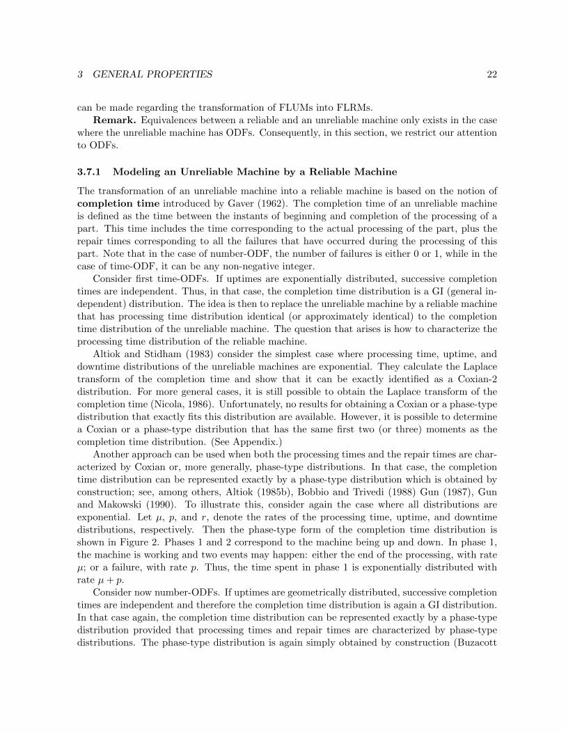
Another approach can be used when both the processing times and the repair times are char-acterized by Coxian or, more generally, phase-type distributions. In that case, the completiontime distribution can be represented exactly by a phase-type distribution which is obtained byconstruction; see, among others, Altiok (1985b), Bobbio and Trivedi (1988) Gun (1987), Gunand Makowski (1990). To illustrate this, consider again the case where all distributions areexponential. Let µ, p, and r, denote the rates of the processing time, uptime, and downtimedistributions, respectively. Then the phase-type form of the completion time distribution isshown in Figure 2. Phases 1 and 2 correspond to the machine being up and down. In phase 1,the machine is working and two events may happen: either the end of the processing, with rateµ; or a failure, with rate p. Thus, the time spent in phase 1 is exponentially distributed withrate µ+ p.

Consider now number-ODFs. If uptimes are geometrically distributed, successive completiontimes are independent and therefore the completion time distribution is again a GI distribution.In that case again, the completion time distribution can be represented exactly by a phase-typedistribution provided that processing times and repair times are characterized by phase-typedistributions. The phase-type distribution is again simply obtained by construction (Buzacott


Figure 2: Completion Time Distribution

and Kostelski, 1987; Gun,1987).Finally, we note that by using this approach, both types of ODFs can be combined. Also,

this approach can be used to incorporate inspection and rework, and moreover failure andinspection features can be combined (Sastry and Awate, 1988). Thus, this approach is veryattractive since it makes it possible to incorporate many features into an equivalent completiontime distribution. We note, however, that the number of phases of the resulting distribution maybe large, especially if the original processing and repair phase-type distributions have severalphases. This is the drawback of this approach compared to the approach based on identificationof moments.

3.7.2 Modeling a Reliable Machine by an Unreliable Machine

We now discuss the transformation of a reliable machine into an unreliable machine. Considerfirst the case where the reliable machine has a Coxian-2 processing time distribution with pa-rameters (µ1, a1, µ2). It can be modeled exactly by an unreliable machine with number-ODFswith processing speed µ1, repair rate µ2, and where a1 is the probability of having a failureat the completion of an operation. See Buzacott (1972). Alternatively, it can also exactly bemodeled by an unreliable machine with time-ODFs whose parameters are obtained by reversingthe transformation of Altiok and Stidham (1983). It is easy to check that this can be done onlyif the original distribution of processing times has a coefficient of variation greater than 1.

In more general cases, there is no simple way of doing an exact transformation. However,it is again possible to determine the parameters of an unreliable machine whose associatedcompletion time distribution is close to the original processing time distribution. In that case,one must first choose the characterization of the unreliable machine, i.e., the distributions ofprocessing times, uptimes, and downtimes, as well as the type of ODFs. Then, the parameters


of these distributions are determined in such a way that the resulting distribution of completiontime has the same first two (or three) moments as the distribution of processing times of thereliable machine. Such an approximate transformation was used by Liu and Buzacott (1989).

3.8 Relationships Among Models

In Section 2, we introduced three major classes of models: asynchronous, synchronous, andcontinuous. Each model is of interest as a representation of a physical system. For instance, aproduction line may operate in such a way that parts can only be transferred every T units oftime, in which case the synchronous model is probably the model of choice.

However, each of these models can also be of interest as an approximation of another model.Most importantly, the synchronous and the continuous models can be used as approximationsof the asynchronous model. Since several authors have followed this approach, it is worthwhiledescribing how it works.

3.8.1 Approximation of the Asynchronous Model

Consider an asynchronous FLUM model with the following features: the processing times aredeterministic; the uptimes and downtimes are exponentially distributed; failures are operationdependent (ODFs). Consider first the case where all machines have the same processing time,T . No exact solution of this asynchronous model has yet been obtained, even for the simplecase of two-machine lines, except in the case of no intermediate storage (Commault and Dallery,1990). As a result, several authors have proposed to use either the synchronous model or thecontinuous model as an approximation to the behavior of the asynchronous model.

Approximation by continuous model; identical machine speeds. The idea is to ap-proximate the discrete flow of parts by a continuous flow of material. Each machine of thecontinuous model has the same distributions for uptimes and downtimes as the correspondingmachine of the asynchronous model. All the machines of the continuous model have the samespeed, µ, which is the inverse of the processing time: µ = 1/T .

The question is whether or not the continuous model is a good approximation. It was shownexperimentally (e.g., Alvarez, Dallery, and David, 1991) that it is actually a good approximationprovided that the following assumption is satisfied.

Assumption MTS (Multiple Time Scale). The uptimes and downtimes of the machinesof the flow line are much larger (at least one order of magnitude) than the processing times.

A theoretical justification was provided by David, Xie, and Dallery (1990). They showedthat, in the case of BAS, the production rate of the asynchronous model with buffer capacity Nis bounded by the production rates of the continuous model with appropriate buffer capacities,namely:

P (Cont,N − 1) ≤ P (Asynch,N) ≤ P (Cont,N + 1) (28)

FLUMs in which the uptimes and downtimes are large compared to the processing timesare likely to have large buffers. In this case, the difference between the first and third terms in


equation (28) is small. This further implies that the production rate of the continuous model isa very good approximation of that of the asynchronous model.

Approximation by synchronous model; identical machine speeds. The asynchronousmodel may alternatively be approximated by a synchronous model. Each machine of the syn-chronous model has constant processing T , and has geometric uptimes and downtimes havingthe same means as the exponential uptimes and downtimes of the asynchronous model. In otherwords, the synchronous model forces events to occur only a times multiple of T , whereas inthe original asynchronous model, events could occur at any time. Again, this model is a goodapproximation of the asynchronous model under Assumption MTS.

Approximation by continuous model; different machine speeds. Consider now thecase where the machines of the asynchronous model have different processing times, Ti. Theasynchronous model can no longer be approximated by a synchronous model, since the majorfeature of the synchronous model is that all machines have the same processing times. On theother hand, it can still be approximated by a continuous model. The speed of machine Mi in thecontinuous model is µi = 1/Ti. The characterization of uptimes requires special attention in thecase of ODFs. Let pi and ri be the failure and repair rates of Machine Mi in the asynchronousmodel. If Machine Mi of the continuous model is working at its own speed, µi, its failure rate issimply pi. However, Machine Mi may also be slowed down, as discussed in Section 2.3. Supposefor a period of time, Machine Mi is slowed down by Machine Mj , where µj < µi. During thistime, machine Mi has a reduced failure rate equal to pi(µj/µi). The reason is that the behaviorof the continuous model must be as close as possible to that of the asynchronous model.

For the sake of simplicity, consider the case where j = i − 1. Machine Mi slowed down byMachine Mi−1 in the continuous model corresponds to the case where buffer Bi−1,i is empty inthe asynchronous model. In that case, the behavior of the asynchronous model is as follows.Both machines start working on a part at the same instant. Machine Mi completes its operationTi time units after while Machine Mi−1 completes its operation Ti−1 time units after. As aresult, Machine Mi is idle (starved) for a length of time equal to Ti−1 − Ti. During the first Titime units, Machine Mi may fail at rate pi, whereas during the remaining Ti−1 − Ti time units,it cannot fail since it is starved and we assume ODFs. Therefore, its average failure rate in thissituation is pi(Ti/Ti−1) = pi(µi−1/µi). The continuous model must reflect this and, as a result,Machine Mi has a reduced failure rate. On the other hand the repair times are exponentiallydistributed with rate ri. Note that in the case of TDFs, Machine Mi of the continuous modelhas always a failure rate of pi since in the asynchronous model Machine Mi may still fail whenidle.

As for the case of identical machine speeds, the continuous model is a good approximationof the asynchronous model provided that Assumption MTS is satisfied (Alvarez, Dallery, andDavid, 1991). Also, the bounding properties expressed in equation (28) still hold (David, Xie,and Dallery, 1990). The fact that the continuous model can approximate asynchronous modelswith non-identical processing times is one of its major advantages over the synchronous model.

In many FLUMs, failures occur much less often than processing of parts and therefore,Assumption MTS is likely to be often satisfied. Thus, continuous or synchronous models used as


approximation of asynchronous models will often provide very good estimates of the performanceparameters.

Most of the work pertaining to the approximation of asynchronous models of FLUMs withdeterministic processing times assumes exponential and geometric up- and downtimes in the caseof continuous and synchronous models, respectively. However, such an approximation can alsobe used in the case of general distributions of up and down-times. Again, this approximationwill be accurate provided that Assumption MTS is satisfied (David, Xie, and Dallery, 1990).

Other approximations. The major usefulness of the continuous (or synchronous) model asan approximation of the asynchronous model is in the case of FLUMs having deterministicprocessing times. However, it can also be used in other cases, especially in the case of FLUMswith random processing times satisfying Assumption MTS. Finally, continuous and synchronousmodels have also been used as approximations of FLRMs (De Koster and Winjgaard; 1989, Liuand Buzacott, 1989). Such approximations should especially work well in the case where theprocessing times have large variances.

3.8.2 Approximation of the Synchronous Model

The continuous model can also be used as an approximation of the synchronous model ofFLUMs. Gershwin and Schick (1980) investigated the relationships between two-machine syn-chronous FLUM systems and two-machine continuous material FLUM systems by means of theδ-transformation. In this transformation, the failure and repair rates of both machines aremultiplied by a small number δ and the buffer size is divided by δ. That is, (r1, p1, r2, p2, N) arethe parameters of one synchronous two-machine system, and (r′1, p

′1, r′2, p′2, N

′) are the parame-ters of the other, with:

r′i = riδ (29)

p′i = piδ (30)

N ′ =N

δ(31)

The only restriction on δ is that the new buffer size N ′ must be an integer.When N ′ is large, the performance measures of the systems are approximately related.

Production rate P ′ is close to P , and average buffer level n′ is approximately n/δ. In thelimit as δ→0, the new synchronous system approaches a continuous material flow system whoseproduction rate is also approximately that of the original system. This approximation providesespecially good results for systems that satisfy Assumption MTS.

The reason that this is true is that the δ-transformation is essentially a transformation ofthe cycle time. The new cycle time is δ times the old cycle time, and the amount of materialprocessed during a new cycle time is δ times the amount of material processed during an oldcycle time. Consequently, the probability of a failure or a repair during a new cycle is δ timesthe probability during an old cycle. The size of the buffer has not changed, but if it is measuredin units of the amount material processed during a cycle time, it must be divided by δ.


We would suggest that this transformation can be extended to relate all models: synchronous,asynchronous, and continuous, and a variety of failure and repair time distributions, blockingmodels, etc. It can be useful in reducing numerical effort in analyzing systems.

Finally, we note that numerical results on the approximation of the synchronous model ofFLUMs with TDFs by a continuous model are reported by De Koster and Wijngaard (1989).Again, it appears that this approximation is accurate provided that Assumption MTS is satisfied.

3.8.3 Other Relationships Among Models

In this section, we discuss results pertaining to the transformation of an asynchronous FLUMwith non-identical deterministic processing times into an asynchronous FLUM with identicaldeterministic processing times. Such a transformation, although only an approximation, is ofinterest for several reasons. First, it appears from the above discussion that the synchronousmodel can be used as an approximation of asynchronous lines with deterministic processingtimes only in the case where all the processing times are equal. Therefore, if one wants to usesynchronous models, it is necessary to be able to transform an asynchronous line with non-identical processing times into an asynchronous line with identical processing times. Secondly,even though continuous models can handle non-identical processing times, such a transformationmay still be of interest when using such models. The reason is that some solution techniquesmay be restricted to (or at least simpler) the case of identical processing times. (See Section5.2.1.)

Several transformations have been proposed. Gershwin (1987b) suggested replacing eachmachine of the original line, except the fastest, by a set of two machines with no intermediatebuffer. One machine captures the unreliability behavior of the original machine, while the otherrepresents the effective processing time. All the machines of the resulting line have the sameprocessing time which is equal to the processing time of the fastest machine of the original line.This transformation was referred to as disaggregation by Dallery, David, and Xie (1989). It isvery accurate as long as the failure and repair rates of the machine representing the processingtime are much larger than those of the machine capturing the unreliability behavior.

A second transformation was proposed by Dallery, David, and Xie (1989) and referred to ashomogenization. It consists of replacing each machine of the original line except the fastest bya single equivalent machine. As in the case of disaggregation, all the equivalent machines have thesame processing time equal to the processing time of the fastest machine of the original line. Theparameters of each equivalent machine are obtained as follows. Its repair rate is the same as thatof the original machine. Its failure rate is obtained by prescribing that the equivalent machinehas the same production rate in isolation as that of the original machine. Homogenization isa simpler transformation than disaggregation but is not as accurate. However, it provides agood approximation for nearly homogeneous lines, i.e., lines where the processing times ofall machines are close to one another.

A third transformation was proposed by Liu and Buzacott (1990). It is similar to homog-enization except that the failure and repair rates of the equivalent machine are determined byprescribing that the first and second moments of the completion time of the equivalent machinein isolation is the same as those of the original machine. Note that the first moment is nothingbut the production rate in isolation. The accuracy of that transformation is similar to that of


Figure 3: Production rate as a function of buffer size for a two-machine synchronous line inwhich r1 = 0.08, p1 = 0.01, r2 = 0.09, p2 = 0.01.

homogenization.

3.9 Qualitative Behavior

In all the models described in the following sections, several important features were observed.In some cases, they were demonstrated analytically for a limited class of systems. In others,they were observed by numerical experimentation or by simulations. They include

Saturation and Limiting behavior Production rate is a saturating function of buffer size;that is, it is an increasing function with a finite upper bound that it approaches asymptoticallyas buffer size increases without limit. (See Section 3.5.) Saturation is illustrated in Figure3. This upper bound is the production rate of the slowest machine, in the sense of isolatedproduction rate ρi. If any one machine is significantly slower than the others, in that sense,then it limits the behavior of the system. The system production rate is less than that of thatmachine; buffers upstream of that machine tend to be full, and buffer downstream tend to beempty. In Figure 3, the limiting production rate is 0.8889, which is the isolated production rateof Machine M1, the slower of the two machines.

Effectiveness of buffers – buffers and disruptions Buffers increase the production rateof systems only by decoupling the effects of disruptions from one part of the system to otherparts. If a failure happens upstream of a buffer, and the buffer has enough material in it, thedownstream part of the system can keep operating. Similarly, if a failure happens downstream ofa buffer, and the buffer has enough space, the upstream part of the system can keep operating.Therefore, for a buffer to be effective, its size must be the same order of magnitude as the


disruptions that it must block, when measured in comparable units. If the mean down time ofMachine Mi is 1/ri time units, then the size of buffers Bi−1,i and Bi,i+1 should be on the orderof the amount of material that the machines typically produce in 1/ri time units. On the otherhand, if the system is reliable (FLRM) and operation times are random, then the buffer sizeshould be roughly the standard deviation of an operation time. If the buffer is much smallerthan this estimate, it will have very little effect on performance; if it is much larger, it is in theflat part of the saturation curve, and much of its capacity is wasted. In Figure 3, the maximumcurvature of the curve occurs around N = 40, which is on the order of 1/ri = 12.5. (A moreaccurate value of the optimal N depends on the performance measure, as well as all four machinereliability parameters.)

Effectiveness of buffers – system balance and imbalance Because buffers increase theproduction rate of systems only by decoupling the effects of disruptions, they do not compensatefor systems that are highly unbalanced. They should not be placed near the bottleneck (neitherthe machine with the smallest ρ nor the machine with the smallest µ); rather they should beplaced where disruptions are greatest. A large buffer upstream of a bottleneck will be emptymost of the time; a large buffer downstream of a bottleneck will be full most of the time. Inboth cases, it is wasted (along with the in-process inventory it accumulates, when the upstreampart of the line is faster than the downstream).

Effect of increasing line length on performance Hillier and Boling (1966), using themethod of Hillier and Boling (1967), observed that as a transfer line with identical machinesand buffers increases in length, its production rate seems to decrease to a non-zero limit. DeKok (1988) developed an approximate technique for evaluating long transfer lines consistingof identical machines and buffers. His numerical experiments suggested the same conclusion.Ancelin and Semery (1987), David, Semery, Ancelin, and Terracol (1987), Gershwin (1989), andSemery (1988), made similar observations (and drew similar graphs) for different models usingdifferent methods. (Based on the decompositions reported in Section 5.2.1, Gershwin (1991b)developed an algorithm for predicting the limiting production rate.)

Bowl phenomenon Sevast’yanov (1962) developed a technique for analyzing long transferlines. (See Section 5.2.1.) Based on this approximate method, he studied the optimal design ofa line that has very many machines, where the designer can group the machines into a givennumber of groupings, and where a given amount of storage space can be divided among thesegroupings. He showed that the storage space should be divided equally, and the machines shouldbe grouped together in such a way that the first and last machine groups are equally reliable;and that all the rest of the groups are equally reliable; and that the inner groups should besomewhat more reliable than the outer groups.

Hillier and Boling (1966, 1972, 1977) also observed that the optimal distribution of systemresources is not an equal allocation. That is, if there is a pool of machine speed, and the goalis to maximize the system’s production rate, the pool should not be divided equally among themachines. Instead, the machines in the middle of the line should get more, and the machines atthe ends should get less. (This assumes that the buffer sizes are equal.) The distribution should

4 EXACT ANALYSIS 30

be symmetric. Similarly, if the machines are identical and there is a pool of storage space, thebuffers in the middle of the line should get more, and the buffers at the ends should get less.They called this the “bowl phenomenon” because of the shape of the distribution of operationtime (which is the inverse of machine speed).

While this phenomenon is a real feature of mathematical models of production lines, thereis some question as to whether it is of practical importance. As indicated above, Smunt andPerkins (1985) did not feel that it generally had a large impact. Numerical results of Hillier andBoling (1972) indicate that the gain over an equal distribution is usually less than 1%. Not onlymight this gain be negated by errors in system parameters, but the reason for the bowl shapeis the usual assumption that the first machine is never starved and the last machine is neverblocked. This implies that the machines at the ends of the line are forced to be idle less thanthose in the middle. The bowl shape compensates for this. In a real system, however, the firstmachine is occasionally starved when suppliers fail to deliver raw material, and the last machineis blocked during temporary declines in demand.

3.10 Realistic Values of Parameters

In most real systems,

(1) all machines operate at approximately the same speed while they are operational. Therefore,all µi are close to one another. In other words, the line is nearly homogeneous.

(2) there is no machine which is much worse than all the others. Therefore, all ρi = µiriri+pi

areclose to one another.

(3) failures and repairs are much less frequent than operations. Therefore, pi and ri are at leastan order of magnitude less than µi. That is, Assumption MTS is satisfied.

(4) the production rate of the line (P) is not less than half the isolated production rate of atypical machine (ρi).

It is always possible to find exceptions to these fuzzy rules of thumb. These considerations areimportant to those who design approximate methods for analyzing these systems. If a methodworks well under these conditions, it is likely to be of practical value; if not, it probably will notbe. See also the features described in Section 3.9.

4 Exact Analysis

In this section, we describe flow line models that have exact analytic solutions. Such modelsare important because (1) exact solutions are better than simulations or approximations whenthe models fit real systems closely, (2) they provide useful qualitative insight into the behaviorof systems, and (3) the fact that they can be solved rapidly makes them essential parts of thedecomposition and aggregation methods that are described in Section 5.

Most of the results pertaining to the exact analysis of flow line models are based on Markoviananalysis. In order to be able to describe the behavior of the flow line by a Markov process, thedistributions have to be of special form: exponential or, more generally, continuous phase-type

4 EXACT ANALYSIS 31

distributions in the case of continuous time models; geometric or, more generally, discrete phase-type distributions in the case of discrete time models. (See the Appendix.) However, there aresome exceptions for which the analysis is not based on Markov models. These exceptions aremost often encountered in flow lines with no intermediate storage.

The literature pertaining to this special case is discussed in Section 4.1. Section 4.2 describesthe literature of two-machine FLRM (Flow Line with Reliable Machines) models and theirsolutions. The literature of two-machine FLUM (Flow Line with Unreliable Machines) modelsis presented in Section 4.3. Although the systems are sometimes equivalent, as we argue inSection 3.7, it is helpful to treat them separately. This is especially because different approximatemethods of Section 5 were designed with different kinds of systems in mind. In Section 4.4, wedescribe exact methods for three-machine and larger systems.

We try to indicate which of the models in the literature are blocking-after-service systems(BAS), and which are blocking-before-service systems (BBS). This is not always straightforward,because early authors were evidently not concerned with this distinction. In the two-machinecase, the distinction is not important, and does not warrant new research, because each can betransformed into the other; see Section 3.4. See the review by Perros (1988) for other papers ontwo-stage systems.

Notation. In the case of two-machine flow line, we drop the index of parameters pertainingto the buffer. That is, N1,2 and C1,2 are simply denoted by N and C, respectively.

4.1 Flow Lines with No Intermediate Storage

In this section, we restrict our attention to the case of flow lines with no intermediate storage,that is, Ci,i+1 = 0, for all i = 1, ...,K−1. We review the part of the literature that is devoted tothis special case. The aim is to determine the average production rate of the line. Most often,BAS is assumed.

Flow lines with no intermediate storage can operate under two transfer modes: asyn-chronous transfer mode and synchronous transfer mode. In the former case, parts canmove independently as long as they are not blocked. In the latter case, there is always exactlyone part on each machine and the transfer of all parts occurs simultaneously at the instant whenall machines have completed their processing. Note that the asynchronous transfer mode is im-plicitly assumed in the asynchronous model described in Section 2.1. Let P (AT ) and P (ST )denote the production rate of a flow line operating under the asynchronous transfer mode andsynchronous transfer mode, respectively. It can be shown (Muth, 1973) that a system operat-ing under synchronous transfer mode is less efficient than when operating under asynchronoustransfer mode, i.e.:

P (ST ) ≤ P (AT ) (32)

This relationships hold for any flow line with any number of (reliable or unreliable) machines. Inthe special case of two-machine lines, the two production rates are equal, i.e.: P (ST ) = P (AT ).Indeed, whether or not the part on Machine M2 can be released independently does not affectthe production rate. Consequently, in that case, it is not important to distinguish between thetwo transfer modes.

4 EXACT ANALYSIS 32

Two-machine FLRMs with no intermediate storage and BAS were analyzed by Rao (1975a)and Lau (1986a, 1986b). The production rate can be expressed as

P =1

E[max(S1, S2)](33)

where Si denotes the random variable corresponding to the processing time of Machine Mi,i = 1, 2. Consequently, the problem reduces to that of calculating the expected value of themaximum of two random variables. Rao (1975a) and Lau (1986a, 1986b) gives explicit expres-sions for calculating the production rate for different distributions of processing times, especiallyexponential, Erlang, uniform, and normal distributions.

For FLRMs with more than two machines we need to distinguish between the two transfermodes. In the case of synchronous transfer, the analysis is similar. Indeed, the production rateis now given by P = 1/E[max(S1, ..., SK)]. Again, the problem reduces to that of calculating theexpected value of the maximum of K random variables. In the case of asynchronous transfer,the analysis is much more complex. The case of three machine flow lines was deeply investigatedby Hunt (1956), Hillier and Boling (1967), Hildebrand (1968), Muth (1973, 1977, 1984), Muthand Alkaff (1987), Rao (1976a, 1976b).

The approach introduced by Muth (1973) is fairly general. It is based on the analysis of theholding time distribution at the first machine. The holding time is the total time spent bya part on this machine. It is the sum of the processing time and possibly some blocking time.The holding time at Machine M1, H1, can be expressed as (Muth, 1984)

H1 = max(S1, S2, R3) (34)

where R3 is the residual processing time of the part at Machine M3 at the time at which thenext part is transferred from Machine M1 to Machine M2. The production rate can then beobtained as

P =1

E[H1](35)

Therefore, the problem mainly reduces to that of determining the distribution of R3. Numericalsolutions have been obtained by Muth (1977, 1984) and Rao (1976a, 1976b) for specific distribu-tions of the processing times. A unifying solution is provided by Muth and Alkaff (1987) underthe following assumptions: Machines M1 and M3 have special phase-type distributions, whileMachine M2 has a Laplace transformable distribution. Unfortunately, it does not seem that theanalysis is extendible to flow lines consisting of more than three machines.

We now turn our attention to FLUMS with no intermediate buffer. First, we note that allthe above results are still applicable provided that processing times are replaced by completiontimes. Buzacott (1968) considered the case of flow lines with synchronous transfer, deterministicprocessing times and general distributions of uptimes and downtimes. Let T denote the commonprocessing time of all machines. He obtained the following simple formula for the productionrate

P =1

T

1

1 +∑Ki=1

MTTRiMTTFi

(36)

4 EXACT ANALYSIS 33

This formula was obtained under the following assumption (Buzacott, 1968): if two machinesbreak down in the same cycle, the total duration of line stoppage is the same as the sum ofstoppage durations of the machines when the machines break down in different cycles. Thisformula also holds under the following alternative assumption: when a machine goes down, allother machines stop their processing; the processing of all machines resumes as soon as themachine is repaired. Note that this assumption implies that at most one machine may be downat any time.

When neither of these assumptions satisfied, Buzacott’s formula provides a good approxi-mation of the exact production rate provided that the times to failures are large compared tothe processing time T (Assumption MTS). For models for which this is not true, Commault andDallery (1990) propose a method for calculating the production rate under the assumption thatuptimes are exponentially distributed. It is shown that the analysis reduces to the calculation ofthe expected value of the maximum of Coxian distributions. Approximations are also provided.

4.2 Flow Lines with Two Reliable Machines

In this section, we discuss the exact solutions of two-machine FLRMs with finite buffers. InSection 4.2.1 we describe the relationship between two-machine FLRMs with finite buffers andsingle server queues with finite buffers. In Section 4.2.2 we describe exact methods for analyzingtwo-machine FLRMs with finite buffers and phase-type distributions of operation times. Byanalyzing, we mean calculating the steady state distribution, which can then be used to deter-mine production rates and other performance measures. This technique is closely related to themethods described in Section 4.3.

4.2.1 Equivalence of Two-Machine Flow Lines with Finite Queues

In this section, we briefly discuss the equivalence of two-machine flow lines with finite singleserver queues (FSSQs). A FSSQ consists of a single server fed by an external arrival process ofcustomers. There is a finite buffer in front of the server in order to accommodate the customersthat arrive while the server is busy. Let L denote the capacity of the buffer including the spacein front of the server. Thus, L is the maximum number of customers that can be present in thesystem, either receiving or waiting for service. We further need to define the behavior when thequeue is full. There are two different assumptions and the corresponding models are referred toas the lost model and the switch-off model (Buzacott and Kostelski, 1987).

In the lost model, it is assumed that the arrival process is never stopped and that customersarriving while the queue is full are lost. In the switch-off model, it is assumed that the arrivalprocess is switched off as soon as the queue is full. The arrival process is restarted at theinstant when a space becomes available in the buffer which occurs when the next service iscompleted. Note that in queueing theory, the lost model is usually considered (Kleinrock, 1975).The lost and switch-off models are not equivalent, in general. However, they are equivalent ifthe distribution of the interarrival process of customers is exponential. This follows from thememoryless property of the exponential distribution (Kleinrock, 1975).

There are equivalences between two-machine flow lines and FSSQs with switch-off arrivalprocess. Consider first a two-machine line with blocking-before-service and buffer capacity N .

4 EXACT ANALYSIS 34

Then, the behavior of this system is equivalent to the behavior of the following FSSQ withswitch-off arrival process: the interarrival time distribution is the same as the processing timedistribution of Machine M1; the service time distribution is the same as the processing timedistribution of Machine M2; the buffer capacity is L = N . Now, if instead of BBS, the two-machine line operates under blocking-after-service, then the same equivalence holds providedthat the buffer capacity is L = N + 1.

In summary, by combining the above results, we have the following equivalences: (1) for anytwo-machine flow line, there exists an equivalent FSSQ with switch-off arrival; and (2) for anytwo-machine line for which the first machine has exponential processing times, there exists anequivalent FSSQ with lost arrivals. In both cases, the queue capacity is increased by one if BASis assumed.

Now, consider the case of a two-machine flow line with exponential and general processingtime distributions for the first and second machines, respectively. As stated above, it is equivalentto a M/G/1/L queue (Kleinrock, 1975). Consequently, its solution can be obtained as thesolution of the M/G/1/L queue which is based on the analysis of the embedded Markov chainat departure instants (Cohen, 1982). Note that in the special case where the processing timedistribution of the second machine is also exponential, the analysis reduces to that of aM/M/1/Lqueue whose solution has a very simple geometric form. Finally, we note that the case of a two-machine flow line with general and exponential processing time distributions for the first andsecond machines, respectively, can also be analyzed as a M/G/1/L queue using the dualityproperty of two-machine flow lines (see Section 3.6). Two-machine flow lines of the above typeswere analyzed by Rao (1975b).

4.2.2 Analysis of Two-Machine Flow Lines with Phase-Type Distributions

Consider a two-machine FLRMs where the processing time distribution of each machine is givenin the form of phase-type distribution. (Recall that a Coxian distribution is a special case.) LetPHi refer to the phase-type distribution of Machine Mi, for i = 1, 2, and let si be the numberof phases of PHi. The behavior of such a system can be characterized by a discrete state,continuous time Markov process. Analyzing this system then reduces to that of calculating thesteady-state probabilities of this Markov process, from which all the performance parameterscan be derived.

Any numerical technique for discrete space Markov processes can in principle be used (Stew-art, 1978 and 1988; Philippe, Saad, and Stewart, 1989). However, it is helpful to recognize thatthe Markov process has a very special structure and to take advantage of it. In the followingpresentation, we assume that the blocking mechanism is BBS. However, the type of blocking isnot at all important since we know that in the case of two-machine lines, there is equivalence.(See Section 3.4.)

The state of the Markov process can be expressed as (n, j1, j2), where n is the number ofparts currently present in the buffer (including the part on Machine M2, if any), and ji is thecurrent phase of service of Machine Mi, i = 1, 2. n can take on integer values from 0 to N . j1can take on integer values from 1 to s1, except when Machine M1 is blocked in which case weset j1 = 0. Similarly, j2 can take on integer values from 1 to s2, except when Machine M2 isstarved in which case we set j2 = 0. Let us partition the state space according to the values of

4 EXACT ANALYSIS 35

n. Let p denote the steady-state probability vector and let pn denote the portion of that vectorthat corresponds to a buffer content of n. We can write

p =

p0p1

.

.pN

(37)

Note that pn, n = 1, ..., N − 1, is of size s1s2 while p0 and pN are of size s1 and s2, respectively.Let Q denote the infinitesimal generator of the Markov process. The steady-state prob-

ability vector p of the Markov process is the solution of the equation pTQ = 0; or, equivalently,

QTp = 0. (38)

(In this presentation, we choose to use this equation and therefore we deal with QT .) In addition,p also satisfies the normalization equation

1Tp = 1. (39)

Matrix QT is a block tridiagonal matrix with the following special structure

QT =

B0 A0 0 . . . 0C0 B A 0 . . .0 C B A 0 . .

. . . . . .

. 0 C B A 0

. . 0 C B AN0 . . . 0 CN BN

(40)

where A, B, and C are square matrices of size (s1s2, s1s2); B0 and BN are square matrices of size(s1, s1) and (s2, s2); A0, C0, AN , and CN are of size (s1s2, s1), (s1, s1s2), (s2, s1s2), (s1s2, s2).

QT has this special structure because the Markov process associated with a two-machine flowline is a generalized birth-death process. Transitions can only occur between states that areneighbors of each other with respect to the value of n. That is, the only possible transitions froma state (n, j1, j2) are to a state (n′, j′1, j

′2) such that either n′ = n, or n′ = n− 1, or n′ = n+ 1.

In addition, transition rates are independent of n, for 1 < n < N − 1. Because of the specialblock tridiagonal structure of QT , equation (38) can be decomposed into the following set ofequations

B0p0 +A0p1 = 0 (41)

C0p0 +Bp1 +Ap2 = 0 (42)

Cpn−1 +Bpn +Apn+1 = 0 , 1 < n < N − 1 (43)

CpN−2 +BpN−1 +ANpN = 0 (44)

4 EXACT ANALYSIS 36

CNpN−1 +BNpN = 0 (45)

Two solution techniques that make use of the special structure of the matrix QT have receivedspecial attention. They are known as the recursive technique (Herzog, Woo and Chandy, 1975,Chandy and Sauer, 1981; Stewart, 1988) and the matrix geometric technique (Neuts, 1981).Recursive and matrix geometric techniques to analyze two-machine FLRMs have been used,among others, by Altiok and Ranjan (1987), Buzacott and Kostelski (1987), Gun and Makowski(1987). Another approach, which has only been applied to two-machine FLUM systems, isdescribed in Section 4.3. There is no reason why this method could not be used for the presentclass of systems as well.

The recursive technique can be applied to Markov processes that satisfy the following con-dition: there exists a subset of states, called the boundary states, such that the probabilitiesof all other states can be obtained recursively from the probabilities of the boundary states.The recursive technique is usually implemented using the following procedure (Buzacott andKostelski, 1987). Let k be the total number of states of the Markov process. Determine a subsetof m boundary states satisfying the above condition. Obtain a recursive scheme to derive thenon-boundary state probabilities. This uses k−m equations among the total of k balance equa-tions. Then, express all non-boundary state probabilities as a linear function of the probabilitiesof the boundary states. The coefficient of a particular boundary value in the linear expressionis obtained by setting that boundary value equal to 1 and all other boundary values equal to0, and then follow the recursive scheme. The remaining m balance equations can then be usedtogether with the normalizing equation, (39), to determine the probabilities of the boundarystates, from which the other probabilities can then be derived.

It is important to note that the phrase “boundary states” has a different meaning elsewherein this paper, and in most of the rest of the literature. Boundary states, as defined here, areusually a subset of boundary states, as defined in Section 4.3.

Buzacott and Kostelski (1987) applied this recursive technique in the case where each ma-chine has a Coxian-2 processing time distribution. The states corresponding to an empty buffer(n = 0) are chosen as the boundary states. In this simple case, there are only two boundarystates: (0, 0, 1) and (0, 0, 2). In the general case of phase-type distributions, the recursive tech-nique can still be applied, for instance, by considering the states corresponding to a buffer levelof n = 1 as the boundary states.

The principle of the matrix geometric solution can briefly be described as follows (Gun, 1987,Gun and Makowski, 1987). The first step is to show that the set of transition equations (41) to(45) can be transformed into an equation of the following form:

Npn +Mpn−1 = 0 (46)

where the matrices N and M are of size s1s2 and N is invertible. Let R be the matrix definedas R = −N−1M . Then, we have:

pn = Rpn−1 , 1 < n < N (47)

For the boundary states, it is also possible to define matrices S and U such that p1 = Sp0and pN = UpN−1. The probability vector p0 can be determined by solving an equation of the

4 EXACT ANALYSIS 37

form Zp0 = x. This equation is again obtained from the basic set of equations, (41)-(45). Theremaining probabilities can then be obtained using the above equations. See Gun (1987) andGun and Makowski (1987) for more details.

We note that the matrix geometric solution is also based on a recursive scheme and so ithas relationships with the recursive technique described above. Buzacott and Kostelski (1987)compared these two techniques in the case of Coxian-2 distributions. They showed that bothtechniques can be subject to numerical problems when N is large.

We note that probabilities at specific points in time, especially completion instant prob-abilities, can be derived from the steady-state probabilities; see, e.g., (Gun and Makowski,1989). Such probabilities are useful when using decomposition methods (Section 5.1). Finally,we note that similar analyses can be done in the case of discrete phase-type distributions; seee.g., Gun (1987). In that case, the underlying model is a discrete time Markov process.

4.3 Flow Lines with Two Unreliable Machines

In this section, we discuss the exact solutions of two-machine FLUMs with finite buffers. Thesesystems are modeled as Markov processes with discrete states and continuous times (Sec-tion 4.3.1), as Markov processes with discrete states and discrete times (Section 4.3.2), andas Markov processes with mixed states and continuous times (Section 4.3.3).

4.3.1 Asynchronous Models

Each of the models in this section is described as a Markov process with continuous time anddiscrete state. The state (n, α1, α2) represents the number of parts in the buffer (n) and thecondition of the machines (α1 and α2). Most often, αi can take on two values, which we mayrepresent as 1 for operational (up) and 0 for under repair (down). When there are more thanone failure mode, or when processing times, uptimes, or downtimes are represented by Coxianor phase-type random variables, or when other states (especially idle) are included, αi takes onmore than two values. In fact, it is possible to combine a Coxian model of operation time anda Coxian model of failure, and apply the methods of Section 4.2.2 and this section to it. Thepresent models are not essentially different from those of the earlier section; αi here is the sameas ji there.

As in Section 4.2.2, p is the steady-state probability distribution vector. The componentsof p are p(n, α1, α2). Let pn be the portion of that p that corresponds to a buffer content ofn. The dimensionality of pn depends on the number of different values of α1 and α2. Whenthey can take on two values, the usual case in the literature, the dimensionality of pn is 4. Inthat case, the dimensionality of p is roughly 4(N + 1), since n can take on integer values from0 to N . (We say “roughly” because there may be additional states for idle when the buffer isempty or nearly empty or full or nearly full; or there may be additional states when the bufferis full or nearly full for the piece in the machine’s work area for BAS systems; or there maybe fewer states if transient states are eliminated. Transient states appear when the buffer isempty or nearly empty or full or nearly full.) p can be written (37) and it satisfies (38) (withan appropriate Q) and (39).

As in Section 4.2.2, it is useful to distinguish between internal states and equations and

4 EXACT ANALYSIS 38

boundary states and equations. The latter refers to cases when the buffer is empty or nearlyempty or full or nearly full. For some models, the boundary consists only of states in whichn = 0 and n = N (in which case (42) and (44) are exactly the same as (43)); other models alsoinclude n = 1 and n = N − 1. Internal states are all states that are not on the boundary. Thisterminology comes from differential equations, and some of the solution techniques describedbelow have been influenced by differential equation methods.

Also as in Section 4.2.2, this system is a generalized birth-death process, and pn satisfies (41)-(45). The approach taken in the two-machine FLUM literature is to satisfy (43) by assumingthe following analytic expression for p(n, α1, α2) when n is internal:

p(n, α1, α2) =∑j

DjXnj φj(α1, α2) (48)

for some scalars Dj and Xj and some scalar functions φj (although not all authors write thesolution in this form). Equation (48) can also be written

pn =∑j

DjXnj φj (49)

where φj is the vector whose components are φj(α1, α2).Equation (48) follows from (43) when

pn = Rnφ. (50)

is a solution of (43) for some matrix R and vector φ. Yeralan and Muth (1987) demonstrateconditions for this to hold. They call this the matrix geometric property. Substituting (50)into (43):

ARn+1φ+BRnφ+ CRn−1φ = 0 (51)

or,

(AR2 +BR+ C)Rn−1φ = 0 (52)

so (43) is satisfied if R satisfies

AR2 +BR+ C = 0. (53)

Let X1, ..., Xl be the eigenvalues of R, and φ1, ...,φl be the corresponding eigenvectors. Ifwe write

φ = D1φ1 + ...+Dlφl, (54)

then

Rφ = D1X1φ1 + ...+DlXlφl, (55)

and similarly,

4 EXACT ANALYSIS 39

pn = Rnφ = D1Xn1φ1 + ...+DlX

nl φl, (56)

which is equivalent to (48). When the summation has only one term, Yeralan and Muth (1987)call this the scalar geometric property. The coefficients D1, . . . , Dl and the boundary prob-abilities are determined by satisfying the transition equations on the boundary (i.e., (41), (42),(44), and (45), and the normalization equation (39)).

As a consequence of this, all performance measures are functions of XNj . As indicated earlier,

in all papers in which production rate is evaluated as a function of buffer size, it is a saturatingfunction of storage space. This upper bound is the production rate of the slower — in the senseof isolated production rate — of the two machines.

Buzacott (1972) describes a two-station model with a finite buffer in which the machines areidentical. Both the operation times and repair times are exponentially distributed. There is aconstant probability of failure during each operation. Consequently, they occur according to ageometric distribution of the number of operations since the last failure. Note that this meansthat he assumes number-ODFs. A close study of the transition equations suggests that thisis a blocking-after-service model. He obtains an exact solution of the model, using generatingfunctions (i.e., z-transforms). This solution is equivalent to (48) with one or two terms. He alsoshows an approximate relationship between this model and (I) an exponential model with nofailures and (II) his deterministic processing time model (Buzacott, 1967a and b). His numericalresults demonstrate that production rate is a saturating function of storage space. Sastry (1985)obtained an analytical solution using the method of Gershwin and Berman (1981).

Gershwin and Berman (1981) study the two-machine system in which processing times, timesto failure, and times to repair are all exponentially distributed. The model differs from thatof Buzacott (1972) in that failure is represented by an exponential distribution in time ratherthan a geometric distribution in the number of parts produced. Note that this means that theyassume time-ODFs. They obtain analytic solutions when the machines differ, and they provethat the model satisfies conservation of flow. The solution technique involves specifying (48)for pn for internal states (1 ≤ n ≤ N − 1), and developing other expressions for boundarystates (n = 0 or n = N). They demonstrate that the summation in (48) has four terms, butone of them (corresponding to X = 1) has coefficient D = 0. They also obtain some resultson the limiting behavior of the system as some of the machine parameters approach 0 or ∞.These results, which characterize the effects of bottlenecks in the system, show that the modelis consistent with intuition.

Berman (1982) generalizes the Gershwin and Berman (1981) model by allowing processingtimes to have Erlang distributions. He also proves conservation of flow and generalizes thelimiting results. In numerical examples, the graphs of production rate as a function of machineparameters appear to be increasing, saturating functions (except, of course, for production rateas a function of failure rate), but they appear to be non-convex. Both the Gershwin and Berman(1981) and the Berman (1982) models assumed blocking before service.

Sastry (1985) formulates a two-machine transfer line model in which each machine is subjectto the two types of ODFs: time- and number-ODFs. One mode operates according to Buzacott’s(1972) mechanism and the other is based on Gershwin and Berman’s (1981). The boundaryequations suggest that the system is a blocking-before-service model. Sastry obtains an analytic

4 EXACT ANALYSIS 40

solution following Gershwin and Berman’s technique.Sastry (1985) and Sastry and Awate (1988) study a second extension of Gershwin and

Berman’s (1981) model by including inspection and rework. A part is inspected after its op-eration is completed, but while it is still on the machine. If it fails inspection, it is processedagain, until it passes inspection. Inspection time is assumed exponentially distributed. Machinefailures are allowed during both operation and inspection phases. This system is also a blocking-before-service model. Again, Gershwin and Berman’s technique is used to generate an analyticsolution.

4.3.2 Synchronous Models

Each of the papers in this section models a flow line as a Markov process with discrete time anddiscrete state. As in Section 4.3.1, the state (n, α1, α2) represents the number of parts in thebuffer and the condition of the machines. The approach is similar to the case of asynchronoussystems except that one has to deal with a stochastic matrix instead of the infinitesimal gener-ator. Equations similar to (41)-(45) and (48) for pn are valid here, performance measures arestill functions of XN

j , and production rate is still a saturating function of storage space.Buzacott’s early papers, (1967a and b, 1969), while not the first to focus on flow lines,

were possibly the most influential. They covered a great many topics, including several modelsof synchronous flow lines. In the exact two-machine analyses, both the failure and the repairprocesses are geometric or deterministic. He simplifies his transition equations by assumingthat the probability that two events happen during the same cycle is negligible. He relaxedthis assumption later in Buzacott and Hanifin (1978a). The blocking behavior is evidentlyblocking-after-service, since failures are allowed when the buffer is full.

Analytic solutions of special cases of the models appear in Buzacott (1967a). The solutionof the geometric-repair-time-geometric-failure-time line is of the form of equation (48) (with asingle term); the solution of the constant-repair-time-geometric-failure-time line may also beof that form, but it is rather complicated. Numerical examples show that the production ratefor constant-repair-time-geometric-failure-time lines is greater than for geometric-repair-time-geometric-failure-time lines. In both models, production rate is a saturating function of buffersize. A more general model is also described in Buzacott (1967a): one with general repair timedistributions. Because of the influence of Buzacott’s work, we refer to synchronous geometric-repair-time-geometric-failure-time flow models as Buzacott-type models in the rest of thepaper.

Okamura and Yamashina (1977) formulated a Buzacott-type model and solved it numeri-cally. (It is not clear whether it is a blocking-before-service or blocking-after-service model.)They perform an extensive set of numerical experiments to explore the behavior of performancemeasures (production rate and average buffer level) as a function of system parameters (failureand repair probabilities and buffer size). Production rate is always a saturating function ofbuffer size. The shape of the average-buffer-level vs. buffer size curve depends on the relativevalues of the machine parameters.

Artamonov (1977) studied a two-machine line with deterministic processing time and geo-metric repair and failure times — a model similar to Buzacott’s. Without making Buzacott’sapproximating assumption (that the probability of two events during the same cycle is negligi-

4 EXACT ANALYSIS 41

ble), he obtains a solution in the form of equation (48) with one term. Dudick (1979), Schickand Gershwin (1978), and Gershwin and Schick (1983) obtained essentially the same solutionof the same system. (According to Liu (1990), the Gershwin-Schick model with a buffer of sizeN is close to the Buzacott model with a buffer of size N − 2.) Schick and Gershwin (1978) alsoobserved (43) and (50) and demonstrated (9) and conservation of flow (13). In their numericalexperiments, they showed the saturation curve for production rate vs. buffer size, and theyinvestigated the shape of the average buffer level vs. buffer size curve. Based on equation (48)(in which there is only a single term), they showed that if the first machine is slower than thesecond (in the sense of isolated efficiency) the average buffer level approaches a limit as the buffersize increases without limit. The same approach could have been used to demonstrate that, ifthe first machine is faster than the second, the average buffer level is unbounded as the buffersize increases without limit. (In fact, the part/hole duality of Section 3.6 can be used to showthat the difference between the buffer size and the average buffer level approaches a constant.)Finally, Schick and Gershwin’s approach could also have shown that if the two machines haver1 = r2 and p1 = p2, then the average buffer level is a constant fraction — half — of the buffersize.

Yeralan and Muth (1987) present a very general view of the two-machine transfer line.Although they assumed synchronous transfers, their approach should work equally well forasynchronous systems. By observing (43), they established a relationship with Neuts’ (1981)matrix geometric systems. They demonstrated some very simple, general formulas for productionrate and average buffer levels that are functions of the matrices in (43) as well as others thatdescribe the blocked and starved behavior of the system. This allowed them to compare veryeasily a set of systems based on very different assumptions (concerning operating policy, thenumber of repair personnel, etc.). This work provides an important unifying view of thesemodels. It may be thought of as a summary and generalization of all the previous literature ontwo-machine synchronous transfer lines with finite buffers.

Other work on synchronous models is described in Section 4.4.

4.3.3 Continuous Flow Models

Each of the models in this section is described as a Markov process with continuous time andmixed state (i.e., with both discrete and continuous components). The state (x, α1, α2) repre-sents the amount of material in the buffer (x) and the condition of the machines (α1 and α2).The major feature of the continuous model is that the quantity x is a real number. As in dis-crete state models, αi usually takes on two values, which we represent as 1 for operational and0 for under repair. This is the case when uptimes and downtimes are exponentially distributed.Phase-type distributions would lead to models in which αi would take on more than two values.See De Koster (1988a).

In these systems, the boundary is the set of states where x = 0 or x = N , and all otherstates are internal. The steady state is described by a probability density function in theinterior and probability masses on the boundary. Let the density be given by f(x, α1, α2). Thatis, f(x, α1, α2)δx is the probability that the machine states are α1 and α2 and the amount ofmaterial in the buffer is between x and x+ δx. The masses are p(0, α1, α2) and p(N,α1, α2) forsome α1 and α2. There are masses at x = 0 and x = N because sometimes, when the buffer

4 EXACT ANALYSIS 42

becomes empty, it remains empty until a repair or failure, and sometimes, when the bufferbecomes full, it remains full until a repair or failure.

Because f(x, α1, α2) is a function of a continuous variable, it satisfies a set of differen-tial, rather than difference equations. If we define f(x) as the vector whose components aref(x, α1, α2), these equations can be written

df

dx= Af (57)

where A is a matrix. This equation is analogous to (43). The solution to (57) can be written asa matrix exponential, or, more usefully, as

f(x, α1, α2) =∑j

DjeCjxφj(α1, α2) (58)

This expression is analogous to (48). The only difference is one of notation: now eCj takes theplace of Xj . To complete the model, one must define the behavior when the buffer is empty andfull. This leads to probability masses because the probabilities of finding the buffer empty orfull are non-zero.

There is an important qualitative difference, in this class of models, between systems inwhich the machines operate at the same speed when they are operational, and systems in whichthe machines operate at different speeds when they are operational. This is because, when themachines operate at the same speed, the buffer level stays constant while both machines areup. However, if the machines operate at different speeds, the buffer level changes while they areboth up, and the buffer can become empty or full (depending on which machine is faster).

In systems with machines of different speeds and operation dependent failures (ODFs), theboundary conditions depend on the cause of the buffer becoming empty or full. For example,if the first machine is slower than the second, the buffer will frequently be empty. However,this is different from a failure of the first machine because the second machine can still operate.It is slowed down and operates at the speed of the first machine. This is less than its normalrate, so if its failures are operation dependent, it ought to fail less often than otherwise (see thediscussions in Sections 2.3 and 3.8.1). As a consequence, the boundary conditions of (57) areaffected.

Zimmern (1956) was one of the first papers in the transfer line literature, and is still not aswidely known as it deserves to be. Perhaps this is because it is based on the continuous materialflow assumption, whereas the more fashionable models are based on discrete material. Like mostpapers in this section, Zimmern (1956) assumes exponentially distributed up and down times.The two machines can be completely different, so seven parameters are required to describe thesystem: the operating speeds, the MTTF’s, and MTTR’s of the machines, and the buffer size.Zimmern assumes time dependent failures. (As a result, when one machine is slowed down bythe other, he does not adjust the failure rate.) Among other things in this rich paper, equation(57) is presented in detail, along with a discussion of boundary conditions, a complete solution,and a graph of production rate vs. buffer size that demonstrates the saturation shape.

Sevast’yanov (1962) analyzed a two-machine continuous material system with exponentiallydistributed failure and repair times. He assumed that all machines operated at the same ratesand had equal repair rates. He obtained an analytic solution and extended it to an approximation

4 EXACT ANALYSIS 43

for longer lines which is described in Section 5.2.1. He assumed time-dependent failures (TDF)and that only one machine in a line is allowed to be down at once.

Winjgaard (1979) formulated the problem differently. His system is essentially the sameas Zimmern’s. However, instead of determining a steady state probability distribution andcalculating performance measures from it, he postulates a cost for being in each state, andevaluates the average value of the cost. The production rate is found by choosing the costfunctions appropriately.

Gershwin and Schick (1980) formulated a model similar to Zimmern’s (1956). However, theyassumed ODFs instead of TDFs. Moreover, they assumed that the failure rate of a slowed downmachine was proportional to the speed that it operated at. See Section 3.8.1. They obtained acomplete solution, and evaluated the average in-process inventory. They also investigated therelationship between two-machine synchronous models with geometrically distributed up- anddown-times and continuous material models with exponentially distributed up- and down-times.They found conditions under which one would be a good approximation for the other. SeeSection 3.8.2. A similar study was performed by Dubois and Forestier (1982). They obtainthe usual saturation curve for production rate as a function of buffer size. They also verifiedOkamura and Yamashina’s (1977) observations on average buffer level.

Glassey and Hong (1986a) also analyze a continuous model with ODFs. However, as op-posed to Gershwin and Schick (1980) and Dubois and Forestier (1982), they did not reduce thefailure rate of a slowed down machine. This is not consistent if the model is to be used as anapproximation of an asynchronous model (see Section 3.8.1).

De Koster (1989a) shows that continuous models with general up- and downtimes can alsobe handled provided that the distributions are of phase-type. However, the analysis becomesmuch more complex.

4.4 Longer Lines

Sheskin (1974, 1976), and Soyster, Schmidt, and Rohrer (1979) studied Buzacott-type syn-chronous models in which, for each machine, ri + pi = 1. With this restriction, the probabilitythat a machine is down in any time step is pi, independent of its state in the previous timestep. This allowed the transition equations to be solved more easily for systems with more thantwo machines, and allowed Soyster, Schmidt, and Rohrer (1979) to obtain bounds on produc-tion rate. The consequences of this restriction were studied further by Lim, Meerkov, and Top(1990), Lim and Meerkov (1990), and Top (1990) when all pi are small. Under this condition,easily computable asymptotic results can be obtained.

Buzacott (1967a) extended his two-machine synchronous system equations to a three-machinetransfer line with geometric up-times and general, but identical, repair time distributions. Heapproximated the probabilities — and reduced the number of equations — by assuming thattwo or more machines would not be down at the same time. Because the problem was still toolarge to treat practically, he further specialized it to a system with equal deterministic repairtimes, in which the buffer sizes were small integer multiples of the repair time. (In the course ofthis, he observed a symmetry which was later studied in a more general context: if the buffersare the same, and the first and third machines are identical, then the probability of n1 in thefirst buffer and n2 in the second is the same as the probability of N − n1 in the first buffer and

5 APPROXIMATE ANALYSIS 44

N − n2 in the second.)Gershwin and Schick (1983) attempted to extend their analytic solution of the two-machine

Buzacott model to three machines. To do this, they had to extend the analysis of internal states,which was easy, and the analysis of boundary states, which was hard. A state is on the boundaryif one or more of the buffers is on the boundary, as defined above for single-buffer systems. Theyanalyzed the internal states by extending (48). This satisfied all the internal transition equations.However, the extension to the boundary did not satisfy all the boundary equations. The numberof equations that remained was linear in the buffer sizes, and that many linear equations wouldhave to be satisfied by some general method. As a result, the reduction in computational effortwas not great enough to solve three-machine systems with large buffers. More generally, thiskind of method would reduce the computational effort of solving a K-machine line to that ofsolving a K − 1-machine line by some general linear equation method. This is not enough ofa reduction to be practical. Wiley (1981) made a more sophisticated attempt to extend theGershwin-Berman (1981) technique to a three-machine asynchronous line. He developed aneigenvalue-like technique that allowed him to transform the boundary equations to a smallerset of equations. However, he was only able to reduce the number of equations by a factor ofapproximately 2 in the three-machine case, and this does not suggest greater savings for largersystems.

Zimmern (1956) stated the internal partial differential equations for the continuous materiallong line. Coillard and Proth (1984) formulated and solved a three-machine continuous materialflow model in which all the machines are identical.

Finally, we note that any asynchronous flow line model (with or without failures) can bedescribed as a discrete space continuous time Markov process, provided that all distributionsare given under phase-type forms. Thus, in principle, they can be analyzed by solving thesteady-state probability vector equation, (38), using any appropriate numerical technique, es-pecially iterative techniques (Stewart, 1978; Philippe, Saad and Stewart, 1989). Alternatively,the matrix-geometric approach of Neuts may be applied (Neuts, 1981). However, the number ofstates of the Markov chains grows very fast with the number of machines, the buffer capacities,the number of phases of the distributions. As a consequence, only models of limited sizes aretractable. A similar statement applies to synchronous models. Studies along this line includethe work of Altiok and Stidham (1983), Onvural, Perros, and Altiok (1987), and Fanti, Maione,Peluso, and Truchiano (1987).

5 Approximate Analysis

It appears from Section 4 that exact solutions of two-machine flow lines (either FLRMs orFLUMs) are available for a wide range of models. However, it seems hopeless to expect toobtain exact solutions of flow lines with more machines even when more powerful computers areavailable. The work on three-machine lines reviewed in Section 4.4 involves models that are nottractable, or are subject to numerical problems, or are too limited to be of interest. Therefore,the use of approximate solutions is the only viable alternative. The purpose of this section is toreview the literature devoted to approximate methods.

Most approximate methods are based on decomposition. The common idea is to decompose


the analysis of the original model into the analysis of a set of smaller subsystems which are easierto analyze. Each decomposition method involves three steps: (1) characterizing the subsystems;(2) deriving a set of equations that determines the unknown parameters of each subsystem; and(3) developing an algorithm to solve these equations. The aim of the first step is to define how theoriginal line is decomposed into subsystems and to characterize each subsystem. The subsystemsmust have exact solutions. The purpose of the second step is to establish relationships betweenquantities pertaining to different subsystems so that the parameters of each subsystem can bederived from the parameters and performance measures of other subsystems. In general, the setof equations can be expressed in the following form:

x = F (x) (59)

where x denotes the vector of unknown parameters. In other words, the problem of determiningthe unknown parameters reduces to that of finding a vector x that satisfies the fixed-pointequation (59). Thus, the third step usually consists of deriving an iterative procedure of thefollowing type:

x(j) = F (x(j−1)) (60)

where x(j) is the estimate of x at the j’th step of the iteration procedure.Most decomposition methods in the literature decompose a K-machine flow line into a set of

K−1 subsystems, each subsystem being associated with a buffer of the original line. Decomposi-tion methods are approximations because (1) the subsystems are always simpler than the wholeline, and so cannot exhibit the same behavior; and (2) some of the equations used to determinethe parameters may be approximate, even within their assumptions. In decomposition methods,there is a trade-off between complexity and accuracy. Indeed, a more complex characterizationof subsystems will generally lead to a better approximation of the behavior of the original lineand, as a result, to more accurate results. However, obtaining the exact solution of subsystemswill also be more complex and, since each subsystem must usually be solved several times, theoverall computational complexity will be greater.

Decomposition methods have been designed either for FLRMs or for FLUMs. The basicprinciples of decomposition methods were devised by Zimmern (1956) and Sevast’yanov (1962)in the context of FLUMs, and by Hillier and Boling (1967) in the context of FLRMs. Sincethen, much work has been devoted to approximate methods. Sections 5.1 and 5.2 describe theliterature of decomposition methods dedicated to FLRMs and FLUMs, respectively.

5.1 Flow Lines with Reliable Machines

5.1.1 Decomposition

As stated above, most decomposition methods decompose the original flow line with K machinesinto a set of K−1 subsystems, each subsystem being associated with a buffer of the original line.In some methods the subsystem is a two-machine line while in others the subsystem consists ofa single server queue with a finite buffer. Because of the equivalences between two-machine linesand FSSQs discussed in Section 4.2.1, there are no major differences between these choices.


We first describe the principle of decomposition methods that decompose the original Kmachine (FLRM) line into a set of K − 1 two-machine (FLRM) lines (Altiok and Ranjan, 1987;Dallery and Frein, 1989a; Gun and Makowski, 1989). Each two-machine line is associated with abuffer of the original line. Let L denote the original line and let L(i, i+1) denote the two-machineline associated with buffer Bi,i+1. Except for the names of the buffers Bi,i+1, we use parenthesesto refer to objects and parameters of the two-machine lines. Moreover, we use subscripts uand d to refer to objects and parameters of the upstream and downstream machines. MachineMu(i, i + 1) is the upstream machine of line L(i, i + 1), and Md(i, i + 1) is the downstreammachine.

The basic idea of decomposition is to define upstream and downstream machines for eachtwo-machine line L(i, i + 1) such that the behavior of material through its buffer is close tothe behavior of material in buffer Bi,i+1 in line L. That is, an observer in the buffer of lineL(i, i + 1) would see almost the same arrivals and departures, starvations and blockages, andbuffer level dynamics as an observer in the buffer of the original line. In other words, upstreamand downstream machines of each two-machine line summarize the effects of the entire upstreamportion of the line and the entire downstream portion of the line, respectively, on the buffer. Forinstance, Machine Mu(i, i+ 1) represents in an aggregate way the portion of line L upstream ofBuffer Bi,i+1, that is, Machine M1 to Machine Mi. Similarly, Machine Md(i, i + 1) representsin an aggregate way the portion of line L downstream of Buffer Bi,i+1, that is, Machine Mi+1

to Machine MK . These machines are sometimes called equivalent machines (although theyare not exactly equivalent), pseudo-machines, or virtual machines. Exact solutions of thesubsystems can be obtained using an appropriate technique among those discussed in Section4.2.

This decomposition approach is expressed symbolically in Figure 4. Note that two pseudo-machines correspond to each real machine (other than the first and last). Indeed, MachineMd(i−1, i) in Line L(i−1, i) and Machine Mu(i, i+1) in Line L(i, i+1) correspond to MachineMi. For the behavior of each subsystem to closely match that of the corresponding portion ofthe line, it is reasonable to assume that (1) the capacity of the buffer of each subsystem is thesame as that of the corresponding buffer of the original line; (2) the type of blocking (BAS orBBS) of the subsystems is the same as that of the original line.

Alternatively, some methods decompose the original K-machine line into a set of K−1 finitesingle server queues (FSSQs), e.g. Altiok (1982), Hillier and Boling (1967), Perros and Altiok(1986), Takahashi, Miyahara, and Hasegawa (1980). In this approach, the idea is to determinethe arrival process and service process such that the behavior of material in the buffer closelyapproximates that of the corresponding buffer in the original line. Let Q(i, i + 1) denote theFSSQ associated with Buffer Bi,i+1. The arrival process of Q(i, i+ 1) models the portion of lineL upstream of Buffer Bi,i+1 while the service process models the portion of line L downstreamof Buffer Bi,i+1.

Because of the equivalences reported in Section 4.2.1, this approach is equivalent to decom-posing the line into a set of two-machine lines provided that (1) a switch-off arrival process isassumed, and (2) the buffer capacity of Q(i, i+ 1) is Ni,i+1 in the case of BBS and Ni,i+1 + 1 inthe case of BAS. We note that the assumptions considered in the papers that use this approachmay differ from these assumptions. A discussion of this issue is provided at the end of thissection.


M1 M2 M3 M4 M5��

��

��

��

B1,2 B2,3 B3,4 B4,5- - - -- - - -

Mu(1, 2) Md(1, 2)

��B1,2- -

Mu(2, 3) Md(2, 3)

��B2,3- -

Mu(3, 4) Md(3, 4)

��B3,4- -

Mu(4, 5) Md(4, 5)

��B4,5- -

Figure 4: Flow Line Decomposition


In the following, because of the above equivalence, we only use the two-machine line decompo-sition approach. Also, since most methods are devoted to flow lines with blocking-after-service,we restrict our attention to this case. Decomposition methods for flow lines with blocking-before-service are based on similar approaches, although the detailed analysis is slightly differ-ent; see Gun and Makowski (1989). A unified view of decomposition methods for flow lineswith blocking-after-service has been presented by Dallery and Frein (1989a). The followingpresentation is based on this unified view.

Consider the decomposition of a K-machine flow line with BAS into K − 1 two-machinelines. Let fi denote the probability density function (PDF) of the processing time of MachineMi. Consider Subsystem L(i, i+1). It has buffer capacity N(i, i+1) = Ni,i+1 and operates underblocking-after-service. We define the following quantities pertaining to Subsystem L(i, i + 1).Let fu(i, i+ 1) and fd(, i+ 1) denote the PDFs of the processing times of Machines Mu(i, i+ 1)and Md(i, i+1), respectively. Let Tu(i, i+1) and Td(i, i+1) denote the average processing timesof Machines Mu(i, i+ 1) and Md(i, i+ 1), respectively.

We also need to consider quantities related to the blocking of Machine Mu(i, i + 1) and tothe starvation of Machine Md(i, i + 1). Let BC

u (i, i + 1) denote the probability that MachineMu(i, i+1) is blocked at the instant of completion of the processing of a part. Also, let gCd (i, i+1)be the PDF of the residual processing time of Machine Md(i, i+1) at this instant. BC

u (i, i+1) isreferred to as the completion-instant blocking probability. Similarly, let SCd (i, i+1) denotethe probability that Machine Md(i, i+1) is starved at the instant of completion of the processingof a part, and let gCu (i, i+1) be the PDF of the residual processing time of Machine Mu(i, i+1) atthis instant. SCd (i, i+1) is referred to as the completion-instant starvation probability. Weadd the superscript C to emphasize that these quantities are related to special instants in time,namely the instants of processing completions. The completion-instant blocking probabilityBCu (i, i+ 1) is not, in general, equal to the steady-state blocking probability Bu(i, i+ 1).

The first step of the decomposition method is to characterize the upstream and downstreamservers. The processing time distribution of each machine can be characterized by exponentialdistributions or phase type distributions (including Coxian distributions as a special case). Fora given characterization, the problem is to determine the parameters of the upstream and down-stream machines of all subsystems. First, we note that Machine Mu(1, 2) represents the portionof the line upstream of Buffer B1,2, which consists of only Machine M1. Therefore, MachineMu(1, 2) must be identical to Machine M1. By a similar argument, Machine Md(K−1,K) mustbe identical to Machine MK . Thus, we have the following boundary conditions:

fu(1, 2) = f1 and fd(K − 1,K) = fK (61)

In order to determine the remaining 2(K − 2) machines, three major sets of equations canbe used. The first set of equations is related to the service process of the downstream machinesof the two-machine lines. Consider, for instance, Machine Md(i, i+ 1) in Line L(i, i+ 1). SinceMachine Md(i, i+1) represents the portion of line L downstream of Buffer Bi,i+1, the processingtime of Machine Md(i, i+1) represents the time between the instant of beginning of a processingof a part on Machine Mi+1 and the instant of the transfer of the part into Buffer Bi+1,i+2. Thistime is composed of the processing time followed by a blocking time if Buffer Bi+1,i+2 is full atthe instant of processing completion. The blocking of Machine Mi+1 in Line L is represented by


the blocking of Machine Mu(i+1, i+2) in Line L(i+1, i+2). Thus, the probability that MachineMi+1 is blocked at instant of completion of a part is approximated by the completion-instantblocking probability BC

u (i+ 1, i+ 2) of Machine Mu(i+ 1, i+ 2) in Line L(i+ 1, i+ 2), and theblocking time is approximated by the residual service time of Machine Md(i + 1, i + 2) at theinstant at which blocking occurs. Consequently, with probability 1 − BC

u (i + 1, i + 2), there isa zero blocking time, and with probability BC

u (i + 1, i + 2), there is a non-zero blocking timewhose PDF is gCd (i+1, i+2). Therefore, the PDF of the processing time of Machine Md(i, i+1)can be expressed as

fd(i, i+ 1) = fi+1 ∗((1−BC

u (i+ 1, i+ 2)) 0f + BCu (i+ 1, i+ 2) gCd (i+ 1, i+ 2)

),

i = 1, · · · ,K − 2 (62)

where ∗ denotes the convolution operator and 0f denotes the PDF of the distribution of therandom variable that is equal to 0 with probability 1. This equation will be referred to as theblocking propagation equation.

A similar set of equations is related to the service process of the upstream machines of thetwo-machine lines. Consider Machine Mu(i, i+ 1) in Line L(i, i+ 1). Since Machine Mu(i, i+ 1)represents the portion of line L upstream of Buffer Bi,i+1, the processing time of MachineMu(i, i + 1) represents the time between the instant of transfer of a part into Buffer Bi,i+1

and the instant of the processing completion of the next part on Machine Mi. This time iscomposed of a starvation time, if Buffer Bi−1,i is empty at the instant of transfer, followed by aprocessing time. A starvation of Machine Mi in Line L is represented by a starvation of MachineMd(i − 1, i) in Line L(i − 1, i). Thus, the probability that Machine Mi is starved at instant oftransfer of a part is approximated by the completion-instant starvation probability SCd (i−1, i) ofMachine Mu(i− 1, i) in Line L(i− 1, i), and the starvation time is approximated by the residualservice time of Machine Mu(i−1, i) at the instant at which starvation occurs. Consequently, withprobability 1−SCd (i−1, i), there is a zero starvation time, and with probability SCd (i−1, i), thereis a non-zero starvation time whose PDF is gCu (i − 1, i). Therefore, the PDF of the processingtime of Machine Mu(i, i+ 1) can be expressed as:

fu(i, i+ 1) =(1− SCd (i− 1, i)) 0f + SCd (i− 1, i) gCu (i− 1, i)

)∗ fi ,

i = 2, · · · ,K − 1 (63)

This equation will be referred to as the starvation propagation equation.If we had considered blocking-before-service, the form of equation (62) would have been

slightly different. This is because, in the case of BBS, blocking occurs before the processingstarts whereas in the case of BAS, it occurs at the end of the processing. Actually, the form ofequation (62) would have been similar to that of equation (63). This is simply because of theduality of starvation and blocking-before-service discussed in Section 3.6.

The third set of equations is related to the departure process from Machine Mi. A departurefrom Machine Mi occurs at the instant at which a part is transferred from Buffer Bi−1,i intoBuffer Bi,i+1. The departure process from Machine Mi in line L corresponds to the departure


process of Machine Md(i− 1, i) in Line L(i− 1, i) and also to the departure process of MachineMu(i, i + 1) in Line L(i, i + 1). Consequently, these two processes should be identical. Lethd(i−1, i) and hu(i, i+1) denote the PDFs of the interdeparture times from Machine Md(i−1, i)and Machine Mu(i, i+ 1), respectively. Thus, we have:

hd(i− 1, i) = hu(i, i+ 1) , i = 2, · · · ,K − 1 (64)

This equation will be referred to as the departure process equation.The above equations are sometime used in simpler forms that involve only the means of the

distributions. This is because when an exponential characterization is used for certain machines,its distribution is totally determined by a single parameter (the mean). Consider first the casewhere the downstream machines are characterized by exponential distributions. Then, usingthe memoryless property of the exponential distributions, it is easy to show that equation (62)implies:

Td(i, i+ 1) = Ti+1 + BCu (i+ 1, i+ 2) Td(i+ 1, i+ 2) , i = 1, · · · ,K − 2 (65)

Similarly in the case where the upstream machines are characterized by exponential distri-butions, equation (63) implies:

Tu(i, i+ 1) = SCd (i− 1, i) Tu(i− 1, i) + Ti , i = 2, · · · ,K − 1 (66)

(Recall that Ti, Td(i, i + 1), and Tu(i, i + 1) are the average processing times of Machines Mi,Md(i, i+ 1), and Mu(i, i+ 1), respectively.)

Consider equation (64). By just considering the means of the distributions, this equationimplies that the average interdeparture time from Machines Md(i− 1, i) is equal to the averageinterdeparture time from Mu(i, i+ 1). The average interdeparture time from a machine is equalto the inverse of its production rate. Thus, if Pd(i− 1, i) and Pu(i, i+ 1) denote the productionrates of Machines Md(i− 1, i) and Mu(i, i+ 1), respectively, we have:

Pd(i− 1, i) = Pu(i, i+ 1) , i = 2, · · · ,K − 1 (67)

Because of the conservation of flow through each two-machine line (equation (13)), i.e. Pd(i, i+1) = Pu(i, i+ 1) = P (i, i+ 1), this equation can simply be written as:

P (i− 1, i) = P (i, i+ 1) , i = 2, · · · ,K − 1 (68)

Equation (68) means that all subsystems should have the same production rate. Thus, anyapproximate method that uses this equation will be consistent with the basic conservation offlow relationship, equation (13).

We note that equation (68) holds for any characterization of both the upstream and thedownstream machines, whereas equation (65) (resp. (66)) holds provided that the distributionsof downstream (resp. upstream) machines are exponential. Equations (65), (66), and (68) willbe referred to as the simpler version of equations (62), (63), and (64), respectively.

These equations (or their simpler versions) can be combined to determine the distributionsof the processing times of the upstream and downstream machines. As shown by Dallery andFrein (1989a), there are three main approaches. A first set of equations, called SE1, is obtained


by combining equations (62) and (64). A second set of equations, referred to as SE2, is obtainedby combining equations (63) and (64). Finally, a third set of equations, SE3, is obtained bycombining equations (62) and (63).

It is important to notice that (1) System SE2 is the dual of System SE1 in the sense thatSE1 uses the blocking propagation equation while System SE2 uses the starvation propagationequation; (2) any solution of SE1 (or SE2) satisfies conservation of flow since equation (64)implies equation (68); (3) System SE3 offers a symmetrical view of the decomposition sinceboth the blocking and the starvation propagation equations are involved. It was proved byDallery and Frein (1989a) that these three systems of equations are equivalent. A consequenceof this result is that any solution of System SE3 will satisfy conservation of flow, although thisequation is not explicitly involved in SE3.

To solve any of these three systems of equations, an iterative procedure must be used. Theprocedure must be appropriate for the system of equations that is chosen. There are threemajor types of algorithms, referred to as Algorithms A1, A2, and A3, which are associated withSystems SE1, SE2, and SE3, respectively. However, slightly different algorithms can be usedfor a given system of equations. (See Dallery and Frein (1989a), for more details).

An approach of type SE1 was used, among others, by Altiok (1982), Perros and Altiok(1986), Pollock, Birge, and Alden (1985), and Takahashi, Miyahara, and Hasegawa (1980), forflow lines with exponential processing times. In all these papers the subsystems are FSSQswith lost arrivals and exponential interarrival times. As a result, they are equivalent to atwo-machine line decomposition with exponential characterization of the upstream machines.(See Section 4.2.1.) The parameter of the exponential distribution of the upstream machines isdetermined by using conservation of flow, equation (68).

Pollock, Birge, and Alden (1985), and Takahashi, Miyahara, and Hasegawa (1980) consideran exponential characterization for the downstream machine as well. In Pollock, Birge, andAlden (1985), the parameter of each exponential distribution is determined by using an equationthat is equivalent to the simpler form of equation (62), that is, equation (65). Takahashi,Miyahara, and Hasegawa (1980) also use equation (65). However, they use the steady-stateblocking probabilities instead of the completion-instant blocking probabilities. Also, althoughthey are considering BAS, they do not increase the capacity of the FSSQ by 1.

Perros and Altiok (1986) assume that the downstream machines are characterized by phase-type distributions. The phase-type distribution of each downstream machine is obtained byusing equation (62). This work is actually an extension of an earlier work of Altiok (1982)where it was assumed that a machine may only be blocked by its immediate successor. Altiok(1989) extended the method of Perros and Altiok (1986) to the case of flow lines with phase-typeprocessing time distributions. For the same class of systems, Jun and Perros (1987) decomposethe system into a set of FSSQs with lost arrivals and phase-type interarrival and service times.Although there is no exact equivalence in that case (because the lost model differs from theswitch-off model), their approach is similar to an approach of type SE1.

Hillier and Boling (1967) analyzed flow lines with exponential processing times using anapproach of type SE2. They decompose the original line into a set of FSSQs with exponentialinterarrival and service times, which is equivalent to a two-machine line decomposition with ex-ponential characterizations for both machines. The parameter of the exponential distribution ofeach downstream server is obtained by using conservation of flow, equation (68). The parameter


of the exponential distribution of each upstream server is obtained by using an equation whichdiffers significantly from equation (66). This equation is a reduced service rate approximationand does not seem to be extendible to more general cases, e.g., phase-type characterizations.

An approach of type SE3 was independently proposed by Altiok and Ranjan (1987) and Gun(1987); see also Gun and Makowski (1989). Both the upstream and the downstream machinesof each two-machine line is characterized by phase-type distributions. The distributions ofthe upstream and downstream machines are obtained by means of equations (63) and (62),respectively. Algorithm A3 designed to solve System SE3 consists of successive forward andbackward passes. During each forward (resp. backward) pass, the estimates of the parametersof the phase-type distributions of the upstream (resp. downstream) machines are improved.Because the number of phases of the distributions of upstream and downstream machines maybe very large, Altiok and Ranjan (1987) suggest approximating the distributions of starvationand blocking times that appear in equations (63) and (62) by Coxian-2 distributions. (SeeAppendix.)

This approach is attractive since it offers a symmetrical view of the decomposition in thesense that starvation and blocking play a similar role. Let us illustrate how this symmetricaldecomposition method works by means of a simple example. Consider a three-machine flow linewhere the processing time distribution of each machine is assumed to be a Coxian-2 distribution.Let (µi,1, ai,1, µi,2) be the parameters of the Coxian-2 distribution corresponding to Machine Mi,i = 1, 2, 3. From the boundary conditions (equation (61)), we know that the distributions ofMachines Mu(1, 2) and Md(2, 3) are identical to those of Machines M1 and M3, respectively.

The distribution of Machine Md(1, 2) is determined using (62), the blocking propagationequation. According to this equation, the phase-type distribution of Machine Md(1, 2) has theform shown in Figure 5. In the case of phase-type distributions, the residual processing timedistribution gCd (2, 3) is characterized by the parameters αCj (2, 3), j = 1, 2, where αCj (2, 3) isthe probability that Machine Md(2, 3) is in phase j at the instant at which blocking of MachineMu(2, 3) occurs. Thus, there are three parameters that characterize the phase-type distributionsof Machine Md(1, 2), namely BC

u (2, 3), αC1 (2, 3), and αC2 (2, 3), which can be derived from theexact analysis of Line L(2, 3). Note that in Figure 5, the transition probabilities of the phase-typedistribution are not expressed explicitly, but they are easily obtained. For instance, the transitionprobability c1,4 from the first stage to the fourth is given by c1,4 = (1− a2,1)BC

u (2, 3)αC2 (2, 3).Similarly, the distribution of Machine Mu(2, 3) is determined from (63), the starvation prop-

agation equation. According to this equation, the phase-type distribution of Machine Mu(2, 3)has the form shown in Figure 6. The distribution gCu (1, 2) is characterized by the parametersβCj (1, 2), j = 1, 2, where βCj (1, 2) is the probability that Machine Mu(1, 2) is in phase j at theinstant at which starvation of Machine Md(1, 2) occurs. Thus, there are three parameters thatcharacterize the phase-type distributions of Machine Mu(2, 3), namely SCd (1, 2), βC1 (1, 2), andβC2 (1, 2), which can be derived from the exact analysis of Line L(1, 2).

Very few theoretical results are available about the existence or uniqueness of the solution orabout the convergence of the iterative algorithm associated with a particular decomposition. Incase of an exponential characterization of both the upstream and downstream machines, Dalleryand Frein (1989a) proved that the three systems of equations, SE1, SE2, SE3, have a uniquesolution, and that Algorithm A3 associated with System SE3 always converges.

All the above methods are based on the decomposition of a K-machine line into K − 1


Figure 5: Phase-Type Distribution of Machine Md(1, 2)

Figure 6: Phase-Type Distribution of Machine Mu(2, 3)


two-machine lines. Alternative decompositions that involve larger subsystems are also possible.For instance, a K-machine line can be decomposed into a set of K − 2 three-machine lines.This approach was investigated by Brandwajn and Jow (1988). It may provide more accurateresults. However, it requires repetitive solutions of three-machine subsystems that, as discussedin Section 4.4, are usually complex.

5.1.2 Other Results

Several authors have derived simple approximate formulas for estimating the production rate of aFLRM where all stations are identical (that is, their processing time distributions have the samemean and coefficient of variation) and all buffers have the same capacity. A formula was obtainedby Knott (1967, 1970a) in the case of two-machine flow lines with identical Erlang distributions.Haydon (1973) (cited by Buzacott, 1990) extended Knott’s formula to flow lines with any numberof machines. A formula was obtained by Muth (1987) (cited by Brumenfield, 1990) in the caseof flow lines with any number of machines and no intermediate storage. Brumenfield (1990)extended Muth’s formula to flow lines with intermediate buffers.

Recently, there have been several attempts to establish bounds for the production rate ofFLRMs. Van Dijk and Lamond (1988) considered a model which is equivalent to a three-machineFLRM. All processing times are exponentially distributed. The type of blocking consideredis blocking-before-service. Lower and upper bounds on the production rate are obtained byconsidering two different modifications of the original model. For instance, the lower boundmodel is the same as the original model except that there is no limitation on the capacity ofeach buffer but there is a global limitation on the total number of parts that can be presentin the first and second buffers. This model has an exact product-form solution (Baskett et al.,1975). Shanthikumar and Jafari (1987) considered the same model. They suggested alternativelower and upper bounds. These bounds are obtained as the production rates of two differenttwo-machine lines.

Onvural and Perros (1989) derived an upper bound on the production rate of a flow line withexponential service times. The idea is based on using an equivalent closed model. In the case ofBBS, for instance, the production rate of the original flow line is identical to the production rateof a closed model whose population is equal to the total number of buffer spaces of the originalmodel. An upper bound on the production rate of the closed model is obtained by replacing allfinite buffers by infinite buffers. The production rate of the resulting closed model can simplybe calculated since this model has a product-form solution (Baskett et al., 1975).

5.2 Flow Lines with Unreliable Machines

5.2.1 Decomposition

All decomposition methods for flow lines with unreliable machines decompose the original linewith K machines into a set of K − 1 two-machine (FLUM) lines, each one being associatedwith a buffer of the original line. The basic principle of decomposition methods presented inSection 5.1.1 in the case of FLRMs remains valid in the case of FLUMs. Here again, the upstreammachine of Line L(i, i+1), Machine Mu(i, i+1) represents the effects of the entire portion of theline upstream of Buffer Bi,i+1, as illustrated in Figure 4. Similarly, Md(i, i+1)), the downstream


machine of Line L(i, i+ 1), represents the effects of the entire portion of the line downstream ofBuffer Bi,i+1.

However, existing decomposition methods for FLRMs and FLUMs are somewhat different,even though they are based on similar principles. This is because decomposition methods forFLUMs are designed mainly to capture the effect of failures of machines. As a consequence,they are based on the assumption that starvation and blocking in FLUMS are due to failures ofmachines rather than variations in processing times.

Decomposition methods developed so far assume that the uptime and downtime distributionsof all machines of the original flow line are memoryless, i.e., exponential for asynchronous orcontinuous models and geometric for synchronous models. In the case of asynchronous modelthe processing time distributions is also assumed to be exponential.

In all decomposition methods proposed for FLUMs that we are aware of, the characterizationof the upstream and downstream machines of all two-machine FLUMs is the same as that of themachines of the original line. For instance, if the machines of the original line have exponentialdistributions for processing times, uptimes, and downtimes, the upstream and downstream ma-chines of all the two-machine lines have exponential distribution for processing times, uptimes,and downtimes as well. As a result, they are also characterized by three parameters. Exact solu-tions of the subsystems can be obtained using an appropriate technique among those discussedin Section 4.3.

Evidence for the exponential/geometric distribution comes from the observations of Vladzievskii(1952), who studied the output processes of actual lines, and found that they were closely fittedto exponential distributions; of Buzacott (1967a), who calculated the variance of the outputprocesses of different models, and found that the coefficient of variation was always close to 1;and of Schick (Schick and Gershwin, 1978) who studied the output processes of simulations ofBuzacott-type two-machine lines, and found that both uptimes and downtimes had distributionsthat appeared to be very close to geometric.

As in the case of FLRMs, several equations can be used to determine the unknown parametersof the upstream and downstream machines of each two-machine line. Since all distributions areexponential (or geometric), they are determined by a single parameter. Therefore, one needs asmany equations as the number of unknown distributions. Typical decomposition methods forFLUMs use some or all of the following:

Conservation of Flow One of the basic principles of decomposition, as indicated in Section5.1.1, is that the behavior of material in the buffer of Line L(i, i+ 1) is close to the behavior ofmaterial in Buffer Bi,i+1 in Line L. In particular, the average flow rate of material out of thebuffer of Line L(i, i+ 1) is close to the average flow rate of material out of Buffer Bi,i+1 in LineL, that is, P (i, i + 1) ≈ Pi+1. As a result of the conservation of flow in Line L, equation (13),this implies the following conservation of flow between the two-machine lines:

P (i− 1, i) = P (i, i+ 1) , i = 2, · · · ,K − 1 (69)

Note that this equation is identical to equation (68) for FLRMs. This is not surprising sinceconservation of flow is not related to whether the machines are reliable or unreliable.


Flow Rate-Idle Time A second set of equations is based on (10) for systems with operationdependent failures. It can be written

1

µu(i, i+ 1)eu(i, i+ 1)=

1

µiei+

1

P (i− 1, i)− 1

µd(i− 1, i)ed(i− 1, i)(70)

It may also be expressed in the following alternative form:

1

µd(i− 1, i)ed(i− 1, i)=

1

µiei+

1

P (i, i+ 1)− 1

µu(i, i+ 1)eu(i, i+ 1)(71)

These equations are obtained from equation (10) by assuming that the probability of Ma-chine Mi being idle can be expressed as the sum of the probability of it being starved and theprobability of it being blocked, i.e.:

Ii = Si +Bi (72)

In the case of discrete material systems (asynchronous or synchronous models), this relationshipis only approximate because a machine can be simultaneously starved and blocked. In fact,Ii < Si+Bi. If the buffers are large, the probability of being starved and blocked simultaneouslyis very small and therefore equation (72) is a good approximation. For continuous models, (72)is exact since in that case, a machine cannot be blocked and starved simultaneously (Dallery,David, and Xie, 1989).

The probability of starvation of Machine Mi in Line L is approximated by the probabilityof starvation of Machine Md(i − 1, i) in Line L(i − 1, i), i.e., Si = Sd(i − 1, i). Similarly, theprobability of blocking of Machine Mi in Line L is approximated by the probability of blockingof Machine Mu(i, i+ 1) in Line L(i, i+ 1), i.e., Bi = Bu(i, i+ 1). Therefore, using equation (72),equation (10) implies:

Ei = ei(1− Sd(i− 1, i)−Bu(i, i+ 1)) (73)

Equation (10) also holds for Machine Md(i− 1, i) in Line L(i− 1, i). This machine is neverblocked, so that the equation reduces to:

Ed(i− 1, i) = ed(i− 1, i)(1− Sd(i− 1, i)) (74)

Similarly, equation (10) applied to Machine Mu(i, i+ 1) yields:

Eu(i, i+ 1) = eu(i, i+ 1)(1−Bu(i, i+ 1)) (75)

Incorporating equations (74) and (75) into equation (73) yields:

Eiei

+ 1 =Ed(i− 1, i)

ed(i− 1, i)+

Eu(i, i+ 1)

eu(i, i+ 1)(76)

Equations (70) and (71) are then obtained from equation (76) by using the following rela-tionships: Ei = Pi/µi; Ed(i− 1, i) = P (i− 1, i)/µd(i− 1, i); Eu(i, i+ 1) = P (i, i+ 1)/µu(i, i+ 1);and Pi = P (i− 1, i) = P (i, i+ 1).

We note that equations similar to (70) and (71) can also be obtained for systems with timedependent failures, using equation (12) instead of equation (10).


Resumption of Flow These equations propagate the distribution of repair times in pseudo-machines. That is, if Machine Mu(i, i + 1) is down, they determine the probability distribu-tion of when it will be up. They determine the mean time to repair of Machine Mu(i, i + 1),MTTRu(i, i + 1), or alternatively its repair rate (or probability of repair in the case of a syn-chronous system), ru(i, i + 1). These quantities are functions of corresponding parameters ofMu(i− 1, i), among other things.

These equations are based on the following arguments. Machine Mu(i, i+ 1) represents theportion of the line upstream of Buffer Bi,i+1. Thus, Machine Mu(i, i + 1) is down if eitherMachine Mi is down, or Machine Mi is starved as a result of one of its upstream machines beingdown. The second condition is equivalently represented by Machine Mu(i − 1, i) being down.The time when Mu(i, i + 1) comes back up is therefore related to the time when Mu(i − 1, i)would come back up (if it were the culprit) and to the time when Mi would come back up.Similarly, repair parameters of Md(i, i+ 1) are related to those of Md(i+ 1, i+ 2).

When probabilities or rates are propagated, these equations are in the form:

ru(i, i+ 1) = ru(i− 1, i)X(i, i+ 1) + ri(1−X(i, i+ 1)) (77)

where X(i, i+ 1) is the conditional probability, given that Mu(i, i+ 1) is down (i.e., that thereis no material entering Bi,i+1), that Bi−1,i is empty, and Mu(i− 1, i) is down. Similarly,

rd(i, i+ 1) = rd(i− 1, i)Y (i, i+ 1) + ri+1(1− Y (i, i+ 1)) (78)

Alternatively, when MTTR’s are propagated the resumption of flow equations are of theform:

1

ru(i, i+ 1)=

1

ru(i− 1, i)γ(i, i+ 1) +

1

ri(1− γ(i, i+ 1)) (79)

where γ(i, i + 1) is the fraction of failures of Machine Mu(i, i + 1) that are caused by a failureof Machine Mu(i− 1, i). Similarly,

1

rd(i, i+ 1)=

1

rd(i− 1, i)β(i, i+ 1) +

1

ri+1(1− β(i, i+ 1)) (80)

Recall that pseudo-machines have been characterized as having exponentially (or geomet-rically) distributed repair times. It appears from the above discussion that the repair time ofMachine Mu(i, i+ 1) corresponds to a repair time of either Machine Mi, or one of the machinesfurther upstream, Mi−1, or Mi−2, ..., or M1. Since all these machines have exponential repairtimes, the repair time of Machine Mu(i, i+ 1) should be a mixture of these exponentials, a hy-perexponential distribution (Kleinrock, 1975), which is a special case of phase-type distribution.Consequently, a more accurate characterization of the repair time of Machine Mu(i, i+ 1) wouldbe a hyperexponential distribution. Assuming an exponential characterization of repair timesimplies that the hyperexponential distribution is approximated by an exponential distributionhaving the same mean.

When all the machines of the original line have the same repair rate, the hyperexponentialdistribution reduces to an exponential distribution. In other words, all the repair times of thepseudo-machines are exponentially distributed with the same rate as the common repair rate of


all the machines of the original line. More generally, if the repair rates of the machines of theoriginal line are close to one another, the hyperexponential distributions are close to exponentialdistributions. We therefore expect that methods based on these equations are more accuratewhen the repair parameters are more nearly equal.

A potentially interesting research area would be to develop approximation techniques basedon hyperexponential distributions. It would be important to avoid adding unnecessary complex-ity to improve accuracy.

Interruption of Flow These equations propagate the distribution of failure times in pseudo-machines. That is, if Machine Mu(i, i+ 1) is up, they determine the probability distribution ofwhen it will next be down. They determine the mean time to failure of Machine Mu(i, i + 1),MTTFu(i, i + 1), or alternatively its failure rate (or probability of failure in the case of asynchronous system), pu(i, i + 1). These quantities are functions of parameters of Mu(i− 1, i),among other things.

These equations are based on the following arguments. If Mu(i, i+ 1) is up, it may fail dueto Mi going down or due to Buffer Bi−1,i becoming empty as a result of one of the upstreammachines of Mi being down. This second condition is equivalently represented by the buffer ofLine L(i−1, i) becoming empty as a result of a failure of Mu(i−1, i). The time when Mu(i, i+1)goes down is therefore related to the time when Mu(i − 1, i) would go down and to the timethat Mi would go down. Similarly, failure parameters of Md(i, i + 1) are related to those ofMd(i+ 1, i+ 2).

These equations are often of the form

pu(i, i+ 1) = pi + V (i, i+ 1)Sd(i− 1, i) (81)

and

pd(i, i+ 1) = pi+1 +W (i, i+ 1)Bu(i+ 1, i+ 2) (82)

where V (i, i + 1) and W (i, i + 1) are appropriate parameters. Similarly, they could insteadpropagate MTTF, so they would be written

1

pu(i, i+ 1)=

1

pi+ η(i, i+ 1)

1

ps(i− 1, i)(83)

and

1

pd(i, i+ 1)=

1

pi+1+ δ(i, i+ 1)

1

pb(i+ 1, i+ 2)(84)

where η(i, i+ 1) and δ(i, i+ 1) are appropriate parameters.

Boundary Conditions Since the first machine is never starved, Mu(1, 2) is chosen to be thesame as M1. Since the last machine is never blocked, Md(K − 1,K) is chosen to be the same asMK . This leads to a set of equations which may be summarized as

all parameters of Mu(1, 2) = all parameters of M1 (85)


all parameters of Md(K − 1,K) = all parameters of MK (86)

We now describe the different decomposition methods that have been proposed in the liter-ature. The number of equations used by each method depends on the number of free variablesin the system. For a given number of free variables, the methods differ by the precise equationsthat are used and/or the algorithm used to solve the set of equations. We note that all methodsuse equations (85) and (86).

One-Parameter Machine Sevast’yanov (1962) extended his continuous material, two-machinesolution to develop an approximate decomposition technique for a long line. He assumed thatthe line consisted of machines that operate at the same speed and have the same exponentialrepair time distributions. The failure time distributions are also exponential but need not bethe same. Consequently, we classify it as a one-parameter machine method because there isonly one parameter that distinguishes each machine from the others in the line. For each buffer,approximately equivalent upstream and downstream machines are defined. These machines rep-resent the effects of the entire upstream portion of the line and the entire downstream portionof the line on the buffer. They are assumed to have the speed and repair rates as the machinesin the long line. Equations like (81) and (82) for the approximate values of the failure rates ofthe equivalent machines are developed. (The equations are constructed by making use of “anti-articles,” which is the same concept used in developing duality of flow lines. See Section 3.6.)Sevast’yanov (1962) demonstrated uniqueness of the solution to his set of equations.

Zimmern (1956) earlier discussed such an approach in an informal way. Sevast’yanov wasevidently unaware of this work. Buzacott (1967a) also discussed a similar method for three-stageand longer lines.

Two-Parameter Machine Gershwin (1987a) developed a decomposition method for a gen-eral Buzacott-type model of synchronous transfer lines. Since the machines may have differentfailure and repair parameters but the same operating speed, it is a two-parameter machinemethod. It makes use of (69), (70), (77), (78), (85), and (86). This paper also offered analgorithm for solving these equations.

Numerical results (1) were close to simulation results, both previously published and per-formed for that paper; (2) suggested that production rates decreased to a non-zero limit as thelengths of lines of identical machines and buffers increase without bound; (3) confirmed earlierwork on reversibility and duality; (4) showed that the addition of a nearly perfectly reliablemachine to an unreliable line affects performance in a predictable way; (5) demonstrated thatbuffer levels, in lines of identical machines and buffers, are high near the upstream end of theline, are nearly constant throughout the middle of the line, and are low near the downstreamend of the line; (6) indicated that the production rate of a line with buffer space divided intomany small buffers is greater than the production rate when the same space is divided into afew large buffers. In addition, the numerical experiments provided evidence that the methodwas efficient, since it was applied to lines with 20 machines.

Dallery, David, and Xie (1988) developed an algorithm (called the DDX algorithm) forGershwin’s (1987a) decomposition equations which was a great improvement over Gershwin’s


algorithm. They repeated some examples, and obtained identical results in less time. Theirnumerical results showed a reduction of computer time by a factor of 4 to 10, with the greatestimprovement in longer lines. They also analyzed a line with 40 machines. Finally, the DDXalgorithm converged for examples on which the earlier algorithm failed. The set of equationsused in the DDX algorithm consists of equations (70), (71), (77), and (78). The algorithm is inthe form of an iterated downstream and upstream sweep. After initialization, the downstreamsweep consists of (77) and (70). The upstream sweep consists of (78) and (71). Boundaryconditions are again determined by (85) and (86).

Dallery, David, and Xie (1988) used equation (71) instead of (69). The advantage of this isto offer a symmetrical view of the decomposition method, in which upstream and downstreammachines play a similar role. This symmetrical set of equations naturally leads to the simpleback and forth iterative procedure described above. The new set of equations is equivalent tothat used by Gershwin (1987a). As a result, conservation of flow, equation (69), although notexplicitly used, is satisfied when the algorithm converges. We note that the DDX method isconceptually similar to the decomposition methods for FLRMs that use an approach of typeSE3. (See Section 5.1.1.)

Dallery, David, and Xie (1989) derived a similar decomposition as Gershwin’s (1987a) forcontinuous lines with equal processing rates, which they term homogeneous lines. Their equa-tions were the same as those of Dallery, David, and Xie (1988): (70), (71), (77), and (78). Asnoted above, the Flow Rate-Idle Time equations ((70) and (71)) are now exact because, in acontinuous material line, a machine cannot be starved and blocked simultaneously. They alsoapplied the DDX algorithm to this case. Also, equations (77) and (78) were derived from equa-tions (79) and (80). Dallery, David, and Xie (1989) implicitly showed that equations (77) (whichpropagates the repair rates) and (79) (which propagates the MTTR’s) are equivalent. A similarstatement can be made for equations (78) and (80). They concluded from their numerical andsimulation experiments that the method “provides very good estimates of the production rates,and fairly good estimates of the average buffer levels”. Moreover, they emphasized that thisdecomposition method is consistent with the duality property of continuous flow lines. (SeeSection 3.6.) This again results from using symmetrical equations with respect to upstream anddownstream machines.

Glassey and Hong (1986b) develop essentially the same method as Gershwin’s (1987a) forcontinuous lines with equal processing rates. They compared their results numerically withthose of Gershwin (1987a) (for synchronous systems) and found close agreement. They do notindicate how they solved their equations, but they seem to use Gershwin’s algorithm. They findthat their version converges faster.

We note that all the above papers used the resumption of flow equations but not the inter-ruption of flow equations. Thus, one question that naturally arises is what would be obtainedby using the latter instead of the former. It is possible to show that there is an equivalence be-tween these two sets of equations. Indeed, in the case of two-parameter machine (synchronousor continuous model), it is possible to show that equation (81), for instance, can be obtainedby combining equations (70) and (77) by using the fact that the processing rates of all pseudo-machines are equal. However, informal numerical experimentation suggests that algorithms thatuse the interruption of flow equations may have poor convergence properties.

Xie (1990) proposed a simplified version of the decomposition method of Dallery, David,


and Xie (1989) for continuous lines with equal processing rates. The simplification is to setthe repair rates of all pseudo-machines equal to the repair rates of the corresponding machinesin the original line. That is, equations (77) and (78) are replaced by ru(i, i + 1) = ri andrd(i, i + 1) = ri+1. The advantage of this simplified method is that Xie (1990) was able toprove the existence and uniqueness of the solution of the set of equations and the convergenceof a simplified version of the DDX algorithm. However, this method can be expected to be lessaccurate than the method of Dallery, David, and Xie (1989) except when the repair rates of themachines of the original line are equal. Indeed, in the case where all the machines of the originalline have the same repair rates, it is easy to check that the algorithm proposed by Xie (1990)and the DDX algorithm are identical. Thus, the results of Xie (1990) provides a proof of theexistence and uniqueness of the solution and of the convergence of the DDX algorithm (Dallery,David, and Xie, 1989) in the special case where all the machines of the original line have thesame repair rate.

Recently, a slightly different decomposition method was proposed by Liu and Buzacott(1989). As in Gershwin (1987a), they consider a general Buzacott-type model of synchronoustransfer lines. The general principle is again to decompose the original line into a set of two-machine lines. Each equivalent machine is of the same type as the machines of the original line.Liu and Buzacott (1989) use the boundary conditions, equations (85) and (86). They also useequations similar to (70) and (71). The other equations are based on second-moment equiva-lence between equivalent machines corresponding to the same machine of the original line. Theyrequire that the second moment of the inter-output process of Machine Mu(i, i + 1) be equalto the second moment of the inter-input process of Machine Md(i− 1, i). Thus, the method ofLiu and Buzacott (1989) mainly differs from that of Gershwin (1987a) and Dallery, David andXie (1988) in imposing second moment conditions instead of using equations (77) and (78). Wenote that the idea of using two-moment information has similarities with equation (64) used incertain decomposition methods for FLRMs.

In the derivation of their method, Liu and Buzacott (1989) introduce the concept of zero-buffer equivalence. Consider a two-machine flow line with a finite intermediate buffer. It ispossible to define two different two-machine lines with no intermediate buffer that are equivalentto the original line with respect to the departure times one with the original first machine andan equivalent second machine and the other with the original second machine and an equivalentfirst machine.

Transformation of Three-Parameter Machine into Two-Parameter Machine A firstway of handling lines with three-parameter machine is to proceed as follows. In a first step,the original line with non-identical processing times is transformed into a line with identicalprocessing times using one of the transformations presented in Section 3.8.3. In a second step,the resulting homogeneous line is analyzed using the above decomposition methods. As a result,this approach involves two stages of approximation.

This was used by Gershwin (1987b) to extend his decomposition method (Gershwin, 1987a)to lines with different processing times. He used disaggregation (Section 3.8.3) as the transfor-mation step. Dallery, David, and Xie (1989) pointed out, however, that these disaggregation anddecomposition methods are not well suited to each other. The reason is that the parameters,especially the repair rates, of the equivalent machines of the resulting homogeneous line differ


by several orders of magnitude. As stated earlier, decomposition methods cannot be expectedto be very accurate in that case.

Dallery, David, and Xie (1989) (Section 3.8.3) used the homogenization transformation cou-pled with the decomposition method. They found that the results are good when the originalline is nearly homogeneous. If this is not the case, significant errors may be encountered sincehomogenization is no longer an accurate transformation. Similar results are obtained if thetransformation proposed by Liu and Buzacott (1990) (Section 3.8.3) is used instead of homoge-nization.

Three-Parameter-Machine New difficulties arise when machine speeds (µi) differ from oneanother. This is because pseudo-machines are assumed to be like real machines in having aspeed that does not change over time. On the other hand, the arrival and departure processesfrom buffers have different speeds at different times. They change over time as a result of buffersbecoming empty or full. If Machine Mi is not starved or blocked or down, the rate that materialflows into Buffer Bi,i+1 is µi. However, if Buffer Bi−1,i is empty because the speed of MachineMi−1, µi−1, is less than µi, then the rate that material flows into Buffer Bi,i+1 is µi−1. Thus,it would be more accurate to represent pseudo-machine Mu(i, i + 1) as having a time-varyingspeed.

More generally, the rate that material flows into a buffer may have many different values,depending on the relative speeds of its upstream machines, and the rate that material departsfrom a buffer may also change over time, depending on the distribution of speeds of machinesdownstream. If these speeds are not very different, the decomposition methods may work well.If they are, we should not expect great accuracy.

Choong and Gershwin (1987) extended Gershwin’s (1987a) decomposition equations to asyn-chronous systems in which all machines could have different speeds, failure rates, and repair rates(that is, a long version of Gershwin and Berman’s two-machine line). All the distributions ofprocessing times, uptimes, and downtimes are assumed to be exponential. In addition to theequations used by Gershwin (1987a), Choong and Gershwin (1987) used the Interruption ofFlow equations, that is (81) and (82). They used an algorithm similar to Gershwin’s (1987a).While the method worked for some problems, it seemed to diverge for many others. Sastry(1985) performed a similar analysis using equations like (79), (80), (83), (84). See also Awateand Sastry (1987).

Gershwin (1989) transformed the set of equations derived by Choong and Gershwin (1987)into an equivalent set of equations in a similar way as Dallery, David, and Xie (1988) did forGershwin’s method (1987a). Indeed, the set of equations used by Gershwin (1989) consistsof equations (70), (71), (77), (78), (81) and (82). Again, this approach is attractive since itoffers a symmetrical view of the decomposition. Gershwin (1989) used an extension of the DDXalgorithm to solve this set of equations. As in the case of two-parameter machines, he found thatthe new algorithm was substantially faster and more reliable. Sastry’s (1985) earlier algorithmalso sweeps up and down the line. It differs in that it uses the conservation of flow equationsto update µd(i, i + 1), and flow rate-idle time to update µu(i, i + 1). It appears to require,as an iterated step, the determination of a parameter so that a two-machine line has a givenproduction rate. This is the inversion of the exact methods described in Section 4. Such aninversion caused the method of Gershwin (1987a) to be slow, and the method of Choong and


Gershwin (1987) to be slow and unstable.Hong and Seong (1989) proposed a slightly different decomposition method for asynchronous

exponential lines. They set the processing time of each pseudo-machines equal to that of thecorresponding machine in the original line. That is, they choose µu(i, i+1) = µi and µd(i, i+1) =µi+1. Again, as in the case of two-parameter machines, it is possible to show that it is equivalentto use the Resumption of Flow equations or the Interruption of Flow equations.

Glassey and Hong (1986b) extended their two-parameter method to continuous lines withdifferent processing rates. They derived a set of equations which is identical to that used byChoong and Gershwin (1987). That is, they added the Interruption of Flow equations (81) and(82). They do not indicate how they solve their set of equations. Also, it should be noted thattheir continuous model is the same as that of their two-machine line study (Glassey and Hong,1986a). That is, they do not reduce the failure rate of a slowed down machine.

Semery (1987 and 1988) also considered continuous lines with different processing times. Hismodel is the same as that of Gershwin and Schick (1980) and Dubois and Forestier (1982). Heextended the decomposition method of Dallery, David, and Xie (1989). As in Hong and Seong(1989), he set the processing time of each pseudo-machine equal to that of the correspondingmachine in the original line. His set of equations is again symmetrical and he used an extensionof the DDX algorithm to solve the set of equations.

5.2.2 Aggregation

Several authors have independently developed approximation methods, which they refer to asaggregation methods (Ancelin and Semery, 1987; De Koster, 1987; Terracol and David,1987a). The basic idea of aggregation is to replace a two-machine-one-buffer sub-line by a singleequivalent machine. Most often, the equivalent machine is of the same type as the machines ofthe original line. Thus, an aggregation method for analyzing a line with K machines consists inapplying K − 1 single aggregation steps. The aggregation of machines can be performed in anyorder.

Analysis of continuous flow lines using aggregation was proposed by Ancelin and Semery(1987) and Terracol and David (1987a) in the case of operation-dependent failures and De Koster(1987) in the case of time-dependent failures. The uptimes and downtimes are exponentiallydistributed. The machines may have different processing rates. Thus, the machines of theoriginal line as well as the equivalent machines have three parameters. For illustration purpose,consider the case where the aggregation is performed in the order of the machines. In that case,the aggregation method works as follows.

The first sub-line to be analyzed consists of Machines M1 and M2 and Buffer B1,2. Thissub-line, L1,2, is then replaced by a single equivalent machine, Ma

2 , which represents it in anaggregate way with respect to the rest of the line. Consider the flow of material out of MachineM2 in sub-line L1,2. The average uptime of Machine M2 is equal to the average time duringwhich the rate of flow out of Machine M2 is positive in sub-line L1,2. The average downtimeof Machine Ma

2 is equal to the average time during which the rate of flow out of Machine M2

is zero in sub-line L1,2. This corresponds to a situation where Machine M2 is either down orstarved as a consequence of Machine M1 being down. Finally, the processing rate of MachineMa

2 is equal to the average rate of flow out of Machine M2 in sub-line L1,2. It is a weighted


average of the processing rates of Machines M1 and M2. Thus, Machine Ma2 represents in a

aggregate way sub-line L1,2. The second sub-line to be analyzed consists of Machines Ma2 and

M3 and Buffer B2,3. This sub-line is in turn aggregated into a single equivalent machine, Ma3 .

This aggregation procedure is repeated until the last machine of the line. The last step consistsof aggregating the sub-line consisting of Machines Ma

K−1 and MK and Buffer BK−1,K into asingle equivalent machine, Machine Ma

K .It appears that the aggregation method can also be viewed as a decomposition of the original

line into K − 1 two-machine sub-lines. Machine Mai , i = 2, ...K − 1, is the upstream machine

of sub-line L(i, i + 1), that is Machine Mu(i, i + 1). However, the major difference betweenaggregation and decomposition methods is that in the case of the aggregation method, theparameters of Machine Ma

i do not depend on the portion of the line downstream of MachineMi, while in the case of the decomposition method they do. In other words, the parametersof Machine Ma

i are calculated as if Machine Mi was never blocked. Another way of lookingat the aggregation method is to view it as a simplified decomposition method in which thedownstream machine of each sub-line is the same as the corresponding machine of the originalline, i.e., Md(i, i+ 1) = Mi+1, i = 1, ...,K − 1. As a result, applying the aggregation method isequivalent to applying a single forward step of the DDX algorithm. In light of this, it is easyto find examples for which the aggregation method is not accurate. To overcome this problem,different improvements of the aggregation method have been proposed by Terracol and David(1987b) and De Koster (1988b). However, the analysis becomes much more complex.

Jafari and Shanthikumar (1987b) proposed an approximation method for synchronous flowlines with operation-dependent failures and possible scrapping of parts. Their method can beviewed as a refinement of the aggregation method. In order to present it, it is useful to viewit as a decomposition method. Consider the decomposition of the original line into K − 1 two-machine subsystems. The method involves two slightly different analyses for each subsystem. Inthe first case, Machine Md(i, i+ 1) is identical to Machine Mi+1, as in the original aggregationmethod. The corresponding subsystem will be denoted by La(i, i + 1). In the second case,Machine Md(i, i + 1) also models the blocking effect of Machine Mi+2 on Machine Mi+1. Thecorresponding subsystem will be denoted by Lb(i, i+ 1). The method consists of a K − 2 steps.The aim of the i’th step is to determine the parameters of Machines Md(i, i+ 1) in SubsystemLb(i, i + 1) and the parameters of Machine Mu(i + 1, i + 2) in Subsystem La(i + 1, i + 2). Inorder to do this, step i consists of an iterative procedure that alternatively analyzes SubsystemLb(i, i+ 1) and Subsystem La(i+ 1, i+ 2).

We note that this method can again be viewed as a simplified decomposition method in thesense that the downstream machine of Subsystem Lb(i, i+1) does not model the entire portion ofthe line downstream of Buffer Bi. Indeed, the effect of failures of Machines Mi+3,Mi+4, · · · ,MK

on the behavior of material through Buffer Bi is neglected. (A failure of one of these machinescan indeed cause a blocking of Machine Mi+1.)

Finally, we note that the method of Jafari and Shanthikumar (1987b) also differs from theother approximation methods for FLUMs (either aggregation or decomposition methods) by thefact that the characterization of the upstream and downstream machines of each subsystem isdifferent from that of the machines of the original line. In the model of Jafari and Shanthikumar(1987b), Machine Mu(i, i + 1) being down is represented by two different states depending onwhether it is down as a result of Machine Mi being down or as a result of Machine Mi being

6 EXTENSIONS 65

starved. Similarly Machine Md(i, i+ 1) being down (in Subsystem Lb(i, i+ 1)) is represented bytwo different states depending on whether it is down as a result of Machine Mi+1 being downor as a result of Machine Mi+1 being blocked.

It is interesting to note that using such a more complex characterization of subsystemscould also be done in decomposition methods. It is expected that this would improve theiraccuracy, especially in cases where the repair rates of the machines of the original line are verydifferent. We note however that it would significantly increase the computational complexity ofdecomposition methods. Nevertheless, it may be worth investigating what would be the effectof such a modification on, for instance, the Gershwin-DDX decomposition method.

6 Extensions

In this section, we briefly review some flow line papers that relax the more typical assumptionsof Section 2.4, or that study issues other than steady state production rate and mean bufferlevels. We also briefly survey the literature pertaining to assembly and closed loop systems.

6.1 Variance of Output

All the methods described in Sections 4 and 5 deal with steady-state average production ratesand steady-state average buffer levels. However, the variance of the production and of the bufferlevels during a time period is also important.

This issue has been entirely neglected. As far as we are aware, there are only two publishedpapers that deal with the calculation of the variance of the behavior of a transfer line over alimited time period: Miltenburg (1987) and Lavenberg (1975). (There is also an unpublishedpaper by Ou and Gershwin (1989).) These papers only treat two-machine lines, and obtainresults that are difficult to use and to understand intuitively. It is not clear how to extend theresults of these papers either exactly or approximately.

This is a tremendously important area because manufacturers must deliver products on adaily or weekly basis. Informal numerical and simulation experimentation (Gershwin, 1991b),as well as factory observation, indicate that the standard deviation of weekly production can beover 10% of the mean. This implies that, over the course of a year, it is not surprising to see thatthe production of some weeks can be half that of other weeks. This variability is an inherentcharacteristic of these systems. It is striking that it is so little appreciated by researchers in thisarea. Perhaps it is of greater importance now than in the past because of the current emphasison “just-in-time” production.

Prediction of this variability is no less important than that of the prediction of the mean;in fact, it may be more important. It would be reasonable for the buyer of a transfer line notonly to specify its mean production rate; in addition, or instead, the firm might insist that itbe able to deliver a certain amount of finished product each week with a certain probability. Inorder to do this, the research community must be able to provide statistical information on thenumber of parts produced during a given time interval other than just the mean: ideally, theprobability distribution; more realistically, it can provide the standard deviation of the numberof parts produced during a time interval, and the probability can be estimated based on, forinstance, a normal distribution.

6 EXTENSIONS 66

Furthermore, the variance of the number of parts in buffers, or in the whole line, may be justas important. Indeed, the time spent by a part to go through the line is highly influenced by thenumber of parts currently in the line. Since manufacturers must respond quickly to customers,a variable response time is just as undesirable as a variable production rate.

6.2 Models with Scrapping of Parts

Scrapping refers to the rejection of bad parts. When a part is rejected, it leaves the line anddoes not go into the machines and buffers downstream of the point where the rejection occurs.Conservation of flow must be generalized to account for scrapping.

Shanthikumar and Tien (1983) analyzed a synchronous two-machine FLUM with geometricdistributions for up- and downtimes in which scrapping of workpieces occurs with a certainprobability when a failure occurs; see Section 2.1.3. They presented an algorithmic solution ofthe transition equations based on the matrix geometric property; see Section 4.3.1. Jafari andShanthikumar (1987a) considered the more general case where the distributions of uptimes anddowntimes are discrete phase-type distributions. They also proposed an aggregation method forthe approximate analysis of flow lines with any number of machines; see Section 5.2.2.

6.3 Machines in Parallel

Ignall and Silver (1977) developed an approximation for two-stage systems with multiple identi-cal machines in each stage. The approximation is based on Buzacott’s (1967b) observation thatthe production rate of a two-machine line (i.e., a two-stage system with a single machine in eachstage) can be written (in our notation)

E(N) = E0 + (E∞ − E0)m(N)

where m(N) is a monotonically increasing function of the buffer size, and E0 and E∞ are theproduction rates with no buffers and with infinite buffers. Expressions for E0 and E∞ are givenin Sections 3.5 and 4.1. To extend this formula for multiple machines per stage, E0 and E∞are adjusted. (They evidently had synchronous systems in mind, but this equation applies toasynchronous and continuous systems as well.)

Elsayed and Hwang (1984) considered a two-stage synchronous system in which each stageconsists of two machines in parallel. The machines may be operated in a splitting arrangement,in which the two machines at a stage are operated at half the required production rate when theyare both operational. When one fails, the other operates at the production rate. Alternatively,they may be operated in a standby arrangement, in which the backup machine at a stage isonly operated when the primary machine goes down. The backup machine may be in a cold,warm, or hot standby status. There is a different failure rate associated with each status.Presumably, it takes least time to switch over to a hot standby machine, and most time toswitch over to a cold standby machine, but this is not stated clearly. Thus, insurance againstdisruption due to failures is provided not only by the buffers (as in all the other models), butalso by multiple machines. Numerical solutions are provided, and the production rate followsthe familiar saturating pattern.

6 EXTENSIONS 67

Forestier (1980) formulated a generalizization of the Zimmern-Wijngaard-Gershwin-Schickcontinuous model. He replaced the single machines before and after the buffer with banks ofmachine operating in parallel. Thus αi became an integer, rather than a binary variable. Thedifferential equations and boundary conditions for the steady-state probability distribution aregeneralizations of Zimmern’s and Gershwin and Schick’s.

Mitra (1988) studied essentially the same system and obtained a solution by formulating theproblem as an eigenvalue problem. He demonstrated numerically that several small machinesat each station are better than a few large machines (when the production rates of an isolatedstation composed of the small machines is the same as that of an isolated station composed ofthe large machines).

Finally, Iyama and Ito (1987) analyzed a line with parallel machines and exponential pro-cessing times by solving the underlying Markov chain.

6.4 Limited Repair Personnel

Dudick (1979) studied synchronous systems in which there are limited repair personnel. Heconsidered a set of strategies which assign priorities to machines under a variety of conditions.For example, one class of strategies is to always repair Machine i first whenever both machinesare down. Another is to always repair Machine i first whenever both machines are down andthe buffer level is above or below some threshold. In all graphs provided, the production rate isa saturating function of the buffer size. Buzacott (1982) extended some of Dudick’s results.

Elsayed and Turley (1980) assumed that each machine has two modes of failure, and thatthere are a limited number of repair personnel. In one policy, the machines are treated the samewhen they are both down, but in the other policies, one machine is favored over another if itis in one failure mode and the other is in the other mode. They solved the Markov transitionequations numerically and found, for the examples they considered, that (1) production rate isa saturating function of buffer size; (2) the policy of treating all failures equally is superior tofavoring one over the other; (3) the difference between the latter policies only appears as buffersize is sufficiently large. It is not stated explicitly, but this is evidently a synchronous line. Theymake the same assumption as Buzacott (1967b): that the probability of two events occurringin a cycle is negligible. This is evidently a blocking-after-service model since the first machinemay fail while the buffer is full.

6.5 Non-Zero Transfer Time In Buffers

Commault and Semery (1990) pointed out that for some systems, the time that it takes a partto move through a buffer, even when the buffer is empty, may be significant. In that case,the models covered in this paper are inadequate, since they assume that the transit time is 0.Commault and Semery used a two-machine line with non-zero buffer transit time to demonstratethe effects of buffer delays. They propose an approximation in which a two-machine line whosebuffer is smaller than that of the original line, but which has no delays, is nearly equivalent tothe original line. This issue is also investigated by Liu (1990).

6 EXTENSIONS 68

6.6 Line Design

The line design problem is that of choosing buffer sizes or machine parameters to maximize per-formance or minimize cost subject to constraints. In order to solve this problem, it is necessaryto evaluate the performance measures of lines. Existing methods ignore variability since thereare essentially no methods for evaluating variability.

Sevast’yanov (1962) studied the optimal allocation of storage space for his one-parametersystem. Hillier and Boling (1966, 1967, 1972, 1977, 1979) studied the allocation of machine ca-pacity and storage space and discovered the “bowl phenomenon” and made related observations.(However, see Sections 1.4 and 3.9.)

Other analytic papers that deal with line design include Sheskin (1974, 1976), Soyster andToof (1976), and Soyster, Schmidt, and Rohrer (1979). Coillard and Proth (1984) study a systemsimilar to that of Dubois and Forestier (1982) and use the analysis to find the optimal locationof a single buffer among a line of several machines. This is similar to the problem considered bySoyster and Toof (1976).

Ho, Eyler, Chien (1978) and Caramanis (1987) optimize line performance by using pertur-bation analysis techniques to calculate gradients from simulations. In fact, Ho, Eyler, Chien(1978) was the paper in which perturbation analysis was developed.

6.7 Assembly/Disassembly (Fork/Join) Networks

Throughout the paper, we have been concerned with flow line models. The special structure ofthese models, i.e., a series of machines separated by buffers, allowed many results to be obtained.Although flow line structures are often encountered in industry, there also exist manufacturingsystems exhibiting more general structures. Among these, two are of great interest and canbe viewed as extensions of the flow line structure, namely assembly systems and closed loopsystems.

An assembly system is a manufacturing system in which some machines perform assemblyoperations. There are two kinds of assembly systems (Liu, 1990): (1) those that add compo-nents to a workpiece (such as printed circuit or surface mount assembly), and (2) those thatassemble different entities (workpieces) that have themselves already been processed within themanufacturing system. With respect to modeling and analysis, the first case is not differentfrom a flow line. The second, which can form a network, is what we deal with here.

A closed loop system is a flow line in which resources such as pallets are required. There is afinite set of resources available. To be loaded into the system, a part must first get a resource. Itthen holds this resource during its sojourn in the system. When the part leaves the system, theresource is again available and a new part may enter the system. Resources may also correspondto a control policy, for example where they correspond to kanbans; see e.g. Di Mascolo, Frein,Dallery, and David (1990). In a kanban policy, only a limited number of parts are allowed insome portion of the system. Each part is associated with one of a limited number of kanbans(cards).

Flow lines, assembly, and closed loop structures are special cases of a general structurereferred to as assembly/disassembly (A/D) or fork/join (F/J) networks. Assembly is theprocess of creating a single entity out of more than one. Disassembly is the reverse: it is the

7 CONCLUSIONS AND NEW DIRECTIONS FOR RESEARCH 69

process of creating more than one entity out of one. The terms fork and join are also often usedfor disassembly and assembly, respectively. An A/D system consists of a set of A/D machinesinterconnected by a set of buffers such that each buffer has exactly one upstream server and onedownstream machine. An A/D machine has a set of input buffers and a set of output buffers.An A/D machine pulls one entity from each of its upstream buffers and delivers one entity toeach of its downstream buffers.

Many of the results presented in Section 3 for flow line models have extensions in the caseof A/D models. First, the results pertaining to a single machine (see Section 3.2) easily extendto a single A/D machine. The sample path behavior of A/D networks can still be describedby means of evolution equations that are generalizations of those presented in Section 3.3;see Dallery, Liu, and Towsley (1990, 1991). As a result, properties like conservation of flow,monotonicity, reversibility, can again be established using these evolution equations; see Ammar(1980), Adan and Van der Wal (1989), Shanthikumar and Yao (1989), Liu (1990), and Dallery,Liu, and Towsley (1990 and 1991). Duality properties do also exist for general A/D networks;see Ammar and Gershwin (1989), Dallery, Liu, and Towsley (1990) and Liu (1990). Anotherproperty of interest is that of symmetry, which can be obtained by combining reversibility andduality properties (Dallery and Towsley, 1990; Dallery, Liu, and Towsley, 1990).

As for flow line systems, analysis techniques for A/D networks are mainly based on approx-imations. Present approximation methods are limited to two kinds of systems: tree-structuredA/D networks and closed loop systems. A tree structured A/D system is an A/D systemwhose associated graph does not contain cycles. To the best of our knowledge, all approximationmethods for tree structured A/D systems pertain to systems with unreliable machines. Thesemethods are extensions of the decomposition and aggregation methods presented in Section 5.2.As in flow lines, all decomposition methods for tree structured A/D networks decompose theoriginal system into a set of two-machine, one-buffer systems (that is, two-machine flow lines).Details can be found in Gershwin (1986a, b, 1991a), Di Mascolo, David, and Dallery (1991), Liu(1990), De Koster (1987, 1988a)

Closed loop systems are more complex to analyze than flow line systems because of thepopulation constraint imposed by the closed loop structure, i.e., the total number of entities inthe different buffers is a constant. This quantity corresponds, for instance, to the total number ofpallets available. Approximation methods for closed loop systems with reliable machines havebeen proposed by Suri and Diehl (1984, 1986), Akyildiz (1988), Onvural and Perros (1987),Dallery and Frein (1989b), Frein and Dallery (1989), Liu (1990). See also Onvural (1990) fora survey of these results. An approximation method for closed loop systems with unreliablemachines has been developed by Frein, Commault, and Dallery (1991).

7 Conclusions and New Directions for Research

In this paper, we have tried to be as exhaustive as possible in describing the most important, andmost widely studied, issues and problems in manufacturing flow lines. The literature pertainingto the class of models considered in Section 2 is fairly complete. Certain issues, however, requirefurther investigations.

As described in Section 5, several approximation methods for FLRMs and FLUMs have been

A APPENDIX 70

developed. Although some numerical experiments have been reported in the literature, it wouldbe useful to have a systematic study of the accuracy of the different methods. Moreover, sinceFLUMs can be transformed into FLRMs and vice versa (see Section 3.7), it would be usefulto compare the accuracy of the methods devoted to FLRMs to that of the methods devotedto FLUMs when applied to either FLRMS or FLUMs. We suggest that these comparisons beperformed using data chosen according to the guidelines in Section 3.10. Also, approximationmethods for FLUMs that can handle more general distributions of times to failures and timesto repair than exponential (or geometric) ones, should be developed. Another possible researchdirection is to apply the theory of Markov chain aggregation to the analysis of these systems.See Schweitzer and Altiok (1989).

The issues discussed in Section 6 have not yet been completely resolved, although partialresults are available. One missing area is that of variability. As we describe in Section 6,there are only two published papers that deal with the question of the variance of the outputof a transfer line. This class of problems should be high on the research agenda of the field.Approximation methods for flow lines with parallel machines should also be developed. Theresults pertaining to A/D networks are not as complete as those pertaining to flow lines. Thisarea needs more investigation. In particular, approximation methods that can handle a largerclass of A/D networks than those currently available should be developed.

Other issues include multiple part types, routing, control, correlated failures, and systemswith machines of different types. An example of the latter is a system with batched continuousmaterial, so the upstream portion of the line is continuous and the downstream portion issynchronous. Another example is a line consisting of some automated stations and some manualstations. A portion of the line might be synchronous while the rest is asynchronous.

There have been some recent papers on pull systems and kanban-operated lines. This area,and the general issue of just-in-time production, is very close to the literature surveyed here,and will prove to be important in the near future.

On the other hand, there is already enough literature on allocation of storage or machinecapacity, particularly based on optimization methods. We say this because there seems tobe very little difference in performance between intuitively reasonable and optimal allocations(much less than the error in estimating machine parameters). It would however be of interestto develop simple rules of thumb for resource allocation, and to prove bounds on their distancefrom optimality.

Acknowledgment We are grateful for the helpful comments of the editors, Professor John A.Buzacott and Professor J. George Shanthikumar, and of two anonymous reviewers. This workwas partly supported by the National Science Foundation under Grant DDM-8914277.

A Appendix

A.1 Coxian and Phase-Type Distributions

In general, the only tractable models are those that can be described by Markov processes, eithercontinuous time or discrete time (Kleinrock, 1975). Here we restrict our attention to continuoustime Markov processes (CTMPs). CTMPs are naturally obtained when all the distributions in

A APPENDIX 71

the original model are exponential distributions. This is due to the famous and importantmemoryless property of the exponential distribution (Kleinrock, 1975). The probability den-sity function (pdf) of an exponential distribution is f(t) = µe−µt. The exponential distributionis characterized by a single parameter, µ, called the rate. Its mean is m = 1/µ and its coefficientof variation (CV ) is 1.

Because it naturally gives rise to Markov processes, the exponential distribution has beenwidely used in the literature. However, it is not always an appropriate candidate for representingactual distributions of real systems. In particular, distributions encountered in real systems mayhave coefficients of variation far from 1. Fortunately, it is possible to overcome this difficulty,while keeping the tractability of Markov processes, by using the so-called method of stages.The idea is to represent a non-exponential distribution as a mixture of exponential distributions.

The simplest distribution of this form is the so-called Erlang distribution. An Erlangdistribution consists of a series of s exponential distributions with common rate µ. The randomvariable associated with the Erlang distribution is then the sum of s independent exponentialrandom variables with rate µ.

A more general distribution is the so-called Coxian distribution (Kleinrock, 1975). ACoxian distribution with s stages, also termed phases, is represented in Figure 7. The Coxiandistribution is more general than the Erlang distribution since it allows non-identical rates andbranching probabilities. In order to understand the meaning of this distribution, it is convenientto give it a physical interpretation. Suppose it represents the overall processing time of a taskthat can be decomposed into a set of s subtasks. The processing time of subtask j is exponentiallydistributed with rate µj . Subtask 1 is first performed. Upon completion of subtask 1, eithersubtask 2 is performed, with probability a1, or the overall task is completed, with probabilityb1 = 1 − a1. More generally, upon completion of subtask j, either subtask j + 1 is performed,with probability aj , or the overall task is completed, with probability bj = 1 − aj . Note thatbs = 1, that is, at most s subtasks are performed. Finally, we note that in the most general formof Coxian distribution, it is possible to have a zero processing time with non-zero probability(Kleinrock, 1975). This is achieved by adding a branching probability (a0, b0) before stage 1.

The most general form of distributions that are mixtures of exponential distributions is theso-called phase-type distribution (Neuts, 1981). A phase-type distribution with s stages(or phases) is represented in Figure 8. One can again give a physical interpretation of thisdistribution in terms of an overall task that is decomposed into a set of s exponential subtasks.(The processing time of subtask j is exponentially distributed with rate µj .) In that case, thefirst subtask to be processed is subtask j with probability c0,j . Upon completion of subtaskj, either subtask k is performed, with probability cj,k, or the overall task is completed, withprobability cj,0. The branching and transition probabilities satisfy c0,1 + ... + c0,s = 1, andcj,1 + ... + cj,s + cj,0 = 1. Again, one may add the possibility of having a zero processing timewith non-zero probability. A Coxian distribution is a special case of phase-type distributions.

Remark. We note that phase-type distributions can alternatively be described as the ab-sorption time of a continuous time Markov process with s transient states and a single absorbingstate (Neuts, 1981). A state of the CTMP is associated with each of the s stages, and the extrastate, state 0, is the absorbing state. The parameters of the distribution are now the initial stateprobabilities and the transition rates of the CTMP. The initial state probabilities correspond tothe branching probabilities c0,j . The transitions rates from state j to state k, µj,k, are given by

A APPENDIX 72

Figure 7: Coxian Distribution with s Phases

Figure 8: Phase-Type Distribution with s Phases

A APPENDIX 73

µj,k = µjcj,k, for k = 0, 1, ..., s. It should be emphasized that the two descriptions are equivalent.However, in order to be consistent when dealing with Coxian and phase-type distributions, wechoose to only use the first description.

Coxian and phase-type distributions give rise to Markovian processes by extending the orig-inal state space to incorporate the detailed information of which stage each distribution iscurrently in. This increase of the size of the state space is the price to pay to deal with modelsinvolving non-exponential distributions. As the feasibility and complexity of numerical solutionsof Markov processes are very much dependent on the size of the state space, the number of stagesof phase-type distributions should be kept as small as possible. (See Section 4.)

The practical question is then how to get (exact or approximate) phase type representationsof non-exponential distributions. There are two ways of obtaining phase-type distributions:either by construction or by identification. The first way corresponds to the case where thestages of the phase-type distribution have a physical interpretation. For instance, suppose amachine performs an operation that takes an exponential time with rate 3.0. Moreover, at theend of the processing, some parts stay on the machine for an inspection phase that takes anexponential time with rate 4.0. Only one tenth of the parts are inspected and these parts areselected at random. Then, the overall processing time (including inspection) of the machine isexactly represented as a Coxian-2 distribution with parameters µ1 = 3.0; a1 = 0.1;µ2 = 4.0.

The second way is to identify a phase-type distribution to a given distribution. In thatcase, the stages of the resulting phase-type distribution have no physical interpretation. Theyare often called fictitious stages. Except in a limited number of cases (see Section 3.7 foran example), it is usually not possible to identify the whole distribution. Instead, it is easy todetermine a phase-type distribution that has the same first and second moments, that is thesame mean and coefficient of variation, as those of a given distribution (Marie, 1980; Pierrat1987). Identifying the first two moments is usually a good enough approximation, except fordistributions with large coefficients of variation in which case significant improvements may beobtained by also identifying the third moment (Altiok, 1985a; Pierrat, 1987).

Finally, we note that similar results can be obtained in the case of discrete time Markovprocesses. In that case, the geometric distribution plays the same role as the exponential dis-tribution for CTMPs. Discrete time Coxian and phase-type distributions can be defined in asimilar way.

A.2 Uptime-Downtime Relationship

Property 1 Consider any machine of a flow line with unreliable machines. Let MTTF andMTTR denote its average time to failure and average time to repair, respectively. Let E, I,and D denote the proportions of time during which the machine is working, idle, and down,respectively. Then, these quantities are related by

E

D=MTTF

MTTR(87)

if the machine has operation-dependent failures, and by

E + I

D=MTTF

MTTR(88)

A APPENDIX 74

Figure 9: Illustration of the Proof

if the machine has time-dependent failures.

Proof. The machine alternates periods during which it is up (up-periods) and periods duringwhich it is down (down-periods). Let tk be the time at which the k-th down-period ends andthe (k + 1)-th up period begins. During each up-period, the machine alternates periods of timeduring which it is working and periods of time during which it is idle. This is illustrated inFigure 9. Let us define the following quantities

δUk : length of the k-th up-period.

δDk : length of the k-th down-period.

δWk : total working time during the k-th up-period.

δIk: total idle time during the k-th up-period.

Note that δIk may be equal to zero. The quantities E, I, and D can then be expressed as

E =E[δWk ]

E[tk − tk−1]; I =

E[δIk]

E[tk − tk−1]; D =

E[δDk ]

E[tk − tk−1](89)

Note that δWk + δIk = δUk and as a result, E[δUk ] = E + I. Then, the proof follows bynoticing that E[δDk ] = MTTR; E[δWk ] = MTTF , in the case of operation-dependent failures;E[δUk ] = MTTF , in the case of time-dependent failures. 2

We note that the above proof does not require any assumptions on the distributions ofprocessing times, up-times, and down-times.

B REFERENCES 75

B References

Adan, I. and Wal, J. (1989), “Monotonicity of the Throughput in Single Server Production andAssembly Networks with Respect to the Buffer Sizes,” In Queueing Networks with Blocking, H.G. Perros and T. Altiok (eds.), North-Holland, Amsterdam, pp. 435- 356.

Akyildiz, I. F. (1988), “On the Exact and Approximate Throughput Analysis of Closed QueueingNetworks with Blocking,” IEEE Trans. on Soft. Eng., Vol. 14, pp. 62-70.

Altiok, T. (1982), “Approximate Analysis of Exponential Tandem Queues with Blocking,” Eu-ropean Journal of Operations Research, Vol. 11, 1982.

Altiok, T. (1985a), “On the Phase-Type Approximations of Generals Distributions,” IIE Trans-actions, Vol. 17, pp. 110-116.

Altiok, T. (1985b), “Production Lines with Phase-Type Operation and Repair Times and FiniteBuffers,” Int. J. Prod. Res., Vol. 23, pp. 489-498.

Altiok, T. (1989), “Approximate Analysis of Queues in Series with Phase-type Service Timesand Blocking,” Operations Research, Vol. 37, pp. 601-610.

Altiok, T. and Ranjan, R. (1987), “Analysis of Production Lines with General Service Times andFinite Buffers: A Two-Node Decomposition Approach, Tech. Rep., Department of Industrialand System Eng., Rutgers University, Piscataway.

Altiok, T. and Stidham, S., Jr. (1982), “A Note on Transfer Lines with Unreliable Machines,Random processing Times, and Finite Buffers,” IIE Transactions, Vol. 14, No. 2, pp. 125-127.

Altiok, T. and Stidham, S., Jr. (1983), “The Allocation of Interstage Buffer Capacities inProduction Lines,” IIE Transactions, Vol. 15, pp. 292-299.

Alvarez, R., Dallery, Y. and David, R. (1991), “An Experimental Study of the Continuous FlowModel of Transfer Lines with Unreliable Machines and Finite Buffers,” IMACS Int. Symp. onModelling and Control of Technological Systems, Lille, May 1991.

Ammar, M. H. (1980), “Modelling and Analysis of Unreliable Manufacturing Assembly Networkswith Finite Storages,” MIT Laboratory for Information and Decision Systems Report LIDS-TH-1004.

Ammar, M. H. and Gershwin, S. B. (1989), “Equivalence Relations in Queuing Models ofFork/Join Queueing Networks with Blocking,” Performance Evaluation, Vol. 10, pp. 233-245.

Ancelin, B. and Semery, S. (1987), “Calcul de la Productivite d’une Ligne Integree de Fabri-cation: CALIF, un Logiciel Industriel Base sur une Nouvelle Heuristique,” APII, Vol. 21, pp.209-238.

Anderson, D. R. (1968), “Transient and Steady-State Minimum Cost In-Process Inventory Ca-pacities for Production Lines,” Ph. D. Thesis, Department of Industrial Engineering, PurdueUniversity.

Artamonov, G. T. (1976), “Productivity of a Two-Instrument Discrete Processing Line in thePresence of Failures,” Kibernetika, Vol. 3, pp. 126-130 (In Russian). (Eng. tr. Cybernetics,Vol. 12, pp. 464-468 (1977)).

B REFERENCES 76

Avi-Itzhak, B. (1965), “A Sequence of Service Stations with Arbitrary I and Regular ServiceTimes,” Manag. Sci., Vol. 11, pp. 565-571.

Awate, P. G. and Sastry, B. L. N. (1987), “Analysis and decomposition of Transfer and FlowLines,” Opsearch, Vol. 24, No. 3, pp. 175-196.

Baccelli, F. (1989), “Ergodic Theory of Stochastic Petri Networks,” Research Report, INRIANo 1037, May 1989, to appear in Annals of Probability.

Baker, K. R., Powell, S. G., and Pyke, D. F. (1989), “Buffered and Unbuffered Assembly Systemswith Variable Processing Times,” Working Paper No. 246, Amos Tuck School of BusinessAdministration, Dartmouth College, October, 1989.

Baskett, F., Chandy, K. M., Muntz, R. R., and Palacios, F. G. (1975), “Open, Closed and MixedNetworks of Queues with Different Classes of Customers,” J. ACM, Vol. 22, No. 2, pp. 248-260.

Berman, O. (1982), “Efficiency and Production Rate of a Transfer Line with Two Machines anda Finite Storage Buffer,” Euro. J. of Oper. Res., Vol. 9, pp. 295-308.

Bobbio, A. and Trivedi, K. S. (1988), “Computation of the Completion Time when the WorkRequirement is a PH Random Variable,” Int. Conf. on Analysis and Control of Large ScaleStochastic Systems, Chapel Hill, NC, May 1988.

Boxma, O. J. (1977), “Analysis of Models for Tandem Queues,” Doctoral thesis, University ofUtrecht.

Brandwajn, A., and Jow, Y-L. L. (1988), “An Approximation Method for Tandem Queues withBlocking,” Operations Research, Vol. 36, pp. 73-83.

Brumenfield, D. E. (1990), “A Simple Formula for Estimating Throughput of Serial ProductionLines with Variable Processing Times and Limited Buffer Capacity,” Int. Jour. of Prod. Res.,Vol. 28, No. 6, pp. 1163-1182.

Buxey, G. M., Slack, N. D. and Wild, R. (1973), “Production Flow Line System Design — AReview,” AIIE Trans., Vol. 5, No. 1, pp. 37-48.

Buzacott, J. A. (1967a), “Markov Chain Analysis of Automatic Transfer Line with Buffer Stock,”Ph. D. Thesis, Department of Engineering Production, University of Birmingham.

Buzacott, J. A. (1967b), “Automatic Transfer Lines with Buffer Stocks,” Int. J. Prod. Res.,Vol. 5, No. 3, pp. 182-200.

Buzacott, J. A. (1968), “Prediction of the Efficiency of Production Systems without InternalStorage,” Int. J. Prod. Res., Vol. 6, No. 3, pp. 173-188.

Buzacott, J. A. (1969), “Methods of Reliability Analysis of Production Systems Subject toBreakdowns,” in D. Grouchko ed., Operations Research and Reliability, Proc. of a NATO Conf.(Turin, Italy, June 24 -July 4, 1969), pp. 211-232.

Buzacott, J.A. (1972), “The Effect of Station Breakdowns and Random Processing Times onthe Capacity of Flow Lines,” AIIE Transactions, Vol. 4, pp. 308-312.

Buzacott, J. A. (1982), “ ‘Optimal’ Operating Rules for Automatic Manufacturing Systems,”,IEEE Trans. Automatic Control, Vol. AC- 27, pp. 80-86.

B REFERENCES 77

Buzacott, J. A. (1990), “Abandoning the Moving Assembly Line: Models of Human Operatorsand Job Sequencing,” Int. J. Prod. Res., Vol. 28, No. 5, pp. 821-839.

Buzacott, J. A. and Hanifin, L. E. (1978a), “Models of Automatic Transfer Lines with InventoryBanks — A Review and Comparison,” IIE Transactions, Vol. 10, pp. 197-207.

Buzacott, J. A. and Hanifin, L. E. (1978b), “Transfer Line Design and Analysis — An Overview,”1978 Fall IE Conference, pp. 277-286.

Buzacott, J. A. and Kostelski, D. (1987), “Matrix-geometric and Recursive Algorithm Solutionof a Two-stage Unreliable Flow Line,” IIE Transactions, Vol. 19, pp. 429-438.

Caramanis, M. (1987), “Production System Design: A Discrete Event Dynamic System andGeneralized Benders’ Decomposition Approach,” International Journal of Production Research,Vol. 25, No. 8, pp. 1223-1234, 1987.

Choong, Y. F. and Gershwin, S. B. (1987), “A Decomposition Method for the ApproximateEvaluation of Capacitated Transfer Lines With Unreliable Machines and Random ProcessingTimes,” IIE Transactions, Vol. 19, pp. 150-159.

Cohen, J. W. (1982), The Single Server Queue, North Holland, Amsterdam.

Coillard, P. and Proth, J.-M. (1984), “Sur L’Effet des Stocks Tampons dans une Fabrication enLigne,” Revue Belge de Statistique, d’Informatique et de Recherche Operationelle, Volume 24,pp. 3-27, 1984.

Commault, C. and Dallery, Y. (1990), “Production Rate of Transfer Lines with No IntermediateStorage, IIE Transactions, Vol. 22, No. 4.

Commault, C. and Semery, A. (1990), “Taking into Account Delays in Buffers for AnalyticalPerformance Evaluation of Transfer Lines,” IIE Transactions, Vol. 22, No. 2, pp. 133-142.

Dallery, Y., David., R., and Xie, X.-L. (1988), “An Efficient Algorithm for Analysis of TransferLines with Unreliable Machines and Finite Buffers,” IIE Transactions, Vol. 20, pp. 280-283.

Dallery, Y., David, R., and Xie, X.-L. (1989), “Approximate Analysis of Transfer Lines withUnreliable Machines and Finite Buffers,” IEEE Transactions on Automatic Control, Vol. 34,pp. 943-953.

Dallery, Y., and Frein, Y. (1989a), “On Decomposition Methods for Tandem Queueing Networkswith Blocking,” Technical Report MASI, Universite Pierre et Marie Curie, Paris, July. To appearin Operations Research.

Dallery, Y., and Frein, Y. (1989b), “A Decomposition Method for Approximate Analysis ofClosed Queueing Networks with Blocking, In Queueing Networks with Blocking, H. G. Perrosand T. Altiok (eds. ), North-Holland, Amsterdam, pp. 193-216.

Dallery, Y., Liu, Z., and Towsley, D. (1990), “Equivalence, Reversibility, and Symmetry Prop-erties in Fork/Join Queueing Networks with Blocking,” Technical Report MASI, No 90-32,Universite Pierre et Marie Curie, Paris, June.

Dallery, Y., Liu, Z., and Towsley, D. (1991), “Reversibility in Fork/Join Queueing Networkswith Blocking-After-Service,” in preparation.

B REFERENCES 78

Dallery, Y., and Towsley, D. (1990), “Symmetry Property of the Throughout in Closed TandemQueueing Networks with Finite Buffers,” Technical Report MASI, No 90-23, Universite Pierreet Marie Curie, Paris, May, to appear in Oper. Res. Letters.

Dattatreya, E. S. (1978), “Tandem Queueing Systems with Blocking,” Ph. D. Thesis, Depart-ment of Industrial Engineering and Operations Research, University of California, Berkeley.

David, R., Semery, A., Ancelin, B., and Terracol, C. (1987), “Evaluation des Performances d’uneLigne de Production par des Methodes d’Agregation,” INRIA Second International Conferenceon Production Systems, Paris, April, 1987.

David, R., Xie, X.-L., and Dallery, Y. (1990), “Properties of Continuous Models of TransferLines with Unreliable Machines and Finite Buffers,” IMA J. of Mathematics in Business andIndustry, Vol. 6, pp. 281-308.

De Kok, A. G. (1988), “Computationally Efficient Approximations for Balanced Flowlines withFinite Intermediate Storage,” Philips Centre for Quantitative Methods Report CQM-Note nr.073.

De Koster, M. B. M. (1987), “Estimation of Line Efficiency by Aggregation,” Int. Jour. of Prod.Res., Vol. 25, No. 4, pp. 615-626.

De Koster, M. B. M. (1987), “Approximation of Assembly-Disassembly Systems,” Report BDK/ORS/87-02, Department of Industrial Engineering, Eindhoven University of Technology, Netherlands.

De Koster, M. B. M. (1988a), “Capacity Oriented Analysis and Design of Production Systems,”Ph. D. Thesis, Department of Ind. Eng. and Manag. Sci., Eindhoven University of Technology,Eindhoven.

De Koster, M. B. M. (1988b), “An Improved Algorithm to Approximate the Behaviour of FlowLines,” Int. Jour. of Prod. Res. , Vol. 26, pp. 691-700.

De Koster, M. B. M. (1988c), “Approximate Analysis of Production Systems,” Europ. J. Opnl.Res, Vol. 37, pp. 214-226.

De Koster, M. B. M. and Wijngaard, J. (1989), “Continuous vs. Discrete Models for ProductionLines with Blocking,” In Queueing Networks with Blocking, H. G. Perros and T. Altiok (eds. ),North- Holland, Amsterdam, pp. 175-192.

Di Mascolo, M., David, R., and Dallery, Y. (1991), “Modelling and Analysis of Assembly Systemswith Unreliable Machines and Finite Buffers,” IIE Transactions, to appear.

Di Mascolo, M., Frein, Y., Dallery, Y., and David, R. (1990), “A Unified Modeling of KanbanSystems Using Petri Nets,” Int. Jour. of Flexible Manufacturing Systems, to appear.

Dubois, D. and Forestier, J.-P. (1982), “Productivite et en Cours Moyen d’un Ensemble deDeux Machines Separees par une Zone de Stockage,” RAIRO Automatique, Vol. 16, No. 2, pp.105-132.

Dudick, A. (1979), “Fixed-Cycle Production Systems with In-Line Inventory and Limited RepairCapability,” Ph. D. Thesis, Columbia University, 1979.

Elsayed, E.A. and Turley, R.E. (1980), “Reliability Analysis of Production Systems with BufferStorage,” Int. Jour. of Prod. Res., Vol. 18, No. 5.

B REFERENCES 79

Elsayed and Hwang (1984), “Analysis of Manufacturing Systems with Buffer Storage and Re-dundant Machines,” IE Working Paper 84-101, Department of Industrial Engineering, RutgersUniversity.

Erpsher, Y. B. (1952), “Losses of Working Time and Division of Automatic Lines into Sections,”Stanki i Instrument, Vol. 23, No. 7, pp. 7-11 and pp. 12-16. (In Russian). (English translationDSIR CTS 631 and CTS 634).

Fanti, M. P., Maione, B., Peluso, R., and Turchiano, B. (1977), “Large Markov Chain Modellingand Analysis of Transfer Lines with Unreliable Work Stations and Finite Buffers,” WorkingPaper, Dipartimento di Elettrotecnica ed Ellectronica, Universita di BARI, Italy.

Forestier, J.-P. (1980), “Modelisation Stochastique et Comportement Asymptotique d’un Sys-teme Automatise de Production,” RAIRO Automatique, Vol. 14, No. 2, pp. 127-144.

Frein, Y., Commault, C., and Dallery, Y. (1989), “Analytical Performance Evaluation of ClosedTransfer Lines with Limited Number of Pallets,” Laboratoire d’Automatique de Grenoble Tech-nical Report, September, 1991.

Frein, Y. and Dallery, Y. (1989), “Analysis of cyclic queueing networks with finite buffers andservice blocking,” Performance Evaluation, Vol. 10.

Gaver, D. P. (1962), “A Waiting Line with Interrupted Service, Including Priorities,” J. Roy.Stat. Soc., Vol. B24, pp. 73-90.

Gershwin, S. B. (1986a), “Assembly/Disassembly Systems: An Efficient Decomposition Algo-rithm for Tree-Structured Networks,” Massachusetts Institute of Technology Laboratory forInformation and Decision Systems Report LIDS-P-1579, July, 1986.

Gershwin, S. B. (1986b), “Assembly/Disassembly Systems: An Efficient Decomposition Algo-rithm for Tree-Structured Networks,” IEEE SMC.

Gershwin, S. B. (1987a), “An Efficient Decomposition Algorithm for The Approximate Evalu-ation of Tandem Queues with Finite Storage Space and Blocking,” Opns. Res., Vol. 35, pp.291-305.

Gershwin, S. B. (1987b), “Representation and Analysis of Transfer Lines with Machines thathave Different Processing Rates,” Annals of Operations Research, Volume 9, pp. 511-530, 1987.

Gershwin, S. B. (1989), “An Efficient Decomposition Algorithm for Unreliable Tandem QueuingSystems with Finite Buffers,” In Queueing Networks with Blocking, H.G. Perros and T. Altiok(eds.), North-Holland, Amsterdam, pp. 127-146.

Gershwin, S. B. (1991a), “Assembly/Disassembly Systems: An Efficient Decomposition Algo-rithm for Tree-Structured Networks,” IIE Transactions, to appear, 1991.

Gershwin, S. B. (1991b), Manufacturing Systems Engineering, in preparation.

Gershwin, S. B. and O. Berman (1981), “Analysis of Transfer Lines Consisting of Two UnreliableMachines with Random Processing Times and Finite Storage Buffers,” AIIE Transactions, Vol.13, No. 1, March 1981.

Gershwin, S. B. and Schick, I. C. (1980), “Continuous Model of an Unreliable Two-Stage MaterialFlow System with a Finite Interstage Buffer, Report LIDS-R-1039, Massachusetts Institute ofTechnology, Cambridge.

B REFERENCES 80

Gershwin, S. B. and Schick, I. C. (1983), “Modelling and Analysis of Three-Stage TransferLines with Unreliable Machines and Finite Buffers,” Operations Research, Vol. 31, No. 2, pp.354-380.

Glassey C. R. and Hong Y. (1986a), “The Analysis of Behavior of an Unreliable Two-StageAutomatic Transfer Line with Inter-Stage Buffer Storage,” Tech. Rep., Dept. of Ind. Eng. andOper. Res., University of California, Berkeley, CA.

Glassey, C. R. and Hong Y. (1986b), “The Analysis of Behavior of an Unreliable N-Stage Au-tomatic Transfer Line with (N-1) Inter-Stage Buffer Storages,” Tech. Rep., Dept. of Ind. Eng.and Oper. Res., University of California, Berkeley, CA.

Gordon, W. J. and Newell, G. F. (1967), “Cyclic Queueing Systems with Restricted LengthQueues,” Op. Res., Vol. 15, No. 2, pp. 266-277.

Gun, L. (1987), “Tandem Queueing Systems Subject to Blocking with Phase-Type Servers:Analytic Solutions and Approximations,” M.S. Thesis, Department of Elec. Eng., University ofMaryland, College Park.

Gun, L. and Makowski, A. M. (1987), “Matrix-Geometric Solution for Finite Capacity Queueswith Phase-Type Distributions,” Stochastic Models, Performance’87, P.-J. Courtois and G. La-touche (eds.), North-Holland, Amsterdam, pp. 269-282.

Gun, L. and Makowski, A. M. (1989), “An Approximation Method for General Tandem QueueingSystems Subject to Blocking,” In Queueing Networks with Blocking, H.G. Perros and T. Altiok(eds.), North-Holland, Amsterdam, pp. 147-174.

Gun, L. and Makowski, A. M. (1990), “Matrix-Geometric Solution for Two-Node TandemQueueing Systems with Phase-Type Servers Subject to Blocking and Failures,” Stochastic Mod-els, to appear.

Harrison, J. M. (1973),“Assembly-Like Queues,” Journal of Applied Probability, Volume 10, pp.354-367, 1973.

Haydon, B. J. (1973), “The Behavior of Systems of Finite Queues,” Unpublished Ph.D. thesis,University of New South Wales, Kensington.

Herzog, U., Woo, R., and Chandy, K. M. (1975), “Solution of Queueing Problems by a RecursiveTechnique,” IBM J. Res. Develop., Vol. 19, pp. 295-300.

Hildebrand, D. K. (1967), “Stability of Finite Queue, Tandem Server Systems,” J. Appl. Prob.,Vol. 4, pp. 571-583.

Hildebrand, D. K. (1968), “On the Capacity of Tandem Server, Finite Queue, Service Systems,”Op. Res., Vol. 16, pp. 72-82.

Hillier, F. S. and Boling, R. W. (1966), “The Effect of Some Design Factors on the Efficiency ofProduction Lines with Variable Operation Times,” J. Ind. Eng., Vol. 17, No. 12, pp. 651-658.

Hillier, F. S. and Boling, R. W. (1967), “Finite Queues in Series with Exponential or ErlangService Times — a Numerical Approach,” Op. Res., Vol. 16, No. 2, pp. 286-303.

Hillier, F. S. and Boling, R. W. (1972), “Optimal Allocation of Work in Production Line Sys-tems with Variable Operation Times,” Stanford University, Department of Operations Research,Technical Report No. 33, December 30, 1972.

B REFERENCES 81

Hillier, F. S. and Boling, R. W. (1977), “Toward Characterizing the Optimal Allocation of Workin Production Lines with Variable Operation Times,” in Advances in Operations Research,Proceedings of EURO II, Marc Reubens, Editor; North-Holland, Amsterdam.

Hillier, F. S. and Boling, R. W. (1979), “On the Optimal Allocation of Work in SymmetricallyUnbalanced Production Line Systems with Variable Operation Times,” Management Systems,Vol.

Ho, Y. C., Eyler, M. A., and Chien, T. T. (1979), “A Gradient Technique for General BufferStorage Design in a Production Line,” International Journal of Production Research, Vol. 17,No. 6, pp 557-580.

Hong, Y. and Seong, D. (1989), “The Analysis of an Unreliable N-Machine Flow-Line Manufac-turing System with Random Processing Times, Tech. Rep. 89-03, Dept. of Ind. Eng., PohangInstitute of Science and Technology.

Hopp, W. J., and Simon, J. T. (1989), “Bounds and Heuristics for Assembly-Like Queues,”Queueing Systems, Volume 4, pp. 137-156, 1989.

Hunt, G. C. (1956), “Sequential Arrays of Waiting Lines,” Op. Res., Vol. 4, No. 6, pp. 674-683.

Ignall, E. and Silver, A. (1977), “The Output of a Two-Stage System with Unreliable Machinesand Limited Storage,” AIIE Trans., Vol. 9, No. 2, pp. 183-188.

Jafari, M. A. (1982), Ph. D. Thesis proposal, Syracuse University.

Jafari, M. and Shantikumar, J. G. (1987a), “Exact and Approximate Solutions to Two-StageTransfer Lines with General Uptime and Downtime Distributions,” IIE Transactions, Vol. 19,pp. 412-420.

Jafari, M. and Shanthikumar, J. G. (1987b), “An Approximate Model of Multistage AutomaticTransfer Lines with Possible Scrapping of Workpieces,” IIE Transactions, Vol. 19, pp. 252-265.

Jun, K. P. and Perros, H. G. (1987), “An Approximate Analysis of Open Tandem QueueingNetworks with Blocking and General Service Times, Computer Science Report 87-17, NorthCarolina State University.

Kleinrock, L. (1975), Queueing Systems, Vol. 1, John Wiley.

Knott, A. D. (1967), “The Efficiency of Series Production Lines,” Unpublished Ph. D. thesis,University of New South Wales.

Knott, A. D. (1970), “The Inefficiency of a Series of Work Stations — A Simple Formula,” Int.J. Prod. Res., Vol. 8, No. 2, pp. 109-119.

Koenigsberg, E. (1959), “Production Lines and Internal Storage -A Review,” Manag. Sci., Vol.5, pp. 410-433.

Lau, H.-S. (1986a), “The Production Rate of a Two-Stage System with Stochastic ProcessingTimes,” Int. J. of Prod. Res., Vol. 24, No. 2, pp. 401-412.

Lau, H.-S. (1986b), “A Directly-Coupled Two-Stage Unpaced Line,” IIE Transactions, Vol. 18,pp. 304-312.

Lavenberg, S. S. (1975), “The Steady-State Queueing Time Distribution for the M/G/1 FiniteCapacity Queue,” Management Science, Vol. 21, No. 5, pp. 501-506, January, 1975.

B REFERENCES 82

Lim, J.-T., Meerkov, S. M., and Top, F. (1990), “Homogeneous, Asymptotically Reliable SerialProduction Lines: Theory and a Case Study,” IEEE Transactions on Automatic Control, Vol.35, No. 5, May, 1990.

Little, J. D. C., (1961), “A Proof of the Queueing Formula L = λW ,” Operations Research, Vol.9, pp. 383-387, 1961.

Lim, J.-T., and Meerkov, S. M. (1990), “Analysis and Synthesis of Asymptotically ReliableClosed Serial Production Lines,” Proceedings of the 29th IEEE Conference on Decision andControl, Honolulu, Hawaii, December, 1990

Liu, X.-G. (1990), “Toward Modeling Assembly Systems: Applications of Queueing Networkswith Blocking,” Ph. D. Thesis, Department of Management Sciences, University of Waterloo,Waterloo.

Liu, X.-G. and Buzacott, J. A. (1989), “A Zero-buffer Equivalence Technique for DecomposingQueueing Networks with Blocking,” In Queueing Networks with Blocking, H. G. Perros and T.Altiok (eds.), North-Holland, Amsterdam, pp. 87-104.

Liu, X.-G. and Buzacott, J. A. (1990), “Approximate Models of Assembly Systems with FiniteInventory Banks,” Europ. J. Opnl. Res., Vol. 45, pp. 143-154.

Marie, R. (1980), “Calculating Equilibrium Probabilities for λ(n)/Ck/1/N Queues,” Proceedingsof Performance 80 International Symposium on Computer Modelling, pp. 117-125.

Melamed B. (1986) “A Note on the Reversibility and Duality of some Tandem Blocking QueueingSystems,” Management Science, Vol. 32, pp. 1648-1650.

Miltenburg, G. J. (1987), “Variance of the Number of Units Produced on a Transfer Line withBuffer Inventories During a Period of Length T,” Naval Research Logistics, Vol. 34, pp. 811-822.

Mitra, D. (1988), “Stochastic Theory of a Fluid Model of Multiple Failure-Susceptible Producersand Consumers Coupled by a Buffer,” Advances in Applied Probability, September 1988.

Muth, E. J. (1973), “The Production Rate of a Series of Work Stations with Variable ServiceTimes,” Int. J. Prod. Res., Vol. 11, No. 2, pp. 155-169.

Muth, E. J. (1977), “Numerical Methods Applicable to a Production Line,” In AlgorithmicMethods in Probability, North-Holland/TIMS Studies in the Management Sciences, M. F. Neuts(ed.), North- Holland, Amsterdam, pp. 143-160.

Muth, E. J. (1979), “The Reversibility Property of Production Lines,” Mgmt. Sci. 25, 152-158.

Muth, E. J. (1984), “Stochastic Processes and their Network Representations Associated witha Production Line Queueing Model,” Europ. J. Oper. Res., Vol. 15, pp. 63-83.

Muth, E. J. (1987), “An Update on Analytic Models of Serial Transfer Lines,” Research ReportNo. 87-15, Dept. of Ind. and Syst. Eng., University of Florida, Gainesville, FL.

Muth, E. J. and Alkaff, A. (1987), “The Throughput Rate of Three- Station Production Lines:A Unifying Solution,” Int. J. Prod. Res., Vol. 25, pp. 1405-1413.

Neuts, M. F. (1981), Matrix-Geometric Solutions in Stochastic Models: An Algorithmic Ap-proach, The John Hopkins Univ. Press.

B REFERENCES 83

Newell, G. F. (1979), “Approximate Behavior of Tandem Queues,” Springer-Verlag LectureNotes in Economics and Mathematical Systems Number 171.

Nicola, V. F. (1986), “A Single Server Queue with Mixed Types of Interruptions,” Acta Infor-matica, Vol. 23, pp. 465-486.

Okamura, K. and Yamashina, H. (1977), “Analysis of the Effect of Buffer Storage Capacity inTransfer Line Systems,” AIIE Trans., Vol. 9, No. 2, pp. 127-135.

Onvural, R. (1990), “A Survey of Closed Queueing Networks with Finite Buffers,” ACM Com-puting Surveys, Vol. 22, No. 2, pp. 83-121.

Onvural, R. and Perros, H. G. (1986), “On Equivalencies of Blocking Mechanism in QueueingNetworks with Blocking,” Oper. Res. Lett., Vols. 5-6, pp. 293-298.

Onvural, R. and Perros, H. G. (1987), “Throughput Analysis of Cyclic Queueing Networks withBlocking,” Technical Report, CS Dept., North Carolina State University, Raleigh.

Onvural, R. and Perros, H. G. (1989), “Some Equivalencies between Open and Closed QueueingNetworks with Finite Buffers,” Performance Evaluation, Vol. 9, pp. 111-118.

Onvural, R., Perros, H. G., and Altiok, T. (1987), “On the Complexity of the Matrix-GeometricSolution of Exponential Open Queueing Networks with Blocking,” Int. Workshop on ModellingTechniques and Performance Evaluation (Pujolle et al., Eds), North Holland, 1987.

Otero, E. (1987) “A New Algorithm for the Analysis of Tree-Structured Assembly/DisassemblyNetworks,” unpublished private communication, July, 1987.

Ou, J. and Gershwin, S. B. (1989), “The Variance of the Lead Time Distribution of a Two-Machine Transfer Line With a Finite Buffer,” MIT Laboratory for Manufacturing and Produc-tivity Report LMP-89-028, August, 1989.

Perros, H. G. (1986), “Queueing Networks with Blocking: A Bibliography,” Perf. Eval. Rev.,Vol. 12, pp. 8-14.

Perros, H. G. (1988), “A Survey of Two-Node Queueing Networks with Blocking,” TechnicalReport No. 88-06, CS Dept., North Carolina State University, Raleigh.

Perros, H. G. (1989), “Open Queueing Networks with Blocking,” in Stochastic Analysis ofComputer and Communication Systems, H. Takagi (ed.), North Holland, Amsterdam.

Perros, H. G. and Altiok, T. (1986), “Approximate Analysis of Open Networks of Queues withBlocking: Tandem Configurations,” IEEE Trans. Software Eng., Vol. 12, pp. 450-461.

Perros, H. G. and Altiok, T. (1989), Queuing Networks with Blocking, Proceedings of the FirstInternational Workshop held in Raleigh, North Carolina, May 20-21, 1988, Edited by H. G.Perros and T. Altiok (1989), Elsevier, 1989.

Philippe, B., Saad, Y., and Stewart, W. J., (1989), “Numerical Methods in Markov Modeling,”Tech. Rep. INRIA No. 495, September 1989.

Pierrat, J.-J. (1987), “Modelisation de Systemes a Evenements Discrets Sujets a des Pannes,”Doctoral thesis, Laboratoire d’Automatique de Grenoble, Institut National Polytechnique deGrenoble, Grenoble.

B REFERENCES 84

Pollock, S. M., Birge, J. R., and Alden J. M. (1985), “Approximation Analysis for Open TandemQueues with Blocking,” IOE Report 85-30, University of Michigan.

Rao, N. P. (1975a), “On the Mean Production Rate of a Two-Stage Production System of theTandem Type,” Int. J. Prod. Res., Vol. 13, No. 2, pp. 207-217.

Rao, N. P. (1975b), “Two-Stage Production Systems with Intermediate Storage,” AIIE Trans.,Vol. 7, No. 4, pp. 414-421.

Rao, N. P. (1976a), “A Generalization of the Bowl Phenomenon in Series Production Systems,”Int. J. Prod. Res., Vol. 14, pp. 437-443.

Rao, N. P. (1976b), “A Viable Alternative to the Method of Stages Solution of Series ProductionSystems with Erlang Service Times, Int. J. Prod. Res., Vol. 14, pp. 699-702.

Sastry, B.L.N. (1985), “Analysis of Two-Machine Markovian Production Lines and Decompo-sition of Longer Lines,” Ph. D Thesis, Ind. Eng. and Oper. Res. Group, Indian Institute ofTechnology, Bombay.

Sastry, B.L.N. and Awate, P.G. (1988), “Analysis of a Two Station Flow-Line with MachineProcessing Subject to Inspection and Rework,” Opsearch, Vol. 25, No. 2, pp. 89-97.

Sauer, C.H. and Chandy, K.M. (1981), Computer Systems Performance Modeling, Prentice-Hall.

Schick, I. C. and Gershwin, S. B. (1978), “Modelling and Analysis of Unreliable Transfer Lineswith Finite Interstage Buffers,” Massachusetts Institute of Technology Electronic Systems Lab-oratory Report ESL-FR-834-6.

Schweitzer, P. J. and Altiok, T. (1989), “Aggregate Modelling of Tandem Queues without In-termediate Buffers,” In Queueing Networks with Blocking, H. G. Perros and T. Altiok (eds.),North-Holland, Amsterdam, pp. 47-72.

Semery, A. (1987), “Modelisation des LIF: Integration du Modele de Dubois et Forestier al’Heuristique de Gershwin, pour les Lignes a Temps de Cycle Differents, Rapport de RechercheAS/619-87, Regie Renault, Direction de la Recherche.

Semery, A. (1988), “Modelisation des LIF: Comportement et Limites des Modeles Bases sur laMethode de Decomposition de Gershwin,” Rapport de Recherche AS/641-88, Regie Renault,Direction de la Recherche, April 1988.

Sevast’yanov, B. A. (1962), “Influence of Storage Bin Capacity on the Average Standstill Timeof a Production Line,” Teoriya Veroyatnostey i ee Primeneniya, Vol. 7, No. 4, pp. 438-447 InRussian). (Eng. tr. Theory of Probability and its Applications, Vol. 7, No. 4 , pp. 429-438(1962)).

Shanthikumar, J. G. and Tien, C. C. (1983), “An Algorithmic Solution to Two-Stage TransferLines with Possible Scrapping of Units,” Mgmt. Sci., Vol. 29, pp. 1069-1086.

Shanthikumar, J. G. and Jafari, M. A. (1987), “Bounding the Performance of Tandem Queueswith Finite Buffer Spaces,” Working Paper, University of California at Berkeley, October.

Shanthikumar, J. G. and Yao, D. D. (1989), “Monotonicity and Concavity Properties in CyclicQueueing Networks with Finite Buffers,” In Queueing Networks with Blocking, H. G. Perrosand T. Altiok (eds. ), North-Holland, Amsterdam, pp. 325-345.

B REFERENCES 85

Sheskin, T. J. (1974), “Allocation of Interstage Storage Along an Automatic Transfer Pro-duction Line with Discrete Flow,” Ph. D. Thesis, Department of Industrial and ManagementEngineering, Pennsylvania State University.

Sheskin, T. J. (1976), “Allocation of Interstage Storage Along an Automatic Production Line,”AIIE Trans., Vol. 8, No. 1, pp. 146-152.

Smunt, T. L. and Perkins, W. C. (1985), “Stochastic Unpaced Line Design: Review and FurtherExperimental Results,” Journal of Operations Management, Vol. 5, pp. 351-373.

Soyster, A. L. and Toof, D. I. (1976), “Some Comparative and Design Aspects of Fixed CycleProduction Systems,” Naval Res. Logistics. Quart., Vol. 23, No. 3, pp. 437-454.

Soyster, A. L., Schmidt, J. W., and Rohrer M. W.(1979), “Allocations of Buffer Capacities fora Class of Fixed Cycle Production Systems,” AIIE Transactions, Vol. 11, No. 2.

Stewart, W. J. (1978), A Comparison of Numerical Techniques in Markov Modeling,” Comm.of ACM, Vol. 21, No. 2, pp. 144-152.

Stewart, W. J. (1988), “Numerical Solution of Markov Chains: Block Hessenberg Matrices andSolution by Recursion, Tech. Rep. No. 88-29, Department of Computer Science, North CarolinaState University.

Suri, R. and Diehl, G. (1984), “A New Building Block for Performance Evaluation of QueueingNetworks with Finite Buffers,” Proc. ACM Sigmetrics Conf. on Measurement and Modeling ofComputer Systems, pp. 134-142.

Suri, R. and Diehl, G. (1986), “A Variable Buffer-Size Model and Its Use in Analyzing ClosedQueueing Networks with Blocking,” Mgmt. Sci., Vol. 32, pp. 206-224.

Takahashi, Y., Miyahara, H., and Hasegawa, T., (1980), “An Approximation Method for OpenRestricted Queuing Networks,” Opns. Res., Vol. 28, No. 3, Part I.

Terracol, C. and David, R. (1987a), “Performances d’une Ligne Composee de Machines et deStocks Intermediaires,” APII, Vol. 21, pp. 239-262.

Terracol, C. and David, R. (1987b), “An Aggregation Method for Performance Evaluation ofTransfer Lines with Unreliable Machines and Finite Buffers,” IEEE Int. Conf. on Robotics andAutomation, Raleigh, NC, April.

Top, F. (1990), “Asymptotic Analysis and Synthesis of Serial Production Systems,” Ph. D.Thesis, University of Michigan, 1990.

Van Dijk, N. M. and Lamond, B. F. (1988), “Simple Bounds for Finite Single-Server ExponentialTandem Queues,” Opns. Res., Vol. 36, pp. 470-477.

Vladzievskii, A. P. (1952), “Probabilistic Law of Operation and Internal Storage of AutomaticLines,” Avtomatika i Telemekhanika, Vol. 13, No. 3, pp. 227-281. (In Russian).

Vladzievskii, A. P. (1953), “Losses of Working Time and the Division of Automatic Lines intoSections,” Stanki i Instrument, Vol. 24, No. 10, pp. 9-15 (In Russian). (English translationDSIR CTS 632).

Vladzievskii, A.P. (1958), Avtomaticheskii Linii v Mashinostroenii, Mashgiz.

B REFERENCES 86

Wijngaard, J. (1979), “The Effect of Interstage Buffer Storage on the Output of Two UnreliableProduction Units in Series with Different Production Rates,” AIIE Trans. Vol. 11, pp. 42-47.

Wiley, R. P. (1981), “Analysis of a Tandem Queue Model of a Transfer Line,” MassachusettsInstitute of Technology Laboratory for Information and Decision Systems Report LIDS-P-1150,September 1981.

Xie, X.-L. (1989), “An Efficient Algorithm for Performance Analysis of Transfer Lines and ItsConvergence,” Working Paper, INRIA-LORRAINE, France.

Yamazaki, G., Sakasegawa, H. (1975), “Properties of Duality in Tandem Queueing Systems,”Annals of the Institute of Statistical Mathematics,” Vol. 27, pp. 201-212.

Yamazaki, G., Kawashima, T., and Sakasegawa, H. (1985), “Reversibility of Tandem BlockingQueueing Systems,” Mgmt. Sci., Vol. 31, pp. 78-83.

Yeralan, S., and Muth, E. J. (1987), “A General Model of a Production Line with IntermediateBuffer and Station Breakdown,” IIE Trans. Vol. 19, pp. 130-139.

Yu Retsker, I. and Bunin A. A. (1964), “Determining the Main Parameters of Transfer Lines”,Stanki i Instrument Volume 35, No. 6, 17.

Zimmern, B. (1956), “Etudes de la Propagation des Arrets Aleatoires dans les Chaines deProduction,” Revue de statistique appliquee, Vol. 4, p. 85-104.

Manufacturing Flow Line Systems: A Review of Models and ...

Documents

Transcript of Manufacturing Flow Line Systems: A Review of Models and ...